


Bahasa
Halaman
Hukum

RRH based Massive MIMOwith “on the Fly” Pilot Contamination Control
Ozgun Y. Bursalioglu, Chenwei Wang, Haralabos PapadopoulosWireless Systems Project, MNTG
Docomo Innovations Inc. Palo Alto, CA, 94304, USAobursalioglu, cwang, [email protected]
Giuseppe CaireCommunications and Information Theory Group,
Technische Universitat Berlin, 10587 Berlin, [email protected]
Abstract— Dense large-scale antenna deployments are oneof the most promising technologies for delivering very largethroughputs per unit area in the downlink (DL) of cellularnetworks. We consider such a dense deployment involving adistributed system formed by multi-antenna remote radio head(RRH) units connected to the same fronthaul serving a geograph-ical area. Knowledge of the DL channel between each active userand its nearby RRH antennas is most efficiently obtained at theRRHs via reciprocity based training, that is, by estimating auser’s channel using uplink (UL) pilots transmitted by the user,and exploiting the UL/DL channel reciprocity.
We consider aggressive pilot reuse across an RRH system,whereby a single pilot dimension is simultaneously assigned tomultiple active users. We introduce a novel coded pilot approach,which allows each RRH unit to detect pilot collisions, i.e.,when more than a single user in its proximity uses the samepilot dimensions. Thanks to the proposed coded pilot approach,pilot contamination can be substantially avoided. As shown,such strategy can yield densification benefits in the form ofincreased multiplexing gain per UL pilot dimension with respectto conventional reuse schemes and some recent approachesassigning pseudorandom pilot vectors to the active users.
Index Terms—Multiuser MIMO, massive MIMO, small cells,channel reciprocity, pilot contamination, interference mitigation,channel estimation.
I. INTRODUCTION
Dense large-scale MIMO deployments are an attractiveoption for providing the vast throughputs per unit area neededto cope with the explosive growth in wireless traffic. Smallcells [1] enable dense spatial resource reuse, i.e., coexistenceof spatially separated short-range links on the same channelresource. Combined with large antenna arrays to spatiallymultiplex many users on the same channel resource [2],[3], dense deployments can potentially provide 100-fold orhigher increases in throughput per unit area and bandwidth.Such dense massive MIMO operation is possible at higherfrequencies (e.g., 6-60 GHz), where large numbers of antennascan be packed in a small form factor, [4], [5].
In order to achieve large spectral efficiencies in the downlink(DL) via multiuser (MU) MIMO, channel state informationat the transmitter (CSIT) is needed. Following the massiveMIMO approach [2], CSIT can be obtained from the users’uplink (UL) pilots via Time-Division Duplexing (TDD) andUL/DL radio-channel reciprocity. This allows training largeantenna arrays by allocating as few UL pilot dimensions asthe number of single-antenna users simultaneously served.
Although from the point of view of training a massivearray at a single site the pilot efficiency of reciprocity-basedtraining is very attractive, to enable operation in a denseantenna-site environment the uplink pilot dimensions need tobe aggressively reused. However, having nearby users transmitthe same pilots can lead to significant pilot contamination atnearby sites and can greatly impact performance.
In [2], for example, a macro-cellular network is consideredand spatial pilot-reuse of 7 is advocated to alleviate pilotcontamination. Such a large pilot-reuse distance, however,is equivalent to a very poor spatial reuse of resources. In[3] geographical scheduling across the cellular network isexploited to optimize the spatial reuse and the MIMO methodseparately at cell-center and cell-edge locations throughout thecellular layout. As a result, high spectral efficiencies can beachieved with reuse-one pilot assignments to cell-center users,while reuse-3 can be exploited at the cell-edge. Another lineof work to avoid pilot contamination includes exploiting theknowledge of covariance matrices to allocate pilot resourcesto users based on their support of angle of arrival [6]. Unlike[6], we schedule users randomly.
Pilot assignment in dense antenna-site deployments is muchmore challenging. First, due to the typically irregular antenna-site layouts different user terminals may train different num-bers of nearby antennas. Unlike the symmetric macro scenarioconsidered in [3], there are no simple geographic rules thatresult in scheduling users across the network with symmetricpilot-contamination characteristics, thereby making the prob-lem of optimized coordinated scheduling and pilot assignmentsacross the network a non-trivial one.
In this work, we consider aggressive reuse of the pi-lot dimensions across a remote radio head (RRH) system.The combination of aggressive pilot reuse and random userscheduling inherently results in pilot contamination and pilotcollisions at different RRH sites. By assigning the same pilotdimension to multiple users across the RRH coverage area forsimultaneous UL pilot transmission, and by employing fastuser proximity detection at each RRH site based on thesetransmissions, different RRH sites can serve the packets ofmultiple users whose codes are aligned on the same pilotdimension. As a result, densification benefits can be achievedand the multiplexing gain of the system can be substantiallyincreased compared to traditional schemes.
arX
iv:1
601.
0198
3v1
[cs
.IT
] 8
Jan
201
6

A distributed massive MIMO system with single antennaat each location is considered in [7], whereby multiple usersbroadcast pilots over the same pilot dimensions causing pilotcontamination. [7] proposes a greedy algorithm for pilot codedesign and a power allocation optimization between eachantenna and user to mitigate pilot contamination. Our workis different from [7] in that it relies on pilot allignment, andfast user proximity detection at each fast RRH site (which canalso be viewed as a decentralized RRH-site selection methodfor each user’s packet). More important, unlike [7], we alsoadvocate the use of large antenna arrays at each RRH site as ameans for reducing the number of RRH sites needed to achievea certain multiplexing gain. As we demonstrate, by leveragingthe inherently narrow angular spread in the user channels, largeantenna arrays at each RRH site, aggressive pilot reuse, andfast user RRH-sector proximity detection, large increases inmultiplexing gains can be harvested at a fraction of the RRHsites required by single antenna RRH deployments such as [7].
II. SYSTEM MODEL
We consider a setting involving an RRH system comprisedof N M -antenna radio heads uniformly (and randomly) dis-tributed over a square wrap-around geographical region Awith area A. The RRH system serves a large set Ktot of userterminals (uniformly and randomly distributed over the RRHcoverage region) via reciprocity-based MIMO over OFDM.
We assume a slotted system according to which the RRHsystem schedules users for transmission over scheduling slots.Each slot comprises a subset of concurrent resource blocks(RBs), with each RB corresponding to a contiguous block ofOFDM resource elements (REs). Without loss of generality weconsider a quasistatic channel model where the user-channelsremain fixed within any RB, but are independent across RBs.
We consider a generic scheduling slot t, and assume that theusers with indices from Kptq Ă Ktot are active in this slot forsome preselected scheduling size K “ |Kptq|. We let L denotethe number of RBs in the slot and Q the number of dimensions(REs) allocated for uplink pilots in each RB. The k-th activeuser (for any given k P Kptq) broadcasts a Qˆ 1 uplink pilotin pilot RE n given by ?γpakrns, where akrns denotes theunit-norm normalized version of the UL pilot vector assignedto the user by the RRH system and where γp represents the apriori known UL pilot transmit energy.
The received signal at the M -dimensional array of RRHsite j from all pilot transmissions during the Q pilots REson RB n can be expressed (after rescaling by 1{?γp) in theform of the following qˆM matrix (The dependence on t forYjrns, xjrns, etc. is suppressed in (1)–(3).)
Yjrns “ÿ
k“KptqakrnshT
kjrns `Wjrns (1)
where hkjrns „ CN p0, gkjIq denotes the channel between theantenna of the k-th active user and the M antennas of RRHsite j. The hkjrns’s are independent in k, j, n. We assume thatRRH site j does not know a priori the gkj’s. Wjrns represents
noise compromising of IID CN p0, No{γpq entries, where Nodenotes the thermal noise power.
In the system we consider RRH j has available for (poten-tial) transmission to user k in RB n a coded packet ukrns(common across all RRHs). We focus on linear precodingoptions whereby, during the data transmission portion of theRB n, RRH site j transmits the following Mˆ1 vector signalover its M -dimensional array
xjrns “ÿ
kPSjptqvkrnsukrns (2)
where vkrns denotes the precoding vector for user k andSjptq Ă Kptq is a suitably chosen subset of active users. Theset Sjptq for which RRH j transmits their packet at slot t andthe precoding vectors tvku are chosen based on the receivedsignal over the Q UL pilot REs in RB n. The received signalat active user k during the data-transmission portion is
yDLk rns “
Nÿ
j“1
hTkjrnsxjrns ` wDL
k rns (3)
where wDLk rns „ CN p0, Noq represents thermal noise.
In general, for a RRH system with a sufficiently largecoverage area, each user pilot is received at “sufficiently” highpower by only a fraction of RRH sites in the proximity of theusers, i.e., only by RRH sites with sufficiently large gkj’s.For simplicity we consider a distance-based user RRH-siteproximity model, according to which a user pilot is receivedat “sufficiently” high power by RRH site j if the distancebetween the user and the RRH site is less than ro, for somevalue ro. As a result, a user can be served by only the RRHsites within a distance ro from the user. Given that a usercan also be interfered by RRH sites within a distance ro,we assume that a user can be served if and only if the userexperiences no pilot contamination by any RRH site withindistance ro to the user.
This modeling abstraction is reasonable for reciprocity-based DL MIMO transmission (as the pilot contaminationfrom a RRH site to a user depends on the large-scale channelstrength between the RRH and the user [2]) and correspondsto neglecting pilot contamination from RRH sites at distanceslarger than ro. It is especially justified for milimeter Wave(mmWave) channels, where the blocking probability growssuch rapidly with distance that it is reasonable to assumethat beyond a certain distance no signal is received, despitethe purely distance-based pathloss which, although sharplydecreasing function of distance, may be nevertheless non-zero.Letting Kjptq Ă Kptq denote the subset of active users inproximity of RRH j in slot t, the set of active users servedby RRH j must thus satisfy Sjptq Ă Kjptq.
We focus on pilot schemes where the Q pilot REs in an RBare split into disjoint groups of q pilot dimensions (there areQ{q such groups). When q ą 1, the users sharing a group of qpilot REs are assigned pseudorandomly generated codewords.
The scenario is illustrated via the toy example in Fig. 1involving q “ Q “ 1, an RRH system with 6 RRH sites,

RRH 2
RRH 3
RRH 1 RRH 4
RRH 5
RRH 6
UT 1
UT 2
UT 3
Fig. 1. q “ Q “ 1, 3 active user terminals (UTs) and 6 RRH sites.
serving 3 active user terminals (UTs). The 3 UTs broadcastpilots on the same pilot RE on an RB in slot t. As it can be seenin the figure, RRH 1 can serve none of the UTs as it is not inthe proximity of any of the UTs. In contrast, RRH sites 2 and3 are in proximity of only UT 1 and transmit the same codedpacket u1rns to UT 1. Similarly, RRH 4 transmits u2rns to UT2. In contrast, RRH sites 5 and 6 are in the vicinity of multipleUTs (pilot collision event) and thus serve none of the UTs. Itis also evident that UT 3 is not served in the given schedulingslot as its transmitted pilot is contaminated (collided) at eachRRH in its proximity by other user terminals. Then, S2ptq “S3ptq “ t1u, S4ptq “ t2u, and S1ptq “ S5ptq “ S6ptq “ H.In summary, three active UTs broadcast pilots on a commonpilot RE, and the 6 RRH-site system can serve two of theseUTs yielding an instantaneous multiplexing gain equal to 2.
We consider a user k as “served” by the RRH system att, if its packet is transmitted by at least one RRH site in itsvicinity, i.e., if and only if Dj s.t., k P Sjptq. Then, lettingSptq “ YjSjptq, the multiplexing gain of the RRH systemin slot t is given by |Sptq|. An implicit assumption in callingthis the RRH-system instantaneous multiplexing gain is thatfor any user k P Sptq, any RRH j1 within distance ro mustalso not create pilot contamination at user k. When user codesare aligned on a single pilot RE then no RRH serves activeusers in a pilot dimension when multiple active users in thepilot dimension are in the proximity of the RRH.
Similarly, consider the case where a set of active users shareQ “ q ą 1 pilot REs on an RB and assume the users areassigned pseudorandom pilots over the q pilot REs on an RBso that the pilots of any q active users are linearly independent.In the same spirit as in the q “ 1 case, the RRH serves allthe active UTs (on the shared q pilot REs) in proximity of theRRH, if no more than q UTs are in the proximity of the RRH,and serves no UTs otherwise. Then for q “ Q,
Sjptq “ Sjpt; qq “#H if |Kjptq| ą q
Kjptq if |Kjptq| ď q(4)
III. MULTIPLEXING GAINS WITH GENIE-AIDEDPROXIMITY DETECTION
We next consider the genie-aided scenario according towhich each RRH knows the identities and the pilot codes ofthe active user terminals that are in its proximity. A methodfor achieving such knowledge based on coded UL pilots ispresented in Sec. IV. We investigate the average multiplexinggains per pilot RE that can be obtained over coverage area
A during a sufficiently large number of scheduling slots,T . Given that the multiplexing gains per dimension for theQ{q “ 1 setting are the same as those for the Q{q ą 1 settingit suffices to study the multiplexing gains per RE in the caseq “ Q:
mqpK,Nq “ limTÑ8
1
Tq
Tÿ
t“1
|Spt; qq|, (5)
with Spt; qq “ YjSjpt; qq. The maximum multiplexing gainper pilot RE for a given q “ Q scheme is given by
mq pNq “ maxK
mqpK,Nq (6)
with the optimizing active-user scheduling size given by
Kq pNq “ arg maxK
mqpK,NqA. Upper Bounds based on Structured Scheduling
Upper bounds on the multiplexing gain per pilot RE canbe obtained by assuming that the region A is blanketed withinfinitely many RRH sites and users and assuming the abilityto freely schedule users on suitably chosen locations. For thisupper bound we focus on q “ Q “ 1. On a given slot, our aimis to schedule in A as many as users possible that can be servedby an RRH without causing pilot contamination to other users,thereby obtaining an upper-bound on the multiplexing gainsper pilot RE with randomly scheduled users and randomlyplaced RRHs. Since the area is completely covered by RRHs,a scheduled user can be served as long as it has an infinitesimalarea in its disc of radius r0 with no other user disc overlaping.This can be achieved by packing as many discs as possibleover the coverage area A with a non-overlapped area per disc.
As explained next, the maximum packing can be obtainedby putting the discs on a hexagonal lattice. In particular,consider a hexagonal lattice in the form of two sets of offsetsquare-grid sub-lattices. Letting d “ 2r0 denote the diameterof the user discs with area of size D “ pπ{4qd2, we considerspacing the lattice points at a distance of d{?β. Such latticeexamples for various values of β P t0.5, 1.5, 2u are shownin Fig. 2 where blue and black circles simply correspond tothe two set of discs on the two square sub-lattices. To avoid“edge” effects we scale the area A to “match” the lattice.Assume that c2 discs are spaced on each of the blue and blackrectangular sub-lattice (See Fig. 2 with c “ 3 examples) andthat there is one scheduled user at the center of each disc. Withthis lattice-based scheduling there are KLpβq “ 2c2 manyscheduled users in each slot. For a given β, A “ c2d2{β andthe set of active users is KLpβq “ pπ{2qβpA{Dq. As the figureillustrates, for β ă 2, all active users are served as there is atleast a point within each active users disc that is not overlappedby other user discs. Since for β ą 2, no scheduled user canbe served (as any point in its region is covered by other userdiscs), the multiplexing gains per dimension are maximizedwith β “ 2 yielding an upper bound on the multiplexing gainequal to mmax “ πA{D.
Next consider lattice-based scheduling in the case of finiteN , there is a trade-off between the number of active users
β = 0.5 β = 1.5
pilot contamination to other users. This is an upper boundon what we can get with randomly dropped users and RRHs.Since the area is completely covered by RRHs, a user canbe served as long as it has an infinitesimal area in its discof radius r0 where no other user disc has overlapped. Thiscan be achieved by packing as many discs as possible in thefinite region with some non-overlapped area per each disc. Themaximum packing can be obtained by putting the discs on ahexagonal lattice as explained next.
Consider a lattice formed by two sets of square-grid sub-lattices that are offset from one another. Letting d “ 2r0
denote the diameter of the user discs with area of sizeD “ p⇡{4qd2, we consider spacing the lattice points at adistance of d{?
�. Lattice examples for various values of� P t0.5, 1.5, 2u is shown in Fig. 2. Note that in Fig. 2 the bluecircles and the black circles simply correspond to the two setsof discs on the square sub-lattice. To avoid ”edge” effects wescale the area A to ”match” the lattice. Assume `2 discs arespaced on each of the blue and black rectangular sub-lattice(See Fig. 2, (b) ), where K “ 2`2 and there is one scheduleduser at the center of each disc. For a given �, A “ `2d2{�then K “ p⇡{2q�pA{Dq.
At one extreme � “ 0.5 shows a setting where the usersare so sparsely deployed that users discs do not overlap. Inthis case as long as an RRH site falls within a user’s disc,the user is served. As we increase � from 0.5 to 2 the areawhere the BS has to fall for the user to be served shrinks andeventually becomes a single point at � “ 2. In this extreme,a user can be served only if there is an RRH at the samelocation with each user (in the centers of discs). Clearly for afinite number of RRH sites, there is a trade-off between thenumber of active users and the probability that a user is served.As � is increased, more users are scheduled but the probabilitythat a user can be served becomes smaller (the exclusive areawithin which an RRH must fall to serve a user shrinks).
Going back to infinitely many RRHs, we notice that as� Ñ 2, the non-overlapped are in each disc shrinks to aninfinitesimal region and disappears at � “ 2. At this extreme,the area A is completely covered by user discs and each userdisc has the smallest possible non-overlapped region. Thereis no room for an additional user to be added to the regionthat can have non-overlapped region. Thus the maximummultiplexing gain per user group that can be achieved withinfinitely many RRHs is ⇡A{D hence mmax “ Q⇡A{D intotal.
For finite |J | we can choose the value of � that maximizesthe multiplexing gain in a lattice based user scheduling:mLUp|J |q “ Q max� Kp�qp1p�q, where p1p�q is the prob-ability that at least one RRH can serve a user assuming ascheduling lattice with spacing d{?
�. An RRH can serve auser if it is in the exclusive area of this user. The size of thisexclusive area, �p�q determines the possibility of an RRH tofall within this region, namely �p�q{A. Then
p1p�q “ 1 ´ r1 ´ �p�q{As|J |.
101
102
103
104
105
0
5
10
15
20
25
30
Number of RRHs
Norm
aliz
ed m
ulti
ple
xing g
ain
s
mmax
mLU
mLR
Sim. q = 1Sim. q = 2Sim. q = 4Sim. q = 8Baseline
Fig. 3.
As seen in Fig. 2, for large values of �, we can approximatethis region by the smallest square that includes that area.Thesquare has sides equal to d
a2{� ´ d, so the area of interest
is given by �p�q « d2pa2{� ´ 1q2 “ p4{⇡qDpa
2{� ´ 1q2.
B. Simulated Performance
Fig. 3, compares the upper bound mmax with mLUp|Jc|qas well as the simulation results obtained for random RRHand UE locations for various q values and the performanceof the baseline scheme where at each RB only Q users areserved in the system. Fair comparisons between different qvalue simulations are obtained by using the same total numberof pilot resources per RB, Q. Fig. 3, the multiplexing gainsare normalized by A{D as multiplexing gain is scaled linearlywith A{D. As long as there are enough number of RRH s suchthat each user has one RRH in its vicinity, the baseline schemehas a normalized multiplexing gain of Q{pA{Dq. In Fig. 3, weused A{D “ 10 and Q “ 8.
We first focus on the q “ 1 case. As expected, mmax isgreater than both random user locations (Sim. q “ 1 curvein the figure) and lattice based scheduling, mLU. It can beseen that as the number of RRH increases the ratio betweenmmax and random scheduling with q “ 1 simulation resultconverges to ⇡{2. We can also observe that mLU reaches mmax
as |J | increases and the lattice based scheduling has betterperformance than random scheduling.
In Fig. 3, we have also included the performance of asimulation, mLR where RRHs are located in lattice points(similar to earlier described user lattice) and UEs are randomlydropped. We can see that the gain obtained by structuring RRHlocations is only marginal compared to random RRH locations.
Next, we compare the simulation results for different qvalues, namely t1, 2, 4, 8u. Fig. 3 reveals that scheduling oneuser per each pilot slot i.e. q “ 1 is the best compared toq “ 2, q “ 4, q “ 8 cases. Focusing on the two extreme q “ 1and q “ Q “ 8, in terms of multiplexing gains, it is better toschedule Q many users in each RB with Q orthogonal codes(one code per slot) than scheduling Q many users at the sametime via linearly independent codes over Q slots.
In order to understand this, we need to consider the collisionevent (RRH not transmitting due to many users scheduled) in
pilot
conta
minatio
nto
other
users
. Thisis
anup
per bo
und
onwha
t we can ge
t withran
domly
dropp
edus
ersan
d RRHs.
Since
theare
ais
comple
tely
cove
redby
RRHs,a
user
can
beser
ved
aslon
gas
itha
s aninfi
nitesi
malare
ain
itsdis
c
ofrad
iusr 0
where
nooth
erus
erdis
cha
s overl
appe
d.This
can
beac
hieve
dby
pack
ingas
many
discs
aspo
ssible
inthe
finite reg
ionwith
some no
n-ove
rlapp
edare
a per ea
chdis
c.The
maxim
umpa
cking
can
beob
taine
dby
puttin
gthe
discs
ona
hexa
gona
l lattic
e asex
plaine
d next.
Consid
era lat
tice for
medby
two
sets of
squa
re-gri
dsu
b-
lattic
estha
t areoff
setfro
mon
ean
other.
Letting
d“
2r0
deno
tethe
diamete
rof
theus
erdis
cswith
area
ofsiz
e
D“
p⇡{4qd
2 , weco
nside
r spac
ingthe
lattic
epo
ints
ata
distan
ceof
d{? �. Latt
iceex
ample
sfor
vario
usva
lues
of
�P t0.5
, 1.5, 2
u issh
own in
Fig.2.
Notetha
t inFig.
2 theblu
e
circle
s and the
black
circle
s simply
corre
spon
d tothe
two set
s
ofdis
cson
thesq
uare
sub-l
attice
. To avoid
”edg
e”eff
ects
we
scale
theare
a Ato
”matc
h”the
lattic
e.Assu
me `2 dis
csare
spac
edon
each
ofthe
blue an
dbla
ckrec
tangu
larsu
b-latt
ice
(See
Fig.2,
(b)),
where
K“ 2`
2 and the
reis
one sch
edule
d
user
atthe
cente
r ofea
chdis
c.For
a given�, A
“ `2 d
2 {�
then K
“ p⇡{2q�
pA{Dq.
At one ex
treme �
“ 0.5
show
s a settin
gwhe
rethe
users
areso
spars
elyde
ploye
dtha
t users
discs
dono
t overl
ap. In
this ca
seas
long
asan
RRHsit
efal
lswith
ina
user’
s disc,
theus
eris
serve
d.As we inc
rease�
from
0.5to
2the
area
where
theBS
has to
fall for
theus
erto
beser
ved sh
rinks
and
even
tually
beco
mesa sin
glepo
intat�
“ 2.In
this ex
treme,
aus
erca
nbe
serve
don
lyif
there
isan
RRHat
thesam
e
locati
onwith
each
user
(inthe
cente
rsof
discs)
. Clearly
fora
finite nu
mber of
RRHsit
es,the
reis
a trade
-off be
twee
nthe
numbe
r ofac
tive us
ersan
d thepro
babil
itytha
t a user
isser
ved.
As �is
increa
sed, m
oreus
ersare
sched
uled bu
t thepro
babil
ity
that a us
erca
n beser
ved be
comes
small
er(th
e exclu
sive are
a
within
which an
RRHmus
t fall to
serve
a user
shrin
ks).
Going
back
toinfi
nitely
many
RRHs,we
notic
etha
t as
�Ñ
2,the
non-o
verla
pped
arein
each
disc
shrin
ksto
an
infinit
esimal
region
and dis
appe
arsat�
“ 2.At thi
s extre
me,
theare
a Ais
comple
tely co
vered
byus
erdis
csan
d each
user
disc
has the
small
estpo
ssible
non-o
verla
pped
region
. There
isno
room
foran
addit
ional
user
tobe
adde
dto
thereg
ion
that
can
have
non-o
verla
pped
region
. Thus
themax
imum
multipl
exing
gain
per us
ergro
uptha
t can
beac
hieve
dwith
infinit
elyman
yRRHs is
⇡A{D
henc
em
max
“ Q⇡A
{Din
total.
Forfinit
e |J | we can ch
oose
theva
lueof�
that max
imize
s
themult
iplex
ingga
inin
alat
tice
based
user
sched
uling
:
mLU
p|J|q “ Q
max
�K
p�qp 1p�q, whe
rep 1
p�q isthe
prob-
abilit
ytha
t atlea
ston
eRRH
can
serve
aus
erass
uming
a
sched
uling
lattic
e withsp
acing
d{? �. An
RRHca
nser
vea
user
ifit
isin
theex
clusiv
e area of
this us
er.The
size of
this
exclu
sive are
a,�p�
q deter
mines the
possi
bility
ofan
RRHto
fall with
inthi
s region
, namely
�p�q{A
. Then
p 1p�q “ 1
´ r1 ´ �p�q{A
s|J| .
101
102
103
104
105
0
5
10
15
20
25
30
Numbe
r of R
RHs
Nor
mal
ized
mul
tiple
gai
ns
m max
m LU
m LR
Sim. q
= 1
Sim. q
= 2
Sim. q
= 4
Sim. q
= 8
Basel
ine
Fig.3.
As seen in
Fig.2,
forlar
geva
lues of
�, we ca
n appro
ximate
this reg
ionby
thesm
allest
squa
retha
t includ
estha
t area.T
he
squa
reha
s sides
equa
l toda 2{�
´ d,so
theare
a ofint
erest
isgiv
enby�p�
q « d2 pa
2{�´ 1q2
“ p4{⇡qD
pa2{�
´ 1q2.
B. Simula
tedPerf
orman
ce
Fig.3,
compa
resthe
uppe
r boun
dm
max
withm
LUp|J
c|q
aswell
asthe
simula
tion
result
s obtai
ned
forran
dom
RRH
and
UEloc
ation
s forva
rious
qva
lues an
dthe
perfo
rman
ce
ofthe
basel
inesch
eme
where
atea
chRB
only
Qus
ersare
serve
din
thesy
stem. Fair
compa
rison
s betw
een
differ
ent q
value
simula
tions
areob
taine
d byus
ingthe
same tot
alnu
mber
ofpil
otres
ource
s per RB, Q
. Fig.3,
themult
iplex
ingga
ins
areno
rmali
zed by
A{D
asmult
iplex
ingga
inis
scaled
linea
rly
withA
{D. As lon
g asthe
reare
enou
ghnu
mber of
RRHs su
ch
that ea
chus
erha
s one RRH
inits
vicini
ty,the
basel
inesch
eme
has a no
rmali
zed mult
iplex
ingga
inof
Q{pA
{Dq. InFig.
3,we
used
A{D
“ 10an
d Q“ 8.
We
firstfoc
uson
theq
“ 1ca
se.As ex
pecte
d,m
max
is
greate
r than
both
rando
mus
erloc
ation
s (Sim
. q“ 1
curve
inthe
figure)
and
lattic
eba
sedsch
eduli
ng, m
LU. It
can
be
seen
that as
thenu
mber of
RRHinc
reases
therat
iobe
twee
n
mmax
and
rando
msch
eduli
ngwith
q“ 1
simula
tion
result
conv
erges
to⇡{2
. We ca
n also ob
serve
that m
LUrea
ches
mmax
as|J | inc
reases
and
thelat
tice
based
sched
uling
has be
tter
perfo
rman
cetha
n rando
msch
eduli
ng.
InFig.
3,we
have
also
includ
edthe
perfo
rman
ceof
a
simula
tion,
mLR
where
RRHsare
locate
din
lattic
epo
ints
(simila
r toea
rlier
descr
ibed us
erlat
tice)
and UEs are
rando
mly
dropp
ed. W
e can see
that th
e gain
obtai
ned by
struc
turing
RRH
locati
ons is
only
margina
l com
pared
toran
dom
RRHloc
ation
s.
Next,
weco
mpare
thesim
ulatio
nres
ults
fordif
feren
t q
value
s,na
melyt1,
2,4,
8u.Fig.
3 revea
lstha
t sched
uling
one
user
per ea
chpil
otslo
t i.e. q
“ 1is
thebe
stco
mpared
to
q“ 2,
q“ 4,
q“ 8
cases
. Focus
ingon
thetw
o extre
me q“ 1
and q
“ Q“ 8,
inter
ms ofmult
iplex
ingga
ins, it
isbe
tter to
sched
uleQ
many us
ersin
each
RBwith
Qort
hogo
nal co
des
(one co
depe
r slot)
than sch
eduli
ngQ
many us
ersat
thesam
e
time via
linea
rlyind
epen
dent
code
s over
Qslo
ts.
Inord
erto
unde
rstan
d this,
we need
toco
nside
r theco
llision
even
t (RRH
not tra
nsmitti
ngdu
e toman
y users
sched
uled)
in
β = 2
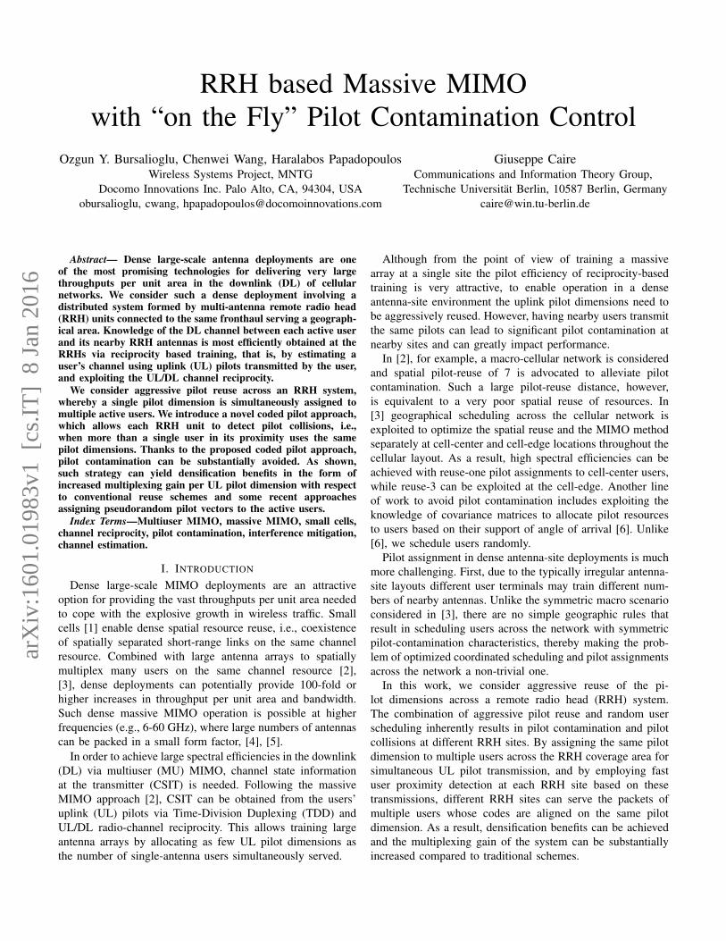
Fig. 2. Lattice based user scheduling with c “ 3
and the probability that a user is served. At one extreme ofβ “ 0.5, scheduled users are so sparsely located that activeuser discs do not overlap. In this case as long as an RRHsite falls within a user’s disc, any scheduled user is served.As we increase β from 0.5 to 2 the area where the BS hasto fall for the user to be served (e.g., the gray area in Fig.2-β “ 1.5) shrinks and eventually becomes a single point atβ “ 2. Clearly, as β is increased, more users are scheduledbut the probability that a user can be served becomes smaller.
The maximum multiplexing gain per RE in a lattice baseduser scheduling for finite N is given by:
m˚LU1 pNq “ maxβ
Kpβqp1pβ,Nq, (7)
where p1pβ,Nq is the probability that at least one RRH canserve a user assuming a scheduling lattice with spacing d{?β.An RRH site can serve a user if it falls in the region of theuser disc where other user discs overlap. Letting λpβq denotethe area of this region, the probability of an RRH site fallwithin this region is given by p1pβ,Nq “ 1´r1´λpβq{AsN .
As seen in Fig. 2, for large values of β, we can approximatethis region by the smallest square that includes that area.Thesquare has sides equal to d
a2{β ´ d, so the area of interest
is given by λpβq « d2pa2{β ´ 1q2 “ p4{πqDpa2{β ´ 1q2.
B. Random Scheduling Simulations
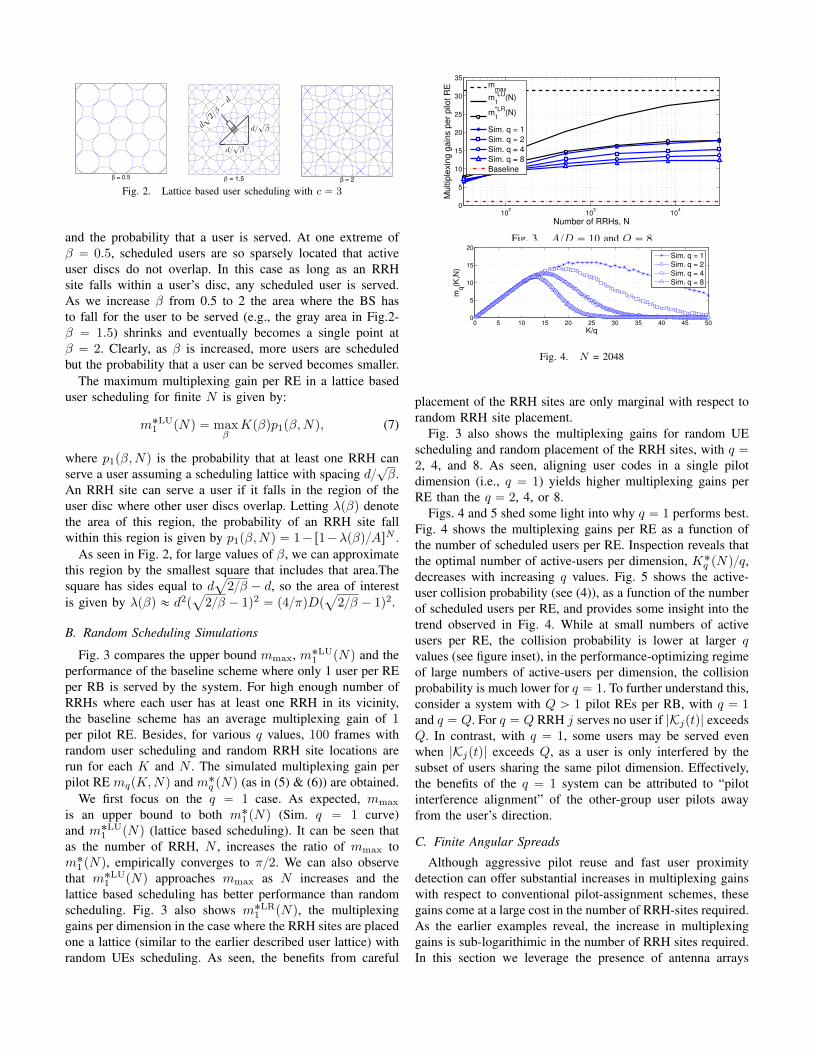
Fig. 3 compares the upper bound mmax, m˚LU1 pNq and theperformance of the baseline scheme where only 1 user per REper RB is served by the system. For high enough number ofRRHs where each user has at least one RRH in its vicinity,the baseline scheme has an average multiplexing gain of 1per pilot RE. Besides, for various q values, 100 frames withrandom user scheduling and random RRH site locations arerun for each K and N . The simulated multiplexing gain perpilot RE mqpK,Nq and mq pNq (as in (5) & (6)) are obtained.
We first focus on the q “ 1 case. As expected, mmax
is an upper bound to both m1 pNq (Sim. q “ 1 curve)and m˚LU1 pNq (lattice based scheduling). It can be seen thatas the number of RRH, N , increases the ratio of mmax tom1 pNq, empirically converges to π{2. We can also observethat m˚LU1 pNq approaches mmax as N increases and thelattice based scheduling has better performance than randomscheduling. Fig. 3 also shows m˚LR1 pNq, the multiplexinggains per dimension in the case where the RRH sites are placedone a lattice (similar to the earlier described user lattice) withrandom UEs scheduling. As seen, the benefits from careful
102
103
104
0
5
10
15
20
25
30
35
Number of RRHs, N
Multip
lexin
g g
ain
s p
er
pilo
t R
E
mmax
m*LU
1(N)
m*LR
1(N)
Sim. q = 1
Sim. q = 2
Sim. q = 4
Sim. q = 8
Baseline
Fig. 3. A{D “ 10 and Q “ 8
0 5 10 15 20 25 30 35 40 45 500
5
10
15
20
K/q
mq(K
,N)
Sim. q = 1
Sim. q = 2
Sim. q = 4
Sim. q = 8
Fig. 4. N = 2048
placement of the RRH sites are only marginal with respect torandom RRH site placement.
Fig. 3 also shows the multiplexing gains for random UEscheduling and random placement of the RRH sites, with q “2, 4, and 8. As seen, aligning user codes in a single pilotdimension (i.e., q “ 1) yields higher multiplexing gains perRE than the q “ 2, 4, or 8.
Figs. 4 and 5 shed some light into why q “ 1 performs best.Fig. 4 shows the multiplexing gains per RE as a function ofthe number of scheduled users per RE. Inspection reveals thatthe optimal number of active-users per dimension, Kq pNq{q,decreases with increasing q values. Fig. 5 shows the active-user collision probability (see (4)), as a function of the numberof scheduled users per RE, and provides some insight into thetrend observed in Fig. 4. While at small numbers of activeusers per RE, the collision probability is lower at larger qvalues (see figure inset), in the performance-optimizing regimeof large numbers of active-users per dimension, the collisionprobability is much lower for q “ 1. To further understand this,consider a system with Q ą 1 pilot REs per RB, with q “ 1and q “ Q. For q “ Q RRH j serves no user if |Kjptq| exceedsQ. In contrast, with q “ 1, some users may be served evenwhen |Kjptq| exceeds Q, as a user is only interfered by thesubset of users sharing the same pilot dimension. Effectively,the benefits of the q “ 1 system can be attributed to “pilotinterference alignment” of the other-group user pilots awayfrom the user’s direction.
C. Finite Angular Spreads
Although aggressive pilot reuse and fast user proximitydetection can offer substantial increases in multiplexing gainswith respect to conventional pilot-assignment schemes, thesegains come at a large cost in the number of RRH-sites required.As the earlier examples reveal, the increase in multiplexinggains is sub-logarithimic in the number of RRH sites required.In this section we leverage the presence of antenna arrays

0 5 10 15 20 25 30 35 40 45 500
0.2
0.4
0.6
0.8
1
K/q
Col
lisio
n Pr
obab
ility
Sim. q = 1Sim. q = 2Sim. q = 4Sim. q = 8
5 10 150
0.050.1
Fig. 5. N = 2048
at each RRH site to improve the number of RRH sites vs.multiplexing gain trade-offs. We remark that placing manyarray elements on a small footprint at each RRH unit becomesincreasingly feasible at higher (e.g., mmWave) frequencies andallows RRH-site sectorization. Sectorization is a well knowntechnique that increases the spectral efficiency per site incellular networks by partitioning each site radially into sectorsand reusing the spectral resources in each sector [8].
We assume a simplified scenario where the channel of anygiven user in the proximity of a given RRH site (i.e. withindistance ro) has a finite angular spread θ ą 0. An RRHcan separate the received pilot observations (1) into angular“sectors” by appropriate spatial filtering on Yjrns (for a givensector this may correspond to, e.g., projecting Yjrns onto a setof DFT vectors spanning a sector’s angular frequency range).
Note that an active user in the proximity of an RRH site (e.g.within distance ro) will appear to be present (i.e., its pilot willbe received at sufficiently high power) on only the subset of theRRH site sectors that have (significant) overlap with the user’sangular spectrum support. Consequently we assume that user kis in proximity of a sector s of RRH j, if the distance betweenuser k and RRH j is less than ro, and if the intersection ofthe supports of the angular spectrum of user k and sector sof RRH j is non-empty. We can thus consider straighforwardextensions of the techniques of the preceding section replacingthe notion of RRH sites with RRH-site sectors. For instance,in the system with q “ Q “ 1, an RRH-site sector can servean active user if it is the only active user in proximity to theRRH-site sector.
In Fig. 6, a sectorization abstraction is shown where we plottwo RRHs within the proximity of one UT with angular spreadθ. Each RRH site has 6 sectors shown by regions between twoconsecutive arrows. In this figure, the UT is in the proximityof one of the sectors of RRH 1 while it is in the proximity oftwo sectors of RRH 2 as shown by letter H.
Fig. 7 illustrates the benefits of sectorization comparingagainst the omni-scenario in Fig. 3 with q “ 1 and Q “ 8.The figure considers user angular spreads of θ “ π (asin Fig. 3) and θ “ π{6. As expected, for θ “ π weget the “omni” performance in Fig. 3 with S “ 1 andS “ 8 sectors. When the user-angular spread, however, isθ “ π{6, sectorization provides substantial gains. Indeed, themultiplexing gain obtained by 104 RRHs (see Fig. 3) can beobtained by 45 RRH sites if S “ 4 sectors are used, by 30sites if S “ 6 and by 23 sites if S “ 8.
In this section, we exploited the narrow angular spread of
C. Finite Angular Spreads
Although aggressive pilot reuse and fast user proximitydetection can offer substantial increases in multiplexing gainswith respect to conventional pilot-assignment schemes, thesegains come at a large cost in the number of RRH-sites required.As the earlier examples reveal, the increase in multiplexinggains is sub-logarithimic in the number of RRH sites required.In this section we leverage the presence of antenna arraysat each RRH site to improve the number of RRH sites vs.multiplexing gain trade offs. We remark that placing manyarray elements on a small footprint at each RRH unit becomesincreasingly feasible at higher (e.g., mmWave) frequencies andallows RRH-site sectorization. Sectorization is a well knowntechnique that increases the spectral efficiency per site incellular networks by partitioning each site radially into sectorsand reusing the spectral resources in each sector [8].
We assume a simplified scenario where the channel of anygiven user in the proximity of a given RRH site (i.e. withindistance ro) has a finite angular spread ✓ ° 0. An RRHcan separate the received pilot observations (1) into angular“sectors” by appropriate spatial filtering on Yjrns (for a givensector this may correspond to, e.g., projecting Yjrns onto a setof DFT vectors spanning a sector’s angular frequency range).
Note that an active user in the proximity of an RRH site (e.g.within distance ro) will appear to be present (i.e., its pilot willbe received at sufficiently high power) on only the subset of theRRH site sectors that have (significant) overlap with the user’sangular spectrum support. Consequently we assume that user kis in proximity of a sector s of RRH j, if the distance betweenuser k and RRH j is less than ro, and if the intersection ofthe supports of the angular spectrum of user k and sector sof RRH j is non-empty. We can thus consider straighforwardextensions of the techniques of the preceding section replacingthe notion of RRH sites with RRH-site sectors. For instance,in the system with q “ Q “ 1, an RRH-site sector can servean active user if it is the only active user in proximity to theRRH-site sector.
Fig. 7 illustrates the benefits of sectorization comparingagainst the omni-scenario in Fig. 3 with q “ 1 and Q “ 8.The figure considers user angular spreads of ✓ “ ⇡ (asin Fig. 3) and ✓ “ ⇡{6. As expected, for ✓ “ ⇡ weget the “omni” performance in Fig. 3 with S “ 1 andS “ 8 sectors. When the user-angular spread, however, is✓ “ ⇡{6, sectorization provides substantial gains. Indeed, themultiplexing gain obtained by 104 RRHs (see Fig. 3) can beobtained by 45 RRH sites if S “ 4 sectors are used, by 30sites if S “ 6 and by 23 sites if S “ 8.
IV. PILOT CODING FOR FAST PROXIMITY DETECTION
In this section we present codes for active-user proximitydetection. Following the approach in [2] each scheduling slotspans the whole bandwidth and comprises the totality of a setof consecutive OFDM symbols. The time-duration of a slot iswithin the coherence time of the user channels and that themaximum user-channel multipath spread is L samples long(with L not exceeding the OFDM circular prefix). L pilot
S = 6
θ θ
S = 6
θ θ
H L
L L L
L H H L
L L L
RRH1
RRH2
UT
r0
Fig. 6. ???
101
102
0
10
20
30
40
Number of Sites
Mu
ltple
xin
g G
ain
pe
r p
ilot R
E
S = 1, θ = π/6
S = 2, θ = π/6
S = 4, θ = π/6
S = 6, θ = π/6
S = 8, θ = π/6
S = 1, θ = π
S = 8, θ = π
Fig. 7. q “ 1, Q “ 8
dimensions per user (on distinct OFDM tones) are neededto learn a user’s channel over the whole bandwidth for theduration of such a scheduling slot1. In terms of the requiredtraining overheads to learn a user’s channel, this setting isequivalent to the abstracted scenario in the previous sectionwhereby each scheduling slot comprises L concurrent RBs andthe user channels are quasistatic over each RB [2]. Further-more, the Q pilot dimensions per RB (of the previous section)correspond here to assuming that within each scheduling slota set of QL orthogonal pilot vectors (spanning QL OFDMtime-frequency REs) are allocated for UL training.
Since at least L UL pilot dimensions are required forlearning a users’ channel, we consider the case whereby aset of L1 “ L ` ` ° L pilot dimensions (for some ` ° 0to be determined) are aggressively assigned to a set of Kactive users across the RRH coverage area. Without loss ofgenerality, we assume that these pilot dimensions correspondto a set of L1 REs (on distinct tones) in the OFDM plane. Weenumerate the pilot REs shared by an active group from 1 toL1 and consider “on-off” type pilot codes. The k-th active userpilot pattern is specified by means of an L1 ˆ 1 binary vectorbk, describing whether or not user k transmits a pilot in each
1In practice, L “ ↵L,↵ ° 1 many pilot dimensions can be used to ensurethe quality of channel estimation based on any L random pilot locations overOFDM block [9]. In this case, the analysis provided in this section will bevalid by using L instead of L.
Fig. 6. Two RRHs are shown within r0 distance from UT. UT is in theproximity of a sector if its angular spectrum support overlaps with the sector.The sectors where the UT is in the proximity are denoted by H, the othersare denoted by L.
101
102
0
10
20
30
40
Number of Sites
Multple
xin
g G
ain
per
pilo
t R
E
S = 1, θ = π/6
S = 2, θ = π/6
S = 4, θ = π/6
S = 6, θ = π/6
S = 8, θ = π/6
S = 1, θ = π
S = 8, θ = π
Fig. 7. q “ 1, Q “ 8
user channels by considering sectorization. In [6], the samecharacteristic of user channels is used to carefully design userschedules. In contrast, here, RRH-sector proximity detectioncombined with aggressive pilot reuse allows us to randomlyschedule users while still maintaining high multiplexing gains.
IV. PILOT CODING FOR FAST PROXIMITY DETECTION
In this section we present codes for active-user proximitydetection. Following the approach in [2] each scheduling slotspans the whole bandwidth and comprises the totality of a setof consecutive OFDM symbols. The time-duration of a slot iswithin the coherence time of the user channels and that themaximum user-channel multipath spread is L samples long(with L not exceeding the OFDM circular prefix). L pilotdimensions per user (on distinct OFDM tones) are neededto learn a user’s channel over the whole bandwidth for theduration of such a scheduling slot1. In terms of the requiredtraining overheads to learn a user’s channel, this setting isequivalent to the abstracted scenario in the previous sectionwhereby each scheduling slot comprises L concurrent RBs andthe user channels are quasistatic over each RB [2]. Further-more, the Q pilot dimensions per RB (of the previous section)correspond here to assuming that within each scheduling slota set of QL orthogonal pilot vectors (spanning QL OFDMtime-frequency REs) are allocated for UL training.
1In practice, L “ L ` ∆,∆ ą 0 many pilot dimensions can be usedto ensure the quality of channel estimation based on any L random pilotlocations over OFDM block. In this case, the analysis provided in this sectionwill be valid by using L instead of L.

pilot
ener
gypilot
ener
gypilot
ener
gy
L + ` pilot dimensions
L + ` pilot dimensions
L + ` pilot dimensions
User 1
User 2
(a)
(b)
(c)
Fig. 8. Received pilot energy
Since at least L UL pilot dimensions are required forlearning a users’ channel, we consider the case whereby aset of L1 “ L ` ` ą L pilot dimensions (for some ` ą 0to be determined) are aggressively assigned to a set of Kactive users across the RRH coverage area. Without loss ofgenerality, we assume that these pilot dimensions correspondto a set of L1 REs (on distinct tones) in the OFDM plane. Weenumerate the pilot REs shared by an active group from 1 toL1 and consider “on-off” type pilot codes. The k-th active userpilot pattern is specified by means of an L1 ˆ 1 binary vectorbk, describing whether or not user k transmits a pilot in eachof the L1 RBs in the scheduling slot. Let bkrns “ tbkun, thenuser k transmits a pilot on shared pilot RE n if bkrns “ 1and remains silent if bkrns “ 0. In Fig. 8, a simple exampleis shown with L “ 5 and ` “ 3 where two users share 8 pilotdimensions.
Fig. 8 (a) shows the received pilot energy at an RRH ifonly the first user is in the proximity of this RRH while (b)shows the received pilot energy if only the second user isin the proximity of this RRH. The probability of any pilotdimension being in deep fade is negligible due to large Mand coherent combining, and noise floor is easily distinguishedfrom any received pilot energy. Then the individual receivedpilot energy plots (Fig. 8 (a) & (b)) can be also seen as avisualization of the on-off pilot pattern for each user. Thespecific on-off code assignment to each user in this examplelets two users’ pilots overlap at pilot dimensions 5, 7 and 8.The received pilot energy at a nearby RRH (within r0 distanceto both users) is the superimposition of two pilot sequences,shown in Fig. 8 (c).
Next we consider user proximity detection at a fixed RRHsite and suppressing the dependence of variables on RRH siteindex. Let zk “ 1 if user k is within distance ro of RRH j,and zk “ 0 otherwise. According to the example in Fig. 1,to enable proximity detection, the detection mechanism basedon a set of active-user codewords must satisfy the following:
‚ if multiple users are within distance ro of the RRH site(i.e., if
řKk“1 zk ą 1), the RRH must be able to determine
that there is a pilot collision;‚ if a single active user is within distance ro of the RRH
site (i.e., ifřKk“1 zk “ 1), the RRH must be able to
identify that a single user is in proximity and the identityof that user (i.e., the k index for which zk “ 1);
‚ the RRH must also be able to identify when no users arein proximity of the RRH.
We also note that if a single active user on these L1 pilotdimensions is the proximity of the RRH and is detected bythe RRH, the user can be served by the RRH provided theuser channel can be estimated, that is, provided the user hastransmitted a pilot over at least L out of of L1 shared pilotREs (i.e., the user codeword must have at least L ones). Notethat, the code example in Fig. 8 with two users satisfies theseconditions. If the RRH observes higher than noise floor energyat more than 3 locations, it rightfully declares a collision (thecase seen in Fig. 8 (c)). If it observes exactly 3 “off” pilotdimensions, by matching the on-off pattern it decides who theunique user is (Fig. 8 (a) or (b)). In case it observes no receivedpilot energy in any of the pilot dimensions, it declares there areno users in its proximity signaling at these pilot dimensions.
Inspired by the received pilot energy example shown inFig. 8, the pilot energy detection at an RRH can be seen “OR”-type channel (formal justification is also provided at the endof the section), whereby an RRH receives an “1” (indicatingsufficiently high received power) if at least one active usertransmitting a pilot is in the proximity of the RRH and 0otherwise. Specifically, for all 1 ď n ď L1, the RRH at pilotRE n observes the following:
εrns “ ORpz1b1rns, z2b2rns, ¨ ¨ ¨ , zKbKrnsq , (8)
The simplest codes that enable active-user proximity detec-tion are comprised of K ď L ` 1 codewords (correspondingto the case ` “ 1) given by
bp1qk rns “ 1´ δrk ´ ns, for 1 ď k ď K. (9)
It can be verified that for the user-proximity model (8), theobservations tεrns; 1 ď n ď L1u satisfy the following:
εrns “
$’&’%
1 ifřKk“1 zk ą 1
1´δrn´kos if zk “ δrk´kos for some ko0 if zk “ 0 for all 1 ď k ď K
.
Consequently, if the RRH receives the all 1’s pattern (active-user pilot collision) or the all 0’s pattern (no active user is closeby) it does not send any user data. If, however, it receives apattern εrns “ 1´ δrn´ kos, it can identify the single user inproximity as user ko. Effectively, a single user is present whenthere is exactly one zero observed, and the index of the pilotRE where a zero is observed identifies the user in proximity(as this is the only user that did not transmit a pilot on thegiven pilot RE). Subsequently, when user ko is identified asthe single user in proximity, the set of L pilot observations onthe L pilot REs except pilot RE ko allow the RRH to estimate

1 6 11 16 21 56 66 1000.4
0.6
0.8
1
K
η
L = 5
L = 10
L = 15
L = 20
Fig. 9. Code Efficiency vs. number of active users per pilot dimension forvarious values of L .
the user channel across the whole bandwidth and thus servethe user in the data portion of the scheduling slot.
Since L ` 1 pilot REs are used per user, as opposed tothe minimum required of L, the pilot code efficiency is η “L{pL ` 1q. Furthermore, letting Kmax denote the number ofcode codewords, the maximum number of active users that canbe supported on the common set of L1 pilot REs by a givencode is Kmax. For the code in (9), Kmax “ L` 1 users.
Extensions of the code in (9) can be developed that tradeoff η with Kmax. One such family of codes that includes thecode in (9) is parametrized by a pair of integers L and ` with` ě 1. The code for a given p`, Lq pair is the constant weightcode comprising all binary codewords of length L1 “ L ` `,with L ones and ` zeros. The active users using such a codeshare L1 “ L` ` REs for UL training.
Consider using such a code for a fixed ` and assume eachactive user (sharing the L`` REs for UL training) is assigned aunique codeword. For the model (8), it can be readily verifiedthat if more than 1 active users are in the proximity of theRRH, then there are at most `´ 1 zeros in tεrnsu, while thepresence and identity of a single user in proximity are readilyrecovered at the RRH from the set of ` values of n for whichεrns “ 0. Also, the observations on the L pilot REs wherethe detected user has ones in its codeword allow the RRH toestimate the active user channel over the whole bandwidth andserve the user. Clearly, Kp`qmax “
`L```
˘, and ηp`q “ L{pL` `q.
Given a target value for K, the number of active users ona set of pilot REs, we may select the code (among the onesfor which Kp`qmax ě K) that yields the highest efficiency. Thisis equivalent to finding the lowest ` for which K ď `
L```
˘.
Hence, the highest efficiency for a given K is given by
η pK;Lq“#
1 if K “ 1LL`` if
`L ` 1`´1
˘ăKď`L ``
˘for some `ě1
Subsequently, the achieved net multiplexing gains by theRRH system is given by mnetpK,Lq “ mpKq η˚pK;Lq .
Fig. 9 shows the maximum efficiency possible with thegiven family of codes as a function of K, for various values ofL. As seen, even small values of L provides high efficiencies.Finally, it is worth justifying the use of the OR channel in (8)
at RRH site j. Given an L-tap channel hkrτ s between user kand RRH site j (suppressing again the dependence of variables
on j), the channel response on tone n is given by
hkrns “L´1ÿ
τ“0
hkrτ se´j 2πN nτ
where 2π{N is the OFDM tone spacing. Assuming also thatthe hkrτ s’s are independent in k and τ , and that hkrτ s „CN p0, ρk,τ Iq with ρk,τ unknown we have gk “ řL´1
τ“0 ρk,τ .Next, note that the observation on the n-th pilot RE (n-th
OFDM tone) is given by the Q “ 1 specialization of (1)
yrns “Kÿ
k“1
bkrnshTk rns `wrns
with bkrns denoting the pilot of user k on the n-th RE (withbkrns P t0, 1u). The RRH site first obtains the sample-averagereceived energy per antenna estimate Erns “ }yrns}2{M .
Noting that E”Erns
ı“ řK
k“1 bkrnsgk ` No, a hypothesistest of the form
Ernsεrns“1
¡εrns“0
Γ
for some appropriately defined threshold enables proximitydetection. For the abstracted example of Sec. II, where a user’slarge scale gain gk “ zkg, i.e., it is a non-zero value g if theuser k is within ro distance of the RRH j and zero otherwise,setting the threshold to Γ “ 0.5g ` No, and taking the limitM Ñ8 yields εrns “ εrns, with εrns from (8).
REFERENCES
[1] V. Chandrasekhar, J. Andrews, and A. Gatherer, “Femtocell networks: Asurvey,” IEEE Commun. Mag., vol. 46, no. 9, pp. 59 –67, Sep. 2008.
[2] T. Marzetta, “Noncooperative cellular wireless with unlimited numbers ofbase station antennas,” IEEE Trans. on Wireless Commun., vol. 9, no. 11,pp. 3590 –3600, Nov. 2010.
[3] H. Huh, G. Caire, H. Papadopoulos, and S. Ramprashad, “Achieving mas-sive MIMO spectral efficiency with a not-so-large number of antennas,”IEEE Trans. on Wireless Commun., vol. 11, no. 9, pp. 3226–3239, Sep.2012.
[4] A. Adhikary, E. Al Safadi, M. K. Samimi, R. Wang, G. Caire, T. S.Rappaport, and A. F. Molisch, “Joint spatial division and multiplexingfor mm-wave channels,” IEEE J. Sel. Areas Commun., vol. PP, no. 99,2014.
[5] T. Rappaport, S. Sun, R. Mayzus, H. Zhao, Y. Azar, K. Wang, G. Wong,J. Schulz, M. Samimi, and F. Gutierrez, “Millimeter wave mobile commu-nications for 5G cellular: It will work!” IEEE Access, vol. 1, pp. 335–349,May 2013.
[6] H. Yin, D. Gesbert, M. Filippou, and Y. Liu, “A coordinated approachto channel estimation in large-scale multiple-antenna systems,” IEEEJournal on Selected Areas in Commun., vol. 31, no. 2, pp. 264–273,February 2013.
[7] H. Q. Ngo, A. Ashikhmin, H. Yang, E. G. G. Larsson, and T. L. Marzetta,“Cell-free massive MIMO: Uniformly great service for everyone,” arXivpreprint arXiv:1505.02617, 2015.
[8] H. Huang, O. Alrabadi, J. Daly, D. Samardzija, C. Tran, R. Valenzuela,and S. Walker, “Increasing throughput in cellular networks with higher-order sectorization,” in Proceedings of the Forty-Fourth Asilomar Con-ference on Signals, Systems and Computers,, Nov. 2010, pp. 630–635.
Top Related
Copyright © 2022 FDOKUMEN

