


Bahasa
Halaman
Hukum


Query Focused Summarization Using Seq2seq Models
Thesis submitted in partial fulfillment of the requirements for the degree of
“DOCTOR OF PHILOSOPHY”
by
Tal Baumel
Submitted to the Senate of Ben-Gurion University of the Negev
January 2018
Beer-Sheva
Query Focused Summarization Using Seq2seq Models
Thesis submitted in partial fulfillment of the requirements for the degree of
“DOCTOR OF PHILOSOPHY”
by
Tal Baumel
Submitted to the Senate of Ben-Gurion University of the Negev
Approved by the advisor Approved by the Dean of the Kreitman School of Advanced Graduate Studies
January 2018
Beer-Sheva

This work was carried out under the supervision of
f Computer Scienceo In the Department
of Natural ScienceFaculty

Research-Student's Affidavit when Submitting the Doctoral Thesis for Judgment I_____________________, whose signature appears below, hereby declare that (Please mark the appropriate statements): ___ I have written this Thesis by myself, except for the help and guidance offered by my Thesis Advisors. ___ The scientific materials included in this Thesis are products of my own research, culled from the period during which I was a research student. ___ This Thesis incorporates research materials produced in cooperation with others, excluding the technical help commonly received during experimental work. Therefore, I am attaching another affidavit stating the contributions made by myself and the other participants in this research, which has been approved by them and submitted with their approval. Date: _________________ Student's name: ________________ Signature:______________

Abstract
Automatic summarization is one of the many tasks in the interdisciplinary field
of natural language processing (NLP). This task has gained popularity in the past
twenty years with the increased availability of large numbers of texts. Ever since
the introduction of the field by Luhn in the 1950s, automatic summarization meth-
ods have relied on extracting salient sentences from input texts. Such extractive
methods succeed in producing summaries which capture salient information, but
often fail to produce fluent and coherent summaries. Recent advances in neural
methods in NLP have achieved much improved results in most tasks and bench-
marks, including automatic summarization. In this work, we start with a survey
of the field of automatic summarization in general, and focus on the application of
neural network methods to this task. In particular, we critically review the datasets
that have been used to enable supervised methods in automatic summarization.
We cover the variant tasks of summarization – generic vs. query-focused sum-
marization, single document vs. multi-document and extractive vs. abstractive
methods. Neural methods have recently been shown to apply well to single-
document generic abstractive summarization under supervised training. We ex-
tend this initial step towards abstractive techniques by developing and assess-
ing neural techniques for multi-document generic summarization and abstractive
I

II
query-focused summarization.
Our method combines supervised and unsupervised steps, combining new
forms of attention-based sequence to sequence neural models and established
models of relevance assessment developed in extractive summarization. We study
separately techniques for document encoding and relevance assessment.
The main contribution of this work is the development of a new method for
abstractive multi-document query-focused summarization; this method combines
the strength of a supervised headline generator with the agility of an unsupervised
relevance model in a modular manner: we investigate separately each compo-
nent of a neural model for summarization – lexical information encoding with
word embeddings, source text encoding with RNNs, attention mechanism, rel-
evance assessment, and summary decoding with a conditioned RNN. For each
component we provide experimental description of the standard datasets used in
similar research, and verify their adequacy within the context of abstractive, multi-
document query focused summarization.
In the case of Query-Focused summarization, we identify a problematic aspect
of existing datasets (from the DUC family) – namely high topic concentration in
the text clusters – and introduce a new dataset which avoids this problem.
To assess the quality of word embeddings for the task of summarization, we
introduce a new embeddings evaluation method which exploits existing annota-
tions used in human summarization datasets (DUC with Pyramids).
In order to assess the quality of the text encoder, we study an auxiliary task:
multi-label classification. We study a challenging experimental setting in the do-
main of Electronic Health Records, where each document (a patient release letter
written by doctors at the end of an hospitalization episode) is long and annotated

III
by many medical diagnostic labels. Within this setting, we establish the effective-
ness of the embed-encode-attend neural architecture for text encoding.
Finally, we present the details of our end to end method for abstractive multi-
document query focused summarization. We demonstrate the effectiveness of the
method against strong existing baselines - both abstractive and extractive.

Acknowledgments
One of the best results of my research is the amazing people I got to meet and
collaborate with. Just the privilege of meeting them made the journey worthwhile.
First, I would like to thank my advisor Prof. Michael Elhadad: not only one of
the smartest people I ever got to meet but a kind, contingency enthusiastic, and all
around one of the nicest. Michael entering the lab excited to tell someone about
the latest NLP research or just a podcast he heard is one of the things I will miss
the most (luckily for me he keeps posting papers he finds exciting on Slack). I
cant imagine having so much fun with any other advisor.
Raphael Cohen: I met Rafi during my 1st (and last) field trip as a member of
CS department, I just started my MSc. and Rafi advised me to talk to Michael.
Soon we became lab mates and I got to enjoy (not sarcastically) Rafis unique view
just about everything. Rafi deserves a lot of credit not only for explaining LDA
but for reminding that while research is lots of fun I eventually need to publish
something.
Yael Netzer: Hearing about Yaels work on generating haikus (with David
Gabay and Yoav Goldberg) is what got me excited about NLP. Yaels work al-
ways reminded me the importance of creativity in research. Through the years
Yael became a great friend and helped me a lot with the self doubt that raises
IV

V
while researching.
The BGU NLP Lab: Meni Adler, Avi Hayon, Jumana Nassour, Tal (ha‘bat)
Achimeir, Imri hefner, Ben Eyal, Dan Schulman, and Matan Eyal.
The Israeli NLP research community: Ido Dagan, Yoav Goldberg, Reut Tsar-
fati, Marina Litvak, Jonathan Berant, Roee Aharoni, Omer Levi, Gabi Stanovsky,
Eli Kipperwasser, Asaf Amrami, Nir Ofek, Oren Hazai, David Gabay, Schahar
Mirkin, and Idan Spekztor
Honorary lab mates (people I shared many cups of coffee with): Ehud Barnea,
Noemie Elhadad, Guy Rapaport, Alex Lan, Hagit Cohen, Tamir Grosinger, Rotem
Miron, Boaz Arad, Shir Gur, Michael Dimeshitz, Yehonatan Cohen, Dolav Soker,
Majeed Kasis, Alon Grubstien, Nimrod Milo, Omer Shwartz, Achiya Eliasaf, and
Mazal Gagulashvily
My family: my grandmother Isabel, my mom Tzofia and dad Jacob, my
brother Dudi, his wife Dorit, and my two wonderful nieces Noga and Maya.

Contents
1 Introduction 1
1.1 Contribution . . . . . . . . . . . . . . . . . . . . . . . . . . . . . 3
I Automatic Summarization 6
2 Overview 7
2.1 Automatic Summarization . . . . . . . . . . . . . . . . . . . . . 7
2.2 Query-Focused Summarization . . . . . . . . . . . . . . . . . . . 10
2.3 Summarization Datasets . . . . . . . . . . . . . . . . . . . . . . 11
2.3.1 Large-Scale Summarization Datasets . . . . . . . . . . . 12
2.3.2 Query-Focused Summarization Datasets . . . . . . . . . . 15
2.4 Summarization Evaluation . . . . . . . . . . . . . . . . . . . . . 15
2.4.1 Manual Evaluation Methods . . . . . . . . . . . . . . . . 16
2.4.2 Automatic Evaluation Methods . . . . . . . . . . . . . . 18
2.5 Summary . . . . . . . . . . . . . . . . . . . . . . . . . . . . . . 21
3 Topic Concentration in Query Focused Summarization Datasets 23
3.1 Topic Concentration . . . . . . . . . . . . . . . . . . . . . . . . . 24
VI

CONTENTS VII
3.2 Measuring Topic concentration in Document Clusters . . . . . . . 26
3.3 The TD-QFS Dataset . . . . . . . . . . . . . . . . . . . . . . . . 30
3.4 Relevance-based QFS Models . . . . . . . . . . . . . . . . . . . 34
3.5 Conclusion . . . . . . . . . . . . . . . . . . . . . . . . . . . . . 36
II Neural Methods for Automatic Summarization 38
4 Neural Networks 40
4.1 Introduction . . . . . . . . . . . . . . . . . . . . . . . . . . . . . 40
4.2 Neural-Network Concepts for NLP . . . . . . . . . . . . . . . . . 41
4.2.1 Word-Embeddings . . . . . . . . . . . . . . . . . . . . . 41
4.2.2 Sequence-to-Sequence Architectures . . . . . . . . . . . . 45
4.3 Challenges of Neural-Networks for Automatic Summarization . . 49
4.3.1 Predicting High-Dimension Output . . . . . . . . . . . . 50
4.4 Survey of Abstractive Summarization Systems . . . . . . . . . . . 52
4.4.1 A Neural Attention Model for Sentence Summarization . . 53
4.4.2 Abstractive Text Summarization using Sequence-to-sequence
RNNs and Beyond . . . . . . . . . . . . . . . . . . . . . 57
4.4.3 Get To The Point: Summarization with Pointer-Generator
Networks . . . . . . . . . . . . . . . . . . . . . . . . . . 60
4.4.4 Sentence Simplification with Deep Reinforcement Learning 62
4.5 Conclusion . . . . . . . . . . . . . . . . . . . . . . . . . . . . . 66
III Application of Neural Methods for Automatic Summa-

CONTENTS VIII
rization 68
5 Sentence Embedding Evaluation Using Pyramid Annotation 69
5.1 Introduction . . . . . . . . . . . . . . . . . . . . . . . . . . . . . 70
5.2 Repurposing Pyramid Annotations . . . . . . . . . . . . . . . . . 72
5.3 Baseline Embeddings Evaluation . . . . . . . . . . . . . . . . . . 73
5.4 Task Significance . . . . . . . . . . . . . . . . . . . . . . . . . . 75
5.5 Conclusion . . . . . . . . . . . . . . . . . . . . . . . . . . . . . 75
6 Multi-Label Classification on Patient Notes With Neural Encoders 76
6.1 Introduction . . . . . . . . . . . . . . . . . . . . . . . . . . . . . 77
6.2 Previous Work . . . . . . . . . . . . . . . . . . . . . . . . . . . . 78
6.2.1 Multi-label Patient Classifications . . . . . . . . . . . . . 79
6.2.2 Multi-label Extreme Classification . . . . . . . . . . . . . 81
6.3 Dataset and Preprocessing . . . . . . . . . . . . . . . . . . . . . 82
6.3.1 MIMIC Datasets . . . . . . . . . . . . . . . . . . . . . . 82
6.3.2 ICD9 Codes . . . . . . . . . . . . . . . . . . . . . . . . . 83
6.3.3 Input Texts . . . . . . . . . . . . . . . . . . . . . . . . . 84
6.4 Methods . . . . . . . . . . . . . . . . . . . . . . . . . . . . . . . 85
6.5 Results . . . . . . . . . . . . . . . . . . . . . . . . . . . . . . . . 91
6.5.1 Model Comparison . . . . . . . . . . . . . . . . . . . . . 91
6.5.2 Label Frequency . . . . . . . . . . . . . . . . . . . . . . 92
6.5.3 Model Explaining Power . . . . . . . . . . . . . . . . . . 94
6.6 Conclusion . . . . . . . . . . . . . . . . . . . . . . . . . . . . . 96
7 Abstractive Query Focused Summarization 97

CONTENTS IX
7.1 Introduction . . . . . . . . . . . . . . . . . . . . . . . . . . . . . 98
7.2 Previous Work . . . . . . . . . . . . . . . . . . . . . . . . . . . . 101
7.2.1 Extractive Methods . . . . . . . . . . . . . . . . . . . . . 101
7.2.2 Sequence-to-Sequence Models for Abstractive Summa-
rization . . . . . . . . . . . . . . . . . . . . . . . . . . . 101
7.3 Query Relevance . . . . . . . . . . . . . . . . . . . . . . . . . . 104
7.4 Methods . . . . . . . . . . . . . . . . . . . . . . . . . . . . . . . 105
7.4.1 Incorporating Relevance in Seq2Seq with Attention Models105
7.4.2 Calibrating the Relevance Score . . . . . . . . . . . . . . 107
7.4.3 Adapting Abstractive Models to Multi-Document Sum-
marization with Long Output . . . . . . . . . . . . . . . . 108
7.5 Experiments . . . . . . . . . . . . . . . . . . . . . . . . . . . . . 110
7.5.1 Evaluation . . . . . . . . . . . . . . . . . . . . . . . . . 110
7.5.2 Abstractive Baselines . . . . . . . . . . . . . . . . . . . . 111
7.5.3 Extractive Baselines . . . . . . . . . . . . . . . . . . . . 114
7.5.4 Evaluation Using the Debatepedia Dataset . . . . . . . . . 115
7.6 Analysis . . . . . . . . . . . . . . . . . . . . . . . . . . . . . . . 116
7.6.1 Output Abstractiveness . . . . . . . . . . . . . . . . . . . 116
7.7 Conclusion . . . . . . . . . . . . . . . . . . . . . . . . . . . . . 117
8 Conclusion 119

List of Figures
2.1 A query and an abstract taken from DUC 2007. . . . . . . . . . . 13
2.2 Pyramid method file illustration. . . . . . . . . . . . . . . . . . . 17
3.1 ROUGE—Comparing QFS methods to generic summarization meth-
ods: Biased-LexRank is not significantly better than generic algo-
rithms. . . . . . . . . . . . . . . . . . . . . . . . . . . . . . . . . 25
3.2 Two-stage query-focused summarization scheme. . . . . . . . . . 26
3.3 Comparing retrieval components on DUC 2005. . . . . . . . . . . 29
3.4 DUC 2005-7 vs. QCFS dataset structure. . . . . . . . . . . . . . . 30
3.5 ROUGE-Recall results of KLSum on relevance-filtered subsets of
the TD-QFS dataset compared to DUC datasets. . . . . . . . . . . 33
3.6 Comparison of QFS to Non-QFS algorithms performance on the
TD-QFS dataset. . . . . . . . . . . . . . . . . . . . . . . . . . . 35
3.7 Comparison of retrieval-based algorithms performance on the TD-
QFS dataset. . . . . . . . . . . . . . . . . . . . . . . . . . . . . . 35
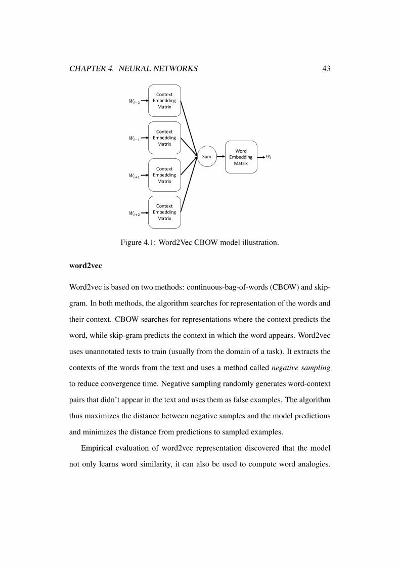
4.1 Word2Vec CBOW model illustration. . . . . . . . . . . . . . . . 43
4.2 RNN interface illustration. . . . . . . . . . . . . . . . . . . . . . 45
4.3 RNN network for POS tagging illustration. . . . . . . . . . . . . 46
X

LIST OF FIGURES XI
4.4 Encoder-Decoder model for input and output of size n. . . . . . . 48
4.5 Hierarchal vocabulary tree. . . . . . . . . . . . . . . . . . . . . . 51
4.6 Example of attention based encoder attention weights values for
different generation steps. . . . . . . . . . . . . . . . . . . . . . . 56
4.7 Comparison of different abstractive summarization with repeti-
tion highlighted. Repetition avoidance is achieved with a cover-
age mechanism. . . . . . . . . . . . . . . . . . . . . . . . . . . 61
4.8 Reinforcement learning settings. . . . . . . . . . . . . . . . . . . 64
5.1 Binary test pairs example . . . . . . . . . . . . . . . . . . . . . . 72
5.2 Ranking test example question . . . . . . . . . . . . . . . . . . . 73
6.1 CBOW architecture on the left and CNN model architecture on
the right. . . . . . . . . . . . . . . . . . . . . . . . . . . . . . . . 87
6.2 HA-GRU model architecture overview. . . . . . . . . . . . . . . . 89
6.3 Zoom-in of the sentence encoder and classifier. . . . . . . . . . . 91
6.4 Sample text of a patient note (one sentence per line). On the left,
visualization for the with attention weights at the sentence and
word levels associated with the ICD9 codes, on the left sentence
level attention weights for ICD9 code “Heart failure”, on the the
right for code “Traumatic pneumothorax and hemothorax”. . . . . 93
6.5 Effect label frequency on HA-GRU performance when trained on
MIMIC III. X-axis represents the bins of labels ranked by their
frequency in the training set. . . . . . . . . . . . . . . . . . . . . 93

LIST OF FIGURES XII
7.1 Comparison of the output of the unmodified seq2seq model of
See et al. vs. our model RSA-QFS on a QFS data sample. The
unmodified summary lacks coherence and is not relevant to the
input query. . . . . . . . . . . . . . . . . . . . . . . . . . . . . . 100
7.2 Two stage query focused summarization scheme. . . . . . . . . . 105
7.3 Illustration of the RSA-QFS architecture: RelV ector is a vector
of the same length as the input (n) where the ith element is the
relevance score of the ith input word. RelV ector is calculated in
advance and is part of the input. . . . . . . . . . . . . . . . . . . 108
7.4 A demonstration of the scale sensitivity of the softmax function.
Both figures illustrate a softmax operation over 1,000 samples
from a uniform distribution; left is sampled from the range 0–1
and the right from 0–100. . . . . . . . . . . . . . . . . . . . . . . 109

Chapter 1
Introduction
Automatic summarization is the task of shortening a text while preserving its most
important information. The task has become extremely useful because of the con-
stant increase of on-line information1 available and the need to process and under-
stand it.
Early work in the field used statistical information from the input text (such as
lexical word occurrences [1] and document structure [2]) to identify salient sen-
tences from a text and to extract them to achieve a salient summarization. Such
extractive summarizers generate text which is not always well organized or read-
able, but they have remained the most effective baseline for over 20 years.
The availability of affordable, fast, and parallel computing power in the form
of Graphical Processing Units (GPUs) and of large-scale training data has enabled
applying neural network-based supervised methods [3, 4] to generate automatic
summaries. These neural models are trained to produce abstractive summarizers.
These recent models remain harder to interpret and modify than their extractive1http://www.worldwidewebsize.com/
1

CHAPTER 1. INTRODUCTION 2
predecessors, since they are learned in an end-to-end manner, in a supervised
manner. It is often difficult to justify or adjust the decisions made when generating
a new specific summary given a source document.
Automatic summarization with neural networks is the main starting point of
this work, with a focus on the transition from extractive to abstractive techniques.
We start in Chapter 2 with a survey of automatic summarization research: the
definition of the task and its variants, the standard datasets used in the field, and
the key techniques that have established the state of the art.
We analyze the task of summarization as the combination of multiple indepen-
dent sub-tasks: content selection, content planning with redundancy elimination,
and summary realization.
We initially focus on the stage of content selection: how does the summa-
rizer decide which content from the source documents deserves to be kept in the
summary, as opposed to content which can be skipped. To better analyze this
question, we contrast between generic summarization (where the central elements
of the source documents must be identified) and query-focused summarization
(QFS) where only information relevant to an input query must be selected. In
Chapter 3, we empirically analyze the standard datasets used in the QFS field, and
identify that they fail to exercise the relevance identification part of the QFS task,
because they exhibit high topic concentration. We design an automated model to
assess topic concentration in a dataset. On the basis of this analysis, we introduce
our first contribution to the field of QFS: a new dataset we have constructed to
refine the notion of query-focused summarization.
We then describe, in Chapter 4, the field of neural network techniques as ap-
plied to automatic summarization which has started in the past two years.

CHAPTER 1. INTRODUCTION 3
We discuss evaluation methods for summarization, which are particularly chal-
lenging because there is not a single best summary that can be produced from a
given input document collection. We review how established evaluation meth-
ods ought to be adapted to assess the performance of supervised neural methods
for abstractive summarization, as opposed to the existing extractive methods. In
Chapter 5, we contribute a study of how word embeddings (used in most neural
networks) can gain from the pyramid annotations, available in most summariza-
tion datasets.
In Chapter 6, we move to an analysis of the first module of a neural abstractive
model: the text encoder. To analyze text encoding in a modular manner, we assess
the task of document encoding for an auxiliary task – that of multi-label document
classification. We introduce an interpretable neural network model trained for
electric health care records (EHR) classification. The same model can be used for
automatic summarization in a multi-task setting.
Finally, in Chapter 7, we show how to modify a neural network trained for
generic abstractive single-document summarization to handle the QFS abstractive
multi-document task. We compare different baselines to adapt a single-document
abstractive model to the multi-document setting. We then compare different tech-
niques to introduce relevance in abstractive summarization – combining word-
level and sentence-level relevance cues.
1.1 Contribution
The contribution of this work is both in the field of automatic summarization and
neural methods for NLP. This work synthesizes results presented in the following
CHAPTER 1. INTRODUCTION 4
papers:
Topic Concentration in Query-Focused Summarization Dataset [5]: This
work explores an abstract attribute of QFS we call topic concentration. This
attribute measures how much the query aspect of the task should be considered
as opposed to the generic summarization part. This contribution also presents a
new dataset with better topic concentration and relevancy based summarization
methods.
Query Chain Focused Summarization [6]: This contribution introduces the
novel task of query chain focused summarization, a new dataset constructed for
evaluating the task, and summarization methods designed for the task. The dataset
presented in this contribution can be used to assess topic concentration in Query-
Focused Summarization Datasets.
Sentence Embedding Evaluation Using Pyramid Annotation [7]: This con-
tribution suggests using pyramid annotation, a resource to evaluate automatic
summarization, as a benchmark to perform extrinsic evaluation of neural word
embeddings.
Multi-Label Classification on Patient Notes [8]: This contribution evaluated
the ability of different neural encoders (the first building block of most neural ab-
stractive summarization methods) to capture medical diagnoses in a patient note.
We argue that this task is a proxy for the encoder’s ability to capture the key
concepts of a summary, and hence, can play a role within a multi-task learning
architecture combined with abstractive summarization.

CHAPTER 1. INTRODUCTION 5
Abstractive Query-Focused Summarization [9]: In this contribution, we present
a method to achieve abstractive QFS using a remotely supervised neural network.
This is the first at applying neural abstractive methods for the QFS task, and
demonstrating that abstractive methods with good relevance models can improve
state-of-the-art.

Part I
Automatic Summarization
6
Chapter 2
Overview
The task of automatic summarization is extremely desirable since overwhelming
amounts of text are generated daily and need to be summarized in order to be
understood. The task is challenging since it requires automatic summarization
systems to understand texts and to identify salient information from source texts,
using it to generate a coherent short text. In this chapter, we survey the field of
automatic summarization and its different facets. Within the map of the field, we
introduce our contribution to the field of QFS dataset evaluation.
2.1 Automatic Summarization
Automatic summarization is a field in natural language processing that involves
reducing a text document (or a set of topically related documents) into a shorter
summary using a computer program. The constantly increasing amount of textual
information available to users on the Internet has led to the development of many
automatic summarization techniques. These techniques can be classified along
7

CHAPTER 2. OVERVIEW 8
the following dimensions:
• Informative vs. Indicative summaries: An informative summary should
capture all the important information of the text and could replace the need
to read the entire document. On the other hand, indicative summaries only
help the user decide whether he wants to read the text. Indicative summaries
are usually snippets of text associated with search results from information
retrieval systems.
• Single vs. Multi-document summaries: A single document summary cap-
tures the information of a single document, while a multi-document sum-
mary captures the information from a set of documents covering a similar
set of topics. When summarizing a document set, it is easier to find im-
portant information, since important information should appear in all of the
documents, while marginal information should appear in only a few docu-
ments. When summarizing a single document with no previous knowledge,
it is harder to distinguish between important information and less central
information. In contrast, when summarizing a single document, it is easier
to maintain coherence in the summary just by extracting sentences, since all
of them share the same writing style, and ordering the extracted content ac-
cording to the order in which they appear in the source document preserves
coherence. Ordering information within a single summary originating from
multiple documents is much more challenging.
• Extractive vs. Abstractive summaries: Extractive summaries construct
the summary from sentences that appear in the original text, in a cut-and-
paste manner. In contrast, an abstractive summary extracts information from

CHAPTER 2. OVERVIEW 9
the original text but generates an entirely new text to summarize it.
• Generic vs. Focused summaries: Generic summaries determine what
is the central information in the source documents without any additional
guidance. Focused summaries use external guidance to determine which
part of the source documents are relevant to the reader, and construct a
summary which focuses on this subset of the conveyed information only.
The guidance to focus the summaries may take multiple forms, such as a
query which characterizes the intended information, or a collection of doc-
uments which represent known information with the intention that only new
information should be included in the summary.
The summarization task is challenging because it requires a system to balance
the following attributes:
• Detecting central topics: Automatic summarization systems should cap-
ture central topics from articles. These topics might be mentioned only
a few times in the source documents. For example, an article discussing
a “phone call between Barack Obama and Hassan Rouhani” should not
repeat the fact that phone calls were made more than once, but we could
expect this detail to be mentioned in a summary of the article.
• Redundancy: Salient segments coming from different documents often
carry similar information, which is repeated in multiple documents. The
summarizer must avoid including segments conveying the same informa-
tion into the summary, but it must be capable of merging information com-
ing from multiple sentences each one contributing a different angle [10].

CHAPTER 2. OVERVIEW 10
For example, “Chinese courts sentenced three of the nation’s most promi-
nent dissidents.” and “By sentencing two of the country’s most prominent
democracy campaigners to long prison terms” could be merge to a sentence
containing both the facts that country where the sentence is held is China
an that the verdict is “long prison terms.”
• Coherence: the task of controlled text generation [11] is extremely chal-
lenging. When segments are extracted from their source document, they
may include references to textual entities within the source which have not
been selected for inclusion in the summary. Similarly, when extracting a
sentence, it may include connectives which relate to other sentences which
are not included in the summary. Such discourse references must also be re-
solved or avoided. For example, the sentence “It qualified earlier this year
leaving the disparate allies without so clear a reason to stay together.” does
not make much sense out of context.
2.2 Query-Focused Summarization
The task of Query-Focused Summarization (QFS) was introduced as a variant
of generic multi-document summarization in shared-tasks since DUC 2005 [12].
QFS goes beyond factoid extraction and consists of producing a brief, well-organized,
fluent answer to a need for information (Dang, 2005), which is directly applicable
in real-world settings.
As a research objective, QFS is a useful variant of generic multi-document
summarization because it helps articulate the difference between content central-
ity within the documents in the cluster and query relevance. This distinction is

CHAPTER 2. OVERVIEW 11
critical when dealing with complex information needs (such as the TREC 2006
Legal Track [13]) because we expect the summary to cover multiple aspects of
the same general topic.
The difference between central and topic-relevant content will only be signifi-
cant when we can observe a clear difference between these two components in the
dataset. Interestingly, it has been observed in [14] that generic summarization al-
gorithms (which simply ignore the query) perform as well as many proposed QFS
algorithms on standard QFS datasets, such as the DUC 2005. We hypothesize that
this is due to the fact that existing QFS datasets have very high topic concentration
in the input (the document cluster). In other words, the datasets used to evaluate
QFS are not geared towards distinguishing central and topic content, a notion that
we explore later in this chapter.
2.3 Summarization Datasets
An important resource for automatic summarization is the various datasets avail-
able. In this chapter, we will cover a number of these datasets, especially large-
scale summarization datasets (used by supervised summarization systems) and
QFS datasets used to evaluate the task.
The de-facto standard datasets for automatic single document summariza-
tion are those produced for the Document Understanding Conferences (DUC)
2001–2007 [15] and the Text Analysis Conferences (TAC) 2008–2016 [16], all
constructed under the auspices of the National Institute of Standards and Tech-
nology (NIST). These datasets cover a variety of summarization variants (single-
document summarization, multi-document summarization, update summarization,
CHAPTER 2. OVERVIEW 12
query-focused summarization, and summarization evaluation). The DUC and
TAC datasets usually contain about 50 document clusters, each containing about
10 articles and 3–4 manually created summaries. This data is used for evalua-
tion and is certainly insufficient (when compared to datasets discussed later) to
train supervised abstractive summarization models. Accordingly, up to the past
two years, most approaches to summarization have been unsupervised learning
techniques.
2.3.1 Large-Scale Summarization Datasets
The large-scale datasets used in recent work to train summarizers were not orig-
inally constructed for summarization. Examples include the Gigaword corpus
[17], the CNN/Daily Mail Corpus [18], and the Wikipedia dataset PWKP[19].
Those existing resources were adapted to simulate summarization contexts.
The Gigaword corpus was produced by the Linguistic Data Consortium (LDC),
and it is an ensemble of various corpora: The North American News text corpora,
DT corpora, the AQUAINT text corpus, and data released for the first time, all in
the news domain. In order to adapt this corpus to the task of summarization, a
subset of the data was extracted including pairs of articles headlines and first sen-
tences, where both share a fixed number of words and the headline is shorter than
the first sentence. There are 3.8M training examples and 400K validation and test
examples. Since the data were obtained automatically, there is no guarantee that
the headline is a good summarization of the first sentence, but it is an affordable
way to achieve large enough training data. The Gigaword corpus is not available
free of charge, which limits its availability.

CHAPTER 2. OVERVIEW 13
Query:“Describe the activities of Morris Dees and the Southern Poverty Law Center .”Abstract:“Morris Dees was co-founder of the Southern Poverty Law Center -LRB- SPLC -RRB- in 1971 and has served as its Chief Trial Counsel and Executive Director .The SPLC participates in tracking down hate groups and
publicizing their activities in its Intelligence Report , teaching tolerance and bringing lawsuits against discriminatory practices and hate groups .As early as 1973 the SPLC won a federal case which forced funeral homes throughout the U.S. to provide equal services to blacks and whites .In 1991 it started a classroom program `` Teaching Tolerance ''
which features books , videos , posters and a magazine that goes to more than 400,000 teachers .It also funded a civil rights litigation program in Georgia to
provide free legal assistance to poor people .The SPLC 's most outstanding successes , however , have been
in its civil lawsuits against hate groups .Dees and the SPLC have fought to break the organizations by
legal action resulting in severe financial penalties .Described as `` wielding the civil lawsuit like a Buck Knife ,
carving financial assets out of hate group leaders , '' the technique has been most impressive : 1987 - $ 7 million against the United Klans of America in Mobile , Alabama ; 1989 - $ 1 million against Klan groups in Forsyth County , Georgia ; 1990 - $ 9 million against the White Aryan Resistance in Portland , Oregon ; and 1998 - $ 20 million against The Christian Knights of the Ku Klux Klan in Charleston , South Carolina .But despite these judgments the Ku Klux Klan and White Aryan
Resistance have survived .”
Figure 2.1: A query and an abstract taken from DUC 2007.
CHAPTER 2. OVERVIEW 14
The CNN/Daily Mail Corpus was automatically curated by matching arti-
cles to their summary from the CNN and Daily Mail websites. The dataset in-
cludes 90k documents from CNN and 196k documents from the Daily Mail. The
CNN/Daily Mail dataset is available on-line.1 Each abstract in the dataset contains
up to 100 words, while the source documents are up to 800 words.
The PWKP dataset contains Wikipedia edit history; a subset of the edits can
be considered as sentence simplification. The dataset was automatically aligned
to find original sentences and simplified pairs. Again, this is not a proper sum-
marization dataset, but it includes pairs of long sentences/short sentences, which
is useful in learning how to shorten and paraphrase sentences in an abstractive
manner.
These datasets are good sources of knowledge to learn how to rephrase infor-
mation in a compact manner. But they are weak proxies of the real summarization
task because they do not cover the challenges of content selection across multiple
documents, relevance assessment, and redundancy avoidance, which have been
the key characteristics of the traditional DUC/TAC summarization datasets in the
past. In addition, in all of the supervised datasets, there is a single summary for
a given source document, while for DUC/TAC datasets, there are usually four or
more human summaries for each source document cluster.
This is an important point, as it highlights that what is addressed in the group
of abstractive summarization methods we survey later is a task different in nature
from what was studied a decade ago. Still, the same evaluation metrics (mainly
ROUGE) are applied uniformly across the two variant tasks – which induces un-
expected bias.1\RRR{https://github.com/danqi/rc-cnn-dailymail}

CHAPTER 2. OVERVIEW 15
2.3.2 Query-Focused Summarization Datasets
In multiple DUC datasets (2005, 2006, 2007) [12, 20], the QFS task asks for an
answer to a query as a summary of at most 250 words created from a cluster of
25–50 documents (newspaper articles). As part of the dataset preparation, asses-
sors were instructed to populate the cluster with at least 25 documents that were
relevant to the query. The instructions, thus, encouraged the creation of topically
coherent document sets as input to the summarization task. Notably, the extent
to which the document clusters are focused on the query is not directly observ-
able: assessors could select between 50% to 100% of the documents as “relevant
to the topic.” Our empirical evaluation (presented below) indicate that, in fact, the
selected documents are almost fully relevant to the topic, hence making the rele-
vance finding aspect of the task practically not effective to succeed on this dataset
for the QFS task.
2.4 Summarization Evaluation
One of the challenges of the automatic summarization task is evaluation. The eval-
uation score should be well-defined even when done manually (i.e., if the score
relies on the evaluator’s judgment it will not be consistent across other evalua-
tors). In this section, we discuss popular methods of automatic summarization
evaluation methods.

CHAPTER 2. OVERVIEW 16
2.4.1 Manual Evaluation Methods
DUC Evaluation Procedure
The DUC evaluation procedure consists of the following steps:
1. A human annotator produces a reference summary according to the summa-
rization task guidelines. This summary is called a model.
2. The model summary is split into clauses. This step is performed automati-
cally using the SPADE tool.2
3. Given an automatically generated summarization (called a peer), it is also
split into clauses using the SPADE tool.
4. A human evaluator manually compares the clauses from the model and peer
summary and determines the coverage percentage of clauses from the peer
summary.
One of the main problems with the DUC evaluation procedure is its reliance
on a single gold-summarization. Not only may different annotators not agree with
each other regarding what clauses should be included in the ideal summary, in a
study performed by Lin and Hovy in 2002 [21], only 83% of human evaluators
agreed with their own prior judgment.
The Pyramid Method
The Pyramid method was designed to solve the single gold-summarization re-
liance problem of the DUC evaluation procedure. In order to use the method, a
Pyramid file must first be created manually (Fig. 2.2):2https://www.isi.edu/licensed-sw/spade/

CHAPTER 2. OVERVIEW 17
Model Summaries SCUs are weighted by the number of summaries they appear in
Create pyramid
W=3
W=2
W=1
Figure 2.2: Pyramid method file illustration.
1. A set of model summaries is created.
2. Each summary is divided into Summary Content Units (SCUs). SCUs are
key facts extracted from the manual summarizations and are no longer than
a single clause.
3. A Pyramid file is created where each SCU is given a score by the num-
ber of summaries in which it is mentioned (i.e., SCUs mentioned in three
summaries will obtain a score of 3).
After the Pyramid is created, it can be used to evaluate a peer summary:
1. All the SCUs in the summary are manually located.
2. The score of all the found SCUs is summed and divided by the maximum
score that the same number of SCUs can achieve.
SCUs are extracted from different source summaries, written by different au-
thors. When counting the number of occurrences of an SCU, annotators effec-
tively create clusters of text snippets that are judged semantically equivalent in
the context of the source summaries. They actually refer to clusters of text frag-

CHAPTER 2. OVERVIEW 18
ments from the summaries and a label written by the pyramid annotator describing
the meaning of the SCU.
Analysis done on the DUC 2003 dataset [22] shows that score consistency
across annotators does not improve when using more than four summaries.
2.4.2 Automatic Evaluation Methods
Manual evaluation is expensive, time consuming, and inconsistent between dif-
ferent evaluators. For all these reasons, the need for an automatic summarization
evaluation scheme has arisen.
BLEU Metric
The BLEU (bilingual evaluation understudy) metric [23] originally proposed to
evaluate machine translation in a study from 2003 [24] shows high agreement
to human annotators when using the BLEU metric for evaluating automatically
generated summaries.
BLEU is a precision-based method which is explained in the following exam-
ple from Papineni et al.:
Automatic Translation (AT): the, the, the, the, the, the, the
Reference Translation 1 (RT1): the, cat, is, on, the, mat
Reference Translation 2 (RT2): there, is, a, cat, on, the, mat
Since every word (the) in AT appears in both reference translations, AT will
receive a precision score of matchlength = 7
7 = 1. The BLEU metric modifies the preci-
sion score by clipping the number of times a word can be counted as a match by
the maximum appearances of the word in a single reference translation matchmax.

CHAPTER 2. OVERVIEW 19
In the example matchmax for the word the is 2 since it appears two times in RT2
and only once in RT1. The BLEU score of AT is matchmaxlength = 2
7 .
In the example, we see a unigram variation of the BLEU score, but any n-gram
configuration can be used. Longer n-grams are used to measure text fluency, and
shorter n-grams measure its coverage.
BLEU remains an extremely popular method of evaluating automatic transla-
tions and summaries to this day. The method relies on few gold reference texts so
it is inexpensive and can be applied automatically; thus, it is very fast. BLEU is
designed to approximate human judgment at corpus level, and performs poorly if
used to evaluate the quality of individual sentences.
ROUGE Metric
The most common method to evaluate automatic summaries is ROUGE (Recall-
Oriented Understudy for Gisting Evaluation) [25]. Like BLEU, ROUGE relies on
lexical comparison of automatically generated n-grams to manually created gold
standard models. Unlike BLEU, ROUGE scores rely on measuring recall instead
of precision. ROUGE relies on recall because automatic summaries are bounded
by a strict maximal word limit i.e., a perfect precision score can be achieved by
generating a summary containing only the word ”the”.
The ROUGE metric includes a suite of different score functions:
• ROUGE-N (n-gram): The ROUGE-N function measures the recall of n-
grams between the model summaries and the peer summaries. Pearson cor-
relation to manual evaluation ranges from 0.76 (ROUGE-9) to 0.87 (ROUGE-
2).

CHAPTER 2. OVERVIEW 20
ROUGEN =
PS2ModelSummaries
PnGram2S CountMatch(nGram)P
S2ModelSummaries
PnGram2S Count(nGram)
(2.1)
• ROUGE-L (Longest Common Subsequence):
Recalllcs =LCS(peer,model)
length(model)(2.2)
Precisionlcs =LCS(peer,model)
length(peer)(2.3)
Flcs =LCS(1 + �
2)RecalllcsPrecisionlcs
Recalllcs + �2Precisionlcs(2.4)
Where LCS should return the length of the longest common sub-sequence,
and � is the ratio of recall importance to precision (set to the high value of
8 for the DUC evaluations).
• ROUGE-W (Weighted Longest Common Subsequence): A modified ver-
sion of ROUGE-L that favors consecutive common subsequences. 0.86
Pearson correlation to manual evaluation.
• ROUGE-S (Skip-Bigram Co-Occurrence Statistics): ROUGE-S counts
the number of overlapping skip-bigrams between the model and peer sum-
maries. Skip-bigrams refer to common subsequences of length 2. 0.87
Pearson correlation to manual evaluation.
• ROUGE-SU (Extension of ROUGE-S): In order to credit summaries with
zero skip-bigram overlap. ROUGE-SU adds a unigram aspect to the ROUGE-
S. The unigram aspect is achieved by simply adding a start-of-sentence

CHAPTER 2. OVERVIEW 21
token at the beginning of each sentence of the input summaries before
ROUGE-S is applied. 0.87 Pearson correlation to manual evaluation.
METEOR
The last automatic evaluation method we cover is METEOR [26]. METEOR was
designed for machine translation but can be used for evaluating automatic sum-
maries as well. The METEOR method computes a score by first achieving word-
to-word alignment between the evaluated text and the reference text. There are
two ways to achieve this alignment: (a) based on the Porter stem algorithm [27]
(based on pre-defined regular expressions), or (b) based on WordNet [28] syn-
onyms. Once the alignment is achieved, Precision, Recall, and F-measure scores
can be calculated, where aligned words are considered a match. While METEOR
achieves the highest correlation to human judgment of all the automatic methods
presented, the requirement of manually curated resources for stemming makes it
hard to implement for languages other than English and limits its applicability
to the vocabulary covered by WordNet (excluding proper nouns and named en-
tity variants which are extremely frequent in the News domain most often used in
Summarization datasets).
2.5 Summary
In this chapter we covered various types of automatic summarization (i.e. ex-
tractive vs. abstractive), automatic summarization tasks (i.e., generic and query
focused), evaluation methods (i.e., manual such as pyramid and semi-automatic
such as ROUGE), and datasets (i.e., DUC, CNN/Daily-Mail etc). This thesis will

CHAPTER 2. OVERVIEW 22
focus on a current trend to shift from extractive methods to abstractive methods.
It is important to note that most topics covered in this chapter are currently biased
towards generic extractive summarization methods:
1. Most semi-automatic evaluation methods were tested for correlation to man-
ual evaluation only for extractive methods, i.e., an adversarial abstractive
method that scrambles the words of a reference summary will yield a per-
fect ROUGE-1 score while being completely unreadable.
2. Some QFS datasets fail to measure essential aspects of the task such as
relevance (we cover this issue in the next chapter)
3. All currently available datasets large enough to enable supervised learning
are used for the generic summarization task. It is important to note that, they
are all created using proxy tasks and may require cleaning before being used
for summarization.
In the second part of the thesis we review abstractive summarization methods,
and in the third part we present three contributions that share the theme of adapting
summarization resources to other tasks.

Chapter 3
Topic Concentration in Query
Focused Summarization Datasets
One example of the automatic summarization field bias toward generic summa-
rization is the fact that the same methodology for constructing generic summariza-
tion datasets is used when constructing QFS datasets. In this chapter we explore
problems caused by this bias.
The QFS task consists of summarizing a document cluster in response to a
specific input query. QFS algorithms must combine query relevance assessment,
central content identification, and redundancy avoidance. Frustratingly, state of
the art algorithms designed for QFS do not significantly improve upon generic
summarization methods, which ignore query relevance, when evaluated on tradi-
tional QFS datasets. We hypothesize this lack of success stems from the nature
of the dataset. We define a task-based method to quantify topic concentration in
datasets, i.e., the ratio of sentences within the dataset that are relevant to the query,
and observe that the DUC 2005, 2006 and 2007 datasets suffer from very high
23
CHAPTER 3. TOPIC CONCENTRATION 24
topic concentration. We introduce TD-QFS, a new QFS dataset with controlled
levels of topic concentration. We compare competitive baseline algorithms on
TD-QFS and report strong improvement in ROUGE performance for algorithms
that properly model query relevance as opposed to generic summarizers. We fur-
ther present three new and simple QFS algorithms, RelSum, ThresholdSum, and
TFIDF-KLSum that outperform state of the art QFS algorithms on the TD-QFS
dataset by a large margin.
3.1 Topic Concentration
Topic concentration is an abstract property of the dataset and there is no explicit
way to quantify it. A direct method of quantifying this property was introduced
before [14] and tested on DUC 2005. The method measures similarity between
sentences in the documents cluster and an Oracle expansion of the query. As
many as 86% of the sentences in the overall document set were found similar to
the query. We find, however, that this direct method has problems that we will
discuss later. We introduce an alternative way to assess topic concentration in
a dataset, which compares the behavior of summarization algorithms on varying
subsets of the document cluster. On the DUC 2005, DUC 2006 and DUC 2007
datasets, our method indicates that these datasets have high topic concentration,
which makes it difficult to distinguish content centrality and query relevance.
We aim to define a new QFS dataset that suffers less prone to topic concentra-
tion. In the new dataset we constructed, we explicitly combine documents cover-
ing multiple topics in each document cluster. We call this new dataset Topically
Diverse QFS (TD-QFS). By construction, TD-QFS is expected to be less topi-

CHAPTER 3. TOPIC CONCENTRATION 25
0
0.02
0.04
0.06
0.08
0.1
0.12
0.14
0.16
R2 SU4
Biased-LexRank KLSum tfidf10 RelModel10 Gold10
Figure 3.1: ROUGE—Comparing QFS methods to generic summarization meth-ods: Biased-LexRank is not significantly better than generic algorithms.
cally concentrated than DUC datasets. We confirm that, as expected, our method
to measure topic concentration finds TD-QFS less concentrated than earlier DUC
datasets and that generic summarization algorithms do not manage to capture
query relevance when tested on TD-QFS. We observe that a strong QFS algo-
rithm such as Biased-LexRank [29] performs significantly better on TD-QFS than
generic summarization baselines whereas it showed relatively little benefit when
tested on DUC 2005 (see Fig. 3.1).
To refine our assessment of topic concentration, we analyze a 2-stage model
of QFS: (i) first filter the document set to retain only content relevant to the query
using various models; (ii) then apply a generic summarization algorithm on the
relevant subset. This model allows us to investigate the impact of various rele-
vance models on QFS performance (see Fig. 3.2).
In the rest of the chapter, we introduce ways to measure topic concentration
in QFS datasets based on this model, and show that existing DUC datasets suffer
from very high topic concentration. We then introduce TD-QFS, a dataset con-
structed to exhibit lower topic concentration. We finally compare the behavior of
strong baselines on TD-QFS and introduce three new algorithms that outperform

CHAPTER 3. TOPIC CONCENTRATION 26
DocumentSetDocumentSetDocumentSetDocumentSet
Query
Retrieve RelevantPassages
GenericSummarization Summary
Figure 3.2: Two-stage query-focused summarization scheme.
QFS state of the art by a very large margin on the TD-QFS dataset.
3.2 Measuring Topic concentration in Document Clus-
ters
Our objective is to assess the level of “topic concentration” in a QFS document
dataset, so that we can determine the extent to which performance of QFS algo-
rithms depends on topic concentration. For example, the DUC 2005 instructions
to topic creators when preparing the dataset were to construct clusters of 50 doc-
uments for each topic, with 25 documents marked as relevant, so that, we would
expect that about 50% of the documents be directly related to the topic expressed
by the query.
Gupta et al. (2007) proposed to measure topic concentration in a direct man-
ner: a sentence is considered relevant to the query if it contains at least one word
from the query. They also measured similarity based on an Oracle query expan-
sion: The Oracle takes the manual summaries as proxies of the relevance model,
and assesses that a sentence is “similar to the query” if it shares a content word
with one of the manual summaries. With this direct similarity measure, 57% of

CHAPTER 3. TOPIC CONCENTRATION 27
the sentences in DUC 2005 are found similar to the query; with Oracle similarity,
as many as 86% of the sentences are found similar to the query. This is much
higher than the expected 50% that was aimed for at construction time.
We have found that this direct measure of similarity predicts levels of topic
concentration that are not good predictors of the margin between generic and fo-
cused summarization performance. We propose instead a task-based measure of
topic concentration with finer granularity. We first describe the method and the
new dataset we have constructed, and then show that the direct measure incor-
rectly predicts high concentration on a topically diverse dataset, while our new
topic concentration measure distinguishes between the two datasets.
We model QFS as a 2-stage process as illustrated in Figure 3.2: (1) rank pas-
sages in the cluster by similarity to the query; (2) filter the document cluster and
apply a generic summarization algorithm on the most relevant passages. We can
now use various content retrieval methods to assess whether a passage is relevant
to the query, and keep the same generic summarization method to organize the set
of sentences found relevant into a set of non-redundant central sentences.
In our experiments, we use the KLSum method [1] as the generic summariza-
tion method. KLSum selects a set of sentences from the source documents such
that the distribution of words in the selected sentences is as similar as possible to
the overall distribution of words in the entire document cluster. To measure sim-
ilarity across word distributions, KLSum uses the KL-Divergence [30] measure
between the unigram word distributions. KLSum provides a well-motivated way
to remove redundancy and select central sentences and obtains near state of the
art results for generic summarization. Since we rank passages by similarity to the
query, we can control the degree to which the input document cluster is filtered.

CHAPTER 3. TOPIC CONCENTRATION 28
We compare three content retrieval methods in our experiments:
• The traditional TF-IDF method [31].
• Lavrenko and Croft’s Relevance Model [32].
• Oracle gold retrieval model: passages (defined as non-overlapping windows
of 5 sentences extracted from each document) are represented as unigram
vectors; they are then ranked by comparing the KL-Divergence of the pas-
sage vector (interpreted as a word distribution) with the vocabulary distri-
bution in the manual summaries.1
For each retrieval model, we keep only the top-N sentences before applying
the generic method so that we obtain variants with the top most-relevant passages
containing up to 750, 1,000 ... 2,250 words. As a baseline, we also apply KLSum
on the whole document set, with no query relevance filtering (thus as a generic
summarization method). We report for each configuration the standard ROUGE-2
and ROUGE-SU4 recall metric. Note that these metrics take into account “re-
sponsiveness to the query”2 because they compare the summary generated by the
algorithm to human created summaries aimed at answering the query.
In our setting, the retrieval component makes the summary responsive to the
query, and the generic summarization component makes the summary non-redundant
and focused around the central aspect of the content relevant to the query.
Our hypothesis in this setting is that: if a QFS dataset is not fully saturated
by the input topic, the results of the same generic summarization algorithm will1Because the summaries have been written by humans as an answer to the query, they capturerelevance.
2The ability to provide query specific information.

CHAPTER 3. TOPIC CONCENTRATION 29
improve when the quality of the retrieval component increases. In other words,
the ROUGE score of the algorithm will increase when the retrieval improves. In
contrast, when the dataset is fully saturated by content that is exclusively relevant
to the query, the quality of the retrieval component, and even the level of filtering
applied in the retrieval component will not significantly affect the score of the
QFS algorithm.3
0
0.02
0.04
0.06
0.08
0.1
0.12
R2 SU4
Relevance Model Retrieval for DUC2005
00.02
0.040.060.08
0.10.12
0.140.16
R2 SU4
Gold Retrieval for DUC2005
750 Words 1,000 Words 1,250 Words 1,500 Words
1,750 Words 2,000 Words 2,250 Words
00.02
0.040.060.08
0.1
0.120.14
R2 SU4
TF-IDF Retrieval for DUC2005
Figure 3.3: Comparing retrieval components on DUC 2005.
The results when applied to the DUC-2005 dataset are shown in Figure 3.3:
remarkably, the ROUGE metrics are not significantly different regardless of the
level of filtering. The graphs remain flat generic summarization performs as well
on 750 words as on 2,250 words of input (out of about 12,000 total words in each
cluster and output summarization length is 250 words).
This experiment shows that the specific DUC 2005 dataset does not exercise
the content retrieval component of QFS. The dataset behaves as if all sentences3In other words, we identify the quality of the relevance model with the quality of the summaryderived from it in an extrinsic manner.

CHAPTER 3. TOPIC CONCENTRATION 30
were relevant, and the QFS algorithms must focus their energy on selecting the
most central sentences among these relevant sentences. This task-based evaluation
indicates that DUC-2005 suffers from excessive topic concentration. We observe
exactly the same pattern on DUC 2006 and DUC 2007.
3.3 The TD-QFS Dataset
We introduce and make available a new dataset that we call the Topically Di-
verse QFS (TD-QFS) dataset to try to create a QFS benchmark with less topic
concentration. The TD-QFS re-uses queries and document-sets from the Query
Chain Focused Summarization (QCFS) [6] but adds new manual summaries that
are suitable for the traditional QFS task.
QCFS defined a variant summarization task combining aspects of update and
query-focused summarization. In QCFS, a chain of related queries is submitted
on the same document cluster (up to three queries in a chain). A new summary is
produced for each query in the chain, that takes into account the current query qi
and the previous summaries produced to answer the previous queries in the same
chain.
DUC 2005-7
Document Set
Query
Summaries
Document Set
Query
Summaries
…
QCFS
Document Set
Query1
Summaries
Query2
Summaries
…
Document Set
Query1
Summaries
Query2
Summaries
…
…
Figure 3.4: DUC 2005-7 vs. QCFS dataset structure.
Multiple queries are associated to each document cluster (as seen in Fig. 3.4).

CHAPTER 3. TOPIC CONCENTRATION 31
All the queries were extracted from PubMed4 query logs. These query formula-
tions are much shorter than the topic descriptions used in DUC datasets, but the
context provided by the chain helps elucidate the information need. To construct
the document clusters, medical experts were asked to collect documents from reli-
able consumer health web-sites relating to the general topic covered by the query
chains (Wikipedia, WebMD, and the NHS).
In this chapter, we compare the TD-QFS dataset with traditional QFS datasets.
We expect that TD-QFS, by construction will be less topic-concentrated than tra-
ditional QFS datasets because each document cluster is collected to answer mul-
tiple queries.
When constructing the TD-QFS dataset, we first observe that producing a sum-
mary for the first query of each chain in QCFS is identical to a QFS task, since
there is no prior context involved. To compare different queries on the same docu-
ment cluster, we asked multiple annotators to generate manual summaries for the
second query in each query chain out of context (that is, without reading the first
query in the chain). The statistics of the expanded dataset, TD-QFS5 appear in
Table 3.1.
We first verify that, as hypothesized, the TD-QFS dataset has lower topic con-
centration than DUC 2005. The document clusters have been constructed so that
they contain answers to multiple queries (about 15 short queries for each of the
four topics). To confirm this, we measure the KL-Divergence of the unigram dis-
tribution of the manual summaries obtained for each query with that of the overall
document cluster. While in DUC 2005, this KL-Divergence was 2.3; in the QCFS4https://www.ncbi.nlm.nih.gov/pubmed/5TD-QFS is available at http://www.cs.bgu.ac.il/˜talbau/TD-QFS/dataset.html

CHAPTER 3. TOPIC CONCENTRATION 32
Document clusters # Docs # Sentences # Tokens/ Unique
Asthma 125 1,924 19,662 / 2,284Lung-Cancer 135 1,450 17,842 / 2,228Obesity 289 1,615 21,561 / 2,907Alzheimers Disease 191 1,163 1 4,813 / 2,508
Queries # Queries # Tokens/ Unique
Asthma 9 21 / 14Lung-Cancer 11 47 / 23Obesity 12 36 / 24Alzheimers Disease 8 19 / 18
Manual Summaries # Docs # Tokens/ Unique
Asthma 27 3,415 / 643Lung-Cancer 33 3,905 / 660Obesity 36 3,912 / 899Alzheimers Disease 24 2,866 / 680
Table 3.1: TD-QFS dataset statistics.
dataset, we obtain 6.7 indicating that the manual summaries in TD-QFS exhibit
higher diversity.
We then reproduce the task-based experiment described above on the TD-QFS
dataset and compare it to the DUC dataset. The results are now markedly different:
Figure 5 reports the ROUGE-recall metrics when performing TF*IDF ranking of
the documents, selecting the top N passages (750, 1,000 ... 2,250 words) and
then applying the generic summarization KLSum method to eliminate redundancy
and meet the summary length constraint. As expected, we find that filtering out
irrelevant content produces better results: instead of the flat curves observed on
DUC datasets, the quality of the retrieval clearly influences ROUGE results on the
TD-QFS dataset, with curves decreasing sharply as less relevant content is added.
We next compare different retrieval models: Figure 3.1 shows the respec-

CHAPTER 3. TOPIC CONCENTRATION 33
0
0.05
0.1
0.15
0.2
0.25
0.3
7 5 0 1 , 0 0 0 1 , 2 5 0 1 , 5 0 0 1 , 7 5 0 2 , 0 0 0 2 , 2 5 0
ROUGE R2 SCORE
TFIDF RETRIEVAL SIZE (# WORDS TO ROUGE SCORE )
0
0.05
0.1
0.15
0.2
0.25
0.3
0.35
7 5 0 1 , 0 0 0 1 , 2 5 0 1 , 5 0 0 1 , 7 5 0 2 , 0 0 0 2 , 2 5 0
ROUGE SU4 SCORE
TFIDF RETRIEVAL SIZE (# WORDS TO ROUGE SCORE)
0
0.05
0.1
0.15
0.2
0.25
0.3
0.35
7 5 0 1 , 0 0 0 1 , 2 5 0 1 , 5 0 0 1 , 7 5 0 2 , 0 0 0 2 , 2 5 0
ROUGE R2 SCORE
GOLD RETRIEVAL SIZE (# WORDS TO ROUGE SCORE ) TD-QFS DUC2005 DUC2006 DUC2007
0
0.05
0.1
0.15
0.2
0.25
0.3
0.35
0.4
7 5 0 1 , 0 0 0 1 , 2 5 0 1 , 5 0 0 1 , 7 5 0 2 , 0 0 0 2 , 2 5 0
ROUGE SU4 SCORE
GOLD RETRIEVAL SIZE (# WORDS TO ROUGE SCORE )
Figure 3.5: ROUGE-Recall results of KLSum on relevance-filtered subsets of theTD-QFS dataset compared to DUC datasets.
tive ROUGE results when applying KLSum as a generic summarization method,
Biased-LexRank as a state of the art QFS algorithm and the Gold Retrieval model
where the most relevant passages are passed to KLSum up to a number of words
limit and relevance is measured as KL-Divergence to the manual summaries. The
Gold Retrieval model performance indicates the theoretical higher bound we can
achieve by improving the retrieval model.
The results demonstrate the critical importance of the relevance model on
ROUGE performance for QFS when the dataset contains sufficient variability:
ROUGE-SU4 scores vary from 0.155 to 0.351 while the whole range of scores
observed on DUC 2005 was limited to [0.119–0.136].
Note that, in contrast to what our task-based evaluation demonstrates, the di-
rect method described above to measure topic-concentration using the binary rel-
evance model of Gupta et al. would have predicted that TD-QFS is also highly

CHAPTER 3. TOPIC CONCENTRATION 34
Original query Oracle query expansion
Min 1.4% 67.8%Average 28.5% 83.7%Max 57.0% 92.0%
Table 3.2: Topic Concentration as predicted by the Direct Method on the TD-QFSDataset.
concentrated (see Table 3.2). This could be explained by the fact that Gupta’s Ora-
cle Expansion test measures lexical overlap between the manual summary and the
document cluster; key terms found in the document cluster are bound to appear in
both manual summaries and most sentences from the cluster. For example, it is
unlikely that all of these sentences match a given query just because both of them
contain the term “asthma.”
3.4 Relevance-based QFS Models
We introduce three new QFS algorithms that account for query relevance in differ-
ent ways. Those methods attempt to eliminate the need of determining a specific
threshold size that was used in the experiments above. We compare the meth-
ods to the three baselines presented above: KLSum as generic summarization,
Biased-LexRank, and Gold Retrieval as a theoretical upper bound.
In the RelSum method, instead of using N-gram distribution to represent the
document set we construct a hierarchical model that increases the probability of
words taken from relevant documents. In pure KLSum, the probability of each
word in the document cluster is modeled as:P (w) =P
d2c freq(w, d) . In con-
trast, RelSum introduces the document relevance in the formula as: P (w) =

CHAPTER 3. TOPIC CONCENTRATION 35
0
0.05
0.1
0.15
0.2
0.25
0.3
0.35
0.4
R2 SU4
Gold Re tr ieval 750 Words Biase d-LexRank KLSum Generic
Figure 3.6: Comparison of QFS to Non-QFS algorithms performance on the TD-QFS dataset.
Pd2c rel(d)⇥freq(w, d) where rel(d)6 is the normalized relevance score of doc-
ument d.
0
0.1
0.2
0.3
0.4
0.5
R2 SU4
Gold Re tr ieval 750Words
TFIDF Retrieval750 Words
KLThre shold
RelSum
Biase d-LexRank
Figure 3.7: Comparison of retrieval-based algorithms performance on the TD-QFS dataset.
Finally, we assess the threshold in the list of ranked candidate documents for
summarization by learning the average number of documents actually used in the
manual summaries. This is a weakly supervised method which learns the cutoff
parameter from the manual document dataset. We find that five documents are
used as sources for manual summaries on average. We define the TFIDF-KLSum
method as the method that consists of ranking all documents by similarity to the
query and passing the top five documents to the KLSum generic summarizer.6For this chapter we tested TF*IDF relevance as rel()

CHAPTER 3. TOPIC CONCENTRATION 36
We observe (Figure 3.7) that the TFIDF-KLSum method outperforms RelSum
and KLThreshold and closes the gap between Biased-LexRank and the theoretical
upper bound represented by the Gold Retrieval method. All three methods based
on the methods show impressive ROUGE improvements compared to QFS state
of the art.
3.5 Conclusion
We have investigated the topic concentration level of the DUC datasets for query-
focused summarization. We found that the very high topic concentration of those
datasets removes the challenge of identifying relevant material from the QFS task.
We have introduced the new TD-QFS dataset for the QFS task, and have showed
that it has much lower topic concentration through a task-based analysis. The
low topic concentration setting allows us to articulate the difference between pas-
sage retrieval (a typical Information Retrieval task) and QFS. We discovered that
given perfect IR, the gold retrieval model, a standard sum summarization algo-
rithm achieves an order of magnitude improvement in rouge score.
We introduce three algorithms that combine an explicit relevance model to se-
lect documents based on the input query, and then apply a generic summarization
algorithm on the relevant documents. While these three algorithms significantly
outperform state of the art QFS methods on the TD-QFS dataset, the gap with
the theoretical upper bound identified by the Gold Retrieval method remains high
(from ROUGE 0.25 to 0.34). We make the TD-QFS dataset available to the com-
munity. We intend to continue analyzing IR models that can help us further bridge
that gap. We also attempt to develop joint models that combine relevance, cen-

CHAPTER 3. TOPIC CONCENTRATION 37
trality and redundancy avoidance in a single model.

Part II
Neural Methods for Automatic
Summarization
38

39

Chapter 4
Neural Networks
4.1 Introduction
Neural network models achieve state-of-the-art results in various tasks that were
considered impossible less than a decade ago. Notable examples of such cases
can be seen in the field of computer-vision, in which automatic object recognition
is currently on par with human ability [33, 34], as well as in NLP, where voice-to-
text systems [35], and machine-translation models [36] also achieve state-of-the-
art results using neural network models.
These models have been proven capable of learning complex tasks involving
rich types of inputs and outputs, and for the first time, the hope of achieving truly
abstractive automatic summarization systems appears reachable. In this chapter,
we review key concepts in neural-networks for NLP, specifically, word embed-
dings and sequence-to-sequence architectures. We explore the challenges of de-
veloping abstractive summarization models, namely acquiring large scale training
data needed for summarization and various problems with predicting output of
40

CHAPTER 4. NEURAL NETWORKS 41
very high dimensions (computing a vector of the entire vocabulary size). Finally,
we survey state-of-the-art techniques addressing the task of abstractive automatic
summarization.
4.2 Neural-Network Concepts for NLP
The concept of artificial neural networks has been first introduced back in 1954
[37] and since then has been applied and specialized to a wide range of domains.
The success neural networks achieved in the last decade is due to improvements
in hardware with the introduction of GPUs, the wide availability of training data,
advanced training methods, and better optimization methods. In this section, we
review components and architectures specialized for NLP tasks.
We assume the reader is familiar with generic neural-networks techniques,
including perceptrons [38], various non-linear activation functions (sigmoid, hy-
perbolic tangent, rectified linear unit, soft-max), back propagation [39], and opti-
mization methods (SGD, ADAM, etc). We refer to Goldberg’s survey [40] for a
concise and up to date presentation of applications of neural networks to NLP.
4.2.1 Word-Embeddings
The first concept we explore is the earliest stage of the neural-automatic-summarization
pipeline, that is, word-embeddings. Word-embeddings refer to a set of methods
for representing words as dense high-dimension vectors. An example of word rep-
resentation commonly used is written English, words are represented as sequences
of characters. Sometimes similar sequences of letters have similar meanings (e.g.,
“dog” vs. “dogs”). In other cases, however, slight difference in the sequence mean

CHAPTER 4. NEURAL NETWORKS 42
a great difference in meaning (e.g., “cat” vs. “cut”). Another way of represent-
ing words (less common in day-to-day uses but very common for computational
use) is one-hot-encoding: each word is represented by a vector and all the values
of the vector are zeros except one value which is set to one. Each dimension of
this sparse vector represents a different word. When using one-hot-encoding, all
words are represented as orthogonal vectors hence they are equally dissimilar to
each other (“dog”, “dogs”, “cat”, “cut” are all different in the same way as far as
one-hot-encoding predicts).
Word-embeddings aim to bridge the gap between representing words as se-
quences of characters and sparse high-dimensional vectors by representing words
as dense vectors. These dense vectors are selected so that they model semantic
similarity, i.e., semantically similar words should be represented as similar vec-
tors while words with no semantic similarity should have different vectors under
a vector metric. Typically, vectors are compared using a metric such as cosine
similarity, euclidean distance, or the earth movers distance [41].
Notable methods to acquire such dense vector representations are word2vec
[42] and GloVe [43]. Both methods are based on the concept of distributional se-
mantics, which exploits the assumption that similar words tend to occur in similar
surroundings. For example, the words “cat” and “dog” should appear close to the
word “cute” more than the word “brick” since they are both pets and pets are often
referred to as “cute” (we approximate the notion of surroundings with the word
immediate context). Both methods try to find a representation where words with
similar environments have similar dense representations.
CHAPTER 4. NEURAL NETWORKS 43
ContextEmbeddingMatrix
ContextEmbeddingMatrix
ContextEmbeddingMatrix
ContextEmbeddingMatrix
!"#$
!"#%
!"&%
!"&$
SumWord
EmbeddingMatrix
'"
Figure 4.1: Word2Vec CBOW model illustration.
word2vec
Word2vec is based on two methods: continuous-bag-of-words (CBOW) and skip-
gram. In both methods, the algorithm searches for representation of the words and
their context. CBOW searches for representations where the context predicts the
word, while skip-gram predicts the context in which the word appears. Word2vec
uses unannotated texts to train (usually from the domain of a task). It extracts the
contexts of the words from the text and uses a method called negative sampling
to reduce convergence time. Negative sampling randomly generates word-context
pairs that didn’t appear in the text and uses them as false examples. The algorithm
thus maximizes the distance between negative samples and the model predictions
and minimizes the distance from predictions to sampled examples.
Empirical evaluation of word2vec representation discovered that the model
not only learns word similarity, it can also be used to compute word analogies.

CHAPTER 4. NEURAL NETWORKS 44
For example the model can predict that the word ‘France’ is to the word ‘Paris’
as the word ‘Spain’ is to the word ‘Madrid’. Analogies are achieved using vector
arithmetics. The word vector closest to V ector(‘Paris0) � V ector(‘France
0) +
V ector(‘Spain0) was found to be the representation of ‘Madrid’. The model was
tested [42] on a word analogy task and achieved 50.4% accuracy.
In various language-based tasks such as classification with low amount of
training data, word2vec can be pre-trained on a larger corpus related to the task
[44].
A document can be represented as the sum of its word embeddings and be fed
into a classifier such as a Support Vector Machine (SVM) or a Multi-Layer Percep-
tron (MLP). Such representations of documents are called “bag of embeddings.”
[45] Alternatively, a document can be encoded by feeding an ordered sequence
of the word embeddings representations into a recurrent neural network (RNN).
This document representation has been the basis of a wide range of successful
applications called sequence-to-sequence models.
GloVe
The Global Vector model (GloVe) is aimed to achieve faster training time and
more scalable model than word2vec. Like word2vec the idea behind GloVe is
to construct a word representation with the idea that similar words have similar
context.
First the GloVe model constructs a co-occurrence matrix P of dimensions
|V ocab| ⇥ |V ocab| where the Pij entry in the matrix represents the number of
times the word i appeared near word j in a given corpus. After P is constructed,
we optimize the following objective function 12
PWi,j=0 f(Pi,j)(uT
i vj � log(Pi,j))2

CHAPTER 4. NEURAL NETWORKS 45
RNN!"$%&%'
!"()%
*)%$%&%'
*)%()%
Figure 4.2: RNN interface illustration.
where f is a weighting function that is designed to avoid rare co-occurring words
from being overweighted, u is the word representation matrix and v is the context-
word representation matrix. The GloVe model training time is only dependent on
vocabulary size unlike word2vec that is dependent on the corpus size.
4.2.2 Sequence-to-Sequence Architectures
Recurrent Neural Networks (RNNs) are useful for modeling and solving tasks
where the length of the input texts vary; they allow us to avoid learning different
features for each position while considering word contexts (order). RNN refers
to a family of architectures (Simple RNNs, GRUs [46], LSTMs [47]) that all im-
plement similar interfaces: an input, input state, output state, and output. All are
represented as dense vectors: input and output are the same size, and input state
and output state are the same size. The state vector captures task-relevant context
information needed to process the next word - it encodes the “memory” of the
network as it traverses the sequence of words left to right.
RNNs proved successful for tagging tasks such as part of speech (POS) tag-
ging [48] since their state vector can model relevant context information for each
word automatically. While previous models used Markovian assumption where

CHAPTER 4. NEURAL NETWORKS 46
RNN
Embeddings
Predict
!ℎ#
$%&
ℎ' RNN
Embeddings
Predict
()*
++
ℎ, RNN
Embeddings
Predict
-#.!
/
ℎ0 RNN
Embeddings
Predict
!)
11
ℎ2ℎ3
Figure 4.3: RNN network for POS tagging illustration.
only the previous n-words are relevant to the current tag, RNNs enable us to cap-
ture contexts of unknown length since we can chain any number of RNN cells.
To capture global context information instead of just context information from
the left of the current word, we can use a bidirectional RNN (BiRNN) [49].
BiRNNs use two RNN layers, one layer scans the input from left-to-right and the
other scans the input from right-to-left. The output vector of the BiRNN for each
word is the concatenation of the two RNNs output vectors for the corresponding
word.
RNNs and BiRNNs can handle tasks where the input has variable length and
the size of the output is constant or is the same as the input. In the task of sum-
marization, the desired output is shorter than the input. In the next paragraphs,
we discuss architectures that can handle variable length outputs and inputs, those
architectures are globally known as sequence-to-sequence (seq2seq) [50].

CHAPTER 4. NEURAL NETWORKS 47
Encoder-Decoder
The first seq2seq architecture we discuss is the encoder-decoder [51] model,
where the encoder first encodes the input sequence to a fixed-length vector and
then the decoder decodes the vector into an ordered list of outputs, in our case it
will be the sequence of the summary words. It is common to use the last output
vector of an RNN as the encoded vector that will be used as input for the decoder.
The decoder is also an RNN.
The decoder is an RNN where the input of each node is the encoded vector
concatenated with the embedding of the last output. The decoder should continue
generating outputs until it generates an end-of-sequence token or reaches a pre-
determined maximal length. There are many ways to “wire” an encoder-decoder
model but the model always uses a fixed size representation of the input sequence
obtained by an RNN/BiRNN and a 2nd RNN that uses this representation to gen-
erate the output sequence.
Encoder-decoder models have achieved impressive results in machine transla-
tion tasks [51] but proven less effective when translating longer sentences. The
reason for the lower performance is that regardless of the input length, the model
will always encode it into a vector with the same length. Intuitively, the longer a
sentence is, the more information it may contain, thus a longer vector is needed to
represent it. This effect is called the transduction bottleneck.
Attention Mechanism
One of the models created in order to solve the problem of trying to decode various
length input sequences to fixed-length vector in encoder-decoder models is the

CHAPTER 4. NEURAL NETWORKS 48
Decoder
Encoder
RNN
Embeddings
!"#
RNN
Embeddings
!"$
RNN
Embeddings
!"%
RNN
Embeddings
!"&
…
RNN
Predict
'()#
RNN
Predict
'()$
RNN
Predict
'()%
RNN
Predict
'()&
…
*# *$ *% *&X X X
Figure 4.4: Encoder-Decoder model for input and output of size n.
attention mechanism [36]. The attention mechanism enables the decoder RNN
to select which parts of the input are important at each decoding step. This is
achieved by computing a normalized importance score for the encoder outputs
and then encoding the input as a weighted sum of all the encoder outputs. The
decoder uses a different encoded vector for each decoding step.
More formally the attention mechanism can be described by the following
equations:
ai,t = tanh(ei ·W1 + st�1 ·W2) · v (4.1)
at = softmax(a1,t, a2,t, ..., an,t) (4.2)
encodedt =nX
i=0
at,i · ei (4.3)
where ei is the output of the encoder representing the ith input item, st�1 is
the decoder state of decoding step t � 1, W1 and W2 are learnable matrices, v is
CHAPTER 4. NEURAL NETWORKS 49
learnable vector, ai,t is the importance score of input word i at decoding step t, at
is the normalized importance vector at decoding step t, encodedt is the attended
decoder for the tth decoding step.
The attention mechanism has been successfully applied to various text gen-
eration tasks such as image captioning [52], machine translation, and abstractive
summarization [3].
We provide Python code implementing all the seq2seq models described above1
using two popular neural network libraries (PyTorch and Dynet) to make the mod-
els as precise as possible.
In general, the combination of the seq2seq architecture with an attention mech-
anism has been demonstrated to work as a very general learnable transducer model,
which can be trained in an end-to-end manner (where all components are trained
simultaneously) when sufficient amounts of training pairs (input sequence, out-
put sequence) are available. When applied to the task of summarization, specific
aspects of the linguistic task make the application of this general architecture chal-
lenging.
4.3 Challenges of Neural-Networks for Automatic
Summarization
We now discuss the challenges of applying seq2seq models for automatic ab-
stractive summarization. These include: how to obtain training data (covered
previously under large scale summarization dataset); how to deal with very large
vocabulary and a large number of proper nouns which is typical of many news-1https://talbaumel.github.io/attention/

CHAPTER 4. NEURAL NETWORKS 50
oriented summarization datasets; how to deal with the large discrepancy in length
between the source and target sequences; how to improve training and generation
computation time which can be very slow when generating texts with a long input
and very large vocabulary.
4.3.1 Predicting High-Dimension Output
When using encoder-decoder based models, the network is required to predict the
next word at each decoding step. In the Gigaword corpus, there are 69K unique
words. To predict a word using the decoder output, it is common to apply the
softmax method: formally the probability of outputting a word given the decoder
output (context) is defined as:
P (w|c) = exp(cTV 0w)P
w02V exp(cTV 0w0)
(4.4)
Where V 0 is a learnable weight matrix with a column assigned to each vocabu-
lary word (|C|⇥ |V |). When predicting extremely large vocabulary such as in the
Gigaword case, this computation is time consuming (time complexity of O(|V |))
and requires maintaining many parameters (space complexity of O(|V |)).
Sampled Softmax
One of the methods to speed-up the softmax function while training is to use a
variation called sampled softmax [53]. The sampled softmax method speeds up
computation by approximating the denominator of the softmax function: instead
of computing a sum of |V | vector multiplications, only a subset of the vocabu-
lary is sampled. Empirical results show low effect on accuracy while achieving a

CHAPTER 4. NEURAL NETWORKS 51
!"
!#
!$
%
!
&
'
(
)
Figure 4.5: Hierarchal vocabulary tree.
constant speedup. A comprehensive list of different sampling methods to improve
softmax computation is reviewed in Ruder’s 2016 review.2
Hierarchal Softmax
Another method to speedup the computation of softmax is the hierarchal softmax
[54]. The method splits the assignment of probability to each word from the
vocabulary to selecting a route in a predetermined tree where the leaves are the
words from the vocabulary.
Given a vocabulary arranged in a tree as seen in Fig. 4.1, the hierarchal soft-
max requires creating a softmax layer for each node of the tree. The probability
of a tree node will be the multiplication of the probabilities in the path from the
root to the leaf.
We provide Python code implementing hierarchal softmax3 as a detailed ref-
erence.
For example the probability of selecting the token ‘A’ is equal to the probabil-2http://sebastianruder.com/word-embeddings-softmax/index.html#samplingbasedapproaches
3https://talbaumel.github.io/softmax/

CHAPTER 4. NEURAL NETWORKS 52
ity of selecting the path from B1 to B2 times the probability of selecting the path
from node B2 to ‘A’.
P (w =0A
0|c) = PB1(w =0B
02|c) ⇤ PB2(w =0
A0|c) (4.5)
PB1(w =0B
02|c) =
exp(cTV 0B2)P
w02{B2,B3} exp(cTV 0
w0)(4.6)
4.4 Survey of Abstractive Summarization Systems
In this section, we survey four seminal attempts at creating a neural network
based abstractive summarization system. These models implement full end to
end single-document generic abstractive summarizers using neural architectures.
They all introduce incremental improvements that can be analyzed separately. The
systems are:
• A Neural Attention Model for Sentence Summarization [3]: this is the first
system which attacked the task of abstractive summarization with the model
of seq2seq and attention. It demonstrated the feasibility of the approach on
large-scale data and showed solid improvement over existing phrase statis-
tics based techniques.
• Abstractive Text Summarization using Sequence-to-sequence RNNs and
Beyond [55]: this paper improved upon Rush et al’s by introducing an ex-
plicit mechanism to deal with large vocabulary and unknown words.
• Get To The Point: Summarization with Pointer-Generator Networks [4]
• Sentence Simplification with Deep Reinforcement Learning [56].

CHAPTER 4. NEURAL NETWORKS 53
4.4.1 A Neural Attention Model for Sentence Summarization
In this work [3] the summarization task is described as a conditional language
model, where the model should generate to most likely abstractive summarization
given a document. This work explores three different methods of encoding a
document, where the encoding is then used to condition the language model of
the decoder. For all the encoders described, the same LSTM decoder was used
to generate the output summary from the encoded input document. Beam-search
was applied to avoid greedy predictions while generating output.
Bag-of-Words Encoder
The Bag-of-Words encoder ignores the document word order and represents a doc-
ument as the averaged sum of its word embeddings. The only learned parameter
in this model is the word embeddings matrix.
The model uses the following equations, where Di denotes the word i in the
document D:
encbow(D) = sum(pT D) (4.7)
D = [emb(D1), emb(D2), ..., emb(Dn)] (4.8)
p = [1/n, 1/n, ..., 1/n] (4.9)
Convolutional Encoder
One of the major problems of bag-of-words based methods is the inability to un-
derstand multi-words expressions, for example if the input document contains two

CHAPTER 4. NEURAL NETWORKS 54
different full names the bag-of-words encoder cannot encode the 4 words repre-
senting names as two distinctive entities since it ignores all word order. The so-
lution to this problem is the convolutional encoder [57, 58] (CE). The CE applies
a series of 1-dimensional convolutions and max pooling operations over the em-
bedded document in order to represent it as a fixed size vector. The convolution
operation can be considered as an n-gram feature extractor.
encconv(D) = convl(D) (4.10)
D = [emb(D1), emb(D2), ..., emb(Dn)] (4.11)
conv(V ) = maxpool(conv1d(V )) (4.12)
The parameters of this model include the embedding matrix (1 row for each
word in the vocabulary times the number of dimensions used for the word embed-
dings), and the convolution filters.
Attention-Based Encoder
The last encoder described in the paper is an attention-based encoder (ATB) sim-
ilar to the one described in the previous section - a combination of an RNN en-
coder, attention mechanism and RNN decoder. This ATB encoder produces the
best results on the task.
Experiments
The model was trained on the GIGAWORD dataset and tested on DUC-2004 sin-
gle sentence summaries and a subset of held out sentences from GIGAWORD.

CHAPTER 4. NEURAL NETWORKS 55
DUC-2004MODEL ROUGE-1 ROUGE-2 ROUGE-LTopiary 25.12 6.46 20.12MOSES 26.50 8.13 22.85
BOW 22.15 4.60 18.23ABS 28.18 8.49 23.81
GIGAWORDMODEL ROUGE-1 ROUGE-2 ROUGE-LMOSES 28.77 12.10 26.44
ABS 31.00 12.65 28.34
Table 4.1: Experimental results for “A Neural Attention Model for Sentence Sum-marization.” ABS refers to the Attention-based encoder model, BOW to the samemodel with bag-of-words encoder.
For evaluation ROUGE [25] was used. For baseline scores, the MOSES statistical
phrase translation method [59] was used: that is, abstractive summarization was
cast as a problem of translating from “long source language” to “short target lan-
guage.” They also compare with the Topiary [60] system which was the winning
system in the DUC 2004 shared task.
Example of ATB encoder Summaries
INPUT:“a detained iranian-american academic accused of acting against na-
tional security has been released from a tehran prison after a hefty bail was
posted, a to p judiciary official said tuesday.”
GOLD: “iranian-american academic held in tehran released on bail.”
OUTPUT: “detained iranian-american academic released from prison after hefty
bail.”
The attention-based mechanism produces much better results than the bag-of-
words encoder on the task. As a language model, it also produces dramatically

CHAPTER 4. NEURAL NETWORKS 56
Figure 4.6: Example of attention based encoder attention weights values for dif-ferent generation steps.
lower perplexity (27) than an n-gram model (perplexity of 183), the bag-of-words
model (43) or the convolution model (37).
Another advantage of the attention-based model is that it produces alignment
data between source and target sequences which can be visualized (see Fig. 4.6)
and interpreted.
Training of the ABS system on the Gigaword dataset takes about 4 days and
relies critically on GPU hardware to converge fast enough. The code of the method
is available.4
4https://github.com/facebookarchive/NAMAS

CHAPTER 4. NEURAL NETWORKS 57
4.4.2 Abstractive Text Summarization using Sequence-to-sequence
RNNs and Beyond
The paper “Abstractive Text Summarization using Sequence-to-sequence RNNs
and Beyond” [55] introduces two novel concepts to neural encoder-decoder archi-
tecture for summarization: the large vocabulary trick (LVT) [61] and Switching
Generator-Pointer. The paper is also the first to use the CNN/Daily-Mail corpus
for training, so it is able to generate summaries longer than one sentence.
Large Vocabulary Trick
The LVT is a method to speed-up neural-networks that generates words from
a large vocabulary by exploiting domain knowledge. As discussed above, in
seq2seq architectures words are generated by sampling the output of a softmax
distribution. The computation of this softmax function on very large vocabularies
(50,000 and more distinct words) is a computational bottleneck. It is also un-
likely to provide robust predictions when sampling rare words. The LVT comes
to improve on this situation.
For summarization, we can assume that summaries will not introduce con-
cepts that didn’t appear in the original text. In more practical terms, the output
vocabulary of the network can be restricted to the vocabulary of the current input
document (together with a set of stop-words/very common words). Restricting
the vocabulary can be achieved by using only the relevant vectors from the matrix
used to transform the decoder output to the vocabulary-size output vector. The
LVT both reduces computation time (since we multiply a smaller matrix) and ef-
fectively automatically assigns zero probability to irrelevant terms, thus improving

CHAPTER 4. NEURAL NETWORKS 58
the perplexity of the model.
Switching Generator-Pointer
In the news-stories domain used for training most summarization methods, each
story introduces story specific named-entities. In order to adapt to such rare en-
tities, they can be replaced with the UNK (unknown) token. This method pro-
duces unreadable summaries and introduces systematic confusion between dif-
ferent named entities. Another way to deal with rare words is the switching
generator-pointer mechanism.
The switching generator-pointer enables the network to copy words from its
input instead of just selecting words from the general vocabulary. It does this by
changing the output of the network: first it introduces a switch gate St – if the
value of the switch at decoding step t is 0, then the network will produce a word
from the vocabulary (using softmax over a vocabulary size vector); if the value of
the switch is 1, then it will copy a word from the input. In order to make sure the
attention mechanism will point to the correct word, categorical cross-entropy loss
is applied to the attention weights (where the copied word value should be one
and zero for other words). The value of the switch is determined by the following
equation:
P (St = 1) = sigmoid(Vs · (Ws1 · enct +Ws2 · E(Ot�1) +Ws3 · ht +Bs))
(4.13)
where Vs,Ws1,Ws2,Ws3, Bs are learned parameters, enct is the attended en-
coder output at step t, E(Ot�1) is the embedded value of the previously generated

CHAPTER 4. NEURAL NETWORKS 59
DUC-2004MODEL ROUGE-1 ROUGE-2 ROUGE-L
ABS 28.18 8.49 23.81LVT+switch 28.35 9.46 24.59
Table 4.2: Comparison of Attention-Based Encoder (ABS) to Attention-BasedEncoder with LVT and switching generator-pointer mechanism.
word and ht is the decoder state.
In order to determine the word the network should copy when St = 1, the
network uses the attention weights, the word with the highest attention value at
decoding step t is copied.
Losst = Gt log atiP (St) + (1�Gt) log (P (Wj))(1� P (St)) (4.14)
The loss at decoding step t is Losst, where Gt is the observed switch value at
step t and P (St) is the predicted switch value, ati is the normalized attention value
of the word at index i where i is the index designated to be copied, and P (Wi) is
the probability of generating the word Wi (and Wi is the ground truth).
Experiments
When compared to the best model presented in the ABS system (“A Neural At-
tention Model for Sentence Summarization”) training on GIGAWORD and testing
with DUC-2004, the addition of LVT and switching generator-pointer improves
all ROUGE scores.
Since the paper was presented after the introduction of the CNN/Daily-Mail
dataset it was possible to test it on tasks longer than a single sentences. The
paper tested the presented model on other DUC single document tasks but didn’t

CHAPTER 4. NEURAL NETWORKS 60
compare it to other abstractive models.
4.4.3 Get To The Point: Summarization with Pointer-Generator
Networks
This paper improves the architecture to attend to another problem in existing ab-
stractive summarization methods: repetition when generating multi-sentence text
as observed in Figure 4.7.
Coverage Mechanism
The coverage mechanism contains a coverage vector Cv that contains the sum of
all attention weights (a) from previous decoding steps.
Ct =t�1X
i=1
ai (4.15)
Once Cv is obtained it can be used to force the attention mechanism to attend to
words it didn’t previously attend to by using it as an input to the attention function
eti = v
T tanh(W1hi +W2st +W3Ct + battn) (4.16)
and adding a special loss term to force the attention mechanism to attend to new
words:
CovLoss =X
i
min(at,i, ct,i) (4.17)
Losst = LogLoss+ �CovLoss (4.18)

CHAPTER 4. NEURAL NETWORKS 61
Figure 4.7: Comparison of different abstractive summarization with repetitionhighlighted. Repetition avoidance is achieved with a coverage mechanism.

CHAPTER 4. NEURAL NETWORKS 62
CNN/Daily-MailMODEL ROUGE-1 ROUGE-2 ROUGE-L
ABS+ 30.49 11.17 28.08LVT+switch 35.46 13.30 32.65
switch+coverage 39.53 17.28 36.38
Table 4.3: Comparison of Attention-Based Encoder (ABS) to Attention-BasedEncoder with LVT and switching generator-pointer mechanism and switchinggenerator-pointer mechanism and coverage mechanism.
Experiments
A model with the coverage mechanism and switching generator-pointer was trained
and tested on the CNN/Daily-Mail dataset.
The combination of the improvements addressing large vocabulary, rare words
and named entities and coverage provides dramatic improvements to all ROUGE
measures. It also enabled the models to work in a reliable manner on longer input
documents 5.
The code of the system is available.6
4.4.4 Sentence Simplification with Deep Reinforcement Learn-
ing
The last improvement we will discuss is the introduction of reinforcement learn-
ing (RL) to sequence-to-sequence neural architectures. RL enables the network
to be trained on sequence level loss instead of per-word loss (aka imitation learn-
ing), which enables us to train the model to achieve more abstract features such
as text coherence instead of just copying the correct answer. Another important5Training time on the CNN/Dialy-Mail dataset and ge-force 1080 GPU is one week6https://github.com/abisee/pointer-generator

CHAPTER 4. NEURAL NETWORKS 63
advantage to RL is that it addresses “exposure bias” [62, 63], the notion that while
training, the model will only encounter scenarios in which all previous prediction
were ground truth. This scenario is not realistic at prediction time – as soon as
one prediction is off, later predictions are performed in uncharted territory.
Reinforcement Learning Algorithm
The REINFORCE algorithm [64] is usually used to solve sequential-decision
problems. Such problems are modeled as an agent that can take actions that affect
an environment. After a sequence of actions has been executed, the agent receives
a reward which enables the agent to adjust its action taking policy to maximize
the reward. 7
Reinforcement Learningplayer ( init player()while training do
env ( init env()decisions ( empty list()while env.game not ended() do
move ( player.choose move(env)decisions.append(move, env.copy())env ( env.update env(move)
reward = env.get reward()for move, env ( decisions do
player.update weights(move, env)
For example in order to apply the algorithm to the game of chess, the agent
will be the player, the environment will be the chess-board and pieces position,
actions are the player’s moves and reward will be the eventual outcome of the
game 1 if the player won and -1 if the player lost. At each turn, the player will7For further reading about reinforcement learning, we recommend this blog-post http://karpathy.github.io/2016/05/31/rl/
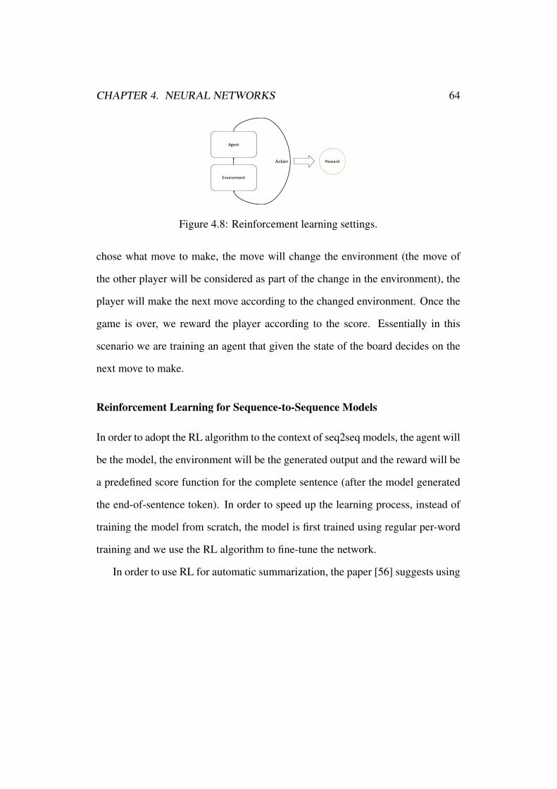
CHAPTER 4. NEURAL NETWORKS 64
Agent
Environment
Action Reward
Figure 4.8: Reinforcement learning settings.
chose what move to make, the move will change the environment (the move of
the other player will be considered as part of the change in the environment), the
player will make the next move according to the changed environment. Once the
game is over, we reward the player according to the score. Essentially in this
scenario we are training an agent that given the state of the board decides on the
next move to make.
Reinforcement Learning for Sequence-to-Sequence Models
In order to adopt the RL algorithm to the context of seq2seq models, the agent will
be the model, the environment will be the generated output and the reward will be
a predefined score function for the complete sentence (after the model generated
the end-of-sentence token). In order to speed up the learning process, instead of
training the model from scratch, the model is first trained using regular per-word
training and we use the RL algorithm to fine-tune the network.
In order to use RL for automatic summarization, the paper [56] suggests using

CHAPTER 4. NEURAL NETWORKS 65
PWKPMODEL BLEU SARI
ABS+ 88.85 35.66RL+switch 80.12 37.27
Table 4.4: Comparison of Attention-Based Encoder (ABS) to Attention-BasedEncoder with switching generator-pointer mechanism trained using reinforcementlearning algorithm
the following reward function.
Reward(sent) = �ss(sent) + �rr(sent) + �ff(sent) (4.19)
s(sent) = SARI(sent) (4.20)
r(sent) = cos(sent, gold) (4.21)
f(sent) = LM(sent) (4.22)
The s term represents the sentence simplicity score, it is calculated using the
SARI function defined to measure text simplicity in Xu et al. [65]. The r term
represents the relevance of the output to the source sentence: it is the cosine sim-
ilarity function on the generated sentence and the ground truth vectors. The f
term is the fluency score (how fluent is the text) measured using an LSTM-trained
language model.
Experiments
The model was trained and tested on the PWKP dataset and compared the attention-
encoder-decoder model. The output of the model was scored using BLEU [23] and
the SARI function (also used for reinforcement).
While the RL algorithm did not improve the network term coverage, it gener-

CHAPTER 4. NEURAL NETWORKS 66
ated simpler text according to the SARI evaluation.
4.5 Conclusion
In this chapter, we covered recent developments in abstractive summarization us-
ing neural networks. We first covered the available datasets for the task. We
then introduced the basic building blocks used by all the recent models: RNNs,
sequence to sequence models, attention mechanism.
We then surveyed incremental advancements of abstractive summarization
starting from the first neural encoder-decoder model with attention mechanism.
The following techniques bring significant improvements to abstractive summa-
rizers:
• Deal with large vocabularies using the large-vocabulary-trick which exploits
the shared vocabulary of the input and output
• Deal with rare words by adding the ability of switching between generating
words and copying pointers to the source sequence.
• Avoid repetitions by adding a distraction mechanism to improve attention
coverage.
• Finally, we covered attempts at using reinforcement learning to fine-tune
our summarization models at the sentence level.
All the methods covered have brought dramatic improvements to the field of
single document generic abstractive summarization in the last couple of years.
These early steps indicate that fully abstractive summarization addressing longer

CHAPTER 4. NEURAL NETWORKS 67
documents and more advanced tasks such as query-focused and multi-document
summarization can be achieved by combining the re-usable building blocks we
have described with higher-level models that address rhetorical and information
flow aspects of the challenging summarization task.

Part III
Application of Neural Methods for
Automatic Summarization
68

Chapter 5
Sentence Embedding Evaluation
Using Pyramid Annotation
Word embedding vectors are used as input for seq2seq models. Choosing the
right model and features for producing such vectors is not a trivial task and dif-
ferent embedding methods can greatly affect results. In this chapter we repurpose
the “Pyramid Method” annotations used for evaluating summarization to create
a benchmark for comparing embedding models when identifying paraphrases of
text snippets containing a single clause. We present a method of converting pyra-
mid annotation files into two distinct sentence embedding tests. We show that our
method can produce a good amount of testing data, analyze the quality of the test-
ing data, perform test on several leading embedding methods, and finally explain
the downstream usages of our task and its significance.
69
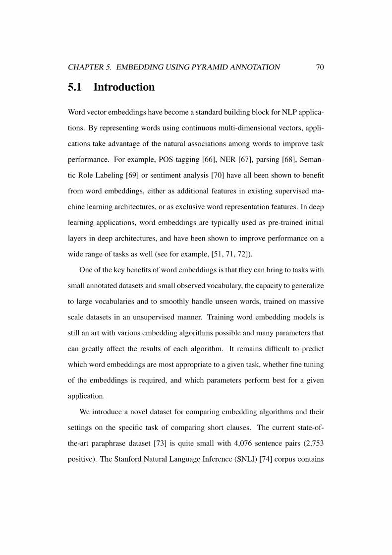
CHAPTER 5. EMBEDDING USING PYRAMID ANNOTATION 70
5.1 Introduction
Word vector embeddings have become a standard building block for NLP applica-
tions. By representing words using continuous multi-dimensional vectors, appli-
cations take advantage of the natural associations among words to improve task
performance. For example, POS tagging [66], NER [67], parsing [68], Seman-
tic Role Labeling [69] or sentiment analysis [70] have all been shown to benefit
from word embeddings, either as additional features in existing supervised ma-
chine learning architectures, or as exclusive word representation features. In deep
learning applications, word embeddings are typically used as pre-trained initial
layers in deep architectures, and have been shown to improve performance on a
wide range of tasks as well (see for example, [51, 71, 72]).
One of the key benefits of word embeddings is that they can bring to tasks with
small annotated datasets and small observed vocabulary, the capacity to generalize
to large vocabularies and to smoothly handle unseen words, trained on massive
scale datasets in an unsupervised manner. Training word embedding models is
still an art with various embedding algorithms possible and many parameters that
can greatly affect the results of each algorithm. It remains difficult to predict
which word embeddings are most appropriate to a given task, whether fine tuning
of the embeddings is required, and which parameters perform best for a given
application.
We introduce a novel dataset for comparing embedding algorithms and their
settings on the specific task of comparing short clauses. The current state-of-
the-art paraphrase dataset [73] is quite small with 4,076 sentence pairs (2,753
positive). The Stanford Natural Language Inference (SNLI) [74] corpus contains

CHAPTER 5. EMBEDDING USING PYRAMID ANNOTATION 71
570k sentences pairs labeled with one of the tags: entailment, contradiction, and
neutral. SNLI improves on previous paraphrase datasets by eliminating indeter-
minacy of event and entity coreference which make human entailment judgment
difficult. Such indeterminacies are avoided by eliciting descriptions of the same
images by different annotators.
We repurpose manually created data sets from automatic summarization to
create a new paraphrase dataset with 197,619 pairs (8,390 positive and challeng-
ing distractors in the negative pairs). Like SNLI, our dataset avoids semantic
indeterminacy because the texts are generated from the same news reports we
thus obtain definite entailment judgments but in the richer domain of news report
as opposed to image descriptions. The propositions in our dataset are on average
12.1 words long (as opposed to about 8 words for the SNLI hypotheses).
In addition to paraphrase, our dataset captures a notion of centrality, the clause
elements captured are Summary Content Units (SCU) which are typically shorter
than full sentences and intended to capture proposition-level facts. As such, the
new dataset is relevant for exercising the large family of “Sequence to Sequence”
(seq2seq) tasks involving the generation of short text clauses [50].
The chapter is structured as follows: 5.2 describes the process for generating
a paraphrase dataset from a pyramid dataset; in 5.3, we evaluate a number of
algorithms on the new benchmark and in 5.4, we explain the importance of the
task.

CHAPTER 5. EMBEDDING USING PYRAMID ANNOTATION 72
Non-paraphrase pair:‘Countries worldwidesent Equipment,’ ‘Coun-tries worldwide sentRelief Workers’
Paraphrase pair:‘countries worldwidesent money equipment,’‘rescue equipmentpoured in from aroundthe world’
Figure 5.1: Binary test pairs example
5.2 Repurposing Pyramid Annotations
We define two types of tests that can be produced from a pyramid file: a binary
decision test and a ranking test. For the binary decision test, we collect pairs
of different SCUs from manual summaries and the label given to the SCU by
annotators. The binary decision consists of deciding whether the pair is taken
from the same SCU. In order to make the test challenging and still achievable, we
add the following constraints on pair selection:
• Both items must contain at least 3 words;
• For non-paraphrase pairs, both items must match on more than 3 words;
• Both items must not include any pronouns;
• The pair must be lexically varied (at least one content word must be different
across the items)
For the ranking test, we generate a set of multiple choice questions by taking
as a question an SCU appearance in the text and the correct answer is another
appearance of the same SCU in the test. To create synthetic distractors, we use
the 3 most lexically similar text segments from distinct SCUs:

CHAPTER 5. EMBEDDING USING PYRAMID ANNOTATION 73
Morris Dees co-founded the SPLC:
1. Morris Dees was co-founder of the Southern Poverty Law Center(SPLC) in 1971 and has served as its Chief Trial Counsel andExecutive Director
2. Dees and the SPLC seek to destroy hate groups through multi-milliondollar civil suits that go after assets of groups and their leaders
3. Dees and the SPLC have fought to break the organizations by legalaction resulting in severe financial penalties
4. The SPLC participates in tracking down hate groups and publicizingtheir activities in its Intelligence Report
Figure 5.2: Ranking test example question
Using DUC-2007, 2006 and 2005 pyramid files (all contain news stories), we
created 8,755 questions for the ranking test and for the binary test we generated
8,390 positive pairs, 189,229 negative pairs for a total 197,619 pairs. The propo-
sitions in the dataset contain 95,286 words (6,882 unique).
5.3 Baseline Embeddings Evaluation
In order to verify that this task indeed is sensitive to differences in word em-
beddings, we evaluated 8 different word embeddings on the task as a baseline:
Random, None (One-Hot embedding), word2vec [75] trained on Google News
and two models trained on Wikipedia with different window sizes [76], word2vec
trained with Wikipedia dependencies [76], GloVe [43] and Open IE based em-
beddings [77]. For all of the embeddings, we measured sentence similarity as the
cosine similarity of the normalized sum of all the words in the sentences.1
1Using spaCy for tokenization

CHAPTER 5. EMBEDDING USING PYRAMID ANNOTATION 74
Binary Test (F-measure)
Ranking Test(Success Rate)
Ranking Test(Mean reciprocalrank)
Random-Baseline 0.04059 24.662% 0.52223
One-Hot 0.26324 63.973% 0.77202word2vec-BOW(google-news) 0.42337 66.960% 0.78933
word2vec-BOW2(Wikipedia)
0.39450 61.684% 0.75274
word2vec-BOW5(Wikipedia)
0.40387 62.886% 0.76292
word2vec-Dep 0.39097 60.025% 0.74003GloVe 0.37870 63.000% 0.76389Open IE Embed-ding 0.42516 65.667% 0.77847
Table 5.1: Different embedding performance on binary and ranking tests.
For the binary decision test, we evaluated the embedding by finding a thresh-
old for answering where a pair is a paraphrase that maximizes the F-measure
(trained over 10% the dataset and tested on the rest) of the embedding decision.
For the rank test, we computed the percentage of questions where the correct an-
swer achieved the highest similarity score and the MRR measure [78].
The OpenIE Embedding model scored the highest for the binary test (0.42
F). Word2vec model trained on google news achieved the best success rate in the
ranking test (precision@1 of 66.9%), significantly better than the word2vec model
trained on Wikipedia (62.8%). MRR for ranking was dominated by word2vec with
0.41.

CHAPTER 5. EMBEDDING USING PYRAMID ANNOTATION 75
5.4 Task Significance
The task of identifying paraphrases specifically extracted from pyramids can aid
NLP sub-fields such as:
• Automatic Summarization: Identifying paraphrases can both help identi-
fying salient information in multi-document summarization and evaluation
by recreating pyramid files and applying them on automatic summaries;
• Textual Entailment: Paraphrases are bi-directional entailments;
• Sentence Simplification: SCUs capture the central elements of meaning in
observable long sentences.
• Expansion of Annotated Datasets: Given an annotated dataset (e.g., aligned
translations), unannotated sentences could be annotated the same as their
paraphrases
5.5 Conclusion
We presented a method of using pyramid files to generate paraphrase detection
tasks. The suggested task has proven challenging for the tested methods, as indi-
cated by the relatively low F-measures reported in Table 1 on most models. Our
method can be applied on any pyramid annotated dataset so the reported numbers
could increase by using other datasets such as TAC 2008, 2009, 2010, 2011 and
2014.2 We believe that the improvement that this task can provide to downstream
applications is a good incentive for further research.
2http://www.nist.gov/tac/tracks/index.html

Chapter 6
Multi-Label Classification on
Patient Notes With Neural Encoders
In the context of the Electronic Health Record, automated diagnosis coding of
patient notes is a useful task, but a challenging one due to the large number of
codes and the length of patient notes. We investigate three different neural en-
coders and an SVM model for assigning multiple ICD codes to discharge sum-
maries taken from both MIMIC II and III. We present Hierarchical Attention-
bidirectional Gated Recurrent Unit (HA-GRU), a hierarchical approach to tag a
document by identifying the sentences relevant for each label. HA-GRU achieves
state-of-the art results. Furthermore, the learned sentence-level attention layer
highlights the model decision process, allows easier error analysis, and suggests
future directions for improvement.
In the context of our analysis of neural network architectures for abstractive
summarizations, the task of multi-label document classification we study here
serves as an auxiliary task to assess the capability of RNN encoders to capture
76
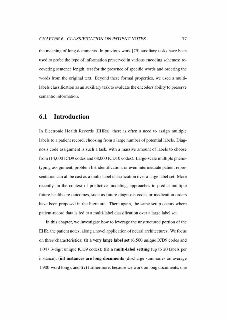
CHAPTER 6. CLASSIFICATION ON PATIENT NOTES 77
the meaning of long documents. In previous work [79] auxiliary tasks have been
used to probe the type of information preserved in various encoding schemes: re-
covering sentence length, test for the presence of specific words and ordering the
words from the original text. Beyond these formal properties, we used a multi-
labels classification as an auxiliary task to evaluate the encoders ability to preserve
semantic information.
6.1 Introduction
In Electronic Health Records (EHRs), there is often a need to assign multiple
labels to a patient record, choosing from a large number of potential labels. Diag-
nosis code assignment is such a task, with a massive amount of labels to choose
from (14,000 ICD9 codes and 68,000 ICD10 codes). Large-scale multiple pheno-
typing assignment, problem list identification, or even intermediate patient repre-
sentation can all be cast as a multi-label classification over a large label set. More
recently, in the context of predictive modeling, approaches to predict multiple
future healthcare outcomes, such as future diagnosis codes or medication orders
have been proposed in the literature. There again, the same setup occurs where
patient-record data is fed to a multi-label classification over a large label set.
In this chapter, we investigate how to leverage the unstructured portion of the
EHR, the patient notes, along a novel application of neural architectures. We focus
on three characteristics: (i) a very large label set (6,500 unique ICD9 codes and
1,047 3-digit unique ICD9 codes); (ii) a multi-label setting (up to 20 labels per
instance); (iii) instances are long documents (discharge summaries on average
1,900-word long); and (iv) furthermore, because we work on long documents, one

CHAPTER 6. CLASSIFICATION ON PATIENT NOTES 78
critical aspect of the multi-label classification is transparency—to highlight the
elements in the documents that explain and support the predicted labels. While
there has been much work on each of these characteristics, there has been limited
work to tackle all at once, particularly in the clinical domain.
We experiment with four approaches to classification: an SVM-based one-vs-
all model, a continuous bag-of-words (CBOW) model, a convolutional neural
network (CNN) model, and a bidirectional Gated Recurrent Unit model with
a Hierarchical Attention mechanism (HA-GRU). Among them, the attention
mechanism of the HA-GRU model provides full transparency for classification
decisions. We rely on the publicly available MIMIC datasets to validate our exper-
iments. A characteristic of the healthcare domain is long documents with a large
number of technical words and typos/misspellings. We experiment with simple
yet effective preprocessing of the input texts.
Our results show that careful tokenization of the input texts, and hierarchical
segmentation of the original document allow our Hierarchical Attention GRU ar-
chitecture to yield the most promising results, over the SVM, CBOW, and CNN
models, while preserving the full input text and providing effective transparency.
6.2 Previous Work
We review previous work in the healthcare domain as well as recent approaches
to extreme multi-label classification, which take place in a range of domains and
tasks.

CHAPTER 6. CLASSIFICATION ON PATIENT NOTES 79
6.2.1 Multi-label Patient Classifications
Approaches to classification of patient records against multiple labels fall into
three types of tasks: diagnosis code assignment, patient record labeling, and pre-
dictive modeling.
Diagnosis Code Assignment. Automated ICD coding is a well established task,
with several methods proposed in the literature, ranging from rule based [80, 81]
to machine learning such as support vector machines, Bayesian ridge regression,
and K-nearest neighbor [82, 83]. Some methods exploit the hierarchical structure
of the ICD taxonomy [84, 85], while others incorporated explicit co-occurrence
relations between codes [86]. In many cases, to handle the sheer amount of labels,
the different approaches focus on rolled-up ICD codes (i.e., 3-digit version of the
codes and their descendants in the ICD taxonomy) or on a subset of the codes,
like in the shared community task for radiology code assignment [87].
It is difficult to compare the different methods proposed, since each relies
on different (and usually not publicly available) datasets. We experiment with the
MIMIC dataset, since it is publicly available to the research community. Methods-
wise, our approach departs from previous work in two important ways: we ex-
periment with both massively large and very large label sets (all ICD9 code and
rolled-up ICD9 codes), and we experiment with transparent models that highlight
portions of the input text that support the assigned codes.
Patient Record Labeling. Other than automated diagnosis coding, most multi-
label patient record classifiers fall in the tasks of phenotyping across multiple
conditions at once. For instance, the UPhenome model takes a probabilistic gen-

CHAPTER 6. CLASSIFICATION ON PATIENT NOTES 80
erative approach to assign 750 latent variables [88]. More recently, in the context
of multi-task learning, Harutyunyan and colleagues experimented with phenotyp-
ing over 25 critical care conditions [89].
Predictive Modeling. Previous work in EHR multi-label classification has mostly
focused on predictive scenarios. The size of the label set varies from one approach
to another, and most limit the label set size however: DeepPatient [90] predicts
over a set of 78 condition codes. [91] leverage an LSTM model to predict over
a vocabulary of 128 diagnosis codes. DoctorAI [92] predicts over a set of 1,183
3-digit ICD codes and 595 medication groups. The Survival Filter [93] predicts a
series of future ICD codes across approximately 8,000 ICD codes.
Inputs to Multi-Label Classifications. Most work in multi-label classification
takes structured input. For instance, the Survival Filter expects ICD codes as
input to predict the future ICD codes. DoctorAI takes as input medication orders,
ICD codes, problem list, and procedure orders at a given visit. Deep Patient does
take the content of notes as input, but the content is heavily preprocessed into a
structured input to their neural network, by tagging all texts with medical named
entities. In contrast, our approach is to leverage the entire content of the input
texts. Our work contributes to clinical natural language processing [94], which
only recently investigated neural representations and architectures for traditional
tasks such as named entity recognition [95].

CHAPTER 6. CLASSIFICATION ON PATIENT NOTES 81
6.2.2 Multi-label Extreme Classification
In extreme multi-label learning, the objective is to annotate each data point with
the most relevant subset of labels from an extremely large label set. Much work
has been carried outside of the healthcare domain on tasks such as image clas-
sification [96, 97], question answering [98], and advertising [99]. In [97], the
task of annotating a very large dataset of images (> 10M ) with a very large label
set (> 100K) was first addressed. The authors introduced the WSABIE method
which relies on two main features: (i) records (images) and labels are embed-
ded in a shared low-dimension vector space; and (ii) the multi-label classification
task is modeled as a ranking problem, evaluated with a Hamming Loss on a P@k
metric. The proposed online approximate WARP loss allowed the algorithm to
perform fast enough on the scale of the dataset. We found that in our case, the
standard Micro-F measure is more appropriate as we do not tolerate approximate
annotations to the same extent as in the image annotation task.
The SLEEC method [100] also relies on learning an embedding transforma-
tion to map label vectors into a low-dimensional representation. SLEEC learns
an ensemble of local distance preserving embeddings to accurately predict infre-
quently occurring labels. This approach attempts to exploit the similarity among
labels to improve classification, and learns different representations for clusters
of similar labels. Other approaches attempt to reduce the cost of training over
very large datasets by considering only part of the labels for each classification
decision [101]. SLEEC was later improved in [99] with the PfastreXML method
which also adopted P@k loss functions aiming at predicting tail labels.
In [102], the FastText method was introduced as a simple and scalable neural

CHAPTER 6. CLASSIFICATION ON PATIENT NOTES 82
bag of words approach for assigning multiple labels to text. We test a similar
model (CBOW) in our experiments as one of our baselines.
6.3 Dataset and Preprocessing
We use the publicly available de-identified MIMIC dataset of ICU stays from Beth
Israel Deaconess Medical Center [103, 104].
6.3.1 MIMIC Datasets
To test the impact of training size, we relied on both the MIMIC II (v2.6) and
MIMIC III (v1.4) datasets. MIMIC III comprises records collected between 2001
and 2012, and can be described as an expansion of MIMIC II (which comprises
records collected between 2001 and 2008), along with some edits to the dataset
(including de-identification procedures).
To compare our experiments to previous work in ICD coding, we used the
publicly available split of MIMIC II from [85]. It contains 22,815 discharge
summaries divided into a training set (20,533 summaries) and a test-set of unseen
patients (2,282 summaries). We thus kept the same train and the test-set from
MIMIC II, and constructed an additional training set from MIMIC III. We made
sure that the test-set patients remained unseen in this training set as well. Overall,
we have two training sets, which we refer to as MIMIC II and MIMIC III, and a
common test-set comprising summaries of unseen patients.
While there is a large overlap between MIMIC II and MIMIC III, there are
also marked differences. We found many cases where discharge summaries from
2001-2008 are found in one dataset but not in the other. In addition, MIMIC III

CHAPTER 6. CLASSIFICATION ON PATIENT NOTES 83
MIMIC II MIMIC III Test Set
# of records 20,533 49,857 2,282# of unique tokens 69,248 119,171 33,958Avg # of tokens / record 1,529 1,947 1,893Avg # of sentences / record 90 112 104# of full labels 4,847 6,527 2,451# of rolled-up labels 948 1,047 684Label Cardinality 9.24 11.48 11.42Label Density 0.0019 0.0018 0.0047% labels with 50+ records 11.33% 18.19% 4.08%
Table 6.1: Datasets descriptive statistics.
contains addenda to the discharge summaries that were not part of MIMIC II.
After examining the summaries and their addenda, we noticed that the addenda
contain vital information for ICD coding that is missing from the main discharge
summaries; therefore, we decided to concatenate the summaries with their ad-
denda.
Table 6.1 reports some descriptives statistics regarding the datasets. Overall,
MIMIC III is larger than MIMIC II from all standpoints, including amounts of
training data, vocabulary size, and overall number of labels.
6.3.2 ICD9 Codes
Our label set comes from the ICD9 taxonomy. The International Classification
of Diseases (ICD) is a repository maintained by the World Health Organization
(WHO) to provide a standardized system of diagnostic codes for classifying dis-
eases. It has a hierarchical structure, connecting specific diagnostic codes through
is-a relations. The hierarchy has eight levels, from less specific to more specific.
ICD codes contain both diagnosis and procedure codes. In this chapter, we focus

CHAPTER 6. CLASSIFICATION ON PATIENT NOTES 84
on diagnosis codes only. ICD9 codes are conveyed as 5 digits, with 3 primary
digits and 2 secondary ones.
Table 6.1 provides the ICD9 label cardinality and density as defined by [96].
Cardinality is the average number of codes assigned to records in the dataset.
Density is the cardinality divided by the total number of codes. For both training
sets, the number of labels is of the same order as the number of records, and the
label density is extremely low. This confirms that the task of code assignment
belongs to the family of extreme multi-label classification.
We did not filter any ICD code based on their frequency. We note, however
that there are approximately 1,000 frequent labels (defined as assigned to at least
50 records) (Table 6.1). We experimented with two versions of the label set: one
with all the labels (i.e., 5-digit), and one with the labels rolled up to their 3-digit
equivalent.
6.3.3 Input Texts
Tokenization. Preprocessing of the input records comprised the following steps:
(i) tokenize all input texts using spaCy library; 1 (ii) convert all non-alphabetical
characters to pseudo-tokens (e.g., “11/2/1986” was mapped to “dd/d/dddd”); (iii)
build the vocabulary as tokens that appear at least 5 times in the training set; and
(iv) map any out-of-vocabulary word to its nearest word in the vocabulary (us-
ing the edit distance). This step is simple, yet particularly useful in reducing the
number of misspellings of medical terms. These preprocessing steps has a strong
impact on the vocabulary. For instance, there were 1,005,489 unique tokens in
MIMIC III and test set before preprocessing, and only 121,595 remaining in the1https://spacy.io/

CHAPTER 6. CLASSIFICATION ON PATIENT NOTES 85
vocabulary after preprocessing (an 88% drop). This step improved F-measure per-
formance by ˜0.5% when tested on the CBOW and CNN methods (not reported).
Hierarchical Segmentation. Besides tokenization of the input texts, we carried
one more level of segmentation, at the sentence level (using the spaCy library
as well). There are two reasons for preprocessing the input texts with sentence
segmentation. First, because we deal with long documents, it is impossible and
ineffective to train a sequence model like an GRU on such long sequences. In pre-
vious approaches in document classification, this problem was resolved by trun-
cating the input documents. In the case of discharge summaries, however, this
is not an acceptable solution: we want to preserve the entire document for trans-
parency. Second, we are inspired by the moving windows of [105] and posit that
sentences form linguistically inspired windows of word sequences.
Beyond tokens and sentences, discharge summaries exhibit strong discourse-
level structure (e.g., history of present illness and past medical history, followed by
hospital course, and discharge plans) [106]. This presents an exciting opportunity
for future work to exploit discourse segments as an additional representation layer
of input texts.
6.4 Methods
We describe the four models with which we experimented. ICD coding has been
evaluated in the literature according to different metrics: Micro-F, Macro-F, a vari-
ant of Macro-F that takes into account the hierarchy of the codes [85], Hamming
and ranking loss [107], and a modified version of mean reciprocal rank (MRR)

CHAPTER 6. CLASSIFICATION ON PATIENT NOTES 86
[108]. We evaluate performance using the Micro-F metric, since it is the most
commonly used metric.
SVM. We used Scikit Learn [109] to implement a one-vs-all, multi-label binary
SVM classifier. Features were bag of words, with tf*idf weights (determined from
the corpus of release notes) for each label. Stop words were removed using Scikit
Learn default English stop-word list. The model fits a binary SVM classifier for
each label (ICD code) against the rest of the labels. We also experimented with �2
feature filtering to select the top-N words according to their mutual information
with each label, but this did not improve performance.
We experimented with various ways to exploit the ICD label hierarchy in the
one-vs-rest schemes, but this did not lead to any measurable improvement.
CBOW. The continuous-bag-of-words (CBOW) model is inspired by the word2vec
CBOW model [42] and FastText [102]. Both methods use a simple neural-network
to create a dense representation of words and use the average of this representation
for prediction. The word2vec CBOW tries to predict a word from the words that
appear around it, while our CBOW model for ICD classification predicts ICD9
codes from the words of its input discharge summary.
The model architecture consists of an embedding layer applied to all the words
in a given input text [w1, w2, ..., wn], where wi is a one-hot encoding vector of the
vocabulary. E is the embedding matrix with dimension nemb ⇥ V , where V is the
size of the vocabulary and nemb is the embedding size (set to 100).
The embedded words are averaged into a fixed-size vector and are fed to a
fully connected layer with a matrix W and bias b, where the output dimension is
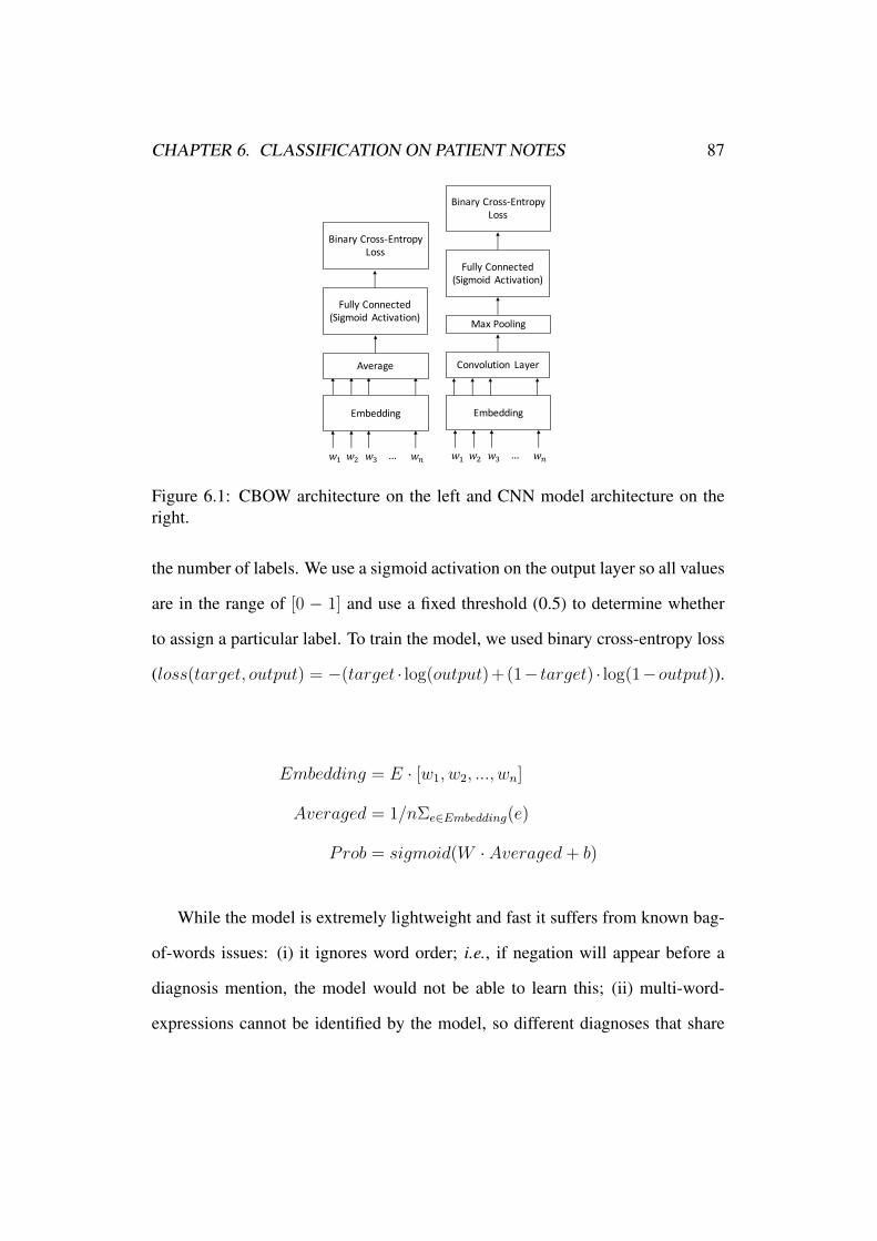
CHAPTER 6. CLASSIFICATION ON PATIENT NOTES 87
Embedding
!" !# !$ !%…
MaxPooling
FullyConnected(Sigmoid Activation)
BinaryCross-EntropyLoss
Convolution Layer
Embedding
!" !# !$ !%…
Average
FullyConnected(Sigmoid Activation)
BinaryCross-EntropyLoss
Figure 6.1: CBOW architecture on the left and CNN model architecture on theright.
the number of labels. We use a sigmoid activation on the output layer so all values
are in the range of [0 � 1] and use a fixed threshold (0.5) to determine whether
to assign a particular label. To train the model, we used binary cross-entropy loss
(loss(target, output) = �(target · log(output)+(1� target) · log(1�output)).
Embedding = E · [w1, w2, ..., wn]
Averaged = 1/n⌃e2Embedding(e)
Prob = sigmoid(W · Averaged+ b)
While the model is extremely lightweight and fast it suffers from known bag-
of-words issues: (i) it ignores word order; i.e., if negation will appear before a
diagnosis mention, the model would not be able to learn this; (ii) multi-word-
expressions cannot be identified by the model, so different diagnoses that share

CHAPTER 6. CLASSIFICATION ON PATIENT NOTES 88
lexical words will not be distinguished by the model.
CNN. To address the problems of the CBOW model, the next model we inves-
tigate is a convolutional neural network (CNN). A one dimensional convolution
applied on list of embedded words could be considered as a type of n-gram model,
where n is the convolution filter size.
The architecture of this model is very similar to the CBOW model, but instead
of averaging the embedded words we apply a one dimensional convolution layer
with filter f , followed by a max pooling layer. On the output of the max pool
layered a fully connected layer was applied, like in the CBOW model. We also
experimented with deeper convolution networks and inception module [110], but
they did not yield improved results.
Embedding = E · [w1, w2, ..., wn]
Conved = maxi2channels
([wi, wi+1, ..., wi+filter size] ⇤ filter)
Prob = sigmoid(W · Conved+ b)
In our experiments, we used the same embedding parameter as in the CBOW
model. In addition, we set the number of channels to 300, and the filter size to 3.
HA-GRU. We now introduce the Hierarchical Attention-bidirectional Gated Re-
current Unit model (HA-GRU) an adaptation of a Hierarchical Attention Net-
works [111] to be able to handle multi-label classification. A Gated Recurrent
Unit (GRU) is a type of Recurrent Neural Network. Since the documents are long
CHAPTER 6. CLASSIFICATION ON PATIENT NOTES 89
(see Table 6.1 up to 13,590 tokens in the MIMIC III training set), a regular GRU
applied over the entire document is too slow as it requires a number of layers of
the document length. Instead we apply a hierarchal model with two levels of bidi-
rectional GRU encoding. The first bidirectional GRU operates over tokens and
encodes sentences. The second bidirectional GRU encodes the document, applied
over all the encoded sentences. In this architecture, each GRU is applied to a
much shorter sequence compared to a flat GRU model.
To take advantage of the property that each label is invoked from different parts
of the text, we use an attention mechanism over the second GRU with different
weights for each label. This allows the model to focus on the relevant sentences
for each label [98]. To allow clarity into what the model learns and enable error
analysis, attention is also applied over the first GRU with the same weights for all
the labels.
ClassifiersClassifiers
!","!",$!",% !",&'…
SentenceEncoder
DocumentGRULayer
Classifiers
!$,"!$,$!$,% !$,&)… !*,"!*,$!*,% !*,&+…
SentenceEncoder SentenceEncoder
…Figure 6.2: HA-GRU model architecture overview.
Each sentence in the input text is encoded to a fixed length vector (64) by ap-
plying an embedding layer over all the inputs, applying a bidirectional GRU layer
on the embedded words, and using a neural attention mechanism to encode the

CHAPTER 6. CLASSIFICATION ON PATIENT NOTES 90
bidirectional GRU outputs (size of 128). After the sentences are encoded into a
fixed length vector, we apply a second bidirectional GRU layer over the sentences
using different attention layers to generate an encoding specified to each class
(128⇥#labels). Finally we applied a fully connected layer with softmax for each
classifier to determine if the label should be assigned to the document. Train-
ing is achieved by using categorical cross-entropy on every classifier separately
(loss(target, output) = �P
x output(x) · log(target(x)))
AttWeight(ini, v, w) = v · tanh(w · (ini))
AttWeight(ini, v, w) =eAttWeight(ini,v,w)
e
Pj AttWeightj(v,w)
Attend(in, v, w) = sum(ini · AttWeight(ini, v, w))
Embedding = E · [w1, w2, ..., wn]
EncSentsj = Attend(GRUwords(Embedding), vwords, wwords)
EncDoclabel = Attend(GRUsents(EncSents, vlabel, wlabel), )
Problabel = softmax(pwlabel · EncDoclabel + pblabel)
Where wi is a one-hot encoding vector of the vocabulary size V , E is an
embedding matrix size of nemb ⇥ V , GRUwords is a GRU layer with state size
hstate, wwords is a square matrix (hstate⇥hstate) and vwords is a vector (hstate) for the
sentence level attention. GRUsents is a GRU layer with state size of hstate. wlabel
is a square matrix (hstate ⇥ hstate) and vlabel is a vector (hstate) for the document
level attention for each class, pwlabel is a matrix (hstate ⇥ 2) and pblabel is a bias
vector with a size of 2 for each label. We implemented the model using DyNet

CHAPTER 6. CLASSIFICATION ON PATIENT NOTES 91
[112].2
Embedding
!",$ !",% !",& !",'(…
SentenceGRULayer
SentenceAttention
SentenceEncoder
*"
WeightedAverage
Classifier
*$ *% *& *'…
LabelAttention
WeightedAverage
FullyConnectedLayer
Softmax
CategoricalCross-Entropyloss
+"
Figure 6.3: Zoom-in of the sentence encoder and classifier.
6.5 Results
6.5.1 Model Comparison
To evaluate the proposed methods on the MIMIC datasets, we conducted the fol-
lowing experiments. In the first setting we considered all ICD9 codes as our label
set. We trained the SVM, CBOW, and CNN on the MIMIC II and on the MIMIC
III training sets separately. All models were evaluated on the same test set ac-
cording to Micro-F. In the second setting, we only considered the rolled-up ICD92Code available at https://github.com/talbaumel/MIMIC.

CHAPTER 6. CLASSIFICATION ON PATIENT NOTES 92
ICD9 codes Rolled-up ICD9 codesMIMIC II MIMIC III MIMIC II MIMIC III
SVM 28.13% 22.25% 32.50% 53.02%CBOW 30.60% 30.02% 42.06% 43.30%CNN 33.25% 40.72% 46.40% 52.64%HA-GRU 36.60% 40.52% 53.86% 55.86%
Table 6.2: Micro-F on two settings (full and rolled-up ICDs) and for the fourmodels when trained on MIMIC II or MIMIC III datasets.
codes to their 3-digit codes. There (Table 6.2).
HA-GRU gives the best results in the rolled-up ICD9 setting, with a 7.4% and
3.2% improvement over the CNN and SVM, the second best methods, in MIMIC
II and MIMIC III respectively. In the full ICD-9 scenario, all methods yield better
results when trained on MIMIC III rather than on MIMIC II. This is expected
considering the larger size of MIMIC III over II. We note that our CNN yields the
best Micro-F when trained on MIMIC III passing the HA-GRU by a small margin.
In comparison to the previous work of [85], our one-vs-all SVM yielded bet-
ter results than their flat and hierarchy classifiers. This trend was confirmed when
training on the new MIMIC III set, as well as when using the same evaluation met-
rics of [85]. We attribute these improved results both to the one-vs-all approach
as well as our tokenization approach.
6.5.2 Label Frequency
We tested the effect of label frequency on the performance of the HA-GRU classi-
fier. We recalculated precision and recall scores on subsets of labels. The subsets
were created by sorting the labels by frequency they appear in MIMIC-III dataset
and binning them to groups of 50 labels. As such, bin 1 comprises the 50 most

CHAPTER 6. CLASSIFICATION ON PATIENT NOTES 93
Figure 6.4: Sample text of a patient note (one sentence per line). On the left, visu-alization for the with attention weights at the sentence and word levels associatedwith the ICD9 codes, on the left sentence level attention weights for ICD9 code“Heart failure”, on the the right for code “Traumatic pneumothorax and hemoth-orax”.
Figure 6.5: Effect label frequency on HA-GRU performance when trained onMIMIC III. X-axis represents the bins of labels ranked by their frequency in thetraining set.
frequent ICD9 codes in the training set (with an average 12% frequency over the
records in the training set), codes in bin 2 had an average 1.9% frequency, codes
in bin 3 appeared in 1.1% of the records, up to bin 8 which 0.2% of the records in
the training set. The effect can be seen in Figure 6.5. We note that the recall score
drops much more dramatically than the precision as the label frequency decreases.
CHAPTER 6. CLASSIFICATION ON PATIENT NOTES 94
6.5.3 Model Explaining Power
We discuss how the CNN and HA-GRU architectures can support model explain-
ing power.
CNN. To analyze the CNN prediction we can test which n-grams triggered the
max-pooling layer. Given a sentence with n words we can feed it forward through
the embedding layer and the convolution layer. The output of the convolution a
list of vectors each the size of the number of channels of the convolution layer
where vector corresponds to an n-gram. We can identify what triggered the max
pooling layer by finding the maximum value of each channel. Thus, for predicted
labels, one of the activated n-grams does include information relevant for that label
(whether correct for true positive labels or incorrect for false positive labels). For
example in our experiments, for the label: “682.6-Cellulitis and abscess of leg,
except foot” one of the activated n-gram detected was “extremity cellulitis prior”.
This transparency process can also be useful for error analysis while building
a model, as it can highlight True Positive and False Positive labels. However, it is
difficult in the CNN to trace back the decisions for False Negatives predictions.
HA-GRU For the HA-GRU model we can use attention weights to better un-
derstand what sentences and what words in that sentence contributed the most to
each decision. We can find which sentence had the highest attention score for each
label, and given the most important sentence, we can find what word received the
highest attention score. For example, in our experiments for label “428-Heart
failure” we found that the sentence with the highest attention score was “d . con-
gestive heart failure ( with an ejection fraction of dd % to dd % ) .”, while the

CHAPTER 6. CLASSIFICATION ON PATIENT NOTES 95
token “failure” was found most relevant across all labels. Figure 6.4 provides ad-
ditional examples. Note that the “d” and “dd” tokens are from the pre-procecssing
step, which mapped all numbers to pseudo-tokens.
Like in the CNN, we can use this process for error analysis. In fact, the HA-
GRU model explains prediction with greater precision, at the sentence level. For
instance, we could explore the following False Positive prediction: the model as-
signed the label “331-Other cerebral degenerations” to the sentence:“alzheimer
’s dementia .”. We can see that the condition was relevant to the medical note,
but was mentioned under the patient’s past medical history (and not a current
problem). In fact, many of the False Positive labels under the HA-GRU model
were due to mentions belonging to the past medical history section. This suggests
that the coding task would benefit from a deeper architecture, with attention to
discourse-level structure.
In contrast to the CNN, the HA-GRU model can also help analyze False Neg-
ative label assignments. When we explored the False Negative labels, we found
that in many cases the model found a relevant sentence, but failed to classify cor-
rectly. This suggests the document-level attention mechanism is successful. For
instance, for the False Negative “682-Other cellulitis and abscess”, the most at-
tended sentence was “... for right lower extremity cellulitis prior to admission ...”.
The false positive codes for this sentence included “250-Diabetes mellitus” and
“414-Other forms of chronic ischemic heart disease”. We note that in the case of
cellulitis, it is reasonable that the classifier preferred other, more frequent codes,
as it is a common comorbid condition in the ICU.3
3Full visualizations of sample discharge summaries are provided at https://www.cs.bgu.ac.il/˜talbau/mimicdemo

CHAPTER 6. CLASSIFICATION ON PATIENT NOTES 96
6.6 Conclusion
We investigate four modern models for the task of extreme multi-label classifica-
tion on the MIMIC datasets. Unlike previous work, we evaluate our models on all
ICD9 codes thus making sure our models could be used for real world ICD9 tag-
ging. The tokenization step, mapping rare variants using edit distance, improved
results for CBOW and CNN models by ˜0.5%, highlighting the importance of
preprocessing data noise problems in real-world settings. The HA-GRU model
not only achieves the best performance on the task of rolled-up codes (55.86%
F1 on MIMIC III, ˜2.8% absolute improvement on the best SVM baseline) but is
able to provide insight on the task for future work such as using discourse-level
structure available in medical notes yet never used before. The ability to highlight
the decision process of the model is important for adoption of such models by
medical experts. On the sub-task of MIMIC II, which includes a smaller training
dataset, HA-GRU achieved ˜7% absolute F1 improvement, suggesting it requires
less training data to achieve top performance, which is important for domain adap-
tation efforts when applying such models to patient records from other sources
(such as different hospitals).

Chapter 7
Abstractive Query Focused
Summarization
Query Focused Summarization (QFS) has been addressed mostly using extractive
methods. Such methods, however, produce text which suffers from low coherence.
We investigate how abstractive methods can be applied to QFS, to overcome such
limitations. Recent developments in neural-attention based sequence-to-sequence
models have led to state-of-the-art results on the task of abstractive generic sin-
gle document summarization. Such models are trained in an end to end method
on large amounts of training data. We address three aspects to make abstractive
summarization applicable to QFS: (a) since there is no training data, we incor-
porate query relevance into a pre-trained abstractive model; (b) since existing
abstractive models are trained in a single-document setting, we design an iter-
ated method to embed abstractive models within the multi-document requirement
of QFS; (c) the abstractive models we adapt are trained to generate text of spe-
cific length (about 100 words), while we aim at generating output of a different
97

CHAPTER 7. ABSTRACTIVE QFS 98
size (about 250 words); we design a way to adapt the target size of the generated
summaries to a given size ratio. We compare our method (Relevance Sensitive
Attention for QFS) to extractive baselines and with various ways to combine ab-
stractive models on the DUC QFS datasets and demonstrate solid improvements
on ROUGE performance.
7.1 Introduction
The query-focused summarization (QFS) task was first introduced in DUC 2005
[12]. This task provides a set of queries paired with relevant document collections,
each collection sharing a topic. The expected output is a short summary answering
the query according to data in the documents. Current state-of-the-art methods
for the task [113, 114, 115] are extractive, i.e., the produced summary is a set of
sentences extracted from the document set.
Extractive methods tend to produce less coherent summaries than manually
crafted ones. Some examples of the weaknesses of extractive methods include
unresolved anaphora, unreadable sentence ordering, and lack of cohesiveness in
text. Another problem of extractive methods is the lack of ability to extract salient
information from a long sentence without including less salient information in-
cluded in the sentence: once the system is committed to a sentence, the full sen-
tence will be extracted. It has been well documented that extractive algorithms
[1, 116] tend to prefer longer sentences.
While most of the reasons for the weaknesses of extractive summarization
methods are hard to quantify, we can illustrate the high probability of achieving
incoherent text when applying extractive methods for QFS. We assume that a

CHAPTER 7. ABSTRACTIVE QFS 99
sentence cannot be well understood without its context if it starts with a connective
phrase (which we identify by matching a closed set of connectives) or breaks a co-
reference chain (sentences where a non-proper definite noun phrase or a pronoun
refers to a noun phrase from a preceding sentence – we identified co-reference
chains using core-NLP [117]). The percent of sentences in DUC 2007 that passed
the two conditions mentioned was lower than 11%, so only 11% of the sentences
in DUC 2007 can be understood without context.
This data on the risks of producing low coherence text is a great incentive
to test abstractive summarization methods for the task of QFS. In this work, we
aim at adapting abstractive single document summarization methods to handle the
QFS task.
The first obstacles we face are: (a) no training data is available for training end
to end QFS in a way similar to what was recently done for single document generic
abstractive summarization; (b) existing abstractive models cannot handle multiple
documents as input and do not include an explicit query relevance criterion in
their computation of salient summary content; (c) existing abstractive models have
been trained to produce short summaries regardless of the information density of
the input document. For all these reasons, a direct application of an existing state
of the art abstractive model to a QFS data sample produces inappropriate output
(see Fig. 7.1).
We hypothesize that an existing trained abstractive model encapsulates reusable
linguistic knowledge which we can leverage for the QFS task. We investigate
ways to augment such a pre-trained single document abstractive model with ex-
plicit modeling of query relevance, the ability to handle multiple input documents
and to adjust the length of the produced summary accordingly.

CHAPTER 7. ABSTRACTIVE QFS 100
Query:Where are birth rates declining ? What are the reasons for declining birth rates ? What are the effects of a declining birth rate ?
Unmodified seq2seq model:The factory is a decade away , but there are a few showcase examples including Fanuc , the machine tool manufacturer 's factory near Mount Fuji , where robots make robots .But focused on maximising the use of people , money , time and materials , and humans had to find a way to fit in with the complex machinery beginning to surround them .The rise in the labour force is expected to be 0.8 per cent a year until 1993 .
Modified seq2seq model with word count:labour shortage , brought about by a declining birth rate and a more affluent ad highly educated society . Makes robots an important component of factory automation . Do-or-die escalating skilled labour shortage , brought about by declining birth rate and a more affluent and highly educated society .
Figure 7.1: Comparison of the output of the unmodified seq2seq model of See etal. vs. our model RSA-QFS on a QFS data sample. The unmodified summarylacks coherence and is not relevant to the input query.
We validate this hypothesis within the framework of a sequence to sequence
(seq2seq) architecture with attention mechanism which has been adopted by most
abstractive approaches. We systematically explore the stage at which query rele-
vance is most beneficial to the QFS abstractive process. Further, we experiment
with a method to build a summary through an iterative process of extraction / ab-
straction pairs: batches of relevant content from multiple documents are identified,
then abstracted into a sequence of coherent segments of text.
We compare our system both with top extractive methods and with various
combinations of a pre-trained abstractive model with relevance matching and mul-
tiple document input. We evaluate the proposed model, called Relevance Sensitive
Abstractive QFS (RSA-QFS), on the traditional DUC datasets. Our experiments
demonstrate the potential of abstractive QFS models with solid ROUGE gains
over those baselines.

CHAPTER 7. ABSTRACTIVE QFS 101
7.2 Previous Work
7.2.1 Extractive Methods
Current state-of-the-art methods on the task of QFS on the DUC dataset could be
categorized into unsupervised methods and small scale supervised methods:
Unsupervised methods search for a set sentences that optimizes a gain func-
tion. The Cross Entropy Summarizer (CES) [115] optimizes relevance under
length constraint. This method achieves current state-of-the-art ROUGE scores
on DUC 2005-7 datasets.
Small scale supervised methods use small datasets (usually previous DUC
datasets) to learn a representation of the dataset, and using this representation,
optimize a gain function. A recent example of this approach is DocRebuild [118],
which trains a neural network to find a set of sentences that minimize that origi-
nal document reconstruction error. The method uses DUC 2006-7 to learn word
representations, and obtains results slightly lower than CES.
All of the extractive methods suffer from the coherence problems mentioned
above.
7.2.2 Sequence-to-Sequence Models for Abstractive Summa-
rization
Abstractive methods in generation have emerged as practical tools since 2015.
At this point, the most successful attempts at abstractive summarization are on
the task of generic single document summarization [3, 55, 119, 62] and are based

CHAPTER 7. ABSTRACTIVE QFS 102
on the sequence-to-sequence (seq2seq) approach with attention mechanism [120].
These models include the following components:
Encoder: a neural network transforms a list of words into a list of dense vector
representations. These dense representations aim to capture both the word and
its context. Encoders are most commonly implemented using a word embedding
layer followed by a Recurrent Neural Network (RNN), i.e., a Long Short Term
Memory (LSTM) component [47] or Gated Recurrent Units (GRU) [46]).
Decoder: a neural network generates the next word in the summary conditioned
on the representation of the prefix of the generated text and a dense context vector
representing the input sequence. The decoder is commonly implemented by an
RNN, a fully connected layer with the dimension of the output matching the size
of the vocabulary, and a softmax layer that turns a vector into a distribution over
the vocabulary.
Attention mechanism: a neural network determines the importance of each
encoded word at each decoding step, and maps the variable length list of en-
coded words representations into a fixed-size context representation. The attention
mechanism is commonly implemented using multiple levels of fully connected
layers to calculate the unnormalized attention weight of each word in the input
and a softmax layer to normalize these weights.
The training of such models for abstractive single document summarization has
been made possible by the availability of large scale datasets such as GIGAWORD
[121], the New-York Times dataset [122] and CNN/Daily News [123], which con-

CHAPTER 7. ABSTRACTIVE QFS 103
tain pairs of source text / short text examples. For example, the CNN/Daily Mail
Corpus was automatically curated by matching articles to the summary created by
the site editor. The dataset includes 90K documents from CNN and 196K docu-
ments from the Daily Mail. The average size of an abstract in the corpus is ⇠100
words, and the size of input documents is about 1,000 words. In contrast, the
average abstract length in the DUC QFS dataset is ⇠250 words.
No such large scale dataset is currently available for the QFS task under the
DUC settings. We hypothesize that models trained on such datasets capture the
linguistic capability to combine small windows of coherent sentences into concise
paraphrases. Accordingly, our objective is to adapt such a pre-trained, generic
abstractive summarization architecture to the more complex task of QFS.
Recent work in abstractive QFS summarization [124] attempt to solve the issue
of missing training data by introducing a new dataset for abstractive QFS based
on Debatepedia. The dataset introduced is, however, very different from the DUC
QFS datasets since the summaries presented are debate key points that are not
more than a single short sentence with on average 10 words per summary vs. 250
words in the DUC data; the input texts are also short snippets of text with an
average of 60 words vs. DUC that can reach more than 1,000 words. Because
of the distinct size differences between the DUC and Debatepedia datasets, we
cannot compare the methods directly.
In this work, we focus on adapting a specific architecture: the pointer-generator
with coverage mechanism network of [119], to the QFS task. This model achieves
state-of-the-art ROUGE [25] and readability scores on the single document generic
abstractive summarization task. Although the pointer-generator with coverage
mechanism network includes significant modifications (pointer-network and cov-

CHAPTER 7. ABSTRACTIVE QFS 104
erage mechanisms), it still adheres to the general encoder-decoder-attention archi-
tecture. We thus present our proposed modification in the simplified context of the
generic architecture, as the handling of relevance is orthogonal to the processing
of rare words using switch-generator and the coverage mechanism ability to avoid
redundancy. Our experiments are using the full network.
7.3 Query Relevance
We adopt the approach to QFS formulated in [5]: the QFS task is split into two
stages, a relevance model determines the extent to which passages in the source
documents are relevant to the input query; and a generic summarization method
is applied to combine the relevant passages into a coherent summary. The rel-
evance model identifies redundant, un-ordered passages using Information Re-
trieval methods; whereas the summarization model selects the most salient con-
tent, removes redundancy and organizes the target summary. This schematic ap-
proach is illustrated in Figure 7.2). This method achieves good ROUGE results
when using simple extractive summarization methods such as KL-sum [1] when
the relevance model is of high quality.
Accordingly, in order to adapt abstractive methods to QFS, the first baseline
we consider consists of filtering the input documents according to relevance and
then pass the filtered relevant passages to an abstractive model. We hypothesize
that this approach will not adapt well for abstractive methods because the input
that is generated by the filtering process is quite different from the type of doc-
uments on which the abstractive model was trained: it is not a well structured
coherent document. Abstractive models rely critically on the sequential structure

CHAPTER 7. ABSTRACTIVE QFS 105
DocumentSetDocumentSetDocumentSetDocumentSet
Query
Retrieve RelevantPassages
GenericSummarization Summary
Figure 7.2: Two stage query focused summarization scheme.
of the input to take decision at generation time. Our method aims at preserving
the document structure while infusing relevance into the abstractive model during
decoding.
In this chapter, we consider very simple relevance models and do not attempt
to optimize them – we compare relevance measures based on unigram overlap
between query and sentences, and TF-IDF and word2vec encodings with cosine
distance between the query and sentences. To get an upper bound on the impact
a good relevance model can have, we also consider an Oracle relevance model,
where we compare sentences with the gold summaries using the word count cosine
measure. Our focus is to assess whether the mechanism we propose in order to
combine relevance and abstractive capabilities is capable of producing fluent and
relevant summaries given a good relevance model.
7.4 Methods
7.4.1 Incorporating Relevance in Seq2Seq with Attention Mod-
els
As discussed above, the lack of a large scale dataset similar to QFS task presented
in DUC 2005-7 prevents us from attempting an end-to-end solution that learns to

CHAPTER 7. ABSTRACTIVE QFS 106
generate a relevant summary using a the documents and the query as input. In
order to overcome this obstacle, we split the problem in two tasks - a relevance
model and an abstractive model that takes relevance into account. Relevance can
be introduced into an existing seq2seq with attention model in different ways:
(a) Filter the input to include only sentences with high relevance score and
pass the filtered input to the model at generation time; we test this method as a
baseline. (b) Inject the relevance score into the pre-trained model.
Given a document and a query, we calculate the relevance of each sentence to
the query (as a pre-processing step) and use this relevance as an additional input
to the network. The relevance model predicts the relevance of a sentence given the
query. We project the relevance score of sentences to all the words in the sentence
to obtain a word-level relevance score.
At each decoding step in the abstractive seq2seq model, we multiply each
(unnormalized) attention score of each word calculated by the model by the pre-
computed relevance score, as illustrated in Fig. 7.3. In the unmodified seq2seq
model we adapted [119], the (unnormalized) attention of word i at step t is calcu-
lated by:
eti = v
T tanh(Whhi +WsSt + battn)
where v,Wh,Ws and battn are trained parameters, hi is the encoder output for
word i, and St is the decoder state at step t � 1. The attention scores are later
normalized using a softmax function. In our model, we multiply each word by its

CHAPTER 7. ABSTRACTIVE QFS 107
relevance score before normalization:
eti = Reli ⇥ e
ti
where Reli is the relevance score of wi which combines sentence relevance and
lexical relevance, as predicted using the relevance ranking model (all words in the
same sentence are given the same relevance score). We discuss below the range of
relevance models with which we experimented and how the relevance scores are
calibrated in the model.
In this scheme, the adapted model is able to ignore irrelevant sentences at
generation time, while still benefiting from their context information at encoding
time. This is in contrast to the Filtering baseline, where the encoder is not fed
low-relevance sentences at all. We hypothesize that in our proposed scheme, the
encoder will produce a better representation of the input documents than in the
Filtered baseline because it is used in the same regime in which it was trained.
It is important to note that we do not re-train any of the model, the original pa-
rameters of the baseline encoder-decoder-attention model are re-used unchanged.
7.4.2 Calibrating the Relevance Score
Unlike other normalization methods, the softmax function is very sensitive to the
scale of the input values: when the scale of the input is lower, the variance of the
softmax output is similarly low (see Figure 7.4). When the variance of the soft-
max output is low, there is no single word that receives most of the normalized
attention, and the model is unable to “focus” on a single word. Since most atten-
tion models use softmax to normalize the attention weights it is important to keep

CHAPTER 7. ABSTRACTIVE QFS 108
Decoder
Encoder
RNN
Predict
!"#$
…
%&%' … %)
…
*##%+#,!+-
.$ .$/'Attention
0' 01
#2+ℎ
4
0' 01
#2+ℎ
4
.$ .$%)%&
SoftMax
5"6%&%' … %)
7%6&× 7%6)×
7%69%:#!;
0<
=$
0<
=$
…=$
Figure 7.3: Illustration of the RSA-QFS architecture: RelV ector is a vector ofthe same length as the input (n) where the ith element is the relevance score of theith input word. RelV ector is calculated in advance and is part of the input.
their scale when multiplying them by the relevance scores to keep well calibrated
attention scores.
To address this issue, we multiplied the cosine similarity scores (from the TF-
IDF and word2vec based methods) by 10 in order to increase the scale from 0–1
to 0–10 before applying softmax normalization. This scale modification had a
significant impact on the reported ROUGE performance.
7.4.3 Adapting Abstractive Models to Multi-Document Sum-
marization with Long Output
Summarization datasets such as the Daily-Mail/CNN include single-document in-
put and short summary (about 100 words where DUC requires 250 words). We
need to adapt the pre-trained abstractive model to handle the multi-document sce-

CHAPTER 7. ABSTRACTIVE QFS 109
Figure 7.4: A demonstration of the scale sensitivity of the softmax function. Bothfigures illustrate a softmax operation over 1,000 samples from a uniform distribu-tion; left is sampled from the range 0–1 and the right from 0–100.
nario and produce longer output.
One possible solution is to use an extractive summarization method to gen-
erate the input and apply an abstractive method over it. While this method may
handle multiple documents as input, it suffers from two problems: it can only
decrease recall since it is unlikely that the abstractive method can introduce rele-
vant information not included in the input and it will suffer from the abstractive
model bias for short output – we cannot directly encourage the abstractive model
to generate longer text to cover more content.
Instead, we use the following simple eager algorithm to produce summaries
from multiple documents and control the length of the output. We first sort the
input documents by overall TF-IDF cosine similarity to the query, then iteratively
summarize the documents till the budget of 250 words is achieved. To avoid
redundancy, we filter out generated sentences from the generated summary when
more than half of their words are already included in the current summary.
This algorithm ignores document structure and topic progression and uses a
simplistic model of redundancy. We leave for future work the comparison of this
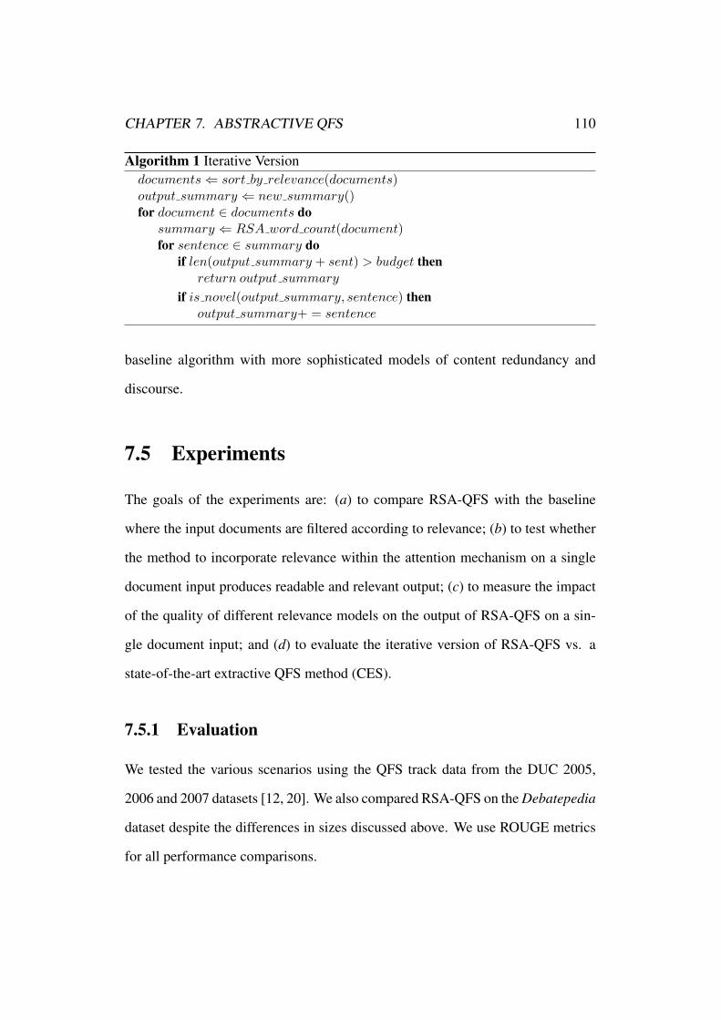
CHAPTER 7. ABSTRACTIVE QFS 110
Algorithm 1 Iterative Versiondocuments ( sort by relevance(documents)output summary ( new summary()for document 2 documents do
summary ( RSA word count(document)for sentence 2 summary do
if len(output summary + sent) > budget thenreturn output summary
if is novel(output summary, sentence) thenoutput summary+ = sentence
baseline algorithm with more sophisticated models of content redundancy and
discourse.
7.5 Experiments
The goals of the experiments are: (a) to compare RSA-QFS with the baseline
where the input documents are filtered according to relevance; (b) to test whether
the method to incorporate relevance within the attention mechanism on a single
document input produces readable and relevant output; (c) to measure the impact
of the quality of different relevance models on the output of RSA-QFS on a sin-
gle document input; and (d) to evaluate the iterative version of RSA-QFS vs. a
state-of-the-art extractive QFS method (CES).
7.5.1 Evaluation
We tested the various scenarios using the QFS track data from the DUC 2005,
2006 and 2007 datasets [12, 20]. We also compared RSA-QFS on the Debatepedia
dataset despite the differences in sizes discussed above. We use ROUGE metrics
for all performance comparisons.

CHAPTER 7. ABSTRACTIVE QFS 111
We evaluate separately the incorporation of the relevance model with a pre-
trained abstractive model on a single document as an ablation study, and we test
the iterative algorithm to handle multiple input documents in a second round of
experiments.
In the first round of experiments, we compare various abstractive baselines on
the longest input document from the QFS topic set (we also experimented with
the most relevant document but obtained lower ROUGE performance). For such
comparisons, we use ROUGE-1, ROUGE-2 and ROUGE-L metrics (ROUGE-L
measures recall on the longest common substrings). When comparing RSA-QFS
to the extractive method, we use ROUGE-1, ROUGE-2 and ROUGE-SU4 which
are most usually reported for extractive method performance.
The ROUGE values obtained in the single-document ablation study are ex-
pected to be much lower than competitive QFS results for two main reasons: (1)
we use as reference the DUC reference summaries with no modifications. These
reference summaries were created manually to cover the full topic set; in con-
trast, in the ablation study we read only a single document, and the best summary
we can generate will lack coverage; (2) the pointer-generator abstractive model
was trained to generate a ⇠100 words summary, while DUC datasets summaries
contain ⇠250 words. Still the reported ROUGE performance indicates trends to
detect whether the generated short summaries manage to capture relevance.
7.5.2 Abstractive Baselines
We compare RSA-QFS with the following baselines:

CHAPTER 7. ABSTRACTIVE QFS 112
BlackBox: We run the document through the pointer-generator abstractive model
without any modifications. This weak baseline indicates whether our method im-
prove QFS performance vs. an abstractive method that completely ignores the
query.
Filtered: We filtered half of the document sentences by selecting the ones with
the highest relevance score. We maintained the original ordering of the sentences.
We then used the filtered document as an input to the pointer-generator abstractive
model. The relevance score we used was the count of shared words betwen the
query and the sentence (see below the list of other relevance models we tested -
this model of relevance provided the best results on the filtered baseline).
Relevance Sensitive Attention (RSA-QFS): This method is the main contribu-
tion of this work.
We tested the method using the following relevance score functions:
Word Count is a simple count of word overlap between the query and a given
sentence.
RSA-TF-IDF: We generated a TF-IDF representation of the entire document
set for each topic and aggregated the sentence scores using cosine similarity be-
tween the query and the sentence TF-IDF vectors (RSA TF-IDF).
RSA word2vec: We use a word2vec model [125], pre-trained on the Google
News dataset. Relevance is measured as the cosine similarity between the summed

CHAPTER 7. ABSTRACTIVE QFS 113
representation vector of each word in the query and in the sentence. Words that
did not appear in the pre-trained word2vec model vocabulary were ignored.
Results are given in Table 7.1. As expected, the “Blackbox” method which
ignores the query completely performs poorly. More surprisingly, we observe that
the Filtered model (where we filter the input document according to the word-
count relevance model and then apply the abstractive model) does not behave any
better than the blackbox unmodified model. In contrast, RSA-QFS improve signif-
icantly (all improvements are significant within 5% except DUC-2005 ROUGE-2)
over the Filtered pipeline - while processing exactly the same input material as the
Filtered method. This indicates that the way we incorporate relevance within the
Attention mechanism is more effective than directly adjusting the input represen-
tation.
The word count relevance model achieves the highest ROUGE scores when
compared with other relevance models. On all the datasets, it outperforms the
filtered baseline by a large amount. The word2vec-based method is close and
consistently within confidence interval of the word count method. We speculate
that the fact that out of vocabulary words are ignored, and the fact that DUC
queries tend to be verbose and do not need much expansion explain the fact that
word2vec does not improve on the Word count model. The TF-IDF-based method
performed poorly. We presume this is due to the fact that the ROUGE settings1
did not eliminate stop words and frequent words for the evaluation.1PyRouge default settings as used in the pointer-generator evaluation [119]

CHAPTER 7. ABSTRACTIVE QFS 114
DUC2005 DUC2006 DUC2007Single Document 1 2 L 1 2 L 1 2 L
BlackBox 12.11 1.38 11.28 14.76 2.29 13.35 15.33 2.68 14.04Filtered 12.09 1.33 11.20 14.71 2.25 13.48 16.23 2.89 14.76RSA Word Count 12.65 1.61 11.79 16.34 2.56 14.69 17.80 3.45 16.38RSA TF-IDF 11.84 1.57 11.00 13.93 2.12 12.90 14.71 2.61 13.50RSA word2vec 12.44 1.39 11.52 15.80 2.43 14.46 17.55 3.21 15.90
Table 7.1: Incorporating Relevance on a Single (Longest) Document Input
DUC2005 DUC2006 DUC2007Multi-Document 1 2 SU4 1 2 SU4 1 2 SU4
CES 40.33 7.94 13.89 43.00 9.69 15.63 45.43 12.02 17.50Filtered Iterative 33.95 5.76 10.95 37.34 7.57 12.63 39.23 8.551 13.83Iterative RSA Word Count 39.82 6.98 15.73 42.89 8.73 17.75 43.92 10.13 18.54Iterative RSA Oracle 43.48 8.75 17.94 46.64 10.96 20.34 47.91 12.77 21.37
Table 7.2: Iterative RSA-QFS vs. Extractive Methods
7.5.3 Extractive Baselines
In this part of the experiments, we compare the RSA-QFS method extended with
the iterative algorithm to consume multiple documents and a query under the exact
DUC conditions and produce summaries comparable to existing extractive meth-
ods. We compare with CES, the current state of the art extractive algorithm on
QFS. Results are in Table 7.2.
We compare two relevance models with RSA-QFS: the word-count model
which we identified as the best performing one in the ablation study, and the Or-
acle model. In the Oracle model, we compute the relevance of an input sentence
by comparing it to the reference models instead of with the query. This gives us
a theoretical upper bound on the potential benefit of more sophisticated retrieval
ranking methods. We also compared the RSA-QFS method with iteratively apply-
ing the base abstractive summarization on the documents filtered be relevancy to
the query.

CHAPTER 7. ABSTRACTIVE QFS 115
DebatepediaRecall-ROUGE 1 2 L
SD2 41.26 18.75 40.43RSA Word Count 53.09 16.10 46.18
Table 7.3: Results for Debatepedia QFS dataset
We observe that RSA-QFS is competitive with state-of-the-art extractive meth-
ods and outperforms them in the SU4 metric. The oracle baseline shows that a
more sophisticated relevance method has the potential to improve performance by
a significant amount and way above the current extractive top model.
7.5.4 Evaluation Using the Debatepedia Dataset
We used the Debatepedia QFS dataset [124] to evaluate our method vs. the LSTM
based diversity attention trained end to end on the Debatepedia dataset (SD2)
model. We compare with the ROUGE recall results provided in the original paper.
While the result in Table 7.3 may suggest our method outperforms the model that
is trained on the actual dataset, it must be noted that our model yielded summaries
ten times longer than required and achieved very low ROUGE precision. We did
not compare precision score since it was not provided in the original research.
This comparison indicates the datasets are not directly comparable, but that even
on a completely different domain, the abstractive capability encapsulated in the
model provides readable and realistic summaries.

CHAPTER 7. ABSTRACTIVE QFS 116
7.6 Analysis
7.6.1 Output Abstractiveness
In order to test if our model is truly abstractive, instead of simply copying rel-
evant fragments verbatim from the input documents, we counted the amount of
sentences from the summary generated by our model (using word count similarity
function) which are substrings of the original text. We found that on average only
about 33% of the sentences were copied from the original document and that the
average word edit-distance between each generated sentence and the most similar
sentence is about 39 edits (tested on DUC 2007 summarized by the iterative RSA
word count method).
We observed that the generated sentences, while significantly different from
the source sentences do not introduce many new content words. Almost all gen-
erated words are present in the source documents. While these two measures
indicate a good level of “abstractiveness”, it remains a challenge to measure ab-
stractiveness in an interpretable and quantitative manner. Cursory reading of the
generated summaries still “feels” very literal.
We assessed readability by reading the summaries generated by the best per-
forming methods, the RSA Word Count (an example can be seen in Fig. 7.1) and
the Oracle Based Iterative Method. We found that the summaries produced by
the single document variant maintained the readability of the unmodified model.
We did notice that the coverage mechanism was affected due to our modification
and some sentences were repeated in the summaries our model produced (com-
pared to the original abstractive model). The iterative version did not suffer from
repeated sentences, since they are dismissed by the algorithm, but did suffer from

CHAPTER 7. ABSTRACTIVE QFS 117
lack of coherence between sentences, indicating a better discourse model is re-
quired than the simple eager iterative model we used. Improved coherence also
requires better evaluation metrics than the ROUGE metrics we have used.
All the produced summaries for all the methods and the code required to pro-
duce them are available at https://github.com/talbaumel/RSAsummarization.
7.7 Conclusion
In this work, we present RSA-QFS, a novel method for incorporating relevance
into a neural seq2seq models with attention mechanism for abstractive summa-
rization to the QFS task, without additional training. RSA-QFS significantly
improves ROUGE scores for the QFS task when compared to both unmodified
models and a two steps filtered QFS scheme, while preserving readability of the
output summary. The method can be used with various relevance score functions.
We compared the method with state-of-the-art extractive methods and showed
it produces competitive ROUGE scores for the QFS task even with very simple
relevance models and a simple iterative model to account for multiple input doc-
uments. When using an ideal Oracle relevance model, our method achieves very
high ROUGE results compared to extractive methods.
This study frames future work on multi-document abstractive summarization:
we need to design quantitative measures of abstractiveness (how much re-formulation
is involved in producing a summary given the input documents) and of summary
coherence to overcome the known limitations of ROUGE evaluation when applied
to non-extractive methods. We also find that relevance models remain a key as-
pect of summarization and the gap between Oracle and practical relevance models

CHAPTER 7. ABSTRACTIVE QFS 118
indicates there is potential for much improvement on these models.

Chapter 8
Conclusion
In this thesis we discussed the field of automatic summarization and state-of-the-
art neural-based attempts at confronting various tasks in this field. In the first
part of the thesis we over-viewed the field of automatic summarization: presented
the many tasks associated with the field, presented the most common datasets
on the field, and the various ways to evaluate automatic summaries; finally we
presented an in-depth analysis of issues in query-focused-summarization datasets
and suggested ways to amend them.
In the second part of the thesis we provided an overview of common neural-
methods for natural-language-processing. In this part we covered how words
can be represented (word embeddings), how sentences can be represented (using
RNNs), and various specialized deep architectures for automatic summarization
(seq2seq, attention, copy-mechanism, etc). This technical overview is required to
better understand the final part of the thesis.
In the final part of the thesis we presented three contribution to the field: a
way to evaluate different word embeddings based on resources available from the
119

CHAPTER 8. CONCLUSION 120
pyramid-method for summarization evaluation, a proxy task for evaluating the
ability of different text encoders to surface semantic information from input text
and presented a state-of-the-art method for multi-label classification of medical
records, finally we presented the first attempt of achieving abstractive query fo-
cused summarization.

Bibliography
[1] Aria Haghighi and Lucy Vanderwende. Exploring content models for
multi-document summarization. In Proceedings of Human Language Tech-
nologies: The 2009 Annual Conference of the North American Chapter of
the Association for Computational Linguistics, pages 362–370. Association
for Computational Linguistics, 2009.
[2] Marina Litvak, Mark Last, Menahem Friedman, and Slava Kisilevich.
Muse–a multilingual sentence extractor. Computational linguistics & ap-
plications (CLA 11), Jachranka. http:// bib. dbvis. de/ uploadedFiles, 362,
2011.
[3] Alexander M Rush, Sumit Chopra, and Jason Weston. A neural at-
tention model for abstractive sentence summarization. arXiv preprint
arXiv:1509.00685, 2015.
[4] Abigail See, Peter J Liu, and Christopher D Manning. Get to the
point: Summarization with pointer-generator networks. arXiv preprint
arXiv:1704.04368, 2017.
[5] Tal Baumel, Raphael Cohen, and Michael Elhadad. Topic concentration in
query focused summarization datasets. In AAAI, pages 2573–2579, 2016.
121

BIBLIOGRAPHY 122
[6] Tal Baumel, Raphael Cohen, and Michael Elhadad. Query-chain focused
summarization. In ACL (1), pages 913–922, 2014.
[7] Tal Baumel, Raphael Cohen, and Michael Elhadad. Sentence embedding
evaluation using pyramid annotation. In Proceedings of the 1st Work-
shop on Evaluating Vector-Space Representations for NLP, pages 145–149,
2016.
[8] Tal Baumel, Jumana Nassour-Kassis, Michael Elhadad, and Noemie El-
hadad. Multi-label classification of patient notes a case study on icd code
assignment. arXiv preprint arXiv:1709.09587, 2017.
[9] T. Baumel, M. Eyal, and M. Elhadad. Query Focused Abstractive Summa-
rization: Incorporating Query Relevance, Multi-Document Coverage, and
Summary Length Constraints into seq2seq Models. ArXiv e-prints, January
2018.
[10] Lidong Bing, Piji Li, Yi Liao, Wai Lam, Weiwei Guo, and Rebecca J. Pas-
sonneau. Abstractive multi-document summarization via phrase selection
and merging. CoRR, abs/1506.01597, 2015.
[11] Jessica Ficler and Yoav Goldberg. Controlling linguistic style aspects in
neural language generation. arXiv preprint arXiv:1707.02633, 2017.
[12] Hoa Trang Dang. Overview of duc 2005. In Proceedings of the document
understanding conference, volume 2005, pages 1–12, 2005.
[13] Jason R Baron, David D Lewis, and Douglas W Oard. Trec 2006 legal track
overview. In TREC, 2006.

BIBLIOGRAPHY 123
[14] Surabhi Gupta, Ani Nenkova, and Dan Jurafsky. Measuring importance and
query relevance in topic-focused multi-document summarization. In Pro-
ceedings of the 45th Annual Meeting of the ACL on Interactive Poster and
Demonstration Sessions, pages 193–196. Association for Computational
Linguistics, 2007.
[15] Ani Nenkova. Automatic text summarization of newswire: Lessons learned
from the document understanding conference. In AAAI, volume 5, pages
1436–1441, 2005.
[16] Hoa Trang Dang and Karolina Owczarzak. Overview of the tac 2008 update
summarization task. In TAC, 2008.
[17] Linguistic Data Consortium et al. English gigaword. Catalog number
LDC2003T05. Available from LDC at http://www. ldc. upenn. edu, 2003.
[18] Karl Moritz Hermann, Tomas Kocisky, Edward Grefenstette, Lasse Espe-
holt, Will Kay, Mustafa Suleyman, and Phil Blunsom. Teaching machines
to read and comprehend. In Advances in Neural Information Processing
Systems, pages 1693–1701, 2015.
[19] Delphine Bernhard and Iryna Gurevych. A monolingual tree-based trans-
lation model for sentence simplification. In The 23˜(rd) International Con-
ference on Computational Linguistics Proceedings of the Main Conference
(Volume 2), 2010.
[20] TD Hoa. Overview of duc 2006. In Document Understanding Conference,
2006.

BIBLIOGRAPHY 124
[21] Chin-Yew Lin and Eduard Hovy. Automatic evaluation of summaries us-
ing n-gram co-occurrence statistics. In Proceedings of the 2003 Conference
of the North American Chapter of the Association for Computational Lin-
guistics on Human Language Technology - Volume 1, NAACL ’03, pages
71–78, Stroudsburg, PA, USA, 2003. Association for Computational Lin-
guistics.
[22] Hans Van Halteren and Simone Teufel. Examining the consensus between
human summaries: initial experiments with factoid analysis. In Proceed-
ings of the HLT-NAACL 03 on Text summarization workshop-Volume 5,
pages 57–64. Association for Computational Linguistics, 2003.
[23] Kishore Papineni, Salim Roukos, Todd Ward, and Wei-Jing Zhu. Bleu: a
method for automatic evaluation of machine translation. In Proceedings
of the 40th annual meeting on association for computational linguistics,
pages 311–318. Association for Computational Linguistics, 2002.
[24] Chin-Yew Lin and Eduard Hovy. Automatic evaluation of summaries using
n-gram co-occurrence statistics. In Proceedings of the 2003 Conference of
the North American Chapter of the Association for Computational Linguis-
tics on Human Language Technology-Volume 1, pages 71–78. Association
for Computational Linguistics, 2003.
[25] Chin-Yew Lin. Rouge: A package for automatic evaluation of summaries.
In Text summarization branches out: Proceedings of the ACL-04 workshop,
volume 8. Barcelona, Spain, 2004.

BIBLIOGRAPHY 125
[26] Satanjeev Banerjee and Alon Lavie. Meteor: An automatic metric for mt
evaluation with improved correlation with human judgments. In Proceed-
ings of the acl workshop on intrinsic and extrinsic evaluation measures for
machine translation and/or summarization, volume 29, pages 65–72, 2005.
[27] Steven Bird. Nltk: the natural language toolkit. In Proceedings of the
COLING/ACL on Interactive presentation sessions, pages 69–72. Associa-
tion for Computational Linguistics, 2006.
[28] George A Miller. Wordnet: a lexical database for english. Communications
of the ACM, 38(11):39–41, 1995.
[29] Jahna Otterbacher, Gunes Erkan, and Dragomir R Radev. Biased lexrank:
Passage retrieval using random walks with question-based priors. Informa-
tion Processing & Management, 45(1):42–54, 2009.
[30] Solomon Kullback and Richard A Leibler. On information and sufficiency.
The annals of mathematical statistics, 22(1):79–86, 1951.
[31] Gerard Salton, Chung-Shu Yang, and Clement T. Yu. Contribution to the
theory of indexing. Technical report, Cornell University, 1973.
[32] Victor Lavrenko and W Bruce Croft. Relevance based language models.
In Proceedings of the 24th annual international ACM SIGIR conference on
Research and development in information retrieval, pages 120–127. ACM,
2001.

BIBLIOGRAPHY 126
[33] Ren Wu, Shengen Yan, Yi Shan, Qingqing Dang, and Gang Sun. Deep
image: Scaling up image recognition. arXiv preprint arXiv:1501.02876,
7(8), 2015.
[34] Alex Krizhevsky, Ilya Sutskever, and Geoffrey E Hinton. Imagenet clas-
sification with deep convolutional neural networks. In F. Pereira, C. J. C.
Burges, L. Bottou, and K. Q. Weinberger, editors, Advances in Neural In-
formation Processing Systems 25, pages 1097–1105. Curran Associates,
Inc., 2012.
[35] Geoffrey Hinton, Li Deng, Dong Yu, George E Dahl, Abdel-rahman
Mohamed, Navdeep Jaitly, Andrew Senior, Vincent Vanhoucke, Patrick
Nguyen, Tara N Sainath, et al. Deep neural networks for acoustic modeling
in speech recognition: The shared views of four research groups. IEEE
Signal Processing Magazine, 29(6):82–97, 2012.
[36] Dzmitry Bahdanau, Kyunghyun Cho, and Yoshua Bengio. Neural machine
translation by jointly learning to align and translate. In ICLR 2015, 2014.
[37] BWAC Farley and W Clark. Simulation of self-organizing systems by dig-
ital computer. Transactions of the IRE Professional Group on Information
Theory, 4(4):76–84, 1954.
[38] Marvin Minsky and Seymour Papert. Perceptrons. 1969.
[39] David E Rumelhart, Geoffrey E Hinton, and Ronald J Williams. Learning
representations by back-propagating errors. Cognitive modeling, 5(3):1,
1988.

BIBLIOGRAPHY 127
[40] Yoav Goldberg. Neural network methods for natural language processing.
Synthesis Lectures on Human Language Technologies, 10(1):1–309, 2017.
[41] M. J. Kusner, Y. Sun, N. I. Kolkin, and K. Q. Weinberger. From word
embeddings to document distances. In ICML, 2015.
[42] Tomas Mikolov, Kai Chen, Greg Corrado, and Jeffrey Dean. Effi-
cient estimation of word representations in vector space. arXiv preprint
arXiv:1301.3781, 2013.
[43] Jeffrey Pennington, Richard Socher, and Christopher D Manning. Glove:
Global vectors for word representation. In EMNLP, volume 14, pages
1532–1543, 2014.
[44] Yoon Kim. Convolutional neural networks for sentence classification.
arXiv preprint arXiv:1408.5882, 2014.
[45] Peng Jin, Yue Zhang, Xingyuan Chen, and Yunqing Xia. Bag-of-
embeddings for text classification. In IJCAI, pages 2824–2830, 2016.
[46] Junyoung Chung, Caglar Gulcehre, KyungHyun Cho, and Yoshua Bengio.
Empirical evaluation of gated recurrent neural networks on sequence mod-
eling. arXiv preprint arXiv:1412.3555, 2014.
[47] Sepp Hochreiter and Jurgen Schmidhuber. Long short-term memory. Neu-
ral computation, 9(8):1735–1780, 1997.
[48] Cicero D Santos and Bianca Zadrozny. Learning character-level represen-
tations for part-of-speech tagging. In Proceedings of the 31st International
Conference on Machine Learning (ICML-14), pages 1818–1826, 2014.

BIBLIOGRAPHY 128
[49] Trias Thireou and Martin Reczko. Bidirectional long short-term memory
networks for predicting the subcellular localization of eukaryotic proteins.
IEEE/ACM Transactions on Computational Biology and Bioinformatics,
4(3), 2007.
[50] Ilya Sutskever, Oriol Vinyals, and Quoc V Le. Sequence to sequence learn-
ing with neural networks. In Advances in neural information processing
systems, pages 3104–3112, 2014.
[51] Kyunghyun Cho, Bart Van Merrienboer, Caglar Gulcehre, Dzmitry Bah-
danau, Fethi Bougares, Holger Schwenk, and Yoshua Bengio. Learning
phrase representations using rnn encoder-decoder for statistical machine
translation. arXiv preprint arXiv:1406.1078, 2014.
[52] Kelvin Xu, Jimmy Ba, Ryan Kiros, Kyunghyun Cho, Aaron Courville, Rus-
lan Salakhudinov, Rich Zemel, and Yoshua Bengio. Show, attend and tell:
Neural image caption generation with visual attention. In International
Conference on Machine Learning, pages 2048–2057, 2015.
[53] Minh-Thang Luong, Ilya Sutskever, Quoc V Le, Oriol Vinyals, and Woj-
ciech Zaremba. Addressing the rare word problem in neural machine trans-
lation. arXiv preprint arXiv:1410.8206, 2014.
[54] Frederic Morin and Yoshua Bengio. Hierarchical probabilistic neural net-
work language model. In Aistats, volume 5, pages 246–252. Citeseer, 2005.
[55] Ramesh Nallapati, Bowen Zhou, Caglar Gulcehre, Bing Xiang, et al. Ab-
stractive text summarization using sequence-to-sequence rnns and beyond.
arXiv preprint arXiv:1602.06023, 2016.

BIBLIOGRAPHY 129
[56] Xingxing Zhang and Mirella Lapata. Sentence simplification with deep
reinforcement learning. CoRR, abs/1703.10931, 2017.
[57] Nal Kalchbrenner, Edward Grefenstette, and Phil Blunsom. A con-
volutional neural network for modelling sentences. arXiv preprint
arXiv:1404.2188, 2014.
[58] Kevin J Lang, Alex H Waibel, and Geoffrey E Hinton. A time-delay neu-
ral network architecture for isolated word recognition. Neural networks,
3(1):23–43, 1990.
[59] Philipp Koehn, Hieu Hoang, Alexandra Birch, Chris Callison-Burch, Mar-
cello Federico, Nicola Bertoldi, Brooke Cowan, Wade Shen, Christine
Moran, Richard Zens, et al. Moses: Open source toolkit for statistical ma-
chine translation. In Proceedings of the 45th annual meeting of the ACL on
interactive poster and demonstration sessions, pages 177–180. Association
for Computational Linguistics, 2007.
[60] Bonnie Dorr David Zajic and Richard Schwartz. Bbn/umd at duc-2004:
Topiary. In Proceedings of the HLT-NAACL 2004 Document Understand-
ing Workshop, Boston, pages 112–119, 2004.
[61] Sebastien Jean, Kyunghyun Cho, Roland Memisevic, and Yoshua Ben-
gio. On using very large target vocabulary for neural machine translation.
CoRR, abs/1412.2007, 2014.
[62] Romain Paulus, Caiming Xiong, and Richard Socher. A deep reinforced
model for abstractive summarization. CoRR, abs/1705.04304, 2017.

BIBLIOGRAPHY 130
[63] Arun Venkatraman, Martial Hebert, and J Andrew Bagnell. Improving
multi-step prediction of learned time series models. In AAAI, pages 3024–
3030, 2015.
[64] Ronald J Williams. Simple statistical gradient-following algorithms for
connectionist reinforcement learning. Machine learning, 8(3-4):229–256,
1992.
[65] Wei Xu, Courtney Napoles, Ellie Pavlick, Quanze Chen, and Chris
Callison-Burch. Optimizing statistical machine translation for text sim-
plification. Transactions of the Association for Computational Linguistics,
4:401–415, 2016.
[66] Rami Al-Rfou, Bryan Perozzi, and Steven Skiena. Polyglot: Distributed
word representations for multilingual nlp. arXiv preprint arXiv:1307.1662,
2013.
[67] Alexandre Passos, Vineet Kumar, and Andrew McCallum. Lexicon in-
fused phrase embeddings for named entity resolution. arXiv preprint
arXiv:1404.5367, 2014.
[68] Mohit Bansal, Kevin Gimpel, and Karen Livescu. Tailoring continuous
word representations for dependency parsing. In ACL (2), pages 809–815,
2014.
[69] Karl Moritz Hermann, Dipanjan Das, Jason Weston, and Kuzman Ganchev.
Semantic frame identification with distributed word representations. In
ACL (1), pages 1448–1458, 2014.

BIBLIOGRAPHY 131
[70] Richard Socher, Jeffrey Pennington, Eric H Huang, Andrew Y Ng, and
Christopher D Manning. Semi-supervised recursive autoencoders for pre-
dicting sentiment distributions. In Proceedings of the conference on empir-
ical methods in natural language processing, pages 151–161. Association
for Computational Linguistics, 2011.
[71] Andrej Karpathy and Li Fei-Fei. Deep visual-semantic alignments for gen-
erating image descriptions. In Proceedings of the IEEE Conference on
Computer Vision and Pattern Recognition, pages 3128–3137, 2015.
[72] Dumitru Erhan, Yoshua Bengio, Aaron Courville, Pierre-Antoine Man-
zagol, Pascal Vincent, and Samy Bengio. Why does unsupervised pre-
training help deep learning? Journal of Machine Learning Research,
11(Feb):625–660, 2010.
[73] William B Dolan and Chris Brockett. Automatically constructing a corpus
of sentential paraphrases. In Proc. of IWP, 2005.
[74] Samuel R Bowman, Gabor Angeli, Christopher Potts, and Christopher D
Manning. A large annotated corpus for learning natural language inference.
arXiv preprint arXiv:1508.05326, 2015.
[75] Tomas Mikolov, Wen-tau Yih, and Geoffrey Zweig. Linguistic regularities
in continuous space word representations. In hlt-Naacl, volume 13, pages
746–751, 2013.
[76] Yoav Goldberg and Omer Levy. word2vec explained: deriving mikolov
et al.’s negative-sampling word-embedding method. arXiv preprint
arXiv:1402.3722, 2014.

BIBLIOGRAPHY 132
[77] Gabriel Stanovsky, Ido Dagan, et al. Open ie as an intermediate struc-
ture for semantic tasks. In Proceedings of the 53rd Annual Meeting of the
Association for Computational Linguistics and the 7th International Joint
Conference on Natural Language Processing (Volume 2: Short Papers),
volume 2, pages 303–308, 2015.
[78] Nick Craswell. Mean reciprocal rank. In Encyclopedia of Database Sys-
tems, pages 1703–1703. Springer, 2009.
[79] Yossi Adi, Einat Kermany, Yonatan Belinkov, Ofer Lavi, and Yoav Gold-
berg. Fine-grained analysis of sentence embeddings using auxiliary predic-
tion tasks. arXiv preprint arXiv:1608.04207, 2016.
[80] Koby Crammer, Mark Dredze, Kuzman Ganchev, Partha Pratim Talukdar,
and Steven Carroll. Automatic code assignment to medical text. In Pro-
ceedings of the ACL Workshop on BioNLP 2007: Biological, Translational,
and Clinical Language Processing, pages 129–136, 2007.
[81] Richard Farkas and Gyorgy Szarvas. Automatic construction of rule-based
ICD-9-CM coding systems. BMC bioinformatics, 9(3):S10, 2008.
[82] Leah S Larkey and W Bruce Croft. Automatic assignment of ICD9 codes
to discharge summaries. Technical report, University of Massachusetts at
Amherst, Amherst, MA, 1995.
[83] Lucian Vlad Lita, Shipeng Yu, Radu Stefan Niculescu, and Jinbo Bi. Large
scale diagnostic code classification for medical patient records. In Proceed-
ings of the International Joint Conference on Natural Language Processing
(IJCNLP), pages 877–882, 2008.
BIBLIOGRAPHY 133
[84] Adler J Perotte, Frank Wood, Noemie Elhadad, and Nicholas Bartlett. Hi-
erarchically supervised latent dirichlet allocation. In Advances in Neural
Information Processing Systems (NIPS), pages 2609–2617, 2011.
[85] Adler Perotte, Rimma Pivovarov, Karthik Natarajan, Nicole Weiskopf,
Frank Wood, and Noemie Elhadad. Diagnosis code assignment: models
and evaluation metrics. Journal of the American Medical Informatics As-
sociation, 21(2):231–237, 2014.
[86] Ramakanth Kavuluru, Anthony Rios, and Yuan Lu. An empirical eval-
uation of supervised learning approaches in assigning diagnosis codes to
electronic medical records. Artificial Intelligence in Medicine, 65(2):155–
166, 2015.
[87] John P Pestian, Christopher Brew, Paweł Matykiewicz, Dj J Hovermale,
Neil Johnson, K Bretonnel Cohen, and Włodzisław Duch. A shared task
involving multi-label classification of clinical free text. In Proceedings
of the ACL Workshop on BioNLP: Biological, Translational, and Clinical
Language Processing, pages 97–104, 2007.
[88] Rimma Pivovarov, Adler J Perotte, Edouard Grave, John Angiolillo,
Chris H Wiggins, and Noemie Elhadad. Learning probabilistic phenotypes
from heterogeneous EHR data. Journal of Biomedical Informatics, 58:156–
165, 2015.
[89] Hrayr Harutyunyan, Hrant Khachatrian, David C Kale, and Aram Galstyan.
Multitask learning and benchmarking with clinical time series data. arXiv
preprint arXiv:1703.07771, 2017.

BIBLIOGRAPHY 134
[90] Riccardo Miotto, Li Li, Brian A Kidd, and Joel T Dudley. Deep Patient:
An unsupervised representation to predict the future of patients from the
electronic health records. Scientific Reports, 6, 2016.
[91] Zachary C Lipton, David C Kale, Charles Elkan, and Randall Wetzell.
Learning to diagnose with LSTM recurrent neural networks. arXiv preprint
arXiv:1511.03677, 2015.
[92] Edward Choi, Mohammad Taha Bahadori, and Jimeng Sun. Doctor AI:
Predicting clinical events via recurrent neural networks. arXiv preprint
arXiv:1511.05942, 2015.
[93] Rajesh Ranganath, Adler J Perotte, Noemie Elhadad, and David M Blei.
The Survival Filter: joint survival analysis with a latent time series. In UAI,
pages 742–751, 2015.
[94] Dina Demner Fushman and Noemie Elhadad. Aspiring to unintended con-
sequences of natural language processing: A review of recent developments
in clinical and consumer-generated text processing. Yearbook of Medical
Informatics, 10(1):224–233, 2016.
[95] Abhyuday N Jagannatha and Hong Yu. Structured prediction models for
RNN based sequence labeling in clinical text. In Proceedings of the Con-
ference on Empirical Methods in Natural Language Processing (EMNLP),
page 856, 2016.
[96] Grigorios Tsoumakas and Ioannis Katakis. Multi-label classification: An
overview. International Journal of Data Warehousing and Mining, 3(3),
2006.

BIBLIOGRAPHY 135
[97] Jason Weston, Samy Bengio, and Nicolas Usunier. WSABIE: Scaling
up to large vocabulary image annotation. In Proceedings of the Interna-
tional Joint Conference on Artificial Intelligence (IJCAI), volume 11, pages
2764–2770, 2011.
[98] Eunsol Choi, Daniel Hewlett, Alexandre Lacoste, Illia Polosukhin, Jakob
Uszkoreit, and Jonathan Berant. Hierarchical question answering for long
documents. arXiv preprint arXiv:1611.01839, 2016.
[99] Himanshu Jain, Yashoteja Prabhu, and Manik Varma. Extreme multi-label
loss functions for recommendation, tagging, ranking & other missing label
applications. In Proceedings of the 22nd ACM SIGKDD International Con-
ference on Knowledge Discovery and Data Mining, pages 935–944, 2016.
[100] Kush Bhatia, Himanshu Jain, Purushottam Kar, Manik Varma, and Prateek
Jain. Sparse local embeddings for extreme multi-label classification. In
Advances in Neural Information Processing Systems (NIPS), pages 730–
738, 2015.
[101] Ian EH Yen, Xiangru Huang, Kai Zhong, Pradeep Ravikumar, and Inder-
jit S Dhillon. PD-Sparse: A primal and dual sparse approach to extreme
multiclass and multilabel classification. In Proceedings of the International
Conference on Machine Learning (ICML), 2016.
[102] Armand Joulin, Edouard Grave, Piotr Bojanowski, Matthijs Douze, Herve
Jegou, and Tomas Mikolov. Fasttext.zip: Compressing text classification
models. arXiv preprint arXiv:1612.03651, 2016.

BIBLIOGRAPHY 136
[103] Mohammed Saeed, Mauricio Villarroel, Andrew T Reisner, Gari Clifford,
Li-Wei Lehman, George Moody, Thomas Heldt, Tin H Kyaw, Benjamin
Moody, and Roger G Mark. Multiparameter intelligent monitoring in in-
tensive care II (MIMIC-II): a public-access intensive care unit database.
Critical Care Medicine, 39(5):952, 2011.
[104] Alistair EW Johnson, Tom J Pollard, Lu Shen, Li-wei H Lehman, Mengling
Feng, Mohammad Ghassemi, Benjamin Moody, Peter Szolovits, Leo An-
thony Celi, and Roger G Mark. MIMIC-III, a freely accessible critical care
database. Scientific Data, 3, 2016.
[105] Rie Johnson and Tong Zhang. Effective use of word order for
text categorization with convolutional neural networks. arXiv preprint
arXiv:1412.1058, 2014.
[106] Ying Li, Sharon Lipsky Gorman, and Noemie Elhadad. Section classifica-
tion in clinical notes using supervised hidden Markov model. In Proceed-
ings of the 1st ACM International Health Informatics Symposium, pages
744–750. ACM, 2010.
[107] Sen Wang, Xiaojun Chang, Xue Li, Guodong Long, Lina Yao, and Quan Z
Sheng. Diagnosis code assignment using sparsity-based disease correla-
tion embedding. IEEE Transactions on Knowledge and Data Engineering,
28(12):3191–3202, 2016.
[108] Michael Subotin and Anthony R Davis. A system for predicting ICD-10-
PCS codes from electronic health records. In Proceedings of the ACL Work-

BIBLIOGRAPHY 137
shop on Biomedical Natural Language Processing (BioNLP), pages 59–67.
Citeseer, 2014.
[109] Fabian Pedregosa, Gael Varoquaux, Alexandre Gramfort, Vincent Michel,
Bertrand Thirion, Olivier Grisel, Mathieu Blondel, Peter Prettenhofer, Ron
Weiss, Vincent Dubourg, et al. Scikit-learn: Machine learning in python.
Journal of Machine Learning Research, 12(Oct):2825–2830, 2011.
[110] Yann LeCun et al. Lenet-5, convolutional neural networks. URL:
http://yann. lecun. com/exdb/lenet, 2015.
[111] Zichao Yang, Diyi Yang, Chris Dyer, Xiaodong He, Alex Smola, and Ed-
uard Hovy. Hierarchical attention networks for document classification. In
Proceedings of NAACL-HLT, pages 1480–1489, 2016.
[112] Graham Neubig, Chris Dyer, Yoav Goldberg, Austin Matthews, Waleed
Ammar, Antonios Anastasopoulos, Miguel Ballesteros, David Chiang,
Daniel Clothiaux, Trevor Cohn, et al. Dynet: The dynamic neural network
toolkit. arXiv preprint arXiv:1701.03980, 2017.
[113] Hal Daume III. Bayesian query-focused summarization. CoRR,
abs/0907.1814, 2009.
[114] Seeger Fisher and Brian Roark. Query-focused summarization by super-
vised sentence ranking and skewed word distributions. In Proceedings
of the Document Understanding Conference, DUC-2006, New York, USA,
2006.
BIBLIOGRAPHY 138
[115] Guy Feigenblat, Haggai Roitman, Odellia Boni, and David Konopnicki.
Unsupervised query-focused multi-document summarization using the
cross entropy method. In Proceedings of the 40th International ACM SI-
GIR Conference on Research and Development in Information Retrieval,
SIGIR ’17, pages 961–964, New York, NY, USA, 2017. ACM.
[116] Ramesh Nallapati, Feifei Zhai, and Bowen Zhou. Summarunner: A recur-
rent neural network based sequence model for extractive summarization of
documents. hiP (yi= 1— hi, si, d), 1:1, 2017.
[117] Heeyoung Lee, Angel Chang, Yves Peirsman, Nathanael Chambers, Mi-
hai Surdeanu, and Dan Jurafsky. Deterministic coreference resolution
based on entity-centric, precision-ranked rules. Computational Linguistics,
39(4):885–916, 2013.
[118] Shulei Ma, Zhi-Hong Deng, and Yunlun Yang. An unsupervised multi-
document summarization framework based on neural document model. In
COLING, pages 1514–1523, 2016.
[119] Abigail See, Peter J. Liu, and Christopher D. Manning. Get to the point:
Summarization with pointer-generator networks. CoRR, abs/1704.04368,
2017.
[120] Dzmitry Bahdanau, Kyunghyun Cho, and Yoshua Bengio. Neural machine
translation by jointly learning to align and translate. CoRR, abs/1409.0473,
2014.
[121] David Graff and C Cieri. English gigaword corpus. Linguistic Data Con-
sortium, 2003.

BIBLIOGRAPHY 139
[122] Evan Sandhaus. The new york times annotated corpus. Linguistic Data
Consortium, Philadelphia, 6(12):e26752, 2008.
[123] Karl Moritz Hermann, Tomas Kocisky, Edward Grefenstette, Lasse Espe-
holt, Will Kay, Mustafa Suleyman, and Phil Blunsom. Teaching machines
to read and comprehend. In Advances in Neural Information Processing
Systems (NIPS), 2015.
[124] Preksha Nema, Mitesh Khapra, Anirban Laha, and Balaraman Ravindran.
Diversity driven attention model for query-based abstractive summariza-
tion. arXiv preprint arXiv:1704.08300, 2017.
[125] Tomas Mikolov, Ilya Sutskever, Kai Chen, Greg S Corrado, and Jeff Dean.
Distributed representations of words and phrases and their compositional-
ity. In Advances in neural information processing systems, pages 3111–
3119, 2013.

ריצקת
םינשב הבר תויראלופופ הרבצ תאז המישמ .תיעבטה הפשה דוביע םוחתמ תומישמה תחא אוה יטמוטוא םוכיס
תוטישה ,םישימחה תונשב םוחתה תא דסי ןהול רטיפ סנהש זאמ .םיטסקט לש הברה תונימזה תובקעב תונורחאה
לש המישמה תא וחלצ ולאכש תויביטקרטסקא תוטיש .טסקטהמ םיבושח םיטפשמ תאיצמב ודקמתה תוליבומה
םינוריונ תותשר יססובמ םילדומ תונורחאה םינשב .ריהנ טסקט רוציל ולשכנ לבא טסקטהמ בושחה הדימה תאיצמ
ימוחת תא רוקסנ תאז הדובעב .יטמוטוא םוכיסב רתיה ןיב ,תובר תיתוכאלמ הניב תומישמב םיעוציב ורפיש
םוכיס תריציל םינוריונ תותשרב תושמתשמש תודובע גיצנו הפש דוביע רובע םינוריונ תותשרו יטמוטואה םוכיסה
.ולאש תותשר רופישל םוכיס יבאשמב שומישו

הצהרת תלמיד המחקר עם הגשת עבודת הדוקטור לשיפוט
ה בזאת: (אנא סמן):/מצהיר אני החתום מטה
מנחה/ים.___ חיברתי את חיבורי בעצמי, להוציא עזרת ההדרכה שקיבלתי מאת
.מתקופת היותי תלמיד/ת מחקר___ החומר המדעי הנכלל בעבודה זו הינו פרי מחקרי
___ בעבודה נכלל חומר מחקרי שהוא פרי שיתוף עם אחרים, למעט עזרה טכנית
הנהוגה בעבודה ניסיונית. לפי כך מצורפת בזאת הצהרה על תרומתי ותרומת שותפי
למחקר, שאושרה על ידם ומוגשת בהסכמתם.
תאריך ________ שם התלמיד/ה _______________ חתימה ___________

העבודה נעשתה בהדרכת
פרופסור מיכאל אלחדד
למדעי המחשבבמחלקה
למדעי הטבע בפקולטה

לרצף-סיכום מונחה שאילתא בעזרת מודל רצף
מחקר לשם מילוי חלקי של הדרישות לקבלת תואר "דוקטור לפילוסופיה"
מאת
באומל טל
הוגש לסינאט אוניברסיטת בן גוריון בנגב
____________________ אישור המנחה
ייטמן ____________________אישור דיקן בית הספר ללימודי מחקר מתקדמים ע"ש קר
2018: ינואר תאריך לועזי שבט תשע״ח :תאריך עברי
באר שבע

לרצף-סיכום מונחה שאילתא בעזרת מודל רצף
מחקר לשם מילוי חלקי של הדרישות לקבלת תואר "דוקטור לפילוסופיה"
מאת
טל באומל
הוגש לסינאט אוניברסיטת בן גוריון בנגב
2018: ינואר תאריך לועזי ט תשע״ח : שבתאריך עברי
באר שבע
Top Related
Copyright © 2022 FDOKUMEN

