


Bahasa
Halaman
Hukum

POTENTIAL THEORY IN GRAVITY AND MAGNETICAPPLICATIONS

The Stanford-Cambridge Program is an innovative publishing ventureresulting from the collaboration between Cambridge University Pressand Stanford University and its Press.
The Progam provides a new international imprint for the teachingand communication of pure and applied sciences. Drawing on Stanford'seminent faculty and associated institutions, books within the Programreflect the high quality of teaching and research at Stanford University.
The Program includes textbooks at undergraduate and graduate level,and research monographs, across a broad range of the sciences.
Cambridge University Press publishes and distributes books in theStanford-Cambridge Program throughout the world.

POTENTIAL THEORY INGRAVITY AND MAGNETIC
APPLICATIONS
RICHARD J. BLAKELY
CAMBRIDGEUNIVERSITY PRESS
PUBLISHED BY THE PRESS SYNDICATE OF THE UNIVERSITY OF CAMBRIDGEThe Pitt Building, Trumpington Street, Cambridge CB2 IRP
CAMBRIDGE UNIVERSITY PRESSThe Edinburgh Building, Cambridge CB2 2RU, United Kingdom
40 West 20th Street, New York, NY 10011-4211, USA10 Stamford Road, Oakleigh, Melbourne 3166, Australia
© Cambridge University Press 1996
This book is in copyright. Subject to statutory exceptionand to the provisions of relevant collective licensing agreements,
no reproduction of any part may take place withoutthe written permission of Cambridge University Press.
First published 1995Reprinted 1996
First paperback edition 1996
Printed in the United States of America
Library of Congress Cataloging-in-Publication Data is available.
A catalog record for this book is available from the British Library.
ISBN 0-521-41508-X hardbackISBN 0-521-57547-8 paperback

To Diane

Contents
Introduction1 The Potential1.1 Potential Fields1.1.1 Fields1.1.2 Points, Boundaries, and Regions1.2 Energy, Work, and the Potential1.2.1 Equipotential Surfaces1.3 Harmonic Functions1.3.1 Laplace's Equation1.3.2 An Example from Steady-State Heat Flow1.3.3 Complex Harmonic Functions1.4 Problem Set2 Consequences of the Potential2.1 Green's Identities2.1.1 Green's First Identity2.1.2 Green's Second Identity2.1.3 Green's Third Identity2.1.4 Gauss's Theorem of the Arithmetic Mean2.2 Helmholtz Theorem2.2.1 Proof of the Helmholtz Theorem2.2.2 Consequences of the Helmholtz Theorem2.2.3 Example2.3 Green's Functions2.3.1 Analogy with Linear Systems2.3.2 Green's Functions and Laplace's Equation2.4 Problem Set3 Newtonian Potential
page xiii12234889
111417191920232427282931323434374143
Vll
viii Contents
3.1 Gravitational Attraction and Potential 433.2 The Potential of Distributions of Mass 463.2.1 Example: A Spherical Shell 493.2.2 Example: Solid Sphere 513.2.3 Example: Straight Wire of Finite Length 543.3 Potential of Two-Dimensional Distributions 553.3.1 Potential of an Infinite Wire 553.3.2 General Two-Dimensional Distributions 573.4 Gauss's Law for Gravity Fields 593.5 Green's Equivalent Layer 613.6 Problem Set 634 Magnetic Potential 654.1 Magnetic Induction 654.2 Gauss's Law for Magnetic Fields 684.3 The Vector and Scalar Potentials 704.4 Dipole Moment and Potential 724.4.1 First Derivation: Two Current Loops 724.4.2 Second Derivation: Two Monopoles 744.5 Dipole Field 754.6 Problem Set 795 Magnetization 815.1 Distributions of Magnetization 815.1.1 Alternative Models 835.2 Magnetic Field Intensity 855.3 Magnetic Permeability and Susceptibility 875.4 Poisson's Relation 915.4.1 Example: A Sphere 935.4.2 Example: Infinite Slab 945.4.3 Example: Horizontal Cylinder 955.5 Two-Dimensional Distributions of Magnetization 965.6 Annihilators 975.7 Problem Set 986 Spherical Harmonic Analysis 1006.1 Introduction 1016.2 Zonal Harmonics 1036.2.1 Example 1076.3 Surface Harmonics 1096.3.1 Normalized Functions 1136.3.2 Tesseral and Sectoral Surface Harmonics 1156.4 Application to Laplace's Equation 116
Contents ix
6.4.1 Homogeneous Functions and Euler's Equation 1176.4.2 Point Source away from Origin 1186.4.3 General Spherical Surface Harmonic Functions 1216.5 Problem Set 1267 Regional Gravity Fields 1287.1 Introduction 1287.2 The "Normal" Earth 1297.3 Gravity Anomalies 1367.3.1 Free-Air Correction 1407.3.2 Tidal Correction 1427.3.3 Eotvos Correction 1427.3.4 Bouguer Correction 1437.3.5 Isostatic Residual 1467.4 An Example 1507.5 Problem Set 1538 The Geomagnetic Field 1548.1 Parts of Internal and External Origin 1558.2 Description of the Geomagnetic Field 1598.2.1 The Elements of the Geomagnetic Field 1618.2.2 The International Geomagnetic Reference Field 1638.2.3 The Dipole Field 1648.2.4 The Nondipole Field 1698.2.5 Secular Variation 1728.3 Crustal Magnetic Anomalies 1748.3.1 Total-Field Anomalies 1788.4 Problem Set 1809 Forward Method 1829.1 Methods Compared 1829.2 Gravity Models 1849.2.1 Three-Dimensional Examples 1869.2.2 Two-Dimensional Examples 1919.3 Magnetic Models 1959.3.1 A Choice of Models 1969.3.2 Three-Dimensional Examples 1999.3.3 Two-Dimensional Example 2059.4 Problem Set 21010 Inverse Method 21410.1 Introduction 21410.2 Linear Inverse Problem 21810.2.1 Magnetization of a Layer 218
x Contents
10.2.2 Determination of Magnetization Direction 22310.3 Nonlinear Inverse Problem 22810.3.1 Shape of Source 22810.3.2 Depth to Source 23810.3.3 Ideal Bodies 25010.4 Problem Set 25611 Fourier-Domain Modeling 25811.1 Notation and Review 25911.1.1 Fourier Transform 25911.1.2 Properties of Fourier Transforms 26211.1.3 Random Functions 26411.1.4 Generalized Functions 26611.1.5 Convolution 26611.1.6 Discrete Fourier Transform 27011.2 Some Simple Anomalies 27111.2.1 Three-Dimensional Sources 27411.2.2 Two-Dimensional Sources 28111.3 Earth Filters 28311.3.1 Topographic Sources 29211.3.2 General Sources 29711.4 Depth and Shape of Source 29811.4.1 Statistical Models 30011.4.2 Depth to Bottom 30711.5 Problem Set 30812 Transformations 31112.1 Upward Continuation 31312.1.1 Level Surface to Level Surface 31512.1.2 Uneven Surfaces 32012.2 Directional Derivatives 32412.3 Phase Transformations 32812.3.1 Reduction to the Pole 33012.3.2 Calculation of Vector Components 34212.4 Pseudogravity Transformation 34312.4.1 Pseudomagnetic Calculation 34712.5 Horizontal Gradients and Boundary Analysis 34712.5.1 Terracing 35012.6 Analytic Signal 35012.6.1 Hilbert Transforms 35112.6.2 Application to Potential Fields 35212.7 Problem Set 356
Contents XI
Appendix AAppendix BAppendix CAppendix DBibliographyIndex
Review of Vector CalculusSubroutinesReview of Sampling TheoryConversion of Units
359369413417419437

Introduction
Though this be madness, yet there is method in't.(William Shakespeare)
I think I did pretty well, considering I started out with nothing but abunch of blank paper.
(Steve Martin)
Pierre Simon, Marquis de Laplace, showed in 1782 that Newtonian po-tential obeys a simple differential equation. Laplace's equation, as it nowis called, arguably has become the most universal differential equationin the physical sciences because of the wide range of phenomena that itdescribes. The theory of the potential spawned by Laplace's equation isthe subject of this book, but with particular emphasis on the applica-tion of this theory to gravity and magnetic fields of the earth and in thecontext of geologic and geophysical investigations.
A Brief History of Magnetic and Gravity MethodsThe geomagnetic field must surely rank as the longest studied of all thegeophysical properties of the earth. Curiosity about the mutual attrac-tion of lodestones can be traced back at least to the time of Thales, aphilosopher of ancient Greece in the sixth century B.C. (Needham [194]).The tendency of lodestones to align preferentially in certain directionswas known in China by the first century A.D., and perhaps as early asthe second century B.C. This apparently was the first recognition thatthe earth is associated with a property that affects magnetic objects,thus paving the way for the advent of the magnetic compass in Chinaand observations of magnetic declination.
xin
xiv Introduction
The compass arrived in Europe much later, probably late in the twelfthcentury A.D., but significant discoveries were to follow. Petrus Pere-grinus, a scholar of thirteenth-century Italy, performed several impor-tant experiments on spherical pieces of lodestone. His findings, writtenin 1269, described for the first time the concepts of magnetic polar-ity, magnetic meridians, and the idea that like poles repel but oppositepoles attract. Georg Hartmann, Vicar of Nuremberg, was the first Euro-pean to measure magnetic declination in about 1510. He also discoveredmagnetic inclination in 1544, but his writings went undiscovered un-til after Robert Norman, an English hydrographer, published his owncareful experiments on inclination conducted in 1576. In 1600, WilliamGilbert, physician to Queen Elizabeth I, published his landmark treatise,De Magnete, culminating centuries of European and Chinese thoughtand experimentation on the geomagnetic field. Noting that the earth'smagnetic field has a form much like that of a spherically shaped pieceof lodestone, Gilbert proclaimed that "magnus magnes ipse est globusterrestris" ("the whole earth is a magnet"), and magnetism thus be-came the first physical property, other than roundness, attributed tothe earth as a whole (Merrill and McElhinny [183]). In 1838, the Ger-man mathematician Carl Friederich Gauss gave geomagnetic observa-tions their first global-scale mathematical formalism by applying spher-ical harmonic analysis to a systematic set of magnetic measurementsavailable at the time.
The application of magnetic methods to geologic problems advancedin parallel with the development of magnetometers. Geologic applica-tions began at least as early as 1630, when a sundial compass wasused to prospect for iron ore in Sweden (Hanna [110]), thus makingmagnetic-field interpretation one of the oldest of the geophysical ex-ploration techniques. Early measurements of the magnetic field for ex-ploration purposes were made with land-based, balanced magnets sim-ilar in principle of operation to today's widely used gravity meters.Max Thomas Edelmann used such a device during the first decadeof this century to make the first airborne magnetic measurements viaballoon (Heiland [121]). It was soon recognized that measurements ofthe magnetic field via aircraft could provide superior uniform coveragecompared to surface measurements because of the aircraft's ability toquickly cover remote and inaccessible areas, but balanced-magnet in-struments were not generally amenable to the accelerations associatedwith moving platforms. It was military considerations, related to WorldWar II, that spurred the development of a suitable magnetometer for
A Brief History of Magnetic and Gravity Methods xv
routine aeromagnetic measurements. In 1941, Victor Vacquier, GaryMuffly, and R. D. Wyckoff, employees of Gulf Research and Devel-opment Company under contract with the U.S. government, modified10-year-old flux-gate technology, combined it with suitable stabilizingequipment, and thereby developed a magnetometer for airborne detec-tion of submarines. In 1944, James R. Balsley and Homer Jensen of theU.S. Geological Survey used a magnetometer of similar design in thefirst modern airborne geophysical survey near Boyertown, Pennsylvania(Jensen [143]).
A second major advance in magnetometer design was the developmentof the proton-precession magnetometer by Varian Associates in 1955.This relatively simple instrument measures the magnitude of the totalfield without the need for elaborate stabilizing or orienting equipment.Consequently, the proton-precession magnetometer is relatively inexpen-sive and easy to operate and has revolutionized land-based and shipbornemeasurements. Various other magnetometer designs have followed withgreater resolution (Reford [240]) to be sure, but the proton-precessionmagnetometer remains a mainstay of field surveys.
Shipborne magnetic measurements were well under way by the 1950s.By the mid 1960s, ocean-surface measurements of magnetic intensityin the Northeast Pacific (Raff and Mason [234]) had discovered cu-rious anomalies lineated roughly north-south. Fred Vine and Drum-mond Matthews [286] and, independently, Lawrence Morley and AndreLarochelle [186] recognized that these lineations reflect a recording of thereversing geomagnetic field by the geologic process of seafloor spreading,and thus was spawned the plate-tectonic revolution.
The gravity method too has a formidable place in the history of sci-ence. The realization that the earth has a force of attraction surelymust date back to our initial awareness that dropped objects fall to theground, observations that first were quantified by the well-known exper-iments of Galileo Galilei around 1590. In 1687 Isaac Newton publishedhis landmark treatise, Philosophiae Naturalis Principia Mathematical inwhich he proposed (among other revolutionary concepts) that the forceof gravity is a property of all matter, Earth included.
In 1672 a French scholar, Jean Richer, noted that a pendulum-basedclock designed to be accurate in Paris lost a few minutes per day inCayenne, French Guiana, and so pendulum observations were discov-ered as a way to measure the spatial variation of the geopotential. New-ton correctly interpreted the discrepancy between these two measure-ments as reflecting the oblate shape of the earth. The French believed
xvi Introduction
otherwise at the time, and to prove the point, the French Academy ofSciences sent two expeditions, one to the equatorial regions of Ecuadorand the other to the high latitudes of Sweden, to carefully measure andcompare the length of a degree of arc at both sites (Fernie [88, 89, 90]).The Ecuador expedition was led by several prominent French scientists,among them Pierre Bouguer, sometimes credited for the first carefulobservations of the shape of the earth and for whom the "Bougueranomaly" is named.
The reversible pendulum was constructed by H. Kater in 1818, therebyfacilitating absolute measurements of gravity. Near the end of the samecentury, R. Sterneck of Austria reported the first pendulum instrumentand used it to measure gravity in Europe. Other types of pendulum in-struments followed, including the first shipborne instrument developedby F. A. Vening Meinesz of The Netherlands in 1928, and soon gravitymeasurements were being recorded worldwide. The Hungarian geode-sist, Roland von Eotvos, constructed the first torsional balance in 1910.Many gravity meters of various types were developed and patented dur-ing 1928 to 1930 as U.S. oil companies became interested in explorationapplications. Most modern instruments suitable for field studies, such asthe LaCoste and Romberg gravity meter and the Worden instrument, in-volve astatic principles in measuring the vertical displacement of a smallmass suspended from a system of delicate springs and beams. Variousmodels of the LaCoste and Romberg gravity meter are commonly used inland-based and shipborne studies and, more recently, in airborne surveys(e.g., Brozena and Peters [43]).
The application of gravity measurements to geological problems canbe traced back to the rival hypotheses of John Pratt and George Airypublished between 1855 and 1859 concerning the isostatic support oftopography. They noted that plumb lines near the Himalayas were de-flected from the vertical by amounts less than predicted by the topo-graphic mass of the mountain range. Both Airy and Pratt argued thatin the absence of forces other than gravity, the rigid part of the crustand mantle "floats" on a mobile, denser substratum, so the total mass inany vertical column down to some depth of compensation must balancefrom place to place. Elevated regions, therefore, must be compensatedat depth by mass deficiencies, whereas topographic depressions are un-derlain by mass excesses. Pratt explained this observation in terms oflateral variations in density; that is, the Himalayas are elevated becausethey are less dense than surrounding crust. Airy proposed, on the otherhand, that the crust has laterally uniform density but variable thickness,
About This Book xvii
so mountain ranges rise above the surrounding landscape by virtue ofunderlying crustal roots.
The gravity method also has played a key role in exploration geo-physics. Hugo V. Boeckh used an Eotvos balance to measure gravityover anticlines and domes and explained his observations in terms ofthe densities of rocks that form the structures. He thus was apparentlythe first to recognize the application of the gravity method in the ex-ploration for petroleum (Jakosky [140]). Indeed the first oil discoveredin the United States by geophysical methods was located in 1926 usinggravity measurements (Jakosky [140]).
About This BookConsidering this long and august history of the gravity and magneticmethods, it might well be asked (as I certainly have done during thewaning stages of this writing) why a new textbook on potential theoryis needed now. I believe, however, that this book will fill a significantgap. As a graduate student at Stanford University, I quickly found my-self involved in a thesis topic that required a firm foundation in potentialtheory. It seemed to me then, and I find it true today as a professionalgeophysicist, that no single textbook is available covering the topic of po-tential theory while emphasizing applications to geophysical problems.The classic texts on potential theory published during the middle of thiscentury are still available today, notably those by Kellogg [146] and byRamsey [235] (which no serious student of potential theory should bewithout). These books deal thoroughly with the fundamentals of po-tential theory, but they are not concerned particularly with geophysicalapplications. On the other hand, several good texts are available on thebroad topics of applied geophysics (e.g., Telford, Geldart, and Sheriff[279]) and global geophysics (e.g., Stacey [270]). These books cover thewide range of geophysical methodologies, such as seismology, electro-magnetism, and so forth, and typically devote a few chapters to gravityand magnetic methods; of necessity they do not delve deeply into theunderlying theory.
This book attempts to fill the gap by first exploring the principles ofpotential theory and then applying the theory to problems of crustal andlithospheric geophysics. I have attempted to do this by structuring thebook into essentially two parts. The first six chapters build the founda-tions of potential theory, relying heavily on Kellogg [146], Ramsey [235],and Chapman and Bartels [56]. Chapters 1 and 2 define the meaning
xviii Introduction
of a potential and the consequences of Laplace's equation. Special at-tention is given therein to the all-important Green's identities, Green'sfunctions, and Helmholtz theorem. Chapter 3 focuses these theoreticalprinciples on Newtonian potential, that is, the gravitational potential ofmass distributions in both two and three dimensions. Chapters 4 and 5expand these discussions to magnetic fields caused by distributions ofmagnetic media. Chapter 6 then formulates the theory on a sphericalsurface, a topic of obvious importance to global representations of theearth's gravity and magnetic fields.
The last six chapters apply the foregoing principles of potential theoryto gravity and magnetic studies of the crust and lithosphere. Chapters 7and 8 examine the gravity and magnetic fields of the earth on a globaland regional scale and describe the calculations and underlying theoryby which measurements are transformed into "anomalies." These discus-sions set the stage for the remaining chapters, which provide a samplingof the myriad schemes in the literature for interpreting gravity and mag-netic anomalies. These schemes are divided into the forward method(Chapter 9), the inverse method (Chapter 10), inverse and forward ma-nipulations in the Fourier domain (Chapter 11), and methods of data en-hancement (Chapter 12). Here I have concentrated on the mathematicalrather than the technical side of the methodology, neglecting such topicsas the nuts-and-bolts operations of gravity meters and magnetometersand the proper strategies in designing gravity or magnetic surveys.
Some of the methods discussed in Chapters 9 through 12 are accom-panied by computer subroutines in Appendix B. I am responsible for theprogramming therein (user beware), but the methodologies behind thealgorithms are from the literature. They include some of the "classic"techniques, such as the so-called Talwani method discussed in Chapter 9,and several more modern methods, such as the horizontal-gradient calcu-lation first discussed by Cordell [66]. Those readers wishing to make useof these subroutines should remember that the programming is designedto instruct rather than to be particularly efficient or "elegant."
It would be quite beyond the scope of this or any other text to fullydescribe all of the methodologies published in the modern geophysicalliterature. During 1992 alone, Geophysics (the technical journal of theU.S.-based Society of Exploration Geophysicists) published 17 papersthat arguably should have been covered in Chapters 9 through 12. Mul-tiply that number by the several dozen international journals of similarstature and then times the 50 some-odd years that the modern method-ology has been actively discussed in the literature, and it becomes clear
Acknowledgments xix
that each technique could not be given its due. Instead, my approachhas been to describe the various methodologies with key examples fromthe literature, including both classic algorithms and promising new tech-niques, and with apologies to all of my colleagues not sufficiently cited!
AcknowledgmentsThe seeds of this book began in graduate-level classes that I preparedand taught at Oregon State University and Stanford University be-tween 1973 and 1990. The final scope of the book, however, is partlya reflection of interactions and discussions with many friends and col-leagues. Foremost are my former professors at Stanford University dur-ing my graduate studies, especially Allan Cox, George Thompson, andJon Claerbout, who introduced me to geological applications of poten-tial theory and time-series analysis. My colleagues at the U.S. Geologi-cal Survey, Stanford University, Oregon State University, and elsewherewere always available for discussions and fomentation, especially RobertJachens, Robert Simpson, Thomas Hildenbrand, Richard Saltus, AndrewGriscom, V. J. S. Grauch, Gerald Connard, Gordon Ness, and MichaelMcWilliams. I am grateful to Richard Saltus and Gregory Schreiber forcarefully checking and critiquing all chapters, and to William Hinze, TikiRavat, Robert Langel, and Robert Jachens for reviewing and proofread-ing various parts of early versions of this manuscript. I am especiallygrateful to Lauren Cowles, my chief contact and editor at CambridgeUniversity Press, for her patience, assistance, and flexible deadlines.
Finally, but at the top of the list, I thank my wife, Diane, and children,Tammy and Jason, for their unwavering support and encouragement,not just during the writing of this book, but throughout my career. Thisbook is dedicated to Diane, who could care less about geophysics butalways recognized its importance to me.
Richard J. Blakely

1The Potential
Laplace's equation is the most famous and most universal of all partialdifferential equations. No other single equation has so many deep anddiverse mathematical relationships and physical applications.
(G. F. D. Duff and D. Naylor)
Every arrow that flies feels the attraction of the earth.(Henry Wadsworth Longfellow)
Two events in the history of science were of particular significance tothe discussions throughout this book. In 1687, Isaac Newton put forththe Universal Law of Gravitation: Each particle of matter in the uni-verse attracts all others with a force directly proportional to its massand inversely proportional to the square of its distance of separation.Nearly a century later, Pierre Simon, Marquis de Laplace, showed thatgravitational attraction obeys a simple differential equation, an equationthat now bears his name. These two hallmarks have subsequently devel-oped into a body of mathematics called potential theory that describesnot only gravitational attraction but also a large class of phenomena,including magnetostatic and electrostatic fields, fields generated by uni-form electrical currents, steady transfer of heat through homogeneousmedia, steady flow of ideal fluids, the behavior of elastic solids, prob-ability density in random-walk problems, unsteady water-wave motion,and the theory of complex functions and confermal mapping.
The first few chapters of this book describe some general aspects ofpotential theory of most interest to practical geophysics. This chapterdefines the meaning of a potential field and how it relates to Laplace'sequation. Chapter 2 will delve into some of the consequences of thisrelationship, and Chapters 3, 4, and 5 will apply the principles of po-tential theory to gravity and magnetic fields specifically. Readers finding
2 The Potential
these treatments too casual are referred to textbooks by Ramsey [235],Kellogg [146], and MacMillan [172].
1.1 Potential FieldsA few definitions are needed at the outset. We begin by building anunderstanding of the general term field and, more specifically, potentialfield. The cartesian coordinate system will be used in the following devel-opment, but any orthogonal coordinate system would provide the sameresults. Appendix A describes the vector notation employed throughoutthis text.
1.1.1 FieldsA field is a set of functions of space and time. We will be concernedprimarily with two kinds of fields. Material fields describe some physicalproperty of a material at each point of the material and at a giventime. Density, porosity, magnetization, and temperature are examples ofmaterial fields. A force field describes the forces that act at each pointof space at a given time. The gravitational attraction of the earth andthe magnetic field induced by electrical currents are examples of forcefields.
Fields also can be classed as either scalar or vector. A scalar field isa single function of space and time; displacement of a stretched string,temperature of a volume of gas, and density within a volume of rockare scalar fields. A vector field, such as flow of heat, velocity of a fluid,and gravitational attraction, must be characterized by three functions ofspace and time, namely, the components of the field in three orthogonaldirections.
Gravitational and magnetic attraction will be the principal focus oflater chapters. Both are vector fields, of course, but geophysical instru-ments generally measure just one component of the vector, and thatsingle component constitutes a scalar field. In later discussions, we oftenwill drop the distinction between scalar and vector fields. For example,gravity meters used in geophysical surveys measure the vertical compo-nent gz (a scalar field) of the acceleration of gravity g (a vector field),but we will apply the word "field" to both g and gz interchangeably.
A vector field can be characterized by its field lines (also known aslines of flow or lines of force), lines that are tangent at every point to thevector field. Small displacements along a field line must have x, ?/, and z
1.1 Potential Fields 3
components proportional to the corresponding x, y, and z componentsof the field at the point of its displacement. Hence, if F is a continuousvector field, its field lines are described by integration of the differentialequation
dx_ _dy_ __dz_F ~ F ~ F ' ^ 'r x L y ± z
Exercise 1.1 We will find in Chapter 3 that the gravitational attraction ofa uniform sphere of mass M, centered at point Q, and observed outsidethe sphere at point P is given by g = — 'yMr/r2, where 7 is a constant, ris the distance from Q to P, and f is a unit vector directed from Q to P.Let Q be at the origin and use equation 1.1 to describe the gravitationalfield lines at each point outside of the sphere.
1.1.2 Points, Boundaries, and RegionsRegions and points are also part of the language of potential theory, andprecise definitions are necessary for future discussions. A set of pointsrefers to a group of points in space satisfying some condition. Generally,we will be dealing with infinite sets, sets that consist of a continuum ofpoints which are infinite in number even though the entire set may fitwithin a finite volume. For example, if r represents the distance fromsome point Q, the condition that r < 1 describes an infinite set of pointsinside and on the surface of a sphere of unit radius. A set of points isbounded if all points of the set fit within a sphere of finite radius.
Consider a set of points £. A point P is said to be a limit point of £if every sphere centered about P contains at least one point of £ otherthan P itself. A limit point does not necessarily belong to the set. Forexample, all points satisfying r < 1 are limit points of the set of pointssatisfying r < 1. A point P is an interior point of £ if some sphere aboutP contains only points of £. Similarly, P is an exterior point of £ if asphere exists centered about P that contains no points of £.
The boundary of £ consists of all limit points that are not interior to £.For example, any point satisfying r = 1 lies on the boundary of the setof points satisfying r < 1. A frontier point of £ is a point that, althoughnot an exterior point, is nevertheless a limit point of all exterior points.The set of all frontier points is the frontier of £. The distinction betweenboundary and frontier is a fine one but will be an issue in one derivationin Chapter 2.
A set of points is closed if it contains all of its limit points and openif it contains only interior points. Hence, the set of points described by
4 The Potential
r < 1 is closed, whereas the set of points r < 1 is open. A domain is anopen set of points such that any two points of the set can be connectedby a finite set of connected line segments composed entirely of interiorpoints. A region is a domain with or without some part of its boundary,and a closed region is a region that includes its entire boundary.
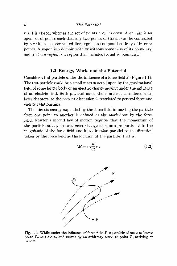
1.2 Energy, Work, and the PotentialConsider a test particle under the influence of a force field F f Figure 1.1).The test particle could be a small mass m acted upon by the gravitationalfield of some larger body or an electric charge moving under the influenceof an electric field. Such physical associations are not considered untillater chapters, so the present discussion is restricted to general force andenergy relationships.
The kinetic energy expended by the force field in moving the particlefrom one point to another is defined as the work done by the forcefield. Newton's second law of motion requires that the momentum ofthe particle at any instant must change at a rate proportional to themagnitude of the force field and in a direction parallel to the directiontaken by the force field at the location of the particle; that is,
AF = m ^ v , (1.2)
Fig. 1.1. While under the influence of force field F, a particle of mass m leavespoint Po at time to and moves by an arbitrary route to point P, arriving attime t.
1.2 Energy, Work, and the Potential 5
where A is a constant that depends on the units used, and v is thevelocity of the particle. We select units in order to make A = 1 andmultiply both sides of equation 1.2 by v to obtain
1 d 2F v = -m—vz
2 dt
where E is the kinetic energy of the particle. If the particle moves frompoint Po to P during time interval to to t (Figure 1.1), then the changein kinetic energy is given by integration of equation 1.3 over the timeinterval,
t
E-Eo= IF -vdtf
to
t
Po
= W(P,P0), (1.4)
where ds represents elemental displacement of the particle. The quantityW(P, Po) is the work required to move the particle from point Po to P.Equation 1.4 shows that the change in kinetic energy of the particleequals the work done by F.
In general, the work required to move the particle from Po to P differsdepending on the path taken by the particle. A vector field is said to beconservative in the special case that work is independent of the path ofthe particle. We assume now that the field is conservative and move theparticle an additional small distance Ax parallel to the x axis, as shownin Figure 1.2. Then
W(P, Po) + W(P + Ax, P) = W(P + Ax, Po),
and rearranging terms yields
W(P + Ax, Po) - W(P, Po) = W(P + Ax, P)P+Ax
= / Fx(x,y,z)dx.
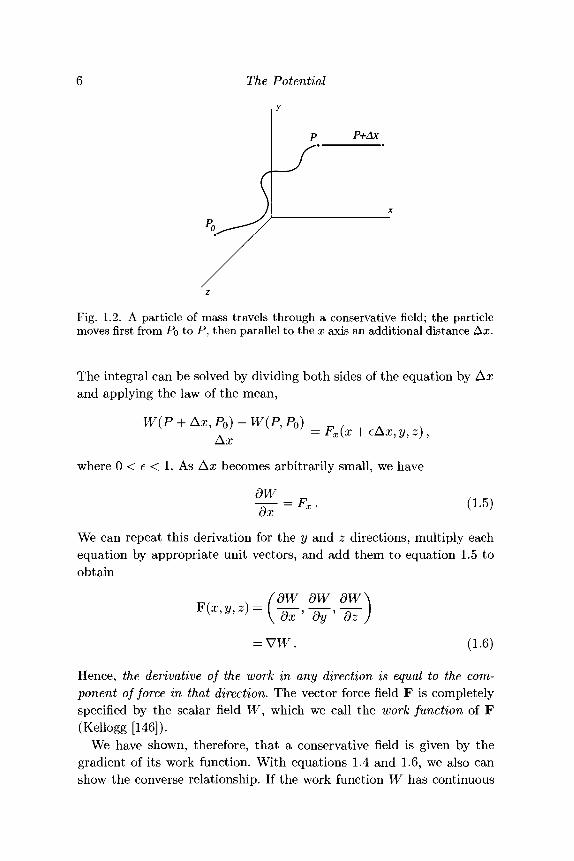
Fig. 1.2. A particle of mass travels through a conservative field; the particlemoves first from PQ to P, then parallel to the x axis an additional distance Ax.
The integral can be solved by dividing both sides of the equation by Axand applying the law of the mean,
Axwhere 0 < e < 1. As Ax becomes arbitrarily small, we have
dWdx = FX (1.5)
We can repeat this derivation for the y and z directions, multiply eachequation by appropriate unit vectors, and add them to equation 1.5 toobtain
, fdW dW dW\F(x,y,z) = ——, ——, ——\ dx dy dz J
(1.6)
Hence, the derivative of the work in any direction is equal to the com-ponent of force in that direction. The vector force field F is completelyspecified by the scalar field W, which we call the work function of F(Kellogg [146]).
We have shown, therefore, that a conservative field is given by thegradient of its work function. With equations 1.4 and 1.6, we also canshow the converse relationship. If the work function W has continuous
1.2 Energy, Work, and the Potential
derivatives, then we can integrate equation 1.6 as follows:
p
W(P,P0)= / V d s
pf (dW dW dW= / -z—dx + -K~dy + -z-dzJ \ ox ay oz
Po
Po
= W(P)-W(P0). (1.7)
Hence, the work depends only on the values of W at endpoints P andPo, not on the path taken, and this is precisely the definition of a con-servative field. Consequently, any vector field that has a work functionwith continuous derivatives as described in equation 1.6 is conservative.A corollary to equation 1.7 results if the path of the particle is a closedloop. Then P equals Po, W(P,Po) = 0, and no net work is required tomove the particle around the closed loop.
The potential <fi of vector field F is defined as the work function or asits negative depending on the convention used. Kellogg [146] summarizesthese conventions as follows: If particles of like sign attract each other(e.g., gravity fields), then F — V0 and the potential equals the workdone by the field. If particles of like sign repel each other (e.g., electro-static fields), then F = — V0, and the potential equals the work doneagainst the field by the particle. In the latter case, the potential <fi is thepotential energy of the particle; in the former case, (j) is the negative ofthe particle's potential energy.
Note that any constant can be added to <fi without changing the im-portant result that
This constant is chosen generally so that (p approaches 0 at infinity. Inother words, the potential at point P is given by
p
= JF-ds. (1.8)
8 The Potential
The value of the potential at a specific point, therefore, is not nearly soimportant as the difference in potential between two separated points.
1.2.1 Equipotential SurfacesAs its name implies, an equipotential surface is a surface on which thepotential remains constant; that is,
</>(#, y, z) — constant.
If s is a unit vector lying tangent to an equipotential surface of F, thens • F = £j at any point and must vanish according to the definitionof an equipotential surface. It follows that field lines at any point arealways perpendicular to their equipotential surfaces and, conversely, anysurface that is everywhere perpendicular to all field lines must be anequipotential surface. Hence, no work is done in moving a test particlealong an equipotential surface. Only one equipotential surface can existat any point in space. The distance between equipotential surfaces is ameasure of the density of field lines; that is, a force field will have greatestintensity in regions where its equipotential surfaces are separated bysmallest distances.
Exercise 1.2 Prove that equipotential surfaces never intersect.
1.3 Harmonic FunctionsTo summarize the previous section, a conservative field F has a scalarpotential 0 given by F = V0 (or F = — V</>, depending on sign conven-tion). Moreover, if F = V0, then F is conservative and is said to be apotential field. In the following we discuss another property of potentialfields: The potential <fi of field F, under certain conditions to be discussedin Chapter 2, satisfies an important second-order differential equationcalled Laplace's equation,
V20 = O, (1.9)
at points not occupied by sources of F. Several surprising and illustrativeresults follow from this statement. We start by discussing the physicalmeaning of Laplace's equation, first with the trivial one-dimensional caseand then the general equation.
1.3 Harmonic Functions 9
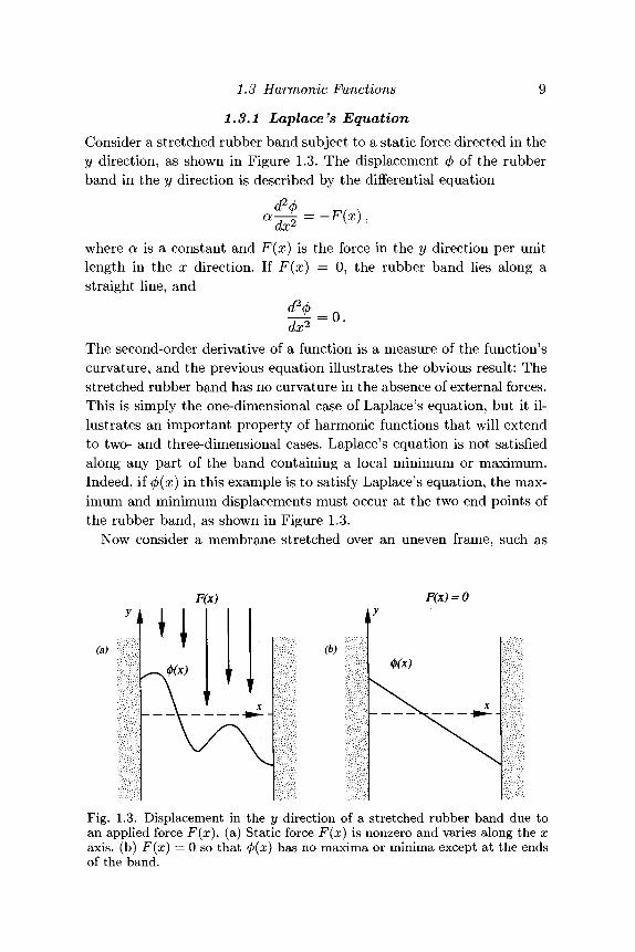
1.3.1 Laplace'}s EquationConsider a stretched rubber band subject to a static force directed in they direction, as shown in Figure 1.3. The displacement <p of the rubberband in the y direction is described by the differential equation
where a is a constant and F(x) is the force in the y direction per unitlength in the x direction. If F(x) = 0, the rubber band lies along astraight line, and
The second-order derivative of a function is a measure of the function'scurvature, and the previous equation illustrates the obvious result: Thestretched rubber band has no curvature in the absence of external forces.This is simply the one-dimensional case of Laplace's equation, but it il-lustrates an important property of harmonic functions that will extendto two- and three-dimensional cases. Laplace's equation is not satisfiedalong any part of the band containing a local minimum or maximum.Indeed, if 4>(x) in this example is to satisfy Laplace's equation, the max-imum and minimum displacements must occur at the two end points ofthe rubber band, as shown in Figure 1.3.
Now consider a membrane stretched over an uneven frame, such as
(a)
F(x) = 0
(b)
Fig. 1.3. Displacement in the y direction of a stretched rubber band due toan applied force F(x). (a) Static force F(x) is nonzero and varies along the xaxis, (b) F(x) = 0 so that <j>(x) has no maxima or minima except at the endsof the band.
10 The Potential
mm
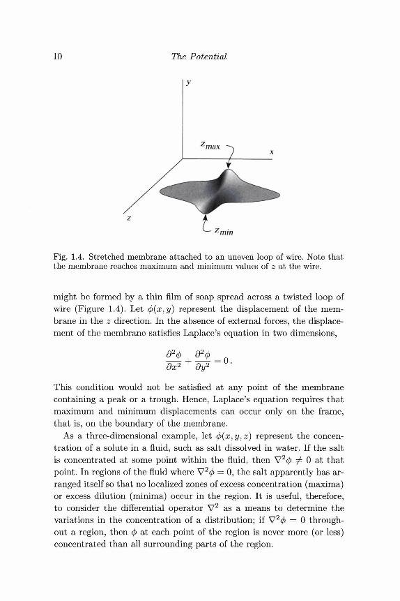
Fig. 1.4. Stretched membrane attached to an uneven loop of wire. Note thatthe membrane reaches maximum and minimum values of z at the wire.
might be formed by a thin film of soap spread across a twisted loop ofwire (Figure 1.4). Let (j)(x,y) represent the displacement of the mem-brane in the z direction. In the absence of external forces, the displace-ment of the membrane satisfies Laplace's equation in two dimensions,
dx2 dy2
This condition would not be satisfied at any point of the membranecontaining a peak or a trough. Hence, Laplace's equation requires thatmaximum and minimum displacements can occur only on the frame,that is, on the boundary of the membrane.
As a three-dimensional example, let (j){x,y,z) represent the concen-tration of a solute in a fluid, such as salt dissolved in water. If the saltis concentrated at some point within the fluid, then V20 ^ 0 at thatpoint. In regions of the fluid where V2(/> = 0, the salt apparently has ar-ranged itself so that no localized zones of excess concentration (maxima)or excess dilution (minima) occur in the region. It is useful, therefore,to consider the differential operator V2 as a means to determine thevariations in the concentration of a distribution; if V2</> = 0 through-out a region, then </> at each point of the region is never more (or less)concentrated than all surrounding parts of the region.
1.3 Harmonic Functions 11
With these preliminary remarks, we define a harmonic function as anyfunction that (1) satisfies Laplace's equation; (2) has continuous, single-valued first derivatives; and (3) has second derivatives. We might expectfrom the previous examples (and soon will prove) that a function thatis harmonic throughout a region R must have all maxima and minimaon the boundary of R and none within R itself. The converse is notnecessarily true, of course; a function with all maxima and minima onits boundary is not necessarily harmonic because it may not satisfy thethree criteria listed.
The definition of the second derivative of a one-dimensional functiondemonstrates another important property of a harmonic function. Thesecond derivative of </>(x) is given by
( x ) - \[4>{x - A x ) + ^
If 4> satisfies the one-dimensional case of Laplace's equation, then theright-hand side of the previous equation vanishes and
(j)[x) = - lim [<j>(x - Ax) + 4>(x + Ax)} .
Hence, the value of a harmonic function 0 at any point is the averageof (j> at its neighboring points. This is simply another way of stating thenow familiar property of a potential: A function can have no maxima orminima within a region in which it is harmonic. We will discuss a morerigorous proof of this statement in Chapter 2.
1.3.2 An Example from Steady-State Heat FlowConsider a temperature distribution T specified throughout some regionR of a homogeneous material. All heat sources and sinks are restrictedfrom the region. According to Fourier's law, the flow of heat J at anypoint of R is proportional to the change in temperature at that point,that is,
J = -fcVT, (1.10)
where k is thermal conductivity, a constant of the medium. Equation 1.10tells us, on the basis of the discussion in Section 1.2, that temperatureis a potential, and flow of heat J is a potential field analogous to a forcefield. Field lines for J describe the pattern and direction of heat transfer,
12 The Potential
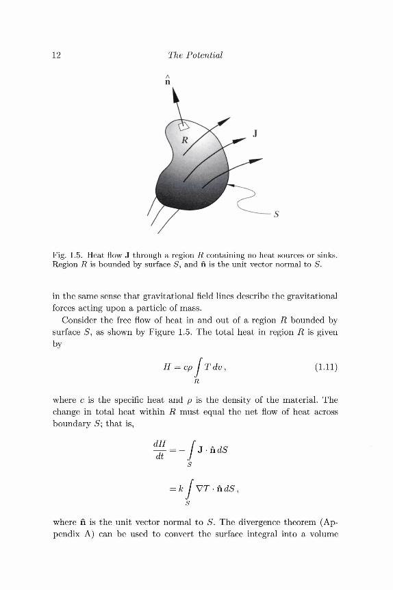
Fig. 1.5. Heat flow J through a region R containing no heat sources or sinks.Region R is bounded by surface S, and n is the unit vector normal to S.
in the same sense that gravitational field lines describe the gravitationalforces acting upon a particle of mass.
Consider the free flow of heat in and out of a region R bounded bysurface 5, as shown by Figure 1.5. The total heat in region R is givenby
Tdv, (1.11)
where c is the specific heat and p is the density of the material. Thechange in total heat within R must equal the net flow of heat acrossboundary 5; that is,
dH _ f~dt~~J
s
•I
J -hdS
= k / VT-nc/5,
where n is the unit vector normal to S. The divergence theorem (Ap-pendix A) can be used to convert the surface integral into a volume
1.3 Harmonic Functions 13
integral; that is,AH I
V -VTdvdt JR
= k fv2Tdv. (1.12)R
From equation 1.11, the change in heat over time is also given bydH fdTJ t
R
and combining equations 1.13 and 1.12 provides
8T \cp— - kV2T dv = 0. (1.14)
(J L JR
This integral vanishes for every choice of the region R. If the integrand,which we assume is continuous, is not zero throughout i?, then we couldchoose some portion of R so as to contradict equation 1.14. Hence, theintegrand itself must be zero throughout R, or
« V 2 T = ^ , (1.15)
where K = k/cp is thermal diffusivity. Equation 1.15 is the equation ofconductive heat transfer. If all heat sources and sinks lie outside of regionR and do not change with time, then steady-state conditions eventuallywill be obtained and equation 1.15 becomes
V2T = 0 (1.16)
throughout R. Hence, temperature under steady-state conditions satis-fies Laplace's equation and is harmonic.
The temperature distribution accompanying steady-state transfer ofheat is an easily visualized example of a harmonic function, one whichclarifies some of the theoretical results discussed earlier. For example,imagine a volume of rock with no internal heat sources or heat sinks(Figure 1.5) and in steady-state condition. On the basis of previous dis-cussions, we can state a number of characteristics of the temperaturedistribution within the volume of rock. (1) We conclude that the tem-perature within the volume of rock cannot reach any maximum or min-imum values. This is a reasonable result; if temperature is in a steady-state condition, all maxima and minima should occur at heat sources
14 The Potential
and sinks, and these have been restricted from this part of the rock. (2)Furthermore, maximum and minimum temperatures must occur on theboundary of the volume and not within the volume. After all, some pointof the boundary must be closer to any external heat sources (or sinks)than all interior points; likewise, some point of the boundary will befarther from any external heat source (or sink) than all interior points.(3) It also is reasonable that the temperature at any point is the averageof the temperatures in a small region around that point.Exercise 1.3 One end of a glass rod is kept in boiling water and the opposite
end in ice water until the temperature of the rod reaches equilibrium.Suddenly the two ends are switched so that the hot end is in ice waterand the cold end is in boiling water. Describe how the temperature ofthe rod changes with time. Is the temperature harmonic?
Finding a solution to Laplace's equation, if indeed one exists, is aboundary-value problem of, in this case, the Dirichlet type; that is, finda representation for (j) throughout a region i?, given that V20 = 0 withinR and given specified values of <j) on the surface that bounds R. Forexample, the steady-state temperature can be calculated, in principle,throughout a spherically shaped region of homogeneous matter by solv-ing equation 1.16 subject to specified boundary conditions. We will haveconsiderably more to say about this subject in later chapters.
1.3.3 Complex Harmonic FunctionsThis section provides a very brief review of complex functions sufficientto draw one important conclusion: The real and imaginary parts of acomplex function are harmonic in regions where the complex function isanalytic. For additional information about complex functions, the inter-ested reader is referred to the textbook by Churchill [59].
First we need some definitions. In the following, x and y are realvariables describing a two-dimensional cartesian coordinate system. Thecoordinate system represents the complex plane, and any point of theplane is identified by the complex number z = x + iy, where i = A/~T-As discussed in Section 1.1.2 for general cases, we can consider sets ofpoints of the complex plane. A neighborhood of a point z0 of the complexplane is the set of all points such that \z — zo\ < e, where e is a positiveconstant. An interior point of a set of points has some neighborhoodcontaining only points of the set. Sets that contain only interior pointsare called open regions. Open, connected regions of the complex planeare called domains.
1.3 Harmonic Functions 15
If a complex number w is prescribed for each value of a set of com-plex numbers z, usually a domain, then if is a complex function of thecomplex variable z, written w(z). Complex functions can be written interms of their real and imaginary parts,
w(z) = u(z) + iv(z),
where u(z) and v(z) are real functions of the complex variable z. Forexample, if
w(z) = z2
= x2 — y2 + 2ixy ,
then u(x, y) — x2 — y2 and v(x, y) = 2xy, and the domain of definitionin this case is the entire complex plane.
The derivative of a complex function requires special consideration. Inorder for a real function f(x) to have a derivative, the ratio of the changein / to a change in x, Af/Ax, must have a limit as Ax approaches 0.Similarly, for the derivative of complex function w(z) to exist in a do-main, it is necessary that the ratio
riz) = lim —— ,
have a limit. In the complex plane, however, there are different pathsalong which Az can approach zero, and the value of the ratio r(z) maydepend on that path. For example, the complex function w(z) = z2 hasr(z) = 2(#o + Wo) a t point (xo,yo)5 independent of how Az approacheszero, whereas the complex function w(z) = x2 -\- y2 — i 2xy is dependenton the path taken as Az —> 0. In this latter case, the ratio has no limitand the derivative does not exist.
A function w(z) = u(x,y) + iv(x,y) is said to be analytic in a do-main of the complex plane if the real functions u(x,y) and v(x,y) havecontinuous partial derivatives and if w(z) has a derivative with respectto z at every point of the domain. The Cauchy-Riemann conditionsprovide an easy way to determine whether such conditions are met. Ifu(x,y) and v(x,y) have continuous derivatives of first order, then theCauchy-Riemann conditions,

16 The Potential
are necessary and sufficient conditions for the analyticity of w(z). Thederivative of the complex function is given by
dw du . dvdz dx dx
dv .dudy dy '
Now consider a complex function analytic within some domain T. Thetwo-dimensional Laplacian of its real part u(x,y) is given by
« d2u d2uox1 oyz
The Cauchy-Riemann conditions are applicable here because w(z) isanalytic; hence, we assume that derivatives of second order exist andemploy the Cauchy-Riemann conditions to get
dxdy dxdy= 0.
Consequently, the real part of a complex function satisfies the two-dimensional case of Laplace's equation in domains in which the func-tion is analytic, and since the necessary derivatives exist, the real partof w(z) must be harmonic. Hence, if a complex function is analytic indomain T', it has a real part that is harmonic in T. Likewise, it can beshown that the imaginary part of an analytic complex function also isharmonic in domains of analyticity.
Exercise 1.4 Use the Cauchy-Riemann conditions to show that the imagi-nary part of an analytic function satisfies Laplace's equation.
Conversely, if u is harmonic in T, there must exist a function v such thatu + iv is analytic in T, and v is given by
zf\dun du 7v = / - —-dx+ --dyJ [ dy dx
We will have occasion later in this text to use these rather abstract prop-erties of complex numbers in some practical geophysical applications.
1.4 Problem Set 17
1.4 Problem Set1. The potential of F is given by (x2 -\- y2)~l.
(a) Find F.(b) Describe the field lines of F.(c) Describe the equipotential surfaces of F.(d) Demonstrate by integration around the perimeter of a rectangle
in the x, y plane that F is conservative. Let the rectangle extendfrom x\ to X2 in the x direction and from y\ to 2 m the ydirection, and let x\ > 0.
2. Prove that the intensity of a conservative force field is inverselyproportional to the distance between its equipotential surfaces.
3. If all mass lies interior to a closed equipotential surface S on whichthe potential takes the value C, prove that in all space outside of Sthe value of the potential is between C and 0.
4. If the lines of force traversing a certain region are parallel, what maybe inferred about the intensity of the force within the region?
5. Two distributions of matter lie entirely within a common closedequipotential surface C. Show that all equipotential surfaces outsideof C also are common.
6. For what integer values of n is the function {x2-\-y2-\-z2)^ harmonic?7. You are monitoring the magnetometer aboard an interstellar space-
craft and discover that the ship is approaching a magnetic sourcedescribed by
(a) Remembering Maxwell's equation for B, will you report to Mis-sion Control that the magnetometer is malfunctioning, or is thisa possible source?
(b) What if the magnetometer indicates that B is described by
8. The physical properties of a spherical body are homogeneous. De-scribe the temperature at all points of the sphere if the temperatureis harmonic throughout the sphere and depends only on the distancefrom its center.
9. As a crude approximation, the temperature of the interior of theearth depends only on distance from the center of the earth. Based
18 The Potential
on the results of the previous exercise, would you expect the temper-ature of the earth to be harmonic everywhere inside? Explain youranswer?
10. Assume a spherical coordinate system and let r be a vector directedfrom the origin to a point P with magnitude equal to the distancefrom the origin to P. Prove the following relationships:
V - r = 3,
Vr = - ,r
V- (^)=°> ^ o ,
V x r = 0,
r r6
(A-V)r = Ar-.r
2Consequences of the Potential
It may be no surprise that human minds can deduce the laws offalling objects because the brain has evolved to devise strategiesfor dodging them.
(Paul Davies)
Only mathematics and mathematical logic can say as little as thephysicist means to say.
(Bertrand Russell)
In Chapter 1, we learned that a conservative vector field F can be ex-pressed as the gradient of a scalar </>, called the potential of F, andconversely F is conservative if F = V<f>. It was asserted that such po-tentials satisfy Laplace's equation at places free of all sources of F andare said to be harmonic. This led to several important characteristics ofthe potential. In the same spirit, this chapter investigates a number ofadditional consequences that follow from Laplace's equation.
2.1 Green's IdentitiesThree identities can be derived from vector calculus and Laplace's equa-tion, and these lead to several important theorems and additional in-sight into the nature of potential fields. They are referred to as Green'sidentities.^
f The name Green, appearing repeatedly in this and subsequent chapters, refers toGeorge Green (1793-1841), a British mathematician of Caius College, Cambridge,England. He is perhaps best known for his paper, Essay on the Application ofMathematical Analysis to the Theory of Electricity and Magnetism, and was ap-parently the first to use the term "potential."
19
20 Consequences of the Potential
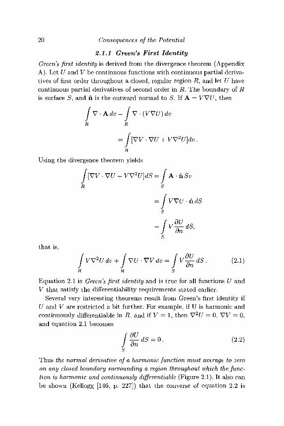
2.1.1 Green's First IdentityGreen's first identity is derived from the divergence theorem (AppendixA). Let U and V be continuous functions with continuous partial deriva-tives of first order throughout a closed, regular region R, and let U havecontinuous partial derivatives of second order in R. The boundary of Ris surface #, and h is the outward normal to S. If A = WE/ , then
R R
= Aw-
Using the divergence
R
theorem
•VE/ +
R
yields
VV2U]dS -1s
-ls
A-hSv
VVU -ndS
that is,
fw2Udv+ fvUVVdv= fv^dS. (2.1)
Equation 2.1 is Green's first identity and is true for all functions U andV that satisfy the differentiability requirements stated earlier.
Several very interesting theorems result from Green's first identity ifU and V are restricted a bit further. For example, if U is harmonic andcontinuously differentiate in R, and if V = 1, then V2E/ = 0, VT/ = 0,and equation 2.1 becomes
J On (2.2)
Thus the normal derivative of a harmonic function must average to zeroon any closed boundary surrounding a region throughout which the func-tion is harmonic and continuously differentiable (Figure 2.1). It also canbe shown (Kellogg [146, p. 227]) that the converse of equation 2.2 is
2.1 Green's Identities 21
F= VU
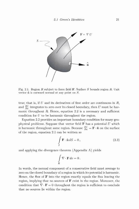
Fig. 2.1. Region i? subject to force field F. Surface S bounds region R. Unitvector n is outward normal at any point on S.
true; that is, if U and its derivatives of first order are continuous in R,and ^ integrates to zero over its closed boundary, then U must be har-monic throughout R. Hence, equation 2.2 is a necessary and sufficientcondition for U to be harmonic throughout the region.
Equation 2.2 provides an important boundary condition for many geo-physical problems. Suppose that vector field F has a potential U whichis harmonic throughout some region. Because ^ = F • n on the surfaceof the region, equation 2.1 can be written as
F-ndS = 0, (2.3)
and applying the divergence theorem (Appendix A) yields
V • F dv = 0 ./ •R
In words, the normal component of a conservative field must average tozero on the closed boundary of a region in which its potential is harmonic.Hence, the flux of F into the region exactly equals the flux leaving theregion, implying that no sources of F exist in the region. Moreover, thecondition that V • F = 0 throughout the region is sufficient to concludethat no sources lie within the region.
22 Consequences of the Potential
Steady-state heat flow, for example, is harmonic (as discussed in Chap-ter 1) in regions without heat sources or sinks and must satisfy equa-tion 2.3. If region R is in thermal equilibrium and contains no heatsources or sinks, the heat entering R must equal the heat leaving R.Equation 2.3 is often called Gauss's law and will prove useful in subse-quent chapters.
Now let U be harmonic in region R and let V = U. Then, from Green'sfirst identity,
f(VU)2dv= fu^dS. (2.4)J J onR S
Consider equation 2.4 when U = 0 on S. The right-hand side vanishesand, because (VC/)2 is continuous throughout R by hypothesis, (VLQ2 =0. Therefore, U must be a constant. Moreover, because U = 0 on Sand because U is continuous, the constant must be zero. Hence, if Uis harmonic and continuously differentiate in R and if U vanishes atall points of S, U also must vanish at all points of R. This result isintuitive from steady-state heat flow. If temperature is zero at all pointsof a region's boundary and no sources or sinks are situated within theregion, then clearly the temperature must vanish throughout the regiononce equilibrium is achieved.
Green's first identity leads to a statement about uniqueness, some-times referred to as Stokes's theorem. Let U\ and U2 be harmonic in Rand have identical boundary conditions, that is,
U1(S) = U2(S).
The function U1 — U2 also must be harmonic in R. But U1 — U2 vanishes onS and the previous theorem states that U\ — U2 also must vanish at everypoint of R. Therefore, U\ and U2 are identical. Consequently, a functionthat is harmonic and continuously differentiate in R is uniquely deter-mined by its values on S, and the solution to the Dirichlet boundary-value problem is unique. Stokes's theorem makes intuitive sense whenapplied to steady-state heat flow. A region will eventually reach thermalequilibrium if heat is allowed to flow in and out of the region. It seemsreasonable that, for any prescribed set of boundary temperatures, theregion will always attain the same equilibrium temperature distributionthroughout the region regardless of the initial temperature distribution.In other words, the steady-state temperature of the region is uniquelydetermined by the boundary temperatures.
2.1 Green's Identities 23
The surface integral in equation 2.4 also vanishes if ^ = 0 on S. Asimilar proof could be developed to show that if U is single-valued, har-monic, and continuously differentiate in R and if Qj£ = 0 on S, then Uis a constant throughout R. Again, steady-state heat flow provides someinsight. If the boundary of R is thermally insulated, equilibrium tem-peratures inside R must be uniform. Moreover, a single-valued harmonicfunction is determined throughout R, except for an additive constant, bythe values of its normal derivatives on the boundary.
Exercise 2.1 Prove the previous two theorems.
These last theorems relate to the Neumann boundary-value problem andshow that such solutions are unique to within an additive constant.
The uniqueness of harmonic functions also extends to mixed boundary-value problems. // U is harmonic and continuously differentiate in Rand if
onon S, where h and g are continuous functions of S, and h is nevernegative, then U is unique in R.
Exercise 2.2 Prove the previous theorem.
We have shown that under many conditions Laplace's equation hasonly one solution in a region, thus describing the uniqueness of harmonicfunctions. But can we say that even that one solution always exists? Theanswer to this interesting question requires a set of "existence theorems"for harmonic functions that are beyond the scope of this chapter. Inter-ested readers are referred to Chapter XI of Kellogg [146, p. 277] for acomprehensive discussion.
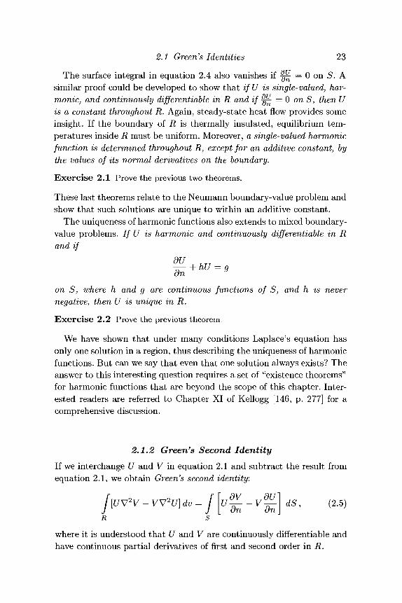
2.1.2 Green's Second IdentityIf we interchange U and V in equation 2.1 and subtract the result fromequation 2.1, we obtain Green's second identity.
^ ] ^ , (2.5)
where it is understood that U and V are continuously differentiate andhave continuous partial derivatives of first and second order in R.
24 Consequences of the Potential
A corollary results if U and V are both harmonic:
This relationship will prove useful later in this chapter in discussingcertain kinds of boundary-value problems. Also notice that if V = 1 inequation 2.5 and if U is the potential of F, then
f\/2Udv= [R S
In regions of space where U is harmonic, we have the same result as inSection 2.1.1,
F-hdS = 0,s
namely, that the normal component of a conservative field averages tozero over any closed surface.
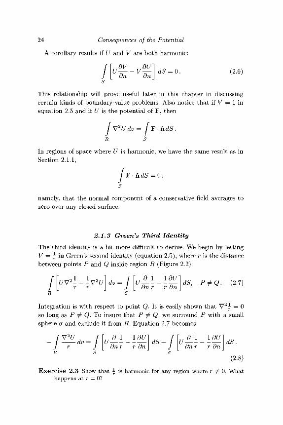
2.1.3 Green's Third Identity
The third identity is a bit more difficult to derive. We begin by lettingV = ^ in Green's second identity (equation 2.5), where r is the distancebetween points P and Q inside region R (Figure 2.2):
^u}dv[\u^f}dS, P^Q. (2.7)r r J J [ dnr r dn\
Integration is with respect to point Q. It is easily shown that V2^ = 0so long as P ^ Q. To insure that P ^ Q, we surround P with a smallsphere a and exclude it from R. Equation 2.7 becomes
f^2U ^ f \ r r d l l d U ] ^ f \ r r d l ldU],n- / dv= / \u- — ds+ / \u- ir\dS'J r J I on r r on J J |_ onr r on JR s a
(2.8)Exercise 2.3 Show that ^ is harmonic for any region where r ^ 0. What
happens at r = 0?
2.1 Green's Identities
S
25
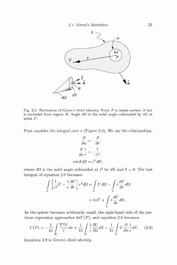
Fig. 2.2. Derivation of Green's third identity. Point P is inside surface S butis excluded from region R. Angle dQ, is the solid angle subtended by dS atpoint P.
First consider the integral over a (Figure 2.2). We use the relationships,
____dn dr'
dr r
where dfl is the solid angle subtended at P by dS and 0 = 0. The lastintegral of equation 2.8 becomes
dUdfl.
As the sphere becomes arbitrarily small, the right-hand side of the pre-vious expression approaches 4TTU(P)1 and equation 2.8 becomes
! , s . ( 2 . 9 )r4?r
R S
Equation 2.9 is Green's third identity.
26 Consequences of the Potential
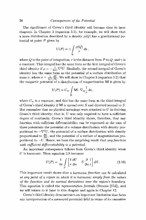
The significance of Green's third identity will become clear in laterchapters. In Chapter 3 (equation 3.5), for example, we will show thata mass distribution described by a density p(Q) has a gravitational po-tential at point P given by
where Q is the point of integration, r is the distance from P to Q, and 7 isa constant. This integral has the same form as the first integral of Green'sthird identity if p = — 4^V2 t / . Similarly, the second integral of Green'sidentity has the same form as the potential of a surface distribution ofmass cr, where a = ^ - ^ . We will show in Chapter 5 (equation 5.2) thatthe magnetic potential of a distribution of magnetization M is given by
R
where Cm is a constant, and this has the same form as the third integralof Green's third identity if M is spread over S and directed normal to S.But remember that no physical meanings were attached to U in derivingGreen's third identity; that is, U was only required to have a sufficientdegree of continuity. Green's third identity shows, therefore, that anyfunction with sufficient differentiability can be expressed as the sum ofthree potentials: the potential of a volume distribution with density pro-portional to — V2C/, the potential of a surface distribution with densityproportional to ^ , and the potential of a surface of magnetization pro-portional to — U. Hence, we have the surprising result that any functionwith sufficient differentiability is a potential.
An important consequence follows from Green's third identity whenU is harmonic. Then equation 2.9 becomes
This important result shows that a harmonic function can be calculatedat any point of a region in which it is harmonic simply from the valuesof the function and its normal derivatives over the region's boundary.This equation is called the representation formula (Strauss [274]), andwe will return to it later in this chapter and again in Chapter 12.
Green's third identity demonstrates an important limitation that facesany interpretation of a measured potential field in terms of its causative
2.1 Green's Identities 27
sources. It was shown earlier that a harmonic function satisfying a givenset of Dirichlet boundary conditions is unique, but the converse is nottrue. If U is harmonic in a region R, it also must be harmonic in eachsubregion of R. Likewise equation 2.10 must apply to the boundary ofeach subregion. It follows that the potential within any subregion ofR can be related to an infinite variety of surface distributions. Hence,no unique boundary conditions exist for a given harmonic function. Thisproperty of nonuniqueness will be a common theme in following chapters.
2.1.4 Gauss's Theorem of the Arithmetic MeanAnother consequence of Green's third identity occurs when U is har-monic, the boundary S is the surface of a sphere, and point P is at thecenter of the sphere. If a is the radius of the sphere, then equation 2.10becomes
47m J dn 4?rs s
The first integral vanishes according to Green's first identity, so that
sHence, the value of a harmonic function at any point is simply the av-erage of the harmonic function over any sphere concentric about thepoint, so long as the function is harmonic throughout the sphere. Thisrelationship is called Gauss's theorem of the arithmetic mean.
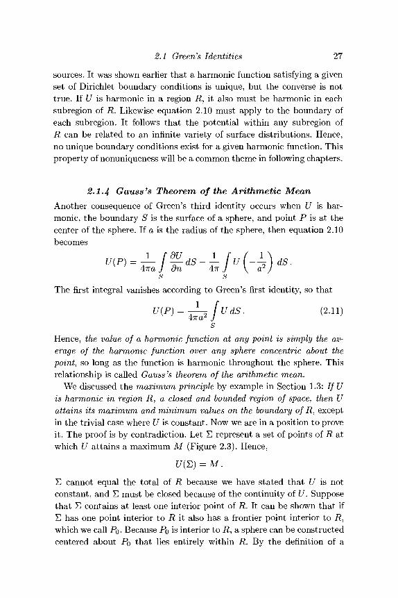
We discussed the maximum principle by example in Section 1.3: IfUis harmonic in region R, a closed and bounded region of space, then Uattains its maximum and minimum values on the boundary of R, exceptin the trivial case where U is constant. Now we are in a position to proveit. The proof is by contradiction. Let E represent a set of points of R atwhich U attains a maximum M (Figure 2.3). Hence,
£/(£) = M.
E cannot equal the total of R because we have stated that U is notconstant, and E must be closed because of the continuity of U. Supposethat E contains at least one interior point of R. It can be shown that ifE has one point interior to R it also has a frontier point interior to R,which we call PQ. Because Po is interior to R, a sphere can be constructedcentered about PQ that lies entirely within R. By the definition of a

28 Consequences of the Potential
Fig. 2.3. Region R includes a set of points E at which U attains a maximum.Point PQ is a frontier point of E. Any sphere centered on PQ must contain atleast one point of E and one point of R not in E.
frontier point (Section 1.1.2), such a sphere must pass outside of E whereU < M. Gauss's theorem of the arithmetic mean and the continuity ofU therefore imply that U(Po) < M. But PQ is also a member of E, andthis requires that U(PQ) = M. A contradiction arises, and our originalsuppositions, that Po a n d at least one point of E lie interior to R, mustbe in error. Hence, no maxima of U can exist interior to R. An analogousproof can be constructed to show that the same is true of all minimaoft/.
2.2 Helmholtz TheoremWe said in Chapter 1 that a vector field F is conservative if the workrequired to move a particle through the field is independent of the pathof the particle, in which case F can be represented as the gradient of ascalar 0,
called the potential of F. Conversely, if F has a scalar potential, then F isconservative. These concepts are a subset of the Helmholtz theorem (Duffand Nay lor [81]) which states that any vector field F that is continuous
2.2 Helmholtz Theorem 29
and zero at infinity can be expressed as the gradient of a scalar and thecurl of a vector, that is,
F = V0 + V x A , (2.12)
where V0 and V x A are orthogonal in the integral norm. The quantity<fi is the scalar potential of F, and A is the vector potential.
2.2.1 Proof of the Helmholtz TheoremGiven that F is continuous and vanishes at infinity, we can constructthe integral
[ d v , (2.13)4TT J r
where Q is the point of integration, r is the distance between P andQ, and the integral is taken over all space. Each of the three cartesiancomponents of W has a form like
l (2J4)At this point, we borrow a result from Chapter 3: Equation 2.14 is asolution to a very important differential equation, Poisson's equation:
V2WX = -FX. (2.15)
The relationship between equations 2.14 and 2.15 follows from Green'sthird identity because the integration in equation 2.14 is over all space,and we have stipulated that F and, therefore, the three components ofF vanish at infinity.
Exercise 2.4 Show that equations 2.14 and 2.15 are consistent with Green'sthird identity.
With W defined as in equation 2.13, the relationship between equa-tions 2.14 and 2.15 suggests that
V2W = - F , (2.16)
where each component of F leads to an example of Poisson's equation.A vector identity (Appendix A) shows that V 2W can be represented bya gradient plus a curl, that is,
- V2W = -V(V • W) + V x (V x W ) , (2.17)
and hence F is represented as the gradient of a scalar (V • W) plus the
30 Consequences of the Potential
curl of a vector (V x W). We define (ft = —V • W and A = V x W andsubstitute these definitions along with equation 2.16 into equation 2.17to get the Helmholtz theorem,
F = V0 + V x A.
E x e r c i s e 2 . 5 P r o v e t h e v e c t o r i d e n t i t y V ( V - W ) - V x V x W = V 2 W .
Hence, the Helmholtz theorem is proven: If F is continuous and vanishesat infinity, it can be represented as the gradient of a scalar potential plusthe curl of a vector potential.
The Helmholtz theorem is useful, however, only if the scalar and vec-tor potentials can be derived directly from F. This should be possiblebecause of the way (ft and A were defined, and the relationships can beseen by taking the divergence and curl of both sides of equation 2.12.The divergence yields
V2(ft = V - F ,
which, comparing with equations 2.14 and 2.15, has the solution
<£ = -T- f^-^-dv. (2.18)4TT J r
The curl of equation 2.12 provides
V2A = V(V- A ) - V x F .
For convenience, we define A so that it has no divergence, and conse-quently
V2A = - V x F .
Comparing this result with equations 2.13 and 2.16 leads toV X — dv. (2.19)= - / •
4WExercise 2.6 Show that equation 2.19 implies that V • A = 0.
Consequently, the scalar potential (ft and vector potential A can be de-rived from integral equations taken over all space and involving the di-vergence and curl, respectively, of F itself.Exercise 2.7 Prove the last statement of the Helmholtz theorem; that is,
show that V</> and V x A, both vanishing at infinity, are orthogonalunder integration over three-dimensional space.
2.2 Helmholtz Theorem 31
2.2.2 Consequences of the Helmholtz TheoremThe Helmholtz theorem shows that a vector field vanishing at infinityis completely specified by its divergence and its curl if they are knownthroughout space. If both the divergence and curl vanish at all points,then the field itself must vanish or be constant everywhere.
In addition to this statement, the following important observationsfollow directly from the Helmholtz theorem and from the integral repre-sentation for scalar and vector potentials.
Irrotational FieldsA vector field is irrotational in a region if its curl vanishes at each point ofthe region; that is, F is irrotational in a region if V x F = 0 throughoutthe region. Such fields have no vorticity or "eddies." For example, ifthe flow of a fluid can be represented as an irrotational field, then asmall paddlewheel placed within the fluid will not rotate. Examples ofirrotational fields are common and include gravitational attraction, ofconsiderable importance to future chapters.
Consider any surface S entirely within a region where V x F = 0.Integration of the curl over the surface provides
(V x F) -hdS = 0,s
and applying Stokes's theorem (Appendix A) provides
F • ds - 0 ,/ •where the closed line integral is taken around the perimeter of S. Becausethe integral holds for any closed surface within the region, no net workis done in moving around any closed loop that lies within an irrotationalfield, that is, work is independent of path, and F is conservative, asufficient condition for the existence of a scalar potential such that F =V</>. Hence, the condition that V x F = 0 at each point of a region issufficient to say that F = V</>. Furthermore, a field that has a scalarpotential has no curl because V x F = V x V</> vanishes identically(Appendix A). Hence, the property that V x F = 0 at every point of aregion is a necessary and sufficient condition for the existence of a scalarpotential such that F = V0.
32 Consequences of the Potential
Solenoidal Fields
A vector field F is said to be solenoidal in a region if its divergencevanishes at each point of the region. A physical meaning for solenoidalfields can be had by integrating the divergence of F over any volume Vwithin the region,
/ •
V • F dv = 0 ,v
and applying the divergence theorem (Appendix A) to get
F-ndS = 0, (2.20)s
where S is the closed boundary of V. Hence, if the divergence of Fvanishes in a region, the normal component of the field vanishes whenintegrated over any closed surface within the region. Or put another way,the "number" of field lines entering a region equals the number that exitthe region, and sources or sinks of F do not exist in the region. Forexample, gravitational attraction is solenoidal in regions not occupiedby mass.
It was stated in Section 2.1.1 that if a function </> can be found suchthat F = V</>, then the condition expressed by equation 2.20 is necessaryand sufficient to say that <fi is harmonic throughout the region. From theHelmholtz theorem, V • F = V20 + V • V x A. The last term of thisequation vanishes identically (Appendix A), and V • F = V20. Hence, ifthe divergence of a conservative field vanishes in a region, the potentialof the field is harmonic in the region.
Note that if F = V x A, then V • F = 0; that is, the divergence of avector field vanishes if the vector can be expressed purely as the curl ofanother vector. Furthermore, the converse can be shown to be true bytaking the curl of both sides of equation 2.19. Hence, the property thatV • F = 0 is a necessary and sufficient condition for F = V x A.
2.2.3 ExampleEquation 2.18 is important to the geophysical interpretation of gravityand magnetic anomalies caused by crustal masses and magnetic sources,respectively. To see this, we use the magnetic field as an example andanticipate the results of future chapters.
2.2 Helmholtz Theorem 33
A set of differential equations, called Maxwell's equations, describesthe spatial and temporal relationships of electromagnetic fields and theirsources. One of Maxwell's equations relates magnetic induction B andmagnetization M in the absence of macroscopic currents:
V x B = /i0V x M ,
where /io is the permeability of free space. Magnetic field intensity H isrelated to magnetic induction and magnetization by the equation
B = /io(H + M) . (2.21)
Hence, in the absence of macroscopic currents,
V x H = 0,
and it follows from the Helmholtz theorem that magnetic field intensityis irrotational and can be expressed in terms of a scalar potential, that is,H = — VV, where the minus sign is a matter of convention as discussedin Chapter 1. Moreover, equation 2.18 provides an expression for thatscalar potential:
V=T- / ^ V (2-22)4TT J r
where it is understood that the integration is over all space. Another ofMaxwell's equations states that magnetic induction has no divergence,that is, V • B = 0. This fact plus equation 2.21 yields
V H = - V M , (2.23)
and substituting into equation 2.22 provides
™*dv. (2.24)r
Again integration is over all space. Equation 2.24 provides a way to cal-culate magnetic potential and magnetic field from a known (or assumed)spatial distribution of magnetic sources. This is called the forward prob-lem when applied to the geophysical interpretation of measured magneticfields. Equation 2.24 also is a suitable starting point for discussions ofthe inverse problem: the direct calculation of the distribution of magne-tization from observations of the magnetic field. We will return to thisequation in Chapter 5 and subsequent chapters.
34 Consequences of the Potential
2.3 Green's Functions
We now turn to Green's functions, important tools for solving certainclasses of problems in potential theory. A heuristic approach will be used,first considering a mechanical system and then extending this result toLaplace's equation.
2.3.1 Analogy with Linear Systems
We begin with the differential equation describing motion of a particlesubject to both a resistance R and an external force
dm —v(t) = -Rv(t) + f(t), (2.25)
where v(t) is the velocity and m is the mass of the particle, respectively.One conceptual way to solve equation 2.25 is to abruptly strike theparticle and observe its response; that is, we let the force be zero exceptover a short time interval Ar,
(-£-, i f r < £ < r + Ar;f(t) = \ AT (2.26)
( 0, otherwise.
As soon as the force returns to zero, the velocity of the particle behaveslike a decaying exponential, and the solution has the form
v(t) = Aexp (t - (r + Ar)) , t > r + AT . (2.27)
The coefficient A can be found if the velocity of the particle is knownat the moment that the force returns to zero; that is, v{r + Ar) = A.To find this velocity, we integrate both sides of equation 2.25 over theduration of the force
T+AT T+AT
m[v(r + Ar) - v(r)] = -R I v(t) dt + — / dt.T T
The first integral can be ignored if Ar is small and the particle has somemass. Also v(r) = 0. Hence,
mv(r + Ar) = / ,
2.3 Green's Functions 35
X X+AX
Time
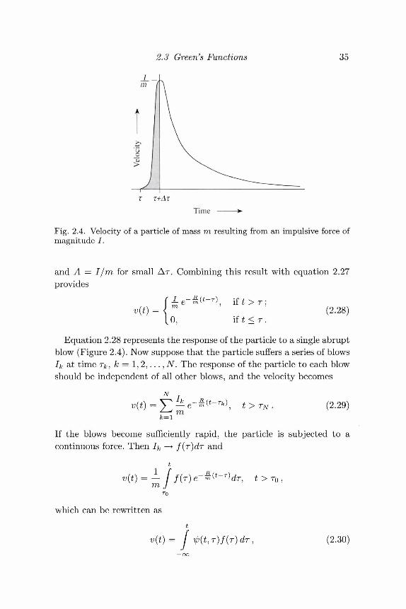
Fig. 2.4. Velocity of a particle of mass m resulting from an impulsive force ofmagnitude / .
and A = I/m for small AT. Combining this result with equation 2.27provides
v(t) =0, if t < r.
(2.28)
Equation 2.28 represents the response of the particle to a single abruptblow (Figure 2.4). Now suppose that the particle suffers a series of blowsIk at time r^, k = 1, 2 , . . . , N. The response of the particle to each blowshould be independent of all other blows, and the velocity becomes
Nt>rN. (2.29)
If the blows become sufficiently rapid, the particle is subjected to acontinuous force. Then /& —-> f(r)dr and
v(t) = -m t > T0 ,
which can be rewritten ast
V(t)= J i{>(t,T)f(T)dT, (2.30)
36 Consequences of the Potential
where(0, iit<r
Equation 2.30 is the solution to the differential equation 2.25. It pre-sumes that the response of the particle at each instant of impact isindependent of all other times. Given this property, the response of theparticle to f(t) is simply the sum of all the instantaneous forces, andthe particle is said to be a linear system. Many mechanical and electricalsystems (and, as it turns out, many potential-field problems) have thisproperty.
The function ip(t,r) is the response of the particle at time t due to animpulse at time r; it is called the impulse response or Green's functionof the linear system. The Green's function, therefore, satisfies the initialconditions and is the solution to the differential equation 2.25 subjectto the initial conditions when the forcing function is an impulse.
Equation 2.26 is a heuristic description of an impulse. In the limit asAT approaches zero, the impulse of equation 2.26 becomes arbitrarilylarge in amplitude and short in duration while its integral over timeremains the same. The limiting case is called a Dirac delta function 8(t),which has the properties
oo
J 6(t)>
f(t)S(t)dt =— oo
oo
f(t)6(T-t)dt = f(T). (2.31)-oo
These definitions and properties are meaningless if 8(i) is viewed asan ordinary function. It should be considered rather as a "generalizedfunction" characterized by the foregoing properties.
Green's functions are very useful tools; equation 2.30 shows that ifthe Green's function i\) is known for a particular linear system, then thestate of the linear system due to any forcing function can be derived forany time.
2.3 Green's Functions 37
2.3.2 Green's Functions and Laplace's EquationThe previous mechanical example provides an analogy for potential the-ory. In Chapter 3, we will derive Poisson's equation
2 (2.32)
This second-order differential equation describes the Newtonian poten-tial U throughout space due to a mass distribution with density p.Clearly V2U = 0 and U is harmonic in regions where p = 0. We seek asolution for U that satisfies the differential equation and the boundarycondition that U is zero at infinity.
The density distribution in Poisson's equation is obviously the sourceof U and in this sense is analogous to the forcing function f(t) of theprevious section. We know from the previous section that the responseto an impulsive forcing function f(t) = 6(t) is the Green's function, sowe could try representing the density distribution in R as an "impulse"and see what happens to U. An impulsive source in three dimensionscan be written as <5(P, Q), where
6(P,Q)dv = l,
6(P, Q)=0 if P ^ g ,
and where Q is the point of integration as in Section 2.2.1.Hence, we let the density be <5(P, Q) and the potential be ip\ in equa-
tion 2.32,
Then from the Helmholtz theorem and equations 2.14 and 2.15,
where r is the distance between P and Q. This is a very interestingresult. We see that 7/r is the solution to Poisson's equation when p isan "impulsive" density distribution located at Q. Indeed, we will showin Chapter 3 that 7/r is the Newtonian potential at P due to a pointmass at Q. Hence, 7/r is the "impulse response" for Poisson's relation;with it, the potential due to any density distribution can be determinedwith an integral equation analogous to equation 2.30:
v (2.34)
38 Consequences of the Potential
p(Q)-I- dv, (2.35)
where it is understood that integration is over all space. This fundamen-tal equation relating gravitational potential to causative density distri-butions will be derived in a different way in Chapter 3. The importantpoint to be made here is that the function ipi = 7/r is analogous to theGreen's function of the mechanical example in the previous section: Itsatisfies the required boundary condition, that ipi is zero at infinity, andis the solution to Poisson's differential equation when the density is an"impulse."
Half-Space RegionsThe representation formula, which followed from Green's third identity,shows that the value of a function harmonic in R can be found at anypoint within R strictly from the behavior of U and its normal derivativeon the boundary of i?, that is,
dnr
where Q is the point of integration and r is the distance from P toQ. In practical situations, we are unlikely to have both the potentialand its normal derivative at our disposal, and elimination of wouldmake this equation much more useful. We should expect that such asimplification is possible because earlier results have shown that thepotential is uniquely determined by its boundary conditions.
To eliminate ^ from the third identity, we begin with Green's secondidentity. Let both U and V be harmonic in equation 2.5 so that
s
Adding this equation to equation 2.36 provides
4TT J |_ dn r r dn dn dn J
.-inu±(v+i)-(v+i)%}«.
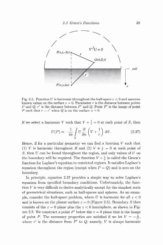
2.3 Green's Functions 39
/ P(x,y,-Az) iV2U=0
I ^^rx, \
— Z=0
P'(x,y,Az)
Fig. 2.5. Function U is harmonic throughout the half-space z < 0 and assumesknown values on the surface z = 0. Parameter r is the distance between pointsP and Q\ r' is the distance between P' and Q. Point P' is the image of pointP such that r = rf when Q is on the surface z = 0.
If we select a harmonic V such that V + - = 0 at each point of 5, then
Hence, if for a particular geometry we can find a function V such that(1) V is harmonic throughout R and (2) V + £ = 0 at each point of5, then £/ can be found throughout the region, and only values of U onthe boundary will be required. The function V + Ms called the Green'sfunction for Laplace's equation in restricted regions. It satisfies Laplace'sequation throughout the region (except when P = Q) and is zero on theboundary.
In principle, equation 2.37 provides a simple way to solve Laplace'sequation from specified boundary conditions. Unfortunately, the func-tion V is very difficult to derive analytically except for the simplest sortsof geometrical situations, such as half-spaces and spheres. As an exam-ple, consider the half-space problem, where U is harmonic for all z < 0and is known on the planar surface z = 0 (Figure 2.5). Boundary S thenconsists of the z = 0 plane plus the z < 0 hemisphere, as shown in Fig-ure 2.5. We construct a point P' below the z — 0 plane that is the imageof point P. The necessary properties are satisfied if we let V = — p-,where r' is the distance from P' to Q: namely, V is always harmonic
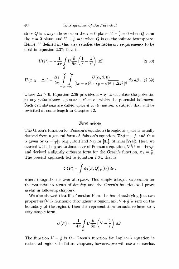
40 Consequences of the Potential
since Q is always above or on the z = 0 plane, V + ^ = 0 when Q is onthe z = 0 plane, and 7 + ^ = 0 when Q is on the infinite hemisphere.Hence, V defined in this way satisfies the necessary requirements to beused in equation 2.37; that is,
IU7T (~ ~ On \r r's
oo oo
f f U^M rdadp, (2.39)J J [ ( x _ a ) 2 + (y_/3)2 + A22]f ^ ' ^ >27T
— oo —oo
where Az > 0. Equation 2.39 provides a way to calculate the potentialat any point above a planar surface on which the potential is known.Such calculations are called upward continuation, a subject that will berevisited at some length in Chapter 12.
TerminologyThe Green's function for Poisson's equation throughout space is usuallyderived from a general form of Poisson's equation, V20 = —/, and thusis given by G = -^ (e.g., Duff and Naylor [81], Strauss [274]). Here, westarted with the gravitational case of Poisson's equation, V2£/ = — 4TT7/?,and derived a slightly different form for the Green's function, '01 = ^-The present approach led to equation 2.34, that is,
where integration is over all space. This simple integral expression forthe potential in terms of density and the Green's function will proveuseful in following chapters.
We also showed that if a function V can be found satisfying just twoproperties (V is harmonic throughout a region, and V + ^ is zero on theboundary of the region), then the representation formula reduces to avery simple form,
The function V + \ is the Green's function for Laplace's equation inrestricted regions. In future chapters, however, we will use a somewhat
24 Problem Set 41
looser terminology. If we let ip2(P, Q) — ~-^-§^(Y +^) m this equation,then
U(P) =
which has a form similar to equation 2.34. For this reason, we also willrefer to ip2(P,S) = —-^-§^(Y+\) a s a kind of Green's function, onewhich provides U at points away from boundaries on which U is known.
2.4 Problem Set1. In the following, T is temperature in region R bounded by surface
S, and h is the unit vector normal to S. If V2T = —f(P) in regionR and ^ = g(S) on surface 5, show that
fdv+ gdS = 0 ,R S
and interpret the meaning of this equation.2. Show, starting with Green's first identity, that if U is harmonic
throughout all space, it must be zero everywhere.3. Show that if two harmonic functions U\ and U2 satisfy JJ\ < U2 at
each point of the boundary of a region, then JJ\ < U2 throughout theregion.
4. A radial field is described by F = arnr.(a) In regions where r / 0, find the values of n for which F is
solenoidal.(b) For what values of n (r ^ 0) is the field irrotational?
5. Maxwell's equations state that magnetic induction B in the absenceof moving charge is both solenoidal and irrotational, that is,
V • B = 0,V x B = 0.
Show that the three cartesian components of B are each harmonicin such situations.
6. Function U satisfies the two-dimensional Laplace's equation at everypoint of a circle. Find a Green's function that will provide the value of
42 Consequences of the Potential
U at any point inside the circle from the values of U on the boundaryof the circle.
7. Function U is harmonic everywhere inside a sphere of radius a. Finda Green's function that will provide the value of U at any point insidethe sphere from values of U on the surface of the sphere.
3Newtonian Potential
And the Newtonian scheme was based on a set of assumptions, so fewand so simple, developed through so clear and so enticing a line ofmathematics that conservatives could scarcely find the heart andcourage to fight it.
(Isaac Asimov)
The airplane stays up because it doesn't have the time to fall.(Orville Wright)
The previous chapters reviewed Laplace's differential equation and itsimplications for conservative fields and scalar potentials in general. Inthis chapter, we become more specific and focus on the most impor-tant application of Laplace's equation, the force of gravity. As before,much of the discussion herein relies heavily on developments presentedby Kellogg [146], Ramsey [235], and MacMillan [172].
3.1 Gravitational Attraction and PotentialIn 1687, Newton published Philosophiae Naturalis Principia Mathemat-ica, which, among other profundities, stated Newton's law of gravita-tional attraction: The magnitude of the gravitational force between twomasses is proportional to each mass and inversely proportional to thesquare of their separation. In cartesian coordinates (Figure 3.1), the mu-tual force between a particle of mass m centered at point Q = (#', y', z')and a particle of mass mo at P = (x,y,z) is given by
mmo
r2
where
43
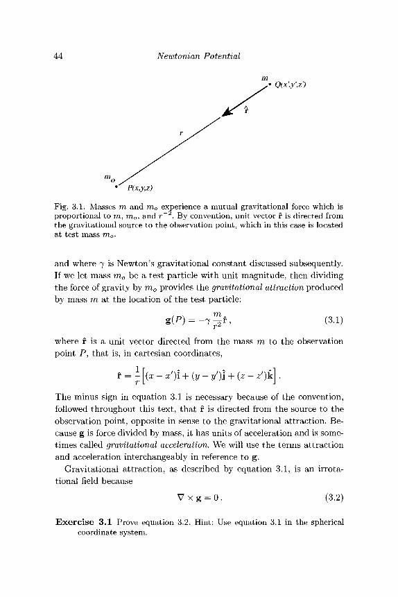
44 Newtonian Potential
mQ(x',y',z')
P(x,y,z)
Fig. 3.1. Masses m and mo experience a mutual gravitational force which isproportional to ra, rao, and r~2. By convention, unit vector r is directed fromthe gravitational source to the observation point, which in this case is locatedat test mass mo.
and where 7 is Newton's gravitational constant discussed subsequently.If we let mass mo be a test particle with unit magnitude, then dividingthe force of gravity by mo provides the gravitational attraction producedby mass m at the location of the test particle:
in
f ( 3 1 }
where f is a unit vector directed from the mass m to the observationpoint P, that is, in cartesian coordinates,
r = - [(x - x')\ + { y - y')l + (z - ^ ) k j .
The minus sign in equation 3.1 is necessary because of the convention,followed throughout this text, that f is directed from the source to theobservation point, opposite in sense to the gravitational attraction. Be-cause g is force divided by mass, it has units of acceleration and is some-times called gravitational acceleration. We will use the terms attractionand acceleration interchangeably in reference to g.
Gravitational attraction, as described by equation 3.1, is an irrota-tional field because
V x g = 0. (3.2)
Exercise 3.1 Prove equation 3.2. Hint: Use equation 3.1 in the sphericalcoordinate system.
3.1 Gravitational Attraction and Potential 45
Hence, from the Helmholtz theorem and equation 2.12 (Chapter 2), grav-itational acceleration is a conservative field and can be represented asthe gradient of a scalar potential
g(P) = VU(P), (3.3)
where
U(P) = <y™ . (3.4)
The function U is called the gravitational potential or Newtonian poten-tial, and gravitational acceleration g is a potential field.
Exercise 3.2 Prove that the gradient of equation 3.4 yields equation 3.1.
Some textbooks (e.g., Grant and West [99]) consider gravitationalpotential to be the work done by the test particle, so that equation 3.3is written g = —VU. Equation 3.3, however, follows the convention ofKellogg [146]: The gravitational potential is the work done by the fieldon a test particle and is the negative of the particle's potential energy.Because gravity is a conservative field, no net work is required to movea mass around a closed loop. Cross-country skiers and bicycle riders willappreciate that this statement pertains only to an ideal (frictionless,windless, etc.) world.
Units and the Gravitational ConstantIn the Systeme Internationale (International System, abbreviated SI)and mksa system of units, m and mo have units of kilograms, distance isin meters, and gravitational attraction is reported in m-sec~2. In the cgssystem of units, mass has units of grams, distance is in centimeters, andgravitational attraction is reported in units of cm-sec"2. The cgs unit ofacceleration is often referred to as the Gal (short for "Galileo"), where1 Gal = 1 cm-sec"2, and the geophysical literature commonly reportsgravitational attraction in units of mGal (1 mGal — 10~3 Gal). Theconversion from cgs to SI units is 1 mGal = 10~5 m-sec~2.
Newton's gravitational constant 7 is 6.67 x 10~n m3-kg"1-sec"2 inSI units and 6.67 x 10~8 cm3-g"1-see"2 in cgs units. Some texts, espe-cially those dealing primarily with Newtonian attraction, use astronom-ical units for force, arranged so that 7 = 1.
Refinements to Newton's gravitational constant have progressed eversince Newton proposed his law of gravitational attraction three cen-turies ago. Some concern still remains, however, as to just how constantNewton's gravitational constant really is. Recent work has reported very
46 Newtonian Potential
small deviations in the inverse-square relationship between gravitationalforce and distance (e.g., Stacey et al. [271]), but questions remain as towhether these deviations reflect a nonconstant gravitational constant orare caused by other physical processes in effect during the experiments(Zumberge et al. [297]). The question has not been resolved as of thewriting of this book. Although of considerable interest for scientific andphilosophical reasons, the issue of the constancy of Newton's gravita-tional constant has little impact on the applications for which this bookis intended, and the problem will be ignored henceforth.
3.2 The Potential of Distributions of MassGravitational potential obeys the principle of superposition: The gravi-tational potential of a collection of masses is the sum of the gravitationalattractions of the individual masses. Hence, the net force on a test par-ticle is simply the vector sum of the forces due to all masses in space.The superposition principle can be applied to find the gravitational at-traction in the limit of a continuous distribution of matter. A continuousdistribution of mass m is simply a collection of a great many, very smallmasses dm = p(x, y, z) dv, where p(x, y, z) is the density distribution.Applying the principle of superposition yields
(3.5)
where integration is over V, the volume actually occupied by mass. Asusual, P is the point of observation, Q is the point of integration, and ris distance between P and Q. Density p has units of kilogram-meter"3
in SI units and gram-centimeter"3 in the cgs system. The conversionbetween the two systems is 1 kg-m~3=10~3 g-cm"3.
First consider observation points located outside of a mass distribution(Figure 3.2). If density is well behaved, integral 3.5 converges for all Poutside of the mass (Kellogg [146]), and differentiation with respect tox, y, and z can be moved inside the integral. For example, the partialderivative of U with respect to x is
dU(P) __dx
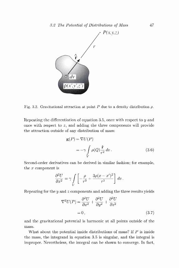
3.2 The Potential of Distributions of Mass
P(x,y,z)47
Fig. 3.2. Gravitational attraction at point P due to a density distribution p.
Repeating the differentiation of equation 3.5, once with respect to y andonce with respect to z, and adding the three components will providethe attraction outside of any distribution of mass:
(3.6)
Second-order derivatives can be derived in similar fashion; for example,the x component is
d2u _ f :
vdx2 7 / r3
Repeating for the y and z components and adding the three results yieldsd2U d2U d2Udx2
= 0,
dy2 dz2
(3.7)
and the gravitational potential is harmonic at all points outside of themass.
What about the potential inside distributions of mass? If P is insidethe mass, the integrand in equation 3.5 is singular, and the integral isimproper. Nevertheless, the integral can be shown to converge. In fact,
48 Newtonian Potential
Kellogg [146] shows that the integral
is convergent for P inside V and is continuous throughout V if n < 3,V is bounded, and p is piecewise continuous. Hence, U(P) and g(-P)exist and are continuous everywhere, both inside and outside the mass;so long as the density is well behaved. Kellogg [146] also shows thatg(P) = VU(P) for P inside the mass. This last point is not obviousbecause derivatives cannot be moved inside improper integrals.
The Helmholtz theorem (Section 2.2.2) tells us that if g satisfies g =VU and vanishes strongly at infinity, then
£/ = J- / ^—? dv . (3.8)4?r J r
Comparing the integrand of equation 3.8 with the integrand of equa-tion 3.5 suggests that
V2U(P) = -4TT 7 P(P) . (3.9)
Equation 3.9 is Poisson's equation, which describes the potential at allpoints, even inside the mass distribution. Laplace's equation is simply aspecial case of Poisson's equation, valid for mass-free regions of space.Although the foregoing is not a rigorous proof of the relationship betweenequations 3.5 and 3.9, the example in Section 3.2.2 will demonstrate thevalidity of Poisson's equation.
The following theorems can be stated in summary:
1. The Newtonian potential U and the acceleration of gravity g exist andare continuous throughout space if caused by a bounded distributionof piecewise-continuous density.
2. The potential U is everywhere differentiate so equation g = VU istrue throughout space.
3. Poisson's equation V2U = — Air^p describes the relationship betweenmass and potential throughout space. Laplace's equation V2C/ = 0is a special case of Poisson's equation valid in regions of space notoccupied by mass.
Surface and Line DistributionsIt is sometimes useful, as will be seen in the next sections, to considerthe gravitational attraction and potential of mass distributions that are
3.2 The,Potential of Distributions of Mass 49
spread over vanishingly thin surfaces and along vanishingly narrow lines.The potential of a mass distribution spread over surface S and viewedat a point P not on the surface is given by
U(P)=-y f^-dS, (3.10)s
where a is the surface density with units of mass per unit area. Thepotential of a mass concentrated along a line / is given by
U{P)=1 ^dl, (3.11)
where A is the line density with units of mass per unit length. Thegravitational attractions of these hypothetical distributions are easilyderived from g = VU.
3.2.1 Example: A Spherical ShellTo investigate some of the points of the previous sections, consider thegravitational effects of a thin-walled, spherical shell of radius a and uni-form surface density a. We simplify the task (Figure 3.3) by arrangingthe coordinate system in order to take advantage of the symmetry of theproblem: The origin is placed at the center of the sphere, and one axisis oriented so that it passes through P.
For P outside the shell, the potential is given by equation 3.10,
s
=w/7—<»*,.7/-:0 0
The distance from P to any point on the sphere is
r = [R2 + a2 - ^
sodr aR sin 0
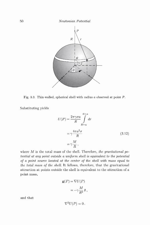
50 Newtonian Potential
P
Fig. 3.3. Thin-walled, spherical shell with radius a observed at point P.
Substituting yieldsR+a
27T^fO~a fU(P) = / dr
R-a
= 7- R(3.12)
M
where M is the total mass of the shell. Therefore, the gravitational po-tential at any point outside a uniform shell is equivalent to the potentialof a point source located at the center of the shell with mass equal tothe total mass of the shell It follows, therefore, that the gravitationalattraction at points outside the shell is equivalent to the attraction of apoint mass,
M
and thatV2U(P) = 0 .
a-\-t
/
3.2 The Potential of Distributions of Mass 51
Now consider P inside the shell. The previous derivation can be re-peated but with slightly different limits of integration; that is,
a+R
dra-R
•a (3.13)M
All quantities in equation 3.13 are constant, so the gravitational potentialis constant everywhere inside a uniform shell. Consequently, no gravita-tional forces exist inside the hollow shell because
/ MV a
= 0.
Obviously, V2U = 0 within the shell because U is uniform throughoutits interior.
Exercise 3.3 Equation 3.13 is easy to understand when P is located at thecenter of the shell. Observed at the center, the attraction due to anypatch of the shell is exactly canceled by the attraction of an identicalpatch on the opposite side, so it seems reasonable that g = 0 at thecenter. Less obvious is the fact that g = 0 at points away from thecenter. Explain in terms of geometry and solid angles why all forcescancel at any point inside the shell.
3.2.2 Example: Solid SphereEquations 3.12 and 3.13 provide an easy way to investigate the gravi-tational effects of a solid sphere. For P outside the sphere, the problemis simple. A solid sphere of radius a is just a collection of concentric,thin-walled shells with radii ranging from 0 to a. The superpositionprinciple states that the gravitational potential of the entire set of con-centric shells is the sum of their individual potentials, which, accordingto the previous section, are each equivalent to a point mass at their cen-ters. Consequently, the potential of a solid sphere appears at all externalpoints as a single point of mass located at the center of the sphere withmagnitude equal to the total mass of the sphere; that is,
i&p-, (3.14)
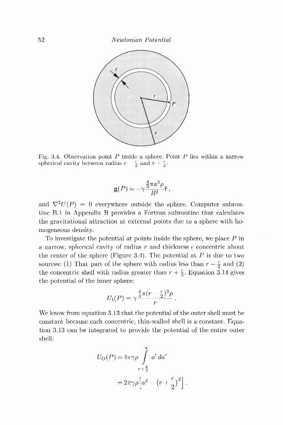
52 Newtonian Potential
Fig. 3.4. Observation point P inside a sphere. Point P lies within a narrowspherical cavity between radius r — | and r + | .
and V2U(P) = 0 everywhere outside the sphere. Computer subrou-tine B.I in Appendix B provides a Fortran subroutine that calculatesthe gravitational attraction at external points due to a sphere with ho-mogeneous density.
To investigate the potential at points inside the sphere, we place P ina narrow, spherical cavity of radius r and thickness e concentric aboutthe center of the sphere (Figure 3.4). The potential at P is due to twosources: (1) That part of the sphere with radius less than r — | and (2)the concentric shell with radius greater than r + | . Equation 3.14 givesthe potential of the inner sphere:
We know from equation 3.13 that the potential of the outer shell must beconstant because each concentric, thin-walled shell is a constant. Equa-tion 3.13 can be integrated to provide the potential of the entire outershell:
a da
r+i
3.2 The Potential of Distributions of Mass 53
Adding U\(P) and Uo(P) and letting e —>• 0 provide the potential insidea spherical mass:
= §777,9 [3a2 - r2] . (3.15)
The gravitational attraction is given by
and £fte attraction at internal points of a uniform sphere is proportionalto the distance from the center. The Laplacian (in spherical coordinates)of equation 3.15 yields
which is Poisson's equation.
Exercise 3.4 Show that U(P) and g(P) are continuous across the surfaceof the sphere.
The last result shows that Poisson's differential equation describes thepotential inside a uniformly dense sphere, and this result can be usedto show that Poisson's equation holds inside all continuous distributionsof mass. Within any well-behaved mass, we simply surround P with asmall sphere and consider the potential as the sum of two parts, that is,
where Us(P) is the potential at P due to the sphere and Uo(P) is thepotential caused by everything outside of the sphere. But V2Uo(P) = 0because no mass exists inside the spherical cavity. Furthermore, if thedensity is continuous around P, the sphere can be reduced in radius untilits density is essentially uniform. Hence, V2C/s(P) = —4?r7p(P), and
V2U{P) = -4TT 7 P(P)
for P inside a continuous density distribution.
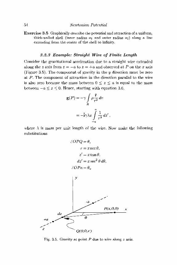
54 Newtonian Potential
Exercise 3.5 Graphically describe the potential and attraction of a uniform,thick-walled shell (inner radius a\ and outer radius CI2) along a lineextending from the center of the shell to infinity.
3.2.3 Example: Straight Wire of Finite LengthConsider the gravitational acceleration due to a straight wire extendedalong the z axis from z = — a to z = -fa and observed at P on the x axis(Figure 3.5). The component of gravity in the y direction must be zeroat P. The component of attraction in the direction parallel to the wireis also zero because the mass between 0 < z < a is equal to the massbetween —a < z < 0. Hence, starting with equation 3.6,
;>— dv
a= — i^Xx / — dz f,
J r6
where A is mass per unit length of the wire. Now make the followingsubstitutions
r = xsecO,
dz' = xsec2 OdO,lOPa = 6o
y
Q(0,0,z')Fig. 3.5. Gravity at point P due to wire along z axis.
3.3 Potential of Two-Dimensional Distributions 55
to derive
= _i2* fx J
cos OdO
*2 7 A= —l srn0 ox
(3.16)
Hence, the gravitational attraction of a finite length of wire viewed alonga line perpendicular to the midpoint of the wire is directed toward thecenter of the wire.
3.3 Potential of Two-Dimensional DistributionsMasses that are infinitely extended in one dimension are said to be two-dimensional, for reasons that soon will become obvious. We begin byinvestigating the potential and attraction of infinite wires and applythese results to bodies of arbitrary cross-sectional shape.
3.3.1 Potential of an Infinite WireFirst consider the attraction of an infinitely long wire. As a —• oo inequation 3.16, the attraction becomes
Hence, the attraction of an infinitely long wire is inversely proportionalto and in the direction of the perpendicular distance to the wire. A generalrelationship is seen if P is moved to an arbitrary point of the x, y plane:
^ , (3.17)
where r is directed from the wire to P and is understood to lie in thex, y plane; that is, r2 = (x — x')2 + (y — yf)2.
Although the gravitational attraction of an infinite wire is straightfor-ward, the potential of an infinite wire is something of a problem. First
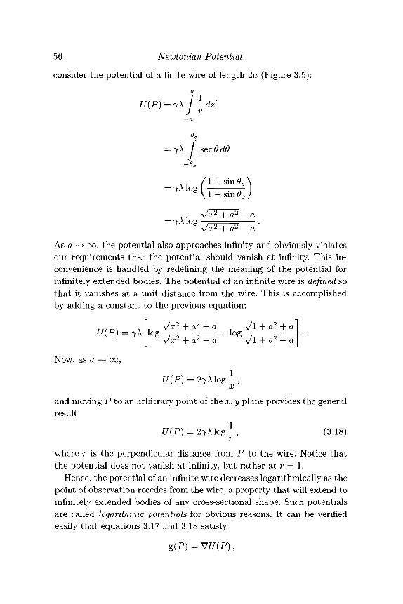
56 Newtonian Potential
consider the potential of a finite wire of length 2a (Figure 3.5):
aU(P)=j\ f ^dz'
sec 0 dO
= 7 A log1 — sin 6O
= 7 A log
As a —» 00, the potential also approaches infinity and obviously violatesour requirements that the potential should vanish at infinity. This in-convenience is handled by redefining the meaning of the potential forinfinitely extended bodies. The potential of an infinite wire is defined sothat it vanishes at a unit distance from the wire. This is accomplishedby adding a constant to the previous equation:
U(P) = 7 A
Now, as a 0 0 ,
C/(P)=2 7 Alog- ,
and moving P to an arbitrary point of the x, y plane provides the generalresult
U{P) = 27Alog-,r
(3.18)
where r is the perpendicular distance from P to the wire. Notice thatthe potential does not vanish at infinity, but rather at r = 1.
Hence, the potential of an infinite wire decreases logarithmically as thepoint of observation recedes from the wire, a property that will extend toinfinitely extended bodies of any cross-sectional shape. Such potentialsare called logarithmic potentials for obvious reasons. It can be verifiedeasily that equations 3.17 and 3.18 satisfy
g(P) =
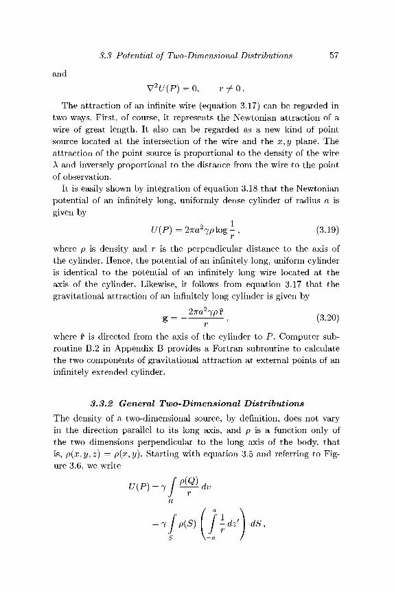
3.3 Potential of Two-Dimensional Distributions 57
and2 O , r/0.
The attraction of an infinite wire (equation 3.17) can be regarded intwo ways. First, of course, it represents the Newtonian attraction of awire of great length. It also can be regarded as a new kind of pointsource located at the intersection of the wire and the x, y plane. Theattraction of the point source is proportional to the density of the wireA and inversely proportional to the distance from the wire to the pointof observation.
It is easily shown by integration of equation 3.18 that the Newtonianpotential of an infinitely long, uniformly dense cylinder of radius a isgiven by
2 (3.19)r
where p is density and r is the perpendicular distance to the axis ofthe cylinder. Hence, the potential of an infinitely long, uniform cylinderis identical to the potential of an infinitely long wire located at theaxis of the cylinder. Likewise, it follows from equation 3.17 that thegravitational attraction of an infinitely long cylinder is given by
(3.20)
where f is directed from the axis of the cylinder to P. Computer sub-routine B.2 in Appendix B provides a Fortran subroutine to calculatethe two components of gravitational attraction at external points of aninfinitely extended cylinder.
3.3.2 General Two-Dimensional DistributionsThe density of a two-dimensional source, by definition, does not varyin the direction parallel to its long axis, and p is a function only ofthe two dimensions perpendicular to the long axis of the body, thatis, p(x,y,z) = p(x,y). Starting with equation 3.5 and referring to Fig-ure 3.6, we write
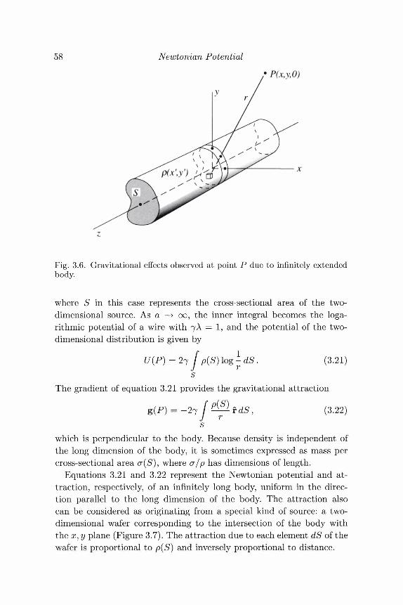
58 Newtonian Potential
P(x,y,O)
Fig. 3.6. Gravitational effects observed at point P due to infinitely extendedbody.
where S in this case represents the cross-sectional area of the two-dimensional source. As a —* oo, the inner integral becomes the loga-rithmic potential of a wire with 7A = 1, and the potential of the two-dimensional distribution is given by
C/(P) = 27 Jp(S) log ^ (3.21)
The gradient of equation 3.21 provides the gravitational attraction
(3.22)
which is perpendicular to the body. Because density is independent ofthe long dimension of the body, it is sometimes expressed as mass percross-sectional area c(S), where a/p has dimensions of length.
Equations 3.21 and 3.22 represent the Newtonian potential and at-traction, respectively, of an infinitely long body, uniform in the direc-tion parallel to the long dimension of the body. The attraction alsocan be considered as originating from a special kind of source: a two-dimensional wafer corresponding to the intersection of the body withthe x, y plane (Figure 3.7). The attraction due to each element dS of thewafer is proportional to p(S) and inversely proportional to distance.
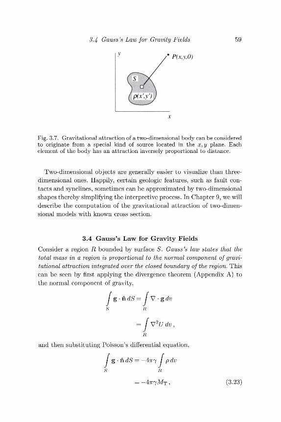
\4 Gauss's Law for Gravity Fields
/ P(x,y,O)
59
Fig. 3.7. Gravitational attraction of a two-dimensional body can be consideredto originate from a special kind of source located in the x, y plane. Eachelement of the body has an attraction inversely proportional to distance.
Two-dimensional objects are generally easier to visualize than three-dimensional ones. Happily, certain geologic features, such as fault con-tacts and synclines, sometimes can be approximated by two-dimensionalshapes thereby simplifying the interpretive process. In Chapter 9, we willdescribe the computation of the gravitational attraction of two-dimen-sional models with known cross section.
3.4 Gauss's Law for Gravity FieldsConsider a region R bounded by surface S. Gauss's law states that thetotal mass in a region is proportional to the normal component of gravi-tational attraction integrated over the closed boundary of the region. Thiscan be seen by first applying the divergence theorem (Appendix A) tothe normal component of gravity,
S R
-I'V • gdv
and then substituting Poisson's differential equation,
/ g • n dS = —4TT7 pdv
(3.23)
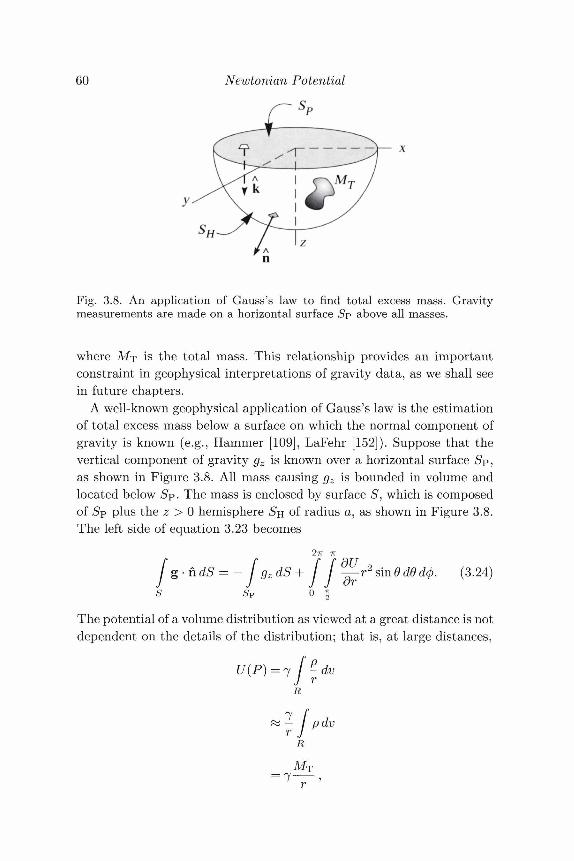
60 Newtonian Potential
Fig. 3.8. An application of Gauss's law to find total excess mass. Gravitymeasurements are made on a horizontal surface Sp above all masses.
where MT is the total mass. This relationship provides an importantconstraint in geophysical interpretations of gravity data, as we shall seein future chapters.
A well-known geophysical application of Gauss's law is the estimationof total excess mass below a surface on which the normal component ofgravity is known (e.g., Hammer [109], LaFehr [152]). Suppose that thevertical component of gravity gz is known over a horizontal surface Sp,as shown in Figure 3.8. All mass causing gz is bounded in volume andlocated below Sp. The mass is enclosed by surface S, which is composedof Sp plus the z > 0 hemisphere SH of radius a, as shown in Figure 3.8.The left side of equation 3.23 becomes
g-ndS = - gzdS+ —r 2 sinOdOdcf). (3.24)S SP Of
The potential of a volume distribution as viewed at a great distance is notdependent on the details of the distribution; that is, at large distances,
-dv
7 f A— I pavr J
R
= 7"M T
3.5 Green's Equivalent Layer 61
where again MT is the total mass. In other words, the potential of anybounded mass distribution appears as a point source when viewed suffi-ciently far away. Hence, as a —> oc, r2^ can be moved outside the lastintegral of equation 3.24, and
gz J T s'mOdOsP f
/ g-hdS = - gzdS - 2TTJMT / s's sP
= - gzdS -
Combining with equation 3.23 provides
/ gzdS = 2TT7MT, (3.25)SP
where Sp now includes the entire horizontal plane.Hence, the vertical component of gravity integrated over an infinite
plane is proportional to the total mass below the plane, so long as themass is bounded in volume. In principle, equation 3.25 provides a way toestimate the total excess mass causing an anomaly in measured gravity ifwe can successfully isolate the field of the anomalous mass from all othergravitational sources. No assumptions are required about the shape ofthe source or how the density is distributed, so long as it is small withrespect to the dimensions of the survey.
This may seem simple enough, but Gauss's law has many limitationsin such applications. Gravity surveys are never available over infiniteplanes. The best that we can hope for is that the survey extends wellbeyond the localized sources of interest. Unfortunately, isolated sourcesnever exist in nature, and it is often difficult to separate the gravitationalanomaly caused by the masses of interest from anomalies caused byall other local and regional sources. We'll have more to say about thisproblem of "regional-residual" separation in a later chapter.
3.5 Green's Equivalent LayerAn argument was presented in Section 2.1.3 on the basis of Green's thirdidentity that any given potential has an infinite variety of consistent
62 Newtonian Potential
boundary conditions. Here we carry that point a little further and showthat a gravitational potential caused by a three-dimensional density dis-tribution is identical to the potential caused by a surface density spreadover any of its equipotential surfaces (Ramsey [235]).
Let Se be a closed equipotential surface resulting from a distributionof mass with density p, and let R represent the region inside Se. Thegravitational potential is observed at point P outside of Se. Green'ssecond identity (Section 2.1.2) is given by
R Se
[UV2V - VW2U] dv= f \u^- - V^-} dS,J [ dn dn\
where U and V are any functions with partial derivatives of first andsecond order. Now let U be the potential of the mass and let V = 1/r,where r represents the distance away from P. Because P is locatedoutside the region, the second identity reduces to
f V 2 f / _ [ d I f 1 dU— I dv = L/s / — do / — do ,
J r J onr J r on
where Us is the constant potential of the equipotential surface. The firstintegral on the right-hand side vanishes according to equation 2.2, andsubstituting Poisson's equation into the integral on the left-hand sideprovides
I^dS. (3.26)r dn
Se
The left-hand side of equation 3.26 is the potential of the density dis-tribution observed at P. The right-hand side is the potential at P of asurface distribution a spread over 5e, where a = — -^-^- Hence, fromthe perspective of point P, the potential caused by a three-dimensionaldensity distribution is indistinguishable from a thin layer of mass spreadover any of its equipotential surfaces. This relationship is called Green'sequivalent layer.
Furthermore, the total mass of the body is equivalent to the totalmass of the equivalent layer. This can be seen by integrating the surface
3.6 Problem Set 63
density over the entire surface and applying the divergence theorem (Ap-pendix A), that is,
Lds=--L faJLJ 4TT7 J anse s
= / p dv .R
Green's equivalent layer is of more than just academic interest. Itshows that a potential can be caused by an infinite variety of sources,thus demonstrating the nonuniqueness of causative mass distributions.In later chapters, we will discuss applications of equivalent layers to theinterpretation of gravity and magnetic data. The fact that the equivalentlayer may have no resemblance to the true source will be of no impor-tance in those applications. These hypothetical sources simply prove tobe handy tools in manipulating the potential field.
3.6 Problem Set
1. Starting with the equation for gravitational attraction outside a uni-form sphere, derive the "infinite slab formula"
g = 27T7^k, (3.27)
where p and t are the density and thickness of the slab, respectively,and k is a unit vector directed vertically down. (Hint: Use superpo-sition of two spheres and let their radii —* oo.)
2. A nonzero density distribution that produces no external field fora particular source geometry is called an annihilator (Parker [207]).The annihilator quantitatively describes the nonuniqueness of poten-tial field data because any amount of the annihilator can be addedto a possible solution without affecting the field of the source. Finda simple annihilator p for a spherical mass of radius a as viewedfrom outside the sphere. (Hint: Let p represent density contrast sothat p can reach negative values.)
3. Let the radius and density of the earth be represented by a and p,respectively.
64 Newtonian Potential
(a) Show that the initial rate of decrease in g in descending a mineshaft is equal to g/a if p is constant.
(b) Assume that the earth has a spherical core of radius b and den-sity pc 7 p. Show that
' l - \ \ a3'2 + APc = 9 1 +
where Xg/a is the initial rate of decrease of g in descending theshaft.
Use subroutine B.I (Appendix B) to write a program that calculatesthe vertical attraction of gravity along a horizontal profile directlyover a buried sphere.(a) Use the program to verify that the shape (but not the amplitude)
of the profile is independent of the sphere's radius.(b) The horizontal profile has two points at which the horizontal
gradient is maximum. Derive an expression for the depth d tothe center of the sphere in terms of the horizontal separation ofthese two maximum horizontal gradients.
(c) Use the program to verify the answer in part (b).An alluvium-filled basin lies within an otherwise homogeneous plain.Surrounding crustal rocks have a density everywhere of pc. Thethickness of the basin (i.e., the depth to basement) is D. At thesurface, the alluvium has a density of pa. The density of the basin,however, varies with depth because of compaction of the alluvium.The density of the alluvium at the surface is pai but the densitycontrast Ap between alluvium and surrounding rocks decreases ex-ponentially with increasing depth according to the equation
where d is depth below the surface and Apo = P&—pc- The horizontaldimensions of the basin are much larger than its depth, so the shapeof the basin can be approximated as an infinite slab.(a) Consider the gravitational attraction g measured above the cen-
ter of the basin. Show that g reaches a limiting value as D in-creases.
(b) What is this limit in terms of pa, pc, and A?(c) Based on these results, discuss the limitations in trying to de-
termine D from g for deep basins.
4Magnetic Potential
There is about the Earth a magnetic field. Its cause and origin are veiledin mystery as in the case of that other great natural phenomenon,gravitation.
(J. A. Fleming)
It is well to observe the force and virtue and consequence of discoveries,and these are to be seen nowhere more conspicuously than in printing,gunpowder, and the magnet.
(Francis Bacon)
Under certain conditions, a magnetic field is uniquely determined by ascalar potential, analogous to the relationship between a gravity fieldand its corresponding gravitational potential. Happily for us, these spe-cial conditions are approximately obtained in typical geophysical mea-surements of the magnetic field. Consequently, much of what has beendeveloped in previous chapters concerning Newtonian potentials will ap-ply directly to magnetic fields as well. This chapter is primarily a reviewof the principles of electricity and magnetism, for which additional in-formation is easily found (e.g., Panofsky and Phillips [201]).
4.1 Magnetic InductionThe discussion of Newtonian potentials in Chapter 3 began by investi-gating the mutual attraction of two point masses. We begin Chapter 4in the same spirit by considering the mutual magnetic attraction of twosmall loops of electric current, the magnetic analog of two point masses.Consider the two loops of current shown in Figure 4.1 with currents Iaand /fc, respectively. The force acting on a small element dla of loop acaused by electric current in element dl^ of the second loop is given bythe Lorentz force
65
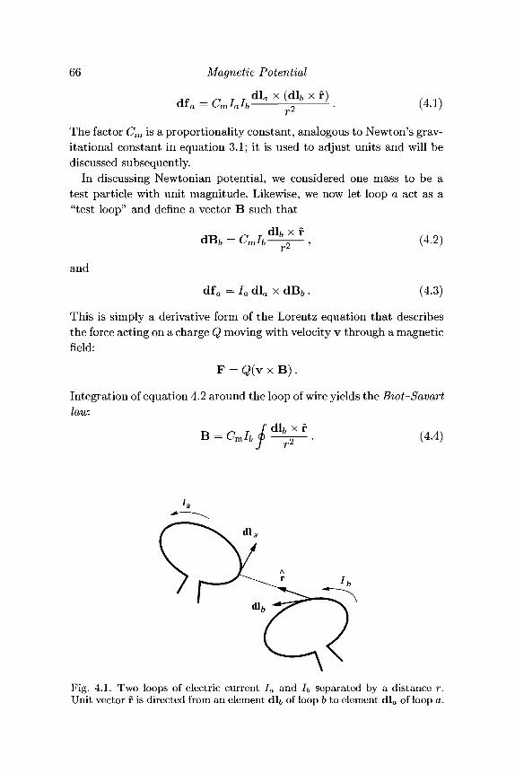
66 Magnetic Potential
dla x (dl6 x f) (4.1)
The factor Cm is a proportionality constant, analogous to Newton's grav-itational constant in equation 3.1; it is used to adjust units and will bediscussed subsequently.
In discussing Newtonian potential, we considered one mass to be atest particle with unit magnitude. Likewise, we now let loop a act as a"test loop" and define a vector B such that
x r
and
fa = /adlaxdB6.
(4.2)
(4.3)
This is simply a derivative form of the Lorentz equation that describesthe force acting on a charge Q moving with velocity v through a magneticfield:
F = Q(v x B).
Integration of equation 4.2 around the loop of wire yields the Biot-Savartlaw:
B = CmIbf x f (4.4)
Fig. 4.1. Two loops of electric current Ia and h separated by a distance r.Unit vector f is directed from an element dl& of loop b to element dla of loop a.
4.1 Magnetic Induction 67
Vector B in equation 4.4 is called the magnetic induction, magnetic fluxdensity, or simply the magnetic field of a loop of current. Magnetic in-duction is denned as follows: Electric current induces a force on a movingcharge; the force is the vector product of the magnetic induction fieldand the velocity of the charge. Note that, as in gravitational sources, f isdirected from the source (loop b in this case) to the point of observation.
Units
Two basic systems of units are commonly used in geophysical applica-tions of magnetism. Most of the literature published prior to about 1980employed the cgs system of units, also known as electromagnetic units(emu). More recently, the Systeme Internationale (International System,abbreviated SI) has become more common and, indeed, is required bymost geophysical journals today. In the gravitational case (Chapter 3),the conversion between cgs and SI units was simply a matter of multi-plying by an appropriate power of ten, but the magnetic case is moreproblematic, as will become particularly evident in Chapter 5.
For example, the proportionality constant Cm in equation 4.4 differsboth in magnitude and dimensions between the two systems: In emu,Cm = 1 and is dimensionless, whereas in SI units, Cm = ^ = 10~7
henry-meter"1, where /io is called the magnetic permeability of free space.The difference in the proportionality constants in emu and SI units isa common source of frustration. We will attempt to avoid the problemin this book by employing the parameter Cm wherever possible withoutreference to any particular system of units. In most equations, lettingCm = 1 will make the equation compatible with emu, or letting Cm = ^will transform the equation to SI units. However, we will have to aban-don Cm in Chapter 5 because there even the mathematical derivationwill depend on the system of units! Appendix D describes conversionfactors for all magnetic units of importance to this text. For additionalinformation, the interested reader is referred to books by Butler [47,pp. 15-18], Panofsky and Phillips [201, pp. 459-65], and the Society ofExploration Geophysicists [266]. Articles by Shive [255], Lowes [169],Payne [213], and Moskowitz [189] are also helpful.
In the emu system, magnetic induction B is reported in units of gauss(G), and current has units of abamperes. In SI units, B has units ofweber-meter"2, which is given the name tesla (T), and current is inunits of amperes (1 ampere = 0.1 abampere). In geophysical studies, the
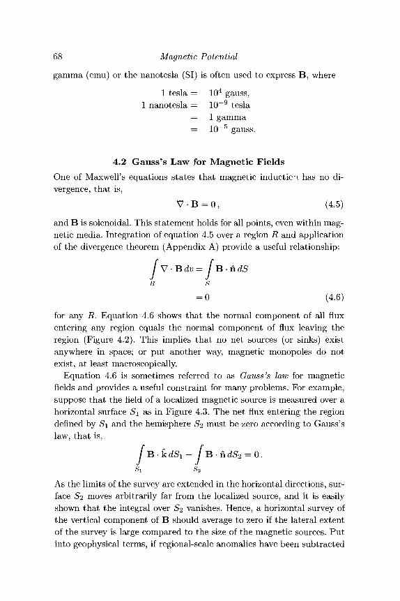
68 Magnetic Potential
gamma (emu) or the nanotesla (SI) is often used to express B, where
1 tesla = 104 gauss,1 nanotesla = 10~9 tesla
= 1 gamma= 10~5 gauss.
4.2 Gauss's Law for Magnetic FieldsOne of Maxwell's equations states that magnetic induction has no di-vergence, that is,
V - B = 0, (4.5)
and B is solenoidal. This statement holds for all points, even within mag-netic media. Integration of equation 4.5 over a region R and applicationof the divergence theorem (Appendix A) provide a useful relationship:
f = / B-ndSs
= 0 (4.6)
for any R. Equation 4.6 shows that the normal component of all fluxentering any region equals the normal component of flux leaving theregion (Figure 4.2). This implies that no net sources (or sinks) existanywhere in space; or put another way, magnetic monopoles do notexist, at least macroscopically.
Equation 4.6 is sometimes referred to as Gauss's law for magneticfields and provides a useful constraint for many problems. For example,suppose that the field of a localized magnetic source is measured over ahorizontal surface Si as in Figure 4.3. The net flux entering the regiondefined by Si and the hemisphere S2 must be zero according to Gauss'slaw, that is,
/ = 0.* J
Si
As the limits of the survey are extended in the horizontal directions, sur-face S2 moves arbitrarily far from the localized source, and it is easilyshown that the integral over S2 vanishes. Hence, a horizontal survey ofthe vertical component of B should average to zero if the lateral extentof the survey is large compared to the size of the magnetic sources. Putinto geophysical terms, if regional-scale anomalies have been subtracted
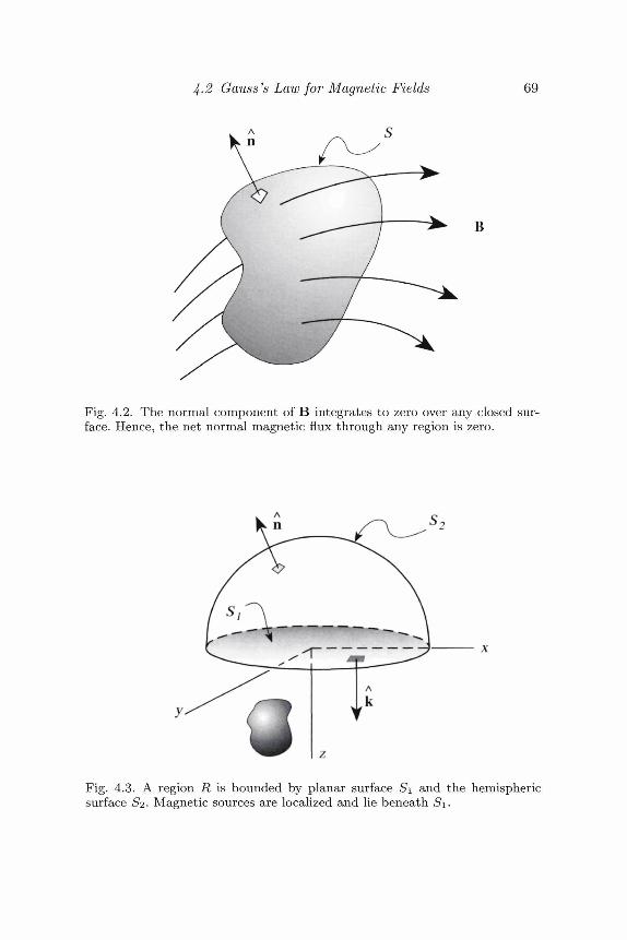
4-2 Gauss's Law for Magnetic Fields 69
B
Fig. 4.2. The normal component of B integrates to zero over any closed sur-face. Hence, the net normal magnetic flux through any region is zero.
Fig. 4.3. A region R is bounded by planar surface Si and the hemisphericsurface £2. Magnetic sources are localized and lie beneath Si.
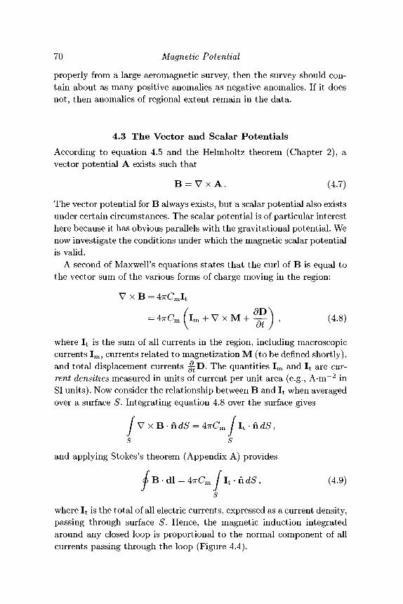
70 Magnetic Potential
properly from a large aeromagnetic survey, then the survey should con-tain about as many positive anomalies as negative anomalies. If it doesnot, then anomalies of regional extent remain in the data.
4.3 The Vector and Scalar PotentialsAccording to equation 4.5 and the Helmholtz theorem (Chapter 2), avector potential A exists such that
B = V x A . (4.7)
The vector potential for B always exists, but a scalar potential also existsunder certain circumstances. The scalar potential is of particular interesthere because it has obvious parallels with the gravitational potential. Wenow investigate the conditions under which the magnetic scalar potentialis valid.
A second of Maxwell's equations states that the curl of B is equal tothe vector sum of the various forms of charge moving in the region:
V x B = 47rCmIt
^ ) (4.8)
where I t is the sum of all currents in the region, including macroscopiccurrents Im, currents related to magnetization M (to be defined shortly),and total displacement currents J^D. The quantities Im and I t are cur-rent densities measured in units of current per unit area (e.g., A-m~2 inSI units). Now consider the relationship between B and I t when averagedover a surface S. Integrating equation 4.8 over the surface gives
/ V x B-ndS = 4irCm / I t -ndS,s s
and applying Stokes's theorem (Appendix A) provides
(4.9)f
where I t is the total of all electric currents, expressed as a current density,passing through surface S. Hence, the magnetic induction integratedaround any closed loop is proportional to the normal component of allcurrents passing through the loop (Figure 4.4).
4-3 The Vector and Scalar Potentials 71
Fig. 4.4. The normal component of all currents I t passing through a surfaceS is proportional to B • dl integrated around the loop that bounds S.
If no currents exist in the region of investigation, then
V x B = 0,
and B is irrotational. According to the Helmholtz theorem, B then hasa scalar potential V such that
B = - W , (4.10)
and B is a potential field in the absence of currents. The negative signin equation 4.10 follows the convention of Kellogg [146], as discussed inChapters 1 and 3.
In many geophysical situations, electrical currents are negligible in re-gions where the magnetic field is actually measured. Hence, equation 4.10is often a suitable approximation outside of magnetic materials. Thisis a fortunate happenstance. For example, derivations of the magneticfields caused by bodies of specified shape are generally more easily doneby first deriving V and then applying equation 4.10. Moreover, underconditions where equation 4.10 holds, the potential of magnetic induc-tion has obvious similarities to gravitational potential, and many of thestatements made in earlier chapters apply immediately to magnetostatictheory. However, it should always be remembered that equation 4.10 isvalid only outside of magnetic media and where line integrals encircleno currents.
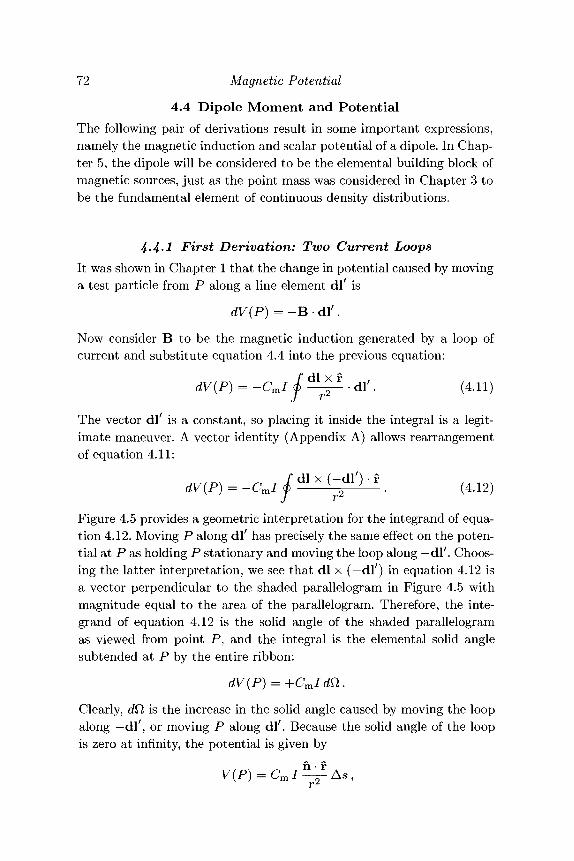
72 Magnetic Potential
4.4 Dipole Moment and PotentialThe following pair of derivations result in some important expressions,namely the magnetic induction and scalar potential of a dipole. In Chap-ter 5, the dipole will be considered to be the elemental building block ofmagnetic sources, just as the point mass was considered in Chapter 3 tobe the fundamental element of continuous density distributions.
4-4-1 First Derivation: Two Current LoopsIt was shown in Chapter 1 that the change in potential caused by movinga test particle from P along a line element dl7 is
dV(P) = - B • dl7.
Now consider B to be the magnetic induction generated by a loop ofcurrent and substitute equation 4.4 into the previous equation:
^ - A \ ' . (4.11)
The vector dl7 is a constant, so placing it inside the integral is a legit-imate maneuver. A vector identity (Appendix A) allows rearrangementof equation 4.11:
(4.12)
Figure 4.5 provides a geometric interpretation for the integrand of equa-tion 4.12. Moving P along dl' has precisely the same effect on the poten-tial at P as holding P stationary and moving the loop along —dl'. Choos-ing the latter interpretation, we see that dl x (—dl7) in equation 4.12 isa vector perpendicular to the shaded parallelogram in Figure 4.5 withmagnitude equal to the area of the parallelogram. Therefore, the inte-grand of equation 4.12 is the solid angle of the shaded parallelogramas viewed from point P, and the integral is the elemental solid anglesubtended at P by the entire ribbon:
Clearly, dQ is the increase in the solid angle caused by moving the loopalong —dl7, or moving P along dl7. Because the solid angle of the loopis zero at infinity, the potential is given by
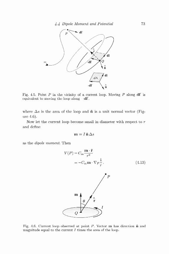
4-4 Dipole Moment and Potential 73
Fig. 4.5. Point P in the vicinity of a current loop. Moving P along dl' isequivalent to moving the loop along —dl'.
where As is the area of the loop and h is a unit normal vector (Fig-ure 4.6).
Now let the current loop become small in diameter with respect to rand define
m = In As
as the dipole moment. Then
V(P) = Crm • r
= - C m m V P - .r
(4.13)
m
Fig. 4.6. Current loop observed at point P. Vector m has direction fi andmagnitude equal to the current / times the area of the loop.
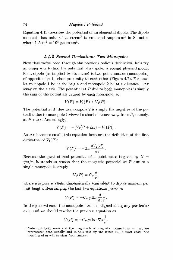
74 Magnetic Potential
Equation 4.13 describes the potential of an elemental dipole. The dipolemomentf has units of gauss-cm3 in emu and ampere-m2 in SI units,where 1 A-m2 = 103 gauss-cm3.
4-4-^ Second Derivation: Two MonopolesNow that we've been through the previous tedious derivation, let's tryan easier way to find the potential of a dipole. A second physical modelfor a dipole (as implied by its name) is two point masses (monopoles)of opposite sign in close proximity to each other (Figure 4.7). For now,let monopole 1 be at the origin and monopole 2 be at a distance — Azaway on the z axis. The potential at P due to both monopoles is simplythe sum of the potentials caused by each monopole, so
The potential at P due to monopole 2 is simply the negative of the po-tential due to monopole 1 viewed a short distance away from P, namely,at P + Az. Accordingly,
V{P) = -[V1{P + Az)-V1(P)].
As Az becomes small, this equation becomes the definition of the firstderivative of V\{P):
dZ
Because the gravitational potential of a point mass is given by U =7?7i/r, it stands to reason that the magnetic potential at P due to asingle monopole is simply
where q is pole strength, dimensionally equivalent to dipole moment perunit length. Rearranging the last two equations provides
In the general case, the monopoles are not aligned along any particularaxis, and we should rewrite the previous equation as
f Note that both mass and the magnitude of magnetic moment, ra = |m|, arerepresented traditionally and in this text by the letter ra. In most cases, themeaning of ra will be clear from context.
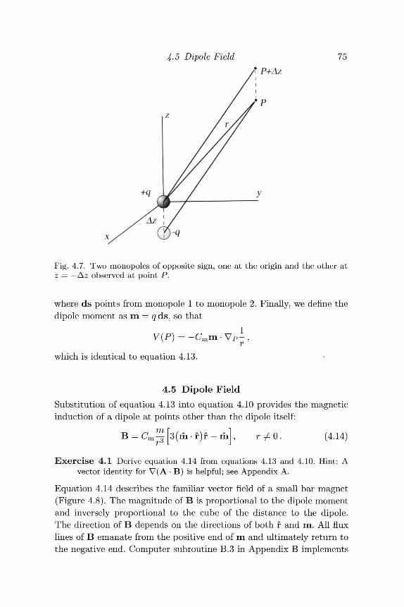
4-5 Dipole Field 75P+Az
Fig. 4.7. Two monopoles of opposite sign, one at the origin and the other atz = —Az observed at point P.
where ds points from monopole 1 to monopole 2. Finally, we define thedipole moment as m = gds, so that
which is identical to equation 4.13.
4.5 Dipole FieldSubstitution of equation 4.13 into equation 4.10 provides the magneticinduction of a dipole at points other than the dipole itself:
• r r m (4.14)
Exercise 4.1 Derive equation 4.14 from equations 4.13 and 4.10. Hint: Avector identity for V(A • B) is helpful; see Appendix A.
Equation 4.14 describes the familiar vector field of a small bar magnet(Figure 4.8). The magnitude of B is proportional to the dipole momentand inversely proportional to the cube of the distance to the dipole.The direction of B depends on the directions of both r and m. All fluxlines of B emanate from the positive end of m and ultimately return tothe negative end. Computer subroutine B.3 in Appendix B implements
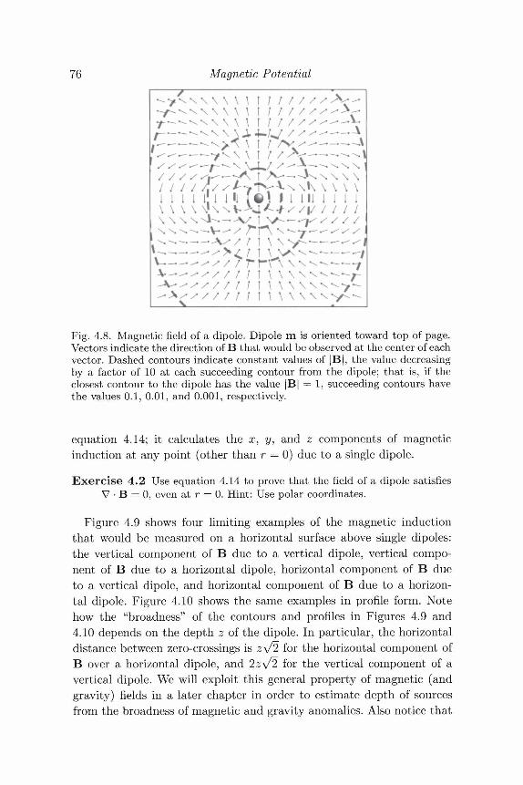
76 Magnetic Potential
y v w \ \ \ lWWII
f—^v\N \ \ \
• w i
Fig. 4.8. Magnetic field of a dipole. Dipole m is oriented toward top of page.Vectors indicate the direction of B that would be observed at the center of eachvector. Dashed contours indicate constant values of |B|, the value decreasingby a factor of 10 at each succeeding contour from the dipole; that is, if theclosest contour to the dipole has the value |B| — 1, succeeding contours havethe values 0.1, 0.01, and 0.001, respectively.
equation 4.14; it calculates the x, y, and z components of magneticinduction at any point (other than r = 0) due to a single dipole.
Exercise 4.2 Use equation 4.14 to prove that the field of a dipole satisfiesV • B = 0, even at r = 0. Hint: Use polar coordinates.
Figure 4.9 shows four limiting examples of the magnetic inductionthat would be measured on a horizontal surface above single dipoles:the vertical component of B due to a vertical dipole, vertical compo-nent of B due to a horizontal dipole, horizontal component of B dueto a vertical dipole, and horizontal component of B due to a horizon-tal dipole. Figure 4.10 shows the same examples in profile form. Notehow the "broadness" of the contours and profiles in Figures 4.9 and4.10 depends on the depth z of the dipole. In particular, the horizontaldistance between zero-crossings is zy/2 for the horizontal component ofB over a horizontal dipole, and 2z\/2 for the vertical component of avertical dipole. We will exploit this general property of magnetic (andgravity) fields in a later chapter in order to estimate depth of sourcesfrom the broadness of magnetic and gravity anomalies. Also notice that
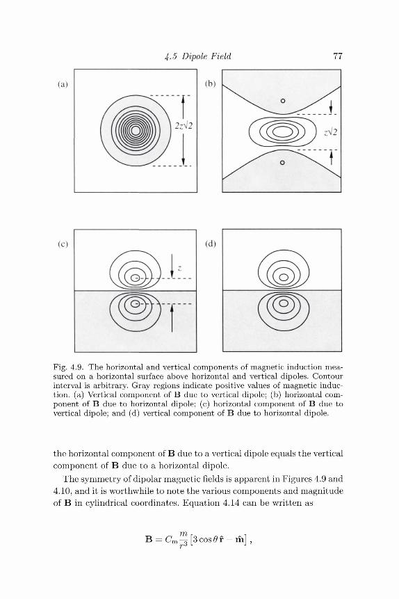
4.5 Dipole Field 77
(b)
uli
Fig. 4.9. The horizontal and vertical components of magnetic induction mea-sured on a horizontal surface above horizontal and vertical dipoles. Contourinterval is arbitrary. Gray regions indicate positive values of magnetic induc-tion, (a) Vertical component of B due to vertical dipole; (b) horizontal com-ponent of B due to horizontal dipole; (c) horizontal component of B due tovertical dipole; and (d) vertical component of B due to horizontal dipole.
the horizontal component of B due to a vertical dipole equals the verticalcomponent of B due to a horizontal dipole.
The symmetry of dipolar magnetic fields is apparent in Figures 4.9 and4.10, and it is worthwhile to note the various components and magnitudeof B in cylindrical coordinates. Equation 4.14 can be written as
mB = Cm~2 [3cos6r - m] ,
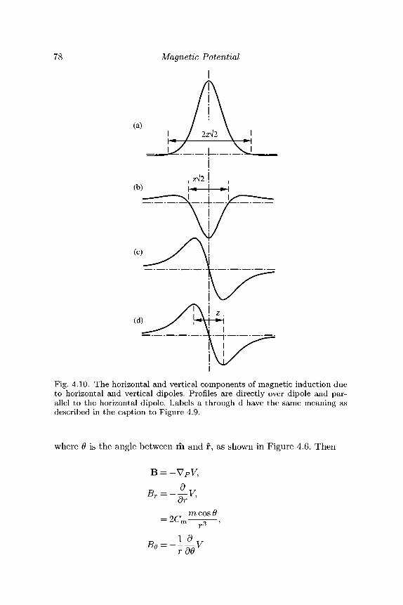
78 Magnetic Potential
i
(c)
(d)
Fig. 4.10. The horizontal and vertical components of magnetic induction dueto horizontal and vertical dipoles. Profiles are directly over dipole and par-allel to the horizontal dipole. Labels a through d have the same meaning asdescribed in the caption to Figure 4.9.
where 6 is the angle between m and f, as shown in Figure 4.6. Then
B = - VpV,
mcosO
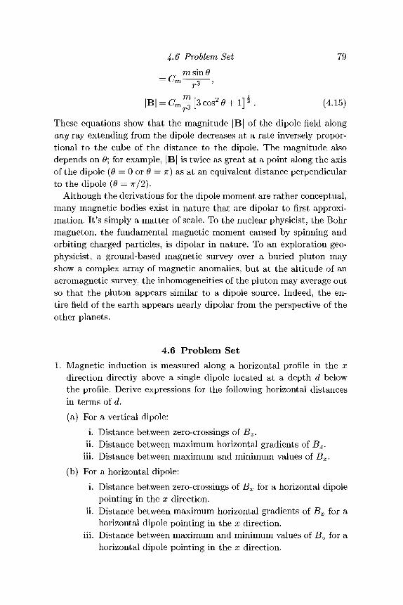
4-6 Problem Set 79
TTl r o -i iB = C m ^ 3cos2(9 + 1 2 . (4.15)
r6 L J
These equations show that the magnitude |B| of the dipole field alongany ray extending from the dipole decreases at a rate inversely propor-tional to the cube of the distance to the dipole. The magnitude alsodepends on 0; for example, |B| is twice as great at a point along the axisof the dipole (0 — 0 or 6 = n) as at an equivalent distance perpendicularto the dipole (0 = TT/2).
Although the derivations for the dipole moment are rather conceptual,many magnetic bodies exist in nature that are dipolar to first approxi-mation. It's simply a matter of scale. To the nuclear physicist, the Bohrmagneton, the fundamental magnetic moment caused by spinning andorbiting charged particles, is dipolar in nature. To an exploration geo-physicist, a ground-based magnetic survey over a buried pluton mayshow a complex array of magnetic anomalies, but at the altitude of anaeromagnetic survey, the inhomogeneities of the pluton may average outso that the pluton appears similar to a dipole source. Indeed, the en-tire field of the earth appears nearly dipolar from the perspective of theother planets.
4.6 Problem Set1. Magnetic induction is measured along a horizontal profile in the x
direction directly above a single dipole located at a depth d belowthe profile. Derive expressions for the following horizontal distancesin terms of d.(a) For a vertical dipole:
i. Distance between zero-crossings of Bz.ii. Distance between maximum horizontal gradients of Bz.
iii. Distance between maximum and minimum values of Bx.(b) For a horizontal dipole:
i. Distance between zero-crossings of Bx for a horizontal dipolepointing in the x direction,
ii. Distance between maximum horizontal gradients of Bx for ahorizontal dipole pointing in the x direction,
iii. Distance between maximum and minimum values of Bz for ahorizontal dipole pointing in the x direction.
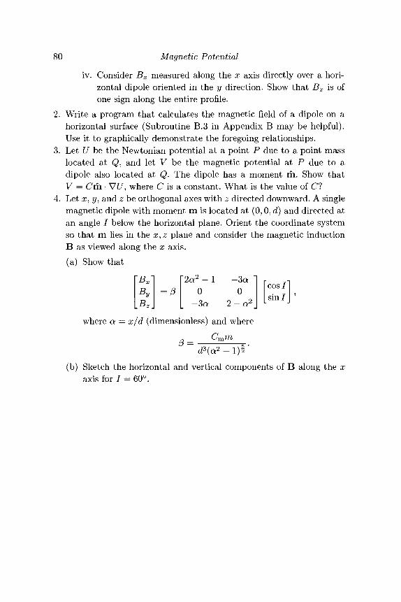
80 Magnetic Potential
iv. Consider Bx measured along the x axis directly over a hori-zontal dipole oriented in the y direction. Show that Bx is ofone sign along the entire profile.
2. Write a program that calculates the magnetic field of a dipole on ahorizontal surface (Subroutine B.3 in Appendix B may be helpful).Use it to graphically demonstrate the foregoing relationships.
3. Let U be the Newtonian potential at a point P due to a point masslocated at Q, and let V be the magnetic potential at P due to adipole also located at Q. The dipole has a moment m. Show thatV = Cm • VJ7, where C is a constant. What is the value of C?
4. Let x,y, and z be orthogonal axes with z directed downward. A singlemagnetic dipole with moment m is located at (0,0, d) and directed atan angle / below the horizontal plane. Orient the coordinate systemso that m lies in the x, z plane and consider the magnetic inductionB as viewed along the x axis.(a) Show that
ByBz
= 02a2 - 1
0- 3 a
-3a0
2 - a2
[cos/][sin/J '
where a = x/d (dimensionless) and whereCmm
d3(a2 + l ) i "(b) Sketch the horizontal and vertical components of B along the x
axis for 7 = 60°.
5Magnetization
Magnetes Geheimnis, erklare mir das!Kein grosser Geheimnis als Lieb und Hass.[The mystery of magnetism, explain that to me!no greater mystery, except love and hate-]
(Johann Wolfgang von Goethe)
We know that the magnet loves the lodestone,but we do not know whether the lodestonealso loves the magnet or is attracted to itagainst its will.
(Arab physicist of twelfth century)
5.1 Distributions of Magnetization
The magnetic induction B of an elemental dipole was derived in Chap-ter 4 by examining the magnetic induction of a vanishingly small loop ofelectrical current. Accordingly, the bulk magnetic properties of a volumeof material can be considered either in terms of the net magnetic effectof all the dipoles within the volume, or in terms of the net effect of allthe elemental electrical currents. Using the former concept, we define avector quantity called magnetization M as follows: The magnetizationof a volume V is defined as the vector sum of all the individual dipolemoments m^ divided by the volume, that is,
81
82 Magnetization
Magnetization is reported in units of ampere-meter"1 in the SystemeInternationale (SI) and in units of gaussf in the electromagnetic system(emu), where 1 gauss = 103 A-m"1.
In Chapter 3, we considered a volume of mass with density p(x, ?/, z)to be composed of a great many small masses dm = p(x, y, z) dv, eachsmall mass acting like a point source. This led to an integral equationfor the potential of a volume density distribution,
R
We do likewise here for magnetic sources. A small element of magneticmaterial with magnetization M can be considered to act like a singledipole M dv — m. The potential as observed at point P is given by
V(P) = --CmM-Vp- dv ,rwhere r is distance from P to the dipole. As discussed in Chapter 4,the constant Cm is used to balance units and has a value that dependson the system in use. In the emu system Cm = 1 and is dimensionless,whereas in SI units Cm = ^ = 10~7 henry-meter"1, where JIQ is thepermeability of free space. In general, magnetization M is a function ofposition, where both direction and magnitude can vary from point topoint, that is, M = M(Q), where Q is the position of dv. Integratingthis equation over all of the elemental volumes provides the potential ofa distribution of magnetization
V(P) = Cm J M(Q) • VQ i dv , (5.2)R
analogous to equation 5.1. Magnetic induction at P is given by
B(P) = -VpV(P)
= — CmVp / M(Q) • V Q - dv . (5.3)
In these last equations, we have changed the subscript of the gradientoperator from P to Q when the operator is inside the volume integral.This is to indicate that the gradient is to be taken with respect to thesource coordinates rather than with respect to the observation point.
f Magnetization is often reported in the geophysical literature in units of emu-cm"3,where 1 emu-cm"3 = 1 gauss.
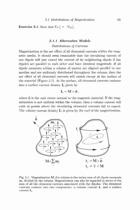
5.1 Distributions of Magnetization
Exercise 5.1 Show that VP± = -VQ\.
83
5.1.1 Alternative ModelsDistributions of Currents
Magnetization is the net effect of all elemental currents within the mag-netic media. It should seem reasonable that the circulating current ofone dipole will just cancel the current of its neighboring dipole if thedipoles are parallel to each other and have identical magnitude. If alldipole moments within a volume of matter are aligned parallel to oneanother and are uniformly distributed throughout the volume, then thenet effect of all elemental currents will vanish except at the surface ofthe material (Figure 5.1). At the surface, all elemental currents coalesceinto a surface current density Is given by
Is = M x fi,
where fi is the unit vector normal to the magnetic material. If the mag-netization is not uniform within the volume, then a volume current willexist at points where the circulating elemental currents fail to cancel.The volume current density Iv is given by the curl of the magnetization,
1=2,111, Iv = M x nIv = V x M
Fig. 5.1. Magnetization M of a volume is the vector sum of all dipole momentsrrij divided by the volume. Magnetization can also be regarded in terms of thesum of all the elemental currents associated with the dipoles. The elementalcurrents coalesce into two components: a volume current Iv and a surfacecurrent Is.
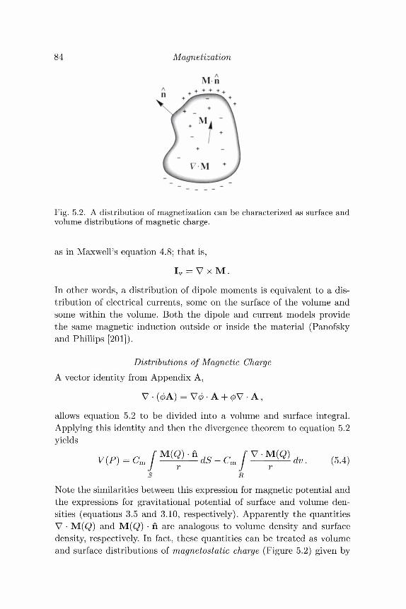
84 Magnetization
Fig. 5.2. A distribution of magnetization can be characterized as surface andvolume distributions of magnetic charge.
as in Maxwell's equation 4.8; that is,
Iv = V x M .
In other words, a distribution of dipole moments is equivalent to a dis-tribution of electrical currents, some on the surface of the volume andsome within the volume. Both the dipole and current models providethe same magnetic induction outside or inside the material (Panofskyand Phillips [201]).
Distributions of Magnetic ChargeA vector identity from Appendix A,
V • (0A) = V0 • A + 0V • A,
allows equation 5.2 to be divided into a volume and surface integral.Applying this identity and then the divergence theorem to equation 5.2yields
,. (5.4)S R
Note the similarities between this expression for magnetic potential andthe expressions for gravitational potential of surface and volume den-sities (equations 3.5 and 3.10, respectively). Apparently the quantitiesV • M(Q) and M(Q) • n are analogous to volume density and surfacedensity, respectively. In fact, these quantities can be treated as volumeand surface distributions of magneto static charge (Figure 5.2) given by
5.2 Magnetic Field Intensity 85
Qv = - V • M
QS = M n,
respectively, and substituting into equation 5.4 provides
Although magnetic charge does not physically exist, the conceptualmodel is a useful one as we will see in Chapter 9.
Hence, we have seen three ways to characterize the magnetizationof a material: as a distribution of magnetic dipoles, as distributions ofelectrical current on the surface and within the material, and as surfaceand volume distributions of magnetostatic charge. All three concepts areused in geophysical applications and will reappear in future chapters.
5.2 Magnetic Field IntensityEquation 4.8 in Chapter 4 shows that magnetic induction B originatesfrom all currents, both microscopic and macroscopic. Now we considera second kind of magnetic field which proves useful in the presence ofmagnetic materials. This new field is just that part of B arising from allcurrents other than atomic-level currents associated with magnetization.Assuming that dielectric properties of the region of interest are negligible(a good assumption in most geophysical applications), equation 4.8 canbe written
V x B = 47rCm(lm + V x M) . (5.5)
From here on, the derivation differs between the emu system and SIunits. In each case, we begin with equation 5.5.
In the emu system,
Vx(B-47rCmM)=47rCmIm ,
V x H = 47rCmIm,
H = B - 4TTM , (5.6)
86
whereas in SI units,
\7y IV /N 1
Magnetization
B \
V x H = Im
H = *Mo
M. (5.7)
Note that Cm has been replaced in equations 5.6 and 5.7 by its appro-priate value for the particular system of units.
Vector H is a new quantity called the magnetic field intensity, and, ascan be seen from the defining equations, is simply magnetic induction(except for a factor //o m SI units) minus the effects of magnetization.Field intensity has units of oersteds (Oe) in the emu system and unitsof ampere-meter"1 in SI units. The conversion between the two systemsis 1 Oe = ^ r A-m"1. Note that gauss and oersted units have equivalentmagnitude and dimensions in the emu system; the first quantity is usedfor magnetic induction, the latter for magnetic field intensity. Moreover,H and B in the emu system are identical outside of magnetic materi-als. In SI units, however, H and B have the same direction outside ofmagnetic materials but differ in both magnitude and dimensions.
Equations 5.6 and 5.7 show that the magnetic field intensity is a hy-brid vector function composed of two components with quite differentphysical meanings. Whereas magnetic induction B originates from allcurrents, both atomic and macroscopic, magnetic field intensity H arisesonly from true currents (again ignoring displacement currents). Mag-netic field intensity has a remarkable property that can be seen fromequations 4.9 and 5.7, namely, that
= Jlm-ndS (SI),s
that is, the line integral of field intensity around any closed loop is equalto the total macroscopic current crossing the surface bounded by theloop. In the absence of such currents,
and a scalar potential exists such that
H = - W ' .
5.3 Magnetic Permeability and Susceptibility 87
There is little to be gained from the distinction between B and H inmost geophysical measurements of the magnetic field of the earth. Mea-surements of the earth's magnetic field, whether from aircraft, ship, orsatellite, are made in environments very nearly free of magnetic material(e.g., Lowes [169]). Electrical currents can pose problems in some situ-ations, such as problems associated with ionospheric currents at satel-lite altitudes, but this issue is not relevant to our choice of B versusH. Indeed, the geophysical literature dealing with the interpretation ofmagnetic anomalies uses both B and H interchangeably. Here we willattempt to use B whenever possible.
5.3 Magnetic Permeability and SusceptibilityMaterials can acquire a component of magnetization in the presence ofan external magnetic field. For low-amplitude magnetic fields, say onthe order of the earth's magnetic field, this induced magnetization isproportional in magnitude and is parallel (or antiparallel) in directionto the external field, that is,
M = X H . (5.8)
The proportionality constant \ is called the magnetic susceptibility.Equation 5.8 is the same in both the SI and emu systems. Suscepti-bility is dimensionless in both systems but differs in magnitude by 4?r:Susceptibility in emu equals 4TT times susceptibility in SI units.
A related quantity, the magnetic permeability /i, differs slightly be-tween the two systems, and separate derivations are necessary. Startingwith equations 5.6 and 5.7, respectively, the derivations are as follows.
In the emu system,
B = H + 4TTM
- H + 4TTXH
= (1 + 4TTX)H
(5.9)
88 Magnetization
whereas in SI units,
B = /xo(H + M)
(5-10)
Kinds of MagnetizationAlthough x a nd M a r e derived in a simplistic mathematical way, theyare in fact complex products of the atomic and macroscopic proper-ties of the magnetic material. The relationship between M and H is notnecessarily linear as implied by equation 5.8; x m a v vary with field inten-sity, may be negative, and may be represented more accurately in somematerials as a tensor. This section provides a very cursory descriptionof the magnetization of solid materials. Indeed, this subject is worthyof its own textbook, and the interested reader is referred to books byChikazumi [57] and Morrish [187] for information on magnetic materialsin general, and to the book by Butler [47] for applications related topaleomagnetic and geomagnetic problems specifically. The implicationsof rock magnetism for magnetic-anomaly studies have been reviewedconcisely and comprehensively by Reynolds et al. [243].
There are many kinds of magnetization. Diamagnetism, for example,is an inherent property of all matter. In diamagnetism, an applied mag-netic field disturbs the orbital motion of electrons in such a way as toinduce a small magnetization in the opposite sense to the applied field.Consequently, diamagnetic susceptibility is negative. Paramagnetism isa property of those solids that have atomic magnetic moments. Appli-cation of a magnetic field causes the atomic moments to partially alignparallel to the applied field thereby producing a net magnetization inthe direction of the applied field. Thermal effects tend to oppose thisalignment, and paramagnetism vanishes in the absence of applied fieldsbecause thermal effects act to randomly orient the atomic moments. Allminerals are diamagnetic and some are paramagnetic, but in either casethese magnetizations are insignificant contributors to the geomagneticfield.
There is, however, a class of magnetism of great importance to geo-magnetic studies. Certain materials not only have atomic moments, but
5.3 Magnetic Permeability and Susceptibility 89
neighboring moments interact strongly with each other. This interactionis a result of a quantum mechanical effect called exchange energy, whichis beyond the scope of this book. Suffice it to say that the exchangeenergy causes a spontaneous magnetization that is many times greaterthan paramagnetic or diamagnetic effects. Such materials are said to beferromagnetic. There are various kinds of ferromagnetic materials too,depending on the way that the atomic moments align. These includeferromagnetism proper, in which atomic moments are aligned parallel toone another; antiferromagnetism, where atomic moments are aligned an-tiparallel and cancel one another; and ferrimagnetism, in which atomicmoments are antiparallel but do not cancel.
At the scale of individual mineral grains, spontaneous magnetizationof a ferromagnetic material can be very large. At the outcrop scale, how-ever, the magnetic moments of individual ferromagnetic grains may berandomly oriented, and the net magnetization may be negligible. Themagnetization of individual grains is affected, however, by the applica-tion of a magnetic field, similar to but far greater in magnitude thanfor paramagnetism. Hence, rocks containing ferromagnetic minerals willacquire a net magnetization, called induced magnetization and denotedby Mi, in the direction of an applied field H, where
Of course the earth's magnetic field produces the same response in suchmaterials, and the material is magnetic in its natural state. In smallfields, with magnitudes comparable to the earth's magnetic field, the re-lationship between induced magnetization and applied field is essentiallylinear, and the susceptibility \ is constant.
Induced magnetization falls to zero if the rock is placed in a field-freeenvironment. However, ferromagnetic materials also have the ability toretain a magnetization even in the absence of external magnetic fields.This permanent magnetization is called remanent magnetization, whichwe denote here by M r. In crustal materials, remanent magnetization is afunction not only of the atomic, crystallographic, and chemical make-upof the rocks, but also of their geologic, tectonic, and thermal history. Ingeophysical studies, it is customary to consider the total magnetizationM of a rock as the vector sum of its induced and remanent magnetiza-tions, that is,
M = Mi + M r
90 Magnetization
The relative importance of remanent magnetization to induced magne-tization is expressed by the Koenigsberger ratio
In subsequent discussions regarding magnetic fields of crustal materials,we will consider just two kinds of magnetization: induced and remanent.It is well to keep in mind, however, that both of these magnetizationsarise from spontaneous magnetization, a complex property of the ferro-magnetic minerals in the earth's crust.
The spontaneous magnetization is dependent on temperature. As amaterial is heated, the spacing between neighboring atomic momentsincreases until a point is reached where the spontaneous magnetiza-tion falls to zero. This temperature is called the Curie temperature.Hence, both induced and remanent magnetizations vanish at temper-atures greater than the Curie temperature. Paramagnetic and diamag-netic effects persist at these temperatures, but from the perspective ofmagnetic-anomaly studies we may consider rocks above the Curie tem-perature to be nonmagnetic.
Magnetite (FesO4) and its solid solutions with ulvospinel (Fe2TiC>4)are the most important magnetic minerals to geophysical studies ofcrustal rocks. Other minerals, such as hematite, pyrrhotite, and alloysof iron and nickel, are important in certain geologic situations, but thevolume percentage, size, shape, and history of magnetite grains are ofgreatest importance in most magnetic surveys. Magnetite is a ferrimag-netic material with a Curie temperature of about 580° C.
Typical values of |Mr| and % f°r representative rock types are pro-vided by Lindsley, Andreasen, and Balsley [165] and Carmichael [54].Generally speaking, mafic rocks are more magnetic than silicic rocks.Hence, basalts are usually more magnetic than rhyolites, and gabbrosare more magnetic than granites. Also, extrusive rocks generally havea higher remanent magnetization and lower susceptibility than intru-sive rocks with the same chemical composition. Sedimentary and meta-morphic rocks often have low remanent magnetizations and susceptibil-ities. These statements and the compilations referenced are only statis-tical guidelines with many exceptions. Values of M r and \ often varyby several orders of magnitude within the same outcrop, for example.Whenever feasible, interpretation of a magnetic survey should include
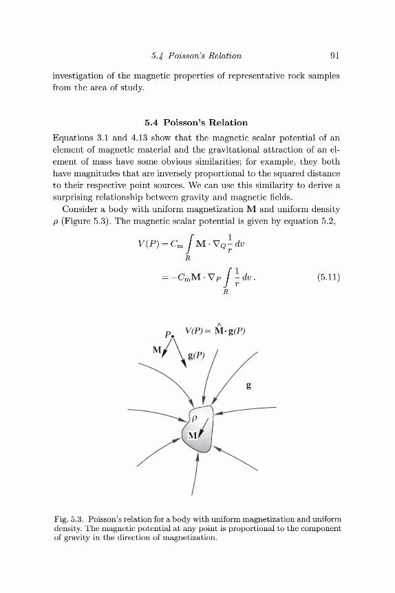
5.4 Poisson's Relation 91
investigation of the magnetic properties of representative rock samplesfrom the area of study.
5.4 Poisson's RelationEquations 3.1 and 4.13 show that the magnetic scalar potential of anelement of magnetic material and the gravitational attraction of an el-ement of mass have some obvious similarities; for example, they bothhave magnitudes that are inversely proportional to the squared distanceto their respective point sources. We can use this similarity to derive asurprising relationship between gravity and magnetic fields.
Consider a body with uniform magnetization M and uniform densityp (Figure 5.3). The magnetic scalar potential is given by equation 5.2,
> - dvR
CmM • V P -dv.J rR
(5.11)
Fig. 5.3. Poisson's relation for a body with uniform magnetization and uniformdensity. The magnetic potential at any point is proportional to the componentof gravity in the direction of magnetization.
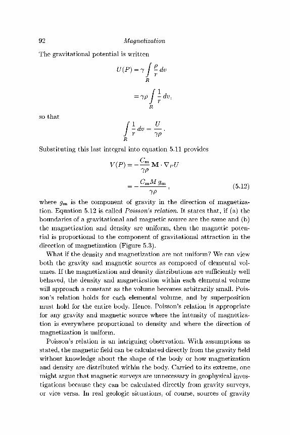
92 Magnetization
The gravitational potential is written
£/(P)=7 [ -dvJ rR
so that
- f l
R
J r 7pR
Substituting this last integral into equation 5.11 provides
_ CmMgm
~ ^ — ' ( 5 J 2 )
where gm is the component of gravity in the direction of magnetiza-tion. Equation 5.12 is called Poisson's relation. It states that, if (a) theboundaries of a gravitational and magnetic source are the same and (b)the magnetization and density are uniform, then the magnetic poten-tial is proportional to the component of gravitational attraction in thedirection of magnetization (Figure 5.3).
What if the density and magnetization are not uniform? We can viewboth the gravity and magnetic sources as composed of elemental vol-umes. If the magnetization and density distributions are sufficiently wellbehaved, the density and magnetization within each elemental volumewill approach a constant as the volume becomes arbitrarily small. Pois-son's relation holds for each elemental volume, and by superpositionmust hold for the entire body. Hence, Poisson's relation is appropriatefor any gravity and magnetic source where the intensity of magnetiza-tion is everywhere proportional to density and where the direction ofmagnetization is uniform.
Poisson's relation is an intriguing observation. With assumptions asstated, the magnetic field can be calculated directly from the gravity fieldwithout knowledge about the shape of the body or how magnetizationand density are distributed within the body. Carried to its extreme, onemight argue that magnetic surveys are unnecessary in geophysical inves-tigations because they can be calculated directly from gravity surveys,or vice versa. In real geologic situations, of course, sources of gravity
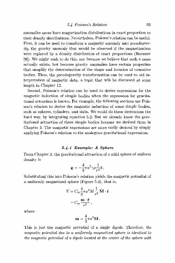
5.4 Poisson's Relation 93
anomalies never have magnetization distributions in exact proportion totheir density distributions. Nevertheless, Poisson's relation can be useful.First, it can be used to transform a magnetic anomaly into pseudograv-ity, the gravity anomaly that would be observed if the magnetizationwere replaced by a density distribution of exact proportions (Baranov[9]). We might wish to do this, not because we believe that such a massactually exists, but because gravity anomalies have certain propertiesthat simplify the determination of the shape and location of causativebodies. Thus, the pseudogravity transformation can be used to aid in-terpretation of magnetic data, a topic that will be discussed at somelength in Chapter 12.
Second, Poisson's relation can be used to derive expressions for themagnetic induction of simple bodies when the expression for gravita-tional attraction is known. For example, the following sections use Pois-son's relation to derive the magnetic induction of some simple bodies,such as spheres, cylinders, and slabs. We could do these derivations thehard way, by integrating equation 5.3. But we already know the grav-itational attraction of these simple bodies because we derived them inChapter 3. The magnetic expressions are more easily derived by simplyapplying Poisson's relation to the analogous gravitational expressions.
5.^.1 Example: A SphereFrom Chapter 3, the gravitational attraction of a solid sphere of uniformdensity is
4 3 1 ~g = - - ™ 7p—r.
Substituting this into Poisson's relation yields the magnetic potential ofa uniformly magnetized sphere (Figure 5.4), that is,
= cm-where
4 om = -7ra M.
This is just the magnetic potential of a single dipole. Therefore, themagnetic potential due to a uniformly magnetized sphere is identical tothe magnetic potential of a dipole located at the center of the sphere with
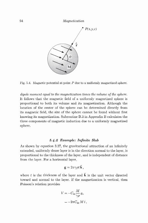
94 Magnetization
* P(x,y,z)
Fig. 5.4. Magnetic potential at point P due to a uniformly magnetized sphere.
dipole moment equal to the magnetization times the volume of the sphere.It follows that the magnetic field of a uniformly magnetized sphere isproportional to both its volume and its magnetization. Although thelocation of the center of the sphere can be determined directly fromits magnetic field, the size of the sphere cannot be found without firstknowing its magnetization. Subroutine B.3 in Appendix B calculates thethree components of magnetic induction due to a uniformly magnetizedsphere.
5.4-2 Example: Infinite SlabAs shown by equation 3.27, the gravitational attraction of an infinitelyextended, uniformly dense layer is in the direction normal to the layer, isproportional to the thickness of the layer, and is independent of distancefrom the layer. For a horizontal layer,
where t is the thickness of the layer and k is the unit vector directedtoward and normal to the layer. If the magnetization is vertical, thenPoisson's relation provides
cjgzIP
= -2-KCmMt,
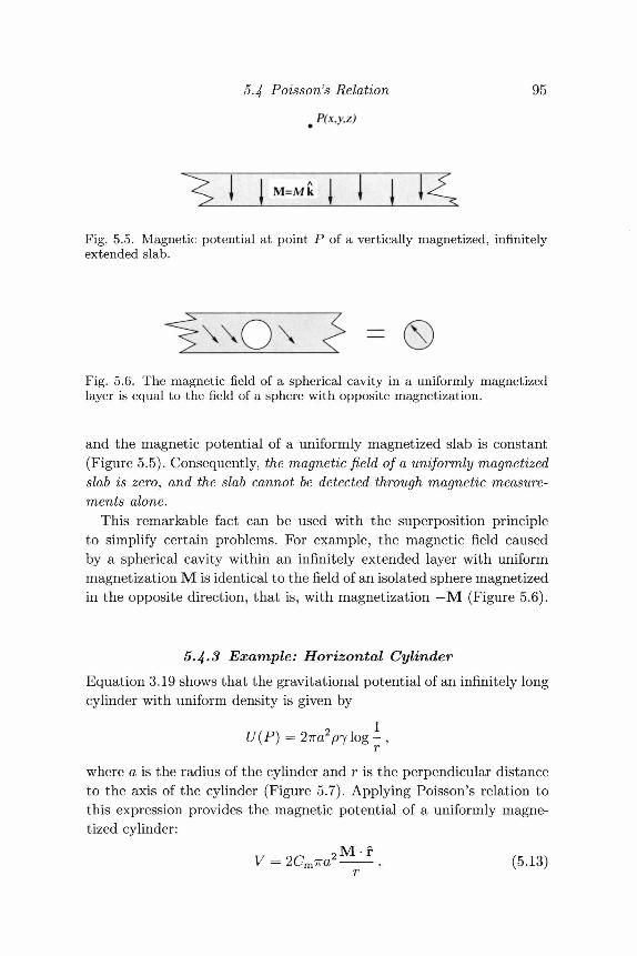
5.4 Poisson's Relation 95
P(x,y,z)
Fig. 5.5. Magnetic potential at point P of a vertically magnetized, infinitelyextended slab.
Fig. 5.6. The magnetic field of a spherical cavity in a uniformly magnetizedlayer is equal to the field of a sphere with opposite magnetization.
and the magnetic potential of a uniformly magnetized slab is constant(Figure 5.5). Consequently, the magnetic field of a uniformly magnetizedslab is zero, and the slab cannot be detected through magnetic measure-ments alone.
This remarkable fact can be used with the superposition principleto simplify certain problems. For example, the magnetic field causedby a spherical cavity within an infinitely extended layer with uniformmagnetization M is identical to the field of an isolated sphere magnetizedin the opposite direction, that is, with magnetization —M (Figure 5.6).
5.1^.3 Example: Horizontal CylinderEquation 3.19 shows that the gravitational potential of an infinitely longcylinder with uniform density is given by
U(P) = V 7 g
where a is the radius of the cylinder and r is the perpendicular distanceto the axis of the cylinder (Figure 5.7). Applying Poisson's relation tothis expression provides the magnetic potential of a uniformly magne-tized cylinder:
V = 2Cm7ra2^-^-. (5.13)
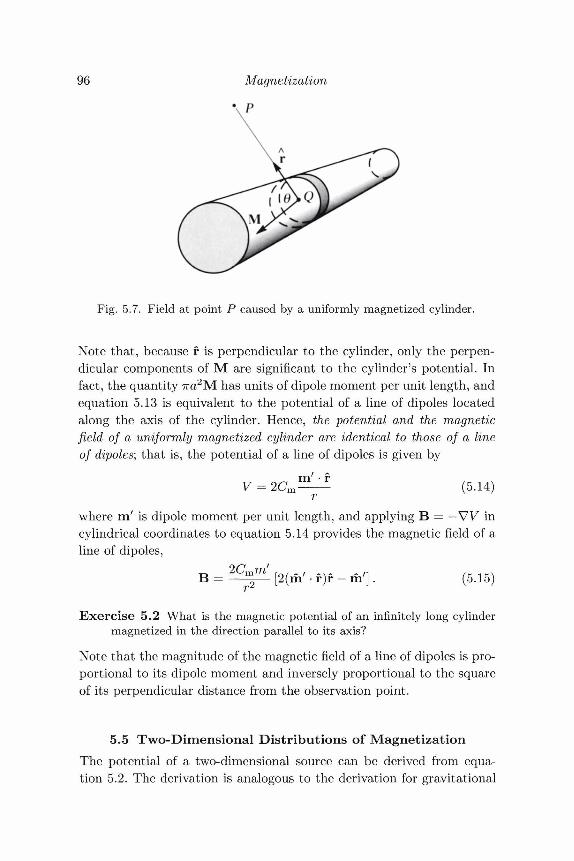
96 Magnetization
\P
Fig. 5.7. Field at point P caused by a uniformly magnetized cylinder.
Note that, because f is perpendicular to the cylinder, only the perpen-dicular components of M are significant to the cylinder's potential. Infact, the quantity 7ra2M has units of dipole moment per unit length, andequation 5.13 is equivalent to the potential of a line of dipoles locatedalong the axis of the cylinder. Hence, the potential and the magneticfield of a uniformly magnetized cylinder are identical to those of a lineof dipoles; that is, the potential of a line of dipoles is given by
V = 2cJ^- (5.14)r
where m' is dipole moment per unit length, and applying B = — VV incylindrical coordinates to equation 5.14 provides the magnetic field of aline of dipoles,
B = 29™pL [2(m' • f )f - m'] . (5.15)
Exercise 5.2 What is the magnetic potential of an infinitely long cylindermagnetized in the direction parallel to its axis?
Note that the magnitude of the magnetic field of a line of dipoles is pro-portional to its dipole moment and inversely proportional to the squareof its perpendicular distance from the observation point.
5.5 Two-Dimensional Distributions of MagnetizationThe potential of a two-dimensional source can be derived from equa-tion 5.2. The derivation is analogous to the derivation for gravitational
5.6 Annihilators 97
potential of two-dimensional masses in Chapter 3. The body is first con-sidered to be of finite length 2a, as in Figure 3.6, and the volume integralin equation 5.2 is replaced with a surface integral over the cross-sectionalarea of the body and a line integral along its length:
r iV(P) = Cm M(Q) -VQ-dv
JM(Q)- ijvQl-dz\ dS,
S Vo /where S is the cross-sectional area of the body. As a —> oo, the innerintegral approaches the potential of an infinite line of dipoles of unitmagnitude. Hence,
V(P) = 2Cm / M ( Q ) ' * dS (5.16)J rs
is the potential of a two-dimensional distribution of magnetic material,and applying B = — W provides
B(P) = 2Cm f ^ ^ [2(M • f )f - M] dS. (5.17)s
As before, r is understood to be normal to the long axis of the cylin-der and r is the perpendicular distance. Notice that the component ofmagnetic induction parallel to the long axis of the body is zero, andthe component of magnetization parallel to the long axis of the bodycontributes nothing to the magnetic field.
As discussed in Chapter 3 for the gravitational case, the magneticfield of an infinitely long body, uniform in the direction parallel to thelong dimension of the body, can be thought of as originating from a two-dimensional source. The source is essentially a thin wafer correspondingto the intersection of the body and a normal plane containing the ob-servation point (see Figure 3.7).
5.6 AnnihilatorsA nonzero distribution of magnetization (or density) that produces noexternal field for a particular source geometry is called an annihilator(Parker [207]). The annihilator can be added to its respective sourcegeometry without affecting the magnetic (or gravity) field. We see that
98 Magnetization
the magnetic annihilator for infinite slabs is just M = constant. A hor-izontal layer with variable magnetization M(x,y,z), therefore, is indis-tinguishable from a horizontal layer with the same magnetization plusany constant, that is, M.(x,y,z) + MQ. Hence, an infinite variety of mag-netizations can be conceived for the infinite slab, all producing preciselythe same magnetic field. We will have more to say about annihilators inlater chapters.
5.7 Problem Set1. Use Poisson's relation to find the magnetic field of a uniformly mag-
netized spherical shell.2. What nonzero distribution of magnetization within a sphere pro-
duces no magnetic field (i.e., what is the magnetic annihilator for aspherical source)?
3. Use Poisson's relation to prove the general statement that a uni-formly magnetized slab has no magnetic attraction, regardless of thedirection of magnetization.
4. Consider a line of dipoles aligned parallel to the y axis, with dipolemoment per unit length m = (mx,my,mz), and intersecting the x, zplane at coordinates (x',zf).(a) Let / = 2Cm/(x'2 + z'2)2, g = xf2-zr2, and h = 2x'z'. Show that
the three components of magnetic induction observed at (0,0,0)are given by
Bx
By = /90h
000
h '0
-g
mxVflymz_
(5.18)
(b) Use this expression to show that the horizontal component of Bdue to a line of dipoles magnetized vertically equals the verticalcomponent of B due to a line of dipoles magnetized horizontally.
(c) Show that the vertical component of B due to a line of dipolesmagnetized vertically equals the negative of the horizontal com-ponent of a line of dipoles magnetized horizontally.
5. A spherical cavity of radius a is buried with its center at depth ain a vertically and homogeneously magnetized layer. The layer hasthickness t (t > 2a) and magnetization M = Mk.(a) Find an expression for B in terms of M at the point directly over
the cavity.
5.7 Problem Set 99
(b) What is the dependence of B on a?6. The crust of Planet X is permanently magnetized proportional to the
field of an ancient centered dipole. The ancient field no longer exists.Consider the crust to be a shell with radii a\ and <i2 and show that thefield of the crust is zero at all external points. (Note: This problemis a demonstration of a more comprehensive theorem discussed indetail by Runcorn [248]: A shell magnetized proportional to the fieldof any internal source produces no external field. The magnetizationis therefore an annihilator for the shell.)
6Spherical Harmonic Analysis
But that to say in difficult problems the use of spherical harmonics islaborious is not to slight the method, because any other accuratetreatment would be still more difficult.
(Sydney Chapman and Julius Bartels)
Gravity is the ballast of the soul, which keeps the mind steady.(Thomas Fuller)
Physical quantities measured on or above the earth's surface are natu-rally suited to mathematical descriptions in spherical coordinates. Themost common such framework is spherical harmonic analysis. Sphericalharmonic analysis can be useful for any reasonably well-behaved, globalphenomenon and has been applied to a diverse range of data, from freeoscillations of the earth to global climate change. At the very least,spherical harmonic analysis provides a way to synthesize from a scatterof discrete measurements on a sphere an equation applicable to the entiresphere. Such an equation then can be used to interpolate the behaviorof the phenomenon to regions of the sphere that have no measurements.
As the name implies, however, spherical harmonic analysis takes onspecial meaning when applied to potential fields, because the build-ing blocks of spherical harmonic analysis are a natural consequence ofLaplace's equation in spherical coordinates. In particular, the variousterms of a spherical harmonic expansion are sometimes related (withcaution) to specific physical phenomena. The most well-known exampleis the separation of the dipole and nondipole components of the geomag-netic field: A spherical harmonic expansion based on discrete measure-ments of the geomagnetic field directly provides separate descriptions ofthe dipole and nondipole fields, and these two fields often are attributedto separate but linked processes in the earth's core.
100
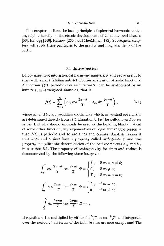
6.1 Introduction 101
This chapter outlines the basic principles of spherical harmonic analy-sis, relying heavily on the classic developments of Chapman and Bartels[56], Kellogg [146], Ramsey [235], and MacMillan [172]. Subsequent chap-ters will apply these principles to the gravity and magnetic fields of theearth.
6.1 Introduction
Before launching into spherical harmonic analysis, it will prove useful tostart with a more familiar subject, Fourier analysis of periodic functions.A function /(£), periodic over an interval T, can be synthesized by aninfinite sum of weighted sinusoids, that is,
v dm cos -7Fr- + 6 m sin — ^ - ) , (6.1)ra=0
where am and 6m are weighting coefficients which, as we shall see shortly,are determined directly from f(t). Equation 6.1 is the well-known Fourierseries. But why should sinusoids be used as the building blocks insteadof some other function, say exponentials or logarithms? One reason isthat fit) is periodic and so are sines and cosines. Another reason isthat sines and cosines have a property called orthogonality, and thisproperty simplifies the determination of the best coefficients am and bmin equation 6.1. The property of orthogonality for sines and cosines isdemonstrated by the following three integrals:
f f , if m = n 0;r 2ixmt 27rnt 7/ cos cos at = < 0, if m f n;
Jo * * I\T , if m = n — 0;
I T . 2ixmt 27rnt , f f , if ra = n;sin sin dt=<
o T T }o, ifm^n;T
/27T7Tit 27rri^
sm ——— cos dt — \).
If equation 6.1 is multiplied by either sin ^^ o r c o s P^ a n ( i integratedover the period T, all terms of the infinite sum are zero except one! The
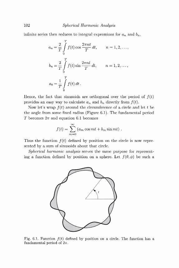
102 Spherical Harmonic Analysis
infinite series then reduces to integral expressions for an and 6n,T
2 ? 2nnt ,C 0 S " l 7 " ' ^ = 1, 2 , . . . ,
oT
bn = T ^ S i n ~T~ d t j ^ = 1, 2 , . . . ,oT
Hence, the fact that sinusoids are orthogonal over the period ofprovides an easy way to calculate an and bn directly from f(t).
Now let's wrap f(t) around the circumference of a circle and let t bethe angle from some fixed radius (Figure 6.1). The fundamental periodT becomes 2TT and equation 6.1 becomes
f(i) = ^2 (a™ cos mt + bm sin mt) .m=0
Thus the function f(t) defined by position on the circle is now repre-sented by a sum of sinusoids about that circle.
Spherical harmonic analysis serves the same purpose for represent-ing a function defined by position on a sphere. Let f(0,4>) be such a
Fig. 6.1. Function /(£) defined by position on a circle. The function has afundamental period of 2TT.
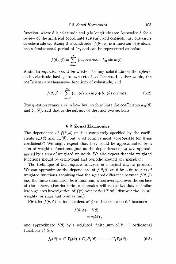
6.2 Zonal Harmonics 103
function, where 6 is colatitude and 0 is longitude (see Appendix A for areview of the spherical coordinate system), and consider just one circleof colatitude 0O. Along this colatitude, /(0o> <t>) is a function of <j> alone,has a fundamental period of 2TT, and can be represented as before,
f(0o,<t>) = ^2 («m cosm0 + 6m sinm0) .m=0
A similar equation could be written for any colatitude on the sphere,each colatitude having its own set of coefficients. In other words, thecoefficients are themselves functions of colatitude, and
/ (0, <t>) = ] T (am (6) cos nuj> + bm (6) sin mcj)) . (6.2)ra=0
The question remains as to how best to formulate the coefficients am(0)and bm(0), and that is the subject of the next two sections.
6.2 Zonal HarmonicsThe dependence of /(#, 0) on 6 is completely specified by the coeffi-cients am(0) and bm(0), but what form is most appropriate for thesecoefficients? We might expect that they could be approximated by asum of weighted functions, just as the dependence on 0 was approxi-mated by a sum of weighted sinusoids. We also expect that the weightedfunctions should be orthogonal and periodic around any meridian.
The technique of least-squares analysis is a logical way to proceed.We can approximate the dependence of /(#, </>) on 0 by a finite sum ofweighted functions, requiring that the squared difference between /(#, 0)and the finite summation be a minimum when averaged over the surfaceof the sphere. (Fourier-series aficionados will recognize that a similarleast-squares investigation of f(t) over period T will discover the "best"weights for sines and cosines too.)
First let /(#, 0) be independent of (j) so that equation 6.2 becomes
and approximate f(0) by a weighted, finite sum of k 4- 1 orthogonalfunctions Pn(0),
fk(0) = CoPo(0) + CiPi(0) + • • • + CkPk(0). (6.3)
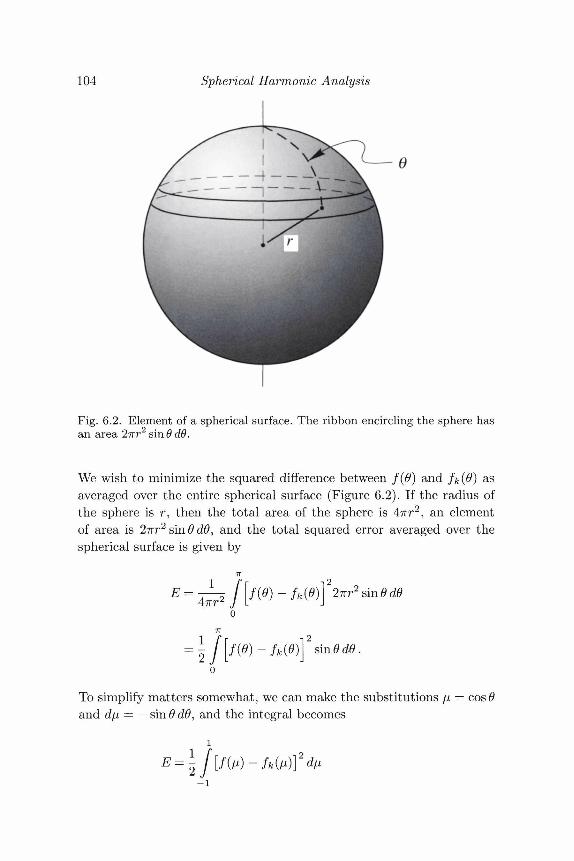
104 Spherical Harmonic Analysis
Fig. 6.2. Element of a spherical surface. The ribbon encircling the sphere hasan area 2nr2 sin 0 dO.
We wish to minimize the squared difference between f(0) and /&(#) asaveraged over the entire spherical surface (Figure 6.2). If the radius ofthe sphere is r, then the total area of the sphere is 47rr2, an elementof area is 27rr2sin#d#, and the total squared error averaged over thespherical surface is given by
7T
f(O)-fk(O)\22irr2sinOd6
To simplify matters somewhat, we can make the substitutionsand d\i — — sin 9 d6, and the integral becomes
= cos#
- 1
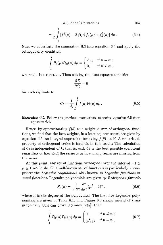
6.2 Zonal Harmonics 1051
= \ J [f (/*) - 2 /(/X) fk (I*) + ft (A*)] dn. (6.4)- 1
Next we substitute the summation 6.3 into equation 6.4 and apply theorthogonality condition
/An. if n = m:0, if n 7= m,
where An is a constant. Then solving the least-squares conditiondEocr0
for each C\ leads tol
Q = Tj'/(M)^(A*)^- (6-5)- 1
Exercise 6.1 Follow the previous instructions to derive equation 6.5 fromequation 6.4.
Hence, by approximating f(0) as a weighted sum of orthogonal func-tions, we find that the best weights, in a least-squares sense, are given byequation 6.5, an integral expression involving f{0) itself. A remarkableproperty of orthogonal series is implicit in this result: The calculationof C\ is independent of k; that is, each C\ is the best possible coefficientregardless of how long the series is or how many terms are missing fromthe series.
At this point, any set of functions orthogonal over the interval — 1 </i < 1 would do. One well-known set of functions is particularly appro-priate: the Legendre polynomials, also known as Legendre functions orzonal functions. Legendre polynomials are given by Rodrigues 's formula
where n is the degree of the polynomial. The first five Legendre poly-nomials are given in Table 6.1, and Figure 6.3 shows several of thesegraphically. One can prove (Ramsey [235]) that
/0, if n ^ n';
\ ., ; (6-7)
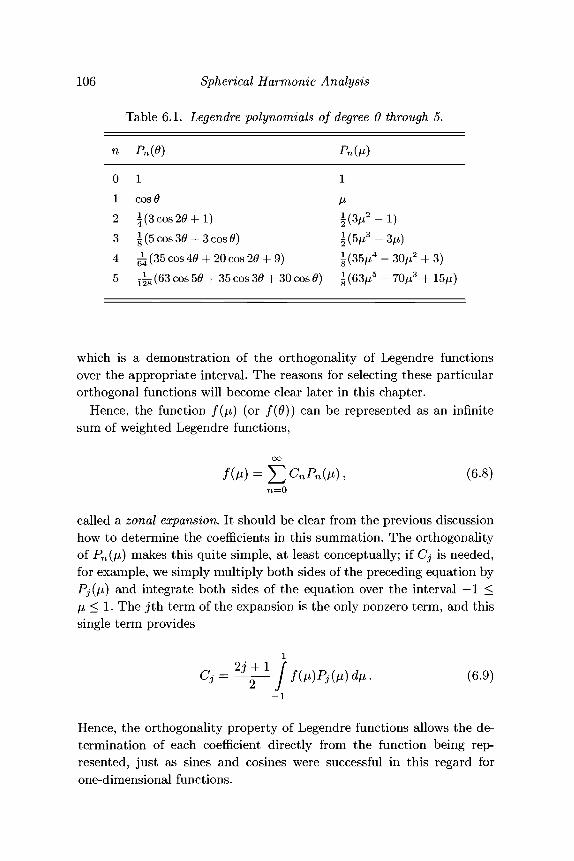
106 Spherical Harmonic Analysis
Table 6.1. Legendre polynomials of degree 0 through 5.
n
0
1
2
3
4
5
Pn(O)
1
COS0
|(3 cos 20 + 1)
|(5 cos 30+ 3 cos 0)
-^(35 cos 40+ 20 cos 20 +
^ (63 cos 50 + 35 cos 30 -\
pn(.
i
fi
5(3/*
5(5/*9) |(35,
-30 cos 6») |(63,
• )
2-l)3 - 3/x)M4 - 30/u2
M5 - 70p3
+ 3)+ 15//)
which is a demonstration of the orthogonality of Legendre functionsover the appropriate interval. The reasons for selecting these particularorthogonal functions will become clear later in this chapter.
Hence, the function /(/i) (or /(#)) can be represented as an infinitesum of weighted Legendre functions,
CnPn(n), (6.8)n=0
called a zonal expansion. It should be clear from the previous discussionhow to determine the coefficients in this summation. The orthogonalityof Pn(l^) makes this quite simple, at least conceptually; if Cj is needed,for example, we simply multiply both sides of the preceding equation byPj(fJ>) and integrate both sides of the equation over the interval — 1 <\JL < 1. The jth term of the expansion is the only nonzero term, and thissingle term provides
• ' -*• / i V . . \ r > / . . \ J . . / £ ? Q \
- 1
Hence, the orthogonality property of Legendre functions allows the de-termination of each coefficient directly from the function being rep-resented, just as sines and cosines were successful in this regard forone-dimensional functions.
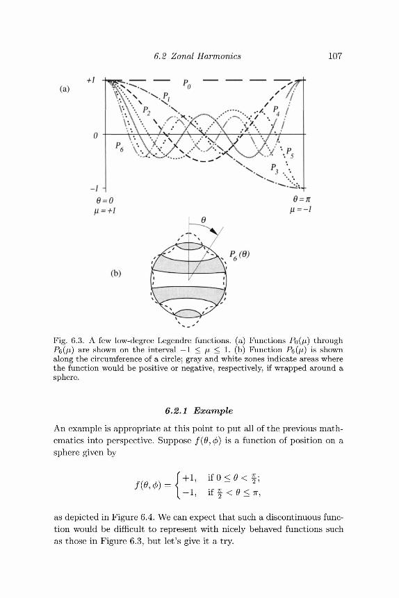
6.2 Zonal Harmonics 107
(a)+/
^m;xxx-1 -
9 = 0» = +!
(b)
Fig. 6.3. A few low-degree Legendre functions, (a) Functions PO((JL) throughPQ(H) are shown on the interval — 1 < /i < 1. (b) Function PQ(IJ) is shownalong the circumference of a circle; gray and white zones indicate areas wherethe function would be positive or negative, respectively, if wrapped around asphere.
6.2.1 Example
An example is appropriate at this point to put all of the previous math-ematics into perspective. Suppose /(#, (f>) is a function of position on asphere given by
i f O < 0 < | ;if f <6<7T,
as depicted in Figure 6.4. We can expect that such a discontinuous func-tion would be difficult to represent with nicely behaved functions suchas those in Figure 6.3, but let's give it a try.
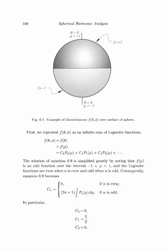
108 Spherical Harmonic Analysis
t=-i
Fig. 6.4. Example of discontinuous /(#, (f>) over surface of sphere.
First, we represent /(#,(/>) as an infinite sum of Legendre functions.
+ + C2P2(fi) +
The solution of equation 6.9 is simplified greatly by noting that /(/i)is an odd function over the interval — 1 < \x < 1, and the Legendrefunctions are even when n is even and odd when n is odd. Consequently,equation 6.9 becomes
Cn = (2n + l ) j .0
if n is even;
x, if n is odd.
In particular,
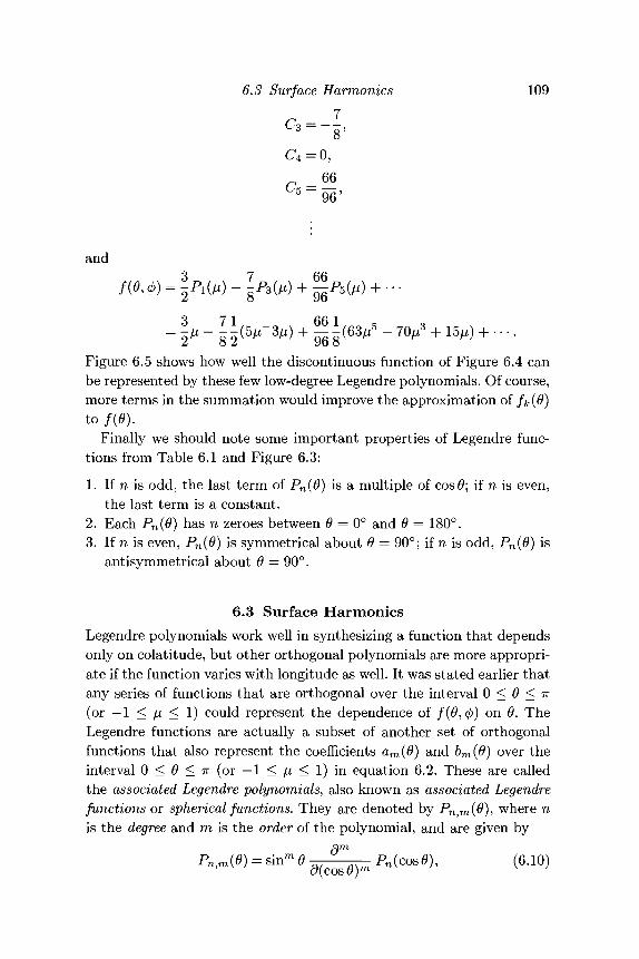
6.3 Surface Harmonics 109
C4 = 0,66
°5~96'
and
f(0,4>) = ^
Figure 6.5 shows how well the discontinuous function of Figure 6.4 canbe represented by these few low-degree Legendre polynomials. Of course,more terms in the summation would improve the approximation of fk(0)to f(0).
Finally we should note some important properties of Legendre func-tions from Table 6.1 and Figure 6.3:
1. If n is odd, the last term of Pn(0) is a multiple of cos#; if n is even,the last term is a constant.
2. Each Pn{9) has n zeroes between 9 = 0° and 9 = 180°.3. If n is even, Pn(0) is symmetrical about 9 = 90°; if n is odd, Pn(9) is
antisymmetrical about 9 = 90°.
6.3 Surface HarmonicsLegendre polynomials work well in synthesizing a function that dependsonly on colatitude, but other orthogonal polynomials are more appropri-ate if the function varies with longitude as well. It was stated earlier thatany series of functions that are orthogonal over the interval 0 < 9 < n(or — 1 < ji < 1) could represent the dependence of f{0,(j>) on 9. TheLegendre functions are actually a subset of another set of orthogonalfunctions that also represent the coefficients am(9) and bm(9) over theinterval 0 < 9 < n (or — 1 < // < 1) in equation 6.2. These are calledthe associated Legendre polynomials, also known as associated Legendrefunctions or spherical functions. They are denoted by Pn,m(9), where nis the degree and m is the order of the polynomial, and are given by
QmPn,m(0) = sin™ 0 — Pn(cos 0), (6.10)
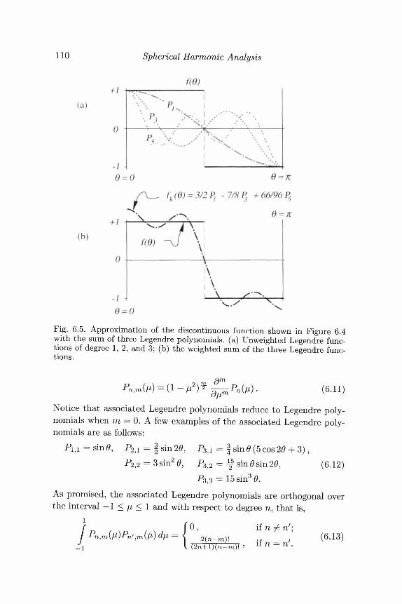
110
(a)
(b)
Spherical Harmonic Analysis
f(6)-/ -
o -
1 -
• ' • • • • p ,
p5 V /y * \
6 = 0
fk (6) = 3/2 7/8P3 + 66/96
\
f(d) -J \\
\- / 1
Fig. 6.5. Approximation of the discontinuous function shown in Figure 6.4with the sum of three Legendre polynomials, (a) Unweighted Legendre func-tions of degree 1, 2, and 3; (b) the weighted sum of the three Legendre func-tions.
dr
(6.11)
Notice that associated Legendre polynomials reduce to Legendre poly-nomials when m = 0. A few examples of the associated Legendre poly-nomials are as follows:
Pi,i =sin<9, P2 j l = § sin 20, P3A = f sin 0 (5 cos 2(9 + 3),
P2,2 = 3 sin2 (9, P3j2 = M gin 6 sin 20, (6.12)
P3,3 = 15 sin3 6.
As promised, the associated Legendre polynomials are orthogonal overthe interval - 1 < // < 1 and with respect to degree n, that is,
fO, *„*„';(6.13)2 ( n + m ) , , II 77- — 72 .
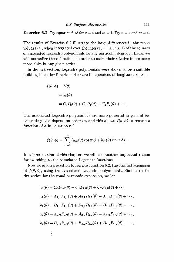
6.3 Surface Harmonics 111
Exercise 6.2 Try equation 6.13 for n = 4 and m — 1. Try n = 4 and m = 4.
The results of Exercise 6.2 illustrate the large differences in the meanvalues (i.e., when integrated over the interval — 1 < \x < 1) of the squaresof associated Legendre polynomials for any particular degree n. Later, wewill normalize these functions in order to make their relative importancemore alike in any given series.
In the last section, Legendre polynomials were shown to be a suitablebuilding block for functions that are independent of longitude, that is,
= CoPo(0) + CiPi(0) + C2P2(O)
The associated Legendre polynomials are more powerful in general be-cause they also depend on order ra, and this allows /(#, </>) to remain afunction of (j) in equation 6.2,
f{O,<t>) = Y, (am{6) cosm<j>+ bm(6) sinm<j>) .ra=O
In a later section of this chapter, we will see another important reasonfor switching to the associated Legendre functions.
Now we are in a position to rewrite equation 6.2, the original expansionof /(#, 0), using the associated Legendre polynomials. Similar to thederivation for the zonal harmonic expansion, we let
ao(0) =
blT Bi,i
B2,2
b,o(6
-f2,2
P2,2
') + '(6)-\
(0)^
(0)-
CiPi,o(O)
h^2>1P2,i
hS2,iP2,i
hB3 2P32
+ cs!^2,0
• ^ , :
•B4.
(0)-
LP3,
1^3,
2P4
((X\1 1 (7 1
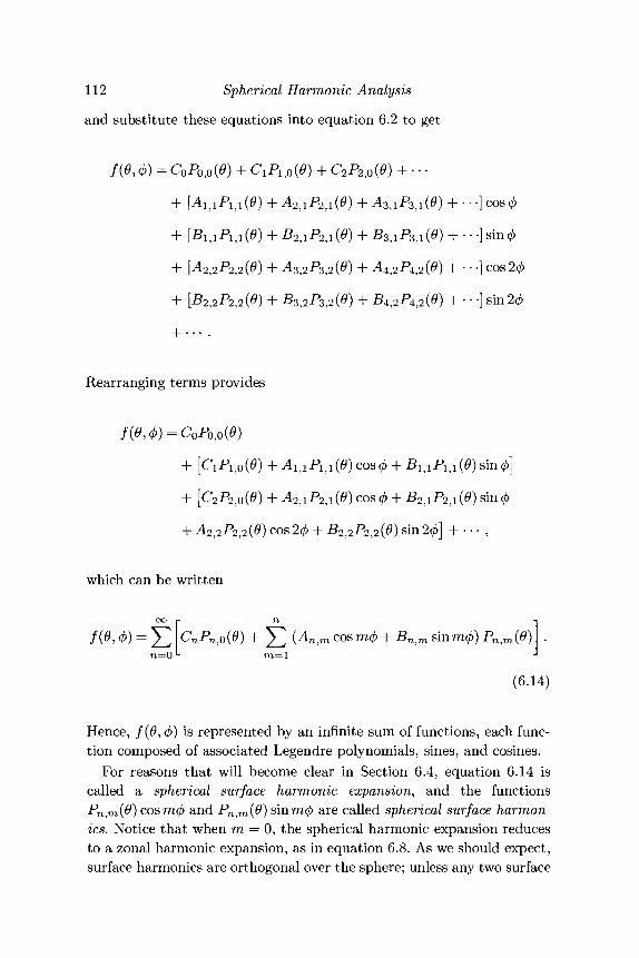
112 Spherical Harmonic Analysis
and substitute these equations into equation 6.2 to get
f{9, <f>) = CoPo,o(0) + CiPi,Q{6)
+ [Ai,iPu(0) + A2,iP2,i(9) + A3>1P3tl(0)
+ [Bi,iPi,i(e) + B2,iP2,i(J) + B3.1P3.1W + • • •] sin^
+ [^2,2^2,2(0) + A3,2P3,2(0) + ^4,2^4,2(0) + • • •] COS 20
+ [B2fiP2,2(e) + B3,2Ps,2(°) + Bi,2P4,2(°) + ' ' '] s i n 2(P
-\ •
Rearranging terms provides
COS 20 + ^2,2^2,2^) Sin 20]
which can be written
f(0,0) = J j CnPn,0(6>) + X ! (An,m cosm0 + 5 n , m sinmn=0 •- m=l
(6.14)
Hence, f(0, 0) is represented by an infinite sum of functions, each func-tion composed of associated Legendre polynomials, sines, and cosines.
For reasons that will become clear in Section 6.4, equation 6.14 iscalled a spherical surface harmonic expansion, and the functionsPn,m(6) cosm0 and Pn,m(0) sinm0 are called spherical surface harmon-ics. Notice that when m = 0, the spherical harmonic expansion reducesto a zonal harmonic expansion, as in equation 6.8. As we should expect,surface harmonics are orthogonal over the sphere; unless any two surface
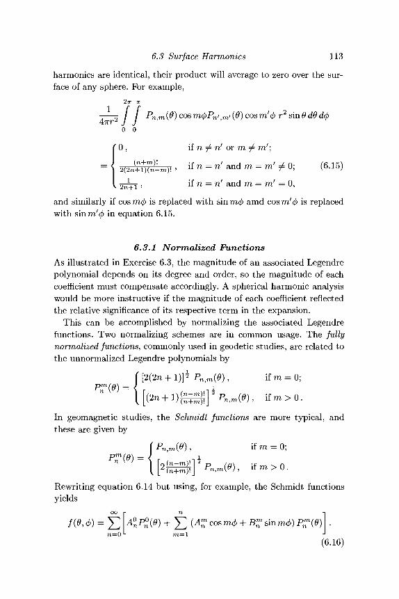
6.3 Surface Harmonics 113
harmonics are identical, their product will average to zero over the sur-face of any sphere. For example,
o Pnm (0) cos vn(\)Pni m/ {&) cos ml'(p r2 sin 6 dO d(f)47rrz J J
0 0
' 0 , if n ^ n' or m ^ m'\
2(2n%7n-my. > if n = n'and m = m ' ^ 0; (6.15)if n = n' and m = m! = 0,
and similarly if cos ra0 is replaced with sin mcj) amd cos TTI'C/) is replacedwith sinra^ in equation 6.15.
6.3.1 Normalized FunctionsAs illustrated in Exercise 6.3, the magnitude of an associated Legendrepolynomial depends on its degree and order, so the magnitude of eachcoefficient must compensate accordingly. A spherical harmonic analysiswould be more instructive if the magnitude of each coefficient reflectedthe relative significance of its respective term in the expansion.
This can be accomplished by normalizing the associated Legendrefunctions. Two normalizing schemes are in common usage. The fullynormalized functions, commonly used in geodetic studies, are related tothe unnormalized Legendre polynomials by
P™{6) =
In geomagnetic studies, the Schmidt functions are more typical, andthese are given by
ifm = 0;
Rewriting equation 6.14 but using, for example, the Schmidt functionsyields
OO r U
« W + E W cosm0 + B% sin m^P^(m=l
(6.16)
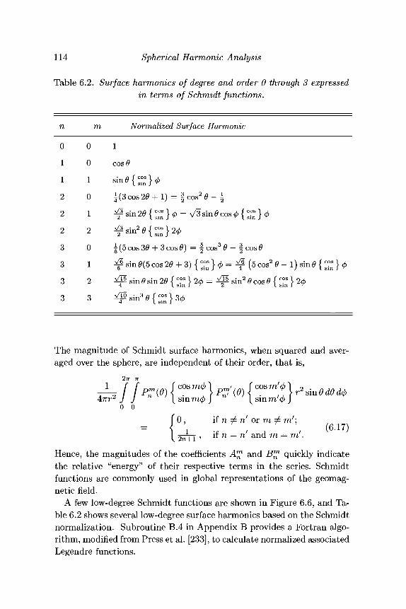
114 Spherical Harmonic Analysis
Table 6.2. Surface harmonics of degree and order 0 through 3 expressedin terms of Schmidt functions.
n
0
1
1
2
2
2
3
3
3
3
m
0
0
1
0
1
2
0
1
2
3
Normalized Surface Harmonic
1
COS0
|(3cos20 + l) = §cos26>- \
^- sin 2$ 1 ^ | 0 = v 3 sin 0 cos 0 | ^ | 0
^sin20{-ns}20
|(5cos30+ 3cos0) = f cos30- f cos0
^ sin 0(5 cos 20 + 3) { ™ } 4> = ^ (5 cos2 0^sin0sin20{^}2(/>= ^psin20cos0{^P sin3 0 { c°* } 30
- l ) s in0{- s }0
" n } 2<t>
The magnitude of Schmidt surface harmonics, when squared and aver-aged over the sphere, are independent of their order, that is,
2n ir
ft™0 0
{0, if n / n' or m ^ m7:
•f / H / ( 6 - 1 7 )
2^pj , if n = n and m = m .Hence, the magnitudes of the coefficients A™ and I?^1 quickly indicatethe relative "energy" of their respective terms in the series. Schmidtfunctions are commonly used in global representations of the geomag-netic field.
A few low-degree Schmidt functions are shown in Figure 6.6, and Ta-ble 6.2 shows several low-degree surface harmonics based on the Schmidtnormalization. Subroutine B.4 in Appendix B provides a Fortran algo-rithm, modified from Press et al. [233], to calculate normalized associatedLegendre functions.
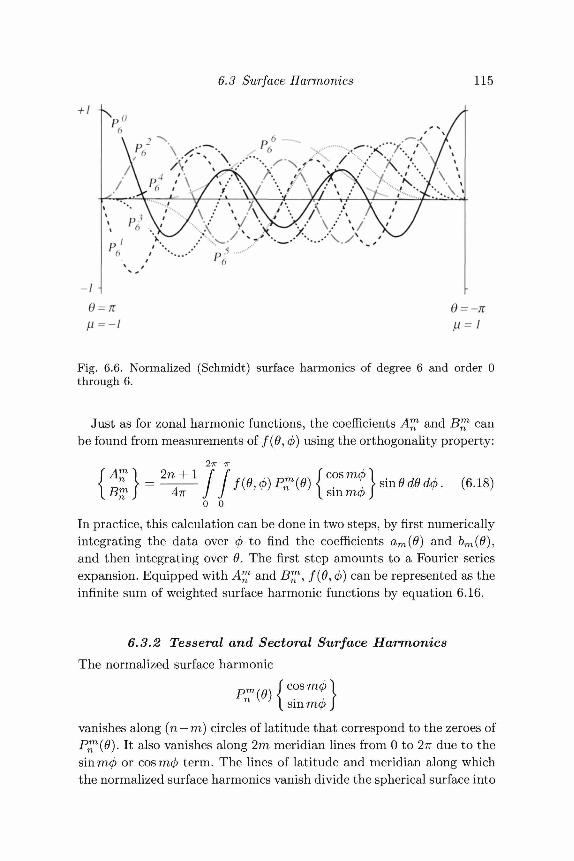
6.3 Surface Harmonics 115
fi=-l
Fig. 6.6. Normalized (Schmidt) surface harmonics of degree 6 and order 0through 6.
Just as for zonal harmonic functions, the coefficients A™ and B™ canbe found from measurements of /(#, 0) using the orthogonality property:
0 0
In practice, this calculation can be done in two steps, by first numericallyintegrating the data over <j> to find the coefficients am(^) and &m(^),and then integrating over 0. The first step amounts to a Fourier seriesexpansion. Equipped with A™ and B™, /(#, (j>) can be represented as theinfinite sum of weighted surface harmonic functions by equation 6.16.
6.3.2 Tesseral and Sectoral Surface HarmonicsThe normalized surface harmonic
p™rm J c o s m ( H{ sinvanishes along (n — m) circles of latitude that correspond to the zeroes ofP™(6). It also vanishes along 2m meridian lines from 0 to 2?r due to thesin mcj) or cos ra0 term. The lines of latitude and meridian along whichthe normalized surface harmonics vanish divide the spherical surface into
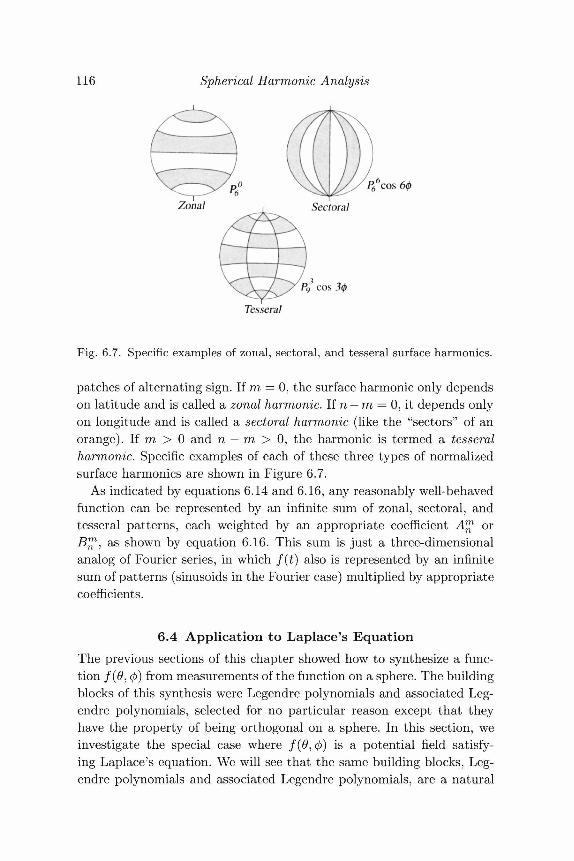
116 Spherical Harmonic Analysis
cos
Pg COS 3<t>
Tesseral
Fig. 6.7. Specific examples of zonal, sectoral, and tesseral surface harmonics.
patches of alternating sign. If TTT, = 0, the surface harmonic only dependson latitude and is called a zonal harmonic. If n — m = 0, it depends onlyon longitude and is called a sectoral harmonic (like the "sectors" of anorange). If m > 0 and n — m > 0, the harmonic is termed a tesseralharmonic. Specific examples of each of these three types of normalizedsurface harmonics are shown in Figure 6.7.
As indicated by equations 6.14 and 6.16, any reasonably well-behavedfunction can be represented by an infinite sum of zonal, sectoral, andtesseral patterns, each weighted by an appropriate coefficient A™ orB™, as shown by equation 6.16. This sum is just a three-dimensionalanalog of Fourier series, in which f(t) also is represented by an infinitesum of patterns (sinusoids in the Fourier case) multiplied by appropriatecoefficients.
6.4 Application to Laplace's EquationThe previous sections of this chapter showed how to synthesize a func-tion /(#, (j)) from measurements of the function on a sphere. The buildingblocks of this synthesis were Legendre polynomials and associated Leg-endre polynomials, selected for no particular reason except that theyhave the property of being orthogonal on a sphere. In this section, weinvestigate the special case where /(#, (f>) is a potential field satisfy-ing Laplace's equation. We will see that the same building blocks, Leg-endre polynomials and associated Legendre polynomials, are a natural
6.4 Application to Laplace's Equation 117
consequence of and provide additional insights into the representationof harmonic functions on a sphere.
6.4.I Homogeneous Functions and Euler's EquationAs we are well aware by now, potential fields outside of source regionssatisfy Laplace's equation, which in cartesian coordinates is given by
~ , d2V d2V 02VV V = 1 1dx2 dy2 dz2
= 0.
Every solution to Laplace's equation is a harmonic function if the firstderivatives of the function are continuous and the second derivativesexist. Now let D or Df represent any spatial differential operation incartesian coordinates, such as ^ , f -, or V2. Any two such operationsare commutative, that is,
and in particular
DV2U(x,y,z) = V2DU(x,y,z).
Hence, ifU(x,y, z) is a harmonic function, then so is any spatial deriva-tive of U(x, y, z).
This theorem provides a means of generating a host of harmonic func-tions from known solutions to Laplace's equation. For example, because
V 2 - = 0 ,rwe know immediately that J ~ , V^, and m • V^ (the magnetic poten-tial of a dipole) are also harmonic. This is an important result for futurechapters. If it can be shown, for example, that the scalar magnetic po-tential of the earth is harmonic, then any component of the magneticfield of the earth also must be harmonic.
A function V is said to be homogeneous of degree n if it satisfies Euler'sequation,
jy+/y+/y=nV. ( ( U 9 )ox dy dz
Homogeneous functions that also satisfy Laplace's equation are calledspherical solid harmonic functions for reasons that will become apparent
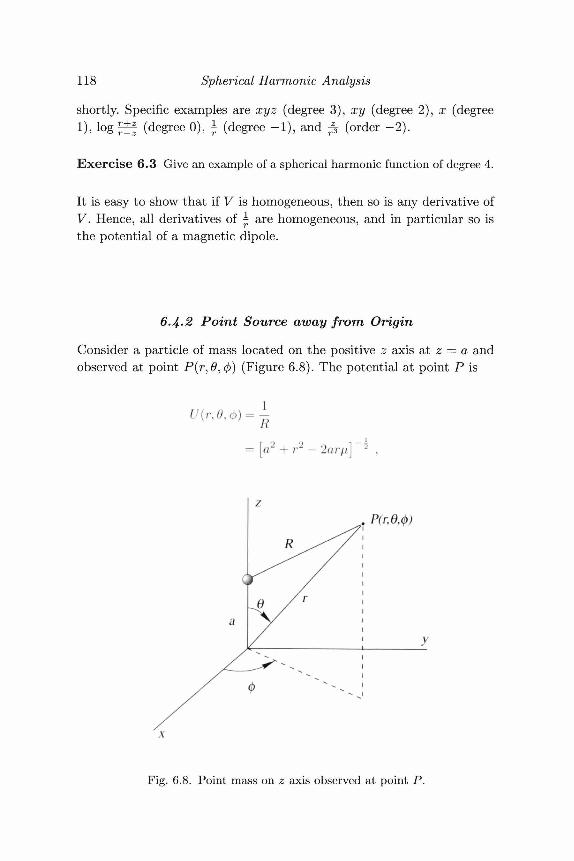
118 Spherical Harmonic Analysis
shortly. Specific examples are xyz (degree 3), xy (degree 2), x (degree1), log£f (degree 0), ± (degree -1), and ^ (order -2).
Exercise 6.3 Give an example of a spherical harmonic function of degree 4.
It is easy to show that if V is homogeneous, then so is any derivative ofV. Hence, all derivatives of £ are homogeneous, and in particular so isthe potential of a magnetic dipole.
6,4*2 Point Source away from Origin
Consider a particle of mass located on the positive z axis at z = a andobserved at point P(r, 0,0) (Figure 6.8). The potential at point P is
R
= [a2 + r2 -2arti]~* .
.. P(r.e,4>)
Fig. 6.8. Point mass on z axis observed at point P.
6.4 Application to Laplace's Equation 119
where \i = cos#.f First we consider the case where r < a. We factor outthe parameter a,
1 1 f r2 r 1~*- = - 1 + ^ - 2 - J , (6.20)R a az a
expand the potential in a binomial series
2! \ a2 a
l r , 1 / r 2 o r \ 3 f r4 r3
aL 2 \ a 2 a / 8 \ a 4 a3
15 fr6 r5 r4 o r3
48 V «6 a5 a4 a3
and rearrange terms into powers of r/a to get
1
A quick comparison of this series with Table 6.1 shows that the factorscontaining \i are each a Legendre function, namely,
n = 0
Hence, the potential of a point mass displaced from the origin can berepresented by an infinite sum of weighted Legendre functions.
f Note that Newton's gravitational constant has been dropped in the following dis-cussion for convenience.
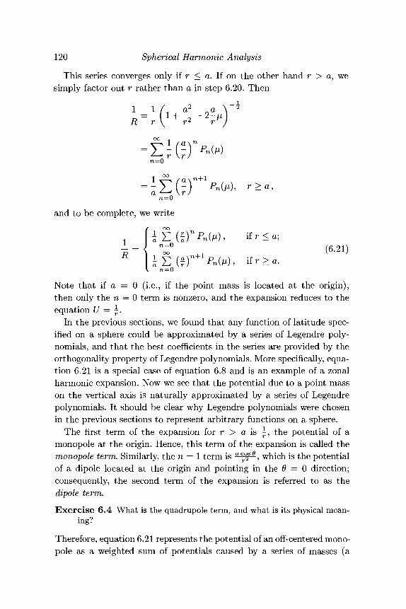
120 Spherical Harmonic Analysis
This series converges only if r < a. If on the other hand r > a, wesimply factor out r rather than a in step 6.20. Then
1 - l (l ^ - 2 -R r \ r2 r
-(-)n=0
n=0
and to be complete, we write
S ( r ) Pn{v) , if r < a;
, " " , ,„+! (6"21)
a Z^ Vr ) ^nlAv 5 II 7" > a.Note that if a = 0 (i.e., if the point mass is located at the origin),then only the n = 0 term is nonzero, and the expansion reduces to theequation U = K
In the previous sections, we found that any function of latitude spec-ified on a sphere could be approximated by a series of Legendre poly-nomials, and that the best coefficients in the series are provided by theorthogonality property of Legendre polynomials. More specifically, equa-tion 6.21 is a special case of equation 6.8 and is an example of a zonalharmonic expansion. Now we see that the potential due to a point masson the vertical axis is naturally approximated by a series of Legendrepolynomials. It should be clear why Legendre polynomials were chosenin the previous sections to represent arbitrary functions on a sphere.
The first term of the expansion for r > a is £, the potential of amonopole at the origin. Hence, this term of the expansion is called themonopole term. Similarly, the n = 1 term is ac°£0, which is the potentialof a dipole located at the origin and pointing in the 0 = 0 direction;consequently, the second term of the expansion is referred to as thedipole term.
Exercise 6.4 What is the quadrupole term, and what is its physical mean-ing?
Therefore, equation 6.21 represents the potential of an off-centered mono-pole as a weighted sum of potentials caused by a series of masses (a
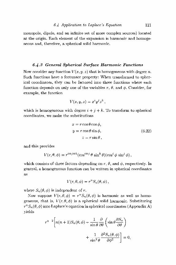
6.4 Application to Laplace's Equation 121
monopole, dipole, and an infinite set of more complex sources) locatedat the origin. Each element of the expansion is harmonic and homoge-neous and, therefore, a spherical solid harmonic.
6.1^.3 General Spherical Surface Harmonic FunctionsNow consider any function V(x, y, z) that is homogeneous with degree n.Such functions have a fortunate property: When transformed to spher-ical coordinates, they can be factored into three functions where eachfunction depends on only one of the variables r, 6, and 0. Consider, forexample, the function
V(x,y,z) =xiyjzk ,
which is homogeneous with degree i + j + k. To transform to sphericalcoordinates, we make the substitutions
x = r cos 0 cos 0,y = r cos 0 sin 0, (6.22)
z = r sin 0 ,
and this provides
V(r, 0, (j)) = ri+j+k(cosi+j 0 sin^ 0) (cos' 0 sin ' 0),
which consists of three factors depending on r, 0, and 0, respectively. Ingeneral, a homogeneous function can be written in spherical coordinatesas
V(r,9,4>)=rnSn(0,<t>),
where Sn(0, (j)) is independent of r.Now suppose V(r, #,</>) = rnSn(0, </>) is harmonic as well as homo-
geneous, that is, V(r,0,(j)) is a spherical solid harmonic. SubstitutingrnSn(0, 0) into Laplace's equation in spherical coordinates (Appendix A)yields
1 d2Sn(6,<P)}s in 2 0 dd>2
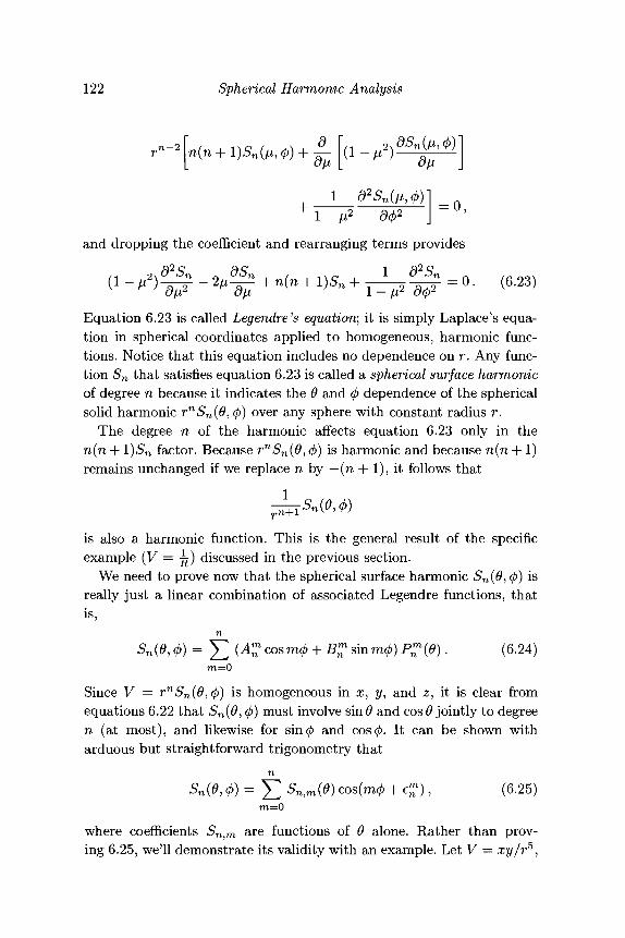
122 Spherical Harmonic Analysis
=+ 1 - ^ d<t>2
and dropping the coefficient and rearranging terms provides
Equation 6.23 is called Legendre's equation; it is simply Laplace's equa-tion in spherical coordinates applied to homogeneous, harmonic func-tions. Notice that this equation includes no dependence on r. Any func-tion Sn that satisfies equation 6.23 is called a spherical surface harmonicof degree n because it indicates the 9 and <\> dependence of the sphericalsolid harmonic rnSn(9,(j)) over any sphere with constant radius r.
The degree n of the harmonic affects equation 6.23 only in then(n + l)Sn factor. Because rnSn(9,(/>) is harmonic and because n(n+ 1)remains unchanged if we replace n by — (n + 1), it follows that
1——Dn\9* (b)
is also a harmonic function. This is the general result of the specificexample (V — j^) discussed in the previous section.
We need to prove now that the spherical surface harmonic Sn(9, 0) isreally just a linear combination of associated Legendre functions, thatis,
nSn(0,<t>) = ^2 (A^cosm0 + ^s inm0)P^( (9 ) . (6.24)
ra=0
Since V = rnSn(9,(j)) is homogeneous in x, y, and z, it is clear fromequations 6.22 that Sn(9,0) must involve sin9 and cos 9 jointly to degreen (at most), and likewise for sin0 and cos</>. It can be shown witharduous but straightforward trigonometry that
n
5n((9, (/)) = Y^ Sn,m(°) cos(m0 + C ) , (6-25)
where coefficients Sn^m are functions of 9 alone. Rather than prov-ing 6.25, we'll demonstrate its validity with an example. Let V = xy/r5,
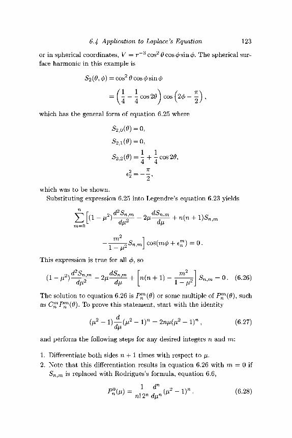
6.4 Application to Laplace's Equation 123
or in spherical coordinates, V — r~3 cos2 0 cos <p sin </>. The spherical sur-face harmonic in this example is
62 (0? 0) = c o s 2 0 c o s 0 sin <fi
which has the general form of equation 6.25 where
S2,o(0)=O,
which was to be shown.Substituting expression 6.25 into Legendre's equation 6.23 yields
n
£ra=0
= 0.
This expression is true for all 0, so
(1 _ )^f^ - 2/x^p^ + \n(n + 1) - yz-^\ S^™ = ° • (6-26)
The solution to equation 6.26 is P™{0) or some multiple of P™(0), suchas C™P™(0). To prove this statement, start with the identity
(^2 - l ) - f (M2 - 1)" = 2nM(M2 - 1)" , (6.27)
and perform the following steps for any desired integers n and m:
1. Differentiate both sides n + 1 times with respect to \i.2. Note that this differentiation results in equation 6.26 with m = 0 if
5 n ? m is replaced with Rodrigues's formula, equation 6.6,
124 Spherical Harmonic Analysis
3. Differentiate m times.4. Note that the result is again equation 6.26, but 5n,ra has been re-
placed by
P™(H) = (1 - /x2)? _ P n ( M ) , (6.29)
which, from equation 6.11, is the associated Legendre polynomial ofdegree n and order m.
Hence,
Sn,m(6>) = C T W ) ,and rewriting equation 6.25 accordingly,
Sn(0,4>)=
This is the most general expression for a surface harmonic of degree n.
Exercise 6.5 Use the previous steps to prove that 5i,o(0) = C®Pi{9). Provethat 5i,i(0) = C{Pl{0).
Recall thatoo
YnSn{e,cl>), (6.30)n=0
oroo
V(r,e,<f>) = Y,r~in+1)S"(e>4>)- (6-31)n=0
Therefore, a harmonic function can be represented by an infinite sumof spherical solid harmonics (equation 6.25) where the dependence on6 and 0 is contained within spherical surface harmonics, which in turnare represented by sums of weighted associated Legendre polynomials.It should be clear why, when we had to represent the 9 dependenceof f{9,<j)) by an orthogonal series, we chose the associated Legendrepolynomials.
Notice that if Sn(9,(j)) can be found, perhaps from measurements ofV(r, #, (j)) on the surface of a sphere, equation 6.31 immediately providesV(r,9, (j)) at any point outside the sphere. Hence, the potential fielddue to sources lying entirely within a sphere can be found at any pointoutside the sphere strictly from the behavior of the potential field on thesphere. Indeed, equations 6.30 and 6.31 together permit a determination
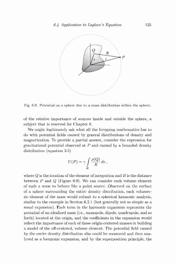
6.4 Application to Laplace's Equation 125
Fig. 6.9. Potential on a sphere due to a mass distribution within the sphere.
of the relative importance of sources inside and outside the sphere, asubject that is reserved for Chapter 8.
We might legitimately ask what all the foregoing mathematics has todo with potential fields caused by general distributions of density andmagnetization. To provide a partial answer, consider the expression forgravitational potential observed at P and caused by a bounded densitydistribution (equation 3.5)
P(Q)R dv,
where Q is the location of the element of integration and R is the distancebetween P and Q (Figure 6.9). We can consider each volume elementof such a mass to behave like a point source. Observed on the surfaceof a sphere surrounding the entire density distribution, each volumet-ric element of the mass would submit to a spherical harmonic analysis,similar to the example in Section 6.2.1 (but generally not so simple as azonal expansion). Each term in the harmonic expansion represents thepotential of an idealized mass (i.e., monopole, dipole, quadrupole, and soforth) located at the origin, and the coefficients in the expansion wouldreflect the importance of each of these origin-centered masses in buildinga model of the off-centered, volume element. The potential field causedby the entire density distribution also could be measured and then ana-lyzed as a harmonic expansion, and by the superposition principle, the
126 Spherical Harmonic Analysis
resulting terms of the expansion will represent the integrated effects ofthe entire mass. The coefficients will be related to the manner in whichmass is distributed about the origin.
Consider, as a trivial example, the potential of a uniform, sphericalmass measured at various points on a larger sphere symmetrically placedaround the spherical mass. A spherical harmonic analysis of these datawould find that all coefficients are zero except for the n = 0 term ofthe expansion, immediately indicating that the mass is equivalent to acentered monopole, as it should be. Similarly, a spherical harmonic anal-ysis of the magnetic potential caused by a uniformly magnetized spherewould reduce to just the n = 1 term of the expansion, immediately in-dicating the nature of the magnetization distribution, namely, that thespherical magnetic body is equivalent to a centered dipole. Chapters 7and 8 will apply some of these principles to global gravity and magneticfields, respectively.
6.5 Problem Set
1. Let /(#, 0) = A sin 20 cos 40 on a spherical surface. Find a represen-tation for /(#, (/)) in terms of normalized (Schmidt) associated Legen-dre polynomials.
2. Let /(#,</>) be defined on a sphere such that
f l , i fO<0<7r ;[0, lf7T<0<27T.
Use Subroutine B.4 in Appendix B to calculate a ten-term approxima-tion to /(#, 4>) and plot the approximated values around the equator.
3. Are the following functions spherical solid harmonic functions? If so,find their degree.
(a) V = x2+y2.(b) V = 3x2 + xy.(c) V = x2y + xz.(d) V = (x2 +y2+^2)3/2 •(e) V=± + ^ + ^.
4. Show that if V is harmonic and homogeneous of degree n, thenTfcz ir^l^V ls h a r m °m c and homogeneous of degree n — a — b — c.
5. Let V = x2 —y2. Find Sn{6). Show that it satisfies equation 6.23 andthat it can be represented as summation 6.25.
6.5 Problem Set 127
6. Consider the potential outside a uniformly magnetized sphere. Ar-range the coordinate system so that the magnetization is in the di-rection 0 = 0.(a) Let the center of the sphere be at the origin and expand the
potential in a zonal harmonic expansion.(b) Let the center of the sphere be displaced a distance a in the
0 = 0 direction and expand the potential in a zonal harmonicexpansion.
(c) Discuss what happens to the expansion if the dipole points in adirection other than 6 = 0.
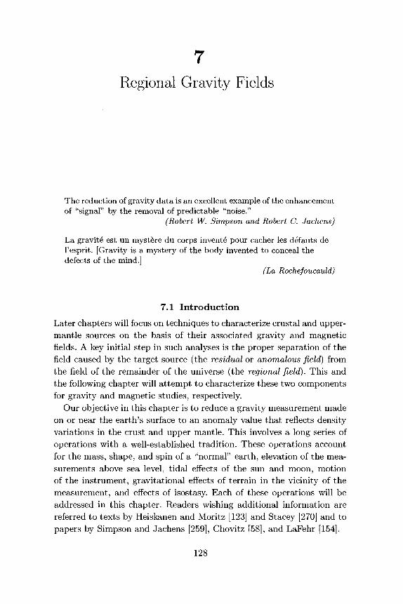
7Regional Gravity Fields
The reduction of gravity data is an excellent example of the enhancementof "signal" by the removal of predictable "noise."
(Robert W. Simpson and Robert C. Jachens)
La gravite est un mystere du corps invente pour cacher les defauts del'esprit. [Gravity is a mystery of the body invented to conceal thedefects of the mind.]
(La Rochefoucauld)
7.1 IntroductionLater chapters will focus on techniques to characterize crustal and upper-mantle sources on the basis of their associated gravity and magneticfields. A key initial step in such analyses is the proper separation of thefield caused by the target source (the residual or anomalous field) fromthe field of the remainder of the universe (the regional field). This andthe following chapter will attempt to characterize these two componentsfor gravity and magnetic studies, respectively.
Our objective in this chapter is to reduce a gravity measurement madeon or near the earth's surface to an anomaly value that reflects densityvariations in the crust and upper mantle. This involves a long series ofoperations with a well-established tradition. These operations accountfor the mass, shape, and spin of a "normal" earth, elevation of the mea-surements above sea level, tidal effects of the sun and moon, motionof the instrument, gravitational effects of terrain in the vicinity of themeasurement, and effects of isostasy. Each of these operations will beaddressed in this chapter. Readers wishing additional information arereferred to texts by Heiskanen and Moritz [123] and Stacey [270] and topapers by Simpson and Jachens [259], Chovitz [58], and LaFehr [154].
128
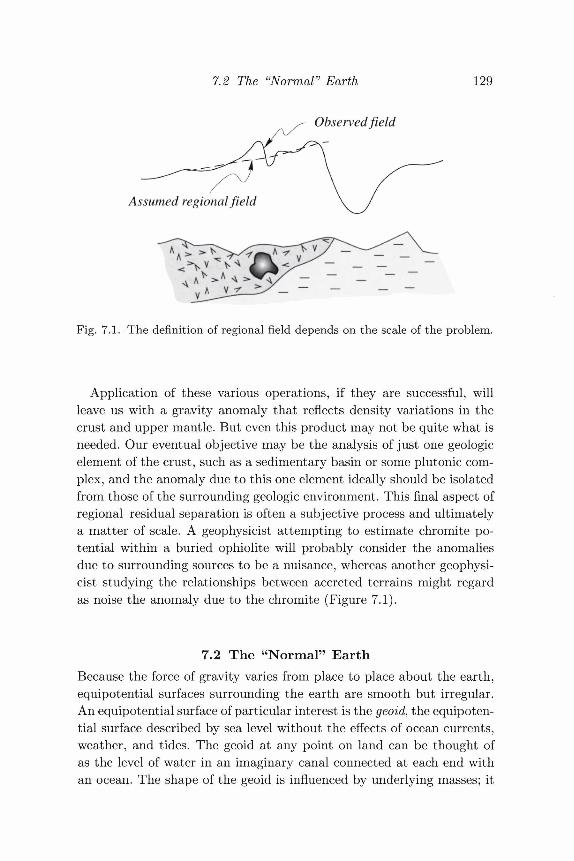
7.2 The "Normal" Earth 129
Observed field
Assumed regional field
Fig. 7.1. The definition of regional field depends on the scale of the problem.
Application of these various operations, if they are successful, willleave us with a gravity anomaly that reflects density variations in thecrust and upper mantle. But even this product may not be quite what isneeded. Our eventual objective may be the analysis of just one geologicelement of the crust, such as a sedimentary basin or some plutonic com-plex, and the anomaly due to this one element ideally should be isolatedfrom those of the surrounding geologic environment. This final aspect ofregional-residual separation is often a subjective process and ultimatelya matter of scale. A geophysicist attempting to estimate chromite po-tential within a buried ophiolite will probably consider the anomaliesdue to surrounding sources to be a nuisance, whereas another geophysi-cist studying the relationships between accreted terrains might regardas noise the anomaly due to the chromite (Figure 7.1).
7.2 The "Normal" EarthBecause the force of gravity varies from place to place about the earth,equipotential surfaces surrounding the earth are smooth but irregular.An equipotential surface of particular interest is the geoid, the equipoten-tial surface described by sea level without the effects of ocean currents,weather, and tides. The geoid at any point on land can be thought ofas the level of water in an imaginary canal connected at each end withan ocean. The shape of the geoid is influenced by underlying masses; it
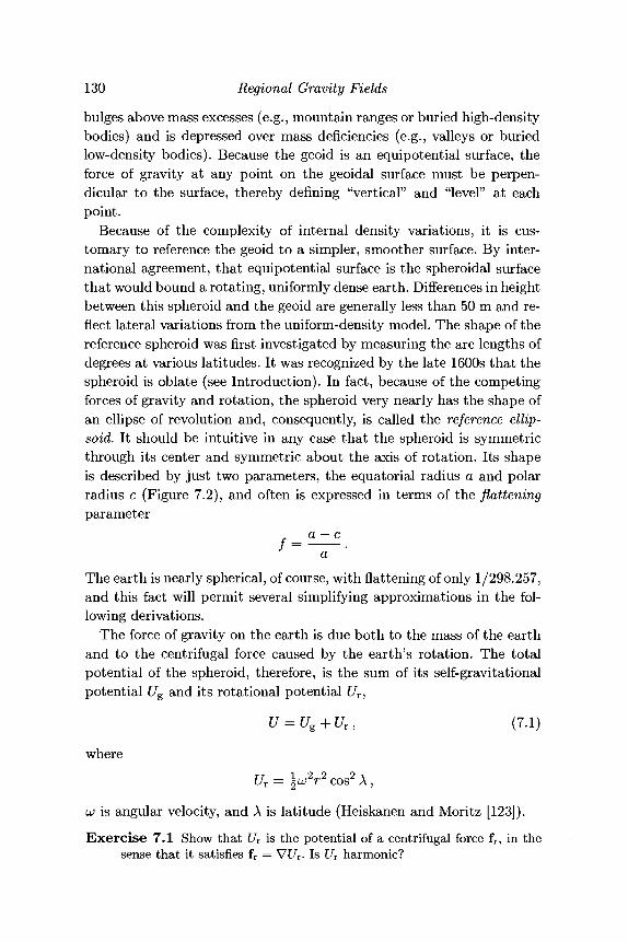
130 Regional Gravity Fields
bulges above mass excesses (e.g., mountain ranges or buried high-densitybodies) and is depressed over mass deficiencies (e.g., valleys or buriedlow-density bodies). Because the geoid is an equipotential surface, theforce of gravity at any point on the geoidal surface must be perpen-dicular to the surface, thereby defining "vertical" and "level" at eachpoint.
Because of the complexity of internal density variations, it is cus-tomary to reference the geoid to a simpler, smoother surface. By inter-national agreement, that equipotential surface is the spheroidal surfacethat would bound a rotating, uniformly dense earth. Differences in heightbetween this spheroid and the geoid are generally less than 50 m and re-flect lateral variations from the uniform-density model. The shape of thereference spheroid was first investigated by measuring the arc lengths ofdegrees at various latitudes. It was recognized by the late 1600s that thespheroid is oblate (see Introduction). In fact, because of the competingforces of gravity and rotation, the spheroid very nearly has the shape ofan ellipse of revolution and, consequently, is called the reference ellip-soid. It should be intuitive in any case that the spheroid is symmetricthrough its center and symmetric about the axis of rotation. Its shapeis described by just two parameters, the equatorial radius a and polarradius c (Figure 7.2), and often is expressed in terms of the flatteningparameter
The earth is nearly spherical, of course, with flattening of only 1/298.257,and this fact will permit several simplifying approximations in the fol-lowing derivations.
The force of gravity on the earth is due both to the mass of the earthand to the centrifugal force caused by the earth's rotation. The totalpotential of the spheroid, therefore, is the sum of its self-gravitationalpotential Ug and its rotational potential Ur,
U = Ug + Ur, (7.1)
where
UY = \u2r2 cos2 A,
uo is angular velocity, and A is latitude (Heiskanen and Moritz [123]).
Exercise 7.1 Show that UT is the potential of a centrifugal force fr, in thesense that it satisfies fr = VC/r. Is UT harmonic?
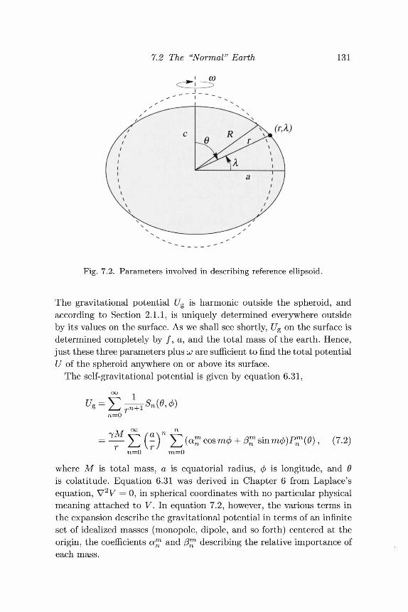
7.2 The "Normal" Earth
CO
131
Fig. 7.2. Parameters involved in describing reference ellipsoid.
The gravitational potential Ug is harmonic outside the spheroid, andaccording to Section 2.1.1, is uniquely determined everywhere outsideby its values on the surface. As we shall see shortly, Ug on the surface isdetermined completely by / , a, and the total mass of the earth. Hence,just these three parameters plus uo are sufficient to find the total potentialU of the spheroid anywhere on or above its surface.
The self-gravitational potential is given by equation 6.31,
n=0
n = 0, (7-2)
ra=O
where M is total mass, a is equatorial radius, 4> is longitude, and 6is colatitude. Equation 6.31 was derived in Chapter 6 from Laplace'sequation, V2V = 0, in spherical coordinates with no particular physicalmeaning attached to V. In equation 7.2, however, the various terms inthe expansion describe the gravitational potential in terms of an infiniteset of idealized masses (monopole, dipole, and so forth) centered at theorigin, the coefficients a™ and /?™ describing the relative importance ofeach mass.
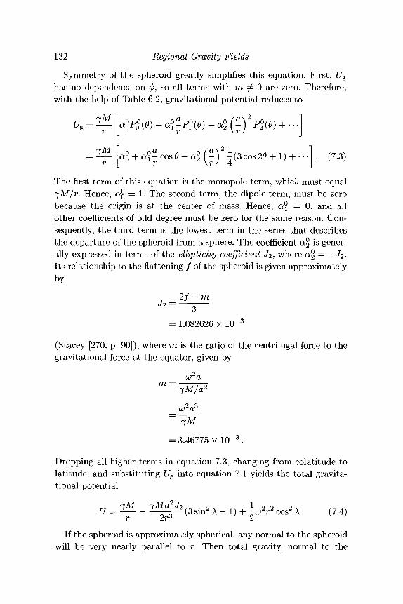
132 Regional Gravity Fields
Symmetry of the spheroid greatly simplifies this equation. First, Ug
has no dependence on 0, so all terms with m ^ 0 are zero. Therefore,with the help of Table 6.2, gravitational potential reduces to
Lo + a o « c o s 0 + ao (*\ i o g 2 0 + 1 } + . . 1 ( 7 3 )
The first term of this equation is the monopole term, which must equal7M/V. Hence, a$ = 1. The second term, the dipole term, must be zerobecause the origin is at the center of mass. Hence, a\ — 0, and allother coefficients of odd degree must be zero for the same reason. Con-sequently, the third term is the lowest term in the series that describesthe departure of the spheroid from a sphere. The coefficient a® is gener-ally expressed in terms of the ellipticity coefficient J2, where a® = —Ji-Its relationship to the flattening / of the spheroid is given approximatelyby
2f-m
= 1.082626 x 1(T3
(Stacey [270, p. 90]), where m is the ratio of the centrifugal force to thegravitational force at the equator, given by
m = -fM/a2
_oo2a3
~ -yM
= 3.46775 x 10"3 .
Dropping all higher terms in equation 7.3, changing from colatitude tolatitude, and substituting Ug into equation 7.1 yields the total gravita-tional potential
Jf M£J (3 sin2 A - 1) + \jr> cos2 A. (7.4)
If the spheroid is approximately spherical, any normal to the spheroidwill be very nearly parallel to r. Then total gravity, normal to the
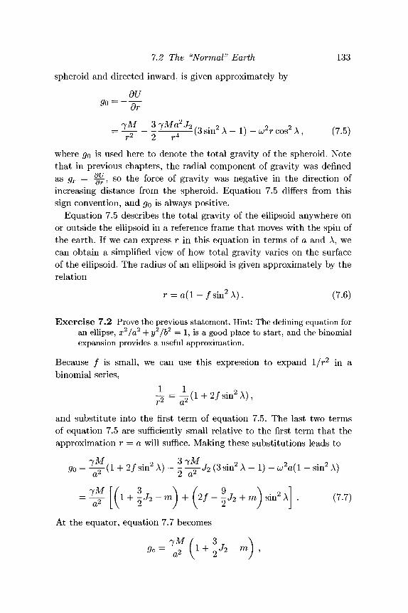
7.2 The "Normal" Earth 133
spheroid and directed inward, is given approximately by
dUgo — —-£-
or<yM 3 7 M Q 2 J 2 . 2 2 2= — -: (3 sm A — 1) — UJ r cos A , (7.5)rz 2 r4
where go is used here to denote the total gravity of the spheroid. Notethat in previous chapters, the radial component of gravity was definedas gr = |^7, so the force of gravity was negative in the direction ofincreasing distance from the spheroid. Equation 7.5 differs from thissign convention, and go is always positive.
Equation 7.5 describes the total gravity of the ellipsoid anywhere onor outside the ellipsoid in a reference frame that moves with the spin ofthe earth. If we can express r in this equation in terms of a and A, wecan obtain a simplified view of how total gravity varies on the surfaceof the ellipsoid. The radius of an ellipsoid is given approximately by therelation
r = a ( l - / s i n 2 A ) . (7.6)
Exercise 7.2 Prove the previous statement. Hint: The defining equation foran ellipse, x2/a2 + y2/b2 — 1, is a good place to start, and the binomialexpansion provides a useful approximation.
Because / is small, we can use this expression to expand 1/r2 in abinomial series,
i_ = 1 ( 1 + 2/ sin2 A),
and substitute into the first term of equation 7.5. The last two termsof equation 7.5 are sufficiently small relative to the first term that theapproximation r = a will suffice. Making these substitutions leads to
go = _4_(i + 2/sin2 A) - - V J2 (3sin2 A - 1) - u2a(l - sin2 A)cr 2 or
2f-^J2+m\sm2\\ • (7.7)
At the equator, equation 7.7 becomes
3h - J 2 -
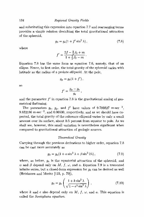
134 Regional Gravity Fields
and substituting this expression into equation 7.7 and rearranging termsprovides a simple relation describing the total gravitational attractionof the spheroid,
<7o = <7e(l + / 's in2A), (7.8)
whereOf2/-§J2
Equation 7.8 has the same form as equation 7.6, namely, that of anellipse. Hence, to first order, the total gravity of the spheroid varies withlatitude as the radius of a prolate ellipsoid. At the pole,
gp = ge(l + / ' ) ,
so
J 5
and the parameter / ' in equation 7.8 is the gravitational analog of geo-metrical flattening.
The parameters ge, #p, and / ' have values of 9.780327 m-sec~2,9.832186 m-sec~2, and 0.00530, respectively, and as we should have ex-pected, the total gravity of the reference ellipsoid varies by only a smallamount over its surface, about 0.5 percent from equator to pole. As weshall see, however, this small variation is nevertheless significant whencompared to gravitational attraction of geologic sources.
Theoretical GravityCarrying through the previous derivations to higher order, equation 7.8can be cast more accurately as
go = ge(l + a sin2 A + /3sin2 2A), (7.9)
where, as before, ge is the equatorial attraction of the spheroid, anda and (5 depend only on M, / , a;, and a. Equation 7.9 is a truncatedinfinite series, but a closed-form expression for go can be derived as well(Heiskanen and Moritz [123, p. 70]),
/ l + /csin2A \g0 = g e [ , 7 .10V\/l-e2sin2Ay
where k and e also depend only on M, / , CJ, and a. This equation iscalled the Somigliana equation.
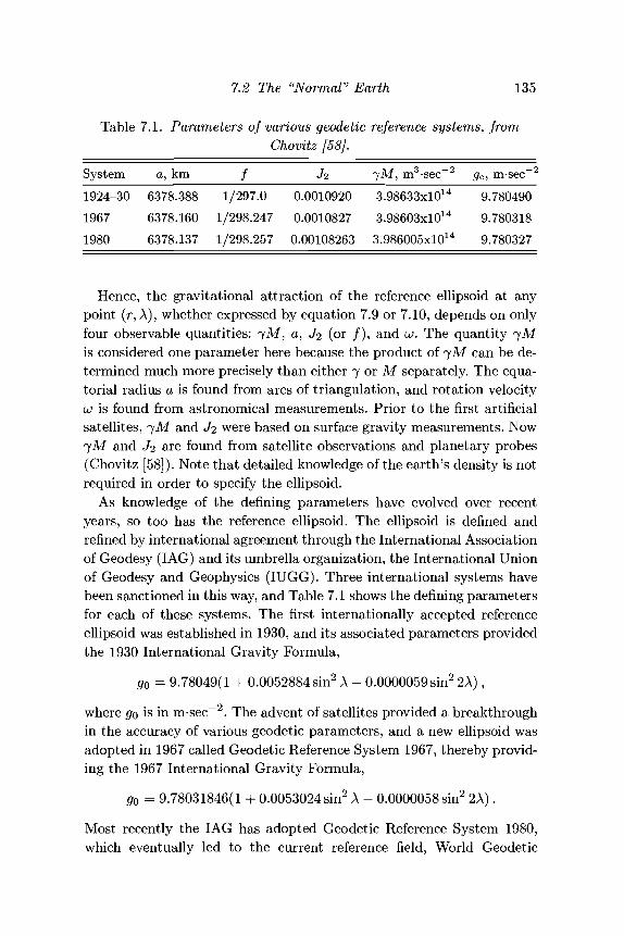
7.2 The "Normal" Earth 135
Table 7.1. Parameters of various geodetic reference systems, fromChovitz [58].
System a, km / J2 7M, m3-sec~2 ge, m-sec - 2
1924-30 6378.388 1/297.0 0.0010920 3.98633xl014 9.7804901967 6378.160 1/298.247 0.0010827 3.98603xl014 9.7803181980 6378.137 1/298.257 0.00108263 3.986005xl014 9.780327
Hence, the gravitational attraction of the reference ellipsoid at anypoint (r, A), whether expressed by equation 7.9 or 7.10, depends on onlyfour observable quantities: 7M, a, J2 (or / ) , and uo. The quantity 7 Mis considered one parameter here because the product of 7M can be de-termined much more precisely than either 7 or M separately. The equa-torial radius a is found from arcs of triangulation, and rotation velocityUJ is found from astronomical measurements. Prior to the first artificialsatellites, 7M and J2 were based on surface gravity measurements. Now7M and J2 are found from satellite observations and planetary probes(Chovitz [58]). Note that detailed knowledge of the earth's density is notrequired in order to specify the ellipsoid.
As knowledge of the defining parameters have evolved over recentyears, so too has the reference ellipsoid. The ellipsoid is defined andrefined by international agreement through the International Associationof Geodesy (IAG) and its umbrella organization, the International Unionof Geodesy and Geophysics (IUGG). Three international systems havebeen sanctioned in this way, and Table 7.1 shows the defining parametersfor each of these systems. The first internationally accepted referenceellipsoid was established in 1930, and its associated parameters providedthe 1930 International Gravity Formula,
go = 9.78049(1 + 0.0052884sin2 A - 0.0000059 sin2 2A),
where go is in m-sec~2. The advent of satellites provided a breakthroughin the accuracy of various geodetic parameters, and a new ellipsoid wasadopted in 1967 called Geodetic Reference System 1967, thereby provid-ing the 1967 International Gravity Formula,
go = 9.78031846(1 + 0.0053024 sin2 A - 0.0000058 sin2 2A).
Most recently the IAG has adopted Geodetic Reference System 1980,which eventually led to the current reference field, World Geodetic
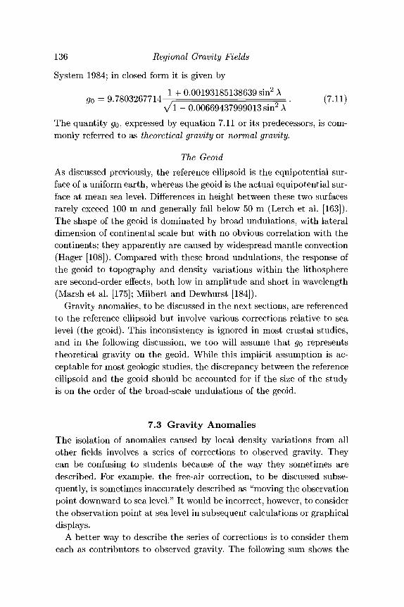
136 Regional Gravity Fields
System 1984; in closed form it is given by
,o = — 1 + 0-00193185138639^^VI - 0.00669437999013 sin2 A
The quantity go, expressed by equation 7.11 or its predecessors, is com-monly referred to as theoretical gravity or normal gravity.
The GeoidAs discussed previously, the reference ellipsoid is the equipotential sur-face of a uniform earth, whereas the geoid is the actual equipotential sur-face at mean sea level. Differences in height between these two surfacesrarely exceed 100 m and generally fall below 50 m (Lerch et al. [163]).The shape of the geoid is dominated by broad undulations, with lateraldimension of continental scale but with no obvious correlation with thecontinents; they apparently are caused by widespread mantle convection(Hager [108]). Compared with these broad undulations, the response ofthe geoid to topography and density variations within the lithosphereare second-order effects, both low in amplitude and short in wavelength(Marsh et al. [175]; Milbert and Dewhurst [184]).
Gravity anomalies, to be discussed in the next sections, are referencedto the reference ellipsoid but involve various corrections relative to sealevel (the geoid). This inconsistency is ignored in most crustal studies,and in the following discussion, we too will assume that go representstheoretical gravity on the geoid. While this implicit assumption is ac-ceptable for most geologic studies, the discrepancy between the referenceellipsoid and the geoid should be accounted for if the size of the studyis on the order of the broad-scale undulations of the geoid.
7.3 Gravity AnomaliesThe isolation of anomalies caused by local density variations from allother fields involves a series of corrections to observed gravity. Theycan be confusing to students because of the way they sometimes aredescribed. For example, the free-air correction, to be discussed subse-quently, is sometimes inaccurately described as "moving the observationpoint downward to sea level." It would be incorrect, however, to considerthe observation point at sea level in subsequent calculations or graphicaldisplays.
A better way to describe the series of corrections is to consider themeach as contributors to observed gravity. The following sum shows the
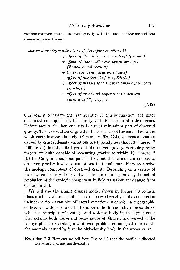
7.3 Gravity Anomalies 137
various components to observed gravity with the name of the correctionsshown in parentheses:
observed gravity = attraction of the reference ellipsoid+ effect of elevation above sea level (free-air)+ effect of "normal" mass above sea level
(Bouguer and terrain)+ time-dependent variations (tidal)+ effect of moving platform (Eb'tvos)+ effect of masses that support topographic loads
(isostatic)+ effect of crust and upper mantle density
variations ("geology").(7.12)
Our goal is to isolate the last quantity in this summation, the effectof crustal and upper mantle density variations, from all other terms.Unfortunately, this last quantity is a relatively minor part of observedgravity. The acceleration of gravity at the surface of the earth due to thewhole earth is approximately 9.8 m-sec"2 (980 Gal), whereas anomaliescaused by crustal density variations are typically less than 10~3 m-sec~2
(100 mGal), less than 0.01 percent of observed gravity. Portable gravitymeters are quite capable of measuring gravity to within 10~7 m-sec~2
(0.01 mGal), or about one part in 108, but the various corrections toobserved gravity involve assumptions that limit our ability to resolvethe geologic component of observed gravity. Depending on a variety offactors, particularly the severity of the surrounding terrain, the actualresolution of the geologic component in field situations may range from0.1 to 5 mGal.
We will use the simple crustal model shown in Figure 7.3 to helpillustrate the various contributions to observed gravity. This cross sectionincludes various examples of lateral variations in density: a topographicedifice, a low-density root that supports the topography in accordancewith the principles of isostasy, and a dense body in the upper crustthat extends both above and below sea level. Gravity is observed at thetopographic surface along a west-east profile, and our goal is to isolatethe anomaly caused by just the high-density body in the upper crust.
Exercise 7.3 How can we tell from Figure 7.3 that the profile is directedwest-east and not north-south?
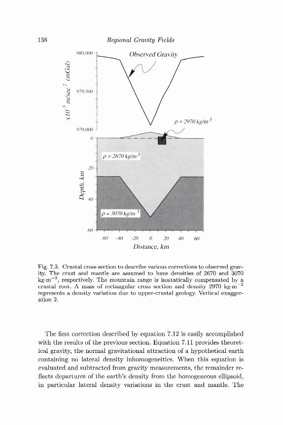
138
9H0JHX) H
Regional Gravity Fields
Observed Gravity
i= 297()kg/m3
-60 -40 -20 0 20 40 60
Distance, km
Fig. 7.3. Crustal cross section to describe various corrections to observed grav-ity. The crust and mantle are assumed to have densities of 2670 and 3070kg-m~3, respectively. The mountain range is isostatically compensated by acrustal root. A mass of rectangular cross section and density 2970 kg-m~3
represents a density variation due to upper-crustal geology. Vertical exagger-ation 2.
The first correction described by equation 7.12 is easily accomplishedwith the results of the previous section. Equation 7.11 provides theoret-ical gravity, the normal gravitational attraction of a hypothetical earthcontaining no lateral density inhomogeneities. When this equation isevaluated and subtracted from gravity measurements, the remainder re-flects departures of the earth's density from the homogeneous ellipsoid,in particular lateral density variations in the crust and mantle. The
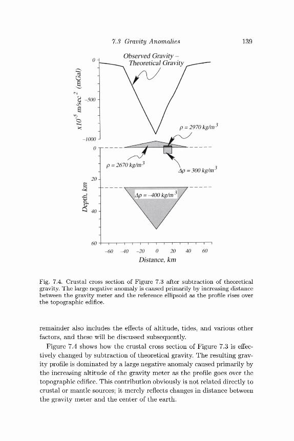
7.3 Gravity Anomalies
Observed Gravity -Theoretical Gravity
139
-60 -40 -20 0 20
Distance, km
Fig. 7.4. Crustal cross section of Figure 7.3 after subtraction of theoreticalgravity. The large negative anomaly is caused primarily by increasing distancebetween the gravity meter and the reference ellipsoid as the profile rises overthe topographic edifice.
remainder also includes the effects of altitude, tides, and various otherfactors, and these will be discussed subsequently.
Figure 7.4 shows how the crustal cross section of Figure 7.3 is effec-tively changed by subtraction of theoretical gravity. The resulting grav-ity profile is dominated by a large negative anomaly caused primarily bythe increasing altitude of the gravity meter as the profile goes over thetopographic edifice. This contribution obviously is not related directly tocrustal or mantle sources; it merely reflects changes in distance betweenthe gravity meter and the center of the earth.
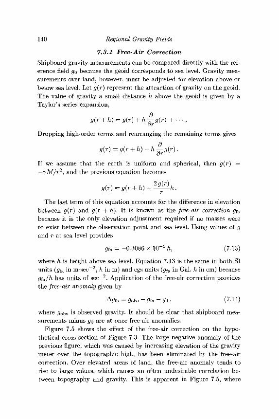
140 Regional Gravity Fields
7.3.1 Free-Air CorrectionShipboard gravity measurements can be compared directly with the ref-erence field go because the geoid corresponds to sea level. Gravity mea-surements over land, however, must be adjusted for elevation above orbelow sea level. Let g(r) represent the attraction of gravity on the geoid.The value of gravity a small distance h above the geoid is given by aTaylor's series expansion,
g(r + h) = g{r) + h —g(r) + • • • .
Dropping high-order terms and rearranging the remaining terms gives
g(r) =g(r + h)-h 7 ^ # 0 ) •
If we assume that the earth is uniform and spherical, then g(r) =—'jM/r2, and the previous equation becomes
The last term of this equation accounts for the difference in elevationbetween g(r) and g(r -\- h). It is known as the free-air correction #fabecause it is the only elevation adjustment required if no masses wereto exist between the observation point and sea level. Using values of gand r at sea level provides
0fa = -0.3086 x 10~5 h, (7.13)
where h is height above sea level. Equation 7.13 is the same in both SIunits (#fa in m-sec~2, h in m) and cgs units (#fa in Gal, h in cm) becausegfa/h has units of sec"2. Application of the free-air correction providesthe free-air anomaly given by
A#fa = gobs ~ #fa - £o , (7.14)
where gobs is observed gravity. It should be clear that shipboard mea-surements minus go are at once free-air anomalies.
Figure 7.5 shows the effect of the free-air correction on the hypo-thetical cross section of Figure 7.3. The large negative anomaly of theprevious figure, which was caused by increasing elevation of the gravitymeter over the topographic high, has been eliminated by the free-aircorrection. Over elevated areas of land, the free-air anomaly tends torise to large values, which causes an often undesirable correlation be-tween topography and gravity. This is apparent in Figure 7.5, where
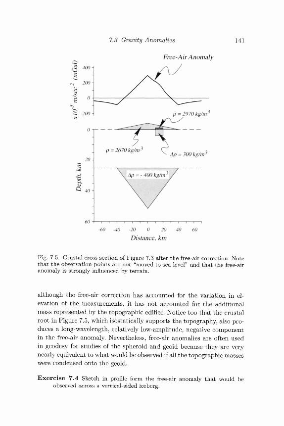
7.3 Gravity Anomalies
Free-Air Anomaly
141
-60 -20 0 20
Distance, km60
Fig. 7.5. Crustal cross section of Figure 7.3 after the free-air correction. Notethat the observation points are not "moved to sea level" and that the free-airanomaly is strongly influenced by terrain.
although the free-air correction has accounted for the variation in el-evation of the measurements, it has not accounted for the additionalmass represented by the topographic edifice. Notice too that the crustalroot in Figure 7.5, which isostatically supports the topography, also pro-duces a long-wavelength, relatively low-amplitude, negative componentin the free-air anomaly. Nevertheless, free-air anomalies are often usedin geodesy for studies of the spheroid and geoid because they are verynearly equivalent to what would be observed if all the topographic masseswere condensed onto the geoid.
Exercise 7.4 Sketch in profile form the free-air anomaly that would beobserved across a vertical-sided iceberg.
142 Regional Gravity Fields
The free-air correction is sometimes referred to as moving the obser-vation point to sea level, but this description is misleading. More ac-curately, the free-air correction adjusts measured gravity for one factornot accounted for by the reference ellipsoid: the elevation of the gravitymeasurement above the reference ellipsoid. Although the free-air correc-tion accounts for the elevation of the observation point, the observationpoint still remains fixed in space with respect to all causative masses(Figure 7.5).
7.3.2 Tidal CorrectionEarth-tides caused by the sun and moon are of sufficient amplitude tobe detected by gravity meters as time-varying gravity. The effect is bothtime- and latitude-dependent; it is greatest at low latitudes and has astrong periodic component with period on the order of 12 hours. Thetidal effect never exceeds 3 x 10~6 m-sec~2 (0.3 mGal), a small quantityin comparison to other corrections to observed gravity. Nevertheless,tidal effects should be accounted for in high-precision surveys. Formulasexist to calculate the tidal effect at any time and at any place on theearth's surface (Longman [166]).
It may be appropriate in less precise surveys to assume that the tidaleffect is linear over periods of several hours and to remove the tidaleffect along with other temporal adjustments. For example, most grav-ity meters used in gravity surveys produce readings that drift slightlyover the course of a day's fieldwork. This problem usually is treated byreoccupying certain observation points at various times during the day,assuming that drift has been linear between the repeated measurements,and subtracting the linear drift from all other readings. The tidal effectcan be considered part of the instrumental drift.
7.3.3 Eotvos CorrectionAs discussed in Section 7.2, the attraction of the earth at a point fixedwith respect to the earth is reduced by the centrifugal force related tothe earth's rotation. It stands to reason that the angular velocity of anobserver moving east is greater than for an observer remaining station-ary with respect to the earth's surface, and consequently gravitationalattraction will be slightly reduced for the moving observer. Likewise,gravitational attraction will be slightly increased for an observer mov-ing in a westerly direction. This motion-related effect, called the Eotvos
7.3 Gravity Anomalies 143
effect, must be accounted for in gravity measurements made on movingplatforms, such as ships or aircraft. The Eotvos correction is given by
gE = 7.503 v cos A sin a + 0.004154 v2 ,
where v is in knots, a is heading with respect to true north, A is latitude,and g^ is in mGal.Exercise 7.5 Derive the Eotvos correction starting with equation 7.1.
The Eotvos correction can reach significant magnitudes in applica-tions involving moving platforms. For example, the Eotvos correction is5.4xlO~5 m-sec~2 (5.4 mGal) for gravity measurements made on a shipat latitude 45°N heading easterly at 1 knot. Errors in heading or veloc-ity, therefore, can produce errors in reduced gravity measurements thatare similar in magnitude to anomalies caused by typical crustal sources.Indeed, the Eotvos correction is often the limiting factor in the precisionof shipborne and airborne surveys.
7.3.4 Bouguer CorrectionThe free-air correction and theoretical gravity ignore mass that may ex-ist between the level of observation and sea level. The Bouguer correc-tion accounts for this additional mass. The simple Bouguer correctionapproximates all mass above sea level with a homogeneous, infinitelyextended slab of thickness equal to the height of the observation pointabove sea level (Figure 7.6). The attraction of an infinite slab is describedby equation 3.27,
gsh = 27r-yph,
where h is the thickness of the slab. Using a typical crustal density of2670 kg-m~3, the simple Bouguer correction becomes
gsh = 0.1119 x 10~5/i, (7.15)
for both SI units (#sb in m-sec~2, h in m) and cgs units (gsh in Gal, hin cm), where h is height above sea level. Therefore, ignoring tidal andEotvos corrections, the simple Bouguer anomaly is given by
A#sb = #obs - 0fa - 9sb - 90 . (7.16)
For gravity measurements over water, the Bouguer correction amountsto replacing the water (density = 1000 kg-m~3) with a slab of density2670 kg-m~3 and thickness equal to bathymetric depth. Hence, the sign
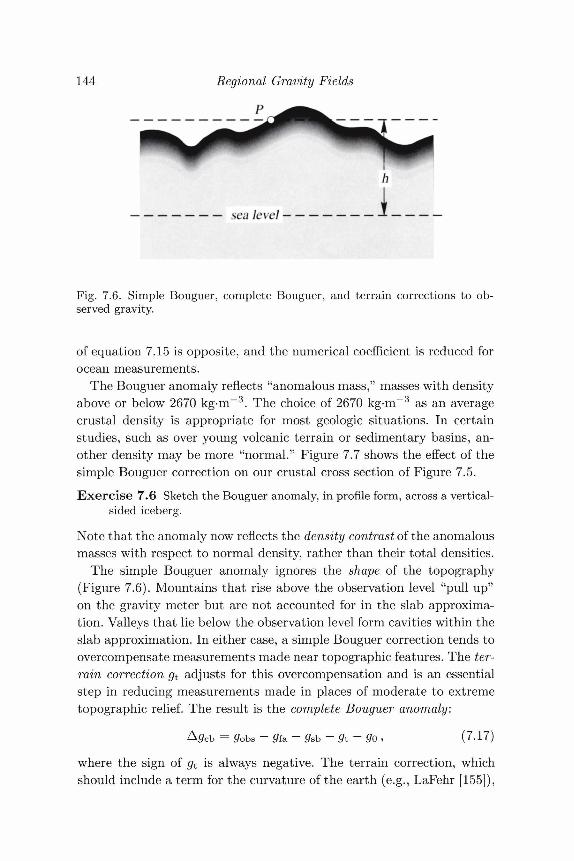
144 Regional Gravity Fields
P
Fig. 7.6. Simple Bouguer, complete Bouguer, and terrain corrections to ob-served gravity.
of equation 7.15 is opposite, and the numerical coefficient is reduced forocean measurements.
The Bouguer anomaly reflects "anomalous mass," masses with densityabove or below 2670 kg-m~3. The choice of 2670 kg-m~3 as an averagecrustal density is appropriate for most geologic situations. In certainstudies, such as over young volcanic terrain or sedimentary basins, an-other density may be more "normal." Figure 7.7 shows the effect of thesimple Bouguer correction on our crustal cross section of Figure 7.5.
Exercise 7.6 Sketch the Bouguer anomaly, in profile form, across a vertical-sided iceberg.
Note that the anomaly now reflects the density contrast of the anomalousmasses with respect to normal density, rather than their total densities.
The simple Bouguer anomaly ignores the shape of the topography(Figure 7.6). Mountains that rise above the observation level "pull up"on the gravity meter but are not accounted for in the slab approxima-tion. Valleys that lie below the observation level form cavities within theslab approximation. In either case, a simple Bouguer correction tends toovercompensate measurements made near topographic features. The ter-rain correction gt adjusts for this overcompensation and is an essentialstep in reducing measurements made in places of moderate to extremetopographic relief. The result is the complete Bouguer anomaly:
A # c b = gobs — <7fa — 9sb — 9t — go , (7.17)
where the sign of gt is always negative. The terrain correction, whichshould include a term for the curvature of the earth (e.g., LaFehr [155]),
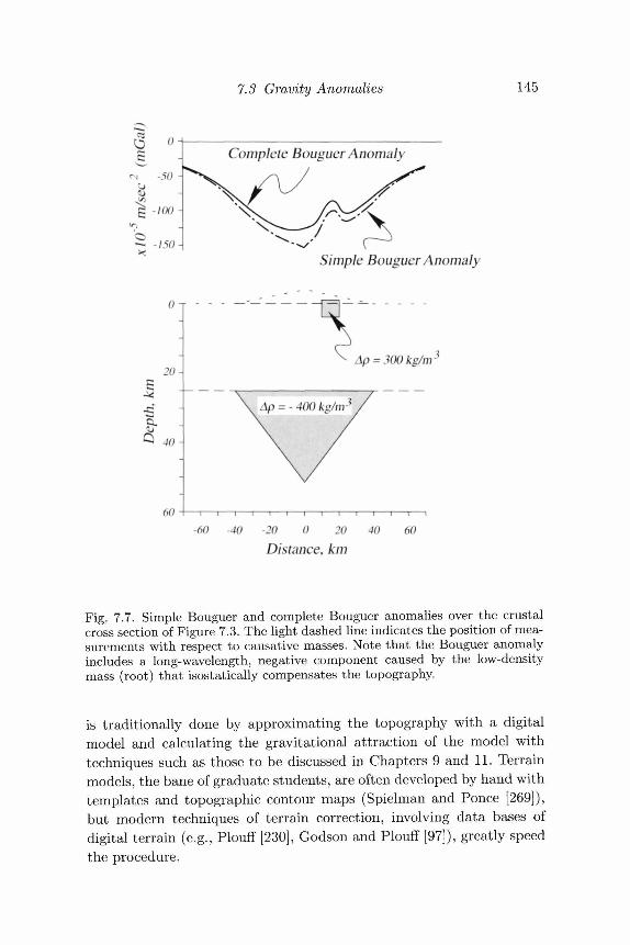
7.3 Gravity Anomalies 145
3
r i
>
11/*-..01
• <
-50
-100
-150
Complete Bouguer Anomaly
Simple Bouguer Anomaly
0 -_-
20-
f 40 A
60
= 300kg/m-i
-60 -40 -20 0 20Distance, km
60
Fig. 7.7. Simple Bouguer and complete Bouguer anomalies over the crustalcross section of Figure 7.3. The light dashed line indicates the position of mea-surements with respect to causative masses. Note that the Bouguer anomalyincludes a long-wavelength, negative component caused by the low-densitymass (root) that isostatically compensates the topography.
is traditionally done by approximating the topography with a digitalmodel and calculating the gravitational attraction of the model withtechniques such as those to be discussed in Chapters 9 and 11. Terrainmodels, the bane of graduate students, are often developed by hand withtemplates and topographic contour maps (Spielman and Ponce [269]),but modern techniques of terrain correction, involving data bases ofdigital terrain (e.g., Plouff [230], Godson and Plouff [97]), greatly speedthe procedure.
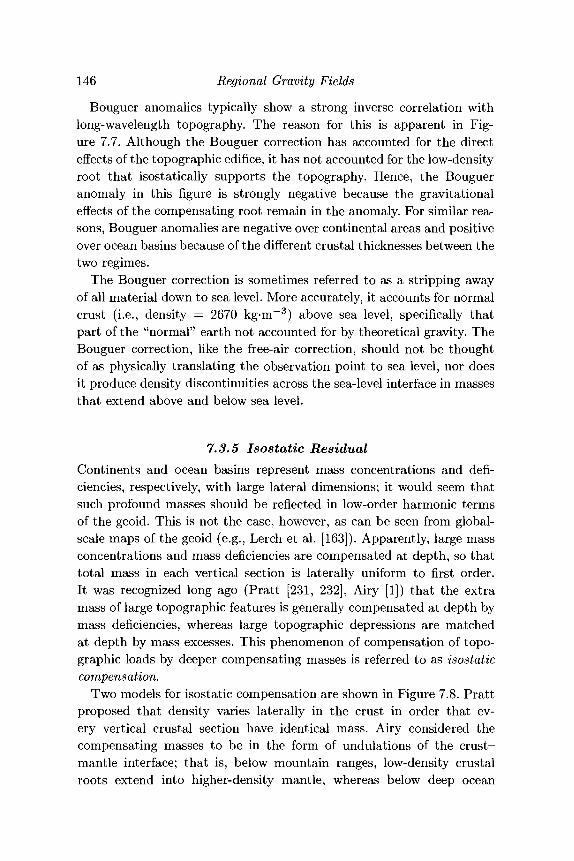
146 Regional Gravity Fields
Bouguer anomalies typically show a strong inverse correlation withlong-wavelength topography. The reason for this is apparent in Fig-ure 7.7. Although the Bouguer correction has accounted for the directeffects of the topographic edifice, it has not accounted for the low-densityroot that isostatically supports the topography. Hence, the Bougueranomaly in this figure is strongly negative because the gravitationaleffects of the compensating root remain in the anomaly. For similar rea-sons, Bouguer anomalies are negative over continental areas and positiveover ocean basins because of the different crustal thicknesses between thetwo regimes.
The Bouguer correction is sometimes referred to as a stripping awayof all material down to sea level. More accurately, it accounts for normalcrust (i.e., density = 2670 kg-m~3) above sea level, specifically thatpart of the "normal" earth not accounted for by theoretical gravity. TheBouguer correction, like the free-air correction, should not be thoughtof as physically translating the observation point to sea level, nor doesit produce density discontinuities across the sea-level interface in massesthat extend above and below sea level.
7.3.5 Isostatic ResidualContinents and ocean basins represent mass concentrations and defi-ciencies, respectively, with large lateral dimensions; it would seem thatsuch profound masses should be reflected in low-order harmonic termsof the geoid. This is not the case, however, as can be seen from global-scale maps of the geoid (e.g., Lerch et al. [163]). Apparently, large massconcentrations and mass deficiencies are compensated at depth, so thattotal mass in each vertical section is laterally uniform to first order.It was recognized long ago (Pratt [231, 232], Airy [1]) that the extramass of large topographic features is generally compensated at depth bymass deficiencies, whereas large topographic depressions are matchedat depth by mass excesses. This phenomenon of compensation of topo-graphic loads by deeper compensating masses is referred to as isostaticcompensation.
Two models for isostatic compensation are shown in Figure 7.8. Prattproposed that density varies laterally in the crust in order that ev-ery vertical crustal section have identical mass. Airy considered thecompensating masses to be in the form of undulations of the crust-mantle interface; that is, below mountain ranges, low-density crustalroots extend into higher-density mantle, whereas below deep ocean
7.3 Gravity Anomalies 147
(a) (b) C^ Sen Level
Compensation Level
Fig. 7.8. Two early models for isostatic compensation of topographic loads.(a) Airy [1]; (b) Pratt [231].
basins, high-density mantle warps upward into the lower-density crust.The truth undoubtedly is more complicated than either of these models,and the mechanism varies from place to place depending on the geo-logical setting. In any case, the anomalies caused by the compensatingmasses are generally long in wavelength and approximately negativelycorrelated with long-wavelength attributes of topography (Figure 7.7).
It is sometimes desirable to remove from gravity measurements thelong-wavelength gravitational effects of compensating masses. Forexample, studies of crustal geology in mountainous terrain (e.g., Jachensand Griscom [136]) typically are concerned with lateral variations ofcrustal density rather than deep-crustal and upper-mantle sources thatisostatically support the topography. Given a digital terrain model, it isa relatively straightforward procedure to (1) calculate the shape of thecrust-mantle interface consistent with the Airy model for isostatic com-pensation and (2) calculate at each observation point the gravitationaleffect of the volume (Jachens and Roberts [138], Simpson, Jachens, andBlakely [260]). According to the Airy model of isostatic compensation,the total mass must be equal for all columns extending from the earth'ssurface to some depth of compensation. Consider the two columns inFigure 7.9. The mass in column 1 is proportional to dspc + (dm — ds)pm,where ds is the depth of compensation at shorelines, dm is the depthbelow sea level of the compensating root, pc is crustal density, and pm
is mantle density. The mass in column 2 is proportional to hpt + dmpc,where pt is the average density of rocks that make up the terrain, andh is elevation of the observation point above sea level. Equating the twomass columns provides
dm = h-g- + dB, (7.18)
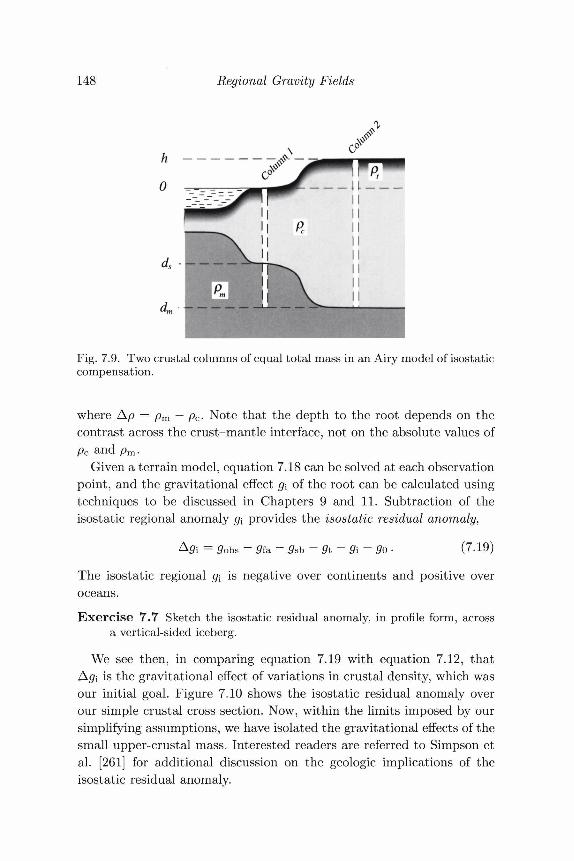
148 Regional Gravity Fields
Fig. 7.9. Two crustal columns of equal total mass in an Airy model of isostaticcompensation.
where Ap = pm — pc. Note that the depth to the root depends on thecontrast across the crust-mantle interface, not on the absolute values ofpc and pm.
Given a terrain model, equation 7.18 can be solved at each observationpoint, and the gravitational effect gx of the root can be calculated usingtechniques to be discussed in Chapters 9 and 11. Subtraction of theisostatic regional anomaly g\ provides the isostatic residual anomaly,
= gobs - £fa ~ - 9t - 9i - 9o (7.19)
The isostatic regional g\ is negative over continents and positive overoceans.Exercise 7.7 Sketch the isostatic residual anomaly, in profile form, across
a vertical-sided iceberg.
We see then, in comparing equation 7.19 with equation 7.12, thatAgx is the gravitational effect of variations in crustal density, which wasour initial goal. Figure 7.10 shows the isostatic residual anomaly overour simple crustal cross section. Now, within the limits imposed by oursimplifying assumptions, we have isolated the gravitational effects of thesmall upper-crustal mass. Interested readers are referred to Simpson etal. [261] for additional discussion on the geologic implications of theisostatic residual anomaly.
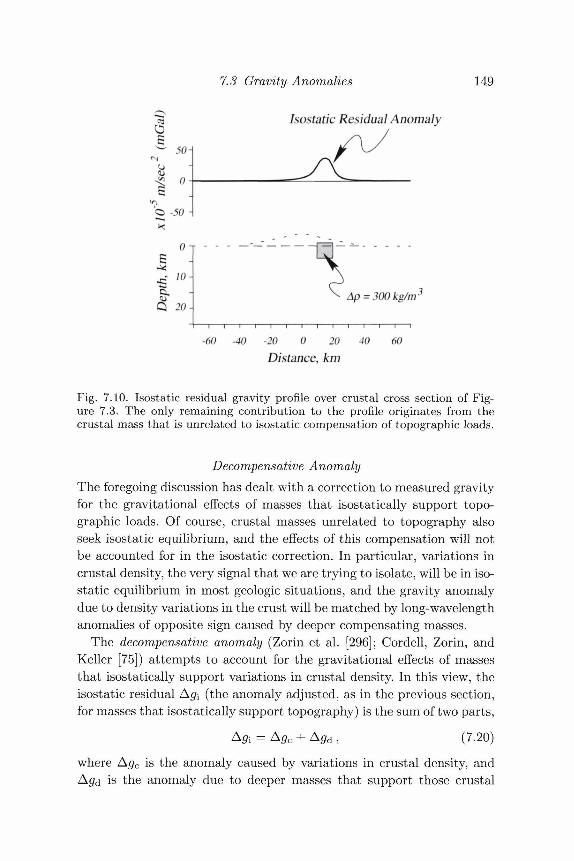
7.3 Gravity Anomalies 149
I o--50 H
Isostatic Residual Anomaly
tQ 20-
-40 -20 0 20
Distance, km40 60
Fig. 7.10. Isostatic residual gravity profile over crustal cross section of Fig-ure 7.3. The only remaining contribution to the profile originates from thecrustal mass that is unrelated to isostatic compensation of topographic loads.
Decompensative AnomalyThe foregoing discussion has dealt with a correction to measured gravityfor the gravitational effects of masses that isostatically support topo-graphic loads. Of course, crustal masses unrelated to topography alsoseek isostatic equilibrium, and the effects of this compensation will notbe accounted for in the isostatic correction. In particular, variations incrustal density, the very signal that we are trying to isolate, will be in iso-static equilibrium in most geologic situations, and the gravity anomalydue to density variations in the crust will be matched by long-wavelengthanomalies of opposite sign caused by deeper compensating masses.
The decompensative anomaly (Zorin et al. [296]; Cordell, Zorin, andKeller [75]) attempts to account for the gravitational effects of massesthat isostatically support variations in crustal density. In this view, theisostatic residual A#i (the anomaly adjusted, as in the previous section,for masses that isostatically support topography) is the sum of two parts,
?i = Agc (7.20)
where Agc is the anomaly caused by variations in crustal density, andis the anomaly due to deeper masses that support those crustal
150 Regional Gravity Fields
variations. The desired quantity is Agc, referred to as the decompen-sative anomaly. Zorin et al. [296] and Cordell et al. [75] assumed a verysimple model for the process of compensation in order to solve for Agc
from A^: Every mass excess or deficiency in the crust is underlain atdepth z by an identical mass of opposing sign. As the effects of thecompensating masses are long in wavelength, the unrealistic nature ofthis model should not greatly affect the end result (Cordell et al. [75]).Hence, Ag^ observed at the level of the gravity survey, is identical, apartfrom sign, to the anomaly due to crust al density variations observed ata height z above the gravity survey. In other words, A (fa is the negativeof Agc continued upward to a height z and, as discussed in Section 2.3.2,can be calculated from Agc without detailed knowledge of the sourcesof Agc or Agd.
We will investigate upward continuation in more detail in Chapter 12,but here anticipate one result: With the simple model for compensationdescribed previously, Agc can be continued upward a distance z simplyby multiplying the Fourier transform of Agc by the function e~^z, where|fc| is inversely proportional to wavelength. Denoting Fourier transfor-mation of a function f(x,y) by the symbol .F[/], equation 7.20 can bewritten as
and the desired quantity Agc is given in the Fourier domain by
(Cordell et al. [75]). Consequently, given an assumed value for z, thedecompensative anomaly Agc can be found directly from the isostaticanomaly Ag[ by Fourier transforming A#i, multiplying by (1 — e~^z)~1,and inverse Fourier transforming the product.
7.4 An ExampleFigure 7.11 compares the free-air, simple Bouguer, complete Bouguer,and isostatic residual anomalies over parts of the Klamath Mountainsand Cascade Range in north-central California. The pre-Cenozoic sed-imentary and volcanic rocks of the Klamath Mountains are generallymore dense than the Tertiary and Quaternary volcanic rocks related tothe Cascade arc. The Trinity ultramafic sheet, the largest ultramafic
74 An Example 151
body in North America, lies in this part of the Klamath Mountains. Ad-ditional information regarding the geophysical setting of this area wasprovided by Griscom [105], LaFehr [153], and Blakely and Jachens [30].
Figure 7.11 illustrates the following:
1. Free-air anomalies (Figure 7.11(c)) are strongly correlated with ter-rain (Figure 7.11(b)). This correlation is particularly apparent overMount Shasta, Medicine Lake Volcano, and the Klamath Mountains.
2. Simple and complete Bouguer anomalies (Figures 7.11(d) and 7.11(e))over continental areas are strongly negative. This happens becausethe Bouguer correction has removed the effects of normal crust abovesea level but has left the effects of deeper masses that isostaticallysupport that crust.
3. Simple and complete Bouguer anomalies have regional-scale compo-nents that are approximately inversely correlated with very long-wavelength attributes of the terrain. In Figure 7.11(e), this regionalcomponent appears as a broad trend decreasing from west to east.The regional trend in Bouguer gravity is caused by an increase fromwest to east in the amount of deep, low-density material that supportsthe topography. In terms of the Airy model for isostatic compensa-tion, the trend in Bouguer gravity is caused by a low-density rootthat thickens from west to east in order to support the continentaledifice, although in actuality the support may be distributed in otherways; for example, through variable densities in the upper mantle.
4. The simple Bouguer map includes short-wavelength anomalies re-lated to topography, whereas these effects are largely missing fromthe complete Bouguer map, which included a terrain correction. Thelarge-amplitude negative anomaly directly over Mount Shasta on Fig-ure 7.11(d) is the best example.
5. The isostatic residual anomaly (Figure 7.11(f)) most closely repre-sents lateral variations in density of the middle and upper crust. Itclearly shows, for example, the high-density Trinity ultramafic bodyand where it lies below pre-Cenozoic rocks of the Klamath Moun-tains (Griscom [105]). Low-density rocks of the Cascade Range arealso apparent in the central and eastern parts of the map. The neg-ative anomaly over and extending northeast from Mount Shasta isthought to be caused by low-density volcanic rocks (LaFehr [153];Blakely and Jachens [30]).
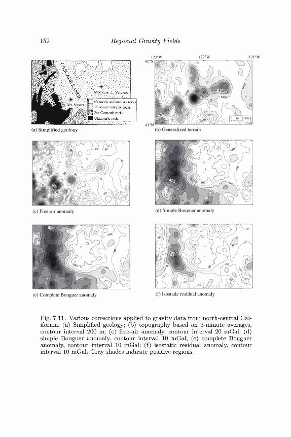
152 Regional Gravity Fields
|22°W
is :^," Medicine L. Volcano
| | Cenozoic sedimentary rocks
0J Cenozoic volcanic rocks| Pre-Cenozoic rocks| Ultramafic rocks
(a) Simplified geology
I21°W
(b) Generalized terrain
(c) Free-air anomaly (d) Simple Bouguer anomaly
(e) Complete Bouguer anomaly (0 Isostatic residual anomaly
Fig. 7.11. Various corrections applied to gravity data from north-central Cal-ifornia, (a) Simplified geology; (b) topography based on 5-minute averages,contour interval 200 m; (c) free-air anomaly, contour interval 20 mGal; (d)simple Bouguer anomaly, contour interval 10 mGal; (e) complete Bougueranomaly, contour interval 10 mGal; (f) isostatic residual anomaly, contourinterval 10 mGal. Gray shades indicate positive regions.
7.5 Problem Set 153
7.5 Problem Set1. Imagine that you are chief science officer on a mission to investigate
a newly discovered planet. Your spaceship is located in the plane ofthe planet's rotation at a distance r from the planet's center and adistance h from the planet's surface. Your spaceship is stationary withrespect to the planet's rotation and is experiencing a gravitationalattraction of G. Your sensors tell you that the planet is rotating withan angular velocity of a;, has the shape of an oblate spheroid withflattening / , and has dynamical properties much like Earth. Twolanding parties are being sent to the planet: one to the equator andone to the north pole. The captain wants to know how much the forceof gravity will differ between the two landing sites and is willing toaccept some simplifying assumptions. What can you advise? Expressyour answer in terms of a, / , r, /i, a;, and G.
2. Suppose that the earth begins to rotate more and more rapidly untilthe gravity experienced by an observer at the equator falls to zero.How long is the length of a day?
3. Show that to first order f + f = §ra. Note: This result is moreimportant than it may seem; it shows that the geometrical shape ofthe ellipsoid can be determined from gravity measurements alone.
4. A sphere of density 3.17 g-cm"3 and radius 5 km is partially buriedin a flat prairie so that the summit of the sphere is 2 km abovethe surrounding prairie. The prairie is 2 km above sea level. Assumecrustal density is 2.67 g-cm~3 and use the Geodetic Reference System1967 to sketch the following profiles (show appropriate shapes andamplitudes) as observed along a traverse directly over the center ofthe sphere:(a) observed gravity,(b) free-air anomaly,(c) Bouguer anomaly,(d) isostatic residual anomaly.
5. Explain why the following statement is wrong: "The isostatic residualanomaly is always zero over perfectly compensated topography."
6. The mass in Figure 7.10 is not isostatically compensated. What wouldthe profile look like if it were?
8The Geomagnetic Field
Magnus magnes ipse est globus terrestris.[The whole earth is a magnet.]
(William Gilbert)
It has always been and still is [my] impression thata magnetometer survey is just as much a means ofmapping geology as are the air photograph and thesurface geological traverse.
(Norman R. Pater son)
The previous chapter discussed the steps by which gravity measurementsare converted into gravity anomalies that reflect geological sources. Thepresent chapter treats magnetic anomalies in a similar vein. Whereas thegravity field of the earth is largely time invariant, except for relativelyminor or long-term changes due to redistribution of mass (tides, mov-ing magma, glacial rebound, erosion, mountain building, and so forth),the geomagnetic field varies in both direction and intensity over timescales ranging from milliseconds to millennia. It would seem that thisadded complexity would make the reduction of magnetic measurementssignificantly more difficult than that for gravity data, but in practice thecalculation of magnetic anomalies is relatively straightforward.
Our intent in this chapter is to characterize the global magnetic fieldin order to isolate the magnetic field caused by crustal sources. Thisagenda glosses over a large body of information that ordinarily wouldbe included in a chapter of this title, such topics as the origins of thegeomagnetic field (magnetohydrodynamic theories); the behavior of thefield in the geologic past (paleomagnetic studies); reversals of geomag-netic polarity; the magnetic properties of the sun, moon, meteorites,and other planets; and the interaction of the earth's magnetic field withsolar phenomena. Other textbooks are dedicated to just these topics,
154
8.1 Parts of Internal and External Origin 155
and readers are referred in particular to books by Merrill and McEl-hinny [183], Jacobs [139], Butler [47], Parkinson [211], and Chapmanand Bartels [56] for more comprehensive discussions.
We begin this chapter with a general discussion of dividing potentialfields measured on a sphere into parts originating from inside and outsidethe sphere. Later sections of this chapter will use spherical harmonicanalysis to describe the internal geomagnetic field.
8.1 Parts of Internal and External OriginSpherical harmonic analysis provides the means with which to determinefrom measurements of a potential field and its gradients on a spherewhether the sources of the field lie within or outside the sphere. CarlFriederich Gauss in 1838 was the first to describe the geomagnetic fieldin this way, and he came to the conclusion that the field observed at theearth's surface originates entirely from within the earth. We know now,with the benefit of satellites, space probes, and vastly more data, that hewas only approximately correct; that is, a small part of the geomagneticfield originates from outside the earth. In this section, we investigate thegeneral problem of separating a potential field into parts of external andinternal origin, following the development of Chapman and Bartels [56].We use magnetic induction in this derivation, but the discussion appliesto any potential field.
Consider the magnetic induction B and its potential V, where B =—VV, and suppose that we have the ability to measure V or any com-ponent of B on a spherical surface with radius a. Assume further thatin source-free regions V is harmonic and satisfies Laplace's equation,
Specifically, V is harmonic on the surface of the sphere so long as sourcesof V do not extend across the surface. If no sources exist outside thesphere, then both V and ^ must vanish as r —> oo, and V can berepresented by a spherical harmonic expansion similar to equation 6.31,
oo , -. n(^) '%2(A™coBm<l> + B™i8him<t>)PZt(0), r > a ,
n=0 ra=0(8.1)
where 0 is colatitude, cj> is longitude, and P™{0) is an associated Le-gendre polynomial of degree n and order m normalized according to the
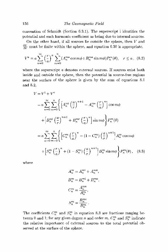
156 The Geomagnetic Field
convention of Schmidt (Section 6.3.1). The superscript i identifies thepotential and each harmonic coefficient as being due to internal sources.
On the other hand, if all sources lie outside the sphere, then V and^ must be finite within the sphere, and equation 6.30 is appropriate,
( ) J^(A™e cosm(f)+B™e sinm(t))P™(0), r<a, (8 .2 )
where the superscript e denotes external sources. If sources exist bothinside and outside the sphere, then the potential in source-free regionsnear the surface of the sphere is given by the sum of equations 8.1and 8.2,
V = V1 + Ve
i, (8.3)L \ a / \ / • / J I
where
s~im
The coefficients C™ and S™ in equation 8.3 are fractions ranging be-tween 0 and 1; for any given degree n and order ra, C™ and S™ indicatethe relative importance of external sources to the total potential ob-served at the surface of the sphere.
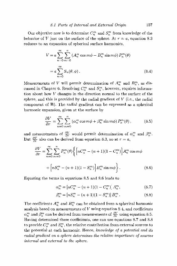
8.1 Parts of Internal and External Origin 157
Our objective now is to determine C™ and S™ from knowledge of thebehavior of V just on the surface of the sphere. At r = a, equation 8.3reduces to an expansion of spherical surface harmonics,
n=0ra=0
n=0
Measurements of V will permit determination of A™ and B™, as dis-cussed in Chapter 6. Resolving C™ and S™, however, requires informa-tion about how V changes in the direction normal to the surface of thesphere, and this is provided by the radial gradient of V (i.e., the radialcomponent of B). The radial gradient can be expressed as a sphericalharmonic expansion, given at the surface by
BV °° n
-?T- = W (<C cosra0 + /?™ sinra</>) P^(l9), (8.5)n=0m=0
and measurements of ^ would permit determination of a™ and /J^1.But ^ also can be derived from equation 8.3, so at r = a,
O T A oo n
n=0m—0
(8.6)
Equating the terms in equations 8.5 and 8.6 leads to
(8.7)
(8.8)
The coefficients A™ and 5 ^ can be obtained from a spherical harmonicanalysis based on measurements of V using equation 8.4, and coefficientsa™ and (3™ can be derived from measurements of using equation 8.5.Having determined these coefficients, one can use equations 8.7 and 8.8to provide C™ and S^\ the relative contribution from external sources tothe potential at each harmonic. Hence, knowledge of a potential and itsradial gradient on a sphere determines the relative importance of sourcesinternal and external to the sphere.
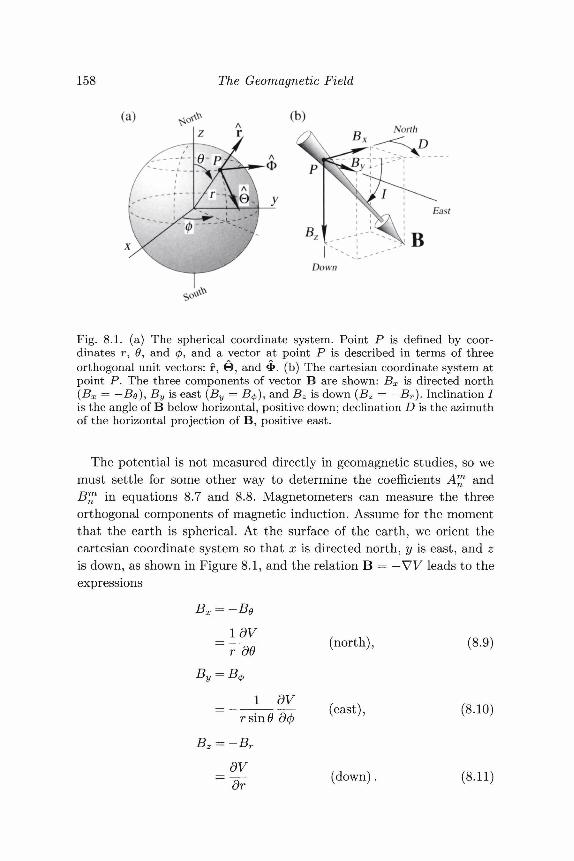
158 The Geomagnetic Field
(b)North
Fig. 8.1. (a) The spherical coordinate system. Point P is defined by coor-dinates r, 0, and <j), and a vector at point P is described in terms of threeorthogonal unit vectors: f, 0 , and ^ . (b) The cartesian coordinate system atpoint P. The three components of vector B are shown: Bx is directed north(Bx = —Be), By is east (By = B^), and Bz is down (Bz = — Br). Inclination /is the angle of B below horizontal, positive down; declination D is the azimuthof the horizontal projection of B, positive east.
The potential is not measured directly in geomagnetic studies, so wemust settle for some other way to determine the coefficients A™ andB™ in equations 8.7 and 8.8. Magnetometers can measure the threeorthogonal components of magnetic induction. Assume for the momentthat the earth is spherical. At the surface of the earth, we orient thecartesian coordinate system so that x is directed north, y is east, and zis down, as shown in Figure 8.1, and the relation B = — \7V leads to theexpressions
Bx = —Be
_ ldV~r~dO (north), (8.9)
1 dVrsinO
Bz = -Br
_dv_~ dr
—- (east),
(down).
(8.10)
(8.11)
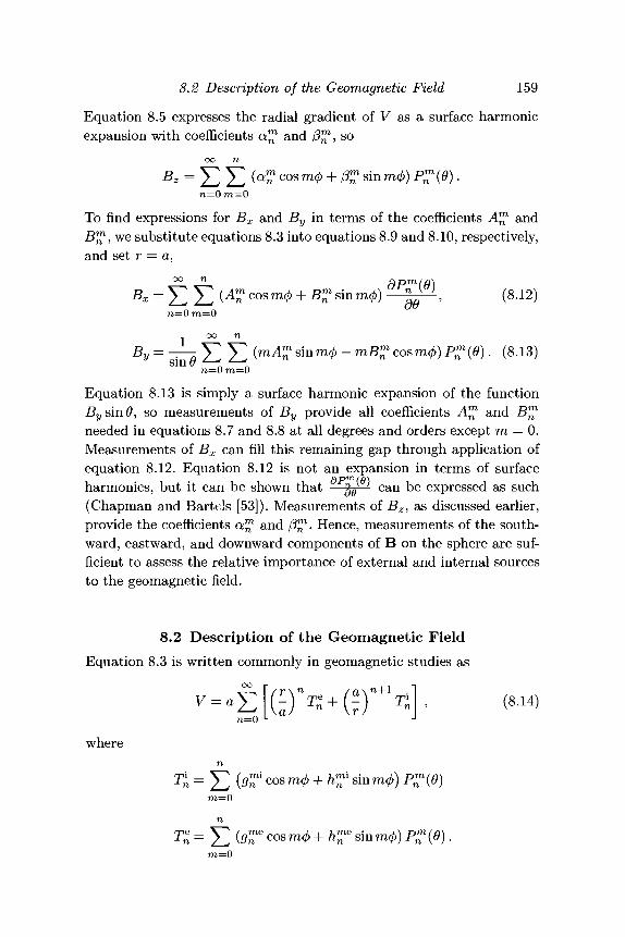
8.2 Description of the Geomagnetic Field 159
Equation 8.5 expresses the radial gradient of V as a surface harmonicexpansion with coefficients a™ and /3™, so
Pn sin m<t>) P™{6).n=0m=0
To find expressions for Bx and By in terms of the coefficients A™ andB™, we substitute equations 8.3 into equations 8.9 and 8.10, respectively,and set r = a,
Bx = Y,I2(An c°s m4> + B™ sin m<t>) —gAJ, (8.12)n=0ra=0
^1 sinra</> - mB™ cosrn^) P^(6>). (8.13)5 y =n=0 m=0
Equation 8.13 is simply a surface harmonic expansion of the functioni^sinfl, so measurements of By provide all coefficients A™ and B™needed in equations 8.7 and 8.8 at all degrees and orders except m — 0.Measurements of Bx can fill this remaining gap through application ofequation 8.12. Equation 8.12 is not an expansion in terms of surfaceharmonics, but it can be shown that —g^^- can be expressed as such(Chapman and Bartels [53]). Measurements of J5Z, as discussed earlier,provide the coefficients a™ and (3™. Hence, measurements of the south-ward, eastward, and downward components of B on the sphere are suf-ficient to assess the relative importance of external and internal sourcesto the geomagnetic field.
8.2 Description of the Geomagnetic FieldEquation 8.3 is written commonly in geomagnetic studies as
wheren
J2 C sin m<t>) P™(9)ra=0
9™ cosm<t> + hT sinm<t>) P™m=0
160 The Geomagnetic Field
The new coefficients g™1, g™Q, h™1, and h™6 are called Gauss coefficients,have the same dimensions as magnetic induction, and generally are ex-pressed in units of nanotesla (or gamma). As before, the superscriptse and i denote either external or internal terms. Gauss coefficients arerelated to the old coefficients (equation 8.3) according to
nm\ /i
9n — U ~ume Qm r>m
Gauss made the first quantitative spherical harmonic analysis of thegeomagnetic field in 1838. He determined the harmonic coefficients frommeasurements of Bx, By, and Bz at a total of only 84 points (spaced 30°apart in the </> direction along seven circles of latitude) and concludedthat the external coefficients g™e and h™e are zero. Now we know thatexternal sources contribute several tens of nT (and often much more) tothe total magnetic field at the earth's surface, and that this contributionis highly variable in both time and space.
The magnetic field originating from inside the earth is approximatelydipolar, as we shall see shortly, and would appear very much like Fig-ure 4.8 if the earth were isolated in space. The earth, however, is con-tinuously bathed by the solar wind, a stream of charged plasma emittedby the sun. The region of interaction between the solar wind and theinternal magnetic field is called the magneto sphere, a region of consid-erably more magnetic complexity than depicted by Figure 4.8. It is thiscomplex interaction between the earth's internal magnetic field and thesolar wind, coupled with the earth's rotation, tidal forces, and thermaleffects, that produces the external magnetic field. The ionosphere, whichsurrounds the earth at altitudes between roughly 50 and 1,500 km, is animportant part of this interaction; the earth's rotation and tidal effectsgenerate electrical currents in the ionosphere, which in turn producemagnetic fields that can reach magnitudes of up to 1,000 nT at theearth's surface.
The details of the origins of the external magnetic field are beyondthe scope of this chapter, and the interested reader is referred to thetext by Merrill and McElhinny [183] for a lucid and concise summary ofthis subject. The following discussion focuses on just the internal partsof the field. For convenience we will drop the superscripts i and e insubsequent spherical harmonic expansions with the understanding thatg™ and h™ pertain to internal sources.
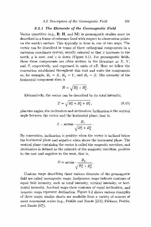
8.2 Description of the Geomagnetic Field 161
8.2.1 The Elements of the Geomagnetic FieldVector quantities (e.g., B, H, and M) in geomagnetic studies must bedescribed in a frame of reference fixed with respect to observation pointson the earth's surface. This typically is done in one of two ways. Thevector can be described in terms of three orthogonal components in acartesian coordinate system, usually oriented so that x increases to thenorth, y is east, and z is down (Figure 8.1). For geomagnetic fields,these three components are often written in the literature as X, Y,and Z, respectively, and expressed in units of nT. Here we follow theconvention established throughout this text and write the componentsas, for example, Bx — X, By = Y, and Bz = Z. The intensity of thehorizontal component then is
H = V / B 1 + B .
Alternatively, the vector can be described by its total intensity,
l + Bl + Bl, (8.15)
plus two angles, the inclination and declination. Inclination is the verticalangle between the vector and the horizontal plane, that is,
BzI = arctan -
By convention, inclination is positive when the vector is inclined belowthe horizontal plane and negative when above the horizontal plane. Thevertical plane containing the vector is called the magnetic meridian, anddeclination is defined as the azimuth of the magnetic meridian, positiveto the east and negative to the west, that is,
RD = arcsin 2 + B2
Contour maps describing these various elements of the geomagneticfield are called isomagnetic maps. Isodynamic maps indicate contours ofequal field intensity, such as total intensity, vertical intensity, or hori-zontal intensity. Isoclinal maps show contours of equal inclination, andisogonic maps represent declination. Figure 8.2 shows various examplesof these maps; similar charts are available from a variety of sources atmore convenient scales (e.g., Peddie and Zunde [215]; Fabiano, Peddie,and Zunde [87]).
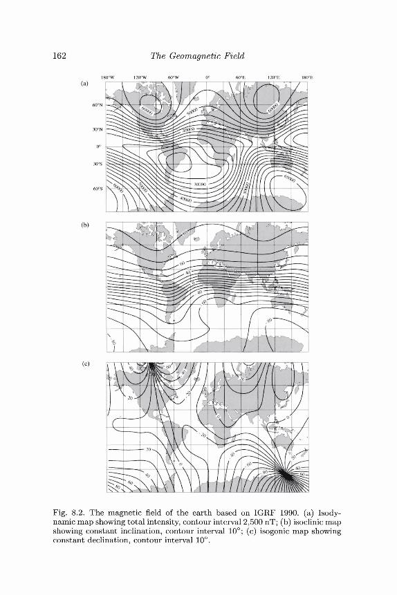
162 The Geomagnetic Field
(a)18O°W 120°W 60° W 60"E I2O°E
(b)
(c)
Fig. 8.2. The magnetic field of the earth based on IGRF 1990. (a) Isody-namic map showing total intensity, contour interval 2,500 nT; (b) isoclinic mapshowing constant inclination, contour interval 10°; (c) isogonic map showingconstant declination, contour interval 10°.
8.2 Description of the Geomagnetic Field 163
The foregoing discussion has assumed that the earth is precisely spher-ical. Actual measurements of Bx, By, and Bz in studies of the maingeomagnetic field, however, are generally oriented instead with respectto a spheroidal model (Langel [157]), and mathematical representationsof the main field, such as those displayed on Figure 8.2, reflect thisspheroidal coordinate system. Changing from a spherical to a spheroidalcoordinate system has no effect on the By component and only a smalleffect on Bx and By, and the discrepancies are often ignored in studiesof crustal magnetization.
8.2.2 The International Geomagnetic Reference FieldLike the reference ellipsoid and theoretical gravity (Section 7.2), themathematical representation of the low-degree parts of the geomag-netic field is determined by international agreement. This mathemat-ical description is called the International Geomagnetic Reference Fieldand is the purview of the International Association of Geomagnetismand Aeronomy (IAGA) and its umbrella organization, the InternationalUnion of Geodesy and Geophysics (IUGG). The IGRF consists of Gausscoefficients through degree and order 10 because, as we will discuss sub-sequently, these low-order terms are believed to represent in large partthe field of the earth's core. Subtracting these low-order terms from mea-sured magnetic fields provides in principle the magnetic field of the crust.As discussed in Section 8.3, however, a 10-degree harmonic expansion isnot sufficient to isolate the crustal field.
The geomagnetic field changes with time, however, and so must itsmathematical description. Because international agreement is not eas-ily achieved on a day-to-day basis, IAGA adopts new IGRF models atfive-year intervals which are intended to represent the geomagnetic fieldfor the following five-year period, called an epoch. To provide this pre-dictive ability, each Gauss coefficient for any particular IGRF modelhas a derivative term that predicts the field into the immediate futureassuming each coefficient changes linearly with time.
Unfortunately the changes in the geomagnetic field are not entirelypredictable, and differences between the predictive IGRF and the truegeomagnetic field begin to grow over the course of each epoch. Thisdivergence is treated in the short term by establishing a new IGRFmodel every five years. In the long term, it is possible to improve oldIGRF models with the benefit of accumulating data. Therefore, IAGA
164 The Geomagnetic Field
periodically adopts models for past epochs, called Definitive Geomag-netic Reference Field (DGRF) models. DGRF models are not estab-lished until it becomes unlikely that the data sets will be significantlyimproved. DGRF models, therefore, become the official record of howthe geomagnetic field has behaved in past epochs. Nine DGRF modelsare in effect at the present: DGRF 1945 through DGRF 1985, each rep-resenting the subsequent five-year epoch. These nine models, along withIGRF 1990 and its predictive terms, give a complete description of thegeomagnetic field from 1945 through 1995. Shortly after 1995, IAGA willadopt a new DGRF 1990, to replace IGRF 1990, and establish a newIGRF 1995 complete with new predictive terms.
Table 8.1 shows the IGRF 1990 model and its predictive terms. Acomplete description of the IGRF has been published in various places(IAGA [134], Langel [157, 160]); these descriptions provide coefficientsfor all DGRF models from 1945 through 1985, list the coefficients andpredictive terms for IGRF 1990, and include a concise discussion of thehistory of the IGRF. Figure 8.2 shows isodynamic, isoclinic, and isogonicmaps based on the IGRF 1990 model.
8.2.3 The Dipole Field
Table 8.2 shows how the first few harmonic terms of the geomagneticfield have changed since the time of Gauss and illustrates some generalcharacteristics of the earth's internal field. Notice that this table hasno #o coefficient because, as discussed in Chapter 6, the zero-degreeharmonic term varies as 1/r (for internal sources) and corresponds tothe potential of a monopole; #§ must vanish, therefore, because magneticmonopoles do not exist. Also notice the overwhelming dominance ofthe first-degree coefficients (#°, g\, and h\). As discussed in Chapter 6and in the following paragraphs, the first-degree harmonic describes thepotential of a dipole centered at the center of the sphere, and the largeamplitudes of these coefficients reflect the generally geocentric dipolarcharacter of the main geomagnetic field. Finally, notice the systematicchange of all coefficients (especially those of higher order) over time since1835. Part of this change is due to improvements in field definition, butmost of the change reflects real temporal variations of the geomagneticfield. We will return to this subject in Section 8.2.5.
We now investigate the n = 1 harmonic term of the geomagnetic field.
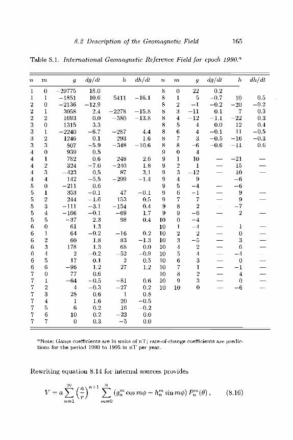
8.2 Description of the Geomagnetic Field 165
Table 8.1. International Geomagnetic Reference Field for epoch 199O.a
n
11222333344444555555666666677777777
m
01012012301234012345012345601234567
-29775-1851-2136305816931315
-22401246807939782324
-423142
-211353244
-111-166-37616460
-178217
-9677
-6442816100
dg/dt
18.010.6
-12.92.40.03.3
-6.70.1
-5.90.50.6
-7.00.5
-5.50.6
-0.1-1.6-3.1-0.12.31.3
-0.21.81.3
-0.20.11.20.6
-0.5-0.30.61.60.20.20.3
h
5411
-2278-380
-287293
-348
248-240
87-299
47153
-154-6998
-168368
-52227
-81-27
12016
-23-5
dh/dt
-16.1
-15.8-13.8
4.41.6
-10.6
2.61.83.1
-1.4
-0.10.50.41.70.4
0.2-1.30.0
-0.90.51.2
0.60.20.8
-0.5-0.20.00.0
n
88888888899999999991010101010101010101010
m
0123456780123456789012345678910
9
225
-1-11-12
443
-64101
-129
-4-172
-6-4-42
-5-2431230
dg/dt
0.2-0.7-0.20.1
-1.10.0
-0.1-0.5-0.6
—————————
——————————
h
10-207
-221211
-16-11
-211510-6-699
-72
1036
-40
-140
-6
dh/dt
0.5-0.20.30.30.4
-0.5-0.30.6
—————————
——————————
aNote: Gauss coefficients are in units of nT; rate-of-change coefficients are predic-tions for the period 1990 to 1995 in nT per year.
Rewriting equation 8.14 for internal sources provides
oo ..I nV = aY,{-y Yl^oosm^ + h^sinm^P^ie), (8.16)
n=l V m=0
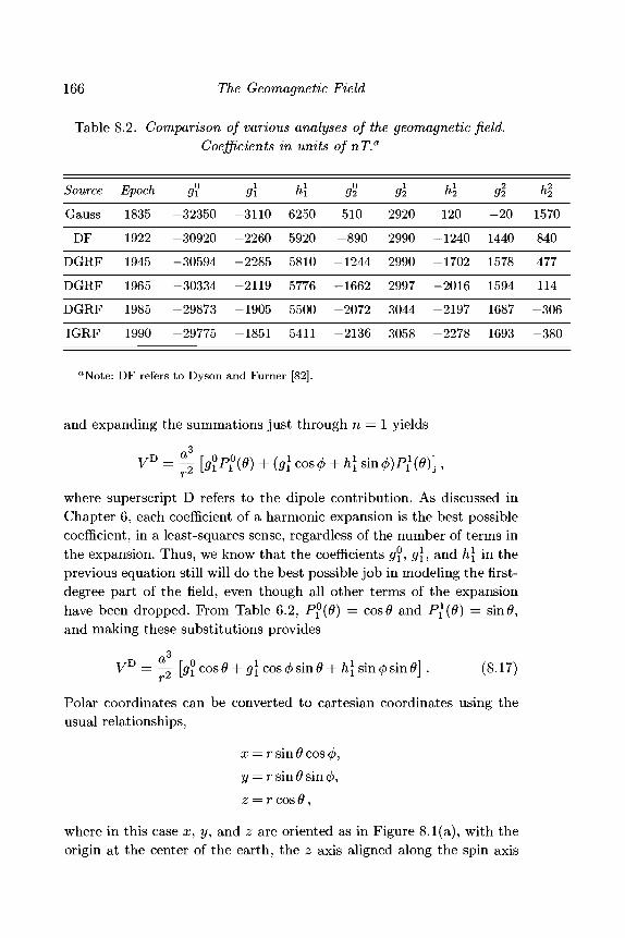
166 The Geomagnetic Field
Table 8.2. Comparison of various analyses of the geomagnetic field.Coefficients in units of nT.a
Source
Gauss
DF
DGRF
DGRF
DGRF
IGRF
Epoch
1835
1922
1945
1965
1985
1990
9°i-32350
-30920
-30594
-30334
-29873
-29775
g\
-3110
-2260
-2285
-2119
-1905
-1851
h\
6250
5920
5810
5776
5500
5411
gl510
-890
-1244
-1662
-2072
-2136
g\
2920
2990
2990
2997
3044
3058
h\
120
-1240
-1702
-2016
-2197
-2278
gl-20
1440
1578
1594
1687
1693
to to
1570
840
477
114
-306
-380
aNote: DF refers to Dyson and Furner [82].
and expanding the summations just through n = 1 yields
^° = 4 [5?Pi°(0) + (9l W + h\ si
where superscript D refers to the dipole contribution. As discussed inChapter 6, each coefficient of a harmonic expansion is the best possiblecoefficient, in a least-squares sense, regardless of the number of terms inthe expansion. Thus, we know that the coefficients gj, g{, and h\ in theprevious equation still will do the best possible job in modeling the first-degree part of the field, even though all other terms of the expansionhave been dropped. From Table 6.2, P?(0) = cos0 and Pf(0) = sin(9,and making these substitutions provides
a3
VB = — [g\ cos 0 + g\ cos 0 sin 0 + h\ sin 0 sin 0] . (8.17)
Polar coordinates can be converted to cartesian coordinates using theusual relationships,
x = r sin 0 cos 0,y = r sin 0 sin 0,z = r cos 0,
where in this case x, y, and z are oriented as in Figure 8.1 (a), with theorigin at the center of the earth, the z axis aligned along the spin axis
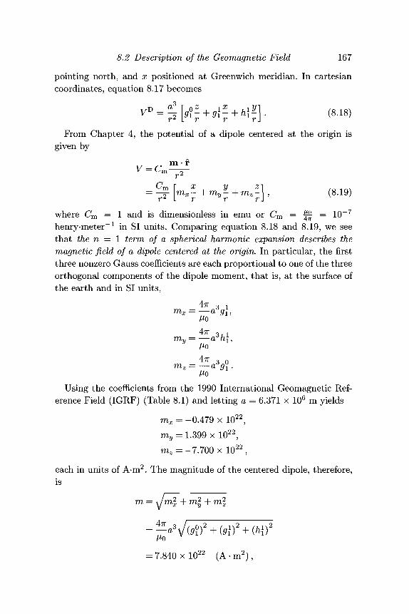
8.2 Description of the Geomagnetic Field 167
pointing north, and x positioned at Greenwich meridian. In cartesiancoordinates, equation 8.17 becomes
From Chapter 4, the potential of a dipole centered at the origin isgiven by
/ , , (8.19)r r r\
where Cm = 1 and is dimensionless in emu or Cm = ^ = 10~7
henry-meter"1 in SI units. Comparing equation 8.18 and 8.19, we seethat the n = 1 term of a spherical harmonic expansion describes themagnetic field of a dipole centered at the origin. In particular, the firstthree nonzero Gauss coefficients are each proportional to one of the threeorthogonal components of the dipole moment, that is, at the surface ofthe earth and in SI units,
4TT O Imx = —a*gi,
Mo4TT 3 7 1
my = —a hi,Mo4TT o nmz = —a6g^ .Mo
Using the coefficients from the 1990 International Geomagnetic Ref-erence Field (IGRF) (Table 8.1) and letting a = 6.371 x 10⁶ m yields
mx = -0.479 x 10²²,my = 1.399 x 10²²,mz = -7.700 x 10²² ,
each in units of A-m2. The magnitude of the centered dipole, therefore,is
+7771+777,2
= 7.840 x 10²² (A • m 2 ) ,
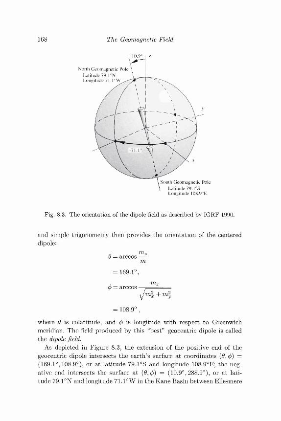
168 The Geomagnetic Field
10.9
North Geomagnetic PoleLatitude 79. ]°NLongitude 71.1°W
South Geomagnetic PoleLatitude 79.1°SLongitude 108.9°E
Fig. 8.3. The orientation of the dipole field as described by IGRF 1990.
and simple trigonometry then provides the orientation of the centereddipole:
9 = arccos —m
= 169.1°,
> — arccosmx
= 108.9° ,
where 0 is colatitude, and 0 is longitude with respect to Greenwichmeridian. The field produced by this "best" geocentric dipole is calledthe dipole field.
As depicted in Figure 8.3, the extension of the positive end of thegeocentric dipole intersects the earth's surface at coordinates (0,0) =(169.1°, 108.9°), or at latitude 79.1°S and longitude 108.9°E; the neg-ative end intersects the surface at (0,0) = (10.9°, 288.9°), or at lati-tude 79.1°N and longitude 71.1°W in the Kane Basin between Ellesmere
8.2 Description of the Geomagnetic Field 169
Island and Greenland. These two points are called the south and northgeomagnetic poles, respectively. The magnetic poles, on the other hand,are the points where the total field is normal to the surface of the earth,that is, the south magnetic pole is that point where the inclinationis —90° and the north magnetic pole is located where the inclinationreaches +90°. If the geomagnetic field were perfectly dipolar (i.e., ifg™ = h™ = 0 for all n > 1), the distinction between geomagnetic polesand magnetic poles would be unnecessary. Table 8.1 shows that the fielddeparts significantly from that of a geocentric dipole, however, and thenorth magnetic pole, as defined by the IGRF 1990 field model, is locatedoff the south coast of Ellef Ringnes Island in the Queen Elizabeth Is-lands, roughly 700 km from the geomagnetic pole. The departure of thegeomagnetic field from that of a geocentric dipole will be the subject ofthe next section.Exercise 8.1 Use Table 8.2 to describe the centered dipole of the earth in
1965. How many degrees did the dipole "rotate" between 1965 and 1980?
The first three nonzero coefficients of the spherical harmonic expan-sion define the single magnetic dipole, centered at the origin, that bestfits the observed magnetic field. A better approximation results if thedipole is not constrained to be at the origin. The overall "best-fit" dipoleis located about 400 km up the positive z axis from the earth's center,and the field that it produces is called the eccentric dipole field.
8.2.4 The Nondipole FieldExcluding the n — 1 harmonic from equation 8.16 eliminates the dipoleterm from the geomagnetic field. The remainder, given by
00 . ., nvN=aJ2(i) E^cosm^ + Csinm^P™^), ( 8 2 0 )
n=2 rn=0
is called the nondipole field. To estimate the relative importance of thenondipole field, consider the vertical component Br as measured at thenorth geographic pole (r = a, 0 — 0°). Differentiating equation 8.16 withrespect to r yields
dVor
00 n+2 n
n = l ra=0
170 The Geomagnetic Field
Now we let r = a and 9 = 0° and note from Table 6.2 that P™(0) = 1if m = 0 and P^(0) = 0 otherwise. Thus the radial component of B atthe north geographic pole is simply
7 1 = 1
Let B^ and B^ represent the radial components of the dipole andnondipole fields, respectively, at the north geographic pole. Then fromTable 8.1,
R D r* 0Br = 2 # 1
= -59,550 (nT),
10
71 = 2
^3,518 (nT),
and the percent provided by the nondipole field to the total vertical fieldat this particular location is
100 x \B?TB?\ = 6-3 (percent) •Though this percentage is of only one component at only one location,it is characteristic of the main field as a whole: The nondipole field com-prises only about 10 percent of the main field, and thus the geomagneticfield is dipolar to a very good first approximation. The spatial characterof the nondipole field is one of large-scale anomalies (Figure 8.4), eightor ten in number, with spatial dimensions comparable to continentalsize (although no correlation is apparent), and with magnitudes on theorder of 104 nT.
It is tempting but not advisable to attach physical significance to thenondipole and dipole geomagnetic fields. As discussed in Chapter 6, thevarious terms of a spherical harmonic expansion represent the poten-tials of highly idealized sources (monopoles, dipoles, quadrupoles, andso forth) situated precisely at the center of the sphere. These geocentricmodels are not unique, of course; the same potential could be modeledequally well by more complex, distributed sources, and Problem 2 at theend of this chapter provides one example. Moreover, it is well establishedon the basis of many lines of evidence that the low-degree terms of the
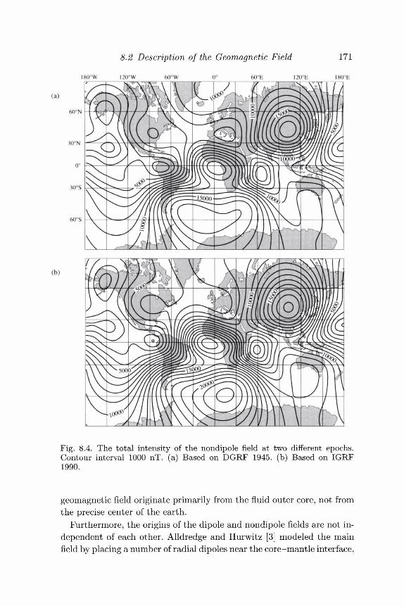
8.2 Description of the Geomagnetic Field 111
180°W I2O°W 60°W 60°E 120°E 180°E
(a)
60°N
(b)
Fig. 8.4. The total intensity of the nondipole field at two different epochs.Contour interval 1000 nT. (a) Based on DGRF 1945. (b) Based on IGRF1990.
geomagnetic field originate primarily from the fluid outer core, not fromthe precise center of the earth.
Furthermore, the origins of the dipole and nondipole fields are not in-dependent of each other. Alldredge and Hurwitz [3] modeled the mainfield by placing a number of radial dipoles near the core-mantle interface,
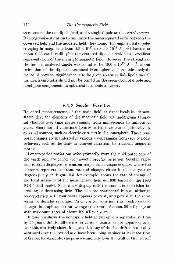
172 The Geomagnetic Field
to represent the nondipole field, and a single dipole at the earth's center.By progressive iteration to minimize the mean squared error between theobserved field and the modeled field, they found that eight radial dipoles(ranging in magnitude from 0.8 x 10²² to 3.6 x 10²² A-m2) located atabout 0.25 earth radii, plus the centered dipole, provided an excellentrepresentation of the main geomagnetic field. However, the strength ofthe best-fit centered dipole was found to be 18.0 x 10²² A-m2, abouttwice that of the dipole determined from spherical harmonic analysis.Hence, if physical significance is to be given to the radial-dipole model,too much emphasis should not be placed on the separation of dipole andnondipole components in spherical harmonic analyses.
8.2.5 Secular VariationRepeated measurements of the main field at fixed localities demon-strate that the elements of the magnetic field are undergoing tempo-ral changes over time scales ranging from milliseconds to millions ofyears. Short-period variations (yearly or less) are caused primarily byexternal sources, such as electric currents in the ionosphere. These tem-poral changes are manifested in various ways, ranging from very periodicbehavior, such as the daily or diurnal variation, to transient magneticstorms.
Longer-period variations arise primarily from the fluid outer core ofthe earth and are called geomagnetic secular variation. Secular varia-tion is often displayed by contour maps, called isoporic maps, where thecontours represent constant rates of change, either in nT per year ordegrees per year. Figure 8.5, for example, shows the rate of change ofthe total intensity of the geomagnetic field in 1990 based on the 1990IGRF field model. Such maps display cells (or anomalies) of either in-creasing or decreasing field. The cells are continental in size, althoughno correlation with continents appears to exist, and persist in the samesense for decades or longer. At any given location, the nondipole fieldchanges in amplitude at an average (rms) rate of about 50 nT per yearwith maximum rates of about 100 nT per year.
Figure 8.4 shows the nondipole field at two epochs separated in timeby 45 years. Subtle differences in various anomalies are apparent, evenover this relatively short time period. Many of the foci drifted noticeablywestward over this period and have been doing so since at least the timeof Gauss; for example, the positive anomaly over the Gulf of Guinea (off
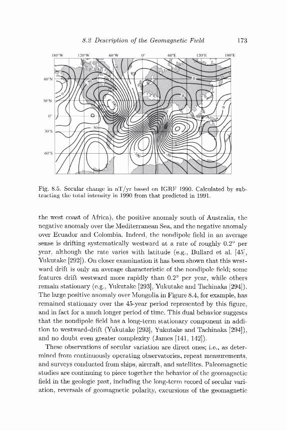
8.2 Description of the Geomagnetic Field
I KM \\ I2O°W 60°W
60° N
60°S
173
60°E 120°E I8O°E
Fig. 8.5. Secular change in nT/yr based on IGRF 1990. Calculated by sub-tracting the total intensity in 1990 from that predicted in 1991.
the west coast of Africa), the positive anomaly south of Australia, thenegative anomaly over the Mediterranean Sea, and the negative anomalyover Ecuador and Colombia. Indeed, the nondipole field in an averagesense is drifting systematically westward at a rate of roughly 0.2° peryear, although the rate varies with latitude (e.g., Bullard et al. [45],Yukutake [292]). On closer examination it has been shown that this west-ward drift is only an average characteristic of the nondipole field; somefeatures drift westward more rapidly than 0.2° per year, while othersremain stationary (e.g., Yukutake [293], Yukutake and Tachinaka [294]).The large positive anomaly over Mongolia in Figure 8.4, for example, hasremained stationary over the 45-year period represented by this figure,and in fact for a much longer period of time. This dual behavior suggeststhat the nondipole field has a long-term stationary component in addi-tion to westward-drift (Yukutake [293], Yukutake and Tachinaka [294]),and no doubt even greater complexity (James [141, 142]).
These observations of secular variation are direct ones; i.e., as deter-mined from continuously operating observatories, repeat measurements,and surveys conducted from ships, aircraft, and satellites. Paleomagneticstudies are continuing to piece together the behavior of the geomagneticfield in the geologic past, including the long-term record of secular vari-ation, reversals of geomagnetic polarity, excursions of the geomagnetic
174 The Geomagnetic Field
poles, and true polar wander. This considerable body of information isbeyond the scope of this text, and the interested reader is referred tobooks by Merrill and McElhinny [183] and Butler [47] for informationon these subjects.
8.3 Crustal Magnetic AnomaliesThe internal sources of the geomagnetic field are located primarily intwo regions of the earth. The majority of the field is generated in thefluid outer core by way of complex magnetohydrodynamic processes andis called the core field or main field. The remainder, called the crustalfield, originates primarily from a relatively thin outer shell of the earthwhere temperatures are below the Curie temperatures of important mag-netic minerals, primarily magnetite and titanomagnetite (Chapter 5).The depth to which such minerals exist is still a matter of discussion,however. The mantle is generally considered to be nonmagnetic (e.g.,Wasilewski, Thomas, and Mayhew [289]; Frost and Shive [92]), so accord-ing to this view, the depth extent of magnetic rocks is either the crust-mantle interface or the Curie-temperature isotherm, whichever is shal-lower. Some studies have concluded, on the other hand, that upper mantlerocks may have significant magnetizations, especially in oceanic regions(e.g., Arkani-Hamed [6]; Harrison and Carle [117]; Counil, Achache, andGaldeano [76]). In the following, we will loosely regard the crust-mantleinterface as magnetic basement, with the understanding that rocks in theuppermost mantle in some geologic environments may also contributeto the geomagnetic field. Hence, the vast region between the Curie-temperature isotherm (or crust-mantle interface, whichever is shallower)and the core-mantle interface is generally considered to be nonmagnetic.The calculation of crustal magnetic anomalies then amounts to subtract-ing the core field from measurements of the total magnetic field. Patersonand Reeves [212, Figure 8] showed an excellent example of the enhance-ment of an airborne magnetic survey by this simple residual calculation.
The large difference in depth between the sources of the crustal andcore field is reflected in spherical harmonic analyses. This depth informa-tion is perhaps best displayed by way of the power spectrum Rn, definedas the scalar product B n B n averaged over the spherical surface; that is,
2TT IT
j / f ~Bn-Bn a2 sin8 d0d<t>, (8.21)0 0
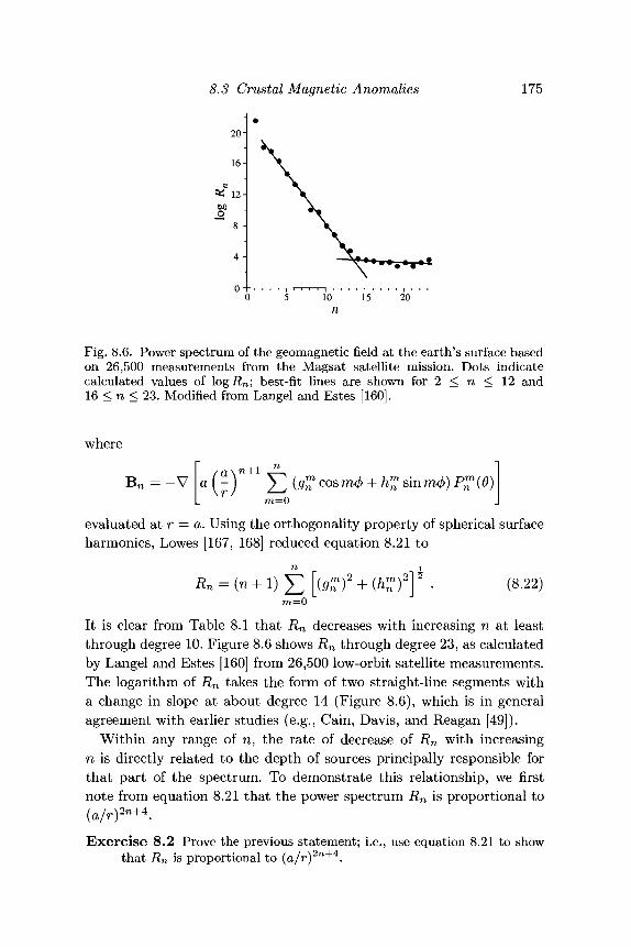
8.3 Crustal Magnetic Anomalies 175
g?
20-
16-
' 12-
8 -
4 -
10 15 20n
Fig. 8.6. Power spectrum of the geomagnetic field at the earth's surface basedon 26,500 measurements from the Magsat satellite mission. Dots indicatecalculated values of logi?n; best-fit lines are shown for 2 < n < 12 and16 < n < 23. Modified from Langel and Estes [160].
where
n+1(#™ cos mcf) + K sin mcp) P™ (t
evaluated at r = a. Using the orthogonality property of spherical surfaceharmonics, Lowes [167, 168] reduced equation 8.21 to
(8.22)ra=0
It is clear from Table 8.1 that Rn decreases with increasing n at leastthrough degree 10. Figure 8.6 shows Rn through degree 23, as calculatedby Langel and Estes [160] from 26,500 low-orbit satellite measurements.The logarithm of Rn takes the form of two straight-line segments witha change in slope at about degree 14 (Figure 8.6), which is in generalagreement with earlier studies (e.g., Cain, Davis, and Reagan [49]).
Within any range of n, the rate of decrease of Rn with increasingn is directly related to the depth of sources principally responsible forthat part of the spectrum. To demonstrate this relationship, we firstnote from equation 8.21 that the power spectrum Rn is proportional to(a/r)2n+4.Exercise 8.2 Prove the previous statement; i.e., use equation 8.21 to show
that Rn is proportional to (a/r)2n+4.
176 The Geomagnetic Field
Then to transform Rn based at the surface of the earth into a spectrumthat would be determined at some new radius r, we simply have tomultiply Rn by the factor (a/r)2 n + 4 , or add (2n + 4) log(a/r) to logRn.This manipulation changes the slope of the logarithmic power spectrumby a constant 21og(a/r). If r > a, Rn is transformed onto a largersphere, the slope of \ogRn is steepened, and the procedure is calledupward continuation. If r < a, Rn is transformed to a smaller sphere(within the earth), the slope of \ogRn is flattened, and the procedureis called downward continuation. Downward continuation is legitimate,however, only if all currents and other sources of magnetic fields areabsent between radii a and r (e.g., Booker [34], Lowes [168]). We willhave considerably more to say about upward and downward continuationin Chapter 12.
It is commonly assumed that the radius required to make logRn asnearly constant as possible (i.e., to make the power spectrum "white")is the radius at which the important sources of the field are located(e.g., Lowes [168], Langel and Estes [160]). With this assumption, theprincipal sources are located at a radius given by the value of r thatsatisfies
S + 21og- = 0 ,r
where S is the slope of log Rn. The line that best fits log Rn for n < 14 inFigure 8.6 has a slope of —1.309 (Langel and Estes [160]). Substitutingthis value into the previous equation provides r = 3311 km, which placesthe sources of this part of the spectrum at a radius about 174 km belowthe seismic core-mantle boundary. The spectrum at n > 14 indicatessources within the upper 100 km of the earth.
Hence, it is logical to interpret the steep part of the spectrum (n < 14)in Figure 8.6 to be caused by sources within the outer core, and theflatter part of the spectrum (n > 14) to be dominated by lithosphericsources (e.g., Bullard [44], Booker [34], Lowes [168], Cain et al. [49]; Lan-gel and Estes [160]). It would seem, therefore, that a crustal magneticmap could be constructed from satellite data by subtracting a 13-degreespherical harmonic expansion derived from the same data (e.g., May-hew [177]; Regan, Cain, and Davis [241]; Cain, Schmitz, and Math [50];Langel, Phillip, and Horner [159]).
This assumption deserves consideration, however. Carle and Harri-son [53] showed that residual fields calculated in this way may con-tain long-wavelength components, too long to be caused by near-surfacesources. This happens in part because in practice we usually measure
8.3 Crustal Magnetic Anomalies 177
the total intensity of the geomagnetic field (discussed more fully in Sec-tion 8.3.1) rather than a single component of the field. The residualcrustal anomaly in such cases is computed by subtracting the magni-tude of a low-degree regional field from measurements of the geomag-netic intensity. The total intensity is the square root of the sum of thesquares of three orthogonal components, as in equation 8.15. Althoughthe potential is modeled in a spherical harmonic expansion as the sumof sinusoidal terms, in squaring the three components to form the in-tensity, each of those sinusoidal terms becomes a combination of bothlonger and shorter wavelength terms, as demonstrated by the followingexercise.Exercise 8.3 Consider a potential field given by B = -VV, where V =
a(a/r)2giPi(0). Show that each component of B (i.e., Br and Be) hasonly one sinusoidal term of wavelength 2TT, but that |B| has two terms,one with infinite wavelength and a second with wavelength TT.
Hence, a value of n that represents the transition from dominantly coreto dominantly crustal contributions to the geomagnetic field may notbe appropriate for the total intensity of the field. A residual anomalycomputed by subtracting the magnitude of a regional field truncated atn still will contain contributions from harmonics less than n.
Langel [156] agreed that the anomaly field includes long wavelengths,but that these can originate strictly from crustal sources by virtue of theway the anomaly field is calculated and do not necessarily imply con-tamination from sources in the core. Arkani-Hamed and Strangway [7]and Harrison, Carle, and Hayling [118] independently concluded thatthe crustal portion of the magnetic field dominates the total intensity atdegrees 19 and greater; that is, to be sure that the residual anomaly rep-resents only crustal sources, they recommended truncation of anomaliesup through degree 18.
The important conclusion for our purposes here is that subtractionof a 10-degree IGRF model, such as that shown in Table 8.1, from amagnetic survey will be inadequate to eliminate the entire core field.Magnetic studies of continental or global scale should be evaluated care-fully in the context of long-wavelength anomalies that might originatefrom the core and that may be confused with the crustal field. The long-wavelength shortcomings of the 10-degree IGRF are much less significantfor local- or regional-scale magnetic studies applied to geologic problems.In such cases, additional regional fields can be removed subsequent tosubtraction of the IGRF using a variety of techniques, such as simplecurve fitting and digital filtering.
178 The Geomagnetic Field
Chapter 7 focused on the reduction of measurements of the total grav-itational attraction of the earth to gravity anomalies reflecting crustaldensity variations. This reduction procedure consists of a series of steps,including a subtraction of the gravitational effects of an average earth,the elevation of the measurement, and terrain. In crustal magnetic stud-ies, the calculation of anomalies is often treated in a more cavalier way,usually consisting of only two steps: (1) an adjustment for daily varia-tions and magnetic disturbances and (2) the subtraction of a suitableregional field, such as the IGRF model appropriate for the date of thesurvey. Some of the corrections routinely applied to gravity measure-ments generally are not attempted in magnetic studies simply becausethey are less tractable in the magnetic case. Terrain corrections in grav-ity studies, for example, although tedious are nevertheless straightfor-ward because the density of the terrain is relatively uniform. Crustalmagnetization, however, can vary by several orders of magnitude (andchange sign) at essentially all spatial scales. This additional complex-ity requires less-straightforward techniques to correct for terrain effects(e.g., Clarke [61], Grauch [101]), and the effects of terrain are often leftto the modeling and interpretation stage.Exercise 8.4 Discuss the magnetic analog of the simple Bouguer correction.
8.3.1 Total-Field AnomaliesTotal-field magnetometers are usually the instrument of choice for air-borne and shipborne magnetic surveys. As the name implies, total-fieldmagnetometers measure the magnitude of the total magnetic field with-out regard to its vector direction. The total-field anomaly is calculatedfrom total-field measurements by subtracting the magnitude of a suit-able regional field, usually the IGRF model appropriate for the date ofthe survey. If T represents the total field at any point, and F is theregional field at the same point, then the total-field anomaly is given by
AT = |T| - |F | . (8.23)
Because AT will form the basis of future discussions on interpretationof magnetic data, it is important to establish under what conditionsAT is harmonic. Let AF represent the perturbation of F due to someanomalous magnetic source. Then the total field is given by
T=F+AF
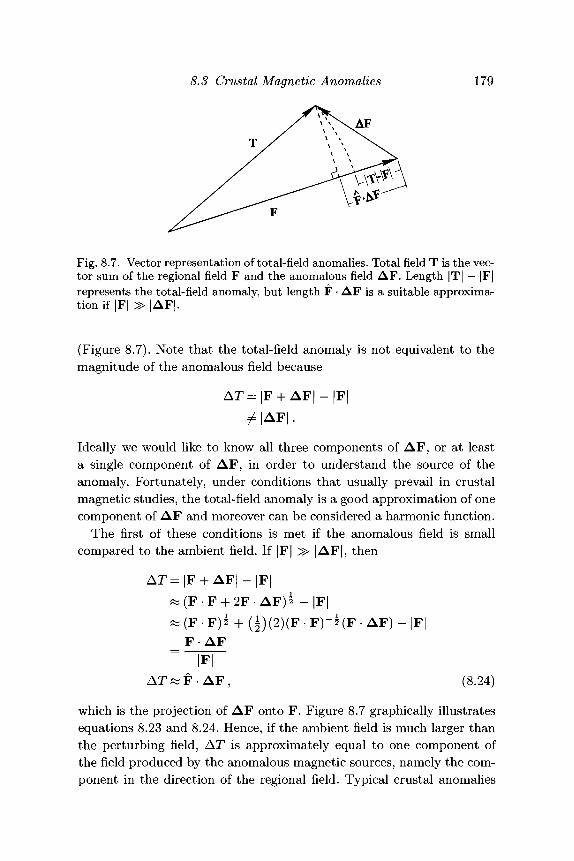
8.3 Crustal Magnetic Anomalies 179
Fig. 8.7. Vector representation of total-field anomalies. Total field T is the vec-tor sum of the regional field F and the anomalous field AF. Length |T| — |F|represents the total-field anomaly, but length F • AF is a suitable approxima-tion if |F| > |AF|.
(Figure 8.7). Note that the total-field anomaly is not equivalent to themagnitude of the anomalous field because
A T = | F + A F | - |F|
Ideally we would like to know all three components of AF, or at leasta single component of AF, in order to understand the source of theanomaly. Fortunately, under conditions that usually prevail in crustalmagnetic studies, the total-field anomaly is a good approximation of onecomponent of AF and moreover can be considered a harmonic function.
The first of these conditions is met if the anomalous field is smallcompared to the ambient field. If |F| >• |AF|, then
A T = | F + AF| - |F|« (F • F + 2F •~ (F • F)2 -f- (-
F AF) - *•F)-2(F- A F ) - |F|
|FF A F , (8.24)
which is the projection of AF onto F. Figure 8.7 graphically illustratesequations 8.23 and 8.24. Hence, if the ambient field is much larger thanthe perturbing field, AT is approximately equal to one component ofthe field produced by the anomalous magnetic sources, namely the com-ponent in the direction of the regional field. Typical crustal anomalies
180 The Geomagnetic Field
measured in airborne and shipborne surveys range in magnitude froma few nT to several 1,000 nT, but rarely exceed 5,000 nT. Hence, thecondition that |F| > | AF | is usually met in studies of crustal magneti-zation.
Another condition is also necessary, however, in order for AT to satisfyLaplace's equation and be harmonic over the dimensions of the survey.In general, the total-field anomaly is not harmonic because, as definedby equation 8.23, V2AT ^ 0. If, however, the anomaly field is smallcompared to the total field, then
V2AT = V2(F- AF) .
If in addition the direction of the regional field is approximately constantover the dimensions of the survey, then F is a constant and can be movedoutside of the Laplacian, that is,
V2AT = F - V 2 AF.
As discussed in Section 6.4, specific components of a harmonic potentialfield are themselves harmonic. Hence, each component of A F in theprevious equation is harmonic, V2AT = 0, and AT itself is harmonic.The condition of invariant field direction depends on the scope of thestudy; it is a reasonable assumption for local and regional surveys, butnot for studies of continental or larger scale. We will revisit this problemin Section 12.3.1.
In summary, the total-field anomaly at any point is approximatelyequal to the component of the anomalous field in the direction of theregional field if the anomaly field is small compared to the ambientfield. In addition, the total-field anomaly is a potential and satisfiesLaplace's equation if the direction of the ambient field is constant overthe dimensions of the survey. Both conditions generally prevail in studiesof local and regional scale, a conclusion with fortunate implications fordiscussions in future chapters.
8.4 Problem Set1. Suppose that the northward-directed component of a force field F
is known on the surface of a sphere with radius a. The field has apotential V that is harmonic in source-free regions. Sources may existboth inside and outside the sphere but not at the surface. Show fromspherical harmonic analysis that the eastward-directed component of
84 Problem Set 181
F can be determined at any point on the sphere from knowledge ofthe northward-directed component.
2. Use a spherical harmonic expansion to show that the field of a singleeccentric dipole is equivalent to the field produced by multiple sourceslocated at the center of the sphere (geocentric dipole, quadrupole, andso forth).
3. On the surface of a planet with radius a the only nonzero Gauss co-efficients are g^ and gf, and these have values 0.3 and 0.5, respectively.(a) Find the declination D, inclination /, and intensity |B| at a point
with colatitude 90° and longitude 45°.(b) Repeat for a point with the same colatitude and longitude but at
five planetary radii (r = 5a).4. The magnetic field of Planet X is known on the basis of orbiting satel-
lite measurements to have a power spectrum satisfying the equationRn = 0.5 x 10⁹ • (0.3)n (nT2). The radius of the planet is 8000 km,and the satellite altitude was 500 km above the planet's surface.(a) Assume that the magnetic field is caused by a very thin, spherical,
concentric, randomly magnetized layer. What is the radius of thelayer?
(b) Suppose instead that the field is actually caused by a thick layer ofbroadly circulating electrical currents. Discuss the errors involvedin erroneously assuming a thin, randomly magnetized layer.
5. A vertically and uniformly magnetized sphere is buried at the mag-netic equator. The radius of the sphere is 10 m, its center is 15 mbelow the profile, and its magnetization is 1 A-m"1. Assume the sur-rounding rocks are nonmagnetic.(a) Calculate the total-field anomaly along a profile directly over the
sphere.(b) Quantitatively describe the error in using the approximation ex-
pressed by equation 8.24.6. The electrical current flowing in a spherical shell is adjusted so that
the field inside the shell is uniform. Show that the magnetic field ofthe shell appears dipolar at points outside the sphere.
9Forward Method
Physicists believe that known laws should suffice to explain the Earth'sbehavior, but the complexities of geology have defied simple explanation.
(J. Tuzo Wilson)The purpose of models is not to fit the data but to sharpen the questions.
(Samuel Karlin)
9.1 Methods ComparedThe magnetic or gravity survey is complete, the data are processed, andregional fields have been removed appropriately. Now comes the inter-esting challenge of interpretation. The problem is conceptually straight-forward: Estimate one or more parameters of the source from observedgravity or magnetic fields, while incorporating all available geologic, geo-physical, and other independent information.
The many techniques of interpretation can be divided into three cat-egories (Figure 9.1). Each category has the same goal, to illuminate thespatial distribution of gravity or magnetic sources, but they approachthe goal with quite different logical processes.
1. Forward method: An initial model for the source body is constructedbased on geologic and geophysical intuition. The model's anomalyis calculated and compared with the observed anomaly, and modelparameters are adjusted in order to improve the fit between the twoanomalies. This three-step process of body adjustment, anomaly cal-culation, and anomaly comparison is repeated until calculated andobserved anomalies are deemed sufficiently alike.
2. Inverse method: One or more body parameters are calculated auto-matically and directly from the observed anomaly. Simplifying as-sumptions are inevitable.
182
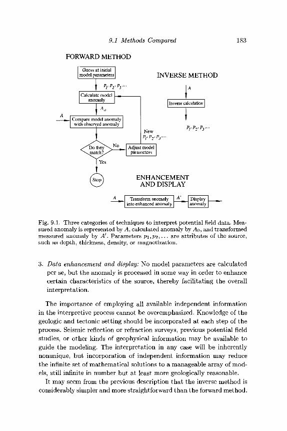
9.1 Methods Compared
FORWARD METHOD
183
Compare model anomalywith observed anomaly
INVERSE METHOD
Inverse calculation
ENHANCEMENTAND DISPLAY
Transform anomalyinto enhanced anomaly
A' Displayanomaly
Fig. 9.1. Three categories of techniques to interpret potential field data. Mea-sured anomaly is represented by A, calculated anomaly by Ao, and transformedmeasured anomaly by A'. Parameters pi,p2, • • • are attributes of the source,such as depth, thickness, density, or magnetization.
3. Data enhancement and display: No model parameters are calculatedper se, but the anomaly is processed in some way in order to enhancecertain characteristics of the source, thereby facilitating the overallinterpretation.
The importance of employing all available independent informationin the interpretive process cannot be overemphasized. Knowledge of thegeologic and tectonic setting should be incorporated at each step of theprocess. Seismic reflection or refraction surveys, previous potential fieldstudies, or other kinds of geophysical information may be available toguide the modeling. The interpretation in any case will be inherentlynonunique, but incorporation of independent information may reducethe infinite set of mathematical solutions to a manageable array of mod-els, still infinite in number but at least more geologically reasonable.
It may seem from the previous description that the inverse method isconsiderably simpler and more straightforward than the forward method.
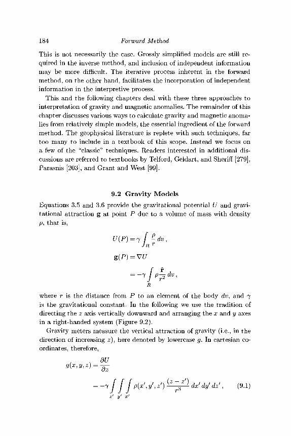
184 Forward Method
This is not necessarily the case. Grossly simplified models are still re-quired in the inverse method, and inclusion of independent informationmay be more difficult. The iterative process inherent in the forwardmethod, on the other hand, facilitates the incorporation of independentinformation in the interpretive process.
This and the following chapters deal with these three approaches tointerpretation of gravity and magnetic anomalies. The remainder of thischapter discusses various ways to calculate gravity and magnetic anoma-lies from relatively simple models, the essential ingredient of the forwardmethod. The geophysical literature is replete with such techniques, fartoo many to include in a textbook of this scope. Instead we focus ona few of the "classic" techniques. Readers interested in additional dis-cussions are referred to textbooks by Telford, Geldart, and Sheriff [279],Parasnis [203], and Grant and West [99].
9.2 Gravity ModelsEquations 3.5 and 3.6 provide the gravitational potential U and gravi-tational attraction g at point P due to a volume of mass with densityp, that is,
U(P)=-y f P-JR r
g(P) = W
where r is the distance from P to an element of the body dv, and 7is the gravitational constant. In the following we use the tradition ofdirecting the z axis vertically downward and arranging the x and y axesin a right-handed system (Figure 9.2).
Gravity meters measure the vertical attraction of gravity (i.e., in thedirection of increasing z), here denoted by lowercase g. In cartesian co-ordinates, therefore,
g(x,y,z) = —oz
= - 7 J J J P(x', y', z1) ^ = 3 ^ dx1 dy' dz', (9.1)z' yf x1
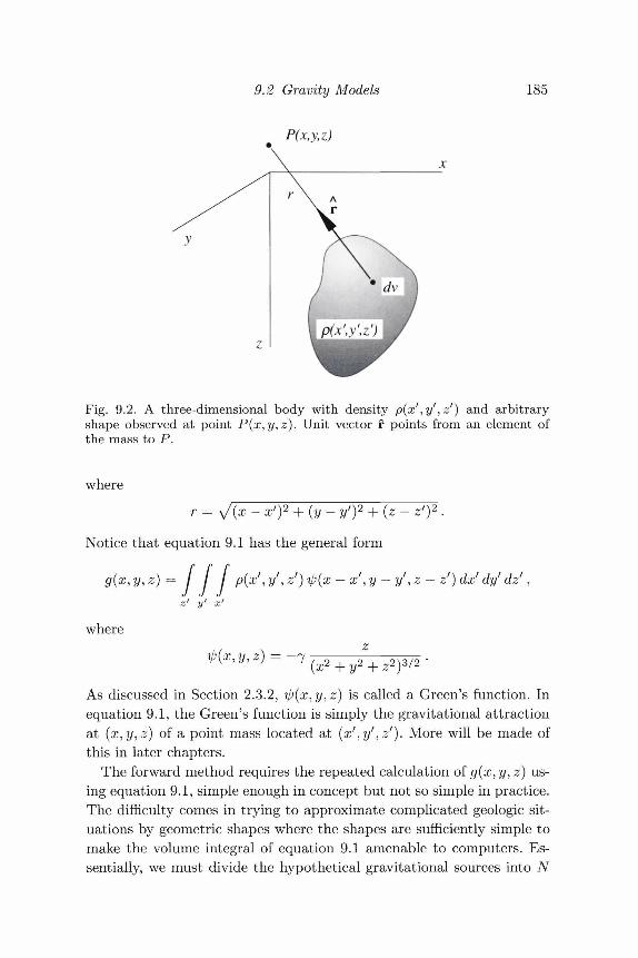
9.2 Gravity Models
P(x,y,z)
185
Fig. 9.2. A three-dimensional body with density p(x',y',z) and arbitraryshape observed at point P(x,y,z). Unit vector f points from an element ofthe mass to P.
where
Notice that equation 9.1 has the general form
g(x,y,z)= / / / p(x\y',z')i/;(x-x\y-y',z- z')dx'dy'dzf,z' y' x'
tp(x,y,z) = -7-where
As discussed in Section 2.3.2, ip(x,y,z) is called a Green's function. Inequation 9.1, the Green's function is simply the gravitational attractionat (x,y,z) of a point mass located at (xf,yf,zf). More will be made ofthis in later chapters.
The forward method requires the repeated calculation of g(x, y, z) us-ing equation 9.1, simple enough in concept but not so simple in practice.The difficulty comes in trying to approximate complicated geologic sit-uations by geometric shapes where the shapes are sufficiently simple tomake the volume integral of equation 9.1 amenable to computers. Es-sentially, we must divide the hypothetical gravitational sources into N
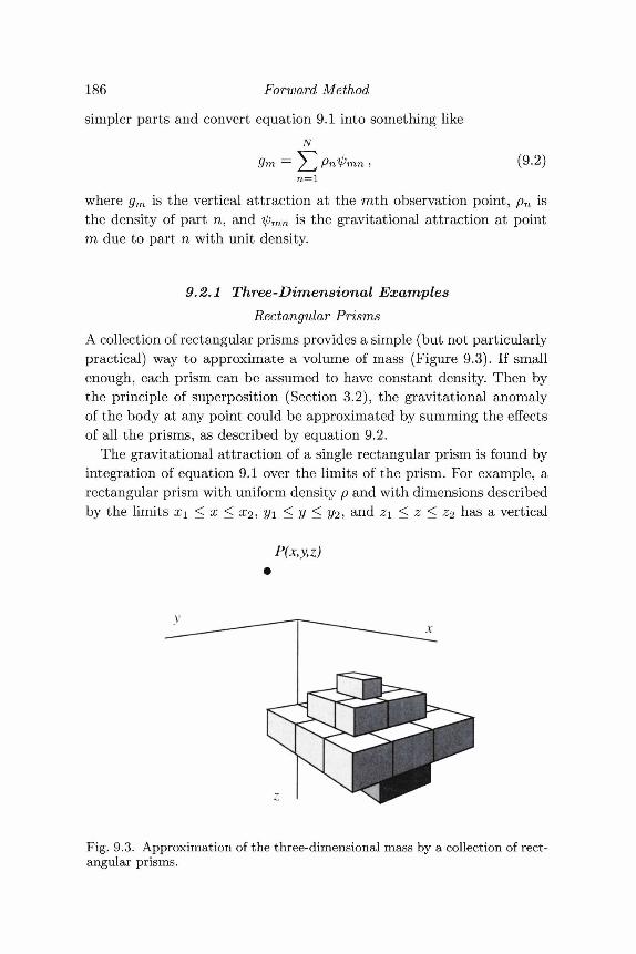
186 Forward Method
simpler parts and convert equation 9.1 into something likeN
9m — / J Pntymn in=l
(9.2)
where gm is the vertical attraction at the rath observation point, pn isthe density of part n, and iprnn is the gravitational attraction at pointra due to part n with unit density.
9.2.1 Three-Dimensional ExamplesRectangular Prisms
A collection of rectangular prisms provides a simple (but not particularlypractical) way to approximate a volume of mass (Figure 9.3). If smallenough, each prism can be assumed to have constant density. Then bythe principle of superposition (Section 3.2), the gravitational anomalyof the body at any point could be approximated by summing the effectsof all the prisms, as described by equation 9.2.
The gravitational attraction of a single rectangular prism is found byintegration of equation 9.1 over the limits of the prism. For example, arectangular prism with uniform density p and with dimensions describedby the limits x\ < x < #2, Vi < y < 1/2, and z\ < z < z^ has a vertical
P(x,y,z)
Fig. 9.3. Approximation of the three-dimensional mass by a collection of rect-angular prisms.
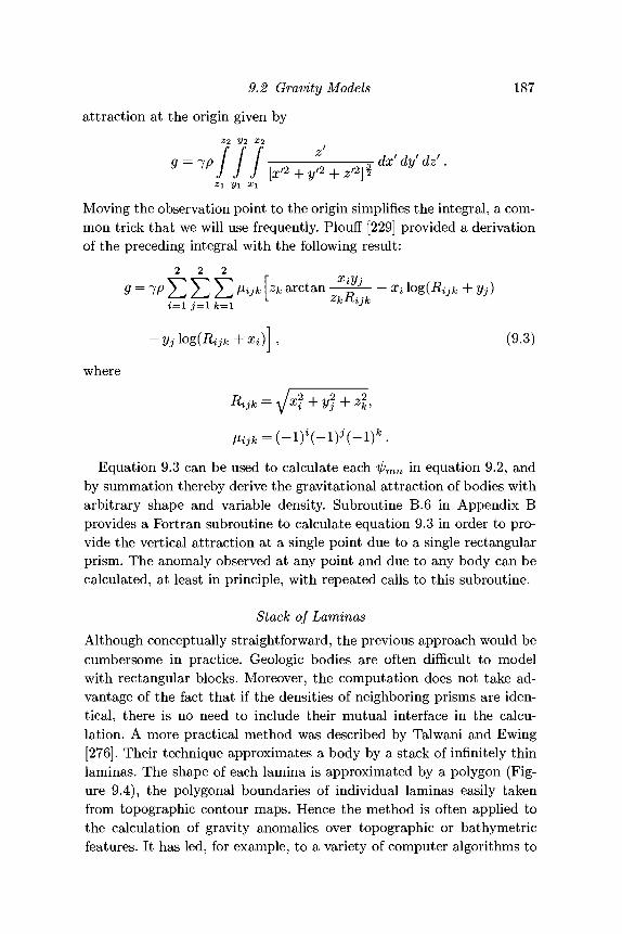
9.2 Gravity Models 187
attraction at the origin given byZ2 VI X2 f
9 = IP j j Z 5 dx'dy'dz'.
J J J [x/2 + y12 -f z / Jj 2
Moving the observation point to the origin simplifies the integral, a com-mon trick that we will use frequently. Plouff [229] provided a derivationof the preceding integral with the following result:
2 2 2
[ X V 'Zk arctan —l— Xi \og(Rijk + yj)
i=1 - = 1 /e_1 zkRijk
-yjlogiRijk+Xi)] , (9.3)
where
Equation 9.3 can be used to calculate each ipmn in equation 9.2, andby summation thereby derive the gravitational attraction of bodies witharbitrary shape and variable density. Subroutine B.6 in Appendix Bprovides a Fortran subroutine to calculate equation 9.3 in order to pro-vide the vertical attraction at a single point due to a single rectangularprism. The anomaly observed at any point and due to any body can becalculated, at least in principle, with repeated calls to this subroutine.
Stack of LaminasAlthough conceptually straightforward, the previous approach would becumbersome in practice. Geologic bodies are often difficult to modelwith rectangular blocks. Moreover, the computation does not take ad-vantage of the fact that if the densities of neighboring prisms are iden-tical, there is no need to include their mutual interface in the calcu-lation. A more practical method was described by Talwani and Ewing[276]. Their technique approximates a body by a stack of infinitely thinlaminas. The shape of each lamina is approximated by a polygon (Fig-ure 9.4), the polygonal boundaries of individual laminas easily takenfrom topographic contour maps. Hence the method is often applied tothe calculation of gravity anomalies over topographic or bathymetricfeatures. It has led, for example, to a variety of computer algorithms to
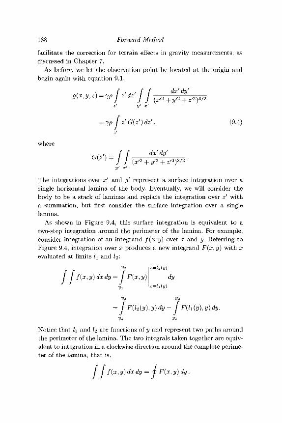
188 Forward Method
facilitate the correction for terrain effects in gravity measurements, asdiscussed in Chapter 7.
As before, we let the observation point be located at the origin andbegin again with equation 9.1,
g(x,y,z)=<yp z'dz' —dx' dy'
y> x>
yf2 + ^2)3/2
= jpJz'G(z')dz', (9.4)
wheredx' dy'
G(z') = 2 + y'2 + zf2fl2
The integrations over x' and y' represent a surface integration over asingle horizontal lamina of the body. Eventually, we will consider thebody to be a stack of laminas and replace the integration over z' witha summation, but first consider the surface integration over a singlelamina.
As shown in Figure 9.4, this surface integration is equivalent to atwo-step integration around the perimeter of the lamina. For example,consider integration of an integrand f(x,y) over x and y. Referring toFigure 9.4, integration over x produces a new integrand F(x, y) with xevaluated at limits l\ and I2'.
3/2
/ / f(x,y)dxdy= / F(x,y)x=l2(y)
dyx=h(y)
= j F(l2(y),y)dy - f F(h(y),y) dy.
Notice that l\ and I2 are functions of y and represent two paths aroundthe perimeter of the lamina. The two integrals taken together are equiv-alent to integration in a clockwise direction around the complete perime-ter of the lamina, that is,
/ / f(x, y) dxdy = (b F(x, y) dy .
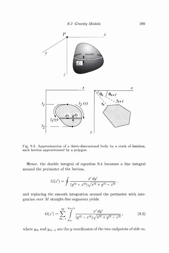
9.2 Gravity Models 189
h(y)
Fig. 9.4. Approximation of a three-dimensional body by a stack of laminas,each lamina approximated by a polygon.
Hence, the double integral of equation 9.4 becomes a line integralaround the perimeter of the lamina,
G(z') = x'dy'(y'2 + z/2)y/xf2+y/2
and replacing the smooth integration around the perimeter with inte-gration over M straight-line segments yields
G(z') = V / X?V , (9.5)Urn
where 7/m and ym+i are the y coordinates of the two endpoints of side m.
190 Forward Method
The variable x' can be eliminated in equation 9.5 by using the equationof a straight line
x' =
where
' = ay' +
2/m+l - Vm
2/m+l — Vm
Substitution of am and /3m in equation 9.5 providesM y^1
G(z') = Y —*-" i (V2
(amy' + j3m) dy'(yf2 + ^ / 2 ) \ / (^ m + l)y'2 + 2ami9m2// + ^ + z/2
which according to Grant and West [99] can be written
M
G(z') = V^{arctanOm+i — arctanf2m} , (9.6)m=l
where
^m+1 =
Although cumbersome in appearance, equation 9.6 can be programmedeasily to provide G(z') for any lamina; depth z' and the x, y coordinatesof its M vertices are all that is required. Substituting equation 9.6 intoequation 9.4 provides the vertical attraction of a stack of laminas. Inte-gration over z' can be done with numerical quadrature techniques (e.g.,Press et al. [233]).
Measured gravity anomalies over bodies of unknown shape can bemodeled by trial-and-error adjustment of density and polygon vertices.If the anomalies are caused by known topographic or bathymetric fea-tures, the trial-and-error process is greatly simplified. This method isparticularly powerful in such applications because the polygonal lami-nas can be constructed simply by digitizing contours on topographic orbathymetric maps.
9.2 Gravity Models 191
In the method of Talwani and Ewing [276], the mass is approximatedby a stack of infinitely thin laminas. Plouff [227, 229] took this repre-sentation one step farther. In effect, he used equation 9.4 to derive thegravitational attraction of a layer of finite thickness, with vertical sidesand with top and bottom surfaces approximated by polygons. Analo-gous to the method of Talwani and Ewing [276], these polygonal layerscan be stacked on top of one another in order to approximate three-dimensional bodies of arbitrary shape. Plouff [229] used the method tocalculate gravitational effects of terrain, and the method has been im-plemented in various programs for removing the effects of terrain fromgravity surveys (Plouff [230], Godson and Plouff [97]).
9.2.2 Two-Dimensional ExamplesGeologic structures are often longer than they are wide. Fracture zones,faults, dikes, rift zones, and anticlines, for example, are often lineated ina particular horizontal direction, and the gravity or magnetic anomaliesthat they produce are similarly lineated (Figure 9.5). If anomalies aresufficiently "linear," it may be possible to consider the gravitational ormagnetic sources as completely invariant in the direction parallel to thelong direction. The y axis is directed parallel to the invariant directionleaving only the x and z dimensions to consider further; the body is saidto be two dimensional Density, for example, becomes
p(x,y,z) = p(x,z).
Section 3.3 discusses some of the theory behind the potential of two-dimensional masses.
"Sufficiently linear" is, of course, a rather subjective criterion. Pe-ters [219], in discussing a method for estimating depth to magneticsources, considered a body to be two-dimensional when it producesclosed anomaly contours roughly elliptical in shape, with long dimen-sions at least three times greater than their short dimensions. Grantand West [99], in discussing anomalies over ribbon-like sources, suggestedthat a shallowly buried ribbon must be at least 20 times longer than it iswide for the two-dimensional assumption to be legitimate. Problem 7 atthe end of this chapter further investigates the two-dimensional assump-tion. As discussed subsequently, end corrections have been devised forsome two-dimensional calculations to allow bodies that are not ideallytwo-dimensional (Rasmussen and Pedersen [237], Cady [48]).
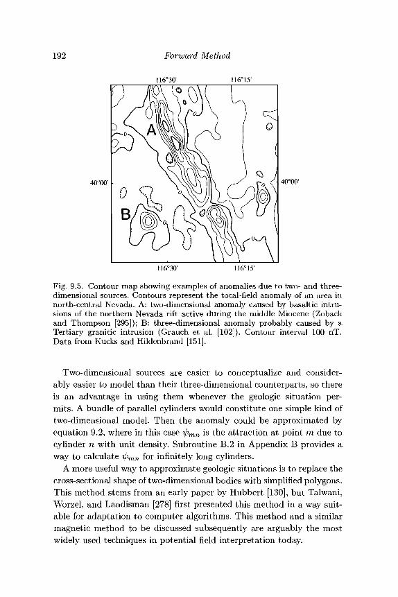
192 Forward Method
40°00' 40°00'
116°30'
Fig. 9.5. Contour map showing examples of anomalies due to two- and three-dimensional sources. Contours represent the total-field anomaly of an area innorth-central Nevada. A: two-dimensional anomaly caused by basaltic intru-sions of the northern Nevada rift active during the middle Miocene (Zobackand Thompson [295]); B: three-dimensional anomaly probably caused by aTertiary granitic intrusion (Grauch et al. [102]). Contour interval 100 nT.Data from Kucks and Hildenbrand [151].
Two-dimensional sources are easier to conceptualize and consider-ably easier to model than their three-dimensional counterparts, so thereis an advantage in using them whenever the geologic situation per-mits. A bundle of parallel cylinders would constitute one simple kind oftwo-dimensional model. Then the anomaly could be approximated byequation 9.2, where in this case iprnn is the attraction at point m due tocylinder n with unit density. Subroutine B.2 in Appendix B provides away to calculate ^ m n for infinitely long cylinders.
A more useful way to approximate geologic situations is to replace thecross-sectional shape of two-dimensional bodies with simplified polygons.This method stems from an early paper by Hubbert [130], but Talwani,Worzel, and Landisman [278] first presented this method in a way suit-able for adaptation to computer algorithms. This method and a similarmagnetic method to be discussed subsequently are arguably the mostwidely used techniques in potential field interpretation today.
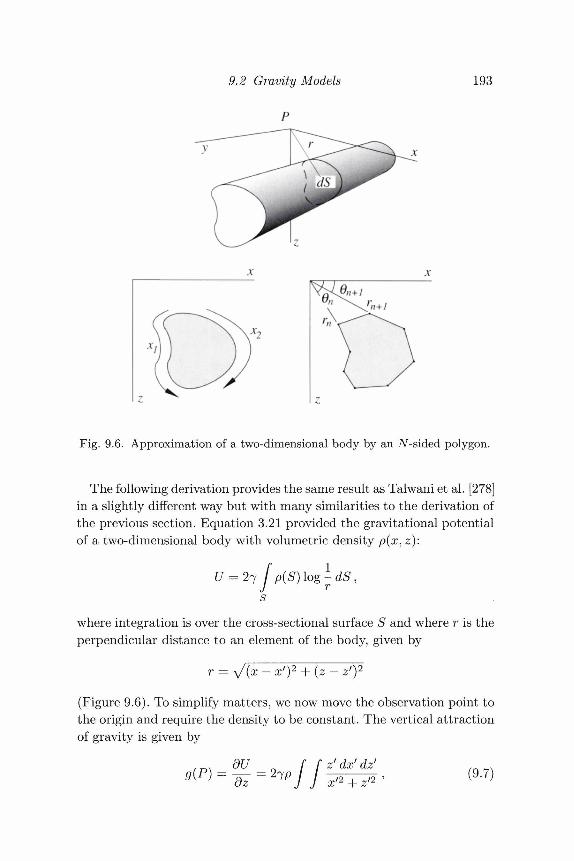
9.2 Gravity Models
P
193
Fig. 9.6. Approximation of a two-dimensional body by an iV-sided polygon.
The following derivation provides the same result as Talwani et al. [278]in a slightly different way but with many similarities to the derivation ofthe previous section. Equation 3.21 provided the gravitational potentialof a two-dimensional body with volumetric density p(x, z):
= 27 [J p(S)\og-dS,r
where integration is over the cross-sectional surface S and where r is theperpendicular distance to an element of the body, given by
= y/(x - x')2 - z1)2z1)2
(Figure 9.6). To simplify matters, we now move the observation point tothe origin and require the density to be constant. The vertical attractionof gravity is given by
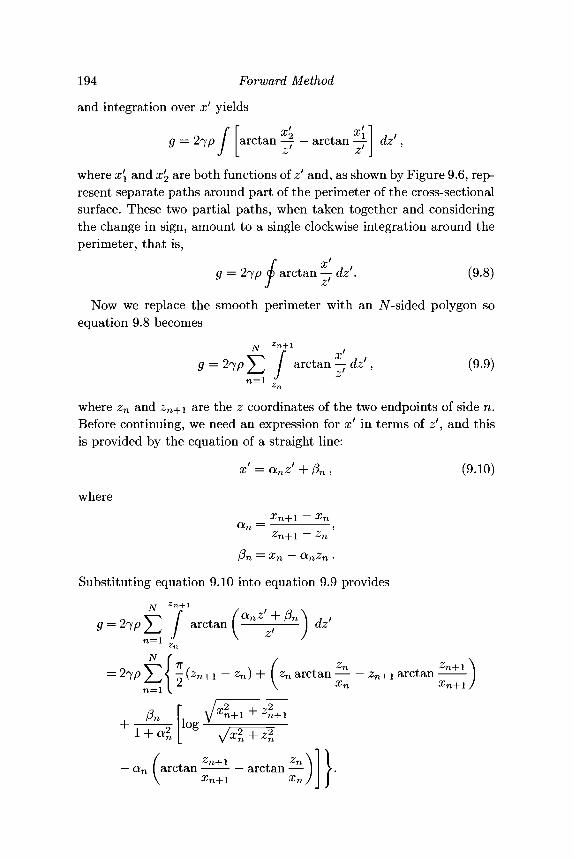
194 Forward Method
and integration over x' yields
f \ x' x' 1g = 27p / arctan - 7 — arctan - 7 dz'
J \_ z z \where x[ and x'2 are both functions of z' and, as shown by Figure 9.6, rep-resent separate paths around part of the perimeter of the cross-sectionalsurface. These two partial paths, when taken together and consideringthe change in sign, amount to a single clockwise integration around theperimeter, that is,
/ x'g = 27/9 (p arctan — dz'. (9.8)
J zNow we replace the smooth perimeter with an TV-sided polygon so
equation 9.8 becomesN ^jt1
f
g = 2jp 2_. / arctan — dz', (9.9)n=l Jn
Z
where zn and zn+i are the z coordinates of the two endpoints of side n.Before continuing, we need an expression for x' in terms of z1', and thisis provided by the equation of a straight line:
x' = anz' + /3n, (9.10)
where
otn. =Zn+l ~ Zn
ft — T — CM 7
Substituting equation 9.10 into equation 9.9 provides
g — 27^ 2_^ / arctan I 1 dzn=l J \ Z J
Zn
A f 7T / Z^ ^ { 7:(zn+i — zn) + ( zn arctan — — zn+i arctan
i + i + •
,1— xn+l
Pn log
( . Zn+1 Z n \ \ \
— an I arctan arctan — 1 >.V %n-\-l %n J I
J J
9.3 Magnetic Models 195
The first two terms in parentheses of the summation add to zero aroundany closed polygon, so the previous equation simplifies to
^ [loS <*(* ° ) \ (9.11)n=l
in such cases where r n and 0n are defined as shown in Figure 9.6.
Exercise 9.1 Some license was used in the preceding derivation. In particu-lar, an and /3n are not defined if the ribbon is horizontal. What happensto equation 9.2.2 in this case and how might the problem be treated ina computer algorithm?
The gravitational attraction of the two-dimensional body, therefore, de-pends on the position of the N corners of the polygon. If we imagineN lines drawn from the observation point to each of the corners of thepolygon, the gravitational attraction depends on the lengths of thoselines and the angles that they make with the horizontal (Figure 9.6).
Exercise 9.2 What happens if the observation point falls on a corner of thepolygon? How might this problem be treated in practice?
Equation 9.2.2 is implemented in Subroutine B.7 (Appendix B). Thissubroutine provides the vertical attraction at a single point due to atwo-dimensional body with polygonal cross section. Similar subroutinesform the core of various two-dimensional modeling systems availablefrom commercial software companies and from public-domain sources(e.g., Saltus and Blakely [251]).
Strictly speaking, the preceding discussion applies to bodies that areinfinitely extended along one horizontal axis. End corrections to thesetwo-dimensional calculations have been developed (Rasmussen and Ped-ersen [237], Cady [48]) for anomalies that seem to be caused by two-dimensional bodies of limited extent. Such calculations are sometimesreferred to as the "2 -dimensional" case.
9.3 Magnetic ModelsEquation 5.3 describes the magnetic field of a volume of magnetic ma-terial,
^dv, (9.12)R
where M is magnetization, and r is distance from the observation pointP to element dv of the body. The value of the constant Cm depends
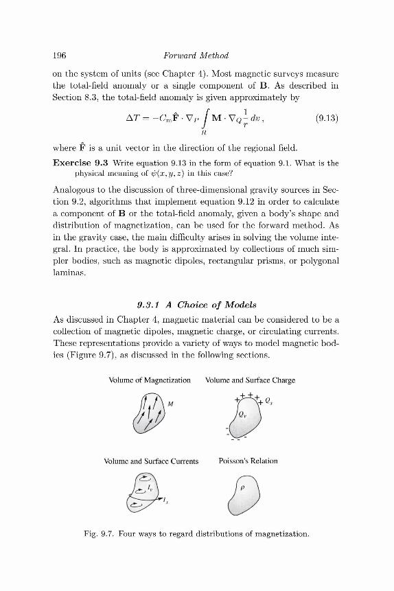
196 Forward Method
on the system of units (see Chapter 4). Most magnetic surveys measurethe total-field anomaly or a single component of B. As described inSection 8.3, the total-field anomaly is given approximately by
AT = - C m F - V P fM-Vq-dv, (9.13)
where F is a unit vector in the direction of the regional field.
Exercise 9.3 Write equation 9.13 in the form of equation 9.1. What is thephysical meaning of ip(x, y, z) in this case?
Analogous to the discussion of three-dimensional gravity sources in Sec-tion 9.2, algorithms that implement equation 9.12 in order to calculatea component of B or the total-field anomaly, given a body's shape anddistribution of magnetization, can be used for the forward method. Asin the gravity case, the main difficulty arises in solving the volume inte-gral. In practice, the body is approximated by collections of much sim-pler bodies, such as magnetic dipoles, rectangular prisms, or polygonallaminas.
9.3.1 A Choice of ModelsAs discussed in Chapter 4, magnetic material can be considered to be acollection of magnetic dipoles, magnetic charge, or circulating currents.These representations provide a variety of ways to model magnetic bod-ies (Figure 9.7), as discussed in the following sections.
Volume of Magnetization Volume and Surface Charge
ife-o.
Volume and Surface Currents Poisson's Relation
Fig. 9.7. Four ways to regard distributions of magnetization.
9.3 Magnetic Models 197
Volume of MagnetizationEquation 9.12 or 9.13 could be evaluated directly. In practice, however,this can be done analytically for only simple shapes and is not an ap-propriate strategy for trial-and-error forward modeling. Alternatively, avolume of magnetic material could be divided into N magnetic cells,analogous to equation 9.2. The three components of magnetic field be-come
N^ b i j , (9.14)
where Bj is the magnetic field at the j th observation point, Mi is themagnitude of the magnetization of the ith cell, and b^ is the magneticfield at the jth observation point due to the ith cell with unit magneti-zation,
[-VQ^OIV. (9.15)
If the cells are sufficiently small, they each can be considered to haveuniform magnetization. In practice, cells would have to consist of simpleshapes, such as rectangular prisms or magnetic dipoles, in order to easilycompute equation 9.14 and so that the aggregate of all cells is easilyvisualized and adjusted.
Surface ChargeAs discussed in Section 5.1, the volume integral of equation 9.12 can beconverted into the sum of a volume and surface integral by first applyingthe vector identity V • (</>A) = V</> • A + </>V • A and then applying thedivergence theorem. The magnetic potential, for example, expands to
R
m / do ~~ ^m IJ r J
dv. (9.16)S R
The integrals in equation 9.16 have the same form as gravitational poten-tial, where the scalar quantities Qs and Qv represent magnetic "charge"on the surface and within the interior of the body, respectively.
198 Forward Method
Exercise 9.4 Prove that the number of positive magnetic charges must equalthe number of negative magnetic charges within and on the surface ofany isolated magnetic volume.
If magnetization is uniform, then the second integral of equation 9.16vanishes, and the potential is given by
V = Cm f^—^dS. (9.17)
If magnetization is uniform, therefore, the body can be completely repre-sented by a distribution of magnetic charge on the body's surface. Thisrepresentation has led to a number of powerful algorithms, several ofwhich will be discussed in detail subsequently.
Surface CurrentsThe Biot-Savart law (equation 4.4) was used in Chapter 4 to show thatthe magnetic field of a small current loop appears at a distance like thefield of a dipole. Hence a distribution of dipoles can be considered tobe a volume of elemental currents. (This is not surprising; the ultimatesources of magnetization are circulating currents.)
As discussed in Section 5.1, circulating currents resolve into surfaceand volume currents,
Is = M x n ,Iv = V x M .
If the magnetization is uniform, then the volume current vanishes, and amagnetic body can be replaced with an empty volume of identical shapecarrying electrical currents on its surface (Figure 9.8).
This representation is rarely applied to forward modeling of magneticanomalies but is useful in a variety of other geophysical applications.For example, a cylindrical rock sample uniformly magnetized along itsaxis is equivalent to a nonmagnetic cylinder with electrical currents onits surface. It is clear from Figure 9.9 that Iv = 0 and Is = M x n.Hence, Is is zero on the top and bottom of the cylinder and directedin a circular fashion around the cylindrical surface; that is, the currenthas the form of a simple solenoid, as shown in Figure 9.9. Laboratorymagnetometers for measuring magnetization of cylindrical rock samplescould be calibrated with a properly designed solenoid.
Exercise 9.5 Design a device to approximate cubical magnetic samples.
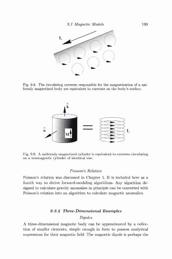
9.3 Magnetic Models 199
Fig. 9.8. The circulating currents responsible for the magnetization of a uni-formly magnetized body are equivalent to currents on the body's surface.
Fig. 9.9. A uniformly magnetized cylinder is equivalent to currents circulatingon a nonmagnetic cylinder of identical size.
Poisson's RelationPoisson's relation was discussed in Chapter 5. It is included here as afourth way to derive forward-mo deling algorithms. Any algorithm de-signed to calculate gravity anomalies in principle can be converted withPoisson's relation into an algorithm to calculate magnetic anomalies.
9.3.2 Three-Dimensional ExamplesDipoles
A three-dimensional magnetic body can be approximated by a collec-tion of smaller elements, simple enough in form to possess analyticalexpressions for their magnetic field. The magnetic dipole is perhaps the
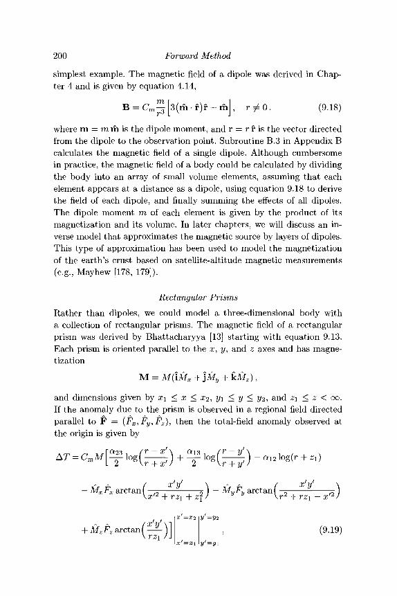
200 Forward Method
simplest example. The magnetic field of a dipole was derived in Chap-ter 4 and is given by equation 4.14,
(9.18)
where m = m m i s the dipole moment, and r = r f is the vector directedfrom the dipole to the observation point. Subroutine B.3 in Appendix Bcalculates the magnetic field of a single dipole. Although cumbersomein practice, the magnetic field of a body could be calculated by dividingthe body into an array of small volume elements, assuming that eachelement appears at a distance as a dipole, using equation 9.18 to derivethe field of each dipole, and finally summing the effects of all dipoles.The dipole moment m of each element is given by the product of itsmagnetization and its volume. In later chapters, we will discuss an in-verse model that approximates the magnetic source by layers of dipoles.This type of approximation has been used to model the magnetizationof the earth's crust based on satellite-altitude magnetic measurements(e.g., Mayhew [178, 179]).
Rectangular Prisms
Rather than dipoles, we could model a three-dimensional body witha collection of rectangular prisms. The magnetic field of a rectangularprism was derived by Bhattacharyya [13] starting with equation 9.13.Each prism is oriented parallel to the x, y, and z axes and has magne-tization
and dimensions given by x\ < x < X2-, y\ < y < 2/2, and z\ < z < oo.If the anomaly due to the prism is observed in a regional field directedparallel to F = (Fx,Fy,Fz), then the total-field anomaly observed atthe origin is given by
— MXFX arctanf —Vx/2
T 11~ ) — MVFV arctanf
z{ ) \r2
i 11
f\r2
)- x'2J
+ MZFZ arctanf )V rz\ /J
y =y
y'=yi
(9.19)
9.3 Magnetic Models 201
where
Equation 9.19 provides the total-field anomaly of a prism with top atZ\ and bottom at infinity. If this equation is evaluated twice, once forZ\ = zt and M = MQ and once for z\ = Zb and M = —Mo, thenaccording to the superposition principle, the sum of the two calculationswill provide the magnetic field of a prism with magnetization MQ, topat zt, and bottom at z^. Subroutine B.8 in Appendix B provides analgorithm to calculate equation 9.19.
By dividing the body into a collection of rectangular prisms, equa-tion 9.19 could be used to iteratively model bodies of arbitrary shape.Rectangular prisms have also been used in the inverse method to di-rectly derive vector M from the total-field anomaly (Vacquier [285]);more about this is given in Chapter 10.
Stack of Laminas
Talwani [275] used the volume integral of equation 9.12 to derive an al-gorithm for the calculation of magnetic fields due to bodies of arbitraryshape. His method and its derivation are analogous to the method ofTalwani and Ewing [276] for calculating gravity anomalies over three-dimensional bodies, discussed earlier in this chapter. The magnetic bodyis approximated by a stack of laminas, and each lamina is approximatedby a polygon. Hence the volume integral of equation 9.12 is solved ana-lytically in the x and y directions and numerically in the z direction. Themethod is particularly amenable to anomalies caused by topographic orbathymetric features because contours can be digitized directly from to-pographic or bathymetric maps in order to represent individual laminas.
Plouff [228, 229] extended the method of Talwani [275] by replacingthe infinitely thin laminas with layers of finite thickness, thereby provid-ing more accurate representation of the modeled body. The theoreticalexpression for the magnetic field of an individual polygonal layer wasderived (Plouff [228]) by integration with respect to depth of the fieldcaused by one lamina.
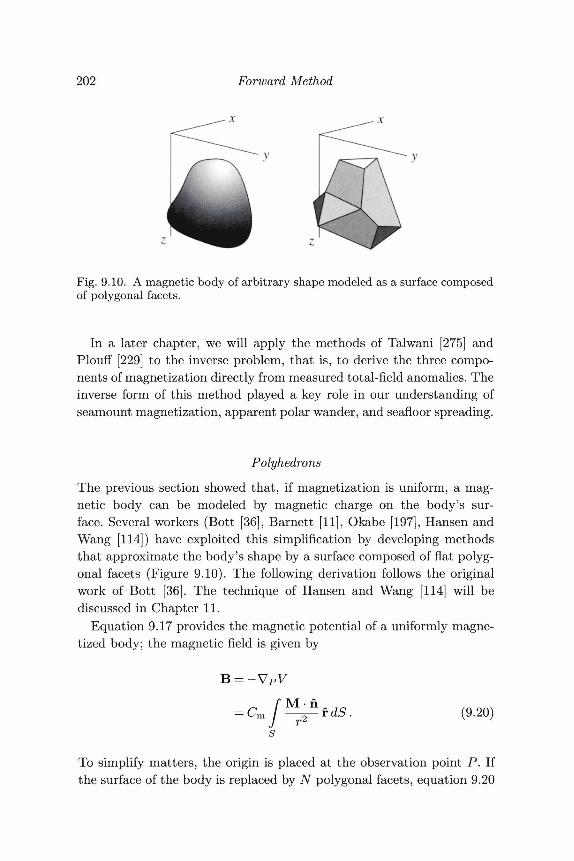
202 Forward Method
Fig. 9.10. A magnetic body of arbitrary shape modeled as a surface composedof polygonal facets.
In a later chapter, we will apply the methods of Talwani [275] andPlouff [229] to the inverse problem, that is, to derive the three compo-nents of magnetization directly from measured total-field anomalies. Theinverse form of this method played a key role in our understanding ofseamount magnetization, apparent polar wander, and seafloor spreading.
PolyhedronsThe previous section showed that, if magnetization is uniform, a mag-netic body can be modeled by magnetic charge on the body's sur-face. Several workers (Bott [36], Barnett [11], Okabe [197], Hansen andWang [114]) have exploited this simplification by developing methodsthat approximate the body's shape by a surface composed of flat polyg-onal facets (Figure 9.10). The following derivation follows the originalwork of Bott [36]. The technique of Hansen and Wang [114] will bediscussed in Chapter 11.
Equation 9.17 provides the magnetic potential of a uniformly magne-tized body; the magnetic field is given by
(9.20)
To simplify matters, the origin is placed at the observation point P. Ifthe surface of the body is replaced by N polygonal facets, equation 9.20
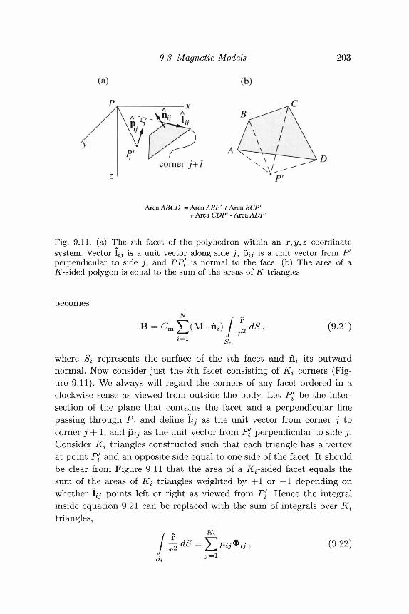
(a)
9.3 Magnetic Models
(b)
B
203
corner j+1
Area ABCD = Area ABP' + Area BCP'+ Area CDP' - Area ADP'
Fig. 9.11. (a) The zth facet of the polyhedron within an x,y,z coordinatesystem. Vector 1 - is a unit vector along side j , pij is a unit vector from P'perpendicular to side j , and PP( is normal to the face, (b) The area of aif-sided polygon is equal to the sum of the areas of K triangles.
becomesN
fi,) / ±I r (9.21)
where Si represents the surface of the zth facet and hi its outwardnormal. Now consider just the ith facet consisting of Ki corners (Fig-ure 9.11). We always will regard the corners of any facet ordered in aclockwise sense as viewed from outside the body. Let P[ be the inter-section of the plane that contains the facet and a perpendicular linepassing through P, and define 1 as the unit vector from corner j tocorner j + 1, and p^- as the unit vector from P[ perpendicular to side j .Consider Ki triangles constructed such that each triangle has a vertexat point P[ and an opposite side equal to one side of the facet. It shouldbe clear from Figure 9.11 that the area of a if^-sided facet equals thesum of the areas of Ki triangles weighted by +1 or —1 depending onwhether 1 points left or right as viewed from P[. Hence the integralinside equation 9.21 can be replaced with the sum of integrals over Kitriangles,
(9.22)
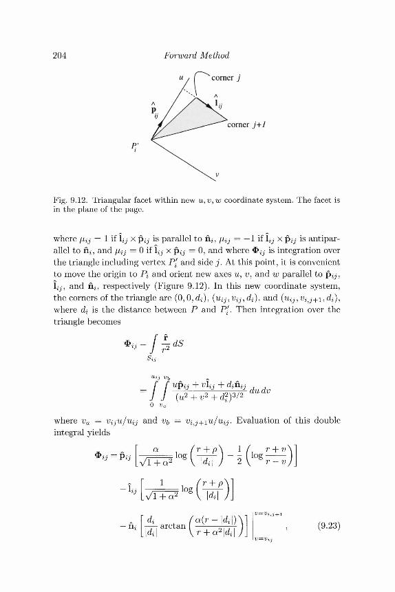
204 Forward Method
P:
corner j
corner j+1
Fig. 9.12. Triangular facet within new u,v,w coordinate system. The facet isin the plane of the page.
where \±ij = 1 if 1 - x p^- is parallel to fi , /i^- = — 1 if 1^ x p^- is antipar-allel to hi, and /x^ = 0 if 1^ x p^- = 0, and where <J> - is integration overthe triangle including vertex P[ and side j . At this point, it is convenientto move the origin to Pi and orient new axes u, v, and w parallel to p ^ ,1^, and hi, respectively (Figure 9.12). In this new coordinate system,the corners of the triangle are (0,0, d$), (uij, Vij, di), and (uij, ^i j+i , di),where di is the distance between P and P[. Then integration over thetriangle becomes
*« = dS
where va = Viju/uij and v^ — Viintegral yields
f f upij + vlij + dihij
= ] J (u2+,2 + rf|)3/2j . Evaluation of this double
- n (9.23)
9.3 Magnetic Models 205
where
p=Ju2ij+v2,
If P lies in the plane of the face, however, equation 9.23 becomes singular.This problem is treated by removing a small sector around P[ from thetriangle, with the result that
r + p 1 r +l og ~1T - 2 l o g 7=
where e is a small number. Equation 9.23 (or 9.24) is evaluated for eachside of the facet, transformed back to the original coordinate system, andsummed in equation 9.22. This result provides the attraction of facet iwhich then can be used in equation 9.21 for the entire polyhedron. Sub-routine B.10 in Appendix B uses equations 9.23 and 9.24 to calculatethe three components of magnetic field due to a polygonal sheet of mag-netic charge. The magnetic anomaly of an arbitrary polyhedron can befound with repeated calls to this subroutine, one call for each face of thepolyhedron.
9.3.3 Two-Dimensional ExampleWe again use the concept of surface magnetic charges, this time to de-velop an algorithm to model two-dimensional bodies. As in Section 9.2.2of this chapter, we will replace the cross-sectional shape of the bodywith an TV-sided polygon. If the body is uniformly magnetized, the mag-netization can be replaced with magnetic "charge" on its surface (Fig-ure 9.13). Hence, the problem reduces to the calculation of the magneticattraction of N flat ribbons of charge, infinitely extended in the + yand — y directions. Although this two-dimensional forward method wasfirst presented by Talwani and Heirtzler [277] nearly 20 years ago, it andits gravity counterpart (Talwani et al. [278]) probably remain the mostwidely used algorithms in potential field interpretation today.
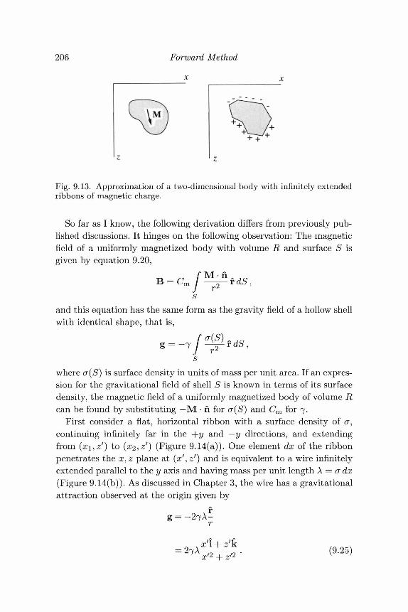
206 Forward Method
x
Fig. 9.13. Approximation of a two-dimensional body with infinitely extendedribbons of magnetic charge.
So far as I know, the following derivation differs from previously pub-lished discussions. It hinges on the following observation: The magneticfield of a uniformly magnetized body with volume R and surface S isgiven by equation 9.20,
Mn-cf rdS,
and this equation has the same form as the gravity field of a hollow shellwith identical shape, that is,
g = -^
where a(S) is surface density in units of mass per unit area. If an expres-sion for the gravitational field of shell S is known in terms of its surfacedensity, the magnetic field of a uniformly magnetized body of volume Rcan be found by substituting —M • h for o~(S) and Cm for 7.
First consider a flat, horizontal ribbon with a surface density of cr,continuing infinitely far in the +y and —y directions, and extendingfrom (xi,z') to (x2,zf) (Figure 9.14(a)). One element dx of the ribbonpenetrates the x, z plane at (V, zf) and is equivalent to a wire infinitelyextended parallel to the y axis and having mass per unit length A = a dx(Figure 9.14(b)). As discussed in Chapter 3, the wire has a gravitationalattraction observed at the origin given by
; = -2 7 A-r
x'\ + z'kr /2 yl2 (9.25)
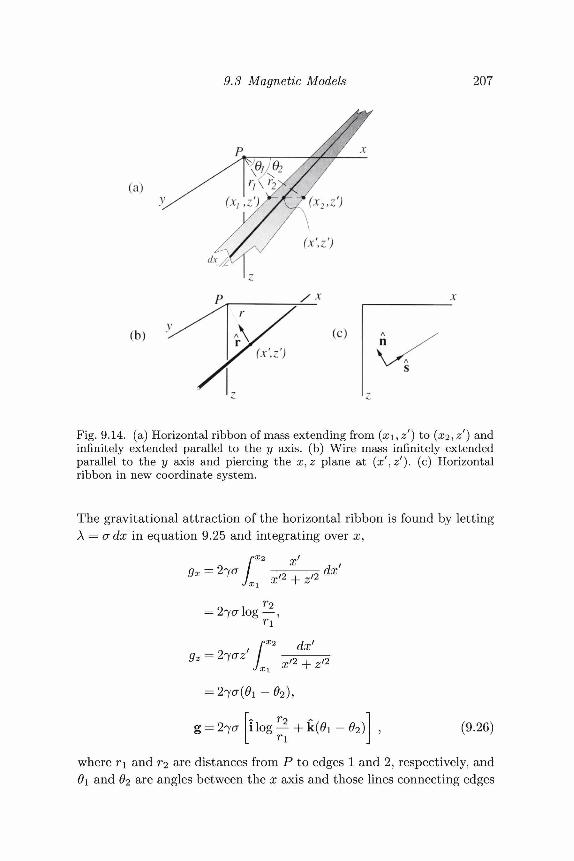
9.3 Magnetic Models 207
(a)
(b)
Fig. 9.14. (a) Horizontal ribbon of mass extending from (xi, z) to (x2, zf) andinfinitely extended parallel to the y axis, (b) Wire mass infinitely extendedparallel to the y axis and piercing the x,z plane at (x',zf). (c) Horizontalribbon in new coordinate system.
The gravitational attraction of the horizontal ribbon is found by lettingA = a dx in equation 9.25 and integrating over x,
= 27a log—,
gz = 2r)azr I — —Jx1
x + z
= 2<ya(01-02),
(9.26)
where r\ and T2 are distances from P to edges 1 and 2, respectively, and0i and 02 are angles between the x axis and those lines connecting edges
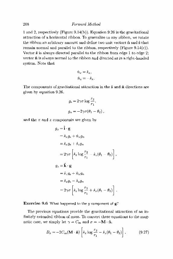
208 Forward Method
1 and 2, respectively (Figure 9.14(b)). Equation 9.26 is the gravitationalattraction of a horizontal ribbon. To generalize to any ribbon, we rotatethe ribbon an arbitrary amount and define two unit vectors fi and s thatremain normal and parallel to the ribbon, respectively (Figure 9.14(c)).Vector s is always directed parallel to the ribbon from edge 1 to edge 2;vector n is always normal to the ribbon and directed as in a right-handedsystem. Note that
nz = -sx.The components of gravitational attraction in the s and n directions aregiven by equation 9.26,
#s = 27crlog—,
gn = -21CJ{01 - 02),
and the x and z components are given by
9x = i • g= sxgs + nxgn
= sxgs + szgn
log ~-s*(0i-0
9z = k • g= szgs + hzgn
SxQn
log ^ + 5 ^ ( 0 1 -
Exercise 9.6 What happened to the y component of g?
The previous equations provide the gravitational attraction of an in-finitely extended ribbon of mass. To convert these equations to the mag-netic case, we simply let 7 = Cm and a — — M • n,
Bx = -2Cm(M • n) L log - 8,(0! - 02)j , (9.27)
9.3 Magnetic Models 209
Bz = -2Cm(M • n) L log Ty + a* (ft - 62) 1 . (9.28)
Exercise 9.7 Describe Bx and Bz for both horizontal and vertical ribbons.
Equations 9.27 and 9.28 represent the magnetic attraction of a ribbonof magnetic charge; they can be used N times to calculate the magneticattraction of an iV-sided prism, that is
NB = J2 (\Blx + kB,*) , (9.29)
i=i
where B\x and B\z are the x and z components of B due to side I. Finally,the total-field anomaly can be found by substituting equation 9.29 intoequation 8.24,
N
where Fx and Fz are the x and z components of the ambient, unper-turbed field.
The earlier comments concerning the advantages of two-dimensionalforward modeling of gravity anomalies hold doubly for the magneticcase. Two-dimensional models are far easier to construct than three-dimensional models, and they generally should be used whenever thegeologic situation permits. Subroutine B.15 in Appendix B performs thecalculations described by equations 9.27 and 9.28. The magnetic attrac-tion of an TV-sided prism at a single point can be calculated by summingthe results returned from N calls to this subroutine. Algorithms simi-lar to Subroutine B.15 are the essential ingredients in a variety of two-dimensional forward-modeling programs (e.g., Saltus and Blakely [251]).
As discussed in Section 9.22, the question of whether an anomalyis sufficiently linear to permit the two-dimensional approximation isproblematic. A useful variation on this two-dimensional method replacesthe infinitely extended prisms with prisms of finite length (Shuey andPasquale [256], Rasmussen and Pedersen [237], Cady [48]). This so-called 2 \-dimensional calculation comes in handy when the anomaliesare somewhat linear but depart substantially from two-dimensionality.The anomaly in the south-central part of Figure 9.5 is an example ofan anomaly that might suitably be treated with the 2^-dimensional ap-proach.
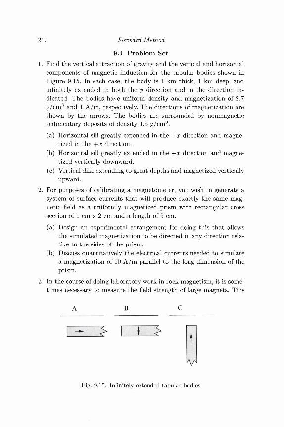
210 Forward Method
9.4 Problem Set1. Find the vertical attraction of gravity and the vertical and horizontal
components of magnetic induction for the tabular bodies shown inFigure 9.15. In each case, the body is 1 km thick, 1 km deep, andinfinitely extended in both the y direction and in the direction in-dicated. The bodies have uniform density and magnetization of 2.7g/cm3 and 1 A/m, respectively. The directions of magnetization areshown by the arrows. The bodies are surrounded by nonmagneticsedimentary deposits of density 1.5 g/cm3.(a) Horizontal sill greatly extended in the +x direction and magne-
tized in the +x direction.(b) Horizontal sill greatly extended in the -\-x direction and magne-
tized vertically downward.(c) Vertical dike extending to great depths and magnetized vertically
upward.2. For purposes of calibrating a magnetometer, you wish to generate a
system of surface currents that will produce exactly the same mag-netic field as a uniformly magnetized prism with rectangular crosssection of 1 cm x 2 cm and a length of 5 cm.(a) Design an experimental arrangement for doing this that allows
the simulated magnetization to be directed in any direction rela-tive to the sides of the prism.
(b) Discuss quantitatively the electrical currents needed to simulatea magnetization of 10 A/m parallel to the long dimension of theprism.
3. In the course of doing laboratory work in rock magnetism, it is some-times necessary to measure the field strength of large magnets. This
B
Fig. 9.15. Infinitely extended tabular bodies.
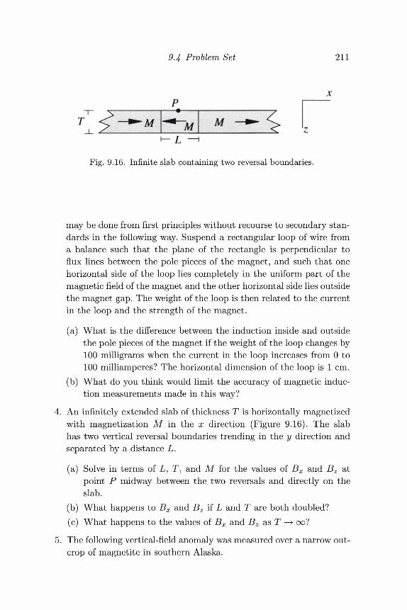
£
94 Problem Set 211
P•-
Mi - L —i
Fig. 9.16. Infinite slab containing two reversal boundaries.
may be done from first principles without recourse to secondary stan-dards in the following way. Suspend a rectangular loop of wire froma balance such that the plane of the rectangle is perpendicular toflux lines between the pole pieces of the magnet, and such that onehorizontal side of the loop lies completely in the uniform part of themagnetic field of the magnet and the other horizontal side lies outsidethe magnet gap. The weight of the loop is then related to the currentin the loop and the strength of the magnet.
(a) What is the difference between the induction inside and outsidethe pole pieces of the magnet if the weight of the loop changes by100 milligrams when the current in the loop increases from 0 to100 milliamperes? The horizontal dimension of the loop is 1 cm.
(b) What do you think would limit the accuracy of magnetic induc-tion measurements made in this way?
4. An infinitely extended slab of thickness T is horizontally magnetizedwith magnetization M in the x direction (Figure 9.16). The slabhas two vertical reversal boundaries trending in the y direction andseparated by a distance L.
(a) Solve in terms of L, T, and M for the values of Bx and Bz atpoint P midway between the two reversals and directly on theslab.
(b) What happens to Bx and Bz if L and T are both doubled?(c) What happens to the values of Bx and Bz as T —* oo?
5. The following vertical-field anomaly was measured over a narrow out-crop of magnetite in southern Alaska.
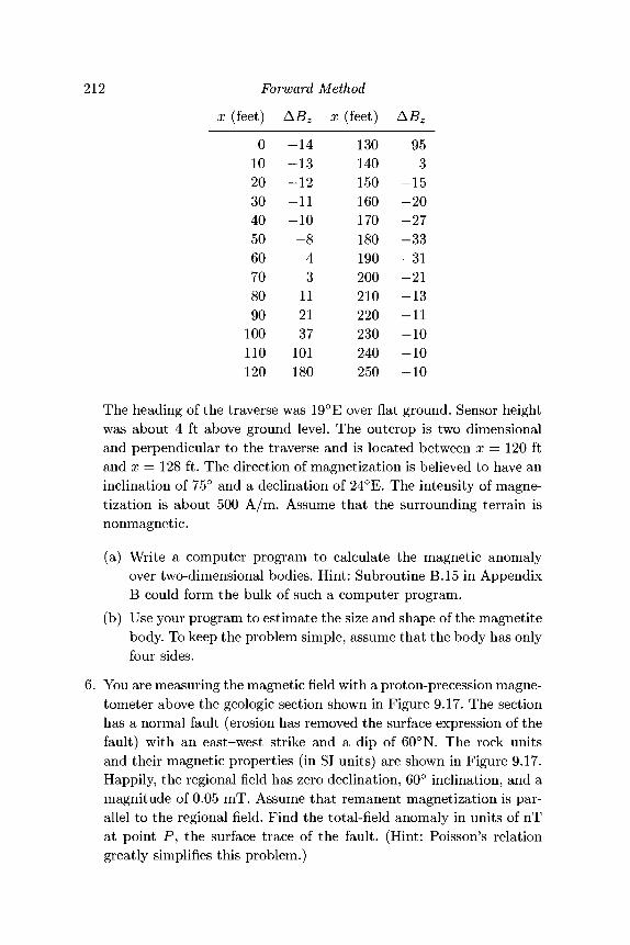
212 Forward
x (feet)
0102030405060708090100110120
ABZ
-14
-12-11-10-8-43112137101180
Method
x (feet)
130140150160170180190200210220230240250
ABZ
953
-15-20-27-33-31-21-13-11-10-10-10
The heading of the traverse was 19°E over flat ground. Sensor heightwas about 4 ft above ground level. The outcrop is two dimensionaland perpendicular to the traverse and is located between x = 120 ftand x = 128 ft. The direction of magnetization is believed to have aninclination of 75° and a declination of 24°E. The intensity of magne-tization is about 500 A/m. Assume that the surrounding terrain isnonmagnetic.
(a) Write a computer program to calculate the magnetic anomalyover two-dimensional bodies. Hint: Subroutine B.15 in AppendixB could form the bulk of such a computer program.
(b) Use your program to estimate the size and shape of the magnetitebody. To keep the problem simple, assume that the body has onlyfour sides.
6. You are measuring the magnetic field with a proton-precession magne-tometer above the geologic section shown in Figure 9.17. The sectionhas a normal fault (erosion has removed the surface expression of thefault) with an east-west strike and a dip of 60°N. The rock unitsand their magnetic properties (in SI units) are shown in Figure 9.17.Happily, the regional field has zero declination, 60° inclination, and amagnitude of 0.05 mT. Assume that remanent magnetization is par-allel to the regional field. Find the total-field anomaly in units of nTat point P, the surface trace of the fault. (Hint: Poisson's relationgreatly simplifies this problem.)
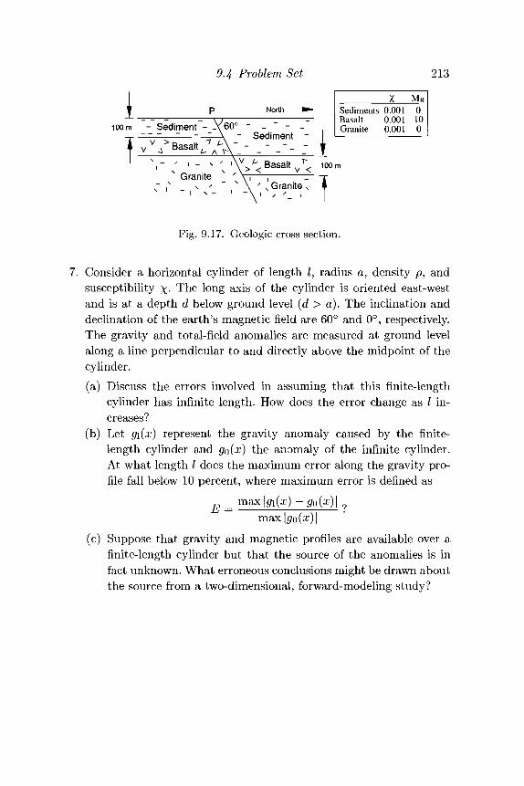
94 Problem Set 213
i.loom - Sediment - _y60° - -
^ — - " \ - Sediment -
v: ' - -v^^y^ lo
JC MRSediments 0.001 0Basalt 0.001 10Granite 0.001 0
Granitee _ ' \\ j — ~r' , \ ' N Granite x #
Fig. 9.17. Geologic cross section.
7. Consider a horizontal cylinder of length /, radius a, density p, andsusceptibility x- The long axis of the cylinder is oriented east-westand is at a depth d below ground level (d > a). The inclination anddeclination of the earth's magnetic field are 60° and 0°, respectively.The gravity and total-field anomalies are measured at ground levelalong a line perpendicular to and directly above the midpoint of thecylinder.(a) Discuss the errors involved in assuming that this finite-length
cylinder has infinite length. How does the error change as / in-creases?
(b) Let g\(x) represent the gravity anomaly caused by the finite-length cylinder and go(x) the anomaly of the infinite cylinder.At what length / does the maximum error along the gravity pro-file fall below 10 percent, where maximum error is defined as
i(x) - go(x)\ ?E = ?
max |go (x) |(c) Suppose that gravity and magnetic profiles are available over a
finite-length cylinder but that the source of the anomalies is infact unknown. What erroneous conclusions might be drawn aboutthe source from a two-dimensional, forward-modeling study?
10Inverse Method
The goal of inverse theory is to determine the parameters fromthe observations or, in the face of the inevitable limitations ofactual measurement, to find out as much as possible about them.
(Robert L. Parker)
Errors using inadequate data are much less than those using nodata at all.
(Charles Babbage)
Solid-earth geophysical studies generally aspire to learn something aboutthe interior of the earth from measurements of physical quantities takenon or above the earth's surface. The previous chapter in particular dis-cussed a general methodology, forward modeling, in which crustal andupper-mantle lithology and structure can be deduced from gravity ormagnetic measurements. In that methodology, source parameters areestimated indirectly through trial-and-error calculations. The presentchapter deals with another methodology, the inverse method (or directmethod), in which source parameters are determined in a direct wayfrom gravity or magnetic measurements.
The following discussion is sometimes heuristic in nature, relying onexamples from the literature. Readers are referred to reviews by Parker[207] and Parker, Shure, and Hildenbrand [210] and to the textbook byMenke [182] for more rigorous discussions. We will revisit this subjectin Chapter 11 where the inverse formulation will be transformed to theFourier wavenumber domain.
10.1 IntroductionIn Chapter 9, we became familiar with integral relations between po-tential fields and their causative sources. A few examples are listed
214
10.1 Introduction 215
subsequently, where in each case R is the volume occupied by the caus-ative source, P is the observation point located at (x,y,z) and alwaysoutside of R, Q is the point of integration (V, y', z') within R, and r isa vector directed from Q to P:
Vertical attraction of gravity
Z^-dv. (10.1)
Vertical magnetic field
BZ(P) = -Cm-^ jM(Q) • VQJ dv
R
Total-field anomaly (approximately)
AT(P) = -CmP • V P f M(Q)
= Cmj ^ P • [3(F • f)f - F] dv. (10.3)R
In these equations, p(Q) and M(Q) have the usual meaning of densityand magnetization, respectively. Unit vector F is in the direction ofthe unperturbed magnetic field, and unit vector k is directed verticallydown. Factors 7 and Cm are constants discussed in Chapters 3 and 4,respectively.
Exercise 10.1 Fill in the missing steps leading to equations 10.2 and 10.3.
Equations 10.2 and 10.3 both have the general form
f(P) = Js(Q)-G(P,Q)dv. (10.4)R
We may be willing to specify the directional behavior of the magneti-zation in some situations. It is sometimes assumed, for example, thatmagnetization is entirely induced by the ambient field. Then magneti-zation will be nearly unidirectional if susceptibility is isotropic and the
216 Inverse Method
magnetic survey is not too large. In these cases, we can let M(Q) =M(Q)M in equations 10.2 and 10.3 and move the unit vector into thebracketed term. Then all three equations, 10.1 through 10.3, have thesame general form
J ) d v , (10.5)
where f(P) is the potential field at P, s(Q) describes the physical quan-tity (density or magnetization) at Q, and ip(P,Q) is a function thatdepends on the geometric placement of observation point P and sourcepoint Q. Equation 10.5 is known as a Fredholm equation of the firstkind (Morse and Feshbach [188]). As in Section 2.3.2, we call ip(P,Q)and G(P, Q) Green's functions. The remaining comments of this sectionrefer to equation 10.5 but could be generalized readily to equation 10.4.
Equation 10.5 is a convenient vehicle with which to contrast the for-ward and inverse methods. The forward calculation is the calculation of/(P) from known or assumed functions s(Q) and ip(P,Q) and the vol-ume R. For any given calculation of equation 10.5, f(P) is completelydetermined with a complete knowledge of s(Q), t/i(P, Q), and R; that is,the forward calculation has a unique solution. The forward method, asdiscussed in Chapter 9, involves the repeated adjustment of s(Q) and R,calculation of / (P) , and comparison with measured values of the fielduntil the calculated field suitably "fits" the measured field. Althoughthe forward calculation is unique in a mathematical sense, a model formagnetic or gravity sources developed by way of the forward method is,of course, not unique. The inverse method, on the other hand, insertsmeasurements of / (P) directly into the left side of equation 10.5 andsolves for some aspect of s(Q) or R. Calculation of s(Q) is known as thelinear inverse problem, whereas calculation of some property of R is thenonlinear inverse problem.
First consider the linear problem. We could, for example, reformulateequation 10.5 as a matrix equation,
NS 3 ^ i = l , 2 , . . . , L , (10.6)
and if L > N use least squares to find the N values of Sj. This is notas simple as it seems. The first fundamental difficulty is the problemof nonuniqueness. Even if we knew /(P) precisely, we might not beable to determine a unique inverse solution for s(Q). Uniqueness can
10.1 Introduction 217
be determined by asking whether there are any nontrivial solutions fora(Q) in the equation
[ a(Q)i/j(P,Q)dv = O.R
If the answer is yes, then s(Q) is nonunique. The class of all a(Q) isknown as the annihilator for that particular kernel ^(P, Q) and volumeR (Parker [207]).
What can we do faced with limitations of nonuniqueness? There aretwo approaches: We could make simplifying assumptions about thesource. We might, for example, be willing to assume that magnetizationis uniform throughout the body or that the body is infinitely extendedin one direction. Such assumptions may reduce the number of permis-sible solutions, but the solution may still be nonuniquef and certainlywill be much simpler than reality. Nevertheless, this is the tack gener-ally taken in inverse studies. A second approach would be to attemptto find aspects about the source that are common to the entire infiniteset of solutions. For example, we might be able to determine the maxi-mum depth of burial of any realistic source. This leads to the theory ofideal bodies to be discussed subsequently. Regardless of which methodis favored, independent geologic and geophysical information should beemployed whenever possible to narrow the range of realistic solutions.
The second problem is instability. According to equation 10.5, the po-tential field at a single point depends on the entire source distribution. Infact, the potential field at a single point is a weighted average of all partsof the source, where the weighting function is ^(P, Q). In the languageof linear systems analysis, f(P) is a linear functional of s(Q). For allP ^ Q, ip(P,Q) is a smoothly varying function. Hence, f(P) is always"smoother" than s(Q) as long as P is outside the body. Consequently,the inverse problem of deriving s(Q) from equation 10.5 amounts to an"unsmoothing" of f(P). Small changes to f(P) cause large and unreal-istic variations in s(Q), and the solution is said to be unstable. Potentialfield inversion is notoriously unstable. There are ways to reduce the in-stability, as we will see in this and the next chapter, but only at theexpense of giving up information about the source.
f Unique solutions may exist for a given anomaly if enough assumptions are stated.Smith [264] showed, for example, that a gravity anomaly has only one possiblesolution if the density of the body is uniform, the body is finite in extent, andevery vertical line passes through the body at most one time.
218 Inverse Method
Exercise 10.2 Demonstrate that calculation of potential fields from equa-tion 10.5 is always a smoothing operation. Hint: Let f(P) be the verticalattraction of gravity and let s(Q) = po6(P — Q). What is the physicalmeaning of this s(Q)7
The third problem is one of construction. Inverse methods are madetractable by modeling the source distribution with simple geometries. Aparticular method may assume, for example, that the causative body iscomposed of simple parts, such as dipoles, line sources, or thin sheets,and we will discuss a number of techniques in the next sections that arehighly model dependent. Of course geology is never so simple, and ourresults almost certainly will be less than accurate.
10.2 Linear Inverse ProblemSome of the problems of the previous section are best demonstratedwith some examples from the geophysical literature. From equation 10.5,magnetic or gravity fields are linearly dependent on magnetization ordensity, and estimation of magnetization or density from magnetic orgravity fields is a linear inverse problem.
Estimation of a single best density for a given mass is a simple exam-ple. Equation 9.4 describes the vertical attraction of gravity for a bodyof uniform density. If the shape of the body is known, the integral termin this equation could be calculated by one of the forward techniquesof Chapter 9. The gravity anomaly measured at N discrete locations isthen
gi=pipi i = 1,2,..., AT,
and the constant p could be determined by simple linear regression.Plouff [229] and Ishihara [135] discuss this type of calculation in detail.
We could complicate this procedure by dividing the body into smallercompartments and use least-squares methods to solve for the density ofeach compartment. This approach is considered in the next section forthe magnetic case.
10.2.1 Magnetization of a LayerEarly attempts to model the magnetization of ocean crust with inversemethods (Bott [37], Bott and Hutton [39], Emilia and Bodvarsson [84])were motivated by an interest in seafloor spreading and how this dynamicprocess records geomagnetic field behavior. Magnetization was assumed
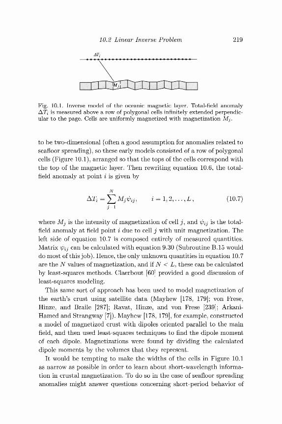
10.2 Linear Inverse Problem 219
AT,
Fig. 10.1. Inverse model of the oceanic magnetic layer. Total-field anomalyATi is measured above a row of polygonal cells infinitely extended perpendic-ular to the page. Cells are uniformly magnetized with magnetization Mj.
to be two-dimensional (often a good assumption for anomalies related toseafloor spreading), so these early models consisted of a row of polygonalcells (Figure 10.1), arranged so that the tops of the cells correspond withthe top of the magnetic layer. Then rewriting equation 10.6, the total-field anomaly at point i is given by
N
Y,MJ^Ji i = l , 2 , . . . , L , (10.7)
where Mj is the intensity of magnetization of cell j , and ipij is the total-field anomaly at field point i due to cell j with unit magnetization. Theleft side of equation 10.7 is composed entirely of measured quantities.Matrix ipij can be calculated with equation 9.30 (Subroutine B.15 woulddo most of this job). Hence, the only unknown quantities in equation 10.7are the N values of magnetization, and if N < L, these can be calculatedby least-squares methods. Claerbout [60] provided a good discussion ofleast-squares modeling.
This same sort of approach has been used to model magnetization ofthe earth's crust using satellite data (Mayhew [178, 179]; von Frese,Hinze, and Braile [287]; Ravat, Hinze, and von Frese [239]; Arkani-Hamed and Strangway [7]). Mayhew [178, 179], for example, constructeda model of magnetized crust with dipoles oriented parallel to the mainfield, and then used least-squares techniques to find the dipole momentof each dipole. Magnetizations were found by dividing the calculateddipole moments by the volumes that they represent.
It would be tempting to make the widths of the cells in Figure 10.1as narrow as possible in order to learn about short-wavelength informa-tion in crustal magnetization. To do so in the case of seafloor spreadinganomalies might answer questions concerning short-period behavior of
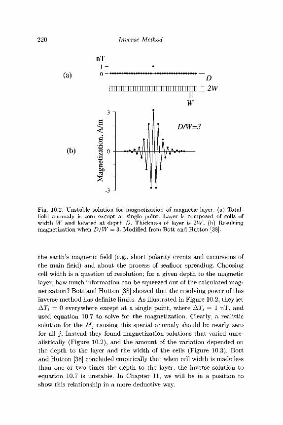
220 Inverse Method
(a)
(b)
nTl -
3 -|
DU~2W
Fig. 10.2. Unstable solution for magnetization of magnetic layer, (a) Total-field anomaly is zero except at single point. Layer is composed of cells ofwidth W and located at depth D. Thickness of layer is 2W'. (b) Resultingmagnetization when D/W — 3. Modified from Bott and Hutton [38].
the earth's magnetic field (e.g., short polarity events and excursions ofthe main field) and about the process of seafloor spreading. Choosingcell width is a question of resolution; for a given depth to the magneticlayer, how much information can be squeezed out of the calculated mag-netization? Bott and Hutton [38] showed that the resolving power of thisinverse method has definite limits. As illustrated in Figure 10.2, they letATi = 0 everywhere except at a single point, where ATi = 1 nT, andused equation 10.7 to solve for the magnetization. Clearly, a realisticsolution for the Mj causing this special anomaly should be nearly zerofor all j . Instead they found magnetization solutions that varied unre-alistically (Figure 10.2), and the amount of the variation depended onthe depth to the layer and the width of the cells (Figure 10.3). Bottand Hutton [38] concluded empirically that when cell width is made lessthan one or two times the depth to the layer, the inverse solution toequation 10.7 is unstable. In Chapter 11, we will be in a position toshow this relationship in a more deductive way.
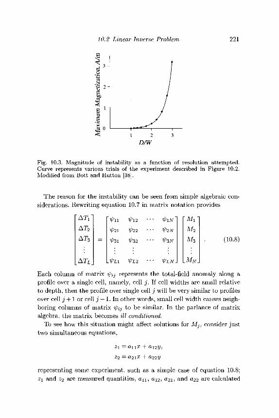
10.2 Linear Inverse Problem 221
D/W
Fig. 10.3. Magnitude of instability as a function of resolution attempted.Curve represents various trials of the experiment described in Figure 10.2.Modified from Bott and Hutton [38].
The reason for the instability can be seen from simple algebraic con-siderations. Rewriting equation 10.7 in matrix notation provides
AT2
AT3
ATL
0:21 022032
_0>L1 01
1plN~02JV
03AT
"Mi"M2
M3
-M.V.
(10.8)
Each column of matrix -0^ represents the total-field anomaly along aprofile over a single cell, namely, cell j . If cell widths are small relativeto depth, then the profile over single cell j will be very similar to profilesover cell j + 1 or cell j — 1. In other words, small cell width causes neigh-boring columns of matrix tpij to be similar. In the parlance of matrixalgebra, the matrix becomes ill conditioned.
To see how this situation might affect solutions for Mj , consider justtwo simultaneous equations,
Z2 = CI21X + CL22V
representing some experiment, such as a simple case of equation 10.8;z\ and Z2 are measured quantities, a n , a i 2 , a2i, and a22 are calculated
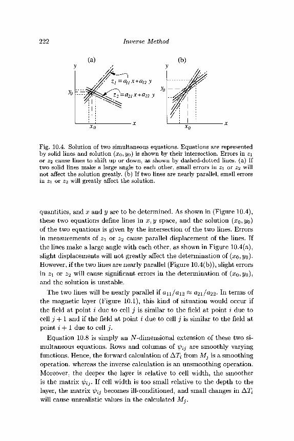
222 Inverse Method
Fig. 10.4. Solution of two simultaneous equations. Equations are representedby solid lines and solution (xo,2/o) is shown by their intersection. Errors in z\or Z2 cause lines to shift up or down, as shown by dashed-dotted lines, (a) Iftwo solid lines make a large angle to each other, small errors in z\ or z^ willnot affect the solution greatly, (b) If two lines are nearly parallel, small errorsin z\ or z<i will greatly affect the solution.
quantities, and x and y are to be determined. As shown in (Figure 10.4),these two equations define lines in x,y space, and the solution (xo>2/o)of the two equations is given by the intersection of the two lines. Errorsin measurements of Z\ or z2 cause parallel displacement of the lines. Ifthe lines make a large angle with each other, as shown in Figure 10.4(a),slight displacements will not greatly affect the determination of (x0, yo).However, if the two lines are nearly parallel (Figure 10.4(b)), slight errorsin z\ or z2 will cause significant errors in the determination of (xo,2/o),and the solution is unstable.
The two lines will be nearly parallel if an/a\2 ~ ^21/ 22- In terms ofthe magnetic layer (Figure 10.1), this kind of situation would occur ifthe field at point i due to cell j is similar to the field at point i due tocell j + 1 and if the field at point i due to cell j is similar to the field atpoint i + 1 due to cell j .
Equation 10.8 is simply an TV-dimensional extension of these two si-multaneous equations. Rows and columns of i/jij are smoothly varyingfunctions. Hence, the forward calculation of ATi from Mj is a smoothingoperation, whereas the inverse calculation is an unsmoothing operation.Moreover, the deeper the layer is relative to cell width, the smootheris the matrix ^ . If cell width is too small relative to the depth to thelayer, the matrix ipij becomes ill-conditioned, and small changes inwill cause unrealistic values in the calculated Mj.
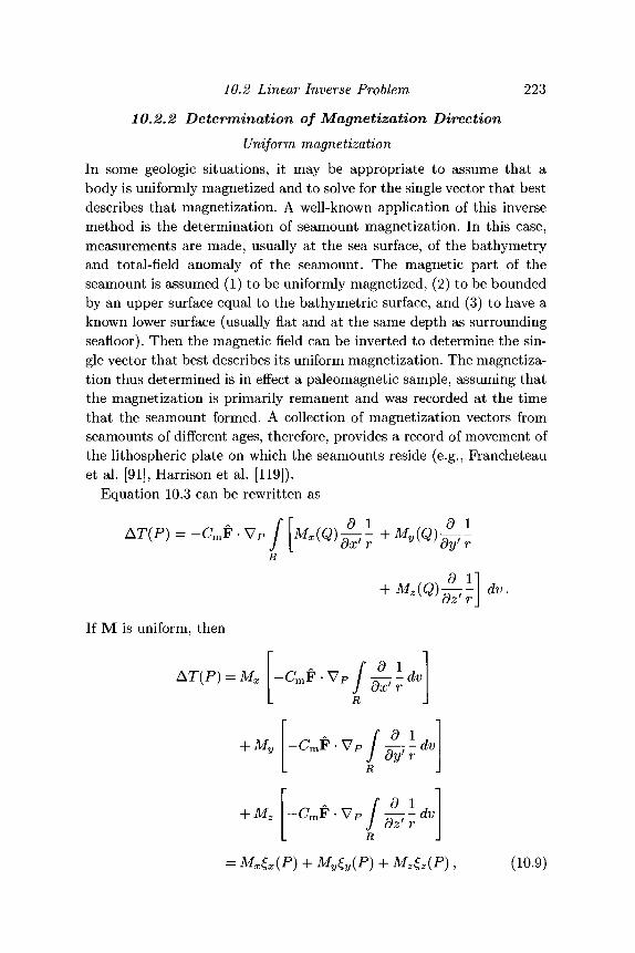
10.2 Linear Inverse Problem 223
10.2.2 Determination of Magnetization DirectionUniform magnetization
In some geologic situations, it may be appropriate to assume that abody is uniformly magnetized and to solve for the single vector that bestdescribes that magnetization. A well-known application of this inversemethod is the determination of seamount magnetization. In this case,measurements are made, usually at the sea surface, of the bathymetryand total-field anomaly of the seamount. The magnetic part of theseamount is assumed (1) to be uniformly magnetized, (2) to be boundedby an upper surface equal to the bathymetric surface, and (3) to have aknown lower surface (usually flat and at the same depth as surroundingseafloor). Then the magnetic field can be inverted to determine the sin-gle vector that best describes its uniform magnetization. The magnetiza-tion thus determined is in effect a paleomagnetic sample, assuming thatthe magnetization is primarily remanent and was recorded at the timethat the seamount formed. A collection of magnetization vectors fromseamounts of different ages, therefore, provides a record of movement ofthe lithospheric plate on which the seamounts reside (e.g., Francheteauet al. [91], Harrison et al. [119]).
Equation 10.3 can be rewritten as
AT(P) = - C m F • VP
If M is uniform, then
AT(P) = MX -CmF •r d 1
J dx' r dv
MV
+ MZ
- C m F • V P
-CmF•VP
J dyf rR
J dz1 r
dv
dv
(10.9)
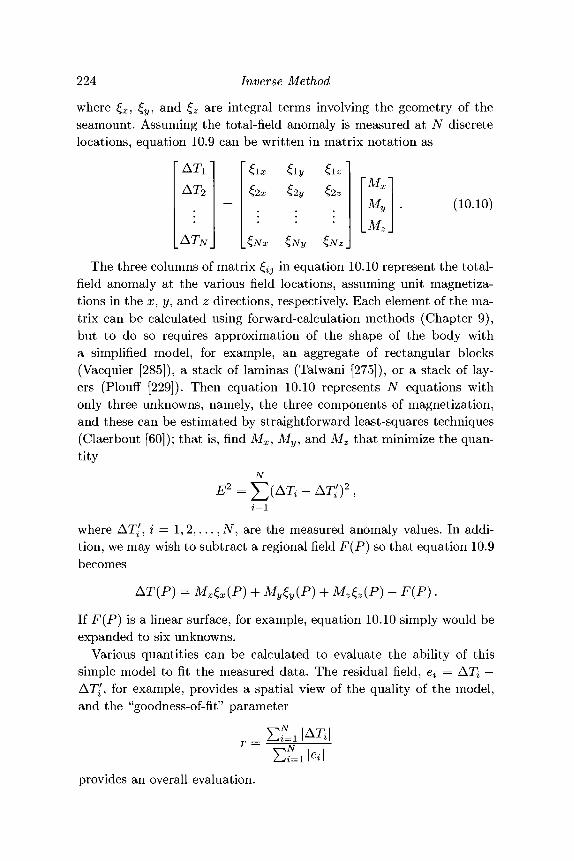
224 Inverse Method
AT2 i€NZ_
'Mx-My
.Mz.
where £x, £y, and £z are integral terms involving the geometry of theseamount. Assuming the total-field anomaly is measured at N discretelocations, equation 10.9 can be written in matrix notation as
(10.10)
The three columns of matrix ^ in equation 10.10 represent the total-field anomaly at the various field locations, assuming unit magnetiza-tions in the x, y, and z directions, respectively. Each element of the ma-trix can be calculated using forward-calculation methods (Chapter 9),but to do so requires approximation of the shape of the body witha simplified model, for example, an aggregate of rectangular blocks(Vacquier [285]), a stack of laminas (Talwani [275]), or a stack of lay-ers (Plouff [229]). Then equation 10.10 represents TV equations withonly three unknowns, namely, the three components of magnetization,and these can be estimated by straightforward least-squares techniques(Claerbout [60]); that is, find Mx, My, and Mz that minimize the quan-tity
NE2 =
2 = 1
where AT/, i = 1,2,..., TV, are the measured anomaly values. In addi-tion, we may wish to subtract a regional field F(P) so that equation 10.9becomes
AT(P) = MXUP) + MyZy(P) + MZUP) - F{P) •
If F(P) is a linear surface, for example, equation 10.10 simply would beexpanded to six unknowns.
Various quantities can be calculated to evaluate the ability of thissimple model to fit the measured data. The residual field, e$ = ATi —AT/, for example, provides a spatial view of the quality of the model,and the "goodness-of-fit" parameter
r =
provides an overall evaluation.
NN l e i=i le*l
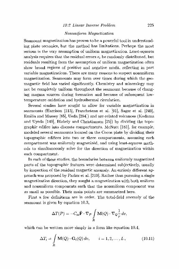
10.2 Linear Inverse Problem 225
Nonuniform MagnetizationSeamount magnetization has proven to be a powerful tool in understand-ing plate tectonics, but the method has limitations. Perhaps the mostserious is the very assumption of uniform magnetization. Least-squaresanalysis requires that the residual errors e* be randomly distributed, butresiduals resulting from the assumption of uniform magnetization oftenshow broad regions of positive and negative misfit, reflecting in partvariable magnetizations. There are many reasons to suspect nonuniformmagnetization. Seamounts may form over times during which the geo-magnetic field has varied significantly. Chemistry and mineralogy maynot be completely uniform throughout the seamount because of chang-ing magma sources during formation and because of subsequent low-temperature oxidation and hydrothermal circulation.
Several studies have sought to allow for variable magnetization inseamounts (Harrison [115], Francheteau et al. [91], Sager et al. [249],Emilia and Massey [85], Ueda [284]) and arc-related volcanoes (Kodamaand Uyeda [149], Blakely and Christiansen [25]) by dividing the topo-graphic edifice into discrete compartments. McNutt [181], for example,modeled several seamounts located on the Cocos plate by dividing theirtopographic edifices into two or three compartments, assuming eachcompartment was uniformly magnetized, and using least-squares meth-ods to simultaneously solve for the direction of magnetization withineach compartment.
In each of these studies, the boundaries between uniformly magnetizedparts of the topographic features were determined subjectively, usuallyby inspection of the residual magnetic anomaly. An entirely different ap-proach was proposed by Parker et al. [210]. Rather than pursuing a singlemagnetization direction, they sought a magnetization with both uniformand nonuniform components such that the nonuniform component wasas small as possible. Their main points are summarized here.
First a few definitions are in order. The total-field anomaly of theseamount is given by equation 10.3,
AT(P) = - C m F • V P f M(Q) • V Q 1 dv,R
which can be written more simply in a form like equation 10.4,
= jM(Q)-Gi(Q)dv, i = l,2,...,L, (10.11)R
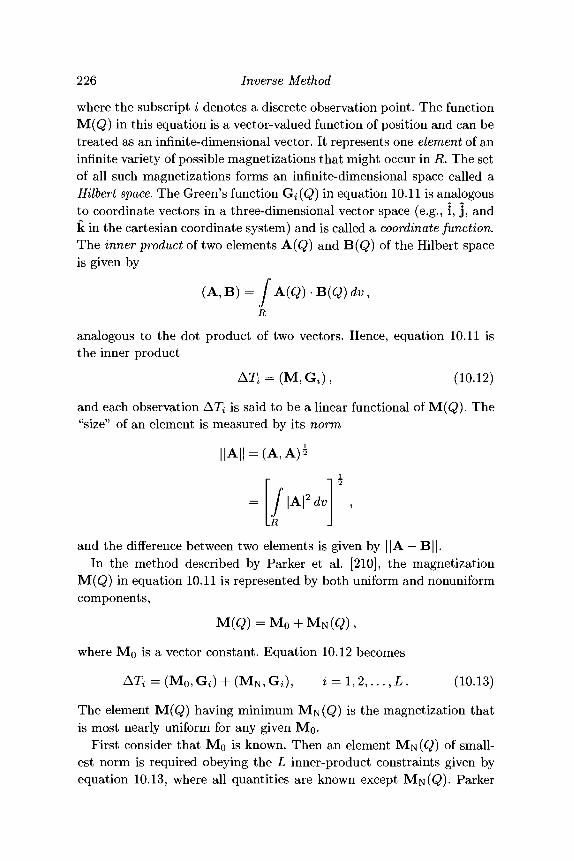
226 Inverse Method
where the subscript i denotes a discrete observation point. The functionM(Q) in this equation is a vector-valued function of position and can betreated as an infinite-dimensional vector. It represents one element of aninfinite variety of possible magnetizations that might occur in R. The setof all such magnetizations forms an infinite-dimensional space called aHilbert space. The Green's function G$(Q) in equation 10.11 is analogousto coordinate vectors in a three-dimensional vector space (e.g., i, j , andk in the cartesian coordinate system) and is called a coordinate function.The inner product of two elements A(Q) and B(Q) of the Hilbert spaceis given by
(A,B)= JA(Q).B(Q)dv,
analogous to the dot product of two vectors. Hence, equation 10.11 isthe inner product
ATi = (M,G i) , (10.12)
and each observation AT; is said to be a linear functional of M(Q). The"size" of an element is measured by its norm
/\A\2dv
and the difference between two elements is given by ||A — B||.In the method described by Parker et al. [210], the magnetization
M(Q) in equation 10.11 is represented by both uniform and nonuniformcomponents,
where MQ is a vector constant. Equation 10.12 becomes
AT, = (Mo, Gi) + (MN, G;), i = 1,2,..., L. (10.13)
The element M(Q) having minimum MN(Q) is the magnetization thatis most nearly uniform for any given Mo.
First consider that Mo is known. Then an element M N (Q) of small-est norm is required obeying the L inner-product constraints given byequation 10.13, where all quantities are known except M N ( Q ) . Parker
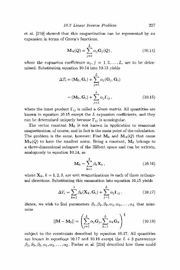
10.2 Linear Inverse Problem 227
et al. [210] showed that this magnetization can be represented by anexpansion in terms of Green's functions,
L
> G ; ( 3 ) , (10.14)
where the expansion coefficients OLJ, j — 1,2, . . . , L , are to be deter-mined. Subst i tut ing equation 10.14 into 10.13 yields
3 = 1
ajTij, (10.15)3=1
where the inner product F^- is called a Gram matrix. All quantities areknown in equation 10.15 except the L expansion coefficients, and theycan be determined uniquely because F^- is nonsingular.
The vector constant M o is not known in application to seamountmagnetization, of course, and in fact is the main point of the calculation.The problem is the same, however: Find M o and MN(Q) that causeM N ( Q ) to have the smallest norm. Being a constant, M o belongs toa three-dimensional subspace of the Hilbert space and can be written,analogously to equation 10.14, as
3
Mo = ^ A X , , (10.16)k=l
where X&, k = 1, 2,3, are unit magnetizations in each of three orthogo-nal directions. Substituting this summation into equation 10.15 yields
3 L
AT, = ^ ^ ( X , , G 2 ) + Y^aJTiJ • (10-17)fc=i j=i
Hence, we wish to find parameters /3i, /?2? ft, «i , c*2,..., OLL that mini-mize
( y||M-M0||= ^ ^ G ^ a A (10.18)
subject to the constraints described by equation 10.17. All quantitiesare known in equations 10.17 and 10.18 except the L + 3 parameters/5i)/?2>/?3? <^I?<^25 • • • 5 OLL- Parker et al. [210] described how these could
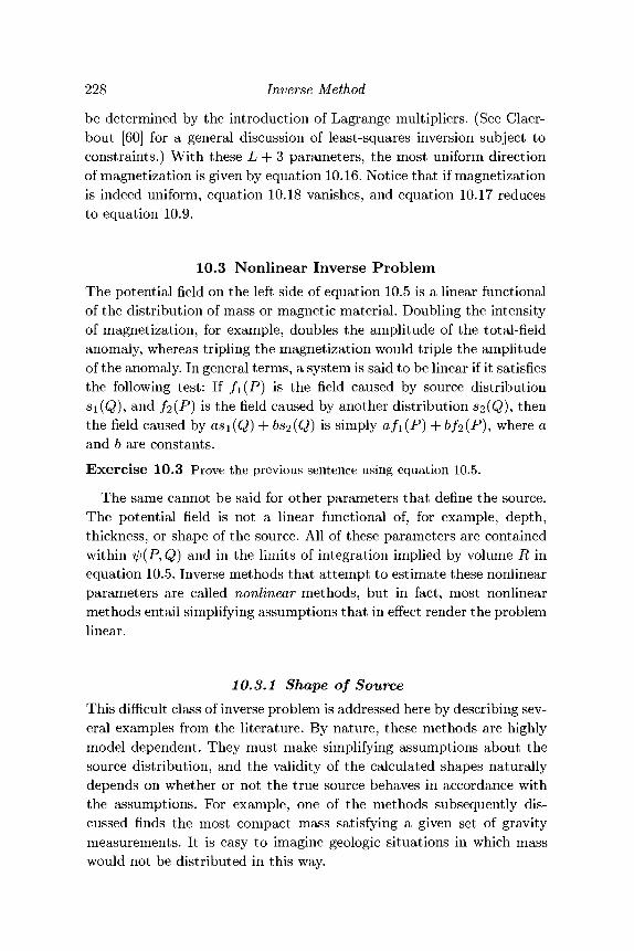
228 Inverse Method
be determined by the introduction of Lagrange multipliers. (See Claer-bout [60] for a general discussion of least-squares inversion subject toconstraints.) With these L + 3 parameters, the most uniform directionof magnetization is given by equation 10.16. Notice that if magnetizationis indeed uniform, equation 10.18 vanishes, and equation 10.17 reducesto equation 10.9.
10.3 Nonlinear Inverse ProblemThe potential field on the left side of equation 10.5 is a linear functionalof the distribution of mass or magnetic material. Doubling the intensityof magnetization, for example, doubles the amplitude of the total-fieldanomaly, whereas tripling the magnetization would triple the amplitudeof the anomaly. In general terms, a system is said to be linear if it satisfiesthe following test: If fi(P) is the field caused by source distributionsi(Q), and J2(P) is the field caused by another distribution 52(Q), thenthe field caused by as\(Q) + bs2(Q) is simply afi(P) + 6/2(P), where aand b are constants.Exercise 10.3 Prove the previous sentence using equation 10.5.
The same cannot be said for other parameters that define the source.The potential field is not a linear functional of, for example, depth,thickness, or shape of the source. All of these parameters are containedwithin ip(P,Q) and in the limits of integration implied by volume R inequation 10.5. Inverse methods that attempt to estimate these nonlinearparameters are called nonlinear methods, but in fact, most nonlinearmethods entail simplifying assumptions that in effect render the problemlinear.
10.3.1 Shape of SourceThis difficult class of inverse problem is addressed here by describing sev-eral examples from the literature. By nature, these methods are highlymodel dependent. They must make simplifying assumptions about thesource distribution, and the validity of the calculated shapes naturallydepends on whether or not the true source behaves in accordance withthe assumptions. For example, one of the methods subsequently dis-cussed finds the most compact mass satisfying a given set of gravitymeasurements. It is easy to imagine geologic situations in which masswould not be distributed in this way.
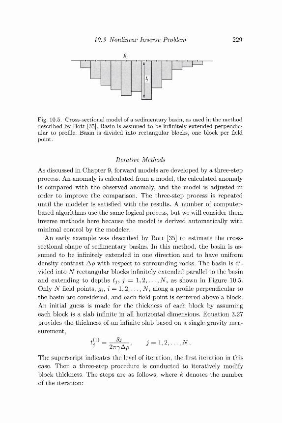
10.3 Nonlinear Inverse Problem 229
Fig. 10.5. Cross-sectional model of a sedimentary basin, as used in the methoddescribed by Bott [35]. Basin is assumed to be infinitely extended perpendic-ular to profile. Basin is divided into rectangular blocks, one block per fieldpoint.
Iterative MethodsAs discussed in Chapter 9, forward models are developed by a three-stepprocess. An anomaly is calculated from a model, the calculated anomalyis compared with the observed anomaly, and the model is adjusted inorder to improve the comparison. The three-step process is repeateduntil the modeler is satisfied with the results. A number of computer-based algorithms use the same logical process, but we will consider theminverse methods here because the model is derived automatically withminimal control by the modeler.
An early example was described by Bott [35] to estimate the cross-sectional shape of sedimentary basins. In this method, the basin is as-sumed to be infinitely extended in one direction and to have uniformdensity contrast Ap with respect to surrounding rocks. The basin is di-vided into N rectangular blocks infinitely extended parallel to the basinand extending to depths tj, j = 1, 2 , . . . , TV, as shown in Figure 10.5.Only N field points, g^ i — 1, 2 , . . . , AT, along a profile perpendicular tothe basin are considered, and each field point is centered above a block.An initial guess is made for the thickness of each block by assumingeach block is a slab infinite in all horizontal dimensions. Equation 3.27provides the thickness of an infinite slab based on a single gravity mea-surement,
The superscript indicates the level of iteration, the first iteration in thiscase. Then a three-step procedure is conducted to iteratively modifyblock thickness. The steps are as follows, where k denotes the numberof the iteration:
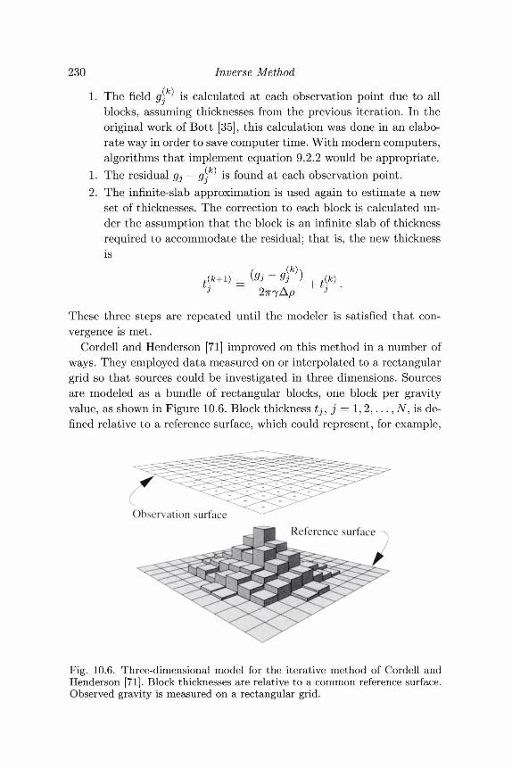
230 Inverse Method
The field g^ is calculated at each observation point due to allblocks, assuming thicknesses from the previous iteration. In theoriginal work of Bott [35], this calculation was done in an elabo-rate way in order to save computer time. With modern computers,algorithms that implement equation 9.2.2 would be appropriate.The residual gj — g^ is found at each observation point.The infinite-slab approximation is used again to estimate a newset of thicknesses. The correction to each block is calculated un-der the assumption that the block is an infinite slab of thicknessrequired to accommodate the residual; that is, the new thicknessis
+*Sfc
These three steps are repeated until the modeler is satisfied that con-vergence is met.
Cordell and Henderson [71] improved on this method in a number ofways. They employed data measured on or interpolated to a rectangulargrid so that sources could be investigated in three dimensions. Sourcesare modeled as a bundle of rectangular blocks, one block per gravityvalue, as shown in Figure 10.6. Block thickness t/, j = 1,2,..., JV, is de-fined relative to a reference surface, which could represent, for example,
Fig. 10.6. Three-dimensional model for the iterative method of Cordell andHenderson [71]. Block thicknesses are relative to a common reference surface.Observed gravity is measured on a rectangular grid.
10.3 Nonlinear Inverse Problem 231
the top or bottom of all blocks. Similar to the method of Bott [35], ini-tial block thickness is estimated by assuming each block to be an infiniteslab. However, the ratio
is used to revise block thickness rather than an infinite-slab approxima-tion. As before, the three-step procedure of calculation, comparison, andadjustment is carried out automatically at each iteration. This algorithmhas been implemented in a Fortran program described by Cordell [65],and a similar version is available in a form compatible with microcom-puters (Cordell, Phillips, and Godson [73]).
A somewhat different approach was described by Jachens and Mor-ing [137]. Like the two previous methods, their method estimates theshapes of basins filled with low-density deposits, but their method takesinto account the possibility that underlying basement rocks may havevariable density. Their method proceeds by separating gravity measure-ments into two components: the component caused by the basins them-selves and the component due to variations in density of underlyingbasement. Let g represent observed gravity after regional fields are re-moved (isostatic residual gravity (Chapter 7) would be an appropriatestarting point) and let g = #b + 9d, where g^ is the anomaly causedby underlying basement and g<\ is the anomaly caused by low-densitydeposits. Then the following steps are conducted:
1. The first iteration assumes that g^ is defined by just those stations lo-cated on basement outcrops and calculates a smooth surface throughjust these data, as shown by the dashed line in Figure 10.7. Thisconstitutes the first approximation g^ ' to the basement field g\>; it isonly a crude approximation because stations will still include the ef-fects of nearby basins. These effects are to be removed in subsequentiterations.
2. The first approximation to g^ is found by subtracting g^ from ob-served gravity g. This new residual gy is used to find a first ap-proximation to basement depth using the infinite slab approximation,similar to the method of Bott [35].
3. The gravitational effect of the basins can then be calculated by avariety of methods. Jachens and Moring [137] used the method ofParker [204], to be discussed in Chapter 11. This result is subtracted
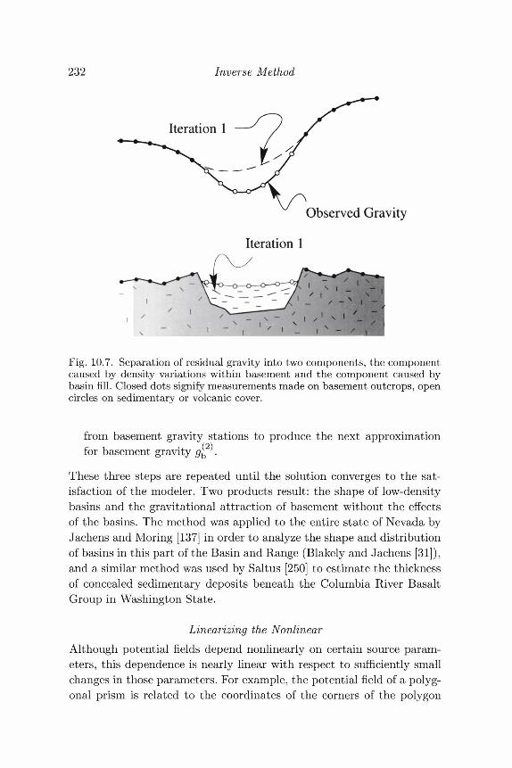
232 Inverse Method
Observed Gravity
Iteration 1
Fig. 10.7. Separation of residual gravity into two components, the componentcaused by density variations within basement and the component caused bybasin fill. Closed dots signify measurements made on basement outcrops, opencircles on sedimentary or volcanic cover.
from basement gravity stations to produce the next approximationfor basement gravity g^ .
These three steps are repeated until the solution converges to the sat-isfaction of the modeler. Two products result: the shape of low-densitybasins and the gravitational attraction of basement without the effectsof the basins. The method was applied to the entire state of Nevada byJachens and Moring [137] in order to analyze the shape and distributionof basins in this part of the Basin and Range (Blakely and Jachens [31]),and a similar method was used by Saltus [250] to estimate the thicknessof concealed sedimentary deposits beneath the Columbia River BasaltGroup in Washington State.
Linearizing the NonlinearAlthough potential fields depend nonlinearly on certain source param-eters, this dependence is nearly linear with respect to sufficiently smallchanges in those parameters. For example, the potential field of a polyg-onal prism is related to the coordinates of the corners of the polygon
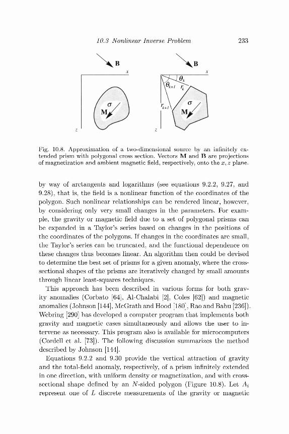
10.3 Nonlinear Inverse Problem 233
B
Fig. 10.8. Approximation of a two-dimensional source by an infinitely ex-tended prism with polygonal cross section. Vectors M and B are projectionsof magnetization and ambient magnetic field, respectively, onto the x, z plane.
by way of arctangents and logarithms (see equations 9.2.2, 9.27, and9.28), that is, the field is a nonlinear function of the coordinates of thepolygon. Such nonlinear relationships can be rendered linear, however,by considering only very small changes in the parameters. For exam-ple, the gravity or magnetic field due to a set of polygonal prisms canbe expanded in a Taylor's series based on changes in the positions ofthe coordinates of the polygons. If changes in the coordinates are small,the Taylor's series can be truncated, and the functional dependence onthese changes thus becomes linear. An algorithm then could be devisedto determine the best set of prisms for a given anomaly, where the cross-sectional shapes of the prisms are iteratively changed by small amountsthrough linear least-squares techniques.
This approach has been described in various forms for both grav-ity anomalies (Corbato [64], Al-Chalabi [2], Coles [62]) and magneticanomalies (Johnson [144], McGrath and Hood [180], Rao and Babu [236]).Webring [290] has developed a computer program that implements bothgravity and magnetic cases simultaneously and allows the user to in-tervene as necessary. This program also is available for microcomputers(Cordell et al. [73]). The following discussion summarizes the methoddescribed by Johnson [144].
Equations 9.2.2 and 9.30 provide the vertical attraction of gravityand the total-field anomaly, respectively, of a prism infinitely extendedin one direction, with uniform density or magnetization, and with cross-sectional shape defined by an TV-sided polygon (Figure 10.8). Let A{represent one of L discrete measurements of the gravity or magnetic
234 Inverse Method
anomaly. Both equations then have the form
Ai = A[x1^ z l 5 x 2 , £2, • • • i xNi zNi xi-> zi)-> i = 1,2,.
where (a^, zi) is the location of the ith measurement. The primed coor-dinates are the N corners of the polygon, represented in shorthand bythe 2N-dimensional array w. Array w includes only the body coordi-nates for the sake of discussion, but other parameters, such as density,the three components of magnetization, and parameters that describe aregional field, could be included as well. Furthermore, the following dis-cussion treats all corners of the polygon as free to move in any direction.A practical algorithm would have the flexibility to analyze only specifiedcorners.
Let Ai and Ai represent the observed and calculated anomalies, re-spectively, at one observation point. We wish to find the vector w suchthat the squared error
is as small as possible. Because Ai is a nonlinear function of w, we cannotuse the usual techniques of least-squares analysis. Instead, we will changethe elements of w only small amounts over a number of iterations. If thechanges in w are small, Ai will be nearly a linear function of thosechanges.
A Taylor's series is a convenient way to do this. For example, the valueof a function f(x,y) can be extrapolated to location (x + Ax, y + Ay)by the series
where the higher-order terms have been dropped because Ax and Ayare taken sufficiently small.
Similarly, we let w^ represent the values of (x[, z[, x2, zf2,..., xf
N, z'N)after the A:th iteration. Then, the Taylor's series expansion of the anomalyat point i is
2N f)Ai(w<fc)) + J2 a^ J *<( w ( f c ) ) A u # ) ' * = 1,2,..., L,
(10.20)
10.3 Nonlinear Inverse Problem 235
where Awin = ^m — Wm • Notice that ^ ( w ^ 1 ) ) is a linear func-tion of Awin , where m = 1,2,. . . , 27V, that is, we have "linearized" anonlinear problem.
Now substitute equation 10.20 into equation 10.19 to get
2N f) n 2
A. / 4 ( w ) 7 A • (
m=ldWrn
Expressions for Ai(w) have already been derived, namely, equations 9.2.2and 9.30, and we could just as easily derive expressions for their partialderivatives. Thus, given an initial array of parameters w^k\ the onlyunknowns in the above equation are Awm , rn = 1,2,. . . , 27V. To findthe set of these parameters that provides the smallest E2, we calculatethe partial derivative of E2 with respect to w^ j = 1, 2 , . . . , 27V, and seteach equation equal to zero:
2N o 1
E g ^ ) ^ ] [ i,(w»)] - o,
where again we have dropped higher-order terms. This complicated equa-tion is just a matrix expression of the form
2N
whereL r,
~ "* _ ^ . ( w ( * 0 ) (10.22)
The steps in the solution then are as follows:
1. Pick an initial set of corner coordinates w = (x/1,z/
lJx/2, z'2,...). The
foregoing discussion has assumed that all corners of the polygon arefree to move. In practice, most corners would be fixed and only a fewcorners allowed to move during a given calculation.
2. Calculate Ai(w^) and ^ - i i f w W ) for i = 1,2,... ,L and m =1,2,...,27V.
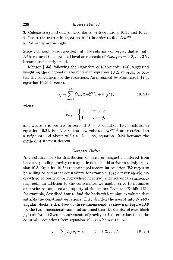
236 Inverse Method
3. Calculate ctj and Gmj in accordance with equations 10.22 and 10.23.4. Invert the matrix in equation 10.21 in order to find Aw^^.5. Adjust w accordingly.
Steps 2 through 5 are repeated until the solution converges, that is, untilE2 is reduced to a specified level or elements of Awm, m = 1,2,..., 2iV,become sufficiently small.
Johnson [144], following the algorithm of Marquardt [174], suggestedweighting the diagonal of the matrix in equation 10.21 in order to con-trol the convergence of the iterations. As discussed by Marquardt [174],equation 10.21 becomes
M
<*j = E GmjAw£>(l + SmjX), (10.24)
where_ f 0 , i f r a ^ j ;
and where A is positive or zero. If A = 0, equation 10.24 reduces toequation 10.21. For A > 0, the new values of w(fc+1) are restricted toa neighborhood about w^; as A —> oo, equation 10.24 becomes themethod of steepest descent.
Compact BodiesAny solution for the distribution of mass or magnetic material fromits corresponding gravity or magnetic field should strive to satisfy equa-tion 10.5. Equation 10.5 is the principal constraint equation. We may alsobe willing to add other constraints, for example, that density should ev-erywhere be positive (or everywhere negative) with respect to surround-ing rocks. In addition to the constraints, we might strive to minimizeor maximize some scalar property of the source. Last and Kubik [161],for example, described how to find the body with minimum volume thatsatisfies the constraint equations. They divided the source into N rect-angular blocks, either two- or three-dimensional, as shown in Figure 10.9for the two-dimensional case, and assumed that the density of each blockpj is uniform. Given measurements of gravity at L discrete locations, theconstraint equations from equation 10.5 can be written as
N
9i = Y2^JPj+ei' i = l ,2 , . . . ,L , (10.25)
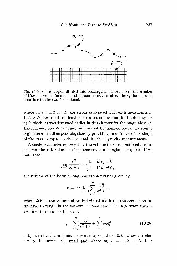
10.3 Nonlinear Inverse Problem 237
Fig. 10.9. Source region divided into rectangular blocks, where the numberof blocks exceeds the number of measurements. As shown here, the source isconsidered to be two-dimensional.
where e , i = 1, 2 , . . . , L, are errors associated with each measurement.If L > TV, we could use least-squares techniques and find a density foreach block, as was discussed earlier in this chapter for the magnetic case.Instead, we select TV > L, and require that the nonzero part of the sourceregion be as small as possible, thereby providing an estimate of the shapeof the most compact body that satisfies the L gravity measurements.
A single parameter representing the volume (or cross-sectional area inthe two-dimensional case) of the nonzero source region is required. If wenote that
"2 (0, ifft=0;
l l , iipj^O,lim
+°Pi
the volume of the body having nonzero density is given by
N
V = AV lim
where AV is the volume of an individual block (or the area of an in-dividual rectangle in the two-dimensional case). The algorithm then isrequired to minimize the scalar
N L
(10.26)
subject to the L constraints expressed by equation 10.25, where e is cho-sen to be sufficiently small and where w^i = 1,2,...,L, is a
238 Inverse Method
noise-weighting function. Last and Kubik [161] described an iterative,least-squares procedure to achieve such a solution while allowing theweights and densities to depend on the outcome of the previous itera-tion.
Hence, the solution minimizes both the volume of the body and aweighted sum of squared residuals. The TV values of pj will have bothzero and nonzero values. The nonzero cells within the source regionprovide an estimate of the shape of the most compact body satisfyingthe gravity measurements. Whether or not such a body is geologicallyreasonable is another matter; it is easy to imagine geological situations inwhich masses are not expected to be packed into the smallest of volumes.
10.3.2 Depth to SourceMethods of estimation of the depth to magnetic or gravity sources can beclassed into two categories: those that analyze a single, isolated anomalyand those that analyze a profile over many sources. A few examples ofeach type are described here. In the next chapter, we will visit the subjectagain in the Fourier domain.
Peters's MethodOne early and useful depth rule was described by Peters [219]. If a mag-netic anomaly is caused by a two-dimensional body with vertical sides,uniform and nearly vertical magnetization, and great depth extent, thenthe depth to the top of the body can be found approximately by the fol-lowing graphical procedure (Figure 10.10). Draw two parallel lines withslope equal to one half of the maximum gradient of the anomaly, oneline tangent to the peak of the anomaly and the other tangent to theminimum part of the anomaly. The horizontal separation of the two linesis proportional to the depth to the top of the body. The proportionalityconstant is 1.2 for very thin bodies and 2.0 for very thick bodies; a valueof 1.6 is often used.
Peters's method requires many simplifying assumptions about thebody (Skillbrei [262]). Yet it provides, with just graph paper and a pen-cil, a quick and rough estimate of depth to source in many geologicalsituations at high latitudes. It amounts to finding the horizontal dis-tance over which the anomaly is roughly a linear function of distance.Therefore, it is amenable to contour maps of gravity or magnetic anoma-lies; the distance over which the contours are roughly equally spaced isproportional to the depth to the source.
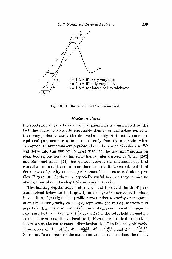
10.3 Nonlinear Inverse Problem 239
x = 1.2 d if body very thinx = 2.0 d if body very thickx= 1.6 d for intermediate thickness
'2a I
Fig. 10.10. Illustration of Peters's method.
Maximum DepthInterpretation of gravity or magnetic anomalies is complicated by thefact that many geologically reasonable density or magnetization solu-tions may perfectly satisfy the observed anomaly. Fortunately, some un-equivocal parameters can be gotten directly from the anomalies with-out appeal to numerous assumptions about the source distribution. Wewill delve into this subject in more detail in the upcoming section onideal bodies, but here we list some handy rules derived by Smith [263]and Bott and Smith [41] that quickly provide the maximum depth ofcausative sources. These rules are based on the first, second, and thirdderivatives of gravity and magnetic anomalies as measured along pro-files (Figure 10.11); they are especially useful because they require noassumptions about the shape of the causative body.
The limiting depths from Smith [263] and Bott and Smith [41] aresummarized below for both gravity and magnetic anomalies. In theseinequalities, A(x) signifies a profile across either a gravity or magneticanomaly. In the gravity case, A(x) represents the vertical attraction ofgravity. In the magnetic case, A(x) represents the component of magneticfield parallel to f = (rx,ry,rz) (e.g., if A(x) is the total-field anomaly, fis in the direction of the ambient field). Parameter d is depth to a planebelow which the entire source distribution lies. The following abbrevia-tions are used: A = A(x), A! — dA}*', A" — d j 4 ^ , and A!" = d j 4 ^ .
x ' CLX CLX ' CLX
Subscript "max" signifies the maximum value obtained along the x axis.
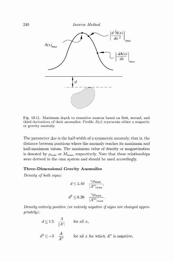
240 Inverse Method
d 2A(x)
A(x)
Fig. 10.11. Maximum depth to causative sources based on first, second, andthird derivatives of their anomalies. Profile A(x) represents either a magneticor gravity anomaly.
The parameter Aw is the half-width of a symmetric anomaly, that is, thedistance between positions where the anomaly reaches its maximum andhalf-maximum values. The maximum value of density or magnetizationis denoted by pmax or Mmax, respectively. Note that these relationshipswere derived in the emu system and should be used accordingly.
Three-Dimensional Gravity AnomaliesDensity of both signs:
d < 5.40\A"\
d2<6.26
A II
Density entirely positive (or entirely negative if signs are changed appro-priately):
d< 1.5 r—— for all x,I A |
< — 3 —- for all x for which A" is negative,
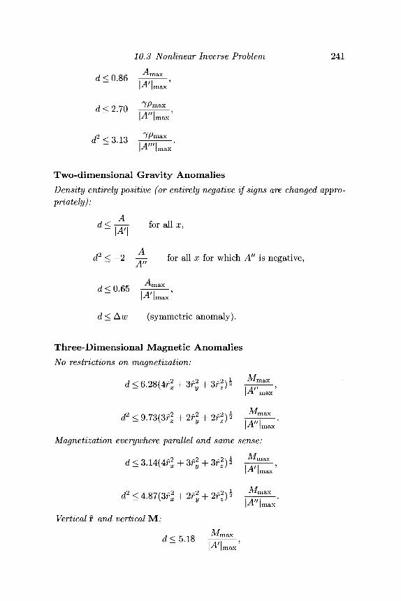
d<0.86
10.3 Nonlinear Inverse Problem 241
d<2.70 7 / WI A " '\J*- max
72 ^ o I o TPmaxI **• I max
Two-dimensional Gravity AnomaliesDensity entirely positive (or entirely negative if signs are changed appro-priately):
d < —— for all x,
d2 < —2 — for all x for which A" is negative,
d<0.65
AA
ax
d < Aw (symmetric anomaly).
Three-Dimensional Magnetic AnomaliesNo restrictions on magnetization:
| -ft- I max
Magnetization everywhere parallel and same sense:
Vertical f and vertical M:
1 | max
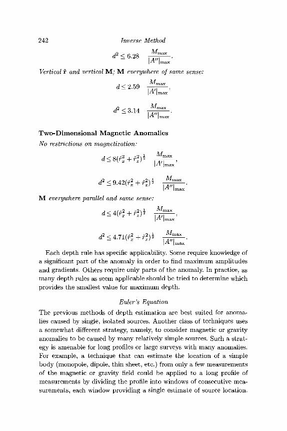
242 Inverse Method
— I An\I Si- | max
Vertical f and vertical M; M everywhere of same sense:
d<2.59 ^ L ,
d2<3.14 Mn
|i4"
Two-Dimensional Magnetic AnomaliesNo restrictions on magnetization:
d2 < 9A2(fl + f2z)
M everywhere parallel and same sense:
d2<4.71(f2x+r2)i
M m a x
\A' max
M m a x
^ max
n a xi
max
M m a x
\A"\I si |
Each depth rule has specific applicability. Some require knowledge ofa significant part of the anomaly in order to find maximum amplitudesand gradients. Others require only parts of the anomaly. In practice, asmany depth rules as seem applicable should be tried to determine whichprovides the smallest value for maximum depth.
Euler's EquationThe previous methods of depth estimation are best suited for anoma-lies caused by single, isolated sources. Another class of techniques usesa somewhat different strategy, namely, to consider magnetic or gravityanomalies to be caused by many relatively simple sources. Such a strat-egy is amenable for long profiles or large surveys with many anomalies.For example, a technique that can estimate the location of a simplebody (monopole, dipole, thin sheet, etc.) from only a few measurementsof the magnetic or gravity field could be applied to a long profile ofmeasurements by dividing the profile into windows of consecutive mea-surements, each window providing a single estimate of source location.
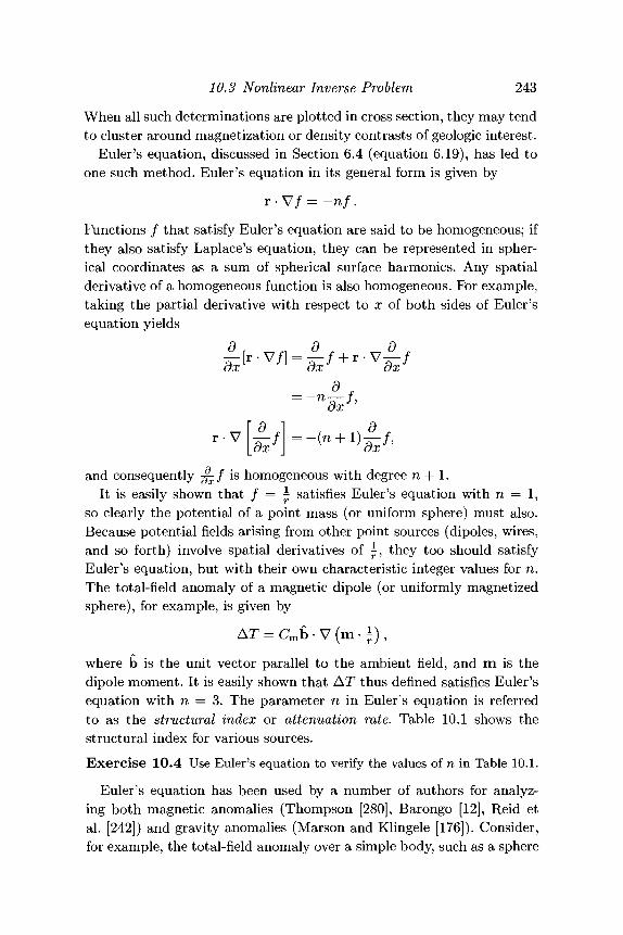
10.3 Nonlinear Inverse Problem 243
When all such determinations are plotted in cross section, they may tendto cluster around magnetization or density contrasts of geologic interest.
Euler's equation, discussed in Section 6.4 (equation 6.19), has led toone such method. Euler's equation in its general form is given by
r • V / = -nf .
Functions / that satisfy Euler's equation are said to be homogeneous; ifthey also satisfy Laplace's equation, they can be represented in spher-ical coordinates as a sum of spherical surface harmonics. Any spatialderivative of a homogeneous function is also homogeneous. For example,taking the partial derivative with respect to x of both sides of Euler'sequation yields
and consequently J^f is homogeneous with degree n + 1.It is easily shown that / = £ satisfies Euler's equation with n = 1,
so clearly the potential of a point mass (or uniform sphere) must also.Because potential fields arising from other point sources (dipoles, wires,and so forth) involve spatial derivatives of £, they too should satisfyEuler's equation, but with their own characteristic integer values for n.The total-field anomaly of a magnetic dipole (or uniformly magnetizedsphere), for example, is given by
where b is the unit vector parallel to the ambient field, and m is thedipole moment. It is easily shown that AT thus defined satisfies Euler'sequation with n = 3. The parameter n in Euler's equation is referredto as the structural index or attenuation rate. Table 10.1 shows thestructural index for various sources.Exercise 10.4 Use Euler's equation to verify the values of n in Table 10.1.
Euler's equation has been used by a number of authors for analyz-ing both magnetic anomalies (Thompson [280], Barongo [12], Reid etal. [242]) and gravity anomalies (Marson and Klingele [176]). Consider,for example, the total-field anomaly over a simple body, such as a sphere
244 Inverse Method
Table 10.1. "Structural index" for various gravityand magnetic sources.
n Type of Body
1 line of mass2 line of dipoles2 point mass (sphere of uniform density)3 point dipole (sphere of uniform magnetization)
or cylinder. Let ATi be the ith point of a magnetic survey over a sim-ple body, such as a sphere or cylinder, with the point of measurementat (x,y,z), and the center of the body at (#o?2/o>£())• Substituting intoequation 6.19 provides
ox oy
X
y_z
- %o~-yo- zo .
= nAT
Assuming we have some way of measuring or calculating horizontal andvertical gradients of the total-field anomaly, this equation has only fourunknowns: XQ, yo, zo, and n, the first three of which provide the locationof the body. We can obtain as many equations as necessary by writingthis equation for various measurement locations,
—ox
oy
oy
rp IT r\
y-yo_z - z0 _
— n\ATl]AT2
- ' -
and use least-squares methods to solve for the unknowns. If the positionof the body is known, we can solve for n and learn something about thekind of body involved (Barongo [12]). If on the other hand we suspect thenature of the body (e.g., we might believe that the body is spherical inshape), we can select an appropriate n and solve for the body's position.
Although Euler's equation provides a useful way to locate bodies ofideal shape, such as spheres and cylinders, the method has definite limi-tations when applied to more typical, distributed sources. In these morerealistic cases, n may not be a constant with respect to depth and po-sition of the source (Steenland [272]; LaFehr, as quoted by Steenland
10.3 Nonlinear Inverse Problem 245
[272]; Ravat [238]), because / is no longer simply a derivative of ^ butrather an integration over the entire source distribution. Reid et al. [242]showed that anomalies over certain extended bodies, such as thin dippingsheets, do satisfy Euler's equation, but such is not the case in general.Ravat [238] concluded that the method is strictly valid only when theanomaly has constant attenuation rate with respect to distance from thesource.
In spite of these theoretical limitations, Euler's method seems to pro-vide useful results in practical applications. Thompson [280] applied theEuler method to profile data. In this application, the source distributionis assumed to be two dimensional, and the derivative with respect to yis not needed. The profile is divided into groups of points, and a sourcelocation (x0, yo) is calculated for each group using the previous equationand least-squares methods. Source locations, when plotted in cross sec-tion, tend to cluster around presumed magnetization contrasts. Ratherthan solving for n simultaneously, Thompson [280] recommended speci-fying various values of n. Reid et al. [242] and Mar son and Klingele [176]expanded this general technique to two-dimensional magnetic and grav-ity surveys, respectively, over three-dimensional source distributions. Inthis case, the survey is divided into square, perhaps overlapping win-dows, and for a specified value of n, each window is analyzed for thelocation of a causative source.
It is clear that Euler's method requires not only the anomaly butalso its gradient in three directions. We might be fortunate enough tohave actual gradient measurements at our disposal (Hood [129]), butmore likely the gradients would have to be calculated from anomalymeasurements, a subject that is left until Section 12.2.
Werner DeconvolutionThe magnetic field of a thin sheetlike body has a very simple form thatdirectly depends in part on its location and depth. It is possible in princi-ple to estimate the location of the top of the body and its magnetizationfrom only four measurements of the total-field anomaly. A profile oftotal-field measurements over the body could be divided into groups offour or more measurements, each group providing an estimate of thesource location. When locations are plotted in cross section, individualdepth estimates tend to cluster around the true location of the sheetlikebody. If the true geologic section can be modeled appropriately by a col-lection of such bodies, then analyzing numerous groups of consecutivepoints along the profile may indicate their locations.
246 Inverse Method
This technique was discussed by Werner [291] and later implementedin a practical way by Hartman, Teskey, and Friedberg [120]. Groupsof consecutive points are treated as a "window" sliding along the pro-file. The method is similar in some respects to deconvolution in seis-mic interpretation, where seismic waves are transformed into impulsesrepresenting individual reflectors. Hence the method is called Wernerdeconvolution.
Vertical dikes may seem like a highly specialized application. How-ever, as shown by Hartman et al. [120] and Hansen and Simmonds [113],it is relatively straightforward to generalize the method to other hy-pothetical bodies. For example, the anomaly over a very thin dike isequivalent to the horizontal gradient of a semi-infinite half-space. (Proofof this relationship is left for the problem set at the end of this chapter.)Hence the horizontal gradient of the anomaly can be analyzed in pre-cisely the same way, thereby providing a way to detect abrupt offsets inmagnetic layers, as well as dikelike bodies. Klitgord and Behrendt [148]described an application of Werner deconvolution to a detailed aeromag-netic survey along the entire Atlantic seaboard of the United States. Kuand Sharp [150] combined the Werner deconvolution method with theMarquardt inversion scheme (discussed in a previous section) in orderto analyze the shapes of two-dimensional magnetic sources. An algo-rithm to perform Werner deconvolution on total-field data was writtenby L. Cordell and R. Godson and is available in a form suitable formicrocomputers (Cordell et al. [73]).
Ku and Sharp [150] provided an excellent discussion of Werner de-convolution, which is summarized here. A magnetic sheet of vanishingthickness is equivalent to a sheet of dipoles, as shown in Figure 10.12. Tofind the anomaly of a semi-infinite sheet, we begin with the equationsfor a single line of dipoles and integrate from depth d to infinity. Thehorizontal and vertical components of a horizontal line of dipoles aregiven by equations 5.18. Dipole moment per unit length m is equivalentto magnetization M times the cross-sectional area. We let the width ofthe sheet be Ax and let m = M Ax dz. The x and z components of themagnetic field due to a line of dipoles and observed at the origin thenare given by
^%\Mz(z'2-x'2)+2MxX'z>}dz>,,X + Z ) L J
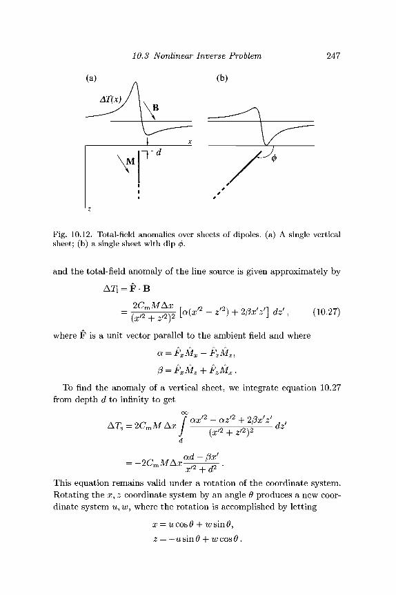
10.3 Nonlinear Inverse Problem
(a) „ (b)
AT(x)j
247
Fig. 10.12. Total-field anomalies over sheets of dipoles. (a) A single verticalsheet; (b) a single sheet with dip <j>.
and the total-field anomaly of the line source is given approximately by
ATi - F B
- P T S F [a{x'2 ~ z'2)+Wx'z'] dz'' (10-27)where F is a unit vector parallel to the ambient field and where
a = FxMx-FzMz,
To find the anomaly of a vertical sheet, we integrate equation 10.27from depth d to infinity to get
ATS = 2CmM Ax 1 OLXt2-OLZf2 + 2t3x'z' If/ M dz'J (xf2 + z'2)2
= -2CmMAxad - (3xf
This equation remains valid under a rotation of the coordinate system.Rotating the x, z coordinate system by an angle 0 produces a new coor-dinate system w, w, where the rotation is accomplished by letting
z — —u sin 9 + w cos 0 .
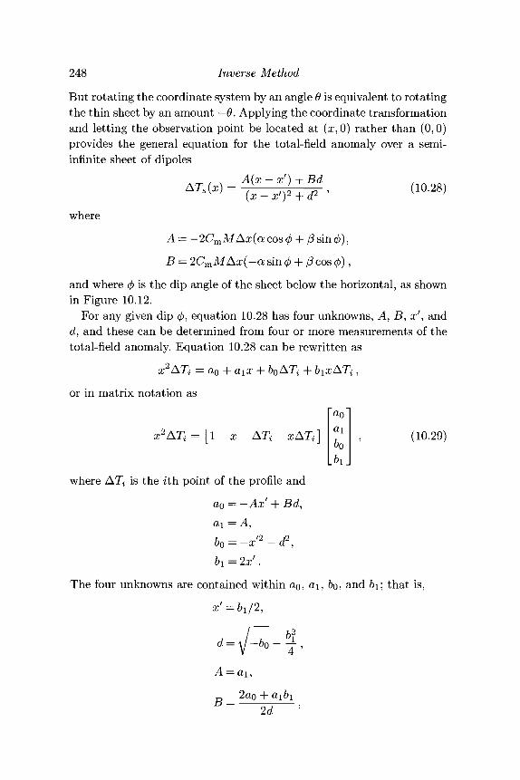
248 Inverse MethodBut rotating the coordinate system by an angle 9 is equivalent to rotatingthe thin sheet by an amount —9. Applying the coordinate transformationand letting the observation point be located at (x,0) rather than (0,0)provides the general equation for the total-field anomaly over a semi-infinite sheet of dipoles
_ A{x-x') + Bd(10-28)
where
A— -2CmMAx(a cos 04-/3 sin 0),B = 2CmMAx(-a sin 0 + (3cos 0),
and where <fi is the dip angle of the sheet below the horizontal, as shownin Figure 10.12.
For any given dip </>, equation 10.28 has four unknowns, A, B, x\ andd, and these can be determined from four or more measurements of thetotal-field anomaly. Equation 10.28 can be rewritten as
i = &o
or in matrix notation as
where
2ATZ=[1 x AT,
is the ith point of the profile and
ag = —Ax -\- Bd,
a0
L&iJ
(10.29)
^0 = — x'2 — d2,
h = 2xf.
The four unknowns are contained within ao, ai, 60, and 61; that is,
x; = 6i/2,
d=\/-6o-j,
A = <
B =2ao
2d
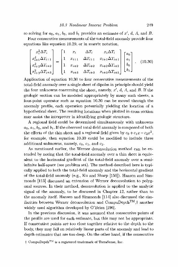
10.3 Nonlinear Inverse Problem 249
so solving for ao, ai, 60, and b\ provides an estimate of x', a7, A, and B.Four consecutive measurements of the total-field anomaly provide four
equations like equation 10.29, or in matrix notation,
s?+2AT i+2
a0
bo. (10.30)
Application of equation 10.30 to four consecutive measurements of thetotal-field anomaly over a single sheet of dipoles in principle should yieldthe four unknowns concerning the sheet, namely, x7, d, A, and B. If thegeologic section can be modeled appropriately by many such sheets, afour-point operator such as equation 10.30 can be moved through theanomaly profile, each operation potentially yielding the location of ahypothetical sheet. The resulting locations when plotted in cross sectionmay assist the interpreter in identifying geologic structure.
A regional field could be determined simultaneously with unknownsao, ai, 605
a nd 61. If the observed total-field anomaly is composed of boththe effects of the thin sheet and a regional field given by Co + c\x + c^x1,for example, then equation 10.30 could be modified to include threeadditional unknowns, namely, Co, ci, and c2.
As mentioned earlier, the Werner deconvolution method can be ex-tended by noting that the total-field anomaly over a thin sheet is equiv-alent to the horizontal gradient of the total-field anomaly over a semi-infinite half-space (see problem set). The method described here is typi-cally applied to both the total-field anomaly and the horizontal gradientof the total-field anomaly (e.g., Ku and Sharp [150]). Hansen and Sim-monds [113] discussed an extension of Werner deconvolution to polyg-onal sources. In their method, deconvolution is applied to the analyticsignal of the anomaly, to be discussed in Chapter 12, rather than tothe anomaly itself. Hansen and Simmonds [114] also discussed the sim-ilarities between Werner deconvolution and CompuDepth™,f anotherwidely used algorithm developed by O'Brien [196].
In the previous discussion, it was assumed that consecutive points ofthe profile are used for each estimate, but this may not be appropriate.If consecutive points are too close together relative to the depth to thebody, they may fall on relatively linear parts of the anomaly and lead todepth estimates that are too deep. On the other hand, if the consecutivef CompuDepth™ is a registered trademark of TerraSense, Inc.
250 Inverse Method
points are too far apart, they may sample more than one anomaly leadingto erroneous results. In practice, profiles can be analyzed numerous timeswith successive decimation of the measured total-field profile.
10.3.3 Ideal BodiesThe previous sections of this chapter discussed a variety of techniquesto find various details about source distributions from their gravity ormagnetic fields. These methods sometimes take a cavalier approach inconfronting the problems of nonuniqueness and model construction. Theiterative methods, for example, iterate until the calculated anomaly sat-isfies some measure of goodness of fit; the model is deemed successfulif it fits the geologic intuition of the modeler. Measures of goodness offit can be misleading. The Taylor's series method, for example, tries tofind the minimum squared error E2 in a multi-dimensional parameterspace w by changing the elements of w by small amounts. The methodmay converge rapidly to acceptably low levels of E2, but there is noguarantee that w will seek the true rather than a local minimum of E2.Moreover, there is no guarantee of uniqueness even if the fit is perfect.(The depth rules of the previous section are an exception; they providelimiting depths to the top of a body with only minor assumptions aboutthe body.)
Rather than attempting to find detailed information about the caus-ative source, we could look instead for fundamental properties that arecommon to the entire infinite set of reasonable sources. It should be clearthat such fundamental properties are available; the total excess mass of abody, for example, can be found from its gravity anomaly using Gauss'slaw (Chapter 3) with no assumptions about the shape or density ofthe mass.f "Reasonable" is, of course, a subjective term. A reasonablemass distribution, for example, would have a density distribution thatnowhere exceeds the greatest density contrast expected on the basis ofrock property studies.
Parker [205, 206] discussed how to find the greatest lower bound onmaximum density p\ consistent with a set of gravity measurements.If such a bound could be found, then every body that produces theobserved anomaly must somewhere have a density contrast equal toor greater than p\. This parameter is of some interest in itself. For
f But even this calculation has basic assumptions: The gravity anomaly must beisolated from the effects of all other sources, a difficult proposition in practicalapplications. See Grant and West [99] for further discussion on this calculation.
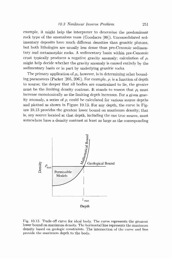
10.3 Nonlinear Inverse Problem 251
example, it might help the interpreter to determine the predominantrock type of the anomalous mass (Goodacre [98]). Unconsolidated sed-imentary deposits have much different densities than granitic plutons,but both lithologies are usually less dense than pre-Cenozoic sedimen-tary and metamorphic rocks. A sedimentary basin within pre-Cenozoiccrust typically produces a negative gravity anomaly; calculation of p\might help decide whether the gravity anomaly is caused entirely by thesedimentary basin or in part by underlying granitic rocks.
The primary application of ph however, is in determining other bound-ing parameters (Parker [205, 206]). For example, p\ is a function of depthto source; the deeper that all bodies are constrained to lie, the greatermust be the limiting density contrast. It stands to reason that p\ mustincrease monotonically as the limiting depth increases. For a given grav-ity anomaly, a series of p\ could be calculated for various source depthsand plotted as shown in Figure 10.13. For any depth, the curve in Fig-ure 10.13 provides the greatest lower bound on maximum density; thatis, any source located at that depth, including the one true source, mustsomewhere have a density contrast at least as large as the corresponding
&
Geological Bound
Fig. 10.13. Trade-off curve for ideal body. The curve represents the greatestlower bound on maximum density. The horizontal line represents the maximumdensity based on geologic constraints. The intersection of the curve and lineprovide the maximum depth to the body.
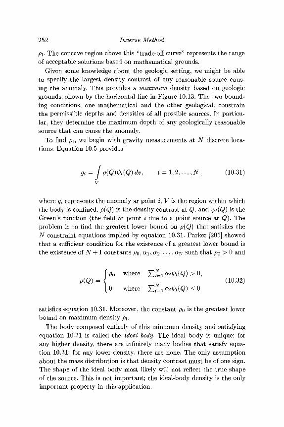
252 Inverse Method
p\. The concave region above this "trade-off curve" represents the rangeof acceptable solutions based on mathematical grounds.
Given some knowledge about the geologic setting, we might be ableto specify the largest density contrast of any reasonable source caus-ing the anomaly. This provides a maximum density based on geologicgrounds, shown by the horizontal line in Figure 10.13. The two bound-ing conditions, one mathematical and the other geological, constrainthe permissible depths and densities of all possible sources. In particu-lar, they determine the maximum depth of any geologically reasonablesource that can cause the anomaly.
To find pi, we begin with gravity measurements at TV discrete loca-tions. Equation 10.5 provides
9i = J P(Q)MQ) dv, i = 1, 2 , . . . , N , (10.31)
where gi represents the anomaly at point i, V is the region within whichthe body is confined, p(Q) is the density contrast at Q, and ^ (Q) is theGreen's function (the field at point i due to a point source at Q). Theproblem is to find the greatest lower bound on p(Q) that satisfies theTV constraint equations implied by equation 10.31. Parker [205] showedthat a sufficient condition for the existence of a greatest lower bound isthe existence of N + 1 constants po> ai, a2, • • • > < N such that po > 0 and
p0 where £ i l i c*Wi(Q) >0,p(Q) = { (10.32)
[0 where E J ^ a ^ C Q ) < 0
satisfies equation 10.31. Moreover, the constant po is the greatest lowerbound on maximum density p\.
The body composed entirely of this minimum density and satisfyingequation 10.31 is called the ideal body. The ideal body is unique; forany higher density, there are infinitely many bodies that satisfy equa-tion 10.31; for any lower density, there are none. The only assumptionabout the mass distribution is that density contrast must be of one sign.The shape of the ideal body most likely will not reflect the true shapeof the source. This is not important; the ideal-body density is the onlyimportant property in this application.
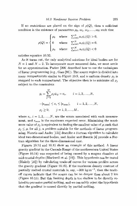
10.3 Nonlinear Inverse Problem 253
If no restrictions are placed on the sign of p(Q), then a sufficientcondition is the existence of parameters p0, a\, a2l..., aN such that
P(Q) =
where Y^iLi ai^i(Q) >
0 where $^=i air{
po where J2iLi ai^i(Q) < 0
satisfies equation 10.32.As it turns out, the only analytical solutions for ideal bodies are for
N = 1 and N — 2. To incorporate more measured data, we must settlefor an approximation. Parker [206] described how to use the techniquesof linear programming (e.g., Gass [93]). The source region is divided intomany compartments similar to Figure 10.9, and a uniform density pj isassigned to each compartment. The objective then is to minimize all pjsubject to the constraints
Mp^ij + eii i = 1, 2 , . . . , iV,
< \p i — 1 9 N
Pj>0,
where e , i = 1, 2 , . . . , JV, are the errors associated with each measure-ment, and emax is the maximum expected error. Minimizing the maxi-mum value of pj is equivalent to finding the smallest value of p\ such thatPj < P\ for all j , a problem suitable for the methods of linear program-ming. Huestis and Ander [131] describe a Fortran algorithm to calculateideal two-dimensional bodies, and Ander and Huestis [4] provide a For-tran algorithm for the three-dimensional case.
Figures 10.14 and 10.15 show an example of this method. A lineargravity gradient in the Cascade Range of the northwestern United States(Figure 10.14) was suspected of being caused by a magma chamber atmid-crustal depths (Blackwell et al. [19]). This hypothesis can be tested(Blakely [24]) by calculating trade-off curves for various profiles acrossthe gravity gradient (Figure 10.15). If the maximum density contrast ofpartially melted crustal materials is, say, —300 kg-m~3, then the trade-off curves indicate that the source can be no deeper than about 2 km(Figure 10.15). But this limiting depth is too shallow to be directly re-lated to pervasive partial melting, and we can safely reject the hypothesisthat the gradient is caused directly by partial melting.
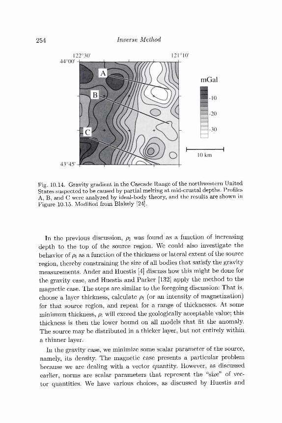
254 Inverse Method
122°30'44°00'
I2T10'
4} 4.S1
mGal
10 km
Fig. 10.14. Gravity gradient in the Cascade Range of the northwestern UnitedStates suspected to be caused by partial melting at mid-crustal depths. ProfilesA, B, and C were analyzed by ideal-body theory, and the results are shown inFigure 10.15. Modified from Blakely [24].
In the previous discussion, p\ was found as a function of increasingdepth to the top of the source region. We could also investigate thebehavior of p\ as a function of the thickness or lateral extent of the sourceregion, thereby constraining the size of all bodies that satisfy the gravitymeasurements. Ander and Huestis [4] discuss how this might be done forthe gravity case, and Huestis and Parker [132] apply the method to themagnetic case. The steps are similar to the foregoing discussion: That is,choose a layer thickness, calculate p\ (or an intensity of magnetization)for that source region, and repeat for a range of thicknesses. At someminimum thickness, p\ will exceed the geologically acceptable value; thisthickness is then the lower bound on all models that fit the anomaly.The source may be distributed in a thicker layer, but not entirely withina thinner layer.
In the gravity case, we minimize some scalar parameter of the source,namely, its density. The magnetic case presents a particular problembecause we are dealing with a vector quantity. However, as discussedearlier, norms are scalar parameters that represent the "size" of vec-tor quantities. We have various choices, as discussed by Huestis and
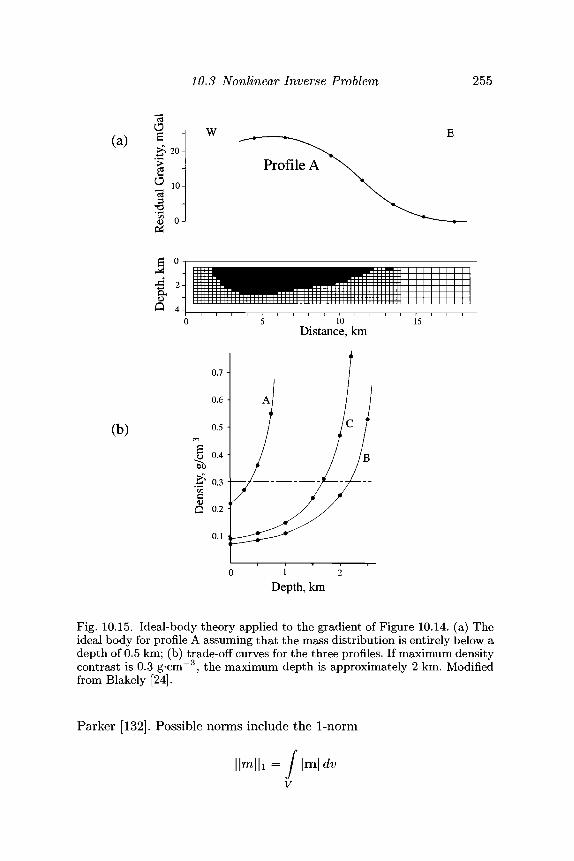
10.3 Nonlinear Inverse Problem 255
(a)o£> 20-
a 10
W
Profile A
(b)
n,
De
2 -
4 -0
m
a
Den
sity
,
0.7 -
0.6 -
0.5 •
0.4 •
0.3 -
0 .2 •
0.1 •
•lllllllllll5
/
/
^ ^
1 I 1 1 I I I 1 I 1 1 I I I I I I 1 W 4 # =
1 1 F " H l l l l l l l l l l l••---WM 1 1 1 1 1 I + H
10 15Distance, km
C f
/ B
Depth, km
Fig. 10.15. Ideal-body theory applied to the gradient of Figure 10.14. (a) Theideal body for profile A assuming that the mass distribution is entirely below adepth of 0.5 km; (b) trade-off curves for the three profiles. If maximum densitycontrast is 0.3 g-cm~3, the maximum depth is approximately 2 km. Modifiedfrom Blakely [24].
Parker [132]. Possible norms include the 1-norm
| dv
256 Inverse Method
used in this section, the 2-norm
/ •\m\\2 = / m • mdv
y
discussed earlier in Section 10.2.2, or the sup norm
ra oo = max m .x,z
10.4 Problem Set1. Suppose that you have N discrete measurements of the total-field
anomaly along a horizontal profile over a very thin, vertical dike.Assume that you know the direction of magnetization and the depthto the top of the dike.(a) Write the equations and describe an iterative scheme that uses
Taylor's series to find the depth extent of the dike.(b) Write a computer program that implements your scheme. Use
Subroutine B.15 in Appendix B, or one like it, to calculate thetotal-field anomaly over various thin, vertical dikes and use theseanomalies to test your algorithm.
2. The vertical magnetic field of a buried dipole is measured at fivelocations on the z = 0 plane as follows:
Coordinates, m
(0,0,0)(-10,0,0)(0,-10,0)(0,10,0)(10,0,0)
B*,nT
1730385285
20- 7 5
Assume that the dipole is located at coordinates (0,0,10) and calcu-late its inclination, declination, and magnitude in the sense of leastsquares.
3. Show that the following bodies satisfy the inequalities discussed inSection 10.3.2 of this chapter.(a) A sphere of radius a and uniform density p buried so that its
center is at a depth d (d > a).
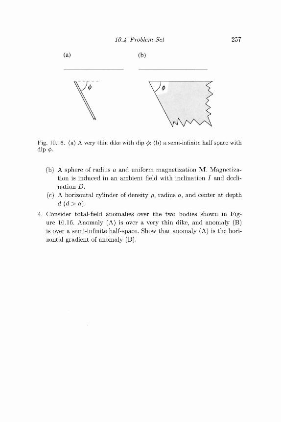
(a)
104 Problem Set
(b)
257
Fig. 10.16. (a) A very thin dike with dip 0; (b) a semi-infinite half space withdip 0.
(b) A sphere of radius a and uniform magnetization M. Magnetiza-tion is induced in an ambient field with inclination / and decli-nation D.
(c) A horizontal cylinder of density p, radius a, and center at depthd (d > a).
4. Consider total-field anomalies over the two bodies shown in Fig-ure 10.16. Anomaly (A) is over a very thin dike, and anomaly (B)is over a semi-infinite half-space. Show that anomaly (A) is the hori-zontal gradient of anomaly (B).
11Fourier-Domain Modeling
If your experiment needs statistics, you ought to have done a betterexperiment.
(Ernest Rutherford)
Fourier is a mathematical poem.(W. Thompson and P. G. Tait)
The relationship between the dominant wavelengths of a potential-fieldanomaly and the size, depth, and shape of its causative source was a con-tinuing theme of previous chapters. Figure 4.9, for example, shows thatthe width of an anomaly produced by a dipole is fundamentally relatedto the depth of the dipole. It stands to reason that Fourier analysis, amethodology that maps functions of space (or time) into functions ofwavenumber (or frequency), might provide insights into the relationshipbetween potential fields and causative sources. We will see, for example,that Fourier transformation of the gravity or magnetic anomaly causedby a layered source immediately separates the anomaly into two multi-plicative factors: a function that describes the depth and thickness of thelayer and a function that describes the distribution of density or magne-tization within the layer. The source distribution can be determined inthis case, at least in principle, by simply dividing the Fourier transformof the anomaly by a simple function that depends on the depth andthickness of the layer.
Tsuboi and Fuchida [282, 283] were apparently the earliest to applyFourier analysis to the interpretation of potential-field anomalies; theyused Fourier series to show the relationship between gravity anoma-lies and mass distributions, both two and three dimensional, confinedto horizontal planes. In the 1960s, a number of authors used Fourieranalysis in the interpretation of marine magnetic anomalies, notably
258
11.1 Notation and Review 259
Gudmundsson [106,107], Heirtzler and Le Pichon [122], and Neidell [195].Harrison [116] has provided a good review of this general topic. At aboutthe same time, Bhattacharyya published several key papers [14, 15, 16]on Fourier analysis of gravity and magnetic anomalies. Perhaps his mostsignificant contribution in this regard [16] was his recognition that manyoperations, such as upward continuation and reduction to the pole, arerelatively simple linear relationships in the Fourier domain.
We begin here with a brief review of Fourier transforms and linearsystems analysis, and then derive the Fourier transforms of anomaliescaused by simple sources, such as dipoles, monopoles, and line sources.These simple Fourier transforms provide a foundation for the treatmentof more complicated magnetic and gravity sources.
11.1 Notation and ReviewA brief review of Fourier analysis and linear systems analysis is presentedhere. For more complete discussions, the interested reader is referred totextbooks by Lee [162], Bracewell [42], and Papoulis [202].
11.1.1 Fourier TransformMost textbooks devoted to Fourier analysis focus on functions of time.Consequently they employ time-related terms such as "frequency," "pe-riod," and "time domain." In this chapter, however, we will be concernedprimarily with the analysis of functions of distance, such as the behav-ior of gravity or magnetic fields as measured on specified surfaces. Tominimize confusion, we will use terms relevant to functions of distance(e.g., wavenumber, wavelength, space domain) and reserve time-relatedterms for when temporal analogies are required.
The Fourier series was discussed briefly in Chapter 6. In short, a peri-odic function can be synthesized by an infinite sum of weighted sinusoids,where the weights of the sinusoids are determined through analysis ofthe periodic function. For example, if f(x) is a function that repeatsitself over an interval X, it can be represented as
/(*)= £ Fneik«x, (11.1)
260 Fourier-Domain Modeling
where kn — ^ p and i = y^T. The weights Fn in this summation arecomplex numbers and can be determined with the integral
xo+X
I f(x)e-ik^dx. (11.2)
Exercise 11.1 Show that equation 11.1 and equation 6.1 are equivalentrepresentations of /(#), where Fn = | (an — ibn).
Now suppose that f(x) does not repeat itself over a finit: segment ofthe x axis. Instead we require that f(x) be reasonably well behaved andhave its variation confined to a finite-length segment of the x axis. Inother words, we will require that
oo
/\f(x)\dx < oo. (11.3)
It stands to reason that gravity and magnetic anomalies satisfy this prop-erty if the survey extends well beyond the lateral extent of all causativebodies. Then letting X —> oo in equation 11.2 provides the Fourier trans-form of an aperiodic function /(#),
oo
F{k)= / f{x)e~lkxdx. (11.4)
Exercise 11.2 Use Gauss's law to show that gravity and magnetic anomaliesmeasured along a horizontal profile satisfy inequality 11.3, given that allsources are restricted to a localized region below the profile.
The variable k in equation 11.4 is called wavenumber and has units ofinverse distance; it is analogous to angular frequency in time-domainFourier transforms, which has units of inverse time. Wavenumber is in-versely related to wavelength A, that is,
Notice from equation 11.4 that the Fourier transform of a function f(x)evaluated at k = 0 is simply the average of f(x) over the entire x axis,that is,
oo
F(0)= I f{x)dx.
11.1 Notation and Review 261
The Fourier transform F(k) is, in general, a complex function withreal and imaginary parts, that is, F(k) = ReF(k) + iImF(k). It also canbe written as
F(k) = \F(k)\ei@ik\
where
ImF(k)
The functions \F(k)\ and 0(fc) are called the amplitude and phase spec-trum, respectively. The total energy of f(x) is given by
oo
E= I \F{k)\2dx,
and \F(k)\2 is called the energy-density spectrum.Of particular importance is the fact that the Fourier transform has
an inverse operation. Analogous to equation 11.1, the inverse Fouriertransform is given by
oo
f{x) = — [ F(k)eikxdk. (11.5)2?r J
— oo
If f(x) satisfies inequality 11.3, then the Fourier transform F(k) existsand satisfies both equations 11.4 and 11.5.
The discussion thus far has dealt with a function of one variable, butthe Fourier transform can be extended easily to functions of two vari-ables. The Fourier transform of f(x, y) and its inverse Fourier transform,for example, are given by
oo oo
F(kx, ky)= J j f(x, y)e-i^+kyy^ dx dy, (11.6)— oo —oo
oo oo
f(x,y) = -^ [ f F(kx,ky)ei^+kyy)dkxdky, (11.7)" J J
— oo —oo
where kx and ky are inversely related to wavelengths in the x and ydirections, respectively: kx = 2TT/XX and ky = 2TT/Xy.
It is important to note that f(x) and F(k) are simply different ways of
262 Fourier-Domain Modeling
looking at the same phenomenon. The Fourier transform maps a functionfrom one domain (space or time) into another domain (wavenumber orfrequency). Consequently, the following discussion will refer to the spacedomain and the Fourier domain as two different frameworks to view thesame phenomenon.
In the remainder of this chapter and in the subsequent chapter, theFourier transform of a function f(x) will sometimes be denoted by theshorthand notation •?•*[/], that is,
oo
f{x)e~lkxdx.
11.1.2 Properties of Fourier TransformsThe Fourier transform has a number of important properties that willbe particularly useful in later discussions and derivations. Some of theseproperties are described subsequently. The proofs are straightforwardand left to the exercises. As a shorthand notation in the following,f(x) <-> F(k) should be read "f(x) has a Fourier transform given byF{k).n
Symmetries
If f(x) <-> F(k), and if fix) is a real function, then F(k) has a realpart that is symmetric and an imaginary part that is antisymmetricabout k — 0; that is, if f(x) is real, then F(k) — F*(—k), where theasterisk denotes complex conjugation, and the Fourier transform of areal function is said to be Hermitian. Moreover, if F(k) — F*(—k),then f[x) must be a real function; that is, the Hermitian property is anecessary and sufficient condition for fix) to be real.
Linearity
The Fourier transform is a linear operation. For example, if fi(x) <-•Fi(k) and f2(x) <-> F2(k), then
x) + a2f2(x)} <-> [aiFi(fc) + a2F2{k)) ,
where a\ and a2 are arbitrary constants.
11.1 Notation and Review 263
Scaling
I f / O ) <-> F(k), then
where a is an arbitrary constant. This implies that the x interval con-taining most of the energy of f(x) is inversely related to the bandwidthcontaining most of the energy of F(k). In terms of gravity or magneticanomalies, the scaling property shows that a broad anomaly will have anarrower amplitude spectrum than will a narrow anomaly. Because thewidth of an anomaly is directly related to the depth of its source, wecan expect that the narrowness of a Fourier-transformed anomaly alsowill be related to depth of source.
ShiftingShifting a function along the x axis in the space domain is equivalent toadding a linear phase factor to the function's Fourier transform; that is,if f(x) <->F(ifc), then
f(x - x0) <-> F(k)e-ixok .
Note that the amplitude spectrum and the energy-density spectrum off(x) are unaffected by a shift of f{x) along the x axis.
DifferentiationDifferentiation of a function in the space domain is equivalent to multi-plication by a power of wavenumber in the Fourier domain. For example,if f(x) <->F(Jfe), then
f()(ik)^ (11.8)
If the function depends on two variables and if / (# , y) <-> F(kx, ky), then
£Jp ky). (11.9)We will have much use for this theorem in subsequent discussions.Exercise 11.3 Prove each of the preceding properties (symmetry, linearity,
scaling, shifting, and differentiation). In each case, start with the definingequations 11.4 and 11.6.
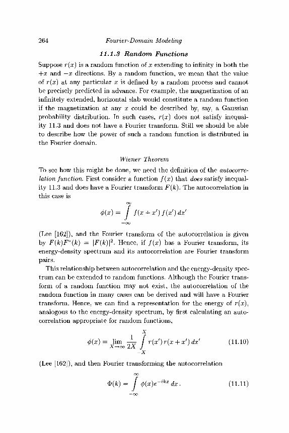
264 Fourier-Domain Modeling
11.1.3 Random FunctionsSuppose r(x) is a random function of x extending to infinity in both the-\-x and —x directions. By a random function, we mean that the valueof r(x) at any particular x is defined by a random process and cannotbe precisely predicted in advance. For example, the magnetization of aninfinitely extended, horizontal slab would constitute a random functionif the magnetization at any x could be described by, say, a Gaussianprobability distribution. In such cases, r(x) does not satisfy inequal-ity 11.3 and does not have a Fourier transform. Still we should be ableto describe how the power of such a random function is distributed inthe Fourier domain.
Wiener TheoremTo see how this might be done, we need the definition of the autocorre-lation function. First consider a function f(x) that does satisfy inequal-ity 11.3 and does have a Fourier transform F(k). The autocorrelation inthis case is
CXJ
= f f(x + x')f{x')dx'
(Lee [162]), and the Fourier transform of the autocorrelation is givenby F(k)F*(k) — \F(k)\2. Hence, if f(x) has a Fourier transform, itsenergy-density spectrum and its autocorrelation are Fourier transformpairs.
This relationship between autocorrelation and the energy-density spec-trum can be extended to random functions. Although the Fourier trans-form of a random function may not exist, the autocorrelation of therandom function in many cases can be derived and will have a Fouriertransform. Hence, we can find a representation for the energy of r(x),analogous to the energy-density spectrum, by first calculating an auto-correlation appropriate for random functions,
x(j){x)= lim — r(xf)r(x + x')dx' (11.10)
x^oo 2X J-x
(Lee [162]), and then Fourier transforming the autocorrelation
= I <f){x)e-ikx dx . (11.11)
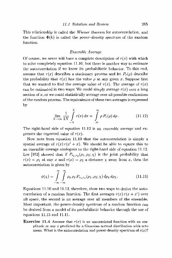
11.1 Notation and Review 265
This relationship is called the Wiener theorem for autocorrelation, andthe function $(fc) is called the power-density spectrum of the randomfunction.
Ensemble AverageOf course, we never will have a complete description of r(x) with whichto solve completely equation 11.10, but there is another way to estimatethe autocorrelation if we know its probabilistic behavior. To this end,assume that r(x) describes a stationary process and let Pr{p) describethe probability that r(x) has the value p at any given x. Suppose firstthat we wanted to find the average value of r(x). The average of r(x)can be estimated in two ways: We could simply average r(x) over a longsection of x, or we could statistically average over all possible realizationsof the random process. The equivalence of these two averages is expressedby
X oo
lim ^- f r{x)dx= f pPr(p)dp. (H-12)x^oo 2X J J
-X -ooThe right-hand side of equation 11.12 is an ensemble average and ex-presses the expected value of r(x).
Now note from equation 11.10 that the autocorrelation is simply aspatial average of r(x)r(x' + x). We should be able to equate this toan ensemble average analogous to the right-hand side of equation 11.12.Lee [162] showed that if Pr1,r2(pi,p2\x) is the joint probability thatr(x) — p\ at any x and r(x) = P2 & distance x away from x, then theautocorrelation is given by
oo oo
</>(Y) = / / Pi P2 Pri roipli P2'i'X) dpidpo . (11.13)
J J— oo —oo
Equations 11.10 and 11.13, therefore, show two ways to derive the auto-correlation of a random function. The first averages r(x) r(x + xr) overall space, the second is an average over all members of the ensemble.Most important, the power-density spectrum of a random function canbe derived from a model of its probabilistic behavior through the use ofequations 11.13 and 11.11.Exercise 11.4 Assume that r(x) is an uncorrelated function with an am-
plitude at any x predicted by a Gaussian normal distribution with zeromean. What is the autocorrelation and power-density spectrum of r(x)l
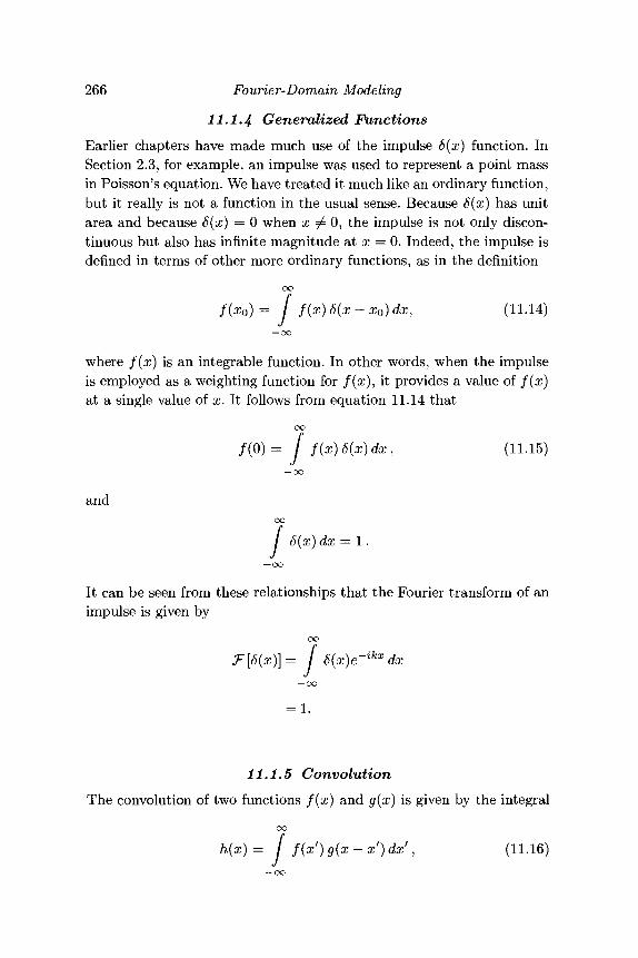
266 Fourier-Domain Modeling
11.1.4 Generalized FunctionsEarlier chapters have made much use of the impulse 6(x) function. InSection 2.3, for example, an impulse was used to represent a point massin Poisson's equation. We have treated it much like an ordinary function,but it really is not a function in the usual sense. Because 6(x) has unitarea and because 6(x) = 0 when x ^ 0, the impulse is not only discon-tinuous but also has infinite magnitude at x = 0. Indeed, the impulse isdefined in terms of other more ordinary functions, as in the definition
00
• /f(xo)= / f(x)6(x-xo)dx, (11.14)
where f(x) is an integrable function. In other words, when the impulseis employed as a weighting function for /(#), it provides a value of f(x)at a single value of x. It follows from equation 11.14 that
00
/(0)= / f(x)6(x)dx, (11.15)
and00
r1./ 6(x) dx —
It can be seen from these relationships that the Fourier transform of animpulse is given by
00
e-ikxf 6(x), )e~lKxdx
— OO
= 1.
11.1.5 ConvolutionThe convolution of two functions f(x) and g{x) is given by the integral
00
h(x) = I f{x') g{x - xf) dx1, (11.16)
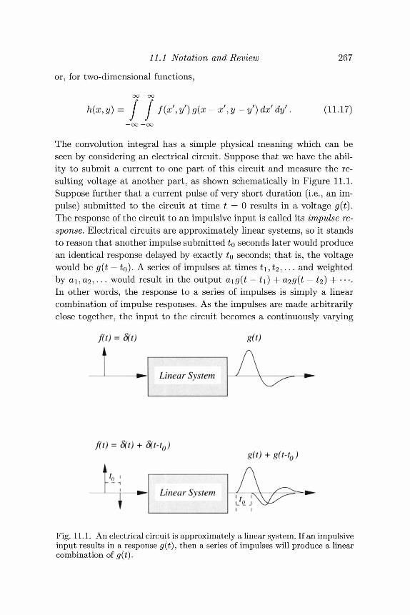
11.1 Notation and Review
or, for two-dimensional functions,
267
oo oo
(x,y)= I f f(x',y')g(x-x',y-y')dx'dy'. (11.17)
The convolution integral has a simple physical meaning which can beseen by considering an electrical circuit. Suppose that we have the abil-ity to submit a current to one part of this circuit and measure the re-sulting voltage at another part, as shown schematically in Figure 11.1.Suppose further that a current pulse of very short duration (i.e., an im-pulse) submitted to the circuit at time t = 0 results in a voltage g(i).The response of the circuit to an impulsive input is called its impulse re-sponse. Electrical circuits are approximately linear systems, so it standsto reason that another impulse submitted to seconds later would producean identical response delayed by exactly to seconds; that is, the voltagewould be g(t — to). A series of impulses at times t±, £2, • • • a nd weightedby ai, a2,. . . would result in the output a\g(t — t\) + a<ig(t — t<i) + • • •.In other words, the response to a series of impulses is simply a linearcombination of impulse responses. As the impulses are made arbitrarilyclose together, the input to the circuit becomes a continuously varying
f(0k1
= #/>Linear System
8(0AA
/W = 5T0 + fifr-r0)g(t-t0)
Linear System AFig. 11.1. An electrical circuit is approximately a linear system. If an impulsiveinput results in a response g(t), then a series of impulses will produce a linearcombination of g(t).
268 Fourier-Domain Modeling
current. It should be clear that, at this limit, the output voltage will bea continuous combination of impulse responses.
The convolution integral, equation 11.16, is the mathematical expres-sion of this linear relationship between input and output, where f(x) isthe input and h(x) is the output. Accordingly, if f(x) is an impulse inequation 11.16, we see from the definition of an impulse (equation 11.14)that
CXJ
/
6(xf) g(x — xr) dxr = g(x),
and g[x) is the impulse response. It is also easy to show that if theimpulse is displaced by a distance #o and amplified by ao, the impulseresponse is similarly delayed and amplified,
oo
/— xo)g(x — xf) dxf =
which is exactly the property of the electrical circuit. In general, a se-ries of weighted impulses produces an output consisting of a series ofweighted impulse responses,
nr*^ i I . . •)ri(rr nr \ nnr%XJ 2, ) I i u l *AJ *XJ I \JbtXj
a2g(x -x2)-\ •
In the limit, the series of weighted impulses becomes a continuous func-tion /(#), and the convolution integral (equation 11.16) represents thecontinuous output h(x) resulting from this continuous input.
Fourier-Convolution TheoremA very important property of linear systems can be seen by transformingthe convolution integral to the Fourier domain. If the convolution of f(x)and g(x) produces a function /i(x), the Fourier transform of h(x) is givenby
H(k) = F(k)G(k), (11.18)
where f(x) <-• F(k) and g(x) <-> G(k). Similarly, for two-dimensionalfunctions,
H(kx, ky) = F(kx, ky) G{kx, ky). (11.19)
Exercise 11.5 Prove equation 11.18.
11.1 Notation and Review 269
Thus convolution in the space (or time) domain transforms to multipli-cation in the Fourier domain.
This relationship between convolution in the space (or time) domainand multiplication in the Fourier domain is important for several rea-sons. First, suppose that g(x) is the impulse response of a linear system;when f(x) is submitted to the system, we can expect the output to beh(x). Further suppose that g(x) is known on theoretical grounds so thatG(k) can be derived. We might be very interested in finding the input tothe system that resulted in some measured output, and equation 11.18in principle provides a straightforward way to make this analysis: (1)Fourier transform h(x) to get H(k), (2) divide H(k) by G(k) to getF(k), and (3) inverse Fourier transform F(k) to get /(#). Second, equa-tion 11.18 (or equation 11.19) provides a straightforward description ofhow the wavenumber (or frequency) content of any input will be trans-formed by the linear system. The energy-density spectrum of any inputwill be multiplied by |G(fc)|2.
Just as the convolution of two functions of space has a Fourier trans-form given by the product of the Fourier transforms of the two functions,it is easy to show that a similar relation holds for convolution in theFourier domain. If /(#), g(x), and h(x) have Fourier transforms givenby F(k), G(k), and H(k), respectively, and if h(x) = f(x)g(x), then
H{k) = — f F{k')G{k-k')dk'. (11.20)2TT J
— oo
A similar relationship can be written for two-dimensional functions.Exercise 11.6 Prove equation 11.20.
ParsevaVs FormulaThe total energy of a real function f(x) can be found by either integrat-ing f2(x) over all space or by integrating the energy-density spectrumof f(x) over all k. This relationship is expressed by ParsevaVs formula:If f(x) is real and if f(x) <->• F(k), then
oo oo
2TT / \f{x)\2dx= f \F(k)\2dk.j J
— oo —oo
Parseval's formula is easily derived from equation 11.20 by letting g(x) =
270 Fourier-Domain Modeling
11.1.6 Discrete Fourier TransformThe preceding discussion has treated convolution and Fourier transformsof continuous functions. In practice, we must deal with sampled data,and this limitation has profound effects on the kind of information avail-able through Fourier analysis. Bracewell [42] provides a general reviewof this aspect of Fourier transforms, and Cordell and Grauch [69] andRicard and Blakely [244] have discussed its limitations in the context ofpotential-field data. Appendix C briefly reviews sample theory; here wesummarize the most important results.
The Fourier transform of sampled data is known as the discrete Fouriertransform. It has limitations at both the longest and shortest wave-lengths. It should be clear, for example, that wavelengths less than twicethe sample interval cannot be represented adequately by the discreteFourier transform. This limitation is expressed in the Fourier domainin an interesting way: The discrete Fourier transform is periodic with aperiod inversely proportional to the sample interval.
Consider N sequential samples of f(x) evenly spaced at Ax intervals.If we assume that f(x) is zero beyond these TV samples, then we canconsider N to be effectively infinite. In this case, the discrete Fouriertransform FD(k) is related to the true Fourier transform F(k) by thesummation
-SOj = oo /
(see Appendix C). At any given fco, we obviously would like for Fo(fco) toequal F(ko). Unfortunately, according to the previous equation F]j(ko)actually equals F(ko) plus F(k) evaluated at an infinite number of otherwavenumbers. This "self-contamination" is known as aliasing. The pe-riod of the discrete Fourier transform is ks = 2TT/AX, and ks is calledthe sampling wavenumber, half of the sampling wavenumber (TT/AX) iscalled the Nyquist wavenumber. Because the discrete Fourier transformrepeats itself each 2TT/AX, all unique information lies between ±7r/Ax.Hence, the Nyquist wavenumber is the largest wavenumber at our dis-posal. Note that it has a wavelength of twice the sample interval.
As we will see shortly, potential-field anomalies, like many physicalphenomena, can be considered to be band-limited, that is, they haveFourier transforms that decay with increasing wavenumber. Hence, thecontaminating high-wavenumber terms in the foregoing summation maybe relatively small, especially if the sample interval is made sufficiently
11.2 Some Simple Anomalies 271
small relative to the significant wavelengths of f(x). These principles areimportant considerations in developing a digitizing strategy.
Numerous algorithms are available to perform the discrete Fouriertransform. Many of these employ a manipulation called doubling (Claer-bout [60]) that makes them computationally efficient; such algorithmsare called fast Fourier transforms. Appendix B provides two such sub-routines. Subroutine B.16 is from Claerbout [60] and performs the one-dimensional discrete Fourier transform. Subroutine B.17 is from Presset al. [233] and performs multi-dimensional transforms.
11.2 Some Simple AnomaliesUsing the principles of the previous section, we now can derive theFourier transforms of potential fields caused by a variety of simple sources,such as dipoles, monopoles, lines, and ribbons. This effort will be wellspent; these transforms will form the foundation for more complex grav-ity and magnetic sources, eventually leading to a wide variety of applica-tions, including forward and inverse calculations, upward continuation,and depth-to-source estimations.
Let r describe the distance between point P located at (x, y, z) andpoint Q at point (x',y',z'). The Fourier transform of 1/r is the cor-nerstone of this discussion because potential fields depend on variousderivatives of 1/r. With the Fourier transform of 1/r in hand and withthe aid of the differentiation theorem (Section 11.1.2), subsequent deriva-tions will be relatively straightforward. Spector and Bhattacharyya [267]used the same sort of strategy in deriving energy-density spectra and au-tocorrelation functions for dipole and line-source anomalies.
We will confine P to a horizontal plane at height Zo and, for themoment, consider Q to be fixed and located on the z axis at (0,0,z;),where z1 > ZQ (Figure 11.2). The two-dimensional Fourier transform of1/r is given by
oo oo
— oo —oo
We can simplify this equation considerably by noting that the function1/r is cylindrically symmetrical about the z axis and by converting theintegral to polar coordinates. If we let
x = acos#,
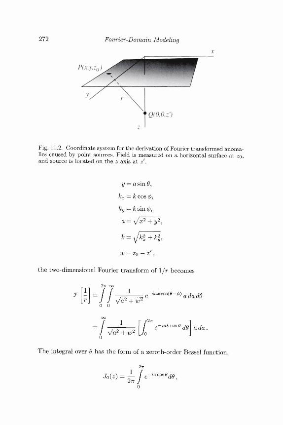
272 Fourier-Domain Modeling
P(x,y,zo)
"Q(O.O.z')
Fig. 11.2. Coordinate system for the derivation of Fourier transformed anoma-lies caused by point sources. Field is measured on a horizontal surface at z0,and source is located on the z axis at z .
kx = k cos </>,
ky = k sin 0,
a= y2
w = z0 - z',
the two-dimensional Fourier transform of 1/r becomes
2TT OO
-1 = / / , /r\ J J Va2 +o o
oo
= J 7^+2TT
The integral over 0 has the form of a zeroth-order Bessel function,
2TT
9de,
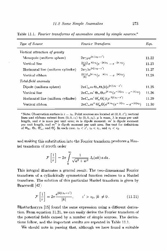
11.2 Some Simple Anomalies 273
Table 11.1. Fourier transforms of anomalies caused by simple sources.a
Type of Source Fourier Transform Eqn.
Vertical attraction of gravityMonopole (uniform sphere) 27T7/iie'fe'^0~z ^ 11.22Vertical line ^\e\k\zQ^e-\k\Zl _ e-\k\z2^ n 2 3
Horizontal line (uniform cylinder) 27T^yXe^k^z°~z ' 11.27Vertical ribbon 2,™ l*l*o( e-l*l*i _ e-|*l*2) n 2 g
\K\
Total-field anomalyDipole (uniform sphere) 27rCmraBmBf |fc|e'fe'^°~* ^ 11.25
Vertical line 27rCmra' BmBfe|/c|2:o(e~|/c|2:i - e~^Z2) 11.26
Horizontal line (uniform cylinder) 27vCmm B^Bf |fc|e|fe|(*°~z/) 11.29
Vertical ribbon 27rCmra" 0 ' Bfe|fc|z°(e~|fc|21 - e~lklz2) 11.30
aNote: Observation surface is z = ZQ. Point sources are located at (0, 0, z')\ verticallines and ribbons extend from (0,0, zi) to (0,0, 22)- ^ is mass, A is mass per unitlength, and a is mass per unit area; m is dipole moment, m' is dipole momentper unit length, and m" is dipole moment per unit area. See text for definitionsof B m , Bf, GJn, and Bf
r In each case, ZQ < zf, ZQ < z\, and z\ < 2:2 •
and making this substitution into the Fourier transform produces a Han-kel transform of zeroth order
0 0
T - = 2TT / = Jo (ak) a da.o
This integral illustrates a general result: The two-dimensional Fouriertransform of a cylindrically symmetrical function reduces to a Hankeltransform. The solution of this particular Hankel transform is given byBracewell [42]:
^ J = 2 7 r [A | ' * ' > ^ 1*1^0. (11.21)
Bhattacharyya [15] found the same expression using a different deriva-tion. From equation 11.21, we can easily derive the Fourier transform ofthe potential fields caused by a number of simple sources. The deriva-tions follow, and the important results are repeated in Table 11.1.
We should note in passing that, although we have found a suitable
274 Fourier-Domain Modeling
expression for ^"[^], 1/f does not satisfy inequality 11.3 because theintegral
2TT OO
f f dxdy f fJ J Jx2 + y2 + (zo-zf)2~J J x/o2
adadOxjx2 + y2 + (z0 " z')2 J J x/a2 + (z0 - z1)2
a daQ Ja2 + {z,-z<)2
is not finite. Hence, the Fourier transform of 1/r does not exist in therigorous sense of inequality 11.3, a fact expressed in equation 11.21 by theundefined nature of T [£] at infinite wavelength (|fc| = 0). We can takesome solace in the fact that any spatial derivative of 1/r (and thereforegravity and magnetic anomalies in general) does satisfy inequality 11.3.Exercise 11.7 Show that any horizontal derivative of 1/r has a Fourier
transform.
11.2.1 Three-Dimensional SourcesIn this section and the next, the Fourier transforms of several simpletwo- and three-dimensional sources will be discussed. The terminologyherein can be a source of confusion. The anomaly of a three-dimensionalbody (e.g., a sphere) is appropriately measured on a two-dimensionalsurface, and to study the anomaly in the Fourier domain requires a two-dimensional Fourier transform. Likewise, a two-dimensional source (e.g.,a cylinder) is measured along a profile that requires the one-dimensionalFourier transform. We will continue to refer to sources as either two-or three-dimensional in accordance with their geometries, with the un-derstanding that their anomalies are analyzed in the Fourier domain ineither one or two dimensions, respectively.
MonopoleConsider the Fourier transform of the gravitational potential observedon a horizontal plane at z — zo and caused by a point mass (equivalent ofcourse to a spherical mass with uniform density) located below the plane.The Fourier transform of this potential can be written immediately fromequation 11.21. The gravitational potential of a point mass \i is given by
11.2 Some Simple Anomalies 275
JJ = 7/i/r, where 7 is the gravitational constant; the Fourier transformof this potential observed on a horizontal plane is simply
Gravitational acceleration g is related to the potential by the equationg = VpC/, so any component of g is simply a directional derivative ofU. In particular, the vertical attraction of gravity due to a point massis the vertical derivative of 7/x/r, that is,
d 1
Observed on a horizontal plane, this field has a Fourier transform givenby
( 2°-* / ) , z' > z0. (11.22)
A number of important characteristics of gravity anomalies can beseen from equation 11.22 and are illustrated by Figure 11.3(a). Maximumenergy of the gravitational field occurs at |fc| = 0, and the value of theenergy-density spectrum at |fc| = 0 is proportional to the total mass; theproof of this assertion is left to the problem set at the end of this chap-ter. Energy decreases exponentially with increasing wavenumber; thatis, the energy at each wavelength dominates the energy at all shorterwavelengths. Moreover, the rate of decrease in energy with respect towavenumber depends on the depth to the mass; the deeper the mass,the less significant are short wavelengths as compared with longer wave-lengths of the anomaly. In other words, equation 11.22 and Figure 11.3show that the gravity anomaly is approximately band limited; althoughall wavenumbers contribute to the anomaly, the largest wavenumbersare relatively insignificant.
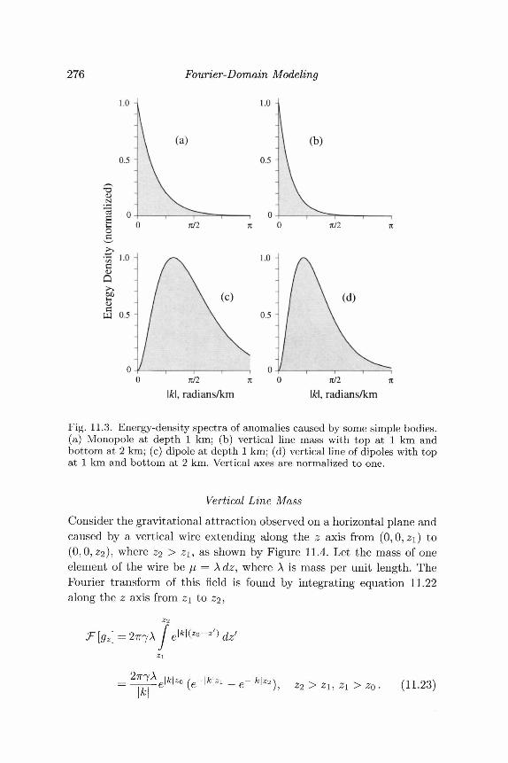
276
i.o
Fourier-Domain Modeling
1.0
TI/2 n
:l, radians/km71/2
, radians/km
Fig. 11.3. Energy-density spectra of anomalies caused by some simple bodies.(a) Monopole at depth 1 km; (b) vertical line mass with top at 1 km andbottom at 2 km; (c) dipole at depth 1 km; (d) vertical line of dipoles with topat 1 km and bottom at 2 km. Vertical axes are normalized to one.
Vertical Line MassConsider the gravitational attraction observed on a horizontal plane andcaused by a vertical wire extending along the z axis from (0, 0, 21) to(0,0,22), where z2 > Z\, as shown by Figure 11.4. Let the mass of oneelement of the wire be /JL = Xdz, where A is mass per unit length. TheFourier transform of this field is found by integrating equation 11.22along the z axis from z\ to z2.
Z2
f
\k\ z2>z1,z1>z0. (11.23)
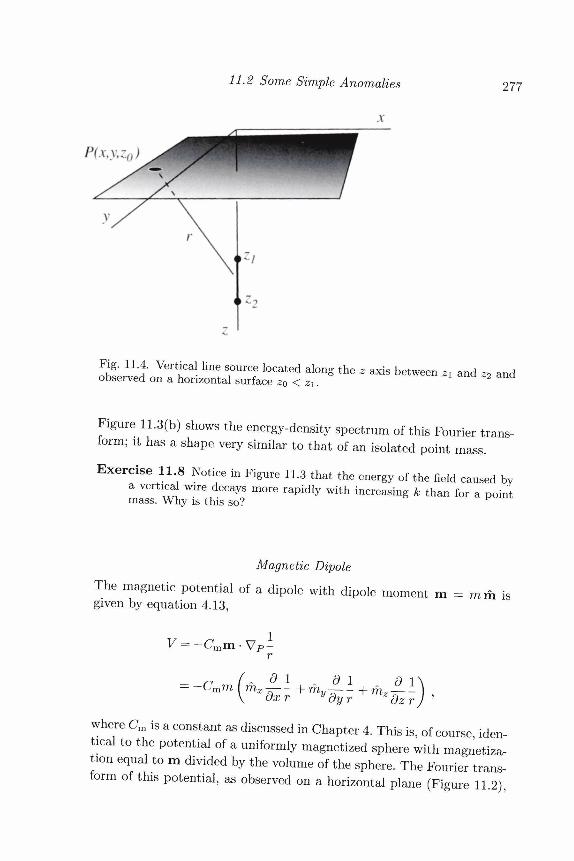
11.2 Some Simple Anomalies 277
t h e z a x i s b e t w e e n * a n d
Figure 11.3(b) shows the energy-density spectrum of this Fourier trans-form; it has a shape very similar to that of an isolated point mass.
Exercise 118 Notice in Figure 11.3 that the energy of the field caused bya vertical wire decays more rapidly with increasing k than for a pointmass. Why is this so?
Magnetic DipoleThe magnetic potential of a dipole with dipole moment m = m m isgiven by equation 4.13,
^ = - C m m - V P -r
n (- d I d 1 d 1= -Cmm[mx-—+m y-—+m z~ -
\ dxr vdyr dz rwhere Cm is a constant as discussed in Chapter 4. This is, of course iden-tical to the potential of a uniformly magnetized sphere with magnetiza-tion equal to m divided by the volume of the sphere. The Fourier trans-form of this potential, as observed on a horizontal plane (Figure 11 2)
278 Fourier-Domain Modeling
is given by application of equation 11.9 to equation 11.21:
mxikxT -li rii d ri- + rhyikyJ7 - + rfiz—-T -r\ y y \r\ dz \r
= -27rCmm Bm e l f c l^-^) , ^ > o , (H-24)
where
is a complex function of /cx and /c that depends only on the orientationof the dipole.
The magnetic field is related to the potential by the equation B =—VpV, so any component of B can be found by deriving a directionalderivative of V. For example, the total-field anomaly is given approxi-mately by
AT = - f •
where f is the unit vector parallel to the ambient field. Therefore, ob-served on a horizontal plane, the Fourier transform of the total-fieldanomaly is
= ~iUk,T [V\ - ifykyf \V\ ~ U f [V\ ,and combining this equation with equation 11.24 yields
f[AT] - 27rCmmemef \k\ elfcK*°-*'), z' > z0 , (11.25)
whereQ f I JxkX + fyky
Exercise 11.9 As discussed in Section 11.1.2, the Fourier transform of anyreal function must be Hermitian. Show that this is indeed the case forthe Fourier transform of the total-field anomaly of a dipole.
11.2 Some Simple Anomalies 279
In equation 11.25, note that the orientations of vectors m and f arecontained entirely within Bm and Bf, respectively, whereas the depthof the dipole is contained exclusively within the exponential term. Thisseparation of source distribution and source location into multiplicativefactors is an important attribute of Fourier-transformed potential fieldsthat will be exploited later in this chapter.
The functions Gm and Of behave in interesting ways. Although theyboth are variables of kx and /cy, they assume constant values along anyray projected from the origin. This can be seen by converting kx and kyto polar coordinates. In general, the value along each ray differs fromneighboring rays, and rays on opposite sides of the origin are complexconjugates of one another. Consequently, the imaginary parts of Gm and6f are discontinuous through the origin. The average of 6 m and Bf alongany circle concentric about the origin is given by
Q dd> = rhz2TT J {
o
and2TT
respectively. Hence, although Bm and Bf are not radially symmetricin general, they have average values along any concentric circle thatare independent of the radius of the circle. It follows that the shape ofthe amplitude spectrum (or energy-density spectrum) of the anomalyis identical, to within a multiplicative constant, when viewed along anyray projected from the origin, and the shape of the spectrum along anyray is proportional to the radially averaged spectrum. Consequently, theshape of the amplitude spectrum as a function of \k\ depends only onthe exponential term of equation 11.25 which in turn depends only onthe depth of the dipole; the shape is independent of the orientation ofthe dipole and the orientation of the ambient field.
The energy-density spectrum of the total-field anomaly over a verticaldipole is shown in Figure 11.3(c). Unlike point masses, the maximumenergy of the total-field anomaly does not occur at |fc| = 0, but ratherat a value of |fc| that depends on the depth of the dipole.Exercise 11.10 At what wavenumber, in terms of ZQ and zf, does the max-
imum of equation 11.25 occur? What does this imply about the shapeof the anomaly as a function of depth to the dipole?
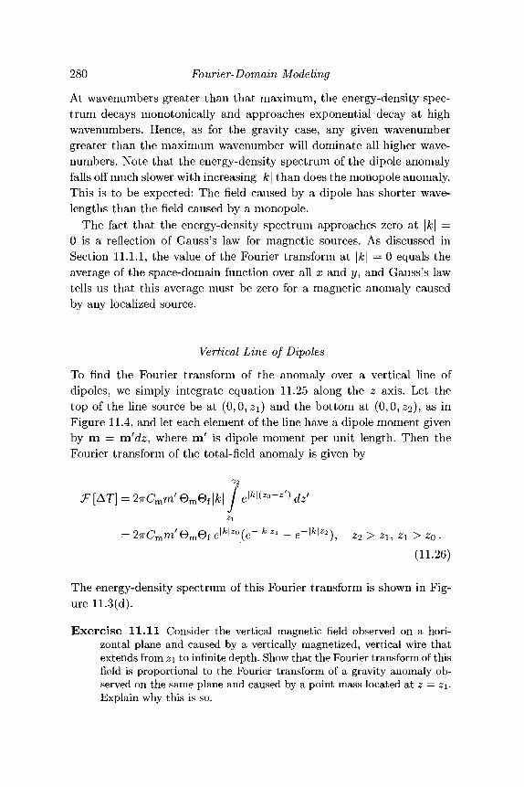
280 Fourier-Domain Modeling
At wavenumbers greater than that maximum, the energy-density spec-trum decays monotonically and approaches exponential decay at highwavenumbers. Hence, as for the gravity case, any given wavenumbergreater than the maximum wavenumber will dominate all higher wave-numbers. Note that the energy-density spectrum of the dipole anomalyfalls off much slower with increasing \k\ than does the monopole anomaly.This is to be expected: The field caused by a dipole has shorter wave-lengths than the field caused by a monopole.
The fact that the energy-density spectrum approaches zero at \k\ =0 is a reflection of Gauss's law for magnetic sources. As discussed inSection 11.1.1, the value of the Fourier transform at |A;| = 0 equals theaverage of the space-domain function over all x and y, and Gauss's lawtells us that this average must be zero for a magnetic anomaly causedby any localized source.
Vertical Line of Dipoles
To find the Fourier transform of the anomaly over a vertical line ofdipoles, we simply integrate equation 11.25 along the z axis. Let thetop of the line source be at (0,0, z\) and the bottom at (0,0,2:2)7 as inFigure 11.4, and let each element of the line have a dipole moment givenby m = m'dz, where m' is dipole moment per unit length. Then theFourier transform of the total-field anomaly is given by
^[AT]=27rCmm/emef|A:| I dz'
= 27rCmm/ B m e f e l ^ e - l * ! * 1 - e ^ ' * 2 ) , z2>z1,z1>z0.(11.26)
The energy-density spectrum of this Fourier transform is shown in Fig-ure 11.3(d).
Exercise 11.11 Consider the vertical magnetic field observed on a hori-zontal plane and caused by a vertically magnetized, vertical wire thatextends from z\ to infinite depth. Show that the Fourier transform of thisfield is proportional to the Fourier transform of a gravity anomaly ob-served on the same plane and caused by a point mass located at z = z\.Explain why this is so.
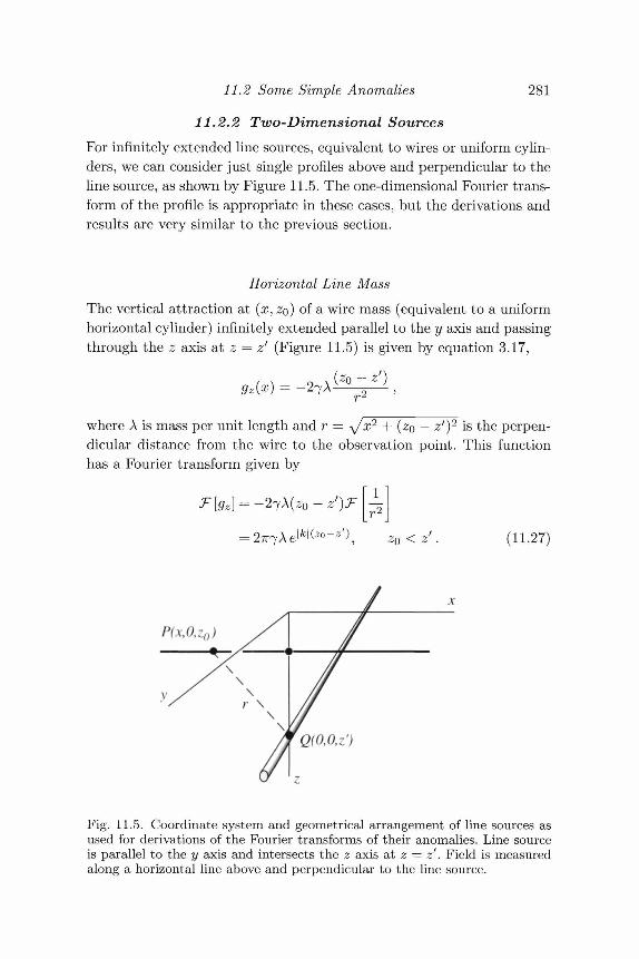
11.2 Some Simple Anomalies
11.2.2 Two-Dimensional Sources
281
For infinitely extended line sources, equivalent to wires or uniform cylin-ders, we can consider just single profiles above and perpendicular to theline source, as shown by Figure 11.5. The one-dimensional Fourier trans-form of the profile is appropriate in these cases, but the derivations andresults are very similar to the previous section.
Horizontal Line MassThe vertical attraction at (X,ZQ) of a wire mass (equivalent to a uniformhorizontal cylinder) infinitely extended parallel to the y axis and passingthrough the z axis at z = z1 (Figure 11.5) is given by equation 3.17,
gz(x) = -27A Z ,
where A is mass per unit length and r = yjx2 + (ZQ — zf)2 is the perpen-dicular distance from the wire to the observation point. This functionhas a Fourier transform given by
< z (11.27)
P(x,0,z0)
Fig. 11.5. Coordinate system and geometrical arrangement of line sources asused for derivations of the Fourier transforms of their anomalies. Line sourceis parallel to the y axis and intersects the z axis at z = z'. Field is measuredalong a horizontal line above and perpendicular to the line source.
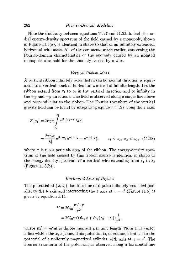
282 Fourier-Domain Modeling
Note the similarity between equations 11.27 and 11.22. In fact, the ra-dial energy-density spectrum of the field caused by a monopole, shownin Figure 11.3(a), is identical in shape to that of an infinitely extended,horizontal wire mass. All of the comments made earlier, concerning theFourier-domain characteristics of the anomaly caused by an isolatedmonopole, also hold for the anomaly caused by a wire.
Vertical Ribbon Mass
A vertical ribbon infinitely extended in the horizontal direction is equiv-alent to a vertical stack of horizontal wires all of infinite length. Let theribbon extend from z\ to Z2 in the vertical direction and to infinity inthe +y and —y directions. The field is observed along a single line aboveand perpendicular to the ribbon. The Fourier transform of the verticalgravity field can be found by integrating equation 11.27 along the z axis:
^ lklzo(e~lklZ1 ~ e - ' ^ 2 ) , *i < «., ^ < z0 , (11.28)| /C |
where a is mass per unit area of the ribbon. The energy-density spec-trum of the field caused by this ribbon source is identical in shape tothe energy-density spectrum of a vertical wire extending from z\ to z^(Figure 11.3(b)).
Horizontal Line of Dipoles
The potential at (x,zo) due to a line of dipoles infinitely extended par-allel to the y axis and intersecting the z axis at z = zr (Figure 11.5) isgiven by equation 5.14
= 2Cmm'(mxx + mz(z0 - z'))-^ ,rz
where m' = ra'm is dipole moment per unit length. Note that vectorr lies within the x, z plane. This potential is, of course, identical to thepotential of a uniformly magnetized cylinder with axis at z = z'. TheFourier transform of the potential, as observed along a horizontal line
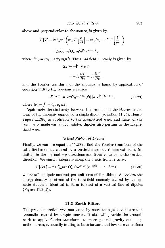
11.3 Earth Filters 283
above and perpendicular to the source, is given by
T[V}=2Cmm' (mxf [^] + mz(z0 - z')T \^\
where B^ = rhz + imx sgn k. The total-field anomaly is given by
AT = - f •
__f ay _ fdv_" u dx h dz '
and the Fourier transform of the anomaly is found by application ofequation 11.8 to the previous equation,
T [AT] = 27rCmm/ 9^0^ |fc| e1*1**0-*'* , (11.29)
where Of = fz + ifx sgn /c.Again note the similarity between this result and the Fourier trans-
form of the anomaly caused by a single dipole (equation 11.25). Hence,Figure 11.3(c) is applicable to the magnetized wire, and many of thecomments made earlier for isolated dipoles also pertain to the magne-tized wire.
Vertical Ribbon of DipolesFinally, we can use equation 11.29 to find the Fourier transform of thetotal-field anomaly caused by a vertical magnetic ribbon extending in-finitely in the +y and — y directions and from z\ to z2 in the verticaldirection. We simply integrate along the z axis from z\ to z^-,
f[AT] =27rCmm / /e /me^lfc^°(e- | /e |zi - e~^Z2), (11.30)
where m" is dipole moment per unit area of the ribbon. As before, theenergy-density spectrum of the total-field anomaly caused by a mag-netic ribbon is identical in form to that of a vertical line of dipoles(Figure 11.3(d)).
11.3 Earth FiltersThe previous section was motivated by more than just an interest inanomalies caused by simple sources. It also will provide the ground-work to apply Fourier transforms to more general gravity and mag-netic sources, eventually leading to both forward and inverse calculations
284 Fourier-Domain Modeling
and other applications. The keystone in this discussion is the Fourier-convolution theorem of Section 11.1.5.
Equation 10.5 shows the relationship between a potential field / andthe distribution of source material s:
f{P) = j s{Q)^{P1Q)dv1 (11.31)
where R is the region occupied by source material, P is the point ofobservation, Q is one point of the distribution, and i/)(P, Q) is the Green'sfunction. Recall that the Green's function depends on the geometricalplacement of P and Q and is simply the potential field at point P due toa single element of the source located at Q. If f(P) represents verticalattraction of gravity, for example, then s(Q) is density and ip(P,Q) isthe vertical attraction at P due to a monopole at Q. If f(P) representsthe total-field anomaly, then s(Q) is magnetization and ip(P,Q) is thetotal-field anomaly of a single dipole.
Now suppose that the source distribution is confined to a horizontallayer with top at z\ and bottom at 22. As usual, we will orient the zaxis down so that z\ < Z2- We also will require the source distributionto vary in only the x and y directions, which will cause s(Q) to be con-stant along any vertical line through the layer. With these restrictions,equation 11.31 becomes
00 00 00
f(x,y,z)= / / / s(xt,y')\l){x-x'1y-yl,z-z/)dxfdy'dzf
—00 —00 —00
OO OO Z2
= j j s(x',y') I\p(x-x',y-y',z-z')dz'dx'dy'
OO OO
= J J s(x', y') S(x - x ' , y - y') dx' dy', (11.32)— oo —oo
which is the two-dimensional convolution integral. The Green's function£ in this case represents the field at (x, y) due to a single element ofthe layer, namely, a vertical line element extending from (x',yf,zi) to(Z',2,',22).
We now assume that the field is measured on a horizontal plane atheight z = ZQ, where z0 < z\, and Fourier transform both sides of
11.3 Earth Filters 285
equation 11.32. The Fourier-convolution theorem leads to
F[f]=F[s] ?[£]', (11.33)
that is, the Fourier transform of the potential field is equal to the Fouriertransform of the source distribution multiplied by T [£], the Fouriertransform of the Green's function. In the previous section, several Fouriertransforms were derived that will serve for T [£]. Equation 11.23, for ex-ample, describes the Fourier transform of the vertical attraction of avertical line, and substituting into equation 11.33 yields
(11.34)where p is the density of the slab, a function of x and y only. Hence, inthe Fourier domain, the vertical attraction of a horizontal layer is equalto two multiplicative factors: the Fourier transform of the density and afunction that depends on the depth and thickness of the layer.
Exercise 11.12 Show that equation 11.34 reduces to the "infinite slabformula," gz = 2ivyp(z2 — 2i), if 21, 22, and p are constants. Hint:
For the total-field anomaly, T [£] comes from equation 11.26, and equa-tion 11.33 becomes
zo<zu z1<z2, (11.35)
where M is magnetization, a function of x and y only. As before, theFourier transform has separated the total-field anomaly into two factors:the magnetization and a function that depends on other attributes ofthe layer, namely, its depth, thickness, and direction of magnetization.
Exercise 11.13 Use equation 11.35 to show that a uniformly magnetized,infinite slab produces no magnetic field.
If the magnetization or density varies in only one horizontal direction,then equation 11.31 reduces to a single convolution integral,
00
f(x) = / s(x') £(x - x') dx',
where s(x) is the source distribution of a horizontal layer. The Green'sfunction in this case is the field caused by a vertical ribbon extending
286 Fourier-Domain Modeling
from z\ to z2 in the vertical direction and infinitely extended parallelto y. In the Fourier domain, therefore, JF[£] is given by equation 11.28for the two-dimensional gravity case and by equation 11.30 for the two-dimensional magnetic case.
Exercise 11.14 What form would equations 11.34 and 11.35 take if densityand magnetization were confined to a vanishingly thin plane?
The function .F[£] in equation 11.33 relates the spectrum of the po-tential field to the spectrum of the causative source in a very simple way.It not only provides insights into the spectral relationship between fieldand source, but it also facilitates a simple calculation of one from theother. Two landmark papers by Schouten [252] and Schouten and Mc-Camy [253] discussed these principles in detail for the two-dimensionalmagnetic case. They called T [£] the earth filter, here we will apply theterm generally to both gravity and magnetic fields and to both two- andthree-dimensional situations.
Forward CalculationEquations 11.34 and 11.35 permit a calculation of the vertical gravityanomaly or total-field magnetic anomaly from a given distribution ofdensity or magnetization, respectively, when the distribution is confinedto a horizontal layer and varies in only horizontal directions. The stepsare to (1) Fourier transform s(x,y), (2) multiply by the earth filter, and(3) inverse Fourier transform the product. Algorithms B.18 and B.19 inAppendix B show the application of these three steps to gravity and mag-netic sources, respectively. These subroutines treat the three-dimensionalcase and employ the two-dimensional discrete Fourier transform. Sim-ilar algorithms could be developed for the two-dimensional case usingthe one-dimensional discrete transform (Subroutine B.16).
The spectrum of the field caused by a layer source, therefore, is equiv-alent to the spectrum of the source distribution after "shaping" by theearth filter. The earth filter in this case is merely the Fourier transformof the anomaly caused by a vertical line element, so all of the earliercomments regarding these line-element transforms are applicable here.Moreover, the energy-density spectra shown on Figure 11.3 also reflectthe spectra of their respective earth filters. For example, Figure 11.3(a)shows that the contributions of p(x,y) to a gravity anomaly gz(x,y)will be attenuated exponentially as a function of increasing wavenum-ber, and the rate of that attenuation will increase with increasing depthto the layer. It follows that the k = 0 component of p(x, y) will be least
11.3 Earth Filters 287
attenuated. Put another way, the gravity anomaly will always besmoother than the density distribution, in the sense that all wavenum-bers (except | A:| =0) of the gravity anomaly are attenuated relative tothe density distribution; the higher the wavenumber (shorter the wave-length), the greater the attenuation.Exercise 11.15 Show that when p(x,y) is a constant, equation 11.34 re-
duces to the infinite-slab formula (equation 3.27). Hint: L'Hospital's ruleis helpful.
Likewise, many of the comments of Section 11.2.1 concerning verti-cal lines of dipoles are relevant to the earth filter for a magnetic layer.In particular, the earth filter for a magnetic layer has its maximumvalue at a wavenumber fcmax that depends on the depth and thicknessof the layer (Figures 11.3(c) and 11.6). Hence, the |fc| = fcmax compo-nent of magnetization will be less attenuated than all other wavenum-bers in the total-field anomaly. Notice in Figure 11.6 that fcmax shiftsto higher wavenumbers (shorter wavelengths) as depth of the layer de-creases. Wavenumbers higher than fcmax are each attenuated less thanall higher wavenumbers, and this attenuation approaches exponentialdecay at high wavenumbers. The rate of attenuation with increasingwavenumber increases with increasing depth to the magnetic layer. Thek = 0 component of magnetization is eliminated entirely by the earthfilter.Exercise 11.16 Use equation 11.35 to show that a uniformly magnetized
slab produces no magnetic anomaly.
Parameters that determine the location and shape of the source (i.e.,the depth and thickness of the layer) are restricted to the exponentialterms of equation 11.35; they influence the behavior of the earth filter asa function of |fc| only. On the other hand, the direction of magnetizationand the direction of the regional field are restricted entirely to the func-tions Om and Of, respectively. The direction of magnetization and thedirection of the regional field, therefore, have no effect on the behaviorof the earth filter as a function of |fc|, but they completely control itsphase. For example, if the magnetization and regional field are directedvertically (mx = my = fx = fy = 0), then Om and Of will be realconstants. This implies that the phase of the source distribution and thephase of the anomaly will be identical when magnetization and regionalfield are vertical; for example, if M(x, y) is symmetric about the origin,AT(x, y) also will be symmetric. On the other hand, if magnetizationis horizontal (fhz = 0) and the regional field is vertical (fx = fy = 0),
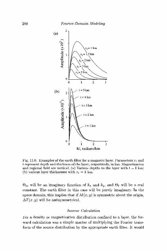
288 Fourier-Domain Modeling
(b) 2-
OX
Ltud
epl
i
<
0-
A ^ ^ t = 5 km
t \ ^ t = 4km
f\L^ t = 3 km\TA \ i ^ t = 2km
\ 1/"x VL ^ ^ t = 1 k m
1 2 3Ikl, radians/km
Fig. 11.6. Examples of the earth filter for a magnetic layer. Parameters z\ andt represent depth and thickness of the layer, respectively, in km. Magnetizationand regional field are vertical, (a) Various depths to the layer with t = 1 km;(b) various layer thicknesses with z\ = 3 km.
0 m will be an imaginary function of kx and ky, and 6f will be a realconstant. The earth filter in this case will be purely imaginary. In thespace domain, this implies that if M(x, y) is symmetric about the origin,AT(x, y) will be antisymmetrical.
Inverse CalculationFor a density or magnetization distribution confined to a layer, the for-ward calculation was a simple matter of multiplying the Fourier trans-form of the source distribution by the appropriate earth filter. It would
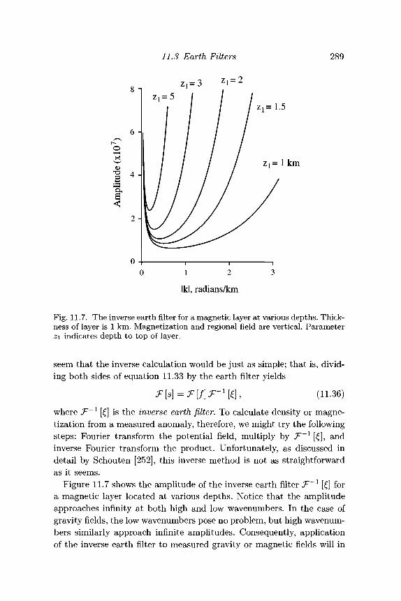
11.3 Earth Filters 289
z 1 = 1 .5
= 1 km
1 2 3
Ikl, radians/km
Fig. 11.7. The inverse earth filter for a magnetic layer at various depths. Thick-ness of layer is 1 km. Magnetization and regional field are vertical. Parameterz\ indicates depth to top of layer.
seem that the inverse calculation would be just as simple; that is, divid-ing both sides of equation 11.33 by the earth filter yields
J- [s\ = J- [j\ J- [£J , (11.oo)
where T~x [£] is the inverse earth filter. To calculate density or magne-tization from a measured anomaly, therefore, we might try the followingsteps: Fourier transform the potential field, multiply by T~x [£], andinverse Fourier transform the product. Unfortunately, as discussed indetail by Schouten [252], this inverse method is not as straightforwardas it seems.
Figure 11.7 shows the amplitude of the inverse earth filter T~x [£] fora magnetic layer located at various depths. Notice that the amplitudeapproaches infinity at both high and low wavenumbers. In the case ofgravity fields, the low wavenumbers pose no problem, but high wavenum-bers similarly approach infinite amplitudes. Consequently, applicationof the inverse earth filter to measured gravity or magnetic fields will in
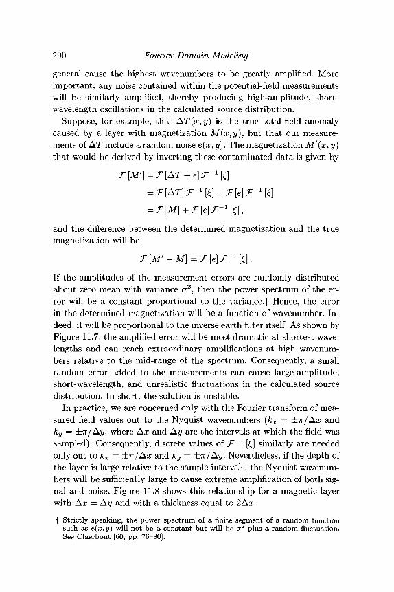
290 Fourier-Domain Modeling
general cause the highest wavenumbers to be greatly amplified. Moreimportant, any noise contained within the potential-field measurementswill be similarly amplified, thereby producing high-amplitude, short-wavelength oscillations in the calculated source distribution.
Suppose, for example, that AT(x, y) is the true total-field anomalycaused by a layer with magnetization M(x,y), but that our measure-ments of AT include a random noise e(x,y). The magnetization M'(x, y)that would be derived by inverting these contaminated data is given by
and the difference between the determined magnetization and the truemagnetization will be
If the amplitudes of the measurement errors are randomly distributedabout zero mean with variance cr2, then the power spectrum of the er-ror will be a constant proportional to the variance.f Hence, the errorin the determined magnetization will be a function of wavenumber. In-deed, it will be proportional to the inverse earth filter itself. As shown byFigure 11.7, the amplified error will be most dramatic at shortest wave-lengths and can reach extraordinary amplifications at high wavenum-bers relative to the mid-range of the spectrum. Consequently, a smallrandom error added to the measurements can cause large-amplitude,short-wavelength, and unrealistic fluctuations in the calculated sourcedistribution. In short, the solution is unstable.
In practice, we are concerned only with the Fourier transform of mea-sured field values out to the Nyquist wavenumbers (kx = ±n/Ax andky = ±7r/Ay, where Ax and Ay are the intervals at which the field wassampled). Consequently, discrete values of T~x [£] similarly are neededonly out to kx = ±7r/Ax and ky = ±ir/Ay. Nevertheless, if the depth ofthe layer is large relative to the sample intervals, the Nyquist wavenum-bers will be sufficiently large to cause extreme amplification of both sig-nal and noise. Figure 11.8 shows this relationship for a magnetic layerwith Ax — Ay and with a thickness equal to 2Ax.
f Strictly speaking, the power spectrum of a finite segment of a random functionsuch as e(x,y) will not be a constant but will be a2 plus a random fluctuation.See Claerbout [60, pp. 76-80].
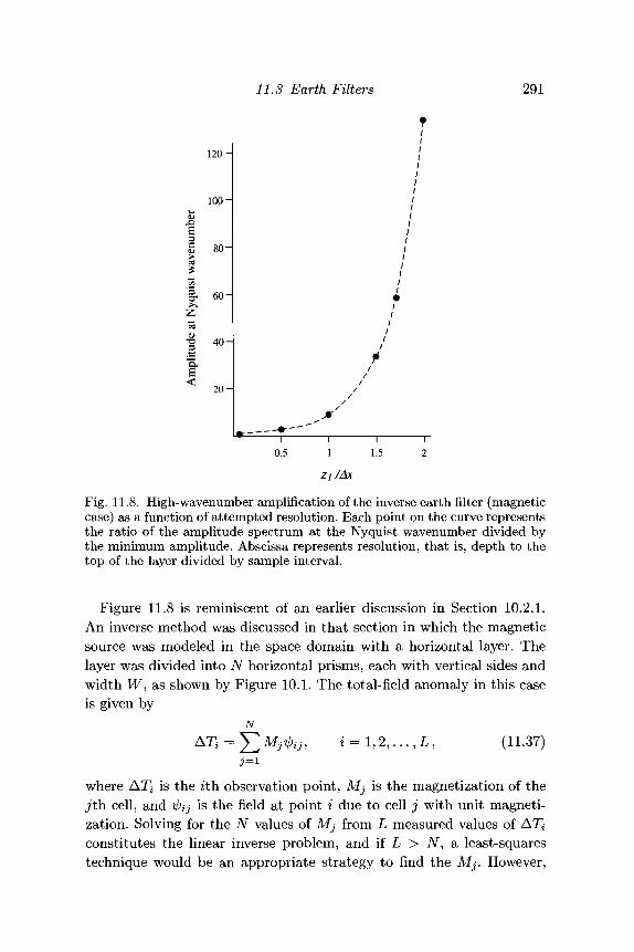
11.3 Earth Filters 291
a
1 2 0 -
1 0 0 -
8 0 -
& 60-
3
a.<
4 0 -
2 0 -
I0.5
I I1 1.5
Fig. 11.8. High-wavenumber amplification of the inverse earth filter (magneticcase) as a function of attempted resolution. Each point on the curve representsthe ratio of the amplitude spectrum at the Nyquist wavenumber divided bythe minimum amplitude. Abscissa represents resolution, that is, depth to thetop of the layer divided by sample interval.
Figure 11.8 is reminiscent of an earlier discussion in Section 10.2.1.An inverse method was discussed in that section in which the magneticsource was modeled in the space domain with a horizontal layer. Thelayer was divided into N horizontal prisms, each with vertical sides andwidth W, as shown by Figure 10.1. The total-field anomaly in this caseis given by
AT
^ i j - , i = l , 2 , . . . , L , (11.37)
where ATi is the ith. observation point, Mj is the magnetization of thejfth cell, and -0^ is the field at point i due to cell j with unit magneti-zation. Solving for the N values of Mj from L measured values of ATiconstitutes the linear inverse problem, and if L > N, a least-squarestechnique would be an appropriate strategy to find the Mj. However,
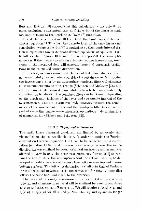
292 Fourier-Domain Modeling
Bott and Hutton [38] showed that this calculation is unstable if toomuch resolution is attempted, that is, if the width of the blocks is madetoo small relative to the depth of the layer (Figure 10.3).
Now if the cells in Figure 10.1 all have the same top and bottomdepths, equation 11.37 is just the discrete form of the one-dimensionalconvolution, where cell width W is equivalent to the sample interval Ax.Hence, equation 11.37 is the space-domain equivalent of equation 11.33.It follows that Figures 10.3 and 11.8 both represent the same phe-nomenon. If the inverse calculation attempts too much resolution, smallerrors in the measured field will generate large and unrealistic oscilla-tions in the calculated source distribution.
In practice, we can assume that the calculated source distribution isnot meaningful at wavenumbers outside of a certain range. Multiplyingthe inverse earth filter by an appropriate bandpass filter will eliminateall wavenumbers outside of this range (Schouten and McCamy [253]), ineffect forcing the determined source distribution to be band-limited. Byadjusting the bandwidth, the combined filter can be "tuned" dependingon the depth and thickness of the layer and the sample interval of themeasurements. Caution is still required, however, because the combi-nation of the inverse earth filter and the band-pass filter has a narrow,peaked shape that can generate unrealistic oscillations in determinationsof magnetization (Blakely and Schouten [32]).
11.3.1 Topographic SourcesThe earth filters discussed previously are limited by an overly sim-ple model for the source distribution. In order to apply the Fourier-convolution theorem, equation 11.31 had to be rendered into a convo-lution (equation 11.32), and this was possible only because the sourcedistribution was confined between horizontal surfaces z\ and Z2 and wasallowed to vary in only the horizontal directions. Parker [204] showedhow the first of these two assumptions could be relaxed; that is, he de-veloped a model consisting of a source layer with uneven top and unevenbottom surfaces. The following derivation is similar to that of Parker'sthree-dimensional magnetic case; the derivation for gravity anomaliesfollows the same lines and is left to the exercises.
The total-field anomaly is measured on a horizontal surface at alti-tude zo, and all magnetic material will be confined between two surfacesz\{x,y) and Z2(x,y), as in Figure 11.9. We will require z\{x^y) > ZQ andZ2(x,y) > zi(x,y) for all x and y. Note that z\ and Z2 are no longer
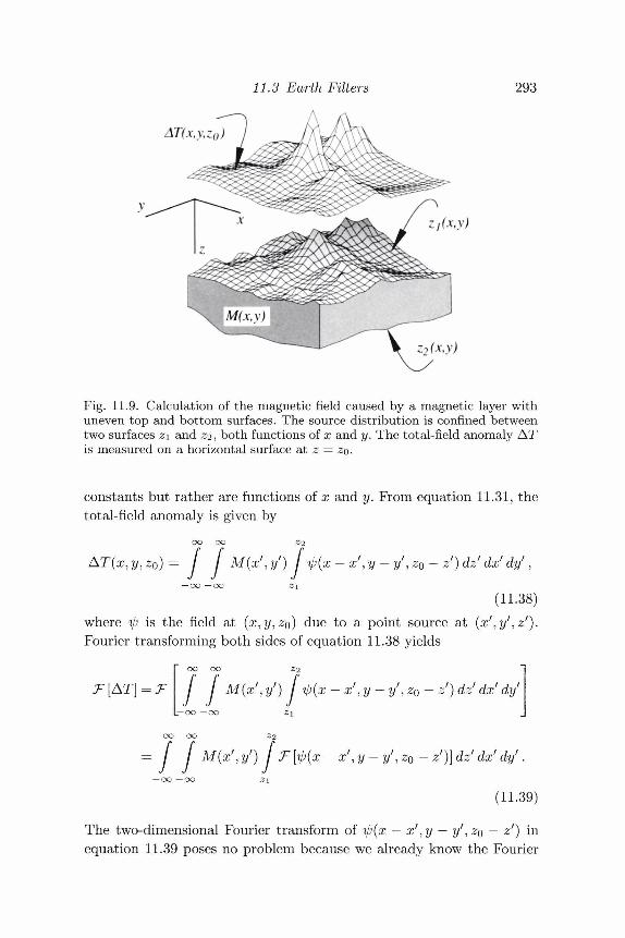
11.3 Earth Filters 293
AT(x,y,z
Zj(x,y)
Z2(x,y)
Fig. 11.9. Calculation of the magnetic field caused by a magnetic layer withuneven top and bottom surfaces. The source distribution is confined betweentwo surfaces z\ and 22, both functions of x and y. The total-field anomaly ATis measured on a horizontal surface at z — ZQ.
constants but rather are functions of x and y. From equation 11.31, thetotal-field anomaly is given by
AT(x, y , ZQ) = J J M(x', y') J ^{x -x',y- y ' , z0 - z') dzf dx' dy',— OO — OO
(11.38)where if) is the field at (x,y,zo) due to a point source at {x'^y'^z1).Fourier transforming both sides of equation 11.38 yields
Z2
j2
J J M{x', y') j ${x -x',y- y', z0 - z') dz' dx' dy'
O O O O Z2
= J J M(x', y') J T [iP(x -x',y- y', z0 - z')} dz' dx' dy'.— OO —OO
(11.39)
The two-dimensional Fourier transform of ijj(x — x',y — yf', z0 — z1) inequation 11.39 poses no problem because we already know the Fourier
294 Fourier-Domain Modeling
transform of ip(x, y, z); it is simply the Fourier transform of the anomalycaused by a single dipole (equation 11.25). Using the shifting property(Section 11.1.2) and equation 11.25, we get
ooJ M(x',y')— oo —oo
/ < e-i{kxx'+kyy')
OO OO
The top and bottom surfaces of the magnetic layer are carried inthis equation by the bracketed exponentials. Parker [204] suggested re-placing these exponential terms with their equivalent power series. Thedouble integral then is converted to a sum of two-dimensional Fouriertransforms, each taken with respect to x',yf coordinates. Making thesemodifications and collecting terms leads to the equation
n=0
(\\em9 f elfel*° £ [-^l>-^ [M(z? - %)]. (11.40)n.n=l
Hence, the Fourier transform of the total-field anomaly caused by alayer with uneven top and bottom surfaces is represented as a summa-tion; each element of the summation includes a Fourier transform ofthe magnetization weighted by a power of either the top or bottom sur-face. After the summation is completed, the inverse Fourier transformwill provide the total-field anomaly. Notice that if z\ and Z2 are bothconstant, equation 11.40 reduces to equation 11.35. Parker [207] showedthat this summation converges most rapidly if the origin is selected sothat z = 0 midway between the minimum values of z\ and z^.
11.3 Earth Filters 295
The gravitational equivalent of equation 11.40 is
J fc|fV[p(^ - 4)1, (11-41)71.n= l
where the mass is confined between surfaces z\(x,y) and Z2{x,y) and isdescribed by density p(x,y).Exercise 11.17 Derive equation 11.41 along the same lines as done for
equation 11.40.
The forward calculation of equation 11.40 has been particularly usefulin investigating magnetic anomalies over magnetic terrain or bathymetry(e.g., Macdonald [170]; Grauch [101]; Blakely [22]; Blakely and Grauch[28]; Hildenbrand, Rosenbaum, and Kauahikaua [128]). The gravitationalequivalent of equation 11.40 (equation 11.41) has been used in a varietyof applications, such as calculating isostatic residual gravity anomalies(Simpson, Jachen, and Blakely [260]) and estimating the gravitationaleffects of sedimentary basins (e.g., Jachens and Moring [137], Saltus[250]). Subroutine B.23 in Appendix B is a Fortran implementation ofequation 11.40.
Equation 11.40 also provides a framework for the inverse problem;that is, to calculate the magnetization M from measurements of AT(Parker [204], Parker and Huestis [208]). This calculation requires thatthe thickness of the layer t — Z2 — z\ remain uniform. If t is a constant,then equation 11.40 can be written
T [AT] = 2irCm BmBf e'^° (1 - e"'^) ]T izlMLjr [Mz^ . (1L42)n=0 U'
Isolating the n = 0 term of the summation on the left side of equa-tion 11.42 yields
{-\k\)n\
Equation 11.43 can be solved iteratively by (1) making an initial guessat the magnetization on the right side of equation 11.43, (2) solving theequation for a revised magnetization, (3) moving this revised magneti-zation to the right-hand side, and (4) repeating steps 2 and 3 until thesolution converges. As discussed earlier, step 2 involves a summationthat converges rapidly if the origin is midway between the topographicextremes. The iterations, on the other hand, converge most rapidly if theorigin is at a different level, namely, at the minimum value of topography
296 Fourier-Domain Modeling
(Parker and Huestis [208]). The change in origin can be accommodatedthrough the exponential term containing z$.
The solution to equation 11.43 is susceptible to the same instabil-ities discussed earlier in this and the previous chapter, and the higherwavenumber components must be filtered at each iteration. Nevertheless,this inverse method has proved useful in many applications, particularlyin the analysis of marine magnetic anomalies (e.g., Macdonald [170];Macdonald et al. [171]) where the magnetic part of ocean crust cansometimes be considered uniform in thickness.
Equation 11.43 can be used to find the annihilator for a particularlayer with constant thickness and a specified upper topographic surface(Parker and Huestis [208]). Recall that the annihilator for a volume Ris the source distribution a(Q) that satisfies the equation
a(Q)iP(P,Q)dv = O,R
where tp(P, Q) is the appropriate Green's function. A magnetizationa(Q) that satisfies
n = 0
(11.44)
will produce no anomaly when confined to the layer because substitut-ing equation 11.44 into 11.42 causes the total-field anomaly to vanish.This can be verified by comparing the preceding equations with equa-tion 11.15. Hence, we rewrite equation 11.44 as
T[a] = 6(kx)6(ky) - J2 ^-tf-riaz?], (11.45)n=l
which can be solved iteratively for the annihilator a(x, y) as was doneearlier for magnetization M(x,y). The annihilator represents the non-uniqueness of the solution for M. Any amount of the annihilator can beadded to the magnetization without affecting the calculated total-fieldanomaly; that is, the anomaly caused by M(x, y) + aa(x, y) is indepen-dent of a.
Exercise 11.18 Use equation 11.44 to show that the annihilator for aninfinite slab with flat top and flat bottom is a constant.
11.3 Earth Filters 297
11.3.2 General SourcesAt this point, we return to equation 11.31 and derive general relation-ships in the Fourier domain between a gravity or magnetic anomalymeasured on a horizontal surface and its causative source distributionlocated entirely below the surface. As before, we assume that the fieldis measured on a horizontal plane at height z — z$ and rewrite equa-tion 11.31 in a cartesian coordinate system with z positive down,
oo oo oo
f(x, y,zo) = / / s(x', y ' , z') %l){x -x',y- y ' , z0 - zf) dx' dy' dz'.ZQ —OO —OO
It is assumed in this equation that s(x',y',z') is zero outside of a re-gion with finite dimensions and especially at all z < ZQ. Applying theFourier transform to both sides of the equation (and remembering thatthe Fourier transform involves integration with respect to x and y, notx' and y'), we have
oo oo oo
ZQ — OO — OO
The shifting property of Fourier transforms (Section 11.1.2) allows asubstitution for the Green's function in the previous equation, that is,
In the gravitational case, the anomaly / is the vertical attraction ofgravity g, the source distribution s is density p, and i/; is the field of amonopole with Fourier transform given by equation 11.22. Making thesesubstitutions, we have
oo oo oo
T [g] = 2 7 T 7 e ^ z o I f f p(x', y', z') e~^z> e-i(-k*x'+k^ dx' dy' dz'.
ZQ — OO — OO
Now the two inner integrals are simply another two-dimensional Fouriertransform, in this case taken with respect to x' and ?/, so
oo
dz', (11.46)
where the term T [p(zr)} represents the two-dimensional Fourier trans-form of the density on one horizontal slice through the body at depth z'.
298 Fourier-Domain Modeling
In the same way, we can derive a similar relationship for the magneticcase,
oo
•F[AT]=27rCmemef|A:|elfel*° f T[M(z')}e-^z> dz', (11.47)
where the term T [M(V)] represents the Fourier transform of the mag-netization on one horizontal slice through the body at depth zf.
Equations 11.46 and 11.47 provide general relationships in the Fourierdomain between arbitrary mass or magnetization distributions and theanomalies that they produce. The integral terms in each equation essen-tially consist of dividing the source into horizontal slices, Fourier trans-forming the density or magnetization of each slice, weighting the Fouriertransform by an exponential term that depends on the depth of the slice,and summing the results over all slices. We will have use for these rela-tionships in Chapter 12. Notice that equations 11.46 and 11.47 reduce toequations 11.34 and 11.35 if the source is confined to a horizontal layerwith top at depth zi, bottom at Z2, and density or magnetization thatvaries in only the horizontal directions.
11.4 Depth and Shape of SourceAs we have seen, Fourier analysis under certain assumptions can greatlyfacilitate solutions to the linear inverse problem. If the source materialis confined to a horizontal layer, for example, equation 11.36 provides adirect calculation of magnetization or density from the potential field ofthe layer, thus rendering the linear inverse problem for this particularcase quite easy, at least conceptually.
Fourier transforms also can assist in determining the shape and lo-cation of potential-field sources. Oldenburg [200], for example, modifiedthe method of Parker [204] in order to estimate the shape of a causativemass from its gravity anomaly. If the body has uniform density contrastand a flat bottom at z = 0, then the right side of equation 11.41 reducesto a summation of Fourier transforms of powers of the upper surface,that is,
n = l
Isolating the first term of this summation, as was done for magnetiza-tion in Section 11.3.1, leads to an iterative scheme to estimate the shape
11.4 Depth and Shape of Source 299
of the upper surface. The free parameters p and ZQ in this equation, aswell as the requisite bandpass filtering at each iteration, characterize thenonuniqueness of this inversion scheme; the solution for z\ depends onthe values selected for these parameters (Oldenburg [200]). Pilkingtonand Crossley [221, 222] described a similar technique for estimating theshape of magnetic basement or crust al interfaces from magnetic anoma-lies.
Hansen and Wang [114] simplified a Fourier-domain formulation, orig-inally from Pedersen [216], that approximates potential-field sources bypolyhedrons, similar to the space-domain models described by Bott [36]and Barnett [11]. The bodies are assumed to have uniform magnetizationor density. The potential field f(x,y) of a polyhedron can be expressedin the Fourier domain as a summation over the iV vertices of the poly-hedron,
TV
n=l
where (xn,yn,zn) are the coordinates of vertex n, and an depends onthe orientation of each edge of each facet composing vertex n and, in themagnetic case, on the direction of magnetization and regional field. Thecoordinates of each vertex, therefore, are represented in the argument ofa specific exponential term in the summation, so the forward problemis reasonably straightforward. Because the summation depends on thevertex coordinates, the polyhedron does not need to be decomposed intoindividual facets, as was done in Section 9.3.2 and in Subroutine B.10.
Wang and Hansen [288] showed how this formalism could be adaptedto the inverse problem for magnetic anomalies, that is to estimate thelocations in space of the vertices of a magnetic polyhedron from its mea-sured anomaly. Here we use the total-field anomaly, but their discus-sion applies to any component of the anomalous field. The exponentialin each term of summation 11.48 includes both an attenuation factorrelated to the depth of one vertex and a phase factor related to thehorizontal position of the same vertex. The problem then is to analyzeT [AT] in order to resolve these various factors for each vertex. First letF(kx, ky) = \k\2 T [AT]. We will show in the next chapter that F(kx, ky)so defined is the Fourier transform of the second vertical derivative ofAT. Wang and Hansen [288] defined TV complex parameters
_ kxXj + kyyj 7 - 1 2 N
300 Fourier-Domain Modeling
and showed that the first N inward derivatives of F(kx, ky) are relatedby a summation,
7 V - 1
d(-\k\)N t<0 'n d(-\k\r ' y ^where the various 7n are factors in a complex polynomial equation,
N-l
The roots of equation 11.50 are the various <5j, and these as definedpreviously are related to the vertex coordinates.
The algorithm of Wang and Hansen [288] essentially proceeds by com-puting the first N inward derivatives of l&l2.?7 [AT]; using these in equa-tion 11.49 to solve for 7n, n = 0,1, 2 , . . . , N — 1, along rays of the kxi kyplane; and finally solving for 6j, j = 1, 2 , . . . , JV, in equation 11.50, alsoalong rays of the kx, ky plane.
11.4-1 Statistical ModelsThe previous examples are applicable to potential fields caused by oneor a few causative bodies. In the remainder of this section, we will focuson estimating the average depth of a large collection of gravity or mag-netic sources from their statistical properties, an approach pioneered bySpector and Grant [268] and Treitel, Clement, and Kaul [281]. Magneticfields are used here for illustration, but the discussion could easily beadapted to gravity fields as well.
To see how the statistical approach works in a general way, considerthe total-field anomaly measured on a horizontal surface and causedby a horizontal layer with top at depth d and thickness t. From equa-tion 11.35,
T [AT] = T [M] {27rCmBmefe-|fc|d(l - e'^1)} . (11.51)
The total-field anomaly is measured at discrete locations, and T [AT]and Gf are easily calculated. If by some lucky happenstance we alsoknow the distribution of magnetization, then only the exponential termsremain to be determined in equation 11.51. These could be transposedto one side of the equation, and curve fitting could be used to estimated and t.
11.4 Depth and Shape of Source 301
It is unlikely that we would know M(x,y) in detail, but we may havesome idea about how magnetization behaves statistically. For example,we might assume that the layer extends infinitely far in all horizontaldirections and that M(x, y) is a random function of x and y. In this case,^"[M] and F[AT] do not exist because inequality 11.3 is not satisfied.Equation 11.51 should be written instead as
$ A T ( ^ , ky) = $M{kx, ky) - F(kx, ky), (11.52)
where <I>AT and <I>M are power-density spectra of the total-field anomalyand the magnetization, respectively, and
F(kx, ky) = 47r2C£|em |2 |e f\2e-Wd(l - e-W) 2 .
If the probabilistic behavior of M(x, y) is known or assumed, its power-density spectrum can be analytically derived as described in Section11.1.3. Moreover, although we only have measurements of AT(x, y) overfinite distances, a variety of ways are available to estimate power-densityspectra from finite segments of a random function. Hence, with a suit-able probabilistic model for M(x,y), the remaining unknown functionF(kx, ky) can be analyzed in terms of d and t.
This analysis can be simplified greatly by noting that all terms, except|Om |2 and |Of|2, in equation 11.52 are radially symmetric.f Moreover,as discussed in Section 11.2.1, the radial averages of Bm and Gf areconstants. Hence, the radial average of $ A T is
$AT(\k\)=A<f>M(\k\)e-2Wd(l-e-Wt)2, (11.53)
where A is a constant that depends on the orientations of magneti-zation and regional field. We now need a suitable statistical model forM(x, y). For example, if M(x, y) is completely random and uncorrelated,^M(kxjky) is a constant, and equation 11.53 becomes
where B is a constant. Finally, taking the logarithm of both sides yields
21og(l - e'^). (11.54)
As shown by Figure 11.10, this equation at medium to high wavenumbers(wavelengths less than about twice the thickness of the layer) is approxi-mately that of a straight line with slope equal to — Id. We could estimate
f We have assumed here that the probabilistic behavior of M(x,y) is isotropic, thatis, its statistical behavior is the same in all horizontal directions.
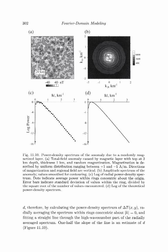
302 Fourier-Domain Modeling
-16-1 -16-1
Fig. 11.10. Power-density spectrum of the anomaly due to a randomly mag-netized layer, (a) Total-field anomaly caused by magnetic layer with top at 3km depth, thickness 1 km, and random magnetization. Magnetization is de-scribed by uniform distribution ranging between +1 and —1 A/m. Directionsof magnetization and regional field are vertical, (b) Amplitude spectrum of theanomaly; values smoothed for contouring, (c) Log of radial power-density spec-trum. Dots indicate average power within rings concentric about the origin.Error bars indicate standard deviation of values within the ring, divided bythe square root of the number of values encountered, (d) Log of the theoreticalpower-density spectrum.
d, therefore, by calculating the power-density spectrum of AT(x,y), ra-dially averaging the spectrum within rings concentric about |fc| = 0, andfitting a straight line through the high-wavenumber part of the radiallyaveraged spectrum. One-half the slope of the line is an estimate of d(Figure 11.10).
11.4 Depth and Shape of Source 303
Exercise 11.19 Show that the same result is achieved if M(x,y) = Mo +r(x,y), where Mo is a constant and r(x,y) is a random function of x andy with zero mean. In other words, show that a slab, principally uniformin magnetization but having a small random component, also satisfies$M = constant.
Ensemble SourcesIn a landmark paper, Spector and Grant [268] framed the random de-scription of the source distribution in a more complete context. In theirmodel, the anomaly is assumed to be produced by a large number ofblocks. The parameters describing any one block (e.g., depth, thickness,width, length, magnetization) are assumed to obey probabilities commonto the entire set. Such a distribution of sources constitutes an ensemble.Equation 11.12 showed that the expected value of a continuous randomvariable r can be expressed as an ensemble average,
OO
(r) = f pPr(p)dp,
where Pr(p) is the probability that r takes the value p. Similarly, if g isa measurable function of various random variables a\, <22,..., then g hasan expected value given by
OO OO
(9) = / •' • /— 00 —00
where Pai,a2,...(ai>a2, • • •) is the joint probability distribution for therandom variables of g.
Now consider the magnetic anomaly caused by an ensemble of sources,where the parameters (depth, thickness, and so forth) describing eachelement of the ensemble are each a random variable. We wish to framethe power-density spectrum of the anomaly in terms of an ensembleaverage, as shown by the previous equation. If Pd,t,...(^r5...) is thejoint probability that depth d assumes the value <5, thickness t assumesthe value r, and so on, then the expected value of the power-densityspectrum is given by
00 00
($AT) = I ... I \f[AT}\2PdA...(6,T,...)d6dT--- ,
304 Fourier-Domain Modeling
where ^[AT]]2 is the spectrum of the anomaly caused by just oneelement of the ensemble having parameters <5, r, and so on. Presumablythe random parameters vary independently of one another, so the jointprobability can be factored, that is,
oo oo
($AT) = J ... j \f[AT]\2Pd(6)Pt(T)---d6dT--- . (11.55)— oo —oo
Next we need an expression for |JF[AT]|2 in equation 11.55. Spectorand Grant [268] let each member of the ensemble be a rectangular par-allelepiped. Equation 11.51 can provide the spectrum of the anomalycaused by a rectangular parallelepiped if we let M(x,y) = 0 exceptwithin a rectangular patch. Let the patch have dimensions 2a and 2bin the x and y directions, respectively, and let M{x,y) = Mo, a con-stant, within the patch. The parameters a, 6, and MQ become additionalrandom variables in equation 11.55. From equation 11.51,
2(a,&), (11.56)
where. 4 sin kxa sin kyb
IxiX ivy
is the "shape factor."Now we exploit a result that has recurred throughout this chapter. In
the Fourier domain, the potential field separates into multiplicative fac-tors, where each factor is a function of just one of the random variables.Substituting equation 11.56 into equation 11.55 yields
($AT)=47T2C^ I e-2^sPd{6)dS I (l-e- | fc | r)2F t(r)rfr...— OO —OO
2^2 / -2= 4 7 F
(^2(a,6))(M2)(|em|2)(|ef|2). (11.57)
Hence, the expected value of the power-density spectrum is factored intovarious ensemble averages, where each average involves just one of therandom variables.
Consider the first of these factors. Suppose that the depth to the topof each element of the ensemble can lie with equal probability between
11.4 Depth and Shape of Source 305
depths d- Ad and d + Ad. Then
d+Ad
"~4|fc|Ad
If Ad is taken small compared to J, then
d-Ad
-2|fc|d/ 2|fc|Ad _ -2\k\Ad\
Hence, we have the surprising result that the power-density spectrumof an entire ensemble depends on depth in the same way that an "aver-age" member of the ensemble depends on depth. It is easy to show that(|6m|2) and (|6f|2) do not depend on |fc|, but that (S2(a,b)) will affectthe shape of the radially averaged spectrum depending on the values ofa and b.
To estimate d, therefore, we could proceed as before: From the mea-sured anomaly, calculate the logarithm of the radially averaged power-density spectrum; the slope of this function at medium to high wavenum-bers is proportional to the depth of the ensemble. This implies, however,that all other factors of the ensemble (i.e., (52(a,&))) are accountedfor. In order to investigate how depth varies throughout a large region,various authors (e.g., Connard, Couch, and Gemperle [63]; Okubo etal. [198]; Phillips [220]; Blakely and Hassanzadeh [29]; Blakely [21]) havedivided magnetic surveys into overlapping cells (or segments of long pro-files) and made calculations for each cell similar to those described here.
Fractal Source DistributionsThe foregoing statistical models have assumed that magnetization (ordensity) has no spatial correlation. The method of Spector and Grant[268], for example, employs a model with infinitely many rectangularprisms each with random dimensions; the magnetization of such a modelbecomes spatially uncorrelated if the characteristic dimensions of theprisms are assumed to be small. Similarly, the model of Blakely andHassanzadeh [29] assumes that the magnetization is an uncorrelatedrandom function of just one horizontal dimension. Such models imply
306 Fourier-Domain Modeling
that any two samples taken from the source distribution will be totallyindependent of one another, regardless of their proximity.
There is mounting evidence from aeromagnetic data (Gregotski, Jen-sen, and Arkani-Hamed [104]; Pilkington and Todoeschuck [226]), fromtruck-mounted magnetometer surveys (Gettings, Bultman, and Fisher[94, 95]; Bultman and Gettings [46]), and from density and suscepti-bility logs (Pilkington and Todoeschuck [225, 226]) that magnetizationand density are not completely uncorrelated but rather have a degree ofself-similarity. These authors have argued that magnetization and den-sity can be described as a form of fractal geometry, called scaling noise.Such random processes have power-density spectra proportional to somepower of wavenumber. A one-dimensional process of this sort, for exam-ple, has a power-density spectrum given by <fr(k) = Aka, where A anda are constants, and k is wavenumber. If a = 0, the process is uncorre-lated, as in the foregoing statistical models. If a < 0, on the other hand,the process is correlated, and the degree of correlation is indicated bythe magnitude of a. The parameter a is called the fractal dimension; in asense, it describes the "roughness" of the random process. Gettings et al.[94, 95] and Bultman and Gettings [46] have related a, determined fromtruck-mounted magnetometer profiles, to near-surface lithologies. Vol-canic terrain might possess a different fractal dimension than plutonicterrain, for example, and determination of a along a magnetic profilemight help to distinguish between these two lithologies when concealedbeneath sediments.
Pilkington and Todoeschuk [226] compared magnetic anomalies overthree-dimensional fractal models. They confined the magnetization to alayer and let the magnetization be fractal in both the horizontal andvertical directions. A magnetization with a = — 4 produces an anomalythat is similar in appearance to typical observed anomalies and in thissense is far superior to anomalies produced by an uncorrelated mag-netization (a = 0). They further argued that the fractal behavior ofmagnetization may not be isotropic; that is, the fractal dimension in thehorizontal directions may be different from that in the vertical direction.These results have important implications for statistical models to es-timate depth to source (Pilkington, Gregotski, and Todoeschuck [223]);the often-used assumption in these models, that the power-density spec-trum of magnetization is constant, may be inaccurate and may lead tosystematic errors in depth estimation.
11.4 Depth and Shape of Source 307
11.4.2 Depth to BottomThe depth extent of magnetic sources can be of considerable geologic in-terest. The limiting depth may be controlled, for example, by the Curie-temperature isotherm. If the Curie temperature of crustal rocks in theregion of the magnetic survey is known from geologic and rock magneticconsiderations, then an estimate of the depth to the Curie-temperatureisotherm based on magnetic anomalies can help characterize the geother-mal setting of the area. Unfortunately, this calculation ranks among themost difficult in potential-field inversion. As can be seen from equa-tion 11.35, e~\k\Z2 dominates e~^Zl throughout all wavelengths of thespectrum; that is, the contribution of the bottom of the source is domi-nated at all wavelengths by the contributions from shallower parts.
Several methods to estimate z2 in the Fourier domain have been de-veloped in recent years and have shown encouraging results in spite ofthe difficulties involved. Various workers (Connard et al. [63], Smith etal. [265], Shuey et al. [257], Miyazaki [185], and Blakely [23]) have usedthe shape of radially averaged spectra to estimate the depth extent ofmagnetic sources. In particular, the position kmax of the maximum alongthe \k\ axis is related to the depth to the bottom of the layer according to
_ log2:2 -logZ!"-max —
Z2 - ZiTo estimate depths to the Curie-temperature isotherm in Oregon, forexample, Connard et al. [63] divided a magnetic survey into overlappingcells and calculated for each cell a radially averaged power-density spec-trum, as in Figure 11.10. From these spectra, they attempted to locate&max and, using the preceding equation, to estimate z2. Note that z2 inthis equation cannot be determined independently of z\.
Bhattacharyya and Leu [18] determined depth to the bottom of in-dividual sources by analyzing isolated anomalies. They calculated thelocation of the centroid of isolated magnetic sources from the momentsof their respective anomalies. If the depth to the top of the sourceis also known, perhaps determined with the method of Spector andGrant [268], then the depth to the bottom of the source is easily cal-culated. This method requires isolating individual anomalies from allsurrounding anomalies and regional fields, a challenging task in mostgeologic environments.
Okubo et al. [198, 199] expanded on the method of Bhattacharyya andLeu [18] by treating ensembles of sources. They reframed equation 11.57into an expression dependent on the centroid of the ensemble average.
308 Fourier-Domain Modeling
By making calculations for various patches of the magnetic survey, theywere able to derive a map of the Curie-temperature isotherm for a partof the Japanese arc.
Each of these methods has fundamental limitations. First, the de-termination of the depth to the bottom of a source cannot be madewithout knowledge of the depth to its top, which in itself is a difficultinverse determination. Second, estimation of the bottom of potential-field sources, by their nature, must focus on the lowest wavenumberparts of the Fourier domain. This part of the spectrum is susceptibleto noise from various sources, particularly from poorly known regionalfields that may be unrelated to the bottom parts of the sources of con-cern. Moreover, discrete Fourier analysis provides relatively little infor-mation about the lowest wavenumbers of the power-density spectrum.With conventional techniques, the smallest wavenumber at our disposalis the fundamental wavenumber k = 2TT/L, where L is the dimension ofthe magnetic survey. Connard et al. [63] reasoned that &max should be atleast twice the fundamental wavenumber in order to be able to resolvea peak in the spectrum. Thus,
log z2 - log ziA magnetic survey conducted 1 km above the tops of magnetic sources,therefore, must have minimum dimensions on the order of 50 km in orderto resolve depth extents of 10 km; the survey dimensions must be at least160 km for sources extending to 50 km.
Finally, the shape of the power-density spectrum and, hence, depthdeterminations depend on the characteristic shapes of the magnetic bod-ies, expressed by the factor S2(a,b) in equation 11.57. At wavelengthslarge compared to the body dimensions, the ensemble average is equiv-alent to that of a random distribution of dipoles (Okubo et al. [198]).In such cases, the low-wavenumber part of the spectrum is independentof the exact model (blocks, cylinders, spheres, and the like) used for theelements of the ensemble. The true dimensions of the source, however,are not likely to be well understood in most geologic settings.
11.5 Problem Set1. Consider a cartesian coordinate system with the z axis directed down,
and let (j>(x, y, z) be the potential of a source distribution locatedentirely below the plane z = ZQ. The Dirichlet integral relates the
11.5 Problem Set 309
potential field observed on one plane z — z\ to the potential observedon another plane z = z2, where z2 < z\ and z\ < z0:
oo oo,/ x zi-z2 f f <p{x',y',zi) , ,<p(x,y,Z2) = — / / 3 dx dy , z2 < zx,z7T j J r
— OO — OO
where r = ^/(x — a;')2 + (2/ — y')2 + (zi ~(a) Show for any Z3 that
00 00
/ / (p(x,y,z3)dxdy = A,—00 —00
where 23 < ZQ, and A is a constant independent of z%.(b) How does this result relate to Gauss's law for both the gravita-
tional and magnetic potentials?(c) Show that the total energy of the potential observed on a plane
above the source decreases with the plane's distance from thesource; that is, show that
00 00
/ / 4>2{x,y,z2)dxdy < / / c/>2 (x, y, z±) dx dy— 00 —00 —ex) —00
for any z2 < z\.2. Let gz be the vertical gravitational attraction of a mass distribution
located below a horizontal plane, and let T [gz] be the Fourier trans-form of gz observed on the plane.(a) Show that the value of T [gz] at k = 0 is proportional to the total
mass of the distribution.(b) More generally, show that the amplitude spectrum satisfies the
inequality
where M is the total mass and z$ is the depth to the top of thesource distribution.
3. At the north magnetic pole, the total-field anomaly due to a given dis-tribution of magnetization has a phase spectrum given by 0(/cx, ky).(a) What is the phase spectrum of the same magnetization distri-
bution if it is relocated at the magnetic equator? Assume thatmagnetization is entirely induced.
(b) What is the phase spectrum at the south magnetic pole?
310 Fourier-Domain Modeling
(c) What is the phase spectrum if the local field has an inclinationof 63° and a declination of 18°?
4. A total-field anomaly AT(x,y) is measured on a horizontal surfaceat height z0 above a uniformly magnetized, rectangular prism withmagnetization M, thickness T, and horizontal dimensions D. Theprism is at the north magnetic pole and has negligible Koenigsbergerratio.(a) Describe the amplitude spectrum of AT(x, y) at all wavenumbers
(including kx — ky = 0) in terms of zo, T, D, and M. Hint: Itmight be helpful to consider the prism as part of an infinite slab.
(b) Discuss the feasibility of determining z0, T, D, and M from theamplitude spectrum.
12Transformations
The third, or depth, dimension of geology is a major frontier at present.(Jack Oliver)
A theory has only the alternative of being right or wrong. A model hasa third possibility: it may be right, but irrelevant.
(Paul R. Ehrlich)
Now we are ready to undertake the third category of potential field meth-ods depicted in Figure 9.1, those methods that facilitate geologic inter-pretations by transforming measured data into some new form. Thesetransformations, in general, do not directly define the distribution ofsources, but they often provide insights that help to build a general un-derstanding of the nature of the sources. Upward continuation, for ex-ample, is a method that transforms anomalies measured on one surfaceinto those that would have been measured on some higher surface. Theupward-continued anomalies do not provide direct information aboutthe source, but they can be instructive nonetheless. In particular, theprocess of upward continuation tends to attenuate anomalies caused bylocal, near-surface sources relative to anomalies caused by deeper, moreprofound sources.
The aeromagnetic data shown in Figure 12.1 will serve to illustratesome of the methods discussed subsequently. These data are from a re-gion of the Basin and Range geologic province in north-central Nevada.The mountain ranges in this area typically expose sedimentary rocksof Paleozoic age and volcanic tuffs of Tertiary age. The linear mag-netic anomaly that trends north-northwest across the entire map (Fig-ure 12.1 (a)), however, is associated with exposures of basaltic flows anddikes of middle Miocene age, which are largely concealed. This associa-tion between the linear anomaly and basaltic dikes and flows has beeninterpreted as indicating a rift zone active during the middle Miocene
311
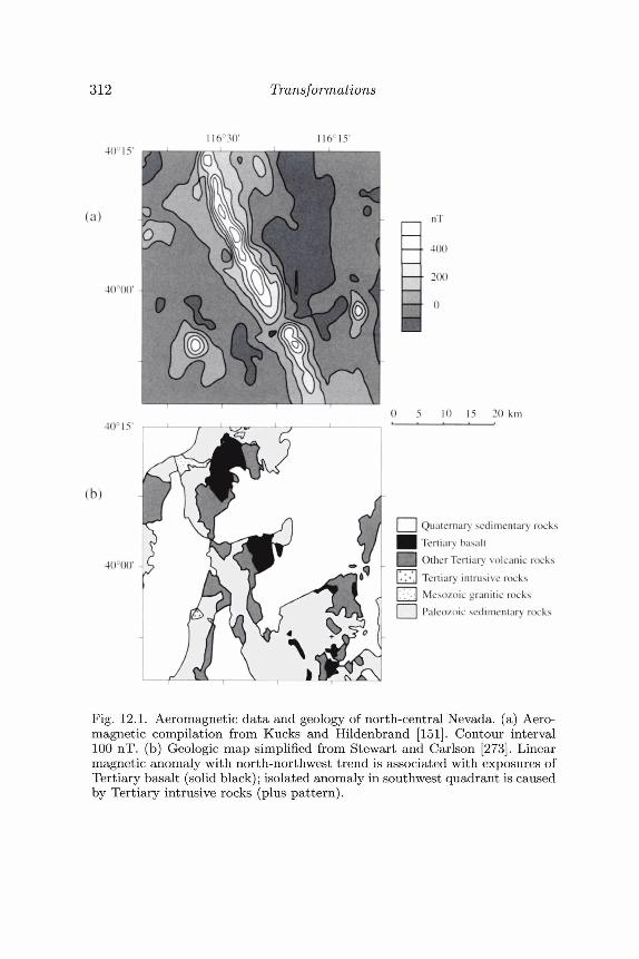
312 Transformations
\\6°M)'40° 15"
400
20040o(X)'
40° 15'
(b)
40°<X)1
10 \5 20 km
| | Quaternary sedimentary rocks
| Tertiary basalt
| Other Tertiary volcanic rocks
]**+*} Tertiary intrusive rocks
J Mesozoic granitic rocks
| J Paleozoic sedimentary rocks
Fig. 12.1. Aeromagnetic data and geology of north-central Nevada, (a) Aero-magnetic compilation from Kucks and Hildenbrand [151]. Contour interval100 nT. (b) Geologic map simplified from Stewart and Carlson [273]. Linearmagnetic anomaly with north-northwest trend is associated with exposures ofTertiary basalt (solid black); isolated anomaly in southwest quadrant is causedby Tertiary intrusive rocks (plus pattern).
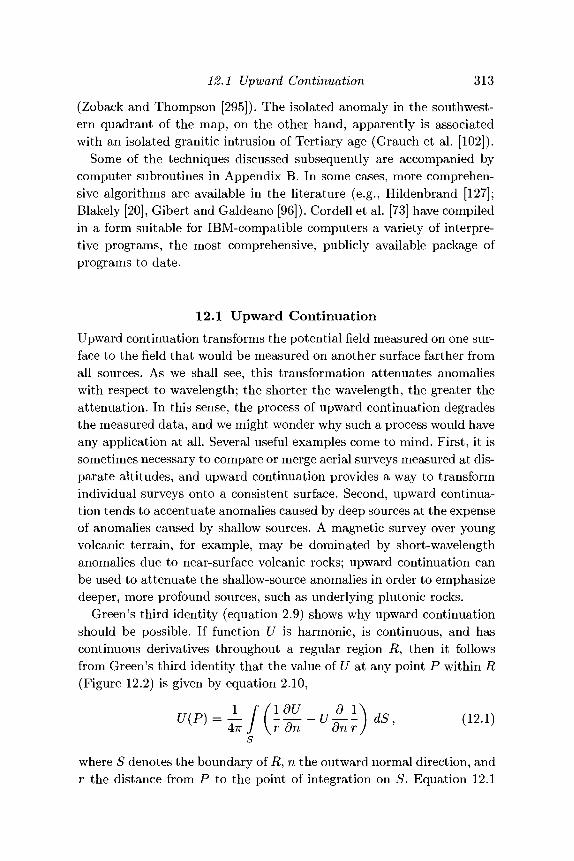
12.1 Upward Continuation 313
(Zoback and Thompson [295]). The isolated anomaly in the southwest-ern quadrant of the map, on the other hand, apparently is associatedwith an isolated granitic intrusion of Tertiary age (Grauch et al. [102]).
Some of the techniques discussed subsequently are accompanied bycomputer subroutines in Appendix B. In some cases, more comprehen-sive algorithms are available in the literature (e.g., Hildenbrand [127];Blakely [20], Gibert and Galdeano [96]). Cordell et al. [73] have compiledin a form suitable for IBM-compatible computers a variety of interpre-tive programs, the most comprehensive, publicly available package ofprograms to date.
12.1 Upward ContinuationUpward continuation transforms the potential field measured on one sur-face to the field that would be measured on another surface farther fromall sources. As we shall see, this transformation attenuates anomalieswith respect to wavelength; the shorter the wavelength, the greater theattenuation. In this sense, the process of upward continuation degradesthe measured data, and we might wonder why such a process would haveany application at all. Several useful examples come to mind. First, it issometimes necessary to compare or merge aerial surveys measured at dis-parate altitudes, and upward continuation provides a way to transformindividual surveys onto a consistent surface. Second, upward continua-tion tends to accentuate anomalies caused by deep sources at the expenseof anomalies caused by shallow sources. A magnetic survey over youngvolcanic terrain, for example, may be dominated by short-wavelengthanomalies due to near-surface volcanic rocks; upward continuation canbe used to attenuate the shallow-source anomalies in order to emphasizedeeper, more profound sources, such as underlying plutonic rocks.
Green's third identity (equation 2.9) shows why upward continuationshould be possible. If function U is harmonic, is continuous, and hascontinuous derivatives throughout a regular region R, then it followsfrom Green's third identity that the value of U at any point P within R(Figure 12.2) is given by equation 2.10,
where S denotes the boundary of R, n the outward normal direction, andr the distance from P to the point of integration on S. Equation 12.1
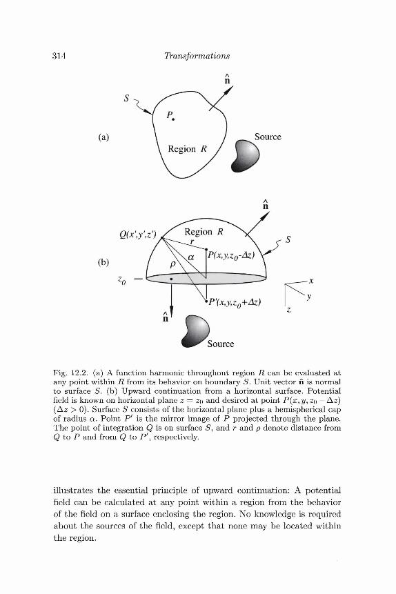
314 Transformations
(a) Source
Q(x',y',z')
(b)
Source
Fig. 12.2. (a) A function harmonic throughout region R can be evaluated atany point within R from its behavior on boundary S. Unit vector h is normalto surface S. (b) Upward continuation from a horizontal surface. Potentialfield is known on horizontal plane z = zo and desired at point P(x, y, zo — Az)(Az > 0). Surface S consists of the horizontal plane plus a hemispherical capof radius a. Point P' is the mirror image of P projected through the plane.The point of integration Q is on surface S, and r and p denote distance fromQ to P and from Q to P' , respectively.
illustrates the essential principle of upward continuation: A potentialfield can be calculated at any point within a region from the behaviorof the field on a surface enclosing the region. No knowledge is requiredabout the sources of the field, except that none may be located withinthe region.
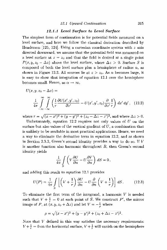
12.1 Upward Continuation 315
12.1.1 Level Surface to Level SurfaceThe simplest form of continuation is for potential fields measured on alevel surface, and here we follow the classical derivation described byHenderson [125, 124]. Using a cartesian coordinate system with z axisdirected downward, we assume that the potential field was measured ona level surface at z = ZQ and that the field is desired at a single pointP(x, y, ZQ — Az) above the level surface, where Az > 0. Surface S iscomposed of both the level surface plus a hemisphere of radius a, asshown in Figure 12.2. All sources lie at z > z0. As a becomes large, itis easy to show that integration of equation 12.1 over the hemispherebecomes small. Hence, as a —> oo,
U(x,y,z0 - Az) =oo oo
1 f f fldU(x',y',z0) ^dl\j>j> , 1 0 o^to j } [r fl? U(x,y,zo) — -)dxdy, (12.2)
— oo —oo
where r = y/(x — x')2 + (y — yf)2 + (ZQ — Az — z')2, and where Az > 0.Unfortunately, equation 12.2 requires not only values of U on the
surface but also values of the vertical gradient of £/, a combination thatis unlikely to be available in most practical applications. Hence, we needa way to eliminate the derivative term in equation 12.2, and as shownin Section 2.3.2, Green's second identity provides a way to do so. If Vis another function also harmonic throughout R, then Green's secondidentity yields
4TT J \ dn dn Js
and adding this result to equation 12.1 provides
To eliminate the first term of the integrand, a harmonic V is neededsuch that V + £ = 0 at each point of S. We construct P', the mirrorimage of P, at (x, y, ZQ + Az) and \etV = —~ where
p= ^{x - x')2 + (y - y')2 + (zo + Az - z')2.
Note that V defined in this way satisfies the necessary requirements:V+- = 0 on the horizontal surface, V + - will vanish on the hemisphere
316 Transformations
as a becomes large, and V is always harmonic because p never vanishes.Hence, equation 12.3 becomes
.1p
sAs the hemisphere becomes large, the first term vanishes at each point
of S, and the second term vanishes except on the horizontal surface,
',y',,0)A[i_i] dx'dy'.— oo —oo
Carrying out the derivative and letting z' move to the horizontal surfaceleads to
oo oo
/ / x - x'Y + (y - 2/0 -
Az>0. (12.4)
Equation 12.4 is the upward-continuation integral. It shows how to cal-culate the value of a potential field at any point above a level, horizontalsurface from complete knowledge of the field on the surface. Some com-promises will be required in practical applications, of course; we neverwill know the potential field precisely at each point of an infinite plane.It is particularly important to know the field well beyond the lateralextent of all sources, a recommendation that is difficult to implement inpractice.
Fourier-Domain RepresentationEquation 12.4 can be used to continue data measured on a level surfaceto another surface, level or not. For each point of the new surface, thetwo-dimensional integral must be evaluated, a computationally intensivetask. The procedure can be made more efficient and insightful, however,if it is recast in the Fourier domain. In doing so, we will have to settlefor level-surface-to-level-surface applications.
Note that equation 12.4 is simply a two-dimensional convolution,oo oo
U(x, y, zo-Az)= j J U(x', y', z0) M* -x',y-y', Az) dx' dy',— oo —oo
12.1 Upward Continuation 317
where
Mx, y, Az) = £ {x2 + / (125)
If the potential field U measured on surface z = ZQ satisfies inequal-ity 11.3, then it has a Fourier transform T [U]. The Fourier-domain rep-resentation of equation 12.4 is found by transforming both sides of equa-tion 12.4 to the Fourier domain and applying the Fourier-convolutiontheorem (Section 11.1.5),
F[Uu]=F[U]r[il>u\, (12.6)
where T [Uu] is the Fourier transform of the upward-continued field. Allthat is needed is an analytical expression for T [ipu], which can be foundfrom the Fourier transform of equation 12.5. First note that
where r = \J x2 + y2 + Az2. With the help of equation 11.21, therefore,the Fourier transform of equation 12.7 is given by
ddAz \k\
= e-Az\k\^ Az>0. (12.8)
A level-to-level continuation can be achieved, therefore, by Fourier trans-forming the measured data, multiplying by the exponential term of equa-tion 12.8, and inverse Fourier transforming the product.
It is clear from equation 12.8 and shown by Figure 12.3 that (1)the process of upward continuation attenuates all wavenumbers except\k\ = 0, (2) each wavenumber is attenuated to a greater degree thanall lower wavenumbers, and (3) the degree of attenuation increases withincreasing Az. Equation 12.8 is a real function, that is, it has no phasecomponent, and consequently imparts no phase changes to the upward-continued field. As an example, Figure 12.4 shows the total-field anomalyof central Nevada (Figure 12.1 (a)) continued upward 5 km. Notice thatthe shortest wavelengths of the original anomalies are essentially elim-inated in Figure 12.4, whereas the fundamental anomalies remain in asmoother form.
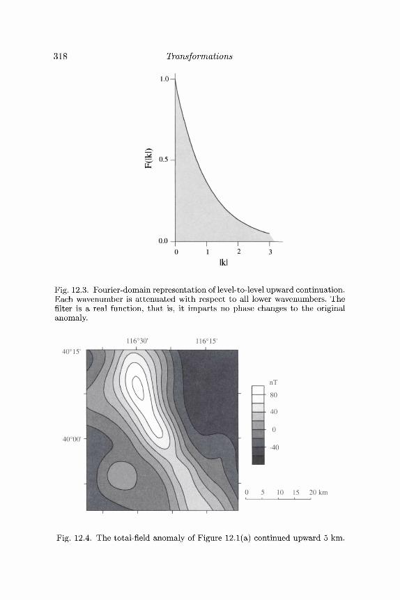
318 Transformations
Fig. 12.3. Fourier-domain representation of level-to-level upward continuation.Each wavenumber is attenuated with respect to all lower wavenumbers. Thefilter is a real function, that is, it imparts no phase changes to the originalanomaly.
40° 15'
40°00"
0 5 10 15 20 km
Fig. 12.4. The total-field anomaly of Figure 12.1 (a) continued upward 5 km.
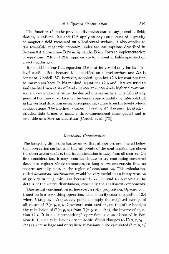
12.1 Upward Continuation 319
The function U in the previous discussion can be any potential field;that is, equations 12.4 and 12.6 apply to any component of a gravityor magnetic field measured on a horizontal surface. It also applies tothe total-field magnetic anomaly, under the assumptions described inSection 8.3. Subroutine B.24 in Appendix B is a Fortran implementationof equations 12.6 and 12.8, appropriate for potential fields specified ona rectangular grid.
It should be clear that equation 12.6 is strictly valid only for level-to-level continuation, because U is specified on a level surface and Az isconstant. Cordell [67], however, adapted equation 12.6 for continuationto uneven surfaces. In his method, equations 12.6 and 12.8 are used tofind the field on a series of level surfaces at successively higher elevations,some above and some below the desired uneven surface. The field at anypoint of the uneven surface can be found approximately by interpolatingin the vertical direction using corresponding values from the level-to-levelcontinuations. The method is called "chessboard" (because the stack ofgridded data brings to mind a three-dimensional chess game) and isavailable as a Fortran algorithm (Cordell et al. [73]).
Downward Continuation
The foregoing discussion has assumed that all sources are located belowthe observation surface and that all points of the continuation are abovethe observation surface, that is, continuation is away from all sources. Onfirst consideration, it may seem legitimate to try continuing measureddata into regions closer to sources, so long as we are certain that nosources actually exist in the region of continuation. This calculation,called downward continuation, would be very useful in an interpretationof gravity or magnetic data because it would tend to accentuate thedetails of the source distribution, especially the shallowest components.
Downward continuation is, however, a risky proposition. Upward con-tinuation is a smoothing operation. This is easily seen in equation 12.4where U(x,y, z$ — Az) at any point is simply the weighted average ofall values of U(x,y,zo). Downward continuation, on the other hand, isthe calculation of U(x, y, ZQ) from U(x,y,zo — Az), the inverse of equa-tion 12.4. It is an "unsmoothing" operation, and as discussed in Sec-tion 10.1, such calculations are unstable. Small changes to U(x,y,z$ —Az) can cause large and unrealistic variations in the calculated U(x, y, ZQ).
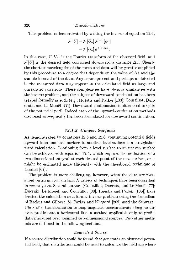
320 Transformations
This problem is demonstrated by writing the inverse of equation 12.6,
In this case, T [Uu] is the Fourier transform of the observed field, andT [U] is the desired field continued downward a distance Az. Clearlythe shortest wavelengths of the measured data will be greatly amplifiedby this procedure to a degree that depends on the value of Az and thesample interval of the data. Any errors present and perhaps undetectedin the measured data may appear in the calculated field as large andunrealistic variations. These complexities have obvious similarities withthe inverse problem, and the subject of downward continuation has beentreated formally as such (e.g., Huestis and Parker [133]; Courtillot, Dun-cruix, and Le Mouel [77]). Downward continuation is often used in spiteof the potential peril. Indeed each of the upward-continuation methodsdiscussed subsequently has been formulated for downward continuation.
12.1.2 Uneven SurfacesAs demonstrated by equations 12.6 and 12.8, continuing potential fieldsupward from one level surface to another level surface is a straightfor-ward calculation. Continuing from a level surface to an uneven surfacecan be achieved with equation 12.4, which requires the evaluation of atwo-dimensional integral at each desired point of the new surface, or itmight be estimated more efficiently with the chessboard technique ofCordell [67].
The problem is more challenging, however, when the data are mea-sured on an uneven surface. A variety of techniques have been describedin recent years. Several authors (Courtillot, Ducruix, and Le Mouel [77];Ducruix, Le Mouel, and Courtillot [80]; Huestis and Parker [133]) havetreated the calculation as a formal inverse problem using the formalismof Backus and Gilbert [8]. Parker and Klitgord [209] used the Schwarz-Christoffel transformation to map magnetic measurements along an un-even profile onto a horizontal line, a method applicable only to profiledata measured over assumed two-dimensional sources. Two other meth-ods are outlined in the following sections.
Equivalent SourceIf a source distribution could be found that generates an observed poten-tial field, that distribution could be used to calculate the field anywhere
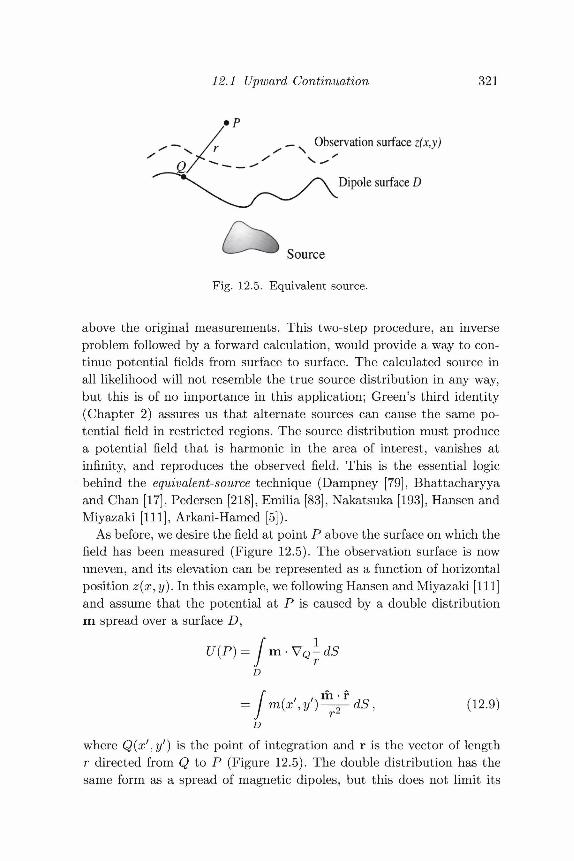
12.1 Upward Continuation 321
_ Observation surface z(x,y)
Dipole surface D
Source
Fig. 12.5. Equivalent source.
above the original measurements. This two-step procedure, an inverseproblem followed by a forward calculation, would provide a way to con-tinue potential fields from surface to surface. The calculated source inall likelihood will not resemble the true source distribution in any way,but this is of no importance in this application; Green's third identity(Chapter 2) assures us that alternate sources can cause the same po-tential field in restricted regions. The source distribution must producea potential field that is harmonic in the area of interest, vanishes atinfinity, and reproduces the observed field. This is the essential logicbehind the equivalent-source technique (Dampney [79], Bhattacharyyaand Chan [17], Pedersen [218], Emilia [83], Nakatsuka [193], Hansen andMiyazaki [111], Arkani-Hamed [5]).
As before, we desire the field at point P above the surface on which thefield has been measured (Figure 12.5). The observation surface is nowuneven, and its elevation can be represented as a function of horizontalposition z(x, y). In this example, we following Hansen and Miyazaki [111]and assume that the potential at P is caused by a double distributionm spread over a surface D,
U{P)=D
= J'm(x'\y')^- dS, (12.9)D
where Q(xf\yr) is the point of integration and r is the vector of lengthr directed from Q to P (Figure 12.5). The double distribution has thesame form as a spread of magnetic dipoles, but this does not limit its
322 Transformations
application to magnetic fields; U can represent a potential field of anykind. The shape and location of surface D is yet to be determined, but itshould lie at or below the observation surface and above all true sources.This source distribution will achieve our goals iiU(P) is harmonic abovethe observation surface, vanishes as z approaches — oo, and equals theobserved field whenever P lies on the observation surface. The first twoconditions are satisfied because equation 12.9 is essentially the potentialfield of a dipole distribution (see Section 5.1). The third condition issatisfied if we select m(x,y) so that
U(x, y, z(x, y)) = J m(z', yf)^ dS. (12.10)D
Because the left side of equation 12.10 is known, the problem reducesto (1) selecting models for the unit vector m (which is not necessarilyuniform) and surface D, (2) finding a solution for m(x,y), and (3) usingra(x,y) in equation 12.9 to find U(P), the upward-continued field.
If P is always above (or on) the observation surface, then D can beplaced at the observation surface, in which case equation 12.10 becomes
U(x,y,z(x,y)) = 2?rm(x,y) m • n + / m(x*\yf)—^- dS , (12.11)D=z(x,y)
where n is normal to the observation surface (Hansen and Miyazaki [111]).Equation 12.11 can be solved for m(x,y) by the methods of succes-sive approximations once a model is selected for m. Bhattacharyya andChan [17] oriented m normal to the observation surface, whereas Nakat-suka [193] let m be vertical. In practice, the observed potential field usu-ally is interpolated to a grid, so the surface integrals in equations 12.9and 12.11 can be replaced with a double summation. The spread ofdipoles can be approximated by discrete dipoles at grid intersections(e.g., Bhattacharyya and Chan [17]) or by rectangular facets with eachfacet centered about a grid intersection and possessing uniform dipolemoment (Hansen and Miyazaki [111]).
Taylor's-Series ApproximationA Taylor's series uses derivatives of a function evaluated at one point toextrapolate the function to nearby points. Taylor's series was discussedin Section 10.3.1 as a way to modify in an optimal way the shape ofcausative bodies in order to solve the nonlinear inverse problem. Taylor'sseries also can be used to predict the value of a potential field at points
12.1 Upward Continuation 323
away from the observation surface (Cordell and Grauch [70], Pilkingtonand Roest [224]).
First consider the continuation of a potential field U(x,y, ZQ) measuredon a level surface (zo = constant) and desired on an uneven surfacez(x, y). The value of the potential field at one point (x, y, z) of the newsurface is given by
U(x, y, z) = U(x, y, z0) + (z - zQ)-^U(x, y, z0)
(z - z0)2 d2 ...+ U(xyz) +
n=0
Cordell and Grauch [70] found empirically that convergence of equa-tion 12.12 is most rapid if z0 is placed at the mean of z{x,y), and thiscan be achieved with a level-to-level continuation using equations 12.6and 12.8. A solution to equation 12.12 requires vertical derivatives of themeasured field, and these can be found using the Fourier domain. Wewill show in Section 12.2 that the Fourier transform of the nth verticalderivative of a potential field is given by the Fourier transform of thepotential field times |A:|n, that is,
Using equation 12.13, the various vertical derivatives of the observedfield can be found, and these can be used in summation 12.12 to find thefield on surface z(x,y). Cordell and Grauch [70] found that the first threeterms of the summation are generally sufficient to achieve satisfactoryresults.Exercise 12.1 Show that if z(x,y) is a constant, equation 12.12 reduces to
equations 12.6 and 12.8. Hint: Equation 12.13 may be helpful.Equation 12.12 is appropriate for continuation from a level surface to
an uneven surface. The more difficult case of continuation from an un-even surface can be achieved by rearranging the terms of equation 12.12.Isolating the first term of the summation on the left side of the equationyields
U(x,y,zo) = U(x,y,z) - £ J Q^U(x,y,zo) • (12.14)71=1
324 Transformations
The desired quantity U(x,y,zo) can be estimated by successive approx-imations; that is, U(x, y, ZQ) determined at the zth iteration can be usedto find U(x, y, z$) at the (i + l)th iteration,
n = l
An initial guess at U(x,y,zo) is needed. Cordell and Grauch [70] sug-gested on empirical grounds that this initial guess can be found by as-suming (erroneously) that U(x, y, z) is actually measured on a horizon-tal surface and continuing it to the uneven surface z(x,y) using sum-mation 12.12. As before, the vertical derivatives in equation 12.14 canbe estimated with equation 12.13, although this relationship does notstrictly apply to data measured on uneven surfaces.
Grauch [100] described a Fortran program implementing the Taylor'sseries method, and this program is available on diskette (Cordell etal. [73]).
12.2 Directional DerivativesConsider a smoothly varying scalar quantity <fi(x,y) measured on ahorizontal surface. The horizontal derivatives of (j)(x,y) are easily esti-mated using simple finite-difference methods and discrete measurementsof 0(x, y). For example, if the values faj, i — 1, 2 , . . . , j — 1, 2,.. . , rep-resent discrete measurements of (j>(x, y) at uniform sample intervals Axand A?/, then the horizontal derivatives of </>(#, y) at point z,j are givenapproximately by
d<t>(x,y) ^ 02+i,j ~ 0i-i,jdx ~ 2Ax
dy ~ 2A?/Horizontal derivatives are easily done in the Fourier domain as well(e.g., Pedersen [217]). According to the differentiation theorem (Sec-tion 11.1.2), the horizontal derivatives of <j){x,y) are given by
12.2 Directional Derivatives 325
Hence, (ikx)n and (iky)n are filters that transform a function measuredon a horizontal surface into nth-order derivatives with respect to x or y,respectively.
If (f) is a potential, we also have the ability to calculate vertical gra-dients. Indeed, the second vertical derivative is a direct consequence ofLaplace's equation, for if 0 is a potential, then V2(/> = 0 and
^ = _ ^ _ ^ (1217)dz2 dx2 dy2' K J
If <p is measured on a horizontal surface, then Laplace's equation canbe transformed to the Fourier domain with the help of equations 12.15and 12.16, that is,
= \k\2T[<j>}. (12.18)
Hence, the second vertical derivative of a potential field measured on ahorizontal surface is framed as a three-step filtering operation: Fouriertransform the potential field, multiply by |fc|2, and inverse Fourier trans-form the product.
The second vertical derivative was an early mainstay of interpretationtechniques (Evjen [86], Henderson and Zietz [126]) because it helps toresolve and accentuate shallow sources. To see why this should be thecase, consider two monopoles observed at point P, one at shallow depthd\ and the other at greater depth d>2. The field of each monopole isinversely proportional to the squared distance to P. Hence, as P movestoward the monopoles, the field due to the shallow monopole will increasemore rapidly than the field of the deep monopole. It stands to reasonthat the second vertical derivative will have the same effect. Similarly,the second vertical derivative accentuates and helps to resolve edgesof magnetic or gravity sources. These characteristics are illustrated byFigure 12.6, which shows the second vertical derivative of the total-fieldanomaly of central Nevada.
These properties of the second vertical derivative also follow fromequation 12.18: Multiplying the potential field by \k\2 clearly ampli-fies short-wavelength components of the field at the expense of long-wavelength components. Needless to say, all of the cautionary commentsmade earlier concerning downward continuation are applicable to thesecond vertical derivative as well.
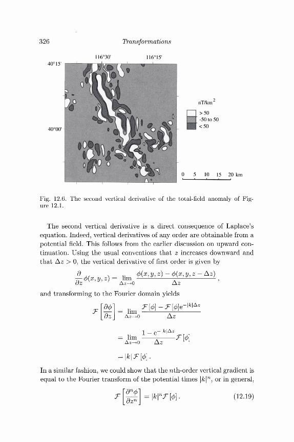
326 Transformations
116°30'40° 15'
nT/km
40°00'
0 5 10 15 20 km
Fig. 12.6. The second vertical derivative of the total-field anomaly of Fig-ure 12.1.
The second vertical derivative is a direct consequence of Laplace'sequation. Indeed, vertical derivatives of any order are obtainable from apotential field. This follows from the earlier discussion on upward con-tinuation. Using the usual conventions that z increases downward andthat Az > 0, the vertical derivative of first order is given by
d _ </>(x, y, z) - </>(x, y,z - Az)dz ' ' Az^o Az
and transforming to the Fourier domain yields
az = lim
= lim
Az
Az
In a similar fashion, we could show that the nth-order vertical gradient isequal to the Fourier transform of the potential times |fc|n, or in general,
(12.19)
12.2 Directional Derivatives 327
Subroutine B.25 in Appendix B is an implementation of the three stepsimplied by equation 12.19; it Fourier transforms gridded potential-fielddata, multiplies by |/c|n, and inverse Fourier transforms the product.
Transformations from Field to PotentialEquations 12.15, 12.16, and 12.19 provide ways to calculate derivativesin all three orthogonal directions from a potential field measured on ahorizontal surface. We can write these relationships more compactly asa single equation,
(12.20)
where k = (ikx,iky, |fe|), as shown by Pedersen [216] using a somewhatdifferent derivation.
A force field F is related to its potential 0 according to F = V0, andequation 12.20 expresses this relationship in the Fourier domain. Thecomponent of the force field in any direction f, therefore, is simply adirectional derivative of 0, given in the Fourier domain by
T [f • V0J = (f • k) T [(/)}. (12.21)
The vertical attraction of gravity, for example, is given by gz = -§^U, orin the Fourier domain by
T[gz\ = \k\T[U}. (12.22)
Similarly, the total-field anomaly measured in an ambient field f is, to agood approximation, given by AT = —f • VV, where V is the magneticpotential of the anomalous body. In the Fourier domain this is expressedby
= -ef\k\F[V], (12.23)
where 6f was defined in Section 11.2.1 as
k
Equations 12.22 and 12.23 express the vertical attraction of gravity andthe total-field anomaly in terms of their respective potentials. Rearrang-ing terms provides
^ , |fc|^0, (12.24)
328 Transformations
^ | A ; | / 0 ' ( 1 2-2 5 )
and these equations describe vertical gravity anomalies and total-fieldmagnetic anomalies measured on a horizontal surface in terms of theirrespective potentials on that same surface.
12.3 Phase TransformationsThe shape of a gravity anomaly naturally depends on the shape anddistribution of mass, as described by the density distribution p(x,y,z).Magnetic anomalies have an added complexity: The anomaly dependsnot only on the distribution of magnetization M(x,y,z), but also onthe direction of magnetization and on the direction in which the fieldis measured.f For a total-field anomaly, of course, the component ofmeasurement is parallel to the ambient field.
This added complexity is easily described in the Fourier domain. Con-sider a three-dimensional distribution of magnetization M(x,y,z) lo-cated entirely below the plane of observation at ZQ. The distributionwill be defined as zero outside a finite region with horizontal dimensionssmaller than the dimensions of the survey, and we assume that the direc-tion of magnetization (but not the intensity of magnetization) is uniformthroughout the body. The Fourier transform of the total-field anomalycaused by M(x,y,z) is given by equation 11.47,
oo
T [AT] = 27rCmemef |fc| e^z° f e~^z>T [M(z')\ dz', (12.26)
where .FfM^')] denotes the Fourier transform of the magnetization onone horizontal slice through the body at depth z'. The parameters Bmand Of in equation 12.26 are given by
@m = rriz + i fTj— '\K\
Q f I JxkX+fyky
where m = (mx,my,mz) and f = (fx,fy,fz) are unit vectors in the
f Of course, the shape of a gravity anomaly also depends on the direction in whichthe field is measured, but conventional gravity meters measure the total gravityfield of the earth, which is always vertical.
12.3 Phase Transformations 329
direction of the magnetization and in the direction of the ambient field,respectively. The integral term in equation 12.26 carries all of the in-formation concerning M(x,y,z), including the shape of the magneticbody. This term certainly will contribute to the phase of the anomaly,depending on how the magnetization is distributed, and this contribu-tion will be difficult to assess without some a priori knowledge aboutM(x,y,z). The functions Bm and Of also contribute to the phase ofthe anomaly and contain all information regarding the directions of themagnetization and of the component being measured.
Suppose that a different component of the magnetic field or the effectof a different direction of magnetization is of interest. In either case,only f and m are to be altered in equation 12.26; M(x,y,z) remainsunchanged. Denoting the new directions of magnetization and ambientfield as m' = (mx,my,m'z) and f' = (fx,fy,ff
z), respectively, the trans-formed anomaly will be
f z''F[M{z')]dz', (12.27)zo
where
Q( = fz + i .Combining equations 12.26 and 12.27 in order to eliminate the commonfactors provides
T[ATt]=T[AT}T[^t], (12.28)
where
= 7rrr (1 2 2 9)Equations 12.28 and 12.29 describe a filtering operation that transformsa total-field anomaly with given directions of magnetization and ambientfield into a new anomaly caused by the same distribution of magneti-zation but with new vector directions. No assumptions are necessaryconcerning the shape of the body or the distribution of magnetization,except that it should be sufficiently localized for the Fourier transformto exist.
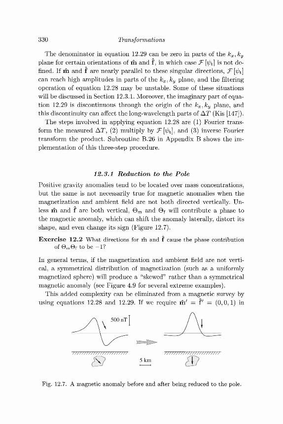
330 Transformations
The denominator in equation 12.29 can be zero in parts of the kx, kyplane for certain orientations of m and f, in which case T |/0t] is not de-fined. If m and f are nearly parallel to these singular directions, T [ipt]can reach high amplitudes in parts of the kx, ky plane, and the filteringoperation of equation 12.28 may be unstable. Some of these situationswill be discussed in Section 12.3.1. Moreover, the imaginary part of equa-tion 12.29 is discontinuous through the origin of the kx,ky plane, andthis discontinuity can affect the long-wavelength parts of AT (Kis [147]).
The steps involved in applying equation 12.28 are (1) Fourier trans-form the measured AT, (2) multiply by Ffyt], and (3) inverse Fouriertransform the product. Subroutine B.26 in Appendix B shows the im-plementation of this three-step procedure.
12.3.1 Reduction to the PolePositive gravity anomalies tend to be located over mass concentrations,but the same is not necessarily true for magnetic anomalies when themagnetization and ambient field are not both directed vertically. Un-less m and f are both vertical, 6 m and Bf will contribute a phase tothe magnetic anomaly, which can shift the anomaly laterally, distort itsshape, and even change its sign (Figure 12.7).
Exercise 12.2 What directions for m and f cause the phase contributionof Bmef to be -1?
In general terms, if the magnetization and ambient field are not verti-cal, a symmetrical distribution of magnetization (such as a uniformlymagnetized sphere) will produce a "skewed" rather than a symmetricalmagnetic anomaly (see Figure 4.9 for several extreme examples).
This added complexity can be eliminated from a magnetic survey byusing equations 12.28 and 12.29. If we require m' = f' = (0,0,1) in
500 nT |
5km
Fig. 12.7. A magnetic anomaly before and after being reduced to the pole.
12.3 Phase Transformations 331
equation 12.29, then equation 12.28 will transform a measured total-field anomaly into the vertical component of the field caused by the samesource distribution magnetized in the vertical direction. The transformedanomaly in the Fourier domain is given by
JT[ATr] =.Fty>r].F[AT], (12.30)
where1
BmBf
= — 2 2 —TIT v lfel^°> (12.31)
= rhzfz -rhxfx,
> = -rhyfx -rhxfy,fry) f I irri /•'' l"X J Z \^ 111>z Jx ,
^ +rhzfy
The application of T [ipr] is called reduction to the pole (Baranov andNaudy [10]) because ATr is the anomaly that would be measured at thenorth magnetic pole, where induced magnetization and ambient fieldboth would be directed vertically down (Figure 12.7). Reduction to thepole removes one level of complexity from the interpretive process: Itshifts anomalies laterally to be located over their respective sources andalters their shape so that symmetrical sources cause symmetrical anoma-lies. The direction of magnetization and ambient field are required inequation 12.31, but no other assumptions about the distribution of mag-netization are necessary, except those concerning the lateral dimensionsof the sources described earlier.
Many of the comments concerning Om and Of in Section 11.2.1 applyto T [ipr]. The filter attains a constant value along any ray projected fromthe origin of the kx,ky plane. Two rays directed in opposite directionsare complex conjugates of one another, so the imaginary part of T [ r]is discontinuous at the origin. Each ray, in general, differs in value fromneighboring rays, but the average of T [ r] around any circle concentricabout the origin is independent of the radius of the circle. Thus reductionto the pole has no effect on the shape of the radially averaged spectrum.
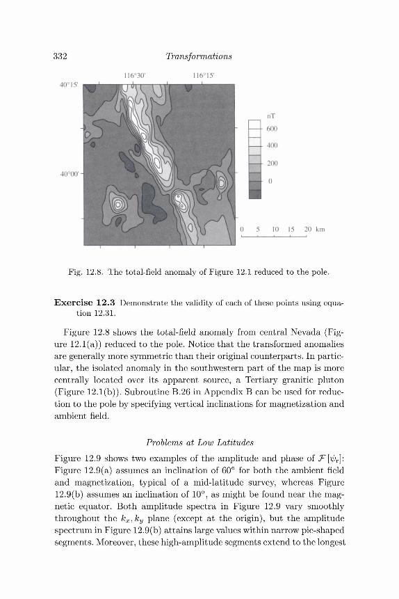
332
40° 15'
Transformations
40W -
20 km
Fig. 12.8. The total-field anomaly of Figure 12.1 reduced to the pole.
Exercise 12.3 Demonstrate the validity of each of these points using equa-tion 12.31.
Figure 12.8 shows the total-field anomaly from central Nevada (Fig-ure 12.1(a)) reduced to the pole. Notice that the transformed anomaliesare generally more symmetric than their original counterparts. In partic-ular, the isolated anomaly in the southwestern part of the map is morecentrally located over its apparent source, a Tertiary granitic pluton(Figure 12.1(b)). Subroutine B.26 in Appendix B can be used for reduc-tion to the pole by specifying vertical inclinations for magnetization andambient field.
Problems at Low LatitudesFigure 12.9 shows two examples of the amplitude and phase ofFigure 12.9(a) assumes an inclination of 60° for both the ambient fieldand magnetization, typical of a mid-latitude survey, whereas Figure12.9(b) assumes an inclination of 10°, as might be found near the mag-netic equator. Both amplitude spectra in Figure 12.9 vary smoothlythroughout the kx,ky plane (except at the origin), but the amplitudespectrum in Figure 12.9(b) attains large values within narrow pie-shapedsegments. Moreover, these high-amplitude segments extend to the longest
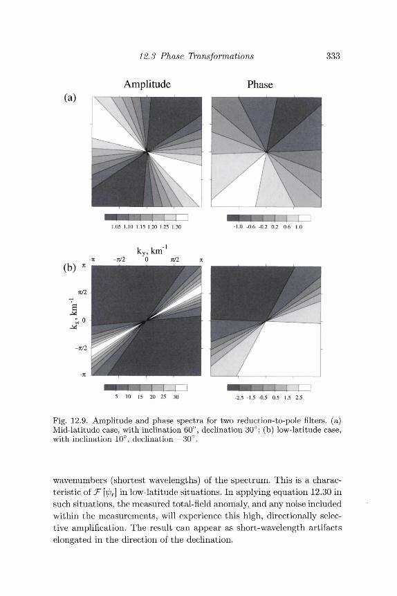
12.3 Phase Transformations 333
Amplitude Phase
5 10 15 20 25 30 -2.5 -1.5 -0.5 0.5 1.5 2.5
Fig. 12.9. Amplitude and phase spectra for two reduction-to-pole filters, (a)Mid-latitude case, with inclination 60°, decimation 30°; (b) low-latitude case,with inclination 10°, declination —30°.
wavenumbers (shortest wavelengths) of the spectrum. This is a charac-teristic of T [ipr] in low-latitude situations. In applying equation 12.30 insuch situations, the measured total-field anomaly, and any noise includedwithin the measurements, will experience this high, directionally selec-tive amplification. The result can appear as short-wavelength artifactselongated in the direction of the declination.
334 Transformations
We can better understand the reason for this selective amplificationby converting equation 12.31 to polar coordinates,
a\ cos2 A + 2 sin2 A + cts COS A sin A + i(b\ cos A + b<i sin A)(12.32)
where A = arctan^/A^). Equation 12.32 can be calculated at all pointsof the kx, ky plane (except at |fc| =0) if the magnetization and ambientfield have nonzero inclinations, but -F[^r] is undefined for certain A ifthe magnetization and ambient field are both horizontal. For example,if m = f = (1,0,0), then
cos2 Aand in this case T [xjjr] is not defined along the ky axis. If the inclinationsare shallow but nonzero, as they are in Figure 12.9(b), the amplitudespectrum of T [ipr] will be defined at each point away from the originbut will attain large values within narrow pie-shaped segments.
Several techniques have been developed to improve reduction to thepole in low-latitude situations. One straightforward approach is to re-duce low-latitude magnetic data to the magnetic equator rather than tothe pole (Leu [164], Gibert and Galdeano [96]). Although this procedurewill tend to center anomalies over their respective sources, the anoma-lies will be stretched in the east-west direction relative to the horizontaldimensions of the source (e.g., see Figure 4.9(b)).Exercise 12.4 Derive an expression like equation 12.31 for reduction to the
equator.
Reduction to the pole can be achieved using an equivalent-sourcescheme (Silva [258], Emilia [83], Bott and Ingles [40]), much in the sameway that upward continuation was treated in Section 12.1.2. Such meth-ods consist of two steps: a solution to the inverse problem followed bya forward calculation. First, the observed anomaly is used to find a hy-pothetical source distribution that can produce the observed anomaly,assuming an appropriate direction of magnetization for the survey site.Second, the vertical component of the magnetic field is found assum-ing that the equivalent source is vertically magnetized. The equivalentsource most likely will have no resemblance to the true source, but thisis of no importance so long as it produces the observed magnetic field.Equivalent sources typically are modeled as a layer of discrete magneticsources, such as pairs of monopoles of opposite sign (Silva [258]), lines

12.3 Phase Transformations 335
of dipoles (Emilia [83]), or uniformly magnetized blocks (Bott and In-gles [40]). According to Silva [258], the equivalent-source technique islargely free of the instabilities often associated with reduction to thepole of low-latitude data. But this improvement comes at the expense ofsignificantly more computational effort as compared to the applicationof equation 12.30.
Hansen and Pawlowski [112] and Pearson and Skinner [214] appliedWiener filtering to the problem of low-latitude reduction to the pole.Equation 12.30 can be considered to be the inverse of
This operation is always stable, as can be demonstrated with the recipro-cal of equation 12.32. In real situations, an observed total-field anomalyAT0 will include a noise component N so that AT0 = AT + AT. TheFourier transform of the observed anomaly is
T [AT0] = T~x [W] T [ATr] +F[N].
An operator a is then required such that laJ^ATo] — .F[ATr]|2 is aminimum when averaged over all values. The filter a is a regulated ver-sion of T [ipr] suitable for noisy data. According to Wiener theory, a canbe written in terms of ^[T/V], which can easily be calculated, and thepower spectra of TV and AT. The spectra can be found by assuming thestatistical nature of the noise and the ideal spectral characteristics ofreduced-to-pole anomalies. Hansen and Pawlowski [112] reported signif-icant improvement using this technique in low-latitude applications ofreduction to the pole.
Nonuniform Direction of Magnetization and Ambient FieldThe foregoing has assumed that the magnetization and regional field areuniform throughout the study area, often an appropriate assumption forsmall-scale surveys where the direction of the geomagnetic field varies byonly small amounts over the limits of the survey. Over continental-scaleareas, however, the geomagnetic field varies to a considerable degree, andalgorithms that assume uniformly directed magnetization and regionalfield may produce errors when applied to similarly sized compilations ofaeromagnetic data.
Arkani-Hamed [5] discussed a reduction-to-pole technique that per-mits variable directions of magnetization and regional field while main-taining the efficiency of the Fourier-domain methodology. His techniqueemploys an equivalent layer of magnetization; variations in the direction
336 Transformations
of magnetization and in the direction of the ambient field are describedby perturbations about uniform directions.
The magnetic potential observed at point P is given by
VQ^dv, (12.33)
where Q is the point of integration and r is the distance from Q to P.Both the intensity and direction of magnetization are permitted to varyin this case. We restrict P to a horizontal plane at z = ZQ and model themagnetic source as a vanishingly thin layer at depth d (d > z$), that is,we let
M(Q)=M(x',y')6(z'-d).
Substituting this magnetization into equation 12.33 and integrating overz' reduces the triple integral to a two-dimensional convolution overx' and y1. Fourier transforming both sides and applying the Fourier-convolution theorem leads to
e\k\{z0-d)T [V] = -27rC m - k • T [M],
\K\
where k = (ikx,iky, \k\). Now we let the equivalent layer be located atthe plane of observation so that d —> z$. We also resolve the direction ofmagnetization into two components, a uniform vector m0 and a smallperturbation Am about this uniform direction, that is, we let M(x, y) =M(x,y)(mo + Am(x,y)). Making these substitutions provides
\K\
and isolating T [M] on one side of the equation yields
k . T [MAm] I / ( k . m o ) .JEquation 12.34 can be solved recursively in order to derive M(x,y) fromV(x, y). An initial guess is made for M(x, y) (M(x, y) = 0, for example),and equation 12.34 is used to obtain a second approximation for M(x, y).This new solution is substituted back into equation 12.34 to get a thirdapproximation, and the procedure continues until the solution convergesappropriately.
Equation 12.34 requires the magnetic potential, and this can be ob-tained from the observed total-field anomalies. Like the magnetization,we describe the direction of the ambient field as the sum of a uniform
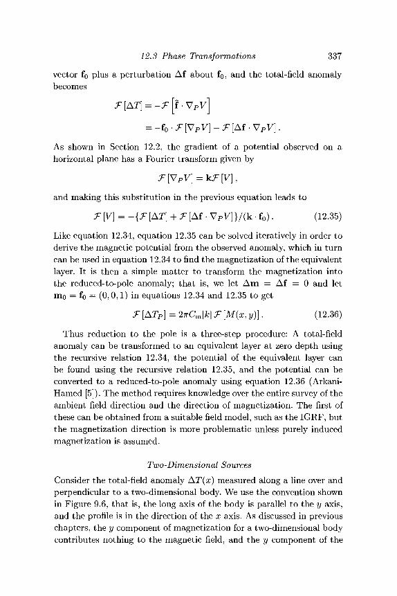
12.3 Phase Transformations 337
vector f0 plus a perturbation Af about f0, and the total-field anomalybecomes
= -f0 • T [\/PV] - T [Af • VPV].
As shown in Section 12.2, the gradient of a potential observed on ahorizontal plane has a Fourier transform given by
and making this substitution in the previous equation leads to
T [V] = -{T [AT] + T [Af • VPV]}/(k • f0). (12.35)
Like equation 12.34, equation 12.35 can be solved iteratively in order toderive the magnetic potential from the observed anomaly, which in turncan be used in equation 12.34 to find the magnetization of the equivalentlayer. It is then a simple matter to transform the magnetization intothe reduced-to-pole anomaly; that is, we let Am = Af = 0 and letm0 = fo — (0,0,1) in equations 12.34 and 12.35 to get
T [ATP] = 27rCm\k\ T [M(x, y)\. (12.36)
Thus reduction to the pole is a three-step procedure: A total-fieldanomaly can be transformed to an equivalent layer at zero depth usingthe recursive relation 12.34, the potential of the equivalent layer canbe found using the recursive relation 12.35, and the potential can beconverted to a reduced-to-pole anomaly using equation 12.36 (Arkani-Hamed [5]). The method requires knowledge over the entire survey of theambient field direction and the direction of magnetization. The first ofthese can be obtained from a suitable field model, such as the IGRF, butthe magnetization direction is more problematic unless purely inducedmagnetization is assumed.
Two-Dimensional SourcesConsider the total-field anomaly AT(x) measured along a line over andperpendicular to a two-dimensional body. We use the convention shownin Figure 9.6, that is, the long axis of the body is parallel to the y axis,and the profile is in the direction of the x axis. As discussed in previouschapters, the y component of magnetization for a two-dimensional bodycontributes nothing to the magnetic field, and the y component of the
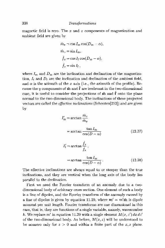
338 Transformations
magnetic field is zero. The x and z components of magnetization andambient field are given by
mx = cos Jm cos(£>m - a),
rhz = sin/m,
fz = sin If,
where Im and Dm are the inclination and declination of the magnetiza-tion, If and Df are the inclination and declination of the ambient field,and a is the azimuth of the x axis (i.e., the azimuth of the profile). Be-cause the y components of in and f are irrelevant in the two-dimensionalcase, it is useful to consider the projections of m and f onto the planenormal to the two-dimensional body. The inclinations of these projectedvectors are called the effective inclinations (Schouten[252]) and are givenby
(12.37)
If
= arctan
— arctan
= arctan
— arctan
mz
mx
tan/m
cos(D — a)
fz
tan/m
cos(D — a) (12.38)
The effective inclinations are always equal to or steeper than the trueinclinations, and they are vertical when the long axis of the body liesparallel to the declination.
First we need the Fourier transform of an anomaly due to a two-dimensional body of arbitrary cross section. One element of such a bodyis a line of dipoles, and the Fourier transform of the anomaly caused bya line of dipoles is given by equation 11.29, where m' = mfm is dipolemoment per unit length. Fourier transforms are one dimensional in thiscase, that is, they are functions of a single variable, namely, wavenumberk. We replace m' in equation 11.29 with a single element M(x, z') dx dzf
of the two-dimensional body. As before, M(x, z) will be understood tobe nonzero only for z > 0 and within a finite part of the x, z plane.
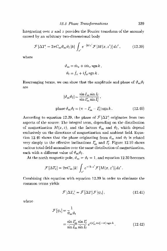
12.3 Phase Transformations 339
Integrating over x and z provides the Fourier transform of the anomalycaused by an arbitrary two-dimensional body
T [AT] = 27rCmtfmtff \k\ f e~^z'T [M(x, z')] dzr, (12.39)J z'
where
#m = mz + irhx sgn fc ,
#f = A + */x sgn fc .
Rearranging terms, we can show that the amplitude and phase of tfmtffare
sin/msin/ f
sin / ^ sin I/
phase m ^ f = (TT - 4 - I[) sgn fe . (12.40)
According to equation 12.39, the phase of ^*[AT] originates from twoaspects of the source: The integral term, depending on the distributionof magnetization M(x,z), and the factors #m and #f, which dependexclusively on the directions of magnetization and ambient field. Equa-tion 12.40 shows that the phase originating from #m and i?f is relatedvery simply to the effective inclinations 1^ and I[. Figure 12.10 showsvarious total-field anomalies over the same distribution of magnetization,each with a different value of ^m^f.
At the north magnetic pole, $m = #f = 1, and equation 12.39 becomes
T [ATr] - 27rCm |fc| / e - | f c | *> [M(x, z')\ dz1.
Combining this equation with equation 12.39 in order to eliminate thecommon terms yields
T[ATr]=T[AT}j:{A}, (12.41)
where
sin / m sin If(12.42)
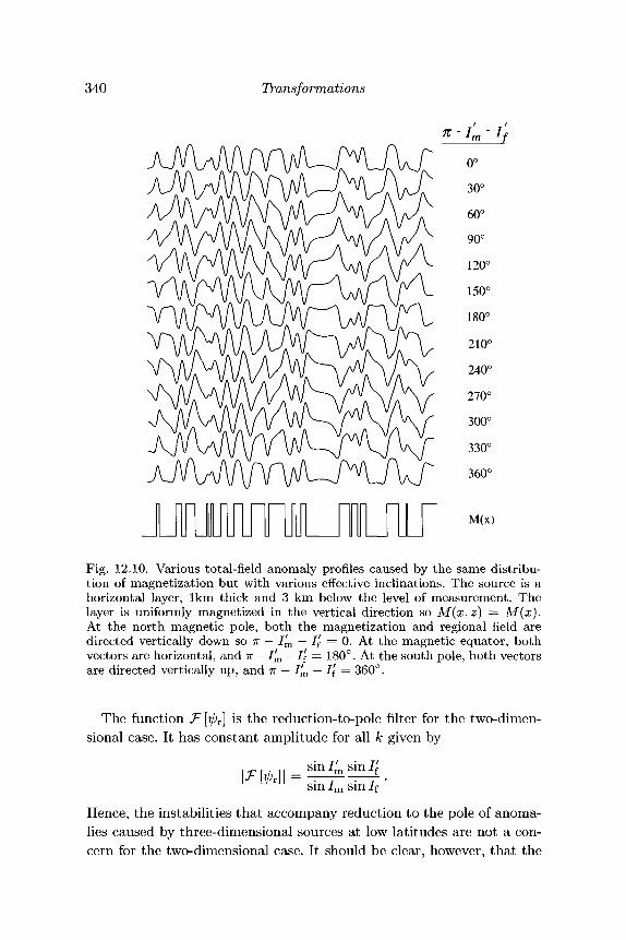
340 Transformations
n -o°30°
60°
90°
120°
150°
180°
210°
240°
270°
300°
330°
360°
M(x)
Fig. 12.10. Various total-field anomaly profiles caused by the same distribu-tion of magnetization but with various effective inclinations. The source is ahorizontal layer, lkm thick and 3 km below the level of measurement. Thelayer is uniformly magnetized in the vertical direction so M(x,z) = M(x).At the north magnetic pole, both the magnetization and regional field aredirected vertically down so TT — 1^ — /f = 0. At the magnetic equator, bothvectors are horizontal, and TT — l'm —1[ = 180°. At the south pole, both vectorsare directed vertically up, and TT — I'm — I[ = 360°.
The function T [tpr] is the reduction-to-pole filter for the two-dimen-sional case. It has constant amplitude for all k given by
Hence, the instabilities that accompany reduction to the pole of anoma-lies caused by three-dimensional sources at low latitudes are not a con-cern for the two-dimensional case. It should be clear, however, that the
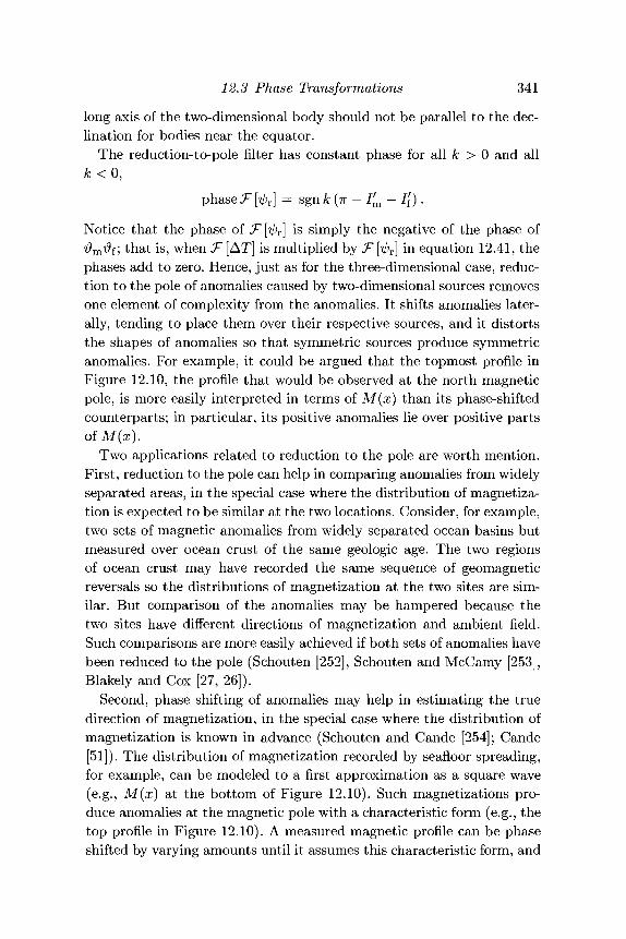
12.3 Phase Transformations 341
long axis of the two-dimensional body should not be parallel to the dec-lination for bodies near the equator.
The reduction-to-pole filter has constant phase for all k > 0 and allk <0 ,
phase T [ipT] = sgn k (n - Ifm - Jf').
Notice that the phase of T [ipr] is simply the negative of the phase of#m$ f; that is, when T [AT] is multiplied by T [ r] in equation 12.41, thephases add to zero. Hence, just as for the three-dimensional case, reduc-tion to the pole of anomalies caused by two-dimensional sources removesone element of complexity from the anomalies. It shifts anomalies later-ally, tending to place them over their respective sources, and it distortsthe shapes of anomalies so that symmetric sources produce symmetricanomalies. For example, it could be argued that the topmost profile inFigure 12.10, the profile that would be observed at the north magneticpole, is more easily interpreted in terms of M(x) than its phase-shiftedcounterparts; in particular, its positive anomalies lie over positive partsofM(x).
Two applications related to reduction to the pole are worth mention.First, reduction to the pole can help in comparing anomalies from widelyseparated areas, in the special case where the distribution of magnetiza-tion is expected to be similar at the two locations. Consider, for example,two sets of magnetic anomalies from widely separated ocean basins butmeasured over ocean crust of the same geologic age. The two regionsof ocean crust may have recorded the same sequence of geomagneticreversals so the distributions of magnetization at the two sites are sim-ilar. But comparison of the anomalies may be hampered because thetwo sites have different directions of magnetization and ambient field.Such comparisons are more easily achieved if both sets of anomalies havebeen reduced to the pole (Schouten [252], Schouten and McCamy [253],Blakely and Cox [27, 26]).
Second, phase shifting of anomalies may help in estimating the truedirection of magnetization, in the special case where the distribution ofmagnetization is known in advance (Schouten and Cande [254]; Cande[51]). The distribution of magnetization recorded by seafloor spreading,for example, can be modeled to a first approximation as a square wave(e.g., M(x) at the bottom of Figure 12.10). Such magnetizations pro-duce anomalies at the magnetic pole with a characteristic form (e.g., thetop profile in Figure 12.10). A measured magnetic profile can be phaseshifted by varying amounts until it assumes this characteristic form, and
342 Transformations
the total phase shift will be an estimate of /^ + /f' — n. Because /f' pre-sumably is known at the survey site, the total phase shifting provides adirect measure of the effective inclination of magnetization J^.
The effective inclination in turn provides a means of estimating thevirtual geomagnetic pole for the oceanic plate, under the assumptionthat the direction of magnetization is parallel to the paleomagnetic field.Although a virtual geomagnetic pole can be calculated uniquely fromthe paleomagnetic inclination and declination observed at a single site(e.g., Butler [47, pp. 157-60]), here we only have an effective inclination,and according to equation 12.37, an effective inclination has an infinitevariety of compatible inclination-declination pairs. Because of this am-biguity, a single effective inclination is compatible with an infinite setof permissible paleomagnetic poles all lying along a semi-great circle,which is not a particularly instructive result. However, a second set ofanomalies of the same age and on the same rigid plate could be analyzedin the same way in order to produce a second great circle of permissi-ble pole positions. The intersection of the two great circles provides anestimate of the single paleomagnetic pole compatible with both sitesand for the rigid plate over which both sets of anomalies are measured(Schouten and Cande [252], Cande [51]). Systematic discrepancies in theintersection of more than two great circles, called anomalous skewness,indicate that one or more of the underlying assumptions are in error;such discrepancies may reflect complexities in the behavior of the paleo-magnetic field or in the way reversals are recorded at spreading centers(Cande [51], Cande and Kent [52]).
12.3.2 Calculation of Vector ComponentsEquations 12.28 and 12.29 also can be used to transform a total-fieldanomaly into some other component of the magnetic field. For example,the vertical component Bz of the magnetic field can be calculated froma total-field anomaly by letting 6'm = Om and Of = 1 in equation 12.29,that is,
where
12.4 Pseudogravity Transformation 343
Knowing the direction of the ambient field, therefore, is sufficient totransform a total-field anomaly into the vertical component of the mag-netic field.
It should be clear that such transformations will be limited for certainambient-field directions in the same way that reduction to the pole islimited at low latitudes. Consider, for example, a total-field anomalymeasured near the magnetic equator and caused by a body with purelyinduced magnetization. Both f and m will have shallow inclinationsin this case, and transforming the total-field anomaly into the verticalcomponent of the magnetic field can be expected to be an unstableoperation. Any noise within the measurements will generate artifacts,typically short in wavelength and elongated parallel to the declination.Exercise 12.5 Derive Fourier-domain filters that will transform a total-field
anomaly into the horizontal-north component and the horizontal-eastcomponent of the magnetic field. Discuss the conditions under whichthese filters are expected to be unstable.
12.4 Pseudogravity TransformationPoisson's relation was discussed at some length in Section 5.4, where itwas shown that the magnetic potential V and gravitational potential Ucaused by a uniformly dense and uniformly magnetized body are relatedby a directional derivative, that is,
Cm M ^ TTV = m • VpU
7 P
= - ^ a » , (12.43)7 P
where p is the density, M is the intensity of magnetization, m is thedirection of magnetization, and gm is the component of the gravity fieldin the direction of magnetization rh. In deriving Poisson's relation, weassumed that M and p are constant. However, we can consider a variabledistribution of magnetization or density to be composed of arbitrarilysmall regions of uniform magnetization or density; equation 12.43 is ap-propriate for each of these small regions and, invoking the superpositionprinciple, must be appropriate for variable distributions of density andmagnetization.
Baranov [9] described an application of Poisson's relation in which thetotal-field magnetic anomaly is converted into the gravity anomaly that
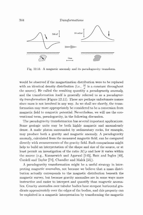
344 Transformations
lOmGal
77777777777/
OFig. 12.11. A magnetic anomaly and its pseudogravity transform.
would be observed if the magnetization distribution were to be replacedwith an identical density distribution (i.e., — is a constant throughoutthe source). He called the resulting quantity a pseudogravity anomaly,and the transformation itself is generally referred to as a pseudograv-ity transformation (Figure 12.11). These are perhaps unfortunate namessince mass is not involved in any way. As we shall see shortly, the trans-formation may more appropriately be considered to be a conversion frommagnetic field to magnetic potential. Nevertheless, we will use the con-ventional term, pseudogravity, in the following discussion.
The pseudogravity transformation has several important applications.Some geologic units may be both highly magnetic and anomalouslydense. A mafic pluton surrounded by sedimentary rocks, for example,may produce both a gravity and magnetic anomaly. A pseudogravityanomaly, calculated from the measured magnetic field, can be compareddirectly with measurements of the gravity field. Such comparisons mighthelp to build an interpretation of the shape and size of the source, or atleast permit an investigation of the ratio M/p and how it varies withinthe source (e.g., Kanasewich and Agarwal [145], Bott and Ingles [40],Cordell and Taylor [74], Chandler and Malek [55]).
A pseudogravity transformation might be a useful strategy in inter-preting magnetic anomalies, not because we believe that a mass distri-bution actually corresponds to the magnetic distribution beneath themagnetic survey, but because gravity anomalies are in some ways moreinstructive and easier to interpret and quantify than magnetic anoma-lies. Gravity anomalies over tabular bodies have steepest horizontal gra-dients approximately over the edges of the bodies, and this property canbe exploited in a magnetic interpretation by transforming the magnetic
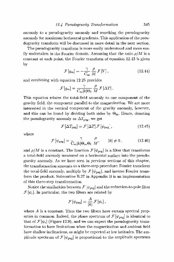
12.4 Pseudogravity Transformation 345
anomaly to a pseudogravity anomaly and searching the pseudogravityanomaly for maximum horizontal gradients. This application of the pseu-dogravity transform will be discussed in more detail in the next section.
The pseudogravity transform is more easily understood and more eas-ily undertaken in the Fourier domain. Assuming that the ratio p/M is aconstant at each point, the Fourier transform of equation 12.43 is givenby
^ ^ ( 1 2-4 4 )
and combining with equation 12.25 provides
This equation relates the total-field anomaly to one component of thegravity field, the component parallel to the magnetization. We are moreinterested in the vertical component of the gravity anomaly, however,and this can be found by dividing both sides by Bm . Hence, denotingthe pseudogravity anomaly as ATpsg, we get
T [ATpsg] = T [AT] T [Vpsg], (12.45)
where
i b * £ ' |Jfe|*0' (12-46)and p/M is a constant. The function T [ psg] is a filter that transformsa total-field anomaly measured on a horizontal surface into the pseudo-gravity anomaly. As we have seen in previous sections of this chapter,the transformation amounts to a three-step procedure: Fourier transformthe total-field anomaly, multiply by ^[^psg]? and inverse Fourier trans-form the product. Subroutine B.27 in Appendix B is an implementationof this three-step transformation.
Notice the similarities between T [ psg] and the reduction-to-pole filter\. In particular, the two filters are related by
where A is a constant. Thus the two filters have certain spectral prop-erties in common. Indeed, the phase spectrum of T [ psg] is identical tothat of T [ipr] (Figure 12.9), and we can expect the pseudogravity trans-formation to have limitations when the magnetization and ambient fieldhave shallow inclinations, as might be expected at low latitudes. The am-plitude spectrum of T [Vwl is proportional to the amplitude spectrum
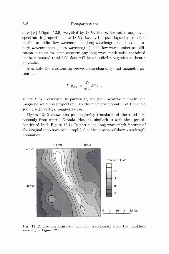
346 Transformations
of .F^r] (Figure 12.9) weighted by l/|fc|. Hence, the radial amplitudespectrum is proportional to l/|fc|; that is, the pseudogravity transfor-mation amplifies low wavenumbers (long wavelengths) and attenuateshigh wavenumbers (short wavelengths). The low-wavenumber amplifi-cation is cause for some concern; any long-wavelength noise containedin the measured total-field data will be amplified along with authenticanomalies.
Also note the relationship between pseudogravity and magnetic po-tential,
where B is a constant. In particular, the pseudogravity anomaly of amagnetic source is proportional to the magnetic potential of the samesource with vertical magnetization.
Figure 12.12 shows the pseudogravity transform of the total-fieldanomaly from central Nevada. Note its similarities with the upward-continued field (Figure 12.4). In particular, long-wavelength features ofthe original map have been amplified at the expense of short-wavelengthanomalies.
1I6°3OT
40° 15'
Pseudo mGal"
10
40°00'
10 15 20 km
Fig. 12.12. The pseudogravity anomaly transformed from the total-fieldanomaly of Figure 12.1.
12.5 Horizontal Gradients and Boundary Analysis 347
12.^.1 Pseudomagnetic CalculationThe inverse of equation 12.45 can be used to transform a measuredgravity anomaly into the magnetic anomaly that would be observed ifthe density distribution were replaced by a magnetic distribution in one-to-one proportion. Rearranging equation 12.45 yields
^bpsm]=^b]^[V'psm], (12.47)
where #psm denotes the transformed anomaly and
*%. (12.48)
This operation, called a pseudomagnetic transformation, does not sufferfrom the low-latitude limitations of its pseudogravity counterpart, but itclearly can suffer from instabilities. In particular, short-wavelength com-ponents of gz are amplified; the shorter the wavelength, the greater willbe the amplification. Any noise present at these wavelengths will be sim-ilarly amplified, and this can lead to high-amplitude, short-wavelengthartifacts in the transformed result.
12.5 Horizontal Gradients and Boundary AnalysisThe steepest horizontal gradient of a gravity anomaly gz(x,y) (or of apseudogravity anomaly) caused by a tabular body tends to overlie theedges of the body. Indeed, the steepest gradient will be located directlyover the edge of the body if the edge is vertical and far removed fromall other edges or sources.Exercise 12.6 Consider a uniform, horizontal, semi-infinite slab with ver-
tical face (i.e., the slab occupies the region 0 < x < oo, —oo < y < oo,z\ < z < £2), like that shown in Figures 9.15(a) and 9.15(b). Show fromequation 9.2.2 that a gravity profile over the edge of the slab measuredin the x direction will have its maximum gradient over the edge of theslab.
We can exploit this characteristic of gravity anomalies in order to locateabrupt lateral changes in density directly from gravity measurements(Cordell [66]). Moreover, the same technique could be applied to mag-netic measurements by first transforming them to pseudogravity anoma-lies, in which case the steepest horizontal gradients would reflect abruptlateral changes in magnetization (Cordell and Grauch [68, 70]).
The magnitude of the horizontal gradient of the gravity or pseudo-gravity anomaly, loosely referred to here as the horizontal gradient, is
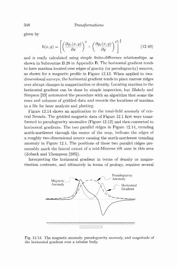
348 Transformations
given by
h(x,y) =dgz(x,y)
dxdgz(x,y)
dy (12.49)
and is easily calculated using simple finite-difference relationships, asshown in Subroutine B.28 in Appendix B. The horizontal gradient tendsto have maxima located over edges of gravity (or pseudogravity) sources,as shown for a magnetic profile in Figure 12.13. When applied to two-dimensional surveys, the horizontal gradient tends to place narrow ridgesover abrupt changes in magnetization or density. Locating maxima in thehorizontal gradient can be done by simple inspection, but Blakely andSimpson [33] automated the procedure with an algorithm that scans therows and columns of gridded data and records the locations of maximain a file for later analysis and plotting.
Figure 12.14 shows an application to the total-field anomaly of cen-tral Nevada. The gridded magnetic data of Figure 12.1 first were trans-formed to pseudogravity anomalies (Figure 12.12) and then converted tohorizontal gradients. The two parallel ridges in Figure 12.14, trendingnorth-northwest through the center of the map, indicate the edges ofa roughly two-dimensional source causing the north-northwest trendinganomaly in Figure 12.1. The positions of these two parallel ridges pre-sumably mark the lateral extent of a mid-Miocene rift zone in this area(Zoback and Thompson [295]).
Interpreting the horizontal gradient in terms of density or magne-tization contrasts, and ultimately in terms of geology, requires several
MagneticAnomaly
PseudogravityAnomaly
HorizontalGradient
Fig. 12.13. The magnetic anomaly, pseudogravity anomaly, and magnitude ofthe horizontal gradient over a tabular body.
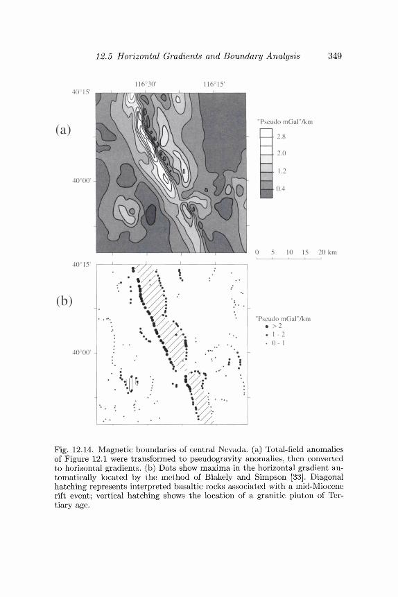
12.5 Horizontal Gradients and Boundary Analysis 349
116 MY4(1 JV
(a)
40 001
40 LV
(b)
4()0(K)' -
0 5 10 15 20 km
"Pscudo mGal7km• > 2. 1 - 2• 0-1
Fig. 12.14. Magnetic boundaries of central Nevada, (a) Total-field anomaliesof Figure 12.1 were transformed to pseudogravity anomalies, then convertedto horizontal gradients, (b) Dots show maxima in the horizontal gradient au-tomatically located by the method of Blakely and Simpson [33]. Diagonalhatching represents interpreted basaltic rocks associated with a mid-Miocenerift event; vertical hatching shows the location of a granitic pluton of Ter-tiary age.
350 Transformations
underlying assumptions. In particular, we have assumed that contrasts inphysical properties occur across vertical and abrupt boundaries isolatedfrom other sources. Geology, unfortunately, is not so simple. Magnetiza-tion and density can vary in all directions within a geologic unit, and con-tacts between units are not generally vertical. Grauch and Cordell [103]have quantified some of the errors that can occur when these underly-ing assumptions are violated, but in spite of these potential pitfalls, thetechnique has proven effective in interpretation of regional-scale databases.
12.5.1 TerracingCordell and McCafferty [72] described a related technique to produce akind of equivalent source from measured gravity or magnetic anomalies.The guiding principle behind their technique is that density or magneti-zation within the equivalent layer should remain constant except acrossabrupt boundaries. The resulting patchwork of density or magnetizationvalues brings to mind a terraced landscape, where the "hills and val-leys" of the potential field are transformed into horizontal surfaces withabrupt edges. Consequently, the technique is referred to as terracing.Maps of terraced physical properties have the general appearance of ageology map, where lithologies are depicted as uniform bodies exceptacross contacts.
Terracing is not an inverse scheme in the usual sense. No inverse cal-culations are made, but rather the values of the gravity or pseudogravityfield are iteratively increased or decreased in order to approach the ter-raced form. Specifically, the value at each point of the grid is revisedupward or downward based on the algebraic sign of the curvature (i.e.,the second vertical derivative) at that point. Repeated adjustments aremade until the terraced effect is achieved. The resulting terraces do notdirectly reflect density or magnetization but can be scaled in order todo so. For example, the magnetization or density of each terrace can betreated as one unknown in an over-determined system of linear equa-tions. Assuming top and bottom surfaces for the layer, least-squarestechniques can be used to solve for the best single value of magnetiza-tion or density for each terrace.
12.6 Analytic SignalThe analytic signal is formed through a combination of the horizontaland vertical gradients of a magnetic anomaly. The analytic signal has a
12.6 Analytic Signal 351
form over causative bodies that depends on the locations of the bodiesbut not on their directions of magnetization. The application of analyticsignals to magnetic interpretation was pioneered by Nabighian [190, 191]for the two-dimensional case, primarily as a tool to estimate depth andposition of sources. More recently, the method has been expanded tothree-dimensional problems (Nabighian [192]; Roest, Verhoef, and Pilk-ington [247]) as a mapping and depth-to-source technique and as a wayto learn about the nature of the causative magnetization (Roest, Arkani-Hamed, and Verhoef [245]; Roest and Pilkington [246]).
12.6.1 Hilbert TransformsThe Hilbert transform plays an important role in the analytic signal,and we begin the discussion with a very brief review thereof. The inter-ested reader is referred to texts by Bracewell [42] and Papoulis [202] foradditional information.
The Hilbert transform of f(x) is given by
dx', (12.50)j ( ) / 47T J _ o o X - X
and its inverse by
Equation 12.50 amounts to the convolution of f{x) with — 1/TTX. Ithas, therefore, a one-dimensional Fourier transform given by the Fouriertransform of f(x) times the Fourier transform of — I/THC, namely,
,F[F/] =isgnkJr[f]. (12.52)
The Hilbert transform has a curious effect on /(#), as demonstrated byequation 12.52: It leaves the amplitude of f(x) unchanged but shifts thephase of f(x) by TT/2 for k > 0 and by —TT/2 for k < 0.
The analytic signal of f(x) is defined as
a(x) = f(x)-iFI(x) (12.53)
(Bracewell [42]). With equation 12.52 it is easy to derive the Fouriertransform of the analytic signal,
sgnfc). (12.54)
352 Transformations
Hence, the spectrum of the analytic signal of f(x) is twice the Fouriertransform of f(x) at k > 0 and zero for k < 0. It follows that theanalytic signal of f(x) could be found in either of two ways: (1) bydirectly calculating the Hilbert transform of /(#), as in equation 12.50,and then adding this transform to /(#), as in equation 12.53; or (2) byFourier transforming /(#), setting to zero all values at k < 0, doublingall values at k > 0, and inverse Fourier transforming the result.
Exercise 12.7 Find the analytic signal for f(x) = cos ax.
12.6.2 Application to Potential FieldsIn Section 12.2, we found simple relationships, expressed by equation12.20, between a potential field measured on a horizontal surface andits derivatives with respect to any direction. Now consider a potentialfield (/>{x, z) measured along the x axis and caused by a two-dimensionalsource aligned parallel to the y axis, as in Figure 9.6. In the two-dimensional case, equation 12.20 can be expressed as
], (12.55)
(12.56)
From these relationships, it is easily shown that ^ and -^ are a Hilberttransform pair. In particular, equation 12.52 is satisfied if we let f(x) =-^ and Fj(x) = — -^, and we form the analytic signal from equa-tion 12.53 as
a{x,z) = ^ + i ^ . (12.57)ox oz
This version of a(x, z) satisfies the Cauchy-Riemann conditions (Sec-tion 1.3.3), the proof of which is left to the problem set at the end ofthis chapter, hence, a(x, z) is analytic at each point of the x axis. InSection 1.3.3 it was shown that if a(x,z) is analytic in a domain, thenthe real part of a(x, z) must be harmonic; that is, in the present case,
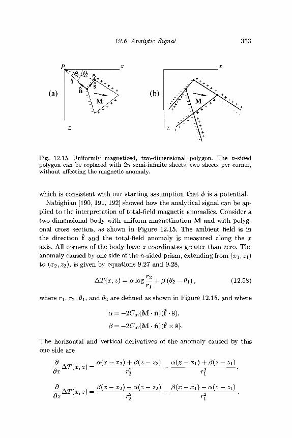
12.6 Analytic Signal 353
(a) (b)
Fig. 12.15. Uniformly magnetized, two-dimensional polygon. The n-sidedpolygon can be replaced with 2n semi-infinite sheets, two sheets per corner,without affecting the magnetic anomaly.
which is consistent with our starting assumption that </> is a potential.Nabighian [190, 191, 192] showed how the analytical signal can be ap-
plied to the interpretation of total-field magnetic anomalies. Consider atwo-dimensional body with uniform magnetization M and with polyg-onal cross section, as shown in Figure 12.15. The ambient field is inthe direction f and the total-field anomaly is measured along the xaxis. All corners of the body have z coordinates greater than zero. Theanomaly caused by one side of the n-sided prism, extending from (#i, z\)to (#2,22)? 1S given by equations 9.27 and 9.28,
where ri, r2, #1, and 92 are defined as shown in Figure 12.15, and where
a = -2C m (M.n)( f . s ) ,
/? = -2C m (M.n ) ( fxs ) .
The horizontal and vertical derivatives of the anomaly caused by thisone side are
a(x-x2) + P(z- z2) a(x - xi) +/3(z - zi)
U £
P(x - xi) - a(z -
354 Transformations
We now replace each side of the polygon with two semi-infinite sheetsarranged so that the sheets do not cross the x axis, as shown in Fig-ure 12.15. It should be clear from Figure 12.15 that this trick will notaffect the magnetic anomaly in any way. Now the polygon side extendingfrom (xi,2i) to (x2,z2) *s replaced with two semi-infinite sheets, withopposite sign but identical a and /3, one extending away from (#i,zi)and the other from (x2,z2).
Consider just the semi-infinite sheet extending from (#2,22)- Thederivative of the total-field anomaly caused by this sheet can be foundby letting r\ —>• 00 in the previous equations. Parameters a and (3 donot change, but the second term of each equation vanishes. The analyticsignal of this one sheet then is given by
a(z, z) = ^ f r . (12.59)x - x2 - i(z - z2)
It can be shown that this equation satisfies the Cauchy-Riemann condi-tions for the complex variable UJ = x—iz, so a(x, z) is analytic. Moreover,it has a Fourier transform given by
F[a] = -7ri(a + i(3)e-mz2-z)e-ikX2(l+ sgnfc), z < z2,
which satisfies the requirement that J~[a] = 0 for k < 0.The analytic signal expressed by equation 12.59 is of special interest.
It is a function of a complex variable UJ = x — iz and can be written( , a + i/3
LO — CO2
where LO2 = x2 — iz2. The numerator depends strictly on the orientationof the sheet (as defined by n and s) with respect to M and f. Thedenominator, on the other hand, depends exclusively on the location atwhich the sheet terminates, that is, (x2, z2). The point LU2 is an isolatedsingular point of the complex plane, meaning that a (a;) has a simplepole at that location.
Nabighian [190, 191] showed how a(x, z) can be used to locate the endof the sheet. The amplitude of a(x, z) is given by
Thus \a(x, z)\ as measured along the x axis has the form of a symmetric,bell-shaped curve centered about x = x2, and the width of the curve isrelated to z2. Specifically, the width of the curve at half its maximumheight is 2\z — z2\. Hence, the horizontal position and depth of the end
12.6 Analytic Signal 355
of the sheet (#2,22) c a n ^ e estimated through simple examination ofa(x,z) along the x axis.
Now we return to the n-sided polygon. The polygon is equivalent to 2nsheets, each sheet terminating at a polygon corner. Hence, the analyticsignal constructed from the total-field anomaly of the prism will have apeak centered over each corner of the polygon, and the width of eachpeak will be related to the depth of its respective corner. An analysis ofAT(x, z) as measured along the x axis might involve the following steps:
1. Differentiate AT(x,z) with respect to x.2. Find the analytic signal by
(a) Fourier transforming J^AT(x,z),(b) doubling values at k > 0 and canceling values at k < 0, and(c) inverse Fourier transforming.
3. Calculate and interpret |a(x,z)|.
The difficulty comes in resolving the various bell-shaped curves of a(x, z).The various curves superimpose and coalesce when polygon corners areclose together or lie above one another.
For the three-dimensional case, the analytic signal is given by
(Roest et al. [247]), where i, j , and k are unit vectors in the x, y, and zdirections, respectively, and where now AT(x, y,z) is measured on thex, y plane. This function possesses the necessary property of analytic sig-nals, that is, its real and imaginary parts form a Hilbert transform pair.Roest et al. [247] described how this function could be used in the in-terpretation of gridded data in terms of three-dimensional sources. Onestrategy would be to (1) form |A(x, y, z)\ from the partial derivatives ofthe magnetic anomaly; (2) locate the maxima of this function, perhapswith the technique of Blakely and Simpson [33]; (3) automatically calcu-late the half-width at each maximum in the direction perpendicular tothe strike of the maximum; and (4) plot the maxima in a map projectionwith a symbol that indicates depth to source.
Analytic Signal and Direction of MagnetizationIt is clear from equation 12.59 that the magnitude of the analytic signalis independent of the direction of magnetization for the two-dimensionalcase, and this can similarly be shown to be true for the three-dimensional
356 Transformations
case. This fact can be used to investigate the nature of the magnetizationof causative bodies. Roest and Pilkington [246] described a method thatinvolves computing from measured total-field anomalies both |A(x, y, z)\and the horizontal gradient of the pseudogravity anomaly. The pseudo-gravity calculation implicitly requires an assumption about the direc-tion of magnetization. If this direction is selected properly, the hori-zontal gradient of the pseudogravity anomaly will have a form similarto \A(x,y,z)\. Hence, the appropriate magnetization can be estimatedby repeated adjustment of the direction of magnetization, calculationof the horizontal gradient of the pseudogravity anomaly, and compari-son with \A(x,y,z)\. Roest et al. [245] quantified this comparison usingcross-correlation methods and thereby applied the method to investigateanomalous skewness in marine magnetic anomalies (see Section 12.3.1).
12.7 Problem Set1. Consider a marine magnetic profile AT(x) measured over an ocean
basin of given age. Assume that the source of AT(x) is a flat-lyingcrustal layer and approximate the crust as a horizontal slab withtop and bottom at depths Z\ and z2, respectively. Let the magne-tization of the slab be uniform in both the y and z directions soM(x,y,z) = M(x). Assume that M(x) is a precise recording of thepaleomagnetic field as the crust evolved at an ancient spreading cen-ter with spreading rate V.
(a) Design a filter that will transform AT(x) into the profile thatwould be observed over a different ocean basin of the same agebut created with a faster spreading rate V2 (V2 > V). Describethe stability of the filter.
(b) What happens to the stability of the filter if V2 < VI
2. Consider a potential field measured on a horizontal surface. Discussthe amplification that would occur at Nyquist wavenumbers if thepotential field were downward continued a distance Az. Express theamplification in terms of Az and the sample intervals Ax and Ay.Do the same for the pseudogravity transform and the second verticalderivative.
3. Consider the total-field anomaly over a two-dimensional body locatedat the magnetic equator and lying parallel to the magnetic decli-nation. If the magnetization is entirely induced, what happens to
12.7 Problem Set 357
the effective inclinations? Discuss the implications for the total-fieldanomaly and the reduction-to-the-pole filter.
4. A measured total-field anomaly has the unusual form
2nx A 2nyAT(x, y) = Ai sin — \- A2 sin —— .
Ai A2
Assume that the anomaly continues in this periodic way outside of thelimits of the survey. Derive an expression for the total-field anomalymeasured on a surface that is Az higher than the original survey.Express the result in terms of A\, A2, Ai, A2, and Az. Hints:
T [sin ax] = in[S(k + a) — S(k — a)],
f(x) 6(x - a) = / (a) 6(x - a).
5. Prove the following theorems:
(a) The Fourier transform of the gradient of a scalar is the Fouriertransform of the scalar times a vector; that is,
x,iky, —
(b) If (f) represents any potential measured on a horizontal surface,then
6. Consider a vertical gravity anomaly gz(x,y) measured on a horizon-tal surface and caused by a density distribution entirely below thesurface.
(a) Use the Fourier domain to find an equivalent density distributionthat causes gz(x,y) but that is spread over a vanishingly thinlayer at depth d below the level of observation, that is, the densityis described by p(x, y, z) = p(x, y) 6(z — d).
(b) Show that p(x, y) is proportional to gz(x, y) if d —> 0.(c) Repeat (a) for a total-field anomaly; that is, given a total-field
anomaly AT(x,y), find an equivalent magnetization M(x,y) ona vanishingly thin layer at depth d.
(d) Show that the distribution of magnetization M(x,y) is propor-tional to the pseudogravity anomaly if d —> 0. In other words,prove that an equivalent layer at the elevation of a total-fieldanomaly is proportional to the pseudogravity anomaly.
358 Transformations
7. Let <p(x,z) be a potential field caused by two-dimensional sources andobserved along the horizontal x axis over and perpendicular to thesources. Show that
a{x,z) = ^-0 + ^^-0ox ozis analytic along the line. In particular, show that this equation sat-isfies the Cauchy-Riemann conditions of Section 1.3.3. Caution: Thecoordinate system in Section 1.3.3 was different than in the presentchapter.
8. Find the analytic signal a(x, z) for the total field anomaly over andperpendicular to a single line of dipoles. Express a(x, z) in terms ofthe depth and position of the line of dipoles.(a) Show that this a(x, z) satisfies the Cauchy-Riemann conditions.(b) Show that T [a] is zero for k < 0.(c) Describe how a(x, z) could be used to estimate the depth and
lateral position of the line source.
Appendix AReview of Vector Calculus
For everything works through innate forces shown by lines, angles andfigures.
(Roger Bacon)
Many standard texts on advanced calculus and vector analysis providethorough treatments of vector calculus. The purpose here is not to re-produce those treatments in detail, but rather to introduce the vectornotation used in this text and to provide a reference for the importantdifferential operations (gradient, divergence, and so forth) used herein.Readers wanting a more extensive review are referred to Marion [173,pp. 1-55].
A.I Vector RepresentationsThe geometric vector is a mathematical quantity with both direction andmagnitude. Vectors in this text are represented by boldface characters(e.g., A), whereas scalar quantities are not so emphasized (e.g., ip). Themagnitude of a vector is written as either A or |A|. Vectors of equalmagnitude and having the same direction are said to be equal. Twovectors pointing in opposite directions are negatives of one another, thatis, —A is directed opposite to A. Multiplying a vector with a scalar leavesthe direction unchanged but increases the magnitude by a factor equalto the scalar, that is, the vector B = ipA has the same direction as Abut magnitude "01 A|. Unit vectors are vectors with unit magnitude andare represented by boldface characters topped with a circumflex (e.g.,A). The unit vector directed parallel to vector A is given by
AA = | A | "
359
360 Review of Vector Calculus
Vectors can be combined by addition, for example, C = A + B. Vectoraddition is commutative,
associative,
(A + B) + C = A + (B 4- C) ,
and distributive,
I/J (A + B) = ^A +
A geometric vector can be expanded along a complete set of linearlyindependent basis vectors. A set of basis vectors is complete if any arbi-trary vector can be expanded in terms of its projections along the basisvectors. Here we are concerned either with three-dimensional or two-dimensional orthogonal spaces. In such cases, vectors can be expandedin terms of two (in two-dimensional cases) or three (in three-dimensionalcases) orthogonal unit vectors, with each unit vector weighted by theprojection of the vector parallel to the direction of the basis vector. Forexample, if xi, X2, and X3 represent three orthogonal unit vectors, thenvector A can be expanded into
A = A1X1 4- A2±2 + ^3X3 ,
where A\, A2, and A3 are the projections of A parallel to xi, x2, andx3, respectively.
This text deals with only three coordinate systems: the cartesian,cylindrical, and spherical systems. The notation for each of these is de-scribed briefly in the following sections.
Cartesian Coordinates
The cartesian coordinate system is represented in this text with orthog-onal axes x, y, and z, as shown in Figure A.I. Unit vectors i, j , and kare directed parallel to the x, y, and z axes, respectively, so vector Acan be represented as
A = Ax\ + Ay} + Azk,
where Ax, Ay, and Az are components of A found by projecting A ontothe x, ?/, and z axes, respectively. The magnitude of A is given by
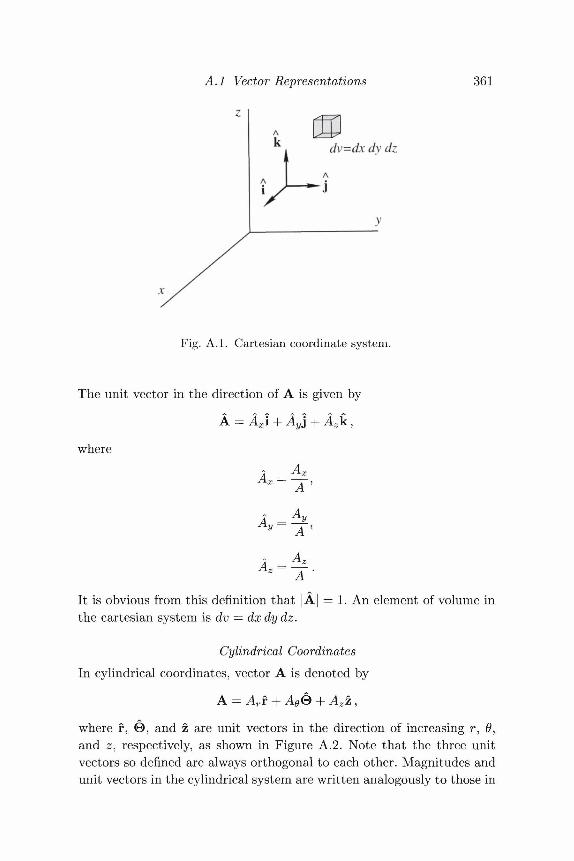
A.I Vector Representations
z
361
dv=dx dy dz
Fig. A.I. Cartesian coordinate system.
The unit vector in the direction of A is given by
where
A -^Ax- A ,
A - AyAy- A ,
It is obvious from this definition that | A| = 1. An element of volume inthe cartesian system is dv = dxdydz.
Cylindrical CoordinatesIn cylindrical coordinates, vector A is denoted by
A = Arr + Ae® + Azz ,
where f, 0 , and z are unit vectors in the direction of increasing r, 0,and z, respectively, as shown in Figure A.2. Note that the three unitvectors so defined are always orthogonal to each other. Magnitudes andunit vectors in the cylindrical system are written analogously to those in
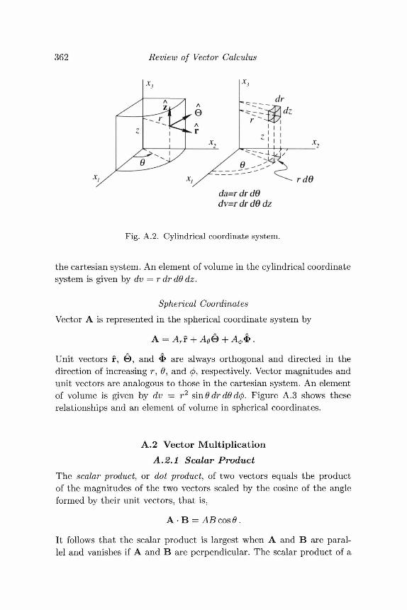
362 Review of Vector Calculus
da=rdrd6dv=rdrd6dz
Fig. A.2. Cylindrical coordinate system.
the cartesian system. An element of volume in the cylindrical coordinatesystem is given by dv = r dr dO dz.
Spherical CoordinatesVector A is represented in the spherical coordinate system by
A = Arr + Ae& + A<t>& .
Unit vectors f, 0 , and ^ are always orthogonal and directed in thedirection of increasing r, #, and </>, respectively. Vector magnitudes andunit vectors are analogous to those in the cartesian system. An elementof volume is given by dv = r2 sinOdrdOdcp. Figure A.3 shows theserelationships and an element of volume in spherical coordinates.
A.2 Vector MultiplicationA.2.1 Scalar Product
The scalar product, or dot product, of two vectors equals the productof the magnitudes of the two vectors scaled by the cosine of the angleformed by their unit vectors, that is,
A • B = AB cos 6 .
It follows that the scalar product is largest when A and B are paral-lel and vanishes if A and B are perpendicular. The scalar product of a
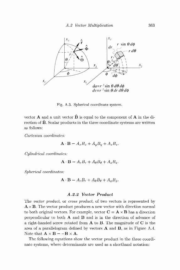
A.2 Vector Multiplication 363
r sin 9 d<p
da=r2s\n 6d6d<pdv=r2 sin 9drd9d0
Fig. A.3. Spherical coordinate system.
vector A and a unit vector B is equal to the component of A in the di-rection of B. Scalar products in the three coordinate systems are writtenas follows:Cartesian coordinates:
A B = AXBX + AyBy + AZBZ.
Cylindrical coordinates:
A B = ArBr + AeB9 + A ^ .
Spherical coordinates:
A B = A r £ r
A.2.2 Vector ProductThe vector product, or cross product, of two vectors is represented byA x B. The vector product produces a new vector with direction normalto both original vectors. For example, vector C = A x B has a directionperpendicular to both A and B and is in the direction of advance ofa right-handed screw rotated from A to B. The magnitude of C is thearea of a parallelogram defined by vectors A and B, as in Figure A.4.Note that A x B = - B x A.
The following equations show the vector product in the three coordi-nate systems, where determinants are used as a shorthand notation:
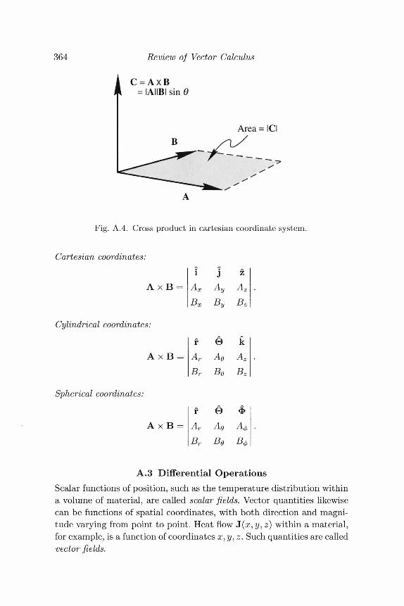
364 Review of Vector Calculus
A x BIAIIBI sin B
Area = ICl
Fig. A.4. Cross product in cartesian coordinate system.
Cartesian coordinates:
Cylindrical coordinates:
A x B =
Spherical coordinates:
A x B =
A A
BX By
f 0Ar AQ
Br BQ
f 0Ar AQ
Br BQ
A
BZ
kAZ
BZ
A.3 Differential OperationsScalar functions of position, such as the temperature distribution withina volume of material, are called scalar fields. Vector quantities likewisecan be functions of spatial coordinates, with both direction and magni-tude varying from point to point. Heat flow J(x, y, z) within a material,for example, is a function of coordinates x,y,z. Such quantities are calledvector fields.
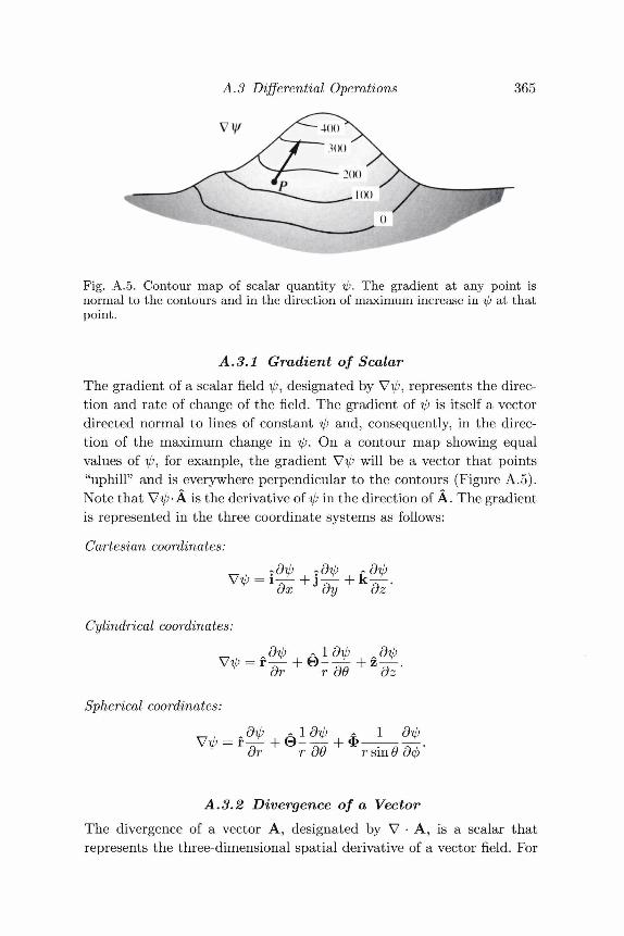
A.3 Differential Operations 365
Fig. A.5. Contour map of scalar quantity ip. The gradient at any point isnormal to the contours and in the direction of maximum increase in ip at thatpoint.
A.3.1 Gradient of ScalarThe gradient of a scalar field ip, designated by V^, represents the direc-tion and rate of change of the field. The gradient of ip is itself a vectordirected normal to lines of constant ip and, consequently, in the direc-tion of the maximum change in I/J. On a contour map showing equalvalues of i/;, for example, the gradient Vip will be a vector that points"uphill" and is everywhere perpendicular to the contours (Figure A.5).Note that Vip- A is the derivative of ip in the direction of A. The gradientis represented in the three coordinate systems as follows:
Cartesian coordinates:
Cylindrical coordinates:
—or
oy
r oO
Spherical coordinates:dib - 1 dibf—- + 0dr rdO
oz
1 dib
A.3.2 Divergence of a VectorThe divergence of a vector A, designated by V • A, is a scalar thatrepresents the three-dimensional spatial derivative of a vector field. For
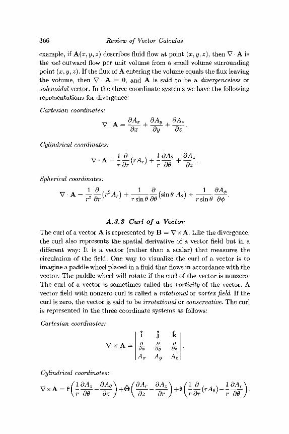
366 Review of Vector Calculus
example, if A(x, y, z) describes fluid flow at point (x, y, z), then V • A isthe net outward flow per unit volume from a small volume surroundingpoint (x, y, z). If the flux of A entering the volume equals the flux leavingthe volume, then V • A = 0, and A is said to be a divergenceless orsolenoidal vector. In the three coordinate systems we have the followingrepresentations for divergence:
Cartesian coordinates:
dx dy dz
Cylindrical coordinates:
Spherical coordinates:1 dAd
A.3.3 Curl of a VectorThe curl of a vector A is represented by B = V x A. Like the divergence,the curl also represents the spatial derivative of a vector field but in adifferent way: It is a vector (rather than a scalar) that measures thecirculation of the field. One way to visualize the curl of a vector is toimagine a paddle wheel placed in a fluid that flows in accordance with thevector. The paddle wheel will rotate if the curl of the vector is nonzero.The curl of a vector is sometimes called the vorticity of the vector. Avector field with nonzero curl is called a rotational or vortex field. If thecurl is zero, the vector is said to be irrotational or conservative. The curlis represented in the three coordinate systems as follows:
Cartesian coordinates:
V x A = A.dxA.X
A.dy
A
A.dz
y
Cylindrical coordinates:
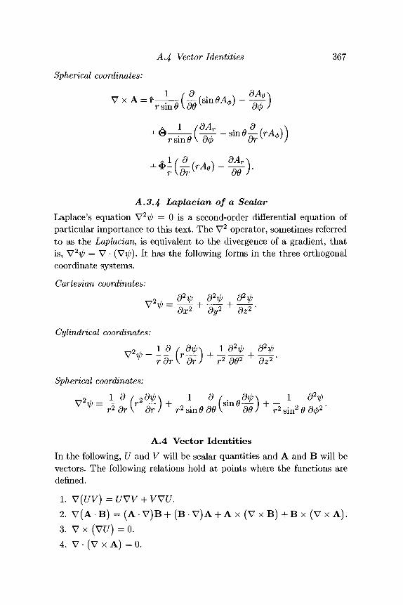
A.4 Vector Identities 367
Spherical coordinates:
d
A.S.4 Laplacian of a ScalarLaplace's equation S/2tp — 0 is a second-order differential equation ofparticular importance to this text. The V2 operator, sometimes referredto as the Laplacian, is equivalent to the divergence of a gradient, thatis, V2^ = V • (VVO- It has the following forms in the three orthogonalcoordinate systems.
Cartesian coordinates:
Cylindrical coordinates:
Spherical coordinates:
rdr\ dr) r2 d62 dz2 '
2 / ^ 9 / 29ip\ 1 d / .r2sm20W
A.4 Vector IdentitiesIn the following, U and V will be scalar quantities and A and B will bevectors. The following relations hold at points where the functions aredefined.
1. V(UV) =2. V(A-B) - (A-V)B+(B-V)A + A x (V x B) + B x (Vx A).3. V x ( W ) = 0.4. V • (V x A) = 0.
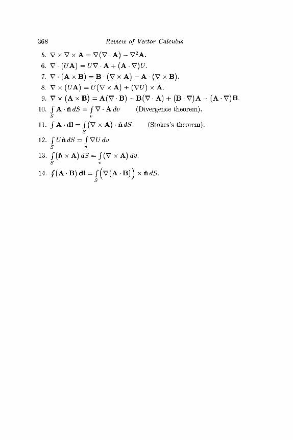
368 Review of Vector Calculus
5. V x V x A = V(V • A) - V2A.6. V • (UA) = f/V • A + (A • V)U.7. V • (A x B) = B • (V x A) - A • (V x B).8. V x (UA) = U(V x A) + ( W ) x A.9. V x (A x B) = A(V • B) - B(V • A) 4- (B • V) A - (A • V)B.
10. jA-hdS = j\/-Adv (Divergence theorem).S v
11. / A • dl = / (V x A) • hdS (Stokes's theorem).s
12. JUhdS = JVUdv.S v
13. / (n x A) dS = /(V x A) dv.S v
14. /(A B) dl = /(V(A • B)) x hdS.
Appendix BSubroutines
Computers are useless. They can only give you answers.(Pablo Picasso)
The following pages provide listings of all subroutines referred to invarious parts of the text. They appear in the order in which they werereferenced. Table B.I lists them alphabetically and summarizes theirfunctions.
All subroutines are written in ANSI-standard Fortran 77. They havebeen compiled on a Sun SPARCstation running SunOS 4.13 and SunFortran version 1.3, and therefore should compile under any standardFortran 77 compiler. Each subroutine has been tested in simple applica-tions, but users should be prepared for unknown bugs. All input and out-put parameters are passed as subroutine arguments rather than throughcommon blocks. Single precision is used throughout (except in subrou-tine FOURN); users may find it advisable to switch to double precisionin some applications.
These subroutines are designed to instruct rather than to be efficient.For example, several of the algorithms require the computation of radialwavenumber
at grid intersections throughout the kx,ky plane. This is done here bycalculating |fc| explicitly at each grid intersection, so that the reader caneasily see the logic involved. A clever programmer, however, could applysome simple tricks in order to exploit the symmetry of |fc| in the kx,kyplane and thereby greatly speed these computations.
Several of the subroutines (GLAYER, MLAYER, MTOPO, CONTIN,VERDER, NEWVEC, and PSEUDO) make use of the two-dimensionalFourier transform and its inverse. As discussed in Appendix C, the
369
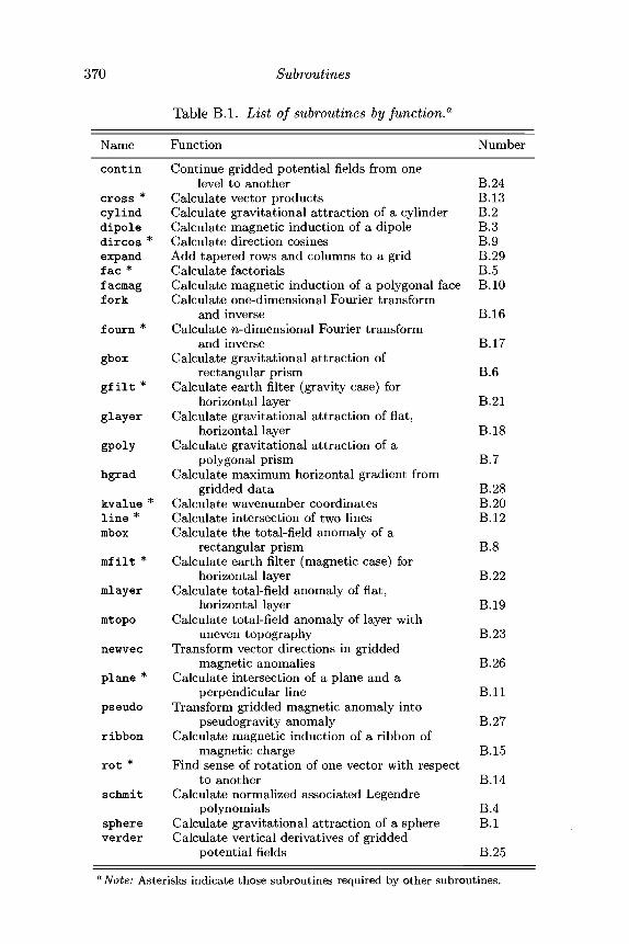
370 Subroutines
Table B.I. List of subroutines by function.0
Name Function Numbercontin
cross *cylinddipoledircos *expandf ac *facmagfork
fourn *
gbox
gfilt *
glayer
hgrad
kvalue *line *mbox
mfilt *
mlayer
mtopo
newvec
plane *
pseudo
ribbon
rot *
schmit
sphereverder
Continue gridded potential fields from onelevel to another B.24
Calculate vector products B.13Calculate gravitational attraction of a cylinder B.2Calculate magnetic induction of a dipole B.3Calculate direction cosines B.9Add tapered rows and columns to a grid B.29Calculate factorials B.5Calculate magnetic induction of a polygonal face B.10Calculate one-dimensional Fourier transform
and inverse B.16Calculate n-dimensional Fourier transform
and inverse B.17Calculate gravitational attraction of
rectangular prism B.6Calculate earth filter (gravity case) for
horizontal layer B.21Calculate gravitational attraction of flat,
horizontal layer B.18Calculate gravitational attraction of a
polygonal prism B.7Calculate maximum horizontal gradient from
gridded data B.28Calculate wavenumber coordinates B.20Calculate intersection of two lines B.12Calculate the total-field anomaly of a
rectangular prism B.8Calculate earth filter (magnetic case) for
horizontal layer B.22Calculate total-field anomaly of flat,
horizontal layer B.19Calculate total-field anomaly of layer with
uneven topography B.23Transform vector directions in gridded
magnetic anomalies B.26Calculate intersection of a plane and a
perpendicular line B.llTransform gridded magnetic anomaly into
pseudogravity anomaly B.27Calculate magnetic induction of a ribbon of
magnetic charge B.15Find sense of rotation of one vector with respect
to another B.14Calculate normalized associated Legendre
polynomials B.4Calculate gravitational attraction of a sphere B.ICalculate vertical derivatives of gridded
potential fields B.25a Note: Asterisks indicate those subroutines required by other subroutines.
Subroutines 371
discrete Fourier transform inherently assumes that a rectangular gridis periodic, in effect repeating itself infinitely many times in all hori-zontal directions, like a vast checkerboard. This can cause undesirable"edge effects" if the edges of the data grid do not meet smoothly withtheir repetitive neighbors. It is strongly recommended, therefore, thatgrids be adjusted in some way prior to calling these subroutines in orderto eliminate abrupt discontinuities at the edges. One way to do this isto add artificial rows and columns to the data grid in such a way as toproduce smooth transitions to neighboring grids. These extra rows andcolumns can be eliminated from the output grid after the subroutine hasexecuted. Subroutine EXPAND provides a simple algorithm to expandgrids in this way.
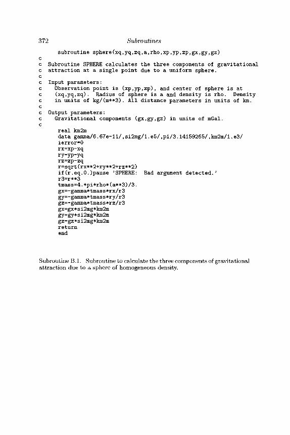
372 Subroutinessubroutine sphere(xq,yq,zq,a,rho,xp,yp,zp,gx,gy,gz)
cc Subroutine SPHERE calculates the three components of gravitationalc attraction at a single point due to a uniform sphere,cc Input parameters:c Observation point is (xp,yp,zp), and center of sphere is atc (xq,yq,zq). Radius of sphere is a and density is rho. Densityc in units of kg/(m**3). All distance parameters in units of km.cc Output parameters:c Gravitational components (gx,gy,gz) in units of mGal.c
real km2mdata gamma/6.67e-l1/,si2mg/l.e5/,pi/3.14159265/,km2m/l.e3/ierror=0rx=xp-xqry=yp-yqrz=zp-zqr=sqrt(rx**2+ry**2+rz**2)if(r.eq.O.)pause 'SPHERE: Bad argument detected.'r3=r**3tmass=4.*pi*rho*(a**3)/3.gx=-gamma*tmass*rx/r3gy=-gamma*tmass*ry/r3gz=-gamma*tmass*rz/r3gx=gx*si2mg*km2mgy=gy*si2mg*km2mgz=gz*si2mg*km2mreturnend
Subroutine B.I. Subroutine to calculate the three components of gravitationalattraction due to a sphere of homogeneous density.
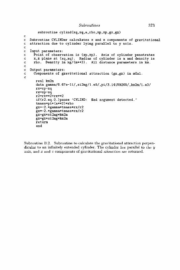
Subroutines 373subroutine cylind(xq,zq,a,rho,xp,zp,gx,gz)
cc Subroutine CYLINDer calculates x and z components of gravitationalc attraction due to cylinder lying parallel to y axis,cc Input parameters:c Point of observation is (xp,zp). Axis of cylinder penetratesc x,z plane at (xq,zq). Radius of cylinder is a and density isc rho. Density in kg/(m**3). All distance parameters in km.cc Output parameters:c Components of gravitational attraction (gx,gz) in mGal.c
real km2mdata gamma/6.67e-ll/,si2mg/l.e5/,pi/3.14159265/,km2m/l.e3/rx=xp-xqrz=zp-zqr2=rx**2+rz**2if(r2.eq.0.)pause 'CYLIND: Bad argument detected.'tmass=pi*(a**2)*rhogx=-2.*gamma*tmass*rx/r2gz=-2.*gamma*tmass*rz/r2gx=gx* s i2mg*km2mgz=gz*si2mg*km2mreturnend
Subroutine B.2. Subroutine to calculate the gravitational attraction perpen-dicular to an infinitely extended cylinder. The cylinder lies parallel to the yaxis, and x and z components of gravitational attraction are returned.
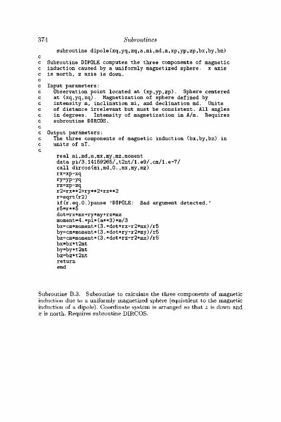
374 Subroutinessubroutine dipole(xq,yq,zq,a,mi,md,m,xp,yp,zp,bx,by,bz)
cc Subroutine DIPOLE computes the three components of magneticc induction caused by a uniformly magnetized sphere, x axisc is north, z axis is down,cc Input parameters:c Observation point located at (xp,yp,zp). Sphere centeredc at (xq,yq,zq). Magnetization of sphere defined byc intensity m, inclination mi, and declination md. Unitsc of distance irrelevant but must be consistent. All anglesc in degrees. Intensity of magnetization in A/m. Requiresc subroutine DIRCOS.cc Output parameters:c The three components of magnetic induction (bx,by,bz) inc units of nT.c
real mi,md,m,mx,my,mz,momentdata pi/3.14159265/,t2nt/l.e9/,cm/1.e-7/call dircos(mi,md,0.,mx,my,rnz)rx=xp-xqry=yp-yqrz=zp-zqr2=rx**2+ry**2+rz**2r=sqrt(r2)if(r.eq.O.)pause 'DIPOLE: Bad argument detected.'r5=r**5dot=rx*mx+ry*my+rz*mzmoment=4.*pi*(a**3)*m/3bx=cm*moment*(3.*dot*rx-r2*mx)/r5by=cm*moment*(3.*dot*ry-r2*my)/r5bz=cm*moment*(3.*dot*rz-r2*mz)/r5bx=bx*t2ntby=by*t2ntbz=bz*t2ntreturnend
Subroutine B.3. Subroutine to calculate the three components of magneticinduction due to a uniformly magnetized sphere (equivalent to the magneticinduction of a dipole). Coordinate system is arranged so that z is down andx is north. Requires subroutine DIRCOS.
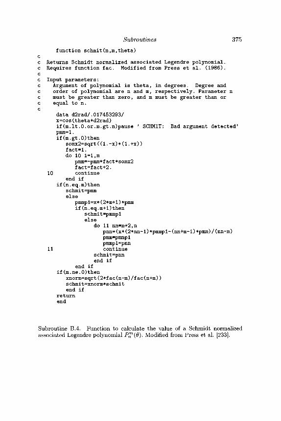
Subroutines 375function schmit(n,m,theta)
cc Returns Schmidt normalized associated Legendre polynomial,c Requires function fac. Modified from Press et al. (1986).cc Input parameters:c Argument of polynomial is theta, in degrees. Degree andc order of polynomial are n and m, respectively. Parameter nc must be greater than zero, and m must be greater than orc equal to n.c
data d2rad/.017453293/x=cos(theta*d2rad)if(m.lt.O.or.m.gt.n)pause ' SCHMIT: Bad argument detected'pmm=l.if(m.gt.O)then
somx2=sqrt((1.-x)*(1.+x))fact=l.do 10 i=l,m
pmm=-pmm*fact*somx2fact=fact+2.
10 continueend if
if(n.eq.m)thenschmit=pmmelse
pmmpl=x*(2*m+l) *pmmif(n.eq.m+1)then
schmit=pmmplelse
do 11 nn=m+2,npnn=(x*(2*nn-l)*pmmpl-(nn+m-1)*pmm)/(nn-m)pmm=pmmp1pmmpl=pnn
11 continueschmit=pnnend if
end ifif (m.ne.O)then
xnorm=sqrt (2*f ac (n-m) /fac (n+m) )schmit=xnorm*schmitend if
returnend
Subroutine B.4. Function to calculate the value of a Schmidt normalizedassociated Legendre polynomial P™(0). Modified from Press et al. [233].
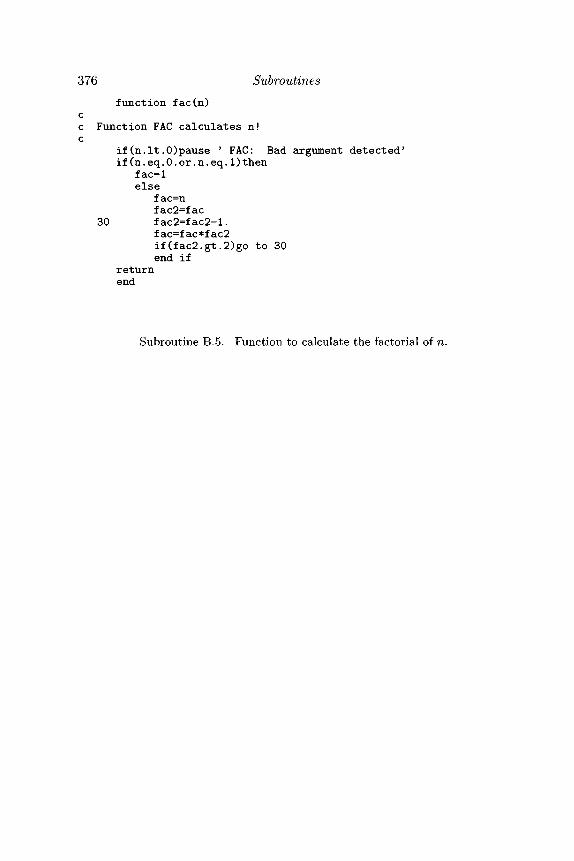
376 Subroutinesfunction fac(n)
cc Function FAC calculates n!c
if(n.It.0)pause J FAC: Bad argument detected'if(n.eq.0.or.n.eq.1)then
fac=lelse
f ac=nfac2=fac
30 fac2=fac2-l.fac=fac*fac2if(fac2.gt.2)go to 30end if
returnend
Subroutine B.5. Function to calculate the factorial of n.
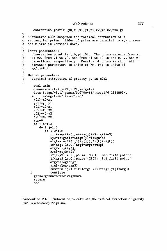
Subroutines 377subroutine gbox(xO,yO,zO,xl,y1,zl,x2,y2,z2,rho,g)
cc Subroutine GBOX computes the vertical attraction of ac rectangular prism. Sides of prism are parallel to x,y,z axes,c and z axis is vertical down,cc Input parameters:c Observation point is (xO,yO,zO). The prism extends from xlc to x2, from yl to y2, and from zl to z2 in the x, y, and zc directions, respectively. Density of prism is rho. Allc distance parameters in units of km; rho in units ofc kg/(m**3).cc Output parameters:c Vertical attraction of gravity g, in mGal.c
real km2mdimension x(2),y(2),z(2),isign(2)data isign/-l,1/,gamma/6.670e-l1/,twopi/6.2831853/,& si2mg/l.e5/,km2m/l.e3/x(l)=xO-xly(l)=yO-ylz(l)=zO-zlX(2)=x0-x2y(2)=yO-y2z(2)=zO-z2sum=0.do 1 i=l,2
do 1 j=l,2do 1 k=l,2
rijk=sqrt(x(i)**2+y(j)**2+z(k)**2)ijk=isign(i)*isign(j)*isign(k)argl=atan2((x(i)*y(j)),(z(k)*rijk))if(argl.It.0.)argl=argl+twopiarg2=rijk+y(j)arg3=rij k+x(i)if(arg2.1e.O.)pause JGB0X: Bad field point>if(arg3.1e.O.)pause 'GBOX: Bad field point'arg2=alog(arg2)arg3=alog(arg3)sum=sum+ijk*(z(k)*argl-x(i)*arg2-y(j)*arg3)
1 continueg=rho*gamma*sum*si2mg*km2mreturnend
Subroutine B.6. Subroutine to calculate the vertical attraction of gravitydue to a rectangular prism.

378 Subroutinessubroutine gpoly(xO,zO,xcorn,zcorn,ncorn,rho,g)
cc Subroutine GPOLY computes the vertical attraction of a two-c dimensional body with polygonal cross section. Axes arec right-handed system with y axis parallel to long directionc of body and z axis vertical down,cc Input parameters:c Observation point is (xO,zO). Arrays xcorn and zcorn (eachc of length ncorn) contain the coordinates of the polygonc corners, arranged in clockwise order when viewed with x axisc to right. Density of body is rho. All distance parametersc in units of km; rho in units of kg/(m**3).cc Output parameters:c Vertical attraction of gravity g, in mGal.c
real km2mdimension xcorn(ncorn),zcorn(ncorn)data gamma/6.670e-ll/,si2mg/l.e5/,km2m/l.e3/sum=0.do 1 n=l,ncorn
if(n.eq.ncorn)thenn2=lelse
n2=n+lend if
xl=xcorn(n)-xOzl=zcorn(n)-zOx2=xcorn(n2)-xOz2=zcorn(n2)-z0rlsq=xl**2+zl**2r2sq=x2**2+z2**2if(rlsq.eq.O.)pause 'GPOLY: Field point on corner'if(r2sq.eq.O.)pause 'GPOLY: Field point on corner'denom=z2-zlif(denom.eq.O.)denom=l.e-6alpha=(x2-xl)/denombeta=(xl*z2-x2*zl)/denomfactor=beta/(1.+alpha**2)terml=0.5*(alog(r2sq)-alog(rlsq))term2=atan2(z2,x2)-atan2(zl,xl)sum=sum+factor*(terml-alpha*term2)
1 continueg=2.*rho*gamma*sum*si2mg*km2mreturnend
Subroutine B.7. Subroutine to calculate the vertical gravitational attractiondue to a two-dimensional prism of polygonal cross section. Axis of prism liesparallel to y axis; z axis is down. Polygon corners are contained within arraysxcorn and zcorn in clockwise order as viewed with the x axis to the right.
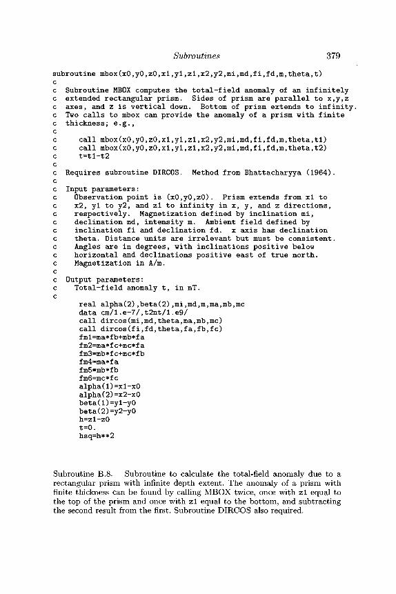
Subroutines 379
subroutine mbox(xO,yO,zO,x1,y1,z1,x2,y2,mi,md,f i,fd,m,theta,t)cc Subroutine MBOX computes the total-field anomaly of an infinitelyc extended rectangular prism. Sides of prism are parallel to x,y,zc axes, and z is vertical down. Bottom of prism extends to infinity.c Two calls to mbox can provide the anomaly of a prism with finitec thickness; e.g.,cc call mbox(xO,yO,zO,xl,yl,zl,x2,y2,mi,md,fi,fd,m,theta,tl)c call mbox(xO,yO,zO,xl,yl,zl,x2,y2,mi,md,fi,fd,m,theta,t2)c t=tl-t2cc Requires subroutine DIRCOS. Method from Bhattacharyya (1964).cc Input parameters:c Observation point is (xO,yO,zO). Prism extends from xl toc x2, yl to y2, and zl to infinity in x, y, and z directions,c respectively. Magnetization defined by inclination mi,c declination md, intensity m. Ambient field defined byc inclination fi and declination fd. x axis has declinationc theta. Distance units are irrelevant but must be consistent.c Angles are in degrees, with inclinations positive belowc horizontal and declinations positive east of true north.c Magnetization in A/m.cc Output parameters:c Total-field anomaly t, in nT.c
real alpha(2),beta(2),mi,md,m,ma,mb,mcdata cm/l.e-7/,t2nt/l.e9/call dircos(mi,md,theta,ma,mb,mc)call dircos(fi,fd,theta,fa,fb,fc)fml=ma*fb+mb*fafm2=ma*fc+mc*fafm3=mb*fc+mc*fbfm4=ma*fafm5=mb*fbfm6=mc*fcalpha(l)=xl-xOalpha(2)=x2-xObeta(l)=yl-yObeta(2)=y2-y0h=zl-zOt=0.hsq=h**2
Subroutine B.8. Subroutine to calculate the total-field anomaly due to arectangular prism with infinite depth extent. The anomaly of a prism withfinite thickness can be found by calling MBOX twice, once with zl equal tothe top of the prism and once with zl equal to the bottom, and subtractingthe second result from the first. Subroutine DIRCOS also required.
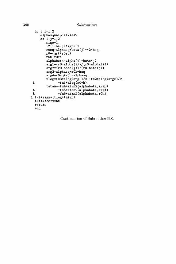
380 Subroutinesdo 1 i=l,2
alphasq=alpha(i)**2do 1 j=l,2
sign=l.if(i.ne.j)sign=-1.rOsq=alphasq+beta(j)**2+hsqrO=sqrt(rOsq)r0h=r0*halphabeta=alpha(i)*beta(j)argl=(rO-alpha(i))/(rO+alpha(i))arg2=(rO-beta(j))/(rO+beta(j))arg3=alphasq+r0h+hsqarg4=r0sq+r0h-alphasqtlog=fm3*alog(argl)/2.+fm2*alog(arg2)/2.
& -fml*alog(rO+h)tatan=-fm4*atan2(alphabeta,arg3)
& -fm5*atan2(alphabeta,arg4)& +fm6*atan2(alphabeta,r0h)
1 t=t+sign*(tlog+tatan)t=t*m*cm*t2ntreturnend
Continuation of Subroutine B.8.
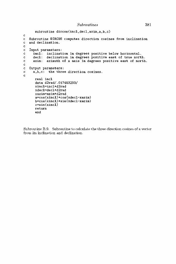
Subroutines 381subroutine dircos(incl,decl,azim,a,b,c)
cc Subroutine DIRCOS computes direction cosines from inclinationc and declination,cc Input parameters:c incl: inclination in degrees positive below horizontal,c decl: declination in degrees positive east of true north,c azim: azimuth of x axis in degrees positive east of north,cc Output parameters:c a,b,c: the three direction cosines,c
real incldata d2rad/.017453293/xincl=incl*d2radxdecl=decl*d2radxazim=azim*d2rada=cos(xincl)*cos(xdecl-xazim)b=cos(xincl)*sin(xdecl-xazim)c=sin(xincl)returnend
Subroutine B.9. Subroutine to calculate the three direction cosines of a vectorfrom its inclination and declination.
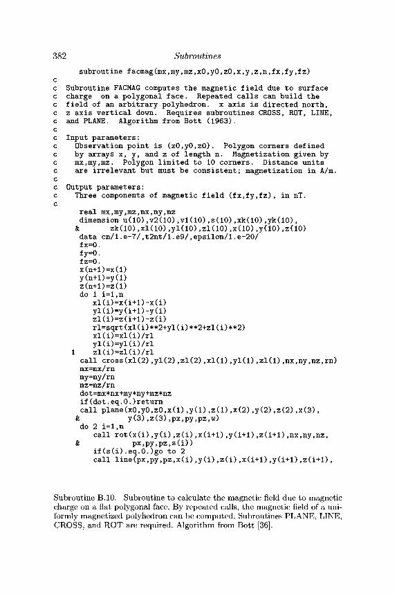
382 Subroutinessubroutine facmag(mx,my,mz,xO,yO,zO,x,y,z,n,fx,fy,fz)
cc Subroutine FACMAG computes the magnetic field due to surfacec charge on a polygonal face. Repeated calls can build thec field of an arbitrary polyhedron, x axis is directed north,c z axis vertical down. Requires subroutines CROSS, ROT, LINE,c and PLANE. Algorithm from Bott (1963).cc Input parameters:c Observation point is (xO,yO,zO). Polygon corners definedc by arrays x, y, and z of length n. Magnetization given byc mx,my,mz. Polygon limited to 10 corners. Distance unitsc are irrelevant but must be consistent; magnetization in A/m.cc Output parameters:c Three components of magnetic field (fx,fy,fz), in nT.c
real mx,my,mz,nx,ny,nzdimension u(10),v2(10),vl(10),s(10),xk(10),yk(10),
& zk(10),xl(10),yl(10),zl(10),x(10),y(10),z(10)data cm/1.e-7/,t2nt/l.e9/,epsilon/1.e-20/fx=0.fy=O.fz=0.x(n+l)=x(l)y(n+l)=y(l)z(n+l)=z(l)do 1 i=l,n
rl=sqrt(xl(i)**2+yl(i)**2+zl(i)**2)( ) ( ) /
yy1 zl(i)=zl(i)/rlcall cross(xl(2),yl(2),zl(2),xl(l),yl(l),zl(l),nx,ny,nz,rn)nx=nx/rnny=ny/rnnz=nz/rndot=mx*nx+my*ny+mz*nzif(dot.eq.0.)returncall plane(xO,yO,zO,x(l),y(l),z(l),x(2),y(2),z(2),x(3),
& y(3),z(3),px,py,pz,w)do 2 i=l,n
call rot(x(i),y(i),z(i),x(i+l),y(i+l),z(i+l),nx,ny,nz,& px,py,pz,s(i))
if(s(i).eq.0.)go to 2call line(px,py,pz,x(i),y(i),z(i),x(i+l),y(i+l),z(i+l),
Subroutine B.10. Subroutine to calculate the magnetic field due to magneticcharge on a flat polygonal face. By repeated calls, the magnetic field of a uni-formly magnetized polyhedron can be computed. Subroutines PLANE, LINE,CROSS, and ROT are required. Algorithm from Bott [36].
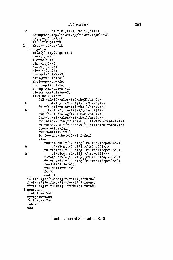
Subroutines 383& ul,v,wl,vl(i),v2(i),u(i))
rk=sqrt((ul-px)**2+(v-py)**2+(wl-pz)**2)xk(i)=(ul-px)/rkyk(i)=(v-py)/rk
2 zk(i)=(wl-pz)/rkdo 3 j=l,n
if(s(j).eq.0.)go to 3us=u(j)**2v2s=v2(j)**2vls=vl(j)**2a2=v2(j)/u(j)
( ) / ( )j jf2=sqrt(l.+a2*a2)fl=sqrt(l.+al*al)rho2=sqrt(us+v2s)rhol=sqrt(us+vls)r2=sqrt(us+v2s+w**2)rl=sqrt(us+vls+w**2)if(w.ne.O.)then
fu2=(a2/f2)*alog((r2+rho2)/abs(w))& -.5*alog((r2+v2(j))/(r2-v2(j)))
ful=(al/fl)*alog((rl+rhol)/abs(w))-& .5*alog((rl+vl(j))/(rl-vl(j)))
fv2=(1./f2)*alog((r2+rho2)/abs(w))fvl=(l./fl)*alog((rl+rhol)/abs(w))fw2=atan2((a2*(r2-abs(w))),(r2+a2*a2*abs(w)))fwl=atan2((al*(r1-abs(w))),(rl+al*al*abs(w)))fu=dot*(fu2-ful)fv=-dot*(fv2-fvl)fw=(-w*dot/abs(w))*(fw2-fwl)else
fu2=(a2/f2)*(1.+alog((r2+rho2)/epsilon))-k .5*alog((r2+v2(j))/(r2-v2(j)))
ful=(al/f1)*(1.+alog((rl+rhol)/epsilon))-& .5*alog((rl+vl(j))/(rl-vl(j)))
fv2=(1./f2)*(1.+alog((r2+rho2)/epsilon))fvl=(l./fl)*(l.+alog((rl+rhol)/epsilon))fu=dot*(fu2-ful)fv=-dot*(fv2-fvl)fw=0.end if
f x=f x-s ( j ) * (f u*xk (j ) +f v*xl ( j ) +f w*nx)f y=f y-s (j) * (f u*yk (j ) +f v*yl ( j ) +f w*ny )fz=fz-s(j)*(fu*zk(j)+fv*zl(j)+fw*nz)
3 continuefx=fx*cm*t2ntfy=fy*cm*t2ntfz=fz*cm*t2ntreturnend
Continuation of Subroutine B.10.
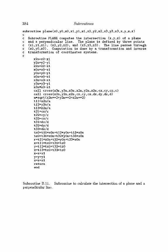
384 Subroutines
subroutine plane(xO,yO,zO,xl,y1,z1,x2,y2,z2,x3,y3,z3,x,y,z,r)cc Subroutine PLANE computes the intersection (x,y,z) of a planec and a perpendicular line. The plane is defined by three pointsc (xl,yl,zl), (x2,y2,z2), and (x3,y3,z3). The line passes throughc (xO,yO,zO). Computation is done by a transformation and inversec transformation of coordinates systems.c
x2n=x2-xly2n=y2-ylz2n=z2-zlxOn=xO-xlyOn=yO-ylzOn=zO-zlx3n=x3-xly3n=y3-ylz3n=z3-zlcall cross(x3n,y3n,z3n,x2n,y2n,z2n,ex,cy,cz,c)call cross(x2n,y2n,z2n,ex,cy,cz,dx,dy,dz,d)a=sqrt(x2n**2+y2n**2+z2n**2)tll=x2n/atl2=y2n/atl3=z2n/at21=cx/ct22=cy/ct23=cz/ct31=dx/dt32=dy/dt33=dz/dtxO=t1l*xOn+t12*y0n+t13*z0ntz0=t31*x0n+t32*y0n+t33*z0nr=t21*x0n+t22*y0n+t23*z0nx=tll*txO+t31*tzOy=tl2*tx0+t32*tz0z=tl3*txO+t33*tzOx=x+xly=y+ylz=z+zlreturnend
Subroutine B.ll. Subroutine to calculate the intersection of a plane and aperpendicular line.
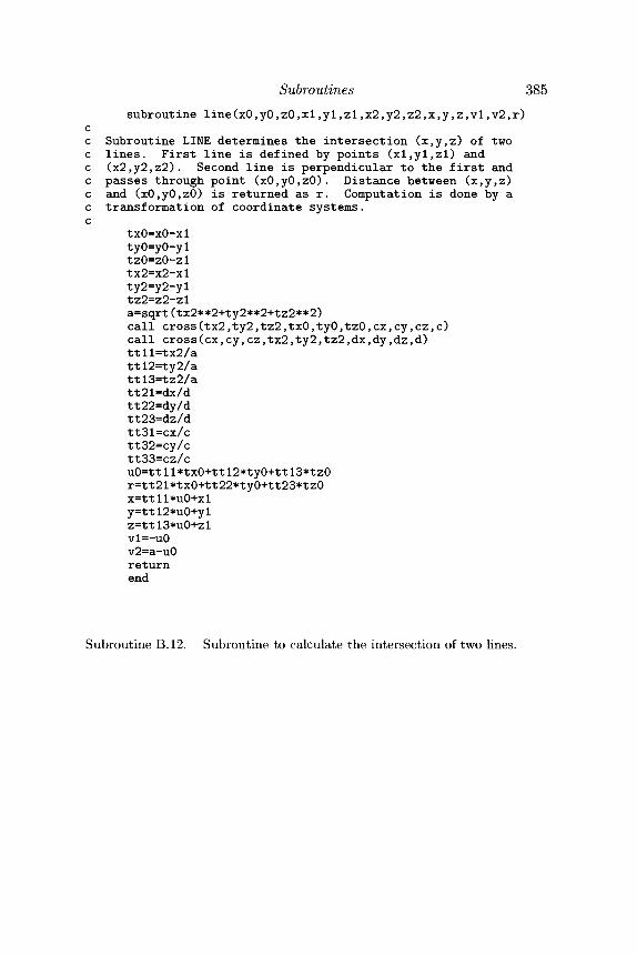
Subroutines 385
subroutine line(xO,yO,zO,xl,y1,zl,x2,y2,z2,x,y,z,vl,v2,r)cc Subroutine LINE determines the intersection (x,y,z) of twoc lines. First line is defined by points (xl,yl,zl) andc (x2,y2,z2). Second line is perpendicular to the first andc passes through point (xO,yO,zO). Distance between (x,y,z)c and (xO,yO,zO) is returned as r. Computation is done by ac transformation of coordinate systems,c
txO=xO-xltyO=yO-yltzO=zO-zltx2=x2-xlty2=y2-yltz2=z2-zla=sqrt(tx2**2+ty2**2+tz2**2)call cross(tx2,ty2,tz2,txO,tyO,tzO,ex,cy,cz,c)call cross(ex,cy,cz,tx2,ty2,tz2,dx,dy,dz,d)ttll=tx2/attl2=ty2/attl3=tz2/att21=dx/dtt22=dy/dtt23=dz/dtt31=cx/ctt32=cy/ctt33=cz/cuO=ttll*txO+ttl2*tyO+ttl3*tzOr=tt21*txO+tt22*tyO+tt23*tzOx=ttll*uO+xly=ttl2*u0+ylz=ttl3*u0+zlvl=-uOv2=a-uOreturnend
Subroutine B.12. Subroutine to calculate the intersection of two lines.
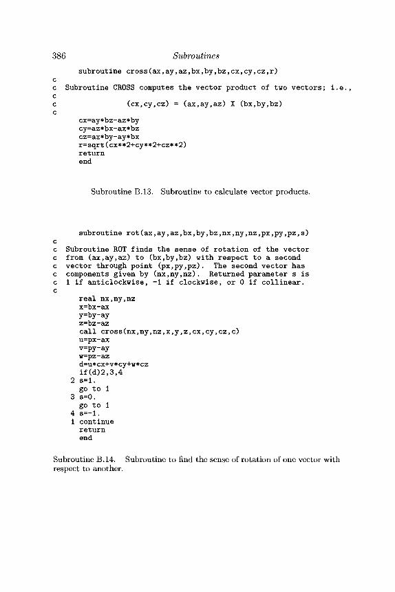
386 Subroutinessubroutine cross(ax,ay,az,bx,by,bz,ex,cy,cz,r)
cc Subroutine CROSS computes the vector product of two vectors; i.e.,cc (cx,cy,cz) = (ax,ay,az) X (bx,by,bz)c
cx=ay*bz-az*bycy=az*bx-ax*bzcz=ax*by-ay*bxr=sqrt(cx**2+cy**2+cz**2)returnend
Subroutine B.13. Subroutine to calculate vector products.
subroutine rot(ax,ay,az,bx,by,bz,nx,ny,nz,px,py,pz,s)cc Subroutine ROT finds the sense of rotation of the vectorc from (ax,ay,az) to (bx,by,bz) with respect to a secondc vector through point (px,py,pz). The second vector hasc components given by (nx,ny,nz). Returned parameter s isc 1 if anticlockwise, -1 if clockwise, or 0 if collinear.c
real nx,ny,nzx=bx-axy=by-ayz=bz-azcall cross(nx,ny,nz,x,y,z,ex,cy,cz,c)u=px-axv=py-ayw=pz-azd=u* cx+v* cy+w* czif(d)2,3,4
2 s=l.go to 1
3 s=0.go to 1
4 s=-l.1 continuereturnend
Subroutine B.14. Subroutine to find the sense of rotation of one vector withrespect to another.
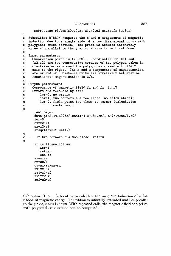
Subroutines 387subroutine ribbon(xO,zO,xl,z1,x2,z2,mx,mz,fx,fz,ier)
cc Subroutine RIBBON computes the x and z components of magneticc induction due to a single side of a two-dimensional prism withc polygonal cross section. The prism is assumed infinitelyc extended parallel to the y axis; z axis is vertical down,cc Input parameters:c Observation point is (xO,zO). Coordinates (xl,zl) andc (x2,z2) are two consecutive corners of the polygon taken inc clockwise order around the polygon as viewed with the xc axis to the right. The x and z components of magnetizationc are mx and mz. Distance units are irrelevant but must bec consistent; magnetization in A/m.cc Output parameters:c Components of magnetic field fx and fz, in nT.c Errors are recorded by ier:c ier=0, no errors;c ier=l, two corners are too close (no calculation);c ier=2, field point too close to corner (calculationc continues).c
real mx,mzdata pi/3.14159265/,small/1.e-18/,cm/1.e-7/,t2nt/l.e9/ier=0sx=x2-xlsz=z2-zls=sqrt(sx**2+sz**2)
cc — If two corners are too close, returnc
if (s.It.small)thenier=lreturnend if
sx=sx/ssz=sz/sqs=mx*sz-mz*sxrxl=xl-xOrzl=zl-zOrx2=x2-xOrz2=z2-zO
Subroutine B.15. Subroutine to calculate the magnetic induction of a flatribbon of magnetic charge. The ribbon is infinitely extended and lies parallelto the y axis; z axis is down. With repeated calls, the magnetic field of a prismwith polygonal cross section can be computed.
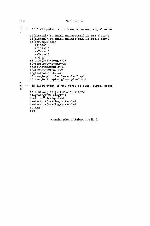
388 Subroutinescc — If field point is too near a corner, signal errorc
if(abs(rxl).It.small.and.abs(rzl).It.small)ier=2if(abs(rx2).It.small.and.abs(rz2).It.small)ier=2if(ier.eq.2)then
rxl=smallrzl=smallrx2=smallrz2=smallend if
rl=sqrt(rxl**2+rzl**2)r2=sqrt(rx2**2+rz2**2)thetal=atan2(rzl,rxl)theta2=atan2(rz2,rx2)angle=thetal-theta2if (angle.gt.pi)angle=angle-2.*piif (angle.lt.-pi)angle=angle+2.*pi
cc — If field point is too close to side, signal errorc
if (abs(angle).gt.(.995*pi))ier=2flog=alog(r2)-alog(rl)factor=-2.*cm*qs*t2ntfx=factor*(sx*flog-sz*angle)fz=factor*(sz*flog+sx*angle)returnend
Continuation of Subroutine B.15.
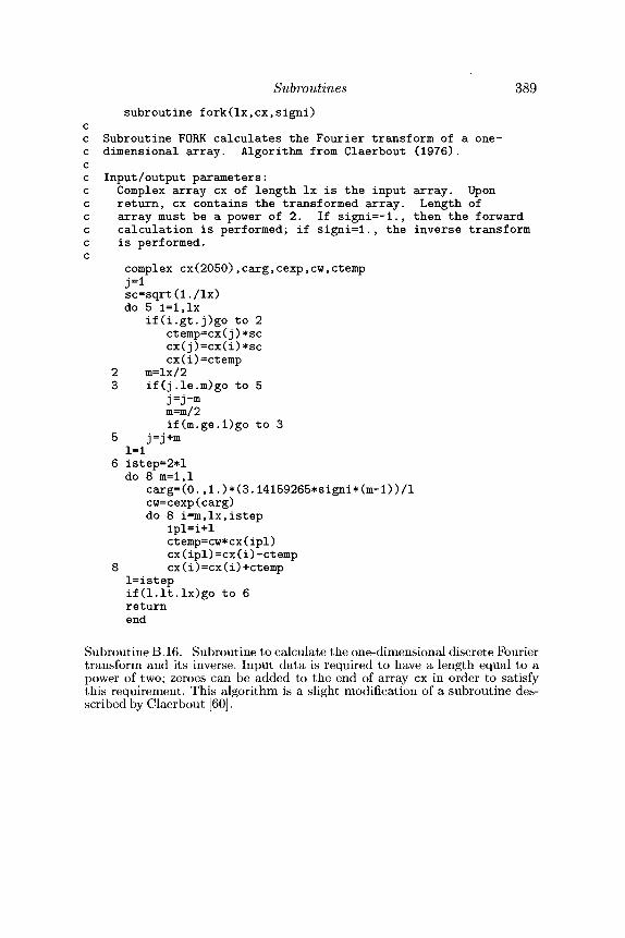
Subroutines 389subroutine fork(lx,cx,signi)
cc Subroutine FORK calculates the Fourier transform of a one-c dimensional array. Algorithm from Claerbout (1976).cc Input/output parameters:c Complex array ex of length lx is the input array. Uponc return, ex contains the transformed array. Length ofc array must be a power of 2. If signi=-l., then the forwardc calculation is performed; if signi=l., the inverse transformc is performed,c
complex ex(2050),carg,cexp,cw,ctemp
sc=sqrt(1./lx)do 5 i=l,lx
if( i .gt . j )go to 2ctemp=cx(j)*sccx(j)=cx(i)*sccx(i)=ctemp
2 m=lx/23 if(j.le.m)go to 5
m=m/2if(m.ge.l)go to 3
5 j =j +m1=1
6 istep=2*ldo 8 m=l,l
carg=(0. , l . )*(3.14159265*signi*(m-l)) / lcw=cexp(carg)do 8 i=m,lx, is tep
ipl=i+lctemp=cw*cx(ipl)cx(ipl)=cx(i)-ctemp
8 cx(i)=cx(i)+ctempl=istepif(l.lt.lx)go to 6returnend
Subroutine B.16. Subroutine to calculate the one-dimensional discrete Fouriertransform and its inverse. Input data is required to have a length equal to apower of two; zeroes can be added to the end of array ex in order to satisfythis requirement. This algorithm is a slight modification of a subroutine des-scribed by Claerbout [60].
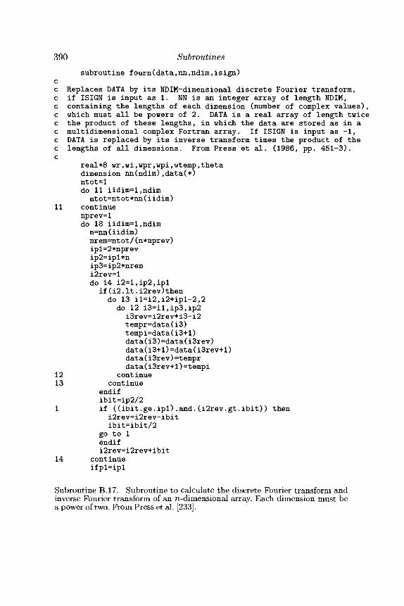
390 Subroutinessubroutine fourn(data,nn,ndim,isign)
cc Replaces DATA by its NDIM-dimensional discrete Fourier transform,c if ISIGN is input as 1. NN is an integer array of length NDIM,c containing the lengths of each dimension (number of complex values),c which must all be powers of 2. DATA is a real array of length twicec the product of these lengths, in which the data are stored as in ac multidimensional complex Fortran array. If ISIGN is input as -1,c DATA is replaced by its inverse transform times the product of thec lengths of all dimensions. From Press et al. (1986, pp. 451-3).c
real*8 wr,wi,wpr,wpi,wtemp,thetadimension nn(ndim),data(*)ntot=ldo 11 iidim=l,ndimntot=ntot*nn(iidim)
11 continuenprev=ldo 18 iidim=l,ndimn=nn(iidim)nrem=ntot/(n*nprev)ipl=2*nprevip2=ipl*nip3=ip2*nremi2rev=ldo 14 i2=l,ip2,ipl
if(i2.It.i2rev)thendo 13 il=i2,i2+ipl-2,2
do 12 i3=il,ip3,ip2i3rev=i2rev+i3-i2tempr=data(i3)tempi=data(i3+l)data(i3)=data(i3rev)data(i3+l)=data(i3rev+l)data(i3rev)=temprdata(i3rev+l)=tempi
12 continue13 continue
endifibit=ip2/2
1 if ((ibit.ge.ipl).and.(i2rev.gt.ibit)) theni2rev=i2rev-ibitibit=ibit/2
go to 1endifi2rev=i2rev+ibit
14 continueifpl=ipl
Subroutine B.17. Subroutine to calculate the discrete Fourier transform andinverse Fourier transform of an n-dimensional array. Each dimension must bea power of two. From Press et al. [233].
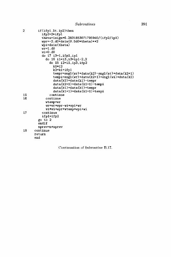
Subroutines 3912 if (if pl.lt. ip2) then
ifp2=2*ifpltheta=isign*6.28318530717959d0/(ifp2/ipl)wpr=-2.dO*dsin(O.5dO*theta)**2wpi=dsin(theta)wr=l.dOwi=O.dOdo 17 i3=l,ifpl,ipldo 16 il=i3,i3+ipl-2,2
do 15 i2=il,iP3,ifp2kl=i2k2=kl+ifpltempr=sngl(wr)*data(k2)-sngl(wi)*data(k2+l)tempi=sngl(wr)*data(k2+l)+sngl(wi)*data(k2)data(k2)=data(kl)-temprdata(k2+l)=data(kl+l)-tempidata(kl)=data(kl)+temprdata(kl+l)=data(kl+l)+tempi
15 continue16 continue
wtemp=wrwr=wr*wpr-wi*wpi+wrwi=wi*wpr+wtemp*wpi+wi
17 continueifpl=ifp2
go to 2endifnprev=n*nprev
18 continuereturnend
Continuation of Subroutine B.17.
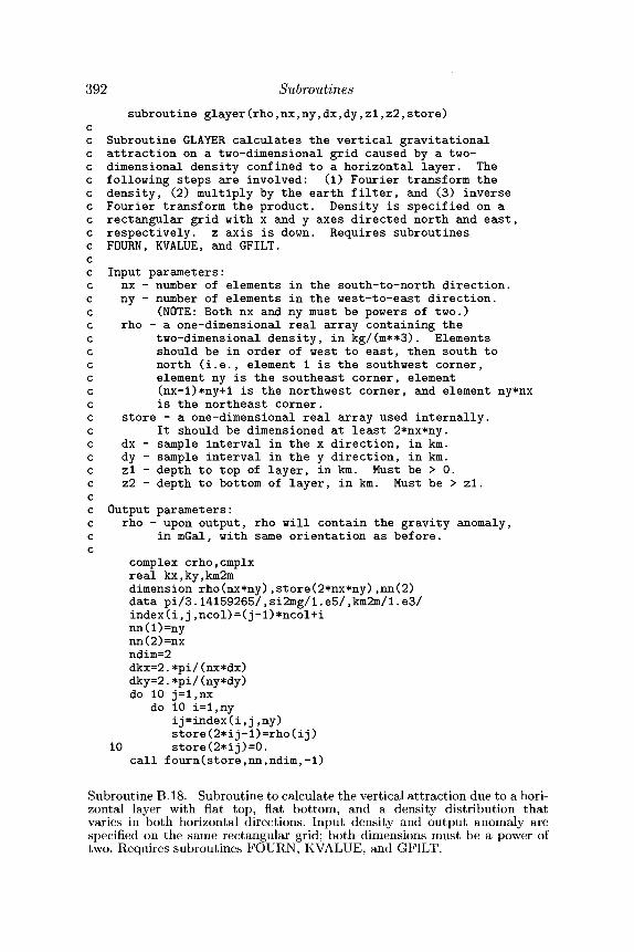
392 Subroutinessubroutine glayer(rho,nx,ny,dx,dy,zl,z2,store)
cc Subroutine GLAYER calculates the vertical gravitationalc attraction on a two-dimensional grid caused by a two-c dimensional density confined to a horizontal layer. Thec following steps are involved: (1) Fourier transform thec density, (2) multiply by the earth filter, and (3) inversec Fourier transform the product. Density is specified on ac rectangular grid with x and y axes directed north and east,c respectively, z axis is down. Requires subroutinesc FOURN, KVALUE, and GFILT.cc Input parameters:c nx - number of elements in the south-to-north direction,c ny - number of elements in the west-to-east direction,c (NOTE: Both nx and ny must be powers of two.)c rho - a one-dimensional real array containing thec two-dimensional density, in kg/(m**3). Elementsc should be in order of west to east, then south toc north (i.e., element 1 is the southwest corner,c element ny is the southeast corner, elementc (nx-l)*ny+l is the northwest corner, and element ny*nxc is the northeast corner.c store - a one-dimensional real array used internally,c It should be dimensioned at least 2*nx*ny.c dx - sample interval in the x direction, in km.c dy - sample interval in the y direction, in km.c zl - depth to top of layer, in km. Must be > 0.c z2 - depth to bottom of layer, in km. Must be > zl.cc Output parameters:c rho - upon output, rho will contain the gravity anomaly,c in mGal, with same orientation as before,c
complex crho,cmplxreal kx,ky,km2mdimension rho(nx*ny),store(2*nx*ny),nn(2)data pi/3.14159265/,si2mg/l.e5/,km2m/l.e3/index(i,j,ncol)=(j-l)*ncol+inn(1)=nynn(2)=nxndim=2dkx=2.*pi/(nx*dx)dky=2.*pi/(ny*dy)do 10 j=l,nx
do 10 i=l,nyij=index(i,j,ny)store(2*ij-l)=rho(ij)
10 store(2*ij)=0.call fourn(store,nn,ndim,-l)
Subroutine B.18. Subroutine to calculate the vertical attraction due to a hori-zontal layer with flat top, flat bottom, and a density distribution thatvaries in both horizontal directions. Input density and output anomaly arespecified on the same rectangular grid; both dimensions must be a power oftwo. Requires subroutines F O U R N , K V A L U E , and GFILT.
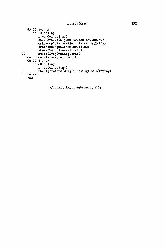
Subroutines 393do 20 j=l,nx
do 20 i=l,nyij =index(i,j,ny)call kvalue(i,j,nx,ny,dkx,dky,kx,ky)crho=cmplx(store(2*ij-l),store(2*ij))crho=crho*gfilt(kx,ky,zl,z2)store(2*ij-l)=real(crho)
20 store(2*ij)=aimag(crho)call fourn(store,nn,ndim,+l)do 30 j=l,nx
do 30 i=l,nyij=index(i,j,ny)
30 rho(ij)=store(2*ij-1)*si2mg*km2m/(nx*ny)returnend
Continuation of Subroutine B.18.
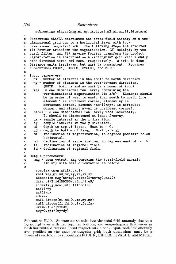
394 Subroutinessubroutine mlayer(mag,nx,ny,dx,dy,z1,z2,mi,md,f i,fd,store)
cc Subroutine MLAYER calculates the total-field anomaly on a two-c dimensional grid due to a horizontal layer with two-c dimensional magnetization. The following steps are involved:c (1) Fourier transform the magnetization, (2) multiply by thec earth filter, and (3) inverse Fourier transform the product,c Magnetization is specified on a rectangular grid with x and yc axes directed north and east, respectively, z axis is down,c Distance units irrelevant but must be consistent. Requiresc subroutines FOURN, DIRCOS, RVALUE, and MFILT.cc Input parameters:c nx - number of elements in the south-to-north direction,c ny - number of elements in the west-to-east direction,c (NOTE: both nx and ny must be a power of two.)c mag - a one-dimensional real array containing thec two-dimensional magnetization (in A/m). Elements shouldc be in order of west to east, then south to north (i.e.,c element 1 is southwest corner, element ny isc southeast corner, element (nx-l)*ny+l is northwestc corner, and element ny*nx is northeast corner),c store - a one-dimensional real array used internally,c It should be dimensioned at least 2*nx*ny.c dx - sample interval in the x direction,c dy - sample interval in the y direction,c zl - depth to top of layer. Must be > 0.c z2 - depth to bottom of layer. Must be > zl.c mi - inclination of magnetization, in degrees positive belowc horizontal.c md - declination of magnetization, in degrees east of north,c fi - inclination of regional field,c fd - declination of regional field,cc Output parameters:c mag - upon output, mag contains the total-field anomalyc (in nT) with same orientation as before,c
complex cmag,mf ilt,cmplxreal mag,mi,md,mx,my,mz,kx,kydimension mag(nx*ny),store(2*nx*ny),nn(2)data pi/3.14159265/,t2nt/l.e9/index(i,j,ncol)=(j-l)*ncol+inn(1)=nynn(2)=nxndim=2call dircos(mi,md,0.,mx,my,rnz)call dircos(fi,fd,O.,fx,fy,fz)dkx=2.*pi/(nx*dx)dky=2.*pi/(ny*dy)
Subroutine B.19. Subroutine to calculate the total-field anomaly due to ahorizontal layer with flat top, flat bottom, and magnetization that varies inboth horizontal directions. Input magnetization and output total-field anomalyare specified on the same rectangular grid; both dimensions must be apower of two. Requires subroutines FOURN, DIRCOS, RVALUE, and MFILT.
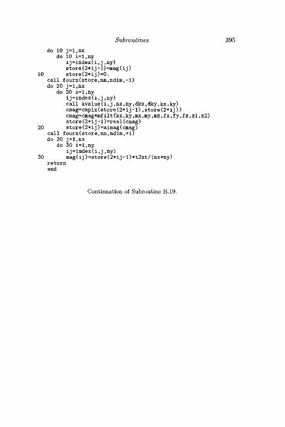
Subroutines 395do 10 j=l,nx
do 10 i=l,nyij=index(i,j,ny)store(2*ij-l)=mag(ij)
10 store(2*ij)=0.call fourn(store,nn,ndim,-l)do 20 j=l,nx
do 20 i=l,nyij=index(i,j,ny)call kvalue(i,j,nx,ny,dkx,dky,kx,ky)cmag=cmplx(store(2*ij-l),store(2*ij))cmag=cmag*mfilt(kx,ky,mx,my,mz,fx,fy,fz,zl,z2)store(2*ij-l)=real(cmag)
20 store(2*ij)=aimag(cmag)call fourn(store,nn,ndim,+l)do 30 j=l,nx
do 30 i=l,nyij=index(i,j,ny)
30 mag(ij)=store(2*ij-1)*t2nt/(nx*ny)returnend
Continuation of Subroutine B.19.
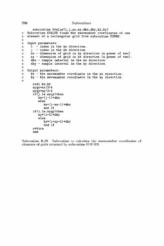
396 Subroutinessubrout ine kvalue(i,j,nx,ny,dkx,dky,kx,ky)
c Subroutine KVALUE finds the wavenumber coordinates of onec element of a rectangular grid from subroutine FOURN.cc Input parameters:c i - index in the ky direction,c j - index in the kx direction.c nx - dimension of grid in ky direction (a power of two).c ny - dimension of grid in kx direction (a power of two).c dkx - sample interval in the kx direction,c dky - sample interval in the ky direction,cc Output parameters:c kx - the wavenumber coordinate in the kx direction,c ky - the wavenumber coordinate in the ky direction,c
real kx,kynyqx=nx/2+lnyqy=ny/2+lif(j.le.nyqx)then
kx=(j-l)*dkxelse
kx=(j-nx-l)*dkxend if
if(i.le.nyqy)thenky=(i-l)*dkyelse
ky=(i-ny-l)*dkyend if
returnend
Subroutine B.20. Subroutine to calculate the wavenumber coordinates ofelements of grids returned by subroutine FOURN.
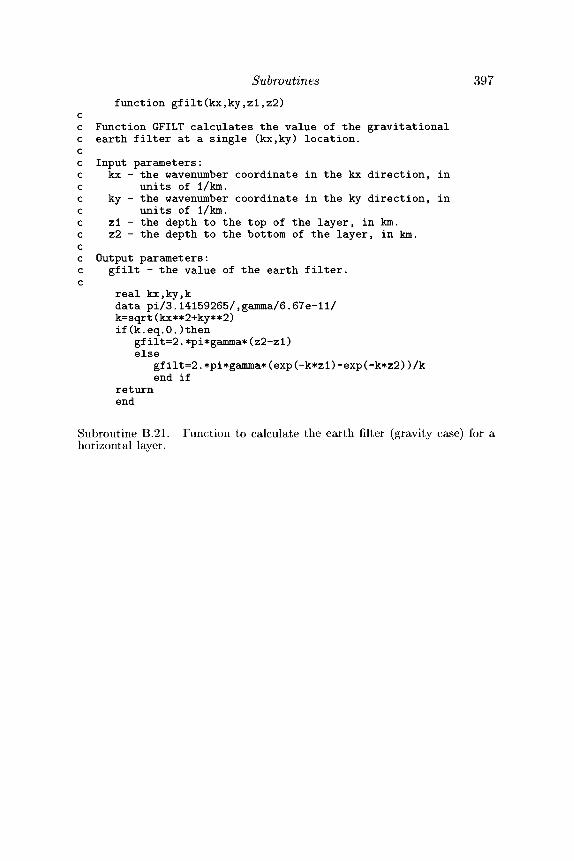
Subroutines 397function gfilt(kx,ky,zl,z2)
cc Function GFILT calculates the value of the gravitationalc earth filter at a single (kx,ky) location,cc Input parameters:c kx - the wavenumber coordinate in the kx direction, inc units of I/km.c ky - the wavenumber coordinate in the ky direction, inc units of I/km.c zl - the depth to the top of the layer, in km.c z2 - the depth to the bottom of the layer, in km.cc Output parameters:c gfilt - the value of the earth filter,c
real kx,ky,kdata pi/3.14159265/,gamma/6.67e-ll/k=sqrt(kx**2+ky**2)if(k.eq.O.)then
gfilt=2.*pi*gamma*(z2-zl)else
gf ilt=2.*pi*gamma*(exp(-k*zl)-exp(-k*z2))/kend if
returnend
Subroutine B.21. Function to calculate the earth filter (gravity case) for ahorizontal layer.
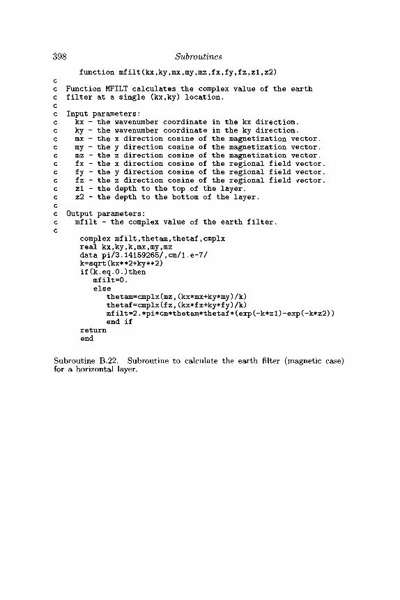
398 Subroutinesfunction mf ilt(kx,ky,mx,my,mz,fx,fy,fz,zl,z2)
cc Function MFILT calculates the complex value of the earthc filter at a single (kx,ky) location,cc Input parameters:c kx - the wavenumber coordinate in the kx direction,c ky - the wavenumber coordinate in the ky direction,c mx - the x direction cosine of the magnetization vector,c my - the y direction cosine of the magnetization vector,c mz - the z direction cosine of the magnetization vector,c fx - the x direction cosine of the regional field vector,c fy - the y direction cosine of the regional field vector,c fz - the z direction cosine of the regional field vector,c zl - the depth to the top of the layer,c z2 - the depth to the bottom of the layer,cc Output parameters:c mfilt - the complex value of the earth filter,c
complex mfilt,thetam,thetaf,cmplxreal kx,ky,k,mx,my,mzdata pi/3.14159265/,cm/1.e-7/k=sqrt(kx**2+ky**2)if(k.eq.O.)then
mfilt=0.else
thetam=cmplx(mz,(kx*mx+ky*my)/k)thetaf=cmplx(fz,(kx*fx+ky*fy)/k)mfilt=2.*pi*cm*thetam*thetaf*(exp(-k*zl)-exp(-k*z2))end if
returnend
Subroutine B.22. Subroutine to calculate the earth filter (magnetic case)for a horizontal layer.
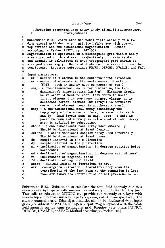
Subroutines 399subroutine mtopo(mag,ztop,nx,ny,dx,dy,mi,md,fi,fd,nstop,err,
& store,cstore)cc Subroutine MTOPO calculates the total-field anomaly on a two-c dimensional grid due to an infinite half-space with unevenc top surface and two-dimensional magnetization. Methodc according to Parker (1972, pp. 447-55).c Magnetization is specified on a rectangular grid with x and yc axes directed north and east, respectively, z axis is downc and anomaly is calculated at z=0; topographic grid should bec arranged accordingly. Units of distance irrelevant but must bec consistent. Requires subroutines FOURN, DIRCOS, RVALUE, and FAC.cc Input parameters:c nx - number of elements in the south-to-north direction,c ny - number of elements in the west-to-east direction,c (NOTE: both nx and ny must be powers of two.)c mag - a one-dimensional real array containing the two-c dimensional magnetization (in A/m). Elements shouldc be in order of west to east, then south to northc (i.e., element 1 is southwest corner, element ny isc southeast corner, element (nx-l)*ny+l is northwestc corner, and element ny*nx is northeast corner).c ztop - a one-dimensional real array containing thec topography of the upper surface, in same units as dxc and dy. Grid layout same as mag. Note: z axis isc positive down and anomaly is calculated at z=0. Arrayc ztop is modified by subroutine.c store - a one-dimensional real array used internally,c Should be dimensioned at least 2*nx*ny.c cstore - a one-dimensional complex array used internally,c Should be dimensioned at least nx*ny.c dx - sample interval in the x direction,c dy - sample interval in the y direction.c mi - inclination of magnetization, in degrees positive belowc horizontal.c md - declination of magnetization, in degrees east of north,c fi - inclination of regional field,c fd - declination of regional field,c nstop - maximum number of iterations to try.c err - convergence criterion. Iterations stop when thec contribution of the last term to the summation is lessc than err times the contribution of all previous terms,c
Subroutine B.23. Subroutine to calculate the total-field anomaly due to asemi-infinite half space with uneven top surface and infinite depth extent.Two calls to subroutine MTOPO can provide the anomaly of a layer withuneven top and bottom surfaces. Input arrays mag and ztop are specified on thesame rectangular grid. Edge discontinuities should be eliminated from inputgrids (see subroutine EXPAND). Upon output, mag is replaced with the total-field anomaly on the same rectangular grid. Requires subroutines FOURN,DIRCOS, RVALUE, and FAC. Method according to Parker [204].
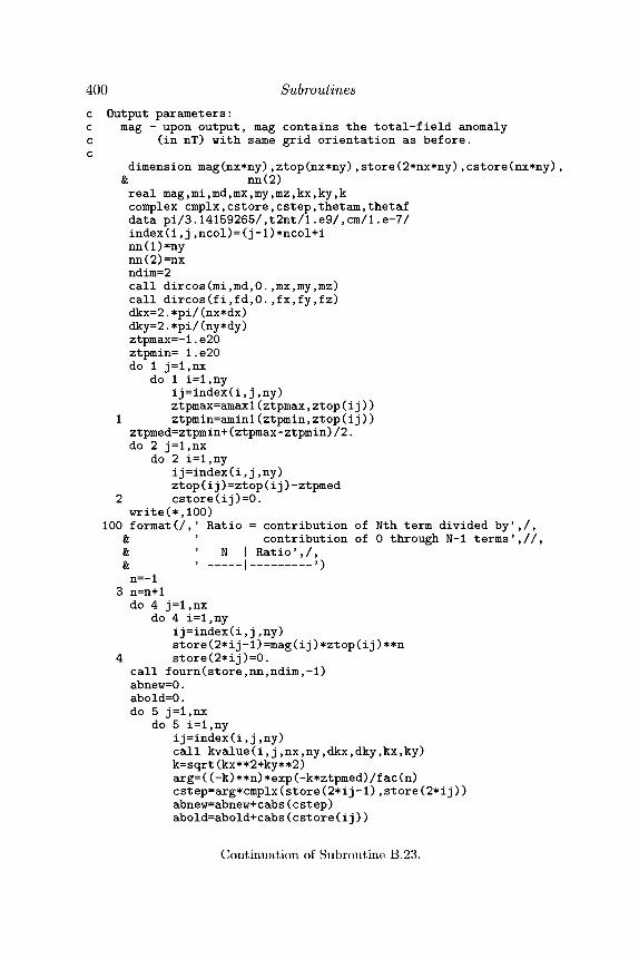
400 Subroutinesc Output parameters:c mag - upon output, mag contains the total-field anomalyc (in nT) with same grid orientation as before.c
dimension mag(nx*ny),ztop(nx*ny),store(2*nx*ny),cstore(nx*ny),& nn(2)real mag,mi,md,mx,my,mz,kx,ky,kcomplex cmplx,cstore,cstep,thetam,thetafdata pi/3.14159265/,t2nt/l.e9/,cm/1.e-7/index(i,j,ncol)=(j-l)*ncol+inn (1)=nynn(2)=nxndim=2call dircos(mi,md,0.,mx,my,rnz)call dircos(fi,fd,0.,fx,fy,fz)dkx=2.*pi/(nx*dx)dky=2.*pi/(ny*dy)ztpmax=-l.e20ztpmin= 1.e20do 1 j=l,nx
do 1 i=l,nyij =index(i,j,ny)ztpmax=amaxl(ztpmax,ztop(ij))
1 ztpmin=aminl(ztpmin,ztop(ij))ztpmed=ztpmin+(ztpmax-ztpmin)/2.do 2 j=l,nx
do 2 i=l,nyij=index(i,j,ny)ztop(ij)=ztop(ij)-ztpmed
2 cstore(ij)=0.write(*,100)
100 format(/,' Ratio = contribution of Nth term divided by',/,& } contribution of 0 through N-l terms',//,& N I Ratio',/,& , | ,)n=-l
3 n=n+ldo 4 j=l,nx
do 4 i=l,nyij=index(i,j,ny)store(2*ij-l)=mag(ij)*ztop(ij)**n
4 store(2*ij)=0.call fourn(store,nn,ndim,-l)abnew=0.abold=0.do 5 j=l,nx
do 5 i=l,nyij=index(i,j,ny)call kvalue(i,j,nx,ny,dkx,dky,kx,ky)k=sqrt(kx**2+ky**2)arg=((-k)**n)*exp(-k*ztpmed)/fac(n)cstep=arg*cmplx(store(2*ij-1),store(2*ij))abnew=abnew+cabs(cstep)abold=abold+cabs(cstore(ij))
Continuation of Subroutine B.23.
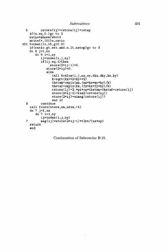
Subroutines 4015 cstore(ij)=cstore(ij)+cstep
if(n.eq.O.)go to 3ratio=abnew/aboldwrite(*,101)n,ratio
101 format(lx,i5,gl0.3)if(ratio.gt.err.and.n.It.nstop)go to 3do 6 j=l,nx
do 6 i=l,nyij=index(i,j,ny)if (ij .eq.Dthen
store(2*ij-l)=0.store(2*ij)=0.else
call kvalue(i,j,nx,ny,dkx,dky,kx,ky)k=sqrt(kx**2+ky**2)thetam=cmplx(mz,(mx*kx+my*ky)/k)thetaf=cmplx(fz,(fx*kx+fy*ky)/k)cstore(ij)=2.*pi*cm*thetam*thetaf*cstore(ij)store(2*ij-l)=real(cstore(ij))store(2*ij)=aimag(cstore(ij))end if
6 continuecall fourn(store,nn,ndim,+l)do 7 j=l,nx
do 7 i=l,nyij=index(i,j,ny)
7 mag(ij)=store(2*ij-1)*t2nt/(nx*ny)returnend
Continuation of Subroutine B.23.
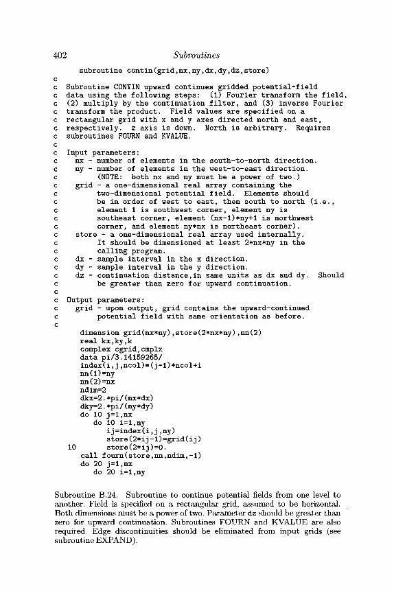
402 Subroutinessubroutine contin(grid,nx,ny,dx,dy,dz,store)
cc Subroutine CONTIN upward continues gridded potential-fieldc data using the following steps: (1) Fourier transform the field,c (2) multiply by the continuation filter, and (3) inverse Fourierc transform the product. Field values are specified on ac rectangular grid with x and y axes directed north and east,c respectively, z axis is down. North is arbitrary. Requiresc subroutines FOURN and RVALUE,cc Input parameters:c nx - number of elements in the south-to-north direction,c ny - number of elements in the west-to-east direction,c (NOTE: both nx and ny must be a power of two.)c grid - a one-dimensional real array containing thec two-dimensional potential field. Elements shouldc be in order of west to east, then south to north (i.e.,c element 1 is southwest corner, element ny isc southeast corner, element (nx-l)*ny+l is northwestc corner, and element ny*nx is northeast corner).c store - a one-dimensional real array used internally,c It should be dimensioned at least 2*nx*ny in thec calling program.c dx - sample interval in the x direction,c dy - sample interval in the y direction.c dz - continuation distance,in same units as dx and dy. Shouldc be greater than zero for upward continuation,cc Output parameters:c grid - upon output, grid contains the upward-continuedc potential field with same orientation as before,c
dimension grid(nx*ny),store(2*nx*ny),nn(2)real kx,ky,kcomplex cgrid,cmplxdata pi/3.14159265/index(i,j,ncol)=(j-l)*ncol+inn(1)=nynn(2)=nxndim=2dkx=2.*pi/(nx*dx)dky=2.*pi/(ny*dy)do 10 j=l,nx
do 10 i=l,nyij=index(i,j,ny)store(2*ij-l)=grid(ij)
10 store(2*ij)=0.call fourn(store,nn,ndim,-l)do 20 j=l,nx
do 20 i=l,ny
Subroutine B.24. Subroutine to continue potential fields from one level toanother. Field is specified on a rectangular grid, assumed to be horizontal.Both dimensions must be a power of two. Parameter dz should be greater thanzero for upward continuation. Subroutines FOURN and KVALUE are alsorequired. Edge discontinuities should be eliminated from input grids (seesubroutine EXPAND).
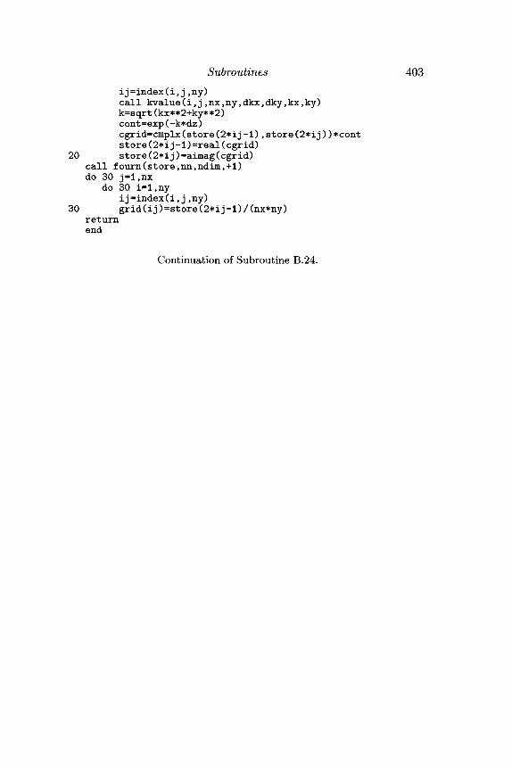
Subroutines 403ij=index(i,j,ny)call kvalue(i,j,nx,ny,dkx,dky,kx,ky)k=sqrt(kx**2+ky**2)cont=exp(-k*dz)cgrid=cmplx(store(2*ij-1),store(2*ij))*contstore(2*ij-l)=real(cgrid)
20 store(2*ij)=aimag(cgrid)call fourn(store,nn,ndim,+l)do 30 j=l,nx
do 30 i=l,nyij=index(i,j,ny)
30 grid(ij)=store(2*ij-l)/(nx*ny)returnend
Continuation of Subroutine B.24.
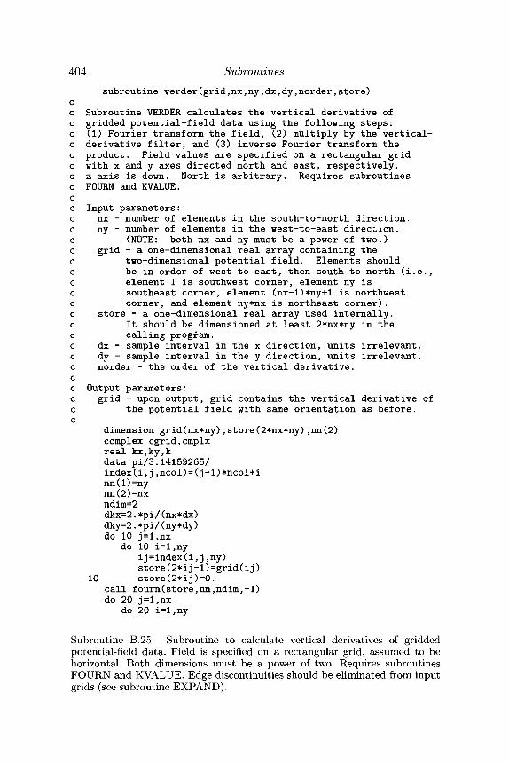
404 Subroutinessubroutine verder(grid,nx,ny,dx,dy,norder,store)
cc Subroutine VERDER calculates the vertical derivative ofc gridded potential-field data using the following steps:c (1) Fourier transform the field, (2) multiply by the vertical-c derivative filter, and (3) inverse Fourier transform thec product. Field values are specified on a rectangular gridc with x and y axes directed north and east, respectively,c z axis is down. North is arbitrary. Requires subroutinesc FOURN and KVALUE.cc Input parameters:c nx - number of elements in the south-to-north direction,c ny - number of elements in the west-to-east direction,c (NOTE: both nx and ny must be a power of two.)c grid - a one-dimensional real array containing thec two-dimensional potential field. Elements shouldc be in order of west to east, then south to north (i.e.,c element 1 is southwest corner, element ny isc southeast corner, element (nx-l)*ny+l is northwestc corner, and element ny*nx is northeast corner),c store - a one-dimensional real array used internally,c It should be dimensioned at least 2*nx*ny in thec calling program.c dx - sample interval in the x direction, units irrelevant,c dy - sample interval in the y direction, units irrelevant,c norder - the order of the vertical derivative,cc Output parameters:c grid - upon output, grid contains the vertical derivative ofc the potential field with same orientation as before,c
dimension grid(nx*ny),store(2*nx*ny),nn(2)complex cgrid,cmplxreal kx,ky,kdata pi/3.14159265/index(i,j,ncol)=(j-l)*ncol+inn(1)=nynn(2)=nxndim=2dkx=2.*pi/(nx*dx)dky=2.*pi/(ny*dy)do 10 j=l,nx
do 10 i=l,nyij=index(i,j,ny)store(2*ij-l)=grid(ij)
10 store(2*ij)=0.call fourn(store,nn,ndim,-l)do 20 j=l,nx
do 20 i=l,ny
Subroutine B.25. Subroutine to calculate vertical derivatives of griddedpotential-field data. Field is specified on a rectangular grid, assumed to behorizontal. Both dimensions must be a power of two. Requires subroutinesFOURN and KVALUE. Edge discontinuities should be eliminated from inputgrids (see subroutine EXPAND).
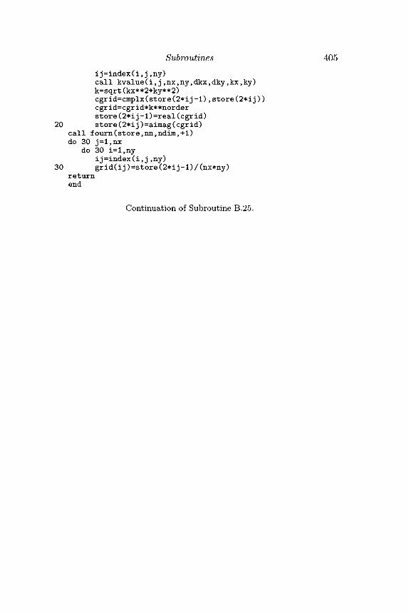
Subroutines 405ij=index(i,j,ny)call kvalue(i,j,nx,ny,dkx,dky,kx,ky)k=sqrt(kx**2+ky**2)cgrid=cmplx(store(2*ij-1),store(2*ij))cgrid=cgrid*k**norderstore(2*ij-l)=real(cgrid)
20 store(2*ij)=aimag(cgrid)call fourn(store,nn,ndim,+l)do 30 j=l,nx
do 30 i=l,nyij=index(i,j,ny)
30 grid(ij)=store(2*ij-l)/(nx*ny)returnend
Continuation of Subroutine B.25.
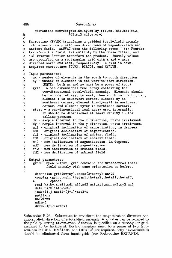
406 Subroutinessubroutine newvec(grid,nx,ny,dx,dy,fi1,fdl,mi1,mdl,fi2,
& fd2,mi2,md2,store)cc Subroutine NEWVEC transforms a gridded total-field anomalyc into a new anomaly with new directions of magnetization andc ambient field. NEWVEC uses the following steps: (1) Fourierc transform the field, (2) multiply by the phase filter, andc (3) inverse Fourier transform the product. Anomaly valuesc are specified on a rectangular grid with x and y axesc directed north and east, respectively, z axis is down,c Requires subroutines FOURN, DIRCOS, and RVALUE,cc Input parameters:c nx - number of elements in the south-to-north direction,c ny - number of elements in the west-to-east direction,c (NOTE: both nx and ny must be a power of two.)c grid - a one-dimensional real array containing thec two-dimensional total-field anomaly. Elements shouldc be in order of west to east, then south to north (i.e.,c element 1 is southwest corner, element ny isc southeast corner, element (nx-l)*ny+l is northwestc corner, and element ny*nx is northeast corner).c store - a one-dimensional real array used internally,c It should be dimensioned at least 2*nx*ny in thec calling program.c dx - sample interval in the x direction, units irrelevant,c dy - sample interval in the y direction, units irrelevant,c mil - original inclination of magnetization, in degrees,c mdl - original declination of magnetization,c fil - original inclination of ambient field,c fdl - original declination of ambient field,c mi2 - new inclination of magnetization, in degrees,c md2 - new declination of magnetization,c fi2 - new inclination of ambient field,c fd2 - new declination of ambient field,cc Output parameters:c grid - upon output, grid contains the transformed total-c field anomaly with same orientation as before,c
dimension grid(nx*ny),store(2*nx*ny),nn(2)complex cgrid,cmplx,thetaml,thetam2,thetaf1,thetaf2,
& cphasere al kx,ky,k,mi1,md1,mi2,md2,mx1,my1,mz1,mx2,my2,mz2data pi/3.14159265/index(i,j,ncol)=(j-l)*ncol+inn(1)=nynn(2)=nxndim=2dkx=2.*pi/(nx*dx)
Subroutine B.26. Subroutine to transform the magnetization direction andambient-field direction of a total-field anomaly. Anomalies can be reduced tothe pole by letting mi2=fi2=90. Anomaly is specified on a rectangular grid,assumed to be horizontal. Both dimensions must be a power of two. Sub-routines FOURN, RVALUE, and DIRCOS are required. Edge discontinuitiesshould be eliminated from input grids (see Osubroutine EXPAND).
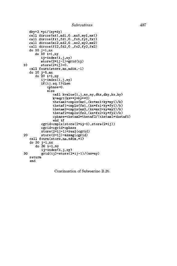
Subroutines 407dky=2.*pi/(ny*dy)call dircos(mil,mdl,0.,mxl,myl,rnzl)call dircos(fil,fdl,0.,fxl,fyl,fzl)call dircos(mi2,md2,0.,mx2,my2,mz2)call dircos(fi2,fd2,0.,fx2,fy2,fz2)do 10 j=l,nx
do 10 i=l,nyij =index(i,j,ny)store(2*ij-l)=grid(ij)
10 store(2*ij)=0.call fourn(store,nn,ndim,-1)do 20 j=l,nx
do 20 i=l,nyij =index(i,j,ny)if(ij.eq.l)then
cphase=0.else
call kvalue(i,j,nx,ny,dkx,dky,kx,ky)k=sqrt(kx**2+ky**2)thetaml=cmplx(mzl,(kx*mxl+ky*myl)/k)thetafl=cmplx(fzl,(kx*fxl+ky*fyl)/k)thetam2=cmplx(mz2,(kx*mx2+ky*my2)/k)thetaf2=cmplx(fz2,(kx*fx2+ky*fy2)/k)cphase=thetam2*thetaf2/(thetaml*thetaf1)end if
cgrid=cmplx(store(2*ij-l),store(2*ij))cgrid=cgrid*cphasestore(2*ij-l)=real(cgrid)
20 store(2*i j)=aimag(cgrid)call fourn(store,nn,ndim,+1)do 30 j=l,nx
do 30 i=l,nyij=index(i,j,ny)
30 grid(ij)=store(2*ij-l)/(nx*ny)returnend
Continuation of Subroutine B.26.
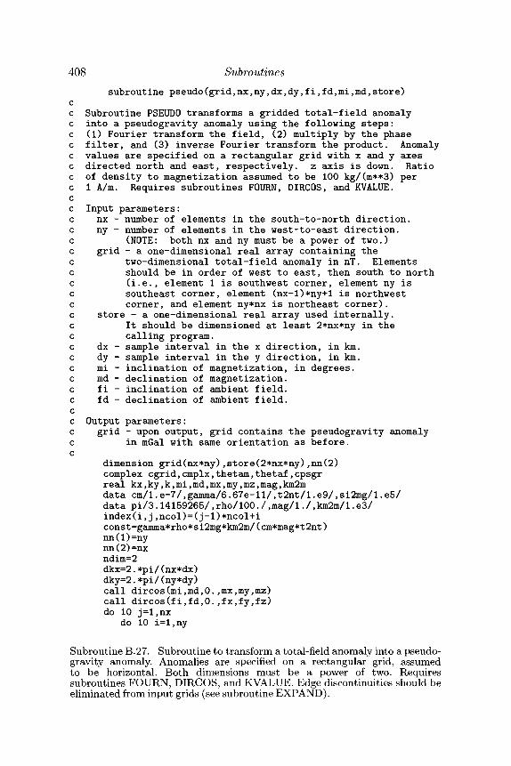
408 Subroutinessubroutine pseudo(grid,nx,ny,dx,dy,fi,fd,mi,md,store)
cc Subroutine PSEUDO transforms a gridded total-field anomalyc into a pseudogravity anomaly using the following steps:c (1) Fourier transform the field, (2) multiply by the phasec filter, and (3) inverse Fourier transform the product. Anomalyc values are specified on a rectangular grid with x and y axesc directed north and east, respectively, z axis is down. Ratioc of density to magnetization assumed to be 100 kg/(m**3) perc 1 A/m. Requires subroutines FOURN, DIRCOS, and KVALUE.cc Input parameters:c nx - number of elements in the south-to-north direction,c ny - number of elements in the west-to-east direction,c (NOTE: both nx and ny must be a power of two.)c grid - a one-dimensional real array containing thec two-dimensional total-field anomaly in nT. Elementsc should be in order of west to east, then south to northc (i.e., element 1 is southwest corner, element ny isc southeast corner, element (nx-l)*ny+l is northwestc corner, and element ny*nx is northeast corner),c store - a one-dimensional real array used internally,c It should be dimensioned at least 2*nx*ny in thec calling program.c dx - sample interval in the x direction, in km.c dy - sample interval in the y direction, in km.c mi - inclination of magnetization, in degrees,c md - declination of magnetization,c fi - inclination of ambient field,c fd - declination of ambient field,cc Output parameters:c grid - upon output, grid contains the pseudogravity anomalyc in mGal with same orientation as before,c
dimension grid(nx*ny),store(2*nx*ny),nn(2)complex cgrid,cmplx,thetam,thetaf,cpsgrreal kx,ky,k,mi,md,mx,my,mz,mag,km2mdata cm/1.e-7/,gamma/6.67e-ll/,t2nt/l.e9/,si2mg/l.e5/data pi/3.14159265/,rho/100./,mag/1./,km2m/l.e3/index(i,j,ncol)=(j-l)*ncol+iconst=gamma*rho*si2mg*km2m/(cm*mag*t2nt)nn(1)=nynn(2)=nxndim=2dkx=2.*pi/(nx*dx)dky=2.*pi/(ny*dy)call dircos(mi,md,0.,mx,my,rnz)call dircos(fi,fd,0.,fx,fy,fz)do 10 j=l,nx
do 10 i=l,ny
Subroutine B.27. Subroutine to transform a total-field anomaly into a pseudo-gravity anomaly. Anomalies are specified on a rectangular grid, assumedto be horizontal. Both dimensions must be a power of two. Requiressubroutines FOURN, DIRCOS, and KVALUE. Edge discontinuities should beeliminated from input grids (see subroutine EXPAND).
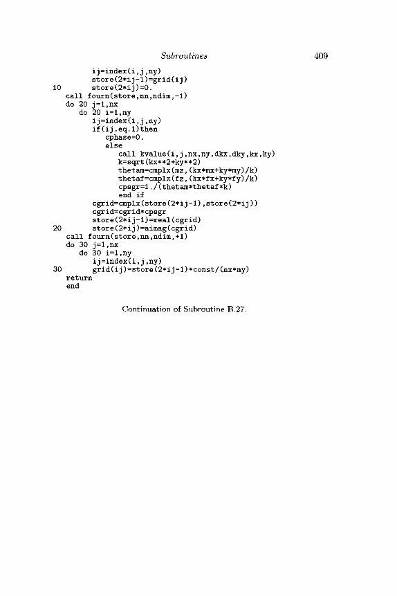
Subroutines 409ij=index(i,j,ny)store(2*ij-l)=grid(ij)
10 store(2*ij)=0.call fourn(store,nn,ndim,-l)do 20 j=l,nx
do 20 i=l,nyij=index(i,j,ny)if(ij.eq.l)then
cphase=0.else
call kvalue(i,j,nx,ny,dkx,dky,kx,ky)k=sqrt(kx**2+ky**2)thetam=cmplx(mz,(kx*mx+ky*my)/k)thetaf=cmplx(fz,(kx*fx+ky*fy)/k)cpsgr=l./(thetam*thetaf*k)end if
cgrid=cmplx(store(2*ij-1),store(2*ij))cgrid=cgrid*cpsgrstore(2*ij-l)=real(cgrid)
20 store(2*ij)=aimag(cgrid)call fourn(store,nn,ndim,+l)do 30 j=l,nx
do 30 i=l,nyij=index(i,j,ny)
30 grid(ij)=store(2*ij-l)*const/(nx*ny)returnend
Continuation of Subroutine B.27.
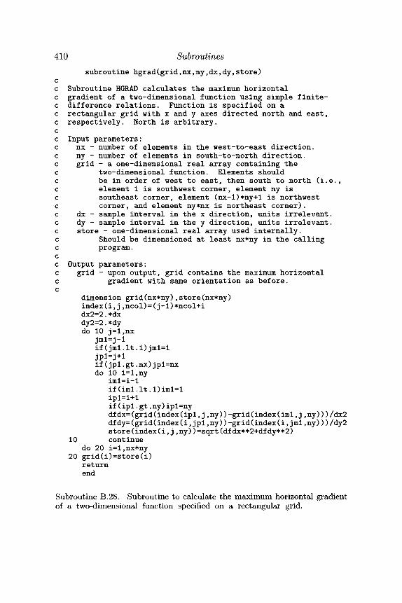
410 Subroutinessubroutine hgrad(grid,nx,ny,dx,dy,store)
cc Subroutine HGRAD calculates the maximum horizontalc gradient of a two-dimensional function using simple finite-c difference relations. Function is specified on ac rectangular grid with x and y axes directed north and east,c respectively. North is arbitrary,cc Input parameters:c nx - number of elements in the west-to-east direction,c ny - number of elements in south-to-north direction,c grid - a one-dimensional real array containing thec two-dimensional function. Elements shouldc be in order of west to east, then south to north (i.e.,c element 1 is southwest corner, element ny isc southeast corner, element (nx-l)*ny+l is northwestc corner, and element ny*nx is northeast corner),c dx - sample interval in the x direction, units irrelevant,c dy - sample interval in the y direction, units irrelevant,c store - one-dimensional real array used internally,c Should be dimensioned at least nx*ny in the callingc program.cc Output parameters:c grid - upon output, grid contains the maximum horizontalc gradient with same orientation as before,c
dimension grid(nx*ny),store(nx*ny)index(i,j,ncol)=(j-l)*ncol+idx2=2.*dxdy2=2.*dydo 10 j=l,nx
jml=j-lif(jml.lt.l)jml=ljpl=j+lif(jpl.gt.nx)jpl=nxdo 10 i=l,ny
iml=i-lif(iml.lt.l)iml=lipl=i+lif(ipl.gt.ny)ipl=nydfdx=(grid(index(ipl,j,ny))-grid(index(iml,j,ny)))/dx2dfdy=(grid(index(i,jpl,ny))-grid(index(i,jml,ny)))/dy2store(index(i,j,ny))=sqrt(dfdx**2+dfdy**2)
10 continuedo 20 i=l,nx*ny
20 grid(i)=store(i)returnend
Subroutine B.28. Subroutine to calculate the maximum horizontal gradientof a two-dimensional function specified on a rectangular grid.
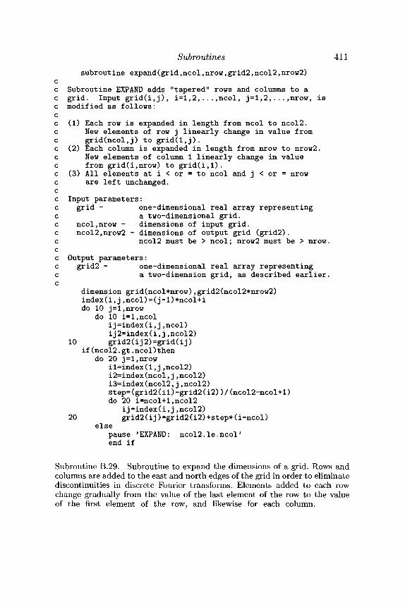
Subroutines 411subroutine expand(grid,ncol,nrow,grid2,ncol2,nrow2)
cc Subroutine EXPAND adds "tapered" rows and columns to ac grid. Input grid(i,j), i=l,2,...,ncol, j=l,2,...,nrow, isc modified as follows:cc (1) Each row is expanded in length from ncol to ncol2.c New elements of row j linearly change in value fromc grid(ncol,j) to grid(l,j).c (2) Each column is expanded in length from nrow to nrow2.c New elements of column 1 linearly change in valuec from grid(i,nrow) to grid(i,l).c (3) All elements at i < or = to ncol and j < or = nrowc are left unchanged,cc Input parameters:c grid - one-dimensional real array representingc a two-dimensional grid,c ncol,nrow - dimensions of input grid,c ncol2,nrow2 - dimensions of output grid (grid2).c ncol2 must be > ncol; nrow2 must be > nrow.cc Output parameters:c grid2 - one-dimensional real array representingc a two-dimension grid, as described earlier,c
dimension grid(ncol*nrow),grid2(ncol2*nrow2)index(i,j,ncol)=(j-l)*ncol+ido 10 j=l,nrow
do 10 i=l,ncolij=index(i,j,ncol)ij2=index(i,j,ncol2)
10 grid2(ij2)=grid(ij)if(ncol2.gt.ncol)then
do 20 j=l,nrowil=index(l,j,ncol2)i2=index(ncol,j,ncol2)i3=index(ncol2,j,ncol2)Step=(grid2(il)-grid2(i2))/(ncol2-ncol+l)do 20 i=ncol+l,ncol2
ij=index(i,j,ncol2)20 grid2(ij)=grid2(i2)+step*(i-ncol)
elsepause 'EXPAND: ncol2.1e.ncol'end if
Subroutine B.29. Subroutine to expand the dimensions of a grid. Rows andcolumns are added to the east and north edges of the grid in order to eliminatediscontinuities in discrete Fourier transforms. Elements added to each rowchange gradually from the value of the last element of the row to the valueof the first element of the row, and likewise for each column.
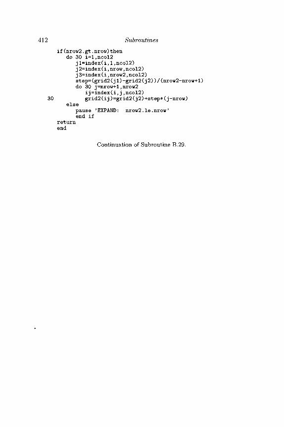
412 Subroutinesif (nrow2. gt. nrow) then
do 30 i=l,ncol2jl=index(i,1,ncol2)j 2=index(i,nrow,ncol2)j 3=index(i,nrow2,ncol2)step=(grid2(j1)-grid2(j 2))/(nrow2-nrow+l)do 30 j=nrow+l,nrow2
ij=index(i,j,ncol2)30 grid2(ij)=grid2(j 2)+step*(j-nrow)
elsepause 'EXPAND: nrow2.le.nrowJ
end ifreturnend
Continuation of Subroutine B.29.
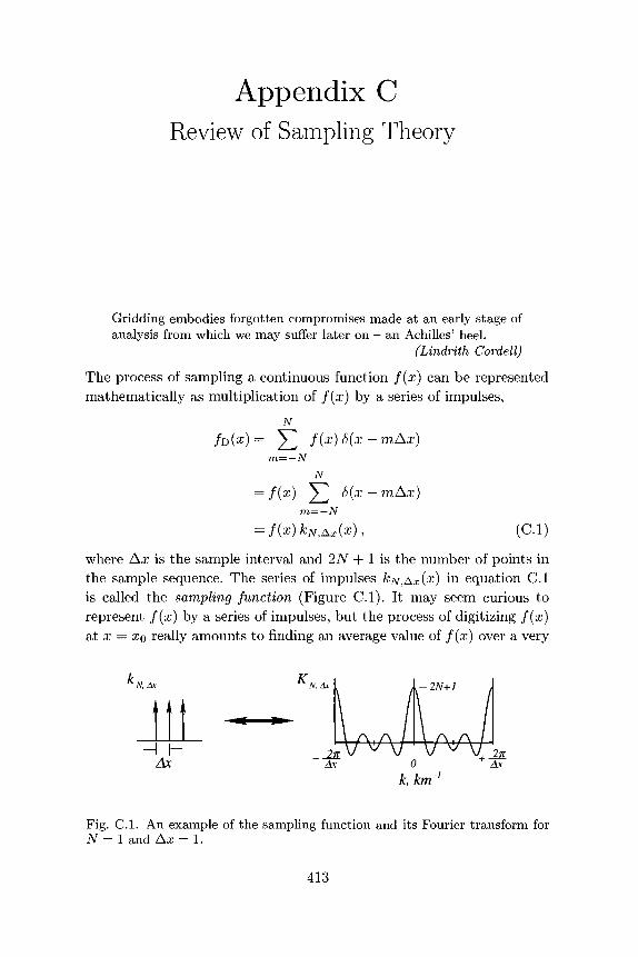
Appendix CReview of Sampling Theory
Gridding embodies forgotten compromises made at an early stage ofanalysis from which we may suffer later on - an Achilles' heel.
(Lindrith Cordell)
The process of sampling a continuous function f(x) can be representedmathematically as multiplication of f(x) by a series of impulses,
N
m=-NN
= f(x) S(x-mAx)m=-N
(C.I)
where Ax is the sample interval and 2N + 1 is the number of points inthe sample sequence. The series of impulses kN,Ax(x) in equation C.Iis called the sampling function (Figure C.I). It may seem curious torepresent f(x) by a series of impulses, but the process of digitizing f(x)at x — XQ really amounts to finding an average value of f(x) over a very
Ax
Fig. C.I. An example of the sampling function and its Fourier transform forN = 1 and Ax = 1.
413
414 Review of Sampling Theory
narrow range of x centered about x0, and equation 11.14 shows that thevalue of a function f(x) at x0 is given by the convolution of f(x) withan impulse,
f(xo)= / f(x)6(x-xo)dx.
Note that /D(^) and f(x) do not have the same units because 6(x) hasunits of inverse distance.
We want to investigate the differences between f(x) and /D(#) in theFourier domain, so we begin by Fourier transforming equation C.I andthen employing equation 11.20. Hence, the Fourier transform of /D(^)will be given by the convolution of the Fourier transforms of f(x) and
oo
FD(k) = -^ J F(k')KNAx(k - k') dk'.— oo
The Fourier transform of the sampling function, therefore, will describehow the Fourier transform of a digitized function differs from the trans-form of its continuous form. From equation 11.15, it follows that theFourier transform of an impulse at the origin is given by
oo
— oo
6(x)e
and the shifting theorem of Section 11.1.2 leads tooo
f 8{x - mAx)e-ikx dx = e-ikmAx
— OO
andN
KNAx(k)= ^ e-ikmAxm
m=-N
After some algebraic manipulations, the previous equation can be writ-ten in a more instructive form,
Equation C.2 shows that the Fourier transform of the sampling func-tion is periodic and repeats itself over the interval ^ . Figure C.I shows
Review of Sampling Theory 415
an example for TV = 3. The narrowness of the large peaks and the numberof zero-crossings between the large peaks both increase with increasingN. In fact, it can be shown that as N becomes very large, the Fouriertransform of the sampling function approaches an infinitely long seriesof impulses spaced along the k axis at intervals of -^ ,
2?r °° /
Hence an infinite set of impulses spaced Ax apart Fourier transforms toan infinite set of impulses spaced ^ apart.
Suppose now that we were able to digitize an infinitely long continuousfunction /(x). (This is not as impossible as it may seem; if we assumethat /(x) = 0 for |x| > N Ax, then we may consider N to be infiniteand /(x) to be infinitely long.) According to equation 11.20, the Fouriertransform of this infinite series would be
j=-oo
This summation describes aliasing, an important phenomenon of sam-pled data. We would like the Fourier transform of the digital function toequal the Fourier transform of the continuous function at any arbitrarywavenumber; that is, we would like AxFD(&o) = F(ko). Unfortunately,equation C.3 shows that the discrete Fourier transform is equal to F(ko)plus an infinite set of additional values:
In other words, the periodic nature of Fj^(k) produces contamination ateach value of k0; instead of F(fco), we get F(ko) plus F(k) evaluated atan infinite number of other values of k.
The amplitude spectrum for many kinds of physical phenomena (in-cluding potential-field anomalies) decreases rapidly with increasing |fc|.Hence, the low-wavenumber part of Fj^(k) may be a good approximationto F(k) if /(x) has been properly sampled. This should be clear fromequation C.3; the contaminating terms in the summation will be small ifF(k) decreases rapidly with increasing |fc|. Aliasing will be most severeat wavenumbers near k = ^ . This is the symmetry point in Figure C.Iand is called the Nyquist or folding wavenumber. Clearly one way toreduce aliasing is to increase the Nyquist wavenumber, and this can bedone only by making the sample interval Ax smaller.
416 Review of Sampling Theory
Note that the Nyquist wavenumber corresponds to a wavelength oftwice the sample interval. We cannot find information at wavelengthssmaller than this threshold. For some physical phenomena, it might beappropriate to assume that the energy-density spectrum or the power-density spectrum of a process is zero at wavenumbers greater than somecritical wavenumber kc. Such a function is said to be band limited. Thesampling theorem states that if f(x) is band limited with no energy atwavelengths less than Ac, FD(&) will contain all the information of F(k)so long as Ax < Ac/2.
Appendix DConversion of Units
The only known antidotes to discussions of units are undisturbed silencein a dark room for 15 minutes or a brisk walk in the park.
(Robert F. Butler)
Two systems of electromagnetic units are in common usage in the geo-physical literature: The venerable cgs system, also known as electro-magnetic units (emu), and the more modern and internationally ac-cepted Systeme Internationale (International System, abbreviated SI).Geophysical journals now require the use of SI units, and for the mostpart SI units are adhered to in this text. Geophysical journals pub-lished prior to 1980, however, employed emu, and even some recentlypublished textbooks (e.g., Butler [47]) continue its usage. Consequently,reading the geophysical literature requires conversion between the twosystems, a common source of frustration because the two systems aresignificantly different.
The following table summarizes these two important systems of unitsand the conversion factors between them. Additional discussions can befound in textbooks by Panofsky and Phillips [201, pp. 459-65], But-ler [47, pp. 15-18], and the Society of Exploration Geophysicists [266],and in papers by Shive [255], Payne [213], and Moskowitz [189].
417
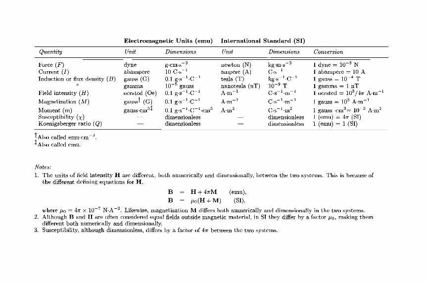
Electromagnetic Units (emu) International Standard (SI)
Quantity
Force (F)Current (/)Induction or flux density (B)
u
Field intensity (H)Magnetization (M)Moment (m)Susceptibility (x)Koenigsberger ratio (Q)
Unit
dyneabamperegauss (G)gammaoersted (Oe)gauss' (G)
ofgauss • cm +
——
Dimensions
g-cm-s"2
10 C-s"1
0.1 g-s^-C"1
10"5 gauss0.1 g-s-^C"1
0.1 g-s^-C"1
0.1 g-s"1-C~1-cm:
dimensionlessdimensionless
Unit
newton (N)ampere (A)tesla (T)nanotesla (nT)A-m"1
A-m"1
3 A-m2
——
Dimensions
kg-m-s"2
C-s"1
kg-s^-C"1
1 0 -9 T
C-S"1-!)!"1
C-S"1-!!!2
dimensionlessdimensionless
Conversion
1 dyne = 10"5 N1 abampere = 10 A1 gauss = 10"4 T1 gamma = 1 nT1 oersted = 103/4TT A-m"1
1 gauss = 103 A-m"1
1 gauss -cm3= 10~3 A-m2
1 (emu) = 4TT (SI)1 (emu) = 1 (SI)
'Also called"•"Also called emu.
emu-cm
Notes:1. The units of field intensity H are different, both numerically and dimensionally, between the two systems. This is because of
the different defining equations for H,B = H + 4TTM (emu),B = /iO(H + M) (SI),
where /x0 = 4?r x 10~7 N-A~2. Likewise, magnetization M differs both numerically and dimensionally in the two systems.2. Although B and H are often considered equal fields outside magnetic material, in SI they differ by a factor /xo, making them
different both numerically and dimensionally.3. Susceptibility, although dimensionless, differs by a factor of 4TT between the two systems.
Bibliography
[1] Airy, G. B., "On the computation of the effect of the attraction ofmountain-masses, as disturbing the apparent astronomical latitude ofstations in geodetic surveys," Philosophical Transactions of the RoyalSociety of London 145 (1855), 101-4.
[2] Al-Chalabi, M., "Interpretation of gravity anomalies by non-linearoptimisation," Geophysical Prospecting 20 (1972), 1-16.
[3] Alldredge, L. R., and Hurwitz, L., "Radial dipoles as the sources ofthe earth's main magnetic field," Journal of Geophysical Research 69(1964), 2631-40.
[4] Ander, M. E., and Huestis, S. P., "Gravity ideal bodies," Geophysics52 (1987), 1265-78.
[5] Arkani-Hamed, J., "Differential reduction-to-the-pole of regionalmagnetic anomalies," Geophysics 53 (1988), 1592-600.
[6] Arkani-Hamed, J., "Thermoviscous remanent magnetization of oceaniclithosphere inferred from its thermal evolution," Journal ofGeophysical Research 94 (1989), 17, 421-36.
[7] Arkani-Hamed, J., and Strangway, D. W., "Lateral variations ofapparent magnetic susceptibility of lithosphere deduced from Magsatdata," Journal of Geophysical Research 90, 2655-64, 1985.
[8] Backus, G. E., and Gilbert, F., "Uniqueness in the inversion ofinaccurate gross Earth data," Philosophical Transactions of the RoyalSociety of London, Series A 226 (1970), 123-92.
[9] Baranov, V., "A new method for interpretation of aeromagnetic maps:pseudo-gravimetric anomalies," Geophysics 22 (1957), 359-83.
[10] Baranov, V., and Naudy, H., "Numerical calculation of the formula ofreduction to the magnetic pole," Geophysics 29 (1964), 67-79.
[11] Barnett, C. T., "Theoretical modeling of the magnetic andgravitational fields of an arbitrarily shaped three-dimensional body,"Geophysics 41 (1976), 1353-64.
[12] Barongo, J. O., "Euler's differential equation and the indent meat ionof the magnetic point-pole and point-dipole sources," Geophysics 49(1984), 1549-53.
[13] Bhattacharyya, B. K., "Magnetic anomalies due to prism-shapedbodies with arbitrary polarization," Geophysics 29 (1964), 517-31.
[14] Bhattacharyya, B. K., "Two-dimensional harmonic analysis as a toolfor magnetic interpretation," Geophysics 30 (1965), 829-57.
[15] Bhattacharyya, B. K., "Continuous spectrum of thetotal-magnetic-field anomaly due to a rectangular prismatic body,"Geophysics 31 (1966), 97-121.
419
420 Bibliography
[16] Bhattacharyya, B. K., "Some general properties of potential fields inspace and frequency domain: a review," Geoexploration 5 (1967),127-43.
[17] Bhattacharyya, B. K., and Chan, K. C, "Reduction of magnetic andgravity data on an arbitrary surface acquired in a region of hightopographic relief," Geophysics 42 (1977), 1411-30.
[18] Bhattacharyya, B. K., and Leu, L.-K., "Analysis of magneticanomalies over Yellowstone National Park; mapping of Curie pointisothermal surface for geothermal reconnaissance," Journal ofGeophysical Research 80 (1975), 4461-65.
[19] Blackwell, D. D.; Bowen, R. G.; Hull, D. A.; Riccio, J.; and Steele,J. L., "Heat flow, arc volcanism, and subduction in northern Oregon,"Journal of Geophysical Research 87 (1982), 8735-54.
[20] Blakely, R. J., Documentation for Subroutine REDUC3, an Algorithmfor the Linear Filtering of Gridded Magnetic Data, Open-FileReport 77-784, U.S. Geological Survey, 1977.
[21] Blakely, R. J., "Statistical averaging of marine magnetic anomalies,"Journal of Geophysical Research 88 (1983), 2289-96.
[22] Blakely, R. J., "The effect of topography on aeromagnetic data in thewavenumber domain," in Proceedings of the International Meeting onPotential Fields in Rugged Topography, Bulletin 7, pages 102-9,Institut de Geophysique de Universite de Lausanne, Lausanne,Switzerland, 1985.
[23] Blakely, R. J., "Curie temperature isotherm analysis and tectonicimplications of aeromagnetic data from Nevada," Journal ofGeophysical Research 93 (1988), 11,817-32.
[24] Blakely, R. J., "Extent of magma chambers in the Cascade Range ofwestern North America: constraints from gravity anomalies," Journalof Geophysical Research 99 (1994), 2757-73.
[25] Blakely, R. J., and Christiansen, R. L., "The magnetization of MountShasta and implications for virtual geomagnetic poles determined fromseamounts," Journal of Geophysical Research 83 (1978), 5971-8.
[26] Blakely, R. J., and Cox, A., "Evidence for short geomagnetic polarityintervals in the Early Cenozoic," Journal of Geophysical Research 77(1972), 7065-72.
[27] Blakely, R. J., and Cox, A., "Identification of short polarity events bytransforming marine magnetic profiles to the pole," Journal ofGeophysical Research 77 (1972), 4339-49.
[28] Blakely, R. J., and Grauch, V. J. S., "Magnetic models of crystallineterrane; accounting for the effect of topography," Geophysics 48(1983), 1551-7.
[29] Blakely, R. J., and Hassanzadeh, S., "Estimation of depth to magneticsource using maximum entropy power spectra, with application to thePeru-Chile Trench," in Nazca Plate; Crustal Formation and AndeanConvergence, 667-82, Geological Society of America Memoir 154,Boulder, CO (1981).
[30] Blakely, R. J., and Jachens, R. C, "Volcanism, isostatic residualgravity, and regional tectonic setting of the Cascade volcanicprovince," Journal of Geophysical Research 95 (1990), 19, 439-51.
[31] Blakely, R. J., and Jachens, R. C, "Regional study of mineralresources in Nevada: insights from three-dimensional analysis ofgravity and magnetic anomalies," Geological Society of AmericaBulletin 103 (1991), 795-803.
Bibliography 421
[32] Blakely, R. J., and Schouten, H., "Comments on 'Filtering marinemagnetic anomalies' by Hans Schouten and Keith McCamy," Journalof Geophysical Research 79 (1974), 773-4.
[33] Blakely, R. J., and Simpson, R. W., "Approximating edges of sourcebodies from magnetic or gravity anomalies," Geophysics 51 (1986),1494-8.
[34] Booker, J. R., "Geomagnetic data and core motions," Proceedings ofthe Royal Society of London, Series A 309 (1969), 27-40.
[35] Bott, M. H. P., "The use of rapid digital computing methods fordirect gravity interpretation of sedimentary basins," GeophysicalJournal of the Royal Astronomical Society 3 (1960), 63-7.
[36] Bott, M. H. P., "Two methods applicable to computers for evaluatingmagnetic anomalies due to finite three dimensional bodies,"Geophysical Prospecting 11 (1963), 292-9.
[37] Bott, M. H. P., "Solution of the linear inverse problem in magneticinterpretation with application to oceanic magnetic anomalies,"Geophysical Journal of the Royal Astronomical Society 13 (1967),313-23.
[38] Bott, M. H. P., and Hutton, M. A., "Limitations on the resolutionpossible in the direct interpretation of marine magnetic anomalies,"Earth and Planetary Science Letters 8 (1970), 317-19.
[39] Bott, M. H. P., and Hutton, M. A., "A matrix method for interpretingoceanic magnetic anomalies," Geophysical Journal of the RoyalAstronomical Society 20 (1970), 149-57.
[40] Bott, M. H. P., and Ingles, A., "Matrix methods for jointinterpretation of two-dimensional gravity and magnetic anomalies withapplication to the Iceland-Faeroe Ridge," Geophysical Journal of theRoyal Astronomical Society 30 (1972), 55-67.
[41] Bott, M. H. P., and Smith, R. A., "The estimation of the limitingdepth of gravitating bodies," Geophysical Prospecting 6 (1958), 1-10.
[42] Bracewell, R., The Fourier Transform and Its Applications,McGraw-Hill, New York, 1965.
[43] Brozena, J. M., and Peters, M. F., "An airborne gravity study ofeastern North Carolina," Geophysics 53 (1988), 245-53.
[44] Bullard, E. C, "The removal of trend from magnetic surveys," Earthand Planetary Science Letters 2 (1967), 293-300.
[45] Bullard, E. C; Freedman, C; Gellman, H.; and Nixon, J., "Thewestward drift of the earth's magnetic field," PhilosophicalTransactions of the Royal Society of London, Series A 243 (1950), 67.
[46] Bultman, M. W., and Gettings, M. E., New Techniques of GeophysicalData Analysis; an Investigation of the Geometry, Structure, andBedrock Lithology of the San Rafael Basin, Arizona, U.S. GeologicalCircular 1103-A (1994), 14-15.
[47] Butler, Robert F., Paleomagnetism, Magnetic Domains to GeologicTerranes, Blackwell, Oxford, 1992.
[48] Cady, J. W., "Calculation of gravity and magnetic anomalies offinite-length right polygonal prisms," Geophysics 45 (1980), 1507-12.
[49] Cain, J. C; Davis, W. M.; and Regan, R. D., "An TV = 22 model ofthe geomagnetic field," EOS, Transactions of the AmericanGeophysical Union 56 (1974), 1108.
[50] Cain, J. C; Schmitz, D. R.; and Muth, L., "Small-scale features in theearth's magnetic field observed by Magsat," Journal of GeophysicalResearch 89 (1984), 1070-6.
422 Bibliography
[51] Cande, S. C, "A palaeomagnetic pole from Late Cretaceous marinemagnetic anomalies in the Pacific," Geophysical Journal of the RoyalAstronomical Society 44 (1976), 547-66.
[52] Cande, S. C, and Kent, D. V., "Constraints imposed by the shape ofmarine magnetic anomalies on the magnetic source," Journal ofGeophysical Research 81 (1976), 4157-62.
[53] Carle, H. M., and Harrison, C. G. A., "A problem in representing thecore magnetic field of the earth using spherical harmonics,"Geophysical Research Letters 9 (1982), 265-8.
[54] Carmichael, R. S., "Magnetic properties of minerals and rocks," inHandbook of Physical Properties of Rocks, vol. 2, R. S. Carmichael(ed.), 229-87, CRC Press, Boca Raton, FL (1982).
[55] Chandler, V. W., and Malek, K. C, "Moving-window Poisson analysisof gravity and magnetic data from the Penokean orogen, east-centralMinnesota," Geophysics 56 (1991), 123-32.
[56] Chapman, S., and Bartels, J., Geomagnetism, Oxford UniversityPress, Oxford, 1940.
[57] Chikazumi, S., Physics of Magnetism, Wiley, New York, 1964; Englishedition prepared by S. J. Charap.
[58] Chovitz, B. H., "Modern geodetic earth reference models," EOS,Transactions of the American Geophysical Union 62 (1981), 65-7.
[59] Churchill, R. V., Complex Variables and Applications, 2nd ed.,McGraw-Hill, New York (1960).
[60] Claerbout, J. F., Fundamentals of Geophysical Data Processing withApplications to Petroleum Prospecting, McGraw-Hill, New York(1976).
[61] Clarke, G. K., "Linear filters to suppress terrain effects on geophysicalmaps," Geophysics 36 (1971), 963-6.
[62] Coles, R. L., "A flexible iterative magnetic anomaly interpretationtechnique using multiple rectangular prisms," Geoexploration 14(1976), 125-41.
[63] Connard, G.; Couch, R.; and Gemperle, M., "Analysis ofaeromagnetic measurements from the Cascade Range in centralOregon," Geophysics 48 (1983), 376-90.
[64] Corbato, C. E., "A least-squares procedure for gravity interpretation,"Geophysics 30 (1965), 228-33.
[65] Cordell, L., Iterative Three-Dimensional Solution of Gravity AnomalyData, National Technical Information Service PB-196-979, U.S.Department of Commerce (1970).
[66] Cordell, L., "Gravimetric expression of graben faulting in Santa Fecountry and the Espafiola Basin, New Mexico," in Guidebook to SantaFe Country, 30th Field Conference, R. V. Ingersoll (ed.), 59-64, NewMexico Geological Society (1979).
[67] Cordell, L., "Applications and problems of analytical continuation ofNew Mexico aeromagnetic data between arbitrary surfaces of very highrelief," in Proceedings of the International Meeting on Potential Fieldsin Rugged Topography, Bulletin 7, 96-101, Institut de Geophysique deUniversite de Lausanne, Lausanne, Switzerland (1985).
[68] Cordell, L., and Grauch, V. J. S., "Mapping basement magnetizationzones from aeromagnetic data in the San Juan Basin, New Mexico,"Technical Program Abstracts and Biographies, Fifty-Second AnnualInternational Meeting and Exposition, Dallas, Texas, October 17-21,246-7, Society of Exploration Geophysicists (1982).
[69] Cordell, L., and Grauch, V. J. S., "Reconciliation of the discrete andintegral Fourier transforms," Geophysics 47 (1982), 237-43.
Bibliography 423
[70] Cordell, L., and Grauch, V. J. S., "Mapping basement magnetizationzones from aeromagnetic data in the San Juan basin, New Mexico," inThe Utility of Regional Gravity and Magnetic Anomaly Maps,William J. Hinze (ed.), 181-97, Society of Exploration Geophysicists,Tulsa, OK (1985).
[71] Cordell, L., and Henderson, R. G., "Iterative three-dimensionalsolution of gravity anomaly data using a digital computer,"Geophysics 33 (1968), 596-601.
[72] Cordell, L., and McCafferty, A. E., "A terracing operator for physicalproperty mapping with potential field data," Geophysics 54 (1989),621-34.
[73] Cordell, L.; Phillips, J. D.; and Godson, R. EL, U.S. Geological SurveyPotential-Field Software Version 2.0, Open-File Report 92-18, U.S.Geological Survey (1992).
[74] Cordell, L., and Taylor, P. T., "Investigation of magnetization anddensity of a North Atlantic seamount using Poisson's theorem,"Geophysics 36 (1971), 919-37.
[75] Cordell, L.; Zorin, Y. A.; and Keller, G. R., "The decompensativegravity anomaly and deep structure of the region of the Rio Granderift," Journal of Geophysical Research 96 (1991), 6557-68.
[76] Counil, J.-L.; Achache, J.; and Galdeano, A., "Long-wavelengthmagnetic anomalies in the Caribbean: plate boundaries andallochthonous continental blocks," Journal of Geophysical Research 94(1989), 7419-31.
[77] Courtillot, V. E.; Ducruix, J.; and Le Mouel, J. L., "Le prolongementd'un champ de potentiel d'un contour quelconque sur un contourhorizontal: une application de la methode de Backus et Gilbert," Ann.Geophys. 29 (1973), 361-66.
[78] Courtillot, V.; Ducruix, J.; and Le Mouel, J. L., "A solution of someinverse problems in geomagnetism and gravimetry," Journal ofGeophysical Research 79 (1974), 4933-40.
[79] Dampney, C. N. G., "The equivalent source technique," Geophysics34 (1969), 39-53.
[80] Ducruix, J.; Le Mouel, J. L.; and Courtillot, V., "Continuation ofthree-dimensional potential fields measured on an uneven surface,"Geophysical Journal of the Royal Astronomical Society 38 (1974),299-314.
[81] Duff, G. F. D., and Naylor, D., Differential Equations of AppliedMathematics, Wiley, New York (1966).
[82] Dyson, F. W., and Furner, H., "The earth's magnetic potential,"Monthly Notices, Royal Astronomical Society of London, GeophysicsSupplement 1 3 (1923), 76-88.
[83] Emilia, D. A., "Equivalent sources used as an analytic base forprocessing total magnetic field profiles," Geophysics 38 (1973), 339-48.
[84] Emilia, D. A., and Bodvarsson, G., "Numerical methods in the directinterpretation of marine magnetic anomalies," Earth and PlanetaryScience Letters 7 (1969), 194-200.
[85] Emilia, D. A., and Massey, R. L., "Magnetization estimation fornonuniformly magnetized seamounts," Geophysics 39 (1974), 223-31.
[86] Evjen, H. M., "The place of the vertical gradient in gravitationalinterpretations," Geophysics 1 (1936), 127-36.
[87] Fabiano, E. B.; Peddie, N. W.; and Zunde, A. K., The Magnetic Fieldof the Earth, 1980, Miscellaneous Investigations Series, U.S.Geological Survey (1983). Five charts showing magnetic declination
424 Bibliography
(1-1457), inclination (1-1458), horizontal intensity (1-1459), verticalintensity (1-1460), and total intensity (1-1461); scale 1:40,053,700.
[88] Fernie, J. D., "The shape of the earth," American Scientist 79 (1991),108-10.
[89] Fernie, J. D., "The shape of the earth. Part II," American Scientist79 (1991), 393-5.
[90] Fernie, J. D., "The shape of the earth. Part III," American Scientist80 (1991), 125-7.
[91] Francheteau, J.; Harrison, C. G. A.; Sclater, J. G.; and Richards,M. L., "Magnetization of Pacific seamounts: a preliminary polar curvefor the Northeastern Pacific," Journal of Geophysical Research 75(1970), 2035-61.
[92] Frost, B. R., and Shive, P. N., "Magnetic mineralogy of the lowercontinental crust," Journal of Geophysical Research 91 (1986),6513-21.
[93] Gass, S. I., Linear Programming: Methods and Applications,McGraw-Hill, New York, 4th edition (1975).
[94] Gettings, M. E.; Bultman, M. W.; and Fisher, F. S., Detailed Profilesof Southeastern Arizona Obtained by a Truck-Mounted Magnetometer- A Step Toward Better Utilization of the Information Content ofGeophysical Data, U.S. Geological Survey Circular 1062 (1991), 31-2.
[95] Gettings, M. E.; Bultman, M. W.; and Fisher, F. S., "Geophysicalinvestigation in the search for covered mineral deposits," in IntegratedMethods in Exploration and Discovery, S. B. Romberger and D. I.Fletcher (eds.), AB35-AB36, Society of Economic Geologists andothers (1993).
[96] Gibert, D., and Galdeano, A., "A computer program to performtransformations of gravimetric and aeromagnetic surveys," Computersand Geosciences 11 (1985), 553-88.
[97] Godson, R. H., and Plouff, D., BOUGUER Version 1.0, aMicrocomputer Gravity-Terrain-Correction Program, Open-FileReport 88-644, U.S. Geological Survey (1988).
[98] Goodacre, A. K., "Estimation of the minimum density contrast of ahomogeneous body as an aid to the interpretation of gravityanomalies," Geophysical Prospecting 28 (1980), 408-14.
[99] Grant, F. S., and West, G. F., Interpretation Theory in AppliedGeophysics, McGraw-Hill, New York (1965).
[100] Grauch, V. J. S., TAYLOR: a FORTRAN Program Using TaylorSeries Expansion for Level-Surface or Surface-Level Continuation ofPotential Field Data, Open-File Report 84-501, U.S. GeologicalSurvey (1984).
[101] Grauch, V. J. S., "A new variable-magnetization terrain correctionmethod for aeromagnetic data," Geophysics 52 (1987), 94-107.
[102] Grauch, V. J. S.; Blakely, R. J.; Blank, H. R.; Oliver, H. W., Plouff,D.; and Ponce, D. A., Geophysical Delineation of Granitic Plutons inNevada, Open-File Report 88-11, U.S. Geological Survey (1988).
[103] Grauch, V. J. S., and Cordell, L., "Limitations of determining densityor magnetic boundaries from the horizontal gradient of gravity orpseudogravity data," Geophysics 52 (1987), 118-21.
[104] Gregotski, M. E.; Jensen, O. G.; and Arkani-Hamed, J., "Fractalstochastic modeling of aeromagnetic data," Geophysics 56 (1991),627-30.
[105] Griscom, A., "Klamath Mountains province," in Interpretation of theGravity Map of California and Its Continental Margin, Howard W.
Bibliography 425
Oliver (ed.), 34-6, California Division of Mines and Geology Bulletin205, Sacramento, CA (1980).
[106] Gudmundsson, G., "Interpretation of one-dimensional magneticanomalies by use of the Fourier-transform," Geophysical Journal ofthe Royal Astronomical Society 12 (1966), 87-97.
[107] Gudmundsson, G., "Spectral analysis of magnetic surveys,"Geophysical Journal of the Royal Astronomical Society 13 (1967),325-37.
[108] Hager, B. EL, "Subducted slabs and the geoid: Constraints on mantlerheology and flow," Journal of Geophysical Research 84 (1984),6003-15.
[109] Hammer, S., "Estimating ore masses in gravity prospecting,"Geophysics 10 (1945), 50-62.
[110] Hanna, W. F., "Some historical notes on early magnetic surveying inthe U.S. Geological Survey," in Geologic Application of ModernAeromagnetic Surveys, W. F. Hanna (ed.), 63-73, U.S. GeologicalSurvey Bulletin 1924, Denver, CO (1990).
[Ill] Hansen, R. O., and Miyazaki, Y., "Continuation of potential fieldsbetween arbitrary surfaces," Geophysics 49 (1984), 787-95.
[112] Hansen, R. O., and Pawlowski, R. S., "Reduction to the pole at lowlatitudes by Wiener filtering," Geophysics 54 (1989), 1607-13.
[113] Hansen, R. O., and Simmonds, M., "Multiple-source Wernerdeconvolution," Geophysics 58 (1993), 1792-800.
[114] Hansen, R. O., and Wang, X., "Simplified frequency-domainexpressions for potential fields of arbitrary three-dimensional bodies,"Geophysics 53 (1988), 365-74.
[115] Harrison, C. G. A., "A seamount with a nonmagnetic top,"Geophysics 36 (1971), 349-57.
[116] Harrison, C. G. A., "Marine magnetic anomalies—the origin of thestripes," Annual Reviews of Earth and Planetary Science 15 (1987),505-43.
[117] Harrison, C. G. A., and Carle, H. M., "Intermediate wavelengthmagnetic anomalies over ocean basins," Journal of GeophysicalResearch 86 (1981), 11,585-99.
[118] Harrison, C. G. A.; Carle, H. M.; and Hayling, K. L., "Interpretationof satellite elevation magnetic anomalies," Journal of GeophysicalResearch 91 (1986), 3633-50.
[119] Harrison, C. G. A.; Jarrard, R. D.; Vacquier, V.; and Larson, R. L.,"Palaeomagnetism of Cretaceous Pacific seamounts," GeophysicalJournal of the Royal Astronomical Society 42 (1970), 859-82.
[120] Hartman, R. R.; Teskey, D. J.; and Friedberg, J. L., "A system forrapid digital aeromagnetic interpretation," Geophysics 36 (1971),891-918.
[121] Heiland, C. A., "Geophysical mapping from the air; its possibilitiesand advantages," Engineering and Mining Journal 136 (1963), 609-10.
[122] Heirtzler, J. R., and Le Pichon, X., "Crustal structure of themid-ocean ridges. 3," Magnetic anomalies over the Mid-AtlanticRidge," Journal of Geophysical Research 70 (1965), 4013-33.
[123] Heiskanen, W. A., and Moritz, H., Physical Geodesy, Freeman, SanFrancisco (1967).
[124] Henderson, R. G., "On the validity of the use of the upwardcontinuation integral for total magnetic intensity data," Geophysics35 (1970), 916-19.
426 Bibliography
[125] Henderson, R. G., and Zietz, I., "The upward continuation ofanomalies in total magnetic intensity fields," Geophysics 14 (1949),517-34.
[126] Henderson, R. G., and Zietz, L, "The computation of second verticalderivatives of geomagnetic fields," Geophysics 14 (1949), 508-16.
[127] Hildenbrand, T. G., FFTFIL: A Filtering Program Based onTwo-Dimensional Fourier Analysis, Open-File Report 83-237, U.S.Geological Survey (1983).
[128] Hildenbrand, T. G.; Rosenbaum, J. G.; and Kauahikaua, James P.,"Aeromagnetic study of the island of Hawaii," Journal of GeophysicalResearch 98 (1993), 4099-119.
[129] Hood, P., "Gradient measurements in aeromagnetic surveying,"Geophysics 30 (1965), 891-902.
[130] Hubbert, M. K., "A line-integral method of computing the gravimetriceffects of two-dimensional masses," Geophysics 13 (1948), 215-25.
[131] Huestis, S. P., and Ander, M. E., "IDB2-A Fortran program forcomputing extremal bounds in gravity data interpretation,"Geophysics 48 (1983), 999-1010.
[132] Huestis, S. P., and Parker, R. L., "Bounding the thickness of theoceanic magnetized layer," Journal of Geophysical Research 82 (1977),5293-303.
[133] Huestis, S. P., and Parker, R. L., "Upward and downwardcontinuation as inverse problems," Geophysical Journal of the RoyalAstronomical Society 57 (1979), 171-88.
[134] International Association of Geomagnetism and Aeronomy (IAGA)Division V, Working Group 8: Analysis of the main field and secularvariation, R. A. Langel, Chairman, "International GeomagneticReference Field, 1991 revision," Geophysics 57 (1992), 956-9.
[135] Ishihara, T., "Gravimetric determination of the density of the ZenisuRidge," Tectonophysics 160 (1989), 195-205.
[136] Jachens, R. C., and Griscom, A., "An isostatic residual map ofCalifornia: a residual map for interpretation of anomalies fromintracrustal sources," in Technical Program Abstracts and Biographies,Fifty-Second Annual International Meeting and Exposition, Dallas,Texas, October 17-21, 299-301, Society of Exploration Geophysicists(1982).
[137] Jachens, R. C, and Moring, B. C, Maps of Thickness of CenozoicDeposits and the Isostatic Residual Gravity over Basement forNevada, Open-File Report 90-404, U.S. Geological Survey (1990).
[138] Jachens, R. C, and Roberts, C. W., Documentation of a FORTRANProgram, 'Isocomp', for Computing Isostatic Residual Gravity,Open-File Report 81-574, U.S. Geological Survey (1981).
[139] Jacobs, J. A. (ed.), Geomagnetism, 4 volumes, Academic Press,London (1987-91).
[140] Jakosky, J. J., Exploration Geophysics, 2nd ed., Trija PublishingCompany, Newport Beach, CA (1950).
[141] James, R. W., "More on secular variation," Comments on EarthSciences: Geophysics 2 (1971), 28-9.
[142] James, R. W., "The inability of latitude-dependent westward drift toaccount for zonal secular variation," Journal of Geomagnetism andGeoelectricity 26 (1974), 359-61.
[143] Jensen, H., "The airborne magnetometer," Scientific American 204(1961), 151-62.
Bibliography 427
[144] Johnson, W. M., "A least-squares method of interpreting magneticanomalies caused by two-dimensional structures," Geophysics 34(1969), 65-74.
[145] Kanasewich, E. R., and Agarwal, R. G., "Analysis of combined gravityand magnetic fields in wave number domain," Journal of GeophysicalResearch 75 (1970), 5702-12.
[146] Kellogg, O. D., Foundations of Potential Theory, Dover, New York(1953).
[147] Kis, K. I., "Transfer properties of the reduction of magnetic anomaliesto the pole and to the equator," Geophysics 55 (1990), 1141-7.
[148] Klitgord, K. D., and Behrendt, J. C, "Basin structure of the U.S.Atlantic margin," in Geological and Geophysical Investigations ofContinental Margins, J. S. Watkins, L. Montadert, and P. W.Dickerson (eds.), 85-112, American Association of PetroleumGeologists Memoir 29 (1979).
[149] Kodama, K., and Uyeda, S., "Magnetization of Isu Islands withspecial reference to Oshima Volcano," Journal of Volcanology andGeothermal Research 34 (1979), 65-74.
[150] Ku, C. C., and Sharp, J. A., "Werner deconvolution for automatedmagnetic interpretation and its refinement using Marquardt's inversemodeling," Geophysics 48 (1983), 754-74.
[151] Kucks, R. P., and Hildenbrand, T. G., Description of Magnetic TapeContaining Nevada State Magnetic Anomaly Data, Earth ResourceObservation System Data Center Report D87-0270, U.S. GeologicalSurvey, Sioux Falls, SD (1987).
[152] LaFehr, T. R., "The estimation of the total amount of anomalousmass by Gauss's theorem," Journal of Geophysical Research 70(1965), 1911-19.
[153] LaFehr, T. R., "Gravity, isostasy, and crustal structure in the southernCascade Range," Journal of Geophysical Research 70 (1965), 5581-97.
[154] LaFehr, T. R., "Standardization in gravity reduction," Geophysics 56(1991), 1170-8.
[155] LaFehr, T. R. "An exact solution for the gravity curvature (BullardB) correction," Geophysics 56 (1991), 1179-84.
[156] Langel, R. A., "Study of the crust and mantle using magnetic surveysby Magsat and other satellites," Proceedings of the Indian Academy ofSciences 99 (1990), 581-618.
[157] Langel, R. A., "International geomagnetic reference field: the sixthgeneration," Journal of Geomagnetism and Geoelectricity 44 (1992),679-707.
[158] Langel, R. A., Chair, IAGA Division V, Working Group 8, "IGRF,1991 revision," EOS, Transactions of the American Geophysical Union73 (1992), 182.
[159] Langel, R. A.; Phillips, J. D.; and Horner, R. J., "Initial scalarmagnetic anomaly map from Magsat," Geophysical Research Letters 9(1982), 269-72.
[160] Langel, R. A., and Estes, R. H., "A geomagnetic field spectrum,"Geophysical Research Letters 9 (1982), 250-3.
[161] Last, B. J., and Kubik, K., "Compact gravity inversion," Geophysics48 (1983), 713-21.
[162] Lee, Y. W., Statistical Theory of Communication, Wiley, New York(1960).
[163] Lerch, F. J.; Klosko, S. M.; Laubscher, R. E.; and Wagner, C. A.,"Gravity model improvement using Geos 3 (GEM 9 and 10)," Journalof Geophysical Research 84 (1979), 3897-916.
428 Bibliography
[164] Leu, L.-K., "Use of reduction-to-equator process for magnetic datainterpretation," in Fifty-First Annual International Meeting, 445,Society of Exploration Geophysicists (1981).
[165] Lindsley, D. H.; Andreasen, G. E.; and Balsley, J. R., "Magneticproperties of rocks and minerals," in Handbook of Physical Constants,revised edition, S. P. Clark, Jr. (ed.), 543-52, Geological Society ofAmerica Memoir 97, New York (1966).
[166] Longman, I. M., "Formulas for computing the tidal accelerations dueto the moon and the sun," Journal of Geophysical Research 64 (1959),2351-5.
[167] Lowes, F. J., "Mean-square values on sphere of spherical harmonicvector fields," Journal of Geophysical Research 71 (1966), 2179.
[168] Lowes, F. J., "Spatial power spectrum of the main geomagnetic field,and extrapolation to the core," Geophysical Journal of the RoyalAstronomical Society 36 (1974), 717-30.
[169] Lowes, F. J., "Do magnetometers measure B or H?2' GeophysicalJournal of the Royal Astronomical Society 37 (1974), 151-5.
[170] Macdonald, K. C., "Near-bottom magnetic anomalies, asymmetricspreading, oblique spreading, and tectonics of the Mid-Atlantic Ridgenear lat 37°N," Geological Society of America Bulletin 88 (1977),541-55.
[171] Macdonald, K. C; Miller, S. P.; Luyendyk, B. P.; Atwater, T. M.; andShure, L., "Investigation of a Vine-Matthews magnetic lineation froma submersible: the source and character of marine magneticanomalies," Journal of Geophysical Research 88 (1983), 3403-18.
[172] MacMillan, W. D., The Theory of the Potential, Dover, New York(1958).
[173] Marion, J. B., Classical Dynamics of Particles and Systems, AcademicPress, New York (1965).
[174] Marquardt, D. W., "An algorithm for least-squares estimation ofnonlinear parameters," Journal Soc. Indust. Appl. Math. 11 (1963),431-41.
[175] Marsh, J. G.; Koblinsky, C. J.; Zwally, H. J.; Brenner, A. C; andBeckley, B. D., "A global mean sea surface based upon GEOS 3 andSeasat altimeter data," Journal of Geophysical Research 97 (1992),4915-21.
[176] Marson, I., and Klingele, E. E., "Advantages of using the verticalgradient of gravity for 3-D interpretation," Geophysics 58 (1993),1588-95.
[177] Mayhew, M. A., "Inversion of satellite magnetic anomaly data,"Journal of Geophysical Research 45 (1979), 119-28.
[178] Mayhew, M. A., "An equivalent layer magnetization model for theUnited States derived from satellite altitude magnetic anomalies,"Journal of Geophysical Research 87 (1982), 4837-45.
[179] Mayhew, M. A., "Magsat anomaly field inversion for the U. S.," Earthand Planetary Science Letters 71 (1984), 290-6.
[180] McGrath, P. H., and Hood, P. J., "An automatic least-squaresmultimodel method for magnetic interpretation," Geophysics 38(1973), 349-58.
[181] McNutt, M., "Nonuniform magnetization of seamounts: a least squaresapproach," Journal of Geophysical Research 91 (1986), 3686-700.
[182] Menke, W., Geophysical Data Analysis: Discrete Inverse Theory,Academic Press, Orlando, FL (1984).
Bibliography 429
[183] Merrill, R. T., and McElhinny, M. W., The Earth's Magnetic Field,Its History, Origin and Planetary Perspective, Academic Press,London (1983).
[184] Milbert, D. G., and Dewhurst, W. T., "The Yellowstone-Hebgen Lakegeoid obtained through the integrated geodesy approach," Journal ofGeophysical Research 97 (1992), 545-57.
[185] Miyazaki, Y., "Analysis of potential field data over Long Valley,California; 2, mapping of Curie isothermal depth from aeromagneticanomalies," Butsuri-Tansa (Geophysical Exploration) 44 (1991),289-310.
[186] Morley, L. W., and Larochelle, A., "Paleomagnetism as a means ofdating geological events," in Geochronology in Canada, F. F. Osborne(ed.), 39-51, Royal Society of Canada Special Publication Number 8,University of Toronto Press, Toronto (1964).
[187] Morrish, A. EL, The Physical Principles of Magnetism, Wiley, NewYork (1965).
[188] Morse, P. M., and Feshbach, H., Methods of Theoretical Physics,McGraw-Hill, New York (1953).
[189] Moskowitz, B. M., "Fundamental physical constants and conversionfactors," in Handbook of Physical Constants, T. J. Ahrens (ed.),American Geophysical Union, Washington, D. C, in press.
[190] Nabighian, M. N., "The analytic signal of two-dimensional magneticbodies with polygonal cross section: its properties and use forautomated anomaly interpretation," Geophysics 37 (1972), 507-17.
[191] Nabighian, M. N., "Additional comments on the analytic signal oftwo-dimensional magnetic bodies with polygonal cross section,"Geophysics 39 (1974), 85-92.
[192] Nabighian, M. N., "Toward a three-dimensional automaticinterpretation of potential field data via generalized Hilberttransforms: fundamental relations," Geophysics 49 (1984), 780-6.
[193] Nakatsuka, T., "Reduction of magnetic anomalies to and from anarbitrary surface," Butsuri-Tanko 34 (1981), 6-12.
[194] Needham, J., Science and Civilization in China, Vol. 4, Physics andPhysical Technology, Part 1, Physics, Cambridge University Press,Cambridge (1962).
[195] Neidell, N. S., "Spectral studies of marine geophysical profiles,"Geophysics 31 (1966), 122-34.
[196] O'Brien, D. P., "CompuDepth - a new method for depth-to-basementcalculation," presented at the 42nd Meeting of the Society ofExploration Geophysicists, Anaheim, CA (1972).
[197] Okabe, M., "Analytical expressions for gravity anomalies due tohomogeneous polyhedral bodies and translations into magneticanomalies," Geophysics 44 (1979), 730-41.
[198] Okubo, Y.; Graf, R. J.; Hansen, R. O.; Ogawa, K.; and Tsu, H.,"Curie point depths of the island of Kyushu and surrounding areas,Japan," Geophysics 50 (1985), 481-94.
[199] Okubo, Y.; Tsu, H.; and Ogawa, K., "Estimation of Curie pointtemperature and geothermal structure of island arcs of Japan,"Tectonophysics 159 (1989), 279-90.
[200] Oldenburg, D. W., "The inversion and interpretation of gravityanomalies," Geophysics 39 (1974), 526-36.
[201] Panofsky, W. K. H., and Phillips, M., Classical Electricity andMagnetism, 2nd ed., Addison-Wesley, Reading, MA (1962).
[202] Papoulis, A., The Fourier Integral and Its Applications, McGraw-Hill,New York (1962).
430 Bibliography
[203] Parasnis, D. S., Principles of Applied Geophysics, 4th ed., Chapmanand Hall, London (1986).
[204] Parker, R. L., "The rapid calculation of potential anomalies,"Geophysical Journal of the Royal Astronomical Society 31 (1972),447-55.
[205] Parker, R. L., "Best bounds on density and depth from gravity data,"Geophysics 39 (1974), 644-9.
[206] Parker, R. L., "The theory of ideal bodies for gravity interpretation,"Geophysical Journal of the Royal Astronomical Society 42 (1975),315-34.
[207] Parker, R. L., "Understanding inverse theory," Annual Reviews ofEarth and Planetary Sciences 5 (1977), 35-64.
[208] Parker, R. L., and Huestis, S. P., "The inversion of magneticanomalies in the presence of topography," Journal of GeophysicalResearch 79 (1974), 1587-93.
[209] Parker, R. L., and Klitgord, K. D., "Magnetic upward continuationfrom an uneven track," Geophysics 37 (1972), 662-8.
[210] Parker, R. L.; Shure, L.; and Hildenbrand, J. A., "The application ofinverse theory to seamount magnetism," Reviews of Geophysics 25(1987), 17-40.
[211] Parkinson, W. D., Introduction to Geomagnetism, Scottish AcademicPress, Edinburgh, Scotland (1983).
[212] Paterson, N. R., and Reeves, C. V., "Applications of gravity andmagnetic surveys: the state-of-the-art in 1985," Geophysics 50 (1985),2558-94.
[213] Payne, M. A., "SI and Gaussian CGS units, conversions and equationsfor use in geomagnetism," Physics of the Earth and PlanetaryInteriors 26 (1981), P10-P16.
[214] Pearson, W. C, and Skinner, C. M., "Reduction-to-the-pole of lowlatitude magnetic anomalies," In Technical Program Abstracts andBiographies, Fifty-Second Annual International Meeting andExposition, Dallas, Texas, Society of Exploration Geophysicists,October 17-21, 356-8 (1982).
[215] Peddie, N. W., and Zunde, A. K., The Magnetic Field in the UnitedStates, 1985, Geophysical Investigations Map GP-986, U.S. GeologicalSurvey (1988).
[216] Pedersen, L. B., "Wavenumber domain expressions for potential fieldsfrom arbitrary 2-, 2 1/2-, and 3-dimensional bodies," Geophysics 43(1978), 626-30.
[217] Pedersen, L. B., "Relations between horizontal and vertical gradientsof potential fields," Geophysics 54 (1989), 662-3.
[218] Pedersen, L. B., "On: 'Reduction of magnetic and gravity data on anarbitrary surface acquired in a region of high topographic relief by B.K. Bhattacharyya and K. C. Chan, with reply by K. C. Chan,"Geophysics 54 (1989), 664-5.
[219] Peters, L. J., "The direct approach to magnetic interpretation and itspractical application," Geophysics 14 (1949), 290-320.
[220] Phillips, J. D., ADEPT: A Program to Estimate Depth to MagneticBasement from Sampled Magnetic Profiles, Open-File Report 79-367,U.S. Geological Survey (1979).
[221] Pilkington, M., and Crossley, D. J., "Determination of crustal interfacetopography from potential fields. Geophysics 51 (1986), 1277-84.
[222] Pilkington, M., and Crossley, D. J., "Inversion of aeromagnetic datafor multilayered crustal models," Geophysics 51 (1986), 2250-4.
Bibliography 431
[223] Pilkington, M.; Gregotski, M. E.; and Todoeschuck, J. P., "Usingfractal crustal magnetization models in magnetic interpretation,"Geophysical Prospecting, in press.
[224] Pilkington, M., and Roest, W., "Draping aeromagnetic data in areasof rugged topography," Journal of Applied Geophysics 29 (1992),135-142.
[225] Pilkington, M., and Todoeschuck, J. P., "Naturally smooth inversionswith a priori information from well logs," Geophysics 56 (1991),1811-18.
[226] Pilkington, M., and Todoeschuck, J. P., "Fractal magnetization ofcontinental crust," Geophysical Research Letters 20 (1993), 627-30.
[227] Plouff, D., Derivation of Formulas and FORTRAN Programs toCompute Gravity Anomalies of Prisms, National TechnicalInformation Service PB-243-526, U.S. Department of Commerce(1975).
[228] Plouff, D., Derivation of Formulas and FORTRAN Programs toCompute Magnetic Anomalies of Prisms, National TechnicalInformation Service PB-243-526, U.S. Department of Commerce(1975).
[229] Plouff, D., "Gravity and magnetic fields of polygonal prisms andapplication to magnetic terrain corrections," Geophysics 41 (1976),727-41.
[230] Plouff, D., Preliminary Documentation for a FORTRAN Program toCompute Gravity Terrain Corrections Based on Topography Digitizedon a Geographic Grid, Open-File Report 77-535, U.S. GeologicalSurvey (1977).
[231] Pratt, J. H., "On the attraction of the Himalaya Mountains and of theelevated regions beyond them, upon the plumb-line in India,"Philosophical Transactions of the Royal Society of London 145 (1855),53-100.
[232] Pratt, J. H., "On the deflection of the plumb-line in India, caused bythe attraction of the Himalaya Mountains and of the elevated regionsbeyond; and its modification by the compensating effect of a deficiencyof matter below the mountain mass," Philosophical Transactions ofthe Royal Society of London 149 (1859), 745-78.
[233] Press, W. H.; Flannery, B. P.; Teukolsky, S. A.; and Vetterling, W. T.,Numerical Recipes, The Art of Scientific Computing, CambridgeUniversity Press, Cambridge (1986).
[234] Raff, A. D., and Mason, R. G., "Magnetic survey off the west coast ofNorth America, 40° N latitude to 52° N latitude," Geological Society ofAmerica Bulletin 72 (1961), 1267-70 .
[235] Ramsey, A. S., An Introduction to the Theory of NewtonianAttraction, Cambridge University Press, Cambridge (1940).
[236] Rao, D. B., and Babu, N. R., "A rapid method for three-dimensionalmodeling of magnetic anomalies," Geophysics 56 (1991), 1729-37.
[237] Rasmussen, R., and Pedersen, L. B., "End corrections in potentialfield modeling," Geophysical Prospecting 27 (1979), 749-60.
[238] Ravat, D., "Use of fractal dimension to determine the applicability ofEuler's homogeneity equation for finding source locations of gravityand magnetic anomalies," in Proceedings of the Symposium of theApplication of Geophysics to Engineering and EnvironmentalProblems, Boston, Massachusetts, March 1994, 1 (1994), 41-53;Environmental and Engineering Geophysical Society, Englewood, CO.
432 Bibliography
[239] Ravat, D. N.; Hinze, W. J.; and von Frese, R. R. B., "Lithosphericmagnetic property contrasts within the South American plate derivedfrom damped least-squares inversion of satellite magnetic data,"Tectonophysics 192 (1991), 159-68.
[240] Reford, M. S., "Magnetic method," Geophysics 45 (1985), 1640-58.[241] Regan, R. D.; Cain, J. C; and Davis, W. M., "A global magnetic
anomaly map," Journal of Geophysical Research 80 (1975), 794-802.[242] Reid, A. B.; Allsop, J. M.; Granser, EL; Millett, A. J.; and Somerton,
I. W., "Magnetic interpretation in three dimensions using Eulerdeconvolution," Geophysics 55 (1990), 80-91.
[243] Reynolds, R. L.; Rosenbaum, J. G.; Hudson, M. R.; and Fishman,N. S., "Rock magnetism, the distribution of magnetic minerals in theearth's crust, and aeromagnetic anomalies," in Geologic Application ofModern Aeromagnetic Surveys, W. F. Hanna (ed.), 24-45, U.S.Geological Survey Bulletin 1924, Denver, CO (1990).
[244] Ricard, Y., and Blakely, R. J., "A method to minimize edge effects intwo-dimensional discrete Fourier transforms," Geophysics 53 (1988),1113-17.
[245] Roest, W. R.; Arkani-Hamed, J.; and Verhoef, J., "The seafloorspreading rate dependence of the anomalous skewness of marinemagnetic anomalies," Geophysical Journal International 109 (1992),653-69.
[246] Roest, W. R., and Pilkington, M., "Identifying remanentmagnetization effects in magnetic data," Geophysics 58 (1993), 653-9.
[247] Roest, W. R.; Verhoef, J.; and Pilkington, M., "Magneticinterpretation using the 3-D analytic signal," Geophysics 57 (1992),116-25.
[248] Runcorn, S. K., "On the interpretation of lunar magnetism," Physicsof the Earth and Planetary Interiors 10 (1975), 327-35.
[249] Sager, W. W.; Davis, G. T.; Keating, B. EL; and Philpotts, J. A., "Ageophysical and geologic study of Nagata seamount, northern LineIslands," Journal of Geomagnetism and Geoelectricity 34 (1982),283-305.
[250] Saltus, R. W., "Upper-crustal structure beneath the Columbia RiverBasalt Group, Washington: Gravity interpretation controlled byborehole and seismic studies," 105 (1993), 1247-59.
[251] Saltus, R. W., and Blakely, R. J., HYPERMAG, An Interactive, 2-and 2 1/2-Dimensional Gravity and Magnetic Modeling Program,Version 3.5, Open-File Report 93-287, U.S. Geological Survey (1993).
[252] Schouten, J. A., "A fundamental analysis of magnetic anomalies overoceanic ridges," Marine Geophysical Researches 1 (1971), 111-44.
[253] Schouten, H., and McCamy, K., "Filtering marine magneticanomalies," Journal of Geophysical Research 77 (1972), 7089-99.
[254] Schouten, H., and Cande, S. C, "Palaeomagnetic poles from marinemagnetic anomalies," Geophysical Journal of the Royal AstronomicalSociety 44 (1976), 567-75.
[255] Shive, P. N., "Suggestions for the use of SI units in magnetism," EOS,Transactions of the American Geophysical Union 67 (1986), 25.
[256] Shuey, R. T., and Pasquale, A. S., "End corrections in magneticprofile interpretation," Geophysics 38 (1973), 507-12.
[257] Shuey, R. T.; Schellinger, D. K.; Tripp, A. C; and Alley, L. B.,"Curie-depth determination from aeromagnetic spectra," GeophysicalJournal of the Royal Astronomical Society 50 (1977) 75-101.
[258] Silva, B. C. J., "Reduction to the pole as an inverse problem and itsapplication to low latitude anomalies," Geophysics 51 (1986), 369-82.
Bibliography 433
[259] Simpson, R. W., and Jachens, R. C, "Gravity methods in regionalstudies," in Geophysical Framework of the Continental United States,L. C. Pakiser and W. D. Mooney (eds.), 35-44, Geological Society ofAmerica Memoir 172, Boulder, CO (1989).
[260] Simpson, R. W.; Jachens, R. C.; and Blakely, R. J., AIRYROOT: AFortran Program for Calculating the Gravitational Attraction of anAiry Isostatic Root Out to 166.7 km, Open-File Report 83-883, U.S.Geological Survey (1983).
[261] Simpson, R. W.; Jachens, R. C; Blakely, R. J.; and Saltus, R. W., "Anew isostatic residual gravity map of the conterminous United Stateswith a discussion on the significance of isostatic residual anomalies,"Journal of Geophysical Research 91 (1986), 8348-72.
[262] Skillbrei, J. R., "The straight-slope method for basement depthdetermination revisited," Geophysics 58 (1993), 593-5.
[263] Smith, R. A., "Some depth formulae for local magnetic and gravityanomalies," Geophysical Prospecting 7 (1959), 55-63.
[264] Smith, R. A., "A uniqueness theorem concerning gravity fields,"Proceedings of the Cambridge Philosophical Society 57 (1961), 865-70.
[265] Smith, R. B.; Shuey, R. T.; Freidline, R. O.; Otis, R. M.; and Alley,L. B., "Yellowstone hot spot: new magnetic and seismic evidence,"Geology 2 (1974), 451-5.
[266] Society of Exploration Geophysicists. The SI Metric System of Unitsand SEG Tentative Metric Standard, Published by the SEGMetrification Subcommittee, chaired by L. Lenz, Society ofExploration Geophysicists, Tulsa, OK.
[267] Spector, A., and Bhattacharyya, B. K., "Energy density spectrum andautocorrelation function of anomalies due to simple magnetic models,"Geophysical Prospecting 14 (1966), 242-72.
[268] Spector, A., and Grant, F. S., "Statistical models for interpretingaeromagnetic data," Geophysics 35 (1970), 293-302.
[269] Spielman, J. B., and Ponce, D. A., Handtc, a Fortran Program toCalculate Inner-Zone Terrain Corrections, Open-File Report 84-777,U.S. Geological Survey (1984).
[270] Stacey, F. D., Physics of the Earth, 3rd ed., Brookfleld Press,Brisbane, Australia (1992).
[271] Stacey, F. D.; Tuck, G. J.; Moore, G. L; Holding, S. C; Goodwin,B. D.; and Zhou, R., "Geophysics and the law of gravity," Reviews ofModern Physics 59 (1987), 157-74.
[272] Steenland, N. C, "Discussion on 'The geomagnetic gradiometer' byH. A. Slack, V. M. Lynch, and L. Langan {Geophysics, October 1967,pp. 877-992)," Geophysics 33 (1968), 680-3.
[273] Stewart, J. EL, and Carlson, J. E., Geologic Map of Nevada, TechnicalReport, U.S. Geological Survey (1978).
[274] Strauss, W. A., Partial Differential Equations, an Introduction, Wiley,New York (1992).
[275] Talwani, M. "Computation with the help of a digital computer ofmagnetic anomalies caused by bodies of arbitrary shape," Geophysics30 (1965), 797-817.
[276] Talwani, M., and Ewing, M., "Rapid computation of gravitationalattraction of three-dimensional bodies of arbitrary shape," Geophysics25 (1960), 203-25.
[277] Talwani, M., and Heirtzler, J. R., Computation of Magnetic AnomaliesCaused by Two-Dimensional Structures of Arbitrary Shape, StanfordUniversity Publications of the Geological Sciences, Computers in theMineral Industries, Stanford University, Stanford, CA (1964), 464-80.
434 Bibliography
[278] Talwani, M.; Worzel, J. L.; and Landisman, M., "Rapid gravitycomputations for two-dimensional bodies with application to theMendocino submarine fracture zone," Journal of Geophysical Research64 (1959), 49-59.
[279] Telford, W. M.; Geldart, L. P.; and Sheriff, R. E., Applied Geophysics,2nd ed., Cambridge University Press, Cambridge (1990).
[280] Thompson, D. T., "EULDPH: a new technique for makingcomputer-assisted depth estimates from magnetic data," Geophysics47 (1982), 31-7.
[281] Treitel, S.; Clement, W. G.; and Kaul, R. K., "The spectraldetermination of depths to buried magnetic basement rocks,"Geophysical Journal of the Royal Astronomical Society 24 (1971),415-28.
[282] Tsuboi, C, and Fuchida, T., "Relations between gravity values andcorresponding subterranean mass distribution," Earthquake ResearchInstitute of the Tokyo Imperial University, Bulletin 15 (1937), 636-49,1937.
[283] Tsuboi, C, and Fuchida, T., "Relation between gravity anomalies andthe corresponding subterranean mass distribution (II.)?" EarthquakeResearch Institute of the Tokyo Imperial University, Bulletin 16(1938), 273-84.
[284] Ueda, Y., "Geophysical study of two seamounts near Minami-ToriSima (Marcus) Island, Western Pacific Ocean," Journal ofGeomagnetism and Geoelectricity 40 (1988), 1481-501.
[285] Vacquier, V., "A machine method for computing the magnitude andthe direction of magnetization of a uniformly magnetized body fromits shape and a magnetic survey," in Proceedings of the BenedumEarth Magnetism Symposium, 1962, 123-37, University of PittsburghPress, Pittsburgh, PA (1963).
[286] Vine, F. J., and Matthews, D. H., "Magnetic anomalies over oceanridges," Nature 199 (1963), 947-9.
[287] von Frese, R. R. B.; Hinze, W. J.; and Braile, L. W., "Spherical earthgravity and magnetic anomaly analysis by equivalent point sourceinversion," Earth and Planetary Science Letters 53 (1981), 69-83.
[288] Wang, X., and Hansen, R. O., "Inversion for magnetic anomalies ofarbitrary three-dimensional bodies," Geophysics 55 (1990), 1321-26.
[289] Wasilewski, P.; Thomas, EL; and Mayhew, M. A., "The Moho as amagnetic boundary," Geophysical Research Letters 6 (1979), 541-4.
[290] Webring, M., SAKI: A Fortran Program for Generalized LinearInversion of Gravity and Magnetic Profiles, Open-File Report 85-122,U.S. Geological Survey (1985).
[291] Werner, S., "Interpretation of magnetic anomalies at sheet-likebodies," Sveriges Geologiska Undersok., Arsbok 43, no. 6, series C, no.508 (1953).
[292] Yukutake, T., "The westward drift of the magnetic field of the earth,"Bulletin of the Earthquake Research Institute 40 (1962), 1-65.
[293] Yukutake, T., "Complexity of the geomagnetic secular variation,"Comments on Earth Sciences: Geophysics 1 (1970), 55-64.
[294] Yukutake, T., and Tachinaka, H., "Separation of the earth's magneticfield into the drifting and the standing parts," Bulletin of theEarthquake Research Institute 47 (1969), 65-97.
[295] Zoback, M. L., and Thompson, G. A., "Basin and Range rifting innorthern Nevada: clues from a mid-Miocene rift and its subsequentoffsets," Geology 6 (1978), 111-16.
Bibliography 435
[296] Zorin, Y. A.; Pismenny, B. M.; Novoselova, M. R.; and Turutanov,E. K., "Decompensative gravity anomaly," Geol. Geofiz. 8 (1985),104-5 (in Russian).
[297] Zumberge, M. A.; Ander, M. E.; Lautzenhiser, T. V.; Parker, R. L.,Aiken, C. L. V.; Gorman, M. R.; Nieto, M. M.; Cooper, A. P. R.,Ferguson, J. F.; Fisher, E.; Greer, J.; Hammer, P.; Hansen, B. L.,McMechan, G. A.; Sasagawa, G. S.; Sidles, C.; Stevenson, J. M, andWirtz, J., "The Greenland gravitational constant experiment,"Journal of Geophysical Research 95 (1990), 15, 483-501.

Index
Airy, George, xv, 146aliasing, 270, 415analytic function, 15, 352analytic signal, 350-2, 354-6
application to potential fields, 352-6estimation of direction of
magnetization, 355—6three-dimensional case, 355
annihilator, 63, 97, 99, 217, 296anomalous skewness, 342, 356antiferromagnetism, 89associated Legendre function, see
associated Legendre polynomialassociated Legendre polynomial, 109
normalized, 113attenuation rate, 243autocorrelation, 264
band-limited function, 270-1, 416Biot-Savart law, 66, 198Bouguer anomaly, see gravity anomalyBouguer, Pierre, xv
Cascade Range, 150-1, 152fCauchy-Riemann conditions, 15, 352,
354China, xiicomplete Bouguer anomaly, see gravity
anomalycomplex harmonic function, 14-16component transformation, 328-30,
342-3convolution 266-9coordinate function, 226coordinate systems, 360-2Curie temperature, 90curl, 366-7
daily variation, see diurnal variationdefinitive Geomagnetic Reference Field,
164depth-to-source calculations, see
nonlinear inverse method;statistical models
diamagnetism, 88dipole moment, 72-5direct method, see inverse methoddirectional derivative, 324-8
potential calculated from field, 327-8,see also pseudogravitytransformation
second vertical derivative, 325vertical derivative, 326-7
Dirichlet boundary-value problem, 14,22
diurnal variation, 172divergence, 365—6divergence theorem, 368downward continuation, 176, 319-20
earth filter, 283-6forward calculation, 286-8inverse calculation, 288-92
Edelmann, Max Thomas, xiiieffective inclination, 338ellipticity coefficient, 132, 135tenergy-density spectrum, 261ensemble average, 265Eotvos balance, xviEotvos correction, 142-3Eotvos, Roland von, xvequipotential surface, 8, see also
Green's equivalent layerequivalent source, see reduction to pole;
upward continuationEuler's equation, 117, 243-4
437
438 Index
Euler's method, see nonlinear inversecalculation, types of
excess mass, 60, 250exchange energy, 89
ferrimagnetism, 89ferromagnetism, 89field
conservative, 5, 31dipole, 75-9force, 2irrotational, 31material, 2potential, see potential fieldscalar, 2solenoidal, 32vector, 2
field lines, 2-3flattening parameter, 130, 135tforward calculation, gravity
21-dimensional models, 195three-dimensional models, 184—91two-dimensional models, 191-5see also earth filter
forward calculation, magnetic2^-dimensional models, 209surface charge, 197—8surface currents, 198—9three-dimensional models, 199-205two-dimensional models, 205-9volume magnetization, 197see also earth filter
forward method, 33, 182-4, 216forward problem, see forward methodFourier series, 101Fourier transform, 259—63
discrete Fourier transform, 270-1,414-16
properties of, 262—3Fourier transform of simple anomalies,
271-83, 273tdipole, 277-80horizontal line mass, 281—2horizontal line of dipoles, 282—3monopole, 274—5vertical line mass, 276—7vertical line of dipoles, 280vertical ribbon mass, 282vertical ribbon of dipoles, 283
Fourier transform, application ofdepth and shape of source, 298—300general sources, 297-8topographic sources, 292—6
Fourier's law, 11Fourier-convolution theorem, 268—9Fredholm equation, 216free-air anomaly, see gravity anomaly
Galileo Galilei, xivGauss coefficients, 160Gauss, Carl Friederich, xiii, 155, 160Gauss's law, 22
gravity fields, 59-61, 250magnetic fields, 68
Gauss's theorem of the arithmeticmean, 27
generalized function, 36, 266geoid, 129, 130, 136geomagnetic field
core field, 174-8crustal field, 174-8dipole field, 164-9eccentric dipole field, 169elements of, 161-3internal-external separation, 155-9nondipole field, 169-72power spectrum, 174-7secular variation, 172westward drift, 173
geomagnetic pole, 169Gilbert, William, xiiigoodness-of-fit parameter, 224gradient, 365gram matrix, 227Gravitation, Universal Law of, 1, 43gravitational acceleration, see
gravitational attractiongravitational attraction, 43-5gravitational constant, 45gravitational potential
defined, 45of finite-length wire, 54—5of infinite wire, 55-7of line distributions, 48-9of solid sphere, 51—4of spherical shell, 49-51of surface distributions, 48—9of two-dimensional distributions, 55-9of volume distributions, 46—8
gravity anomalyBouguer anomaly, 143—6complete Bouguer anomaly, 144-6,
145f, 152fdecompensative anomaly, 149—50free-air anomaly, 136, 140-2, 141f,
152fisostatic residual anomaly, 146-8,
149f, 152fsimple Bouguer anomaly, 143, 145f,
152fgravity meter, xv, 184Green, George, 19nGreen's equivalent layer, 61Green's function, 34-41, 185, 216, 252,
284
Index 439
and Laplace's equation, 37-40half-space regions, 38—40linear systems, 34-6
Green's identities, 19-27first, 19-23second, 23-4, 315third, 24-7, 61, 313
harmonic function, defined, 11Hartmann, Georg, xiiiheat flow, 11-14, 22, 23, 41Helmholtz theorem, 28f, 45
consequences of, 31example of, 32proof of, 29
Hilbert space, 226Hilbert transform, 351homogeneous function, see Euler's
equationhorizontal gradient, 347—50
ill-conditioned matrix, 221impulse response, see Green's functioninduced magnetization, 89inner product, 226International Geomagnetic Reference
Field, 163-4, 165t, 167, 177inverse method, 33, 214—16, see also
linear inverse calculation; nonlinearinverse calculation
inverse method, limitations of, 216-18construction, 218nonuniqueness, 216-17unstable solutions, 217
inverse problem, see inverse methodionosphere, 160isoclinal map, 161isodynamic map, 161isogonic map, 161isomagnetic map, 161isoporic map, 172isostasy, xv, 146-50isostatic residual anomaly, see gravity
anomaly
Kater, H., xvKlamath Mountains, 150-1, 152fKoenigsberger ratio, 90
Laplace, Pierre Simon, xii, 1Laplace's equation, 8-14, see also
Green's functionsLaplacian, 367Legendre function, see Legendre
polynomialLegendre polynomial, 105Legendre's equation, 122
linear inverse calculation, types ofmagnetization direction, nonuniform,
225-8magnetization direction, uniform,
223-4matrix inversion, 218—22see also earth filter
linear inverse method, 216, 218-28linear system, 267-8lines of flow, see field lineslines of force, see field lineslodestone, xiiilogarithmic potential, 56Lorentz force, 65
magnetic compass, xii—xiiimagnetic declination, 161magnetic field intensity, 85-7magnetic flux density, see magnetic
inductionmagnetic inclination, 161magnetic induction, 65—7
of dipole, 75-9magnetic meridian, 161magnetic minerals, 90magnetic permeability, 87magnetic permeability of free space, 67magnetic pole, 169magnetic potential, 65—97
of dipole, 72-5of horizontal cylinder, 95—6of infinite slab, 94-5of sphere, 93of two-dimensional distributions, 96-7scalar potential, 70-1vector potential, 70
magnetic susceptibility, 87magnetic units, 67, 417-18magnetization, 81-90
modeled as current distribution, 83-4,198-9
modeled as magnetic charge, 84-5,197-8
types of, 88-91magnetometer, xiii
fluxgate, xivproton precession, xiv
magnetosphere, 160main field, see geomagnetic field, core
fieldmaximum principle, 27Maxwell's equations, 33, 41, 68Meinesz, F.A. Vening, xvmixed boundary-value problem, 23
Neumann boundary-value problem, 23Newton, Isaac, xiv, 1
440 Index
Newtonian potential, see gravitationalpotential
nonlinear inverse calculation, types ofcompact bodies, 236—8Euler's method, 242-5ideal bodies, 250—6iterative methods, 229-32maximum depth-to-source, 239-42Peters's method, 238Taylor's series, 232-6Werner deconvolution, 245—50
nonlinear inverse method, 216norm, 226, 255-6normal gravity, see theoretical gravityNorman, Robert, xiiiNorthern Nevada rift, 192f, 311, 312f,
313, 348Nyquist wavenumber, 270, 415
orthogonality, 101, 105—6
paramagnetism, 88Parseval's formula, 269Peregrinus, Petrus, xiiipoint, 3
exterior, 3frontier, 3, 28interior, 3limit, 3
Poisson's equation, 29, 48, 53, 343Poisson's relation, 91-6, 199potential field, defined, 7, see also
gravitational potential; magneticpotential
power-density spectrum, 265power spectrum, geomagnetic field, see
geomagnetic fieldPratt, John, xv, 146pseudogravity, 93, 344pseudogravity transformation, 343-7pseudomagnetic transformation, 347
random functions, 264-5reduction to pole, 330-42
application to marine magneticanomalies, 341-2
equivalent-source method, 334—5nonuniform direction of
magnetization, 335—7problems at low latitudes, 332—5two-dimensional sources, 337—42Wiener filter method, 335
reference ellipsoid, 130-6, 142region, 4regional-residual separation, 128-9remanent magnetization, 89representation formula, 26, 38
resolution, 220Richer, Jean, xivRodriques's formula, 105, 123
sampling theory, 413-16Schmidt functions, 113seafloor spreading, xivseamount magnetization, 223, 225sectoral surface harmonic, 116set of points, 3, 14
bounded, 3closed, 3domain, 4, 14interior, 14neighborhood of, 14open, 3, 14
simple Bouguer anomaly, see gravityanomaly
solar wind, 160Somigliana equation, 134spherical functions, see associated
Legendre polynomialsspherical harmonic analysis, 100—26
and Laplace's equation, 116—26spherical solid harmonic, 117spherical surface harmonic, 115—16,
121-2spherical surface harmonic expansion,
109-13spheroid, see reference ellipsoidspontaneous magnetization, 89statistical models, 300-8
depth-to-bottom of source, 307-8depth-to-source, 300—6fractal source distributions, 305-6limitations, 308Spector-Grant method, 303—5
Sterneck, R., xvStokes's theorem, 22, 368structural index, 243, 244tsuperposition, principle of, 46, 125
terracing, 350terrain correction, 144-5, 191tesseral surface harmonic, 116Thales, xiitheoretical gravity, 134-6, 138, 139
1930 International Gravity Formula,135
1967 International Gravity Formula,135
World Geodetic System 1984, 135-6tidal correction, 142total-field anomaly, 178-80trade-off curve, 252Trinity ultramafic sheet, 150-1, 152f
Index 441
uniqueness, 22, 27, 63, 216-17, see also wavenumber, defined, 260annihilator; inverse method, Werner deconvolution, see nonlinearlimitations of inverse calculation, types of
upward continuation, 40, 176, 313-19 Wiener theorem, 264-5equivalent-source method, 320-2 work, 4f, 45level-to-level, 315—19 work function, 6Taylor's series method, 322-4uneven surfaces, 320-4 zonal expansion, 106
zonal function, see Legendre polynomialvector identities, 367-8 z o n a i surface harmonic, 103, 116vector multiplication, 362-4vertical derivative, see directional
derivative
Top Related
Copyright © 2022 FDOKUMEN

