


Bahasa
Halaman
Hukum


PORTFOLIO DIVERSIFICATION: AN ECONOMETRIC APPROACH
Abstract
This paper examines the opportunities of diversification across the
European (specifically Eurozone’s) stock exchange markets by using
three econometric approaches: short-run correlation, long-run
correlation and co-integration in 200 securities randomly obtained from
several of capital markets. In the last section the interest is shifted from
the econometrics to the real market conditions examining a case study,
where a moderate investor choose either the constructed portfolios or
10-year of maturity German bonds.
Name: IOANNIS KORKOS
Tutor: THEODOROS PANAGIOTIDIS
SEPTEMBER 2013

PORTFOLIO DIVERSIFICATION: AN ECONOMETRIC APPROACH
2
TABLE OF CONTENTS
INTRODUCTION ............................................................................................ 3
LITERATURE REVIEW .................................................................................. 5
METHODOLOGY ............................................................................................ 6
RESULTS ........................................................................................................ 9
CONCLUSION ............................................................................................... 16
BIBLIOGRAPHY .......................................................................................... 18

PORTFOLIO DIVERSIFICATION: AN ECONOMETRIC APPROACH
3
INTRODUCTION
A portfolio that diminishes risk for various levels of returns is defined as an efficient portfolio.
Low risk acts like an incentive for a construction of a diversified portfolio. Apparently,
investors aim to achieve high returns and manage risk. This can be achieved by combining
financial objects with low correlation.
The greater the riskiness of each individual asset and the degree of dependence among the
equities, the greater the total risk of the portfolio. Whereas the number of equities included in
a portfolio rise, the portfolio variance decline so much is necessary to achieve negative or low
positive correlations but when the number become larger, the variance levels off.
Diversification can be achieved in three ways: by choosing stocks across countries, selecting
stocks across industries or picking stocks across both countries and industries. When
investing globally, an international diversified portfolio appears less risky in comparison with a
typical domestic portfolio. Offsetting can be crucial for the diversification: stocks doing better
in one market would probably offset the losses of the securities doing worse in another
country.
However, if the markets are highly correlated the advantages of diversification will be
eliminated. Correlation is notorious as a measure used for estimating the relations between
pairs of securities. The lower the correlation of the securities with their home market, the
greater the benefits of diversifying.
Yet, these gains require from the international markets not to move in a lockstep and often
depend on how foreign and domestic stocks move together. The optimization of this
technique can only be achieved by investing on emerging and frontier markets as
international diversification can offer more investment choices combined with low fluctuations
in returns. Usually, due to exposure in global crisis and contagion, international portfolio
diversification only reduces risk in the medium or long term.
Over the last two decades, the majority of the emerging economies appear to be highly
correlated with the European stock exchange markets. Whilst, capital flows are not
constrained and taking into consideration the globalized and integrated markets, correlation
between securities is expected to increase. It is often argued that one effect of globalization
in the capital markets are the increased correlations between stocks.
In periods of non-crisis, markets appear to have lower but still positive correlations with the
global benchmarks. Yet, in periods of economic stagnation securities seem to be more
associated than ever before, appearing higher correlations. Additionally, in periods of high
downward volatility or crisis securities seem to be more correlated with their benchmarks.
As empirical analysis has already showed, the benefit of diversification seems to sink in
phases of downturn, whilst correlation between equities increases to peak at 1 when the
market breaks down.

PORTFOLIO DIVERSIFICATION: AN ECONOMETRIC APPROACH
4
Traditionally, correlation and cointegration were used in order to achieve portfolio
diversification. In previous decades the most popular tool in portfolio construction used to be
the correlation coefficient: however the recent years, cointegration emerged as a more
efficient method.
Correlation coefficient (symbolized as ρ) refers to comovements in returns and asset prices.
Though, ρ is subject to significant fluctuations due to its short-term nature. Correlation always
lies between +1 and -1. The more positive (negative) the ρ the more synchronous (opposite)
the connection between two assets.
However, correlation is considered to be a static measure (valid only for I(0) variables), often
offering misleading results as it fails to take into account the dynamic relations among the
securities. That means that portfolios constructed based on ρ would probably require
rebalancing in the medium or long term (creating severe transaction costs), because there is
nothing to ensure that the relation between the assets will be tight for long.
Cointegration analysis refers to comovements in asset prices in a long-term basis. This
method is not being affected of short term variances. In addition cointegration is capable of
distinguishing the relation between two assets into short and long-term relation.
The main benefit of using cointegration is that allows access to the whole set of information
given by the financial variables. This method is capable to interpret the long run performance
of the time series and can be used to model the dynamics of a system in short and long-run
basis, while correlation lacks of being stable.
Cointegration and correlation seems to be related. Though, high (low) cointegration does not
imply high (low) correlation and conversely. Bearing in mind that the use of cointegration
does not crowd-out the correlation method as a short-run tool, we can use a combination of
these techniques: short-term correlation for stock selection and cointegration for the portfolio
optimization.

PORTFOLIO DIVERSIFICATION: AN ECONOMETRIC APPROACH
5
LITERATURE REVIEW
Plethora of bibliography has been written until now, referring to the techniques of
diversification. From a quite theoretical level of presenting the portfolio diversification benefits
and opportunities to a rather deep empirical analysis aiming to the construction of diversified
portfolios.
However, there is not a significant amount of academic literature developed on the three approaches of diversification simultaneously let alone about the European stock markets. Using data from African stock exchange markets, Alagidede, Panagiotidis and Zhang (2011) estimate the contemporaneous and the long-run correlation coefficients between the African markets as also cointegrtation to examine in what degree these markets are integrated.
Furthermore, Solnik (1995) presents the benefits of international diversification in the risk
reduction. For the period 1965-1974, Solnik demonstrates that through international
diversification risk can be reduced to half as the number of the stocks increases, compared to
the American stocks’ behavior.
In addition, Moss and Thuotte (2013) argue that African markets offer rather good
opportunities of diversification. Yet, these benefits can only be exist in a short-term basis. In
long-term more and more capital will be moved to exploit that opportunities that in the end
these benefits will evaporate.
Moreover, some papers work only on the long-run correlation estimator and its applications.
Albuquerque (2005) develops an alternative approach of choosing the optimal time interval
selection and alignment criteria for the nonparametric long-run correlation coefficients.
Kanas and Ioannidis (2010) are using the nonparametric correlation coefficient in order to
measure the statistical relation between spot and forward rate.
Regarding on cointegration, Alexander and Dimitriou (2002) offer two trading strategies
based on the concept of cointegration: the classic index tracking strategy and the long-short
market equity strategy. Similarly, Dunis and Ho (2005) use the same strategies in order to
build portfolios with European assets. Additionally, Alexander (1999) mobilizes cointegration
method in developing a model used for hedging activities worldwide.
Finally, Caldeira and Moura (2012) employ cointegration in order to locate the appropriate
stocks for the composition of a diversified portfolio from the Brazilian stock market.
PORTFOLIO DIVERSIFICATION: AN ECONOMETRIC APPROACH
6
METHODOLOGY
This project aims to examine which of the three methods: short-term correlation, long-term
(nonparametric) correlation and cointegration are more effective in the construction of a
diversified portfolio. By the term of diversified portfolio, is meant a portfolio that minimizes risk
(standard deviation or sigma) for various levels of returns.
First of all, daily close prices of 200 stocks from European stock exchange markets (Lisbon,
Paris, Berlin, Athens, Frankfurt, Milan, Amsterdam etc.) have been randomly obtained from
the yahoo financial website1 daily for 6 years, from the period January 2007 to December
2012. Missing observations were replaced with NA (not available) and close prices from all
the stock exchange markets were perfectly synchronized with the 1562 dates. In a true
trading environment distortions would have been created, if the closing prices were slightly
non-synchronous.
Secondly, daily returns of the 200 stocks were calculated2. Each portfolio constructed above
contains 40 equally weighted stocks. The advantage of this process is that by choosing the
European stock exchange markets, all the securities are denominated in a common currency,
the euro, staying away from exchange rate fluctuations.
This section is separated in three parts. The first part contains the methodology of estimating
the short-term correlation coefficient. Then, in the second part, the long-term correlation
coefficient is assessed. In the last part close prices time series are being cointegrated.
Short-term correlation
Correlation coefficient (symbolized as ρ) refers to comovements in returns and asset prices.
Though, ρ is subject to significant fluctuations. The main characteristic of this correlation is
the short-term behavior. The more frequent the fluctuations in the asset prices the more
frequent the variations in the correlation coefficient.
The time series of close prices of the stocks were imported in EVIEWS program and a table
with the correlation coefficients of all the pairs of stocks was exported in EXCEL. Then, ρ
were sorted from the most negative to positive, with every ρ corresponding to a pair of
stocks.
After that, stocks were sorted from these with the most negative ρ to these with the less
negative or positive ρ. Finally, five portfolios were constructed with 40 stocks each. The first
portfolio contains the stocks with the most negative ρ, whilst the fifth contains the stock with
the less negative or positive ρ.
The same procedure has been followed for the time series of the returns of the stocks. Five
portfolios were constructed too.
1 http://finance.yahoo.com/
2 ( Pt+1 – Pt)/ Pt

PORTFOLIO DIVERSIFICATION: AN ECONOMETRIC APPROACH
7
Finally, the close prices and the returns of each portfolio were calculated as also the average
return, the variance, the standard deviation, the skewness and the kurtosis.
Long-term correlation
Long-run correlation estimators are frequently used in economics (assessing the relations
between monetary and real variables) as also in finance (in the study of stock returns). Long-
run correlation is a non-parametric estimator, not appearing misspecification problems.
This part of the project is based on the article “Optimal Time Interval Selection in Long-Run
Correlation Estimation” (2005) written by Mr. Professor Pedro H. Albuquerque, Associate
Professor at the KEDGE Business School. Mr. Professor has developed a Long-Run
Correlation Estimator Code for EVIEWS3, this code calculates pairwise nonparametric long-
run correlation coefficients by using the optimal time interval selection and alignment criteria,
as described in "Optimal Time Interval Selection in Long-Run Correlation Estimation".
A similar process as in the sort-term correlation has been followed: long-term correlation
coefficients (symbolized as λ) have been gauged both for the close prices of the 200 stocks
and for the returns too. The contribution of Mr. Albuquerque at this point was crucial. Then
two tables were exported in EXCEL and the stocks have been sorted from the most negative
to less negative or positive.
Five portfolios were constructed with 40 stocks each for the close prices and the returns of
the stocks respectively: the first portfolios contain the stocks with the most negative λ, whilst
the fifths contain the stock with the less negative or positive λ.
At last average return, variance, standard deviation, skewness and kurtosis were estimated
after the construction of each portfolio based on the close prices and the returns.
Cointegration
The last decade, the method of cointegration has been a rather popular approach of
diversification among financial analysts and econometricians. They often use this method in
order to implement a long-short plan with would lead to the expected returns and low
correlation with the market.
Cointegration refers to comovement in asset prices and it is considered to be a great
statistical technique, allowing the application of simple estimation methods (OLS, maximum
likelihood) into non-stationary variables. That is the innovation of this method: the usage of
non-stationary data in comparison with other methods.
3 Source: http://www.pedrohalbuquerque.net/research.htm#codes . The Professor attempted to estimate the
long-run correlation coefficients for us, since we were doubtful whether the code is capable of managing so many data.

PORTFOLIO DIVERSIFICATION: AN ECONOMETRIC APPROACH
8
The time series of the close prices of the stocks have been imported in EVIEWS and tau-
statistics (symbolized as τ) were calculated for each pair of stocks manually using the Engle-
Granger cointegration test4 taking into account the ADF adjustment. Thus, a table has been
created in EXCEL containing the tau statistics.
Once again, stocks have been classified, this time from the most positive to negative and five
portfolios were constructed. Τhe first portfolio contains the stocks with the most positive τ,
whilst the fifth contains the stock with the less positive or negative τ.
Finally, the close prices of each portfolio were calculated as also the average return, the
variance, the standard deviation, the skewness and the kurtosis.
4 Engle, R.F. and C.W.J. Granger (1987), “Cointegration and Error-Correction:
Representation, Estimation, and Testing”, Econometrica 55

PORTFOLIO DIVERSIFICATION: AN ECONOMETRIC APPROACH
9
RESULTS
There are considered to be some basic statistics, describing the behavior of a portfolio.
These statistics are average return, variance and standard deviation. Yet, in this project
skewness and kurtosis have been also estimated.
The results of each method of diversification are presented above.
Short-run correlation
As already mentioned, in the short-term correlation two groups of portfolios were constructed.
One based on the close prices of the stocks and the other one based on stocks’ returns.
Here are the statistical measures, estimated on the close prices:
Portfolio 1 Portfolio 2 Portfolio 3 Portfolio 4 Portfolio 5
RETURN 0,1646 0,0328 0,1906 -0,0121 0,1241
VARIANCE 165,7219 80,2366 47,8006 14,6791 15,1004
STANDARD
DEVIATION
12,8733 8,9575 6,9138 3,8313 3,8859
SKEWNESS -0,3965 -0,8749 -0,8332 -0,7156 1,6663
KURTOSIS -0,1885 -0,1614 0,6224 0,2085 15,1250
To begin with, several fluctuations are noticed in the portfolios’ returns. The third one results
the highest return, when the forth one appears negative return. Quit high return also attains
the first portfolio.
Standard deviation (sigma), measures risk. In the first portfolio, which contains the stocks
with the more negative correlation, sigma is 12,873. Next, the sigma declines steadily to
reach 3,8 at the fourth and fifth portfolio.
Furthermore, the distribution of the first four portfolios appears slightly negative skewness.
This means that data spread out more to the left of the distribution. In the fifth portfolio
skewness appears to be positive and quite enough above zero: close prices spread more to
the right of the average mean.
Finally, kurtosis (sometimes referred as volatility of volatility) describes the trends of the
distribution. Since kurtosis in the first four portfolios is very close to zero, the distribution

PORTFOLIO DIVERSIFICATION: AN ECONOMETRIC APPROACH
10
approaches the normal distribution. In contrast with the fifth portfolio, where the distribution is
leptokurtic with higher peaks around the mean as also thick tails.
To continue with, now we present the table of the statistical measures assessed on portfolios
returns.
Portfolio 1 Portfolio 2 Portfolio 3 Portfolio 4 Portfolio 5
RETURN 0,0010 0,0011 0,0020 0,0008 0,0011
VARIANCE 0,0002 0,0002 0,0002 0,0002 0,0002
STANDARD
DEVIATION
0,0140 0,0127 0,0134 0,0143 0,0158
SKEWNESS 6,7103 1,4327 1,1610 0,3400 0,8775
KURTOSIS 116,2840 13,2800 19,1535 5,9526 12,9013
Portfolio returns range from 0,08% to 0,2%, not appearing negative returns. Standard
deviation fluctuates slightly from 1,27% in the second portfolio reaching 1,43% in the forth
portfolio and peaking at 15,8% in the fifth portfolio.
Moreover, skewness appears to be positive in all of the fifth portfolios. From very close to
zero in portfolios 4 and 5 to 6,71 in the first portfolio meaning that returns spread out more to
the right of the distribution. Finally, kurtosis being positive in all portfolios led to a leptokurtic
distribution.
Long-run correlation
Similarly, as mentioned in the methodology, in the long-run nonparametric correlation two
groups of portfolios were constructed. One based on the close prices of the stocks and the
other one based on stocks’ returns.
The statistical measures for the portfolios contain close prices are given in the table above:

PORTFOLIO DIVERSIFICATION: AN ECONOMETRIC APPROACH
11
Portfolio 1 Portfolio 2 Portfolio 3 Portfolio 4 Portfolio 5
RETURN 0,996 -0,374 -0,109 0,095 -0,086
VARIANCE 270,968 108,598 22,365 57,959 53,458
STANDARD
DEVIATION
16,461 10,421 4,729 7,613 7,312
SKEWNESS 0,580 0,462 0,909 -0,988 4,427
KURTOSIS -0,520 0,013 3,036 1,938 48,996
Portfolios based on the long-run correlation estimator appear to have positive as well as
negative returns. Return of the second portfolio slumps to -0,374 in contrast with the first
portfolio which achieve rather high return about 0,996. Standard deviation fluctuates from
16,46 in the first portfolio to decline at 4,73 in the fourth.
In addition, skewness of the portfolios is very close to zero approaching the normal
distribution, except of the fifth portfolio which appears high positive skewness with close
prices spread out more to the right of the average mean. Finally, all the portfolios except the
first one appear being leptokurtic from the second one very close to zero to the fifth one
having leptokurtic distribution with higher peaks around the mean.
The next table contain the statistical measures for the portfolios constructed based on the
returns of the stocks.
Portfolio 1 Portfolio 2 Portfolio 3 Portfolio 4 Portfolio 5
RETURN 0,0022 0,0007 0,0008 0,0012 0,0011
VARIANCE 0,0003 0,0001 0,0002 0,0002 0,0206
STANDARD
DEVIATION
0,0163 0,0119 0,0124 0,0155 0,1435
SKEWNESS 4,8260 -0,1165 1,6807 0,9344 1,7713
KURTOSIS 66,8428 4,0506 30,8187 9,1686 35,1816

PORTFOLIO DIVERSIFICATION: AN ECONOMETRIC APPROACH
12
Portfolio returns range between 0,07% of the second portfolio to 0,22% of the first portfolio.
The highest standard deviation appears in the first portfolio about 1,63% , when the second
portfolio seems to be the least risky of all.
Furthermore, the first portfolio appears positive skewness with the returns spread out the
right side of the distribution as also do the third, the forth and the fifth but more weakly. To
end up with kurtosis, all the portfolios have leptokurtic distribution with the first one having the
higher peaks around the mean.
Cointegration
Cointegration method has also followed in the methodology and with the Engle-Granger test:
five portfolios have been made based on the close prices. The results are presented above.
Portfolio 1 Portfolio 2 Portfolio 3 Portfolio 4 Portfolio 5
RETURN -0,355 0,016 0,051 0,499 0,384
VARIANCE 63,341 40,116 100,925 101,072 57,436
STANDARD
DEVIATION
7,961 6,336 10,049 10,057 7,581
SKEWNESS 1,265 -0,375 -0,918 0,094 -0,377
KURTOSIS 1,947 8,583 -0,091 -0,422 1,015
The first portfolio has negative returns in contrast with the other four appearing to have less
or more positive returns. Firstly, standard deviation swings from 7,96 in the first portfolio to
6,33 in the second, rising up at in the third and forth and decline at the fifth.
Finally, except of the first portfolio, all the other tend to approach a normal distribution, as
they have skewness very close to zero. The second portfolio appears to be the most
leptokurtic, with higher peaks concentrated around the mean.
PORTFOLIO DIVERSIFICATION: AN ECONOMETRIC APPROACH
13
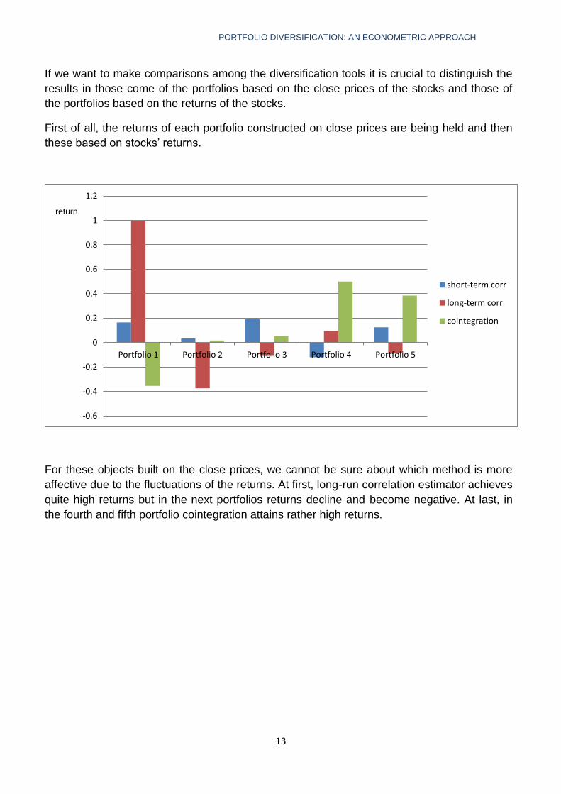
If we want to make comparisons among the diversification tools it is crucial to distinguish the
results in those come of the portfolios based on the close prices of the stocks and those of
the portfolios based on the returns of the stocks.
First of all, the returns of each portfolio constructed on close prices are being held and then
these based on stocks’ returns.
For these objects built on the close prices, we cannot be sure about which method is more
affective due to the fluctuations of the returns. At first, long-run correlation estimator achieves
quite high returns but in the next portfolios returns decline and become negative. At last, in
the fourth and fifth portfolio cointegration attains rather high returns.
-0.6
-0.4
-0.2
0
0.2
0.4
0.6
0.8
1
1.2
Portfolio 1 Portfolio 2 Portfolio 3 Portfolio 4 Portfolio 5
short-term corr
long-term corr
cointegration
return

PORTFOLIO DIVERSIFICATION: AN ECONOMETRIC APPROACH
14
0
0,0005
0,001
0,0015
0,002
0,0025
Portfolio 1 Portfolio 2 Portfolio 3 Portfolio 4 Portfolio 5
short-term corr
long-term corr
To continue with portfolios made on stocks’ returns, long-term correlation appears to reach
higher returns, but only in the first portfolio, in the next two short-term correlation estimators
achieve relatively high returns. In the fifth one, the two methods reach the same return.
On the next diagram, standard deviations (symbolized as σ) are illustrated for the five
portfolios, based on the close prices, for each diversification method.
0
2
4
6
8
10
12
14
16
18
Portfolio 1 Portfolio 2 Portfolio 3 Portfolio 4 Portfolio 5
short-term corr
long-term corr
cointegration
standard
deviation
return

PORTFOLIO DIVERSIFICATION: AN ECONOMETRIC APPROACH
15
To begin with, long-run correlation seems to appear the highest σ to the first two portfolios
when cointegration attains quite high σ to the last three. Standard deviation based on short-
run correlation decline steadily to stabilize at the last two portfolios.
Then, the portfolios built according the stock returns appear standard deviations represented
above.
Standard deviation related to the short-run correlation estimator seems to be quite weak,
lower than 2% in the first four portfolios but in the fifth one, σ based on the long-run
correlation booms sharply.
0
0.02
0.04
0.06
0.08
0.1
0.12
0.14
0.16
Portfolio 1 Portfolio 2 Portfolio 3 Portfolio 4 Portfolio 5
short-term corr
long-term corr
standard
deviation

PORTFOLIO DIVERSIFICATION: AN ECONOMETRIC APPROACH
16
CONCLUSION
Researchers, financial analysts and econometricians argue that a monetary union, like the
Eurozone tends to diminish the gains of diversification mainly due to the stock market
integration. The tighter the relation between the European economies the weaker the benefits
of diversification. Frankel and Rose (1998) advocate that by the time a country enters in a
monetary union, the stock markets appear to be more correlated than ever before.
When examining the advantages of the diversification methods in the Eurozone’s stock
exchange markets we were doubtful about how adequate these benefits would be.
This argument lies on the method of calculating the Sharpe Ratio5. This ratio gives us the
excess return for each unit of risk in comparison with the risk free return. The greater the
Sharpe ratio the better deal with the risk.
Suppose we have an investor, who is neither risk-lover nor risk-averse, but moderate. He has
two options. The first one is to invest his money on the portfolios constructed above. The
second one is to invest his money on 10-year of maturity German bonds with return about
1,941.6
In the tables above the Sharp ratios for each method of diversification are being represented
as also for each portfolio, firstly for those based on the close prices and then for those based
on the returns.
Sharpe ratios Portfolio 1 Portfolio2 Portfolio 3 Portfolio 4 Portfolio 5
short-run correlation -0,138 -0,213 -0,253 -0,510 -0,468
long-run correllation -0,057 -0,222 -0,433 -0,242 -0,277
cointegration -0,288 -0,304 -0,188 -0,143 -0,205
5 Sharpe Ratio = (rp – rf)/σp , where rp is the return of the portfolio, rf the return of a risk free asset and σp the
standard deviation of the portfolio, known as risk. 6 Source http://gr.investing.com/rates-bonds/germany-10-year-bond-yield (visited on 4/9/2013).

PORTFOLIO DIVERSIFICATION: AN ECONOMETRIC APPROACH
17
In the two tables held above all the Sharpe ratios are negative. That means that the risk-less
equity would perform better than the portfolios built on the European stock exchange
markets.
In our case study, the investor would definitely choose to invest in the German bonds, as
their offer quite high returns (compared to our portfolios), for zero risk.
Diversifying across European stock exchange markets (especially in the Eurozone) does not
seem to be a very profitable process. Either short-run correlation or long-run correlation or
the cointegration does not offer sufficient investment opportunities. High returns can be
attained through the construction of the portfolios based on the close prices, but also the
quite high standard deviations cannot be ignored.
Globalization, market integration as also the common currency would apparently eliminate
any opportunities. Traditionally, during periods of economic and financial integration, markets
tend to reach extremely high (near to +1) correlations.
Investors seem to be possessed of confusion: one the one hand they want to reach high
returns and tend to look for secluded stock markets, which will not be related to the global
markets. On the other hand they are afraid of dispersing their money across regions.
Diversification can only benefit investors in a short term basis. Once a capital market
becomes notorious for offering quite high returns, capitals from other markets will flow
together in that market and in the long term any gain will evaporate. Then, investors will
search for a new effective capital market etc.
Sharpe ratios Portfolio 1 Portfolio2 Portfolio 3 Portfolio 4 Portfolio 5
short-run
correlation
-138,144 -152,825 -144,821 -135,648 -123,141
long-run
correllation
-118,753 -162,892 -156,575 -125,144 -13,514

PORTFOLIO DIVERSIFICATION: AN ECONOMETRIC APPROACH
18
BIBLIOGRAPHY
Adam, K., Jappelli, T., Menichini A., Padula M., & Pagano M. (2002). Analyse, Compare, and Apply
Alternative Indicators and Monitoring Methodologies to Measure the Evolution of Capital Market
Integration in the European Union, Centre for Studies in Economics and Finance (CSEF), Department
of Economics and Statistics, University of Salerno.
Alagidede, P., Panagiotidis, P., & Zhang X. (2011). Why a diversified portfolio should include African
assets, Applied Economics Letters, 18:14, 1333-1340.
Albuquerque, P. H. (2008). Optimal Time Interval Selection in Long-Run Correlation Estimation, Mimeo, Texas A&M International University, Laredo, TX. Alexander, C. (1999). Optimal Hedging using Co-integration, Philosophical Transactions of the Royal Society, London, Series A 357, pp. 2039-2058. Alexander, C. (1998). Volatility and Correlation: Measurement, Models and Applications, Risk Management and Analysis: Measuring and Modeling Financial Risk, Wileys. Alexander, C. (1999). Cointegration and correlation in energy markets, Managing Energy Price Risk, 2nd edition, Chapter 15, pp. 291-304. Risk Publications. Alexander, C., & Dimitriu, A. (2002). The Cointegration Alpha: Enhanced Index Tracking and Long-Short Equity Market Neutral Strategies, ISMA Discussion Papers in Financial 2002-08, ISMA Centre, University of Reading. Alexander, C., & Dimitriu, A. (2005). Indexing, cointegration and equity market regimes, International Journal of Finance and Economics, 10, 213–231. Alexander, C., Giblin I., & Weddington W. (2001). Cointegration and Asset Allocation: A New Active Hedge Fund Strategy, ISMA Center Discussion Papers in Finance 2001-03. Alexander, C. (1995) ‘Common volatility in the foreign exchange market’, Applied Financial Economics, 5, 1-10. Aslanidis, N., & Savva, C. (2011). Are there still portfolio diversification benefits in Eastern Europe? Aggregate versus sectoral stock market data, The Manchester School, Volume 79, Issue 6, pages 1323–1352. Benninga, S. (2008). Financial Modeling, The MIT Press, Cambridge, Chapters 10, 12, 33. Benninga, S. (2005). Principles of Finance with Excel, Oxford University Press, 2nd Edition, Chapters 10, 11, 12, 13. Brealey, R., & Myers, S. (2003). Principles of Corporate Finance, The MacGraw-Hill Companies, 7th edition, Chapters 4, 7, 8. Bugar G., & Maurer, R. (2002). International Portfolio Diversification for European Countries: The Viewpoint of Hungarian and German Investors, ASTIN BULLETIN, Vol. 32, No. 1, 2002, pp. 171-197. Caldeira, J., & Moura. G. (2012). Selection of a Portfolio of Pairs Based on Cointegration: The Brazilian Case, Economic Bulletin, 2 March 2012.
PORTFOLIO DIVERSIFICATION: AN ECONOMETRIC APPROACH
19
Chua, T. C., Lai, S., & Lewis K. (2010). Are the Gains from Foreign Diversification Diminishing? Assessing the Impact with Cross-listed Stocks, The National Bureau of Economic Research, NBER Working Paper No. 18627. Danthine, J., P., Giavazzi, F., & Thadden E. L. (2000). European Financial Markets After EMU: A First Assessment, The National Bureau of Economic Research, NBER Working Paper No 8044. Dunis, C., & Ho, R., (2005). Cointegration Portfolios of European Equities for Index Tracking and Market Neutral Strategies, Journal of Asset Management, Volume 6, Number 1, 1 June 2005 , pp. 33-52. Embrechts, P., McNeil, A., & Straumann, D. (1998). Correlation and Dependency in Risk Management: Properties and Pitfalls in ‘Risk Management: Value at Risk and Beyond, edited by M. A. H. Dempster, Cambridge University Press, pp. 176-237. Engle, R. F., &Granger, C. W. J. (1987). Cointegration and Error-Correction: Representation, Estimation, and Testing, Econometrica 55. Flavin, T., Hurley, M., & Rousseau, F. (2002). Explaining Stock Market Correlation: A Gravity Model Approach, The Manchester School, Volume 70, Issue S1, pages 87–106. Frankel, J. A., and. Rose, A. K. (1998). The endogeneity of the optimum currency area criteria, The Economic Journal 108, 1009-1025. Goetzmann, W., Li, L., & Rouwenhorst, G. (2001). Long-Term Global Market Correlations, The National Bureau of Economic Research, NBER Working Paper No. 8612. Hourvouliades, N. (2009). International Portfolio Diversification: Evidence from European Emerging Markets’, European Research Studies, Volume XII, Issue 4. Jorion, P. (1992). Portfolio Optimization in Practice, Financial Analysts Journal, Jan/Feb 1992, 48. Kanas, A., & Ioannidis, C. (2012). Revisiting the forward—spot relation: an application of the nonparametric long-run correlation coefficient, Journal of Economics and Finance, January 2012, Volume 36, Issue 1, pp 148-161. Lewis, K. (2012). Global Stock Market Linkages Reduce Potential for Diversification, Economic Letter: Insights from the Federal Reserve Bank of Dallas, Vol. 7, No. 2, February 2012. Marshall, C., & Siegel, M. (1996). Value-at-Risk: Implementing a Risk Measurement Standard’, 96-47, available at SSRN: http://dx.doi.org/10.2139/ssrn.1212.
McNeil, A., Frey, R., & Embrechts, P. (2005). Quantitative Risk Management: Concepts, Techniques and Tools, Chapter 7, pp. 283-351.
Moss, T., & Thuotte, R. (2013). Nowhere Left to Hide? Stock Market Correlation, Regional Diversification, and the Case for Investing in Africa, Working Paper 316, March 2013, the Center for Global Development.
Obstfeld, M. (1994). Risk-Taking, Global Diversification, and Growth, The American Economic Review, Vol. 84, No. 5, pp. 1310-1329.
Solnik, B. (1974). Why Not Diversify Internationally Rather Than Domestically, Financial Analysts Joumal, Vol. 30, No. 4.

PORTFOLIO DIVERSIFICATION: AN ECONOMETRIC APPROACH
20
Stangă, E., Anghel, F., & Avrigeanu, A. (2010). The Long – Short Strategy Based on Cointegration Concept, Romanian Economic and Business Review, Vol. 5, No. 1.
Tjostheim, D., & Hufthammer, K. (2013). Local Gaussian correlation: A new measure of dependence’, Journal of Econometrics, Volume 172, Issue 1, pp. 33–48.

PORTFOLIO DIVERSIFICATION: AN ECONOMETRIC APPROACH
21
Copyright © 2022 FDOKUMEN

