IEEE TRANSACTIONS ON SYSTEMS, MAN, AND CYBERNETICS—PART A: SYSTEMS AND HUMANS, VOL. 41, NO. 5, SEPTEMBER 2011 977

Pattern- and Network-Based ClassificationTechniques for Multichannel Medical Data

Signals to Improve Brain DiagnosisWanpracha Art Chaovalitwongse, Senior Member, IEEE, Rebecca S. Pottenger, Shouyi Wang,

Ya-Ju Fan, and Leon D. Iasemidis, Member, IEEE

Abstract—There is an urgent need for a quick screening processthat could help neurologists diagnose and determine whether apatient is epileptic versus simply demonstrating symptoms linkedto epilepsy but actually stemming from a different illness. Aninaccurate diagnosis could have fatal consequences, particularly inoperating rooms and intensive care units. Electroencephalogram(EEG) has been traditionally used, as a gold standard, to diagnosepatients by evaluating those brain functions that might correspondto epilepsy and other brain disorders. This research thereforefocuses on developing new classification techniques for multichan-nel EEG recordings. Two time-series classification techniques,namely, Support Feature Machine (SFM) and Network-BasedSupport Vector Machine (SVM) (NSVM), are proposed in thispaper to predict from EEG readings whether a person is epilepticor nonepileptic. The SFM approach is an optimization modelthat maximizes classification accuracy by selecting a group ofelectrodes (features) that has strong class separability based ontime-series similarity measures and correctly classifies EEG sam-ples in the training phase. The NSVM approach integrates anew network-based model for multidimensional time-series datawith traditional SVMs to exploit both the spatial and temporalcharacteristics of EEG data. The proposed techniques are testedon two EEG data sets acquired from ten and five patients, re-spectively. Compared with other commonly used classificationtechniques such as SVM and decision trees, the proposed SFM andNSVM techniques provide very promising and practical resultsand require much less time and memory resources than traditionaltechniques. This study is a necessary application of data mining toadvance the diagnosis and treatment of human epilepsy.

Index Terms—Electroencephalogram (EEG) classification,epilepsy diagnosis, multidimensional time series, optimization,pattern recognition.

Manuscript received September 30, 2009; revised April 1, 2010 andSeptember 12, 2010; accepted October 30, 2010. Date of publicationMarch 10, 2011; date of current version August 23, 2011. The work ofW. Chaovalitwongse, S. Wang, Y.-J. Fan, and R. S. Pottenger was supportedin part by the National Science Foundation under a CAREER Grant and inpart by the Center for Discrete Mathematics and Theoretical Computer Scienceunder the Research Experiences for Undergraduates Program. The work ofL. D. Iasemidis was supported by the National Institutes of Health, VeteransAffairs, Defense Advanced Research Projects Agency, and the Whitaker Foun-dation. This paper was recommended by Associate Editor J. M. Carmena.

W. A. Chaovalitwongse, S. Wang, and Y.-J. Fan are with the Department ofIndustrial and Systems Engineering, Rutgers University, Piscataway, NJ 08855-0909 USA (e-mail: wchaoval@rci.rutgers.edu; shouyi@eden.rutgers.edu;yjfan@eden.rutgers.edu).

R. S. Pottenger is with the Department of Computer Science, PrincetonUniversity, Princeton, NJ 08540-5233 USA (e-mail: rpotteng@princeton.edu).

L. D. Iasemidis is with the Department of Bioengineering, Arizona StateUniversity, Tempe, AZ 85287 USA (e-mail: Leon.Iasemidis@asu.edu).

Color versions of one or more of the figures in this paper are available onlineat http://ieeexplore.ieee.org.

Digital Object Identifier 10.1109/TSMCA.2011.2106118

I. INTRODUCTION

E PILEPSY, a disease characterized by a tendency for recur-rent seizures, is one of the most common brain disorders

in the world, coming second only to strokes. Currently, about3 million Americans and 40 million people worldwide (about1% of human population) suffer from epilepsy [1]–[3]. Ascommon as epilepsy is, the accuracy of epilepsy diagnosisvaries greatly, from a misdiagnosis rate of 5% in a prospectivechildhood epilepsy study to at least 23% in a British population-based study [4]. In fact, the rate may be even higher in ev-eryday practice. For instance, temporal lobe epilepsy is a lesscommon form of epilepsy that does not result in the typicalphysical seizures. Rather, patients suffer from symptoms suchas depression, moodiness, anger, or irritability. Misdiagnosisof this condition as depression is extremely common [3]. Intoday’s brain diagnosis studies, particularly in epilepsy stud-ies, the electroencephalogram (EEG) recordings are the mostcommonly used neurophysiological signal employed to eval-uate brain functions that might be related to brain disordersand abnormal cognitive functions. Neurologists are trained torecognize certain prominent patterns in EEG signals that reflectthe brain’s activity. For diagnosis purposes, pattern recognitionis a natural method that neurologists employ to identify thepresence of a disease such as epilepsy. However, neurologistshave to “eye ball” EEG signals, spatially and temporally, inan attempt to recognize abnormal patterns (e.g., epileptiforms)in the brain activity. “Eye balling” these massive signals forhours or even days can be very tedious and challenging. Forneurologists, there is an urgent need for new automated signal-processing and pattern-recognition techniques that help thesephysicians diagnose, with more accuracy and speed, patientswho have epilepsy or other related brain disorders.

The main application of this study is to improve currentepilepsy diagnosis by developing a new medical signal-pattern-recognition framework to identify (or distinguish) abnormalspatiotemporal patterns from multichannel EEG recordings. Inthis computational framework, we develop two new classifica-tion techniques for multidimensional time-series classification,namely, support feature machine (SFM) and network-basedsupport vector machine (SVM) (NSVM). SFM is a pattern-based classification technique employing the nearest neighborrule and time-series similarity measures, whereas its optimiza-tion model selects the features with strong class separabilityso that the classification accuracy is maximized. NSVM is a

1083-4427/$26.00 © 2011 IEEE

978 IEEE TRANSACTIONS ON SYSTEMS, MAN, AND CYBERNETICS—PART A: SYSTEMS AND HUMANS, VOL. 41, NO. 5, SEPTEMBER 2011

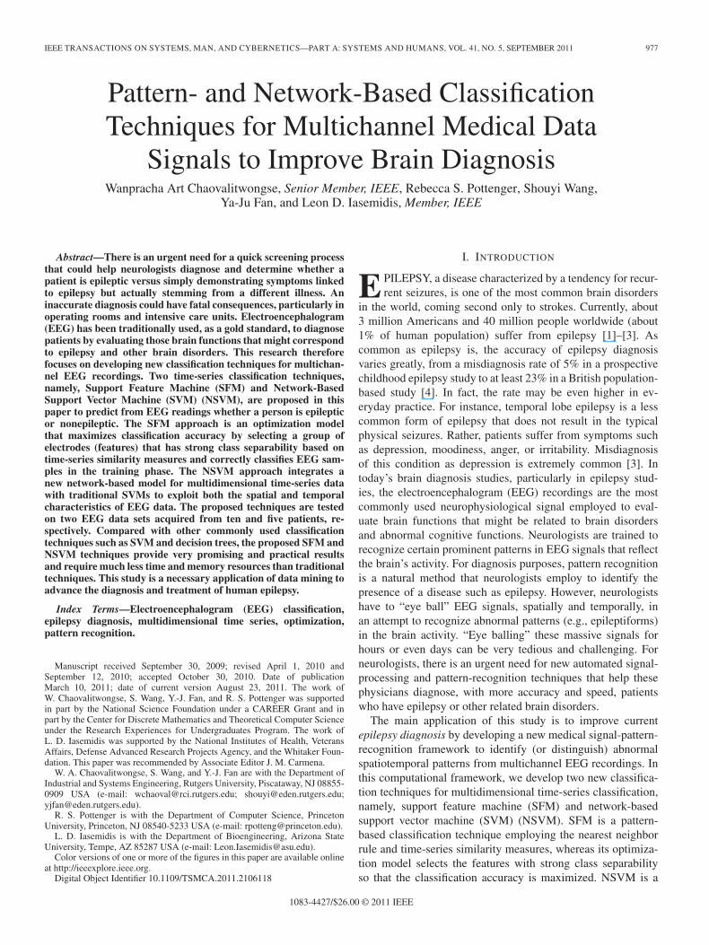
Fig. 1. Simplified scalp EEG recording placement and an example of 10-sEEG recordings.

network-based version of SVM that incorporates statistical andcorrelation measures of temporal synchronization among time-series profiles. It can overcome the drawback of SVM regardingtime-series classification as SVM generally treats each timestamp of a time-series epoch as an independent attribute al-though data in the epoch are actually highly correlated. We eval-uate and assess the performances of the proposed techniques onan EEG data set acquired from ten patients, five epileptic andfive nonepileptic, during their routine EEG checks. The pro-posed framework can be applied as a medical decision-supportsystem to improve the current medical diagnosis and prognosisby assisting physicians in recognizing via data mining abnormalpatterns in complex medical data, particularly EEG recordings.Such a system could be used in a quick screening process thatcould determine whether a patient is epileptic or nonepileptic.

The organization of the succeeding sections of this paperis as follows. In Section II, the research background andprevious work are discussed. In Section III, the SFM andNSVM frameworks including time-series similarity measuresand optimization models are described. Section IV describesthe acquisition and cleansing procedures of the EEG data setand the design of experiments. The computational results andthe performance characteristics of our classification techniquesare provided in Section V. The concluding remarks are given inSection VI.

II. BACKGROUND

A. Epilepsy Diagnosis

There are many diseases that cause changes in brain behaviorand can be confused with epilepsy [3]; specifically, severalmedical conditions can cause seizures or seizurelike episodes.Therefore, the evaluation of patients with these symptoms isaimed at determining the type (epileptic or nonepileptic) andcause of the seizures. Out of the commonly used medicaltests such as blood tests, magnetic resonance imaging, positronemission tomography, as well as studying the patient’s medicalhistory, EEG reading is the most important part of epilepsydiagnosis because it directly detects electrical activity in thebrain. During an EEG test, electrodes are attached to specificlocations on the patient’s scalp (see Fig. 1 for simplified scalpEEG recordings). A routine EEG test for epilepsy diagnosisusually records about 20–30 min of brain waves; however, inmost cases, the results of routine EEG studies are often incon-

clusive, even in people known to have epilepsy, so prolonged(24-h) EEG monitoring can be necessary. Epilepsy diagnosiscan be very complicated, particularly in immediate life-and-death situations [e.g., in emergency rooms (ERs)] when thedecision needs to be made promptly. Also, in many cases ofcoma, trauma, and surgical critical care, the medical diag-nostic tools used to differentiate epileptic seizures from othersymptoms that have similar EEG morphological patterns arevery critical to the patients’ welfare. Inaccurate diagnosis andtreatment could have severe consequences, particularly in life-threatening situations in ERs and intensive care units. An accu-rate quick EEG analysis that can identify whether a patient hasepilepsy could drastically improve the accuracy of diagnosisof epilepsy and thereby save patients’ lives. There is a desper-ate need for a new technology providing quick and accurateepilepsy screening, which would serve as an initial medicaldiagnostic tool.

This study is of significant importance to improving currentbrain diagnosis as it offers great potential for the developmentof computerized techniques to differentiate between EEG pat-terns from epileptic patients and those with different diseasesbut morphologically similar EEG patterns. This study presentsa framework for a quick EEG analysis and screening processthat has an overarching potential to help save lives, improve theaccuracy of medical diagnosis, and reduce associated health-care costs.

B. Pattern Recognition for Neurophysiological Signals

Over the past decade, there have been a number of researchstudies in quantitative signal-processing techniques (both uni-variate and multivariate) applied to neurophysiological datasuch as EEG. For EEG analysis, linear univariate techniques(e.g., power spectrum analysis and time–frequency analysis)have often been used in conjunction with nonlinear methodswhich incorporate high-order statistics, nonlinear dynamics(e.g., chaos theory), and information-theoretical quantifica-tion. New similarity measures called the Kullback–Leiblerdiscrimination information and the Chernoff information fordiscrimination between multivariate series in the multivariatenon-Gaussian case were proposed in [5]. Subsequently, neuralnetwork methods were developed for a nonlinear aspect ofanalysis for multivariate time series, where a unified view ofnonlinear principal component analysis, nonlinear canonicalcorrelation analysis, and nonlinear singular spectrum analysistechniques were presented [6]. A constructive induction methodfor classifying time series was proposed in [7], where the scopeof attribute-value learning was expanded by using metafeaturesto the domains that contain instances with recurring substruc-ture. A new technique that vectorizes components of a corre-lation coefficient matrix of multidimensional time-series datawas proposed in [8]. Recently, there have been a few studiesregarding detecting changes in spatiotemporal data [9], [10].One such study was conducted to detect and identify changes inbrain waves through event-related potential data [10]. However,the problem of detecting spatiotemporal changes in known EEGpatterns is much easier than the problem of finding unseenpatterns in EEGs. Despite converging evidence and consistency

CHAOVALITWONGSE et al.: CLASSIFICATION TECHNIQUES FOR MEDICAL DATA SIGNALS 979

in reported findings on the potential usefulness of these uni-variate and multivariate techniques, their added value to thediagnosis of brain disorders in clinical settings remains ques-tionable. Complex brainwave patterns and their relationships tobrain disorders may be very specific for an individual patient,yet vary from one patient to another. This suggests the needfor a new development of data-analysis and signal-pattern-recognition techniques that allow the identification of morecomplex relationships.

C. EEG Classification

Over the past few years, there has been a substantial body ofwork in EEG classification. In the previous studies by our group[11]–[14], it is suggested that EEG signals of epileptic pa-tients during normal and preseizure states may be classifiable.In those studies, we employed a feature-extraction techniquebased on the chaos theory to characterize nonlinear dynamicalpatterns in EEG signals. That technique was motivated bymathematical models used to characterize multidimensionalcomplex systems and by the prospect of reduction of thedimensionality of the EEG data [15]–[19]. In our first attemptto classify EEG signals, we implemented the SVM approachto classify normal and preseizure EEGs with some degree ofsuccess [11]. However, the classification results were inferiorto a standard nearest neighbor classification. In a more recentstudy, we proposed a time-series k-nearest neighbor approachwith advanced time-series similarity approaches (e.g., t-indexand dynamic time warping) and tested it on a larger EEG dataset [12]. The main drawback of traditional pattern-based (orinstance-based) classification techniques like k-nearest neigh-bor is their sensitivity to noisy features because most techniquesdo not incorporate the feature-selection process. Although thefeature-selection process can be carried out as a separate stepbefore classification, the process is usually not trained (super-vised) to select the best combination of features (which requirescombinatorial optimization) as each feature is evaluated ona one-to-one basis. Our group has recently proposed a newoptimization framework for supervised feature selection withk-nearest neighbor classification [13], [14]. The frameworkhas been very effective in classifying normal and preseizureEEGs. Based on our initial discovery of detectable EEG patternchanges before a seizure, we believe that the concept of EEGclassification may be applicable to the epilepsy diagnosis prob-lem. It is important to note that, in all of our previous studies,the classification was done on individual patients, where weused the training and testing data from the same patient. Inaddition, we tested the hypothesis that there were significantchanges in EEG patterns prior to seizure onsets. In this paper,however, we focus on the classification of EEG recordingsfrom epileptic and nonepileptic patients, which are much morechallenging than what we have studied in the past. We makean attempt to test the hypothesis that epileptic and nonepilepticEEG recordings during a nonseizure episode can be classified.It is even more challenging when the training has to be doneacross multiple patients. In addition, this study presents thenew NSVM as a multidimensional time-series classificationalgorithm, which has not been introduced elsewhere.

D. Advances in Classification

Feature selection and classification are supervised learning,which constructs a predictive function or model from train-ing data. Generally, classification deals with a set of desiredinput–output pairs by trying to find a global mapping from thecollected inputs to outputs to the highest possible extent andthen making predictions of future outputs. A decision tree is analgorithm that creates a mapping model to data instances basedon some feature values. In a decision tree, nodes representclassification features and branches represent conjunctions offeatures that lead to those classifications. Starting at the rootnode, the data instances are sorted based on their feature values.The most well-know algorithm to generate decision trees is analgorithm called C4.5 [20]. C4.5 builds decision trees from aset of training data by using the concept of Shannon entropy[21], which is a measure of the uncertainty associated with arandom variable. Ruggieri [22] provided an improved versionof C4.5, called EC4.5, which was claimed to be able to computethe same decision trees as C4.5 with a performance gain of up tofive times. Yildiz and Dikmen [23] presented three parallel C4.5algorithms which are applicable to large data sets. Baik andBala [24] presented a distributed version of decision trees. SVMis a widely used technique for data classification and regression[25]. The key concept of SVM is its projection of input datainstances into a higher dimensional space and division of thespace with a continuous separation hyperplane while iterativelyminimizing the distance of misclassified data instances from thehyperplane. In other words, SVM generally tries to constructa hyperplane that minimizes the upper bound on the out-of-sample error. There have been many variations of SVM models.In practice, most data sets are not perfectly separable. For thisreason, one should try to approximate the goal of maximizingmargin by minimizing an average sum of violations. This leadsto the development of robust linear programming formulation[26]. A number of linear programming formulations for SVMshave also been used to explore the properties of the structure ofthe optimization problem and solve large-scale problems [27],[28]. The SVM technique proposed in [28] was also demon-strated to be applicable to the generation of complex spacepartitions similar to those obtained by C4.5 [20] and CART[29]. SVMs have been applied to many real-life problemsincluding handwritten digit recognition [30], object recognition[31], speaker identification [32], face detection in images [33],and text categorization [34]. SVM can also be extended tomulticlass problems [30], [35], [36]. Kernel transformation,also known as kernel trick, is one of the most successful ap-proaches applied to SVM. It uses the idea that once a data set istransformed into a high-dimensional space, each data instancecan be classified by a separating plane if the new dimension issufficiently high enough [37]. A good separation is achieved bya hyperplane with the largest distance from the neighboring datapoints of both classes. This concept is very intuitive because,in general, the larger the margin, the better the generalizationerror of the classifier. The most simple kernel function is thelinear kernel k(x, y) = x · y. The decision function takes theformula f(x) = wx+ b. In time-series prediction, the linearkernel can be interpreted as a statistical autoregressive model of

980 IEEE TRANSACTIONS ON SYSTEMS, MAN, AND CYBERNETICS—PART A: SYSTEMS AND HUMANS, VOL. 41, NO. 5, SEPTEMBER 2011

the order k(AR[k]). Another commonly used kernel function isthe radial basis function (RBF) kernel kγ(x, y) = exp(−γ‖x−y‖2). The similarity of two samples in the RBF kernel canbe interpreted as their Euclidian distance. Recently, there havebeen a number of research studies proposing the use of kernelfunctions for single time-series transformation such as speechrecognition [38]–[42]. To the best of our knowledge, a formaltime-series classification study based on data mining was intro-duced in the late 1990s [43], [44]. A new type of self-organizingneural network was developed to classify control-chart time-series data [43]. A new representation of time series for fasterclassification was proposed [44]. Subsequently, the feature-extraction technique was introduced to classify time-series data[45]. More sophisticated classification techniques such as clas-sification trees and SVM were employed with some degree ofsuccess [46], [47]. In later studies [48], [49], the research focuswas shifted to time-series motif discovery where new algo-rithms were developed to find an efficient and effective discreteapproximation of the time series. The dynamic-time-warpingmeasure has been applied and improved to efficiently classifytime series [50]. In a recent study [51], a disk-aware algorithmwas employed to find exact time-series motifs in large-scaledatabases. Most recently, an efficient online classification toolfor time-series data based on support vector regression (SVR)was developed [52]. Whenever a sample is added to or removedfrom the training set, this technique is capable of updatinga trained SVR model efficiently without retraining the entiretraining data.

Although there has been an expanded body of work intime-series classification, most studies only deal with singletime-series data (univariate) and very few methods are ap-plicable to multidimensional time series (multivariate) likeEEG recordings. Similarly, most studies on EEG analysis inthe literature focus on univariate analysis of the recordings.The NSVM and SFM approaches proposed in this study aredesigned to work with multidimensional time-series data. TheNSVM approach captures the interactions between differentpairs of time series while the SFM approach uses baselinepatterns and fuse the similarities of individual series into asingle framework. In addition, the SFM approach can be viewedas an ensemble classification version of the nearest neighborapproach for time series. The feature-extraction step of theNSVM approach can be viewed as a new way to generatefeatures that are more interpretable to the end users (e.g.,physicians).

III. CLASSIFICATION TECHNIQUES FOR

MULTICHANNEL EEG SIGNALS

We propose two new classification techniques for multidi-mensional time-series data that will be used to identify epilepticand nonepileptic patients from EEG data samples. Each EEGsample is represented by a multidimensional time series, shownin Fig. 1, where each trace represents a time series of anelectrode. The key idea of both techniques is to integrate bothspatial and temporal features of EEG data into the classificationmodels.

A. SFM

The key idea of SFM is the integration of accuracy optimiza-tion into feature selection and the nearest neighbor classifica-tion in the training phase. The procedure of SFM is describedby the following steps.

1) Step 1—Apply the Nearest Neighbor Rule: The nearestneighbor rule is a very intuitive classification method, whichassigns an unlabeled sample to the class whose baseline sam-ples are the closest. During the training phase, we have twogroups of baseline (labeled) EEG data samples, epileptic andnonepileptic. Since each EEG data sample is in the form of mul-tidimensional time-series data, we employ the nearest neighborrule based on time-series similarity measures to quantify thecloseness between data samples. Generally, time-series similar-ity measures deal with a single time-series profile. Here, weapply an ensemble classification concept to modify the nearestneighbor approach for multidimensional time series [12]. Givenmultiple decisions from multiple features (electrodes), we em-ploy two commonly used schemes, distance averaging andmajority voting, to combine these decisions in classifying anunlabeled sample. In the distance-averaging scheme, for everyfeature, each class gets a score equal to the statistical distancefrom each of its training samples to all other baseline samplesof the same class. The overall score of each class is equalto the summation of the scores for all features (electrodes).The sample is then classified to the class with the lowestoverall score. In the majority-voting scheme, for every feature,a class (category) gets one vote if the nearest neighbor ruleclassifies the training sample to that class. The sample is, inturn, classified to the class with the maximum number of votes,i.e., majority of features/electrodes.

Here, we employ two commonly used time-series similar-ity measures, Euclidean distance and T-Statistical distance(T-Statistics). Euclidean distance is the most commonly usedsimilarity measure. It measures the degree of similarity interms of the amplitude of the data. The Euclidean distancebetween EEG samples u and v of length t at electrode j isdefined as EDj

uv = (∑t

i=1(uji − vji )

2)/t. T-statistical distanceis a measure of statistical distance between two time seriesderived from the t-test, which is frequently used to determine iftwo time series differ from each other in a significant way underthe assumptions that the paired differences are independent andidentically normally distributed. The t-index can be seen asa ratio of the difference between the two means or averagesand a measure of the variability or dispersion of the scores.The t-index between EEG samples u and v of length t atelectrode j is defined as T j

uv = (∑t

i=1 |uji − vji |/

√tσ|uj−vj |),

where σ|uj−vj | is the sample standard deviation of the absolutedifference between EEG time series u and v estimated over awindow with length t.

In the training phase, since we already know the true class(label) for each of the training samples, we use the nearestneighbor rule to evaluate the classification accuracy of everyelectrode on every training sample. The SFM optimizationmodels are then formulated to incorporate all the classificationdecisions made by all the electrodes and select the best subsetof electrodes that maximizes the classification accuracy. For

CHAOVALITWONGSE et al.: CLASSIFICATION TECHNIQUES FOR MEDICAL DATA SIGNALS 981

the distance-averaging scheme, the input information of SFMincludes n×m intraclass-distance matrix (D) and n×minterclass-distance matrix (D). The entry of intraclass matrixdij is the average statistical distance between training sample iand all other training samples from the same class at electrode j.The entry of interclass matrix dij is the average statistical dis-tance between training sample i and all other training samplesfrom different classes at electrode j. For the majority-votingscheme, the SFM input is an accuracy n×m matrix (A), wheren is the number of training samples and m is the number offeatures. The entry aij = 1 indicates that the nearest neighborrule correctly classifies training sample i at feature j and iszero otherwise. The time complexity of the matrix-generationprocedure for both schemes is O(n2mτ), where n2 is requiredfor a pairwise comparison of all data, m is required for allelectrodes, and τ is required for the calculation of time-seriessimilarity measures. Here, τ = O(t) for Euclidean distance andτ = O(t2) for T-Statistical distance.

2) Step 2—Optimization Models of SFM: The SFM opti-mization model is formulated to select a group of features(electrodes) that maximizes classification accuracy based onthe nearest neighbor rule. To formally formulate the SFMoptimization problem into a mathematical programming model,we define the following sets and decision variables. Denotei ∈ I as a set of training samples where |I| = n and j ∈ Jas a set of features where |J | = m. We let xj ∈ {0, 1} be adecision variable indicating if feature j is selected by SFMand yi ∈ {0, 1} be a decision variable indicating if trainingsample i is correctly classified.

Averaging SFM (A-SFM): The input of A-SFM are theintra- and interclass distance matrices D and D generated inStep 1. The objective function in (1) is to maximize the totalnumber of correctly classified samples. There are two sets ofconstraints in (2) and (3) to ensure that the training samplesare classified based on the distance-averaging nearest neighborrule. There is a set of logical constraints in (4) to ensure thatat least one feature (electrode) is selected in the distance-averaging nearest neighbor rule. The mixed-integer program(MIP) of A-SFM is given by

maxn∑

i=1

yi (1)

s.t.m∑

j=1

dijxj −m∑

j=1

dijxj ≤ M1iyi, ∀i ∈ I (2)

m∑

j=1

dijxj −m∑

j=1

dijxj ≤ M2i(1− yi), ∀i ∈ I (3)

m∑

j=1

xj ≥ 1 (4)

x ∈ {0, 1}m y ∈ {0, 1}n (5)

where dij is the average statistical distance between trainingsample i and all other training samples from the same class atelectrode j (intraclass distance), dij is the average statisticaldistance between training sample i and all other training sam-

ples from different classes at electrode j (interclass distance),M1i =

∑mj=1 dij , and M2i =

∑mj=1 dij .

Voting SFM (V-SFM): The input of V-SFM is the accuracymatrix A generated in Step 1. The objective function of V-SFMin (6) is the same as that of A-SFM. There are two sets ofconstraints in (7) and (8) to ensure that the training samples areclassified based on the voting scheme. There is a set of logicalconstraints in (9) to ensure that at least one feature is used in thevoting nearest neighbor rule. The MIP of V-SFM is given by

max

n∑

i=1

yi (6)

s.t.m∑

j=1

aijxj −m∑

j=1

xj

2≤ Myi, ∀i ∈ I (7)

m∑

j=1

xj

2−

m∑

j=1

aijxj + ε ≤ M(1− yi) ∀i ∈ I (8)

m∑

j=1

xj ≥ 1 (9)

x ∈ {0, 1}m y ∈ {0, 1}n (10)

where aij = 1 if the nearest neighbor rule correctly classifiedtraining sample i at feature j and is zero otherwise, n is the totalnumber of training samples, m is the total number of features,M = m/2, and 0 < ε < 1/2 is used to break ties during voting.

In the training phase (Steps 1 and 2), the SFM optimizationmodels of A-SFM and V-SFM are individually solved using anoff-the-shelf CPLEX optimization solver. It is very importantto note that these optimization models are very compact. Thespace complexity grows linearly with the number of trainingsamples and the number of features (electrodes), specificallyO(n+m). The majority of computational efforts will be inStep 1. This depends solely on the number of features andthe length (number of data points) of EEG epochs. After theSFM models are solved, a group of optimally selected features(electrodes) that maximize the classification accuracy will beobtained and used in Step 3.

3) Step 3—Using SFM to Classify Unlabeled EEG Sample:In the testing phase, the classification will be done based onthe features (electrodes) selected in the training phase. A-SFMclassifies an unlabeled EEG sample to the class whose baselinetraining EEG data are the nearest (closest) based on the averagedistance of selected electrodes. Similarly, V-SFM classifies anunlabeled EEG sample to the class with the highest votescounted only from selected electrodes.

B. NSVM

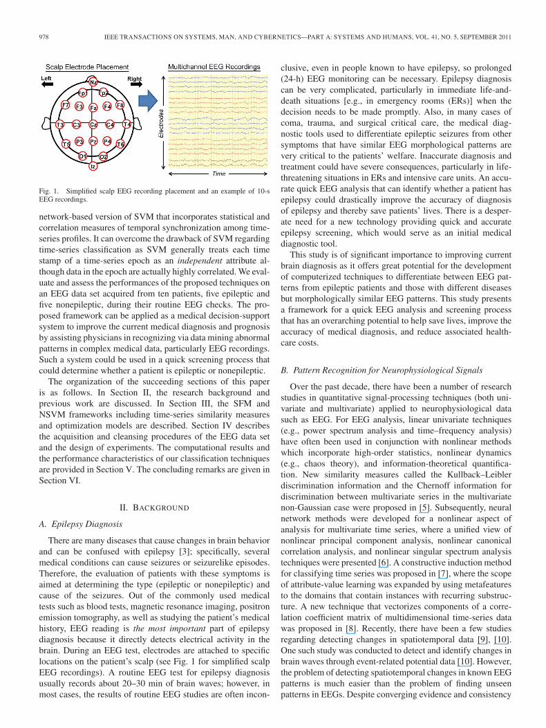
NSVM employs a new network modeling technique to incor-porate SVM with spatiotemporal EEG analysis by representingan EEG sample as a “Brain Graph” or “Brain Network.”Essentially, NSVM maps each multichannel EEG sample intoa network representation and applies the SVM classificationto the mapped data. Fig. 2 shows a hypothetical schematic

982 IEEE TRANSACTIONS ON SYSTEMS, MAN, AND CYBERNETICS—PART A: SYSTEMS AND HUMANS, VOL. 41, NO. 5, SEPTEMBER 2011

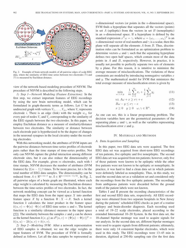
Fig. 2. Example of brain network models of all pairwise edges of scalp EEGdata, where the similarity of EEG time series between two electrodes T4 andT5 is measured by Euclidean distance.

view of the network-based modeling procedure of NSVM. Theprocedure of NSVM is described in the following steps.

1) Step 1—Network Modeling (Feature Extraction): In thefirst step, we extract important features of EEG recordingsby using the new brain networking model, which can beformulated in graph-theoretic terms as follows. Let G be anundirected graph with vertices V1, . . . , Vm, where Vi representselectrode i. There is an edge (link) with the weight wij forevery pair of nodes Vi and Vj corresponding to the similarity ofthe EEG signals between the two electrodes. In this paper, weemploy Euclidean distance as a measure of similarity/distancebetween two electrodes. The similarity or distance betweeneach electrode pair is hypothesized to be the degree of changesin the neuronal synapses in the local circuitry under the record-ing electrodes.

With this networking model, the attributes of SVM inputs arethe pairwise distances between time-series profiles of electrodepairs rather than the time stamps of time-series profiles. Notonly can NSVM capture the global interaction among differentelectrode sites, but it can also reduce the dimensionality ofthe EEG data. For example, given m electrodes, each with ttime stamps, NSVM decreases the number of attributes (SVMfeatures) by 2(m− 1)/t times. To be more precise, let n be thetotal number of EEG data samples. The dimensionality can bereduced from A ∈ �n×m×t to A ∈ �n×(m(m−1)/2). In Fig. 2,all pairwise edges of a brain graph are illustrated, where eachedge weight is calculated by measuring the Euclidean distancebetween the time-series profiles of two electrodes. In fact, thenetwork modeling concept can be viewed as a kernel functionthat maps the EEG data from the input space X into anotherfeature space X by a function Φ : X → X . Such a kernelfunction k calculates the inner product in the feature spacek(u, v) = Φ(u) · Φ(v) of EEG time series u and v. The kernelfunction is a similarity (distance) measure in the input space[53]. The similarity between the samples x and y can be shownas the kernel function k(x, y) as d2(u, v) = (Φ(u)− Φ(v))2 =k(u, u)− 2k(u, v) + k(v, v).

2) Step 2—Modeling SVM: After a network representationof EEG samples is obtained, we use the edge weights asinput features of SVM. The procedure of SVM is formallydefined as follows. Let all the data samples be represented as

n-dimensional vectors (or points in the n-dimensional space).SVM finds a hyperplane that separates all the vectors (points)in set A (epileptic) from the vectors in set B (nonepileptic)in an n-dimensional space. If a hyperplane is defined by thestandard expression xTω = γ, where ω = (ω1, . . . , ωn)

T is ann-dimensional vector of real numbers and γ is a scalar, then thisplane will separate all the elements A from B. Thus, discrim-ination rules can be formulated as an optimization problem todetermine vectors ω and γ such that the separating hyperplanedefines two open half spaces, which contain most of the datapoints in A and B, respectively. However, in practice, it isusually not possible to perfectly separate two sets of elementsby a plane. For this reason, it is intuitive to minimize theaverage measure of misclassifications. The violations of theseconstraints are modeled by introducing nonnegative variables xand y. The mathematical model for SVM that minimizes thetotal average measure of misclassification errors is given by

minω,γ,x,y

1

m

m∑

i=1

xi +1

k

k∑

j=1

yj (11)

s.t. Aω + x ≥ eγ + e (12)

Bω − y ≤ eγ − e (13)

x ≥ 0 y ≥ 0 ω, γ ∈ Rn. (14)

As one can see, this is a linear programming problem. Thedecision variables here are the geometrical parameters of theseparating plane ω and γ, as well as the variables representingmisclassification error x and y.

IV. MATERIALS AND METHODS

A. Data Acquisition and Sampling

In this paper, two EEG data sets were acquired. The firstEEG data set was acquired from short-term EEG recordingsof ten patients, five epileptic and five nonepileptic. The secondEEG data set was acquired from ten patients; however, only fiveof those patients were known to be epileptic while the otherfive patients were not known to be epileptic or nonepileptic. Inpractice, it was hard to find a clean data set in which patientswere definitely labeled as nonepileptic. Thus, in this study, weused the second data set as a validation set and considered onlythe recordings from the five epileptic patients. The recordingsfrom ambiguous patients were discarded before the groundtruth of the patient labels were not known.

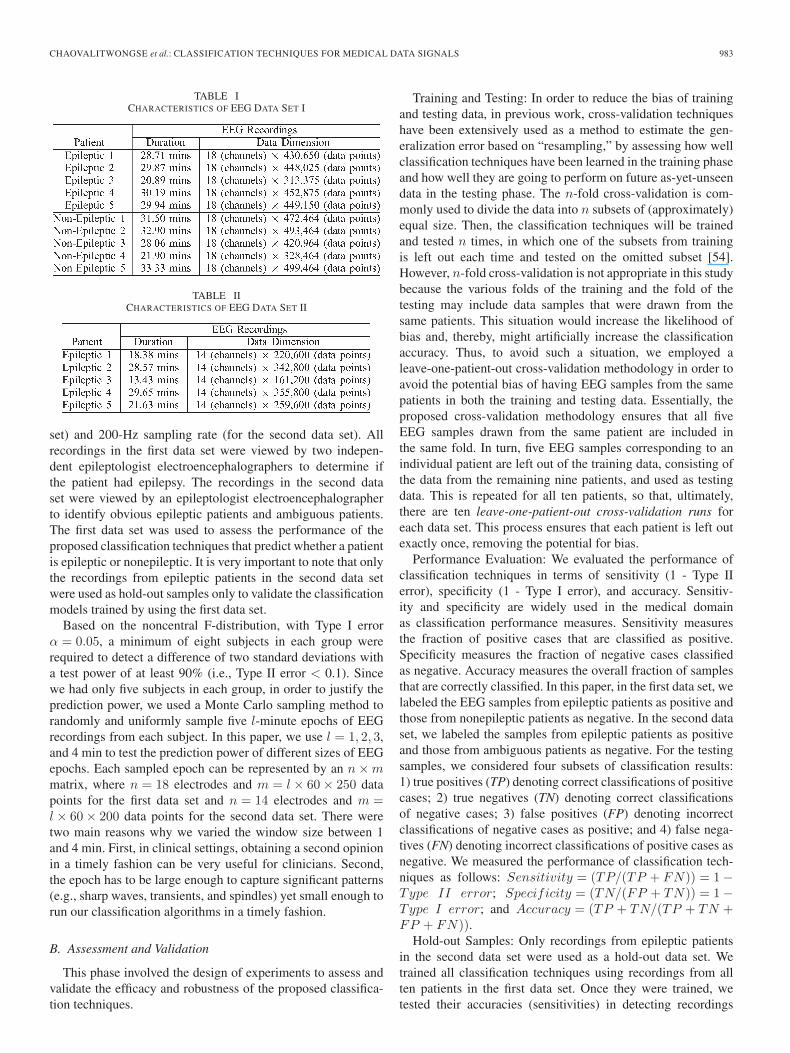
Tables I and II present the recording characteristics of thefirst and second EEG data sets, respectively. All EEG record-ings were obtained from two separate hospitals in New Jerseyduring the patients’ scheduled EEG checks as part of a routineepilepsy and brain-disorder diagnosis. Each recording useda total of 19–22 scalp electrodes, placed according to theextended International 10–20 System. In the first data set, the18-channel bipolar montage was used to acquire signals forour analysis. In the second data set, different bipolar montageswere used to acquire signals from different patients; ultimately,there were only 14 consistent bipolar electrodes, which wereused in this study. The EEG recordings were 13–45 min induration, digitized at 250-Hz sampling rate (for the first data

CHAOVALITWONGSE et al.: CLASSIFICATION TECHNIQUES FOR MEDICAL DATA SIGNALS 983

TABLE ICHARACTERISTICS OF EEG DATA SET I

TABLE IICHARACTERISTICS OF EEG DATA SET II

set) and 200-Hz sampling rate (for the second data set). Allrecordings in the first data set were viewed by two indepen-dent epileptologist electroencephalographers to determine ifthe patient had epilepsy. The recordings in the second dataset were viewed by an epileptologist electroencephalographerto identify obvious epileptic patients and ambiguous patients.The first data set was used to assess the performance of theproposed classification techniques that predict whether a patientis epileptic or nonepileptic. It is very important to note that onlythe recordings from epileptic patients in the second data setwere used as hold-out samples only to validate the classificationmodels trained by using the first data set.

Based on the noncentral F-distribution, with Type I errorα = 0.05, a minimum of eight subjects in each group wererequired to detect a difference of two standard deviations witha test power of at least 90% (i.e., Type II error < 0.1). Sincewe had only five subjects in each group, in order to justify theprediction power, we used a Monte Carlo sampling method torandomly and uniformly sample five l-minute epochs of EEGrecordings from each subject. In this paper, we use l = 1, 2, 3,and 4 min to test the prediction power of different sizes of EEGepochs. Each sampled epoch can be represented by an n×mmatrix, where n = 18 electrodes and m = l × 60× 250 datapoints for the first data set and n = 14 electrodes and m =l × 60× 200 data points for the second data set. There weretwo main reasons why we varied the window size between 1and 4 min. First, in clinical settings, obtaining a second opinionin a timely fashion can be very useful for clinicians. Second,the epoch has to be large enough to capture significant patterns(e.g., sharp waves, transients, and spindles) yet small enough torun our classification algorithms in a timely fashion.

B. Assessment and Validation

This phase involved the design of experiments to assess andvalidate the efficacy and robustness of the proposed classifica-tion techniques.

Training and Testing: In order to reduce the bias of trainingand testing data, in previous work, cross-validation techniqueshave been extensively used as a method to estimate the gen-eralization error based on “resampling,” by assessing how wellclassification techniques have been learned in the training phaseand how well they are going to perform on future as-yet-unseendata in the testing phase. The n-fold cross-validation is com-monly used to divide the data into n subsets of (approximately)equal size. Then, the classification techniques will be trainedand tested n times, in which one of the subsets from trainingis left out each time and tested on the omitted subset [54].However, n-fold cross-validation is not appropriate in this studybecause the various folds of the training and the fold of thetesting may include data samples that were drawn from thesame patients. This situation would increase the likelihood ofbias and, thereby, might artificially increase the classificationaccuracy. Thus, to avoid such a situation, we employed aleave-one-patient-out cross-validation methodology in order toavoid the potential bias of having EEG samples from the samepatients in both the training and testing data. Essentially, theproposed cross-validation methodology ensures that all fiveEEG samples drawn from the same patient are included inthe same fold. In turn, five EEG samples corresponding to anindividual patient are left out of the training data, consisting ofthe data from the remaining nine patients, and used as testingdata. This is repeated for all ten patients, so that, ultimately,there are ten leave-one-patient-out cross-validation runs foreach data set. This process ensures that each patient is left outexactly once, removing the potential for bias.

Performance Evaluation: We evaluated the performance ofclassification techniques in terms of sensitivity (1 - Type IIerror), specificity (1 - Type I error), and accuracy. Sensitiv-ity and specificity are widely used in the medical domainas classification performance measures. Sensitivity measuresthe fraction of positive cases that are classified as positive.Specificity measures the fraction of negative cases classifiedas negative. Accuracy measures the overall fraction of samplesthat are correctly classified. In this paper, in the first data set, welabeled the EEG samples from epileptic patients as positive andthose from nonepileptic patients as negative. In the second dataset, we labeled the samples from epileptic patients as positiveand those from ambiguous patients as negative. For the testingsamples, we considered four subsets of classification results:1) true positives (TP) denoting correct classifications of positivecases; 2) true negatives (TN) denoting correct classificationsof negative cases; 3) false positives (FP) denoting incorrectclassifications of negative cases as positive; and 4) false nega-tives (FN) denoting incorrect classifications of positive cases asnegative. We measured the performance of classification tech-niques as follows: Sensitivity = (TP/(TP + FN)) = 1−Type II error; Specificity = (TN/(FP + TN)) = 1−Type I error; and Accuracy = (TP + TN/(TP + TN +FP + FN)).

Hold-out Samples: Only recordings from epileptic patientsin the second data set were used as a hold-out data set. Wetrained all classification techniques using recordings from allten patients in the first data set. Once they were trained, wetested their accuracies (sensitivities) in detecting recordings

984 IEEE TRANSACTIONS ON SYSTEMS, MAN, AND CYBERNETICS—PART A: SYSTEMS AND HUMANS, VOL. 41, NO. 5, SEPTEMBER 2011

from epileptic patients. Note that the sensitivity is extremelyimportant because, in medical diagnosis, a false negative ismuch more costly than a false positive. In other words, it isbetter to overdiagnose the patients than to not pick up if thepatient indeed has the disease (i.e., epilepsy in this case). It isimportant to note that the sampling rates of EEG recordings inthe two data sets were different. We employed a spline functionto downsample the EEG recordings in both data sets to 100and 200 Hz.

C. Computational Implementation

All optimization problems associated with SFM were mod-eled in MATLAB through a callable GAMS library and solvedusing ILOG CPLEX version 10.0 with the default setting. Allof the SFM experiments were implemented and performed onan Intel Xeon 3.0-GHz workstation with 3 GB of memoryrunning Windows XP. All calculations and algorithms wereimplemented and run on MATLAB version R2007a. The com-putational time required to solve the SFM model was, onaverage, less than 5 min, and the time required to process anunknown EEG epoch to classify it to a patient group was,on average, less than 3 min. All the calculations associatedwith SVM were done using the WEKA Workbench [55]. Inorder to employ the WEKA algorithms, we converted theEEG data into the Attribute Relation File Format, which isthe WEKA default format, using a Java program. Due to thevery large dimensionality of the EEG data, the WEKA GUIcould not be employed on our local workstation. The WEKAalgorithms were executed on a supercomputer named Cobaltat the National Center for Supercomputing Applications inChampaign–Urbana, IL. Cobalt contains 96 GB of globallyaccessible memory and therefore provided substantial resourcesto conduct the experiments in this study.

V. COMPUTATIONAL RESULTS

We employed the leave-one-patient-out cross-validation toassess the classification performance of A-SFM, V-SFM, andNSVM on both data sets I and II independently. Specifically,for each data set, ten classification iterations were performed,in each of which, all five EEG samples drawn from one patientwere used as the testing set while the rest of the EEG sampleswere used as the training set. In each iteration, sensitivitiesand specificities were measured for different EEG epoch sizes.The sensitivities and specificities were then averaged acrossten iterations. In order to show the superiority of the proposedtechniques, we implemented various different classificationalgorithms in order to discover which model most accuratelypredicted an individual patient’s diagnosis. In the initial stepsof the experiment, a few different algorithms were selectedin order to explore the space of algorithm performance andeventually narrow the selection down to the most effectivealgorithms. The algorithms selected for initial experimentationwere J48 (a Decision-Tree Learner), SVM, OneR (Holte’sOneR), Naive Bayes classifier, Instance-Based Learning, theDecision Stump, and the Hoeffding tree algorithm. We notethat the Hoeffding tree algorithm is a time-series classification,

which appears to be an appropriate choice of EEG classifica-tion. Because the Hoeffding tree algorithm works by assuminga stream of data consisting of many records, the leave-one-patient-out cross-validation is not applicable in this case. Inour experiments, we performed bootstrapping to oversamplethe EEG epochs to obtain a stream of 1 million instances. Thisresampled stream was used as both the training and testingdata sets while a different seed was used for random selectionfrom the stream during testing to ensure that the Hoeffding treealgorithm used a different set of data during training and testing.Given the various results, the most effective algorithms selectedfor further experimentation in this study were J48 and linearand quadratic SVMs. J48 is a decision-tree algorithm in whichnonterminal nodes indicate tests on one or more attributes usingan attribute selected as the best differentiator and terminalnodes indicate classifications. Note that the implementation ofstandard linear and quadratic SVMs was very similar to the oneof NSVMs. The main difference is the input data, as for thenonnetworking implementation, we simply concatenated thetime-series data from all electrodes for each sample as a largevector.

A. Classification Results of Data Set I

The classification results of A-SFM, V-SFM, SVM, NSVM,and Decision Tree (J48) on the testing data of data set I aresummarized in Table III. We note that, in every experiment, allof the classification techniques yielded 100% training accuracy.From the table, the various consistencies of classification resultsacross different epoch sizes are observed. For J48 (decision-treealgorithm), the classification performance appears to decreaseas the epoch size increases. This might be due to the numberof input features that grows with the epoch size, which mightlead to data overfitting. Both linear and quadratic SVMs con-sistently achieved very high sensitivity and specificity. NSVMalso consistently provided very high competitive sensitivity andspecificity, except in the 4-min epoch case. It is also importantto note that the size of the input vectors for NSVM is muchsmaller than the size of the vectors used as input for standardSVM. Specifically, as the features of NSVM are the pairwisedistances between electrode pairs, each input data sample ofNSVM contains only 18× 17 = 306 features, whereas eachinput data sample of SVM contains 18× 45 000 = 810 000features. Most importantly, it only required a fraction of timeto solve (compared with standard SVM) and did not requirethe use of large computing clusters. As for SFM approaches,A-SFM consistently outperformed V-SFM. We speculated thatV-SFM might not perform well when there were not manyfeatures in the model. Thus, in order to get consensus voting,a larger number of features may provide more accurate reli-able classification. These results indicate that the optimizationcomponent in SFMs is very effective at capturing the dynamicinteractions of the EEG’s spatial components, i.e., electrodeinteractions of epileptic and nonepileptic patients. These resultsalso validate the need for feature selection through spatial com-ponent optimization in multidimensional time-series classifica-tion. All in all, the proposed SFM and NSVM approaches werecapable of separating and identifying EEG samples collected

CHAOVALITWONGSE et al.: CLASSIFICATION TECHNIQUES FOR MEDICAL DATA SIGNALS 985

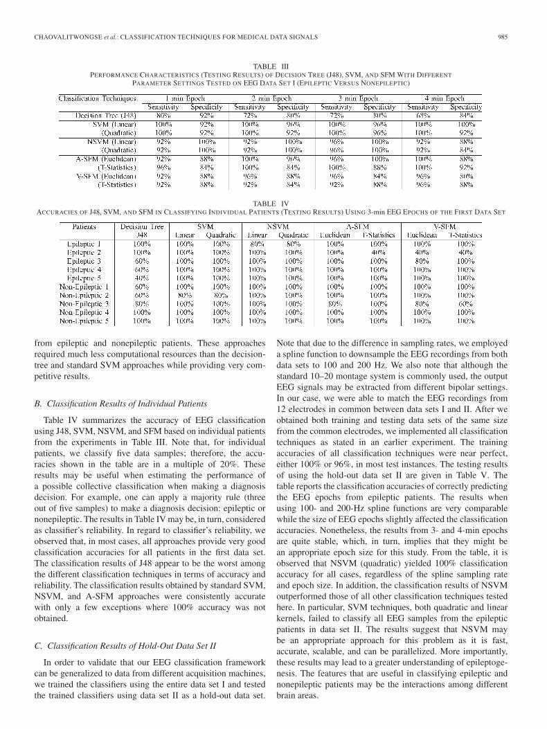
TABLE IIIPERFORMANCE CHARACTERISTICS (TESTING RESULTS) OF DECISION TREE (J48), SVM, AND SFM WITH DIFFERENT

PARAMETER SETTINGS TESTED ON EEG DATA SET I (EPILEPTIC VERSUS NONEPILEPTIC)

TABLE IVACCURACIES OF J48, SVM, AND SFM IN CLASSIFYING INDIVIDUAL PATIENTS (TESTING RESULTS) USING 3-min EEG EPOCHS OF THE FIRST DATA SET

from epileptic and nonepileptic patients. These approachesrequired much less computational resources than the decision-tree and standard SVM approaches while providing very com-petitive results.

B. Classification Results of Individual Patients

Table IV summarizes the accuracy of EEG classificationusing J48, SVM, NSVM, and SFM based on individual patientsfrom the experiments in Table III. Note that, for individualpatients, we classify five data samples; therefore, the accu-racies shown in the table are in a multiple of 20%. Theseresults may be useful when estimating the performance ofa possible collective classification when making a diagnosisdecision. For example, one can apply a majority rule (threeout of five samples) to make a diagnosis decision: epileptic ornonepileptic. The results in Table IV may be, in turn, consideredas classifier’s reliability. In regard to classifier’s reliability, weobserved that, in most cases, all approaches provide very goodclassification accuracies for all patients in the first data set.The classification results of J48 appear to be the worst amongthe different classification techniques in terms of accuracy andreliability. The classification results obtained by standard SVM,NSVM, and A-SFM approaches were consistently accuratewith only a few exceptions where 100% accuracy was notobtained.

C. Classification Results of Hold-Out Data Set II

In order to validate that our EEG classification frameworkcan be generalized to data from different acquisition machines,we trained the classifiers using the entire data set I and testedthe trained classifiers using data set II as a hold-out data set.

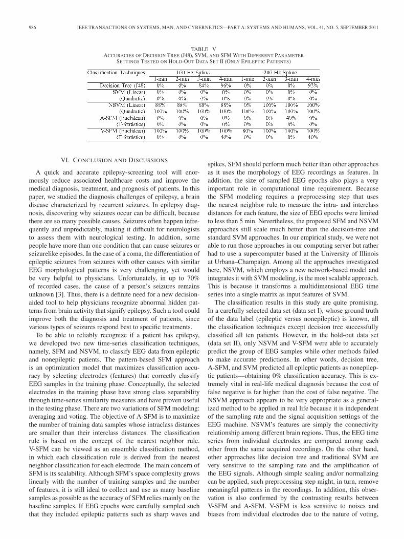
Note that due to the difference in sampling rates, we employeda spline function to downsample the EEG recordings from bothdata sets to 100 and 200 Hz. We also note that although thestandard 10–20 montage system is commonly used, the outputEEG signals may be extracted from different bipolar settings.In our case, we were able to match the EEG recordings from12 electrodes in common between data sets I and II. After weobtained both training and testing data sets of the same sizefrom the common electrodes, we implemented all classificationtechniques as stated in an earlier experiment. The trainingaccuracies of all classification techniques were near perfect,either 100% or 96%, in most test instances. The testing resultsof using the hold-out data set II are given in Table V. Thetable reports the classification accuracies of correctly predictingthe EEG epochs from epileptic patients. The results whenusing 100- and 200-Hz spline functions are very comparablewhile the size of EEG epochs slightly affected the classificationaccuracies. Nonetheless, the results from 3- and 4-min epochsare quite stable, which, in turn, implies that they might bean appropriate epoch size for this study. From the table, it isobserved that NSVM (quadratic) yielded 100% classificationaccuracy for all cases, regardless of the spline sampling rateand epoch size. In addition, the classification results of NSVMoutperformed those of all other classification techniques testedhere. In particular, SVM techniques, both quadratic and linearkernels, failed to classify all EEG samples from the epilepticpatients in data set II. The results suggest that NSVM maybe an appropriate approach for this problem as it is fast,accurate, scalable, and can be parallelized. More importantly,these results may lead to a greater understanding of epileptoge-nesis. The features that are useful in classifying epileptic andnonepileptic patients may be the interactions among differentbrain areas.

986 IEEE TRANSACTIONS ON SYSTEMS, MAN, AND CYBERNETICS—PART A: SYSTEMS AND HUMANS, VOL. 41, NO. 5, SEPTEMBER 2011

TABLE VACCURACIES OF DECISION TREE (J48), SVM, AND SFM WITH DIFFERENT PARAMETER

SETTINGS TESTED ON HOLD-OUT DATA SET II (ONLY EPILEPTIC PATIENTS)

VI. CONCLUSION AND DISCUSSIONS

A quick and accurate epilepsy-screening tool will enor-mously reduce associated healthcare costs and improve themedical diagnosis, treatment, and prognosis of patients. In thispaper, we studied the diagnosis challenges of epilepsy, a braindisease characterized by recurrent seizures. In epilepsy diag-nosis, discovering why seizures occur can be difficult, becausethere are so many possible causes. Seizures often happen infre-quently and unpredictably, making it difficult for neurologiststo assess them with neurological testing. In addition, somepeople have more than one condition that can cause seizures orseizurelike episodes. In the case of a coma, the differentiation ofepileptic seizures from seizures with other causes with similarEEG morphological patterns is very challenging, yet wouldbe very helpful to physicians. Unfortunately, in up to 70%of recorded cases, the cause of a person’s seizures remainsunknown [3]. Thus, there is a definite need for a new decision-aided tool to help physicians recognize abnormal hidden pat-terns from brain activity that signify epilepsy. Such a tool couldimprove both the diagnosis and treatment of patients, sincevarious types of seizures respond best to specific treatments.

To be able to reliably recognize if a patient has epilepsy,we developed two new time-series classification techniques,namely, SFM and NSVM, to classify EEG data from epilepticand nonepileptic patients. The pattern-based SFM approachis an optimization model that maximizes classification accu-racy by selecting electrodes (features) that correctly classifyEEG samples in the training phase. Conceptually, the selectedelectrodes in the training phase have strong class separabilitythrough time-series similarity measures and have proven usefulin the testing phase. There are two variations of SFM modeling:averaging and voting. The objective of A-SFM is to maximizethe number of training data samples whose intraclass distancesare smaller than their interclass distances. The classificationrule is based on the concept of the nearest neighbor rule.V-SFM can be viewed as an ensemble classification method,in which each classification rule is derived from the nearestneighbor classification for each electrode. The main concern ofSFM is its scalability. Although SFM’s space complexity growslinearly with the number of training samples and the numberof features, it is still ideal to collect and use as many baselinesamples as possible as the accuracy of SFM relies mainly on thebaseline samples. If EEG epochs were carefully sampled suchthat they included epileptic patterns such as sharp waves and

spikes, SFM should perform much better than other approachesas it uses the morphology of EEG recordings as features. Inaddition, the size of sampled EEG epochs also plays a veryimportant role in computational time requirement. Becausethe SFM modeling requires a preprocessing step that usesthe nearest neighbor rule to measure the intra- and interclassdistances for each feature, the size of EEG epochs were limitedto less than 5 min. Nevertheless, the proposed SFM and NSVMapproaches still scale much better than the decision-tree andstandard SVM approaches. In our empirical study, we were notable to run those approaches in our computing server but ratherhad to use a supercomputer based at the University of Illinoisat Urbana–Champaign. Among all the approaches investigatedhere, NSVM, which employs a new network-based model andintegrates it with SVM modeling, is the most scalable approach.This is because it transforms a multidimensional EEG timeseries into a single matrix as input features of SVM.

The classification results in this study are quite promising.In a carefully selected data set (data set I), whose ground truthof the data label (epileptic versus nonepileptic) is known, allthe classification techniques except decision tree successfullyclassified all ten patients. However, in the hold-out data set(data set II), only NSVM and V-SFM were able to accuratelypredict the group of EEG samples while other methods failedto make accurate predictions. In other words, decision tree,A-SFM, and SVM predicted all epileptic patients as nonepilep-tic patients—obtaining 0% classification accuracy. This is ex-tremely vital in real-life medical diagnosis because the cost offalse negative is far higher than the cost of false negative. TheNSVM approach appears to be very appropriate as a general-ized method to be applied in real life because it is independentof the sampling rate and the signal acquisition settings of theEEG machine. NSVM’s features are simply the connectivityrelationship among different brain regions. Thus, the EEG timeseries from individual electrodes are compared among eachother from the same acquired recordings. On the other hand,other approaches like decision tree and traditional SVM arevery sensitive to the sampling rate and the amplification ofthe EEG signals. Although simple scaling and/or normalizingcan be applied, such preprocessing step might, in turn, removemeaningful patterns in the recordings. In addition, this obser-vation is also confirmed by the contrasting results betweenV-SFM and A-SFM. V-SFM is less sensitive to noises andbiases from individual electrodes due to the nature of voting,

CHAOVALITWONGSE et al.: CLASSIFICATION TECHNIQUES FOR MEDICAL DATA SIGNALS 987

i.e., every selected electrode equally contributes a vote of one.On the other hand, A-SFM may be biased by some selectedelectrodes with a higher scale of similarity distance. Althoughthe results in this experiment appear to be conclusive, it wouldbe ideal if we were able to obtain a hold-out data set thatcontains nonepileptic patients. In practice, carefully selecteddata sets with known labels (epileptic versus nonepileptic) areextremely hard to obtain due to the fact that it takes severalmonths or years for physicians to ascertain whether a patient isepileptic or nonepileptic.

ACKNOWLEDGMENT

The authors would like to thank R. C. Sachdeo, M.D.,D. Tikku, M.D., and B. Y. Wu, M.D., Ph.D. for providing in-sightful information and discussion that has led us to investigatethe problem addressed in this study.

REFERENCES

[1] O. Cockerell, I. Eckle, D. Goodridge, J. Sander, and S. Shorvon, “Epilepsyin a population of 6000 re-examined: Secular trends in first attendancerates, prevalence, and prognosis,” J. Neurol., Neurosurg., Psychiatry,vol. 58, no. 5, pp. 570–576, May 1995.

[2] W.H.O. (WHO), Epilepsy: Historical Overview, 2004. [Online].Available: http://www.who.int/mediacentre/factsheets/fs168/en/

[3] Epilepsy Foundation, Epilepsy Foundation—Not Another Moment Lost toSeizures, 2006. [Online]. Available: http://www.epilepsyfoundation.org

[4] C. A. van Donselaar, H. Stroink, and W.-F. Arts, “How confident arewe of the diagnosis of epilepsy?” Epilepsia, vol 47, no. S1, pp. 9–13,Oct. 2006.

[5] Y. Kakizawa, R. Shumway, and M. Taniguchi, “Discrimination and clus-tering for multivariate time series,” J. Amer. Stat. Assoc., vol. 93, no. 441,pp. 328–340, Mar. 1998.

[6] W. Hsieh, “Nonlinear multivariate and time series analysis by neuralnetwork methods,” Rev. Geophys., vol. 42, p. RG1 003, 2004.

[7] M. Kadous and C. Sammut, “Constructive induction for classifying timeseries,” in Proc. ECML, vol. 3201. Berlin, Germany: Springer-Verlag,2004, pp. 192–204.

[8] K. Yang, H. Yoon, and C. Shahabi, “A supervised feature subset selectiontechnique for multivariate time series,” in Proc. Int. Workshop FSDM:Interfacing Mach. Learn. With Statist. in conjunction with SIAM Int. Conf.Data Mining (SDM), Newport Beach, CA, Apr. 2005.

[9] X. Song, M. Wu, C. Jermaine, and S. Ranka, “Statistical change detec-tion for multi-dimensional data,” in Proc. 13th ACM SIGKDD Int. Conf.Knowl. Discov. Data Mining, 2007, pp. 667–676.

[10] D. Dou, G. Frishkoff, J. Rong, R. Frank, A. Malony, and D. Tucker, “De-velopment of neuroelectromagnetic ontologies (NEMO): A framework formining brain wave ontologies,” in Proc. 13th ACM SIGKDD Int. Conf.Knowl. Discov. Data Mining, 2007, pp. 270–279.

[11] W. Chaovalitwongse, P. Pardalos, and O. Prokoyev, “Electroencephalo-gram (EEG) time series classification: Applications in epilepsy,”Ann. Oper. Res., vol. 148, no. 1, pp. 227–250, Nov. 2006.

[12] W. Chaovalitwongse, Y. Fan, and R. Sachdeo, “On the time seriesk-nearest neighbor for abnormal brain activity classification,” IEEE Trans.Syst., Man, Cybern. A, Syst., Humans, vol. 37, no. 6, pp. 1005–1016,Nov. 2007.

[13] W. Chaovalitwongse, Y. Fan, and R. Sachdeo, “Support feature machinefor classification of abnormal brain activity,” in Proc. 13th ACM SIGKDDInt. Conf. Knowl. Discov. Data Mining, 2007, pp. 113–122.

[14] W. Chaovalitwongse, Y. Fan, and R. Sachdeo, “Novel optimization mod-els for abnormal brain activity classification,” Oper. Res., vol. 56, no. 6,pp. 1450–1460, Nov./Dec. 2008.

[15] A. Babloyantz and A. Destexhe, “Low dimensional chaos in an instanceof epilepsy,” Proc. Nat. Acad. Sci. U.S.A., vol. 83, no. 10, pp. 3513–3517,May 1986.

[16] L. Iasemidis, H. Zaveri, J. Sackellares, and W. Williams, “Phase spaceanalysis of EEG in temporal lobe epilepsy,” in Proc. 10th Annu. Int. Conf.IEEE Eng. Med. Biol. Soc., 1988, pp. 1201–1203.

[17] N. Packard, J. Crutchfield, and J. Farmer, “Geometry from time series,”Phys. Rev. Lett., vol. 45, no. 9, pp. 712–716, Sep. 1980.

[18] P. Rapp, I. Zimmerman, and A. M. Albano, “Experimental stud-ies of chaotic neural behavior: Cellular activity and electroencephalo-graphic signals,” in Nonlinear Oscillations in Biology and Chemistry,H. Othmer, Ed. Berlin, Germany: Springer-Verlag, 1986, pp. 175–205.

[19] F. Takens, “Detecting strange attractors in turbulence,” in Dynami-cal Systems and Turbulence, vol. 898, Lecture Notes in Mathematics,D. Rand and L. Young, Eds. Berlin, Germany: Springer-Verlag, 1981,pp. 366–381.

[20] J. Quinlan, C4.5: Programs for Machine Learning. San Mateo, CA:Morgan Kaufmann, 1993.

[21] C. Shannon, “A mathematical theory of communication,” Bell Syst. Tech.J., vol. 27, pp. 379–423, Jul. 1948.

[22] S. Ruggieri, “Efficient C4.5,” IEEE Trans. Knowl. Data Eng., vol. 14,no. 2, pp. 438–444, Mar./Apr. 2002.

[23] O. Yildiz and O. Dikmen, “Parallel univariate decision trees,” PatternRecognit. Lett., vol. 28, no. 7, pp. 825–832, May 2007.

[24] S. Baik and J. Bala, “A decision tree algorithm for distributed data mining:Towards network intrusion detection,” in Proc. Int. Conf. Comput. Sci.Appl., 2004, vol. 3046, pp. 206–212.

[25] N. Cristianini and J. Taylor, An Introduction to Support Vector Ma-chines and Other Kernel-Based Learning Methods. Cambridge, U.K.:Cambridge Univ. Press, 2000.

[26] K. P. Bennett and O. L. Mangasarian, “Robust linear programming dis-crimination of two linearly inseparable sets,” Optim. Methods Softw.,vol. 1, no. 1, pp. 23–34, 1992.

[27] P. Bradley, U. Fayyad, and O. Mangasarian, “Mathematical programmingfor data mining: Formulations and challenges,” INFORMS J. Comput.,vol. 11, no. 3, pp. 217–238, 1999.

[28] O. Mangasarian, W. Street, and W. Wolberg, “Breast cancer diagnosis andprognosis via linear programming,” Oper. Res., vol. 43, no. 4, pp. 570–577, Jul./Aug. 1995.

[29] L. Breiman, J. Friedman, R. Olsen, and C. Stone, Classification andRegression Trees. Belmont, CA: Wadsworth, 1993.

[30] B. Schölkopf, C. Burges, and V. Vapnik, “Extracting support data fora given task,” in Proc. 1st Int. Conf. Knowl. Discov. Data Mining,U. M. Fayyad and R. Uthurusamy, Eds., 1995, pp. 252–257.

[31] V. Blanz, B. Scholkopf, H. Bulthoff, C. Burges, V. Vapnik, and T. Vetter,“Comparison of view-based object recognition algorithms using realistic3D models,” in Proc. ICANN, vol. 1112. Berlin, Germany: Springer-Verlag, 1996, pp. 251–256.

[32] M. Schmidt, “Identifying speaker with support vector networks,” in Proc.Interface, Sydney, Australia, 1996.

[33] E. Osuna, R. Freund, and F. Girosi, “Training support vector machines: Anapplication to face detection,” in Proc. IEEE Conf. Comput. Vis. PatternRecog., 1997, pp. 130–136.

[34] T. Joachims, “Text categorization with support vector machines: Learningwith many relevant features,” in Proc. 10th Eur. Conf. Mach. Learn.,Chemnitz, Germany, Apr. 1998, vol. 1398, pp. 137–142.

[35] C.-W. Hsu and C.-J. Lin, “A comparison of methods multi-class supportvector machines,” IEEE Trans. Neural Netw., vol. 13, no. 2, pp. 415–425,Mar. 2002.

[36] U. Krebel, “Pairwise classification and support vector machines,” in Ad-vances in Kernel Methods—Support Vector Learning. Cambridge, MA:MIT Press, 1999, pp. 255–268.

[37] C. Burges, “Tutorial on support vector machines for pattern recognition,”Data Mining Knowl. Discov., vol. 2, pp. 121–167, 1998.

[38] H. Shimodaira, K. ichi Noma, M. Naka, and S. Sagayama, “Support vectormachine with dynamic time-alignment kernel for speech recognition,” inProc. Eurospeech, 2001, pp. 1841–1844.

[39] S. Rüping, “SVM kernels for time series analysis,” in Proc.LLWA—Tagungsband der GI-Workshop-Woche Lernen-Lehren-Wissen-Adaptivität, R. Klinkenberg, S. Rüping, A. Fick, N. Henze, C. Herzog,R. Molitor, and O. Schröder, Eds., 2001, pp. 43–50.

[40] V. Wan and J. Carmichael, “Polynomial dynamic time warping kernelsupport vector machines for dysarthric speech recognition with sparsetraining data,” in Proc. Interspeech, 2005, pp. 3321–3324.

[41] K. M. Borgwardt, S. Vishwanathan, and H.-P. Kriegel, “Classprediction from time series gene expression profiles using dyna-mical systems kernels,” in Proc. Pacific Symp. Biocomputing, 2006,pp. 547–558.

[42] K. Yang and C. Shahabi, “A PCA-based kernel for kernel PCA on mul-tivariate time series,” in Proc. ICDM Workshop Temporal Data Mining:Algorithms, Theory and Applications held in conjunction with 5th IEEEICDM, 2005.

[43] D. Pham and A. Chan, “Control chart pattern recognition using a newtype of self organizing neural network,” in Proc. Inst. Mech. Eng. I, J.Syst. Control Eng., 1998, vol. 212, no. 2, pp. 115–127.

988 IEEE TRANSACTIONS ON SYSTEMS, MAN, AND CYBERNETICS—PART A: SYSTEMS AND HUMANS, VOL. 41, NO. 5, SEPTEMBER 2011

[44] E. Keogh and M. Pazzani, “An enhanced representation of time serieswhich allows fast and accurate classification, clustering and relevancefeedback,” in Proc. 4th ACM SIGKDD Int. Conf. Knowl. Discov. DataMining, 1998, pp. 239–241.

[45] R. Olszewski, “Generalized feature extraction for structural pattern recog-nition in time-series data,” Ph.D. dissertation, Carnegie Mellon Univ.,Pittsburgh, PA, 2001.

[46] D. Eads, D. Hill, S. Davis, S. Perkins, J. Ma, R. Porter, and J. Theiler,“Genetic algorithms and support vector machines for time series classifi-cation,” Proc. SPIE, vol. 4787, pp. 74–85, 2002.

[47] P. Geurts, “Contributions to decision tree induction: Bias/variance tradeoffand time series classification,” Ph.D. dissertation, Univ. Liege, Liege,Belgium, 2002.

[48] E. Keogh and S. Kasetty, “On the need for time series data miningbenchmarks: A survey and empirical demonstration,” in Proc. 8th ACMSIGKDD Int. Conf. Knowl. Discov. Data Mining, 2002, pp. 102–111.

[49] B. Chiu, E. Keogh, and S. Lonardi, “Probabilistic discovery of time seriesmotifs,” in Proc. 9th ACM SIGKDD Int. Conf. Knowl. Discov. DataMining, 2003, pp. 493–498.

[50] X. Xi, E. Keogh, C. Shelton, L. Wei, and C. A. Ratanamahatana, “Fasttime series classification using numerosity reduction,” in Proc. 23rd Int.Conf. Mach. Learn., 2006, vol. 148, pp. 1033–1040.

[51] A. Mueen, E. Keogh, Q. Zhu, S. Cash, and B. Westover, “Exact discoveryof time series motifs,” in Proc. SIAM Int. Conf. Data Mining (SDM), 2009,pp. 473–484.

[52] O. Omitaomu, M. Jeong, and A. Badiru, “Online support vector regressionwith varying parameters for time-dependent data,” IEEE Trans. Syst.,Man, Cybern. A, Syst., Humans, vol. 41, no. 1, pp. 191–197, Jan. 2011.

[53] B. Scholkopf, “The kernel trick for distances,” in Proc. Adv. Neural Inf.Process. Syst., 2001, pp. 301–307.

[54] B. Efron, “Estimating the error rate of a prediction rule: Improvement oncross-validation,” J. Amer. Stat. Assoc., vol. 78, no. 382, pp. 316–331,Jun. 1983.

[55] I. H. Witten and E. Frank, Data Mining: Practical Machine LearningTools and Techniques, 2nd ed. San Mateo, CA: Morgan Kaufmann,2005.

Wanpracha Art Chaovalitwongse (M’05–SM’11)received the B.S. degree in telecommunicationengineering from King Mongkut’s Institute ofTechnology Ladkrabang, Bangkok, Thailand, in1999 and the M.S. and Ph.D. degrees in industrialand systems engineering from the University ofFlorida, Gainesville, in 2000 and 2003, respectively.

He is an Associate Professor of Industrialand Systems Engineering with Rutgers University,Piscataway, NJ. Before joining Rutgers, he was withCorporate Strategic Research, ExxonMobil Research

and Engineering Company, in 2004, where he managed research in developingefficient mathematical models and novel statistical data analyses for upstreamand downstream business operations.

Rebecca S. Pottenger is a rising junior atPrinceton University, Princeton, NJ, in the Depart-ment of Computer Science.

She has been interested and involved in data min-ing research since her junior year of high school.In 2007, she conducted a research project enti-tled “Classifying String Quartets by Composer viaData Mining” which she presented at the Consor-tium for Computing Science in Colleges (2007),Fredericksburg, MD, and published in the Proceed-ings of the IEEE 2006 Lehigh Valley Science Tech-

nology Engineering and Math Conference, Bethlehem, PA, in November. Shepreviously worked with Prof. W. Art Chaovaltiwongse at Rutgers University,Piscataway, NJ, through the Rutgers/Center for Discrete Mathematics and The-oretical Computer Science Research Experience for Undergraduates Program,studying the classification of epileptic patients.

Shouyi Wang received the B.S. degree in controlscience and engineering from Harbin Institute ofTechnology, Harbin, China, in 2003 and the M.S.degree in systems and control engineering from DelftUniversity of Technology, Delft, The Netherlands,in 2005. Currently, he is working toward the Ph.D.degree in the Department of Industrial and SystemsEngineering, Rutgers University, Piscataway, NJ, un-der the supervision of Prof. W. Art Chaovaltiwongse.

His current research interests include data miningand pattern discovery, machine learning, intelligent

decision-making systems, multivariate time-series modeling, and forecasting.

Ya-Ju Fan received the B.B.A. degree in productionand operations management from Fu Jen CatholicUniversity, Taipei, Taiwan, and the M.S. degree inindustrial engineering from the University ofWisconsin, Madison. In the fall of 2006, she joinedthe graduate program in the Department of In-dustrial and Systems Engineering, Rutgers Univer-sity, Piscataway, NJ, to work with Prof. W. ArtChaovalitwongse. She received the Ph.D. degreefrom the Rutgers University in 2010.

Leon D. Iasemidis (M’96) received the Diplomadegree in electrical and electronics engineering fromthe National Technical University of Athens, Athens,Greece, in 1982 and the M.S. degree in physics andthe M.S. and Ph.D. degrees in biomedical engineer-ing from the University of Michigan, Ann Arbor, in1985, 1986, and 1991, respectively.

From 1991 to 1993, he was a PostdoctoralFellow with the Departments of Electrical Engineer-ing and Neurology, University of Michigan, AnnArbor. From 1993 to 2000, he was the Director

of the Clinical Neurophysiology Laboratory and the Founder of the BrainDynamics Laboratory at the Malcolm Randall VA Medical Center, Gainesville,FL, and a Research Assistant Professor with the Departments of ElectricalEngineering, Neurology, and Neuroscience, University of Florida, Gainesville.Since 2000, he has been an Associate Professor of Bioengineering with theArizona State University (ASU), Tempe, and the Director and Founder of theASU Brain Dynamics Laboratory. He is recognized as an expert in the dynamicsof epileptic seizures, and his research and publications have stimulated aninternational interest in the prediction and control of epileptic seizures and theunderstanding of the mechanisms of epileptogenesis.