Annals of Nuclear Energy 63 (2014) 371–381

Contents lists available at ScienceDirect

Annals of Nuclear Energy

journal homepage: www.elsevier .com/locate /anucene

Numerically stable Monte Carlo-burnup-thermal hydraulic couplingschemes

0306-4549/$ - see front matter � 2013 Elsevier Ltd. All rights reserved.http://dx.doi.org/10.1016/j.anucene.2013.08.016

⇑ Corresponding author. Tel.: +972 86472175.E-mail address: kotlyar@bgu.ac.il (D. Kotlyar).

D. Kotlyar ⇑, E. ShwagerausDepartment of Nuclear Engineering, Ben-Gurion University, POB 653, Beer Sheva 84105, Israel

a r t i c l e i n f o

Article history:Received 23 May 2013Received in revised form 28 July 2013Accepted 2 August 2013

Keywords:Monte CarloDepletionNeutronic thermal hydraulic couplingBGCoreImplicit methodSIMP

a b s t r a c t

This paper presents stochastic implicit coupling method intended for use in Monte-Carlo (MC) basedreactor analysis systems that include burnup and thermal hydraulic (TH) feedbacks. Both feedbacksare essential for accurate modeling of advanced reactor designs and analyses of associated fuel cycles.In particular, we investigate the effect of different burnup-TH coupling schemes on the numerical stabil-ity and accuracy of coupled MC calculations. First, we present the beginning of time step method which isthe most commonly used. The accuracy of this method depends on the time step length and it is only con-ditionally stable. This work demonstrates that even for relatively short time steps, this method can benumerically unstable. Namely, the spatial distribution of neutronic and thermal hydraulic parameters,such as nuclide densities and temperatures, exhibit oscillatory behavior. To address the numerical stabil-ity issue, new implicit stochastic methods are proposed. The methods solve the depletion and TH prob-lems simultaneously and use under-relaxation to speed up convergence. These methods are numericallystable and accurate even for relatively large time steps and require less computation time than the exist-ing methods.

� 2013 Elsevier Ltd. All rights reserved.

1. Introduction

Monte-Carlo (MC) neutron transport codes gain popularity inthe reactor analysis applications due to their flexibility in simulat-ing complex fuel and core geometries without any significantapproximations. However, MC codes lack the ability to performtime-dependent burnup calculations and, therefore, must be cou-pled with external codes in order to perform fuel cycle analyses.A number of different methods to couple the MC and burnup codeshave been suggested. The simplest and the most commonly used isthe explicit predictor Euler method. It is used in many MC-burnupcoupling programs and shown to produce accurate results in manypractical applications, for example as shown in Bomboni et al.(2010). Among such coupled codes are MOCUP (Moore et al.,1995), MCODE (Xu et al., 2002), MONTEBURNS (Trellue, 2003),SERPENT (Leppänen, 2007), BGCore (Fridman et al., 2008b),MCNPX (Fensin et al., 2010) and many others.

Recent advances in high performance computing capabilities al-low substantial reduction in execution time of such burnup-MCcodes. This, in turn, enables consideration of problems with muchhigher degree of complexity, such as introduction of thermalhydraulic (TH) feedback into the calculation scheme. In several re-cent studies, coupled MC and TH codes were successfully applied

to model fuel assembly and mini-core size problems. For example,a coupling scheme between MCNP (Briesmeister, 2000) and CO-BRA-TF (Basile et al., 1999) was reported in Sanchez et al. (2009),for the prediction of pin power distribution in a PWR fuel assem-bly. A coupled system MCNP5/SUBCHANFLOW was described inIvanov et al. (2011). It was developed for the fuel pin and assemblywise simulation of LWRs as well as advanced reactors. However, innone of the studies mentioned above, the burnup and TH feedbackswere applied simultaneously. In a recent work, we reported on thedevelopment of a coupled code, BGCore, which is capable of per-forming both depletion and TH analyses. To demonstrate the capa-bilities of BGCore system, a coupled neutronic TH analysis of a fullPWR core was performed and reported in Kotlyar et al. (2011).BGCore produced very good results closely matching those ob-tained with the state of the art 3D deterministic nodal diffusioncode DYN3D (Grundmann et al., 2000).

The current analysis presents a new incremental step in thedirection of fully coupled MC calculation with burnup and TH feed-backs. In addition, various coupling schemes are examined to as-sess their accuracy and numerical stability.

The simplest and the most commonly used approach is thebeginning of time step (BOT) method. However, the explicit natureof this method makes it only conditionally stable. That is, in someproblems, if the time step size used in the calculations is suffi-ciently large, the solution can be numerically instable. It wasshown in Dufek and Hoogenboom (2009); Dufek et al. (2013a)

372 D. Kotlyar, E. Shwageraus / Annals of Nuclear Energy 63 (2014) 371–381

and Kotlyar and Shwageraus (2013) that applying the BOT methodto MC-burnup calculations may result in oscillatory behavior of thespatial flux distribution. To overcome the instability issues, impli-cit methods were proposed (Dufek et al., 2013b) to couple burnupwith MC transport codes.

In the current work, we first show that similar instabilities existin the BOT MC-burnup-TH coupling analyses. The BOT methodwith relatively short time steps is commonly adopted in determin-istic codes because the neutron transport solution is relativelyinexpensive from the computational resources point of view. Onthe other hand, in MC calculations, very short time steps may re-sult in prohibitively high computational costs and, therefore, notpractical for the fuel cycle analysis applications.

In order to address the issue of numerical stability, while keep-ing reasonably low computational costs, two alternative methodsare proposed here. Both methods are referred to as stochastic im-plicit mid-point (SIMP) methods, which, as we will show, producestable and accurate results for the studied test case. In contrast totraditional approach, where TH and burnup iterations are per-formed sequentially, in the proposed methods, the depletion andTH problems are solved simultaneously and iteratively with thetransport problem. The iterative scheme uses a variable relaxationfactor, known as step-size, based on the Robbins–Monro algorithm(1951). An example for the use of variable step-size in reactor anal-ysis at steady state conditions can be found in Dufek and Gudowski(2006). Their work presented the coupling between neutron fluxes,obtained from MC transport calculations, and strong feedbacks,such as coolant density and Xe-135 fission product density.

The SIMP methods proposed here are intended to be applied toMC-burnup-TH coupling problems. As will be demonstrated, notonly both methods are unconditionally stable, because of their im-plicit nature, they also allow using relatively large time steps infuel cycle calculations with minimal effect on the accuracy of theresults. Large time steps allow substantial reduction of computa-tion time.

An additional feature of the proposed methods is in the ap-proach for evaluating different quantities of interest, such as powerand temperature distributions. In fuel depletion analysis, the nu-clide densities are obtained at fixed time points (beginning andend of time steps). This is typically done by assuming that the spa-tial power distribution is constant during the time step and corre-sponds to some fixed point in time (usually beginning of timestep). This assumption is not strictly true, especially if the timesteps are relatively large. Furthermore, the assumption of constantpower during the time step implies fixed TH conditions and alsoleads to neglecting the effect of changing neutron spectrum. Ide-ally, the depletion step should be performed using the ‘‘time stepaverage’’ power, TH conditions and spectrum (cross sections) andnot using these quantities at some fixed point in time, as done bymost of the existing codes. Finding such ‘‘time step average’’parameters necessary for performing the depletion step is the maininnovative feature of the two methods discussed here.

As a test case, we performed depletion of a typical 17 � 17 PWRfuel assembly with reflective boundary conditions in the radialdirection. The assembly was axially divided into multiple burnableand thermal hydraulic zones. This division was introduced in orderto obtain detailed flux distribution and account for the depletionand TH conditions in each burnable region. The calculations wereperformed with BGCore reactor analysis system.

2. Description of BGCore code system

The proposed SIMP methods were programmed into the BGCoresystem. BGCore is a system of codes developed at Ben-Gurion Uni-versity, in which Monte-Carlo code MCNP4C is coupled with fuel

depletion and decay module SARAF. Data library for SARAF is basedon JEFF-3.1 files (Koning et al., 2006). BGCore utilizes multi-groupmethodology for calculation of one group transmutation cross-sec-tions (Haeck and Verboomen, 2007; Fridman et al., 2008a) whichsignificantly improves the speed of burnup calculations. In addi-tion to the depletion module, BGCore system also includes a THfeedbacks module – THERMO. The modules are executed itera-tively so that the coupled system is capable of predicting fuel com-position, power, coolant density and temperature distributions invarious types of reactor systems.

3. Description of burnup-thermal hydraulic coupling methods

The objective of coupled burnup-TH analysis is to obtain the nu-clide field NF(r, t) and the TH properties NT(r, t) as a function ofspace and time. Knowing, NF(r, t) and NT(r, t) allows, then, to deter-mine the spatial, energy and time dependent neutron flux/(r,E, t).However, NF(r, t) and NT(r, t) themselves depend on /(r,E, t). Thatis, /(r,E, t) requires a prior knowledge of NF(r, t) and NT(r, t), whichare both driven by the neutron flux. This non-linear problem can bedescribed by three coupled equations. First one is the burnup equa-tion that determines the nuclide field changes, as described in Eq.(1). The second is the heat balance equation that computes thetemperature distribution from which also the coolant and/or mod-erator densities can be derived. The last is the neutron transporteigenvalue equation that provides the fundamental neutron fluxmode:

Nðr; tÞ ¼ exp½Mð/; TÞðt � t0Þ� � Nðr; t0Þ ð1Þ

In Eq. (1), N(r, t0) describes the nuclide field at time t0. The neu-tron flux /(r,E, t) at time t is determined by the fundamental modeof the neutron transport equation and will be denoted here as ‘‘/B’’. In other words, the operator /BðNFðr;tÞÞ;NTðr;tÞÞ computes /(r,E, t).

The operator M in Eq. (1) is described in following equation:

Mð/; TÞ ¼Z 1

0/ðr; E; tÞXðTÞdEþ D ð2Þ

where X is a cross section and fission yields matrix, D is a decay ma-trix, and T(r, t) is the temperature at point r and time t. T(r, t) is ob-tained by solving heat conduction and convection problem and willbe denoted here by the operator ’T’. Consequently, the operator T(/)computes T(r, t).

There are various schemes to couple the burnup and TH feed-backs with the neutron transport equation. The most commonlyused BOT method is based on dividing the entire irradiation timeinterval into ‘‘small’’ time step increments. Fixed time point THiterations are performed at BOT until convergence on power distri-bution or reaction rates is achieved. Then, the space and energydependent microscopic reaction rates are assumed to be constantduring each time step. Knowing these reaction rates allows obtain-ing the concentration at the EOT in a single calculation step. Thismethod is known as the explicit Euler method. The accuracy ofthe BOT method obviously depends on the time step length. Fur-thermore, it is only conditionally stable. As mentioned earlier,short time steps would require prohibitively high computationalresources and, as a result, will be not practical in fuel cycleanalysis.

Therefore, two alternative methods are proposed. Both methodsare implicit in nature and therefore avoid the numerical oscilla-tions. The implicit solution is obtained by using the so-called sto-chastic approximation. The mathematical derivation of themethods is presented in the following section along with the algo-rithms for each of the burnup-TH coupling procedures. The nomen-clature is given in Table 1.

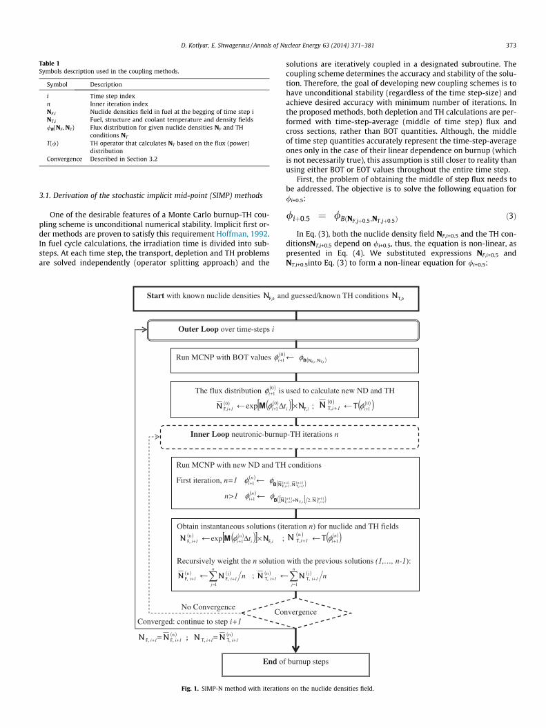
Table 1Symbols description used in the coupling methods.

Symbol Description

i Time step indexn Inner iteration indexNF,i Nuclide densities field in fuel at the begging of time step iNT,i Fuel, structure and coolant temperature and density fields/B(NF, NT) Flux distribution for given nuclide densities NF and TH

conditions NT

T(/) TH operator that calculates NT based on the flux (power)distribution

Convergence Described in Section 3.2

D. Kotlyar, E. Shwageraus / Annals of Nuclear Energy 63 (2014) 371–381 373

3.1. Derivation of the stochastic implicit mid-point (SIMP) methods

One of the desirable features of a Monte Carlo burnup-TH cou-pling scheme is unconditional numerical stability. Implicit first or-der methods are proven to satisfy this requirement Hoffman, 1992.In fuel cycle calculations, the irradiation time is divided into sub-steps. At each time step, the transport, depletion and TH problemsare solved independently (operator splitting approach) and the

Fig. 1. SIMP-N method with iteration

solutions are iteratively coupled in a designated subroutine. Thecoupling scheme determines the accuracy and stability of the solu-tion. Therefore, the goal of developing new coupling schemes is tohave unconditional stability (regardless of the time step-size) andachieve desired accuracy with minimum number of iterations. Inthe proposed methods, both depletion and TH calculations are per-formed with time-step-average (middle of time step) flux andcross sections, rather than BOT quantities. Although, the middleof time step quantities accurately represent the time-step-averageones only in the case of their linear dependence on burnup (whichis not necessarily true), this assumption is still closer to reality thanusing either BOT or EOT values throughout the entire time step.

First, the problem of obtaining the middle of step flux needs tobe addressed. The objective is to solve the following equation for/i+0.5:

/iþ0:5 ¼ /BðNF;jþ0:5;NT;jþ0:5Þ ð3Þ

In Eq. (3), both the nuclide density field NF,i+0.5 and the TH con-ditionsNT,i+0.5 depend on /i+0.5, thus, the equation is non-linear, aspresented in Eq. (4). We substituted expressions NF,i+0.5 andNT,i+0.5into Eq. (3) to form a non-linear equation for /i+0.5:

s on the nuclide densities field.

374 D. Kotlyar, E. Shwageraus / Annals of Nuclear Energy 63 (2014) 371–381

/iþ0:5 ¼ /B ½NF;iþexp½Mð/iþ0:5DtiÞ��NF;i�=2;Tð/iþ0:5Þð Þ ð4Þ

where T(/) and M(/) are the TH and the transmutation matrixoperators, respectively, as were defined at the beginning of thischapter. It should be noted that in Eq. (4), the average flux isassumed to be proportional to the middle of step nuclidedensity NF,i+0.5. In this derivation, we assume that NF,i+0.5 can beobtained by using linear interpolation of the nuclide density field(NF,i + NF,i+l)/2.

Dufek and Gudowski (2006) presented a solution to such non-linear stochastic root-finding problem as described in Eq. (4). Theproblems of this nature are often transformed into a stochasticoptimization problem that aims at finding a minimum of a stochas-tic objective function. The stochastic optimization problem can besolved most efficiently by the stochastic approximation method,where, the right-hand side of Eq. (4) is approximated by thestochastic function v̂ .

The solution is obtained iteratively until the flux convergence isachieved. In our work, we use similar implicit method that wasderived for MC burnup calculations by Dufek et al. (2013b).However, in this work, we also include the thermal–hydraulicfeedback.

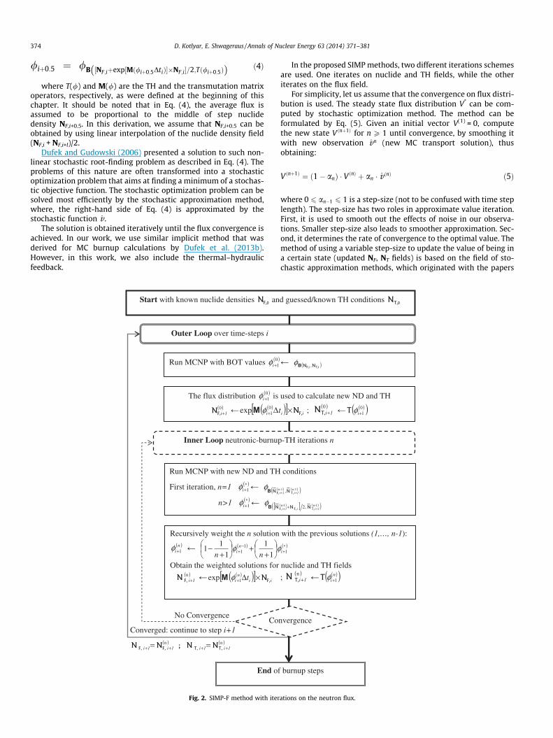
Fig. 2. SIMP-F method with iter

In the proposed SIMP methods, two different iterations schemesare used. One iterates on nuclide and TH fields, while the otheriterates on the flux field.

For simplicity, let us assume that the convergence on flux distri-bution is used. The steady state flux distribution V* can be com-puted by stochastic optimization method. The method can beformulated by Eq. (5). Given an initial vector V(1) = 0, computethe new state V ðnþ1Þ for n P 1 until convergence, by smoothing itwith new observation v̂n (new MC transport solution), thusobtaining:

V ðnþ1Þ ¼ ð1� anÞ � V ðnÞ þ an � v̂ ðnÞ ð5Þ

where 0 6 an�1 6 1 is a step-size (not to be confused with time steplength). The step-size has two roles in approximate value iteration.First, it is used to smooth out the effects of noise in our observa-tions. Smaller step-size also leads to smoother approximation. Sec-ond, it determines the rate of convergence to the optimal value. Themethod of using a variable step-size to update the value of being ina certain state (updated NF, NT fields) is based on the field of sto-chastic approximation methods, which originated with the papers

ations on the neutron flux.

1.2E-08

4

1.15

1.20

1.25

1.30

1.35

1.40

0 50 100 150 200 250 300 350 400Time, days

eige

n va

lue

10d25d50d

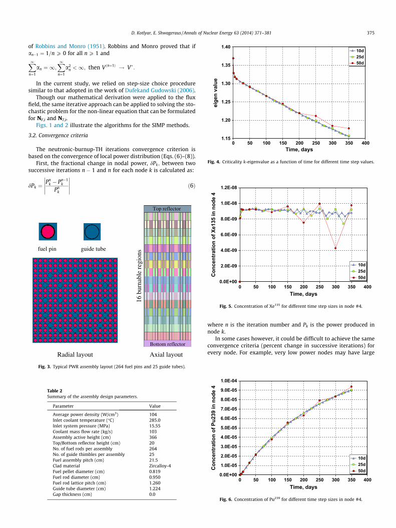
Fig. 4. Criticality k-eigenvalue as a function of time for different time step values.

D. Kotlyar, E. Shwageraus / Annals of Nuclear Energy 63 (2014) 371–381 375

of Robbins and Monro (1951). Robbins and Monro proved that ifan�1 ¼ 1=n P 0 for all n P 1 and

X1n¼1

an ¼ 1;X1n¼1

a2n <1; then V ðnþ1Þ ! V�:

In the current study, we relied on step-size choice proceduresimilar to that adopted in the work of Dufekand Gudowski (2006).

Though our mathematical derivation were applied to the fluxfield, the same iterative approach can be applied to solving the sto-chastic problem for the non-linear equation that can be formulatedfor NF,i and NT,i.

Figs. 1 and 2 illustrate the algorithms for the SIMP methods.

3.2. Convergence criteria

The neutronic-burnup-TH iterations convergence criterion isbased on the convergence of local power distribution (Eqs. (6)–(8)).

First, the fractional change in nodal power, dPk; between twosuccessive iterations n � 1 and n for each node k is calculated as:

dPk ¼Pn

k � Pn�1k

Pnk

���������� ð6Þ

guide tube fuel pin

Radial layout Axial layout

Top reflector

Bottom reflector

16 b

urna

ble

regi

ons

Fig. 3. Typical PWR assembly layout (264 fuel pins and 25 guide tubes).

Table 2Summary of the assembly design parameters.

Parameter Value

Average power density (W/cm3) 104Inlet coolant temperature (�C) 285.0Inlet system pressure (MPa) 15.55Coolant mass flow rate (kg/s) 103Assembly active height (cm) 366Top/Bottom reflector height (cm) 20No. of fuel rods per assembly 264No. of guide thimbles per assembly 25Fuel assembly pitch (cm) 21.5Clad material Zircalloy-4Fuel pellet diameter (cm) 0.819Fuel rod diameter (cm) 0.950Fuel rod lattice pitch (cm) 1.260Guide tube diameter (cm) 1.224Gap thickness (cm) 0.0

0.0E+00

2.0E-09

4.0E-09

6.0E-09

8.0E-09

1.0E-08

0 50 100 150 200 250 300 350 400Time, days

Con

cent

ratio

n of

Xe1

35 in

nod

e

10d25d50d

Fig. 5. Concentration of Xe135 for different time step sizes in node #4.

where n is the iteration number and Pk is the power produced innode k.

In some cases however, it could be difficult to achieve the sameconvergence criteria (percent change in successive iterations) forevery node. For example, very low power nodes may have large

0.0E+00

1.0E-05

2.0E-05

3.0E-05

4.0E-05

5.0E-05

6.0E-05

7.0E-05

8.0E-05

9.0E-05

1.0E-04

Time, days

Con

cent

ratio

n of

Pu2

39 in

nod

e 4

10d25d50d

0 50 100 150 200 250 300 350 400

Fig. 6. Concentration of Pu239 for different time step sizes in node #4.

1200

1400

1600

1800

e di

strib

utio

n 200250300

376 D. Kotlyar, E. Shwageraus / Annals of Nuclear Energy 63 (2014) 371–381

fluctuations due to the poor MC statistics and, thus, may nevermeet the convergence criterion. Therefore, fractional change in no-dal power from iteration to iteration is weighted with relativeimportance (relative power) of the node:

hk ¼PkP

Pkð7Þ

Then, the weighted fractional difference in the power of eachnode is compared with the convergence criterion eP:

maxjhk � dPkj < eP ð8Þ

In this case, the high power (high importance) nodes will havemore stringent convergence criteria, while the criteria in the lowpower nodes will be more relaxed.

In this study, eP was arbitrarily chosen to be 2 � 10�4.

0

200

400

600

800

1000

0 50 100 150 200 250 300 350 400Height, cm

Cen

ter l

ine

tem

pera

tur

(a) time step size = 50 days

0

200

400

600

800

1000

1200

1400

1600

1800

Height, cm

Cen

ter l

ine

tem

pera

ture

dis

trib

utio

n 225250275

(b) time step size = 25 days

0

200

400

600

800

1000

1200

1400

1600

1800

Height, cm

Cen

ter l

ine

tem

pera

ture

dis

trib

utio

n 210220230

(c) time step size = 10 days

0 50 100 150 200 250 300 350 400

0 50 100 150 200 250 300 350 400

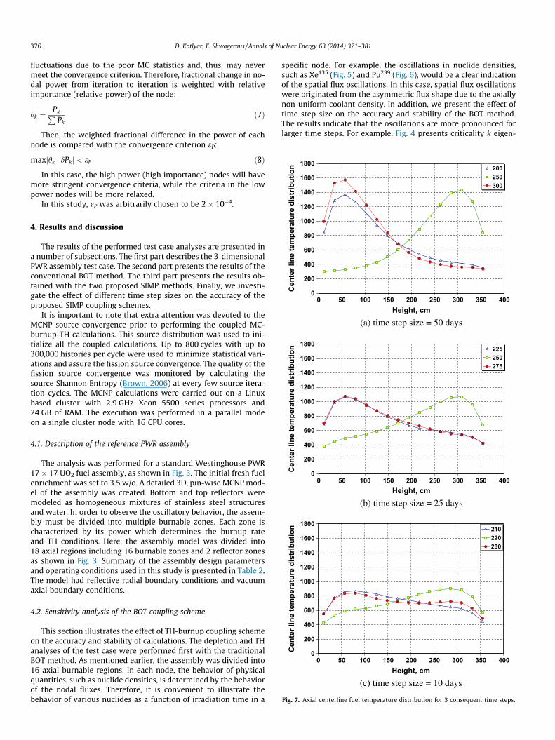
Fig. 7. Axial centerline fuel temperature distribution for 3 consequent time steps.

4. Results and discussion

The results of the performed test case analyses are presented ina number of subsections. The first part describes the 3-dimensionalPWR assembly test case. The second part presents the results of theconventional BOT method. The third part presents the results ob-tained with the two proposed SIMP methods. Finally, we investi-gate the effect of different time step sizes on the accuracy of theproposed SIMP coupling schemes.

It is important to note that extra attention was devoted to theMCNP source convergence prior to performing the coupled MC-burnup-TH calculations. This source distribution was used to ini-tialize all the coupled calculations. Up to 800 cycles with up to300,000 histories per cycle were used to minimize statistical vari-ations and assure the fission source convergence. The quality of thefission source convergence was monitored by calculating thesource Shannon Entropy (Brown, 2006) at every few source itera-tion cycles. The MCNP calculations were carried out on a Linuxbased cluster with 2.9 GHz Xeon 5500 series processors and24 GB of RAM. The execution was performed in a parallel modeon a single cluster node with 16 CPU cores.

4.1. Description of the reference PWR assembly

The analysis was performed for a standard Westinghouse PWR17 � 17 UO2 fuel assembly, as shown in Fig. 3. The initial fresh fuelenrichment was set to 3.5 w/o. A detailed 3D, pin-wise MCNP mod-el of the assembly was created. Bottom and top reflectors weremodeled as homogeneous mixtures of stainless steel structuresand water. In order to observe the oscillatory behavior, the assem-bly must be divided into multiple burnable zones. Each zone ischaracterized by its power which determines the burnup rateand TH conditions. Here, the assembly model was divided into18 axial regions including 16 burnable zones and 2 reflector zonesas shown in Fig. 3. Summary of the assembly design parametersand operating conditions used in this study is presented in Table 2.The model had reflective radial boundary conditions and vacuumaxial boundary conditions.

4.2. Sensitivity analysis of the BOT coupling scheme

This section illustrates the effect of TH-burnup coupling schemeon the accuracy and stability of calculations. The depletion and THanalyses of the test case were performed first with the traditionalBOT method. As mentioned earlier, the assembly was divided into16 axial burnable regions. In each node, the behavior of physicalquantities, such as nuclide densities, is determined by the behaviorof the nodal fluxes. Therefore, it is convenient to illustrate thebehavior of various nuclides as a function of irradiation time in a

specific node. For example, the oscillations in nuclide densities,such as Xe135 (Fig. 5) and Pu239 (Fig. 6), would be a clear indicationof the spatial flux oscillations. In this case, spatial flux oscillationswere originated from the asymmetric flux shape due to the axiallynon-uniform coolant density. In addition, we present the effect oftime step size on the accuracy and stability of the BOT method.The results indicate that the oscillations are more pronounced forlarger time steps. For example, Fig. 4 presents criticality k eigen-

0.0E+00

2.0E-09

4.0E-09

6.0E-09

8.0E-09

1.0E-08

1.2E-08

Time, days

Con

cent

ratio

n of

Xe1

35 in

nod

e 4

10d25d50d

0.00E+00

2.00E-09

4.00E-09

6.00E-09

8.00E-09

1.00E-08

1.20E-08

0 50 100 150 200 250 300 350 400 0 50 100 150 200 250 300 350 400Time, days

Con

cent

ratio

n of

Xe1

35 in

nod

e 4

10d25d50d100d

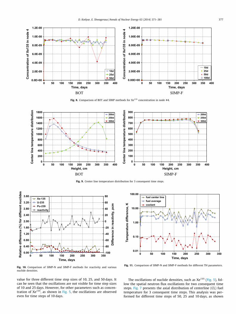
SIMP-FBOT

Fig. 8. Comparison of BOT and SIMP methods for Xe135 concentration in node #4.

0

200

400

600

800

1000

1200

1400

1600

1800

Height, cm

Cen

ter l

ine

tem

pera

ture

dis

trib

utio

n

200d250d300d

0

100

200

300

400

500

600

700

800

900

0 50 100 150 200 250 300 350 400 0 50 100 150 200 250 300 350 400Height, cm

Cen

ter l

ine

tem

pera

ture

dis

trib

utio

n

200d250d300d

SIMP-FBOT

Fig. 9. Center line temperature distribution for 3 consequent time steps.

0.00

0.40

0.80

1.20

1.60

2.00

2.40

2.80

3.20

3.60

0 50 100 150 200 250 300 350Time, days

Rel

ativ

e di

ffere

nce

(%) f

or d

iffer

ent n

uclid

es

-100

-80

-60

-40

-20

0

20

40

60

80

Diff

eren

ce in

reac

tivity

, pcm

Xe-135U-235Pu-239reactivity

Fig. 10. Comparison of SIMP-N and SIMP-F methods for reactivity and variousnuclide densities.

0.01

0.10

1.00

10.00

100.00

0 50 100 150 200 250 300 350Time, days

Tem

pera

ture

diff

eren

ce, K

fuel center linefuel averagecoolant

Fig. 11. Comparison of SIMP-N and SIMP-F methods for different TH parameters.

D. Kotlyar, E. Shwageraus / Annals of Nuclear Energy 63 (2014) 371–381 377

value for three different time step sizes of 10, 25, and 50 days. Itcan be seen that the oscillations are not visible for time step sizesof 10 and 25 days. However, for other parameters such as concen-tration of Xe135, as shown in Fig. 5, the oscillations are observedeven for time steps of 10 days.

The oscillations of nuclide densities, such as Xe135 (Fig. 5), fol-low the spatial neutron flux oscillations for two consequent timesteps. Fig. 7 presents the axial distribution of centerline (CL) fueltemperature for 3 consequent time steps. This analysis was per-formed for different time steps of 50, 25 and 10 days, as shown

378 D. Kotlyar, E. Shwageraus / Annals of Nuclear Energy 63 (2014) 371–381

in Fig. 7a–c. It can be seen that the amplitude of the oscillations in-creases with the time step size. However, the oscillations do notcompletely diminish even for relatively short time step sizes, e.g.10 days.

The results show that the BOT method exhibits numerical insta-bilities due to the coupling with depletion and thermal hydraulicfeedbacks. Moreover, the numerical instability issue does notdiminish even for time steps considerably shorter than typicallyused in routine fuel depletion analyses.

4.3. Results of the SIMP methods

This section presents the comparison of the two proposed SIMPmethods. Fig. 8 shows the concentration of Xe135 and Fig. 9 pre-

-100

-80

-60

-40

-20

0

20

40

Time, days

Diff

eren

ce in

reac

tivity

, [pc

m] 25d

50d100d

SIMP-N

150 250 350

Fig. 12. Reactivity comparison of the SIMP me

0.0

0.2

0.4

0.6

0.8

1.0

1.2

Time, days

Rel

ativ

e di

ffere

nce

(%) i

n Xe

135 25d

50d100d

0.00.20.40.60.81.01.21.41.61.82.0

Time, days

Rel

ativ

e di

ffere

nce

(%) i

n Pu

239 25d

50d100d

SIMP-N

150 250 350

150 250 350

Fig. 13. Nuclide densities comparison of the S

sents the center line temperature distribution for 3 consequenttime steps. The shown results were obtained with the SIMP-Fmethod and compared to the BOT method.

The results presented in Figs. 8 and 9 show that the SIMP meth-ods are unconditionally stable (Fig. 8) and that the fuel tempera-ture distribution does not suffer from any spatial oscillationissues (Fig. 9).

For the comparison of the burnup-TH coupling methods, weused very fine time steps of 10 days. With the use of progressivelysmall time steps, all methods should converge to the same solu-tion. In this section, we present the difference in neutronic andthermal hydraulic parameters as a function of time obtained withdifferent methods. The relative difference (e) in nuclide densitieswas computed using the following equation:

-100

-80

-60

-40

-20

0

20

40

150 250 350

Time, days

Diff

eren

ce in

reac

tivity

, [pc

m]

25d 50d100d

SIMP-F

thods for different time step size values.

0.0

0.2

0.4

0.6

0.8

1.0

1.2

Time, days

Rel

ativ

e di

ffere

nce

(%) i

n Xe

135

25d 50d100d

0.000.200.400.600.801.001.201.401.601.802.00

150 250 350

150 250 350Time, days

Rel

ativ

e di

ffere

nce

(%) i

n Pu

239

25d 50d100d

SIMP-F

IMP methods for different time step sizes.

0.00

5.00

10.00

15.00

20.00

25.00

30.00

35.00

40.00

Time intervals, days

Max

imum

diff

eren

ce in

TC

L (o C

) 25d 50d100d

0.00

5.00

10.00

15.00

20.00

25.00

30.00

35.00

40.00

Time intervals, days

Max

imum

diff

eren

ce in

TC

L (o C

) 25d 50d100d

0.000.050.100.150.200.250.300.350.400.450.50

Time intervals, days

Max

imum

diff

eren

ce in

Tco

olan

t (o C

)

25d 50d100d

SIMP-N

0.000.050.100.150.200.250.300.350.400.450.50

50-150 150-250 250-350 50-150 150-250 250-350

50-150 150-250 250-350 50-150 150-250 250-350Time intervals, days

Max

imum

diff

eren

ce in

Tco

olan

t (o C

)

25d 50d100d

SIMP-F

Fig. 14. Thermal properties comparison of the SIMP methods for different time step sizes.

480

485

490

495

500

505

510

515

520

150 160 170 180 190 200 210 220 230 240 250Time, days

Cen

ter l

ine

fuel

tem

pera

ture

[K] timestep = 100 days

timestep = 25 days

timestep = 10 days

100 d

25 d

10 d

Fig. 15. CL fuel temperature within the interval [150,250] days in node #2, ascalculated by SIMP-F method.

D. Kotlyar, E. Shwageraus / Annals of Nuclear Energy 63 (2014) 371–381 379

eð%Þ ¼ 100� 116�Xz¼16

z¼11� N1

z

N2z

���������� ð9Þ

where the subscript z represents the axial node, and the superscript1 and 2 represent SIMP-N and SIMP-F methods, respectively. N isthe nuclide density for which the e is being computed. In our case,e(%) was computed for Xe135, U235 and Pu239.

In addition, the absolute difference error in different tempera-ture distributions was computed using the following equation:

DT ¼ 100� 116�Xz¼16

z¼1jT1

z � T2z j ð10Þ

where T is the fuel centerline, fuel average or coolant temperature.As can be observed from Fig. 10, there is a very good agreement

between different neutronic parameters. The relative difference inreactivity predicted by the methods is about 20 pcm, which iswithin the statistical error of the MCNP calculation. The methodsalso agreed well on the concentration of high absorbing and fissilenuclides, as can be seen from Fig. 10. The relative difference forXe135, U235 and Pu239 densities is about 0.25%, 0.03% and 0.08%respectively. Fig. 11 demonstrates a very good agreement also indifferent temperature distributions. The average differences forCL fuel, fuel average and coolant temperatures are 4.5 �C, 2.3 �Cand 0.07 �C respectively.

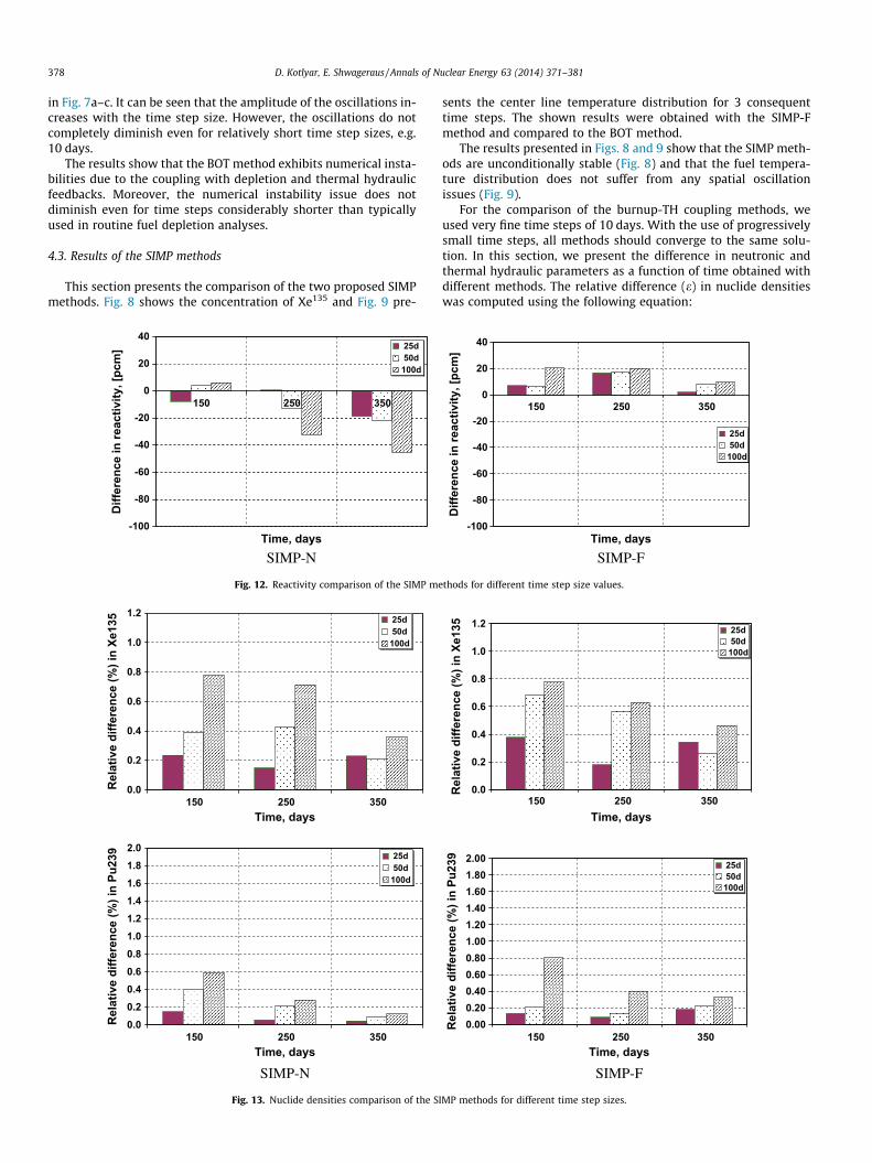
4.4. Sensitivity of SIMP methods to time step size

Previous section presented the results obtained by the SIMPmethods, for the 3D test case, using very fine time steps of 10 days.The results presented in this section illustrate the effect of timestep size on the accuracy of the SIMP methods. We used 3 differenttime step sizes of 25, 50 and 100 days in order to investigate theirimpact on the accuracy of the results. A number of parameters ofinterest were compared at 3 time points, 150, 200 and 250 days.The neutronic parameters of SIMP-N and SIMP-F methods are com-pared in Fig. 12 showing the difference in reactivity and Fig. 13showing the difference in concentration of Xe135 and Pu239. Thecurrent sensitivity analysis showed that increasing the time stepsize to practical values has negligible impact on the accuracy ofthe results. For example, when the time step equals to 100 days,the maximum difference in reactivity is 45 and 20 pcm betweenthe two methods, as shown in Fig. 12.

73 75 69

217

28 3424

86

13 14 20

47

7 8 823

0255075

100125150175200225250

Time intervals, days

Num

ber o

f tra

nspo

rt c

alcu

latio

ns 10 25 50100

SIMP-N

3756 53

146

14 20 21

55

10 8 1432

6 7 720

0255075

100125150175200225250

50-150 150-250 250-350 Total 50-150 150-250 250-350 TotalTime intervals, days

Num

ber o

f tra

nspo

rt c

alcu

latio

ns

10d 25d 50d100d

SIMP-F

Fig. 16. Number of transport solutions of the SIMP methods for different time step values.

380 D. Kotlyar, E. Shwageraus / Annals of Nuclear Energy 63 (2014) 371–381

In this section, the relative error (e) of different nuclide densi-ties was computed by following equation:

eð%Þ ¼ 100� 116�Xz¼16

z¼11� NDTi

z

NDT¼10z

���������� ð11Þ

NDT¼10z is the nuclide density at the axial node z obtained with time

step size of 10 days. The superscript DTi represents the size of thetime step (25, 50 and 100 days) for which the relative error is beingcomputed. The results show that the time step size has a minor im-pact on the concentration of high absorbing and fissile nuclides asshown in Fig. 13.

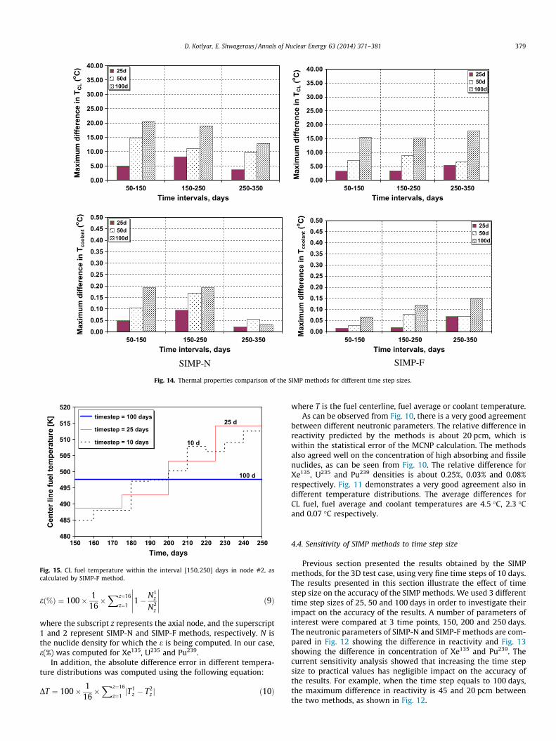
The comparison of thermal hydraulic parameters obtained bythe two methods is presented in Fig. 14, namely:

— Difference in centerline fuel temperature (TCL)— Difference in bulk coolant temperature (T1)

The nuclide density is a property which describes the isotopicconcentration at a time point. However, flux and power distribu-tions are properties that are evaluated for a time interval. There-fore, we can compare the temperature distributions obtainedwith different time steps (10, 25, 50 and 100 days) within the timeinterval only, as shown in Fig. 15. For this purpose, 3 time intervals,with the increment of 100 days, were chosen. In each time interval,the thermal properties were averaged according to followingequation:

T ½t0 ;t0þ100� ¼1N

XN

i¼1Tðt0 þ i � DtÞ ð12Þ

where T is the average temperature in the interval [t0, t0 + 100]. N isthe number of intervals for each time step size. T is the temperaturethat is a time interval representative. For example, T in the interval[150, 250] days, for time step of 25, days can be calculated as:T ½150;250� ¼ ðTð150Þ þ Tð175Þ þ Tð200Þ þ Tð225ÞÞ=4

Fig. 14 presents the maximum absolute temperature differencein TCL and T1. It can be seen that the thermal hydraulic propertiesare calculated very accurately even for relatively large time steps.

For example, the value of max j T100dCL

!

� T10dCL

!

j in the interval[150,250] days equals to 19 �C and 15 �C for SIMP-N and SIMP-Frespectively.

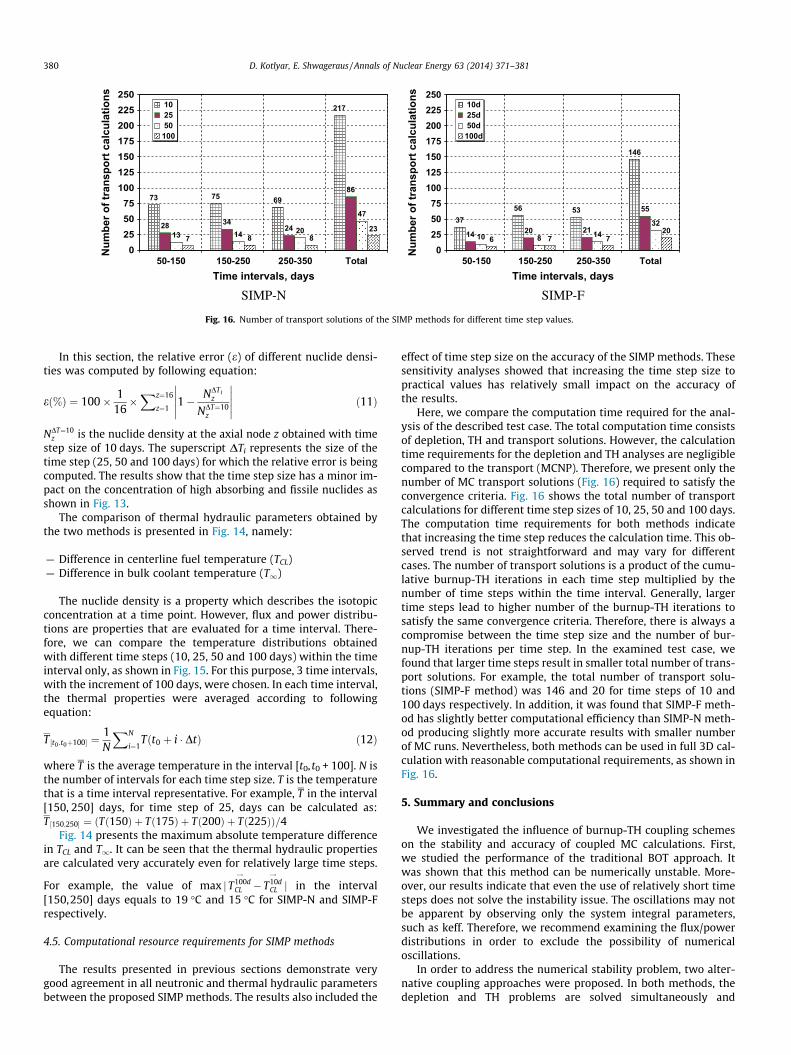
4.5. Computational resource requirements for SIMP methods

The results presented in previous sections demonstrate verygood agreement in all neutronic and thermal hydraulic parametersbetween the proposed SIMP methods. The results also included the

effect of time step size on the accuracy of the SIMP methods. Thesesensitivity analyses showed that increasing the time step size topractical values has relatively small impact on the accuracy ofthe results.

Here, we compare the computation time required for the anal-ysis of the described test case. The total computation time consistsof depletion, TH and transport solutions. However, the calculationtime requirements for the depletion and TH analyses are negligiblecompared to the transport (MCNP). Therefore, we present only thenumber of MC transport solutions (Fig. 16) required to satisfy theconvergence criteria. Fig. 16 shows the total number of transportcalculations for different time step sizes of 10, 25, 50 and 100 days.The computation time requirements for both methods indicatethat increasing the time step reduces the calculation time. This ob-served trend is not straightforward and may vary for differentcases. The number of transport solutions is a product of the cumu-lative burnup-TH iterations in each time step multiplied by thenumber of time steps within the time interval. Generally, largertime steps lead to higher number of the burnup-TH iterations tosatisfy the same convergence criteria. Therefore, there is always acompromise between the time step size and the number of bur-nup-TH iterations per time step. In the examined test case, wefound that larger time steps result in smaller total number of trans-port solutions. For example, the total number of transport solu-tions (SIMP-F method) was 146 and 20 for time steps of 10 and100 days respectively. In addition, it was found that SIMP-F meth-od has slightly better computational efficiency than SIMP-N meth-od producing slightly more accurate results with smaller numberof MC runs. Nevertheless, both methods can be used in full 3D cal-culation with reasonable computational requirements, as shown inFig. 16.

5. Summary and conclusions

We investigated the influence of burnup-TH coupling schemeson the stability and accuracy of coupled MC calculations. First,we studied the performance of the traditional BOT approach. Itwas shown that this method can be numerically unstable. More-over, our results indicate that even the use of relatively short timesteps does not solve the instability issue. The oscillations may notbe apparent by observing only the system integral parameters,such as keff. Therefore, we recommend examining the flux/powerdistributions in order to exclude the possibility of numericaloscillations.

In order to address the numerical stability problem, two alter-native coupling approaches were proposed. In both methods, thedepletion and TH problems are solved simultaneously and

D. Kotlyar, E. Shwageraus / Annals of Nuclear Energy 63 (2014) 371–381 381

iteratively with the transport problem. The coupling methods areimplicit in nature and therefore unconditionally numerically sta-ble. First, we compared the burnup-TH coupling methods by creat-ing a reference solution using very fine time steps. The neutronicand thermal hydraulic results obtained with both proposed meth-ods were found to be in good agreement. We also studied the effectof time step size on the accuracy of the proposed methods. Bothmethods showed that increasing the time step size to practical val-ues has negligible impact on the accuracy of the results. Finally, itwas shown that the amount of computational resources requiredby both methods is quite reasonable and, therefore, the methodscan be readily implemented and used in 3D coupled calculationseven of large reactor systems.

Acknowledgement

The authors would like to thank Jan Dufek for his review andinsightful comments on this paper.

References

Basile, D. et al. 1999. COBRA-EN. An updated version of the COBRA-3C/MIT code forthermal-hydraulic transient analysis of light water reactor fuel assemblies andcores. Report 1010/1, ENEL SpA, Milano, Italy, 1999.

Bomboni, E., Cerullo, N., Fridman, E., Lomonaco, G., Shwageraus, E., 2010.Comparison among MCNP-based depletion codes applied to burnupcalculations of pebble-bed HTR lattices. Nuclear Engineering and Design 240.

Briesmeister, J.F. (Ed.), 2000. MCNP - a general Monte Carlo N-particle code, Version4C, Los Alamos National Laboratory, LA-13709-M.

Brown, F.B., 2006. On the use of shannon entropy of the fission distribution forassessing convergence of Monte Carlo criticality calculations. In: Proc. PHYSOR,British Columbia Canada.

Dufek, J., Gudowski, W., 2006. Stochastic approximation for Monte Carlo calculationof steady-state conditions in thermal reactors. Nuclear Science and Engineering152, 274–283.

Dufek, J., Hoogenboom, J.E., 2009. Numerical stability of existing Monte Carloburnup codes in cycle calculations of critical reactors. Nuclear Science andEngineering 162, 307–311.

Dufek, J., Kotlyar, D., Shwageraus, E., Leppänen, J., 2013a. Numerical stability of thepredictor–corrector method in Monte Carlo burnup calculations of criticalreactors. Annals of Nuclear Energy 56, 34–38.

Dufek, J., Kotlyar, D., Shwageraus, E., 2013b. The stochastic implicit euler method – astable coupling scheme for Monte Carlo burnup calculations. Annals of NuclearEnergy (in press).

Fensin, M.L., Hendricks, J.S., Trellue, H.R., Anhaie, S., 2006. The enhancements andtesting for the MCNPX 2.6.0 depletion capability. Journal of Nuclear Technology170, 68–79.

Fridman, E., Shwageraus, E., Galperin, A., 2008a. Efficient generation of one-groupcross sections for coupled Monte Carlo depletion calculations. Nuclear Scienceand Engineering 159, 37–47.

Fridman, E., Shwageraus, E., Galperin, A., 2008b. Implementation of multi-groupcross-section methodology in BGCore MC-depletion code. In: Proc. PHYSOR2008, Interlaken, Switzerland, 2008b.

Grundmann, U., Rohde, U., Mittag, S., 2000. DYN3D – three dimensional core modelfor steady-state and transient analysis of thermal reactors. In: Proc. PHYSOR2000, Pittsburgh, PA (USA), 2000.

Haeck, W., Verboomen, B., 2007. An optimum approach to Monte Carlo burnup.Nuclear Science and Engineering 156, 180–196.

Hoffman J. D., 1992. Numerical Methods for Engineers and Scientists, McGraw-Hill,Inc., New York.

Ivanov, A., Sanchez, V., Imke, U. 2011. Development of a coupling scheme betweenMCNP5 and SUBCHANFLOW for the pin- and fuel assembly-wise simulation ofLWR and innovative reactors. In: Proc. M&C 2011, Rio de Janeiro, RJ (Brazil),2011.

Koning, A., Forrest, R., Kellett, M., Mills, R., Henrikson, H., Rugama, Y., 2006. TheJEFF-3.1 Nuclear Data Library, JEFF Report 21, OECD/NEA, Paris, France,2006.

Kotlyar, D., Shwageraus, E., 2013. On the use of predictor–corrector methodfor coupled Monte Carlo burnup codes. Annals of Nuclear Energy 58, 228–237.

Kotlyar, D., Shaposhnik, Y., Fridman, E., Shwageraus, E., 2011. Coupled neutronicthermo-hydarulic analysis of full PWR core with Monte-Carlo based BGCoresystem. Nuclear Engineering and Design 241 (9), 3777–3786.

Leppänen, J., 2007. Development of a new Monte Carlo reactor physics code. In:D.Sc. Thesis. vol. 640. Helsinki University of Technology, VTT Publications.

Moore, R.L., Schnitzler, B.G., Wemple, C.A., Babcock, R.S., Wessol, D.E., 1995.MOCUP: MCNP ORIGEN2 Coupled Utility Program, Idaho National EngineeringLaboratory, INEL-95/0523, 1995.

Robbins, H., Monro, S., 1951. A stochastic approximation method. Annals ofMathematical Statistics 22, 400.

Sanchez, V., Al-Hamry, A., 2009. Development of a coupling scheme between MCNPand COBRA-TF for the prediction of the pin power of a PWR fuel assembly. In:Proc. M&C, Saratoga Springs, New York, USA.

Trellue, H.R., 2003. MONTEBURNS 2.0. An automated, multi-step Monte Carloburnup code system, User’s manual version 2.0., Oak Ridge National Laboratory,PSR-455, 2003.

Xu, Z., Hejzlar, P., Driscoll, M.J., Kazimi, M.S., 200. An improved MCNP-ORIGENdepletion program (MCODE) and its verification for high-burnup applications.In: Proc. of PHYSOR-2002, Seoul, Korea, 2002.