Download - Non-oscillatory methods for relaxation approximation of Hamilton–Jacobi equations

INTERNATIONAL JOURNAL FOR NUMERICAL METHODS IN FLUIDSInt. J. Numer. Meth. Fluids (2015)Published online in Wiley Online Library (wileyonlinelibrary.com). DOI: 10.1002/fld.4067

A meshless method for numerical simulation of depth-averagedturbulence flows using a k-� model

Yasser Alhuri1;�, Fayssal Benkhaldoun2;�, Driss Ouazar3, Mohammed Seaid4 andAhmed Taik1;�;�;‘

1Department of Mathematics, UFR-MASI FST, Hassan II University Mohammedia, Morocco2LAGA, Université Paris 13, 99 Av J.B. Clement, 93430 Villetaneuse, France

3Department of Genie Civil, LASH EMI, Mohammed V University Rabat, Morocco4School of Engineering and Computing Sciences, University of Durham, South Road, Durham, DH1 3LE, UK

SUMMARY

We investigate the performance of a meshless method for the numerical simulation of depth-averaged tur-bulence flows. The governing equations are shallow water equations obtained by depth averaging of the fullReynolds equations including bed frictions, eddy viscosity, wind shear stresses, and Coriolis forces. As adouble-phase closure turbulence model, we consider the depth-averaged k-� model. A truly meshless numer-ical method based on radial basis functions is employed to obtain an accurate approximation to the solutionof the model. We validate the algorithm on a linear shallow water problem where analytical solutions areavailable. Numerical results are also compared with experimental data for a backward-facing flow problem.Furthermore, we test the method on a practical problem by simulating tidal flows in the Strait of Gibraltar.The main focus is to examine the performance of the meshless method for complex geometries with irregu-lar bathymetry. The obtained results demonstrate its ability to capture the main flow features. Copyright ©2015 John Wiley & Sons, Ltd.

Received 23 December 2014; Revised 5 June 2015; Accepted 20 June 2015

KEY WORDS: shallow water equations; turbulence model; depth-averaged k-� model; meshless method;radial basis functions; tidal flows

1. INTRODUCTION

In general, water flows represent a three-dimensional turbulent Newtonian flow in complicated geo-metrical domains. The cost of incorporating three-dimensional features in natural water coursesis often excessively high. Computational efforts that needed to simulate three-dimensional turbu-lent flows can also be significant. In view of such considerations, many researchers have tended touse rational approximations in order to develop two-dimensional hydrodynamical models for waterflows. Shallow water equations, derived from three-dimensional incompressible Navier–Stokesequations using the assumption that the vertical scale is much smaller than any typical horizontalscale and the hydrostatic pressure assumption, are a standard mathematical representation, valid formost types of flow encountered in coastal sea, river, channel, and ocean modeling; see [1] amongothers. The shallow water equations in depth-averaged form have been successfully applied to manyengineering problems, and their application fields include a wide spectrum of phenomena other

*Correspondence to: Ahmed Taik, Department of Mathematics, UFR-MASI FST, Hassan II University Mohammedia,Morocco.

†E-mail: [email protected]�Present address: Yaser Alhuri: Department of Basic Engineering Science Faculty of Engineering Sana’a University,Yemen.�Fayssal Benkhaldoun: Universite Paris 13, Sorbonne Paris Cite, LAGA, CNRS, UMR 7539, F-93430, Villetaneuse,France.‘Ahmed Taik: Department of Mathematics, Laboratory MAC & PM FSTM, Hassan II University, Morocco.

Copyright © 2015 John Wiley & Sons, Ltd.

Y. ALHURI ET AL.

than water waves. For instance, the shallow water equations have applications in environmental andhydraulic engineering such as tidal flows in an estuary or coastal regions, rivers, reservoir, and openchannel flows. Such practical flow problems are not trivial to simulate because the geometry canbe complex, and the topography tends to be irregular. In addition, most of water free-surface flowsencountered in engineering practice are turbulent characterized by: (i) highly unsteady features suchthat time series of the flow field at any point in the computational domain would appear random toan observer unfamiliar with these flows; (ii) appearance of a great deal of vorticity in which vortexstretching is one of the principal mechanisms by which the intensity of turbulence is increased; (iii)reduction of the velocity gradients due to the action of viscosity, which reduces the kinetic energyof the flow, that is, mixing is a dissipative process, and the lost energy is irreversibly converted intointernal energy of the water; (iv) existence of repeatable coherent structures and essentially deter-ministic events that are responsible for a large part of the mixing; and (v) turbulent flows fluctuateon a broad range of length and time scales. This property makes direct numerical simulation of tur-bulent flows very difficult. It should also be stressed that turbulent flows contain variations on amuch wider range of length and time scales than laminar flows. However, the random componentof turbulent flows causes these events to differ from each other in size, strength, and time inter-val between occurrences, making their analysis very difficult. Despite that they are similar to thelaminar flow, the equations describing turbulent flows are usually much more difficult and compu-tationally demanding to solve. Considering the usual length scales in engineering practice, and thesmall kinematic viscosity of water, in most cases, the Reynolds number is large enough in order toconsider the flow as fully turbulent. Even in the simplest situations of river flow, we can observesmall eddies that appear and disappear with an apparently chaotic movement, showing the complex-ity of turbulent motion. In coastal regions, large eddies often occur because of the separation of theflow past a headland, a breakwater, or an island. These eddies are very important in environmentalengineering, and they may influence the solute and sediment trapping.

The modeling of turbulence in shallow water flows has not been treated so profusely as in otherfluid dynamics areas. Some depth-averaged turbulence models have been proposed for the depth-averaged turbulence flows. Those models are mainly derived from well-known Reynolds-AveragedNavier-Stokes (RANS) turbulence models including the effects of bed friction in the turbulencefield. Special mention should be given to the depth-averaged k-� model proposed in [2], which wasthe first depth-averaged two-equation eddy viscosity model, and it is still the most commonly usedwith the depth-averaged models when turbulent effects are accounted for in the computation. Inthis model of mixture length, the turbulent viscosity is calculated from the local characteristics ofthe shallow water flow by means of both the turbulent kinetic energy k and the rate of turbulencedissipation �. The model solves a transport equation for each variable k and �, where it considersthe production due to bed friction, the production by velocity and dissipation gradients, and theconvective transport. In order to show the capabilities of depth-averaged models in the computationof turbulent flows, a finite volume model has been studied in [3] for a flow problem in a coastalestuary and in a vertical slot fishway. The authors in this reference compared the numerical resultswith the experimental data. It should also be pointed out that large-eddy simulation has also beenused to simulate turbulent shallow water flows in [4] among others. A comparative study of differentdepth-averaged turbulence models has been carried out in [5] for river flows. For research studies onmodeling and numerical simulation of turbulent shallow water flows, we cite, for example, [6, 7].The numerical methods covered in these references are mesh-based techniques using finite volumediscretization of the flow domains.

Mesh-based techniques such as finite element and finite volume methods have been widely usedfor solving partial differential equations governing environmental models. However, the accuracyof these methods is affected by the quality of the meshes, which hinders their applications to solv-ing real problems with irregular coastal boundaries and complex bathymetries. Recently, somesignificant developments in meshless methods for solving linear and nonlinear partial differentialequations have been achieved. For instance, the meshless local Petrov–Galerkin and local bound-ary integral equations methods were studied in [8, 9]. These two methods basically transformedthe original problem into a local weak formulation, and the shape functions were constructed fromusing the moving least squares approximation to interpolate the solution variables. Meshless radial

Copyright © 2015 John Wiley & Sons, Ltd. Int. J. Numer. Meth. Fluids (2015)DOI: 10.1002/fld

A MESHLESS METHOD FOR DEPTH-AVERAGED TURBULENCE FLOWS

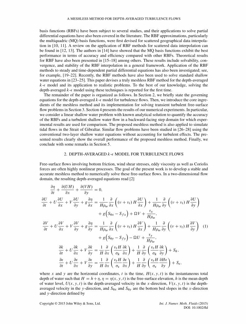
basis functions (RBFs) have been subject to several studies, and their applications to solve partialdifferential equations have also been covered in the literature. The RBF approximations, particularlythe multiquadric (MQ) basis functions, were first devised for scattered geographical data interpola-tion in [10, 11]. A review on the application of RBF methods for scattered data interpolation canbe found in [12, 13]. The authors in [14] have showed that the MQ basis functions exhibit the bestperformance in terms of accuracy and efficiency compared with other RBFs. Theoretical resultsfor RBF have also been presented in [15–18] among others. These results include solvability, con-vergence, and stability of the RBF interpolation in a general framework. Application of the RBFmethods to steady and time-dependent partial differential equations has also been investigated; see,for example, [19–22]. Recently, the RBF methods have also been used to solve standard shallowwater equations in [23–25]. This paper devises a truly meshless RBF method for the depth-averagedk-� model and its application to realistic problems. To the best of our knowledge, solving thedepth-averaged k-� model using these techniques is reported for the first time.

The remainder of the paper is organized as follows. In Section 2, we briefly state the governingequations for the depth-averaged k-� model for turbulence flows. Then, we introduce the core ingre-dients of the meshless method and its implementation for solving transient turbulent free-surfaceflow problems in Section 3. Section 4 presents the results of our numerical experiments. In particular,we consider a linear shallow water problem with known analytical solution to quantify the accuracyof the RBFs and a turbulent shallow water flow in a backward-facing step domain for which exper-imental results are used for comparison. The proposed meshless method is also applied to simulatetidal flows in the Strait of Gibraltar. Similar flow problems have been studied in [26–28] using theconventional two-layer shallow water equations without accounting for turbulent effects. The pre-sented results clearly show the overall performance of the proposed meshless method. Finally, weconclude with some remarks in Section 5.

2. DEPTH-AVERAGED k-� MODEL FOR TURBULENCE FLOWS

Free-surface flows involving bottom friction, wind shear stresses, eddy viscosity as well as Coriolisforces are often highly nonlinear processes. The goal of the present work is to develop a stable andaccurate meshless method to numerically solve these free-surface flows. In a two-dimensional flowdomain, the resulting depth-averaged equations read [2]

@�

@[email protected]/

@[email protected]/

@yD 0;

@U

@tC U

@U

@xC V

@U

@yC g

@�

@xD

1

H�!

@

@x

�.� C �t /H

@U

@x

�C

1

H�!

@

@y

�.� C �t /H

@U

@y

�

C g�S0x � Sfx

�C�V C

�x

H�!;

@V

@tC U

@V

@xC V

@V

@yC g

@�

@yD

1

H�!

@

@x

�.� C �t /H

@V

@x

�C

1

H�!

@

@y

�.� C �t /H

@V

@y

�

C g�S0y � Sfy

��U C

�y

H�!;

@k

@tC U

@k

@xC V

@k

@yD

1

H

@

@x

��tH

�k

@k

@x

�C

1

H

@

@y

��tH

�k

@k

@y

�C Sk;

@�

@tC U

@�

@xC V

@�

@yD

1

H

@

@x

��tH

��

@�

@x

�C

1

H

@

@y

��tH

��

@H�

@y

�C S�;

(1)

where x and y are the horizontal coordinates, t is the time, H.x; y; t/ is the instantaneous totaldepth of water such thatH D hC�, � D �.x; y; t/ is the free-surface elevation, h is the mean depthof water level, U.x; y; t/ is the depth-averaged velocity in the x-direction, V.x; y; t/ is the depth-averaged velocity in the y-direction, and S0x and S0y are the bottom bed slopes in the x-directionand y-direction defined by


Y. ALHURI ET AL.

S0x D �@´b

@x; S0y D �

@´b

@y

with ´b.x; y/ as the prescribed bed elevation. The bottom friction slopes Sfx and Sfy areapproximated by the Manning formula

Sfx Dn2bUpU 2 C V 2

H 4=3; Sfy D

n2bVpU 2 C V 2

H 4=3;

where nb is the Manning roughness coefficient, and �x and �y are the wind stresses given by

�x D CwWx

qW 2x CW

2y ; �y D CwWy

qW 2x CW

2y ;

with Cw as the surface friction coefficient, andWx andWy are the wind velocities in the x-directionand y-direction, respectively. In (1),� is the Coriolis force parameter, g is the gravitational acceler-ation, �! is the density of water, k and � are, respectively, the average of the kinetic turbulent energyand the average of its dissipation rate, � is the kinematic viscosity of water, and �t is a turbulenteddy viscosity computed from the k-� turbulence model [2] as

�t D c�k2

�; Sk D PH C Pk � �; (2)

where

PH D �t

2

�@U

@x

�2C 2

�@V

@y

�C

�@U

@yC@V

@x

�2!; Pk D

1pcfH

U �3;

with

U � D

rc�k2

�j@U j; S� D c1�

�

kPH C P�V � c2�

�2

k; P�V D c�

U �4

H 2:

Here, PH is the production of k due to interactions of turbulent stresses with horizontal mean-velocity gradients, and Pk and P�v are the productions of k and � due to vertical velocity gradientsand are related to the friction velocity U �. The empirical constants c�, c1� , c2� , �k , �� , cf , and considered in the current study are given in Table I.

Note that Eq. 1 has to be solved in a bounded spatial domain � equipped with given boundaryand initial conditions. In practice, these conditions are problem dependent, and in most commonhydraulic applications, we use the following:

� On solid walls,

@�

@nD 0; U D V D 0; k D

U �2

pc�; � D

U �3

Ny;

where D 0:41 is the Karman parameter, n denotes the unit outward normal to the wall, andNy is the normal distance to the wall.

� On water boundaries,

Inlet conditions: the water free-surface � is given and for the remaining variables

@U

@nD 0;

@V

@nD 0; k D 2:06655U �2; � D 1:008687

�1U�3

H;

Table I. Empirical constants used in the depth-averaged k-� model.

c� c1� c2� �k �� cf

0.09 1.44 1.92 1.0 1.3 5.19 0.41



where �1 D 9:8 for Reynolds numbers between 104 and 105. These expressions can also beused to estimate the initial values unless other more adequate values are available.Outlet conditions: the water free-surface � is given and for the remaining variables

@U

@nD 0;

@V

@nD 0;

@k

@nD 0;

@�

@nD 0:

It should be stressed that other boundary conditions are also possible and they can easily be handledby the proposed meshless method.

3. A MESHLESS RADIAL BASIS FUNCTION METHOD FOR THE DEPTH-AVERAGED k-�MODEL

Although the finite element and finite volume methods have been widely used in computationalhydraulics, one of the major disadvantages of these methods is their dependence on meshes. Thismay limit the application of these mesh-based methods to high-dimensional or highly nonlinearproblems. Despite that automated grid generation programs are available, the generation of a finiteelement or finite volume mesh with several thousand nodes and with elements of various sizes,shapes, and orientation is still a non-trivial task. On the other hand, the rapid development ofmeshless methods in the last two decades has overcome this mesh dependent disadvantage; see,for example, [10, 12, 15]. Meshless RBFs have the advantage of achieving spectral accuracy formultidimensional problems using arbitrary node distributions and with extreme algorithmic sim-plicity. The meshless RBFs have been successfully applied to a large variety of problems, compare[13, 14, 19–21, 23, 24, 29–31] among others. In the current study, we investigate the performanceof meshless RBFs to the depth-averaged k-� model.

The principal idea of the interpolation using RBF is to interpolate a finite series of an unknownfunction f .X/ at N distinct points Xj on the computational domain by the expansion

f .X/ 'NXjD1

˛j'��X � Xj

��C MXkD1

˛kpk .X/ ; (3)

where pk.X/ are exactly the polynomials spanning M , which are polynomials of degree at mostM and satisfying the constraints

NXjD1

˛jpk�Xj�D 0; k D 1; 2; : : : ;M; (4)

where ˛j ’s are the unknown coefficients to be calculated, kX � Xj k D rj Dp.xi � xj /2 C .yi � yj /2 is the Euclidean distance between the points X D .xi ; yi / and Xj D

.xj ; yj /, and '.kX�Xj k/ is the RBF. Although there are many possible RBFs, the most commonlyused are the following:

MQ: '.r/ Dpr2 C c2;

Inverse multiquadrics (IMQ): '.r/ D1

pr2 C c2

;

Gaussian (GS): '.r/ D exp��.cr/2

�:

Here, c ¤ 0 is the shape parameter controlling the fitting of a smooth surface to the data. The lackof the mathematical theory makes it very difficult to choose a suitable value c for the RBF. Investi-gations in [12, 32] have shown that the computational accuracy of the radial basis interpolation canbe improved by varying the shape parameter with the selected basis function. In the present work,we used the following selection [33]


Y. ALHURI ET AL.

c D 0:815dmin; (5)

with dmin denoting the minimum distance between any two adjacent collocation points. Note thatother selections for the shape constant c and other RBFs can easily be incorporated in our analysiswithout major conceptual modifications.

Given scalar function values Wi .t/ D W.xi ; yi ; t /, the expansion coefficients ˛i .t/ in (3) areobtained by solving the following system of linear equations0

BBBBBBBBBBBBB@

'.x1; y1/ '.x1; y1/ : : : '.x1; y1/

'.x2; y2/ '.x2; y2/ : : : '.x2; y2/

::::::

: : ::::

'.xN ; yN / '.xN ; yN / : : : '.xN ; yN /

1CCCCCCCCCCCCCA

0BBBBBBBBBBBBB@

˛1.t/

˛2.t/

:::

˛N .t/

1CCCCCCCCCCCCCAD

0BBBBBBBBBBBBB@

W1.t/

W2.t/

:::

WN .t/

1CCCCCCCCCCCCCA; (6)

where '.xi ; yj / D '�kXi � Xj k

�, with kXi � Xj k D

p.xi � xj /2 C .yi � yj /2. The linear

system (6) can be reformulated in a compact matrix form as

H� D w; (7)

where H is anN �N matrix with entries 'j .xi ; yj /, and� and w areN -valued vectors with entries˛ni and W n

i , respectively. For many choices of RBFs ', the interpolation matrix H in (7) is guar-anteed to be nonsingular for any set of distinct points, and the invertibility is therefore guaranteed;see, for example, [18, 34]. Notice that adding the polynomial terms to the considered radial basisinterpolation (3) is not generally required. However, this argument may not be applicable to otherRBFs.

Partial derivatives of the interpolant (3) may be calculated in a straightforward manner. Forinstance, using the interpolant in (6), the temporal and spatial derivatives at the points xj can becalculated as

@W

@tD

NXjD1

@˛j .t/

@t'j .xi ; yi /;

@W

@xD

NXjD1

˛j .t/@'j

@x.xi ; yi /;

@W

@yD

NXjD1

˛j .t/@'j

@y.xi ; yi /:

Similar to (7), the partial derivatives can also be written in a compact matrix form as

@w@tD H

@�

@t;

@w@xD@H@x�;

@w@yD@H@y�:

Note that for time-dependent problems, the spatial derivatives may need to be evaluated thousands tomillions of times during the time-integration procedure. Therefore, for efficiency reason, the spatialderivative matrix is formed once as

Dx D@H@x

H�1; Dy D@H@y

H�1; (8)

and the derivatives can be evaluated as a single matrix by vector multiplication as

@w@xD Dxw;

@w@yD Dyw:

Applied to the depth-averaged k-� Eq. 1, the meshless RBF method approximates the water free-surface �, velocity field .U; V /, the kinetic energy k, and the dissipative energy � as



�.xi ; yi ; t / '

NXjD1

�j .t/'.xi ; yi /;

U.xi ; yi ; t / '

NXjD1

˛j .t/'.xi ; yi /; V .xi ; yi ; t / '

NXjD1

ˇj .t/'.xi ; yi /;

k.xi ; yi ; t / '

NXjD1

j .t/'.xi ; yi /; �.xi ; yi ; t / '

NXjD1

�j .t/'.xi ; yi /:

Inserting the aforementioned expressions in (1) and using the spatial derivatives matrices (8), asemi-discrete formulation of system (1) can be obtained as

0BBBBBBBBBBBBBBBBBB@

H 0 0 0 0

0 H 0 0 0

0 0 H 0 0

0 0 0 H 0

0 0 0 0 H

1CCCCCCCCCCCCCCCCCCA


dƒdt

d�dt

d„dt

d‡dt

d‚dt


D


F�

FU

FV

Fk

F�


; (9)

whereƒ, � ,„,‡ , and‚ are vectors with entries �j .t/, ˛j .t/, ˇj .t/, j .t/, and �j .t/, respectively.In (9), the right-hand side functions include the RBF discretization of the convective, diffusive, andsource terms from system (1) obtained by matrix–vector multiplications using the matrices H, Dx ,and Dy . The RBF discretization (9) can be easily rearranged in a canonical system of ordinarydifferential equations of this form

dUdtD F .U/ ; t 2 .0; T �; (10)

where U D .ƒ; �;„;‡;‚/T and F .U/ obtained accordingly from (9). To integrate Eq. 10, wedivide the time interval into subintervals Œtn; tnC1� with duration �t D tnC1 � tn for n D 0; 1; : : : .We use the notation W n to denote the value of a generic function W at time tn. The procedure toadvance the solution from the time tn to the next time tnC1 can be carried out using an explicitRunge–Kutta method studied in [35] as

U .1/ D Un C�tF.Un/;

U .2/ D 3

4Un C

1

4U .1/ C 1

4�tF.U .1//;

UnC1 D1

3Un C

2

3U .2/ C 2

3�tF.U .2//:

(11)

This class of explicit time-integration schemes has become popular in computational fluid dynamics;see, for example, [36]. The main feature of this method lies on the fact that (11) is a convexcombination of first-order Euler steps, which exhibit strong stability properties. Therefore, scheme(11) is Total Variation Diminishing (TVD), third-order accurate in time, and stable under the usualCourant–Friedrichs–Lewy condition.


Y. ALHURI ET AL.

It is worth remarking that, because the RBFs are time independent, the system matrix of the linearsystem resulting from (9) is also time independent. A major advantage is then the ability to retainthe system matrix assembled at the first time step to be reused at later time steps without alteration.This is achieved by factorizing the system matrix using an LDL> decomposition where L is a lowermatrix and D is a diagonal matrix [37]. This factorization is only carried out at the first time stepwhile resolving the system that is reduced to forward , diagonal, and back substitutions at any timestep after updating the right-hand side of the system. This can significantly increase the efficiencywhen a large number of time steps are needed, compared with updating the matrix and fully solvingthe system if a time-dependent RBFs are to be used. It should also be stressed that to solve the linearsystems resulting from the RBF, we used the singular value decomposition algorithm [38]. Theperformance of the singular value decomposition solver for solving highly ill-conditioned systemsas those obtained in the current study is commonly well established, compare, for example, [38].

4. NUMERICAL RESULTS

To demonstrate the performance of the meshless method, several examples are presented. For thefirst example, an exact solution is readily available, which makes it ideal for a quantitative as wellas qualitative validation of the considered meshless method. We also compare numerical resultsobtained using different RBFs in the meshless method for this example. As a second example, weconsider the turbulent flow in a channel with forward-facing step for which experimental results areavailable. The objective of this test example is to compare the simulation results obtained using themeshless method to the experimental data for the velocity field and the kinetic energy. In the thirdexample, we simulate the tidal flow in the Strait of Gibraltar. This last example represents a practicaldemonstration of the capabilities of the meshless method in simulations of tidal flow problemsfor two major reasons. Firstly, the computational domain in the Strait of Gibraltar is a large-scaledomain including high gradients of the bathymetry and well-defined shelf regions. Secondly, theStrait of Gibraltar contains complex fully two-dimensional tidal flow structures, eddy viscosity, andCoriolis forces, which present a challenge for most numerical methods used in tidal flow modeling.The aim is to show that, using reasonably low number of collocation points, the meshless methodreproduces the corresponding flow patterns and accurately captures the flow structures with verylittle numerical diffusion, even after long time simulations. In all the computations reported herein,the Courant number Cr is set to 0.8, and the time stepsize �t is adjusted at each step according tothe stability condition

�t D Crdmin

max�U ˙

pgH; V ˙

pgH

� ; (12)

where dmin is the calculated minimum distance between any two adjacent collocation points. Thegravitational acceleration is fixed to g D 9:81 m/s2 for all examples presented here.

4.1. Accuracy test problems

We consider the linear shallow water equations considered in [23] and obtained by neglecting thewind stress, bottom friction, diffusion, and the Coriolis force terms as

@�

@tCH

�@u

@xC@v

@y

�D 0;

@u

@tC g

@�

@xD 0;

@v

@tC g

@�

@yD 0:

(13)

System (13) is solved in a rectangular domain with length L D 872 km and width of 50 km for atime interval of 72 h. The total water level is H D 20 m such that the mean water depth is definedas h D H � �. Initial and boundary conditions for this problem are obtained using the analyticalsolution [24]



�.x; y; t/ D �0 cos

�!pgH

.L � x/

�cos .!t/

cos�

!pgHL� ;

u.x; y; t/ D ��0

rg

Hsin

�!pgH

.L � x/

�sin .!t/

cos�

!pgHL� ; v.x; y; t/ D 0;

(14)

with �0 D 1m and ! D 1:45444�10�4/s. The aim of this test example is to assess the performanceof the MQ, IMQ, and GS RBFs in the meshless method. Because the analytical solution is known,we evaluate the error function En at time tn for any generic function W as

En D W Exact .xi ; yi ; tn/ �Wni ;

where W Exact and W ni are the analytical and numerical solutions, respectively, evaluated at the

collocation points .xi ; yi / and time tn. For this test example, the collocation points are uniformlydistributed where the total number N D nx � ny , with nx and ny the numbers of nodal points inthe x-direction and y-direction, respectively. Notice that, from Eqs. 13–(14), this flow problem canbe interpreted as a one-dimensional problem where the dynamics occur mostly in the x-direction.For this reason, the number of collocation points in the y-direction is fixed to ny D 5, and errorsare only computed for the water free-surface � and the velocity U .

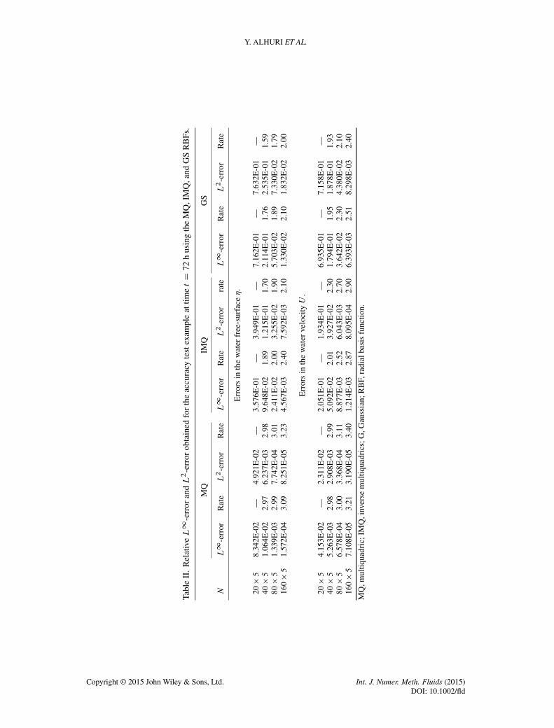
In Figure 1, we display the time evolution of L2-error in the water free-surface � and the watervelocity U using N D 40 � 5. It is clear from the obtained results that the errors in both freesurface and velocity exhibit periodic behavior for all considered RBF functions. Larger errors aredetected for the water free surface than for the water velocity for all RBFs with the GS methodbeing less accurate than the IMQ and MQ methods. For the considered flow conditions, the MQmeshless method is more accurate than the IMQ and GS methods. To further demonstrate this trend,a quantitative comparison of the results computed using MQ, IMQ, and GS methods for differentvalues for the number of collocation points N is presented in Table II. In this table, we list theL2-error, L1-error, and their convergence rates for the considered RBF functions. It reveals thatincreasing the number of collocation points in the computational domain results in a decay of botherror norms. The MQ method exhibits good convergence behavior for this linear problem and it issuperior than the IMQ and GS methods. As can be seen from the errors presented in Table II, athird-order accuracy is achieved in the MQ method for this test example in terms of the considerederror norms. Hence, our next computations are realized using only the MQ method and are hereafterreferred to as the meshless method.

Next, we check the accuracy of the MQ method for a nonlinear shallow water system with knownanalytical solution studied in [39]. Here, we solve the frictionless shallow water Eq. 1 without

1 2 3 4 5 6 7 8 9 10 11 12 13 14 15 16 17 18 19 20 21 22 23 24 25 26 270

0.5

1

1.5

2

x 10−3

Time [hours]

Err

or in

η

GSIMQMQ

1 2 3 4 5 6 7 8 9 10 11 12 13 14 15 16 17 18 19 20 21 22 23 24 25 26 270

0.1

0.2

0.3

0.4

0.5

0.6

0.7

0.8

0.9

1

Time [hours]

Err

or in

U

GSIMQMQ

x 10−3

Figure 1. Time evolution of the errors in the water free-surface � (left) and the water velocity U (right) forthe accuracy test problem.


Y. ALHURI ET AL.

Tabl

eII

.R

elat

iveL1

-err

oran

dL2

-err

orob

tain

edfo

rth

eac

cura

cyte

stex

ampl

eat

timetD72

hus

ing

the

MQ

,IM

Q,a

ndG

SR

BFs

.

MQ

IMQ

GS

NL1

-err

orR

ate

L2

-err

orR

ate

L1

-err

orR

ate

L2

-err

orra

teL1

-err

orR

ate

L2

-err

orR

ate

Err

ors

inth

ew

ater

free

-sur

face�

.

20�5

8.34

2E-0

2—

4.92

1E-0

2—

3.57

6E-0

1—

3.94

9E-0

1—

7.16

2E-0

1—

7.63

2E-0

1—

40�5

1.06

4E-0

22.

976.

237E

-03

2.98

9.64

8E-0

21.

891.

215E

-01

1.70

2.11

4E-0

11.

762.

535E

-01

1.59

80�5

1.33

9E-0

32.

997.

742E

-04

3.01

2.41

1E-0

22.

003.

255E

-02

1.90

5.70

3E-0

21.

897.

330E

-02

1.79

160�5

1.57

2E-0

43.

098.

251E

-05

3.23

4.56

7E-0

32.

407.

592E

-03

2.10

1.33

0E-0

22.

101.

832E

-02

2.00

Err

ors

inth

ew

ater

velo

cityU

.

20�5

4.15

3E-0

2—

2.31

1E-0

2—

2.05

1E-0

1—

1.93

4E-0

1—

6.93

5E-0

1—

7.15

8E-0

1—

40�5

5.26

3E-0

32.

982.

908E

-03

2.99

5.09

2E-0

22.

013.

927E

-02

2.30

1.79

4E-0

11.

951.

878E

-01

1.93

80�5

6.57

8E-0

43.

003.

368E

-04

3.11

8.87

7E-0

32.

526.

043E

-03

2.70

3.64

2E-0

22.

304.

380E

-02

2.10

160�5

7.10

8E-0

53.

213.

190E

-05

3.40

1.21

4E-0

32.

878.

095E

-04

2.90

6.39

3E-0

32.

518.

298E

-03

2.40

MQ

,mul

tiqua

dric

;IM

Q,i

nver

sem

ultiq

uadr

ics;

G,G

auss

ian;

RB

F,ra

dial

basi

sfu

nctio

n.



Table III. L1-error and CPU times (in seconds) obtained for the accuracy testexample at time t D 100 using the MQ method.

� U V

M L1-error Rate L1-error Rate L1-error Rate CPU

10 � 10 7.976E-02 — 8.127E-02 — 8.054E-02 — 12120 � 20 1.253E-02 2.67 1.605E-02 2.34 1.579E-02 2.35 20540 � 40 1.577E-03 2.99 2.165E-03 2.89 2.101E-03 2.91 38980 � 80 1.813E-04 3.12 2.687E-04 3.01 2.501E-04 3.07 816

CPU, central processing unit; MQ, multiquadric.

Coriolis force and turbulence in the squared domain � D Œ�50; 50� � Œ�50; 50� with an analyticalsolution for the water depth and velocity given by

�.x; y; t/ D 1 �a

4bge�2b. Nx

2C Ny2/; U.x; y; t/ D1

2cos � C a Nye�b. Nx

2C Ny2/;

(15)

V.x; y; t/ D1

2sin � � a Nxe�b. Nx

2C Ny2/;

where Nx D x C 20 � t2

cos � and Ny D y C 10 � t2

sin � . Initial and boundary conditions are setaccording to the exact solution (15). In our simulations, we use the same parameters as in [39] forg D 1, a D 0:04, b D 0:02, and � D

6, and results are displayed at time t D 100. In Table III, we

summarize the L1-error in the depth-averaged water variables �, U , and V using different numbersof collocation points in the computational domain. As in the previous test example, we considera uniform distribution with a total number of collocation points N D nx � ny , with nx and nythe numbers of nodal points in the x-direction and y-direction, respectively. It is clear that theMQ method performs well for this nonlinear shallow water problem and it produces numericalerrors of decreasing order as the number of collocation points increases. The third-order accuracyis also achieved by the MQ method for this test example in all water variables, whereas a smalldeterioration in this convergence rate is detected in the water velocities U and V compared withthe water depth �. It is also clear from the results reported in Table III that an increase in thenumber of collocation points results in an increase in the computational cost referred to by the CPUtime. It should be stressed that a large part of this CPU time is devoted to the linear solver in theMQ method.

4.2. Shallow water flow in a backward-facing step

Our second example is the turbulent shallow water flow over a backward-facing step. This test exam-ple has excessively been studied in [3], and experimental measurements have also been reportedtherein. Here, we solve Eq. 1 without wind stresses, Coriolis forces, bottom bed slopes, and bot-tom friction slopes. The computational domain is of height 0.5 m, length before the step 1 m,height of the step 0.3 m, and length after the step 3.5 m. The Manning roughness coefficient isnb D 0:01 s/m1=3 and the eddy viscosity is � D 10�3 m2/s. All the experimental data in [3] wereobtained at the Hydraulics Laboratory of the Civil Engineering School in Coruña with SONTEKmicro-acoustic doppler velocimeters that produce a small distortion of the velocity field. In all theexperimental points, the mean current speed and the turbulent kinetic energy were measured at inter-vals of 100 s, each represents an average of several measures. Measurements were taken on 368points in a rectangular zone behind the step as depicted in Figure 2.

In our meshless simulations, we use the same initial and boundary conditions as in [3]. Thus, ini-tially, the flow system is at rest with a water height set to 24.2 cm. A water discharge of 20.2 l/s isset at the upstream boundary, and the water height at the downstream boundary is fixed to 24.2 cm.The computational domain is covered with 427 collocation points, where 338 collocation pointsare in the interior, 19 collocation points are on the water boundary (inlet and outlet), and 70 col-location points are on the wall boundary. This collocation structure has been selected after a nodal


Y. ALHURI ET AL.

Figure 2. General view of the domain with measurement zone covered by collocation points.

Figure 3. Comparison between experimental (left column) and computed results (right column) for the testproblem of flow in a backward-facing step. Snapshot of velocity U (first row), kinetic energy (second

row), and flow fields (third row).

independence study assessed by comparing different nodal distributions. In Figure 3, we present acomparison between experimental and computational results on the measurement zone. Here, weillustrate the snapshot of the velocity U and the kinetic energy along with the velocity fields.For clear presentation, we have also included streamlines within the presented results. From theseresults, we can see that the proposed meshless method resolves accurately the flow structures, andthe vortices seem to be localized in the correct place in the flow domain. For instance, the recircu-lation zone and the position of the reattachment point in the meshless results are in good agreementwith the experimental measurements. For more comparisons, Figure 4 shows profiles of the veloc-ity U and the kinetic energy at different locations within the measurement zone. As in [3], thevertical cross sections are carried out at x D 1:53 m, x D 2:03 m, and x D 2:53 m. A very goodagreement between measured and predicted meshless profiles has been obtained, particularly in thewater velocity U .



1 2 3 4 5 6 7 8x 10

0.05

0.1

0.15

0.2

0.25

0.3

0.35

0.4

Dis

tanc

e y

Energy k

Section at x = 1.53 m

1 2 3 4 5 6 7 80.05

0.1

0.15

0.2

0.25

0.3

0.35

0.4

Dis

tanc

e y

Energy k


1 2 3 4 5 6 70.05

0.1

0.15

0.2

0.25

0.3

0.35

0.4

Dis

tanc

e y

Energy k


−0.05 0 0.05 0.1 0.15 0.2 0.25 0.3 0.350.05

0.1

0.15

0.2

0.25

0.3

0.35

0.4

Dis

tanc

e y

Velocity u


−0.1 −0.05 0 0.05 0.1 0.15 0.2 0.25 0.30.05

0.1

0.15

0.2

0.25

0.3

0.35

0.4

Dis

tanc

e y

Velocity u


−0.05 0 0.05 0.1 0.15 0.2 0.25 0.30.05

0.1

0.15

0.2

0.25

0.3

0.35

0.4

Dis

tanc

e y

Velocity u


x 10 x 10

Figure 4. Cross sections of the velocity U (first row) and kinetic energy (second row) at different locationswithin the measurement zone for the test problem of flow in a backward-facing step.

Table IV. Errors in the velocity U and kinetic energy along the three consideredcross sections using different sets of collocation points. CPU times are given in

minutes.

Errors in velocity U Errors in energy

Set Section L1-error L2-error L1-error L2-error CPU (min)

x D 1:53 m 9.32E-02 8.87E-03 8.02E-03 9.05E-05I x D 2:03 m 8.01E-02 8.54E-03 8.83E-03 1.09E-04 5.73

x D 2:53 m 9.15E-02 8.00E-03 7.97E-03 9.89E-04x D 1:53 m 3.27E-02 2.55E-03 1.41E-03 2.83E-05

II x D 2:03 m 1.39E-02 2.11E-03 1.55E-03 3.02E-05 23.92x D 2:53 m 2.11E-02 1.80E-03 1.03E-03 7.73E-04x D 1:53 m 3.01E-02 2.29E-03 1.19E-03 2.77E-05

III x D 2:03 m 1.32E-02 2.09E-03 1.43E-03 2.99E-05 95.68x D 2:53 m 2.07E-02 1.53E-03 1.00E-03 7.68E-04

CPU, central processing unit.

In order to quantify the errors between the computational results obtained using the meshlessmethod and the experimental results for this test problem, we present in Table IV the L1-error andL2-error in the velocity U and kinetic energy along the three considered cross sections. We alsouse this example to check the sensibility of these results on the distribution of collocation pointsin the domain. To this end, we consider three sets of collocation points for which the statistics ofinterior points, points on the water boundary, and points on the wall boundary are listed in Table V.Comparing the errors at these cross sections in the flow domain confirms that the meshless methodcaptures the correct flow features and it reproduces small numerical errors in both velocity fieldand kinetic energy. Note that smaller errors are obtained for kinetic energy compared with theerrors for the water velocity U for all three sets of collocation points. It is also evident that forthe considered flow properties, the obtained results show little sensibility on the distribution ofcollocation points in the flow domain. As can be observed in Table IV, there are little differencesbetween the results obtained for the considered sets of collocation points. For instance, we havefound that the discrepancies in the values of L1-error and L2-error for the velocity U on sets Iand II are less than 0.8%. These differences become less than 0.2% on sets II and III. Therefore,


Y. ALHURI ET AL.

Table V. Statistics for the three sets of collocation points used in the simulations.

Set Number of interior points Number of water boundary points Number of wall boundary points

I 169 9 34II 338 19 70III 675 37 139

Figure 5. Schematic map of the Strait of Gibraltar along with relevant cities and locations.

bearing in mind the slight change in the results from sets II and III at the expense of rather significantincrease in CPU times, set II is believed to be adequate to obtain the numerical results free ofcollocation effects.

In summary, as accuracy is usually important in the development of hydraulics, the meshlessmodel proposed in this study is not only realistic enough to yield meaningful flow predictions butalso simple and fast enough to avoid overcharging the computational cost.

4.3. Tidal flow in the Strait of Gibraltar

In this final test example, we solve the problem of tidal flow in the Strait of Gibraltar. The mainobjective in this example is to examine the performance of the meshless method to handle complexgeometry and irregular topography as those offered in the Strait of Gibraltar. A schematic map ofthe Strait of Gibraltar along with relevant cities and locations is shown in Figure 5. The system isbounded to the north and south by the Iberian and African continental forelands, respectively, andto the west and east by the Atlantic ocean and the Mediterranean sea. In geographical coordinates,the Strait is 35ı450 to 36ı150 N latitude and 5ı150 to 6ı050 W longitude. Here, the computationaldomain is limited by the Tangier–Barbate section from the Atlantic ocean and the Ceuta–Algecirassection from the Mediterranean sea. This restricted domain has also been considered in [40, 41]among others and it is chosen for numerical simulations mainly because measured data are usuallyprovided by the stations located at the aforementioned locations. Therefore, we have adapted thesame domain for our simulations using the proposed meshless method. It should also be pointedout that flow exchange in the Strait of Gibraltar has been investigated in [26–28] using the standardlaminar two-layer shallow water equations.

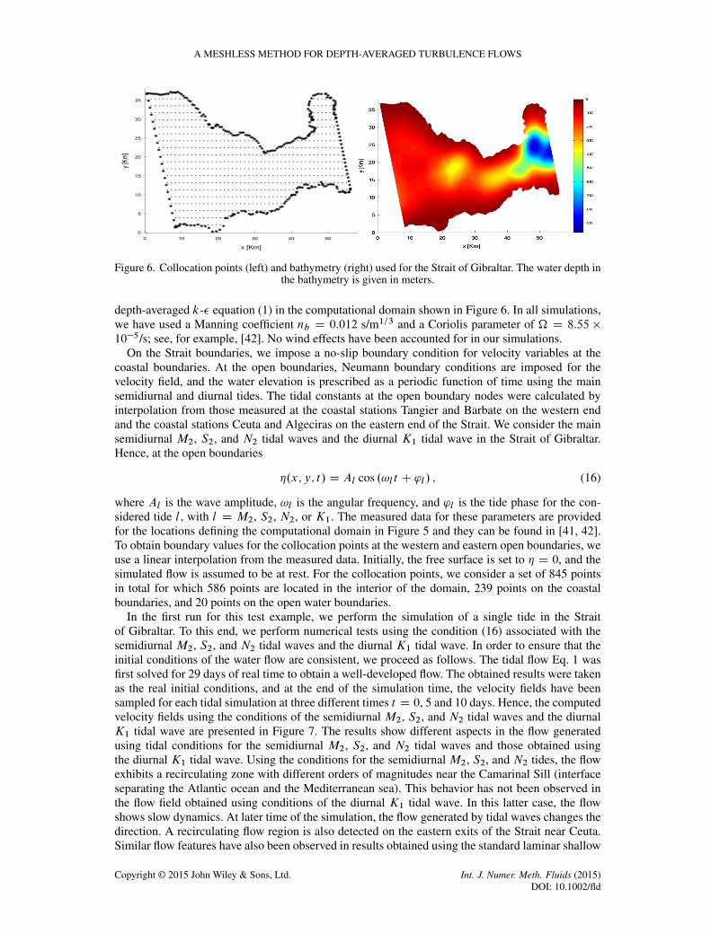
The coastal boundaries and the bed topography in the Strait of Gibraltar are very irregular, andseveral regions of varying depth exist. In our simulations, we have used a bathymetry reconstructedfrom published data in [41] and illustrated in Figure 6. It is evident that the bathymetry is notsmooth and exhibits irregular features with different length scales. For instance, two bumps withminimum bathymetric values of 997 and 463 m are localized in the vicinity of the eastern exit ofthe Strait and the Camarinal Sill, respectively. Hence, our problem statement consists of solving the



Figure 6. Collocation points (left) and bathymetry (right) used for the Strait of Gibraltar. The water depth inthe bathymetry is given in meters.

depth-averaged k-� equation (1) in the computational domain shown in Figure 6. In all simulations,we have used a Manning coefficient nb D 0:012 s/m1=3 and a Coriolis parameter of � D 8:55 �10�5/s; see, for example, [42]. No wind effects have been accounted for in our simulations.

On the Strait boundaries, we impose a no-slip boundary condition for velocity variables at thecoastal boundaries. At the open boundaries, Neumann boundary conditions are imposed for thevelocity field, and the water elevation is prescribed as a periodic function of time using the mainsemidiurnal and diurnal tides. The tidal constants at the open boundary nodes were calculated byinterpolation from those measured at the coastal stations Tangier and Barbate on the western endand the coastal stations Ceuta and Algeciras on the eastern end of the Strait. We consider the mainsemidiurnal M2, S2, and N2 tidal waves and the diurnal K1 tidal wave in the Strait of Gibraltar.Hence, at the open boundaries

�.x; y; t/ D Al cos .!l t C 'l/ ; (16)

where Al is the wave amplitude, !l is the angular frequency, and 'l is the tide phase for the con-sidered tide l , with l D M2, S2, N2, or K1. The measured data for these parameters are providedfor the locations defining the computational domain in Figure 5 and they can be found in [41, 42].To obtain boundary values for the collocation points at the western and eastern open boundaries, weuse a linear interpolation from the measured data. Initially, the free surface is set to � D 0, and thesimulated flow is assumed to be at rest. For the collocation points, we consider a set of 845 pointsin total for which 586 points are located in the interior of the domain, 239 points on the coastalboundaries, and 20 points on the open water boundaries.

In the first run for this test example, we perform the simulation of a single tide in the Straitof Gibraltar. To this end, we perform numerical tests using the condition (16) associated with thesemidiurnal M2, S2, and N2 tidal waves and the diurnal K1 tidal wave. In order to ensure that theinitial conditions of the water flow are consistent, we proceed as follows. The tidal flow Eq. 1 wasfirst solved for 29 days of real time to obtain a well-developed flow. The obtained results were takenas the real initial conditions, and at the end of the simulation time, the velocity fields have beensampled for each tidal simulation at three different times t D 0, 5 and 10 days. Hence, the computedvelocity fields using the conditions of the semidiurnal M2, S2, and N2 tidal waves and the diurnalK1 tidal wave are presented in Figure 7. The results show different aspects in the flow generatedusing tidal conditions for the semidiurnal M2, S2, and N2 tidal waves and those obtained usingthe diurnal K1 tidal wave. Using the conditions for the semidiurnal M2, S2, and N2 tides, the flowexhibits a recirculating zone with different orders of magnitudes near the Camarinal Sill (interfaceseparating the Atlantic ocean and the Mediterranean sea). This behavior has not been observed inthe flow field obtained using conditions of the diurnal K1 tidal wave. In this latter case, the flowshows slow dynamics. At later time of the simulation, the flow generated by tidal waves changes thedirection. A recirculating flow region is also detected on the eastern exits of the Strait near Ceuta.Similar flow features have also been observed in results obtained using the standard laminar shallow


Y. ALHURI ET AL.

Figure 7. Velocity fields at different times for the tidal waves in the Strait of Gibraltar. M2 (first row), N2(second row), S2 (third row), and K1 (fourth row). From left to right t D 0, 5, and 10 days.

water equations reported in [40, 41]. Compared with the results published in these references, itcan be seen that the k-� model considered in the current study generates larger areas with intensivevelocity fields than those presented in [40, 41], but the vortices seem to be localized in the correctplace in the flow domain. Note that the proposed meshless method performs very satisfactorily onthis nonlinear coupled problem because it does not diffuse the moving tidal fronts, and no spuriousoscillations have been detected near steep gradients of the flow field in the computational domain.It can be clearly seen that the damped flow structures on the Camarinal Sill are being captured bythe meshless method.

To further ascertain the quality in the resolution of the meshless method, we performed a har-monic analysis on the tidal elevations to be compared with observations from [42] measured for tworelevant locations in the Strait of Gibraltar, namely, Tarifa and Sidi Kankouch; compare Figure 5.The tidal amplitudes and phases computed using the meshless method are compared in Table VIwith measurements from [42]. In this table, we also include numerical results obtained using thestandard laminar shallow water equations presented in [41]. Furthermore, in order to test the sensi-bility of the results on the collocation points, we present k-� results on three sets with total numbersof points N D 437, 845, and 1710. A comparison of the k-� results on the three sets reveals that no



Table VI. Comparison between observed and simulated amplitudes A and phases ' of the semidiurnal M2tide and the diurnal K1 tide at the Tarifa and Sidi Kankouch locations.

Tarifa Sidi Kankouch

M2 tide K1 tide M2 tide K1 tide

Station A (cm) ' .ı/ A (cm) ' .ı/ A (cm) ' .ı/ A (cm) ' .ı/

Measurements 41.4 57 2.2 131 51.8 69 4.6 88k-� results .N D 437/ 43.9 55.1 1.5 126.5 54.6 66.0 3.8 85.9k-� results .N D 845/ 42.6 55.9 1.9 127.8 53.1 67.9 4.1 87.5k-� results .N D 1710/ 42.5 56.0 1.9 127.9 53.0 67.9 4.2 87.6SWE results 48.3 50.1 1.7 94.5 55.7 64.9 3.0 77.8

SWE, shallow water equation.

Figure 8. Time evolution of water free surface at Tarifa.

significant differences are observed in the computed results, and for the proposed meshless method,a collocation set with 845 points would be enough to produce numerical results independent of thecollocation effects. It is clear from Table VI that the simulated results using the meshless methodmostly compared favorably with all the experimental results from reference [42, 43]. It is evidentthat accounting for turbulence in the computational analysis using the k-� model has produced bet-ter agreement between the prediction and the experimental data. A very good agreement betweenmeasured and predicted tidal amplitudes has been obtained, particularly in the semidiurnal M2 tide.The influence of turbulence on the tidal amplitude and phase has been clearly demonstrated. In ourcomputations, the amplitude of the M2 tide at Tarifa is overpredicted by about 17% without con-sidering turbulence and by about 3% considering the k-� model. The experimental and meshlessresults are substantially in agreement. The incorporation of turbulence in the tidal analysis has pro-duced a better agreement between numerical predictions and experimental data. It is clear that thek-� model gives further improvements over the standard shallow water equations. To illustrate theeffect of turbulence on tidal simulations, we also run the model using all the main astronomical tidalconstituents on the open boundaries, that is,

�.x; y; t/ D AM2 cos�!M2 t C 'M2

�C AS2 cos

�!S2 t C 'S2

�C

AN2 cos�!N2 t C 'N2

�C AK1 cos

�!K1 t C 'K1

�:

(17)

Figure 8 illustrates the time evolution of the water free surface in the Tarifa location at time intervalof 29 days. For comparison, we have also included results obtained using the standard shallow waterequations investigated in [41]. As expected, the inclusion of turbulence in shallow water flows usingthe k-� model results in a damping in the tidal amplitudes. A small shift in the tidal phase has alsobeen detected in the results obtained with and without k-� model. The results shown in Table VIand Figure 8 have confirmed that the effect of turbulence is important in tidal predictions. It shouldbe stressed that the present meshless method is easily implemented, effective, and produces highaccurate numerical results comparable with the experimental data. In addition, the presented resultsclearly indicate that the proposed meshless method is suited for prediction of tidal flow in the Straitof Gibraltar.


Y. ALHURI ET AL.

5. CONCLUSIONS

In this paper, we have presented a simple meshless method for solving the two-dimensional depth-averaged k-� model for turbulent shallow water flows. The method uses a class of RBFs fordiscretization in space, and the time integration of the resulting semi-discretized system is performedusing the third-order Runge–Kutta scheme. The considered method does not introduce artificialdiffusion effects and it accurately resolves the turbulent structures regardless whether the flow isconvection or diffusion dominated. From a practical viewpoint, the method is straightforward, irre-spective of the smoothness of the bathymetry and the shape of the flow domain under consideration,and easy to implement because no mesh is required and only radial distance between the nodes isused to approximate the flow solutions. Validation of the method has been carried out using sev-eral test problems of shallow water and tidal flow problems. The numerical results were comparedwith the measured data for a backward-facing step flow problem. Reasonable agreement betweenthe simulated and measured data was observed. The method was also applied to solve the tidal flowproblem in the Strait of Gibraltar. The method exhibited good shape, high accuracy, and stabilitybehavior, even coarse nodal distributions are used in computations. Quantitative comparisons havebeen made with other published works on tidal flow in the Strait of Gibraltar, and a good agree-ment is found. The presented results demonstrate the capability of the meshless method that canprovide insight to complex tidal flow features. In addition, the computed results for all consideredtest examples verify the performance and robust nature of the numerical model.

Future work will concentrate on the extension of the proposed method to multi-layer depth-averaged k-� model for turbulent shallow water flows. From a modeling viewpoint, a more realisticmodel, which takes into consideration variations along the depth of water in the flow domain, shouldbe built. The present model is a relatively idealized two-dimensional model, where only the depth-averaged variation is modeled. In marine systems, stratification often occurs in summer, variationin different layers of a water body from the surface down to the seabed cannot be ignored. Theseaspects may affect the prediction accuracy of the model. A more realistic multi-layer model withthe use of RBF is currently being investigated. Finally, it should be remarked that the limitationsof the proposed meshless method are usually because the resultant coefficient matrix of the systemof equations that resulted from the method is usually full and unsymmetric and hence leads to anill-conditioning problem. Future work will also concentrate on developing efficient solvers for theassociated linear systems.

ACKNOWLEDGEMENTS

Financial support provided by the project FINCOME is gratefully acknowledged. The authors wish tothank Prof. Fe from Coruña for providing experimental data for numerical computation of backward-facingstep flow.

REFERENCES

1. Toro EF. Shock-capturing Methods for Free-surface Shallow Flows. Wiley and Sons, 2001.2. Rastogi AK, Rodi W. Predictions of heat and mass transfer in open channels. Journal of the Hydraulics Division,

ASCE 1978; 104:397–420.3. Fe J, Navarrina F, Puertas J, Vellando P, Ruiz D. Experimental validation of two depth-averaged turbulence models.

International Journal for Numerical Methods in Fluids 2009; 60:177–202.4. Abdellaoui R, Benkhaldoun F, Elmahi I, Seaid M. A finite volume method for large-eddy simulation of shallow water

equations. Finite Volumes for Complex Applications VII, Springer Proceedings in Mathematics & Statistics 2014;78:741–748.

5. Wu W, Wang P, Chiba N. Comparison of five depth-averaged 2-D turbulence models for river flows. Archives ofHydro-Engineering and Environmental Mechanics 2004; 51:183–200.

6. Cea L, Puertas J, Vázquez-Cendón ME. Depth averaged modelling of turbulent shallow water flow with wet-dryfronts. Architecture Computation Methods Engineering 2007; 14:303–34.

7. Cea L, French JR, Vázquez-Cendón ME. Numerical modelling of tidal flows in complex estuaries including turbu-lence: an unstructured finite volume solver and experimental validation. International Journal Numerical MethodsEngineering 2006; 67:1909–1932.



8. Atluri SN, Zhu T. A new meshless local Petrov–Galerkin (MLPG) approach in computational mechanics. Computa-tional Mechanics 1998; 22:117–127.

9. Belytschko T, Krongauz Y, Organ D, Fleming M, methods P. Krysl. Meshless. An overview and recent developments.Computer Methods in Applied Mechanics and Engineering 1996; 139:3–47.

10. Wendland H. Scattered Data Approximation. Cambridge university press, 2005.11. Micchelli CA. Interpolation of scattered data: distance matrices and conditionally positive definite functions.

Constructive approximation 1986; 1:11–22.12. Kansa EJ. Multiquadrics-a scattered data approximation scheme with applications to computational fluid-dynamics-

I surface approximations and partial derivative estimates. Computers and Mathematics with Applications 1990;19:127–145.

13. Ahmed SG. A collocation method using new combined radial basis functions of thin plate and multiquadraic types.Engineering Analysis with Boundary Elementary 2006; 30:697–701.

14. Golberg MA, Chen CS. Improved multiquadric approximation for partial differential equations. Engineering Analysiswith Boundary Elementary 1996; 18:9–17.

15. Buhamman M. Radial Basis Functin: Theory and Implementations. Cambridge university press, 2003.16. Yoon J. Interpolation by radial basis functions on Sobolev space. Journal Approximation Theory 2001; 112:1–15.17. Kansa EJ, Aldredge RC, Ling L. Numerical simulation of two-dimensional combustion using mesh-free methods.

Engineering Analysis with Boundary Elements 2009; 33:940–950.18. Powell MJD. The Theory of Radial Basis Function Approximation in 1990. In Advances in Numerical Analysis, Light

W (ed.)., Wavelets, Subdivision Algoritms and Radial Functions. Oxford University Press: UK, 1992; II:105–210.19. Kansa EJ, Hon Y.C. Circumventing the ill-conditioning problem with multiquadric radial basis functions:

applications to elliptic partial differential equations. Computers and mathematics with applications 2000; 39:123–137.

20. Chen CS, Marcozzi MD, Cho S. The method of fundamental solution and compactly supported radial basis function:a meshless approach to 3D problems. International series on advances in boundary elements, 1999.

21. Golberg MA, Chen CS. The theory of radial basis function applied to the BEM for inhomogeneous partial differentialequations. Boundary element communications 1994; 5:57–61.

22. Kansa EJ, Power H, Fasshauer GE, Ling L. A volumetric integral radial basis function method for time-dependentpartial differential equations I. formulation. Engineering Analysis with Boundary Elements 2004; 28:1191–1206.

23. Hon YC, Cheung KF, Mao XZ, Kansa EJ. A multiquadric solution for the shallow water equations. ASCE Journal ofHydrolic Engineering. 1999; 125:524–533.

24. Wong SM, Hon YC, Golberg MA. Compactly supported radial basis functions shallow water equations. JournalApplication Science Computations 2002; 127:79–101.

25. Khoshfetrat A, Abedini MJ. Numerical modeling of long waves in shallow water using LrBF-DQ and hybridDQ/LRBF-DQ. Ocean Modelling 2013; 65:1–10.

26. Castro MJ, García-Rodriguez JA, González-Vida JM, Macías J, Parés C, Vázquez-Cendón ME. Numerical simulationof two-layer shallow water flows through channels with irregular geometry. Journal Computational Physics 2004;195:202–235.

27. Castro MJ, Macías J, Parés C. A Q-scheme for a class of systems of coupled conservation laws with source term.Application to a two-layer 1D shallow water system. M2AN Mathematical Model Numerical Analysis 2001; 35:107–127.

28. Macías J, Parés C, Castro MJ. Improvement and genralization of a finite element shallow water solver to multi-layersystems. International Journal Numerical Methods Fluids. 1999; 31:1037–1059.

29. Dubal MR. Construction of three-dimensional black-hole initial data via multiquadrics. Physical Review D 1992;45:1178–1187.

30. Fasshauer GE. On the numerical solution of differential equations with radial basis functions. In Boundary ElementTechnology XIII, Chen CS, Brebbia CA, Pepper DW (eds)., 1999; 291–300.

31. Fornberg B, Piret C. On choosing a radial basis function and a shape parameter when solving a convective PDE on asphere. Journal of Computational Physics 2008; 227:2758–2780.

32. Buhmann M, Dinew S, Larsson E. A note on radial basis function interpolant limits. IMA Journal Numerical Analysis2010; 30:543–554.

33. Ferreira AJM, Kansa EJ, Fasshauer GE, Leitao VMA. Progress on Meshless Methods. Springer, 2009.34. Micchelli CA. Interpolation of scattered data: distance matrices and conditionally positive definite functions.

Constructive approximation 1986; 2:11–22.35. Shu CW. Total variation diminishing time discretizations. SIAM Journal Science Statistic Computations 1988;

9:1073–1084.36. Gottlieb S, Shu CW, Tadmor E. Strong stability preserving high order time integration methods. SIAM Review 2001;

43:89–112.37. Bettess P, Bettess JA. A profile matrix solver with built-in constraint facility. Engineering Computations 1986;

3(3):209–216.38. Golub G, Kahan W. Calculating the singular values and pseudo-inverse of a matrix. Journal of the Society for

Industrial & Applied Mathematics, Series B: Numerical Analysis 1965; 2(2):205–224.39. Mishra S, Fjordholm US. Vorticity preserving finite volume schemes for the shallow water equations. SIAM Journal

Science Computations 2011; 33:588–611.


Y. ALHURI ET AL.

40. Almazán JI, Bryden H, Kinder T, Parrilla G (Eds.). Seminario Sobre la Oceanografía Física del Estrecho deGibraltar. SECEG: Madrid, 1988.

41. El-Amrani M, Seaid M. An essentially non-oscillatory semi-Lagrangian method for tidal flow simulations. Interna-tional Journal for Numerical Methods in Engineering 2010; 81:805–834.

42. Tejedor L, Izquierdo A, Kagan BA, Sein DV. Simulation of the semidiurnal tides in the strait of Gibraltar. JournalGeophysical Research 1999; 104:13541–13557.

43. Lafuente JG, Almazán JL, Catillejo F, Khribeche A, Hakimi A. Sea level in the strait of Gibraltar, Tides. InternationalHydrographic Review 1990; 1:111–130.
