


Bahasa
Halaman
Hukum


1 Fault Diagnosis of Monoblock Centrifugal Pump Using Stationary 1Wavelet Features and Bayes AlgorithmV. Muralidharan, V.Sugumaran and N.R. Sakthivel
2 Experimental Investigations on Finding Ball Bearing Defects Using 5Signature AnalysisK.Gunasekar and A.Pugazhenthi
3 Flow Measurement Using RTDs 8Nagaraju B.P and Rathanraj K.J
4 An Investigation on Instantaneous Workability Behavior of Aluminium 12SiC Air Quenched Powder Composites During Cold UpsettingM. Prabhakar, T. Ramesh, R. Narayanasamy and V. Anandakrishnan
5 Solar Radiation Catalyzed Aerobic Photooxidation of 1-Naphthol on 25Some SemiconductorsS. Karuthapandian and K. Arunsunaikumar
6 New Visualizing Agents for Developing Latent Fingerprints on Various 33Porous and Non-Porous Surfaces Using Different Household Food ItemsRicha Rohatgi and A. K. Kapoor
7 Experimental Investigation for Tool Life by Optimizing Machining and 39Geometric Parameters of CNC End Mill ToolNilesh S. Pohokar, Lalit B. Bhuyar
Asian Journal of Science and Applied Technology
Volume 3 Number 2 July - December 2014
Contents
Sl. No. Title Page No.
Fault Diagnosis of Monoblock Centrifugal Pump Using Stationary Wavelet Features and Bayes Algorithm
V. Muralidharan1, V.Sugumaran2 and N.R. Sakthivel3
1Department of Mechanical Engineering, B.S.Abdur Rahman University, Chennai - 600048. Tamil Nadu, India 2V.Sugumaran, School of Mechanical and Building Sciences, VIT University, Chennai, Tamil Nadu, India
3N.R. Sakthivel, 3Department of Mechanical Engineering, Amrita University, Coimbatore, Tamil Nadu, India E-mail: [email protected], [email protected], [email protected]
Abstract - Fault diagnosis of monoblock centrifugal pump is conceived as a pattern recognition problem. There are three important steps to be performed in pattern recognition namely feature extraction, feature selection and classification. In this study, Stationary wavelet transform (SWT) is used for feature extraction from the input signals and Bayes net classifier is used for classification. A WEKA implementation of Bayes net algorithm is used. The different fault conditions considered for the present study are Cavitation (CAV), Impeller fault (FI), Bearing Fault (BF) and both Impeller and Bearing Fault (FBI). The representative signal is acquired for all faulty conditions, Features are extracted, classified and the results are presented. The experimental setup and the procedure for conducting the experiments are discussed in detail. Keywords: Stationary wavelets transform, fault diagnosis, wavelet feature, Bayesnet.
I. INTRODUCTION In a monoblock centrifugal pump, defective bearing, defect on the impeller and cavitation cause a very serious problems. Cavitation results in undesirable effects, such as deterioration of hydraulic performance (drop in head capacity and efficiency). Fault detection is achieved by comparing the signals of monoblock centrifugal pump running under normal and faulty conditions. Vibration signals are widely used in condition monitoring of centrifugal pumps. For the measurement of the vibration levels for each condition, seismic or piezoelectric transducers along with data acquisition system is used. From the vibration signal relevant features are extracted using Stationary Wavelet Transformations (SWT) and classification is done using bayesnet classifier and the results are presented. V. Muralidharan and V. Sugumaran (2012) have reported the comparative study of bayes classifier and bayes net classifier for pump data using discrete wavelet transform features (DWT features). Finally, concluded that bayes net classifier seem to be good for DWT features. The same authors (2013) also investigated in detail with J48 algorithm and support vector machines for continuous wavelet and DWT features. Jiangping Wang, Hong Tao Hu (2006) focuses on a problem of vibration-based condition monitoring and fault diagnosis of pumps. The vibration-based machine condition monitoring and fault diagnosis incorporate a number of machinery fault detections and diagnostic techniques. They used fuzzy logic principle as a fault diagnostic technique to describe the uncertain and ambiguous relationship between different fault symptoms
and classify frequency spectra representing various pump faults. Fansen Kong, Ruheng Chen (2004) proposed a new combined method based on wavelet transformation, fuzzy logic and neuro-networks for fault diagnosis of a triplex pump. The failure characteristics of the fluid and dynamic-end can be divided into wavelet transform in different scales. Therefore, the characteristic variables can be constructed making use of the coefficients of Edge worth asymptotic spectrum expansion formula and fuzzified to train the neuro-network to identify the faults of fluid- and dynamic-end of triplex pump in fuzzy domain. Tests indicate that the information of wavelet transformation in scale 2 is related to the meshing state of the gear and the information in scales 4 and 5 is related to the running state of fluid-end. Good agreement between analytical and experimental results has been obtained. V. Muralidharan et al., discussed that classification capability of J48 algorithm and SVM algorithm with DWT features. The similar types of faulty conditions were considered and the experiments were performed. Also, they have performed an experiment with rough set theory and support vector machine algorithms. However, there is a scope for conditional probability based algorithms in the field of fault diagnosis. Hence, this work has been taken up with stationary wavelet transforms and bayesnet algorithm for fault diagnosis of monoblock centrifugal pump in order to fill the gap.
II. EXPERIMENTAL STUDIES The main idea of this study is to find whether the monoblock centrifugal pump is in good condition or in faulty condition by a systematic procedure following certain steps. If the pump is found to be in faulty condition then the next step is to segregate the faults into Cavitation (CAV), Impeller fault (FI), Bearing Fault (BF) and both Impeller and Bearing Fault (FBI)defect together. A.Experimental Setup Description The monoblock centrifugal pump is taken for this study. The motor (2HP) is used to drive the pump. Piezoelectric type accelerometer is used to measure the vibration signals. The accelerometer is mounted on the pump inlet using adhesive and connected to the signal conditioning unit where signal goes through the charge amplifier and an analog to digital converter (ADC) and the signal is stored in the memory. Then the signal is processed from the memory and it is used to extract the features.
1 AJSAT Vol.3 No.2 Julu - December 2014

B.Procedure The pump was allowed to rotate at a speed of 2880 rpm at normal working condition and the vibration signals are measured. The sampling frequency of 24 KHz and sample length of 1024 were considered for all conditions of pump. The sample length was chosen arbitrarily to an extent; however, the following points were considered. After calculating the wavelet transforms it would be more meaningful when the number of sample is more. On the other hand, as the number of sample increases, the computation time increases. To strike a balance, sample length of around 1,000 was chosen. The specification of the monoblock centrifugal pump is given as below.
TABLE I SPECIFICATION OF THE PUMP UNDER STUDY
Rotational Speed 2880 rpm
Pump Size 50 mm x 50mm
Current 11.5 A
Discharge 392 lps
Head 20m
Power 2 hp In the present study the following faults were simulated as described below. Cavitation - by intentionally closing the suction gate valve partially. Impeller fault - chipping to dislodge one material to simulate pitting. Bearing fault – a thin cut through wire cut EDM. Bearing and Impeller fault together. The faults were introduced one at a time and vibration signals were taken.
III. FEATURE EXTRACTION Stationary Wavelet Transform (SWT) has been widely used and provides the physical characteristics of time-frequency domain data. The advantage of using SWT is that it avoids the down sampling process and hence one can preserve the length of the signal for analysis. SWT of different versions of different wavelet families have been considered. The following wavelet families and their sub families have been tried for the present study. Daubechies wavelet, Coiflet, bi-orthogonal wavelet, reversed bi- orthogonal wavelet, symlets and Meyer wavelet. Basian algorithms are used for validation of the output.
IV. FEATURE DEFINITION Feature extraction constitutes computation of specific measures, which characterize the signal. The stationary wavelet transform (SWT) provides an effective method for generating features. The collection of all such features forms the feature vector.
A feature vector is given by
1 2 8, ,...Tswt swt swt swtv v v v (1)
A component in the feature vector is related to the individual resolutions by the following equation
2,
1
1, 1, 2,...8
inswti i j
ji
v w in
(2)
Where, vi swt is the ith feature element in a SWT feature vector. ni is the number of samples in an w2
i,j individual sub-band.
V.CLASSIFICATION Bayesian decision making refers to choosing the most likely class given the value of feature or features. Consider the classification problem with two classes C1 and C2 based on a single feature x. From the training sets of the two classes, histograms can be prepared and the respective a priori probabilities determined. Information extracted there from can be used to carry out classification based on the feature x. The parameters of classification and confusion matrix pertaining to the best one is presented in Table 2.
TABLE II BAYES NET PARAMETERS FOR SWT FEATURES
Test Parameter Values Test mode 10-fold cross-
validation Time taken to build model 0.06 seconds Total Number of Instances 1250 Correctly Classified Instances 1025 (82 %) Incorrectly Classified Instances 125 (18 %) Mean absolute error 0.0932 Root mean squared error 0.2365
VI. RESULTS AND DISCUSSION
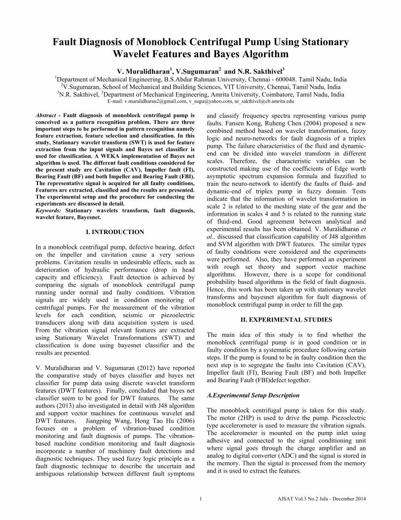
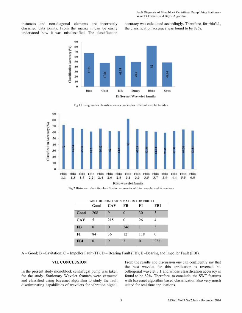
All the wavelet families and its sub-groups were used to find the stationary wavelet transform which form the feature vectors. The extracted features were then given as an input to the classifier (Bayes NET algorithm) and the classification accuracies were found. Fig.1. will describe the classification accuracies among the different families of wavelet. One can easily understand that the classification accuracy of reverse bi-orthogonal family is high. The performance among the reverse bi-orthogonal wavelet and its versions is presented in Fig.2. Form Fig. 2, one can easily understand the maximum classification accuracy is 82% which is against rbio3.1. This means that the 3.1 version of reverse bi-orthogonal wavelet performs relatively better than any other versions of the wavelet families. The detailed classification detail for rbio 3.1 is given below in the form of confusion matrix in Table. 3. The confusion matrix can be interpreted as follows. The diagonal elements in the matrix are correctly classified
V. Muralidharan, V.Sugumaran and N.R. Sakthivel
2AJSAT Vol.3 No.2 Julu - December 2014
instances and non-diagonal elements are incorrectly classified data points. From the matrix it can be easily understood how it was misclassified. The classification
accuracy was calculated accordingly. Therefore, for rbio3.1, the classification accuracy was found to be 82%.
Fig.1 Histogram for classification accuracies for different wavelet families
Fig.2 Histogram chart for classification accuracies of rbior wavelet and its versions
TABLE.III. CONFUSION MATRIX FOR RBIO3.1
Good CAV FB FI FBI
Good 208 9 0 30 3
CAV 5 215 0 26 4
FB 0 0 246 1 3
FI 84 36 12 118 0
FBI 0 9 3 0 238
A – Good; B –Cavitation; C – Impeller Fault (FI); D – Bearing Fault (FB); E –Bearing and Impeller Fault (FBI).
VII. CONCLUSION In the present study monoblock centrifugal pump was taken for the study. Stationary Wavelet features were extracted and classified using bayesnet algorithm to study the fault discriminating capabilities of wavelets for vibration signal.
From the results and discussion one can confidently say that the best wavelet for this application is reversed bi-orthogonal wavelet 3.1 and whose classification accuracy is found to be 82%. Therefore, to conclude, the SWT features with bayesnet algorithm based classification also very much suited for real time applications.
Fault Diagnosis of Monoblock Centrifugal Pump Using Stationary Wavelet Features and Bayes Algorithm
3 AJSAT Vol.3 No.2 Julu - December 2014

REFERENCES [1] V. Muralidharan and V. Sugumaran, “Selection of Discrete
Wavelets for Fault Diagnosis of Monoblock Centrifugal Pump using the J48 Algorithm”, Applied Artificial Intelligence, Vol. 27, pp. 1-19,2013.
[2] V. Muralidharan, V. Sugumaran and N.R.Sakthivel, “Wavelet decomposition and support vector machine for fault diagnosis of monoblock centrifugal pump”, International Journal of Data Analysis and Strategies, Vol. 3, pp.159 – 177, 2011.
[3] Jiangping Wang, Hongtao Hu, “Vibration based fault diagnosis of pump using fuzzy technique”, Measurement, Vol.39, pp.176-185, 2006.
[4] Fansen Kong and Ruheng Chen, “A combined method for triplex pump fault diagnosis based on wavelet transforms, fuzzy logic and neuro-networks” Mechanical System and signal processing, Vol.18, pp. 161-168, 2004.
[5] V. Muralidharan, V. Sugumaran and Hemantha Kumar, “Fault Diagnosis of Monoblock Centrifugal Pump Using Discrete Wavelet Features and J48 Algorithm”, International Journal of Mechanical Engineering and Technology, Vol. 3, pp.120 – 126,2012.
[6] V Muralidharan and V. Sugumaran, “Feature Extraction using Wavelets and classification through Decision Tree Algorithm for Fault Diagnosis of Mono-Block Centrifugal Pump”, Measurement, Vol.46, pp.353 – 359, 2013.
[7] D. Zogg, E. Shafai, H.P. Geering, “Fault diagnosis of heat pumps with parameter identification and clustering”, Control Engineering practice , Vol.12, pp.1435-1444, 2006.
[8] V. Muralidharan and V. Sugumaran, “Rough Set Based Rule Learning and Fuzzy Classification of Wavelet Features for Fault Diagnosis of Monoblock Centrifugal Pump” Measurement, Vol. 46, Issue 9, pp. 3057-3063, Nov. 2013.
[9] V. Muralidharan, S. Ravikumar and H.Kanagasabapathy, “Condition monitoring of Self aligning carrying idler (SAI) in belt-conveyor system using statistical features and decision tree algorithm”, Measurement, Vol. 58, pp. 274–279, Dec. 2014.
[10] V. Muralidharan, V.Sugumaran and M. Indira, “Fault Diagnosis of Monoblock Centrifugal pump using SVM” Engineering Science and Technology, an International Journal, Vol. 17, pp.152-157, Sep 2014.
[11] V. Muralidharan, V. Sugumaran and Gaurav Pandey, “SVM Based Fault Diagnosis of Monoblock Centrifugal pump using Stationary Wavelet Features” International Journal of Design and Manufacturing Technology, Vol. 2, Issue 1, pp. 1-6, 2011.
V. Muralidharan, V.Sugumaran and N.R. Sakthivel
4AJSAT Vol.3 No.2 Julu - December 2014

Experimental Investigations on Finding Ball Bearing Defects Using Signature Analysis
K.Gunasekar1 and A.Pugazhenthi2
1Assistant Professor, Department of Mechanical Engineering,
PSNA College of Engineering and Technology, Dindigul, Tamil Nadu, India 2Assistant Professor, Department of Mechanical Engineering Anna University,
University College of Engineering, Dindigul, Tamil Nadu, India E-mail: [email protected]
Abstract - This paper presents for identify the defected bearing using vibration frequency. There have been a lot of researches on diagnosing rolling element bearing faults using wavelet analysis, but almost all methods are not ideal for picking up fault signal characteristics under strong noise. The rolling element bearing is used widely in all rotating components. It is one of the most susceptible components in a machine because it is most often under maximum load and high speed running conditions. This paper describes the suitability of vibration monitoring and analysis techniques to become aware of defects in antifriction bearings. Time domain analysis, frequency domain analysis and spike energy analysis have been working to identify different defects in bearings. Keywords: Signal characteristics, Time domain analysis, and frequency domain analysis. Notation BD, PD : roller diameter and pitch d respectively,
mm fo , fi,, fR : outer race, inner race an malfunction
frequencies, r espectively, H fr : rotational frequency, Hz n : number of rollers b : angle of contact
I. INTRODUCTION
Bearings are what enable things to roll. Without bearings our industrial world would, in many respects, stand still. The first bearing with the help of the wheel enabled people to move themselves and their goods from one village to another. It helped them in producing their food. Today, bearing technology has developed to a stage where bearings are one of the most advanced mechanical components with regard to optimized design, high quality materials and accurate manufacturing. Condition monitoring of antifriction bearings in rotating machinery using vibration analysis is a very well established method. It offers the advantages of reducing down time and improving maintenance efficiency. The machine need not be stopped for diagnosis. Even new or geometrically perfect bearings may generate vibration due to contact forces, which exist between the various components of bearings. Antifriction bearing defects may be categorized as localized and dispersed. The localized defects include cracks, pits and spalls caused by fatigue on rolling surfaces. The other category, ie, distributed defects includes surface roughness, waviness, and misaligned races and off size rolling
elements. These defects may result from manufacturing error and abrasive wear. Hence, study of vibrations generated by these defects is important for quality inspection as well as for condition monitoring. Antifriction bearing failures result in serious problems, mainly in places where machines are rotating at constant and high speeds. In order to prevent any terrible consequences caused by a bearing failure, bearing condition monitoring techniques, such as, temperature monitoring, wear debris analysis, oil analysis, vibration analysis and acoustic emission analysis have been developed to identify life of flaws in running bearings. Among them vibration analysis is most generally accepted technique due to its easiness of application.
Vibration signature monitoring and analysis in one of the main techniques used to predict and diagnose various defects in antifriction bearings. Vibration signature analysis provides early information about progressing malfunctions and forms the basic reference signature or base line signature for future monitoring purpose. Defective rolling elements in antifriction bearings generate vibration frequencies at rotational speed of each bearing component and rotational frequencies are related to the motion of rolling elements, cage and races. Initiation and progression of flaws on antifriction bearing generate specific and predictable characteristic of vibration. Components flaws (inner race, outer race and rolling elements) generate specific defect frequencies calculated.
The time domain and frequency domain analyses are widely accepted for detecting malfunctions in bearings. The frequency domain spectrum is more useful since it also identifies the exact nature of defect in the bearings. Spike energy analysis makes use of spike energy meter to measure three parameters of high frequency pulses, namely, pulse amplified, pulse rate and high frequency ‘random vibratory energy’ associated with bearing defects.
II.EXPERIMENTAL SETUP An experimental test rig built to predict defects in antifriction bearings is shown in Figure 1. The test rig consists of a shaft with central rotor, which is supported on two bearings. An induction motor coupled by a flexible coupling drives the shaft. Self aligning double row ball bearing is mounted at driver end and cylindrical roller bearing is mounted at free end. The cylindrical roller
5 AJSAT Vol.3 No.2 Julu - December 2014
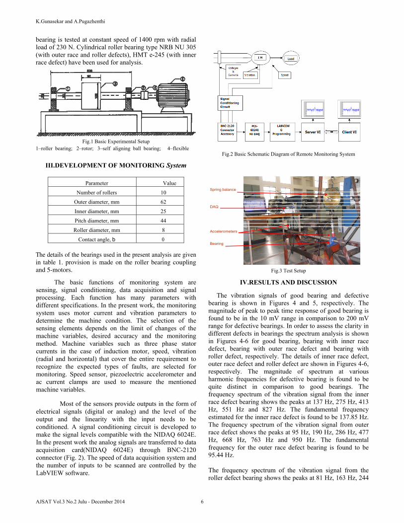
bearing is tested at constant speed of 1400 rpm with radial load of 230 N. Cylindrical roller bearing type NRB NU 305 (with outer race and roller defects), HMT e-245 (with inner race defect) have been used for analysis.
Fig.1 Basic Experimental Setup 1–roller bearing; 2–rotor; 3–self aligning ball bearing; 4–flexible
III.DEVELOPMENT OF MONITORING System
Parameter Value
Number of rollers 10
Outer diameter, mm 62
Inner diameter, mm 25
Pitch diameter, mm 44
Roller diameter, mm 8
Contact angle, b 0
The details of the bearings used in the present analysis are given in table 1. provision is made on the roller bearing coupling and 5-motors. The basic functions of monitoring system are sensing, signal conditioning, data acquisition and signal processing. Each function has many parameters with different specifications. In the present work, the monitoring system uses motor current and vibration parameters to determine the machine condition. The selection of the sensing elements depends on the limit of changes of the machine variables, desired accuracy and the monitoring method. Machine variables such as three phase stator currents in the case of induction motor, speed, vibration (radial and horizontal) that cover the entire requirement to recognize the expected types of faults, are selected for monitoring. Speed sensor, piezoelectric accelerometer and ac current clamps are used to measure the mentioned machine variables.
Most of the sensors provide outputs in the form of electrical signals (digital or analog) and the level of the output and the linearity with the input needs to be conditioned. A signal conditioning circuit is developed to make the signal levels compatible with the NIDAQ 6024E. In the present work the analog signals are transferred to data acquisition card(NIDAQ 6024E) through BNC-2120 connector (Fig. 2). The speed of data acquisition system and the number of inputs to be scanned are controlled by the LabVIEW software.
Fig.2 Basic Schematic Diagram of Remote Monitoring System
Accelerometers
Spring balance
Bearing
DAQ
Fig.3 Test Setup
IV.RESULTS AND DISCUSSION
The vibration signals of good bearing and defective bearing is shown in Figures 4 and 5, respectively. The magnitude of peak to peak time response of good bearing is found to be in the 10 mV range in comparison to 200 mV range for defective bearings. In order to assess the clarity in different defects in bearings the spectrum analysis is shown in Figures 4-6 for good bearing, bearing with inner race defect, bearing with outer race defect and bearing with roller defect, respectively. The details of inner race defect, outer race defect and roller defect are shown in Figures 4-6, respectively. The magnitude of spectrum at various harmonic frequencies for defective bearing is found to be quite distinct in comparison to good bearings. The frequency spectrum of the vibration signal from the inner race defect bearing shows the peaks at 137 Hz, 275 Hz, 413 Hz, 551 Hz and 827 Hz. The fundamental frequency estimated for the inner race defect is found to be 137.85 Hz. The frequency spectrum of the vibration signal from outer race defect shows the peaks at 95 Hz, 190 Hz, 286 Hz, 477 Hz, 668 Hz, 763 Hz and 950 Hz. The fundamental frequency for the outer race defect bearing is found to be 95.44 Hz. The frequency spectrum of the vibration signal from the roller defect bearing shows the peaks at 81 Hz, 163 Hz, 244
K.Gunasekar and A.Pugazhenthi
6AJSAT Vol.3 No.2 Julu - December 2014
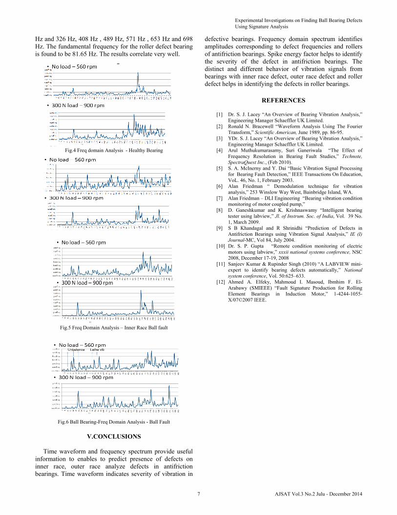
Hz and 326 Hz, 408 Hz , 489 Hz, 571 Hz , 653 Hz and 698 Hz. The fundamental frequency for the roller defect bearing is found to be 81.65 Hz. The results correlate very well.
Fig.4 Freq domain Analysis - Healthy Bearing
Fig.5 Freq Domain Analysis – Inner Race Ball fault
Fig.6 Ball Bearing-Freq Domain Analysis - Ball Fault
V.CONCLUSIONS
Time waveform and frequency spectrum provide useful information to enables to predict presence of defects on inner race, outer race analyze defects in antifriction bearings. Time waveform indicates severity of vibration in
defective bearings. Frequency domain spectrum identifies amplitudes corresponding to defect frequencies and rollers of antifriction bearings. Spike energy factor helps to identify the severity of the defect in antifriction bearings. The distinct and different behavior of vibration signals from bearings with inner race defect, outer race defect and roller defect helps in identifying the defects in roller bearings.
REFERENCES
[1] Dr. S. J. Lacey “An Overview of Bearing Vibration Analysis,”
Engineering Manager Schaeffler UK Limited. [2] Ronald N. Bracewell “Waveform Analysis Using The Fourier
Transform,” Scientific American, June 1989, pp. 86-95. [3] YDr. S. J. Lacey “An Overview of Bearing Vibration Analysis,”
Engineering Manager Schaeffler UK Limited. [4] Arul Muthukumarasamy, Suri Ganeriwala “The Effect of
Frequency Resolution in Bearing Fault Studies,” Technote, SpectraQuest Inc., (Feb 2010).
[5] S. A. McInerny and Y. Dai “Basic Vibration Signal Processing for Bearing Fault Detection,” IEEE Transactions On Education, VoL. 46, No. 1, February 2003.
[6] Alan Friedman “ Demodulation technique for vibration analysis,” 253 Winslow Way West, Bainbridge Island, WA.
[7] Alan Friedman – DLI Engineering “Bearing vibration condition monitoring of motor coupled pump,”
[8] D. Ganeshkumar and K. Krishnaswamy “Intelligent bearing tester using labview,” Jl. of Instrum. Soc. of India, Vol. 39 No. 1, March 2009.
[9] S B Khandagal and R Shrinidhi “Prediction of Defects in Antifriction Bearings using Vibration Signal Analysis,” IE (I) Journal-MC, Vol 84, July 2004.
[10] Dr. S. P. Gupta “Remote condition monitoring of electric motors using labview,” xxxii national systems conference, NSC 2008, December 17-19, 2008
[11] Sanjeev Kumar & Rupinder Singh (2010) “A LABVIEW mini-expert to identify bearing defects automatically,” National system conference, Vol. 50:625–633.
[12] Ahmed A. Elfeky, Mahmoud I. Masoud, Ibmhim F. El-Arabawy (SMIEEE) “Fault Signature Production for Rolling Element Bearings in Induction Motor,” 1-4244-1055-X/07©2007 IEEE.
Experimental Investigations on Finding Ball Bearing Defects Using Signature Analysis
7 AJSAT Vol.3 No.2 Julu - December 2014

Flow Measurement Using RTDs
Nagaraju B.P1 and Rathanraj K.J2
1Border Security Force Institute of Technology, BSF STC, Bangalore-63. 2Professor, Dept of Industrial Engineering & Management, B.M.S.College Engineering, Bangalore-19, Karnataka, India.
E-Mail:[email protected] Abstract- In many processing industries, it is essential to measure either the flow rate or just to know whether the flow or no flow conditions exists. The change in resistance measures the prevailing temperature differential in the flow pipe. The temperature difference could be related to flow rate or flow or no-flow conditions. This may be achieved by the selection of right sensor, signal conditioning circuit and display. Keywords: Flow Or No Flow Conditions, Temperature differential, sensor, signal conditioning and display
I.INTRODUCTION The flow rate can be measured using venturimeter, orifice meter, turbine flow meter and ultrasonic flow meter. However, just to know the flow or No-flow conditions in the flow, the simplest reliable system developed is based on the thermal dispersion principle
II.THERMAL DISPERSION PRINCIPLE The typical sensing element contains two thermowell-protected precision platinum Resistance Temperature Detectors (RTDs). When placed in the process stream, one RTD is heated and the other RTD sense the process temperature. The temperature difference between the two RTDs is related to the process flow rate as well as the properties of the process media. Higher flow rates or denser media cause increased cooling of the heated RTD and a reduction in the RTD temperature difference. Thermal dispersion technology to provide the highest reliability in flow, level and temperature detection. The sensing element is composed of two matched RTD's. One RTD is preferentially heated. The other RTD is unheated and thermally isolated to provide continuous process condition temperature and baseline indication. At no flow or under dry conditions, the temperature differential between the two RTDs is greatest. For flow / no flow detection, No-flow conditions produce a large signal. As flow increases, the heated RTD is cooled and proportionally reduces temperature differential. Changes in flow velocity directly affect this rate of heat [11] The acronym “RTD” is derived from the term “Resistance Temperature Detector”. The most stable, linear and repeatable RTD is made of platinum metal. The temperature coefficient of the RTD element is positive. An approximation of the platinum RTD resistance change over temperature can be calculated by using the constant 0.00385//°C. This constant is easily used to calculate the absolute resistance of the RTD at temperature. [2] Equation RTD(T) = RTD0 + T X RT D0 X 0.00385//°C
where: RTD(T) is the resistance value of the RTD element at temperature ToC RTD0 is the specified resistance of the RTD element at 0°C and, ToC is the temperature environment that the RTD is placed. The RTD element resistance is extremely low when compared to the resistance of a NTC thermistor element, which ranges up to 1 M at 25°C. Typical specified 0°C values for RTDs are 50, 100, 200, 500, 1000 or 2000. Of these options, the 100 platinum RTD is the most stable over time and linear over temperature. If the RTD element is excited with a current reference at a level that does not create an error due to self-heating, the accuracy can be ±4.3°C over its entire temperature range of -200°C to 800°C. If a higher accuracy temperature measurement is required, the linearity formula below (Calendar-Van Dusen Equation) can be used in a calculation in the controller engine or be used to generate a look-up table. RTD ( T ) = RTD0 [1+ AT+ BT 2 - (100CT3 +CT4 ) where: RTD(T) is the resistance of the RTD element at temperature, RTD0 is the specified resistance of the RTD element at 0°C, T is the temperature that is applied to the RTD element (Celsius) and, A, B, and C are constants derived from resistance measurements at 0°C, 100°C and 260°C.
III.SENSOR FABRICATION TECHNOLOGY Realization of a thin film sensor involves the deposition of a sensing film on a suitable substrate. There could be combination of metals and insulating materials needs to be deposited on one another depending upon the application or sensing requirements. [3] Film Deposition Methods for Sensor Fabrication Based on the thickness of the deposited film and the technology used to deposit these films, fabrication technology is broadly divided into two categories like i) thick film technology and ii) thin film technology, details of which are given below.
IV.THICK FILM TECHNOLOGY Thick film technology uses pastes or “inks” with fine particles (5μ average diameter) of common or noble metals dispersed in an organic vehicle, along with a glass frit that binds them. Depending on the dispersed particles, the paste can be conductive, resistive or dielectric. Those pastes are screen printed on a substrate according to pattern involving width lines from 10 μ to 200μ. The printed film is dried by
8AJSAT Vol.3 No.2 Julu - December 2014
heating at about 150o
C to remove the organic solvent that provided the low viscosity needed for the paste to squeeze through the open areas in the screen. The substrate with the deposited film is then fired on a conveyor belt furnace, usually in the air atmosphere, so that the metal powder sinters and glass frit melts, thereby bonding the film to the substrate. The result is 10μ to 25μ thick film, impermeable to many substances but relatively porous for specific chemical or biological agents. Thick film components have a printed tolerance of about ±10% to ± 20%, but they can be later trimmed to within ±0.2% to ±0.5% through selective abrasion or laser evaporation. Thick film technology finds at least three different uses in sensors. It has been used for years to fabricate hybrid circuits offering improved performance compared to monolithic integrated circuits for signal conditioning and processing. Thick film circuits and some sensors can be integrated in the same package, which improves the reliability (strong connections), permit functional trimming and reduces cost. It is also used to create support structures or substrates onto which a sensing material is deposited. Some thick film pastes directly responds to physical and chemical quantities. There are pastes – some developed for sensing applications- with high temperature coefficients of resistance useful for temperature sensing, piezo-resistive pastes, magneto-resistive pastes, pastes with high Seeback coefficient among others. Pastes based on organic polymers and metal oxides such as SnO
2 can detect humidity and
gases because of adsorption and absorption. Using thick film technology, it is straightforward to define the inter-digitated structures required for those sensors. Thick film sensors with ceramic substrate withstand high temperatures, can be driven with relatively large voltages and currents, can integrate heaters and can resist corrosion. Because the paste is fired into the ceramic, thick film sensors are compact and sturdy. The printing process is quite inexpensive, which permits competitive low volume fabrication. [4-6]
V.THIN FILM TECHNOLOGY Thin films (generally less than 1 micron thick) are obtained, in general by vacuum deposition on a substrate. Sensor and circuit patterns are defined by masks and transferred by photolithography, similar to monolithic IC fabrication. Even though their names may suggest that the only difference between thick film and thin film technology is in film thickness, they are quite different technologies. In fact, metallized thin films may become thicker than some thick films. The properties of thin film differ from the bulk material. Common materials in thin film circuits are nichrome for resistors, gold for conductors, and silicon dioxide for dielectrics. Many thin film sensors are resistive.Piezo-resistors use nichrome and poly crystalline silicon, conductivity sensors use platinum, strain gauge based sensors use platinum – tungsten alloys, and gas sensors use zinc oxide.
NI MULTISIM The National Instruments Electronics Workbench Group (formerly Electronics Workbench) equips the professional printed circuit board (PCB) designer with world-class tools for schematic capture, interactive simulation, board layout, and integrated test. [7] VI.SOURCES OF ERRORS AND CORRECTION RTDs are externally powered sensors and based on the variation of resistance with temperature. The accuracy of platinum Resistance Thermometer (PRT) temperature measurement is largely determined by the number of leads used between the probe and the instrument. Two leads are often acceptable in the case of short cable runs; three leads compensating for lead resistance variations give improved accuracy; and four leads provide the greatest precision. Self-heating of RTD also causes measurement inaccuracy. The maximum excitation current is determined by the self-heating within the RTD and this limits the maximum signal for a required measurement temperature range. To produce a higher-level signal for indication and recording, a separate signal conditioner is needed. Noise interference can have a significant effect on accuracy. Shielded twisted pair signal cable minimizes noise interference on measuring circuit. For long cable runs a 4-20m A current transmitter may be used. RTD elements are, in fact very vulnerable to contamination of all kinds, and must be used only in hermetically sealed probes for any industry application. Moisture, dirt or any seriously affect the accuracy of RTD. [1]
TABLE 1. RTD ADVANTAGES AND DISADVANTAGES
Advantages Disadvantages Very Accurate and Stable Expensive Solution Fairly Linear to ±4%C Requires Current Excitation Good Repeatability Danger of Self-Heating
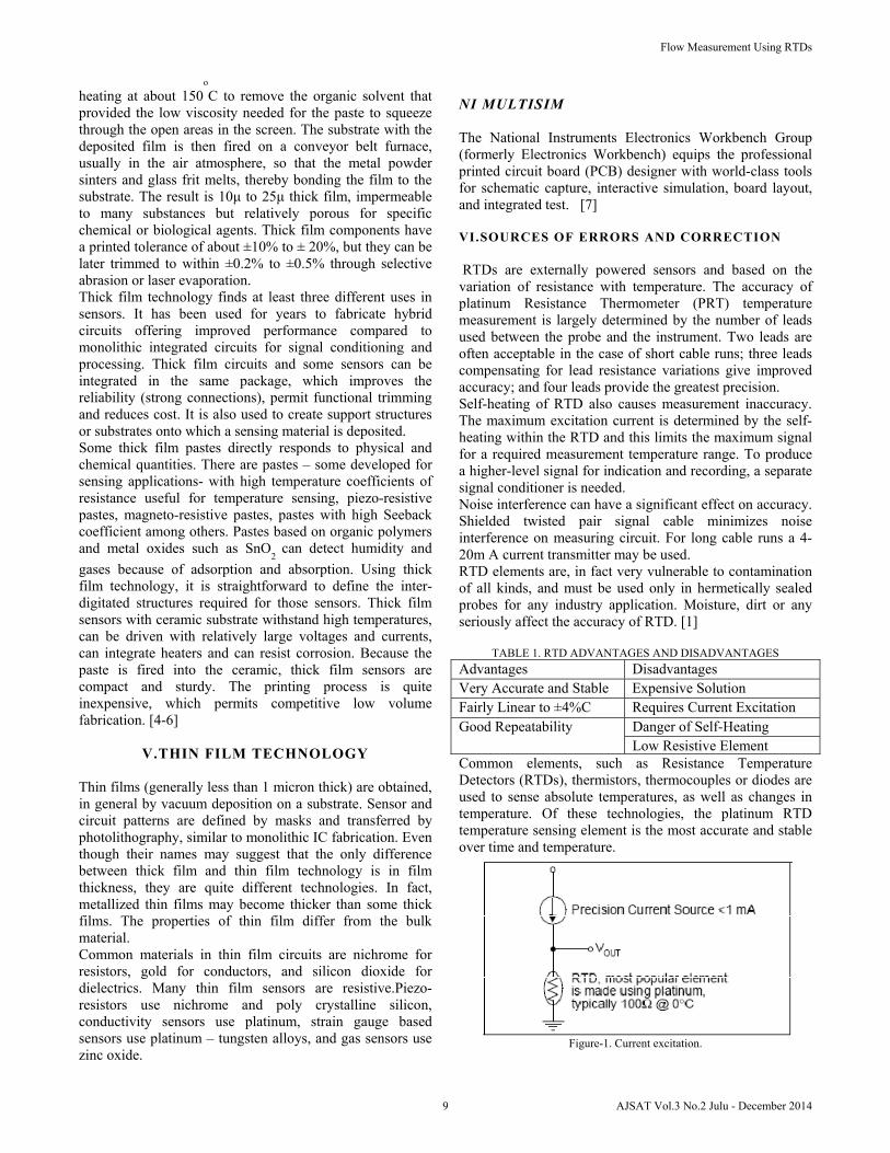
Low Resistive Element Common elements, such as Resistance Temperature Detectors (RTDs), thermistors, thermocouples or diodes are used to sense absolute temperatures, as well as changes in temperature. Of these technologies, the platinum RTD temperature sensing element is the most accurate and stable over time and temperature.
Figure-1. Current excitation.
Flow Measurement Using RTDs
9 AJSAT Vol.3 No.2 Julu - December 2014

VII.RTD CURRENT EXCITATION CIRCUIT For best linearity, the RTD sensing element requires a stable current reference for excitation. In this circuit, a voltage reference, along with two operational amplifiers, are used to generate a floating 1 mA current source.
Figure 2. A Current Source For The RTD element can be constructed in a single-supply environment from two operational amplifiers
and a precision voltage reference.
This is accomplished by applying a 2.5V precision voltage reference to R4 of the circuit. Since R4 is equal to R3, and the non-inverting input to U1 is high impedance, the voltage drop across these two resistors is equal. The voltage
between R3 and R4 is applied to the non-inverting input of U1. That voltage is gained by (1 + R2/R1) to the output of the amplifier and the top of the reference resistor, RREF. If R1 = R2, the voltage at the output of U1 is equal to:
EQUATION
R4REF1
2OUTU1 VVR
R1V
R4REFOUTU1 VV2V
Where: VOUTU1 is the voltage at the output of U1 and VR4 is the voltage drop across R4. The voltage at the output of U1 is equal to: EQUATION
R3R4REFOUTU1 VVVV
This same voltage appears at the inverting input of U2 and across to the non-inverting input of U2. Solving these equations, the voltage drop across the reference resistor, RREF, is equal to:
OUTA2OUTA1RREF VVV
R3R4REFR4REFRREF VVVVV2V
REFRREF VV
where: VRREF is the voltage across the reference resistor, RREF and, VR3 is the voltage drop across R3 The current through RREF is equal to: EQUATION
REFREFRTD R / V I
Nagaraju B.P and Rathanraj K.J
10AJSAT Vol.3 No.2 Julu - December 2014
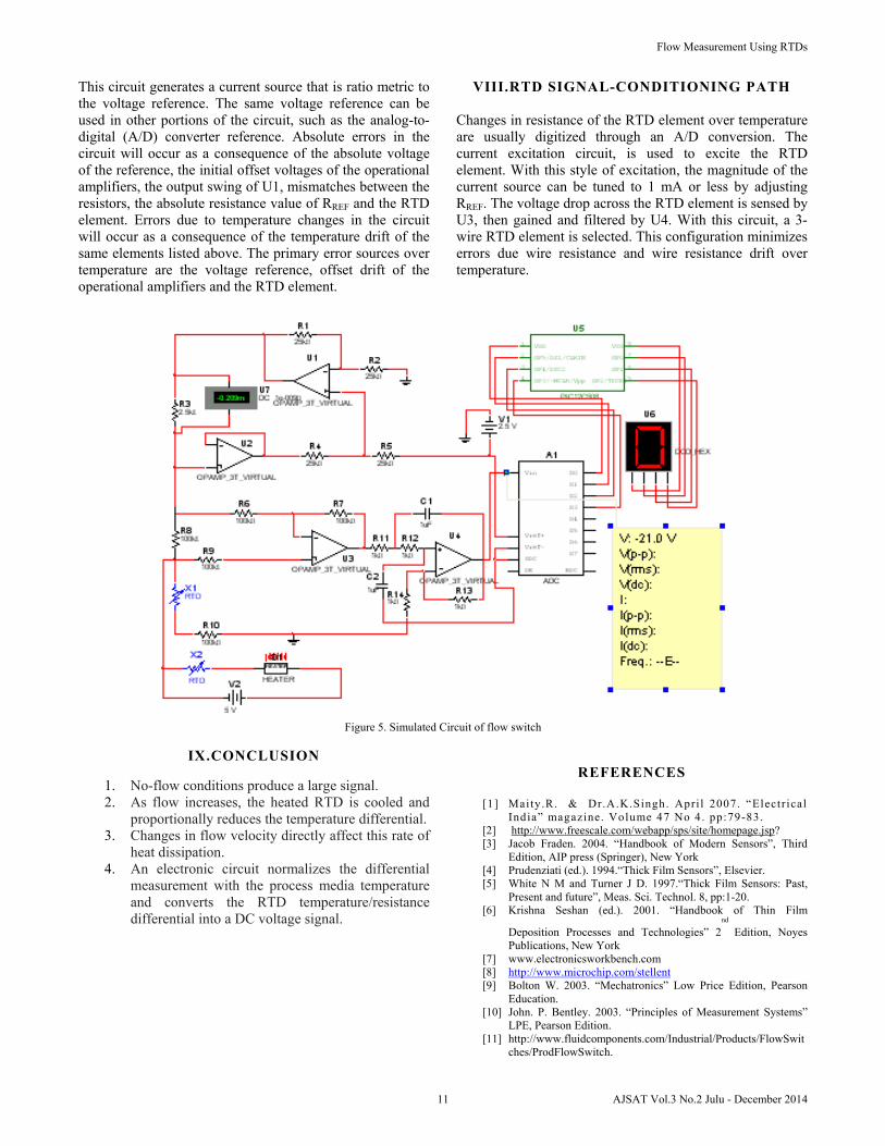
This circuit generates a current source that is ratio metric to the voltage reference. The same voltage reference can be used in other portions of the circuit, such as the analog-to-digital (A/D) converter reference. Absolute errors in the circuit will occur as a consequence of the absolute voltage of the reference, the initial offset voltages of the operational amplifiers, the output swing of U1, mismatches between the resistors, the absolute resistance value of RREF and the RTD element. Errors due to temperature changes in the circuit will occur as a consequence of the temperature drift of the same elements listed above. The primary error sources over temperature are the voltage reference, offset drift of the operational amplifiers and the RTD element.
VIII.RTD SIGNAL-CONDITIONING PATH Changes in resistance of the RTD element over temperature are usually digitized through an A/D conversion. The current excitation circuit, is used to excite the RTD element. With this style of excitation, the magnitude of the current source can be tuned to 1 mA or less by adjusting RREF. The voltage drop across the RTD element is sensed by U3, then gained and filtered by U4. With this circuit, a 3-wire RTD element is selected. This configuration minimizes errors due wire resistance and wire resistance drift over temperature.
Figure 5. Simulated Circuit of flow switch
IX.CONCLUSION
1. No-flow conditions produce a large signal. 2. As flow increases, the heated RTD is cooled and
proportionally reduces the temperature differential. 3. Changes in flow velocity directly affect this rate of
heat dissipation. 4. An electronic circuit normalizes the differential
measurement with the process media temperature and converts the RTD temperature/resistance differential into a DC voltage signal.
REFERENCES
[1] Maity.R. & Dr.A.K.Singh. Apri l 2007. “Electr ical
India” magazine. Volume 47 No 4. pp:79-83. [2] http://www.freescale.com/webapp/sps/site/homepage.jsp? [3] Jacob Fraden. 2004. “Handbook of Modern Sensors”, Third
Edition, AIP press (Springer), New York [4] Prudenziati (ed.). 1994.“Thick Film Sensors”, Elsevier. [5] White N M and Turner J D. 1997.“Thick Film Sensors: Past,
Present and future”, Meas. Sci. Technol. 8, pp:1-20. [6] Krishna Seshan (ed.). 2001. “Handbook of Thin Film
Deposition Processes and Technologies” 2nd
Edition, Noyes Publications, New York
[7] www.electronicsworkbench.com [8] http://www.microchip.com/stellent [9] Bolton W. 2003. “Mechatronics” Low Price Edition, Pearson
Education. [10] John. P. Bentley. 2003. “Principles of Measurement Systems”
LPE, Pearson Edition. [11] http://www.fluidcomponents.com/Industrial/Products/FlowSwit
ches/ProdFlowSwitch.
Flow Measurement Using RTDs
11 AJSAT Vol.3 No.2 Julu - December 2014
An Investigation on Instantaneous Workability Behavior of Aluminium SiC Air Quenched Powder Composites During Cold Upsetting
M. Prabhakar 1, T. Ramesh2, R. Narayanasamy3 and V. Anandakrishnan4
1 Professor, Department of Mechanical Engineering, TRP Engineering College, Trichirappalli, Tamil Nadu, India
2 Asst. Professor, Department of Mechanical Engineering, 3 Professor, 4 Asst. Professor, Department of Production Engineering, National Institute of Technology, Trichirappalli, Tamil Nadu, India
E-mail:[email protected]
Abstract - Strain hardening of a material is an important phenomenon, which is required to study the plastic deformation of any material and also is an important parameter in the study of workability criteria of metals. The present investigation has been undertaken to evaluate the instantaneous strain hardening behaviour experienced during the cold working of sintered aluminium SiC composites from 0 to 15% under various stress state conditions namely uniaxial, plane and triaxial. Sintered preforms with three different aspect ratios namely 0.38, 0.76 and 1.19 with for different per cent of SiC contents ranging from 0 to 15% were prepared and cold forged. The results were obtained for each aspect ratios and SiC contents at different stress state conditions. Keywords: Upsetting; Strain hardening exponent; Strength coefficient; Powder Metallurgy; Triaxial stress
I. INTRODUCTION Powder metallurgy (P/M) process provides several advantages when comparing with conventional manufacturing process. It can provide a reasonable improvement in specific strength, stiffness and wear resistant, compared with monolithic alloys. At present, the powder metallurgy components are being widely used for sophisticated industrial applications. The worldwide popularity of powder metallurgy lies in the ability of this technique to produce such complex shapes with exact dimensions at a high rate of production with low cost prices. Frequently, this technology is used for material systems that are hard to machine such as tungsten or molybdenum or very much difficult to cast due to detrimental solidification behavior of material chosen. Abdel-Rahman and Sheikh [1] discussed workability criterion of powder metallurgy compacts and they investigated the effect of the relative density on the forming limit of P/M compacts in upsetting. They proposed a workability factor (β) for describing the effect of the mean stress and the effective stresses with the help of two theories and they discussed the effect of relative density. Narayanasamy and Pandey [2] performed an excellent work on the strain hardening behaviour of the powder metallurgy composites. They evaluated the work hardening characteristics of sintered aluminium–iron composite preform conducting experimental works under uniaxial stress state conditions and studied the strength coefficient value for various iron particle sizes.
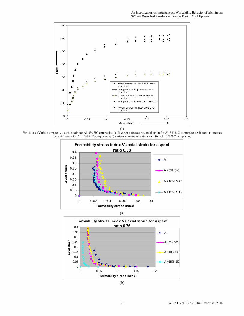
Narayanasamy and Pandey [3] investigated the evaluation of cold upset-forming and densification features in aluminium–3.5% alumina sintered powder preforms and they concluded that the preforms possessing lower initial aspect ratios have shown enhanced densification compared to preforms of higher initial aspect ratios, subject to the condition where the initial preform densities maintained constant. Further they studied the effect of Poisson’s ratio with respect to the fractional theoretical density attained exhibited three distinct stages, namely, a steep rise, a steady state, followed by a rapid rise approaching to value of 0.5 in the close vicinity of the theoretical density [4]. Narayanasamy and Ramesh investigated the workability criteria under triaxial conditions for Aluminum and iron compacts with various particle sizes and they found the triaxial stress conditions with various aspect ratios [5], the same author investigated the strain hardening exponent and strength coefficient for the same combination composites [6]. Sridhar and fleck [7] did their experiment on triaxial test on cold compaction behavior of lead shot with steel reinforcement as well as Aluminium and 40% silicon carbide powder under hydrostatic loading conditions and they found the shape deformations and hardening parameters along the loading directions. Li and Mohamed [8] investigated the creep behavior on 10vol % SiC with 2124Aluminium composites. Z. Lin [9] also investigated with the same aluminium combination with 5vol % SiC additions and investigated the creep behavior of the composites. In this paper, a complete investigation deformation behavior of aluminium powder metallurgy composites with various percent of SiC contents ranging from 0 to 15% for the various stress state conditions namely, uniaxial, plane and triaxial conditions with three different aspect ratios were performed. The formability stress index found for various per cent of SiC content of preforms for various stress state conditions were calculated and plotted against the axial strain. From the plot it is observed that the addition of SiC particles in the aluminium powder preforms do have great changes in the formability stress index ‘β’ and axial strain.
12AJSAT Vol.3 No.2 Julu - December 2014

Nomenclature Db bulged diameter Dc contact diameter D0 initial diameter Hf height of the compact at fracture H0 initial height of compact Greek letters α Poisson’s ratio εeff effective strain component εr radial strain component εz axial strain component εθ hoop strain component σeff effective stress component σm mean stress σr radial stress component σz axial stress component σθ hoop stress component
II. THEORETICAL INVESTIGATIONS The mathematical expressions used and proposed for the determination of various upsetting parameters for various stress state conditions are discussed below. A. Uniaxial stress state and plane stress state conditions In the compression of P/M part, under frictional conditions, the average density is increased. Friction enhances densification and at the same time decreases the height reduction at fracture. The state of stress in a homogeneous compression process is as follows. According to Abdel-Rahman and Sheikh [1]: σz = −σeff, σr = σθ = 0 (1) where σz is the axial stress, σeff is the effective stress, σr is the radial stress and σθ is the hoop stress.
3Z
m
(2)
where σm is the mean or hydrostatic stress and the strain state is
fZ h
h0ln (3)
and
2
22
3
2ln
o
cb
D
DD (4)
where Db is the bulged diameter of compacts; Dc is the contact diameter of compacts and; D0 is the initial diameter of compacts.
When the compression continues, the final diameter increases and the corresponding hoop strain, which
is tensile in nature, also increases until it reaches the fracture limit. The associated flow characteristics for porous materials under plane stress state condition can be expressed as dεz = dλ(σz − νσθ) (5) dεθ = dλ(σθ − νσz) (6) where dεz is the plastic strain increment in the axial direction, dεθ is the plastic strain increment in the hoop direction, dλ is the constant. As an evidence of experimental investigation implying the importance of the spherical component of the stress state on fracture called a formability stress index ‘β’ which is given by:
eff
m
3
(7)
This index determines the fracture limit According to Narayanasamy and Pandey [4], the state of stress in a plane stress condition is as follows: σeff = (0.5 + α)[3(1 + α + α2)]1/2σz (8) where σeff-is the effective stress, α is the Poisson’s ratio = (εθ/2εz) Since, the radial stress σr is zero at the free surface it follows from the flow rule that,
Z
2
21 (9)
Further using the values of σz and σθ, the hydrostatic stress (σm) can be calculated as follows:
Zm 3
1 (10)
Fig. 1. SEM photo of the aluminium powder.
An Investigation on Instantaneous Workability Behavior of Aluminium SiC Air Quenched Powder Composites During Cold Upsetting
13 AJSAT Vol.3 No.2 Julu - December 2014
(a) (b) (c)
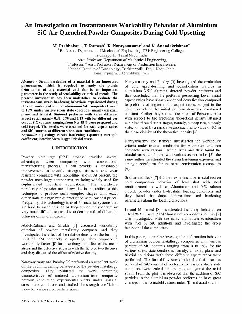
Fig. 2. (a) Al + 5% SiC specimen- SiC particle size 180 microns- macrostructure (b) Al + 10% SiC specimen- SiC particle size 180 microns- macrostructure (c) Al + 15% SiC specimen- SiC particle size 180 microns- macrostructure
(a) (b)
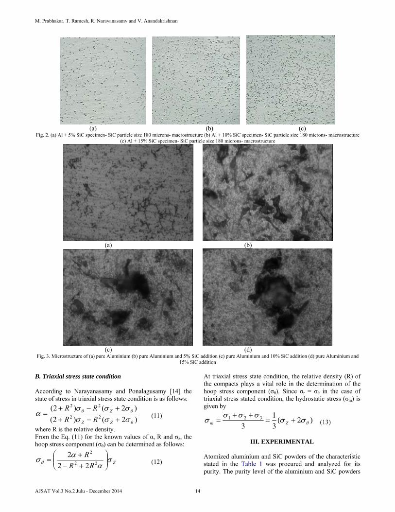
(c) (d) Fig. 3. Microstructure of (a) pure Aluminium (b) pure Aluminium and 5% SiC addition (c) pure Aluminium and 10% SiC addition (d) pure Aluminium and
15% SiC addition B. Triaxial stress state condition According to Narayanasamy and Ponalagusamy [14] the state of stress in triaxial stress state condition is as follows:
)2()2(
)2()2(22
22
ZZ
Z
RR
RR (11)
where R is the relative density. From the Eq. (11) for the known values of α, R and σz, the hoop stress component (σθ) can be determined as follows:
ZRR
R
22
2
22
2 (12)
At triaxial stress state condition, the relative density (R) of the compacts plays a vital role in the determination of the hoop stress component (σθ). Since σr = σθ in the case of triaxial stress stated condition, the hydrostatic stress (σm) is given by
)2(3
1
3321
Zm (13)
III. EXPERIMENTAL
Atomized aluminium and SiC powders of the characteristic stated in the Table 1 was procured and analyzed for its purity. The purity level of the aluminium and SiC powders
M. Prabhakar, T. Ramesh, R. Narayanasamy and V. Anandakrishnan
14AJSAT Vol.3 No.2 Julu - December 2014

was found to be 99.7 and 99.62%, respectively. Fig. 1 show the SEM photographs of aluminium powder. The compacts were prepared from aluminium and SiC powders with different aspect ratios at the compacting pressure range of 200–225MPa (410-485 MPa) in order to obtain the initial preform density ranging from 0.85 to 0.92 of the theoretical value. The powder metal compacts were prepared by blending aluminium and SiC powders of different SiC
contents (0–15%) with SiC powders of particle size namely 180μm. The ceramic coating was applied over the surface of the compacts to protect them from oxidation during sintering. The ceramic-coated compacts were sintered in an electric muffle furnace at 550 ◦C for period of 90 min and air quenched by switching off the furnace power supply and opened to the room temperature.
TABLE I CHARACTERISTICS OF ALUMINIUM AND SIC POWDERS
------------------------------------------------------------------------------------------------------------ Sieve analysis (aluminium) Characteristics of aluminium powder ------------------------------------------------------------------------------------------------------------ Sieve number (μm) wt.% retained --------------------------------------------------------------------------------------------------------------- +106 0.26 Apparent density (g cm−3) 1.030 +90 2.54 Flow rate, S (by Hall flow meter) (50 g−1) 32.00 +75 14.73 Compressibility at a pressure +63 17.58 of 300MPa (g cm−3) 2.344 +53 24.86 +45 12.33 +38 6.27 −38 21.42 SiC particle size 180 μm ------------------------------------------------------------------------------------------------------------
The sintered preforms were cleaned from the sand particles and the dimensional measurement made before and after each deformation. The deformation of the compact was carried out between two flat open dies hardened to Rc 50–55 and tempered to Rc 46–50 on a 100 t capacity hydraulic press. Each compact was applied with the compressive loading in step of 0.01MN (one metric ton) until the appearance of first
visible cracks on the free surface. No lubricant was used for axial deformation. Immediately after the completion of each step of loading, the deformed height, the contact diameters, the bulged diameters and the density were measured. The axial stress (σz) is used for the calculation of strength coefficient (Ki) and strain hardening exponent (ni) for the case of uniaxial stress condition and the hoop stress (σθ) is used for the case of plane stress state conditions.
(a)
An Investigation on Instantaneous Workability Behavior of Aluminium SiC Air Quenched Powder Composites During Cold Upsetting
15 AJSAT Vol.3 No.2 Julu - December 2014

(b)
(c)
M. Prabhakar, T. Ramesh, R. Narayanasamy and V. Anandakrishnan
16AJSAT Vol.3 No.2 Julu - December 2014
(d)
(e)
An Investigation on Instantaneous Workability Behavior of Aluminium SiC Air Quenched Powder Composites During Cold Upsetting
17 AJSAT Vol.3 No.2 Julu - December 2014
(f)
(g)
M. Prabhakar, T. Ramesh, R. Narayanasamy and V. Anandakrishnan
18AJSAT Vol.3 No.2 Julu - December 2014

(h)
(i)
An Investigation on Instantaneous Workability Behavior of Aluminium SiC Air Quenched Powder Composites During Cold Upsetting
19 AJSAT Vol.3 No.2 Julu - December 2014
(j)
(k)
M. Prabhakar, T. Ramesh, R. Narayanasamy and V. Anandakrishnan
20AJSAT Vol.3 No.2 Julu - December 2014
(l)
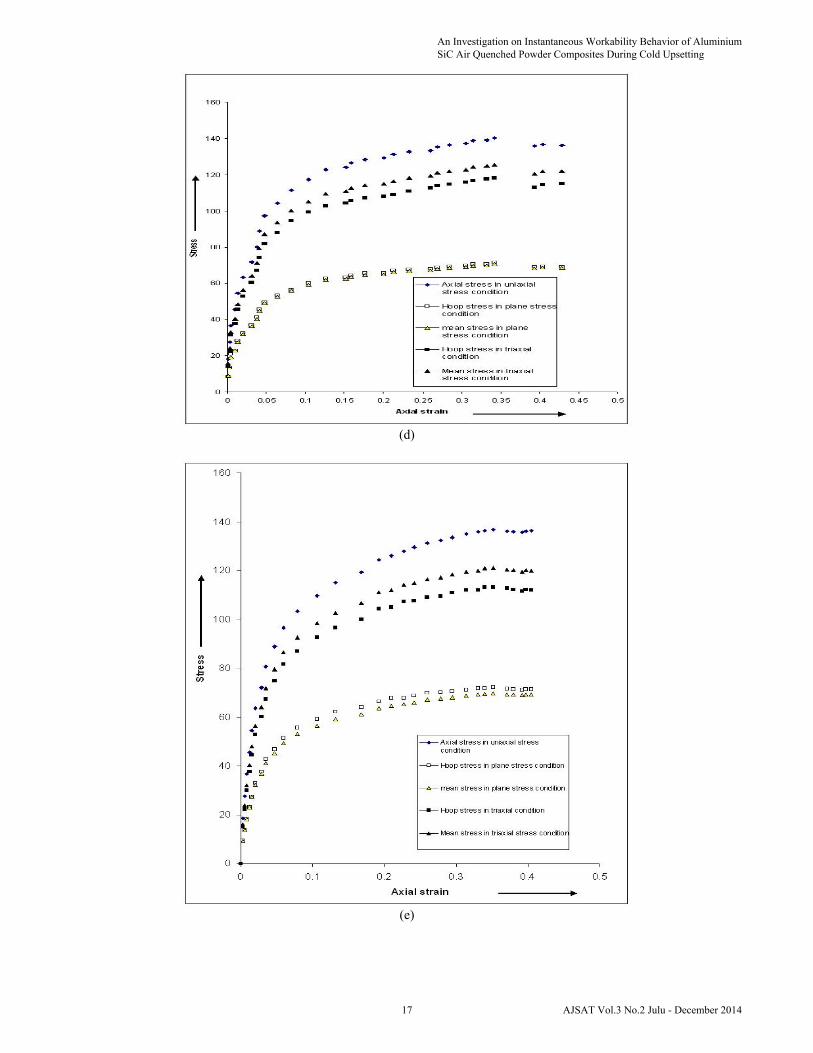
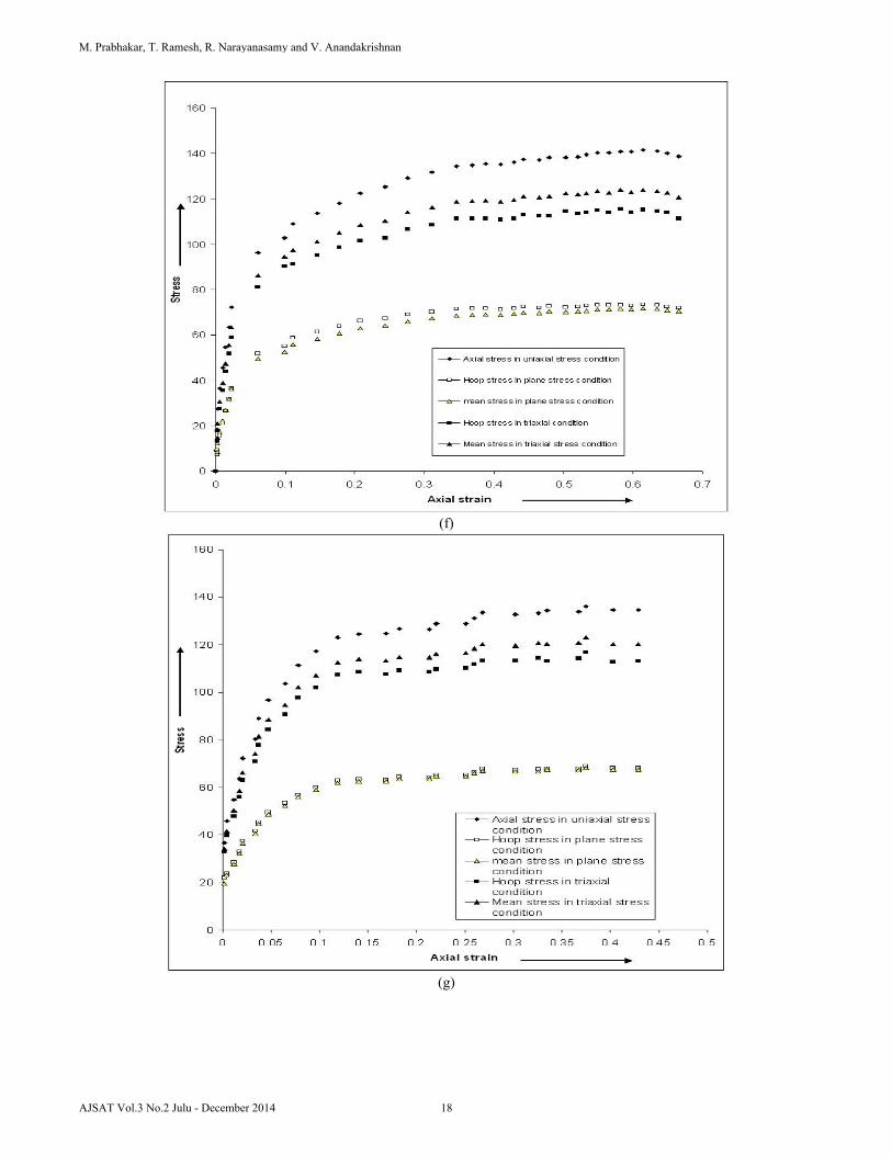
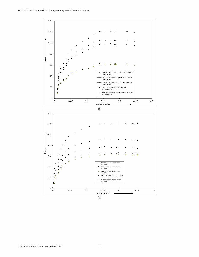
Fig. 2. (a-c) Various stresses vs. axial strain for Al–0% SiC composite; (d-f) various stresses vs. axial strain for Al–5% SiC composite; (g-i) various stresses vs. axial strain for Al–10% SiC composite; (j-l) various stresses vs. axial strain for Al–15% SiC composite;
Formability stress index Vs axial strain for aspect ratio 0.38
00.05
0.10.15
0.20.25
0.30.35
0.4
0 0.02 0.04 0.06 0.08 0.1Formability stress index
Axi
al s
trai
n
Al
Al+5% SiC
Al+10% SiC
Al+15% SiC
(a)
Formability stress index Vs axial strain for aspect ratio 0.76
0
0.050.1
0.150.2
0.25
0.30.35
0.4
0 0.05 0.1 0.15 0.2
Formability stress index
Axi
al s
trai
n
Al
Al+5% SiC
Al+10% SiC
Al+15% SiC
(b)
An Investigation on Instantaneous Workability Behavior of Aluminium SiC Air Quenched Powder Composites During Cold Upsetting
21 AJSAT Vol.3 No.2 Julu - December 2014

Formability stress index Vs axial strain for aspect ratio 1.12
0
0.1
0.2
0.3
0.4
0.5
0.6
0.7
0 0.1 0.2 0.3 0.4Formability stress index
Axi
al s
trai
n
Al
Al+5%SiCAl+10%SiCAl+15%SiC
(c)
Fig. 3 (a-c) Axial strain (εz) vs. formability stress index β – triaxial stress state condition for various aspect ratios
Relative density Vs stress ratio parameter σm/ σeff for aspect ratio 0.38
0
0.00001
0.00002
0.00003
0.00004
0.00005
0.85 0.9 0.95 1Relative Density
Stre
ss ra
tio
para
met
er 1
Al
Al+5%SiCAl+10%SiCAl+15%SiC
(a)
Relative density Vs stress ratio parameter σm/ σeff for aspect ratio 0.76
00.0000020.0000040.0000060.0000080.00001
0.0000120.0000140.0000160.0000180.00002
0.8 0.85 0.9 0.95 1Relative Density
Stre
ss ra
tio p
aram
eter
1
Al
Al+5%SiCAl+10%SiCAl+15%SiC
(b)
M. Prabhakar, T. Ramesh, R. Narayanasamy and V. Anandakrishnan
22AJSAT Vol.3 No.2 Julu - December 2014

Relative density Vs stress ratio parameter σm/ σeff for aspect ratio 1.12
0
0.000005
0.00001
0.000015
0.00002
0.92 0.94 0.96 0.98 1Relative Density
Stre
ss ra
tio
para
met
er 1
Al
Al+5%SiCAl+10%SiCAl+15%SiC
(c)
Fig. 4 (a-c) Stress ratio parameter (σm/σeff) vs. relative density (R).
Relative density Vs stress ratio parameter σr/ σeff for aspect ratio 0.38
00.05
0.1
0.150.2
0.250.3
0.350.4
0.85 0.9 0.95 1Relative Density
Stre
ss ra
tio p
aram
eter
2
Al
Al+5%SiCAl+10%SiCAl+15%SiC
(a)
Relative density Vs stress ratio parameter σr/ σeff for aspect ratio 0.76
0
0.05
0.1
0.15
0.2
0.25
0.3
0.35
0.4
0.8 0.85 0.9 0.95 1Relative Density
Stre
ss ra
tio p
aram
eter
2
Al
Al+5%SiCAl+10%SiCAl+15%SiC
(b)
An Investigation on Instantaneous Workability Behavior of Aluminium SiC Air Quenched Powder Composites During Cold Upsetting
23 AJSAT Vol.3 No.2 Julu - December 2014

Relative density Vs stress ratio parameter σr/ σeff for aspect ratio 1.12
0
0.05
0.1
0.15
0.2
0.25
0.3
0.35
0.4
0.92 0.94 0.96 0.98 1Relative Density
Stre
ss ra
tio p
aram
eter
2
Al
Al+5%SiCAl+10%SiCAl+15%SiC
(c)
Fig. 5 (a-c) Stress ratio parameter (σr/σeff) vs. relative density (R).
IV. RESULTS AND DISCUSSION
Fig. 2(a)–(f) have been plotted between the stresses namely axial–uniaxial, hoop-plane stress, hoop–triaxial, mean-plane stress and mean–triaxial and axial strain (ez) for different SiC content ranging from 0 to 15%. When the SiC addition is made, then all the above stresses and the axial strain (εz) value increase. It is also observed that hoop stresses according to plane stress and the axial stress value increase with the increase in SiC addition in the composite. The hydrostatic stress value according to triaxial stress condition increases with an increase in SiC addition. But, this value is less when comparing with compact with no addition of SiC. Here upto 10% SiC addition the axial stress and triaxial stresses namely hoop stress as well as mean stress are slightly higher than 120 MPa even upto 140 MPa recorded but addition of more silicon carbnide particles above this levcel shows reduction in the stress level, this may due to the particle size which we selected is higher so the void closure may be the reason for this reductions.
REFERENCES
[1] M. Abdel-Rahman, M.N. El-Sheikh, Workability in forging of powder metallurgy compacts, Journal of Materials Processing Technology, Vol.54, 1995, pp. 97-102.
[2] R. Narayanasamy, K S. Pandey, Some aspects of work hardening in sintered aluminium–iron composite preforms during cold axial forming, Journal of Materials Processing Technology, Vol. 84, 1998, pp.136–142.
[3] R. Narayanasamy, K S. Pandey, salient features in the cold upset-forming of sintered aluminum-3.5% alumina powder composite preforms, Journal of Materials Processing Technology, vol. 72, 1997, pp. 201-207.
[4] J. Bensam, P. Marimuthu, M. Prabhakar, V. Anandakrishnan, Effect of Sintering temperature on the Formability and Pore Closure Behavior of Al-SiC matrix P/M composite, Applied Mechanics and Materials, Vol.392, 2013, pp.24-30.
[5] R. Narayanasamy, T. Ramesh, K.S. Pandey, Some aspects on workability of aluminium–iron powder metallurgy composite during cold upsetting, Materials Science and Engineering, Vol. A 391,2005, pp. 418–426
[6] R. Narayanasamy, T. Ramesh, K.S. Pandey, Some aspects on strain hardening behaviour in three dimensions of aluminium–iron powder metallurgy composite during cold upsetting, Materials and Design, Vol. 27, 2006, pp. 640–650.
[7] Sridhar and N. A. Fleck, Yield behaviour of cold compacted composite powders, Acta mater. , Vol.48, 2000, pp. 3341-3352.
[8] Yong li and f. A. Mohamed, An investigation of creep behavior in an SiC-2124 Al composite, Acta mater. Vol. 45, No. 11, pp. 4775-4785,
[9] Zhigang Lin, Yong Li, Farghalli A. Mohamed, Creep and substructure in 5 vol.% SiC–2124 Al composite, Materials Science and Engineering, Vol. A332, 2002, pp. 330–342.
M. Prabhakar, T. Ramesh, R. Narayanasamy and V. Anandakrishnan
24AJSAT Vol.3 No.2 Julu - December 2014

Solar Radiation Catalyzed Aerobic Photooxidation of 1-Naphthol on Some Semiconductors
S. Karuthapandian and K. Arunsunaikumar
Department of Chemistry, V.H.N.Senthikumaranadar College, Virudhunagar – 626 001, Tamil Nadu, India E-mail: [email protected]
Abstract - Phototransformation of 1-naphthol into 1,2-naphthoquinone (1,2-NQ) using photocatalysts; TiO2, V2O5, PbO2, ZnO, Fe2O3, ZnS and Al2O3 has been studied in ethanol in the presence of air, under sunlight. The photooxidation exhibits saturation type kinetics with respect to [1-naphthol] and air. The rate of formation of 1,2-naphthoquinone increases linearly with respect to illumination area. The photooxidation rate is not suppressed by Singlet oxygen quencher, azide ion. Vinyl monomers and sacrificial electron donors do not interfere in photooxidation. The mechanisms of solar photocatalysis on semiconductor and non-semiconductor surfaces have been discussed and a kinetic law deduced. The solar photocatalytic efficiencies of the catalysts follow the order: Al2O3 > Fe2O3 > V2O5 > TiO2 > ZnO > PbO2 > ZnS. UV-visible, FT-IR and NMR spectroscopy spectral data clearly indicate that the photo product is 1,2-NQ.
I. INTRODUCTION
Photochemical processes in heterogeneous systems have gained popularity in recent years because of their wide applications in degradation and mineralization of pollutants, bactericidal activity, chemical synthesis and conversion and storage of solar light energy. Semiconductor mediated photocatlysis involves photo-excitation that causes charge separation in semiconductor particles followed by simultaneous oxidation and reduction of adsorbed substrates. Reports on photocatalyzed oxidation of a variety of substrates on semiconductor surfaces are numerous; titania is the most extensively used photocatalyst.1-3
Photosensitization of the titania nanoparticles with carotenoids leads to the formation of superoxide anion and singlet oxygen on red light irradiation.4 The dye photosensitization of zinc oxide occurs by injection of electron by the directly adsorbed dye.5 Doping of titania with iron(III) shifts the adsorption to longer wavelength and the absorbance increases with increasing dopant concentration.6 An increase in dopant ion content favours electron-hole separation and therefore enhances the photoactivity. Although doping of titania with chromium(III) shifts the absorbance to visible region the photocatalytic activity is nil in the visible region and diminished by 25-1000 times under UV light.7 This is attributed to an increase in electron-hole recombination at the chromium(III) ion site. On the other hand, doping of titania with lithium increases the photocatalytic efficiency, as seen from the degradation of malachite green.8 The photo-oxidation of iodide on 60% and 80% of aqueous ethanol was studied as a function of iodide ion
concentration, amount of catalyst suspended, airflow rate, light-intensity and solvent composition and wavelength of illumination, conform to Langmuir-Hinshelwood kinetic model. Iron(II) undergoes photooxidation generating iron(III)12-14 which is simultaneously photoreduced on the metal oxides surfaces.15 The photooxidation of 4-chloroaniline in aqueous solution has been reported.16 A photo-oxidation of aniline to azobenzene on titania in ethanol medium has been studied.17 The catalytic efficiency of titania has been increased for the photooxidation of aniline by doping with transition metal (or) noblemetals.18 The bimetallic catalyst of Au-Cu/Tio2 has employed for the partial oxidation of methanol to produce hydrogen.19
The photooxidation of cyclohexane shows that the photocatalytic efficiency depends on the particle size of the photocatalyst.20 The rate of photocatalytic production of hydrogen peroxide is 100 to 1000 times faster with Q-sized particles than with bulk zinc oxide particles.21 The photocatalytic oxidation of ethanol on small and large zinc sulfide particles reveals selective oxidation,22 ethanol is selectively oxidized at micrometer particles to acetaldehyde without side products by a “two hole” process. In the case of nanometer particles the primarily formed -hydroxyethyl radicals in a “one hole” process undergo a secondary reaction, i.e., the dimerization and disproportionation of the free radicals. A two hole process on nanometer particles becomes impossible because the time interval between two successive photon absorption incidents which lead to a successful hole transfer process in a nanometer particle is much longer than the maximum life time of the -Hydroxyethyl radicals formed in the first step. Photooxidation of 1- naphthol to 1,2-naphthoquinone has been studied extensively. The product of photooxidation of 1-naphthol affords significant amount of 1,2-naphthoquinone. 23-25 Oxidation of 1-naphthol using a sunlight on heterogeneous photocatalyzed oxidation of a variety of organic substrates are numerous literature lacks reports using solar radiation and hence this work. II. EXPERIMENTAL A. Materials 1-naphthol AR (merck) was used as received. TiO2, Al2O3, ZnO, Fe2O3, PbO2, ZnS and V2O5 were used as received from merck. Commercially available ethanol was distilled over calcium oxide and used.
25 AJSAT Vol.3 No.2 Julu - December 2014

B. Solar Photocatalysis Photooxidations of 1 – naphthol using sunlight in presence of catalysts TiO2, V2O5, PbO2, ZnO, Fe2O3, ZnS and Al2O3
were made from 11.30 am to 12.30 pm during summer, February to May on open terrace exposed to sunlight. The intensity of solar radiation was measured using Digital Illuminance Meter (LUX-METER), Model: TES-1332A, TES Electrical Electronic Corp., Taiwan. The reactions were carried out in glass case; solutions of 1-naphthol (1-NAPH), prepared afresh were taken in wide reaction vessels of uniform diameter and catalyst beds covering the entire bottom of the reaction vessels were maintained. Air was bubbled using micro pumps without disturbing the catalyst bed. The volume of the reaction solution was kept as 25 mL and the loss of solvent due to evaporation was compensated periodically (every 20 min). The area of cross section of the reaction vessel was determined from the measured height of known volume of deionized distilled water taken in the reaction vessel.
C. Product Analysis and Estimation Solar photooxidation of 1-naphthol in ethanol on TiO2, Al2O3, ZNO, Fe2O3, PbO2, ZnS yields a single product as 1, 2-naphthoquinone (max = 380nm)26 which is confirmed by TLC. The reaction solution was evaporated and the product isolated using column chromatography using benzene as eluent. The brownish yellow solid was obtained (mp: 147°). The analysis of the product by FT-IR spectrum of a powder sample of 1,2-naphthoquinone was recorded using Shimadzu (8400S) spectrometer using KBr disc and the NMR Spectra were record on a 300 MHz Bruker spectrometer (using CDCl3 as a solvent). The UV-vis spectra of the reaction solutions irradiated with sunlight, were identical with that of reported 1, 2-naphthoquinone (max = 380nm).27 The absorbance of the product formed conforms to the Beer-Lambert law and the product was estimated using the reported value of the molar extinction coefficient (3.162103 L mol-1 cm-1).28 The photo product identified by using UV, IR and 1H-nuclear magnetic resonance (NMR) spectral datas are: IR : 3319, 3051, 1701, 1458, 1515, 1579 and 1625 and 1273 cm-1 ; 1H NMR: 8.10, 7.74, 7.40, 7.30, 7.10 and 6.70 ppm; 13C NMR: 180, 178,144, 135, 134.5, 132, 131, 130, 129 and 128 ppm.
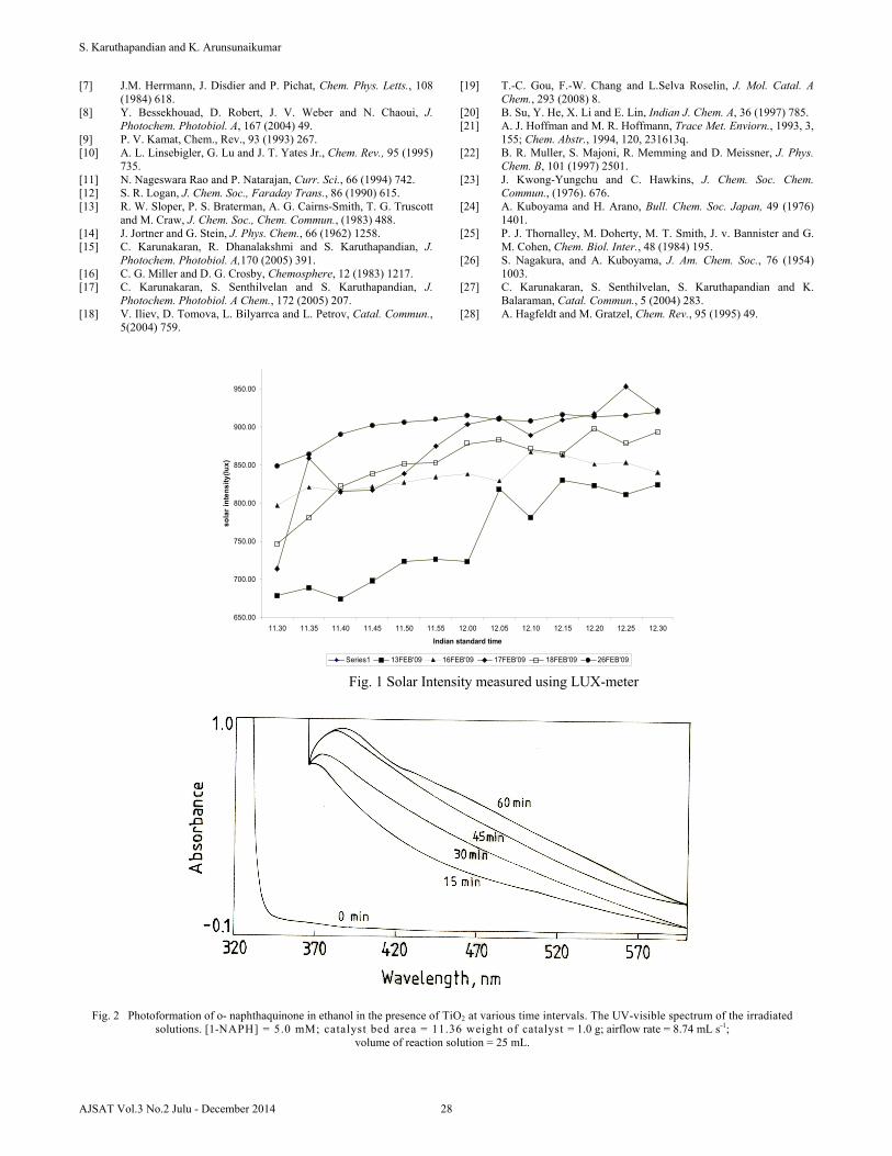
III. RESULTS AND DISCUSSION A. Solar Photooxidation of 1-Naphthol in the Presence of Semiconductors The measurement of solar radiation shows fluctuation of sunlight intensity during the course of the photooxidation even under clear sky (Fig.1, Table I). Also, the intensity of solar radiation is different on different days. Now, for solar photooxidation experiments of different reaction conditions carried out in a set, the quantum of sunlight incident on unit area was made the same, by carrying out the experiments simultaneously, side-by-side, thus making it possible to
compare the solar results. The solar photooxidation results are consistent. Solar photooxidation of 1-naphthol in ethanol on Titania, vanadia, zinc oxide, ferric oxide, lead dioxide, zinc sulfide and alumina yields 1, 2-naphthoquinone as the product. The progress of the solar photooxidation on observed using TiO2 catalysts at various time intervals is shown in Fig. 2. The spectra clearly show a maximum absorbance (λmax) at 380 nm; however there is no such absorbance is observed at 0 min. It reveals that the maximum absorbance at 380 nm is corresponding to 1,2-naphthoquinone which was identical with that of reported in literature.101 A couple of solar experiments of identical reaction conditions carried out simultaneously, side by side, yield results within ± 5% and this is so on different days. This reproducibility is not surprising as the quantum of solar radiation absorbed by the test is the same as that of the control (standard) and the ratio becomes independent of fluctuation. B. Factors Influencing Solar Photocatalysis The various factors such as concentration of 1-naphthol, air flow rate and bed area influencing the solar photocatalyzed reactions in ethanol was examined by carrying out a set of experiments simultaneously under identical illumination; also an experiment under standard conditions was carried out side by side with the entire rate measuring experiments. The rate of formation of 1,2-naphthoquinone (1,2-NQ) at different concentration of 1-naphthol at various semiconductor catalysts show that the oxidation rate increases with increase in the concentration and the variation conforms to Langmuir-Hinshelwood model (Fig. 3, Table II). The double reciprocal plot of rate versus [1-NAPHTHOL] affords straight line with positive y-intercept in all cases ( Table III). The effect of airflow rate on the rate of formation of 1,2-NQ was also carried out. Study of the photo catalyzed oxidation 1-naphthol as a function of airflow rate reveals that the enhancement of photo catalysis with oxygen concentration in the formation of 1,2-NQ (Fig 4, Table IV ). The variation of rate with airflow rate suggests Langmuir-Hinshelwood kinetic model. The double reciprocal plots of rate versus airflow rate confirm the same (Table V). The reaction was also studied without bubbling air but the solutions were not deaerated. The dissolved oxygen itself brings out the reaction but the photo oxidation is weak. The reaction does not occur in dark. The photo catalysts used do not lose their catalytic activities on irradiation. Study of the photocatalyzed oxidation of 1-naphthol as a function of illumination area on the rate of formation of 1,2-NQ was also carried out. The reaction rate increases linearly with the apparent area of the catalytic bed (Fig. 5, Table VI). The Photoformation of 1,2-NQ have been studied in the presence of surfactants, vinyl monomer and azide ion (Table VII). The surfactants, singlet oxygen quencher and azide ion does not interfere the photochemical reaction. The vinyl monomers neither retard and nor polymerize during the course of photocatalysis.
S. Karuthapandian and K. Arunsunaikumar
26AJSAT Vol.3 No.2 Julu - December 2014

C. Mechanism Of the seven photocatalyst employed in this study alumina is an insulator providing non-reactive surface while others are semiconductors with finite band gap energies. The bandgap excitation of semiconductors results in creation of electron-hole pairs such as holes in the valence band and electrons in the conductance band. Illumination of the semiconductors with light of an energy greater than the bandgap results in electron-hole pair generation. Since the recombination of a photogenerated electron-hole pair in a semiconductor is so rapid (occurring in a picoseconds time scale) (Eq. 3.1), for an effective photocatalysis the reactants
are to be adsorbed on the catalysts7. The hole reacts with the adsorbed 1-naphthol molecule to form 1-naphthol radical-
cation (1 NAPH ) (Eq. 3.2), while the electron is effectively removed by transfer to the adsorbed oxygen resulting in highly active superoxide radical-anion,
2O (Eq. 3.3).27 The 1-naphthol radical-cation may react
with superoxide radical-anion yielding 1,2-naphthoquinone and water molecules (Eq. 3.4). And this mechanism is similar to the ZnO photocatalyzed oxidation of aniline in ethanol.27
)()( cbvb ehhvtorSemiconduc (3.1)
NAPHhNAPH vbads 11 )()( (3.2)
2)()(2 OeO cbads (3.3)
21 ONAPH OH2 (3.4)
The donor and acceptor adsorbed on the photocatalyst surface undergoes photoexcitation followed by electron transfer. The donor excitation results in the transfer of excited electron whereas the acceptor excitation leads to an electron jump from the donor level to the vacant acceptor level.28 D. Kinetic Law The photocatalysis on reactive as well as non-reactive surfaces requires adsorption of 1-naphthol and oxygen
molecules on the catalyst surface. The rate of formation of 1,2-naphthoquinone is a function of (i) The fraction of the surface adsorbed by the 1-naphthol molecule, (ii) The fraction of the surface on which oxygen molecule is adsorbed, (iii) The surface area of the catalyst bed, and (iv) The intensity of illumination.
Hence
Rate =
1 2
1 2 1 2
[1-NAPHTHOL] 1 [1-NAPHTHOL] [1-NAPHTHOL]
kK K A IK K K K
where K1 and K2 are the adsorption coefficients of 1-naphthol and oxygen molecules on the catalyst surface, k is the specific rate of oxidation of 1-naphthol, is the airflow rate, A is the surface area of the catalyst bed and I is the intensity of light. The fitment of the experimental data (Fig. 2 and 3) to the Langmuir-Hinshelwood curve, drawn using a computer program based on saturation kinetics with respect to 1-naphthol and airflow rate, confirms the kinetic equation. The kinetic expression explains satisfactorily the product formation as a function of 1-naphthol concentration, the airflow rate and the apparent surface area of the catalytic bed. The experimentally determined photocatalytic efficiencies of the catalysts reveal that they are not determined solely by the bandgap energies.
IV. CONCLUSION
Solar radiations catalysed photooxidation of 1-naphthol in ethanol in the presence of air on semiconductors yields 1-
naphthoquinone and the conversion follows satutation kinetic with respect to 1-naphthol and airflow rate. The kinetic expression explains satisfactorily the product formation as a function of 1-naphthol concentration, the airflow rate and the apparent surface area of the catalytic bed.
REFERENCES [1] C. Kutal, J. Chem. Edu., 60 (1983) 882. [2] (a) D. J. Michel and H. Huber, Trends Biochem. Sci., 10 (1985)
243; (b) Z. H. Brunisholz and R. Sidler, in New Comprehensive Biochemistry: Photosynthesis, J. Amesz (Ed.), Elsevier, Amsterdam, 1987.
[3] M. Muneer, M. Qamar and D. Bahmemann, J. Mol. Catal. A: Chem., 234 (2005) 151.
[4] T.A. Konovalova, J. Lawerence and L.D. Kispert, J. Photochem. Photobiol. A, 1 (2004) 162.
[5] R Katoh, A. Furube, Y. Tamaki, T. Yoshihara, M. Murai, K. Hara, S. Murata, H. Arakawa and M. Tachiya, J. Photochem. Photobiol. A, 166 (2004) 69.
[6] K.T. Ranjit and B. Viswanathan, J. Photochem. Photobiol. A, 108 (1997) 79.
Solar Radiation Catalyzed Aerobic Photooxidation of 1-Naphthol on Some Semiconductors
27 AJSAT Vol.3 No.2 Julu - December 2014
[7] J.M. Herrmann, J. Disdier and P. Pichat, Chem. Phys. Letts., 108 (1984) 618.
[8] Y. Bessekhouad, D. Robert, J. V. Weber and N. Chaoui, J. Photochem. Photobiol. A, 167 (2004) 49.
[9] P. V. Kamat, Chem., Rev., 93 (1993) 267. [10] A. L. Linsebigler, G. Lu and J. T. Yates Jr., Chem. Rev., 95 (1995)
735. [11] N. Nageswara Rao and P. Natarajan, Curr. Sci., 66 (1994) 742. [12] S. R. Logan, J. Chem. Soc., Faraday Trans., 86 (1990) 615. [13] R. W. Sloper, P. S. Braterman, A. G. Cairns-Smith, T. G. Truscott
and M. Craw, J. Chem. Soc., Chem. Commun., (1983) 488. [14] J. Jortner and G. Stein, J. Phys. Chem., 66 (1962) 1258. [15] C. Karunakaran, R. Dhanalakshmi and S. Karuthapandian, J.
Photochem. Photobiol. A,170 (2005) 391. [16] C. G. Miller and D. G. Crosby, Chemosphere, 12 (1983) 1217. [17] C. Karunakaran, S. Senthilvelan and S. Karuthapandian, J.
Photochem. Photobiol. A Chem., 172 (2005) 207. [18] V. Iliev, D. Tomova, L. Bilyarrca and L. Petrov, Catal. Commun.,
5(2004) 759.
[19] T.-C. Gou, F.-W. Chang and L.Selva Roselin, J. Mol. Catal. A Chem., 293 (2008) 8.
[20] B. Su, Y. He, X. Li and E. Lin, Indian J. Chem. A, 36 (1997) 785. [21] A. J. Hoffman and M. R. Hoffmann, Trace Met. Enviorn., 1993, 3,
155; Chem. Abstr., 1994, 120, 231613q. [22] B. R. Muller, S. Majoni, R. Memming and D. Meissner, J. Phys.
Chem. B, 101 (1997) 2501. [23] J. Kwong-Yungchu and C. Hawkins, J. Chem. Soc. Chem.
Commun., (1976). 676. [24] A. Kuboyama and H. Arano, Bull. Chem. Soc. Japan, 49 (1976)
1401. [25] P. J. Thornalley, M. Doherty, M. T. Smith, J. v. Bannister and G.
M. Cohen, Chem. Biol. Inter., 48 (1984) 195. [26] S. Nagakura, and A. Kuboyama, J. Am. Chem. Soc., 76 (1954)
1003. [27] C. Karunakaran, S. Senthilvelan, S. Karuthapandian and K.
Balaraman, Catal. Commun., 5 (2004) 283. [28] A. Hagfeldt and M. Gratzel, Chem. Rev., 95 (1995) 49.
650.00
700.00
750.00
800.00
850.00
900.00
950.00
11.30 11.35 11.40 11.45 11.50 11.55 12.00 12.05 12.10 12.15 12.20 12.25 12.30
Indian standard time
sola
r int
ensi
ty(lu
x)
Series1 13FEB'09 16FEB'09 17FEB'09 18FEB'09 26FEB'09
Fig. 1 Solar Intensity measured using LUX-meter
Fig. 2 Photoformation of o- naphthaquinone in ethanol in the presence of TiO2 at various time intervals. The UV-visible spectrum of the irradiated solutions. [1-NAPH] = 5.0 mM; catalyst bed area = 11.36 weight of catalyst = 1.0 g; airflow rate = 8.74 mL s-1;
volume of reaction solution = 25 mL.
S. Karuthapandian and K. Arunsunaikumar
28AJSAT Vol.3 No.2 Julu - December 2014
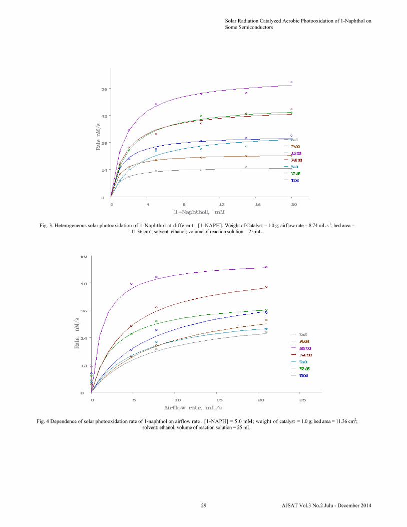
Fig. 3. Heterogeneous solar photooxidation of 1-Naphthol at different [1-NAPH]. Weight of Catalyst = 1.0 g; airflow rate = 8.74 mL s-1; bed area =
11.36 cm2; solvent: ethanol; volume of reaction solution = 25 mL.
Fig. 4 Dependence of solar photooxidation rate of 1-naphthol on airflow rate . [1-NAPH] = 5.0 mM; weight of catalyst = 1.0 g; bed area = 11.36 cm2;
solvent: ethanol; volume of reaction solution = 25 mL.
Solar Radiation Catalyzed Aerobic Photooxidation of 1-Naphthol on Some Semiconductors
29 AJSAT Vol.3 No.2 Julu - December 2014

0
10
20
30
40
50
60
70
80
0 10 20 30 40 50 60
Catalyst bed area, cm2
1,2-
NQ
form
atio
n, n
M s
-1
ZnOFe2O3Al2O3PbO2ZnSTIO2V2O5
Fig. 5 Solar photooxidation of 1-Naphthol in ethanol as a function of illumination area. [1-NAPH] = 5.0 mM; weight of catalyst = 1.0 g; airflow rate =
8.74 mL s-1; Solvent: ethanol; volume of reaction solution = 25 mL.
TABLE I SOLAR INTENSITY MEASURED USING LUX-METER
IST Solar intensity 100 LUX
13 Feb 2009 16 Feb 2009 17 Feb 2009 18 Feb 2009 26 Feb 2009
11.30 678 797 714 747 849
11.35 689 821 859 781 864
11.40 674 816 815 822 890
11.45 698 822 817 838 902
11.50 724 827 839 851 906
11.55 726 834 875 853 910
12.00 723 838 903 878 915
12.05 818 829 912 883 910
12.10 781 867 889 871 908
12.15 830 863 909 864 916
12.20 823 851 917 898 914
12.25 811 853 953 878 915
12.30 824 840 922 893 920
S. Karuthapandian and K. Arunsunaikumar
30AJSAT Vol.3 No.2 Julu - December 2014
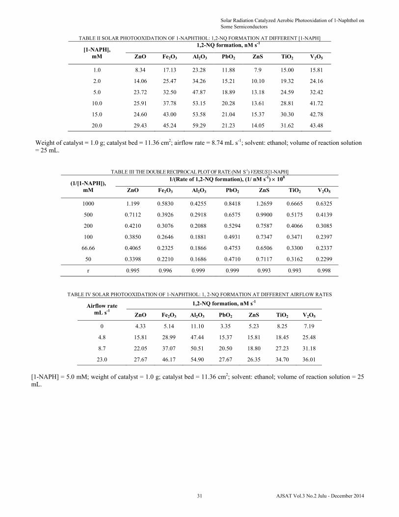
TABLE II SOLAR PHOTOOXIDATION OF 1-NAPHTHOL: 1,2-NQ FORMATION AT DIFFERENT [1-NAPH]
[1-NAPH], mM
1,2-NQ formation, nM s-1
ZnO Fe2O3 Al2O3 PbO2 ZnS TiO2 V2O5
1.0 8.34 17.13 23.28 11.88 7.9 15.00 15.81
2.0 14.06 25.47 34.26 15.21 10.10 19.32 24.16
5.0 23.72 32.50 47.87 18.89 13.18 24.59 32.42
10.0 25.91 37.78 53.15 20.28 13.61 28.81 41.72
15.0 24.60 43.00 53.58 21.04 15.37 30.30 42.78
20.0 29.43 45.24 59.29 21.23 14.05 31.62 43.48
Weight of catalyst = 1.0 g; catalyst bed = 11.36 cm2; airflow rate = 8.74 mL s-1; solvent: ethanol; volume of reaction solution = 25 mL.
TABLE III THE DOUBLE RECIPROCAL PLOT OF RATE (NM S-1) VERSUS [1-NAPH]
(1/[1-NAPH]), mM
1/(Rate of 1,2-NQ formation), (1/ nM s-1) 108
ZnO Fe2O3 Al2O3 PbO2 ZnS TiO2 V2O5
1000 1.199 0.5830 0.4255 0.8418 1.2659 0.6665 0.6325
500 0.7112 0.3926 0.2918 0.6575 0.9900 0.5175 0.4139
200 0.4210 0.3076 0.2088 0.5294 0.7587 0.4066 0.3085
100 0.3850 0.2646 0.1881 0.4931 0.7347 0.3471 0.2397
66.66 0.4065 0.2325 0.1866 0.4753 0.6506 0.3300 0.2337
50 0.3398 0.2210 0.1686 0.4710 0.7117 0.3162 0.2299
r 0.995 0.996 0.999 0.999 0.993 0.993 0.998
TABLE IV SOLAR PHOTOOXIDATION OF 1-NAPHTHOL: 1, 2-NQ FORMATION AT DIFFERENT AIRFLOW RATES
Airflow rate mL s-1
1,2-NQ formation, nM s-1
ZnO Fe2O3 Al2O3 PbO2 ZnS TiO2 V2O5
0 4.33 5.14 11.10 3.35 5.23 8.25 7.19
4.8 15.81 28.99 47.44 15.37 15.81 18.45 25.48
8.7 22.05 37.07 50.51 20.50 18.80 27.23 31.18
23.0 27.67 46.17 54.90 27.67 26.35 34.70 36.01
[1-NAPH] = 5.0 mM; weight of catalyst = 1.0 g; catalyst bed = 11.36 cm2; solvent: ethanol; volume of reaction solution = 25 mL.
Solar Radiation Catalyzed Aerobic Photooxidation of 1-Naphthol on Some Semiconductors
31 AJSAT Vol.3 No.2 Julu - December 2014
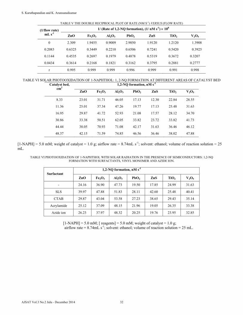
TABLE V THE DOUBLE RECIPROCAL PLOT OF RATE (NM S-1) VERSUS (FLOW RATE)
(1/flow rate) mL s-1
1/ (Rate of 1,2-NQ formation), (1/ nM s-1) 108
ZnO Fe2O3 Al2O3 PbO2 ZnS TiO2 V2O5
0 2.309 1.9455 0.9009 2.9850 1.9120 1.2120 1.3908
0.2083 0.6325 0.3449 0.2210 0.6506 0.7241 0.5420 0.3925
0.1144 0.4535 0.2697 0.1979 0.4878 0.5319 0.3672 0.3207
0.0434 0.3614 0.2168 0.1821 0.3162 0.3795 0.2881 0.2777
r 0.995 0.999 0.999 0.996 0.999 0.991 0.998
TABLE VI SOLAR PHOTOOXIDATION OF 1-NAPHTHOL: 1, 2-NQ FORMATION AT DIFFERENT AREAS OF CATALYST BED
Catalyst bed, cm2
1,2-NQ formation, nM s-1
ZnO Fe2O3 Al2O3 PbO2 ZnS TiO2 V2O5
8.33 23.01 31.71 46.05 17.13 12.30 22.84 28.55
11.36 25.01 37.34 47.26 19.77 17.13 25.48 31.63
16.95 29.87 41.72 52.93 21.08 17.57 28.12 34.70
30.86 33.38 50.51 62.05 33.82 23.72 33.82 41.73
44.44 38.05 70.93 71.08 42.17 31.63 36.46 46.12
48.37 42.15 71.59 74.85 46.56 36.46 38.02 47.88
[1-NAPH] = 5.0 mM; weight of catalyst = 1.0 g; airflow rate = 8.74mL s-1; solvent: ethanol; volume of reaction solution = 25 mL.
TABLE VI PHOTOOXIDATION OF 1-NAPHTHOL WITH SOLAR RADIATION IN THE PRESENCE OF SEMICONDUCTORS: 1,2-NQ
FORMATION WITH SURFACTANTS, VINYL MONOMER AND AZIDE ION.
Surfactant
1,2-NQ formation, nM s-1
ZnO Fe2O3 Al2O3 PbO2 ZnS TiO2 V2O5
- 24.16 36.90 47.73 19.50 17.85 24.99 31.63
SLS 39.97 47.88 51.83 28.11 42.60 25.48 40.41
CTAB 29.87 43.04 53.58 27.23 38.65 29.43 35.14
Acrylamide 25.12 37.09 48.15 21.96 19.05 26.35 33.38
Azide ion 26.23 37.97 48.32 20.25 19.76 23.95 32.85
[1-NAPH] = 5.0 mM; [ reagents] = 5.0 mM; weight of catalyst = 1.0 g; airflow rate = 8.74mL s-1; solvent: ethanol; volume of reaction solution = 25 mL.
S. Karuthapandian and K. Arunsunaikumar
32AJSAT Vol.3 No.2 Julu - December 2014
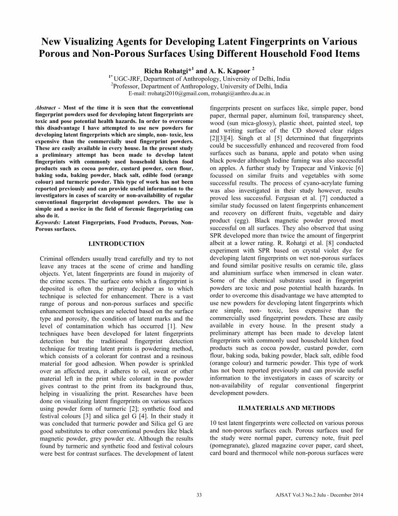
New Visualizing Agents for Developing Latent Fingerprints on Various Porous and Non-Porous Surfaces Using Different Household Food Items
Richa Rohatgi*1 and A. K. Kapoor 2
1* UGC-JRF, Department of Anthropology, University of Delhi, India 2Professor, Department of Anthropology, University of Delhi, India
E-mail: [email protected], [email protected]
Abstract - Most of the time it is seen that the conventional fingerprint powders used for developing latent fingerprints are toxic and pose potential health hazards. In order to overcome this disadvantage I have attempted to use new powders for developing latent fingerprints which are simple, non- toxic, less expensive than the commercially used fingerprint powders. These are easily available in every house. In the present study a preliminary attempt has been made to develop latent fingerprints with commonly used household kitchen food products such as cocoa powder, custard powder, corn flour, baking soda, baking powder, black salt, edible food (orange colour) and turmeric powder. This type of work has not been reported previously and can provide useful information to the investigators in cases of scarcity or non-availability of regular conventional fingerprint development powders. The use is simple and a novice in the field of forensic fingerprinting can also do it. Keywords: Latent Fingerprints, Food Products, Porous, Non-Porous surfaces.
I.INTRODUCTION Criminal offenders usually tread carefully and try to not leave any traces at the scene of crime and handling objects. Yet, latent fingerprints are found in majority of the crime scenes. The surface onto which a fingerprint is deposited is often the primary decipher as to which technique is selected for enhancement. There is a vast range of porous and non-porous surfaces and specific enhancement techniques are selected based on the surface type and porosity, the condition of latent marks and the level of contamination which has occurred [1]. New techniques have been developed for latent fingerprints detection but the traditional fingerprint detection technique for treating latent prints is powdering method, which consists of a colorant for contrast and a resinous material for good adhesion. When powder is sprinkled over an affected area, it adheres to oil, sweat or other material left in the print while colorant in the powder gives contrast to the print from its background thus, helping in visualizing the print. Researches have been done on visualizing latent fingerprints on various surfaces using powder form of turmeric [2]; synthetic food and festival colours [3] and silica gel G [4]. In their study it was concluded that turmeric powder and Silica gel G are good substitutes to other conventional powders like black magnetic powder, grey powder etc. Although the results found by turmeric and synthetic food and festival colours were best for contrast surfaces. The development of latent
fingerprints present on surfaces like, simple paper, bond paper, thermal paper, aluminum foil, transparency sheet, wood (sun mica-glossy), plastic sheet, painted steel, top and writing surface of the CD showed clear ridges [2][3][4]. Singh et al [5] determined that fingerprints could be successfully enhanced and recovered from food surfaces such as banana, apple and potato when using black powder although Iodine fuming was also successful on apples. A further study by Trapecar and Vinkovic [6] focussed on similar fruits and vegetables with some successful results. The process of cyano-acrylate fuming was also investigated in their study however, results proved less successful. Fergusan et al. [7] conducted a similar study focussed on latent fingerprints enhancement and recovery on different fruits, vegetable and dairy product (egg). Black magnetic powder proved most successful on all surfaces. They also observed that using SPR developed more than twice the amount of fingerprint albeit at a lower rating. R. Rohatgi et al. [8] conducted experiment with SPR based on crystal violet dye for developing latent fingerprints on wet non-porous surfaces and found similar positive results on ceramic tile, glass and aluminium surface when immersed in clean water. Some of the chemical substrates used in fingerprint powders are toxic and pose potential health hazards. In order to overcome this disadvantage we have attempted to use new powders for developing latent fingerprints which are simple, non- toxic, less expensive than the commercially used fingerprint powders. These are easily available in every house. In the present study a preliminary attempt has been made to develop latent fingerprints with commonly used household kitchen food products such as cocoa powder, custard powder, corn flour, baking soda, baking powder, black salt, edible food (orange colour) and turmeric powder. This type of work has not been reported previously and can provide useful information to the investigators in cases of scarcity or non-availability of regular conventional fingerprint development powders.
II.MATERIALS AND METHODS
10 test latent fingerprints were collected on various porous and non-porous surfaces each. Porous surfaces used for the study were normal paper, currency note, fruit peel (pomegranate), glazed magazine cover paper, card sheet, card board and thermocol while non-porous surfaces were
33 AJSAT Vol.3 No.2 Julu - December 2014

granite, wood (sun-mica coated), glass, mirror, aluminium foil, ceramic tile, plastic sheet, steel, writable surface of CD and rubber. The test sebum latent prints were collected from the subjects on different surfaces. For collecting sebum prints, subjects were asked to touch their forehead or face for getting sebum on their fingertips these in turn were applied to various substrates. No particular care was taken for contamination on fingertips as sebum prints are a complex mixture of natural secretion and contaminants from the environment. The method used in development of prints was powder dusting without using brush as preliminary study. Application of powder to the prints by brushing is a simple and easy technique but it also has a disadvantage that the brush on coming in contact with the surface having prints destroys the print and hence the ridge characteristics get destroyed. In order to develop latent fingerprints with food products, 20-30 grams commercially available cocoa powder, custard powder, corn flour, baking soda, baking powder, black salt, edible food (orange colour) and turmeric were procured in dry powder form. The powders (as available in the market) were weighed and dried in oven (for 5 minutes at 500C) and sprinkled over the affected surface. The excess powder was removed by tapping in order to get clear prints. This method was repeated for all powders and on all surfaces, ten times each (for 10 test latent prints on each surface per powder). Out of these only the best developed prints were recorded for the result computation. The experiment was carried out in the month of June-July 2014 when the temperature varied from 31-420C and the relative humidity between 46% and 70%. In order to check the comparative evaluation of surfaces, the different powders were applied on all mentioned porous and non-porous surfaces respectively as shown in Tables 1 and 2 and Graphs 1 and 2.
III.RESULTS AND DISCUSSION
The results obtained from present investigation using different food products in powder form on various porous and non-porous surfaces are shown in Figures -1 to 4. The latent fingerprints present on majority of the surfaces examined can be successfully developed with all employed food products. It has been observed that latent fingerprints were not developed on rubber using any powder. In case of white ceramic tile the prints were developed but lacked contrast in cases of corn flour, custard powder, black salt, baking powder and baking soda. Most clear and visible prints were developed on almost all porous surfaces such as currency note, card sheet, plain paper, glossy magazine cover as revealed by Figures 1 and 3. While non-porous surfaces such as aluminium foil, steel (spoon) and plastic sheet showed very clear decipherable prints with all powders as revealed by Figures- 2 and 4. Among the food powders used for
this experiment, cocoa powder, custard powder, corn flour, baking soda and turmeric powder demonstrated best results on all porous and non-porous surfaces. It was noted that all these powders give better results on contrast surfaces. The latent fingerprints present on surfaces such as plain paper, currency note, fruit peel (pomegranate), glazed magazine cover paper, card sheet, card board, thermocol, granite, wood (sun-mica coated), glass, mirror, aluminium foil, ceramic tile, plastic sheet, steel and writable surface of CD, were developed and showed clear ridges as is evident from the figures with all food powders used in the present experiment. The negative results were obtained on white ceramic tile, transparent polythene and thermocol due to poor contrast in cases of custard powder, corn flour, baking soda, baking powder and black salt. However, these surfaces showed clear visible fingerprints with edible (orange) colour and turmeric. No prints could be developed on rubber and card board due to lack of adherence of sebum from latent fingerprints and developing agents on these surfaces. The present study is a preliminary work in this field which is based on physical method of enhancement of latent prints and works on the mechanical adherence of the fingerprint powder particles to the oily components of the skin ridge deposits. These preliminary observations indicate that the common food products can also be used for the visualization of latent fingerprints present on various porous and non-porous substrates. A similar study conducted by Garg et al. [2] revealed development of latent fingerprints using turmeric powder on varied surfaces. Similarly, in another study by Kumari et al. [3] new method of visualizing latent fingerprints using synthetic food and festival colours was reported. The present study also substantiated that decipherment of fingerprints depends upon the type of powder used and the type of surface on which the finger prints are present.
IV.CONCLUSION
It can be concluded from the present study that these commonly and easily available as well as less expensive and non-toxic agents could be a useful substitute for the decipherment of latent fingerprints deposited on different surfaces. These can provide a good substitute for fingerprint visualization in comparison particularly to commercially available chemical powders, under the instances of scarcity. Further work on the decipherment of aged latent fingerprints needs to be taken up.
ACKNOWLEDGEMENTS
RR is grateful to UGC for financial support in the form of Junior Research Fellowship in the present study and highly thankful to all the subjects who contributed their fingerprint samples for the experiment purposes.
Richa Rohatgi and A. K. Kapoor
34AJSAT Vol.3 No.2 Julu - December 2014

REFERENCES
[1] Morimoto S., Kaminogoa A. And Hiranob T., A new method to enhance visualization of latent finger marks by sublimating dyes and its practical used with a combination of cyano acrylate fuming. Forensic Science International 97(2) 101-108 (1998).
[2] Garg R. K., Kumari H. and Kaur R., A new technique for visualization of latent fingerprints on various substrates using powder from turmeric: a rhizomatous herbaceous plant (Curcuma longa) Egypt J Forensic Sci, 1, pp. 53–57 (2011).
[3] Kumari H. and Garg R.K., New visualizing agents for latent fingerprints: Synthetic food and festival colors. Egyptian Journal of Forensic Sciences,Volume 1, Issues 3–4, Pages 133–139 (2011).
[4] Singh K., Sharma S. And Garg R.K., Visualization of latent fingerprints using silica gel G: A new technique Egyptian Journal of Forensic Sciences, 3(1), Pages 20–25 (2013).
[5] Singh G., Sodhi G.S., and Jasuja O.P., Detection of latent fingerprints on fruits and vegetables. Journal of Forensic Identification, 56(3) 374-381 (2006).
[6] Trapecar M. and Vinkovic M.K., Techniques for fingerprint recovery on vegetable and fruit surfaces used in Slovenia- a preliminary study. Science and Justice 48(4) 192-195 (2008).
[7] Ferguson S., Nicholson L., Farrugia K. J., Bremner D. H. and Gentles D., A preliminary investigation into the acquisition of fingerprints on food. Science and Justice. 53(1): pp.67-72 (2013). ISSN 1355-0306
[8] Rohatgi R., Sodhi G.S. and Kapoor A.K., Small Particle Reagent based on crystal violet dye for developing latent fingerprints on non-porous wet surfaces. Egyptian Journal of Forensic Science. (2014) Accepted: In Press.
TABLE 1 QUALITY OF DEVELOPED FINGERPRINTS ON POROUS SURFACES
Porous surfaces
Food powders Cocoa powder
Custard powder
Cornflour Baking
soda Baking powder
Black salt Edible colour
Turmeric powder
Paper 5 5 5 5 5 4 5 5 Currency Note
3 4 4 2 2 2 3 3
Fruit peel 2 1 2 1 0 0 1 1 Glossy paper 2 2 2 2 0 0 1 1 Cardsheet 4 0 0 0 0 0 4 4 Thermocol 1 0 0 0 0 0 1 1 Cardboard 0 0 0 0 0 0 0 0
Graph 1. showing quality of prints on porous surfaces
TABLE II QUALITY OF DEVELOPED FINGERPRINTS ON NON-POROUS SURFACES
Non-porous surfaces
Food powders Cocoa powder
Custard powder
Cornflour Baking
soda Baking powder
Black salt
Edible colour
Turmeric powder
Granite 5 5 5 5 3 3 3 5 Stainless steel spoon
5 5 5 5 4 4 3 5
Wood (sun-mica) 4 4 4 4 2 2 2 4 Glass 5 5 5 5 3 3 3 5 Mirror 5 5 4 3 2 2 3 5 Aluminium foil 5 5 5 5 4 4 4 5 Ceramic tile 5 0 0 0 0 0 5 5 Plastic sheet 4 3 3 2 2 2 2 3 CD (writable surface)
4 4 4 4 3 3 3 4
Rubber 0 0 0 0 0 0 0 0
New Visualizing Agents for Developing Latent Fingerprints on Various Porous and Non-Porous Surfaces Using Different Household Food Items
35 AJSAT Vol.3 No.2 Julu - December 2014

Graph 2 showing quality of prints on non-porous surfaces
(A) (B)
(C) (D)
Fig. 1Showing comparative visualization of latent fingerprints on porous surfaces- (A) thermocol; (B) glossy magazine cover; (C) card sheet and (D) currency note with cocoa powder.
Richa Rohatgi and A. K. Kapoor
36AJSAT Vol.3 No.2 Julu - December 2014
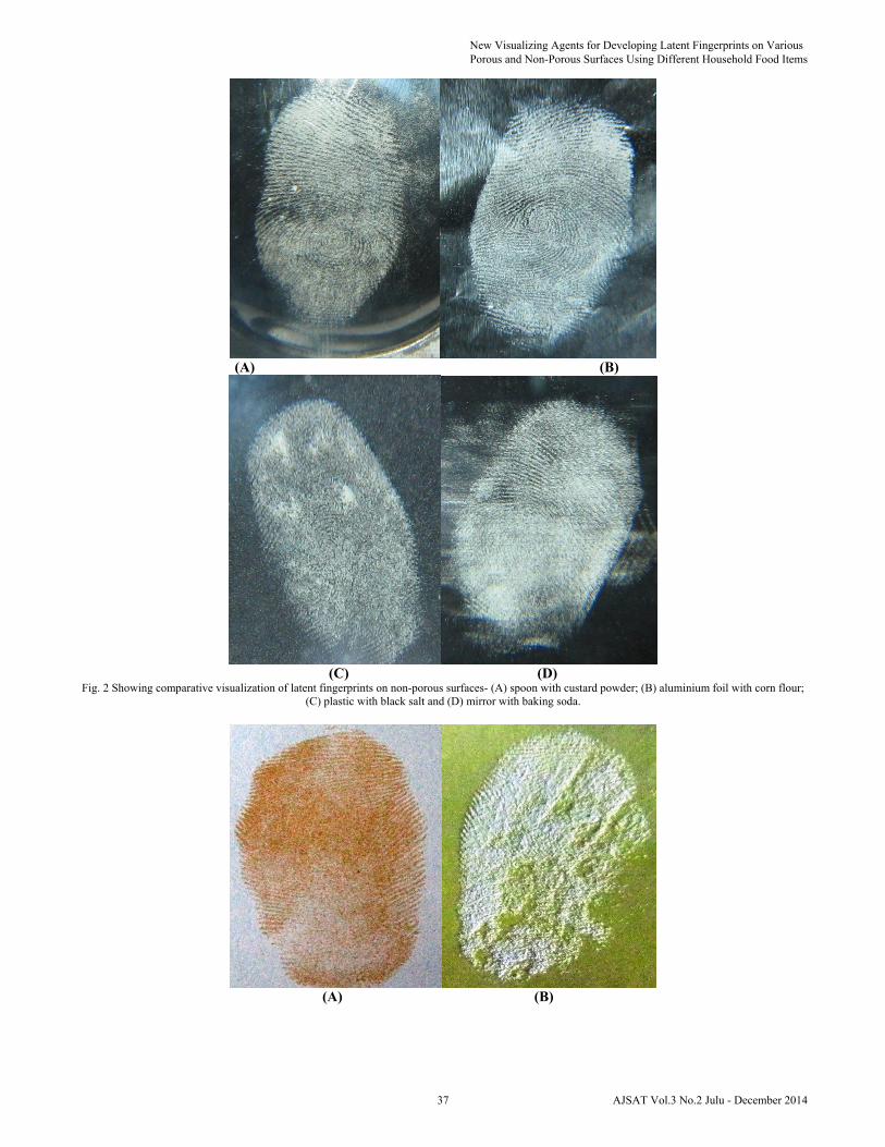
(A) (B)
(C) (D)
Fig. 2 Showing comparative visualization of latent fingerprints on non-porous surfaces- (A) spoon with custard powder; (B) aluminium foil with corn flour; (C) plastic with black salt and (D) mirror with baking soda.
(A) (B)
New Visualizing Agents for Developing Latent Fingerprints on Various Porous and Non-Porous Surfaces Using Different Household Food Items
37 AJSAT Vol.3 No.2 Julu - December 2014

(C) (D)
Fig. 3 Showing comparative visualization of latent fingerprints onporous surfaces-(A) plain paper with edible (orange) colour; (B) magazine cover with corn flour; (C) currency note with turmeric powder and (D) card sheet with cocoa powder.
(A) (B)
(C) (D)
Fig. 4 Showing comparative visualization of latent fingerprints on non-porous surfaces- (A) plastic with edible colour; (B) spoon with turmeric powder; (C)aluminium foil with turmeric and (D) aluminium foil with custard powder.
Richa Rohatgi and A. K. Kapoor
38AJSAT Vol.3 No.2 Julu - December 2014
Experimental Investigation for Tool Life by Optimizing Machining and Geometric Parameters of CNC End Mill Tool
Nilesh S. Pohokar 1, Lalit B. Bhuyar2
1,2Mechanical Engineering Department, Prof. Ram Meghe Institute of Technology and Research, Badnera , Amravati nilesh. [email protected],[email protected]
Abstract - CNC end milling is a unique adaption of the conventional milling process which uses an end mill tool for the machining process. During the End milling process, the material is removed by the end mill cutter. The effects of machining parameters of end milling process like spindle speed, depth of cut and feed rate and geometric parameter rake angle of a 14 mm diameter HSS end mill tool have been investigated on a AISI 1025 MS plate work material for pocket milling operation to reveal their impact on tool life using Taguchi Methodology. Experimental plan is performed by a Standard Orthogonal Array three times. The results of analysis of variance (ANOVA) indicate that the proposed mathematical model can be adequately describing the performance within the limit of factors being studied. The optimal set of process parameters has also been predicted to maximize the tool life. Keywords— CNC end milling, Taguchi method, ANOVA, Tool life
I. INTRODUCTION In present time the technology of CNC vertical milling
machine has been improved significantly to meet the advance requirements in various manufacturing fields, especially in the precision metal cutting industry. This experiment gives the effect of different machining parameters (spindle speed, feed, and depth of cut) and one geometric parameter rake angle of end mill tool on tool life. The demand for high quality and fully automated production focus attention on the surface condition of the product, surface finish of the machined surface is most important due to its effect on product appearance, function, and reliability. For these reasons it is important to maintain consistent tolerances and surface finish. Among several CNC industrial machining processes, milling is a fundamental machining operation. End milling is the most common metal removal operation encountered. It is widely used in a variety of manufacturing industries. The quality of the surface plays a very important role in the performance of milling as a good-quality milled surface significantly improves fatigue strength, corrosion resistance, or creep life. The surface generated during milling is affected by different factors such as vibration, spindle run–out, temperature, tool geometry, feed, cross-feed, tool path and other parameters. During finish milling, the depth of cut is small. Technological parameter range plays a very important role on surface roughness. In end milling, use of high cutting speed, low feed rate and low depth of cut are recommended to obtained better surface finish for the specific test range in a specified material. Cutting feed is the most dominated factor for surface finish. The most important interactions, that effect surface roughness of machined surfaces, are between the cutting feed and depth of cut, and between
cutting feed and spindle speed. Surface Roughness is affected negatively if the applied force is increased. With the more precise demands of modern engineering products, the control of surface texture together with dimensional accuracy has become more important. This experimental investigation outlines the Taguchi optimization methodology, which is applied trice to optimize tool life in end milling operation. The experiment is conducted on a AISI 1025 MS plate the processing of the job is done by High Speed Steel (HSS) end-mill tool of 14 mm diameter under rough milling conditions. The machining parameters evaluated are spindle speed, feed rate, depth of cut and only one geometric parameter is taken into consideration tool rake angle. The experiments are conducted by using Taguchi L9 orthogonal array as suggested by Taguchi and this method is applying trice. Signal-to-Noise (S/N) ratio and Analysis of Variance (ANOVA) is employed to analyse the effect of milling parameters on tool life.
II. LITERATURE REVIEW
Optimization, in its broadest sense, can be applied to
solve any engineering problem. Some typical applications from manufacturing area indicate the wide scope of the subject [1],
1. Selection of machining conditions in metal-cutting processes for minimum production cost
2. Design of material handling equipment, such as conveyors, trucks, and cranes, for minimum cost
3. Optimal production planning, controlling, and scheduling
4. Optimum design of chemical processing equipment and plants
5. Planning of maintenance and replacement of equipment to reduce operating costs
6. Allocation of resources or services among several activities to maximize the benefit
7. Controlling the waiting and idle times and queueing in production lines to reduce the costs
8. Planning the best strategy to obtain maximum profit in the presence of a competitor.
Genichi Taguchi is a Japanese engineer who has been
active in the improvement of Japan’s industrial products and processes since the late 1940s. He has developed both the philosophy and methodology for process or product quality improvement that depends heavily on statistical concepts and tools, especially statistically designed experiments. Many Japanese firms have achieved great success by applying his methods. Barker [2] reported that since 1983, after Taguchi’s association with the top companies and
39 AJSAT Vol.3 No.2 Julu - December 2014

institutes in USA (AT & T Bell Laboratories, Xerox, Lawrence Institute of Technology (LIT), Ford Motor Company etc.), his methods have been called a radical approach to quality, experimental design and engineering.
L. Eriksson et. al. [3] pointed out that the key element for
achieving high quality and low cost is parameter design & optimization. Through parameter design, levels of product and process factors are determined, such that the product’s functional characteristics are optimized and the effect of noise factors is minimized.
H. Singh et. al. [4] applied Taguchi’s technique for
optimizing surface finish, tool wear, cutting force and power consumed in turning operations for machining En24 steel with titanium carbide-coated tungsten carbide inserts. The success of many applications has demonstrated the power of Taguchi’s overall approach. It is also worth mentioning that many of the specific statistical techniques he has proposed for implementing robust parameter design have generated a great deal of controversy. However, most commentators agree that Taguchi’s loss function concept represents a solid contribution. Furthermore, there is general agreement that off-line experiments during the product or process design stage are of great value and the methodology is based on solid engineering principles. Reducing quality loss by designing the products and processes to be insensitive to variations in noise variables is a novel concept to statisticians and quality engineers.
Gupta et. al. [5] investigated the application of Taguchi
method with logical fuzzy reasoning for multiple output optimization of high speed CNC turning of AISI P-20 tool steel using TiN coated tungsten carbide coatings. The machining parameters (cutting speed, feed rate, depth of cut, nose radius and cutting environment) are optimized with considerations of the multiple performance measures (surface roughness, tool life, cutting force and power consumption). Taguchi’s concepts of orthogonal arrays, signal to noise (S/N) ratio, ANOVA have been fuzzified to optimize the high speed CNC turning process parameters through a single comprehensive output measure (COM).
They investigated the following results related to
combination of parameters multi-response problem and response and multi-response optimization analysis
(1) The factor/level combination S3F2D2N3E3 for surface roughness,S1F1D1N2E3 for the tool life, S1F1D1N2E3 for power consumption and S2F1D1N2E3 for cutting force are the recommended optimum parameters, for high speed CNC turning when all four responses are considered independently.
(2) In the multi-response problem, all the four responses tool life, power consumption, cutting force and surface roughness were simultaneously considered, and S2F1D1N2E3 was the recommended optimum condition as per the hybrid Taguchi-fuzzy approach.
(3) It can be concluded that middle level of cutting speed (160 m/min) and nose radius (0.8 mm) and lower level of
feed (0.1 mm/rev) and depth of cut (0.2 mm) yield the optimal result. Cryogenic environment is the most favorable condition out of three cutting environments.
(4) Both single response and multi-response optimization analysis proved that cryogenic machining environment E3 is favorable in increasing tool life and reducing surface roughness, cutting force and power consumption compared to wet (conventional coolant ILO cut 154 Indian Oil recommended for CNC machine) and dry machining.
They also presented the use of fuzzy logics to the
Taguchi method in optimization of the high speed CNC turning with multiple performance characteristics. A fuzzy reasoning of the multiple performance characteristics has been performed by the fuzzy logic unit. As a result, four performance characteristics namely surface roughness, tool life, cutting force and power consumption can be improved. It can be concluded that the optimization methodology developed in this study is useful in improving multiple performance characteristics in high speed CNC turning.
A. Cicek & T. Kivak [6] investigated the application of Taguchi method for Surface roughness and roundness error in drilling of AISI 316 stainless steel. In his study, the effects of deep drilling parameters on surface roughness and roundness error were investigated in drilling of AISI 316 austenitic stainless steel with M35 HSS twist drills. In addition, optimal control factors for the whole quality were determined by using Taguchi technique. Two cutting tools, cutting speeds and feed rates were considered as control factors, and L8 (23) orthogonal array was determined for experimental trials. Multiple regression analysis was employed to derive the predictive equations of the surface roughness and roundness error achieved via experimental design. Minimum surface roughness and roundness error were obtained with treated drills at 14 m/min cutting speed and 0.08 mm/rev feed rate. Confirmation experiments showed that Taguchi method precisely optimized the drilling parameters in drilling of stainless steel. Moshat S. & Datta S. [7] investigated the Optimization of CNC end milling process parameters using PCA-based Taguchi method. To optimize aforesaid quality attributes in a manner that these multi-criterions could be fulfilled simultaneously up to the expected level. This invites a multi-objective optimization problem which has been solved by PCA based Taguchi method. To meet the basic assumption of Taguchi method; in his work, individual response correlations have been eliminated first by means of Principal Component Analysis (PCA). Correlated responses have been transformed into uncorrelated or independent quality indices called principal components. Finally Taguchi method has been adapted to solve this optimization problem. The aforesaid methodology has been found fruitful in the cases where simultaneous optimization of huge number of responses is required.
Nilesh S. Pohokar, Lalit B. Bhuyar
40AJSAT Vol.3 No.2 Julu - December 2014
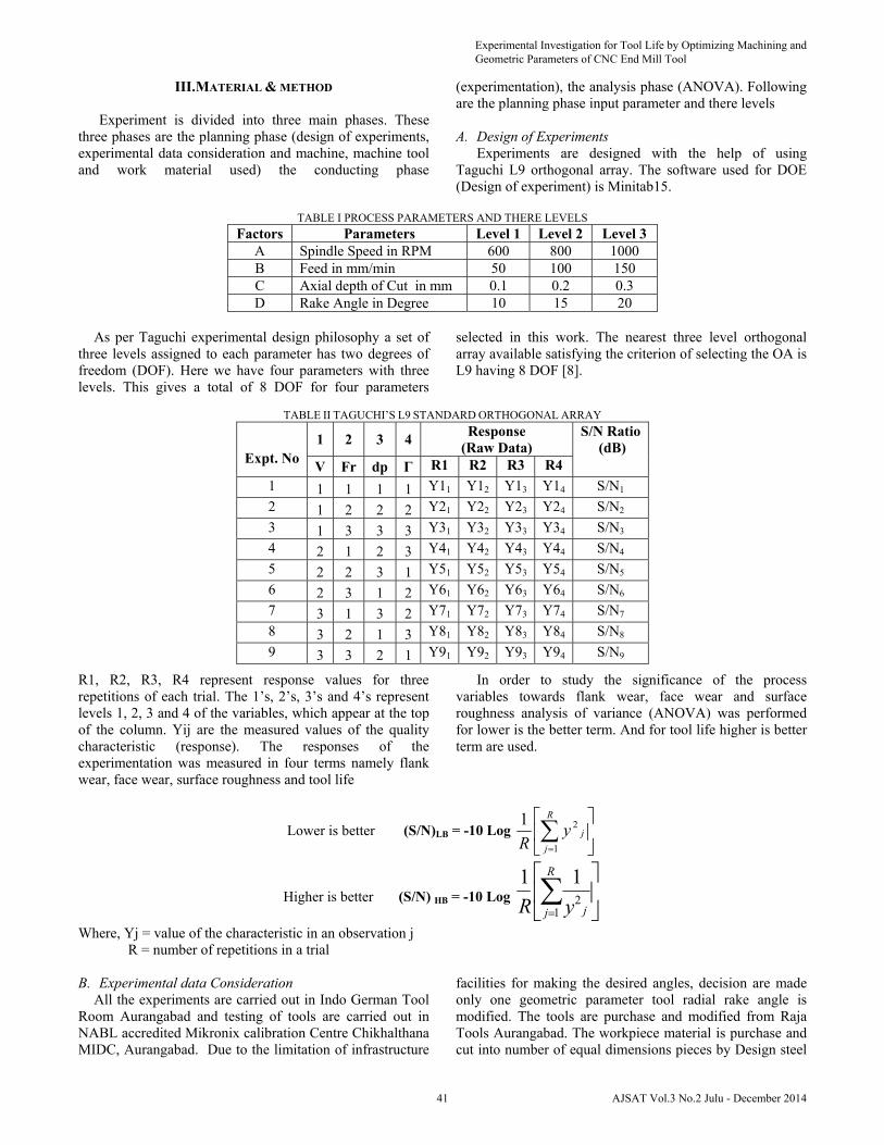
III. MATERIAL & METHOD
Experiment is divided into three main phases. These three phases are the planning phase (design of experiments, experimental data consideration and machine, machine tool and work material used) the conducting phase
(experimentation), the analysis phase (ANOVA). Following are the planning phase input parameter and there levels
A. Design of Experiments
Experiments are designed with the help of using Taguchi L9 orthogonal array. The software used for DOE (Design of experiment) is Minitab15.
TABLE I PROCESS PARAMETERS AND THERE LEVELS
Factors Parameters Level 1 Level 2 Level 3 A Spindle Speed in RPM 600 800 1000 B Feed in mm/min 50 100 150 C Axial depth of Cut in mm 0.1 0.2 0.3 D Rake Angle in Degree 10 15 20
As per Taguchi experimental design philosophy a set of
three levels assigned to each parameter has two degrees of freedom (DOF). Here we have four parameters with three levels. This gives a total of 8 DOF for four parameters
selected in this work. The nearest three level orthogonal array available satisfying the criterion of selecting the OA is L9 having 8 DOF [8].
TABLE II TAGUCHI’S L9 STANDARD ORTHOGONAL ARRAY
R1, R2, R3, R4 represent response values for three repetitions of each trial. The 1’s, 2’s, 3’s and 4’s represent levels 1, 2, 3 and 4 of the variables, which appear at the top of the column. Yij are the measured values of the quality characteristic (response). The responses of the experimentation was measured in four terms namely flank wear, face wear, surface roughness and tool life
In order to study the significance of the process variables towards flank wear, face wear and surface roughness analysis of variance (ANOVA) was performed for lower is the better term. And for tool life higher is better term are used.
Lower is better (S/N)LB = -10 Log
R
j
jyR 1
21
Higher is better (S/N) HB = -10 Log
R
j jyR 12
11
Where, Yj = value of the characteristic in an observation j R = number of repetitions in a trial
B. Experimental data Consideration All the experiments are carried out in Indo German Tool
Room Aurangabad and testing of tools are carried out in NABL accredited Mikronix calibration Centre Chikhalthana MIDC, Aurangabad. Due to the limitation of infrastructure
facilities for making the desired angles, decision are made only one geometric parameter tool radial rake angle is modified. The tools are purchase and modified from Raja Tools Aurangabad. The workpiece material is purchase and cut into number of equal dimensions pieces by Design steel
Expt. No 1 2 3 4
Response (Raw Data)
S/N Ratio (dB)
V Fr dp Γ R1 R2 R3 R4
1 1 1 1 1 Y11 Y12 Y13 Y14 S/N1
2 1 2 2 2 Y21 Y22 Y23 Y24 S/N2
3 1 3 3 3 Y31 Y32 Y33 Y34 S/N3
4 2 1 2 3 Y41 Y42 Y43 Y44 S/N4
5 2 2 3 1 Y51 Y52 Y53 Y54 S/N5
6 2 3 1 2 Y61 Y62 Y63 Y64 S/N6
7 3 1 3 2 Y71 Y72 Y73 Y74 S/N7
8 3 2 1 3 Y81 Y82 Y83 Y84 S/N8
9 3 3 2 1 Y91 Y92 Y93 Y94 S/N9
Experimental Investigation for Tool Life by Optimizing Machining and Geometric Parameters of CNC End Mill Tool
41 AJSAT Vol.3 No.2 Julu - December 2014

private limited Waluj M.I.D.C. Aurangabad. In this work only one geometric parameter is modified and other parameters such as helix angle, end cutting edge concavity angle, axial and radial relief angle are kept constant. This modified radial rake angle is supplied by the supplier and marked as per the requirement and tested in the laboratory with the help of video measuring machine. Also the three machining parameters spindle speed, feed and axial depth of cut are considered for the optimization and other parameters such as machine power environment and redial depth of cut kept constant. The CNC machine is utilized to make control and accurate measurement of these parameters on the screen of display monitor. All the ranges of value of selected parameters are taken as per hand book recommendations.
C. Machine, Machine tool and work material The experiments were carried out on 3-axis on Surya
VF30CNC VS this CNC machine is a quality product of Bharat Fritz Werner Ltd. Bangalore. The HSS M2 grade four flute end mill tool was chosen for the experiments as it is most widely used in the industries because of its superior performance characteristics like good red-hardness and retains its cutting edge longer than other general purpose high speed steels. The table III shows the chemical composition of the tool material. The AISI 1025 (122 X 100 X 10 mm) MS plates are used for the experimentation the chemical composition are shown in table IV.
Figure 1b. . HSS M2 grade four flute end mill tool
Figure 1a. 3-axis Surya VF30CNC VS CNC machine Figure 1.c. AISI 1025 M.S. Plate Figure1 (a,b,c). Machine, Machine tool and Work Material used in the Experimentation
TABLE III CHEMICAL COMPOSITION OF HSS M2 GRADE TOOL
Element W % Cr % V % C % Mo %
Composition 6 4 2 0.8 9.5
TABLE IV CHEMICAL COMPOSITION OF WORK MATERIAL
C % Mn % P % S % Density Hardness Tensile Strength 0.26 0.4 0.03 0.04 8.41 kg/m3 115 BHN 750 Mpa
D. Tool wear and tool life criteria
The maximum acceptable flank wear for end milling is 0.5 mm stated by W. R. Devries [9]. This criterion is tested by doing the preliminary experimentation and the result obtained for the work and tool material was 0.25 mm is the uniform wear stage. So it is acceptable for all the
experiments. The tool life criteria were based on the desired flank wear of 0.25mm is accepted.
Nilesh S. Pohokar, Lalit B. Bhuyar
42AJSAT Vol.3 No.2 Julu - December 2014

IV. OBSERVATION RECORDED As per hand book recommendation the parameters are
first selected. The units of these values are converted as per the input system of CNC program. In this work the Taguchi method applied trice to find the optimal parameters. The observations are divided into three sets
1. First set: Parameters selected as per range given in handbook
2. Second set: Parameters selected just above and below the optimal parameters obtained in first set
3. Final set: Final parameters selected just above and below the optimal parameters obtained in second set
A. Observation of first experiment set
In the first set of experimentation the parameters range are selected as per handbook values. The Table I shows the factors and levels selected for experimentation. For each combination of parameter three trials are conducted.
TABLE V
OBSERVATION RECORDED IN THE SECOND EXPERIMENTATION SET Ex. No.
Cutting speed
in rpm
Feed rate in
mm/min
Depth of cut
in mm
Rake angle
in degree
Flank wear
in mm
Face wear
in mm
Surface roughness
in µm
TL
minute
1 600 50 0.1 10 0.213 0.241 4.21 178 0.221 0.242 4.26 176 0.212 0.245 4.24 177
2 600 100 0.2 15 0.228 0.250 4.34 165 0.219 0.249 4.32 167 0.230 0.243 4.37 169
3 600 150 0.3 20 0.198 0.248 3.57 174 0.211 0.245 3.49 175 0.213 0.248 3.66 176
4 800 50 0.2 20 0.192 0.250 4.87 179 0.193 0.249 4.84 178 0.195 0.251 4.65 177
5 800 100 0.3 10 0.178 0.221 4.76 183 0.181 0.213 4.72 182 0.179 0.223 4.71 182
6 800 150 0.1 15 0.216 0.248 3.16 179 0.221 0.249 3.20 178 0.218 0.251 3.18 178
7 1000 50 0.3 15 0.253 0.259 4.34 163 0.251 0.258 4.38 164 0.249 0.261 4.36 163
8 1000 100 0.1 20 0.261 0.259 3.33 171 0.259 0.262 3.48 173 0.258 0.260 3.51 172
9 1000 150 0.2 10 0.254 0.261 3.59 173 0.251 0.265 3.37 174 0.249 0.262 3.34 175
B. Observation of second experimentation set :
In the second set of experimentation the parameters range are selected as per optimized values obtained from the
first set of experimentation. The Table VI shows the factors and levels selected for experimentation.
TABLE VI PROCESS PARAMETERS SELECTED IN SECOND SET
Factors Parameters Level 1 Level 2 Level 3 A Spindle Speed in RPM 790 800 810 B Feed in mm/min 95 100 105 C Axial depth of Cut in mm 0.2 0.25 0.3 D Rake Angle in Degree 9 10 11
Again the L9 orthogonal array is selected which is
discussed earlier, for each parametric combination three trials are conducted to achieve a better accuracy for observation. Table VII shows the observations recorded for
Experimental Investigation for Tool Life by Optimizing Machining and Geometric Parameters of CNC End Mill Tool
43 AJSAT Vol.3 No.2 Julu - December 2014

flank wear, face wear and surface finish for every trial the readings are noted. The average values of flank wear, face
wear surface roughness and tool life are taken in each trial.
TABLE VII OBSERVATION RECORDED IN THE SECOND EXPERIMENTATION SET
Ex. No.
Cutting speed
in rpm
Feed rate in
mm/min
Depth of cut
in mm
Rake angle
in degree
Flank wear
in mm
Face wear
in mm
Surface roughness
in µm
TL
minute
1 790 95 0.2 9 0.190 0.22 3.56 181 0.191 0.21 3.54 180 0.192 0.22 3.55 183
2 790 100 0.25 10 0.177 0.22 3.31 184 0.178 0.23 3.32 182 0.176 0.21 3.31 183
3 790 105 0.3 11 0.178 0.22 3.35 180 0.177 0.23 3.34 179 0.178 0.21 3.35 181
4 800 95 0.25 11 0.181 0.25 3.45 178 0.182 0.25 3.44 179 0.183 0.26 3.45 180
5 800 100 0.3 9 0.185 0.27 3.49 177 0.184 0.28 3.49 176 0.185 0.29 3.48 178
6 800 105 0.2 10 0.192 0.28 3.78 178 0.194 0.29 3.76 179 0.195 0.29 3.75 177
7 810 95 0.3 10 0.198 0.29 3.76 176 0.199 0.28 3.75 175 0.201 0.27 3.76 178
8 810 100 0.2 11 0.210 0.28 3.23 176 0.221 0.27 3.24 177 0.212 0.29 3.25 176
9 810 105 0.25 9 0.219 0.26 3.45 175 0.225 0.25 3.46 174 0.226 0.26 3.47 173
C. Observation of Final Experimentation set:
In the final set of experimentation the parameters range are selected as per optimized values obtained from the
second set of experimentation. The Table VIII shows the factors and levels selected for experimentation.
TABLE VIII PROCESS PARAMETERS SELECTED IN FINAL SET
Factors Parameters Level 1 Level 2 Level 3 A Spindle Speed in RPM 785 790 795 B Feed in mm/min 98 100 102 C Axial depth of Cut in mm 0.24 0.25 0.26 D Rake Angle in Degree 9 10 11
Again the L9 orthogonal array is selected which is
discussed earlier, for each parametric combination three trials are conducted to achieve a better accuracy for observation. Table IX shows the observations recorded for flank wear, face wear and surface finish for every trial the readings are noted. The average values of flank wear, face wear surface roughness and tool life are taken in each trial.
On the basic of optimal results obtained in the second and final set of experimentation the mathematical model and the ANOVA response of flank wear, face wear, surface
roughness and tool life are discuss in the results and analysis. The mathematical model is prepared by considering both sets parameters combination results. The observation suggested that the slight difference in the variation of parameters and there levels whereas the final experimentation set are prepared for micro level observations. These observations imply the vital role for finding the response characterises of tool wear and surface roughness by knowing the exact significant parameter which has to be again optimized to the greater extent.
Nilesh S. Pohokar, Lalit B. Bhuyar
44AJSAT Vol.3 No.2 Julu - December 2014

TABLE IX OBSERVATIONS RECORDED IN THE FINAL EXPERIMENTATION SET
Ex. No.
Cutting speed
in rpm
Feed rate in
mm/min
Depth of cut
in mm
Rake angle
in degree
Flank wear
in mm
Face wear
in mm
Surface roughness
In µm
TL
minute
1 785 98 0.24 9 0.181 0.22 3.37 183 0.182 0.21 3.35 182 0.183 0.22 3.36 184
2 785 100 0.25 10 0.177 0.22 3.34 182 0.178 0.23 3.35 183 0.176 0.21 3.34 184
3 785 102 0.26 11 0.178 0.22 3.35 181 0.177 0.23 3.34 180 0.178 0.21 3.35 182
4 790 98 0.25 11 0.180 0.23 3.31 179 0.181 0.23 3.32 180 0.179 0.22 3.34 181
5 790 100 0.26 9 0.179 0.24 3.32 182 0.178 0.24 3.31 181 0.175 0.23 3.32 183
6 790 102 0.24 10 0.176 0.22 3.45 184 0.177 0.21 3.46 183 0.178 0.22 3.47 184
7 795 98 0.25 10 0.175 0.22 3.23 179 0.176 0.21 3.33 179 0.178 0.22 3.34 180
8 795 100 0.24 11 0.170 0.23 3.29 179 0.171 0.21 3.30 179 0.172 0.22 3.28 178
9 795 102 0.25 9 0.182 0.24 3.24 179 0.181 0.23 3.25 179 0.183 0.22 3.24 178
V. TOOL LIFE MODEL
The relationship between the independent variables of milling parameters (cutting speed, feed rate, depth of cut and
rake angle) and machining response of tool life can be represented by the following mathematical model.
where TL is tool life in minutes, V, fr, dp and γ are the cutting speed (rpm), feed rate (mm/min) depth of cut (mm) rake angle
in degree respectively. C, l, a, b,c are constants and ε is a random error. Equation 3.1 can be written in the following
logarithmic form: ln T=ln C + l ln V + a ln Fr + b ln dp + c ln + ln έ
In micros Q1 software, equation of predicted tool life can be rewritten in the following form:
TP10 (predicted tool life) = constant + β1V + β 2 fr + β 3dp + β 4
Instead of just an intercept and slope, the multiple linear
regression equation contains a constant (analogous to
intercept) and four coefficients (β1-β4), one for each of the
three independent variables. These coefficients are called
partial regression coefficients. Before using the micros Q1
software, one needs to assume that the relationship between
the dependent and independent variables is linear and that
for each combination of values of the independent variables,
the distribution of the dependent variable is normal with a
constant variance. If the independent variables are not
linearly related to the dependent variable, in order to
estimate the coefficients, one has to transform the data. The
mathematical equation of tool life can be written as follows
Experimental Investigation for Tool Life by Optimizing Machining and Geometric Parameters of CNC End Mill Tool
45 AJSAT Vol.3 No.2 Julu - December 2014

TL= 433.691-0.31 [v] -0.065[Fr]-10.684[dp]+0.167[γ]
Where, V- cutting speed in rpm Fr- feed rate in m/min dp- depth of cut in mm and γ-rake angle in degree
VI. RESULT AND DISCUSSION
A. Effect on flank wear It was found that cutting speed and depth of are less
significant process parameters for flank wear. Non significant parameters were pooled and the pooled versions
of ANOVA of the S/N data and the raw data for flank wear are given in Tables X. From this table, it is clear that feed rate and rake angle significantly affect the variation in the flank wear values.
TABLE X RESPONSE FOR FLANK WEAR
Level V Fr Dp γ
1 14.95 14.92 15.06 14.87
2 14.99 15.13 14.95 15.15
3 15.07 14.95 15.02 15.08
Delta 0.12 0.21 0.11 0.22
Rank 3 1 4 2
Figure 2 show that the flanks wear decreases with
the increase in the cutting speed. For a speed of 785 rpm, feed rate of 98 mm/min, depth of cut 0.24 mm and at rake angle of 90 lowest flank wear is registered. Figure also indicates that flank wear increases with rise in feed rate but
suddenly it is decreases. Increase in rake angle is seen with larger flank wear is observed. This is because the chip formation is continuous. Further, increases in flank wear after 100.
795790785
15.1
15.0
14.9
10210098
0.260.250.24
15.1
15.0
14.9
11109
V
Mea
n of
SN
rati
os
Fr
Dp γ
Main Effects Plot for SN ratiosData Means
Signal-to-noise: Smaller is better
Figure 2. Main effect plot for S/N ratios for flank wear
B. Effect of face wear Similarly from Table XI it is clear that the cutting speed and the depth of cut are more significant parameter for face wear.
The cutting speed and rake angle in comparison of S/N ratio are less significant.
Nilesh S. Pohokar, Lalit B. Bhuyar
46AJSAT Vol.3 No.2 Julu - December 2014
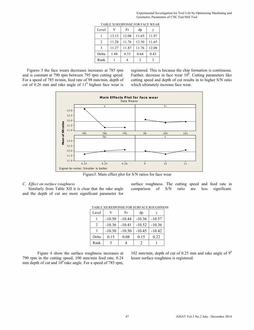
TABLE XI RESPONSE FOR FACE WEAR
Level V Fr dp γ
1 13.15 12.08 11.65 11.97
2 11.28 11.76 12.30 11.65
3 11.27 11.87 11.76 12.08
Delta 1.88 0.33 0.64 0.43
Rank 1 4 2 3
Figures 3 the face wears decreases increases at 785 rpm
and is constant at 790 rpm between 795 rpm cutting speed. For a speed of 785 m/min, feed rate of 98 mm/min, depth of cut of 0.26 mm and rake angle of 110 highest face wear is
registered. This is because the chip formation is continuous. Further, decrease in face wear 100. Cutting parameters like cutting speed and depth of cut results in to higher S/N ratio which ultimately increase face wear.
795790785
13.0
12.5
12.0
11.5
11.010210098
0 .260 .250.24
13.0
12.5
12.0
11.5
11.011109
V
Mea
n of
SN
rati
os
F r
Dp γ
M ain Effects P lot for face w e arData M eans
S igna l- to-no ise : S m a lle r is be tte r
Figure3. Main effect plot for S/N ratios for face wear C. Effect on surface roughness
Similarly from Table XII it is clear that the rake angle and the depth of cut are more significant parameter for
surface roughness. The cutting speed and feed rate in comparison of S/N ratio are less significant.
TABLE XII RESPONSE FOR SURFACE ROUGHNESS
Level V Fr dp γ
1 -10.50 -10.44 -10.36 -10.57
2 -10.36 -10.41 -10.52 -10.36
3 -10.50 -10.50 -10.45 -10.42
Delta 0.15 0.08 0.15 0.22
Rank 3 4 2 1 Figure 4 show the surface roughness increases at
790 rpm in the cutting speed, 100 mm/min feed rate, 0.24 mm depth of cut and 100 rake angle. For a speed of 785 rpm,
102 mm/min, depth of cut of 0.25 mm and rake angle of 90 lesser surface roughness is registered.
Experimental Investigation for Tool Life by Optimizing Machining and Geometric Parameters of CNC End Mill Tool
47 AJSAT Vol.3 No.2 Julu - December 2014
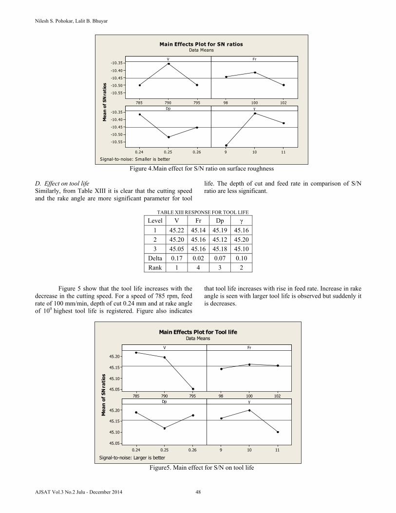
795790785
-10.35
-10.40
-10.45
-10.50
-10.55
10210098
0.260.250.24
-10.35
-10.40
-10.45
-10.50
-10.55
11109
V
Mea
n of
SN
rati
os
Fr
Dp γ
Main Effects Plot for SN ratiosData Means
S ignal-to-noise: Smaller is better
Figure 4.Main effect for S/N ratio on surface roughness
D. Effect on tool life Similarly, from Table XIII it is clear that the cutting speed and the rake angle are more significant parameter for tool
life. The depth of cut and feed rate in comparison of S/N ratio are less significant.
TABLE XIII RESPONSE FOR TOOL LIFE
Level V Fr Dp γ
1 45.22 45.14 45.19 45.16
2 45.20 45.16 45.12 45.20
3 45.05 45.16 45.18 45.10
Delta 0.17 0.02 0.07 0.10
Rank 1 4 3 2
Figure 5 show that the tool life increases with the decrease in the cutting speed. For a speed of 785 rpm, feed rate of 100 mm/min, depth of cut 0.24 mm and at rake angle of 100 highest tool life is registered. Figure also indicates
that tool life increases with rise in feed rate. Increase in rake angle is seen with larger tool life is observed but suddenly it is decreases.
795790785
45.20
45.15
45.10
45.05
10210098
0.260.250.24
45.20
45.15
45.10
45.05
11109
V
Mea
n of
SN
rati
os
Fr
Dp γ
Main Effects Plot for Tool lifeData Means
Signal-to-noise: Larger is better
Figure5. Main effect for S/N on tool life
Nilesh S. Pohokar, Lalit B. Bhuyar
48AJSAT Vol.3 No.2 Julu - December 2014
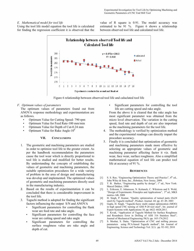
E. Mathematical model for tool life Using the tool life model equation the tool life is calculated for finding the regression coefficient it is observed that the
value of R square is 0.91. The model accuracy was estimated to be 91 %. Figure 6 shows a relationship between observed tool life and calculated tool life.
Figure 6 relationship between observed tool life and caluclated tool life
F. Optimum values of parameters
The optimum values of parameters found out from ANOVA response methodology and experimentation are as follows.
• Optimum Value for Cutting Speed- 790 rpm • Optimum Value for Feed Rate-100 mm/min • Optimum Value for Depth of Cut-0.24 mm • Optimum Value for Rake Angle-100
VII. CONCLUSIONS
1. The geometric and machining parameters are studied
in order to optimize tool life to the greater extent. As per the handbook recommendation the parameters cause the tool wear which is directly proportional to tool life is studied and modified for better results. By understanding the concepts of establishing the values of geometric and machining parameters, the suitable optimization procedures for a wide variety of problem in the area of design and manufacturing was develop and implemented. The optimized values of geometric and machining parameters directly used in the manufacturing industry.
2. Based on the results of experimentation it can be concluded that there is considerable improvement in the tool life.
3. Taguchi method is adopted for finding the significant factors influencing the output S/N and ANOVA • Significant parameters for controlling the flank
wear are feed rate and rake angle. • Significant parameters for controlling the face
wear are cutting speed and rake angle • Significant parameters for controlling the
surface roughness value are rake angle and depth of cut.
• Significant parameters for controlling the tool life are cutting speed and rake angle.
From the above it is cleared that the rake angle has most significant parameter was obtained from the micro level observation. The variation in the cutting speed, feed rate and depth of cut are also important as the machining parameters for the tool life.
4. The methodology is verified by optimization method and the experimental readings can directly impart the procedure accuracy.
5. Finally it is concluded that optimization of geometric and machining parameters made more effective by selecting an appropriate values of geometric and machining parameter affecting factor it viz. flank wear, face wear, surface roughness. Also a simplified mathematical equation of tool life can predict tool life at accuracy of 91 %.
REFERENCES
[1] S. S. Rao, “Engineering Optimization Theory and Practice”, 4th ed.,
John Wiley & Sons, Inc., Hoboken, New Jersey, 2009. [2] T. B. Barker, “Engineering quality by design”, 1st ed., New York:
Marcel Dekker, 1990 [3] L. Eriksson, E. Johansson, N. Kettaneh, C. Wikstrom and S. Wold,
“Design of Experiments: Principles and Applications”, 3rd ed., MKS metrics AB, 2008
[4] H. Singh, P. Kumar, “Quality optimization of turned parts (En24 steel) by Taguchi method”, Product. Journal. 44: pp. 43–49, 2003
[5] Gupta, H. Singh, “Taguchi-fuzzy multi output optimization (MOO) in high speed CNC turning of AISI P-20 tool steel”, Int. journal of Expert Systems with Applications 38, pp. 6822–6828,2011.
[6] T. Kıvak, “Application of Taguchi Method for Surface Roughness and Roundness Error in Drilling of AISI 316 Stainless Steel”, Journal of Mechanical Engineering 58(3): pp. 165-174,2012
[7] S. Moshat, S. Datta, “Optimization of CNC end milling process parameters using PCA-based Taguchi method”, Int. Journal of Engineering, Science and Technology Vol. 2(1): pp. 92-102, 2010
Experimental Investigation for Tool Life by Optimizing Machining and Geometric Parameters of CNC End Mill Tool
49 AJSAT Vol.3 No.2 Julu - December 2014

[8] Ross P.J., “Taguchi techniques for Quality Engineering”, 6th ed., McGraw-Hill Book Company, New York. ,1988
[9] F. W. Taylor, “On the art of cutting metals”, Trans. ASME 28: pp. 31–35, 1907
[10] A. Aggarwal, H..Singh, “Optimization of machining techniques – A retrospective and literature review”, Indian Journal sadhana, 30 (6): pp. 699–711, 2005
[11] S. Anderberg, “Methods for improving performance of process planning for CNC machine”, Chalmers reproservice Goteborg, Sweden: pp. 2-7, 2012
[12] E. Isakov, “Cutting Data for Turning of Steel Technology & Engineering”, 2nd ed., Industrial Press Inc., pp. 100-103, 2008
[13] G.T. Smith , “Advanced Machining: The Handbook of Cutting Technology”, IFS Publications 1989
[14] P. V. Astakhov and J. P. Davim ,”Tools (Geometry and Material) and Tool Wear in machinining: fundamental and recent advances”, springer London pp. 29-58, 2008
[15] J. Paulo Davim, “Machining: Fundamentals and Recent Advances”, Springer Science & Business Media,pp.50-55, 2008
[16] R. K. Rajput, “Manufacturing technology and manufacturing processes”, 6th ed., Laxmi publications ltd. New Delhi first edition pp. 396-397, 2007
Nilesh S. Pohokar, Lalit B. Bhuyar
50AJSAT Vol.3 No.2 Julu - December 2014
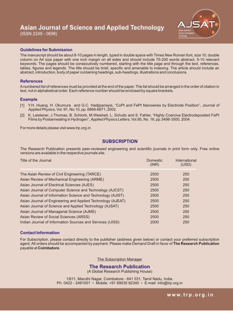

Top Related
Copyright © 2022 FDOKUMEN

