NPS-MAE-09-002

NAVAL POSTGRADUATE

SCHOOL

MONTEREY, CALIFORNIA

A STUDY ON FRAGILITY ASSESSMENT

FOR EQUIPMENT IN A SHOCK ENVIRONMENT

by

Beomsoo Lim Jarema M. Didoszak

December 2009

Approved for public release; distribution is unlimited

NAVAL POSTGRADUATE SCHOOL Monterey, California 93943-5000

Daniel T. Oliver Leonard A. Ferrari President Executive Vice President and Provost This report was prepared by and funded by the Naval Postgraduate School, Monterey, CA 93943.

Reproduction of all or part of this report is authorized. This report was prepared by: __________________ ___________________ Beomsoo Lim Jarema M. Didoszak Visiting Professor of Research Assistant Professor Mechanical & Astronautical Engineering Reviewed by: Released by: __________________ _______________________ Knox T. Millsaps Karl van Bibber Department of Mechanical & Vice President and Astronautical Engineering Dean of Research

REPORT DOCUMENTATION PAGE Form Approved

OMB No. 0704-0188 Public reporting burden for this collection of information is estimated to average 1 hour per response, including the time for reviewing instructions, searching existing data sources, gathering and maintaining the data needed, and completing and reviewing this collection of information. Send comments regarding this burden estimate or any other aspect of this collection of information, including suggestions for reducing this burden to Department of Defense, Washington Headquarters Services, Directorate for Information Operations and Reports (0704-0188), 1215 Jefferson Davis Highway, Suite 1204, Arlington, VA 22202-4302. Respondents should be aware that notwithstanding any other provision of law, no person shall be subject to any penalty for failing to comply with a collection of information if it does not display a currently valid OMB control number. PLEASE DO NOT RETURN YOUR FORM TO THE ABOVE ADDRESS. 1. REPORT DATE (DD-MM-YYYY) 20-12-2009

2. REPORT TYPE Technical

3. DATES COVERED (From - To)Dec 2008 – Dec 2009

4. TITLE AND SUBTITLE A Study on Fragile Assessment for Equipment in a Shock Environment

5a. CONTRACT NUMBER

5b. GRANT NUMBER

5c. PROGRAM ELEMENT NUMBER

6. AUTHOR(S) Lim, Beomsoo

5d. PROJECT NUMBER

Didoszak, Jerema M. 5e. TASK NUMBER

5f. WORK UNIT NUMBER

7. PERFORMING ORGANIZATION NAME(S) AND ADDRESS(ES) Naval Postgraduate School

8. PERFORMING ORGANIZATION REPORT NUMBER

Monterey, CA 93943-5000

NPS-MAE-09-002

9. SPONSORING / MONITORING AGENCY NAME(S) AND ADDRESS(ES) 10. SPONSOR/MONITOR’S ACRONYM(S) N/A 11. SPONSOR/MONITOR’S REPORT NUMBER(S) 12. DISTRIBUTION / AVAILABILITY STATEMENT Approved for public release; distribution is unlimited 13. SUPPLEMENTARY NOTES The views expressed in this report are those of the authors and do not reflect the official policy or position of the Department of Defense or the U.S. Government. 14. ABSTRACT In this report, the Damage Boundary Theory and related analysis using the Shock Response Spectrum have been investigated. In particular, physics-based computer modeling and simulation using the MSC/NASTRAN code has been performed for the case of a rotational drop test model. Application of the Damage Boundary Theory and subsequent analysis using the Shock Response Spectrum is useful in understanding the isolation level of packaging systems. The results of the computer simulations show the effects of the flexibility in the equipment and nonlinearity of the shock mounts analyzed in this research. The data from these simulations have been compared with the shock test specification, MIL-STD-810. 15. SUBJECT TERMS Shock, Fragility, Damage Boundary, Shock Response Spectrum, Modeling and Simulation

16. SECURITY CLASSIFICATION OF:

17. LIMITATION OF ABSTRACT

18. NUMBER OF PAGES

19a. NAME OF RESPONSIBLE PERSON Didoszak, Jerema

a. REPORT U

b. ABSTRACT U

c. THIS PAGE U

SAR 62

19b. TELEPHONE NUMBER (include area code) (831)656-2604

Standard Form 298 (Rev. 8-98) Prescribed by ANSI Std. Z39.18

ii

THIS PAGE INTENTIONALLY LEFT BLANK

iii

ABSTRACT

In this report, the Damage Boundary Theory and related analysis using the Shock

Response Spectrum have been investigated. In particular, physics-based computer

modeling and simulation using the MSC/NASTRAN code has been performed for the

case of a rotational drop test model. Application of the Damage Boundary Theory and

subsequent analysis using the Shock Response Spectrum is useful in understanding the

isolation level of packaging systems. The results of the computer simulations show the

effects of the flexibility in the equipment and nonlinearity of the shock mounts analyzed

in this research. The data from these simulations have been compared with the shock test

specification, MIL-STD-810.

iv

THIS PAGE INTENTIONALLY LEFT BLANK

v

TABLE OF CONTENTS

I.  INTRODUCTION........................................................................................................1 

II.  SHOCK RESPONSE SPECTRUM............................................................................3 A.  INTRODUCTION............................................................................................3 B.  CONCEPT OF SHOCK RESPONSE SPECTRA ........................................3 C.  CALCULATING SHOCK RESPONSE SPECTRA ....................................6 D.  FOUR COORDINATE PAPER (4CP) ..........................................................9 

III.  SHOCK FRAGILITY ASSESSMENT AND TEST PROCEDURE.....................10 A.  INTRODUCTION..........................................................................................10 B.  DAMAGE BOUNDARY THEORY.............................................................10 C.  DAMAGE BOUNDARY TEST METHOD (ASTM D3332-99) ................15 

1.   Test Method A: Critical Velocity Change Shock Test....................15 2.   Test Method B: Critical Acceleration shock test ............................16 

VI.  SIMULATION OF A PACKAGE SYSTEM ..........................................................18 A.  RIGID BODY ANALYSIS............................................................................19 

1.   Model Description..............................................................................20 2.   Normal Mode Analysis ......................................................................20 3.   Transient Analysis .............................................................................22 

B.  FLEXIBLE BODY ANALYSIS ...................................................................24 1.   Model Description..............................................................................24 2.   Normal Mode Analysis ......................................................................25 3.   Transient Analysis .............................................................................27 

C.  NON-LINEAR TRANSIENT ANALYSIS ..................................................39 D.  COMPARISON BETWEEN RESPONSES AND SPECIFICATION......42 

V.  CONCLUSION ..........................................................................................................44 

LIST OF REFERENCES......................................................................................................46 

INITIAL DISTRIBUTION LIST .........................................................................................48 

vi

THIS PAGE INTENTIONALLY LEFT BLANK

vii

LIST OF FIGURES

Figure 1.  The Concept of Shock Response Spectrum (SRS) ............................................4 Figure 2.  Acquiring the Graph of Shock Response Spectrum ..........................................5 Figure 3.  SDOF System with Spring and Damper ............................................................6 Figure 4.  Various Shock Pulse Types ...............................................................................8 Figure 5.  Shock Spectra Resulting from Various Pulses...................................................8 Figure 6.  Shock Response Spectrum Curve ......................................................................9 Figure 7.  Velocity Change of Shock Pulse......................................................................10 Figure 8.  Shock Spectrum of a Rectangular Pulse ..........................................................12 Figure 9.  Ideal Damage Boundary Curve........................................................................14 Figure 10.  Damage boundary test......................................................................................16 Figure 11.  Drop Test Model ..............................................................................................19 Figure 12.  Configuration of the Rigid Body Model..........................................................20 Figure 13.  Rigid Body Mode Shapes ................................................................................21 Figure 14.  Responses from Rigid Body Analysis .............................................................22 Figure 15.  Time Histories for Y Acceleration at the Center of Gravity............................23 Figure 16.  Time Histories for Z Acceleration at the Center of Gravity ............................23 Figure 17.  Finite Element Model for the Flexible Body ...................................................24 Figure 18.  Mode Shape of the Flexible Body ...................................................................26 Figure 19.  Time Histories for Y Acceleration at the Center of Gravity (High

Stiffness Case) .................................................................................................29 Figure 20.  Pseudo Velocity for Y Acceleration at the Center of Gravity (High

Stiffness Case) .................................................................................................29 Figure 21.  Time Histories for Z Acceleration at the Center of Gravity

(High Stiffness Case) .......................................................................................30 Figure 22.  Pseudo Velocity for Z Acceleration at the Center of Gravity (High

Stiffness Case) .................................................................................................30 Figure 23.  Time Histories for Y Acceleration at the Center of Gravity

(Medium Stiffness Case)..................................................................................31 Figure 24.  Pseudo Velocity for Y Acceleration at the Center of Gravity (Medium

Stiffness Case) .................................................................................................31 Figure 25.  Time Histories for Z Acceleration at the Center of Gravity

(Medium Stiffness Case)..................................................................................32 Figure 26.  Pseudo Velocity for Z Acceleration at the Center of Gravity (Medium

Stiffness Case) .................................................................................................32 Figure 27.  Time Histories for Y Acceleration at the Center of Gravity

(Low Stiffness Case)........................................................................................33 Figure 28.  Pseudo Velocity for Y Acceleration at the Center of Gravity (Low

Stiffness Case) .................................................................................................33 Figure 29.  Time Histories for Z Acceleration at the Center of Gravity (Low

Stiffness Case) .................................................................................................34 Figure 30.  Pseudo Velocity for Z Acceleration at the Center of Gravity (Low

Stiffness Case) .................................................................................................34 Figure 31.  Time Histories for Y Acceleration at Various Locations ................................36 

viii

Figure 32.  Pseudo Velocity for Y Acceleration at Various Locations..............................36 Figure 33.  Time Histories for Z Acceleration at Various Locations.................................37 Figure 34.  Pseudo Velocity for Z Acceleration at Various Locations ..............................37 Figure 35.  Displacement of a Shock Mount......................................................................38 Figure 36.  Non-linear Stiffness Curve ..............................................................................39 Figure 37.  Displacement of Non-linear Shock Mounts.....................................................40 Figure 38.  Time Histories for Z Acceleration of the Non-linear Stiffness........................41 Figure 39.  Pseudo Velocity for Z Acceleration of the Non-linear Stiffness .....................41 Figure 40.  Comparison of SRS Responses and Specification...........................................42 Figure 41.  Comparison of All Y Accelerations with Specification ..................................43 Figure 42.  Comparison of All Z Accelerations with Specification...................................43 

ix

LIST OF TABLES

Table 1.  Dimension of Container and Payload ..............................................................19 Table 2.  Natural Frequencies for the Rigid Body Model...............................................21 Table 3.  Peak response comparisons..............................................................................23 Table 4.  Model Natural Frequencies..............................................................................25 Table 5.  Peak Response Comparisons ...........................................................................27 Table 6.  Peak Response Comparisons ...........................................................................35 

x

THIS PAGE INTENTIONALLY LEFT BLANK

1

I. INTRODUCTION

The reliability of complicated electronic equipment, requiring a high amount of

accuracy, depends on the environment in which it is operated. The shock environment is

a critical element that affects survivability of these types of equipment. As such, it is

important to clearly identify the limitation of shock endurance definitely and provide

proper isolation so as not to allow the equipment to exceed the shock endurance range.

There are two separate kinds of requirements to consider in solving the shock problem. It

is necessary to first establish the shock fragility of equipment and then to design the

shock isolation system to mitigate the shock environmental condition which the

equipment will experience.

Since R. D. Mindlin announced “Dynamics of Package Cushioning” in 1945,

many studies have been made describing the phenomenon of shock and the

corresponding shock response. In order to establish a method as an indicator of

mechanical shock severity, Shock Response Spectrum (SRS) analysis was developed in

the early 1960’s by the U.S Department of Defense engineering contractors and

government Research & Development facilities. [Ref. 1, 2]

SRS is the response curve which gives the peak response value at any frequencies

that a shock would cause a Single Degree of Freedom (SDOF) to respond. SRS analysis

is also used to define the environmental condition of equipment [Ref. 3]. From SRS

analysis, Pseudo Velocity (PV), which is the relative displacement multiplied by the

frequency, is primarily obtained and plotted on Four Coordinate Paper (4CP). The

resulting plot is called a Pseudo Velocity Shock Response Spectrum (PVSRS). PVSRS

can be used to estimate the damage potential of a shock to a SDOF system.

A simplification of the SRS analysis combined with availability of repeatable

shock machines has resulted in the Damage Boundary theory [Ref. 4]. This method was

developed in the late 1960’s by R. Newton at the Naval Postgraduate School in Monterey,

CA.

2

The fragility of equipment is another characteristic unique to the system or

equipment just like size, weight and color. The equipment fragility is determined by

using calibrated inputs and measuring a product’s response to those specific inputs. This

measurement takes the form of a Damage Boundary Curve for shock. This graph defines

an area bounded by peak acceleration on the vertical axis and velocity change on the

horizontal axis. Any shock pulse experienced by the equipment which can be plotted

inside this boundary will cause damage to the equipment whether or not it is packaged.

This report examines the shock response spectrum theory and Damage Boundary

theory to better understand the fragility of equipment. Using the finite element method,

rotational drop simulations of packaging system have been accomplished for various

stiffness cases of a representative piece of equipment. PVSRS of the equipment were

obtained at the critical points and the corresponding damage potential was estimated by

comparing them to the shock test standard, MIL-STD-810G [Ref. 5].

3

II. SHOCK RESPONSE SPECTRUM

A. INTRODUCTION Shock is defined as a non-periodic acceleration or deceleration due to collision,

drop, earthquake or explosion. The word “shock” implies a degree of suddenness and

severity. Most equipment in weapon systems is exposed to a shock environment during

its packaging, handling, shipping and transportation.

Shock Response Spectrum is the curve of maximum response as a function of

natural frequency of the responding system. A pulse is a particular form of shock motion.

Each shock motion has a characteristic shock spectrum. A shock motion has a

characteristic effective value of time duration which need not be defined specifically.

Instead, the spectra are made to apply explicitly to a given shock motion by using the

natural frequency as a dimensional parameter on the abscissa. Thus the maximum

response can be anticipated from the shock spectrum curve easily, if the frequency

characteristic of system is given.

In more recent times, even though computer and signal processing technology has

made it possible to directly compute the response of specific structures under transient

loading, the SRS analysis method continues to be used to assess the shock fragility

because of its simplicity and effectiveness [Ref. 2].

B. CONCEPT OF SHOCK RESPONSE SPECTRA SRS represents the maximum responses of every conceivable SDOF (Single

Degree Of Freedom) system mounted base structure, when the base structure is excited

by a shock pulse.

Imagine a platform with 1000 different SDOF components mounted on it as

shown in Figure 1. Each component has a different resonance frequency, so that every

resonance frequency of possible interest is represented. We have the equivalent of such a

system when applying the SRS method. We enforce on that platform the acceleration

transient that was present on our base frame. Each of the SDOF components will respond

with its own unique acceleration transient. The peak response acceleration level is then

computed for each SDOF component. The set of all peak levels is seen to be

representative of the severity of the base frame shock transient. This set of peak levels

can be collected together to form a spectrum across the frequency range of interest. This

is the SRS [Ref. 2].

In Figure 2, the X axis represents Time, the Y axis represents Acceleration and

the Z axis represents Frequency. If the time histories for the every frequency of SDOF are

plotted in the X-Y plane and the maximum response in each frequency is plotted in the Z-

Y plane, then the plot of the Z-Y plane is the SRS.

Figure 1. The Concept of Shock Response Spectrum (SRS)

4

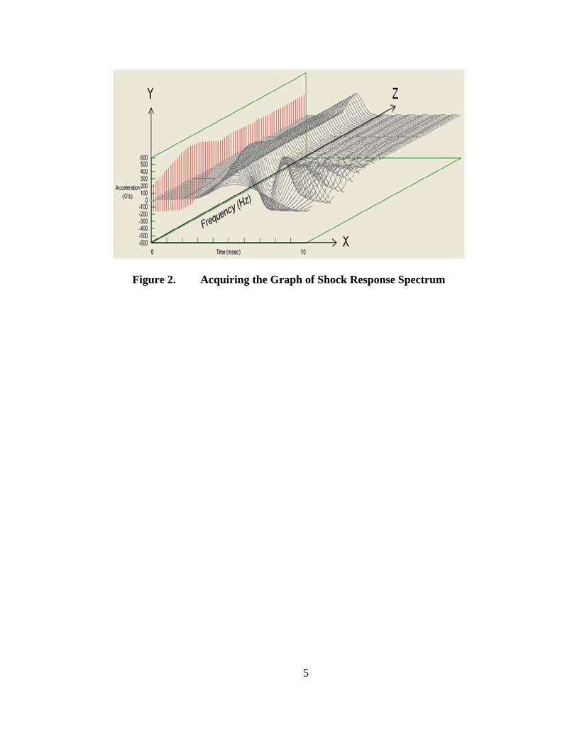
Figure 2. Acquiring the Graph of Shock Response Spectrum

5

C. CALCULATING SHOCK RESPONSE SPECTRA The simplest SDOF system is shown in Figure 3. It consists of mass m attached

by means of spring k and damping c to a movable base. The mass is constrained to

translational motion in the direction x axis [Ref. 11].

Figure 3. SDOF System with Spring and Damper

The differential equation of motion for the SDOF shown in Figure 3 excited by

base motion y is as follows:

(1)

The response motion to be solved in Equation (1) is the relative displacement, z, between

the mass response motion, x, and the input displacement, y:

Letting and substituting it into Equation (1) gives

(2)

6

Let , , 2 and substituting those into Equation (2) gives

(3)

Calculation of the differential equation (3) gives the time domain response of relative

displacement z. The Pseudo Velocity Shock Response Spectrum (PVSRS) value at each

frequency is computed by solving for z as a function of time, picking off the maximum

value, and then multiplying by as follows:

(4)

Equation (4) shows that pseudo velocity is the relative displacement multiplied by

the frequency in radians. Pseudo velocity is not equal to velocity change , but high

PVSRS will indicate what frequencies are seeing the highest . PV is also equal to

the square root of half the stored energy per unit mass, as shown in Equation (5). This

potential energy is equal to the maximum energy stored in the spring of a SDOF system.

“U” can also be viewed as the maximum energy that the shock can deliver to a SDOF

system at a particular frequency [Ref. 3].

(5)

Equation (5) shows how pseudo velocity can be used to estimate the damage potential of

shock to a SDOF system.

Figure 4 and 5 illustrate several shock pulse inputs and their resulting Shock

Response Spectra. In Figure 4 and 5, Ap represents the level of the peak acceleration

pulse of input, Ac represents the peak acceleration of equipment and fc represents the

natural frequency of equipment. Te, which is the effective duration of the acceleration

pulse, is obtained from the velocity change divided by Ap. For example, Te = T for the

rectangular pulse and for the half sine wave pulse.

7

Figure 4. Various Shock Pulse Types

Figure 5. Shock Spectra Resulting from Various Pulses

8

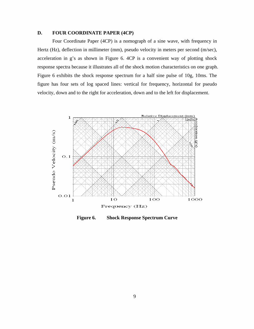
D. FOUR COORDINATE PAPER (4CP) Four Coordinate Paper (4CP) is a nomograph of a sine wave, with frequency in

Hertz (Hz), deflection in millimeter (mm), pseudo velocity in meters per second (m/sec),

acceleration in g’s as shown in Figure 6. 4CP is a convenient way of plotting shock

response spectra because it illustrates all of the shock motion characteristics on one graph.

Figure 6 exhibits the shock response spectrum for a half sine pulse of 10g, 10ms. The

figure has four sets of log spaced lines: vertical for frequency, horizontal for pseudo

velocity, down and to the right for acceleration, down and to the left for displacement.

Figure 6. Shock Response Spectrum Curve

9

III. SHOCK FRAGILITY ASSESSMENT AND TEST PROCEDURE

A. INTRODUCTION It is important to assess how severe of a shock the equipment can endure in order

to provide proper and economic protective package. This is called “Shock Fragility

Assessment”. Many studies were conducted and test standards developed in order to

establish the procedure of shock fragility assessment. Among them, Damage Boundary

theory [Ref. 4] and ASTM-D3332 [Ref. 6] are most well-known.

B. DAMAGE BOUNDARY THEORY The concept of Damage Boundary theory is well-established having been

published by Dr. Robert Newton in 1968. The original concept of Damage Boundary was

a simplification of Shock Response Spectrum (SRS) where the plot of the damage

potential area is bounded by peak acceleration and velocity change. The shock load on

the equipment is represented by acceleration level (Ap) and duration time (T) as shown in

Figure 7.

Figure 7. Velocity Change of Shock Pulse

10

The shaded areas under the time-acceleration curves are velocity change. The

velocity change is obtained by Equation (6).

(6)

Te is the effective duration obtained from real duration time T as was explained in the

previous section.

Damage Boundary Curve is obtained from the relationship between peak

acceleration and velocity change using Equation (6) and Shock Response Spectrum of

various pulses. Consider the shock spectrum for the rectangular pulse shown Figure 8.

In the segments of OA, AB, BC of Figure 8, relationships between the

acceleration ratio (Ac/Ap) and frequency ratio (fc/Te) of the SRS for the rectangular pulse

are as follows:

(7)

(8)

(9)

11

Figure 8. Shock Spectrum of a Rectangular Pulse

Assume that the critical equipment has a specified natural frequency, fc and the

peak acceleration without damage, Acs. In case that effective duration (Te) of input pulse

is short ( ), substituting in Equation (7) and solving for V

gives

(10)

Equation (10) represents the maximum velocity change without damage when the

excitation frequency of the input pulse is very high compared to the natural frequency of

the equipment. Equation (10) indicates that the allowable velocity change is determined

by natural frequency and the allowable acceleration of equipment. The acceleration level

and duration of input pulse are obtained from Equation (6).

In case that effective duration (Te) of input pulse is long ( ), substituting

in Equation (9) gives

(11)

Thus Equation (11) represents the maximum acceleration without damage when

the excitation frequency of the input pulse is very low compared to the natural frequency

12

of equipment. Equation (11) then dictates that the allowable acceleration level of shock

input is only half of the allowable acceleration of equipment, irrespective of velocity

change.

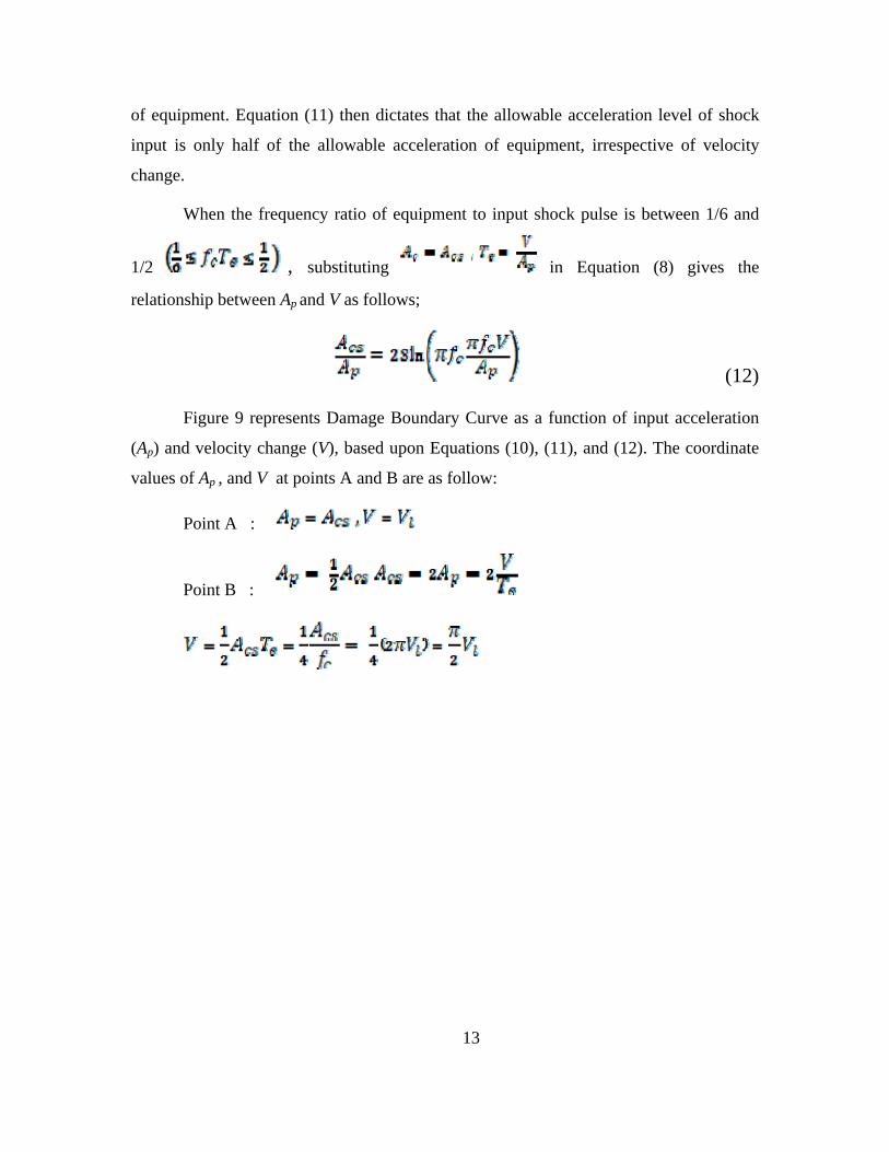
When the frequency ratio of equipment to input shock pulse is between 1/6 and

1/2 , substituting in Equation (8) gives the

relationship between Ap and V as follows;

(12)

Figure 9 represents Damage Boundary Curve as a function of input acceleration

(Ap) and velocity change (V), based upon Equations (10), (11), and (12). The coordinate

values of Ap , and V at points A and B are as follow:

Point A :

Point B :

13

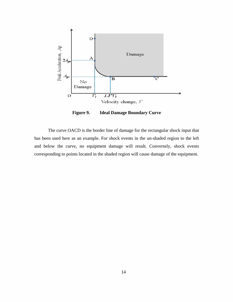
Figure 9. Ideal Damage Boundary Curve

The curve OACD is the border line of damage for the rectangular shock input that

has been used here as an example. For shock events in the un-shaded region to the left

and below the curve, no equipment damage will result. Conversely, shock events

corresponding to points located in the shaded region will cause damage of the equipment.

14

C. DAMAGE BOUNDARY TEST METHOD (ASTM D3332-99) In order to design a package system or shipping container for a piece of specific

equipment, the shock fragility of that equipment should be first determined. ASTM-

D3332-99 provides a test method and procedure to determine the fragility of equipment.

When equipment or systems are exposed to a shock environment, the damage of the

equipment depends on the velocity change and acceleration. ASTM-D3332-99 defines

the procedure to obtain the critical velocity change and critical acceleration at which

damage begins using Damage Boundary Curve as was derived in the previous section.

Two test methods, the Critical Velocity Change Shock Test, and the Critical Acceleration

Shock Test, are outlined here.

1. Test Method A: Critical Velocity Change Shock Test This test method is used to determine the critical velocity change (Vl) portion of

the damage boundary plot for a particular equipment. A shock pulse having any

waveform and duration (Tp) between 0.5 and 3ms can be used to perform this test. Since

they are relatively easy to control, shock pulses having a half sine shock waveform are

normally used. In general, the pulse duration should satisfy the following condition.

where Tp is maximum shock test machine pulse duration in ms and fc is the equipment

natural frequency in Hz.

To perform this test, initially set the shock test machine so that the shock pulse

produced has a velocity change below the anticipated critical velocity change of the

equipment. Perform one shock test and examine whether damage due to this shock

loading has occurred. Repeat the shock test with incrementally increasing velocity change

values until equipment damage occurs. If damage has occurred, the critical velocity

change (Vl) is the midpoint between the last successful test and the test that produced

failure.

15

2. Test Method B: Critical Acceleration shock test This test method is used to determine the critical acceleration (Acs) portion of the

damage boundary plot for a particular equipment. Trapezoidal shock pulses are normally

used to perform this test. The rise and fall times of 1.8 ms, or less are required in the

trapezoidal pulse input because it is not possible to obtain a pulse having infinitely short

rise and fall times. Longer rise and fall times cause the pulse form to deviate from the

horizontal, introducing errors into the test results.

At first, set the shock test machine so that it will produce a trapezoidal shock

pulse having a velocity change of at least 1.57 times as great as the critical velocity

change determined in Test Method A. This is done to avoid the rounded intersection of

the critical velocity change and critical acceleration lines. Perform one shock test and

examine whether damage due to shock has occurred. Repeat the shock test with

incrementally increasing acceleration, until equipment damage occurs. If damage has

occurred, critical acceleration (Acs) is found to be the midpoint between the last

successful test and the test that produced failure. Figure 10 shows an example of the

Damage Boundary Test.

Figure 10. Damage boundary test

16

17

Test Method A was performed to determine the critical velocity change. If

damage occurs at the 7th test, as indicated in the figure, the midpoint between the 6th and

7th data is defined as critical velocity change. In the second stage of testing, perform Test

Method B in order to determine the critical acceleration. If damage occurs at the point of

the14th test, as is shown in the figure, the midpoint between 13th and 14th data is defined

as critical acceleration.

Test Method A is performed without shock isolator while Test Method B is

performed with shock isolator. If no cushioning materials are to be used in the package,

the critical acceleration test may be unnecessary. Only the critical velocity change test

may suffice in this case.

18

VI. SIMULATION OF A PACKAGE SYSTEM

Computer simulations were carried out for the drop shock impact of large

container to illustrate the application of shock response spectrum analysis. The model

was taken from Himelblau and Sheldon’s [Ref. 9] chapter on “Vibration of a Resiliently

Supported Rigid Body”, found in the Shock and Vibration Handbook, 4th Ed. by Harris.

It represents a missile container in which a missile is supported by several isolators to

protect it from shock impact. The system was subjected to a rotational velocity shock as a

result of a drop event where one end of the container was raised to a standardized height.

This represents the edgewise drop test in the package test specification.

MSC/PATRAN [Ref. 13] was used in the finite element modeling of this

equipment container while MSC/NASTRAN [Ref. 14] was used for conducting the

analysis. Normal mode analysis, linear and nonlinear transient analysis were performed

for several cases. The analyses were divided into four stages. The first stage was rigid

body analysis. The normal mode and linear transient analyses for the rigid body model

were conducted and the results were compared with previous research [Ref. 10]. In the

second stage, the rigid body model of equipment was replaced by a beam element model

using the Finite Element Method. Three kinds of stiffness: low, medium and high, were

used to analyze the effects of flexibility of the equipment. The normal mode and linear

transient analyses were performed and the results were compared with those of the rigid

body analysis of the previous stage. The effects of location of critical component were

also investigated. The third stage is a non-linear transient analysis. The nonlinear

effects of the isolators were investigated when the equipment was modeled with a

medium stiffness. In general, shock mounts using rubber material show a non-linearity

in the displacement vs. force curve. In the final stage of this investigation the results

were compared with the specifications of shock test as per the MIL-STD-810 and some

suggestions are included based upon the results.

Figure 11 shows the 2-dimensional drop test model with symmetry about the YZ

plane. This system was subjective to a rotational shock velocity as a result of an edgewise

drop. Table 1 shows the dimensions of Figure 11.

Figure 11. Drop Test Model

Table 1. Dimension of Container and Payload

Item Unit Dimension

Length(Lc) mm 4,267.2 Container

Width/Height(H) mm 1,066.8

Length(Lp) mm 3,657.6

Diameter(D) mm 609.6

Weight kg

19

680.4 Payload

MOI(Ixx) kg mm2 7.74×108

Location(ly1

,ly2

) mm 660.4, 1727.2

Location(lz) mm 266.7

Stiffness_y(ky) N/m 8.75×104 Isolator

Stiffness_z(kz) N/m 1.75×105 A. RIGID BODY ANALYSIS

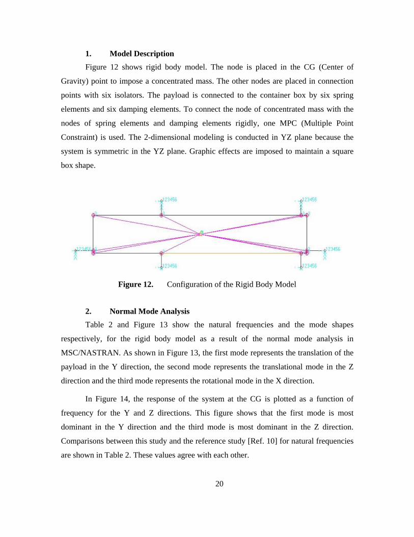
1. Model Description Figure 12 shows rigid body model. The node is placed in the CG (Center of

Gravity) point to impose a concentrated mass. The other nodes are placed in connection

points with six isolators. The payload is connected to the container box by six spring

elements and six damping elements. To connect the node of concentrated mass with the

nodes of spring elements and damping elements rigidly, one MPC (Multiple Point

Constraint) is used. The 2-dimensional modeling is conducted in YZ plane because the

system is symmetric in the YZ plane. Graphic effects are imposed to maintain a square

box shape.

Figure 12. Configuration of the Rigid Body Model

2. Normal Mode Analysis Table 2 and Figure 13 show the natural frequencies and the mode shapes

respectively, for the rigid body model as a result of the normal mode analysis in

MSC/NASTRAN. As shown in Figure 13, the first mode represents the translation of the

payload in the Y direction, the second mode represents the translational mode in the Z

direction and the third mode represents the rotational mode in the X direction.

In Figure 14, the response of the system at the CG is plotted as a function of

frequency for the Y and Z directions. This figure shows that the first mode is most

dominant in the Y direction and the third mode is most dominant in the Z direction.

Comparisons between this study and the reference study [Ref. 10] for natural frequencies

are shown in Table 2. These values agree with each other.

20

Table 2. Natural Frequencies for the Rigid Body Model

Items 1st 2nd 3rd

M.A.Talley 3.58 6.02 9.75

MSC/NASTRAN 3.58 6.03 9.75

Figure 13. Rigid Body Mode Shapes

21

Figure 14. Responses from Rigid Body Analysis

3. Transient Analysis Linear transient analysis was performed using the MSC/NASTRAN Transient

Module. The system was subjective to a rotational shock velocity of 0.38 rad/sec, as a

result of a drop event where one end was raised to a height of 36 inches. In the modeling,

initial velocities of center of gravity (CG) are calculated and inputted at the moment that

the container touches the ground.

Comparisons between the current study and Himelblau’s [Ref. 11] along with M.

A. Talley’s [Ref. 10] calculations for peak acceleration at the center of gravity are shown

in Table 3 for the case without damping. There is good agreement with one another.

Figures 15 and 16 show the calculated time histories for the Z and Y directions,

respectively. Comparing them to the case where 10% damping is applied, the differences

in peak acceleration and phasing are observed if damping is ignored. For example, in the

Z direction in Figure 5, the peak un-damped acceleration is about 1.2 times greater than

the 10% damped acceleration case, which also occurs at a much later time.

22

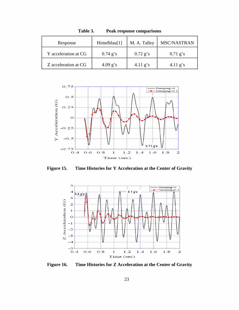
Table 3. Peak response comparisons

Response Himelblau[1] M. A. Talley MSC/NASTRAN

Y acceleration at CG 0.74 g’s 0.72 g’s 0.71 g’s

Z acceleration at CG 4.09 g’s 4.11 g’s 4.11 g’s

Figure 15. Time Histories for Y Acceleration at the Center of Gravity

Figure 16. Time Histories for Z Acceleration at the Center of Gravity 23

B. FLEXIBLE BODY ANALYSIS

1. Model Description Figure 17 shows the finite element model for the package system. The modeling

process was accomplished using the computer code MSC/PATRAN. Beam elements are

used to make the model of the representative payload loaded inside of the container. The

2-dimensional modeling is conducted in the YZ plane because the system is symmetric

for the YZ plane. 18 beam elements, 6 spring elements and 6 damping elements are used

for the model as shown Figure 7. The beam cross section is in the shape of a pipe and the

supporting points of the shock mounts are placed in the surface of the payload. Here four

MPCs (Multiple Point Constraint) are used to constrain the nodes of the beam elements

and supporting points of the mounts.

Figure 17. Finite Element Model for the Flexible Body

24

25

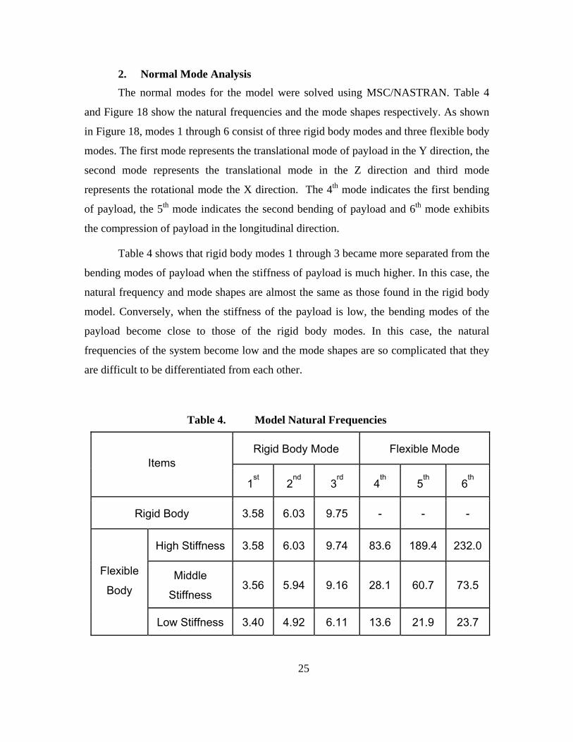
2. Normal Mode Analysis The normal modes for the model were solved using MSC/NASTRAN. Table 4

and Figure 18 show the natural frequencies and the mode shapes respectively. As shown

in Figure 18, modes 1 through 6 consist of three rigid body modes and three flexible body

modes. The first mode represents the translational mode of payload in the Y direction, the

second mode represents the translational mode in the Z direction and third mode

represents the rotational mode the X direction. The 4th mode indicates the first bending

of payload, the 5th mode indicates the second bending of payload and 6th mode exhibits

the compression of payload in the longitudinal direction.

Table 4 shows that rigid body modes 1 through 3 became more separated from the

bending modes of payload when the stiffness of payload is much higher. In this case, the

natural frequency and mode shapes are almost the same as those found in the rigid body

model. Conversely, when the stiffness of the payload is low, the bending modes of the

payload become close to those of the rigid body modes. In this case, the natural

frequencies of the system become low and the mode shapes are so complicated that they

are difficult to be differentiated from each other.

Table 4. Model Natural Frequencies

Rigid Body Mode Flexible Mode Items

1st

2nd

3rd

4th

5th

6th

Rigid Body 3.58 6.03 9.75 - - -

High Stiffness 3.58 6.03 9.74 83.6 189.4 232.0

Middle Stiffness

3.56 5.94 9.16 28.1 60.7 73.5 Flexible

Body

Low Stiffness 3.40 4.92 6.11 13.6 21.9 23.7

26Figure 18. Mode Shape of the Flexible Body

27

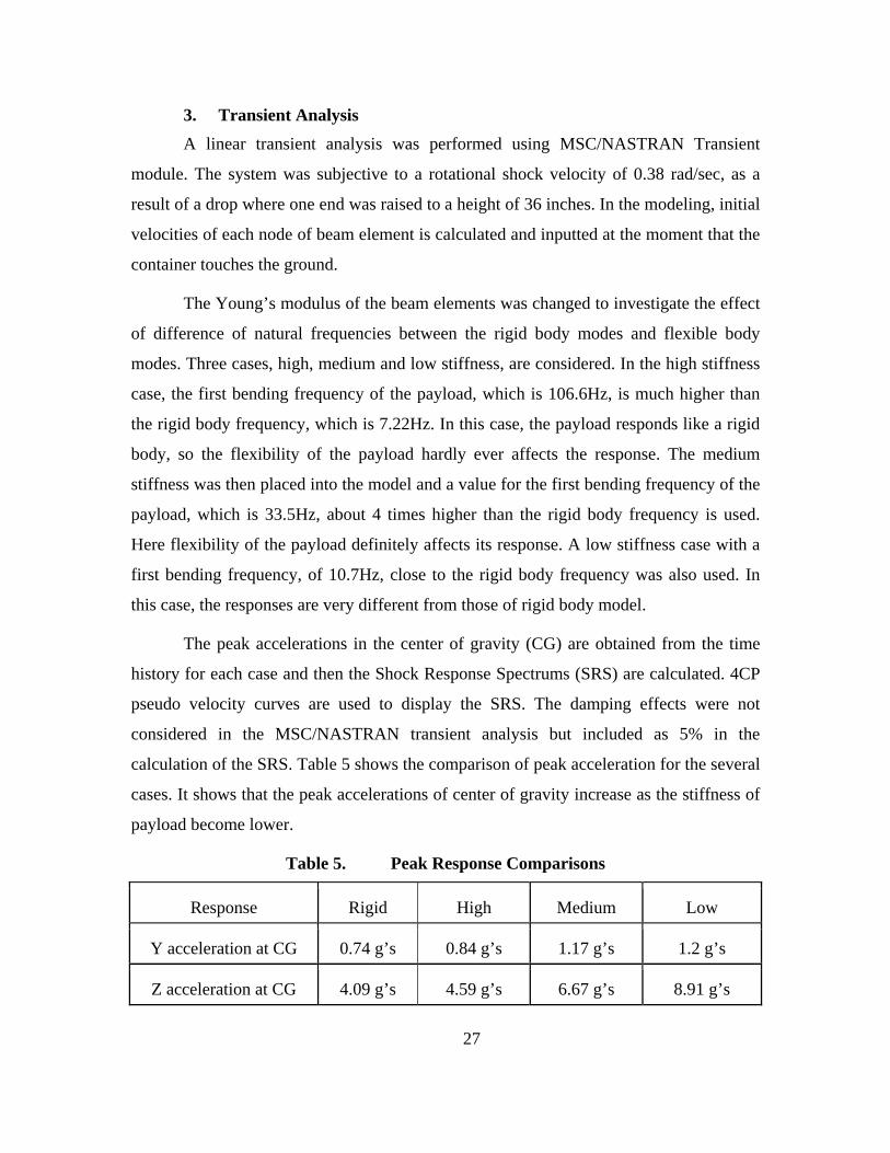
3. Transient Analysis A linear transient analysis was performed using MSC/NASTRAN Transient

module. The system was subjective to a rotational shock velocity of 0.38 rad/sec, as a

result of a drop where one end was raised to a height of 36 inches. In the modeling, initial

velocities of each node of beam element is calculated and inputted at the moment that the

container touches the ground.

The Young’s modulus of the beam elements was changed to investigate the effect

of difference of natural frequencies between the rigid body modes and flexible body

modes. Three cases, high, medium and low stiffness, are considered. In the high stiffness

case, the first bending frequency of the payload, which is 106.6Hz, is much higher than

the rigid body frequency, which is 7.22Hz. In this case, the payload responds like a rigid

body, so the flexibility of the payload hardly ever affects the response. The medium

stiffness was then placed into the model and a value for the first bending frequency of the

payload, which is 33.5Hz, about 4 times higher than the rigid body frequency is used.

Here flexibility of the payload definitely affects its response. A low stiffness case with a

first bending frequency, of 10.7Hz, close to the rigid body frequency was also used. In

this case, the responses are very different from those of rigid body model.

The peak accelerations in the center of gravity (CG) are obtained from the time

history for each case and then the Shock Response Spectrums (SRS) are calculated. 4CP

pseudo velocity curves are used to display the SRS. The damping effects were not

considered in the MSC/NASTRAN transient analysis but included as 5% in the

calculation of the SRS. Table 5 shows the comparison of peak acceleration for the several

cases. It shows that the peak accelerations of center of gravity increase as the stiffness of

payload become lower.

Table 5. Peak Response Comparisons

Response Rigid High Medium Low

Y acceleration at CG 0.74 g’s 0.84 g’s 1.17 g’s 1.2 g’s

Z acceleration at CG 4.09 g’s 4.59 g’s 6.67 g’s 8.91 g’s

28

Figures 19 through 30 show the time history and SRS of acceleration at the

center of gravity location of the payload. Here the rigid body models for several stiffness

cases are compared. They show that the responses are closer to those of rigid body model

as the stiffness of payload is higher, and it hardly affects the longitudinal responses.

Figures 19 through 22 compare the high stiffness case of the payload to the rigid

body model. These time histories and SRSs are very similar. So, when the difference of

the natural frequencies between the rigid body mode and the first bending mode are great,

simple rigid body analysis is good enough for accurate results.

Figures 23 through 26 show the time history and SRSs for the medium stiffness

case of the payload. In the time history plots there seems to be large differences between

the two curves, but the SRS curves show that these differences occur in the high

frequency range. In the low frequency range, the rigid body motion is dominant and

almost same as rigid body model. In the high frequency range, which is taken to be

higher than 20Hz, response of the medium stiffness model is higher than the rigid body

model due to the flexible mode of the payload. So in this area, the shock fragility is

investigated.

Figures 27 through 30 represent the time history and SRSs for the low stiffness

case of the payload. These plots show there is little difference in the longitudinal

direction (Y), but the acceleration of vertical direction (Z) is greatly increased. The

pseudo velocities are also increased in the bending mode of the payload as well as the

rigid body mode cases. This then indicates that when the package system is designed,

isolators should be selected not to be close to natural frequency of payload.

Figure 19. Time Histories for Y Acceleration at the Center of Gravity (High Stiffness Case)

Figure 20. Pseudo Velocity for Y Acceleration at the Center of Gravity (High Stiffness Case)

29

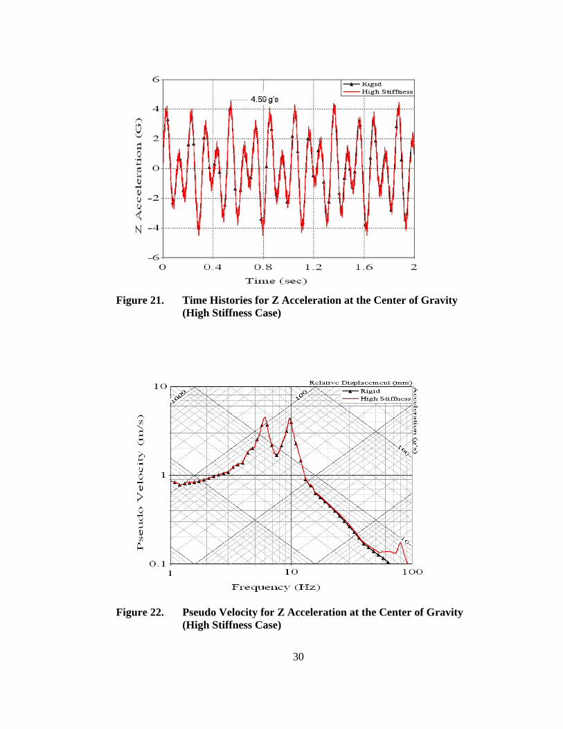
Figure 21. Time Histories for Z Acceleration at the Center of Gravity

(High Stiffness Case)

Figure 22. Pseudo Velocity for Z Acceleration at the Center of Gravity (High Stiffness Case)

30

Figure 23. Time Histories for Y Acceleration at the Center of Gravity

(Medium Stiffness Case)

Figure 24. Pseudo Velocity for Y Acceleration at the Center of Gravity (Medium Stiffness Case)

31

Figure 25. Time Histories for Z Acceleration at the Center of Gravity

(Medium Stiffness Case)

Figure 26. Pseudo Velocity for Z Acceleration at the Center of Gravity (Medium Stiffness Case)

32

Figure 27. Time Histories for Y Acceleration at the Center of Gravity

(Low Stiffness Case)

Figure 28. Pseudo Velocity for Y Acceleration at the Center of Gravity (Low Stiffness Case)

33

Figure 29. Time Histories for Z Acceleration at the Center of Gravity

(Low Stiffness Case)

Figure 30. Pseudo Velocity for Z Acceleration at the Center of Gravity (Low Stiffness Case)

34

35

Table 6 shows the peak acceleration of several locations of payload. The

responses of both ends are higher than that of the center of gravity.

Table 6. Peak Response Comparisons

Response Left End CG Right End

Y acceleration at CG 1.63 g’s 1.17g’s 2.20 g’s

Z acceleration at CG 11.95 g’s 6.67 g’s 11.78 g’s

Figures 31 through 34 compare the time history and SRSs for the various

locations of the payload. The SRSs show that there is little difference in the longitudinal

direction but the vertical responses are very different from each other. The responses of

the left and right ends are higher than those at the center of gravity. So the effects of

location of the critical item should be considered when the package system for a long

payload such as a missile is designed.

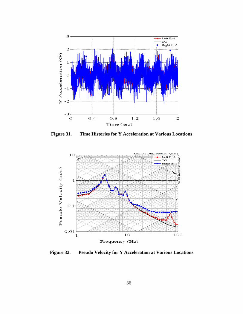
Figure 31. Time Histories for Y Acceleration at Various Locations

Figure 32. Pseudo Velocity for Y Acceleration at Various Locations

36

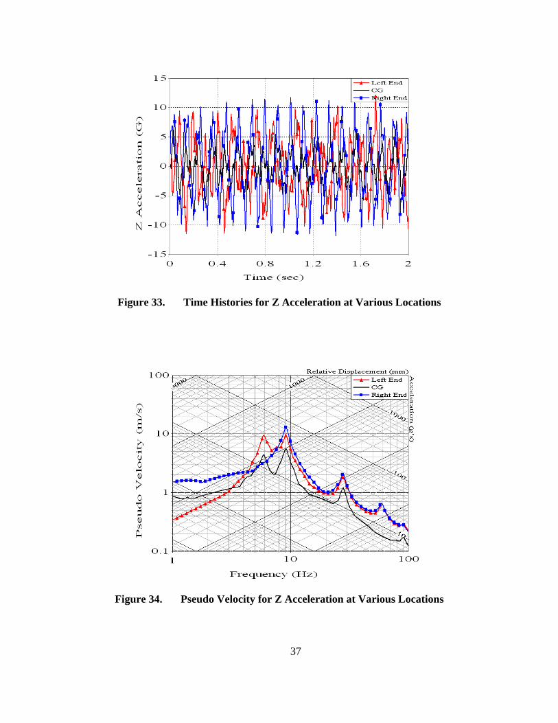
Figure 33. Time Histories for Z Acceleration at Various Locations

Figure 34. Pseudo Velocity for Z Acceleration at Various Locations

37

Figure 35 shows the vertical displacement (Z) of the isolators. The displacement

at the right end is greater than that of the left end because the rotation drop is performed

at the right position. Maximum vertical displacement (Z) of right isolator is 22.4mm,

16.2mm in the left isolator and only 9.4mm in the longitudinal isolator (Y).

Time (sec)

Z D

isp

lacem

en

t (m

m)

-30

-20

-10

0

10

20

30

0 0.4 0.8 1.2 1.6 2

Right MountLeft Mount

Figure 35. Displacement of a Shock Mount

38

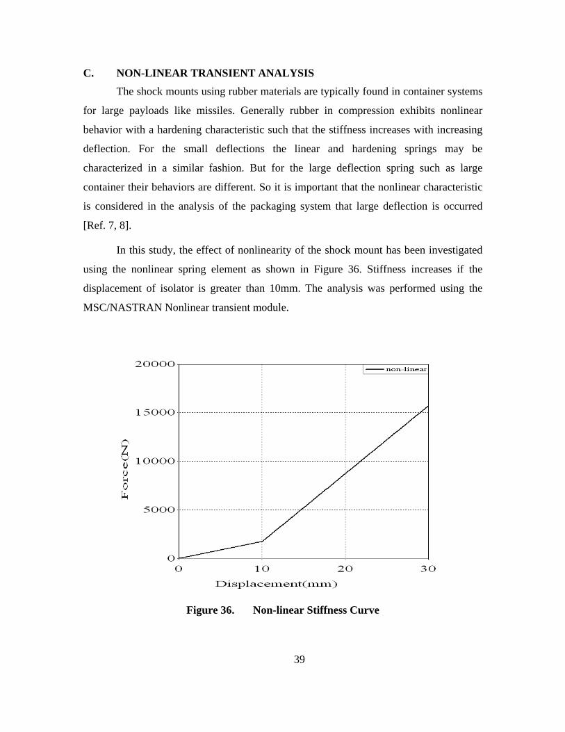
C. NON-LINEAR TRANSIENT ANALYSIS The shock mounts using rubber materials are typically found in container systems

for large payloads like missiles. Generally rubber in compression exhibits nonlinear

behavior with a hardening characteristic such that the stiffness increases with increasing

deflection. For the small deflections the linear and hardening springs may be

characterized in a similar fashion. But for the large deflection spring such as large

container their behaviors are different. So it is important that the nonlinear characteristic

is considered in the analysis of the packaging system that large deflection is occurred

[Ref. 7, 8].

In this study, the effect of nonlinearity of the shock mount has been investigated

using the nonlinear spring element as shown in Figure 36. Stiffness increases if the

displacement of isolator is greater than 10mm. The analysis was performed using the

MSC/NASTRAN Nonlinear transient module.

Figure 36. Non-linear Stiffness Curve

39

Figure 37 shows the displacement of the isolator for the nonlinear model

compared to the results for the linear model. The displacement decreases in the nonlinear

model.

Figure 38 shows the time history of the payload at the center of gravity. The

acceleration level of the payload increased greatly in the nonlinear model.

Figure 39 shows the SRS of the payload at the center of gravity. In this figure, the

response of the rigid body mode has changed from point a (9.17Hz, 32g) into point a’

(11.2Hz, 40g) and the response of the first bending mode has changed from point b

(27.9Hz, 21g) into point b’ (29.4Hz, 90g). The change in the acceleration of the bending

mode is greater than that of the rigid body mode. It shows that the nonlinearity should be

considered when the packaging system for this type of long and flexible payload is

designed.

Figure 37. Displacement of Non-linear Shock Mounts

40

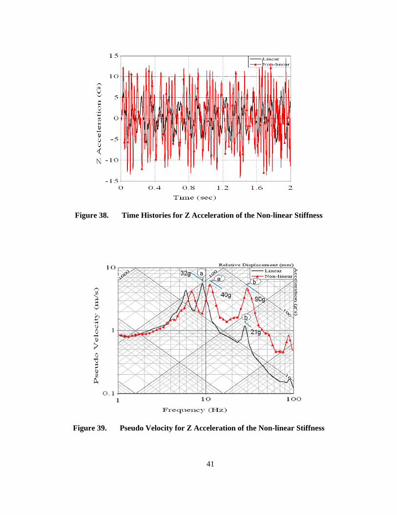
Figure 38. Time Histories for Z Acceleration of the Non-linear Stiffness

Figure 39. Pseudo Velocity for Z Acceleration of the Non-linear Stiffness

41

D. COMPARISON BETWEEN RESPONSES AND SPECIFICATION

The acceleration of the center of gravity of the payload is compared with the

shock test specification, MIL-STD-810. The terminal peak saw tooth shock pulse shown

in Figure 4 is recommended for use in the testing. The peak acceleration magnitude of

the saw tooth pulse is 20g and its duration is 11ms, as is used in flight vehicle equipment

testing.

Figure 40 shows the comparison of the pseudo velocity of the payload with the

shock test specifications. The response in Z direction is higher than the one in Y direction.

Both of the responses are higher than the specification standards in the low frequency

range. As shown in the figure, the ranges that the responses exceed the specification are

below 6.1Hz in Y direction and below 14.1Hz and between 26.3Hz and 29.8Hz in Z

direction. It should be further investigated if there are natural frequencies of the

equipment that fall in the frequency range that the responses exceed the specification.

Figure 40. Comparison of SRS Responses and Specification

42

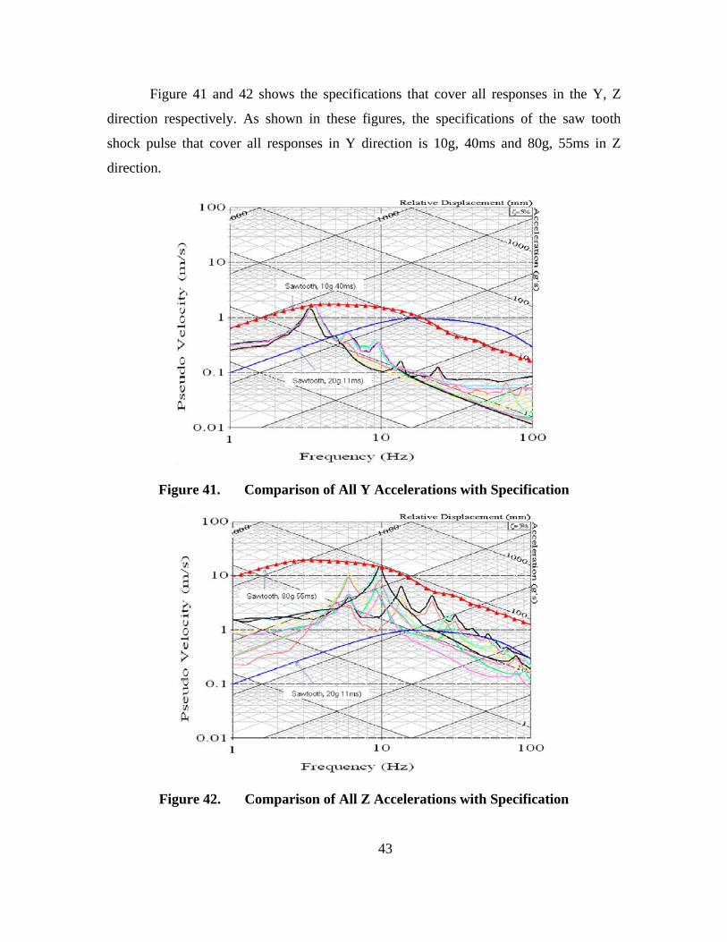
Figure 41 and 42 shows the specifications that cover all responses in the Y, Z

direction respectively. As shown in these figures, the specifications of the saw tooth

shock pulse that cover all responses in Y direction is 10g, 40ms and 80g, 55ms in Z

direction.

Figure 41. Comparison of All Y Accelerations with Specification

Figure 42. Comparison of All Z Accelerations with Specification

43

44

V. CONCLUSION

Damage Boundary Theory and Shock Response Spectrum Analysis have been

investigated to evaluate the shock fragility of equipment. Computer simulation using

MSC/NASTRAN have been performed to illustrate the shock design procedure of a

packaging system. It is necessary that establish the shock fragility of equipment and

design the shock isolation system to mitigate the shock environment loading upon the

equipment. The Damage Boundary Test is an effective method in establishing the shock

fragility level of the equipment itself, while the Shock Response Spectrum Analysis is

useful in understanding the isolation level of packaging system.

The finite element modeling and subsequent computer simulations conducted for

the rotational drop model have shown the effects of flexibility of the payload and the

nonlinearity of the isolator. The results show that the close natural frequency between the

rigid body mode of isolator and the bending mode of payload can increase the shock

response of the payload. Furthermore, due to the nonlinearity of the isolator, the stiffness

of isolator increases with increasing deflection, so the acceleration increases while the

displacement of isolator decreases.

The results of simulation for the rotational drop have been compared with shock

test specification, MIL-STD-810. The results of the simulation were found to be higher

than the specification in the low frequency range.

45

THIS PAGE INTENTIONALLY LEFT BLANK

46

LIST OF REFERENCES

1. R. D. Kelly and G. Richman, “Principles and Techniques of Shock Data Analysis”, The Shock and Vibration Information Center, 1969.

2. Signalysis.com, “Shock Response Spectrum Analysis” 3. American National Standard Institute, Inc., “Shock Test Requirements for Equipment

in a Rugged Shock Environment”, 2007. 4. Robert E. Newton, “Fragility Assessment Theory and Test Procedure”, Monterey

Research Laboratory, Inc., 1968. 5. MIL-STD-810G Method 516.6, “Shock” in Environmental Engineering Considerations

and Laboratory Tests, 2008. 6. ASTM D 3332-99, “Standard Test Methods for Mechanical-Shock Fragility of

Products, Using Shock Machines”, ASTM International, 2004. 7. Herbert H. Schueneman, “Fragility Assessment: An In-Depth Look at A Now Familiar

Process”, Westpak, Inc. 8. Herbert H. Schueneman, “Product Fragility Analysis Made Easy”, Westpak, Inc. 9. H. Himelblau and S. Rubin, “Vibration of a Resiliently Supported Rigid Body”, in

Shock and Vibration Handbook, 4th ed., McGraw-Hill, 1996 10. Michael A. Talley and Shahram Sarkani, “A New Simulation Method Providing

Shock Mount Selection Assurance”, Shock and Vibration 10, 2003, pp.231-267. 11. C. M. Harris, “Shock and Vibration Handbook, 4th ed”, McGraw-Hill, 1996 12. D. H. Merkle, M. A. Rochefort and C. Y. Tuan, “Equipment Shock Tolerance”, AD-

A279689, Engineering Research Division of Air Force Civil Engineering Support Agency, 1993.

13. MSC Software Corporation, “MSC/PATRAN User’s Manual”, Los Angeles, CA,

2008 14. MSC Software Corporation, “MSC/NASTRAN User’s Manual”, Los Angeles, CA,

2008

47

THIS PAGE INTENTIONALLY LEFT BLANK

48

INITIAL DISTRIBUTION LIST

1. Defense Technical Information Center Ft. Belvoir, Virginia

2. Dudley Knox Library Naval Postgraduate School Monterey, California

3. Naval/Mechanical Engineering Curriculum Code 73

Naval Postgraduate School Monterey, California

4. Visiting Professor Beomsoo Lim Department of Mechanical And Astronautical Engineering Naval Postgraduate School Monterey, California

5. Research Assistant Professor Jarema M. Didoszak Department of Mechanical and Astronautical Engineering Naval Postgraduate School Monterey, California

6. Distinguished Professor Emeritus Young S. Shin

Department of Mechanical and Astronautical Engineering Naval Postgraduate School Monterey, California

7. Professor Young W. Kwon

Department of Mechanical and Astronautical Engineering Naval Postgraduate School Monterey, California