


Bahasa
Halaman
Hukum

Monitoring the Cray XC30 Power Management
Hardware Counters
Michael Bareford, EPCC
Version 1.5, January 12, 2015
2 Monitoring Cray XC30 PM Counters
1. Introduction
This document is concerned with how to record and analyse the data provided by the
power monitoring hardware counters on ARCHER, a Cray XC30 platform. Basic de-
scriptions of these counters can be obtained by running papi_native_avail on the
compute nodes of the host system using the aprun command.
There are two groups of power monitoring counters, running average power limit
(RAPL) and power management (PM), see the following two tables.
Table 1: Running average power limit counters
Name Description Units
UNITS:POWER Scaling factor for power (3) n/a
UNITS:ENERGY Scaling factor for energy (16) n/a
UNITS:TIME Scaling factor for time (10) n/a
THERMAL SPEC Thermal specification (130) W
MINIMUM POWER Minimum power (64) W
MAXIMUM POWER Maximum power (200) W
MAXIMUM TIME WINDOW Maximum time window (0.046) s
PACKAGE ENERGY Energy used by chip package nJ
DRAM ENERGY Energy used by package DRAM nJ
PP0 ENERGY Power-plane zero package energy nJ
The counters have a time resolution of 100 ms [4]. The term package relates to the
compute node processor: each node has two 12-core processors and therefore two pack-
ages. This means there is one set of RAPL counters per socket, whereas for PM coun-
ters, there is one set per node (or per two sockets). The PP0 package energy counter
value is a summation of the energy used by all the cores (including processor caches)
within a package [6]. Note, several of the hardware counters are by definition fixed (e.g.,
UNITS:POWER) and so only ever have one value, which is given in brackets at the end
Monitoring Cray XC30 PM Counters 3
Table 2: Power management counters
Name Description Units
PM POWER CAP:NODE Compute node power cap W
PM POWER:NODE Compute node point-in-time power W
PM ENERGY:NODE Compute node accumulated energy J
PM POWER CAP:ACC Accelerator power cap W
PM POWER:ACC Accelerator point-in-time power W
PM ENERGY:ACC Accelerator accumulated energy J
PM FRESHNESS Number of times HSS has updated data structure n/a
PM GENERATION Number of times a power cap change was made n/a
PM STARTUP Timestamp of the last startup cycles
PM VERSION Version of sysfs directory tree n/a
of the counter description.
Two molecular modelling codes (DL POLY v4.05 and CP2K v2.6.14482) are used to
show how to access power management data for simulation jobs that run over multiple
compute nodes. The former application achieves parallelism through MPI exclusively,
and can be built for all three programming environments available on ARCHER (Cray,
Intel and gnu). We would expect that the choice of compiler should not impact energy
use, nevertheless this paper will confirm whether this is indeed the case. The second
code, CP2K, will be run in a mixed OpenMP/MPI mode (using the gnu environment):
this provides a more useful case as we explore whether or not adding more threads raises
or lowers the energy use.
4 Monitoring Cray XC30 PM Counters
2. CrayPat
We begin with the Cray Performance and Analysis Tool (CrayPat) as the most straightfor-
ward way to obtain power management data. This tool requires that the application code
is instrumented before it is submitted to the job launcher. Before the code is compiled the
perftools software module must be loaded.
module load perftools
Then, after compilation, the application executable is instrumented by the pat_build
command.
pat_build DLPOLY.Z
This produces a new executable with a +pat suffix. It is this instrumented program that is
launched via the aprun command and controlled according to various properties supplied
by the job submission script, an excerpt of which follows.
module load perftools
export PAT_RT_SUMMARY=1
export PAT_RT_PERFCTR=UNITS:POWER,UNITS:ENERGY,UNITS:TIME, /
THERMAL_SPEC,MINIMUM_POWER,MAXIMUM_POWER,MAXIMUM_TIME_WINDOW, /
PACKAGE_ENERGY,PP0_ENERGY,DRAM_ENERGY, /
PM_POWER_CAP:NODE,PM_POWER:NODE,PM_ENERGY:NODE, /
PM_FRESHNESS,PM_GENERATION,PM_STARTUP,PM_VERSION
export OMP_NUM_THREADS=1
aprun -n 96 ./DLPOLY.Z+pat >& stdouterr
Monitoring Cray XC30 PM Counters 5
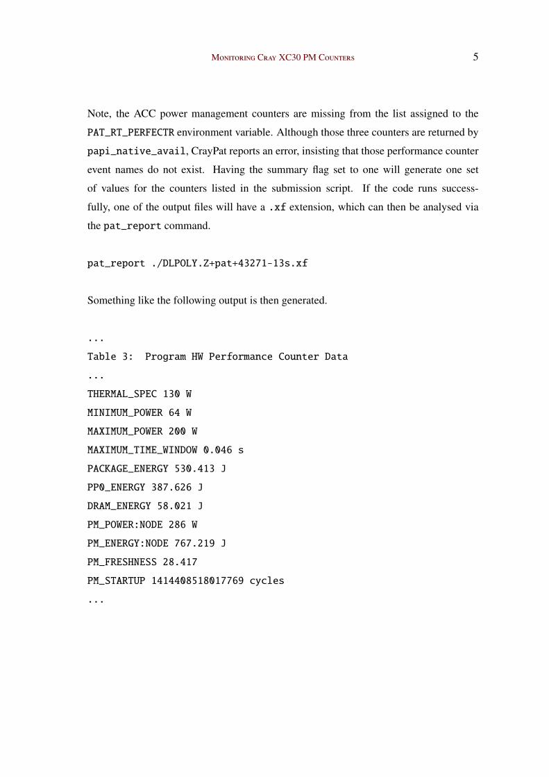
Note, the ACC power management counters are missing from the list assigned to the
PAT_RT_PERFECTR environment variable. Although those three counters are returned by
papi_native_avail, CrayPat reports an error, insisting that those performance counter
event names do not exist. Having the summary flag set to one will generate one set
of values for the counters listed in the submission script. If the code runs success-
fully, one of the output files will have a .xf extension, which can then be analysed via
the pat_report command.
pat_report ./DLPOLY.Z+pat+43271-13s.xf
Something like the following output is then generated.
...
Table 3: Program HW Performance Counter Data
...
THERMAL_SPEC 130 W
MINIMUM_POWER 64 W
MAXIMUM_POWER 200 W
MAXIMUM_TIME_WINDOW 0.046 s
PACKAGE_ENERGY 530.413 J
PP0_ENERGY 387.626 J
DRAM_ENERGY 58.021 J
PM_POWER:NODE 286 W
PM_ENERGY:NODE 767.219 J
PM_FRESHNESS 28.417
PM_STARTUP 1414408518017769 cycles
...
6 Monitoring Cray XC30 PM Counters
In the previous example, the DL POLY code was run over four nodes, and so, by
default the energies are averages, whereas the powers (also by default) are maximum val-
ues: e.g., PACKAGE ENERGY is the average energy used by the eight processors, and
PM POWER:NODE is the maximum point-in-time power recorded (for one node) during
the execution run. The pat_report tool has the flexibility to accept different aggrega-
tions [4].
Unfortunately, it doesn’t seem possible to record multiple counter readings during ex-
ecution on a per node basis. A CrayPat sampling job is specified by using the -S option
with the pat_build command and by adding two extra options to the job script, see be-
low.
export PAT_RT_EXPERIMENT=samp_pc_time
export PAT_RT_INTERVAL=1000
The interval is in microseconds. This setup does not generate a set of sampling data
that could be used to investigate how energy use varies throughout the run; the only data
generated specific to the selected counters appears to be in aggregate form only.
3. PM MPI Library
Hart et al. [3] have provided a library that allows one to monitor the power manage-
ment (hereafter PM) counters directly. This library, pm lib, accesses the actual counter
files, located at /sys/cray/pm_counters. There are five counters available, instanta-
neous power and cumulative energy for normal nodes and for accelerated nodes — these
measurements cover CPU, memory and any other hardware contained on the processor
daughter card; any consumption due to the Aries network controllers and beyond is ex-
cluded however. The fifth counter is the freshness counter, which should always be read
before reading the other counters. After a set of readings have been taken, the freshness
counter is read again and if the value is unchanged, we know we have a consistent set
of measurements: i.e., the power and energy were taken at the same time. The counters
Monitoring Cray XC30 PM Counters 7
have a temporal resolution of 100 ms. The library can be linked with Fortran and C/C++
programs: however, for codes running on several multi-core nodes it is necessary to ex-
tend the library in two significant ways. First, only one MPI process per node must use
pm lib to access the PM counters on that node; and second, only one MPI process (e.g.,
rank 0) should collate the data, writing it to a single file.
The result of these extensions is a new library called pm mpi lib, which has an inter-
face featuring just three functions, defined in Appendix A. When instrumenting a code
for the first time, the area of interest is the main loop that controls how the simulation pro-
gresses. For DL POLY, this is the loop at the start of the ./VV/w_md_v.f90 source file,
which can be instrumented as follows. A call to the pm mpi lib function, pm_mpi_open,
should be placed immediately before the loop. This function establishes the MPI rank of
the calling process and then obtains the unique number of the node on which the process
is running via MPI_Get_processor_name. The node number is then used to split the
MPI_COMM_WORLD communicator: i.e., the node number is used as the colour of the sub-
communicator, which is effectively a communicator for all processes on the same node.
Thus, an appropriate MPI_Allreduce can be used to determine which process has the
lowest numerical rank value on any given node, thereby choosing the process that will
monitor the PM counters. All such monitoring processes (one per node) then go on to
create another sub-communicator, one that unites them all, which allows rank 0 to deter-
mine the number of monitors. In addition to these tasks, the monitoring processes open
their respective PM counter files; rank 0 also gets the current MPI time.
The second pm mpi lib function call, pm_mpi_monitor, can be placed at various
points within the application loop. As the name suggests, this function allows all mon-
itoring processes to read the PM counters; for all other processes, no read is performed
and the holding variables are set to zero. A subsequent MPI_Allreduce can then be used
to sum the counter values over all nodes; thus the total cumulative energy can be ob-
tained. For the point-in-time power counters however, the sum is divided by the number
of monitoring processes in order to calculate an average. Rank 0 then writes this data to
the output file, see Appendix A for a description of the output format.
Finally, the third and last call, pm_mpi_close, is placed immediately outside the main
8 Monitoring Cray XC30 PM Counters
application loop: this call ensures that each monitoring process closes its PM counter files
and that rank 0 also closes the output file.
4. Results
The three functions of the pm mpi lib library have been used to instrument the DL POLY
and CP2K codes mentioned earlier, such that the PM counters for cumulative energy and
point-in-time power are read for each node (four for DL POLY and eight for CP2K). The
data is then collated and output as a total energy and as an average power for each time
step of the simulation.
4.1. Compiler Dependence
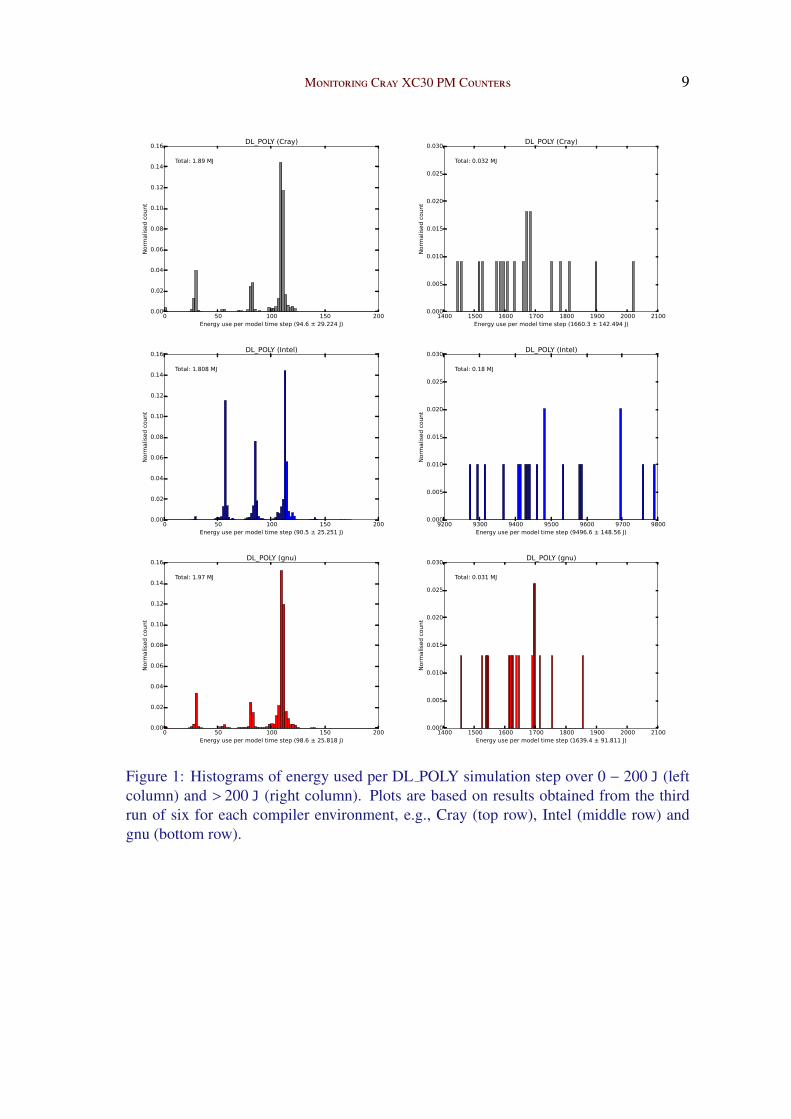
Figure 1 shows histograms of energy use per simulation step, defined as one iteration of
the loop at the start of the DL POLY source file, ./VV/w_md_v.f90. There are three sets
of histograms, one for each compiler environment: grey represents the Cray compiler,
blue is Intel and red is gnu. For each run, the number of nodes assigned (4) and the input
data set were the same: the latter was taken from the standard DL POLY test case 40
(ionic liquid dimethylimidazolium chloride), see Section 8.1 of the user manual [5]. Fur-
thermore, the molecular simulation defined by the test case was extended by increasing
the value of the steps parameter in the CONTROL file from 750 to 20 000.
The histograms do not correspond with a single normal distribution: in general, there
is one main peak and two minor ones appearing at lower energies, see Figure 1 (left col-
umn). In addition, there are high-energy simulation steps that occur every one thousand
iterations (right column): this is how often the DL_POLY restart files are written to disk.
The same DL POLY job was run six times for each compiler environment and an average
performance was calculated in order to tease out any compiler dependence. Repeatedly
running exactly the same executable with the same input data will produce some varia-
tion in energy usage: however, we expect this variation to be mitigated by the fact that
all jobs were run on the ARCHER test development server, where resource contention is
minimal.
Monitoring Cray XC30 PM Counters 9
0 50 100 150 200Energy use per model time step (94.6 ± 29.224 J)
0.00
0.02
0.04
0.06
0.08
0.10
0.12
0.14
0.16Normalised count
Total: 1.89 MJ
DL_POLY (Cray)
1400 1500 1600 1700 1800 1900 2000 2100Energy use per model time step (1660.3 ± 142.494 J)
0.000
0.005
0.010
0.015
0.020
0.025
0.030
No
rma
lise
d c
ou
nt
Total: 0.032 MJ
DL_POLY (Cray)
0 50 100 150 200Energy use per model time step (90.5 ± 25.251 J)
0.00
0.02
0.04
0.06
0.08
0.10
0.12
0.14
0.16
Normalised count
Total: 1.808 MJ
DL_POLY (Intel)
9200 9300 9400 9500 9600 9700 9800Energy use per model time step (9496.6 ± 148.56 J)
0.000
0.005
0.010
0.015
0.020
0.025
0.030
No
rma
lise
d c
ou
nt
Total: 0.18 MJ
DL_POLY (Intel)
0 50 100 150 200Energy use per model time step (98.6 ± 25.818 J)
0.00
0.02
0.04
0.06
0.08
0.10
0.12
0.14
0.16
Normalised count
Total: 1.97 MJ
DL_POLY (gnu)
1400 1500 1600 1700 1800 1900 2000 2100Energy use per model time step (1639.4 ± 91.811 J)
0.000
0.005
0.010
0.015
0.020
0.025
0.030
No
rma
lise
d c
ou
nt
Total: 0.031 MJ
DL_POLY (gnu)
Figure 1: Histograms of energy used per DL POLY simulation step over 0 − 200 J (leftcolumn) and > 200 J (right column). Plots are based on results obtained from the thirdrun of six for each compiler environment, e.g., Cray (top row), Intel (middle row) andgnu (bottom row).

10 Monitoring Cray XC30 PM Counters
The Cray-compiled code had the lowest energy usage (1.92 ± 0.02 MJ over 1748 ±
2.6 s), followed by the Intel-compiled code (1.97 ± 0.01 MJ over 1770 ± 2.7 s), and
lastly, the gnu-compiled code (2 ± 0.02 MJ over 1823 ± 2 s). The Cray energy usage
is approximately 3% lower (1.92/1.97≈ 0.97) than the Intel result and 4% lower than
the mean result for the gnu runs. Unsurprisingly, energy usage follows execution time.
However, the Intel runs show a marked difference as regards the high-energy iterations:
for the Cray and gnu runs, these high-energy iterations are a factor of sixteen higher
than the energy used for 99.9% of the simulation steps, whereas for the Intel runs, this
factor increases to around ninety-five. Note, the Intel-compiled code would be the most
energy efficient, if the total for the high-energy iterations (0.18 MJ) was reduced such
that it matched the high-energy totals achieved by the Cray and gnu runs: in fact, this
hypothetical reduction would make the Intel runs the most efficient (∼ 5% lower than the
Cray energy usage).
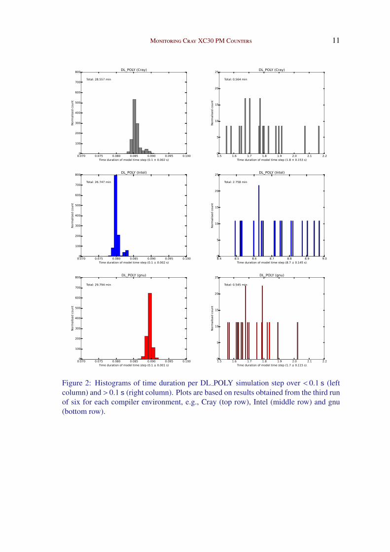
In order to understand more fully the impact of execution times on energy consump-
tion, we show the distributions of execution times per simulation step (Figure 2) for the
same runs as those featured in Figure 1. Again, the distributions are divided into two
groups, short iterations (left column) and long iterations (right column) occurring every
1000 simulation steps (i.e., the restart dumps). The high energy steps consume more en-
ergy because those iterations take longer to execute; also, the Intel high-energy iterations
run for the longest (by almost an order of magnitude).
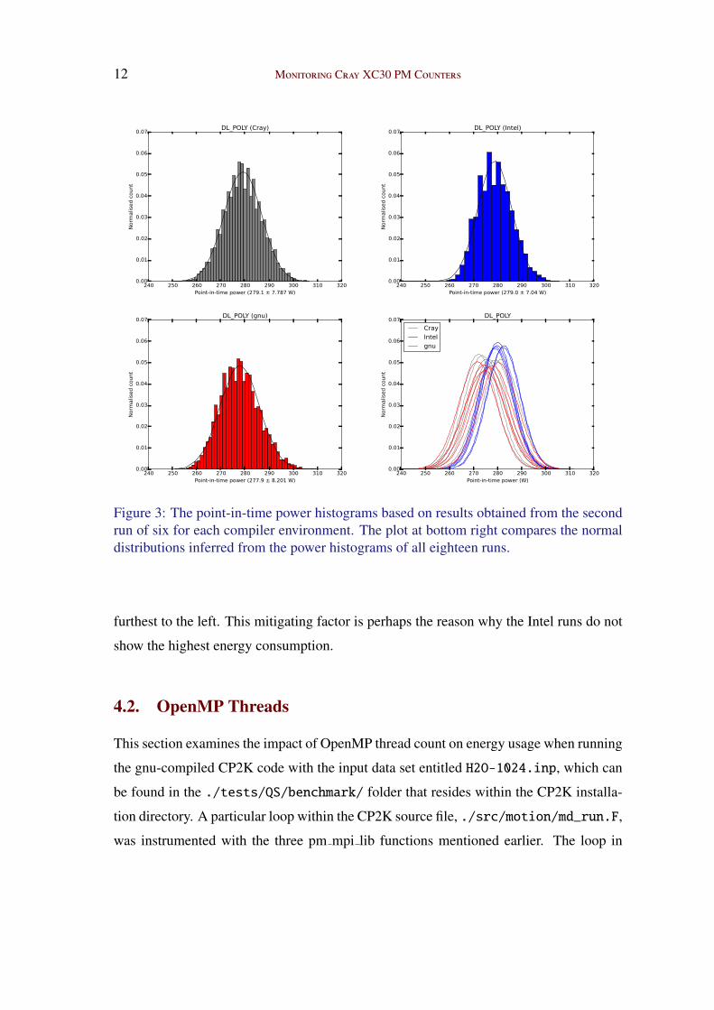
Figure 3 presents example point-in-time power histograms. Unlike the cumulative
energy results, these histograms correspond with a single normal distribution, giving a
meaningful average and deviation, see the x-axis labels. Hence, the normal distributions
inferred by the power histograms for all eighteen runs are also given in the bottom right
plot. The Cray and gnu compiled codes have similar distributions as regards power mea-
surements: therefore, the difference in energy usage for these two codes can be attributed
to execution time. Overall, the Intel runs show the highest mean power and we also know
that the high-energy iterations for the Intel runs are the most time consuming. Neverthe-
less, the Intel energy usage is mitigated by the fact that the majority low-energy iterations
execute the fastest on average: in the left column of Figure 2, the Intel distribution is
Monitoring Cray XC30 PM Counters 11
0.070 0.075 0.080 0.085 0.090 0.095 0.100Time duration of model time step (0.1 ± 0.002 s)
0
100
200
300
400
500
600
700
800Norm
alised count
Total: 28.557 min
DL_POLY (Cray)
1.5 1.6 1.7 1.8 1.9 2.0 2.1 2.2Time duration of model time step (1.8 ± 0.153 s)
0
5
10
15
20
25
Norm
alised count
Total: 0.564 min
DL_POLY (Cray)
0.070 0.075 0.080 0.085 0.090 0.095 0.100Time duration of model time step (0.1 ± 0.002 s)
0
100
200
300
400
500
600
700
800
Norm
alised count
Total: 26.747 min
DL_POLY (Intel)
8.4 8.5 8.6 8.7 8.8 8.9 9.0Time duration of model time step (8.7 ± 0.145 s)
0
5
10
15
20
25
Norm
alised count
Total: 2.758 min
DL_POLY (Intel)
0.070 0.075 0.080 0.085 0.090 0.095 0.100Time duration of model time step (0.1 ± 0.001 s)
0
100
200
300
400
500
600
700
800
Norm
alised count
Total: 29.794 min
DL_POLY (gnu)
1.5 1.6 1.7 1.8 1.9 2.0 2.1 2.2Time duration of model time step (1.7 ± 0.115 s)
0
5
10
15
20
25
Norm
alised count
Total: 0.545 min
DL_POLY (gnu)
Figure 2: Histograms of time duration per DL POLY simulation step over < 0.1 s (leftcolumn) and > 0.1 s (right column). Plots are based on results obtained from the third runof six for each compiler environment, e.g., Cray (top row), Intel (middle row) and gnu(bottom row).
12 Monitoring Cray XC30 PM Counters
240 250 260 270 280 290 300 310 320Point-in-time power (279.1 ± 7.787 W)
0.00
0.01
0.02
0.03
0.04
0.05
0.06
0.07Norm
alised count
DL_POLY (Cray)
240 250 260 270 280 290 300 310 320Point-in-time power (279.0 ± 7.04 W)
0.00
0.01
0.02
0.03
0.04
0.05
0.06
0.07
Norm
alised count
DL_POLY (Intel)
240 250 260 270 280 290 300 310 320Point-in-time power (277.9 ± 8.201 W)
0.00
0.01
0.02
0.03
0.04
0.05
0.06
0.07
Norm
alised count
DL_POLY (gnu)
240 250 260 270 280 290 300 310 320Point-in-time power (W)
0.00
0.01
0.02
0.03
0.04
0.05
0.06
0.07
Normalised count
DL_POLY
CrayIntelgnu
Figure 3: The point-in-time power histograms based on results obtained from the secondrun of six for each compiler environment. The plot at bottom right compares the normaldistributions inferred from the power histograms of all eighteen runs.
furthest to the left. This mitigating factor is perhaps the reason why the Intel runs do not
show the highest energy consumption.
4.2. OpenMP Threads
This section examines the impact of OpenMP thread count on energy usage when running
the gnu-compiled CP2K code with the input data set entitled H2O-1024.inp, which can
be found in the ./tests/QS/benchmark/ folder that resides within the CP2K installa-
tion directory. A particular loop within the CP2K source file, ./src/motion/md_run.F,
was instrumented with the three pm mpi lib functions mentioned earlier. The loop in
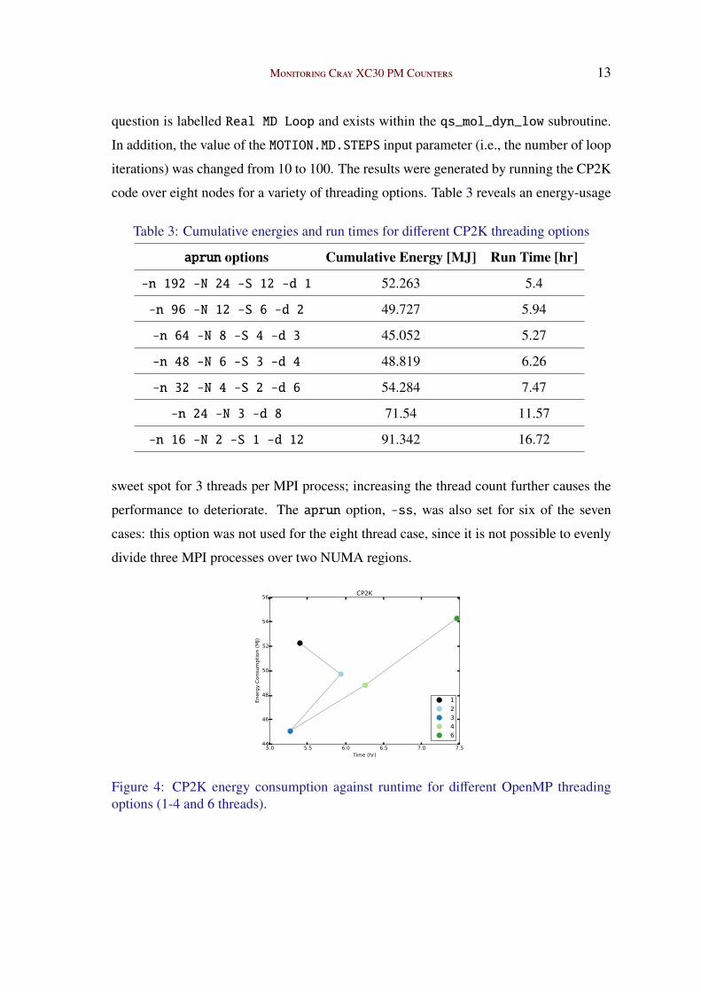
Monitoring Cray XC30 PM Counters 13
question is labelled Real MD Loop and exists within the qs_mol_dyn_low subroutine.
In addition, the value of the MOTION.MD.STEPS input parameter (i.e., the number of loop
iterations) was changed from 10 to 100. The results were generated by running the CP2K
code over eight nodes for a variety of threading options. Table 3 reveals an energy-usage
Table 3: Cumulative energies and run times for different CP2K threading options
aprun options Cumulative Energy [MJ] Run Time [hr]
-n 192 -N 24 -S 12 -d 1 52.263 5.4
-n 96 -N 12 -S 6 -d 2 49.727 5.94
-n 64 -N 8 -S 4 -d 3 45.052 5.27
-n 48 -N 6 -S 3 -d 4 48.819 6.26
-n 32 -N 4 -S 2 -d 6 54.284 7.47
-n 24 -N 3 -d 8 71.54 11.57
-n 16 -N 2 -S 1 -d 12 91.342 16.72
sweet spot for 3 threads per MPI process; increasing the thread count further causes the
performance to deteriorate. The aprun option, -ss, was also set for six of the seven
cases: this option was not used for the eight thread case, since it is not possible to evenly
divide three MPI processes over two NUMA regions.
5.0 5.5 6.0 6.5 7.0 7.5Time (hr)
44
46
48
50
52
54
56
Energy Consumption (MJ)
CP2K
12346
Figure 4: CP2K energy consumption against runtime for different OpenMP threadingoptions (1-4 and 6 threads).
14 Monitoring Cray XC30 PM Counters
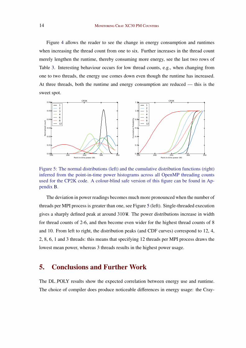
Figure 4 allows the reader to see the change in energy consumption and runtimes
when increasing the thread count from one to six. Further increases in the thread count
merely lengthen the runtime, thereby consuming more energy, see the last two rows of
Table 3. Interesting behaviour occurs for low thread counts, e.g., when changing from
one to two threads, the energy use comes down even though the runtime has increased.
At three threads, both the runtime and energy consumption are reduced — this is the
sweet spot.
150 200 250 300 350Point-in-time power (W)
0.00
0.01
0.02
0.03
0.04
0.05
0.06
Normalised count
CP2K
12346812
150 200 250 300 350Point-in-time power (W)
0.0
0.2
0.4
0.6
0.8
1.0
1.2
Cumulative Probability
CP2K
12346812
Figure 5: The normal distributions (left) and the cumulative distribution functions (right)inferred from the point-in-time power histograms across all OpenMP threading countsused for the CP2K code. A colour-blind safe version of this figure can be found in Ap-pendix B.
The deviation in power readings becomes much more pronounced when the number of
threads per MPI process is greater than one, see Figure 5 (left). Single-threaded execution
gives a sharply defined peak at around 310 W. The power distributions increase in width
for thread counts of 2-6, and then become even wider for the highest thread counts of 8
and 10. From left to right, the distribution peaks (and CDF curves) correspond to 12, 4,
2, 8, 6, 1 and 3 threads: this means that specifying 12 threads per MPI process draws the
lowest mean power, whereas 3 threads results in the highest power usage.
5. Conclusions and Further Work
The DL POLY results show the expected correlation between energy use and runtime.
The choice of compiler does produce noticeable differences in energy usage: the Cray-
Monitoring Cray XC30 PM Counters 15
compiled code uses the least energy, followed by Intel then gnu. However, the results also
show that the evenly-spaced restart write iterations (19 out of 20 000) run for significantly
longer, and furthermore, this disparity is more extreme for the Intel runs. Closer exami-
nation of the data, reveals that the Intel runs would use the least energy, if the compiler
options could be set such that the Intel high-energy iterations had runtimes comparable
with the Cray and gnu results.
Energy use will depend on the number of threads per MPI process: using multiple
threads can reduce runtimes and energy usage but not beyond a certain thread count.
Three threads is the optimum thread count for CP2K running over eight nodes with the
H2O-1024.inp data set. Further work could investigate the importance of node assign-
ment within the ARCHER dragonfly topology [1] as regards energy consumption. For
example, running with three threads per MPI process, one could compare energy usages
for the following scenarios.
1. All eight nodes from the same chassis.
2. Four nodes from one chassis and four nodes from a different chassis.
3. Same as scenario two but involving a chassis from a different group.
The first scenario involves communication within the rank 1 network only, the second
will also feature communication over the rank 2 network, whereas the final scenario will
involve communication over the optical rank 3 network. It is assumed that runtimes
will increase should more communication hops between nodes be required: hence, these
different scenarios should result in different node energies being recorded. The usefulness
of this work would be in understanding the energy cost of communicating via the rank
2 and/or rank 3 networks. This work would of course need to be done on ARCHER
itself as opposed to the test and development server (tds), which comprises only one
group containing two cabinets. Note, the CP2K tests involving thread counts of 4 and 12
were performed on nodes that resided in different cabinets; the other CP2K tests involved
nodes within the same chassis, thereby utilising the rank 1 network only. Regarding the
DL POLY results, 16 out of 18 runs were executed on nodes within the same chassis:
the remaining two runs (one Cray and one gnu) featured a single node in the second tds
cabinet.
16 Monitoring Cray XC30 PM Counters
A PM MPI Library
The source code is held in a Git repository [2] together with a makefile, and two small test
harnesses that demonstrate how to call the library functions from Fortran and C codes.
There is also a test folder containing readme.txt files that explain exactly how to inte-
grate the pm mpi lib source with the DL POLY and CP2K source codes. The following
text describes the interface provided by the three functions of the pm mpi lib library.
1. void pm_mpi_open(char* pmc_out_fn): the parameter, pmc_out_fn, points
to a null-terminated string that specifies the name of the file that will hold the PM
counter data: a NULL parameter will set the output file name to ./PMC. The open
function also calls pm_mpi_monitor(0) in order to determine a baseline for the
cumulative energy. In addition, rank 0 establishes a temporal baseline by calling
MPI_Wtime and also writes a one-line header to the output file, which gives the
library version followed by the names of the data items that will appear in the
subsequent lines.
2. void pm_mpi_monitor(int nstep): the parameter, nstep, allows the client to
label each set of counter values that are output by rank 0. The output file comprises
lines of space-separated fields. A description of each field follows (the C-language
data type is given in square brackets).
Time [double]: the time as measured by MPI_Wtime (called by rank zero) that
has elapsed since the last call to pm_mpi_open.
Step [int]: a simple numerical label: e.g., the iteration count, assuming
pm_mpi_monitor is being called from within a loop.
Point-in-time power [double]: the average power reading across all assigned
compute nodes.
Energy [unsigned long long int]: the energy used by all assigned compute nodes
since the last call to pm_mpi_open.
3. void pm_mpi_close(void): calls pm_mpi_monitor(nstep+1). All counter
files are closed, then rank 0 closes the output file.
Monitoring Cray XC30 PM Counters 17
B Colour-blind Safe Version of Figure 5
150 200 250 300 350Point-in-time power (W)
0.00
0.01
0.02
0.03
0.04
0.05
0.06
Normalised count
CP2K
12346812
150 200 250 300 350Point-in-time power (W)
0.0
0.2
0.4
0.6
0.8
1.0
1.2
Cumulative Probability
CP2K
12346812
Figure 6: The normal distributions (left) and the cumulative distribution functions (right)inferred from the point-in-time power histograms across all OpenMP threading countsused for the CP2K code.
18 Monitoring Cray XC30 PM Counters
References
[1] Bob Alverson, Edwin Froese, Larry Kaplan, and Duncan Roweth. Cray xc series
network. http://www.cray.com/Assets/PDF/products/xc/CrayXC30Networking.pdf,
2012.
[2] Michael R. Bareford, Alastair Hart, and Harvey Richardson. The pm mpi library.
https://github.com/cresta-eu/pm mpi lib, 2014.
[3] Alastair Hart, Harvey Richardson, Jens Doleschal, Thomas Ilsche, Mario Bielert, and
Matthew Kappel. User-level power monitoring and application performance on cray
xc30 supercomputers. Proceedings of CUG2014, 2014.
[4] Cray Inc. Using Cray Performance Measurement and Analysis Tools. Number S-
2376-60. Cray Inc., 2012.
[5] I. T. Todorov and W. Smith. The DL POLY 4 User Manual. STFC Daresbury Labo-
ratory, 2014.
[6] Vincent M. Weaver, Matt Johnson, Kiran Kasichayanula, James Ralph, Piotr
Luszczek, Dan Terpstra, and Shirley Moore. Measuring energy and power with papi.
41st International Conference on Parallel Processing Workshops, pages 262–268,
2012.
Copyright © 2022 FDOKUMEN

