


Bahasa
Halaman
Hukum


MOLECULES ROTATING IN ELECTRIC FIELDS BY
QUANTUM AND SEMI-QUANTUM MECHANICS
A Dissertation
Presented to the Faculty of the Graduate School
of Cornell University
in Partial Fulfillment of the Requirements for the Degree of
Doctor of Philosophy
by
William W. Kennerly
August 2005

c© 2005 William W. Kennerly
ALL RIGHTS RESERVED
MOLECULES ROTATING IN ELECTRIC FIELDS BY QUANTUM AND
SEMI-QUANTUM MECHANICS
William W. Kennerly, Ph.D.
Cornell University 2005
The quantum and semi-quantum mechanics of rigid molecules rotating in static
electric and intense nonresonant laser fields have been studied. Basic quantum fea-
tures including energy level correlation diagrams, eigenfunctions, alignment, orien-
tation, and time-dependent wave functions propagated under pulsed fields are cal-
culated. Energy level nearest neighbor spacing disributions are the primary semi-
quantum approach, but Husimi distributions, periodic orbits, and monodromy
diagrams are also investigated. We have elucidated these facets of the quantum-
classical correspondence in this important rotational model, which is classically
nonscaling with mixed phase space.
BIOGRAPHICAL SKETCH
William W. Kennerly was born in Philadelphia, Pennsylvania, in 1978. He first
attended Penn Christian Academy (Norristown, Pennsylvania) and graduated salu-
tatorian in 1992. He then transferred into the local public system to attend
Plymouth-Whitemarsh High School, from which he graduated in 1996. He was
admitted to Worcester Polytechnic Institute (Worcester, Massachusetts) as a chem-
istry major but spent much time in pure math and physics classes. He won awards
for analytical chemistry research and mathematical modeling in the COMAP com-
petition. He graduated with a B.S. in Chemistry, with distinction, in 2000. He im-
mediately entered the Ph.D. program in the Department of Chemistry and Chem-
ical Biology at Cornell University (Ithaca, New York) and soon started working
with Greg Ezra to obtain fundamental understanding of quantum mechanics. After
two years of teaching introductory chemistry, he won the departmental teaching
assistant award. Later that year he helped persuade the Cornell graduate student
body to not unionize. He earned the M.S. degree at the end of 2002 and finished
his Ph.D. research in the summer of 2005. He then moved to Albany, New York,
to pursue further opportunities.
Kennerly enjoys backpacking and bowling. In the spring of 2005, he was captain
of the Alpha Chi Sigma bowling team, and they did not occupy last place in the
league.
iii
ACKNOWLEDGEMENTS
It is a pleasure to acknowledge the enduring patience of Greg Ezra, who has ex-
plained group theory to me many times, among other mathematical and physical
topics. Also, Carlos Arango has been very helpful by providing results correspond-
ing to the present work but entirely within classical and semi-classical mechanics.
Finally, Ben Widom and Paul Houston served well on my committee, making sure
I knew something about avoided crossings and the supersonic nozzle (respectively).
The department of Chemistry and Chemical Biology has been a wonderful host,
providing funding and a great research community.
iv
TABLE OF CONTENTS
1 Elements of the Tilted Field Problem by Quantum Mechanics 11.1 Motivation . . . . . . . . . . . . . . . . . . . . . . . . . . . . . . . . 11.2 Kinetic Energy . . . . . . . . . . . . . . . . . . . . . . . . . . . . . 31.3 Potential Energy . . . . . . . . . . . . . . . . . . . . . . . . . . . . 61.4 Dimensionless Units and Practical Conversions . . . . . . . . . . . . 121.5 Hamiltonian Symmetry . . . . . . . . . . . . . . . . . . . . . . . . . 161.6 The Potential Energy Surface . . . . . . . . . . . . . . . . . . . . . 171.7 The Hamiltonian Matrix . . . . . . . . . . . . . . . . . . . . . . . . 20
2 Correlation Diagrams and Wave Functions 242.1 Correlation Diagrams: Energy, Alignment, and Orientation . . . . . 242.2 Wave Functions . . . . . . . . . . . . . . . . . . . . . . . . . . . . . 31
3 Quantum Propagation 343.1 Preliminaries . . . . . . . . . . . . . . . . . . . . . . . . . . . . . . 343.2 Static Hamiltonian Propagation . . . . . . . . . . . . . . . . . . . . 373.3 Field-free Alignment . . . . . . . . . . . . . . . . . . . . . . . . . . 38
4 Energy Level Spacing Distributions 454.1 Avoided Crossings and Classical Chaos . . . . . . . . . . . . . . . . 454.2 Definition and History . . . . . . . . . . . . . . . . . . . . . . . . . 474.3 Interpreting Nearest Neighbor Spacing Distributions . . . . . . . . . 514.4 How to Obtain a Nearest Neighbor Spacing Histogram . . . . . . . 534.5 Results . . . . . . . . . . . . . . . . . . . . . . . . . . . . . . . . . . 57
5 Other Semi-Quantum Approaches 635.1 Monodromy . . . . . . . . . . . . . . . . . . . . . . . . . . . . . . . 635.2 Husimi Distributions . . . . . . . . . . . . . . . . . . . . . . . . . . 675.3 Periodic Orbits . . . . . . . . . . . . . . . . . . . . . . . . . . . . . 71
6 Summary and Future Work 73
A Calculating the Basis Functions 77A.1 Spherical Harmonics and Associated Legendre Functions . . . . . . 77A.2 Probability Distributions . . . . . . . . . . . . . . . . . . . . . . . . 82A.3 Symmetric Rotor Eigenstates and Jacobi Polynomials . . . . . . . . 84
B Hamiltonian Matrix Element Derivations 90B.1 Matrix Elements in Spherical Harmonic Basis . . . . . . . . . . . . 90B.2 Symmetrized Spherical Harmonics . . . . . . . . . . . . . . . . . . . 94B.3 Matrix Elements in Symmetric Top Basis . . . . . . . . . . . . . . . 96B.4 Symmetrized Asymmetric Rotor Basis . . . . . . . . . . . . . . . . 101
v
C Propagation Derivations 104C.1 Formal Correspondance of Quantum and Classical Dynamics . . . . 104C.2 Symplectic Integrators . . . . . . . . . . . . . . . . . . . . . . . . . 106C.3 Deriviation of the SI2 Coefficients . . . . . . . . . . . . . . . . . . . 109C.4 Proof that the Integrators are Symplectic . . . . . . . . . . . . . . . 110C.5 Time-dependent Hamiltonians . . . . . . . . . . . . . . . . . . . . . 112C.6 Sudden Approximation for a Short Laser Pulse . . . . . . . . . . . . 114
References 116
vi
LIST OF FIGURES
1.1 Asymmetric rotor iodobenzene with molecular frame definition andour unconventional assignment of rotational constants to the molec-ular axes. . . . . . . . . . . . . . . . . . . . . . . . . . . . . . . . . 5
1.2 Coordinate system for linear rotor in tilted fields. Laser is parallelto lab fixed Z with static field tilted at angle β in the XZ plane.xyz is the molecular frame rotated by Euler angles φ, θ, χ from thelab frame XY Z. . . . . . . . . . . . . . . . . . . . . . . . . . . . . 12
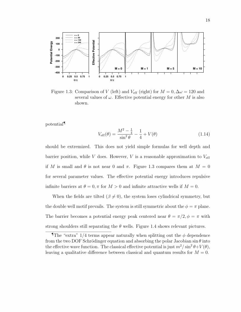
1.3 Comparison of V (left) and Veff (right) for M = 0,∆ω = 120 andseveral values of ω. Effective potential energy for other M is alsoshown. . . . . . . . . . . . . . . . . . . . . . . . . . . . . . . . . . . 18
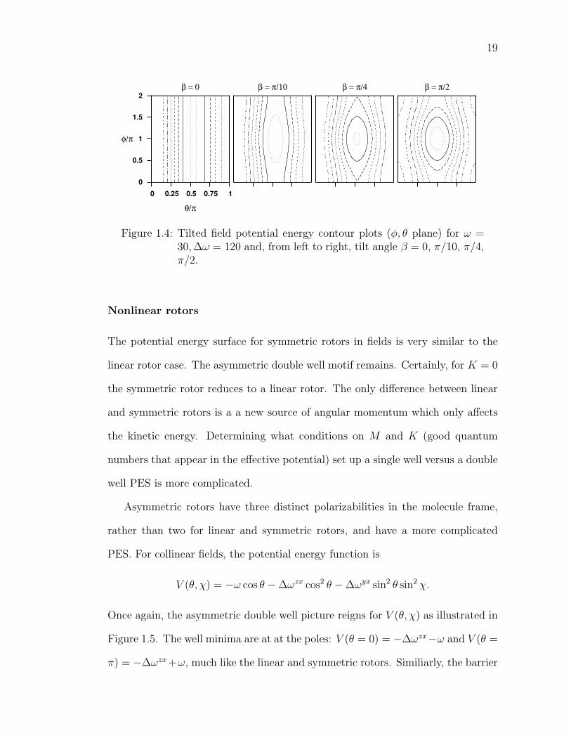
1.4 Tilted field potential energy contour plots (φ, θ plane) for ω =30,∆ω = 120 and, from left to right, tilt angle β = 0, π/10, π/4,π/2. . . . . . . . . . . . . . . . . . . . . . . . . . . . . . . . . . . . 19
1.5 Potential energy surfaces for an asymmetric rotor in collinear fields∆ωzx = 63, ∆ωyx = 28.4 (appropriate for iodobenzene) and ω =0, 5, 20, 40. . . . . . . . . . . . . . . . . . . . . . . . . . . . . . . . 20
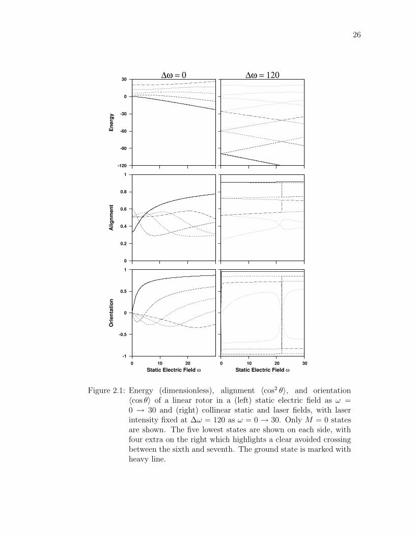
2.1 Energy (dimensionless), alignment 〈cos2 θ〉, and orientation 〈cos θ〉of a linear rotor in a (left) static electric field as ω = 0 → 30 and(right) collinear static and laser fields, with laser intensity fixed at∆ω = 120 as ω = 0 → 30. Only M = 0 states are shown. Thefive lowest states are shown on each side, with four extra on theright which highlights a clear avoided crossing between the sixthand seventh. The ground state is marked with heavy line. . . . . . 26
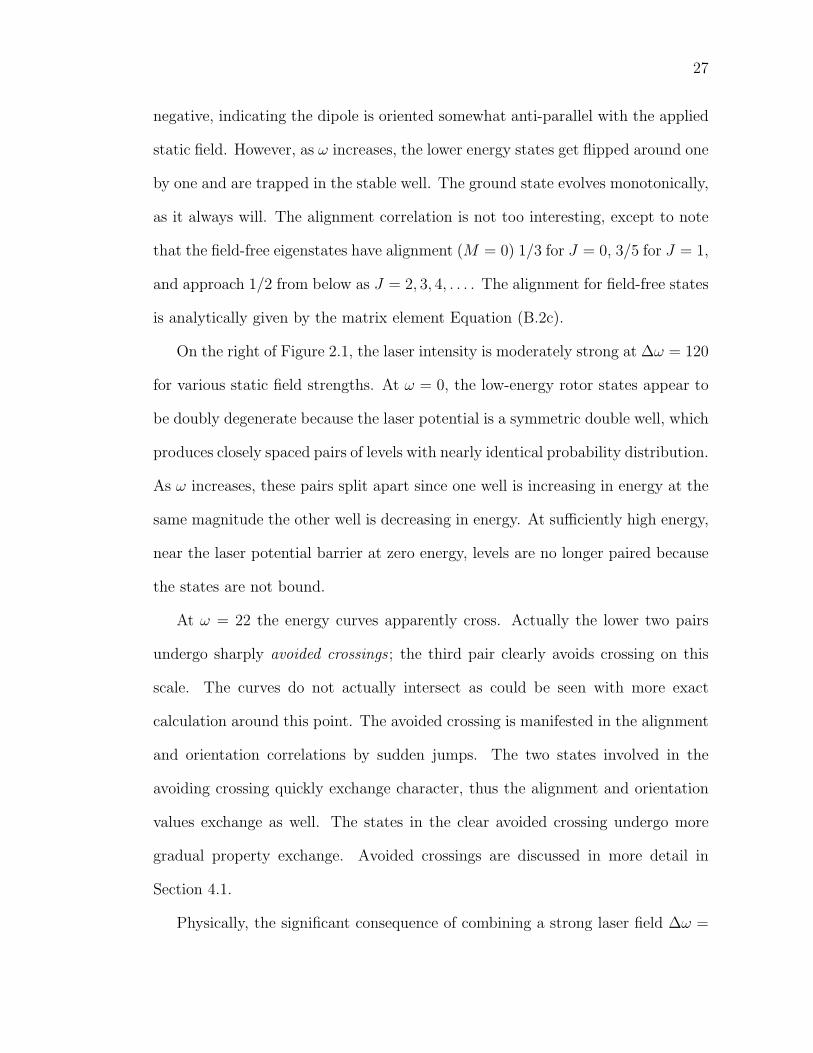
2.2 Energy (dimensionless), alignment, and orientation of a linear rotorin a (left) laser field as ∆ω = 0 → 120 and (right) collinear staticand laser fields, with static field strength fixed at ω = 30 as ∆ω =0 → 120. The eight lowest M = 0 states are shown. The groundstate is marked with heavy line. . . . . . . . . . . . . . . . . . . . 29
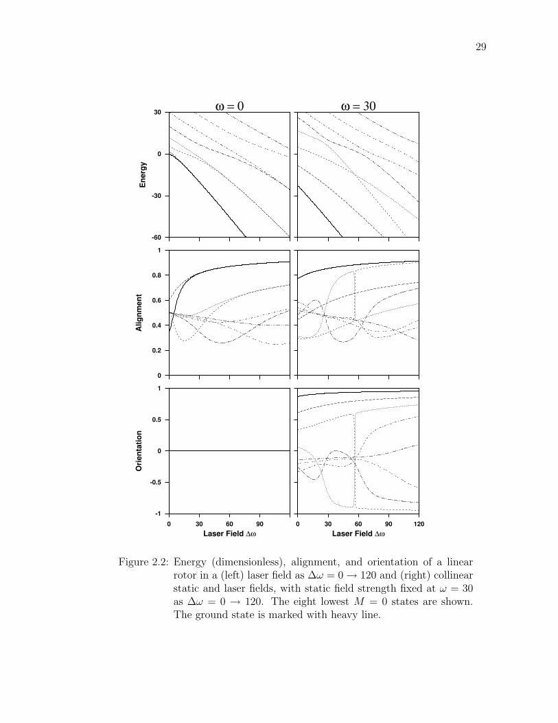
2.3 Energy correlation diagram with tilt angle β, tilting fields ω = 30,∆ω = 120 for parity= +1 linear rotor eigenstates. At left are thelowest eight states; at right about fifteen states at intermediateenergies near barriers. . . . . . . . . . . . . . . . . . . . . . . . . . 30
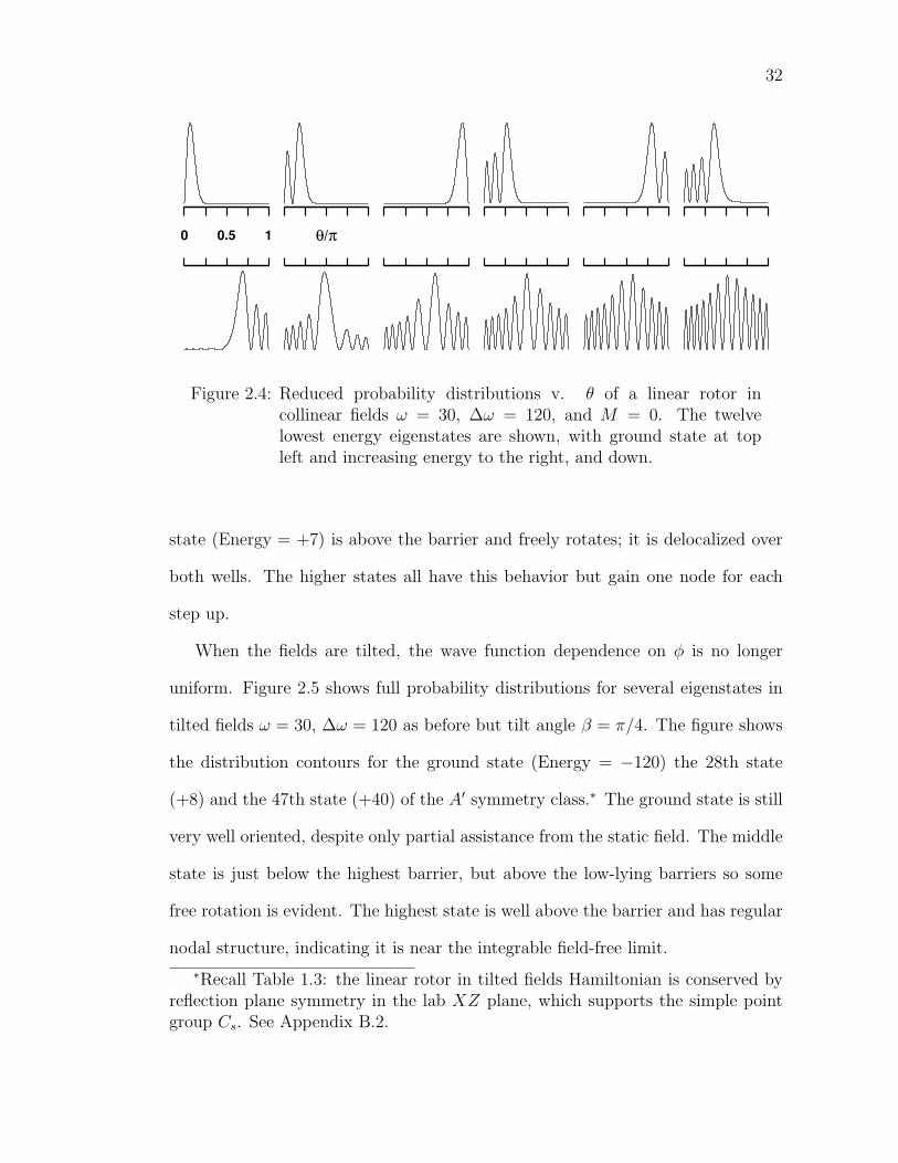
2.4 Reduced probability distributions v. θ of a linear rotor in collinearfields ω = 30, ∆ω = 120, and M = 0. The twelve lowest energyeigenstates are shown, with ground state at top left and increasingenergy to the right, and down. . . . . . . . . . . . . . . . . . . . . 32
vii
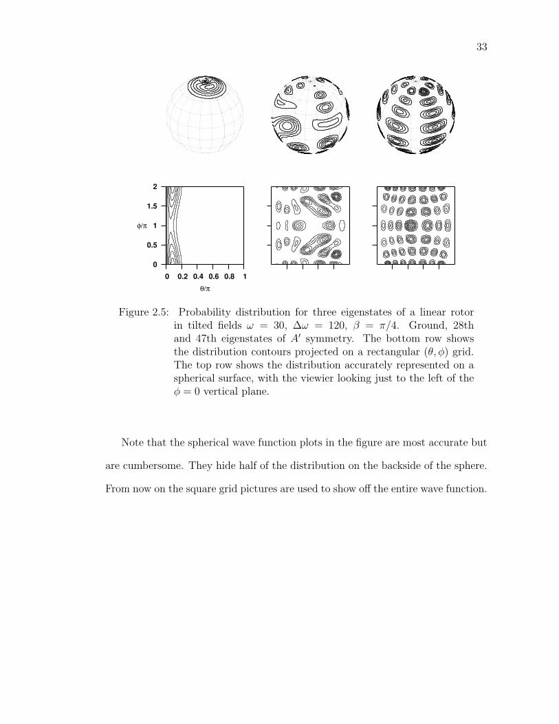
2.5 Probability distribution for three eigenstates of a linear rotor intilted fields ω = 30, ∆ω = 120, β = π/4. Ground, 28th and 47theigenstates of A′ symmetry. The bottom row shows the distributioncontours projected on a rectangular (θ, φ) grid. The top row showsthe distribution accurately represented on a spherical surface, withthe viewier looking just to the left of the φ = 0 vertical plane. . . . 33
3.1 Average angular momentum quantum number 〈J〉 vs dimension-less temperature Y for a linear rotor, as determined by canonicalstatistical mechanics. . . . . . . . . . . . . . . . . . . . . . . . . . . 36
3.2 Time-independent Hamiltonian propagations, linear rotor in fieldsω = 30, (left) ∆ω = 120 and (right) 500 with tilt angle (solid)β = 0, (long dashes) π/4, and (short dashes) π/2. From top tobottom: autocorrelation function (initial state is J = 0 sphericalharmonic, a s orbital), alignment 〈cos2 θ〉, and orientation 〈cos θ〉. . 39
3.3 Alignment (〈cos2 θ〉) of a linear rotor hit with a gaussian laser pulse(width σ, intensity ∆ω = 500) at time τ = 5σ, for increasingwidths in the non-adiabatic (σ = 0.01, 0.02, 0.05), intermediate(σ = 0.15, 0.25, 0.5), and adiabatic (σ = 1, 2, 5) regimes. Initialstate is the isotropic J = 0 spherical harmonic, which has align-ment 1/3. The gaussian laser pulse profile is shown with heavyline. . . . . . . . . . . . . . . . . . . . . . . . . . . . . . . . . . . . 41
3.4 Post-pulse autocorrelation function after a gaussian laser pulse ofintensity ∆ω, for three short pulse widths σ = 0.01, 0.03, 0.05. Ini-tial state is the isotropic J = 0 spherical harmonic. Numericalresults (solid) compared to sudden approximation (dashed). . . . . 42
3.5 Alignment of a linear rotor after a gaussian laser pulse of widthσ = 0.5, with intensity ∆ω = 195, 199.7, and 205. Pulse profile isalso shown. . . . . . . . . . . . . . . . . . . . . . . . . . . . . . . . 43
3.6 Autocorrelation function of a linear rotor after a gaussian laserpulse (width σ = 0.25) has gone by, as a function of the pulseintensity ∆ω. . . . . . . . . . . . . . . . . . . . . . . . . . . . . . . 44
4.1 Avoided crossing of sixth (bottom) and seventh (top) eigenstatesof a linear rotor in collinear fields, ∆ω = 150, M = 0 with energycorrelation diagram at left and probability distributions at right(a)-(e) ω = 20, 24, 24.5, 25, 30. . . . . . . . . . . . . . . . . . . . 46
4.2 (a) Staircase N(E) and polynomial fit N(E) of the lowest 25 energylevels for a linear rotor in collinear fields ω = 60,∆ω = 150 with(b) corresponding histogram of smoothed spacings and fitted Brodydistrubtion with shown q. (c) Histogram of smoothed spacings forlowest 100 levels. . . . . . . . . . . . . . . . . . . . . . . . . . . . 55
viii
4.3 Compiled nearest neighbor spacing histograms for a linear rotorin collinear fields, ω = 60,∆ω = 150 → 300 (increments of 0.5),using the N lowest levels in each spectrum: (left) N = 25, (center)N = 50, (right) N = 100. The Brody distribution is fit to thehistograms with shown q. . . . . . . . . . . . . . . . . . . . . . . . 58
4.4 Surfaces of section (pθ − θ, φ = 0, pφ > 0) for linear rotors in fieldsω = 60,∆ω = 240, and (a)-(c) β = 0, (d)-(f) β = π/4, and (g)-(i) β = 2π/5. The top, middle, and bottom rows contain sos atenergy E = 300, 0,−240 (well above, just below, and well belowthe rotational barrier). . . . . . . . . . . . . . . . . . . . . . . . . . 59
4.5 Brody parameter fitted to compiled nearest neighbor spacing his-tograms of a linear rotor in fields ω = 60, ∆ω = 150 → 300 (incre-ments of 0.5) using N levels, as a function of the base state wherethe N levels begin. (a)-(c) β = 0, (d)-(f) β = π/4, (g)-(i) β = 2π/5.N = 25, 50, 100 down each column. . . . . . . . . . . . . . . . . . 61
4.6 Brody parameter fitted to compiled nearest neighbor spacing his-tograms of a linear rotor in fields ω = 60, ∆ω = 240, and β/π =(a) 0 → 0.1, (b) 0.1 → 0.2, (c) 0.2 → 0.3, (d) 0.3 → 0.4 and (e)0.4 → 0.5 (increments of 0.001) using N = 100 levels, as a func-tion of the base state. Each plot is overlayed with aggregate q forβ/π = 0 → 0.5, the entire tilt angle range studied. . . . . . . . . . 61
5.1 Energy vs. M monodromy diagram for a linear rotor in a staticelectric field ω = 60. Superimposed on the quantum levels (rep-resented by circles) is the parallel transport of a “cell” formed byconnecting levels with locally adjacent quantum numbers. . . . . . 65
5.2 Energy vs. M monodromy diagrams for a linear rotor in collinearfields (left) ω = 60,∆ω = 0 (center) ω = 0,∆ω = 180 and (right)ω = 60,∆ω = 180. The quantum eigenstates (dots) are plottedwith classical relative equilibria (lines). One isolated unstable clas-sical equilibrium is in the middle of the left figure. . . . . . . . . . 66
5.3 Energy vs. root mean square M monodromy diagrams for a linearrotor in tilted fields with ω = 60,∆ω = 180 and tilt angle (left)β = 0 (center) β = π/100 and (right) β = π/20. Plotted arequantum energies and classical periodic orbits. . . . . . . . . . . . 66
5.4 Energy vs K monodromy diagrams for a prolate symmetric rotor(rotational constants a = 2, c = 1) in collinear fields ω = 50,∆ω = 200 for M = 0, 2, 6, 10. . . . . . . . . . . . . . . . . . . . . . 68
5.5 Husimi distributions of collinear fields eigenstates with ω = 30,∆ω =120,M = 0. First, third, and tenth lowest energies from left toright. Heavy line is classical Hamiltonian contour at shown quan-tum eigenenergy. . . . . . . . . . . . . . . . . . . . . . . . . . . . . 70
ix
5.6 Stable periodic orbits superimposed on quantum probability dis-tributions of eigenstates from ω = 60, ∆ω = 240, and β = π/4.
. . . . . . . . . . . . . . . . . . . . . . . . . . . . . . . . . . . . . 725.7 Unstable periodic orbits superimposed on quantum probability dis-
tributions of eigenstatesfrom ω = 60, ∆ω = 240, and β = π/4. . . . 72
A.1 Associated Legrendre Function pyramid. Left shows the JM quan-tum numbers applied to this schematic; right shows the recurrencerelations, with 1–4 corresponding to the numerical scheme sug-gested by Eqns. (A.6). Arrows representing the last step are notshown. . . . . . . . . . . . . . . . . . . . . . . . . . . . . . . . . . . 79
A.2 J-K pyramid illustrating basis convention for symmetric top wave-functions and the algorithm for calculating Jacobi polynomials.Circles represent physical states used in the basis, and crosses rep-resent mathematically valid unphysical states that are calculatedas part of the recurrence scheme to obtain values represented bycircles below them. Pictured here is the M = 0 case; |M | ≥ 0changes circles representing invalid states J ≤ |M | to crosses. . . . 88
x

LIST OF TABLES
1.1 Physical and dimensionless parameters for linear molecules. Eachdatum is from the most recent one of [1, 2, 3]. Values in parentheseswere copied from [4, Table 3]; other values from that reference havebeen independently verified (and slightly modified). . . . . . . . . . 14
1.2 Physical and dimensionless parameters for asymmetric rotors iodoben-zene [5] and pyridazine. [6] The reduced rotational constants area = A/B and c = C/B. . . . . . . . . . . . . . . . . . . . . . . . . 15
1.3 Hamiltonians of linear, symmetric, and asymmetric rotors in laser,static, and tilted fields with their symmetry groups. The full groupis the direct product group of “lab frame”⊗“molecular frame” in-dependent symmetry groups. . . . . . . . . . . . . . . . . . . . . . 16
3.1 Rotational constant B, rotational temperature θrot, dimensionlesstemperature Y and corresponding rotational period Trot for sev-eral linear molecules. The latter two are linked since any giventemperature fixes an average angular momentum, which affects therotational period. . . . . . . . . . . . . . . . . . . . . . . . . . . . . 36
B.1 Rotation matrix C elements in symmetric top basis, as reduced bythe Wigner-Eckart theorem. Compare to Kroto [7, Table 4.1]. (TheJ ′ = J − 1 column is redundant.) The molecular frame is xyz, andthe lab frame is XY Z. First rank spherical tensor ladder operatorsin the lab frame are c∓ = cX ∓ icY , and in the molecular frame arec± = cx ± icy. . . . . . . . . . . . . . . . . . . . . . . . . . . . . . 99
B.2 Chacter table of D2 point group. Extended to include correspon-dence between asymmetric rotor symmetrized basis quantum num-bers and D2 irreducible representations. . . . . . . . . . . . . . . . 103
xi
Chapter 1
Elements of the Tilted Field Problem by
Quantum MechanicsHere the tilted fields problem, rigid rotating molecules in tilted static electric and
intense nonresonant laser fields, is introduced. The Hamiltonian matrix elements
are discussed, with lengthy derivations relegated to Appendix B. All modeling
assumptions are stated.
1.1 Motivation
Chemists want to control molecules. Specifically, we study in detail how small
molecules interact so we can manipulate chemical reactions at the molecular level.
First we need to control single molecules. Then we can adjust collision parame-
ters and carefully monitor the products. While all facets of molecular motion—
vibrations, rotations, and translations—need to be understood, the present paper
covers rotations only.
The simplest way one might try to control molecular rotation is with a static
electric field, if the molecule has a permanent dipole. But at room temperature,
the rotational state is a broad distribution of high angular momentum J states.
Such quickly rotating molecules are impossible to control with an experimentally
feasible static electric field. This simple fact stymied physical chemists until almost
1990, when a supersonic nozzle was first put into a static electric field. This creates
a beam of molecules in pendular states at temperature near 1 K. [8] Loesch, [9]
and separately Friedrich and Herschbach, [10] demonstrated this effect: brute force
1
2
orientation of molecular dipoles using strong static electric fields.
Several years later, Friedrich and Herschbach [11] developed a simple model
of a molecule interacting with a nonresonant intense laser that explained an ex-
periment from the literature, where carbon monoxide was aligned with the laser
plane polarization axis. The model uses the inherent polarizability of any molecule
coupled to the electric field component of the intense laser. This interaction is only
capable of molecular alignment along the polarization axis, leaving the dipole to
point either up or down the axis. Nevertheless, this study sparked a lot of work in
molecular alignment. [12]
Then in 1999, Friedrich and Herschbach [4] predicted that combining a static
electric field with an intense nonresonant laser permitted great improvement in
orientation (the desired effect) with relatively weak static fields. The intense laser
aligns the molecule along an axis, and the parallel static field picks a preferred ori-
entation by preferentially stabilizing one axial direction over the other. Minemoto
et. al. [13] observed this effect for OCS and HCl in 2003.
I have developed software that calculates all of the relevant quantities for com-
bined static electric and intense nonresonant laser fields acting on a dipolar, po-
larizable molecule. In addition, my program models symmetric and asymmetric
rotors in these fields, as well as linear rotors in these fields tilted at an arbitrary
angle from each other.
Chapter 1 covers the various model Hamiltonians for these systems and all
modeling assumptions are stated and justified. Relevant physical parameters are
listed. The potential energy surfaces are illustrated and discussed. Finally, the
Hamiltonian matrix structure is expounded. Chapter 2 shows correlation diagrams
of energy, alignment, and orientation as the field parameters change. Also, wave
3
functions are plotted. They display the basic time-independent physics of the rotor-
in-fields problems and are dutifully discussed. Chapter 3, on the other hand, is
for quantum dynamics. Wave functions are propagated under the time-dependent
Schrodinger equation simulating linear rotors in an intense nonresonant pulsed
laser.
I have also implemented several semi-quantum techniques, which have had
little role previously in analyzing rotational problems. Chapter 4 has level spacing
distributions which use quantum energy level spacings to predict to what extent
the corresponding classical phase space is chaotic. Chapter 5 shows off several
conceptual items of the quantum-classical correspondence: monodromy, scarring
periodic orbits, and Husimi phase space distributions.
1.2 Kinetic Energy
The rigid rotator kinetic energy is a staple in angular momentum textbooks, no-
tably Zare. [14] Here we state the kinetic energy for linear, symmetric, and asym-
metric rotors along with relevant quantum numbers.
Rotors are distinguished by their rotational constants A, B, C about three
orthogonal axes (or equivalently by three moments of inertia, with B = 1/2Iz).
The simplest case is a linear rotor, where one rotational constant is zero and the
other two are equal and called B. The kinetic energy is simply
linear rotor T = BJ2, (1.1)
where J is angular momentum. In quantum theory, linear rotor eigenstates are
specified by two good integer quantum numbers, J and M . Each energy eigenstate
4
is 2J + 1-fold degenerate and further delineated by the eigenvalue M :
J2 |JM〉 = J(J + 1)~2 |JM〉 J = 0, 1, 2, . . .
JZ |JM〉 = M~ |JM〉 −J ≤M ≤ +J.
The quantum number M is the lab frame Z component of angular momentum (in
multiples of ~).
A symmetric rotor has two rotational constants equal and one other nonzero:
if A = B > C it is prolate; if A > B = C it is oblate. The “extra” mass away from
the symmetry axis adds a squared angular momentum component to the kinetic
energy:
prolate rotor T = BJ2 + (A− C)J2z (1.2a)
oblate rotor T = BJ2 + (C − A)J2z . (1.2b)
The z axis is a different molecular axis in each case. It is associated with A for the
prolate rotor and with C for the oblate rotor; the distinguishable axis is singled
out.
The symmetric rotor eigenstates have one additional quantum number over
linear rotors, K:
Jz |JMK〉 = K~ |JMK〉 − J ≤ K ≤ +J. (1.3)
The quantum numberK is the molecular frame z component of angular momentum
J (in multiples of ~).
Thus, for example, the energy of a free prolate symmetric rotor in the state
|JMK〉 is BJ(J + 1) + (A− C)K2 (in multiples of ~2). For given J and K, each
energy is 2× (2J +1) degenerate: 2 for ±K degeneracy and 2J +1 for the various
M values.
5
y / A
z / BI
x / C
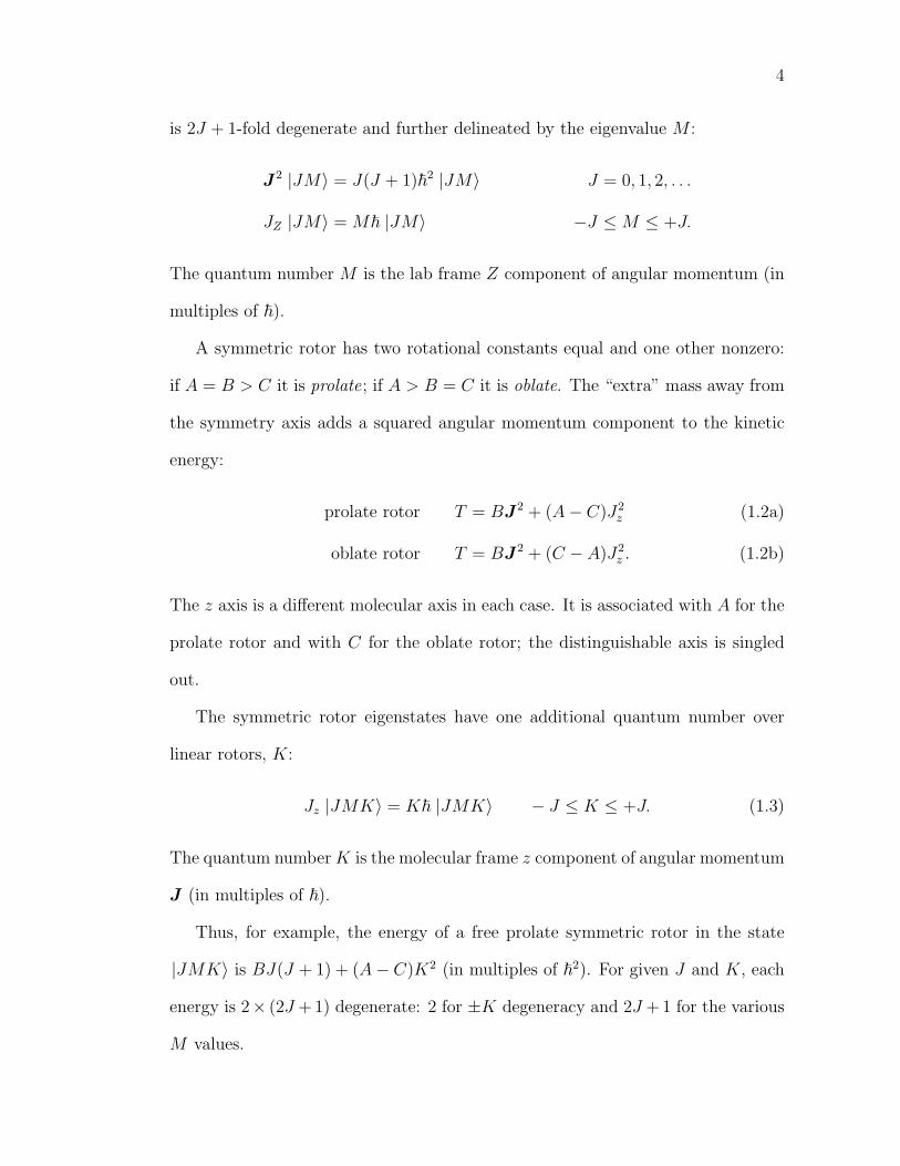
Figure 1.1: Asymmetric rotor iodobenzene with molecular frame definitionand our unconventional assignment of rotational constants to themolecular axes.
Note that a linear rotor, by definition, cannot have any angular momentum
about its (z) axis. Thus setting K = 0 for a symmetric rotor recovers exactly the
linear rotor case.
Asymmetric rotors have three distinct rotational constants. The normal con-
vention defines A > B > C and sets the molecular frame with ABC ↔ yzx, associ-
ating the intermediate rotational constant B with the molecular z axis which best
exhibits the asymmetry. However, we are foremost concerned with rotor electrical
properties, and we define the dipole moment as the molecular z axis and B as the
associated rotational constant. Likewise, y is the in-plane axis orthogonal to z,
and y is associated with A; x is the out-of-plane axis associated with C.∗ Figure
1.1 illustrates the convention. Thus, for any asymmetric rotor, the dipole axis is
defined as z and the association of molecular axes with rotational constants follows
(ABC ↔ yzx). This does not necessarily reflect rotational constant asymmetry,
since A,B, or C may be the intermediate one.
All that being said, the kinetic energy of an asymmetric rotor is
T = AJ2y +BJ2
z + CJ2x .
∗This arrangement is possible only for sufficiently symmetric asymmetric rotors,such as those with C2v symmetry. We only model such molecules. This is furtherdiscussed in Section 1.3, where our convention keeps the potential energy simplest.
6
With some simple algebra, the kinetic energy can be written
T =1
2(A+ C)J2 +
1
2(A− C)
[J2
y + κJ2z − J2
x
], κ =
2B − (A+ C)
A− C. (1.4)
The asymmetry parameter is normally restricted to |κ| ≤ 1, but our unusual
rotational constant convention allows κ to take any value. Under both conventions,
κ = −1 corresponds to a prolate symmetric rotor and κ = +1 an oblate symmetric
rotor.†
1.3 Potential Energy
Classically, the potential energy of an electric dipole d in an electric field E is the
projection of one vector onto the other, −E · d. But an ideal permanent dipole
does not accurately model a real molecule; the dipole itself is affected by electric
fields. A better model includes a contribution proportional to the electric field in
each direction. This is written as the proportionality constants α contracted with
the electric field, added to the permanent dipole moment µ:
d = µ +1
2α ·E. (1.5)
The polarizability tensor α determines how an electric field linearly induces dipole
moments in the molecule. Nonlinear effects (hyperpolarizabilities) are ignored
because they are very small compared to the linear response of the dipole for the
fields and molecules we are modeling.‡ Thus the potential energy is
V = −µ ·E − 1
2E ·α ·E. (1.6)
†The symmetric top convention previously stated forbids A = C, so the asym-metry parameter is always defined.
‡The first hyperpolarizability coefficients are about 10−10 (mks units) of the po-larizibility coefficients. Bogaard and Orr [15] provide background, some calculationnotes, and applications to nonlinear optics.
7
The dipole moment and polarizability are a vector and tensor written in the molec-
ular frame, while an external electric field is a vector in the lab frame. The molecule
rotates relative to the lab frame, so to calculate the potential energy we must con-
vert one cartesian frame to the other. Euler angles φ, θ, χ parameterize how a
molecular frame xyz is rotated from a lab frame XY Z. We use the convention
shared by Zare [14], Kroto [7], Brink and Satchler [16], and several other — but not
all — authors. The transformation matrix that actively rotates lab fixed vectors
to the angle parameterized by φ, θ, χ is
C =
cos φ cos θ cos χ− sinφ sinχ − sinφ cos θ cos χ + cos φ sinχ − sin θ cos χ
− cos φ cos θ sinχ− sinφ cos χ − sinφ cos θ sinχ + cos φ cos χ sin θ sinχ
cos φ sin θ sinφ sin θ cos θ
(1.7)
where CiI = fi · ˆI , i ∈ x, y, z, I ∈ X, Y, Z.
Mainly we use electric fields in one direction, either a static field or a plane
polarized laser. Then the field direction is taken as ˆZ and E = E ˆ
Z .
Static electric field-permanent dipole potential energy
The molecular z axis labels the orientation of a rotating molecule, and we need
to know how electric charge in the molecule is distributed with respect to this
axis so we can write down the Hamiltonian. We always define the permanent
dipole moment vector as the molecular z axis. A linear molecule’s dipole moment
is along the internuclear axis which is labeled z. Symmetric rotors have at least
a third order rotation axis, which by symmetry must be the permanent dipole
axis and is labeled z Asymmetric rotors, in general, can have permanent dipoles
in any direction relative to any symmetry axis. However, sufficiently symmetric
asymmetric molecules must have their permanent dipole moment aligned along
8
a symmetry axis, for example, the C2 axis of the C2v point group (water). We
restrict our study to these cases, where the permanent dipole moment is µ = µfz.
When one of these simple molecules is in a static electric field, the model
potential energy is proportional to fz · ˆZ = CzZ , thus
static electric field V (θ) = −µES cos θ. (1.8)
Laser field-induced dipole potential energy
In addition to static electric fields we model molecules rotating in a laser beam.
The laser is modeled classically, as an oscillating electric field in the lab-fixed Z
direction EL(t) = EL cosωt ˆZ . But if we only use a very high frequency laser,
then any permanent dipole could never be carried in phase with the oscillating
field simply because it oscillates too quickly. The permanent dipole is anchored
by heavy atoms and cannot respond. On average, there is no interaction of a
permanent dipole with a high frequency oscillating field. However, an induced
dipole created by the extremely fast response of electrons can be influenced by
the high frequency field. The induced dipole then interacts with the laser field,
practically instantaneously. This requires analyzing the molecular polarizability.§
The results derived here can be found in the literature. [4, 5]
We disregard the orthogonal oscillating magnetic field since interaction with
the magnetic dipole is negligible.
The potential energy of an induced dipole in a high frequency laser is −12EL ·
α ·EL. The polarizability tensor is written in the molecular frame and has three
nonzero elements on the diagonal. (This implicitly assumes the the frame which
§Near infrared light at 1014 Hz satisfies the high frequency condition, sincemolecules rotate with frequency 1010–1012 Hz depending on the molecule and an-gular momentum state.

9
diagonalizes the inertial tensor and the polarizability tensor are the same. This
is true for sufficiently symmetric molecules, such as C2v asymmetric rotors and
all symmetric rotors, and we will only model such molecules.) The polarizability
tensor for an asymmetric rotor is thus fxαxxfx + fyαyyfy + fzαzzfz. Symmetric
rotors must have αxx = αyy. Linear rotors are given the special notation αzz = α‖
for the polarizability parallel to the molecular axis, and αxx = αyy = α⊥ for the
polarizability perpendicular to the molecular axis.
The laser-induced dipole potential energy for any type of rotor is found by a
generic tensor calculation:
V = −1
2EL ·α ·EL
= −1
2(EI
ˆI)(fiαij fj)(EJ
ˆJ)
= −1
2EIEJαij(ˆI · fi)(fj · ˆJ)
= −1
2EIEJαijC
TIiCjJ
= −1
2EIEJαijCiICjJ .
This nine term sum has six zero terms, since the electric field is parallel to the Z
direction (I = J = Z must hold in nonzero terms) and the polarizability tensor is
diagonal (i = j must hold in nonzero terms). Thus
V = −1
2E2
ZαiiC2iZ
V (θ, χ) = −1
2E2
Z
[αxx sin2 θ cos2 χ+ αyy sin2 θ sin2 χ+ αzz cos2 θ
].
As a brief aside, recall that the laser magnitude is time dependent since E2Z ≡
EL·EL = E2L cos2 ωt. We assumed that the laser frequency ω is very high compared
to rotational frequency. The rotor does not feel the effect of the passing minima
and maxima of the laser field cosine. The effective interaction is governed by the
10
square magnitude cos2 ωt averaged over one period, which is 1/2. Thus E2Z = E2
L/2.
For the various rotors (linear, symmetric, asymmetric) the potential energy
simplifies. Strategically adding and subtracting terms inside the parentheses pro-
vides
V = −1
4E2
L
[sin2 θ
(αxx cos2 χ+ αyy sin2 χ+ αxx sin2 χ− αxx sin2 χ
)+ αzz cos2 θ
]= −1
4E2
L
[sin2 θ
(∆αyx sin2 χ+ αxx
)+ αzz cos2 θ
]= −1
4E2
L
[∆αyx sin2 θ sin2 χ+ αzz cos2 θ + αxx sin2 θ + αxx cos2 θ − αxx cos2 θ
]= −1
4E2
L
[∆αyx sin2 θ sin2 χ+ ∆αzx cos2 θ + αxx
]where the polarizability differences ∆αzx := αzz − αxx and ∆αyx := αyy − αxx are
used. Of course, the constant term can be omitted, which leaves the final form of
the potential energy of a molecule in a laser, within our modeling approximations:
V (θ, χ) = −1
4E2
L
[∆αyx sin2 θ sin2 χ+ ∆αzx cos2 θ
](1.9)
This is the least complicated form for asymmetric rotors. For symmetric and linear
rotors, this simplifies more since αyy = αxx leaving
symmetric rotor V (θ) = −1
4E2
L∆αzx cos2 θ (1.10)
linear rotor V (θ) = −1
4E2
L∆α cos2 θ (1.11)
where conventially ∆α := α‖ − α⊥ for a linear rotor. All the ∆α parameters
defined here are assumed positive, so that the laser-molecule interation is purely
attractive. Certainly this is reasonable for linear molecules, as the electrons are
distributed along the molecular axis, and a field applied in this direction shifts
electrons towards other positively charged nuclei. A perpendicular field cannot
as easily polarize the charge distribution off the molecular axis (away from all
11
nuclei), so α‖ > α⊥ holds. However, ∆αzx,∆αyx > 0 does not necessarily hold
for all symmetric and asymmetric rotors, but we only model such molecules. For
instance, iodobenzene satisifies this since iodine is highly polarizable, is on the z
axis, and is not bonded to an atom off this axis.
Tilted, combined static and laser fields
When both static and laser fields are on and in the same direction, the potential
energy is simply the sum of terms indicated above. However, we want to study the
nonlinear dynamics of rotors in noncollinear fields, which we call tilted fields.
Some subtle effects are explicitly ignored. These include any dipole induced by
the static field interacting with either field and the laser-induced dipole interacting
with the static field. There are only two interactions: the permanent dipole with
the static electric field, and the laser-induced dipole with the time-averaged laser
field.
The new coordinate system uses the laser field polarization direction as the
lab frame Z axis, so the induced dipole potential energy derived above remains
valid. However, the static field is tilted away from +Z by the tilt angle β in
the XZ plane, in the +X direction, so that ES = ES(sin β, 0, cos β) in the lab
frame. Figure 1.2 illustrates tilted fields superimposed on the coordinate system.
Previously we demanded the permanent dipole be parallel to fz, which in the lab
frame is (CzX ,CzY ,CzZ) read from the bottom row of the direction cosine matrix
(1.7). Thus the potential energy of the permanent dipole with the static field is
V (θ, φ) = −µES(sin β, 0, cos β) · (cosφ sin θ, sinφ sin θ, cos θ)
= −µES(sin β sin θ cosφ+ cos β cos θ). (1.12)

12
z
θβstatic
lase
r
φ
lase
r
Z
X
Y
Figure 1.2: Coordinate system for linear rotor in tilted fields. Laser is parallelto lab fixed Z with static field tilted at angle β in the XZ plane.xyz is the molecular frame rotated by Euler angles φ, θ, χ fromthe lab frame XY Z.
The salient difference is the new variable φ, since the static field has a new com-
ponent in the space fixed +X direction.
1.4 Dimensionless Units and Practical Conversions
The experimental parameters used above need to be modified for two reasons.
First, they are not used in practice. Experimentalists use different quantities, such
as laser intensity instead of electric field amplitude. Second, the parameters are
tied to a given experimental setup and specific molecule. Switching to dimen-
sionless parameters allows many physically identical experiments to be modeled
with one calculation. The dimensionless parameters will be related to the common
experimental parameters.
Dimensionless parameters are obtained by dividing the entire Hamiltonian by
13
B~2. The quantum-mechanical squared angular momentum operator implicitly
carries a ~2 factor (its eigenvalues are ~2J(J + 1)), so define j2 := J2/~2. Thus, a
typical quantum Hamiltonian for a linear rotor in collinear static and laser fields,
from Equations (1.8) and (1.11), is (still omitting the constant shift α⊥)
H = BJ2 − µES cos θ − E2L∆α
4cos2 θ
h = j2 − ω cos θ −∆ω cos2 θ (1.13)
with h := H/B~2, ω := µES/B~2, and ∆ω := E2L∆α/4B~2. The dimension-
less parameter ω sets the permanent dipole-static field interaction strength and
likewise ∆ω for the laser-induced dipole and laser field interaction strength. The
Hamiltonian h is explicitly dimensionless.
The dimensionless constants are currently expressed in terms of experimental
parameters in SI (mks) units, which experimentalists never use. For example,
rather than amplitude of the laser field electric component E[N/C], they use laser
field intensity I[W/cm2]. The conversions are (recall that a N = J/m, a V = J/C,
and a W = J/s):
B[cm−1] = B[J]× 1
c[s/cm]× 1
h[1/(J·s)]
εS[kV/cm] = ES[N/C]× 10−2[m/cm]× 10−3[kV/V]
µ[D] = 2.999× 1029[D/(C·m)]× µ[C·m]
α[A3] = α[C2·m2/J]× (1× 10¹⁰)3[A3/m3]× 1
4πε0
[J·m/C2]
IL[W/cm2] = E2L[N2/C2]× ε0[C
2/J·m]× 1
2c[m/s]× 10−4[m2/cm2]
14
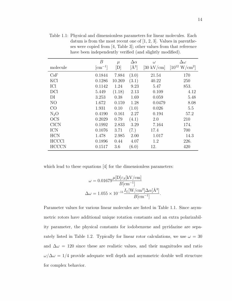
Table 1.1: Physical and dimensionless parameters for linear molecules. Eachdatum is from the most recent one of [1, 2, 3]. Values in parenthe-ses were copied from [4, Table 3]; other values from that referencehave been independently verified (and slightly modified).
B µ ∆α ω ∆ωmolecule [cm−1] [D] [A3] [30 kV/cm] [1012 W/cm2]
CsF 0.1844 7.884 (3.0) 21.54 170KCl 0.1286 10.269 (3.1) 40.22 250ICl 0.1142 1.24 9.23 5.47 853.DCl 5.449 (1.18) 2.13 0.109 4.12DI 3.253 0.38 1.69 0.059 5.48NO 1.672 0.159 1.28 0.0479 8.08CO 1.931 0.10 (1.0) 0.026 5.5N2O 0.4190 0.161 2.27 0.194 57.2OCS 0.2029 0.79 (4.1) 2.0 210ClCN 0.1992 2.833 3.29 7.164 174.ICN 0.1076 3.71 (7.) 17.4 700HCN 1.478 2.985 2.00 1.017 14.3HCCCl 0.1896 0.44 4.07 1.2 226.HCCCN 0.1517 3.6 (6.0) 12. 420
which lead to these equations [4] for the dimensionless parameters:
ω = 0.01679µ[D]εS[kV/cm]
B[cm−1]
∆ω = 1.055× 10⁻¹¹ IL[W/cm2]∆α[A3]
B[cm−1].
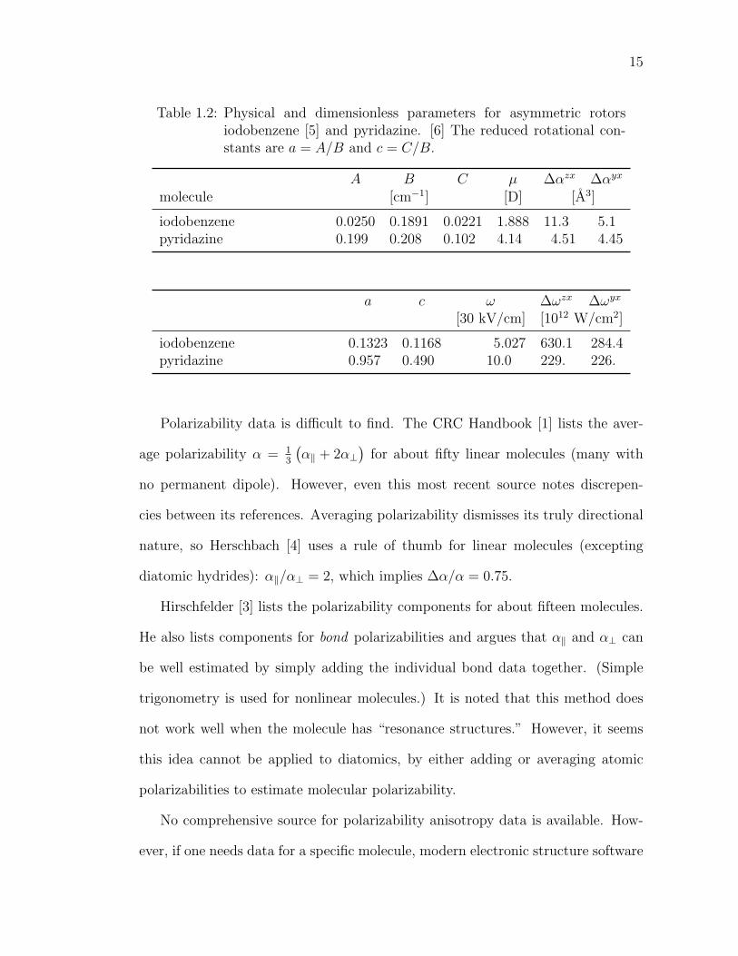
Parameter values for various linear molecules are listed in Table 1.1. Since asym-
metric rotors have additional unique rotation constants and an extra polarizabil-
ity parameter, the physical constants for iodobenzene and pyridazine are sepa-
rately listed in Table 1.2. Typically for linear rotor calculations, we use ω = 30
and ∆ω = 120 since these are realistic values, and their magnitudes and ratio
ω/∆ω = 1/4 provide adequate well depth and asymmetric double well structure
for complex behavior.
15
Table 1.2: Physical and dimensionless parameters for asymmetric rotorsiodobenzene [5] and pyridazine. [6] The reduced rotational con-stants are a = A/B and c = C/B.
A B C µ ∆αzx ∆αyx
molecule [cm−1] [D] [A3]
iodobenzene 0.0250 0.1891 0.0221 1.888 11.3 5.1pyridazine 0.199 0.208 0.102 4.14 4.51 4.45
a c ω ∆ωzx ∆ωyx
[30 kV/cm] [1012 W/cm2]
iodobenzene 0.1323 0.1168 5.027 630.1 284.4pyridazine 0.957 0.490 10.0 229. 226.
Polarizability data is difficult to find. The CRC Handbook [1] lists the aver-
age polarizability α = 13
(α‖ + 2α⊥
)for about fifty linear molecules (many with
no permanent dipole). However, even this most recent source notes discrepen-
cies between its references. Averaging polarizability dismisses its truly directional
nature, so Herschbach [4] uses a rule of thumb for linear molecules (excepting
diatomic hydrides): α‖/α⊥ = 2, which implies ∆α/α = 0.75.
Hirschfelder [3] lists the polarizability components for about fifteen molecules.
He also lists components for bond polarizabilities and argues that α‖ and α⊥ can
be well estimated by simply adding the individual bond data together. (Simple
trigonometry is used for nonlinear molecules.) It is noted that this method does
not work well when the molecule has “resonance structures.” However, it seems
this idea cannot be applied to diatomics, by either adding or averaging atomic
polarizabilities to estimate molecular polarizability.
No comprehensive source for polarizability anisotropy data is available. How-
ever, if one needs data for a specific molecule, modern electronic structure software
16
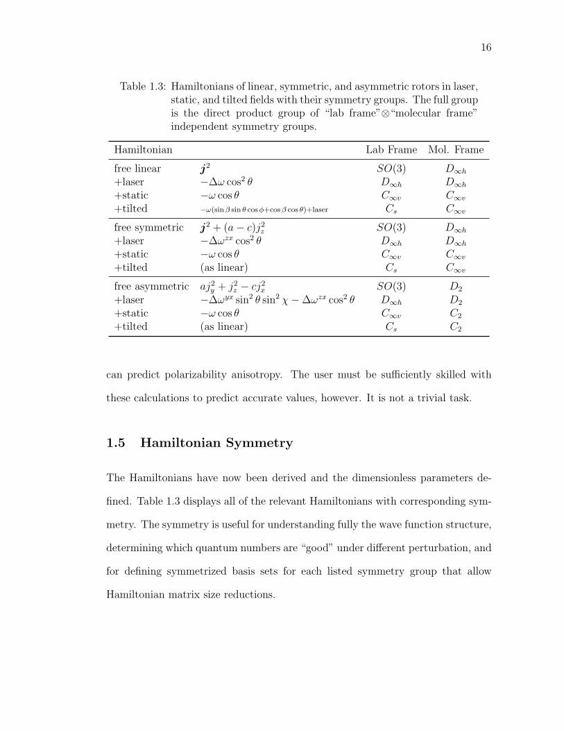
Table 1.3: Hamiltonians of linear, symmetric, and asymmetric rotors in laser,static, and tilted fields with their symmetry groups. The full groupis the direct product group of “lab frame”⊗“molecular frame”independent symmetry groups.
Hamiltonian Lab Frame Mol. Frame
free linear j2 SO(3) D∞h
+laser −∆ω cos2 θ D∞h D∞h
+static −ω cos θ C∞v C∞v
+tilted −ω(sin β sin θ cos φ+cos β cos θ)+laser Cs C∞v
free symmetric j2 + (a− c)j2z SO(3) D∞h
+laser −∆ωzx cos2 θ D∞h D∞h
+static −ω cos θ C∞v C∞v
+tilted (as linear) Cs C∞v
free asymmetric aj2y + j2
z − cj2x SO(3) D2
+laser −∆ωyx sin2 θ sin2 χ−∆ωzx cos2 θ D∞h D2
+static −ω cos θ C∞v C2
+tilted (as linear) Cs C2
can predict polarizability anisotropy. The user must be sufficiently skilled with
these calculations to predict accurate values, however. It is not a trivial task.
1.5 Hamiltonian Symmetry
The Hamiltonians have now been derived and the dimensionless parameters de-
fined. Table 1.3 displays all of the relevant Hamiltonians with corresponding sym-
metry. The symmetry is useful for understanding fully the wave function structure,
determining which quantum numbers are “good” under different perturbation, and
for defining symmetrized basis sets for each listed symmetry group that allow
Hamiltonian matrix size reductions.
17
1.6 The Potential Energy Surface
The various potential energy surfaces are different, but they all share high field
(low energy) and low field (high energy) limits. At low fields and high energy, the
molecule is practically a free rigid rotor and has the corresponding energies and
wave functions. At high fields and low energies, the system resembles a harmonic
oscillator. The rotors-in-fields systems all have these analytically soluble limits.
Linear rotors
At intermediate field strengths, the potential energy surface is dominated by a
double well in the polar angle θ.
For initial simplicity, assume the fields are parallel (β = 0). If the static field is
off (ω = 0) the PES is a symmetric double well of depth ≈ ∆ω and barrier centered
at θ = π/2. If the static field is on, the barrier shifts right to θ ≈ arccos(−ω/2∆ω)
and one well deepens (left) as the other becomes shallow (right). If ω & 2∆ω
then the system reverts to a single well between θ = 0 and π/2. If the fields
are antiparallel (β = π) then the stable and unstable wells are swapped in this
discussion.
If ∆ω = 0 the PES is a cosinusoidal single well. Thus the double well potential
disappears, and many interesting effects go with it; similarly if ω & 2∆ω. Thus
these regimes are not studied, except as limiting cases.
The above quantitative results are only approximate since they come from
extremizing the potential energy V (θ) = −ω cos θ−∆ω cos2 θ. Rather, the effective
18
-400
-300
-200
-100
0
100
200
0 0.25 0.5 0.75 1
Pote
ntia
l Ene
rgy
θ/π
ω = 0ω = 30ω = 120ω = 240
0 0.25 0.5 0.75 1
Effe
ctiv
e Po
tent
ial
θ/π
M = 0 M = 1 M = 5 M = 10
Figure 1.3: Comparison of V (left) and Veff (right) for M = 0,∆ω = 120 andseveral values of ω. Effective potential energy for other M is alsoshown.
potential¶
Veff(θ) =M2 − 1
4
sin2 θ− 1
4+ V (θ) (1.14)
should be extremized. This does not yield simple formulas for well depth and
barrier position, while V does. However, V is a reasonable approximation to Veff
if M is small and θ is not near 0 and π. Figure 1.3 compares them at M = 0
for several parameter values. The effective potential energy introduces repulsive
infinite barriers at θ = 0, π for M > 0 and infinite attractive wells if M = 0.
When the fields are tilted (β 6= 0), the system loses cylindrical symmetry, but
the double well motif prevails. The system is still symmetric about the φ = π plane.
The barrier becomes a potential energy peak centered near θ = π/2, φ = π with
strong shoulders still separating the θ wells. Figure 1.4 shows relevant pictures.
¶The “extra” 1/4 terms appear naturally when splitting out the φ dependencefrom the two DOF Schrodinger equation and absorbing the polar Jacobian sin θ intothe effective wave function. The classical effective potential is justm2/ sin2 θ+V (θ),leaving a qualitative difference between classical and quantum results for M = 0.
19
θ/π
φ/π
β = 0
0 0.25 0.5 0.75 1 0
0.5
1
1.5
2β = π/10 β = π/4 β = π/2
Figure 1.4: Tilted field potential energy contour plots (φ, θ plane) for ω =30,∆ω = 120 and, from left to right, tilt angle β = 0, π/10, π/4,π/2.
Nonlinear rotors
The potential energy surface for symmetric rotors in fields is very similar to the
linear rotor case. The asymmetric double well motif remains. Certainly, for K = 0
the symmetric rotor reduces to a linear rotor. The only difference between linear
and symmetric rotors is a a new source of angular momentum which only affects
the kinetic energy. Determining what conditions on M and K (good quantum
numbers that appear in the effective potential) set up a single well versus a double
well PES is more complicated.
Asymmetric rotors have three distinct polarizabilities in the molecule frame,
rather than two for linear and symmetric rotors, and have a more complicated
PES. For collinear fields, the potential energy function is
V (θ, χ) = −ω cos θ −∆ωzx cos2 θ −∆ωyx sin2 θ sin2 χ.
Once again, the asymmetric double well picture reigns for V (θ, χ) as illustrated in
Figure 1.5. The well minima are at at the poles: V (θ = 0) = −∆ωzx−ω and V (θ =
π) = −∆ωzx +ω, much like the linear and symmetric rotors. Similiarly, the barrier
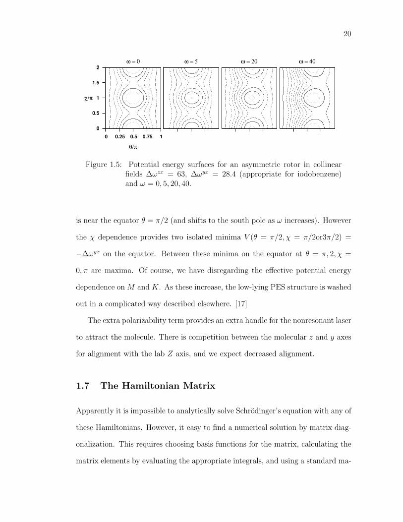
20
θ/π
χ/π
ω = 0
0 0.25 0.5 0.75 1 0
0.5
1
1.5
2ω = 5 ω = 20 ω = 40
Figure 1.5: Potential energy surfaces for an asymmetric rotor in collinearfields ∆ωzx = 63, ∆ωyx = 28.4 (appropriate for iodobenzene)and ω = 0, 5, 20, 40.
is near the equator θ = π/2 (and shifts to the south pole as ω increases). However
the χ dependence provides two isolated minima V (θ = π/2, χ = π/2or3π/2) =
−∆ωyx on the equator. Between these minima on the equator at θ = π, 2, χ =
0, π are maxima. Of course, we have disregarding the effective potential energy
dependence on M and K. As these increase, the low-lying PES structure is washed
out in a complicated way described elsewhere. [17]
The extra polarizability term provides an extra handle for the nonresonant laser
to attract the molecule. There is competition between the molecular z and y axes
for alignment with the lab Z axis, and we expect decreased alignment.
1.7 The Hamiltonian Matrix
Apparently it is impossible to analytically solve Schrodinger’s equation with any of
these Hamiltonians. However, it easy to find a numerical solution by matrix diag-
onalization. This requires choosing basis functions for the matrix, calculating the
matrix elements by evaluating the appropriate integrals, and using a standard ma-
21
trix diagonalization routine (rsm in EISPACK) to calculate eigenvalues (quantum
energies) and eigenvectors (energy eigenstates).
Linear rotors
Spherical harmonics Y MJ (θ, φ) ≡ 〈θ φ|JM〉 form a useful basis. First, they are the
exact energy eigenstates in the field-free limit, so relatively few basis functions will
be needed to get a good approximate wave function when fields are on. Second,
spherical harmonics have a well known structure that can be used to construct the
Hamiltonian matrix and related quantities.
The spherical harmonics have recurrence relations which allow explicit formulas
for the several types of matrix elements we need. [18] The relevant properties are
reviewed in Appendix A.1.
The matrix elements in the spherical harmonics basis are derived in Appendix
B.1. A brief overview of their stucture is nevertheless useful here. The field free
Hamiltonian j2 contributes only a diagonal element J(J + 1), meaning the kinetic
energy operator only “connects” basis states with quantum number differences
∆J = 0, ∆M = 0. Each term in the Hamiltonian carries such selection rules.
The static electric field (1.8) induces selection rules ∆J = ±1, ∆M = 0, which is
familiar from the elementary perturbation theory approach to the Stark effect. The
laser field (1.11) has selection rules ∆J = 0,±2, ∆M = 0, which is reminiscient
of the rotational Raman effect. Combined collinear fields have exactly the same
selection rules, although the matrix is pentadiagonal. Lastly, when the fields are
tilted (1.12) an azimuthal angle φ term is introduced causing M mixing. This term
induces ∆J = ±1, ∆M = ±1 selection rules.
22
Nonlinear rotors
The symmetric top eigenstates 〈φ θ χ|JMK〉 form the useful basis for symmetric
and asymmetric tops in fields, for the same reasons spherical harmonics are used
for linear rotors. The basis functions use the Jacobi polynomials (alternatively,
the reduced Wigner rotation matrix elements), which have well-known structure
described in Appendix A.3. The corresponding matrix elements are derived in
Appendix B.3.
Briefly, the symmetric top kinetic energy is, of course, diagonal in this basis.
There are three quantum numbers to consider, so the kinetic energy (1.2) selection
rule is ∆J = 0, ∆M = 0, ∆K = 0. Changes in K occur when the potential energy
includes the Euler angle χ, which does not happen for symmetric tops, as seen in
Table 1.3. Thus ∆K = 0 holds for all symmetric top matrix elements. The static
electric field has the selection rule ∆J = 0,±1 and the laser ∆J = 0,±1,±2.
When the fields are tilted, the same static field J selection rule applies but M is
not strictly conserved; instead ∆M = ±1.
The asymmetric rotor kinetic energy (1.4) is not diagonal in the symmetric top
basis; the selection rule is ∆J = 0, ∆K = 0,±2. The static field element is as
for symmetric rotors, ∆J = 0,±1 with no change in M or K. But the laser field
(1.9) now has an extra component sin2 θ sin2 χ due to the completely anisotropic
polarizability tensor, and this term induces changes in K. This term has selection
rules ∆J = 0,±1,±2, ∆K = 0,±2 while the cos2 θ term sets ∆J = 0,±1,±2,
∆K = 0 as with symmetric tops. For tilted fields, since the static field-dipole
configuration has not changed, the selection rule is still ∆J = 0,±1, ∆M = ±1.
Just as a note, the asymmetric top kinetic energy separation (1.4) was histori-
cally done to allow efficient tabulation of asymmetric rotor energy levels [2, App.
23
IV]. We use it to separate the kinetic energy into easy and hard pieces. The easy
piece is j2, which is diagonal in the symmetric top eigenstate basis. The hard
part is j2y + κj2
z − j2x, which is not diagonal in the symmetric top eigenstate basis:
∆J = 0,∆K = 0,±2 is the selection rule.
In all cases the Hamiltonian matrix is real and symmetric. It does not have
banded structure, but is very sparse due to the selection rules. The rsm (“real
symmetric matrix”) routine in EISPACK most efficiently diagonalizes such Hamil-
tonians.

Chapter 2
Correlation Diagrams and Wave
Functions
2.1 Correlation Diagrams: Energy, Alignment, and Orien-
tation
Correlation diagrams reveal basic properties of rotor states in various field con-
figurations. For linear rotors in the fields discussed previously, the energy levels
are functions of three dimensionless field parameters: static field strength ω, laser
field intensity ∆ω, and mutual field tilt angle β. Mapping out the energy levels as
these three parameters vary yields complicated structure; indeed, one needs only
two parameters for the existence of “diabolical points” [19] where “accidental” de-
generacies can occur in an energy spectrum. Of course, avoided crossings are rife,
as usual when just one free parameter exists. Discovering the new structures found
with three free parameters is a weighty task and not attempted here. However,
several two dimensional slices of the four dimensional energy-parameter space are
shown in this section.
Also, the alignment and orientation of eigenstates as functions of the field
parameters show how well external fields restrict rotational motion. Alignment is
〈cos2 θ〉 and orientation is 〈cos θ〉 measured relative to the lab-fixed Z axis. The
geometrical distinction is that alignment measures only how parallel the rotor
and lab axes are on average, while orientation goes one step further and picks a
preferred direction as would a compass needle. In our context, we expect high
alignment and no orientation for a very intense laser and high alignment with high
24
25
orientation for a very strong static electric field.
Alignment and orientation in these correlation diagrams can be interpreted
by the Hellmann-Feynman theorem. [20] As either field strength parameter is
changed, the rate of energy level increase is equal to the average Hamiltonian
derivative in that state:
∂En
∂ω=
⟨n
∣∣∣∣∣∂h∂ω∣∣∣∣∣n
⟩= −〈n |cos θ|n〉
∂En
∂∆ω=
⟨n
∣∣∣∣∣ ∂h
∂∆ω
∣∣∣∣∣n⟩
=⟨n
∣∣cos2 θ∣∣n⟩
(2.1)
for dimensionless Hamiltonian (linear rotor in collinear fields) h = j2 − ω cos θ −
∆ω cos2 θ. Thus the energy correlation diagram curves can only decrease when
laser intensity ∆ω increases, and is dependent on the sign of 〈n |cos θ|n〉 in the nth
state when static field strength ω increases. The change in an energy correlation
diagram is linked to the eigenstates’ alignment and orientation behavior.
Linear rotors in collinear fields
As a first step, Figure 2.1 shows energy, alignment, and orientation correlation
diagrams for M = 0 states as the static field strength ω increases from 0 to 30. In
each panel, the heavy black line is the ground state and the various dashed lines
correspond between the panels as the second, third, and so on energy states as
seen at top.
On the left, the laser is turned off (∆ω = 0). The energies evolve from the
field-free eigenvalues J(J + 1) to the exact Stark eigenenergies. Note that as the
Hellmann-Feynman theorem allows, the higher states initially increase in energy
due to being localized on the unstable side of the potential energy surface (θ = π).
The lowest panel directly corresponds since the orientation of these states all tend
26
-120
-90
-60
-30
0
30
Ener
gy
∆ω = 0 ∆ω = 120
0
0.2
0.4
0.6
0.8
1
Alig
nmen
t
-1
-0.5
0
0.5
1
0 10 20
Orie
ntat
ion
Static Electric Field ω 0 10 20 30
Static Electric Field ω
Figure 2.1: Energy (dimensionless), alignment 〈cos2 θ〉, and orientation〈cos θ〉 of a linear rotor in a (left) static electric field as ω =0 → 30 and (right) collinear static and laser fields, with laserintensity fixed at ∆ω = 120 as ω = 0 → 30. Only M = 0 statesare shown. The five lowest states are shown on each side, withfour extra on the right which highlights a clear avoided crossingbetween the sixth and seventh. The ground state is marked withheavy line.
27
negative, indicating the dipole is oriented somewhat anti-parallel with the applied
static field. However, as ω increases, the lower energy states get flipped around one
by one and are trapped in the stable well. The ground state evolves monotonically,
as it always will. The alignment correlation is not too interesting, except to note
that the field-free eigenstates have alignment (M = 0) 1/3 for J = 0, 3/5 for J = 1,
and approach 1/2 from below as J = 2, 3, 4, . . . . The alignment for field-free states
is analytically given by the matrix element Equation (B.2c).
On the right of Figure 2.1, the laser intensity is moderately strong at ∆ω = 120
for various static field strengths. At ω = 0, the low-energy rotor states appear to
be doubly degenerate because the laser potential is a symmetric double well, which
produces closely spaced pairs of levels with nearly identical probability distribution.
As ω increases, these pairs split apart since one well is increasing in energy at the
same magnitude the other well is decreasing in energy. At sufficiently high energy,
near the laser potential barrier at zero energy, levels are no longer paired because
the states are not bound.
At ω = 22 the energy curves apparently cross. Actually the lower two pairs
undergo sharply avoided crossings ; the third pair clearly avoids crossing on this
scale. The curves do not actually intersect as could be seen with more exact
calculation around this point. The avoided crossing is manifested in the alignment
and orientation correlations by sudden jumps. The two states involved in the
avoiding crossing quickly exchange character, thus the alignment and orientation
values exchange as well. The states in the clear avoided crossing undergo more
gradual property exchange. Avoided crossings are discussed in more detail in
Section 4.1.
Physically, the significant consequence of combining a strong laser field ∆ω =

28
120 with a weak static electric field ω = 1 is that strong orientation occurs with
a much weaker electric field than otherwise possible. Comparing the middle and
bottom panels of Figure 2.1 reveals that the alignment and orientation for the
lowest few states at right are much higher than any pure static field result shown
at left. This effect was first theoretically proposed in 1999 [4] and experimentally
verified in 2003. [13]
Figure 2.2 shows correlation diagrams as the laser intensity ∆ω increases from
0 to 120. On the left, the static field is off (ω = 0). The energy levels start at free
rigid rotor energies J(J + 1) and then pair up as the laser intensity increases. The
eventual degeneracies are the result of the deepening symmetric double well, which
can bind more and more nearly degenerate pairs as ∆ω →∞. Usually one thinks
the energy levels must repel, as with avoided crossings. But the selection rule for
the laser-induced dipole interaction is ∆J = 0, ±2 leaving no mechanism for the
bottom two states (adiabatically correlated to field free J = 0 and J = 1) no way
to couple and repel—that would require a ∆J = ±1 matrix element. At high field,
these adjacent even/odd pairs become almost identical, except for an additional
node in the odd J member. Note that the energies are everywhere decreasing,
as demanded by the Hellmann-Feynman theorem (2.1). The energy level pairing
shows in the alignment diagram, as well. The orientation correlation is identically
zero for all states since the symmetric double well does not favor a direction; either
pointing up or down is equally well allowed leaving the average at zero.
The right side of Figure 2.2 shows the effect of a collinear static field ω = 30
as the laser intensity ∆ω increases 0 → 120. The pair structure from the left
has been broken, but at even higher ∆ω the static field will be overcome and the
symmetric well reemerges. Three avoided crossings are clearly present, as seen in
29
-60
-30
0
30
Ener
gy
ω = 0 ω = 30
0
0.2
0.4
0.6
0.8
1
Alig
nmen
t
-1
-0.5
0
0.5
1
0 30 60 90
Orie
ntat
ion
Laser Field ∆ω0 30 60 90 120
Laser Field ∆ω
Figure 2.2: Energy (dimensionless), alignment, and orientation of a linearrotor in a (left) laser field as ∆ω = 0 → 120 and (right) collinearstatic and laser fields, with static field strength fixed at ω = 30as ∆ω = 0 → 120. The eight lowest M = 0 states are shown.The ground state is marked with heavy line.
30
-130
-120
-110
-100
-90
-80
-70
-60
-50
0 0.1 0.2 0.3 0.4 0.5
Ener
gy
β/π
-20
-15
-10
-5
0
5
10
15
Figure 2.3: Energy correlation diagram with tilt angle β, tilting fieldsω = 30, ∆ω = 120 for parity= +1 linear rotor eigenstates. Atleft are the lowest eight states; at right about fifteen states atintermediate energies near barriers.
the alignment and orientation diagrams.
Linear rotors in tilted fields
Changing the tilt angle β between static and laser fields introduces many features,
as seen in Figure 2.3 for ω = 30 and ∆ω = 120. The lowest energy states on the
left have simple structure. Several states are widely separated in collinear fields
but pair up in perpendicular fields β = π/2. These two states have the same nodal
structure but localized on opposite poles of the sphere. The states become almost
degenerate as the tilting field brings the wells to the same depth −∆ω. The states
become closely split pairs, each state localized in both wells. The intermediate
energy states on the right are qualitatively different. Here many of the avoided
31
crossings are widely avoided, instead of very closely avoided. There are even some
regions where three states are interacting, suggesting the wave functions are very
delocalized. Some states seem to pair up at β = π/2 and others do not. Such wild
behavior will be linked to underlying classical chaotic dynamics in Chapter 4.
2.2 Wave Functions
Each energy eigenstate is calculated as a linear superposition of basis states; ma-
trix diagonalization yields the superposition coefficients. Probability distribution
pictures show where the wave function is localized and how many nodes it has.
This requires calculating the basis functions over a coordinate grid, which is ex-
plained in Appendix A.1 for spherical harmonics and Appendix A.3 for symmetric
top eigenstates.
Linear rotors
A physically significant quantity derived from the wave function is the reduced
probability distribution. Given a wave function ψ(θ, φ) the full probability distri-
bution ψ∗ψ sin(θ) is reduced by integrating out the (often trivial) φ dependence.
The remaining function tells how the rotor is distributed in the polar angle θ
irrespective of φ.
Figure 2.4 shows the twelve lowest M = 0 energy eigenstates for a linear rotor
in collinear fields ω = 30, ∆ω = 120. Clearly the ground state (Energy = −127)
is strongly localized in the stable well. The next highest state (−85) is also in
the stable well, but with one node. The third state (−71) is high enough to be
localized in the higher lying well and has no nodes. The progression continues
gaining additional nodes in states localized in alternating wells. Finally the eighth
32
0 0.5 1 θ/π
Figure 2.4: Reduced probability distributions v. θ of a linear rotor incollinear fields ω = 30, ∆ω = 120, and M = 0. The twelvelowest energy eigenstates are shown, with ground state at topleft and increasing energy to the right, and down.
state (Energy = +7) is above the barrier and freely rotates; it is delocalized over
both wells. The higher states all have this behavior but gain one node for each
step up.
When the fields are tilted, the wave function dependence on φ is no longer
uniform. Figure 2.5 shows full probability distributions for several eigenstates in
tilted fields ω = 30, ∆ω = 120 as before but tilt angle β = π/4. The figure shows
the distribution contours for the ground state (Energy = −120) the 28th state
(+8) and the 47th state (+40) of the A′ symmetry class.∗ The ground state is still
very well oriented, despite only partial assistance from the static field. The middle
state is just below the highest barrier, but above the low-lying barriers so some
free rotation is evident. The highest state is well above the barrier and has regular
nodal structure, indicating it is near the integrable field-free limit.
∗Recall Table 1.3: the linear rotor in tilted fields Hamiltonian is conserved byreflection plane symmetry in the lab XZ plane, which supports the simple pointgroup Cs. See Appendix B.2.
33
θ/π
φ/π
0 0.2 0.4 0.6 0.8 1 0
0.5
1
1.5
2
Figure 2.5: Probability distribution for three eigenstates of a linear rotorin tilted fields ω = 30, ∆ω = 120, β = π/4. Ground, 28thand 47th eigenstates of A′ symmetry. The bottom row showsthe distribution contours projected on a rectangular (θ, φ) grid.The top row shows the distribution accurately represented on aspherical surface, with the viewier looking just to the left of theφ = 0 vertical plane.
Note that the spherical wave function plots in the figure are most accurate but
are cumbersome. They hide half of the distribution on the backside of the sphere.
From now on the square grid pictures are used to show off the entire wave function.

Chapter 3
Quantum PropagationThe previous chapter covered static properties of rigid rotating molecules in various
field types and configurations. But to take advantage of the enhanced orientation
possible using collinear laser and static fields, a field-free system must first evolve
to the desired pendular state. The details of how the free molecule enters the
field can drastically change the final state, and in this chapter these details are
elucidated.
First, results for static Hamiltonians are presented, showing how non-stationary
states evolve under constant applied fields. Then the dynamics of rotors subject
to pulsed laser fields, governed by the laser-induced dipole model used previously,
are illustrated. This has become a popular proposal, with some experimental
verification, for aligning molecules along a space-fixed axis without a field being
present. This sub-field has recently been reviewed by Stapelfeldt and Seideman.
[12]
The numerical integration algorithm is discussed in Appendix C. We use sym-
plectic integration, which should help guard against long time instabilities, as
explained in the appendix.
3.1 Preliminaries
We use the dimensionless time dependent Schrodinger equation (TDSE), formed
as follows. Divide the TDSE
i~d
dt|ψ(t)〉 = H(t) |ψ(t)〉
34
35
by B~2, since this energy scale is present in all rotational Hamiltonians we use
(Section 1.4), and use dimensionless time τ = B~t. The new variable τ roughly
measures time in multiples of the J = 1 state field-free rotational period T =
π/B~.∗ The TDSE becomes
id
dτ|ψ(τ)〉 = h(τ) |ψ(τ)〉 (3.1)
using dimensionless Hamiltonian h = H/B~2.
As shown later, the rotational dynamics is governed by the field-free rotational
period. Table 3.1 displays various rotational parameters of several linear rotors.
Also shown is the dimensionless temperature at 1 K and 298 K, implying an aver-
age J value from a statistical mechanical calculation to determine the rotational
period. The calculation is just the canonical average of J given the dimensionless
temperature Y , over linear rotor eigenstates:
〈J〉 =1
Q
∞∑J=0
J(2J + 1)e−J(J+1)/Y (3.2)
with Q the canonical partition function and J(J + 1) the eigenenergies of the
(2J + 1) degenerate eigenstates. The average angular momentum as a function of
dimensionless temperature Y is plotted in Figure 3.1.
Here is how the dimensionless temperature and related parameters are calcu-
lated, considering units in detail. The basic parameters are
rotational temperature θrot[K] = B[J]× 1
k[K/J]
dimensionless temperature Y = k[J/K]× T [K]× 1
B[1/J]
rotational period Trot[ps] = π × 1012[ps/s]× 1
B[J s2]× 1
~[1/J s]× 1
J[1]
∗Rotational period: the classical Hamiltonian in action-angle variables (qj, j)is H = Bj2. By Hamilton’s equation, qj = 2Bj. Since one rotational period isparameterized by qj = 0 → 2π as t = 0 → T , integrating yields T = π/Bj. Inquantum terms, T = π/B~J , where J is a dimensionless quantum number.

36
Table 3.1: Rotational constant B, rotational temperature θrot, dimensionlesstemperature Y and corresponding rotational period Trot for sev-eral linear molecules. The latter two are linked since any giventemperature fixes an average angular momentum, which affectsthe rotational period.
B θrot Y Trot Y Trot
molecule. [cm−1] [K] [1 K] [ps, J = 1] [298 K] [ps, J = 25]
CsF 0.1844 0.2653 3.770 90.45 1123. 3.618KCl 0.1286 0.1850 5.405 129.7 1611. 5.188ICl 0.1142 0.1643 6.086 146.0 1814. 5.842DCl 5.449 7.840 0.1276 3.061 38.01 0.1224DI 3.253 4.680 0.2137 5.127 63.67 0.2051NO 1.672 2.406 0.4157 9.975 123.9 0.3990CO 1.931 2.778 0.3599 8.637 107.3 0.3455N2O 0.4190 0.6028 1.659 39.80 494.3 1.592OCS 0.2029 0.2919 3.426 82.20 1021. 3.288ClCN 0.1992 0.2866 3.490 83.73 1040. 3.349ICN 0.1076 0.1548 6.460 155.0 1925. 6.200HCN 1.478 2.127 0.4703 11.28 140.1 0.4514HCCCl 0.1896 0.2728 3.666 87.97 1092. 3.519HCCCN 0.1517 0.2183 4.582 109.9 1365. 4.398
0 5
10 15 20 25 30
0 200 400 600 800 1000
Aver
age
J
Temperature Y
Figure 3.1: Average angular momentum quantum number 〈J〉 vs dimension-less temperature Y for a linear rotor, as determined by canonicalstatistical mechanics.
37
where J in the last formula is the dimensionless angular momentum quantum
number, and k is Boltzmann’s constant. The rotational constant B can usefully
come in several different units. Typically it is given in wavenumbers [cm−1], as in
Table 3.1. But other useful dimensions are
B[1/J s2] =1
2πB[cm−1]× c[cm/s]× 1
~[1/J s]
B[J] = 2πB[cm−1]× c[cm/s]× ~[J s].
The point is to figure out the rotational period for rotating molecules. The condi-
tions of the experiments described here are typically around 1 K, which averaged
over the molecules in Table 3.1 corresponds to Y = 2.9. Figure 3.1 links this Y to
an average quantum number 〈J〉 = 1, corresponding to rotational period Trot = 69
ps. For other temperatures, the rotational period is:
T = 1 K → Y = 2.86 → J = 1 → Trot = 69 ps
T = 10 K → Y = 28.6 → J = 4 → Trot = 17 ps
T = 100 K → Y = 286 → J = 14 → Trot = 4.9 ps
T = 298 K → Y = 854 → J = 25 → Trot = 2.8 ps.
3.2 Static Hamiltonian Propagation
The most basic calculation is propagating an initial state with a time-independent
Hamiltonian. Figure 3.2 shows the interesting quantities. Here the spherically
symmetric state J = 0 is propagated subject to static and laser fields at various
tilt angles. Pictured, at two different laser intensities ∆ω = 120 and 500, are the
autocorrelation function, alignment 〈cos2 θ〉, and orientation 〈cos θ〉.
Experimentalists are interested in high alignment and orientation, and the fig-
ure shows that simply raising the laser intensity is not enough to provide either.
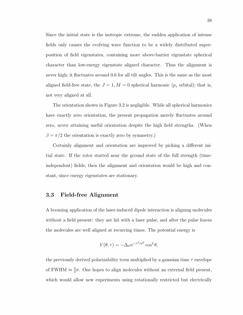
38
Since the initial state is the isotropic extreme, the sudden application of intense
fields only causes the evolving wave function to be a widely distributed super-
position of field eigenstates, containing more above-barrier eigenstate spherical
character than low-energy eigenstate aligned character. Thus the alignment is
never high; it fluctuates around 0.6 for all tilt angles. This is the same as the most
aligned field-free state, the J = 1,M = 0 spherical harmonic (pz orbital); that is,
not very aligned at all.
The orientation shown in Figure 3.2 is negligible. While all spherical harmonics
have exactly zero orientation, the present propagation merely fluctuates around
zero, never attaining useful orientation despite the high field strengths. (When
β = π/2 the orientation is exactly zero by symmetry.)
Certainly alignment and orientation are improved by picking a different ini-
tial state. If the rotor started near the ground state of the full strength (time-
independent) fields, then the alignment and orientation would be high and con-
stant, since energy eigenstates are stationary.
3.3 Field-free Alignment
A booming application of the laser-induced dipole interaction is aligning molecules
without a field present: they are hit with a laser pulse, and after the pulse leaves
the molecules are well aligned at recurring times. The potential energy is
V (θ, τ) = −∆ωe−τ2/σ2
cos2 θ,
the previously derived polarizability term multiplied by a gaussian time τ envelope
of FWHM ≈ 53σ. One hopes to align molecules without an external field present,
which would allow new experiments using rotationally restricted but electrically
39
0
0.2
0.4
0.6
0.8
1
Auto
corr
elat
ion
∆ω = 120 ∆ω = 500
0
0.2
0.4
0.6
0.8
1
Alig
nmen
t
-1
-0.5
0
0.5
1
0 0.2 0.4 0.6 0.8
Orie
ntat
ion
time τ
Figure 3.2: Time-independent Hamiltonian propagations, linear rotor infields ω = 30, (left) ∆ω = 120 and (right) 500 with tilt angle(solid) β = 0, (long dashes) π/4, and (short dashes) π/2. Fromtop to bottom: autocorrelation function (initial state is J = 0spherical harmonic, a s orbital), alignment 〈cos2 θ〉, and orienta-tion 〈cos θ〉.
unperturbed molecules.
The key is that the alignment 〈cos2 θ〉 can change after the laser pulse has gone
by, when the Hamiltonian has no potential energy term. This is, apparently, a
purely quantum effect. The wavefunction ψ(t) changes because each coefficient in
the spherical harmonic superposition has a time-dependent phase:
|ψ(t)〉 =∑
J
e−iJ(J+1)τcJ |JM〉 . (field free conditions) (3.3)
Here the autocorrelation function |〈ψ(0)|ψ(τ)〉|2 is constant since the time depen-
dent complex exponential phase factors cancel. But the alignment is still time
40
dependent, even after the pulse:
⟨ψ(t)
∣∣cos2 θ∣∣ψ(t)
⟩=
∑J ′J
ei[J ′(J ′+1)−J(J+1)]τc∗J ′cJ⟨J ′M ′ ∣∣cos2 θ
∣∣ JM⟩. (3.4)
It turns out that the post-pulse alignment highly depends on the width σ and
intensity ∆ω, as first discovered by Ortigoso et. al. [21] There are three distinct
pulse regimes: nonadiabatic, intermediate, and adiabatic. Figure 3.3 shows the
alignment of a linear rotor before, during and after various width pulses illustrating
the full range of behavior.
The nonadiabatic regime (σ � 1) is marked by a pulse so fast relative to
the rotational period that maximum alignment occurs after the pulse has gone
by. The induced rotational wavepacket quickly oscillates and even attains greater
alignment well after the pulse than the first maximum.
Using the analytic sudden approximation helps quantify what maximum width
σ guarantees a non-adiabatic process. The sudden approximation posits a pulse
so short that the lowest order propagator provides accurate results for post-pulse
quantities. (See Appendix C.6.) Figure 3.4 compares the numerical propagation
(as used to calculate all previous results) to the sudden approximation. The post-
pulse autocorrelation function is shown for several short pulses. At σ = 0.01 the
match is near-perfect. Width σ = 0.03 reveals a slight discrepancy at higher laser
intensities. However, σ = 0.05 must be past the non-adiabatic limit since there
are major differences between the methods at moderately high laser intensity.
The adiabatic regime (σ � 1) is marked by maximum alignment when the pulse
is at maximum intensity. When the width is much greater than the rotational
period, the pulse gently carries the field-free initial state to the instantaneous
Hamiltonian eigenstate and back down to the initial state. There is little, if any,
field-free alignment.
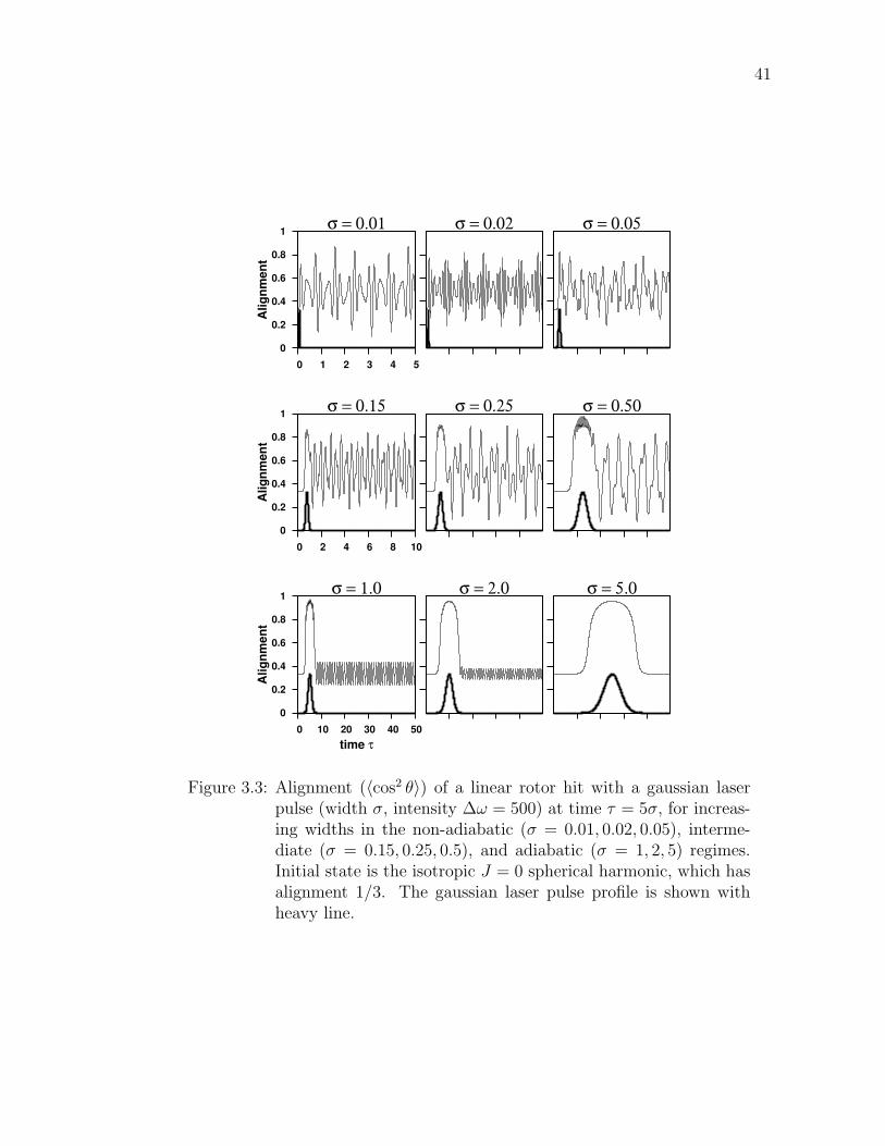
41
0
0.2
0.4
0.6
0.8
1
0 10 20 30 40 50
Alig
nmen
t
time τ
σ = 1.0 σ = 2.0 σ = 5.0
0
0.2
0.4
0.6
0.8
1
0 2 4 6 8 10
Alig
nmen
t
σ = 0.15 σ = 0.25 σ = 0.50
0
0.2
0.4
0.6
0.8
1
0 1 2 3 4 5
Alig
nmen
t
σ = 0.01 σ = 0.02 σ = 0.05
Figure 3.3: Alignment (〈cos2 θ〉) of a linear rotor hit with a gaussian laserpulse (width σ, intensity ∆ω = 500) at time τ = 5σ, for increas-ing widths in the non-adiabatic (σ = 0.01, 0.02, 0.05), interme-diate (σ = 0.15, 0.25, 0.5), and adiabatic (σ = 1, 2, 5) regimes.Initial state is the isotropic J = 0 spherical harmonic, which hasalignment 1/3. The gaussian laser pulse profile is shown withheavy line.
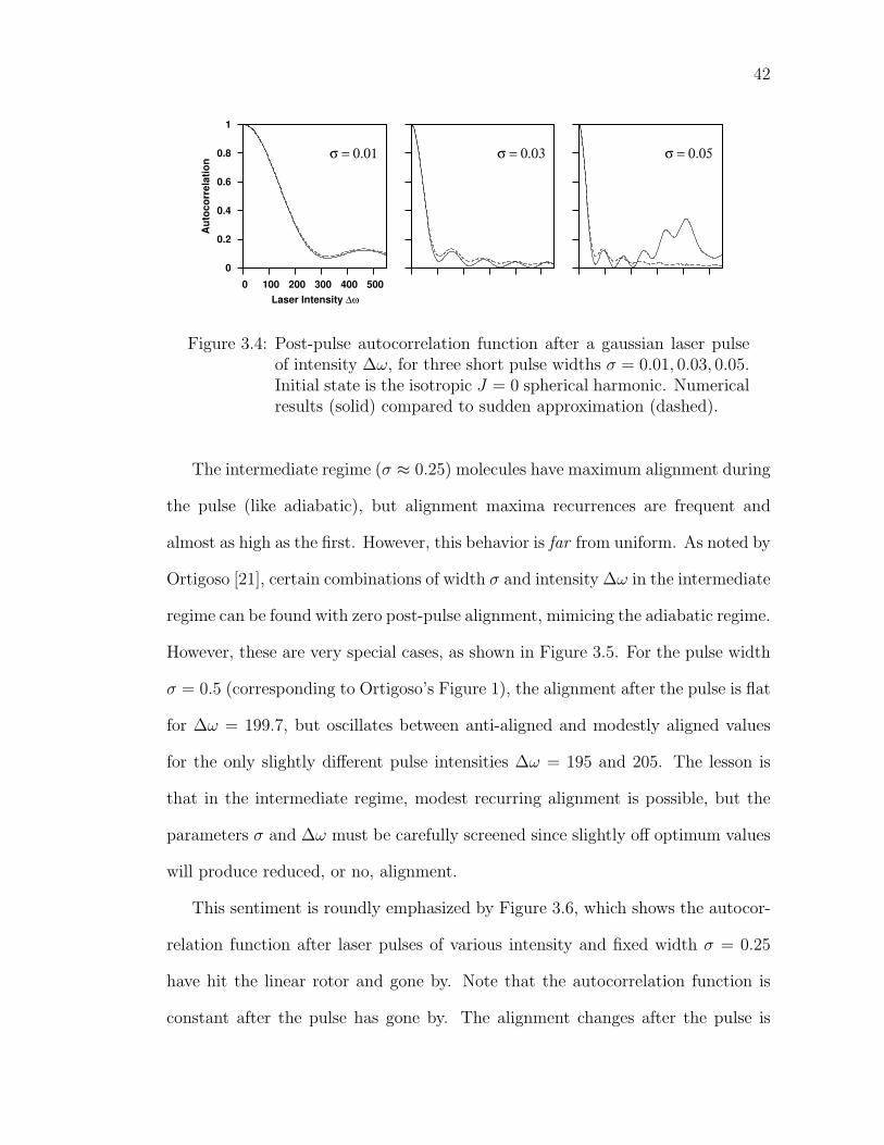
42
0
0.2
0.4
0.6
0.8
1
0 100 200 300 400 500
Aut
ocor
rela
tion
Laser Intensity ∆ω
σ = 0.01 σ = 0.03 σ = 0.05
Figure 3.4: Post-pulse autocorrelation function after a gaussian laser pulseof intensity ∆ω, for three short pulse widths σ = 0.01, 0.03, 0.05.Initial state is the isotropic J = 0 spherical harmonic. Numericalresults (solid) compared to sudden approximation (dashed).
The intermediate regime (σ ≈ 0.25) molecules have maximum alignment during
the pulse (like adiabatic), but alignment maxima recurrences are frequent and
almost as high as the first. However, this behavior is far from uniform. As noted by
Ortigoso [21], certain combinations of width σ and intensity ∆ω in the intermediate
regime can be found with zero post-pulse alignment, mimicing the adiabatic regime.
However, these are very special cases, as shown in Figure 3.5. For the pulse width
σ = 0.5 (corresponding to Ortigoso’s Figure 1), the alignment after the pulse is flat
for ∆ω = 199.7, but oscillates between anti-aligned and modestly aligned values
for the only slightly different pulse intensities ∆ω = 195 and 205. The lesson is
that in the intermediate regime, modest recurring alignment is possible, but the
parameters σ and ∆ω must be carefully screened since slightly off optimum values
will produce reduced, or no, alignment.
This sentiment is roundly emphasized by Figure 3.6, which shows the autocor-
relation function after laser pulses of various intensity and fixed width σ = 0.25
have hit the linear rotor and gone by. Note that the autocorrelation function is
constant after the pulse has gone by. The alignment changes after the pulse is
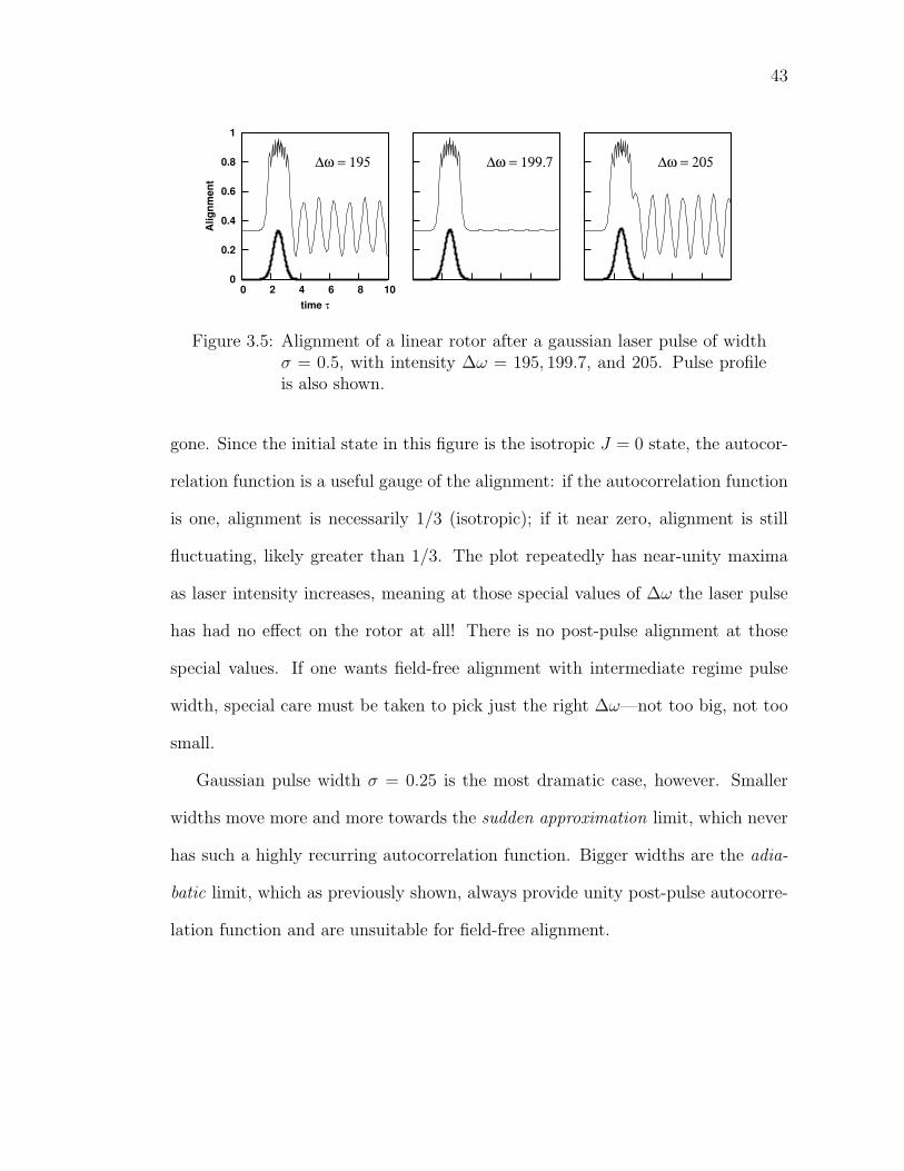
43
0
0.2
0.4
0.6
0.8
1
0 2 4 6 8 10
Alig
nmen
t
time τ
∆ω = 195 ∆ω = 199.7 ∆ω = 205
Figure 3.5: Alignment of a linear rotor after a gaussian laser pulse of widthσ = 0.5, with intensity ∆ω = 195, 199.7, and 205. Pulse profileis also shown.
gone. Since the initial state in this figure is the isotropic J = 0 state, the autocor-
relation function is a useful gauge of the alignment: if the autocorrelation function
is one, alignment is necessarily 1/3 (isotropic); if it near zero, alignment is still
fluctuating, likely greater than 1/3. The plot repeatedly has near-unity maxima
as laser intensity increases, meaning at those special values of ∆ω the laser pulse
has had no effect on the rotor at all! There is no post-pulse alignment at those
special values. If one wants field-free alignment with intermediate regime pulse
width, special care must be taken to pick just the right ∆ω—not too big, not too
small.
Gaussian pulse width σ = 0.25 is the most dramatic case, however. Smaller
widths move more and more towards the sudden approximation limit, which never
has such a highly recurring autocorrelation function. Bigger widths are the adia-
batic limit, which as previously shown, always provide unity post-pulse autocorre-
lation function and are unsuitable for field-free alignment.
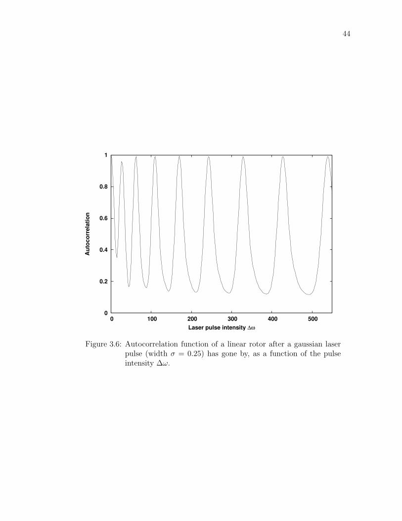
44
0
0.2
0.4
0.6
0.8
1
0 100 200 300 400 500
Aut
ocor
rela
tion
Laser pulse intensity ∆ω
Figure 3.6: Autocorrelation function of a linear rotor after a gaussian laserpulse (width σ = 0.25) has gone by, as a function of the pulseintensity ∆ω.
Chapter 4
Energy Level Spacing DistributionsQuantum level spacing distributions for rotors in laser and static electric fields are
calculated. Following a review of conceptual and historical development of this
subject, the results emphasize that this approach qualitatively correlates classical
chaos with purely quantum data. The analagous classical calculation is much more
difficult than the quantum method presented here.
Spacing distributions (often called nearest neighbor spacing distributions) can
describe many different phenomena—anything that occurs sequentially, from quan-
tum energy levels, to roots of the Riemann zeta function, to bridges over a high-
way. Hayes [22] wrote an entertaining article exploring this facet. Haake [23] wrote
a useful technical book connecting level spacing distributions with time reversal
symmetry and random matrix theory, which is the basis for much of the material
presented here. Gutzwiller [24, Ch. 16] has a nice overview.
A condensed version of this chapter has been published as Section V of ref.
[25].
4.1 Avoided Crossings and Classical Chaos
It all starts with avoided crossings. They have long been studied by semiclassical
methods since they present the challenge of being superficially purely a quantum
phenomenon. But for those looking for further facets of the classical-quantum
correspondence, the eigenstates during an avoided crossing behave analogously to
classical invariant torii breaking by a nonintegrable perturbation.
Figure 4.1 shows an isolated avoided crossing in an energy correlation diagram
45

46
-40
-30
-20
-10
10 20 25 30 40
Ene
rgy
ω 0 0.25 0.5 0.75 1
ψ2
θ/π
(a)
(b)
(c)
(d)
(e)
Figure 4.1: Avoided crossing of sixth (bottom) and seventh (top) eigenstatesof a linear rotor in collinear fields, ∆ω = 150, M = 0 with energycorrelation diagram at left and probability distributions at right(a)-(e) ω = 20, 24, 24.5, 25, 30.
and corresponding probability distributions of the sixth and seventh eigenstates
of a linear rotor with ∆ω = 150, β = 0, M = 0 and several close values of ω.
At ω = 20 the states have different character, two nodes in the right-hand well
versus three nodes in the left-hand well. The states start to noticeably obtain each
others character at ω = 24. The states are almost identical, except the higher
energy one has a node in the middle, at ω = 24.5 which just about corresponds to
the sharply avoided crossing in the energy correlation diagram in the Figure. For
further increases in ω, the states fully exchange character—thus the state with two
nodes in the right hand well becomes the one with higher energy.
During the avoided crossing each wave function occupies more of coordinate
space through delocalization. When a classical system is perturbed, typically
some invariant torii break to form stochastic layers visible in a surface of sec-
tion. A stochastic layer or region is formed, in principle, by one trajectory which
wanders through more of coordinate space than it did when it was constrained to
a torus. Thus in both quantum avoided crossings and classical irregularities, the
47
system occupies more space. This is the physical connection that suggests avoided
crossings and chaos can be quantitatively linked.
Let’s approach the connection from the quantum side. Avoided crossings can be
hard to spot in a correlation diagram. Some are easy to to spot, such as in Figure
4.1. Others may be so close to crossing they appear to truly cross. Some may
be so widely avoided you couldn’t guess that the states are significantly mixing.
Some avoided crossings may involve more than two states, producing behavior not
usually considered in simple theories. In short, this is a complicated business.
A way out is to statistically analyze the energy level spacings. A higher average
level spacing througout a spectrum should mean more chaos in the related classical
phase space. One way this connection has been explored is with nearest neighbor
spacing distributions.
4.2 Definition and History
The spacing distribution P (s) is the probability of finding a spacing s between two
adjacent energy levels in a small interval centered at s. In practice, level spacings
from calculation or experiment are sorted into a histogram, whose bar heights
approximate a smooth P (s). In theory, the limits of no level repulsion and linear
level repulsion are known exactly. Heuristic derivations∗ of these forms follow.
A spacing s is formed if there are levels at x and x+s with none in the interval
I = (x, x+ s). Also define an infinitesimal interval dI = (x+ s, x+ s+ ds). The
probability there is exactly one level in dI given no levels in I is defined as µ(s).
∗This derivation is from Bohigas and Giannoni [26] who credit Wigner [27], butI could only find a puzzling sketch of this derivation in that article. A later articleby Wigner [28] derives these distributions with differential equations.
48
Thus the probability P (s) that given a level at x the next level is in dI is
P (s) = (prob. no level in I)× (one level in dI given no level in I)
=
(1−
∫ s
0
P (s′) ds′)× µ(s)
=
(∫ ∞
s
P (s′) ds′)µ(s)
This simple integral equation has the solution
P (s) = Cµ(s) exp
(−
∫ s
µ(s′) ds′)
where C is a normalization constant. In the first case, suppose µ(s) is constant,
meaning the next level may occur anywhere after x regardless of s. Then there is
no correlation between levels. In the second case, suppose µ(s) ∝ s, meaning the
next level cannot be at s ≈ 0. The corresponding forms of the spacing distribution
are†
P (s) =
e−s no level repulsion → exponential, “Poisson”
π2se−πs2/4. linear level repulsion → “Wigner”
(4.1)
The important difference is P (0) is unity for the exponential distribution and
zero for the Wigner distribution. The forms of µ(s) show that spectra with un-
correlated levels have many small spacings, while linearly repulsed levels have few
small spacings. Both distributions approach zero as s becomes large because of the
decreasing exponential factor, despite the forms of µ(s) being non-zero in this limit.
The exponential has maximum probability at s = 0 while the Wigner maximum
is close to s = 1.
†Schlier [29] reminds us to call this distribution exponential despite thewidespread use of Poisson, since that name is widely used for a different statisticaldistribution.
49
The exponential spacing distribution results from a Poisson “process” formed
by the quantum energy levels. Normally one thinks of a Poisson process as any
sequence of events in which occurrences after any given time are independent of
occurrences before that time—as with individual radioactive decays. This directly
implies the exponential law governing first order kinetics. In terms of energy levels,
the appearance of each level after the previous does not depend on how much
energy range has been passed since the previous level. Many call such a spectrum
“random” or “uncorrelated” since it obeys this law, and P (s) = e−s must be the
corresponding spacing distribution.
Wigner developed his distribution (the “Wigner surmise”) while studying nu-
clear spectra. [28] He discovered that the statistics of nuclear spectra are the same
as the eigenvalue statistics of random matrices. That is, a set of random hermi-
tian matrices (the Gaussian Orthogonal Ensemble) taken as Hamiltonians provided
eigenvalues with exactly the same spacing distribution as the experimental nuclear
spectra. Porter [30] collected important articles that reflect the state in 1965.
Perhaps the first connection of classical dynamics to quantum level spacing
distribution was given by Percival [31] in 1973. He qualitatively showed how there
should be a quantum-classical correspondence between regular/irregular spectra
and regular/irregular dynamics. Gradually, people began calculating spacing dis-
tributions for model systems, like harmonic oscillators [32] and Sinai billiards [33].
In sum, various authors did numerical work that verified regular and fully chaotic
systems provide exponential and Wigner spacing distributions, respectively. Bohi-
gas and Giannoni [26] provide a review of work done to 1984.
The most important work of these early years was furthering semi-classical
understanding of the spacing distributions analytically and numerically. Berry
50
and Robnik [34] derived a distribution of quantum spacings starting from a generic
classical system that has a mixed phase space with one connected chaotic region
and an arbitrary number of isolated regular regions. This formula is never used.
Instead, the simplest case with one regular region is always used. This is sometimes
the case when it is applied; often this constraint is ignored. The distribution
has one adjustable parameter that interpolates between exponential (q = 0) and
Wigner (q = 1). Intermediate values of q correlate to the fraction of chaotic phase
space in the classical system. The Berry-Robnik distribution is
PBR(s) = (1− q)2e−(1−q)s erfc
[√π
2qs
]+
[2q(1− q) +
π
2sq3
]e−(1−q)s−π
4s2q2
. (4.2)
In 1981, Brody et. al [35] published a review article on statistical theories of
nuclear spectra. They included a distribution that empirically interpolates between
exponential and Winger. That is, there is no theoretical basis at all for the formula.
They termed q the “repulsion parameter” since it measured repulsion between
energy levels. The Brody distribution is
PBrody(s) = (1 + q)βxq exp(−βx1+q
)(4.3)
β =
[Γ
(q + 2
q + 1
)]q+1
.
The Brody and Berry-Robnik distributions are both used to estimate the fraction
of chaotic classical phase space using only quantum energies. Berry-Robnik has a
rigorous semi-classical foundation while Brody does not.
Later, researchers began studying systems relevant to atomic and molecular
physics. For instance, level spacing distributions of hydrogen atom in a magnetic
field [36] and combined electric and magnetic fields with arbitrary mutual orien-
tation [37] have been calculated to study the transition from irregular to regular
51
classical dynamics. In all studies of this sort, Brody or Berry-Robnik parameters
serve as a guide for determining or confirming classical phase space structure.
Several people have worked on rotor problems specifically. Grozdanov and Mc-
Carroll [38] calculated level spacing distributions of an asymmetric rotor in a static
electric field. They divided a spectrum of 1300 levels into three sections and showed
how the spacing distribution evolves from Wigner to exponential with increasing
energy, suggesting the classical phase space evolves from chaos to regularity. Man-
fredi and Salasnich published [39], and then corrected [40], an assertion that free
asymmetric rotor energies formed the anomalous distribution peaked at s = 1
seen by Berry [32] for harmonic oscillators. There were mistaken because they
reduced the fully three dimensional asymmetric rotor system to one dimension (all
levels corresponding to changing one good quantum number) which is guaranteed
to yield the anomalous distribution. (This is discussed fully below, Section 4.3.)
Lastly, Marchesan et. al. [41] calculated spacing distributions using experimental
data and show coupling between internal and total rotation of methanol, based on
transition from exponential to Wigner spacing distribution.
4.3 Interpreting Nearest Neighbor Spacing Distributions
The basic effect producing Wigner behavior, i.e. P (s) → 0 as s→ 0, in the spacing
distribution is level repulsion. This should only arise when the system has coupled
degrees of freedom and chaotic phase space. When either of these conditions are
not fulfilled, we expect exponential behavior, i.e P (s) → 1 as s→ 0, in the spacing
distribution.
First, a one DOF system has a Dirac delta spacing distribution peaked at
s = 1. This is obviously true for the harmonic oscillator, which has equispaced
52
levels. But after the unfolding process (Section 4.4), one DOF spectra, such as
the anharmonic oscillator spectrum, are transformed and resemble the harmonic
oscillator spectrum. Some pathological one DOF systems yielding a Wigner spac-
ing distribution may be constructed, [42] but they are certainly not germane to
models studied here.
A n DOF separable system (trivially completely regular) decomposes into n
one-dimensional problems, producing a completely uncorrelated spectrum and an
exponential spacing distribution. Each energy level of the full system is a n-fold
sum of energy levels, one from each separate one DOF spectrum. The individual
spectra are not correlated with each other, and thus the full spectrum is uncorre-
lated. The spacing distribution is exponential, corresponding to completely regular
dynamics.
A n > 1 DOF coupled (nonseparable) system will have some, perhaps small,
degree of chaos. A chaotic trajectory breaks away from an unperturbed n-torus and
samples more than n dimensions of phase space. The corresponding quantum effect
is an avoided crossing, where two states mix and occupy previously unaccessed
configuration space while the energies repel (Section 4.1). Thus a spectrum with
many avoided crossings corresponds to chaotic classical dynamics, and the level
spacing distribution P (s) → 0 as s→ 0, quite unlike the exponential distribution.
A spectrum corresponding to mixed phase space, with both regular and irregular
regions, will provide P (0) between zero and one, intermediate between Wigner and
exponential behavior.
Also, any two uncorrelated spectra, no matter the internal correlations, will
combine to form an exponential spacing distribution. Thus when a Wigner spacing
distribution is found, we can be confident the underlying dynamical mechanism
53
is classical chaos and not an artifact. If a combined spectrum is exponential,
it could be that all underlying spectra are exponential, or that (in a four DOF
system with two separate chaotic subsystems) two separate spectra with Wigner
spacing distributions have been combined. In the first case, regular dynamics truly
support the exponential spacing distribution. In the second irregular dynamics
falsely support an exponential spacing distribution.
Harmonic oscillators form the single known exception to this discussion. Berry
[32] explored various incommensurate two DOF harmonic oscillators and found
spacing distributions peaked away from s = 0. This is apparently an artifact of
the exactly equal level spacings of the underlying one DOF harmonic oscillators.
This effect can cause confusion if the spectrum contains some harmonic oscillator-
like equispaced levels. The equal spacings support a spacing distribution peak at
s = 1, which appears to be signature Wigner character to the untrained eye.
4.4 How to Obtain a Nearest Neighbor Spacing Histogram
The basic idea is to take adjacent energy levels in a spectrum and calculate their
differences (“spacings”), and then sort them into histogram bins. However, some
laborious procedures are needed to work around a few problems.
First, many Hamiltonians have discrete symmetries leading to trivially uncorre-
lated spectra. The linear rotor-tilted fields Hamiltonian has reflection plane (σXZ)
symmetry. The full Hamiltonian matrix can be block diagonalized through a basis
transformation into two sub-blocks. The new basis functions are eigenfunctions
of the symmetry operator. Each sub-block can be independently diagonalized to
produce a sub-spectrum. In our case, two sub-blocks produce two independent
spectra associated with states having positive and negative parity with respect
54
to reflection plane symmetry. As the two spectra are independent and will pro-
duce exponential nearest neighbor spacing distributions when the full spectrum is
analyzed, we must consider one symmetry species at a time.
Second, we want to compare different systems which may have inherently differ-
ent energy scales and level densities, so that a raw energy spacing in one spectrum
is not directly comparable to a spacing from a different system. In particular for
rotational spectra, different energy regions of a single spectrum can have different
local level densities. These barriers are surmounted by reducing all spectra to unit
mean level density by “unfolding” them. The spacings in the unfolded spectra are
histogrammed.
Here is how the unfolding process works. A given spectrum {Ei} has raw spac-
ings {Ei+1 − Ei}, which are not suitable for histogramming as just discussed. To
remedy the problem of varying level density between systems we want to com-
pare, we might try to use the staircase function N(E), defined as the number of
energy levels with Ei ≤ E. N(E) maps the spectrum to one with exactly unit
level spacings and thus exactly unit level density, no matter the original spec-
trum . (The graph of N(E) resembles a jagged staircase over the entire spectrum,
each step having height one at each eigenenergy Ei.) The new spectrum {N(Ei)}
contains no information about the original raw spacings since all spacings have
been mapped to unity: the new spacings {N(Ei+1) − N(Ei)} are all identically
one, by definition. But if the jagged staircase N(E) is replaced with a smooth
low-order polynomial approximation N(E), some useful spectral fluctuations are
reintroduced. Whereas with N(E) the average level spacing was exactly one, with
N(E) the average spacing N(Ei+1) − N(Ei) is approximately unity because the
individual spacings now fluctuate about unity by construction. In other words, the
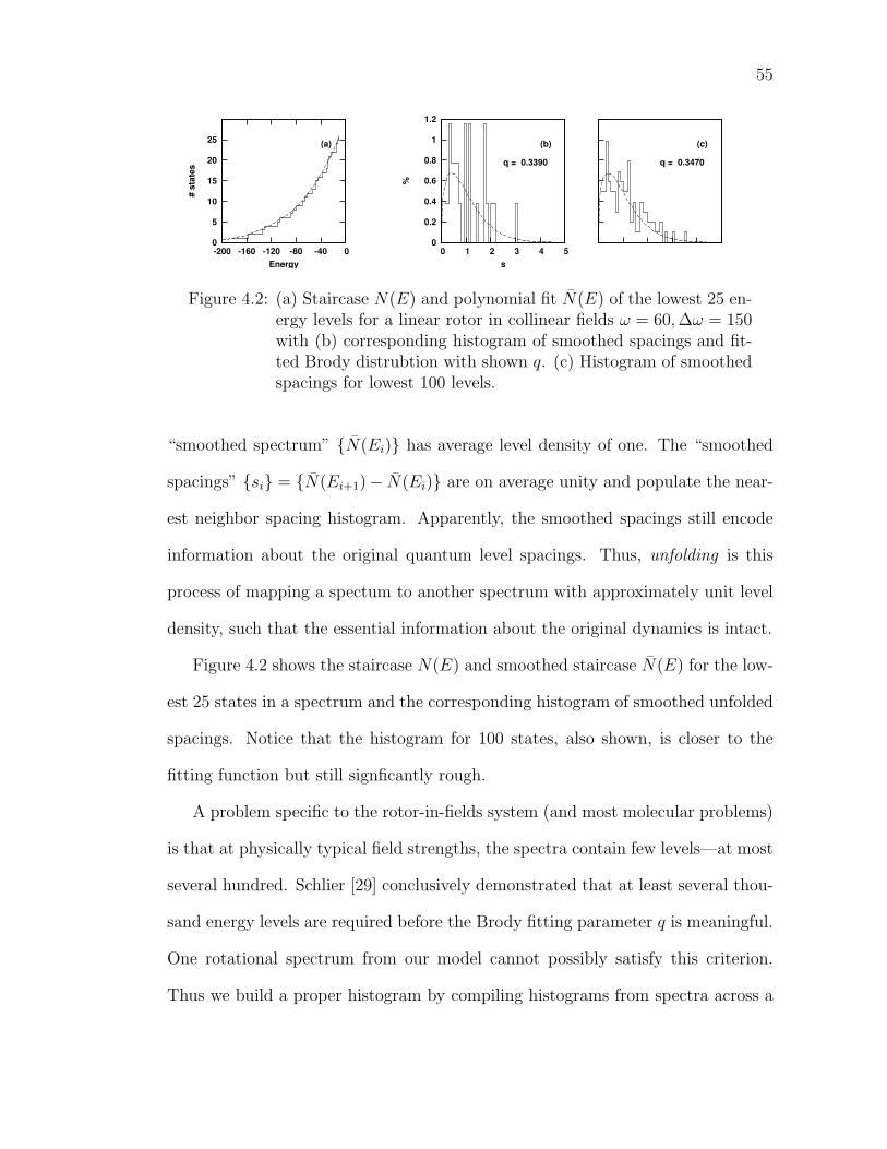
55
0
5
10
15
20
25
-200 -160 -120 -80 -40 0
# st
ates
Energy
(a)
0
0.2
0.4
0.6
0.8
1
1.2
0 1 2 3 4 5
%
s
(b)
q = 0.3390
(c)
q = 0.3470
Figure 4.2: (a) Staircase N(E) and polynomial fit N(E) of the lowest 25 en-ergy levels for a linear rotor in collinear fields ω = 60,∆ω = 150with (b) corresponding histogram of smoothed spacings and fit-ted Brody distrubtion with shown q. (c) Histogram of smoothedspacings for lowest 100 levels.
“smoothed spectrum” {N(Ei)} has average level density of one. The “smoothed
spacings” {si} = {N(Ei+1)− N(Ei)} are on average unity and populate the near-
est neighbor spacing histogram. Apparently, the smoothed spacings still encode
information about the original quantum level spacings. Thus, unfolding is this
process of mapping a spectum to another spectrum with approximately unit level
density, such that the essential information about the original dynamics is intact.
Figure 4.2 shows the staircase N(E) and smoothed staircase N(E) for the low-
est 25 states in a spectrum and the corresponding histogram of smoothed unfolded
spacings. Notice that the histogram for 100 states, also shown, is closer to the
fitting function but still signficantly rough.
A problem specific to the rotor-in-fields system (and most molecular problems)
is that at physically typical field strengths, the spectra contain few levels—at most
several hundred. Schlier [29] conclusively demonstrated that at least several thou-
sand energy levels are required before the Brody fitting parameter q is meaningful.
One rotational spectrum from our model cannot possibly satisfy this criterion.
Thus we build a proper histogram by compiling histograms from spectra across a
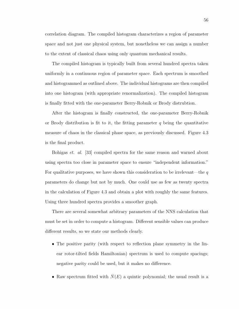
56
correlation diagram. The compiled histogram characterizes a region of parameter
space and not just one physical system, but nonetheless we can assign a number
to the extent of classical chaos using only quantum mechanical results.
The compiled histogram is typically built from several hundred spectra taken
uniformly in a continuous region of parameter space. Each spectrum is smoothed
and histogrammed as outlined above. The individual histograms are then compiled
into one histogram (with appropriate renormalization). The compiled histogram
is finally fitted with the one-parameter Berry-Robnik or Brody distrubtion.
After the histogram is finally constructed, the one-parameter Berry-Robnik
or Brody distribution is fit to it, the fitting parameter q being the quantitative
measure of chaos in the classical phase space, as previously discussed. Figure 4.3
is the final product.
Bohigas et. al. [33] compiled spectra for the same reason and warned about
using spectra too close in parameter space to ensure “independent information.”
For qualitative purposes, we have shown this consideration to be irrelevant—the q
parameters do change but not by much. One could use as few as twenty spectra
in the calculation of Figure 4.3 and obtain a plot with roughly the same features.
Using three hundred spectra provides a smoother graph.
There are several somewhat arbitrary parameters of the NNS calculation that
must be set in order to compute a histogram. Different sensible values can produce
different results, so we state our methods clearly.
• The positive parity (with respect to reflection plane symmetry in the lin-
ear rotor-tilted fields Hamiltonian) spectrum is used to compute spacings;
negative parity could be used, but it makes no difference.
• Raw spectrum fitted with N(E) a quintic polynomial; the usual result is a

57
slightly non-parabolic quintic.
• Histogram bins have width ∆ = 0.10; smaller values are feasible, and larger
values have been used but this seems like a good compromise between sorting
accuracy and histogram smoothness.
• The Berry-Robnik or Brody distribution is fitted to the final histogram at
the righthand bin edge, i.e. at s = 0.1, 0.2, . . . not at s = 0, 0.1, . . .. Tri-
als using the latter points produced sloping results when the former results
trended flat. Also, it seems that putting a fit point right at s = 0 which
would inaccurately reflect the range of spacings sorted into that bin, since
the ultimate difference between exponential and Wigner behavior of P (s) is
the value at s = 0. Apparently our value of histogram bin width keeps this
calculation under control.
4.5 Results
We studied linear rotors in collinear and tilted fields with nearest neighbor spacing
histograms. For each compiled histogram, the fitted Brody parameter quantifies
the extent of classical chaos.
Figure 4.3 shows compiled spacing histograms for a linear rotor in collinear
fields of strength ω = 60,∆ω = 150 → 300 (increments of 0.5, for a total of
301 spectra). The three presented histograms use the lowest N energies in each
spectrum for N = 25, 50, and 100. The calculation uses 400 states at each point
in the correlation diagram, starting at the ground state. The energies for ω =
60,∆ω = 150 are in (−184, 724) with thirty bound states. When ω = 60,∆ω = 300
the energies are in (−325, 670) with sixty bound states.
58
0
0.2
0.4
0.6
0.8
1
0 1 2 3 4 5
Prob
ablit
y
s
q = 0.3605
q = 0.2303
q = 0.1206
Figure 4.3: Compiled nearest neighbor spacing histograms for a linear rotorin collinear fields, ω = 60,∆ω = 150 → 300 (increments of 0.5),using the N lowest levels in each spectrum: (left) N = 25, (cen-ter) N = 50, (right) N = 100. The Brody distribution is fit tothe histograms with shown q.
The important point is that even though we know the classical phase space is
entirely regular (no chaotic regions) the spacing distributions indicate significant
irregularity if too few spacings are used. We expect Brody parameter q = 0. From
these plots, 25×301 produces a jagged histogram with a medium Brody parameter
q = 0.36. However, using 100 × 301 yields a smoother histogram with low, but
not zero, Brody parameter q = 0.12. Clearly this method is not foolproof and will
only safely produce qualitative results.
Let us briefly review the classical phase space structure of linear rotors in
tilted fields. Figure 4.4 shows surfaces of section at several tilt angles and energies
well below, just below, and well above the rotational barrier. Clearly the classical
structure is regular at all energies when β = 0. At tilt angle β = π/4 and π/2, there
is little if any chaos at high and low energy but is rife at intermediate energy. One
might naively estimate the chaotic fraction of phase space to be 70% for (e). But
different sections may show different relative chaotic volumes. Certainly a θ = 4π/5
section corresponding to (e) would not have any regular regions associated with
the stable wells which are rigorously θ-localized elsewhere. Calculating chaotic
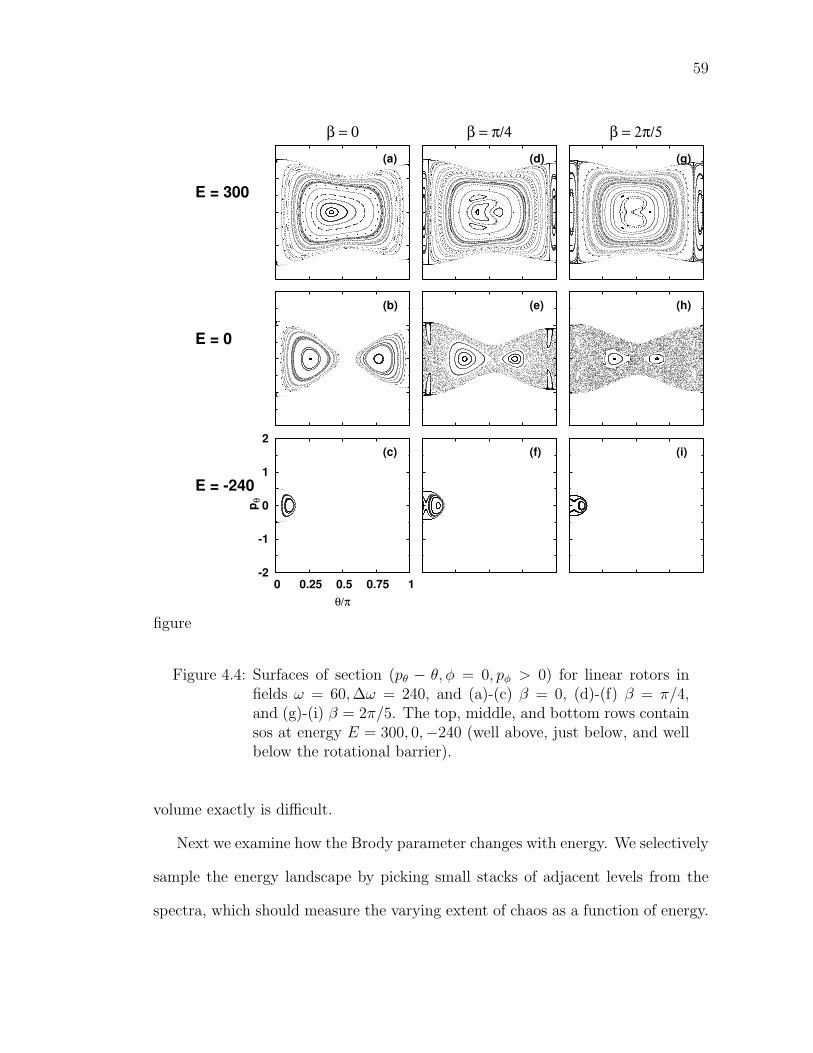
59
figure
-2
-1
0
1
2
0 0.25 0.5 0.75 1
pθ
θ/π
(c)
E = -240
(b)
E = 0
(a)
E = 300
β = 0
(f)
(e)
(d)
β = π/4
(i)
(h)
(g)
β = 2π/5
Figure 4.4: Surfaces of section (pθ − θ, φ = 0, pφ > 0) for linear rotors infields ω = 60,∆ω = 240, and (a)-(c) β = 0, (d)-(f) β = π/4,and (g)-(i) β = 2π/5. The top, middle, and bottom rows containsos at energy E = 300, 0,−240 (well above, just below, and wellbelow the rotational barrier).
volume exactly is difficult.
Next we examine how the Brody parameter changes with energy. We selectively
sample the energy landscape by picking small stacks of adjacent levels from the
spectra, which should measure the varying extent of chaos as a function of energy.
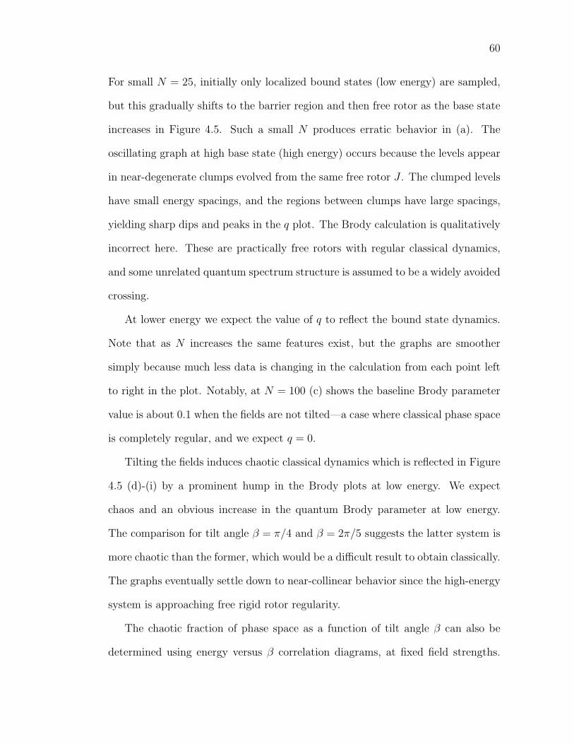
60
For small N = 25, initially only localized bound states (low energy) are sampled,
but this gradually shifts to the barrier region and then free rotor as the base state
increases in Figure 4.5. Such a small N produces erratic behavior in (a). The
oscillating graph at high base state (high energy) occurs because the levels appear
in near-degenerate clumps evolved from the same free rotor J . The clumped levels
have small energy spacings, and the regions between clumps have large spacings,
yielding sharp dips and peaks in the q plot. The Brody calculation is qualitatively
incorrect here. These are practically free rotors with regular classical dynamics,
and some unrelated quantum spectrum structure is assumed to be a widely avoided
crossing.
At lower energy we expect the value of q to reflect the bound state dynamics.
Note that as N increases the same features exist, but the graphs are smoother
simply because much less data is changing in the calculation from each point left
to right in the plot. Notably, at N = 100 (c) shows the baseline Brody parameter
value is about 0.1 when the fields are not tilted—a case where classical phase space
is completely regular, and we expect q = 0.
Tilting the fields induces chaotic classical dynamics which is reflected in Figure
4.5 (d)-(i) by a prominent hump in the Brody plots at low energy. We expect
chaos and an obvious increase in the quantum Brody parameter at low energy.
The comparison for tilt angle β = π/4 and β = 2π/5 suggests the latter system is
more chaotic than the former, which would be a difficult result to obtain classically.
The graphs eventually settle down to near-collinear behavior since the high-energy
system is approaching free rigid rotor regularity.
The chaotic fraction of phase space as a function of tilt angle β can also be
determined using energy versus β correlation diagrams, at fixed field strengths.
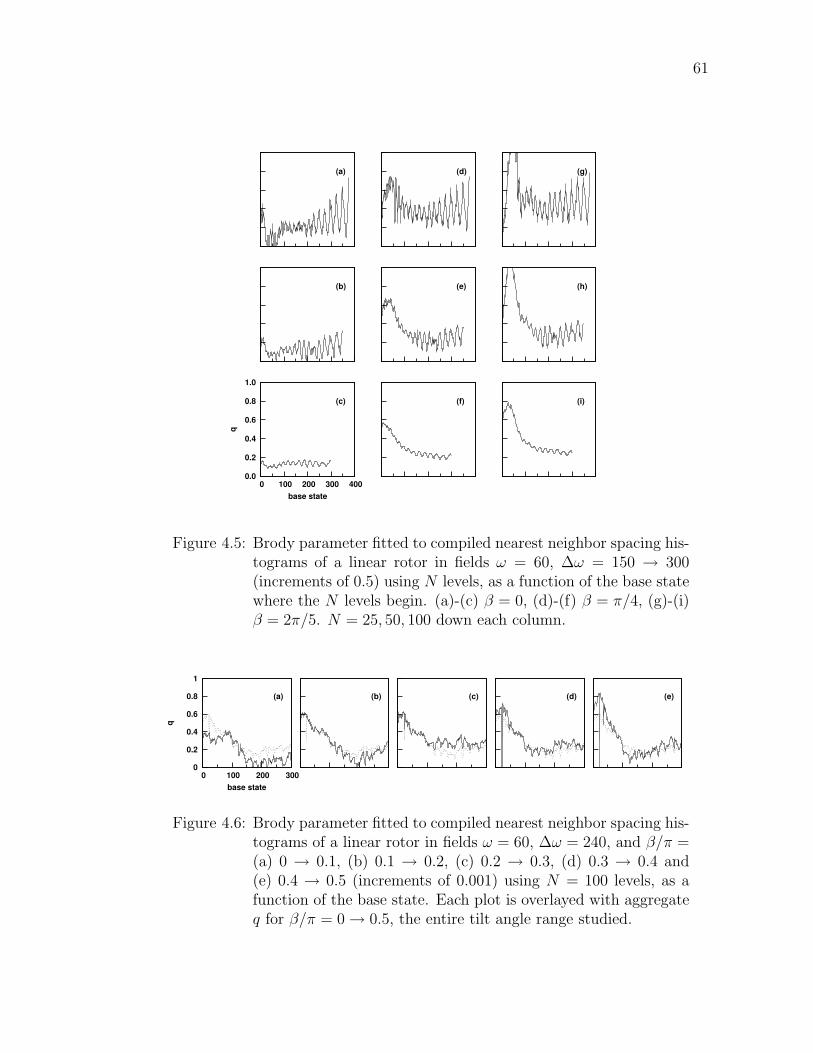
61
(a)
(b)
(d)
(e)
(f)
(g)
(h)
(i)
0.0
0.2
0.4
0.6
0.8
1.0
0 100 200 300 400
q
base state
(c)
Figure 4.5: Brody parameter fitted to compiled nearest neighbor spacing his-tograms of a linear rotor in fields ω = 60, ∆ω = 150 → 300(increments of 0.5) using N levels, as a function of the base statewhere the N levels begin. (a)-(c) β = 0, (d)-(f) β = π/4, (g)-(i)β = 2π/5. N = 25, 50, 100 down each column.
0
0.2
0.4
0.6
0.8
1
0 100 200 300
q
base state
(a) (b) (c) (d) (e)
Figure 4.6: Brody parameter fitted to compiled nearest neighbor spacing his-tograms of a linear rotor in fields ω = 60, ∆ω = 240, and β/π =(a) 0 → 0.1, (b) 0.1 → 0.2, (c) 0.2 → 0.3, (d) 0.3 → 0.4 and(e) 0.4 → 0.5 (increments of 0.001) using N = 100 levels, as afunction of the base state. Each plot is overlayed with aggregateq for β/π = 0 → 0.5, the entire tilt angle range studied.
62
Figure 4.6 shows the Brody parameter fitted to level spacing histograms compiled
as β changes, for a linear rotor in fields ω = 60 and ∆ω = 240. Panel (a) corre-
sponds to the tilt angle region closest to collinearity, β = 0 → 0.1π. Also plotted
is the aggregate Brody parameter corresponding to levels collected over the whole
β = 0 → 0.5π domain. (This is reproduced in all five panels.) Thus panel (a)
reveals a lower chaotic fraction in the near-collinear region than over the whole
domain, which is sensible. The next panel (b) for β/π = 0.1 → 0.2 shows almost
identical behavior relative to the aggregate. The further panels (c), (d), and (e)
each show increasing Brody parameter relative to the aggregate, particularly in
the low energy (low base state N) regime, suggesting chaos is most important at
energies near the rotational barriers when β/π ∼ 0.4 or 0.5. This is in accord with
Figure 4.5.
Chapter 5
Other Semi-Quantum ApproachesHere several other semi-quantum techniques are developed and applied to the rigid
rotor in fields model. Illustrations of the classical-quantum correspondence seen
here are mostly conceptual and qualitative. Nonetheless, they are interesting and
may serve as starting points for future quantitative work. Certainly periodic orbits
[24] have long been used in other systems, and the modern topic of monodromy
[43] has yet to find a great application.
5.1 Monodromy
The basic goal of any physics problem is to solve the equations of motion. This is
only analytically possible for a few simple models. In classical mechanics this means
solving for action-angle variables, one pair for each degree of freedom. In quantum
mechanics this means obtaining formulas for eigenenergies and eigenstates, which
always result from separating Schrodinger’s equation for n DOF into n ordinary
differential equations. There is no obvious way to a priori know whether a given
system is analytically solvable, but existence of monodromy necessarily forbids an
analytic solution.
Monodromy (“once around”) existence can be determined using a simple dia-
gram of relative equilibria, whose construction is now explained in terms of our
linear rotor in collinear fields problem. This model has cylindrical symmetry corre-
sponding to the angular momentum projection M being a good quantum number.
That is, the motion in azimuthal angle φ has successfully been separated and
analytically solved. The motion in polar angle θ has yet to be solved. But by
63

64
calculating the extrema of the classical effective potential energy surface
Veff(θ;m) =m2
sin2 θ+ V (θ)
(where m is the classical analog of quantized M) some features of the system are
revealed. The solutions of ∂Veff(θ;m)∂θ
= 0 are called relative equilibria, as opposed
to global equilibria, because for nonzero m the system is actually moving but θ
is constant. The potential energy of the classical relative equilibria are plotted as
a function of m, forming an energy vs. m picture. The quantum energy levels
can be superimposed, and they nest nicely inside the classical lines, as evident in
Figure 5.1 for a linear rotor in a static electric field ω = 60. Now monodromy is
illustrated as follows.
Pick a quantum level in the figure, and then join it to an adjacent state. This
serves as a local definition of quantum number, and by logical extension of your line
segment a global definition of the quantum number should be established. This
would be a handy definition to use so as to completely classify a spectrum. The
process is pictured by parallel transport of a “cell” of adjacent quantum states.
Transport carries this cell around an isolated unstable equilibrium at m = 0. At
every stage the obvious extension of the local definition is made, but after go-
ing once around the unstable equilibrium the cells do not match. Apparently the
local definition has changed. In other words, no global definition of the the quan-
tum numbers is possible, meaning the Schrodinger equation cannot be analytically
solved for this system. The classical analog is that no global set of action-angle
variables can be analytically found.
Figure 5.2 shows energy vs. M diagrams for linear rotors in collinear fields.
The left and right panels display systems with monodromy, corresponding to a
linear rotor in static and collinear fields. For the static field, cell parallel transport
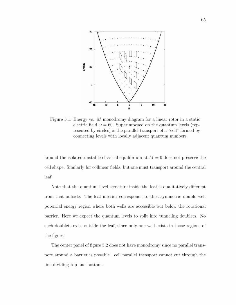
65
Figure 5.1: Energy vs. M monodromy diagram for a linear rotor in a staticelectric field ω = 60. Superimposed on the quantum levels (rep-resented by circles) is the parallel transport of a “cell” formed byconnecting levels with locally adjacent quantum numbers.
around the isolated unstable classical equilibrium at M = 0 does not preserve the
cell shape. Similarly for collinear fields, but one must transport around the central
leaf.
Note that the quantum level structure inside the leaf is qualitatively different
from that outside. The leaf interior corresponds to the asymmetric double well
potential energy region where both wells are accessible but below the rotational
barrier. Here we expect the quantum levels to split into tunneling doublets. No
such doublets exist outside the leaf, since only one well exists in those regions of
the figure.
The center panel of figure 5.2 does not have monodromy since no parallel trans-
port around a barrier is possible—cell parallel transport cannot cut through the
line dividing top and bottom.
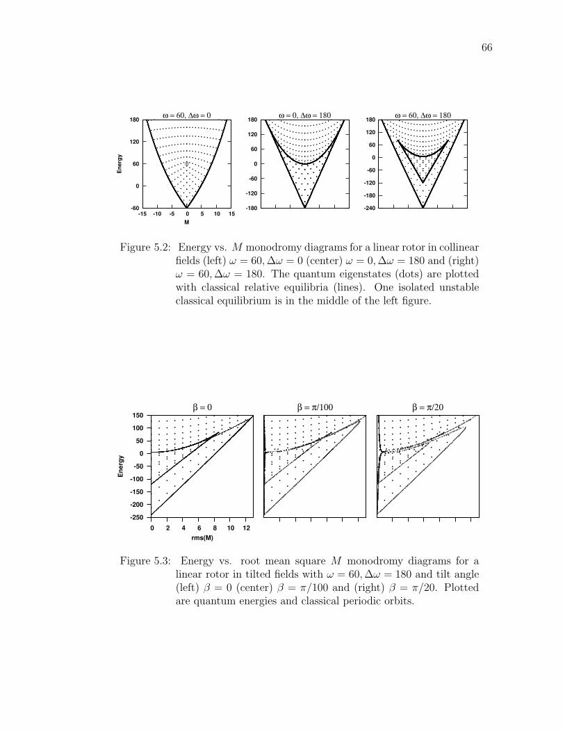
66
-60
0
60
120
180
-15 -10 -5 0 5 10 15
Ener
gy
M
ω = 60, ∆ω = 0
-180
-120
-60
0
60
120
180 ω = 0, ∆ω = 180
-240
-180
-120
-60
0
60
120
180 ω = 60, ∆ω = 180
Figure 5.2: Energy vs. M monodromy diagrams for a linear rotor in collinearfields (left) ω = 60,∆ω = 0 (center) ω = 0,∆ω = 180 and (right)ω = 60,∆ω = 180. The quantum eigenstates (dots) are plottedwith classical relative equilibria (lines). One isolated unstableclassical equilibrium is in the middle of the left figure.
-250
-200
-150
-100
-50
0
50
100
150
0 2 4 6 8 10 12
Ener
gy
rms(M)
β = 0 β = π/100 β = π/20
Figure 5.3: Energy vs. root mean square M monodromy diagrams for alinear rotor in tilted fields with ω = 60,∆ω = 180 and tilt angle(left) β = 0 (center) β = π/100 and (right) β = π/20. Plottedare quantum energies and classical periodic orbits.
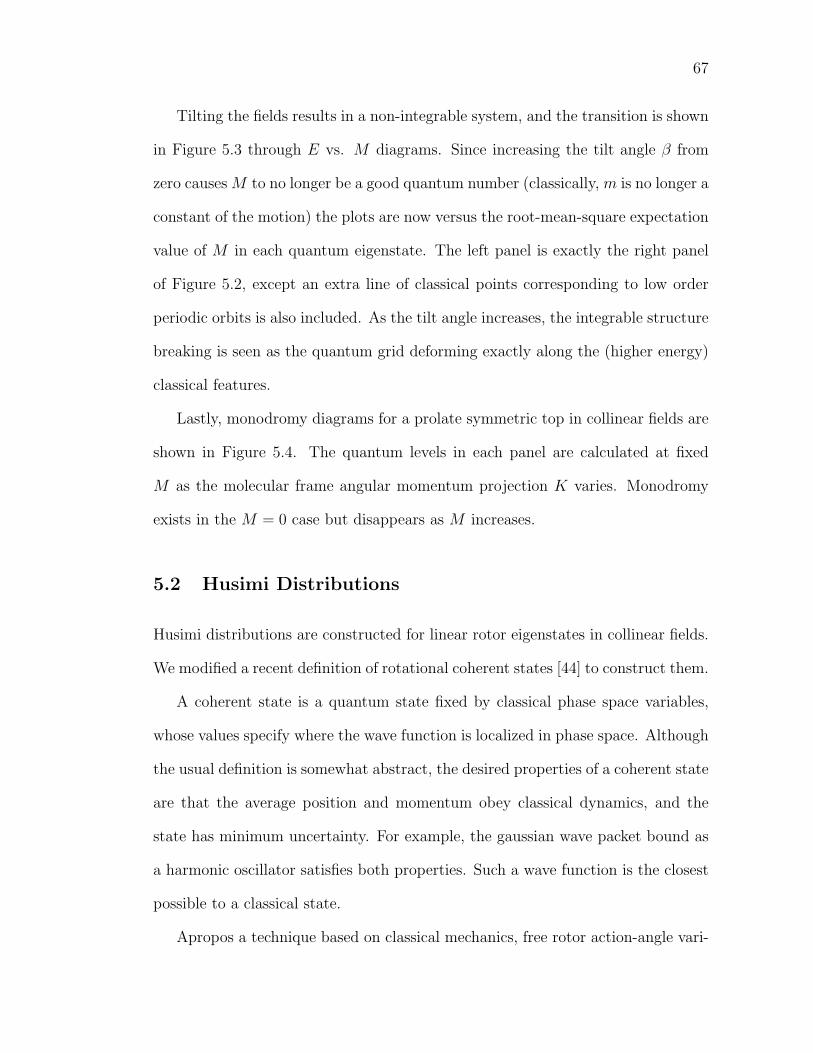
67
Tilting the fields results in a non-integrable system, and the transition is shown
in Figure 5.3 through E vs. M diagrams. Since increasing the tilt angle β from
zero causes M to no longer be a good quantum number (classically, m is no longer a
constant of the motion) the plots are now versus the root-mean-square expectation
value of M in each quantum eigenstate. The left panel is exactly the right panel
of Figure 5.2, except an extra line of classical points corresponding to low order
periodic orbits is also included. As the tilt angle increases, the integrable structure
breaking is seen as the quantum grid deforming exactly along the (higher energy)
classical features.
Lastly, monodromy diagrams for a prolate symmetric top in collinear fields are
shown in Figure 5.4. The quantum levels in each panel are calculated at fixed
M as the molecular frame angular momentum projection K varies. Monodromy
exists in the M = 0 case but disappears as M increases.
5.2 Husimi Distributions
Husimi distributions are constructed for linear rotor eigenstates in collinear fields.
We modified a recent definition of rotational coherent states [44] to construct them.
A coherent state is a quantum state fixed by classical phase space variables,
whose values specify where the wave function is localized in phase space. Although
the usual definition is somewhat abstract, the desired properties of a coherent state
are that the average position and momentum obey classical dynamics, and the
state has minimum uncertainty. For example, the gaussian wave packet bound as
a harmonic oscillator satisfies both properties. Such a wave function is the closest
possible to a classical state.
Apropos a technique based on classical mechanics, free rotor action-angle vari-
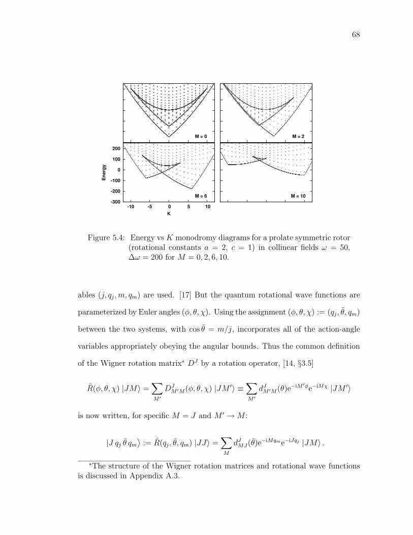
68
-300
-200
-100
0
100
200
-10 -5 0 5 10
Ener
gy
K
M = 6
M = 0 M = 2
M = 10
Figure 5.4: Energy vs K monodromy diagrams for a prolate symmetric rotor(rotational constants a = 2, c = 1) in collinear fields ω = 50,∆ω = 200 for M = 0, 2, 6, 10.
ables (j, qj,m, qm) are used. [17] But the quantum rotational wave functions are
parameterized by Euler angles (φ, θ, χ). Using the assignment (φ, θ, χ) := (qj, θ, qm)
between the two systems, with cos θ = m/j, incorporates all of the action-angle
variables appropriately obeying the angular bounds. Thus the common definition
of the Wigner rotation matrix∗ DJ by a rotation operator, [14, §3.5]
R(φ, θ, χ) |JM〉 =∑M ′
DJM ′M(φ, θ, χ) |JM ′〉 ≡
∑M ′
dJM ′M(θ)e−iM ′φe−iMχ |JM ′〉
is now written, for specific M = J and M ′ →M :
|J qj θ qm⟩
:= R(qj, θ, qm) |JJ〉 =∑M
dJMJ(θ)e−iMqme−iJqj |JM〉 .
∗The structure of the Wigner rotation matrices and rotational wave functionsis discussed in Appendix A.3.
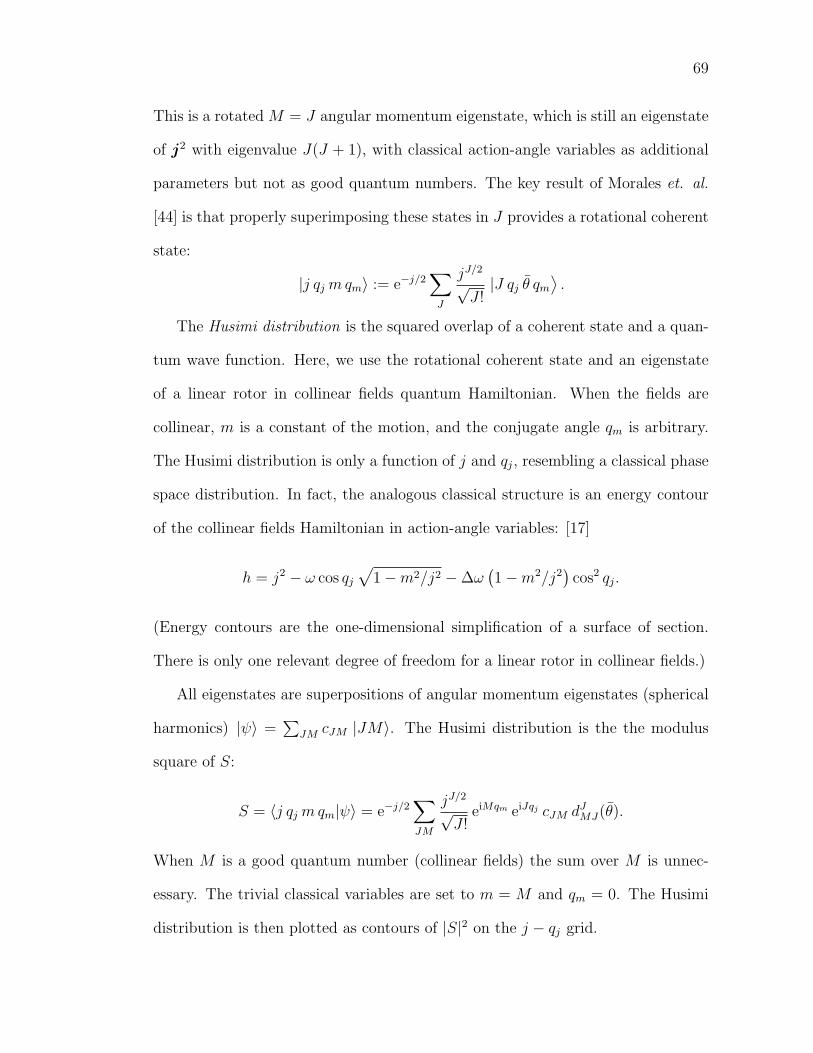
69
This is a rotated M = J angular momentum eigenstate, which is still an eigenstate
of j2 with eigenvalue J(J + 1), with classical action-angle variables as additional
parameters but not as good quantum numbers. The key result of Morales et. al.
[44] is that properly superimposing these states in J provides a rotational coherent
state:
|j qj mqm〉 := e−j/2∑
J
jJ/2
√J !|J qj θ qm
⟩.
The Husimi distribution is the squared overlap of a coherent state and a quan-
tum wave function. Here, we use the rotational coherent state and an eigenstate
of a linear rotor in collinear fields quantum Hamiltonian. When the fields are
collinear, m is a constant of the motion, and the conjugate angle qm is arbitrary.
The Husimi distribution is only a function of j and qj, resembling a classical phase
space distribution. In fact, the analogous classical structure is an energy contour
of the collinear fields Hamiltonian in action-angle variables: [17]
h = j2 − ω cos qj√
1−m2/j2 −∆ω(1−m2/j2
)cos2 qj.
(Energy contours are the one-dimensional simplification of a surface of section.
There is only one relevant degree of freedom for a linear rotor in collinear fields.)
All eigenstates are superpositions of angular momentum eigenstates (spherical
harmonics) |ψ〉 =∑
JM cJM |JM〉. The Husimi distribution is the the modulus
square of S:
S = 〈j qj mqm|ψ〉 = e−j/2∑JM
jJ/2
√J !
eiMqm eiJqj cJM dJMJ(θ).
When M is a good quantum number (collinear fields) the sum over M is unnec-
essary. The trivial classical variables are set to m = M and qm = 0. The Husimi
distribution is then plotted as contours of |S|2 on the j − qj grid.

70
qj/π
j
E = 127.7
0 0.5 1 1.5 2 0
5
10
15
20
qj/π
j
E = 127.7
0 0.5 1 1.5 2 0
5
10
15
20E = -70.6E = -70.6 E = 36.0E = 36.0
Figure 5.5: Husimi distributions of collinear fields eigenstates with ω =30,∆ω = 120,M = 0. First, third, and tenth lowest energiesfrom left to right. Heavy line is classical Hamiltonian contour atshown quantum eigenenergy.
Figure 5.5 shows several Husimi distributions of collinear fields eigenstates.
First let us relate these pictures to the asymmetric double well potential energy
surface reviewed in Section 1.6. The angle variable qj is directly related to the
Euler angle θ by [17]
qj = π/2− arcsinj cos θ√j2 −m2
mod 2π.
The PES extrema occur roughly at θ = 0, π (wells) and θ = π/2 (barrier). This
corresponds to wells at qj = 0, π (for m = 0) and barriers at qj = π/2, 3π/2.
(Multiple values of arcsin must be properly used.)
Thus the left panel of Figure 5.5, the Husimi distribution of the collinear fields
ground state, shows classical phase space distribution localized in the more stable
well. The center panel corresponds to an eigenstate of energy above both minima
but below the barrier, and it happens to be localized in the high-lying well. Note
that the heavy line is the corresponding classical Hamiltonian contour and shows
accessible phase space in both wells, but the Husimi distribution is clearly confined
71
to one well in this picture, as is the corresponding quantum eigenstate. The right
panel is the Husimi distribution for an an above barrier eigenstate. The contours
reflect accessible free rotation in qj at high j values but probability density maxima
for low j at the barrier. This is correct, since a classical particle with energy just
above a barrier slows down as it passes over due to energy conservation. Slowing
over a barrier means the particle is increasingly likely to be found (thus more
contours) at corresponding qj, albeit at lower momentum j.
Unfortunately, developing Husimi distributions for tilted fields is harder. When
M is not a good quantum number, the classical m is not conserved. The appro-
priate quantum analogue to the classical surface of section is not straightforward.
5.3 Periodic Orbits
Periodic orbits have long played a role in studying classical mechanics because
phase space tends to organize around them. For example, in the classical surfaces
of section Figure 4.4 the stable resonance zones are centered at a point, which
reveals the existence of a periodic orbit that pierces the surface only at that point.
The immediate phase space neighborhood consists of a dense set of quasi-periodic
orbits that revolve around the true periodic orbit.
It hardly suffices to just say it, but periodic orbits have played a major role
in semiclassical theories throughout the last thirty years. Certainly a high point
are the trace formulas [24, Ch. 17] that equate a quantum density of states to a
classical expression summed over periodic orbits.
We’ll leave it at that, and note that we have calculated eigenstates for the linear
rotor in tilted fields that nicely match classical periodic orbits, both stable (Figure
5.6) and unstable (Figure 5.7).
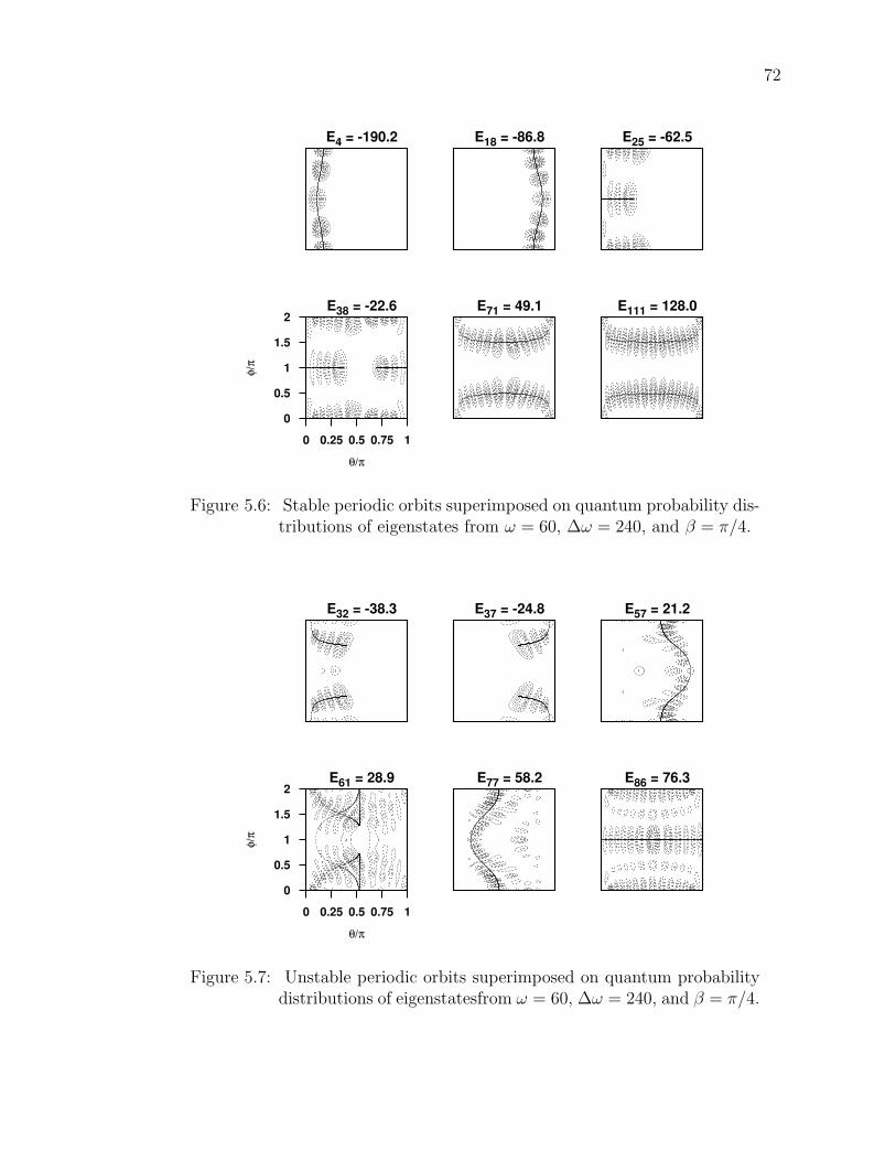
72
E4 = -190.2 E18 = -86.8 E25 = -62.5
2
1.5
1
0.5
00 0.25 0.5 0.75 1
φ/π
θ/π
E38 = -22.6 E71 = 49.1 E111 = 128.0
Figure 5.6: Stable periodic orbits superimposed on quantum probability dis-tributions of eigenstates from ω = 60, ∆ω = 240, and β = π/4.
E32 = -38.3 E37 = -24.8 E57 = 21.2
2
1.5
1
0.5
00 0.25 0.5 0.75 1
φ/π
θ/π
E61 = 28.9 E77 = 58.2 E86 = 76.3
Figure 5.7: Unstable periodic orbits superimposed on quantum probabilitydistributions of eigenstatesfrom ω = 60, ∆ω = 240, and β = π/4.
Chapter 6
Summary and Future WorkSoftware has been developed to calculate all the important quantities of rigid
rotating molecules in static electric and intense nonresonant laser fields, either
alone or combined at arbitrary tilt angle using quantum mechanics. Primarily,
this means energy levels and eigenstate probability distributions. The physically
prescient alignment and orientation parameters were also calculated. Furthermore,
arbitrary wave functions were numerically propagated under these Hamiltonians,
including the presently important area of rotors in pulsed laser fields.
In particular we have reproduced the basic quantum calculations presented by
Friedrich and Herschbach [4] for linear rotors in collinear fields. We extended their
results by tilting the fields apart and calculating the same quantities as in the
collinear case. The purpose was to investigate the quantum-classical correspon-
dence of a rotational model when the classical dynamics is irregular.
The software also simulates symmetric and asymmetric rotors in static and
intense nonresonant laser fields, although these results have not been presented
here.
The quantum propagation of a linear rotor in a pulsed, intense nonresonant
laser reproduced results from the literature; for instance, Ortigoso et. al. [21] We
have emphasized the importance of pulse width relative to the rotational period
regarding the post-pulse state and field-free alignment, as is well known, but also
how the pulse intensity delicately affects the outcomes.
Some aspects of the quantum-classical correspondence for rotors in fields were
developed. The main method was energy level spacing distributions for linear ro-
73
74
tors in tilted fields, which attempts to quantify the percentage of classical chaotic
phase space using only quantum mechanical energy levels. The method was fully
explained, including a technique for combining the data from spectra with too
few levels into one set, which was necessary for better statistics. Indeed, the fun-
damental problem confronted here was that relevant molecular models have, at
most, about one hundred levels in their spectrum which is too few for reliable re-
sults. Nevertheless, qualitative agreement was found. For instance, our prediction
for the percentage of classical chaos necessarily increased as the fields tilted away
from collinearity. Furthermore, the perhaps nontrivial result of greater chaos at
β ∼ 0.4π than β ∼ 0.25π was found.
The other, purely conceptual, aspects of the quantum-classical corresondence
illustrated were monodromy, Husimi distributions, and periodic orbits.
Quantum monodromy was shown to exist for a linear rotor in a static field
and for a linear rotor in collinear static and laser fields. The perserverance of
the correspondence between classical and quantum structure was shown in the
energy-momentum diagrams as the fields were tilted. Also, quantum monodromy
existence for symmetric rotors in collinear fields was illustrated.
Husimi distributions, which represent quantum eigenstates in terms of classical
action-angle variables, for a linear rotor in collinear fields were calcuated. This
required modifying a definition of a rotational quantum coherent state.
Lastly, classical periodic orbits that follow quantum eigenstates in this model
were found.
Every section of the work presented here can be extended. The most basic step
is to complete the catalog of correlation diagrams and wave functions of rotors in
fields. The focus should be on nonlinear rotors, which have not been fully explored

75
because so many physical parameters are required to specify the inertial tensor
and field configuration.
Quantum propagation of rotors in pulsed nonresonant laser fields needs to
be extended to include nonlinear rotors. This will be in line with results for
iodobenzene alignment. [5] Then further modifications of the pulse shape and
sequence can be explored to optimize alignment (preferably field-free alignment).
For example, some recent work [45] showed theoretical results for aligning all axes
of ethene using several different pulse configurations, including a single elliptically
polarized pulse, and two separate linearly polarized pulses. Also, Floquet analysis
could be used to find periodic pulse sequences that leave the rotor in a persistent
aligned state, unlike all the previous techniques which only have a periodically
recurring alignment. Software developed for the present research can be adapted
to calcuate Floquet states and quasi-energies.
The semi-quantum energy level spacing distribution calculations can be refined.
Schlier [29] proposed the maximum likelihood method to replace histogramming of
level spacings, which introduces an arbitrary histogram bin width parameter into
the calculation. The maximum likelihood method may improve accuracy.
We used level spacing distributions to calculate the chaotic fraction of classi-
cal phase space using only quantum mechanics. The analagous classical calcula-
tion is difficult but would provide a quantitative check on the quantum-classical
correspondence. This would involve determining the Lyapunov exponent for a
representative sample of trajectories in phase space.
We only applied level spacing distributions to linear rotors. It would be easy to
also use this technique for nonlinear rotors, and we could compare with Grozdanov
and McCarroll’s results [38] for an asymmetric rotor in a static electric field.
76
Husimi distributions should be extended to include tilted field configurations
for linear rotors. The resulting picture would be a “quantum surface of section”
that corresponds to a classical surface of section for the associated nonseparable
two degree of freedom system.
Appendix A
Calculating the Basis FunctionsThis appendix details the algorithms used to calculate the basis functions in this
thesis, namely the associated Legendre functions for linear rotors and symmetric
top eigenstates (equivalently, Wigner rotation matrices) for nonlinear rotors. Also,
a useful formula for calculating probability distributions is derived.
A.1 Spherical Harmonics and Associated Legendre Func-
tions
Here are the essential formulas (A.6) used to calculate normalized associated Leg-
endre functions PMJ , which in turn support the bases and eigenstates used in cal-
culations throughout this work. These definitions are widely, but not universally,
used. See Arfken’s text. [18] The route starts with unnormalized ALFs, derives
formulas with the correct form, and then expresses them in terms of normalized
ALFs.
The basic definitions are:
Legendre Polynomials(Rodrigues’s Formula)J = 0, 1, 2, . . .
PJ(x) :=1
2JJ !
(d
dx
)J
(x2 − 1)J (A.1a)
Associated LegendreFunctions, |M | ≤ J
PMJ (x) := (1− x2)M/2
(d
dx
)M
PJ(x) (A.1b)
Spherical Harmonics Y MJ (θ, φ) := NM
J PMJ (cos θ)eiMφ (A.1c)
NMJ := (−1)M
√2J + 1
4π
(J −M)!
(J +M)!(A.1d)
Note that the spherical harmonics Y MJ use the Condon-Shortley phase (−1)M , and
NMJ is the normalization coefficient, defined separately for convenience.
77
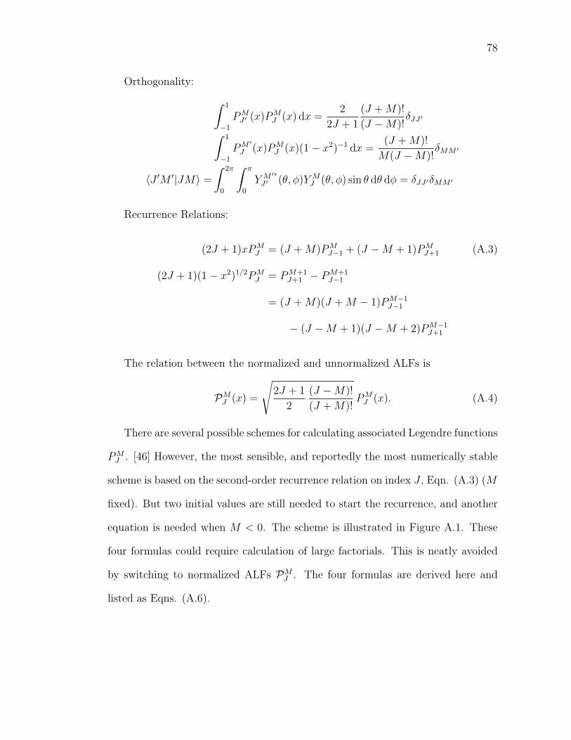
78
Orthogonality: ∫ 1
−1
PMJ ′ (x)PM
J (x) dx =2
2J + 1
(J +M)!
(J −M)!δJJ ′∫ 1
−1
PM ′
J (x)PMJ (x)(1− x2)−1 dx =
(J +M)!
M(J −M)!δMM ′
〈J ′M ′|JM〉 =
∫ 2π
0
∫ π
0
Y M ′∗
J ′ (θ, φ)Y MJ (θ, φ) sin θ dθ dφ = δJJ ′δMM ′
Recurrence Relations:
(2J + 1)xPMJ = (J +M)PM
J−1 + (J −M + 1)PMJ+1 (A.3)
(2J + 1)(1− x2)1/2PMJ = PM+1
J+1 − PM+1J−1
= (J +M)(J +M − 1)PM−1J−1
− (J −M + 1)(J −M + 2)PM−1J+1
The relation between the normalized and unnormalized ALFs is
PMJ (x) =
√2J + 1
2
(J −M)!
(J +M)!PM
J (x). (A.4)
There are several possible schemes for calculating associated Legendre functions
PMJ . [46] However, the most sensible, and reportedly the most numerically stable
scheme is based on the second-order recurrence relation on index J , Eqn. (A.3) (M
fixed). But two initial values are still needed to start the recurrence, and another
equation is needed when M < 0. The scheme is illustrated in Figure A.1. These
four formulas could require calculation of large factorials. This is neatly avoided
by switching to normalized ALFs PMJ . The four formulas are derived here and
listed as Eqns. (A.6).
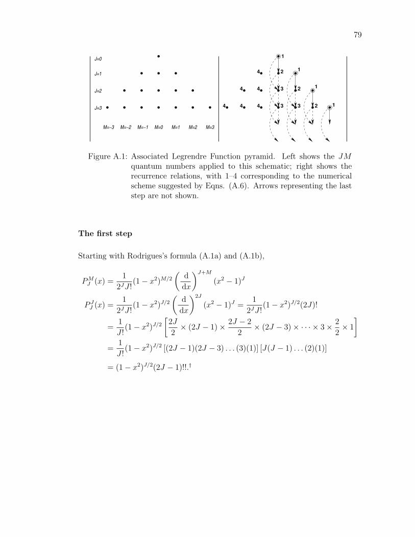
79
M=0 M=1 M=2 M=3M=−1M=−2M=−3
J=1
J=2
J=3
3
3 3
4
44
4 4 4
2
2
2 1
1
J=0
1
1
Figure A.1: Associated Legrendre Function pyramid. Left shows the JMquantum numbers applied to this schematic; right shows therecurrence relations, with 1–4 corresponding to the numericalscheme suggested by Eqns. (A.6). Arrows representing the laststep are not shown.
The first step
Starting with Rodrigues’s formula (A.1a) and (A.1b),
PMJ (x) =
1
2JJ !(1− x2)M/2
(d
dx
)J+M
(x2 − 1)J
P JJ (x) =
1
2JJ !(1− x2)J/2
(d
dx
)2J
(x2 − 1)J =1
2JJ !(1− x2)J/2(2J)!
=1
J !(1− x2)J/2
[2J
2× (2J − 1)× 2J − 2
2× (2J − 3)× · · · × 3× 2
2× 1
]=
1
J !(1− x2)J/2 [(2J − 1)(2J − 3) . . . (3)(1)] [J(J − 1) . . . (2)(1)]
= (1− x2)J/2(2J − 1)!!.†
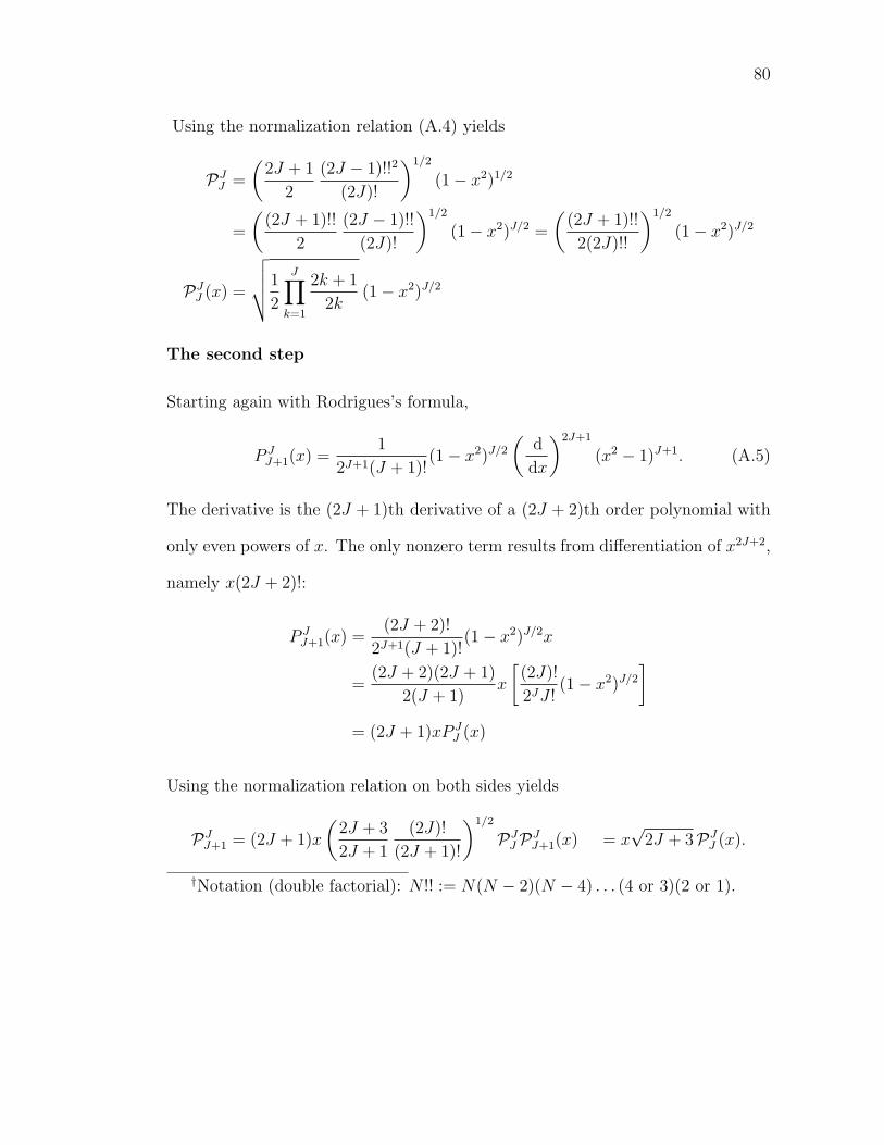
80
Using the normalization relation (A.4) yields
PJJ =
(2J + 1
2
(2J − 1)!!2
(2J)!
)1/2
(1− x2)1/2
=
((2J + 1)!!
2
(2J − 1)!!
(2J)!
)1/2
(1− x2)J/2 =
((2J + 1)!!
2(2J)!!
)1/2
(1− x2)J/2
PJJ (x) =
√√√√1
2
J∏k=1
2k + 1
2k(1− x2)J/2
The second step
Starting again with Rodrigues’s formula,
P JJ+1(x) =
1
2J+1(J + 1)!(1− x2)J/2
(d
dx
)2J+1
(x2 − 1)J+1. (A.5)
The derivative is the (2J + 1)th derivative of a (2J + 2)th order polynomial with
only even powers of x. The only nonzero term results from differentiation of x2J+2,
namely x(2J + 2)!:
P JJ+1(x) =
(2J + 2)!
2J+1(J + 1)!(1− x2)J/2x
=(2J + 2)(2J + 1)
2(J + 1)x
[(2J)!
2JJ !(1− x2)J/2
]= (2J + 1)xP J
J (x)
Using the normalization relation on both sides yields
PJJ+1 = (2J + 1)x
(2J + 3
2J + 1
(2J)!
(2J + 1)!
)1/2
PJJPJ
J+1(x) = x√
2J + 3PJJ (x).
†Notation (double factorial): N !! := N(N − 2)(N − 4) . . . (4 or 3)(2 or 1).
81
The third step
The corresponding recurrence relation for unnormalized ALFs, Eqn. (A.3), is
available, so one needs only to rearrange slightly and use the normalization relation:
PMJ =
1
J −M
[(2J − 1)xPM
J−1 − (J +M − 1)PMJ−2
]PM
J =1
J −M
(2J + 1
2
(J −M)!
(J +M)!
)1/2[(2J − 1)x
(2
2J − 1
(J +M − 1)!
(J −M − 1)!
)1/2
PMJ−1
− (J +M − 1)
(2
2J − 3
(J +M − 2)!
(J −M − 2)!
)1/2
PMJ−2
]
=1
J −M
[x(2J − 1)
(J −M
J +M
2J + 1
2J − 1
)1/2
PMJ−1
− (J +M − 1)
((J −M)(J −M − 1)
(J +M)(J +M − 1)
2J + 1
2J − 3
)1/2
PMJ−2
]
= x
√(2J − 1)(2J + 1)
(J +M)(J −M)PM
J−1 −
√(J −M − 1)(J +M − 1)
(J +M)(J −M)
2J + 1
2J − 3PM
J−2
PMJ =
1√J2 −M2
[x√
4J2 − 1PMJ−1 −
√2J + 1
2J − 3((J − 1)2 −M2)PM
J−2
]
The fourth step
A standard formula relates a M < 0 ALF to the ALF with the same |M | and J .
Then use the normalization relation:
P−MJ = (−1)M (J −M)!
(J +M)!PM
J
P−MJ = (−1)M (J −M)!
(J +M)!
((J +M)!(J +M)!
(J −M)!(J −M)!
)1/2
PMJ P−M
J = (−1)MPMJ .
82
The four formulas are listed here for convenience:
PJJ =
√√√√1
2
J∏k=1
2k + 1
2k(1− x2)J/2 (A.6a)
PJJ+1 = x
√2J + 3PJ
J (A.6b)
PMJ =
1√J2 −M2
[x√
4J2 − 1PMJ−1 −
√2J + 1
2J − 3((J − 1)2 −M2)PM
J−2
](A.6c)
P−MJ = (−1)M PM
J . (A.6d)
Note that the coefficient of (A.6a) reflects how it is calculated: as a sequential
product of numbers between one and two, which will never cause numerical overflow
as may occur if organized another way.
Also, using normalized ALFs simplifies the spherical harmonic definition (A.1c)
to
Y MJ (θ, φ) =
(−1)M
√2π
PMJ (cos θ)eiMφ. (A.7)
A.2 Probability Distributions
The full probability distribution P (θ, φ) is easily calculated for each point on a
(θ, φ) grid, but a few tricks let it be calculated more efficiently. Each eigenvector
ψ(θ, φ) =∑
JM cMJ YMJ (θ, φ) is given by a set of coefficients {cMJ }. Recall that any
complex function can be written as a sum of real and imaginary parts:
ψ(θ, φ) =1√2π
∑JM
cMJ (−1)MPMJ (cos θ)eiMφ
=1√2π
∑JM
cMJ (−1)MPMJ (cos θ) cosMφ
+ i1√2π
∑JM
cMJ (−1)MPMJ (cos θ) sinMφ
≡ Re [ψ] + i Im [ψ] .
83
Then the probablity distribution is simplified (the Jacobian for this coordinate
system is sin θ):
P (θ, φ) = ψ∗ψ sin θ
= sin θ(Re [ψ]− i Im [ψ])(Re [ψ] + i Im [ψ])
= sin θ(Re [ψ]2 + Im [ψ]2).
Note that P (θ, φ) has a reflection plane at φ = π so only half of the coordinate grid
is actually used in the computations. This formula is the best way to calculate
P (θ, φ) since the real and imaginary parts of the wave function have the difficult
parts in common and are calculated just once.
When M is a good quantum number, the (two-dimensional) probability distri-
bution becomes uniform with respect to φ. Thus a full plot of P (θ, φ) is unnecessary
and even masks information. A reduced probability distrubition Pθ(θ) is determined
by integrating P over the polar angle φ:
Pθ =
∫ 2π
0
ψ∗ψ sin θ dφ
=1
2π
∫ 2π
0
[(−1)M ′
cM′
J ′ PM ′
J ′ (cos θ)e−iM ′φ(−1)McMJ PMJ (cos θ)eiMφ
]sin θ dφ
=1
2π
∫ 2π
0
(−1)M+M ′cM
′
J ′ cMJ PM ′
J ′ PMJ sin θ (cos(M ′ −M)φ+ i sin(M ′ −M)φ) dφ
where the implied sum is over all allowed quantum number pairs J ′,M ′ and J,M .
The only φ dependence is in the complex exponential. Note that M−M ′ is always
an integer. Integrating a sine or cosine function over an integer number of cycles
yields zero. The exception is when M ′−M = 0: the cosine integral is 2πδMM ′ . So
Pθ = cMJ ′ cMJ PMJ ′ (cos θ)PM
J (cos θ),
where the sum is now restricted to those quantum number pairs with |M | ≤ J and
|M | ≤ J ′. The sum can be reorganized by separating J = J ′ terms from J 6= J ′
84
terms:
Pθ =∑JM
[cMJ PM
J (cos θ)]2
+∑
J ′ 6=J,M
cMJ ′ cMJ PMJ ′ (cos θ)PM
J (cos θ). (A.8)
The latter sum has pair structure: each term with a given (J ′, J) is exactly equal
to, and counted again as, the term for (JJ ′). A factor of two can be extracted
upon specifying summation indices:
Pθ(θ) =∞∑
J=0
J∑M=−J
[cMJ PM
J (cos θ)]2
+ 2∞∑
J=0
∞∑J ′=J+1
J∑M=−J
cMJ ′ cMJ PMJ ′ (cos θ)PM
J (cos θ).
(A.9)
This a computationally useful form. Of course, in practice the infinite upper
bounds are replaced by Jmax fixed by the basis size.
A.3 Symmetric Rotor Eigenstates and Jacobi Polynomials
Symmetric top eigenstates form the orthonormal basis for the Hamiltonian matrix
when we study symmetric and asymmetric rotors (tops) in fields. First I review
their basic properties and definition in terms of Jacobi polynomials (equivalently,
reduced rotation matrix elements). Then I discuss the algorithm for calculating
these special functions.
Symmetric top eigenstates are determined by three quantum numbers J,M,K
satisfying
J2 |JMK〉 = J(J + 1) |JMK〉
JZ |JMK〉 = M |JMK〉
Jz |JMK〉 = K |JMK〉
with J2, JZ , Jz as the square of the total angular momentum operator, the operator
for projection of angular momentum on a lab-fixed axis Z, and the operator for
85
projection of angular momentum on a body-fixed axis z, all measured in multiples
of ~. The symmetric top eigenstates in terms of the Euler angles (φ, θ, χ) are
〈φ θ χ|JMK〉 = DJ∗
MK(θ, φ, χ) =
√2J + 1
8π2eiMφdJ
MK(θ)eiKχ
with
dJMK(θ) =
√(J +K)!(J −K)!
(J +M)!(J −M)!
(sin
θ
2
)K−M (cos
θ
2
)K+M
P(K−M,K+M)J−K (cos θ).
The special function dJMK(θ) is the reduced rotation matrix, which is further ex-
pressed in terms of Jacobi polynomials P(α,β)n (x).∗ These are well known special
functions that are a generalization of Legendre polynomials. Jacobi polynomials
are orthogonalized over −1 ≤ x ≤ 1 with weighting function (1−x)α(1+x)β, while
Legendre polynomials are the special case α = β = 0. In fact, when the symmet-
ric rotor reduces to a linear rotor (K = 0) the eigenstates reduce to spherical
harmonics, as they should.
∗Using α = K −M,β = K +M,n = J −K, x = cos θ. The α, β, n notation isnormally used in the classical mathematics context for Jacobi polynomials. TheJ,M,K, θ notations is used for quantum wavefunctions.
86
Basic properties of the Jacobi polynomials are:
orthogonality∫ 1
−1P (α,β)
m (x)P (α,β)n (x) (1− x)α(1 + x)β dx
=2α+β+1
2n + α + β + 1Γ(n + α + 1)Γ(n + β + 1)
Γ(n + α + β + 1)n!δmn
recurrence 2(n + 1)(n + α + β + 1)(2n + α + β)P (α,β)n+1 (x) (A.10)
= [(2n + α + β + 1)(α2 − β2) + (2n + α + β)3x]P (α,β)n (x)
− 2(n + α)(n + β)(2n + α + β + 2)P (α,β)n−1 (x)
Rodrigues P (α,β)n (x) :=
(−1)n
2nn!(1− x)−α(1 + x)−β dn
dxn
[(1− x)α+n(1 + x)β+n
](A.11)
alt. definition P (α,β)n (x) := (n + α)!(n + β)!
∑s
(x−1
2
)n−s (x+1
2
)s
s!(n + α− s)!(β + s)!(n− s)!
(A.12)
where the sum in the last formula is over all s such that the factorials have
nonnegative argument.
Strictly speaking, Jacobi polynomials defined by the Rodrigues formula are
valid only for α, β > −1 to ensure the weighting function (1 − x)α(1 + x)β does
not cause divergent integrals.† But α = K −M ≤ −1 and β = K + M ≤ −1
are physically permissible and we need to use the corresponding wave functions.
Several adjunct formulas are used to relate negative α or β (or both) Jacbobi
polynomials to those with postive α or β:
α < 0 P (α,β)n (x) =
(n+ α)!(n+ β)!
n!(n+ α+ β)!
(x− 1
2
)−α
P(−α,β)
n+α (x) (A.13)
β < 0 P (α,β)n (x) =
(n+ α)!(n+ β)!
n!(n+ α+ β)!
(x+ 1
2
)−β
P(α,−β)
n+β (x)
α, β < 0 P (α,β)n (x) =
(x− 1
2
)−α (x+ 1
2
)−β
P(−α,−β)
n+α+β (x)
†In particular, Mathematica produces strange results when using JacobiP[]
with negative α, β.

87
These formulas can be derived from the alternate definition (A.12), which is valid
for negative α, β. For instance, when α < 0,
P (−α,β)n (x) = (n− α)!(n+ β)!
∑s
(x−1
2
)n−s (x+1
2
)s
s!(n− α− s)!(β + s)!(n− s)!
(n+ α)!(n+ β)!
n!(n+ α+ β)!
(x− 1
2
)−α
P(−α,β)
n+α (x) =(n+ α)!(n+ β)!
n!(n+ α+ β)!
(x− 1
2
)−α
× n!(n+ α+ β)!∑
s
(x−1
2
)n+α−s (x+1
2
)s
s!(n− s)!(β + s)!(n+ α− s)!
which simplifies to the (A.13) when checking the definition (A.12).
Calculating symmetric top eigenfunctions dJMK(cos θ) hinges on calculating Ja-
cobi polynomials P(α,β)
n (x). The latter are calculated by the second-order recur-
rence (A.10) with seed formulas for the n = 0 and n = 1 Jacobi polynomials
obtained from the Rodrigues definition (A.11):
P(α,β)
n=0 (x) = 1
P(α,β)
n=1 (x) =1
2[2(α+ 1) + (α+ β + 2)(x− 1)] .
For given α, β the Jacobi polynomials are thus determined. However, rota-
tional problems usually require many different values of α, β in one calculation,
corresponding to all allowed values of K and M .
When the electric fields are collinear, M is fixed and (except for symmetric
rotors with fixed K) the basis contains symmetric top eigenstates of all J from
zero to some maximum and all allowed K. A “pyramid” schematically represents
this basis, shown in Figure A.2, analagous to the J − M pyramid for spherical
harmonics and linear rotors. Each column of the pyramid represents one sequence
of Jacobi polynomials indexed by n bound by successive application of the recur-
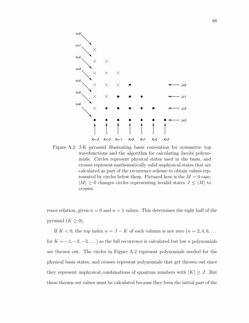
88
n=0
n=1
n=2
n=3
J=0
J=1
J=2
J=3
K=−3 K=−2 K=−1 K=0 K=1 K=2 K=3
n=4
n=5
n=6
Figure A.2: J-K pyramid illustrating basis convention for symmetric topwavefunctions and the algorithm for calculating Jacobi polyno-mials. Circles represent physical states used in the basis, andcrosses represent mathematically valid unphysical states that arecalculated as part of the recurrence scheme to obtain values rep-resented by circles below them. Pictured here is the M = 0 case;|M | ≥ 0 changes circles representing invalid states J ≤ |M | tocrosses.
rence relation, given n = 0 and n = 1 values. This determines the right half of the
pyramid (K ≥ 0).
If K < 0, the top index n = J −K of each column is not zero (n = 2, 4, 6, . . .
for K = −1,−2,−3. . . . ) so the full recurrence is calculated but low n polynomials
are thrown out. The circles in Figure A.2 represent polynomials needed for the
physical basis states, and crosses represent polynomials that get thrown out since
they represent unphysical combinations of quantum numbers with |K| ≥ J . But
these thrown out values must be calculated because they form the initial part of the
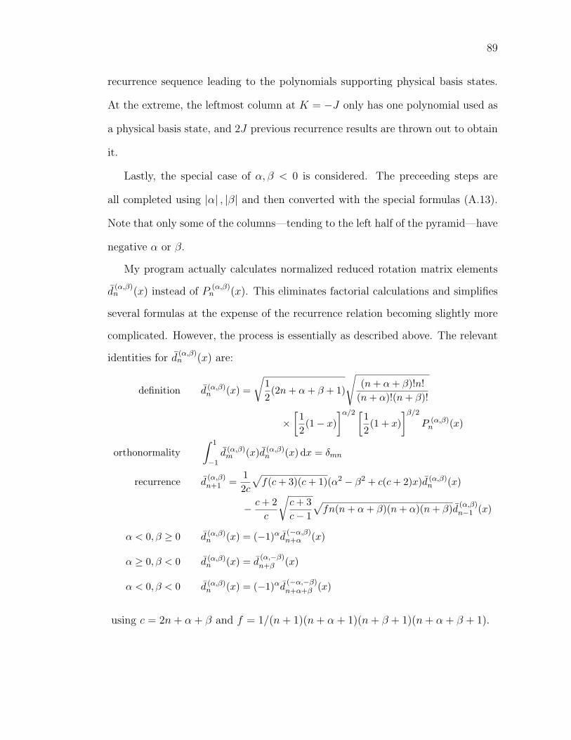
89
recurrence sequence leading to the polynomials supporting physical basis states.
At the extreme, the leftmost column at K = −J only has one polynomial used as
a physical basis state, and 2J previous recurrence results are thrown out to obtain
it.
Lastly, the special case of α, β < 0 is considered. The preceeding steps are
all completed using |α| , |β| and then converted with the special formulas (A.13).
Note that only some of the columns—tending to the left half of the pyramid—have
negative α or β.
My program actually calculates normalized reduced rotation matrix elements
d(α,β)n (x) instead of P
(α,β)n (x). This eliminates factorial calculations and simplifies
several formulas at the expense of the recurrence relation becoming slightly more
complicated. However, the process is essentially as described above. The relevant
identities for d(α,β)n (x) are:
definition d (α,β)n (x) =
√12(2n + α + β + 1)
√(n + α + β)!n!
(n + α)!(n + β)!
×[12(1− x)
]α/2 [12(1 + x)
]β/2
P (α,β)n (x)
orthonormality∫ 1
−1d (α,β)
m (x)d (α,β)n (x) dx = δmn
recurrence d(α,β)n+1 =
12c
√f(c + 3)(c + 1)(α2 − β2 + c(c + 2)x)d (α,β)
n (x)
− c + 2c
√c + 3c− 1
√fn(n + α + β)(n + α)(n + β)d (α,β)
n−1 (x)
α < 0, β ≥ 0 d (α,β)n (x) = (−1)αd
(−α,β)n+α (x)
α ≥ 0, β < 0 d (α,β)n (x) = d
(α,−β)n+β (x)
α < 0, β < 0 d (α,β)n (x) = (−1)αd
(−α,−β)n+α+β (x)
using c = 2n+ α+ β and f = 1/(n+ 1)(n+ α+ 1)(n+ β + 1)(n+ α+ β + 1).
Appendix B
Hamiltonian Matrix Element Derivations
B.1 Matrix Elements in Spherical Harmonic Basis
Matrix elements for the various linear rotor Hamiltonians in the spherical harmonic
basis are derived here.
Static field matrix elements
〈J ′M ′ |cos θ| JM〉
= NMJ NM ′
J ′
[∫ 2π
0
e−i(M ′−M)φ dφ
] [∫ π
0
PM ′
J ′ (cos θ)PMJ (cos θ) cos θ sin θ dθ
]= NM ′
J ′ NMJ [2πδMM ′ ]
[∫ 1
−1
xPMJ ′ (x)PM
J (x) dx
]〈J ′M |cos θ| JM〉
=2π
2J ′ + 1NM
J ′ NMJ
∫ 1
−1
[(J ′ +M)PM
J ′−1 + (J ′ −M + 1)PMJ+1
]PM
J dx
By orthogonality, this is nonzero only when J ′ = J ± 1. Take J ′ = J + 1 :
〈J + 1 M |cos θ| JM〉 =2π
2(J + 1) + 1NM
J NMJ+1 × (J +M + 1)
2
2J + 1
(J +M)!
(J −M)!
=
[(J +M + 1)(J −M + 1)
(2J + 1)(2J + 3)
]1/2
〈J + 1 M |cos θ| JM〉 =
[(J + 1)2 −M2
(2J + 1)(2J + 3)
]1/2
.
Note that the result for J ′ = J−1 is directly recoverable from this formula: simply
apply hermiticity and a dummy substitution J → J − 1 on both sides.
90
91
And when the fields are tilted, the X component of the static field requires:
〈J ′M ′ |cosφ sin θ| JM〉 = NM ′
J ′ NMJ
[∫ 2π
0
e−i(M ′−M)φ cosφ dφ
]×
[∫ π
0
PM ′
J ′ (cos θ) sin θPMJ (cos θ) sin θ dθ
]= NM ′
J ′ NMJ [πδM±1 M ′ ]
[∫ 1
−1
PM ′
J ′ (x)(1− x2)1/2PMJ (x) dx
].
The two cases M ′ = M ± 1 will be calculated separately. Take M ′ = M + 1:
〈J ′M + 1 |cosφ sin θ| JM〉
= πNM+1J ′ NM
J
∫ 1
−1
PM+1J ′ (x)(1− x2)1/2PM
J (x) dx
=πNM+1
J ′ NMJ
2J ′ + 1
∫ 1
−1
[(J ′ +M + 1)(J ′ +M)PM
J ′−1
− (J ′ −M)(J ′ −M + 1)PMJ ′+1
]PM
J dx
and using orthgonality and taking J ′ = J + 1 leaves
〈J + 1 M + 1 |cosφ sin θ| JM〉
=πNM+1
J+1 NMJ
2J + 3(J +M + 2)(J +M + 1)
2
2J + 1
(J +M)!
(J −M)!
= −1
2
[(J +M + 2)(J +M + 1)
(2J + 1)(2J + 3)
]1/2
.
Now with M ′ = M − 1:
〈J ′M − 1 |cosφ sin θ| JM〉 = πNM−1J ′ NM
J
∫ 1
−1
PM−1J ′ (x)(1− x2)1/2PM
J (x) dx
=πNM−1
J ′ NMJ
2J ′ + 1
∫ 1
−1
[PM
J ′+1 − PMJ ′−1
]PM
J dx
and using orthgonality and taking J ′ = J + 1 leaves
〈J + 1 M − 1 |cosφ sin θ| JM〉 =−πNM−1
J+1 NMJ
2J + 3
2
2J + 1
(J +M)!
(J −M)!
=1
2
[(J −M + 2)(J −M + 1)
(2J + 1)(2J + 3)
]1/2
.
92
It is amazing that the two results for M ′ = M ± 1 are so similar, yet one cannot
be derived from the other (by using the hermiticity-dummy substitution method).
This is possible for one index (J) but not both indices simultaneously. Thus,
〈J + 1 M ± 1 |cosφ sin θ| JM〉 = ∓1
2
[(J ±M + 2)(J ±M + 1)
(2J + 1)(2J + 3)
]1/2
. (B.1)
Laser field matrix elements
The laser field matrix elements are 〈J ′M ′ |cos2 θ| JM〉. Since calculation of the
static field element 〈J ′M ′ |cos θ| JM〉 required using the second order recurrence
in J once, the laser field element requires using this recurrence relation twice. This
leads to two independent elements: J is increased twice, or it is increased and then
decreased for no net change. The matrix element is:
⟨J ′M ′ ∣∣cos2 θ
∣∣ JM⟩= NM ′
J ′ NMJ
[∫ 2π
0
e−i(M ′−M)φ dφ
] [∫ π
0
PM ′
J ′ (cos θ) cos2 θPMJ (cos θ) sin θ dθ
]= NM ′
J ′ NMJ [2πδMM ′ ]
[∫ 1
−1
PM ′
J ′ (x)x2PMJ (x) dx
]⟨J ′M
∣∣cos2 θ∣∣ JM⟩
= 2πNMJ ′ NM
J
1
2J ′ + 1
∫ 1
−1
[(J ′ +M)PM
J ′−1 + (J ′ −M + 1)PMJ ′+1
]xPM
J dx
=2πNM
J ′ NMJ
2J ′ + 1
{(J ′ +M)
∫ 1
−1
xPMJ ′−1P
MJ dx+ (J ′ −M + 1)
∫ 1
−1
xPMJ ′+1P
MJ dx
}=
2πNMJ ′ NM
J
2J ′ + 1
{J ′ +M
2(J ′ − 1) + 1
∫ 1
−1
[(J ′ − 1 +M)PM
J ′−2 + (J ′ −M)PMJ ′
]PM
J dx
+J ′ −M + 1
2(J ′ + 1) + 1
∫ 1
−1
[(J ′ + 1 +M)PM
J ′ + (J ′ −M + 2)PMJ ′+2
]PM
J dx
}.
One of three nonzero terms appears by using one of J ′ = J or J ′ = J ± 2. The
latter two yield the same information. J ′ = J could also be calculated, but this
93
matrix element will be determined by other means. Take J ′ = J + 2:
⟨J + 2 M
∣∣cos2 θ∣∣ JM
⟩=
2πNMJ+2N
MJ
2J + 5
[(J + M + 2)(J + M + 1)
2J + 3× 2
2J + 1(J + M)!(J −M)!
]=
(J + M + 2)!(2J + 1)(2J + 3)(2J + 5)(J −M)!
[(2J + 1)(J −M)!
(J + M)!(2J + 5)(J −M + 2)!
(J + M + 2)!
]1/2
=1
2J + 3
[(J + M + 1)(J + M + 2)(J −M + 2)(J −M + 1)
(2J + 1)(2J + 5)
]1/2
or
⟨J + 2 M
∣∣cos2 θ∣∣ JM
⟩=
12J + 3
[((J + 1)2 −M2)
2J + 1((J + 2)2 −M2)
2J + 5
]1/2
.
The matrix element 〈JM |cos2 θ| JM〉 can be calculated by inserting a com-
pleteness relation and using the static field matrix element 〈J + 1 M |cos θ| JM〉:
⟨JM
∣∣cos2 θ∣∣ JM⟩
=⟨JM
∣∣cos θ 1 cos θ∣∣ JM⟩
=
⟨JM
∣∣∣∣∣cos θ∑J ′M ′
|J ′M ′〉〈J ′M ′|
∣∣∣∣∣ JM⟩
=∑J ′M ′
〈JM |cos θ| J ′M ′〉 〈J ′M ′ |cos θ| JM〉 .
The sum has two nonzero terms: when J ′ = J ± 1 and M ′ = M . Each term is
the square of the matrix element (B.2b); the first term is from J ′ = J + 1 and the
second from J ′ = J − 1:
⟨JM
∣∣cos2 θ∣∣ JM⟩
=(J + 1)2 −M2
(2J + 1)(2J + 3)+
J2 −M2
(2J − 1)(2J + 1).
Note that a slight complication can be overlooked. If J = 0 one must neglect the
J ′ = J − 1 term since −1 is not an allowed value for the quantum number J .
Similarly, if M = ±J then the J ′ = J − 1 term should be omitted since |M | > J is

94
not allowed. But in those cases the offending term evaluates to zero, so no special
cases need to be cited.
The nonzero matrix element expressions are (for allowed combinations of J and
M):
⟨JM
∣∣j2∣∣ JM⟩
= J(J + 1) (B.2a)
〈J + 1 M |cos θ| JM〉 =
[(J + 1)2 −M2
(2J + 1)(2J + 3)
]1/2
(B.2b)
〈J + 1 M ± 1 |cosφ sin θ| JM〉 = ∓1
2
[(J ±M + 2)(J ±M + 1)
(2J + 1)(2J + 3)
]1/2
⟨JM
∣∣cos2 θ∣∣ JM⟩
=1
2J + 1
[J2 −M2
2J − 1+
(J + 1)2 −M2
2J + 3
](B.2c)
⟨J + 2 M
∣∣cos2 θ∣∣ JM⟩
=1
2J + 3
[((J + 1)2 −M2)
2J + 1
((J + 2)2 −M2)
2J + 5
]1/2
.
B.2 Symmetrized Spherical Harmonics
There are several different convenient basis sets to use for the linear rotor in fields
problem. Spherical harmonics Y MJ (θ, φ) are the first choice, since the matrix ele-
ments are easy to calculate, as are the functions themselves. When the fields are
collinear, M is a good quantum number and a basis can be restricted to spherical
harmonics with given common M . When the fields are tilted (M is not fixed), one
could use all spherical harmonics as a basis, but that would be roughly twice as
large as necessary.
The basis can be reduced by using symmetry. The tilted fields Hamiltonian
for linear rotors always has reflection plane XZ symmetry in the lab frame. The
symmetry operator σXZ (φ → −φ, θ → θ) commutes with all linear rotor Hamil-
tonians H used here and has two eigenvalues, p = ±1. Each energy eigenfunction
can be labeled with the parity p with respect to reflection. Since the Hamiltonian
95
does not mix basis states of different parity, only basis states of common p need
be used to set up the Hamiltonian matrix. Basis size is cut by half over using all
spherical harmonics, so the matrix diagonalization is faster. Also, in some applica-
tions (such as nearest neighbor spacing distributions) all states must belong to the
same symmetry class, i.e. they all transform the same way under the symmetry
operations that leave the Hamiltonian invariant.
The symmetrized basis is constructed as follows. Since
σXZYMJ (θ, φ) = Y M
J (θ,−φ) = Y M∗
J (θ, φ) = (−1)MY MJ (θ, φ),
define new kets
|JMp〉 := [2(1 + δM0)]−1/2 (
|JM〉+ p(−1)M |J −M〉)
(B.3)
with the provision J ≥ M ≥ 0, and when M = 0, only p = +1 is allowed. These
states are orthonormal. Symmetric (even) states have p = 1, and antisymmetric
(odd) states have p = −1. The formation used here should be familiar; the sym-
metrized states are the real and imaginary parts of the spherical harmonics and are
used to depict s, p, d, f, . . . orbitals of one electron atoms as purely real functions:
〈φ θ|JMp〉 =
(−1)M√
πPM
J (cos θ) cosMφ , M > 0, p = 1
i (−1)M√
πPM
J (cos θ) sinMφ , M > 0, p = −1
1√2πPM
J (cos θ) , M = 0, p = 1.
The Hamiltonian matrix elements corresponding to φ-independent terms are
not different in this basis. The only φ-dependent term (1.12) is sin β sin θ cosφ
from the static electric field X component interacting with the permanent dipole.
All nonzero linear rotor matrix elements are shown below for completeness. There
are three cases for sin θ cosφ since the basis definition changes from M = 0 to
M > 0.
96
The linear rotor Hamiltonian matrix elements in the symmetrized basis (B.3)
are
⟨J ′M ′p′
∣∣j2∣∣ JMp
⟩= J(J + 1)δJ ′JδM ′Mδp′p
〈J ′M ′p′ |cos θ| JMp〉 = 〈J ′M ′ |cos θ| JM〉 δp′p⟨J ′M ′p′
∣∣cos2 θ∣∣ JMp
⟩=
⟨J ′M ′ ∣∣cos2 θ
∣∣ JM⟩δp′p
〈J + 1M ′p′ |sin θ cosφ| JMp〉 =
=
〈J + 1M ′ |sin θ cosφ| JM〉 δp′p , M ′ > 0,M > 0
√2 〈J + 1M ′ |sin θ cosφ| JM〉 δp′p , M ′ = 1(0),M = 0(1), p(p′) = 1.
All of the matrix elements in the symmetrized basis are in terms of the matrix
elements in the spherical harmonics basis. This is how they are programmed.
B.3 Matrix Elements in Symmetric Top Basis
Matrix elements of the various symmetric and asymmetric rotor in fields Hamilto-
nians in the symmetric top basis |JMK〉 are easy to calculate. First the kinetic
energy matrix elements are derived, followed by the potential energy matrix ele-
ments using the Wigner-Eckart theorem.
The kinetic energy matrix elements are widely derived in angular momentum
texts. The free asymmetric rotor Hamiltonian is Equation (1.4),
T = AJ2y +BJ2
z + CJ2x
T =1
2(A+ C)J2 +
1
2(A− C)
[J2
y + κJ2z − J2
x
](B.4)
with the asymmetry parameter κ = 2B−(A+C)A−C
and T (κ) := J2y + κJ2
z − J2x is used
below. (Recall that we use a peculiar rotational constant convention described in
97
Section 1.2.) We will calculate matrix elements of the squared angular momentum
components and then piece together the full kinetic energy matrix elements.
The easiest way is to recall the ladder operator approach to angular momen-
tum theory. In the molecular frame, the ladder operators J± = Jx ± iJy act on
symmetric top kets as [7, §3.4]
J± |JMK〉 =√
(J ±K)(J ∓K + 1) |JMK ∓ 1〉
=√J(J + 1)−K(K ∓ 1) |JMK ∓ 1〉
where J+ and J− are actually the lowering and raising operators in the molecular
frame, changing the eigenstate within a J-block by decrementing and incrementing
K. Since Jx = 12(J+ + J−) and Jy = 1
2i(J+ − J−),
J2x =
1
4
(J+2
+ J−2
+ J+J− + J−J+)
J2y = −1
4
(J+2
+ J−2 − J + J− − J−J+
).
The free asymmetric rotor selection rules ∆J = 0,∆K = 0,±2 follow immediately,
since J+2lowers K by two, J−
2raises K by two, and J+J−, J−J+ do not change
K. The matrix elements of J2x are⟨
JK ± 2∣∣J2
x
∣∣ JK⟩=
1
4
√J(J + 1)−K(K ± 1)
√J(J + 1)− (K ± 1)(K ± 2)⟨
JK∣∣J2
x
∣∣ JK⟩=
1
2J(J + 1)− 1
2K2.
The matrix elements of J2y are⟨
JK ± 2∣∣J2
y
∣∣ JK⟩= −1
4
√J(J + 1)−K(K ± 1)
√J(J + 1)− (K ± 1)(K ± 2)⟨
JK∣∣J2
y
∣∣ JK⟩=
1
2J(J + 1)− 1
2K2.
Finally, J2z has the simplest nonzero matrix element with selection rule ∆J =
0,∆K = 0: ⟨JK
∣∣J2z
∣∣ JK⟩= K2.
98
Note that when summing these matrix elements J2 = J2x + J2
y + J2z as in
Equation (B.4), the ∆K = ±2 elements exactly cancel. Only the diagonal matrix
element is nonzero, 〈JK |J2| JK〉 = J(J + 1), identical to a linear rotor. This is
the first part of the free asymmetric rotor kinetic energy.
The second part of the asymmetric rotor kinetic energy, T (κ), has ∆K =
0,±2 nonzero matrix elements pieced together from the above squared angular
momentum component matrix elements:
〈JK ± 2 |T (κ)| JK〉 = −1
2
√J(J + 1)−K(K ± 1)
√J(J + 1)− (K ± 1)(K ± 2)
〈JK |T (κ)| JK〉 = κK2
Recall that we use the dimensionless kinetic energy T/B~2, so dimensionless
rotational constants a := A/B, c := C/B are used. The full kinetic energy matrix
elements, combining the first and second parts of Equation (B.4), are
〈JK ± 2 |T | JK〉 =1
4(c− a)
√J(J + 1)−K(K ± 1) (B.5)
×√J(J + 1)− (K ± 1)(K ± 2)
〈JK |T | JK〉 =1
2(a+ c)J(J + 1) +
1
2(a− c)κK2. (B.6)
The potential energy matrix elements are derived using the Wigner-Eckart
theorem, which separates the matrix element of any function in the rotation matrix
(1.7) into one dynamic and two geometric pieces.
Recall that the molecular frame is xyz, and the lab frame is XY Z. First rank
irreducible spherical tensor (ladder) operators, also known as vector operators, in
the lab frame are c∓ = cX ∓ icY , and in the molecular frame are c± = cx ± icy.
Whatever direction cosine matrix element you want is formed by
〈J ′M ′K ′ |CiI | JMK〉 = 〈J ′ ||C|| J〉 〈J ′K ′ |ci| JK〉 〈J ′M ′ |cI | JM〉 (B.7)
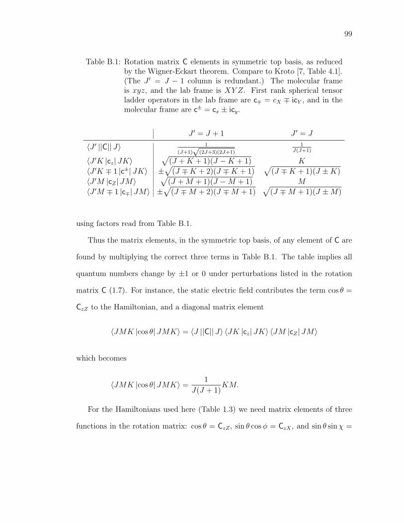
99
Table B.1: Rotation matrix C elements in symmetric top basis, as reducedby the Wigner-Eckart theorem. Compare to Kroto [7, Table 4.1].(The J ′ = J − 1 column is redundant.) The molecular frameis xyz, and the lab frame is XY Z. First rank spherical tensorladder operators in the lab frame are c∓ = cX ∓ icY , and in themolecular frame are c± = cx ± icy.
J ′ = J + 1 J ′ = J
〈J ′ ||C|| J〉 1
(J+1)√
(2J+3)(2J+1)
1J(J+1)
〈J ′K |cz| JK〉√
(J +K + 1)(J −K + 1) K
〈J ′K ∓ 1 |c±| JK〉 ±√
(J ∓K + 2)(J ∓K + 1)√
(J ∓K + 1)(J ±K)
〈J ′M |cZ | JM〉√
(J +M + 1)(J −M + 1) M
〈J ′M ∓ 1 |c∓| JM〉 ±√
(J ∓M + 2)(J ∓M + 1)√
(J ∓M + 1)(J ±M)
using factors read from Table B.1.
Thus the matrix elements, in the symmetric top basis, of any element of C are
found by multiplying the correct three terms in Table B.1. The table implies all
quantum numbers change by ±1 or 0 under perturbations listed in the rotation
matrix C (1.7). For instance, the static electric field contributes the term cos θ =
CzZ to the Hamiltonian, and a diagonal matrix element
〈JMK |cos θ| JMK〉 = 〈J ||C|| J〉 〈JK |cz| JK〉 〈JM |cZ | JM〉
which becomes
〈JMK |cos θ| JMK〉 =1
J(J + 1)KM.
For the Hamiltonians used here (Table 1.3) we need matrix elements of three
functions in the rotation matrix: cos θ = CzZ , sin θ cosφ = CzX , and sin θ sinχ =
100
CyZ . The results for all nonzero matrix elements derived in this way are:
〈J + 1MK |cos θ| JMK〉 = (B.8)√(J +K + 1)(J −K + 1)(J +M + 1)(J −M + 1)
(J + 1)√
(2J + 3)(2J + 1)
〈JMK |cos θ| JMK〉 = (B.9)
KM
J(J + 1)
〈J + 1M ± 1K |sin θ cosφ| JMK〉 =
∓√
(J ±M + 2)(J ±M + 1)(J +K + 1)(J −K + 1)
2(J + 1)√
(2J + 3)(2J + 1)
〈JM ± 1K |sin θ cosφ| JMK〉 =
K√
(J ±M + 1)(J ∓M)
2J(J + 1)
〈J + 1MK ± 1 |sin θ sinχ| JMK〉 =√(J ±K + 2)(J ±K + 1)(J +M + 1)(J −M + 1)
2i(J + 1)√
(2J + 3)(2J + 1)
〈JMK ± 1 |sin θ sinχ| JMK〉 =
∓M
√(J ±K + 1)(J ∓K)
2iJ(J + 1).
These basic results are used to build up the matrix elements for squares of
functions in the rotation matrix. The squares are needed for laser terms in the
Hamiltonians, namely, cos2 θ and sin2 θ sin2 χ. Just by inserting a completeness re-
lation, an abstract expression for the desired matrix element appears. For instance,
the cos2 θ matrix element can be written as
⟨J ′M ′K ′ ∣∣cos2 θ
∣∣ JMK⟩
=∑
′′
〈J ′M ′K ′ |cos θ| J ′′M ′′K ′′〉 〈J ′′M ′′K ′′ |cos θ| JMK〉 .
(B.10)
The factors in the sum are known from Equations (B.8) and (B.9). Using the
101
selection rules for these building blocks, you can find three possible “paths” that
lead to nonzero matrix elements. The selection rules for cos2 θ are ∆J = 0,±1,±2,
∆M = 0, ∆K = 0. For a term that changesK as well as J , such as sin2 θ sin2 χ, the
nonzero terms are plentiful and have several terms each. In this case, an equation
like (B.10) is explicitly programmed by selection rules picking the right path over
sums of pair-multiplied underlying functions.
B.4 Symmetrized Asymmetric Rotor Basis
Using the full complement of symmetric rotor basis functions (fixed M) for the
asymmetric rotor is excessive. When the asymmetric rotor is free, the Hamilto-
nian is invariant under the operations of the D2 point group. These operations also
do not change the Hamiltonian of an asymmetric rotor in the laser field. When an
asymmetric rotor is immersed in collinear static and laser fields, the Hamiltonian
is invariant only under the operations of the C2 point group. We want to develop
symmetrized basis sets in these two cases to reduce the size of the matrix diag-
onalizations. The symmetrized basis for the totally symmetric representation is
coded in each case.
The D2 point group (in the molecular frame) consists of the identity and two-
fold rotation about each molecular axis. The coordinate changes corresponding to
each operation are [14, Ch. 6]
C2(x) : φ→ π + φ θ → π − θ χ→ −χ
C2(y) : φ→ π + φ θ → π − θ χ→ π − χ
C2(z) : φ→ φ θ → θ χ→ π + χ
None of these operations change the asymmetric rotor kinetic energy Hamiltonian:
102
they just rotate angular momentum component Ji to −Ji, which is squared for
the kinetic energy AJ2y + BJ2
z + CJ2x . Likewise, the laser potential energy terms
sin2 θ sin2 χ and cos2 θ are invariant.
The symmetric rotor states are changed:
C2(x) |JMK〉 = (−1)−J |JM −K〉
C2(y) |JMK〉 = (−1)−J−K |JM −K〉
C2(z) |JMK〉 = (−1)K |JMK〉
Since the symmetric rotor kets are not eigenkets of x and y two-fold rotation, but
they transform K → −K, the symmetrized basis is defined as
|JMKs〉 := [2(1 + δK0)]−1/2 ( |JMK〉+ s |JM −K〉) , (B.11)
where K ≥ 0 for s = 1 and K > 0 for s = −1. Note the similarity to the
symmetrized spherical harmonics Equation (B.3).
This is a properly symmetrized basis, since they are eigenkets of all D2 opera-
tions:
C2(x) |JMKs〉 = (−1)−Js |JMKs〉
C2(y) |JMKs〉 = (−1)−J−Ks |JMKs〉
C2(z) |JMKs〉 = (−1)K |JMKs〉 .
However, the symmetry is a little tricky. The values of (J,K, s) being (even/odd,
even/odd, +1/−1) in any of eight combinations determine which of the four D2
point group irreducible representations the state |JMKs〉 belongs to. The answers
are summarized in the extended character table of the D2 point group, Table
B.2. The right hand columns show how the symmetrized basis quantum numbers
103
Table B.2: Chacter table of D2 point group. Extended to include corre-spondence between asymmetric rotor symmetrized basis quantumnumbers and D2 irreducible representations.
D2 E C2(x) C2(z) C2(y) J K s
A 1 1 1 1 oddeven
eveneven
-1+1
Bx 1 1 -1 -1 oddeven
oddodd
-1+1
Bz 1 -1 1 -1 oddeven
eveneven
+1-1
By 1 -1 -1 1 oddeven
oddodd
+1-1
correspond to each of the irreducible representations. For instance, if (J,K, s) are
(odd, even, −1), that symmetrized basis state belongs to the totally symmetric
A irreducible representation. However, symmetrized basis states with (J,K, s) as
(even, even, +1) also belong to the A representation. When only one symmetry
class of eigenstates of these Hamiltonians is desired, then pick symmetric rotor
basis states with values of J,K, s corresponding to the desired symmetry class,
according to the table.
When an asymmetric rotor is in collinear laser and static fields, the relevant
symmetry group is reduced to C2, with C2(z) the remaining symmetry operation
in the molecular frame. The symmetric rotor basis is already symmetrized with
respect to the C2 operations; the two symmetry classes A,B are separated by K
being even or odd (i.e. no matter the J value, and s is not needed). The totally
symmetric A representation contains all of the K even symmetric rotor states.
Appendix C
Propagation Derivations
C.1 Formal Correspondance of Quantum and Classical Dy-
namics
Gray & Verosky [47] provide the basic ideas of the formal classical-quantum corre-
spondence and of symplectic integration used here. The time dependent Schrodinger
equation is
i~d
dt|ψ(t)〉 = H(t) |ψ(t)〉 (C.1)
The Hamiltonian is generally time dependent, so we need to numerically solve the
TDSE. As a first step we reduce the dimensionless TDSE (3.1) to a coupled set
of ordinary differential equations. The time-dependent state ket written in the
spectral representation |ψ(t)〉 =∑
n cn(t) |n〉 facilitates this. Noting the basis kets
are time independent,
i~∑
n
cn(t) |n〉 =∑
n
cn(t) H(t) |n〉 .
The matrix element of this equation with 〈m | yields a new form of the TDSE,
i~cm(t) =∑
n
Hmncm(t) (C.2a)
i~c(t) = Hc(t). (C.2b)
The former Equation (C.2a) is explicitly in terms of individual coefficents cm and
dimensionless hamiltonian matrix elements Hmn. The latter Equation (C.2b) has
the same content, but explicitly shows how the TDSE has been reduced to matrix-
vector multiplication. Propagating wave functions using these equations is con-
venient since Hamiltonian matrix elements in the free rotor eigenbasis are simple
104
105
analytical results previously needed when calculating correlation diagrams; formu-
las are in Appendix B. (The time dependence in the problems treated here is a
simple envelope factor of the model field terms, a gaussian-attenuated laser pulse.)
Equation (C.2a) is just a set of coupled homogeneous ordinary differential equa-
tions in cm, which could be numerically integrated by standard methods such as
fourth-order Runge-Kutta. [46]
However, we use a method called symplectic integration, which is specially
tailored for integrating classical trajectories. Since we do quantum propagation,
first we show a formal equivalence between quantum and classical dynamics. [47]
Then symplectic integration is used to accurately calculate “classical trajectories”
and then translate them back to quantum wave functions.
Given quantum superposition coefficients c(t) and Hamiltonian matrix H, de-
fine position q, momentum p, and scalar function H(q,p, t),
q(t) :=√
2~ Re [c(t)]
p(t) :=√
2~ Im [c(t)]
H(q,p, t) :=1
2~(qT − ipT )H(q + ip) ≡ c†(t)Hc(t) ≡ 〈H〉.
We now show that Hamilton’s equations for these classical variables
q =∂H
∂p, p = −∂H
∂q,
is equivalent to Schrodinger’s equation (C.2b). Substitute, differentiate,∗ and find
∗Differentiating the vector and matrix products is easy; just treat qT Hq asquadratic in q, for example. You can also use subscript-summation notation andfind the same result.
106
H =1
2~(qT Hq + pT Hp + iqT Hp− ipT Hq
)q =
∂H
∂p=
1
2~(2Hp + iHq − iHq) = Hp/~ (C.3a)
−p =∂H
∂q=
1
2~(2Hq + iHp− iHp) = Hq/~. (C.3b)
Testing Equation (C.2b) verifies
i~c =i~√2~
(q + ip) =1√2~
H(q + ip) = Hc.
The TDSE in vector form has been recovered. All steps here are reversible, so
equivalency between quantum (Schrodinger’s equation) and classical (Hamilton’s
equations) dynamics given these definitions is proved. We translate our quantum
wavefunctions into classical positions and momenta and use classical symplectic
integration to propagate wavefunctions.
C.2 Symplectic Integrators
Symplectic integration is a numerical integration technique built specially for cal-
culating classical trajectories. It automatically conserves the Poincare integral
invariants. [48, §8.3] We know analytically that any classical canonical transfor-
mation, such as classical time evolution, must preserve these integral invariants.
Obviously, it is advantageous to propagate classical trajectories with an algorithm
that guarantees their invariance. Standard algorithms, such as Runge-Kutta, do
not conserve the integral invariants.
Recall that the Poincare invariants are a hierarchy of quantities, properties
of all trajectories taken together, that are rigorously conserved in Hamiltonian

107
systems. The last invariant in the hierarchy is the best known: phase space volume,
conservation of which is known as Liouville’s theorem.
To start, let’s employ symplectic notation for Hamilton’s equations. For N
degrees of freedom, define z := (q,p) as a 2N -vector, but for the present formalism
we can use just one degree of freedom z = (q, p). Then Hamilton’s equations can
be written using the Poisson bracket
z = {z,H(z)} :=∂z
∂q
∂H
∂p− ∂z
∂p
∂H
∂q.
Further, the Poisson bracket can be thought of as a differential operator DH , called
the Liouvillian,
DHz :=
[∂H
∂p
∂
∂q− ∂H
∂q
∂
∂p
]z ≡
[q∂
∂q+ p
∂
∂p
]z ≡ {·, H}z. (C.4)
Classical mechanics is now cast in terms of two operators; let us call them A and
B for the following abstract treatment, with A = ∂H∂p
∂∂q
and B = −∂H∂q
∂∂p
.
Of course, a formal solution of Hamilton’s equation (C.4) in terms of DH is
z(t) = exp(tDH)z(0) = exp[t(A + B)]z(0) (assuming the Hamiltonian is time
independent). This has exactly the same interpretation, and is the classical coun-
terpart of, the familiar quantum propagator U(t, 0) = exp(−itH/~). In both cases,
the exponential operator propagates the state function at time zero into the state
function at time t.
We know howA andB individually propagate the state, since their exponentials
are defined by Taylor series. For example, a propagator term etA is approximated
by 1 + tA = 1 + ∂H∂p
∂∂q
. Each term (except zeroth order) in the operator expansion
first differentiates z with respect to q. Only the position component survives dif-
ferentiation, which is then increased by t∂H∂p
. The propagator etA propagates the
position q by time t but does not affect the momentum p since it does not remain

108
after differentiation with respect to q. Using the classical-quantum correspon-
dence outlined above, classical propagation by etA corresponds to multiplying the
quantum Hamiltonian matrix and “momentum” vector for the position increment,
according to Equation (C.3a).
However, propagating the full Hamiltonian et(A+B) is in general intractable
since A and B do not commute and the exponential cannot be factored. However,
a simple approximation is widely known (lowest order Trotter factorization) and
derived in Appendix C.3:
DH,2(t) = eAt/2eBteAt/2. (C.5)
This propagator is second-order in the time step. It is interpreted as follows, as
an operator from right to left: first advance the position by a half time step, then
the momenta by a full time step, then position by another half time step. This is
a simple idea dressed in operator finery. This algorithm is also known as position
Verlet [49] (the same idea as velocity Verlet, with A and B switched) and symplectic
leapfrog. [47]
Via the classical-quantum correspondence, classical symplectic integration cor-
responds to repeated matrix-vector multiplications and vector additions.
The fact DH,2 is actually a symplectic transformation is proved in Appendix
C.4. I also prove that the simple Euler method is not symplectic. The key ele-
ment of propagator (C.5) that guarantees conservation of the integral invariants is
how the momentum increment in each symplectic integration step depends on the
position calculated in the first half time step.
Second-order symplectic integration can be used for time-dependent Hamiltoni-
ans. The algorithm is almost the same as that for time-independent Hamiltonians.
The formulas are derived in Appendix C.5.
109
The integration routine should also obey time reversal symmetry, from which we
see no odd order symplectic integration routines exist. By time reversal symmetry
we mean that after propagating a system by time t, further propagating by time
−t returns the system to its original state. This is another classical property, in
addition to preservation of the Poincare invariants, that the integration routine
satisfies. The symmetric construction guarantees this.
C.3 Deriviation of the SI2 Coefficients
Yoshida [50] nicely frames the problem: for desired order n and number of steps
k, an approximation to
et(A+B) =k∏
i=1
ecitAeditB +O(tn+1) (C.6)
can be found by determining coefficients {ci, di}, i = 1, . . . , k.
First we want a second-order propagator with two steps (each operator A and
B can act twice). That is, solve for c1, d1, c2, d2 that satisfy
et(A+B) = ec1tAed1tBec2tAed2tB +O(t3). (C.7)
Now expand each exponential in a second-order Taylor series (which defines the
110
exponential of an operator) and multiply the result:
1 + t(A+B) +1
2t2(A+B)2 =
= (1 + c1tA+c212t2A2)(1 + d1tB +
d21
2t2B2)
+ (1 + c2tA+c222t2A2)(1 + d2tB +
d22
2t2B2) +O(t3)
= 1 + t(c1A+ d1B + c2A+ d2B)
+t2
2(c21A
2 + d21B
2 + c22A2 + d2
2B2 + 2c1d1AB + 2d1c2BA
+ 2d1d2B2 + 2c1c2A
2 + 2c1d2AB + 2c2d2AB) +O(t3)
= 1 + t[(c1 + c2)A+ (d1 + d2)B]
+t2
2[(c1 + c2)
2A2 + (d1 + d2)2B2 + 2(c1d1 + c1d2 + c2d2)AB
+ 2d1c2BA] +O(t3).
Matching operator coefficients in terms of same order in t on left and right provides
restricting conditions on these coefficients. To first order, c1+c2 = d1+d2 = 1 must
hold. To second order, two additional conditions must hold: c1d1 + c1d2 + c2d2 =
1/2, and d1c2 = 1/2. Actually, the last of these four constraints is redundant,
since the first three can be combined to create the fourth. Thus there are four
unknowns and three constraints, leaving one coefficient arbitrary—choose d2 = 0.
Then the coefficients that define this two step, second order propagator are c1 =
c2 = 1/2, d1 = 1, d2 = 0.
C.4 Proof that the Integrators are Symplectic
This propagator is symplectic—it automatically preserves the Poincare invariants.
As an example, consider the ultimate invariant, phase space volume. It is proved
invariant if the Jacobian determinant of the coordinate change represented by time
111
evolution is one, since the Jacobian determinant is the ratio of volumes contained
by infinitesimal boxes in two different coordinate systems. I use the quantum
notation from the classical-quantum correspondence of Equation (C.3),
q =∂H
∂p= Hp/~
−p =∂H
∂q= Hq/~,
where H is the quantum Hamiltonian matrix and q,p are valid classical position
and momenta. Using shorthand x = Ht/~, one sub-step of a symplectic integration
step is written as
q = q0 + cx
p = p0 − dxq = p0 − dxq0 − cdx2p0.
In matrix notation, this reads as a simple linear transformationq
p
=
1 cx
−dx 1− cdx2
q0
p0
with determinant equal to one. Thus the phase space volume is conserved under
the symplectic integration step. Using exactly the same notation but limited to
any subset of the degrees of freedom proves conservation of the other Poincare
invariants, which are the volume element projected onto any of the 2, 4, 6, . . . , 2n−
2 hyperplanes of 2n dimensional phase space. They key facet that guarantees
invariance is how the momentum increment in each symplectic integration step
depends on the position calculated in the same step.
In contradistinction, the simple Euler method appears asq
p
=
1 cx
−dx 1
q0
p0
,

112
whose transformation matrix has nonunity Jacobian determinant. One should
expect inaccuracies, perhaps only after long times, when using such numerical
integration algorithms.
C.5 Time-dependent Hamiltonians
The above derivation assumed the Hamiltonian was time independent, leaving
pulsed laser fields from consideration. However, a very simple trick common in
classical mechanics allows easy quantum propagation with time-dependent Hamil-
tonians. This was reported by Sanz-Serna and Portillo [51] in different notation.
The time-independent Hamiltonian formal solution is z(t) = etDHz(0), but this
is not valid for a time-dependent Hamiltonian. Using this proposed solution with
H = H(t) in the equation of motion (C.4) yields
z(t) = etDH
(DH + tDH
)z(0)
= DHz(t) + tetDHDHz(0)
which is certainly not the original differential equation.
The classical trick is using extended phase space to formally hide the time
dependence. When the Hamiltonian H(t) is a function of time, formally consider
time t as a degree of freedom. There are now n+1 position variables, q1, q2, . . . , qn, t.
Define the extended Hamiltonian H(q, p, t,−E) := H(q, p, t) − E. The extended
Hamiltonian is explicitly time-independent, since the “time” here is a new variable
denoted τ . The equations of motion for the four independent variables (q, p, t,−E)
113
are
q =∂H
∂p=∂H
∂pt =
∂H
∂(−E)= 1
p = −∂H∂q
= −∂H∂q
−E = −∂H∂t
= −∂H∂t
with “dot” now meaning total derivative with respect to τ . Now a proper formal
solution is z(τ) = exp(τDH)z(0), with Liouvillian
DH =∂H
∂p
∂
∂q− ∂H
∂q
∂H
∂p+∂
∂t− ∂H
∂t
∂
∂(−E).
Now form the second-order symplectic integrator for this Liouvillian. Defining
shorthand as DH =: A+B+C +D, note that the time-independent second-order
formula (C.5) can be applied stepwise:
DH(τ) = eτ(A+B+C+D)
DH,2(τ) = eτD/2eτ(A+B+C)eτD/2 +O(τ 3)
= eτD/2(eτC/2eτ(A+B)eτC/2
)eτD/2 +O(τ 3)
= eτD/2(eτC/2eτ(A+B)eτC/2
)eτD/2 +O(τ 3)
= eτD/2eτC/2eτB/2eτAeτB/2eτC/2eτD/2 +O(τ 3).
Note that the D factors only propagate the momentum −E, which is uncoupled
from the equations of motion for q, p, t. Thus the D factors can be ignored without
affecting the “important” variables. Also, the C factors have such a simple asso-
ciated equation, t = 1, they only increase the time τ by τ/2 before the remaining
propagators are applied. Thus the only new feature of time-dependent SI2, rela-
tive to time-independent SI2, is to use the Hamiltonian matrix at one-half greater
time increment when applying the A and B propagators that increase position and
momentum. The underlying computer code is almost the same!

114
C.6 Sudden Approximation for a Short Laser Pulse
The time dependent Schrodinger equation has a formal solution for time indepen-
dent Hamiltonian H:
|ψ(t)〉 = exp
(i
~
∫ t
H dt
)|ψ(0)〉 .
Substituting a time-dependent Hamiltonian is a good approximation when the
time dependence is very rapid, for then the Hamiltonian is time-independent most
of the time! In Section 3.3, I modeled linear rotors in pulsed laser fields using the
polarizability interaction governed by a gaussian pulse envelope. The Hamiltonian
in dimensionless time τ = B~t is
h(τ) = j2 −∆ωe−τ2/σ2
cos2 θ
with corresponding approximate propagator
exp
(−i
∫ τ
h(τ ′) dτ ′).
If the time τ is well after the short pulse has gone by, then the standard gaussian
integral formula can be used leaving the approximate propagated state
|ψ(τ)〉 = exp(−iτj2 + i∆ωσ
√π cos2 θ
)|ψ(0)〉 .
Generally, the time-evolved state can be written as a spherical harmonic superpo-
sition, with time dependent coefficients and phase factors rotating at the field-free
frequencies:
|ψ(τ)〉 =∑JM
cJM(τ)e−iτJ(J+1) |JM〉 .
These two expressions equated, using the isotropic J = M = 0 spherical harmonic
as the ground state, and “splitting” the Hamiltonian (a simple approximation),
115
yield a useful formula for the superposition coefficients in time:
∑JM
cJM(τ)e−iτJ(J+1) |JM〉 = e−iτj2
ei∆ωσ√
π cos2 θ |00〉
cJM(τ)e−iτJ(J+1) =⟨JM
∣∣∣e−iτj2
ei∆ωσ√
π cos2 θ∣∣∣ 00
⟩cJM(τ) =
⟨JM
∣∣∣ei∆ωσ√
π cos2 θ∣∣∣ 00
⟩.
The final field-free probabilities are thus determined, and they are constant post-
pulse since the Hamiltonian is then constant with time.
The indicated integral is difficult to calculate analytically† but Mathematica
makes short work of it for particular J,M values. Results are shown in Figure 3.4.
†In other related cases, the intergral reduces nicely. Persico and Van Leuven[52] use the sudden approximation for a dipole that follows the laser field oscillation(we modelled that this action was quenched by rapid oscillation). Arango [17] usesthe same short laser pulse-polarizability interaction but for a rotor confined to acircle, using a plane wave basis. In each of these cases, a simple formula involvingBessel functions results, which is apparently unachievable here.
REFERENCES
[1] D. R. Lide, editor. CRC Handbook of Chemistry and Physics. CRC PressLLC, Boca Raton, Florida, 82nd edition, 2001.
[2] C. H. Townes and A. L. Schawlow. Microwave Spectroscopy. Dover Publica-tions, Inc., New York, 1975.
[3] J. O. Hirschfelder, C. F. Curtiss, and R. B. Bird. Molecular Theory of Gasesand Liquids. John Wiley & Sons, Inc., New York, 1954.
[4] B. Friedrich and D. Herschbach. Manipulating molecules via combined staticand laser fields. J. Phys. Chem. A, 103:10280–10288, 1999.
[5] M. D. Poulsen, E. Peronne, H. Stapelfeldt, C. Z. Bisgaard, S. S. Viftrup,E. Hamilton, and T. Seideman. Nonadiabatic alignment of asymmetric topmolecules: Rotational revivals. J. Chem. Phys., 121(2):783–791, 2004.
[6] H. Li, K. J. Franks, R. J. Hanson, and W. Kong. Brute force orientation andalignment of pyridazine probed by resonantly enhanced multiphoton ioniza-tion. J. Phys. Chem. A, 102:8084–8090, 1998.
[7] H. W. Kroto. Molecular Rotation Spectra. Dover Publications, Inc., NewYork, 1992.
[8] D. Herschbach. Chemical physics: Molecular clouds, clusters, and corrals.Rev. Mod. Phys., 71(2):S411–S418, 1999.
[9] H. J. Loesch and A. Remscheid. Brute force in molecular reaction dynamics: Anovel technique for measuring steric effects. J. Chem. Phys., 93(7):4779–4790,1990.
[10] B. Friedrich and D. R. Herschbach. On the possibility of orienting rotationallycooled polar molecules in an electric field. Z. Phys. D—Atoms, Molecules, andClusters, 18:153–161, 1991.
[11] B. Friedrich and D. Herschbach. Alignment and trapping of molecules inintense laser fields. Phys. Rev. Lett., 74(23):4623–4626.
[12] H. Stapelfeldt and T. Seideman. Colloquium: Aligning molecules with stronglaser pulses. Rev. Mod. Phys., 75(2):543–557, 2003.
[13] S. Minemoto, H. Nanjo, H. Tanji, T. Suzuki, and H. Sakai. Observation ofmolecular orientation by the combination of electrostatic and nonresonant,pulsed laser fields. J. Chem. Phys., 118(9):4052–4059, 2003.
[14] R. N. Zare. Angular Momentum. Wiley-Interscience, New York, 1988.
116
117
[15] M. P. Bogaard and B. J. Orr. Electric dipole polarisabilities of atoms andmolecules. In A. D. Buckingham, editor, MTP International Review of Sci-ence: Physical Chemistry: Molecular Structure and Properties, volume 2 of 2,pages 149–194. Butterworths, London, 1975.
[16] D. M. Brink and G. R. Satchler. Angular Momentum. Clarendon Press,Oxford, third edition, 1993.
[17] C. A. Arango. Classical and Semiclassical Mechanics of Molecular Rotors inTilted Fields. PhD thesis, Cornell University, 2005.
[18] G. Arfken. Mathematical Methods for Physicists. Academic Press, New York,second edition, 1970.
[19] M. V. Berry and M. Wilkinson. Diabolical points in the spectra of triangles.Proc. R. Soc. Lond. A, 392:15–43, 1984.
[20] R. P. Feynman. Forces in molecules. Phys. Rev., 56:340–343, 1939.
[21] J. Ortigoso, M. Rodrıguez, M. Gupta, and B. Friedrich. Time evolution ofpendular states created by the interaction of molecular polarizability with apulsed nonresonant laser field. J. Chem. Phys., 110(8):3870–3875, 1999.
[22] B. Hayes. The spectrum of riemannium. American Scientist, 91(4):296–300,2003.
[23] F. Haake. Quantum Signatures of Chaos. Springer-Verlag, 1991.
[24] M. C. Gutzwiller. Chaos in Classical and Quantum Mechanics. Springer-Verlag, New York, 1990.
[25] C. A. Arango, W. W. Kennerly, and G. S. Ezra. Classical and quantummechanics of diatomic molecules in tilted fields. J. Chem. Phys., 122:184303,2005.
[26] O. Bohigas and M. J. Giannoni. Chaotic motion and random matrix theories.In J. S. Dehesa et. al., editor, Mathematical and Computational Methods inNuclear Physics, volume 209 of Lecture Notes in Physics, pages 1–99. Springer-Verlag, 1984.
[27] E. P. Wigner. Results and theory of resonance absorption. ORNL-2309reprinted in [30], pp. 199–211, November 1956.
[28] E. P. Wigner. Random matrices in physics. SIAM Review, 9(1):1–23, 1967.
[29] C. Schlier. How much can we learn from nearest neighbor distributions? J.Chem. Phys., 117(7):3098–3102, 2002.
118
[30] C. E. Porter, editor. Statistical Theories of Spectra: Fluctuations. AcademicPress, 1965.
[31] I. C. Percival. Regular and irregular spectra. J. Phys. B: Atom. Molec. Phys.,6:L229–L232, 1973.
[32] M. V. Berry and M. Tabor. Level clustering in the regular spectrum. Proc.R. Soc. Lond. A, 356:375–394, 1977.
[33] O. Bohigas, M. J. Giannoni, and C. Schmit. Characterization of chaoticquantum spectra and universality of level fluctuation laws. Phys. Rev. Lett.,52:1–4, 1984.
[34] M. V. Berry and M. Robnik. Semiclassical level spacings when regular andchaotic orbits coexist. J. Phys. A: Math. Gen., 17:2413–2421, 1984.
[35] T. A. Brody, J. Flores, J. B. French, P. A. Mello, A. Pandey, and S. S. M.Wong. Random-matrix physics: spectrum and strength fluctuations. Rev.Mod. Phys., 53:385–479, 1981.
[36] D. Wintgen and H. Friedrich. Classical and quantum-mechanical transitionbetween regularity and irregularity in a hamiltonian system. Phys. Rev. A,35(3):1464–1466, 1987.
[37] J. Main, M. Schwacke, and G. Wunner. Hydrogen atom in combined elec-tric and magnetic fields with arbitrary mutual orientations. Phys. Rev. A,57(2):1149–1157, 1998.
[38] T. P. Grozdanov and R. McCarroll. Level statistics for asymmetric-top rotorsin strong electric fields. Z. Phys. D, 38:45–49, 1996.
[39] V. R. Manfredi and L. Salasnich. Pathological behavior in the spectral statis-tics of the asymmetric rotor model. Phys. Rev. E, 64:066201, 2001.
[40] V. R. Manfredi, V. Penna, and L. Salasnich. Spectral statistics of the triaxialrigid rotator: Semiclassical origin of their pathological behavior. Mod. Phys.Lett. B, 17(15):803–812, 2003.
[41] D. Marchesan, G. Moruzzi, and N. Rahman. Quantum chaotic behavior invibro-roto-torsional levels of methanol and its isotopomers. Chem. Phys. Lett.,381:556–564, 2003.
[42] H. Wu, M. Vallieres, D. H. Feng, and D. W. L. Sprung. Gaussian-orthogonal-ensemble level statistics in a one-dimensional system. Phys. Rev.A, 42(3):1027–1032, 1990.
[43] C. A. Arango, W. W. Kennerly, and G. S. Ezra. Quantum monodromy fordiatomic molecules in combined electrostatic and pulsed nonresonant laserfields. Chem. Phys. Lett., 392:486–492, 2004.
119
[44] J. A. Morales, E. Deumens, and Y. Ohrn. On rotational coherent states inmolecular quantum dynamics. J. Math. Phys., 40(2):766–786, 1999.
[45] J. G. Underwood, B. J. Sussman, and A. Stolow. Field-free three dimensionalmolecular axis alignment. Phys. Rev. Lett., 94:143002, 2005.
[46] W. H. Press, S. A. Teukolsky, W. T. Vetterling, and B. P. Flannery. NumericalRecipes in C: The Art of Scientific Computing. Cambridge University Press,Cambridge, UK, second edition, 1992.
[47] S. K. Gray and J. M. Verosky. Classical hamiltonian structures in wave packetdynamics. J. Chem. Phys., 100(7):5011–5022, 1994.
[48] H. Goldstein. Classical Mechanics. Addison-Wesley Publishing Company,Inc., Cambridge, Mass., first edition, 1950.
[49] M. Tuckerman, B. J. Berne, and G. J. Martyna. Reversible multiple timescale molecular dynamics. J. Chem. Phys., 97(3):1990–2001, 1992.
[50] H. Yoshida. Construction of higher order symplectic integrators. Phys. Lett.A, 150(5,6,7):262–268, 1990.
[51] J. M. Sanz-Serna and A. Portillo. Classical numerical integrators for wave-packet dynamics. J. Chem. Phys., 104(6):2349–2355, 1995.
[52] M. Persico and P. Van Leuven. Short-time quantum dynamics of the drivenrigid rotor. Z. Phys. D, 41:139–141, 1997.
Top Related
Copyright © 2022 FDOKUMEN

