http://ijr.sagepub.com

The International Journal of Robotics Research

DOI: 10.1177/0278364904050917 2005; 24; 239 The International Journal of Robotics Research

Ioannis Poulakakis, James Andrew Smith and Martin Buehler Robot

Modeling and Experiments of Untethered Quadrupedal Running with a Bounding Gait: The Scout II

http://ijr.sagepub.com/cgi/content/abstract/24/4/239 The online version of this article can be found at:

Published by:

http://www.sagepublications.com

On behalf of:

Multimedia Archives

can be found at:The International Journal of Robotics Research Additional services and information for

http://ijr.sagepub.com/cgi/alerts Email Alerts:

http://ijr.sagepub.com/subscriptions Subscriptions:

http://www.sagepub.com/journalsReprints.navReprints:

http://www.sagepub.com/journalsPermissions.navPermissions:

http://ijr.sagepub.com/cgi/content/refs/24/4/239SAGE Journals Online and HighWire Press platforms):

(this article cites 13 articles hosted on the Citations

© 2005 SAGE Publications. All rights reserved. Not for commercial use or unauthorized distribution. at PENNSYLVANIA STATE UNIV on February 7, 2008 http://ijr.sagepub.comDownloaded from

Ioannis PoulakakisJames Andrew SmithAmbulatory Robotics LaboratoryDepartment of Mechanical Engineering andCentre for Intelligent MachinesMcGill University3480 University StreetMontreal, QC H3A 2A7, Canada{poulakas,jasmith}@cim.mcgill.ca

Martin BuehlerBoston Dynamics515 Massachusetts AvenueCambridge, MA 02139, USAbuehler@bostondynamics.com

Modeling andExperiments ofUntetheredQuadrupedalRunning witha Bounding Gait:The Scout II Robot

Abstract

In this paper we compare models and experiments involving Scout II,an untethered four-legged running robot with only one actuator percompliant leg. Scout II achieves dynamically stable running of upto 1.3 m s−1 on flat ground via a bounding gait. Energetics analy-sis reveals a highly efficient system with a specific resistance of only1.4. The running controller requires no task-level or body-state feed-back, and relies on the passive dynamics of the mechanical system.These results contribute to the increasing evidence that apparentlycomplex dynamically dexterous tasks may be controlled via simplecontrol laws. We discuss general modeling issues for dynamicallystable legged robots. Two simulation models are compared with ex-perimental data to test the validity of common simplifying assump-tions. The need for including motor saturation and non-rigid torquetransmission characteristics in simulation models is demonstrated.Similar issues are likely to be important in other dynamically sta-ble legged robots as well. An extensive suite of experimental resultsdocuments the robot’s performance and the validity of the proposedmodels.

KEY WORDS—legged locomotion, modeling, quadrupedalrobot, dynamic running, bounding gait, dynamic stability

1. Introduction

As mobile robots are required to operate outside the labora-tory, the limitations of traditional wheeled and tracked vehi-

The International Journal of Robotics ResearchVol. 24, No. 4, April 2005, pp. 239-256,DOI: 10.1177/0278364904050917©2005 Sage Publications

cle designs become increasingly apparent. To overcome theselimitations, one branch of the mobile robotics field has turnedto biological inspiration for other possible solutions, includ-ing legged systems, which promise a versatility and mobilityunparalleled in more traditional designs.

Early attempts to implement legged designs resulted inslow moving, statically stable systems. These designs are stillthe most prevalent today. One of the more successful examplesof this large class of legged robots is the Titan series of Hirose(2001). Because of the negligible momentum in the gaits de-veloped by such vehicles, maintaining stability requires onlythat the position of the center of mass (COM) is kept withinthe polygon of support created by the stance legs (Song andWaldron 1989).

In this paper we focus on dynamically stable legged robots.To date, the most significant research on dynamic legged lo-comotion was led by Raibert at the Carnegie-Mellon Univer-sity (CMU) and Massachusetts Institute of Technology (MIT)Leglabs in the 1980s and 1990s (Raibert 1986). His researchrevolved around fundamental principles for controlling hop-ping height, forward speed, and body posture, making var-ious gaits possible on monopedal, bipedal, and quadrupedalrobots. His controllers resulted in fast and stable dynamic run-ning with different paired-leg gaits, such as the trot, pace, andbound.

Other dynamically stable running designs have been pro-posed since Raibert, including the articulated-knee Scamperbounding quadruped by Furusho et al. (1995). The controllerdivided one running cycle into eight states and switched thetwo joints per leg between free rotation, position control,and velocity control. Following a different approach, Kimura,

239

© 2005 SAGE Publications. All rights reserved. Not for commercial use or unauthorized distribution. at PENNSYLVANIA STATE UNIV on February 7, 2008 http://ijr.sagepub.comDownloaded from

240 THE INTERNATIONAL JOURNAL OF ROBOTICS RESEARCH / April 2005

Akiyama, and Sakurama (1999) implemented bounding bytransitioning from pronking in the Patrush robot based on prin-ciples from neurobiology.They combined explicit compliancewith a neural oscillator network, whose frequency matchedthat of the vertical spring–mass environment–system oscil-lation. Patrush’s three-degrees-of-freedom (3-DoF) legs eachfeatured an actuated hip and knee, and an unactuated, compli-ant foot joint, while the robot was physically constrained tomove in the sagittal plane by overhead beams. Other leg de-signs have also been proposed, most involving more actuatorsthan Scout II. One such recent design is the Ohio State Uni-versity (OSU)–Stanford KOLT quadrupedal robot that housesall of the leg actuators at the hip or on the body (Nichol andWaldron 2002).

Various models have been proposed to study dynamicallystable quadrupeds. Murphy and Raibert studied bounding andpronking using a model with kneed legs whose lengths werecontrollable (Raibert et al. 1985). They discovered that activeattitude control in bounding is not necessary when the body’smoment of inertia is smaller than the mass times the squareof the hip spacing. Following up on their work, Berkemeier(1998) showed that this result applies to a simple linearizedrunning-in-place model and that it can also be extended topronking. Brown and Raibert investigated the conditions forobtaining passive cyclic motion (Raibert et al. 1985). Theystudied two limiting cases of system behavior—the groundedand the flight regimes—and they found that the system in bothregimes can passively trot, gallop, or bound if provided withthe proper initial conditions. More recently, from a minimalistopen-loop perspective and inspired by results in biomechanics(Kubow and Full 1999), and dynamical systems (Ghigliazzaet al. 2003), Poulakakis (2002) and Poulakakis, Papadopou-los, and Buehler (2003) have shown that passively generatedstable bounding of a conservative model of Scout II is possi-ble under appropriate initial conditions and sufficiently highspeeds.

In a different spirit, Formalsky, Chevallereau, and Perrin(2000) investigated ballistic motions of a sagittal quadrupedalmodel involving leg pairs such as the trot, the pace, and thebound, which were achieved by appropriate initial speeds re-sulting from impulsive active control torques acting at theboundaries of support phases. Other work on modeling thedynamics of quadrupedal running includes studies of morecomplex gaits such as galloping, where no legs are used inpairs. Schmiedeler and Waldron (1999) studied the kinemat-ics and dynamics of the gallop on a three-dimensional, 5-DoFquadruped with massless legs, where they found that as dragincreases, the footfall patterns approach the half-bound gait.Herr and McMahon (2001) studied the transverse gallop of ahorse-type model and concluded that their robot model couldexhibit stable galloping without requiring control over postu-ral orientation and also without any sensing of body attitude.

This paper addresses a subject that is central to advancingthe state of the art in autonomous, dynamically stable-legged

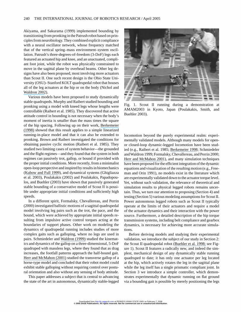
Fig. 1. Scout II running during a demonstration atAMAM2003 in Kyoto, Japan (Poulakakis, Smith, andBuehler 2003).

locomotion beyond the purely experimental realm: experi-mentally validated models. Although many models for open-or closed-loop dynamic-legged locomotion have been stud-ied (e.g., Raibert et al. 1985; Berkemeier 1998; SchmiedelerandWaldron 1999; Formalsky, Chevallereau, and Perrin 2000;Herr and McMahon 2001), and many simulation techniqueshave been proposed for the efficient integration of the dynamicequations and visualization of the resulting motion (e.g., Free-man and Orin 1991), no models exist in the literature whichare experimentally validated down to the actuator torque level.Yet, without such validation, the relevance of theoretical andsimulation results to physical legged robots remains uncer-tain. Thus, we turn our attention to proposing (Section 4) andtesting (Section 5) various modeling assumptions for Scout II.Power autonomous legged robots such as Scout II typicallyoperate at the limits of their actuators and require a modelof the actuator dynamics and their interaction with the powersource. Furthermore, a detailed description of the hip torquetransmission systems, including belt compliance and gearboxdynamics, is necessary for achieving more accurate simula-tions.

Before deriving models and studying their experimentalvalidation, we introduce the subject of our study in Section 2:the Scout II quadrupedal robot (Buehler et al. 1998; see Fig-ure 1). Scout II features a radically new, and indeed the sim-plest, mechanical design of any dynamically stable runningquadruped to date; it has only one actuator per leg locatedat the hip, which actively rotates the leg in the sagittal planewhile the leg itself has a single prismatic compliant joint. InSection 3 we introduce a simple controller, which demon-strates experimentally that dynamic running on flat groundvia a bounding gait is possible by merely positioning the legs

© 2005 SAGE Publications. All rights reserved. Not for commercial use or unauthorized distribution. at PENNSYLVANIA STATE UNIV on February 7, 2008 http://ijr.sagepub.comDownloaded from

Poulakakis, Smith, and Buehler / The Scout II Robot 241

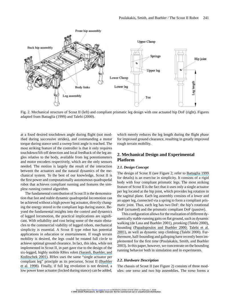
Fig. 2. Mechanical structure of Scout II (left) and compliant prismatic leg design with one actuated hip DoF (right). Figuresadapted from Battaglia (1999) and Talebi (2000).

at a fixed desired touchdown angle during flight (not mod-ified during successive strides), and commanding a motortorque during stance until a sweep limit angle is reached. Themost striking feature of the controller is that it only requirestouchdown/lift-off detection and local feedback of the leg an-gles relative to the body, available from leg potentiometersand motor encoders respectively, which are the only sensorsneeded. The motion is largely the result of the interactionbetween the actuators and the natural dynamics of the me-chanical system. To the best of our knowledge, Scout II isthe first power and computationally autonomous quadrupedalrobot that achieves compliant running and features the sim-plest running control algorithm.

The fundamental contribution of Scout II is the demonstra-tion that fast and stable dynamic quadrupedal locomotion canbe achieved without a high power leg actuator, directly chang-ing the energy stored in the compliant legs during stance. Be-yond the fundamental insights into the control and dynamicsof legged locomotion, the practical implications are signifi-cant. With reliability and cost being some of the main obsta-cles to the commercial viability of legged robots, mechanicalsimplicity is essential. A Scout II type robot has potentialapplications in education or entertainment. If rough terrainmobility is desired, the legs could be rotated full circle toachieve optimal ground clearance. In fact, this idea, while notimplemented in Scout II, in part gave rise to the design of thesix-legged, highly mobile RHex robot (Saranli, Buehler, andKoditschek 2001). RHex uses the same “single actuator percompliant leg” principle as its precursor, Scout II (Buehleret al. 1998). Finally, if full leg revolution is not desired, alow power knee actuator (locked during stance) can be added,

which merely reduces the leg length during the flight phasefor improved ground clearance, resulting in greatly improvedrough terrain mobility.

2. Mechanical Design and ExperimentalPlatform

2.1. Design Concept

The design of Scout II (see Figure 2; refer to Battaglia 1999for details) is an exercise in simplicity. It consists of a rigidbody with four compliant prismatic legs. The most strikingfeature of Scout II is the fact that it uses only a single actuatorper leg located at the hip joint, which provides leg rotation inthe sagittal plane. Each leg assembly consists of a lower andan upper leg, connected via a spring to form a compliant pris-matic joint. Thus, each leg has two DoF: the hip’s rotationalDoF (actuated) and the prismatic compliant DoF (passive).

This configuration allows for the realization of different dy-namically stable running gaits on flat ground, such as dynamicwalking (de Lasa and Buehler 2001), pronking (Talebi 2000),bounding (Papadopoulos and Buehler 2000; Talebi et al.2001), as well as dynamic step climbing (Talebi 2000). Fur-thermore, half-bounding and galloping have recently been im-plemented for the first time (Poulakakis, Smith, and Buehler2003). In this paper, however, we concentrate on the boundingrunning behavior both in simulation and in experiments.

2.2. Hardware Description

The chassis of Scout II (see Figure 2) consists of three mod-ules: one torso and two hip assemblies. The torso forms a

© 2005 SAGE Publications. All rights reserved. Not for commercial use or unauthorized distribution. at PENNSYLVANIA STATE UNIV on February 7, 2008 http://ijr.sagepub.comDownloaded from

242 THE INTERNATIONAL JOURNAL OF ROBOTICS RESEARCH / April 2005

Sagittal Plane

FrontVirtual Leg

BackVirtualLeg

Physical Legs

L

lf

b

b

f

lb

kb

b

kfb

(x,y)

m,I

x

y

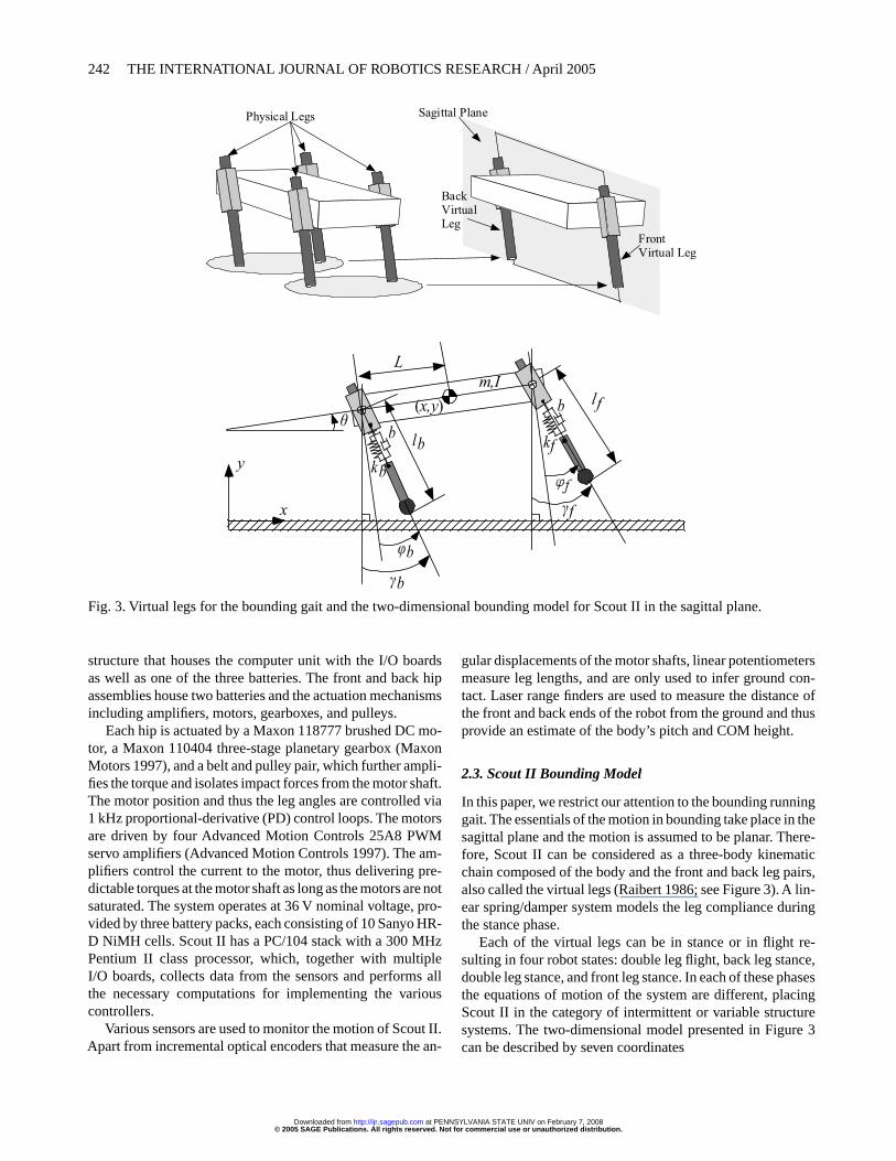
Fig. 3. Virtual legs for the bounding gait and the two-dimensional bounding model for Scout II in the sagittal plane.

structure that houses the computer unit with the I/O boardsas well as one of the three batteries. The front and back hipassemblies house two batteries and the actuation mechanismsincluding amplifiers, motors, gearboxes, and pulleys.

Each hip is actuated by a Maxon 118777 brushed DC mo-tor, a Maxon 110404 three-stage planetary gearbox (MaxonMotors 1997), and a belt and pulley pair, which further ampli-fies the torque and isolates impact forces from the motor shaft.The motor position and thus the leg angles are controlled via1 kHz proportional-derivative (PD) control loops. The motorsare driven by four Advanced Motion Controls 25A8 PWMservo amplifiers (Advanced Motion Controls 1997). The am-plifiers control the current to the motor, thus delivering pre-dictable torques at the motor shaft as long as the motors are notsaturated. The system operates at 36 V nominal voltage, pro-vided by three battery packs, each consisting of 10 Sanyo HR-D NiMH cells. Scout II has a PC/104 stack with a 300 MHzPentium II class processor, which, together with multipleI/O boards, collects data from the sensors and performs allthe necessary computations for implementing the variouscontrollers.

Various sensors are used to monitor the motion of Scout II.Apart from incremental optical encoders that measure the an-

gular displacements of the motor shafts, linear potentiometersmeasure leg lengths, and are only used to infer ground con-tact. Laser range finders are used to measure the distance ofthe front and back ends of the robot from the ground and thusprovide an estimate of the body’s pitch and COM height.

2.3. Scout II Bounding Model

In this paper, we restrict our attention to the bounding runninggait. The essentials of the motion in bounding take place in thesagittal plane and the motion is assumed to be planar. There-fore, Scout II can be considered as a three-body kinematicchain composed of the body and the front and back leg pairs,also called the virtual legs (Raibert 1986; see Figure 3). A lin-ear spring/damper system models the leg compliance duringthe stance phase.

Each of the virtual legs can be in stance or in flight re-sulting in four robot states: double leg flight, back leg stance,double leg stance, and front leg stance. In each of these phasesthe equations of motion of the system are different, placingScout II in the category of intermittent or variable structuresystems. The two-dimensional model presented in Figure 3can be described by seven coordinates

© 2005 SAGE Publications. All rights reserved. Not for commercial use or unauthorized distribution. at PENNSYLVANIA STATE UNIV on February 7, 2008 http://ijr.sagepub.comDownloaded from

Poulakakis, Smith, and Buehler / The Scout II Robot 243

x = [x y θ ϕb lb ϕf lf

]T, (1)

where all the variables and the sign conventions are shownin Figure 3 and are summarized in Table 1. The design pa-rameters of the robot are presented in Table 2. Note that analternative representation of the system’s configuration wouldbe to express the leg angles relative to the vertical, i.e.

γi = ϕi + θ, (2)

wherei = b, f .

3. Bounding Controllers

3.1. Constant Touchdown Angle Bounding Controller

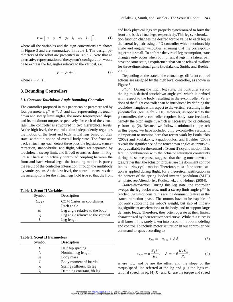
The controller proposed in this paper can be parametrized byfour parameters,ϕtd ,ϕswl,A, andτmax , representing the touch-down and sweep limit angles, the motor torque/speed slope,and its maximum torque, respectively, for each of the virtuallegs. The controller is structured in two hierarchical levels.At the high level, the control action independently regulatesthe motion of the front and back virtual legs based on theirstate, without a notion of overall body state. The front andback virtual legs each detect three possible leg states: stance-retraction, stance-brake, and flight, which are separated bytouchdown, sweep limit, and lift-off events, as shown in Fig-ure 4. There is no actively controlled coupling between thefront and back virtual legs: the bounding motion is purelythe result of the controller interaction through the multibodydynamic system. At the low level, the controller ensures thatthe assumptions for the virtual legs hold true so that the front

Table 1. Scout II VariablesSymbol Description

(x, y) COM Cartesian coordinatesθ Pitch angleϕt Leg angle relative to the bodyγi Leg angle relative to the verticalli Leg length

Table 2. Scout II ParametersSymbol Description

L Half hip spacinglo Nominal leg lengthm Body massI Body moment of inertiaki Spring stiffness,ith legki Damping constant,ith leg

and back physical legs are properly synchronized to form thefront and back virtual legs, respectively. This leg synchroniza-tion function changes the desired torque value to each leg inthe lateral leg pair using a PD controller which monitors hipangle and angular velocities, ensuring that the correspond-ing error is small. To enforce the virtual leg assumption, statechanges only occur when both physical legs in a lateral pairhave the same state, a requirement that can be relaxed to allowfor three-dimensional gaits (Poulakakis, Smith, and Buehler2003).

Depending on the state of the virtual legs, different controlactions are assigned by the high level controller, as shown inFigure 5.

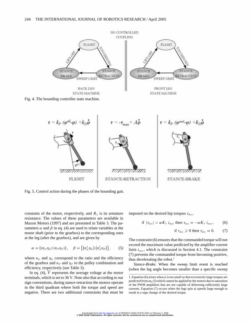
Flight. During the flight leg state, the controller servosthe leg to a desired touchdown angleϕtd , which is definedwith respect to the body, resulting in theϕ-controller. Varia-tions of the flight controller can be introduced by defining thetouchdown angles with respect to the vertical, resulting in theγ -controller (see Talebi 2000). However, as opposed to theϕ-controller, theγ -controller requires body-state feedback,namely the pitch angleθ , which is necessary for calculatingγ from eq. (2). Because we follow a minimalist approachin this paper, we have included onlyϕ-controller results. Itis important to mention here that recent work by Poulakakis(2002) and Poulakakis, Papadopoulos, and Buehler (2003)reveals the significance of the touchdown angles as inputs di-rectly available for the control of Scout II’s cyclic motion.Thisfact, in combination with the actuator saturation constraintsduring the stance phase, suggests that the leg touchdown an-gles, rather than the actuator torques, are the dominant controlinputs during cyclic motion. Therefore, most of the control ac-tion is applied during flight; for a theoretical justification inthe context of the spring loaded inverted pendulum (SLIP)template, see Altendorfer, Koditschek, and Holmes (2004).

Stance-Retraction. During this leg state, the controllersweeps the leg backwards, until a sweep limit angleϕswl isreached. Actuator constraints are the dominant feature in thestance-retraction phase. The motors have to be capable ofnot only supporting the robot’s weight, but also of impart-ing significant accelerations to the body, and to support largedynamic loads. Therefore, they often operate at their limits,characterized by their torque/speed curve. While this curve iswell known, it is rarely taken into account in robot modelingand control. To include motor saturation in our controller, wecommand torques according to

τdes = −τmax + A ϕ (3)

τmax = αKT V

RA

, A = −βKT Kω

RA

, (4)

where τmax and A are the offset and the slope of thetorque/speed line referred at the leg andϕ is the leg’s ro-tational speed. In eq. (4)KT andKω are the torque and speed

© 2005 SAGE Publications. All rights reserved. Not for commercial use or unauthorized distribution. at PENNSYLVANIA STATE UNIV on February 7, 2008 http://ijr.sagepub.comDownloaded from

244 THE INTERNATIONAL JOURNAL OF ROBOTICS RESEARCH / April 2005

Fig. 4. The bounding controller state machine.

Fig. 5. Control action during the phases of the bounding gait.

constants of the motor, respectively, andRA is its armatureresistance. The values of these parameters are available inMaxon Motors (1997) and are presented in Table 3. The pa-rametersα andβ in eq. (4) are used to relate variables at themotor shaft (prior to the gearbox) to the corresponding onesat the leg (after the gearbox), and are given by

α = [(nGηG) (nP ηP )] , β = [(n2

GηG

) (n2

PηP

)], (5)

wherenG andηG correspond to the ratio and the efficiencyof the gearbox andnP andηP to the pulley combination andefficiency, respectively (see Table 3).

In eq. (4),V represents the average voltage at the motorterminals, which is set to 36 V. Note also that according to oursign conventions, during stance-retraction the motors operatein the third quadrant where both the torque and speed arenegative. There are two additional constraints that must be

imposed on the desired hip torquesτdes ,

if |τdes | > αKT imax thenτdes = −αKT imax, (6)

if τdes � 0 thenτdes = 0. (7)

The constraint (6) ensures that the commanded torque will notexceed the maximum value predicted by the amplifier currentlimit imax , which is discussed in Section 4.1. The constraint(7) prevents the commanded torque from becoming positive,thus decelerating the robot.1

Stance-Brake. When the sweep limit event is reached(when the leg angle becomes smaller than a specific sweep

1. Equation (6) arises whenϕ is too small so that excessively large torques arepredicted from eq. (3) which cannot be applied by the motors due to saturationof the PWM amplifiers that are not capable of delivering sufficiently largecurrents. Equation (7) occurs when the legs spin at speeds large enough toresult in a sign change of the desired torque.

© 2005 SAGE Publications. All rights reserved. Not for commercial use or unauthorized distribution. at PENNSYLVANIA STATE UNIV on February 7, 2008 http://ijr.sagepub.comDownloaded from

Poulakakis, Smith, and Buehler / The Scout II Robot 245

Table 3. Motor ParametersParameter Value Units

Torque constant 0.0389 Nm A−1

Speed constant 6.78× 10−4 V deg−1s−1

Armature resistance 1.23

Belt and pulley combination 48/34 n/aBelt and pulley efficiency 96% n/aPlanetary gear ratio 72.38 n/aMaximum gear efficiency 68% n/a

limit angle ϕswl), a PD controller holds the leg at that an-gle. Although this modification has the undesirable effect ofbraking the robot, it is necessary for ensuring toe clearance,especially during the early protraction phase, because of theabsence of active control of the leg length during flight. Theaddition of the sweep limit was found to significantly improvethe robustness of the motion at the expense of performanceand energy consumption.

It is important to mention that the controllers describedhere are simpler than those proposed by Raibert in two re-spects. First, no task-level (e.g., forward velocity) and nobody-state (e.g., body posture) feedback are required. Sec-ondly, no explicit control over leg length ensuring toe clear-ance during the leg protraction phase is necessary, providedthat the modification outlined above is added to the stancephase. These characteristics have had and are expected tohave significant implications in the design of other leggedrobots too. Indeed, similar design and control ideas have beensuccessfully used to generate bounding in the modified (oneactuator per leg)AIBO (Yamamoto et al. 2001), and by Camp-bell and Buehler (2003) in the hexapedal RHex, developed bySaranli, Buehler, and Koditschek (2001).

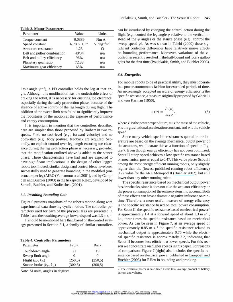
3.2. Resulting Bounding Gait

Figure 6 presents snapshots of the robot’s motion along withexperimental data showing cyclic motion. The controller pa-rameters used for each of the physical legs are presented inTable 4 and the resulting average forward speed was 1.3 m s−1.

It should be mentioned here that, based on the control strat-egy presented in Section 3.1, a family of similar controllers

Table 4. Controller ParametersParameter Front Back

Touchdown angle 21 19Sweep limit angle 0 0Flight (kP , kD) (250,5) (250,5)Stance-brake(kP , kD) (300,5) (300,5)

Note. SI units, angles in degrees

can be introduced by changing the control action during theflight (e.g., control the leg angleγ relative to the vertical in-stead of theϕ angle) or the stance phase (e.g., control thesweep speedϕ). As was shown in Talebi (2000) these sig-nificant controller differences have relatively minor effectson bounding performance. Moreover, variations of theϕ-controller recently resulted in the half-bound and rotary gallopgaits for the first time (Poulakakis, Smith, and Buehler 2003).

3.3. Energetics

For mobile robots to be of practical utility, they must operatein a power autonomous fashion for extended periods of time.An increasingly accepted measure of energy efficiency is thespecific resistance, a measure originally proposed by Gabrielliand von Karman (1950),

ε (υ) = P (υ)

mgυ, (8)

whereP is the power expenditure,m is the mass of the vehicle,g is the gravitational acceleration constant, andυ is the vehiclespeed.

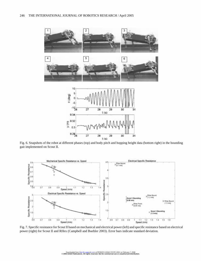
Since many vehicle specific resistances quoted in the lit-erature are based on the average mechanical output power ofthe actuators, we illustrate this as a function of speed in Fig-ure 7. Even though energy efficiency has not been optimized,Scout II at top speed achieves a low specific resistance basedon mechanical power, equal to 0.47. This value places Scout IIamong the most energy efficient running robots, only slightlyhigher than the (lowest published running robot efficiency)0.22 value for the ARL Monopod II (Buehler 2002), but stilllower than any other running robot.

The specific resistance based on mechanical output powerhas drawbacks, since it does not take the actuator efficiency orthe power consumption of the entire system into account. Bothof these effects can have a dramatic negative influence on run-time. Therefore, a more useful measure of energy efficiencyis the specific resistance based on total power consumption.For Scout II, the specific resistance based on electrical power2

is approximately 1.4 at a forward speed of about 1.3 m s−1,i.e., three times the specific resistance based on mechanicalpower. As can be seen in Figure 7, at an average speed ofapproximately 0.85 m s−1 the specific resistance related tomechanical output is approximately 0.75 while the electri-cal specific resistance is approximately 2.2, indicating thatScout II becomes less efficient at lower speeds. For this rea-son we concentrate on higher speeds in this paper. For reasonsof comparison, Figure 7 (right) also includes the specific re-sistance based on electrical power published in Campbell andBuehler (2003) for RHex in bounding and pronking.

2. The electrical power is calculated as the total average product of batterycurrent and voltage.

© 2005 SAGE Publications. All rights reserved. Not for commercial use or unauthorized distribution. at PENNSYLVANIA STATE UNIV on February 7, 2008 http://ijr.sagepub.comDownloaded from

246 THE INTERNATIONAL JOURNAL OF ROBOTICS RESEARCH / April 2005

1 2 3

4 5 6

Fig. 6. Snapshots of the robot at different phases (top) and body pitch and hopping height data (bottom right) in the boundinggait implemented on Scout II.

Fig. 7. Specific resistance for Scout II based on mechanical and electrical power (left) and specific resistance based on electricalpower (right) for Scout II and RHex (Campbell and Buehler 2003). Error bars indicate standard deviation.

© 2005 SAGE Publications. All rights reserved. Not for commercial use or unauthorized distribution. at PENNSYLVANIA STATE UNIV on February 7, 2008 http://ijr.sagepub.comDownloaded from

Poulakakis, Smith, and Buehler / The Scout II Robot 247

3.4. Discussion

Scout II is a highly nonlinear, underactuated, intermittent dy-namical system. Furthermore, as Full and Koditschek (1999,p. 3326) state: “Locomotion results from complex, high-dimensional, nonlinear, dynamically coupled interactions be-tween an organism and its environment.” Thus, the task itselfis also complex and cannot be specified via reference trajec-tories in Cartesian or in state space. Even if such trajectoriescould be found, developing a tracking controller is still notstraightforward or perhaps even possible. Friction, actuatorlimitations, and unilateral ground forces limit the hip torques,which may be required to achieve trajectory tracking. Further-more, there are no experimentally validated models, whichcould be used to derive model-based controllers for leggedrobots. This reveals the necessity for constructing simulationmodels to test the validity of various simplifying modelingassumptions, as will be discussed in Section 5.

It is apparent from the above discussion why direct ap-plication of modern robot control theory had limited successin deriving controllers for dynamically stable legged robots.Despite this complexity, we found that simple Raibert-stylecontrol laws, like those described in Section 3.1 and in Raib-ert (1986), operating mostly in a feedforward fashion, withminimal sensing, can stabilize periodic motions, resulting inrobust and fast running powered by only four hip actuators.It is therefore natural to ask why such a complex system canaccomplish such a complex task via minor control action.

As outlined in Poulakakis (2002) and Poulakakis, Pa-padopoulos, and Buehler (2003), a possible answer is thatScout II’s unactuated, conservative dynamics already exhibitasymptotically stable bounding cycles, and therefore a sim-ple controller is all that is needed to keep the robot bounding.Indeed, for sufficiently high forward speeds and pitch ratesthere exists a regime where the system can be passively stableand can tolerate small perturbations of the nominal conditionswithout any control action taken. This fact could provide apossible explanation as to why the Scout II robot can boundwithout the need for complex state feedback. It is importantto mention that this hypothesis is in agreement with recentresearch in biomechanics, which shows that when animalsrun at high speeds, passive dynamic self-stabilization from afeedforward, tuned mechanical system can reject rapid per-turbations and simplify control (Full and Koditschek 1999;Kubow and Full 1999). Analogous behavior has been discov-ered by McGeer (1989) in his passive bipedal running work,and more recently in the conservative3 SLIP template (Sey-farth et al. 2002; Ghigliazza et al. 2003).

To conclude, Scout II and its simple, body-state and task-level open-loop controller embodies these general underly-ing principles, and can be considered as an experimental

3. An explanation as to why conservative intermittent dynamical systems canexhibit asymptotically stable limit cycles despite the incompressibility of thestance flow was presented in Altendorfer, Koditschek, and Holmes (2004).

demonstration contributing to the increasing evidence that,as Full and Koditschek (1999) suggested, control laws op-erating mostly in the feedforward regime with “mechanicalfeedback” are sufficient to induce stable dynamic behaviorsin legged machines.

4. Modeling Components

4.1. Electrical Subsystem

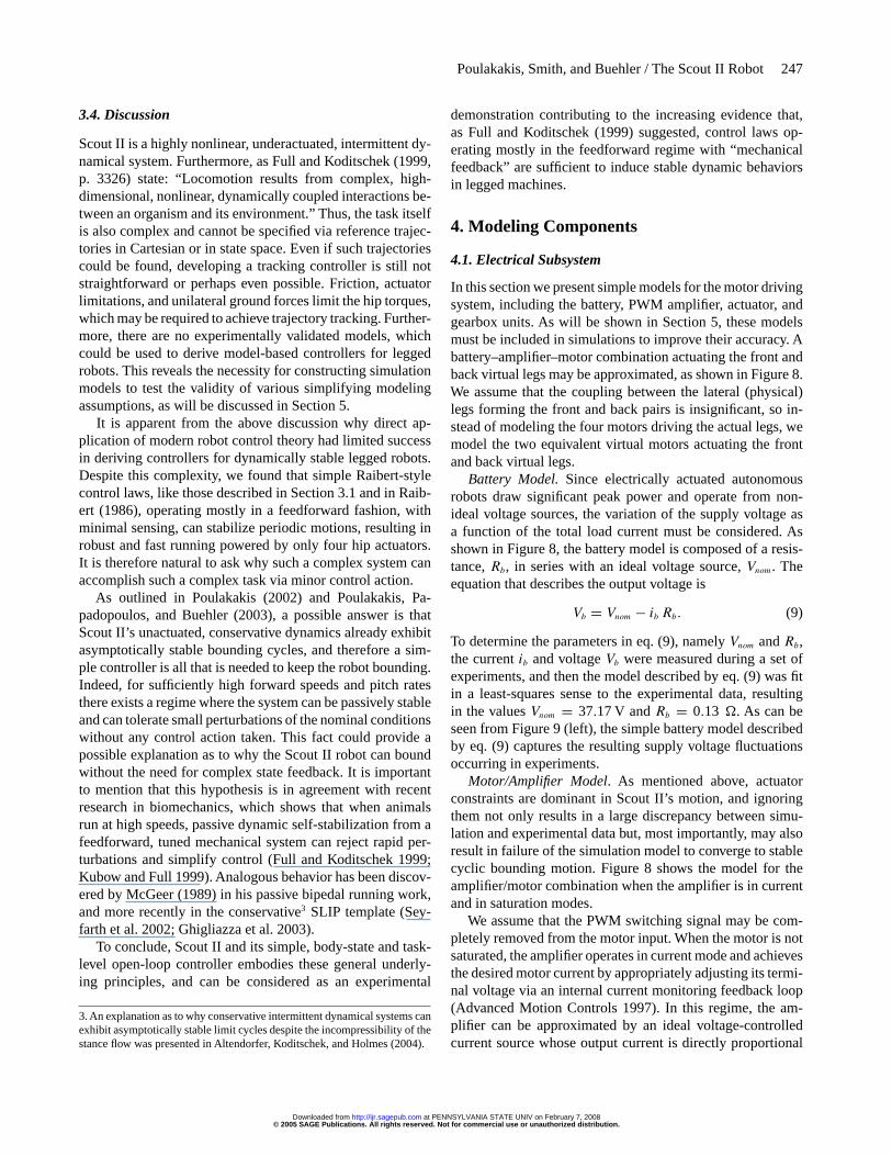
In this section we present simple models for the motor drivingsystem, including the battery, PWM amplifier, actuator, andgearbox units. As will be shown in Section 5, these modelsmust be included in simulations to improve their accuracy. Abattery–amplifier–motor combination actuating the front andback virtual legs may be approximated, as shown in Figure 8.We assume that the coupling between the lateral (physical)legs forming the front and back pairs is insignificant, so in-stead of modeling the four motors driving the actual legs, wemodel the two equivalent virtual motors actuating the frontand back virtual legs.

Battery Model. Since electrically actuated autonomousrobots draw significant peak power and operate from non-ideal voltage sources, the variation of the supply voltage asa function of the total load current must be considered. Asshown in Figure 8, the battery model is composed of a resis-tance,Rb, in series with an ideal voltage source,Vnom. Theequation that describes the output voltage is

Vb = Vnom − ib Rb. (9)

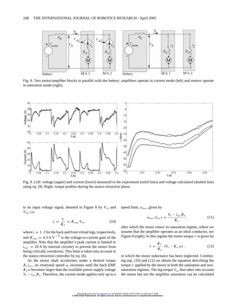
To determine the parameters in eq. (9), namelyVnom andRb,the currentib and voltageVb were measured during a set ofexperiments, and then the model described by eq. (9) was fitin a least-squares sense to the experimental data, resultingin the valuesVnom = 37.17 V andRb = 0.13 . As can beseen from Figure 9 (left), the simple battery model describedby eq. (9) captures the resulting supply voltage fluctuationsoccurring in experiments.

Motor/Amplifier Model. As mentioned above, actuatorconstraints are dominant in Scout II’s motion, and ignoringthem not only results in a large discrepancy between simu-lation and experimental data but, most importantly, may alsoresult in failure of the simulation model to converge to stablecyclic bounding motion. Figure 8 shows the model for theamplifier/motor combination when the amplifier is in currentand in saturation modes.

We assume that the PWM switching signal may be com-pletely removed from the motor input. When the motor is notsaturated, the amplifier operates in current mode and achievesthe desired motor current by appropriately adjusting its termi-nal voltage via an internal current monitoring feedback loop(Advanced Motion Controls 1997). In this regime, the am-plifier can be approximated by an ideal voltage-controlledcurrent source whose output current is directly proportional

© 2005 SAGE Publications. All rights reserved. Not for commercial use or unauthorized distribution. at PENNSYLVANIA STATE UNIV on February 7, 2008 http://ijr.sagepub.comDownloaded from

248 THE INTERNATIONAL JOURNAL OF ROBOTICS RESEARCH / April 2005

Fig. 8. Two motor/amplifier blocks in parallel with the battery: amplifiers operate in current mode (left) and motors operatein saturation mode (right).

Fig. 9. Left: voltage (upper) and current (lower) measured in the experiment (solid lines) and voltage calculated (dashed line)using eq. (9). Right: torque profiles during the stance-retraction phase.

to its input voltage signal, denoted in Figure 8 byVA1 andVA2, i.e.

ii = τi

KT

= Kamp VAi, (10)

wherei = 1, 2 for the back and front virtual legs, respectively,

andKamp = 4.3 A V - 1 is the voltage-to-current gain of theamplifier. Note that the amplifier’s peak current is limited toimax = 20 A by internal circuitry to prevent the motor frombeing critically overdriven. This limit is taken into account inthe stance-retraction controller by eq. (6).

As the motor shaft accelerates under a desired torqueKT ides , its rotational speedω, increases until the back EMFKωω becomes larger than the available power supply voltageVb − idesRA. Therefore, the current mode applies only up to a

speed limit,ωmax , given by

ωmax (ides) = Vb − idesRA

Kω

, (11)

after which the motor enters its saturation regime, where weassume that the amplifier operates as an ideal conductor, seeFigure 8 (right). In this regime the motor torqueτ is given by

τ = KT

RA

(Vb − Kω ω) , (12)

in which the motor inductance has been neglected. Combin-ing eqs. (10) and (12) we obtain the equation describing thetorqueτ applied by the motor in both the saturation and non-saturation regimes. The leg torqueτleg that takes into accountthe motor but not the amplifier saturation can be calculated

© 2005 SAGE Publications. All rights reserved. Not for commercial use or unauthorized distribution. at PENNSYLVANIA STATE UNIV on February 7, 2008 http://ijr.sagepub.comDownloaded from

Poulakakis, Smith, and Buehler / The Scout II Robot 249

by the motor torque using

τleg ={ −αKT ides for |ω| � |ωmax |

−α KT Vb

RA− β KT Kω

RAϕ for |ω| > |ωmax | , (13)

which is valid in the third quadrant of the torque/speed line(stance-retraction). In eq. (13) the velocityωmax is given byeq. (11), the parametersα andβ are given by eq. (5), and thesign conventions described in Section 2.3 have been applied.Finally, the torqueτleg that is delivered at the leg and thatincludes both the motor and amplifier saturation is given by

τleg = sgn(τleg

)min

{∣∣τleg

∣∣ , αKT imax

}(14)

whereimax is the amplifier’s peak current. Equations (13) and(14) constitute the motor model in the third quadrant and,with the appropriate sign changes, can be extended to the firstquadrant of the torque/speed curve.

Figure 9 shows current, voltage, and torque plots. The datacurves in the right-hand plot of Figure 9 are as follows, frombottom to top. The bottommost solid curve represents thedesired torque from the controller as calculated by eq. (3),which is identical to that predicted by eq. (14) for a fixed 36 Vsupply voltage. The second, dashed, curve is the maximumachievable torque and includes the battery voltage fluctuationscalculated by eq. (9). The third, dotted, curve illustrates thetorque with an additional loop gain fix due to amplifier gainmodeling error. Finally, the topmost solid curve represents thecurrent-estimated motor torque measured during a boundingexperiment. The exceptionally good match between the top-most solid and dotted torque curves in the right-hand plot ofFigure 9 validates the model and demonstrates both its impor-tance and its effectiveness in predicting motor saturation.

4.2. Mechanical Subsystem

Throughout the course of this research it has become clear thatmodeling only the motor driving system (batteries, PWM am-plifiers, and actuators) as in Section 4.1 is not sufficient forobtaining simulation results which closely follow the exper-imental data. A more detailed model of the hip unit, whichincludes backlash and belt compliance, must be included insimulation in order to improve its accuracy. It is important tomention here that the assumptions of zero backlash and rigidtorque transmission are very common in modeling dynami-cally stable robots. However, as will be shown in Section 5,for Scout II and the controllers presented in Section 3, theynot only result in large mismatches between simulation andexperimental data but, more importantly, for some set points,they might even result in failure to converge to cyclic mo-tion. Note also that these effects are not specific to Scout II.Indeed, because of space limitations for motor placement,and due to the desire to isolate impact forces from the motorshafts, structural elements such as belts are very common fortorque transmission in leg designs (e.g., Furusho et al. 1995).

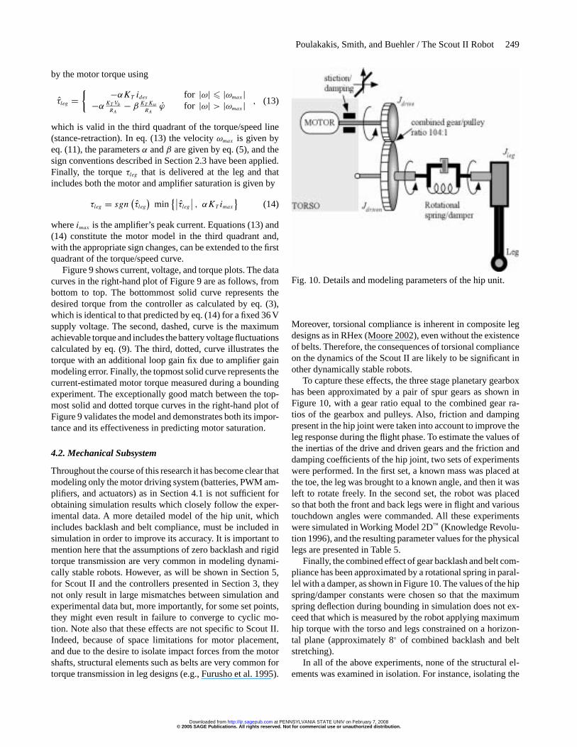
Fig. 10. Details and modeling parameters of the hip unit.

Moreover, torsional compliance is inherent in composite legdesigns as in RHex (Moore 2002), even without the existenceof belts. Therefore, the consequences of torsional complianceon the dynamics of the Scout II are likely to be significant inother dynamically stable robots.

To capture these effects, the three stage planetary gearboxhas been approximated by a pair of spur gears as shown inFigure 10, with a gear ratio equal to the combined gear ra-tios of the gearbox and pulleys. Also, friction and dampingpresent in the hip joint were taken into account to improve theleg response during the flight phase. To estimate the values ofthe inertias of the drive and driven gears and the friction anddamping coefficients of the hip joint, two sets of experimentswere performed. In the first set, a known mass was placed atthe toe, the leg was brought to a known angle, and then it wasleft to rotate freely. In the second set, the robot was placedso that both the front and back legs were in flight and varioustouchdown angles were commanded. All these experimentswere simulated in Working Model 2D™ (Knowledge Revolu-tion 1996), and the resulting parameter values for the physicallegs are presented in Table 5.

Finally, the combined effect of gear backlash and belt com-pliance has been approximated by a rotational spring in paral-lel with a damper, as shown in Figure 10. The values of the hipspring/damper constants were chosen so that the maximumspring deflection during bounding in simulation does not ex-ceed that which is measured by the robot applying maximumhip torque with the torso and legs constrained on a horizon-tal plane (approximately 8◦ of combined backlash and beltstretching).

In all of the above experiments, none of the structural el-ements was examined in isolation. For instance, isolating the

© 2005 SAGE Publications. All rights reserved. Not for commercial use or unauthorized distribution. at PENNSYLVANIA STATE UNIV on February 7, 2008 http://ijr.sagepub.comDownloaded from

250 THE INTERNATIONAL JOURNAL OF ROBOTICS RESEARCH / April 2005

Table 5. Hip Joint Properties

Parameter Value Units

Drive gear inertia 3.5× 10−6 kg m2

Driven gear inertia 10−3 kg m2

Stiction (joint) 5.5× 10−3 NmDamping (joint) 6.2× 10−7 Nm deg−1s−1

Spring (belt) 7.0 Nm deg−1

Damper (belt) 4.0 Nm deg−1s−1

gearbox and performing detailed identification experimentsto find the inertia of the gears requires special equipment notavailable to us. Instead, we performed simple experiments ex-amining the behavior of the hip unit as a whole under differentdynamic conditions as described above. Then, parameter val-ues were selected that matched experiment and simulationunder these different conditions.

5. Experiments and Simulation

5.1. Simulation Models

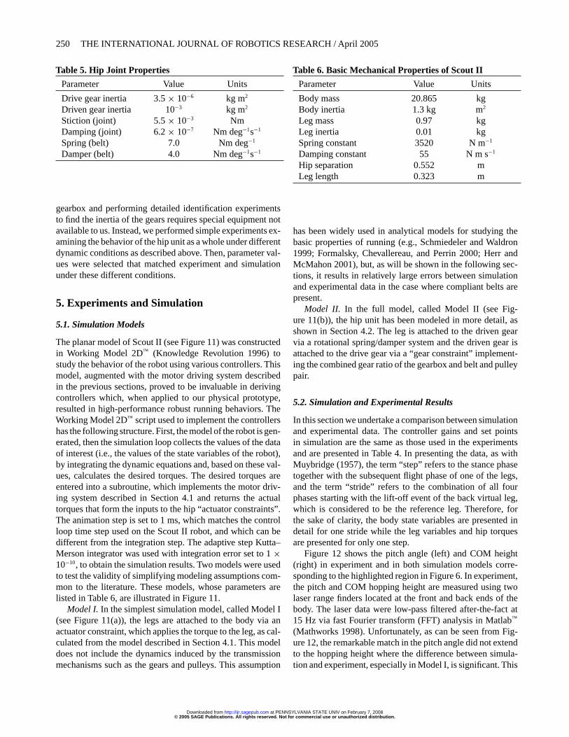
The planar model of Scout II (see Figure 11) was constructedin Working Model 2D™ (Knowledge Revolution 1996) tostudy the behavior of the robot using various controllers. Thismodel, augmented with the motor driving system describedin the previous sections, proved to be invaluable in derivingcontrollers which, when applied to our physical prototype,resulted in high-performance robust running behaviors. TheWorking Model 2D™ script used to implement the controllershas the following structure. First, the model of the robot is gen-erated, then the simulation loop collects the values of the dataof interest (i.e., the values of the state variables of the robot),by integrating the dynamic equations and, based on these val-ues, calculates the desired torques. The desired torques areentered into a subroutine, which implements the motor driv-ing system described in Section 4.1 and returns the actualtorques that form the inputs to the hip “actuator constraints”.The animation step is set to 1 ms, which matches the controlloop time step used on the Scout II robot, and which can bedifferent from the integration step. The adaptive step Kutta–Merson integrator was used with integration error set to 1×10−10, to obtain the simulation results. Two models were usedto test the validity of simplifying modeling assumptions com-mon to the literature. These models, whose parameters arelisted in Table 6, are illustrated in Figure 11.

Model I. In the simplest simulation model, called Model I(see Figure 11(a)), the legs are attached to the body via anactuator constraint, which applies the torque to the leg, as cal-culated from the model described in Section 4.1. This modeldoes not include the dynamics induced by the transmissionmechanisms such as the gears and pulleys. This assumption

Table 6. Basic Mechanical Properties of Scout II

Parameter Value Units

Body mass 20.865 kgBody inertia 1.3 kg m2

Leg mass 0.97 kgLeg inertia 0.01 kgSpring constant 3520 N m−1

Damping constant 55 N m s−1

Hip separation 0.552 mLeg length 0.323 m

has been widely used in analytical models for studying thebasic properties of running (e.g., Schmiedeler and Waldron1999; Formalsky, Chevallereau, and Perrin 2000; Herr andMcMahon 2001), but, as will be shown in the following sec-tions, it results in relatively large errors between simulationand experimental data in the case where compliant belts arepresent.

Model II. In the full model, called Model II (see Fig-ure 11(b)), the hip unit has been modeled in more detail, asshown in Section 4.2. The leg is attached to the driven gearvia a rotational spring/damper system and the driven gear isattached to the drive gear via a “gear constraint” implement-ing the combined gear ratio of the gearbox and belt and pulleypair.

5.2. Simulation and Experimental Results

In this section we undertake a comparison between simulationand experimental data. The controller gains and set pointsin simulation are the same as those used in the experimentsand are presented in Table 4. In presenting the data, as withMuybridge (1957), the term “step” refers to the stance phasetogether with the subsequent flight phase of one of the legs,and the term “stride” refers to the combination of all fourphases starting with the lift-off event of the back virtual leg,which is considered to be the reference leg. Therefore, forthe sake of clarity, the body state variables are presented indetail for one stride while the leg variables and hip torquesare presented for only one step.

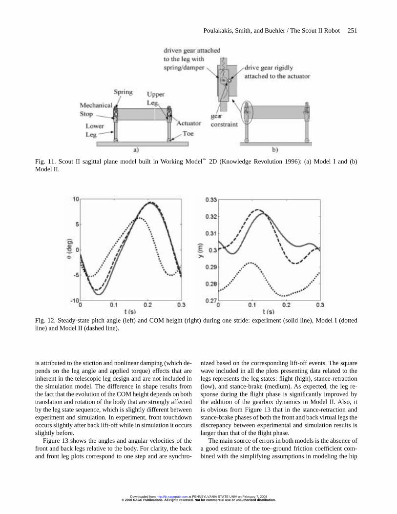
Figure 12 shows the pitch angle (left) and COM height(right) in experiment and in both simulation models corre-sponding to the highlighted region in Figure 6. In experiment,the pitch and COM hopping height are measured using twolaser range finders located at the front and back ends of thebody. The laser data were low-pass filtered after-the-fact at15 Hz via fast Fourier transform (FFT) analysis in Matlab™

(Mathworks 1998). Unfortunately, as can be seen from Fig-ure 12, the remarkable match in the pitch angle did not extendto the hopping height where the difference between simula-tion and experiment, especially in Model I, is significant. This

© 2005 SAGE Publications. All rights reserved. Not for commercial use or unauthorized distribution. at PENNSYLVANIA STATE UNIV on February 7, 2008 http://ijr.sagepub.comDownloaded from

Poulakakis, Smith, and Buehler / The Scout II Robot 251

Fig. 11. Scout II sagittal plane model built in Working Model™ 2D (Knowledge Revolution 1996): (a) Model I and (b)Model II.

Fig. 12. Steady-state pitch angle (left) and COM height (right) during one stride: experiment (solid line), Model I (dottedline) and Model II (dashed line).

is attributed to the stiction and nonlinear damping (which de-pends on the leg angle and applied torque) effects that areinherent in the telescopic leg design and are not included inthe simulation model. The difference in shape results fromthe fact that the evolution of the COM height depends on bothtranslation and rotation of the body that are strongly affectedby the leg state sequence, which is slightly different betweenexperiment and simulation. In experiment, front touchdownoccurs slightly after back lift-off while in simulation it occursslightly before.

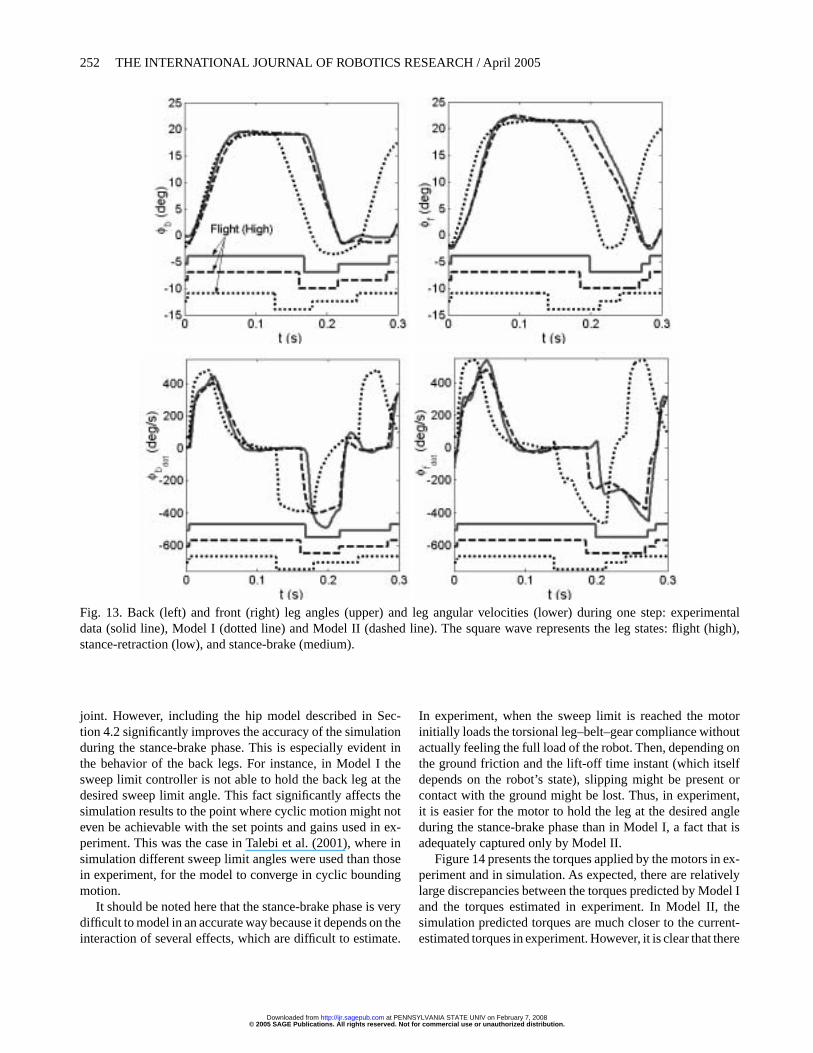
Figure 13 shows the angles and angular velocities of thefront and back legs relative to the body. For clarity, the backand front leg plots correspond to one step and are synchro-

nized based on the corresponding lift-off events. The squarewave included in all the plots presenting data related to thelegs represents the leg states: flight (high), stance-retraction(low), and stance-brake (medium). As expected, the leg re-sponse during the flight phase is significantly improved bythe addition of the gearbox dynamics in Model II. Also, itis obvious from Figure 13 that in the stance-retraction andstance-brake phases of both the front and back virtual legs thediscrepancy between experimental and simulation results islarger than that of the flight phase.

The main source of errors in both models is the absence ofa good estimate of the toe–ground friction coefficient com-bined with the simplifying assumptions in modeling the hip

© 2005 SAGE Publications. All rights reserved. Not for commercial use or unauthorized distribution. at PENNSYLVANIA STATE UNIV on February 7, 2008 http://ijr.sagepub.comDownloaded from

252 THE INTERNATIONAL JOURNAL OF ROBOTICS RESEARCH / April 2005

Fig. 13. Back (left) and front (right) leg angles (upper) and leg angular velocities (lower) during one step: experimentaldata (solid line), Model I (dotted line) and Model II (dashed line). The square wave represents the leg states: flight (high),stance-retraction (low), and stance-brake (medium).

joint. However, including the hip model described in Sec-tion 4.2 significantly improves the accuracy of the simulationduring the stance-brake phase. This is especially evident inthe behavior of the back legs. For instance, in Model I thesweep limit controller is not able to hold the back leg at thedesired sweep limit angle. This fact significantly affects thesimulation results to the point where cyclic motion might noteven be achievable with the set points and gains used in ex-periment. This was the case in Talebi et al. (2001), where insimulation different sweep limit angles were used than thosein experiment, for the model to converge in cyclic boundingmotion.

It should be noted here that the stance-brake phase is verydifficult to model in an accurate way because it depends on theinteraction of several effects, which are difficult to estimate.

In experiment, when the sweep limit is reached the motorinitially loads the torsional leg–belt–gear compliance withoutactually feeling the full load of the robot. Then, depending onthe ground friction and the lift-off time instant (which itselfdepends on the robot’s state), slipping might be present orcontact with the ground might be lost. Thus, in experiment,it is easier for the motor to hold the leg at the desired angleduring the stance-brake phase than in Model I, a fact that isadequately captured only by Model II.

Figure 14 presents the torques applied by the motors in ex-periment and in simulation. As expected, there are relativelylarge discrepancies between the torques predicted by Model Iand the torques estimated in experiment. In Model II, thesimulation predicted torques are much closer to the current-estimated torques in experiment. However, it is clear that there

© 2005 SAGE Publications. All rights reserved. Not for commercial use or unauthorized distribution. at PENNSYLVANIA STATE UNIV on February 7, 2008 http://ijr.sagepub.comDownloaded from

Poulakakis, Smith, and Buehler / The Scout II Robot 253

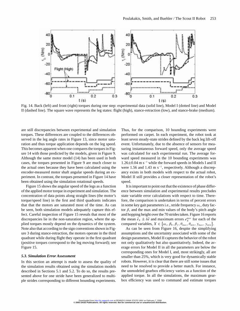
Fig. 14. Back (left) and front (right) torques during one step: experimental data (solid line), Model I (dotted line) and ModelII (dashed line). The square wave represents the leg states: flight (high), stance-retraction (low), and stance-brake (medium).

are still discrepancies between experimental and simulationtorques. These differences are coupled to the differences ob-served in the leg angle rates in Figure 13, since motor satu-ration and thus torque application depends on the leg speed.This becomes apparent when one compares the torques in Fig-ure 14 with those predicted by the models, given in Figure 9.Although the same motor model (14) has been used in bothcases, the torques presented in Figure 9 are much closer tothe actual ones because they have been calculated using theencoder-measured motor shaft angular speeds during an ex-periment. In contrast, the torques presented in Figure 14 havebeen obtained using the simulation rotational speeds.

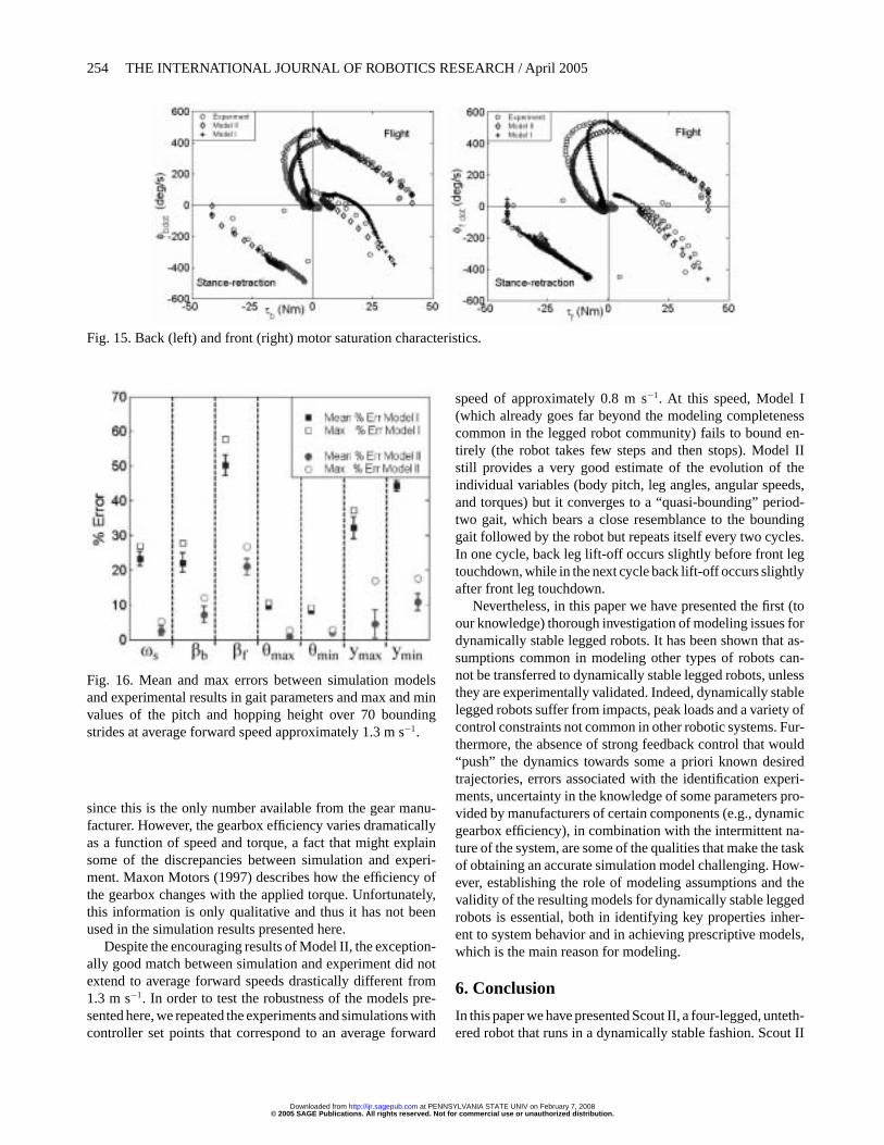
Figure 15 shows the angular speed of the legs as a functionof the applied motor torque in experiment and simulation. Theconcentration of data points along straight lines (the motor’storque/speed line) in the first and third quadrants indicatesthat that the motors are saturated most of the time. As canbe seen, both simulation models adequately capture this ef-fect. Careful inspection of Figure 15 reveals that most of thediscrepancies lie in the non-saturation region, where the ap-plied torques mostly depend on the dynamics of the system.Note also that according to the sign conventions shown in Fig-ure 3 during stance-retraction, the motors operate in the thirdquadrant while during flight they operate in the first quadrant(positive torques correspond to the leg moving forward); seeFigure 15.

5.3. Simulation Error Assessment

In this section an attempt is made to assess the quality ofthe simulation results obtained using the simulation modelsdescribed in Sections 5.1 and 5.2. To do so, the results pre-sented above for one stride have been generalized to multi-ple strides corresponding to different bounding experiments.

Thus, for the comparison, 10 bounding experiments wereperformed on carpet. In each experiment, the robot took atleast seven steady-state strides defined by the back leg lift-offevent. Unfortunately, due to the absence of sensors for mea-suring instantaneous forward speed, only the average speedwas calculated for each experimental run. The average for-ward speed measured in the 10 bounding experiments was1.26±0.04 m s−1 while the forward speeds in Models I and IIwere 1.56 and 1.43 m s−1, respectively. Although a discrep-ancy exists in both models with respect to the actual robot,Model II still provides a closer representation of the robot’sspeed.

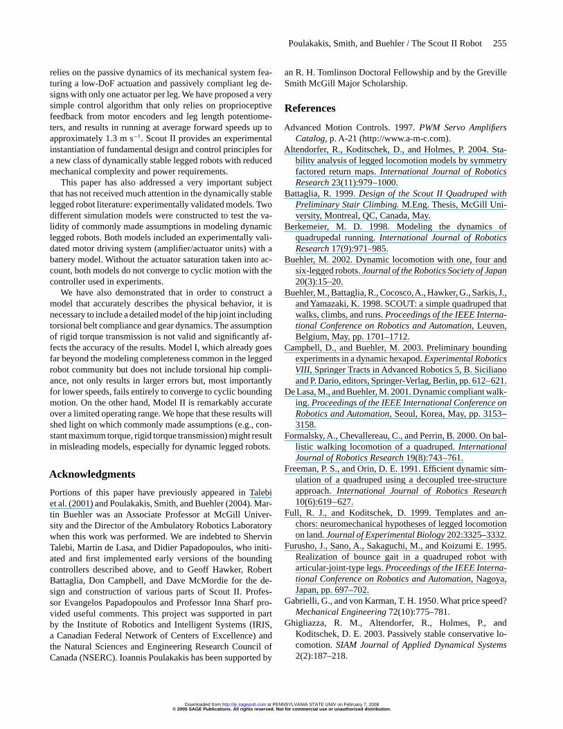
It is important to point out that the existence of phase differ-ence between simulation and experimental results precludesstate variable error calculations with respect to time. There-fore, the comparison is undertaken in terms of percent errorsin some key gait parameters i.e., stride frequencyωs , duty fac-tor β, and the max and min values of the body’s pitch angleand hopping height over the 70 strides taken. Figure 16 reportsthe meaneX ± δe and maximum errorsemax

Xfor each of the

compared variables,X ∈ {ωs, βb, βf , θmax, θmin, ymax, ymin

}.

As can be seen from Figure 16, despite the simplifyingassumptions and the uncertainty associated with some of thedesign parameters, Model II captures the behavior of the robotnot only qualitatively but also quantitatively. Indeed, the av-erage errors for Model II in all the parameters are below thecorresponding ones for Model I, and, most strikingly, all aresmaller than 25%, which is very good for dynamically stablerobots. However, it is clear that there are still some issues thatneed to be resolved to provide a better match. For instance,the unmodeled gearbox efficiency varies as a function of theapplied torque. In all the simulations, the maximum gear-box efficiency was used to command and estimate torques

© 2005 SAGE Publications. All rights reserved. Not for commercial use or unauthorized distribution. at PENNSYLVANIA STATE UNIV on February 7, 2008 http://ijr.sagepub.comDownloaded from

254 THE INTERNATIONAL JOURNAL OF ROBOTICS RESEARCH / April 2005

Fig. 15. Back (left) and front (right) motor saturation characteristics.

Fig. 16. Mean and max errors between simulation modelsand experimental results in gait parameters and max and minvalues of the pitch and hopping height over 70 boundingstrides at average forward speed approximately 1.3 m s−1.

since this is the only number available from the gear manu-facturer. However, the gearbox efficiency varies dramaticallyas a function of speed and torque, a fact that might explainsome of the discrepancies between simulation and experi-ment. Maxon Motors (1997) describes how the efficiency ofthe gearbox changes with the applied torque. Unfortunately,this information is only qualitative and thus it has not beenused in the simulation results presented here.

Despite the encouraging results of Model II, the exception-ally good match between simulation and experiment did notextend to average forward speeds drastically different from1.3 m s−1. In order to test the robustness of the models pre-sented here, we repeated the experiments and simulations withcontroller set points that correspond to an average forward

speed of approximately 0.8 m s−1. At this speed, Model I(which already goes far beyond the modeling completenesscommon in the legged robot community) fails to bound en-tirely (the robot takes few steps and then stops). Model IIstill provides a very good estimate of the evolution of theindividual variables (body pitch, leg angles, angular speeds,and torques) but it converges to a “quasi-bounding” period-two gait, which bears a close resemblance to the boundinggait followed by the robot but repeats itself every two cycles.In one cycle, back leg lift-off occurs slightly before front legtouchdown, while in the next cycle back lift-off occurs slightlyafter front leg touchdown.

Nevertheless, in this paper we have presented the first (toour knowledge) thorough investigation of modeling issues fordynamically stable legged robots. It has been shown that as-sumptions common in modeling other types of robots can-not be transferred to dynamically stable legged robots, unlessthey are experimentally validated. Indeed, dynamically stablelegged robots suffer from impacts, peak loads and a variety ofcontrol constraints not common in other robotic systems. Fur-thermore, the absence of strong feedback control that would“push” the dynamics towards some a priori known desiredtrajectories, errors associated with the identification experi-ments, uncertainty in the knowledge of some parameters pro-vided by manufacturers of certain components (e.g., dynamicgearbox efficiency), in combination with the intermittent na-ture of the system, are some of the qualities that make the taskof obtaining an accurate simulation model challenging. How-ever, establishing the role of modeling assumptions and thevalidity of the resulting models for dynamically stable leggedrobots is essential, both in identifying key properties inher-ent to system behavior and in achieving prescriptive models,which is the main reason for modeling.

6. Conclusion

In this paper we have presented Scout II, a four-legged, unteth-ered robot that runs in a dynamically stable fashion. Scout II

© 2005 SAGE Publications. All rights reserved. Not for commercial use or unauthorized distribution. at PENNSYLVANIA STATE UNIV on February 7, 2008 http://ijr.sagepub.comDownloaded from

Poulakakis, Smith, and Buehler / The Scout II Robot 255

relies on the passive dynamics of its mechanical system fea-turing a low-DoF actuation and passively compliant leg de-signs with only one actuator per leg. We have proposed a verysimple control algorithm that only relies on proprioceptivefeedback from motor encoders and leg length potentiome-ters, and results in running at average forward speeds up toapproximately 1.3 m s−1. Scout II provides an experimentalinstantiation of fundamental design and control principles fora new class of dynamically stable legged robots with reducedmechanical complexity and power requirements.

This paper has also addressed a very important subjectthat has not received much attention in the dynamically stablelegged robot literature: experimentally validated models. Twodifferent simulation models were constructed to test the va-lidity of commonly made assumptions in modeling dynamiclegged robots. Both models included an experimentally vali-dated motor driving system (amplifier/actuator units) with abattery model. Without the actuator saturation taken into ac-count, both models do not converge to cyclic motion with thecontroller used in experiments.

We have also demonstrated that in order to construct amodel that accurately describes the physical behavior, it isnecessary to include a detailed model of the hip joint includingtorsional belt compliance and gear dynamics. The assumptionof rigid torque transmission is not valid and significantly af-fects the accuracy of the results. Model I, which already goesfar beyond the modeling completeness common in the leggedrobot community but does not include torsional hip compli-ance, not only results in larger errors but, most importantlyfor lower speeds, fails entirely to converge to cyclic boundingmotion. On the other hand, Model II is remarkably accurateover a limited operating range. We hope that these results willshed light on which commonly made assumptions (e.g., con-stant maximum torque, rigid torque transmission) might resultin misleading models, especially for dynamic legged robots.

Acknowledgments

Portions of this paper have previously appeared in Talebiet al. (2001) and Poulakakis, Smith, and Buehler (2004). Mar-tin Buehler was an Associate Professor at McGill Univer-sity and the Director of the Ambulatory Robotics Laboratorywhen this work was performed. We are indebted to ShervinTalebi, Martin de Lasa, and Didier Papadopoulos, who initi-ated and first implemented early versions of the boundingcontrollers described above, and to Geoff Hawker, RobertBattaglia, Don Campbell, and Dave McMordie for the de-sign and construction of various parts of Scout II. Profes-sor Evangelos Papadopoulos and Professor Inna Sharf pro-vided useful comments. This project was supported in partby the Institute of Robotics and Intelligent Systems (IRIS,a Canadian Federal Network of Centers of Excellence) andthe Natural Sciences and Engineering Research Council ofCanada (NSERC). Ioannis Poulakakis has been supported by

an R. H. Tomlinson Doctoral Fellowship and by the GrevilleSmith McGill Major Scholarship.

References

Advanced Motion Controls. 1997.PWM Servo AmplifiersCatalog, p. A-21 (http://www.a-m-c.com).

Altendorfer, R., Koditschek, D., and Holmes, P. 2004. Sta-bility analysis of legged locomotion models by symmetryfactored return maps.International Journal of RoboticsResearch 23(11):979–1000.

Battaglia, R. 1999.Design of the Scout II Quadruped withPreliminary Stair Climbing. M.Eng. Thesis, McGill Uni-versity, Montreal, QC, Canada, May.

Berkemeier, M. D. 1998. Modeling the dynamics ofquadrupedal running.International Journal of RoboticsResearch 17(9):971–985.

Buehler, M. 2002. Dynamic locomotion with one, four andsix-legged robots.Journal of the Robotics Society of Japan20(3):15–20.

Buehler, M., Battaglia, R., Cocosco,A., Hawker, G., Sarkis, J.,and Yamazaki, K. 1998. SCOUT: a simple quadruped thatwalks, climbs, and runs.Proceedings of the IEEE Interna-tional Conference on Robotics and Automation, Leuven,Belgium, May, pp. 1701–1712.

Campbell, D., and Buehler, M. 2003. Preliminary boundingexperiments in a dynamic hexapod.Experimental RoboticsVIII, Springer Tracts in Advanced Robotics 5, B. Sicilianoand P. Dario, editors, Springer-Verlag, Berlin, pp. 612–621.

De Lasa, M., and Buehler, M. 2001. Dynamic compliant walk-ing. Proceedings of the IEEE International Conference onRobotics and Automation, Seoul, Korea, May, pp. 3153–3158.

Formalsky, A., Chevallereau, C., and Perrin, B. 2000. On bal-listic walking locomotion of a quadruped.InternationalJournal of Robotics Research 19(8):743–761.

Freeman, P. S., and Orin, D. E. 1991. Efficient dynamic sim-ulation of a quadruped using a decoupled tree-structureapproach.International Journal of Robotics Research10(6):619–627.

Full, R. J., and Koditschek, D. 1999. Templates and an-chors: neuromechanical hypotheses of legged locomotionon land.Journal of Experimental Biology 202:3325–3332.

Furusho, J., Sano, A., Sakaguchi, M., and Koizumi E. 1995.Realization of bounce gait in a quadruped robot witharticular-joint-type legs.Proceedings of the IEEE Interna-tional Conference on Robotics and Automation, Nagoya,Japan, pp. 697–702.

Gabrielli, G., and von Karman, T. H. 1950. What price speed?Mechanical Engineering 72(10):775–781.

Ghigliazza, R. M., Altendorfer, R., Holmes, P., andKoditschek, D. E. 2003. Passively stable conservative lo-comotion.SIAM Journal of Applied Dynamical Systems2(2):187–218.

© 2005 SAGE Publications. All rights reserved. Not for commercial use or unauthorized distribution. at PENNSYLVANIA STATE UNIV on February 7, 2008 http://ijr.sagepub.comDownloaded from

256 THE INTERNATIONAL JOURNAL OF ROBOTICS RESEARCH / April 2005

Herr, H. M., and McMahon, T. A. 2001. A gallopinghorse model.International Journal of Robotics Research20(1):26–37.

Hirose, S. 2001. Super mechano-system: new perspective forversatile robotic system.Experimental Robotics VII, Lec-ture Notes in Control and Information Sciences 271, D. Rusand S. Singh, editors, Springer-Verlag, Berlin, pp. 281–289.

Kimura, H.,Akiyama, S., and Sakurama, K. 1999. Realizationof dynamic walking and running of the quadruped usingneural oscillator.Autonomous Robots 7(3):247–258.

Knowledge Revolution. 1996.Working Model 2D User’sGuide,Version 5.0, San Mateo, CA (http://www.krev.com).

Kubow, T. M., and Full, R. J. 1999. The role of the mechan-ical system in control: a hypothesis of self-stabilizationin hexapedal runners.Philosophical Transactions of theRoyal Society of London Series B – Biological Sciences354(1385):854–862.

McGeer, T. 1989. Passive bipedal running.Technical Report,CSS–IS TR 89-02, Simon Fraser University, Centre ForSystems Science, Burnaby, BC, Canada.

MathWorks. 1998. Matlab, Version 6.1, Natick, MA(http://www.mathworks.com).

Maxon Motors AG. 1997.Motor Catalog, p. 77 (http://www.mpm.maxonmotor.com).

Moore, E. Z. 2002.Leg Design and Stair Climbing Controlfor the RHex Robotic Hexapod. M.Eng. Thesis, McGillUniversity, Montreal, QC, Canada, January.

Muybridge, E. 1957.Animals in Motion, Dover Publications,New York.

Nichol, J. G., and Waldron, K. J. 2002. Biomimetic leg de-sign for untethered quadruped gallop.Proceedings of theInternational Conference on Climbing andWalking Robots(CLAWAR), Paris, France, September 25–27, pp. 49–54.

Papadopoulos, D., and Buehler, M. 2000. Stable running in aquadruped robot with compliant legs.Proceedings of theIEEE International Conference on Robotics and Automa-tion, San Francisco, CA, April 24–28, pp. 444–449.

Poulakakis, I. 2002.On the Passive Dynamics of QuadrupedalRunning. M.Eng. Thesis, McGill University, QC, Canada,July.

Poulakakis, I., Papadopoulos, E., and Buehler, M. 2003. Onthe stable passive dynamics of quadrupedal running.Pro-ceedings of the IEEE International Conference on Roboticsand Automation, Taipei, Taiwan, September 14–19, pp.

1368–1373.Poulakakis, I., Smith, J. A., and Buehler, M. 2003. On the dy-

namics of bounding and extensions towards the half-boundand the gallop gaits.Proceedings of the International Sym-posium on Adaptive Motion of Animals and Machines, Ky-oto, Japan.

Poulakakis, I., Smith, J.A., and Buehler, M. 2004. Experimen-tally validated bounding models for the Scout II quadrupedrobot.Proceedings of the IEEE International Conferenceon Robotics and Automation, New Orleans, LA.

Raibert, M. H. 1986.Legged Robots that Balance. MIT Press,Cambridge, MA.

Raibert, M. H., Brown, H. B. Jr, Chepponis, M., Hodgins,J., Kroechling, J., Miller, J., Murphy, K. N., Murthy, S.S., and Stentz, A. 1985. Dynamically stable legged lo-comotion.Technical Report, CMU-LL-4-1985, CarnegieMellon University, The Robotics Institute, Pittsburgh, PA,February.

Saranli, U., Buehler, M., and Koditschek, D. E. 2001. RHex:a simple and highly mobile hexapod robot.InternationalJournal of Robotics Research 20(7):616–631.

Schmiedeler, J. P., and Waldron, K. J. 1999. The mechanics ofquadrupedal galloping and the future of legged vehicles.International Journal of Robotics Research 18(12):1224–1234.

Seyfarth, A., Geyer, H., Guenther, M., and Blickhan, R. 2002.A movement criterion for running.Journal of Biomechan-ics 35:649–655.

Song, S-M., and Waldron, K. J. 1989.Machines That Walk:The Adaptive Suspension Vehicle. MIT Press, Cambridge,MA.

Talebi, S. 2000.Compliant Running and Step Climbing ofthe Scout II Platform. M. Eng. Thesis, McGill University,Montreal, QC, Canada, November.

Talebi, S., Poulakakis, I., Papadopoulos, E., and Buehler, M.2001. Quadruped robot running with a bounding gait.Ex-perimental Robotics VII, Lecture Notes in Control andInformation Sciences 271, D. Rus and S. Singh, editors,Springer-Verlag, Berlin, pp. 281–289.

Yamamoto, Y., Fujita, M., De Lasa, M., Talebi, S., Jewell,D., Playter, R., and Raibert, M. 2001. Development of dy-namic locomotion for the entertainment robot – teachinga new dog old tricks.Proceedings of the 4th InternationalConference on Climbing and Walking Robots (CLAWAR),Karlsruhe, Germany, September 24–26, pp. 695–702.

© 2005 SAGE Publications. All rights reserved. Not for commercial use or unauthorized distribution. at PENNSYLVANIA STATE UNIV on February 7, 2008 http://ijr.sagepub.comDownloaded from