


Bahasa
Halaman
Hukum

Modeling and Control of Multi-Elastic-Link
Robots under Gravity
From Oscillation Damping and Position Control to Physical Interaction
DISSERTATION
submitted in partial fulfillment
of the requirements for the degree
Doktor Ingenieur
(Doctor of Engineering)
in the
Faculty of Electrical Engineering and Information Technology
at TU Dortmund University
by
Dipl.-Ing. Jörn Malzahn
Essen, Germany
Date of submission: 10th February 2014
First examiner: Univ.-Prof. Dr.-Ing. Prof. h.c. Dr. h.c. Torsten Bertram
Second examiner: Univ.-Prof. Dr.-Ing. Dr. h.c. Burkhard Corves
Date of approval: 27th October 2014

Preface
Robotics is a fascinating scientific discipline. By developing robots we assemble metal
or plastic parts, wires as well as integrated circuits. Through software, we try to equip
this assembly of lifeless components with a certain degree of apparent autonomy,
which makes it move and interact with our environment. We struggle to convert
basic movements and interactions into useful skills enabling e.g. robust locomotion
on uneven terrain or dexterous manipulation of arbitrary objects. The harder we
struggle, the more exciting becomes the moment, when a robot finally accomplishes
some desired task. The struggle also completely changes our everyday perspective
on how impressively rapid, easy and reliable humans learn and adapt to the various
complex situations in life. Just look at young children starting their first grasping
experiments...
When I started studying electrical engineering at TU Dortmund University, my
plan was to dive into this fascinating world of robotics with all its facets as a robot
developer. While writing these lines I can look back and say the plan seems to have
worked out pretty well so far. It would not have worked out without the continuous
unconditional support and patience of my parents Traudel and Hein-Peter Malzahn, for which
I am deeply grateful.
I also thank Prof. Dr.-Ing. Prof. h.c. Dr. h.c. Torsten Bertram for his feedback and
forward-looking strategic debates as well as the freedom to develop my work in the
direction I wanted and to the extent it finally has.
I would like to thank Prof. Dr.-Ing. Dr. h.c. Burkhard Corves, who agreed to review
my thesis as the second examiner. Furthermore I would like to thank Prof. Dr.-Ing.
Peter Krummrich for his valuable comments about my work as well as for being the
third examiner.
Many thanks go to my colleague Anh Son Phung, not only for all the time we spent
working on TUDOR and writing papers together, but also for introducing me into the
Vietnamese cuisine.
A person who deserves many thanks is Jan Braun, who is not only a good friend
to me. He proved to have a lot of patience with my personal impatience in learning
SolidWorks and thought me a lot about mechanical design. He is a reliable source
of valuable feedback on my ideas. This also applies to Johannes Krettek, who, as a
friend, has played a good devil’s advocate so many times.
I am thankful for the friendliness and the comradeship of the remaining staff at
the Institute of Control Theory and Systems Engineering (RST). In particular I would
like to mention Martin Keller and Malte Oeljeklaus for our discussions and their
III

comments on my work, Frank Hoffmann for vibrant controversies without resent-
ment, Jürgen Limhoff for the quick assistance with the laboratory hard- and software
infrastructure, Mareike Leber and Gabriele Rebbe for their kind assistance with ad-
ministrative issues.
I am happy to remember sharing experiences in thesis writing with Christian Häger-
ling during our weekly "‘writer’s coffee corner"’.
I would like to thank Arne Nordmann for inspiring conversations during our stud-
ies as well as the Robotics Round Table NRW, which we founded together. The Ro-
botics Round Table NRW brought me into contact with many other fascinating ro-
boticists. One of them is Felix Reinhart from Bielefeld University, with whom I really
enjoyed working together.
It was a pleasure to supervise many students and especially Ribin Balachandran,
Fabian Bürger, Philipp Gorzcak, Alexander Sapadinski, who allowed me to drop some
of my ideas on them.
The last words of gratitude are dedicated to all my friends, who I have not men-
tioned individually by name. They helped me to find distraction and relaxation, but
also understanding when it was needed.
Thank you!
IV

Contents
Nomenclature VIII
1. Introduction 1
1.1. Motivation . . . . . . . . . . . . . . . . . . . . . . . . . . . . . . . . . . . . 1
1.2. Related work . . . . . . . . . . . . . . . . . . . . . . . . . . . . . . . . . . . 5
1.3. Contribution and outline . . . . . . . . . . . . . . . . . . . . . . . . . . . . 11
2. Experimental Setup 14
2.1. Joints and links . . . . . . . . . . . . . . . . . . . . . . . . . . . . . . . . . 14
2.2. Strain sensors . . . . . . . . . . . . . . . . . . . . . . . . . . . . . . . . . . 15
2.3. Eye in hand camera . . . . . . . . . . . . . . . . . . . . . . . . . . . . . . . 19
2.4. Reference sensors . . . . . . . . . . . . . . . . . . . . . . . . . . . . . . . . 21
2.5. Communication architecture . . . . . . . . . . . . . . . . . . . . . . . . . 25
3. Joint Dynamics and Control 27
3.1. Joint dynamics . . . . . . . . . . . . . . . . . . . . . . . . . . . . . . . . . . 27
3.2. Joint angular control . . . . . . . . . . . . . . . . . . . . . . . . . . . . . . 29
3.3. Controller evaluation . . . . . . . . . . . . . . . . . . . . . . . . . . . . . . 30
3.4. General control architecture . . . . . . . . . . . . . . . . . . . . . . . . . . 32
4. Elastic Link Dynamics Analysis 33
4.1. Preliminary assumptions . . . . . . . . . . . . . . . . . . . . . . . . . . . . 33
4.2. The equation of motion . . . . . . . . . . . . . . . . . . . . . . . . . . . . 33
4.3. The general solution . . . . . . . . . . . . . . . . . . . . . . . . . . . . . . 35
4.4. Special solutions to the boundary value problem . . . . . . . . . . . . . . 36
4.5. Natural frequencies under varying boundary conditions . . . . . . . . . 38
4.6. Mode shapes under varying load mass and inertia . . . . . . . . . . . . 40
4.7. Frequency measurements . . . . . . . . . . . . . . . . . . . . . . . . . . . 41
4.8. Impact of backlash under gravity . . . . . . . . . . . . . . . . . . . . . . . 42
4.9. Conclusions for elastic link robots . . . . . . . . . . . . . . . . . . . . . . 44
5. Proportional Oscillation Feedback 46
5.1. Link transfer function model . . . . . . . . . . . . . . . . . . . . . . . . . 46
5.2. Controller synthesis . . . . . . . . . . . . . . . . . . . . . . . . . . . . . . . 50
5.3. Controller evaluation . . . . . . . . . . . . . . . . . . . . . . . . . . . . . . 53
V
Contents
6. Lumped Parameter Wave Echo Control 55
6.1. Wave properties in a lumped mass model . . . . . . . . . . . . . . . . . . 55
6.2. Wave absorption . . . . . . . . . . . . . . . . . . . . . . . . . . . . . . . . . 57
6.3. Wave component separation . . . . . . . . . . . . . . . . . . . . . . . . . . 58
6.4. Lumped wave impedance . . . . . . . . . . . . . . . . . . . . . . . . . . . 58
6.5. Controller reduction . . . . . . . . . . . . . . . . . . . . . . . . . . . . . . 59
6.6. Controller evaluation . . . . . . . . . . . . . . . . . . . . . . . . . . . . . . 61
7. Spatially Continuous Wave Echo Control 62
7.1. Continuous wave variables . . . . . . . . . . . . . . . . . . . . . . . . . . 62
7.2. Reflection and transmission at junctions and boundaries . . . . . . . . . 63
7.3. Near field contribution . . . . . . . . . . . . . . . . . . . . . . . . . . . . . 64
7.4. Reflection matrix shaping . . . . . . . . . . . . . . . . . . . . . . . . . . . 65
7.5. Approximation of the half-integrator . . . . . . . . . . . . . . . . . . . . . 69
7.6. Controller evaluation . . . . . . . . . . . . . . . . . . . . . . . . . . . . . . 70
8. Experimental Damping Comparison 71
8.1. Experiment design . . . . . . . . . . . . . . . . . . . . . . . . . . . . . . . 71
8.2. Whole workspace step responses . . . . . . . . . . . . . . . . . . . . . . . 72
8.3. Varying payloads . . . . . . . . . . . . . . . . . . . . . . . . . . . . . . . . 74
8.4. Disturbance rejection . . . . . . . . . . . . . . . . . . . . . . . . . . . . . . 75
8.5. Damping with a single actuator . . . . . . . . . . . . . . . . . . . . . . . . 78
8.6. Discussion . . . . . . . . . . . . . . . . . . . . . . . . . . . . . . . . . . . . 79
9. End Effector Control 81
9.1. Visual servoing . . . . . . . . . . . . . . . . . . . . . . . . . . . . . . . . . 81
9.2. Data based kinematics . . . . . . . . . . . . . . . . . . . . . . . . . . . . . 85
9.3. Ball catching . . . . . . . . . . . . . . . . . . . . . . . . . . . . . . . . . . . 88
10. Damped Dynamics Modelling 92
10.1. Motor current model . . . . . . . . . . . . . . . . . . . . . . . . . . . . . . 92
10.2. Link strain model . . . . . . . . . . . . . . . . . . . . . . . . . . . . . . . . 93
10.3. Data-driven reference model . . . . . . . . . . . . . . . . . . . . . . . . . 94
10.4. Identification . . . . . . . . . . . . . . . . . . . . . . . . . . . . . . . . . . . 95
10.5. Validation . . . . . . . . . . . . . . . . . . . . . . . . . . . . . . . . . . . . 97
10.6. Discussion . . . . . . . . . . . . . . . . . . . . . . . . . . . . . . . . . . . . 100
11. Collision Detection and Reaction 102
11.1. Collision detection and isolation . . . . . . . . . . . . . . . . . . . . . . . 102
11.2. Collision reaction . . . . . . . . . . . . . . . . . . . . . . . . . . . . . . . . 105
11.3. Experimental results . . . . . . . . . . . . . . . . . . . . . . . . . . . . . . 106
11.4. Discussion . . . . . . . . . . . . . . . . . . . . . . . . . . . . . . . . . . . . 112
12. Conclusion and Outlook 113
A. Hardware Parameters 117
A.1. Elastic links . . . . . . . . . . . . . . . . . . . . . . . . . . . . . . . . . . . 117
VI
Contents
A.2. Computer systems . . . . . . . . . . . . . . . . . . . . . . . . . . . . . . . 117
A.3. Actuators . . . . . . . . . . . . . . . . . . . . . . . . . . . . . . . . . . . . . 118
A.4. Sensors . . . . . . . . . . . . . . . . . . . . . . . . . . . . . . . . . . . . . . 119
B. Mathematical Definitions and Derivations 121
B.1. Equivalences of trigonometric, hyperbolic and exponential functions . . 121
B.2. Derivatives of general solutions to the boundary value problem . . . . . 122
B.3. Characteristic equation of the boundary value problem . . . . . . . . . . 122
B.4. Performance metrics . . . . . . . . . . . . . . . . . . . . . . . . . . . . . . 127
B.5. Stereo camera accuracy . . . . . . . . . . . . . . . . . . . . . . . . . . . . . 128
B.6. Joint acceleration profile . . . . . . . . . . . . . . . . . . . . . . . . . . . . 130
C. Supplemental Collision Experiments 131
C.1. Blunt impacts with a compliant object . . . . . . . . . . . . . . . . . . . . 131
C.2. Sharp impacts with a fragile object . . . . . . . . . . . . . . . . . . . . . . 131
C.3. Sharp impacts on a human arm . . . . . . . . . . . . . . . . . . . . . . . . 134
D. Steps to Deploy the Techniques 135
Bibliography 137
VII
Nomenclature
The following list explains all abbreviations and symbols used throughout this work.
In general scalar symbols are represented by normal font letters. Vectors are expressed
as bold lower case letters, matrices are indicated by bold upper case letters. If not ob-
vious, coordinate frames of reference are given by leading superscripts to the symbol.
For coordinate transformations the leading superscript indicates the original frame,
while the leading subscript denotes the target frame. Where required, integration
variables are written in Gothic print.
L general beam length
a1...4 coefficients of the hyperbolic solution to the beam deflection
ODE
a5,6 coefficients of the solution to the beam temporal ODE+ a, − a, + an, − an amplitudes of propagating wave and near field components+a, −a vectors of rightwards and leftwards directed wave components+a, −a, +an, −an wave variables for the propagating wave and near field com-
ponents
ag vector of gravitational acceleration
C joint referred robot matrix of Coriolis and centrifugal torques
Cε strain referred robot matrix of Coriolis and centrifugal torques
vc camera velocity
cu modal stiffness
Du modal attenuation factor
du modal damping
E Youngs modulus
E unit matrix
aE end effector acceleration
vE end effector velocity
euv image space control error
f1, f2 friction model switching functions
fext external force density
FL load force
fr collision reaction frictional parameter
fu modal force
Fx, Fy, Fz force in x-, y- and z-direction
G(z), G(s) transfer function in s- or z-domain
Gd first order filter for the joint velocity
VIII
Nomenclature
g joint referred robot vector of gravitational torques
gε strain referred robot vector of gravitational torques
g gravitational acceleration
GB beam transfer function
GCVL closed velocity control loop transfer function
Gd oscillation damping admittance
GFIR FIR filter transfer function
GI IR IIR filter transfer function
Gl,+Gl,
−Gl lumped transfer function
GM motor transfer function
GPD PD controller transfer function
GPI PI controller transfer function
Gr collision reaction admittance
H Heaviside distribution
I joint referred robot inertia matrix
Iε strain referred robot inertia matrix
ui horizontal image coordinate
vi vertical image coordinate
Il lumped inertia
IL payload volume moment of inertia about the bending axis
IM joint rotor and gear moment of inertia
iM motor current
Iz(x) area moment of inertia about the z-axis
Jc image Jacobian matrix
Jr robot Jacobian matrix
kω wave number
kAmp power amplifier gain
Kc visual servoing gain matrix
k+c , k−c Coulomb friction coefficients
kdyn,u dynamic modal gain
kε oscillation damping gain
KI generalized momentum gain
Kr rotational spring stiffness at the joint-link boundary
kl lumped siffness
kM aggregated motor gain
kor collision overreaction gain
kPD PD controller gain
kPI PI controller gain
Kr normalized version of Kr
kr collision reaction spring parameter
kstat,u static modal gain
Kt translational spring stiffness at the joint-link boundary
Kt normalized version of Kt
kτ actuator torque constant
kv, k+v , k−v viscous friction coefficients
l1, l2, l3 lengths associated with the 1st, 2nd and 3rd link body
IX

Nomenclature
Lc hybrid visual servoing interaction matrix
mL payload mass
mr collision reaction inertial parameter
mu modal mass
NFIR number of FIR filter coefficients
nl number of lumped masses
nM gear ratio
nu number of considered modes
pε strain referred generalized momentum
R rotation matrix
rε direct strain residual vector
rp generalized momentum residual vector
s Laplace variable
t time variableAB T homogenous coordinate transform from B to A
TCS settling time
td joint velocity filter time constant
tl lag time constant
tPD PD controller time constant
tPI PI controller time constant
Vcc supply voltage
vM Motor amplifier input voltage
w weighting function
dx infinitesimal element of quantity x
x mean deliberated quantity x
x, y, z coordinates along the x-, y- and z-axes
x, y, z x-, y- and z-axes
xs,j location of the j-th strain gauge pair
Y1, Y2 nonlinear regressors for the inverse kinematics
yb half beam thickness
Yε strain referred dynamics regressor matrix
z discrete domain shift operator
Zw lumped wave impedance
αI IR IIR filter exponential discount factor
βL product of kω and L
χε strain referred dynamics parameter vector
δ Dirac distribution
ε vector of measured strains
ε link surface strain
εc collision strain
εex strain measurement extremum
ε f collision free strain
Λ focal length
λ eigenvalue
µx estimated mean for the quantity x
X
Nomenclature
µx mean of the quantity x
ν temporal deflection amplitude
Ω transmission matrix
ω frequency
ωl lumped frequency
Φ deflection shape function
Ψ reflection matrix
ρb beam mass per unit length
σx variance of quantity x
∆τ offset between the load torque at the strain gauges and at the
joint
τb, τb,i bending moment, lumped bending moments+τb, −τb lumped bending torque wave components
τc vector of collision torques
τE joint electrical torque
τF joint friction torque
τJ joint load torque
τM joint mechanical torque
θ vector of joint angles
θb, θb,i bending angle, lumped bending angles+θb, −θb lumped bending angle wave components
θε angular velocity commanded for oscillation damping
θε set angle commanded for oscillation damping
θPD angular velocity commanded by the position controller
θr commanded collision reaction angular velocity
θw set angle
ζu logarithmic decrement
Abbreviations and acronyms
AMM Assumed Modes Method
APRBS Amplitude Modulated Pseudo Random Binary Signal
BLDC Brushless Direct Current
ELM Extreme Learning Machine
FEM Finite Eelement Method
FIR Finite Impulse Response
HSV Hue Saturation Value color model
IATE Integral Absolute Time-Weighted Error
IATS Integral Absolute Time-Weighted Strain Surface
IIR Infinite Impulse Response
IMU Inertial Measurement Unit
IR Infra Red
ISS International Space Station
ITER International Thermonuclear Experimental Reactor
MEMS Micro-Electro-Mechanical-System
NRMSE Normalized Root Mean Squared Error
ODE Ordinary Differential Equation
XI

Nomenclature
PID Proportional Integral Derivative
PMD Photonic Mixing Device
RGB-D Red Green Blue - Depth
RMSE Root Mean Squared Error
RS-232 serial data interface standard
TCP/IP Transmission Control Protocol / Internet Protocol
TOF Time Of Flight
TUDOR Technische Universität Dortmund Omnilastic Robot
UDP User Datagram Protocol
USB Universal Serial Bus
WTF Wave Transfer Function
XII
1Introduction
"I was up to here in Flexible Frank. [...] I had a bee in my bonnet about the
perfect, all-work household automaton, the general-purpose servant. [...] I
wanted a gadget which could do anything inside the home – cleaning and
cooking, of course, but also really hard jobs, like changing a baby’s diaper
or replacing a typewriter ribbon. [...] I wanted a man and wife to be able to
buy one machine for, oh say about the price of a good automobile [...]. This
meant that you need to cause Flexible Frank to clear the table and scrape
the dishes and load them into the dishwasher only once, and from then on
he could cope with any dirty dishes he ever encountered" Heinlein (1957).
1.1. Motivation
This passage from the novel "The Door Into Summer" by Robert Heinlein written in
1957 represents an early detailed reference to the fascinating anticipation of introdu-
cing robotic assistants in our everyday life. Flexible Frank is the imagination of an
artificial butler that takes care of recurrent, time consuming and annoying tasks of
the daily grind. Heinlein clearly documents that more than half a century ago – even
years before the advent of the first industrial robot in 1961 (Devol 1961) – robot assist-
ants have been envisioned to commonly enter our households to save our valuable
time and to improve quality of life. Since those days the vision steadily enfetters
young and old.
However, still today the cognition and motor skills of robots remain far away from
matching their Science-Fiction ideals. Yet around the turn of the millennium Khatib
et al. (1999) point out that in industrial production "typical operations are composed
of various tasks, some of which are sufficiently structured to be autonomously per-
formed by a robotic system, while many others require skills that are still beyond
current robot capabilities. The introduction of a robot to assist a human [...] will re-
duce fatigue, increase precision, and improve quality; whereas the human can bring
experience, global knowledge and understanding to the execution of task". However,
with today’s conventional robots physical assistance is frequently inconceivable or at
least strongly restricted. The reason is the associated risk potential emerging from
their rigid and precise but also very massive construction.
If in the industrial production a human process specialist can intuitively program
1
1. Introduction
( )b( )a
relative occurrence of answers [%]0 5 10 15 20 25 30 35 40 45 50
It is already commonplace (Spontaneous)
In 10 years time
Don’t know
Never (Spontaneous)
In more than 20 years time
In 20 years time
In 5 years time
“QA9. In your opinion, in Europe, when it will be-come commonplace for robots to do house work?“
0 0.50.5 11part of population [%]
0
10
20
30
40
50
60
70
80
90
100+
ag
e [
years
]
men women
2008 2060
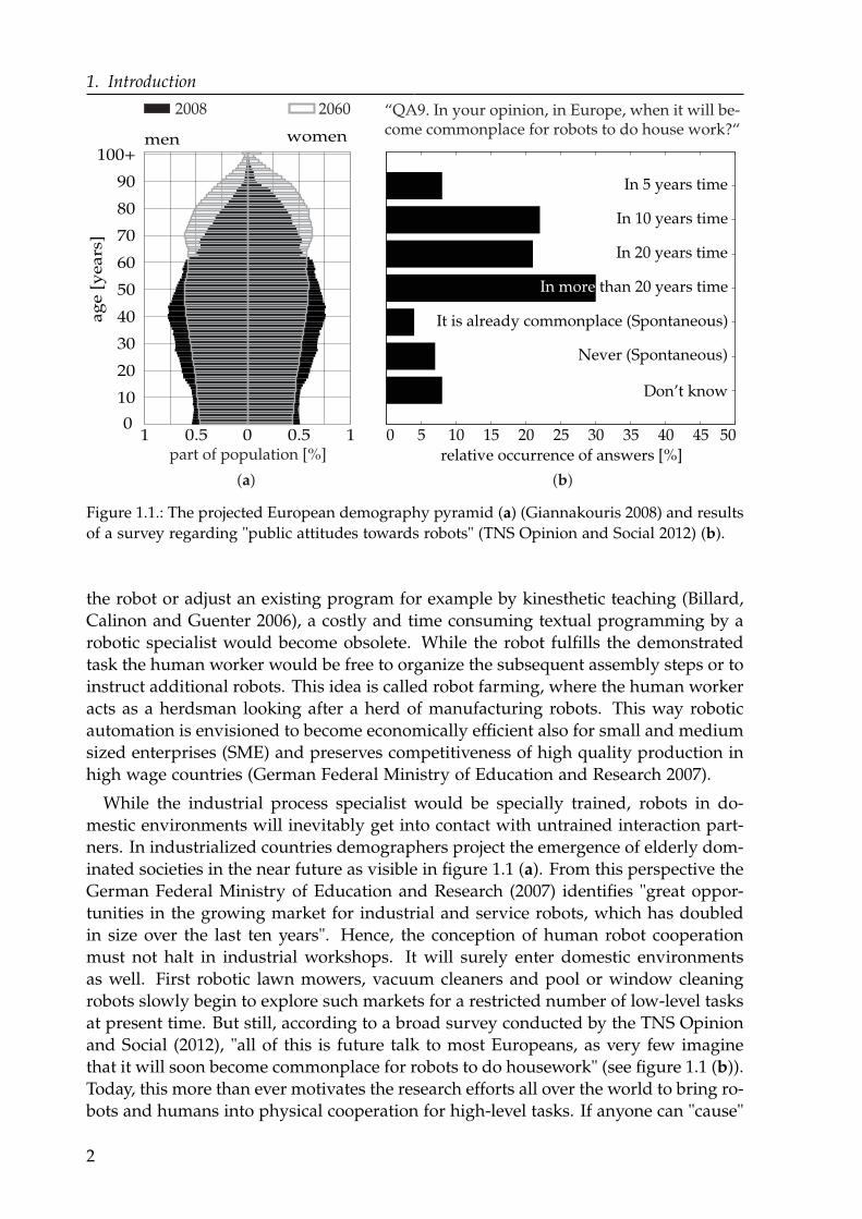
Figure 1.1.: The projected European demography pyramid (a) (Giannakouris 2008) and results
of a survey regarding "public attitudes towards robots" (TNS Opinion and Social 2012) (b).
the robot or adjust an existing program for example by kinesthetic teaching (Billard,
Calinon and Guenter 2006), a costly and time consuming textual programming by a
robotic specialist would become obsolete. While the robot fulfills the demonstrated
task the human worker would be free to organize the subsequent assembly steps or to
instruct additional robots. This idea is called robot farming, where the human worker
acts as a herdsman looking after a herd of manufacturing robots. This way robotic
automation is envisioned to become economically efficient also for small and medium
sized enterprises (SME) and preserves competitiveness of high quality production in
high wage countries (German Federal Ministry of Education and Research 2007).
While the industrial process specialist would be specially trained, robots in do-
mestic environments will inevitably get into contact with untrained interaction part-
ners. In industrialized countries demographers project the emergence of elderly dom-
inated societies in the near future as visible in figure 1.1 (a). From this perspective the
German Federal Ministry of Education and Research (2007) identifies "great oppor-
tunities in the growing market for industrial and service robots, which has doubled
in size over the last ten years". Hence, the conception of human robot cooperation
must not halt in industrial workshops. It will surely enter domestic environments
as well. First robotic lawn mowers, vacuum cleaners and pool or window cleaning
robots slowly begin to explore such markets for a restricted number of low-level tasks
at present time. But still, according to a broad survey conducted by the TNS Opinion
and Social (2012), "all of this is future talk to most Europeans, as very few imagine
that it will soon become commonplace for robots to do housework" (see figure 1.1 (b)).
Today, this more than ever motivates the research efforts all over the world to bring ro-
bots and humans into physical cooperation for high-level tasks. If anyone can "cause"
2
1.1. Motivation
a robotic assistant "to clear the table and scrape the dishes and load them into the dish-
washer only once" by kinesthetic or any other teaching method (Argall et al. 2009),
we finally arrive at a point very close to Heinlein’s vision of Flexible Frank.
Recently Alami et al. (2006); Santis et al. (2008) identified that "safety and depend-
ability are the keys to a successful introduction of robots into human environments".
Moreover, "the first step towards intrinsically safe and dependable design is to reduce
the weight of the moving parts of the robot". Bicchi and Tonietti (2004) propose that
the next step "to increasing the safety level of robot arms interacting with humans is
to intentionally introduce mechanical compliance in the design". It decouples the link
inertia from the effectively larger actuator inertia, which reduces the reflected overall
robot inertia during collisions. Additionally it protects gears and joint-sensors against
external shocks. The insights lead Alami et al. (2006) to formulate an "integrated ap-
proach to the co-design of robots for safe physical interaction with humans, which
revolutionizes the classical approach for designing industrial robots – rigid design for
accuracy, active control for safety – by creating a new paradigm: design robots that
are intrinsically safe and control them to deliver performance". Guizzo and Acker-
man (2012) conclude: "If you want a robot that’s going to deal with an unstructured
environment, it can’t be stiff".
According to Guizzo and Ackerman (2012) within the recent half-decade compan-
ies like ABB, Adept Technology, Barrett Technology, DLR, Kawada Industries, Red-
wood Robotics, Universal Robots and recently Rethink Robotics are developing robot
co-workers to assist humans in SME production lines. They all feature lightweight
structures and intrinsic compliance collocated with the joint actuators. Among the
mentioned examples Universal Robots as well as Rethink Robotics explicitly declare
the robots to be affordable by any small to medium sized enterprise as a main goal.
The rated prices are less than 22 000 USD, which pretty much agrees with Heinlein’s
idea of "one machine for [...] about the price of a good automobile" (Heinlein 1957).
Guizzo and Ackerman (2012) see the key to cutting the costs in giving the robot
through software "the ability to autonomously compensate for its own mechanical
irregularities as well as changes in its environment". This approach waives the need
for costly components by the development of advanced control algorithms. Follow-
ing this paradigm, it is noticeable that recent lightweight robot assistant prototypes
still share one important aspect with conventional robots. It is the strict rigid-link-
design aiming at the preservation of durability and moreover positioning accuracy by
hardware. It appears that the paradigm of affordable robots through sophisticated
software instead of expensive hardware has not yet been driven to the end.
The undesired side effects of intrinsic compliance are structural oscillations and
static deflections. In contrast to a non-collocated distributed elasticity in the robot
links, their attenuation is way simpler from a control point of view, if their origin is
collocated in the actuators as with the examples above. Up to now, the preservation
of link rigidity remains a strong demand, even if it constitutes a substantially time
consuming mechanical design difficulty, which easily inveigles to use pricy novel
materials. Such materials yield lighter structures and allow for less powerful actuators
on one hand, but usually come with a larger ecological footprint during production
on the other hand.
Albeit, Benosman and Le Vey (2004) experience that in large scale industrial pro-
3
1. Introduction
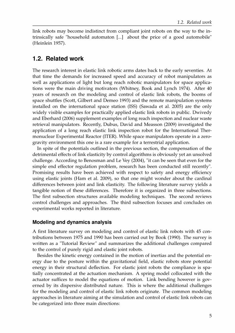
extrinsicmuscles
intrinsicmuscles
whisker
skin withnerve cells
( )a
link
( )b
straingauges
motor
elastic beamsensoractuator
Figure 1.2.: Simplified schematic of a whisker (a) and an elastic joint-link-module (b).
duction with conventional robots the link mass trimming together with emerging link
elasticity gain importance due to steady reduction of cycle times and increasing accur-
acy specifications. Tao et al. (2006) provide a practical example of a Scara type robot
for wafer handling applications in semiconductor manufacturing. Besides robotics
we find link elasticity being a problem to avoid in the constructions of cherry pickers
(Pridgen et al. 2011), fire rescue turntable ladders (Zimmert, Kharitonov and Sawodny
2008), automobile concrete pumps (Cazzulani et al. 2011) and many other machines.
As a consequence, if the problems associated with link elasticity can be solved in ro-
botics, the developed concepts are supposed to be transferable to the aforementioned
applications as well.
Once the undesired effects of link elasticity are sufficiently compensated, a prom-
ising new perspective is to exploit the intrinsic link compliance for the detection and
sensing of contact forces. Behn et al. (2013) explain that the vibrissae of rodents "can
be moved either passively or actively through alternate contractions of the intrinsic
and extrinsic muscles". This enables the passive detection of contact forces as well
as the tactile scanning of surfaces. Miersch et al. (2011) report that even in murky
water pinnipeds use their whiskers to locate and track the hydrodynamic trails of
their pray. While the species differ in the details, figure 1.2 (a) shows a very basic
schematic of a single whisker with the skin realizing the neural connection as well
as the actuation mechanism composed of extrinsic and intrinsic muscles. For com-
parison, figure 1.2 (b) presents a single joint-link-module of an elastic-link robot with
strain gauges and an electrical motor. The whiskers as well as the arm consist of an
elastic beam, which is actuated on one end. The deflection sensor is mounted close
to this actuator on the beam surface. This identical structural arrangement evokes the
biological inspiration by the whiskers of rodents and pinnipeds. It gives raise to the
hypothesis that the intrinsic link compliance can indeed be exploited for the detection
and sensing of contact forces.
The present thesis approaches the promising and still open research direction con-
cerned with the control of elastic link robots. If the hypothesis is correct, the strong
requirements for link rigidity and the associated challenges can be relaxed and elastic
4
1.2. Related work
link robots may become indistinct from compliant joint robots on the way to the in-
trinsically safe "household automaton [...] about the price of a good automobile"
(Heinlein 1957).
1.2. Related work
The research interest in elastic link robotic arms dates back to the early seventies. At
that time the demands for increased speed and accuracy of robot manipulators as
well as applications of light but long reach robotic manipulators for space applica-
tions were the main driving motivators (Whitney, Book and Lynch 1974). After 40
years of research on the modeling and control of elastic link robots, the booms of
space shuttles (Scott, Gilbert and Demeo 1993) and the remote manipulation systems
installed on the international space station (ISS) (Sawada et al. 2005) are the only
widely visible examples for practically applied elastic link robots in public. Dwivedy
and Eberhard (2006) supplement examples of long reach inspection and nuclear waste
retrieval manipulators. Recently, Dubus, David and Measson (2009) investigated the
application of a long reach elastic link inspection robot for the International Ther-
monuclear Experimental Reactor (ITER). While space manipulators operate in a zero-
gravity environment this one is a rare example for a terrestrial application.
In spite of the potentials outlined in the previous section, the compensation of the
detrimental effects of link elasticity by control algorithms is obviously yet an unsolved
challenge. According to Benosman and Le Vey (2004), "it can be seen that even for the
simple end effector regulation problem, research has been conducted still recently".
Promising results have been achieved with respect to safety and energy efficiency
using elastic joints (Ham et al. 2009), so that one might wonder about the cardinal
differences between joint and link elasticity. The following literature survey yields a
tangible notion of these differences. Therefore it is organized in three subsections.
The first subsection structures available modeling techniques. The second reviews
control challenges and approaches. The third subsection focuses and concludes on
experimental works reported in literature.
Modeling and dynamics analysis
A first literature survey on modeling and control of elastic link robots with 45 con-
tributions between 1975 and 1990 has been carried out by Book (1990). The survey is
written as a "Tutorial Review" and summarizes the additional challenges compared
to the control of purely rigid and elastic joint robots.
Besides the kinetic energy contained in the motion of inertias and the potential en-
ergy due to the posture within the gravitational field, elastic robots store potential
energy in their structural deflection. For elastic joint robots the compliance is spa-
tially concentrated at the actuation mechanism. A spring model collocated with the
actuator suffices to model the equations of motion. Link bending however is gov-
erned by its dispersive distributed nature. This is where the additional challenges
for the modeling and control of elastic link robots originate. The common modeling
approaches in literature aiming at the simulation and control of elastic link robots can
be categorized into three main directions:
5
1. Introduction
Lumped mass approach: The elastic links are spatially discretized into lumped masses
interconnected by massless spring-damper-elements. The number of lumped
masses trades off accuracy and model complexity. An example for this ap-
proach is given by Konno and Uchiyama (1996) as well as Konno, Uchiyama
and Murakami (1997), who investigate the horizontal motion of a two link ex-
perimental setup. Feliu, Rattan and Brown (1992) realize a controller for a single
massless elastic link with distributed lumped masses. This view on the sys-
tem decouples the influence of the link geometry and the mass properties on
the elastic dynamics. The decoupling enables the load adaptation scheme for a
single link experimental setup under exclusion of gravitational forces proposed
by Feliu, Feliu and Cerrada (1999).
Euler-Lagrange approach: The equations of motion are derived in analogy to rigid ro-
bots based on the energy balance using the Euler-Lagrange formalism. Link
elasticity adds to the potential and the deflection rates contribute to the kinetic
energy. The additional generalized coordinates required to describe the deflec-
tion states are obtained from a modal analysis. The modal analysis provides
eigenfrequencies and deflection shapes. Even with single links analytical solu-
tions to the involved fourth order partial differential equations are feasible only
for a very limited number of simple link geometries and rather basic boundary
conditions. Popular beam configurations are covered in fundamental textbooks
on structural dynamics (Dukkipati and Srinivas 2005; Meirovitch 2001). Ap-
proximate techniques employ generic polynomials, finite element solutions or
empirical data obtained from experiments to assess the assumed relevant eigen-
frequencies as well as a mathematical description of the associated mode shape
functions. The achievable accuracy is determined by the considered number
of assumed modes, the body geometry and validity of the selected boundary
conditions.
Frequency domain approach: Frequency domain techniques are an alternative to the
time domain approaches above. According to Book (1990) the serial and paral-
lel connection of joint as well as both rigid and flexible links is straightforward
using transfer function models. Book and Majette (1983) report that the ex-
tension to transfer matrices generally allows the propagation of the deflection,
bending angle, shearing force and bending moment through entire kinematic
chains. Krauss (2012) recently published an efficient Python implementation of
this approach. Nevertheless, frequency domain transfer matrix methods have
experienced far less attention in the past than the other two approaches. The
reason may be, that many powerful advanced controller design methods require
time domain models. The conversion between the frequency and time domain
models for nonlinear systems is tedious. Detailed analyses provided by Krauss
(2006) as well as Krauss, Book et al. 2010 are still restricted to linear models.
More citations for each category can be found in the extensive literature survey
conducted by Dwivedy and Eberhard (2006), which reviews a total of 433 modeling
papers. As a summary, the first two categories clutch to modeling concepts that are
well established for the concentrated parameter case of conventional rigid robots and
6
1.2. Related work
seek to extend them for distributed parameter systems. Following Meirovitch (2001,
p. 464), both approaches "model distributed-parameter systems as discrete systems,
which amounts to spatial discretization and truncation". The lumped parameter ap-
proach "is more physical in nature, but lacks rigor", while the assumed modes model
"is more abstract, but has a solid mathematical foundation" and "also tends to be
more predictable and accurate". The frequency domain approach also discretizes the
continuous system to a finite series of assumed modes. Book (1990) remarks that the
obtained models are rather inaccurate with respect to the large robot motions, but
mathematically compact and thus attractive for the description of small oscillatory
motions.
In all these common modeling approaches the spatial and modal truncation entails
crucial consequences for the subsequent controller design. A model based controller
may potentially excite the unmodelled eigenfrequencies, which can destabilize the
closed loop. This effect is known as modal spillover (Balas 1978). A cost analysis
may be carried out to reduce model complexity by considering a smaller number of
eigenfrequencies with acceptable degradation of accuracy (Tsujisawa and Book 1989).
However, no theoretical technique exists, that guarantees relief from spillover. This
must be carefully investigated in real experiments.
In order to circumvent the spillover problematic, a few researchers such as Halevi
and Wagner-Nachshoni (2006) have investigated nonlinear infinite dimensional trans-
fer functions. The transfer functions are derived for different sensor and actuator con-
figurations as well as generalized second order boundary conditions at both ends of
a single beam. On this basis a controller is designed by Halevi (2004). The parameter
tuning and stability analysis is carried out with respect to the generalized boundary
conditions. Although very promising the investigations are limited to elastic systems
governed by second order partial differential equations such as vibrations of strings
or torsional or lateral oscillations in rods.
The accuracy of the modeling techniques discussed so far strongly depends on the
knowledge of the boundary conditions for each link in the kinematic chain. The
introductory boundary value problems discussed in fundamental textbooks on struc-
tural dynamics (Dukkipati and Srinivas 2005; Meirovitch 2001) usually consider static
boundary conditions. In real multi-elastic-link robots the boundary conditions of
each individual link already vary with the joint controller parameters as well as the
relative joint configuration. In spite of exponentially growing computation power the
model complexity under consideration of time varying boundaries "can swamp even
large memories" (Book 1990) and render the resulting dynamics equations poorly in-
spectable. That is why most multi-link models such as the one proposed by Luca
and Siciliano (1991) or Chen (2001) argue the replacement of the varying boundary
conditions by fixed approximations.
Beyond the joint configuration dependent time variance, imperfect clamping and
finite drive train stiffness add non-negligible uncertainty to the boundary model.
Backlash may lead to chaotic or at least non-deterministic boundary dynamics. Fi-
nally, payload changes and physical contacts with the environment unpredictably
but drastically and abruptly alter the boundary conditions. Such events must not
destabilize the closed control loop.
7
1. Introduction
Control approaches
A broad variety of controllers have been investigated in search of a solution to the
oscillation damping and positioning tasks for elastic link arms simultaneously. Ben-
osman and Le Vey (2004) structure a total of 119 papers into control concepts such as
input-output linearization through stable inversion using a state feedback designed
in the frequency and time domain, singular perturbation and sliding mode control,
optimal, robust and adaptive control, feedforward filtering and input shaping.
Identically to rigid robots, the position control objective for elastic link robots is to
perform point-to-point motions or to follow a predefined trajectory. This commonly
implies the actuator torques to be the control inputs and the end effector pose to be
the control output of the plant. However, for elastic link robots this choice of control
inputs and outputs leads to a plant with unstable zero dynamics. The rigid links of
conventional robots cause a control action at the joints to instantaneously affect the
end effector motion. The distributed nature of link elasticity causes the control action
to propagate along the structure with finite speed. As a consequence well known
control concepts from rigid robots such as the computed torque and inverse dynamics
control cannot be applied directly. Luca, Panzieri and Ulivi (1998); Moallem and
Patel (2001); Wang and Vidyasagar (1991) circumvent the difficulties using a method
known as output redefinition, where the actual end effector deflection is replaced by
an artificial control output. The plant with the artificial output shows stable zero
dynamics.
Approaching from the hardware side, oscillations can, at least up to some extend, be
damped passively by using multi-layered link designs with intermediate visco-elastic
layers for energy dissipation or parallel arm structures. Some researchers distribute
additional actuators such as piezo electric ceramic actuators (Khorrami, Zeinoun and
Tome 1993) or dielectric electroactive polymer actuators (Bailey and Ubbard 1985)
along the structure. These devices also show integrated deflection sensing capabilit-
ies. Their arrangement accounts for the distributed nature of the elastic links and they
are controlled to actively stabilize the zero dynamics. Moreover, Konno, Uchiyama
and Murakami (1997) discover in certain joint configurations the modal controllab-
ility through the joint actuators to get lost. In such configurations it might become
infeasible to stabilize or attenuate oscillations of particular modes. The effect does not
occur with elastic joint robots, because of the collocation between the concentrated
elasticity and the actuation mechanism. The distributed actuators mentioned above
can be optimally placed to ensure modal controllability throughout the whole work-
space. However, a practically very inconvenient property of piezo ceramics as well
as dielectric electroactive polymers are the high operating voltages, which necessitate
thorough insulation.
Most researchers use strain gauges as deformation sensors. They are fast, cheap,
operate at low voltages and can be easily glued onto the link surface. An investigation
towards more expensive optical fibers with Bragg gratings as strain sensing device
for increased precision and a larger signal to noise ratio is performed by Franke et al.
(2009).
The strain measurement close to the joint provides stable zero dynamics, which
motivates researchers such as Luo (1993) to directly close proportional and integral
8
1.2. Related work
feedback loops for oscillation damping. In their experiments Luo and Guo (1995) use
a single link in the horizontal plane. Malzahn et al. (2010a) augment the direct pro-
portional feedback for a single link under gravity using feedforward input shaping
filters discussed by Vaughan, Yano and Singhose (2008). The resulting two degree
of freedom control structure joins the individual strengths and alleviates the short-
comings of the feedforward and feedback approaches. Malzahn et al. (2011b) extend
the concept to a multi-link arm under gravity with a more advanced cascaded joint
controller complemented by a jerk minimizing online trajectory planner.
The most promising property of the linear strain feedback is the independence of
any dynamics computation at runtime. Ge, Lee and Zhu (1998) suggest a nonlinear
integral feedback law sharing this property in a purely simulative study. The concept
looks at the dissipation of oscillation energy following a direct Lyapunov synthesis
approach, which avoids a truncation of the arm dynamics and possible spillover ef-
fects.
Experimental studies with this energy based control have emerged simultaneously
and independently by Mansour et al. (2008) as well as within the scope of this thesis
by Franke et al. (2009).
The experiments carried out in a wide workspace and under gravitational influence
reveal an unexpected difficulty with the nonlinear integral feedback law. If any elastic
link passes through a vertical orientation the damping scheme starts a limit cycle. In
the vertical pose the static strain changes the sign, so that an imperfect static strain
cancellation in combination with the integral nature of the concept is suspected to
cause the observed effect. The observation from multiple experiments is, that such
limit cycles do not occur, if link orientations remain on either side of the vertical pose.
Experiments with a backlash free experimental setup allow the exclusion of the gear
backlash as a reason.
While a mathematical proof to this observation is still an open challenge, Malzahn
(2008)1 develops a remedy later published by Franke et al. 2009. The idea is to su-
pervise each link orientation and adapt the sign of the feedback term accordingly.
However, the experiments under gravity indicate that the damping results do not
justify the additional efforts compared to the linear feedback.
The strain measurements close to the joints allow only poor tip position informa-
tion inferred by means of a properly identified dynamics model. Tip sensors provide
accuracy with respect to static configuration and load dependent deflections but in-
troduce unstable zero dynamics into the control system. This gives raise to the fol-
lowing, still open question stated by Book (1990): "how can one combine strain and
tip position sensors to achieve a robust and accurate controller"?
For example, Kharitonov, Zimmert and Sawodny (2007) propose the use of strain
gauges close to the joint with a gyroscope at the tip. During the past decade cam-
era sensors with fast frame rates and high resolutions became widely available at
low cost, which renders them a promising option as tip sensors. This has motiv-
ated researchers such as Bascetta and Rocco (2006a,b); Dubus, David and Measson
(2009); Jiang, Konno and Uchiyama (2007) to work on the use of cameras as a sensor
for oscillation damping as well. During preparation of this thesis Malzahn, Phung
1The cited thesis narrowly focuses on the experimental investigation of the particular nonlinear in-tegral feedback. The main result is the sign adaptation to circumvent the observed instability.
9
1. Introduction
and Bertram (2012c); Malzahn et al. (2010b) contribute experimental results on the
oscillation sensing relying solely on an eye-in-hand camera with a special emphasis
on unstructured and potentially dynamic scenes with varying texture and geometric
structure. Malzahn, Phung and Bertram (2012b) compare three approaches for online
identification of a signal model describing the perceived oscillations. The proposed
method allows to compensate for the sensor delay. Malzahn et al. (2012) aggregate
these works and present the purely camera based oscillation damping using the con-
trol concept explained in chapter 5. While the actual image processing with delay
compensation is beyond the scope of this thesis, chapter 9 includes a brief application
of the camera for end effector positioning.
Experimental studies
Experimental investigations of control concepts are as yet dominated by single link
setups operating in the horizontal plane under exclusion of the variable gravitational
influence. Becedas et al. (2009) propose a generalized PI-controller for a horizontal
single-link setup supported by an air table. Diaz et al. (2010) propose a robustified
variant of the impulse based input shaping technique developed in earlier works of
Singhose (2009). The variant shows an abbreviated filter duration. The increased
robustness results from a numerical optimization, which adapts to changes in the
system dynamics due to varying payload masses.
Publications on multi-elastic-link robots are as yet mostly limited to simulative
studies. They comprise model predictive approaches for up to four-link mechanisms
(Boscariol, Gasparetto and Zanotto 2010). Korayem et al. (2010); Subudhi and Morris
(2009) combine fuzzy approaches with variable structure controllers or neural net-
works. Rong et al. (2010) supplement a PID-controller by an artificial neural network
to form an adaptive controller based on velocity feedback for oscillation damping
with piezo actuators. Benosman and Le Vey 2004 find the reason in "the complexity
of the nonlinear multi-link models, since it is difficult even if not impossible to ap-
ply directly some theoretical closed-loop control strategies, which need closed-form
manipulations of these complex system dynamics".
Along with all the uncertainties associated with the dynamics modeling described
in section 1.2, it is frustrating, tedious and error prone to derive and especially to
identify a holistic dynamics model of a real robot, suited to precisely describe the
structural oscillations along with the static deflections in the entire workspace. In
particular, Book (1984) discusses the complexity and computational burden of a re-
cursive Lagrangian formulation with respect to different mode shape approximations
and compares them to rigid robot models. Theodore and Ghosal (1995) provide sim-
ulations for the model of a multi-link arm in the absence of gravity and compare
the analytical assumed mode method (AMM) with the finite element method (FEM).
The FEM overestimates stiffness which can drive a model based controller unstable.
Their AMM model considers time dependent boundary conditions under simplifying
conditions. Book (1984) supplements the investigation of computational complexity.
Even with today’s available computational power a model of that type most probably
lacks real-time capabilities and such a model would not yet have captured payload
changes and interactions with the environment.
10
1.3. Contribution and outline
The complexity and uncertainty aggravate the experimental proofs of concept for
model based controllers, so that researchers argue that contributions in the control
of elastic link robots should intensify experimental works "to keep realism in the
research" (Book 1990). Hu (1993); Tokhi and Azad (2008) collect and picture experi-
mental setups developed all over the world. The works clearly document the dom-
inance of single link experimental setups. Multi-link setups are almost exclusively
operating in the horizontal plane thereby excluding the influence of gravity. Just a
few multi-link setups moving in the vertical plane exist. Two of them are FLEBOT II
and ADAM in the Space Machines Laboratory at Tohoku University as well as ELLA
and ElRob at the Institut für Robotik, Linz University.
The number of publications concerning the exploitation of link elasticity for force
control or contact detection is vanishingly small. Bazaei and Moallem (2011) follow
the output redefinition approach control the tip force of a single link operating in the
horizontal plane. Garcia and Feliu (2000) as well as Garcia, Feliu and Somolinos (2001)
compare implicit and explicit force control schemes as well as collision detection with
a single-link setup and a modified PID framework. So far, neither simulative nor
experimental studies on force control or collision detection are known that consider
elastic link robots under the influence of gravity or with multiple links.
1.3. Contribution and outline
This work is first and foremost driven by the idea that elasticity in the robot links
does not ultimately need to be a problem, which must be avoided by costly and mo-
mentous constructional efforts. The hypothesis formulated in section 1.1 claims, that
link elasticity can be exploited to sense and control contact forces. The work repres-
ents a first experimental study towards this hypothesis. It considers multi-link arms
under gravitational influence. As a prerequisite, the work develops and exemplifies
solutions to the challenges of oscillation damping and position control under the con-
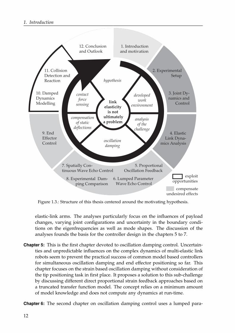
ditions summarized in the previous section. This whole path is visualized in figure 1.3
and reflected by the following outline:
Chapter 2: The preparation of this thesis included the development and installation
of the three degree of freedom elastic link robot named TUDOR along with
the additional external reference sensors. The arm is intentionally designed to
show clearly visible elastic effects, which allows for illustrative evaluations of
the devised control concepts. The chapter introduces the complete experimental
equipment and the communication among all individual units.
Chapter 3: The chapter models and identifies the joint actuators. It describes the
choice and tuning of the cascaded joint angular controllers. The chapter closes
with an experimental evaluation of the control objectives and describes a gener-
alized controller architecture for the unified joint-level integration of all different
oscillation damping control concepts investigated in this work.
Chapter 4: The chapter introduces the mathematical prerequisites of the elastic link
dynamics for the remainder of this work. Supported by experiments, it con-
tributes detailed theoretical analyses of the oscillatory link dynamics of multi-
11
1. Introduction
1. Introductionand motivation
2. ExperimentalSetup
3. Joint Dy-namics and
Control
4. ElasticLink Dyna-
mics Analysis
5. ProportionalOscillation Feedback
6. Lumped ParameterWave Echo Control
7. Spatially Con-tinuous Wave Echo Control
8. Experimental Dam-ping Comparison
9. EndEffectorControl
10. DampedDynamicsModelling
11. CollisionDetection andReaction
12. Conclusionand Outlook
oscillationdamping
analysisof the
challenge
compensationof static
deflections
developedwork
environment
contactforce
sensing
hypothesis
linkelasticity
is notultimatelya problem
alle compensateundesired effects
xploi exploitopportunities
Figure 1.3.: Structure of this thesis centered around the motivating hypothesis.
elastic-link arms. The analyses particularly focus on the influences of payload
changes, varying joint configurations and uncertainty in the boundary condi-
tions on the eigenfrequencies as well as mode shapes. The discussion of the
analyses founds the basis for the controller design in the chapters 5 to 7.
Chapter 5: This is the first chapter devoted to oscillation damping control. Uncertain-
ties and unpredictable influences on the complex dynamics of multi-elastic link
robots seem to prevent the practical success of common model based controllers
for simultaneous oscillation damping and end effector positioning so far. This
chapter focuses on the strain based oscillation damping without consideration of
the tip positioning task in first place. It proposes a solution to this sub-challenge
by discussing different direct proportional strain feedback approaches based on
a truncated transfer function model. The concept relies on a minimum amount
of model knowledge and does not compute any dynamics at run-time.
Chapter 6: The second chapter on oscillation damping control uses a lumped para-
12
1.3. Contribution and outline
meter model of the elastic link dynamics. It revisits the identification of wave
properties in the lumped structure introduced by O’Connor (2007b). The wave
properties are exploited to an alternative derivation of a damping controller
based on the absorption of emitted and echoed wave components. Again, a min-
imum knowledge of the link dynamics is required at run-time. With a structural
reduction this thesis reveals a very close relation to the proportional oscillation
feedback presented in chapter 5.
Chapter 7: The models and control concepts presented so far all involve discretization
or truncation of the oscillatory elastic link dynamics. Following the concept
of mechanical waves this third chapter on oscillation damping control accepts
the continuous spatial distribution of the elastic properties and introduces the
concept of wave reflection and transmission at junctions as well as boundaries.
The chapter discusses three different variants to shape the wave reflection matrix
at the actuator boundary. Cross-relations to the previously derived controllers
are highlighted.
Chapter 8: This final chapter on oscillation damping control provides an extensive
experimental comparison of the oscillation damping concepts presented in this
work. The experimental results cover the whole workspace of the multi-elastic-
link robot TUDOR and include investigations towards varying payloads, step-
like as well as harmonic external disturbances and damping actions at just a
single actuator.
Chapter 9: With the structural oscillations readily damped, the end effector position-
ing task in this chapter drastically simplifies. Two position control approaches
are presented. The first one is a 3D visual servoing controller implemented with
an eye-in-hand mounted RGB-D camera. The second one employs a data driven
inverse kinematics algorithm. A ball catching scenario with a human thrower
sequentially throwing multiple balls towards the robot serves as a testbed to-
wards the question whether time critical positioning tasks can be accomplished
by an elastic link robot arm with sufficient precision.
Chapter 10: In addition to the inverse kinematics also the dynamics of the elastic link
arm are way simpler to model in the presence of an underlying robust and fast
oscillation damping controller. With this chapter the thesis derives a linear rela-
tion between the measured strain and the joint torques, which allow the damped
strain referred dynamics to be formulated with exactly the same mathematical
structure as the dynamics of conventional rigid robots.
Chapter 11: With the oscillations damped, the end effector position controlled as well
as the identified damped dynamics model at hand, the work finally arrives at
the investigation of the hypothesis about the potentials of link elasticity in robot
arms for collision detection and reaction. The chapter provides collision experi-
ments with blunt and sharp impacts, both carried out with durable and stiff but
also with compliant and fragile objects as well as a human arm.
Chapter 12: The work comes full circle with a concluding discussion about the accom-
plished results and suggests directions for future works.
13
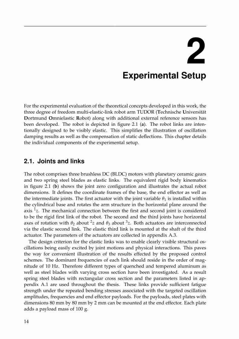
2Experimental Setup
For the experimental evaluation of the theoretical concepts developed in this work, the
three degree of freedom multi-elastic-link robot arm TUDOR (Technische Universität
Dortmund Omnielastic Robot) along with additional external reference sensors has
been developed. The robot is depicted in figure 2.1 (a). The robot links are inten-
tionally designed to be visibly elastic. This simplifies the illustration of oscillation
damping results as well as the compensation of static deflections. This chapter details
the individual components of the experimental setup.
2.1. Joints and links
The robot comprises three brushless DC (BLDC) motors with planetary ceramic gears
and two spring steel blades as elastic links. The equivalent rigid body kinematics
in figure 2.1 (b) shows the joint zero configuration and illustrates the actual robot
dimensions. It defines the coordinate frames of the base, the end effector as well as
the intermediate joints. The first actuator with the joint variable θ1 is installed within
the cylindrical base and rotates the arm structure in the horizontal plane around the
axis 1z. The mechanical connection between the first and second joint is considered
to be the rigid first link of the robot. The second and the third joints have horizontal
axes of rotation with θ2 about 2z and θ3 about 3z. Both actuators are interconnected
via the elastic second link. The elastic third link is mounted at the shaft of the third
actuator. The parameters of the actuators are collected in appendix A.3.
The design criterion for the elastic links was to enable clearly visible structural os-
cillations being easily excited by joint motions and physical interactions. This paves
the way for convenient illustration of the results effected by the proposed control
schemes. The dominant frequencies of each link should reside in the order of mag-
nitude of 10 Hz. Therefore different types of quenched and tempered aluminum as
well as steel blades with varying cross section have been investigated. As a result
spring steel blades with rectangular cross section and the parameters listed in ap-
pendix A.1 are used throughout the thesis. These links provide sufficient fatigue
strength under the repeated bending stresses associated with the targeted oscillation
amplitudes, frequencies and end effector payloads. For the payloads, steel plates with
dimensions 80 mm by 80 mm by 2 mm can be mounted at the end effector. Each plate
adds a payload mass of 100 g.
14
2.2. Strain sensors
2x
2z
2y3x
3z
3yEx
Ez
Ey
l3
l1
l1 = 650 mm
l2 = 440 mm
2x3xEx
2xs,1
3xs,1
2xs,2
3xs,2
1x1y
1z
l3 = 410 mm
spring steel bladeswith strain sensors
camera withtracking spheres
BLDC motorswith planetarygears
TUDOR
echnischeniversitätortmundmnielasticobot
(a)
(b)
(c)
strainsensors
l2
IMU
Figure 2.1.: Photograph of the multi-elastic-link robot arm TUDOR (a) with equivalent rigid
body kinematics (b) and top view schematic (c) including the strain sensor locations.
The thesis accounts for the effect of gravity on the elastic links. To emphasize the
appearance of this effect, the elastic link area moments of inertia about axes parallel
to the joint 2z-axes are designed to be small. This way the structural oscillations
mainly occur in the vertical 2x-2y plane incorporating the gravity vector. Nevertheless
deviation moments due to the unbalanced mounting of the third joint also cause
smaller torsional and horizontal oscillations of the arm.
2.2. Strain sensors
Strain gauge pairs are applied on the top and bottom surfaces of the elastic links
according to the schematic shown in figure 2.1 (c). Each link carries two pairs of
strain gauges. One pair close and one pair more distant to the preceding joint. The
pairwise installation in connection with a Wheatstone half-bridge circuit allows for
the compensation of temperature dependent strain drift in the measurements. The
sensor parameters are listed in appendix A.4. For simplicity, the notation
ε2 = ε(2xs, 1) and ε3 = ε(3xs, 1) (2.2.1)
is used as a convention in the remainder of this thesis.
15
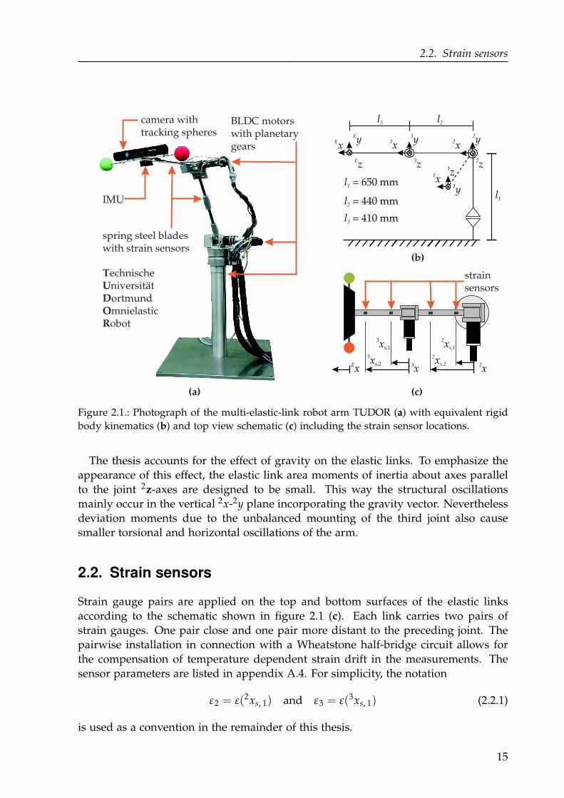
2. Experimental Setup
lowpassfilter
lowpassfilter
- -raw
estimatedmean
meandeliberated
Figure 2.2.: Filter architecture for second order smoothing.
The key difference between elastic link arms that operate under gravity and those
that do not is the presence of configuration and load dependent static deflections.
The static deflections effect non-zero static strain readings, which have to be cancelled
in preparation to oscillation damping control. Otherwise they introduce substantial
steady state positioning and tracking errors or even destabilize an oscillation damping
controller.
There are basically two options to perform static strain cancellation: a model based
or a filter based approach. The static deflection nonlinearly depends on the joint con-
figuration. The transitions between two static deflections due to changes in the joint
motion are dominated by the mechanical actuator time constants. The adaptation
of a model based static strain cancellation to unpredicted load changes as well as to
static strains during contacts with the environment requires fast online identification
and dependable reasoning from a higher cognitive level. A more fundamental limit-
ation of a model based approach arises from the finite accuracy of any model. This
necessitates the implementation of a deadzone around the residual modelling error.
Oscillations with measurements remaining in this deadzone cannot be damped by the
controller.
For low level damping control of the structural oscillations this work therefore pro-
poses a filtering approach. It has no limiting deadzone, it is simpler from a compu-
tational as well as less demanding from a cognitive point of view. It automatically
adapts to varying load conditions. The model based prediction of strain measure-
ments is left for the collision detection and reaction in the chapters 10 and 11.
Highpass filtering of the strain measurements is an obvious first idea for static strain
cancellation. There exist numerous automated filter design algorithms for both finite
impulse reponse filters (FIR) as well as infinite impulse response filters (IIR). Most of
these algorithms compute the filter coefficients based on amplitude gain and cut-off
frequency specifications for the stop- and pass-band. As a result from section 4.7 the
lowest natural frequencies are found to come close to 1 Hz. FIR filters with sharp filter
edges involve a large number of filter coefficients, which increases computational cost
and decreases responsiveness. IIR filters can be desigend with less filter coefficients
at the cost of a more complicated phase characteristic. Large phase shifts aggravate or
even destabilize the oscillation damping control. Phase constraints are more difficult
to set in most automated filter design algorithms. Understanding the relationship
between the typical frequency domain design specifications and the time domain
filtering result requires extensive filter design experience.
The filter design suggested in this work is based on the subtraction of the estimated
static strain signal portion. Besides the static strain cancellation, the availability of this
16
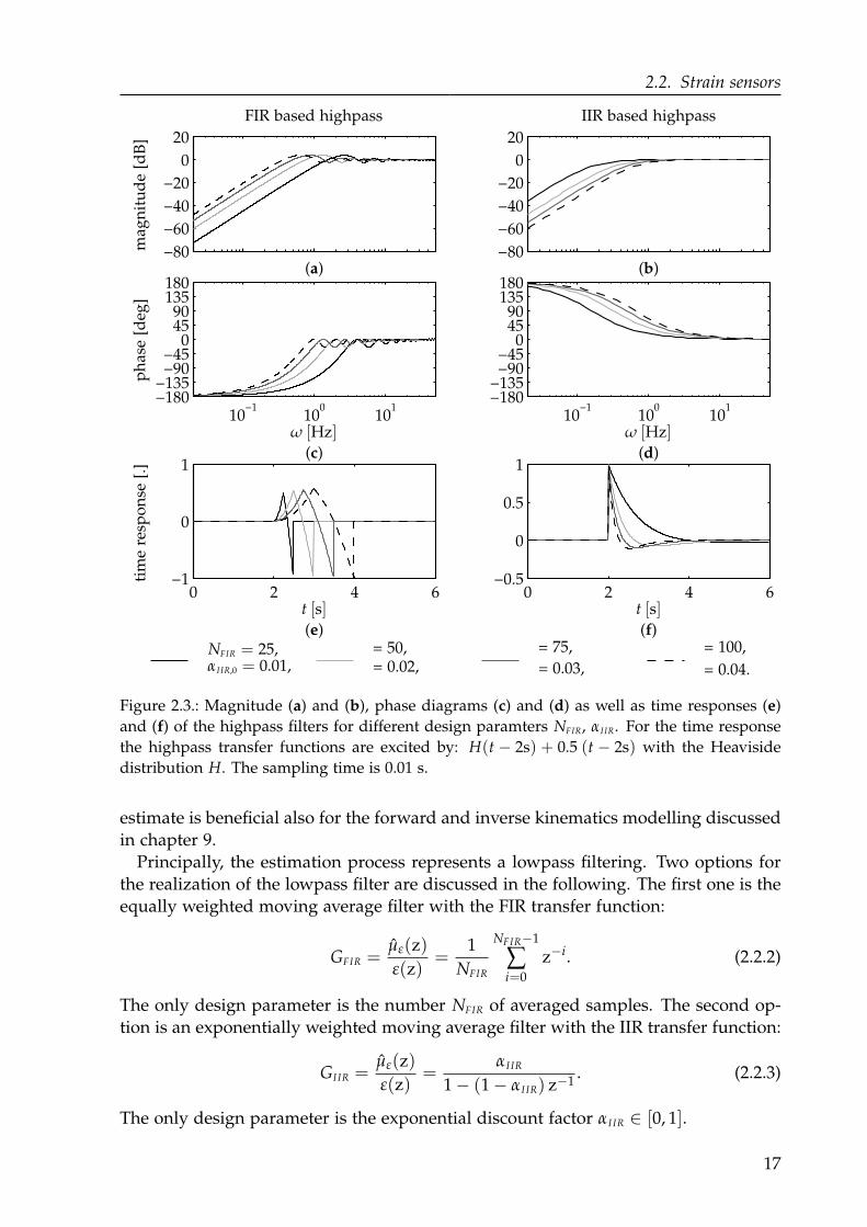
2.2. Strain sensors
−80
−60
−40
−20
0
20
(a)
10−1
100
101
−180−135−90−45
04590
135180
(c)
0 2 4 6−1
0
1
(e)
−80
−60
−40
−20
0
20
(b)
10−1
100
101
−180−135−90−45
04590
135180
(d)
0 2 4 6−0.5
0
0.5
1
(f)NFIR = 25, = 50, = 75, = 100,αI IR,0 = 0.01, = 0.02, = 0.03, = 0.04.
FIR based highpass IIR based highpass
mag
nit
ud
e[d
B]
ph
ase
[deg
]ti
me
resp
on
se[.
]
ω [Hz]ω [Hz]
t [s]t [s]
Figure 2.3.: Magnitude (a) and (b), phase diagrams (c) and (d) as well as time responses (e)
and (f) of the highpass filters for different design paramters NFIR, αI IR. For the time response
the highpass transfer functions are excited by: H(t − 2s) + 0.5 (t − 2s) with the Heaviside
distribution H. The sampling time is 0.01 s.
estimate is beneficial also for the forward and inverse kinematics modelling discussed
in chapter 9.
Principally, the estimation process represents a lowpass filtering. Two options for
the realization of the lowpass filter are discussed in the following. The first one is the
equally weighted moving average filter with the FIR transfer function:
GFIR =µε(z)
ε(z)=
1
NFIR
NFIR−1
∑i=0
z−i. (2.2.2)
The only design parameter is the number NFIR of averaged samples. The second op-
tion is an exponentially weighted moving average filter with the IIR transfer function:
GI IR =µε(z)
ε(z)=
αI IR
1 − (1 − αI IR) z−1. (2.2.3)
The only design parameter is the exponential discount factor αI IR ∈ [0, 1].
17
2. Experimental Setup
0 5 10 15 20 25 30
−500
0
500
(a)
0 5 10 15 20 25 30
−500
0
500
(b)
ε 2[µ
m/
m]
ε 2[µ
m/
m]
t [s]
measurement estimated mean mean liberated
Figure 2.4.: Experimental filtering results for the FIR (a) and the IIR (b) filter with NFIR = 50
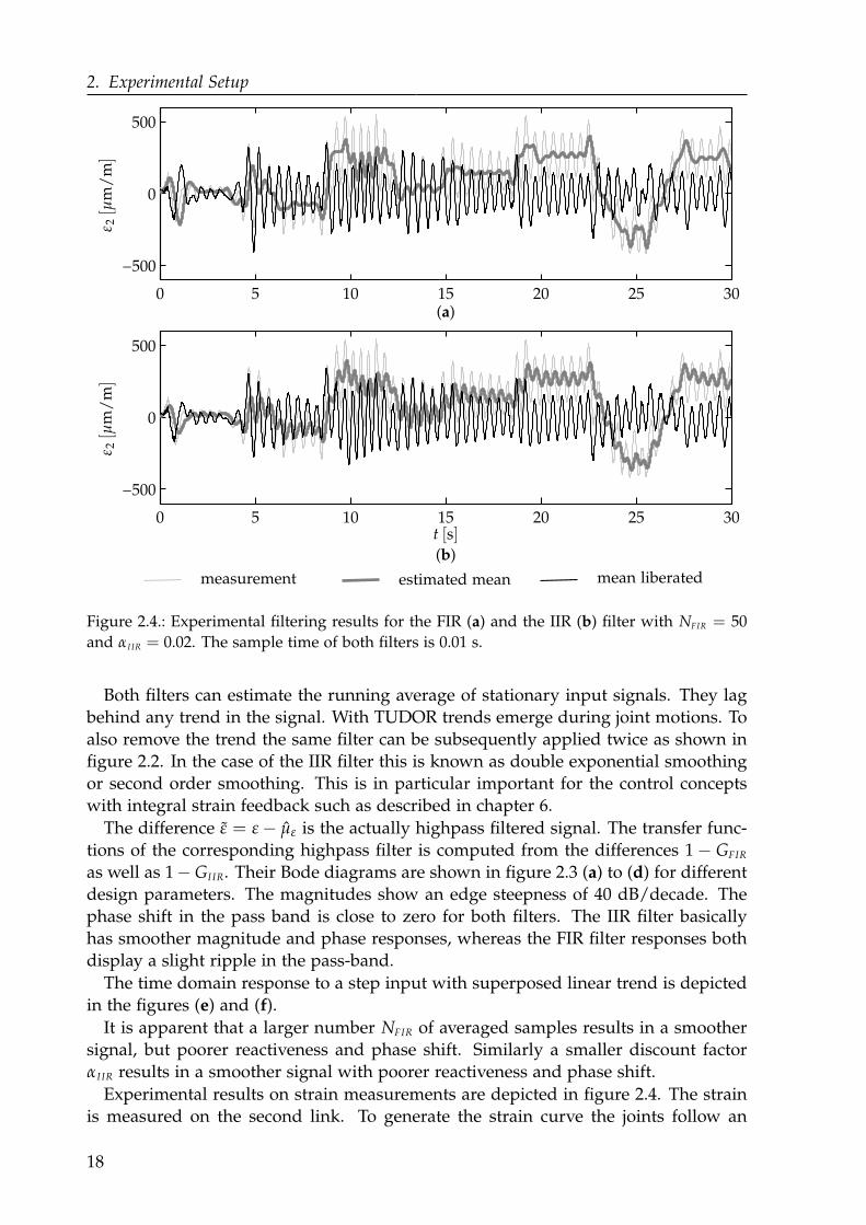
and αI IR = 0.02. The sample time of both filters is 0.01 s.
Both filters can estimate the running average of stationary input signals. They lag
behind any trend in the signal. With TUDOR trends emerge during joint motions. To
also remove the trend the same filter can be subsequently applied twice as shown in
figure 2.2. In the case of the IIR filter this is known as double exponential smoothing
or second order smoothing. This is in particular important for the control concepts
with integral strain feedback such as described in chapter 6.
The difference ε = ε − µε is the actually highpass filtered signal. The transfer func-
tions of the corresponding highpass filter is computed from the differences 1 − GFIR
as well as 1− GI IR. Their Bode diagrams are shown in figure 2.3 (a) to (d) for different
design parameters. The magnitudes show an edge steepness of 40 dB/decade. The
phase shift in the pass band is close to zero for both filters. The IIR filter basically
has smoother magnitude and phase responses, whereas the FIR filter responses both
display a slight ripple in the pass-band.
The time domain response to a step input with superposed linear trend is depicted
in the figures (e) and (f).
It is apparent that a larger number NFIR of averaged samples results in a smoother
signal, but poorer reactiveness and phase shift. Similarly a smaller discount factor
αI IR results in a smoother signal with poorer reactiveness and phase shift.
Experimental results on strain measurements are depicted in figure 2.4. The strain
is measured on the second link. To generate the strain curve the joints follow an
18
2.3. Eye in hand camera
input stimulus. The stimulus for each individual joint consists of angle steps with
random amplitude at random time steps. The mean liberated stimulus responses ε for
both filters properly oscillate around zero with comparably fast reactions to changing
operating points. From the figures, the phase shift between the mean liberated signal
ε and the original measurement ε appears marginal. The intended convergence of
the mean liberated signal ε to zero in static scenarios becomes evident in the damped
single step experiments provided in the chapters 5 to 8 of this work.
Both filters have been designed to show basically the same reactiveness. Under this
conditions the IIR filter shows a larger ripple in the estimated mean. In essence, both
filters can be tuned to have equivalent cut-off frequencies or effective filter durations.
Good trade-offs between phase-shift and bandwidth are observed for NFIR = 50 and
αI IR = 0.02. With these settings the occurring phase shifts within the relevant fre-
quency range are acceptable. However, from the experimental results it is found that
the FIR filter practically allows a better trade-off in terms of reactiveness and ripple in
the moving average. That is why the remainder of this work uses FIR variant despite
the larger computational efforts in comparison to the IIR filter.
2.3. Eye in hand camera
The robot can be equipped with an eye in hand camera for visual servoing purpose
as done in section 9.1. The idea is to minimize the relative pose error between an
actual and a desired view of the scene by commanding appropriate joint velocities.
This elegantly allows to position the end effector of an elastic link arm without the
need for an accurate model of the load and configuration dependent static structural
deflections. The exploitation of the already available sensor as a multi purpose sensor
also for oscillation sensing and damping is beyond the scope of this thesis, but has
nevertheless been investigated during preparation of this work. The oscillation re-
construction from unstructured and possibly dynamic scenes has been published by
Malzahn et al. (2010b) as well as Malzahn, Phung and Bertram (2012c), while the com-
pensation of additional delays introduced by the image acquisition and processing are
( )c( )b( )a
z [m]1 2 3 4 5 6
0
1020
3040
50
60
70
σz(
) [m
m]
z
fitted polynomialmeasurements
depth evaluation region
IRcamera
RGBcamera
IRprojector
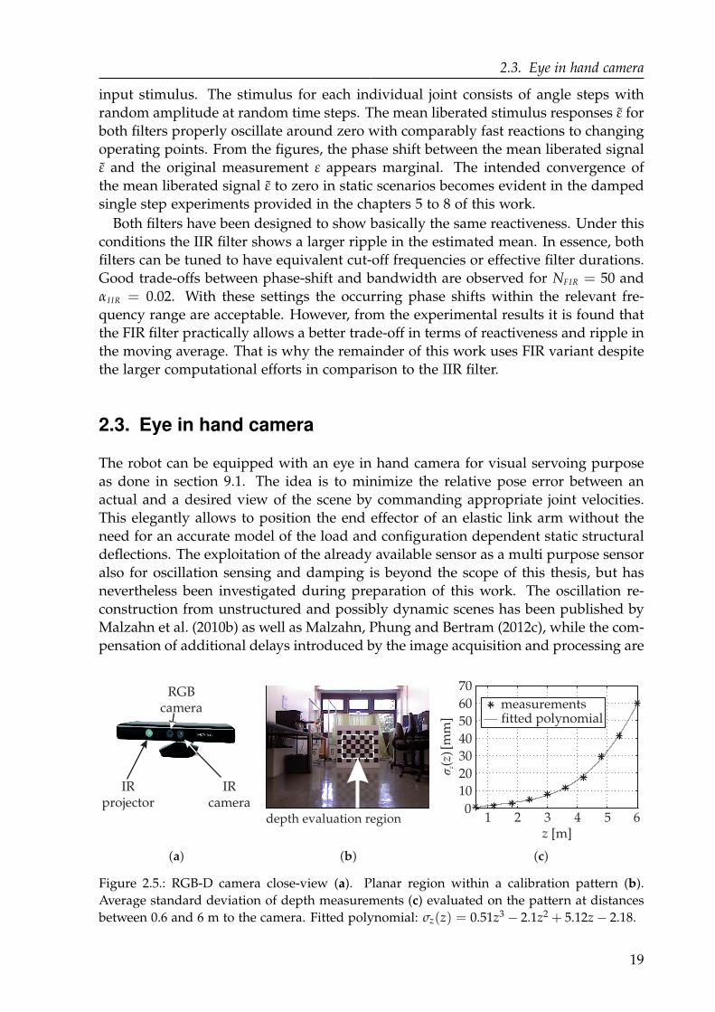
Figure 2.5.: RGB-D camera close-view (a). Planar region within a calibration pattern (b).
Average standard deviation of depth measurements (c) evaluated on the pattern at distances
between 0.6 and 6 m to the camera. Fitted polynomial: σz(z) = 0.51z3 − 2.1z2 + 5.12z − 2.18.
19
2. Experimental Setup
adressed by Malzahn, Phung and Bertram (2012b). The oscillation damping concept
Malzahn, Phung and Bertram (2012b) use, is the one described in section 5.
The eye-in-hand configured camera is the Microsoft Kinect (Freedman et al. 2008)
depicted in figure 2.5 (a). The Kinect integrates a conventional RGB camera with the
infrared (IR) projector and the IR camera as depth (D) sensor in a single housing.
Therefore it is termed to be an RGB-D sensor.
The sensor provides RGB images at a spatial resolution of 640× 480 pixels at a frame
rate of 30 Hz. Each color pixel is augmented by a depth measurement. The depth
measurement principle relies on the projection of a pseudo random structured light
pattern into the scene. The reflected pattern is observed by the IR camera. The per
pixel depth image is computed onboard from the reflected pattern via triangulation.
The camera together with the mechanical mounting and the tracking spheres has an
overall mass of 450 g.
In this work, the effective usable depth range has been determined experimentally
to be within 0.6 to 6.0 m. To obtain this range, the checkerboard pattern visible in
figure 2.5 (b) has been placed at different depths in front of the RGB-D camera per-
pendicular to the optical axis. The depth uncertainty is considered to be the average
standard deviation σz(z) over all depth measurements and 100 sequentially recorded
images per distance step within the planar depth evaluation region indicated in the
figure. The result is plotted against the actual distance z in figure 2.5 (c). Within the
aforementioned effective range the average standard deviation remains below 10 %.
An extrapolation indicates that the uncertainty disproportionally increases beyond
this range.
Alternatives to the use of the Kinect have been considered. A passive stereo camera
setup with comparable accuracy would most probably have a baseline less suitable
for eye-in-hand mounting. Additionally the requirement to search for the correspond-
ences within the image pairs contributes additional error sources. An RGB-D camera
circumvents this issue.
The loss of the scene depth information due to the perspective projection of a con-
ventional camera could have been tackled by software using "structure from motion"
(Oliensis 1999), "depth from focus" (Ens and Lawrence 1993) or "depth from defo-
cus" (Subbarao and Surya 1994) algorithms. Basic techniques are found in textbooks
for example by Hartley and Zisserman (2006) or Wöhler (2013). However, this likely
leads to degradation of the oscillation sensing accuracy due to error propagation in
conjunction with motion reconstruction algorithms applied afterwards.
Data fusion with a motion model incorporating the elastic arm dynamics would
contradict the motivating idea of using the camera to precisely position the end ef-
fector without exact knowledge about the actual link deflections.
Data fusion with a laser scanner would represent the most precise, but also the
most expensive and very bulky alternative.
A technology quite similar to the Kinect is the so-called "Time Of Flight" (TOF)
camera (Hansard et al. 2013). TOF cameras measure the delay of IR light impulses
emitted by a triggered source and reflected by the scene. The depth information is
computed from the known speed of light. The unique measurement range depends
on the trigger frequency. Especially those TOF cameras where the triggered light
impulses are received with Photonic Mixing Devices (PMD) (Xuming Luan 2001) are
20
2.4. Reference sensors
very insensitive to disturbing light sources such as direct sunlight. In this regard the
Kinect is restricted to indoor applications. However, the investigation of the camera
based oscillation sensing for an elastic arm in this work is pursued in an indoor
laboratory environment without direct sunlight. Future technology advances similar
to the PMD are assumed to solve disturbing light issues. In the end the low price of
about 100 € and especially the higher spatial resolution render the Kinect to be the
best choice for the purpose of this work.
2.4. Reference sensors
This section details the reference equipment developed and installed to asses training
data as well as ground truth information about the end effector motion and contact
forces.
Inertial measurement unit
TUDOR can be equipped with an inertial measurement unit (IMU). The one used
here is a CHR-6D unit by CH Robotics. It comprises a ADXL335 3-axes accelerometer
and a LPR510AL 3-axes MEMS gyroscope. The main properties of the sensor are
summarized in appendix A.4. The sensor is used as a ground truth reference for the
camera based oscillation reconstruction. The 6D inter-frame camera motion vector
reconstructed by the techniques described by Malzahn, Phung and Bertram (2012c)
represents the finite difference approximation of the camera velocity. Therefore the
IMU is boxed and mounted directly at the end effector of TUDOR underneath the
camera as visible in figure 2.1 (a).
External stereo camera system
With conventional rigid robot arms the measurement of the joint angles and know-
ledge about the link lengths is sufficient to accurately compute the end effector pose
with respect to the robot base frame. In contrast, the forward kinematics modeling
of elastic link robots is complicated by static deflections. Beyond that, the determina-
tion of the end effector pose during oscillations requires a precise model of the elastic
link dynamics. Two aspects motivate the development of an external stereo camera
setup in this work. The first one is the identification of the forward as well as inverse
kinematics models decribed along with the determination of the position accuracy in
chapter 9. The second aspect is the evaluation of the proposed oscillation damping
concepts presented by Malzahn et al. (2011b). The implementation, calibration and
analysis of the setup has been performed within the scope of a supervised thesis by
Mr. Bürger (February 2011).
The stereo camera setup is depicted in figure 2.6. It is a convergent camera con-
figuration mounted close to the walls underneath the laboratory ceiling. The optical
axes point towards the robot base frame. This way a baseline of 3 m is achieved, while
the field of view covers nearly the entire robot workspace.
The two cameras are VRmC-3+ models manufactured by VRmagic. Each camera
has a resolution of 640 × 480 pixels and provides 50 frames per second. A complete
21
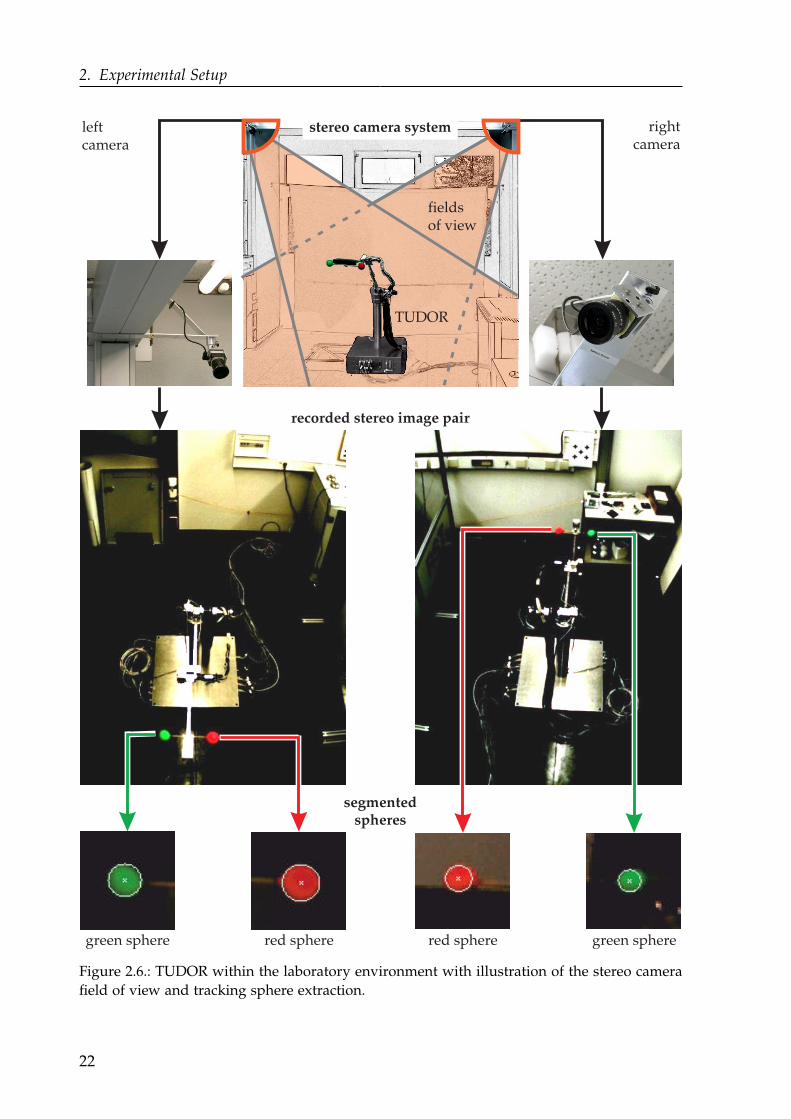
2. Experimental Setup
leftcamera
rightcamera
TUDOR
recorded stereo image pair
green sphere red sphere green spherered sphere
segmentedspheres
fieldsof view
stereo camera system
Figure 2.6.: TUDOR within the laboratory environment with illustration of the stereo camera
field of view and tracking sphere extraction.
22
2.4. Reference sensors
summary of the stereo camera hardware parameters is collected in appendix A.4.
The position measurement is based on the spheres mounted on both sides of the
end effector and visible in figure 2.1 (a) as well as 2.6. One sphere is green. The other
one is red. Therefore the solution to the correspondence problem among the stereo
image pairs is straightforward. The colors further simplify the sphere segmentation.
The segmentation algorithm is a three step process. Similar to histogram back projec-
tion (Swain and Ballard 1990) a normalized Gaussian color model for the spheres is
determined in the first step. The color model is determined for each channel of the
RGB as well as the HSV color space.
The appearance of the sphere colors in the images strongly depends on the proper-
ties of the individual camera sensor as well as the lighting. In the laboratory a mix of
varying daylight and artificial ceiling lighting can be found. The color models for both
cameras are thus semi-automatically calibrated once per recorded image sequence. A
center pixel and an edge pixel are selected for each sphere in a single stereo image
pair. The two selected points per pixel define a circle. All pixels within this circle are
used to compute the Gaussians.
The per-channel Gaussians reflect the probability that a particular channel value
belongs to a sphere pixel. A naive Bayes approach aggregates the individual channel
models and yields a probability estimate for a pixel to belong to either the red or
green sphere. This way the single color image of one camera is transformed into two
probability images, one image for each sphere.
In the second step morphological erosion removes all disturbing pixels in the prob-
ability images. The result of this second step finally serves as seed for the region
growing algorithm (Adams and Bischof 1994) operating on the probability image res-
ults of the first step. The centroid of the region growing output represents the estimate
of the sphere location in the image. A result is exemplified in the zoomed views of
figure 2.6.
The intrinsic and extrinsic stereo camera calibration is done with the checkerboard
pattern visible in figure 2.5 (b) and the Camera calibration toolbox for Matlab based
on the work by Bouguet (2008). For calibration of the stereo camera system with
respect to the robot base frame the robot samples the operating range of the first joint.
The second and third joints are kept in their zero configurations. This way the end
effector moves on a circular trajectory parallel to the 1x-1y-plane. The normal through
the circle center is collinear to the 1z axis. The static deflection of the arm due to its
own weight introduces an offset between the circle and the actual 1x-1y-plane. This
offset is removed based on the known arm length in a vertical arm configuration with
θ = [0, 90, 0]T.
After rectification the position of the segmented spheres with respect to the stereo
camera reference frame is computed via triangulation as discussed by Hartley and
Zisserman (2006, p. 318). The midpoint of the straight line connecting the sphere
centroids is considered to be the end effector position. The tracking of this point
from frame to frame allows the reconstruction of end effector motions such as the one
illustrated in the figures 2.7 (a) to (d).
The high end effector velocity causes the motion blur exemplified in figure 2.7 (e).
It is visible that the first moment of the segmented image regions represents plausible
mean locations of the spheres during the camera integration time.
23
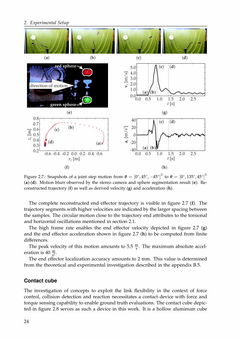
2. Experimental Setup
red sphere
green sphere
direction of motion
( )e ( )g
1.02.03.04.05.0
0.00.0 0.5 1.0 1.5 2.52.0
t [s]
vE
[m/
s]
0.0 0.5 1.0 1.5 2.52.0t [s]
a E[m
/s
]2
40
20
0
-20
-40
( )h
( )a
( )a
( )a
( )b
( )b
( )b
( )c
( )c
( )c
( )d
( )f
0.0 0.60.40.2-0.2-0.4-0.6xE [m]
0.2
0.40.3
0.50.60.7
z E[m
]
0.8
( )a
( )b( )c
( )d
( )d
( )d
Figure 2.7.: Snapshots of a joint step motion from θ = [0, 45,−45]T to θ = [0, 135, 45]T
(a)-(d). Motion blurr observed by the stereo camera and sphere segmentation result (e). Re-
constructed trajectory (f) as well as derived velocity (g) and acceleration (h).
The complete reconstructed end effector trajectory is visible in figure 2.7 (f). The
trajectory segments with higher velocities are indicated by the larger spacing between
the samples. The circular motion close to the trajectory end attributes to the torsional
and horizontal oscillations mentioned in section 2.1.
The high frame rate enables the end effector velocity depicted in figure 2.7 (g)
and the end effector acceleration shown in figure 2.7 (h) to be computed from finite
differences.
The peak velocity of this motion amounts to 5.5 ms . The maximum absolute accel-
eration is 40 ms2 .
The end effector localization accuracy amounts to 2 mm. This value is determined
from the theoretical and experimental investigation described in the appendix B.5.
Contact cube
The investigation of concepts to exploit the link flexibility in the context of force
control, collision detection and reaction necessitates a contact device with force and
torque sensing capability to enable ground truth evaluations. The contact cube depic-
ted in figure 2.8 serves as such a device in this work. It is a hollow aluminum cube
24
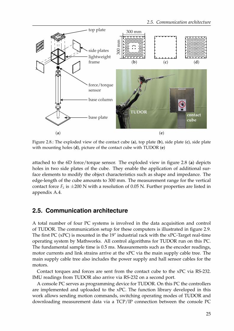
2.5. Communication architecture
side plates
lightweightframe
top plate
force/torquesensor
base plate
( )a
( )c ( )d
( )e
( )b
300 mm
300
mm
TUDORcontactcube
base column
Figure 2.8.: The exploded view of the contact cube (a), top plate (b), side plate (c), side plate
with mounting holes (d), picture of the contact cube with TUDOR (e)
attached to the 6D force/torque sensor. The exploded view in figure 2.8 (a) depicts
holes in two side plates of the cube. They enable the application of additional sur-
face elements to modify the object characteristics such as shape and impedance. The
edge-length of the cube amounts to 300 mm. The measurement range for the vertical
contact force Fz is ±200 N with a resolution of 0.05 N. Further properties are listed in
appendix A.4.
2.5. Communication architecture
A total number of four PC systems is involved in the data acquisition and control
of TUDOR. The communication setup for these computers is illustrated in figure 2.9.
The first PC (xPC) is mounted in the 19" industrial rack with the xPC-Target real-time
operating system by Mathworks. All control algorithms for TUDOR run on this PC.
The fundamental sample time is 0.5 ms. Measurements such as the encoder readings,
motor currents and link strains arrive at the xPC via the main supply cable tree. The
main supply cable tree also includes the power supply and hall sensor cables for the
motors.
Contact torques and forces are sent from the contact cube to the xPC via RS-232.
IMU readings from TUDOR also arrive via RS-232 on a second port.
A console PC serves as programming device for TUDOR. On this PC the controllers
are implemented and uploaded to the xPC. The function library developed in this
work allows sending motion commands, switching operating modes of TUDOR and
downloading measurement data via a TCP/IP connection between the console PC
25

2. Experimental Setup
camera motion,visual servoingerror TUDOR
console
stereo imageprocessor
RGB-D images
usercommands,requesteddata
eye-in-handimage processor
IMUreadings
contact force
USB 2.0
ethernet (UDP)
ethernet (TCP/IP)
RS-232
main supplycable tree
contact cube19" rack
circuits
xPC
amp
Vcc
stereo-camerasystem
image pairs
acquisitiontrigger
offlineprocessing
hard real-time
no real-time
softreal-time
Figure 2.9.: Communication setup for TUDOR
and the xPC.
The console PC triggers the stereo image processor PC to start the stereo image
acquisition via UDP.
The image processing for the eye in hand camera is computationally intensive. Most
image processing algorithms are rarely realizable to meet hard real-time constraints.
Frequently the actual computation time is influenced by the scene contents. Thus, the
image processing takes place on the fourth PC under soft real-time conditions. This
PC communicates the information extracted from the image sequences to the xPC
using UDP. The operating system on this image processing system is Ubuntu-Linux.
As a consequence, services running besides the image processing program contribute
to the variance of the delay associated with the extracted information. A method to
compensate this delay is reported by Malzahn, Phung and Bertram 2012b.
All Ethernet connections are realized within a closed network to avoid package loss
and additional delays due to arbitrary network traffic. The characteristic parameters
of the individual computers are collected in appendix A.2.
26
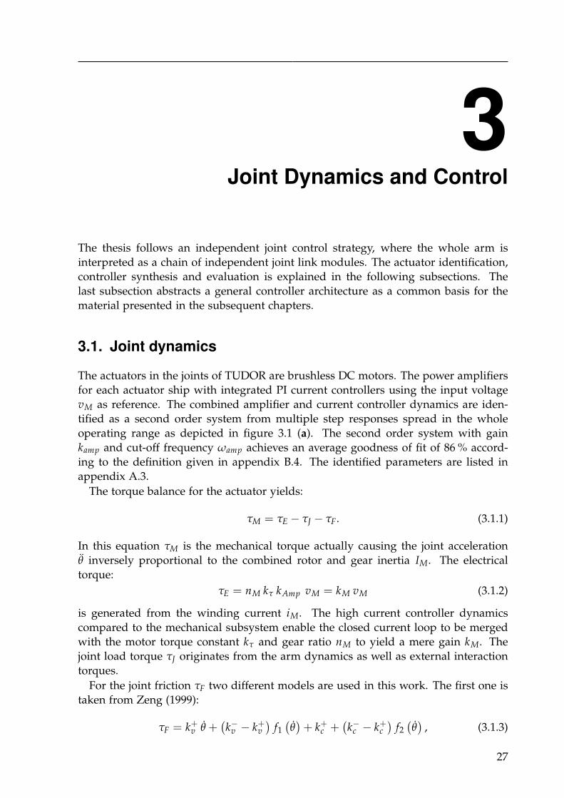
3Joint Dynamics and Control
The thesis follows an independent joint control strategy, where the whole arm is
interpreted as a chain of independent joint link modules. The actuator identification,
controller synthesis and evaluation is explained in the following subsections. The
last subsection abstracts a general controller architecture as a common basis for the
material presented in the subsequent chapters.
3.1. Joint dynamics
The actuators in the joints of TUDOR are brushless DC motors. The power amplifiers
for each actuator ship with integrated PI current controllers using the input voltage
vM as reference. The combined amplifier and current controller dynamics are iden-
tified as a second order system from multiple step responses spread in the whole
operating range as depicted in figure 3.1 (a). The second order system with gain
kamp and cut-off frequency ωamp achieves an average goodness of fit of 86 % accord-
ing to the definition given in appendix B.4. The identified parameters are listed in
appendix A.3.
The torque balance for the actuator yields:
τM = τE − τJ − τF. (3.1.1)
In this equation τM is the mechanical torque actually causing the joint acceleration
θ inversely proportional to the combined rotor and gear inertia IM. The electrical
torque:
τE = nM kτ kAmp vM = kM vM (3.1.2)
is generated from the winding current iM. The high current controller dynamics
compared to the mechanical subsystem enable the closed current loop to be merged
with the motor torque constant kτ and gear ratio nM to yield a mere gain kM. The
joint load torque τJ originates from the arm dynamics as well as external interaction
torques.
For the joint friction τF two different models are used in this work. The first one is
taken from Zeng (1999):
τF = k+v θ +(
k−v − k+v)
f1
(
θ)
+ k+c +(
k−c − k+c)
f2
(
θ)
, (3.1.3)
27
3. Joint Dynamics and Controli M
[A]
i M[A
]
t [s]
( )b
( )d
-100 -50 0 50 100-0.2
-0.1
0
0.1
0.2
0.3
t [ms]
θ [deg/s]
( )a
( )c
model measurement limits
0 10 20 30 40-200
-100
0
100
200
θ[d
eg/
s]
0 10 20 30 40-0.2
-0.1
0
0.1
0.2
0.3
t [s]
i M[A
]
0 1 2 3 4 5-5
0
5
Figure 3.1.: Identification results for the second joint without load. Measured and identified
amplifier step response (a), planned and realized joint angular velocity stimulus with velocity
limits (b), measured and identified joint current plotted over joint velocity (c) and time (d).
with
f1
(
θ)
=
0 if θ ≥ 0
θ if θ < 0(3.1.4)
and
f2
(
θ)
=
0 if θ ≥ 0
1 if θ < 0.(3.1.5)
The parameters k+v and k−v are the velocity-direction dependent viscous friction coef-
ficients while k+c and k−c are the corresponding coulomb friction coefficients. This
model structure is required for the damped dynamics modelling in chapter 10 as well
as detection of collisions between the robot and its environment in chapter 11.
The second and simplified friction model has the form:
τF = kv θ, (3.1.6)
where kv is called the symmetric viscous friction coefficient obtained by averaging
over the asymmetric coefficients from equation (3.1.3). In section 3.2 this second fric-
tion model serves the design of the joint angular controllers based on the linear trans-
28
3.2. Joint angular control
fer function model:
GM(s) =θ(s)
vM(s)=
kM
s(IMs + kv). (3.1.7)
For identification, the velocity controller described in section 3.2 is designed based on
the motor parameters provided by the vendor. The multi-sinus velocity stimulus de-
picted in figure 3.1 (b) excites the joint dynamics. The periodicity allows the noise free
computation of higher order signal derivatives based on Fourier analysis as proposed
by Swevers, Verdonck and Schutter (2007). The stimulus operates in both the upper
and the lower velocity range. The corresponding measured and estimated motor cur-
rents are plotted over the joint velocity in figure 3.1 (c) and over time in figure 3.1 (d).
The asymmetric nature of the coulomb friction is clearly visible. The asymmetry in
the viscous friction is insignificant and justifies the direction independence of the lin-
ear model (3.1.7). The average goodness of fit computed from the motor current iM
on 10 experiments is 89 %. This static result is more than satisfactory against the
background that changes in lubrication and temperature drastically influence these
parameters over time. The parameters for all joints are listed in appendix A.3.
3.2. Joint angular control
The control objective for each joint is the realization of point-to-point movements
without overshoot and vanishing steady state error.
For robotic arms according to Sciavicco and Siciliano (2001) independent joint con-
trol is probably "the simplest control strategy that can be thought of". It interprets
a robot arm as a chain of independent single-input single-output systems (SISO). It
is enabled by the high gear ratios, which reduce coupling forces and torques. In
consequence, coupling effects between the individual systems may be considered as
disturbances.
For the reasons detailed in section 1.2 centralized concepts such as the inverse dy-
namics or computed torque control approach known from rigid robots are difficult
to apply to elastic link robots. Section 1.2 introduces and chapter 4 experimentally
exemplifies the challenges connected with the precise holistic modelling of a multi-
elastic-link robot in realistic manipulation scenarios. It renders the achievable benefit
questionable in comparison to the required mathematical and computational effort.
On the other hand, the analyses show that the natural oscillation frequencies of all
links appear to be measurable with good phase alignment on each of the individual
links. This insight leads to the transfer function model in section 5.1. The independent
joint control strategy fits well with this modelling approach in view of oscillation
damping control of a multi-elastic-link arm.
The independent joint controller described in the following has a cascaded architec-
ture. The cascaded nature simplifies the controller design. At each cascade level the
plant is treated as a second order SISO system. In equivalence to a state feedback the
closed loop dynamcis can be rigorously shaped whereas rejection of disturbances and
nonlinearities improves with each cascade level. The concept is outlined in textbooks
such as Sciavicco and Siciliano (2001) or Schröder (2009).
The innermost cascade level comprises the joint current controller shipped with
the power amplifiers. This controller is a PI type controller, which rejects nonlinear
29
3. Joint Dynamics and Control
effects in the electrical part of the plant and compensates for the mutual induction for
instance. Section 3.1 identifies the fast response of the closed current control loop.
The next cascade level is a PI velocity control loop with the transfer function:
GPI =kPI(tPIs + 1)
s. (3.2.1)
A sampling frequency of 2 kHz justifies the quasi continuous design. The feedback
is based on numerical derivatives of the incremental encoder readings filtered by
a first order transfer function Gd with a time constant td. The PI controller time
constant tPI cancels the slow mechanical time constant of the motor. This mechanical
time constant tM = θmaxτM,max
IM, e f f
kvincludes the effective inertia IM, e f f estimated from the
geometries and masses of the joint as well as attached subsequent bodies in the joint
zero configuration. The gain kPI is tuned according to the symmetrical optimum so
that the closed loop exhibits a damping of DPI = 1/√
2.
Schröder (2009); Sciavicco and Siciliano (2001) realize the position cascade level by
applying a proportional controller. However, in view of the linear oscillation feedback
proposed in chapter 5, the extension to the PD controller with first order lag element:
GPD =kPD(tPDs + 1)
tls + 1(3.2.2)
is advantagous for oscillation damping. The PD time constant tPD is tuned to cancel
the time constant of the first order approximation of the closed velocity loop. The
gain kPD is selected so that the position control loop displays unity gain. A first order
filter with lag time constant tl reduces noise and ensures causality.
A motion planner generates a sinusoidal acceleration profile as detailed by Wenz
(2008, p. 89) for each commanded joint motion. For self-containment the underlying
equations are summarized in the appendix B.6. The profile is continuously differenti-
able of infinite order and elegantly avoids impulsive jerk, which minimizes gear wear.
The absence of impulsive jerk already contributes to a reduced excitation of struc-
tural oscillations. The planner ensures that the controller adheres the acceleration
and velocity limits (see appendix A.3), which becomes apparent in the next section.
3.3. Controller evaluation
Figure 3.2 (a) depicts the joint angle stimulus response of the second joint. During
this experiment TUDOR carries three test mass plates with a total mass of 300 g. All
three joints simultaneously respond to individual stimuli comprising of angle setpoint
steps with random amplitudes at random timesteps. All joints have been operated
with maximum acceleration as well as maximum speed (see appendix A.3).
Figure 3.2 (b) provides a close view on the stimulus response. The close view
illustrates the smooth acceleration phases and the constant velocity phase generated
by the sinusoidal motion planner. The PI velocity controller compensates gravitational
load torques as well as joint friction so that the steady state angular position error
vanishes below the encoder resolution. There is no overshoot. Even at higher zoom
levels disturbances due to the link oscillations are not visible.
30
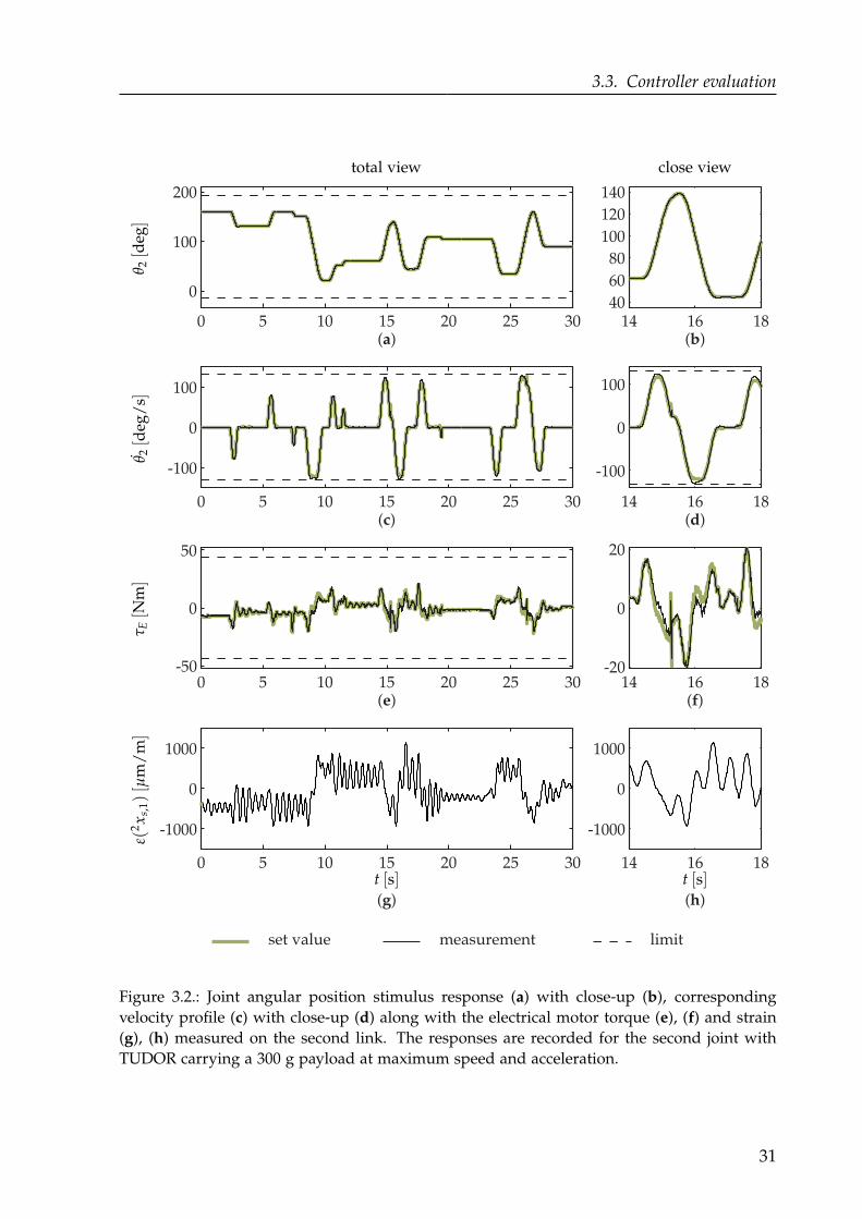
3.3. Controller evaluation
0 5 10 15 20 25 30
0
100
200
(a)
0 5 10 15 20 25 30
-100
0
100
(c)
0 5 10 15 20 25 30-50
0
50
(e)
0 5 10 15 20 25 30
-1000
0
1000
(g)
14 16 1840
60
80
100
120
140
(b)
14 16 18
-100
0
100
(d)
14 16 18-20
0
20
(f)
14 16 18
-1000
0
1000
(h)
set value measurement limit
total view close view
θ 2[d
eg]
θ 2[d
eg/
s]τ E
[Nm]
ε(2x
s,1)[µ
m/
m]
t [s]t [s]
Figure 3.2.: Joint angular position stimulus response (a) with close-up (b), corresponding
velocity profile (c) with close-up (d) along with the electrical motor torque (e), (f) and strain
(g), (h) measured on the second link. The responses are recorded for the second joint with
TUDOR carrying a 300 g payload at maximum speed and acceleration.
31

3. Joint Dynamics and Control
--
dampingscheme
highpass
elasticlink
GM
GD
plantmodel
controllercomponent
GPIGPD
controller specificconnection
θε θε vε
θw
θ
θ
ε
ε
Figure 3.3.: The general independent joint controller architecture developed in this work.
The velocity profile of the stimulus response is depicted in figure 3.2 (c). A close
view is provided in figure 3.2 (d). The velocity profile shows only slight oscillatory
disturbances.
Figure 3.2 (e) depicts the electrical torque produced by the winding current during
the stimulus. Figure 3.2 (f) is the corresponding close view. Besides the larger meas-
urement noise originating from the current readings, the torque signal has clearly
visible harmonic components. They can be interpreted as the action of rejecting dis-
turbances due to the link oscillations before they influence outer cascade levels. The
oscillations are depicted in the figures 3.2 (g) and (h) based on strain measurements.
As a conclusion it may be stated that the joint controller accomplishes the design
objectives.
3.4. General control architecture
The independent joint angular controllers are augmented by the oscillation damp-
ing schemes presented in the chapters 5 to 7. Figure 3.3 illustrates the integration of
the individual damping actions within a general controller architecture. The plant
consists of the motor transfer function (3.1.7) with a controller specific oscillatory dy-
namics representation for the subsequent link connected in series. The oscillations are
superposed by the static strain due to gravity. The strain measurement ε is liberated
from this static signal portion using the technique explained in section 2.2. The mean
liberated measurement ε is fed to the damping controller. Depending on the particu-
lar oscillation damping scheme, additional joint angle feedback may be required. The
cascade level at which the damping action enters the joint controller also varies with
the concept under consideration. Such optional signals are indicated by dashed lines
in the generalized visualization of the controller architecture in figure 3.3.
32

4Elastic Link Dynamics Analysis
The chapter initially introduces the terminology and mathematical relations required
for the remainder of this work. Beyond that, the theoretical analyses and experimental
investigations carried out confirm the notion acquired from the literature survey re-
garding the complexity of the elastic arm dynamics as well as the applicability of
controllers relying on holistic plant models. This chapter constitutes the foundation
of the decisions, which lead to the control strategy proposed in this work.
4.1. Preliminary assumptions
The derivations presented in the remainder of this chapter are based on a set of as-
sumptions, which are summarized in the following.
Assumptions 4.1.1: The elastic links are modeled as Euler-Bernoulli-beams, so that:
(a) . . . the deflections are small in comparison to the beam length,
(b) . . . the neutral fiber has constant length,
(c) . . . the deflections are elastic and reversible so that Hooke’s law applies,
(d) . . . the rotation of a differential beam element is negligible compared to the translation so
that cross sections perpendicular to the neutral fiber remain perpendicular,
(e) . . . the angular distortion of a beam element is small in relation to the transversal bending
deformation,
(f) . . . the beam is uniform and homogenous.
4.2. The equation of motion
Consider the planar differential beam element of infinitesimal length dx sketched in
figure 4.1. In accordance to the rigid body kinematics in figure 2.1 (b) the deflection
of the beam at a time instant t is measured in the preceding joint frame as the y-
coordinate at a location x along the undeflected neutral fiber.
33
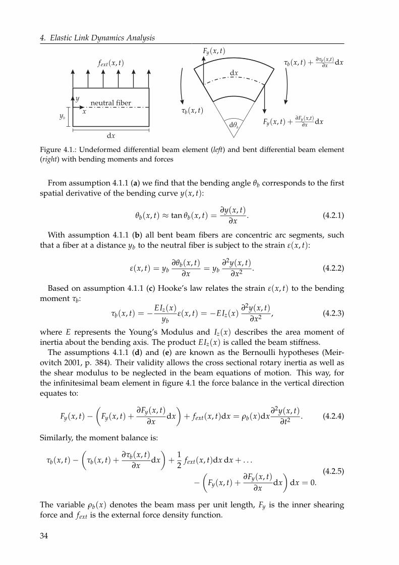
4. Elastic Link Dynamics Analysis
neutral fiber
dx
yb
dx
dθb
x
y
τb(x, t)
τb(x, t) + ∂τb(x,t)∂x dx
Fy(x, t)
Fy(x, t) +∂Fy(x,t)
∂x dx
fext(x, t)
Figure 4.1.: Undeformed differential beam element (left) and bent differential beam element
(right) with bending moments and forces
From assumption 4.1.1 (a) we find that the bending angle θb corresponds to the first
spatial derivative of the bending curve y(x, t):
θb(x, t) ≈ tan θb(x, t) =∂y(x, t)
∂x. (4.2.1)
With assumption 4.1.1 (b) all bent beam fibers are concentric arc segments, such
that a fiber at a distance yb to the neutral fiber is subject to the strain ε(x, t):
ε(x, t) = yb∂θb(x, t)
∂x= yb
∂2y(x, t)
∂x2. (4.2.2)
Based on assumption 4.1.1 (c) Hooke’s law relates the strain ε(x, t) to the bending
moment τb:
τb(x, t) = −EIz(x)
ybε(x, t) = −EIz(x)
∂2y(x, t)
∂x2, (4.2.3)
where E represents the Young’s Modulus and Iz(x) describes the area moment of
inertia about the bending axis. The product EIz(x) is called the beam stiffness.
The assumptions 4.1.1 (d) and (e) are known as the Bernoulli hypotheses (Meir-
ovitch 2001, p. 384). Their validity allows the cross sectional rotary inertia as well as
the shear modulus to be neglected in the beam equations of motion. This way, for
the infinitesimal beam element in figure 4.1 the force balance in the vertical direction
equates to:
Fy(x, t)−(
Fy(x, t) +∂Fy(x, t)
∂xdx
)
+ fext(x, t)dx = ρb(x)dx∂2y(x, t)
∂t2. (4.2.4)
Similarly, the moment balance is:
τb(x, t)−(
τb(x, t) +∂τb(x, t)
∂xdx
)
+1
2fext(x, t)dx dx + . . .
−(
Fy(x, t) +∂Fy(x, t)
∂xdx
)
dx = 0.
(4.2.5)
The variable ρb(x) denotes the beam mass per unit length, Fy is the inner shearing
force and fext is the external force density function.
34
4.3. The general solution
From the infinitesimal perspective, second order terms of dx may be neglected, so
that both balances simplify to:
−∂Fy(x, t)
∂x+ fext(x, t) = ρb(x)
∂2y(x, t)
∂t2, (4.2.6)
Fy(x, t) = −∂τb(x, t)
∂x. (4.2.7)
Using assumption 4.1.1 (f) the area moment of inertia Iz as well as the mass per
unit length ρb becomes constant. Combining equations (4.2.6), (4.2.7) and expressing
the bending moment by the right side of equation (4.2.3) yields the Bernoulli Beam
partial differential equation (PDE):
ρb∂2 y(x, t)
∂t2+ EIz
∂4 y(x, t)
∂x4= fext(x, t). (4.2.8)
Unlike the transversal oscillations of strings, the longitudinal oscillations of rods or
the torsional oscillations of shafts this PDE is fourth order. The consequences become
apparent in chapter 7 for example.
4.3. The general solution
The common approach to solve equation (4.2.8) is to assume a separability of the
spatial and temporal dependances (Dukkipati and Srinivas 2005; Meirovitch 2001):
y(x, t) = Φ(x)ν(t), (4.3.1)
where Φ(x) describes the deflection shape and ν(t) reflects the temporal amplitude.
Consider the harmonic case with fext = 0. The substitution in the PDE (4.2.8) leads
to:
− EIz
ρb
d4 Φ(x)/d x4
Φ(x)=
d2 ν(t)/d t2
ν(t)= ω2. (4.3.2)
Note, the dependance on the spatial variable x is collected on the left while the tem-
poral dependance is kept on the right side of the equation. The equality holds for
all times t and 0 ≤ x ≤ L. Hence, the ratios on both sides of the equations must be
constant. This constant is the eigenvalue denoted by ω2. Both sides of equation (4.3.2)
are independent ordinary differential equations (ODE).
The first ODE depends on the spatial variable x. With the introduction of the wave
number kω:
kω = 4
√
ω2 ρb
EIz, (4.3.3)
it follows:d4 Φ(x)
d x4+ k4
ω Φ(x) = 0. (4.3.4)
By substitution of the exponential form Φ(x) = a eλ x in equation (4.3.4) we find the
characteristic equation λ4 + k4ω = 0. Its roots provide the general solution to the ODE:
Φ(x) = + a e−j kω x + − a e j kω x + + aN e−kω x + − aN e kω x. (4.3.5)
35
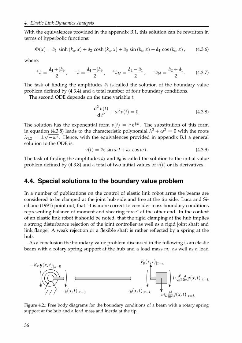
4. Elastic Link Dynamics Analysis
With the equivalences provided in the appendix B.1, this solution can be rewritten in
terms of hyperbolic functions:
Φ(x) = a1 sinh (kω x) + a2 cosh (kω x) + a3 sin (kω x) + a4 cos (kω x) , (4.3.6)
where:
+ a =a4 + ja3
2, − a =
a4 − ja3
2, + aN =
a2 − a1
2, − aN =
a2 + a1
2. (4.3.7)
The task of finding the amplitudes ai is called the solution of the boundary value
problem defined by (4.3.4) and a total number of four boundary conditions.
The second ODE depends on the time variable t:
d2 ν(t)
d t2+ ω2ν(t) = 0. (4.3.8)
The solution has the exponential form ν(t) = a e jλt. The substitution of this form
in equation (4.3.8) leads to the characteristic polynomial λ2 + ω2 = 0 with the roots
λ1,2 = ±√−ω2. Hence, with the equivalences provided in appendix B.1 a general
solution to the ODE is:
ν(t) = a5 sin ω t + a6 cos ω t. (4.3.9)
The task of finding the amplitudes a5 and a6 is called the solution to the initial value
problem defined by (4.3.8) and a total of two initial values of ν(t) or its derivatives.
4.4. Special solutions to the boundary value problem
In a number of publications on the control of elastic link robot arms the beams are
considered to be clamped at the joint hub side and free at the tip side. Luca and Si-
ciliano (1991) point out, that "it is more correct to consider mass boundary conditions
representing balance of moment and shearing force" at the other end. In the context
of an elastic link robot it should be noted, that the rigid clamping at the hub implies
a strong disturbance rejection of the joint controller as well as a rigid joint shaft and
link flange. A weak rejection or a flexible shaft is rather reflected by a spring at the
hub.
As a conclusion the boundary value problem discussed in the following is an elastic
beam with a rotary spring support at the hub and a load mass mL as well as a load
τb(x, t)|x=0
−Kr y(x, t)|x=0Fy(x, t)|x=L
τb(x, t)|x=LmL
∂2
∂t2 y(x, t)|x=L
IL∂2
∂t2∂
∂x y(x, t)|x=L
Figure 4.2.: Free body diagrams for the boundary conditions of a beam with a rotary spring
support at the hub and a load mass and inertia at the tip.
36
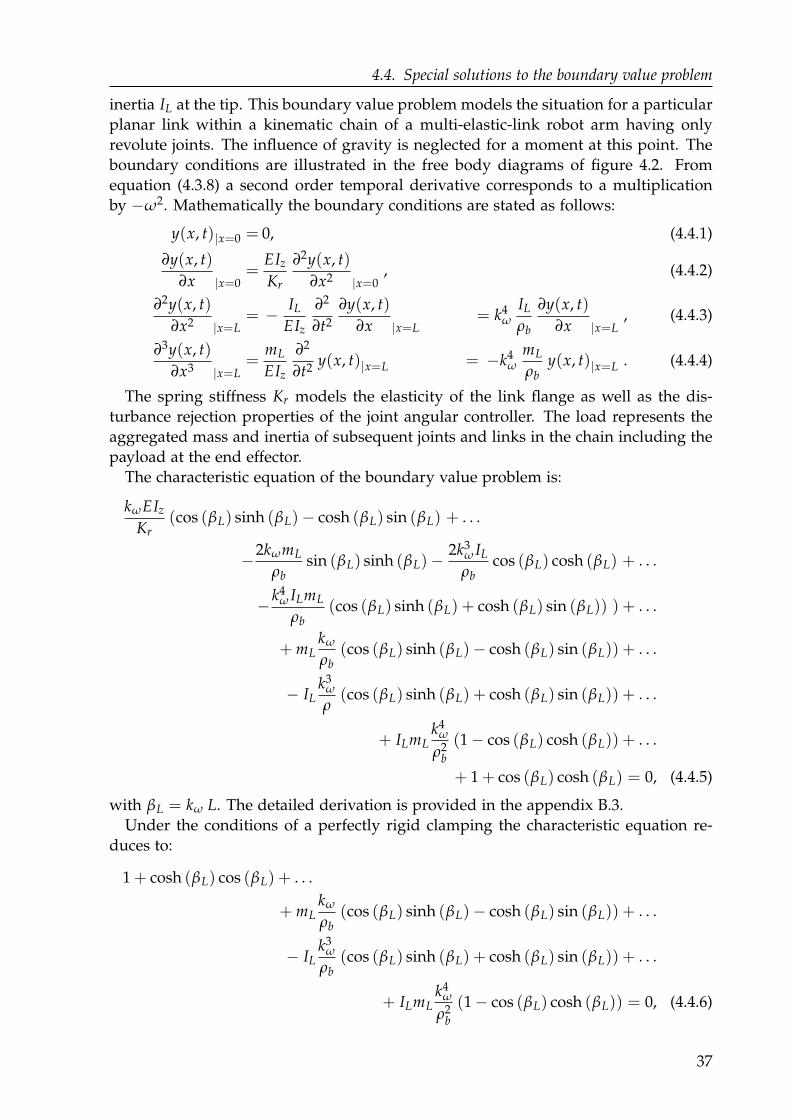
4.4. Special solutions to the boundary value problem
inertia IL at the tip. This boundary value problem models the situation for a particular
planar link within a kinematic chain of a multi-elastic-link robot arm having only
revolute joints. The influence of gravity is neglected for a moment at this point. The
boundary conditions are illustrated in the free body diagrams of figure 4.2. From
equation (4.3.8) a second order temporal derivative corresponds to a multiplication
by −ω2. Mathematically the boundary conditions are stated as follows:
y(x, t)|x=0 = 0, (4.4.1)
∂y(x, t)
∂x |x=0=
EIz
Kr
∂2y(x, t)
∂x2 |x=0, (4.4.2)
∂2y(x, t)
∂x2 |x=L= − IL
EIz
∂2
∂t2
∂y(x, t)
∂x |x=L= k4
ωIL
ρb
∂y(x, t)
∂x |x=L, (4.4.3)
∂3y(x, t)
∂x3 |x=L=
mL
EIz
∂2
∂t2y(x, t)|x=L = −k4
ωmL
ρby(x, t)|x=L . (4.4.4)
The spring stiffness Kr models the elasticity of the link flange as well as the dis-
turbance rejection properties of the joint angular controller. The load represents the
aggregated mass and inertia of subsequent joints and links in the chain including the
payload at the end effector.
The characteristic equation of the boundary value problem is:
kωEIz
Kr(cos (βL) sinh (βL)− cosh (βL) sin (βL) + . . .
−2kωmL
ρbsin (βL) sinh (βL)−
2k3ω IL
ρbcos (βL) cosh (βL) + . . .
−k4ω ILmL
ρb(cos (βL) sinh (βL) + cosh (βL) sin (βL)) ) + . . .
+ mLkω
ρb(cos (βL) sinh (βL)− cosh (βL) sin (βL)) + . . .
− ILk3
ω
ρ(cos (βL) sinh (βL) + cosh (βL) sin (βL)) + . . .
+ ILmLk4
ω
ρ2b
(1 − cos (βL) cosh (βL)) + . . .
+ 1 + cos (βL) cosh (βL) = 0, (4.4.5)
with βL = kω L. The detailed derivation is provided in the appendix B.3.
Under the conditions of a perfectly rigid clamping the characteristic equation re-
duces to:
1 + cosh (βL) cos (βL) + . . .
+ mLkω
ρb(cos (βL) sinh (βL)− cosh (βL) sin (βL)) + . . .
− ILk3
ω
ρb(cos (βL) sinh (βL) + cosh (βL) sin (βL)) + . . .
+ ILmLk4
ω
ρ2b
(1 − cos (βL) cosh (βL)) = 0, (4.4.6)
37

4. Elastic Link Dynamics Analysis
which agrees with the results Luca and Siciliano (1989, 1991) present. Additionally,
the choice IL = mL = 0 results in the characteristic equation of the clamped-free
cantilever found in fundamental textbooks on the mechanics of vibrations (Dukkipati
and Srinivas 2005; Meirovitch 2001).
The characteristic equations (4.4.5) and (4.4.6) represent transcendental equations.
They have an infinite number of roots βL,r, which implies that the beam has an infinite
number of natural frequencies ωr with r = 1, 2, . . . ∞.
From the definition of the wave number kω in equation (4.3.3) the natural frequen-
cies ωr compute to:
ωr = β2L,r
√
EIz
ρb L4. (4.4.7)
In turn, from equation (4.3.6) we find a natural mode shape function Φr(x) for
each natural frequency ωr. The mode shape functions represent the set of possible
beam deformations under the given boundary conditions. Since equation (4.3.4) is
homogenous, they can only be determined up to a scale. The normalization derived
in the appendix B.3 ensures that the mode shapes are orthogonal, so that the total
spatial deflection function Φ(x) can be expressed as a linear combination of all mode
shapes. This leads to the absolutely convergent series:
Φ(x) =nu
∑u=1
wu Φu(x), with nu → ∞. (4.4.8)
where for the example of a perfectly rigid clamping the weights wu are defined ac-
cording to:
wu =∫ L
0ρLΦu(x)Φ(x)dx + mLΦu(x)|x=LΦ(x)|x=L + . . .
+ ILdΦu(x)
dx |x=L
dΦ(x)
dx |x=L. (4.4.9)
In practice the weights wu must be identified experimentally. Therefore the dynamic
deflection has to be observed from distributed strain (Garcia, Feliu and Somolinos
2001; Pisoni et al. 1995) or acceleration (Hillsley and Yurkovich 1993) measurements
or directly measured using markers and an external camera sensor (Feliu, Rattan and
Brown 1992; Li and Chen 2002).
4.5. Natural frequencies under varying boundary conditions
One question arising from the previous section asks how the natural frequencies
change with a variation in the boundary conditions. First, a perfectly rigid clamp-
ing is assumed, so that Kr tends to infinity and the characteristic equation (4.4.6) can
be used. The variable parameters in the equation are the total load mass mL as well
as the total load inertia IL normalized by the beam density per unit length ρb. Initial
values for the frequencies are obtained by graphical inspection of the characteristic
equation. The accurate values are determined using Brent’s method (Brent 1972, ch.
4).
38
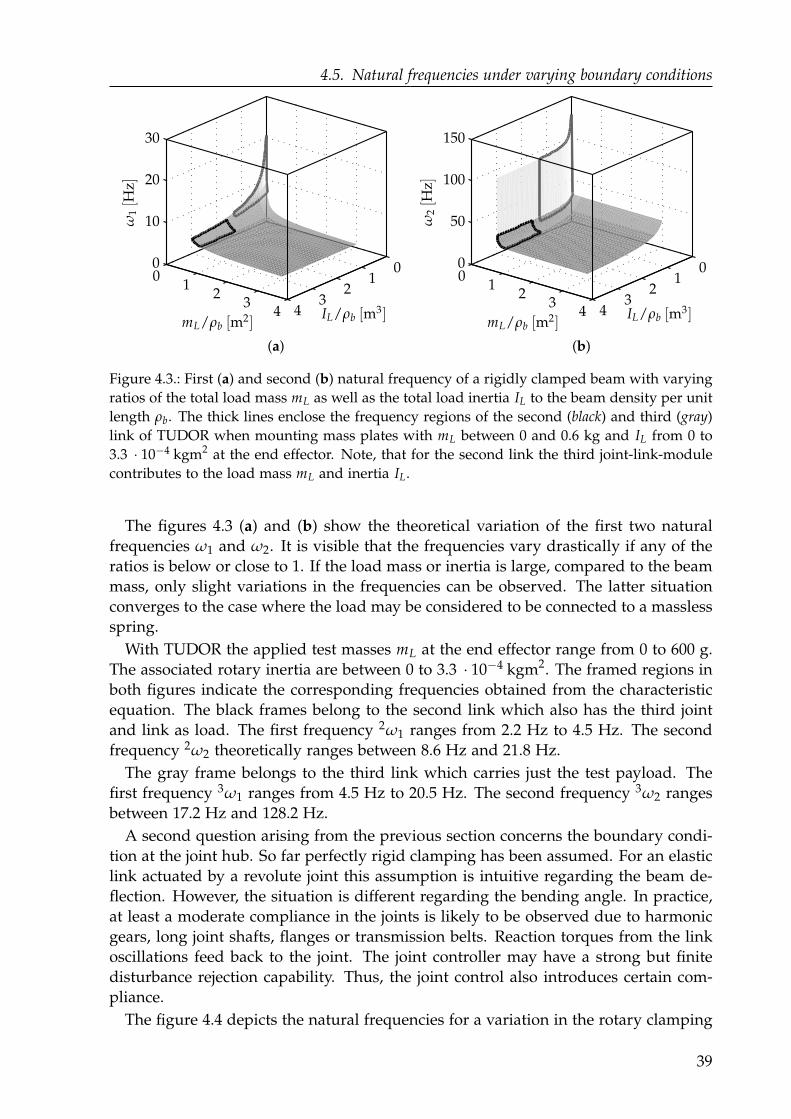
4.5. Natural frequencies under varying boundary conditions
01
23
4
01
23
4
0
10
20
30
01
23
4
01
23
4
0
50
100
150
(a) (b)
ω1[H
z]
ω2[H
z]
IL/ρb [m3]IL/ρb [m
3]mL/ρb [m
2]mL/ρb [m2]
Figure 4.3.: First (a) and second (b) natural frequency of a rigidly clamped beam with varying
ratios of the total load mass mL as well as the total load inertia IL to the beam density per unit
length ρb. The thick lines enclose the frequency regions of the second (black) and third (gray)
link of TUDOR when mounting mass plates with mL between 0 and 0.6 kg and IL from 0 to
3.3 · 10−4 kgm2 at the end effector. Note, that for the second link the third joint-link-module
contributes to the load mass mL and inertia IL.
The figures 4.3 (a) and (b) show the theoretical variation of the first two natural
frequencies ω1 and ω2. It is visible that the frequencies vary drastically if any of the
ratios is below or close to 1. If the load mass or inertia is large, compared to the beam
mass, only slight variations in the frequencies can be observed. The latter situation
converges to the case where the load may be considered to be connected to a massless
spring.
With TUDOR the applied test masses mL at the end effector range from 0 to 600 g.
The associated rotary inertia are between 0 to 3.3 · 10−4 kgm2. The framed regions in
both figures indicate the corresponding frequencies obtained from the characteristic
equation. The black frames belong to the second link which also has the third joint
and link as load. The first frequency 2ω1 ranges from 2.2 Hz to 4.5 Hz. The second
frequency 2ω2 theoretically ranges between 8.6 Hz and 21.8 Hz.
The gray frame belongs to the third link which carries just the test payload. The
first frequency 3ω1 ranges from 4.5 Hz to 20.5 Hz. The second frequency 3ω2 ranges
between 17.2 Hz and 128.2 Hz.
A second question arising from the previous section concerns the boundary condi-
tion at the joint hub. So far perfectly rigid clamping has been assumed. For an elastic
link actuated by a revolute joint this assumption is intuitive regarding the beam de-
flection. However, the situation is different regarding the bending angle. In practice,
at least a moderate compliance in the joints is likely to be observed due to harmonic
gears, long joint shafts, flanges or transmission belts. Reaction torques from the link
oscillations feed back to the joint. The joint controller may have a strong but finite
disturbance rejection capability. Thus, the joint control also introduces certain com-
pliance.
The figure 4.4 depicts the natural frequencies for a variation in the rotary clamping
39
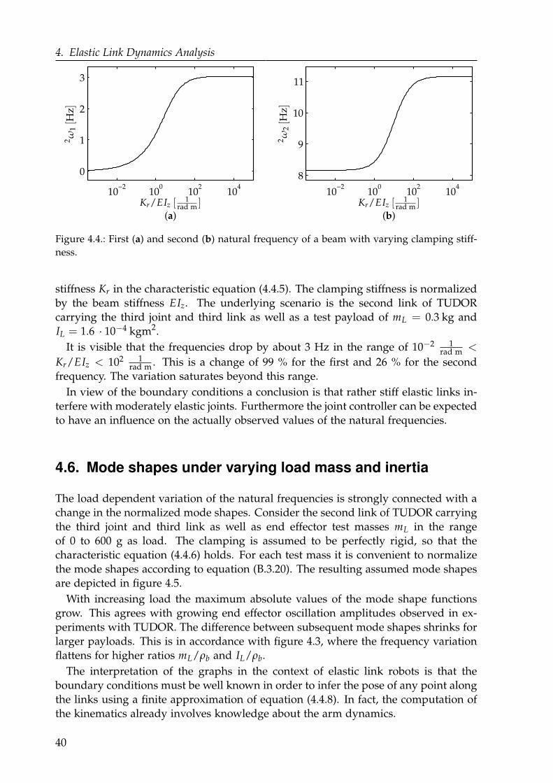
4. Elastic Link Dynamics Analysis
10−2
100
102
104
0
1
2
3
(a)
10−2
100
102
104
8
9
10
11
(b)
2ω
1[H
z]
2ω
2[H
z]
Kr/EIz [1
rad m ]Kr/EIz [1
rad m ]
Figure 4.4.: First (a) and second (b) natural frequency of a beam with varying clamping stiff-
ness.
stiffness Kr in the characteristic equation (4.4.5). The clamping stiffness is normalized
by the beam stiffness EIz. The underlying scenario is the second link of TUDOR
carrying the third joint and third link as well as a test payload of mL = 0.3 kg and
IL = 1.6 · 10−4 kgm2.
It is visible that the frequencies drop by about 3 Hz in the range of 10−2 1rad m <
Kr/EIz < 102 1rad m . This is a change of 99 % for the first and 26 % for the second
frequency. The variation saturates beyond this range.
In view of the boundary conditions a conclusion is that rather stiff elastic links in-
terfere with moderately elastic joints. Furthermore the joint controller can be expected
to have an influence on the actually observed values of the natural frequencies.
4.6. Mode shapes under varying load mass and inertia
The load dependent variation of the natural frequencies is strongly connected with a
change in the normalized mode shapes. Consider the second link of TUDOR carrying
the third joint and third link as well as end effector test masses mL in the range
of 0 to 600 g as load. The clamping is assumed to be perfectly rigid, so that the
characteristic equation (4.4.6) holds. For each test mass it is convenient to normalize
the mode shapes according to equation (B.3.20). The resulting assumed mode shapes
are depicted in figure 4.5.
With increasing load the maximum absolute values of the mode shape functions
grow. This agrees with growing end effector oscillation amplitudes observed in ex-
periments with TUDOR. The difference between subsequent mode shapes shrinks for
larger payloads. This is in accordance with figure 4.3, where the frequency variation
flattens for higher ratios mL/ρb and IL/ρb.
The interpretation of the graphs in the context of elastic link robots is that the
boundary conditions must be well known in order to infer the pose of any point along
the links using a finite approximation of equation (4.4.8). In fact, the computation of
the kinematics already involves knowledge about the arm dynamics.
40
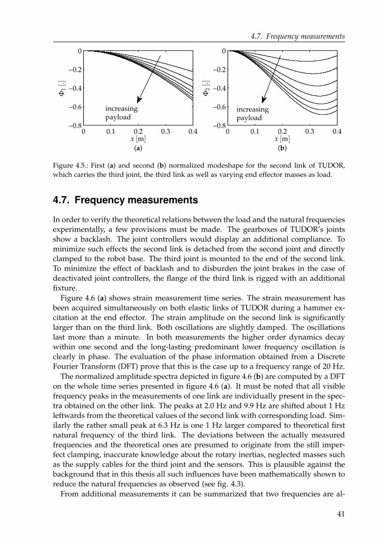
4.7. Frequency measurements
0 0.1 0.2 0.3 0.4−0.8
−0.6
−0.4
−0.2
0
(a)
0 0.1 0.2 0.3 0.4−0.8
−0.6
−0.4
−0.2
0
(b)
increasingpayload
increasingpayload
Φ1[.]
Φ2[.]
x [m]x [m]
Figure 4.5.: First (a) and second (b) normalized modeshape for the second link of TUDOR,
which carries the third joint, the third link as well as varying end effector masses as load.
4.7. Frequency measurements
In order to verify the theoretical relations between the load and the natural frequencies
experimentally, a few provisions must be made. The gearboxes of TUDOR’s joints
show a backlash. The joint controllers would display an additional compliance. To
minimize such effects the second link is detached from the second joint and directly
clamped to the robot base. The third joint is mounted to the end of the second link.
To minimize the effect of backlash and to disburden the joint brakes in the case of
deactivated joint controllers, the flange of the third link is rigged with an additional
fixture.
Figure 4.6 (a) shows strain measurement time series. The strain measurement has
been acquired simultaneously on both elastic links of TUDOR during a hammer ex-
citation at the end effector. The strain amplitude on the second link is significantly
larger than on the third link. Both oscillations are slightly damped. The oscillations
last more than a minute. In both measurements the higher order dynamics decay
within one second and the long-lasting predominant lower frequency oscillation is
clearly in phase. The evaluation of the phase information obtained from a Discrete
Fourier Transform (DFT) prove that this is the case up to a frequency range of 20 Hz.
The normalized amplitude spectra depicted in figure 4.6 (b) are computed by a DFT
on the whole time series presented in figure 4.6 (a). It must be noted that all visible
frequency peaks in the measurements of one link are individually present in the spec-
tra obtained on the other link. The peaks at 2.0 Hz and 9.9 Hz are shifted about 1 Hz
leftwards from the theoretical values of the second link with corresponding load. Sim-
ilarly the rather small peak at 6.3 Hz is one 1 Hz larger compared to theoretical first
natural frequency of the third link. The deviations between the actually measured
frequencies and the theoretical ones are presumed to originate from the still imper-
fect clamping, inaccurate knowledge about the rotary inertias, neglected masses such
as the supply cables for the third joint and the sensors. This is plausible against the
background that in this thesis all such influences have been mathematically shown to
reduce the natural frequencies as observed (see fig. 4.3).
From additional measurements it can be summarized that two frequencies are al-
41
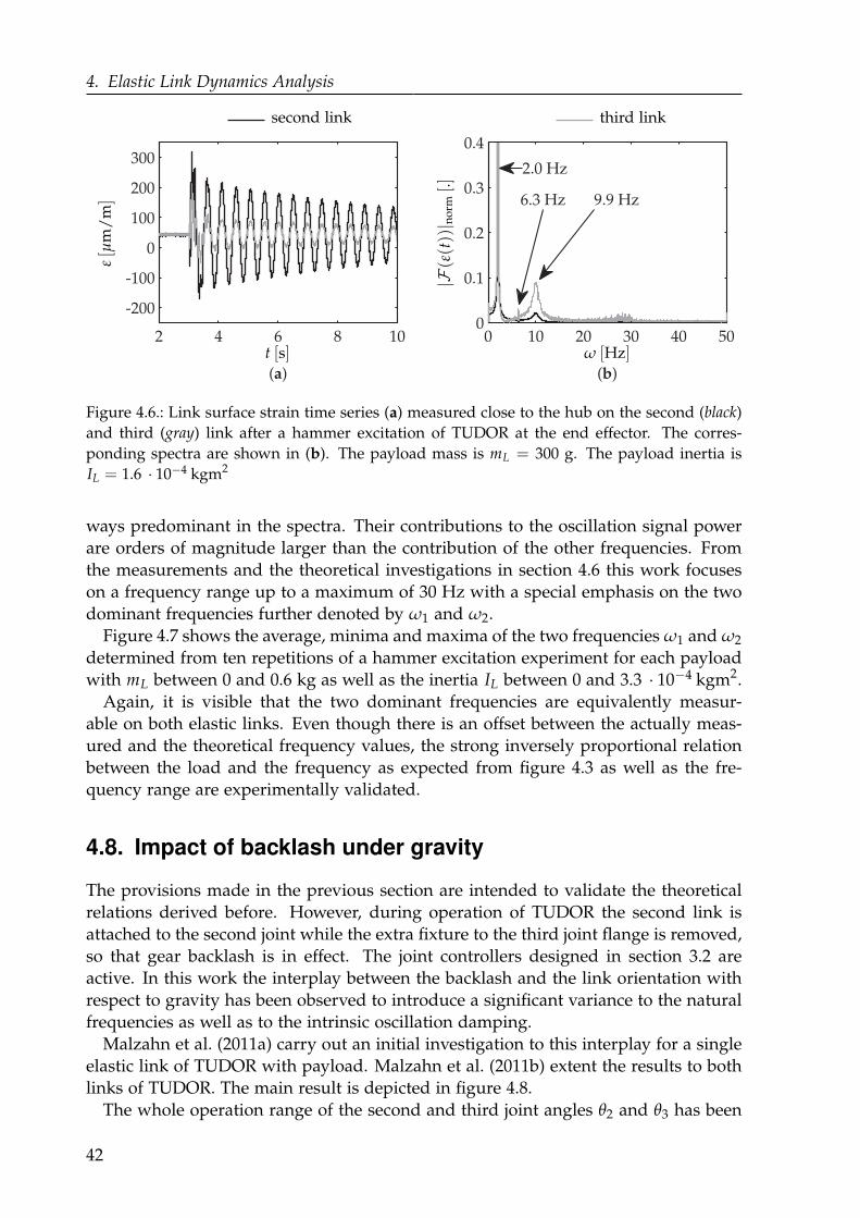
4. Elastic Link Dynamics Analysis
2 4 6 8 10
-200
-100
0
100
200
300
(a)
0 10 20 30 40 500
0.1
0.2
0.3
0.4
(b)
2.0 Hz
6.3 Hz 9.9 Hz
ε[µ
m/
m]
second link third link
|F(ε(t))| no
rm[.]
t [s] ω [Hz]
Figure 4.6.: Link surface strain time series (a) measured close to the hub on the second (black)
and third (gray) link after a hammer excitation of TUDOR at the end effector. The corres-
ponding spectra are shown in (b). The payload mass is mL = 300 g. The payload inertia is
IL = 1.6 · 10−4 kgm2
ways predominant in the spectra. Their contributions to the oscillation signal power
are orders of magnitude larger than the contribution of the other frequencies. From
the measurements and the theoretical investigations in section 4.6 this work focuses
on a frequency range up to a maximum of 30 Hz with a special emphasis on the two
dominant frequencies further denoted by ω1 and ω2.
Figure 4.7 shows the average, minima and maxima of the two frequencies ω1 and ω2
determined from ten repetitions of a hammer excitation experiment for each payload
with mL between 0 and 0.6 kg as well as the inertia IL between 0 and 3.3 · 10−4 kgm2.
Again, it is visible that the two dominant frequencies are equivalently measur-
able on both elastic links. Even though there is an offset between the actually meas-
ured and the theoretical frequency values, the strong inversely proportional relation
between the load and the frequency as expected from figure 4.3 as well as the fre-
quency range are experimentally validated.
4.8. Impact of backlash under gravity
The provisions made in the previous section are intended to validate the theoretical
relations derived before. However, during operation of TUDOR the second link is
attached to the second joint while the extra fixture to the third joint flange is removed,
so that gear backlash is in effect. The joint controllers designed in section 3.2 are
active. In this work the interplay between the backlash and the link orientation with
respect to gravity has been observed to introduce a significant variance to the natural
frequencies as well as to the intrinsic oscillation damping.
Malzahn et al. (2011a) carry out an initial investigation to this interplay for a single
elastic link of TUDOR with payload. Malzahn et al. (2011b) extent the results to both
links of TUDOR. The main result is depicted in figure 4.8.
The whole operation range of the second and third joint angles θ2 and θ3 has been
42
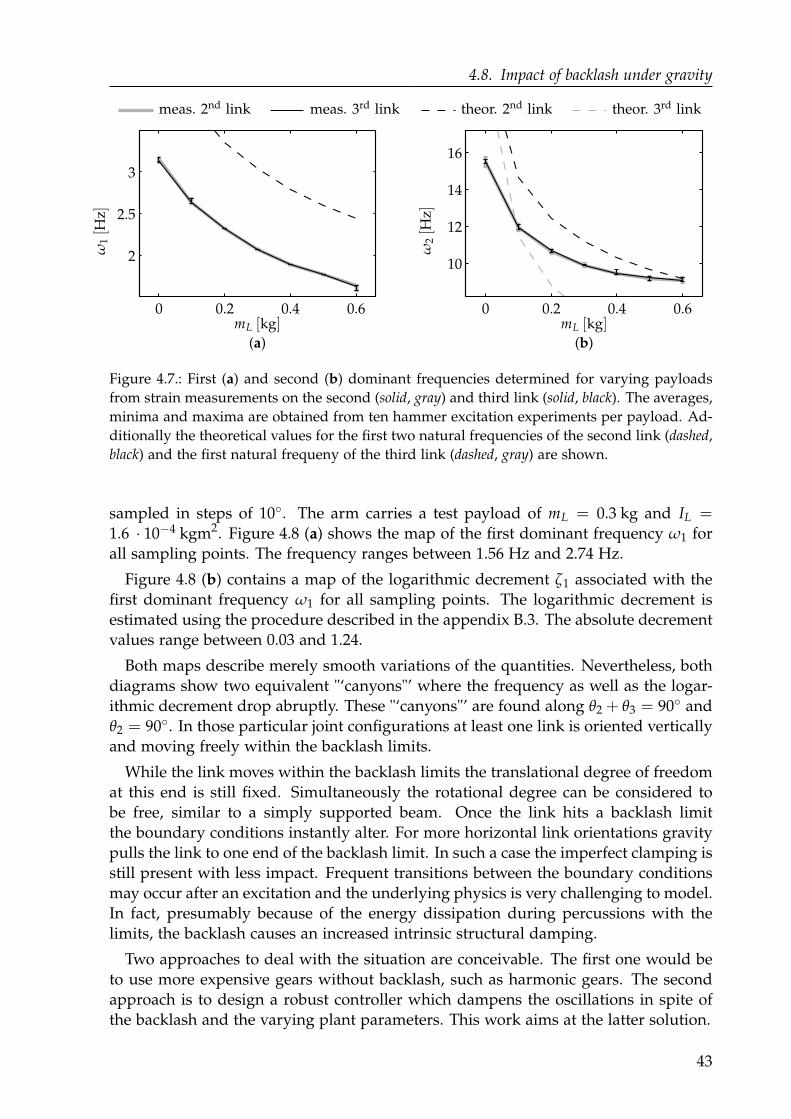
4.8. Impact of backlash under gravity
0 0.2 0.4 0.6
2
2.5
3
(a)
0 0.2 0.4 0.6
10
12
14
16
(b)
meas. 2nd link meas. 3rd link theor. 2nd link theor. 3rd linkω
1[H
z]
ω2[H
z]
mL [kg]mL [kg]
Figure 4.7.: First (a) and second (b) dominant frequencies determined for varying payloads
from strain measurements on the second (solid, gray) and third link (solid, black). The averages,
minima and maxima are obtained from ten hammer excitation experiments per payload. Ad-
ditionally the theoretical values for the first two natural frequencies of the second link (dashed,
black) and the first natural frequeny of the third link (dashed, gray) are shown.
sampled in steps of 10. The arm carries a test payload of mL = 0.3 kg and IL =1.6 · 10−4 kgm2. Figure 4.8 (a) shows the map of the first dominant frequency ω1 for
all sampling points. The frequency ranges between 1.56 Hz and 2.74 Hz.
Figure 4.8 (b) contains a map of the logarithmic decrement ζ1 associated with the
first dominant frequency ω1 for all sampling points. The logarithmic decrement is
estimated using the procedure described in the appendix B.3. The absolute decrement
values range between 0.03 and 1.24.
Both maps describe merely smooth variations of the quantities. Nevertheless, both
diagrams show two equivalent "‘canyons"’ where the frequency as well as the logar-
ithmic decrement drop abruptly. These "‘canyons"’ are found along θ2 + θ3 = 90 and
θ2 = 90. In those particular joint configurations at least one link is oriented vertically
and moving freely within the backlash limits.
While the link moves within the backlash limits the translational degree of freedom
at this end is still fixed. Simultaneously the rotational degree can be considered to
be free, similar to a simply supported beam. Once the link hits a backlash limit
the boundary conditions instantly alter. For more horizontal link orientations gravity
pulls the link to one end of the backlash limit. In such a case the imperfect clamping is
still present with less impact. Frequent transitions between the boundary conditions
may occur after an excitation and the underlying physics is very challenging to model.
In fact, presumably because of the energy dissipation during percussions with the
limits, the backlash causes an increased intrinsic structural damping.
Two approaches to deal with the situation are conceivable. The first one would be
to use more expensive gears without backlash, such as harmonic gears. The second
approach is to design a robust controller which dampens the oscillations in spite of
the backlash and the varying plant parameters. This work aims at the latter solution.
43
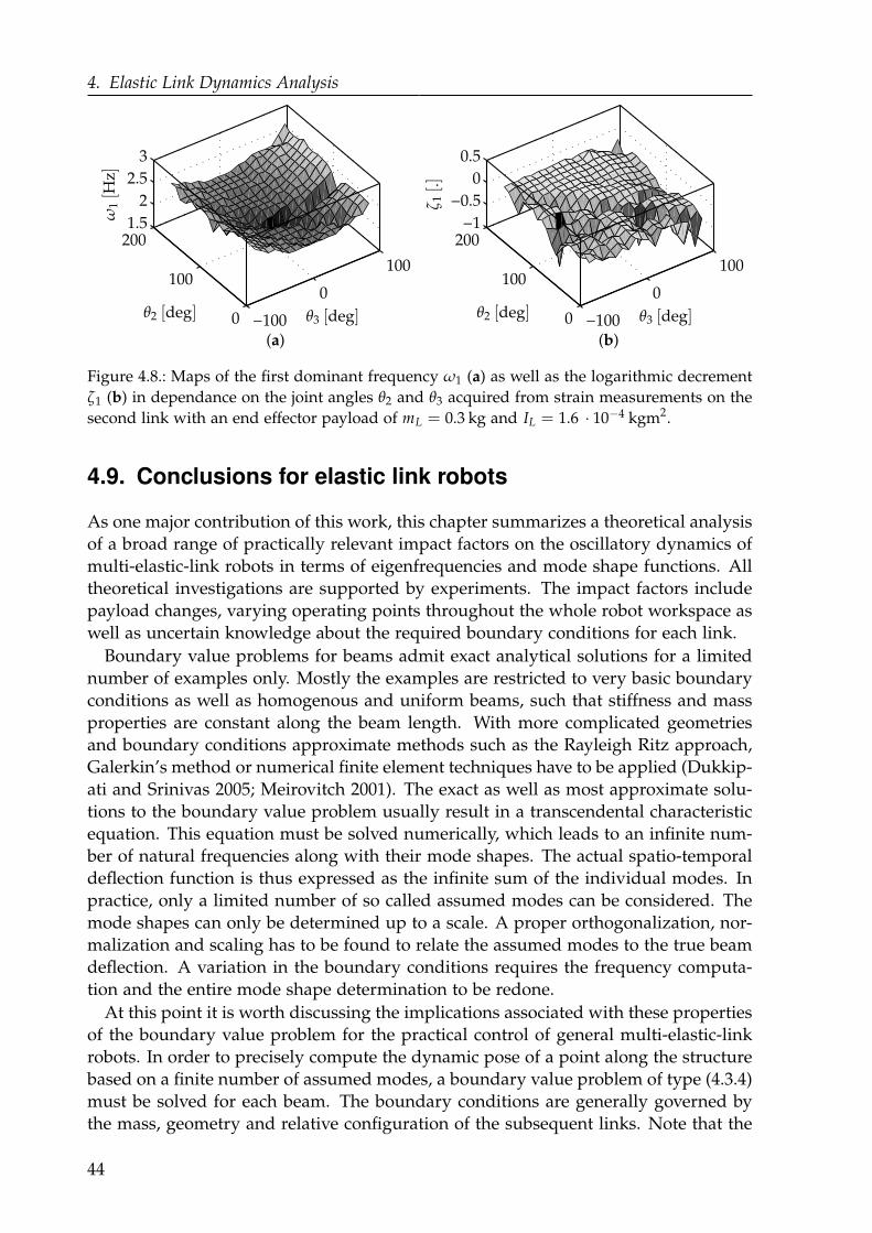
4. Elastic Link Dynamics Analysis
−100
0
100
0
100
2001.5
2
2.5
3
(a)−100
0
100
0
100
200−1
−0.5
0
0.5
(b)
θ3 [deg]θ2 [deg]
ω1[H
z]
θ3 [deg]θ2 [deg]
ζ 1[.]
Figure 4.8.: Maps of the first dominant frequency ω1 (a) as well as the logarithmic decrement
ζ1 (b) in dependance on the joint angles θ2 and θ3 acquired from strain measurements on the
second link with an end effector payload of mL = 0.3 kg and IL = 1.6 · 10−4 kgm2.
4.9. Conclusions for elastic link robots
As one major contribution of this work, this chapter summarizes a theoretical analysis
of a broad range of practically relevant impact factors on the oscillatory dynamics of
multi-elastic-link robots in terms of eigenfrequencies and mode shape functions. All
theoretical investigations are supported by experiments. The impact factors include
payload changes, varying operating points throughout the whole robot workspace as
well as uncertain knowledge about the required boundary conditions for each link.
Boundary value problems for beams admit exact analytical solutions for a limited
number of examples only. Mostly the examples are restricted to very basic boundary
conditions as well as homogenous and uniform beams, such that stiffness and mass
properties are constant along the beam length. With more complicated geometries
and boundary conditions approximate methods such as the Rayleigh Ritz approach,
Galerkin’s method or numerical finite element techniques have to be applied (Dukkip-
ati and Srinivas 2005; Meirovitch 2001). The exact as well as most approximate solu-
tions to the boundary value problem usually result in a transcendental characteristic
equation. This equation must be solved numerically, which leads to an infinite num-
ber of natural frequencies along with their mode shapes. The actual spatio-temporal
deflection function is thus expressed as the infinite sum of the individual modes. In
practice, only a limited number of so called assumed modes can be considered. The
mode shapes can only be determined up to a scale. A proper orthogonalization, nor-
malization and scaling has to be found to relate the assumed modes to the true beam
deflection. A variation in the boundary conditions requires the frequency computa-
tion and the entire mode shape determination to be redone.
At this point it is worth discussing the implications associated with these properties
of the boundary value problem for the practical control of general multi-elastic-link
robots. In order to precisely compute the dynamic pose of a point along the structure
based on a finite number of assumed modes, a boundary value problem of type (4.3.4)
must be solved for each beam. The boundary conditions are generally governed by
the mass, geometry and relative configuration of the subsequent links. Note that the
44
4.9. Conclusions for elastic link robots
inertia of all subsequent bodies have to be expressed with respect to the tip bending
axis using the parallel axis theorem. As also pointed out by Luca and Siciliano (1991),
the load inertia IL in general varies with the robot joint configuration. This way the
mode shape functions become a function of time, which contradicts equation (4.3.1).
Based on the knowledge of the joint values and under the assumption of compar-
ably slow changes or piecewise constant boundary conditions, an idea could be to
recompute the natural frequencies online. This process is computationally involved
and difficult to implement under the hard real-time constraints required for control.
Alternatively a direct mapping from the joint configuration to the natural frequen-
cies and mode shapes in the sense of figure 4.8 would be conceivable. However, this
approach is limited to inspection robots. If the elastic link robot is intended to per-
form manipulation tasks, such as Pick-and-Place, the varying and possibly a priori
unknown payload mass and payload inertia may significantly influence the boundary
conditions on each link. During physical contact with the environment or physical
human robot interaction the impedance of the contact point may impose arbitrary
unknown boundary conditions to the robot.
The uncertainties in the boundary conditions lead to poorly calibrated orthogonal-
ity relations. This renders the model based decoupling of modes infeasible. A con-
troller based on a finite order model at runtime is likely to excite the wrong modeled
or even unmodeled oscillations modes. Similarly, observers suffer from the poor de-
coupling of the individual modes and most probably provide insufficient estimates.
This effect is called modal spillover and is illustrated in more detail for example by
Vepa (2010, p. 338).
Under the painted circumstances and constraints it seems questionable whether it
is practically feasible to realize a stabilizing centralized controller for a multi-elastic-
link robot that dampens structural oscillations and precisely positions the end effector
based on a single holistic plant model including payloads and contact boundary con-
ditions.
Against this background it seems more convenient to follow a divide-and-conquer
strategy. First a decentralized controller modifies the system dynamics of each indi-
vidual link to virtually increase the apparent link damping in a wide frequency range.
Such controllers are proposed in chapters 5 to 7. They are set free from the actual end
effector positioning task and attenuate oscillations originating from the joint motions
as well as external excitations and a variety of boundary conditions. On top of that an
outer end effector control loop such as the ones presented in chapter 9, minimizes the
pose error in the presence of joint configuration and load dependent static deflections
due to gravity. Both controller stages ensure nominal plant dynamics. Deviations
from this nominal dynamics are exploited in order to investigate the potentials of
elastic link robots for planned as well as accidental physical contacts between the
robot and the environment as proposed in chapter 11.
45
5Proportional Oscillation Feedback
This is the first out of four subsequent chapters devoted to oscillation damping con-
trol. The oscillation damping control concept proposed here is based on a straightfor-
ward extension of the modal analysis presented in the previous chapter. The physical
relations are converted into a truncated series of transfer functions superposed by a
nonlinear static component.
5.1. Link transfer function model
Motivated by the workspace sampling results illustrated in figure 4.8 the parameters
of the truncated transfer function model vary but are considered to be quasi static
for a given joint configuration θ0. The model structure together with the parameter
range paves the way for the synthesis of the decentralized linear oscillation feedback
controller in section 5.2. Malzahn et al. (2011b) provide an initial derivation of the
model structure. Nevertheless, a more elaborate derivation is given in the following.
Modal parameters
From the results in section 4.7 it is known that the oscillations of each individual
link can be perceived on the other links in the chain under preservation of phase
alignment. Therefore the whole arm structure is interpreted as a chain of joint-link-
modules. Each joint-link-module virtually possesses all perceivable oscillation modes
as if they were actually obtained as solutions of the modal analysis for the particular
link.
The module consists of a series connection of the joint transfer function (3.1.7) and
a nonlinear transfer function capturing the oscillatory dynamics for the connected vir-
tual elastic link. Due to the high gear ratios a feedback from the elastic link dynamics
to the joint model can be assumed to be inconsequentially small. The joint-link-
modules are therefore treated independently.
The nonlinear elastic link transfer function model has the joint angle θ as input and
the strain measured close to the hub as output. Consider the beam partial differential
equation (4.2.8) augmented by the effects of viscous and mass proportional damping
effects summarized in the damping coefficient kd:
EIz∂4 y(x, t)
∂x4+ kd
∂
∂ty(x, t) + ρb
∂2 y(x, t)
∂t2= fext(x, t). (5.1.1)
46
5.1. Link transfer function model
For simplicity of derivation but without loss of generality the elastic link is assumed
to be rigidly clamped at the hub with quasi static load mass and load inertia as
discussed in section 4.4.
Equation (5.1.1) is multiplied by a particular shape function Φu and integrated over
the link length:
∫ L
0Φu(x) EIz
∂4 y(x, t)
∂x4dx +
∫ L
0Φu(x) kd
∂
∂ty(x, t)dx + . . .
+∫ L
0Φu(x) ρb
∂2 y(x, t)
∂t2dx =
∫ L
0Φu(x) fext(x, t)dx. (5.1.2)
Using the series expansion derived in the appendix B.3 the solution y(x, t) has the
form:
y(x, t) =∞
∑u=1
Φu(x) νu(t). (5.1.3)
Exploiting the orthonormality of modes enables the definition of so called modal
parameters from the individual summands of equation (5.1.2). The first summand
yields the modal stiffness cu:
cu =∫ L
0Φu(x) EIz
∂4 Φu(x)
∂x4dx, (5.1.4)
the second summand is the modal damping du:
du =∫ L
0Φu(x) kd Φu(x)dx, (5.1.5)
the third summand is the modal mass mu:
mu =∫ L
0Φu(x) ρbΦu(x)dx (5.1.6)
and the modal force fu computes to:
fu =∫ L
0Φu(x) fext(x, t)dx. (5.1.7)
With the modal parameters the partial differential equation (5.1.1) transforms to a set
of independent modal ordinary differential equations:
mud2νu(t)
dt2+ du
dνu(t)
dt+ cu νu(t) = fu(t). (5.1.8)
In analogy to equation (5.1.3) the strain measured at a sensor location xs can be
written as:
ε(xs, t) = yb
∞
∑u=1
d2
dx2Φu(x)|xs
νu(t), (5.1.9)
with
εu(xs, t) = ybd2
dx2Φu(x)|xs
νu(t), (5.1.10)
47
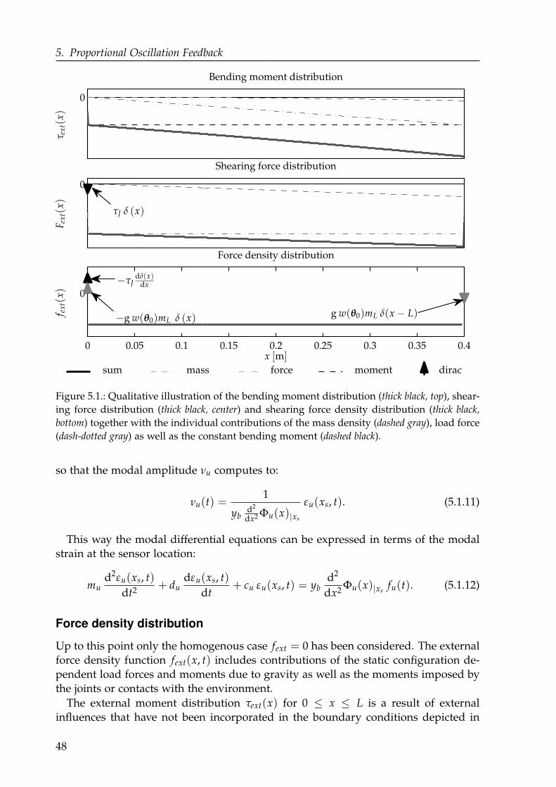
5. Proportional Oscillation Feedback
0 0.05 0.1 0.15 0.2 0.25 0.3 0.35 0.4
0
Force density distribution
0
Shearing force distribution
0
Bending moment distribution
diracsum mass force moment
x [m]
τ ex
t(x)
F ex
t(x)
f ex
t(x)
g w(θ0)mL δ(x − L)−g w(θ0)mL δ (x)
−τJdδ(x)
dx
τJ δ (x)
Figure 5.1.: Qualitative illustration of the bending moment distribution (thick black, top), shear-
ing force distribution (thick black, center) and shearing force density distribution (thick black,
bottom) together with the individual contributions of the mass density (dashed gray), load force
(dash-dotted gray) as well as the constant bending moment (dashed black).
so that the modal amplitude νu computes to:
νu(t) =1
ybd2
dx2 Φu(x)|xs
εu(xs, t). (5.1.11)
This way the modal differential equations can be expressed in terms of the modal
strain at the sensor location:
mud2εu(xs, t)
dt2+ du
dεu(xs, t)
dt+ cu εu(xs, t) = yb
d2
dx2Φu(x)|xs
fu(t). (5.1.12)
Force density distribution
Up to this point only the homogenous case fext = 0 has been considered. The external
force density function fext(x, t) includes contributions of the static configuration de-
pendent load forces and moments due to gravity as well as the moments imposed by
the joints or contacts with the environment.
The external moment distribution τext(x) for 0 ≤ x ≤ L is a result of external
influences that have not been incorporated in the boundary conditions depicted in
48

5.1. Link transfer function model
figure 4.2. By inspection of the figure the distribution can be written as the balance
about the joint axis:
τext(x) = (τM + τL (θ0)) H (x) + . . .
+ g w(θ0)
(
ρbx2
2− mL (x − L) H(x − L) + x mL H (x)
)
. (5.1.13)
The resulting distribution is shown in the top of figure 5.1. The weight function w(θ0)scales the gravitational acceleration g according to the link unit x-direction ex with
respect to the gravitational acceleration vector ag. The gravitational load moment
τL(θ0) scales analogously with the joint configuration.
The function H(x) is the Heaviside function. It approximates the domain restric-
tions and enables the application of distribution theory to compute the derivatives of
τext. The first derivative yields the force distribution Fext(x) as depicted in the center
of figure 5.1:
Fext(x) = (τM + τL (θ0)) δ (x) + g w(θ0) ( ρb x + mL (H (x)− H (x − L))) , (5.1.14)
where δ(x − xg) denotes the Dirac distribution. The second derivative yields the force
density distribution fext(x) shown in the bottom of figure 5.1:
fext(x) = (τM + τL (θ0))dδ (x)
dx+ gw(θ0) (ρb + mL (δ (x)− δ (x − L))) . (5.1.15)
The mechanical torque τM provided by the joint can be replaced by:
τM(t) = IM θ(t). (5.1.16)
Transfer function
Equation (5.1.14) can be split into a static and a dynamic part. At a sensor location
xs the first part including the load mass mL, the load moment τL as well as the mass
per unit length ρb constitutes the static part for a given joint configuration θ0. The
dynamic part depends on the joint acceleration θ(t).With this insight the combination of the modal strain differential equation (5.1.12)
and the modal force equation (5.1.7) yields the modal transfer function after Laplace
transformation for vanishing initial conditions:
εu(xs, s) =kdyn,u s2
s2 + 2Duωu s + ω2u
θ(s) +kstat,u(θ0)
s2 + 2Duωu s + ω2u
, (5.1.17)
where the dynamic modal gain kdyn,u is:
kdyn,u =yb
mu
d2
dx2Φu(x)|xs
IM
∫ L
0Φu(x) δ(x)dx (5.1.18)
and the static modal gain kstat,u computes to:
kstat,u(θ0) =yb
mu
d2
dx2Φu(x)|xs
∫ L
0Φu(x)
(
τL (θ0)dδ (x)
dx+ . . .
+ gw(θ0)
(
ρb + mL
(
δ (x)− δ (x − L))
)
)
dx. (5.1.19)
49
5. Proportional Oscillation Feedback
The attenuation factor Du is related to the logarithmic decrement ζu as well as the
modal damping du and mass mu properties:
Duωu =1
2
du
mu= −ζu. (5.1.20)
From the equations (5.1.4) and (5.1.6) along with equation (4.3.2) it can be verified that
the frequency ωu replaces the modal mass and stiffness according to:
ωu =
√
cu
mu. (5.1.21)
Finally, with equation (5.1.9) the total beam transfer function can be written in the
form:
ε(xs, s) = θ(s) s2nω
∑u=1
kdyn,u
s2 + 2Duωu s + ω2u+
nω
∑u=1
kstat,u(θ0)
s2 + 2Duωu s + ω2u
. (5.1.22)
The dimension of this transfer function is theoretically infinite. Practically only a finite
number nω of oscillation modes can be taken into account for the controller synthesis
and analysis.
Provided that the configuration dependent static strains εstat can be removed by
appropriate filtering, the remaining dynamic strain transfer function GB(s) is charac-
terized by:
GB(xs, s) =εdyn(xs, s)
θ(s)= s2
nω
∑u=1
kdyn,u
s2 + 2Duωu s + ω2u
. (5.1.23)
This transfer function model serves as a basis for the synthesis of the controller
described in the next section.
5.2. Controller synthesis
The assumption of a perfect static strain cancellation renders the remaining plant
dynamics entirely linear. Thus, the Evans root locus may be used to design a pro-
portional strain feedback for the series connection of the cascaded joint controller
and remaining beam transfer function (5.1.23). Motivated by the observations in sec-
tion 4.7 the beam model GB(s) in the root locus analysis combines the predominant
eigenfrequencies of all links together. This way the controller is designed to also damp
the oscillations due to inter-link couplings.
The proportional strain feedback discussed here is strongly related to the work
reported by Luo (1993); Luo and Guo (1995). The authors introduce the concept of
so called A-dependent operators to proof the stability of a proportional as well as
integral strain feedback for a single link in the horizontal plane. In their experiments
the joint angle is left uncontrolled in the first place. In a second step it is controlled by
a single loop PID controller with the actuator input voltage as set value. In contrast to
that, this work operates with a multi-link arm under gravity and chooses the extended
cascaded joint controller from section 3.2 complemented by the jerk minimizing online
trajectory planner provided in appendix B.6. The set value is the amplifier voltage
proportional to the actuator electrical current.
50
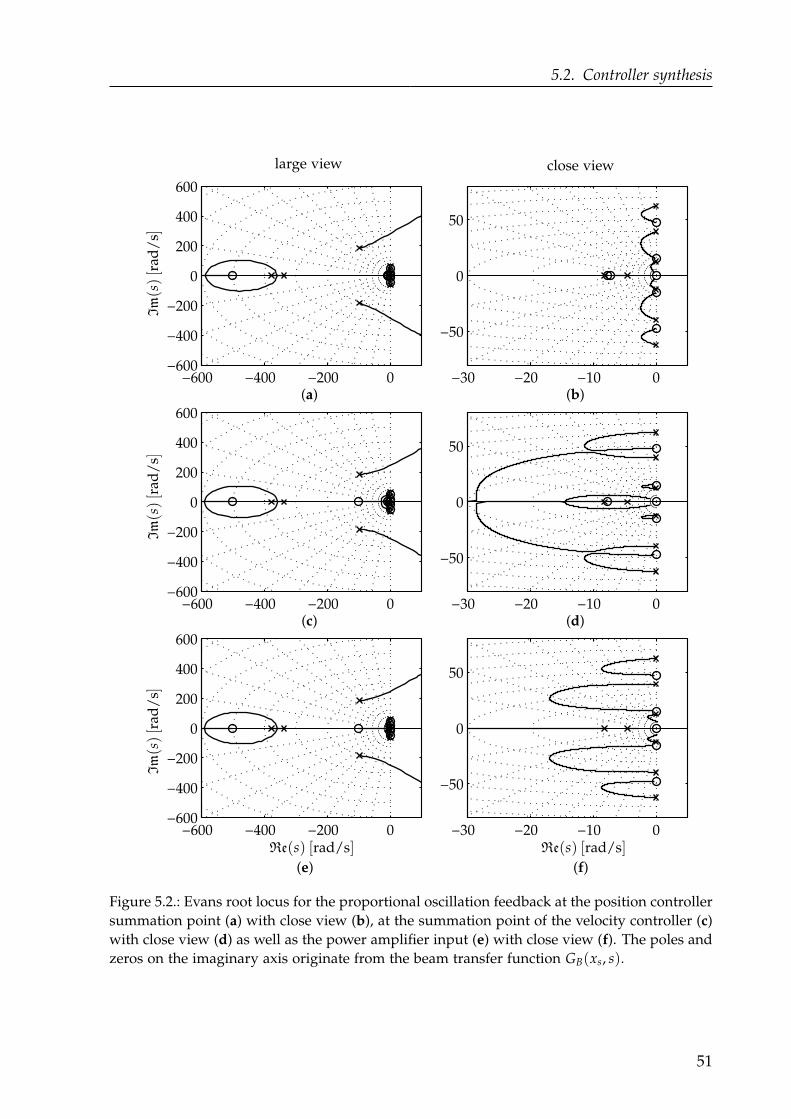
5.2. Controller synthesis
−600 −400 −200 0−600
−400
−200
0
200
400
600
(a)
−30 −20 −10 0
−50
0
50
(b)
−600 −400 −200 0−600
−400
−200
0
200
400
600
(c)
−30 −20 −10 0
−50
0
50
(d)
−600 −400 −200 0−600
−400
−200
0
200
400
600
(e)
−30 −20 −10 0
−50
0
50
(f)
Im(s)[r
ad/
s]Im(s)[r
ad/
s]Im(s)[r
ad/
s]
Re(s) [rad/s]Re(s) [rad/s]
large view close view
Figure 5.2.: Evans root locus for the proportional oscillation feedback at the position controller
summation point (a) with close view (b), at the summation point of the velocity controller (c)
with close view (d) as well as the power amplifier input (e) with close view (f). The poles and
zeros on the imaginary axis originate from the beam transfer function GB(xs, s).
51
5. Proportional Oscillation Feedback
In this chapter, the proportional strain feedback is considered. The integral feedback
is discussed within the scope of chapter 6.
The cascaded structure enables the investigation of the three different feedback
insertion points indicated in figure 3.3: at the position controller input, velocity con-
troller input and at the amplifier voltage input. Figure 5.2 exemplifies the root locus
computed from each of the insertion points to the strain output. The left column
depicts overviews of the whole root locus, while the right column provides the cor-
responding close-ups to the complex pole and zero pairs on the imaginary axis. They
originate from the flexible beam transfer function (5.1.23).
For the feedback insertion point at the position controller input (see figure 5.2 (b)),
the flexible beam poles reside in the stable left-half plane. However, they show poor
damping while approaching the origin of the complex s-plane.
For the feedback insertion point at the velocity controller input (see figure 5.2 (d))
the beam poles move to the left and one pole pair finally joins the real axis. This way,
with increasing feedback gain, we observe a slightly decreasing dominant frequency
and a significantly improving damping.
The insertion point at the voltage input (see figure 5.2 (f)) shows a similar behaviour
compared to the insertion point at the velocity input. However, the lowest beam
eigenfrequency rapidly approaches the origin of the complex s-plane. The path of
this pole pair leads through regions of poor damping.
In summary the insertion point at the velocity controller is most advantageous in
terms of achievable shift of the elastic link poles towards regions of higher damping
in the complex s-plane. The control law is:
θε = −kε ε(xs, t). (5.2.1)
In all three overview plots (left column of figure 5.2) it is visible that a complex
pole pair tends to the right half of the complex s-plane with increasing feedback gain.
This pole pair originates from the PD position controller. The strain feedback gain
is therefore upper bounded to preserve closed loop stability. Nevertheless, the pole
pair possesses a higher eigenfrequency and experiences additional damping due to
the low-pass characteristics of the remaining plant poles. Moreover, it shapes the root
locus of the considered elastic link pole pairs and keeps them in the left half plane.
The critical drawback behind the presented controller synthesis arises from the re-
striction to a finite number of oscillatory modes. As already mentioned in section 1.2,
there exists no technique that guarantees stability with respect to the neglected eigen-
frequencies.
The closed loop dynamics including the elastic link poles could be more generally
influenced with full state feedback control. However, a practically important merit of
the control concept is the simplicity of tuning.
Changes in the plant parameters as observed in figure 4.8 marginally distort the
root locus but the general root locus geometry does not alter for a broad range of
parameter variations. For a more tangible explanation of this fact, consider the already
small natural damping to be negligible. In this case, the complex poles and zeros
belonging to the beam transfer function are exactly located on the imaginary axis.
A variation to the natural frequencies due to payload changes, physical contacts or
altered joint configurations results in a vertical scaling of the root locus only. Increased
52
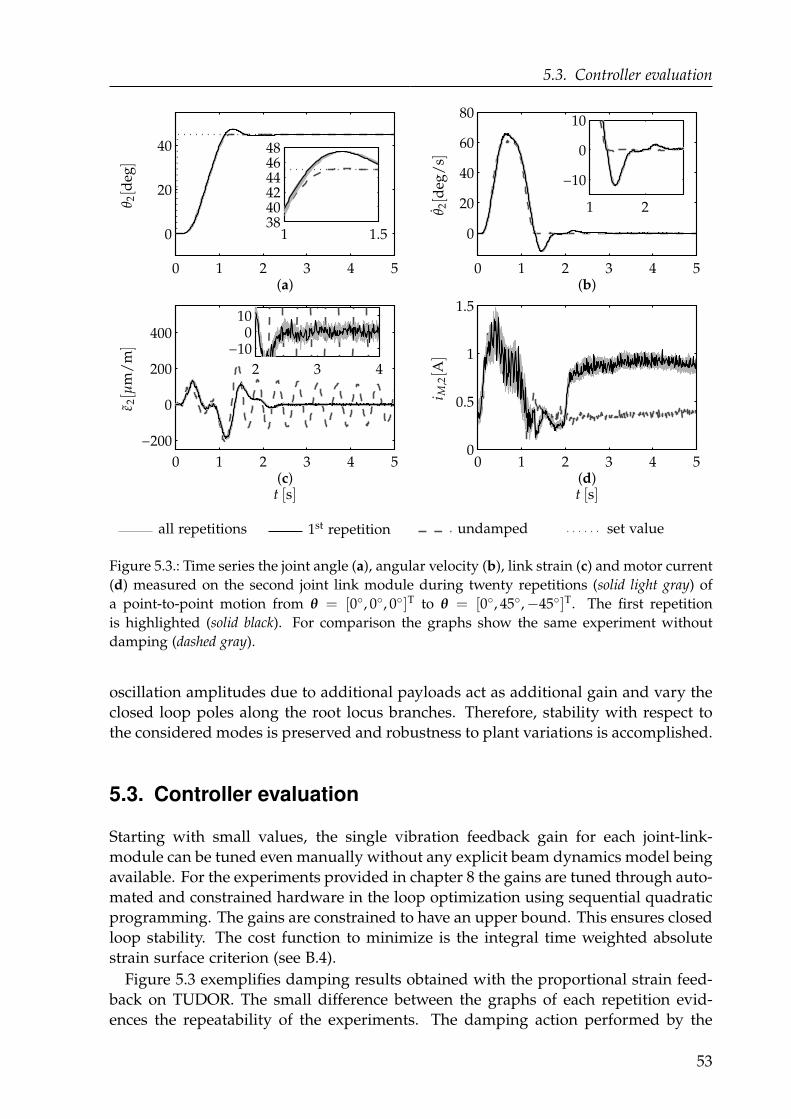
5.3. Controller evaluation
0 1 2 3 4 5
0
20
40
(a)0 1 2 3 4 5
0
20
40
60
80
(b)
0 1 2 3 4 5
−200
0
200
400
(c)0 1 2 3 4 5
0
0.5
1
1.5
(d)
1 1.5384042444648
1 2
−10
0
10
2 3 4
−100
10
θ 2[d
eg]
θ 2[d
eg/
s]
ε 2[µ
m/
m]
i M,2[A
]
t [s]t [s]
all repetitions 1st repetition undamped set value
Figure 5.3.: Time series the joint angle (a), angular velocity (b), link strain (c) and motor current
(d) measured on the second joint link module during twenty repetitions (solid light gray) of
a point-to-point motion from θ = [0, 0, 0]T to θ = [0, 45,−45]T. The first repetition
is highlighted (solid black). For comparison the graphs show the same experiment without
damping (dashed gray).
oscillation amplitudes due to additional payloads act as additional gain and vary the
closed loop poles along the root locus branches. Therefore, stability with respect to
the considered modes is preserved and robustness to plant variations is accomplished.
5.3. Controller evaluation
Starting with small values, the single vibration feedback gain for each joint-link-
module can be tuned even manually without any explicit beam dynamics model being
available. For the experiments provided in chapter 8 the gains are tuned through auto-
mated and constrained hardware in the loop optimization using sequential quadratic
programming. The gains are constrained to have an upper bound. This ensures closed
loop stability. The cost function to minimize is the integral time weighted absolute
strain surface criterion (see B.4).
Figure 5.3 exemplifies damping results obtained with the proportional strain feed-
back on TUDOR. The small difference between the graphs of each repetition evid-
ences the repeatability of the experiments. The damping action performed by the
53

5. Proportional Oscillation Feedback
actuator can be seen in the overshoot of the angular response, which is absent in the
undamped case. Similarly, Figure 5.3 (b) illustrates the damping action as a brief
motion reversal right before the deflections vanish. The accomplished rapid damping
is clearly visible in the strain measurements 5.3 (c). Malzahn and Bertram (2013, at
0:36 min) provide an online available video comprising oscillation damping results
with the proportional strain feedback at the velocity cascade level.
54
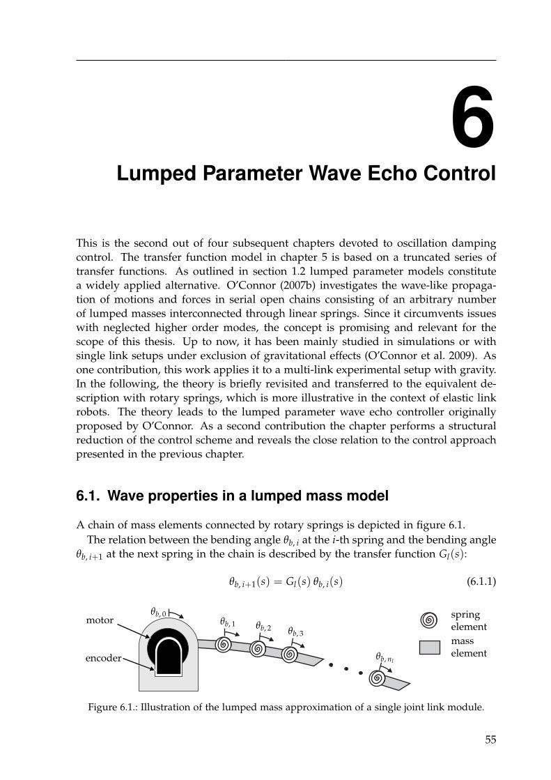
6Lumped Parameter Wave Echo Control
This is the second out of four subsequent chapters devoted to oscillation damping
control. The transfer function model in chapter 5 is based on a truncated series of
transfer functions. As outlined in section 1.2 lumped parameter models constitute
a widely applied alternative. O’Connor (2007b) investigates the wave-like propaga-
tion of motions and forces in serial open chains consisting of an arbitrary number
of lumped masses interconnected through linear springs. Since it circumvents issues
with neglected higher order modes, the concept is promising and relevant for the
scope of this thesis. Up to now, it has been mainly studied in simulations or with
single link setups under exclusion of gravitational effects (O’Connor et al. 2009). As
one contribution, this work applies it to a multi-link experimental setup with gravity.
In the following, the theory is briefly revisited and transferred to the equivalent de-
scription with rotary springs, which is more illustrative in the context of elastic link
robots. The theory leads to the lumped parameter wave echo controller originally
proposed by O’Connor. As a second contribution the chapter performs a structural
reduction of the control scheme and reveals the close relation to the control approach
presented in the previous chapter.
6.1. Wave properties in a lumped mass model
A chain of mass elements connected by rotary springs is depicted in figure 6.1.
The relation between the bending angle θb, i at the i-th spring and the bending angle
θb, i+1 at the next spring in the chain is described by the transfer function Gl(s):
θb, i+1(s) = Gl(s) θb, i(s) (6.1.1)
motor
encoder
springelement
masselement
θb, 0θb, 1 θb, 2 θb, 3
θb, nl
Figure 6.1.: Illustration of the lumped mass approximation of a single joint link module.
55
6. Lumped Parameter Wave Echo Control
and consequently:
θb, i+nl= G
nll θb, i, (6.1.2)
where nl is the integer number of lumped masses considered.
The equation of motion for a lumped spring mass system is characterized by the
lumped inertia Il and a spring stiffness kl:
Il θb, i(t) = kl (θb, i−1(t)− 2 θb, i(t) + θb, i+1(t)), (6.1.3)
which after Laplace transformation and rearrangement yields the quadratic equation
in Gl(s):
G2l (s)−
(
2 +s2
ω2l
)
Gl(s) + 1 = 0, (6.1.4)
where ωl =√
klIl
. The quadratic equation has the two solutions +Gl(s) and −Gl(s):
+Gl(s) = 1 +1
2(s/ωl)
2 − (s/ωl)
√
1 + (s/2ωl)2 , (6.1.5)
−Gl(s) = 1 +1
2(s/ωl)
2 + (s/ωl)
√
1 + (s/2ωl)2 . (6.1.6)
Note, that the first solution (6.1.5) is causal, while the other one (6.1.6) shows an
acausal phase lead. A closer look reveals two symmetries between both solutions.
The first one is a spatial symmetry mathematically expressed by the inverse:
+Gl(s) =−G−1
l (s), −Gl(s) =+G−1
l (s) , (6.1.7)
meaning that the elastic dynamics are reciprocal. The second symmetry is temporal:
+Gl(−s) = −Gl(s),−Gl(−s) = +Gl(s). (6.1.8)
The combination of both symmetries leads to:
+Gl(s) =+G−1
l (−s), −Gl(s) =−G−1
l (−s) , (6.1.9)
which gives the physical interpretation of the acausality in the transfer functions from
the perspective of propagating motion waves. Looking from the left towards the right
end of the beam a motion propagating along the structure in the viewing direction
at finite speed appears causal. An observed acausal bending motion propagates in
the opposite direction and must have been initiated at a distal location previously in
time. Consequently the bending angle θb, i of an i-th spring-beam-element consists of
two components:
θb, i(s) =+Gl(s) C1, i(s) +
−Gl(s) C2, i(s) , (6.1.10)
with the functions C1, i(s) and C2, i(s) to be further specified, while the motion wave
caused by a source on the left side of the link and propagating rightwards within the
structure is given as +θb, i(s) =+Gl(s)C1, i(s). Vice versa −θb, i(s) =
−Gl(s)C2, i(s) cor-
responds to the motion wave propagating leftwards within the structure, originating
from the right side of the link, so that:
θb, i(s) =+θb, i(s) +
−θb, i(s) . (6.1.11)
56
6.2. Wave absorption
This superposition relation analogously exists for the velocity as well as bending mo-
ment propagation in the lumped structure:
θb, i =+ ˇθb, i +
− ˇθb, i , (6.1.12)
τb, i =+τb, i +
−τb, i . (6.1.13)
Exploiting the reciprocity relation (6.1.7) enables the simplified notation +Gl(s) =−G−1
l (s) = Gl(s), where only the causal transfer function is used in different direc-
tions of propagation. This defines C1, i(s) and C2, i(s) in (6.1.10) as:
C1, i(s) =+θb, i−1(s) and C2, i(s) =
−θb, i+1(s) , (6.1.14)
which yields:
θb, i(s) = Gl(s)+θb, i−1(s) + Gl(s)
−θb, i+1(s) , (6.1.15)
or equivalently:
θb, i(s) = Gl(s)+θb, i−1(s) + G−1
l (s) −θb, i−1(s) . (6.1.16)
O’Connor (2007b) calls Gl(s) the wave transfer function (WTF).
6.2. Wave absorption
The wave echo control concept described in the following goes back to a series of
papers by O’Connor (O’Connor 2007a,b; O’Connor and Donogh 1998; O’Connor et
al. 2009). Even though the synthesis is based on the discrete representation of the
elastic link provided in section 6.1, the controller derived with the gained insights
finally waives the need for an online computation of a truncated or discretized plant
dynamics model. It focuses on measurements at the interface between the actuation
mechanism and the elastic structure.
Given a point-to-point motion task with goal θw, the idea behind the wave echo
controller is to launch a motion wave of +θb, 0 and then to absorb the echoed wave
component −θb, 0 to damp the induced oscillations. The question now is, what wave
amplitude +θb, 0 the actuator should launch in order to precisely arrive at the de-
sired goal with all oscillations being completely attenuated. To answer this question,
O’Connor (2007a) assumes free boundary conditions at the link end opposite to the
actuator. At the "free end" he provides an intuition for a total reflection of the incom-
ing wave component +θnlby introduction of virtual masses beyond the n-th mass,
which mirror the physical plant. The wave echo −θnlis equal to the incoming wave,
but propagating in the opposite direction. Once the wave echo arrives at the actuator,
the unit gain of the transfer function Gl(s) leads to +θb,0 = −θb,0 at steady state. The
actuator should thus launch the wave component +θb, 0 = 12 θw. This way the actuator
is commanded to move half the desired distance. The wave echo −θb,0 coming back to
the actuator is computed by means of equation (6.3.5) and added to the commanded
value. Ideal joint position controller dynamics assumed, the actuator absorbs the wave
echo and arrives at the goal without residual oscillations.
57

6. Lumped Parameter Wave Echo Control
6.3. Wave component separation
Equally to the continuous wave variables, the left- and rightwards propagating wave
components in (6.1.11) to (6.1.13) cannot be measured directly. To implement the wave
echo controller it is required to extract them from physical measurements.
Consider a bending wave +θb, 0(s) being launched by the actuator (i = 0) according
to:+θb, 0(s) = θb, 0(s)− −θb, 0(s). (6.3.1)
The motion of the neighboring mass element with i = 1 computes to:
θb, 1 = +θb, 1(s) +−θb, 1(s) = Gl(s)
+θb, 0(s) + G−1l (s)−θb, 0(s), (6.3.2)
which is rearranged to obtain the echo −θb, 0(s) to the launched wave +θb, 0(s):
−θb, 0(s) = Gl(s)(
θb, 1 − Gl(s)+θb, 0(s)
)
. (6.3.3)
The result eliminates −θb, 0(s) in equation (6.3.1):
+θb, 0(s) =θb, 0(s)− Gl(s) θb, 1
1 − G2l (s)
, (6.3.4)
which is the separated rightwards propagating wave component expressed in the
physically measurable variables θb, 0 and θb, 1 at the actuator-link-interface. The echoed
wave motion −θb, 0 is obtained analogously by plugging result (6.3.4) back into equa-
tion (6.3.3):
−θb, 0(s) = Glθb, 1(s)− Gl(s) θb, 0
1 − G2l (s)
. (6.3.5)
The required physical measurements are the motor angle θb,0 as well as the angle of
a first spring element θb,1. It is one measurement on each side of the interface between
the actuator and the elastic structure. With both measurements the launched wave
component +θb, 0 as well as the echoed wave component −θb, 0 can be reconstructed at
any time instant using relations (6.3.4) and (6.3.5).
However, the exact WTFs obtained as the solutions of 6.1.4 are hard to implement
for real-time control. It is not rational and has fractional order. O’Connor (2007b)
discusses different approximations such as "a combination of Bessel functions" or the
"convolution with a suitably truncated impulse response" but finally applies the linear
underdamped second order transfer function:
Gl(s) ≈ω2
l
s2 + ωl s + ω2l
. (6.3.6)
6.4. Lumped wave impedance
Using the approximation (6.3.6) to the WTF, O’Connor et al. (2009) observe a steady
state error arising during fast point-to-point motions in experimental results with
a single link setup under exclusion of gravitational influence. The authors discuss
58
6.5. Controller reduction
different alternatives to alleviate the steady state error for this particular scenario.
They arrive at the reconstruction of the returning wave component at the actuator
from joint angle and link bending torque measurements to be the best solution. Again,
this is one physical measurement on each side of the interface between the actuator
and the elastic structure. They define a wave impedance Zw such that:
θb, i =τb, i
Zw(6.4.1)
and
θb, i =+τb, i
Zw−
−τb, i
Zw. (6.4.2)
The negative sign in equation (6.4.2) can be understood from the convention that the
rightwards propagating angular bending velocity is counted positively, while the left-
wards propagating angular bending velocity is counted negatively. This also aggrees
with the propagating wave amplitudes in the continuous case, as seen from the matrix
elements in equation (7.1.5). With this definition it can be verified from (6.1.13) and
addition that:+τb, i =
1
2
(
τb, i + θb, i Zw
)
(6.4.3)
and symmetrically
−τb, i =1
2
(
τb, i − θb, i Zw
)
. (6.4.4)
Similarly equation (6.1.12) yields:
+ ˇθb, i =1
2
(
τb, i
Zw+ θb, i
)
, (6.4.5)
while:− ˇθb, i =
1
2
(
τb, i
Zw− θb, i
)
. (6.4.6)
The echoed angular wave component is then obtained from (6.4.6) after integration:
−θb, 0(t) =1
2
(
θb, 0(t)−∫
τb, 1(t)
Zwdt
)
. (6.4.7)
6.5. Controller reduction
For control, the bending moment τb, 1 is replaced by the mean liberated strain meas-
urements ε close to the joint hub using equation (4.2.2), so that in the Laplace domain
the approximation of the echoed wave component used as feedback θε becomes:
θε(s) =−θb, 0(s) =
1
2
(
θ(s)− kε
sε(xs, s)
)
, (6.5.1)
where the gain kε computes to:
kε = − EIz
yb Zw. (6.5.2)
59
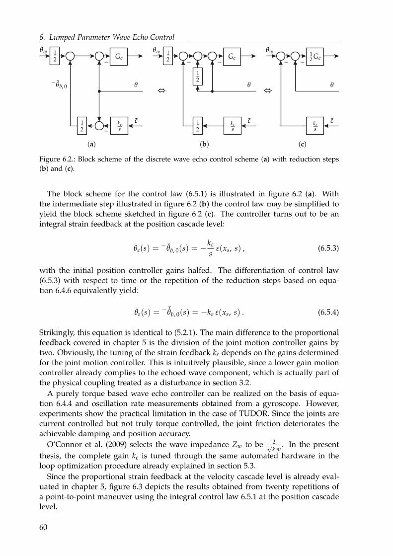
6. Lumped Parameter Wave Echo Control
12_
_ _
12_
12_
12_
_
_
12_
( )a ( )b ( )c
_ _θwθw θw
θθ θ− θb, 0
εε ε kεs
kεs
kεs
Gc Gc12 Gc
⇔⇔
Figure 6.2.: Block scheme of the discrete wave echo control scheme (a) with reduction steps
(b) and (c).
The block scheme for the control law (6.5.1) is illustrated in figure 6.2 (a). With
the intermediate step illustrated in figure 6.2 (b) the control law may be simplified to
yield the block scheme sketched in figure 6.2 (c). The controller turns out to be an
integral strain feedback at the position cascade level:
θε(s) =−θb, 0(s) = −kε
sε(xs, s) , (6.5.3)
with the initial position controller gains halfed. The differentiation of control law
(6.5.3) with respect to time or the repetition of the reduction steps based on equa-
tion 6.4.6 equivalently yield:
θε(s) =− ˇθb, 0(s) = −kε ε(xs, s) . (6.5.4)
Strikingly, this equation is identical to (5.2.1). The main difference to the proportional
feedback covered in chapter 5 is the division of the joint motion controller gains by
two. Obviously, the tuning of the strain feedback kε depends on the gains determined
for the joint motion controller. This is intuitively plausible, since a lower gain motion
controller already complies to the echoed wave component, which is actually part of
the physical coupling treated as a disturbance in section 3.2.
A purely torque based wave echo controller can be realized on the basis of equa-
tion 6.4.4 and oscillation rate measurements obtained from a gyroscope. However,
experiments show the practical limitation in the case of TUDOR. Since the joints are
current controlled but not truly torque controlled, the joint friction deteriorates the
achievable damping and position accuracy.
O’Connor et al. (2009) selects the wave impedance Zw to be 2√k m
. In the present
thesis, the complete gain kε is tuned through the same automated hardware in the
loop optimization procedure already explained in section 5.3.
Since the proportional strain feedback at the velocity cascade level is already eval-
uated in chapter 5, figure 6.3 depicts the results obtained from twenty repetitions of
a point-to-point maneuver using the integral control law 6.5.1 at the position cascade
level.
60
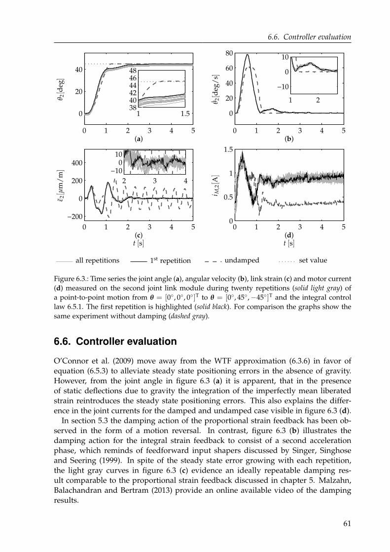
6.6. Controller evaluation
0 1 2 3 4 5
0
20
40
(a)0 1 2 3 4 5
0
20
40
60
80
(b)
0 1 2 3 4 5
−200
0
200
400
(c)0 1 2 3 4 5
0
0.5
1
1.5
(d)
1 1.5384042444648
1 2
−10
0
10
2 3 4
−100
10
θ 2[d
eg]
θ 2[d
eg/
s]
ε 2[µ
m/
m]
i M,2[A
]
t [s]t [s]
all repetitions 1st repetition undamped set value
Figure 6.3.: Time series the joint angle (a), angular velocity (b), link strain (c) and motor current
(d) measured on the second joint link module during twenty repetitions (solid light gray) of
a point-to-point motion from θ = [0, 0, 0]T to θ = [0, 45,−45]T and the integral control
law 6.5.1. The first repetition is highlighted (solid black). For comparison the graphs show the
same experiment without damping (dashed gray).
6.6. Controller evaluation
O’Connor et al. (2009) move away from the WTF approximation (6.3.6) in favor of
equation (6.5.3) to alleviate steady state positioning errors in the absence of gravity.
However, from the joint angle in figure 6.3 (a) it is apparent, that in the presence
of static deflections due to gravity the integration of the imperfectly mean liberated
strain reintroduces the steady state positioning errors. This also explains the differ-
ence in the joint currents for the damped and undamped case visible in figure 6.3 (d).
In section 5.3 the damping action of the proportional strain feedback has been ob-
served in the form of a motion reversal. In contrast, figure 6.3 (b) illustrates the
damping action for the integral strain feedback to consist of a second acceleration
phase, which reminds of feedforward input shapers discussed by Singer, Singhose
and Seering (1999). In spite of the steady state error growing with each repetition,
the light gray curves in figure 6.3 (c) evidence an ideally repeatable damping res-
ult comparable to the proportional strain feedback discussed in chapter 5. Malzahn,
Balachandran and Bertram (2013) provide an online available video of the damping
results.
61
7Spatially Continuous Wave Echo Control
This is the third out of four subsequent chapters devoted to oscillation damping con-
trol. In this work, the controllers derived in the chapters 5 and 6 have been shown
to be structurally equivalent. However, the derivations involve either a spatial dis-
cretization or a modal truncation. While the neglecting higher order dynamics can
theoretically endanger the closed loop stability as already discussed in section 1.2, the
lumped parameter view focuses on bending angles and torques. It neglects shear-
ing forces and transversal deflections. The theory of spatially continuous mechanical
waves provides an alternative way to incorporate all effects of the elastic link dy-
namics without truncation or discretization. The controller derived in the following
is based on the active modification of the boundary conditions at the actuator side
of the links. Parts of this chapter have been previously published by Malzahn and
Bertram (2014).
7.1. Continuous wave variables
The theory starts with a reinterpretation of the general exponential solution (4.3.5) to
the boundary value problem. Again, the whole arm is seen as a chain of independent
joint-link-modules. Similar to chapter 6, the oscillations at any point along a link are
considered to result from the superposition of mechanical wave components. How-
ever, the wave components consist of propagating components accompanied by near
fields. This way equation (4.3.5) is redefined as follows:
y (x) = +a + −a + +aN + −aN. (7.1.1)
The wave variables+a = + a e−jkωx and −a = − a ejkωx (7.1.2)
denote the components of the forward and backward propagating waves. Analog-
ously+aN = + aN e−kω x and −aN = − aN ekωx (7.1.3)
are termed the attenuating near field wave components emerging at both link ends.
The wave components are grouped into the vectors:
+a =[
+a, +aN
]Tand −a =
[−a, −aN
]T, (7.1.4)
62

7.2. Reflection and transmission at junctions and boundaries
and the deflection y, bending angle θb, bending moment τb and shearing force Fy can
be expressed in terms of the wave variables in the compact matrix form:
y1
kω
∂y∂x
1EIk2
ωτb
1EIk3
ωFy
=
1 1 1 1
−j −1 j 1
−1 1 −1 1
j −1 −j 1
[
+a
−a
]
. (7.1.5)
7.2. Reflection and transmission at junctions and boundaries
A travelling wave +a reaching a junction or a boundary splits into a reflected wave
component −a and a transmitted wave component +b. The reflected component −a
computes to:−a = Ψ
+a. (7.2.1)
The generally complex valued matrix Ψ is called the reflection matrix. The transmitted
wave component +b computes to:
+b = Ω+a. (7.2.2)
The generally complex valued matrix Ω is called the transmission matrix. Note, in the
case of the transversal oscillations of strings, the longitudinal oscillations of rods or the
torsional oscillation of shafts near field components do not exist. The reflection and
transmission would be governed just by a reflection and a transmission factor which
corresponds to the top left elements of the matrices Ψ and Ω. For beam bending the
matrix form implies that travelling bending waves arriving at boundaries or junctions
may evoke new travelling wave components. Moreover travelling wave components
can be converted into near field components and vice versa.
Consider a launched wave +a, which passes a constraining junction or support
at x = 0. At this point the wave splits into a reflected wave component −a and a
transmitted wave component +b. The deflection at this location is characterized by:
−y(x) = +a + −a + +aN + −aN, x ≤ 0, (7.2.3)
+y(x) = +b + +bN, x ≥ 0. (7.2.4)
Following Mace (1984), the imposed constraints are modeled as the rotational and
translational stiffnesses Kr and Kt.
Assuming continuity in the deflection variables:
+y|x=0 = −y|x=0 as well as ∂+y(x, t)/∂x|x=0 = ∂−y(x, t)/∂x|x=0 (7.2.5)
and exploiting the first two rows of equation (7.1.5) in terms of −a, +a and +b results
in:[
1 1
−j −1
]
+a +
[
1 1
j 1
]
−a =
[
1 1
−j −1
]
+b. (7.2.6)
Next, the equilibrium of the bending torques and forces is assumed, so that:
Kr θb|x=0 = +τb|x=0 − −τb|x=0 and Kt y|x=0 = − fy|x=0 − + fy|x=0. (7.2.7)
63
7. Spatially Continuous Wave Echo Control
Both expressions can be reformulated using the bottom two rows along with the top
right 2-by-2 submatrix of equation (7.1.5):
[−1 1
j −1
]
+a +
[−1 1
−j 1
]
−a =
[−1 1
j −1
]
+b +
[
jKr Kr
Kt Kt
]
+b, (7.2.8)
where the normalized stiffnesses
Kt =Kt
EI k3ω
and Kr =Kr
EI kω(7.2.9)
abbreviate the notation.
The reflection matrix (7.2.1) and the transmission matrix (7.2.2) allow for the elim-
ination of −a and +b. After rearrangement the reflection and transmission matrix are
expressed in terms of the boundary stiffnesses:
Ω = E + ηt Ct − ηr Cr, Ψ = ηt Ct + ηr Cr, (7.2.10)
with:
Ct =
[
j j
1 1
]
, Cr =
[−j −1
j 1
]
, ηt =Kt
4 − (1 + j)Kt, ηr =
Kr
4 + (1 − j)Kr. (7.2.11)
The normalized stiffnesses Kr and Kt are the characteristic parameters of the reflec-
tion and transmission matrices at boundaries and junctions of beams. The controller
described in section 7.4 makes use of this relation.
7.3. Near field contribution
Without natural damping the absolute value of the travelling waves persists along the
whole beam. The near field wave components are special to bending waves and do not
exist in the case of the transversal oscillations of strings, the longitudinal oscillations
of rods or the torsional oscillation of shafts. It becomes apparent in the previous
section, that the absence of near field components would facilitate the analyses and it
is worth investigating the share of the near fields in the overall oscillation.
The absolute value of the near field components attenuates with the constant 1/kω,
so that for sufficiently long links and higher natural frequencies the near field com-
ponents can be neglected. To give a tangible example, consider the absolute value of
the near field component emerging at one end of a single TUDOR link body. At the
opposite link end this absolute value drops to about 70 % for ω = 1 Hz and down to
10 % for ω = 30 Hz. Obviously, the near field components substantially contribute to
the deflections over the whole link length and in the frequency range of interest.
To give a graphical notion, figure 7.1 shows the contribution of all wave variables for
the first two theoretical frequencies on the second link of TUDOR. This link carries
the third joint, the third link as well as the end effector payload. The case of no
end effector payload is visible in the figures 7.1 (a) and (b). The case with mL =0.6 kg and IE = 3.3 · 10−4 kgm2 is displayed in figures 7.1 (c) and (d). The load
configuration corresponds to the lower and upper bounds already discussed with the
aid of figure 4.5.
64
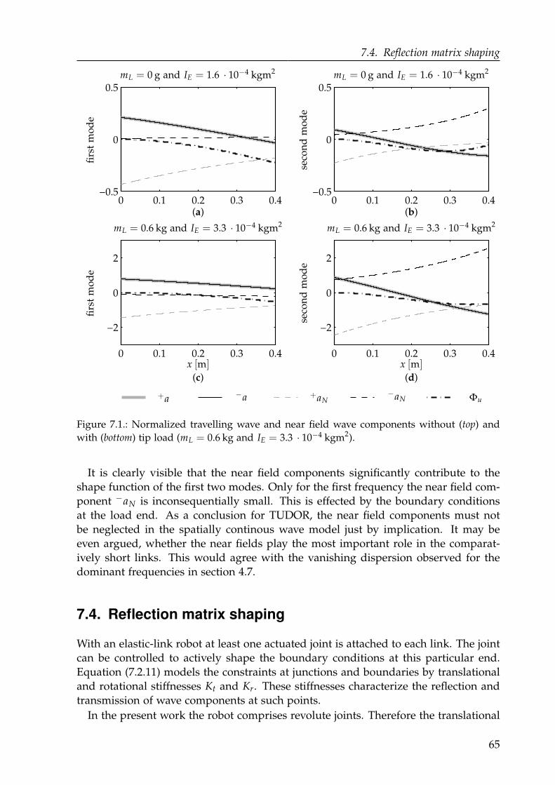
7.4. Reflection matrix shaping
0 0.1 0.2 0.3 0.4−0.5
0
0.5
(a)0 0.1 0.2 0.3 0.4
−0.5
0
0.5
(b)
0 0.1 0.2 0.3 0.4
−2
0
2
(c)
0 0.1 0.2 0.3 0.4
−2
0
2
(d)
+a −a +aN−aN Φu
firs
tm
od
efi
rst
mo
de
seco
nd
mo
de
seco
nd
mo
de
x [m]x [m]
mL = 0 g and IE = 1.6 · 10−4 kgm2 mL = 0 g and IE = 1.6 · 10−4 kgm2
mL = 0.6 kg and IE = 3.3 · 10−4 kgm2 mL = 0.6 kg and IE = 3.3 · 10−4 kgm2
Figure 7.1.: Normalized travelling wave and near field wave components without (top) and
with (bottom) tip load (mL = 0.6 kg and IE = 3.3 · 10−4 kgm2).
It is clearly visible that the near field components significantly contribute to the
shape function of the first two modes. Only for the first frequency the near field com-
ponent −aN is inconsequentially small. This is effected by the boundary conditions
at the load end. As a conclusion for TUDOR, the near field components must not
be neglected in the spatially continous wave model just by implication. It may be
even argued, whether the near fields play the most important role in the comparat-
ively short links. This would agree with the vanishing dispersion observed for the
dominant frequencies in section 4.7.
7.4. Reflection matrix shaping
With an elastic-link robot at least one actuated joint is attached to each link. The joint
can be controlled to actively shape the boundary conditions at this particular end.
Equation (7.2.11) models the constraints at junctions and boundaries by translational
and rotational stiffnesses Kt and Kr. These stiffnesses characterize the reflection and
transmission of wave components at such points.
In the present work the robot comprises revolute joints. Therefore the translational
65
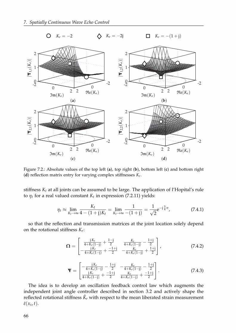
7. Spatially Continuous Wave Echo Control
-20
2
-20
2
0
1
2
(a)
-20
2
-20
2
0
1
2
(b)
-20
2
-20
2
0
1
2
(c)
-20
2
-20
2
0
1
2
(d)
|Ψ1,
1(K
r)|
|Ψ1,
2(K
r)|
|Ψ2,
1(K
r)|
|Ψ2,
2(K
r)|
Re(Kr)Re(Kr)
Re(Kr)Re(Kr)
Im(Kr)Im(Kr)
Im(Kr)Im(Kr)
Kr = −2 Kr = −2j Kr = −(1 + j)
Figure 7.2.: Absolute values of the top left (a), top right (b), bottom left (c) and bottom right
(d) reflection matrix entry for varying complex stiffnesses Kr.
stiffness Kt at all joints can be assumed to be large. The application of l’Hopital’s rule
to ηt for a real valued constant Kt in expression (7.2.11) yields:
ηt ≈ limKt→∞
Kt
4 − (1 + j)Kt= lim
Kt→∞
1
−(1 + j)=
1√2
e−j 54 π, (7.4.1)
so that the reflection and transmission matrices at the joint location solely depend
on the rotational stiffness Kr:
Ω =
j Kr
4+Kr(1−j)+
1−j2
Kr4+Kr(1−j)
− 1+j2
− j Kr
4+Kr(1−j)+
−1+j2 − Kr
4+Kr(1−j)+
1+j2
, (7.4.2)
Ψ =
− j Kr
4+Kr(1−j)− 1+j
2 − Kr4+Kr(1−j)
− 1+j2
j Kr
4+Kr(1−j)+
−1+j2
Kr4+Kr(1−j)
+−1+j
2
. (7.4.3)
The idea is to develop an oscillation feedback control law which augments the
independent joint angle controller described in section 3.2 and actively shape the
reflected rotational stiffness Kr with respect to the mean liberated strain measurement
ε(xs, t).
66
7.4. Reflection matrix shaping
If the strain gauges are applied very close to the joint hub, the gravity liberated net
bending torque at the joint can be approximated with negligible error:
−τb|x=0 − +τb|x=0 ≈ EIz
ybε|x=xs
. (7.4.4)
The rotational stiffness Kr relates this expression to the bending angle θb|x=0 at the
joint:
Kr θb|x=0 =EIz
ybε|x=xs
. (7.4.5)
The rearrangement of (7.4.5) with θε = θb|x=0 using the normalized rotational stiff-
ness Kr introduced in (7.2.9) and inserting the definition of kω from (4.3.3) yields the
generic form of the oscillation damping control law:
θε =1
Kr√
ω
1
yb
4
√
EIz
ρbε|x=xs
. (7.4.6)
Note, that this generic control law is frequency dependent and, by principle, it is
set free from the boundary conditions at the opposite link end as well as the actual
oscillation excitation source. No critical model truncation is involved.
The design objective is to find the rotational stiffness Kr, which modifies the trans-
mission and reflection matrices, so that excited oscillations vanish as fast as possible.
A straight forward idea is to demand absolutely no wave reflection to take place at
the joint. Mathematically this is equivalent to a singular reflection matrix Ψ, which
requires:
det Ψ =Kr(−1 + j)
4 + Kr(1 − j)= 0 (7.4.7)
and consequently Kr = 0. Looking at (7.4.6), this implies an infinite gain controller,
which is practically infeasible to realize. However, the obtained result is intuitively
plausible. A controlled joint that does not act against the external torque admits to be
driven back and absorbs any incoming wave components.
Figure 7.2 shows the absolute values of the individual elements of Ψ for varying
normalized stiffnesses Kr. The graphs suggest a closer view at the three emphasized
characteristic choices of Kr.
A finite gain controller with Kr = −2 causes the reflection coefficient Ψ1,1 to vanish.
In the absence of near fields or in the case of negligible near field components this
would be a highly desired situation. Travelling wave components arriving at the joint
do not initiate a reflected travelling wave. The total reflection matrix becomes:
Ψ =
[
0 −j
−1 −1 + j
]
(7.4.8)
If near field components are not negligible an incoming wave is converted into a
near field component while reaching near field components from the opposite end
also start new reflected propagating waves. The associated control law (7.4.6) results
in:
θε = − 1√ω
1
2 yb
4
√
EIz
ρbε|x=xs
, (7.4.9)
67
7. Spatially Continuous Wave Echo Control
which consists of a frequency dependent gain.
Another remarkable choice is Kr = −2j, for which the reflection matrix computes
to:
Ψ =
[−(1 + j) −1
j 0
]
(7.4.10)
and shows vanishing near field reflection. Looking at the normalized wave compon-
ents illustrated in figure 7.1, it can be expected that the control law:
θε = − 1
2j√
ω
1
yb
4
√
EIz
ρbε|x=xs
(7.4.11)
significantly reduces structural oscillations. Moreover the temporal derivative com-
putes to:
θε = −√
ω
2 yb
4
√
EIz
ρbε|x=xs
. (7.4.12)
A comparison with the previously introduced control law (5.2.1) allows the inter-
pretation of (7.4.12) to be a frequency adaptive generalization of the proportional
strain feedback presented in chapter 5. However, the frequency adaption is hard to
realize in practice. An explicit online frequency estimation is likely too slow and by
nature gets constantly more difficult with increasing damping success.
The most promising choice is the complex valued stiffness Kr = − (j + 1). It yields
the reflection matrix:
Ψ =
[−1 0
0 −1
]
, (7.4.13)
which causes both, incoming propagating waves as well as near field components,
to be directly reflected with the opposite sign. In the absence of natural damping,
which is implied by the real valued wave number kω, incoming and reflected waves
destructively interfere. A conversion between reflected propagating waves and near
field components is inhibited. The insertion into the generic control law (7.4.6) yields
after rearrangement:
θε = − 1
(1 + j)√
ω
1
yb
4
√
EIz
ρbε|x=xs
= − 1√
jωkε ε|x=xs
, (7.4.14)
which is the Fourier domain transfer function of a so-called half-integrator and a gain:
kε =1√2 yb
4
√
EIz
ρb. (7.4.15)
In comparison to the transfer function of the commonly known full-integrator 1jω , the
slope of the logarithmic frequency magnitude is half as steep. The constant phase
angle of the half-integrator is also half the phase angle of the full-integrator.
Flotow and Schäfer (1986) report that feeding back the tip deflection to the actuator
control torque leads to the similar half-differentiator as a wave based controller. Using
strain feedback at the velocity cascade level also leads to the half-differentiator:
θε = −jω1
(1 + j)√
ω
1
yb
4
√
EIz
ρbε|x=xs
= −√
jω kε ε|x=xs. (7.4.16)
68
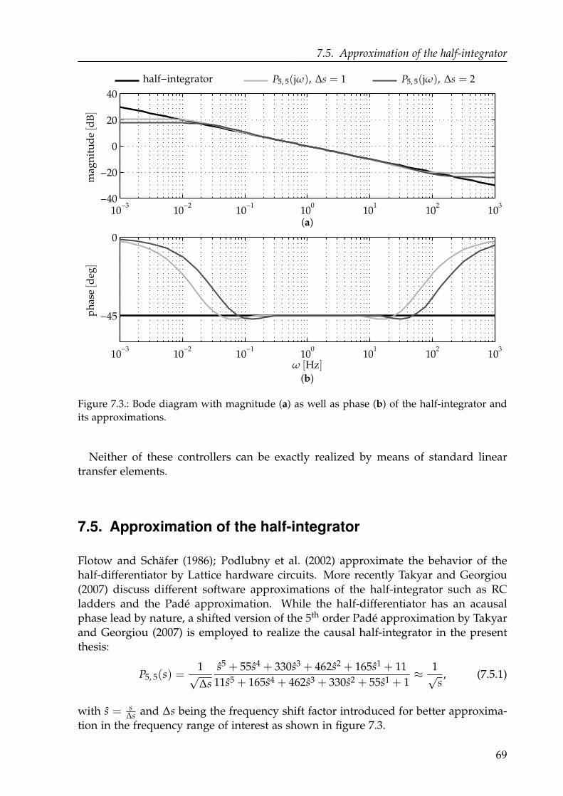
7.5. Approximation of the half-integrator
10−3
10−2
10−1
100
101
102
103
−40
−20
0
20
40
(a)
10−3
10−2
10−1
100
101
102
103
−45
0
(b)
half−integratorm
agn
itu
de[d
B]
ph
ase[d
eg]
ω [Hz]
P5, 5(jω), ∆s = 1 P5, 5(jω), ∆s = 2
Figure 7.3.: Bode diagram with magnitude (a) as well as phase (b) of the half-integrator and
its approximations.
Neither of these controllers can be exactly realized by means of standard linear
transfer elements.
7.5. Approximation of the half-integrator
Flotow and Schäfer (1986); Podlubny et al. (2002) approximate the behavior of the
half-differentiator by Lattice hardware circuits. More recently Takyar and Georgiou
(2007) discuss different software approximations of the half-integrator such as RC
ladders and the Padé approximation. While the half-differentiator has an acausal
phase lead by nature, a shifted version of the 5th order Padé approximation by Takyar
and Georgiou (2007) is employed to realize the causal half-integrator in the present
thesis:
P5, 5(s) =1√∆s
s5 + 55s4 + 330s3 + 462s2 + 165s1 + 11
11s5 + 165s4 + 462s3 + 330s2 + 55s1 + 1≈ 1√
s, (7.5.1)
with s = s∆s and ∆s being the frequency shift factor introduced for better approxima-
tion in the frequency range of interest as shown in figure 7.3.
69

7. Spatially Continuous Wave Echo Control
0 1 2 3 4 5
0
20
40
(a)0 1 2 3 4 5
0
20
40
60
80
(b)
0 1 2 3 4 5
−200
0
200
400
(c)0 1 2 3 4 5
0
0.5
1
1.5
(d)
1 1.5384042444648
1 2
−10
0
10
2 3 4
−100
10
θ 2[d
eg]
θ 2[d
eg/
s]
ε 2[µ
m/
m]
i M,2[A
]
t [s]t [s]
all repetitions 1st repetition undamped set value
Figure 7.4.: Half-integrator damping results. Time series the joint angle (a), angular velocity
(b), link strain (c) and motor current (d) measured on the second joint link module during
twenty repetitions (solid light gray) of a point-to-point motion from θ = [0, 0, 0]T to θ =
[0, 45,−45]T. The first repetition is highlighted (solid black). For comparison the graphs
show the same experiment without damping (dashed gray).
7.6. Controller evaluation
Oscillation damping results with the half-integrator wave reflection controller are ex-
emplified in figure 7.4. Equally to chapters 5 and 6 the gain kε has been automatically
tuned through the hardware in the loop optimization reported in section 5.3. The time
series presented in the figure are very similar to those observed with the proportional
strain feedback in chapter 5. The damping action is observed as an overshoot in the
joint angle in figure 7.4 (a) and a corresponding motion reversal in the joint angular
velocity in figure 7.4 (b). The slim distribution of the measurements of all twenty
repetitions indicate a high repeatability of the damping result without steady state
positioning error. The rapid damping evidenced through the strain measurements
presented in figure 7.4 (c). The evolution of the joint current in figure 7.4 (d) also
reminds of the proportional feedback results in figure 5.3 (d).
70
8Experimental Damping Comparison
This is last out of four subsequent chapters devoted to oscillation damping control.
Chapter 5 discusses the proportional strain feedback at different cascade levels of the
independent joint motion controller designed in chapter 3. From the root locus ana-
lysis carried out in chapter 5, the proportional feedback at the velocity cascade level
is identified to be the best choice. Chapter 6 identifies wave properties in chains of
lumped mass-spring-systems. The derivations arrive at the same damping controller
structure at velocity cascade level and alternatively propose an integral feedback at
position level. A more precise modeling perspective in terms of continuous propagat-
ing waves and near fields leads to fractional order feedback laws in chapter 7. With
the following sections the work contributes an experimental comparison of the pro-
portional strain feedback at the velocity cascade level along with the integral as well
as half-integral strain feedback at the position cascade level.
8.1. Experiment design
The oscillation damping results provided in the chapters 5 to 7 are based on the
automated hardware in the loop optimization of the oscillation damping gains with
respect to the integral absolute time weighted strain surface criterion (see B.4) for
the particular point-to-point motion from θ = [0, 0, 0]T to θ = [0, 45,−45]T. The
accomplished results provided in these chapters represent a principal proof of concept
for the synthesized controllers.
Tuning gains for a single motion task may be adequate for a few low-level tasks
in industrial mass production. However, a robot is actually expected to be equally
functional in the whole workspace and arbitrary motions within that workspace. The
experiments presented in this chapter are therefore carried out around as well as in
between of the operating points illustrated and indexed in figure 8.1. Among all
operating points 3 and 5 are special. The straight vertical pose in operating point
3 maximizes the effect of joint backlash. The straight horizontal pose in operating
point 5 maximizes the effect of gravity.
All joint motions are performed with a maximum speed of 60 deg/s as well as
a maximum acceleration of 200 deg/s2. The basic payload is mL = 300 g. All ex-
periments in this chapter are repeated 20 times. The results are given as mean and
standard deviation over all repetitions. The medium step motion indexed by 06 cor-
71
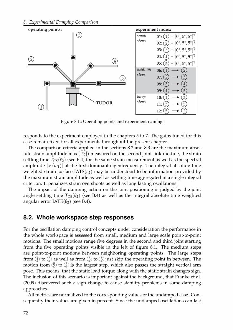
8. Experimental Damping Comparison
experiment index:operating points:
1
2
3
4
5
smallsteps
mediumsteps
largesteps
1 2:06
32:07
3 4:08
4 5:09
31:10
3 5:11
5 2:12
TUDOR
1: +01
2: +02
3: +03
4: +04
5: +05 [0, 5, 5]T[0, 5, 5]T[0, 5, 5]T[0, 5, 5]T[0, 5, 5]T
Figure 8.1.: Operating points and experiment naming.
responds to the experiment employed in the chapters 5 to 7. The gains tuned for this
case remain fixed for all experiments throughout the present chapter.
The comparison criteria applied in the sections 8.2 and 8.3 are the maximum abso-
lute strain amplitude max (|ε2|) measured on the second joint-link-module, the strain
settling time TCS(ε2) (see B.4) for the same strain measurement as well as the spectral
amplitude |F (ω1)| at the first dominant eigenfrequency. The integral absolute time
weighted strain surface IATS(ε2) may be understood to be information provided by
the maximum strain amplitude as well as settling time aggregated in a single integral
criterion. It penalizes strain overshoots as well as long lasting oscillations.
The impact of the damping action on the joint positioning is judged by the joint
angle settling time TCS(θ2) (see B.4) as well as the integral absolute time weighted
angular error IATE(θ2) (see B.4).
8.2. Whole workspace step responses
For the oscillation damping control concepts under consideration the performance in
the whole workspace is assessed from small, medium and large scale point-to-point
motions. The small motions range five degrees in the second and third joint starting
from the five operating points visible in the left of figure 8.1. The medium steps
are point-to-point motions between neighboring operating points. The large steps
from 1 to 3 as well as from 3 to 5 just skip the operating point in between. The
motion from 5 to 2 is the largest step, which also passes the straight vertical arm
pose. This means, that the static load torque along with the static strain changes sign.
The inclusion of this scenario is important against the background, that Franke et al.
(2009) discovered such a sign change to cause stability problems in some damping
approaches.
All metrics are normalized to the corresponding values of the undamped case. Con-
sequently their values are given in percent. Since the undamped oscillations can last
72
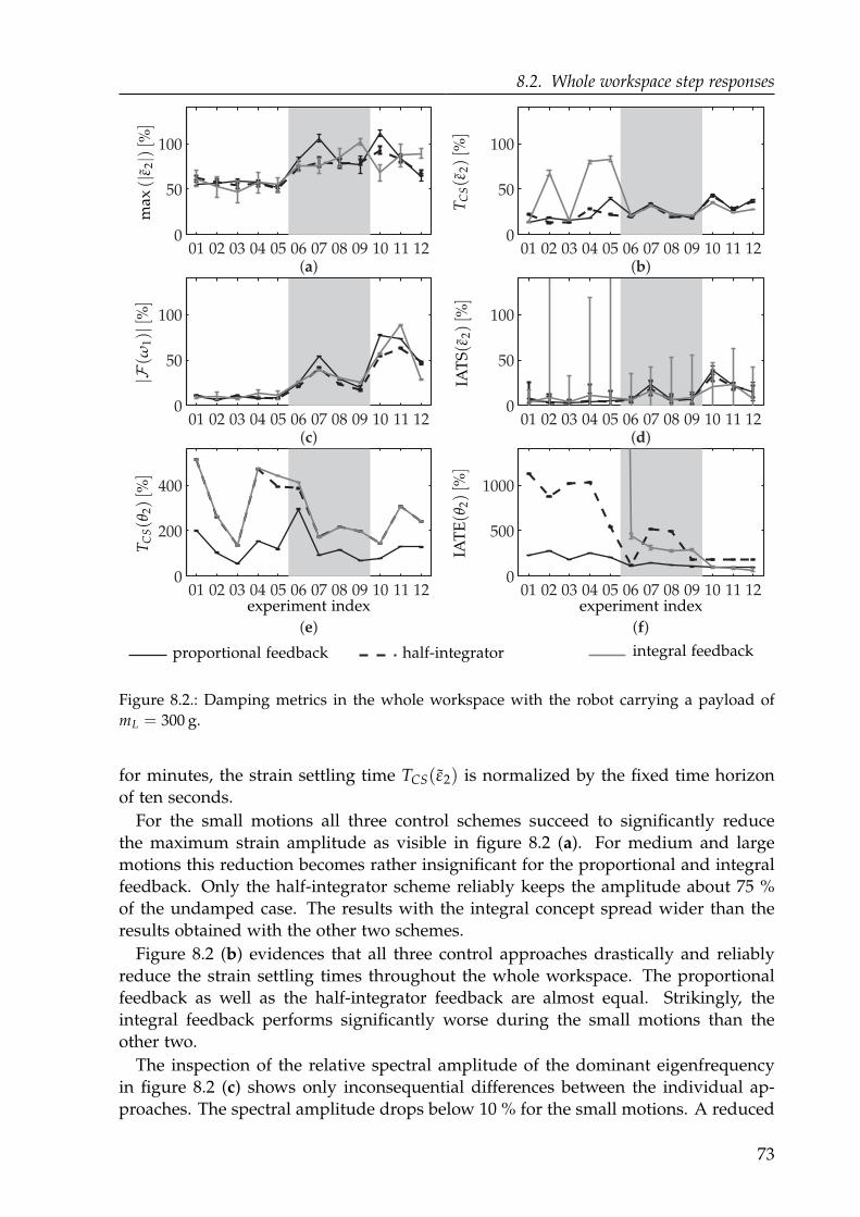
8.2. Whole workspace step responses
01 02 03 04 05 06 07 08 09 10 11 120
50
100
(a)01 02 03 04 05 06 07 08 09 10 11 12
0
50
100
(b)
01 02 03 04 05 06 07 08 09 10 11 120
50
100
(c)01 02 03 04 05 06 07 08 09 10 11 12
0
50
100
(d)
01 02 03 04 05 06 07 08 09 10 11 120
200
400
(e)
01 02 03 04 05 06 07 08 09 10 11 120
500
1000
(f)
max
(|ε2|)[%
]
TC
S(ε
2)[%
]
|F(ω
1)|[%
]
IAT
S(ε
2)[%
]
TC
S(θ
2)[%
]
IAT
E(θ
2)[%
]
proportional feedback half-integrator integral feedback
experiment indexexperiment index
Figure 8.2.: Damping metrics in the whole workspace with the robot carrying a payload of
mL = 300 g.
for minutes, the strain settling time TCS(ε2) is normalized by the fixed time horizon
of ten seconds.
For the small motions all three control schemes succeed to significantly reduce
the maximum strain amplitude as visible in figure 8.2 (a). For medium and large
motions this reduction becomes rather insignificant for the proportional and integral
feedback. Only the half-integrator scheme reliably keeps the amplitude about 75 %
of the undamped case. The results with the integral concept spread wider than the
results obtained with the other two schemes.
Figure 8.2 (b) evidences that all three control approaches drastically and reliably
reduce the strain settling times throughout the whole workspace. The proportional
feedback as well as the half-integrator feedback are almost equal. Strikingly, the
integral feedback performs significantly worse during the small motions than the
other two.
The inspection of the relative spectral amplitude of the dominant eigenfrequency
in figure 8.2 (c) shows only inconsequential differences between the individual ap-
proaches. The spectral amplitude drops below 10 % for the small motions. A reduced
73
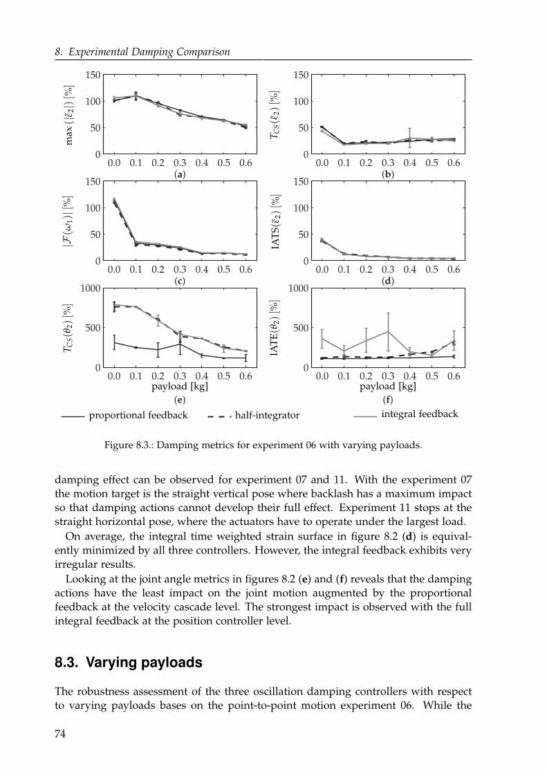
8. Experimental Damping Comparison
0.0 0.1 0.2 0.3 0.4 0.5 0.60
50
100
150
(a)0.0 0.1 0.2 0.3 0.4 0.5 0.6
0
50
100
150
(b)
0.0 0.1 0.2 0.3 0.4 0.5 0.60
50
100
150
(c)0.0 0.1 0.2 0.3 0.4 0.5 0.6
0
50
100
150
(d)
0.0 0.1 0.2 0.3 0.4 0.5 0.60
500
1000
(e)
0.0 0.1 0.2 0.3 0.4 0.5 0.60
500
1000
(f)
max
(|ε2|)[%
]
TC
S(ε
2)[%
]
|F(ω
1)|[%
]
IAT
S(ε
2)[%
]
TC
S(θ
2)[%
]
IAT
E(θ
2)[%
]
proportional feedback half-integrator integral feedback
payload [kg]payload [kg]
Figure 8.3.: Damping metrics for experiment 06 with varying payloads.
damping effect can be observed for experiment 07 and 11. With the experiment 07
the motion target is the straight vertical pose where backlash has a maximum impact
so that damping actions cannot develop their full effect. Experiment 11 stops at the
straight horizontal pose, where the actuators have to operate under the largest load.
On average, the integral time weighted strain surface in figure 8.2 (d) is equival-
ently minimized by all three controllers. However, the integral feedback exhibits very
irregular results.
Looking at the joint angle metrics in figures 8.2 (e) and (f) reveals that the damping
actions have the least impact on the joint motion augmented by the proportional
feedback at the velocity cascade level. The strongest impact is observed with the full
integral feedback at the position controller level.
8.3. Varying payloads
The robustness assessment of the three oscillation damping controllers with respect
to varying payloads bases on the point-to-point motion experiment 06. While the
74
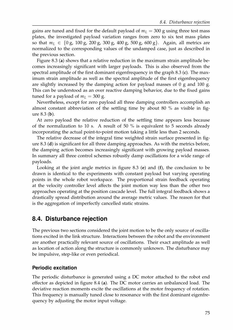
8.4. Disturbance rejection
gains are tuned and fixed for the default payload of mL = 300 g using three test mass
plates, the investigated payload variation ranges from zero to six test mass plates
so that mL ∈ 0 g, 100 g, 200 g, 300 g, 400 g, 500 g, 600 g. Again, all metrics are
normalized to the corresponding values of the undamped case, just as described in
the previous section.
Figure 8.3 (a) shows that a relative reduction in the maximum strain amplitude be-
comes increasingly significant with larger payloads. This is also observed from the
spectral amplitude of the first dominant eigenfrequency in the graph 8.3 (c). The max-
imum strain amplitude as well as the spectral amplitude of the first eigenfrequency
are slightly increased by the damping action for payload masses of 0 g and 100 g.
This can be understood as an over reactive damping behavior, due to the fixed gains
tuned for a payload of mL = 300 g.
Nevertheless, except for zero payload all three damping controllers accomplish an
almost constant abbreviation of the settling time by about 80 % as visible in fig-
ure 8.3 (b).
At zero payload the relative reduction of the settling time appears less because
of the normalization to 10 s. A result of 50 % is equivalent to 5 seconds already
incorporating the actual point-to-point motion taking a little less than 2 seconds.
The relative decrease of the integral time weighted strain surface presented in fig-
ure 8.3 (d) is significant for all three damping approaches. As with the metrics before,
the damping action becomes increasingly significant with growing payload masses.
In summary all three control schemes robustly damp oscillations for a wide range of
payloads.
Looking at the joint angle metrics in figure 8.3 (e) and (f), the conclusion to be
drawn is identical to the experiments with constant payload but varying operating
points in the whole robot workspace. The proportional strain feedback operating
at the velocity controller level affects the joint motion way less than the other two
approaches operating at the position cascade level. The full integral feedback shows a
drastically spread distribution around the average metric values. The reason for that
is the aggregation of imperfectly cancelled static strains.
8.4. Disturbance rejection
The previous two sections considered the joint motion to be the only source of oscilla-
tions excited in the link structure. Interactions between the robot and the environment
are another practically relevant source of oscillations. Their exact amplitude as well
as location of action along the structure is commonly unknown. The disturbance may
be impulsive, step-like or even periodical.
Periodic excitation
The periodic disturbance is generated using a DC motor attached to the robot end
effector as depicted in figure 8.4 (a). The DC motor carries an unbalanced load. The
deviative reaction moments excite the oscillations at the motor frequency of rotation.
This frequency is manually tuned close to resonance with the first dominant eigenfre-
quency by adjusting the motor input voltage.
75

8. Experimental Damping Comparison
DC voltagesource
DC motor withunbalanced load
TUDOR
TUDOR
manually droppedtest mass
( )a
( )c
( )b
( )d
net
tripod
Figure 8.4.: Experimental setups to generate periodic (a)-(b) and step-like disturbances (c)-(d).
In all experiments the arm resides in the horizontally stretched out joint zero config-
uration, which represents the maximum load configuration for the actuators. During
the first two seconds of each repetition the oscillation damping gain is zero. After ap-
proximately two seconds the gains are set to the default ones tuned in the chapters 5
to 7.
Figure 8.5 shows the time series of strain measurements (a) and (b) as well as joint
angular velocity measurements (c) and (d) for the proportional strain feedback as well
as the half-integrator controller. Experimental results with the full integral feedback
at the joint position cascade level are omitted here. The excited oscillations are large
enough to interfere with the static strain cancellation. The interference accumulates
in the integral control law and introduces a drift in the joint angle, so that results are
not comparable to the other control approaches.
The close to resonance strain amplitude is equally visible in the left of figures 8.5 (a)
and (b). In spite of the large gear ratios, the strong oscillations also affect the joint
angles. During the first two seconds in figures 8.5 (c) and (d) the cascaded independ-
ent joint controllers have to visibly compensate for the strong oscillations.
With the activation of the oscillation damping, the strain amplitude abruptly drops
from close to 400 µm/m to approximately 100 µm/m. The half-integrator achieves
a slightly smaller strain amplitude in figure 8.5 (b) compared to the proportional
feedback in figure 8.5 (a) with apparently the same effort as visible in figures 8.5 (c)
and (d).
76
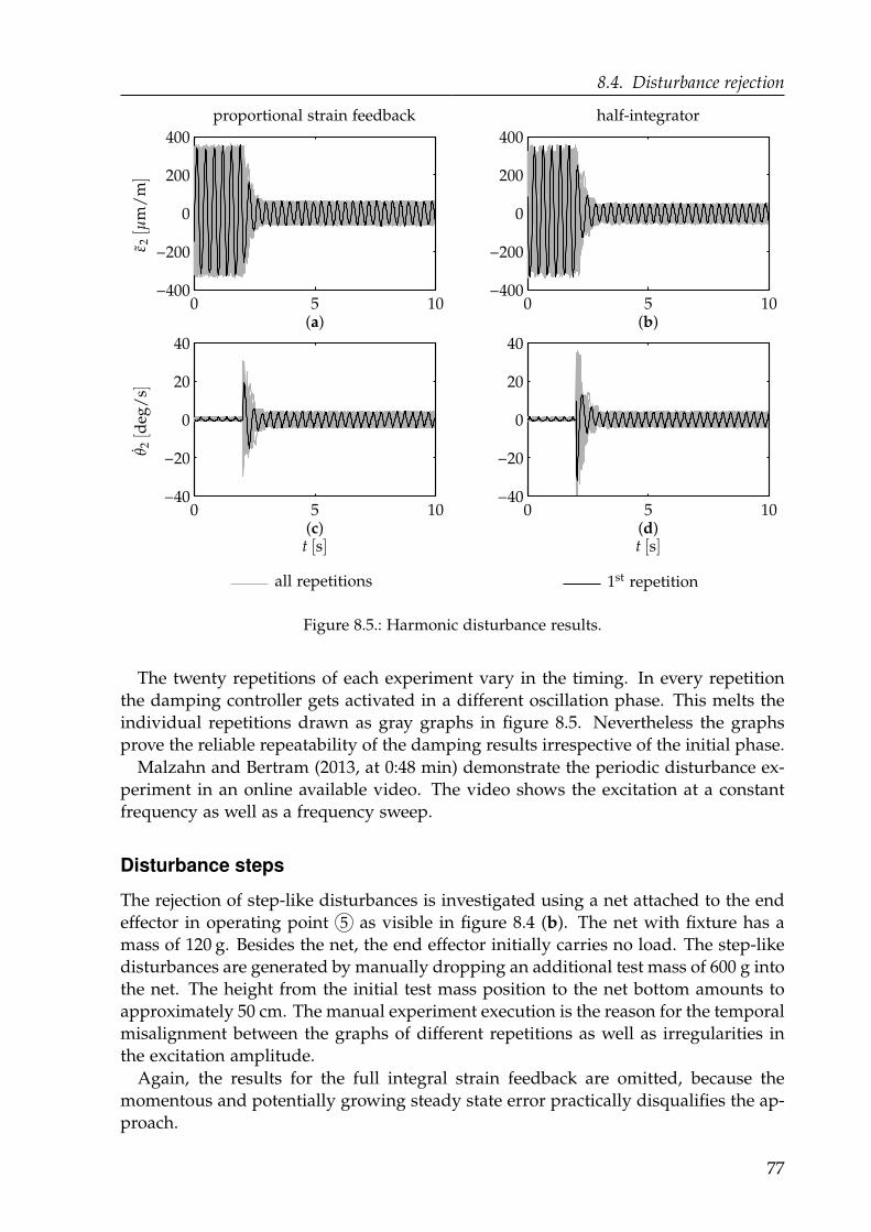
8.4. Disturbance rejection
0 5 10−400
−200
0
200
400
(a)
0 5 10−40
−20
0
20
40
(c)
0 5 10−400
−200
0
200
400
(b)
0 5 10−40
−20
0
20
40
(d)
proportional strain feedback half-integrator
ε 2[µ
m/
m]
θ 2[d
eg/
s]
t [s]t [s]
all repetitions 1st repetition
Figure 8.5.: Harmonic disturbance results.
The twenty repetitions of each experiment vary in the timing. In every repetition
the damping controller gets activated in a different oscillation phase. This melts the
individual repetitions drawn as gray graphs in figure 8.5. Nevertheless the graphs
prove the reliable repeatability of the damping results irrespective of the initial phase.
Malzahn and Bertram (2013, at 0:48 min) demonstrate the periodic disturbance ex-
periment in an online available video. The video shows the excitation at a constant
frequency as well as a frequency sweep.
Disturbance steps
The rejection of step-like disturbances is investigated using a net attached to the end
effector in operating point 5 as visible in figure 8.4 (b). The net with fixture has a
mass of 120 g. Besides the net, the end effector initially carries no load. The step-like
disturbances are generated by manually dropping an additional test mass of 600 g into
the net. The height from the initial test mass position to the net bottom amounts to
approximately 50 cm. The manual experiment execution is the reason for the temporal
misalignment between the graphs of different repetitions as well as irregularities in
the excitation amplitude.
Again, the results for the full integral strain feedback are omitted, because the
momentous and potentially growing steady state error practically disqualifies the ap-
proach.
77
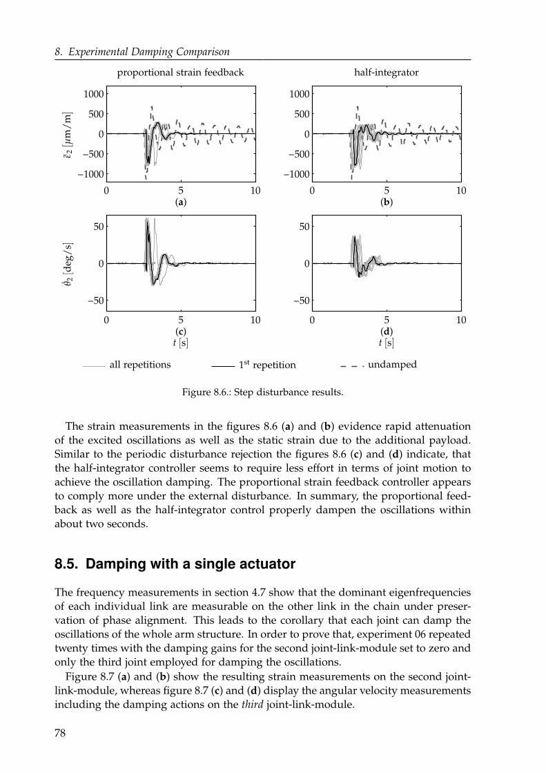
8. Experimental Damping Comparison
0 5 10
−1000
−500
0
500
1000
(a)
0 5 10
−50
0
50
(c)
0 5 10
−1000
−500
0
500
1000
(b)
0 5 10
−50
0
50
(d)
undamped
proportional strain feedback half-integratorε 2
[µm
/m]
θ 2[d
eg/
s]
t [s]t [s]
all repetitions 1st repetition
Figure 8.6.: Step disturbance results.
The strain measurements in the figures 8.6 (a) and (b) evidence rapid attenuation
of the excited oscillations as well as the static strain due to the additional payload.
Similar to the periodic disturbance rejection the figures 8.6 (c) and (d) indicate, that
the half-integrator controller seems to require less effort in terms of joint motion to
achieve the oscillation damping. The proportional strain feedback controller appears
to comply more under the external disturbance. In summary, the proportional feed-
back as well as the half-integrator control properly dampen the oscillations within
about two seconds.
8.5. Damping with a single actuator
The frequency measurements in section 4.7 show that the dominant eigenfrequencies
of each individual link are measurable on the other link in the chain under preser-
vation of phase alignment. This leads to the corollary that each joint can damp the
oscillations of the whole arm structure. In order to prove that, experiment 06 repeated
twenty times with the damping gains for the second joint-link-module set to zero and
only the third joint employed for damping the oscillations.
Figure 8.7 (a) and (b) show the resulting strain measurements on the second joint-
link-module, whereas figure 8.7 (c) and (d) display the angular velocity measurements
including the damping actions on the third joint-link-module.
78
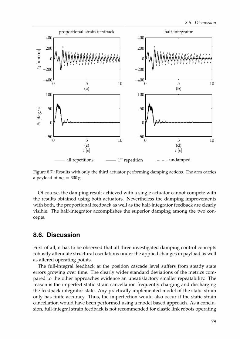
8.6. Discussion
0 5 10−400
−200
0
200
400
(a)
0 5 10−50
0
50
100
(c)
0 5 10−400
−200
0
200
400
(b)
0 5 10−50
0
50
100
(d)
proportional strain feedback half-integrator
ε 2[µ
m/
m]
θ 3[d
eg/
s]
t [s]t [s]
all repetitions 1st repetition undamped
Figure 8.7.: Results with only the third actuator performing damping actions. The arm carries
a payload of mL = 300 g
Of course, the damping result achieved with a single actuator cannot compete with
the results obtained using both actuators. Nevertheless the damping improvements
with both, the proportional feedback as well as the half-integrator feedback are clearly
visible. The half-integrator accomplishes the superior damping among the two con-
cepts.
8.6. Discussion
First of all, it has to be observed that all three investigated damping control concepts
robustly attenuate structural oscillations under the applied changes in payload as well
as altered operating points.
The full-integral feedback at the position cascade level suffers from steady state
errors growing over time. The clearly wider standard deviations of the metrics com-
pared to the other approaches evidence an unsatisfactory smaller repeatability. The
reason is the imperfect static strain cancellation frequently charging and discharging
the feedback integrator state. Any practically implemented model of the static strain
only has finite accuracy. Thus, the imperfection would also occur if the static strain
cancellation would have been performed using a model based approach. As a conclu-
sion, full-integral strain feedback is not recommended for elastic link robots operating
79
8. Experimental Damping Comparison
under gravity.
The half-integrator at the position cascade level as well as the proportional strain
feedback at the velocity cascade level show very similar results. Both control meth-
ods demand for no explicit model knowledge about the actual link dynamics. They
feature just a single additional controller gain per joint-link-module to be tuned. The
dampen oscillations irrespective of their excitation source.
The half-integrator requires the least efforts to reject external disturbances, the pro-
portional strain feedback has the smallest impact on the actual joint positioning. With
the damping results being almost equal to the half-integrator, the proportional feed-
back is therefore the favored oscillation damping controller in the remainder of this
thesis. Nevertheless, the half-integrator concept would produce equivalent results
with respect to the remaining chapters of this thesis. In this regard, the compensation
of the first undesired effect associated with the intentionally introduced link elasticity,
namely the structural oscillations, is accomplished for the scope of this thesis.
80
9End Effector Control
With the structural oscillations readily damped, the forward and inverse kinematics
modeling simplifies. A reconstruction of the end effector location based on a trun-
cated series of oscillation modes or a finite number of lumped parameters may be
omitted. It is sufficient to focus on the compensation of the static deflections in order
to accurately position the end effector.
The oscillation damping controllers derived in chapters 5 to 7 waive the need for
any dynamics model at runtime. It is consistent and desirable to investigate an end
effector positioning approach, which relinquishes any additional modeling compared
to conventional robots. Section 9.1 follows this paradigm using the eye-in-hand moun-
ted camera detailed in section 2.3.
Alternatively, the forward and inverse kinematics have to be modelled under con-
sideration of the static configuration and load dependent deflections in order to posi-
tion the end effector. In comparison to conventional robots the additional static strains
estimated in section 2.2 are required. The data-based load estimation and kinematics
presented in section 9.2 are originally developed for TUDOR and published by Phung
et al. (2011a). Continuatively, Malzahn, Phung and Bertram (2012a) demonstrate the
positioning speed and accuracy of the inverse kinematics with integrated oscillation
damping through the realization of the ball catching task detailed in section 9.3.
9.1. Visual servoing
Visual servoing controllers with an eye-in-hand mounted camera minimize the rel-
ative pose error between a current view and a goal view of the scene. Today visual
servoing is a well understood topic in literature. An early tutorial is given by Hutchin-
son, Hager and Corke (1996). A decade later Chaumette and Hutchinson (2006, 2007)
summarize fundamental concepts and also provide an introduction to more advanced
visual servoing techniques. Visual servoing controllers are categorized as position
based visual servoing controllers (PBVS) or image based visual servoing controllers
(IBVS). PBVS also known as 3D visual servoing controllers use the image information
to explicitly estimate the camera poses and infer the control error with respect to a co-
ordinate frame of reference. In IBVS or 2D visual servoing the control error is directly
formulated in the 2D image space. Hybrid concepts exist, which are basically IBVS
approaches involving a partial pose estimate or measurement. While the concepts
81
9. End Effector Control
have their individual merits and shortcomings, they all operate on the pure basis of
differential robot kinematics. This is a beneficial property for the end effector control
of elastic link robots. The visual servoing controller commands a camera velocity vc,
which may be interpreted as a relative direction towards the goal rather than a partic-
ular absolute metric path to the goal. Outside kinematically singular configurations
the inverse of the end effector referred robot Jacobian EJr(θ) transforms the relative
camera motion vector into the joint space:
θ = EJ−1r (θ) vc (9.1.1)
In the joint space the direction of the rotations θ computed for the individual joints
from the rigid body differential kinematics pretty well agrees with the elastic case
almost irrespective of the static deflections.
Visual servoing control law
TUDOR has three actuated degrees of freedom. The present work employs a hybrid
IBVS concept augmented by the depth readings of the RGB-D sensor to control the
translational degrees of freedom of the end effector.
Using a number of point features extracted from the camera images, the classical
IBVS control law is:
vc = −Kc J†c (ui, vi, ∆z) euv. (9.1.2)
Therein vc =[
vcx, vcy, vcz
]Tdenotes the commanded translational camera velocity
vector. The controller gain matrix Kc is chosen to be positive and diagonal. The
pairwise error between image point features extracted in the goal view and their
correspondences in the image of the current view is euv. J†c (ui, vi, ∆z) represents the
pseudoinverse of the image feature Jacobian Jc(u, v, ∆z). The image feature Jacobian
Jc(ui, vi, ∆z) consists of one column for each considered camera degree of freedom
and two rows per point feature correspondence. In the present case the reduced image
Jacobian for a single point feature computes to:
Jc(ui, vi, ∆z) =
[
Λ∆z , 0, − ui
∆z
0, Λ∆z , − vi
∆z
]
, (9.1.3)
where Λ is the focal length known from a camera calibration, ui and vi are the hori-
zontal and vertical image coordinates of the point feature, ∆z is the distance between
the camera coordinate frame and the scene point represented by the point feature.
The Jacobian (9.1.3) provides two coupled equations per point feature. With respect
to the three degrees of freedom controllable with TUDOR, classical IBVS requires at
least two image features to be extracted for end effector control. In the general case
of 6 degrees of freedom, a minimum of three features are required.
With a conventional monocular camera the distance ∆z is unknown. IBVS control
concepts "traditionally" involve an online estimation or use approximations. The RGB-
D sensor used in this work already provides distance measurements. Point features
are usually extracted from the images with subpixel accuracy. A depth value can be
assigned to each such 2D features by interpolation of the depth measurements. With
82
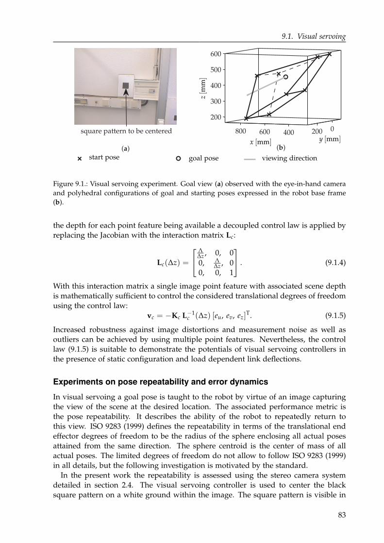
9.1. Visual servoing
400600800 0200
200
300
400
500
600
(b)
(a)
square pattern to be centered
x [mm] y [mm]
z[m
m]
start pose goal pose viewing direction
Figure 9.1.: Visual servoing experiment. Goal view (a) observed with the eye-in-hand camera
and polyhedral configurations of goal and starting poses expressed in the robot base frame
(b).
the depth for each point feature being available a decoupled control law is applied by
replacing the Jacobian with the interaction matrix Lc:
Lc(∆z) =
Λ∆z , 0, 0
0, Λ∆z , 0
0, 0, 1
. (9.1.4)
With this interaction matrix a single image point feature with associated scene depth
is mathematically sufficient to control the considered translational degrees of freedom
using the control law:
vc = −Kc L−1c (∆z) [eu, ev, ez]
T. (9.1.5)
Increased robustness against image distortions and measurement noise as well as
outliers can be achieved by using multiple point features. Nevertheless, the control
law (9.1.5) is suitable to demonstrate the potentials of visual servoing controllers in
the presence of static configuration and load dependent link deflections.
Experiments on pose repeatability and error dynamics
In visual servoing a goal pose is taught to the robot by virtue of an image capturing
the view of the scene at the desired location. The associated performance metric is
the pose repeatability. It describes the ability of the robot to repeatedly return to
this view. ISO 9283 (1999) defines the repeatability in terms of the translational end
effector degrees of freedom to be the radius of the sphere enclosing all actual poses
attained from the same direction. The sphere centroid is the center of mass of all
actual poses. The limited degrees of freedom do not allow to follow ISO 9283 (1999)
in all details, but the following investigation is motivated by the standard.
In the present work the repeatability is assessed using the stereo camera system
detailed in section 2.4. The visual servoing controller is used to center the black
square pattern on a white ground within the image. The square pattern is visible in
83
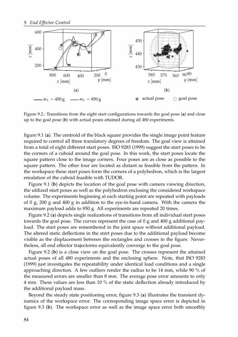
9. End Effector Control
400600800 0200
200
400
600
(a)
565575585 8090
430
440
450
(b)
x [mm]x [mm] y [mm]y [mm]
z[m
m]
z[m
m]
mL = 450 g mL = 850 g actual pose goal pose
Figure 9.2.: Transitions from the eight start configurations towards the goal pose (a) and close
up to the goal pose (b) with actual poses attained during all 480 experiments.
figure 9.1 (a). The centroid of the black square provides the single image point feature
required to control all three translatory degrees of freedom. The goal view is attained
from a total of eight different start poses. ISO 9283 (1999) suggest the start poses to be
the corners of a cuboid around the goal pose. In this work, the start poses locate the
square pattern close to the image corners. Four poses are as close as possible to the
square pattern. The other four are located as distant as feasible from the pattern. In
the workspace these start poses form the corners of a polyhedron, which is the largest
emulation of the cuboid feasible with TUDOR.
Figure 9.1 (b) depicts the location of the goal pose with camera viewing direction,
the utilized start poses as well as the polyhedron enclosing the considered workspace
volume. The experiments beginning at each starting point are repeated with payloads
of 0 g, 200 g and 400 g in addition to the eye-in-hand camera. With the camera the
maximum payload adds to 850 g. All experiments are repeated 20 times.
Figure 9.2 (a) depicts single realizations of transitions from all individual start poses
towards the goal pose. The curves represent the case of 0 g and 400 g additional pay-
load. The start poses are remembered in the joint space without additional payload.
The altered static deflections in the start poses due to the additional payload become
visible as the displacement between the rectangles and crosses in the figure. Never-
theless, all end effector trajectories equivalently converge to the goal pose.
Figure 9.2 (b) is a close view on the goal pose. The crosses represent the attained
actual poses of all 480 experiments and the enclosing sphere. Note, that ISO 9283
(1999) just investigates the repeatability under identical load conditions and a single
approaching direction. A few outliers render the radius to be 14 mm, while 90 % of
the measured errors are smaller than 8 mm. The average pose error amounts to only
4 mm. These values are less than 10 % of the static deflection already introduced by
the additional payload mass.
Beyond the steady state positioning error, figure 9.3 (a) illustrates the transient dy-
namics of the workspace error. The corresponding image space error is depicted in
figure 9.3 (b). The workspace error as well as the image space error both smoothly
84
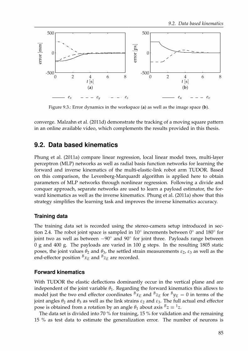
9.2. Data based kinematics
0 2 4 6 8-500
0
500
(a)
0 2 4 6 8-500
0
500
(b)
t [s]t [s]
erro
r[m
m]
erro
r[p
x]
ex ey ez eu ev
Figure 9.3.: Error dynamics in the workspace (a) as well as the image space (b).
converge. Malzahn et al. (2011d) demonstrate the tracking of a moving square pattern
in an online available video, which complements the results provided in this thesis.
9.2. Data based kinematics
Phung et al. (2011a) compare linear regression, local linear model trees, multi-layer
perceptron (MLP) networks as well as radial basis function networks for learning the
forward and inverse kinematics of the multi-elastic-link robot arm TUDOR. Based
on this comparison, the Levenberg-Marquardt algorithm is applied here to obtain
parameters of MLP networks through nonlinear regression. Following a divide and
conquer approach, separate networks are used to learn a payload estimator, the for-
ward kinematics as well as the inverse kinematics. Phung et al. (2011a) show that this
strategy simplifies the learning task and improves the inverse kinematics accuracy.
Training data
The training data set is recorded using the stereo-camera setup introduced in sec-
tion 2.4. The robot joint space is sampled in 10 increments between 0 and 180 for
joint two as well as between −90 and 90 for joint three. Payloads range between
0 g and 400 g. The payloads are varied in 100 g steps. In the resulting 1805 static
poses, the joint values θ2 and θ3, the settled strain measurements ε2, ε3 as well as the
end-effector position BxE and BzE are recorded.
Forward kinematics
With TUDOR the elastic deflections dominantly occur in the vertical plane and are
independent of the joint variable θ1. Regarding the forward kinematics this allows to
model just the two end effector coordinates BxE and BzE for ByE = 0 in terms of the
joint angles θ2 and θ3 as well as the link strains ε2 and ε3. The full actual end effector
pose is obtained from a rotation by an angle θ1 about axis Bz ≡ 1z.
The data set is divided into 70 % for training, 15 % for validation and the remaining
15 % as test data to estimate the generalization error. The number of neurons is
85
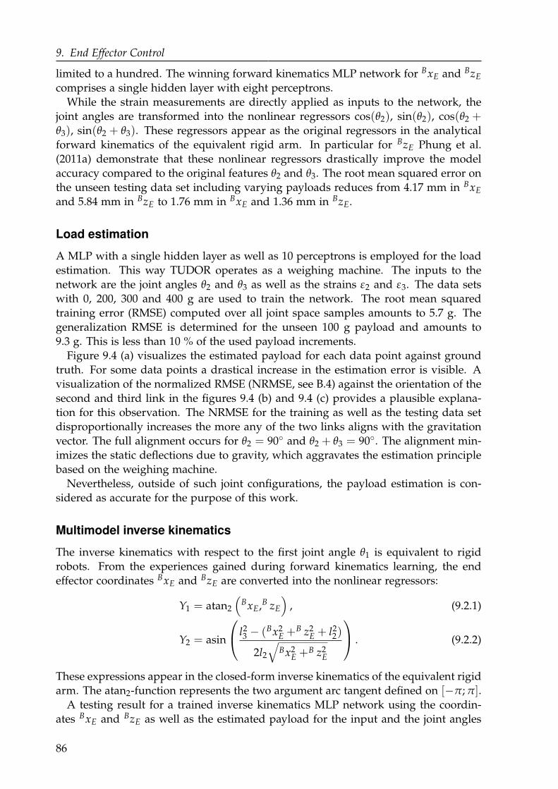
9. End Effector Control
limited to a hundred. The winning forward kinematics MLP network for BxE and BzE
comprises a single hidden layer with eight perceptrons.
While the strain measurements are directly applied as inputs to the network, the
joint angles are transformed into the nonlinear regressors cos(θ2), sin(θ2), cos(θ2 +θ3), sin(θ2 + θ3). These regressors appear as the original regressors in the analytical
forward kinematics of the equivalent rigid arm. In particular for BzE Phung et al.
(2011a) demonstrate that these nonlinear regressors drastically improve the model
accuracy compared to the original features θ2 and θ3. The root mean squared error on
the unseen testing data set including varying payloads reduces from 4.17 mm in BxE
and 5.84 mm in BzE to 1.76 mm in BxE and 1.36 mm in BzE.
Load estimation
A MLP with a single hidden layer as well as 10 perceptrons is employed for the load
estimation. This way TUDOR operates as a weighing machine. The inputs to the
network are the joint angles θ2 and θ3 as well as the strains ε2 and ε3. The data sets
with 0, 200, 300 and 400 g are used to train the network. The root mean squared
training error (RMSE) computed over all joint space samples amounts to 5.7 g. The
generalization RMSE is determined for the unseen 100 g payload and amounts to
9.3 g. This is less than 10 % of the used payload increments.
Figure 9.4 (a) visualizes the estimated payload for each data point against ground
truth. For some data points a drastical increase in the estimation error is visible. A
visualization of the normalized RMSE (NRMSE, see B.4) against the orientation of the
second and third link in the figures 9.4 (b) and 9.4 (c) provides a plausible explana-
tion for this observation. The NRMSE for the training as well as the testing data set
disproportionally increases the more any of the two links aligns with the gravitation
vector. The full alignment occurs for θ2 = 90 and θ2 + θ3 = 90. The alignment min-
imizes the static deflections due to gravity, which aggravates the estimation principle
based on the weighing machine.
Nevertheless, outside of such joint configurations, the payload estimation is con-
sidered as accurate for the purpose of this work.
Multimodel inverse kinematics
The inverse kinematics with respect to the first joint angle θ1 is equivalent to rigid
robots. From the experiences gained during forward kinematics learning, the end
effector coordinates BxE and BzE are converted into the nonlinear regressors:
Y1 = atan2
(
BxE,B zE
)
, (9.2.1)
Y2 = asin
l23 − (Bx2
E +B z2E + l2
2)
2l2
√
Bx2E +B z2
E
. (9.2.2)
These expressions appear in the closed-form inverse kinematics of the equivalent rigid
arm. The atan2-function represents the two argument arc tangent defined on [−π; π].A testing result for a trained inverse kinematics MLP network using the coordin-
ates BxE and BzE as well as the estimated payload for the input and the joint angles
86
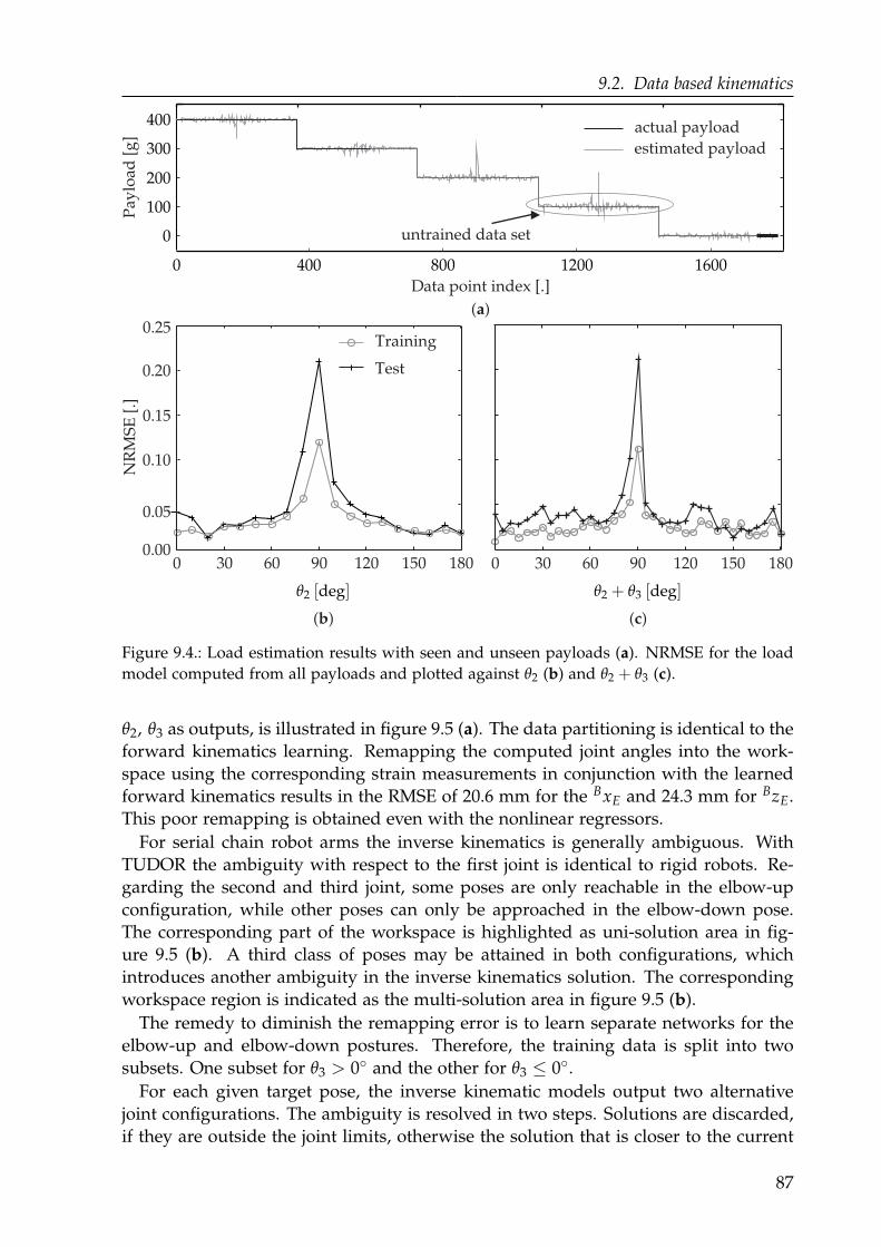
9.2. Data based kinematics
0 400 800 1200 1600
0
100
200
300
400P
aylo
ad [
g]
Data point index [.]
untrained data set
actual payloadestimated payload
NR
MSE
[.]
0.10
0.00
0.15
0.20
0.25
0.05
150 18012090300 60 150 18012090300 60
Test
Training
( )a
( )b ( )c
θ2 [deg] θ2 + θ3 [deg]
Figure 9.4.: Load estimation results with seen and unseen payloads (a). NRMSE for the load
model computed from all payloads and plotted against θ2 (b) and θ2 + θ3 (c).
θ2, θ3 as outputs, is illustrated in figure 9.5 (a). The data partitioning is identical to the
forward kinematics learning. Remapping the computed joint angles into the work-
space using the corresponding strain measurements in conjunction with the learned
forward kinematics results in the RMSE of 20.6 mm for the BxE and 24.3 mm for BzE.
This poor remapping is obtained even with the nonlinear regressors.
For serial chain robot arms the inverse kinematics is generally ambiguous. With
TUDOR the ambiguity with respect to the first joint is identical to rigid robots. Re-
garding the second and third joint, some poses are only reachable in the elbow-up
configuration, while other poses can only be approached in the elbow-down pose.
The corresponding part of the workspace is highlighted as uni-solution area in fig-
ure 9.5 (b). A third class of poses may be attained in both configurations, which
introduces another ambiguity in the inverse kinematics solution. The corresponding
workspace region is indicated as the multi-solution area in figure 9.5 (b).
The remedy to diminish the remapping error is to learn separate networks for the
elbow-up and elbow-down postures. Therefore, the training data is split into two
subsets. One subset for θ3 > 0 and the other for θ3 ≤ 0.
For each given target pose, the inverse kinematic models output two alternative
joint configurations. The ambiguity is resolved in two steps. Solutions are discarded,
if they are outside the joint limits, otherwise the solution that is closer to the current
87
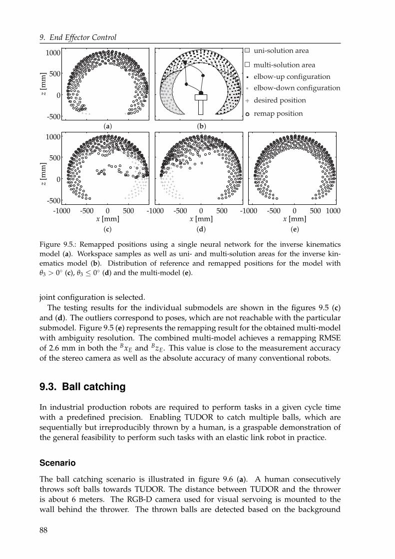
9. End Effector Control
-500
-500
0
0
1000
1000
500
500
z[m
m]
z[m
m]
-1000 0-500 500x [mm]
-1000 0 1000-500 500x [mm]
-1000 0-500 500x [mm]
( )c
( )a ( )b
( )d ( )e
uni-solution area
elbow-up configuration
elbow-down configuration
multi-solution area
desired position
remap position
Figure 9.5.: Remapped positions using a single neural network for the inverse kinematics
model (a). Workspace samples as well as uni- and multi-solution areas for the inverse kin-
ematics model (b). Distribution of reference and remapped positions for the model with
θ3 > 0 (c), θ3 ≤ 0 (d) and the multi-model (e).
joint configuration is selected.
The testing results for the individual submodels are shown in the figures 9.5 (c)
and (d). The outliers correspond to poses, which are not reachable with the particular
submodel. Figure 9.5 (e) represents the remapping result for the obtained multi-model
with ambiguity resolution. The combined multi-model achieves a remapping RMSE
of 2.6 mm in both the BxE and BzE. This value is close to the measurement accuracy
of the stereo camera as well as the absolute accuracy of many conventional robots.
9.3. Ball catching
In industrial production robots are required to perform tasks in a given cycle time
with a predefined precision. Enabling TUDOR to catch multiple balls, which are
sequentially but irreproducibly thrown by a human, is a graspable demonstration of
the general feasibility to perform such tasks with an elastic link robot in practice.
Scenario
The ball catching scenario is illustrated in figure 9.6 (a). A human consecutively
throws soft balls towards TUDOR. The distance between TUDOR and the thrower
is about 6 meters. The RGB-D camera used for visual servoing is mounted to the
wall behind the thrower. The thrown balls are detected based on the background
88
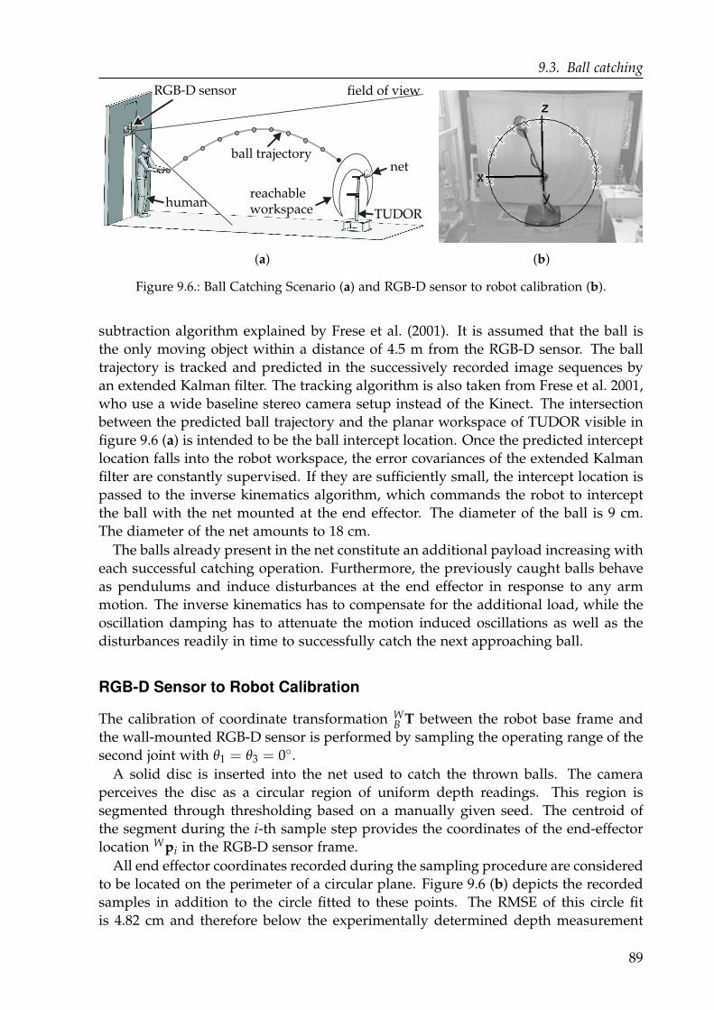
9.3. Ball catching
RGB-D sensor
ball trajectorynet
field of view
TUDORhuman
reachableworkspace
( )a ( )b
Figure 9.6.: Ball Catching Scenario (a) and RGB-D sensor to robot calibration (b).
subtraction algorithm explained by Frese et al. (2001). It is assumed that the ball is
the only moving object within a distance of 4.5 m from the RGB-D sensor. The ball
trajectory is tracked and predicted in the successively recorded image sequences by
an extended Kalman filter. The tracking algorithm is also taken from Frese et al. 2001,
who use a wide baseline stereo camera setup instead of the Kinect. The intersection
between the predicted ball trajectory and the planar workspace of TUDOR visible in
figure 9.6 (a) is intended to be the ball intercept location. Once the predicted intercept
location falls into the robot workspace, the error covariances of the extended Kalman
filter are constantly supervised. If they are sufficiently small, the intercept location is
passed to the inverse kinematics algorithm, which commands the robot to intercept
the ball with the net mounted at the end effector. The diameter of the ball is 9 cm.
The diameter of the net amounts to 18 cm.
The balls already present in the net constitute an additional payload increasing with
each successful catching operation. Furthermore, the previously caught balls behave
as pendulums and induce disturbances at the end effector in response to any arm
motion. The inverse kinematics has to compensate for the additional load, while the
oscillation damping has to attenuate the motion induced oscillations as well as the
disturbances readily in time to successfully catch the next approaching ball.
RGB-D Sensor to Robot Calibration
The calibration of coordinate transformation WB T between the robot base frame and
the wall-mounted RGB-D sensor is performed by sampling the operating range of the
second joint with θ1 = θ3 = 0.
A solid disc is inserted into the net used to catch the thrown balls. The camera
perceives the disc as a circular region of uniform depth readings. This region is
segmented through thresholding based on a manually given seed. The centroid of
the segment during the i-th sample step provides the coordinates of the end-effector
location Wpi in the RGB-D sensor frame.
All end effector coordinates recorded during the sampling procedure are considered
to be located on the perimeter of a circular plane. Figure 9.6 (b) depicts the recorded
samples in addition to the circle fitted to these points. The RMSE of this circle fit
is 4.82 cm and therefore below the experimentally determined depth measurement
89

9. End Effector Control
accuracy of the RGB-D sensor at this distance (see figure 2.5 (c)).
The center of the fitted circle constitutes the origin WoB of the robot base frame with
respect to the wall-mounted camera. The z-axis WzB of the robot base frame is the
unit vector in parallel to the connection from WoB to the end effector location Wp6 in
the straight vertical posture with [θ1, θ2, θ3]T = [0, 90, 0]T, where the arm is nearly
undeformed.
An initial estimate W yB of the y-axis RyB is the normal to the circular plane through
the circle center. The cross product WyB × WzB determines the x-axis WxB. Sub-
sequently WyB = WzB × WxB yields the orientation of the robot base frame as a right-
handed trihedron WB R = [WxB, WyB, WzB].
Catching results
A sequence of images recorded by the wall-mounted RGB-D sensor during a ball
catching experiment is illustrated in figure 9.7.
Figure 9.7 (a) sketches the boundaries of the reachable workspace. The picture
captures the instant after a first ball has been caught and right before a second ball
is thrown. The black circle marks the predicted intercept location, which for each
throw is initialized at the robot base. A history of previously sensed ball positions
as well as the updated intercept location are shown in figure 9.7 (b). It is visible
in figure 9.7 (c), that the inertia causes the previously caught ball in the net, to lag
behind the expedited end effector. In figure 9.7 (d) the robot finally positions the net
at the correctly predicted intercept location properly in time and catches the ball. The
success rate is larger than 66 %, provided that the ball trajectory intersects the robot
workspace. Malzahn et al. (2011c) provide an online available video demonstrating
the ball catching experiments with and without the active vibration damping.
90
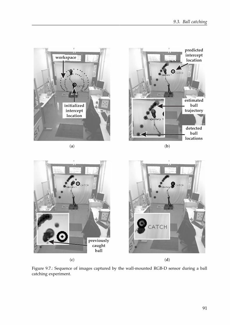
9.3. Ball catching
( )a ( )b
( )c ( )d
initializedinterceptlocation
previouslycaught
ball
detectedball
locations
workspace
predictedinterceptlocation
estimatedball
trajectory
Figure 9.7.: Sequence of images captured by the wall-mounted RGB-D sensor during a ball
catching experiment.
91
10Damped Dynamics Modelling
As a final step before exploiting link elasticity for sensing contact forces, the work
contributes two analytical real-time capable models for the remaining damped arm
dynamics in this chapter. Parts of this chapter have been previously published by
Malzahn, Reinhart and Bertram (2014).
The first model explains the joint currents. The second one models the per link
strain measurements. Both models are derived and also related to each other through
the investigation of the load torque distribution in the links. Mathematically the
model equations share exactly the same structure. A data-driven neural network
models the same outputs without any prior structural knowledge about the dynamics.
The data driven model works on exactly the same input/output data as the analytical
models and provides a benchmark for them. All models are efficiently identified using
linear regression techniques and validated by experiments with multiple payloads
under gravitational influence.
10.1. Motor current model
Consider the motor torque balance given in equation (3.1.1) using the nonlinear fric-
tion model for τF (3.1.3). The vector τJ = τL|x=0 collects the load torques the robot
arm bodies and contact torques τc exert on the individual joints according to:
τ J − τc = I(θ)θ+ C(θ, θ)θ+ g(θ). (10.1.1)
Therein I describes the symmetric positive definite robot inertia matrix. The matrix
C includes the Coriolis and centrifugal terms. The vector g represents the load torque
due to gravity.
At first, consider τc = 0. The expressions for the mechanical torque τM, the friction
torque τF as well as the load torque τJ in equation (10.1.1) are all linear in their
parameters. For parameter identification from experimental data equation (3.1.1) can
be rearranged to form the linear regression problem:
iM = Yi(θ, θ, θ) χi. (10.1.2)
The motor currents iM are measurable at each individual joint. The regressor Yi
only incorporates measurable joint angles and their derivatives. The vector χi is the
minimal set of identifiable base dynamics parameters. Khalil and Dombre (2004)
92
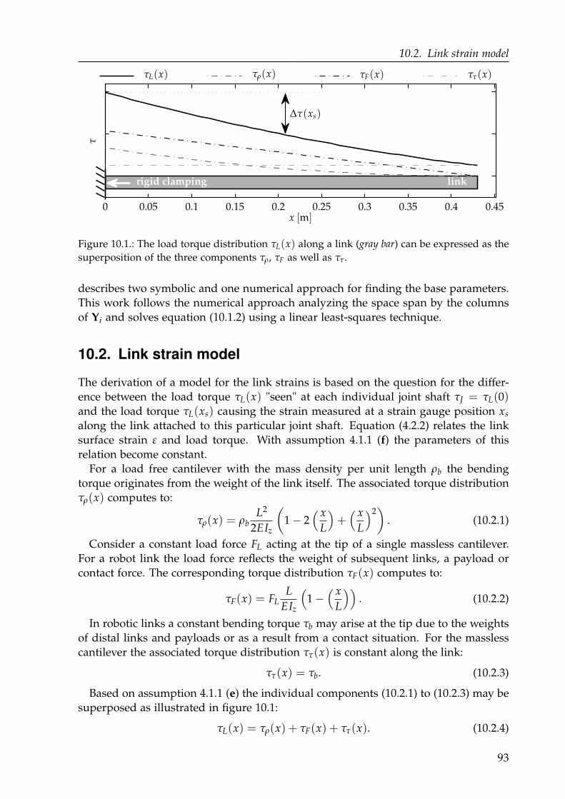
10.2. Link strain model
0 0.05 0.1 0.15 0.2 0.25 0.3 0.35 0.4 0.45
linkrigid clamping
τ
x [m]
τL(x) τρ(x) τF(x) ττ(x)
∆τ(xs)
Figure 10.1.: The load torque distribution τL(x) along a link (gray bar) can be expressed as the
superposition of the three components τρ, τF as well as ττ.
describes two symbolic and one numerical approach for finding the base parameters.
This work follows the numerical approach analyzing the space span by the columns
of Yi and solves equation (10.1.2) using a linear least-squares technique.
10.2. Link strain model
The derivation of a model for the link strains is based on the question for the differ-
ence between the load torque τL(x) "seen" at each individual joint shaft τJ = τL(0)and the load torque τL(xs) causing the strain measured at a strain gauge position xs
along the link attached to this particular joint shaft. Equation (4.2.2) relates the link
surface strain ε and load torque. With assumption 4.1.1 (f) the parameters of this
relation become constant.
For a load free cantilever with the mass density per unit length ρb the bending
torque originates from the weight of the link itself. The associated torque distribution
τρ(x) computes to:
τρ(x) = ρbL2
2EIz
(
1 − 2( x
L
)
+( x
L
)2)
. (10.2.1)
Consider a constant load force FL acting at the tip of a single massless cantilever.
For a robot link the load force reflects the weight of subsequent links, a payload or
contact force. The corresponding torque distribution τF(x) computes to:
τF(x) = FLL
EIz
(
1 −( x
L
))
. (10.2.2)
In robotic links a constant bending torque τb may arise at the tip due to the weights
of distal links and payloads or as a result from a contact situation. For the massless
cantilever the associated torque distribution ττ(x) is constant along the link:
ττ(x) = τb. (10.2.3)
Based on assumption 4.1.1 (e) the individual components (10.2.1) to (10.2.3) may be
superposed as illustrated in figure 10.1:
τL(x) = τρ(x) + τF(x) + ττ(x). (10.2.4)
93
10. Damped Dynamics Modelling
The relation models the load conditions for any link member in the kinematic chain
of a robot arm.
The torque τL(0) exerted on a single joint differs from the torque τL(xs) causing the
strain on a subsequent link in a distance xs by ∆τ:
∆τ = τL(0)− τL(xs) =ρb(xs)
EIz(xs)
(
L xs −1
2x2
s
)
+FL
EIz(xs)xs. (10.2.5)
For any particular strain sensor, the first summand is constant. The load force FL
governs the second summand. This force remains the same for any configuration of
the subsequent links. Thus, in the presence of a constant payload and in the absence
of external contact forces, the difference ∆τL is constant as well.
Under this condition there exists a linear mapping between the strain ε measured
at a location xs along the link and the load torque τJ = τL(0) acting on the joint shaft.
Combining equations (4.2.3) and (10.2.5) the mapping is:
τJ =EIz(xs)
yb(xs)ε(xs) + ∆τ. (10.2.6)
Due to the linearity of this mapping the effect of link motions on the perceived
surface strain can be described in analogy to equation (10.1.1) using exactly the same
mathematical structure:
ε(xs) = Iε(θ)θ+ Cε(θ, θ)θ+ gε(θ). (10.2.7)
where the subscript ε indicates the reference to the strain measurements. A linear
regression problem equivalent to equation (10.1.2) can be formulated with respect to
the link strains:
ε = Yε(θ, θ, θ) χε, (10.2.8)
The key difference between the equations (10.1.2) and (10.2.8) is that the latter ex-
cludes the joint parameters, most importantly the joint friction. Joint friction torques
cannot be measured directly. They have to be observed. The parameters of equa-
tion (3.1.3) frequently vary over time due to temperature dependances, changes in
lubrication, wear and tear (Bona and Indri 2005). A link strain referred dynamics
model such as equation (10.2.7) assesses the actual mechanical load set free from the
joint friction. The links with the applied strain gauges resemble load side torque
sensors.
Malzahn (2013) contributed the Matlab code written to derive the dynamics in sym-
bolic form and to automatically generate real-time compatible Simulink code as a
generic module to the Robotics Toolbox by Corke (2011).
10.3. Data-driven reference model
In the field of machine learning a broad variety of general purpose techniques for
non-linear function approximation exist. An analytical model is generally preferred
for control. Nevertheless, the capability of available data driven techniques to ap-
proximate arbitrary nonlinear functions without prior structural knowledge provides
a benchmark for the analytical models.
94
10.4. Identification
This work applies feedforward neural networks within a learning scheme known
from Huang, Zhu and Siew (2004) as Extreme Learning Machine (ELM). The data
driven reference model describes the same dynamics structure with identical inputs
and outputs as the analytical joint current as well as the link strain models derived
before, but it uses "problem agnostic" input features.
Within the ELM scheme the input weights and biases are randomly drawn from
a normal distribution. They nonlinearly project the inputs into a single high dimen-
sional hidden layer with sigmoidal activation functions. After normalization of the
input/output data the actual training is restricted to the read-out layer and consists
of simple offline linear regression. The denormalization is performed online.
The good generalization properties together with the fact that training any ELMs
comes down to a linear regression task outweighs the increased number of required
hidden neurons compared to other feedforward network types (Huang, Zhu and Siew
2006). A total of 100 neurons are used for both the current as well as the strain models
in this work.
10.4. Identification
Excitation signal
The design of optimal excitation signals for the identification of the robot dynamics
parameters is well studied in literature (Armstrong 1989). For example, band lim-
ited periodic sinusoidal signals parameterized by finite Fourier series elegantly allow
for computation of higher order measurement derivatives even in the presence of
noise (Swevers, Verdonck and Schutter 2007). The Fourier coefficients can be tuned
according to trajectory optimization criteria such as the condition numbers and sin-
gular values of the regression matrices developed in earlier works (Presse and Gautier
1993).
In the following amplitude-modulated pseudo-random binary (APRBS) stimuli (see
Isermann and Münchhof (2011, p. 174)) serve as excitation signals for the analytical
as well as the data driven models. APRBS are generic stimuli for the identification
of nonlinear systems. They are well suited for training the ELM reference networks
and result in good condition numbers and smallest singular values of the regression
matrices Yi and Yε.
Experiment design
This chapter focuses on the damped dynamics modeling of the elastic links. Without
loss of generality the first joint is therefore kept at zero position. During data ac-
quisition an individual stimulus is simultaneously applied to each of the other two
position controlled joints.
For each individual payload between mL ∈ 0 g, 100 g, 200 g, 300 g, 400 g a total
of 10 stimulus responses with a duration of 80 s are recorded at 100 Hz. The data
is subsampled to 20 Hz and randomly split into 50 % for identification and 50 %
for validation. The joint angle amplitude modulation bandwidth is one Hertz. The
amplitudes equally cover the entire joint operating range. The maximum planned
95
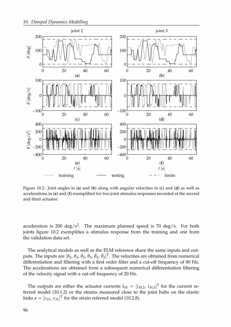
10. Damped Dynamics Modelling
0 20 40 60
0
100
200
(a)
0 20 40 60−100
0
100
(c)
0 20 40 60−400
−200
0
200
400
(e)
0 20 40 60
0
100
200
(b)
0 20 40 60−100
0
100
(d)
0 20 40 60−400
−200
0
200
400
(f)
training testing limits
joint 2 joint 3θ[d
eg]
θ[d
eg/
s]θ[d
eg/
s2]
t [s]t [s]
Figure 10.2.: Joint angles in (a) and (b) along with angular velocities in (c) and (d) as well as
accelerations in (e) and (f) exemplified for two joint stimulus responses recorded at the second
and third actuator.
acceleration is 200 deg/s2. The maximum planned speed is 70 deg/s. For both
joints figure 10.2 exemplifies a stimulus response from the training and one from
the validation data set.
The analytical models as well as the ELM reference share the same inputs and out-
puts. The inputs are [θ2, θ3, θ2, θ3, θ2, θ3]T. The velocities are obtained from numerical
differentiation and filtering with a first order filter and a cut-off frequency of 80 Hz.
The accelerations are obtained from a subsequent numerical differentiation filtering
of the velocity signal with a cut-off frequency of 20 Hz.
The outputs are either the actuator currents iM = [iM,2, iM,3]T for the current re-
ferred model (10.1.2) or the strains measured close to the joint hubs on the elastic
links ε = [ε21, ε31]T for the strain referred model (10.2.8).
96
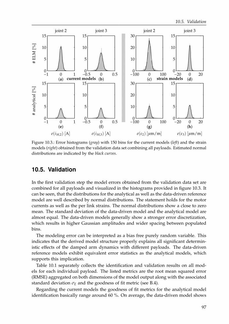
10.5. Validation
−0.5 0 0.50
5
10
15joint 3
(b)
−0.5 0 0.50
5
10
15
(f)
−100 0 1000
10
20
30
(c)
joint 2
−20 0 200
5
10
15joint 3
(d)
−20 0 200
5
10
15
(h)
−1 0 10
5
10
15
(a)
joint 2
−1 0 10
5
10
15
(e)
current models
−100 0 1000
10
20
30
(g)
strain models
#E
LM
[%]
#an
aly
tica
l[%
]
e(iM,2) [A] e(iM,3) [A] e(ε2) [µm/m] e(ε3) [µm/m]
Figure 10.3.: Error histograms (gray) with 150 bins for the current models (left) and the strain
models (right) obtained from the validation data set combining all payloads. Estimated normal
distributions are indicated by the black curves.
10.5. Validation
In the first validation step the model errors obtained from the validation data set are
combined for all payloads and visualized in the histograms provided in figure 10.3. It
can be seen, that the distributions for the analytical as well as the data-driven reference
model are well described by normal distributions. The statement holds for the motor
currents as well as the per link strains. The normal distributions show a close to zero
mean. The standard deviation of the data-driven model and the analytical model are
almost equal. The data-driven models generally show a stronger error discretization,
which results in higher Gaussian amplitudes and wider spacing between populated
bins.
The modeling error can be interpreted as a bias free purely random variable. This
indicates that the derived model structure properly explains all significant determin-
istic effects of the damped arm dynamics with different payloads. The data-driven
reference models exhibit equivalent error statistics as the analytical models, which
supports this implication.
Table 10.1 separately collects the identification and validation results on all mod-
els for each individual payload. The listed metrics are the root mean squared error
(RMSE) aggregated on both dimensions of the model output along with the associated
standard deviation σE and the goodness of fit metric (see B.4).
Regarding the current models the goodness of fit metrics for the analytical model
identification basically range around 60 %. On average, the data-driven model shows
97
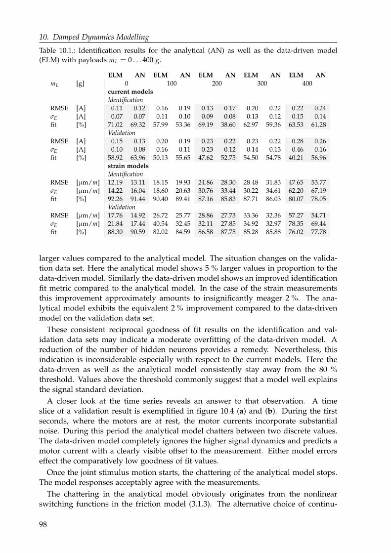
10. Damped Dynamics Modelling
Table 10.1.: Identification results for the analytical (AN) as well as the data-driven model
(ELM) with payloads mL = 0 . . . 400 g.
ELM AN ELM AN ELM AN ELM AN ELM AN
mL [g] 0 100 200 300 400current models
IdentificationRMSE [A] 0.11 0.12 0.16 0.19 0.13 0.17 0.20 0.22 0.22 0.24σE [A] 0.07 0.07 0.11 0.10 0.09 0.08 0.13 0.12 0.15 0.14fit [%] 71.02 69.32 57.99 53.36 69.19 38.60 62.97 59.36 63.53 61.28
ValidationRMSE [A] 0.15 0.13 0.20 0.19 0.23 0.22 0.23 0.22 0.28 0.26σE [A] 0.10 0.08 0.16 0.11 0.23 0.12 0.14 0.13 0.46 0.16fit [%] 58.92 63.96 50.13 55.65 47.62 52.75 54.50 54.78 40.21 56.96
strain models
IdentificationRMSE [µm/m] 12.19 13.11 18.15 19.93 24.86 28.30 28.48 31.83 47.65 53.77σE [µm/m] 14.22 16.04 18.60 20.63 30.76 33.44 30.22 34.61 62.20 67.19fit [%] 92.26 91.44 90.40 89.41 87.16 85.83 87.71 86.03 80.07 78.05
ValidationRMSE [µm/m] 17.76 14.92 26.72 25.77 28.86 27.73 33.36 32.36 57.27 54.71σE [µm/m] 21.84 17.44 40.54 32.45 32.11 27.85 34.92 32.97 78.35 69.44fit [%] 88.30 90.59 82.02 84.59 86.58 87.75 85.28 85.88 76.02 77.78
larger values compared to the analytical model. The situation changes on the valida-
tion data set. Here the analytical model shows 5 % larger values in proportion to the
data-driven model. Similarly the data-driven model shows an improved identification
fit metric compared to the analytical model. In the case of the strain measurements
this improvement approximately amounts to insignificantly meager 2 %. The ana-
lytical model exhibits the equivalent 2 % improvement compared to the data-driven
model on the validation data set.
These consistent reciprocal goodness of fit results on the identification and val-
idation data sets may indicate a moderate overfitting of the data-driven model. A
reduction of the number of hidden neurons provides a remedy. Nevertheless, this
indication is inconsiderable especially with respect to the current models. Here the
data-driven as well as the analytical model consistently stay away from the 80 %
threshold. Values above the threshold commonly suggest that a model well explains
the signal standard deviation.
A closer look at the time series reveals an answer to that observation. A time
slice of a validation result is exemplified in figure 10.4 (a) and (b). During the first
seconds, where the motors are at rest, the motor currents incorporate substantial
noise. During this period the analytical model chatters between two discrete values.
The data-driven model completely ignores the higher signal dynamics and predicts a
motor current with a clearly visible offset to the measurement. Either model errors
effect the comparatively low goodness of fit values.
Once the joint stimulus motion starts, the chattering of the analytical model stops.
The model responses acceptably agree with the measurements.
The chattering in the analytical model obviously originates from the nonlinear
switching functions in the friction model (3.1.3). The alternative choice of continu-
98
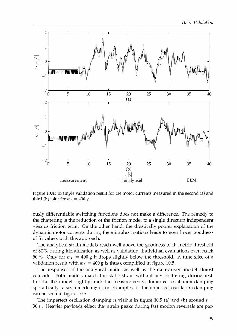
10.5. Validation
0 5 10 15 20 25 30 35 40−2
−1
0
1
2
(a)
0 5 10 15 20 25 30 35 40−2
−1
0
1
2
(b)
measurement ELM
i M,2[A
]i M
,3[A
]
t [s]
analytical
Figure 10.4.: Example validation result for the motor currents measured in the second (a) and
third (b) joint for mL = 400 g.
ously differentiable switching functions does not make a difference. The remedy to
the chattering is the reduction of the friction model to a single direction independent
viscous friction term. On the other hand, the drastically poorer explanation of the
dynamic motor currents during the stimulus motions leads to even lower goodness
of fit values with this approach.
The analytical strain models reach well above the goodness of fit metric threshold
of 80 % during identification as well as validation. Individual evaluations even reach
90 %. Only for mL = 400 g it drops slightly below the threshold. A time slice of a
validation result with mL = 400 g is thus exemplified in figure 10.5.
The responses of the analytical model as well as the data-driven model almost
coincide. Both models match the static strain without any chattering during rest.
In total the models tightly track the measurements. Imperfect oscillation damping
sporadically raises a modeling error. Examples for the imperfect oscillation damping
can be seen in figure 10.5
The imperfect oscillation damping is visible in figure 10.5 (a) and (b) around t =30 s . Heavier payloads effect that strain peaks during fast motion reversals are par-
99
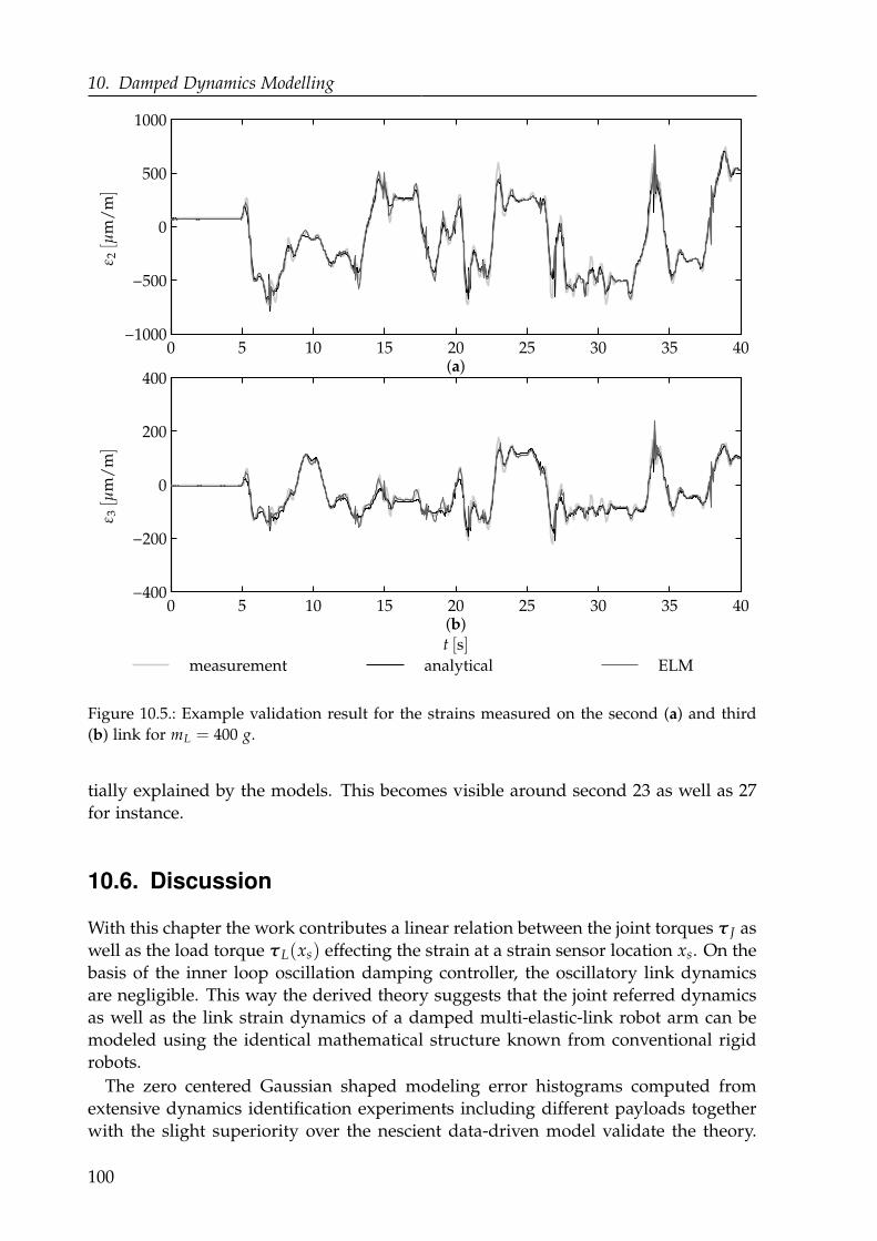
10. Damped Dynamics Modelling
0 5 10 15 20 25 30 35 40−1000
−500
0
500
1000
(a)
0 5 10 15 20 25 30 35 40−400
−200
0
200
400
(b)
measurement ELM
ε 2[µ
m/
m]
ε 3[µ
m/
m]
t [s]
analytical
Figure 10.5.: Example validation result for the strains measured on the second (a) and third
(b) link for mL = 400 g.
tially explained by the models. This becomes visible around second 23 as well as 27
for instance.
10.6. Discussion
With this chapter the work contributes a linear relation between the joint torques τ J as
well as the load torque τL(xs) effecting the strain at a strain sensor location xs. On the
basis of the inner loop oscillation damping controller, the oscillatory link dynamics
are negligible. This way the derived theory suggests that the joint referred dynamics
as well as the link strain dynamics of a damped multi-elastic-link robot arm can be
modeled using the identical mathematical structure known from conventional rigid
robots.
The zero centered Gaussian shaped modeling error histograms computed from
extensive dynamics identification experiments including different payloads together
with the slight superiority over the nescient data-driven model validate the theory.
100
10.6. Discussion
The identified analytical model is valid to explain the pivotal deterministic portion of
the strain measurements. The figures 10.4 and 10.5 emphasize that the RMSE as well
as the standard deviations presented in table 10.1 are indeed just a small fraction of
the de facto appearing signal ranges.
Equivalent statements hold for the joint current models, even though they have to
be gently alleviated. The key difference between the equations (10.1.2) and (10.2.8) is
that equation (10.1.2) includes the joint friction parameters. Tribology is a very broad
topic. In this work the friction model (3.1.3), which is widely used in robotics, has
been selected because it covers broad range of friction effects and fits into the effi-
cient linear regression framework. More sophisticated friction models, which include
phenomena such as Stribeck friction or hysteretic effects may improve the achievable
results at the cost of parameter non-linearity and aggravated identification. Note that
the friction parameters likely vary over time due to temperature dependance, wear
and tear as well as changes in lubrication (Bona and Indri 2005). Additionally the
gears show backlash. All these impact factors deteriorate the modeling accuracy. The
investigation of the individual impacts of these influence factors is a challenging topic
for future works.
The link strain models are set free from the joint friction, so that the applied strain
gauges directly operate as load side torque sensors. The derived models can be ap-
plied in real-time control such that the proposed modeling technique paves the way
for online payload estimation aiming at onward load adaptation for the inner loop os-
cillation damping controller. A further research direction is the development of direct
force control concepts.
101
11Collision Detection and Reaction
The biological inspiration by the whiskers of rodents and pinnipeds in section 1.1 con-
tributes a major motivation of the present work. It gives reasons for the hypothesis
that the intrinsic link compliance can be exploited to sense contact forces between the
robot and its environment, once the undesired oscillations and deflections have been
sufficiently compensated. The end effector control in the presence of varying static
deflections presented in chapter 9, the oscillation damping evaluated in chapter 8
along with the evident accuracy of the identified damped arm dynamics in chapter 10
strongly confirm these prerequisites to be fulfilled. The way has been paved to invest-
igate the validity of the initial hypothesis in this chapter. The following sections apply
the real-time capable damped dynamics model for the detection of accidental colli-
sions and supplement fast reaction strategies. The reaction strategies are extended to
allow intentional physical human robot interaction.
11.1. Collision detection and isolation
The collision detection is realized by the computation of an appropriate residual sig-
nal. This section introduces and discusses two such residuals.
Direct Strain Residual
The identified strain referred damped dynamics model computes an expectation for
the strain measurements at each time step. Unexpected collisions between the ro-
bot and its environment cause a discrepancy between the expectation and the actual
measurement. A quantitative measure of discrepancy is the direct strain residual:
rε = ε − Iε(θ)θ− Cε(θ, θ)θ− gε(θ). (11.1.1)
The residual vector rε indicates a collision, if the absolute value of any element exceeds
a predefined threshold. The directional information is contained in the sign of the
particular elements. The link involved in the collision can be determined as the last
link in the kinematic chain showing the threshold violation.
The major difficulty of this straightforward residual design lies in the requirement
of the joint angular acceleration to be available. In this work the joint angular accel-
eration is computed through double differentiation of the encoder readings. The res-
102
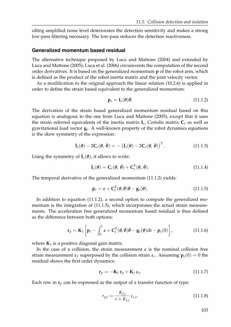
11.1. Collision detection and isolation
ulting amplified noise level deteriorates the detection sensitivity and makes a strong
low-pass filtering necessary. The low-pass reduces the detection reactiveness.
Generalized momentum based residual
The alternative technique proposed by Luca and Mattone (2004) and extended by
Luca and Mattone (2005); Luca et al. (2006) circumvents the computation of the second
order derivatives. It is based on the generalized momentum p of the robot arm, which
is defined as the product of the robot inertia matrix and the joint velocity vector.
As a modification to the original approach the linear relation (10.2.6) is applied in
order to define the strain based equivalent to the generalized momentum:
pε = Iε(θ)θ. (11.1.2)
The derivation of the strain based generalized momentum residual based on this
equation is analogous to the one from Luca and Mattone (2005), except that it uses
the strain referred equivalents of the inertia matrix Iε, Coriolis matrix Cε as well as
gravitational load vector gε. A well-known property of the robot dynamics equations
is the skew symmetry of the expression:
Iε(θ)− 2Cε(θ, θ) = −(
Iε(θ)− 2Cε(θ, θ))T
. (11.1.3)
Using the symmetry of Iε(θ), it allows to write:
Iε(θ) = Cε(θ, θ) + CTε (θ, θ). (11.1.4)
The temporal derivative of the generalized momentum (11.1.2) yields:
pε = ε + CTε (θ, θ)θ− gε(θ). (11.1.5)
In addition to equation (11.1.2), a second option to compute the generalized mo-
mentum is the integration of (11.1.5), which incorporates the actual strain measure-
ments. The acceleration free generalized momentum based residual is thus defined
as the difference between both options:
rp = KI
[
pε −∫ t
0ε + CT
ε (θ, θ)θ− gε(θ)dt− pε(0)
]
, (11.1.6)
where KI is a positive diagonal gain matrix.
In the case of a collision, the strain measurement ε is the nominal collision free
strain measurement ε f superposed by the collision strain εc. Assuming pε(0) = 0 the
residual shows the first order dynamics:
rp = −KI rp + KI εc. (11.1.7)
Each row in rp can be expressed as the output of a transfer function of type:
rp,i =KI,i
s + KI,iεc,i. (11.1.8)
103
11. Collision Detection and Reaction
−20 −10 0 10 200
2
4
6
(a)−10 −5 0 5 100
2
4
6
(b)
rela
tiv
eo
ccu
rren
ce[%
]
rp,2 [µm/m] rp,3 [µm/m]
Figure 11.1.: Generalized momentum residual histogram with 75 bins computed on the whole
validation data set described in section 10.5. Estimated gaussian distribution (solid black) as
well as six sigma detection thresholds (dashed black).
From this transfer function the residual may be interpreted as the strain measurement
filtered by a first order filter. Most importantly, the residual involves numerical in-
tegration, but it is stationary for static contacts and drops back to zero for vanishing
collision strain. This is crucial for the residual based collision reaction in section 11.2.
The isolation of the collided link works identically to the direct strain residual rε dis-
cussed before. Again, the absolute residual values indicate whether a collision has
occurred, while the sign carries the directional information.
The cut-off frequencies are tunable through KI and trade off the detection reactive-
ness and noise sensitivity. Compared to the low-pass filtering required for the direct
strain alternative, the absence of a second order numerical derivative enables larger
cut-off frequencies on behalf of an improved detection reactiveness. Therefore, the
generalized momentum based collision detection is employed in this work.
Tuning thresholds
Next to the measurement noise, the dynamics model accuracy dominates the tuning
of the residual thresholds and hence, the collision detection sensitivity. Figure 11.1
shows the histograms for the generalized momentum based residual. The histograms
are computed on the whole validation data set as described in section 10.5. It includes
the results for all test payloads between 0 g and 400 g.
Both histograms are well approximated by the estimated Gaussians. Only the his-
togram for the third joint-link module shows a slightly irregular error accumulation
around −1.3 µm/m. The detection thresholds are chosen to be six times the standard
deviation identified from the Gaussian distribution estimated on each residual. This
way, the irregular error accumulation of the third joint-link-module does not have any
practical impact on the collision detection.
Luca and Mattone (2004) propose an adaptive thresholding technique for collision
detection. It has been successfully applied to conventional rigid link and elastic joint
robots. The transfer to the elastic link case is left for future investigations.
104
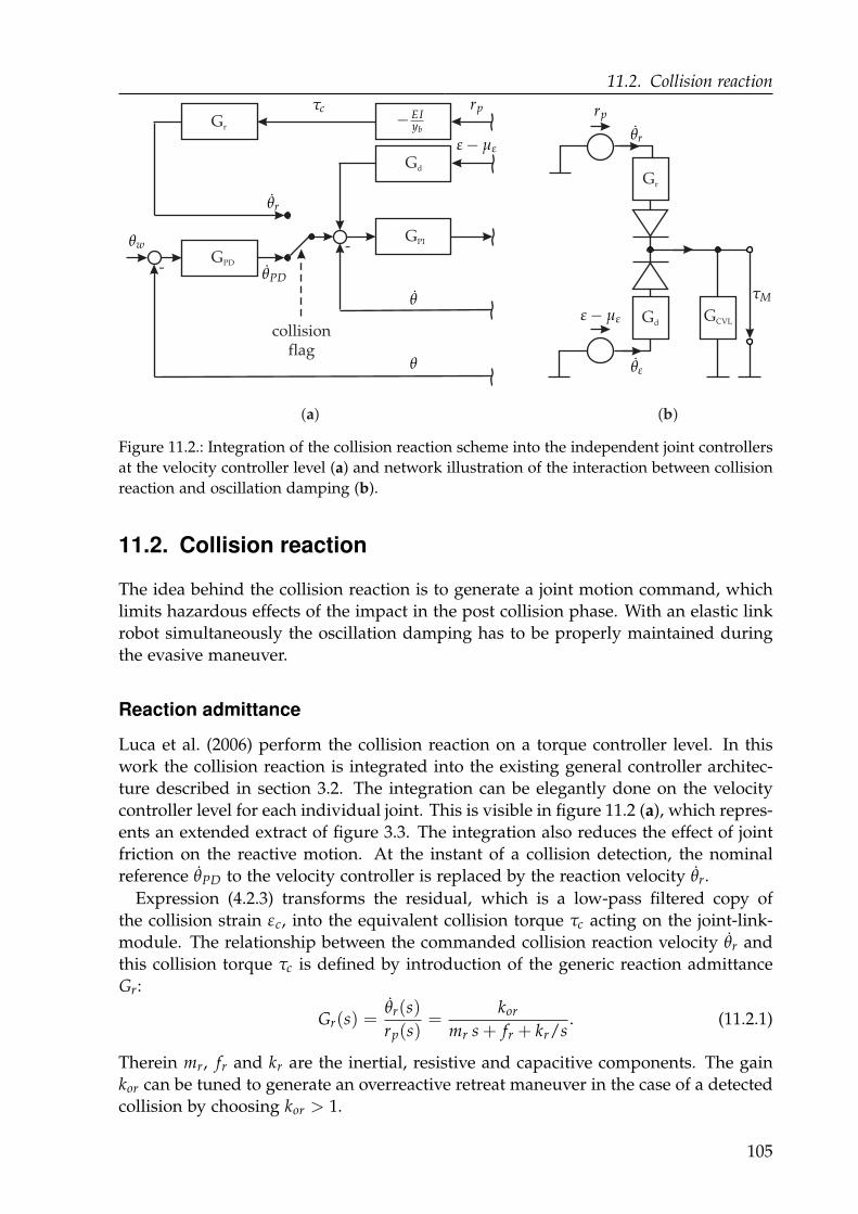
11.2. Collision reaction
( )a
-
collisionflag
GPI
-GPD
Gr
Gd
( )b
Gd
Gr
GCVL
θw
θ
θε − µε
ε − µε
rprp
θr
θr
θPD
θε
τM
τc− EI
yb
Figure 11.2.: Integration of the collision reaction scheme into the independent joint controllers
at the velocity controller level (a) and network illustration of the interaction between collision
reaction and oscillation damping (b).
11.2. Collision reaction
The idea behind the collision reaction is to generate a joint motion command, which
limits hazardous effects of the impact in the post collision phase. With an elastic link
robot simultaneously the oscillation damping has to be properly maintained during
the evasive maneuver.
Reaction admittance
Luca et al. (2006) perform the collision reaction on a torque controller level. In this
work the collision reaction is integrated into the existing general controller architec-
ture described in section 3.2. The integration can be elegantly done on the velocity
controller level for each individual joint. This is visible in figure 11.2 (a), which repres-
ents an extended extract of figure 3.3. The integration also reduces the effect of joint
friction on the reactive motion. At the instant of a collision detection, the nominal
reference θPD to the velocity controller is replaced by the reaction velocity θr.
Expression (4.2.3) transforms the residual, which is a low-pass filtered copy of
the collision strain εc, into the equivalent collision torque τc acting on the joint-link-
module. The relationship between the commanded collision reaction velocity θr and
this collision torque τc is defined by introduction of the generic reaction admittance
Gr:
Gr(s) =θr(s)
rp(s)=
kor
mr s + fr + kr/s. (11.2.1)
Therein mr, fr and kr are the inertial, resistive and capacitive components. The gain
kor can be tuned to generate an overreactive retreat maneuver in the case of a detected
collision by choosing kor > 1.
105
11. Collision Detection and Reaction
During the post collision phase the total input to the velocity controlled joint-link-
module GCVL originates from two branches of the network diagram 11.2 (b). It is
driven by two sources: the residual source with the effort variable rp in the upper
branch as well as the oscillation source with the effort ε − µε in the lower branch. The
reaction admittance Gr as well as the damping admittance Gd convert the efforts into
the flow variables θr and θd, which add to the velocity controller input flow.
Even though a collision inevitably excites oscillations on one hand and strong os-
cillations yield non-zero residuals on the other hand, both branches can be seen as
decoupled from each other. The oscillation feedback with damping admittance Gd
has been shown to stably suppress oscillations irrespective of their origin. The resid-
ual is stationary during contact and vanishes with the collision strain. Thus, with a
stable reaction admittance Gr, the stability of the total damped system with integrated
collision reaction is plausible.
Reaction strategies
A variety of reaction strategies are considerable. Three choices are exemplified with
the multi-elastic-link arm TUDOR in this work.
Just stop: The simplest reaction strategy is to just stop all motions by commanding
θr = 0.
Reflex behavior: The directional information encoded in the sign of the residual is em-
ployed to implement an escaping reflex behavior. This is achieved by choosing
small inertial mr and friction fr parameters, while the spring constant kr is set
to zero. With this setting the robot mimics a small mass gliding on a low fric-
tion surface and colliding with a presumably larger mass. As a result the robot
bounces back from any collision point. An overreaction gain kor > 1 amplifies
this behavior.
Physical interaction mode: During a physical interaction such as a kinesthetic teaching
scenario, the human operator desires to easily reconfigure the arm. This can be
achieved by setting the overreaction gain kor = 1 and the spring constant kr = 0.
The inertial mr and friction fr parameters are tuned to provide a convenient
haptic feedback to the operator. This tuning however depends on the particular
task to be taught as well as the individual user preferences.
11.3. Experimental results
This section provides experimental results for the collision detection and reaction for
blunt as well as sharp impacts and physical interaction with a human. Additional
results are provided in appendix C. The experiments utilize the force sensing contact
cube described in subsection 2.4.
106
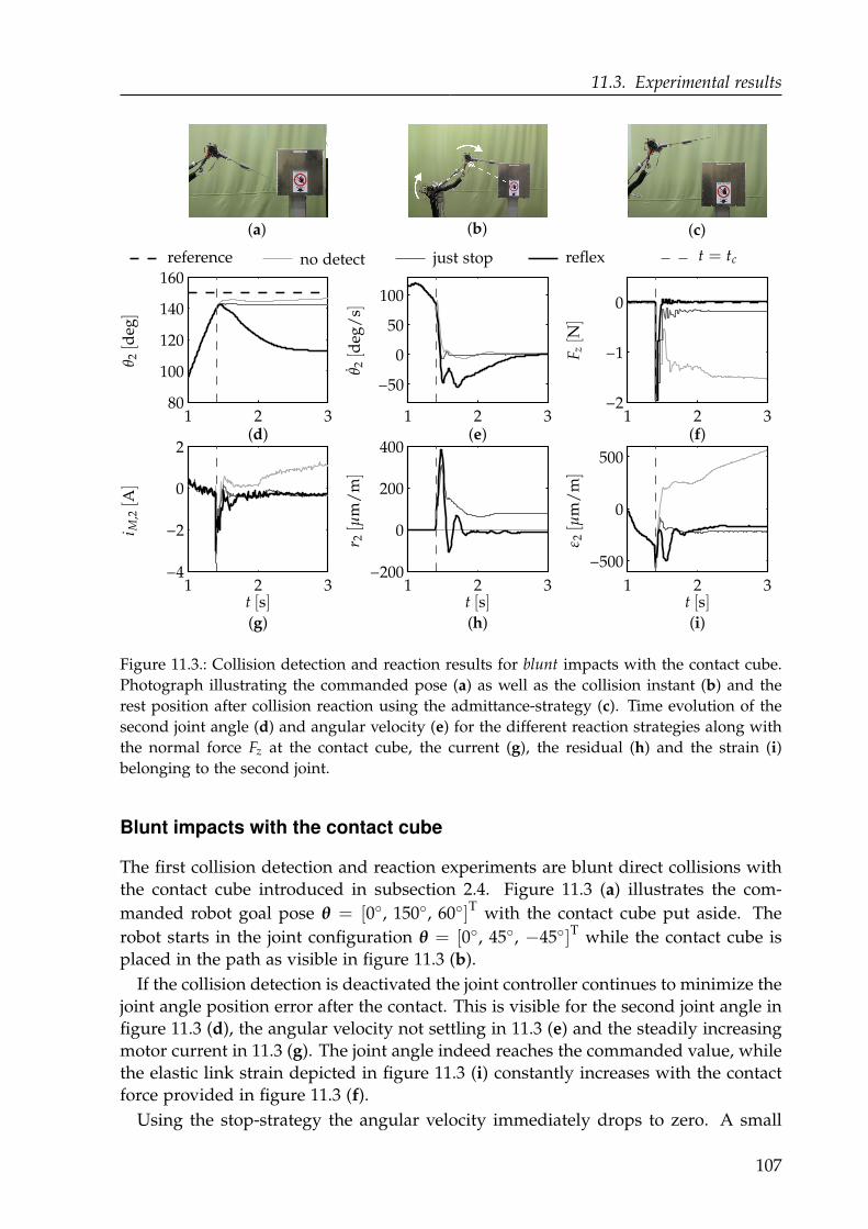
11.3. Experimental results
(a) (b) (c)
1 2 380
100
120
140
160
(d)1 2 3
−50
0
50
100
(e)1 2 3
−2
−1
0
(f)
1 2 3−4
−2
0
2
(g)
1 2 3−200
0
200
400
(h)
1 2 3
−500
0
500
(i)
reference
t [s]t [s]t [s]
θ 2[d
eg]
θ 2[d
eg/
s]
F z[N
]
i M,2[A
]
r 2[µ
m/
m]
ε 2[µ
m/
m]
just stop reflexno detect t = tc
Figure 11.3.: Collision detection and reaction results for blunt impacts with the contact cube.
Photograph illustrating the commanded pose (a) as well as the collision instant (b) and the
rest position after collision reaction using the admittance-strategy (c). Time evolution of the
second joint angle (d) and angular velocity (e) for the different reaction strategies along with
the normal force Fz at the contact cube, the current (g), the residual (h) and the strain (i)
belonging to the second joint.
Blunt impacts with the contact cube
The first collision detection and reaction experiments are blunt direct collisions with
the contact cube introduced in subsection 2.4. Figure 11.3 (a) illustrates the com-
manded robot goal pose θ = [0, 150, 60]T with the contact cube put aside. The
robot starts in the joint configuration θ = [0, 45, −45]T while the contact cube is
placed in the path as visible in figure 11.3 (b).
If the collision detection is deactivated the joint controller continues to minimize the
joint angle position error after the contact. This is visible for the second joint angle in
figure 11.3 (d), the angular velocity not settling in 11.3 (e) and the steadily increasing
motor current in 11.3 (g). The joint angle indeed reaches the commanded value, while
the elastic link strain depicted in figure 11.3 (i) constantly increases with the contact
force provided in figure 11.3 (f).
Using the stop-strategy the angular velocity immediately drops to zero. A small
107
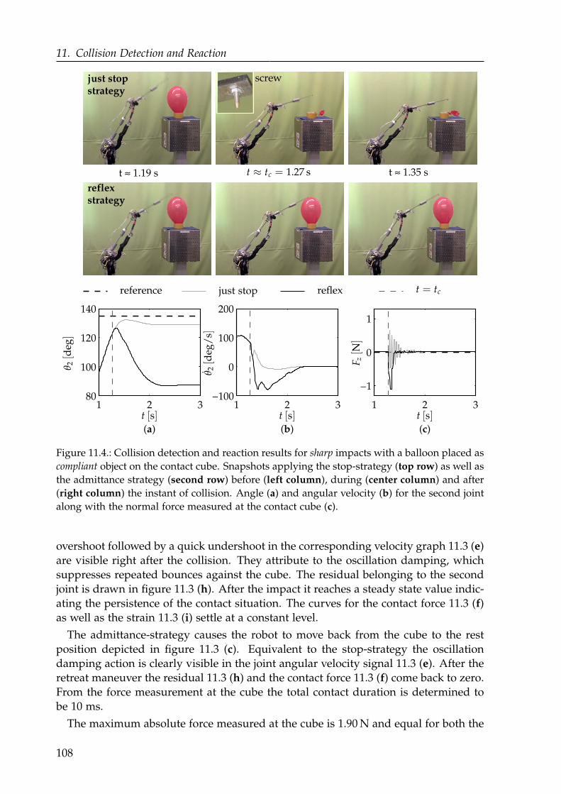
11. Collision Detection and Reaction
1 2 380
100
120
140
(a)
1 2 3−100
0
100
200
(b)
1 2 3
−1
0
1
(c)
just stopstrategy
reflexstrategy
reference
t ≈ 1.19 s t ≈ 1.35 s
screw
t [s]t [s]t [s]
θ 2[d
eg]
θ 2[d
eg/
s]
F z[N
]
t ≈ tc = 1.27 s
just stop t = tcreflex
Figure 11.4.: Collision detection and reaction results for sharp impacts with a balloon placed as
compliant object on the contact cube. Snapshots applying the stop-strategy (top row) as well as
the admittance strategy (second row) before (left column), during (center column) and after
(right column) the instant of collision. Angle (a) and angular velocity (b) for the second joint
along with the normal force measured at the contact cube (c).
overshoot followed by a quick undershoot in the corresponding velocity graph 11.3 (e)
are visible right after the collision. They attribute to the oscillation damping, which
suppresses repeated bounces against the cube. The residual belonging to the second
joint is drawn in figure 11.3 (h). After the impact it reaches a steady state value indic-
ating the persistence of the contact situation. The curves for the contact force 11.3 (f)
as well as the strain 11.3 (i) settle at a constant level.
The admittance-strategy causes the robot to move back from the cube to the rest
position depicted in figure 11.3 (c). Equivalent to the stop-strategy the oscillation
damping action is clearly visible in the joint angular velocity signal 11.3 (e). After the
retreat maneuver the residual 11.3 (h) and the contact force 11.3 (f) come back to zero.
From the force measurement at the cube the total contact duration is determined to
be 10 ms.
The maximum absolute force measured at the cube is 1.90 N and equal for both the
108
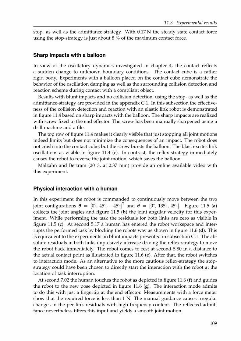
11.3. Experimental results
stop- as well as the admittance-strategy. With 0.17 N the steady state contact force
using the stop-strategy is just about 8 % of the maximum contact force.
Sharp impacts with a balloon
In view of the oscillatory dynamics investigated in chapter 4, the contact reflects
a sudden change to unknown boundary conditions. The contact cube is a rather
rigid body. Experiments with a balloon placed on the contact cube demonstrate the
behavior of the oscillation damping as well as the surrounding collision detection and
reaction scheme during contact with a compliant object.
Results with blunt impacts and no collision detection, using the stop- as well as the
admittance-strategy are provided in the appendix C.1. In this subsection the effective-
ness of the collision detection and reaction with an elastic link robot is demonstrated
in figure 11.4 based on sharp impacts with the balloon. The sharp impacts are realized
with screw fixed to the end effector. The screw has been manually sharpened using a
drill machine and a file.
The top row of figure 11.4 makes it clearly visible that just stopping all joint motions
indeed limits but does not minimize the consequences of an impact. The robot does
not crash into the contact cube, but the screw bursts the balloon. The blast excites link
oscillations as visible in figure 11.4 (c). In contrast, the reflex strategy immediately
causes the robot to reverse the joint motion, which saves the balloon.
Malzahn and Bertram (2013, at 2:37 min) provide an online available video with
this experiment.
Physical interaction with a human
In this experiment the robot is commanded to continuously move between the two
joint configurations θ = [0, 45, −45]T and θ = [0, 135, 45]. Figure 11.5 (a)
collects the joint angles and figure 11.5 (b) the joint angular velocity for this exper-
iment. While performing the task the residuals for both links are zero as visible in
figure 11.5 (c). At second 5.17 a human has entered the robot workspace and inter-
rupts the performed task by blocking the robots way as shown in figure 11.6 (d). This
is equivalent to the experiments on blunt impacts presented in subsection C.1. The ab-
solute residuals in both links impulsively increase driving the reflex-strategy to move
the robot back immediately. The robot comes to rest at second 5.80 in a distance to
the actual contact point as illustrated in figure 11.6 (e). After that, the robot switches
to interaction mode. As an alternative to the more cautious reflex-strategy the stop-
strategy could have been chosen to directly start the interaction with the robot at the
location of task interruption.
At second 7.02 the human touches the robot as depicted in figure 11.6 (f) and guides
the robot to the new pose depicted in figure 11.6 (g). The interaction mode admits
to do this with just a fingertip at the end effector. Measurements with a force meter
show that the required force is less than 1 N. The manual guidance causes irregular
changes in the per link residuals with high frequency content. The reflected admit-
tance nevertheless filters this input and yields a smooth joint motion.
109
11. Collision Detection and Reaction
0 5 10 15 20 25 30−100
0
100
200
(a)
0 5 10 15 20 25 30
−100
0
100
(b)
0 5 10 15 20 25 30−200
0
200
(c)
(d)(e)
(f) (g) (h) (i)(j)
(k)(l)
(m) (n) (o)
joint2 joint3 snapshot
t [s]
θ[d
eg]
θ[d
eg/
s]r[µ
m/
m]
Figure 11.5.: Measurements for the joint angles (a), joint velocities (b) and residuals (c) during
physical human-robot-interaction. The marked time instants correspond to the snapshots
presented in figure 11.6 (d)-(o).
In the next step multiple contacts occur. The generalized momentum based ap-
proach yields decoupled residuals for each link and isolates the individual contacts
as long as the contact force vector has a component normal to the preceding links.
This allows for independent contact reactions on each link. To demonstrate this, the
human places another finger at the end of the second link and reverses the inter-
action force exerted at the end effector around second 9.83. The action results in a
reconfiguration from the elbow-up to the elbow-down pose shown in figure 11.6 (h).
Back in the elbow-up pose (see figure 11.6 (i)), an impulsive interaction force at
the end effector is directed in parallel to the third link. This way, the human shoves
the robot without significantly altering the relative configuration between the second
and third joint as visible in figure 11.6 (j). The impulsive interaction is visible in the
residual for the second joint only.
A short time after the shove the robot comes to rest at the joint configuration shown
in figure 11.6 (k). The distance travelled in response to the shove can be arbitrarily ad-
justed to the human’s requests in a broad range through the virtual friction modeled
110

11.3. Experimental results
t =
5.1
7 s
(d)
t =
5.8
0 s
(e)
t =
7.0
2 s
(f)
t =
10.
12 s
(g)
t =
13.
77 s
(h)
t =
16.
12 s
(i)
t =
17.
35 s
(j)
t =
17.
99 s
(k)
t =
20.
50 s
(l)
t =
21.
36 s
(m)
t =
24.
60 s
(n)
t =
26.
35 s
(o)
Fig
ure
11.6
.:S
nap
sho
tso
fth
ep
arti
cula
rti
me
inst
ants
du
rin
gth
ep
hy
sica
lh
um
an-r
ob
ot-
inte
ract
ion
s(d
)-(o
).T
he
snap
sho
tsco
rres
po
nd
toth
e
das
hed
lin
esin
fig
ure
11.5
.
111
11. Collision Detection and Reaction
in the interaction admittance.
The transition between the figures 11.6 (k) and (l) supplements the previous demon-
stration of the contact isolation. The robot can not only be guided by a contact at the
end effector, but also by pushing at the end of the second link. The figures 11.6 (k)
and (l) exemplify the reconfiguration between the elbow-up and elbow-down pose in
the other half of the robot workspace. The shove from figure 11.6 (n) to (o) mirrors
the previous example. Finally figure 11.6 (o) illustrates the interaction by grasping
the second arm in the vicinity of the strain gauges close to the joint.
Malzahn and Bertram (2013, at 3:47 min) provide an online available video with
this experiment.
11.4. Discussion
The chapter experimentally demonstrates the collision detection and reaction with
a multi-elastic-link robot arm under gravitational influence. This way, it puts the
biological inspiration drawn from the whiskers of rodents and pinnipeds into real
practice.
The experimental results demonstrate different reaction strategies. Each presen-
ted strategy has its merits and shortcomings. During constrained collisions the stop
strategy would mean that a person or object will remain clamped between the robot
and the constraining surface. Any contact force would persist and potentially exper-
ienced as a threat to a human. The alternative reflex behavior causes the robot to
bounce back from any collision point. While the balloon experiment descriptively
demonstrates the improved sensitivity of this approach, the challenge is to tune the
parameters of bouncing behavior. Consider a service robot carrying a cup of coffee.
If the escape motion is too dynamic, the robot would spill the coffee or cause new
collisions. Furthermore, after the danger of collision is successfully averted, the robot
should finish the originally given task.
The appropriate strategy selection and tuning is a challenging research direction,
which involves higher level cognition, situation awareness and reasoning performed
by the robot.
With this chapter the present work proves for the first time the practical feasibility to
provide the required low level functionalities for such higher level decision processes
with a multi-elastic-link robot arm. Up to now this has only been achieved with
elastic joint robots. It ennobles intrinsic link elasticity from "just a problem" to a
factual opportunity for physical interaction between the robot and its environment.
112
12Conclusion and Outlook
Link elasticity is frequently considered an undesired effect in the mechanical design of
robot arms and comparable machines. The driving motivation behind this work ori-
ginates from the contrary perspective of exploiting the intrinsic compliance to grant
elastic link robots force sensing capabilities and to simultaneously reduce the over-
all arm masses. The underlying hypothesis proposes that link elasticity is not ne-
cessarily just a problem, which degrades positioning accuracy and prolongs settling
times. The thesis contributes new theoretical concepts confirmed by extensive exper-
imental results in the fields of oscillation damping and end effector positioning for
a multi-elastic-link arm in the presence of load and joint configuration dependent
static deflections under gravity. On top of that, the work practically demonstrates the
general feasibility of detecting and reacting to external contact forces with a multi-
elastic-link robot operating under gravity. The contact scenarios include unpredicted
or accidental collisions between the robot and the environment as well as intentional
contacts for physical human robot interaction. A guideline, which summarizes the
major steps required to deploy the techniques developed in this thesis, is provided in
appendix D.
Experimental setup and arm dynamics
Multi-elastic-link robots operating under gravitational influence, which allow to test
devised modeling and control algorithms in real experiments, are very rare. There-
fore, the work starts from scratch with the development of an experimental setup. The
complete experimental system consists of the three degree of freedom robot TUDOR
along with external sensory equipment to assess the true end effector position and
contact forces as reference.
The work comprises a comprehensive literature review and contributes an investig-
ation towards the sensitivity of the plant dynamics with respect to joint configuration
and payload changes, the effect of backlash and imperfect link clamping as well as
generally unknown boundary conditions during physical contacts with the environ-
ment. The theoretical investigation is supported by extensive experiments.
With the gained insights the present work proposes a decentralized control archi-
tecture. The kinematic chain is subdivided into independent joint link modules, for
which joint angular and oscillation damping controllers are individually tuned.
113
12. Conclusion and Outlook
Oscillation damping control
Three different approaches for strain based oscillation damping are investigated. All
three approaches are set free from a computation of the plant dynamics at runtime or
the explicit knowledge of all boundary conditions.
The first proposed oscillation damping controller utilizes a truncated model of the
oscillatory dynamics and is devised using the root locus method applied to the lin-
earized plant. The second approach has originally been proposed by O’Connor and
identifies wave propagation properties in a lumped parameter model. This thesis
contributes a unified view on both approaches by revealing their identical controller
structure with minor differences in the parameter tuning. The third proposed con-
trol approach considers the distributed nature as well as continuous wave dynamics
of elastic beams and waives the need for any truncation or discretization. Structural
similarities with the previous approaches suggest that it represents a frequency ad-
aptive generalization of these schemes. A thorough theoretical investigation with the
objective of deriving a global unified view on wave based controllers for elastic link
robots is a promising future research direction.
The work contributes the derivation, practical application and comparison of the
individual oscillation damping concepts at different levels within the underlying cas-
caded joint angular controller. As a conclusion the oscillation damping controllers
operating on the velocity level prove to be most robust with respect to imperfect static
strain cancellations in the presence of gravitational influences and joint friction. At
the same time they have the least impact on the overall joint positioning behavior.
As a concluding remark, full integral strain feedback laws for elastic-link robots un-
der gravitational influence are definitely not recommended. Imperfect static strain
cancellations yield growing steady state errors and deteriorate repeatability.
All presented concepts effect a rapid decay of structural oscillations induced by joint
accelerations and step-like or periodic disturbances, even near resonance. All these
results are robust to the backlash present in the gears. Of course, more homogenous
experimental results can be expected throughout the entire workspace, if backlash can
be eliminated by hardware.
This thesis focuses on multi-elastic-link arms, which predominantly oscillate in a
single plane. Future research should be concerned with the extension of the presented
oscillation damping controllers to multiple planes of oscillation. A major challenge
to solve in this case is to maintain the controllability of the oscillatory degrees of
freedom. One option is to avoid uncontrollable joint configurations in analogy to
kinematic singularities. In contrast, it should be asked and investigated, if an elastic
link robot with multiple planes of oscillations can be designed without the existence of
such configurations. In fact, the present work already illustrates that a single joint link
module can be used to dampen oscillations in distant joint-link-modules. Exploiting
inter module couplings could be a key.
End effector position control
With the readily damped oscillations, the divide and conquer strategy to the control
of elastic link robot arms already pays off in regard to the end effector positioning.
114

Only the static deflections remain to be compensated in comparison to conventional
arms. The thesis presents two methods to solve the end effector positioning task. The
first approach is a visual servoing technique, which preserves the idea of relying on
only marginal model knowledge during the controller design. Well established visual
servoing control schemes minimize the relative pose error between a current and a
desired view of the scene. To approach the goal view they command the direction
of rotation for each individual joint through the differential robot kinematics. The
work demonstrates the sufficiency of the differential kinematics approximation for
the elastic link arm TUDOR on the basis of the equivalent rigid robot Jacobian.
In spite of the elegance and minimal modeling efforts associated with the visual
servoing approach, a shortcoming is the dependance of the control result on the actual
scene structure, which has to be adequately rich in visual features. This motivates the
second positioning concept proposed in this work. It is based on the data driven
learning of the forward and inverse kinematics along with a payload estimator using
MLP neural networks. The key to obtain precise models is to transform the original
input features into nonlinear features using the regressors known from the analytical
rigid body forward and inverse kinematics. In the case of the inverse kinematics the
estimated payload is an additional aggregated feature.
A conventional six degree of freedom robot arm usually provides up to sixteen solu-
tions for a given pose within the dexterous workspace. The ambiguity is resolved by
selecting the feasible solution being the closest to the current joint configuration. Sim-
ilar to that the ambiguity resolution in the inverse kinematics of TUDOR is achieved
by the multi-model approach, in which one dedicated model is trained for the elbow-
up and elbow-down postures.
The work exemplifies the speed and accuracy of the kinematics model in conjunc-
tion with the underlying oscillation damping controller by realizing ball catching ex-
periments with a multi-elastic-link robot arm. The balls are sequentially but irrepro-
ducibly thrown by a human. The robot intercepts the ball with a net at the piercing
point of the ball trajectory with the robot workspace.
Since the successful experiments contribute a major step regarding point-to-point
maneuvers, future works should be dedicated to extensions for precise trajectory con-
trol of multi-elastic-link arms under gravity. Looking at the actually rather imprecise
human motion apparatus it becomes apparent that a lot of human skills emerge from
learned and continuously adapted perception-action-mappings working in a feed-
forward sense. From this inspiration, it can be expected that the augmentation of the
controllers devised in this work by suitable feed-forward schemes leads to fruitful
results. Additionally, the work has proven that the link strains as well as the joint
angles carry the required information to compute the forward and inverse kinemat-
ics. Since analytical solutions are favorable, investigations to derive them should be
pushed forward in this direction by continuing research.
Collision detection and physical interaction
The oscillation damping and the end effector positioning address the originally un-
desired challenges associated with link elasticity. The accomplished results finally
allow for the investigation of the suspected potentials in this thesis. The conducted
115
12. Conclusion and Outlook
investigations reveal a linear relationship between the damped link strains and the
joint load torques. The main difference originates from the friction present in the
joints. In the absence of friction, the link strains could be directly transformed into
the actuator electrical torques and vice versa. The linear mapping is valid in the whole
workspace for a constant given payload.
The mathematical structure of the joint referred arm dynamics known from con-
ventional rigid robots can be directly applied to describe the strain referred damped
arm dynamics. As a consequence, collision detection and reaction schemes origin-
ally developed for rigid and elastic joint robots may be straightly applied to damped
elastic link robots. The work verifies these findings in illustrative experiments includ-
ing blunt and also sharp collisions with intrinsically compliant or fragile objects as
well as a human arm. A stopping and a reflex behavior is implemented as reaction
strategy to detected collisions. Both strategies are shown to visibly reduce the harm
potential of an unforeseen impact situation with a variety of contact impedances.
Beyond the detection and reaction to accidental collisions the work demonstrates
how the force sensing capabilities may be extended to switch the robot into a back-
drivable mode. This enables intentional physical human robot interaction such as
kinesthetic teaching of frequently varying tasks by a non-robotic specialist.
A consequential next step for future work is to take advantage of the force sensing
capabilities evidenced in this work for analytical payload identification. This will help
to automatically adapt the collision detection scheme and to even improve the oscil-
lation damping as well as end effector positioning results. The controllers proposed
in the present work enable ongoing research to be engaged with the development of
direct and hybrid force controllers with a multi-elastic-link robot.
Conclusion
Within the big picture of the affordable and intrinsically safe "household automaton
[...] about the price of a good automobile" (Heinlein 1957) it must be humbly kept in
mind, that TUDOR is a three degree of freedom multi-elastic-link robot with oscilla-
tions taking place mainly in the vertical plane. While short- and mid-term research
directions are given above, long-term research must spawn elastic link robots arms
with six to seven degrees of freedom and strive for the realization of practically relev-
ant robotics tasks.
The contributed concept of the present work follows a divide-and-conquer strategy in that it
separates the control objectives of low-level joint control, oscillation damping and finally end
effector positioning as well as collision detection and reaction.
The results achieved and exemplified with TUDOR strongly confirm that it is in-
deed feasible to have a lightweight robot with intrinsic force sensing capabilities by
relaxing the persistently strong demands for robot link stiffness. The commonly un-
desired link elasticity is intentionally and visibly introduced in the structure of TU-
DOR. The devised control algorithms alleviate the detrimental effects and successfully
exploit the potentials. This confirms:
Link elasticity is not ultimately "just a problem".
116

AHardware Parameters
This appendix summarizes the hardware properties of all important components of
TUDOR as well as the sorrounding reference systems detailed in chapter 2.
A.1. Elastic links
The elastic links are spring steel blades with rectangular cross section.
parameter symbol unit link 1 link 2 link 3
length lB mm 0 430 410
width bB mm 0 15 15
height 2 yb mm 0 4 4
density ρb 103kg/m3 7.8 7.8
Youngs modulus E 109 N/m2 200 200
A.2. Computer systems
All employed computer systems are standard desktop PCs (compare figure 2.9).
parameter unit xPC console stereo cam eye in hand
operating
system
xPC Target Win XP Win XP Ubuntu 12.04
LTS
type TL-
Electronic
CL41xx
DELL Opti-
plex 755
DELL Opti-
plex GX280
DELL Opti-
plex 755
CPU name Intel Pen-
tium 4
Intel Core 2
E6650
Intel Pen-
tium 4
Intel Core 2
Duo E6750
CPU clock GHz 3.8 2.33 2.66
RAM MB 2048 2048 2048 3072
RAM clock MHz 533 400 266 800
117
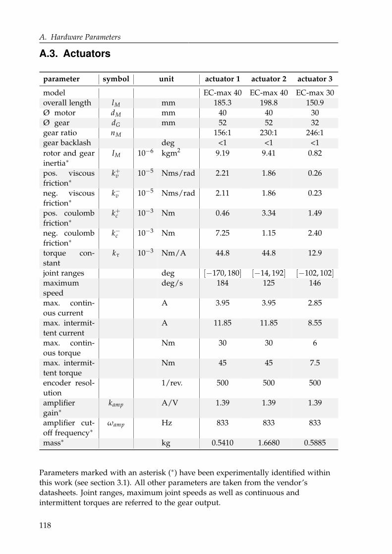
A. Hardware Parameters
A.3. Actuators
parameter symbol unit actuator 1 actuator 2 actuator 3
model EC-max 40 EC-max 40 EC-max 30
overall length lM mm 185.3 198.8 150.9
Ø motor dM mm 40 40 30
Ø gear dG mm 52 52 32
gear ratio nM 156:1 230:1 246:1
gear backlash deg <1 <1 <1
rotor and gear
inertia∗IM 10−6 kgm2 9.19 9.41 0.82
pos. viscous
friction∗k+v 10−5 Nms/rad 2.21 1.86 0.26
neg. viscous
friction∗k−v 10−5 Nms/rad 2.11 1.86 0.23
pos. coulomb
friction∗k+c 10−3 Nm 0.46 3.34 1.49
neg. coulomb
friction∗k−c 10−3 Nm 7.25 1.15 2.40
torque con-
stant
kτ 10−3 Nm/A 44.8 44.8 12.9
joint ranges deg [−170, 180] [−14, 192] [−102, 102]maximum
speed
deg/s 184 125 146
max. contin-
ous current
A 3.95 3.95 2.85
max. intermit-
tent current
A 11.85 11.85 8.55
max. contin-
ous torque
Nm 30 30 6
max. intermit-
tent torque
Nm 45 45 7.5
encoder resol-
ution
1/rev. 500 500 500
amplifier
gain∗kamp A/V 1.39 1.39 1.39
amplifier cut-
off frequency∗ωamp Hz 833 833 833
mass∗ kg 0.5410 1.6680 0.5885
Parameters marked with an asterisk (∗) have been experimentally identified within
this work (see section 3.1). All other parameters are taken from the vendor’s
datasheets. Joint ranges, maximum joint speeds as well as continuous and
intermittent torques are referred to the gear output.
118

A.4. Sensors
A.4. Sensors
Strain sensors
The strain sensors applied in this work are FAE-12S-35-S6E-P type strain gages man-
ufactured by Vishay Precision Group. The measurement amplifiers are GSV-1L by
ME-Messsysteme GmbH.
parameter symbol unit value
sensing element foil-gage
alloy constantan
carrier material polyamide
total gage length mm 5.61
total gage width mm 2.67
active gage length mm 3.18
gage resistance Ω 350 ± 0.2%
creep compensation 8.5
temperature compensation 10−6/C 10.8
Inertial measurement unit
The inertial measurement sensor is a CHR-6D unit consists of a LPR510AL 3-axes
MEMS rotation rate sensor as well as a ADXL335 3-axes accelerometer. It ships with
a 32 bit ARM Cortex processor operating at 64 Mhz.
parameter symbol unit value
supply voltage V 3.3
resolution bit 16
gyroscope range /s ±400
acceleromenter range 9.81ms ±3
mass g 1.5
FIR cutoff frequency Hz [10, 140]
Stereo camera system
The stereo camera system comprises of two VRmC-3+ cameras manufactured by
VRmagic. Both are equipped with a wide angle lens.
119
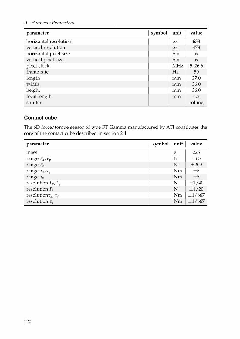
A. Hardware Parameters
parameter symbol unit value
horizontal resolution px 638
vertical resolution px 478
horizontal pixel size µm 6
vertical pixel size µm 6
pixel clock MHz [5, 26.6]
frame rate Hz 50
length mm 27.0
width mm 36.0
height mm 36.0
focal length mm 4.2
shutter rolling
Contact cube
The 6D force/torque sensor of type FT Gamma manufactured by ATI constitutes the
core of the contact cube described in section 2.4.
parameter symbol unit value
mass g 225
range Fx, Fy N ±65
range Fz N ±200
range τx, τy Nm ±5
range τz Nm ±5
resolution Fx, Fy N ±1/40
resolution Fz N ±1/20
resolutionτx, τy Nm ±1/667
resolution τz Nm ±1/667
120

BMathematical Definitions and Derivations
This appendix contains mathematical definitions and derivations to support the ma-
terial provided in this work. It is intended to render the document self-contained.
B.1. Equivalences of trigonometric, hyperbolic and
exponential functions
The general solution of the mode shape ODE can be written using exponential or
hyperbolic functions. The derivation of their equivalence as well as the transformation
between the corresponding coefficients requires knowledge about the mathematical
relationship between:
• . . . trigonometric and exponential functions:
e j x = cos(x) + j sin(x) , (B.1.1)
e− j x = cos(x)− j sin(x) , (B.1.2)
ey+ j x = ey (cos(x) + j sin(x)) , (B.1.3)
sin(x) =e j x − e− j x
j2, (B.1.4)
cos(x) =e j x + e− j x
2; (B.1.5)
• . . . trigonometric and hyperbolic functions:
sin(x) = − j sinh( j x) , (B.1.6)
cos(x) = cosh( j x) , (B.1.7)
sinh(x) = − j sin( j x) , (B.1.8)
cosh(x) = cos( j x) ; (B.1.9)
(B.1.10)
121

B. Mathematical Definitions and Derivations
• . . . hyperbolic and exponential functions:
ex = cosh(x) + sinh(x) , (B.1.11)
e−x = cosh(x)− sinh(x) , (B.1.12)
sinh(x) =ex − e−x
2, (B.1.13)
cosh(x) =ex + e−x
2. (B.1.14)
B.2. Derivatives of general solutions to the boundary value
problem
The derivation of particular solutions to the elastic beam boundary value problem
requires the spatial derivatives of the general solution.
• In the hyperbolic notation the derivatives are:
Φ(x) = a1 sinh (kω x) + a2 cosh (kω x) + . . .
+ a3 sin (kω x) + a4 cos (kω x) ,(B.2.1)
dΦ(x)
dx= kω (a1 cosh (kω x) + a2 sinh (kω x) + . . .
+ a3 cos (kω x)− a4 sin (kω x)) ,
(B.2.2)
d2Φ(x)
dx2= k2
ω (a1 sinh (kω x) + a2 cosh (kω x) + . . .
− a3 sin (kω x)− a4 cos (kω x)) ,
(B.2.3)
d3Φ(x)
dx3= k3
ω (a1 cosh (kω x) + a2 sinh (kω x) + . . .
− a3 cos (kω x) + a4 sin (kω x)) .
(B.2.4)
• In the exponential notation the derivatives compute to:
Φ(x) = + a e− j kω x + − a e j kω x + + an e−kω x + − an e kω x, (B.2.5)
dΦ(x)
dx= kω
(
− j + a e− j kω x + j − a e j kω x − + an e−kω x + − an e kω x)
, (B.2.6)
d2Φ(x)
dx2= k2
ω
(
−1 + a e− j kω x − − a e j kω x + + an e−kω x + − an e kω x)
, (B.2.7)
d3Φ(x)
dx3= k3
ω
(
j + a e− j kω x − j − a e j kω x − + an e−kω x + − an e kω x)
. (B.2.8)
B.3. Characteristic equation of the boundary value problem
This section derives the characteristic equation of the boundary value problem defined
in section 4.4. The boundary conditions are given in the equations (4.4.1) to (4.4.4).
122
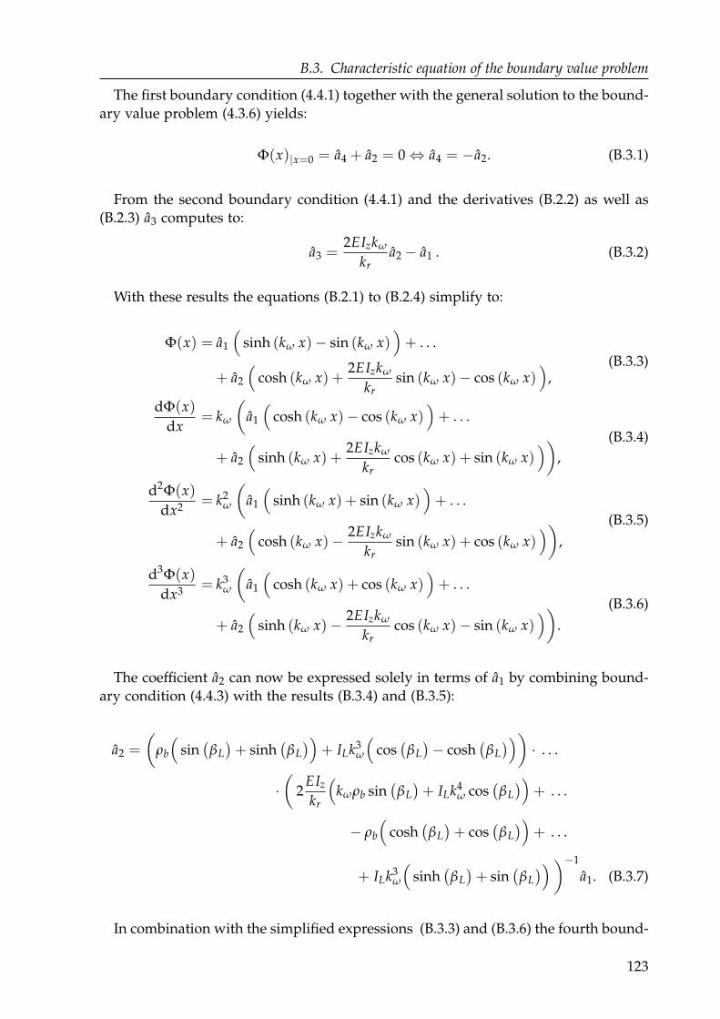
B.3. Characteristic equation of the boundary value problem
The first boundary condition (4.4.1) together with the general solution to the bound-
ary value problem (4.3.6) yields:
Φ(x)|x=0 = a4 + a2 = 0 ⇔ a4 = −a2. (B.3.1)
From the second boundary condition (4.4.1) and the derivatives (B.2.2) as well as
(B.2.3) a3 computes to:
a3 =2EIzkω
kra2 − a1 . (B.3.2)
With these results the equations (B.2.1) to (B.2.4) simplify to:
Φ(x) = a1
(
sinh (kω x)− sin (kω x))
+ . . .
+ a2
(
cosh (kω x) +2EIzkω
krsin (kω x)− cos (kω x)
)
,(B.3.3)
dΦ(x)
dx= kω
(
a1
(
cosh (kω x)− cos (kω x))
+ . . .
+ a2
(
sinh (kω x) +2EIzkω
krcos (kω x) + sin (kω x)
)
)
,
(B.3.4)
d2Φ(x)
dx2= k2
ω
(
a1
(
sinh (kω x) + sin (kω x))
+ . . .
+ a2
(
cosh (kω x)− 2EIzkω
krsin (kω x) + cos (kω x)
)
)
,
(B.3.5)
d3Φ(x)
dx3= k3
ω
(
a1
(
cosh (kω x) + cos (kω x))
+ . . .
+ a2
(
sinh (kω x)− 2EIzkω
krcos (kω x)− sin (kω x)
)
)
.
(B.3.6)
The coefficient a2 can now be expressed solely in terms of a1 by combining bound-
ary condition (4.4.3) with the results (B.3.4) and (B.3.5):
a2 =
(
ρb
(
sin(
βL
)
+ sinh(
βL
)
)
+ ILk3ω
(
cos(
βL
)
− cosh(
βL
)
)
)
· . . .
·(
2EIz
kr
(
kωρb sin(
βL
)
+ ILk4ω cos
(
βL
)
)
+ . . .
− ρb
(
cosh(
βL
)
+ cos(
βL
)
)
+ . . .
+ ILk3ω
(
sinh(
βL
)
+ sin(
βL
)
)
)−1
a1. (B.3.7)
In combination with the simplified expressions (B.3.3) and (B.3.6) the fourth bound-
123
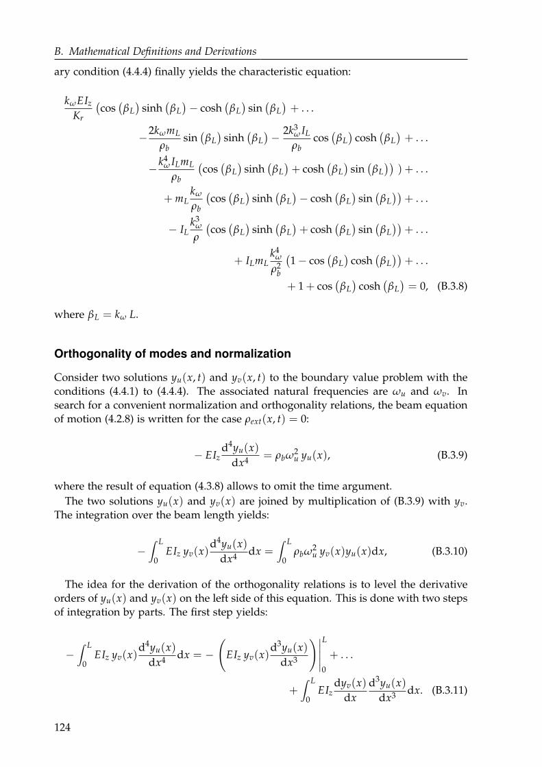
B. Mathematical Definitions and Derivations
ary condition (4.4.4) finally yields the characteristic equation:
kωEIz
Kr
(
cos(
βL
)
sinh(
βL
)
− cosh(
βL
)
sin(
βL
)
+ . . .
−2kωmL
ρbsin(
βL
)
sinh(
βL
)
− 2k3ω IL
ρbcos
(
βL
)
cosh(
βL
)
+ . . .
−k4ω ILmL
ρb
(
cos(
βL
)
sinh(
βL
)
+ cosh(
βL
)
sin(
βL
))
) + . . .
+ mLkω
ρb
(
cos(
βL
)
sinh(
βL
)
− cosh(
βL
)
sin(
βL
))
+ . . .
− ILk3
ω
ρ
(
cos(
βL
)
sinh(
βL
)
+ cosh(
βL
)
sin(
βL
))
+ . . .
+ ILmLk4
ω
ρ2b
(
1 − cos(
βL
)
cosh(
βL
))
+ . . .
+ 1 + cos(
βL
)
cosh(
βL
)
= 0, (B.3.8)
where βL = kω L.
Orthogonality of modes and normalization
Consider two solutions yu(x, t) and yv(x, t) to the boundary value problem with the
conditions (4.4.1) to (4.4.4). The associated natural frequencies are ωu and ωv. In
search for a convenient normalization and orthogonality relations, the beam equation
of motion (4.2.8) is written for the case ρext(x, t) = 0:
− EIzd4yu(x)
dx4= ρbω2
u yu(x), (B.3.9)
where the result of equation (4.3.8) allows to omit the time argument.
The two solutions yu(x) and yv(x) are joined by multiplication of (B.3.9) with yv.
The integration over the beam length yields:
−∫ L
0EIz yv(x)
d4yu(x)
dx4dx =
∫ L
0ρbω2
u yv(x)yu(x)dx, (B.3.10)
The idea for the derivation of the orthogonality relations is to level the derivative
orders of yu(x) and yv(x) on the left side of this equation. This is done with two steps
of integration by parts. The first step yields:
−∫ L
0EIz yv(x)
d4yu(x)
dx4dx = −
(
EIz yv(x)d3yu(x)
dx3
)∣
∣
∣
∣
∣
L
0
+ . . .
+∫ L
0EIz
dyv(x)
dx
d3yu(x)
dx3dx. (B.3.11)
124
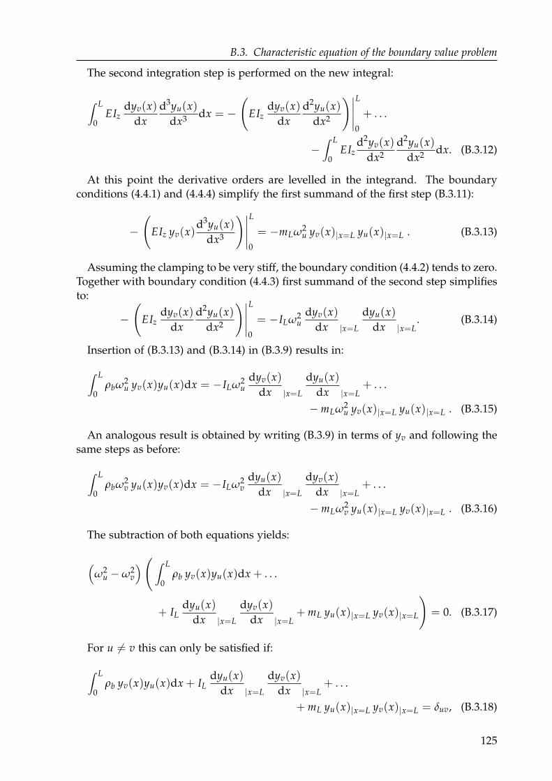
B.3. Characteristic equation of the boundary value problem
The second integration step is performed on the new integral:
∫ L
0EIz
dyv(x)
dx
d3yu(x)
dx3dx = −
(
EIzdyv(x)
dx
d2yu(x)
dx2
)∣
∣
∣
∣
∣
L
0
+ . . .
−∫ L
0EIz
d2yv(x)
dx2
d2yu(x)
dx2dx. (B.3.12)
At this point the derivative orders are levelled in the integrand. The boundary
conditions (4.4.1) and (4.4.4) simplify the first summand of the first step (B.3.11):
−(
EIz yv(x)d3yu(x)
dx3
)∣
∣
∣
∣
∣
L
0
= −mLω2u yv(x)|x=L yu(x)|x=L . (B.3.13)
Assuming the clamping to be very stiff, the boundary condition (4.4.2) tends to zero.
Together with boundary condition (4.4.3) first summand of the second step simplifies
to:
−(
EIzdyv(x)
dx
d2yu(x)
dx2
)∣
∣
∣
∣
∣
L
0
= −ILω2u
dyv(x)
dx |x=L
dyu(x)
dx |x=L. (B.3.14)
Insertion of (B.3.13) and (B.3.14) in (B.3.9) results in:
∫ L
0ρbω2
u yv(x)yu(x)dx = −ILω2u
dyv(x)
dx |x=L
dyu(x)
dx |x=L+ . . .
− mLω2u yv(x)|x=L yu(x)|x=L . (B.3.15)
An analogous result is obtained by writing (B.3.9) in terms of yv and following the
same steps as before:
∫ L
0ρbω2
v yu(x)yv(x)dx = −ILω2v
dyu(x)
dx |x=L
dyv(x)
dx |x=L+ . . .
− mLω2v yu(x)|x=L yv(x)|x=L . (B.3.16)
The subtraction of both equations yields:
(
ω2u − ω2
v
)
(
∫ L
0ρb yv(x)yu(x)dx + . . .
+ ILdyu(x)
dx |x=L
dyv(x)
dx |x=L+ mL yu(x)|x=L yv(x)|x=L
)
= 0. (B.3.17)
For u 6= v this can only be satisfied if:
∫ L
0ρb yv(x)yu(x)dx + IL
dyu(x)
dx |x=L
dyv(x)
dx |x=L+ . . .
+ mL yu(x)|x=L yv(x)|x=L = δuv, (B.3.18)
125
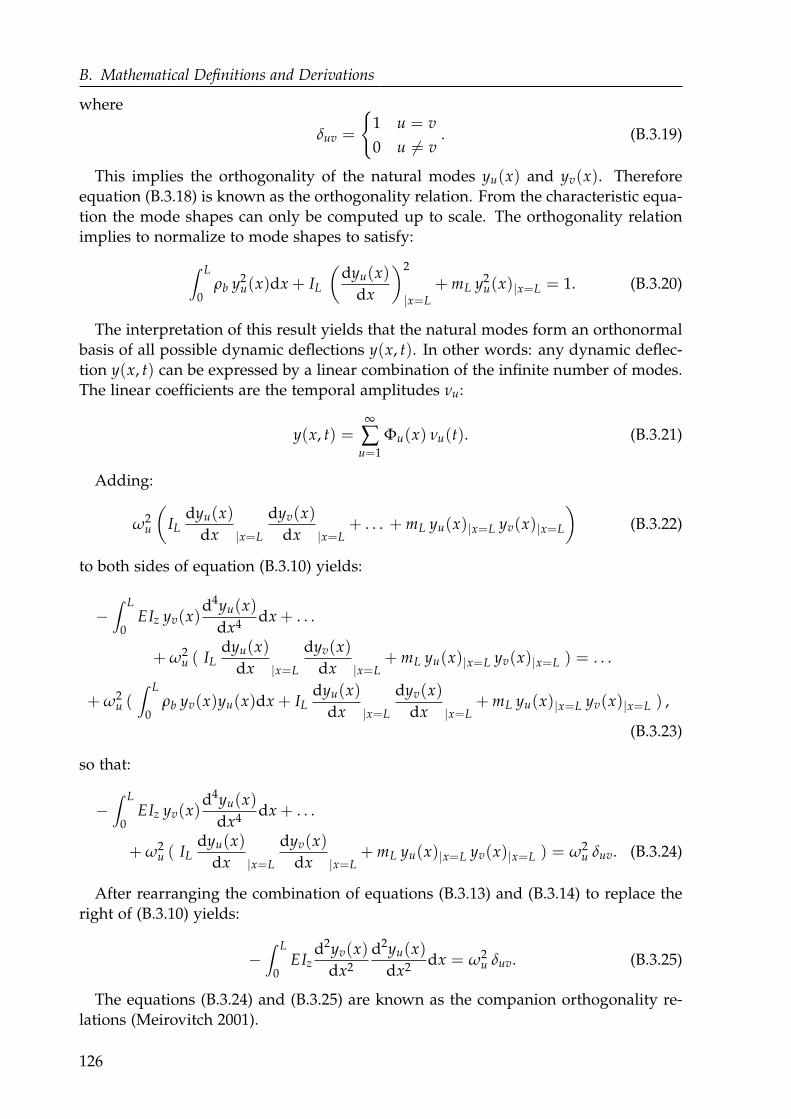
B. Mathematical Definitions and Derivations
where
δuv =
1 u = v
0 u 6= v. (B.3.19)
This implies the orthogonality of the natural modes yu(x) and yv(x). Therefore
equation (B.3.18) is known as the orthogonality relation. From the characteristic equa-
tion the mode shapes can only be computed up to scale. The orthogonality relation
implies to normalize to mode shapes to satisfy:
∫ L
0ρb y2
u(x)dx + IL
(
dyu(x)
dx
)2
|x=L
+ mL y2u(x)|x=L = 1. (B.3.20)
The interpretation of this result yields that the natural modes form an orthonormal
basis of all possible dynamic deflections y(x, t). In other words: any dynamic deflec-
tion y(x, t) can be expressed by a linear combination of the infinite number of modes.
The linear coefficients are the temporal amplitudes νu:
y(x, t) =∞
∑u=1
Φu(x) νu(t). (B.3.21)
Adding:
ω2u
(
ILdyu(x)
dx |x=L
dyv(x)
dx |x=L+ . . . + mL yu(x)|x=L yv(x)|x=L
)
(B.3.22)
to both sides of equation (B.3.10) yields:
−∫ L
0EIz yv(x)
d4yu(x)
dx4dx + . . .
+ ω2u ( IL
dyu(x)
dx |x=L
dyv(x)
dx |x=L+ mL yu(x)|x=L yv(x)|x=L ) = . . .
+ ω2u (∫ L
0ρb yv(x)yu(x)dx + IL
dyu(x)
dx |x=L
dyv(x)
dx |x=L+ mL yu(x)|x=L yv(x)|x=L ) ,
(B.3.23)
so that:
−∫ L
0EIz yv(x)
d4yu(x)
dx4dx + . . .
+ ω2u ( IL
dyu(x)
dx |x=L
dyv(x)
dx |x=L+ mL yu(x)|x=L yv(x)|x=L ) = ω2
u δuv. (B.3.24)
After rearranging the combination of equations (B.3.13) and (B.3.14) to replace the
right of (B.3.10) yields:
−∫ L
0EIz
d2yv(x)
dx2
d2yu(x)
dx2dx = ω2
u δuv. (B.3.25)
The equations (B.3.24) and (B.3.25) are known as the companion orthogonality re-
lations (Meirovitch 2001).
126
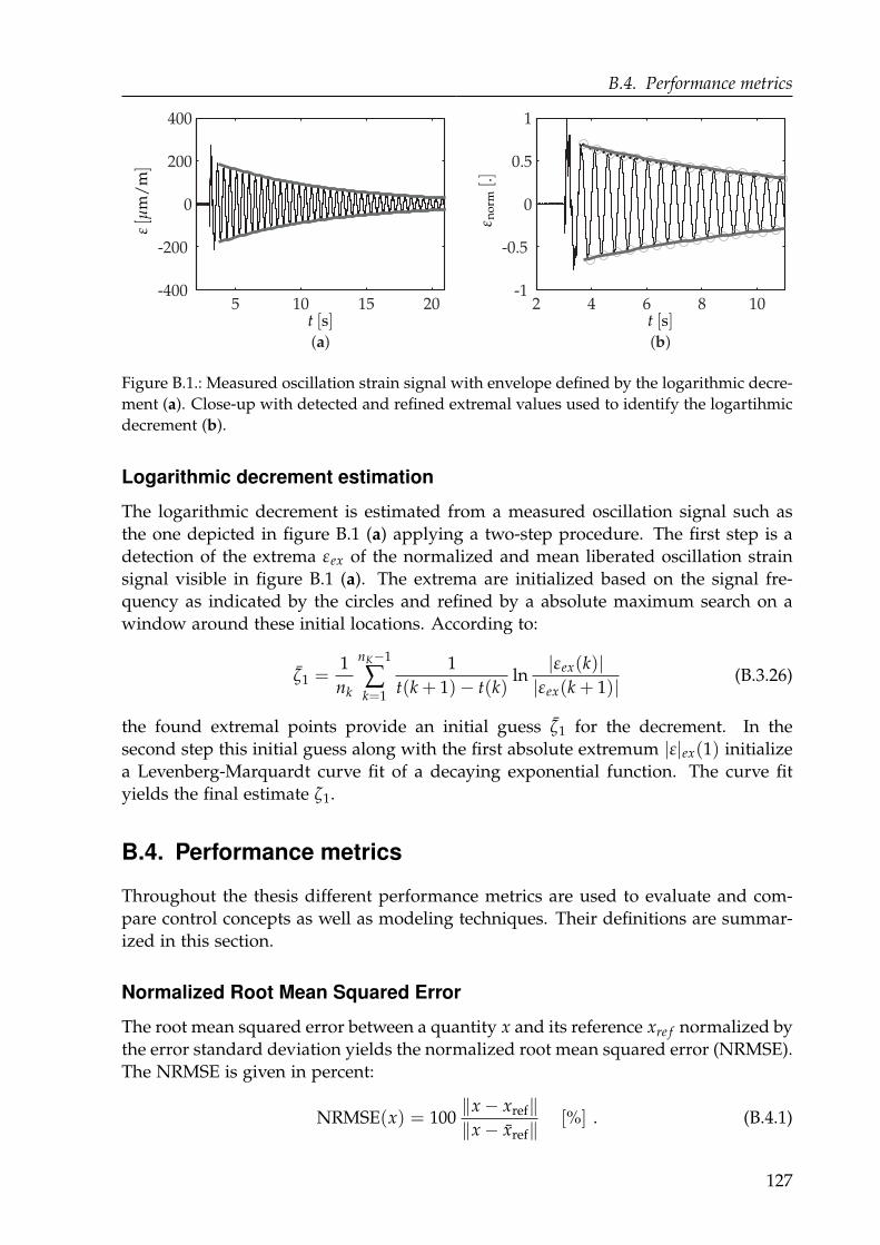
B.4. Performance metrics
5 10 15 20-400
-200
0
200
400
(a)
2 4 6 8 10-1
-0.5
0
0.5
1
(b)
ε[µ
m/
m]
ε no
rm[.]
t [s]t [s]
Figure B.1.: Measured oscillation strain signal with envelope defined by the logarithmic decre-
ment (a). Close-up with detected and refined extremal values used to identify the logartihmic
decrement (b).
Logarithmic decrement estimation
The logarithmic decrement is estimated from a measured oscillation signal such as
the one depicted in figure B.1 (a) applying a two-step procedure. The first step is a
detection of the extrema εex of the normalized and mean liberated oscillation strain
signal visible in figure B.1 (a). The extrema are initialized based on the signal fre-
quency as indicated by the circles and refined by a absolute maximum search on a
window around these initial locations. According to:
ζ1 =1
nk
nK−1
∑k=1
1
t(k + 1)− t(k)ln
|εex(k)||εex(k + 1)| (B.3.26)
the found extremal points provide an initial guess ζ1 for the decrement. In the
second step this initial guess along with the first absolute extremum |ε|ex(1) initialize
a Levenberg-Marquardt curve fit of a decaying exponential function. The curve fit
yields the final estimate ζ1.
B.4. Performance metrics
Throughout the thesis different performance metrics are used to evaluate and com-
pare control concepts as well as modeling techniques. Their definitions are summar-
ized in this section.
Normalized Root Mean Squared Error
The root mean squared error between a quantity x and its reference xre f normalized by
the error standard deviation yields the normalized root mean squared error (NRMSE).
The NRMSE is given in percent:
NRMSE(x) = 100‖x − xref‖‖x − xref‖
[%] . (B.4.1)
127

B. Mathematical Definitions and Derivations
The goodness of fit
The goodness of fit metric used in this work is defined as one minus the normalized
root mean squared error (1 − NRMSE) and given in in percent:
fit(x) = 100 − NRMSE , [%] . (B.4.2)
The goodness of fit reflects the percentage of the standard deviation in a reference
signal xre f explained by the model. A model that achieves a goodness of fit value
above 80 % is commonly accepted as a good model.
Integral of absolute time weighted error
The integral of absolute time weighted error (IATE) computes to:
IATE(x, t) =∫ t
0t∣
∣x(t)− xre f (t)∣
∣ dt . (B.4.3)
It penalizes errors that persist for a longer period more than initial errors.
Integral absolute time weighted strain surface
The integral absolute time weighted strain surface computes to:
IATS(x, t) =∫ t
0t |ε(t)| dt . (B.4.4)
It may be understood as the IATE with x = ε and xre f = 0.
Settling time
The strain settling time TCS is the time elapsed until the error x − xre f resides within
a given band. Again, in the case of strain based oscillations measurements x = ε,
whereas xre f = 0. For joint angles an error band of 0.01 degrees is used. The error
band for strain based oscillations measurements amounts to 15 µm/m.
B.5. Stereo camera accuracy
The theoretical accuracy of the stereo camera setup is approximated within a su-
pervised thesis by Bürger (February 2011). The conservative assumption is that the
tracking object centers are localized in the images with integer pixel accuracy. A
single pixel covers a field of view with a pyramidal volume. At any point within the
robot workspace the pyramidal volumes of the two cameras intersect. The intersection
volume is enclosed by a cuboid, with the edges parallel to the stereo camera reference
frame. The edge lengths of the cuboid represent the approximated localization error.
The computed errors along the x- and z-axes of the stereo camera frame are visual-
ized by isometric lines in figure B.2. Within the workspace of TUDOR the conservative
approximation of the absolute accuracy amounts to 3.5 to 4.5 mm along the x-axis and
3 to 8 mm along the z-axis. Despite sensor noise and segmentation errors the tracking
128
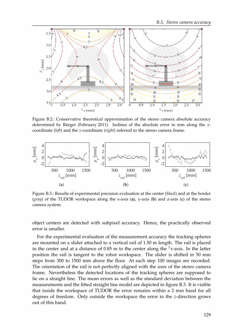
B.5. Stereo camera accuracy
Figure B.2.: Conservative theoretical approximation of the stereo camera absolute accuracy
determined by Bürger (February 2011). Isolines of the absolute error in mm along the x-
coordinate (left) and the z-coordinate (right) referred to the stereo camera frame.
500 1000 1500
-2
0
2
4
zrail
[mm]
µx
[mm
]
µy
[mm
]
µz
[mm
]
500 1000 1500
-2
0
2
4
zrail
[mm]500 1000 1500
-2
0
2
4
zrail
[mm]
( )a ( )b ( )c
Figure B.3.: Results of experimental precision evaluation at the center (black) and at the border
(gray) of the TUDOR workspace along the x-axis (a), y-axis (b) and z-axis (c) of the stereo
camera system.
object centers are detected with subpixel accuracy. Hence, the practically observed
error is smaller.
For the experimental evaluation of the measurement accuracy the tracking spheres
are mounted on a slider attached to a vertical rail of 1.50 m length. The rail is placed
in the center and at a distance of 0.85 m to the center along the 1x-axis. In the latter
position the rail is tangent to the robot workspace. The slider is shifted in 50 mm
steps from 300 to 1500 mm above the floor. At each step 100 images are recorded.
The orientation of the rail is not perfectly aligned with the axes of the stereo camera
frame. Nevertheless the detected locations of the tracking spheres are supposed to
lie on a straight line. The mean errors as well as the standard deviation between the
measurements and the fitted straight line model are depicted in figure B.3. It is visible
that inside the workspace of TUDOR the error remains within a 2 mm band for all
degrees of freedom. Only outside the workspace the error in the z-direction grows
out of this band.
129
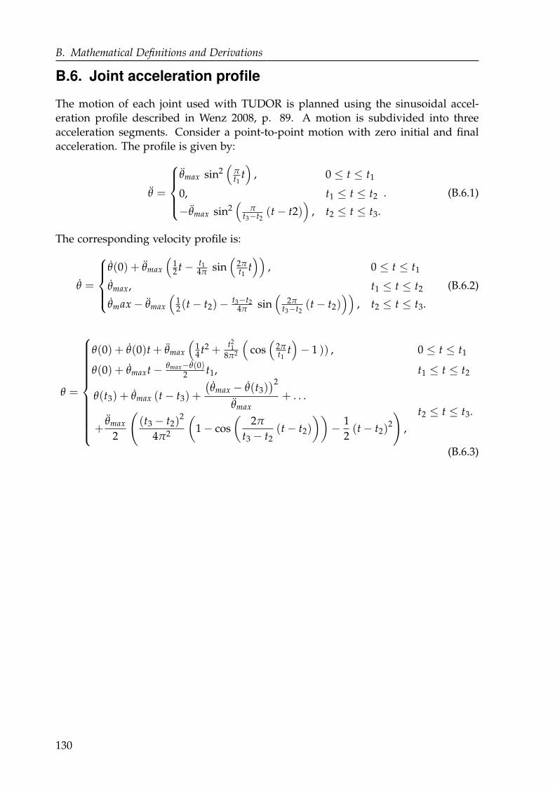
B. Mathematical Definitions and Derivations
B.6. Joint acceleration profile
The motion of each joint used with TUDOR is planned using the sinusoidal accel-
eration profile described in Wenz 2008, p. 89. A motion is subdivided into three
acceleration segments. Consider a point-to-point motion with zero initial and final
acceleration. The profile is given by:
θ =
θmax sin2(
πt1
t)
, 0 ≤ t ≤ t1
0, t1 ≤ t ≤ t2
−θmax sin2(
πt3−t2
(t − t2))
, t2 ≤ t ≤ t3.
. (B.6.1)
The corresponding velocity profile is:
θ =
θ(0) + θmax
(
12 t − t1
4π sin(
2πt1
t))
, 0 ≤ t ≤ t1
θmax, t1 ≤ t ≤ t2
θmax − θmax
(
12(t − t2)− t3−t2
4π sin(
2πt3−t2
(t − t2)))
, t2 ≤ t ≤ t3.
(B.6.2)
θ =
θ(0) + θ(0)t + θmax
(
14 t2 +
t21
8π2
(
cos(
2πt1
t)
− 1 )) , 0 ≤ t ≤ t1
θ(0) + θmaxt − θmax−θ(0)2 t1, t1 ≤ t ≤ t2
θ(t3) + θmax (t − t3) +
(
θmax − θ(t3))2
θmax+ . . .
+θmax
2
(
(t3 − t2)2
4π2
(
1 − cos
(
2π
t3 − t2(t − t2)
))
− 1
2(t − t2)
2
)
,
t2 ≤ t ≤ t3.
(B.6.3)
130
CSupplemental Collision Experiments
In addition to the experimental collision detection results provided in section 11.3 this
appendix complements blunt impacts with the balloon, sharp impacts with a stiff but
fragile object as well as sharp collisions with a human arm.
C.1. Blunt impacts with a compliant object
Prior to the sharp collision impacts presented with the balloon in section 11.3 blunt
collision experiments are carried out. During blunt impacts the balloon remains un-
damaged, even without collision detection. However, an emerging strong deformation
of the balloon is clearly observed in the top right photograph and in the force level
measured at the contact cube in figure C.1 (c). The strong deformation as well as
the increasing force level is absent when the stop strategy is used (center row, right
photograph). Without collision detection, the force level grows until the joint angles
reach the commanded position as visible in figure C.1 (a).
The velocity measurements for the case with no collision detection as well as the
stop strategy being enabled show a short sequence of significant over- and undershoot
right after the collision time instant. Such a sequence is not observed with the blunt
impacts on the rigid contact cube in figure 11.3 (e). It originates from the compliance
of the balloon.
The effect of the admittance strategy is illustrated in the bottom row of photographs
in figure C.1. Remarkably, in this case there is hardly any difference visible in the
blunt impact measurements depicted in the figures C.1 (a) to (b), when compared
with the corresponding sharp impact results sensor readings in figure 11.4.
Malzahn and Bertram (2013, at 2:10 min) published an online available video with
this experiment.
C.2. Sharp impacts with a fragile object
Compared to the balloon, the Christmas sphere is a rather stiff object.
Without collision detection, the link with the sharpened screw penetrates the Christ-
mas sphere. It is visible in the top right photograph of figure C.2 that at t ≈ 1.57 s
the end effector already went right through the Christmas sphere. Finally it hits the
131
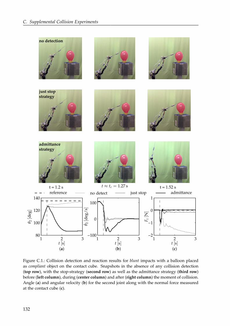
C. Supplemental Collision Experiments
1 2 380
100
120
140
(a)
1 2 3−100
0
100
(b)
1 2 3−2
−1
0
1
(c)
no detection
just stopstrategy
admittancestrategy
reference admittancet ≈ 1.2 s t ≈ 1.52 s
t [s]t [s]t [s]
θ 2[d
eg]
θ 2[d
eg/
s]
F z[N
]
t ≈ tc = 1.27 s
just stopno detect
Figure C.1.: Collision detection and reaction results for blunt impacts with a balloon placed
as compliant object on the contact cube. Snapshots in the absence of any collision detection
(top row), with the stop-strategy (second row) as well as the admittance strategy (third row)
before (left column), during (center column) and after (right column) the moment of collision.
Angle (a) and angular velocity (b) for the second joint along with the normal force measured
at the contact cube (c).
132

C.3. Sharp impacts on a human arm
1 2 380
100
120
140
160
(a)
1 2 3−100
0
100
200
(b)
1 2 3
−2
0
2
(c)
no detection
admittancestrategy
reference admittance
t ≈ 1.25 s t ≈ 1.57 s
t [s]t [s]t [s]
θ 2[d
eg]
θ 2[d
eg/
s]
F z[N
]
t ≈ tc = 1.33 s
no detect t = tc
Figure C.2.: Collision detection and reaction results for sharp impacts with a Christmas ball
placed as fragile object on the contact cube.
contact cube. At this moment, a second impact is visible in the force readings of fig-
ure C.2 (b). With some delay, the Christmas sphere starts burst asunder. Individual
debris begin to lift into the air.
Just as before, the joint angles reach the targeted position, while the robot links
absorb the contact force in their deflections.
Identical to the sharp impact experiments with the balloon, the reflex strategy saves
the Christmas sphere. The measurements provided in the figures C.2 (a) to (c) are
very similar to those observed with the balloon in figure 11.4. As a major difference,
the spheres are made from rather thick glass. Thus, they are sturdy enough to also
survive the impacts when the stop strategy is applied.
Malzahn and Bertram (2013, at 3:02 min) published an online available video of this
experiment.
133
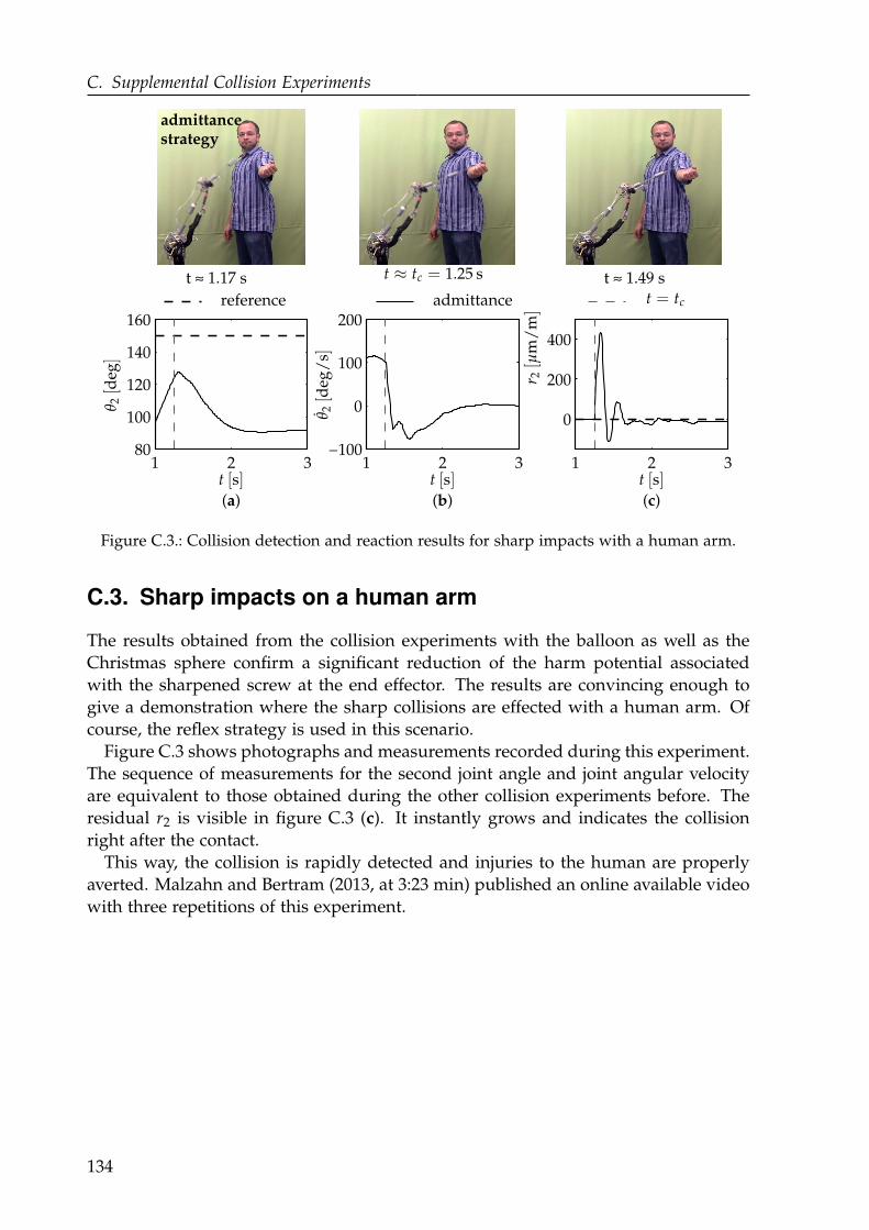
C. Supplemental Collision Experiments
1 2 380
100
120
140
160
(a)
1 2 3−100
0
100
200
(b)
1 2 3
0
200
400
(c)
admittancestrategy
reference admittance
t ≈ 1.17 s t ≈ 1.49 s
t [s]t [s]t [s]
θ 2[d
eg]
θ 2[d
eg/
s]
r 2[µ
m/
m]
t ≈ tc = 1.25 s
t = tc
Figure C.3.: Collision detection and reaction results for sharp impacts with a human arm.
C.3. Sharp impacts on a human arm
The results obtained from the collision experiments with the balloon as well as the
Christmas sphere confirm a significant reduction of the harm potential associated
with the sharpened screw at the end effector. The results are convincing enough to
give a demonstration where the sharp collisions are effected with a human arm. Of
course, the reflex strategy is used in this scenario.
Figure C.3 shows photographs and measurements recorded during this experiment.
The sequence of measurements for the second joint angle and joint angular velocity
are equivalent to those obtained during the other collision experiments before. The
residual r2 is visible in figure C.3 (c). It instantly grows and indicates the collision
right after the contact.
This way, the collision is rapidly detected and injuries to the human are properly
averted. Malzahn and Bertram (2013, at 3:23 min) published an online available video
with three repetitions of this experiment.
134
DSteps to Deploy the Techniques
The following guideline summarizes the major steps required to deploy the tech-
niques developed in this work.
Initial situation: The arm hardware as well as the reference sensors are set up
and ready for operation.
1. Actuator identification and control: The actuator vendor commonly provides
datasheets with good initial values for all parameters required to implement the
controller design used in this work. With the tuned controller, the values for the
individual initial parameters can be verified or refined by additional identification
experiments, as done in this work.
chapter: sensors: parameters per joint-link-module: #
3 current sensors, encoders IM, kM, kv, kPI , tPI , td, kPD, tPD, tl 9
2. Oscillation damping: For oscillation damping the work suggest to proportion-
ally feed the mean liberated strain measurements back to the velocity controller
cascade level for each individual joint-link-module. Therefore, the FIR based high
pass filter for mean liberation is tuned (see 2.2) for the desired frequency range.
Next, the proportional feedback gains kε are determined in two steps. The first
step is a careful manual tuning with determination of the stability limit kε, max.
The second step is the automated hardware in the loop optimization of the gains
as described in section 5.3.
chapters: sensor: parameters per joint-link-module: #
2.2, 5 strain sensor NFIR, kε, kε, max 3
3. Kinematics learning: In order to determine the weights of the data based
kinematics models, end effector positions must be recorded together with static
strains and joint angles by sampling the whole workspace with different payload
masses.
chapter: sensors: parameters per joint-link-module: #
9.2 strain gauges, encoders, weights for the forward kinematics,
external tip position inverse kinematics and
sensor (stereo camera) load estimation network
135
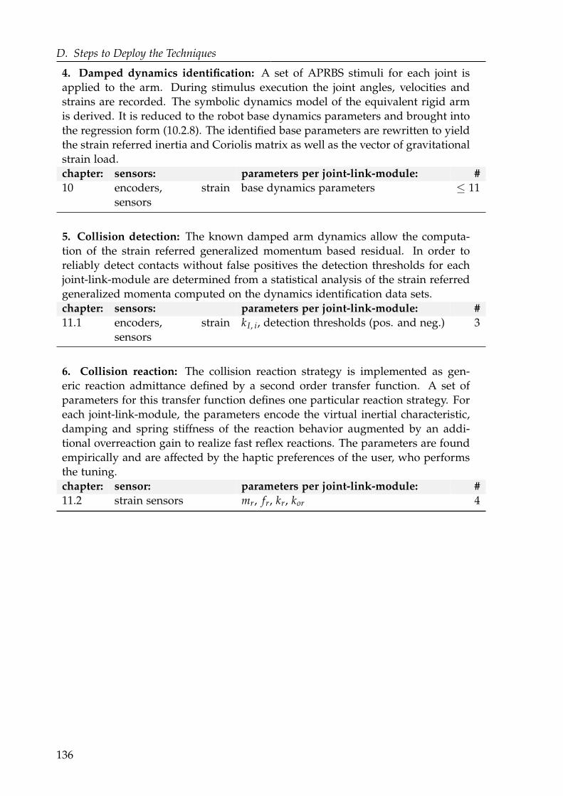
D. Steps to Deploy the Techniques
4. Damped dynamics identification: A set of APRBS stimuli for each joint is
applied to the arm. During stimulus execution the joint angles, velocities and
strains are recorded. The symbolic dynamics model of the equivalent rigid arm
is derived. It is reduced to the robot base dynamics parameters and brought into
the regression form (10.2.8). The identified base parameters are rewritten to yield
the strain referred inertia and Coriolis matrix as well as the vector of gravitational
strain load.
chapter: sensors: parameters per joint-link-module: #
10 encoders, strain
sensors
base dynamics parameters ≤ 11
5. Collision detection: The known damped arm dynamics allow the computa-
tion of the strain referred generalized momentum based residual. In order to
reliably detect contacts without false positives the detection thresholds for each
joint-link-module are determined from a statistical analysis of the strain referred
generalized momenta computed on the dynamics identification data sets.
chapter: sensors: parameters per joint-link-module: #
11.1 encoders, strain
sensors
kI, i, detection thresholds (pos. and neg.) 3
6. Collision reaction: The collision reaction strategy is implemented as gen-
eric reaction admittance defined by a second order transfer function. A set of
parameters for this transfer function defines one particular reaction strategy. For
each joint-link-module, the parameters encode the virtual inertial characteristic,
damping and spring stiffness of the reaction behavior augmented by an addi-
tional overreaction gain to realize fast reflex reactions. The parameters are found
empirically and are affected by the haptic preferences of the user, who performs
the tuning.
chapter: sensor: parameters per joint-link-module: #
11.2 strain sensors mr, fr, kr, kor 4
136
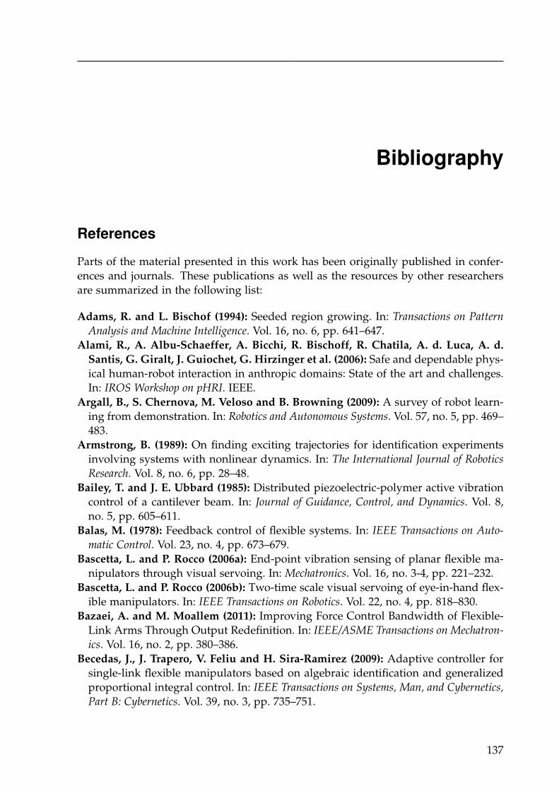
Bibliography
References
Parts of the material presented in this work has been originally published in confer-
ences and journals. These publications as well as the resources by other researchers
are summarized in the following list:
Adams, R. and L. Bischof (1994): Seeded region growing. In: Transactions on Pattern
Analysis and Machine Intelligence. Vol. 16, no. 6, pp. 641–647.
Alami, R., A. Albu-Schaeffer, A. Bicchi, R. Bischoff, R. Chatila, A. d. Luca, A. d.
Santis, G. Giralt, J. Guiochet, G. Hirzinger et al. (2006): Safe and dependable phys-
ical human-robot interaction in anthropic domains: State of the art and challenges.
In: IROS Workshop on pHRI. IEEE.
Argall, B., S. Chernova, M. Veloso and B. Browning (2009): A survey of robot learn-
ing from demonstration. In: Robotics and Autonomous Systems. Vol. 57, no. 5, pp. 469–
483.
Armstrong, B. (1989): On finding exciting trajectories for identification experiments
involving systems with nonlinear dynamics. In: The International Journal of Robotics
Research. Vol. 8, no. 6, pp. 28–48.
Bailey, T. and J. E. Ubbard (1985): Distributed piezoelectric-polymer active vibration
control of a cantilever beam. In: Journal of Guidance, Control, and Dynamics. Vol. 8,
no. 5, pp. 605–611.
Balas, M. (1978): Feedback control of flexible systems. In: IEEE Transactions on Auto-
matic Control. Vol. 23, no. 4, pp. 673–679.
Bascetta, L. and P. Rocco (2006a): End-point vibration sensing of planar flexible ma-
nipulators through visual servoing. In: Mechatronics. Vol. 16, no. 3-4, pp. 221–232.
Bascetta, L. and P. Rocco (2006b): Two-time scale visual servoing of eye-in-hand flex-
ible manipulators. In: IEEE Transactions on Robotics. Vol. 22, no. 4, pp. 818–830.
Bazaei, A. and M. Moallem (2011): Improving Force Control Bandwidth of Flexible-
Link Arms Through Output Redefinition. In: IEEE/ASME Transactions on Mechatron-
ics. Vol. 16, no. 2, pp. 380–386.
Becedas, J., J. Trapero, V. Feliu and H. Sira-Ramirez (2009): Adaptive controller for
single-link flexible manipulators based on algebraic identification and generalized
proportional integral control. In: IEEE Transactions on Systems, Man, and Cybernetics,
Part B: Cybernetics. Vol. 39, no. 3, pp. 735–751.
137
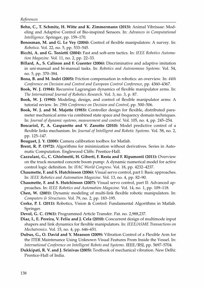
References
Behn, C., T. Schmitz, H. Witte and K. Zimmermann (2013): Animal Vibrissae: Mod-
eling and Adaptive Control of Bio-inspired Sensors. In: Advances in Computational
Intelligence. Springer, pp. 159–170.
Benosman, M. and G. Le Vey (2004): Control of flexible manipulators: A survey. In:
Robotica. Vol. 22, no. 5, pp. 533–545.
Bicchi, A. and G. Tonietti (2004): Fast and soft-arm tactics. In: IEEE Robotics Automa-
tion Magazine. Vol. 11, no. 2, pp. 22–33.
Billard, A., S. Calinon and F. Guenter (2006): Discriminative and adaptive imitation
in uni-manual and bi-manual tasks. In: Robotics and Autonomous Systems. Vol. 54,
no. 5, pp. 370–384.
Bona, B. and M. Indri (2005): Friction compensation in robotics: an overview. In: 44th
Conference on Decision and Control and European Control Conference, pp. 4360–4367.
Book, W. J. (1984): Recursive Lagrangian dynamics of flexible manipulator arms. In:
The International Journal of Robotics Research. Vol. 3, no. 3, p. 87.
Book, W. J. (1990): Modeling, design, and control of flexible manipulator arms: A
tutorial review. In: 29th Conference on Decision and Control, pp. 500–506.
Book, W. J. and M. Majette (1983): Controller design for flexible, distributed para-
meter mechanical arms via combined state space and frequency domain techniques.
In: Journal of dynamic systems, measurement and control. Vol. 105, no. 4, pp. 245–254.
Boscariol, P., A. Gasparetto and V. Zanotto (2010): Model predictive control of a
flexible links mechanism. In: Journal of Intelligent and Robotic Systems. Vol. 58, no. 2,
pp. 125–147.
Bouguet, J. Y. (2008): Camera calibration toolbox for Matlab.
Brent, R. P. (1972): Algorithms for minimization without derivatives. Series in Auto-
matic Computation. Englewood Cliffs: Prentice-Hall.
Cazzulani, G., C. Ghielmetti, H. Giberti, F. Resta and F. Ripamonti (2011): Overview
on the truck mounted concrete boom pump: A dynamic numerical model for active
control logic definition. In: IFAC World Congress. Vol. 18, pp. 4232–4237.
Chaumette, F. and S. Hutchinson (2006): Visual servo control, part I: Basic approaches.
In: IEEE Robotics and Automation Magazine. Vol. 13, no. 4, pp. 82–90.
Chaumette, F. and S. Hutchinson (2007): Visual servo control, part II: Advanced ap-
proaches. In: IEEE Robotics and Automation Magazine. Vol. 14, no. 1, pp. 109–118.
Chen, W. (2001): Dynamic modeling of multi-link flexible robotic manipulators. In:
Computers & Structures. Vol. 79, no. 2, pp. 183–195.
Corke, P. I. (2011): Robotics, Vision & Control: Fundamental Algorithms in Matlab.
Springer.
Devol, G. C. (1961): Programmed Article Transfer. Pat. no. 2,988,237.
Diaz, I., E. Pereira, V. Feliu and J. Cela (2010): Concurrent design of multimode input
shapers and link dynamics for flexible manipulators. In: IEEE/ASME Transactions on
Mechatronics. Vol. 15, no. 4, pp. 646–651.
Dubus, G., O. David and Y. Measson (2009): Vibration Control of a Flexible Arm for
the ITER Maintenance Using Unknown Visual Features From Inside the Vessel. In:
International Conference on Intelligent Robots and Systems. IEEE/RSJ, pp. 5697–5704.
Dukkipati, R. V. and J. Srinivas (2005): Textbook of mechanical vibration. New Delhi:
Prentice-Hall of India.
138
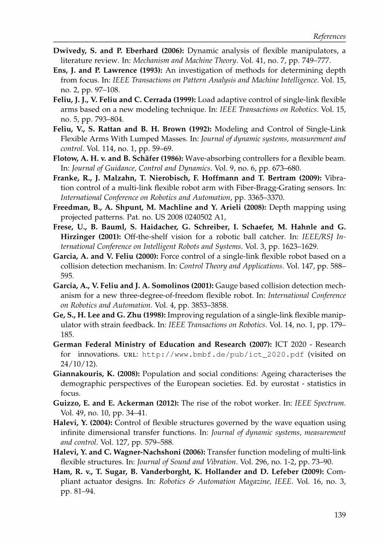
References
Dwivedy, S. and P. Eberhard (2006): Dynamic analysis of flexible manipulators, a
literature review. In: Mechanism and Machine Theory. Vol. 41, no. 7, pp. 749–777.
Ens, J. and P. Lawrence (1993): An investigation of methods for determining depth
from focus. In: IEEE Transactions on Pattern Analysis and Machine Intelligence. Vol. 15,
no. 2, pp. 97–108.
Feliu, J. J., V. Feliu and C. Cerrada (1999): Load adaptive control of single-link flexible
arms based on a new modeling technique. In: IEEE Transactions on Robotics. Vol. 15,
no. 5, pp. 793–804.
Feliu, V., S. Rattan and B. H. Brown (1992): Modeling and Control of Single-Link
Flexible Arms With Lumped Masses. In: Journal of dynamic systems, measurement and
control. Vol. 114, no. 1, pp. 59–69.
Flotow, A. H. v. and B. Schäfer (1986): Wave-absorbing controllers for a flexible beam.
In: Journal of Guidance, Control and Dynamics. Vol. 9, no. 6, pp. 673–680.
Franke, R., J. Malzahn, T. Nierobisch, F. Hoffmann and T. Bertram (2009): Vibra-
tion control of a multi-link flexible robot arm with Fiber-Bragg-Grating sensors. In:
International Conference on Robotics and Automation, pp. 3365–3370.
Freedman, B., A. Shpunt, M. Machline and Y. Arieli (2008): Depth mapping using
projected patterns. Pat. no. US 2008 0240502 A1,
Frese, U., B. Bauml, S. Haidacher, G. Schreiber, I. Schaefer, M. Hahnle and G.
Hirzinger (2001): Off-the-shelf vision for a robotic ball catcher. In: IEEE/RSJ In-
ternational Conference on Intelligent Robots and Systems. Vol. 3, pp. 1623–1629.
Garcia, A. and V. Feliu (2000): Force control of a single-link flexible robot based on a
collision detection mechanism. In: Control Theory and Applications. Vol. 147, pp. 588–
595.
Garcia, A., V. Feliu and J. A. Somolinos (2001): Gauge based collision detection mech-
anism for a new three-degree-of-freedom flexible robot. In: International Conference
on Robotics and Automation. Vol. 4, pp. 3853–3858.
Ge, S., H. Lee and G. Zhu (1998): Improving regulation of a single-link flexible manip-
ulator with strain feedback. In: IEEE Transactions on Robotics. Vol. 14, no. 1, pp. 179–
185.
German Federal Ministry of Education and Research (2007): ICT 2020 - Research
for innovations. url: http://www.bmbf.de/pub/ict_2020.pdf (visited on
24/10/12).
Giannakouris, K. (2008): Population and social conditions: Ageing characterises the
demographic perspectives of the European societies. Ed. by eurostat - statistics in
focus.
Guizzo, E. and E. Ackerman (2012): The rise of the robot worker. In: IEEE Spectrum.
Vol. 49, no. 10, pp. 34–41.
Halevi, Y. (2004): Control of flexible structures governed by the wave equation using
infinite dimensional transfer functions. In: Journal of dynamic systems, measurement
and control. Vol. 127, pp. 579–588.
Halevi, Y. and C. Wagner-Nachshoni (2006): Transfer function modeling of multi-link
flexible structures. In: Journal of Sound and Vibration. Vol. 296, no. 1-2, pp. 73–90.
Ham, R. v., T. Sugar, B. Vanderborght, K. Hollander and D. Lefeber (2009): Com-
pliant actuator designs. In: Robotics & Automation Magazine, IEEE. Vol. 16, no. 3,
pp. 81–94.
139
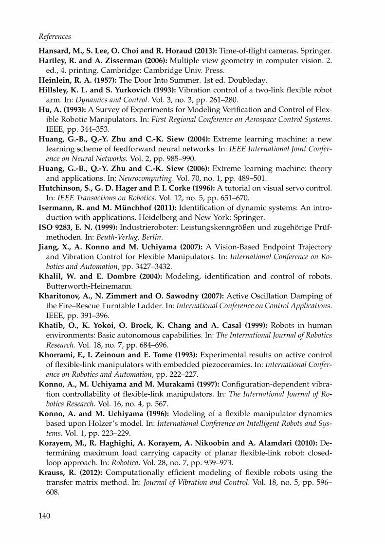
References
Hansard, M., S. Lee, O. Choi and R. Horaud (2013): Time-of-flight cameras. Springer.
Hartley, R. and A. Zisserman (2006): Multiple view geometry in computer vision. 2.
ed., 4. printing. Cambridge: Cambridge Univ. Press.
Heinlein, R. A. (1957): The Door Into Summer. 1st ed. Doubleday.
Hillsley, K. L. and S. Yurkovich (1993): Vibration control of a two-link flexible robot
arm. In: Dynamics and Control. Vol. 3, no. 3, pp. 261–280.
Hu, A. (1993): A Survey of Experiments for Modeling Verification and Control of Flex-
ible Robotic Manipulators. In: First Regional Conference on Aerospace Control Systems.
IEEE, pp. 344–353.
Huang, G.-B., Q.-Y. Zhu and C.-K. Siew (2004): Extreme learning machine: a new
learning scheme of feedforward neural networks. In: IEEE International Joint Confer-
ence on Neural Networks. Vol. 2, pp. 985–990.
Huang, G.-B., Q.-Y. Zhu and C.-K. Siew (2006): Extreme learning machine: theory
and applications. In: Neurocomputing. Vol. 70, no. 1, pp. 489–501.
Hutchinson, S., G. D. Hager and P. I. Corke (1996): A tutorial on visual servo control.
In: IEEE Transactions on Robotics. Vol. 12, no. 5, pp. 651–670.
Isermann, R. and M. Münchhof (2011): Identification of dynamic systems: An intro-
duction with applications. Heidelberg and New York: Springer.
ISO 9283, E. N. (1999): Industrieroboter: Leistungskenngrößen und zugehörige Prüf-
methoden. In: Beuth-Verlag, Berlin.
Jiang, X., A. Konno and M. Uchiyama (2007): A Vision-Based Endpoint Trajectory
and Vibration Control for Flexible Manipulators. In: International Conference on Ro-
botics and Automation, pp. 3427–3432.
Khalil, W. and E. Dombre (2004): Modeling, identification and control of robots.
Butterworth-Heinemann.
Kharitonov, A., N. Zimmert and O. Sawodny (2007): Active Oscillation Damping of
the Fire–Rescue Turntable Ladder. In: International Conference on Control Applications.
IEEE, pp. 391–396.
Khatib, O., K. Yokoi, O. Brock, K. Chang and A. Casal (1999): Robots in human
environments: Basic autonomous capabilities. In: The International Journal of Robotics
Research. Vol. 18, no. 7, pp. 684–696.
Khorrami, F., I. Zeinoun and E. Tome (1993): Experimental results on active control
of flexible-link manipulators with embedded piezoceramics. In: International Confer-
ence on Robotics and Automation, pp. 222–227.
Konno, A., M. Uchiyama and M. Murakami (1997): Configuration-dependent vibra-
tion controllability of flexible-link manipulators. In: The International Journal of Ro-
botics Research. Vol. 16, no. 4, p. 567.
Konno, A. and M. Uchiyama (1996): Modeling of a flexible manipulator dynamics
based upon Holzer’s model. In: International Conference on Intelligent Robots and Sys-
tems. Vol. 1, pp. 223–229.
Korayem, M., R. Haghighi, A. Korayem, A. Nikoobin and A. Alamdari (2010): De-
termining maximum load carrying capacity of planar flexible-link robot: closed-
loop approach. In: Robotica. Vol. 28, no. 7, pp. 959–973.
Krauss, R. (2012): Computationally efficient modeling of flexible robots using the
transfer matrix method. In: Journal of Vibration and Control. Vol. 18, no. 5, pp. 596–
608.
140
References
Krauss, R., W. J. Book et al. (2010): Transfer Matrix Modeling of Systems With Non-
collocated Feedback. In: Journal of dynamic systems, measurement and control. Vol. 132,
no. 6, pp. 13011–130111.
Krauss, R. W. (2006): An Improved Technique for Modeling and Control of Flexible
Structures. Phd thesis. Atlanta: Georgia Institute of Technology.
Li, Y. F. and X. B. Chen (2002): End-point sensing and state observation of a flexible-
link robot. In: IEEE/ASME Transactions on Mechatronics. Vol. 6, no. 3, pp. 351–356.
Luca, A. d. and R. Mattone (2004): An adapt-and-detect actuator FDI scheme for
robot manipulators. In: International Conference on Robotics and Automation. Vol. 5,
pp. 4975–4980.
Luca, A. d. and R. Mattone (2005): Sensorless robot collision detection and hybrid
force/motion control. In: International Conference on Robotics and Automation, pp. 999–
1004.
Luca, A. d., S. Panzieri and G. Ulivi (1998): Stable inversion control for flexible
link manipulators. In: International Conference on Robotics and Automation. Vol. 1,
IEEE/RSJ, pp. 799–805.
Luca, A. d. and B. Siciliano (1989): Trajectory control of a non-linear one-link flexible
arm. In: International Journal of Control. Vol. 50, no. 5, pp. 1699–1715.
Luca, A. d. and B. Siciliano (1991): Closed-form dynamic model of planar multilink
lightweight robots. In: IEEE Transactions on Systems, Man and Cybernetics. Vol. 21,
no. 4, pp. 826–839.
Luca, A. d., A. Albu-Schaffer, S. Haddadin and G. Hirzinger (2006): Collision de-
tection and safe reaction with the DLR-III lightweight manipulator arm. In: Interna-
tional Conference on Intelligent Robots. IEEE/RSJ, pp. 1623–1630.
Luo, Z.-H (1993): Direct strain feedback control of flexible robot arms: new theoretical
and experimental results. In: IEEE Transactions on Automatic Control. Vol. 38, no. 11,
pp. 1610–1622.
Luo, Z.-H. and B. Guo (1995): Further theoretical results on direct strain feedback
control of flexible robot arms. In: IEEE Transactions on Automatic Control. Vol. 40,
no. 4, pp. 747–751.
Mace, B. R. (1984): Wave reflection and transmission in beams. In: Journal of Sound and
Vibration. Vol. 97, no. 2, pp. 237–246.
Malzahn, J. (2008): Modellierung und Regelung eines mehrgliedrigen elastischen Ro-
boterarms. Diploma Thesis. Dortmund: TU Dortmund.
Malzahn, J. and T. Bertram (2014): Fractional Order Strain Feedback for Oscillation
Damping of a Multi-Elastic-Link Arm Under Gravity. In: 45th International Sym-
posium on Robotics and 8th German Conference on Robotics, accepted.
Malzahn, J., A. S. Phung and T. Bertram (2012a): A Multi-Link-Flexible Robot Arm
Catching Thrown Balls. In: 7th German Conference on Robotics, pp. 411–416.
Malzahn, J., A. S. Phung and T. Bertram (2012b): Predictive delay compensation
for camera based oscillation damping of a multi link flexible robot. In: Intelligent
Robotics and Applications. Springer, pp. 93–102.
Malzahn, J., A. S. Phung and T. Bertram (2012c): Scene adaptive RGB-D based os-
cillation sensing for a multi flexible link robot arm in unstructured dynamic en-
vironments. In: International Conference on Intelligent Robots and Systems, pp. 1017–
1022.
141
References
Malzahn, J., R. F. Reinhart and T. Bertram (2014): Dynamics Identification of a Damped
Multi Elastic Link Robot Arm under Gravity. In: International Conference on Robotics,
accepted.
Malzahn, J., M. Ruderman, A. Phung, F. Hoffmann and T. Bertram (2010a): Input
shaping and strain gauge feedback vibration control of an elastic robotic arm. In:
Conference on Control and Fault-Tolerant Systems, pp. 672–677.
Malzahn, J., A. S. Phung, R. Franke, F. Hoffmann and T. Bertram (2010b): Markerless
Visual Vibration Damping of a 3-DOF Flexible Link Robot Arm. In: 41st Interna-
tional Symposium on Robotics (ISR) and 6th German Conference on Robotics (ROBOTIK),
pp. 401–408.
Malzahn, J., A. Phung, F. Hoffmann, M. Ruderman and T. Bertram (2011a): Mod-
ellfreie Schwingungsdämpfung eines eingliedrigen elastischen Roboterarms unter
Gravitationseinfluss. In: Fachtagung Mechatronik. Ed. by T. Bertram, B. Corves and
K. Janschek. TU Dresden, pp. 89–94.
Malzahn, J., A. S. Phung, F. Hoffmann and T. Bertram (2011b): Vibration control of
a multi-flexible-link robot arm under gravity. In: International Conference on Robotics
and Biomimetics, pp. 1249–1254.
Malzahn, J., A. S. Phung, F. Hoffmann and T. Bertram (2012): Bildbasierte Regelung
eines gliedelastischen Roboterarms mit einem RGB-D-Sensor. In: at-Automatisierungs-
technik. Vol. 60, no. 5, pp. 246–259.
Mansour, T., X. Jiang, A. Konno and M. Uchiyama (2008): Experimental verification
on vibration suppression of a flexible manipulator using MPID controller. In: Inter-
national Conference on Robotics and Automation. IEEE, pp. 2896–2901.
Meirovitch, L. (2001): Fundamentals of vibrations. Boston: McGraw-Hill.
Miersch, L., W. Hanke, S. Wieskotten, F. D. Hanke, J. Oeffner, A. Leder, M. Brede,
M. Witte and G. Dehnhardt (2011): Flow sensing by pinniped whiskers. In: Philo-
sophical Transactions of the Royal Society B: Biological Sciences. Vol. 366, no. 1581,
pp. 3077–3084.
Moallem, M. and R. V. Patel (2001): Vibration control of flexible-link manipulators
using generalized output redefinition. In: International Symposium on Computational
Intelligence in Robotics and Automation, pp. 23–28.
Singer, Singhose and Seering (1999): Comparison of Filtering Methods for Reducing
Residual Vibration. In: European Journal of Control. Vol. 5, no. 2, pp. 208–218.
O’Connor, W. J. (2007a): Theory of wave analysis of lumped flexible systems. In:
American Control Conference, pp. 4215–4220.
O’Connor, W. J. (2007b): Wave-based analysis and control of lump-modeled flexible
robots. In: IEEE Transactions on Robotics. Vol. 23, no. 2, pp. 342–352.
O’Connor, W. J. and L. Donogh (1998): Position control of flexible robot arms using
mechanical waves. In: Journal of dynamic systems, measurement and control. Vol. 120,
no. 3, pp. 334–339.
O’Connor, W. J., F. La Ramos de Flor, D. McKeown and V. Feliu (2009): Wave-based
control of non-linear flexible mechanical systems. In: Nonlinear Dynamics. Vol. 57,
no. 1, pp. 113–123.
Oliensis, J. (1999): A multi-frame structure-from-motion algorithm under perspective
projection. In: International Journal of Computer Vision. Vol. 34, no. 2-3, pp. 163–192.
142

References
Phung, A. S., J. Malzahn, F. Hoffmann and T. Bertram (2011a): Data based kinematic
model of a multi-flexible-link robot arm for varying payloads. In: International Con-
ference on Robotics and Biomimetics, pp. 1255–1260.
Pisoni, A. C., C. Santolini, D. E. Hauf and S. Dubowsky (1995): Displacements in
a Vibrating Body by Strain Gage Measurements. In: 13th International Conference on
Modal Analysis. Vol. 2460, Society for Experimental Mechanics, p. 119.
Podlubny, I., I. Petras, B. M. Vinagre, P. O’Leary and L. Dorcak (2002): Analogue
realizations of fractional-order controllers. In: Nonlinear Dynamics. Vol. 29, no. 1-4,
pp. 281–296.
Presse, C. and M. Gautier (1993): New criteria of exciting trajectories for robot iden-
tification. In: IEEE International Conference on Robotics and Automation, pp. 907–912.
Pridgen, B., E. Maleki, W. Singhose, W. Seering, U. Glauser and L. Kaufmann
(2011): A small-scale cherrypicker for experimental and educational use. In: Amer-
ican Control Conference, pp. 681–686.
Rong, B., X. Rui, G. Wang and F. Yang (2010): Discrete time transfer matrix method
for dynamics of multibody system with real-time control. In: Journal of Sound and
Vibration. Vol. 329, no. 6, pp. 627–643.
Santis, A. d., B. Siciliano, A. d. Luca and A. Bicchi (2008): An atlas of physical
human–robot interaction. In: Mechanism and Machine Theory. Vol. 43, no. 3, pp. 253–
270.
Sawada, H., H. Ueno, M. Oda, S. Matunaga and K. Konoue (2005): Input Shaping
Experiment for Damping Vibration in Manual Operation of a Large Robotic Arm.
In: Proceedings of The 8th International Symposium on Artificial Intelligence, Robotics,
and Automation in Space, Sept. 5. Vol. 8,
Schröder, D. (2009): Elektrische Antriebe - Regelung von Antriebssystemen. 3rd ed.
Berlin and Heidelberg: Springer Berlin Heidelberg.
Sciavicco, L. and B. Siciliano (2001): Modelling and Control of Robot Manipulators.
Second. Berlin and Germany: Springer.
Scott, M. A., M. G. Gilbert and M. E. Demeo (1993): Active Vibration Damping of
the Space Shuttle Remote Manipulator System. In: Journal of Guidance, Control and
Dynamics. Vol. 16, no. 2, pp. 275–280.
Singhose, W. (2009): Command shaping for flexible systems: A review of the first
50 years. In: International Journal of Precision Engineering and Manufacturing. Vol. 10,
no. 4, pp. 153–168.
Subbarao, M. and G. Surya (1994): Depth from defocus: a spatial domain approach.
In: International Journal of Computer Vision. Vol. 13, no. 3, pp. 271–294.
Subudhi, B. and A. Morris (2009): Soft computing methods applied to the control of
a flexible robot manipulator. In: Applied Soft Computing. Vol. 9, no. 1, pp. 149–158.
Swain, M. J. and D. H. Ballard (1990): Indexing via color histograms. In: Third Inter-
national Conference on Computer Vision, pp. 390–393.
Swevers, J., W. Verdonck and J. d. Schutter (2007): Dynamic model identification for
industrial robots. In: IEEE Control Systems Magazine. Vol. 27, no. 5, pp. 58–71.
Takyar, M. S. and T. T. Georgiou (2007): The fractional integrator as a control design
element. In: 46th Conference on Decision and Control, pp. 239–244.
143
References
Tao, W. M., M. J. Zhang, M. Liu and X. P. Yun (2006): Residual Vibration Analysis and
Suppression for SCARA Robots in Semiconductor Manufacturing. In: International
Journal of Intelligent Control and Systems. Vol. 11, no. 2, pp. 97–105.
Theodore, R. J. and A. Ghosal (1995): Comparison of the assumed modes and finite
element models for flexible multilink manipulators. In: The International Journal of
Robotics Research. Vol. 14, no. 2, pp. 91–111.
TNS Opinion and Social (2012): Public Attitudes Towards Robots: Report of the
Special EB 382, Wave EB 77.1. Ed. by European Commission.
Tokhi, O. and K. A. Azad (2008): Flexible robot manipulators: Modelling, simulation
and control. London: Inst. of Engineering and Technology.
Tsujisawa, T. and W. J. Book (1989): A reduced order model derivation for lightweight
arms with a parallel mechanism. In: IEEE International Conference on Robotics and
Automation, pp. 728–735.
Vaughan, J., A. Yano and W. Singhose (2008): Comparison of robust input shapers.
In: Journal of Sound and Vibration. Vol. 315, no. 4, pp. 797–815.
Vepa, R. (2010): Dynamics of Smart Structures. Wiley.
Wang, D. and M. Vidyasagar (1991): Transfer functions for a single flexible link. In:
The International Journal of Robotics Research. Vol. 10, no. 5, pp. 540–549.
Wenz, M. (2008): Automatische Konfiguration der Bewegungssteuerung von Indus-
trierobotern. Dissertation. Karlsruhe: University Karlsruhe.
Whitney, D. E., W. J. Book and P. M. Lynch (1974): Design and control considerations
for industrial and space manipulators. In: 15th Joint Automatic Control Conference,
Austin (USA), pp. 591–598.
Wöhler, C. (2013): 3D computer vision: Efficient methods and applications. 2nd ed.
X.media.publishing. London and New York: Springer.
Xuming Luan (2001): Experimental Investigation of Photonic Mixer Device and De-
velopment of TOF 3D Ranging Systems Based on PMD Technology. Dissertation.
Siegen: Universität Siegen.
Zeng, H. (1999): Modeling, Identification and Control of a Multi-Link Lightweight
Manipulator. Dissertation. Bochum: Ruhr-University Bochum.
Zimmert, N., A. Kharitonov and O. Sawodny (2008): A new Control Strategy for
Trajectory Tracking of Fire–Rescue Turntable Ladders. In: Proceedings of the 17th
IFAC World Congress, pp. 869–874.
144
Additional Publications
Additional Publications
The research activities during preparation of this work have reached beyond the actual
scope of this thesis. This lead to the authorship and co-authorship in the following
additional publications:
Kracht, M., J. Malzahn, F. Hoffmann and T. Bertram (2010): Image Based Visual
Servoing For Lane Keeping Assistance. In: FISITA 2010 World Automotive Congress.
FISITA.
Malzahn, J. (February 2012): Einsatz eines RGB-D-Sensors zur schwingungsgedäm-
pften Positionierung eines gliedelastischen Roboterarms. Boppard.
Malzahn, J. (October 2013): Link Elasticity in a Robot Arm: From a Problem to an
Opportunity. München.
Malzahn, J., R. Franke, F. Hoffmann and T. Bertram (2009): Modellierung und Regel-
ung eines mehrgliedrigen elastischen Roboterarms. In: Automation 2009. Vol. 2067,
VDI-Berichte. VDI-Verl., pp. 153–157.
Nierobisch, T., K. V. Patel, J. Malzahn, F. Hoffmann and T. Bertram (2007): Rapid
Prototyping of Visual Servoing Controllers with Virtual Reality. In: System integra-
tion. Ed. by E. Kallenbach. Wiss.-Verl. Thüringen.
Phung, A. S., J. Malzahn, F. Hoffmann and T. Bertram (2010): Lernen durch Demon-
stration und Kollisionsvermeidung mit Dynamischen Bewegungsprimitiven. In: 20.
Workshop Computational Intelligence. Ed. by F. Hoffmann. Vol. 33, KIT Scientific Pub.,
pp. 250–263.
Phung, A. S., J. Malzahn, F. Hoffmann and T. Bertram (2011b): Datenbasiere Mod-
ellierung der Kinematik eines dreigliedrigen elastischen Roboterarms. In: 21. Work-
shop Computational Intelligence. Ed. by F. Hoffmann. Vol. 21, KIT Scientific Publish-
ing, pp. 187–202.
Phung, A. S., J. Malzahn, F. Hoffmann and T. Bertram (2012): Tool centered learning
from demonstration for robotic arms with visual feedback. In: International Confer-
ence on Robotics and Biomimetics, pp. 1117–1122.
Phung, A., J. Malzahn, F. Hoffmann and T. Bertram (2011d): Get Out of the Way-
Obstacle Avoidance and Learning by Demonstration for Manipulation. In: IFAC
World Congress. Vol. 18, pp. 11514–11519.
145
Published Software and Media
Published Software and Media
During preparation of this work the following media and sources have been published
online under open licenses:
Malzahn, J. (2013): CodeGenerator-Module for the Robotic Toolbox by Peter Corke.
Malzahn, J., R. Balachandran and T. Bertram (2013): Video: Experiments on force
control of a multi-fexible-link robot. url: http://youtu.be/AJPZjF7HDxY (vis-
ited on 12/12/13).
Malzahn, J. and T. Bertram (2013): Video: Oscillation Damping, Collision Detec-
tion and Reaction with a Multi-Elastic-Link Robot Arm. url: http://youtu.be/
kJPuenyxeps (visited on 12/12/13).
Malzahn, J., A. S. Phung, F. Hoffmann and T. Bertram (2011c): Video: A multi-
flexible-link robot arm under gravity catching thrown soft-balls. url: http://
youtu.be/P4_i_kGt2jA (visited on 12/12/13).
Malzahn, J., A. S. Phung, F. Hoffmann and T. Bertram (2011d): Video: Initial visual
servoing experiments with a multi-flexible-link arm. url: http://youtu.be/
V2NnEU6yGEA (visited on 12/12/13).
Phung, A. S., J. Malzahn, F. Hoffmann and T. Bertram (2011c): Video: Tip position
control of a multi-flexible-link robot arm for varying payloads using neural net-
works. url: http://youtu.be/VQZ1FF3wAxA (visited on 12/12/13).
146
Supervised theses
Supervised theses
A number of ideas grown during this work emerged from discussions in the context
of the following supervised theses:
Balachandran, R. (November 2012): Experimental Evaluation of Wave-Based Con-
cepts for Oscillation free Motion Control of a Flexible Link Robot Arm. Masterht-
esis. Dortmund: Technische Universität Dortmund.
Breitenbach, T. (September 2009): Bildbasierte Regelung und Schwingungsdämpfung
eines mehrgliedrigen elastischen Roboterarms. Diploma Thesis. Dortmund: Tech-
nische Universität Dortmund.
Bürger, F. (February 2011): Entwicklung eines kamerabasierten Messsystems zur 3D-
Endeffektorlokalisierung für einen elastischen Roboterarm. Studienarbeit. Dortmund:
Technische Universität Dortmund.
Bürger, F. (February 2012): Echtzeit-Schätzung der Endeffektor-Eigenbewegung eines
gliedelastischen Roboterarms mittels einer 3D-Kamera. Diploma Thesis. Dortmund:
Technische Universität Dortmund.
Gorczak, P. (November 2012): Fusion von RGB-D- und Inertial-Sensorik zur örtlich
konzentrierten Schwingungsmessung an einem gliedelastischen Roboterarm unter
Gravitationseinfluss. Bachelorthesis. Dortmund: Technische Universität Dortmund.
Kappen, J. (October 2012): Gravitationskompensation eines gliedelastischen Roboter-
arms. Bachelorthesis. Dortmund: Technische Universität Dortmund.
Koop, A. (May 2011): Adaptive Schwingungsdämpfung eines elastischen Roboter-
arms unter Gravitationseinfluss. Studienarbeit. Dortmund: Technische Universität
Dortmund.
Koop, A. (October 2013): Physische Interaktion mit einem konventionellen Industri-
eroboter auf Basis verteilter Dehnungs-Sensorik. Diploma Thesis. Dortmund: Tech-
nische Universität Dortmund.
Sapadinski, A. (October 2011): Sensitivitätsanalyse für die Dynamik eines gliedelast-
ischen Roboterarms unter Gravitationseinfluss. Bachelorthesis. Dortmund: Technis-
che Universität Dortmund.
Wissing, C. (October 2013): Dual-Quaternionen zur Schätzung der Kamera Eigen-
bewegung aus RGB-D-Bildfolgen. Masterthesis. Dortmund: Technische Universität
Dortmund.
Zimmert, M. (August 2010): 2D-Bildbasierte Regelung zur Realisierung eines Spurhal-
teassistenten für Kraftfahrzeuge. Studienarbeit. Dortmund: Technische Universität
Dortmund.
147
Top Related
Copyright © 2022 FDOKUMEN

