


Bahasa
Halaman
Hukum


Minimax Flow Tree Problems
Hui Chen1, Ann Campbell1, Barrett Thomas1, and Arie Tamir2
1 Dept. of Management Sciences, Tippie College of Business, The University of Iowa, USA
{hui-chen, ann-campbell, barrett-thomas}@uiowa.edu
2 Dept. of Statistics and Operations Research, School of Mathematical Sciences, Tel Aviv University, Israel
July 5, 2007
Abstract
We examine a class of problems which seeks to find tree-structured networks whichminimize the maximum cost among a subset of nodes in a graph. The cost metric ischaracterized by a series of parameters which can represent distance, flow volume, anddelivery deadlines. Derived through variations in problem parameters, we present 17different problems and discuss their worst-case complexity. Fourteen of the problemsare new to the literature. We show that some of the problems are NP-complete andothers are polynomially solvable.Keywords: trees, minimax, flow, complexity, shortest path trees
1

1 Introduction
To be successful in the face of fierce competition and to meet the growing demand for
time-definite services, delivery companies must design their delivery networks to reliably
and efficiently meet their promised delivery times. In the near term, however, redesign
of the network through the opening of new facilities and the closing of existing facilities
is infeasible. Rather, the network can be modified by changing how freight flows through
the network. In particular, companies can change which cities have direct connections to
one another and which cities must flow freight and packages through intermediate cities in
order to make a connection. Each city-to-city connection requires substantial investment,
so delivery companies want to minimize the number of direct connections. Consequently,
this study will focus on restricting the design of the delivery networks to tree structures,
as they connect all of the nodes in the network with the minimum number of connections.
In addition to cost minimization, Powell and Koskosidis (1992) note that tree-structured
networks are easier networks to manage because there is only one path between each origin
and destination pair.
Different tree structures offer different levels of service between customers. Delivery compa-
nies may have stricter service requirements or place more emphasis on service between certain
sets or kinds of customers, and this should be reflected in their choice of tree-structured net-
work. With this in mind, this paper considers different variants in assumptions and objective
function and examines the complexity of each. All of the problems assume a simple, con-
nected, and undirected graph G = (V, E). For each problem, the objective is to minimize
the maximum cost between a source node set S ⊆ V and sink node set U ⊆ V and involves
two parameters: fij ≥ 0 and Hij ≥ 0. A minimax objective optimizes service by minimizing
the worst-case service between customers in the source and sink sets. The definition of the
source and sink node set as well as the parameters define each variant in the class, allowing
the objective to be expressed in the following general form:
maxvi∈S
maxvj∈U
{fij(dT (vi, vj)−Hij)}. (1)
2

The choice of source node set and sink node set reflects the combination of customers whose
service level is considered in the objective function. For example, if S = V and U = V ,
we want to consider the travel time from every customer to every other customer in the
objective. If S 6= V or U 6= V , we want to consider the travel time only between a subset
of nodes in the objective function. The selection of S and U is thus a reflection of priorities
among customers or cities in a delivery network. Next, the parameter fij reflects a weight
placed on the service from customer vi to customer vj. This weight may reflect, for example,
the flow of packages from city vi to city vj, so that cities with heavy flow between them
are prioritized in the objective. We may consider simpler versions where fij is constant for
all vi, vj pairs (f) or only dependent on vi (fi). We will also consider a special case of fij
where it is based on values for fi and fj. Finally, the parameter Hij represents a service
time commitment from customer vi to customer vj. Many delivery providers offer varying
levels of service between customers depending on their location and demand, so Hij forces
Equation 1 to minimize the maximum violation of these commitments. As with fij, we can
consider simpler versions such as where Hij is zero (0), a constant (H), or where Hij is
dependent only on vi (Hi). Note that when Hij = 0 for all vi, vj pairs this represents the
case where there is no established commitment, and the objective is to simply minimize the
maximum travel time between pairs.
Table 1 lists the different problem variants covered in this paper or in the literature and
their worst-case complexity status. It should be noted that each of these problems is in NP
as the objective function associated with a given tree can be evaluated in polynomial time.
For those problems that can be solved in polynomial time, we set n = |V |, m = |E|, k = |S|,l = |U | and n = |S| + |U | = k + l. Without loss of generality, we assume that k > 1 and
l > 1. Otherwise, if either S or U consists of a single node, then the optimal tree is a shortest
path spanning tree rooted at that node.
In this paper, we examine the complexity of these minimax flow tree problems and find
some to be polynomial and others to be NP -Complete. In Section 2, we review the related
literature. In Section 3, we define relevant notation for our study. Section 4 studies the
algorithms for the tractable problems. In Section 5, the NP -Completeness of the intractable
problems is established. Finally, we discuss directions for future work in Section 6.
3

Problem S U fij Hij Complexity Reference
1 MDST S = V U = V 1 0 O(mn + n2 log n) Handler and Mirchandani (1979)
Kariv and Hakimi (1979)
Hassin and Tamir (1995)
2 k-MEST S ⊆ V U = V 1 0 O(mn + n2 log n) Wu (2004)
3 MEMT S ⊆ V U ⊆ V 1 0 O(mn + n2 log n) Krumme and Fragopoulou (2001),
this paper
4 UMVT S ⊆ V U ⊆ V 1 H O(mn + n2 log n) this paper
5 NMVT S ⊆ V U ⊆ V 1 Hi O(mn + n2 log n) this paper
6 PMVT S ⊆ V U ⊆ V 1 Hij NP -Complete this paper
7 NF-MDST S = V U = V fi 0 O(mn log n) this paper
8 NF-MEMT S ⊆ V U ⊆ V fi 0 O(mn + n2 log n + mn log n) this paper
9 NF-UMVT S ⊆ V U ⊆ V fi H O(mn + n2 log n + mn log n) this paper
10 NF-NMVT S ⊆ V U ⊆ V fi Hi O(mn + n2 log n + mn log n) this paper
11 NF-PMVT S ⊆ V U ⊆ V fi Hij NP -Complete this paper
12 SF-MDST S = V U = Vfifj
fi+fj0 O(mn log n) this paper
13 PF-MDST S = V U = V fij 0 NP -Complete this paper
14 PF-MEMT S ⊆ V U ⊆ V fij 0 NP -Complete this paper
15 PF-UMVT S ⊆ V U ⊆ V fij H NP -Complete this paper
16 PF-NMVT S ⊆ V U ⊆ V fij Hi NP -Complete this paper
17 PF-PMVT S ⊆ V U ⊆ V fij Hij NP -Complete this paper
Table 1: Problem Variants
2 Literature Review
The Minimum Diameter Spanning Tree Problem (MDST) is the problem of finding a span-
ning tree T of G with minimum diameter, where the diameter of T is defined as the longest
path in T among the paths between all pairs of nodes in V . Ho et al. (1991) consider the
case where the graph G is a complete Euclidean graph, induced by a set of n points in the
Euclidean plane. Ho et al. call this special case the geometric MDST. Ho et al. develop
an O(n3) algorithm to find a spanning tree of minimum diameter of a Euclidean graph, and
they mention that these results extend to any graph whose edge lengths satisfy the triangle
inequality. Handler and Mirchandani (1979) (see also Hassin and Tamir (1995)) consider the
general case where the edge lengths in a general graph do not necessarily satisfy the trian-
gle inequality. They observe that MDST is identical to the well studied Absolute 1-Center
Problem introduced by Hakimi (1964), where the absolute center of a graph is a point in the
graph whose maximum shortest distance from any node on the graph is minimal. Hassin
4

and Tamir (1995) note that MDST can then be solved by the existing algorithms for the
Absolute 1-Center Problem on a general graph in O(mn+n2 log n) time (Kariv and Hakimi,
1979).
Given the source set S ⊆ V such that |S| = k and the sink set U = V in G, the k-
Source Minimum Max-Eccentricity Spanning Tree Problem (k-MEST) is defined as finding
a spanning tree to minimize the maximal source eccentricities among k sources, where the
source eccentricity in a spanning tree T is the longest distance from a source to all sink nodes.
Farley et al. (2000) explore the variant with uniform edge lengths. First, they prove that
there exists either a vertex x or an edge (y, z), such that the shortest path tree rooted from
either x or the midpoint of (y, z) minimizes the maximal source eccentricity. They introduce
an exact polynomial algorithm for k-MEST with uniform edge length based on solving many
shortest path problems. McMahan and Proskurowski (2004) generalize the result for graphs
with general edge lengths and show there exists a minimum max-eccentricity spanning tree
which is a shortest path tree rooted at either a vertex or a created vertex lying on an
edge. McMahan and Proskurowski (2004) then establish an exact polynomial algorithm
with running time O(n3 + mn log n) for a general graph. Krumme and Fragopoulou (2001)
study the Minimum Eccentricity Multicast Tree (MEMT), which is a generalized version of
k-MEST with the sink set U ⊆ V . By identifying the appropriate edge that can be cut to
create a new vertex from which to construct an optimal shortest path spanning tree, Krumme
and Fragopoulou offer a polynomial algorithm with running time O(mn + n3) for MEMT,
which computes the all pair shortest path distances in O(n3) time. We note that, if we
apply Fibonacci heaps to compute the all pair shortest path distances (Fredman and Tarjan,
1987), the complexity of the algorithm in (Krumme and Fragopoulou, 2001) improves to
O(mn + n2 log n) time. Based on a similar idea as Krumme and Fragopoulou (2001), Wu
(2004) independently describes another polynomial algorithm with O(mn + n2 log n) time
for the k-MEST.
Another problem related to source eccentricity is the k-Source Minimum Sum-Eccentricity
Spanning Tree Problem (k-SSET). This problem seeks to minimize the sum of the eccen-
tricities of the k source nodes instead of the maximum eccentricity of the k source nodes.
Connamacher and Proskurowski (2003) demonstrate that k-SSET is polynomially solvable.
5

Fragopoulou et al. (2005) design an O(mn log n) time algorithm to solve the k-SSET.
The Optimal Communication Spanning Tree Problem (OCST) is the only literature known
to the authors which considers flow in conjunction with tree structures. In this problem,
given a set of communication requirements rij between vi and vj in graph G = (V, E), the
cost measure of a spanning tree is defined as follows. For a pair of nodes vi and vj, there
is a unique path in the spanning tree between them. The cost of communication for the
pair of nodes vi and vj is rij multiplied by the distance of the path, dT (vi, vj). Summing
over all (n2 ) pairs of nodes, we have the cost of the spanning tree. Hu (1974) introduces the
OCST, and Johnson et al. (1978) show that OCST is NP-hard. Ahuja and Murty (1987)
provide an exact algorithm for small problems. Peleg (1997) and Peleg and Reshef (1998)
establish polynomial-time approximation algorithms for OCST. Hu (1974) also studies the
special OCST, which is labeled as ORST and assumes the length of every arc is one, and
demonstrates a polynomial algorithm to solve the ORST in a complete graph. Hu (1974)
introduces another special OCST, which is labeled as ODST and assumes the required flows
are one for all pairs of nodes. Wu (2002) proves that the k-source ODST (k-ODST), where
there are k source nodes, is NP-hard even if k = 2 for a metric graph. Additional ODST
research focuses on finding approximation algorithms (Wu et al., 1999, 2000a,b).
Also related to the research in this paper is the Hop-Constrained Minimum Spanning Tree
Problem (HC-MST). Referring to each arc as a hop, hop constraints limit the number of hops
between nodes and can be viewed as a distance constraint. In the literature, the objective of
HC-MST is to find the minimum spanning tree T such that the number of the hops (arcs)
in the unique path from a single root node to any other node is no greater than a constant
number H. Dahl (1998) proves that the 2-hop constrained minimum spanning tree problem
is NP-Hard. Manyem and Stallmann (1996) show that HC-MST is not APX such that it is
not possible to find a polynomial time heuristic which guarantees a constant approximation
bound. Many different IP formulations and related solution approaches have been studied
by Gouveia (1995), Gouveia (1996), Gouveia (1998), and Gouveia and Requejo (2001). Voss
(1999) uses tabu search to improve a feasible initial solution. Althaus et al. (2005) build an
algorithm with an O(log n)-approximation in running time O(n5k) for the k-hop constrained
minimum spanning tree problem.
6

3 Notation
In this section, we describe the notation used throughout our paper. Let G = (V, E) be a
simple, connected, and undirected graph, where V is the set of nodes vi and E is the set of
edges eij. Without loss of generality, we assume i < j for every edge eij. Each edge eij ∈ E
is associated with a positive length lij and is assumed to be rectifiable. We note that the
literature often equates arc length with distance in the network. Because of our focus on
service-time commitments, we consider these lengths to be travel times. However, the two
measures of distance are equivalent for purposes of the results presented in this paper. Thus,
our service-time commitment can also be thought of as a distance restriction.
A node which is incident to only one edge is a leaf node, otherwise it is an internal node.
An edge incident to a leaf node is a leaf edge. A path from node vi to node vj is denoted
as the vi-vj path. A spanning tree of G is a connected subgraph T = (V, ET ⊆ E) without
cycles. The distance between node vi and node vj in T , dT (vi, vj), is the sum of the lengths
of the edges which are in the unique vi-vj path. For two nodes vi and vj, the shortest path
distance between them in a graph G is denoted by dG(vi, vj).
We define nodes vi ∈ V and vj ∈ V as adjacent in the tree T if eij ∈ ET . The endpoints of
a path are the two nodes at which the path begins and ends. In a path, all the other nodes
except the two endpoints are internal nodes of the path. Let vi1-vi2-...-via be path A and
vj1-vj2-...-vjbbe path B in the graph. We say that path A and path B are disjoint if the sets
{vi1 , ..., via} and {vj1 , ..., vjb} are disjoint. If the above two sets are not disjoint, we say that
path A and path B intersect, and each node in their intersection is called an intersection
node.
We define a point as a location in the graph which could be either a node or a location on an
edge. We will refer to a point on a rectifiable edge by its distances from the two nodes of the
edge. Let I(G) denote the continuum set of points on the edges of G. The edge lengths of
G induce a distance function on I(G). For any two points x, y ∈ I(G), dG(x, y) will denote
the length of a shortest path in I(G) connecting x and y. We refer to I(G) as the network
7

metric space induced by G and its edge lengths.
Recall, we let S ⊆ V and U ⊆ V denote the source node set and sink node set, respectively.
Further, we let k = |S|, l = |U | and n = |S| + |U | = k + l. For a spanning tree T , we
define the longest intra-sink path of T , DT , to be a longest path in T among all the paths
connecting a pair of sink nodes in U . The length of DT is denoted by δT . The center point
of a tree is the middle point of a longest intra-sink path. For a source node vi ∈ S, define
hTi = maxvj∈U{dT (vi, vj)}.
4 The Tractable Problems
This section presents polynomial-time algorithms for the tractable problems for which no
algorithm exists in the literature. For any problem with some Hij 6= 0, we will refer to the
problem as a Minimax Violation Tree Problem (MVT).
4.1 Uniform Commitment Minimax Violation Tree (UMVT)
The service-time commitment in the UMVT is the same for every pair of source and sink
nodes (Hij = H). Here, the maximum violation of a source is achieved by the longest travel-
time or distance from the source to all sinks in the tree, which is the eccentricity of the
source in the tree. As MEMT seeks to minimize the maximal source eccentricities, MEMT
and UMVT are closely related to each other. Theorem 1 states the relationship between
MEMT and UMVT.
Theorem 1 Any optimal solution to MEMT is an optimal solution to UMVT.
Proof: For UMVT, the objective is to minimize
maxvi∈S
maxvj∈U
{dT (vi, vj)−Hij} = maxvi∈S
maxvj∈U
{dT (vi, vj)} −H.
8
For MEMT where Hij = 0, the objective is to minimize
maxvi∈S
maxvj∈U
{dT (vi, vj)−Hij} = maxvi∈S
maxvj∈U
{dT (vi, vj)}.
Thus, if a tree minimizes the objective of MEMT, it also minimizes the objective for UMVT.
Given this result, UMVT can be solved by the algorithms for MEMT. Thus, UMVT can
be solved in O(mn + n2 log n) time (Krumme and Fragopoulou, 2001). In addition, as the
UMVT with S = U = V is the MDST, the special case with S = U = V also takes
O(mn + n2 log n) time to find an optimal solution.
4.2 Node Commitment Minimax Violation Tree (NMVT)
For NMVT, where Hij = Hi, we shall show that it can be transformed into a special MEMT
and solved by an algorithm for MEMT.
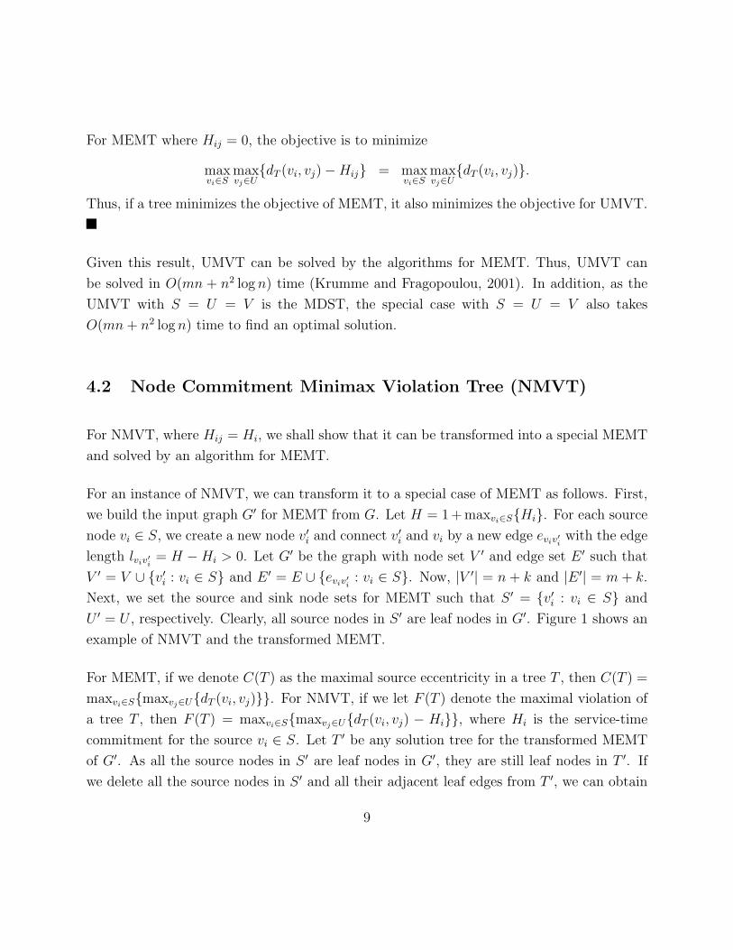
For an instance of NMVT, we can transform it to a special case of MEMT as follows. First,
we build the input graph G′ for MEMT from G. Let H = 1+maxvi∈S{Hi}. For each source
node vi ∈ S, we create a new node v′i and connect v′i and vi by a new edge eviv′iwith the edge
length lviv′i= H −Hi > 0. Let G′ be the graph with node set V ′ and edge set E ′ such that
V ′ = V ∪ {v′i : vi ∈ S} and E ′ = E ∪ {eviv′i: vi ∈ S}. Now, |V ′| = n + k and |E ′| = m + k.
Next, we set the source and sink node sets for MEMT such that S ′ = {v′i : vi ∈ S} and
U ′ = U , respectively. Clearly, all source nodes in S ′ are leaf nodes in G′. Figure 1 shows an
example of NMVT and the transformed MEMT.
For MEMT, if we denote C(T ) as the maximal source eccentricity in a tree T , then C(T ) =
maxvi∈S{maxvj∈U{dT (vi, vj)}}. For NMVT, if we let F (T ) denote the maximal violation of
a tree T , then F (T ) = maxvi∈S{maxvj∈U{dT (vi, vj) − Hi}}, where Hi is the service-time
commitment for the source vi ∈ S. Let T ′ be any solution tree for the transformed MEMT
of G′. As all the source nodes in S ′ are leaf nodes in G′, they are still leaf nodes in T ′. If
we delete all the source nodes in S ′ and all their adjacent leaf edges from T ′, we can obtain
9

1
Example for NMVT k-MEST
NMVT:Source set S={v1, v2, v3};Sink set U={v2, v3, v4};Node Restriction {H1=2, H2=4, H3=6}.
MEMT:Source set S’={v’1, v’2, v’3};Sink set U’={v2, v3, v4}.
Figure 1: An example of NMVT and the transformed special MEMT
a new tree T of G. Conversely, given any T of G, we can also construct a tree T ′ of G′ by
adding all the source nodes of S ′ and all their adjacent leaf edges in G′ to T . We have the
following observation for C(T ′) and F (T ).
Lemma 1 C(T ′) = F (T ) + H, where H = 1 + maxvi∈S{Hi}.
Proof: Clearly, dT (vi, vj) = dT ′(vi, vj) for any vi, vj ∈ V . Because vi ∈ S and v′i ∈ S ′ are
one to one corresponding and U ′ = U ,
C(T ′) = maxv′
i∈S′maxvj∈U ′
{dT ′(v′i, vj)}
= maxvi∈S
maxvj∈U
{dT ′(vi, vj) + lviv′i}
= maxvi∈S
maxvj∈U
{dT (vi, vj) + H −Hi}
= F (T ) + H.
We present the following theorem that follows directly from Lemma 1.
10

Theorem 2 A tree T is an optimal solution to the NMVT in G if and only if the corre-
sponding T ′ is optimal for the transformed MEMT in G′.
Given this result, the algorithm for MEMT can be applied to NMVT. As an optimal solution
for MEMT can be found in O(mn + n2 log n) time (Krumme and Fragopoulou, 2001) and
|V ′| = n + k ≤ 2n and |E ′| = m + k ≤ m + n, NMVT can be solved in O(mn + n2 log n)
computation time as well.
4.3 Node Flow Minimax Violation Tree (NF-MVT)
Now we consider the problem variants with node flow, where fij = fi. We shall study four
polynomially solvable variants in this class. These variants are NF-MDST, NF-MEMT, NF-
UMVT, and NF-NMVT. From Table 1, we can see that NF-NMVT is the most general of
these variants. Therefore, we shall first focus on establishing a polynomial algorithm for
NF-NMVT and later adjust it for the other three variants.
4.3.1 Preliminaries
To begin, we present the following lemma from Connamacher and Proskurowski (2003),
which characterizes the longest travel time or distance from a source node to all the sink
nodes in a tree. A similar result is also described by Handler (1973), for the case where
U = V .
Lemma 2 Given a spanning tree T , let sink nodes v1 and v2 be the two endpoints of DT .
For any source node vi ∈ S, hTi is obtained by either the vi-v1 path or the vi-v2 path.
Handler (1973) further clarifies from a node to which other node it obtains the longest travel
time or distance in a tree. We extend this result in the next lemma, which specifies which
11

endpoint of DT defines hTi for any source vi ∈ S and the value of hT
i . The proof follows
directly from Handler (1973) and is omitted.
Lemma 3 Given a spanning tree T , let sink nodes v1 and v2 be the two endpoints of DT .
Let o be the center point of T . Let vi ∈ S be any source node.
When vi is not on DT , let node vs be the node on DT where the path connecting vi with DT
intersects DT . If vs lies in the v1-o path, then hTi = dT (vi, v2). If vs lies in the v2-o path, then
hTi = dT (vi, v1). Similarly, when vi is on DT , if vi lies on the v1-o path, then hT
i = dT (vi, v2).
If vi lies on the v2-o path, then hTi = dT (vi, v1).
In addition, hTi = dT (vi, o) + 1
2δT .
An important result for the shortest path tree rooted at the center point of an optimal tree
for k-MEST is proved by Farley et al. (2000) and restated by Krumme and Fragopoulou
(2001) and McMahan and Proskurowski (2004). We now extend the result to a more general
form and revisit its proof as it leads to the development of our algorithm.
Lemma 4 Given a spanning tree T in graph G and its center point o, let tree To be the
shortest path tree rooted at o in G. For any source node vi ∈ S, hToi ≤ hT
i .
Proof: For any source vi ∈ S and any sink node vj ∈ U , because of the triangle inequality,
the shortest paths from o in To, the definition of longest intra-sink path, and Lemma 3, we
obtain
dTo(vi, vj) ≤ dTo(vi, o) + dTo(o, vj)
≤ dT (vi, o) + dT (o, vj)
≤ dT (vi, o) +1
2δT
= hTi .
12

Therefore, maxvj∈U{dTo(vi, vj)} = hToi ≤ hT
i .
For the same spanning trees T and To, we can also characterize the relationship between the
length of the longest intra-source paths in T and To.
Lemma 5 Given a spanning tree T in graph G and its center point o, let tree To be the
shortest path tree rooted at o in G. Then, δTo ≤ δT .
Proof: Let vj1 , vj2 ∈ U be any two sinks. By the triangle inequality, shortest paths from o
in To, and the longest intra-sink path,
dTo(vj1 , vj2) ≤ dTo(vj1 , o) + dTo(o, vj2)
≤ dT (vj1 , o) + dT (o, vj2)
≤ 1
2δT +
1
2δT
= δT .
This result implies
δTo = maxvj1
∈Umaxvj2
∈U{dTo(vj1 , vj2)} ≤ δT .
For NF-NMVT, we now further describe the relationship of hTi for any source vi ∈ S in a
tree T and the maximal violation for vi in T .
Lemma 6 For NF-NMVT, the maximal violation for any source vi ∈ S in a spanning tree
T is equal to fihTi − fiHi.
Proof: Let Hi and fi be the node restriction and node flow for vi, respectively. The maximal
violation of vi in T equals
maxvj∈U
{fi(dT (vi, vj)−Hi)} = fi maxvj∈U
{dT (vi, vj)} − fiHi
= fihTi − fiHi.
13

This result implies that, given the node restriction Hi and the node flow fi, the maximal
violation for any source vi ∈ S in T depends on only hTi .
Based on Lemma 4 and Lemma 6, we can show that for any optimal solution to NF-NMVT,
there exists a shortest path spanning tree which is also optimal.
Theorem 3 For NF-NMVT, given an optimal tree T ∗, let o be the center point of T ∗. The
shortest path spanning tree rooted at o, To, is also an optimal tree.
Proof: The result follows directly from Lemmas 4 and 6.
In the light of Theorem 3, given an optimal tree T ∗ and its center point o, we can build
another optimal tree which is the shortest path tree To rooted at o. Because the longest
intra-sink path of To may move, however, the center point of To may no longer be located
at o. In fact, o is not even guaranteed to be on a longest intra-sink path. Nevertheless, we
can prove that there does exist an optimal shortest path tree whose root coincides with its
center point.
Theorem 4 For NF-NMVT, there exists an optimal shortest path spanning tree whose root
is also its center point.
Proof: By Theorem 3, for any optimal tree T ∗ with center point r, we can generate a new
optimal tree Tr, which is a shortest path spanning tree rooted at r. If r is the center point
of Tr, we are done. If r is not the center point of Tr, we must construct another optimal
shortest path tree whose root coincides with its center point.
Let o be the center point of Tr. Let the v1-v2 path be a longest intra-sink path DTr of Tr
with length δTr . Then, o divides Tr into two subtrees, T 1r and T 2
r , containing v1 and v2,
14

respectively. Because r is either in T 1r or in T 2
r , without loss of generality, let r be in T 1r . If
o is a node rather than a point, we let o belong to T 2r . As v2 is in T 2
r , o is on the r-v2 path.
Thus, by the principle of optimality, a shortest path spanning tree To rooted at o contains T 2r
such that T 2r ⊂ To. Let S1 and S2 be two source node subsets, such that S1 and S2 contain
all the sources whose violations are equal to the maximal violation among all the sources in
T 1r and T 2
r , respectively. The maximal violation of Tr is obtained by either the sources in S1
or those in S2. For example, let vi1 and vi2 be two sources such that vi1 ∈ S1 and vi2 ∈ S2.
By Lemma 3, the maximal violation for vi1 and vi2 are obtained by the vi1-v2 path and the
vi2-v1 path, respectively. This situation is shown in Figure 2.
2
v5
v3Or
vi1
v1 v2
vi2
v4
Figure 2: Two subtrees of Tr separated by its center point o
Given the above characterization of Tr, we construct a shortest path spanning tree To rooted
at o, which must also be optimal by Theorem 3. Without loss of generality, we assume that,
in the construction of To, if for a node v ∈ V , the path from o to v in Tr is a shortest path,
then the path is maintained in the new spanning tree To. We now demonstrate the existence
of an optimal shortest path tree rooted at its center point.
Continuing the proof, we next demonstrate that the maximum violation in To must be ob-
tained by a source belonging to either the set S1 or S2. Let F ∗ denote the optimal maximum
violation. By construction of S1 and S2, maxvi /∈S1∪S2{fihTri − fiHi} < maxvi∈S1∪S2{fih
Tri −
15

fiHi} = F ∗ for all sources vi ∈ S. Therefore, because hToi ≤ hTr
i for all sources vi ∈ S by
Lemma 4, we have
maxvi /∈S1∪S2
{fihToi − fiHi} ≤ max
vi /∈S1∪S2
{fihTri − fiHi} < F ∗.
Thus, the maximal violation in To must be still obtained by a source either in S1 or in S2. In
addition, by the optimality of To, there exists such a source vi ∈ S1∪S2 that fihToi −fiHi = F ∗
and thus hToi = hTr
i .
Suppose the maximal violation in To is obtained by a source vi2 ∈ S2. We will show that in
this case o is also the center point of To. Because, by Lemma 2, hTri2
is obtained by the vi2-v1
path in Tr and T 2r is contained in To, hTo
i2must be obtained by the path from vi2 to a sink vj
belonging to T 1r in Tr. Otherwise, the vi2-v1 path in Tr would not have led to the maximal
violation for source vi2 .
We now show that the vj-o path in To contains no nodes belonging to T 2r except o. Suppose
the vj-o path in To contains some nodes belonging to T 2r . By our assumption that To
maintains shortest paths from o that also exist in Tr, we know that dTo(o, vj) < dTr(o, vj).
Thus, because dTr(o, vj) ≤ 12δTr , we also have that dTo(o, vj) < 1
2δTr . Then,
hToi2
= dTo(vi2 , vj)
≤ dTo(o, vj) + dTo(o, vi2)
<1
2δTr + dTo(o, vi2)
= hTri2
,
where the first inequality follows from the triangle inequality and the last equality from
Lemma 3. This result creates a contradiction. Therefore, the vj-o path in To must consist
entirely of nodes originally belonging to T 1r .
As the vj-o path in To contains no nodes belonging to T 2r except o and the vi2-o path in To
contains nodes belonging to only T 2r , hTo
i2= dTo(vj, vi2) = dTo(o, vi2) + dTo(o, vj). Moreover,
because hTri2
= dTr(o, vi2) + 12δTr = dTo(o, vi2) + 1
2δTr and hTr
i2= hTo
i2, we have that dTo(o, vj) =
12δTr . Therefore, as the v2-o path contains nodes belonging to only T 2
r in To, dTo(vj, v2) =
16

dTo(vj, o)+dTo(o, v2) = 12δTr + 1
2δTr = δTr . By Lemma 5, the v2-vj path is a longest intra-sink
path of To and consequently o must be center point of DTo . The result then follows.
We are left to consider the case that a source vi1 ∈ S1 achieves the optimal violation in
To. We will show that in this case the center point o1 of To is on the o-v2 path in T 2r and
dTr(o1, v2) ≤ dTr(o, v2). We first show that dTo(vi1 , o) = dTr(vi1 , o). Because To is a shortest
path tree rooted at o, dTo(vi1 , o) ≤ dTr(vi1 , o). Suppose dTo(vi1 , o) < dTr(vi1 , o). For any sink
vj ∈ U ,
dTo(vi1 , vj) ≤ dTo(vi1 , o) + dTo(o, vj)
< dTr(vi1 , o) + dTr(o, vj)
≤ dTr(vi1 , o) +1
2δTr
= hTri1
.
The derivation implies that hToi1
= maxvj∈U{dTo(vi1 , vj)} < hTri1
, which is a contradiction.
Therefore, dTo(vi1 , o) = dTr(vi1 , o). This result implies that the vi1-o path and consequently
the vi1-v2 path in Tr are kept in To, such that dTo(vi1 , v2) = dTr(vi1 , v2) = hTri1
= hToi1
. That
is, the vi1-v2 path is a longest path from vi1 to all sinks in To.
By Lemma 3, the longest path from source vi1 to all sinks in To must pass the center point
of To and end at one endpoint of DTo . Then, v2 is one endpoint of DTo and o1 lies in the
vi1-v2 path. In addition, because δTo ≤ δTr by Lemma 5, we have
dTo(o1, v2) =1
2δTo ≤
1
2δTr = dTr(o, v2)
Therefore, o1 lies in the o-v2 path in To.
By the above, we can iteratively build optimal shortest path trees rooted at the center point
of former optimal shortest path tree. If the center point of the new tree does not coincide
with its root, then it is closer to v2 on the vi1-v2 path. Although in each such construction,
the center point oθ+1 in the new tree Tθ moves a positive distance towards v2 , oθ+1 can never
reach v2 because dTθ(oθ+1, v2) = 1
2δTθ
must be greater than 0. Therefore, due to the fact that
there is a finite number of tree center points (Kariv and Hakimi, 1979), after a finite number
17

of such iterations, the center point cannot move any further towards v2. In other words, the
center point will eventually coincide with the root of an optimal shortest path tree before v2
is reached.
Theorem 4 characterizes a special property of the structure of an optimal tree for NF-
NMVT. We now provide the notation for the special tree set containing all the trees with
this property. Let T SP be the set of all the shortest path trees rooted at a point in I(G).
Then, T SPo denotes the subset of T SP containing all the trees whose roots coincide with
their center point. Based on Theorem 4, we can identify the optimal tree that minimizes the
maximal violation for NF-NMVT in Corollary 1.
Corollary 1 The tree with the minimax violation among all the trees in T SPo is the optimal
tree for NF-NMVT.
However, the set T SPo is potentially infinite in size. Fortunately, Kariv and Hakimi (1979)
provide an efficient way for us to further examine the set T SPo by studying the points on
an edge which could be the root of a shortest path tree in T SPo . Before introducing these
results, the following definitions are necessary. In a connected graph G, for an arbitrary
edge epq, let x be a point on epq. Let dp(x) and dq(x) denote the distances along the edge
from vp and vq to x, respectively, such that dp(x) + dq(x) = lpq. For any node v ∈ V , the
shortest path distance to x in G is dG(v, x) = min{dG(v, vp) + dp(x), dG(v, vq) + dq(x)}. If
we denote Ipq ⊆ I(G) as all the points on the line segment of epq, then for each node v ∈ V ,
the distance function dG(v, x), such that x ∈ Ipq, is a roof function with slopes 1 or -1. We
define a bottleneck point γv on epq for each node v ∈ V as the unique maximum point of the
distance function dG(v, x). There are at most O(n) different bottleneck points on epq and
the location of γv on epq can be decided by dp(γv) = 12(dG(vq, v)− dG(vp, v) + lpq). Further,
given any point x ∈ Ipq, we can define the maximum distance function from all sinks vj ∈ U
to x as
D(x) : Ipq → R s.t. D(x) = maxvj∈U
{dG(vj, x)}.
For example, the solid line in Figure 3 represents the maximum distance function for an
edge epq. Kariv and Hakimi (1979) provide the following properties for D(x):
18

D(x)
vp vq
Figure 3: An example of the maximum distance function D(x) for epq
1. D(x) is a piecewise linear function with slopes -1 or 1.
2. D(x) has at most l local maximum points, each of which is a bottleneck point for a
sink.
3. D(x) has at most l + 1 local minimum points.
4. Given the shortest distance matrix, the set of local maxima and local minima can be
constructed in O(|U |) = O(l) time.
We now establish the relationship between certain points x ∈ Ipq and the trees in T SPo .
Theorem 5 An interior point x of the edge (p, q) is the root of a shortest path tree Tx ∈ T SPo
if and only if there are at least two sinks in Tx, say vj1 and vj2, such that D(x) = dG(vj1 , x) =
dG(vj2 , x).
Proof: First, if Tx ∈ T SPo , then x is the center point of Tx. Thus, if we let the vj1-vj2 path be
a longest intra-sink path of Tx, then the vj1-vj2 path contains x and dG(vj1 , x) = dG(vj2 , x) =
D(x) = 12δTx . Clearly, the vj1-vj2 path contains epq as well, such that the shortest paths from
vj1 to x and from vj2 to x in Tx approach x from different directions, through vp and vq,
respectively.
19

Second, suppose that there are two sinks vj1 and vj2 such that D(x) = dG(vj1 , x) = dG(vj2 , x)
and the shortest paths from vj1 to x and from vj2 to x in Tx approach x from different
directions, through vp and through vq, respectively. In order to show Tx ∈ T SPo , we need to
show that x is the center point of Tx. We claim the vj1-vj2 path is a longest intra-sink path
of Tx. First of all, the vj1-vj2 path consists of the vj1-vp path, edge epq, and the vq-vj2 path
because the shortest paths from vj1 to x and from vj2 to x in Tx approach x from different
directions, through vp and vq, respectively. In addition, if we let the va-vb path be any other
simple intra-sink path in Tx, then by the triangle inequality
dTx(va, vb) ≤ dTx(va, x) + dTx(vb, x)
≤ 2D(x)
= dG(vj1 , x) + dG(vj2 , x)
= dTx(vj1 , vj2).
Hence, the vj1-vj2 path is a longest intra-sink path such that x is the center point of Tx.
Based on the above, it follows that each interior local minimum point of D(x), which excludes
the endpoints vp and vq of epq, is a potential root for an optimal tree. In addition, any other
point x on epq is a potential root for an optimal tree, if there are two sinks vj1 , vj2 with
D(x) = dG(vj1 , x) = dG(vj2 , x) and x is a bottleneck point for vj1 or vj2 . To conclude, each
potential root for an optimal tree is either an interior local minimum point of D(x) or a
bottleneck point for a sink on D(x), and there are at most 2|U |+ 1 = 2l + 1 such points.
4.3.2 Polynomial-Time Algorithm for NF-NMVT
In the algorithm, we shall check all those points described above to find the one offering an
optimal tree. Before proceeding, we present definitions for calculating the objective function.
For any point x ∈ Ipq, let Tx be a shortest path tree rooted at x. Let Vp(x) and Vq(x) be
the sets of nodes v ∈ V , such that Vp(x)∪ Vq(x) = V , and vp, vq are on the path connecting
v to x in Tx, respectively. If x is not a bottleneck point, Vp(x) and Vq(x) are uniquely
defined. Otherwise, x is a bottleneck point such that x = γv for some v ∈ V , then v could
20
be in either Vp(x) or Vq(x). In this case, we shall specify v ∈ Vp(x) or v ∈ Vq(x) later in
the algorithm. We define the sets Sp(x) and Sq(x) of sources vi such that vi ∈ Vp(x) and
vi ∈ Vq(x), respectively. Similarly, the sets Up(x) and Uq(x) of sinks vj are defined such
that vj ∈ Vp(x) and vj ∈ Vq(x), respectively. We define the longest distance from all sinks
vj ∈ Up(x) to vp and from all sinks vj ∈ Uq(x) to vq in Tx as α(x) and β(x), respectively,
such that
α(x) = maxvj∈Up(x)
{dG(vj, vp)} and β(x) = maxvj∈Uq(x)
{dG(vj, vq)}.
In addition, based on Lemma 6, we define the maximal violation among nodes in Sp(x) and
Sq(x) in Tx as
Fp(x) = maxvi∈Sp(x)
{fi(hTxi −Hi)} and Fq(x) = max
vi∈Sq(x){fi(h
Txi −Hi)},
where hTxi is the longest distance from the source vi to all sinks in Tx. The objective function
valued at x, which is the maximal violation of Tx, is
F (x) = max{Fp(x), Fq(x)}.
Based on Theorem 5, if the point x is the root of a shortest path tree Tx ∈ T SPo , then
α(x) = D(x)− dp(x) (2)
and
β(x) = D(x)− dq(x). (3)
Therefore, given the function D(x) and the location of x represented by dp(x) or dq(x), it
takes constant time to obtain α(x) and β(x). In addition, in this case,
Fp(x) = maxvi∈Sp(x)
{fi(dG(vi, vp) + lpq + β(x)−Hi)} (4)
and
Fq(x) = maxvi∈Sq(x)
{fi(dG(vi, vq) + lpq + α(x)−Hi)}. (5)
21

Therefore, given the node flow fi and node restriction Hi for vi ∈ S and given the shortest
path distance matrix in G, for any point x ∈ Ipq, the objective value F (x) depends on only
Sp(x), Sq(x), α(x), and β(x).
For each edge epq ∈ E, the algorithm identifies the set of points offering a tree T ∈ T SPo and
finds the point in the set which offers the best shortest path tree among all of the points in
the set. After finding the best points for all edges, we choose the best one among these points
and construct the shortest path tree rooted at this point as the optimal tree for NF-NMVT.
Now we describe the algorithm in detail.
Algorithm: Edge-Examination
Before we examine the edges, we first compute all pairs shortest path distances in G and
obtain the sorted sequence of shortest path distances from each node v ∈ V . For each edge
epq ∈ E, do
1. Preprocessing step:
(a) Calculate all the bottleneck points γv for all v ∈ S ∪ U by dp(γv) = 12(dG(vq, v)−
dG(vp, v) + lpq) and sort them in non-decreasing order according to dp(γv).
(b) Using the algorithm in (Kariv and Hakimi, 1979), calculate the piecewise linear
maximum distance function D(x) for x ∈ Ipq, and record its sorted sequence
of break points including local minimum and local maximum points with their
respective values of D(x) and dp(x).
(c) Merge the lists of bottleneck points in (1a) and the break points in (1b) into a
combined and sorted list Lpq.
2. Initialization step:
(a) Check whether x = vp is the center point of a shortest path tree rooted at x. If it
is, evaluate the objective function F (vp) = maxvi∈S{fi(dG(vi, vp) + D(vp)−Hi)}.
22

(b) Define the set Sp(x) and Sq(x) such that x is sufficiently close to vp. For example,
let x be any point between vp and the point closest to vp in the merged list of the
preprocessing step.
(c) Using the data structures described in (Hershberger and Suri, 1996), maintain the
following two piecewise linear convex function for y ∈ R,
Gp(x(y)) = maxvi∈Sp(x)
{fi(dG(vi, vp) + lpq + y −Hi)
and
Gq(x(y)) = maxvi∈Sq(x)
{fi(dG(vi, vp) + lpq + y −Hi).
Note that for any x, Fp(x) = Gp(x(β(x))) and Fq(x) = Gq(x(α(x))). The above
functions are defined as upper envelopes of collections of linear functions. There-
fore, these data structures can support an insertion or a deletion of a linear func-
tion from the respective collection, as well as the evaluation of Gp(x(y)) and
Gq(x(y)) at any given value of y in O(log |S|) = O(log k) time.
3. Updating step:
Consider the next point in the list Lpq generated in the preprocessing step which has
not been visited. Let x denote this point. The following cases shown in Figure 4 are
considered.
(a) Case 1: x is a local minimum point of D(x). Compute α(x), β(x), Fp(x), and
Fq(x) by Equation 2, Equation 3, Equation 4, and Equation 5, respectively,
and evaluate the objective value F (x) = max{Fp(x), Fq(x)}. Additionally, if there
exist some sources vi ∈ S such that γvi= x, then for each source vi such that
γvi= x, delete vi from Sp(x) and insert it into Sq(x).
(b) Case 2: x is a local maximum point of D(x) such that there is a sink vj0 ∈ U
such that dG(vj0 , x) = D(x). Also, there is another sink vj1 6= vj0 , such that
γvj1= x and dG(vj1 , x) = D(x). Compute α(x), β(x), Fp(x), and Fq(x) by
Equations 2, 3, 4, and 5, respectively, and evaluate the objective value F (x) =
max{Fp(x), Fq(x)}. Additionally, if there exist some sources vi ∈ S such that
23

D(x)D(x)
Case 3
D(x)
Case 5Case 4
xx x
D(x)
x
Case 1
D(x)
Case 2
x
x x
vp vq vp vq
vp vqvp vqvp vq
Figure 4: Examples for the cases in the algorithm
γvi= x, then for each source vi such that γvi
= x, delete vi from Sp(x) and insert
it into Sq(x).
(c) Case 3: x is such that D(x) is strictly increasing in the interval [x− ε, x + ε] for
some ε > 0 sufficiently small. Also, there is a sink vj0 , such that γvj0= x and
dG(vj0 , x) = D(x). Compute α(x), β(x), Fp(x), and Fq(x) by Equations 2, 3, 4,
and 5, respectively, and evaluate the objective value F (x) = max{Fp(x), Fq(x)}.Additionally, if there exist some sources vi ∈ S such that γvi
= x, then for each
source vi such that γvi= x, delete vi from Sp(x) and insert it into Sq(x).
(d) Case 4: x is such that the function D(x) is strictly decreasing in the interval
[x − ε, x + ε] for some ε > 0 sufficiently small. Also, there is a sink vj0 , such
that γvj0= x and dG(vj0 , x) = D(x). Compute α(x), β(x), Fp(x), and Fq(x)
by Equations 2, 3, 4, and 5, respectively, and evaluate the objective value
F (x) = max{Fp(x), Fq(x)}. Additionally, if there exist some sources vi ∈ S such
that γvi= x, then for each source vi such that γvi
= x, delete vi from Sp(x) and
insert it into Sq(x).
(e) Case 5: If none of the above cases apply at x, if there exist some sources vi ∈ S
24

such that γvi= x, then for each source vi such that γvi
= x, delete vi from Sp(x)
and insert it into Sq(x).
In the above algorithm, it takes O(mn+n2 log n) to compute all pairs shortest path distances
in G. For each of the m edges, step 1 calculates and sorts the list of bottleneck points for
nodes v ∈ S ∪ U in O(|S| + |U |) = O(n log n) time, generates the maximum distance
function D(x) and calculates the sorted list of its local minimum points and local maximum
points in O(|U |) = O(l) time (Kariv and Hakimi, 1979), and merges the two sorted lists of
points to the list Lpq in O(n) time. Step 3 scans the values in the merged list Lpq defined
in step 1 to calculate F (x) at all potential points on an edge. In step 3, for each such
potential point, it takes constant time to compute α(x), β(x). We will use the dynamic
data structure in (Hershberger and Suri, 1996) for calculating Fp(x) and Fq(x) in step 3.
Since there are O(|S|) = O(k) insertions, deletions, updates, and O(|U |) = O(l) evaluations
of Fp(x) and Fq(x) and each such operation takes O(log |S|) = O(log k) time with this
data structure, the effort for finding the best solution on an edge is O((|S|+ |U |) log |S|) =
O(n log k). Thus, the total time for the algorithm to find an optimal tree for NF-NMVT is
O(mn + n2 log n + mn log n).
4.3.3 NF-MDST, NF-MEMT, and NF-UMVT
Because each of the three variants is a special case of NF-NMVT, they can be solved by
specifically modifying the above algorithm for NF-NMVT. We describe the modifications of
the above algorithm for finding an optimal solution for NF-MDST, NF-MEMT, and NF-
UMVT as follows.
For NF-MDST, set S = V and U = V . For NF-MEMT, set S ⊆ V and U ⊆ V . Further, for
both NF-MDST and NF-MEMT, replace Equations 4 and 5 in the algorithm, respectively,
by
Fp(x) = maxvi∈Sp(x)
{fi(dG(vi, vp) + lpq + β(x))} (6)
25
and
Fq(x) = maxvi∈Sq(x)
{fi(dG(vi, vq) + lpq + α(x))}. (7)
For NF-UMVT, set S ⊆ V and U ⊆ V and replace Equations 4 and 5 in the algorithm,
respectively, by
Fp(x) = maxvi∈Sp(x)
{fi(dG(vi, vp) + lpq + β(x)−H)} (8)
and
Fq(x) = maxvi∈Sq(x)
{fi(dG(vi, vq) + lpq + α(x))−H}. (9)
Therefore, the algorithm solves NF-MEMT and NF-UMVT in O(mn + n2 log n + mn log n)
time, which is the same as NF-NMVT problem. For NF-MDST, the algorithm finds the
optimal solution in O(mn + n2 log n + mn log n) = O(mn log n) time.
4.4 Special Flow Minimax Diameter Spanning Tree (SF-MDST)
In the next section we will prove that PF-MDST is generally NP -hard. Nevertheless, there
are some interesting special cases which are polynomially solvable. In this section, we study
one solvable case, which is equivalent to the classical Weighted Absolute 1-Center problem
(WAC). This problem is a variant of PF-MDST, where S = U = V , Hij = 0, and fij =fifj
fi+fj
for all pairs of nodes vi, vj ∈ V . We label this variant as SF-MDST.
We now show that SF-MDST is equivalent to WAC on a graph G. Recall that the goal of
WAC is to find a point x ∈ I(G) minimizing the objective
maxvi∈V
{fidG(x, vi)}.
Assuming without loss of generality that there are at least two nodes with positive flow
weights, WAC is equivalent to finding a minimum spanning tree T of G minimizing
rT = minx∈I(T )
maxvi∈V
{fidT (x, vi)}.
26

Using the results in Dearing and Francis (1974) (see also Section 7.4 in (Francis et al., 1992)),
we observe that
rT = maxvi,vj∈V
{ fifj
fi + fj
dT (vi, vj)}.
Therefore, we conclude that WAC is equivalent to SF-MDST, whose objective function is the
minimization of rT . Moreover, a spanning tree T ∗ optimizing the SF-MDST can be obtained
in O(mn log n) time as follows. Use the algorithm in Kariv and Hakimi (1979) to find x∗,
an optimal weighted absolute 1-center. T ∗ is a shortest path spanning tree rooted at x∗.
5 The Intractable Problems
In this section, we shall show that all the problem variants with either pairwise service-time
commitments or pairwise flow are NP-Complete. All of the intractable problems involve
transformations with the Tree t-Spanner problem.
5.1 Pairwise Commitment Minimax Violation Tree (PMVT)
We now establish the NP-Completeness of all the problem variants with pairwise service-
time commitment. This class includes PMVT, NF-PMVT, and PF-PMVT. We shall focus
on PMVT and show it is NP-Complete. The NP-Completeness of NF-PMVT and PF-
PMVT follows because PMVT is a special case of the other two problems. We first state
the decision version of PMVT.
Instance: Graph G = (V, E), source set S ⊆ V , sink set U ⊆ V , pairwise service-time
commitment Hij for any pairs of source vi ∈ S and sink vj ∈ U , integer bound K ∈ Z+.
Question: Is there a spanning tree T for G such that the maximum violation in T over all
pairs of source vi ∈ S and sink vj ∈ U , maxvi∈S maxvj∈U{dT (vi, vj)−Hij}, is no more than
K?
27

In order to demonstrate the NP-Completeness of PMVT, we need to first introduce the Tree
t-Spanner problem. The following is the decision version of the Tree t-Spanner problem.
Instance: For a graph G = (V, E), let dG(vi, vj) be the shortest path distance between any
two nodes vi, vj ∈ V in G and dT (vi, vj) be the length of the unique path connecting vi and
vj in a spanning tree T . Given an integer t ∈ Z+.
Question: Is there a spanning tree T for G such that for each pair of nodes vi, vj ∈ V ,
dT (vi, vj) ≤ tdG(vi, vj)?
Chew (1986) and Peleg and Ullman (1987) introduce the notation of Tree t-Spanner. For
general nonnegative edge lengths, Cai and Corneil (1995) demonstrate the Tree t-Spanner
problem is NP-Complete even for t = 2, and it remains NP-Complete for t ≥ 4 for unit
edge lengths. The NP-Completeness of PMVT is presented in the following theorem.
Theorem 6 PMVT is NP-Complete.
Proof: As stated in Section 1, PMVT is in NP , so we need only to prove PMVT is NP-
hard. We shall next prove PMVT is NP-hard by transforming the Tree t-Spanner problem
into a special case of PMVT.
Given an instance of the Tree t-spanner problem, we can define a special case of PMVT by
setting S = V , U = V , the service-time commitment between any source vi ∈ V and sink
vj ∈ V as Hij = tdG(vi, vj), and the integer bound K = 0. We claim that this special case
of PMVT has a solution if and only if the Tree t-Spanner problem has a solution.
Suppose first that this special PMVT has a solution. If we let source vi ∈ V and sink vj ∈ V
be any pair of source and sink nodes in the graph, there exists a tree T such that the violation
between vi and vj is FT (vi, vj) = dT (vi, vj) −Hij = dT (vi, vj) − tdG(vi, vj) ≤ K = 0. Then,
dT (vi, vj) ≤ tdG(vi, vj) for any nodes vi ∈ V and vj ∈ V in T . Hence, the tree T is also the
solution of the Tree t-Spanner problem.
28

Next, suppose the Tree t-Spanner problem has a solution. Thus, there exists a tree T
such that dT (vi, vj) ≤ tdG(vi, vj) for any two nodes vi ∈ V and vj ∈ V in T . The violation
between any source vi ∈ V and any sink vj ∈ V in the tree T is FT (vi, vj) = dT (vi, vj)−Hij =
dT (vi, vj)− tdG(vi, vj) ≤ 0 = K. Hence, the tree T is a solution of the special PMVT as well.
Therefore, because the Tree t-Spanner problem is NP-hard, PMVT is NP-hard as well.
Since PMVT is in NP , it is NP-Complete.
Based on the above reduction, we present two additional observations which demonstrate
that, given the pairwise service-time commitment, both the problem of minimizing a mono-
tone function of violation among all pairs of sources and sinks in a tree and the problem of
finding an approximation solution to PMVT within any constant factor are NP-hard. We
state these results but omit their proofs for the sake of brevity.
Corollary 2 Suppose that S = U = V for the pairwise service-time commitment model.
For each spanning tree T and pair (vi, vj), i < j, define HTij = max(0, dT (vi, vj)−Hij). Let
g(x11, x12, ..., x1n, x23, ..., x2n, ..., xn−1,n) be a monotone nondecreasing function of its n(n −1)/2 arguments. Suppose that g(0, ..., 0) = 0, and g is positive for any nonnegative nonzero
vector. Then, the problem of finding a tree minimizing g(HT11, H
T12, ..., H
T1n, H
T23, ..., H
T2n, ..., H
Tn−1,n)
is NP-hard.
Corollary 3 Finding an approximation solution to PMVT within any constant factor is
NP-hard.
5.2 Pairwise Flow Minimax Violation Tree (PF-MVT)
We shall study the problem variants with pairwise flow. This class includes PF-MDST, PF-
MEMT, PF-UMVT, and PF-NMVT problems. From Table 1, we can see that PF-MDST
is a special case of the other three problems. Therefore, we shall focus on establishing the
29

NP-Completeness for PF-MDST. We will first offer the decision version of PF-MDST and
demonstrate that it is NP-Complete by the transformation from Tree t-Spanner problem.
Instance: Graph G = (V, E) and pairwise flow fij for any pair of two nodes vi ∈ V and
vj ∈ V , integer bound K ∈ Z+.
Question: Is there a spanning tree T for G such that fijdT (vi, vj) ≤ K for all pairs of nodes
vi, vj ∈ V ?
Theorem 7 PF-MDST is NP-Complete.
Proof: As stated in Section 1, PF-MDST is in NP , so we need only to prove it is NP-hard.
We shall prove this result by transforming the Tree t-Spanner problem to a special case of
PF-MDST.
Given an instance of the Tree t-Spanner problem, we can define a special case of PF-MDST
as follows. Let the pairwise flow fij = 1tdG(vi,vj)
and the integer bound K = 1. We claim
that this special PF-MDST has a solution if and only if the Tree t-Spanner problem has a
solution.
For this special PF-MDST, the violation for a pair of node vi and vj in tree T is
fijdT (vi, vj) =1
tdG(vi, vj)dT (vi, vj)
=dT (vi, vj)
tdG(vi, vj).
This special PF-MDST is to find a tree T such thatdT (vi,vj)
tdG(vi,vj)≤ K = 1, that is,
dT (vi,vj)
dG(vi,vj)≤ t
for all pairs of nodes vi, vj ∈ V .
Therefore, any solution tree for this special PF-MDST is also a solution tree for the Tree
t-Spanner problem, and vice versa. Because the Tree t-Spanner problem is NP-hard, PF-
MDST is NP-hard as well.
30

In addition, because we can specify S, U , and Hij for each of PF-MEMT, PF-UMVT, and
PF-NMVT to obtain PF-MDST, PF-MEMT, PF-UMVT, and PF-NMVT are NP-Complete
as well.
6 Future Work
There are several directions deserving further investigation. In this study, we treat the
service-time commitment as a soft constraint. However, in reality it may be a hard constraint
for certain customers. If a spanning tree cannot satisfy the distance constraints, it may
become necessary to find a subgraph, other than a spanning tree, in order to eliminate the
violation. Furthermore, because a delivery company has limited facilities in each city, it may
only be able to support a limited number of connections in each city. Hence, it may be useful
to consider the spanning tree with degree constraints. Likewise, arcs in the network are often
capacity constrained due to the limitations on the number of trucks and truck capacities.
Thus, another interesting variant would be a capacitated minimax flow tree problem.
In this paper, we have discussed minimax objectives. However, companies may instead prefer
to measure the sum of violations in their network. This objective motivates an additional
interesting problem, the minisum violation tree problem. Chen et al. (2007) explore the
complexity and solution approaches for the minisum problem.
Acknowledgments
This work was partially supported by the National Science Foundation through grant number
0237726(Campbell).
31

References
R.K. Ahuja and V.V.S Murty. Exact and heuristic algorithms for the optimum communicationspanning tree problem. Transportation Science, 21:163–170, 1987.
Ernst Althaus, Stefan Funke, Sariel Har-Peled, Jochen Konemann, Edgar A.Ramos, and MartinSkutella. Approximating k-hop minimum spanning trees. Operations Research Letters, 33:115–120, 2005.
Leizhen Cai and Derek G. Corneil. Tree spanners. SIAM Journal on Discrete Mathematics, 8:359–387, 1995.
Hui Chen, Ann M. Campbell, and Barrett Thomas. Minisum distance violation tree problems.Working Paper, 2007.
L. Paul Chew. There is a planar graph almost as good as the complete graph. In Proceedings ofthe Second Annual Symposium on Computational Geometry, pages 169–177, New York, NY,USA, 1986.
Harold S. Connamacher and Andrzej Proskurowski. The complexity of minimizing certain costmetrics for k-source spanning trees. Discrete Applied Mathematics, 131:113–127, 2003.
Geir Dahl. The 2-hop spanning tree problem. Operations Research Letters, 23:21–26, 1998.
P.M. Dearing and R.L. Francis. A minimax location problem on tree networks. TransportationScience, 8:333–343, 1974.
Arthur M. Farley, Paraskevi Fragopoulou, David Krumme, Andrzej Proskurowski, and DanaRichards. Multi-source spanning tree problem. Journal of Interconnection Networks, 1:61–71,2000.
Paraskevi Fragopoulou, Stavros D. Nikolopoulos, and Leonidas Palios. Multi-source trees: Algo-rithms for minimizing eccentricity cost metrics. In ISAAC, volume 3827 of Lecture Notes inComputer Science, pages 1080–1089. Springer, 2005.
Richard L. Francis, Leon F. McGinnis Jr., and John A. White. Facility Layout and Location: AnAnalytical Approach. Prentice Hall, 1992.
Michael L. Fredman and Robert Endre Tarjan. Fibonacci heaps and their uses in improved networkoptimization algorithms. Journal of the Association for Computing Machinery, 34(3):596–615,1987.
Luis Gouveia. Using the Miller-Tucker-Zemlin constraints to formulate a minimal spanning treeproblem with hop constraints. Computers & Operations Research, 22:959–970, 1995.
32

Luis Gouveia. Multicommodity flow models for spanning trees with hop constraints. EuropeanJournal of Operational Research, 95:178–190, 1996.
Luis Gouveia. Using variable redefinition for computing lower bounds for minimum spanning andsteiner trees with hop constraints. Informs Journal on Computing, 10:180–188, 1998.
Luis Gouveia and Cristina Requejo. A new Lagrangian relaxation approach for the hop-constrainedminimum spanning tree problem. European Journal of Operational Research, 132:539–552,2001.
S. L. Hakimi. Optimal locations of switching centers and medians of a graph. Operations Research,12:450–459, 1964.
Gabriel Y. Handler. Minimax location of a facility in an undirected tree graph. TransportationScience, 7:287–293, 1973.
Gabriel Y. Handler and Pitu B. Mirchandani. Location on Networks. MIT Press, Cambridge, MA,1979.
Refael Hassin and Arie Tamir. On the minimum diameter spanning tree problem. InformationProcessing Letters, 53:109–111, 1995.
John Hershberger and Subhash Suri. Off-line maintenance of planar configurations. Journal ofAlgorithms, 21:453–475, 1996.
Jan-Ming Ho, D. T. Lee, Chia-Hsiang Chang, and C. K. Wong. Minimum diameter spanning treesand related problems. SIAM Journal on Computing, 20(5):987–997, 1991.
T.C. Hu. Optimum communication spanning trees. SIAM Journal on Computing, 3:188–195, 1974.
D. S. Johnson, J. K. Lenstra, and A. H. G. Rinnooy Kan. The complexity of the network designproblem. Networks, 8:279–285, 1978.
O. Kariv and S. L. Hakimi. An algorithmic approach to network location problems. I: The p-centers.SIAM Journal on Applied Mathematics, 37:513–538, 1979.
David W. Krumme and Paraskevi Fragopoulou. Minimum eccentricity multicast trees. DiscreteMathematics and Theoretical Computer Science, 4:157–172, 2001.
Prabhu Manyem and Matthias F. M. Stallmann. Some approximation results in multicasting.Working Paper, 1996.
H.Brendan McMahan and Andrzej Proskurowski. Multi-source spanning trees: Algorithm forminimizing source eccentricities. Discrete Applied Mathematics, 137:213–222, 2004.
David Peleg. Polylogarithmic approximation for minimum communication spanning trees. Technical
33

report, Department of Applied Mathematics and Computer Science, The Weizmann Instituteof Science, 1997. CS97-10.
David Peleg and Eilon Reshef. Deterministic polylog approximation for minimum communicationspanning trees (extended abstract). Lecture Notes in Computer Science, 1443:670–681, 1998.
David Peleg and Jeffrey D. Ullman. An optimal synchronizer for the hypercube. Proceedings of the6th ACM Symposium on Principles of Distributed Computing, pages 77–85, 1987.
W. B. Powell and I. A. Koskosidis. Shipment routing algorithms with tree constraints. Transporta-tion Science, 26:230–245, 1992.
Stefan Voss. The steiner tree problem with hop constraints. Annals of Operations Research, 86:321–345, 1999.
Bang Ye Wu. A polynomial-time approximation scheme for the two-source minimum routing costspanning trees. Journal of Algorithms, 44:359–378, 2002.
Bang Ye Wu. An improved algorithm for the k-source maximum eccentricity spanning trees.Discrete Applied Mathematics, 143:342–350, 2004.
Bang Ye Wu, Kun-Mao Chao, and ChuanYi Tang. Approximation algorithm for some optimumcommunication spanning tree problems. Discrete Applied Mathematics, 102:245–266, 2000a.
Bang Ye Wu, Kun-Mao Chao, and ChuanYi Tang. Approximation algorithm for the shortest totalpath length spanning tree problem. Discrete Applied Mathematics, 105:273–289, 2000b.
Bang Ye Wu, Giuseppe Lancia, Vineet Bafna, Kun-Mao Chao, R.Ravi, and Chuan Yi Tang. Apolynomial-time approximation scheme for minimum routing cost spanning trees. SIAM Jour-nal on Computing, 29:761–778, 1999.
34
Copyright © 2022 FDOKUMEN

