Download - Marine stratocumulus aerosol-cloud relationships in the MASE-II experiment: Precipitation susceptibility in eastern Pacific marine stratocumulus

Marine stratocumulus aerosol-cloud relationships in the MASE-II

experiment: Precipitation susceptibility in eastern Pacific

marine stratocumulus

Miao-Ling Lu,1 Armin Sorooshian,2,3,4 Haflidi H. Jonsson,5 Graham Feingold,2

Richard C. Flagan,1,6 and John H. Seinfeld1,6

Received 1 July 2009; revised 21 September 2009; accepted 28 September 2009; published 22 December 2009.

[1] Observational data on aerosol-cloud-drizzle relationships in marine stratocumulus arepresented from the second Marine Stratus/Stratocumulus Experiment (MASE-II)carried out in July 2007 over the eastern Pacific near Monterey, California. Observations,carried out in regions of essentially uniform meteorology with localized aerosolenhancements due to ship exhaust (‘‘ship tracks’’), demonstrate, in accord with those fromnumerous other field campaigns, that increased cloud drop number concentration Nc anddecreased cloud top effective radius re are associated with increased subcloud aerosolconcentration. Modulation of drizzle by variations in aerosol levels is clearly evident.Variations of cloud base drizzle rate Rcb are found to be consistent with the proportionality,Rcb / H3/Nc, where H is cloud depth. Simultaneous aircraft and A-Train satelliteobservations are used to quantify the precipitation susceptibility of clouds to aerosolperturbations in the eastern Pacific region.

Citation: Lu, M.-L., A. Sorooshian, H. H. Jonsson, G. Feingold, R. C. Flagan, and J. H. Seinfeld (2009), Marine stratocumulus

aerosol-cloud relationships in the MASE-II experiment: Precipitation susceptibility in eastern Pacific marine stratocumulus,

J. Geophys. Res., 114, D24203, doi:10.1029/2009JD012774.

1. Introduction

[2] Improving understanding of the response of clouds toaerosol perturbations is a high priority in climate changepredictions [Intergovernmental Panel on Climate Change,2007]. Changes in aerosol levels impact cloud microphysics;as well, effects on cloud-scale dynamics must be accountedfor to understand fully the cloud response to aerosol forcing.Parameterizations of the responses of clouds to aerosolforcing remain crude, in part, because these involve pro-cesses at scales that are not accessible to global climatemodels (GCMs) but also because complete understanding ofthe feedbacks on cloud behavior is lacking.[3] An overall objective of an observational approach to

aerosol-cloud relationships in climate is to quantify therelative susceptibilities of cloud properties to changes inthe general circulation and to internal microphysicalchanges induced by aerosol perturbations [Brenguier and

Wood, 2009]. To optimize the chances of distinguishing anaerosol signal from background meteorological variability,the experimental region should be one in which cloudperturbations due to aerosol variability significantly exceedthose due to meteorological variability and in which thecovariation of meteorological variability with the aerosolvariability is at a minimum. Owing to their climatic impor-tance, marine stratocumulus (Sc) have served as a focus forstudies of aerosol-cloud relationships. The classic caseexhibiting the susceptibility of marine Sc to aerosol pertur-bations is that of ship tracks, e.g., Noone et al. [2000] andPlatnick and Twomey [1994], where over a relatively well-defined spatial scale the aerosol variability substantiallyexceeds natural meteorological variability.[4] We report here on the second of two field experiments

aimed at exploring aerosol-cloud relationships in the cli-matically important regime of eastern Pacific marine stra-tocumulus. Two phases of the Marine Stratus/StratocumulusExperiment (MASE) were conducted over the easternPacific Ocean off the coast of Monterey, California; thefirst phase (MASE-I) was undertaken in July 2005 [Lu etal., 2007], and the second phase (MASE-II) was carried outin July 2007. Each experiment employed the Center forInterdisciplinary Remotely Piloted Aircraft Studies TwinOtter aircraft. During MASE-I, 13 cloud cases were sam-pled, 6 of which exhibited significant aerosol perturbations;1 ship track case was analyzed in detail. During MASE-II, 5flights (Table 1) out of 16 encountered strong, localizedperturbations in aerosol concentration, evidently ship tracks,in contrast to the neighboring unperturbed clouds. An

JOURNAL OF GEOPHYSICAL RESEARCH, VOL. 114, D24203, doi:10.1029/2009JD012774, 2009

1Department of Environmental Science and Engineering, CaliforniaInstitute of Technology, Pasadena, California, USA.

2Chemical Sciences Division, Earth System Research Laboratory,NOAA, Boulder, Colorado, USA.

3Cooperative Institute for Research in the Atmosphere, Colorado StateUniversity, Fort Collins, Colorado, USA.

4Now at Department of Chemical and Environmental Engineering,University of Arizona, Tucson, Arizona, USA.

5Naval Postgraduate School, Monterey, California, USA.6Department of Chemical Engineering, California Institute of Technol-

ogy, Pasadena, California, USA.

Copyright 2009 by the American Geophysical Union.0148-0227/09/2009JD012774

D24203 1 of 11

aircraft flight strategy was employed to locate ship emis-sions in the below-cloud aerosol and subsequently to probethe vertical distribution of cloud droplet properties andabove-cloud aerosol in adjacent unperturbed and ship trackregions. Instrumentation on board the Twin Otter inMASE-II is given by Hersey et al. [2009]. Flight dataanalysis is described in Table 1 and as in the MASE-Iexperiment [Lu et al., 2007]. Simultaneous measurementsfrom NASA’s A-Train constellation of satellites [Stephenset al., 2002] are also compared to aircraft measurements toquantify the precipitation susceptibility of clouds to aerosolperturbations in the region. The goal of the present work isto evaluate aerosol-cloud-drizzle relationships from theMASE-II experiment.

2. Ship Tracks Case Study

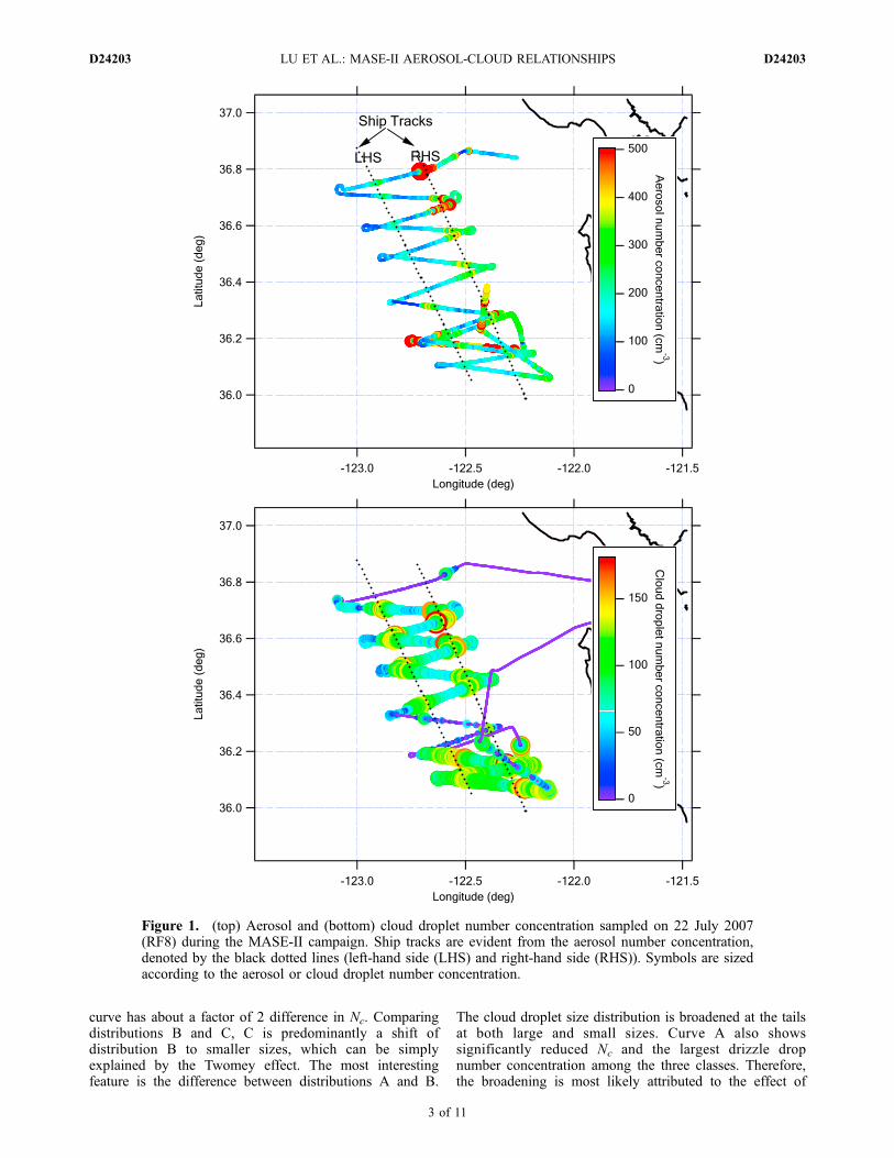
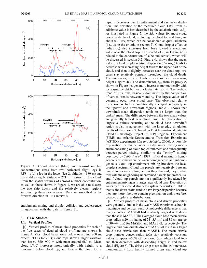
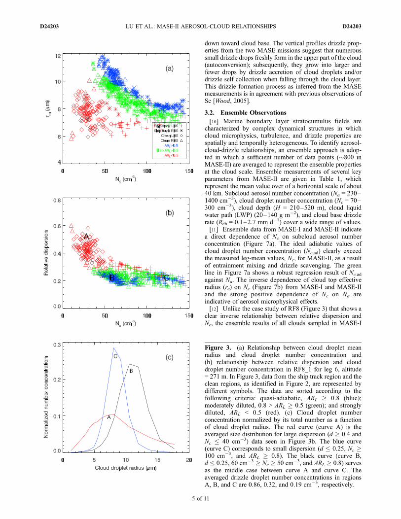
[5] Figure 1 shows the flight path on 22 July 2007(research flight (RF) 8), during which two ship tracks wereencountered. The flight strategy typically consisted of abelow-cloud horizontal leg, a near-base leg, two or three in-cloud legs, and one cloud top leg. In Figure 1, two shiptracks can be discerned from the aerosol number concen-tration, denoted by the black dotted lines (left-hand side(LHS) and right-hand side (RHS)). The two ship tracks areevident from the aerosol number concentrations and highercloud droplet number concentration (Nc) measured in thehorizontal flight legs in the lower and middle portions of thecloud (Figure 2). Figure 3a shows the relationship betweencloud droplet mean radius and Nc from the middle leg of thecloud. The data have been sorted according to the extent towhich the vertical liquid water content (LWC) profile isadiabatic, as represented by the adiabatic ratio [Pawlowskaet al., 2006; Lu et al., 2008], ARL = LWC/LWCad, whereLWCad is the adiabatic liquid water content: quasi-adiabatic,ARL � 0.8 (blue); moderately diluted, 0.8 > ARL � 0.5(green); and strongly diluted, ARL < 0.5 (red). An inverserelationship between cloud droplet mean radius (rm) and Nc

is evident after sorting for those data points, reflecting acloser approach to an adiabatic profile (blue and greencolors). At the same degree of dilution, the ship track

regions, in general, exhibit smaller droplets than the unper-turbed regions.[6] The cloud droplet size spectrum can also be affected

by the aerosol concentration, the so-called dispersion effect,the magnitude and direction of which depend on conden-sational processes, droplet collision coalescence, and clouddynamics (e.g., updraft and entrainment) [Liu and Daum,2002; Lu and Seinfeld, 2006]. The dispersion effect istypically quantified by means of the relative dispersion(d), defined as the ratio of the standard deviation (s, orcloud droplet spectral width) to the mean radius of the clouddroplet size distribution. Analysis of the effect requiresaccurate measurement of the full cloud droplet spectrum.A factor limiting the analysis of droplet spectral dispersionis the inadequacy of the Forward Scattering SpectrometerProbe instrument to resolve the cloud droplet size distribu-tion at the small size end. Figure 3b shows the relationshipbetween relative dispersion and cloud droplet numberconcentration from the leg shown in Figure 2b. In theabsence of sorting, the entire data set exhibits an inverseNc-d relationship. The higher values of d ranging from 0.3to 0.8 are associated with strongly nonadiabatic data points(red) and an inverse relationship between d and Nc; noobvious Nc-d relationship is evident for those data pointsthat more closely approach adiabatic conditions (green andblue), and these points are associated with smaller valuesof d of about 0.15–0.4. The data suggest that the fine-scaleNc-d relationship depends upon both aerosol number con-centration and the departure from adiabaticity. In Figure 3b,data points are also classified into ship track (crosses andasterisks) and clean (open triangles and squares) regions.The ship track regions are characterized generally by smallercloud droplet dispersion than the counterpart clean regions(i.e., more open triangles and squares are clustered at thelarger dispersion values).[7] The cloud droplet number distributions from three

different regimes in the Nc-d relationship (denoted A, B,and C in Figure 3b) are shown in Figure 3c. Curve Arepresents low Nc and high dispersion. Curve C is the datawith high Nc, and curve B represents a middle case. Each

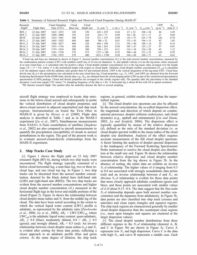
Table 1. Summary of Selected Research Flights and Observed Cloud Properties During MASE-IIa

ResearchFlightb Flight Date

Cloud SamplingTime (UTC)

CloudBase (m)

CloudDepth (m) Na (cm

�3) w (m s�1) Nc (cm�3) Nc,ad (cm

�3)LWP

(g m�2)Rcb

(mm d�1)

RF8_1 22 July 2007 1622–1833 120 330 243 ± 239 0.26 67 ± 32 106 ± 24 46 2.69RF8_2 22 July 2007 1844–2000 130 210 234 ± 73 0.68 84 ± 28 117 ± 17 21 0.68RF10 24 July 2007 1633–1941 180 510 731 ± 135 0.44 155 ± 57 225 ± 78 126 0.70RF11_1 25 July 2007 1645–1925 440 460 786 ± 32 0.91 153 ± 43 196 ± 15 82 1.05RF11_2 25 July 2007 1926–2017 440 220 696 ± 190 2.21 192 ± 40 188 ± 14 29 0.14RF14_1 29 July 2007 1553–1734 180 420 348 ± 263 0.30 105 ± 47 123 ± 27 97 0.93RF14_2 29 July 2007 1735–1914 200 280 359 ± 152 0.11 114 ± 34 124 ± 20 45 1.12RF16_1 31 July 2007 1541–1730 170 515 1271 ± 106 0.32 300 ± 44 312 ± 32 143 0.59RF16_2 31 July 2007 1742–1935 270 400 1433 ± 1700 0.28 164 ± 80 360 ± 71 63 0.62

aCloud top and base are obtained as shown in Figure 5. Aerosol number concentration (Na) is the total aerosol number concentration, measured bythe condensation particle counter (CPC) with smallest cutoff size of 10 nm (in diameter). Na and updraft velocity (w) are the leg-mean values measuredat or near cloud base; w is calculated only for positive values. Cloud droplet number concentration (Nc) is the leg-mean value averaged over the heightrange 1/6 < z* < 5/6, where z* is the normalized height with respect to cloud depth. Adiabatic cloud droplet number concentration (Nc,ad) is calculatedover the adiabatic region with the adiabatic ratio greater than 0.8 and minimal drizzle. LWP is the vertical integration of the leg-mean LWC. Cloud basedrizzle rate (Rcb) is the precipitation rate calculated at the near cloud base leg. Cloud properties, e.g., Nc, LWC, and LWP, are obtained from the ForwardScattering Spectrometer Probe (FSSP) data; drizzle data, e.g., Rcb, are obtained from the cloud imaging probe (CIP) as part of the cloud/aerosol/precipitationspectrometer (CAPS) package. Cloud and drizzle properties are averaged in the cloudy regions only. The quantity after the plus/minus is the standarddeviation. Local time equals UTC minus 7 h. Sampling frequency of the data is 1 Hz. A horizontal leg is about 40 km with 50 m spatial resolution.

bRF denotes research flight. The number after the underline denotes the first or second sampling.

D24203 LU ET AL.: MASE-II AEROSOL-CLOUD RELATIONSHIPS

2 of 11

D24203

curve has about a factor of 2 difference in Nc. Comparingdistributions B and C, C is predominantly a shift ofdistribution B to smaller sizes, which can be simplyexplained by the Twomey effect. The most interestingfeature is the difference between distributions A and B.

The cloud droplet size distribution is broadened at the tailsat both large and small sizes. Curve A also showssignificantly reduced Nc and the largest drizzle dropnumber concentration among the three classes. Therefore,the broadening is most likely attributed to the effect of

Figure 1. (top) Aerosol and (bottom) cloud droplet number concentration sampled on 22 July 2007(RF8) during the MASE-II campaign. Ship tracks are evident from the aerosol number concentration,denoted by the black dotted lines (left-hand side (LHS) and right-hand side (RHS)). Symbols are sizedaccording to the aerosol or cloud droplet number concentration.


3 of 11

D24203

entrainment mixing and droplet collision and coalescence,in agreement with the data in Figure 3b.

3. Case Studies

3.1. Vertical Profiles

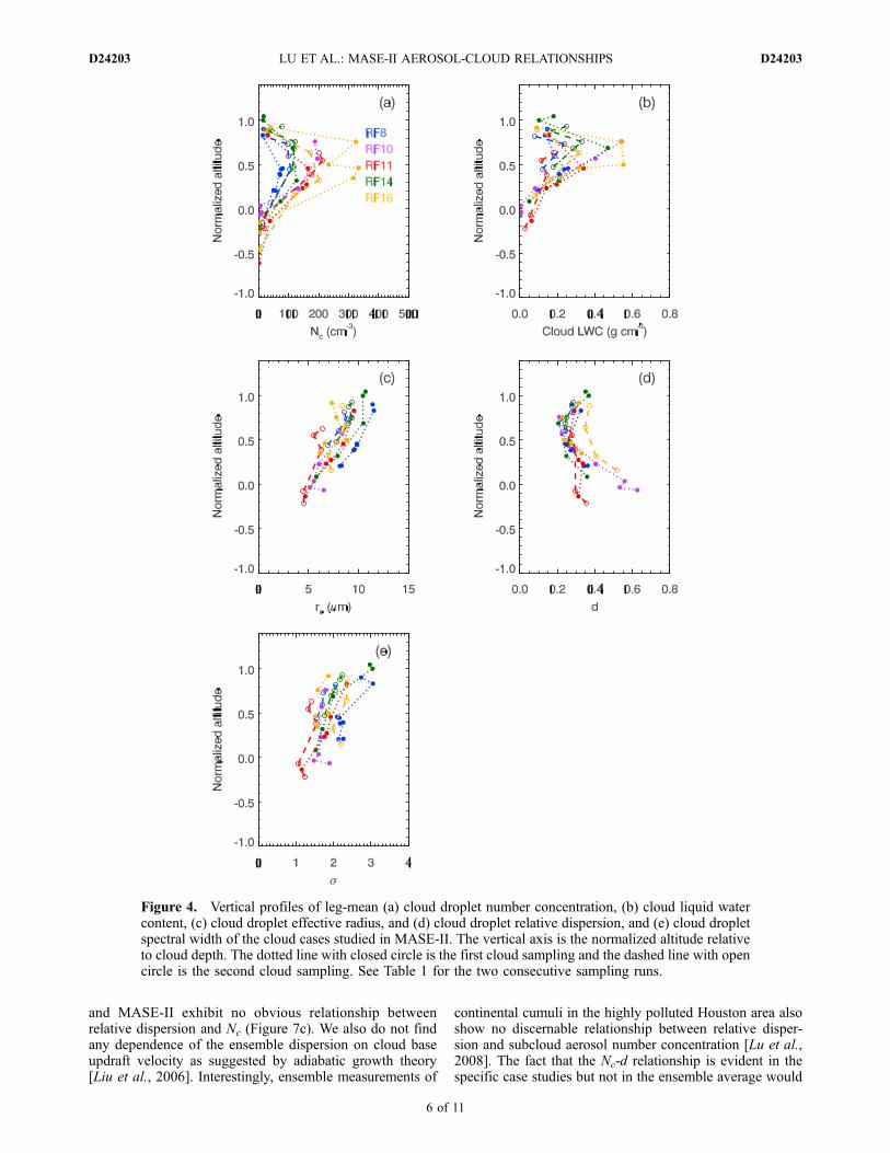
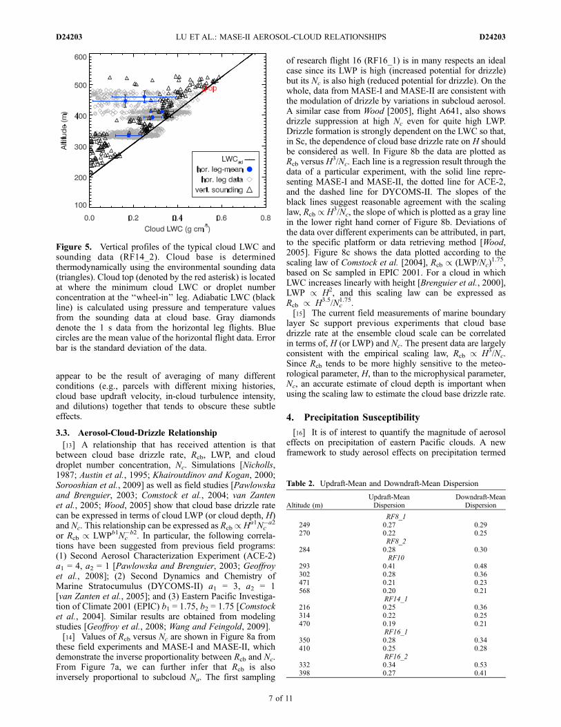
[8] Vertical profiles of mean cloud properties for each ofthe five cases of detailed cloud profiling are shown inFigure 4. Most cloud bases were below or around 200 m,except RF11 (Table 1); cloud tops show a larger variationthan bases, 350–900 m with most around 680 m. Meancloud LWC increases monotonically with height to amaximum below cloud top, and then at the cloud top it

rapidly decreases due to entrainment and rainwater deple-tion. The deviation of the measured cloud LWC from itsadiabatic value is best described by the adiabatic ratio, ARL.As illustrated in Figure 5, the ARL values for most cloudcases inside the cloud, excluding the cloud top and base, areabout 0.7–0.9, which can be considered as quasi-adiabatic(i.e., using the criteria in section 2). Cloud droplet effectiveradius (re) also increases from base toward a maximumvalue near the cloud top. The spread of re in Figure 4c isrelated to the concentration of subcloud aerosol, which willbe discussed in section 3.2. Figure 4d shows that the meanvalue of cloud droplet relative dispersion (d = s/rm) tends todecrease with increasing height toward the upper part of thecloud, and then it slightly increases near the cloud top; twocases stay relatively constant throughout the cloud depth.The numerator, s, also tends to increase with increasingheight (Figure 4e). The denominator, rm, from its proxy reshown in Figure 4c, generally increases monotonically withincreasing height but with a faster rate than s. The verticaltrend of d is, thus, basically dominated by the competitionof vertical trends between s and rm. The largest values of dgenerally occur near cloud base. The observed relativedispersion is further conditionally averaged separately inthe updraft and downdraft regions. Table 2 shows thatdowndraft-mean dispersion tends to be larger than theupdraft mean. The differences between the two mean valuesare generally largest near cloud base. The observation oflargest d values occurring at the cloud base downdraftregion is also in agreement with the large-eddy simulationresults of the marine Sc based on First International SatelliteCloud Climatology Project (ISCCP) Regional Experiment(FIRE) and Atlantic Stratocumulus Transition Experiment(ASTEX) experiments [Lu and Seinfeld, 2006]. A possibleexplanation for this behavior is a dynamical mixing mech-anism consisting of cloud top entrainment and subsequentlybetween-parcel mixing, similar to the ‘‘entity’’ mixingdescribed by Telford et al. [1984]: if local mixing is homo-geneous or somewhere between homogeneous and inhomo-geneous, cloud top entrainment mixing broadens the localdroplet spectrum. Cloud top parcels are negatively buoyantdue to longwave cooling, and as they descend, they furthermix with the neighboring unentrained parcels (updraft cells);and if cloud top parcels are not significantly broadened byentrainment mixing, d is largest near cloud base. Depletion ofwater by drizzle could also help explain the results in Table 2;that is, the downdrafts tend to have larger dispersion becausethey are more likely to contain precipitation and, therefore,broader droplet size distributions.[9] Vertical profiles of mean cloud and drizzle properties

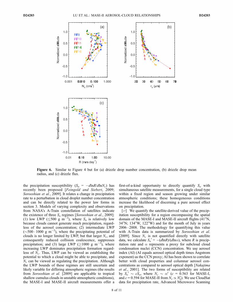
were generally similar in the twoMASE experiments, both inmagnitude and vertical trend. A noticeable difference is thatmany clouds in MASE-II had relatively larger drizzle dropsthan those inMASE-I. The averaged cloud base mean drizzledrop radius is 29 mm (range of 24–35 mm) and 38 mm (rangeof 30–44 mm) for MASE-I and MASE-II, respectively. Thelarger cloud base drizzle drops of MASE-II result in a largercloud base drizzle rate than MASE-I. The mean drizzledrop number concentration (Nd) stay relatively constantvalues in upper �50% of the cloud (excluding cloud top)and then decreases with descending height in and belowcloud (Figure 6). The drizzle drop mean radius (rd) increasesmonotonically from freshly formed drops near cloud top

Figure 2. Cloud droplet (blue) and aerosol numberconcentrations (red) from two horizontal flight legs inRF8_1: (a) a leg in the lower (leg 2, altitude = 189 m) and(b) middle (leg 6, altitude = 271 m) portion of the cloud.From the spatial features of aerosol number concentration,as well as those shown in Figure 1, we are able to discernthe two ship tracks and the relatively cleaner regionssurrounding them (see arrows). Data are smoothed in theforward direction in 10 s intervals.

4 of 11

D24203 LU ET AL.: MASE-II AEROSOL-CLOUD RELATIONSHIPS D24203

down toward cloud base. The vertical profiles drizzle prop-erties from the two MASE missions suggest that numeroussmall drizzle drops freshly form in the upper part of the cloud(autoconversion); subsequently, they grow into larger andfewer drops by drizzle accretion of cloud droplets and/ordrizzle self collection when falling through the cloud layer.This drizzle formation process as inferred from the MASEmeasurements is in agreement with previous observations ofSc [Wood, 2005].

3.2. Ensemble Observations

[10] Marine boundary layer stratocumulus fields arecharacterized by complex dynamical structures in whichcloud microphysics, turbulence, and drizzle properties arespatially and temporally heterogeneous. To identify aerosol-cloud-drizzle relationships, an ensemble approach is adop-ted in which a sufficient number of data points (�800 inMASE-II) are averaged to represent the ensemble propertiesat the cloud scale. Ensemble measurements of several keyparameters from MASE-II are given in Table 1, whichrepresent the mean value over of a horizontal scale of about40 km. Subcloud aerosol number concentration (Na = 230–1400 cm�3), cloud droplet number concentration (Nc = 70–300 cm�3), cloud depth (H = 210–520 m), cloud liquidwater path (LWP) (20–140 g m�2), and cloud base drizzlerate (Rcb = 0.1–2.7 mm d�1) cover a wide range of values.[11] Ensemble data from MASE-I and MASE-II indicate

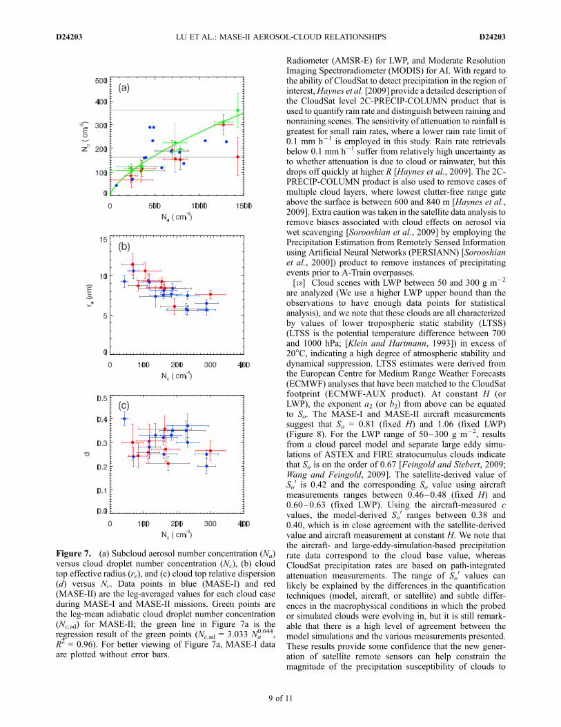
a direct dependence of Nc on subcloud aerosol numberconcentration (Figure 7a). The ideal adiabatic values ofcloud droplet number concentration (Nc,ad) clearly exceedthe measured leg-mean values, Nc, for MASE-II, as a resultof entrainment mixing and drizzle scavenging. The greenline in Figure 7a shows a robust regression result of Nc,ad

against Na. The inverse dependence of cloud top effectiveradius (re) on Nc (Figure 7b) from MASE-I and MASE-IIand the strong positive dependence of Nc on Na areindicative of aerosol microphysical effects.[12] Unlike the case study of RF8 (Figure 3) that shows a

clear inverse relationship between relative dispersion andNc, the ensemble results of all clouds sampled in MASE-I

Figure 3. (a) Relationship between cloud droplet meanradius and cloud droplet number concentration and(b) relationship between relative dispersion and clouddroplet number concentration in RF8_1 for leg 6, altitude= 271 m. In Figure 3, data from the ship track region and theclean regions, as identified in Figure 2, are represented bydifferent symbols. The data are sorted according to thefollowing criteria: quasi-adiabatic, ARL � 0.8 (blue);moderately diluted, 0.8 > ARL � 0.5 (green); and stronglydiluted, ARL < 0.5 (red). (c) Cloud droplet numberconcentration normalized by its total number as a functionof cloud droplet radius. The red curve (curve A) is theaveraged size distribution for large dispersion (d � 0.4 andNc � 40 cm�3) data seen in Figure 3b. The blue curve(curve C) corresponds to small dispersion (d � 0.25, Nc �100 cm�3, and ARL � 0.8). The black curve (curve B,d � 0.25, 60 cm�3 � Nc � 50 cm�3, and ARL � 0.8) servesas the middle case between curve A and curve C. Theaveraged drizzle droplet number concentrations in regionsA, B, and C are 0.86, 0.32, and 0.19 cm�3, respectively.


5 of 11

D24203

and MASE-II exhibit no obvious relationship betweenrelative dispersion and Nc (Figure 7c). We also do not findany dependence of the ensemble dispersion on cloud baseupdraft velocity as suggested by adiabatic growth theory[Liu et al., 2006]. Interestingly, ensemble measurements of

continental cumuli in the highly polluted Houston area alsoshow no discernable relationship between relative disper-sion and subcloud aerosol number concentration [Lu et al.,2008]. The fact that the Nc-d relationship is evident in thespecific case studies but not in the ensemble average would

Figure 4. Vertical profiles of leg-mean (a) cloud droplet number concentration, (b) cloud liquid watercontent, (c) cloud droplet effective radius, and (d) cloud droplet relative dispersion, and (e) cloud dropletspectral width of the cloud cases studied in MASE-II. The vertical axis is the normalized altitude relativeto cloud depth. The dotted line with closed circle is the first cloud sampling and the dashed line with opencircle is the second cloud sampling. See Table 1 for the two consecutive sampling runs.


6 of 11

D24203

appear to be the result of averaging of many differentconditions (e.g., parcels with different mixing histories,cloud base updraft velocity, in-cloud turbulence intensity,and dilutions) together that tends to obscure these subtleeffects.

3.3. Aerosol-Cloud-Drizzle Relationship

[13] A relationship that has received attention is thatbetween cloud base drizzle rate, Rcb, LWP, and clouddroplet number concentration, Nc. Simulations [Nicholls,1987; Austin et al., 1995; Khairoutdinov and Kogan, 2000;Sorooshian et al., 2009] as well as field studies [Pawlowskaand Brenguier, 2003; Comstock et al., 2004; van Zantenet al., 2005; Wood, 2005] show that cloud base drizzle ratecan be expressed in terms of cloud LWP (or cloud depth, H)and Nc. This relationship can be expressed as Rcb/ Ha1Nc

�a2

or Rcb / LWPb1Nc�b2. In particular, the following correla-

tions have been suggested from previous field programs:(1) Second Aerosol Characterization Experiment (ACE-2)a1 = 4, a2 = 1 [Pawlowska and Brenguier, 2003; Geoffroyet al., 2008]; (2) Second Dynamics and Chemistry ofMarine Stratocumulus (DYCOMS-II) a1 = 3, a2 = 1[van Zanten et al., 2005]; and (3) Eastern Pacific Investiga-tion of Climate 2001 (EPIC) b1 = 1.75, b2 = 1.75 [Comstocket al., 2004]. Similar results are obtained from modelingstudies [Geoffroy et al., 2008; Wang and Feingold, 2009].[14] Values of Rcb versus Nc are shown in Figure 8a from

these field experiments and MASE-I and MASE-II, whichdemonstrate the inverse proportionality between Rcb and Nc.From Figure 7a, we can further infer that Rcb is alsoinversely proportional to subcloud Na. The first sampling

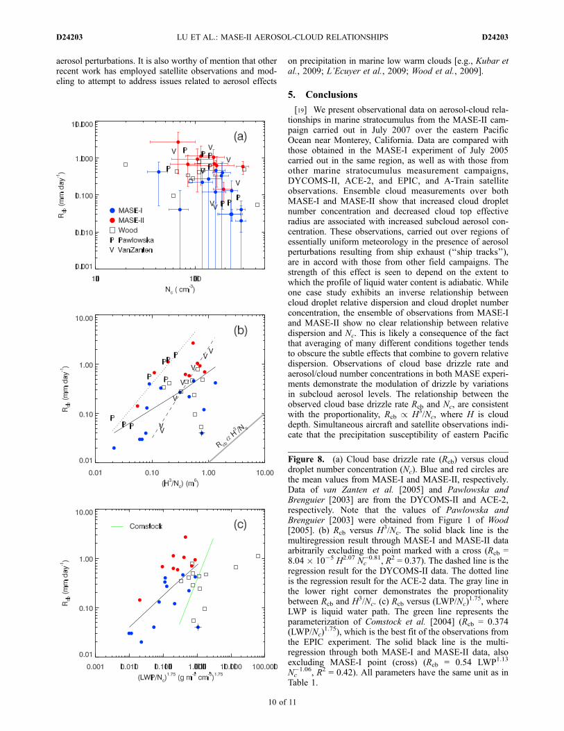
of research flight 16 (RF16_1) is in many respects an idealcase since its LWP is high (increased potential for drizzle)but its Nc is also high (reduced potential for drizzle). On thewhole, data from MASE-I and MASE-II are consistent withthe modulation of drizzle by variations in subcloud aerosol.A similar case from Wood [2005], flight A641, also showsdrizzle suppression at high Nc even for quite high LWP.Drizzle formation is strongly dependent on the LWC so that,in Sc, the dependence of cloud base drizzle rate on H shouldbe considered as well. In Figure 8b the data are plotted asRcb versus H

3/Nc. Each line is a regression result through thedata of a particular experiment, with the solid line repre-senting MASE-I and MASE-II, the dotted line for ACE-2,and the dashed line for DYCOMS-II. The slopes of theblack lines suggest reasonable agreement with the scalinglaw, Rcb / H3/Nc, the slope of which is plotted as a gray linein the lower right hand corner of Figure 8b. Deviations ofthe data over different experiments can be attributed, in part,to the specific platform or data retrieving method [Wood,2005]. Figure 8c shows the data plotted according to thescaling law of Comstock et al. [2004], Rcb / (LWP/Nc)

1.75,based on Sc sampled in EPIC 2001. For a cloud in whichLWC increases linearly with height [Brenguier et al., 2000],LWP / H2, and this scaling law can be expressed asRcb / H3.5/Nc

1.75.[15] The current field measurements of marine boundary

layer Sc support previous experiments that cloud basedrizzle rate at the ensemble cloud scale can be correlatedin terms of, H (or LWP) and Nc. The present data are largelyconsistent with the empirical scaling law, Rcb / H3/Nc.Since Rcb tends to be more highly sensitive to the meteo-rological parameter, H, than to the microphysical parameter,Nc, an accurate estimate of cloud depth is important whenusing the scaling law to estimate the cloud base drizzle rate.

4. Precipitation Susceptibility

[16] It is of interest to quantify the magnitude of aerosoleffects on precipitation of eastern Pacific clouds. A newframework to study aerosol effects on precipitation termed

Figure 5. Vertical profiles of the typical cloud LWC andsounding data (RF14_2). Cloud base is determinedthermodynamically using the environmental sounding data(triangles). Cloud top (denoted by the red asterisk) is locatedat where the minimum cloud LWC or droplet numberconcentration at the ‘‘wheel-in’’ leg. Adiabatic LWC (blackline) is calculated using pressure and temperature valuesfrom the sounding data at cloud base. Gray diamondsdenote the 1 s data from the horizontal leg flights. Bluecircles are the mean value of the horizontal flight data. Errorbar is the standard deviation of the data.

Table 2. Updraft-Mean and Downdraft-Mean Dispersion

Altitude (m)Updraft-MeanDispersion

Downdraft-MeanDispersion

RF8_1249 0.27 0.29270 0.22 0.25

RF8_2284 0.28 0.30

RF10293 0.41 0.48302 0.28 0.36471 0.21 0.23568 0.20 0.21

RF14_1216 0.25 0.36314 0.22 0.25470 0.19 0.21

RF16_1350 0.28 0.34410 0.25 0.28

RF16_2332 0.34 0.53398 0.27 0.41


7 of 11

D24203

the precipitation susceptibility (So = �dlnR/dlnNc) hasrecently been proposed [Feingold and Siebert, 2009;Sorooshian et al., 2009]. It relates a change in precipitationrate to a perturbation in cloud droplet number concentrationand can be directly related to the power law forms insection 3. Models of varying complexity and observationsfrom NASA’s A-Train constellation of satellites indicatethe existence of three So regimes [Sorooshian et al., 2009]:(1) low LWP (�500 g m�2), where So is relatively lowbecause clouds cannot generate much precipitation, regard-less of the aerosol concentration; (2) intermediate LWP(�500–1000 g m�2), where the precipitating potential ofclouds is no longer limited by LWP, but that larger Nc, andconsequently reduced collision coalescence, suppressesprecipitation; and (3) large LWP (�1000 g m�2), whereincreasing LWP dominates precipitation formation regard-less of Nc. Thus, LWP can be viewed as establishing thepotential to which a cloud might be able to precipitate, andNc can be viewed as regulating the precipitation. Althoughthe LWP bounds of these regimes are still uncertain andlikely variable for differing atmospheric regimes (the resultsfrom Sorooshian et al. [2009] are applicable to tropicalshallow cumulus clouds in unstable atmospheric conditions),the MASE-I and MASE-II aircraft measurements offer a

first-of-a-kind opportunity to directly quantify So withsimultaneous satellite measurements, for a single cloud typewithin a fixed region and season growing under similaratmospheric conditions; these homogeneous conditionsincrease the likelihood of discerning a pure aerosol effecton precipitation.[17] We quantify the satellite-derived value of the precip-

itation susceptibility for a region encompassing the spatialdomain of the MASE-I and MASE-II aircraft flights (41�N,34�N; 134�W, 122�W) and for the month of July in years2006–2008. The methodology for quantifying this valuewith A-Train data is summarized by Sorooshian et al.[2009]. Since Nc is not quantified directly with satellitedata, we calculate So

0 = �(dlnR)/(dlna), where R is precip-itation rate and a represents a proxy for subcloud cloudcondensation nuclei (CCN) concentration. We use aerosolindex (AI) (AI equals aerosol optical depth times Angstromexponent) as the CCN proxy; AI has been shown to correlatebetter with cloud properties and columnar aerosol con-centrations as compared to aerosol optical depth [Nakajimaet al., 2001]. The two forms of susceptibility are relatedby So

0 � cSo, where Nc � ac (c = 0.563 for MASE-I,and c = 0.594 for MASE-II from Nc/ Na

c). We use CloudSatdata for precipitation rate, Advanced Microwave Scanning

Figure 6. Similar to Figure 4 but for (a) drizzle drop number concentration, (b) drizzle drop meanradius, and (c) drizzle flux.


8 of 11

D24203

Radiometer (AMSR-E) for LWP, and Moderate ResolutionImaging Spectroradiometer (MODIS) for AI. With regard tothe ability of CloudSat to detect precipitation in the region ofinterest,Haynes et al. [2009] provide a detailed description ofthe CloudSat level 2C-PRECIP-COLUMN product that isused to quantify rain rate and distinguish between raining andnonraining scenes. The sensitivity of attenuation to rainfall isgreatest for small rain rates, where a lower rain rate limit of0.1 mm h�1 is employed in this study. Rain rate retrievalsbelow 0.1 mm h�1 suffer from relatively high uncertainty asto whether attenuation is due to cloud or rainwater, but thisdrops off quickly at higher R [Haynes et al., 2009]. The 2C-PRECIP-COLUMN product is also used to remove cases ofmultiple cloud layers, where lowest clutter-free range gateabove the surface is between 600 and 840 m [Haynes et al.,2009]. Extra caution was taken in the satellite data analysis toremove biases associated with cloud effects on aerosol viawet scavenging [Sorooshian et al., 2009] by employing thePrecipitation Estimation from Remotely Sensed Informationusing Artificial Neural Networks (PERSIANN) [Sorooshianet al., 2000]) product to remove instances of precipitatingevents prior to A-Train overpasses.[18] Cloud scenes with LWP between 50 and 300 g m�2

are analyzed (We use a higher LWP upper bound than theobservations to have enough data points for statisticalanalysis), and we note that these clouds are all characterizedby values of lower tropospheric static stability (LTSS)(LTSS is the potential temperature difference between 700and 1000 hPa; [Klein and Hartmann, 1993]) in excess of20�C, indicating a high degree of atmospheric stability anddynamical suppression. LTSS estimates were derived fromthe European Centre for Medium Range Weather Forecasts(ECMWF) analyses that have been matched to the CloudSatfootprint (ECMWF-AUX product). At constant H (orLWP), the exponent a2 (or b2) from above can be equatedto So. The MASE-I and MASE-II aircraft measurementssuggest that So = 0.81 (fixed H) and 1.06 (fixed LWP)(Figure 8). For the LWP range of 50–300 g m�2, resultsfrom a cloud parcel model and separate large eddy simu-lations of ASTEX and FIRE stratocumulus clouds indicatethat So is on the order of 0.67 [Feingold and Siebert, 2009;Wang and Feingold, 2009]. The satellite-derived value ofSo0 is 0.42 and the corresponding So value using aircraft

measurements ranges between 0.46–0.48 (fixed H) and0.60–0.63 (fixed LWP). Using the aircraft-measured cvalues, the model-derived So

0 ranges between 0.38 and0.40, which is in close agreement with the satellite-derivedvalue and aircraft measurement at constant H. We note thatthe aircraft- and large-eddy-simulation-based precipitationrate data correspond to the cloud base value, whereasCloudSat precipitation rates are based on path-integratedattenuation measurements. The range of So

0 values canlikely be explained by the differences in the quantificationtechniques (model, aircraft, or satellite) and subtle differ-ences in the macrophysical conditions in which the probedor simulated clouds were evolving in, but it is still remark-able that there is a high level of agreement between themodel simulations and the various measurements presented.These results provide some confidence that the new gener-ation of satellite remote sensors can help constrain themagnitude of the precipitation susceptibility of clouds to

Figure 7. (a) Subcloud aerosol number concentration (Na)versus cloud droplet number concentration (Nc), (b) cloudtop effective radius (re), and (c) cloud top relative dispersion(d) versus Nc. Data points in blue (MASE-I) and red(MASE-II) are the leg-averaged values for each cloud caseduring MASE-I and MASE-II missions. Green points arethe leg-mean adiabatic cloud droplet number concentration(Nc,ad) for MASE-II; the green line in Figure 7a is theregression result of the green points (Nc,ad = 3.033 Na

0.644,R2 = 0.96). For better viewing of Figure 7a, MASE-I dataare plotted without error bars.


9 of 11

D24203

aerosol perturbations. It is also worthy of mention that otherrecent work has employed satellite observations and mod-eling to attempt to address issues related to aerosol effects

on precipitation in marine low warm clouds [e.g., Kubar etal., 2009; L’Ecuyer et al., 2009; Wood et al., 2009].

5. Conclusions

[19] We present observational data on aerosol-cloud rela-tionships in marine stratocumulus from the MASE-II cam-paign carried out in July 2007 over the eastern PacificOcean near Monterey, California. Data are compared withthose obtained in the MASE-I experiment of July 2005carried out in the same region, as well as with those fromother marine stratocumulus measurement campaigns,DYCOMS-II, ACE-2, and EPIC, and A-Train satelliteobservations. Ensemble cloud measurements over bothMASE-I and MASE-II show that increased cloud dropletnumber concentration and decreased cloud top effectiveradius are associated with increased subcloud aerosol con-centration. These observations, carried out over regions ofessentially uniform meteorology in the presence of aerosolperturbations resulting from ship exhaust (‘‘ship tracks’’),are in accord with those from other field campaigns. Thestrength of this effect is seen to depend on the extent towhich the profile of liquid water content is adiabatic. Whileone case study exhibits an inverse relationship betweencloud droplet relative dispersion and cloud droplet numberconcentration, the ensemble of observations from MASE-Iand MASE-II show no clear relationship between relativedispersion and Nc. This is likely a consequence of the factthat averaging of many different conditions together tendsto obscure the subtle effects that combine to govern relativedispersion. Observations of cloud base drizzle rate andaerosol/cloud number concentrations in both MASE experi-ments demonstrate the modulation of drizzle by variationsin subcloud aerosol levels. The relationship between theobserved cloud base drizzle rate Rcb and Nc, are consistentwith the proportionality, Rcb / H3/Nc, where H is clouddepth. Simultaneous aircraft and satellite observations indi-cate that the precipitation susceptibility of eastern Pacific

Figure 8. (a) Cloud base drizzle rate (Rcb) versus clouddroplet number concentration (Nc). Blue and red circles arethe mean values from MASE-I and MASE-II, respectively.Data of van Zanten et al. [2005] and Pawlowska andBrenguier [2003] are from the DYCOMS-II and ACE-2,respectively. Note that the values of Pawlowska andBrenguier [2003] were obtained from Figure 1 of Wood[2005]. (b) Rcb versus H3/Nc. The solid black line is themultiregression result through MASE-I and MASE-II dataarbitrarily excluding the point marked with a cross (Rcb =8.04 � 10�5 H2.07 Nc

�0.81, R2 = 0.37). The dashed line is theregression result for the DYCOMS-II data. The dotted lineis the regression result for the ACE-2 data. The gray line inthe lower right corner demonstrates the proportionalitybetween Rcb and H3/Nc. (c) Rcb versus (LWP/Nc)

1.75, whereLWP is liquid water path. The green line represents theparameterization of Comstock et al. [2004] (Rcb = 0.374(LWP/Nc)

1.75), which is the best fit of the observations fromthe EPIC experiment. The solid black line is the multi-regression through both MASE-I and MASE-II data, alsoexcluding MASE-I point (cross) (Rcb = 0.54 LWP1.13

Nc�1.06, R2 = 0.42). All parameters have the same unit as in

Table 1.

10 of 11

D24203 LU ET AL.: MASE-II AEROSOL-CLOUD RELATIONSHIPS D24203

clouds to aerosol perturbations ranges between So0 = 0.42

and So0 = 0.63. Observations of aerosol effects on marine

stratocumulus presented here add to the existing body ofdata, which can serve as constraints in the evaluation ofmodeling studies of the effect of aerosol perturbations onmarine stratocumulus properties. Nevertheless, cloud feed-back mechanisms that ensue once an aerosol perturbationoccurs [Wood, 2007] continue to remain observationallychallenging.

[20] Acknowledgments. This work was supported by the Office ofNaval Research grant N00014-04-1-0018. A.S. acknowledges support fromthe Cooperative Institute for Research in the Atmosphere PostdoctoralResearch Program. G.F. acknowledges NOAA’s Climate Goal. The authorsacknowledge Robert Wood for helpful comments.

ReferencesAustin, P., Y. N. Wang, R. Pincus, and V. Kujala (1995), Precipitation instratocumulus clouds: Observational and modeling results, J. Atmos. Sci.,52, 2329 –2352, doi:10.1175/1520-0469(1995)052<2329:PISCOA>2.0.CO;2.

Brenguier, J. L., and R. Wood (2009), Observational strategies from themicro- to mesoscale, in Clouds in the Perturbed Climate System: TheirRelationship to Energy Balance, Atmospheric Dynamics, and Precipita-tion, edited by J. Heintzenberg and R. J. Charlson, pp. 487–510, MITPress, Cambridge, Mass.

Brenguier, J. L., H. Pawlowska, L. Schuller, R. Preusker, J. Fischer, andY. Fouquart (2000), Radiative properties of boundary layer clouds: Dro-plet effective radius versus number concentration, J. Atmos. Sci., 57,803–821, doi:10.1175/1520-0469(2000)057<0803:RPOBLC>2.0.CO;2.

Comstock, K. K., R. Wood, S. E. Yuter, and C. S. Bretherton (2004),Reflectivity and rain rate in and below drizzling stratocumulus,Q. J. R. Meteorol. Soc., 130, 2891–2918, doi:10.1256/qj.03.187.

Feingold, G., and H. Siebert (2009), Cloud-aerosol interactions from themicro to the cloud scale, in Clouds in the Perturbed Climate System:Their Relationship to Energy Balance, Atmospheric Dynamics, and Pre-cipitation, edited by J. Heintzenberg and R. J. Charlson, pp. 319–338,MIT Press, Cambridge, Mass.

Geoffroy, O., J.-L. Brenguier, and I. Sandu (2008), Relationship betweendrizzle rate, liquid water path and droplet concentration at the scale of astratocumulus cloud system, Atmos. Chem. Phys., 8, 4641–4654.

Haynes, J. M., T. S. L’Ecuyer, G. L. Stephens, S. D. Miller, C. Mitrescu,N. B. Wood, and S. Tanelli (2009), Rainfall retrieval over the oceanwith spaceborne W-band radar, J. Geophys. Res., 114, D00A22,doi:10.1029/2008JD009973.

Hersey, S. P., A. Sorooshian, S. M. Murphy, R. C. Flagan, andJ. H. Seinfeld (2009), Aerosol hygroscopicity in the marine atmosphere:A closure study using high-resolution, size-resolved AMS and multiple-RH DASH-SP data, Atmos. Chem. Phys., 9, 2543–2554.

Intergovernmental Panel on Climate Change (2007), Climate Change: ThePhysical Science Basis: Contribution of Working Group I to the FourthAssessment Report of the Intergovernmental Panel on Climate Change,Cambridge Univ. Press, New York.

Khairoutdinov, M., and Y. Kogan (2000), A new cloud physics parameter-ization in a large-eddy simulation model of marine stratocumulus, Mon.Weather Rev., 128, 229–243, doi:10.1175/1520-0493(2000)128<0229:ANCPPI>2.0.CO;2.

Klein, S. A., and D. L. Hartmann (1993), The seasonal cycle of low strati-form clouds, J. Clim., 6, 1587–1606, doi:10.1175/1520-0442(1993)006<1587:TSCOLS>2.0.CO;2.

Kubar, T., D. Hartmann, and R. Wood (2009), Understanding the impor-tance of microphysics and macrophysics for warm rain in marine lowclouds. Part I. Satellite observations, J. Atmos. Sci., 66, 2953–2972,doi:10.1175/2009JAS3071.1.

L’Ecuyer, T. S., W. Berg, J. Haynes, M. Lebsock, and T. Takemura (2009),Global observations of aerosol impacts on precipitation occurrence inwarm maritime clouds, J. Geophys. Res., 114, D09211, doi:10.1029/2008JD011273.

Liu, Y., and P. H. Daum (2002), Anthropogenic aerosols: Indirect warmingeffect from dispersion forcing, Nature, 419, 580–581, doi:10.1038/419580a.

Liu, Y., P. H. Daum, and S. S. Yum (2006), Analytical expression for therelative dispersion of the cloud droplet size distribution, Geophys. Res.Lett., 33, L02810, doi:10.1029/2005GL024052.

Lu, M.-L., and J. H. Seinfeld (2006), Effect of aerosol number concentra-tion on cloud droplet dispersion: A large-eddy simulation study andimplications for aerosol indirect forcing, J. Geophys. Res., 111, D02207,doi:10.1029/2005JD006419.

Lu, M.-L., W. C. Conant, H. H. Jonsson, V. Varutbangkul, R. C. Flagan,and J. H. Seinfeld (2007), The Marine Stratus/Stratocumulus Experiment(MASE): Aerosol-cloud relationships in marine stratocumulus, J. Geo-phys. Res., 112, D10209, doi:10.1029/2006JD007985.

Lu, M.-L., G. Feingold, H. H. Jonsson, P. Y. Chuang, H. Gates,R. C. Flagan, and J. H. Seinfeld (2008), Aerosol-cloud relationshipsin continental shallow cumulus, J. Geophys. Res., 113, D15201,doi:10.1029/2007JD009354.

Nakajima, T., A. Higurashi, K. Kawamoto, and J. E. Penner (2001), Apossible correlation between satellite-derived cloud and aerosol micro-physical parameters, Geophys. Res. Lett., 28, 1171–1174, doi:10.1029/2000GL012186.

Nicholls, S. (1987), A model of drizzle growth in warm, turbulent, strati-form clouds, Q. J. R. Meteorol. Soc., 113, 1141–1170, doi:10.1256/smsqj.47804.

Noone, K. J., et al. (2000), A case study of ship track formation in apolluted marine boundary layer, J. Atmos. Sci., 57, 2748 – 2764,doi:10.1175/1520-0469(2000)057<2748:ACSOST>2.0.CO;2.

Pawlowska, H., and J. L. Brenguier (2003), An observational study ofdrizzle formation in stratocumulus clouds for general circulationmodel (GCM) parameterizations, J. Geophys. Res., 108(D15), 8630,doi:10.1029/2002JD002679.

Pawlowska, H., W. W. Grabowski, and J.-L. Brenguier (2006), Observa-tions of the width of cloud droplet spectra in stratocumulus, Geophys.Res. Lett., 33, L19810, doi:10.1029/2006GL026841.

Platnick, S., and S. Twomey (1994), Determining the susceptibility of cloudalbedo to changes in droplet concentration with the advanced very high-resolution radiometer, J. Appl. Meteorol., 33, 334–347, doi:10.1175/1520-0450(1994)033<0334:DTSOCA>2.0.CO;2.

Sorooshian, A., G. Feingold, M. D. Lebsock, H. Jiang, and G. L. Stephens(2009), On the precipitation susceptibility of clouds to aerosol perturba-tions, Geophys. Res. Lett., 36, L13803, doi:10.1029/2009GL038993.

Sorooshian, S., K.-L. Hsu, X. Gao, H. V. Gupta, B. Imam, andD. Braithwaite (2000), Evaluation of PERSIANN system satellite–basedestimates of tropical rainfall, Bull. Am. Meteorol. Soc., 81, 2035–2046,doi:10.1175/1520-0477(2000)081<2035:EOPSSE>2.3.CO;2.

Stephens, G. L., et al. (2002), The CloudSat mission and the A-Train: A newdimension of space-based observations of clouds and precipitation, Bull.Am. Meteorol. Soc., 83, 1771–1790, doi:10.1175/BAMS-83-12-1771.

Telford, J. W., T. S. Keck, and S. K. Chai (1984), Entrainment at cloud topsand the droplet spectra, J. Atmos. Sci., 41, 3170–3179, doi:10.1175/1520-0469(1984)041<3170:EACTAT>2.0.CO;2.

van Zanten, M. C., B. Stevens, G. Vali, and D. H. Lenschow (2005),Observations of drizzle in nocturnal marine stratocumulus, J. Atmos.Sci., 62, 88–106, doi:10.1175/JAS-3355.1.

Wang, H., and G. Feingold (2009), Modeling mesoscale cellular structuresand drizzle in marine stratocumulus: Part 1: Impact of drizzle on theformation and evolution of open cells, J. Atmos. Sci., doi:10.1175/2009JAS3022.1, in press.

Wood, R. (2005), Drizzle in stratiform boundary layer clouds. Part 1:Vertical and horizontal structure, J. Atmos. Sci., 62, 3011–3033,doi:10.1175/JAS3529.1.

Wood, R. (2007), Cancellation of aerosol indirect effects in marine strato-cumulus through cloud thinning, J. Atmos. Sci., 64, 2657 – 2669,doi:10.1175/JAS3942.1.

Wood, R., T. Kubar, and D. Hartmann (2009), Understanding the impor-tance of microphysics and macrophysics for warm rain in marine lowclouds. Part II: Heuristic models of rain formation, J. Atmos. Sci., 66,2973–2990, doi:10.1175/2009JAS3072.1.

��G. Feingold, Chemical Sciences Division, Earth System Research

Laboratory, NOAA, R/E/CSD2, 325 Broadway, Boulder, CO 80305, USA.R. C. Flagan and J. H. Seinfeld, Department of Chemical Engineering,

California Institute of Technology, 1200 E. California Blvd., Mail Code210-41, Pasadena, CA 91125, USA. ([email protected])H. H. Jonsson, Naval Postgraduate School, 3200 Imjin Rd., Hangar 507,

Monterey, CA 93933, USA.M.-L. Lu, Department of Environmental Science and Engineering,

California Institute of Technology, 1200 E. California Blvd., Pasadena, CA91125, USA.A. Sorooshian, Department of Chemical and Environmental Engineering,

University of Arizona, JW Harshbarger Bldg., PO Box 210011, Tucson,AZ 85721, USA.


11 of 11

D24203