1

Magnetic ordering above room temperature in the sigma-phase of Fe66V34

Jakub Cieslak1, Benilde F. O. Costa2, Stanislaw M. Dubiel1*, Michael Reissner3 and Walter

Steiner3

1Faculty of Physics and Compute Science, AGH University of Science and Technology, 30-

059 Krakow, Poland, 2 CEMDRX Department of Physics, University of Coimbra, 3000-516

Coimbra, Portugal, 3Institute of Solid State Physics, Vienna University of Technology, 1040

Wien, Austria

PACS: 75.30.Cr, 75.50.Bb, 76.80.+y, 77.80.Bh

Abstract

Magnetic properties of four sigma-phase Fe100-xVx samples with 34.4 ≤ x ≤ 55.1 were

investigated by Mössbauer spectroscopy and magnetic measurements in the temperature

interval 5 – 300 K. Four magnetic quantities viz. hyperfine field, Curie temperature, magnetic

moment and susceptibility were determined. The sample containing 34.4 at% V was revealed

to exhibit the largest values found up to now for the sigma-phase for average hyperfine field,

<B> = 12.1 T, average magnetic moment per Fe atom, <µ> = 0.89 µB, and Curie temperature,

TC = 315.5 K. The quantities were shown to be strongly correlated with each other. In

particular, TC is linearly correlated with <µ> with a slope of 406.5 K/µB, as well as <B> is

so correlated with <µ> yielding 14.3 T/µB for the hyperfine coupling constant.

• Corresponding author: dubiel @novell.ftj.agh.edu.pl

2

1. Introduction Among over 50 examples of the σ-phases (tetragonal unit cell - structure type D14

4h P42/mnm)

known to exist in binary alloy systems, only two viz. σ-FeCr and σ-FeV exhibit magnetic

order [1]. Magnetism of the σ-phase in the Fe-Cr system can be termed as weak itinerant,

with the highest Curie temperature TC = 39 K, and the largest average magnetic moment per

Fe atom <µ> = 0.29 µB found in the sample with 45 at% Cr [2]. Exchange interaction in the

σ-phase of the Fe-V system is much stronger. Here, the highest value of TC = 267.5 K was

recorded for a sample with 37.3 at%V [3], and the largest value of <µ> = 0.92 µB was

reported for a sample containing 36 at% V [4]. However, the latter was not directly measured,

but estimated from the average hyperfine field using a conversion factor (hyperfine coupling

constant) of 14.7 T/µB. The largest value of 0.62 µB was derived from magnetization

measurements for a σ-Fe63.8V34.2 sample [5].

It should be noted that the difference in the values of the above discussed magnetic quantities

i.e. TC and <µ> found for the σ-phase in the Fe-Cr and Fe-V systems, does not only originate

from the difference in composition at which these extreme values were measured. In fact, if

one makes such comparison of the magnetic quantities for similar compositions, one finds a

significant difference for the two systems.. In particular, the difference in the magnetic

moment found for the two systems increases linearly with the increase of Fe content in

favour of FeV i.e. the rate of increase is higher for FeV than the one for FeCr [6,7].

The present investigation was motivated by our previous results recorded on a series of σ-

Fe100-xCrx samples with 45 ≤ x ≤ 50. The results were obtained using magnetization

measurements and Mössbauer-effect techniques [2,8].

First, we found that the values of <µ> determined from magnetization measured in external

magnetic fields, Ba, up to 15 T were shifted by ~0.1 µB to higher values in comparison with

their counterparts derived from similar curves recorded in an external field of 1 T [6,7]. This

3

difference follows from the ill-defined extrapolation condition of the magnetization measured

in the external magnetic field of 1 T to Ba = 0 T.

Second, we have revealed that the correlation of the average hyperfine field with <µ> is not

linear. In other words, the conversion factor (hyperfine coupling constant) changes

continuously its value with composition between ~9 T/µB for x close to 45, and ∼18 T/µB for

x close to 50 [8].

In the light of the above given information, it is of interest to verify whether or not similar

effects can be found for the σ-FeV phase, which is in fact more appropriate for testing the

above-mentioned characteristics because the composition range of the σ-phase occurrence in

Fe-V is by a factor ∼6 larger than the one in the Fe-Cr system [9].

2. Sample preparation

Master alloys of α-Fe100-xVx with a nominal composition x = 36, 40, 48 and 60 were prepared

by melting appropriate amounts of Fe (99.95% purity) and V (99.5% purity) in an arc furnace

under protective argon atmosphere. The ingots received after melting were next solution

treated at 1273 K for 72 hours followed by a water quench. The chemical composition was

determined on the homogenized samples by electron probe microanalysis as x = 34.4, 39.9,

47.9 and 55.1. The transformation into the σ-phase was performed by annealing the ingots at

Ta = 973 K for 25 days. The verification of the α to σ phase transformation was done by

recording room temperature X-ray and neutron diffraction patterns [10]. It should be noted

that the σ-phase samples contained some small fraction of V-rich precipitates, most likely in

form of carbides. These precipitates were not detected in the neutron diffraction patterns.

However, it is known that carbide nucleation often precedes σ-phase nucleation [11].

4

3. Results and discussion

3.1. Curie temperature 3.1.1. Mössbauer-effect measurements

57Fe Mössbauer spectra were recorded in the temperature interval of 4.2 – 300 K with a

standard spectrometer and a 57Co/Rh source of the γ-rays. The temperature of a sample,

which was placed in a cryostat, was kept constant to within ±0.2 K. The shape of the spectra

sensitively depends on a sample composition and, for a given composition, on temperature.

To illustrate the former, a set of the spectra recorded at 4.2 K for x = 34.4, 39.9, 47.9 and 55.0

are presented in Fig. 1. The influence of temperature on the shape of the spectrum is shown in

Fig. 2 for x = 34.4.

The spectra were fitted with the hyperfine field distribution (HFD) method to get the

distribution of the hyperfine field, P(B). It was assumed that the hyperfine field was linearly

correlated with the isomer shift and with the quadrupole splitting. Some examples of the P(B)-

curves obtained in this way are presented in Fig. 3. By their integration, the average hyperfine

field, <B>, was calculated. From the temperature dependence of <B>, the Curie temperature,

TC1, was estimated for each sample. In particular, from the <B>(T) plot obtained for the σ-

Fe65.6V34.4 sample, which is shown in Fig. 4, TC = 324 K was derived (The non-zero value of

<B> at T ≥ 324 K follows from the fact that the spectrum in the paramagnetic phase is not a

single-line, while it was fitted with the HFD method, so the departure from the single-line was

accounted for by a small hyperfine field ). To our best knowledge, this is the highest value of

the Curie temperature ever recorded for a σ-FeV sample.

3.1.2 Magnetization versus temperature measurements Measurements of magnetization, M, were performed with a vibrating sample magnetometer

(VSM) in a constant magnetic field, Ba, versus temperature, T. Typical curves are shown in

5

the upper part of Fig. 5. By plotting dM/dT versus T – see lower part of Fig. 5, the Curie

points were derived. In particular, the value of TC2 = 306.6 K was found for the σ-Fe65.6V34.4

sample. It is smaller than the corresponding value evaluated from the average hyperfine field,

but it is known that such difference between the two methods may occur as far as the Curie

point is concerned. In any case, the record high-value of TC1 found from the <B>(T) plot has

been confirmed with the M(T) plot. TC-values being the arithmetic average over TC1and TC2

are presented in Fig. 6, together with other values obtained in this study, as well as those

found in the literature [3,5-7,12-15]. A non-linear dependence on the compound composition

can be readily seen.

3.2 Magnetic moment and suceptibility Magnetic moment was derived from the magnetization measurements in an external magnetic

field Ba ≤ 9 T at constant temperature. Typical M(Ba) – curves are presented in Fig. 7. By

extrapolation of the linear part of the M(Ba) – curve recorded at 5 K to Ba = 0 T, the saturation

magnetization value Ms was found, and from it the average magnetic moment per Fe atom,

<µ>, was evaluated. Its non-linear dependence on the compound composition can be seen in

Fig. 8, where both the values found in this study as well as those known from the literature are

plotted. An upwards shift of the presently found data relative to those from the literature can

be readily seen. The reason for the shift, also revealed previously for σ-FeCr samples [2], is a

result of the extrapolation condition of the magnetization curves to Ba= 0 T. Our extrapolation

procedure was from much larger Ba- values, hence more reliable. This, in the light of a non-

saturating character of the M(Ba)- curves. had resulted in different zero-field saturation values,

hence <µ>.The M(Ba) data recorded for x = 39.9 and 47.9 at T > TC2 were used to determine

the effective paramagnetic moment, µeff, which was next used to verify the Rhodes-Wohlfarth

criterion for itinerant magnetism. For this purpose the susceptibility, χ = M/Ba , was

6

determined. An example of the data is displayed in Fig. 9. The linear part of the inverse

susceptibility was fitted to the Curie –Weiss formula

oχχ = +Θ−T

C (1)

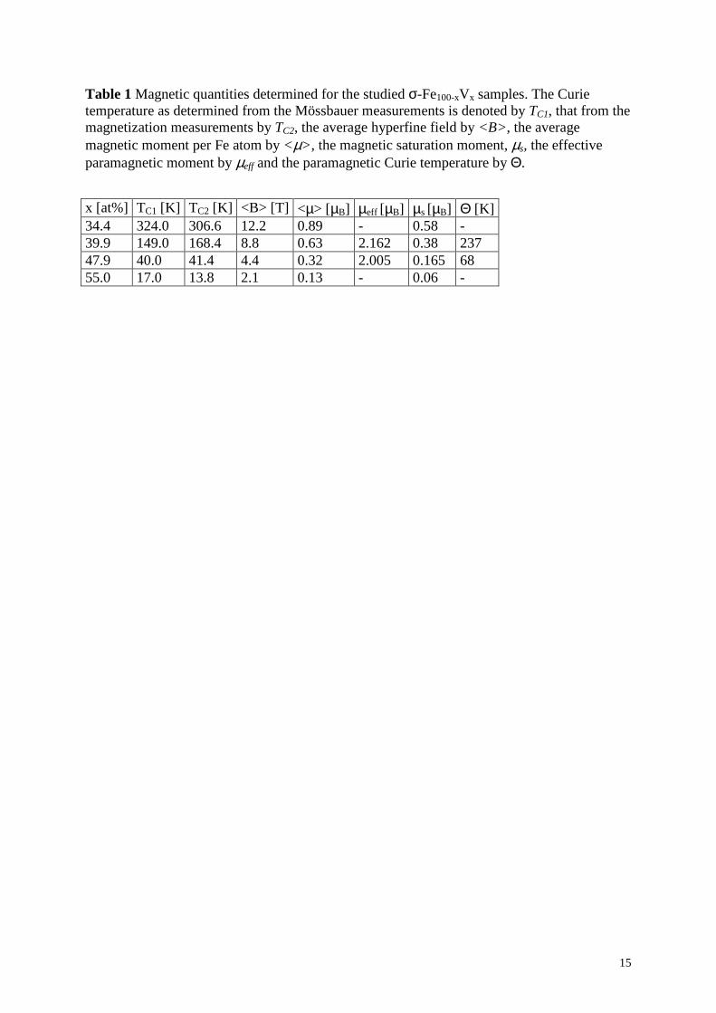
The best-fit values of the parameters obtained in such a way are displayed in Table 1. From C

the µeff – values were derived. The Curie temperature, TC, and the average magnetic moment

per Fe atom, <µ>, and the average hyperfine field, <B>, are included in this table, too. From

the data, and in particular, from the µeff/µs ratio, µs being the saturation moment, it is clear that

according to the Rhodes-Wohlfarth criterion, the magnetism of the studied system has

itinerant character.

3.3. Curie point – magnetic moment correlation It is well known that magnetizations as a function of the valence electron number per atom of

3d transition metal systems form the so-called Slater-Pauling curve. Similarly, the Curie

temperatures of these alloys also exhibit a Slater-Pauling like behaviour [16].

Though the overall shape of the latter is like the former, the two differ in details. It follows

from this fact that the Curie temperature depend not only on the magnetization but also on the

magnetic exchange interactions coefficients that are characteristic of a given alloy system.

Indeed, recent theoretical calculations carried out with the KKR-CPA-LDA method for

several 3d transition binary alloys have clearly demonstrated that the Curie temperature –

magnetic moment relationship is characteristic of a given system [17]. In other words, the two

quantities are, in general, not linearly correlated.

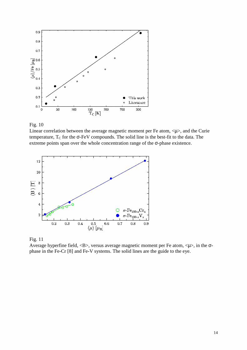
As shown in Fig. 10 for the σ-FeV system, TC is very well linearly correlated with the

magnetic moment, <µ>. The slope is equal to 406.5 K/µB, and is significantly different from

the one found recently for the σ-phase in the Fe-Cr system (i.e. 205 K/µB) [2,8]. A linear

7

correlation between the two magnetic quantities was also observed in the α-phase of the Fe-V

system of similar composition as the one in the presently studied samples [4]. The slope for

the latter is, however, equal to 741 K/µB i.e. almost twice the one in the σ-FeV system.

For comparison, the TC/µ value for a pure iron is equal to 470 K/µB.

This comparison clearly shows that the TC - <µ> relationship depends not only on the alloy

system, but for a given system it depends on its crystallographic structure.

3.4. Average hyperfine field - magnetic moment correlation

As illustrated in Fig. 11 for the σ-FeV compounds, the average hyperfine field, <B> - is

linearly correlated with the average magnetic moment per Fe atom, <µ>, with the slope of

14.3 T/µB. Such correlation is rather strange and unexpected for this system as according to

theoretical calculations performed on bcc-Fe-systems [18-20], only a part of the hyperfine

field viz. the one due to a polarization of the core electrons is proportional to the Fe-site

magnetic moment, while the second part viz. the one due to the polarization of the conduction

electrons, BCEP, is not. In other words, a non-linear <B> - <µ> relationship might be taken as

evidence that a substantial contribution to the hyperfine field originates form the conduction

electrons i.e. the system is magnetically itinerant. In the presently studied case, the Rhodes-

Wohlfarth criterion speaks in favour of the latter. The linear <B> - <µ> relationship means

that also BCEP term is proportional to <µ>. This conclusion must be, however, verified by

theoretical calculations devoted to the investigated system.

The presently found correlation between <B> and - <µ> is also of a practical meaning as it

can be used as the reference plot permitting a unique transformation between the two

quantities. It is linear and different than the one found previously for the σ-Fe-Cr system [8].

The latter feature gives clear evidence that the <B> - <µ> relationship is not universal, but it

is rather characteristic of a given structure and system.

8

4. Conclusions

The results obtained in this study permit drawing the following conclusions:

(a) σ-Fe65.6V34.4 sample shows the strongest magnetic properties ever found for the sigma-

phase as measured in terms of the Curie temperature, magnetic moment and magnetic

hyperfine field.

(b) Curie temperature and magnetic moment per Fe atom show nonlinear decrease with V

content.

(c) Curie temperature and the average hyperfine field are linearly correlated with the

magnetic moment. The latter is rather unexpected for an itinerant system and prompts

theoretical calculations.

Acknowledgement

Dr. Jan śukrowski is thanked for melting the samples.

9

References [1] E. O. Hall and S. H. Algie, Metall. Rev., 11 (1966) 61

[2] J. Cieslak, M. Reissner, W. Steiner and S. M. Dubiel, J. Magn. Magn. Mater., 272-276

(2004) 534; Phys. Stat. Sol (a), (2008)/DOI 10.1002/pssa.200723618

[3] H. H. Ettwig and W. Pepperhoff, Arch. Eisenhuttenwes., 43 (1972) 271

[4] A. M. van der Kraan, D. B. de Mooij and K. H. J. Buschow, Phys. Stat. Sol. (a), 88 (1985)

231

[5] Y. Sumimoto, T. Moriya, H. Ino and F. E. Fujita, J. Phys. Soc. Jpn., 35 (1973) 461

[6] D. A. Read and E. H. Thomas, IEEE Trans. Magn., MAG-2 (1966) 415

[7] D. A. Read, E. H. Thomas and J. B. Forsythe, J. Phys. Chem. Solids, 29 (1968) 1569

[8] J. Cieślak, B. F. O. Costa, S. M. Dubiel, M. Reissner and W. Steiner, J. Phys.,: Condens.

Matter., 17 (2005) 2985

[9] O. Kubaschewski, Iron-Binary Phase Diagrams, Springer Verlag, 1982, Berlin

[10] J. Cieślak, M. Reissner, S. M. Dubiel, J. Wernisch and W. Steiner, J. Alloys Comp., 20

(2008) 20

[11] R. Blower and G. J. Cox, J. Iron Steel Inst., August 1970, 769

[12] D. Parsons, Nature, 185 (1960) 839

[13] M. V. Nevitt and P. A. Beck, Trans. AIME, May 1955, 669

[14] M. Mori and T. Mitsui, J. Phys. Soc. Jpn., 22 (1967) 931

[15] M. V. Nevitt and A. T. Aldred, J. Appl. Phys., 34 (1963) 463

[16] H. P. Wijn, in Magnetic Properties of Metals, 1991, ed. R. Poerschke, Berlin, Springer

[17] C. Takahashi, M. Ogura and H. Akai, J. Phys.: Condens. Matter, 19 (2007) 365233

[18] R. E. Watson and A. J. Freeman, Phys. Rev., 123 (1961) 2027

[19] M. E. Elzain, D. E. Ellis and D. Guenzburger, Phys. Rev. B, 34 (1986) 1430

[20] B. Lingren and J. Sjöström, J. Phys. F: Metal. Phys., 18 (1988) 1563

10

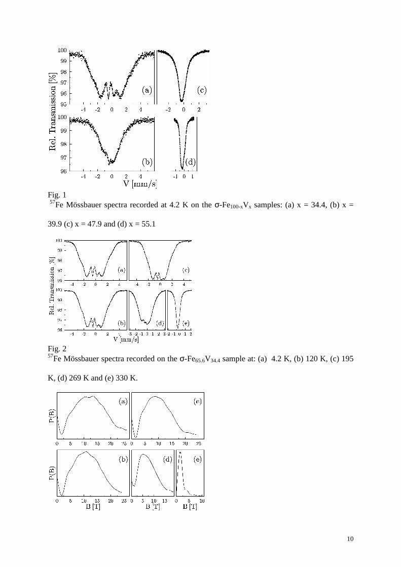
Fig. 1 57Fe Mössbauer spectra recorded at 4.2 K on the σ-Fe100-xVx samples: (a) x = 34.4, (b) x =

39.9 (c) x = 47.9 and (d) x = 55.1

Fig. 2 57Fe Mössbauer spectra recorded on the σ-Fe65.6V34.4 sample at: (a) 4.2 K, (b) 120 K, (c) 195

K, (d) 269 K and (e) 330 K.

11

Fig. 3 Distribution of the hyperfine field for the σ-Fe65.6V34.4 sample obtained from the spectra recorded at: (a) 41 K, (b) 120 K, (c) 195 K, (d) 269 K and (e) 330 K.

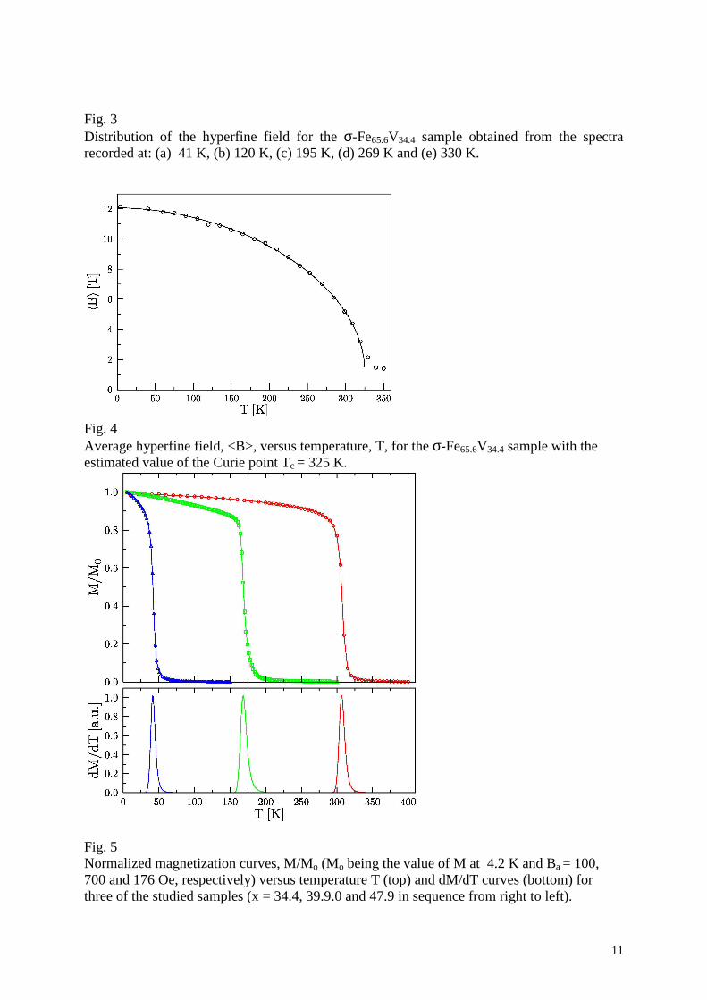
Fig. 4 Average hyperfine field, <B>, versus temperature, T, for the σ-Fe65.6V34.4 sample with the estimated value of the Curie point Tc = 325 K.

Fig. 5 Normalized magnetization curves, M/Mo (Mo being the value of M at 4.2 K and Ba = 100, 700 and 176 Oe, respectively) versus temperature T (top) and dM/dT curves (bottom) for three of the studied samples (x = 34.4, 39.9.0 and 47.9 in sequence from right to left).

12

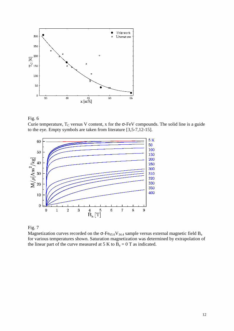
Fig. 6 Curie temperature, TC versus V content, x for the σ-FeV compounds. The solid line is a guide to the eye. Empty symbols are taken from literature [3,5-7,12-15].

Fig. 7 Magnetization curves recorded on the σ-Fe65.6V34.4 sample versus external magnetic field Ba for various temperatures shown. Saturation magnetization was determined by extrapolation of the linear part of the curve measured at 5 K to Ba = 0 T as indicated.

13

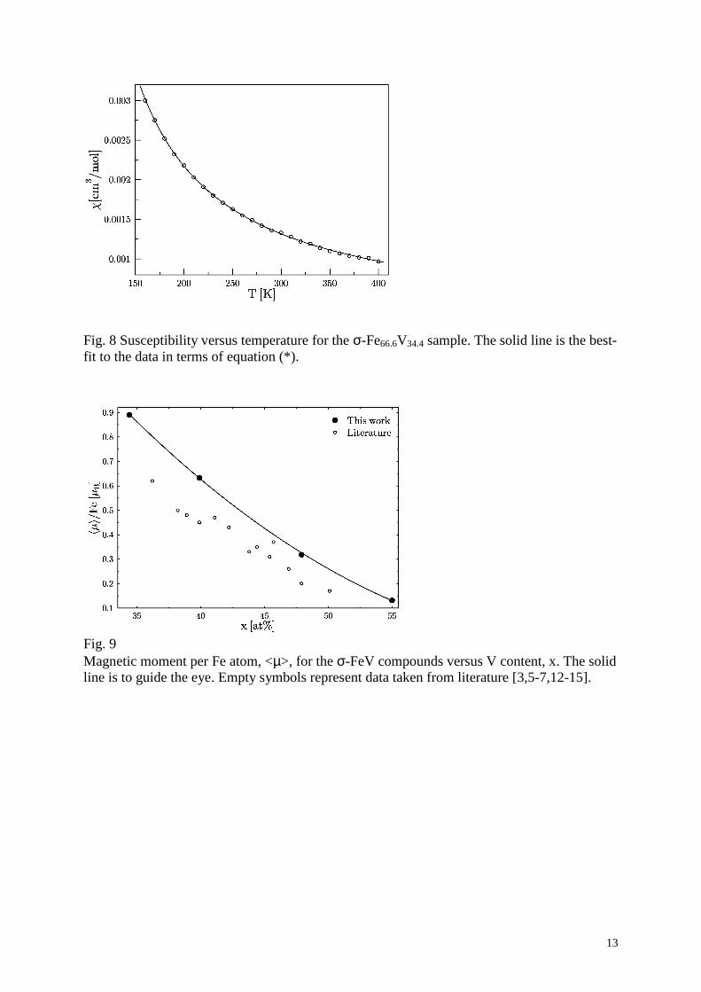
Fig. 8 Susceptibility versus temperature for the σ-Fe66.6V34.4 sample. The solid line is the best-fit to the data in terms of equation (*).

Fig. 9 Magnetic moment per Fe atom, <µ>, for the σ-FeV compounds versus V content, x. The solid line is to guide the eye. Empty symbols represent data taken from literature [3,5-7,12-15].

14

Fig. 10 Linear correlation between the average magnetic moment per Fe atom, <µ>, and the Curie temperature, TC for the σ-FeV compounds. The solid line is the best-fit to the data. The extreme points span over the whole concentration range of the σ-phase existence.

Fig. 11 Average hyperfine field, <B>, versus average magnetic moment per Fe atom, <µ>, in the σ-phase in the Fe-Cr [8] and Fe-V systems. The solid lines are the guide to the eye.

15

Table 1 Magnetic quantities determined for the studied σ-Fe100-xVx samples. The Curie temperature as determined from the Mössbauer measurements is denoted by TC1, that from the magnetization measurements by TC2, the average hyperfine field by <B>, the average magnetic moment per Fe atom by <µ>, the magnetic saturation moment, µs, the effective paramagnetic moment by µeff and the paramagnetic Curie temperature by Θ. x [at%] TC1 [K] TC2 [K] <B> [T] <µ> [µB] µeff [µB] µs [µB] Θ [K] 34.4 324.0 306.6 12.2 0.89 - 0.58 - 39.9 149.0 168.4 8.8 0.63 2.162 0.38 237 47.9 40.0 41.4 4.4 0.32 2.005 0.165 68 55.0 17.0 13.8 2.1 0.13 - 0.06 -