Download - Knowledge discovery from Decision Tables by the use of Multiple-valued logic

Artificial Intelligence Review 19: 153–176, 2003.© 2003 Kluwer Academic Publishers. Printed in the Netherlands.

153

Knowledge Discovery from Decision Tables by the Use ofMultiple-Valued Logic

K.J. ADAMS, D.A. BELL, L.P. MAGUIRE and J. McGREGORFaculty of Informatics, University of Ulster, Magee College, Londonderry BT48 7JL, UK(E-mail: [email protected])

Abstract. This paper describes how succinct rules, which reduce the size of decision tables,can be found by employing multiple-valued logic (MVL). Two multiple-valued algebras aredescribed, one based on level detection, and the other on literal functions. Then a decision tablewhich had also been reduced in size using rough set theory, is now reduced using both algebrasand it is seen that all three approaches lead to reductions of comparable simplicity. The newmethods require coding the values of each attribute as integers. Then an MVL function thatmaps the coding of the condition attributes to the coding of the decision attribute is found. Asthe coded table is sparse only some of the basis functions for each algebra are required. Thena simple approach requiring the reduction of a matrix to row echelon form is used to findingall suitable MVL functions. By decomposing a function in terms of its variables a completeset of rules can be found. The MVL function encodes the data in a very compact form andits decomposition into subfunctions reveals a good way to slice up the table into subtables.The structure of the subfunctions can then be used to simplify each subtable until compactsets of rules emerge. Alternatively, rules can be found by substitution into the MVL function.Encoding a decision table using MVL makes the data easy to manipulate and can uncoverrelationships that may not become apparent when using other methods.

Keywords: decision tables, knowledge discovery, matrix algebra, multiple-valued logic,rough sets, rule induction

1. Introduction

Multiple-valued logic (MVL) is increasingly finding applications in infor-mation technology. Multiple-Valued Logic has been applied to data mining(Steinbach et al. (1999)), machine learning (Tang et al. (1998)), to reasoning(Hanyu et al. (1991), Lu et al. (1998)), and in artificial intelligence (Hanyu etal. (1988)).

In this paper we explore the use of a two level sum of product MVL datastructure, applied to the derivation of simplified sets of rules for decisiontables. A combination of sum type and product type operations can be usedto obtain a two level sum of product representation of data. The early work of(Reed (1954)) and (Muller (1954)) used the exclusive-or operator XOR andthe AND operator to implement functions in Boolean algebra. These opera-

154 K.J. ADAMS, D.A. BELL, L.P. MAGUIRE AND J. MCGREGOR

tions can be considered as addition modulo-2 and multiplication modulo-2respectively. Since then their work has been generalized to higher radixalgebras and a number of MVL transforms now exist. Some examples include(Cohn (1960)) who used addition and multiplication modulo-m, where m is aprime number. This was further extended by (Pradhan (1974)) to considerthe case when m is a power of a prime. (Kodandapani (1975)) used theliteral functions as basis functions with modulo-m arithmetic; (Green et al.(1974), Green (1989, 1990)) used finite field arithmetic. In (Dubrova et al.(1996)) the minimum operation is used instead of modulo multiplication anda canonical form is presented using minimum, modulo-m addition and theset of all literal functions. Binary basis functions, with modulo-4 arithmetichave been used by (Adams et al. (1999)) to produce quaternary logic. Thispaper uses modulo-m arithmetic with two different sets of basis functions.Firstly we introduce the set of level detector functions which respond oncethe information they are reading goes higher than a predetermined fixed level.Secondly we use the set of literal functions.

Rough set theory (Pawlak (1982)) has established itself as a technique indata mining (Pawlak (1991), Pawlak et al. (1995)), and has been applied torough classification and knowledge discovery in nuclear power generationoperation and control (Guan et al. (1998)). Knowledge can be discoveredfrom tables of data. The knowledge can be represented in the form of rulesor in a number of other forms such as equations, which we use here. Theequations are readily transformable into rules subsequently. So the outputfrom this analysis procedure can be compared with that from other methods,such as the rough set methods of (Guan et al. (2000)). In the present examplethe data is in a particular form – a decision table. This means that at leastone of the attributes (columns) is a decision attribute and that its value isinfluenced, in some way to be discovered, by the values of the other attributes.Data originally presented by (Oh (1996)) is analyzed using MVL. This willbe compared with previous results using rough set analysis given in (Guan etal. (2000)).

The structure of this paper is as follows. Section two introduces MVLthrough the medium of the two algebraic systems, literals and level detectors;single variable and two variable examples are given. Section three looks atthe data to be analyzed; it is explained how this is coded into a set of integers.Sections four and five obtain reduced sets of rules using level detector algebraand literal algebra respectively. Section six compares our results with roughset theory applied to the same data. Section seven re-examines the previouswork. A new type of rule structure is described and it is shown how thiscan be found directly from an MVL equation. Section eight contains a broaddiscussion about multiple-valued logic and its possible application to decision

KNOWLEDGE DISCOVERY FROM DECISION TABLES BY MULTIPLE-VALUED LOGIC 155

tables. Lastly Section nine concludes the paper and looks forward to futurework.

2. Description of Two Multiple-valued Algebras

This section is tutorial in nature and will describe the two multiple-valuedalgebras that will be used in the paper. Suppose we have n discrete sets x1,x2, x3, . . . xn and each discrete set can be represented by a set of non-zerointegers xi = {0, 1, 2, . . . |xi | – 1}, where |xi | is the number of elements in xi ;the domain X of a multiple-valued logic function is the Cartesian product ofthe xi ; the range is a discrete set y = {0, 1, 2, . . . m – 1}, where m = |y|. LetF be the set of all such functions, then an algebra α is a subset of F with theproperty that all the members of F can be constructed from members of α.

2.1. Literal algebra

The algebra A will consist of: constants, that is all the elements of y, themodulo-m addition function +, the modulo-m multiplication function × , andthe set of all literal functions xj

i , j ∈ {0, 1, 2, . . . |xi | – 1} defined by the rulethat xj

i = 1 when xi = j and zero otherwise, with 0, 1 ∈ y. This is a special caseof a ring expression (Davio (1978)).

As a one variable example consider the function f : {0, 1, 2} → {0, 1, 2}defined by f(0) = 2, f(1) = 1, f(2) = 2. This can be represented by the columnvector (2, 1, 2)T where T represents transpose. Using modulo-3 arithmeticthis function can be represented as follows, f(x) = 2x0 + x1 + 2x2. This can beconsidered as the following vector relationship

2 ×

100

+ 1 ×

010

+ 2 ×

001

=

212

mod-3

Thus f(x) has been built up from members of A. In future work we shall dropthe multiplication signs i.e. 2x shall mean 2 × x. It is clear that the algebra Ais functionally complete because the set of literals xj , j ∈ {0, 1, 2, . . . |x| – 1},form the columns of the |x| by |x| identity matrix.

2.2. Level detector algebra

The second algebra T consists of: constants, that is all the elements of {y},the modulo-m addition function, the modulo-m multiplication function, andthe set of all Level Detector functions xi

(j) defined by the rule that xi(j) = 1


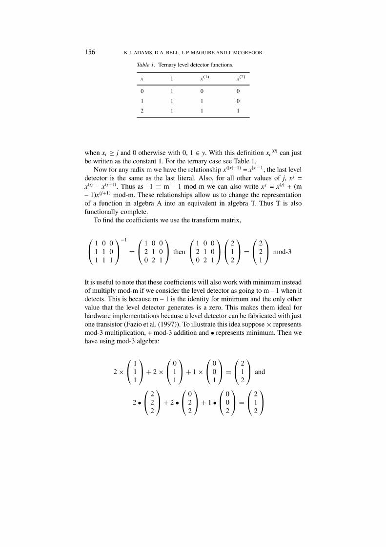
Table 1. Ternary level detector functions.

x 1 x(1) x(2)

0 1 0 0

1 1 1 0

2 1 1 1

when xi ≥ j and 0 otherwise with 0, 1 ∈ y. With this definition xi(0) can just

be written as the constant 1. For the ternary case see Table 1.Now for any radix m we have the relationship x(|x|−1) = x|x|−1, the last level

detector is the same as the last literal. Also, for all other values of j, xj =x(j) – x(j+1). Thus as –1 ≡ m – 1 mod-m we can also write xj = x(j) + (m– 1)x(j+1) mod-m. These relationships allow us to change the representationof a function in algebra A into an equivalent in algebra T. Thus T is alsofunctionally complete.

To find the coefficients we use the transform matrix,

1 0 01 1 01 1 1

−1

=

1 0 02 1 00 2 1

then

1 0 02 1 00 2 1

212

=

221

mod-3

It is useful to note that these coefficients will also work with minimum insteadof multiply mod-m if we consider the level detector as going to m – 1 when itdetects. This is because m – 1 is the identity for minimum and the only othervalue that the level detector generates is a zero. This makes them ideal forhardware implementations because a level detector can be fabricated with justone transistor (Fazio et al. (1997)). To illustrate this idea suppose × representsmod-3 multiplication, + mod-3 addition and • represents minimum. Then wehave using mod-3 algebra:

2 ×

111

+ 2 ×

011

+ 1 ×

001

=

212

and

2 •

222

+ 2 •

022

+ 1 •

002

=

212


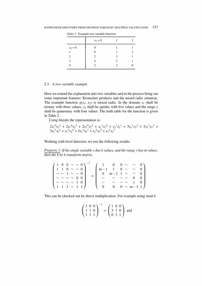
Table 2. Example two variable function.

x1 = 0 1 2

x2 = 0 0 1 1

1 0 1 3

2 2 3 1

3 2 3 1

4 2 3 0

2.3. A two variable example

Here we extend the explanation into two variables and in the process bring outsome important features: Kronecker products and the mixed radix situation.The example function g(x1, x2) is mixed radix. In the domain x1 shall beternary with three values, x2 shall be quintic with five values and the range yshall be quaternary with four values. The truth table for the function is givenin Table 2.

Using literals the representation is:

2x10x2

2 + 2x10x2

3 + 2x10x2

4 + x11x2

0 + x11x2

1 + 3x11x2

2 + 3x11x2

3 +3x1

1x24 + x1

2x20 + 3x1

2x21 + x1

2x22 + x1

2x23

Working with level detectors we use the following results:

Property 1: If the single variable x has k values, and the range y has m values,then the k by k transform matrix,

1 0 0 ∼ ∼ 01 1 0 ∼ ∼ 0∼ ∼ 1 ∼ ∼ 0∼ ∼ ∼ ∼ 0 0∼ ∼ ∼ ∼ 1 01 1 1 ∼ 1 1

−1

=

1 0 0 ∼ ∼ 0m – 1 1 0 ∼ ∼ 0

0 m – 1 1 ∼ ∼ 0∼ ∼ ∼ ∼ 0 0∼ ∼ ∼ ∼ 1 00 0 0 ∼ m – 1 1

This can be checked out by direct multiplication. For example using mod-4

1 0 01 1 01 1 1

−1

=

1 0 03 1 00 3 1

and


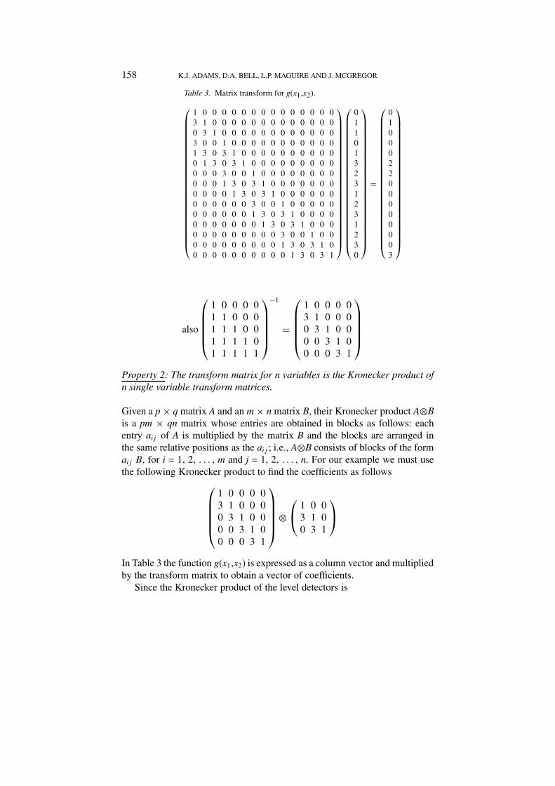
Table 3. Matrix transform for g(x1,x2).

1 0 0 0 0 0 0 0 0 0 0 0 0 0 03 1 0 0 0 0 0 0 0 0 0 0 0 0 00 3 1 0 0 0 0 0 0 0 0 0 0 0 03 0 0 1 0 0 0 0 0 0 0 0 0 0 01 3 0 3 1 0 0 0 0 0 0 0 0 0 00 1 3 0 3 1 0 0 0 0 0 0 0 0 00 0 0 3 0 0 1 0 0 0 0 0 0 0 00 0 0 1 3 0 3 1 0 0 0 0 0 0 00 0 0 0 1 3 0 3 1 0 0 0 0 0 00 0 0 0 0 0 3 0 0 1 0 0 0 0 00 0 0 0 0 0 1 3 0 3 1 0 0 0 00 0 0 0 0 0 0 1 3 0 3 1 0 0 00 0 0 0 0 0 0 0 0 3 0 0 1 0 00 0 0 0 0 0 0 0 0 1 3 0 3 1 00 0 0 0 0 0 0 0 0 0 1 3 0 3 1

011013231231230

=

010002200000003

also

1 0 0 0 01 1 0 0 01 1 1 0 01 1 1 1 01 1 1 1 1

−1

=

1 0 0 0 03 1 0 0 00 3 1 0 00 0 3 1 00 0 0 3 1

Property 2: The transform matrix for n variables is the Kronecker product ofn single variable transform matrices.

Given a p × q matrix A and an m × n matrix B, their Kronecker product A⊗Bis a pm × qn matrix whose entries are obtained in blocks as follows: eachentry aij of A is multiplied by the matrix B and the blocks are arranged inthe same relative positions as the aij ; i.e., A⊗B consists of blocks of the formaij B, for i = 1, 2, . . . , m and j = 1, 2, . . . , n. For our example we must usethe following Kronecker product to find the coefficients as follows

1 0 0 0 03 1 0 0 00 3 1 0 00 0 3 1 00 0 0 3 1

⊗

1 0 03 1 00 3 1

In Table 3 the function g(x1,x2) is expressed as a column vector and multipliedby the transform matrix to obtain a vector of coefficients.

Since the Kronecker product of the level detectors is


[1, x2(1), x2

(2), x2(3), x2

(4)] ⊗ [1, x1(1), x1

(2) ] =[1, x1

(1), x1(2), x2

(1), x1(1)x2

(1), x1(2)x2

(1), x2(2), x1

(1)x2(2), x1

(2)x2(2), x2

(3),x1

(1)x2(3), x1

(2)x2(3), x2

(4), x1(1)x2

(4), x1(2)x2

(4)]

Thus g(x1, x2) = x1(1)+ 2x1

(2)x2(1) + 2x2

(2) + 3x1(2)x2

(4). Here x1(2)x2

(1) meansthat x1

(2) and x2(1) are multiplied. So the term is above zero only when x1 ≥ 2

and x2 ≥ 1.One reason why level detectors may be useful is that in some situations

the decision will change once a critical threshold level is passed by one ormore of the attributes that contribute towards the decision. Another reasonis that when using set theory we would like to consider window literals. Awindow literal x[a,b] is 1 when a ≤ x ≤ b and zero otherwise. They are thecharacteristic equations of step functions, which are subsets of {x} whereelements follow each other consecutively. For a m-valued variable there arem (m + 1)/2 window literals. So for example in a three variable quaternaryexample, each variable has 10 window literals and taking Cartesian productswe arrive at 1,000 possible cuboids upon which the data could be constant. Itis difficult to see patterns here. However there are just m levels to be detected.So for quaternary that is four for the single variable case, and only 64 for threevariables. Thus it is better to look for the edges of cuboids rather than thecuboids themselves. Interpretation of the level detector equation may revealother structures, for example x[a,b] = x(a) – x(b+1).

3. The Data to be Examined

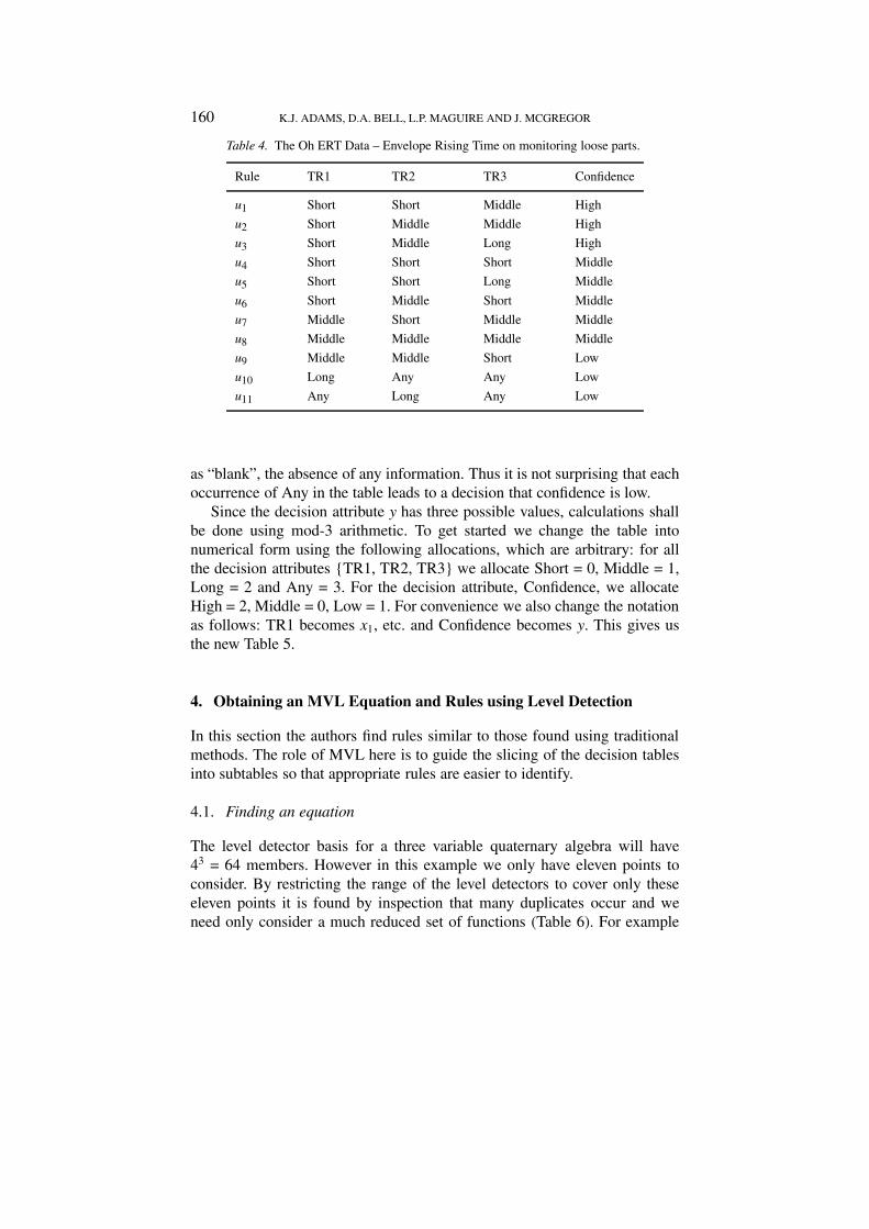
We describe the data used in this paper which was used previously by Guanand Bell for a rough set analysis (Guan et al. (2000)); the original informationwas from (Oh (1996)). A decision table is a table of attributes divided into twoparts, condition attributes C, and decision attributes D, with A = C ∪ D and C∩ D = φ. From a decision table we hope to find a simplified sets of rules thatenable us to predict the decision attributes from the condition attributes. Thedata presented in Table 4 is a decision table where C = {TR1, TR2, TR3} andD = {y}, y = Confidence.

The data is the Envelope Rising Time (ERT) which expresses the featuresof loose parts in a nuclear reactor coolant system. (Oh, (1996)) made a fuzzyrule base for the evaluation of confidence level of input signal based onthe relationship between the wave arrival sequences and envelope patternchanges. In Table 4, TR1, TR2 and TR3 are the Envelope Rising Times ofthe first, second and third signal respectively. Times are categorized as short,middle and long. Following (Guan et al. (2000)) “Any” shall be considered


Table 4. The Oh ERT Data – Envelope Rising Time on monitoring loose parts.

Rule TR1 TR2 TR3 Confidence

u1 Short Short Middle High

u2 Short Middle Middle High

u3 Short Middle Long High

u4 Short Short Short Middle

u5 Short Short Long Middle

u6 Short Middle Short Middle

u7 Middle Short Middle Middle

u8 Middle Middle Middle Middle

u9 Middle Middle Short Low

u10 Long Any Any Low

u11 Any Long Any Low

as “blank”, the absence of any information. Thus it is not surprising that eachoccurrence of Any in the table leads to a decision that confidence is low.

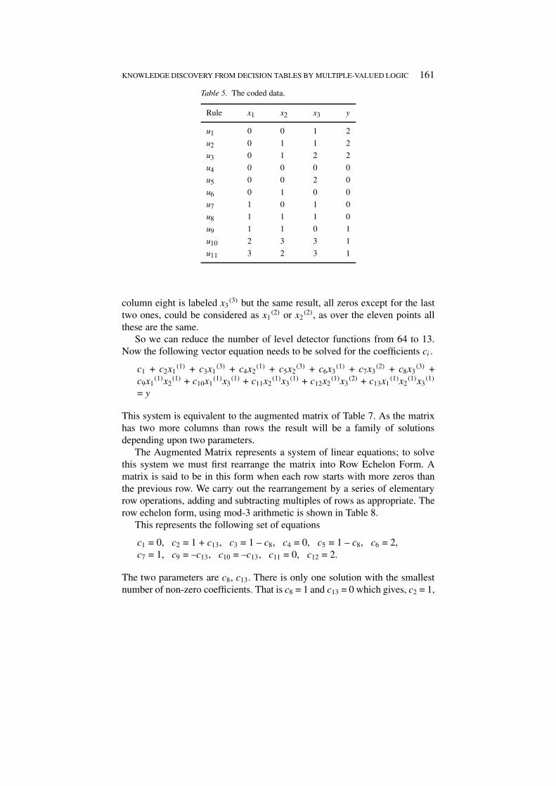
Since the decision attribute y has three possible values, calculations shallbe done using mod-3 arithmetic. To get started we change the table intonumerical form using the following allocations, which are arbitrary: for allthe decision attributes {TR1, TR2, TR3} we allocate Short = 0, Middle = 1,Long = 2 and Any = 3. For the decision attribute, Confidence, we allocateHigh = 2, Middle = 0, Low = 1. For convenience we also change the notationas follows: TR1 becomes x1, etc. and Confidence becomes y. This gives usthe new Table 5.

4. Obtaining an MVL Equation and Rules using Level Detection

In this section the authors find rules similar to those found using traditionalmethods. The role of MVL here is to guide the slicing of the decision tablesinto subtables so that appropriate rules are easier to identify.

4.1. Finding an equation

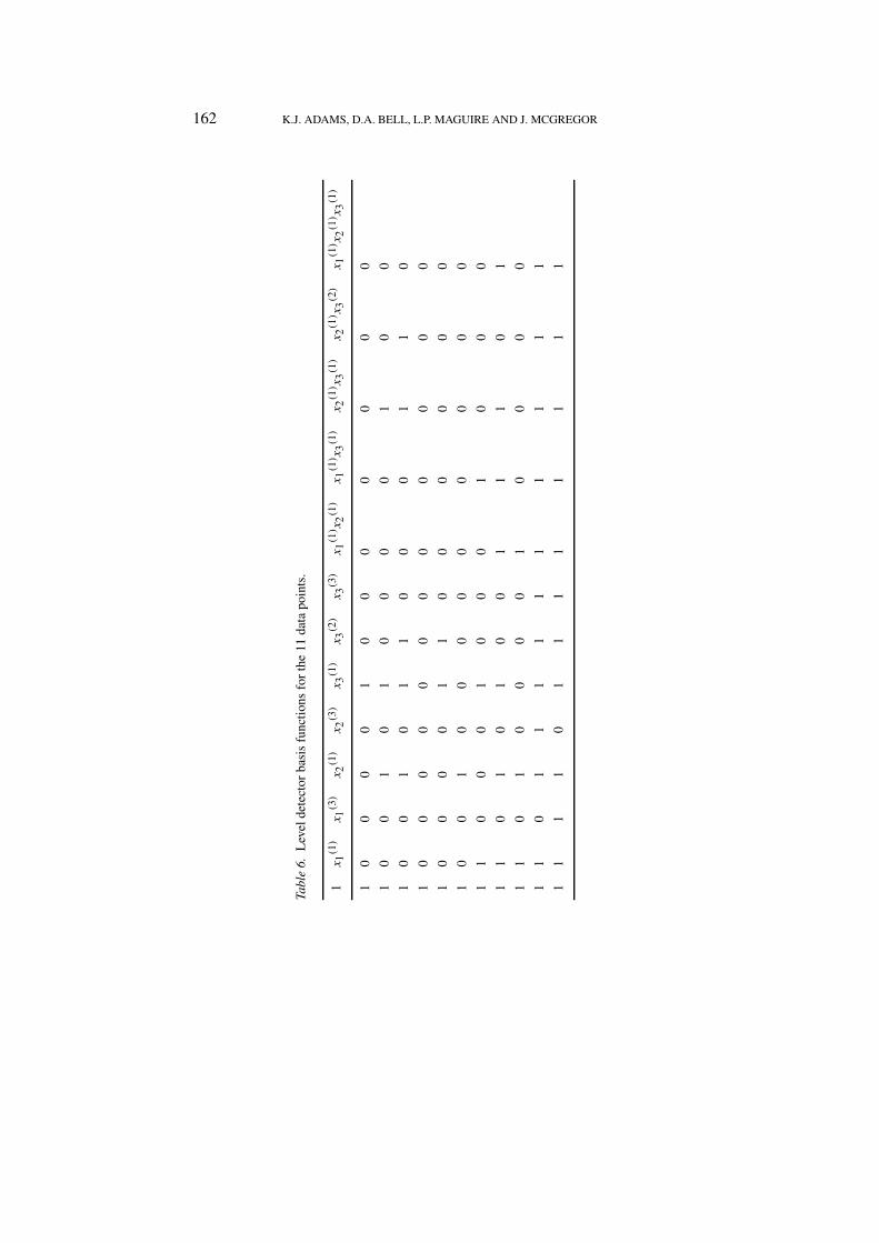
The level detector basis for a three variable quaternary algebra will have43 = 64 members. However in this example we only have eleven points toconsider. By restricting the range of the level detectors to cover only theseeleven points it is found by inspection that many duplicates occur and weneed only consider a much reduced set of functions (Table 6). For example


Table 5. The coded data.

Rule x1 x2 x3 y

u1 0 0 1 2

u2 0 1 1 2

u3 0 1 2 2

u4 0 0 0 0

u5 0 0 2 0

u6 0 1 0 0

u7 1 0 1 0

u8 1 1 1 0

u9 1 1 0 1

u10 2 3 3 1

u11 3 2 3 1

column eight is labeled x3(3) but the same result, all zeros except for the last

two ones, could be considered as x1(2) or x2

(2), as over the eleven points allthese are the same.

So we can reduce the number of level detector functions from 64 to 13.Now the following vector equation needs to be solved for the coefficients ci .

c1 + c2x1(1) + c3x1

(3) + c4x2(1) + c5x2

(3) + c6x3(1) + c7x3

(2) + c8x3(3) +

c9x1(1)x2

(1) + c10x1(1)x3

(1) + c11x2(1)x3

(1) + c12x2(1)x3

(2) + c13x1(1)x2

(1)x3(1)

= y

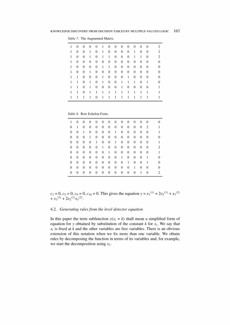
This system is equivalent to the augmented matrix of Table 7. As the matrixhas two more columns than rows the result will be a family of solutionsdepending upon two parameters.

The Augmented Matrix represents a system of linear equations; to solvethis system we must first rearrange the matrix into Row Echelon Form. Amatrix is said to be in this form when each row starts with more zeros thanthe previous row. We carry out the rearrangement by a series of elementaryrow operations, adding and subtracting multiples of rows as appropriate. Therow echelon form, using mod-3 arithmetic is shown in Table 8.

This represents the following set of equations

c1 = 0, c2 = 1 + c13, c3 = 1 – c8, c4 = 0, c5 = 1 – c8, c6 = 2,c7 = 1, c9 = –c13, c10 = –c13, c11 = 0, c12 = 2.

The two parameters are c8, c13. There is only one solution with the smallestnumber of non-zero coefficients. That is c8 = 1 and c13 = 0 which gives, c2 = 1,


Tabl

e6.

Lev

elde

tect

orba

sis

func

tion

sfo

rth

e11

data

poin

ts.

1x 1

(1)

x 1(3

)x 2

(1)

x 2(3

)x 3

(1)

x 3(2

)x 3

(3)

x 1(1

) x2(1

)x 1

(1) x

3(1

)x 2

(1) x

3(1

)x 2

(1) x

3(2

)x 1

(1) x

2(1

) x3(1

)

10

00

01

00

00

00

0

10

01

01

00

00

10

0

10

01

01

10

00

11

0

10

00

00

00

00

00

0

10

00

01

10

00

00

0

10

01

00

00

00

00

0

11

00

01

00

01

00

0

11

01

01

00

11

10

1

11

01

00

00

10

00

0

11

01

11

11

11

11

1

11

11

01

11

11

11

1


Table 7. The Augmented Matrix.

1 0 0 0 0 1 0 0 0 0 0 0 0 2

1 0 0 1 0 1 0 0 0 0 1 0 0 2

1 0 0 1 0 1 1 0 0 0 1 1 0 2

1 0 0 0 0 0 0 0 0 0 0 0 0 0

1 0 0 0 0 1 1 0 0 0 0 0 0 0

1 0 0 1 0 0 0 0 0 0 0 0 0 0

1 1 0 0 0 1 0 0 0 1 0 0 0 0

1 1 0 1 0 1 0 0 1 1 1 0 1 0

1 1 0 1 0 0 0 0 1 0 0 0 0 1

1 1 0 1 1 1 1 1 1 1 1 1 1 1

1 1 1 1 0 1 1 1 1 1 1 1 1 1

Table 8. Row Echelon Form.

1 0 0 0 0 0 0 0 0 0 0 0 0 0

0 1 0 0 0 0 0 0 0 0 0 0 2 1

0 0 1 0 0 0 0 1 0 0 0 0 0 1

0 0 0 1 0 0 0 0 0 0 0 0 0 0

0 0 0 0 1 0 0 1 0 0 0 0 0 1

0 0 0 0 0 1 0 0 0 0 0 0 0 2

0 0 0 0 0 0 1 0 0 0 0 0 0 1

0 0 0 0 0 0 0 0 1 0 0 0 1 0

0 0 0 0 0 0 0 0 0 1 0 0 1 0

0 0 0 0 0 0 0 0 0 0 1 0 0 0

0 0 0 0 0 0 0 0 0 0 0 1 0 2

c3 = 0, c5 = 0, c9 = 0, c10 = 0. This gives the equation y = x1(1) + 2x3

(1) + x3(2)

+ x3(3) + 2x2

(1)x3(2).

4.2. Generating rules from the level detector equation

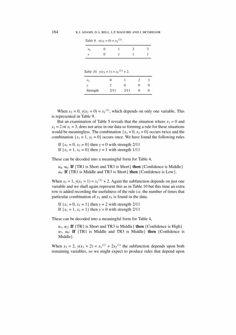
In this paper the term subfunction y(xi = k) shall mean a simplified form ofequation for y obtained by substitution of the constant k for xi . We say thatxi is fixed at k and the other variables are free variables. There is an obviousextension of this notation when we fix more than one variable. We obtainrules by decomposing the function in terms of its variables and, for example,we start the decomposition using x3.


Table 9. y(x3 = 0) = x1(1).

x1 0 1 2 3

y 0 1 1 1

Table 10. y(x3 = 1) = x1(1) + 2.

x1 0 1 2 3

y 2 0 0 0

Strength 2/11 2/11 0 0

When x3 = 0, y(x3 = 0) = x1(1), which depends on only one variable, This

is represented in Table 9.But an examination of Table 5 reveals that the situation where x3 = 0 and

x1 = 2 or x1 = 3, does not arise in our data so forming a rule for these situationswould be meaningless. The combination {x1 = 0, x3 = 0} occurs twice and thecombination {x1 = 1, x3 = 0} occurs once. We have found the following rules

If {x1 = 0, x3 = 0} then y = 0 with strength 2/11If {x1 = 1, x3 = 0} then y = 1 with strength 1/11

These can be decoded into a meaningful form for Table 4,

u4, u6: If {TR1 is Short and TR3 is Short} then {Confidence is Middle}u9: If {TR1 is Middle and TR3 is Short} then {Confidence is Low}.

When x3 = 1, y(x3 = 1) = x1(1) + 2. Again the subfunction depends on just one

variable and we shall again represent this as in Table 10 but this time an extrarow is added recording the usefulness of the rule i.e. the number of times thatparticular combination of x1 and x3 is found in the data.

If {x1 = 0, x3 = 1} then y = 2 with strength 2/11If {x1 = 1, x3 = 1} then y = 0 with strength 2/11


u1, u2: If {TR1 is Short and TR3 is Middle} then {Confidence is High}u7, u8: If {TR1 is Middle and TR3 is Middle} then {Confidence isMiddle}.

When x3 = 2, y(x3 = 2) = x1(1) + 2x2

(1) the subfunction depends upon bothremaining variables, so we might expect to produce rules that depend upon


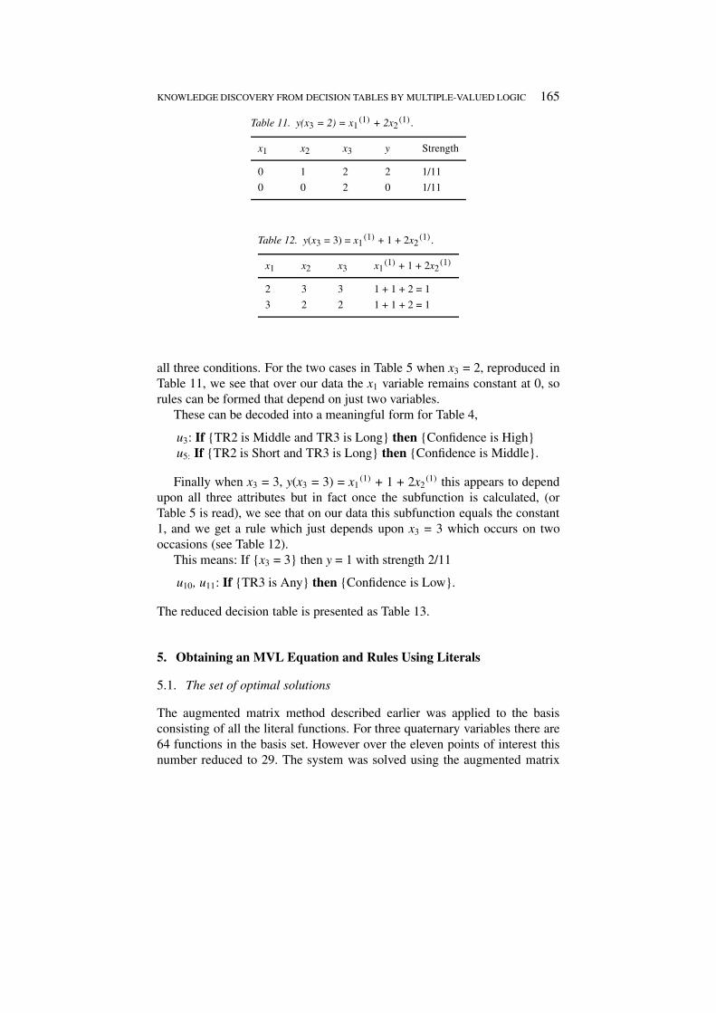
Table 11. y(x3 = 2) = x1(1) + 2x2

(1).

x1 x2 x3 y Strength

0 1 2 2 1/11

0 0 2 0 1/11

Table 12. y(x3 = 3) = x1(1) + 1 + 2x2

(1).

x1 x2 x3 x1(1) + 1 + 2x2

(1)

2 3 3 1 + 1 + 2 = 1

3 2 2 1 + 1 + 2 = 1

all three conditions. For the two cases in Table 5 when x3 = 2, reproduced inTable 11, we see that over our data the x1 variable remains constant at 0, sorules can be formed that depend on just two variables.


u3: If {TR2 is Middle and TR3 is Long} then {Confidence is High}u5: If {TR2 is Short and TR3 is Long} then {Confidence is Middle}.

Finally when x3 = 3, y(x3 = 3) = x1(1) + 1 + 2x2

(1) this appears to dependupon all three attributes but in fact once the subfunction is calculated, (orTable 5 is read), we see that on our data this subfunction equals the constant1, and we get a rule which just depends upon x3 = 3 which occurs on twooccasions (see Table 12).

This means: If {x3 = 3} then y = 1 with strength 2/11

u10, u11: If {TR3 is Any} then {Confidence is Low}.

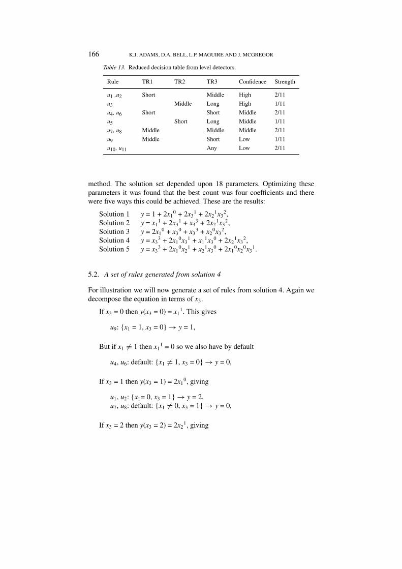
The reduced decision table is presented as Table 13.

5. Obtaining an MVL Equation and Rules Using Literals

5.1. The set of optimal solutions

The augmented matrix method described earlier was applied to the basisconsisting of all the literal functions. For three quaternary variables there are64 functions in the basis set. However over the eleven points of interest thisnumber reduced to 29. The system was solved using the augmented matrix


Table 13. Reduced decision table from level detectors.

Rule TR1 TR2 TR3 Confidence Strength

u1 ,u2 Short Middle High 2/11

u3 Middle Long High 1/11

u4, u6 Short Short Middle 2/11

u5 Short Long Middle 1/11

u7, u8 Middle Middle Middle 2/11

u9 Middle Short Low 1/11

u10, u11 Any Low 2/11

method. The solution set depended upon 18 parameters. Optimizing theseparameters it was found that the best count was four coefficients and therewere five ways this could be achieved. These are the results:

Solution 1 y = 1 + 2x10 + 2x3

1 + 2x21x3

2,Solution 2 y = x1

1 + 2x31 + x3

3 + 2x21x3

2,Solution 3 y = 2x1

0 + x30 + x3

3 + x20x3

2,Solution 4 y = x3

3 + 2x10x3

1 + x11x3

0 + 2x21x3

2,Solution 5 y = x3

3 + 2x10x2

1 + x21x3

0 + 2x10x2

0x31.

5.2. A set of rules generated from solution 4

For illustration we will now generate a set of rules from solution 4. Again wedecompose the equation in terms of x3.

If x3 = 0 then y(x3 = 0) = x11. This gives

u9: {x1 = 1, x3 = 0} → y = 1,

But if x1 = 1 then x11 = 0 so we also have by default

u4, u6: default: {x1 = 1, x3 = 0} → y = 0,

If x3 = 1 then y(x3 = 1) = 2x10, giving

u1, u2: {x1= 0, x3 = 1} → y = 2,u7, u8: default: {x1 = 0, x3 = 1} → y = 0,

If x3 = 2 then y(x3 = 2) = 2x21, giving


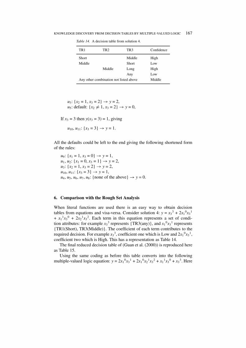
Table 14. A decision table from solution 4.

TR1 TR2 TR3 Confidence

Short Middle High

Middle Short Low

Middle Long High

Any Low

Any other combination not listed above Middle

u3: {x2 = 1, x3 = 2} → y = 2,u5: default: {x2 = 1, x3 = 2} → y = 0,

If x3 = 3 then y(x3 = 3) = 1, giving

u10, u11: {x3 = 3} → y = 1.

All the defaults could be left to the end giving the following shortened formof the rules:

u9: {x1 = 1, x3 = 0} → y = 1,u1, u2: {x1 = 0, x3 = 1} → y = 2,u3: {x2 = 1, x3 = 2} → y = 2,u10, u11: {x3 = 3} → y = 1,u4, u5, u6, u7, u8: {none of the above} → y = 0.

6. Comparison with the Rough Set Analysis

When literal functions are used there is an easy way to obtain decisiontables from equations and visa-versa. Consider solution 4: y = x3

3 + 2x10x3

1

+ x11x3

0 + 2x21x3

2. Each term in this equation represents a set of condi-tion attributes: for example x3

3 represents {TR3(any)}, and x10x3

1 represents{TR1(Short), TR3(Middle)}. The coefficient of each term contributes to therequired decision. For example x3

3, coefficient one which is Low and 2x10x3

1,coefficient two which is High. This has a representation as Table 14.

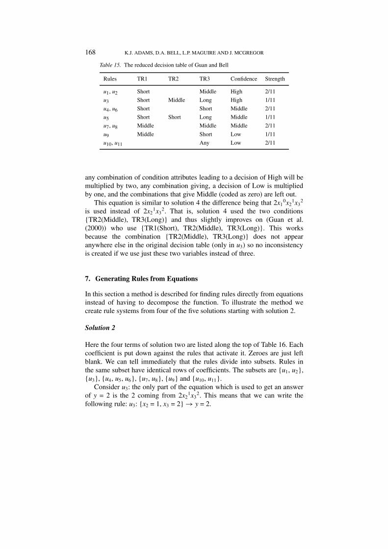
The final reduced decision table of (Guan et al. (2000)) is reproduced hereas Table 15.

Using the same coding as before this table converts into the followingmultiple-valued logic equation: y = 2x1

0x31 + 2x1

0x21x3

2 + x11x3

0 + x33. Here


Table 15. The reduced decision table of Guan and Bell

Rules TR1 TR2 TR3 Confidence Strength

u1, u2 Short Middle High 2/11

u3 Short Middle Long High 1/11

u4, u6 Short Short Middle 2/11

u5 Short Short Long Middle 1/11

u7, u8 Middle Middle Middle 2/11

u9 Middle Short Low 1/11

u10, u11 Any Low 2/11

any combination of condition attributes leading to a decision of High will bemultiplied by two, any combination giving, a decision of Low is multipliedby one, and the combinations that give Middle (coded as zero) are left out.

This equation is similar to solution 4 the difference being that 2x10x2

1x32

is used instead of 2x21x3

2. That is, solution 4 used the two conditions{TR2(Middle), TR3(Long)} and thus slightly improves on (Guan et al.(2000)) who use {TR1(Short), TR2(Middle), TR3(Long)}. This worksbecause the combination {TR2(Middle), TR3(Long)} does not appearanywhere else in the original decision table (only in u3) so no inconsistencyis created if we use just these two variables instead of three.

7. Generating Rules from Equations

In this section a method is described for finding rules directly from equationsinstead of having to decompose the function. To illustrate the method wecreate rule systems from four of the five solutions starting with solution 2.

Solution 2

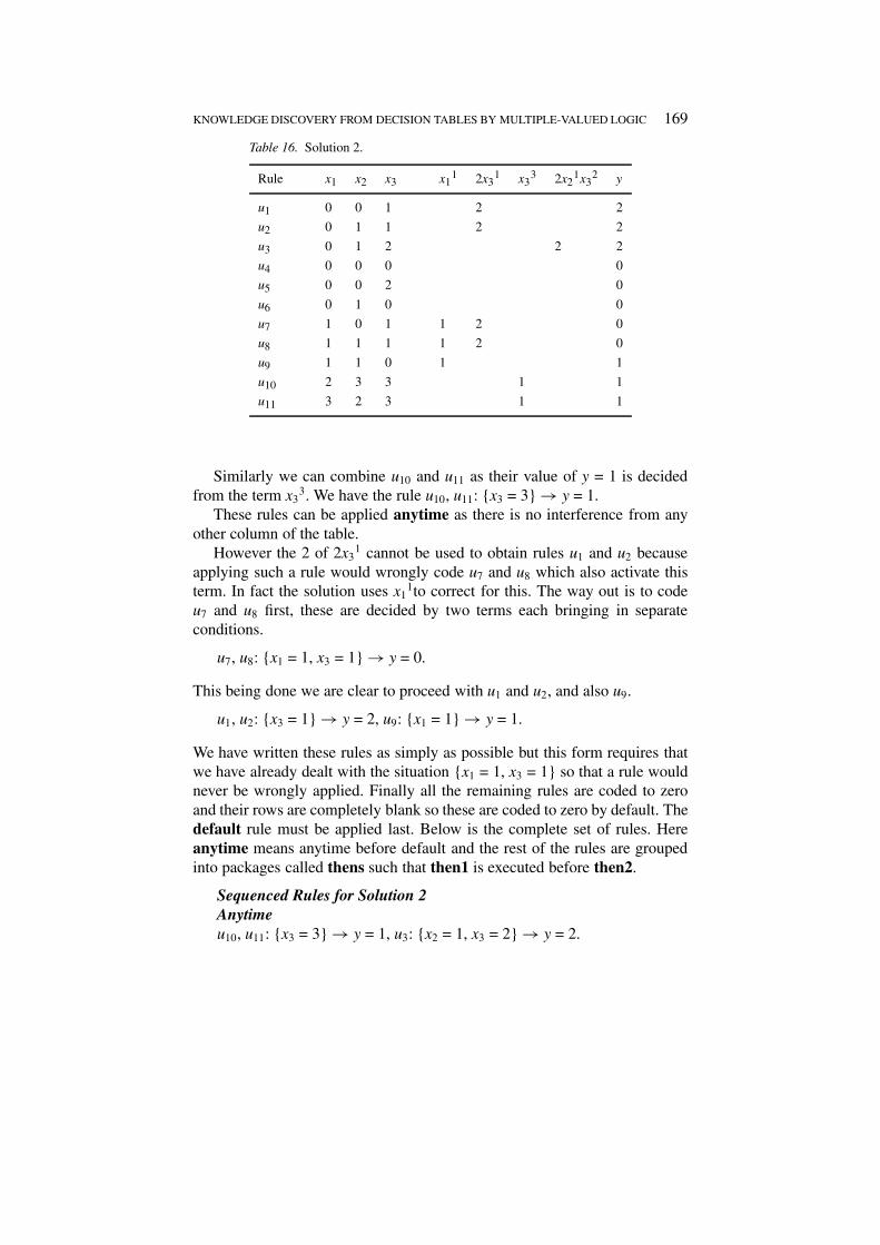
Here the four terms of solution two are listed along the top of Table 16. Eachcoefficient is put down against the rules that activate it. Zeroes are just leftblank. We can tell immediately that the rules divide into subsets. Rules inthe same subset have identical rows of coefficients. The subsets are {u1, u2},{u3}, {u4, u5, u6}, {u7, u8}, {u9} and {u10, u11}.

Consider u3: the only part of the equation which is used to get an answerof y = 2 is the 2 coming from 2x2

1x32. This means that we can write the

following rule: u3: {x2 = 1, x3 = 2} → y = 2.


Table 16. Solution 2.

Rule x1 x2 x3 x11 2x3

1 x33 2x2

1x32 y

u1 0 0 1 2 2

u2 0 1 1 2 2

u3 0 1 2 2 2

u4 0 0 0 0

u5 0 0 2 0

u6 0 1 0 0

u7 1 0 1 1 2 0

u8 1 1 1 1 2 0

u9 1 1 0 1 1

u10 2 3 3 1 1

u11 3 2 3 1 1

Similarly we can combine u10 and u11 as their value of y = 1 is decidedfrom the term x3

3. We have the rule u10, u11: {x3 = 3} → y = 1.These rules can be applied anytime as there is no interference from any

other column of the table.However the 2 of 2x3

1 cannot be used to obtain rules u1 and u2 becauseapplying such a rule would wrongly code u7 and u8 which also activate thisterm. In fact the solution uses x1

1to correct for this. The way out is to codeu7 and u8 first, these are decided by two terms each bringing in separateconditions.

u7, u8: {x1 = 1, x3 = 1} → y = 0.

This being done we are clear to proceed with u1 and u2, and also u9.

u1, u2: {x3 = 1} → y = 2, u9: {x1 = 1} → y = 1.

We have written these rules as simply as possible but this form requires thatwe have already dealt with the situation {x1 = 1, x3 = 1} so that a rule wouldnever be wrongly applied. Finally all the remaining rules are coded to zeroand their rows are completely blank so these are coded to zero by default. Thedefault rule must be applied last. Below is the complete set of rules. Hereanytime means anytime before default and the rest of the rules are groupedinto packages called thens such that then1 is executed before then2.

Sequenced Rules for Solution 2Anytimeu10, u11: {x3 = 3} → y = 1, u3: {x2 = 1, x3 = 2} → y = 2.


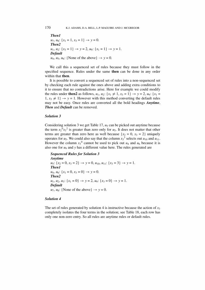
Then1u7, u8: {x1 = 1, x3 = 1} → y = 0.Then2u1, u2: {x3 = 1} → y = 2, u9: {x1 = 1} → y = 1.Defaultu4, u5, u6: {None of the above} → y = 0.

We call this a sequenced set of rules because they must follow in thespecified sequence. Rules under the same then can be done in any orderwithin that then.

It is possible to convert a sequenced set of rules into a non-sequenced setby checking each rule against the ones above and adding extra conditions toit to ensure that no contradictions arise. Here for example we could modifythe rules under then2 as follows, u1, u2: {x1 = 1, x3 = 1} → y = 2, u9: {x1 =1, x3 = 1} → y = 1. However with this method converting the default rulesmay not be easy. Once rules are converted all the bold headings Anytime,Then and Default can be removed.

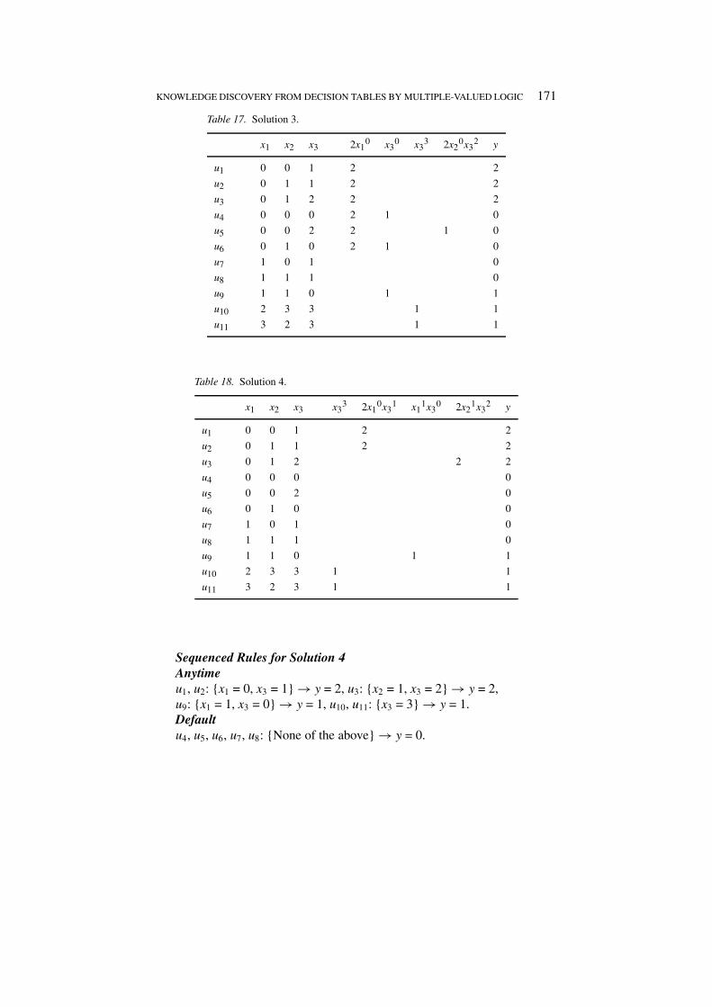
Solution 3

Considering solution 3 we get Table 17, u5 can be picked out anytime becausethe term x2

0x32 is greater than zero only for u5. It does not matter that other

terms are greater than zero here as well because {x2 = 0, x3 = 2} uniquelyoperates for u5. We could also say that the column x3

3 selects out u10 and u11.However the column x3

0 cannot be used to pick out u4 and u6 because it isalso one for u9 and y has a different value here. The rules generated are

Sequenced Rules for Solution 3Anytimeu5: {x2 = 0, x3 = 2} → y = 0, u10, u11: {x3 = 3} → y = 1.Then1u4, u6: {x1 = 0, x3 = 0} → y = 0.Then2u1, u2, u3: {x1 = 0} → y = 2, u9: {x3 = 0} → y = 1.Defaultu7, u8: {None of the above} → y = 0.

Solution 4

The set of rules generated by solution 4 is instructive because the action of x3

completely isolates the four terms in the solution; see Table 18, each row hasonly one non-zero entry. So all rules are anytime rules or default rules.



x1 x2 x3 2x10 x3

0 x33 2x2

0x32 y

u1 0 0 1 2 2

u2 0 1 1 2 2

u3 0 1 2 2 2

u4 0 0 0 2 1 0

u5 0 0 2 2 1 0

u6 0 1 0 2 1 0

u7 1 0 1 0

u8 1 1 1 0

u9 1 1 0 1 1

u10 2 3 3 1 1

u11 3 2 3 1 1


x1 x2 x3 x33 2x1

0x31 x1

1x30 2x2

1x32 y

u1 0 0 1 2 2

u2 0 1 1 2 2

u3 0 1 2 2 2

u4 0 0 0 0

u5 0 0 2 0

u6 0 1 0 0

u7 1 0 1 0

u8 1 1 1 0

u9 1 1 0 1 1

u10 2 3 3 1 1

u11 3 2 3 1 1

Sequenced Rules for Solution 4Anytimeu1, u2: {x1 = 0, x3 = 1} → y = 2, u3: {x2 = 1, x3 = 2} → y = 2,u9: {x1 = 1, x3 = 0} → y = 1, u10, u11: {x3 = 3} → y = 1.Defaultu4, u5, u6, u7, u8: {None of the above} → y = 0.



x1 x2 x3 1 2x10 2x3

1 2x21x3

2 y

u1 0 0 1 1 2 2 2

u2 0 1 1 1 2 2 2

u3 0 1 2 1 2 2 2

u4 0 0 0 1 2 0

u5 0 0 2 1 2 0

u6 0 1 0 1 2 0

u7 1 0 1 1 2 0

u8 1 1 1 1 2 0

u9 1 1 0 1 1

u10 2 3 3 1 1

u11 3 2 3 1 1

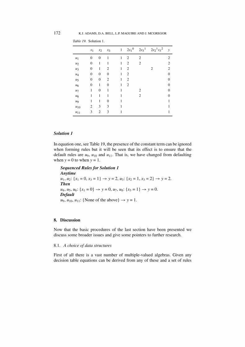
Solution 1

In equation one, see Table 19, the presence of the constant term can be ignoredwhen forming rules but it will be seen that its effect is to ensure that thedefault rules are u9, u10 and u11. That is, we have changed from defaultingwhen y = 0 to when y = 1.

Sequenced Rules for Solution 1Anytimeu1, u2: {x1 = 0, x3 = 1} → y = 2, u3: {x2 = 1, x3 = 2} → y = 2.Thenu4, u5, u6: {x1 = 0} → y = 0, u7, u8: {x3 = 1} → y = 0.Defaultu9, u10, u11: {None of the above} → y = 1.

8. Discussion

Now that the basic procedures of the last section have been presented wediscuss some broader issues and give some pointers to further research.

8.1. A choice of data structures

First of all there is a vast number of multiple-valued algebras. Given anydecision table equations can be derived from any of these and a set of rules


produced. It is an open question how similar these sets of rules would be.Any algebra is a data structure for encoding the information in the table. Theequation is a record of how the value of the decision attribute changes withchanges to the condition attributes but the underlying process is actually settheoretic.

Some of the specialist data structures that are used in MVL other thansum of product may also give an insight into how to split up a decisiontable. For example a decomposition where some of the condition attributesgo into a process (equation) in order to make some intermediate decision;then that decision is combined with the rest of the attributes to arrive at thefinal decision (Luba (1995), Steinbach et al. (1999)). An alternative way ofdecomposing a function is the use of a decision diagram, which is a graphwith nodes and arcs. What arc we leave a node on depends on the value of avariable (Loris et al. (1993), Stankovic (1995), Md et al. (1999)).

8.2. The assignment problem

The method used required assigning integers to the values of the attributesbefore deriving an MVL equation. There are many possible assignments;ideally we would like to find one such that the equation derived from it is assimple as possible. However we do not know if generally speaking a simplerequation also leads to a simpler set of rules, as no research in this area hasbeen done. For the condition attributes, if we wished to be exhaustive, wewould have to consider all possible allocations of the integer set to conditionattribute values.

In our example problem we had information for eleven points in a threevariable quaternary space which means 53 other points were not used. Trans-form techniques that depend upon using all the columns of a transform matrixneed to make up suitable data for these points. The task is considerablefor our small problem as there are 353 possibilities. Fast MVL transformalgorithms similar to the fast Fourier butterfly algorithm have been developed(Falkowski et al. (1995), Stankovic et al. (1998), Dubrova et al. (1996)).When the algebra has a finite field structure, interpolation methods have beenapplied to obtain an equation for incompletely specified functions. Newtoninterpolation was used in (Wesselkamper (1978)), (Menger (1969)) usedLagrange polynomials. Also suitable for unspecified points is (Zilic et al.(1995)) where a polynomial of order k is constructed if there are k specifiedpoints. The values of the function, at these points, are substituted and allthe k equations are solved for the coefficients. In the multidimensional caseZilic assigns optimum values to the "don’t cares" at the first iteration of thetransform; this requires an arbitrary choice of which dimension (variable) totransform first. As large and practical data sets will have lots of blank entries,


algorithms will score that find an equation just using the data given. Both themethods described here, and the rough set method, have this property. TheMVL methods presented here offer an improvement on the previous approachusing rough set theory for this application. However, the robustness of theseMVL-based methods as compared with other data mining techniques wouldrequire testing over a comprehensive set of benchmarks. For very large datasets genetic algorithms offer a method of optimization (Wesselkamper et al.(1995), Freitag et al. (1999)).

8.3. The advantages of using MVL

The method in the text generates all the best solutions, so this allows us tocontrast and compare various sets of rules. Interesting relationships that mightnot have been obvious before can come to light.

With any method the problem is that you find exactly what you are lookingfor. By this we mean that a tree-producing algorithm will be likely to find setsof rules that are easily interpreted by a tree structure and the same applies toany other method. We tend to select evidence that suits our human compre-hension. Our method goes some way to alleviating this. The abstractnessof MVL equations means that we find compact ways to represent the data,and then we are forced to interpret what we see, and not see what we caninterpret.

9. Conclusion

Multiple-Valued logic (MVL) has been used successfully to encode a decisiontable and then reduce its size. A wide choice is offered because any completemultiple-valued algebra can be used for the encoding. This means that thedata can be examined in many different ways and previously undiscoveredrelationships revealed. Specific sets of rules are found by decomposing theencoding function down to subfunctions by fixing subsets of its variables.However as the MVL function is global, applying to all the data, no incon-sistencies can arise. Future work in this new area might include: extendingthe method to more than one decision attribute, applying the method to verylarge problems where only sub-optimal representations of the equation canbe found, and investigating the effect of different coding assignments onthe final result. Suitable algebras for this work will have to handle mixedradix situations, blanks in data bases that produce many “don’t know” pointsand higher radices than are customary in conventional MVL research at themoment.


References

Adams, K. J., Campbell, J. G., Maguire L. P., Webb J. A. C. (1999). State AssignmentTechniques in Multiple Valued Logic. Proc. 29th Int. Symp. on Multiple-Valued Logic,220–225. Freiburg, Germany (IEEE).

Cohn, M. (1960). Switching Function Canonical Form Over Integer Fields. PhD Thesis,Harvard University, Cambridge, Mass.

Davio, M., Deschamps, J. & Thayse, A. (1978). Discrete and Switching Functions. McGraw-Hill.

Dubrova, E. V. & Muzio, J. C. (1996). Generalized Reed-Muller Canonical Form for Multiple-Valued Algebra. Multiple-Valued Logic, An International Journal 1: 65–84. Gordon andBreach, Netherlands.

Falkowski, B. J. & Rahardja, S. (1995). Efficient Algorithm for Generation of Fixed PolarityQuaternary Reed-Muller Expansions. Proc. 25th Int. Symp. on Multiple-Valued Logic,158–163. Bloomington, Indiana, USA (IEEE).

Fazio, A. & Bauer, M. (1997). Intel StrataFlashTM Memory Technology Development andImplementation. Intel Technology Journal 4th Quarter, 1–11 (Intel).

Freitag, K. & Moraga, C. (1999). Quaternary Coded Genetic Algorithms. Proc. 29th Int. Symp.on Multiple-Valued Logic, 194–199, Frieburg, Germany (IEEE).

Green, D. H. & Taylor, I. S. (1974). Modular Representation of Multiple-Valued LogicSystems. Proc. of the IEE 121: 424–429 (IEE).

Green, D. H. (1989). Ternary Reed-Muller Switching Functions with Fixed and MixedPolarities. Int. J. Electronics 67: 761–775, November. Taylor and Francis group.

Green, D. H. (1990). Reed-Muller Expansions with Fixed and Mixed Polarities Over GF(4).IEE Proceedings, Vol. 137, Pt. E, No. 5, September (IEE).

Guan, J. W. & Bell, D. A. (1998). Rough Discovery for Nuclear Safety. FLINS, Third Int.Conf. On Intelligent Techniques and Soft Computing in Nuclear Science and Engineering,203–210. Antwerp, Belgium, World Scientific, Singapore.

Guan, J. W. & Bell, D. A. (2000). Data Mining for Monitoring Loose Parts in NuclearPower Plants. The 2nd International Conference on Rough Sets and Current Trends inComputing, 276–283. Banff, Canada, Technical Report CS-(2000)-07, Ziarko & Yao Eds.,Univ. of Regina Saskatchewan Canada, ISBN 0-7731-0413-5.

Hanyu, T. & Higuchi, T. (1988). Design of a Highly Parallel AI Processor Using NewMultiple-Valued MOS Devices. Proc. 18th Int. Symp. on Multiple-Valued Logic, 300–306.Palma de Mallorca, Spain (IEEE).

Hanyu, T., Kojima, Y. & Higuchi, T. (1991). A Multiple-Valued Logic Array VLSI Based onTwo-Transistor Delta Literal Circuit and Its Application to Real-Time Reasoning Systems.Proc. 21st Int. Symp. on Multiple-Valued Logic, 16–23. Victoria, BC, Canada (IEEE).

Kodandapani, K. L. & Setlur, R. V. (1975). Reed-Muller Canonical Forms in MultivaluedLogic. IEEE Transactions on Computers, Vol. c-24, No. 6, June (IEEE).

Loris A., Gomez, J. & Roman, R. (1993). Using Decision Trees for Minimization of Multiple-Valued Functions. International Journal of Electronics 75(6): 1–35–1041, June. Taylorand Francis group.

Lu, J. J., Murray, N. V. & Rosenthal, E. (1998). Framework for Automated Reasoning inMultiple-Valued Logics. Journal of Automated Reasoning, Vol. 21, No. 1, 39–67, Aug.Kluwer Academic Publishers.

Luba, T. (1995). Decomposition of Multiple-Valued Functions. Proc. 25th Int. Symp. onMultiple-Valued Logic, 256–261. Bloomington, Indiana, USA (IEEE).


Md, H., Babu, H. & Sasao, T. (1999). Shared Multi-Valued Decision Diagrams for Multiple-Output Functions. Proc. 29th Int. Symp. on Multiple-Valued Logic, 166–172. Freiburg,Germany (IEEE).

Menger, K. S. (1969). A Transform for Logic Networks. IEEE Transactions on Computers,Vol. c-18, No. 3, March (IEEE).

Muller, D. E. (1954). Application of Boolean Algebra to Switching Circuit Design and toError Detection. IRE Trans. Electron. Computers, EC-3, 6–12 (IRE).

Oh, Y. G., Hong, H. P., Han, S. J., Chun, C. S. & Kin, B. K. (1996). Fuzzy Logic Utilization forthe Diagnosis of Metallic Loose Part Impact in Nuclear Power Plant. Intelligent Systemsand Soft Computing for Nuclear Science Industry. Proceedings of the 2nd InternationalFLINS Workshop, 372–378. Moi, Belgium, World Scientific, Singapore.

Pawlak, Z. (1982). Rough Sets. International Journal of Computer and Information Sciences11: 341–356. Plenum Press.

Pawlak, Z. (1991). Rough Sets. Theoretical Aspects of Reasoning about Data. KluwerAcademic Publishers, Dordrecht, Boston, London.

Pawlak, Z., Grzymala-Busse, J. W., Slowinski, R. & Ziarko, W. (1995). Rough Sets.Communications of the ACM 38: 88–95. Association for Computing Machinery.

Pradhan, D. K. (1974). A Multi-Valued Algebra Based on Finite Fields. Proc. 4th Int. Symp.on Multiple-Valued Logic, 95–112. Morganstown, W.V., USA (IEEE).

Reed, I. S. (1954). A Class of Multiple-Error Correcting Codes and Their Decoding Scheme.IRE Trans. on Inform. Theory 4: 38–42 (IRE).

Stankovic, R. S. (1995). Functional Decision Diagrams for Multiple-Valued Functions. Proc.25th Int. Symp. on Multiple-Valued Logic, 284–289. Bloomington, Indiana, USA (IEEE).

Stankovic, R. S., Jankovic, D. & Moraga, C. (1998). Reed-Muller-Fourier Versus Galois FieldRepresentation of Four-Valued Logic Functions. Proc. 28th Int. Symp. on Multiple-ValuedLogic, 186–191. Fukuoka, Japan (IEEE).

Steinbach, B., Perkowski, M. A. & Lang, C. (1999). Bi-Decompositions of Multi-ValuedFunctions for Circuit Design and Data Mining Applications. Proc. 29th Int. Symp. onMultiple-Valued Logic, 50–58. Freiburg, Germany (IEEE).

Tang, Z., Cao, Q. & Ishizuka, O. (1998). Learning Multiple-Valued Logic Network: Algebra,Algorithm, and Applications. IEEE Transactions on Computers, Vol. 47, No. 2, 247–251,Feb. (IEEE).

Wesselkamper, T. C. (1978). Divided Difference Methods in Galois Switching Functions.IEEE Transactions on Computers, C-27, No. 3, March (IEEE).

Wesselkamper, T. C. & Danowitz, J. (1995). Some New Results for Multiple-Valued GeneticAlgorithms. Proc. 25th Int. Symp. on Multiple-Valued Logic, 264–269. Bloomington,Indiana, USA (IEEE).

Zilic, Z. & Vranesic, Z. G. (1995). Reed-Muller Forms for Incompletely Specified FunctionsVia Sparse Polynomial Interpolation. Proc. 25th Int. Symp. on Multiple-Valued Logic, 36–43. Bloomington, Indiana, USA (IEEE).