Download - Joint inversion of receiver functions, surface wave dispersion, and magnetotelluric data

ClickHere

for

FullArticle

Joint inversion of receiver functions, surface wave dispersion, andmagnetotelluric data

M. Moorkamp,1,2 A. G. Jones,1 and S. Fishwick3

Received 9 February 2009; revised 19 October 2009; accepted 16 December 2009; published 30 April 2010.

[1] We present joint inversion of magnetotelluric, receiver function, and Raleigh wavedispersion data for a one‐dimensional Earth using a multiobjective genetic algorithm(GA). The chosen GA produces not only a family of models that fit the data sets but alsothe trade‐off between fitting the different data sets. The analysis of this trade‐off givesinsight into the compatibility between the seismic data sets and the magnetotelluric dataand also the appropriate noise level to assume for the seismic data. This additionalinformation helps to assess the validity of the joint model, and we demonstrate the useof our approach with synthetic data under realistic conditions. We apply our method toone site from the Slave Craton and one site from the Kaapvaal Craton. For the SlaveCraton we obtain similar results to our previously published models from joint inversion ofreceiver functions and magnetotelluric data but with improved resolution and control onabsolute velocities. We find a conductive layer at the bottom of the crust, just abovethe Moho; a low‐velocity, low‐resistivity zone in the lithospheric mantle, previouslytermed the Central Slave Mantle Conductor; and indications of the lithosphere‐asthenosphere boundary in terms of a decrease in seismic velocity and resistivity. For theKaapvaal Craton both the seismic and the MT data are of lesser quality, which preventsas detailed and robust an interpretation; nevertheless, we find an indication of a low‐velocity low‐resistivity zone in the mantle lithosphere. These two examples demonstratethe potential of joint inversion, particularly in combination with nonlinear optimizationmethods.

Citation: Moorkamp, M., A. G. Jones, and S. Fishwick (2010), Joint inversion of receiver functions, surface wave dispersion,and magnetotelluric data, J. Geophys. Res., 115, B04318, doi:10.1029/2009JB006369.

1. Introduction

[2] With increasing computational power, methods tojointly invert several data sets are gaining in popularity [e.g.,Julia et al., 2000; Gallardo and Meju, 2003; Linde et al.,2006]. The rationale for this approach is to reduce the influ-ence of noise and to increase resolution. Furthermore, ifdifferent types of data are inverted together the improvedconstraints on various physical parameters can give a betterunderstanding of the underlying geology. However, com-bining different data in a single inversion bears the risk offorcing two or more inherently incompatible data sets into acommon model that is not suitable for either of them.[3] The factors that govern the distribution of seismic

velocities and electrical conductivities within the Earth canbe very different. Seismic velocities, particularly P wavevelocities, are generally determined by bulk properties of the

rock. With wavelengths of several kilometers for teleseismicdata, the effective elastic moduli are an average over a largevolume of material. Long‐period magnetotelluric data alsoaverage over large volumes, but in a fundamentally differentway. Here the question is often that of large‐scale connec-tivity of conductive material; even small fractions of con-ductive material can determine the bulk conductivity, as longas it is connected [Bahr and Simpson, 2002]. These twodifferent characteristics might lead to the conclusion that weshould not expect any correlation between seismic velocitiesand electrical conductivities. This is generally true for themagnitude and its spatial derivatives; higher velocities arenot usually associated with higher resistivities or vice versa,although for the mantle lithosphere of the Kaapvaal Craton[Jones et al., 2009] recently showed a linear relationshipbetween shear wave velocity and the logarithm of resistivity.In sedimentary environments porosity and fluids in the rockmatrix provide a link that causes a correlation of seismicvelocities and electrical conductivities [Carcione et al.,2007]. In the mantle, temperature, iron content and compo-sition all affect both the bulk and shear moduli and electricalconductivity [e.g., Jones et al., 2009].[4] More conservatively though, a geometrical and/or a

structural link between the two parameters is quite likely.

1School of Cosmic Physics, Dublin Institute for Advanced Studies,Dublin, Ireland.

2Now at Leibniz‐Institut für Meereswissenschaften an der UniversitätKiel (IFM‐GEOMAR), Kiel, Germany.

3Department of Geology, University of Leicester, Leicester, UK.

Copyright 2010 by the American Geophysical Union.0148‐0227/10/2009JB006369

JOURNAL OF GEOPHYSICAL RESEARCH, VOL. 115, B04318, doi:10.1029/2009JB006369, 2010

B04318 1 of 23

http://dx.doi.org/10.1029/2009JB006369

Many discontinuities of seismic velocity or electrical prop-erties are interpreted as boundaries between distinct geo-logical units [e.g., Marquis et al., 1995; Lahti et al., 2005;Tournerie and Chouteau, 2005], which in some caseseven originated in different regions and then accreted [e.g.,Jones et al., 2002; Snyder and Bruneton, 2007]. Under thesecircumstances changes in various petrophysical parameterswill occur simultaneously. Also, the two major dis-continuities in the lithosphere, the crust‐mantle boundary(Moho) and the lithosphere‐asthenosphere boundary (LAB)are both likely correlated with changes in conductivity[Jones, 1999; Jones and Ferguson, 1997; Gatzemeier andMoorkamp, 2005]. Therefore we can expect at least somestructural correlation between these parameters. Still, wehave to account for the possibility of disparate interfaces thatdo not allow a common parametrization. We will show towhat extent our genetic algorithm approach helps to identifythese situations.[5] In this study we jointly invert magnetotelluric data,

receiver functions and fundamental mode Rayleigh wavedispersion data. Previously [Moorkamp et al., 2007], weshowed how we can use the combination of magneto-tellurics and receiver functions to construct joint electric andseismic models for two sites on the Slave Craton. Thisapproach was motivated by the observation of similarinterface locations in separate models from that area[Davis et al., 2003; Jones et al., 2003; Snyder et al., 2004]and we obtained encouraging results. However, the limitedsensitivity of receiver functions to absolute S wave ve-locities required us to prescribe crustal velocities takenfrom a regional seismic model [Perry et al., 2002]. Byadding fundamental mode Rayleigh wave dispersion datainto the inversion process, we obtain a reference for abso-lute S wave velocities that should remove the need for tightconstraints on the seismic parameters.

2. Data Sets

2.1. Magnetotelluric Data

[6] Magnetotellurics (MT) is the main geophysicalmethod to derive the conductivity distribution of the Earth’scrust and mantle. From simultaneous measurements of thehorizontal components of the electric fields E and magneticfields H at the surface, we can estimate the compleximpedance tensor Z in the frequency domain, namely,

E ¼ ZH: ð1Þ

For a uniform source field, the impedance tensor solelydepends on the conductivity distribution in the subsurface.The impedances at high frequencies correspond to nearbystructures, whereas the impedances at low frequencies cor-respond to more distant (deeper for a 1‐D Earth) structures.In the most general case all entries of the impedance tensorare nonzero and we need 3‐D modeling and inversionmethods to fit all its components. Due to the difficultiesassociated with a full 3‐D inversion and only recent avail-ability of inversion codes [Siripunvaraporn et al., 2005], anumber of methods have been developed to identify datathat can be adequately modeled with a 2‐D, or even a 1‐Dmodel. We apply dimensionality analysis using the phase

tensor [Caldwell et al., 2004] to our data to identify suitablestations for our 1‐D modeling approach.[7] For distortion by local structures of only the electric

fields, the magnetotelluric phase tensor F represents the partof the impedance tensor that corresponds to the regionalstructure of the Earth and can be extracted without simpli-fying assumptions about dimensionality and galvanic dis-tortion [Bibby et al., 2005]. It is defined as

� ¼ X�1Y where X ¼ Re Zð Þ;Y ¼ Im Zð Þ: ð2Þ

[8] We can use the structure of this tensor to assess elec-tromagnetic dimensionality. For one‐dimensional structuresthe necessary conditions for the phase tensor are vanishingoff‐diagonal elements F21 and F21, equal diagonal elements,and vanishing skew b [Bibby et al., 2005], namely,

� ¼ 1

2tan�1 �12 � �21

�11 þ �22

� �: ð3Þ

[9] This condition can be alternatively expressed in termsof the ellipticity l, as

� ¼ �max � �min

�max þ �min¼ 0 and � ¼ 0: ð4Þ

Here Fmax and Fmin are the maximum and minimum prin-cipal values of F, respectively. For measured data that areaffected by noise, this condition means that both valuesshould not be different from zero in a statistical sense.[10] For real data it is rare to find a site where the

dimensionality condition is met at all frequencies and evenwhen it is met the off‐diagonal elements of the impedancetensor will be different from each other due to measurementnoise. We can reduce the influence of noise and violationsof the 1‐D assumptions by inverting the Berdichevskiyinvariant [Berdichevskiy and Dmitriev, 1976], the arithmeticaverage of the off‐diagonal impedance values. As long aswe do not have strong lateral interfaces we can expect goodresults with this approach [e.g., Park and Livelybrooks,1989]. Another issue for the inversion of real data is theeffect of small‐scale inhomogeneities. The effect of theseinhomogeneities can be described as a static distortion of theimpedance tensor [Bahr, 1988; Groom and Bailey, 1989]and is commonly encountered. Various methods have beenproposed to remove the effect of static distortion, the sim-plest manifestation of which is static shifts of the apparentresistivity curves [Jones, 1988], however these can only beapplied effectively with a dense site coverage. One alter-native is to model phase data alone, as the phases are notaffected by static shifts, the most common form of staticdistortion. As the apparent resistivities define the depth scalein 1‐D inversion [e.g., Jones, 1988], this requires prescrib-ing the resistivity of some part of the model. The data weexamine however do not appear to be affected significantlyby static shift.[11] We calculate synthetic impedances for a 1‐D Earth of

stacked isotropic layers using an implementation of the Waitalgorithm [Wait, 1954]. This simple algorithm is a fast andaccurate way to calculate the impedance for a layered sub-

MOORKAMP ET AL.: JOINT INVERSION WITH A GA B04318B04318

2 of 23

surface. The inversion algorithm typically spends less than5% of its time calculating synthetic MT responses.

2.2. Receiver Functions

[12] Receiver functions (RF) are commonly used as a toolto identify discontinuities in seismic velocities, particularlythe Moho [e.g., Langston, 1979; Kind and Vinnik, 1988;Langston and Hammer, 2001]. Traditionally, analysis ofP to S conversions, the so‐called P receiver functions,have been used for this purpose, but recently also analysisof S to P conversion, also known as S receiver functions[Yuan et al., 2006; Vinnik et al., 2009], have gainedpopularity, particularly for identifying the LAB. In thisstudy we focus solely on P receiver functions.[13] There are various ways to calculate receiver functions

from teleseismic data, the spectral water level deconvolutiontechnique [Langston, 1979] probably being the most popu-lar. In our experience the time domain iterative deconvolu-tion technique [Ligorria and Ammon, 1999] gives superiorresults in the presence of noise. Regardless of the estimationtechnique, the result is a time series where time is a proxyfor depth and significant positive or negative amplitudescorrespond to an increase or decrease in seismic velocity,respectively. The visual interpretation of receiver functionsis complicated though by multiple reverberations that occurparticularly at later times, and the dependence of the time‐depth mapping on the unknown velocity distribution in thesubsurface.[14] For this reason it is beneficial to model receiver

functions for velocity structure, optimally through an in-version algorithm. In this case multiple reverberations are abenefit and help to constrain the position of interfaces.When RFs are used as an imaging tool rather than formodeling a common solution is to stack moveout‐correctedreceiver functions from different events with a wide range ofray parameters [e.g., Nair et al., 2006]. While this reducesthe influence of random noise and brings out primary P toS conversions, it has another effect that is beneficial forvisual interpretation but detrimental for inversion. Multiplereverberations have a different moveout characteristic toprimary conversions and therefore the amplitude of multi-ples is reduced by stacking. For visual interpretation this isbeneficial as the multiples could otherwise be confused withprimary conversions. When we model receiver functions,however, these multiples contain information about theEarth’s structure. Furthermore if we remove them by usinga stacked receiver function, we have to exclude the timewindows of those multiples from the inversion as they willstill be present in the synthetic receiver functions.[15] For these reasons we stack the receiver functions

sorted by ray parameters in bins with a width of 0.01 s/km.With this variation in ray parameter, the moveout of primaryconversions and multiples from structures in the crust andmantle is small. While this increases the computational loadcompared to a single stack, it has the advantage that wepreserve the information contained in the multiple reverbera-tions. In theory the moveout characteristics also carry infor-mation about the structure of the Earth, however in practicethe sensitivity is only small [Ammon et al., 1990]. In any casewe reduce the influence of noise on the inversion.[16] We use a two‐step approach to calculate synthetic

receiver functions for the inversion. First, we calculate

synthetic seismograms using the code of Randall [1989].Then we use the same iterative deconvolution routine thatwe use for real data to calculate receiver functions fromthese synthetic seismograms. In order to ensure that allreverberations are captured correctly, we calculate 200 s ofsynthetic seismograms even though the primary conversionsand crustal multiples are all contained in the first 40 s of thereceiver function. Together with the fact that we have tocalculate separate seismograms for each ray parameter, thismakes it the most time consuming part of the inversion.The inversion spends about 70% calculating the syntheticreceiver functions.

2.3. Rayleigh Wave Dispersion Data

[17] Surface waves are one of the ideal tools for studyingthe structure of the crust and upper mantle, and for manyevents the surface wave train is the largest feature of theseismogram. A good vertical resolution of the variation inshear wave speed can be obtained as the depth sensitivity ofsurface waves are dependent on the period of the waveformthat is exploited. At periods shorter than approximately 40 sthere is strong sensitivity to crustal structure, whereas atlonger periods the waveform becomes increasingly sensitiveto variations in shear wave speed within the upper mantle.The horizontal propagation of the surface waves means thata wide distribution of events and recorders is required toproduce a reliable tomographic image, but with a good pathcoverage it is possible to have reasonably good lateral res-olution even in areas with very few seismic stations.[18] Within the surface wave train it is possible to make

use of both Rayleigh and Love waves, and also both thefundamental and higher modes. As the level of noise isgenerally much higher on the horizontal than vertical com-ponent, it is the Rayleigh wave that is most frequently an-alyzed in surface wave studies. For this reason in this studywe work with Rayleigh wave dispersion data. A variety ofmethods exist to extract information from the component ofthe seismogram produced by the surface waves; for exam-ple, group velocities can be estimated using frequency timeanalysis [e.g., Ritzwoller and Levshin, 1998], two planewave solutions for the wave field can be found for eventsmeasured within an array [e.g., Forsyth and Li, 2005], andmultimode waveform inversion techniques can be used toestimate the path average velocity structure required to pro-duce the observed surface wave dispersion [e.g., Debayle,1999; Lebedev et al., 2005]. In the last method, if disper-sion information is required the path average velocity modelcan be used as an estimator of the average dispersion char-acteristics between the source and receiver [Kennett andYoshizawa, 2002].[19] Tomographic inversions are used to combine the data

from multiple events measured across the array, or formultiple source‐receiver pairs, and thus provide regionalmaps of the dispersion characteristics at a particular period.The local dispersion characteristics at any point within theregion can then be obtained by extracting the informationfrom a series of tomographic maps across the period rangeof interest.[20] We use the surface wave dispersion code sdisp96 that

is part of the Computer Programs in Seismology (R. B.Herrmann, 2002, available at http://www.eas.slu.edu/People/RBHerrmann/ComputerPrograms.html) to calculate


3 of 23

the synthetic dispersion curves. One difficulty with GA basedinversions is that in the early stages the models are purelyrandom and can contain strongly alternating low‐ and high‐velocity layers. These types of structures can be numericallyunstable and present a problem to some codes. With sdisp96we have not encountered such problems. Also the forwardcalculation is relatively fast, only 20% of the time of theinversion is spent calculating the dispersion curves.

3. Inversion Method

[21] We chose the multiobjective genetic algorithm (GA)NSGA‐II [Deb et al., 2002] as the optimization method forour joint inversion approach. There are two main reasons forthis choice: (1) genetic algorithms in general do not dependon any linearized approximation and (2) NSGA‐II in par-ticular yields a set of final models that demonstrate to whatextent fitting one data set trades off against fitting the otherdata sets. When jointly inverting data that are sensitive todifferent parameters, we cannot be sure that these data sensethe same structures and can be described by a joint model.We use the trade‐off as an indicator of the compatibility ofthe data sets. These advantages come at the cost of a muchhigher computational load, as the lack of gradient infor-mation and the stochastic nature of the algorithm require alarge number of forward calculations. In the following wewill describe the basic concept of genetic algorithm inver-sion with particular focus on NSGA‐II and our joint inversionproblem.[22] Genetic Algorithms (GA) are a class of stochastic

optimization methods similar to Monte Carlo and SimulatedAnnealing approaches [e.g., Sambridge and Mosegaard,2002]. The main difference of GAs to these two is thatusually the algorithm does not directly work with the modelparameters, but an encoded binary form that mimics RNA inbiological evolution [Goldberg, 1989]. We therefore have tospecify three parameters for each model parameter mi: Theminimum possible value mi

min, the discretization step Dmi,and the number of bits used for the encoding Ni. Conse-quently genetic algorithms that use this form of represen-tation are inherently constrained optimization methods. Forgeophysical applications this presents no problem, as rea-sonable and physically realistic values for the model para-meters are usually known. For example, we search an Svelocity range between 2.5 km/s and 5.6 km/s which coversrealistic values in the crust and upper mantle [Dziewonskiand Anderson, 1981]. For the MT data the apparent resis-tivity curve gives an indication of the order of magnitudeof the expected resistivities and we search for resistivitiesbetween 1 Wm and 106 Wm. More important is the impact ofthe discretization step Dmi. In the inversion procedure wehave to assure that this step size is small enough to avoidaliasing effects; again for geophysical applications there arereasonable estimates of what minimum variation we canconsider useful and the misfit surface is not that highlynonlinear that very small changes can have a major impacton the data fit. We use a step size of 0.1 km/s for the seismicmodel and 0.1 for logarithmic resistivity for the electricmodel. Comparison with inversions with finer discretizationshows that we obtain essentially the same results but withless forward evaluations.

[23] After we have chosen encoding parameters for eachmodel parameter, the genetic algorithm creates a randompopulation of fixed size P. Each member of this populationrepresents one possible model. For each population memberm we transform the encoded bit string back into physicalparameters and calculate the objective function value Oj(m)for each objective function, e.g., the misfit of each data setand possible regularization functionals. NSGA‐II preservesthe multiobjective nature of the problem by storing theobjective function values in a vector O(m) for each popu-lation member. This is a major difference to linearizedschemes and some GAs that minimize a weighted sum ofthe objective functions values [e.g., Julia et al., 2000;Gallardo and Meju, 2003; Linde et al., 2006]: in our casewe do not need to specify the nature of the weighting of thedifferent data. This is a significant advantage and is dis-cussed in greater detail below.[24] The next step in the algorithm is the selection of

models for the next generation. Each population member isassigned a rank based on the concept of Pareto optimality. Apopulation member mi is said to be partially less than themember mj if all objective function values are less or equaland at least one is less for mi,

mi �p mj , 8k : Ok mið Þ � Ok mj

� �and

9k : Ok mið Þ < Ok mj

� �:

ð5Þ

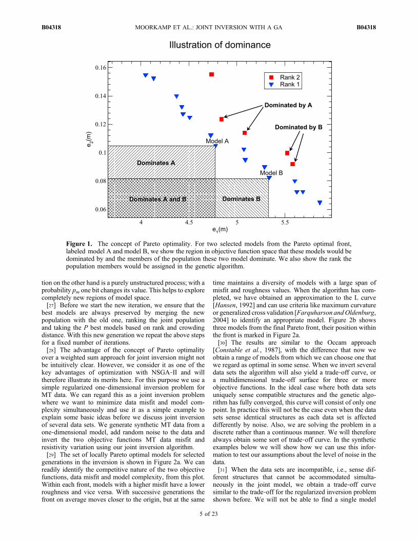
As we can see from equation (5), the algorithm only com-pares objective function values for each data set or regu-larization functional. If there is no member in the populationthat is partially less then a given member m, m is calledlocally Pareto optimal and assigned a rank of one. Con-versely population members that are partially less thananother member of the population are called dominated bythat member. Note that there can be more than one locallyPareto optimal member in the population, the set of Paretooptimal members forms the so‐called Pareto front; we willdiscuss the meaning and the implications of this below.After all locally Pareto optimal members have been identi-fied, they are removed from the ranking procedure. Mem-bers of the population that are Pareto optimal after theremoval of the first front are assigned a rank of two and theprocess is repeated with the remaining members with anincreased rank until the whole population is ranked. Weshow a graphical representation of Pareto optimality and theranking process in Figure 1.[25] After the population has been ranked, candidates for

the new population are selected by binary tournamentselection. Two random members are drawn from the pop-ulation and the one with lower rank is selected. If both havethe same rank, the member with the larger crowding dis-tance, i.e., the average distance to neighboring models inobjective function space [Deb et al., 2002], is used as asecondary criterion. If both criteria are equal one member ischosen randomly.[26] So far the GA has not introduced any variations of the

models. This is done by using crossover between modelsand mutation of individual models. With a probability pctwo models are selected for crossover and exchange theirbinary representation after a randomly chosen location. Thisprocess is very effective at distributing successful segmentsof the model across the population [Goldberg, 1989]. Muta-


4 of 23

tion on the other hand is a purely unstructured process; with aprobability pm one bit changes its value. This helps to explorecompletely new regions of model space.[27] Before we start the new iteration, we ensure that the

best models are always preserved by merging the newpopulation with the old one, ranking the joint populationand taking the P best models based on rank and crowdingdistance. With this new generation we repeat the above stepsfor a fixed number of iterations.[28] The advantage of the concept of Pareto optimality

over a weighted sum approach for joint inversion might notbe intuitively clear. However, we consider it as one of thekey advantages of optimization with NSGA‐II and willtherefore illustrate its merits here. For this purpose we use asimple regularized one‐dimensional inversion problem forMT data. We can regard this as a joint inversion problemwhere we want to minimize data misfit and model com-plexity simultaneously and use it as a simple example toexplain some basic ideas before we discuss joint inversionof several data sets. We generate synthetic MT data from aone‐dimensional model, add random noise to the data andinvert the two objective functions MT data misfit andresistivity variation using our joint inversion algorithm.[29] The set of locally Pareto optimal models for selected

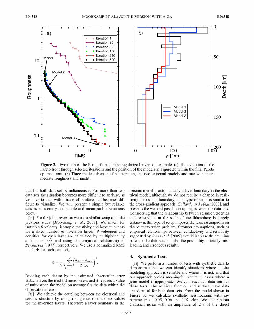
generations in the inversion is shown in Figure 2a. We canreadily identify the competitive nature of the two objectivefunctions, data misfit and model complexity, from this plot.Within each front, models with a higher misfit have a lowerroughness and vice versa. With successive generations thefront on average moves closer to the origin, but at the same

time maintains a diversity of models with a large span ofmisfit and roughness values. When the algorithm has com-pleted, we have obtained an approximation to the L curve[Hansen, 1992] and can use criteria like maximum curvatureor generalized cross validation [Farquharson andOldenburg,2004] to identify an appropriate model. Figure 2b showsthree models from the final Pareto front, their position withinthe front is marked in Figure 2a.[30] The results are similar to the Occam approach

[Constable et al., 1987], with the difference that now weobtain a range of models from which we can choose one thatwe regard as optimal in some sense. When we invert severaldata sets the algorithm will also yield a trade‐off curve, ora multidimensional trade‐off surface for three or moreobjective functions. In the ideal case where both data setsuniquely sense compatible structures and the genetic algo-rithm has fully converged, this curve will consist of only onepoint. In practice this will not be the case even when the datasets sense identical structures as each data set is affecteddifferently by noise. Also, we are solving the problem in adiscrete rather than a continuous manner. We will thereforealways obtain some sort of trade‐off curve. In the syntheticexamples below we will show how we can use this infor-mation to test our assumptions about the level of noise in thedata.[31] When the data sets are incompatible, i.e., sense dif-

ferent structures that cannot be accommodated simulta-neously in the joint model, we obtain a trade‐off curvesimilar to the trade‐off for the regularized inversion problemshown before. We will not be able to find a single model

Figure 1. The concept of Pareto optimality. For two selected models from the Pareto optimal front,labeled model A and model B, we show the region in objective function space that these models would bedominated by and the members of the population these two model dominate. We also show the rank thepopulation members would be assigned in the genetic algorithm.


5 of 23

that fits both data sets simultaneously. For more than twodata sets the situation becomes more difficult to analyze, aswe have to deal with a trade‐off surface that becomes dif-ficult to visualize. We will present a simple but reliablescheme to identify compatible and incompatible situationsbelow.[32] For the joint inversion we use a similar setup as in the

previous study [Moorkamp et al., 2007]. We invert forisotropic S velocity, isotropic resistivity and layer thicknessfor a fixed number of inversion layers. P velocities anddensities for each layer are calculated by multiplying bya factor of

ffiffiffi3

pand using the empirical relationship of

Berteussen [1977], respectively. We use a normalized RMSmisfit F for each data set,

� ¼ 1

N

ffiffiffiffiffiffiffiffiffiffiffiffiffiffiffiffiffiffiffiffiffiffiffiffiffiffiffiffiffiffiffiffiffiffiffiffiffiffiffiXNj¼1

dobs � dsynth�dobs

� �2vuut :

Dividing each datum by the estimated observation errorDdobs makes the misfit dimensionless and it reaches a valueof unity when the model on average fits the data within theobservational error.[33] We achieve the coupling between the electrical and

seismic structure by using a single set of thickness valuesfor the inversion layers. Therefore a layer boundary in the

seismic model is automatically a layer boundary in the elec-trical model, although we do not require a change in resis-tivity across that boundary. This type of setup is similar tothe cross‐gradient approach [Gallardo and Meju, 2003], andpresents the weakest possible coupling between the data sets.Considering that the relationship between seismic velocitiesand resistivities at the scale of the lithosphere is largelyunknown, this type of setup imposes the least assumptions onthe joint inversion problem. Stronger assumptions, such asempirical relationships between conductivity and resistivitysuggested by Jones et al. [2009], would increase the couplingbetween the data sets but also the possibility of totally mis-leading and erroneous results.

4. Synthetic Tests

[34] We perform a number of tests with synthetic data todemonstrate that we can identify situations where a jointmodeling approach is sensible and where it is not, and thatour approach yields meaningful results in cases where ajoint model is appropriate. We construct two data sets forthese tests. The receiver function and surface wave dataare identical for both data sets. From the model shown inFigure 3c we calculate synthetic seismograms with rayparameters of 0.05, 0.06 and 0.07 s/km. We add randomGaussian noise with an amplitude of 2% of the direct

Figure 2. Evolution of the Pareto front for the regularized inversion example. (a) The evolution of thePareto front through selected iterations and the position of the models in Figure 2b within the final Paretooptimal front. (b) Three models from the final iteration, the two extremal models and one with inter-mediate roughness and misfit.


6 of 23

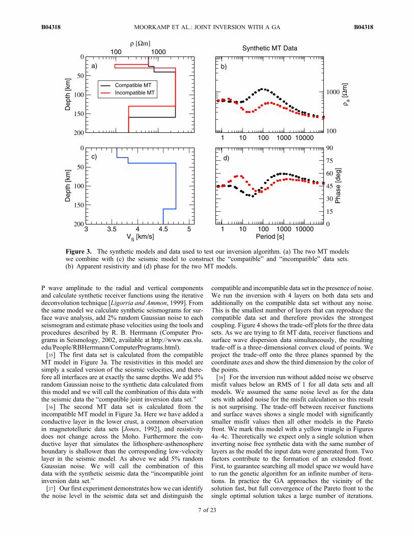
P wave amplitude to the radial and vertical componentsand calculate synthetic receiver functions using the iterativedeconvolution technique [Ligorria and Ammon, 1999]. Fromthe same model we calculate synthetic seismograms for sur-face wave analysis, add 2% random Gaussian noise to eachseismogram and estimate phase velocities using the tools andprocedures described by R. B. Herrmann (Computer Pro-grams in Seismology, 2002, available at http://www.eas.slu.edu/People/RBHerrmann/ComputerPrograms.html).[35] The first data set is calculated from the compatible

MT model in Figure 3a. The resistivities in this model aresimply a scaled version of the seismic velocities, and there-fore all interfaces are at exactly the same depths. We add 5%random Gaussian noise to the synthetic data calculated fromthis model and we will call the combination of this data withthe seismic data the “compatible joint inversion data set.”[36] The second MT data set is calculated from the

incompatible MT model in Figure 3a. Here we have added aconductive layer in the lower crust, a common observationin magnetotelluric data sets [Jones, 1992], and resistivitydoes not change across the Moho. Furthermore the con-ductive layer that simulates the lithosphere‐asthenosphereboundary is shallower than the corresponding low‐velocitylayer in the seismic model. As above we add 5% randomGaussian noise. We will call the combination of thisdata with the synthetic seismic data the “incompatible jointinversion data set.”[37] Our first experiment demonstrates howwe can identify

the noise level in the seismic data set and distinguish the

compatible and incompatible data set in the presence of noise.We run the inversion with 4 layers on both data sets andadditionally on the compatible data set without any noise.This is the smallest number of layers that can reproduce thecompatible data set and therefore provides the strongestcoupling. Figure 4 shows the trade‐off plots for the three datasets. As we are trying to fit MT data, receiver functions andsurface wave dispersion data simultaneously, the resultingtrade‐off is a three‐dimensional convex cloud of points. Weproject the trade‐off onto the three planes spanned by thecoordinate axes and show the third dimension by the color ofthe points.[38] For the inversion run without added noise we observe

misfit values below an RMS of 1 for all data sets and allmodels. We assumed the same noise level as for the datasets with added noise for the misfit calculation so this resultis not surprising. The trade‐off between receiver functionsand surface waves shows a single model with significantlysmaller misfit values then all other models in the Paretofront. We mark this model with a yellow triangle in Figures4a–4c. Theoretically we expect only a single solution wheninverting noise free synthetic data with the same number oflayers as the model the input data were generated from. Twofactors contribute to the formation of an extended front.First, to guarantee searching all model space we would haveto run the genetic algorithm for an infinite number of itera-tions. In practice the GA approaches the vicinity of thesolution fast, but full convergence of the Pareto front to thesingle optimal solution takes a large number of iterations.

Figure 3. The synthetic models and data used to test our inversion algorithm. (a) The two MT modelswe combine with (c) the seismic model to construct the “compatible” and “incompatible” data sets.(b) Apparent resistivity and (d) phase for the two MT models.


7 of 23

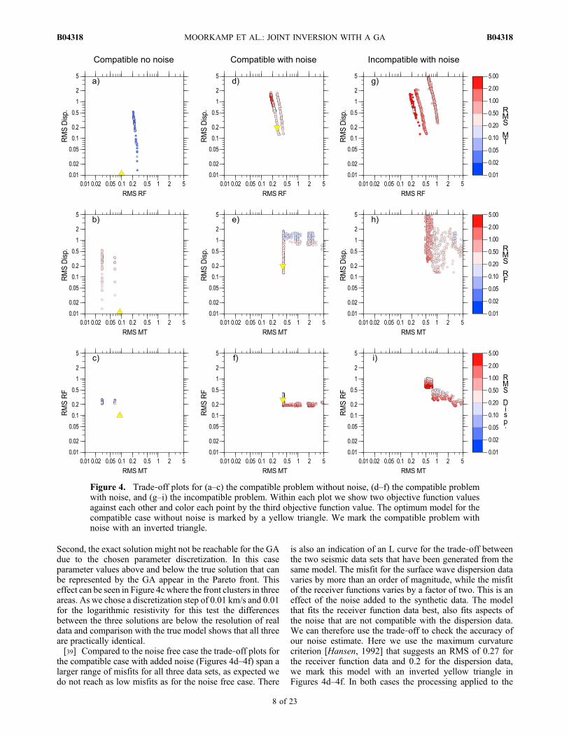
Second, the exact solution might not be reachable for the GAdue to the chosen parameter discretization. In this caseparameter values above and below the true solution that canbe represented by the GA appear in the Pareto front. Thiseffect can be seen in Figure 4c where the front clusters in threeareas. As we chose a discretization step of 0.01 km/s and 0.01for the logarithmic resistivity for this test the differencesbetween the three solutions are below the resolution of realdata and comparison with the true model shows that all threeare practically identical.[39] Compared to the noise free case the trade‐off plots for

the compatible case with added noise (Figures 4d–4f) span alarger range of misfits for all three data sets, as expected wedo not reach as low misfits as for the noise free case. There

is also an indication of an L curve for the trade‐off betweenthe two seismic data sets that have been generated from thesame model. The misfit for the surface wave dispersion datavaries by more than an order of magnitude, while the misfitof the receiver functions varies by a factor of two. This is aneffect of the noise added to the synthetic data. The modelthat fits the receiver function data best, also fits aspects ofthe noise that are not compatible with the dispersion data.We can therefore use the trade‐off to check the accuracy ofour noise estimate. Here we use the maximum curvaturecriterion [Hansen, 1992] that suggests an RMS of 0.27 forthe receiver function data and 0.2 for the dispersion data,we mark this model with an inverted yellow triangle inFigures 4d–4f. In both cases the processing applied to the

Figure 4. Trade‐off plots for (a–c) the compatible problem without noise, (d–f) the compatible problemwith noise, and (g–i) the incompatible problem. Within each plot we show two objective function valuesagainst each other and color each point by the third objective function value. The optimum model for thecompatible case without noise is marked by a yellow triangle. We mark the compatible problem withnoise with an inverted triangle.


8 of 23

noise contaminated synthetic seismograms has reduced theeffective noise on the data used within the inversion. Thisimpression is confirmed by visual inspection of the com-puted receiver functions, for example, and demonstratesthe robustness of the iterative deconvolution approach.The genetic algorithm has therefore helped to identify theappropriate level of noise to avoid overfitting the data.[40] The trade‐off front between surface wave dispersion

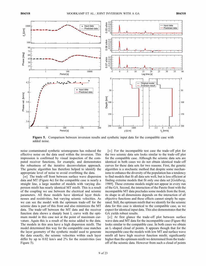
data and MT (Figure 4e) for the compatible case is nearly astraight line, a large number of models with varying dis-persion misfit has nearly identical MT misfit. This is a resultof the coupling we use between the electrical and seismicparameters. All these models have identical layer thick-nesses and resistivities, but varying seismic velocities. Aswe can see the model with the optimum trade‐off for theseismic data is part of this front and also minimizes the MTdata. The trade‐off between the MT data and the receiverfunction data shows a sharply bent L curve with the opti-mum model in this case not at the point of maximum cur-vature. Again this is a result of the noise added to the data.The models in this area have a high dispersion misfit. Themodel determined this way for the compatible case matchesthe layer geometry of the synthetic model used to generatethe data exactly, the seismic velocities within each layerdiffer by up to 0.02 km/s and 2% for the resistivities (seeFigure 5).

[41] For the incompatible test case the trade‐off plot forthe two seismic data sets looks similar to the trade‐off plotfor the compatible case. Although the seismic data sets areidentical in both cases we do not obtain identical trade‐offcurves for these data sets for two reasons. First, the geneticalgorithm is a stochastic method that despite some mechan-isms to enhance the diversity of the population has a tendencyto find models that fit all data sets well, but is less efficient atfinding extreme models that fit only one data set [Goldberg,1989]. These extreme models might not appear in every runof the GA. Second, the interaction of the Pareto front with theincompatible MT data precludes some models from the front,its shape in all dimensions depends on the interaction of allobjective functions and these effects cannot simply be sepa-rated. Still, the optimummisfit that we identify for the seismicdata for this case is identical to the compatible case, as weexpect for identical input data. This also demonstrates that theGA yields robust results.[42] At first glance the trade‐off plot between surface

wave data and MT data for the incompatible case (Figure 4h)looks similar to the compatible case. In both cases we obtainan L‐shaped cloud of points. It appears though that for theincompatible case the models with low MT and surface wavemisfit all have high receiver function misfit; significantlyhigher than the optimummisfit we determined from the trade‐off of the seismic data. However from such a cloud of points

Figure 5. Comparison between inversion results and synthetic input data for the compatible case withadded noise.


9 of 23

it is difficult to infer this reliably and we will quantify thisimpression below when we apply our selection scheme.[43] The trade‐off plot between receiver function and MT

data shows a pronounced difference between the compatible(Figure 4c) and incompatible cases (Figure 4f). In theincompatible case there is a significant gap in the distribu-tion of models in the lower left corner, revealing that thereare no models that acceptably fit both data sets simulta-neously. In addition, the models with MT misfit below 2 anda RF misfit that approaches the optimum misfit have a highsurface wave dispersion misfit. From this plot it appears tobe impossible to find a model that fits all three data setssimultaneously.[44] Although these plots give a good first visual im-

pression of the compatibility, it is important to quantify this,

particularly when the Pareto front contains a significantnumber of models. We apply the scheme we used to identifythe optimum model in the compatible case to the incom-patible case as well. If we select the models with an opti-mum receiver function and surface wave misfit, we onlyfind models with a MT misfit >2.5, significantly higherthan the best fitting MT models. If conversely we examinethe best fitting MT models, both receiver function misfitand surface wave dispersion misfit are significantly higherthan the value determined from the optimum trade‐off ofthe seismic data sets. This indicates that the data sets areincompatible.[45] Next we examine the effect of different numbers of

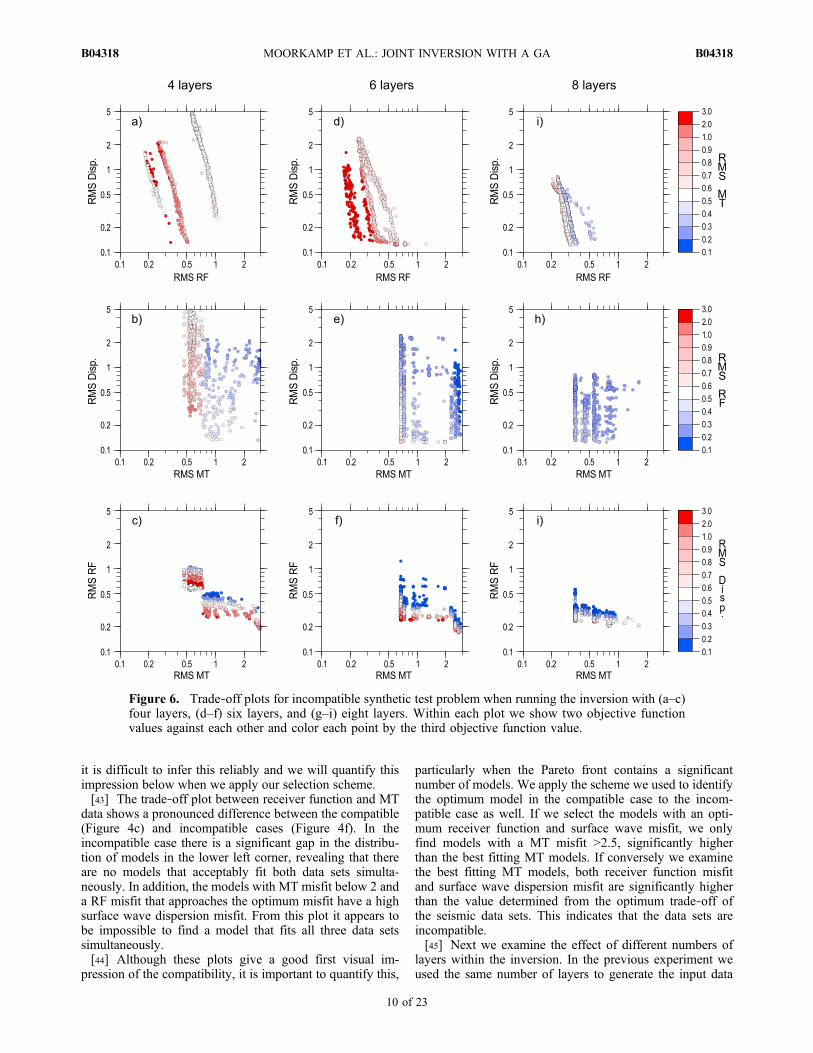
layers within the inversion. In the previous experiment weused the same number of layers to generate the input data

Figure 6. Trade‐off plots for incompatible synthetic test problem when running the inversion with (a–c)four layers, (d–f) six layers, and (g–i) eight layers. Within each plot we show two objective functionvalues against each other and color each point by the third objective function value.


10 of 23

and within the inversion. In practice it is difficult to estimatethe optimal number of layers so we need to find out whenthe coupling between the data sets becomes too weak. Weuse the incompatible data set for this purpose as it alsodemonstrates how the term incompatible depends on thenumber of layers.[46] Figure 6 shows the trade‐off plot for inversion of the

incompatible data set with 4 layers, 6 layers and 8 layers.Generally the minimum misfit decreases with increasingnumber of layers, particularly for receiver functions and MTdata. Also the shape of the trade‐off curve changes dependingon the number of layers. This can be most prominentlyobserved for the trade‐off between surface wave dispersionand receiver functions and MT and receiver functions,respectively. For the comparison between the compatibleand the incompatible cases we saw that the trade‐off betweenMT and receiver functions allows to distinguish these twocases visually. Compared to the inversion with 4 layers, theinversion with 6 layers finds models that minimize both MTand receiver function data, the region toward the lower leftcorner of trade‐off plot (Figure 6f) that was empty wheninverting with 4 layers, now contains somemodels. However,the surface wave dispersion misfit of these models is muchhigher than indicated from the trade‐off between surfacewave dispersion and receiver functions. There is anothercluster of models however with acceptable misfit for bothseismic data sets, but MT misfit >2. The difference betweenthesemodels is the location of the crustal conductor that in theinversion results always coincides with the crustal velocitychange. In the models used to generate the input data thesetwo structures were at different depths and therefore weidentify the incompatibility as we did in the 4 layer case. Thisis somewhat unexpected as 6 layers are enough to describe theincompatible seismic and electric models with a single model.The inversion, however, uses these additional layers tointroduce a gradational velocity change below the Moho thatdoes not exist in the original model. This is a result of addingnoise to the receiver function data. The added noise decreasesthe correlation of theMoho conversion and therefore suggestsa smaller impedance contrast across the Moho. In order toreconcile the smaller contrast with the surface wave disper-sion data, the inversion has to introduce a sequence of smallvelocity changes that have little impact on the receiverfunctions, but raise the velocity in the mantle to a level thatmatches the dispersion observations.[47] When we use 8 layers in the inversion we obtain a

similar trade‐off plot as for the compatible case. Now wehave enough degrees of freedom to model the differentstructures in the electric and seismic models as well as thegradational layers introduced by the noise. Consequentlythe model contains layer interfaces to accommodate both theseismic and electric data. We obtain a good approximationof the crustal structure and the electric LAB, howeverthe model does not reproduce the different position ofthe seismic LAB, but places the low‐velocity zone with theelectric conductor. As it is not a prominent feature in thereceiver functions and the surface wave dispersion data doesnot have sufficient resolution to locate the position of thelow‐velocity zone, this explains both data sets well withinthe noise level.[48] These synthetic tests demonstrate that under realistic

conditions we can identify whether the data sets can be

described by a joint model. One of the important factors forthis success is a sufficient coupling between the modelsthrough a small number of layers. As our synthetic testsdemonstrate the exact number of layers is not critical, but ifwe use a large number of layers the data sets effectivelydecouple and we will be able to accommodate any kind ofstructure. It it therefore important for the inversion of realdata to at least approximately identify the smallest numberof layers with which we can model each data set.

5. Application to Data From Northern Canadaand South Africa

[49] We apply our approach to data from two Archeancratonic regions, the Slave Craton and the Kaapvaal Craton.Both areas contain diamond‐bearing Kimberlites and con-sequently have been the targets of various geophysicalexperiments [e.g., Jones et al., 2003, 2009]. Furthermorethe similarities and differences between these two cratonicplatforms have been a long‐standing question [Jones et al.,2003]. A detailed comparison of the structure of the twocratons is beyond the scope of this paper; we will focus onthe analysis of one site from each region. While this doesnot permit a detailed interpretation it provides a first hint atpossible similarities.

5.1. Slave Craton

[50] We use data from site EKTN of the POLARIS net-work [Eaton et al., 2004] recorded between 2002 and 2005to calculate P receiver functions. We use receiver functionsfrom 27 events that show a clear initial correlation peak,Moho conversions and multiples and stack them in 4 binswith a width of 0.01 s/km each between 0.04 s/km and0.07 s/km. The parameters for the events used to calculatethe receiver functions are listed in Table A1. The MT datawere recorded at a nearby station that was part of theLithoprobe SNORCLE project [Jones et al., 2003] and arethe same data we inverted previously [Moorkamp et al.,2007]. We add fundamental mode Rayleigh wave phasevelocity data derived byChen et al. [2007] directly in the jointinversion.[51] As before we invert for layer thickness t, logarithmic

layer resistivity logr and S wave velocity VS. We calculateVP with a fixed factor of

ffiffiffi3

pand density r using the em-

pirical relationship of Berteussen [1977]. We run the geneticalgorithm with a population size of 1000 for 200 iterationsto ensure sufficient convergence to the true Pareto front[Corne and Knowles, 2007]. Comparison of results fromdifferent inversion runs confirms that the results are stablewith these parameters. Apart from the additional data,another major difference to our previous setup is that we donot prescribe any crustal velocity, but determine the seismicvelocity of all layers within the inversion.[52] Figure 7 shows the trade‐off plots for the three data

sets produced by a single run of the inversion algorithm forinversions with 7 layers, 9 layers and 11 layers. The trade‐off between fitting the receiver function and the dispersiondata shows a more pronounced L shape than we observedin the synthetic experiments and shows similar behaviorregardless of the number of layers used in the inversion. Theoptimum trade‐off point in the Pareto front yields an RMSof 0.3 for the surface wave dispersion data and 2 for the


11 of 23

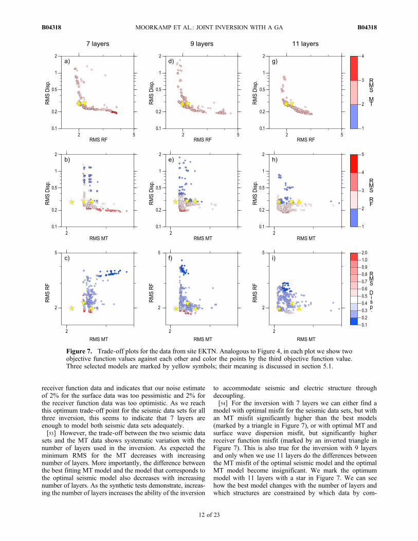
receiver function data and indicates that our noise estimateof 2% for the surface data was too pessimistic and 2% forthe receiver function data was too optimistic. As we reachthis optimum trade‐off point for the seismic data sets for allthree inversion, this seems to indicate that 7 layers areenough to model both seismic data sets adequately.[53] However, the trade‐off between the two seismic data

sets and the MT data shows systematic variation with thenumber of layers used in the inversion. As expected theminimum RMS for the MT decreases with increasingnumber of layers. More importantly, the difference betweenthe best fitting MT model and the model that corresponds tothe optimal seismic model also decreases with increasingnumber of layers. As the synthetic tests demonstrate, increas-ing the number of layers increases the ability of the inversion

to accommodate seismic and electric structure throughdecoupling.[54] For the inversion with 7 layers we can either find a

model with optimal misfit for the seismic data sets, but withan MT misfit significantly higher than the best models(marked by a triangle in Figure 7), or with optimal MT andsurface wave dispersion misfit, but significantly higherreceiver function misfit (marked by an inverted triangle inFigure 7). This is also true for the inversion with 9 layersand only when we use 11 layers do the differences betweenthe MT misfit of the optimal seismic model and the optimalMT model become insignificant. We mark the optimummodel with 11 layers with a star in Figure 7. We can seehow the best model changes with the number of layers andwhich structures are constrained by which data by com-

Figure 7. Trade‐off plots for the data from site EKTN. Analogous to Figure 4, in each plot we show twoobjective function values against each other and color the points by the third objective function value.Three selected models are marked by yellow symbols; their meaning is discussed in section 5.1.


12 of 23

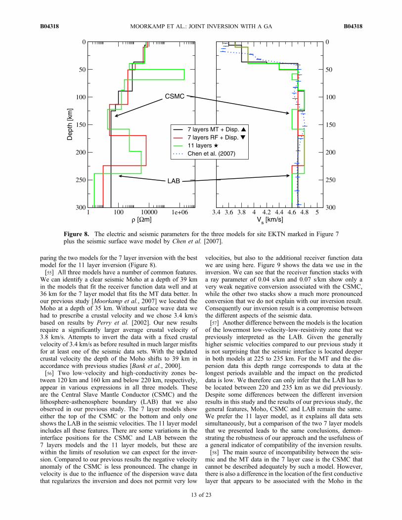
paring the two models for the 7 layer inversion with the bestmodel for the 11 layer inversion (Figure 8).[55] All three models have a number of common features.

We can identify a clear seismic Moho at a depth of 39 kmin the models that fit the receiver function data well and at36 km for the 7 layer model that fits the MT data better. Inour previous study [Moorkamp et al., 2007] we located theMoho at a depth of 35 km. Without surface wave data wehad to prescribe a crustal velocity and we chose 3.4 km/sbased on results by Perry et al. [2002]. Our new resultsrequire a significantly larger average crustal velocity of3.8 km/s. Attempts to invert the data with a fixed crustalvelocity of 3.4 km/s as before resulted in much larger misfitsfor at least one of the seismic data sets. With the updatedcrustal velocity the depth of the Moho shifts to 39 km inaccordance with previous studies [Bank et al., 2000].[56] Two low‐velocity and high‐conductivity zones be-

tween 120 km and 160 km and below 220 km, respectively,appear in various expressions in all three models. Theseare the Central Slave Mantle Conductor (CSMC) and thelithosphere‐asthenosphere boundary (LAB) that we alsoobserved in our previous study. The 7 layer models showeither the top of the CSMC or the bottom and only oneshows the LAB in the seismic velocities. The 11 layer modelincludes all these features. There are some variations in theinterface positions for the CSMC and LAB between the7 layers models and the 11 layer models, but these arewithin the limits of resolution we can expect for the inver-sion. Compared to our previous results the negative velocityanomaly of the CSMC is less pronounced. The change invelocity is due to the influence of the dispersion wave datathat regularizes the inversion and does not permit very low

velocities, but also to the additional receiver function datawe are using here. Figure 9 shows the data we use in theinversion. We can see that the receiver function stacks witha ray parameter of 0.04 s/km and 0.07 s/km show only avery weak negative conversion associated with the CSMC,while the other two stacks show a much more pronouncedconversion that we do not explain with our inversion result.Consequently our inversion result is a compromise betweenthe different aspects of the seismic data.[57] Another difference between the models is the location

of the lowermost low‐velocity‐low‐resistivity zone that wepreviously interpreted as the LAB. Given the generallyhigher seismic velocities compared to our previous study itis not surprising that the seismic interface is located deeperin both models at 225 to 235 km. For the MT and the dis-persion data this depth range corresponds to data at thelongest periods available and the impact on the predicteddata is low. We therefore can only infer that the LAB has tobe located between 220 and 235 km as we did previously.Despite some differences between the different inversionresults in this study and the results of our previous study, thegeneral features, Moho, CSMC and LAB remain the same.We prefer the 11 layer model, as it explains all data setssimultaneously, but a comparison of the two 7 layer modelsthat we presented leads to the same conclusions, demon-strating the robustness of our approach and the usefulness ofa general indicator of compatibility of the inversion results.[58] The main source of incompatibility between the seis-

mic and the MT data in the 7 layer case is the CSMC thatcannot be described adequately by such a model. However,there is also a difference in the location of the first conductivelayer that appears to be associated with the Moho in the

Figure 8. The electric and seismic parameters for the three models for site EKTN marked in Figure 7plus the seismic surface wave model by Chen et al. [2007].


13 of 23

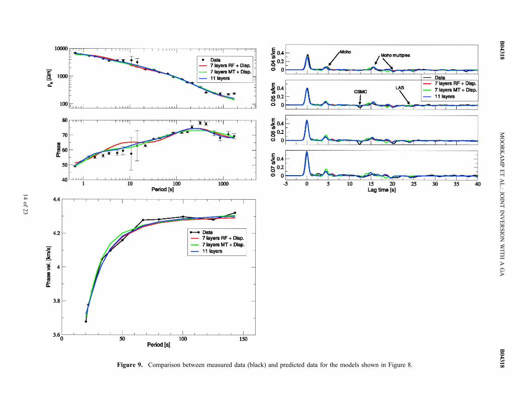
Figure 9. Comparison between measured data (black) and predicted data for the models shown in Figure 8.

MOORKAMPETAL.:JO

INTIN

VERSIO

NWITH

AGA

B04318

B04318

14of

23

E g, • "-

I

10000

1000

lOO

80

70

CD

~60 D..

, .....-~I

• Data - 71ayefs RF + Oisp.

7 layeno MT + Ilisp. - 11 layers

40 ' ",I ",I , "lid ",! 10 100 1000

Period [sI

4.4 " -,--.-,--.-,-,--,-,--,- ,--,-,--,-,--,--,

4.2 - Data 7 layers AF + D18p. 7 layers MT + Dlsp. 11 layers

~ 4

~ 3.8

I I I 3.60 SO lOO ISO

Period [sI

~O.4 gO.2 o 0

~0.4 ~O.2

o 0

f- /" f-

"

U ....

IMohomu~

.-:. ~ 0818

lAB 71aye .. RF + DIop •

CSMC \ 71aye .. MT + Dlsp.

J ....... 11 layers

~0.4 E LJC: ~o.~ j' ",:'7 e v , _ , I

ELL ~ ~0.4 ,.... 0.2

~O , i ~ 9" i i t ~ 0 S 10 IS W ~ ~ g ~

L.ag time [sI

7 layer model that fits the RF data better and in the 11 layermodel, but appears to start just above the Moho in the other7 layer model. In our previous study we speculated whetherthis layer is associated with the Moho that we then located at35 km. We also note that there is a consistent discrepancy

between observed and predicted MT phases between 1 and10 s (Figure 9).[59] Genetic algorithms are very good at finding stable

overall solutions but can fail to reproduce secondary fea-tures that are located at extreme ends of the trade‐off curve

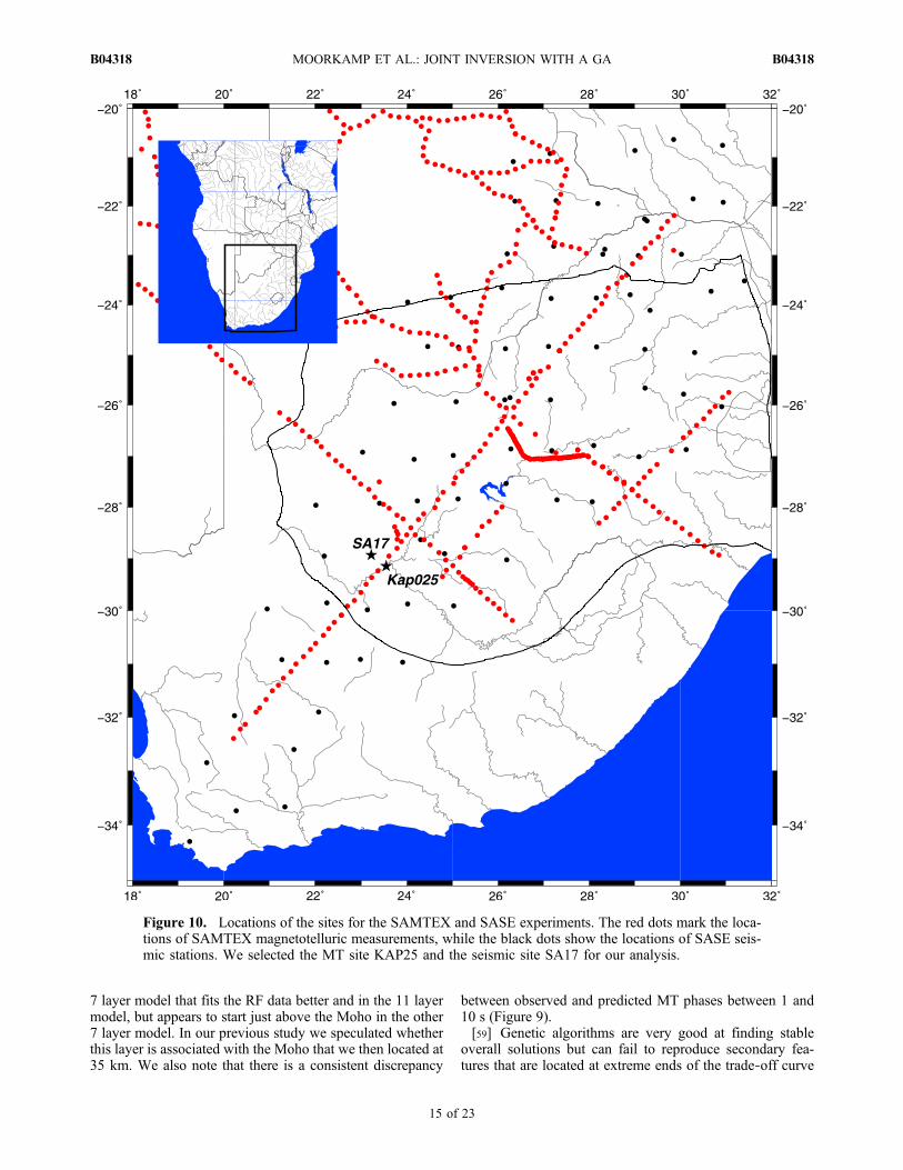
Figure 10. Locations of the sites for the SAMTEX and SASE experiments. The red dots mark the loca-tions of SAMTEX magnetotelluric measurements, while the black dots show the locations of SASE seis-mic stations. We selected the MT site KAP25 and the seismic site SA17 for our analysis.


15 of 23

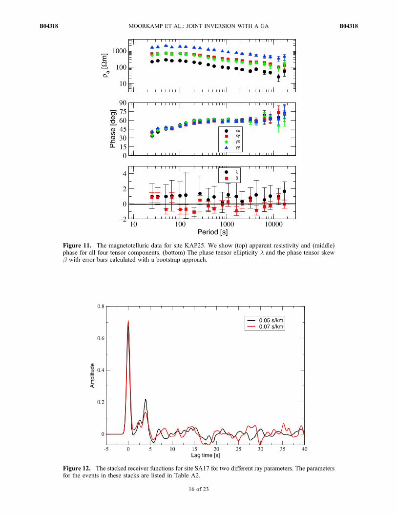
Figure 11. The magnetotelluric data for site KAP25. We show (top) apparent resistivity and (middle)phase for all four tensor components. (bottom) The phase tensor ellipticity l and the phase tensor skewb with error bars calculated with a bootstrap approach.

Figure 12. The stacked receiver functions for site SA17 for two different ray parameters. The parametersfor the events in these stacks are listed in Table A2.


16 of 23

as mentioned above. We therefore run a test inversion inwhich we fix all structure below 50 km depth but introducean additional crustal layer and search with smaller dis-cretization steps of 0.5 km for layer thickness, 0.05 forlogarithmic resistivity and 0.01 km/s for seismic velocities.The resulting models (not shown) have a significantly lowerMT misfit, and even slightly lower misfit for the seismicdata sets. The decrease in misfit for the MT is due to a betteragreement in the critical period range for the phases andthese models show that the top of the conductor should be ata depth between 25 km and 35 km. This conductive layeris also associated with an increase in seismic velocity.Although the influence on the predicted seismic data isbarely visible, the reduced misfit at least supports the pos-sibility that the Moho is associated with a broader transitionin velocities [Hale and Thompson, 1982; Owens and Zandt,1985] and not necessarily a sharp transition.

5.2. Kaapvaal Craton

[60] For the Kaapvaal Craton we analyze seismic datafrom the SASE experiment [Silver et al., 2001] for the re-ceiver functions and magnetotelluric data from the recentSAMTEX experiment [Hamilton et al., 2006; Jones et al.,2009]. The locations of the measurement sites are shownin Figure 10. We use the Rayleigh wave dispersion data byLi and Burke [2006]. They use a two‐plane wave inversiontechnique [Forsyth and Li, 2005] to estimate phase veloci-ties that are the input to our inversion.[61] One problemwhen inverting various data sets together

is that the requirements for each data set and the necessity tohave closely located measurements strongly limit the numberof candidate sites. Although the SAMTEX experiment coversthe whole area of the previous SASE experiment, it was notdesigned for a joint inversion approach and only fewMT sitesare located closer than 40 km to a seismic site. At this distance

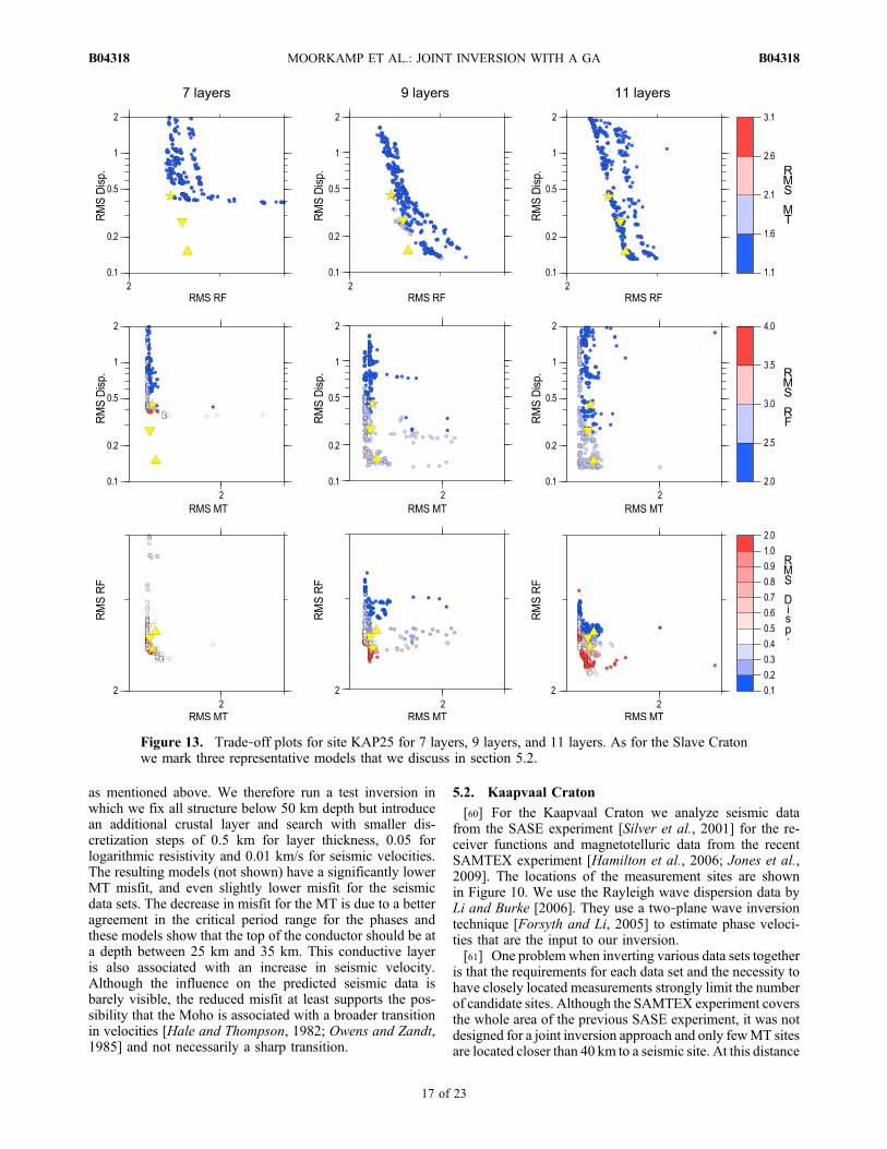
Figure 13. Trade‐off plots for site KAP25 for 7 layers, 9 layers, and 11 layers. As for the Slave Cratonwe mark three representative models that we discuss in section 5.2.


17 of 23

features in the uppermantle should be sensed similarly at bothsites. Considering the data quality and the requirements onelectromagnetic dimension of the more than 550 SAMTEXsites and 80 SASE sites only about 10 remain that can beconsidered suitable. We present here the results from siteKAP25 that is located on the Kaapvaal Craton nearKimberley. For this site the distance between the seismic andmagnetotelluric measurements is 35 km. We show theapparent resistivities and phases for all impedance elementsand the phase tensor dimensionality indicators in Figure 11.[62] From Figure 11 it is clear that the MT data can be

described by a regional 1‐D model with local 3‐D distortion[Larsen, 1975]. Within error the phases of all four imped-ance elements are equal while the apparent resistivities havethe same shape, but are offset against each other. For mostfrequencies the phase tensor dimensionality indicators arenot significantly different from zero although the errors aresurprisingly large. The reason for this is that the phase tensorelements are poorly defined as det(ReZ) is small at mostfrequencies. The equal apparent resistivity values for off‐diagonal elements suggests that the data are not affected bystatic shift.[63] For our receiver function analysis we calculate re-

ceiver functions for 58 events with Mw > 6 recorded be-tween 1997 and 1999. Of those events 13 show a clearinitial correlation peak, Moho conversion and multiples (seeTable A2). We stack these receiver functions in two bins,one with ray parameters between 0.048 s/km and 0.052 s/kmand one with ray parameters between 0.074 s/km and 0.08 s/km. We plot the stacked receiver functions in Figure 12. Ingeneral the data quality is lower than for the Slave Cratonreceiver functions. We can identify a coherent conversion

at 4 s lag time corresponding to the Moho, and there are anumber of negative amplitude conversions that appear onboth stacked receiver functions. Still there is also a largeportion of incoherent amplitude variations that are likely dueto noise.[64] We invert the three data sets with the same settings as

for site EKTN. Separate inversion of the MT data suggeststhat a four‐layer model can capture the main features of theelectrical structure. However we cannot achieve a satisfac-tory fit for the seismic data even with 5 layers. We thereforevary the number of layers for the joint inversion between7 and 11 again. Figure 13 shows the resulting trade‐offsgenerated by our joint inversion code for 7, 9 and 11 layers.The minimum misfit for the MT is approximately 1.2 andessentially the same for all number of layers. Also there is alarge number of models with the same MT misfit in eachinversion. This is not surprising considering that we over-parameterize the problem in terms of the electrical structurewithout applying additional regularization. However, wefound that the regularization of the electrical parametersinteracts with the surface wave data and the models that fitall data sets were essentially unregularized. We thereforeonly show the results of the unregularized inversions forwhich the trade‐off plots are also easier to analyze.[65] The two seismic data sets show considerable trade‐

off, indicating the presence of noise. The minimum misfitfor the surface wave data decreases by a factor of two whenincreasing the number of layers from 7 to 9. When weincrease the number of layers further to 11 the misfit for thesurface waves improves slightly and the point of optimaltrade‐off between surface waves and receiver functionsmoves toward the left of the diagram, indicating animproved receiver function fit. Considering that we only

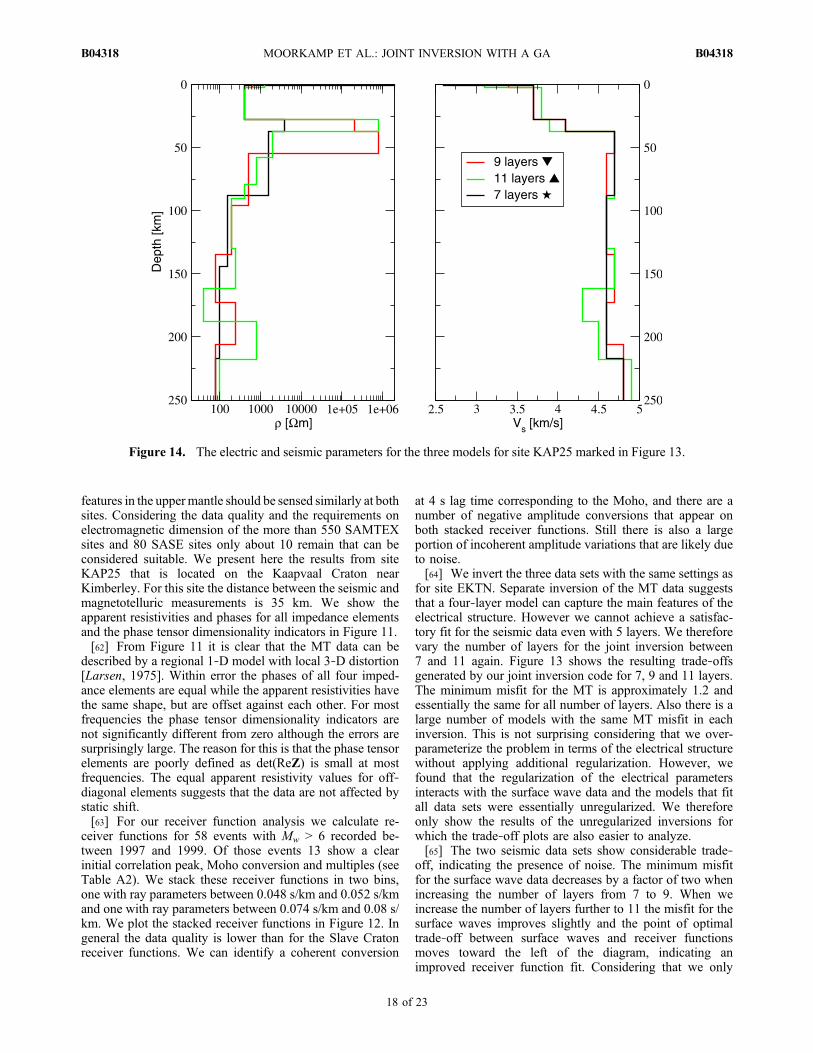
Figure 14. The electric and seismic parameters for the three models for site KAP25 marked in Figure 13.


18 of 23

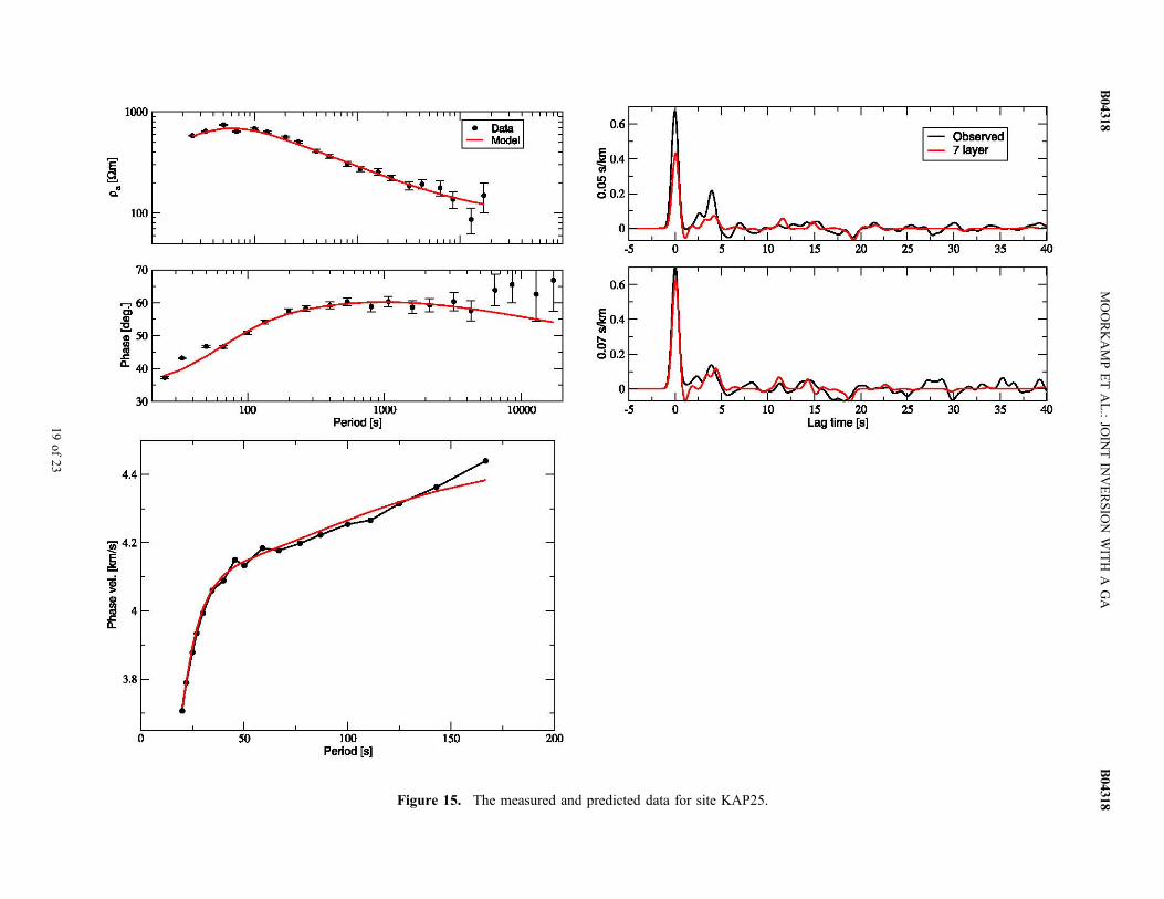
Figure 15. The measured and predicted data for site KAP25.

MOORKAMPETAL.:JO

INTIN

VERSIO

NWITH

AGA

B04318

B04318

19of

23

1000

~ l ~ lOO

70

...,60 C>

" "C

';' 50 gj

.<= 0.40

30

4.4

0 4.2

l ~ " i(l 4 &.

3.8

o

lOO 1000 Period [sI

~ t:>#I

50 lOO Period [sI

I ~ ~:ell

10000

-""

"'"

150 200

0.6

~J Il 1- Observed - llaya,

on 0 00.2

0 I I V I~ I T lt l r- I I

-5 0 5 10 15 20 25 30 35 40

0.6

~ 0.4

.... 0 cl 0.2

0

-5 0 5 10 15 20 25 30 35 40 Lag time [sI

have 18 phase velocity estimates but 21 degrees of freedomin the 11 layer case, this can be expected.[66] We mark the models with an optimal trade‐off

between the seismic data sets with a star for the inversionwith 7 layers, with an inverted triangle for 9 layers and atriangle for 11 layers. All three models have approxi-mately the same misfit for the MT data and for eachinversion there are some models with a lower MT misfit.Comparison between the marked models and the bestmodels with respect to the MT data shows that in all threecases the improvement in misfit is only marginal and ismainly due to one or two data points. We therefore regardthis improvement as not significant and consider the datasets compatible within the resolution.[67] Figure 14 shows a comparison of the three models

marked in the trade‐off plots. All three model show theMoho at a depth of 37 km, in agreement with previousstudies [Nguuri et al., 2001; Nair et al., 2006; Yang et al.,2008]. Apart from this there is considerable variabilitybetween the three models although some common char-acteristics remain. The resistivity model shows a sharpincrease in resistivity that roughly coincides with the seismicMoho. The resistivity gradually decreases from more than100,000 Wm to 80 Wm between 60 km and 100 km depth.In all three cases we observe a relatively conductive zonebelow 80 km that coincides with a low‐velocity zone. Withincreasing number of layers the models contain additionalvariations below 120 km. As the misfit for the MT data andfor the receiver function data is similar for all three modelswe regard the 7 layer model as the most conservative andreliable representation. Here we observe a single low‐velocity zone between 80 km and 220 km, while the othermodels suggest that this zone might be split into two parts.Using only surface wave data, a broad region of low shearwave velocities at this depth have been reported [Li andBurke, 2006; Yang et al., 2008; Priestley et al., 2008].Recent studies using receiver functions have also tended toplace a discontinuity from faster to slower velocities ataround 150 km depth [e.g., Savage and Silver, 2008; Hansenet al., 2009; Vinnik et al., 2009], similar to our models con-strained by a greater number of layers. Our joint inversionresults suggest that this zone coincides with a region of lowresistivity. However, in contrast to the Slave Craton, thediscontinuities marking any boundaries of the low‐velocityzone are not clearly defined due to the higher noise levels.Also the site is located near the boundary of the craton, so itis not clear in how far the results are representative for thearea. We therefore refrain from any detailed interpretationsof the Kaapvaal results in terms of geological structures orprocesses.[68] The problematic nature of the receiver function data

in particular can be recognized from the comparisonbetween the predicted data and the observed data in Figure 15.While the MT data and dispersion curves are matched well,we have problems to obtain a satisfactory fit for the receiverfunctions. While the predicted data matches the initial cor-relation peak and Moho conversion well for a ray parameterof 0.07 s/km, the predicted amplitude for a ray parameter of0.05 s/km is too low. Also, there are other features that arematched for one stack but not for the other, for example thesecond Moho multiple. Still, the low‐velocity zone appears

in all inversion runs and with different inversion settings,so we regard it as a robust feature of our joint inversion.

6. Conclusions

[69] The results of the synthetic tests and the inversion ofthe two data sets demonstrate that our joint inversion ap-proach not only finds a suitable model where appropriate, butalso gives some clear indication of the compatibility of thedata sets and realistic noise levels. We particularly regardthe last two points as a clear advantage over linearizedapproaches. In principle, a similar analysis can be performedby varying the weights of the data sets in a linearized inver-sion scheme, However, not all points of the Pareto front areaccessible for linearized schemes [Kozlovskaya et al., 2007]and the range of weights and their sampling is unclear anddifferent for every problem. Both of these difficulties aresolved by our GA‐based approach. In addition, the compu-tational cost of multiple linearized inversion runs with vary-ing weights is on the order of the computational cost of ourGA based inversion, but requires additional user intervention.[70] A critical component for any joint inversion algo-

rithm is the parametrization and the interaction of the dif-ferent data sets within the inversion. We chose the leastrestricting approach by only requiring coincident interfacesfor the electrical and seismic models. As long as we keep thenumber of inversion layers sufficiently small, we achieve agood coupling of the data sets. The Slave Craton inversionexample demonstrates the types of hypothesis we can testwith joint inversion. The Central Slave Mantle Conductorcan be modeled as a coincident low resistivity, low‐velocityzone. This is a robust result from individual and joint inver-sions and indicates a spatial correlation.[71] For the Kaapvaal Craton the data quality precludes a

detailed interpretation of the models. We can fit both the MTdata and the dispersion data well and reproduce some of themain features of the receiver functions with a joint model.The comparison of different models from the Pareto front,the structure of the trade‐off and the expression of modelfeatures in the synthetic data provide a valuable aid to assessthe validity of the joint models and give a qualitative indi-cation of model errors.[72] The increased information comes at the cost of high

computational cost and simultaneous quality requirementson all data sets. While the first point becomes less and less ofan issue with increasing computational abilities, the qualityrequirements limit the number of sites this approach can beapplied to. With the tendency toward integrated studies andcombined seismic and electromagnetic experiments, moredata suitable for joint inversion will become available.

Appendix A: Event Parameters

[73] Here we show the parameters for the events we usedin the receiver function analysis. Table A1 shows the eventparameters for station EKTN, and Table A2 shows the eventparameters for station SA17.

Appendix B: Software

[74] The joint inversion program, associated tools and doc-umentation can be downloaded from http://gplib.sourceforge.


20 of 23

Table A2. Parameters of the Events Used for Receiver Function Inversion at Site SA17

Event Date Time (UT) Latitude Longitude Depth (km) Mw

1 27 Dec 1997 2011:01.34 −55.7830 −4.2180 10.00 6.202 3 Jan 1998 0610:08.38 −35.4740 −16.1910 10.00 6.303 12 Jan 1998 1014:07.630 −30.985 −71.41 34 6.64 30 Jan 1998 1216:08.69 −23.9130 −70.2070 42.00 7.105 20 Feb 1998 1218:06.23 36.4790 71.0860 235.60 6.406 1 Apr 1998 1756:23.36 −0.5440 99.2610 55.70 7.007 1 Apr 1998 2242:56.90 −40.3160 −74.8740 9.00 6.708 25 Apr 1998 0607:23.44 −35.2660 −17.3260 10.00 6.309 18 Jun 1998 0417:54.98 −11.5720 −13.8940 10.00 6.3010 29 Jul 1998 0714:24.08 −32.3120 −71.2860 51.10 6.4011 3 Sep 1998 1737:58.24 −29.4500 −71.7150 27.00 6.6012 5 Mar 1999 0335:14.71 −34.6730 −69.6000 10.00 6.0013 28 Mar 1999 1905:11.03 30.5120 79.4030 15.00 6.60

Table A1. Parameters of the Events Used for Receiver Function Inversion at Site EKTN

Event Date Time (UT) Latitude Longitude Depth (km) Mw

1 12 Oct 2002 2009:11.46 −8.2950 −71.7380 534.30 6.902 17 Nov 2002 0453:53.54 47.8240 146.2090 459.10 7.303 17 Mar 2003 1636:17.31 51.2720 177.9780 33.00 7.104 19 May 2003 1627:10.20 17.5460 −105.4730 10.00 6.105 21 May 2003 1844:20.10 36.9640 3.6340 12.00 6.806 26 May 2003 0924:33.40 38.8490 141.5680 68.00 7.007 23 Jun 2003 1212:34.47 51.4390 176.7830 20.00 6.908 27 Jul 2003 0625:31.95 47.1510 139.2480 470.30 6.809 25 Sep 2003 1950:06.36 41.8150 143.9100 27.00 8.3010 17 Nov 2003 0643:06.80 51.1460 178.6500 33.00 7.8011 5 Dec 2003 2126:09.48 55.5380 165.7800 10.00 6.7012 14 Apr 2004 2307:39.94 71.0670 −7.7470 12.20 6.0013 29 May 2004 2056:09.60 34.2510 141.4060 16.00 6.5014 10 Jun 2004 1519:57.75 55.6820 160.0030 188.60 6.9015 14 Jun 2004 2254:21.32 16.3370 −97.8450 10.00 5.9016 6 Sep 2004 2329:35.09 33.2050 137.2270 10.00 6.6017 9 Oct 2004 2126:53.69 11.4220 −86.6650 35.00 7.0018 23 Oct 2004 0856:00.86 37.2260 138.7790 16.00 6.6019 15 Nov 2004 0906:56.56 4.6950 −77.5080 15.00 7.2020 28 Nov 2004 1832:14.13 43.0060 145.1190 39.00 7.0021 13 Jun 2005 2244:33.90 −19.9870 −69.1970 115.60 7.8022 26 Jul 2005 1217:14.27 52.8710 160.1050 27.60 5.8023 16 Aug 2005 0246:28.40 38.2760 142.0390 36.00 7.2024 21 Sep 2005 0225:08.11 43.8920 146.1450 103.00 6.1025 26 Sep 2005 0155:37.67 −5.6780 −76.3980 115.00 7.5026 8 Oct 2005 0350:40.80 34.5390 73.5880 26.00 7.6027 12 Dec 2005 2147:46.07 36.3570 71.0930 224.60 6.50


21 of 23

net. We used sac2000 [Goldstein et al., 2003] to processseismograms for receiver function analysis and GMT [Wesseland Smith, 1991] for Figures 4, 6, 7, 10, and 13.

[75] Acknowledgments. Part of this work was carried out under theHPC‐EUROPA project (RII3‐CT‐2003‐506079), with the support of theEuropean Community–Research Infrastructure Action under the FP6 Struc-turing the European Research Area program. S.F. was supported by theNatural Environment Research Council (NERC grant NE/G000859/1).We would like to thank S. Lebedev for comments on an early version ofthe manuscript. C. Chen and A. Li kindly made their Rayleigh wave disper-sion data available for this study. The MT data for the Slave Craton werepart of the Lithoprobe project, and the data for the Kaapvaal Craton werepart of the SAMTEX project. All those acknowledged by Jones et al.[2003, 2009] are acknowledged here.

ReferencesAmmon, C. J., G. E. Randall, and G. Zandt (1990), On the nonuniqueness ofreceiver function inversions, J. Geophys. Res., 95, 15,303–15,318.

Bahr, K. (1988), Interpretation of the magnetotelluric impedance tensor:Regional induction and local telluric distortion, J. Geophys., 62, 119–127.

Bahr, K., and F. Simpson (2002), Electrical anisotropy below slow‐ andfast‐moving plates: Paleoflow in the upper mantle?, Science, 295,1270–1272.

Bank, C. G., M. G. Bostock, R. M. Ellis, and J. F. Cassidy (2000), Areconnaissance teleseismic study of the upper mantle and transition zonebeneath the archean Slave Craton in NW Canada, Tectonophysics, 319(3),151–166.

Berdichevskiy, M. N., and V. I. Dmitriev (1976), Basic principles of inter-pretation of magnetotelluric sounding curves, in Geoelectric and Geo-thermal Studies, edited by A. Adam, pp. 165–221, Akad. Kiado,Budapest.

Berteussen, K. A. (1977), Moho depth determinations based on spectral‐ratio analysis of NORSAR long‐period P waves, Phys. Earth Planet.Inter., 15, 13–27.

Bibby, H. M., T. G. Caldwell, and C. Brown (2005), Determinable andnon‐determinable parameters of galvanic distortion in magnetotellurics,Geophys. J. Int., 163, 915–930.

Caldwell, T. G., H. M. Bibby, and C. Brown (2004), The magnetotelluricphase tensor, Geophys. J. Int., 158, 457–469.

Carcione, J. M., B. Ursin, and J. I. Nordskag (2007), Cross‐property rela-tions between electrical conductivity and the seismic velocity of rocks,Geophysics, 72(5), E193–E204.

Chen, C.‐W., S. Rondenay, D. S. Weeraratne, and D. B. Snyder (2007),New constraints on the upper mantle structure of the Slave craton fromRayleigh wave inversion, Geophys. Res. Lett . , 34 , L10301,doi:10.1029/2007GL029535.

Constable, S. C., R. L. Parker, and C. G. Constable (1987), Occam’s inver-sion: A practical algorithm for generating smooth models from electro-magnetic sounding data, Geophysics, 52(3), 289–300.

Corne, D., and J. Knowles (2007), Techniques for highly multiobjectiveoptimisation: Some nondominated points are better than others, in Pro-ceedings of the 9th Annual Conference on Genetic and EvolutionaryComputation (GECCO), pp. 773–780, Assoc. for Comput. Mach., NewYork.

Davis, W. J., A. G. Jones, W. Bleeker, and H. Grutter (2003), Lithospheredevelopment in the Slave Craton: A linked crustal and mantle perspec-tive, Lithos, 71(2–4), 575–589.

Deb, K., A. Pratap, S. Agarwal, and T. Meyarivan (2002), A fast and elitistmultiobjective genetic algorithm: NSGA‐II, IEEE Trans. Evol. Comput.,6(2), 182–197.

Debayle, E. (1999), SV‐wave azimuthal anisotropy in the Australian uppermantle: Preliminary results from automated Rayleigh waveform inver-sion, Geophys. J. Int., 137, 747–754.

Dziewonski, A. M., and D. L. Anderson (1981), Preliminary reference earthmodel, Phys. Earth Planet. Inter., 25(4), 297–356.

Eaton, D. W., A. G. Jones, and I. J. Ferguson (2004), Lithospheric anisot-ropy structure inferred from collocated teleseismic and magnetotelluricobservations: Great Slave Lake shear zone, northern Canada, Geophys.Res. Lett., 31, L19614, doi:10.1029/2004GL020939.

Farquharson, C. G., and D. W. Oldenburg (2004), A comparison of auto-matic techniques for estimating the regularization parameter in non‐linearinverse problems, Geophys. J. Int., 156(1), 411–425.

Forsyth, D. W., and A. Li (2005), Array analysis of two‐dimensional var-iations in surface wave phase velocity and azimuthal anisotropy in thepresence of multipathing interference, in Seismic Earth: Array Analysisof Broadband Seismograms, Geophys. Monogr. Ser., vol. 157, editedby A. Levander and G. Nolet, pp. 81–97, AGU, Washington, D. C.

Gallardo, L. A., and M. A. Meju (2003), Characterization of heterogeneousnear‐surface materials by joint 2D inversion of dc resistivity and seismicdata, Geophys. Res. Lett., 30(13), 1658, doi:10.1029/2003GL017370.

Gatzemeier, A., and M. Moorkamp (2005), 3D modelling of electrical an-isotropy from electromagnetic array data: Hypothesis testing for differentupper mantle conduction mechanisms, Phys. Earth Planet. Inter., 149,225–242.

Goldberg, D. E. (1989), Genetic Algorithms in Search, Optimization andMachine Learning, Addison‐Wesley, Reading, Mass.

Goldstein, P., D. Dodge, M. Firpo, and L. Minner (2003), Sac2000: Signalprocessing and analysis tools for seismologists and engineers, in TheIASPEI International Handbook of Earthquake and Engineering Seismol-ogy, edited by W. H. K. Lee et al., pp. 1613–1614, Academic, London.

Groom, R. W., and R. C. Bailey (1989), Decomposition of magnetotelluricimpedance tensors in the presence of local three‐dimensional galvanicdistortion, J. Geophys. Res., 94(B2), 1913–1925.

Hale, L. D., and G. A. Thompson (1982), The seismic reflection characterof the continental Mohorovicic discontinuity, J. Geophys. Res., 87,4625–4635.

Hamilton, M., A. G. Jones, R. L. Evans, S. Evans, C. J. S. Fourie, X. Garcia,A. Mountford, J. E. Spratt, and the SAMTEX Team (2006), Electricalanisotropy of South African lithosphere compared with seismic anisot-ropy from shear‐wave splitting analysis, Phys. Earth Planet. Inter.,158, 226–239.

Hansen, P. C. (1992), Analysis of discrete ill‐posed problems by means ofthe L‐curve, SIAM Rev., 34(4), 561–580.

Hansen, S. E., A. A. Nyblade, J. Julià, P. H. G. M. Dirks, and R. J. Durrheim(2009), Upper‐mantle low‐velocity zone structure beneath the Kaapvaalcraton from S‐wave receiver functions, Geophys. J. Int., 178, 1021–1027.

Jones, A. G. (1988), Static shift of magnetotelluric data and its removal in asedimentary basin environment, Geophysics, 53(7), 967–978.

Jones, A. G. (1992), Electrical properties of the lower continental crust, inContinental Lower Crust, edited by D. M. Fountain, pp. 81–131, Elsevier,Amsterdam.

Jones, A. G. (1999), Imaging the continental upper mantle using electro-magnetic methods, Lithos, 48(1–4), 57–80.

Jones, A. G., and I. J. Ferguson (1997), The electric Moho, Nature, 390,331–333.

Jones, A. G., D. Snyder, S. Hanmer, I. Asudeh, D. White, D. Eaton, andG. Clarke (2002), Magnetotelluric and teleseismic study across theSnowbird Tectonic Zone, Canadian Shield: A Neoarchean mantle suture?,Geophys. Res. Lett., 29(17), 1829, doi:10.1029/2002GL015359.

Jones, A. G., P. Lezaeta, I. J. Ferguson, A. D. Chave, R. L. Evans, X. Garcia,and J. Spratt (2003), The electrical structure of the slave craton, Lithos, 71,505–527.

Jones, A. G., R. L. Evans, and D. W. Eaton (2009), Velocity‐conductivityrelationships for mantle mineral assemblages in Archean cratonic litho-sphere based on a review of laboratory data and Hashin‐Shtrikman extre-mal bounds, Lithos, 109, 131–143.

Julia, J., C. J. Ammon, R. B. Herrmann, and A. M. Correig (2000), Jointinversion of receiver function and surface wave dispersion observations,Geophys. J. Int., 143(1), 99–112.

Kennett, B. L. N., and K. Yoshizawa (2002), A reappraisal of regional sur-face wave tomography, Geophys. J. Int., 150, 37–444.

Kind, R., and L. P. Vinnik (1988), The upper‐mantle discontinuities under-neath the GRF array from P‐to‐S converted waves, J. Geophys., 62,138–147.

Kozlovskaya, E., L. Vecsey, J. Plomerová, and T. Raita (2007), Joint inver-sion of multiple data types with the use of multiobjective optimization:problem formulation and application to the seismic anisotropy investiga-tions, Geophys. J. Int., 171, 761–779.

Lahti, I., T. Korja, P. Kaikkonen, and K. Vaittinen (2005), Decompositionanalysis of the BEAR magnetotelluric data: Implications for the uppermantle conductivity in the Fennoscandian Shield, Geophys. J. Int.,163, 900–914.

Langston, C. A. (1979), Structure under Mount Rainier, Washington,inferred from teleseismic body waves, J. Geophys. Res., 84, 4749–4762.

Langston, C. A., and J. K. Hammer (2001), The vertical component P‐wavereceiver function, Bull. Seismol. Soc. Am., 91(6), 1805–1819.

Larsen, J. C. (1975), Low frequency (0.1–6.0 cpd) electromagnetic study ofdeep mantle electrical conductivity beneath the Hawaiian islands, Geo-phys. J. R. Astron. Soc., 43, 17–46.

Lebedev, S., G. Nolet, T. Meier, and R. D. van der Hilst (2005), Automatedmultimode inversion of surface and S waveforms, Geophys. J. Int., 162,951–964.

Li, A., and K. Burke (2006), Upper mantle structure of southern Africafrom Rayleigh wave tomography, J. Geophys. Res., 111, B10303,doi:10.1029/2006JB004321.


22 of 23

Ligorria, J. P., and C. J. Ammon (1999), Iterative deconvolution andreceiver‐function estimation, Bull. Seismol. Soc. Am., 89(5), 1395–1400.

Linde, N., A. Binley, A. Tryggvason, L. B. Pedersen, and A. Revil (2006),Improved hydrogeophysical characterization using joint inversion ofcross‐hole electrical resistance and ground‐penetrating radar traveltimedata, Water Resour. Res., 42, W12404, doi:10.1029/2006WR005131.

Marquis, G., A. G. Jones, and R. D. Hyndman (1995), Coincident conduc-tive and reflective lower crust across a thermal boundary in southern Brit-ish Columbia, Canada, Geophys. J. Int., 120, 111–131.

Moorkamp, M., A. G. Jones, and D. W. Eaton (2007), Joint inversion ofteleseismic receiver functions and magnetotelluric data using a geneticalgorithm: Are seismic velocities and electrical conductivities compati-ble?, Geophys. Res. Lett., 34, L16311, doi:10.1029/2007GL030519.

Nair, S. K., S. S. Gao, K. H. Liu, and P. G. Silver (2006), Southern Africancrustal evolution and composition: Constraints from receiver functionstudies, J. Geophys. Res., 111, B02304, doi:10.1029/2005JB003802.

Nguuri, T. K., J. Gore, D. E. James, S. J. Webb, C. Wright, T. G. Zengeni,O. Gwavava, and J. A. Snoke (2001), Crustal structure beneath southernAfrica and its implications for the formation and evolution of the Kaap-vaal and Zimbabwe cratons, Geophys. Res. Lett., 28, 2501–2504.

Owens, T. J., and G. Zandt (1985), The response of the continental crust‐mantle boundary observed on broadband teleseismic receiver functions,Geophys. Res. Lett., 12, 705–708.

Park, S. K., and D. W. Livelybrooks (1989), Quantitative interpretation ofrotationally invariant parameters in magnetotellurics, Geophysics, 54(11),1483–1490.

Perry, H. K. C., D. W. Eaton, and A. M. Forte (2002), LITH5.0: A revisedcrustal model for Canada based on Lithoprobe results, Geophys. J. Int.,150, 285–294.

Priestley, K., D. McKenzie, E. Debayle, and S. Pilidou (2008), The Africanupper mantle and its relationship to tectonics and surface geology, Geo-phys. J. Int., 175, 1108–1126.

Randall, G. E. (1989), Efficient calculation of differential seismograms forlithospheric receiver functions, Geophys. J. Int., 99, 469–481.

Ritzwoller, M. H., and A. L. Levshin (1998), Eurasian surface wave tomog-raphy: Group velocities, J. Geophys. Res., 103, 4839–4878.

Sambridge, M., and K. Mosegaard (2002), Monte Carlo methods in geo-physical inverse problems, Rev. Geophys., 40(3), 1009, doi:10.1029/2000RG000089.

Savage, B., and P. G. Silver (2008), Evidence for a compositional boundarywithin the lithospheric mantle beneath the Kalahari craton from S receiverfunctions, Earth Planet. Sci. Lett., 272, 600–609.

Silver, P. G., S. S. Gao, and K. H. Liu (2001), Mantle deformation beneathsouthern Africa, Geophys. Res. Lett., 28, 2493–2496.

Siripunvaraporn, W., G. Egbert, Y. Lenbury, and M. Uyeshima (2005),Three‐dimensional magnetotelluric inversion: Data‐space method, Phys.Earth Planet. Inter., 150, 3–14.

Snyder, D. B., and M. Bruneton (2007), Seismic anisotropy of the SlaveCraton, NW Canada, from joint interpretation of SKS and Raleigh waves,Geophys. J. Int., 169, 170–188.

Snyder, D. B., S. Rondenay, M. G. Bostock, and G. D. Lockhart (2004),Mapping the mantle lithosphere for diamond potential using teleseismicmethods, Lithos, 77, 859–872.

Tournerie, B., and M. Chouteau (2005), Three‐dimensional magnetotelluricsurvey to image structure and stratigraphy of a sedimentary basin in Hun-gary, Phys. Earth Planet. Inter., 150, 197–202.

Vinnik, L., S. Oreshin, G. Kosarev, S. Kiselev, and L. Makeyeva (2009),Mantle anomalies beneath southern Africa: Evidence from seismic Sand P receiver functions, Geophys. J. Int., 179, 279–298.

Wait, J. R. (1954), On the relation between telluric currents and the Earth’smagnetic field, Geophysics, 19, 281–289.

Wessel, P., and W. H. F. Smith (1991), Free software helps map and dis-play data, Eos Trans. AGU, 72, 441–441.

Yang, Y., A. Li, and M. H. Ritzwoller (2008), Crustal and uppermost man-tle structure in southern Africa revealed from ambient noise and teleseis-mic tomography, Geophys. J. Int., 174, 235–248.

Yuan, X., R. Kind, X. Li, and R. Wang (2006), The S receiver functions:Synthetics and data example, Geophys. J. Int., 165(1), 555–564.

S. Fishwick, Department of Geology, University of Leicester, UniversityRoad, Leicester, LE1 7RH, UK.A. G. Jones, School of Cosmic Physics, Dublin Institute for Advanced

Studies, 5 Merrion Sq., Dublin, Ireland.M. Moorkamp, Leibniz‐Institut für Meereswissenschaften an der

Universität Kiel (IFM‐GEOMAR), Wischhofstr. 1‐3, D‐24149 Kiel,Germany. (mmoorkamp@ifm‐geomar.de)


23 of 23