IZA DP No. 573

Item Non-Response on Income and WealthQuestionsRegina T. RiphahnOliver Serfling

DI

SC

US

SI

ON

PA

PE

R S

ER

IE

S

Forschungsinstitutzur Zukunft der ArbeitInstitute for the Studyof Labor

September 2002

Item Non-Response on Income and Wealth Questions

Regina T. Riphahn University of Basel, CEPR, DIW Berlin and IZA Bonn

Oliver Serfling

University of Basel

Discussion Paper No. 573 September 2002

IZA

P.O. Box 7240 D-53072 Bonn

Germany

Tel.: +49-228-3894-0 Fax: +49-228-3894-210

Email: iza@iza.org

This Discussion Paper is issued within the framework of IZA’s research area Evaluation of Labor Market Policies and Projects. Any opinions expressed here are those of the author(s) and not those of the institute. Research disseminated by IZA may include views on policy, but the institute itself takes no institutional policy positions. The Institute for the Study of Labor (IZA) in Bonn is a local and virtual international research center and a place of communication between science, politics and business. IZA is an independent, nonprofit limited liability company (Gesellschaft mit beschränkter Haftung) supported by the Deutsche Post AG. The center is associated with the University of Bonn and offers a stimulating research environment through its research networks, research support, and visitors and doctoral programs. IZA engages in (i) original and internationally competitive research in all fields of labor economics, (ii) development of policy concepts, and (iii) dissemination of research results and concepts to the interested public. The current research program deals with (1) mobility and flexibility of labor, (2) internationalization of labor markets, (3) welfare state and labor market, (4) labor markets in transition countries, (5) the future of labor, (6) evaluation of labor market policies and projects and (7) general labor economics. IZA Discussion Papers often represent preliminary work and are circulated to encourage discussion. Citation of such a paper should account for its provisional character. A revised version may be available on the IZA website (www.iza.org) or directly from the author.

IZA Discussion Paper No. 573 September 2002

ABSTRACT

Item Non-Response on Income and Wealth Questions�

After reviewing the literature on item non-response we focus on three issues: First, is there significant heterogeneity in item non-response across financial questions and in the association of covariates with item non-response across outcomes? Second, can the informational value of surveys be improved by matching interviewers and respondents based on their characteristics? Third, how does offering a "don't know" answer option affect respondent behavior? The questions are answered based on detailed survey and interviewer data from the German Socioeconomic Panel, considering a broad set of income and wealth outcomes. JEL Classification: C81, J30, I32 Keywords: item non-response, survey quality, interviewer effects, income and wealth Corresponding author: Regina T. Riphahn WWZ - University of Basel Postfach 517 CH - 4003 Basel Switzerland Tel.: +41 - 61 - 267 3367 Fax: +41 - 61 - 267 3351 Email: regina.riphahn@unibas.ch

*We thank Jörg-Peter Schräpler for generous support in particular regarding the interviewer data used in this study and numerous participants of the GSOEP 2002 conference for very helpful comments.

1 For careful discussions of these problems see Esser (1984) or Reinecke (1991).

2 See the special issues of the Journal of Human Resources (1998.2, 2001.3) and sourcescited there.

1

"... the subject of item nonresponse is badly in need of investigation."

Ferber (1966, p.415)1. Introduction

Survey data form the basis of most empirical research on income and wealth.

Accordingly its quality and the various determinants thereof, as well as the implications of data

deficiencies deserve the attention of researchers.

Within the range of data problems and quality concerns some have garnered more

attention in the social sciences than others: The disciplines of sociology and psychology, where

interest often focuses on subjective statements, are mainly concerned with whether the desired

information might be adulterated by the effects of the interview situation or by interviewer

influences:1 If respondents seek the respect of interviewers, their answers may deviate from the

truth. Issues raised frequently in the economic literature are those of unit non-response and

sample representativeness (cf. Hill and Willis 2001 or Horowitz and Manski 1998). Also

problems of measurement error and recall bias find attention.2 In contrast, the problem of item

non-response is largely neglected. This is astounding as the loss of information due to item non-

response may be just as problematic for sample representativeness as complete respondent

dropout from a survey.

Given the typically high rates of item non-response on sensitive issues such as income

and wealth in surveys it is important to learn about the determinants of nonresponse behavior.

An understanding of the mechanisms driving item non-response may on the one hand permit the

development of tools and techniques to reduce it and thus to substantively increase the value of

interviews and on the other hand it might improve researchers' ability to rigorously deal with non-

response in their own analyses. This study investigates such mechanisms and more specifically

addresses the following questions:

2

First, we ask whether the matching of interviewers to respondents affects respondents'

willingness to provide information. If this were the case, survey administrators might be able to

improve data quality by a conscious pairing of interviewers and respondents. Second, we analyze

whether offering the option of "don't know" answers in questionnaires is beneficial in terms of

the amount of information provided, and third whether there is measurable heterogeneity in the

response propensity for different types of financial questions. Little evidence exists on this last

issue. If item non-response propensities differ for different types of financial questions it might

be possible to utilize this finding to optimize survey strategies and to improve informational

outcomes. One could either avoid the most problematic and challenging questions altogether, or

aid the cognitive process involved in providing the information on the part of the respondent e.g.

by purposefully sequencing the questions.

This study adds to the literature in at least three ways. First, it provides a summary of

theoretical models of non-response behavior and surveys the empirical literature on item non-

response. Second, we exploit excellent data from the German Socioeconomic Panel (GSOEP),

which contains information not only on respondent and household characteristics including

wealth, but also provides data on its interviewers (for details see Schräpler and Wagner 2001).

Thus combining interviewer and respondent information opens up new avenues for research on

e.g. the relevance of particular interviewer-respondent matches. Finally, we extend the scarce

previous literature which concentrated on income measures, by considering item non-response

for a variety of outcomes. This allows us to address questions that have not been looked at before,

such as the heterogeneity in item non-response behavior across financial outcomes, or the

relevance of offering respondents the option of answering "don't know" for the amount and

quality of information gathered.

The main results of the study are first that significant heterogeneity is detected in item

non-response across financial questions. Non-response rates vary widely, which shows up in

significant question specific fixed effects in models of item non-response behavior, and in

3 The by now almost classic reference for the cognitive approach is Sudman et al. (1996).

3

significant differences in the association of covariates with item non-response outcomes. Second,

there is not much to be gained for the informational value of surveys from matching interviewers

and respondents based on their key characteristics, once age and gender effects are controlled for.

Our third key result with respect to "don't know" answer options in the questionnaire is that the

characteristics of "don't know" respondents are neither very close to those providing informative

answers nor to those refusing to respond. Therefore the "don't know" respondents have to be

considered as a separate group, and simple statements as to whether offering the "don't know"

answer takes away from valid answers or from non-responses are not feasible.

The paper proceeds by reviewing the theoretical approaches advanced in the social

sciences to model item non-responses. After a description of prior item non-response studies,

section three discusses our hypotheses regarding item non-response behavior. Section four

describes the available data and provides preliminary evidence. The empirical strategy is lined

out before section five discusses the finding. Section six concludes.

2. Approaches to Item Non-response

2.1 Theoretical Frameworks for the Analysis of Item Non-response

Respondent behavior in interviews and surveys has been addressed in a wide and

interdisciplinary literature. Among various explanations of response behavior in the literature,

the cognitive model and the rational choice framework for item non-response are prominent.

After early models developed in cognitive psychology (cf. Lachman et al. 1979) focused

on individual thought processes, the cognitive model of respondent behavior extended this

framework by also taking social aspects of the survey situation into consideration.3 This

conceptualization of response behavior separates several stages in the process of answering a

question: After having heard or read a question, the respondent must interpret the information.

The issue addressed by the interviewer has to be recognized, and the respondent must understand

4

the content of the question. At this stage of the interview, problems may arise depending on the

technicality of the question or the common understanding and definitions used by respondent and

interviewer. In this situation face-to-face interviews bear the advantage of allowing for feedback

between the interview partners regarding the intended content of the question.

As a second cognitive stage the respondent has to gather the required information. Here

the familiarity of the issue matters: Being asked about ones' age imposes less of a cognitive effort

than answering, say, about the amount of interest earned on building society accounts during the

past calendar year. The more complex the issue the more is required of the respondent's

knowledge, cognitive ability, and willingness to recollect the relevant information.

After the respondent successfully gathered the required information, the questionnaire

may impose a certain format on the response (e.g. categorical answers, or subjective intensity

statements), which may require additional "translation efforts" by the respondent. The final

cognitive stage consists of a possible adjustment of the information to consider objectives such

as self representation or social desirability.Only after the respondent refiltered the intended

answer through these additional "mental screens", the answer is provided.

It is this last stage which is at the focus of rational choice theory. Rational choice theory

was early on advanced by Esser (1984), and is still heavily relied upon (e.g. Däubler 2002). Esser

(1986) views respondent behavior as the outcome of an evaluation process: In any given situation

the respondent evaluates behavioral alternatives based on their expected consequences and

chooses the best maximizing subjectively expected utility. Within this framework responding to

a question consists of three stages: First a particular question must be understood, then behavioral

alternatives are to be evaluated, and finally the preferred behavior is chosen.

The rational choice approach predominates the analysis of survey response: Hill and

Willis (2001, p.418) state that an individual answers a survey if "the act of participation is

expected to bring rewards that exceed the cost of participation." The rewards to participation may

include pecuniary and non-pecuniary rewards such as social acknowledgment by being positively

5

regarded and appreciated by others. The costs consist of the length of time it takes to respond,

but also of the emotional experience of going through potentially embarrassing, painful or

cognitively difficult interviews. These cost considerations allow one to expect different response

behaviors based on the perceived privacy of questions. Schräpler (2001) considers the following

costs and benefits: Benefits of responding consist of supporting a potentially appreciated cause

(e.g. scientific value, public interest) and of avoiding the negative effects of a refusal such as

breaking social norms generated by the interview situation or violating courtesy towards the

interviewer. Key costs of answering a survey consist of the potential negative consequence of

providing private information (e.g. from tax authorities or through data abuse and breach of

privacy) as well as of the necessary effort to recall the facts desired by the questionnaire. The cost

of providing income information in particular is hypothesized by Schräpler to show a U-shaped

pattern: If income is low, individuals may be too embarrassed to tell the truth, if it is very high,

individuals may be reluctant to reveal this information to a stranger.

A separate aspect connected to the rational choice framework of participation decision

is the relevance of trust in the interview situation. If a respondent distrusts the interviewer he is

less ready to expend effort to provide information or even to reveal information at all. Hill and

Willis (2001) refer to Dillman (1978) who emphasized the relevance of trust, and describe steps

taken in the Health and Retirement Survey to render interviewers more trustworthy. Schräpler

(2001) discusses the importance of a process he terms "confidence building" which involves

reducing the social distance between the interviewer and the respondent over time to increase

trust and to reduce the fear of negative consequences of sensitive statements.

In sum, the main theoretical approaches focus on the cognitive process of providing

information as well as on cost-benefit calculations of the individual. The latter may well be

influenced by measures of confidence building on the part of the survey administration and the

level of trust established in the personal relationship between interviewer and respondent.

6

2.2 Prior Evidence on Item Non-response

Given the focus in the social sciences on social desirability effects and on unit non-

response, evidence on the determinants of item non-response is relatively scarce. Among the

earlier studies Lillard et al. (1986), motivated by rising non-response rates, investigate the

distribution of item non-response in the United States' Current Population Survey. The authors

distinguish between individuals who refused to respond only to the income question and those

who did not answer a number of questions. While the latter group represents the lower part of the

income distribution, the probability of an exclusive income non-response increases with income.

Earnings were more likely to be reported in personal compared to telephone interviews.

Similarly, Sousa-Poza and Henneberger (2000) focus on the income question in Swiss

telephone interviews. They find that non-response probabilities are significantly higher for

respondents with low education, and among the self-employed and home owners. The authors

investigate the relevance of matching the characteristics of interviewers and respondents and

show that similarity in age increases the response probability, that education differences do not

affect item non-response, and that male interviewers are more successful in eliciting income

information than females. Since the share of response behavior that can be explained by

characteristics of the interview partners is limited, they conclude that the "observed wage data

are not biased by the large (wage) item non-response encountered in telephone interviews." (p.

98)

This finding is basically confirmed by Biewen (2001), who compares alternative methods

to address item non-response based on GSOEP data, and shows that non-response of income is

highest in the tails of the income distribution. However, he points out that non-response is only

weakly associated with personal characteristics and mainly driven by unobservables. An earlier

study of Zweimüller (1992) using Austrian data is similar to Biewen (2001). Estimating wage

equations for women Zweimüller (2001, p.109) however concludes that "selection due to survey

non-response is of larger importance than the usually addressed selectivity bias."

7

Schräpler (2001) focuses on the longitudinal development of item non-response for gross

earnings and measures of individual concerns. Similar to Lillard et al. (1986) and to Biewen

(2001) he finds evidence that those in low social positions (also females and the young) tend to

withhold income information. Again and just as in the data of Sousa-Poza and Henneberger

(2000), respondents seem to be much more uncooperative in front of females than males.

Schräpler concludes that the relationship between respondent and interviewer is of key

significance, as "with increasing trust the item-nonresponse rate falls off over time." (2001, p.22)

With a focus on improving survey administration Hill and Willis (2001) evaluate the

effectiveness of paying respondents for their time and of enhancing the psychic value of

participation for unit non-response: Reassigning the same interviewer to a given respondent has

powerful effects on the propensity to respond, as trust can be established between the interview

partners over time. The authors emphasize the importance of the respondent's engagement and

cognitive ease with the interview as predictors of survey participation.

Finally, Loosveldt et al. (1999) used Belgian data to compare the correlation of item non-

response behavior for a variety of questions with subsequent unit non-response. The differences

in item non-response across questions are interpreted as a consequence of the questions' varying

cognitive difficulty and the sensitivity of the relevant issues. The authors find a positive

correlation between item and subsequent unit non-response.

2.3 Summing Up

The reported evidence yields four main results: First, item non-response on income

questions is concentrated in the tails of the income distribution, certainly in the lower tail.

However, second, there seems to be only little systematic variation in item non-response behavior

and considerable randomness. Third, among the theoretical approaches outlined above,

particularly the predictions based on the "cognitive process" model and the "trust" framework

find support: The evidence suggests that interviewer-respondent matching affects survey success

4 Exceptions are Schräpler (2001) who also investigates subjective concerns and Loosveldtet al. (1999) who look at political preferences.

5 This issue is much discussed in the literature on attitude surveys. Trometer (1996)summarizes the evidence which suggests that offering respondents who are queried about theiropinions the option of a "don't know" answer affects responses in important ways.

6 We consider the event of the interview, the selection of the respondent, and the fact thatthe individual is in principle willing to respond to the survey as being exogenously given.

7 This simple dichotomy can be generalized to a broader set of replies, when individualshave the option of responding that they do not know the answer. In that case answering "don'tknow" may either reflect that a person is actually uninformed about the desired item, or it may

8

and that certain characteristics, such as a similar age, or having male interviewers may facilitate

response behavior. Finally, the cognitive requirement and the sensitivity of an issue seem to

affect respondents' willingness to answer. Interpreted within the rational choice framework, the

cost of a response seems to be higher when difficult, sensitive, or threatening issues are

considered.

One limitation of this literature is that almost all studies of item non-response investigate

merely the income question. If there is heterogeneity in the level of cognitive challenges and

item-specific sensitivities across financial outcomes this has been neglected in prior analyses.4

Also the literature does not investigate the role of framing: If individuals show differential

response propensities depending on how the question is formulated, this information may be

extremely important in devising and administering future surveys.5 These issues are addressed

below.

3. Synthesis and Hypotheses

Before discussing specific hypotheses and test procedures we describe our "synthetic"

model of response behavior to guide the interpretation of the empirical findings. In principle we

follow a rational choice framework but add factors discussed in other models of item non-

response. We assume that individuals respond to a question when the expected benefits of

answering exceed the perceived costs, and model the decision to respond.6, 7

be a softer way of refusing to answer. These possibilities cannot be distinguished empirically.

8 Hill and Willis (2001, p. 418) provide examples of how respondents might be flatteredinto responding: "It is not known what people like yourself think on these important issues, sowe are attempting to find out." or "Congress is considering doing x which might have animportant effect on the wellbeing of you and your familiy. It is important for Congress to learnthe views of people like you about the effects of x."

9

The response decision is taken by individual i for question j posed by interviewer m. We

assume an underlying, latent index indicating the individual propensity to answer, which is

determined by the utility difference between responding or not for individual i. An individual's

unobserved propensity to answer question j, yij*, may be modeled as follows:

yij* = cij "1 + bij "2 + Xi $1 + Wm $2 + ( Xi * Wm ) $3 + :ij (1)

where cij represents the costs connected to answering question j, bij are the respective benefits,

X and W are characteristics of respondent and interviewer, " and $ are coefficients, and :

represents random noise.

The costs and benefits individuals consider when deciding on answering were discussed

above: The cognitive framework suggests that costs are high when a question requires detailed

information, when the issue is sensitive to individual feeling of privacy, potentially embarrassing,

or painful. Another consideration may be an item's potential for abuse, e.g. by tax authorities.

With our data the benefits involved in answering are non-pecuniary. They consist first of

the experience of being asked for information or opinion. Depending on how the question is

posed, individuals may derive utility from participating in a survey e.g. by feeling acknowledged

or consulted.8 If the importance of the cause can be conveyed this might generate positive

feelings of contributing to worthy efforts. Finally, the benefit of responding may consist of being

courteous and avoiding negative sanctions, or the experience of disappointing an interviewer.

In addition, respondent and interviewer characteristics (X,W), and their interaction may

affect response decisions. Since the propensity to respond, y*, is unobservable, we assume that

individuals respond if y* exceeds a critical threshold level, which we normalize to 0. We observe

individuals responding, i.e. yij = 1 if and only if yij* > 0 and yij = 0 otherwise. Thus

9 We agree with Sousa-Poza and Henneberger who state "One potential source ofnonresponse is the existence of a mis-match between the characteristics of the interviewer and

10

Pr ( yij = 1 ) = Pr ( yij* > 0 ) =

Pr ( cij "1 + bij "2 + Xi $1 + W m $2 + Xi * Wm $3 +:ij > 0 ) =

Pr ( -:ij < cij "1 + bij "2 + Xi $1 + W m $2 + Xi * Wm $3 ) (2)

Assuming a distribution for :ij the coefficients can be estimated by binary choice models.

Within this general framework our investigation focuses on three issues: First we describe

whether item non-response rates differ across outcomes, and study whether such differences are

associated with observable determinants of item non-response. If e.g. wealth holdings are

considered a more private issue than income, the cost of revealing wealth may exceed that of

income and we expect higher non-response for wealth. Similarly, if information on wealth is less

familiar than on income we expect different costs in terms of required cognitive effort and

differences in response based on cognitive ability, possibly measurable through education.

In addition, response probabilities might be affected by the way questions are posed. This

has been looked at in social sciences outside economics (cf. Trometer 1996 and sources cited

there), however, these studies typically do not focus on measures of income and wealth.

Therefore a careful analysis of the effect of alternative answer options for financial questions is

missing in the literature. The GSOEP contains questions on wealth which are asked with the

explicit option of answering "don't know", and others without this option. We describe item non-

response rates for both types of questions, and test whether response processes yielding "don't

know" differ in measurable ways from those resulting in informative answers.

Finally, we investigate whether the match between interviewer and respondent affects the

estimation results. Many authors have confirmed the relevance of trust and confidence building

between interviewer and respondent. The richness of our data on interviewer characteristics

allows us to undertake a careful investigation not only of the association of non-response

behavior with respondent or interviewer characteristics separately but also of the relevance of

matching interviewers and respondents with given characteristics.9 We hypothesize that

the characteristics of the respondent." (2000, p.83)

10 For details on the GSOEP see SOEP Group (2001).

11 The GSOEP has no strict definition of the "head of household". Instead it surveys aknowledgeable person for every household and tries to re-interview that same person insubsequent surveys. (Hanefeld 1987)

11

individuals feel more confident reporting financial information to someone of their own age, sex,

or educational group. – The next section describes the data and provides initial evidence.

4. Data Description and Empirical Strategy

4.1 The Data: GSOEP and Interviewer Panel

Our data are taken from the 1988 wave of the German Socioeconomic Panel (GSOEP).

The GSOEP has been administered annually since 1984 and gathers information on households

and individuals in Germany.10 Its 1988 survey covered 4,814 households in West Germany with

10,023 individuals. The GSOEP regularly gathers information on the characteristics of

respondents and their households, and periodically adds special topical modules to the survey.

The 1988 module was devoted to household wealth. Since we are interested in looking at a broad

range of financial questions we evaluate item non-response for 1988, when financial issues were

extensively covered by the survey.

Our data are taken from three questionnaires. The individual survey was administered to

everybody aged 16 or older, whereas the household questionnaire and the wealth modules were

answered by the heads of households.11 We also take advantage of data describing the GSOEP

interviewers (cf. Schräpler and Wagner 2001), which can be matched to respondent records.

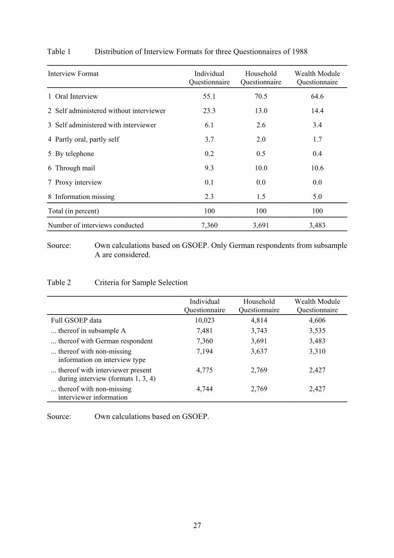
The GSOEP applies a variety of interview methods: Individuals can answer questions

orally, they can fill in the questionnaire themselves with or without interviewer support, some

questionnaires are sent out by mail, and some interviews are conducted via the telephone. In

general, interviewers are required to perform the oral interview but they may use different

formats depending on the situation.

12 In addition the GSOEP covers a subsample B containing an oversample of guestworkers.

13 This was confirmed by our preliminary results (not presented).

14 A comparison of item non-response rates for the pool of all outcome measures describedin the next section yielded a rate of 6.03 percent before selecting on the basis of interviewerpresence and of 4.52 percent when conditioning on interviewer presence.

15 E.g. only those who had indicated employment were asked about labor incomes, or thosewho were retired could indicate retirement benefits.

12

4.2 Sample and Variables

Sample: Our sample was selected based on the following criteria: First, to circumvent

language problems, we select German respondents from the nationally representative subsample

"A".12 Second, we disregard observations where the information was gathered other than by

meeting the interviewer in person, because one of our research interests concerns the interaction

between interviewer and respondent. Finally, we drop a few observations where information on

interviewer characteristics is missing. Table 2 presents the development of the sample sizes for

each part of the survey after each selection step. Clearly, conditioning on an interviewer being

present is the most stringent sample requirement involving a loss of between 35 and 25 percent

of observations. Prior studies provided evidence, that the presence of an interviewer strongly

affects item non-response behavior (cf. Lillard et al. 1986, Schräpler 2001).13, 14

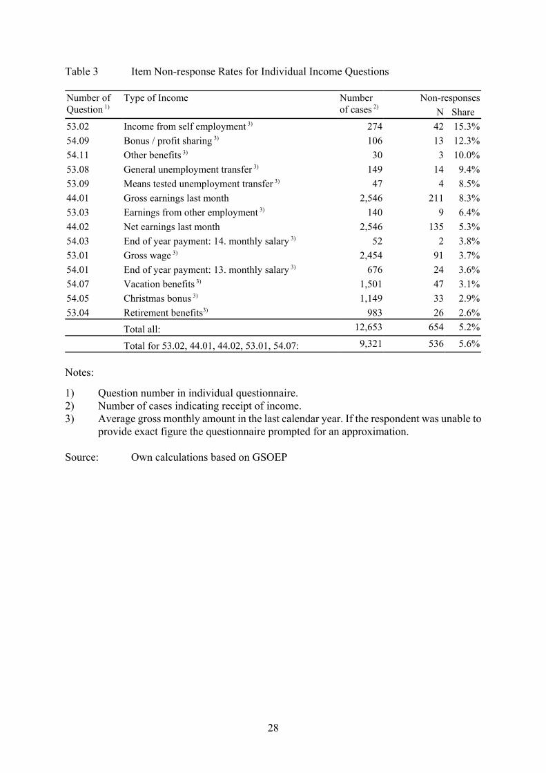
Dependent Variables: The financial variables of interest are taken from the individual,

household, and wealth questionnaires. Table 3 describes the measures gathered in the individual

survey. Due to filtering mechanisms in the questionnaire the sample sizes vary by question.15

Generally two types of variables are presented in Table 3: Those referring to average monthly

amounts in the past calendar year and those referring to the labor earnings of the past month.

The last column of Table 3 describes the item non-response rate for each of the income

measures. The rates vary markedly between 15 percent among those who had indicated income

from self-employment and less than 3 percent among those who were asked to provide the

16 Since 94.4 percent of the households in our sample responded to the wealth survey, theanalysis of item non-response is conditional on responding to the questionnaire. The survey non-response cannot simply be added to individual item non-response rates, say by adding 5.6percent to each rate, because not everybody refusing to answer the questionnaire would haveactually possessed each wealth item.

13

amount of their "13. monthly salary", a common employment benefit in Germany. Averaging

across all outcomes, we obtain a non-response rate of 5.2 percent for individual income variables.

Based on a cognitive ease argument one might assume that indicating last month's

earnings should require less effort than an average monthly figures over the previous calendar

year. However, item non-response on last month's earnings (cf. questions 44.01 and 44.02) are

about twice those for the past calendar year (cf. question 53.01). If it is the sense of privacy that

determines the cost of reporting labor earnings, this outcome may indicate that current earnings

are more sensitive than those of the past. The figures also seem to suggest that regulated

payments, such as end of year, vacation or retirement transfers involve lower reporting costs -

possibly because they are considered as less private information - than those that may entail

information on individual labor market success (e.g. unemployment situation, earnings from

dependent or self-employment).

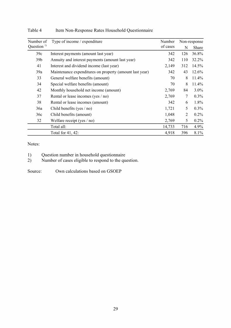
Table 4 describes financial indicators from the household questionnaire. It combines

measures as to whether a household has incomes or expenditures of a given type at all, with those

specifying amounts. Non-response rates are highest at over thirty percent with respect to interest

payments, and annuity and interest payments. Non-response rates for measures relevant for larger

samples, such as interest and dividend income or net income vary between 14.5 and 3 percent.

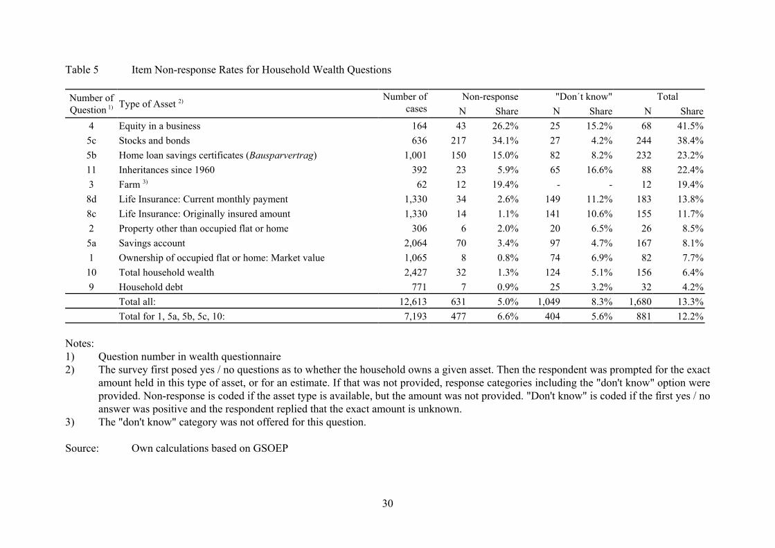
Finally, Table 5 provides information on household wealth indicators. The questionnaire

typically asked the respondent whether the household holds a given asset and if so at which

value.16 If the respondent indicated possession of a given item but could not provide the exact

amount, the person was first asked to guess the amount and if that failed in most cases answer

categories or a "don't know" reply were offered. Again, every outcome measure is described for

a different group of respondents, which is reflected in the varying number of cases in column

14

three. Item non-response was coded if the individual refused to provide the value of the asset held

by the household and "don't know" if the respondent indicated that the amount is unknown. The

last columns in Table 5 describe the frequency of the non-response and don't know outcomes.

The rates of non-response and "don't know" answers vary strongly across items. The

highest refusal rates are observed for the questions on stock, bond, and equity ownership. The

shares of "don't know" responses are somewhat differently distributed across outcomes. Here the

highest rates appear for equity (15 percent) and inheritances since 1960 (16,6%). In both cases

it is plausible that determining the value of these assets is indeed difficult. Therefore "don't

know" may be a reflection of actual lack of knowledge. This seems less plausible in the case of

monthly life insurance payments, where one might assume that the respondent is familiar with

a figure showing up regularly on bank statements. Here an 11 percent don't know rate seems high.

While the non-response rates in Table 5 do not differ markedly from those in Tables 3 and

4, the total share of uninformative responses, combining non-response and don't know answers

more than doubles this figure at about 13 percent. Two factors might explain this difference:

Either, offering an answer option "don't know" induces individuals who may have otherwise

provided an answer to indicate ignorance. Alternatively wealth issues are either more sensitive

than income indicators or it is more difficult to know the correct answer. Both situations could

plausibly prompt high non-response rates.

Explanatory Variables: Equation 1 describes individual response behavior as determined

by the costs and benefits of providing a valid answer, the characteristics of respondent and

interviewer, as well as interactions of these factors. Clearly it is not possible to measure

individually perceived costs and benefits involved in answering a given question. Therefore the

characteristics of respondents and interviewers are interpreted also in the light of their effect on

individual cost and benefit considerations.

In our item non-response model we consider a baseline specification which controls for

17 De Maio (1980) found significantly more survey cooperation among rural people thanamong urban dwellers.

18 For three reasons we do not consider the duration of the ongoing or prior interview eventhough it is much discussed in the non-response literature (Hill and Willis 2001): First, interview

15

the labor market status of interviewer and respondent, and their levels of schooling. We generate

indicators which describe whether the two interview participants have equal characteristics in

these dimensions. Low schooling is coded for mandatory schooling, medium schooling for the

German Realschule, and high schooling for degrees preparing for academic studies.

Since the literature strongly suggests that the sex of the interviewer affects response

behavior (cf. Sousa-Poza and Henneberger 2000, or Schräpler 2001) we control for the gender

combination between interviewer and respondent. Age effects are controlled for by a linear age

term for respondents and an indicator of the age difference between interviewer and respondent.

In addition to these demographic controls we consider indicators which proofed to be

influential in other studies of non-response. Among them is an indicator for whether respondents

work in the public sector which is correlated with low non-response. We control for household

size, because the larger the household, the more difficult it should be to gather financial

information. We take the size of an individual's town of residence as a potential indicator of an

attitude of openness and trust. This is based on evidence that individuals refuse to participate in

surveys because of fear of crimes and that larger cities often entail a sense of anonymity, which

corresponds to guarding the limits of privacy more carefully than in rural areas.17

Finally, we control for whether a household's interviewer has changed since the last

survey year, based on ample evidence that the personal relationship to an interviewer is important

for trust and the provision of information. Also we look at whether a respondent answers a

questionnaire partly by him- or herself in written form as opposed to completely responding to

an oral interview: Following the rational choice model it is much easier to refuse an answer if this

does not have to be communicated to the interviewer. We hypothesize higher non-response rates

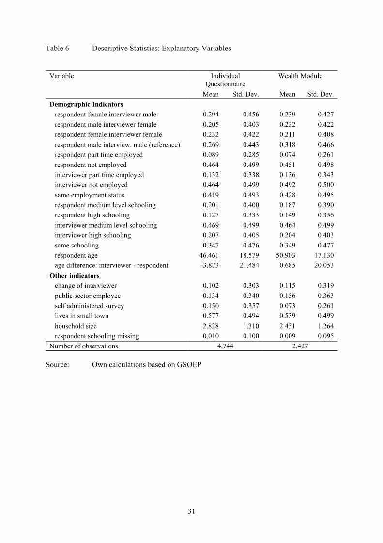
among those filling in the questionnaire by themselves.18 – Table 6 describes descriptive statistics

duration might be a simple function of non-response behavior. Second, it may not be the sameperson representing a household in different surveys, and finally it is not obvious which indicatorshould describe interview duration, as different questionnaires can be considered separately.

19 The classic illustration of the IIA property looks at alternative means of public transport.While taxi, train, and bus constitute valid alternatives, a split between red and blue buses wouldviolate the IIA assumption. We test whether don't know answers are comparable to a "red bus"alternative as opposed to being an independent alternative, such as the train.

16

for the full sample of observations covered by the personal and the wealth surveys.

4.3 Empirical Strategy

The last section already described the heterogeneity in non-response behavior across

outcomes. We first investigate whether these differences in non-response can be explained by the

variables in our model, or whether they go back to unobservable and outcome-specific factors.

We arbitrarily select some outcome measures, and estimate and compare the determinants of non-

response behavior. This also yields evidence as to whether the matching of interviewer and

respondent affects item non-response. For a very intuitive indication of outcome-specific

heterogeneity we then pool item non-response outcomes across questions and test for the

statistical significance of question specific fixed effects as well as of outcome specific differences

in covariate effects.

To address the question to what degree don't know answers differ from valid responses

and from complete refusals we apply the logic underlying the IIA (independence of irrelevant

alternatives) property of the multinomial logit model (Hausman and McFadden 1984): The IIA

property states that the outcome alternatives of the multinomial logit model are correctly

specified only if the estimation does not depend on the set of outcome options. If splitting up an

answer into two separate alternatives affects the results, the alternatives are not truly separable19

We perform a Hausman test of the IIA property after coding the dependent variable "1"

for valid responses, "2" for don't know answers, and "3" for non-responses. The test evaluates the

null hypothesis that category 2 is a valid independent alternative. If this is rejected, don't know

20 Such estimations could compare alternative groupings of the three outcomes within abinary logit model. One might estimate a model after setting the dependent variable "0" for validresponses and "1" for non-responses and don't know answers. A second model might group thedon't know answers with valid responses and a third model might simply drop don't knowoutcomes. The results may suggest conclusions as to which outcomes are more similar.

21 We thus avoid clustering the "don't know" outcome with either valid responses or non-responses, we do not impose an order on the outcomes and keep all observations in the sample.

17

answers are not truly separate and independent outcomes, but instead fundamentally similar to

either valid responses or complete non-responses. In that case we provide estimation results to

determine, whether don't know answers are more similar to the response or the non-response

alternative.20 Section 5 presents the results.

5. Results and Discussion

5.1 Heterogeneity in Item Non-response Behavior and its Determinants

Covariates of item non-response

First we investigate the correlates of item non-response. By comparing the results across

outcome measures the robustness of the findings can be evaluated, which has not found much

attention in prior item non-response research. For individual and household measures (see Tables

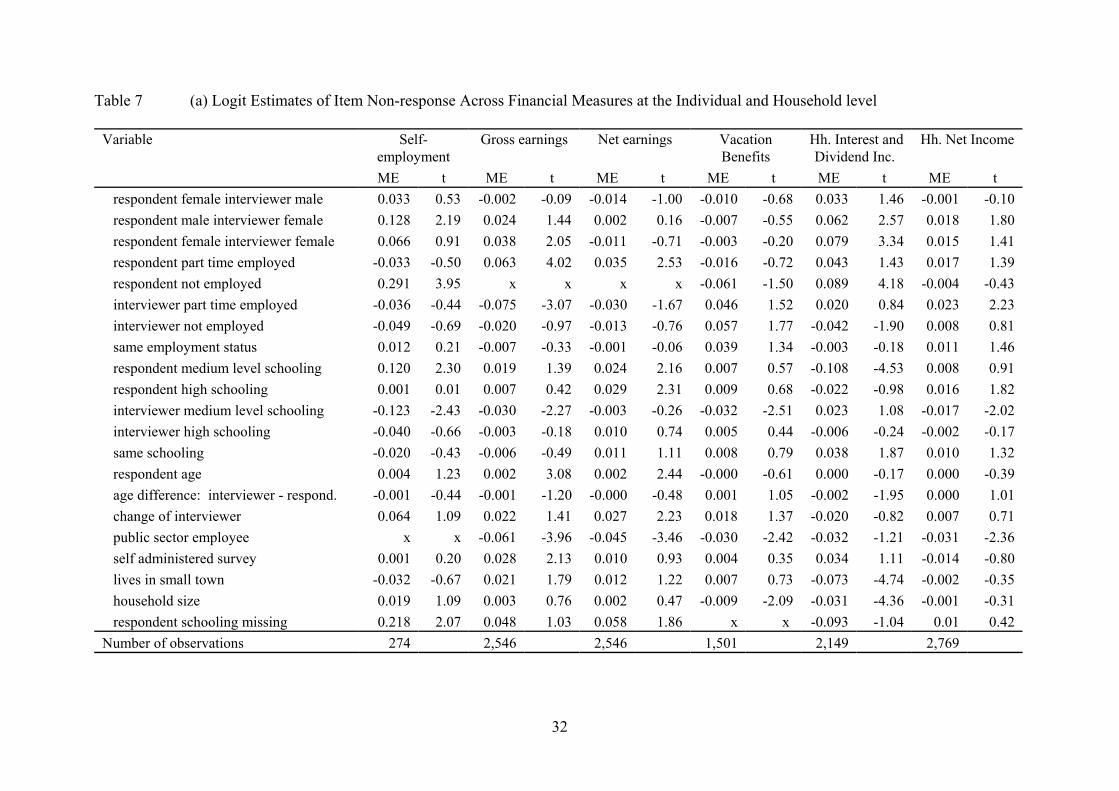
3 and 4) we estimate bivariate logit models and calculate the covariates' marginal effects (Table

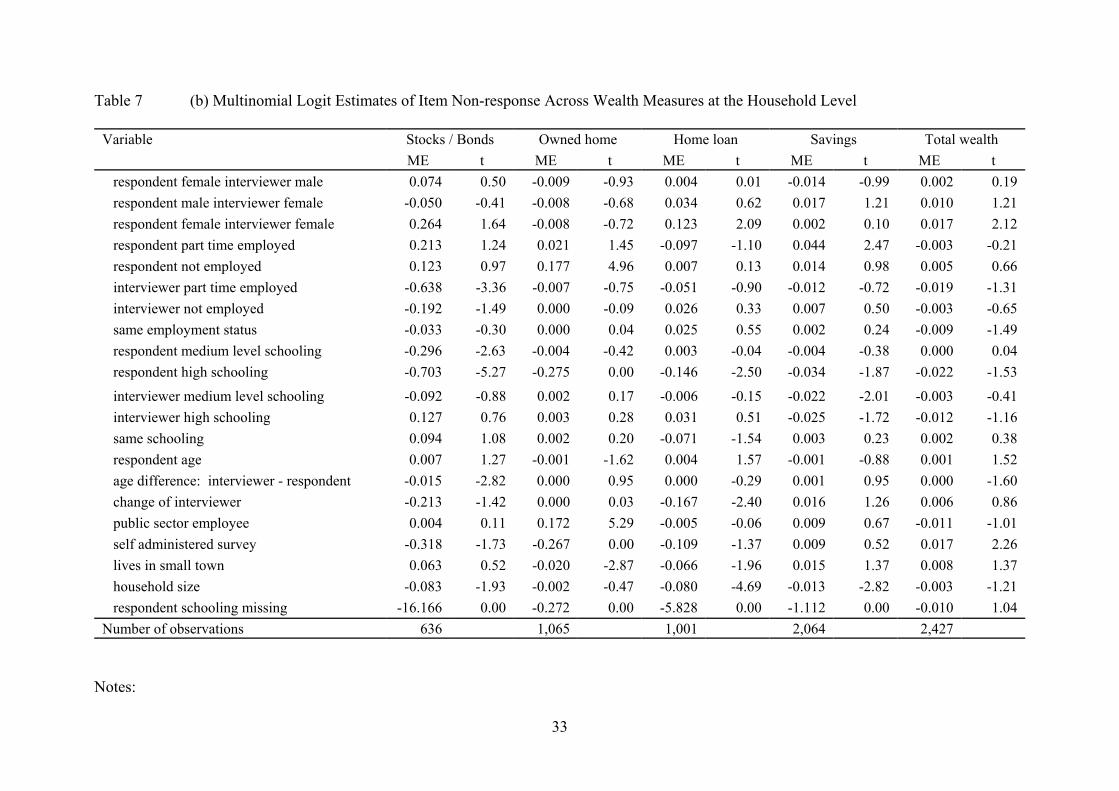
7a). In the case of the wealth measures the dependent variables contain the additional outcome

category "don't know". In order to impose the least restrictive model we estimated multinomial

logits for these outcomes.21 We calculate the covariate marginal effects on the probability of non-

response and present these with asymptotic t-statistics of the coefficient estimates in Table 7b.

The estimations yield a small number of statistically significant coefficients. The first

group of variables describes the gender combination of respondent and interviewer with two

males as the reference category. Notably all marginal effects, which are based on statistically

significant coefficients, indicate positive associations between a female interviewer and item non-

response. This association is particularly sizeable for self-employed income and stock and bond

18

ownership and confirms the findings of Schräpler (2001). If we assume that it is easier to avoid

an answer in front of a female the pattern fits the rational choice model's predictions.

The next set of indicators describes the employment status of respondent and interviewer.

Comparing our results across outcomes there seems to be a weak tendency for respondents who

are not full time employed to refuse the answer. The effect is most clearly measured for self-

employment income. The finding can be explained within the rational choice model: If the

earnings of part-time workers are comparatively low, these respondents are faced with a "social

desirability" problem when they prefer to indicate their personal labor market success to an

interviewer. As a consequence those who are part time or not employed and have low earnings

or wealth may choose non-response. The evidence on the role of the interviewers' employment

status is mixed. There is no evidence for matching effects with respect to employment status.

Similarly, the evidence on schooling effects is mixed and does not suggest clear patterns.

Having respondents and interviewers with similar schooling does not affect the results. The

marginal effects of higher respondent schooling on income are all positive (yet insignificant)

except for income from interest and dividends measure. This confirms the findings of Biewen

(2001). Higher education on the part of the interviewer does not seem to improve response

outcomes. Surprisingly, we find a robust reduction in item non-response when interviewers have

medium level schooling, which is difficult to rationalize.

Older respondents seem to be more prone to item non-response than younger individuals.

We also find some evidence that having interviewers who are older than the respondents reduces

item non-response. Almost all marginal effects of the age difference are negative and some are

statistically significant, suggesting that matching interview partners by age might be helpful.

There are only few consistent patterns in the remaining control variables. Despite of the

strong evidence in the literature concerning the relevance of long term relations between

interviewer and respondent we find a significant increase in non-response after an interviewer

change only in one of our outcome measures. A possible explanation could be that change of an

22 In order to render the bivariate non-response outcome measure of the income variablescomparable to the multivariate outcome measure of the wealth indicators we dropped the wealthobservations with "don't know" answers from the sample. The results presented in section 5.2suggest that the don't konw answers should not be combined with the other outcome categories.

19

interviewer has very strong effects on respondent behavior and causes complete unit non-

response such that item non-response cannot even be observed (cf. Rendtel 1995). Confirming

the findings of prior studies (e.g. Biewen 2001), public sector employees seem to be significantly

more cooperative and less likely to refuse an answer. However, closer inspection yields that this

cooperation seems to be restricted to the income measures.

Evidence as to whether the presence of an interviewer affects non-response is mixed.

Based on the rational choice hypotheses one might expect those who respond without the

controlling influence of interviewers to come out with more non-response. This, however, is

confirmed only for gross earnings and total wealth. The evidence is similarly mixed with respect

to the effect of rural residence on non-response where significant effects go in both directions.

The control for household size was considered as an indicator for potential information

problems. We expected higher non-response in larger households. The results show significant

effects in the opposite direction, which is difficult to explain within the theoretical framework

presented above. – Next, we investigate the importance of heterogeneity across outcomes.

Heterogeneity in item non-response across outcomes

The issue of outcome-specific heterogeneity is addressed in two steps. First, we pool the

data on the outcomes described in Tables 3 through 5 and add fixed outcome specific effects to

the specification. The joint significance of the fixed effects indicates whether there is

heterogeneity in non-response behavior after controlling for covariates.22

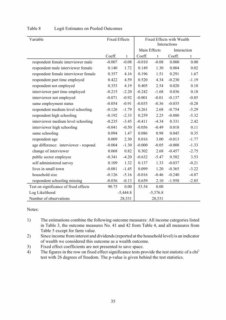
The estimation results for the pooled sample are presented in the first columns of Table

8. The fixed effect controls are highly statistically significant, reflecting the heterogeneity across

outcomes even after controlling for covariates. Adding outcome specific fixed effects to the

23 In these estimations we treat "income from interest and dividend income" as an indicatorof wealth holdings and group it with the outcomes listed in Table 5.

20

model increases the pseudo R2 from about 1.8 (results not presented) to almost 14 percent in the

estimation presented in the first columns of Table 8. This result holds in smaller subsamples as

well, when we pool outcomes at the individual, household, or wealth level only (not presented).

Since overall non-response rates differ between wealth and income outcomes, we next

investigate whether this is simply a level effect or whether the covariate effects differ across the

two outcome groups as well. We reestimate the fixed effects model now adding a full set of

interaction terms between a variable (I) indicating whether the observation describes a wealth

outcome or an income measure.23 The estimated model is thus:

yij* = cij "1 + bij "2 + Xi $1 + Wm $2 + ( Xi * Wm ) $3 +

cij * Ij "1' + bij * Ij "2' + Xi * Ij $1' + Wm * Ij $2' + ( Xi * Wm ) * Ij $3' + :ij

The results are presented in the last columns of Table 8. The explanatory power of the model

increased significantly with the full set of interaction terms added, of which a number are

statistically significant. The increase in non-response for female interviewers appears to be more

pronounced for wealth outcomes, while the full set of sex interaction terms is not statistically

significant. The same holds for the employment status indicators.

A surprisingly clear pattern appears in the correlation of schooling indicators and item

non-response for the two groups of outcomes, confirming the results described in Table 7 above.

Whereas item non-response on income measures increases with higher respondent education, we

find the opposite result for wealth outcomes. The differences are statistically significant and

difficult to interpret. We observe particularly the well educated answering wealth questions. If

education is correlated with the level of information that a respondent has available about

household wealth, then the response pattern might be explained based on cognitive ability. Given

that the same individuals should also be well informed with respect to their income one can only

speculate that they consider income as a more private or sensitive piece of information.

Next the joint effects of age seem to differ between the income and wealth outcomes. The

24 Since the combination of outcomes considered in the sample used in Table 8 is somewhatarbitrary, we performed robustness tests of the results by reestimating the same models foralternative outcome subsets. In these results most coefficients have the same sign, but theirstatistical significance is not robust to modifications of the sample. We find confirmation forsignificant outcome specific differences on some of the schooling interactions, as well as the agedifference effect and its interaction.

21

non-response probability regarding income measures increases with respondent age. This effect

is significantly weaker when it comes to wealth measures. The negative correlation between the

interviewer-respondent age difference and item non-response which we pointed out above seems

to be based mostly on wealth outcomes.

Differences in covariate associations with non-response probabilities by outcome are

observable also for the remaining control variables. While the change of an interviewer increased

non-responses for incomes, it is negatively correlated with non-response for the wealth. The

beneficial effect of public sector employment on the propensity to provide financial information

seems to be limited to incomes: Since the earnings of public sector workers in Germany typically

follow publicly available pay scales, it is possible that these workers are more open about their

income, as it may be considered public knowledge anyway. When it comes to wealth, however,

privacy protection instincts seem to be same as for anyone else. Living in a small town is

correlated with significantly lower non-response on wealth while the effect on income is not

precisely estimated. Similarly the negative effect of household size on non-reporting differs

significantly for the two outcomes. Thus, non-response differs across outcomes and there are

significant differences in the association of covariates with outcome-specific non-response.24

5.2 A Closer Look at "Don't know" Answers

In this section we investigate whether answering "don't know" is an independent outcome,

or whether this response can be grouped either with valid responses or with non-responses. As

described above we apply a Hausman test of the IIA property in a multinomial logit framework.

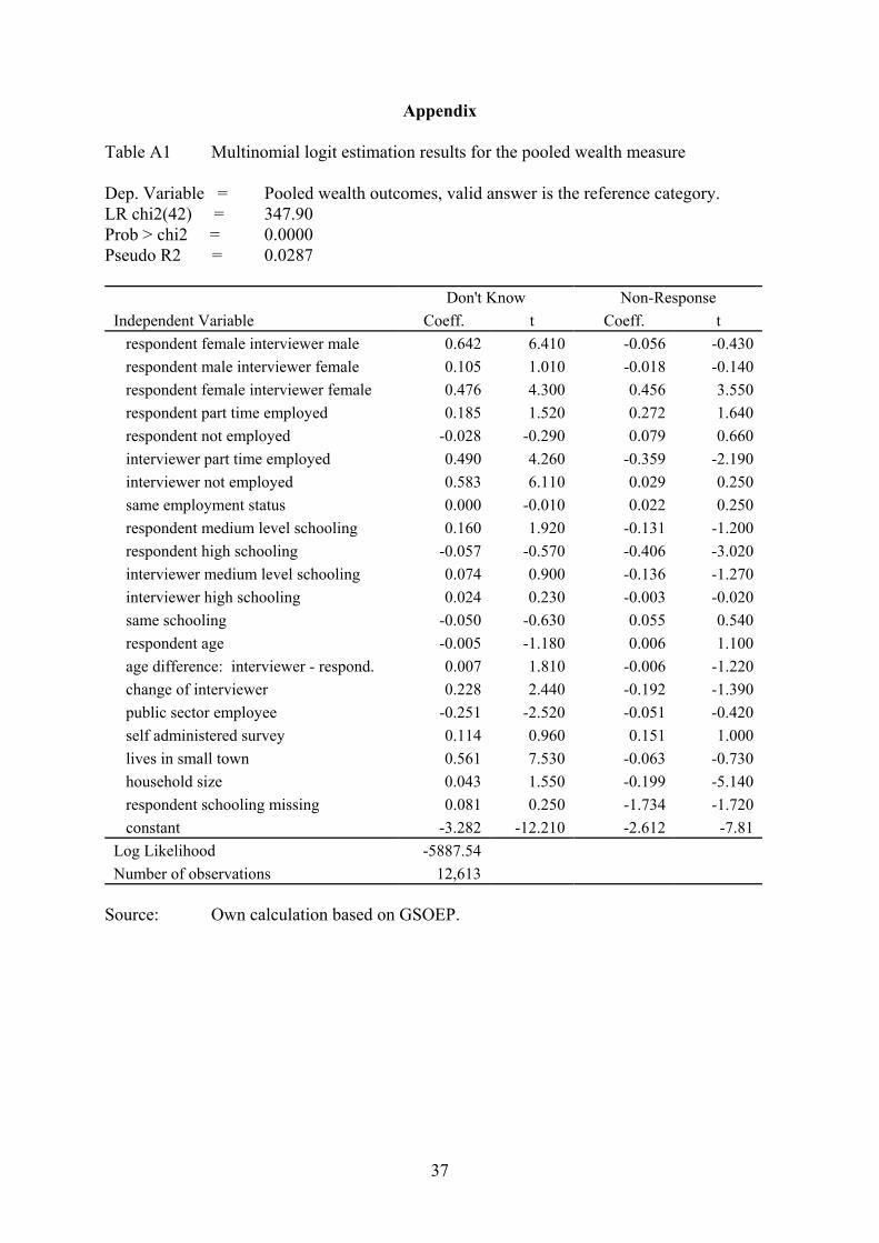
First, we evaluate a dependent variable which pools all of the outcomes presented in Table 5

25 As an example Table A1 in the Appendix presents the estimates obtained with the pooledwealth measure as the dependent variable, which underlie the test in row 1 of Table 9.

22

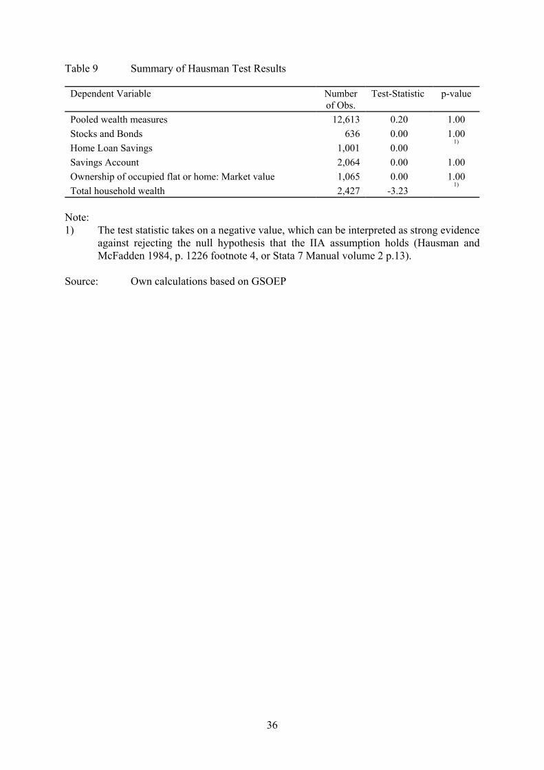
combining the 12,613 observations of the "total" row. Next, we consider some of the wealth

outcomes separately to determine whether the results for the pooled measures are robust.

The evidence presented in Table 9 seems to be strong and clear: The null hypothesis that

the IIA assumption holds cannot be rejected in any of the samples. Therefore "don't know"

answers are "relevant" and "independent" alternatives to informative responses and to non-

responses in the IIA sense. If the IIA assumption had been rejected we would have had to

determine how to interpret "don't know" answers: They might either have to be considered as a

subcategory of informative answers, capturing the group of individuals who are not completely

certain of the correct answer and – without the option of answering "don't know" – may have

guessed the correct answer. Alternatively, one might have to consider "don't know" outcomes as

"soft" refusals: If individuals prefer to withhold information, they would refuse an answer in the

situation without the option of answering "don't know", but given the option of not violating the

rules of courtesy, they prefer to pretend ignorance about the issue at hand.

Neither of these scenarios seems to hold. Instead, the correlation of the covariates with

the answer "don't know" differs significantly from that with the alternative outcomes.25 Given

these unambiguous results "don't know" answers must be viewed as independent outcomes in

their own right, and the hypothesis that they can be combined with either alternative group has

to be rejected. For the correct estimation of models of financial outcomes this implies that a

combination of don't know answers with non-responses or the omission of both types of

responses from the estimation may lead to inconsistent estimates.

6. Conclusions

Any analysis using survey data on income and wealth is affected by item non-response.

Therefore we present a number of findings that are new to the literature on item non-response.

23

We summarized the literature on theoretical frameworks for item non-response behavior which

consists of the cognitive model and the rational choice approach. The empirical literature on item

non-response is quite limited and generally focuses on measures of labor income only.

This limitation is addressed here: We evaluate a variety of financial outcomes and

compare frequency and determinants of item non-response. We find significant heterogeneity in

non-response intensities across financial outcomes. This conclusion from descriptive statistics

is confirmed in regressions of non-response behavior where much explanatory power derives

from the consideration of outcome-specific fixed effects. We confirm many correlations of

respondent and interviewer characteristics with item non-response found in the literature.

However, looking at the homogeneity of non-response determinants across outcomes yields new

information: Estimating a fully interacted model shows clearly that a number of the established

correlates of item non-response depend on the outcome measure under consideration.

We investigate whether the matching of interviewer and respondent characteristics affects

the quality of survey outcomes. Here robust findings could be valuable to improve the

administration of and information gathered from social surveys. We confirm the general result

of the item non-response literature that non-response rates tend to be higher if the interviewer is

female in particular if the respondent is female as well. Having a respondent and an interviewer

with the same employment status or the same educational level does not significantly affect non-

response outcomes. However, our measures of employment and educational attainment may be

too rough to reflect the impact of potential matching effects on non-response behavior. With

respect to age differences there is some evidence that matching an older interviewer to a younger

respondent may increase response propensities particularly with respect to wealth outcomes.

Interestingly, the personal acquaintance of the respondent with the interviewer is beneficial for

wealth but not for income outcomes.

Our third research question concerns "don't know" answers in questionnaires. Tests on

the basis of the independence of irrelevant alternatives assumption of the multinomial logit

24

estimation framework suggest clearly that "don't know" responses cannot be viewed as a

subcategory of valid answers nor as comparable to item non-response. Therefore simple

statements as to how "don't know" answer options affect the set of valid answers are not possible.

In the end researchers have to acknowledge that the group of respondents who refuse to

answer the survey questions is certainly not a random draw from the population, that the group

differs depending on the question they look at, that those answering "don't know" differ from

non-respondents and that simply omitting these individuals from the analysis may well bias

results.

25

Bibliography

Biewen, Martin, 2001, Item non-response and inequality measurement: Evidence from theGerman earnings distribution, Allgemeines Statistisches Archiv 85, 409-425.

Däubler, Thomas, 2002, Nonresponseanalysen der Stichprobe F des SOEP, DIW Berlin,Materialien 15.

De Maio, Theresa J., 1980, Refusals: Who, where and why, Public Opinion Quarterly 44, 223-233.

Dillman, Donald A., 1978, Mail and Telephone Surveys: The Total Design Method, John Wileyand Sons, New York.

Esser, Hartmut, 1984, Determinanten des Interviewer- und Befragtenverhaltens: Probleme dertheoretischen Erklärung und empirischen Untersuchung von Interviewereffekten, in:K.Mayer, P. Schmidt (eds.) Allgemeine Bevölkerungsumfrage der Sozialwissenschaften,26-71, Frankfurt.

Esser, Hartmut, 1986, Können Befragte lügen? Zum Konzept des wahren Wertes im Rahmen derhandlungstheoretischen Erklärung von Situationseinflüssen bei der Befragung, KölnerZeitschrift für Soziologie und Sozialpsychologie 38, 314-336.

Ferber, Robert, 1966, Item Nonresponse in a Consumer Survey, Public Opinion Quarterly 30,399-415.

Hanefeld, Ute, 1987, Das sozio-oekonomische Panel: Grundlagen und Konzeption, CampusVerlag, Frankfurt / Main.

Hausman, Jerry A. and Daniel McFadden, 1984, Specification Tests for the Multinomial LogitModel, Econometrica 52(5), 1219-1240.

Hill, Daniel and Robert J. Willis, 2001, Reducing Panel Attrition: A Search for Effective PolicyInstruments, Journal of Human Resources 36(3), 416-438.

Horowitz, Joel L. and Charles F. Manski, 1998, Censoring of outcomes and regressors due tosurvey nonresponse: Identification and estimation using weights and imputations, Journalof Econometrics 84, 37-58.

Lachman, R., Lachman J.T., and E.C. Butterfield, 1979, Cognitive Psychology and InformationProcessing, Hillsdale, NJ: Erlbaum.

Lillard, Lee, James P. Smith, and Finis Welch, 1986, What do we really know about wages? TheImportance of Nonreporting and Census Imputation, Journal of Political Economy 94(3),489-506.

Loosveldt, Geert, Jan Pickery, and Jaak Billiet, 1999, Item non-response as a predictor of unitnon-response in a panel survey, Paper presented at the International Conference onSurvey Non-response, Portland Oregon, USA.

26

Reinecke, Jost, 1991, Interviewer- und Befragtenverhalten. Theoretische Ansätze undmethodische Konzepte, Westdeutscher Verlag, Opladen.

Rendtel, Ulrich, 1995, Panelausfälle und Panelrepräsentativität, Campus Verlag, Frankfurt, NewYork.

Schräpler, Jörg-Peter and Gert G. Wagner, 2001, Das Verhalten von Interviewern - Darstellungund ausgewählte Analysen am Beispiel des "Interviewerpanels" des Sozio-ökonomischenPanels, Allgemeines Statistisches Archiv 85, 45-66.

Schräpler, Jörg-Peter, 2001, Respondent Behavior in Panel Studies. A Case Study of the GermanSocio-Economic Panel (GSOEP), DIW Discussion Papers No. 244, DIW - Berlin.

SOEP Group, 2001, The German Socio-Economic Panel (GSOEP) after more than 15 years -Overview. In: Elke Holst, Dean R. Lillard and Thomas A. DiPrete (eds.): Proceedings ofthe 2000 Fourth International Conference of German Socio-Economic Panel Study Users(GSOEP2000), Vierteljahrshefte zur Wirtschaftsforschung (Quarterly Journal ofEconomic Research) 70(1), 7-14.

Sousa-Poza, Alfonso and Fred Henneberger, 2000, Wage data collected by telephone interviews:an empirical analysis of the item nonresponse problem and its implications for theestimation of wage functions, Schweizerische Zeitschrift für Volkswirtschaft und Statistik136(1), 79-98.

Sudman, Seymour, Norman M. Bradburn, and Norbert Schwarz, 1996, Thinking About Answers.The Application of Cognitive Processes to Survey Methodology, Jossey Bass Publishers,San Francisco.

Trometer, Reiner, 1996, Warum sind Befragte "meinungslos"? Kognitive und kommunikativeProzesse im Interview, Inauguraldissertation an der Universität Mannheim, mimeo.

Zweimüller, Josef, 1992, Survey non-response and biases in wage regressions, Economics Letters39, 105-109.

27

Table 1 Distribution of Interview Formats for three Questionnaires of 1988

Interview Format IndividualQuestionnaire

HouseholdQuestionnaire

Wealth ModuleQuestionnaire

1 Oral Interview 55.1 70.5 64.6

2 Self administered without interviewer 23.3 13.0 14.4

3 Self administered with interviewer 6.1 2.6 3.4

4 Partly oral, partly self 3.7 2.0 1.7

5 By telephone 0.2 0.5 0.4

6 Through mail 9.3 10.0 10.6

7 Proxy interview 0.1 0.0 0.0

8 Information missing 2.3 1.5 5.0

Total (in percent) 100 100 100

Number of interviews conducted 7,360 3,691 3,483

Source: Own calculations based on GSOEP. Only German respondents from subsampleA are considered.

Table 2 Criteria for Sample Selection

IndividualQuestionnaire

HouseholdQuestionnaire

Wealth ModuleQuestionnaire

Full GSOEP data 10,023 4,814 4,606... thereof in subsample A 7,481 3,743 3,535... thereof with German respondent 7,360 3,691 3,483... thereof with non-missing information on interview type

7,194 3,637 3,310

... thereof with interviewer present during interview (formats 1, 3, 4)

4,775 2,769 2,427

... thereof with non-missing interviewer information

4,744 2,769 2,427

Source: Own calculations based on GSOEP.

28

Table 3 Item Non-response Rates for Individual Income Questions

Number ofQuestion 1)

Type of Income Numberof cases 2)

Non-responsesN Share

53.02 Income from self employment 3) 274 42 15.3%54.09 Bonus / profit sharing 3) 106 13 12.3%54.11 Other benefits 3) 30 3 10.0%53.08 General unemployment transfer 3) 149 14 9.4%53.09 Means tested unemployment transfer 3) 47 4 8.5%44.01 Gross earnings last month 2,546 211 8.3%53.03 Earnings from other employment 3) 140 9 6.4%44.02 Net earnings last month 2,546 135 5.3%54.03 End of year payment: 14. monthly salary 3) 52 2 3.8%53.01 Gross wage 3) 2,454 91 3.7%54.01 End of year payment: 13. monthly salary 3) 676 24 3.6%54.07 Vacation benefits 3) 1,501 47 3.1%54.05 Christmas bonus 3) 1,149 33 2.9%53.04 Retirement benefits3) 983 26 2.6%

Total all: 12,653 654 5.2%

Total for 53.02, 44.01, 44.02, 53.01, 54.07: 9,321 536 5.6%

Notes:

1) Question number in individual questionnaire.2) Number of cases indicating receipt of income.3) Average gross monthly amount in the last calendar year. If the respondent was unable to

provide exact figure the questionnaire prompted for an approximation.

Source: Own calculations based on GSOEP

29

Table 4 Item Non-Response Rates Household Questionnaire

Number ofQuestion 1)

Type of income / expenditure Numberof cases

Non-responseN Share

39c Interest payments (amount last year) 342 126 36.8%39b Annuity and interest payments (amount last year) 342 110 32.2%41 Interest and dividend income (last year) 2,149 312 14.5%39a Maintenance expenditures on property (amount last year) 342 43 12.6%33 General welfare benefits (amount) 70 8 11.4%34 Special welfare benefits (amount) 70 8 11.4%42 Monthly household net income (amount) 2,769 84 3.0%37 Rental or lease incomes (yes / no) 2,769 7 0.3%38 Rental or lease incomes (amount) 342 6 1.8%36a Child benefits (yes / no) 1,721 5 0.3%36c Child benefits (amount) 1,048 2 0.2%32 Welfare receipt (yes / no) 2,769 5 0.2%

Total all: 14,733 716 4.9%Total for 41, 42: 4,918 396 8.1%

Notes:

1) Question number in household questionnaire 2) Number of cases eligible to respond to the question.

Source: Own calculations based on GSOEP

30

Table 5 Item Non-response Rates for Household Wealth Questions

Number ofQuestion 1) Type of Asset 2) Number of

casesNon-response "Don't know" Total

N Share N Share N Share4 Equity in a business 164 43 26.2% 25 15.2% 68 41.5%5c Stocks and bonds 636 217 34.1% 27 4.2% 244 38.4%5b Home loan savings certificates (Bausparvertrag) 1,001 150 15.0% 82 8.2% 232 23.2%11 Inheritances since 1960 392 23 5.9% 65 16.6% 88 22.4%3 Farm 3) 62 12 19.4% - - 12 19.4%

8d Life Insurance: Current monthly payment 1,330 34 2.6% 149 11.2% 183 13.8%8c Life Insurance: Originally insured amount 1,330 14 1.1% 141 10.6% 155 11.7%2 Property other than occupied flat or home 306 6 2.0% 20 6.5% 26 8.5%5a Savings account 2,064 70 3.4% 97 4.7% 167 8.1%1 Ownership of occupied flat or home: Market value 1,065 8 0.8% 74 6.9% 82 7.7%

10 Total household wealth 2,427 32 1.3% 124 5.1% 156 6.4%9 Household debt 771 7 0.9% 25 3.2% 32 4.2%

Total all: 12,613 631 5.0% 1,049 8.3% 1,680 13.3%Total for 1, 5a, 5b, 5c, 10: 7,193 477 6.6% 404 5.6% 881 12.2%

Notes:1) Question number in wealth questionnaire 2) The survey first posed yes / no questions as to whether the household owns a given asset. Then the respondent was prompted for the exact

amount held in this type of asset, or for an estimate. If that was not provided, response categories including the "don't know" option wereprovided. Non-response is coded if the asset type is available, but the amount was not provided. "Don't know" is coded if the first yes / noanswer was positive and the respondent replied that the exact amount is unknown.

3) The "don't know" category was not offered for this question.

Source: Own calculations based on GSOEP

31

Table 6 Descriptive Statistics: Explanatory Variables

Variable IndividualQuestionnaire

Wealth Module

Mean Std. Dev. Mean Std. Dev.Demographic Indicators respondent female interviewer male 0.294 0.456 0.239 0.427 respondent male interviewer female 0.205 0.403 0.232 0.422 respondent female interviewer female 0.232 0.422 0.211 0.408 respondent male interview. male (reference) 0.269 0.443 0.318 0.466 respondent part time employed 0.089 0.285 0.074 0.261 respondent not employed 0.464 0.499 0.451 0.498 interviewer part time employed 0.132 0.338 0.136 0.343 interviewer not employed 0.464 0.499 0.492 0.500 same employment status 0.419 0.493 0.428 0.495 respondent medium level schooling 0.201 0.400 0.187 0.390 respondent high schooling 0.127 0.333 0.149 0.356 interviewer medium level schooling 0.469 0.499 0.464 0.499 interviewer high schooling 0.207 0.405 0.204 0.403 same schooling 0.347 0.476 0.349 0.477 respondent age 46.461 18.579 50.903 17.130 age difference: interviewer - respondent -3.873 21.484 0.685 20.053Other indicators change of interviewer 0.102 0.303 0.115 0.319 public sector employee 0.134 0.340 0.156 0.363 self administered survey 0.150 0.357 0.073 0.261 lives in small town 0.577 0.494 0.539 0.499 household size 2.828 1.310 2.431 1.264 respondent schooling missing 0.010 0.100 0.009 0.095Number of observations 4,744 2,427

Source: Own calculations based on GSOEP

32

Table 7 (a) Logit Estimates of Item Non-response Across Financial Measures at the Individual and Household level

Variable Self-employment

Gross earnings Net earnings VacationBenefits

Hh. Interest andDividend Inc.

Hh. Net Income

ME t ME t ME t ME t ME t ME t respondent female interviewer male 0.033 0.53 -0.002 -0.09 -0.014 -1.00 -0.010 -0.68 0.033 1.46 -0.001 -0.10 respondent male interviewer female 0.128 2.19 0.024 1.44 0.002 0.16 -0.007 -0.55 0.062 2.57 0.018 1.80 respondent female interviewer female 0.066 0.91 0.038 2.05 -0.011 -0.71 -0.003 -0.20 0.079 3.34 0.015 1.41 respondent part time employed -0.033 -0.50 0.063 4.02 0.035 2.53 -0.016 -0.72 0.043 1.43 0.017 1.39 respondent not employed 0.291 3.95 x x x x -0.061 -1.50 0.089 4.18 -0.004 -0.43 interviewer part time employed -0.036 -0.44 -0.075 -3.07 -0.030 -1.67 0.046 1.52 0.020 0.84 0.023 2.23 interviewer not employed -0.049 -0.69 -0.020 -0.97 -0.013 -0.76 0.057 1.77 -0.042 -1.90 0.008 0.81 same employment status 0.012 0.21 -0.007 -0.33 -0.001 -0.06 0.039 1.34 -0.003 -0.18 0.011 1.46 respondent medium level schooling 0.120 2.30 0.019 1.39 0.024 2.16 0.007 0.57 -0.108 -4.53 0.008 0.91 respondent high schooling 0.001 0.01 0.007 0.42 0.029 2.31 0.009 0.68 -0.022 -0.98 0.016 1.82 interviewer medium level schooling -0.123 -2.43 -0.030 -2.27 -0.003 -0.26 -0.032 -2.51 0.023 1.08 -0.017 -2.02 interviewer high schooling -0.040 -0.66 -0.003 -0.18 0.010 0.74 0.005 0.44 -0.006 -0.24 -0.002 -0.17 same schooling -0.020 -0.43 -0.006 -0.49 0.011 1.11 0.008 0.79 0.038 1.87 0.010 1.32 respondent age 0.004 1.23 0.002 3.08 0.002 2.44 -0.000 -0.61 0.000 -0.17 0.000 -0.39 age difference: interviewer - respond. -0.001 -0.44 -0.001 -1.20 -0.000 -0.48 0.001 1.05 -0.002 -1.95 0.000 1.01 change of interviewer 0.064 1.09 0.022 1.41 0.027 2.23 0.018 1.37 -0.020 -0.82 0.007 0.71 public sector employee x x -0.061 -3.96 -0.045 -3.46 -0.030 -2.42 -0.032 -1.21 -0.031 -2.36 self administered survey 0.001 0.20 0.028 2.13 0.010 0.93 0.004 0.35 0.034 1.11 -0.014 -0.80 lives in small town -0.032 -0.67 0.021 1.79 0.012 1.22 0.007 0.73 -0.073 -4.74 -0.002 -0.35 household size 0.019 1.09 0.003 0.76 0.002 0.47 -0.009 -2.09 -0.031 -4.36 -0.001 -0.31 respondent schooling missing 0.218 2.07 0.048 1.03 0.058 1.86 x x -0.093 -1.04 0.01 0.42Number of observations 274 2,546 2,546 1,501 2,149 2,769

33

Table 7 (b) Multinomial Logit Estimates of Item Non-response Across Wealth Measures at the Household Level

Variable Stocks / Bonds Owned home Home loan Savings Total wealthME t ME t ME t ME t ME t

respondent female interviewer male 0.074 0.50 -0.009 -0.93 0.004 0.01 -0.014 -0.99 0.002 0.19 respondent male interviewer female -0.050 -0.41 -0.008 -0.68 0.034 0.62 0.017 1.21 0.010 1.21 respondent female interviewer female 0.264 1.64 -0.008 -0.72 0.123 2.09 0.002 0.10 0.017 2.12 respondent part time employed 0.213 1.24 0.021 1.45 -0.097 -1.10 0.044 2.47 -0.003 -0.21 respondent not employed 0.123 0.97 0.177 4.96 0.007 0.13 0.014 0.98 0.005 0.66 interviewer part time employed -0.638 -3.36 -0.007 -0.75 -0.051 -0.90 -0.012 -0.72 -0.019 -1.31 interviewer not employed -0.192 -1.49 0.000 -0.09 0.026 0.33 0.007 0.50 -0.003 -0.65 same employment status -0.033 -0.30 0.000 0.04 0.025 0.55 0.002 0.24 -0.009 -1.49 respondent medium level schooling -0.296 -2.63 -0.004 -0.42 0.003 -0.04 -0.004 -0.38 0.000 0.04 respondent high schooling -0.703 -5.27 -0.275 0.00 -0.146 -2.50 -0.034 -1.87 -0.022 -1.53

interviewer medium level schooling -0.092 -0.88 0.002 0.17 -0.006 -0.15 -0.022 -2.01 -0.003 -0.41 interviewer high schooling 0.127 0.76 0.003 0.28 0.031 0.51 -0.025 -1.72 -0.012 -1.16 same schooling 0.094 1.08 0.002 0.20 -0.071 -1.54 0.003 0.23 0.002 0.38 respondent age 0.007 1.27 -0.001 -1.62 0.004 1.57 -0.001 -0.88 0.001 1.52 age difference: interviewer - respondent -0.015 -2.82 0.000 0.95 0.000 -0.29 0.001 0.95 0.000 -1.60 change of interviewer -0.213 -1.42 0.000 0.03 -0.167 -2.40 0.016 1.26 0.006 0.86 public sector employee 0.004 0.11 0.172 5.29 -0.005 -0.06 0.009 0.67 -0.011 -1.01 self administered survey -0.318 -1.73 -0.267 0.00 -0.109 -1.37 0.009 0.52 0.017 2.26 lives in small town 0.063 0.52 -0.020 -2.87 -0.066 -1.96 0.015 1.37 0.008 1.37 household size -0.083 -1.93 -0.002 -0.47 -0.080 -4.69 -0.013 -2.82 -0.003 -1.21 respondent schooling missing -16.166 0.00 -0.272 0.00 -5.828 0.00 -1.112 0.00 -0.010 1.04Number of observations 636 1,065 1,001 2,064 2,427

Notes:

34

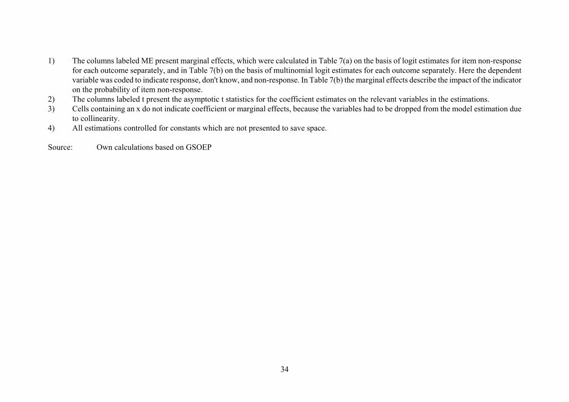
1) The columns labeled ME present marginal effects, which were calculated in Table 7(a) on the basis of logit estimates for item non-responsefor each outcome separately, and in Table 7(b) on the basis of multinomial logit estimates for each outcome separately. Here the dependentvariable was coded to indicate response, don't know, and non-response. In Table 7(b) the marginal effects describe the impact of the indicatoron the probability of item non-response.

2) The columns labeled t present the asymptotic t statistics for the coefficient estimates on the relevant variables in the estimations.3) Cells containing an x do not indicate coefficient or marginal effects, because the variables had to be dropped from the model estimation due

to collinearity. 4) All estimations controlled for constants which are not presented to save space.

Source: Own calculations based on GSOEP

35

Table 8 Logit Estimates on Pooled Outcomes

Variable Fixed Effects Fixed Effects with WealthInteractions

Main Effects InteractionCoeff. t Coeff. t Coeff. t

respondent female interviewer male -0.007 -0.08 -0.010 -0.08 0.000 0.00 respondent male interviewer female 0.140 1.72 0.149 1.30 0.004 0.02 respondent female interviewer female 0.357 4.16 0.196 1.51 0.291 1.67 respondent part time employed 0.422 4.59 0.520 4.34 -0.230 -1.19 respondent not employed 0.353 4.19 0.405 2.54 0.020 0.10 interviewer part time employed -0.215 -2.20 -0.242 -1.68 0.036 0.18 interviewer not employed -0.071 -0.92 -0.001 -0.01 -0.137 -0.85 same employment status -0.054 -0.91 -0.035 -0.36 -0.035 -0.28 respondent medium level schooling -0.126 -1.79 0.261 2.68 -0.754 -5.29 respondent high schooling -0.192 -2.33 0.259 2.25 -0.880 -5.32 interviewer medium level schooling -0.235 -3.45 -0.411 -4.34 0.331 2.42 interviewer high schooling -0.041 -0.50 -0.056 -0.49 0.018 0.11 same schooling 0.094 1.47 0.086 0.98 0.045 0.35 respondent age 0.009 2.30 0.016 3.00 -0.013 -1.77 age difference: interviewer - respond. -0.004 -1.30 -0.000 -0.05 -0.008 -1.33 change of interviewer 0.068 0.82 0.302 2.68 -0.457 -2.75 public sector employee -0.341 -4.20 -0.632 -5.47 0.582 3.53 self administered survey 0.109 1.32 0.137 1.33 -0.037 -0.21 lives in small town -0.081 -1.45 0.099 1.20 -0.365 -3.22 household size -0.126 -5.16 -0.016 -0.46 -0.240 -4.87 respondent schooling missing -0.036 -0.13 0.659 2.10 -1.958 -2.85Test on significance of fixed effects 90.75 0.00 53.54 0.00Log Likelihood -5,444.8 -5,376.8Number of observations 28,531 28,531

Notes:

1) The estimations combine the following outcome measures: All income categories listedin Table 3, the outcome measures No. 41 and 42 from Table 4, and all measures fromTable 5 except for farm value.

2) Since income from interest and dividends (reported at the household level) is an indicatorof wealth we considered this outcome as a wealth outcome.

3) Fixed effect coefficients are not presented to save space.4) The figures in the row on fixed effect significance tests provide the test statistic of a chi2

test with 26 degrees of freedom. The p-value is given behind the test statistics.

36

Table 9 Summary of Hausman Test Results

Dependent Variable Numberof Obs.

Test-Statistic p-value

Pooled wealth measures 12,613 0.20 1.00Stocks and Bonds 636 0.00 1.00Home Loan Savings 1,001 0.00

1)

Savings Account 2,064 0.00 1.00Ownership of occupied flat or home: Market value 1,065 0.00 1.00Total household wealth 2,427 -3.23

1)

Note:1) The test statistic takes on a negative value, which can be interpreted as strong evidence

against rejecting the null hypothesis that the IIA assumption holds (Hausman andMcFadden 1984, p. 1226 footnote 4, or Stata 7 Manual volume 2 p.13).

Source: Own calculations based on GSOEP

37

Appendix

Table A1 Multinomial logit estimation results for the pooled wealth measure

Dep. Variable = Pooled wealth outcomes, valid answer is the reference category.LR chi2(42) = 347.90Prob > chi2 = 0.0000Pseudo R2 = 0.0287

Don't Know Non-ResponseIndependent Variable Coeff. t Coeff. t respondent female interviewer male 0.642 6.410 -0.056 -0.430 respondent male interviewer female 0.105 1.010 -0.018 -0.140 respondent female interviewer female 0.476 4.300 0.456 3.550 respondent part time employed 0.185 1.520 0.272 1.640 respondent not employed -0.028 -0.290 0.079 0.660 interviewer part time employed 0.490 4.260 -0.359 -2.190 interviewer not employed 0.583 6.110 0.029 0.250 same employment status 0.000 -0.010 0.022 0.250 respondent medium level schooling 0.160 1.920 -0.131 -1.200 respondent high schooling -0.057 -0.570 -0.406 -3.020 interviewer medium level schooling 0.074 0.900 -0.136 -1.270 interviewer high schooling 0.024 0.230 -0.003 -0.020 same schooling -0.050 -0.630 0.055 0.540 respondent age -0.005 -1.180 0.006 1.100 age difference: interviewer - respond. 0.007 1.810 -0.006 -1.220 change of interviewer 0.228 2.440 -0.192 -1.390 public sector employee -0.251 -2.520 -0.051 -0.420 self administered survey 0.114 0.960 0.151 1.000 lives in small town 0.561 7.530 -0.063 -0.730 household size 0.043 1.550 -0.199 -5.140 respondent schooling missing 0.081 0.250 -1.734 -1.720 constant -3.282 -12.210 -2.612 -7.81Log Likelihood -5887.54Number of observations 12,613

Source: Own calculation based on GSOEP.

IZA Discussion Papers No.

Author(s) Title

Area Date

559 B. R. Chiswick T. J. Hatton

International Migration and the Integration of Labor Markets

2 08/02

560 J. W. Budd J. Konings M. J. Slaughter

Wages and International Rent Sharing in Multinational Firms

2 08/02

561 W. J. Carrington P. R. Mueser K. R. Troske

The Impact of Welfare Reform on Leaver Characteristics, Employment and Recidivism

3 08/02

562 J. T. Addison W. S. Siebert

Changes in Collective Bargaining in the U.K.

3 08/02

563 T. Dunne L. Foster J. Haltiwanger K. R. Troske

Wage and Productivity Dispersion in U.S. Manufacturing: The Role of Computer Investment

5 08/02

564 J. D. Brown J. S. Earle

The Reallocation of Workers and Jobs in Russian Industry: New Evidence on Measures and Determinants

4 09/02

565 H. L. van Kranenburg F. C. Palm G. A. Pfann

Survival in a Concentrating Industry: The Case of Daily Newspapers in the Netherlands

3 09/02

566 R. Hujer M. Caliendo D. Radić

Skill Biased Technological and Organizational Change: Estimating a Mixed Simultaneous Equation Model Using the IAB Establishment Panel

5 09/02

567 H. Lehmann K. Phillips J. Wadsworth

The Incidence and Cost of Job Loss in a Transition Economy: Displaced Workers in Estonia, 1989-1999

4 09/02

568 H. O. Duleep D. J. Dowhan

Revisiting the Family Investment Model with Longitudinal Data: The Earnings Growth of Immigrant and U.S.-Born Women

1 09/02

569 J. Haltiwanger M. Vodopivec

Worker Flows, Job Flows and Firm Wage Policies: An Analysis of Slovenia

4 09/02

570 T. K. Bauer S. Bender

Technological Change, Organizational Change, and Job Turnover

1 09/02

571 O. Ashenfelter M. Greenstone

Using Mandated Speed Limits to Measure the Value of a Statistical Life

5 09/02

572 C. Y. Co I. N. Gang M.-S. Yun

Self-Employment and Wage Earning: Hungary During Transition

4 09/02

573 R. T. Riphahn O. Serfling

Item Non-Response on Income and Wealth Questions

6 09/02

An updated list of IZA Discussion Papers is available on the center‘s homepage www.iza.org.