


Bahasa
Halaman
Hukum

Integrated Spatial and Feature Image Systems: Retrieval,
Analysis and Compression
John R. Smith
Submitted in partial ful�llment of the
requirements for the degree of
Doctor of Philosophy
in the Graduate School of Arts and Sciences
Columbia University
1997

c 1997
John R. Smith
All Rights Reserved

ABSTRACTIntegrated Spatial and Feature Image Systems: Retrieval, Analysis and
CompressionJohn R. Smith
This thesis presents new methods for integrating spatial and feature information in order to improvesystems for image retrieval, analysis and compression. In particular, this thesis develops and demonstratesan integrated spatial and feature query paradigm for image retrieval, a general framework for extractingspatially localized features from images using histogram and binary set back-projections, a system for imagecompression and analysis based upon a joint-adaptive space and frequency (JASF) graph, and a representationof texture based upon spatial-frequency energy histograms.
These techniques are similar in their exploitation of images as two-dimensional, non-stationary signals. Thevisually important information within images is often con�ned to spatially localized regions, or is representedby the spatial arrangements of these regions. By developing processes that analyze and represent images inthis way, we improve our capabilities to develop powerful content-based image retrieval and image compressionsystems.
This thesis examines several image system applications, such as image and video storage and retrieval,content-based image query, adaptive image compression and image analysis. We demonstrate that by using theproposed integrated spatial and feature approaches, we improve image system performance in each applicationover non-integrated methods.
Integrated Spatial and Feature Image Systems: Retrieval, Analysis and Compression i
Contents
1 Introduction and Motivation 1
1.1. Visual information retrieval : : : : : : : : : : : : : : : : : : : : : : : : : : : : : : : : : : : : : 11.1.1 Why unconstrained imagery? : : : : : : : : : : : : : : : : : : : : : : : : : : : : : : : : 11.1.2 Image and video storage and retrieval systems : : : : : : : : : : : : : : : : : : : : : : 2
1.2. Problem de�nitions : : : : : : : : : : : : : : : : : : : : : : : : : : : : : : : : : : : : : : : : : : 31.2.1 Content-based visual query : : : : : : : : : : : : : : : : : : : : : : : : : : : : : : : : : 31.2.2 Spatial image query : : : : : : : : : : : : : : : : : : : : : : : : : : : : : : : : : : : : : 51.2.3 Spatial and feature image query : : : : : : : : : : : : : : : : : : : : : : : : : : : : : : 61.2.4 Proposed solutions : : : : : : : : : : : : : : : : : : : : : : : : : : : : : : : : : : : : : : 7
1.3. Summary of contributions : : : : : : : : : : : : : : : : : : : : : : : : : : : : : : : : : : : : : : 81.4. Outline of thesis : : : : : : : : : : : : : : : : : : : : : : : : : : : : : : : : : : : : : : : : : : : 8
2 Representing Color 10
2.1. Introduction : : : : : : : : : : : : : : : : : : : : : : : : : : : : : : : : : : : : : : : : : : : : : : 102.2. Feature representation : : : : : : : : : : : : : : : : : : : : : : : : : : : : : : : : : : : : : : : : 102.3. Related work on color image retrieval : : : : : : : : : : : : : : : : : : : : : : : : : : : : : : : 102.4. Colorimetry : : : : : : : : : : : : : : : : : : : : : : : : : : : : : : : : : : : : : : : : : : : : : : 112.5. Color image perception : : : : : : : : : : : : : : : : : : : : : : : : : : : : : : : : : : : : : : : 112.6. Color space transformation and quantization : : : : : : : : : : : : : : : : : : : : : : : : : : : 11
2.6.1 Color transformation : : : : : : : : : : : : : : : : : : : : : : : : : : : : : : : : : : : : : 122.6.2 Color quantization : : : : : : : : : : : : : : : : : : : : : : : : : : : : : : : : : : : : : : 12
2.7. Color spaces : : : : : : : : : : : : : : : : : : : : : : : : : : : : : : : : : : : : : : : : : : : : : : 132.7.1 RGB color space : : : : : : : : : : : : : : : : : : : : : : : : : : : : : : : : : : : : : : : 132.7.2 Linear transform color spaces : : : : : : : : : : : : : : : : : : : : : : : : : : : : : : : : 132.7.3 Munsell color order system : : : : : : : : : : : : : : : : : : : : : : : : : : : : : : : : : 142.7.4 CIE color spaces : : : : : : : : : : : : : : : : : : : : : : : : : : : : : : : : : : : : : : : 152.7.5 HSV color space : : : : : : : : : : : : : : : : : : : : : : : : : : : : : : : : : : : : : : : 15
2.8. Representing color image features : : : : : : : : : : : : : : : : : : : : : : : : : : : : : : : : : : 172.8.1 Color histograms : : : : : : : : : : : : : : : : : : : : : : : : : : : : : : : : : : : : : : : 172.8.2 Color sets : : : : : : : : : : : : : : : : : : : : : : : : : : : : : : : : : : : : : : : : : : : 172.8.3 Color histogram compaction : : : : : : : : : : : : : : : : : : : : : : : : : : : : : : : : : 182.8.4 Binary set fast map (BSFM) : : : : : : : : : : : : : : : : : : : : : : : : : : : : : : : : 18
2.9. Summary : : : : : : : : : : : : : : : : : : : : : : : : : : : : : : : : : : : : : : : : : : : : : : : 20
3 Representing Texture 21
3.1. Introduction : : : : : : : : : : : : : : : : : : : : : : : : : : : : : : : : : : : : : : : : : : : : : : 213.2. What is texture? : : : : : : : : : : : : : : : : : : : : : : : : : : : : : : : : : : : : : : : : : : : 213.3. Related work on texture : : : : : : : : : : : : : : : : : : : : : : : : : : : : : : : : : : : : : : : 233.4. Related work on texture image retrieval : : : : : : : : : : : : : : : : : : : : : : : : : : : : : : 233.5. Representations of texture : : : : : : : : : : : : : : : : : : : : : : : : : : : : : : : : : : : : : : 24
3.5.1 Space/spatial-frequency expansion : : : : : : : : : : : : : : : : : : : : : : : : : : : : : 243.5.2 Gabor Functions : : : : : : : : : : : : : : : : : : : : : : : : : : : : : : : : : : : : : : : 243.5.3 Wavelet expansion : : : : : : : : : : : : : : : : : : : : : : : : : : : : : : : : : : : : : : 263.5.4 QMF �lter bank (FB) : : : : : : : : : : : : : : : : : : : : : : : : : : : : : : : : : : : : 263.5.5 Tree structured separable QMF FB : : : : : : : : : : : : : : : : : : : : : : : : : : : : : 27
ii John R. Smith
3.5.6 Representing texture by s/s-f energies : : : : : : : : : : : : : : : : : : : : : : : : : : : 293.6. Texture classi�cation experiments : : : : : : : : : : : : : : : : : : : : : : : : : : : : : : : : : : 30
3.6.1 K-Class discrimination : : : : : : : : : : : : : : : : : : : : : : : : : : : : : : : : : : : : 303.6.2 Classi�cation results and discussion : : : : : : : : : : : : : : : : : : : : : : : : : : : : 31
3.7. Texture element histogram : : : : : : : : : : : : : : : : : : : : : : : : : : : : : : : : : : : : : 353.7.1 Texture �lter bank (FB) : : : : : : : : : : : : : : : : : : : : : : : : : : : : : : : : : : : 353.7.2 Texture channel generator (TCG) : : : : : : : : : : : : : : : : : : : : : : : : : : : : : 353.7.3 Texture space transformations : : : : : : : : : : : : : : : : : : : : : : : : : : : : : : : 373.7.4 Texture channel quantization : : : : : : : : : : : : : : : : : : : : : : : : : : : : : : : : 393.7.5 Texture histograms : : : : : : : : : : : : : : : : : : : : : : : : : : : : : : : : : : : : : : 433.7.6 Texture sets : : : : : : : : : : : : : : : : : : : : : : : : : : : : : : : : : : : : : : : : : : 433.7.7 Texture set example : : : : : : : : : : : : : : : : : : : : : : : : : : : : : : : : : : : : : 43
3.8. Summary : : : : : : : : : : : : : : : : : : : : : : : : : : : : : : : : : : : : : : : : : : : : : : : 45
4 Feature Similarity and Indexing 46
4.1. Introduction : : : : : : : : : : : : : : : : : : : : : : : : : : : : : : : : : : : : : : : : : : : : : : 464.2. Histogram space : : : : : : : : : : : : : : : : : : : : : : : : : : : : : : : : : : : : : : : : : : : 46
4.2.1 Histogram normalization : : : : : : : : : : : : : : : : : : : : : : : : : : : : : : : : : : : 464.2.2 Histogram metric space : : : : : : : : : : : : : : : : : : : : : : : : : : : : : : : : : : : 47
4.3. Taxonomy of distance metrics : : : : : : : : : : : : : : : : : : : : : : : : : : : : : : : : : : : : 474.3.1 Minkowski-form distance : : : : : : : : : : : : : : : : : : : : : : : : : : : : : : : : : : 474.3.2 Quadratic-form distance : : : : : : : : : : : : : : : : : : : : : : : : : : : : : : : : : : : 514.3.3 Non-histogram distance : : : : : : : : : : : : : : : : : : : : : : : : : : : : : : : : : : : 524.3.4 Distance metric comparison : : : : : : : : : : : : : : : : : : : : : : : : : : : : : : : : : 53
4.4. Retrieval e�ectiveness evaluation : : : : : : : : : : : : : : : : : : : : : : : : : : : : : : : : : : 534.4.1 Image test set : : : : : : : : : : : : : : : : : : : : : : : : : : : : : : : : : : : : : : : : : 534.4.2 Retrieval e�ectiveness : : : : : : : : : : : : : : : : : : : : : : : : : : : : : : : : : : : : 544.4.3 Color retrieval : : : : : : : : : : : : : : : : : : : : : : : : : : : : : : : : : : : : : : : : 544.4.4 Texture retrieval : : : : : : : : : : : : : : : : : : : : : : : : : : : : : : : : : : : : : : : 564.4.5 Color and texture retrieval : : : : : : : : : : : : : : : : : : : : : : : : : : : : : : : : : 57
4.5. Feature indexing : : : : : : : : : : : : : : : : : : : : : : : : : : : : : : : : : : : : : : : : : : : 584.5.1 Pre�ltering : : : : : : : : : : : : : : : : : : : : : : : : : : : : : : : : : : : : : : : : : : 584.5.2 Binary set bounding (BSB) : : : : : : : : : : : : : : : : : : : : : : : : : : : : : : : : : 594.5.3 Dimensionality reduction : : : : : : : : : : : : : : : : : : : : : : : : : : : : : : : : : : 594.5.4 Query optimized distance (QOD) computation : : : : : : : : : : : : : : : : : : : : : : 60
4.6. Summary : : : : : : : : : : : : : : : : : : : : : : : : : : : : : : : : : : : : : : : : : : : : : : : 62
5 Region Extraction 82
5.1. Introduction : : : : : : : : : : : : : : : : : : : : : : : : : : : : : : : : : : : : : : : : : : : : : : 825.2. Visual feature extraction : : : : : : : : : : : : : : : : : : : : : : : : : : : : : : : : : : : : : : : 82
5.2.1 Region extraction strategies : : : : : : : : : : : : : : : : : : : : : : : : : : : : : : : : : 835.2.2 Pattern recognition : : : : : : : : : : : : : : : : : : : : : : : : : : : : : : : : : : : : : : 845.2.3 Image segmentation : : : : : : : : : : : : : : : : : : : : : : : : : : : : : : : : : : : : : 855.2.4 Region detection : : : : : : : : : : : : : : : : : : : : : : : : : : : : : : : : : : : : : : : 85
5.3. Back-projection algorithms : : : : : : : : : : : : : : : : : : : : : : : : : : : : : : : : : : : : : 885.3.1 Con�dence back-projection (BP1) : : : : : : : : : : : : : : : : : : : : : : : : : : : : : 885.3.2 Quadratic con�dence back-projection (BP2) : : : : : : : : : : : : : : : : : : : : : : : : 895.3.3 Local histogramming (BP3) : : : : : : : : : : : : : : : : : : : : : : : : : : : : : : : : : 895.3.4 Binary set back-projection (BP4) : : : : : : : : : : : : : : : : : : : : : : : : : : : : : : 895.3.5 Single element quadratic back-projection (BP5) : : : : : : : : : : : : : : : : : : : : : : 89
5.4. Back-projection region extraction examples : : : : : : : : : : : : : : : : : : : : : : : : : : : : 895.4.1 Color histogram back-projection : : : : : : : : : : : : : : : : : : : : : : : : : : : : : : 895.4.2 Object detection and histogram back-projection : : : : : : : : : : : : : : : : : : : : : 905.4.3 Texture histogram back-projection : : : : : : : : : : : : : : : : : : : : : : : : : : : : : 905.4.4 Combining color and texture histogram back-projection : : : : : : : : : : : : : : : : : 90
5.5. Region extraction systems : : : : : : : : : : : : : : : : : : : : : : : : : : : : : : : : : : : : : : 90
Integrated Spatial and Feature Image Systems: Retrieval, Analysis and Compression iii
5.5.1 Single-element quadratic back-projection system : : : : : : : : : : : : : : : : : : : : : 935.5.2 Binary set iteration (BSI) system : : : : : : : : : : : : : : : : : : : : : : : : : : : : : : 93
5.6. Summary : : : : : : : : : : : : : : : : : : : : : : : : : : : : : : : : : : : : : : : : : : : : : : : 93
6 Adaptive Image Analysis and Compression 95
6.1. Introduction : : : : : : : : : : : : : : : : : : : : : : : : : : : : : : : : : : : : : : : : : : : : : : 956.1.1 Signal expansion : : : : : : : : : : : : : : : : : : : : : : : : : : : : : : : : : : : : : : : 956.1.2 Adaptive signal expansions : : : : : : : : : : : : : : : : : : : : : : : : : : : : : : : : : 966.1.3 Outline : : : : : : : : : : : : : : : : : : : : : : : : : : : : : : : : : : : : : : : : : : : : 98
6.2. Image signal expansion : : : : : : : : : : : : : : : : : : : : : : : : : : : : : : : : : : : : : : : : 986.2.1 Series expansion : : : : : : : : : : : : : : : : : : : : : : : : : : : : : : : : : : : : : : : 986.2.2 Filter bank : : : : : : : : : : : : : : : : : : : : : : : : : : : : : : : : : : : : : : : : : : 986.2.3 Finite signal expansion : : : : : : : : : : : : : : : : : : : : : : : : : : : : : : : : : : : : 996.2.4 Partitionable expansions : : : : : : : : : : : : : : : : : : : : : : : : : : : : : : : : : : : 1006.2.5 Image expansion : : : : : : : : : : : : : : : : : : : : : : : : : : : : : : : : : : : : : : : 103
6.3. Image segmentation : : : : : : : : : : : : : : : : : : : : : : : : : : : : : : : : : : : : : : : : : 1036.3.1 Binary segmentation : : : : : : : : : : : : : : : : : : : : : : : : : : : : : : : : : : : : : 1036.3.2 Image spatial quadtree (QT) segmentation : : : : : : : : : : : : : : : : : : : : : : : : 104
6.4. Combining frequency expansion and segmentation : : : : : : : : : : : : : : : : : : : : : : : : 1046.4.1 Non-partitionable expansion cascade : : : : : : : : : : : : : : : : : : : : : : : : : : : : 1046.4.2 Partitionable expansion cascade : : : : : : : : : : : : : : : : : : : : : : : : : : : : : : : 1056.4.3 Two-step expansion cascades : : : : : : : : : : : : : : : : : : : : : : : : : : : : : : : : 1056.4.4 Multiple step expansion cascades : : : : : : : : : : : : : : : : : : : : : : : : : : : : : : 107
6.5. Tree and graph structured expansions : : : : : : : : : : : : : : : : : : : : : : : : : : : : : : : 1076.5.1 Complexity : : : : : : : : : : : : : : : : : : : : : : : : : : : : : : : : : : : : : : : : : : 1086.5.2 Single-trees : : : : : : : : : : : : : : : : : : : : : : : : : : : : : : : : : : : : : : : : : : 1086.5.3 Double-tree (DT) : : : : : : : : : : : : : : : : : : : : : : : : : : : : : : : : : : : : : : : 1096.5.4 Dual double tree (DDT) : : : : : : : : : : : : : : : : : : : : : : : : : : : : : : : : : : : 1096.5.5 Redundant space and frequency tree (RSFT) : : : : : : : : : : : : : : : : : : : : : : : 1116.5.6 Joint adaptive space and frequency (JASF) graph : : : : : : : : : : : : : : : : : : : : 111
6.6. Basis element library : : : : : : : : : : : : : : : : : : : : : : : : : : : : : : : : : : : : : : : : : 1136.6.1 Basis sets : : : : : : : : : : : : : : : : : : : : : : : : : : : : : : : : : : : : : : : : : : : 1136.6.2 Basis selection : : : : : : : : : : : : : : : : : : : : : : : : : : : : : : : : : : : : : : : : 1146.6.3 Rate-distortion optimization : : : : : : : : : : : : : : : : : : : : : : : : : : : : : : : : 114
6.7. Image compression examples : : : : : : : : : : : : : : : : : : : : : : : : : : : : : : : : : : : : 1156.7.1 Haar �lter JASF graph : : : : : : : : : : : : : : : : : : : : : : : : : : : : : : : : : : : 1156.7.2 QMF JASF graph : : : : : : : : : : : : : : : : : : : : : : : : : : : : : : : : : : : : : : 116
6.8. Summary : : : : : : : : : : : : : : : : : : : : : : : : : : : : : : : : : : : : : : : : : : : : : : : 116
7 Spatial and Feature Query 117
7.1. Introduction : : : : : : : : : : : : : : : : : : : : : : : : : : : : : : : : : : : : : : : : : : : : : : 1177.1.1 Integrating spatial and feature query : : : : : : : : : : : : : : : : : : : : : : : : : : : : 117
7.2. Region query : : : : : : : : : : : : : : : : : : : : : : : : : : : : : : : : : : : : : : : : : : : : : 1187.2.1 Absolute spatial location : : : : : : : : : : : : : : : : : : : : : : : : : : : : : : : : : : 1187.2.2 Size : : : : : : : : : : : : : : : : : : : : : : : : : : : : : : : : : : : : : : : : : : : : : : 1207.2.3 Region query strategies : : : : : : : : : : : : : : : : : : : : : : : : : : : : : : : : : : : 120
7.3. Multiple regions query : : : : : : : : : : : : : : : : : : : : : : : : : : : : : : : : : : : : : : : : 1227.3.1 Multiple regions query strategy { absolute locations : : : : : : : : : : : : : : : : : : : 1237.3.2 Region relative location : : : : : : : : : : : : : : : : : : : : : : : : : : : : : : : : : : : 1237.3.3 Spatial indexing : : : : : : : : : : : : : : : : : : : : : : : : : : : : : : : : : : : : : : : 1257.3.4 Special spatial relations : : : : : : : : : : : : : : : : : : : : : : : : : : : : : : : : : : : 1277.3.5 Multiple regions query strategy { relative locations : : : : : : : : : : : : : : : : : : : : 1277.3.6 Symbolic image retrieval : : : : : : : : : : : : : : : : : : : : : : : : : : : : : : : : : : : 1287.3.7 Relative spatial query e�ciency : : : : : : : : : : : : : : : : : : : : : : : : : : : : : : : 128
7.4. Feature query : : : : : : : : : : : : : : : : : : : : : : : : : : : : : : : : : : : : : : : : : : : : : 1307.4.1 Histogram quadratic distance : : : : : : : : : : : : : : : : : : : : : : : : : : : : : : : : 130
iv John R. Smith
7.4.2 Color sets : : : : : : : : : : : : : : : : : : : : : : : : : : : : : : : : : : : : : : : : : : : 1307.4.3 Color region extraction : : : : : : : : : : : : : : : : : : : : : : : : : : : : : : : : : : : 1317.4.4 Color set query strategy : : : : : : : : : : : : : : : : : : : : : : : : : : : : : : : : : : : 1317.4.5 Synthetic color region image retrieval : : : : : : : : : : : : : : : : : : : : : : : : : : : 1327.4.6 Color photographic image retrieval : : : : : : : : : : : : : : : : : : : : : : : : : : : : : 135
7.5. Summary : : : : : : : : : : : : : : : : : : : : : : : : : : : : : : : : : : : : : : : : : : : : : : : 139
8 Content-based visual query applications 141
8.1. Introduction : : : : : : : : : : : : : : : : : : : : : : : : : : : : : : : : : : : : : : : : : : : : : : 1418.2. WebSEEk image and video search engine : : : : : : : : : : : : : : : : : : : : : : : : : : : : : 141
8.2.1 Overview of search engines : : : : : : : : : : : : : : : : : : : : : : : : : : : : : : : : : 1418.2.2 Image and video collection process : : : : : : : : : : : : : : : : : : : : : : : : : : : : : 1428.2.3 Subject classi�cation process : : : : : : : : : : : : : : : : : : : : : : : : : : : : : : : : 1448.2.4 Search and retrieval processes : : : : : : : : : : : : : : : : : : : : : : : : : : : : : : : : 1478.2.5 Content-based techniques : : : : : : : : : : : : : : : : : : : : : : : : : : : : : : : : : : 1498.2.6 Evaluation : : : : : : : : : : : : : : : : : : : : : : : : : : : : : : : : : : : : : : : : : : 151
8.3. VisualSEEk color/spatial image query system : : : : : : : : : : : : : : : : : : : : : : : : : : : 1558.3.1 System design : : : : : : : : : : : : : : : : : : : : : : : : : : : : : : : : : : : : : : : : : 1558.3.2 Relevance feedback queries : : : : : : : : : : : : : : : : : : : : : : : : : : : : : : : : : 1568.3.3 Image annotation : : : : : : : : : : : : : : : : : : : : : : : : : : : : : : : : : : : : : : : 1598.3.4 Text-based searching : : : : : : : : : : : : : : : : : : : : : : : : : : : : : : : : : : : : : 1598.3.5 Color/spatial image query : : : : : : : : : : : : : : : : : : : : : : : : : : : : : : : : : : 159
8.4. SaFe spatial and feature query system : : : : : : : : : : : : : : : : : : : : : : : : : : : : : : : 1598.4.1 System design : : : : : : : : : : : : : : : : : : : : : : : : : : : : : : : : : : : : : : : : : 1598.4.2 Image query process : : : : : : : : : : : : : : : : : : : : : : : : : : : : : : : : : : : : : 1598.4.3 SaFe image query examples : : : : : : : : : : : : : : : : : : : : : : : : : : : : : : : : : 160
8.5. Summary : : : : : : : : : : : : : : : : : : : : : : : : : : : : : : : : : : : : : : : : : : : : : : : 160
9 Conclusion and future directions 164
9.1. Conclusion : : : : : : : : : : : : : : : : : : : : : : : : : : : : : : : : : : : : : : : : : : : : : : 1649.2. Future directions : : : : : : : : : : : : : : : : : : : : : : : : : : : : : : : : : : : : : : : : : : : 1659.3. Afterword : : : : : : : : : : : : : : : : : : : : : : : : : : : : : : : : : : : : : : : : : : : : : : : 165
References 166
Appendix 177
A. 1-Partitionable frequency expansion : : : : : : : : : : : : : : : : : : : : : : : : : : : : : : : : 177B. Partitionable Haar �lterbank : : : : : : : : : : : : : : : : : : : : : : : : : : : : : : : : : : : : 178

Integrated Spatial and Feature Image Systems: Retrieval, Analysis and Compression v
List of Figures
1-1 Image and video storage and retrieval. : : : : : : : : : : : : : : : : : : : : : : : : : : : : : : : 2
1-2 Taxonomy of image query methods: CBIQ = content-based image query, CBRQ = content-based region query, SQ = spatial query, abs SQ = absolute spatial query, rel SQ = relativespatial query, SaFe = spatial and feature image query. : : : : : : : : : : : : : : : : : : : : : : 3
1-3 Content-based image query (CBIQ). : : : : : : : : : : : : : : : : : : : : : : : : : : : : : : : : 4
1-4 Spatial image query, (a) query image (b) possible absolute spatial match, (c) possible relativespatial match. : : : : : : : : : : : : : : : : : : : : : : : : : : : : : : : : : : : : : : : : : : : : : 6
1-5 Integrated spatial and feature query. : : : : : : : : : : : : : : : : : : : : : : : : : : : : : : : : 7
1-6 Map outlining the work addressed in this thesis. : : : : : : : : : : : : : : : : : : : : : : : : : 9
2-1 Transformation (Tc) and quantization (Qc) produce the color feature space in which the colorhistograms hc and binary color sets sc are de�ned. : : : : : : : : : : : : : : : : : : : : : : : : 13
2-2 Transformation Tc from RGB to HSV and quantization gives 18 hues, 3 saturations, 3 valuesand 4 grays = 166 colors. : : : : : : : : : : : : : : : : : : : : : : : : : : : : : : : : : : : : : : 17
2-3 Relationship between 3-D RGB color histogram and binary color set. : : : : : : : : : : : : : 18
2-4 Compaction of color histogram energy for regions vs. images. : : : : : : : : : : : : : : : : : : 19
3-1 Example textures from the Brodatz texture collection: d001: Woven aluminum wire, d056:Strawmatting, d095: Brick wall, d020: French canvas, d014: Woven aluminumwire, d006:Wovenaluminum wire, d003: Reptile skin, d004: Pressed cork, d087: Sea fan, fossilized with a coralcovering, d005: Expanded mica, d111: Plastic bubbles, d066: Plastic pellets, d011: Homespunwoolen cloth, d103: Loose burlap, d049: Straw screening, d015: Straw. : : : : : : : : : : : : : 22
3-2 Image formation from texture surface. : : : : : : : : : : : : : : : : : : : : : : : : : : : : : : : 23
3-3 Gabor �lter spectrum where contours indicate the half-peak magnitudes of �lters responses.The Gabor �lter responses to pure sinusoids: (a) � = 0 and ! = 30 and (c) � = 45 and ! = 60,are depicted in (b). : : : : : : : : : : : : : : : : : : : : : : : : : : : : : : : : : : : : : : : : : : 25
3-4 2-D QMF �lter bank (FB), (a) s-f plane partitioning, (b) subband interpretation. : : : : : : : 26
3-5 QMF wavelet FB responses to pure sinusoids: (a) � = 0 and ! = 30, (b) wavelet image for (a),and (c) � = 45 and ! = 60, (d) wavelet image for (c). : : : : : : : : : : : : : : : : : : : : : : : 27
3-6 QMF �lters (a) low pass �lter h0, (b) high-pass �lter h1. : : : : : : : : : : : : : : : : : : : : : 273-7 Magnitude of the frequency responses H0 and H1. : : : : : : : : : : : : : : : : : : : : : : : : 28
3-8 2-D wavelet QMF FB. : : : : : : : : : : : : : : : : : : : : : : : : : : : : : : : : : : : : : : : : 28
3-9 Wavelet transformation of a composite image of Brodatz textures. : : : : : : : : : : : : : : : 29
3-10 Brodatz texture classi�cation experiment, texture cuts. : : : : : : : : : : : : : : : : : : : : : : 32
3-11 Brodatz texture classi�cation experiment, retrieved texture cuts that best match query texturecut. : : : : : : : : : : : : : : : : : : : : : : : : : : : : : : : : : : : : : : : : : : : : : : : : : : 32
3-12 E�ect on classi�cation rate of the class size. : : : : : : : : : : : : : : : : : : : : : : : : : : : : 33
3-13 E�ect on classi�cation rate of the number of training classes. : : : : : : : : : : : : : : : : : : 33
3-14 E�ect on classi�cation rate of the number of discriminant functions used for classi�cation. : : 34
3-15 E�ect on classi�cation rate of the number of feature set. : : : : : : : : : : : : : : : : : : : : : 343-16 Generation of texture feature set. The �lter bank (FB) and texture channel generator (TCG)
generate nine texture channels. Transformation Tt and quantization Qt produce the texturefeature space in which texture histograms ht and binary texture sets st are de�ned. : : : : : 35
3-17 Texture �lter bank (FB) and texture channel generator (TCG). : : : : : : : : : : : : : : : : : 363-18 Overall process for representing texture using texture histograms. : : : : : : : : : : : : : : : : 36
vi John R. Smith
3-19 Rotated texture energy features: (a) several rotations of Brodatz texture d049 Straw screening,(b) wavelet images (c) L2 subband energy values. : : : : : : : : : : : : : : : : : : : : : : : : : 38
3-20 Scaled texture energy features: (a) several scalings of the Brodatz texture d035 Lizard skin,(b) wavelet images (c) L2 subband energy values. : : : : : : : : : : : : : : : : : : : : : : : : : 40
3-21 The quantizer Q produces output x for each input x. The quantization error is x� x. : : : : 413-22 Texture channel quantizer training process. : : : : : : : : : : : : : : : : : : : : : : : : : : : : 423-23 Determination of optimal J = 2 output quantizer for texture channel k = 1. : : : : : : : : : : 423-24 Determination of optimal J = 2 output quantizer for texture channel k = 8. : : : : : : : : : : 433-25 Mean texture histograms from 2240 Brodatz texture cuts (a) obtained using Max-Lloyd trained
texture channel quantizers, (b) obtained using median trained texture channel quantizers. : : 443-26 Mean binary texture sets from 2240 Brodatz texture cuts (a) obtained using Max-Lloyd trained
texture channel quantizers, (b) obtained using median trained texture channel quantizers. : : 443-27 Example of texture set representation using a k = 3 channel FB. : : : : : : : : : : : : : : : : 44
4-1 Feature vector representation of discrete-space, two-bin normalized histograms (r = 1). : : : : 474-2 Feature vector representation of discrete-space, two-bin normalized histograms (r = 2). : : : : 474-3 Minkowski-form distance metrics compare only \like" bins between the histograms. : : : : : : 484-4 The cosine distance metric considers the angle � between vectors, irrespective of vector lengths.
The euclidean distance metric D2 considers vector lengths and angle between them. : : : : : 504-5 Binary set Hamming distance metric (D3) computes the exclusive OR between elements. The
`?'s indicate the positions of bit di�erence. : : : : : : : : : : : : : : : : : : : : : : : : : : : : : 504-6 Quadratic-form distance metrics compare multiple bins between the histograms using similarity
matrix A = [aij]. : : : : : : : : : : : : : : : : : : : : : : : : : : : : : : : : : : : : : : : : : : : 514-7 Distance metric retrieval e�ectiveness evaluation experiment setup. : : : : : : : : : : : : : : : 534-8 Results of histogram dimensionality reduction: \A" = DCT, \B" = SVD, \C" = PCA, \D" =
HS (optimal sorting). : : : : : : : : : : : : : : : : : : : : : : : : : : : : : : : : : : : : : : : : : 604-9 Average retrieval e�ectiveness for 23 queries for sunset images using QOD query method, K166
= all 166 colors, K6 = best 6 colors, K4 = best 4 colors, K2 = best 2 colors, K1 = best color. 614-10 Query 1(a). Average retrieval e�ectiveness for 23 queries for sunset images (distances D1, D2,
D3, D4). : : : : : : : : : : : : : : : : : : : : : : : : : : : : : : : : : : : : : : : : : : : : : : : : 634-11 Query 1(b). Average retrieval e�ectiveness for 23 queries for sunset images (distances D5, D6,
D7, D8). : : : : : : : : : : : : : : : : : : : : : : : : : : : : : : : : : : : : : : : : : : : : : : : : 644-12 Query 2(a). Average retrieval e�ectiveness for 21 queries for pink owers images (distances
D1, D2, D3, D4). : : : : : : : : : : : : : : : : : : : : : : : : : : : : : : : : : : : : : : : : : : : 654-13 Query 2(b). Average retrieval e�ectiveness for 21 queries for pink owers images (distances
D5, D6, D7, D8). : : : : : : : : : : : : : : : : : : : : : : : : : : : : : : : : : : : : : : : : : : : 664-14 Query 3(a). Average retrieval e�ectiveness for 42 queries for blue sky images (distances D1,
D2, D3, D4). : : : : : : : : : : : : : : : : : : : : : : : : : : : : : : : : : : : : : : : : : : : : : 674-15 Query 3(b). Average retrieval e�ectiveness for 42 queries for blue sky images (distances D5,
D6, D7, D8). : : : : : : : : : : : : : : : : : : : : : : : : : : : : : : : : : : : : : : : : : : : : : 684-16 Query 4(a). Average retrieval e�ectiveness for 41 queries for lion images (distances D1, D2,
D3, D4). : : : : : : : : : : : : : : : : : : : : : : : : : : : : : : : : : : : : : : : : : : : : : : : : 694-17 Query 4(b). Average retrieval e�ectiveness for 41 queries for lion images (distances D5, D6,
D7, D8). : : : : : : : : : : : : : : : : : : : : : : : : : : : : : : : : : : : : : : : : : : : : : : : : 704-18 Query 5.1(a). Average retrieval e�ectiveness for 20 queries for Brodatz texture (Brodatz #D4:
Pressed cork) (distances D1, D2, D3, D4, D5). : : : : : : : : : : : : : : : : : : : : : : : : : : 714-19 Query 5.2(a). Average retrieval e�ectiveness for 20 queries for Brodatz texture (Brodatz #D1:
Woven aluminum wire) (distances D1, D2, D3, D4, D5). : : : : : : : : : : : : : : : : : : : : : 724-20 Query 6(a). Average retrieval e�ectiveness for 189 queries for coral images (distances D1, D2,
D3, D4). : : : : : : : : : : : : : : : : : : : : : : : : : : : : : : : : : : : : : : : : : : : : : : : : 734-21 Query 6(b). Average retrieval e�ectiveness for 189 queries for coral images (distances D5, D6,
D7, D8). : : : : : : : : : : : : : : : : : : : : : : : : : : : : : : : : : : : : : : : : : : : : : : : : 744-22 Query 6(c). Average retrieval e�ectiveness for 189 queries for coral images using color vs.
texture (distances texture: T(D2), texture: T(D4), color: C(D2), color: C(D4)). : : : : : : : 754-23 Query 7(a). Average retrieval e�ectiveness for 26 queries for wildcats images (distances D1,
D2, D3, D4). : : : : : : : : : : : : : : : : : : : : : : : : : : : : : : : : : : : : : : : : : : : : : 76
Integrated Spatial and Feature Image Systems: Retrieval, Analysis and Compression vii
4-24 Query 7(b). Average retrieval e�ectiveness for 26 queries for wildcats images (distances D5,D6, D7, D8). : : : : : : : : : : : : : : : : : : : : : : : : : : : : : : : : : : : : : : : : : : : : : 77
4-25 Query 7(c). Average retrieval e�ectiveness for 26 queries for wildcats images using color vs.texture (distances texture: T(D2), texture: T(D4), color: C(D2), color: C(D4)). : : : : : : : 78
4-26 Query 8(a). Average retrieval e�ectiveness for 34 queries for yellow owers images (distancesD1, D2, D3, D4). : : : : : : : : : : : : : : : : : : : : : : : : : : : : : : : : : : : : : : : : : : : 79
4-27 Query 8(b). Average retrieval e�ectiveness for 34 queries for yellow owers images (distancesD5, D6, D7, D8). : : : : : : : : : : : : : : : : : : : : : : : : : : : : : : : : : : : : : : : : : : : 80
4-28 Query 8(c). Average retrieval e�ectiveness for 34 queries for yellow owers images using colorvs. texture (distances texture: T(D2), texture: T(D4), color: C(D2), color: C(D4)). : : : : : 81
5-1 Strategy for region extraction in the integrated spatial and feature image query system. : : : 825-2 Pattern recognition is the process of classifying image points into a set of known classes (). (a)
Brodatz texture composite image, (b) example of labels (!k) assigned by pattern recognitionprocess. : : : : : : : : : : : : : : : : : : : : : : : : : : : : : : : : : : : : : : : : : : : : : : : : 84
5-3 Image segmentation is the process of segmenting the image into non-overlapping regions. (a)Brodatz texture composite image, (b) example results of image segmentation. : : : : : : : : : 85
5-4 Demonstration of multiple solutions for image segmentation (a) unsegmented image, (b) seg-mentation into six regions (b) segmentation into eleven regions. : : : : : : : : : : : : : : : : : 86
5-5 Region detection is the process of detecting a model pattern within an image. (a) Brodatztexture composite image, (b) example of the region detected for model pattern = \Cane." : : 86
5-6 Color histogram back-projection comparing methods BP1, BP2, BP3, and BP4 in detectionof yellow grass. : : : : : : : : : : : : : : : : : : : : : : : : : : : : : : : : : : : : : : : : : : : : 90
5-7 Color histogram back-projection comparing methods BP1, BP2, BP3, and BP4 in \Find Waldo". 915-8 Texture histogram back-projection comparing methods BP1, BP2, BP3, and BP4 in detection
of zebra stripes. : : : : : : : : : : : : : : : : : : : : : : : : : : : : : : : : : : : : : : : : : : : : 925-9 Combined color/texture back-projection. : : : : : : : : : : : : : : : : : : : : : : : : : : : : : : 925-10 Results of the single color quadratic back-projection system (BP5) for automated region ex-
traction from the \Baboon" image. : : : : : : : : : : : : : : : : : : : : : : : : : : : : : : : : : 945-11 Results of the single color quadratic back-projection system (BP5) for automated region ex-
traction from the \Stop sign" image. : : : : : : : : : : : : : : : : : : : : : : : : : : : : : : : : 94
6-1 Example time-frequency bases for a four point 1-D signal. The squares depict the 18 possibleways to partition the time-frequency plane. The vertical lines correspond to segmentations intime while the horizontal lines correspond to segmentations in frequency: s = segmentation-only, w = wavelet packet (WP)-tree, d = double-tree (DT), g = JASF graph. : : : : : : : : : 96
6-2 (a) Wavelet packet (WP)-tree adapts to global frequency, (b) spatial quadtree (QT) adapts tospatial content. (White lines = frequency expansion, black lines = spatial segmentation) : : : 97
6-3 (a) Double-tree (DT) expansion treats space and frequency asymmetrically, (b) JASF graphexpansion treats space and frequency symmetrically. (White lines = frequency expansion, blacklines = spatial segmentation) : : : : : : : : : : : : : : : : : : : : : : : : : : : : : : : : : : : : 97
6-4 Two-channel �lter bank (FB). Analysis �ltering with Hi and subsampling generate subbandsY0 and Y1. Upsampling and synthesis �ltering with Gi and adding reconstruct ~X = X. : : : 99
6-5 Binary segmentation and resynthesis. : : : : : : : : : : : : : : : : : : : : : : : : : : : : : : : : 104
6-6 Hybrid cascades with frequency expansion and segmentation (F (1) = fH(1)0 ;H
(1)1 g, and (F (1))�1 =
fG(1)0 ;G
(1)1 g). : : : : : : : : : : : : : : : : : : : : : : : : : : : : : : : : : : : : : : : : : : : : : 106
6-7 Hybrid cascade case 1: F (1) ! S ! (F (1))�1 ! S�1. : : : : : : : : : : : : : : : : : : : : : : : 1066-8 Hybrid cascade case 2: S ! F (1) ! S�1 ! (F (1))�1. : : : : : : : : : : : : : : : : : : : : : : : 1066-9 K step expansion cascade in space and one step in frequency. : : : : : : : : : : : : : : : : : : 107
6-10 JASF graph combines k-PFE �lter banks (F k = fH(k)0 and H
(k)1 g) and segmentation (S). : : 107
6-11 Using compact notation, (a) WP-tree, and (b) spatial QT, where the numbers (1; 4; 16; : : :) givethe number of nodes (or basis elements) at each level. The number of nodes will be omitted inlater �gures. : : : : : : : : : : : : : : : : : : : : : : : : : : : : : : : : : : : : : : : : : : : : : : 108
6-12 Tree-structured �lter bank (FB). : : : : : : : : : : : : : : : : : : : : : : : : : : : : : : : : : : 1096-13 Tree-structured segmentation. : : : : : : : : : : : : : : : : : : : : : : : : : : : : : : : : : : : : 1106-14 Asymmetric joint space and frequency expansions (a) DT, (b) DDT : : : : : : : : : : : : : : 110
viii John R. Smith
6-15 Redundant space and frequency tree (RSFT) provides a symmetric expansion in segmentationand frequency operations. : : : : : : : : : : : : : : : : : : : : : : : : : : : : : : : : : : : : : : 111
6-16 Example RSFT expansion of an image. In the RSFT, the basis elements generated by theF ! S branch are approximately equivalent to those generated by the S ! F branch. : : : : 112
6-17 The JASF graph provides symmetric expansion in space and frequency, and avoids the \near"redundancy of the RSFT. : : : : : : : : : : : : : : : : : : : : : : : : : : : : : : : : : : : : : : 112
6-18 Selection of node t1;1;0;1 excludes all darkened nodes from the basis. : : : : : : : : : : : : : : 1136-19 Example of basis selection which cannot be obtained via the DT or WP-tree. (a) A basis from
dyadic time/frequency library, (b) corresponding time/frequency tiling. : : : : : : : : : : : : 1146-20 Rate-distortion operating points (Ri; Di) and optimal R-D point selection via trade-o� con-
straint �. : : : : : : : : : : : : : : : : : : : : : : : : : : : : : : : : : : : : : : : : : : : : : : : 1156-21 JASF compression, (a) JASF graph basis for Barbara image, (b) reconstructed at 0.25 bpp. : 116
7-1 Matches are found for each query region qk. Target images T that contain matches to all queryregions are candidate image matches. : : : : : : : : : : : : : : : : : : : : : : : : : : : : : : : : 117
7-2 Region spatial distance (a) �xed spatial distance dsq;t, (b) bounded spatial distance ds0
q;t, whereRxy determines the valid spatial bounds. : : : : : : : : : : : : : : : : : : : : : : : : : : : : : : 119
7-3 Spatial indexing techniques, (a) the spatial quad-tree indexes region centroids, and (b) ther-tree indexes region MBRs (rectangles) by using overlapping buckets. : : : : : : : : : : : : : 119
7-4 Parallel attribute query strategy for a single region query with attributes of feature value,location, area and spatial extent. : : : : : : : : : : : : : : : : : : : : : : : : : : : : : : : : : : 121
7-5 Pipeline attribute query strategy for a single region query with attributes of feature value,location, area and spatial extent. : : : : : : : : : : : : : : : : : : : : : : : : : : : : : : : : : : 122
7-6 Overall strategy for computing image matches by joining individual regions queries. : : : : : 1237-7 Symbolic image retrieval { absolute spatial query matches. : : : : : : : : : : : : : : : : : : : : 1247-8 2-D string representation of spatial relationships (a) un-rotated 2-D string, (b) rotated projection.1247-9 2-D String projection. : : : : : : : : : : : : : : : : : : : : : : : : : : : : : : : : : : : : : : : : 1257-10 2-D string compare pseudo-code. : : : : : : : : : : : : : : : : : : : : : : : : : : : : : : : : : : 1267-11 Symbolic image retrieval { relative spatial query matches. : : : : : : : : : : : : : : : : : : : : 1267-12 Symbolic image retrieval { \nearness" relative spatial query matches. : : : : : : : : : : : : : : 1277-13 2-D strings rotation invariance (a) 0� (A < C < B;ABC), (b) 90� (ABC;A < C < B), (c) 45�
(A < C < B;ABC) with projection onto the rotated axis. : : : : : : : : : : : : : : : : : : : 1287-14 Symbolic image retrieval { absolute spatial query matches. : : : : : : : : : : : : : : : : : : : : 1287-15 SaFe user interface with returned symbolic images. : : : : : : : : : : : : : : : : : : : : : : : : 1297-16 Relative spatial query (a) query response time vs. image database size, (b) query response
time vs. number of query symbols. : : : : : : : : : : : : : : : : : : : : : : : : : : : : : : : : 1307-17 Example of the absolute location synthetic image queries: query image is top left, retrieved
images from top left to bottom right in order of best match. : : : : : : : : : : : : : : : : : : : 1337-18 Example of the relative location synthetic image queries: query image is top left, retrieved
images from top left to bottom right in order of best match. : : : : : : : : : : : : : : : : : : : 1337-19 Generation of synthetic images and ground truth database and process for evaluating e�ective-
ness of joint spatial and color queries. : : : : : : : : : : : : : : : : : : : : : : : : : : : : : : : 1347-20 Average retrieval e�ectiveness of 100 randomly generated queries on database of synthetic
images, with the four query methods de�ned as above. : : : : : : : : : : : : : : : : : : : : : : 1357-21 SaFe user interface to the photographic image query system. : : : : : : : : : : : : : : : : : : : 1367-22 Query 1. Sunset image retrievals (A = SaFe query, B = color histograms, C = color sets). : : 1377-23 Query 2. Blue sky with greenery image retrievals (A = SaFe query, B = color histograms, C
= color sets). : : : : : : : : : : : : : : : : : : : : : : : : : : : : : : : : : : : : : : : : : : : : : 1387-24 Example queries (a) region with absolute location, (b) two regions with absolute locations, (c)
multiple regions with relative locations, (d) multiple regions with both absolute and relativelocations. : : : : : : : : : : : : : : : : : : : : : : : : : : : : : : : : : : : : : : : : : : : : : : : 139
8-1 Image and video gathering process. : : : : : : : : : : : : : : : : : : : : : : : : : : : : : : : : : 1438-2 The Traversal Spider traverses the Web and assembles the list of URLs of images and videos. 143
8-3 Portion of the image and video subject taxonomy dfsmg. : : : : : : : : : : : : : : : : : : : : : 1468-4 Search, retrieval and search results list manipulation processes. : : : : : : : : : : : : : : : : : 147
Integrated Spatial and Feature Image Systems: Retrieval, Analysis and Compression ix
8-5 Search results for SUBJECT = \nature." : : : : : : : : : : : : : : : : : : : : : : : : : : : : : : : 1488-6 Content-based visual query results for images/videos ' \red race car". : : : : : : : : : : : : : 1508-7 WebSEEk utilizes the SaFe integrated spatial and feature image search tools. SaFe �nds the
images which contain similar regions in similar spatial arrangements to the query. : : : : : : : 1528-8 Relevance feedback search allows user to select both positive and negative examples. : : : : : 1538-9 VisualSEEk client-server architecture. : : : : : : : : : : : : : : : : : : : : : : : : : : : : : : : 1558-10 Data ow between client and server applications in the VisualSEEk system. : : : : : : : : : : 1568-11 An example VisualSEEk query that speci�es (a) three color regions - blue, green and light
blue, and their locations and sizes, and (b) the query results. : : : : : : : : : : : : : : : : : : 1578-12 Relevance feedback query. (a) Images selected at random from the database, and (b) the results
of a color-query using the image in (a) third down on the left. : : : : : : : : : : : : : : : : : : 1578-13 Image annotation process. (a) Individual image annotation. (b) \Power" annotation allows
groups of similar images to be annotated at once. : : : : : : : : : : : : : : : : : : : : : : : : : 1588-14 Text and color-searching. (a) The text-based search using keyword \lion" yields only two
matches. (b) The color search using one lion image from (a) �nds many more images of lions. 1588-15 SaFe system architecture. Major subsystems are UI = user-interface, IA = image analysis
subsystem, QE = query engine and DB = image database. : : : : : : : : : : : : : : : : : : : 1608-16 SaFe image retrieval of synthetic color-region images. : : : : : : : : : : : : : : : : : : : : : : : 1618-17 SaFe image retrieval of \unconstrained" color photographs. : : : : : : : : : : : : : : : : : : : 162
x John R. Smith
List of Tables
2.1 Comparisons of color transforms (L = linear, NL = non-linear). : : : : : : : : : : : : : : : : : 17
3.1 Rotated texture features. Energy is roughly constant within the same scale during rotation. : 373.2 Scaled texture features. : : : : : : : : : : : : : : : : : : : : : : : : : : : : : : : : : : : : : : : 39
4.1 Summary of the eight histogram distance metrics (D1 : : :D8). : : : : : : : : : : : : : : : : : : 484.2 Query 1: Sunsets. Comparison of eight distance metrics. : : : : : : : : : : : : : : : : : : : : : 554.3 Query 2: Flowers. Comparison of eight distance metrics. : : : : : : : : : : : : : : : : : : : : : 554.4 Query 3: Nature with blue sky. Comparison of eight distance metrics. : : : : : : : : : : : : : 554.5 Query 4: Lions. Comparison of eight distance metrics. : : : : : : : : : : : : : : : : : : : : : : 564.6 Query 5.1: Brodatz texture (Brodatz #D4: Pressed cork). Comparison of �ve distance metrics. 564.7 Query 5.2: Brodatz texture (Brodatz #D1: Woven aluminum wire). Comparison of �ve dis-
tance metrics. : : : : : : : : : : : : : : : : : : : : : : : : : : : : : : : : : : : : : : : : : : : : : 57
6.1 Compression results on the Barbara image using Haar �lter. : : : : : : : : : : : : : : : : : : : 1156.2 Compression results on the Barbara image using QMF12a �lter. : : : : : : : : : : : : : : : : : 116
7.1 The REGION table for query image Q = fq0; q1g. : : : : : : : : : : : : : : : : : : : : : : : : : : 1187.2 The REGION table for target image T = ft0; t1; t2; t3; t4g. : : : : : : : : : : : : : : : : : : : : : 1187.3 The REGION relation with attributes for features f , region centroids (x; y), region sizes area
and widths and heights (w; h) of the minimum bounding rectangles (MBRs). : : : : : : : : : 1217.4 The COLORSET relation with attributes for the decomposed quadratic distance equation param-
eters �t and rt[m]'s. Denotation by � indicates that a secondary index is built on the attributein order to allow range queries to be performed on that attribute. : : : : : : : : : : : : : : : : 131
8.1 MIME mapping between extensions and object types. : : : : : : : : : : : : : : : : : : : : : : 1448.2 Sample (a) terms and their counts ftk : fkg and (b) key-terms counts ft�k : fkg with subjects
sm's and mappings Mkm : t�k ! sm's. Taken from the assessment of over 500; 000 imagesand videos. : : : : : : : : : : : : : : : : : : : : : : : : : : : : : : : : : : : : : : : : : : : : : : 146
8.3 Rates of correct subject classi�cation (precision) for random set of classes. : : : : : : : : : : : 1548.4 Rates of correct automated type classi�cation. : : : : : : : : : : : : : : : : : : : : : : : : : : 154

Integrated Spatial and Feature Image Systems: Retrieval, Analysis and Compression xi
List of Abbreviations
BSB binary set boundingBSFM binary set fast mapBSI binary set iterationCBVQ content-based visual queryCIE Commission Internationale de l'EclairageDCT discrete cosine transformDDT dual double-treeDT double-treeFB �lter bankFDA Fisher discriminant analysisHBP histogram back projectionHS histogram sortingHSV hue-saturation-value color spaceHTML hypertext markup languageHTTP hypertext transfer protocolIVSR image and video storage and retrievalJASF joint adaptive space and frequencyJPEG Joint Photography Experts GroupMPEG Motion Picture Experts GroupPCA principal component analysisQBIC query by image contentQMF quadrature mirror �lterQOD query optimized distanceQT quad-treePR perfect reconstructionRGB red-green-blue color spaceRSFT redundant space and frequency treeSaFe spatial and featureS/S-F space/spatial-frequencyTCG texture channel generatorWP wavelet packetsWWW World-Wide Web
Integrated Spatial and Feature Image Systems: Retrieval, Analysis and Compression 1
Chapter 1
Introduction and Motivation
1.1. Visual information retrieval
The tremendous growth in the numbers and sizes of digital image and video collections is making necessarythe development of tools for indexing this unconstrained imagery. In order to provide a system with imageand video search capabilities, content-based visual query (CBVQ) techniques are being developed which indexthe visual features of the images [102, 3, 112, 105, 156, 146] and videos [153, 45].
The objectives of CBVQ are, in the absence of image understanding, to obtain and utilize discriminantsthat are useful in conducting similarity queries for visual information. Recent e�orts of CBVQ have focusedon a few speci�c visual dimensions, such as color, texture, shape, motion and spatial information. However,without integrating these visual dimensions, the current content-based techniques have limited capacity tocharacterize the content of the visual imagery and to satisfactorily retrieve images.
This thesis presents a powerful enhancement of the recent CBVQ techniques which integrates spatial andfeature information in order to improve systems for image retrieval, analysis and compression. In particular,we develop several new processes that include:
1. Analysis { a technique for extracting spatially localized color and texture regions from images usinghistogram and binary set back-projection,
2. Retrieval { a system for integrating spatial and feature querying of image databases, and
3. Compression { a new data structure and algorithm for analyzing and compressing images, which isbased upon a joint-adaptive space and frequency graph.
These techniques are similar in their exploitation of images as two-dimensional, non-stationary signals. Thevisually important information within images is often contained within spatially localized regions, or is rep-resented by the overall existence and spatial arrangements of these regions. By developing processes thatanalyze and represent images in this way, we improve our capabilities to develop powerful content-basedimage retrieval and compression systems. This thesis presents several new techniques for integrated spatialand feature image systems and demonstrates improved performance in various applications.
1.1.1 Why unconstrained imagery?
The type of visual information referred to in this work is considered to be \unconstrained" because it is notrestricted to a particular domain of imagery. As such, we do not utilize any of the domain-speci�c constraints,which are often components of traditional pattern recognition solutions [40]. The development of systemsthat analyze, compress and retrieve unconstrained imagery is extremely relevant due to the enormous amountof this type of imagery that is accessible and is accumulating.
Consider that everyday we view various forms of visual media, such as television broadcasts, photographs,graphics, animations and videos. These media are provided and stored increasingly in digital form. Forexample, the World-Wide Web (WWW) is one such source for viewing hundreds of gigabytes of digital visualinformation [143]. While there is great accessibility to large stores of digital imagery, new systems need to bedeveloped to better manage, index and search for the visual information.
Since there is no restriction on the content of this visual information, we develop a class of techniquesfor image systems which does not depend on the content or domain of imagery. However, the techniques wepropose are applicable in a variety of particular domains of imagery such as satellite images [28, 87, 82, 92],
2 John R. Smith
medical images [83, 79, 108, 135], environmental images [105] and geographical images [16, 15, 21]. In thesedomains, representations of color and texture that are analogous to those for photographic images do exist.Furthermore, the advantages in providing techniques for spatial and feature analysis of the type de�ned inthis thesis are also clear.
1.1.2 Image and video storage and retrieval systems
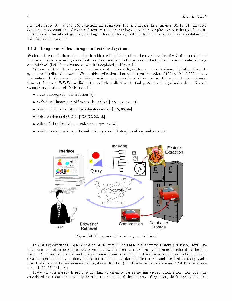
We formulate the basic problem that is addressed in this thesis as the search and retrieval of unconstrainedimages and videos by using visual features. We consider the framework of the typical image and video storageand retrieval (IVSR) environment, which is depicted in Figure 1-1.
We assume that the images and videos are stored in a digital form { in a database, digital archive, �lesystem or distributed network. We consider collections that contain on the order of 100 to 10,000,000 imagesand videos. In the search and retrieval environment, users located on a network (i.e., local area network,intranet, internet, WWW, or dial-up) search the collections to �nd particular images and videos. Severalexample applications of IVSR include:
� stock photography distribution [3],
� Web-based image and video search engines [148, 147, 47, 70],
� on-line publication of multimedia documents [173, 88, 64],
� video-on demand (VOD) [130, 38, 88, 19],
� video editing [96, 95] and video re-purposing [37],
� on-line news, on-line sports and other types of photo-journalism, and so forth.
User
Interface
Database/
Query
Indexing
fv
Feature
Storage
Extraction
CompressionBrowsing/Retrieval
fv
fv
Network
Figure 1-1: Image and video storage and retrieval.
In a straight-forward implementation of the picture database management system (PDBMS), text, an-notations, and other attributes and records allow the users to search using information related to the pic-tures. For example, textual and keyword annotations may include descriptions of the subjects of images,or a photographer's name, date, and so forth. This meta-data is often stored and accessed by using tradi-tional relational database management systems (RDBMS) or object-oriented databases (OODB) (for exam-ple, [21, 16, 15, 161, 28]).
However, this approach provides for limited capacity for retrieving visual information. For one, theassociated meta-data cannot fully describe the contents of the imagery. Very often, the images and videos
Integrated Spatial and Feature Image Systems: Retrieval, Analysis and Compression 3
are annotated manually, which is extremely time-consuming and human-resource intensive, especially if thearchive is large. In general, this approach is not scalable to large archives. Furthermore, it does not anticipatethe myriad of ways in which the content of the visual information is of interest to the users.
To enhance this approach, content-based visual query (CBVQ) techniques use the visual features of theimages and videos in the search process. The CBVQ systems extract and index visual features such ascolors [159, 53, 102, 158, 66, 157], textures [117, 51, 92, 118], shapes [72, 135, 169, 85] and motions [137, 13].The user constructs visual queries using graphical interface tools (for example [71, 151, 142]), or providesexamples of images and videos in order to search for and retrieve the desired items from the archive [3, 45].
Other important components of the system include: image and video compression for e�ciency in storage,browsing and transmission [149], feature access [93, 17], progressive retrieval [109] and viewing [123], andthe use of icons [22, 37, 162, 148]. The systems may also provide tools for browsing and navigating throughthe archive using the visual features [177] and for learning from interaction with the user [97]. For example,relevance feedback techniques [7, 77] guide the system and the user to the desired visual information.
1.2. Problem de�nitions
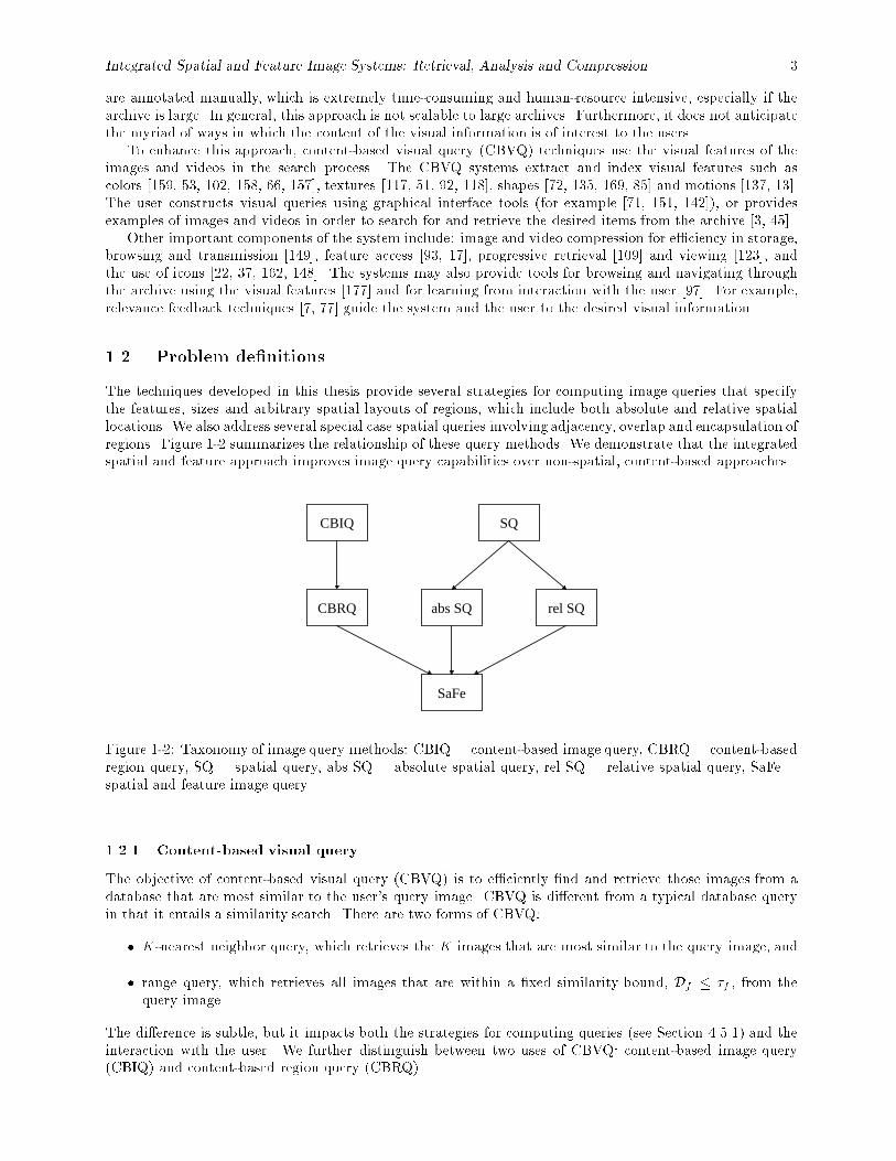
The techniques developed in this thesis provide several strategies for computing image queries that specifythe features, sizes and arbitrary spatial layouts of regions, which include both absolute and relative spatiallocations. We also address several special case spatial queries involving adjacency, overlap and encapsulation ofregions. Figure 1-2 summarizes the relationship of these query methods. We demonstrate that the integratedspatial and feature approach improves image query capabilities over non-spatial, content-based approaches.
CBIQ SQ
abs SQCBRQ rel SQ
SaFe
Figure 1-2: Taxonomy of image query methods: CBIQ = content-based image query, CBRQ = content-basedregion query, SQ = spatial query, abs SQ = absolute spatial query, rel SQ = relative spatial query, SaFe =spatial and feature image query.
1.2.1 Content-based visual query
The objective of content-based visual query (CBVQ) is to e�ciently �nd and retrieve those images from adatabase that are most similar to the user's query image. CBVQ is di�erent from a typical database queryin that it entails a similarity search. There are two forms of CBVQ:
� K-nearest neighbor query, which retrieves the K images that are most similar to the query image, and
� range query, which retrieves all images that are within a �xed similarity bound, Df � �f , from thequery image.
The di�erence is subtle, but it impacts both the strategies for computing queries (see Section 4.5.1) and theinteraction with the user. We further distinguish between two uses of CBVQ: content-based image query(CBIQ) and content-based region query (CBRQ).
4 John R. Smith
1.2.1.1 Content-based image query
Problem 1 Content-based image query (CBIQ). K-nearest neighbor query. Given a collection C ofN images and a feature dissimilarity function Df , �nd the K images IT 2 C with the lowest dissimilarity,Df (IQ; IT ), to the query image IQ.
In this case, a query always returns K images, which are typically sorted by lowest dissimilarity to thequery image. The query computation needs to be more thorough than the bounded CBVQ in order to considerimages that are outside of the similarity bounds in providing the K matches.
Problem 2 Bounded content-based image query. Range query. Given a collection C of N images anda feature dissimilarity function Df , �nd the images IT 2 C such that Df (IQ; IT ) � �f , where IQ is the queryimage and �f is a threshold of feature similarity.
In this case, a query returns any number of images depending on the bounds de�ned by the threshold offeature similarity, �f . The formulation of CBVQ as a bounded similarity search is particularly important inthe investigation of techniques for speeding up the search process. For example, the criteria for evaluatingquery speed-up techniques include the requirement that no images from within the similarity bounds are lostin the search process (no false dismissals, see Section 4.5.1).
We explore both types of CBVQ: unbounded and bounded similarities searches. We note that for anyunbounded query there is an equivalent bounded query with some dissimilarity threshold, which returns onlythe top K matches. As such, we will only di�erentiate between the two formulations when necessary.
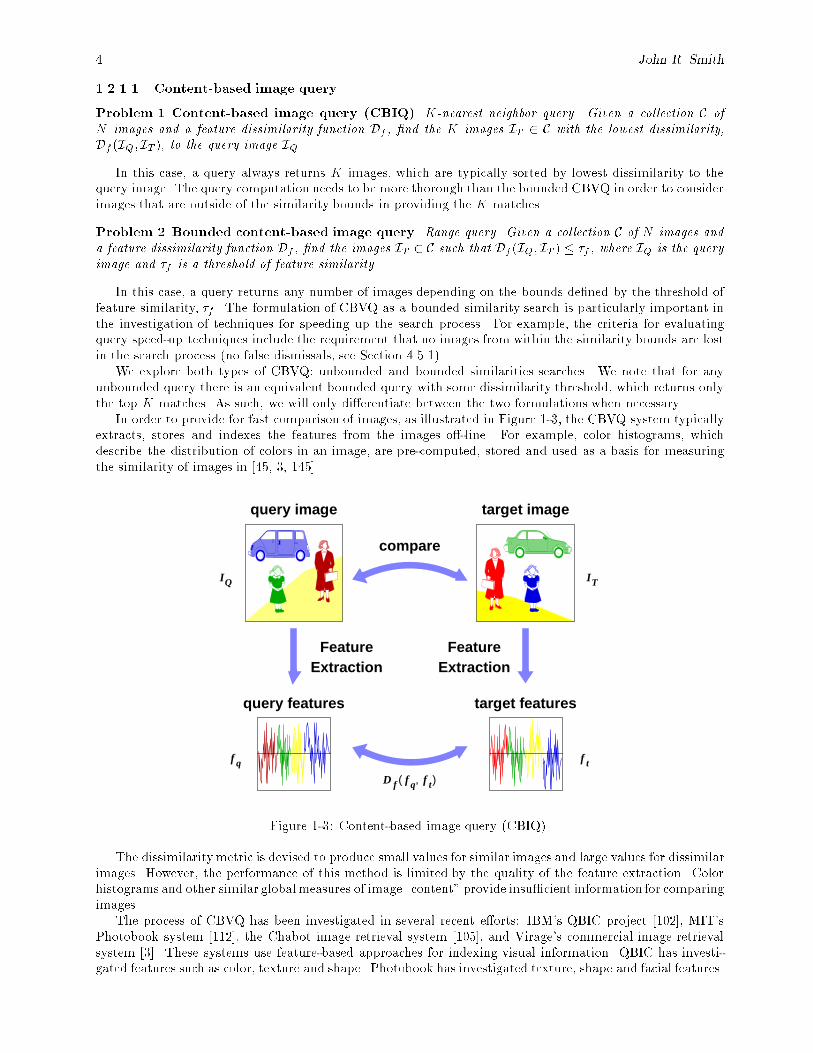
In order to provide for fast comparison of images, as illustrated in Figure 1-3, the CBVQ system typicallyextracts, stores and indexes the features from the images o�-line. For example, color histograms, whichdescribe the distribution of colors in an image, are pre-computed, stored and used as a basis for measuringthe similarity of images in [45, 3, 145].
FeatureExtraction
FeatureExtraction
D f f q f t,( )
f tf q
query image target image
compare
query features target features
ITIQ
Figure 1-3: Content-based image query (CBIQ).
The dissimilaritymetric is devised to produce small values for similar images and large values for dissimilarimages. However, the performance of this method is limited by the quality of the feature extraction. Colorhistograms and other similar globalmeasures of image \content" provide insu�cient information for comparingimages.
The process of CBVQ has been investigated in several recent e�orts: IBM's QBIC project [102], MIT'sPhotobook system [112], the Chabot image retrieval system [105], and Virage's commercial image retrievalsystem [3]. These systems use feature-based approaches for indexing visual information. QBIC has investi-gated features such as color, texture and shape. Photobook has investigated texture, shape and facial features.
Integrated Spatial and Feature Image Systems: Retrieval, Analysis and Compression 5
QBIC has placed a primary research focus on devising strategies for indexing the features [59]. On the otherhand, Photobook has investigated new methods for representing image features which not only provide fordiscrimination of images, but also preserve their semantic information.
When the image database is large and the image feature representations are complex, the exhaustive searchof the database and computation of the image similarities is not expedient. Several recent techniques have beenproposed to speed-up image retrieval. Swain and Ballard [159], Stricker and Orengo [157] and QBIC [102] pre-compute and utilize only simple and fairly compact image features. Petrakis and Faloutsos [114] and QBIC [44]use a combination of data reduction techniques and e�cient indexing structures, one such structure being theR-tree [58], to speed-up image retrieval. QBIC [59] has also investigated e�ective pre-�ltering techniques [59]for reducing the amount of computations at query time. This thesis also presents two new techniques forreducing query computation: binary set bounding (BSB) and query optimized distance (QOD) computation.
However, recent approaches for CBVQ have neglected an important criteria for similarity: region andspatial information and spatial relationships.
1.2.1.2 Content-based region query (CBRQ)
In a content-based region query (CBRQ), the images are compared on the basis of their regions. This di�ersfrom the previous formulation of CBVQ in Problem 1, which uses global feature measurements from theimages. However, the CBRQ can be viewed as an extension of CBVQ in that a �rst stage of the querycomputes the CBVQ on regions instead of images. Then, the �nal stage of the query determines the imagescorresponding to the regions and computes the overall image distance by weighting the region distances.
Problem 3 Content-based Region Query (CBRQ). Given a collection C of N images and feature dis-similarity function Df , �nd the K best images IT 2 C that have at least R regions such that Df (IRQ ; I
RT ) � �f ,
where IRQ is the query image with R regions and �f is a threshold of feature similarity.
CBRQ is improved by adding spatial information into the query. As such, the overall dissimilaritymeasureconsiders the feature and spatial values of the regions. First, we examine the problem of spatial image query.
1.2.2 Spatial image query
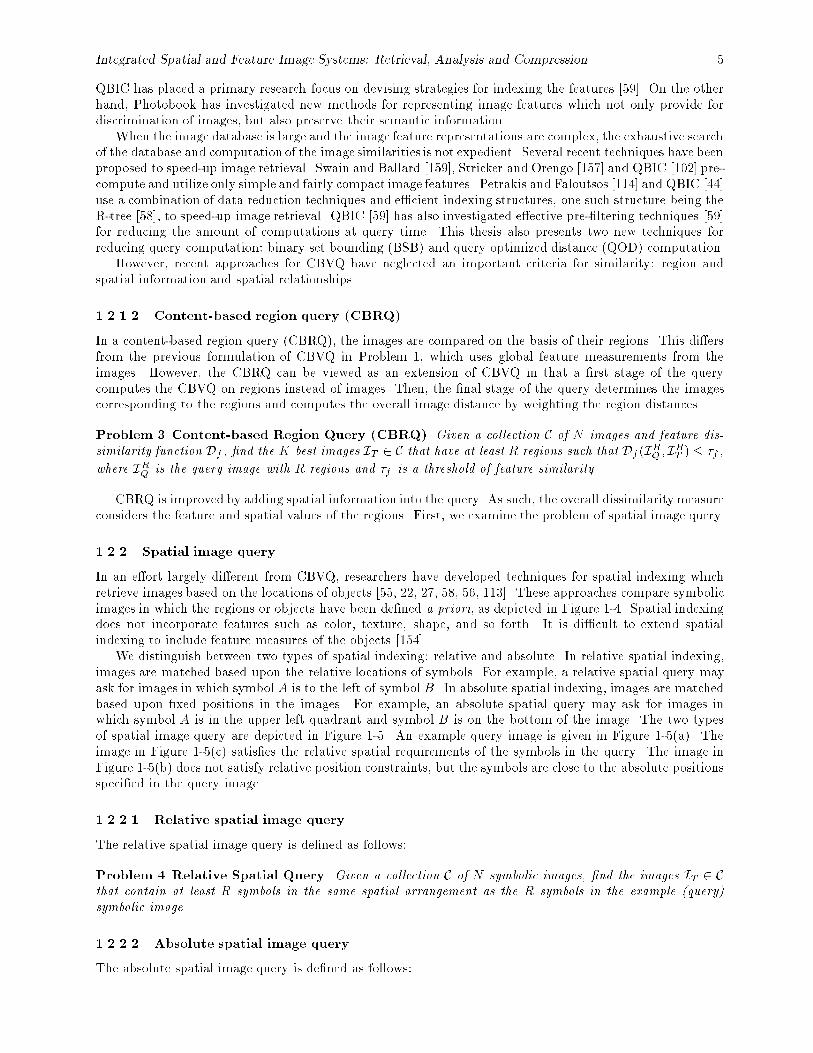
In an e�ort largely di�erent from CBVQ, researchers have developed techniques for spatial indexing whichretrieve images based on the locations of objects [55, 22, 27, 58, 56, 113]. These approaches compare symbolicimages in which the regions or objects have been de�ned a priori, as depicted in Figure 1-4. Spatial indexingdoes not incorporate features such as color, texture, shape, and so forth. It is di�cult to extend spatialindexing to include feature measures of the objects [154].
We distinguish between two types of spatial indexing: relative and absolute. In relative spatial indexing,images are matched based upon the relative locations of symbols. For example, a relative spatial query mayask for images in which symbol A is to the left of symbol B. In absolute spatial indexing, images are matchedbased upon �xed positions in the images. For example, an absolute spatial query may ask for images inwhich symbol A is in the upper left quadrant and symbol B is on the bottom of the image. The two typesof spatial image query are depicted in Figure 1-5. An example query image is given in Figure 1-5(a). Theimage in Figure 1-5(c) satis�es the relative spatial requirements of the symbols in the query. The image inFigure 1-5(b) does not satisfy relative position constraints, but the symbols are close to the absolute positionsspeci�ed in the query image.
1.2.2.1 Relative spatial image query
The relative spatial image query is de�ned as follows:
Problem 4 Relative Spatial Query. Given a collection C of N symbolic images, �nd the images IT 2 C
that contain at least R symbols in the same spatial arrangement as the R symbols in the example (query)symbolic image.
1.2.2.2 Absolute spatial image query
The absolute spatial image query is de�ned as follows:
6 John R. Smith
query image absolute match relative match
A
BC
DE
F
FE
D
B
A
CB
A
C
(a) (b) (c)
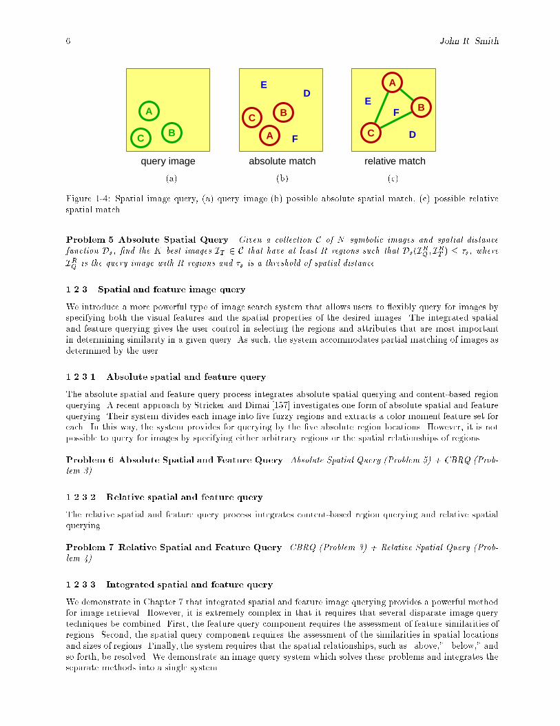
Figure 1-4: Spatial image query, (a) query image (b) possible absolute spatial match, (c) possible relativespatial match.
Problem 5 Absolute Spatial Query. Given a collection C of N symbolic images and spatial distancefunction Ds, �nd the K best images IT 2 C that have at least R regions such that Ds(I
RQ ; I
RT ) � �s, where
IRQ is the query image with R regions and �s is a threshold of spatial distance.
1.2.3 Spatial and feature image query
We introduce a more powerful type of image search system that allows users to exibly query for images byspecifying both the visual features and the spatial properties of the desired images. The integrated spatialand feature querying gives the user control in selecting the regions and attributes that are most importantin determining similarity in a given query. As such, the system accommodates partial matching of images asdetermined by the user.
1.2.3.1 Absolute spatial and feature query
The absolute spatial and feature query process integrates absolute spatial querying and content-based regionquerying. A recent approach by Stricker and Dimai [157] investigates one form of absolute spatial and featurequerying. Their system divides each image into �ve fuzzy regions and extracts a color moment feature set foreach. In this way, the system provides for querying by the �ve absolute region locations. However, it is notpossible to query for images by specifying either arbitrary regions or the spatial relationships of regions.
Problem 6 Absolute Spatial and Feature Query. Absolute Spatial Query (Problem 5) + CBRQ (Prob-lem 3).
1.2.3.2 Relative spatial and feature query
The relative spatial and feature query process integrates content-based region querying and relative spatialquerying.
Problem 7 Relative Spatial and Feature Query. CBRQ (Problem 3) + Relative Spatial Query (Prob-lem 4).
1.2.3.3 Integrated spatial and feature query
We demonstrate in Chapter 7 that integrated spatial and feature image querying provides a powerful methodfor image retrieval. However, it is extremely complex in that it requires that several disparate image querytechniques be combined. First, the feature query component requires the assessment of feature similarities ofregions. Second, the spatial query component requires the assessment of the similarities in spatial locationsand sizes of regions. Finally, the system requires that the spatial relationships, such as \above," \below," andso forth, be resolved. We demonstrate an image query system which solves these problems and integrates theseparate methods into a single system.
Integrated Spatial and Feature Image Systems: Retrieval, Analysis and Compression 7
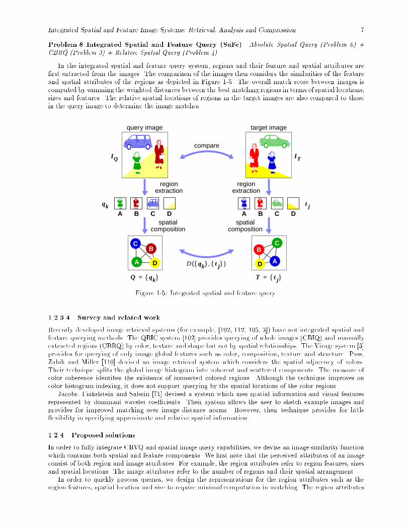
Problem 8 Integrated Spatial and Feature Query (SaFe). Absolute Spatial Query (Problem 6) +CBRQ (Problem 3) + Relative Spatial Query (Problem 4).
In the integrated spatial and feature query system, regions and their feature and spatial attributes are�rst extracted from the images. The comparison of the images then considers the similarities of the featureand spatial attributes of the regions as depicted in Figure 1-5. The overall match score between images iscomputed by summing the weighted distances between the best matching regions in terms of spatial locations,sizes and features. The relative spatial locations of regions in the target images are also compared to thosein the query image to determine the image matches.
B
regionextraction
Q qk{ }=
A C D BA C D
t jqk
regionextraction
query image target image
compare
IQ IT
D qk{ } t j{ },( )
T t j{ }=
CB
A D A
BC
D
spatialcomposition
spatialcomposition
Figure 1-5: Integrated spatial and feature query.
1.2.3.4 Survey and related work
Recently developed image retrieval systems (for example, [102, 112, 105, 3]) have not integrated spatial andfeature querying methods. The QBIC system [102] provides querying of whole images (CBIQ) and manuallyextracted regions (CBRQ) by color, texture and shape but not by spatial relationships. The Virage system [3]provides for querying of only image global features such as color, composition, texture and structure. Pass,Zabih and Miller [110] devised an image retrieval system which considers the spatial adjacency of colors.Their technique splits the global image histogram into coherent and scattered components. The measure ofcolor coherence identi�es the existence of connected colored regions. Although the technique improves oncolor histogram indexing, it does not support querying by the spatial locations of the color regions.
Jacobs, Finkelstein and Salesin [71] devised a system which uses spatial information and visual featuresrepresented by dominant wavelet coe�cients. Their system allows the user to sketch example images andprovides for improved matching over image distance norms. However, their technique provides for little exibility in specifying approximate and relative spatial information.
1.2.4 Proposed solutions
In order to fully integrate CBVQ and spatial image query capabilities, we devise an image similarity functionwhich contains both spatial and feature components. We �rst note that the perceived attributes of an imageconsist of both region and image attributes. For example, the region attributes refer to region features, sizesand spatial locations. The image attributes refer to the number of regions and their spatial arrangement.
In order to quickly process queries, we design the representations for the region attributes such as theregion features, spatial location and size to require minimal computation in matching. The region attributes
8 John R. Smith
are indexed directly to allow for maximal e�ciency in queries. The overall image matches are determinedfrom the candidate regions retrieved in the region queries.
In this way, a query speci�ed by the user is translated directly into pruning operations on the regionattributes. The image attributes, such as region relative locations and special spatial relations, are resolvedonly in the �nal stage of the query. This is because these evaluations have the highest complexity. Thepruning performed by the queries on the regions reduces the number of candidate images and regions thatneed to be evaluated at the �nal stages.
1.3. Summary of contributions
We summarize the contributions of this thesis in improving systems for retrieving, analyzing and compressingimages as follows: in this thesis we
1. demonstrate a new integrated spatial and feature query paradigm for image retrieval,
2. develop a new representation of texture based upon texture channel energy histograms, which is sym-metric to that for color histograms,
3. explore new binary set representations of color and texture and their applications in region extractionand integrated spatial and feature image retrieval,
4. present two new approaches, binary set bounding (BSB) and query-optimized distance (QOD) compu-tation, for e�ciently computing feature similarity queries,
5. develop a new general framework for extracting spatially localized features from images using histogramand binary set back-projections,
6. develop a new system for image compression and analysis based upon a joint-adaptive space and fre-quency (JASF) graph, which includes:
(a) the development of the theory of partitionable expansions,
(b) the creation of a new framework for developing general tree- and graph-structured signal decom-positions, which include spatial quad-tree, wavelet packets, the double-tree and the JASF graph,
7. implement several new image and video retrieval prototype systems, which provide for
(a) cataloging of and searching for visual information on the World-Wide Web,
(b) content-based and relevance feedback searching for images, and
(c) integrated spatial and feature image querying.
1.4. Outline of thesis
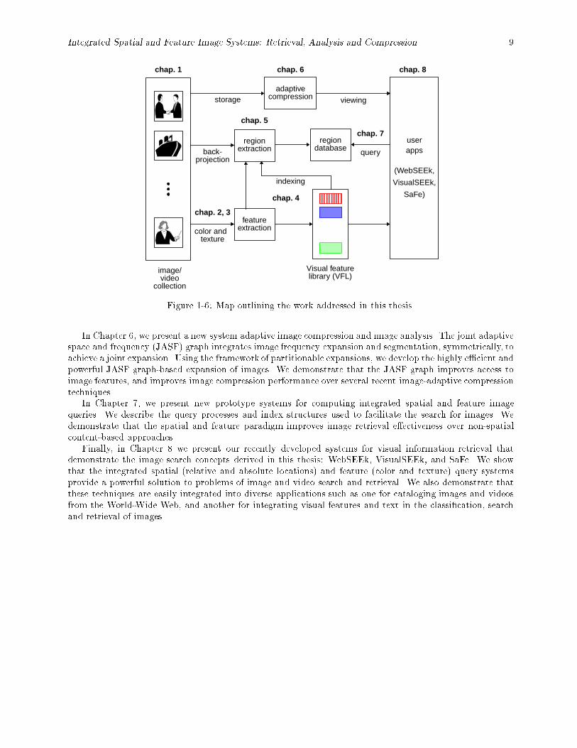
The thesis is organized as follows (see Figure 1-6): we develop representations of color in Chapter 2 andtexture in Chapter 3. In both visual dimensions, we �rst obtain multiple channel representations of images.Through processes of transformation and quantization of the channels, we obtain feature spaces for measuringthe color and texture elements, respectively. From these, we obtain the histograms and binary sets. In short,a color histogram de�nes the distribution of colors and a texture histogram de�nes a distribution of textureelements. The binary sets de�ne only the selection of colors and texture elements, respectively.
In Chapter 4, we de�ne metrics for discriminating among images using measures of the similarities of colorand texture, respectively. We provide a thorough evaluation of eight distance metrics along the dimensions of(1) retrieval e�ectiveness in example image queries and (2) query computation e�ciency. We also introduce thetwo powerful techniques for computing the feature queries: binary set bounding (BSB) and query optimizeddistance (QOD) computation.
In Chapter 5, we investigate the process of extracting color and texture regions from imagery. We presentthe histogram back-projection (HBP) procedure for detecting and extracting color and texture regions. Wedescribe and compare the performance of �ve back-projection algorithms and present some examples of colorand texture back-projection. We also develop a procedure for automatically extracting regions from imagesby using a binary set iteration (BSI) and back-projection procedure.
Integrated Spatial and Feature Image Systems: Retrieval, Analysis and Compression 9
regiondatabase
userapps
image/video
collection
Visual featurelibrary (VFL)
adaptivecompression
chap. 6
chap. 2, 3
chap. 7
chap. 8chap. 1
query
viewingstorage
indexing(WebSEEk,
VisualSEEk,
SaFe)
back-projection
color andtexture
featureextraction
regionextraction
chap. 5
chap. 4
Figure 1-6: Map outlining the work addressed in this thesis.
In Chapter 6, we present a new system adaptive image compression and image analysis. The joint adaptivespace and frequency (JASF) graph integrates image frequency expansion and segmentation, symmetrically, toachieve a joint expansion. Using the framework of partitionable expansions, we develop the highly e�cient andpowerful JASF graph-based expansion of images. We demonstrate that the JASF graph improves access toimage features, and improves image compression performance over several recent image-adaptive compressiontechniques.
In Chapter 7, we present new prototype systems for computing integrated spatial and feature imagequeries. We describe the query processes and index structures used to facilitate the search for images. Wedemonstrate that the spatial and feature paradigm improves image retrieval e�ectiveness over non-spatialcontent-based approaches.
Finally, in Chapter 8 we present our recently developed systems for visual information retrieval thatdemonstrate the image search concepts derived in this thesis: WebSEEk, VisualSEEk, and SaFe. We showthat the integrated spatial (relative and absolute locations) and feature (color and texture) query systemsprovide a powerful solution to problems of image and video search and retrieval. We also demonstrate thatthese techniques are easily integrated into diverse applications such as one for cataloging images and videosfrom the World-Wide Web, and another for integrating visual features and text in the classi�cation, searchand retrieval of images.
10 John R. Smith
Chapter 2
Representing Color
2.1. Introduction
We present a uni�ed framework for representing the color and texture features. The objectives are to providea basis for
1. assessing the similarities of the visual features of images,
2. storing and indexing the visual feature information and
3. extracting the salient regions from images.
We will show that these objectives are accomplished by representing color and texture by histograms. Thehistograms provide a measure of the distribution of features inside a region or image. By appropriatelydesigning the feature spaces in which the histograms are de�ned, the histograms su�ciently represent thevisual dimensions of color and texture and satisfy the above objectives.
In this chapter (for color), and the next chapter (Chapter 3, for texture), we generate and evaluate thefeature spaces for color and texture which allow for representation of color and texture using histogramsand binary sets. For both visual dimensions, we show that candidate feature spaces are generated throughthe processes of transformation T and quantization Q of the image data. The design goal is to identify thetransformation and quantization pairs: (Tc; Qc) for color, and (Tt; Qt) for texture that generate perceptuallyuniform, complete and compact feature spaces. We also examine the special case of histograms that arebinary. These binary sets are extremely compact and are suitable for representing, storing, indexing (seeChapter 4) and extracting image features (see Chapter 5).
2.2. Feature representation
In both visual dimensions, color and texture, the image points are initially represented as multi-dimensionalfeature points: a color point is de�ned by values in three color channels and a texture point is de�ned by theenergy in nine spatial-frequency (s-f) channels. The feature points are transformed and quantized to generatefeature spaces with 166 colors and 512 texture elements, respectively.
Using these feature elements, we utilize two approaches each for representing color and texture: histogramsand binary sets. Histograms are a distribution of feature elements. Binary feature sets are a selection of featureelements.
2.3. Related work on color image retrieval
The use of color histograms for image retrieval has been previously explored in [159, 103, 145, 43, 110].The fundamental elements of this approach include the selection of the color feature space (Tc; Qc) and thehistogram distance metric Dc. There has been no consensus about which color feature space is most suitablefor color histogram-based image retrieval. The problem is a result of the fact there does not exist a universallyaccepted color space, and color perception is signi�cantly subjective [175]. Therefore, we have seen a largevariety of color spaces used in practice.
For example, Swain and Ballard [159] utilize an opponent-axis (OPP) color system [4] quantized to 2048colors in a system for color image retrieval. The IBM QBIC system [103] �rst quantizes the RGB color space
Integrated Spatial and Feature Image Systems: Retrieval, Analysis and Compression 11
into 4096 colors (16 levels per each color channel). Then, each color is transformed to the Munsell color spaceby the MTM transform [98]. Finally, clustering determines the k best Munsell colors (typically, k = 64).
On the other hand, Pass, Zabih and Miller [110] simply utilize the RGB color space, quantized uniformlyto 64 colors, in their image retrieval system. Finally, Gray [53], to retrieve images, transforms RGB �rst toCIE-LUV and then partitions the CIE-LUV color space to 512 colors.
In this chapter, we present a framework for selecting and evaluating the color spaces for the purpose ofcolor histogram-based retrieval. We begin by discussing the basic properties of color and colorimetry.
2.4. Colorimetry
Electromagnetic radiation F (�) in the range of visible light (� 2 f380nm : : :780nmg) is perceived as coloror colored light. It has been veri�ed experimentally that color is perceived through three independent colorreceptors which have peak response at approximately, red, green and blue wavelengths, �r = 700nm; �g =546:1nm; �b = 435:8nm, respectively. By assigning each primary color receptor, k 2 fr; b; gg, a responsefunction ck(�), visible light of any color F (�), is represented by a linear superposition of the ck(�)'s [104], asfollows: by normalizing ck(�)'s to reference white light W (�) such that
W (�) = cr(�) + cg(�) + cb(�);
F (�) produces the tristimulus responses (R;G;B), such that
F (�) = R cr(�) +G cg(�) + B cb(�): (2.1)
As such, any color can be represented by a linear combination of the three primary colors (R;G;B).
2.5. Color image perception
The perception of color images is a complex process, and we make several simplifying assumptions: we assumethat color is a single pixel process. In this sense, the perception of color is assumed to not be in uenced bysurrounding colors. We also assume that viewing conditions, such as ambient lighting, viewer adaptation,viewing distance, and image display quality can be ignored. Generally, it is di�cult to control these parametersin the diverse application environments that are anticipated for color image retrieval.
2.6. Color space transformation and quantization
The space spanned by the R;G; and B values (see Eq 2.1) is complete in that all colors are representedas vectors in the 3-D RGB space. We use this space as the starting point for representing color featuresin images. We investigate the transformations Tc of RGB and subsequent quantizations Qc that generatepartitioned color spaces with properties of uniformity, completeness, compactness and naturalness. Thesespaces allow for image color content to be de�ned by color histograms and color sets.
Property 1 Uniformity. The metric proximity between colors indicates the perceived similarity of colors.
We will see in Chapter 3 that the color-based image comparison utilizes a proximity metric of the colorfeatures. For one, this comparison requires that color proximity is simple to compute. One way to assurethis, is to design the color space transformation such that color proximity is not a function of the position incolor space. The transformation Tc, which is the primary determinant of the uniformity of the color space,also determines along with quantization Qc, it's completeness and compactness.
Property 2 Completeness. The color space includes all perceptually distinct colors.
It is necessary that the color space is complete in that all perceptually distinct colors are included. Visualcompleteness does not guarantee mathematical completeness, however, the converse is true. In general, ifthe transformation Tc is invertible, then the un-quantized color space will be complete. In this case, thequantization Qc will determine the completeness.
Property 3 Compactness. Each color in the color space is perceptually distinct from the other colors.

12 John R. Smith
In order to restrict the dimensionality of the image color feature representation, or similarly, the numberof colors, the color space is non-redundant or \compact." Mathematically, nonredundancy is assured whenthe mapping from RGB is one-to-one or many-to-one. Visually, nonredundancy requires that no two colorsare so similar that they are perceived as identical. In general, selection of quantization Qc will involve atrade-o� between completeness and compactness.
Property 4 Naturalness. The color space provides for a natural breakdown of colors into the three basicperceptual attributes of color: brightness, hue and saturation.
The separation of color into components of brightness, hue and saturation are intuitive for the user [68]. Theease in navigating the color space impacts the user's ability to construct color-based image queries.
1. Brightness. Attribute of visual sensation which corresponds to a color exhibiting more or less light.Variations range from bright to dim.
2. Hue. Attribute of visual sensation which corresponds to a color appearing similar to one or two of theperceived colors red, yellow, green and blue.
3. Saturation. Attribute of visual sensation which corresponds to a color exhibiting more or less of itshue. Saturation allows the judgment to be made of the degree to which a colored light di�ers from anachromatic light regardless of their brightness.
We design the transformation Tc and quantization Qc to produce a color space that meets these objectives.These conditions are typically application speci�c. For example, medical and satellite images require di�erentcolor spaces than unconstrained imagery, such as color photos, in order to retain uniformity, completenessand compactness in representing the color features.
We begin by de�ning a color point as a vector in the RGB color space as follows
De�nition 1 Color point, vc. A color point is a vector vc = (r; g; b) in RGB color space.
The transformation Tc and quantization Qc of the RGB color space reorganizes and groups the vectors vc tocreate a �nite set of M colors.
2.6.1 Color transformation
The color transformation Tc is an operation on the vectors vc 2 RGB to produce the transformed vectorswc. The simplest color transformations are linear. For example, from RGB, the color spaces: Y IQ (NTSCcomposite color TV standard), Y UV (PAL and SECAM color television standards), Y CrCb (JPEG digitalimage standard and MPEG digital video standard) and opponent color space OPP are obtained by lineartransformation [126]. Other color spaces, such as HSV , CIE 1976 (L�a�b�) and CIE 1976 (L�u�v�) aregenerated by non-linear transformations. The overall e�ect of color transformation Tc is to produce a newcolor space.
Since the RGB color space is continuous, or possibly discrete with a large number of values (i.e., digitalphotographs are typically represented in RGB color space discretized to 256 levels per axis, which gives over1:67 million distinct color points), the color space must be quantized or partitioned into a smaller number ofcolors.
2.6.2 Color quantization
Since the color spaces are multi-dimensional, a partitioning of a color space is described by the vectorquantization of the space. In general, a vector quantizer Qc of dimension k and size M is a mapping from avector in k-dimensional space into a �nite set C containing M outputs [50]. Thus, a vector quantizer Qc isde�ned as Qc : <k ! C, where C = (y0;y1; : : : ;yM�1) and ym 2 <k for each m 2 0; 1; : : : ;M � 1. In general,the set C is called the codebook and has size M . In the case of vector quantization of the color space, k = 3,and each entry in the codebook ym corresponds to a color point.
Therefore, the codebook C represents the gamut or collection of colors. In this way, a color, whichcorresponds to one quantized partition Rm of the color space and is an approximate perceptual unit. This isdistinguished from the transformed color point wc, which is a mathematical vector in the continuous space.
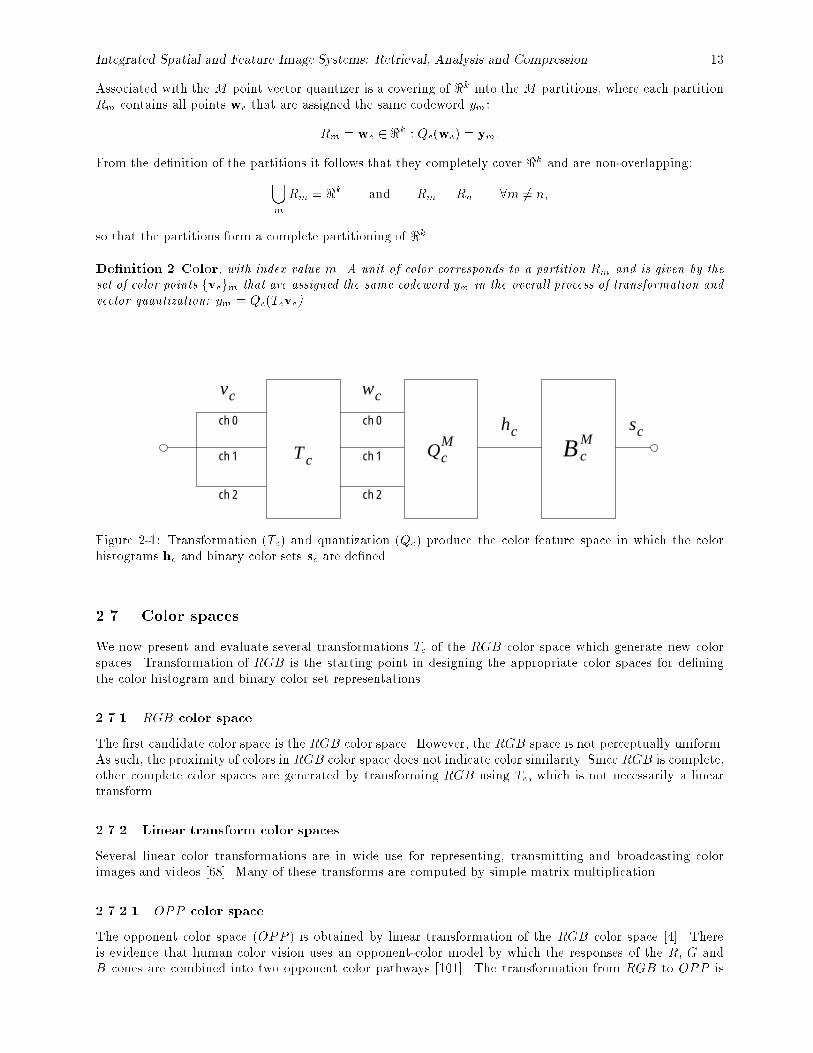
Integrated Spatial and Feature Image Systems: Retrieval, Analysis and Compression 13
Associated with the M point vector quantizer is a covering of <k into the M partitions, where each partitionRm contains all points wc that are assigned the same codeword ym:
Rm = wc 2 <k : Qc(wc) = ym:
From the de�nition of the partitions it follows that they completely cover <k and are non-overlapping:
[m
Rm = <k and Rm
\Rn 8m 6= n;
so that the partitions form a complete partitioning of <k.
De�nition 2 Color, with index value m. A unit of color corresponds to a partition Rm and is given by theset of color points fvcgm that are assigned the same codeword ym in the overall process of transformation andvector quantization: ym = Qc(Tcvc).
T cQc
M B cM
vc wc
hc scch 0
ch 1
ch 2
ch 0
ch 1
ch 2
Figure 2-1: Transformation (Tc) and quantization (Qc) produce the color feature space in which the colorhistograms hc and binary color sets sc are de�ned.
2.7. Color spaces
We now present and evaluate several transformations Tc of the RGB color space which generate new colorspaces. Transformation of RGB is the starting point in designing the appropriate color spaces for de�ningthe color histogram and binary color set representations.
2.7.1 RGB color space
The �rst candidate color space is the RGB color space. However, the RGB space is not perceptually uniform.As such, the proximity of colors in RGB color space does not indicate color similarity. Since RGB is complete,other complete color spaces are generated by transforming RGB using Tc, which is not necessarily a lineartransform.
2.7.2 Linear transform color spaces
Several linear color transformations are in wide use for representing, transmitting and broadcasting colorimages and videos [68]. Many of these transforms are computed by simple matrix multiplication.
2.7.2.1 OPP color space
The opponent color space (OPP ) is obtained by linear transformation of the RGB color space [4]. Thereis evidence that human color vision uses an opponent-color model by which the responses of the R, G andB cones are combined into two opponent color pathways [101]. The transformation from RGB to OPP is
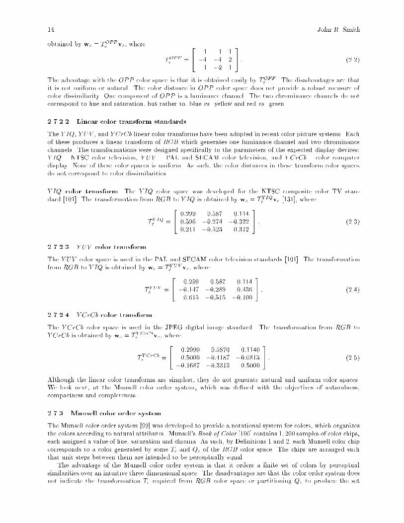
14 John R. Smith
obtained by wc = TOPPc vc, where
TOPPc =
24 1 1 1�1 �1 21 �2 1
35 : (2.2)
The advantage with the OPP color space is that it is obtained easily by TOPPc . The disadvantages are thatit is not uniform or natural. The color distance in OPP color space does not provide a robust measure ofcolor dissimilarity. One component of OPP is a luminance channel. The two chrominance channels do notcorrespond to hue and saturation, but rather to, blue vs. yellow and red vs. green.
2.7.2.2 Linear color transform standards
The Y IQ, Y UV , and Y CrCb linear color transforms have been adopted in recent color picture systems. Eachof these produces a linear transform of RGB which generates one luminance channel and two chrominancechannels. The transformations were designed speci�cally to the parameters of the expected display devices:Y IQ { NTSC color television, Y UV { PAL and SECAM color television, and Y CrCb { color computerdisplay. None of these color spaces is uniform. As such, the color distances in these transform color spacesdo not correspond to color dissimilarities.
Y IQ color transform The Y IQ color space was developed for the NTSC composite color TV stan-dard [101]. The transformation from RGB to Y IQ is obtained by wc = TY IQc vc [131], where
TY IQc =
24 0:299 0:587 0:114
0:596 �0:274 �0:3220:211 �0:523 0:312
35 : (2.3)
2.7.2.3 Y UV color transform
The Y UV color space is used in the PAL and SECAM color television standards [101]. The transformationfrom RGB to Y IQ is obtained by wc = T Y UVc vc, where
TY UVc =
24 0:299 0:587 0:114�0:147 �0:289 0:4360:615 �0:515 �0:100
35 : (2.4)
2.7.2.4 Y CrCb color transform
The Y CrCb color space is used in the JPEG digital image standard. The transformation from RGB toY CrCb is obtained by wc = T Y CrCbc vc, where
T Y CrCbc =
24 0:2990 0:5870 0:1140
0:5000 �0:4187 �0:0813�0:1687 �0:3313 0:5000
35 : (2.5)
Although the linear color transforms are simplest, they do not generate natural and uniform color spaces.We look next, at the Munsell color order system, which was de�ned with the objectives of naturalness,compactness and completeness.
2.7.3 Munsell color order system
The Munsell color order system [99] was developed to provide a notational system for colors, which organizesthe colors according to natural attributes. Munsell's Book of Color [100] contains 1; 200 samples of color chips,each assigned a value of hue, saturation and chroma. As such, by De�nitions 1 and 2, each Munsell color chipcorresponds to a color generated by some Tc and Qc of the RGB color space. The chips are arranged suchthat unit steps between them are intended to be perceptually equal.
The advantage of the Munsell color order system is that it orders a �nite set of colors by perceptualsimilarities over an intuitive three dimensional space. The disadvantages are that the color order system doesnot indicate the transformation Tc required from RGB color space or partitioning Qc to produce the set
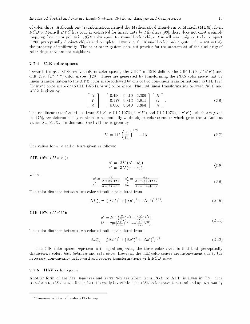
Integrated Spatial and Feature Image Systems: Retrieval, Analysis and Compression 15
of color chips. Although one transformation, named the Mathematical Transform to Munsell (MTM), fromRGB to Munsell HV C has been investigated for image data by Miyahara [98], there does not exist a simplemapping from color points in RGB color space to Munsell color chips. Munsell was designed to be compact(1200 perceptually distinct chips) and complete. However, the Munsell color order system does not satisfythe property of uniformity. The color order system does not provide for the assessment of the similarity ofcolor chips that are not neighbors.
2.7.4 CIE color spaces
Towards the goal of deriving uniform color spaces, the CIE � in 1976 de�ned the CIE 1976 (L�u�v�) andCIE 1976 (L�a�b�) color spaces [129]. These are generated by transforming the RGB color space �rst bylinear transformation to the XY Z color space followed by one of two non-linear transformations: to CIE 1976(L�u�v�) color space or to CIE 1976 (L�a�b�) color space. The �rst linear transformation between RGB andXY Z is given by 2
4 XYZ
35 =
24 0:490 0:310 0:200
0:177 0:813 0:0110:000 0:010 0:990
3524 RGB
35 : (2.6)
The nonlinear transformations from XY Z to CIE 1976 (L�a�b�) and CIE 1976 (L�u�v�), which are givenin [175], are determined by relation to a nominally white object-color stimulus which gives the tristimulusvalues Xn; Yn; Zn. In this case, the lightness is given by
L� = 116
�Y
Yn
�1=3� 16: (2.7)
The values for u, v and a, b are given as follows:
CIE 1976 (L�u�v�):u� = 13L�(u0 � u0n)v� = 13L�(v0 � v0n);
(2.8)
whereu0 = 4X
X+15Y+3Z u0n =4Xn
Xn+15Yn+3Zn
v0 = 9YX+15Y+3Z u0n =
9YnXn+15Yn+3Zn
:(2.9)
The color distance between two color stimuli is calculated from
�E�
uv = [(�L�)2 + (�u�)2 + (�v�)2]1=2: (2.10)
CIE 1976 (L�a�b�):a� = 500[( X
Xn)1=3 � ( Y
Yn)1=3]
b� = 200[( YYn )1=3 � ( ZZn )
1=3]:(2.11)
The color distance between two color stimuli is calculated from:
�E�
ab = [(�L�)2 + (�a�)2 + (�b�)2]1=2: (2.12)
The CIE color spaces represent with equal emphasis, the three color variants that best perceptuallycharacterize color: hue, lightness and saturation. However, the CIE color spaces are inconvenient due to thenecessary non-linearity in forward and reverse transformations with RGB space.
2.7.5 HSV color space
Another form of the hue, lightness and saturation transform from RGB to HSV is given in [68]. Thetransform to HSV is non-linear, but it is easily invertible. The HSV color space is natural and approximately
�Commission Internationale de l'Eclairage
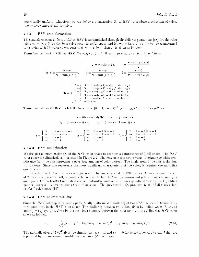
16 John R. Smith
perceptually uniform. Therefore, we can de�ne a quantization Qc of HSV to produce a collection of colorsthat is also compact and complete.
2.7.5.1 HSV transformation
This transformation Tc from RGB to HSV is accomplished through the following equations [68]: let the colortriple vc = (r; g; b) be the to a color point in RGB space and let wc = (h; s; v) be the to the transformedcolor point in HSV color space, such that wc = Tc(vc), then Tc is given as follows:
Transformation 1 RGB to HSV For r; g; b 2 [0 : : :1] then Tc gives h; s; v 2 [0 : : :1] as follows
v = max(r; g; b); s =v �min(r; b; g)
v
let �r =v � r
v �min(r; b; g); �g =
v � g
v �min(r; b; g); �b =
v � b
v �min(r; b; g)
6h =
8>>>><>>>>:
5 + �b if r = max(r; g; b) and g = min(r; b; g)1� �g if r = max(r; g; b) and g 6= min(r; b; g)1 + �r if g = max(r; g; b) and b = min(r; b; g)
3� �b if g = max(r; g; b) and b 6= min(r; b; g)3 + �g if b = max(r; g; b) and r = min(r; b; g)5� �r otherwise
Transformation 2 HSV to RGB For h; s; v 2 [0 : : :1] then T�1c gives r; g; b 2 [0 : : :1] as follows
� = 6h� round(6h); !1 = (1 � s) � v;!2 = (1� (s � �)) � v; !3 = (1� (s � (1� �))) � v
r =
8<:
v if � = 0 or � = 5!1 if � = 2 or � = 3!2 if � = 1!3 if � = 4
g =
8<:
v if � = 1 or � = 2!1 if � = 4 or � = 5!2 if � = 3!3 if � = 0
b =
8<:
v if � = 3 or � = 4!1 if � = 0 or � = 1!2 if � = 5!3 if � = 2
2.7.5.2 HSV quantization
We design the quantization Qc of the HSV color space to produce a compact set of (166) colors. The HSVcolor space is cylindrical, as illustrated in Figure 2-2. The long axis represents value: blackness to whiteness.Distance from the axis represents saturation: amount of color present. The angle around the axis is the hue:tint or tone. Since hue represents the most signi�cant characteristic of the color, it requires the most �nequantization.
In the hue circle, the primaries red, green and blue are separated by 120 degrees. A circular quantizationat 20 degree steps su�ciently separates the hues such that the three primaries and yellow, magenta and cyanare represented each with three sub-divisions. Saturation and value are each quantized to three levels yieldinggreater perceptual tolerance along these dimensions. The quantization Qc provides M = 166 distinct colorsin HSV color space [145].
2.7.5.3 HSV color similarity
Since the HSV color space is nearly perceptually uniform, the similarity of two HSV colors is determined bytheir proximity in the HSV color space. The similarity between two colors given by indices mi = (hi; si; vi)and mj = (hj ; sj; vj) is given by the euclidean distance between the color points in the cylindrical HSV colorspace as follows:
ai;j = 1� 1p5[(vi � vj)
2 + (si coshi � sj coshj)2 + (si sinhi � sj sinhj)
2]1
2 : (2.13)
The normalization by 1=p5 gives the similarities: ai;i = 1, and ai;j = 0 for colors indexed by i and j that are
separated by the maximum possible distance in HSV color space.
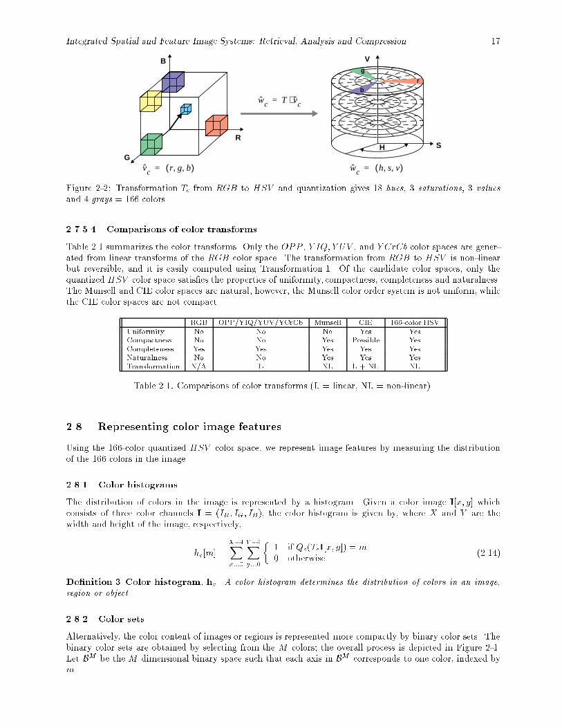
Integrated Spatial and Feature Image Systems: Retrieval, Analysis and Compression 17
vc r g b, ,( )=
R
G
B
S
V
H
wc T vc⋅=
r
g
b
wc h s v, ,( )=
Figure 2-2: Transformation Tc from RGB to HSV and quantization gives 18 hues, 3 saturations, 3 valuesand 4 grays = 166 colors.
2.7.5.4 Comparisons of color transforms
Table 2.1 summarizes the color transforms. Only the OPP , Y IQ; Y UV , and Y CrCb color spaces are gener-ated from linear transforms of the RGB color space. The transformation from RGB to HSV is non-linearbut reversible, and it is easily computed using Transformation 1. Of the candidate color spaces, only thequantized HSV color space satis�es the properties of uniformity, compactness, completeness and naturalness.The Munsell and CIE color spaces are natural, however, the Munsell color order system is not uniform, whilethe CIE color spaces are not compact.
RGB OPP/YIQ/YUV/YCrCb Munsell CIE 166-color HSVUniformity No No No Yes YesCompactness No No Yes Possible YesCompleteness Yes Yes Yes Yes YesNaturalness No No Yes Yes YesTransformation N/A L NL L + NL NL
Table 2.1: Comparisons of color transforms (L = linear, NL = non-linear).
2.8. Representing color image features
Using the 166-color quantized HSV color space, we represent image features by measuring the distributionof the 166 colors in the image.
2.8.1 Color histograms
The distribution of colors in the image is represented by a histogram. Given a color image I[x; y] whichconsists of three color channels I = (IR; IG; IB), the color histogram is given by, where X and Y are thewidth and height of the image, respectively,
hc[m] =X�1Xx:::0
Y�1Xy:::0
�1 if Qc(TcI[x; y]) = m0 otherwise
(2.14)
De�nition 3 Color histogram, hc. A color histogram determines the distribution of colors in an image,region or object.
2.8.2 Color sets
Alternatively, the color content of images or regions is represented more compactly by binary color sets. Thebinary color sets are obtained by selecting from the M colors; the overall process is depicted in Figure 2-1.Let BM be the M dimensional binary space such that each axis in BM corresponds to one color, indexed bym.
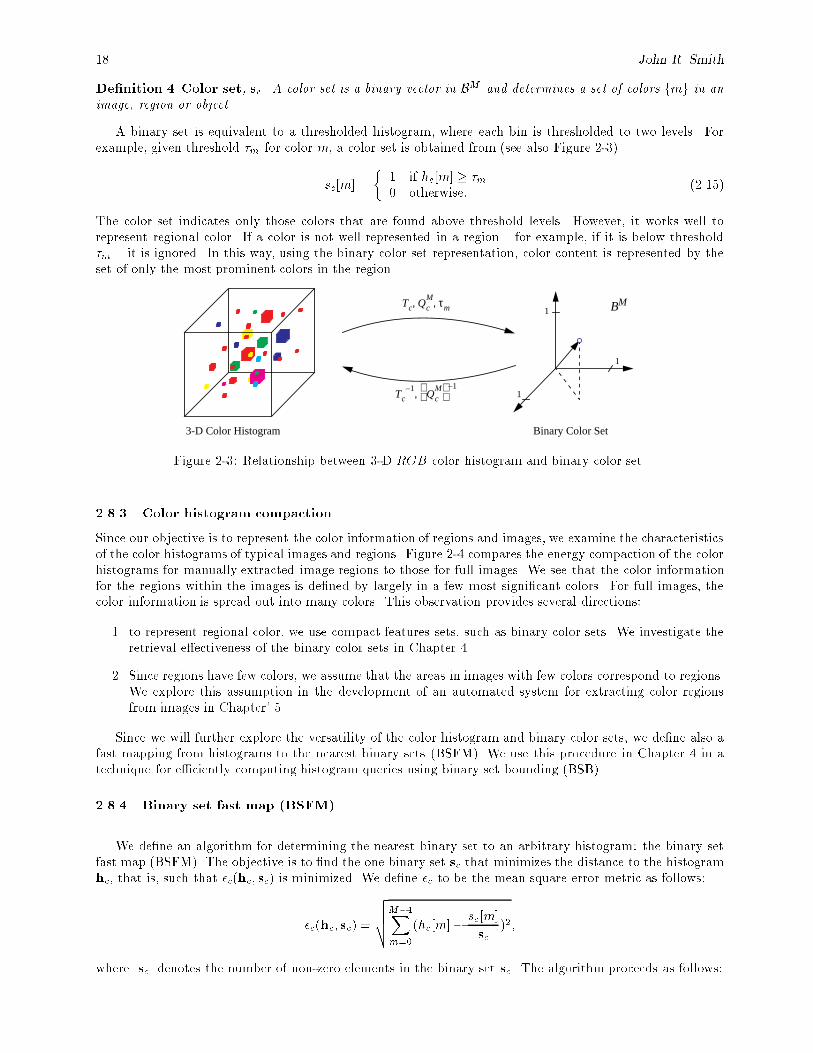
18 John R. Smith
De�nition 4 Color set, sc. A color set is a binary vector in BM and determines a set of colors fmg in animage, region or object.
A binary set is equivalent to a thresholded histogram, where each bin is thresholded to two levels. Forexample, given threshold �m for color m, a color set is obtained from (see also Figure 2-3)
sc[m] =
�1 if hc[m] � �m0 otherwise:
(2.15)
The color set indicates only those colors that are found above threshold levels. However, it works well torepresent regional color. If a color is not well represented in a region { for example, if it is below threshold�m { it is ignored. In this way, using the binary color set representation, color content is represented by theset of only the most prominent colors in the region.
3-D Color Histogram Binary Color Set
Tc QcM τm, ,
Tc1–
QcM
1–
,
BM1
1
1
Figure 2-3: Relationship between 3-D RGB color histogram and binary color set.
2.8.3 Color histogram compaction
Since our objective is to represent the color information of regions and images, we examine the characteristicsof the color histograms of typical images and regions. Figure 2-4 compares the energy compaction of the colorhistograms for manually extracted image regions to those for full images. We see that the color informationfor the regions within the images is de�ned by largely in a few most signi�cant colors. For full images, thecolor information is spread out into many colors. This observation provides several directions:
1. to represent regional color, we use compact features sets, such as binary color sets. We investigate theretrieval e�ectiveness of the binary color sets in Chapter 4.
2. Since regions have few colors, we assume that the areas in images with few colors correspond to regions.We explore this assumption in the development of an automated system for extracting color regionsfrom images in Chapter' 5.
Since we will further explore the versatility of the color histogram and binary color sets, we de�ne also afast mapping from histograms to the nearest binary sets (BSFM). We use this procedure in Chapter 4 in atechnique for e�ciently computing histogram queries using binary set bounding (BSB).
2.8.4 Binary set fast map (BSFM)
We de�ne an algorithm for determining the nearest binary set to an arbitrary histogram: the binary setfast map (BSFM). The objective is to �nd the one binary set sc that minimizes the distance to the histogramhc, that is, such that �c(hc; sc) is minimized. We de�ne �c to be the mean square error metric as follows:
�c(hc; sc) =
vuutM�1Xm=0
(hc[m]� sc[m]
jscj )2;
where jscj denotes the number of non-zero elements in the binary set sc. The algorithm proceeds as follows:
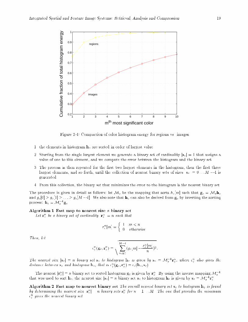
Integrated Spatial and Feature Image Systems: Retrieval, Analysis and Compression 19
1 2 3 4 5 6 7 8 9 100.2
0.3
0.4
0.5
0.6
0.7
0.8
0.9
1
regions
images
mth most significant color
Cum
ulat
ive
frac
tion
of to
tal h
isto
gram
ene
rgy
Figure 2-4: Compaction of color histogram energy for regions vs. images.
1. the elements in histogram hc are sorted in order of largest value.
2. Starting from the single largest element we generate a binary set of cardinality jscj = 1 that assigns avalue of one to this element, and we compute the error between the histogram and the binary set.
3. The process is then repeated for the �rst two largest elements in the histogram, then the �rst threelargest elements, and so forth, until the collection of nearest binary sets of sizes jscj = 0 : : :M � 1 isgenerated.
4. From this collection, the binary set that minimizes the error to the histogram is the nearest binary set.
The procedure is given in detail as follows: let Ms be the mapping that sorts hc[m] such that gc = Mshcand gc[0] � gc[1] � : : : � gc[M �1]. We also note that hc can also be derived from gc by inverting the sortingprocess: hc =M�1
s gc.
Algorithm 1 Fast map to nearest size n binary setLet rnc be a binary set of cardinality jrnc j = n such that
rnc [m] =
�1 m < n0 otherwise
Then, let
�nc (gc; rnc ) =
vuutM�1Xm=0
(gc[m]� rnc [m]
n)2:
The nearest size jscj = n binary set sc to histogram hc is given by sc = M�1s rnc , where �nc also gives the
distance between sc and histogram hc, that is �nc (gc; rnc ) = �c(hc; sc).
The nearest jrnc j = n binary set to sorted histogram gc is given by rnc . By using the inverse mappingM�1s
that was used to sort hc, the nearest size jscj = n binary set sc to histogram hc is given by sc =M�1s rnc .
Algorithm 2 Fast map to nearest binary set The overall nearest binary set sc to histogram hc is foundby determining the nearest size jsnc j = n binary sets snc for n = 1 : : :M . The one that provides the minimum�nc gives the nearest binary set.

20 John R. Smith
Overall, the algorithm requires M logM operations to sort the histogram hc, M computations of meansquare error and M operations to determine the nearest binary set.
2.9. Summary
In this chapter, we evaluated several transformations (Tc) and quantizations (Qc) of color. The objectiveswere to obtain a color feature space in which color histograms are de�ned. We demonstrated that the HSVcolor space, quantized to 166 values provides a suitable color space because it is uniform, complete, compactand natural.
We de�ned the color histograms (hc) as distributions of the HSV colors that appear in an image orregion. We also presented the binary color set representation. Binary color sets (sc) represent only a selectionof colors and provide a compact measure of image and/or region color. We also de�ned a fast algorithm(BSFM) for computing the nearest binary color set to a color histogram.
Using the content-based image query paradigm, we explore the image retrieval e�ectiveness of the colorhistogram and color set representations in Chapter 4. Then, in Chapter 5, we present and evaluate tech-niques for extracting color regions from images using the color histograms and binary color sets. Thesefeature extraction and feature query processes are integrated to produce the spatial and color feature querysystem described in Chapter 7. However, in the next chapter, we �rst develop the texture histogram andbinary texture set representations of texture that are symmetric with those for color. This allows us to usesgeneric methods of feature and region extraction, and feature indexing and querying that are compatible withrepresentations of both visual dimensions.
Integrated Spatial and Feature Image Systems: Retrieval, Analysis and Compression 21
Chapter 3
Representing Texture
3.1. Introduction
The texture representation is symmetric with color in that texture is also de�ned from multiple channels.The texture images are �rst decomposed into nine spatial-frequency subbands using a wavelet �lter bank(FB). Then, from the nine subbands, a texture channel generator (TCG) produces the nine channels. Asinvestigated in Chapter 2 for color, we investigate procedures for transforming (Tt) and quantizing (Qt) thetexture channels to produce a texture element feature space in which to de�ne suitable histogram (ht) andbinary texture set (st) representations of texture.
In this chapter, we present the overall process of representing texture using the texture histograms. Wepresent the wavelet texture energy feature set and compare it to Gabor �lter-based representations. We alsopresent experimental evaluations of the wavelet texture feature sets that demonstrate excellent performance inclassifying the standard evaluation-set of Brodatz textures. We then investigate several transformations thatallow for approximate rotation or scale invariance. Finally, we present the process of generating the texturehistogram and binary texture set-based feature spaces that are symmetric to those for color histogramsdiscussed in Chapter 2.
The objectives of obtaining these representations of texture are to provide systems for measuring thesimilarity of textures and extracting texture regions from images. In Chapter 4, we present and evaluate thevarious techniques for computing texture similarity using the representations presented here. In Chapter 5,we present the system for extracting texture regions from images using texture histograms.
3.2. What is texture?
Textures are homogeneous patterns or spatial arrangements of pixels that regional intensity or color alonedoes not su�ciently describe. As such, textures have statistical properties, structural properties, or both [60].They may consist of the structured and/or random placement of elements, but also may be without funda-mental subunits. For example, Figure 3-1 illustrates the wide variety of textures from the Brodatz collection.Moreover, due to the diversity of textures appearing in natural images it is di�cult to narrowly de�ne texture.
Texture is an important element to human vision. Texture has been found to provide cues to scene depthand surface orientation [4]. People also tend to relate texture elements of varying size to a plausible 3-Dsurface. Even in graphics systems greater realism is achieved when textures are mapped to the 3-D surfaces.Texture features have been used to identify contents of ariel imagery such as bodies of water, crop �elds andmountains [92, 4, 87, 92]. Texture describes the content of many real-world images: for example, clouds,trees, bricks, hair, fabric all have textural characteristics.
It has been hard to adequately model texture. The substantial body of work on texture has not yetproduced any clear solutions for the problems of texture analysis, classi�cation, segmentation and synthe-sis [164]. Furthermore, the analysis and extraction of texture in unconstrained imagery, which is the mostdi�cult problem, has not yet been su�ciently addressed.
Most research on texture is conducted on the Brodatz [9] texture collection (sixteen Brodatz texturesare illustrated in Figure 3-1), which provides a set of mostly homogeneous texture images. In the Brodatzcollection there is little visible distortion in the images that results from viewing perspective and lighting.
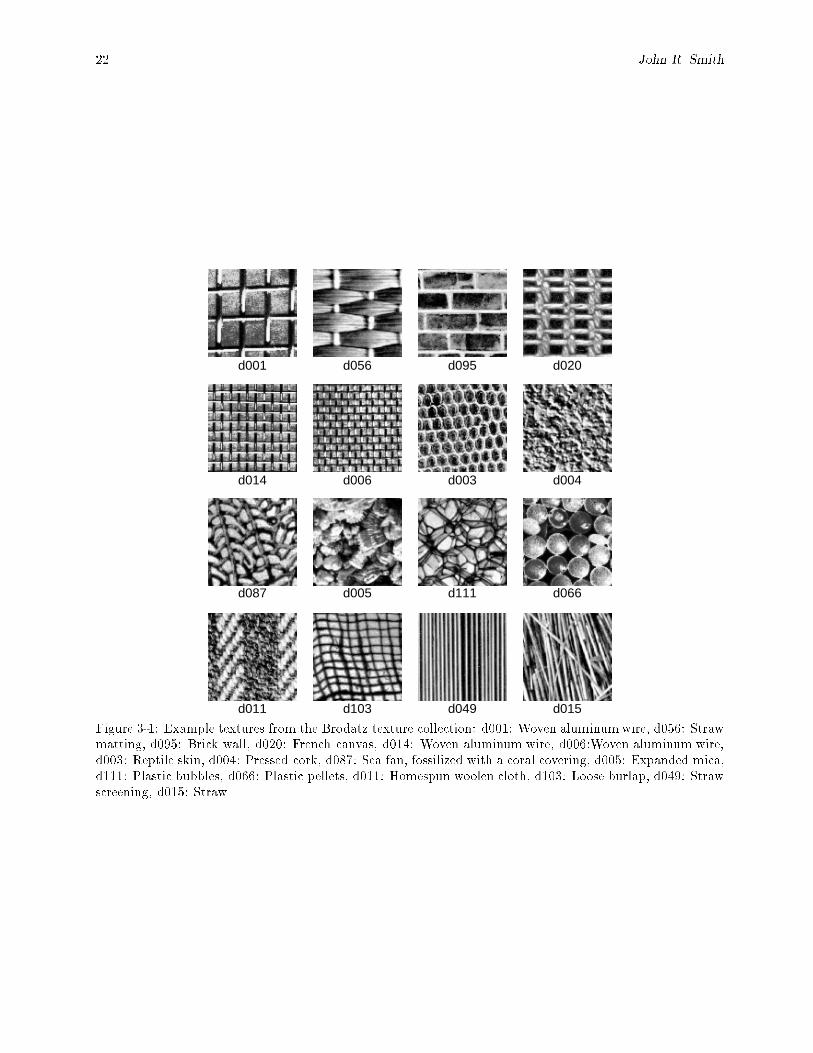
22 John R. Smith
d001 d056 d095 d020
d014 d006 d003 d004
d087 d005 d111 d066
d011 d103 d049 d015
Figure 3-1: Example textures from the Brodatz texture collection: d001: Woven aluminumwire, d056: Strawmatting, d095: Brick wall, d020: French canvas, d014: Woven aluminum wire, d006:Woven aluminum wire,d003: Reptile skin, d004: Pressed cork, d087: Sea fan, fossilized with a coral covering, d005: Expanded mica,d111: Plastic bubbles, d066: Plastic pellets, d011: Homespun woolen cloth, d103: Loose burlap, d049: Strawscreening, d015: Straw.
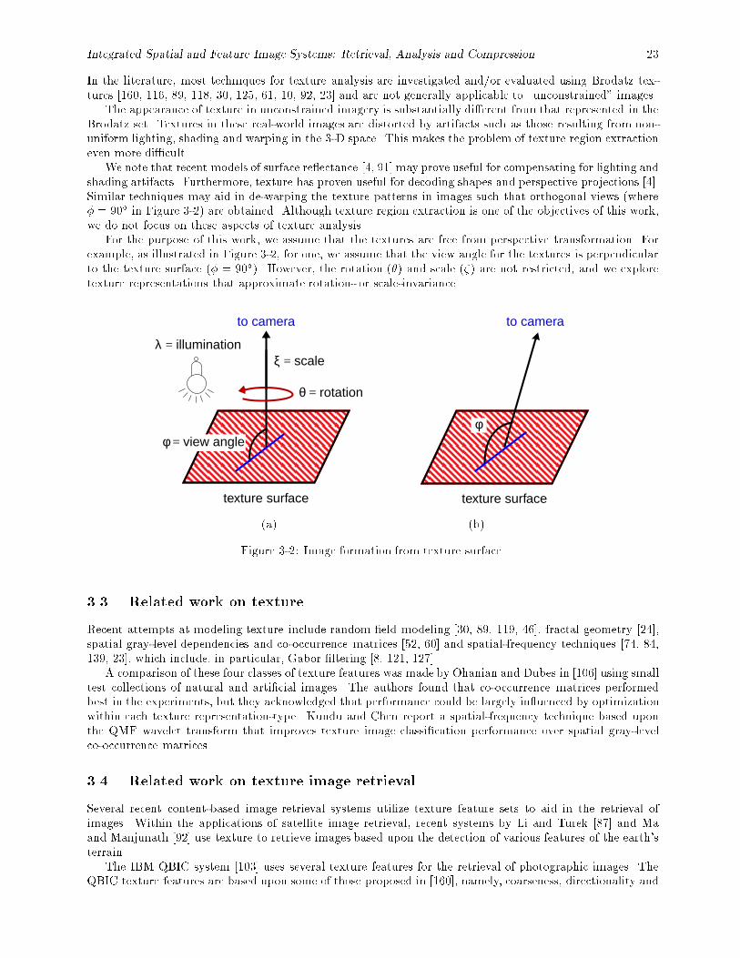
Integrated Spatial and Feature Image Systems: Retrieval, Analysis and Compression 23
In the literature, most techniques for texture analysis are investigated and/or evaluated using Brodatz tex-tures [160, 116, 89, 118, 30, 125, 61, 10, 92, 23] and are not generally applicable to \unconstrained" images.
The appearance of texture in unconstrained imagery is substantially di�erent from that represented in theBrodatz set. Textures in these real-world images are distorted by artifacts such as those resulting from non-uniform lighting, shading and warping in the 3-D space. This makes the problem of texture region extractioneven more di�cult.
We note that recent models of surface re ectance [4, 91] may prove useful for compensating for lighting andshading artifacts. Furthermore, texture has proven useful for decoding shapes and perspective projections [4].Similar techniques may aid in de-warping the texture patterns in images such that orthogonal views (where� = 90� in Figure 3-2) are obtained. Although texture region extraction is one of the objectives of this work,we do not focus on these aspects of texture analysis.
For the purpose of this work, we assume that the textures are free from perspective transformation. Forexample, as illustrated in Figure 3-2, for one, we assume that the view angle for the textures is perpendicularto the texture surface (� = 90�). However, the rotation (�) and scale (�) are not restricted, and we exploretexture representations that approximate rotation- or scale-invariance.
texture surface
θ rotation=
ξ scale=
φ view angle=
λ illumination=
to camera
texture surface
to camera
φ
(a) (b)
Figure 3-2: Image formation from texture surface.
3.3. Related work on texture
Recent attempts at modeling texture include random �eld modeling [30, 89, 119, 46], fractal geometry [24],spatial gray-level dependencies and co-occurrence matrices [52, 60] and spatial-frequency techniques [74, 84,139, 23], which include, in particular, Gabor �ltering [8, 121, 127].
A comparison of these four classes of texture features was made by Ohanian and Dubes in [106] using smalltest collections of natural and arti�cial images. The authors found that co-occurrence matrices performedbest in the experiments, but they acknowledged that performance could be largely in uenced by optimizationwithin each texture representation-type. Kundu and Chen report a spatial-frequency technique based uponthe QMF wavelet transform that improves texture image classi�cation performance over spatial gray-levelco-occurrence matrices.
3.4. Related work on texture image retrieval
Several recent content-based image retrieval systems utilize texture feature sets to aid in the retrieval ofimages. Within the applications of satellite image retrieval, recent systems by Li and Turek [87] and Maand Manjunath [92] use texture to retrieve images based upon the detection of various features of the earth'sterrain.
The IBM QBIC system [103] uses several texture features for the retrieval of photographic images. TheQBIC texture features are based upon some of those proposed in [160], namely, coarseness, directionality and
24 John R. Smith
contrast. Other texture features in [160] such as linelikeness, regularity and roughness are not used. Boththe whole images and manually identi�ed regions are indexed by texture in the QBIC system.
The Virage system [3] also uses texture measures for photographic image retrieval. In the Virage system,the texture features describe the whole image, rather than regions of texture within the images.
A uni�ed approach for the characterization of global color, texture and shape was proposed by Caelli andReye in [12]. Their objective was to classify objects which have color, texture and shape attributes. In theirexperiments, they used hand-written text characters rendered with di�erent color and texture patterns. Theirsystem was not applied to retrieval of unconstrained images.
Liu and Picard [89, 119] and Francos, Meiri and Porat [46] have investigated the Wold random-�eld modelfor modeling texture. The Wold model separates the image into components that correspond, approximately,to periodicity, directionality and randomness [119]. Liu and Picard have applied Wold feature to segmentationand retrieval of natural scene images [89].
Gorkani and Picard have investigated a texture measure based upon \dominant perceived orientation"for sorting photos [51]. The orientation is extracted over levels of a multiresolution steerable pyramid. Theyfound that this texture feature is successful in classifying scenes as \city" vs. \suburb."
We propose a new representation of texture which is derived from spatial-frequency energy of the texture.From the energy values, a texture histogram is generated. The texture histogram is used to discriminatetextures and to retrieve images. This approach is compatible with color histogram-based methods for content-based image systems. Furthermore, since the texture histograms are derived from the QMF wavelet transform,the features are more directly accessible from wavelet-compressed image representations.
3.5. Representations of texture
As described earlier, the objectives in developing the texture feature set are to provide a basis for (1) as-sessing the similarities of the texture features in images, (2) storing and indexing texture information and(3) extracting texture regions from images. In order to develop the texture feature set, we formulate therepresentation of texture from a set of channels. This provides an approach that is symmetric with that forthe color feature sets.
The most suitable models are based upon the spatial-frequency (s-f) techniques. For one, the s-f texturemodels are also most aligned with the vision process. There is support that mechanisms of early humanvision use receptive �eld units tuned to orientations and s-f's [54, 74]. In particular, models of the humanvision system that use Gabor �lters to model the receptive �elds su�ciently account for psychophysical dataobtained in texture discrimination experiments.
3.5.1 Space/spatial-frequency expansion
A space/spatial-frequency (s/s-f) expansion of the image captures its localized spatial-frequency content. Ingeneral, image s-f transforms attain a joint resolution in space and s-f that is bounded by the uncertaintyprinciple [36, 171]. By spacing the �lters at octave-band distances, the wavelet �lter bank (FB) providesdyadic trade-o�s in spatial and s-f resolution. Obtaining a high joint resolution in space and s-f is critical intexture region extraction where the localization of the texture pattern is important.
Gabor �lters are one s-f technique which has been used to characterize texture by dominant s-fs [8].Gabor functions measure the localized s-f information at speci�c s-f scales and orientations. One objectivein modeling texture by Gabor functions is to characterize a texture by a single peak scale and orientationset [8].
Alternatively, Chang and Kuo [23] have used the tree-structured wavelet transform (TSWT) to classifytexture, not by a single narrow subband, but by the overall best wavelet packet basis adapted to each texture.Feature sets based upon s-fs that use multiple subbands have also been investigated in [74, 84, 106]. We nowlook more closely at the Gabor FB and examine their relationship to QMF wavelet FBs.
3.5.2 Gabor Functions
Gabor �lters achieve the theoretical lower bound of the uncertainty principle. They attain maximum jointresolution in space and s-f bounded by the relations �x � �u � 1
4� and �y � �v � 14� where (�x;�y)
gives resolution in space and (�u;�v) gives resolution in s-f. This is highly signi�cant in the process oftexture extraction in which the con icting objectives of accuracy in texture representation and texture spatial
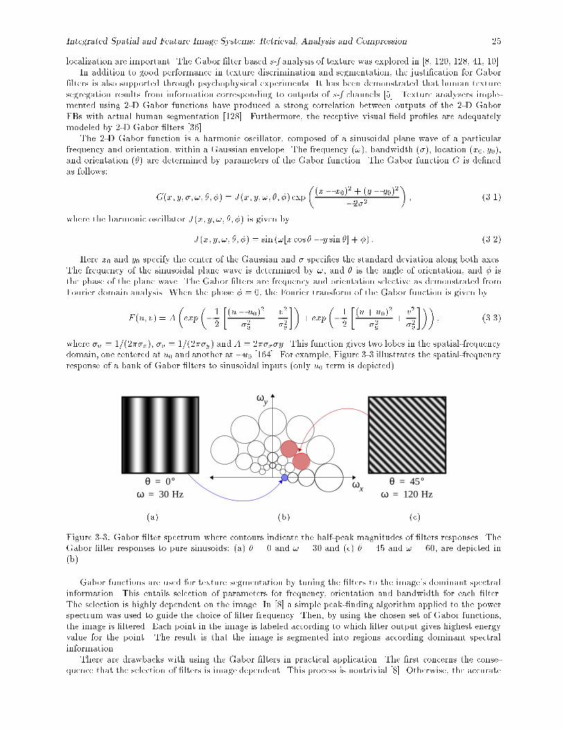
Integrated Spatial and Feature Image Systems: Retrieval, Analysis and Compression 25
localization are important. The Gabor �lter based s-f analysis of texture was explored in [8, 120, 128, 41, 10].In addition to good performance in texture discrimination and segmentation, the justi�cation for Gabor
�lters is also supported through psychophysical experiments. It has been demonstrated that human texturesegregation results from information corresponding to outputs of s-f channels [5]. Texture analyzers imple-mented using 2-D Gabor functions have produced a strong correlation between outputs of the 2-D GaborFBs with actual human segmentation [128]. Furthermore, the receptive visual �eld pro�les are adequatelymodeled by 2-D Gabor �lters [36].
The 2-D Gabor function is a harmonic oscillator, composed of a sinusoidal plane wave of a particularfrequency and orientation, within a Gaussian envelope. The frequency (!), bandwidth (�), location (x0; y0),and orientation (�) are determined by parameters of the Gabor function. The Gabor function G is de�nedas follows:
G(x; y; �; !; �; �) = J(x; y; !; �; �) exp
�(x� x0)
2 + (y � y0)2
�2�2
�; (3.1)
where the harmonic oscillator J(x; y; !; �; �) is given by
J(x; y; !; �; �) = sin (![x cos � � y sin �] + �) : (3.2)
Here x0 and y0 specify the center of the Gaussian and � speci�es the standard deviation along both axes.The frequency of the sinusoidal plane wave is determined by !, and � is the angle of orientation, and � isthe phase of the plane wave. The Gabor �lters are frequency and orientation selective as demonstrated fromFourier domain analysis. When the phase � = 0, the Fourier transform of the Gabor function is given by
F (u; v) = A
�exp
��1
2
�(u � u0)2
�2u+
v2
�2v
��+ exp
��1
2
�(u+ u0)2
�2u+
v2
�2v
���; (3.3)
where �u = 1=(2��x), �v = 1=(2��y) and A = 2��x�y. This function gives two lobes in the spatial-frequencydomain, one centered at u0 and another at �u0 [164]. For example, Figure 3-3 illustrates the spatial-frequencyresponse of a bank of Gabor �lters to sinusoidal inputs (only u0 term is depicted).
θ 45°=ω 120 Hz=
ωx
ωy
θ 0°=ω 30 Hz=
(a) (b) (c)
Figure 3-3: Gabor �lter spectrum where contours indicate the half-peak magnitudes of �lters responses. TheGabor �lter responses to pure sinusoids: (a) � = 0 and ! = 30 and (c) � = 45 and ! = 60, are depicted in(b).
Gabor functions are used for texture segmentation by tuning the �lters to the image's dominant spectralinformation. This entails selection of parameters for frequency, orientation and bandwidth for each �lter.The selection is highly dependent on the image. In [8] a simple peak-�nding algorithm applied to the powerspectrum was used to guide the choice of �lter frequency. Then, by using the chosen set of Gabor functions,the image is �ltered. Each point in the image is labeled according to which �lter output gives highest energyvalue for the point. The result is that the image is segmented into regions according dominant spectralinformation.
There are drawbacks with using the Gabor �lters in practical application. The �rst concerns the conse-quence that the selection of �lters is image dependent. This process is nontrivial [8]. Otherwise, the accurate
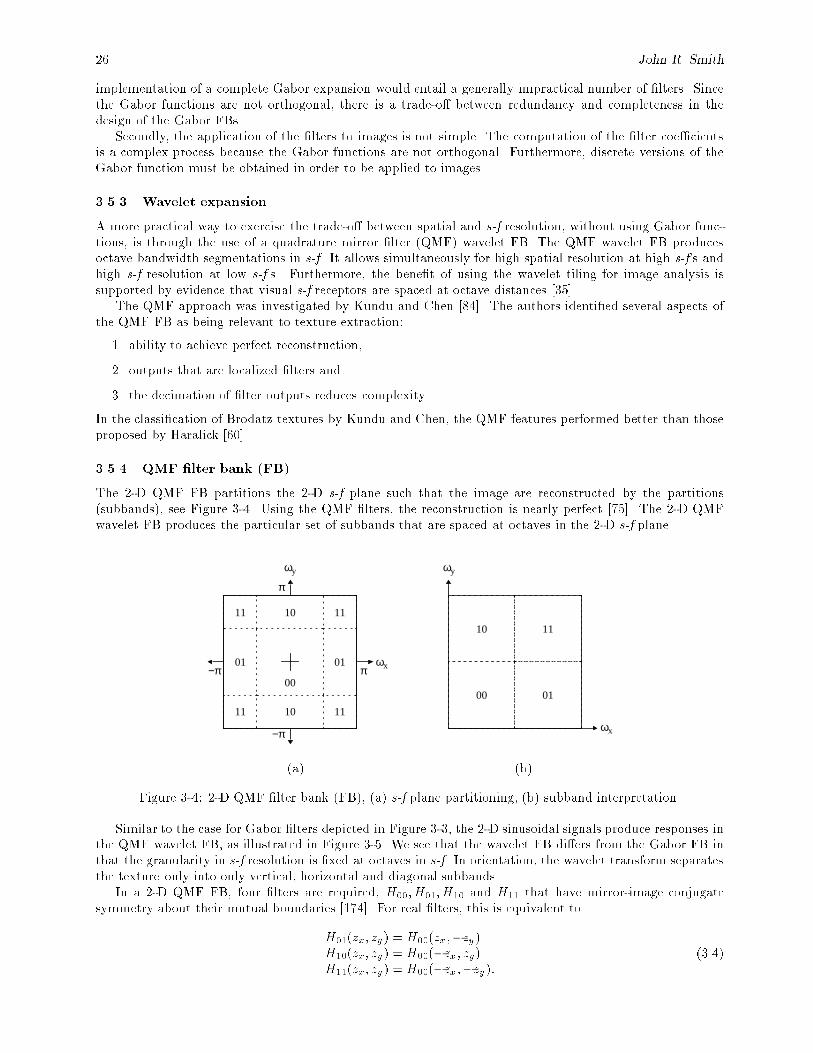
26 John R. Smith
implementation of a complete Gabor expansion would entail a generally impractical number of �lters. Sincethe Gabor functions are not orthogonal, there is a trade-o� between redundancy and completeness in thedesign of the Gabor FBs.
Secondly, the application of the �lters to images is not simple. The computation of the �lter coe�cientsis a complex process because the Gabor functions are not orthogonal. Furthermore, discrete versions of theGabor function must be obtained in order to be applied to images.
3.5.3 Wavelet expansion
A more practical way to exercise the trade-o� between spatial and s-f resolution, without using Gabor func-tions, is through the use of a quadrature mirror �lter (QMF) wavelet FB. The QMF wavelet FB producesoctave bandwidth segmentations in s-f. It allows simultaneously for high spatial resolution at high s-f's andhigh s-f resolution at low s-f's. Furthermore, the bene�t of using the wavelet tiling for image analysis issupported by evidence that visual s-f receptors are spaced at octave distances [35].
The QMF approach was investigated by Kundu and Chen [84]. The authors identi�ed several aspects ofthe QMF FB as being relevant to texture extraction:
1. ability to achieve perfect reconstruction,
2. outputs that are localized �lters and
3. the decimation of �lter outputs reduces complexity.
In the classi�cation of Brodatz textures by Kundu and Chen, the QMF features performed better than thoseproposed by Haralick [60].
3.5.4 QMF �lter bank (FB)
The 2-D QMF FB partitions the 2-D s-f plane such that the image are reconstructed by the partitions(subbands), see Figure 3-4. Using the QMF �lters, the reconstruction is nearly perfect [75]. The 2-D QMFwavelet FB produces the particular set of subbands that are spaced at octaves in the 2-D s-f plane.
00
01
10 1111
11 1110
01 ωx
ωy
π
π
−π
−π
ωx
ωy
00
11
01
10
(a) (b)
Figure 3-4: 2-D QMF �lter bank (FB), (a) s-f plane partitioning, (b) subband interpretation.
Similar to the case for Gabor �lters depicted in Figure 3-3, the 2-D sinusoidal signals produce responses inthe QMF wavelet FB, as illustrated in Figure 3-5. We see that the wavelet FB di�ers from the Gabor FB inthat the granularity in s-f resolution is �xed at octaves in s-f. In orientation, the wavelet transform separatesthe texture only into only vertical, horizontal and diagonal subbands.
In a 2-D QMF FB, four �lters are required, H00;H01;H10 and H11 that have mirror-image conjugatesymmetry about their mutual boundaries [174]. For real �lters, this is equivalent to
H01(zx; zy) = H00(zx;�zy)H10(zx; zy) = H00(�zx; zy)H11(zx; zy) = H00(�zx;�zy):
(3.4)
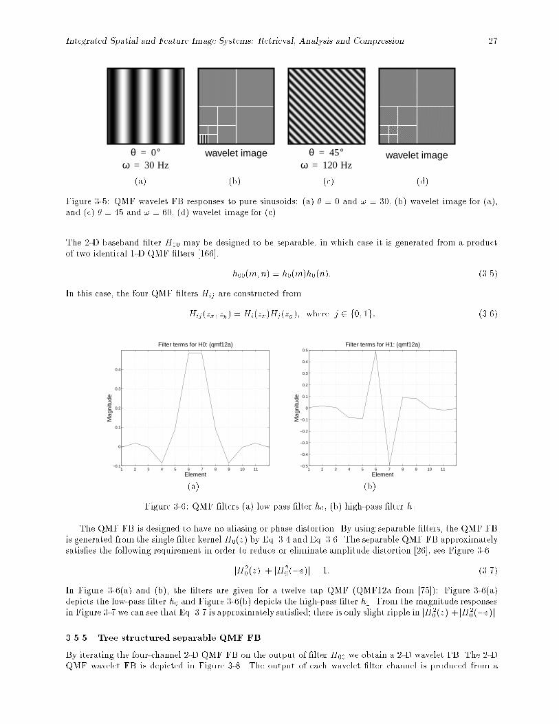
Integrated Spatial and Feature Image Systems: Retrieval, Analysis and Compression 27
θ 45°=ω 120 Hz=
θ 0°=ω 30 Hz=
wavelet image wavelet image
(a) (b) (c) (d)
Figure 3-5: QMF wavelet FB responses to pure sinusoids: (a) � = 0 and ! = 30, (b) wavelet image for (a),and (c) � = 45 and ! = 60, (d) wavelet image for (c).
The 2-D baseband �lter H00 may be designed to be separable, in which case it is generated from a productof two identical 1-D QMF �lters [166],
h00(m;n) = h0(m)h0(n): (3.5)
In this case, the four QMF �lters Hij are constructed from
Hij(zx; zy) = Hi(zx)Hj(zy); where j 2 f0; 1g: (3.6)
1 2 3 4 5 6 7 8 9 10 11−0.1
0
0.1
0.2
0.3
0.4
Element
Mag
nitu
de
Filter terms for H0: (qmf12a)
1 2 3 4 5 6 7 8 9 10 11−0.5
−0.4
−0.3
−0.2
−0.1
0
0.1
0.2
0.3
0.4
0.5
Element
Mag
nitu
de
Filter terms for H1: (qmf12a)
(a) (b)
Figure 3-6: QMF �lters (a) low pass �lter h0, (b) high-pass �lter h1.
The QMF FB is designed to have no aliasing or phase distortion. By using separable �lters, the QMF FBis generated from the single �lter kernel H0(z) by Eq. 3.4 and Eq. 3.6. The separable QMF FB approximatelysatis�es the following requirement in order to reduce or eliminate amplitude distortion [26], see Figure 3-6.
jH20(z)j+ jH2
0(�z)j = 1: (3.7)
In Figure 3-6(a) and (b), the �lters are given for a twelve tap QMF (QMF12a from [75]): Figure 3-6(a)depicts the low-pass �lter h0 and Figure 3-6(b) depicts the high-pass �lter h1. From the magnitude responsesin Figure 3-7 we can see that Eq. 3.7 is approximately satis�ed; there is only slight ripple in jH2
0(z)j+jH20(�z)j.
3.5.5 Tree structured separable QMF FB
By iterating the four-channel 2-D QMF FB on the output of �lter H00 we obtain a 2-D wavelet FB. The 2-DQMF wavelet FB is depicted in Figure 3-8. The output of each wavelet �lter channel is produced from a
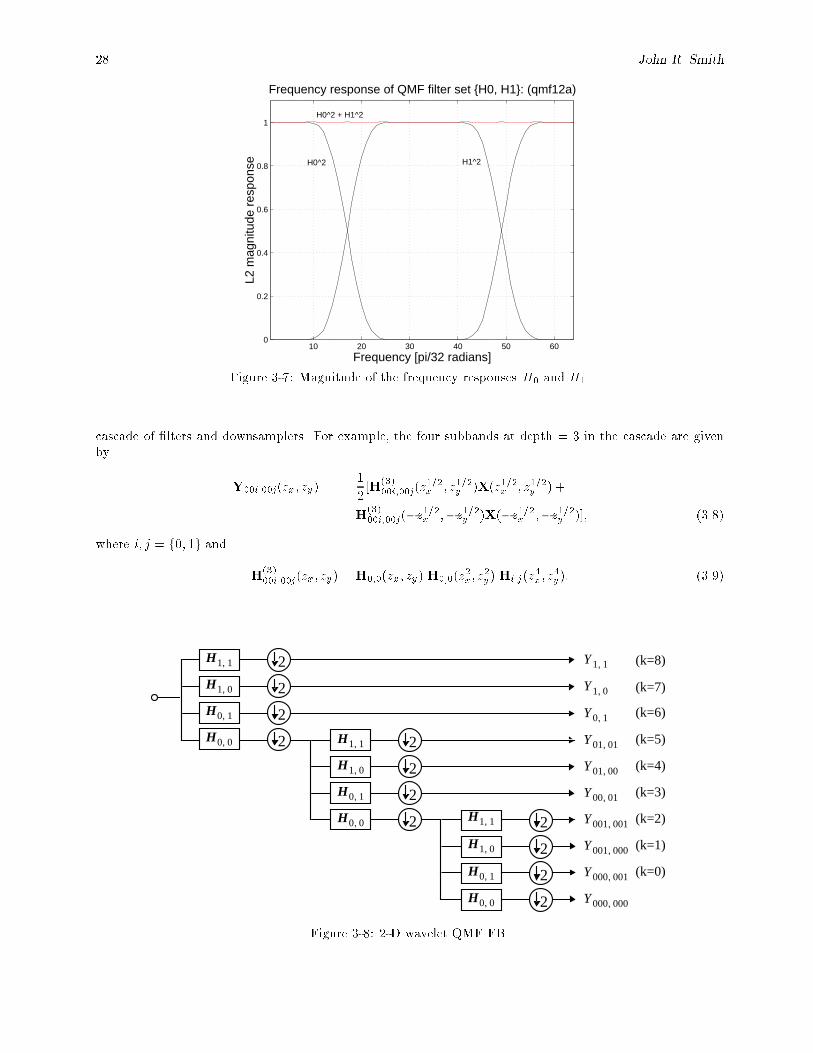
28 John R. Smith
10 20 30 40 50 600
0.2
0.4
0.6
0.8
1
Frequency [pi/32 radians]
L2 m
agni
tude
res
pons
e
Frequency response of QMF filter set {H0, H1}: (qmf12a)
H0^2 + H1^2
H1^2H0^2
Figure 3-7: Magnitude of the frequency responses H0 and H1.
cascade of �lters and downsamplers. For example, the four subbands at depth = 3 in the cascade are givenby
Y00i;00j(zx; zy) =1
2[H(3)
00i;00j(z1=2x ; z1=2y )X(z1=2x ; z1=2y ) +
H(3)00i;00j(�z
1=2x ;�z1=2y )X(�z1=2x ;�z1=2y )]; (3.8)
where i; j = f0; 1g and
H(3)00i;00j(zx; zy) = H0;0(zx; zy)H0;0(z
2x; z
2y) Hi;j(z
4x; z
4y): (3.9)
2
2
2
H1 1,
H1 0,
H0 1,
H0 0, H1 1,
H1 0,
H0 1,
H0 0, H1 1,
H1 0,
H0 1,
Y 1 1,
Y 1 0,
Y 0 1,
Y 01 01,
Y 01 00,
Y 00 01,
Y 001 001,
Y 001 000,
Y 000 001,
2H0 0, Y 000 000,
2
2
2
2 2
2
2
2
(k=0)
(k=6)
(k=7)
(k=8)
(k=5)
(k=1)
(k=3)
(k=4)
(k=2)
Figure 3-8: 2-D wavelet QMF FB.
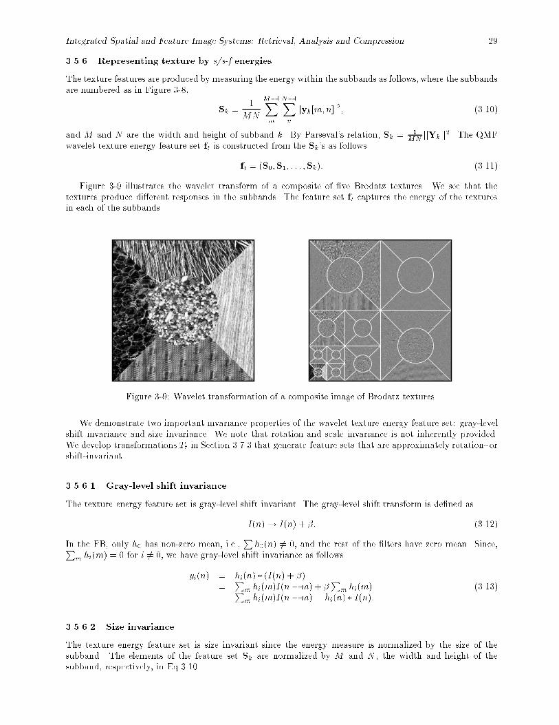
Integrated Spatial and Feature Image Systems: Retrieval, Analysis and Compression 29
3.5.6 Representing texture by s/s-f energies
The texture features are produced by measuring the energy within the subbands as follows, where the subbandsare numbered as in Figure 3-8,
Sk =1
MN
M�1Xm
N�1Xn
jyk[m;n]j2; (3.10)
and M and N are the width and height of subband k. By Parseval's relation, Sk = 1MN
jjYkjj2. The QMF
wavelet texture energy feature set ft is constructed from the Sk's as follows
ft = (S0;S1; : : : ;Sk): (3.11)
Figure 3-9 illustrates the wavelet transform of a composite of �ve Brodatz textures. We see that thetextures produce di�erent responses in the subbands. The feature set ft captures the energy of the texturesin each of the subbands.
Figure 3-9: Wavelet transformation of a composite image of Brodatz textures.
We demonstrate two important invariance properties of the wavelet texture energy feature set: gray-levelshift invariance and size invariance. We note that rotation and scale invariance is not inherently provided.We develop transformations Tt in Section 3.7.3 that generate feature sets that are approximately rotation- orshift-invariant.
3.5.6.1 Gray-level shift invariance
The texture energy feature set is gray-level shift invariant. The gray-level shift transform is de�ned as
I(n)! I(n) + �: (3.12)
In the FB, only h0 has non-zero mean, i.e.,P
h0(n) 6= 0, and the rest of the �lters have zero mean. Since,Pm hi(m) = 0 for i 6= 0, we have gray-level shift invariance as follows
yi(n) = hi(n) � (I(n) + �)=
Pm hi(m)I(n �m) + �
Pm hi(m)
=P
m hi(m)I(n �m) = hi(n) � I(n):(3.13)
3.5.6.2 Size invariance
The texture energy feature set is size invariant since the energy measure is normalized by the size of thesubband. The elements of the feature set Sk are normalized by M and N , the width and height of thesubband, respectively, in Eq 3.10.
30 John R. Smith
3.6. Texture classi�cation experiments
We compare texture energy feature sets that are derived from several image transforms besides the QMFwavelet, including DCT, QMF uniform subband. In the experiments reported here, 112 Brodatz textureimages (512x512) are cut randomly into rectangular pieces (average size 132x132). The texture energy featuresets are used to classify the cuts to the correct Brodatz texture classes. We use a classi�cation procedurebased upon Fisher discriminant analysis.
Classi�cation rates of over 90% are obtained for both wavelet subband and uniform subband decomposi-tions. DCT/Mandala-block gives just over 80% classi�cation rate, while simple spatial block features producesonly 34% correct classi�cation.
3.6.1 K-Class discrimination
Fisher discriminant analysis (FDA) derives the optimal linear classi�cation function from the observation datathat describes the set of classes. The FDA constructs linear composites from training features that providefor maximum average separation among classes. Although the resultant composites are not orthogonal, theyare uncorrelated with each other [39].
FDA is contrasted with principal component analysis (PCA), which is performed on the data covariancematrix. PCA determines the most signi�cant functions to best represent, not to classify, the data. Since ourgoal is classi�cation, we use FDA, which determines the eigenvectors of scatter matrices which describe classseparability. The criteria of class separability is formulated using the following scatter matrices: within-class(W), between-class (B), and total (T) [48].
The FDA procedure is carried out as follows: let K = the number of classes. Each class k, where
k 2 f0; : : : ;K�1g, has a set of nk observations and provides the length m feature vector as the jth observationxjk = (x0jk; x
1jk; : : : ; x
m�1jk ), where j 2 f0; 1; :::; nk� 1g. Let x be the total mean vector over all observations
and all classes
x =K�1Xk=0
nkXj=0
xjk: (3.14)
Then, de�ne tk as follows
tk =
nk�1Xj=0
(xjk � x)t(xjk � x): (3.15)
Then, summing the tk's gives, T =PK�1
k=0 tk, which is the total-mean-corrected sum-of-squares of cross-products of observation data.
Let xk be the mean vector over all observations of class k
xk =nkXj=0
xjk: (3.16)
Then, de�ne wk as follows
wk =nk�1Xj=0
(xjk � xk)t(xjk � xk): (3.17)
Then, summing the wk's gives, W =PK�1
k=0 wk, which is the within-class sum-of-squares matrix.Then, B = T�W gives the between-class sum-of-squares and cross-products matrix. The productW�1B
represents the ratio of between-class to within-class sum-of-squares for K classes. This matrix, which is non-symmetric with rank equal to the minimumof m (the feature vector length) and K�1 (the number of classesminus one) is used in the eigenvector decomposition as follows: denoting the eigenvalues ofW�1B as �k andthe eigenvectors as ek, we determine which discriminant functions capture the most variation that separatesthe classes by expressing each eigenvalue as a percentage of total variance accounted for using
�0k =�kPj �j
: (3.18)
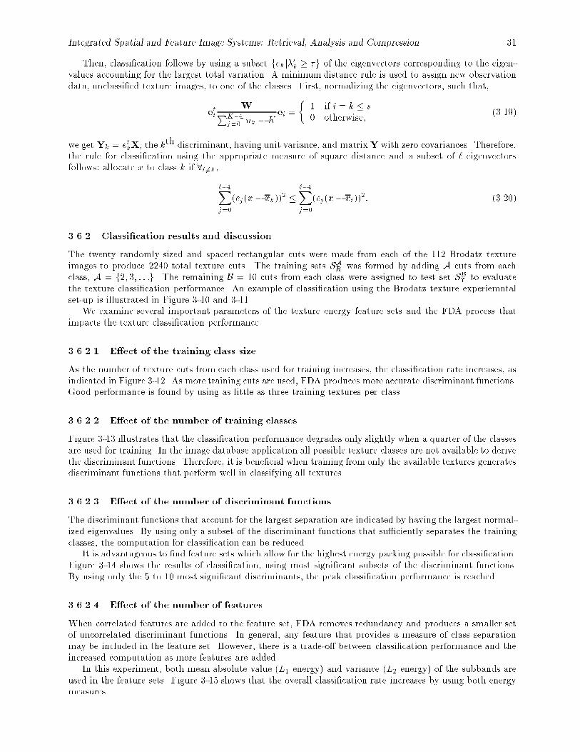
Integrated Spatial and Feature Image Systems: Retrieval, Analysis and Compression 31
Then, classi�cation follows by using a subset fekj�0k � �g of the eigenvectors corresponding to the eigen-
values accounting for the largest total variation. A minimum distance rule is used to assign new observationdata, unclassi�ed texture images, to one of the classes. First, normalizing the eigenvectors, such that,
etiWPK�1
j=0 nk �Kei =
�1 if i = k � s0 otherwise;
(3.19)
we get Yk = etkX, the kth discriminant, having unit variance, and matrixY with zero covariances. Therefore,the rule for classi�cation using the appropriate measure of square distance and a subset of ` eigenvectorsfollows: allocate x to class k if 8i 6=k,
`�1Xj=0
(ej(x � xk))2 �
`�1Xj=0
(ej(x� xi))2: (3.20)
3.6.2 Classi�cation results and discussion
The twenty randomly sized and spaced rectangular cuts were made from each of the 112 Brodatz textureimages to produce 2240 total texture cuts. The training sets SAR was formed by adding A cuts from eachclass, A = f2; 3; : : :g. The remaining B = 10 cuts from each class were assigned to test set SBT to evaluatethe texture classi�cation performance. An example of classi�cation using the Brodatz texture experiemntalset-up is illustrated in Figure 3-10 and 3-11.
We examine several important parameters of the texture energy feature sets and the FDA process thatimpacts the texture classi�cation performance.
3.6.2.1 E�ect of the training class size
As the number of texture cuts from each class used for training increases, the classi�cation rate increases, asindicated in Figure 3-12. As more training cuts are used, FDA produces more accurate discriminant functions.Good performance is found by using as little as three training textures per class.
3.6.2.2 E�ect of the number of training classes
Figure 3-13 illustrates that the classi�cation performance degrades only slightly when a quarter of the classesare used for training. In the image database application all possible texture classes are not available to derivethe discriminant functions. Therefore, it is bene�cial when training from only the available textures generatesdiscriminant functions that perform well in classifying all textures.
3.6.2.3 E�ect of the number of discriminant functions
The discriminant functions that account for the largest separation are indicated by having the largest normal-ized eigenvalues. By using only a subset of the discriminant functions that su�ciently separates the trainingclasses, the computation for classi�cation can be reduced.
It is advantageous to �nd feature sets which allow for the highest energy packing possible for classi�cation.Figure 3-14 shows the results of classi�cation, using most signi�cant subsets of the discriminant functions.By using only the 5 to 10 most signi�cant discriminants, the peak classi�cation performance is reached.
3.6.2.4 E�ect of the number of features
When correlated features are added to the feature set, FDA removes redundancy and produces a smaller setof uncorrelated discriminant functions. In general, any feature that provides a measure of class separationmay be included in the feature set. However, there is a trade-o� between classi�cation performance and theincreased computation as more features are added.
In this experiment, both mean absolute value (L1 energy) and variance (L2 energy) of the subbands areused in the feature sets. Figure 3-15 shows that the overall classi�cation rate increases by using both energymeasures.
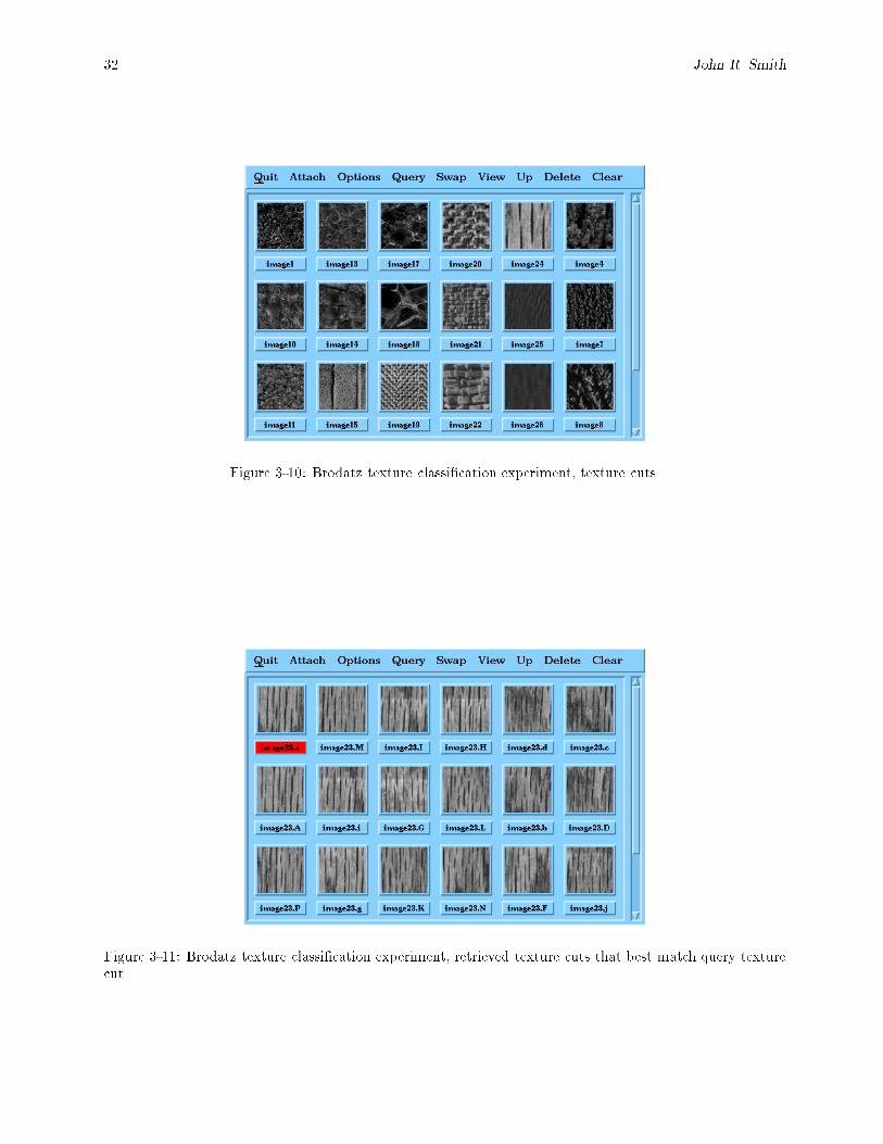
32 John R. Smith
Figure 3-10: Brodatz texture classi�cation experiment, texture cuts.
Figure 3-11: Brodatz texture classi�cation experiment, retrieved texture cuts that best match query texturecut.
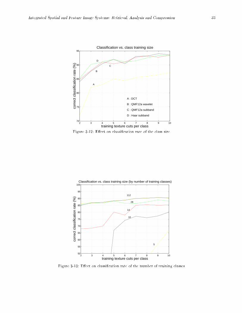
Integrated Spatial and Feature Image Systems: Retrieval, Analysis and Compression 33
2 3 4 5 6 7 8 9 1070
75
80
85
90
95
training texture cuts per class
corr
ect c
lass
ifica
tion
rate
(%
)
Classification vs. class training size
A
B
C
D
A : DCT
B : QMF12a wavelet
C : QMF12a subband
D : Haar subband
Figure 3-12: E�ect on classi�cation rate of the class size.
2 3 4 5 6 7 8 9 1050
55
60
65
70
75
80
85
90
95
100
training texture cuts per class
corr
ect c
lass
ifica
tion
rate
(%
)
Classification vs. class training size (by number of training classes)
112
28
14
10
5
Figure 3-13: E�ect on classi�cation rate of the number of training classes.
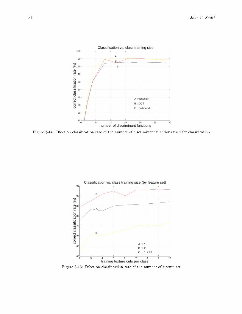
34 John R. Smith
0 5 10 15 20 25 3010
20
30
40
50
60
70
80
90
100
number of discriminant functions
corr
ect c
lass
ifica
tion
rate
(%
)
Classification vs. class training size
A : Wavelet
B : DCT
C : Subband
A
B
C
Figure 3-14: E�ect on classi�cation rate of the number of discriminant functions used for classi�cation.
2 3 4 5 6 7 8 9 1060
65
70
75
80
85
90
95
training texture cuts per class
corr
ect c
lass
ifica
tion
rate
(%
)
Classification vs. class training size (by feature set)
A
B
C
A : L1B : L2C : L1 + L2
Figure 3-15: E�ect on classi�cation rate of the number of feature set.
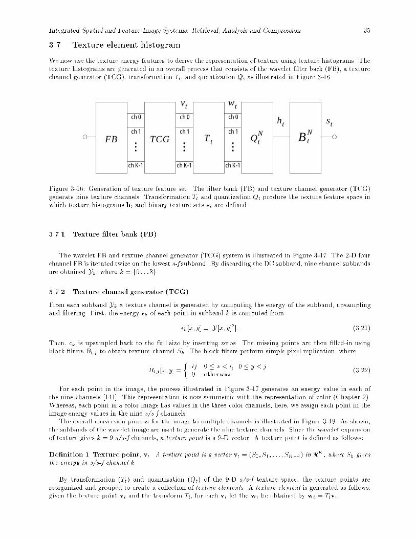
Integrated Spatial and Feature Image Systems: Retrieval, Analysis and Compression 35
3.7. Texture element histogram
We now use the texture energy features to derive the representation of texture using texture histograms. Thetexture histograms are generated in an overall process that consists of the wavelet �lter back (FB), a texturechannel generator (TCG), transformation Tt, and quantization Qt as illustrated in Figure 3-16.
TCG T t
vt wt
ht stch 0
ch 1
ch K-1
FB QtN
ch 0
ch 1
ch K-1
B tN
ch 0
ch 1
ch K-1
Figure 3-16: Generation of texture feature set. The �lter bank (FB) and texture channel generator (TCG)generate nine texture channels. Transformation Tt and quantization Qt produce the texture feature space inwhich texture histograms ht and binary texture sets st are de�ned.
3.7.1 Texture �lter bank (FB)
The wavelet FB and texture channel generator (TCG) system is illustrated in Figure 3-17. The 2-D fourchannel FB is iterated twice on the lowest s-f subband. By discarding the DC subband, nine channel subbandsare obtained Yk, where k = f0 : : :8g.
3.7.2 Texture channel generator (TCG)
From each subband Yk a texture channel is generated by computing the energy of the subband, upsamplingand �ltering. First, the energy �k of each point in subband k is computed from
�k[x; y] = jY[x; y]2j: (3.21)
Then, �k is upsampled back to the full size by inserting zeros. The missing points are then �lled-in usingblock �lters Bi;j to obtain texture channel Sk. The block �lters perform simple pixel replication, where
Bi;j [x; y] =
�ij 0 � x < i; 0 � y < j0 otherwise:
(3.22)
For each point in the image, the process illustrated in Figure 3-17 generates an energy value in each ofthe nine channels [141]. This representation is now symmetric with the representation of color (Chapter 2).Whereas, each point in a color image has values in the three color channels, here, we assign each point in theimage energy values in the nine s/s-f channels.
The overall conversion process for the image to multiple channels is illustrated in Figure 3-18. As shown,the subbands of the wavelet image are used to generate the nine texture channels. Since the wavelet expansionof texture gives k = 9 s/s-f channels, a texture point is a 9-D vector. A texture point is de�ned as follows:
De�nition 1 Texture point, vt. A texture point is a vector vt = (S0; S1; : : : ; SK�1) in <K , where Sk gives
the energy in s/s-f channel k.
By transformation (Tt) and quantization (Qt) of the 9-D s/s-f texture space, the texture points arereorganized and grouped to create a collection of texture elements. A texture element is generated as follows:given the texture point vt and the transform Tt, for each vt let the wt be obtained by wt = Ttvt.
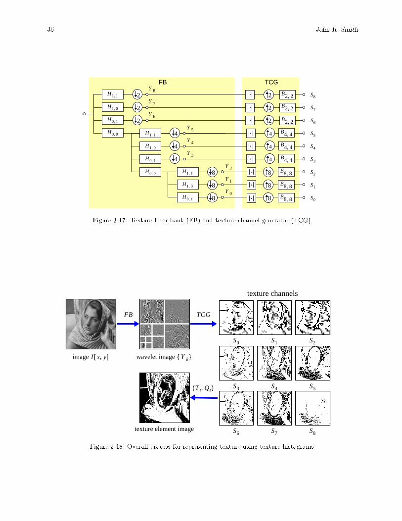
36 John R. Smith
Y 4
Y 5
Y 3
4
4
4
8
8
8
H1 1,
H1 0,
H0 1,
H0 0, H1 1,
H1 0,
H0 1,
H0 0,
2
2
2
2
2
2
4
4
4
8
8
8
H1 1,
H1 0,
H0 1,
B2 2,
B2 2,
B2 2,
B4 4,
B4 4,
B4 4,
B8 8,
B8 8,
B8 8,
S1
S2
S3
S4
S5
S6
S7
S8
S0
Y 7
Y 8
Y 6
Y 2
Y 1
Y 0
FB TCG
Figure 3-17: Texture �lter bank (FB) and texture channel generator (TCG).
FB
T t Qt,( )
image I x y,[ ] wavelet image Y k{ }
S0 S1 S2
S3 S4 S5
S6 S7 S8texture element image
texture channels
TCG
Figure 3-18: Overall process for representing texture using texture histograms.
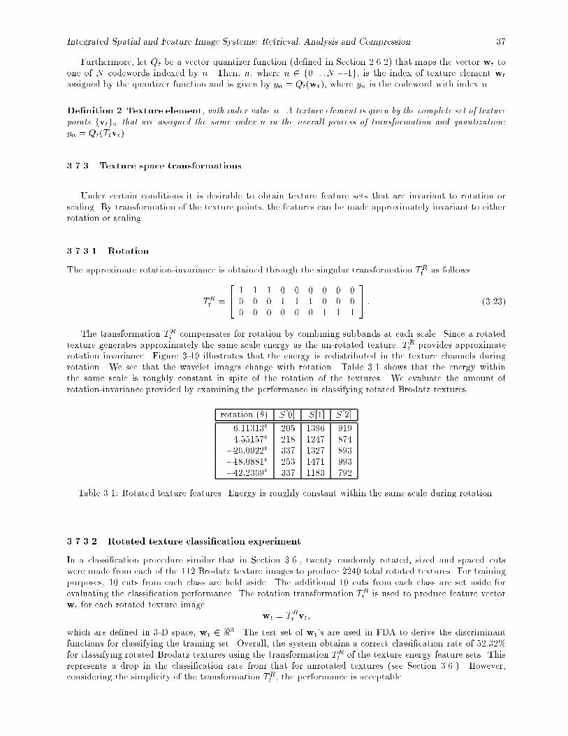
Integrated Spatial and Feature Image Systems: Retrieval, Analysis and Compression 37
Furthermore, let Qt be a vector quantizer function (de�ned in Section 2.6.2) that maps the vector wt toone of N codewords indexed by n. Then, n, where n 2 f0 : : :N � 1g, is the index of texture element wt
assigned by the quantizer function and is given by yn = Qt(wt), where yn is the codeword with index n.
De�nition 2 Texture element, with index value n. A texture element is given by the complete set of texturepoints fvtgn that are assigned the same index n in the overall process of transformation and quantization:yn = Qt(Ttvt).
3.7.3 Texture space transformations
Under certain conditions it is desirable to obtain texture feature sets that are invariant to rotation orscaling. By transformation of the texture points, the features can be made approximately invariant to eitherrotation or scaling.
3.7.3.1 Rotation
The approximate rotation-invariance is obtained through the singular transformation TRt as follows
TRt =
24 1 1 1 0 0 0 0 0 0
0 0 0 1 1 1 0 0 00 0 0 0 0 0 1 1 1
35 : (3.23)
The transformation TRt compensates for rotation by combining subbands at each scale. Since a rotated
texture generates approximately the same scale energy as the un-rotated texture, TRt provides approximate
rotation invariance. Figure 3-19 illustrates that the energy is redistributed in the texture channels duringrotation. We see that the wavelet images change with rotation. Table 3.1 shows that the energy withinthe same scale is roughly constant in spite of the rotation of the textures. We evaluate the amount ofrotation-invariance provided by examining the performance in classifying rotated Brodatz textures.
rotation (�) S[0] S[1] S[2]
6:11313� 205 1396 9194:55157� 218 1247 874
�26:0922� 337 1327 893�18:0881� 253 1471 993�42:2369� 337 1183 792
Table 3.1: Rotated texture features. Energy is roughly constant within the same scale during rotation.
3.7.3.2 Rotated texture classi�cation experiment
In a classi�cation procedure similar that in Section 3.6., twenty randomly rotated, sized and spaced cutswere made from each of the 112 Brodatz texture images to produce 2240 total rotated textures. For trainingpurposes, 10 cuts from each class are held aside. The additional 10 cuts from each class are set aside forevaluating the classi�cation performance. The rotation transformation TR
t is used to produce feature vectorwt for each rotated texture image
wt = TRt vt;
which are de�ned in 3-D space, wt 2 <3. The test set of wt's are used in FDA to derive the discriminantfunctions for classifying the training set. Overall, the system obtains a correct classi�cation rate of 52:32%for classifying rotated Brodatz textures using the transformation TR
t of the texture energy feature sets. Thisrepresents a drop in the classi�cation rate from that for unrotated textures (see Section 3.6.). However,considering the simplicity of the transformation TR
t , the performance is acceptable.
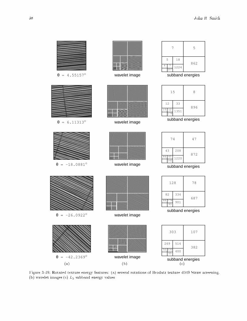
38 John R. Smith
θ = 6.11313o
θ = 4.55157o
θ = -26.0922o
θ = -18.0881o
θ = -42.2369o
896
815
1351
3312
178
15 12
862
57
1224
185
207
4 7
872
4774
1220
20843
142
46 65
687
78128
901
33482
93
66 178
382
107303
400
514269
55
52 230
wavelet image
wavelet image
wavelet image
wavelet image
wavelet image
subband energies
subband energies
subband energies
subband energies
subband energies(a) (b) (c)
Figure 3-19: Rotated texture energy features: (a) several rotations of Brodatz texture d049 Straw screening,(b) wavelet images (c) L2 subband energy values.
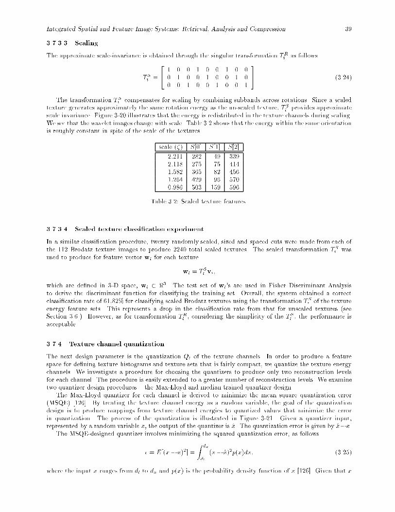
Integrated Spatial and Feature Image Systems: Retrieval, Analysis and Compression 39
3.7.3.3 Scaling
The approximate scale-invariance is obtained through the singular transformation TRt as follows
T St =
24 1 0 0 1 0 0 1 0 0
0 1 0 0 1 0 0 1 00 0 1 0 0 1 0 0 1
35 (3.24)
The transformation TSt compensates for scaling by combining subbands across rotations. Since a scaled
texture generates approximately the same rotation energy as the un-scaled texture, TSt provides approximate
scale invariance. Figure 3-20 illustrates that the energy is redistributed in the texture channels during scaling.We see that the wavelet images change with scale. Table 3.2 shows that the energy within the same orientationis roughly constant in spite of the scale of the textures.
scale (�) S[0] S[1] S[2]
2:211 282 49 3392:118 275 75 4141:582 365 82 4561:264 429 96 5700:986 503 159 596
Table 3.2: Scaled texture features.
3.7.3.4 Scaled texture classi�cation experiment
In a similar classi�cation procedure, twenty randomly scaled, sized and spaced cuts were made from each ofthe 112 Brodatz texture images to produce 2240 total scaled textures. The scaled transformation TS
t wasused to produce for feature vector wt for each texture
wt = TSt vt;
which are de�ned in 3-D space, wt 2 <3. The test set of wt's are used in Fisher Discriminant Analysisto derive the discriminant function for classifying the training set. Overall, the system obtained a correctclassi�cation rate of 61:82% for classifying scaled Brodatz textures using the transformation TS
t of the textureenergy feature sets. This represents a drop in the classi�cation rate from that for unscaled textures (seeSection 3.6.). However, as for transformation TR
t , considering the simplicity of the TSt , the performance is
acceptable.
3.7.4 Texture channel quantization
The next design parameter is the quantization Qt of the texture channels. In order to produce a featurespace for de�ning texture histograms and texture sets that is fairly compact, we quantize the texture energychannels. We investigate a procedure for choosing the quantizers to produce only two reconstruction levelsfor each channel. The procedure is easily extended to a greater number of reconstruction levels. We examinetwo quantizer design procedures { the Max-Lloyd and median trained quantizer design.
The Max-Lloyd quantizer for each channel is derived to minimize the mean square quantization error(MSQE) [126]. By treating the texture channel energy as a random variable, the goal of the quantizationdesign is to produce mappings from texture channel energies to quantized values that minimize the errorin quantization. The process of the quantization is illustrated in Figure 3-21. Given a quantizer input,represented by a random variable x, the output of the quantizer is x. The quantization error is given by x�x.
The MSQE-designed quantizer involves minimizing the squared quantization error, as follows
� = E[(x� x)2] =
Z du
dl
(x� x)2p(x)dx; (3.25)
where the input x ranges from dl to du and p(x) is the probability density function of x [126]. Given that x
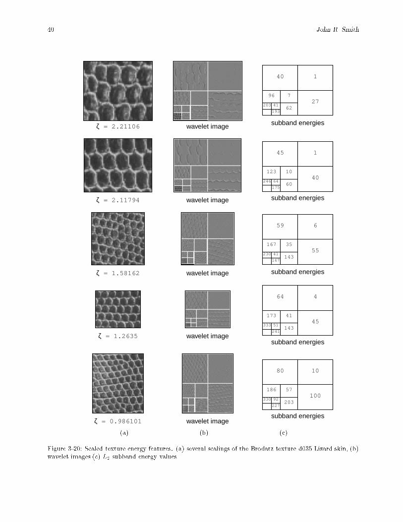
40 John R. Smith
ζ = 2.11794 wavelet image subband energies
ζ = 1.58162
ζ = 1.2635
ζ = 0.986101
27
140
62
796
193
203 41
55
659
143
35167
167
230 41
40
145
60
10123
175
246 64
45
464
143
41173
241
333 51
100
1080
203
57186
227
330 92
wavelet image subband energies
wavelet image subband energies
wavelet imagesubband energies
wavelet imagesubband energies
ζ = 2.21106
(a) (b) (c)
Figure 3-20: Scaled texture energy features: (a) several scalings of the Brodatz texture d035 Lizard skin, (b)wavelet images (c) L2 subband energy values.
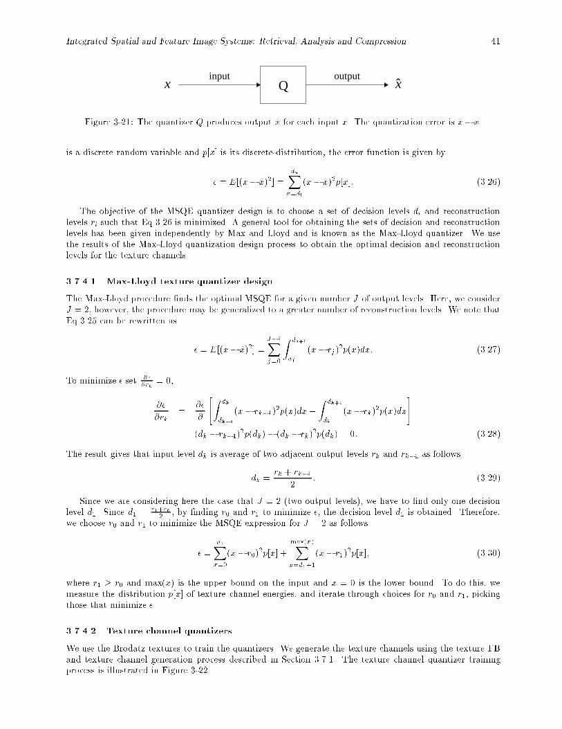
Integrated Spatial and Feature Image Systems: Retrieval, Analysis and Compression 41
x Q xinput output
Figure 3-21: The quantizer Q produces output x for each input x. The quantization error is x� x.
is a discrete random variable and p[x] is its discrete-distribution, the error function is given by
� = E[(x� x)2] =duX
x=dl
(x� x)2p[x]: (3.26)
The objective of the MSQE quantizer design is to choose a set of decision levels di and reconstructionlevels ri such that Eq 3.26 is minimized. A general tool for obtaining the sets of decision and reconstructionlevels has been given independently by Max and Lloyd and is known as the Max-Lloyd quantizer. We usethe results of the Max-Lloyd quantization design process to obtain the optimal decision and reconstructionlevels for the texture channels.
3.7.4.1 Max-Lloyd texture quantizer design
The Max-Lloyd procedure �nds the optimal MSQE for a given number J of output levels. Here, we considerJ = 2, however, the procedure may be generalized to a greater number of reconstruction levels. We note thatEq 3.25 can be rewritten as
� = E[(x� x)2] =J�1Xj=0
Z dj+1
dj
(x� rj)2p(x)dx: (3.27)
To minimize � set @�@rk
= 0,
@�
@rk=
@�
@
"Z dk
dk�1
(x� rk�1)2p(x)dx+
Z dk+1
dk
(x� rk)2p(x)dx
#
= (dk � rk�1)2p(dk)� (dk � rk)
2p(dk) = 0: (3.28)
The result gives that input level dk is average of two adjacent output levels rk and rk�1 as follows
dk =rk + rk�1
2: (3.29)
Since we are considering here the case that J = 2 (two output levels), we have to �nd only one decisionlevel d1. Since d1 =
r1+r02 , by �nding r0 and r1 to minimize �, the decision level d1 is obtained. Therefore,
we choose r0 and r1 to minimize the MSQE expression for J = 2 as follows
� =d1Xx=0
(x� r0)2p[x] +
max(x)Xx=d1+1
(x� r1)2p[x]; (3.30)
where r1 � r0 and max(x) is the upper bound on the input and x = 0 is the lower bound. To do this, wemeasure the distribution p[x] of texture channel energies, and iterate through choices for r0 and r1, pickingthose that minimize �.
3.7.4.2 Texture channel quantizers
We use the Brodatz textures to train the quantizers. We generate the texture channels using the texture FBand texture channel generation process described in Section 3.7.1. The texture channel quantizer trainingprocess is illustrated in Figure 3-22.
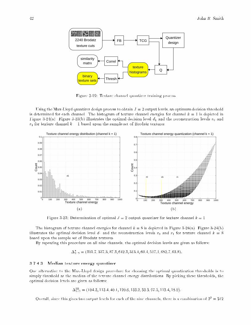
42 John R. Smith
Correl
Thresh
2240 Brodatz
texture cuts
binarytexture sets
similaritymatrx
texturehistograms Q
QuantizerdesignFB TCG
Figure 3-22: Texture channel quantizer training process.
Using the Max-Lloyd quantizer design process to obtain J = 2 output levels, an optimumdecision thresholdis determined for each channel. The histogram of texture channel energies for channel k = 1 is depicted inFigure 3-24(a). Figure 3-23(b) illustrates the optimal decision level d1 and the reconstruction levels r0 andr1 for texture channel k = 1 based upon the sample set of Brodatz textures.
0 100 200 300 400 500 600 700 800 900 10000
0.01
0.02
0.03
0.04
0.05
0.06
0.07
0.08
0.09
0.1
Texture channel energy
Cou
nt
Texture channel energy distribution (channel k = 1)
d1
0 100 200 300 400 500 600 700 800 900 10000
0.1
0.2
0.3
0.4
0.5
0.6
0.7
0.8
Texture channel energy
Cou
ntTexture channel energy quantization (channel k = 1)
r0 r1d1
(a) (b)
Figure 3-23: Determination of optimal J = 2 output quantizer for texture channel k = 1.
The histogram of texture channel energies for channel k = 8 is depicted in Figure 3-24(a). Figure 3-24(b)illustrates the optimal decision level d1 and the reconstruction levels r0 and r1 for texture channel k = 8based upon the sample set of Brodatz textures.
By repeating this procedure on all nine channels, the optimal decision levels are given as follows:
��512 = (303:7; 357:3; 87:3;642:3;313:4;60:4;517:1;682:7;63:8):
3.7.4.3 Median texture energy quantizer
One alternative to the Max-Lloyd design procedure for choosing the optimal quantization thresholds is tosimply threshold at the median of the texture channel energy distributions. By picking these thresholds, theoptimal decision levels are given as follows:
�m512 = (104:3; 113:4;40:1;120:6;133:2;33:3; 97:5; 113:4; 18:9):
Overall, since this gives two output levels for each of the nine channels, there is a combination of 29 = 512
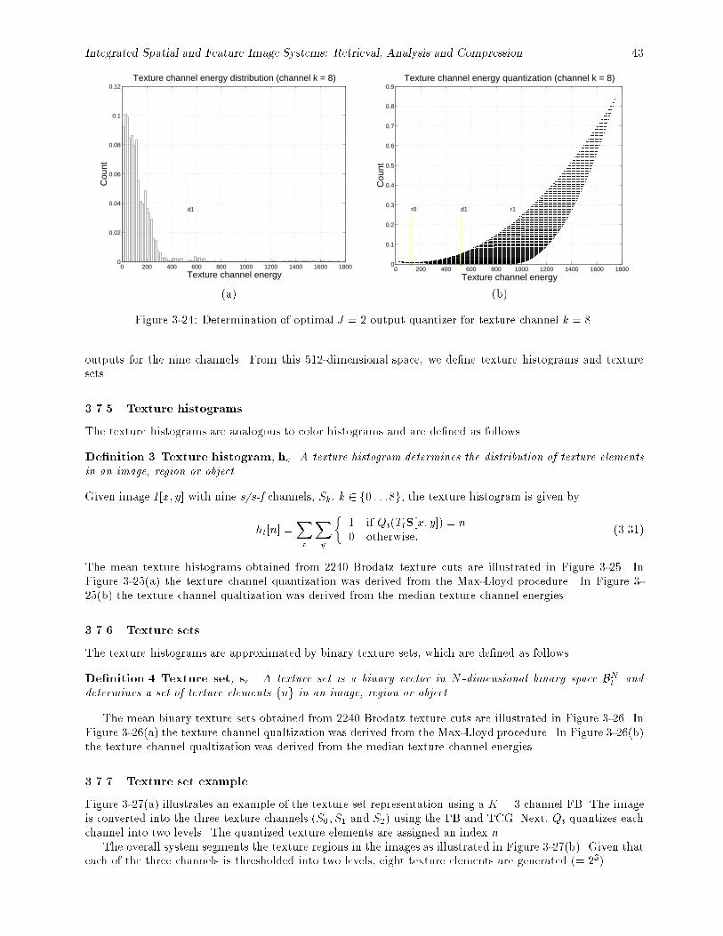
Integrated Spatial and Feature Image Systems: Retrieval, Analysis and Compression 43
0 200 400 600 800 1000 1200 1400 1600 18000
0.02
0.04
0.06
0.08
0.1
0.12
Texture channel energy
Cou
nt
Texture channel energy distribution (channel k = 8)
d1
0 200 400 600 800 1000 1200 1400 1600 18000
0.1
0.2
0.3
0.4
0.5
0.6
0.7
0.8
0.9
Texture channel energy
Cou
nt
Texture channel energy quantization (channel k = 8)
r0 r1d1
(a) (b)
Figure 3-24: Determination of optimal J = 2 output quantizer for texture channel k = 8.
outputs for the nine channels. From this 512-dimensional space, we de�ne texture histograms and texturesets.
3.7.5 Texture histograms
The texture histograms are analogous to color histograms and are de�ned as follows
De�nition 3 Texture histogram, hc. A texture histogram determines the distribution of texture elementsin an image, region or object.
Given image I[x; y] with nine s/s-f channels, Sk, k 2 f0 : : :8g, the texture histogram is given by
ht[n] =Xx
Xy
�1 if Qt(TtS[x; y]) = n0 otherwise:
(3.31)
The mean texture histograms obtained from 2240 Brodatz texture cuts are illustrated in Figure 3-25. InFigure 3-25(a) the texture channel quantization was derived from the Max-Lloyd procedure. In Figure 3-25(b) the texture channel qualtization was derived from the median texture channel energies.
3.7.6 Texture sets
The texture histograms are approximated by binary texture sets, which are de�ned as follows
De�nition 4 Texture set, sc. A texture set is a binary vector in N -dimensional binary space BNt anddetermines a set of texture elements fng in an image, region or object.
The mean binary texture sets obtained from 2240 Brodatz texture cuts are illustrated in Figure 3-26. InFigure 3-26(a) the texture channel qualtization was derived from the Max-Lloyd procedure. In Figure 3-26(b)the texture channel qualtization was derived from the median texture channel energies.
3.7.7 Texture set example
Figure 3-27(a) illustrates an example of the texture set representation using a K = 3 channel FB. The imageis converted into the three texture channels (S0; S1 and S2) using the FB and TCG. Next, Qt quantizes eachchannel into two levels. The quantized texture elements are assigned an index n.
The overall system segments the texture regions in the images as illustrated in Figure 3-27(b). Given thateach of the three channels is thresholded into two levels, eight texture elements are generated (= 23).
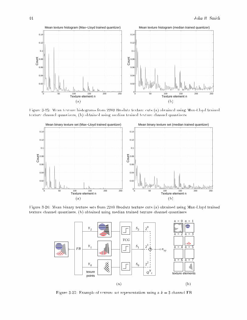
44 John R. Smith
0 50 100 150 200 2500
0.02
0.04
0.06
0.08
0.1
0.12
0.14
Texture element n
Cou
nt
Mean texture histogram (Max−Lloyd trained quantizer)
0 50 100 150 200 2500
0.02
0.04
0.06
0.08
0.1
0.12
0.14
Texture element n
Cou
nt
Mean texture histogram (median trained quantizer)
(a) (b)
Figure 3-25: Mean texture histograms from 2240 Brodatz texture cuts (a) obtained using Max-Lloyd trainedtexture channel quantizers, (b) obtained using median trained texture channel quantizers.
0 50 100 150 200 2500
0.02
0.04
0.06
0.08
0.1
0.12
0.14
Texture element n
Cou
nt
Mean binary texture set (Max−Lloyd trained quantizer)
0 50 100 150 200 2500
0.02
0.04
0.06
0.08
0.1
0.12
0.14
Texture element n
Cou
ntMean binary texture set (median trained quantizer)
(a) (b)
Figure 3-26: Mean binary texture sets from 2240 Brodatz texture cuts (a) obtained using Max-Lloyd trainedtexture channel quantizers, (b) obtained using median trained texture channel quantizers.
texurepoints
FB nxy
QN
t
+
Y 2
Y 1
Y 0
20
21
22
texture elements
n 0= n 1=
n 3=n 2=
n 5=n 4=
n 7=n 6=
TCG
S2
S1
S0
(a) (b)
Figure 3-27: Example of texture set representation using a k = 3 channel FB.

Integrated Spatial and Feature Image Systems: Retrieval, Analysis and Compression 45
3.8. Summary
In this chapter, we derived new representations of texture based upon histograms of texture elements. Thetexture elements are de�ned from the transformation (Tt) and quantization (Qt) of QMF wavelet transformenergies. We presented several experimental evaluations of the wavelet texture feature sets that demonstrateexcellent performance in classifying Brodatz textures. We also investigated several transformations that allowfor approximate rotation (TR
t ) or scale invariance (TSt ).
The texture histogram representation satis�es the objectives of (1) providing a representation for imageor regional texture that is compatible with color methods (namely, color histograms), (2) being compatiblewith compressed-domain texture extraction techniques (QMF wavelets), and (3) being suitable for regionextraction techniques. In Chapter 5, we explore the process of extracting texture regions from images usingtexture histograms. First, in Chapter 4 we present and evaluate several techniques for computing texturesimilarity using the representations presented here.
By using the histogram and binary set representations of color (see Chapter 2) and texture we e�cientlyand e�ectively represent color and texture information in images and region. These visual dimensions areextremely useful for image search and retrieval. When combined with spatial information, the most powerfulsystem for discriminating images is constructed (as we explore in Chapter 7). We now present techniques formeasuring computing color and texture-based image queries using the histograms and binary sets.
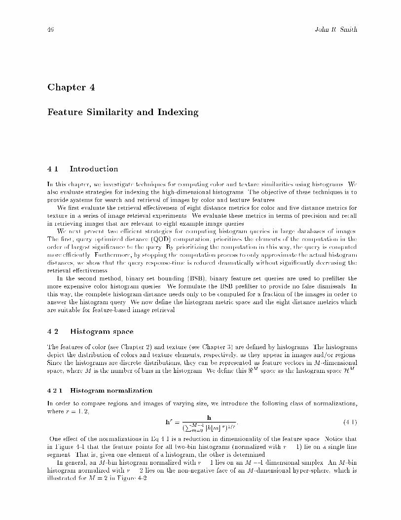
46 John R. Smith
Chapter 4
Feature Similarity and Indexing
4.1. Introduction
In this chapter, we investigate techniques for computing color and texture similarities using histograms. Wealso evaluate strategies for indexing the high-dimensional histograms. The objective of these techniques is toprovide systems for search and retrieval of images by color and texture features.
We �rst evaluate the retrieval e�ectiveness of eight distance metrics for color and �ve distance metrics fortexture in a series of image retrieval experiments. We evaluate these metrics in terms of precision and recallin retrieving images that are relevant to eight example image queries.
We next present two e�cient strategies for computing histogram queries in large databases of images.The �rst, query optimized distance (QOD) computation, prioritizes the elements of the computation in theorder of largest signi�cance to the query. By prioritizing the computation in this way, the query is computedmore e�ciently. Furthermore, by stopping the computation process to only approximate the actual histogramdistances, we show that the query response-time is reduced dramatically without signi�cantly decreasing theretrieval e�ectiveness.
In the second method, binary set bounding (BSB), binary feature set queries are used to pre�lter themore expensive color histogram queries. We formulate the BSB pre�lter to provide no false dismissals. Inthis way, the complete histogram distance needs only to be computed for a fraction of the images in order toanswer the histogram query. We now de�ne the histogram metric space and the eight distance metrics whichare suitable for feature-based image retrieval.
4.2. Histogram space
The features of color (see Chapter 2) and texture (see Chapter 3) are de�ned by histograms. The histogramsdepict the distribution of colors and texture elements, respectively, as they appear in images and/or regions.Since the histograms are discrete distributions, they can be represented as feature vectors in M -dimensionalspace, where M is the number of bins in the histogram. We de�ne this <M space as the histogram space HM .
4.2.1 Histogram normalization
In order to compare regions and images of varying size, we introduce the following class of normalizations,where r = 1; 2,
hr =h
(PM�1
m=0 jh[m]jr)1=r: (4.1)
One e�ect of the normalizations in Eq 4.1 is a reduction in dimensionality of the feature space. Notice thatin Figure 4-1 that the feature points for all two-bin histograms (normalized with r = 1) lie on a single linesegment. That is, given one element of a histogram, the other is determined.
In general, an M -bin histogram normalized with r = 1 lies on an M � 1 dimensional simplex. An M -binhistogram normalized with r = 2 lies on the non-negative face of an M -dimensional hyper-sphere, which isillustrated for M = 2 in Figure 4-2.
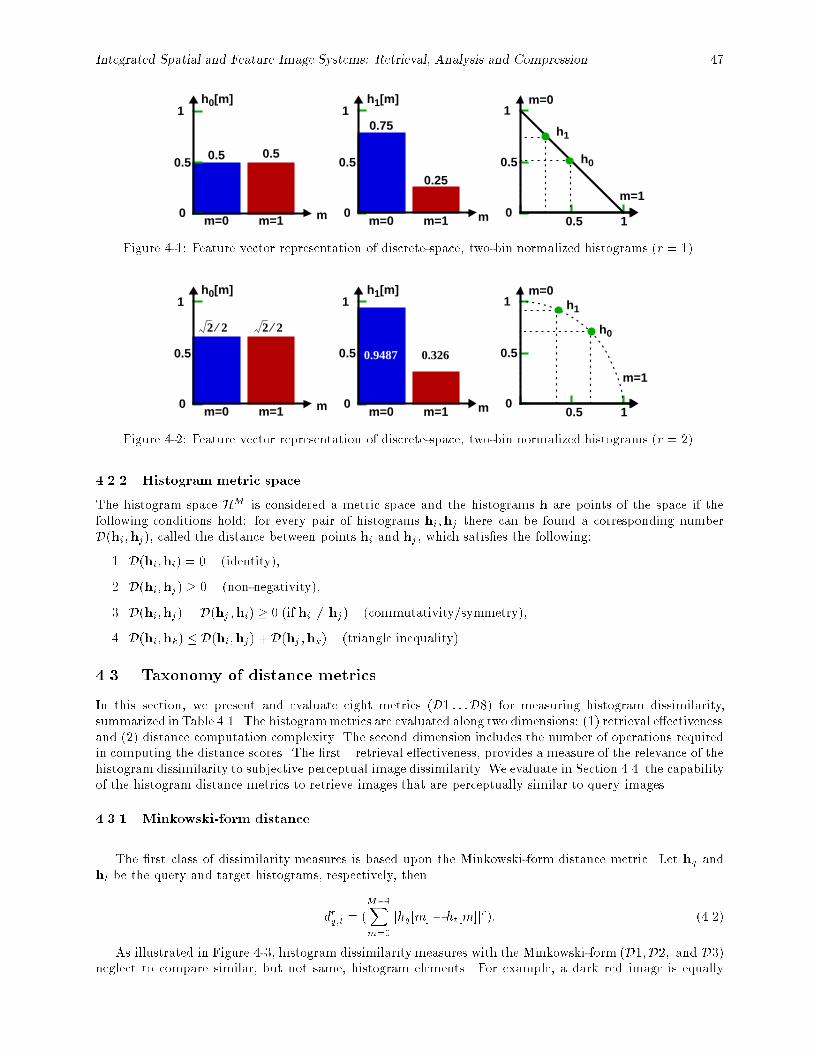
Integrated Spatial and Feature Image Systems: Retrieval, Analysis and Compression 47
0
0.5
1
0
0.5
1
0.5 0.5
0.75
0.25
0
0.5
1
mm=1m=0mm=1m=0 0.5 1
m=1
m=0h0[m] h1[m]
h0
h1
Figure 4-1: Feature vector representation of discrete-space, two-bin normalized histograms (r = 1).
0
0.5
1
0
0.5
1
0
0.5
1
mm=1m=0mm=1m=0 0.5 1
m=1
m=0h0[m] h1[m]
h0
h1
2 2⁄ 2 2⁄
0.9487 0.326
Figure 4-2: Feature vector representation of discrete-space, two-bin normalized histograms (r = 2).
4.2.2 Histogram metric space
The histogram space HM is considered a metric space and the histograms h are points of the space if thefollowing conditions hold: for every pair of histograms hi;hj there can be found a corresponding numberD(hi;hj), called the distance between points hi and hj, which satis�es the following:
1. D(hi;hi) = 0 (identity),
2. D(hi;hj) � 0 (non-negativity),
3. D(hi;hj) = D(hj ;hi) � 0 (if hi 6= hj) (commutativity/symmetry),
4. D(hi;hk) � D(hi;hj) +D(hj ;hk) (triangle inequality).
4.3. Taxonomy of distance metrics
In this section, we present and evaluate eight metrics (D1 : : :D8) for measuring histogram dissimilarity,summarized in Table 4.1. The histogrammetrics are evaluated along two dimensions: (1) retrieval e�ectivenessand (2) distance computation complexity. The second dimension includes the number of operations requiredin computing the distance scores. The �rst { retrieval e�ectiveness, provides a measure of the relevance of thehistogram dissimilarity to subjective perceptual image dissimilarity. We evaluate in Section 4.4. the capabilityof the histogram distance metrics to retrieve images that are perceptually similar to query images.
4.3.1 Minkowski-form distance
The �rst class of dissimilarity measures is based upon the Minkowski-form distance metric. Let hq andht be the query and target histograms, respectively, then
drq;t = (M�1Xm=0
jhq[m]� ht[m]jr): (4.2)
As illustrated in Figure 4-3, histogram dissimilarity measures with the Minkowski-form (D1;D2; and D3)neglect to compare similar, but not same, histogram elements. For example, a dark red image is equally
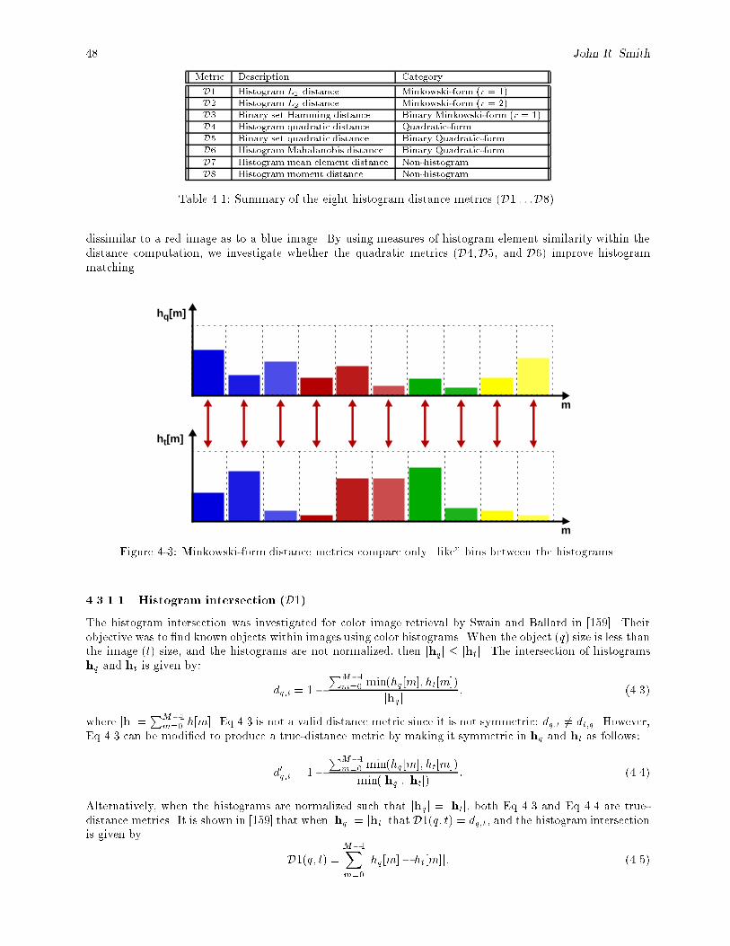
48 John R. Smith
Metric Description Category
D1 Histogram L1 distance Minkowski-form (r = 1)D2 Histogram L2 distance Minkowski-form (r = 2)D3 Binary set Hamming distance Binary Minkowski-form (r = 1)D4 Histogram quadratic distance Quadratic-formD5 Binary set quadratic distance Binary Quadratic-formD6 Histogram Mahalanobis distance Binary Quadratic-formD7 Histogram mean element distance Non-histogramD8 Histogram moment distance Non-histogram
Table 4.1: Summary of the eight histogram distance metrics (D1 : : :D8).
dissimilar to a red image as to a blue image. By using measures of histogram element similarity within thedistance computation, we investigate whether the quadratic metrics (D4;D5; and D6) improve histogrammatching.
m
hq[m]
m
ht[m]
Figure 4-3: Minkowski-form distance metrics compare only \like" bins between the histograms.
4.3.1.1 Histogram intersection (D1)
The histogram intersection was investigated for color image retrieval by Swain and Ballard in [159]. Theirobjective was to �nd known objects within images using color histograms. When the object (q) size is less thanthe image (t) size, and the histograms are not normalized, then jhqj � jhtj. The intersection of histogramshq and ht is given by:
dq;t = 1�
PM�1m=0 min(hq[m]; ht[m])
jhqj; (4.3)
where jhj =PM�1
m=0 h[m]. Eq 4.3 is not a valid distance metric since it is not symmetric: dq;t 6= dt;q. However,Eq 4.3 can be modi�ed to produce a true-distance metric by making it symmetric in hq and ht as follows:
d0q;t = 1�
PM�1m=0 min(hq[m]; ht[m])
min(jhqj; jhtj): (4.4)
Alternatively, when the histograms are normalized such that jhqj = jhtj, both Eq 4.3 and Eq 4.4 are true-distance metrics. It is shown in [159] that when jhqj = jhtj that D1(q; t) = dq;t, and the histogram intersectionis given by
D1(q; t) =M�1Xm=0
jhq[m]� ht[m]j: (4.5)
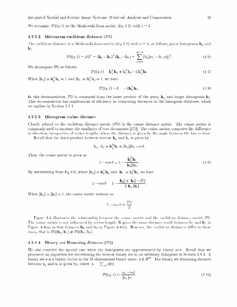
Integrated Spatial and Feature Image Systems: Retrieval, Analysis and Compression 49
We recognize D1(q; t) as the Minkowski-form metric (Eq 4.2) with r = 1.
4.3.1.2 Histogram euclidean distance (D2)
The euclidean distance is a Minkowski-form metric (Eq 4.2) with r = 2, as follows, given histograms hq andht,
D2(q; t) = D22 = (hq � ht)T (hq � ht) =
M�1Xm=0
(hq [m]� ht[m])2: (4.6)
We decompose D2 as followsD2(q; t) = hTq hq + hTt ht � 2hTq ht: (4.7)
When jhqj = hTq hq = 1 and jhtj = hTt ht = 1, we have
D2(q; t)� 2 = �2hTq ht: (4.8)
In this decomposition, D2 is computed from the inner product of the query hq and target histograms ht.This decomposition has implications of e�ciency in computing distances in the histogram database, whichwe explore in Section 4.5.4.
4.3.1.3 Histogram cosine distance
Closely related to the euclidean distance metric (D2) is the cosine distance metric. The cosine metric iscommonly used to measure the similarity of text documents [172]. The cosine metric computes the di�erencein direction, irrespective of vector lengths, where the distance is given by the angle between the two vectors.
Recall that the inner product between vectors hq and ht is given by
hq � ht = hTq ht = jhqjjhtj cos �:
Then, the cosine metric is given as
1� cos � = 1�hTq ht
jhqjjhtj: (4.9)
By substituting from Eq 4.6, where jhqj = hTq hq and jhtj = hTt ht, we have
1� cos � = 1�jhqj+ jhtj � D2
2jhqjjhtj:
When jhqj = jhtj = 1, the cosine metric reduces to
1� cos � =D2
2
.Figure 4-4 illustrates the relationship between the cosine metric and the euclidean distance metric D2.
The cosine metric is not in uenced by vector length. It gives the same distance result between h0 and h1 inFigure 4-4(a) as that between h0 and h2 in Figure 4-4(b). However, the euclidean distances di�er in thesecases, that is D2(h0;h1) 6= D2(h0;h2).
4.3.1.4 Binary set Hamming distance (D3)
We also consider the special case when the histograms are approximated by binary sets. Recall that wepresented an algorithm for determining the nearest binary set to an arbitrary histogram in Section 2.8.4. Abinary set s is a binary vector in the M -dimensional binary space, s 2 BM . The binary set Hamming distancebetween sq and st is given by, where jsj =
Pm s[m]
D3(q; t) =jsq � stj
jsqjjstj: (4.10)
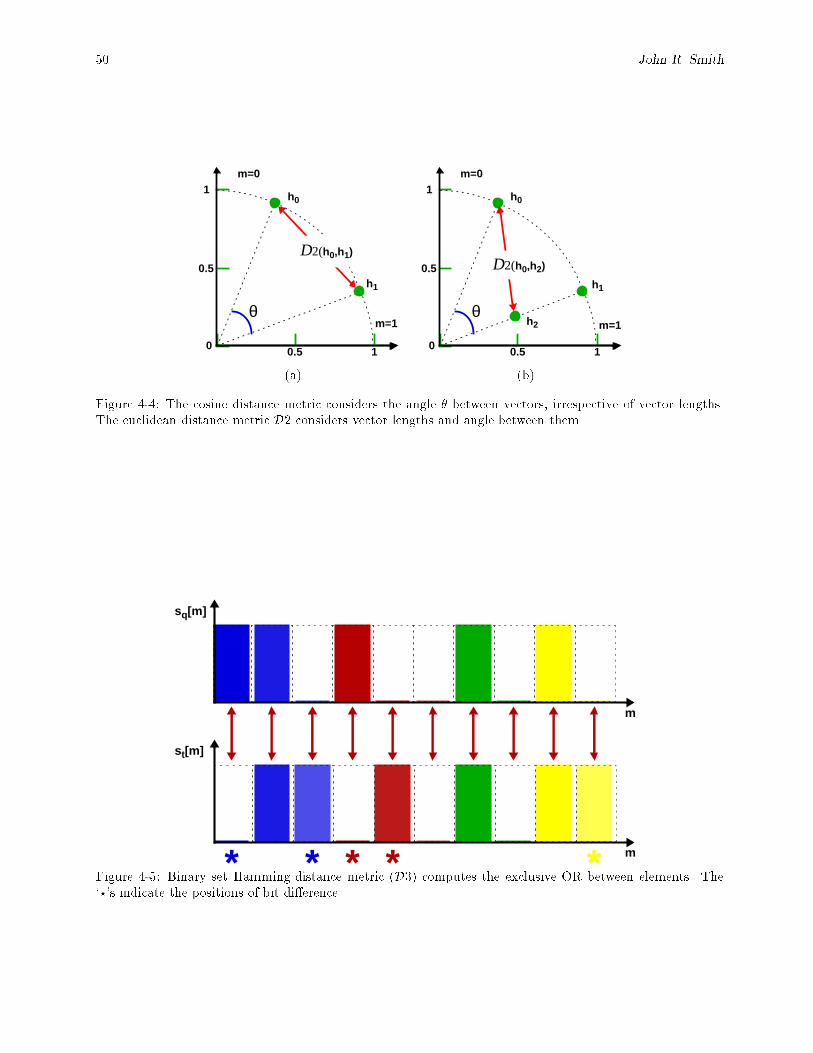
50 John R. Smith
0
0.5
1
0.5 1
m=1
m=0
h1
h0
θ
0
0.5
1
0.5 1
m=1
m=0
h2
h0
θ
h1
D2(h0,h2)D2(h0,h1)
(a) (b)
Figure 4-4: The cosine distance metric considers the angle � between vectors, irrespective of vector lengths.The euclidean distance metric D2 considers vector lengths and angle between them.
m
sq[m]
m
st[m]
* ** * *Figure 4-5: Binary set Hamming distance metric (D3) computes the exclusive OR between elements. The`?'s indicate the positions of bit di�erence.
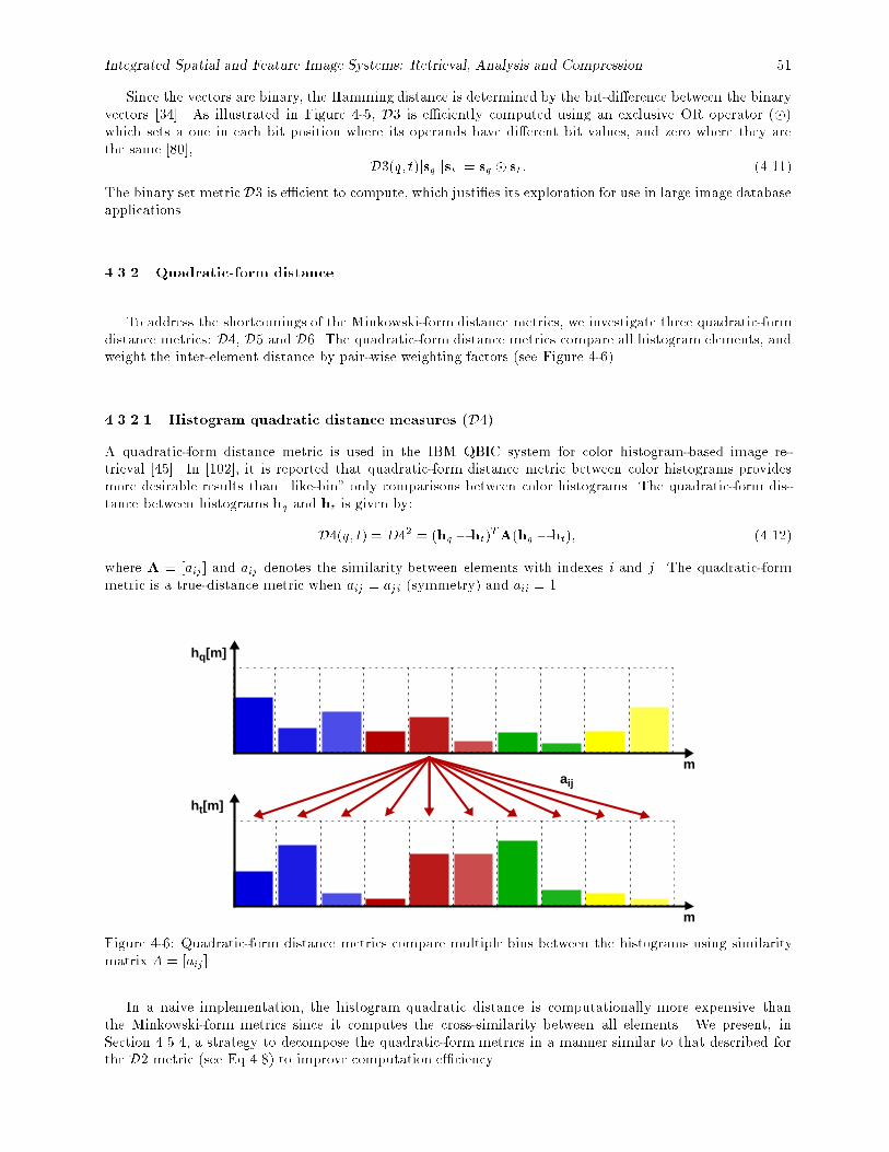
Integrated Spatial and Feature Image Systems: Retrieval, Analysis and Compression 51
Since the vectors are binary, the Hamming distance is determined by the bit-di�erence between the binaryvectors [34]. As illustrated in Figure 4-5, D3 is e�ciently computed using an exclusive OR operator (�)which sets a one in each bit position where its operands have di�erent bit values, and zero where they arethe same [80],
D3(q; t)jsqjjstj = sq � st: (4.11)
The binary set metric D3 is e�cient to compute, which justi�es its exploration for use in large image databaseapplications.
4.3.2 Quadratic-form distance
To address the shortcomings of the Minkowski-form distance metrics, we investigate three quadratic-formdistance metrics: D4, D5 and D6. The quadratic-form distance metrics compare all histogram elements, andweight the inter-element distance by pair-wise weighting factors (see Figure 4-6).
4.3.2.1 Histogram quadratic distance measures (D4)
A quadratic-form distance metric is used in the IBM QBIC system for color histogram-based image re-trieval [45]. In [102], it is reported that quadratic-form distance metric between color histograms providesmore desirable results than \like-bin" only comparisons between color histograms. The quadratic-form dis-tance between histograms hq and ht is given by:
D4(q; t) = D42 = (hq � ht)TA(hq � ht); (4.12)
where A = [aij] and aij denotes the similarity between elements with indexes i and j. The quadratic-formmetric is a true-distance metric when aij = aji (symmetry) and aii = 1.
m
hq[m]
m
ht[m]
aij
Figure 4-6: Quadratic-form distance metrics compare multiple bins between the histograms using similaritymatrix A = [aij].
In a naive implementation, the histogram quadratic distance is computationally more expensive thanthe Minkowski-form metrics since it computes the cross-similarity between all elements. We present, inSection 4.5.4, a strategy to decompose the quadratic-form metrics in a manner similar to that described forthe D2 metric (see Eq 4.8) to improve computation e�ciency.
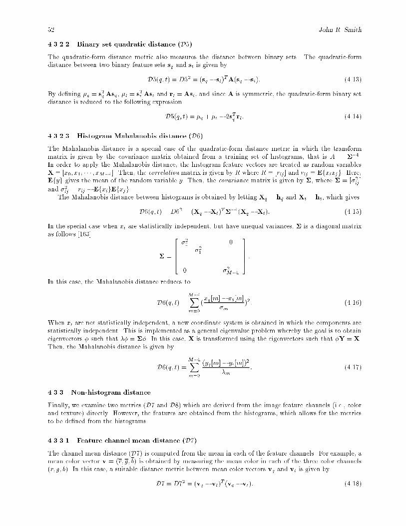
52 John R. Smith
4.3.2.2 Binary set quadratic distance (D5)
The quadratic-form distance metric also measures the distance between binary sets. The quadratic-formdistance between two binary feature sets sq and st is given by
D5(q; t) = D52 = (sq � st)TA(sq � st); (4.13)
By de�ning �q = sTq Asq, �t = sTt Ast and rt = Ast, and since A is symmetric, the quadratic-form binary setdistance is reduced to the following expression
D5(q; t) = �q + �t � 2sTq rt: (4.14)
4.3.2.3 Histogram Mahalanobis distance (D6)
The Mahalanobis distance is a special case of the quadratic-form distance metric in which the transformmatrix is given by the covariance matrix obtained from a training set of histograms, that is A = ��1.In order to apply the Mahalanobis distance, the histogram feature vectors are treated as random variablesX = [x0; x1; � � � ; xM�1]. Then, the correlation matrix is given by R where R = [rij] and rij = Efxixjg. Here,Efyg gives the mean of the random variable y. Then, the covariance matrix is given by �, where � = [�2ij]
and �2ij = rij � EfxigEfxjg.The Mahalanobis distance between histograms is obtained by letting Xq = hq and Xt = ht, which gives
D6(q; t) = D62 = (Xq �Xt)T��1(Xq �Xt): (4.15)
In the special case when xi are statistically independent, but have unequal variances, � is a diagonal matrixas follows [163]
� =
26664
�20 0�21
. . .
0 �2M�1
37775 :
In this case, the Mahalanobis distance reduces to
D6(q; t) =M�1Xm=0
(xq[m]� xt[m]
�m)2: (4.16)
When xi are not statistically independent, a new coordinate system is obtained in which the components arestatistically independent. This is implemented as a general eigenvalue problem whereby the goal is to obtaineigenvectors � such that �� = ��. In this case, X is transformed using the eigenvectors such that �Y = X.Then, the Mahalanobis distance is given by
D6(q; t) =M�1Xm=0
(yq [m]� yt[m])2
�m: (4.17)
4.3.3 Non-histogram distance
Finally, we examine two metrics (D7 and D8) which are derived from the image feature channels (i.e., colorand texture) directly. However, the features are obtained from the histograms, which allows for the metricsto be de�ned from the histograms.
4.3.3.1 Feature channel mean distance (D7)
The channel mean distance (D7) is computed from the mean in each of the feature channels. For example, amean color vector v = (r; g; b) is obtained by measuring the mean color in each of the three color channels(r; g; b). In this case, a suitable distance metric between mean color vectors vq and vt is given by
D7 = D72 = (vq � vt)T (vq � vt): (4.18)
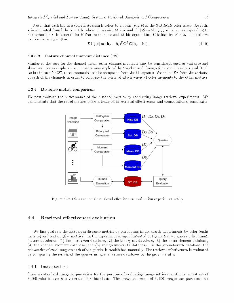
Integrated Spatial and Feature Image Systems: Retrieval, Analysis and Compression 53
Note, that each bin in a color histogram h refers to a point (r; g; b) in the 3-D RGB color space. As such,v is computed from h by v = Ch, where C has size M � 3, and C[i] gives the (r; g; b) triple corresponding tohistogram bin i. In general, for K feature channels and M histogram bins, C is has size K �M . This allowsus to rewrite Eq 4.18 as
D7(q; t) = (hq � ht)TCTC(hq � ht): (4.19)
4.3.3.2 Feature channel moment distance (D8)
Similar to the case for the channel mean, other channel moments may be considered, such as variance andskewness. For example, color moments were explored by Stricker and Orengo for color image retrieval [158].As in the case for D7, these moments are also computed from the histograms. We de�ne D8 from the varianceof each of the channels in order to compare the retrieval e�ectiveness of color moments to the other metrics.
4.3.4 Distance metric comparison
We now evaluate the performance of the distance metrics by conducting image retrieval experiments. Wedemonstrate that the set of metrics o�ers a trade-o� in retrieval e�ectiveness and computational complexity.
Histogram
Computation
Human
Evaluation
Image
Collection
Binary set
Conversion
Queries
Moment
Computation
Query
Evaluation
Hist DB
Set DB
Mean DB
Moment DB
GT DB
D1, D2, D4, D6
D3, D5
D8
D7
Figure 4-7: Distance metric retrieval e�ectiveness evaluation experiment setup.
4.4. Retrieval e�ectiveness evaluation
We �rst evaluate the histogram distance metrics by conducting image search experiments by color (eightmetrics) and texture (�ve metrics). In the experiment setup, illustrated in Figure 4-7, we generate �ve imagefeature databases: (1) the histogram database, (2) the binary set database, (3) the mean element database,(4) the channel moment database, and (5) the ground-truth database. In the ground-truth database, therelevancies of each image to each of the queries is established manually. The retrieval e�ectiveness is evaluatedby comparing the results of the queries using the feature databases to the ground-truths.
4.4.1 Image test set
Since no standard image corpus exists for the purpose of evaluating image retrieval methods, a test set of3; 100 color images was generated for this thesis. The image collection of 3; 100 images was purchased on

54 John R. Smith
CD-ROM from Expert Software�. Each of the 3; 100 images was inspected and assigned a relevance to eachof the following queries in order to measure the query's retrieval e�ectiveness. In this way, the image test setand assigned image relevance scores provide a common framework for comparing the image retrieval methods.
4.4.2 Retrieval e�ectiveness
Two metrics for retrieval e�ectiveness are recall and precision. Recall signi�es the proportion of relevant
images in the entire database that are retrieved in the query. Precision is the proportion of the retrieved
images that are relevant to the query [76]. More precisely, let A be the set of relevant items, let B be the setof retrieved items, and a; b; c and d are given as follows.
� a = retrieved and relevant (detection)
� b = retrieved and not relevant (false alarm)
� c = not retrieved and relevant (miss)
� d = not retrieved and not relevant.
Recall and precision are de�ned by the following conditional probabilities:
recall = P (BjA) = P (A[B)P (A) = a
a+c
precision = P (AjB) = P (A[B)P (B) = a
a+b :(4.20)
The measures of recall and precision require that the relevance to the query of each item in the databaseis established ahead of time. For the experiments, this was done for each query by subjectively assigning oneof three values to each image in the database: relevant = 1, partially or marginally relevant = 0:5 and notrelevant = 0. The relevance value corresponds to the probability that the item is relevant to the query.
In each query experiment, the distance (one of D1 : : :D8) between each relevant image (with relevance =1) and all images in the database is computed. The images are then sorted in order of lowest distance to thequery image. In this order, the recall and precision are measured for each image.
The process is repeated for all the relevant images and an overall average retrieval e�ectiveness is computedfor each distance metric and each query example. This produces just one recall vs. precision curve (i.e., seecurve D1 in Figure 4-10). These experiments are repeated for all distance metrics to provide for comparison.
4.4.3 Color retrieval
We �rst evaluate the retrieval e�ectiveness using color histograms on the test set of 3; 100 color images. Thecollection includes images with a variety of subjects, such as cities, nature, animals and transportation. We�rst examine example color queries: for images of (1) sunsets, (2) pink owers, (3) nature scenes with blueskies and (4) lions.
4.4.3.1 Query 1: Sunsets
In Query 1, the goal is to retrieve images of sunsets. Prior to the trials, the 3; 100 images were inspected,and 23 were designated to be relevant (to depict sunsets). Each of these images was used in turn to querythe collection. This was repeated for each distance metric. Examples of the retrieved images and plots of theretrieval e�ectiveness are shown in Figures 4-10 and 4-11.
We see that all metrics are fairly successful at retrieving sunset images, except for D7. Simply using themean of each color channel does not su�ciently capture color information in the images. Table 4.2 comparesthe retrieval e�ectiveness at several operational values. We see that the quadratic-form metrics D4 and D6perform well in Query 1. However, the retrieval e�ectiveness for D1 is slightly better. Contrary to statementsin [102], in Query 1 we do not see that the quadratic-form color histogram metrics improve performancesubstationally over the Minkowski-form metrics.
�Expert Software, Inc., 800 Douglas Rd., Coral Gables, FL 33134
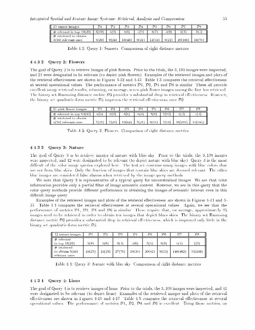
Integrated Spatial and Feature Image Systems: Retrieval, Analysis and Compression 55
23 sunset images D1 D2 D3 D4 D5 D6 D7 D8
# relevant in top 10(20) 6(10) 5(9) 4(6) 5(9) 4(7) 5(9) 2(4) 3(5)# retrieved to obtain5(10) relevant ones 8(20) 9(24) 16(46) 9(22) 12(32) 8(21) 29(186) 18(56)
Table 4.2: Query 1: Sunsets. Comparison of eight distance metrics.
4.4.3.2 Query 2: Flowers
The goal of Query 2 is to retrieve images of pink owers. Prior to the trials, the 3; 100 images were inspected,and 21 were designated to be relevant (to depict pink owers). Examples of the retrieved images and plots ofthe retrieval e�ectiveness are shown in Figures 4-12 and 4-13. Table 4.3 compares the retrieval e�ectivenessat several operational values. The performance of metrics D1, D2, D4 and D6 is similar. These all provideexcellent image retrieval results, returning, on average, seven pink ower images among the �rst ten retrieved.The binary set Hamming distance metric D3 provides a substantial drop in retrieval e�ectiveness. However,the binary set quadratic-form metric D5 improves the retrieval e�ectiveness over D3.
21 pink ower images D1 D2 D3 D4 D5 D6 D7 D8
# relevant in top 10(20) 6(9) 6(9) 5(6) 6(9) 5(8) 7(10) 2(3) 3(3)# retrieved to obtain5(10) relevant ones 7(21) 7(24) 10(62) 7(21) 8(34) 7(18) 48(291) 43(185)
Table 4.3: Query 2: Flowers. Comparison of eight distance metrics.
4.4.3.3 Query 3: Nature
The goal of Query 3 is to retrieve images of nature with blue sky. Prior to the trials, the 3; 100 imageswere inspected, and 42 were designated to be relevant (to depict nature with blue sky). Query 3 is the mostdi�cult of the color image queries explored here. The test set contains many images with blue colors thatare not from blue skies. Only the fraction of images that contain blue skies are deemed relevant. The otherblue images are considered false alarms when retrieved by the image query methods.
We note that Query 3 is representative of a typical query for unconstrained images. We see that colorinformation provides only a partial �lter of image semantic content. However, we see in this query that thecolor query methods provide di�erent performance in obtaining the images of semantic interest even in thisdi�cult image query.
Examples of the retrieved images and plots of the retrieval e�ectiveness are shown in Figures 4-14 and 4-15. Table 4.4 compares the retrieval e�ectiveness at several operational values. Again, we see that theperformance of metrics D1, D2, D4 and D6 is similar. These require that, on average, approximately 25images need to be retrieved in order to obtain ten images that depict blues skies. The binary set Hammingdistance metric D3 provides a substantial drop in retrieval e�ectiveness, which is improved only little in thebinary set quadratic-form metric D5.
42 nature images D1 D2 D3 D4 D5 D6 D7 D8
# relevantin top 10(20) 5(8) 5(8) 3(4) 5(8) 3(5) 5(9) 1(1) 2(3)# retrievedto obtain 5(10) 10(25) 10(26) 27(76) 10(26) 20(62) 9(23) 148(462) 33(108)relevant ones
Table 4.4: Query 3: Nature with blue sky. Comparison of eight distance metrics.
4.4.3.4 Query 4: Lions
The goal of Query 4 is to retrieve images of lions. Prior to the trials, the 3; 100 images were inspected, and 41were designated to be relevant (to depict lions). Examples of the retrieved images and plots of the retrievale�ectiveness are shown in Figures 4-16 and 4-17. Table 4.5 compares the retrieval e�ectiveness at severaloperational values. The performance of metrics D1, D2, D4 and D6 is excellent. Using these metrics, on
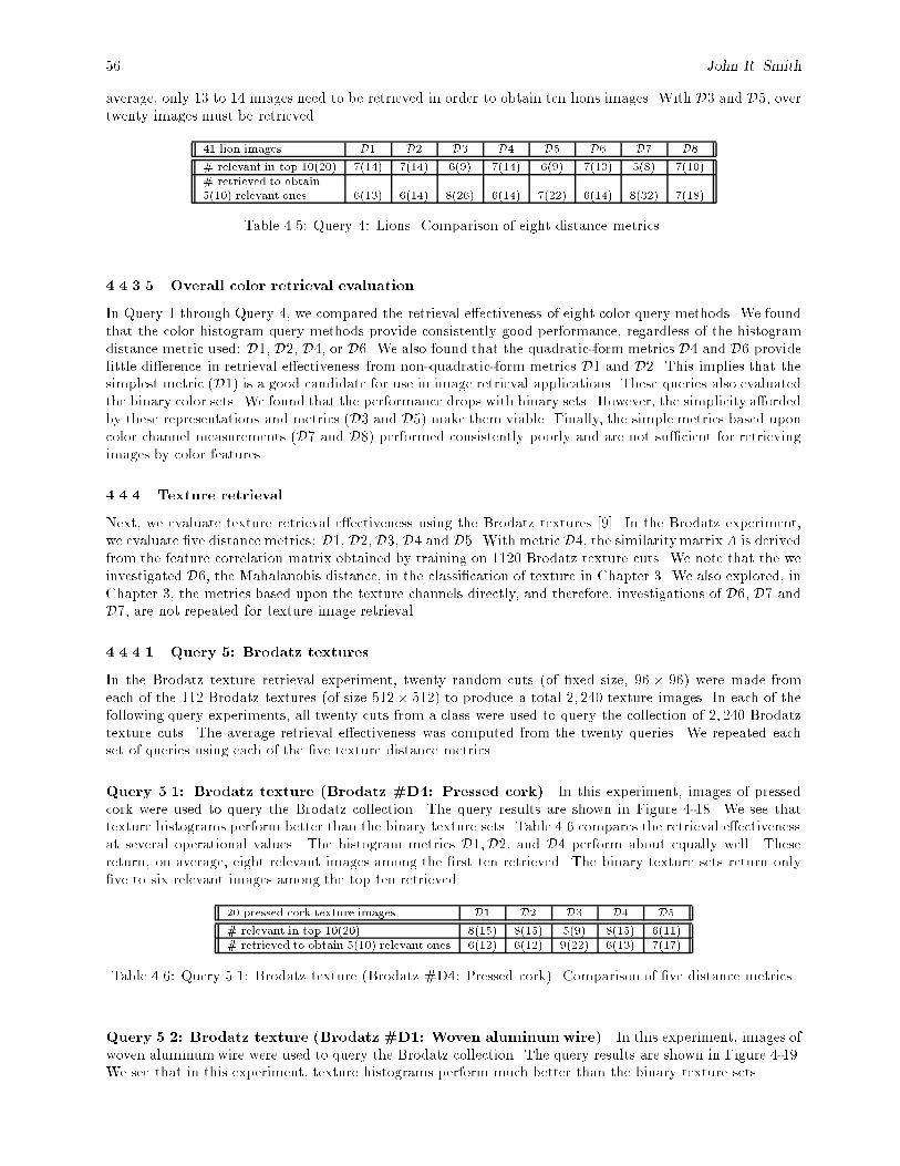
56 John R. Smith
average, only 13 to 14 images need to be retrieved in order to obtain ten lions images. With D3 and D5, overtwenty images must be retrieved.
41 lion images D1 D2 D3 D4 D5 D6 D7 D8
# relevant in top 10(20) 7(14) 7(14) 6(9) 7(14) 6(9) 7(13) 5(8) 7(10)# retrieved to obtain5(10) relevant ones 6(13) 6(14) 8(26) 6(14) 7(22) 6(14) 8(32) 7(18)
Table 4.5: Query 4: Lions. Comparison of eight distance metrics.
4.4.3.5 Overall color retrieval evaluation
In Query 1 through Query 4, we compared the retrieval e�ectiveness of eight color query methods. We foundthat the color histogram query methods provide consistently good performance, regardless of the histogramdistance metric used: D1, D2, D4, or D6. We also found that the quadratic-form metrics D4 and D6 providelittle di�erence in retrieval e�ectiveness from non-quadratic-form metrics D1 and D2. This implies that thesimplest metric (D1) is a good candidate for use in image retrieval applications. These queries also evaluatedthe binary color sets. We found that the performance drops with binary sets. However, the simplicity a�ordedby these representations and metrics (D3 and D5) make them viable. Finally, the simple metrics based uponcolor channel measurements (D7 and D8) performed consistently poorly and are not su�cient for retrievingimages by color features.
4.4.4 Texture retrieval
Next, we evaluate texture retrieval e�ectiveness using the Brodatz textures [9]. In the Brodatz experiment,we evaluate �ve distance metrics: D1, D2, D3, D4 and D5. With metric D4, the similaritymatrixA is derivedfrom the feature correlation matrix obtained by training on 1120 Brodatz texture cuts. We note that the weinvestigated D6, the Mahalanobis distance, in the classi�cation of texture in Chapter 3. We also explored, inChapter 3, the metrics based upon the texture channels directly, and therefore, investigations of D6, D7 andD7, are not repeated for texture image retrieval.
4.4.4.1 Query 5: Brodatz textures
In the Brodatz texture retrieval experiment, twenty random cuts (of �xed size, 96 � 96) were made fromeach of the 112 Brodatz textures (of size 512� 512) to produce a total 2; 240 texture images. In each of thefollowing query experiments, all twenty cuts from a class were used to query the collection of 2; 240 Brodatztexture cuts. The average retrieval e�ectiveness was computed from the twenty queries. We repeated eachset of queries using each of the �ve texture distance metrics.
Query 5.1: Brodatz texture (Brodatz #D4: Pressed cork) In this experiment, images of pressedcork were used to query the Brodatz collection. The query results are shown in Figure 4-18. We see thattexture histograms perform better than the binary texture sets. Table 4.6 compares the retrieval e�ectivenessat several operational values. The histogram metrics D1;D2, and D4 perform about equally well. Thesereturn, on average, eight relevant images among the �rst ten retrieved. The binary texture sets return only�ve to six relevant images among the top ten retrieved.
20 pressed cork texture images D1 D2 D3 D4 D5
# relevant in top 10(20) 8(15) 8(15) 5(9) 8(15) 6(11)# retrieved to obtain 5(10) relevant ones 6(12) 6(12) 9(22) 6(13) 7(17)
Table 4.6: Query 5.1: Brodatz texture (Brodatz #D4: Pressed cork). Comparison of �ve distance metrics.
Query 5.2: Brodatz texture (Brodatz #D1: Woven aluminumwire) In this experiment, images ofwoven aluminumwire were used to query the Brodatz collection. The query results are shown in Figure 4-19.We see that in this experiment, texture histograms perform much better than the binary texture sets.
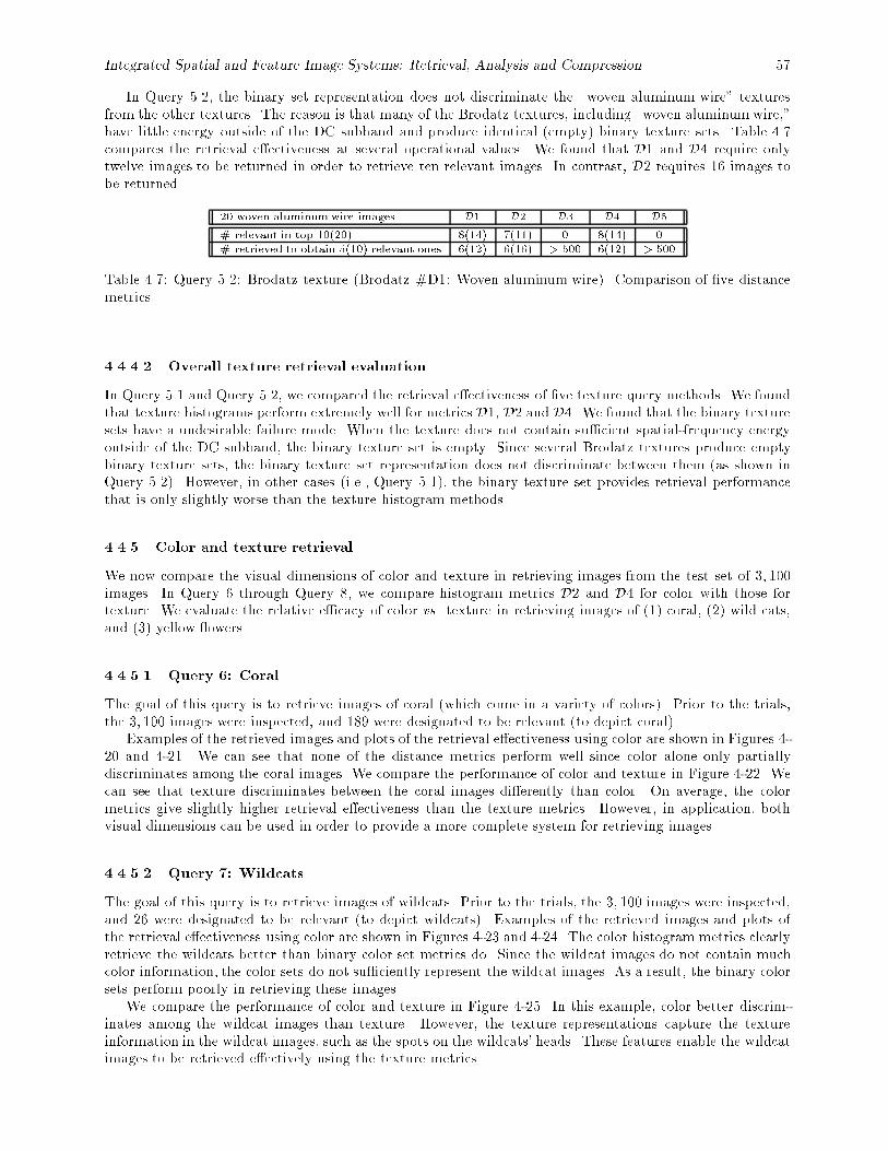
Integrated Spatial and Feature Image Systems: Retrieval, Analysis and Compression 57
In Query 5.2, the binary set representation does not discriminate the \woven aluminum wire" texturesfrom the other textures. The reason is that many of the Brodatz textures, including \woven aluminumwire,"have little energy outside of the DC subband and produce identical (empty) binary texture sets. Table 4.7compares the retrieval e�ectiveness at several operational values. We found that D1 and D4 require onlytwelve images to be returned in order to retrieve ten relevant images. In contrast, D2 requires 16 images tobe returned.
20 woven aluminum wire images D1 D2 D3 D4 D5
# relevant in top 10(20) 8(14) 7(11) 0 8(14) 0# retrieved to obtain 5(10) relevant ones 6(12) 6(16) > 500 6(12) > 500
Table 4.7: Query 5.2: Brodatz texture (Brodatz #D1: Woven aluminum wire). Comparison of �ve distancemetrics.
4.4.4.2 Overall texture retrieval evaluation
In Query 5.1 and Query 5.2, we compared the retrieval e�ectiveness of �ve texture query methods. We foundthat texture histograms perform extremely well for metrics D1, D2 and D4. We found that the binary texturesets have a undesirable failure mode. When the texture does not contain su�cient spatial-frequency energyoutside of the DC subband, the binary texture set is empty. Since several Brodatz textures produce emptybinary texture sets, the binary texture set representation does not discriminate between them (as shown inQuery 5.2). However, in other cases (i.e., Query 5.1), the binary texture set provides retrieval performancethat is only slightly worse than the texture histogram methods.
4.4.5 Color and texture retrieval
We now compare the visual dimensions of color and texture in retrieving images from the test set of 3; 100images. In Query 6 through Query 8, we compare histogram metrics D2 and D4 for color with those fortexture. We evaluate the relative e�cacy of color vs. texture in retrieving images of (1) coral, (2) wild cats,and (3) yellow owers.
4.4.5.1 Query 6: Coral
The goal of this query is to retrieve images of coral (which come in a variety of colors). Prior to the trials,the 3; 100 images were inspected, and 189 were designated to be relevant (to depict coral).
Examples of the retrieved images and plots of the retrieval e�ectiveness using color are shown in Figures 4-20 and 4-21. We can see that none of the distance metrics perform well since color alone only partiallydiscriminates among the coral images. We compare the performance of color and texture in Figure 4-22. Wecan see that texture discriminates between the coral images di�erently than color. On average, the colormetrics give slightly higher retrieval e�ectiveness than the texture metrics. However, in application, bothvisual dimensions can be used in order to provide a more complete system for retrieving images.
4.4.5.2 Query 7: Wildcats
The goal of this query is to retrieve images of wildcats. Prior to the trials, the 3; 100 images were inspected,and 26 were designated to be relevant (to depict wildcats). Examples of the retrieved images and plots ofthe retrieval e�ectiveness using color are shown in Figures 4-23 and 4-24. The color histogram metrics clearlyretrieve the wildcats better than binary color set metrics do. Since the wildcat images do not contain muchcolor information, the color sets do not su�ciently represent the wildcat images. As a result, the binary colorsets perform poorly in retrieving these images.
We compare the performance of color and texture in Figure 4-25. In this example, color better discrim-inates among the wildcat images than texture. However, the texture representations capture the textureinformation in the wildcat images, such as the spots on the wildcats' heads. These features enable the wildcatimages to be retrieved e�ectively using the texture metrics.
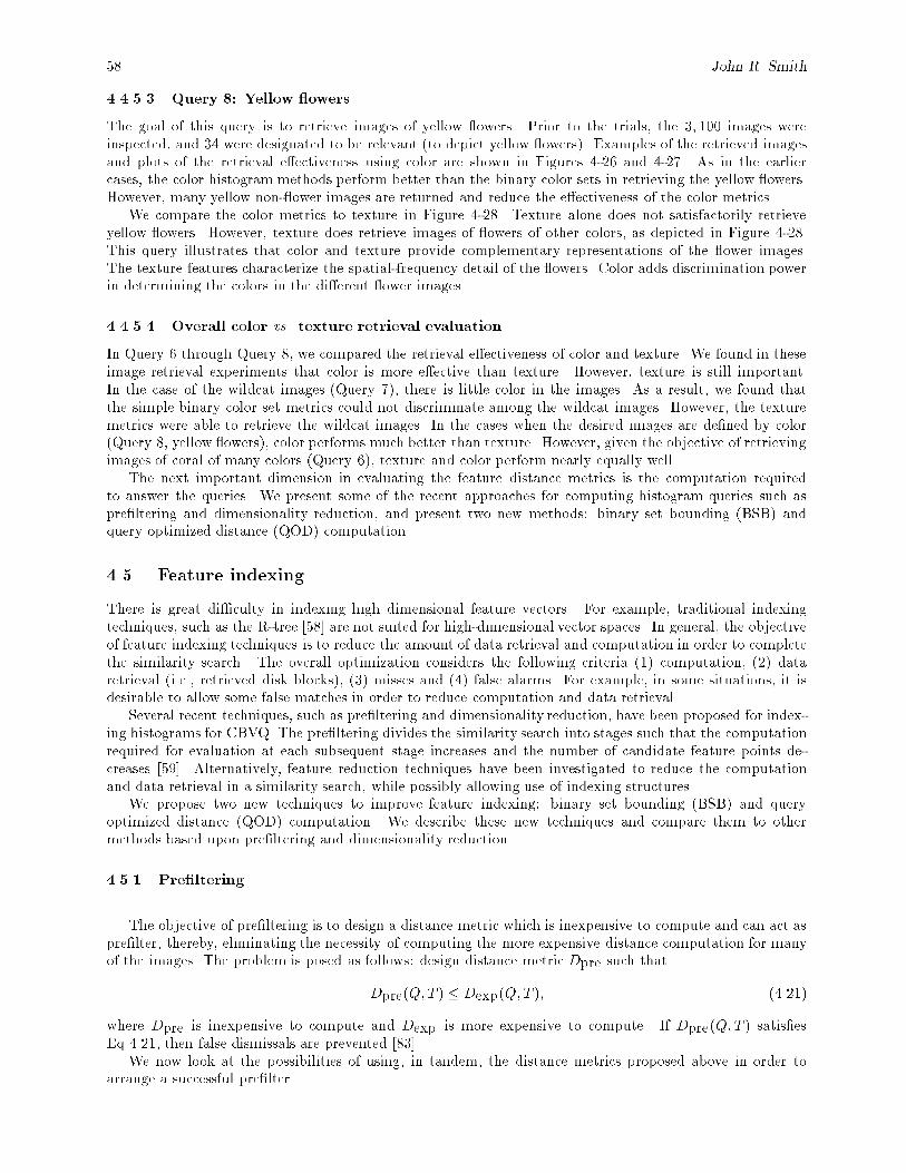
58 John R. Smith
4.4.5.3 Query 8: Yellow owers
The goal of this query is to retrieve images of yellow owers. Prior to the trials, the 3; 100 images wereinspected, and 34 were designated to be relevant (to depict yellow owers). Examples of the retrieved imagesand plots of the retrieval e�ectiveness using color are shown in Figures 4-26 and 4-27. As in the earliercases, the color histogram methods perform better than the binary color sets in retrieving the yellow owers.However, many yellow non- ower images are returned and reduce the e�ectiveness of the color metrics.
We compare the color metrics to texture in Figure 4-28. Texture alone does not satisfactorily retrieveyellow owers. However, texture does retrieve images of owers of other colors, as depicted in Figure 4-28.This query illustrates that color and texture provide complementary representations of the ower images.The texture features characterize the spatial-frequency detail of the owers. Color adds discrimination powerin determining the colors in the di�erent ower images.
4.4.5.4 Overall color vs. texture retrieval evaluation
In Query 6 through Query 8, we compared the retrieval e�ectiveness of color and texture. We found in theseimage retrieval experiments that color is more e�ective than texture. However, texture is still important.In the case of the wildcat images (Query 7), there is little color in the images. As a result, we found thatthe simple binary color set metrics could not discriminate among the wildcat images. However, the texturemetrics were able to retrieve the wildcat images. In the cases when the desired images are de�ned by color(Query 8, yellow owers), color performs much better than texture. However, given the objective of retrievingimages of coral of many colors (Query 6), texture and color perform nearly equally well.
The next important dimension in evaluating the feature distance metrics is the computation requiredto answer the queries. We present some of the recent approaches for computing histogram queries such aspre�ltering and dimensionality reduction, and present two new methods: binary set bounding (BSB) andquery optimized distance (QOD) computation.
4.5. Feature indexing
There is great di�culty in indexing high dimensional feature vectors. For example, traditional indexingtechniques, such as the R-tree [58] are not suited for high-dimensional vector spaces. In general, the objectiveof feature indexing techniques is to reduce the amount of data retrieval and computation in order to completethe similarity search. The overall optimization considers the following criteria (1) computation, (2) dataretrieval (i.e., retrieved disk blocks), (3) misses and (4) false alarms. For example, in some situations, it isdesirable to allow some false matches in order to reduce computation and data retrieval.
Several recent techniques, such as pre�ltering and dimensionality reduction, have been proposed for index-ing histograms for CBVQ. The pre�ltering divides the similarity search into stages such that the computationrequired for evaluation at each subsequent stage increases and the number of candidate feature points de-creases [59]. Alternatively, feature reduction techniques have been investigated to reduce the computationand data retrieval in a similarity search, while possibly allowing use of indexing structures.
We propose two new techniques to improve feature indexing: binary set bounding (BSB) and queryoptimized distance (QOD) computation. We describe these new techniques and compare them to othermethods based upon pre�ltering and dimensionality reduction.
4.5.1 Pre�ltering
The objective of pre�ltering is to design a distance metric which is inexpensive to compute and can act aspre�lter, thereby, eliminating the necessity of computing the more expensive distance computation for manyof the images. The problem is posed as follows: design distance metric Dpre such that
Dpre(Q; T ) � Dexp(Q; T ); (4.21)
where Dpre is inexpensive to compute and Dexp is more expensive to compute. If Dpre(Q; T ) satis�esEq 4.21, then false dismissals are prevented [83].
We now look at the possibilities of using, in tandem, the distance metrics proposed above in order toarrange a successful pre�lter.
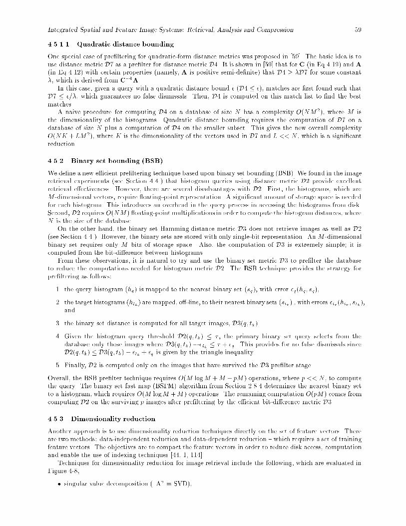
Integrated Spatial and Feature Image Systems: Retrieval, Analysis and Compression 59
4.5.1.1 Quadratic distance bounding
One special case of pre�ltering for quadratic-form distance metrics was proposed in [59]. The basic idea is touse distance metric D7 as a pre�lter for distance metric D4. It is shown in [59] that for C (in Eq 4.19) and A(in Eq 4.12) with certain properties (namely, A is positive semi-de�nite) that D4 � �D7 for some constant�, which is derived from C�1A.
In this case, given a query with a quadratic distance bound � (D4 � �), matches are �rst found such thatD7 � �=�, which guarantees no false dismissals. Then, D4 is computed on this match list to �nd the bestmatches.
A naive procedure for computing D4 on a database of size N has a complexity O(NM2), where M isthe dimensionality of the histograms. Quadratic distance bounding requires the computation of D7 on adatabase of size N plus a computation of D4 on the smaller subset. This gives the new overall complexityO(NK +LM2), where K is the dimensionality of the vectors used in D7 and L << N , which is a signi�cantreduction.
4.5.2 Binary set bounding (BSB)
We de�ne a new e�cient pre�ltering technique based upon binary set bounding (BSB). We found in the imageretrieval experiments (see Section 4.4.) that histogram queries using distance metric D2 provide excellentretrieval e�ectiveness. However, there are several disadvantages with D2. First, the histograms, which areM -dimensional vectors, require oating-point representation. A signi�cant amount of storage space is neededfor each histogram. This introduces an overhead in the query process in accessing the histograms from disk.Second, D2 requires O(NM ) oating-point multiplications in order to compute the histogram distances, whereN is the size of the database.
On the other hand, the binary set Hamming distance metric D3 does not retrieve images as well as D2(see Section 4.4.). However, the binary sets are stored with only single-bit representation. An M -dimensionalbinary set requires only M bits of storage space. Also, the computation of D3 is extremely simple; it iscomputed from the bit-di�erence between histograms.
From these observations, it is natural to try and use the binary set metric D3 to pre�lter the databaseto reduce the computations needed for histogram metric D2. The BSB technique provides the strategy forpre�ltering as follows:
1. the query histogram (hq) is mapped to the nearest binary set (sq), with error �q(hq; sq),
2. the target histograms (htk) are mapped, o�-line, to their nearest binary sets (stk) , with errors �tk(htk ; stk),and
3. the binary set distance is computed for all target images, D3(q; tk).
4. Given the histogram query threshold D2(q; tk) � � , the primary binary set query selects from thedatabase only those images where D3(q; tk) � �tk � � + �q. This provides for no false dismissals sinceD2(q; tk) � D3(q; tk) + �tk + �q is given by the triangle inequality.
5. Finally, D2 is computed only on the images that have survived the D3 pre�lter stage.
Overall, the BSB pre�lter technique requires O(M logM +M + pM ) operations, where p << N , to computethe query. The binary set fast map (BSFM) algorithm from Section 2.8.4 determines the nearest binary setto a histogram, which requires O(M logM +M ) operations. The remaining computation O(pM ) comes fromcomputing D2 on the surviving p images after pre�ltering by the e�cient bit-di�erence metric D3.
4.5.3 Dimensionality reduction
Another approach is to use dimensionality reduction techniques directly on the set of feature vectors. Thereare two methods: data-independent reduction and data-dependent reduction { which requires a set of trainingfeature vectors. The objectives are to compact the feature vectors in order to reduce disk access, computationand enable the use of indexing techniques [44, 1, 114].
Techniques for dimensionality reduction for image retrieval include the following, which are evaluated inFigure 4-8,
� singular value decomposition (\A" = SVD),
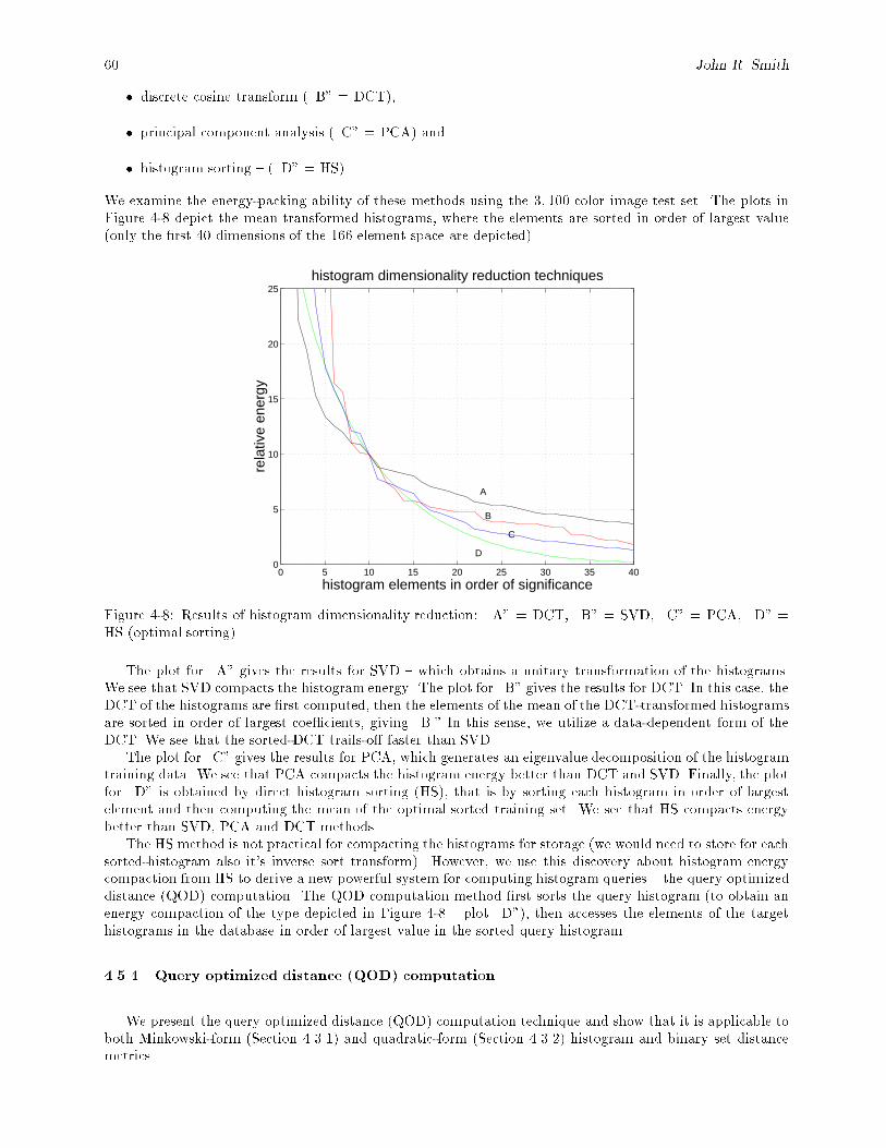
60 John R. Smith
� discrete cosine transform (\B" = DCT),
� principal component analysis (\C" = PCA) and
� histogram sorting { (\D" = HS).
We examine the energy-packing ability of these methods using the 3; 100 color image test set. The plots inFigure 4-8 depict the mean transformed histograms, where the elements are sorted in order of largest value(only the �rst 40 dimensions of the 166 element space are depicted).
0 5 10 15 20 25 30 35 400
5
10
15
20
25
histogram elements in order of significance
rela
tive
ener
gyhistogram dimensionality reduction techniques
A
B
C
D
Figure 4-8: Results of histogram dimensionality reduction: \A" = DCT, \B" = SVD, \C" = PCA, \D" =HS (optimal sorting).
The plot for \A" gives the results for SVD { which obtains a unitary transformation of the histograms.We see that SVD compacts the histogram energy. The plot for \B" gives the results for DCT. In this case, theDCT of the histograms are �rst computed, then the elements of the mean of the DCT-transformed histogramsare sorted in order of largest coe�cients, giving \B." In this sense, we utilize a data-dependent form of theDCT. We see that the sorted-DCT trails-o� faster than SVD.
The plot for \C" gives the results for PCA, which generates an eigenvalue decomposition of the histogramtraining data. We see that PCA compacts the histogram energy better than DCT and SVD. Finally, the plotfor \D" is obtained by direct histogram sorting (HS), that is by sorting each histogram in order of largestelement and then computing the mean of the optimal sorted training set. We see that HS compacts energybetter than SVD, PCA and DCT methods.
The HS method is not practical for compacting the histograms for storage (we would need to store for eachsorted-histogram also it's inverse sort transform). However, we use this discovery about histogram energycompaction from HS to derive a new powerful system for computing histogram queries { the query optimizeddistance (QOD) computation. The QOD computation method �rst sorts the query histogram (to obtain anenergy compaction of the type depicted in Figure 4-8 { plot \D"), then accesses the elements of the targethistograms in the database in order of largest value in the sorted query histogram.
4.5.4 Query optimized distance (QOD) computation
We present the query optimized distance (QOD) computation technique and show that it is applicable toboth Minkowski-form (Section 4.3.1) and quadratic-form (Section 4.3.2) histogram and binary set distancemetrics.
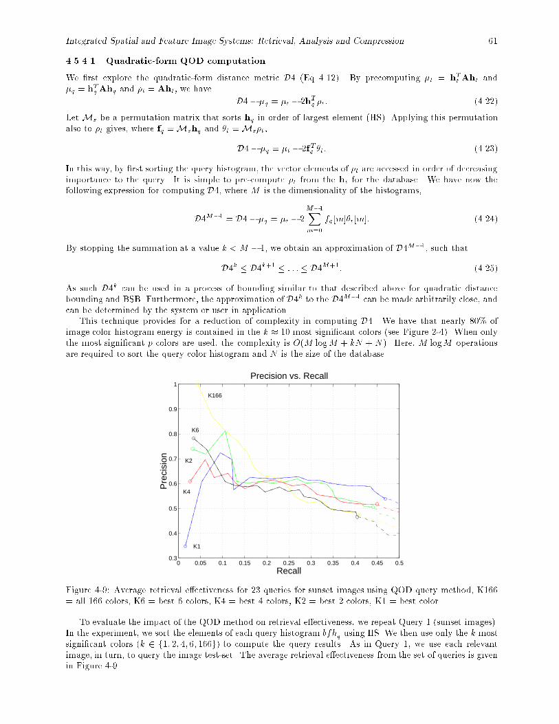
Integrated Spatial and Feature Image Systems: Retrieval, Analysis and Compression 61
4.5.4.1 Quadratic-form QOD computation
We �rst explore the quadratic-form distance metric D4 (Eq 4.12). By precomputing �t = hTt Aht and�q = hTqAhq and �t = Aht, we have
D4 � �q = �t � 2hTq �t: (4.22)
Let Ms be a permutation matrix that sorts hq in order of largest element (HS). Applying this permutationalso to �t gives, where fq =Mshq and �t =Ms�t,
D4� �q = �t � 2fTq �t; (4.23)
In this way, by �rst sorting the query histogram, the vector elements of �t are accessed in order of decreasingimportance to the query. It is simple to pre-compute �t from the ht for the database. We have now thefollowing expression for computing D4, where M is the dimensionality of the histograms,
D4M�1 = D4� �q = �t � 2M�1Xm=0
fq [m]�t[m]: (4.24)
By stopping the summation at a value k < M � 1, we obtain an approximation of D4M�1, such that
D4k � D4k+1 � : : : � D4M+1: (4.25)
As such D4k can be used in a process of bounding similar to that described above for quadratic distancebounding and BSB. Furthermore, the approximation of D4k to the D4M�1 can be made arbitrarily close, andcan be determined by the system or user in application.
This technique provides for a reduction of complexity in computing D4. We have that nearly 80% ofimage color histogram energy is contained in the k � 10 most signi�cant colors (see Figure 2-4). When onlythe most signi�cant p colors are used, the complexity is O(M logM + kN + N ). Here, M logM operationsare required to sort the query color histogram and N is the size of the database.
0 0.05 0.1 0.15 0.2 0.25 0.3 0.35 0.4 0.45 0.50.3
0.4
0.5
0.6
0.7
0.8
0.9
1
Recall
Pre
cisi
on
Precision vs. Recall
K166
K6
K4
K2
K1
Figure 4-9: Average retrieval e�ectiveness for 23 queries for sunset images using QOD query method, K166= all 166 colors, K6 = best 6 colors, K4 = best 4 colors, K2 = best 2 colors, K1 = best color.
To evaluate the impact of the QOD method on retrieval e�ectiveness, we repeat Query 1 (sunset images).In the experiment, we sort the elements of each query histogram bfhq using HS. We then use only the k mostsigni�cant colors (k 2 f1; 2; 4; 6; 166g) to compute the query results. As in Query 1, we use each relevantimage, in turn, to query the image test-set. The average retrieval e�ectiveness from the set of queries is givenin Figure 4-9.
62 John R. Smith
We make several observations from Figure 4-9. As k increases, the initial retrieval e�ectiveness alsoincreases, which is expected. That is, the �rst images retrieved are more likely to be relevant. However,at the point where approximately ten images are retrieved the retrieval e�ectiveness starts to decline as kincreases. We also see that for small values of k, i.e., k = 6, the retrieval e�ectiveness approaches that fork = 166. These results demonstrate that QOD provides a powerful method for reducing the computationrequired to answer the feature-based queries.
4.5.4.2 Binary set quadratic-form QOD computation
The QOD computation technique applies also to the binary set quadratic-form distance metric D5 (Eq 4.14).Since sq 2 B
M (sq is a binary vector), we have, where rt = Ast,
D5(q; t)� �q = �t � 2X
8m; where sq [m]=1
rt[m]: (4.26)
Using this QOD computation, we need only to consider the elements of the query binary set where sq [m] = 1in the computation of the quadratic-form binary set distance D5(q; t).
4.5.4.3 Euclidean-form QOD computation
The euclidean-form QOD computation (of D2) is a special case of the quadratic-form where �q = �t = 1 and�t = ht. Since �t is constant for the query, the complexity is further reduced to O(M logM + pN ).
4.6. Summary
In this chapter, we presented and evaluated techniques for computing color and texture similarities usinghistograms. We presented eight distance metrics and evaluated the retrieval e�ectiveness in experiments ofretrieving images from a test set of images. In summary, we found that the non-quadratic-form metrics (D1and D2) perform as well as the quadratic form metrics (D4 and D6). We also found that binary sets are ane�cient and compact alternative to histograms. Retrieval e�ectiveness with binary set metrics (D3 and D5)is worse than histograms, but examples illustrate that their performance su�ces as a �rst pass query.
We also compared the relative e�cacy of the visual dimensions of color and texture in retrieving imagesfrom the test set. While texture histograms perform well in retrieving Brodatz texture images, color methodsare better than texture methods in retrieving images from the set of \unconstrained" images.
We also presented two new strategies for e�ciently computing the histogram distance queries using binaryset bounding (BSB) and query-optimized distance (QOD) computation. We compared these techniques toquadratic distance bounding and other feature dimensionality reduction techniques. We note that thesetechniques may be combined to provide a powerful solution for e�ciently computing the histogram queries.
In the next chapter, we examine the problem of extracting color and texture regions from unconstrainedimagery. We use the color and texture histograms and binary feature sets in a novel process of regionextraction via histogram back-projection. We demonstrate in Chapter 7 that by extracting the regions fromimages and by utilizing spatial and feature attributes in the query process, we improve retrieval e�ectivenesssigni�cantly over the purely feature-based techniques explored in this chapter.
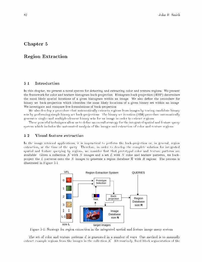
82 John R. Smith
Chapter 5
Region Extraction
5.1. Introduction
In this chapter, we present a novel system for detecting and extracting color and texture regions. We presentthe framework for color and texture histogram back-projection. Histogram back-projection (HBP) determinesthe most likely spatial locations of a given histogram within an image. We also de�ne the procedure forbinary set back-projection which identi�es the most likely locations of a given binary set within an image.We investigate and compare �ve formulations of back-projection.
We also develop a procedure that automatically extracts regions from images by testing candidate binarysets by performing simple binary set back-projections. The binary set iteration (BSI) procedure automaticallygenerates single- and multiple-element binary sets for an image in order to extract regions.
These powerful techniques allow us to de�ne an overall strategy for the integrated spatial and feature querysystem which includes the automated analysis of the images and extraction of color and texture regions.
5.2. Visual feature extraction
In the image retrieval applications, it is impractical to perform the back-projection or, in general, regionextraction, at the time of the query. Therefore, in order to develop the complete solution for integratedspatial and feature querying by regions, we consider �rst that prototypal color and texture patterns areavailable. Given a collection N with N images and a set L with N color and texture patterns, we back-project the L patterns onto the N images to generate a region database R with R regions. The process isillustrated in Figure 5-1.
hist2
VFL
0
1
3
L-1
PrototypeSelection
Back-projection
target images
RegionDatabase
size L
ImageDatabase
QUERIESRegion Extraction System
size R
size N
Figure 5-1: Strategy for region extraction in the integrated spatial and feature image query system.
The set of color and texture patterns L is generated in a number of ways. One method is to manuallyextract example regions from the images in the collection N . Alternatively, �xed block segmentation of the
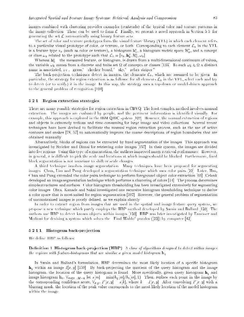
Integrated Spatial and Feature Image Systems: Retrieval, Analysis and Compression 83
images combined with clustering provides examples (centroids) of the typical color and texture patterns inthe image collection. These can be used to form L. Finally, we present a novel approach in Section 5.5. forgenerating the set L automatically using binary feature sets.
The set of color and texture prototypes form the visual feature library (VFL) in which each element refersto a particular visual prototype of color, or texture, or both. Corresponding to each element Lk in the VFLis a feature type vk (such as color or texture), a histogram hvk, a histogram metric space Hv
k, and a conceptor class !k related to the prototype such that Lk = [vk;h
vk;H
vk; !k].
Whereas hvk { the measured feature, or histogram, is drawn from a multidimensional continuum of values,the variable !k comes from a discrete and �nite set of concepts or classes [133]. To each !k 2 a distinctname is associated, i.e., \grass," \checker board," \sky," \zebra stripes."
The back-projection techniques detect in images, the elements Lk, which are assumed to be given. Inparticular, the strategy for region extraction is as follows: for all elements Lk in the VFL, select each and tryto detect (or to verify) it in the image. In this way, the strategy uses a top-down or model-driven approachto the general problem of recognition [104].
5.2.1 Region extraction strategies
There are many possible strategies for region extraction in CBVQ. The least complex method involves manualextraction. The images are evaluated by people, and the pertinent information is identi�ed visually. Forexample, this approach is explored in the IBM QBIC system [102]. However, the manual extraction of regionsand objects is extremely tedious and time-consuming for large image and video collections. Several recenttechniques have been devised to facilitate the manual region extraction process, such as the use of activecontours and snakes [78, 57] to automatically improve the coarse descriptions of region boundaries that areobtained manually.
Alternatively, blocks of regions can be extracted by �xed segmentation of the images. This approach wasinvestigated by Stricker and Dimai for retrieving color images [157]. In their system, the images are dividedinto �ve regions. Using this type of segmentation, the authors improved image retrieval performance. However,in general, it is di�cult to pick the scale and locations at which images should be blocked. Furthermore, �xedblock segmentation is not invariant to shift or scale changes.
A third technique involves image segmentation. Many techniques have been proposed for segmentingimages. Chua, Lim and Pung developed a segmentation technique which uses color pairs [29]. Later, Hsu,Chua and Pung extended the color pairs technique to perform foreground object color extraction [66]. Celenkdeveloped an image segmentation technique which performs a clustering of colors [14]. The process determinessimple structures and surfaces. Color histogram thresholding has been investigated extensively for segmentingcolor images. Ohta, Kanade and Sakai investigated one recursive histogram thresholding technique to derivea color space that is most suited for region segmentation [107]. However, the general problem of segmentationof unconstrained images is poorly de�ned, as we explain shortly.
In order to extract region from images that are used in the spatial and image feature query system, wepropose a new technique which partly employs the HBP method developed by Swain and Ballard [159]. Theauthors use HBP to detect known objects within images [159]. HBP was later investigated by Ennesser andMedioni for devising a system which solves the \Find Waldo" puzzles ([33]) by computer [43].
5.2.1.1 Histogram back-projection
We de�ne HBP as follows:
De�nition 1 Histogram back-projection (HBP). A class of algorithms designed to detect within images
the regions with feature-histograms that are similar a given model histogram hq.
In Swain and Ballard's formulation, HBP determines the most likely location of a speci�c histogramhq within an image I[x; y] [159]. By back-projecting the quotient of the query histogram and the imagehistogram, the location of the query histogram is found. More speci�cally, given query histogram hq andimage histogram ht, 8m20:::M�1 let s[m] = min(hq[m]=ht[m]; 1). Then, replace each point in the image bythe corresponding con�dence score, 8x;y, I0[x; y] = s[k], where k = I[x; y]. After convolving I0[x; y] with ablurring mask, the location of the peak value corresponds to the most likely location of the model histogramwithin the image.
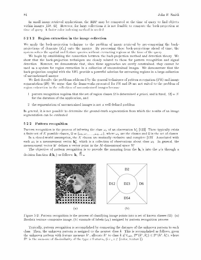
84 John R. Smith
In small image retrieval applications, the HBP may be computed at the time of query to �nd objectswithin images [159, 43]. However, for large collections it is not feasible to compute the back-projection attime of query. A faster color indexing method is needed.
5.2.1.2 Region extraction in the image collection
We apply the back-projection technique to the problem of image retrieval by pre-computing the back-projections of elements fLkg onto the images. By processing these back-projections ahead of time, thesystem solves the spatial and feature queries without extracting regions at the time of the query.
We begin by establishing the connection between the back-projection method and detection theory. Weshow that the back-projection techniques are closely related to those for pattern recognition and signaldetection. However, we demonstrate that, since these approaches are overly constrained, they cannot beused as a system for region extraction in a collection of unconstrained images. We demonstrate that theback-projection coupled with the VFL provide a powerful solution for extracting regions in a large collectionof unconstrained images.
We �rst describe the problems addressed by the general techniques of pattern recognition (PR) and imagesegmentation (IS). We argue that the frameworks presented for PR and IS are not suited to the problem ofregion extraction in the collection of unconstrained images because
1. pattern recognition requires that the set of region classes is determined a priori, and is �xed, jj = Nfor the duration of the application, and
2. the segmentation of unconstrained images is not a well de�ned problem.
In general, it is not possible to determine the ground-truth segmentation from which the results of an imagesegmentation can be evaluated.
5.2.2 Pattern recognition
Pattern recognition is the process of inferring the class !k of an observation hvk [133]. There typically existsa �nite set of K possible classes, = f!0; !1; : : : ; !K�1g, where !k are the classes and is the set of classes.
In a closed-world assumption, the K classes are mutually exclusive and complete [133]. Associated witheach !k is a measurement vector hvk, which is a collection of observations about class !k. In general, themeasurement vector hv de�nes a vector point in the M -dimensional space Hv.
The objective of pattern recognition is to provide the mapping from the hv's into the !'s through a
decision function d(hv) as follows: hvd! !.
D23
D54
D2
D12 D6
(a) (b)
Figure 5-2: Pattern recognition is the process of classifying image points into a set of known classes (). (a)Brodatz texture composite image, (b) example of labels (!k) assigned by pattern recognition process.
Typically, pattern recognition is accomplished by computing the distance of the unknown pattern to eachclass. Then, the unknown pattern is assigned to the nearest class k. This is accomplished as follows, giventhe unknown pattern with feature measure hv, allocate hv to class k if 8i6=k, D
v(hv; hvk) � Dv(hv; hvi ), where
Dv is the measure of dissimilarity of the type v features, (i.e., v 2 fcolor, textureg).
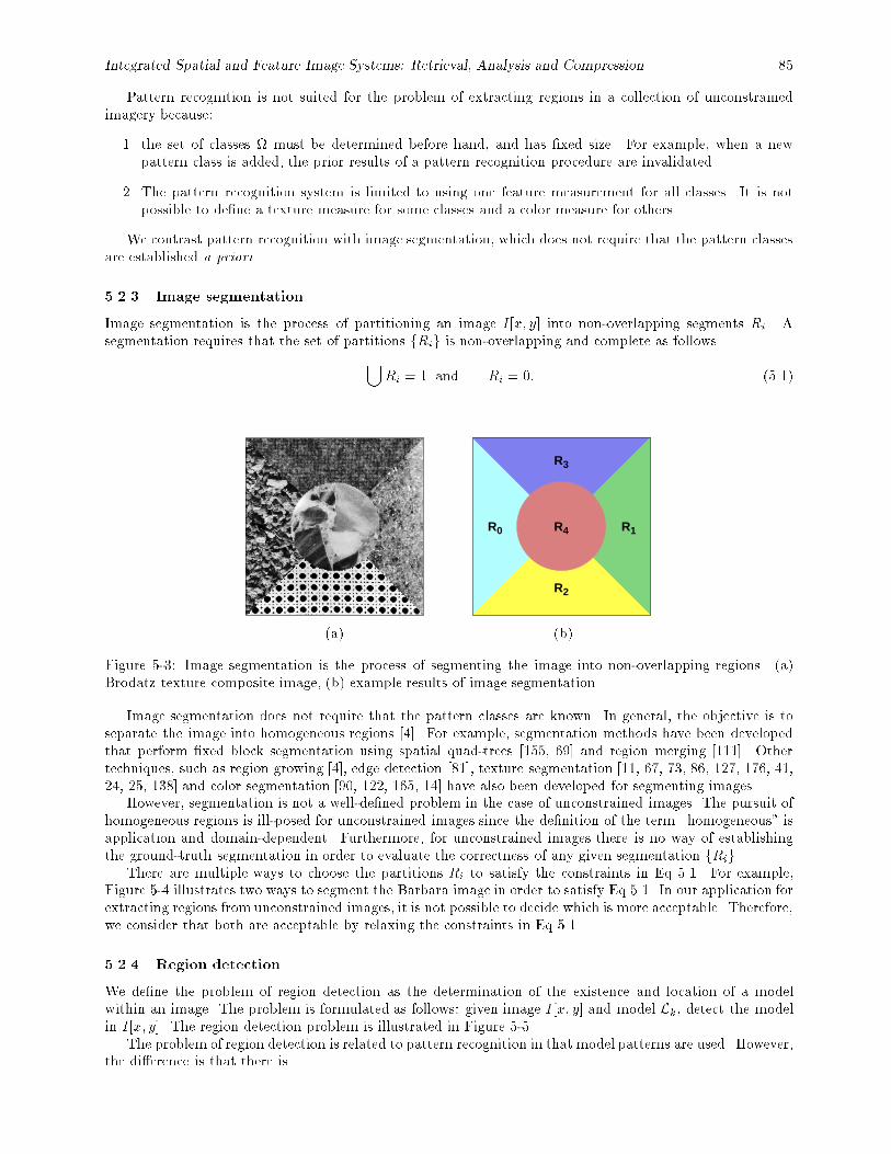
Integrated Spatial and Feature Image Systems: Retrieval, Analysis and Compression 85
Pattern recognition is not suited for the problem of extracting regions in a collection of unconstrainedimagery because:
1. the set of classes must be determined before hand, and has �xed size. For example, when a newpattern class is added, the prior results of a pattern recognition procedure are invalidated.
2. The pattern recognition system is limited to using one feature measurement for all classes. It is notpossible to de�ne a texture measure for some classes and a color measure for others.
We contrast pattern recognition with image segmentation, which does not require that the pattern classesare established a priori.
5.2.3 Image segmentation
Image segmentation is the process of partitioning an image I[x; y] into non-overlapping segments Ri. Asegmentation requires that the set of partitions fRig is non-overlapping and complete as follows
[Ri = 1 and
\Ri = 0: (5.1)
R0
R3
R1R4
R2
(a) (b)
Figure 5-3: Image segmentation is the process of segmenting the image into non-overlapping regions. (a)Brodatz texture composite image, (b) example results of image segmentation.
Image segmentation does not require that the pattern classes are known. In general, the objective is toseparate the image into homogeneous regions [4]. For example, segmentation methods have been developedthat perform �xed block segmentation using spatial quad-trees [155, 69] and region merging [111]. Othertechniques, such as region growing [4], edge detection [81], texture segmentation [11, 67, 73, 86, 127, 176, 41,24, 25, 138] and color segmentation [90, 122, 165, 14] have also been developed for segmenting images.
However, segmentation is not a well-de�ned problem in the case of unconstrained images. The pursuit ofhomogeneous regions is ill-posed for unconstrained images since the de�nition of the term \homogeneous" isapplication and domain-dependent. Furthermore, for unconstrained images there is no way of establishingthe ground-truth segmentation in order to evaluate the correctness of any given segmentation fRig.
There are multiple ways to choose the partitions Ri to satisfy the constraints in Eq 5.1. For example,Figure 5-4 illustrates two ways to segment the Barbara image in order to satisfy Eq 5.1. In our application forextracting regions from unconstrained images, it is not possible to decide which is more acceptable. Therefore,we consider that both are acceptable by relaxing the constraints in Eq 5.1.
5.2.4 Region detection
We de�ne the problem of region detection as the determination of the existence and location of a modelwithin an image. The problem is formulated as follows: given image I[x; y] and model Lk, detect the modelin I[x; y]. The region detection problem is illustrated in Figure 5-5.
The problem of region detection is related to pattern recognition in that model patterns are used. However,the di�erence is that there is
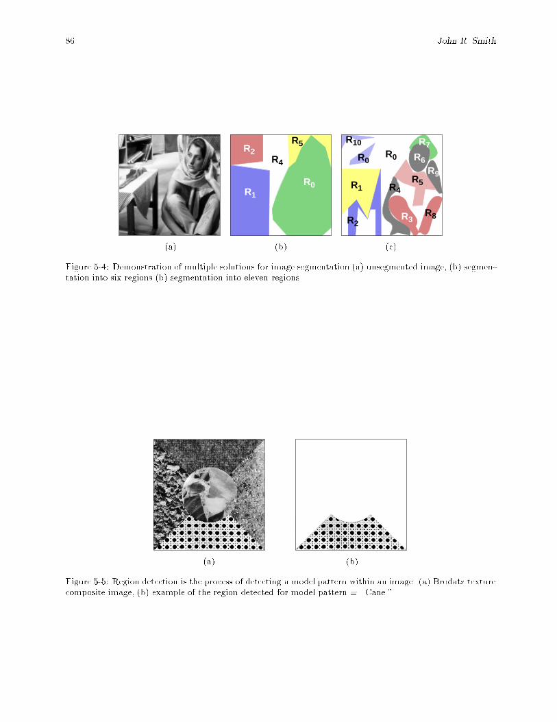
86 John R. Smith
R0R1
R2R4
R5
R3
R1
R2
R6
R5
R0R0
R7
R4
R9
R8
R10
(a) (b) (c)
Figure 5-4: Demonstration of multiple solutions for image segmentation (a) unsegmented image, (b) segmen-tation into six regions (b) segmentation into eleven regions.
(a) (b)
Figure 5-5: Region detection is the process of detecting a model pattern within an image. (a) Brodatz texturecomposite image, (b) example of the region detected for model pattern = \Cane."

Integrated Spatial and Feature Image Systems: Retrieval, Analysis and Compression 87
1. no restriction on the number or collection of models that are used. The complete set of models doesnot need to be de�ned a priori.
2. Each model may use a di�erent feature measurement type v. Some model patterns are de�ned in termsof color and others in terms of texture.
When a library of models is used to extract regions of di�ering patterns from an image, the problemresembles that for image segmentation: a set of regions Ri are extracted from the image. However, thedi�erence is that, here,
SRi � 1 and
TRi � 0. That is, the extracted regions may overlap and may not
necessarily completely partition the image.We now look more closely at the process of region extraction. We propose several HBP algorithms for
extracting regions from images. In order to understand the HBP process, we present the framework of decisiontheory. We �rst show that the con�dence HBP algorithm de�ned in [159] is related to the likelihood ratiotest [163].
5.2.4.1 Decision theory framework
The simplest decision theory problem consists of several components: the source, the probabilistic transitionmechanism, the observation space and the decision rule [163].
In our application, the �rst component corresponds to the source that generates the image. The sourceconsists of the objects in the real-world and the light that is re ected from the objects into the camera. Theprobabilistic transition mechanism corresponds to the light pattern this is probabilistically generated by eachobject depicted in the image.
Given a model, we wish to determine the patterns in the image that correspond to the model. We formulatethis as a simple two-hypothesis decision theory problem with the following two classes
H1 : model present
H0 : model not present:
We assume that the probabilistic transition mechanism generates points according to the corresponding twoconditional probability densities: points generated by the model follow prjH1
(RjH1) and other points followprjH0
(RjH0).Given the a priori probabilities for model presence P1 and model absence P0, and cost assignments for
each course of action Cij the expected cost of the risk < is given by
< = C11P1Pr(detect: H1jH1)
+ C01P1Pr(miss: H0jH1)
+ C10P0Pr(false alarm: H1jH0)
+ C00P0Pr(no detect: H1jH1): (5.2)
By minimizing < the likelihood ratio test is obtained by [163], choose H1 when
prjH1(RjH1)
prjH0(RjH0)
H1
>P0(C10 � C00)
P1(C01 � C11): (5.3)
In our application, it is di�cult to determine the a priori probabilities and cost assignments Cij. We considerinstead, the conditional probabilities for detection PD and false alarm PF , which are de�ned as follows
PF =
ZZ1
prjH0(RjH0) and PD =
ZZ1
prjH1(RjH1): (5.4)
By constraining PF , the PD can be maximized, which gives the Neyman-Pearson criterion,
prjH1(RjH1)
prjH0(RjH0)
H1
> �: (5.5)
Here, � determines the tradeo� between PF and PD. We now apply this to the detection of regions, wherethe conditional probabilities are determined by the feature histograms.
88 John R. Smith
5.2.4.2 Back-projection framework
In the case of images, the probabilistic transition mechanism generates an observation as each point in theimage. We presented measures for these observations in terms of color in Chapter 2 and texture in Chapter 3.In this way, the features of regions are represented by histograms (color histograms and texture histograms).These histograms correspond directly to the transition mechanism probability distributions. That is, a modelHk generates a histogram hk in accordance to hk = pr;HK (RjHk), where r is the measurement vector.
In the general two-class detection problem, we de�ne the histogram h1 for the model and h0 for non-model.From this, we reformulate the likelihood detection using the feature histograms as follows
h1h0
H1
> �: (5.6)
We now present the HBP algorithms, which are variations of Eq 5.6.
5.3. Back-projection algorithms
The HBP process is carried out using the following histograms:
1. model histogram, hq = h1,
2. target image histogram, ht = h0, and
3. local region histogram, hl.
The back-projection systems slide a window through the target image and compute the likelihood that eachimage point belongs to the model. The likelihood image is then �ltered to reduce noise. By thresholding at�, the locations of the model are determined in the image.
We investigate �ve formulations of back-projection: (1) con�dence back-projection, (2) quadratic con�-dence back-projection, (3) local histogramming, (4) binary set back-projection and (5) single-element back-projection. The back-projection algorithms consist of several stages: back-projection, smoothing, thresholdingand detection.
5.3.1 Con�dence back-projection (BP1)
Con�dence back-projection was proposed by Swain and Ballard [159]. The con�dence histogram hr is �rstgenerated by taking the ratio of the model hq and target histograms ht
hr[m] =hq[m]
ht[m]: (5.7)
Each point in the image is assigned a likelihood as follows
let k = I[x; y]; then I0[x; y] = hr [k]: (5.8)
The image I0[x; y] is then smoothed to reduce noise giving I00[x; y] = B[x; y] � I0[x; y], where � gives the 2-Dconvolution with blurring �lter B[x; y] as follows
I00[x; y] =W�1Xw=0
H�1Xh=0
B[x� w; y � h]I0[w; h]: (5.9)
Finally, I00[x; y] is thresholded. The peaks reveal the locations of the detected model hq. One drawbackof BP1 is that the back-projection only compares like-bins. This is similar to the drawback of using theMinkowski-form metrics for computing histogram distance (see Section 4.3.1). To address this, we developBP2 to consider the similarity of each target element ht[m] to all the elements in the model histogram hq.
Integrated Spatial and Feature Image Systems: Retrieval, Analysis and Compression 89
5.3.2 Quadratic con�dence back-projection (BP2)
In quadratic con�dence histogram back-projection, hr is generated by taking the ratio of the model hq andtarget histograms ht as follows
hr [m] =
Pn hq[m]Am;n
ht[m]; (5.10)
where Am;n de�nes the similarity of the histogram elements indexed by m and n. Each point in the image isassigned a likelihood as follows
let k = I[x; y]; then I0[x; y] = hr [k]: (5.11)
The image I0[x; y] is then smoothed to reduce noise and thresholded to reveal the most likely locations of hq.
5.3.3 Local histogramming (BP3)
In local histogramming, the smoothing operation and back-projection steps are combined. In this case, foreach point in the target image I[x; y], a local neighborhood histogram hl is computed and its distance to themodel histogram hq determines whether each image point belongs to the model. De�ne hxyl to be the localneighborhood histogram for the region Rwh
xy in image I[x; y], centered at point (x; y) with size w � h. Then,let
I00[x; y] = dq;l(hq;hxyl ): (5.12)
BP3 is more robust than BP1 and BP2 since the most e�ective distance metric dq;l may be used (seeChapter 4).
5.3.4 Binary set back-projection (BP4)
In binary set back-projection, the target image points are assigned 1 or 0 depending on membership in themodel binary set sq where sq 2 B
M . In this way, BP4 is extremely simple as follows
let k = I[x; y]; then I0[x; y] = sq[k]: (5.13)
The image I 0[x; y] is then smoothed to reduce noise and thresholded to reveal the most likely locations of sq.
5.3.5 Single element quadratic back-projection (BP5)
Single element quadratic back-projection combines BP2 and BP4. The target image points are weighted bysimilarity to the back-projection element m, where sq [m] = 1 and sq [k] = 0; 8k 6=m such that
let k = I[x; y]; then I0[x; y] = Am;k: (5.14)
The image I 0[x; y] is then smoothed to reduce noise and thresholded to reveal the most likely locations of sq.
5.4. Back-projection region extraction examples
We demonstrate the back-projection methods by detecting models of color and texture in example images.The results are given in Figures 5-6, 5-7, 5-8 and 5-9.
5.4.1 Color histogram back-projection
Figure 5-6 illustrates the results of color HBP using algorithms (BP1 : : :BP4). The model image depictsa sample of \yellow grass." The �rst row depicts the back-projection images. The second row depicts the�ltered images. We see that BP2 improves the detection results over BP1, however, BP3 best determinesthe location of the model. The binary set back-projection BP4 detects the model su�ciently well, whichindicates that BP4 has a role as a pre-�lter before a more expensive back-projection, i.e, BP3.
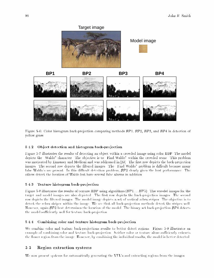
90 John R. Smith
Target image
Model image
BP1 BP2 BP3 BP4
Figure 5-6: Color histogram back-projection comparing methods BP1, BP2, BP3, and BP4 in detection ofyellow grass.
5.4.2 Object detection and histogram back-projection
Figure 5-7 illustrates the results of detecting an object within a crowded image using color HBP. The modeldepicts the \Waldo" character. The objective is to \Find Waldo" within the crowded scene. This problemwas motivated by Ennesser and Medioni and was addressed in [43]. The �rst row depicts the back-projectionimages. The second row depicts the �ltered images. The \Find Waldo" problem is di�cult because manyfalse Waldo's are present. In this di�cult detection problem, BP3 clearly gives the best performance. Theothers detect the location of Waldo but have several false alarms in addition.
5.4.3 Texture histogram back-projection
Figure 5-8 illustrates the results of texture HBP using algorithms (BP1 : : :BP5). The wavelet images for thetarget and model images are also depicted. The �rst row depicts the back-projection images. The secondrow depicts the �ltered images. The model image depicts a set of vertical zebra stripes. The objective is todetect the zebra stripes within the image. We see that all back-projection methods detect the stripes well.However, again BP3 best determines the location of the model. The binary set back-projection BP4 detectsthe model su�ciently well for texture back-projection.
5.4.4 Combining color and texture histogram back-projection
We combine color and texture back-projections results to better detect regions. Figure 5-9 illustrates anexample of combining color and texture back-projection. Neither color or texture alone su�ciently extractsthe ower region from the image. However, by combining the individual results, the model is better detected.
5.5. Region extraction systems
We now present systems for automatically generating the VFL's and extracting regions from the images.
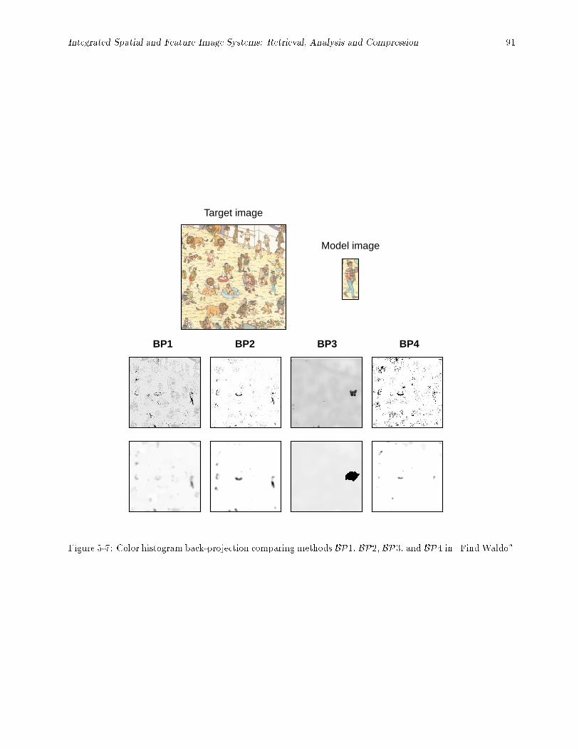
Integrated Spatial and Feature Image Systems: Retrieval, Analysis and Compression 91
Target image
Model image
BP1 BP2 BP3 BP4
Figure 5-7: Color histogram back-projection comparing methods BP1, BP2, BP3, and BP4 in \Find Waldo".
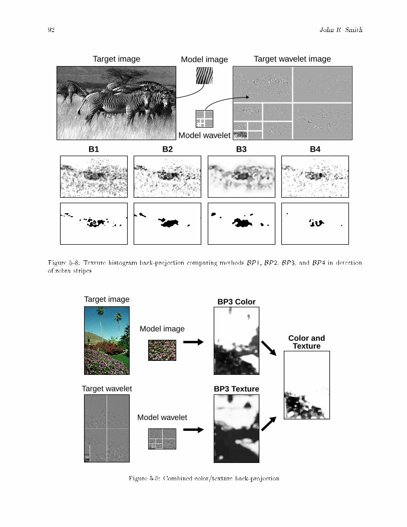
92 John R. Smith
Target image
B1 B2 B3 B4
Target wavelet imageModel image
Model wavelet
Figure 5-8: Texture histogram back-projection comparing methods BP1, BP2, BP3, and BP4 in detectionof zebra stripes.
Target image
Target wavelet
Model image
Model wavelet
BP3 Color
BP3 Texture
Color andTexture
Figure 5-9: Combined color/texture back-projection.
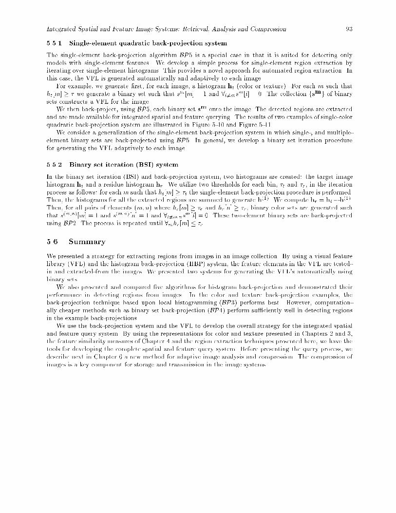
Integrated Spatial and Feature Image Systems: Retrieval, Analysis and Compression 93
5.5.1 Single-element quadratic back-projection system
The single-element back-projection algorithm BP5 is a special case in that it is suited for detecting onlymodels with single-element features. We develop a simple process for single-element region extraction byiterating over single-element histograms. This provides a novel approach for automated region extraction. Inthis case, the VFL is generated automatically and adaptively to each image.
For example, we generate �rst, for each image, a histogram ht (color or texture). For each m such thatht[m] � � we generate a binary set such that sm[m] = 1 and 8i 6=msm[i] = 0. The collection fsmg of binarysets constructs a VFL for the image.
We then back-project, using BP5, each binary set sm onto the image. The detected regions are extractedand are made available for integrated spatial and feature querying. The results of two examples of single-colorquadratic back-projection system are illustrated in Figure 5-10 and Figure 5-11.
We consider a generalization of the single-element back-projection system in which single-, and multiple-element binary sets are back-projected using BP5. In general, we develop a binary set iteration procedurefor generating the VFL adaptively to each image.
5.5.2 Binary set iteration (BSI) system
In the binary set iteration (BSI) and back-projection system, two histograms are created: the target imagehistogram ht and a residue histogram hr. We utilize two thresholds for each bin, �t and �r, in the iterationprocess as follows: for each m such that ht[m] � �t the single-element back-projection procedure is performed.Then, the histograms for all the extracted regions are summed to generate h(1). We compute hr = ht�h(1).Then, for all pairs of elements (m;n) where hr[m] � �r and hr[n] � �r , binary color sets are generated suchthat s(m;n)[m] = 1 and s(m;n)[n] = 1 and 8i6=m;nsm[i] = 0. These two-element binary sets are back-projectedusing BP2. The process is repeated until 8mhr[m] � �r .
5.6. Summary
We presented a strategy for extracting regions from images in an image collection. By using a visual featurelibrary (VFL) and the histogram back-projection (HBP) system, the feature elements in the VFL are tested-in and extracted-from the images. We presented two systems for generating the VFL's automatically usingbinary sets.
We also presented and compared �ve algorithms for histogram back-projection and demonstrated theirperformance in detecting regions from images. In the color and texture back-projection examples, theback-projection technique based upon local histogramming (BP3) performs best. However, computation-ally cheaper methods such as binary set back-projection (BP4) perform su�ciently well in detecting regionsin the example back-projections.
We use the back-projection system and the VFL to develop the overall strategy for the integrated spatialand feature query system. By using the representations for color and texture presented in Chapters 2 and 3,the feature similarity measures of Chapter 4 and the region extraction techniques presented here, we have thetools for developing the complete spatial and feature query system. Before presenting the query process, wedescribe next in Chapter 6 a new method for adaptive image analysis and compression. The compression ofimages is a key component for storage and transmission in the image systems.
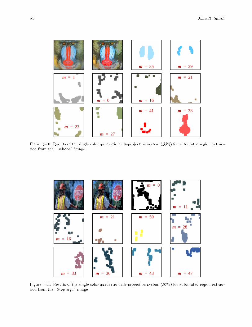
94 John R. Smith
m 35= m 39=
m 21=
m 16=m 0=
m 1=
m 38=m 41=
m 27=
m 23=
Figure 5-10: Results of the single color quadratic back-projection system (BP5) for automated region extrac-tion from the \Baboon" image.
m 47=m 43=m 36=m 33=
m 28=
m 50=m 21=
m 16=
m 11=
m 0=
Figure 5-11: Results of the single color quadratic back-projection system (BP5) for automated region extrac-tion from the \Stop sign" image.
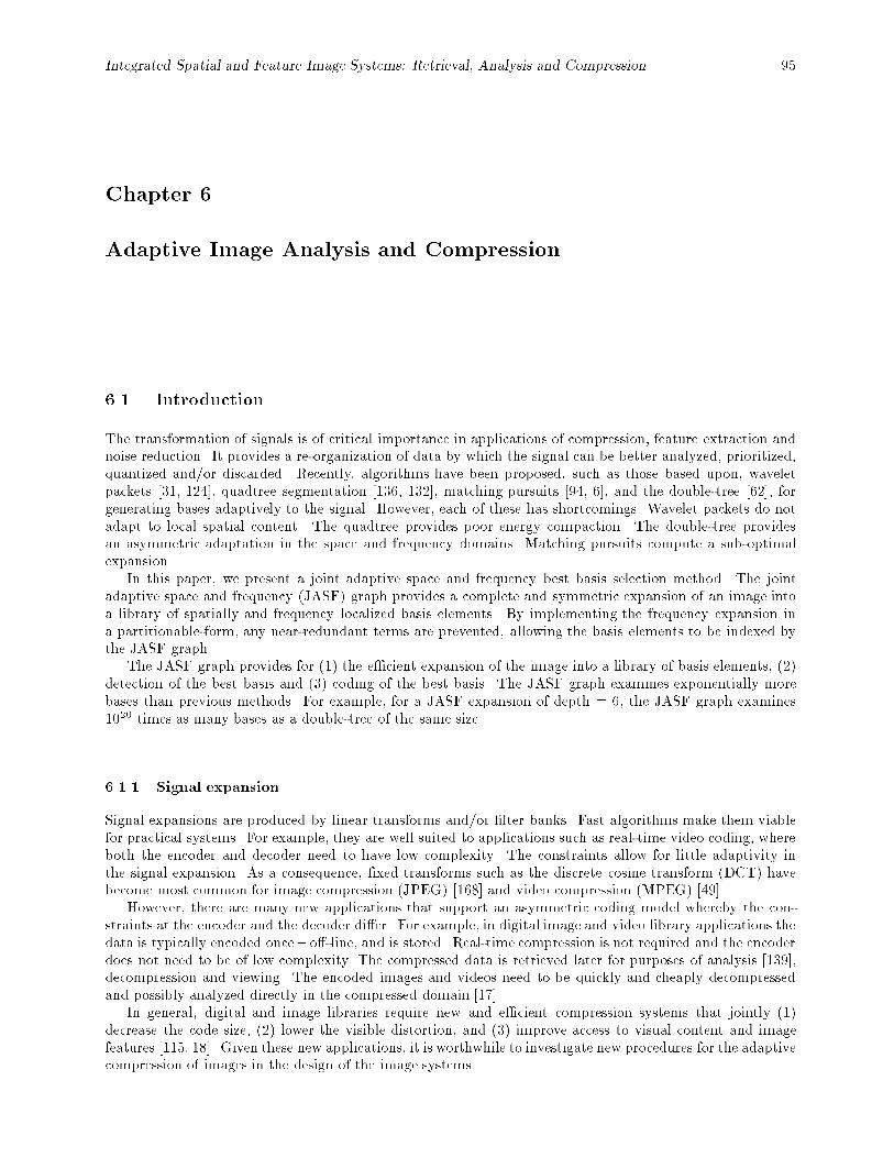
Integrated Spatial and Feature Image Systems: Retrieval, Analysis and Compression 95
Chapter 6
Adaptive Image Analysis and Compression
6.1. Introduction
The transformation of signals is of critical importance in applications of compression, feature extraction andnoise reduction. It provides a re-organization of data by which the signal can be better analyzed, prioritized,quantized and/or discarded. Recently, algorithms have been proposed, such as those based upon, waveletpackets [31, 124], quadtree segmentation [136, 132], matching pursuits [94, 6], and the double-tree [62], forgenerating bases adaptively to the signal. However, each of these has shortcomings. Wavelet packets do notadapt to local spatial content. The quadtree provides poor energy compaction. The double-tree providesan asymmetric adaptation in the space and frequency domains. Matching pursuits compute a sub-optimalexpansion.
In this paper, we present a joint adaptive space and frequency best basis selection method. The jointadaptive space and frequency (JASF) graph provides a complete and symmetric expansion of an image intoa library of spatially and frequency localized basis elements. By implementing the frequency expansion ina partitionable-form, any near-redundant terms are prevented, allowing the basis elements to be indexed bythe JASF graph.
The JASF graph provides for (1) the e�cient expansion of the image into a library of basis elements, (2)detection of the best basis and (3) coding of the best basis. The JASF graph examines exponentially morebases than previous methods. For example, for a JASF expansion of depth = 6, the JASF graph examines1020 times as many bases as a double-tree of the same size.
6.1.1 Signal expansion
Signal expansions are produced by linear transforms and/or �lter banks. Fast algorithms make them viablefor practical systems. For example, they are well suited to applications such as real-time video coding, whereboth the encoder and decoder need to have low complexity. The constraints allow for little adaptivity inthe signal expansion. As a consequence, �xed transforms such as the discrete cosine transform (DCT) havebecome most common for image compression (JPEG) [168] and video compression (MPEG) [49].
However, there are many new applications that support an asymmetric coding model whereby the con-straints at the encoder and the decoder di�er. For example, in digital image and video library applications thedata is typically encoded once { o�-line, and is stored. Real-time compression is not required and the encoderdoes not need to be of low complexity. The compressed data is retrieved later for purposes of analysis [139],decompression and viewing. The encoded images and videos need to be quickly and cheaply decompressedand possibly analyzed directly in the compressed domain [17].
In general, digital and image libraries require new and e�cient compression systems that jointly (1)decrease the code size, (2) lower the visible distortion, and (3) improve access to visual content and imagefeatures [115, 18]. Given these new applications, it is worthwhile to investigate new procedures for the adaptivecompression of images in the design of the image systems.
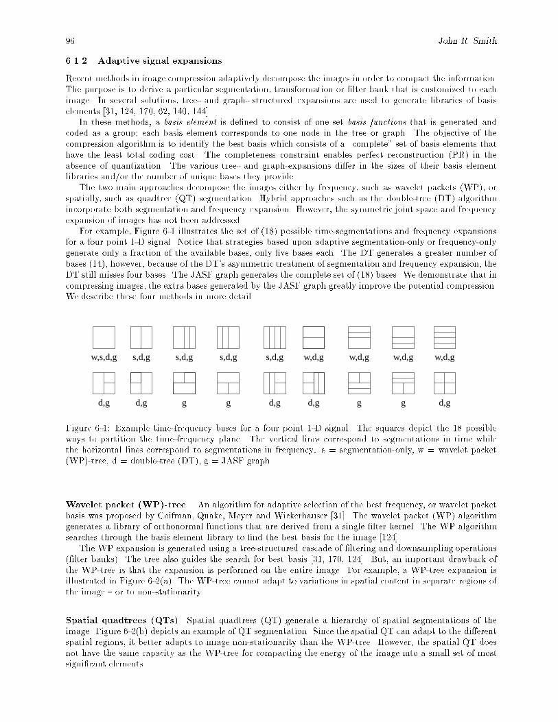
96 John R. Smith
6.1.2 Adaptive signal expansions
Recent methods in image compression adaptively decompose the images in order to compact the information.The purpose is to derive a particular segmentation, transformation or �lter bank that is customized to eachimage. In several solutions, tree- and graph- structured expansions are used to generate libraries of basiselements [31, 124, 170, 62, 140, 144].
In these methods, a basis element is de�ned to consist of one set basis functions that is generated andcoded as a group; each basis element corresponds to one node in the tree or graph. The objective of thecompression algorithm is to identify the best basis which consists of a \complete" set of basis elements thathave the least total coding cost. The completeness constraint enables perfect reconstruction (PR) in theabsence of quantization. The various tree- and graph-expansions di�er in the sizes of their basis elementlibraries and/or the number of unique bases they provide.
The two main approaches decompose the images either by frequency, such as wavelet packets (WP), orspatially, such as quadtree (QT) segmentation. Hybrid approaches such as the double-tree (DT) algorithmincorporate both segmentation and frequency expansion. However, the symmetric joint space and frequencyexpansion of images has not been addressed.
For example, Figure 6-1 illustrates the set of (18) possible time-segmentations and frequency expansionsfor a four point 1-D signal. Notice that strategies based upon adaptive segmentation-only or frequency-onlygenerate only a fraction of the available bases, only �ve bases each. The DT generates a greater number ofbases (14), however, because of the DT's asymmetric treatment of segmentation and frequency expansion, theDT still misses four bases. The JASF graph generates the complete set of (18) bases. We demonstrate that incompressing images, the extra bases generated by the JASF graph greatly improve the potential compression.We describe these four methods in more detail.
w,s,d,g s,d,g w,d,g
d,g g g d,g d,g g g d,gd,g
s,d,g s,d,g w,d,g w,d,g w,d,gs,d,g
Figure 6-1: Example time-frequency bases for a four point 1-D signal. The squares depict the 18 possibleways to partition the time-frequency plane. The vertical lines correspond to segmentations in time whilethe horizontal lines correspond to segmentations in frequency: s = segmentation-only, w = wavelet packet(WP)-tree, d = double-tree (DT), g = JASF graph.
Wavelet packet (WP)-tree An algorithm for adaptive selection of the best frequency, or wavelet packetbasis was proposed by Coifman, Quake, Meyer and Wickerhauser [31]. The wavelet packet (WP) algorithmgenerates a library of orthonormal functions that are derived from a single �lter kernel. The WP algorithmsearches through the basis element library to �nd the best basis for the image [124].
The WP expansion is generated using a tree-structured cascade of �ltering and downsampling operations(�lter banks). The tree also guides the search for best basis [31, 170, 124]. But, an important drawback ofthe WP-tree is that the expansion is performed on the entire image. For example, a WP-tree expansion isillustrated in Figure 6-2(a). The WP-tree cannot adapt to variations in spatial content in separate regions ofthe image { or to non-stationarity.
Spatial quadtrees (QTs) Spatial quadtrees (QT) generate a hierarchy of spatial segmentations of theimage. Figure 6-2(b) depicts an example of QT segmentation. Since the spatial QT can adapt to the di�erentspatial regions, it better adapts to image non-stationarity than the WP-tree. However, the spatial QT doesnot have the same capacity as the WP-tree for compacting the energy of the image into a small set of mostsigni�cant elements.
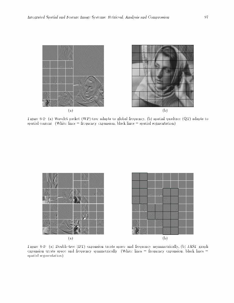
Integrated Spatial and Feature Image Systems: Retrieval, Analysis and Compression 97
(a) (b)
Figure 6-2: (a) Wavelet packet (WP)-tree adapts to global frequency, (b) spatial quadtree (QT) adapts tospatial content. (White lines = frequency expansion, black lines = spatial segmentation)
(a) (b)
Figure 6-3: (a) Double-tree (DT) expansion treats space and frequency asymmetrically, (b) JASF graphexpansion treats space and frequency symmetrically. (White lines = frequency expansion, black lines =spatial segmentation)
98 John R. Smith
Double-tree (DT) To address the problem of non-stationarity without sacri�cing energy compaction, thedouble-tree (DT) algorithm was proposed by Herley, Kova�cevi�c, Ramchandran and Vetterli [62]. The DT�nds the best WP basis for a hierarchy of binary segmentations of the signal. The overall best basis searchidenti�es the best overall segmentation and best WP basis for the segments.
However, the DT does not exploit the full potential of a joint space and frequency expansion. Theinsu�ciency results from the asymmetric treatment of the space and frequency operations in the tree cascades,as illustrated in the example of a DT expansion of the Barbara image in Figure 6-3(a). Furthermore, we willshow that a \single critical pruning decision" reduces the DT to a WP-tree. We have observed for imagesthat the DT is most typically pruned into a WP-tree. Therefore, in practice, the DT o�ers no advantage overthe WP-tree.
JASF graph The JASF algorithm treats the space and frequency operations symmetrically in a graphstructured cascade [140, 144]. An example of a JASF graph expansion of the Barbara image is illustrated inFigure 6-3(b). Both the DT and its dual are embedded in the JASF graph. The JASF graph requires thatthe basis functions are modi�ed to generate a partitionable frequency expansion. While this does impact thefrequency expansion, it allows the JASF graph to examine a greater number of bases, and to adapt to theimage in both space and frequency.
6.1.3 Outline
In this paper, we present the JASF graph image expansion and basis selection method. In Section 6.2., we �rstreview the framework for signal expansion using �lter banks. We also develop the theory of \partitionable"frequency expansions which are fundamental to the JASF graph. In Section 6.3., we present the processof spatial segmentation of images using spatial QTs. In Section 6.4., we integrate frequency expansion andsegmentation by cascading the \partitionable" �lter banks and spatial QT segmentations. We show that byusing \partitionable" expansions, the generation of the basis library and the reconstruction of the image fromthe library elements follows a number of equivalent paths.
In Section 6.5., we show that the JASF graph greatly increases the available number of bases. In Sec-tion 6.6., we describe the basis selection procedure which consists of selecting elements from the JASF libraryvia the graph-structure [150]. In Section 6.5.1, we compare the sizes of the various tree- and graph-structuredbasis element libraries and number of bases they provide. Finally, in Section 6.7. we demonstrate improvedcompression performance using the JASF graph over the WP-tree spatial QT and DT methods.
6.2. Image signal expansion
We �rst consider a 1-D signal, the extension of the 1-D signal expansion to 2-D discrete-space images isstraightforward and will be explained when necessary. We �rst consider that a discrete-time �lter bankproduces a series expansion of a 1-D signal into a set of basis functions.
6.2.1 Series expansion
A series expansion represents the signal using a set of orthonormal basis functions f�kg such that
x[n] =Xk2Z
h�k; xi�k[n]; n 2 Z: (6.1)
Here h�k[n]; �l[n]i = �[k� l] dictates an orthonormality constraint and the inner product is given by hx; yi =P1n=�1 x�[n]y[n]. The expansion of x into the set of basis functions f�kg produces the transform coe�cients
X where X[k] = h�k; xi.
6.2.2 Filter bank
A two-channel �lter bank implements an orthonormal expansion when even shifts of the analysis hi andsynthesis gi �lters are related to the basis functions by [167]
h0[2k � n] = g0[n� 2k] = �2k[n]; and
h1[2k � n] = g1[n� 2k] = �2k+1[n]: (6.2)
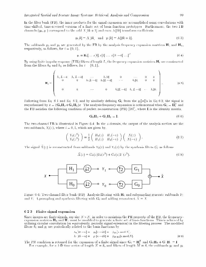
Integrated Spatial and Feature Image Systems: Retrieval, Analysis and Compression 99
In the �lter bank (FB), the inner products for the signal expansion are accomplished using convolutions withtime-shifted, time-reversed versions of a �nite set of basis function prototypes. Furthermore, the two FBchannels (y0; y1) correspond to the odd X[2k + 1] and even X[2k] transform coe�cients
y0[k] = X[2k] and y1[k] = X[2k + 1]: (6.3)
The subbands y0 and y1 are generated by the FB by the analysis frequency expansion matrices H0 and H1,respectively, as follows, for i = f0; 1g,
yi = Hi[: : : x[0]; x[1] : : : x[N � 1] : : :]T (6.4)
By using �nite impulse response (FIR) �lters of length L, the frequency expansion matricesHi are constructedfrom the �lters h0 and h1 as follows, for i = f0; 1g,
Hi =
0BBBBBBB@
.
.
....
.
.
....
.
.
....
hi[L� 1] hi [L� 2] � � � hi[0] 0 � � � 0 00 0 hi[L� 1] hi[L� 2] � � � hi[0] 0 0
. . ... .
.. .. . .
.
..0 0 � � � 0 hi[L� 1] hi[L� 2] � � � hi[0]...
.
.....
.
.....
.
..
1CCCCCCCA
: (6.5)
Following from Eq. 6.1 and Eq. 6.2, and by similarly de�ning Gi from the gi[m]'s in Eq 6.2, the signal isresynthesized by x = (G0H0+G1H1)x. The analysis frequency-expansion is orthonormal whenGi = HT
i andthe FB satis�es the following condition of perfect reconstruction (PR) [167], where I is the identity matrix,
G0H0 +G1H1 = I: (6.6)
The two-channel FB is illustrated in Figure 6-4. In the z-domain, the output of the analysis section are thetwo subbands, Yi(z), where i = 0; 1, which are given by,�
Y0(z2)Y1(z2)
�=
1
2
�H0(z) H0(�z)H1(z) H1(�z)
��X(z)X(�z)
�: (6.7)
The signal ~X(z) is reconstructed from subbands Y0(z) and Y1(z) by the synthesis �lters Gi as follows
~X(z) = G0(z)Y0(z2) + G1(z)Y1(z
2): (6.8)
H1
H0
2
2
X
2
2
G1
G0
+ X
Y1
Y0
Figure 6-4: Two-channel �lter bank (FB). Analysis �ltering with Hi and subsampling generate subbands Y0and Y1. Upsampling and synthesis �ltering with Gi and adding reconstruct ~X = X.
6.2.3 Finite signal expansion
Since images are �nite signals, say size N�N , in order to maintain the PR property of the FB, the frequency-expansion matricesH0 andH1 must be modi�ed to generate a �nite set of basis functions. This is achieved byutilizing circular convolution (or equivalently, periodic signal extension) in the �ltering process. The modi�ed�lters hi and gi are periodically related to the basis functions by
h0 [2k � n] = g0[n� 2k] = �2k[n modN ];
h1 [2k � n] = g1[n� 2k] = �2k+1[n modN ]: (6.9)
The PR condition is retained for the expansion of a �nite signal since Gi =HTi and G0H0 +G1H1 = I.
For example, for a 1-D time series of length N = 8, and �lters of length M = 4, the subbands y0 and y1
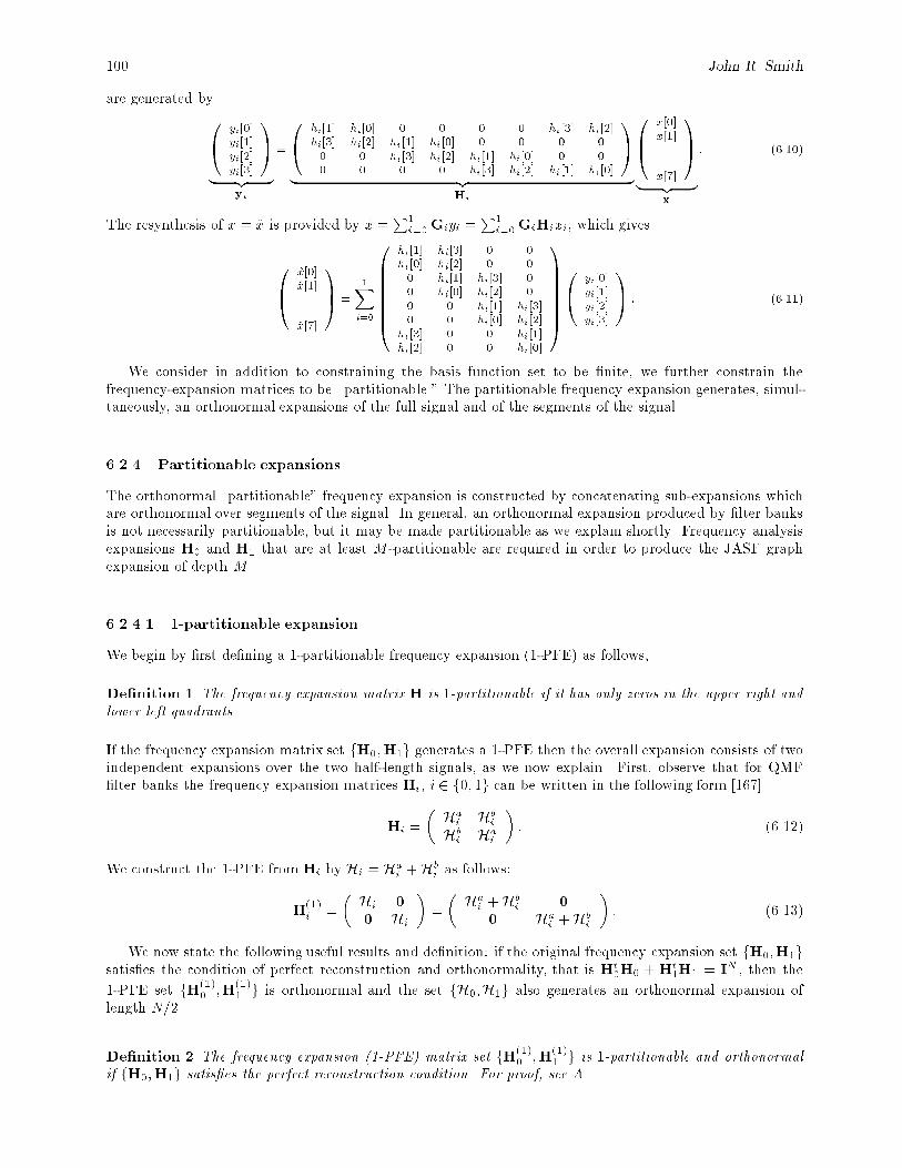
100 John R. Smith
are generated by0@ yi[0]
yi[1]yi[2]yi[3]
1A
| {z }yi
=
0@ hi[1] hi[0] 0 0 0 0 hi[3] hi[2]
hi[3] hi[2] hi[1] hi[0] 0 0 0 00 0 hi[3] hi[2] hi[1] hi[0] 0 00 0 0 0 hi[3] hi[2] hi[1] hi[0]
1A
| {z }Hi
0B@
x[0]x[1]...
x[7]
1CA
| {z }x
: (6.10)
The resynthesis of x = x is provided by x =P1
i=0Giyi =P1
i=0GiHixi, which gives
0B@
x[0]x[1]...
x[7]
1CA =
1Xi=0
0BBBBBB@
hi[1] hi[3] 0 0hi[0] hi[2] 0 00 hi[1] hi[3] 00 hi[0] hi[2] 00 0 hi[1] hi[3]0 0 hi[0] hi[2]
hi[3] 0 0 hi[1]hi[2] 0 0 hi[0]
1CCCCCCA0@ yi[0]
yi[1]yi[2]yi[3]
1A : (6.11)
We consider in addition to constraining the basis function set to be �nite, we further constrain thefrequency-expansion matrices to be \partitionable." The partitionable frequency expansion generates, simul-taneously, an orthonormal expansions of the full signal and of the segments of the signal.
6.2.4 Partitionable expansions
The orthonormal \partitionable" frequency expansion is constructed by concatenating sub-expansions whichare orthonormal over segments of the signal. In general, an orthonormal expansion produced by �lter banksis not necessarily partitionable, but it may be made partitionable as we explain shortly. Frequency analysisexpansions H0 and H1 that are at least M -partitionable are required in order to produce the JASF graphexpansion of depth M .
6.2.4.1 1-partitionable expansion
We begin by �rst de�ning a 1-partitionable frequency expansion (1-PFE) as follows,
De�nition 1 The frequency expansion matrix H is 1-partitionable if it has only zeros in the upper right andlower left quadrants.
If the frequency expansion matrix set fH0;H1g generates a 1-PFE then the overall expansion consists of twoindependent expansions over the two half-length signals, as we now explain. First, observe that for QMF�lter banks the frequency expansion matrices Hi, i 2 f0; 1g can be written in the following form [167]
Hi =
�Hai Hb
i
Hbi Ha
i
�: (6.12)
We construct the 1-PFE from Hi by Hi = Hai +Hb
i as follows:
H(1)i =
�Hi 00 Hi
�=
�Hai +Hb
i 00 Ha
i +Hbi
�: (6.13)
We now state the following useful results and de�nition: if the original frequency expansion set fH0;H1gsatis�es the condition of perfect reconstruction and orthonormality, that is Ht
0H0 + Ht1H1 = IN , then the
1-PFE set fH(1)0 ;H
(1)1 g is orthonormal and the set fH0;H1g also generates an orthonormal expansion of
length N=2.
De�nition 2 The frequency expansion (1-PFE) matrix set fH(1)0 ;H
(1)1 g is 1-partitionable and orthonormal
if fH0;H1g satis�es the perfect reconstruction condition. For proof, see A..
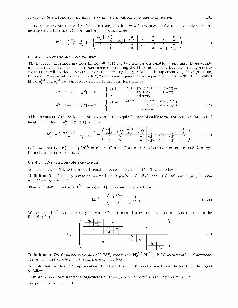
Integrated Spatial and Feature Image Systems: Retrieval, Analysis and Compression 101
It is also obvious to see that for a FB using length L = 2 �lters, such as the Haar expansion, the Hi
generate a 1-PFE since, Hi = Hai and Hb
i = 0, which gives
H(1)i =
�Hi 0
0 Hi
�=
0@ hi[1] hi[0] 0 0 0 0 0 0
0 0 hi[1] hi[0] 0 0 0 00 0 0 0 hi[1] hi[0] 0 00 0 0 0 0 0 hi[1] hi[0]
1A : (6.14)
6.2.4.2 1-partitionable convolution
The frequency expansion matrices Hi for i 2 f0; 1g can be made 1-partitionable by summing the quadrantsas illustrated in Eq 6.13. This is equivalent to wrapping the �lters at the N=2 boundary (using circularconvolutions with period = N=2) as long as the �lter length L � N=2. This is implemented by �rst segmentingthe length N signal into two half lengthN=2 signals and expanding each separately. In the 1-PFE, the modi�ed
�lters h(1)i and g
(1)i are periodically related to the basis functions by
h(1)0 [2k � n] = g
(1)0 [n� 2k] =
(�2k[n mod N=2] (2k < N=2 and n < N=2) or
(2k � N=2 and n � N=2)0 otherwise
h(1)1 [2k � n] = g
(1)1 [n� 2k] =
(�2k+1[n modN=2] (2k < N=2 and n < N=2) or
(2k � N=2 and n � N=2)0 otherwise
(6.15)
This assignment of the basis functions gives H(1)i the required 1-partitionable form. For example, for a set of
length L = 4 �lters, h(1)i ; i 2 f0; 1g, we have
H(1)i =
�Hai +Hb
i 0
0 Hai +Hb
i
�=
0@ hi[1] hi[0] hi[3] hi[2] 0 0 0 0
hi[3] hi[2] hi[1] hi[0] 0 0 0 00 0 0 0 hi[1] hi[0] hi[3] hi[2]0 0 0 0 hi[3] hi[2] hi[1] hi[0]
1A : (6.16)
It follows that G(1)0 H
(1)0 +G
(1)1 H
(1)1 = IN and G0H0 + G1H1 = IN=2, where G
(1)i = (H
(1)i )T and Gi = HT
i ,from the proof in Appendix A..
6.2.4.3 M -partitionable expansions
We extend the 1-PFE to the M -partitionable frequency expansion (M-PFE) as follows:
De�nition 3 A frequency expansion matrix H is M -partitionable if the upper left and lower right quadrantsare (M � 1)-partitionable.
Thus, the M-PFE matrices H(M)i for i 2 f0; 1g are de�ned recursively by
H(M)i =
H
(M�1)i 0
0 H(M�1)i
!: (6.17)
We see that H(M)i are block diagonal with 2M partitions. For example, a 3-partitionable matrix has the
following form:
H(3)i =
0BBBBBBB@
Hi 00 Hi
0
0Hi 00 Hi
0
0
Hi 00 Hi
0
0Hi 00 Hi
1CCCCCCCA
: (6.18)
De�nition 4 The frequency expansion (M-PFE) matrix set fH(M)0 ;H
(M)1 g is M -partitionable and orthonor-
mal if fH0;H1g satisfy perfect reconstruction condition.
We note that the Haar FB implements a (M � 1)-PFE where M is determined from the length of the signalas follows:
Lemma 5 The Haar �lterbank implements a (M � 1)-PFE where 2M is the length of the signal.
For proof, see Appendix B.
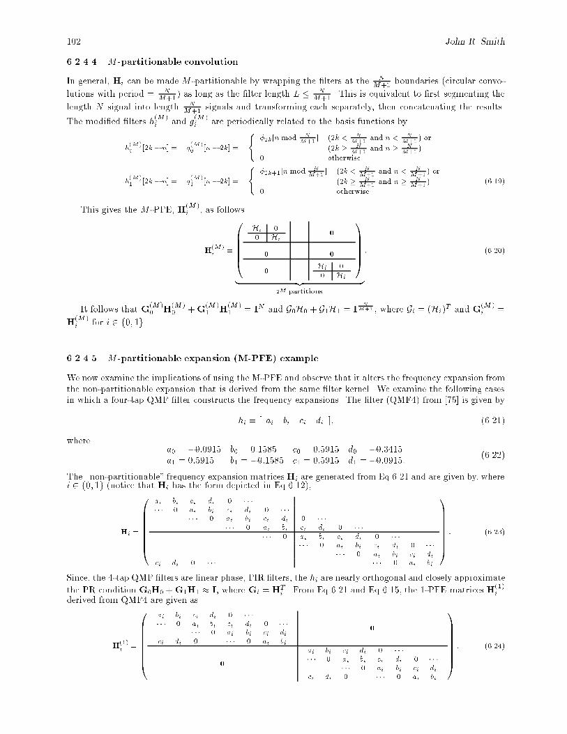
102 John R. Smith
6.2.4.4 M -partitionable convolution
In general, Hi can be made M -partitionable by wrapping the �lters at the NM+1
boundaries (circular convo-
lutions with period = NM+1 ) as long as the �lter length L � N
M+1 . This is equivalent to �rst segmenting the
length N signal into length NM+1 signals and transforming each separately, then concatenating the results.
The modi�ed �lters h(M)i and g
(M)i are periodically related to the basis functions by
h(M)0 [2k� n] = g
(M)0 [n� 2k] =
(�2k[n mod N
M+1 ] (2k < NM+1 and n < N
M+1 ) or
(2k � NM+1 and n � N
M+1 )
0 otherwise
h(M)1 [2k� n] = g
(M)1 [n� 2k] =
(�2k+1[n mod N
M+1 ] (2k < NM+1 and n < N
M+1 ) or
(2k � NM+1 and n � N
M+1 )
0 otherwise
(6.19)
This gives the M -PFE, H(M)i , as follows
H(M)i =
0BBBB@
Hi 00 Hi
. . . 0
0. . . 0
0. . .
Hi 00 Hi
1CCCCA
| {z }2M partitions
: (6.20)
It follows that G(M)0 H
(M)0 +G
(M)1 H
(M)1 = IN and G0H0 + G1H1 = I
NM+1 , where Gi = (Hi)
T and G(M)i =
H(M)i for i 2 f0; 1g.
6.2.4.5 M -partitionable expansion (M-PFE) example
We now examine the implications of using the M-PFE and observe that it alters the frequency expansion fromthe non-partitionable expansion that is derived from the same �lter kernel. We examine the following casesin which a four-tap QMF �lter constructs the frequency expansions. The �lter (QMF4) from [75] is given by
hi = [ ai bi ci di ]; (6.21)
wherea0 = �0:0915 b0 = 0:1585 c0 = 0:5915 d0 = �0:3415a1 = 0:5915 b1 = �0:1585 c1 = 0:5915 d1 = �0:0915:
(6.22)
The \non-partitionable" frequency expansion matricesHi are generated from Eq 6.21 and are given by, wherei 2 f0; 1g (notice that Hi has the form depicted in Eq 6.12),
Hi =
0BBBBBB@
ai bi ci di 0 � � �
� � � 0 ai bi ci di 0 � � �
� � � 0 ai bi ci di 0 � � �
� � � 0 ai bi ci di 0 � � �
� � � 0 ai bi ci di 0 � � �
� � � 0 ai bi ci di 0 � � �
� � � 0 ai bi ci dici di 0 � � � � � � 0 ai bi
1CCCCCCA : (6.23)
Since, the 4-tap QMF �lters are linear phase, FIR �lters, the hi are nearly orthogonal and closely approximate
the PR condition G0H0 +G1H1 � I, where Gi =HTi . From Eq 6.21 and Eq 6.15, the 1-PFE matrices H(1)
iderived from QMF4 are given as
H(1)i =
0BBBBBB@
ai bi ci di 0 � � �
� � � 0 ai bi ci di 0 � � �
� � � 0 ai bi ci dici di 0 � � � 0 ai bi
0
0
ai bi ci di 0 � � �
� � � 0 ai bi ci di 0 � � �
� � � 0 ai bi ci dici di 0 � � � 0 ai bi
1CCCCCCA : (6.24)
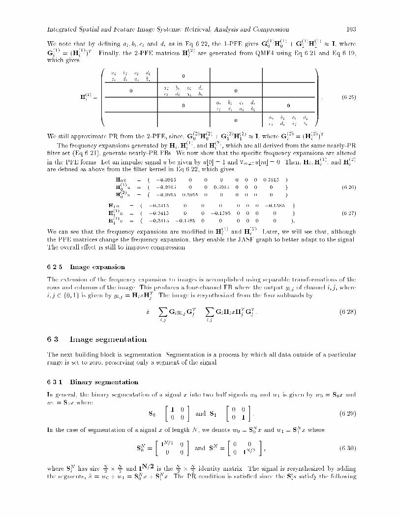
Integrated Spatial and Feature Image Systems: Retrieval, Analysis and Compression 103
We note that by de�ning ai; bi; ci and di as in Eq 6.22, the 1-PFE gives G(1)0 H
(1)0 + G
(1)1 H
(1)1 � I, where
G(1)i = (H
(1)i )T . Finally, the 2-PFE matrices H
(2)i are generated from QMF4 using Eq 6.21 and Eq 6.19,
which gives
H(2)i =
0BBBBBBBBB@
ai bi ci dici di ai bi
0. . .
0ai bi ci dici di ai bi
0. . .
. . . 0ai bi ci dici di ai bi
0
. . . 0ai bi ci dici di ai bi
1CCCCCCCCCA
: (6.25)
We still approximate PR from the 2-PFE, since, G(2)0 H
(2)0 +G
(2)1 H
(2)1 � I, where G(2)
i = (H(2)i )T .
The frequency expansions generated byHi;H(1)i , andH(2)
i , which are all derived from the same nearly-PR�lter set (Eq 6.21), generate nearly-PR FBs. We now show that the speci�c frequency expansions are altered
in the PFE forms. Let an impulse signal u be given by u[0] = 1 and 8m6=0u[m] = 0. Then, Hi;H(1)i , and H
(2)i
are de�ned as above from the �lter kernel in Eq 6.22, which gives
H0u = ( �0:0915 0 0 0 0 0 0 0:5915 )
H(1)0 u = ( �0:0915 0 0 0:5915 0 0 0 0 )
H(2)0 u = ( �0:0915 0:5915 0 0 0 0 0 0 )
(6.26)
H1u = ( �0:3415 0 0 0 0 0 0 �0:1585 )
H(1)1 u = ( �0:3415 0 0 �0:1585 0 0 0 0 )
H(2)1 u = ( �0:3415 �0:1585 0 0 0 0 0 0 ):
(6.27)
We can see that the frequency expansions are modi�ed in H(1)i and H
(2)i . Later, we will see that, although
the PFE matrices change the frequency expansion, they enable the JASF graph to better adapt to the signal.The overall e�ect is still to improve compression.
6.2.5 Image expansion
The extension of the frequency expansion to images is accomplished using separable transformations of therows and columns of the image. This produces a four-channel FB where the output yi;j of channel i; j, wherei; j 2 f0; 1g is given by yi;j = HixH
Tj . The image is resynthesized from the four subbands by
x =Xi;j
Giyi;jGTj =
Xi;j
GiHixHTj G
Tj : (6.28)
6.3. Image segmentation
The next building block is segmentation. Segmentation is a process by which all data outside of a particularrange is set to zero, preserving only a segment of the signal.
6.3.1 Binary segmentation
In general, the binary segmentation of a signal x into two half signals w0 and w1 is given by w0 = S0x andw1 = S1x where
S0 =
�I 00 0
�and S1 =
�0 00 I
�: (6.29)
In the case of segmentation of a signal x of length N , we denote w0 = SN0 x and w1 = SN1 x where
SN0 =
�IN=2 00 0
�and SN1 =
�0 00 IN=2
�; (6.30)
where SNi has size N2 �
N2 and IN=2 is the N
2 �N2 identity matrix. The signal is resynthesized by adding
the segments, x = w0 + w1 = SN0 x+ SN1 x. The PR condition is satis�ed since the S0is satisfy the following
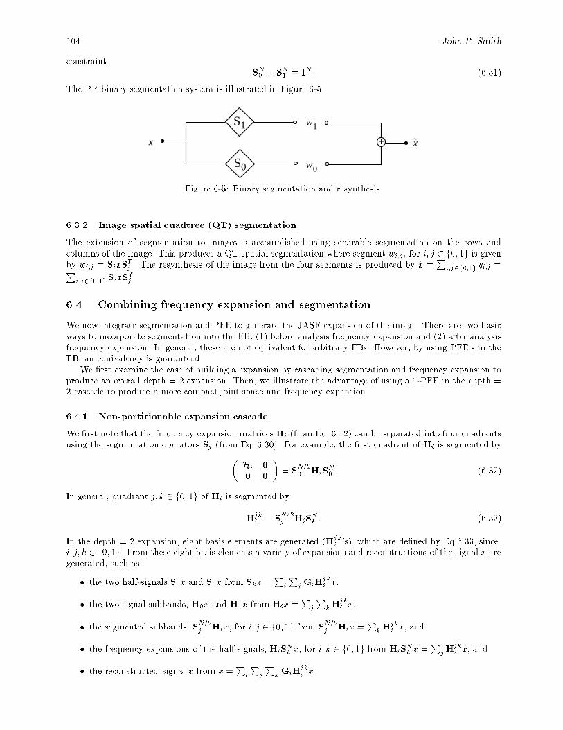
104 John R. Smith
constraintSN0 + SN1 = IN : (6.31)
The PR binary segmentation system is illustrated in Figure 6-5.
S1
S0
x + x
w1
w0
Figure 6-5: Binary segmentation and resynthesis.
6.3.2 Image spatial quadtree (QT) segmentation
The extension of segmentation to images is accomplished using separable segmentation on the rows andcolumns of the image. This produces a QT spatial segmentation where segment wi;j, for i; j 2 f0; 1g is givenby wi;j = SixS
Tj . The resynthesis of the image from the four segments is produced by x =
Pi;j2f0;1g yi;j =P
i;j2f0;1gSixSTj .
6.4. Combining frequency expansion and segmentation
We now integrate segmentation and PFE to generate the JASF expansion of the image. There are two basicways to incorporate segmentation into the FB: (1) before analysis frequency expansion and (2) after analysisfrequency expansion. In general, these are not equivalent for arbitrary FBs. However, by using PFE's in theFB, an equivalency is guaranteed.
We �rst examine the case of building a expansion by cascading segmentation and frequency expansion toproduce an overall depth = 2 expansion. Then, we illustrate the advantage of using a 1-PFE in the depth =2 cascade to produce a more compact joint space and frequency expansion.
6.4.1 Non-partitionable expansion cascade
We �rst note that the frequency expansion matrices Hi (from Eq. 6.12) can be separated into four quadrantsusing the segmentation operators Sj (from Eq. 6.30). For example, the �rst quadrant of Hi is segmented by�
Hi 00 0
�= S
N=20 HiS
N0 : (6.32)
In general, quadrant j; k 2 f0; 1g of Hi is segmented by
Hjki = S
N=2j HiS
Nk : (6.33)
In the depth = 2 expansion, eight basis elements are generated (Hjki 's), which are de�ned by Eq 6.33, since,
i; j; k 2 f0; 1g. From these eight basis elements a variety of expansions and reconstructions of the signal x aregenerated, such as
� the two half-signals S0x and S1x from Skx =P
i
PjGiH
jki x,
� the two signal subbands, H0x and H1x from Hix =P
j
PkH
jki x,
� the segmented subbands, SN=2j Hix, for i; j 2 f0; 1g from S
N=2j Hix =
PkH
jki x, and
� the frequency expansions of the half-signals, HiSNk x, for i; k 2 f0; 1g from HiS
Nk x =
PjH
jki x, and
� the reconstructed signal x from x =P
i
Pj
PkGiH
jki x.
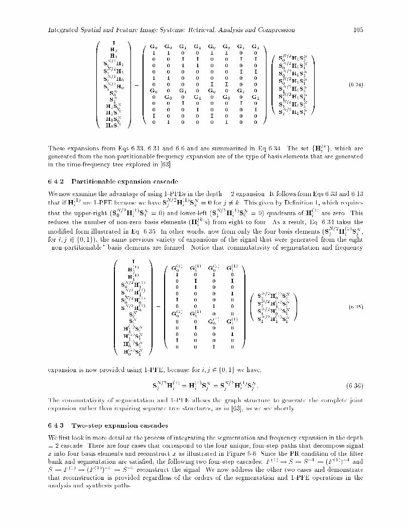
Integrated Spatial and Feature Image Systems: Retrieval, Analysis and Compression 1050BBBBBBBBBBBBBBBB@
I
H0
H1
SN=20 H1
SN=21 H1
SN=20 H0
SN=21 H0
SN0SN1
H1SN0
H1SN1
H0SN0
H0SN1
1CCCCCCCCCCCCCCCCA
=
0BBBBBBBBBBBBBB@
G0 G0 G1 G1 G0 G0 G1 G1
I I 0 0 I I 0 0
0 0 I I 0 0 I I
0 0 I I 0 0 0 0
0 0 0 0 0 0 I I
I I 0 0 0 0 0 0
0 0 0 0 I I 0 0
G0 0 G1 0 G0 0 G1 0
0 G0 0 G1 0 G0 0 G1
0 0 I 0 0 0 I 0
0 0 0 I 0 0 0 I
I 0 0 0 I 0 0 0
0 I 0 0 0 I 0 0
1CCCCCCCCCCCCCCA
0BBBBBBBBB@
SN=20 H0S
N0
SN=20 H0S
N1
SN=20 H1S
N0
SN=20 H1S
N1
SN=21 H0S
N0
SN=21 H0S
N1
SN=21 H1S
N0
SN=21 H1S
N1
1CCCCCCCCCA
(6.34)
These expansions from Eqs 6.33, 6.31 and 6.6 and are summarized in Eq 6.34. The set fHjki g, which are
generated from the non-partitionable frequency expansion are of the type of basis elements that are generatedin the time-frequency tree explored in [63].
6.4.2 Partitionable expansion cascade
We now examine the advantage of using 1-PFEs in the depth = 2 expansion. It follows from Eqs 6.33 and 6.13
that ifH(1)i are 1-PFE because we have SN=2j H
(1)i SNk = 0 for j 6= k. This given by De�nition 1, which requires
that the upper-right (SN=20 H(1)i SN1 = 0) and lower-left (SN=21 H
(1)i SN0 = 0) quadrants of H(1)
i are zero. This
reduces the number of non-zero basis elements (Hjki 's) from eight to four. As a result, Eq. 6.34 takes the
modi�ed form illustrated in Eq. 6.35. In other words, now from only the four basis elements (SN=2j H
(1)i SNj ,
for i; j 2 f0; 1g), the same previous variety of expansions of the signal that were generated from the eight\non-partitionable" basis elements are formed. Notice that commutativity of segmentation and frequency0
BBBBBBBBBBBBBBBBBB@
I
H(1)0
H(1)1
SN=20 H
(1)1
SN=21 H
(1)1
SN=20 H
(1)0
SN=21 H
(1)0
SN0SN1
H(1)1 SN0
H(1)1 SN1
H(1)0 SN0
H(1)0 SN1
1CCCCCCCCCCCCCCCCCCA
=
0BBBBBBBBBBBBBBB@
G(1)0 G
(1)1 G
(1)0 G
(1)1
I 0 I 0
0 I 0 I
0 I 0 0
0 0 0 I
I 0 0 0
0 0 I 0
G(1)0 G
(1)1 0 0
0 0 G(1)0 G
(1)1
0 I 0 0
0 0 0 I
I 0 0 0
0 0 I 0
1CCCCCCCCCCCCCCCA
0B@
SN=20 H
(1)0 SN0
SN=20 H
(1)1 SN0
SN=21 H
(1)0 SN1
SN=21 H
(1)1 SN1
1CA (6.35)
expansion is now provided using 1-PFE, because for i; j 2 f0; 1g we have,
SN=2j H
(1)i = H
(1)i SNj = S
N=2j H
(1)i SNj : (6.36)
The commutativity of segmentation and 1-PFE allows the graph structure to generate the complete jointexpansion rather than requiring separate tree structures, as in [63], as we see shortly.
6.4.3 Two-step expansion cascades
We �rst look in more detail at the process of integrating the segmentation and frequency expansion in the depth= 2 cascade. There are four cases that correspond to the four unique, four-step paths that decompose signalx into four basis elements and reconstruct x as illustrated in Figure 6-6. Since the PR condition of the �lterbank and segmentation are satis�ed, the following two four-step cascades: F (1) ! S ! S�1 ! (F (1))�1 andS ! F (1) ! (F (1))�1 ! S�1 reconstruct the signal. We now address the other two cases and demonstratethat reconstruction is provided regardless of the orders of the segmentation and 1-PFE operations in theanalysis and synthesis paths.
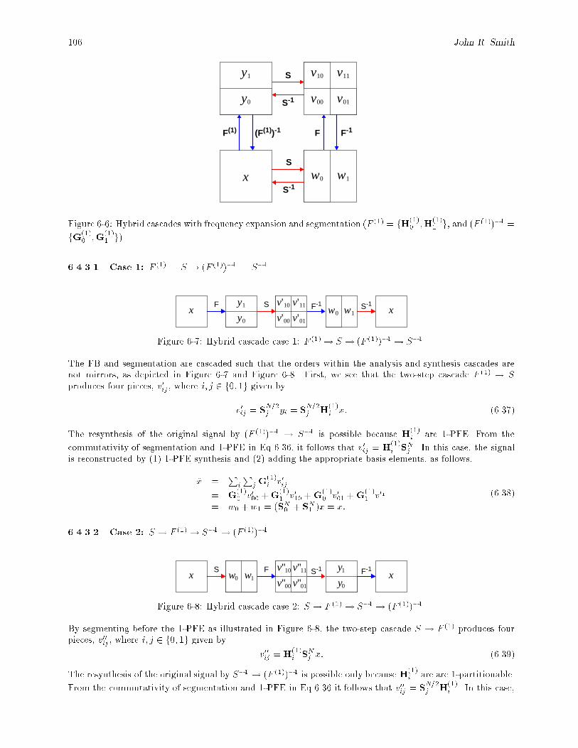
106 John R. Smith
x w0 w1
y0
y1
v00
v10 v11
v01
F(1) (F(1))-1
S
S-1
F F-1
S
S-1
Figure 6-6: Hybrid cascades with frequency expansion and segmentation (F (1) = fH(1)0 ;H
(1)1 g, and (F (1))�1 =
fG(1)0 ;G
(1)1 g).
6.4.3.1 Case 1: F (1) ! S ! (F (1))�1 ! S�1
S F-1F S-1
v'00
v'10 v'11
v'01
w0 w1x xy0
y1
Figure 6-7: Hybrid cascade case 1: F (1) ! S ! (F (1))�1 ! S�1.
The FB and segmentation are cascaded such that the orders within the analysis and synthesis cascades arenot mirrors, as depicted in Figure 6-7 and Figure 6-8. First, we see that the two-step cascade F (1) ! Sproduces four pieces, v0ij, where i; j 2 f0; 1g given by
v0ij = SN=2j yi = S
N=2j H
(1)i x: (6.37)
The resynthesis of the original signal by (F (1))�1 ! S�1 is possible because H(1)i are 1-PFE. From the
commutativity of segmentation and 1-PFE in Eq 6.36, it follows that v0ij = H(1)i SNj . In this case, the signal
is reconstructed by (1) 1-PFE synthesis and (2) adding the appropriate basis elements, as follows,
x =P
i
PjG
(1)i v0ij
= G(1)0 v000 +G
(1)1 v010 +G
(1)0 v001 +G
(1)1 v01
= w0 +w1 = (SN0 + SN1 )x = x:
(6.38)
6.4.3.2 Case 2: S ! F (1) ! S�1 ! (F (1))�1
F S-1S F-1
y0
y1
v''00
v''10 v''11
v''01 y0
y1x xw0 w1
Figure 6-8: Hybrid cascade case 2: S ! F (1) ! S�1 ! (F (1))�1.
By segmenting before the 1-PFE as illustrated in Figure 6-8, the two-step cascade S ! F (1) produces fourpieces, v00ij, where i; j 2 f0; 1g given by
v00ij = H(1)i SNj x: (6.39)
The resynthesis of the original signal by S�1 ! (F (1))�1 is possible only because H(1)i are are 1-partitionable.
From the commutativity of segmentation and 1-PFE in Eq 6.36 it follows that v00ij = SN=2j H
(1)i . In this case,
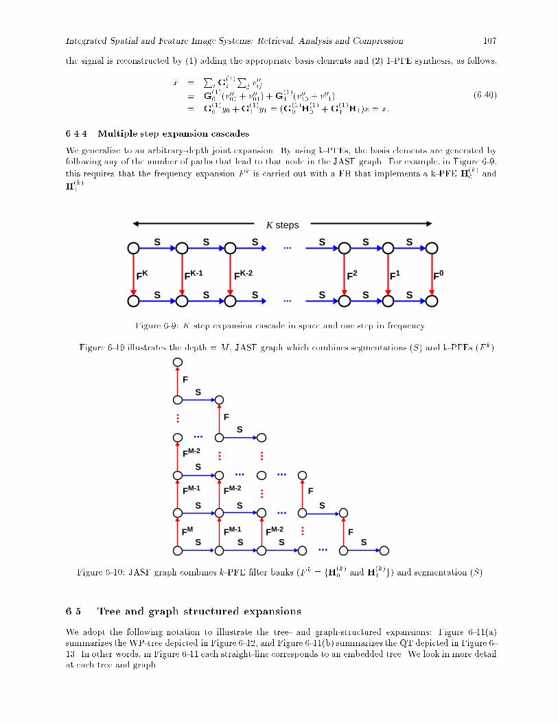
Integrated Spatial and Feature Image Systems: Retrieval, Analysis and Compression 107
the signal is reconstructed by (1) adding the appropriate basis elements and (2) 1-PFE synthesis, as follows,
x =P
iG(1)i
Pj v
00ij
= G(1)0 (v0000 + v0001) +G
(1)1 (v0010 + v0011)
= G(1)0 y0 +G
(1)1 y1 = (G
(1)0 H
(1)0 +G
(1)1 H1)x = x:
(6.40)
6.4.4 Multiple step expansion cascades
We generalize to an arbitrary-depth joint expansion. By using k-PFEs, the basis elements are generated byfollowing any of the number of paths that lead to that node in the JASF graph. For example, in Figure 6-9,
this requires that the frequency expansion F k is carried out with a FB that implements a k-PFE H(k)0 and
H(k)1 .
FK FK-1 FK-2 F2
...
...
S S S
S S S
S
S
S
S
S
S
F1 F0
K steps
Figure 6-9: K step expansion cascade in space and one step in frequency.
Figure 6-10 illustrates the depth = M , JASF graph which combines segmentations (S) and k-PFEs (F k).
FM-2
S
S
FM-1
F
FM-1
S
FM-2
S
FS
FM-2
SF
SS
F
S
SFM
...
...
...
...
...
...
...
...
...
...
Figure 6-10: JASF graph combines k-PFE �lter banks (F k = fH(k)0 and H
(k)1 g) and segmentation (S).
6.5. Tree and graph structured expansions
We adopt the following notation to illustrate the tree- and graph-structured expansions: Figure 6-11(a)summarizes the WP-tree depicted in Figure 6-12, and Figure 6-11(b) summarizes the QT depicted in Figure 6-13. In other words, in Figure 6-11 each straight-line corresponds to an embedded tree. We look in more detailat each tree and graph.
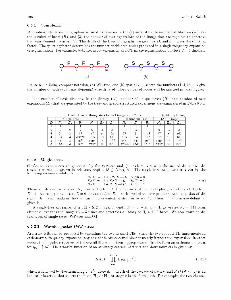
108 John R. Smith
6.5.1 Complexity
We evaluate the tree- and graph-structured expansions in the (1) sizes of the basis element libraries (N ), (2)the number of bases (B), and (3) the number of over-expansions of the image that are required to generatethe basis element libraries (E). The depth of the trees and graphs are given by D, and � = gives the splittingfactor. The splitting factor determines the number of children nodes produced in a single frequency expansionor segmentation. For example, both frequency expansion and QT image segmentation produce � = 4 children.
S S SF F F4 16 641 4 16 641
(a) (b)
Figure 6-11: Using compact notation, (a) WP-tree, and (b) spatial QT, where the numbers (1; 4; 16; : : :) givethe number of nodes (or basis elements) at each level. The number of nodes will be omitted in later �gures.
The number of basis elements in the library (N ), number of unique bases (B), and number of overexpansions (E) that are generated by the tree- and graph-structured expansions are summarized in Table 6.5.1.
Basis element library sizes for 2-D image with � = 4 (splitting factor)Single-Tree DT Redundant Tree JASF Graph
D Ns Es Bs Nd Ed Bd Nr Er Br Ng Eg Bg
1 1 1 1 1 1 1 1 1 1 1 1 12 5 2 2 9 3 3 9 5 3 9 3 33 21 3 17 57 6 98 73 21 163 57 6 1624 85 4 83522 313 10 107 585 85 109 313 10 109
5 341 5 1019 1593 15 1031 4681 341 1036 1593 15 1036
6 1365 6 1078 7737 21 10127 37449 1365 10147 7737 21 10147
6.5.2 Single-trees
Single-tree expansions are generated by the WP-tree and QT. Where N � N is the size of the image, thesingle-trees can be grown to arbitrary depth, D � N log2N . The single-tree complexity is given by thefollowing recursive relations
Ns(D) = 1 + �Ns(D� 1); Ns(0) = 0Es(D) = 1 + Es(D� 1); Es(0) = 0Bs(D) = 1 +Bs(D� 1)� ; Bs(0) = 0:
(6.41)
These are derived as follows: Ns { each depth = D tree consists of one node plus � sub-trees of depth =D � 1. An empty single-tree, D = 0, has no nodes. Es { each level of the tree produces one expansion of thesignal. Bs { each node in the tree can be represented by itself or by its � children. This recursive de�nitiongives Bs.
A single-tree expansion of a 512 � 512 image, of depth D = 5, with � = 4, generates Ns = 341 basiselements, expands the image Es = 5 times and generates a library of Bs � 1019 bases. We now examine thetwo types of single-trees: WP-tree and QT.
6.5.2.1 Wavelet packet (WP)-tree
Arbitrary FBs can be produced by cascading the two-channel FBs. Since the two-channel FB implements anorthonormal frequency expansion, any cascade is orthonormal since it merely iterates the expansion. In otherwords, the impulse responses of the overall �lters and their appropriate shifts also form an orthonormal basisfor l2(z) [167]. The transfer function of an arbitrary cascade of �lters and downsamplers is given by,
Hr(z) =
dr�1Yk=0
HPr(k)(z2k); (6.42)
which is followed by downsampling by 2dr . Here dr = depth of the cascade of path r, and Pr(k) 2 f0; 1g is anindicator function that selects the �lter, H0 or H1, at stage k in the �lter path. For example, the two-channel
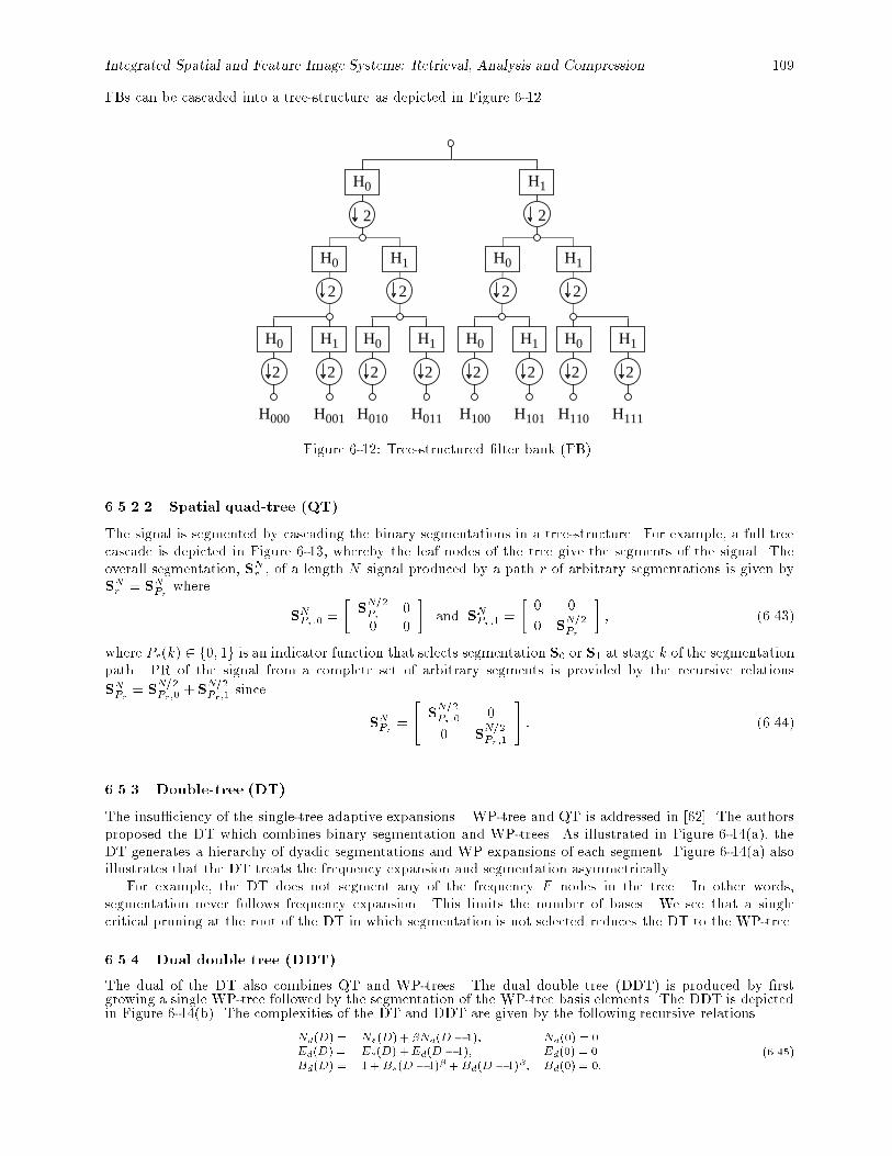
Integrated Spatial and Feature Image Systems: Retrieval, Analysis and Compression 109
FBs can be cascaded into a tree-structure as depicted in Figure 6-12.
22
H1H0
22
H1H0
H1H0
22
22
H1H0
22
H1H0
22
H1H0
22
H1H0
H000 H001 H010 H011 H100 H101 H110 H111
Figure 6-12: Tree-structured �lter bank (FB).
6.5.2.2 Spatial quad-tree (QT)
The signal is segmented by cascading the binary segmentations in a tree-structure. For example, a full treecascade is depicted in Figure 6-13, whereby the leaf nodes of the tree give the segments of the signal. Theoverall segmentation, SNr , of a length N signal produced by a path r of arbitrary segmentations is given bySNr = SNPr where
SNPr;0 =
�SN=2Pr
00 0
�and SNPr;1 =
�0 0
0 SN=2Pr
�; (6.43)
where Pr(k) 2 f0; 1g is an indicator function that selects segmentation S0 or S1 at stage k of the segmentationpath. PR of the signal from a complete set of arbitrary segments is provided by the recursive relations
SNPr = SN=2Pr;0
+ SN=2Pr;1
since
SNPr =
"SN=2Pr;0
0
0 SN=2Pr ;1
#: (6.44)
6.5.3 Double-tree (DT)
The insu�ciency of the single-tree adaptive expansions { WP-tree and QT is addressed in [62]. The authorsproposed the DT which combines binary segmentation and WP-trees. As illustrated in Figure 6-14(a), theDT generates a hierarchy of dyadic segmentations and WP expansions of each segment. Figure 6-14(a) alsoillustrates that the DT treats the frequency expansion and segmentation asymmetrically.
For example, the DT does not segment any of the frequency F nodes in the tree. In other words,segmentation never follows frequency expansion. This limits the number of bases. We see that a singlecritical pruning at the root of the DT in which segmentation is not selected reduces the DT to the WP-tree.
6.5.4 Dual double tree (DDT)
The dual of the DT also combines QT and WP-trees. The dual double tree (DDT) is produced by �rstgrowing a single WP-tree followed by the segmentation of the WP-tree basis elements. The DDT is depictedin Figure 6-14(b). The complexities of the DT and DDT are given by the following recursive relations
Nd(D) = Ns(D) + �Nd(D � 1); Nd(0) = 0Ed(D) = Es(D) + Ed(D � 1); Ed(0) = 0Bd(D) = 1 +Bs(D � 1)� +Bd(D � 1)� ; Bd(0) = 0:
(6.45)
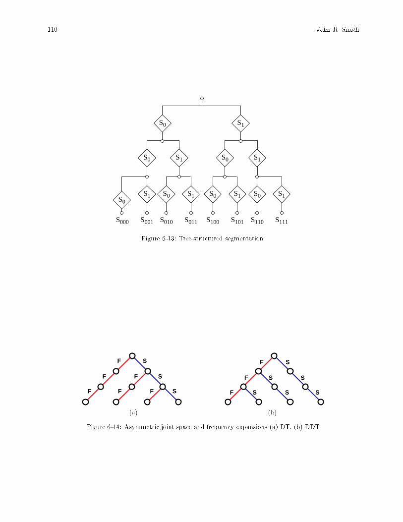
110 John R. Smith
S1
S1S0S1S0 S1S0 S1S0
S0
S0 S1 S0 S1
S000 S001 S010 S011 S100 S101 S110 S111
Figure 6-13: Tree-structured segmentation.
F S
F F S
F F F S
SF
SSF
SSSF
(a) (b)
Figure 6-14: Asymmetric joint space and frequency expansions (a) DT, (b) DDT
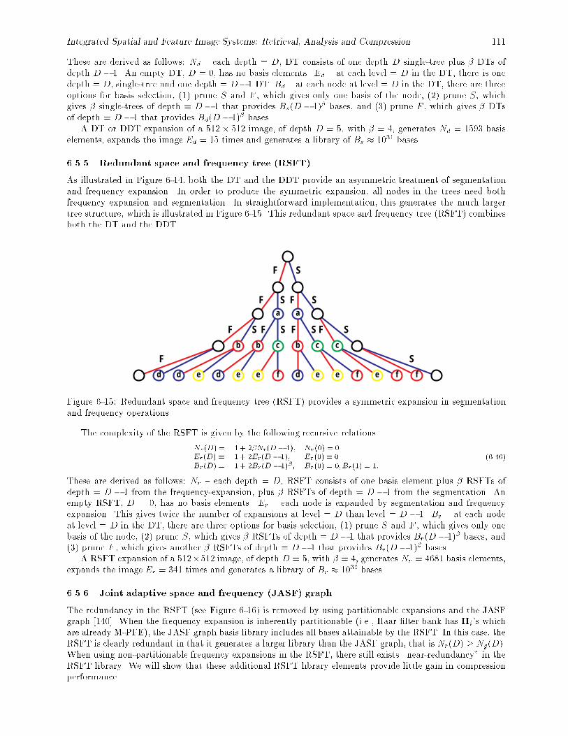
Integrated Spatial and Feature Image Systems: Retrieval, Analysis and Compression 111
These are derived as follows: Nd { each depth = D, DT consists of one depth D single-tree plus � DTs ofdepth D � 1. An empty DT, D = 0, has no basis elements. Ed { at each level = D in the DT, there is onedepth = D, single-tree and one depth = D�1 DT. Bd { at each node at level = D in the DT, there are threeoptions for basis selection, (1) prune S and F , which gives only one basis of the node, (2) prune S, whichgives � single-trees of depth = D � 1 that provides Bs(D � 1)� bases, and (3) prune F , which gives � DTsof depth = D � 1 that provides Bd(D � 1)� bases.
A DT or DDT expansion of a 512� 512 image, of depth D = 5, with � = 4, generates Nd = 1593 basiselements, expands the image Ed = 15 times and generates a library of Bs � 1031 bases.
6.5.5 Redundant space and frequency tree (RSFT)
As illustrated in Figure 6-14, both the DT and the DDT provide an asymmetric treatment of segmentationand frequency expansion. In order to produce the symmetric expansion, all nodes in the trees need bothfrequency expansion and segmentation. In straightforward implementation, this generates the much largertree structure, which is illustrated in Figure 6-15. This redundant space and frequency tree (RSFT) combinesboth the DT and the DDT.
F S
a a
bbb c cc
ddd e e e e ef f ffe d
F S
F S
F S
F S F SF S F S
Figure 6-15: Redundant space and frequency tree (RSFT) provides a symmetric expansion in segmentationand frequency operations.
The complexity of the RSFT is given by the following recursive relations
Nr(D) = 1 + 2�Nr(D� 1); Nr(0) = 0Er(D) = 1 + 2Er(D � 1); Er(0) = 0Br(D) = 1 + 2Br(D � 1)�; Br(0) = 0;Br(1) = 1:
(6.46)
These are derived as follows: Nr { each depth = D, RSFT consists of one basis element plus � RSFTs ofdepth = D � 1 from the frequency-expansion, plus � RSFTs of depth = D � 1 from the segmentation. Anempty RSFT, D = 0, has no basis elements. Er { each node is expanded by segmentation and frequencyexpansion. This gives twice the number of expansions at level = D than level = D � 1. Br { at each nodeat level = D in the DT, there are three options for basis selection, (1) prune S and F , which gives only onebasis of the node, (2) prune S, which gives � RSFTs of depth = D � 1 that provides Br(D � 1)� bases, and(3) prune F , which gives another � RSFTs of depth = D � 1 that provides Br(D � 1)� bases.
A RSFT expansion of a 512�512 image, of depth D = 5, with � = 4, generates Nr = 4681 basis elements,expands the image Er = 341 times and generates a library of Br � 1036 bases.
6.5.6 Joint adaptive space and frequency (JASF) graph
The redundancy in the RSFT (see Figure 6-16) is removed by using partitionable expansions and the JASFgraph [140]. When the frequency expansion is inherently partitionable (i.e., Haar �lter bank has Hi's whichare already M-PFE), the JASF graph basis library includes all bases attainable by the RSFT. In this case, theRSFT is clearly redundant in that it generates a larger library than the JASF graph, that is Nr(D) � Ng(D).When using non-partitionable frequency expansions in the RSFT, there still exists \near-redundancy" in theRSFT library. We will show that these additional RSFT library elements provide little gain in compressionperformance.
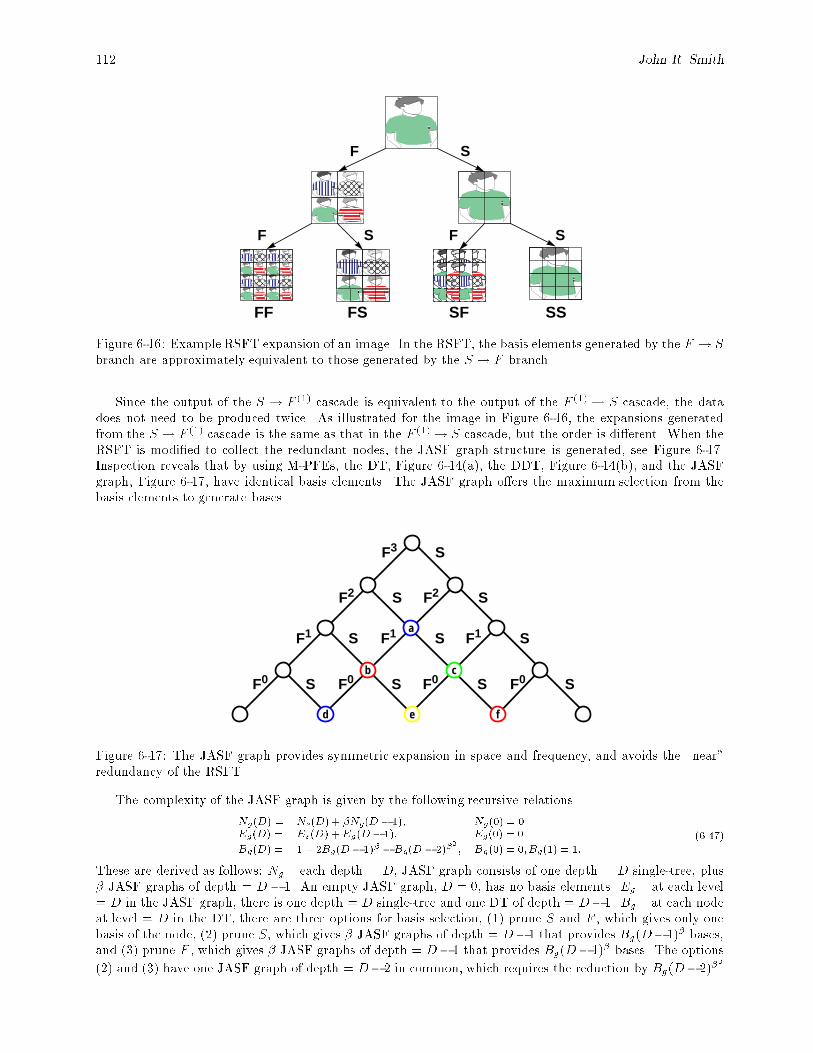
112 John R. Smith
F S
F S F S
FF FS SF SS
Figure 6-16: Example RSFT expansion of an image. In the RSFT, the basis elements generated by the F ! Sbranch are approximately equivalent to those generated by the S ! F branch.
Since the output of the S ! F (1) cascade is equivalent to the output of the F (1) ! S cascade, the datadoes not need to be produced twice. As illustrated for the image in Figure 6-16, the expansions generatedfrom the S ! F (1) cascade is the same as that in the F (1) ! S cascade, but the order is di�erent. When theRSFT is modi�ed to collect the redundant nodes, the JASF graph structure is generated, see Figure 6-17.Inspection reveals that by using M-PFEs, the DT, Figure 6-14(a), the DDT, Figure 6-14(b), and the JASFgraph, Figure 6-17, have identical basis elements. The JASF graph o�ers the maximum selection from thebasis elements to generate bases.
F3 S
F2 S F2 S
F1 S F1 S F1 S
F0 S F0 S F0 S F0 S
a
cb
e fd
Figure 6-17: The JASF graph provides symmetric expansion in space and frequency, and avoids the \near"redundancy of the RSFT.
The complexity of the JASF graph is given by the following recursive relations
Ng(D) = Ns(D) + �Ng(D � 1); Ng(0) = 0Eg(D) = Es(D) + Eg(D� 1); Eg(0) = 0
Bg(D) = 1 + 2Bg(D� 1)� � Bg(D � 2)�2; Bg(0) = 0;Bg(1) = 1:
(6.47)
These are derived as follows: Ng { each depth = D, JASF graph consists of one depth = D single-tree, plus� JASF graphs of depth = D � 1. An empty JASF graph, D = 0, has no basis elements. Eg { at each level= D in the JASF graph, there is one depth = D single-tree and one DT of depth = D�1. Bg { at each nodeat level = D in the DT, there are three options for basis selection, (1) prune S and F , which gives only onebasis of the node, (2) prune S, which gives � JASF graphs of depth = D� 1 that provides Bg(D� 1)� bases,and (3) prune F , which gives � JASF graphs of depth = D� 1 that provides Bg(D� 1)� bases. The options
(2) and (3) have one JASF graph of depth = D� 2 in common, which requires the reduction by Bg(D� 2)�2
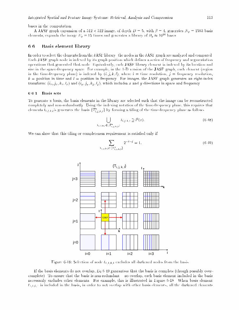
Integrated Spatial and Feature Image Systems: Retrieval, Analysis and Compression 113
bases in the computation.A JASF graph expansion of a 512� 512 image, of depth D = 5, with � = 4, generates Ng = 1593 basis
elements, expands the image Eg = 15 times and generates a library of Bg � 1036 bases.
6.6. Basis element library
In order to select the elements from the JASF library. the nodes in the JASF graph are analyzed and compared.Each JASF graph node is indexed by its graph position which de�nes a series of frequency and segmentationoperations that generated that node. Equivalently, each JASF library element is indexed by its location andsize in the space-frequency space. For example, in the 1-D version of the JASF graph, each element (regionin the time-frequency plane) is indexed by (i; j; k; l), where i = time resolution, j = frequency resolution,k = position in time and l = position in frequency. For images, the JASF graph generates an eight-indextransform: (ix; jx; kx; lx) and (iy; jy; ky; ly), which includes x and y directions in space and frequency.
6.6.1 Basis sets
To generate a basis, the basis elements in the library are selected such that the image can be reconstructedcompletely and non-redundantly. Using the indexing notation of the time-frequency plane, this requires thatelements ti;j;k;l's generates the basis fT
�i;j;k;lg by forming a tiling of the time-frequency plane as follows[ti;j;k;l2fT�
i;j;k;lg
ti;j;k;l � l2(z): (6.48)
We can show that this tiling or completeness requirement is satis�ed only ifXti;j;k;l2fT�
i;j;k;lg
2�i�j = 1: (6.49)
i
j
i=0 i=1 i=2 i=3
j=0
j=3
j=2
j=1
{Ti, j, k, l}
k
l
1,1,0,1
k
l
Figure 6-18: Selection of node t1;1;0;1 excludes all darkened nodes from the basis.
If the basis elements do not overlap, Eq 6.49 guarantees that the basis is complete (though possibly over-complete). To ensure that the basis is non-redundant { no overlap, each basis element included in the basisnecessarily excludes other elements. For example, this is illustrated in Figure 6-18. When basis elementt1;1;0;1 is included in the basis, in order to not overlap with other basis elements, all the darkened elements
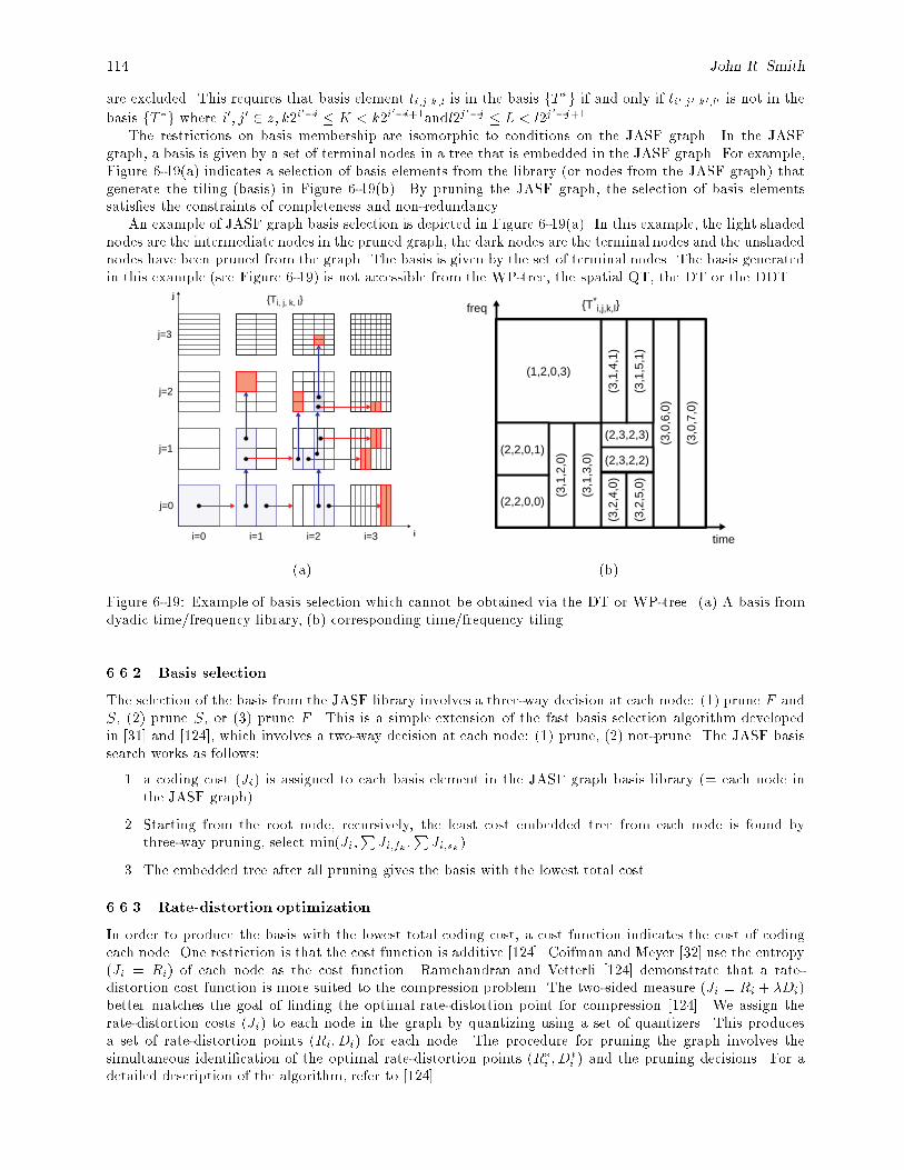
114 John R. Smith
are excluded. This requires that basis element ti;j;k;l is in the basis fT �g if and only if ti0;j0;k0;l0 is not in the
basis fT �g where i0; j0 2 z; k2i0�i � K < k2i
0�i+1andl2j0�j � L < l2j
0�j+1.The restrictions on basis membership are isomorphic to conditions on the JASF graph. In the JASF
graph, a basis is given by a set of terminal nodes in a tree that is embedded in the JASF graph. For example,Figure 6-19(a) indicates a selection of basis elements from the library (or nodes from the JASF graph) thatgenerate the tiling (basis) in Figure 6-19(b). By pruning the JASF graph, the selection of basis elementssatis�es the constraints of completeness and non-redundancy.
An example of JASF graph basis selection is depicted in Figure 6-19(a). In this example, the light shadednodes are the intermediate nodes in the pruned graph, the dark nodes are the terminal nodes and the unshadednodes have been pruned from the graph. The basis is given by the set of terminal nodes. The basis generatedin this example (see Figure 6-19) is not accessible from the WP-tree, the spatial QT, the DT or the DDT.
i
j
i=0 i=1 i=2 i=3
j=0
j=3
j=2
j=1
{Ti, j, k, l}
time
freq {T*i,j,k,l}
(3,0
,7,0
)
(3,0
,6,0
)
(3,1
,5,1
)
(3,1
,4,1
)
(3,2
,5,0
)
(3,2
,4,0
)
(3,1
,3,0
)
(3,1
,2,0
)
(1,2,0,3)
(2,2,0,1)
(2,2,0,0)
(2,3,2,2)
(2,3,2,3)
(a) (b)
Figure 6-19: Example of basis selection which cannot be obtained via the DT or WP-tree. (a) A basis fromdyadic time/frequency library, (b) corresponding time/frequency tiling.
6.6.2 Basis selection
The selection of the basis from the JASF library involves a three-way decision at each node: (1) prune F andS, (2) prune S, or (3) prune F . This is a simple extension of the fast basis selection algorithm developedin [31] and [124], which involves a two-way decision at each node: (1) prune, (2) not-prune. The JASF basissearch works as follows:
1. a coding cost (Ji) is assigned to each basis element in the JASF graph basis library (= each node inthe JASF graph).
2. Starting from the root node, recursively, the least cost embedded tree from each node is found bythree-way pruning, select min(Ji;
PJi;fk ;
PJi;sk).
3. The embedded tree after all pruning gives the basis with the lowest total cost.
6.6.3 Rate-distortion optimization
In order to produce the basis with the lowest total coding cost, a cost function indicates the cost of codingeach node. One restriction is that the cost function is additive [124]. Coifman and Meyer [32] use the entropy(Ji = Ri) of each node as the cost function. Ramchandran and Vetterli [124] demonstrate that a rate-distortion cost function is more suited to the compression problem. The two-sided measure (Ji = Ri + �Di)better matches the goal of �nding the optimal rate-distortion point for compression [124]. We assign therate-distortion costs (Ji) to each node in the graph by quantizing using a set of quantizers. This producesa set of rate-distortion points (Ri; Di) for each node. The procedure for pruning the graph involves thesimultaneous identi�cation of the optimal rate-distortion points (R�i ; D
�i ) and the pruning decisions. For a
detailed description of the algorithm, refer to [124].
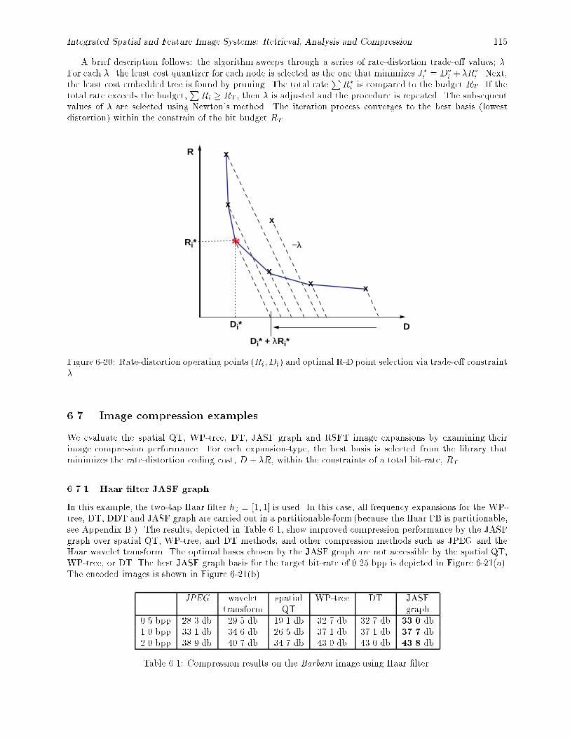
Integrated Spatial and Feature Image Systems: Retrieval, Analysis and Compression 115
A brief description follows: the algorithm sweeps through a series of rate-distortion trade-o� values; �.For each �. the least cost quantizer for each node is selected as the one that minimizes J�i = D�
i +�R�i . Next,the least cost embedded tree is found by pruning. The total rate
PR�i is compared to the budget RT . If the
total rate exceeds the budget,P
Ri � RT , then � is adjusted and the procedure is repeated. The subsequentvalues of � are selected using Newton's method. The iteration process converges to the best basis (lowestdistortion) within the constrain of the bit budget RT .
x
x
x
x
xx
*
R
D
−λRi*
Di*
Di* + λRi*
Figure 6-20: Rate-distortion operating points (Ri; Di) and optimal R-D point selection via trade-o� constraint�.
6.7. Image compression examples
We evaluate the spatial QT, WP-tree, DT, JASF graph and RSFT image expansions by examining theirimage compression performance. For each expansion-type, the best basis is selected from the library thatminimizes the rate-distortion coding cost, D + �R, within the constraints of a total bit-rate, RT .
6.7.1 Haar �lter JASF graph
In this example, the two-tap Haar �lter h0 = [1; 1] is used. In this case, all frequency expansions for the WP-tree, DT, DDT and JASF graph are carried out in a partitionable-form (because the Haar FB is partitionable,see Appendix B.). The results, depicted in Table 6.1, show improved compression performance by the JASFgraph over spatial QT, WP-tree, and DT methods, and other compression methods such as JPEG and theHaar wavelet transform. The optimal bases chosen by the JASF graph are not accessible by the spatial QT,WP-tree, or DT. The best JASF graph basis for the target bit-rate of 0.25 bpp is depicted in Figure 6-21(a).The encoded images is shown in Figure 6-21(b).
JPEG wavelet spatial WP-tree DT JASFtransform QT graph
0.5 bpp 28.3 db 29.5 db 19.1 db 32.7 db 32.7 db 33.0 db1.0 bpp 33.1 db 34.6 db 26.5 db 37.1 db 37.1 db 37.7 db2.0 bpp 38.9 db 40.7 db 34.7 db 43.0 db 43.0 db 43.8 db
Table 6.1: Compression results on the Barbara image using Haar �lter.
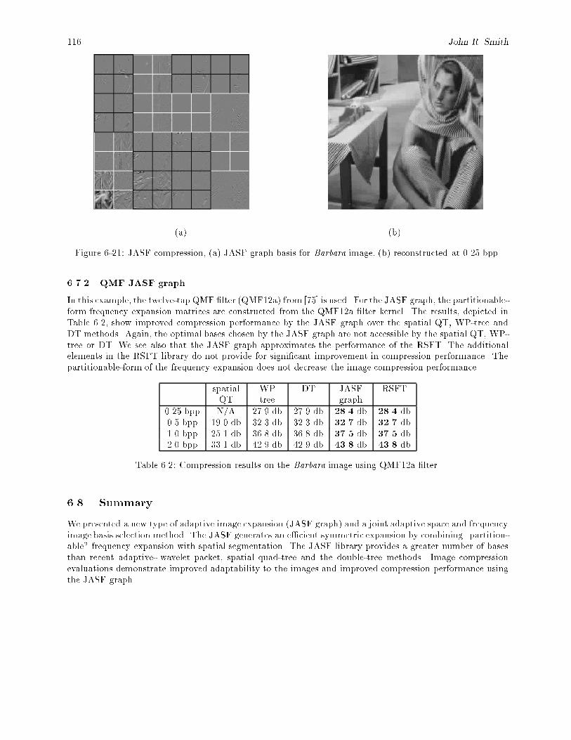
116 John R. Smith
(a) (b)
Figure 6-21: JASF compression, (a) JASF graph basis for Barbara image, (b) reconstructed at 0.25 bpp.
6.7.2 QMF JASF graph
In this example, the twelve-tap QMF �lter (QMF12a) from [75] is used. For the JASF graph, the partitionable-form frequency expansion matrices are constructed from the QMF12a �lter kernel. The results, depicted inTable 6.2, show improved compression performance by the JASF graph over the spatial QT, WP-tree andDT methods. Again, the optimal bases chosen by the JASF graph are not accessible by the spatial QT, WP-tree or DT. We see also that the JASF graph approximates the performance of the RSFT. The additionalelements in the RSFT library do not provide for signi�cant improvement in compression performance. Thepartitionable-form of the frequency expansion does not decrease the image compression performance.
spatial WP DT JASF RSFTQT tree graph
0.25 bpp N/A 27.9 db 27.9 db 28.4 db 28.4 db0.5 bpp 19.0 db 32.3 db 32.3 db 32.7 db 32.7 db1.0 bpp 25.1 db 36.8 db 36.8 db 37.5 db 37.5 db2.0 bpp 33.1 db 42.9 db 42.9 db 43.8 db 43.8 db
Table 6.2: Compression results on the Barbara image using QMF12a �lter.
6.8. Summary
We presented a new type of adaptive image expansion (JASF graph) and a joint adaptive space and frequencyimage basis selection method. The JASF generates an e�cient symmetric expansion by combining \partition-able" frequency expansion with spatial segmentation. The JASF library provides a greater number of basesthan recent adaptive- wavelet packet, spatial quad-tree and the double-tree methods. Image compressionevaluations demonstrate improved adaptability to the images and improved compression performance usingthe JASF graph.
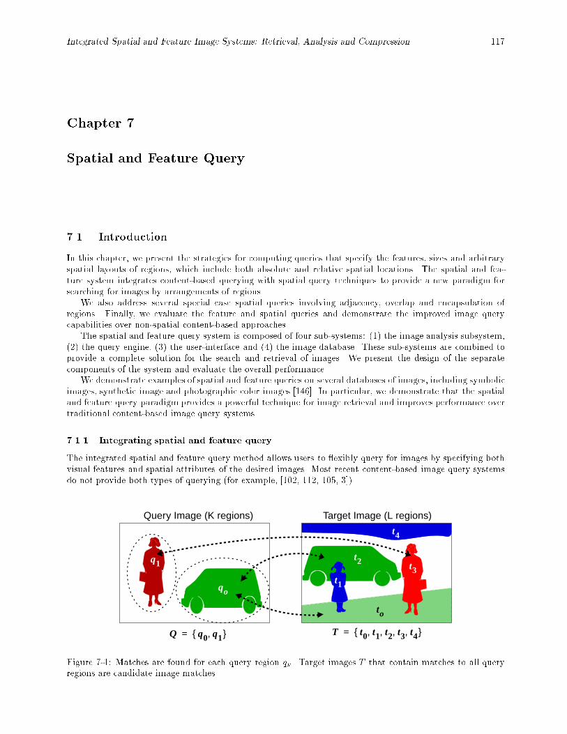
Integrated Spatial and Feature Image Systems: Retrieval, Analysis and Compression 117
Chapter 7
Spatial and Feature Query
7.1. Introduction
In this chapter, we present the strategies for computing queries that specify the features, sizes and arbitraryspatial layouts of regions, which include both absolute and relative spatial locations. The spatial and fea-ture system integrates content-based querying with spatial query techniques to provide a new paradigm forsearching for images by arrangements of regions.
We also address several special case spatial queries involving adjacency, overlap and encapsulation ofregions. Finally, we evaluate the feature and spatial queries and demonstrate the improved image querycapabilities over non-spatial content-based approaches.
The spatial and feature query system is composed of four sub-systems: (1) the image analysis subsystem,(2) the query engine, (3) the user-interface and (4) the image database. These sub-systems are combined toprovide a complete solution for the search and retrieval of images. We present the design of the separatecomponents of the system and evaluate the overall performance.
We demonstrate examples of spatial and feature queries on several databases of images, including symbolicimages, synthetic image and photographic color images [146]. In particular, we demonstrate that the spatialand feature query paradigm provides a powerful technique for image retrieval and improves performance overtraditional content-based image query systems.
7.1.1 Integrating spatial and feature query
The integrated spatial and feature query method allows users to exibly query for images by specifying bothvisual features and spatial attributes of the desired images. Most recent content-based image query systemsdo not provide both types of querying (for example, [102, 112, 105, 3]).
qo
q1
to
t2 t3
t4
t1
Query Image (K regions) Target Image (L regions)
Q q0 q1,{ }= T t0 t1 t2 t3 t4, , , ,{ }=
Figure 7-1: Matches are found for each query region qk. Target images T that contain matches to all queryregions are candidate image matches.
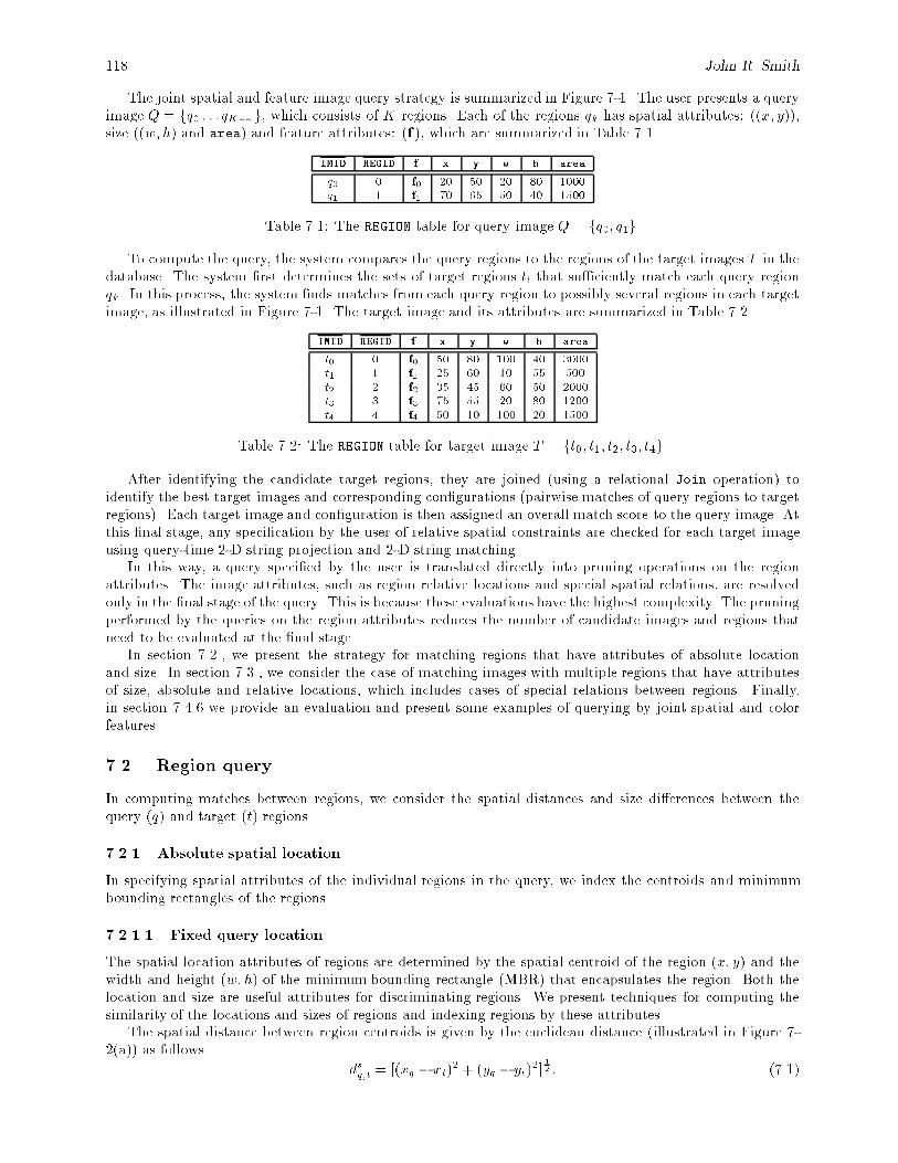
118 John R. Smith
The joint spatial and feature image query strategy is summarized in Figure 7-1. The user presents a queryimage Q = fq0 : : : qK�1g, which consists of K regions. Each of the regions qk has spatial attributes: ((x; y)),size ((w; h) and area) and feature attributes: (f ), which are summarized in Table 7.1.
IMID REGID f x y w h area
q0 0 f0 20 50 20 80 1000q1 1 f1 70 65 50 40 1500
Table 7.1: The REGION table for query image Q = fq0; q1g.
To compute the query, the system compares the query regions to the regions of the target images T in thedatabase. The system �rst determines the sets of target regions tl that su�ciently match each query regionqk. In this process, the system �nds matches from each query region to possibly several regions in each targetimage, as illustrated in Figure 7-1. The target image and its attributes are summarized in Table 7.2.
IMID REGID f x y w h area
t0 0 f0 50 80 100 40 3000t1 1 f1 25 60 10 55 500t2 2 f2 35 45 60 50 2000t3 3 f3 75 55 20 80 1200t4 4 f4 50 10 100 20 1500
Table 7.2: The REGION table for target image T = ft0; t1; t2; t3; t4g.
After identifying the candidate target regions, they are joined (using a relational Join operation) toidentify the best target images and corresponding con�gurations (pairwise matches of query regions to targetregions). Each target image and con�guration is then assigned an overall match score to the query image. Atthis �nal stage, any speci�cation by the user of relative spatial constraints are checked for each target imageusing query-time 2-D string projection and 2-D string matching.
In this way, a query speci�ed by the user is translated directly into pruning operations on the regionattributes. The image attributes, such as region relative locations and special spatial relations, are resolvedonly in the �nal stage of the query. This is because these evaluations have the highest complexity. The pruningperformed by the queries on the region attributes reduces the number of candidate images and regions thatneed to be evaluated at the �nal stage.
In section 7.2., we present the strategy for matching regions that have attributes of absolute locationand size. In section 7.3., we consider the case of matching images with multiple regions that have attributesof size, absolute and relative locations, which includes cases of special relations between regions. Finally,in section 7.4.6 we provide an evaluation and present some examples of querying by joint spatial and colorfeatures.
7.2. Region query
In computing matches between regions, we consider the spatial distances and size di�erences between thequery (q) and target (t) regions.
7.2.1 Absolute spatial location
In specifying spatial attributes of the individual regions in the query, we index the centroids and minimumbounding rectangles of the regions.
7.2.1.1 Fixed query location
The spatial location attributes of regions are determined by the spatial centroid of the region (x; y) and thewidth and height (w; h) of the minimum bounding rectangle (MBR) that encapsulates the region. Both thelocation and size are useful attributes for discriminating regions. We present techniques for computing thesimilarity of the locations and sizes of regions and indexing regions by these attributes.
The spatial distance between region centroids is given by the euclidean distance (illustrated in Figure 7-2(a)) as follows
dsq;t = [(xq � xt)2 + (yq � yt)
2]12 : (7.1)
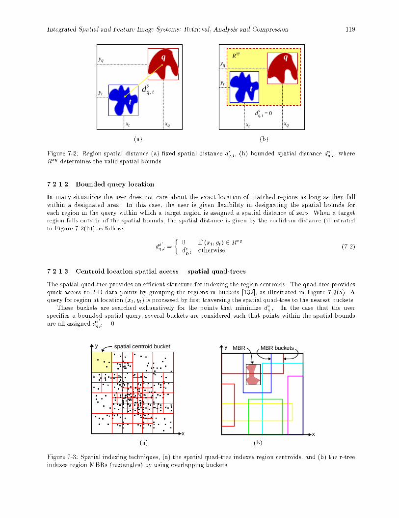
Integrated Spatial and Feature Image Systems: Retrieval, Analysis and Compression 119
dq t,s
xqxt
yq
yt
q
tdq t,
s 0=
xqxt
yq
yt
q
t
Rxy
(a) (b)
Figure 7-2: Region spatial distance (a) �xed spatial distance dsq;t, (b) bounded spatial distance ds0
q;t, whereRxy determines the valid spatial bounds.
7.2.1.2 Bounded query location
In many situations the user does not care about the exact location of matched regions as long as they fallwithin a designated area. In this case, the user is given exibility in designating the spatial bounds foreach region in the query within which a target region is assigned a spatial distance of zero. When a targetregion falls outside of the spatial bounds, the spatial distance is given by the euclidean distance (illustratedin Figure 7-2(b)) as follows
ds0
q;t =
�0 if (xt; yt) 2 Rxy
dsq;t otherwise.(7.2)
7.2.1.3 Centroid location spatial access { spatial quad-trees
The spatial quad-tree provides an e�cient structure for indexing the region centroids. The quad-tree providesquick access to 2-D data points by grouping the regions in buckets [132], as illustrated in Figure 7-3(a). Aquery for region at location (xt; yt) is processed by �rst traversing the spatial quad-tree to the nearest buckets.
These buckets are searched exhaustively for the points that minimize dsq;t. In the case that the userspeci�es a bounded spatial query, several buckets are considered such that points within the spatial boundsare all assigned ds
0
q;t = 0.
x
y spatial centroid bucket
x
y MBR MBR buckets
(a) (b)
Figure 7-3: Spatial indexing techniques, (a) the spatial quad-tree indexes region centroids, and (b) the r-treeindexes region MBRs (rectangles) by using overlapping buckets.
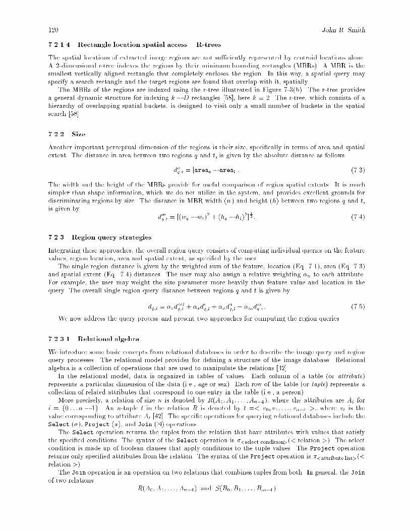
120 John R. Smith
7.2.1.4 Rectangle location spatial access { R-trees
The spatial locations of extracted image regions are not su�ciently represented by centroid locations alone.A 2-dimensional r-tree indexes the regions by their minimum bounding rectangles (MBRs). A MBR is thesmallest vertically aligned rectangle that completely encloses the region. In this way, a spatial query mayspecify a search rectangle and the target regions are found that overlap with it, spatially.
The MBRs of the regions are indexed using the r-tree illustrated in Figure 7-3(b). The r-tree providesa general dynamic structure for indexing k �D rectangles [58], here k = 2. The r-tree, which consists of ahierarchy of overlapping spatial buckets, is designed to visit only a small number of buckets in the spatialsearch [58].
7.2.2 Size
Another important perceptual dimension of the regions is their size, speci�cally in terms of area and spatialextent. The distance in area between two regions q and t, is given by the absolute distance as follows
daq;t = jareaq � areatj: (7.3)
The width and the height of the MBRs provide for useful comparison of region spatial extents. It is muchsimpler than shape information, which we do not utilize in the system, and provides excellent grounds fordiscriminating regions by size. The distance in MBR width (w) and height (h) between two regions q and t,is given by
dmq;t = [(wq � wt)2 + (hq � ht)
2]12 : (7.4)
7.2.3 Region query strategies
Integrating these approaches, the overall region query consists of computing individual queries on the featurevalues, region location, area and spatial extent, as speci�ed by the user.
The single region distance is given by the weighted sum of the feature, location (Eq. 7.1), area (Eq. 7.3)and spatial extent (Eq. 7.4) distances. The user may also assign a relative weighting �n to each attribute.For example, the user may weight the size parameter more heavily than feature value and location in thequery. The overall single region query distance between regions q and t is given by
dq;t = �cdsetq;t + �sd
sq;t + �ad
aq;t + �md
mq;t: (7.5)
We now address the query process and present two approaches for computing the region queries.
7.2.3.1 Relational algebra
We introduce some basic concepts from relational databases in order to describe the image query and regionquery processes. The relational model provides for de�ning a structure of the image database. Relationalalgebra is a collection of operations that are used to manipulate the relations [42].
In the relational model, data is organized in tables of values. Each column of a table (or attribute)represents a particular dimension of the data (i.e., age or sex). Each row of the table (or tuple) represents acollection of related attributes that correspond to one entry in the table (i.e., a person).
More precisely, a relation of size n is denoted by R(A0; A1; : : : ; An�1), where the attributes are Ai fori = f0 : : :n � 1g. An n-tuple t in the relation R is denoted by t =< v0; v1; : : : ; vn�1 >, where vi is thevalue corresponding to attribute Ai [42]. The speci�c operations for querying relational databases include theSelect (�), Project (�), and Join (1) operations.
The Select operation returns the tuples from the relation that have attributes with values that satisfythe speci�ed conditions. The syntax of the Select operation is �<select condition>(< relation >). The selectcondition is made up of boolean clauses that apply conditions to the tuple values. The Project operationreturns only speci�ed attributes from the relation. The syntax of the Project operation is �<attribute list>(<relation >).
The Join operation is an operation on two relations that combines tuples from both. In general, the Joinof two relations
R(A0; A1; : : : ; An�1) and S(B0; B1; : : : ; Bm�1)
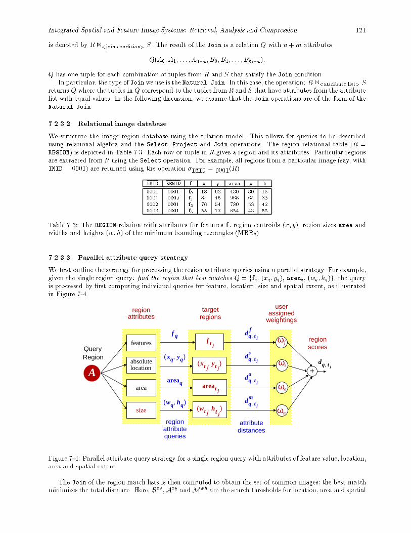
Integrated Spatial and Feature Image Systems: Retrieval, Analysis and Compression 121
is denoted by R 1<join condition> S. The result of the Join is a relation Q with n+m attributes
Q(A0; A1; : : : ; An�1; B0; B1; : : : ; Bm�1):
Q has one tuple for each combination of tuples from R and S that satisfy the Join condition.In particular, the type of Joinwe use is the Natural Join. In this case, the operation: R 1<attribute list> S
returns Q where the tuples in Q correspond to the tuples fromR and S that have attributes from the attributelist with equal values. In the following discussion, we assume that the Join operations are of the form of theNatural Join.
7.2.3.2 Relational image database
We structure the image region database using the relation model. This allows for queries to be describedusing relational algebra and the Select, Project and Join operations. The region relational table (R =REGION) is depicted in Table 7.3. Each row or tuple in R gives a region and its attributes. Particular regionsare extracted from R using the Select operation. For example, all regions from a particular image (say, withIMID = 0001) are returned using the operation �IMID = 0001(R).
IMID REGID f x y area w h
0001 0001 f0 18 63 430 30 150001 0002 f1 34 45 968 65 320002 0001 f2 76 54 780 53 420003 0001 f3 55 12 654 43 55
Table 7.3: The REGION relation with attributes for features f , region centroids (x; y), region sizes area andwidths and heights (w; h) of the minimum bounding rectangles (MBRs).
7.2.3.3 Parallel attribute query strategy
We �rst outline the strategy for processing the region attribute queries using a parallel strategy. For example,given the single region query: �nd the region that best matches Q = ffq; (xq; yq); areaq; (wq ; hq)g, the queryis processed by �rst computing individual queries for feature, location, size and spatial extent, as illustratedin Figure 7-4.
QueryRegion
A
f q
xq yq,( )
wq hq,( )
areaq
ωm
dq t j,
ωf
ωs
ωa
+
dq t j,f
dq t j,s
dq t j,a
dq t j,m
wt jht j
,( )
areat j
xt jyt j
,( )
f t j
regionattributes
targetregions
attributedistances
user
regionscores
regionattributequeries
assignedweightings
features
absolutelocation
area
size
Figure 7-4: Parallel attribute query strategy for a single region query with attributes of feature value, location,area and spatial extent.
The Join of the region match lists is then computed to obtain the set of common images; the best matchminimizes the total distance. Here, Bxy, Axy andMwh are the search thresholds for location, area and spatial
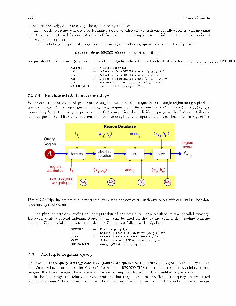
122 John R. Smith
extent, respectively, and are set by the system or by the user.The parallel strategy achieves a performance gain over exhaustive search since it allows for special indexing
structures to be utilized for each attribute of the region. For example, the spatial quad-tree is used to indexthe regions by location.
The parallel region query strategy is carried using the following operations, where the expression,
Select � from REGION where < select condition >
is equivalent to the following expression in relational algebra where the � refers to all attributes ��(�<select condition>(REGION)).
FEATURE Feature query(fq)LOC Select � from REGION where (xt; yt) 2 Bxy
SIZE Select � from REGION where areat 2 Axy
MBR Select � from REGION where (wt; ht) 2Mwh
CAND FEATURE 1IMID LOC 1IMID SIZE 1IMID MBR
REGIONMATCH mindq;t(CAND); (using Eq. 7:5):
7.2.3.4 Pipeline attribute query strategy
We present an alternate strategy for processing the region attribute queries for a single region using a pipelinequery strategy. For example, given the single region query: �nd the region that best matches Q = ffq; (xq; yq);areaq ; (wq; hq)g, the query is processed by �rst computing the individual query on the feature attributes.This output is then �ltered by location, then by size and, �nally, by spatial extent, as illustrated in Figure 7-5.
QueryRegion
A
f q xq yq,( ) wq hq,( )areaq
ωm
dq t j,
ωf ωsωa
wt jht j
,( )areat jxt j
yt j,( )f t j
regionattributes
regionscore
user-assignedweightings
Region Database
featuresabsolutelocation area size
Figure 7-5: Pipeline attribute query strategy for a single region query with attributes of feature value, location,area and spatial extent.
The pipeline strategy avoids the computation of the attribute Join required in the parallel strategy.However, while a special indexing structure may still be used on the feature values, the pipeline strategycannot utilize special indexes for the other attributes that follow in the pipeline.
FEATURE Feature query(fq)LOC Select � from FEATURE where (xt; yt) 2 Bxy
SIZE Select � from LOC where areat 2 Axy
CAND Select � from SIZE where (wt; ht) 2Mwh
REGIONMATCH mindq;t(CAND); (using Eq. 7:5):
7.3. Multiple regions query
The overall image query strategy consists of joining the queries on the individual regions in the query image.The Join, which consists of the Natural Join of the REGIONMATCH tables, identi�es the candidate targetimages. For these images, the image match score is computed by adding the weighted region scores.
In the �nal stage, the relative spatial locations that may have been speci�ed in the query are evaluatedusing query-time 2-D string projection. A 2-D string comparison determines whether candidate target images
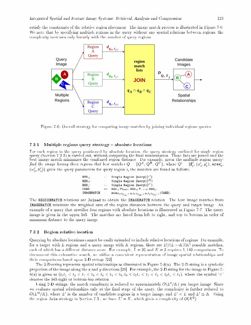
Integrated Spatial and Feature Image Systems: Retrieval, Analysis and Compression 123
satisfy the constraints of the relative region placement. The image match process is illustrated in Figure 7-6.We note that by specifying multiple regions in the query without any spatial relations between regions, thecomplexity increases only linearly with the number of query regions.
Region
QueryB
QueryImage
C
BA
SpatialRelationshipsRegion
QueryC
AB
C
region
qA qB qC∩ ∩
dqA t j l,,
dqB t j l,,
dqC t j l,,
DQ T j,
Region
QueryA
CandidateImagesmatch
lists
JOIN
MultipleRegions
Figure 7-6: Overall strategy for computing image matches by joining individual regions queries.
7.3.1 Multiple regions query strategy { absolute locations
For each region in the query positioned by absolute location, the query strategy outlined for single regionquery (Section 7.2.3) is carried out, without computing the �nal minimization. These lists are joined and thebest image match minimizes the combined region distance. For example, given the multiple region query:�nd the image having three regions that best matches Q = fQA; QB; QCg, where Qi = ff iq; (x
iq; y
iq); area
iq;
(wiq; h
iq)g gives the query parameters for query region i, the matches are found as follows:
REGA Single Region Query(QA)REGB Single Region Query(QB)REGC Single Region Query(QC)CAND REGA 1IMID REGB 1IMID REGCIMAGEMATCH min�0dQA;T+�1dQB;T+�2dQC;T
(CAND):
The REGIONMATCH relations are Joined to obtain the IMAGEMATCH relation. The best image matches fromIMAGEMATCH minimize the weighted sum of the region distances between the query and target image. Anexample of a query that speci�es four regions with absolute locations is illustrated in Figure 7-7. The queryimage is given in the upper left. The matches are listed from left to right, and top to bottom in order ofminimum distance to the query image.
7.3.2 Region relative location
Querying by absolute locations cannot be easily extended to include relative locations of regions. For example,for a target with L regions and a query image with K regions, there are L!=(L � K)!K! possible matches,each of which has a di�erent distance score. For example, L = 20 and K = 3 requires 1; 140 comparisons. Tocircumvent this exhaustive search, we utilize a convenient representation of image spatial relationships andtheir comparisons based upon 2-D strings [22].
The 2-D string represents spatial relationships as illustrated in Figure 7-8(a). The 2-D string is a symbolicprojection of the image along the x and y directions [20]. For example, the 2-D string for the image in Figure 7-8(a) is given as (t0t1 < t2 < t7 < t3 < t6 < t4 < t5; t0 < t5t7 < t6 < t2 < t3t1 < t4), where the symbol `<'denotes the left-right or bottom-top relation.
Using 2-D strings, the match complexity is reduced to approximately O(L3=K) per target image. Sincewe evaluate spatial relationships only at the �nal stage of the query, the complexity is further reduced toO(L03=K), where L0 is the number of candidate regions in a target image, and L0 < L and L0 ' K. Usingthe region Join strategy in Section 7.3., we have L0 = K, which gives a complexity of O(K2).
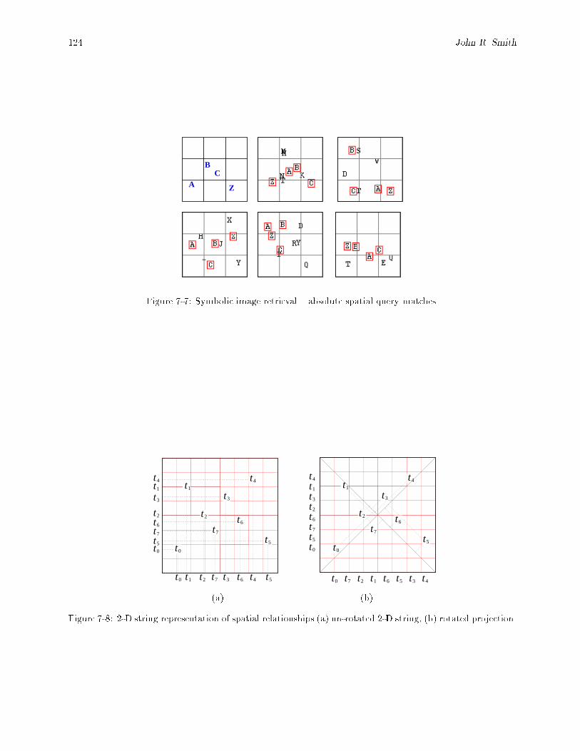
124 John R. Smith
A
BC
Z
Figure 7-7: Symbolic image retrieval { absolute spatial query matches.
t0
t0
t1
t1 t2
t2
t3
t3
t4
t4
t5
t5t6
t6
t7
t7
t0
t1
t6t2
t4
t5
t3
t7
t0
t0
t1
t7 t2
t2
t6
t3
t3
t4
t5
t4t5
t6
t7
t1
t0
t1
t6t2
t4
t5
t3
t7
(a) (b)
Figure 7-8: 2-D string representation of spatial relationships (a) un-rotated 2-D string, (b) rotated projection.
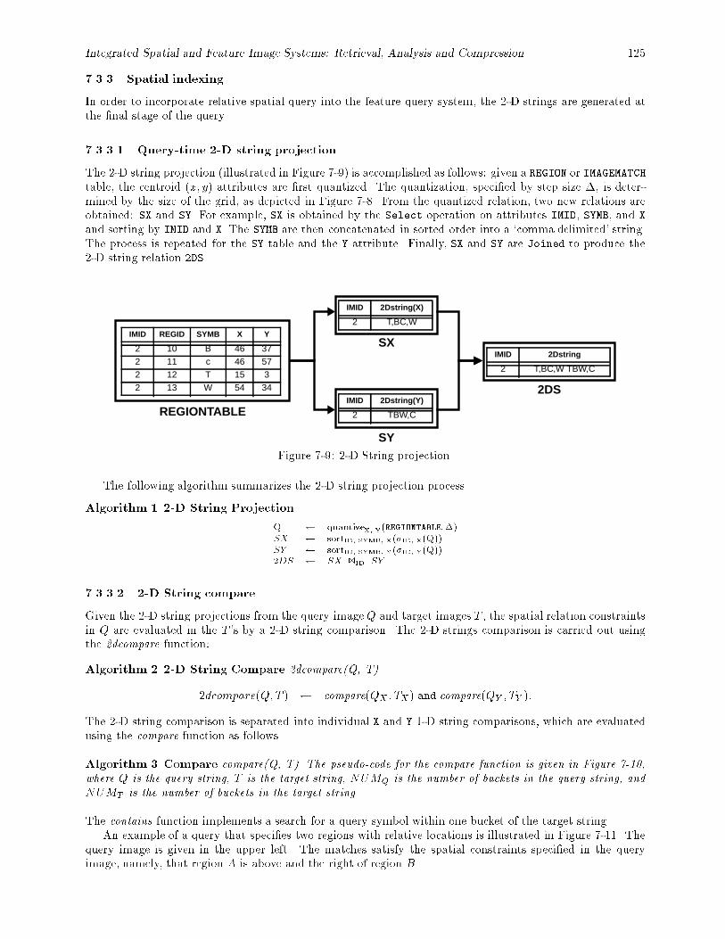
Integrated Spatial and Feature Image Systems: Retrieval, Analysis and Compression 125
7.3.3 Spatial indexing
In order to incorporate relative spatial query into the feature query system, the 2-D strings are generated atthe �nal stage of the query.
7.3.3.1 Query-time 2-D string projection
The 2-D string projection (illustrated in Figure 7-9) is accomplished as follows: given a REGION or IMAGEMATCHtable, the centroid (x; y) attributes are �rst quantized. The quantization, speci�ed by step size �, is deter-mined by the size of the grid, as depicted in Figure 7-8. From the quantized relation, two new relations areobtained: SX and SY. For example, SX is obtained by the Select operation on attributes IMID, SYMB, and X
and sorting by IMID and X. The SYMB are then concatenated in sorted order into a `comma delimited' string.The process is repeated for the SY table and the Y attribute. Finally, SX and SY are Joined to produce the2-D string relation 2DS.
IMID 2Dstring(X)
2 T,BC,WIMID REGID SYMB X Y
2 10 B 46 372 11 c 46 572 12 T 15 32 13 W 54 34
IMID 2Dstring(Y)
2 TBW,C
IMID 2Dstring
2 T,BC,W TBW,C
SX
SY
2DS
REGIONTABLE
Figure 7-9: 2-D String projection.
The following algorithm summarizes the 2-D string projection process.
Algorithm 1 2-D String Projection
Q quantizeX, Y(REGIONTABLE;�)SX sortID, SYMB, X(�ID, X(Q))SY sortID, SYMB, Y(�ID, Y(Q))2DS SX 1ID SY
7.3.3.2 2-D String compare
Given the 2-D string projections from the query imageQ and target images T , the spatial relation constraintsin Q are evaluated in the T 's by a 2-D string comparison. The 2-D strings comparison is carried out usingthe 2dcompare function:
Algorithm 2 2-D String Compare 2dcompare(Q, T)
2dcompare(Q; T ) compare(QX ; TX) and compare(QY ; TY ):
The 2-D string comparison is separated into individual X and Y 1-D string comparisons, which are evaluatedusing the compare function as follows
Algorithm 3 Compare compare(Q, T). The pseudo-code for the compare function is given in Figure 7-10,where Q is the query string, T is the target string, NUMQ is the number of buckets in the query string, andNUMT is the number of buckets in the target string.
The contains function implements a search for a query symbol within one bucket of the target string.An example of a query that speci�es two regions with relative locations is illustrated in Figure 7-11. The
query image is given in the upper left. The matches satisfy the spatial constraints speci�ed in the queryimage, namely, that region A is above and the right of region B.
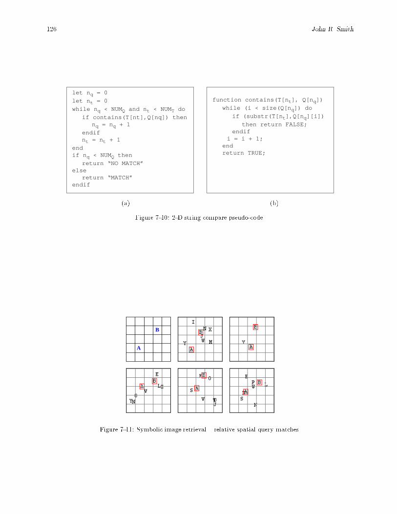
126 John R. Smith
let nq = 0
let nt = 0
while nq < NUMQ and nt < NUMT do
if contains(T[nt],Q[nq]) thennq = nq + 1
endifnt = nt + 1
endif nq < NUMQ then
return “NO MATCH”else
return “MATCH”endif
function contains(T[nt], Q[nq])
while (i < size(Q[nq]) do
if (substr(T[nt],Q[nq][i])
then return FALSE;endif
i = i + 1;endreturn TRUE;
(a) (b)
Figure 7-10: 2-D string compare pseudo-code.
A
B
Figure 7-11: Symbolic image retrieval { relative spatial query matches.
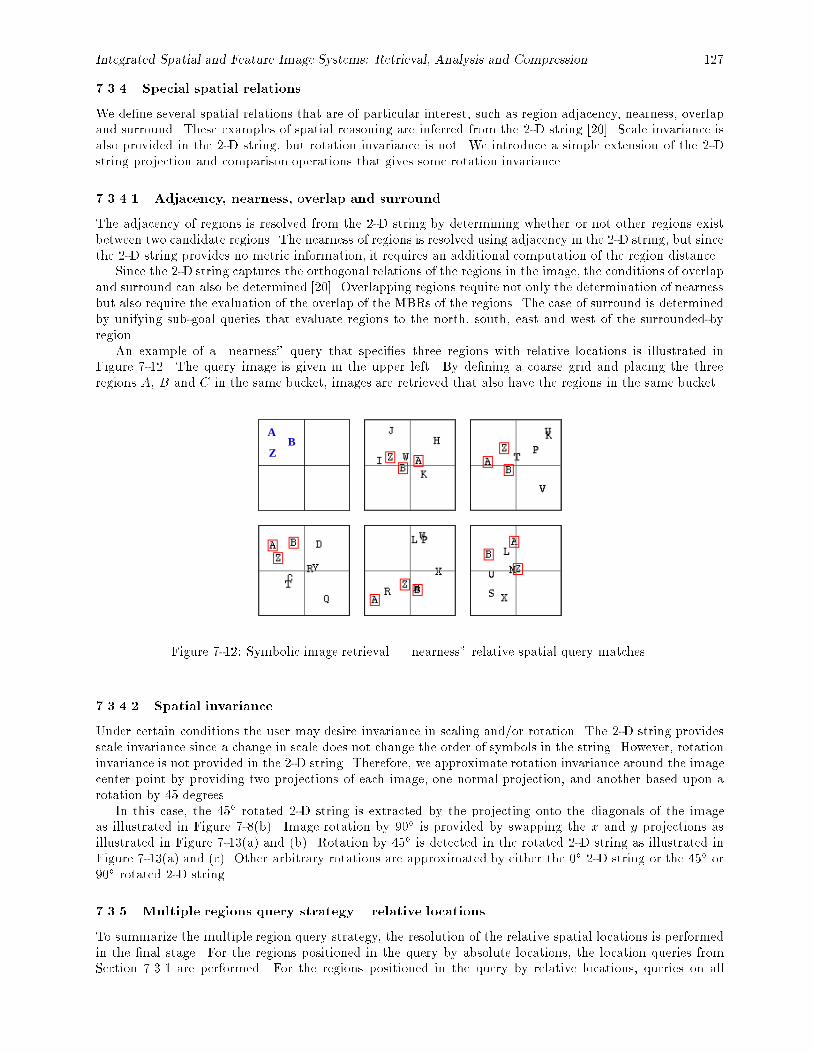
Integrated Spatial and Feature Image Systems: Retrieval, Analysis and Compression 127
7.3.4 Special spatial relations
We de�ne several spatial relations that are of particular interest, such as region adjacency, nearness, overlapand surround. These examples of spatial reasoning are inferred from the 2-D string [20]. Scale invariance isalso provided in the 2-D string, but rotation invariance is not. We introduce a simple extension of the 2-Dstring projection and comparison operations that gives some rotation invariance.
7.3.4.1 Adjacency, nearness, overlap and surround
The adjacency of regions is resolved from the 2-D string by determining whether or not other regions existbetween two candidate regions. The nearness of regions is resolved using adjacency in the 2-D string, but sincethe 2-D string provides no metric information, it requires an additional computation of the region distance.
Since the 2-D string captures the orthogonal relations of the regions in the image, the conditions of overlapand surround can also be determined [20]. Overlapping regions require not only the determination of nearnessbut also require the evaluation of the overlap of the MBRs of the regions. The case of surround is determinedby unifying sub-goal queries that evaluate regions to the north, south, east and west of the surrounded-byregion.
An example of a \nearness" query that speci�es three regions with relative locations is illustrated inFigure 7-12. The query image is given in the upper left. By de�ning a coarse grid and placing the threeregions A, B and C in the same bucket, images are retrieved that also have the regions in the same bucket.
AB
Z
Figure 7-12: Symbolic image retrieval { \nearness" relative spatial query matches.
7.3.4.2 Spatial invariance
Under certain conditions the user may desire invariance in scaling and/or rotation. The 2-D string providesscale invariance since a change in scale does not change the order of symbols in the string. However, rotationinvariance is not provided in the 2-D string. Therefore, we approximate rotation invariance around the imagecenter point by providing two projections of each image, one normal projection, and another based upon arotation by 45 degrees.
In this case, the 45� rotated 2-D string is extracted by the projecting onto the diagonals of the imageas illustrated in Figure 7-8(b). Image rotation by 90� is provided by swapping the x and y projections asillustrated in Figure 7-13(a) and (b). Rotation by 45� is detected in the rotated 2-D string as illustrated inFigure 7-13(a) and (c). Other arbitrary rotations are approximated by either the 0� 2-D string or the 45� or90� rotated 2-D string.
7.3.5 Multiple regions query strategy { relative locations
To summarize the multiple region query strategy, the resolution of the relative spatial locations is performedin the �nal stage. For the regions positioned in the query by absolute locations, the location queries fromSection 7.3.1 are performed. For the regions positioned in the query by relative locations, queries on all
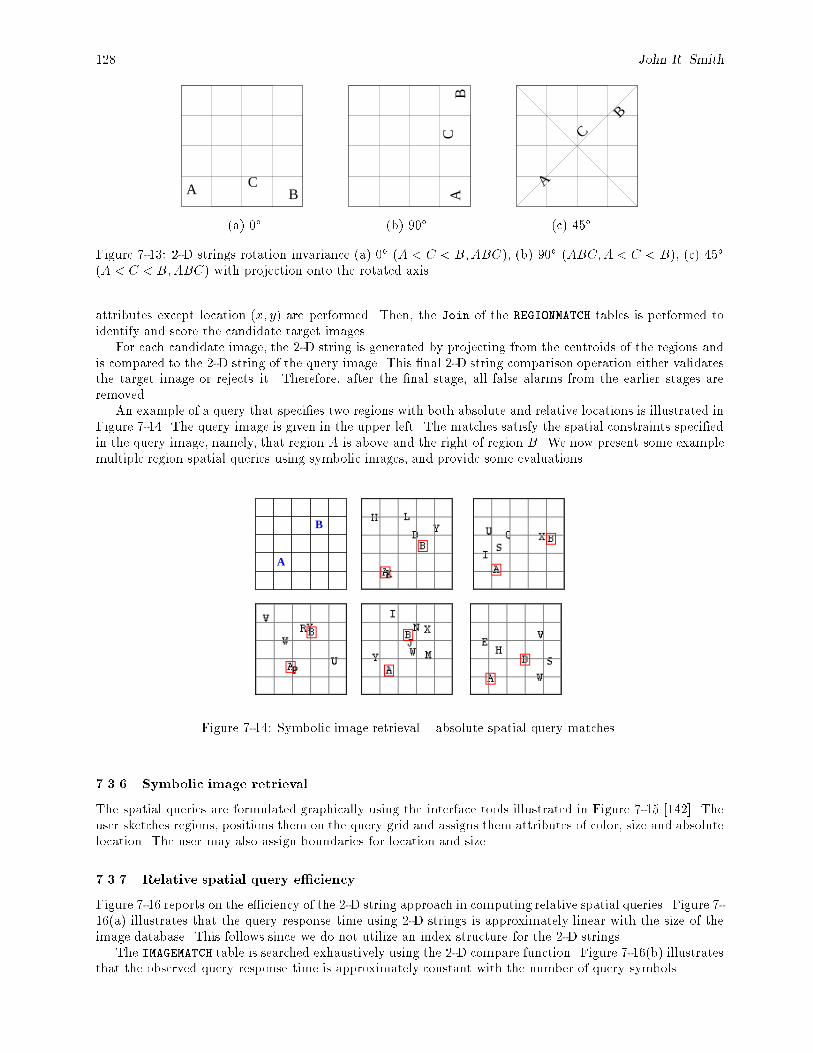
128 John R. Smith
A CB A
CB
A
CB
(a) 0� (b) 90� (c) 45�
Figure 7-13: 2-D strings rotation invariance (a) 0� (A < C < B;ABC), (b) 90� (ABC;A < C < B), (c) 45�
(A < C < B;ABC) with projection onto the rotated axis.
attributes except location (x; y) are performed. Then, the Join of the REGIONMATCH tables is performed toidentify and score the candidate target images.
For each candidate image, the 2-D string is generated by projecting from the centroids of the regions andis compared to the 2-D string of the query image. This �nal 2-D string comparison operation either validatesthe target image or rejects it. Therefore, after the �nal stage, all false alarms from the earlier stages areremoved.
An example of a query that speci�es two regions with both absolute and relative locations is illustrated inFigure 7-14. The query image is given in the upper left. The matches satisfy the spatial constraints speci�edin the query image, namely, that region A is above and the right of region B. We now present some examplemultiple region spatial queries using symbolic images, and provide some evaluations.
A
B
Figure 7-14: Symbolic image retrieval { absolute spatial query matches.
7.3.6 Symbolic image retrieval
The spatial queries are formulated graphically using the interface tools illustrated in Figure 7-15 [142]. Theuser sketches regions, positions them on the query grid and assigns them attributes of color, size and absolutelocation. The user may also assign boundaries for location and size.
7.3.7 Relative spatial query e�ciency
Figure 7-16 reports on the e�ciency of the 2-D string approach in computing relative spatial queries. Figure 7-16(a) illustrates that the query response time using 2-D strings is approximately linear with the size of theimage database. This follows since we do not utilize an index structure for the 2-D strings.
The IMAGEMATCH table is searched exhaustively using the 2-D compare function. Figure 7-16(b) illustratesthat the observed query response time is approximately constant with the number of query symbols.
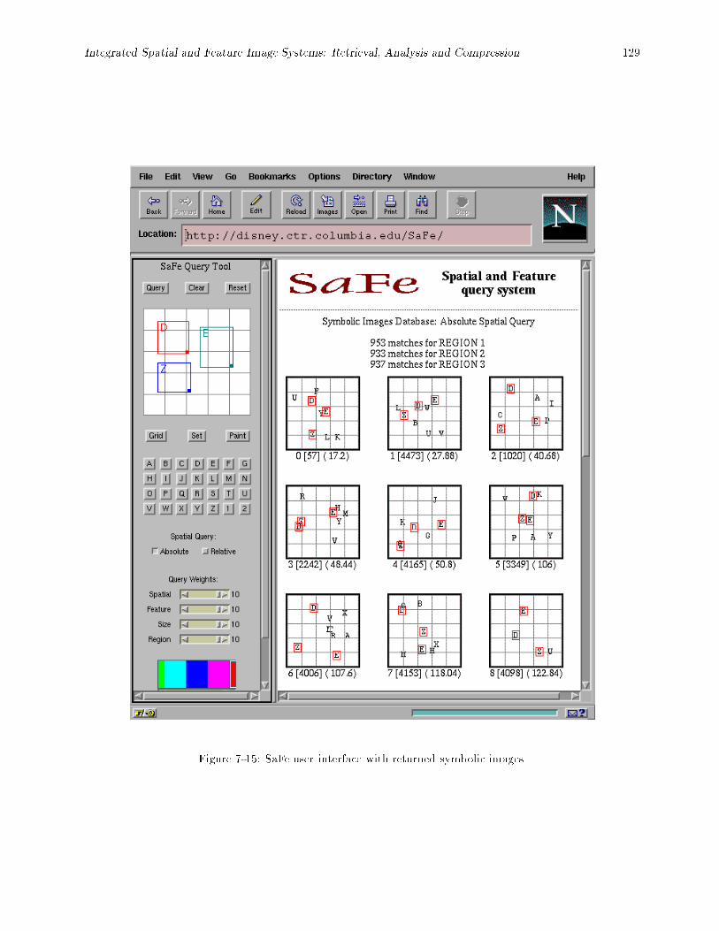
Integrated Spatial and Feature Image Systems: Retrieval, Analysis and Compression 129
Figure 7-15: SaFe user interface with returned symbolic images.
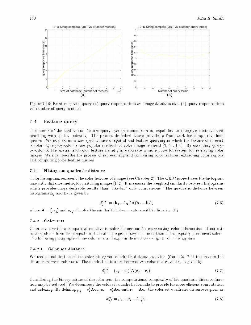
130 John R. Smith
0 1 2 3 4 5 6 7 8 9 10
x 104
0
2
4
6
8
10
12
14
size of database (number of records)
quer
y re
spon
se ti
me
(sec
s)
2−D String compare (QRT vs. Number records)
2 4 6 8 10 12 14 16 18 202
2.2
2.4
2.6
2.8
3
3.2
3.4
3.6
3.8
4
Number of query terms
quer
y re
spon
se ti
me
(sec
s)
2−D String compare (QRT vs. Number query terms)
(a) (b)
Figure 7-16: Relative spatial query (a) query response time vs. image database size, (b) query response timevs. number of query symbols.
7.4. Feature query
The power of the spatial and feature query system comes from its capability to integrate content-basedsearching with spatial indexing. The process described above provides a framework for computing thesequeries. We now examine one speci�c case of spatial and feature querying in which the feature of interestis color. Query-by-color is one popular method for color image retrieval [3, 45, 105]. By extending query-by-color to the spatial and color feature paradigm, we create a more powerful system for retrieving colorimages. We now describe the process of representing and comparing color features, extracting color regionsand computing color feature queries.
7.4.1 Histogram quadratic distance
Color histograms represent the color features of images (see Chapter 2). The QBIC project uses the histogramquadratic distance metric for matching images [102]. It measures the weighted similarity between histogramswhich provides more desirable results than \like-bin" only comparisons. The quadratic distance betweenhistograms hq and ht is given by
dhistq;t = (hq � ht)tA(hq � ht); (7.6)
where A = [ai;j] and ai;j denotes the similarity between colors with indices i and j.
7.4.2 Color sets
Color sets provide a compact alternative to color histograms for representing color information. Their uti-lization stems from the conjecture that salient regions have not more than a few, equally prominent colors.The following paragraphs de�ne color sets and explain their relationship to color histograms.
7.4.2.1 Color set distance
We use a modi�cation of the color histogram quadratic distance equation (from Eq. 7.6) to measure thedistance between color sets. The quadratic distance between two color sets cq and ct is given by
dsetq;t = (cq � ct)tA(cq � ct): (7.7)
Considering the binary nature of the color sets, the computational complexity of the quadratic distance func-tion may be reduced. We decompose the color set quadratic formula to provide for more e�cient computationand indexing. By de�ning �q = ctqAcq, �t = cttAct and rt = Act, the color set quadratic distance is given as
dsetq;t = �q + �t � 2ctqrt: (7.8)
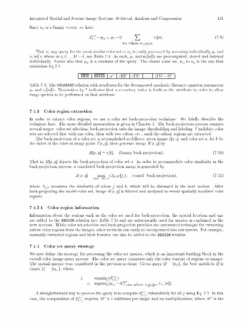
Integrated Spatial and Feature Image Systems: Retrieval, Analysis and Compression 131
Since cq is a binary vector, we have
dsetq;t � �q = �t � 2X
8m where cq[m]=1
rt[m]: (7.9)
That is, any query for the most similar color set to cq is easily processed by accessing individually �t andrt[m]'s, where m 2 0 : : :M � 1, see Table 7.4. As such, �t and rt[m]'s are precomputed, stored and indexedindividually. Notice also that �q is a constant of the query. The closest color set, ct, to cq is the one thatminimizes Eq 7.9.
IMID REGID �� r[0]� r[1]� : : : r[M � 1]�
Table 7.4: The COLORSET relation with attributes for the decomposed quadratic distance equation parameters�t and rt[m]'s. Denotation by � indicates that a secondary index is built on the attribute in order to allowrange queries to be performed on that attribute.
7.4.3 Color region extraction
In order to extract color regions, we use a color set back-projection technique. We brie y describe thetechnique here. The more detailed presentation is given in Chapter 5. The back-projection process requiresseveral stages: color set selection, back-projection onto the image, thresholding and labeling. Candidate colorsets are selected �rst with one color, then with two colors, etc., until the salient regions are extracted.
The back-projection of a color set is accomplished as follows: given image I[x; y] and color set c, let k bethe index of the color at image point I[x; y], then generate image B[x; y] by
B[x; y] = c[k]; (binary back-projection): (7.10)
That is, B[x; y] depicts the back-projection of color set c. In order to accommodate color similarity in theback-projection process, a correlated back-projection image is generated by
B[x; y] = maxj=0:::M�1
(Aj;kc[j]); (correl. back-projection); (7.11)
where Aj;k measures the similarity of colors j and k, which will be discussed in the next section. Afterback-projecting the model color set, image B[x; y] is �ltered and analyzed to reveal spatially localized colorregions.
7.4.3.1 Color region information
Information about the regions such as the color set used for back-projection, the spatial location and sizeare added to the REGION relation (see Table 7.3) and are subsequently used for queries as explained in thenext sections. While color set selection and back-projection provides one automated technique for extractingsalient color regions from the images, other methods can easily be incorporated into our system. For example,manually extracted regions and their features can also be added to the REGION relation.
7.4.4 Color set query strategy
We now de�ne the strategy for processing the color set queries, which is an important building block in theoverall color image query process. The color set query compares only the color content of regions or images.The spatial queries were considered in the previous sections. Given query Q = fcqg, the best match to Q istarget Tj = fctjg, where,
j = argminj(dsetq;tj
)
= argminj(�tj � 2P
8m where cq[m]=1 rtj [m]):
A straightforward way to process the query is to compute dsetq;tjexhaustively for all j using Eq. 7.9. In this
case, the computation of dsetq;tjrequires M 0 + 1 additions per target and no multiplications, where M 0 is the
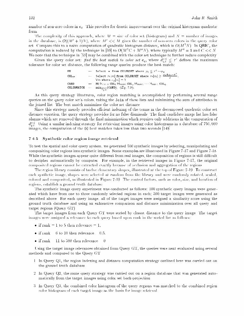
132 John R. Smith
number of non-zero colors in cq . This provides for drastic improvement over the original histogram quadraticform.
The complexity of this approach, where M = size of color set (histogram) and N = number of imagesin the database, is O((M 0 + 1)N ), where M 0 << M gives the number of non-zero colors in the query colorset. Compare this to a naive computation of quadratic histogram distance, which is O(M2N ). In QBIC, thecomputation is reduced by the technique in [59] to O(M2C +M 00N ), where typically M 00 = 3 and C << N .We note that the technique in [59] may be combined with the color set technique to further reduce complexity.
Given the query color set: �nd the best match to color set cq, where dsetq;t � � c de�nes the maximumtolerance for color set distance, the following range queries produce the best match:
MU Select � from COLORSET where �t � �c � �q
COLm Select rt[m] from COLORSET where rt[m] ��q+�t��
c
2;
8m where cq [m] = 1CAND MU 1IMID COLi 1IMID COLj 1IMID � � � 1IMID COLkCOLORMATCH mindset
q;t(CAND); (Eq: 7:9):
As this query strategy illustrates, color region matching is accomplished by performing several rangequeries on the query color set's colors, taking the Join of these lists and minimizing the sum of attributes inthe joined list. The best match minimizes the color set distance.
Since this strategy merely provides e�cient indexing of the terms in the decomposed quadratic color setdistance equation, the query strategy provides for no false dismissals. The �nal candidate image list has falsealarms which are removed through the �nal minimization which requires only additions in the computation ofdsetq;t . Using a similar indexing strategy for retrieving images using color histograms in a database of 750; 000images, the computation of the 60 best matches takes less than two seconds [148].
7.4.5 Synthetic color region image retrieval
To test the spatial and color query system, we generated 500 synthetic images by selecting, manipulating andcompositing color regions into synthetic images. Some examples are illustrated in Figure 7-17 and Figure 7-18.While the synthetic images appear quite di�erent from real images, the composition of regions is still di�cultto decipher automatically by computer. For example, in the retrieved images in Figure 7-17, the originalcomposited regions cannot be extracted exactly because of occlusion and aggregation of the regions.
The region library consists of twelve elementary shapes, illustrated at the top of Figure 7-19. To constructeach synthetic image, shapes were selected at random from the library and were randomly rotated, scaled,colored and composited, as illustrated in Figure 7-19. The control factors, such as color, size, and location ofregions, establish a ground truth database.
The synthetic image query experiment was conducted as follows: 100 synthetic query images were gener-ated which have from one to three randomly selected regions in each; 500 target images were generated asdescribed above. For each query image, all of the target images were assigned a similarity score using theground truth database and using an exhaustive comparison and distance minimization over all query andtarget regions (Query GT).
The target images from each Query GT were sorted by closest distance to the query image. The targetimages were assigned a relevance to each query based upon rank in the sorted list as follows:
� if rank = 1 to 5 then relevance = 1,
� if rank = 6 to 10 then relevance = 0:5,
� if rank = 11 to 500 then relevance = 0.
Using the target image relevances obtained from Query GT, the queries were next evaluated using severalmethods and compared to the Query GT.
1. In Query Q1, the region indexing and distance computation strategy outlined here was carried out onthe ground truth database.
2. In Query Q2, the same query strategy was carried out on a region database that was generated auto-matically from the target images using color set back-projection.
3. In Query Q3, the combined color histogram of the query regions was matched to the combined regioncolor histogram of each target image as the basis for image retrieval.
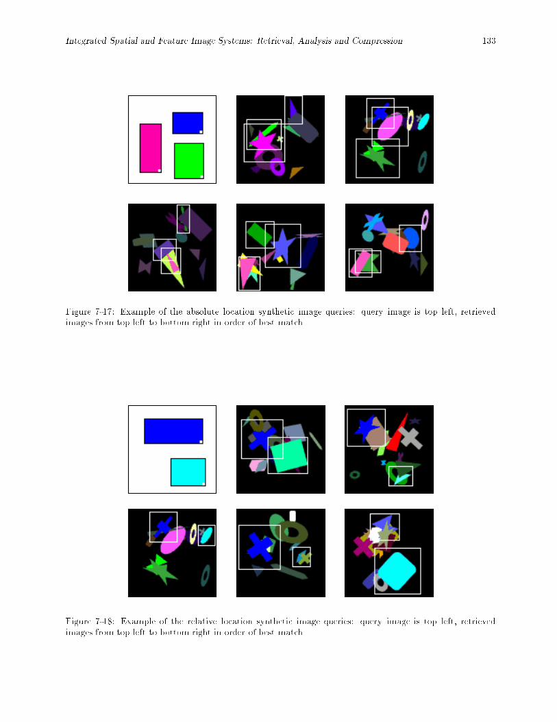
Integrated Spatial and Feature Image Systems: Retrieval, Analysis and Compression 133
Figure 7-17: Example of the absolute location synthetic image queries: query image is top left, retrievedimages from top left to bottom right in order of best match.
Figure 7-18: Example of the relative location synthetic image queries: query image is top left, retrievedimages from top left to bottom right in order of best match.
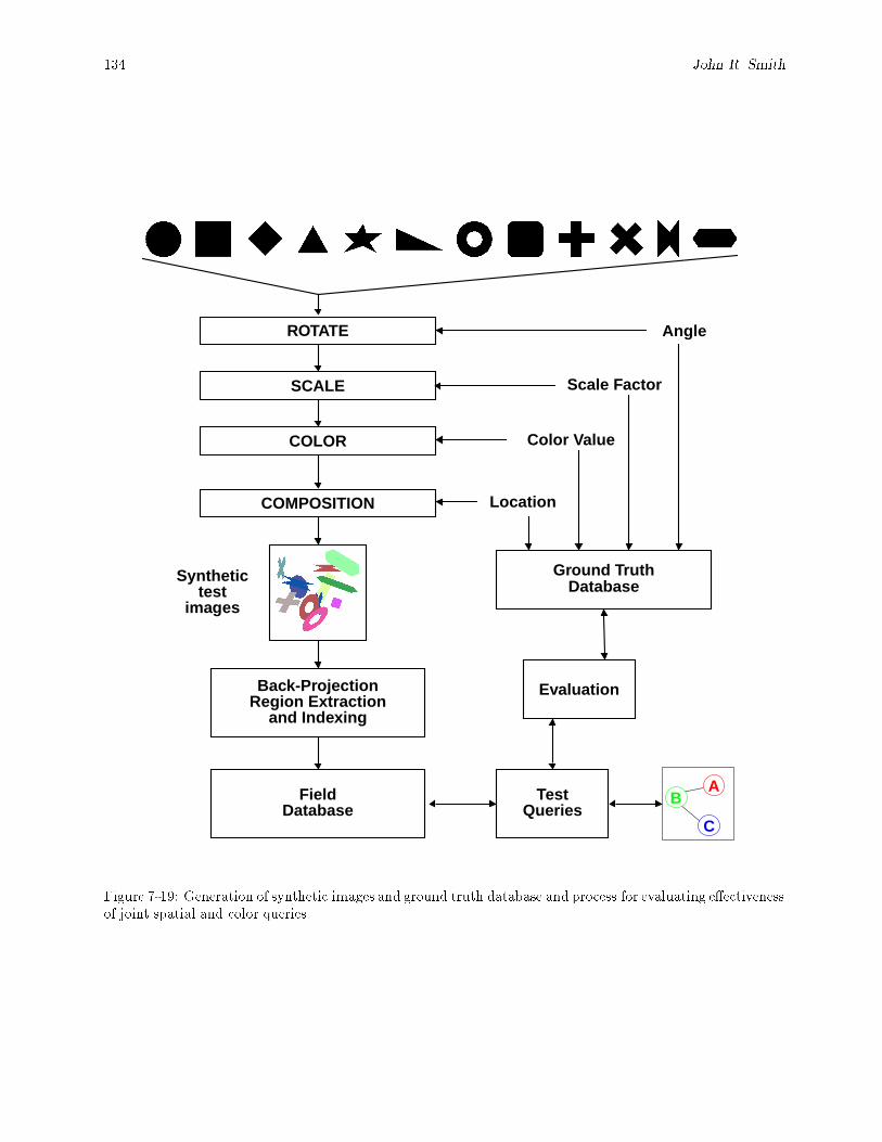
134 John R. Smith
ROTATE
COLOR
SCALE
Angle
Scale Factor
Color Value
Ground TruthDatabase
Back-ProjectionRegion Extraction
and Indexing
FieldDatabase
TestQueries
Evaluation
C
BA
COMPOSITION Location
Synthetictest
images
Figure 7-19: Generation of synthetic images and ground truth database and process for evaluating e�ectivenessof joint spatial and color queries.
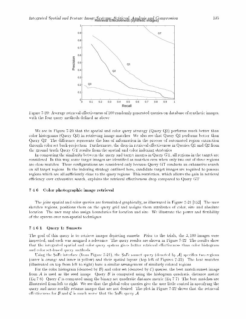
Integrated Spatial and Feature Image Systems: Retrieval, Analysis and Compression 135
0 0.1 0.2 0.3 0.4 0.5 0.6 0.7 0.8 0.9 10
0.1
0.2
0.3
0.4
0.5
0.6
0.7
0.8
0.9
1
Q3
Q2
Q1
GT
Retrieval Effectiveness (synthetic images)
Recall
Pre
cisi
on
Figure 7-20: Average retrieval e�ectiveness of 100 randomly generated queries on database of synthetic images,with the four query methods de�ned as above.
We see in Figure 7-20 that the spatial and color query strategy (Query Q2) performs much better thancolor histograms (Query Q3) in retrieving image matches. We also see that Query Q1 performs better thanQuery Q2. The di�erence represents the loss of information in the process of automated region extractionthrough color set back-projection. Furthermore, the drop in retrieval e�ectiveness in Queries Q1 and Q2 fromthe ground truth Query GT results from the spatial and color indexing strategies.
In computing the similarity between the query and target images in Query GT, all regions in the target areconsidered. In this way, some target images are identi�ed as matches even when only two out of three regionsare close matches. These con�gurations are considered only because Query GT conducts an exhaustive searchon all target regions. In the indexing strategy outlined here, candidate target images are required to possessregions which are all su�ciently close to the query regions. This restriction, which allows the gain in retrievale�ciency over exhaustive search, explains the retrieval e�ectiveness drop compared to Query GT.
7.4.6 Color photographic image retrieval
The joint spatial and color queries are formulated graphically, as illustrated in Figure 7-21 [152]. The usersketches regions, positions them on the query grid and assigns them attributes of color, size and absolutelocation. The user may also assign boundaries for location and size. We illustrate the power and exibilityof the system over non-spatial techniques.
7.4.6.1 Query 1: Sunsets
The goal of this query is to retrieve images depicting sunsets. Prior to the trials, the 3; 100 images wereinspected, and each was assigned a relevance. The query results are shown in Figure 7-22. The results showthat the integrated spatial and color query system gives better retrieval e�ectiveness than color histogramand color set-based query methods.
Using the SaFe interface (from Figure 7-21), the SaFe sunset query (denoted by A) speci�es two regions(outer is orange and inner is yellow) and their spatial layout (top left of Figures 7-22). The best matches(illustrated on top from left to right) have a similar arrangement of similarly colored regions.
For the color histogram (denoted by B) and color set (denoted by C) queries, the best match sunset imagefrom A is used as the seed image. Query B is computed using the histogram quadratic distance metric(Eq 7.6). Query C is computed using the binary set quadratic distance metric (Eq 7.7). The best matches areillustrated from left to right. We see that the global color queries give the user little control in specifying thequery and more readily returns images that are not desired. The plot in Figure 7-22 shows that the retrievale�ectiveness for B and C is much worse that the SaFe query A.
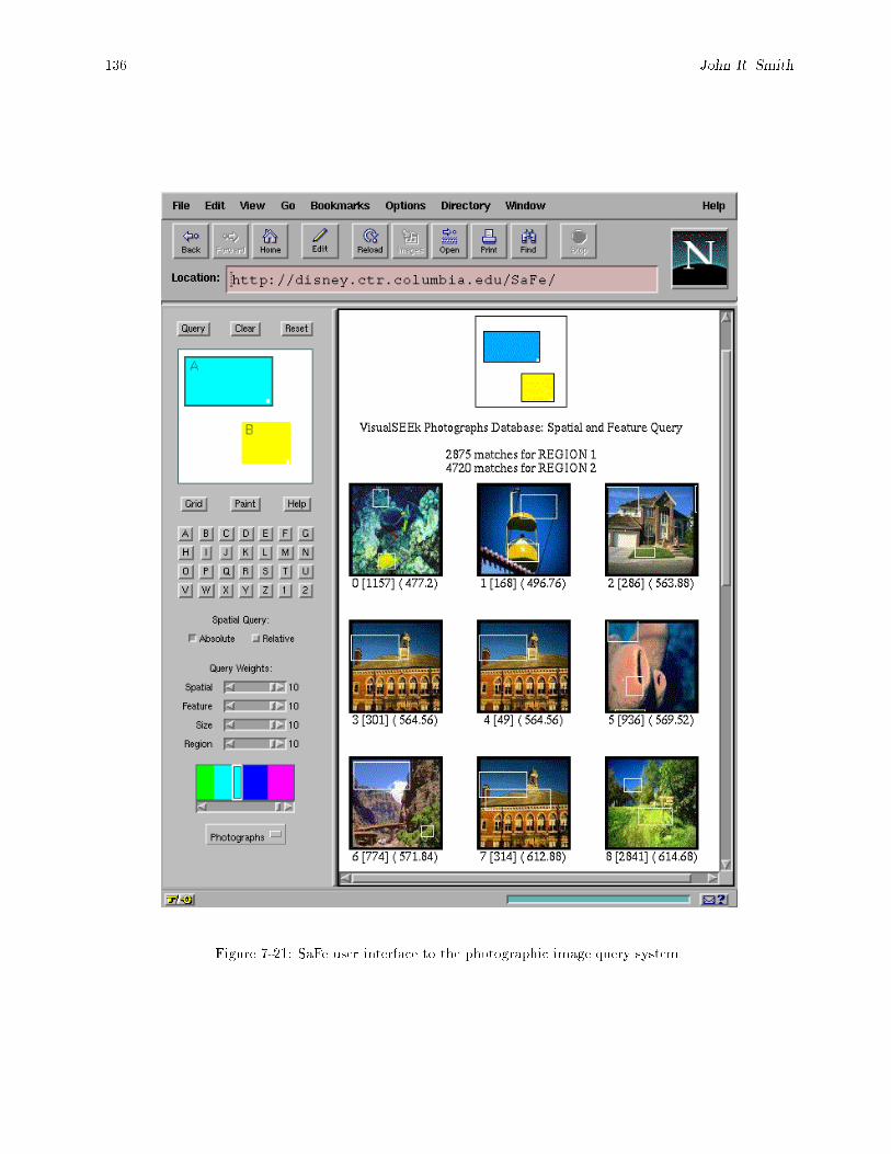
136 John R. Smith
Figure 7-21: SaFe user interface to the photographic image query system.
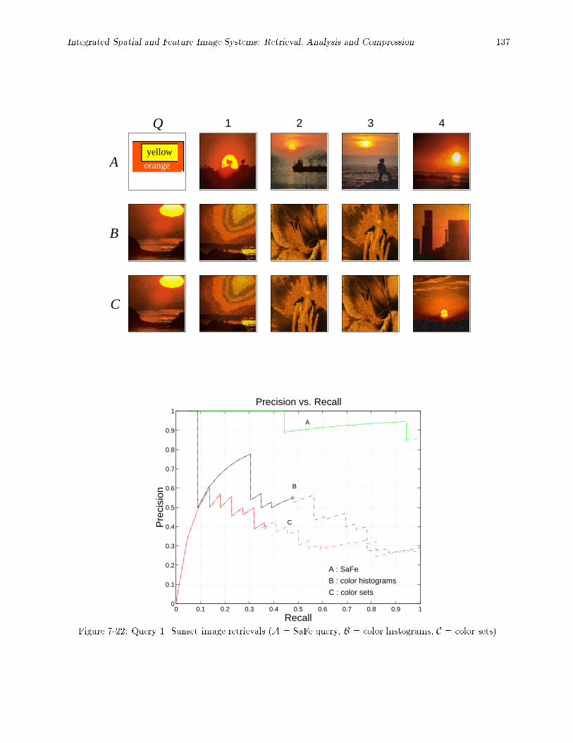
Integrated Spatial and Feature Image Systems: Retrieval, Analysis and Compression 137
A
B
C
Q 1 2 3 4
yellow
orange
0 0.1 0.2 0.3 0.4 0.5 0.6 0.7 0.8 0.9 10
0.1
0.2
0.3
0.4
0.5
0.6
0.7
0.8
0.9
1
Recall
Pre
cisi
on
Precision vs. Recall
A : SaFe
B : color histograms
C : color sets
A
B
C
Figure 7-22: Query 1. Sunset image retrievals (A = SaFe query, B = color histograms, C = color sets).
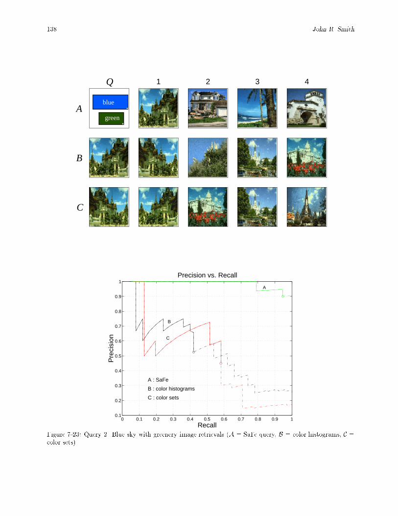
138 John R. Smith
A
B
C
Q 1 2 3 4
blue
green
0 0.1 0.2 0.3 0.4 0.5 0.6 0.7 0.8 0.9 10.1
0.2
0.3
0.4
0.5
0.6
0.7
0.8
0.9
1
Recall
Pre
cisi
on
Precision vs. Recall
A : SaFe
B : color histograms
C : color sets
A
B
C
Figure 7-23: Query 2. Blue sky with greenery image retrievals (A = SaFe query, B = color histograms, C =color sets).
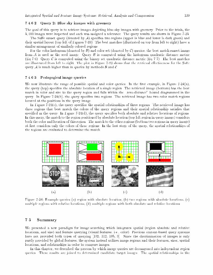
Integrated Spatial and Feature Image Systems: Retrieval, Analysis and Compression 139
7.4.6.2 Query 2: Blue sky images with greenery
The goal of this query is to retrieve images depicting blue sky images with greenery. Prior to the trials, the3; 100 images were inspected and each was assigned a relevance. The query results are shown in Figure 7-23.
The SaFe sunset query (denoted by A) speci�es two regions (upper is blue and lower is dark green) andtheir spatial layout (top left of Figures 7-23). The best matches (illustrated on top from left to right) have asimilar arrangement of similarly colored regions.
For the color histogram (denoted by B) and color set (denoted by C) queries, the best match sunset imagefrom A is used as the seed image. Query B is computed using the histogram quadratic distance metric(Eq 7.6). Query C is computed using the binary set quadratic distance metric (Eq 7.7). The best matchesare illustrated from left to right. The plot in Figure 7-23 shows that the retrieval e�ectiveness for the SaFequery A is much higher than in queries by methods B and C.
7.4.6.3 Pedagogical image queries
We now illustrate the range of possible spatial and color queries. In the �rst example, in Figure 7-24(a),the query (top) speci�es the absolute location of a single region. The retrieved image (bottom) has the bestmatch in color and size to the query region and falls within the \zero-distance" bound diagrammed in thequery. In Figure 7-24(b), the query speci�es two regions. The retrieved image has two color match regionslocated at the positions in the query image.
In Figure 7-24(c), the query speci�es the spatial relationships of three regions. The retrieved image hasthree regions that best match the colors of the query regions and their spatial relationship satis�es thatspeci�ed in the query. In Figure 7-24(d), the query speci�es both absolute and relative locations of regions.In this query, the match to the region positioned by absolute location (top left region in query image) considersboth the color and location of this region. The match to the other regions (bottom two regions in query image)at �rst considers only the colors of these regions. In the last stage of the query, the spatial relationships ofthe regions are evaluated to determine the match.
(a) (b) (c) (d)
Figure 7-24: Example queries (a) region with absolute location, (b) two regions with absolute locations, (c)multiple regions with relative locations, (d) multiple regions with both absolute and relative locations.
7.5. Summary
We presented a new paradigm for image searching which integrates spatial (region absolute and relativelocations, and size) and feature querying (visual features, i.e., color). Previous content-based query systemshave not provided both types of querying [102, 112, 105, 3]. Since the discrimination of images is onlypartly provided by global features, the system instead utilizes image regions and their features, sizes, spatiallocations, and relationships in order to compare images.
In this chapter, we described the process by which image queries are decomposed into independent regionqueries. These results are joined to determined candidate target images. The spatial relationships in the

140 John R. Smith
candidate target images are projected into 2-D string representations. These provide for e�cient validationof the spatial relationships in the target images compared to the query images.
We demonstrated that by integrating content-based and spatial querying a highly functional query systemis generated which allows for a wide variety of complex spatial and feature queries. We evaluated severalexample spatial and color queries on a test-set of synthetic images and a test-set of color photographic images.We demonstrated that retrieval e�ectiveness improves signi�cantly over purely content-based methods.
In the next chapter, we describe some of the details involving the implementation of the SaFe integratedspatial and feature image query system. We also describe a related system: VisualSEEk. The VisualSEEKsystem demonstrates the color/spatial image query paradigm in addition to other image search methods, suchas, relevance feedback searching and text-based searching. We also present the WebSEEk image and videosearch engine. WebSEEk demonstrates the methods of content-based and integrated spatial and feature-basedsearching and cataloging of images and videos from the World-Wide Web.
Integrated Spatial and Feature Image Systems: Retrieval, Analysis and Compression 141
Chapter 8
Content-based visual query applications
8.1. Introduction
In this chapter we introduce three new prototype applications that demonstrate the powerful techniques forcontent-based retrieval developed in this thesis. We �rst present the WebSEEk system, which is a content-based image and video search engine [148, 147]. WebSEEk consists of three components: (1) a collectionsystem for cataloging images and videos, (2) an image and video analysis system which extracts and indexesvisual features of the images and videos, and (3) the query system which consists of the query engine, thesearch tools, and query results display tools. We demonstrate the performance of the system in cataloging,indexing and search and retrieval of over one-half million images and videos collected from the World-WideWeb.
We also present the VisualSEEk color and spatial image query system [151, 146]. VisualSEEk providesseveral methods for searching for images including, integrated color and spatial querying, relevance feedbackquerying and text-based searching. VisualSEEk also provides a system for clustering the images to facilitatethe annotation process for large collections of images.
Finally, we present the SaFe spatial and feature query system [142]. SaFe is an open-platform for computingpowerful image queries that specify spatial arrangements of objects or regions and region feature properties.SaFe allows the user to construct a query image that consists of regions constrained by absolute and/orrelative spatial locations. Potential applications of the SaFe system include geographic image systems (GIS),map retrieval [154], satellite image systems [87, 92] and photographic image databases [3, 45, 145].
8.2. WebSEEk image and video search engine
We �rst describe a system prototype for searching for images and videos on the World-Wide Web. New visualinformation in the form of images, graphics, animations and videos is being published on the Web at anincredible rate. However, cataloging it is beyond the capabilities of current text-based Web search engines.We describe a complete system by which visual information on the Web is
1. collected by automated agents,
2. processed in both text and visual feature domains,
3. catalogued and
4. indexed for fast search and retrieval.
We introduce an image and video search engine which utilizes both text-based navigation and content-basedtechnology for searching visually through the catalogued images and videos. Finally, we provide an initialevaluation based upon the cataloging of over one half million images and videos collected from the Web.
8.2.1 Overview of search engines
A large number of search engines index the plethora of documents on the World-Wide Web. For example,recent systems such as Lycos, Alta Vista, Infoseek and Excite index Web documents by their textual content.These systems periodically scan the Web, analyze the documents, and create compact and searchable indexes.
142 John R. Smith
The user, by entering query terms and/or by selecting subjects, uses these search engines to more easily �ndthe desired Web documents.
Visual information is published on the Web in the form of images, graphics, bitmaps, animations andvideos. As with Web documents in general, the publication of visual information is highly volatile. Newimages and videos are added everyday and others are replaced or removed entirely. In order to catalog thevisual information, a highly e�cient automated system is needed that regularly traverses the Web, detectsvisual information, processes it and indexes it in such a way to allow for e�cient and e�ective search andretrieval.
We have developed a prototype image and video search enginey to ful�ll this need [148, 147]. The systemcollects images and videos from the Web, catalogs them, and provides tools for searching and browsing.The system is novel in that it utilizes text and visual information synergically to provide for cataloging andsearching. The complete system possesses several powerful functionalities, namely,
1. automated collection of visual information from the Web,
2. automated image and video subject classi�cation,
3. searching using innovative visual content-based techniques,
4. image and video subject search and navigation, and text-based searching,
5. compact presentation of images and videos for displaying query results,
6. search results lists manipulations such as intersection, subtraction and concatenation, and
7. query modi�cation using content-based relevance feedback.
Recently, several World-Wide Web image search engines have been reported [134, 148, 47, 70]. TheWebseer system from University of Chicago [47] provides a system for searching for images and animations.The system is novel in that it detects faces within the images and lets the users search by the number offaces. The Webseer system does not classify the images into subject categories and does not provide forcontent-based searching. The Interpix [70] image search engine provides for content-based image searchingusing color histograms. The Interpix system has recently been integrated with Yahoo's search engine allowingfor retrieval of images related to some of Yahoo's Web categories.
8.2.2 Image and video collection process
The image and video collection process is conducted by autonomous Web agents or \spiders." The spiderstraverse the Web by following the hyperlinks between documents. They detect images and videos, retrieveand process them and add the new information to the catalog. The overall collection process, illustrated inFigure 8-1, is carried out using several distinct modules:
1. the Traversal Spider { assembles lists of candidate Web documents that include images, videos orhyperlinks to them,
2. the Hyperlink Parser { extracts the Web addresses (URLs) of the images and videos, and
3. the Content Spider { retrieves, analyzes and iconi�es the images and videos.
8.2.2.1 Image and video detection
In the �rst phase, the Traversal Spider traverses the Web looking for images and videos, as illustrated inFigure 8-2. Starting from seed URLs, the Traversal Spider follows a breadth-�rst search path. It retrieves Webdocuments via Hypertext Transfer Protocol (HTTP) and passes the Hypertext Markup Language (HTML)code to the Hyperlink Parser. In turn, the Hyperlink Parser detects new URLs, encoded as HTML hyperlinks,and adds them back to the queue of Web documents to be retrieved by the Traversal Spider.
yhttp://www.ctr.columbia.edu/webseek
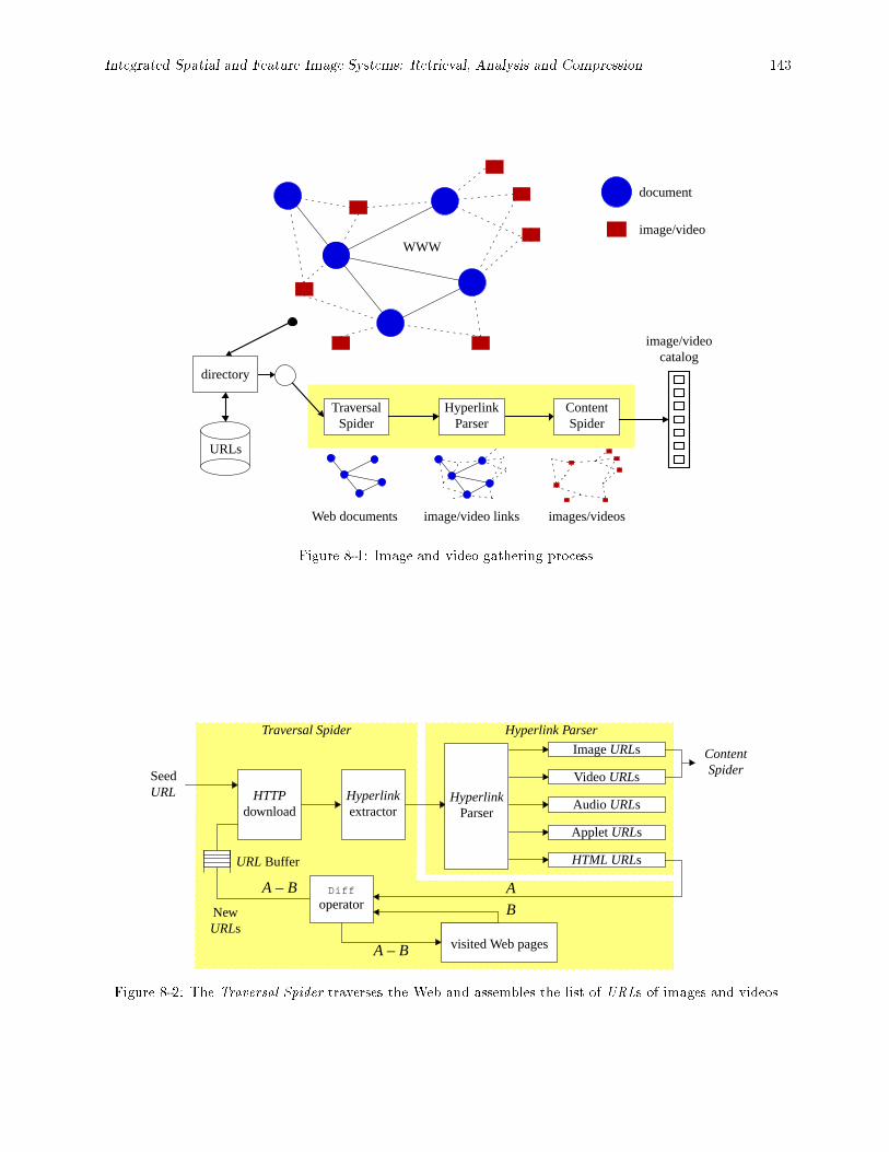
Integrated Spatial and Feature Image Systems: Retrieval, Analysis and Compression 143
Traversal Hyperlink Content
URLs
directory
WWW
catalogimage/video
Web documents image/video links images/videos
document
image/video
Spider SpiderParser
Figure 8-1: Image and video gathering process.
SeedURL
New B
AA B–
A B–
URLs
HyperlinkHyperlinkextractor
HTTPdownload
Diff
operator
Video URLs
HTML URLs
Audio URLs
Image URLs
Applet URLs
Parser
Hyperlink ParserTraversal Spider
Content
URL Buffer
visited Web pages
Spider
Figure 8-2: The Traversal Spider traverses the Web and assembles the list of URLs of images and videos.
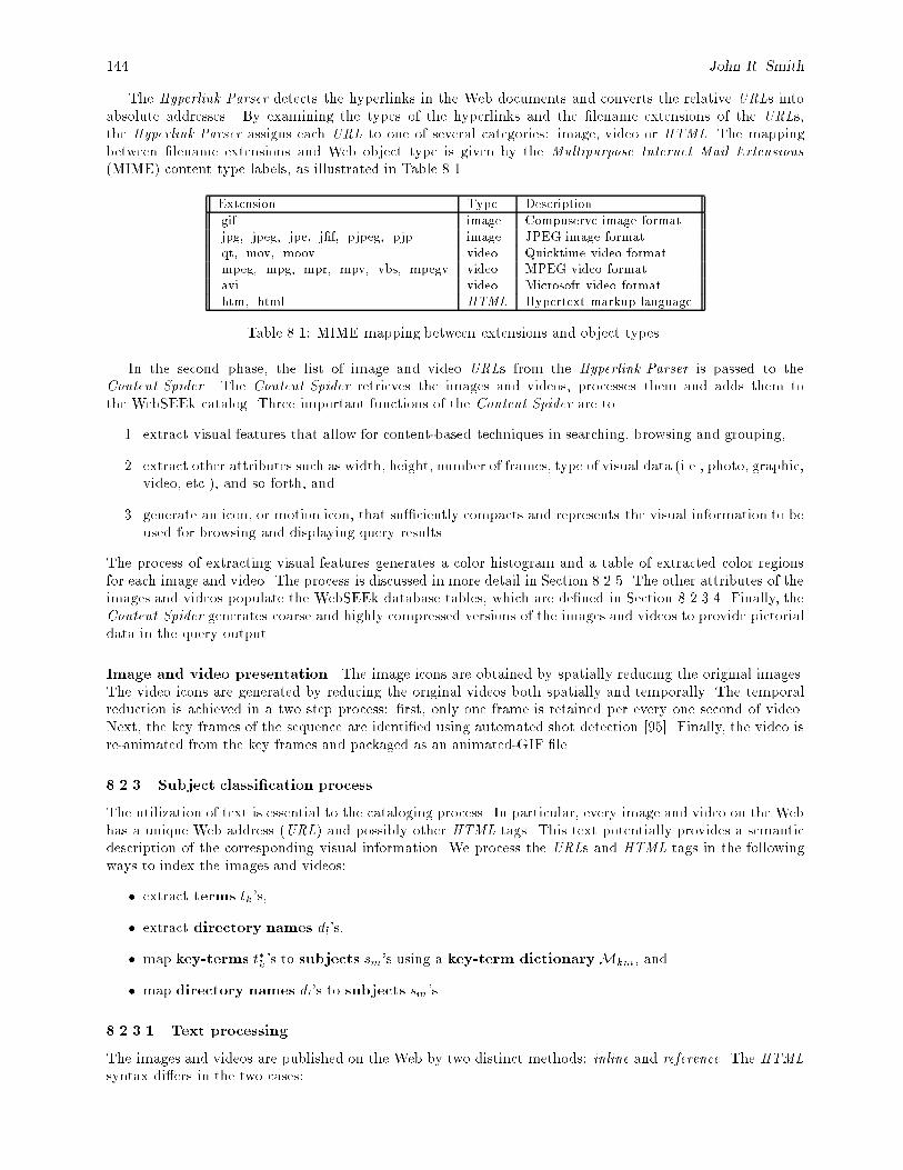
144 John R. Smith
The Hyperlink Parser detects the hyperlinks in the Web documents and converts the relative URLs intoabsolute addresses. By examining the types of the hyperlinks and the �lename extensions of the URLs,the Hyperlink Parser assigns each URL to one of several categories: image, video or HTML. The mappingbetween �lename extensions and Web object type is given by the Multipurpose Internet Mail Extensions
(MIME) content type labels, as illustrated in Table 8.1.
Extension Type Description.gif image Compuserve image format.jpg, .jpeg, .jpe, .j�f, .pjpeg, .pjp image JPEG image format.qt, .mov, .moov video Quicktime video format.mpeg, .mpg, .mpr, .mpv, .vbs, .mpegv video MPEG video format.avi video Microsoft video format.htm, .html HTML Hypertext markup language
Table 8.1: MIME mapping between extensions and object types.
In the second phase, the list of image and video URLs from the Hyperlink Parser is passed to theContent Spider. The Content Spider retrieves the images and videos, processes them and adds them tothe WebSEEk catalog. Three important functions of the Content Spider are to
1. extract visual features that allow for content-based techniques in searching, browsing and grouping,
2. extract other attributes such as width, height, number of frames, type of visual data (i.e., photo, graphic,video, etc.), and so forth, and
3. generate an icon, or motion icon, that su�ciently compacts and represents the visual information to beused for browsing and displaying query results.
The process of extracting visual features generates a color histogram and a table of extracted color regionsfor each image and video. The process is discussed in more detail in Section 8.2.5. The other attributes of theimages and videos populate the WebSEEk database tables, which are de�ned in Section 8.2.3.4. Finally, theContent Spider generates coarse and highly compressed versions of the images and videos to provide pictorialdata in the query output.
Image and video presentation The image icons are obtained by spatially reducing the original images.The video icons are generated by reducing the original videos both spatially and temporally. The temporalreduction is achieved in a two step process: �rst, only one frame is retained per every one second of video.Next, the key frames of the sequence are identi�ed using automated shot detection [95]. Finally, the video isre-animated from the key frames and packaged as an animated-GIF �le.
8.2.3 Subject classi�cation process
The utilization of text is essential to the cataloging process. In particular, every image and video on the Webhas a unique Web address (URL) and possibly other HTML tags. This text potentially provides a semanticdescription of the corresponding visual information. We process the URLs and HTML tags in the followingways to index the images and videos:
� extract terms tk's,
� extract directory names dl's,
� map key-terms t�k's to subjects sm's using a key-term dictionaryMkm, and
� map directory names dl's to subjects sm's.
8.2.3.1 Text processing
The images and videos are published on the Web by two distinct methods: inline and reference. The HTML
syntax di�ers in the two cases:
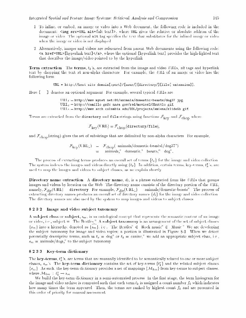
Integrated Spatial and Feature Image Systems: Retrieval, Analysis and Compression 145
1. To inline, or embed, an image or video into a Web document, the following code is included in thedocument: <img src=URL alt=[alt text]>, where URL gives the relative or absolute address of theimage or video. The optional alt tag speci�es the text that substitutes for the inlined image or videowhen the image or video is not displayed.
2. Alternatively, images and videos are referenced from parent Web documents using the following code:<a href=URL>[hyperlink text]</a>, where the optional [hyperlink text] provides the high-lighted textthat describes the image/video pointed to by the hyperlink.
Term extraction The terms, tk's, are extracted from the image and video URLs, alt tags and hyperlinktext by chopping the text at non-alpha characters. For example, the URL of an image or video has thefollowing form
URL = http://host.site.domain[:port]/[user/][directory/][file[.extension]]:
Here [...] denotes an optional argument. For example, several typical URLs are
URL1 = http://www.mynet.net:80/animals/domestic-beasts/dog37.jpg;
URL2 = http://camille.gsfc.nasa.gov/rsd/movies2/Shuttle.gif;
URL3 = http://www.arch.columbia.edu/DDL/projects/amiens/slide6b.gif:
Terms are extracted from the directory and file strings using functions Fkey and Fchop where
Fkey(URL) = Fchop(directory/file);
and Fchop(string) gives the set of substrings that are delimited by non-alpha characters. For example,
Fkey(URL1) = Fchop(\animals/domestic-beasts1/dog37")
= \animals," \domestic," \beasts," \dog":
The process of extracting terms produces an overall set of terms ftkg for the image and video collection.The system indexes the images and videos directly using ftkg. In addition, certain terms, key-terms, t�k's, areused to map the images and videos to subject classes, as we explain shortly.
Directory name extraction A directory name, dl, is a phrase extracted from the URLs that groupsimages and videos by location on the Web. The directory name consists of the directory portion of the URL,namely, Fdir(URL) = directory. For example, Fdir(URL1) = \animals/domestic-beasts". The process ofextracting directory names produces an overall set of directory names fdlg for the image and video collection.The directory names are also used by the system to map images and videos to subject classes.
8.2.3.2 Image and video subject taxonomy
A subject class or subject, sm, is an ontological concept that represents the semantic content of an imageor video, i.e., subject = \The Beatles." A subject taxonomy is an arrangement of the set of subject classes
fsmg into a hierarchy, denoted as dfsmg, i.e., \The Beatles" 2 \Rock music" 2 \Music." We are developingthe subject taxonomy for image and video topics; a portion is illustrated in Figure 8-3. When we detectpotentially descriptive terms, such as tk =\dog" or tk =\canine," we add an appropriate subject class, i.e.,sm =\animals/dogs," to the subject taxonomy.
8.2.3.3 Key-term dictionary
The key-terms, t�k's, are terms that are manually identi�ed to be semantically related to one or more subjectclasses, sm's. The key-term dictionary contains the set of key-terms ft�kg and the related subject classesfsmg. As such, the key-term dictionary provides a set of mappings fMkmg from key-terms to subject classes,where Mkm : t�k ! sm.
We build the key-term dictionary in a semi-automated process. In the �rst stage, the term histogram forthe image and video archive is computed such that each term tk is assigned a count number fk which indicateshow many times the term appeared. Then, the terms are ranked by highest count fk and are presented inthis order of priority for manual assessment.
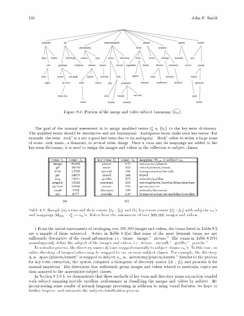
146 John R. Smith
animals art
astronomy
entertainment
food
plants
science
travel
dogs
cats
whales
paintings
sketching
sculpture
comets
planets
nasa
humor
music
movies
television fruits
vegetables drinks
cactus
flowers
asia
europe
biology
sports
chemistry
baseball
soccer
lions
tigers da vinci
renoir van gogh france
germanyearth
jupiter
saturn
cartoons
pop
rock
programs
apples
bananas
roses
sunflowers
neurons
proteins
paris
berlinmoon
elvis
beatles
friends
seinfeld
star trekmona lisa
Figure 8-3: Portion of the image and video subject taxonomy dfsmg.
The goal of the manual assessment is to assign quali�ed terms t�k 2 ftkg to the key-term dictionary.The quali�ed terms should be descriptive and not homonymic. Ambiguous terms make poor key-terms. Forexample, the term \rock" is a not a good key-term due to its ambiguity. \Rock" refers to either a large massof stone, rock music, a diamond, or several other things. Once a term and its mappings are added to thekey-term dictionary, it is used to assign the images and videos in the collection to subject classes.
term: tk count: fkimage 86380gif 28580icon 14798pic 14035img 14011
graphic 10320picture 10026small 9442art 8577
key-term: t�k
count: fk mappingMkm to subject sm
planet 1175 astronomy/planetsmusic 922 entertainment/musicaircraft 458 transportation/aircrafttravel 344 travelgorilla 273 animals/gorillasstarwars 204 entertainment/movies/�lms/starwarssoccer 195 sports/soccer
dinosaur 180 animals/dinosaursporsche 139 transportation/automobiles/porsches
(a) (b)
Table 8.2: Sample (a) terms and their counts ftk : fkg and (b) key-terms counts ft�k : fkg with subjects sm'sand mappingsMkm : t�k ! sm's. Taken from the assessment of over 500; 000 images and videos.
1 From the initial experiments of cataloging over 500; 000 images and videos, the terms listed in Table 8.2are a sample of those extracted. Notice in Table 8.2(a) that some of the most frequent terms are notsu�ciently descriptive of the visual information, i.e., terms: \image," \picture." The terms in Table 8.2(b)unambiguously de�ne the subject of the images and videos, i.e., terms: \aircraft," \gorilla," \porsche."
In a similar process, the directory names dl's are mapped manually to subject classes sm's. In this case, anentire directory of images/videos may be mapped to one or more subject classes. For example, the directorydl = \space/planets/saturn" is mapped to subject sm = \astronomy/planets/saturn." Similar to the processfor key-term extraction, the system computes a histogram of directory names fdl : flg and presents it formanual inspection. The directories that su�ciently group images and videos related to particular topics arethen mapped to the appropriate subject classes.
In Section 8.2.6.1, we demonstrate that these methods of key-term and directory name extraction coupledwith subject mapping provide excellent performance in classifying the images and videos by subject. Byincorporating some results of natural language processing in addition to using visual features, we hope tofurther improve and automate the subject classi�cation process.
Integrated Spatial and Feature Image Systems: Retrieval, Analysis and Compression 147
8.2.3.4 Catalog database
As described above, each retrieved image and video is processed and the following information tables arepopulated:
IMAGES { IMID URL NAME FORMAT WIDTH HEIGHT FRAMES DATE
TYPES { IMID TYPE
SUBJECTS { IMID SUBJECT
TEXT { IMID TERM
FV { IMID COLOR-HISTOGRAM
REGIONS { IMID REGID COLOR-SET X Y WIDTH HEIGHT
where the special (non-alphanumeric) data types are given as follows:
TYPE 2 fColor photo, Color graphic, Video, B/w image, Gray imageg
SUBJECT 2 fSubject classes from taxonomy dfsmg, partially depictedin Figure 8-3g
COLOR-HISTOGRAM 2 R166 (166-bin histogram)COLOR-SET 2 B166 (166-element binary set):
The automated assignment of TYPE to the images and videos using visual features is explained in Sec-tion 8.2.5.3. Queries on the database tables: IMAGES, TYPES, SUBJECTS and TEXT are performed using standardrelational algebra. For example, the query: Give me all records with TYPE = \video", SUBJECT = \news"and TERM = \basketball" can be carried in SQL as follows:
SELECT IMID
FROM TYPES, SUBJECTS, TEXT
WHERE TYPE = \video" AND SUBJECT = \news" AND TERM = \basketball."
However, content-based queries, which involve table FV and REGIONS, require special processing, which isdiscussed in Sections 8.2.4.2 and 8.2.5.
8.2.4 Search and retrieval processes
To retrieve images and videos the user may enter search terms tk's or select an image/video subject sm. Thesearch process and model for user-interaction is depicted in Figure 8-4. The query for images and videosproduces search results A. For example, Figure 8-5 illustrates the search results for a query for images andvideos related to sm =\nature," that is, A = Query(SUBJECT = \nature"). The user may manipulate, searchor view A.
User
Record
Extraction
User
Viewing
Manipulation
Search/Ranking
User
A
C
B C
WebSEEkcatalog
Figure 8-4: Search, retrieval and search results list manipulation processes.
8.2.4.1 Search results list manipulation
The results of a prior search may be fed-back to the manipulation module as list C, as illustrated in Figure 8-4. The user manipulates C by adding or removing records. This is done by issuing a new query thatcreates a second, intermediate list A. The user then generates the new list B by selecting one of the
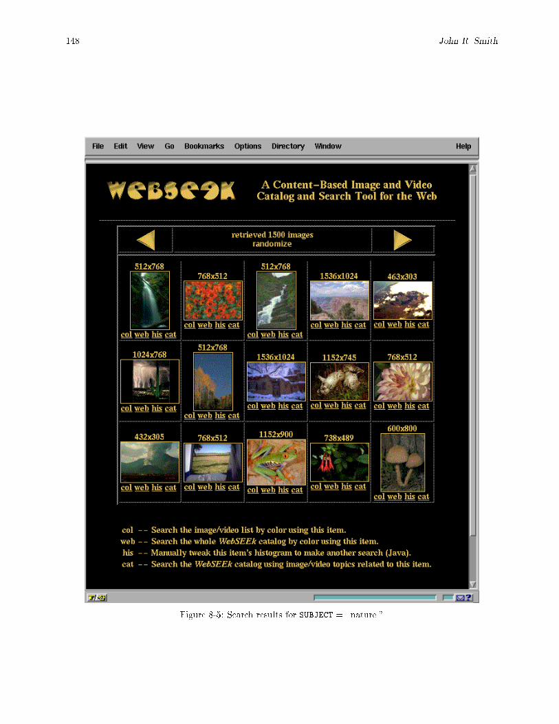
148 John R. Smith
Figure 8-5: Search results for SUBJECT = \nature."
Integrated Spatial and Feature Image Systems: Retrieval, Analysis and Compression 149
following manipulations on C using A, for example, de�ne C = Query(SUBJECT = \nature") and A =Query(TERM = \sunset"), then
union: B = A[C; i.e., B = Query(TERM = \sunset" or SUBJECT = \nature");intersection: B = A\C; i.e., B = Query(TERM = \sunset" and SUBJECT = \nature");subtraction: B = C�A; i.e., B = Query(SUBJECT = \nature" and TERM 6= \sunset");replacement: B = A; i.e., B = Query(TERM = \sunset");keep: B = C; i.e., B = Query(SUBJECT = \nature"):
8.2.4.2 Content-based visual query
The user may browse and search the list B using both content-based and text-based methods. In the caseof content-based searching, the output is a new list C, where C � B is an ordered subset of B such that Cis ordered by highest similarity to the image/video selected by the user (as described in Section 8.2.5). Thesearch and browse operations may be conducted on the input list B or the entire catalog.
For example, C = B ' Bsel, where ' means \visually similar," ranks list B in order of highest similarityto the selected item Bsel. For example, the following content-based visual query:
C = Query(SUBJECT = \nature") ' Bsel(\mountain scene image");
ranks the \nature" images and videos in order of highest visual similarity to the selected \mountain sceneimage." In the example illustrated in Figure 8-6, the query C = B ' Bsel(\red race car"), retrieves theimages and videos from the subject class: SUBJECT = \transportation/automobiles/ferraris" that are visuallysimilar to the selected image of a \red race car."
Alternatively, the user can select one of the items in the current search results list B and then use it tosearch the entire catalog for similar items. For example, C = A ' Bsel ranks list A, where in this case A isthe full catalog, in order of highest visual similarity to the selected item from B.
8.2.5 Content-based techniques
The system provides two methods for content-based searching: (1) by color histograms, and (2) by spatial loca-tions and arrangements of color regions. We adopted these techniques in order to utilize domain-independentapproaches [146]. The content-based methods developed here for indexing, searching and navigation can beapplied, in principle, to other types of features, such as texture, motion and so forth, and to other applicationdomains.
8.2.5.1 Global feature query
The color histograms describe the distribution of colors in each image or video. We de�ne the color histogramsas discrete, 166-bin, distributions in a quantized HSV color space [146]. The system computes a colorhistogram for each image and video scene, which is used to assess its similarity to other images and videoscenes. The color histograms are also used to automatically assign the images and videos to type classes usingFisher discriminant analysis, as described in Section 8.2.5.3.
Color histograms dissimilarity Color histograms are used to measure the dissimilarity of the color con-tents of the images. A histogram dissimilarity metric determines the dissimilarity between a query histogramand a target histogram [45, 3]. In order to achieve high e�ciency in the color histogram query process, weutilize the technique of query optimized distance (QOD) computation. This technique provides both e�cientindexing, retrieval of target histograms and computation of the histogram dissimilarities. In the QOD tech-nique, the retrieval of candidate target images is prioritized in the order of the most signi�cant colors in thequery histogram.
We have found that setting the \color signi�cance" threshold adaptively to select only the 80 � 90%most signi�cant colors in the query histogram decreases query time dramatically without degrading retrievale�ectiveness. By using the e�cient QOD computation method, we are able to greatly reduce the queryprocessing time, as demonstrated in Section 8.2.6.3.
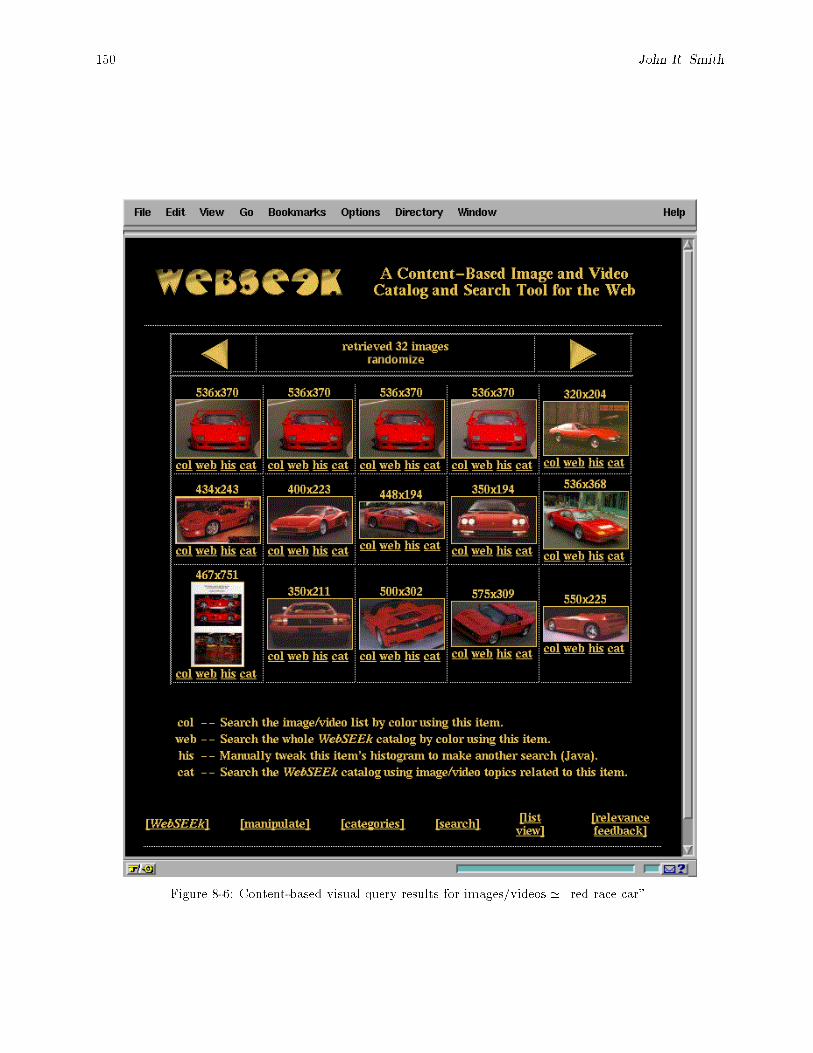
150 John R. Smith
Figure 8-6: Content-based visual query results for images/videos ' \red race car".
Integrated Spatial and Feature Image Systems: Retrieval, Analysis and Compression 151
8.2.5.2 Integrated spatial and color query
While color histograms are useful for indexing images by global color, a signi�cant aspect of discriminatingamong images depends on the sizes, spatial locations and relationships of objects or regions within the images.Therefore, we developed a system for querying by spatial locations and arrangements of color regions [146].With this integrated spatial and feature image query engine, the user graphically constructs a query by placingcolor regions on a query grid, as illustrated in Figure 8-7.
The similarity between the query image and each target image is computed by assessing the similarities ofthe spatial locations, colors and sizes of the regions in the query and target images. The integrated spatial andfeatures system provides greater power and exibility in querying for images than the color histogram-basedmethods [146]. We found that retrieval e�ectiveness improves substantially using this method.
8.2.5.3 Automated type assessment
By training on samples of the color histograms of images and videos, we developed a process of automatedtype assessment using Fisher discriminant analysis (FDA). FDA constructs a series of uncorrelated linearweightings of the color histograms that provide for maximum separation between training classes [48]. Newcolor histograms are automatically assigned to nearest Type 2 fcolor photo, color graphic, video, b/w image,gray imageg class [148].
In Section 8.2.6.2, we show that this approach provides for excellent performance in automatically clas-sifying the images and videos into these broad type classes. We hope to increase the number of type classesand improve the type-classi�cation system by incorporating other visual features such as spatial and colorregion information into the classi�cation process.
8.2.5.4 Relevance feedback
The user best determines from the results of a query which images and videos are relevant and not relevant.The system can use this information to reformulate the query to better retrieve the images and videos theuser desires [77]. Using the color histograms, relevance feedback is accomplished as follows: let Ir = frelevantimages/videosg and In = fnon-relevant images/videosg as determined by the user. The new query vectorhk+1q at round k + 1 is generated by
hk+1q = jj�hkq + �Xi2Ir
hi � Xj2In
hjjj; (8.1)
where jj � jj indicates normalization. The new images and videos are retrieved using hk+1q . One formulationof relevance feedback assigns the values � = 0, and � = = 1, which weights the positive and negativeexamples equally. The process of selecting the example images for content-based relevance feedback searchingis illustrated in Figure 8-8(a). A simpler form of relevance feedback allows the user to select only one positiveexample in order to iterate the query process. In this case, � = = 0, � = 1, jIrj = 1 and jInrj = 0 gives thenew query vector directly from the selected image/video's color histogram, hIr as follows, h
k+1q = hIr .
8.2.5.5 Histogram manipulation
The system also provides a tool for the user to directly manipulate the image and video color histogramsto formulate the search. Using the histogram manipulation tool, illustrated in Figure 8-8(b), the user mayselect one of the images or videos from the results and display its histogram. The user can then modify thehistogram by adding or removing colors. The modi�ed histogram is then used to conduct the next search.The new query histogram hk+1q is generated from a selected histogram hs by adding or removing colors, whichare denoted in the modi�cations histogram hm,
hk+1q = jjhs+ hmjj: (8.2)
8.2.6 Evaluation
In the initial trials, the system has catalogued 513; 323 images and videos from 46; 551 directories at 16; 773Web sites. The process required several months, and was performed simultaneously with the developmentof the user application. Overall the system has catalogued over 129 Gigabytes of visual information. The
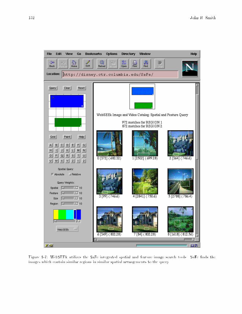
152 John R. Smith
Figure 8-7: WebSEEk utilizes the SaFe integrated spatial and feature image search tools. SaFe �nds theimages which contain similar regions in similar spatial arrangements to the query.
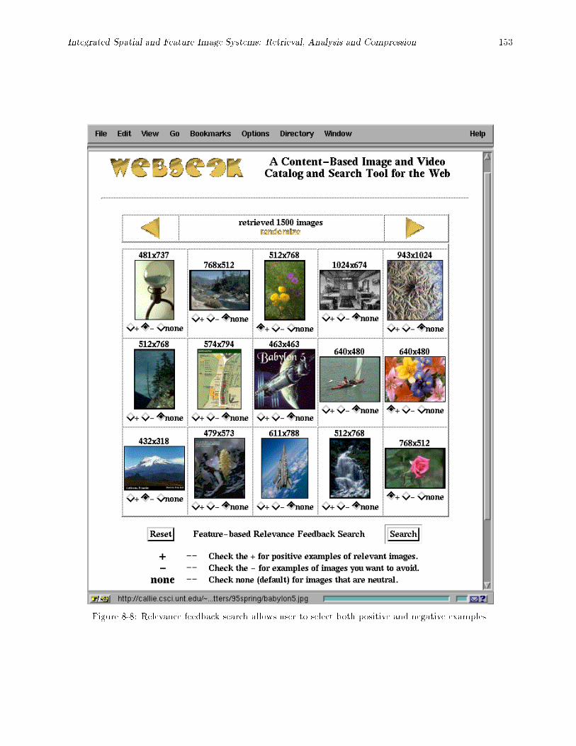
Integrated Spatial and Feature Image Systems: Retrieval, Analysis and Compression 153
Figure 8-8: Relevance feedback search allows user to select both positive and negative examples.
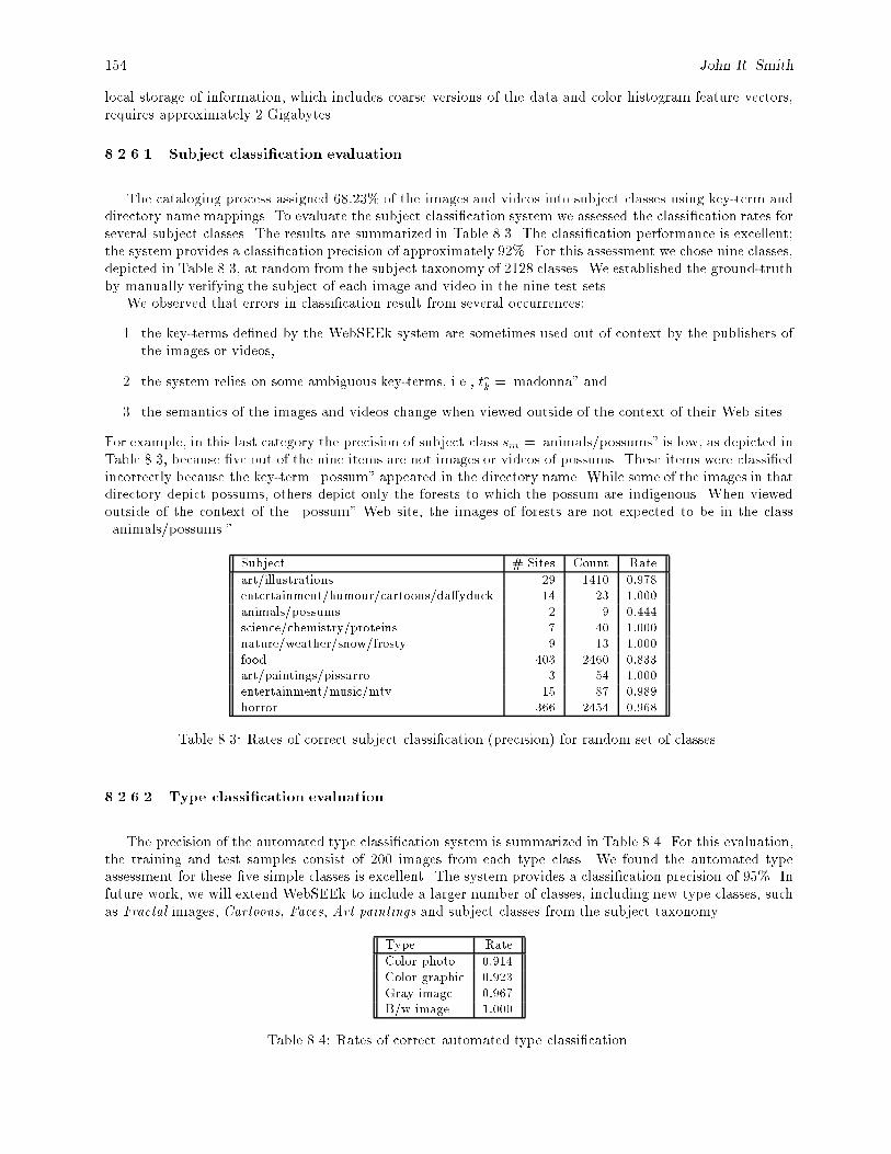
154 John R. Smith
local storage of information, which includes coarse versions of the data and color histogram feature vectors,requires approximately 2 Gigabytes.
8.2.6.1 Subject classi�cation evaluation
The cataloging process assigned 68:23% of the images and videos into subject classes using key-term anddirectory name mappings. To evaluate the subject classi�cation system we assessed the classi�cation rates forseveral subject classes. The results are summarized in Table 8.3. The classi�cation performance is excellent;the system provides a classi�cation precision of approximately 92%. For this assessment we chose nine classes,depicted in Table 8.3, at random from the subject taxonomy of 2128 classes. We established the ground-truthby manually verifying the subject of each image and video in the nine test sets.
We observed that errors in classi�cation result from several occurrences:
1. the key-terms de�ned by the WebSEEk system are sometimes used out of context by the publishers ofthe images or videos,
2. the system relies on some ambiguous key-terms, i.e., t�k =\madonna" and
3. the semantics of the images and videos change when viewed outside of the context of their Web sites.
For example, in this last category the precision of subject class sm =\animals/possums" is low, as depicted inTable 8.3, because �ve out of the nine items are not images or videos of possums. These items were classi�edincorrectly because the key-term \possum" appeared in the directory name. While some of the images in thatdirectory depict possums, others depict only the forests to which the possum are indigenous. When viewedoutside of the context of the \possum" Web site, the images of forests are not expected to be in the class\animals/possums."
Subject # Sites Count Rate
art/illustrations 29 1410 0:978entertainment/humour/cartoons/da�yduck 14 23 1:000animals/possums 2 9 0:444science/chemistry/proteins 7 40 1:000nature/weather/snow/frosty 9 13 1:000food 403 2460 0:833art/paintings/pissarro 3 54 1:000entertainment/music/mtv 15 87 0:989horror 366 2454 0:968
Table 8.3: Rates of correct subject classi�cation (precision) for random set of classes.
8.2.6.2 Type classi�cation evaluation
The precision of the automated type classi�cation system is summarized in Table 8.4. For this evaluation,the training and test samples consist of 200 images from each type class. We found the automated typeassessment for these �ve simple classes is excellent. The system provides a classi�cation precision of 95%. Infuture work, we will extend WebSEEk to include a larger number of classes, including new type classes, suchas Fractal images, Cartoons, Faces, Art paintings and subject classes from the subject taxonomy.
Type RateColor photo 0:914Color graphic 0:923Gray image 0:967B/w image 1:000
Table 8.4: Rates of correct automated type classi�cation.
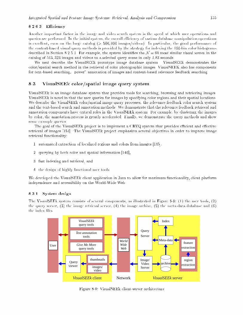
Integrated Spatial and Feature Image Systems: Retrieval, Analysis and Compression 155
8.2.6.3 E�ciency
Another important factor in the image and video search system is the speed at which user operations andqueries are performed. In the initial system, the overall e�ciency of various database manipulation operationsis excellent, even on the large catalog (> 500; 000 images/videos). In particular, the good performance ofthe content-based visual query methods is provided by the strategy for indexing the 166-bin color histogramsdescribed in Section 8.2.5.1. For example, the system identi�es the N = 60 most similar visual scenes in thecatalog of 513; 323 images and videos to a selected query scene in only 1:83 seconds.
We nest describe the VisualSEEk prototype image database system. VisualSEEk demonstrates thecolor/spatial search method in the retrieval of color photographic images. VisualSEEK also has componentsfor text-based searching, \power" annotation of images and content-based relevance feedback searching.
8.3. VisualSEEk color/spatial image query system
VisualSEEk is an image database system that provides tools for searching, browsing and retrieving images.VisualSEEk is novel in that the user queries for images by specifying color regions and their spatial locations.We describe the VisualSEEk color/spatial image query processes, the relevance feedback color search systemand the text-based search and annotation methods. We demonstrate that the relevance feedback retrieval andannotation components have critical roles in the VisualSEEk system. For example, by clustering the imagesby color, the annotation process is greatly accelerated. Finally, we demonstrate the query methods and showsome example queries.
The goal of the VisualSEEk project is to implement a CBVQ system that provides e�cient and e�ectiveretrieval of images [151]. The VisualSEEk project emphasizes several objectives in order to improve imageretrieval functionality:
1. automated extraction of localized regions and colors from images [145],
2. querying by both color and spatial information [146],
3. fast indexing and retrieval, and
4. the design of highly functional user tools.
We developed the VisualSEEk client application in Java to allow for maximum functionality, client platformindependence and accessibility on the World-Wide Web.
8.3.1 System design
The VisualSEEk system consists of several components, as illustrated in Figure 8-9: (1) the user tools, (2)the query server, (3) the image retrieval server, (4) the image archive, (5) the meta-data database and (6)the index �les.
thumbnails
VisualSEEkUser application
VisualSEEkUser application
videoimages/
Queryviewer
VisualSEEkUser application
VisualSEEkquery tools
Text annotationtools
Give Me Morequery tools
VisualSEEk client Network
Index
archive
Meta-data
VisualSEEk server
Query
Image/
Server
VideoServer
region
feature
extraction
extractionWideWeb
WorldUser
Figure 8-9: VisualSEEk client-server architecture.
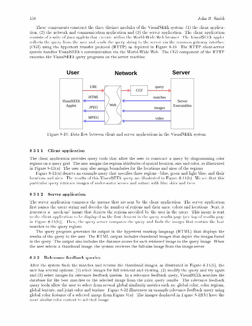
156 John R. Smith
These components construct the three distinct modules of the VisualSEEk system: (1) the client applica-tion, (2) the network and communication application and (3) the server application. The client applicationconsists of a suite of Java applets that execute within the World-Wide Web browser. The VisualSEEk appletcollects the query from the user and sends the query string to the server via the common gateway interface(CGI) using the hypertext transfer protocol (HTTP) as depicted in Figure 8-10. The HTTP client-serversystem handles VisualSEEk's communication via the World-Wide Web. The CGI component of the HTTPexecutes the VisualSEEk query programs on the server machine.
URL
HTML
JPEG
query
matches
images
VisualSEEkWeb
Server
CGI
User ServerNetwork
MPEG video
Applet Executables
Figure 8-10: Data ow between client and server applications in the VisualSEEk system.
8.3.1.1 Client application
The client application provides query tools that allow the user to construct a query by diagramming colorregions on a query grid. The user assigns the regions attributes of spatial location, size and color, as illustratedin Figure 8-11(a). The user may also assign boundaries for the locations and sizes of the regions.
Figure 8-11(a) depicts an example query that speci�es three regions - blue, green and light blue, and theirlocations and sizes. The results of this VisualSEEk query are illustrated in Figure 8-11(b). We see that thisparticular query retrieves images of under-water scenes and nature with blue skies and trees.
8.3.1.2 Server application
The server application computes the queries that are sent by the client application. The server application�rst parses the query string and decodes the number of regions and their sizes, colors and locations. Next, itgenerates a \mock-up" image that depicts the regions speci�ed by the user in the query. This image is sentto the client application to be displayed as the �rst element in the query results page (see top of results pagein Figure 8-11(b)). Then, the query server computes the query and �nds the images that contain the bestmatches to the query regions.
The query program generates its output in the hypertext markup language (HTML) that displays theresults of the query to the user. The HTML output includes thumbnail images that depict the images foundin the query. The output also includes the distance scores for each retrieved image to the query image. Whenthe user selects a thumbnail image, the system retrieves the full-size image from the image server.
8.3.2 Relevance feedback queries
After the system �nds the matches and returns the thumbnail images, as illustrated in Figure 8-11(b), theuser has several options: (1) select images for full retrieval and viewing, (2) modify the query and try againand (3) select images for relevance feedback queries. In a relevance feedback query, VisualSEEk searches thedatabase for the best matches to the selected image from the prior query results. The relevance feedbackquery tools allow the user to select from several global similarity metrics such as: global color, color regions,global texture, and joint color and texture. Figure 8-12 illustrates an example relevance feedback query usingglobal color features of a selected image from Figure 6(a). The images displayed in Figure 8-12(b) have themost similar color content to selected image.
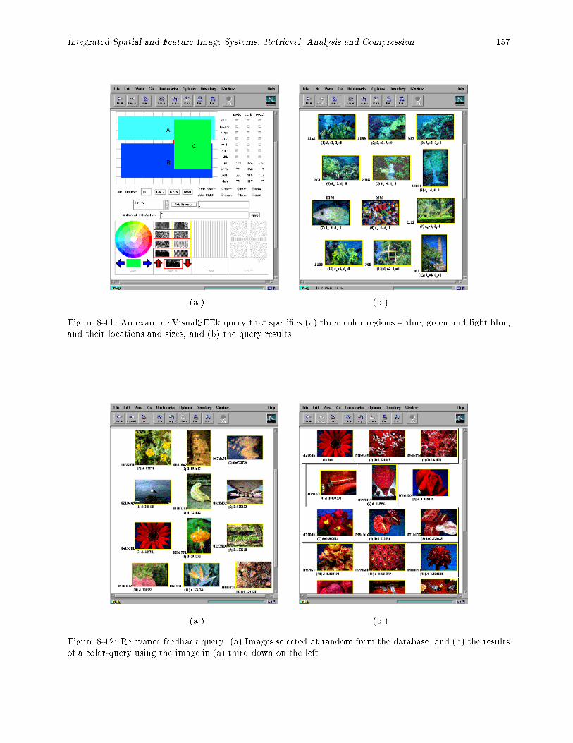
Integrated Spatial and Feature Image Systems: Retrieval, Analysis and Compression 157
(a.) (b.)
Figure 8-11: An example VisualSEEk query that speci�es (a) three color regions - blue, green and light blue,and their locations and sizes, and (b) the query results.
(a.) (b.)
Figure 8-12: Relevance feedback query. (a) Images selected at random from the database, and (b) the resultsof a color-query using the image in (a) third down on the left.
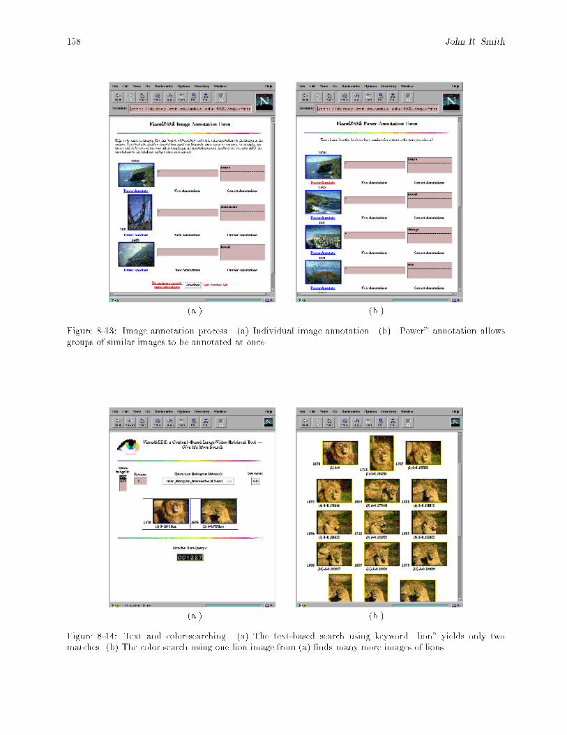
158 John R. Smith
(a.) (b.)
Figure 8-13: Image annotation process. (a) Individual image annotation. (b) \Power" annotation allowsgroups of similar images to be annotated at once.
(a.) (b.)
Figure 8-14: Text and color-searching. (a) The text-based search using keyword \lion" yields only twomatches. (b) The color search using one lion image from (a) �nds many more images of lions.
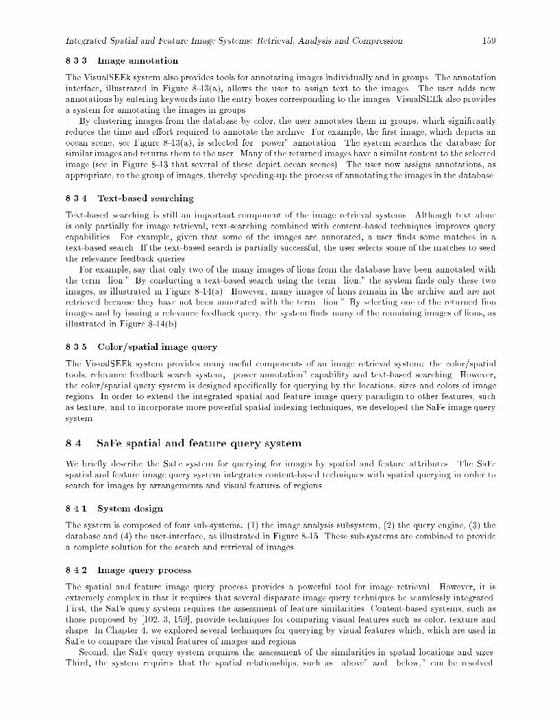
Integrated Spatial and Feature Image Systems: Retrieval, Analysis and Compression 159
8.3.3 Image annotation
The VisualSEEk system also provides tools for annotating images individually and in groups. The annotationinterface, illustrated in Figure 8-13(a), allows the user to assign text to the images. The user adds newannotations by entering keywords into the entry boxes corresponding to the images. VisualSEEk also providesa system for annotating the images in groups.
By clustering images from the database by color, the user annotates them in groups, which signi�cantlyreduces the time and e�ort required to annotate the archive. For example, the �rst image, which depicts anocean scene, see Figure 8-13(a), is selected for \power" annotation. The system searches the database forsimilar images and returns them to the user. Many of the returned images have a similar content to the selectedimage (see in Figure 8-13 that several of these depict ocean scenes). The user now assigns annotations, asappropriate, to the group of images, thereby speeding-up the process of annotating the images in the database.
8.3.4 Text-based searching
Text-based searching is still an important component of the image retrieval systems. Although text aloneis only partially for image retrieval, text-searching combined with content-based techniques improves querycapabilities. For example, given that some of the images are annotated, a user �nds some matches in atext-based search. If the text-based search is partially successful, the user selects some of the matches to seedthe relevance feedback queries.
For example, say that only two of the many images of lions from the database have been annotated withthe term \lion." By conducting a text-based search using the term \lion," the system �nds only these twoimages, as illustrated in Figure 8-14(a). However, many images of lions remain in the archive and are notretrieved because they have not been annotated with the term \lion." By selecting one of the returned lionimages and by issuing a relevance feedback query, the system �nds many of the remaining images of lions, asillustrated in Figure 8-14(b).
8.3.5 Color/spatial image query
The VisualSEEk system provides many useful components of an image retrieval system: the color/spatialtools, relevance feedback search system, \power annotation" capability and text-based searching. However,the color/spatial query system is designed speci�cally for querying by the locations, sizes and colors of imageregions. In order to extend the integrated spatial and feature image query paradigm to other features, suchas texture, and to incorporate more powerful spatial indexing techniques, we developed the SaFe image querysystem.
8.4. SaFe spatial and feature query system
We brie y describe the SaFe system for querying for images by spatial and feature attributes. The SaFespatial and feature image query system integrates content-based techniques with spatial querying in order tosearch for images by arrangements and visual features of regions.
8.4.1 System design
The system is composed of four sub-systems: (1) the image analysis subsystem, (2) the query engine, (3) thedatabase and (4) the user-interface, as illustrated in Figure 8-15. These sub-systems are combined to providea complete solution for the search and retrieval of images.
8.4.2 Image query process
The spatial and feature image query process provides a powerful tool for image retrieval. However, it isextremely complex in that it requires that several disparate image query techniques be seamlessly integrated.First, the SaFe query system requires the assessment of feature similarities. Content-based systems, such asthose proposed by [102, 3, 159], provide techniques for comparing visual features such as color, texture andshape. In Chapter 4, we explored several techniques for querying by visual features which, which are used inSaFe to compare the visual features of images and regions.
Second, the SaFe query system requires the assessment of the similarities in spatial locations and sizes.Third, the system requires that the spatial relationships, such as \above" and \below," can be resolved.
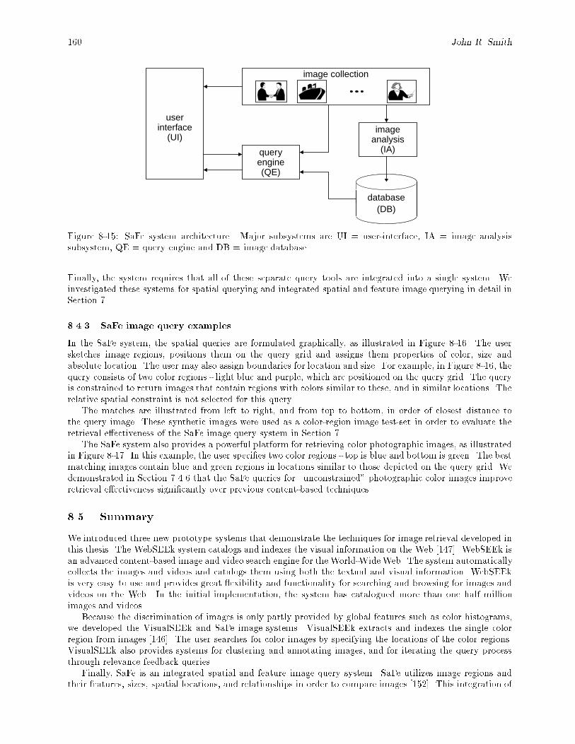
160 John R. Smith
userinterface
(UI)
queryengine(QE)
imageanalysis
(IA)
database(DB)
image collection
Figure 8-15: SaFe system architecture. Major subsystems are UI = user-interface, IA = image analysissubsystem, QE = query engine and DB = image database.
Finally, the system requires that all of these separate query tools are integrated into a single system. Weinvestigated these systems for spatial querying and integrated spatial and feature image querying in detail inSection 7.
8.4.3 SaFe image query examples
In the SaFe system, the spatial queries are formulated graphically, as illustrated in Figure 8-16. The usersketches image regions, positions them on the query grid and assigns them properties of color, size andabsolute location. The user may also assign boundaries for location and size. For example, in Figure 8-16, thequery consists of two color regions - light blue and purple, which are positioned on the query grid. The queryis constrained to return images that contain regions with colors similar to these, and in similar locations. Therelative spatial constraint is not selected for this query.
The matches are illustrated from left to right, and from top to bottom, in order of closest distance tothe query image. These synthetic images were used as a color-region image test-set in order to evaluate theretrieval e�ectiveness of the SaFe image query system in Section 7.
The SaFe system also provides a powerful platform for retrieving color photographic images, as illustratedin Figure 8-17. In this example, the user speci�es two color regions - top is blue and bottom is green. The bestmatching images contain blue and green regions in locations similar to those depicted on the query grid. Wedemonstrated in Section 7.4.6 that the SaFe queries for \unconstrained" photographic color images improveretrieval e�ectiveness signi�cantly over previous content-based techniques.
8.5. Summary
We introduced three new prototype systems that demonstrate the techniques for image retrieval developed inthis thesis. The WebSEEk system catalogs and indexes the visual information on the Web [147]. WebSEEk isan advanced content-based image and video search engine for the World-WideWeb. The system automaticallycollects the images and videos and catalogs them using both the textual and visual information. WebSEEkis very easy to use and provides great exibility and functionality for searching and browsing for images andvideos on the Web. In the initial implementation, the system has catalogued more than one half millionimages and videos.
Because the discrimination of images is only partly provided by global features such as color histograms,we developed the VisualSEEk and SaFe image systems. VisualSEEk extracts and indexes the single colorregion from images [146]. The user searches for color images by specifying the locations of the color regions.VisualSEEk also provides systems for clustering and annotating images, and for iterating the query processthrough relevance feedback queries.
Finally, SaFe is an integrated spatial and feature image query system. SaFe utilizes image regions andtheir features, sizes, spatial locations, and relationships in order to compare images [152]. This integration of
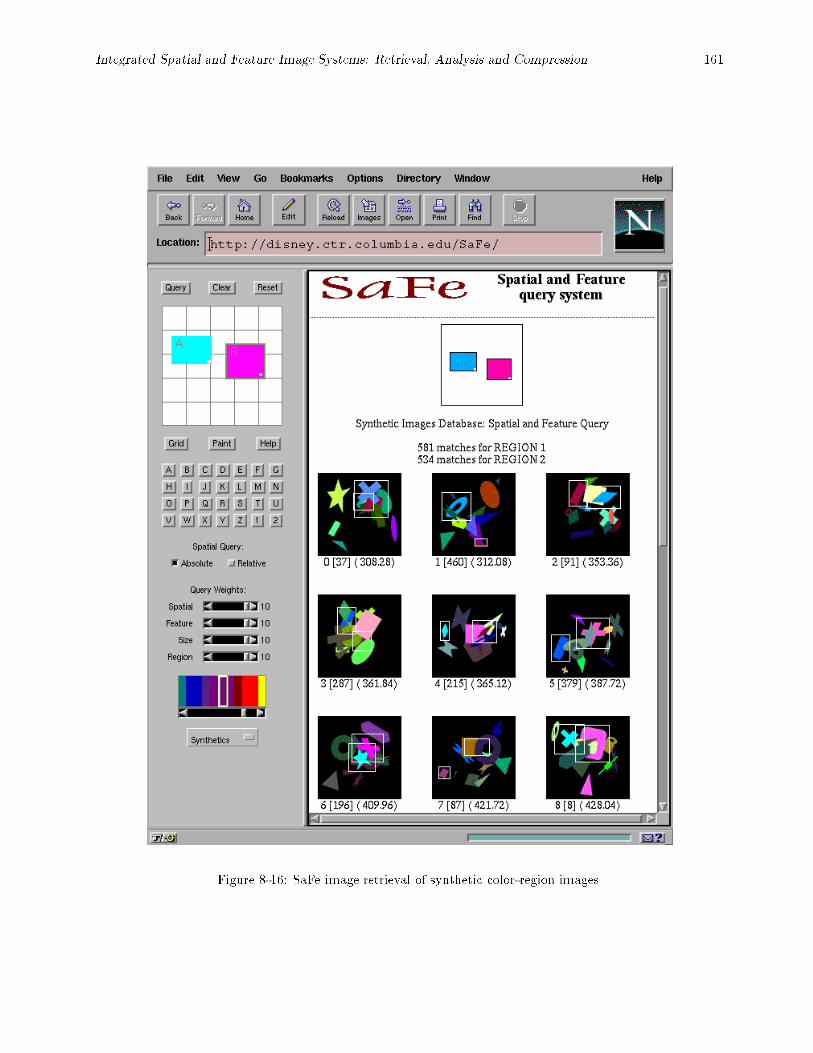
Integrated Spatial and Feature Image Systems: Retrieval, Analysis and Compression 161
Figure 8-16: SaFe image retrieval of synthetic color-region images.
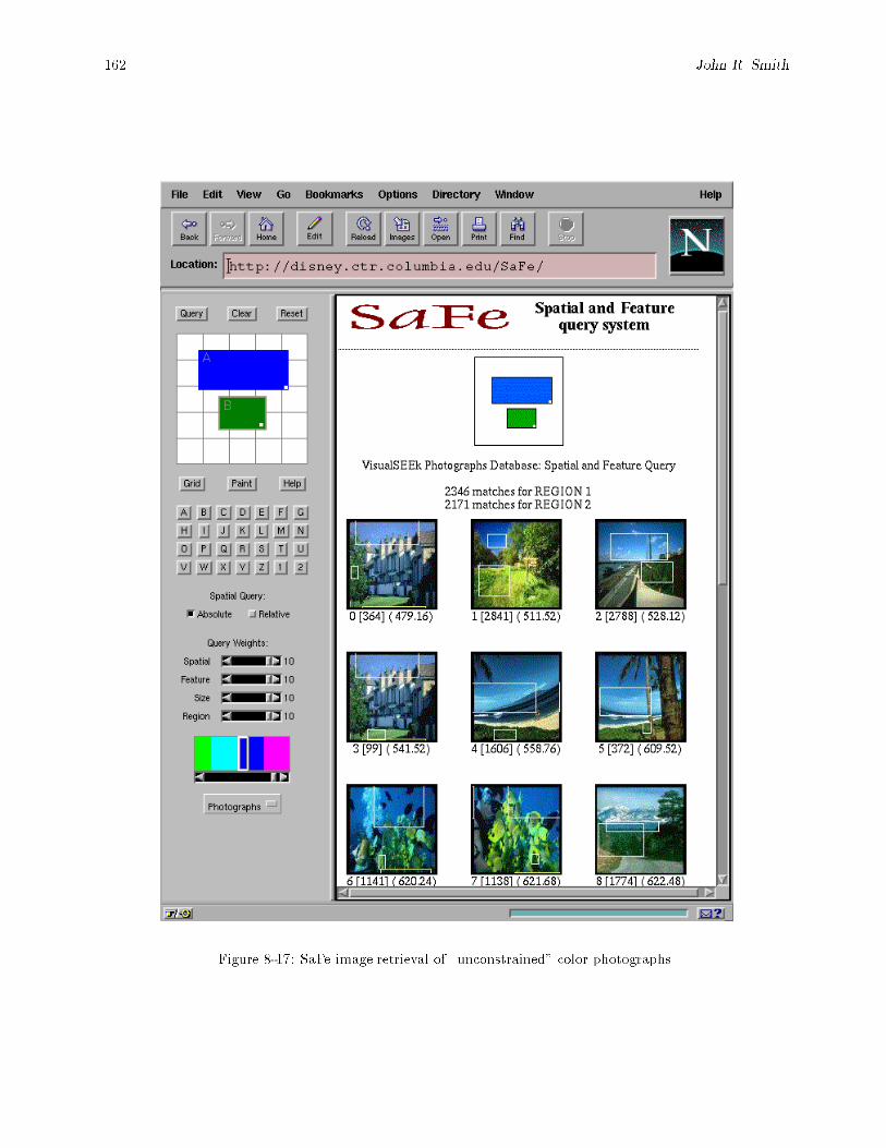
162 John R. Smith
Figure 8-17: SaFe image retrieval of \unconstrained" color photographs.

Integrated Spatial and Feature Image Systems: Retrieval, Analysis and Compression 163
content-based and spatial querying provides for the highly functional image query systems which allow for awide variety of integrated spatial and feature queries.
164 John R. Smith
Chapter 9
Conclusion and future directions
9.1. Conclusion
This thesis developed several new techniques for integrating spatial and feature information in order toimprove systems for image retrieval, analysis and compression. The visually important information withinimages is often contained within spatially localized regions, or is represented by the overall existence andspatial arrangements of these regions. By developing processes that analyze and represent images in this way,we improve our capabilities to develop powerful content-based image retrieval and compression systems. Thisthesis presented several new techniques for integrating spatial and feature image analyses and representations,and demonstrated improved performance in image systems applications.
Recent e�orts in image retrieval applications have focused on indexing a few speci�c visual dimensions ofthe images, such as color, texture, shape, motion and spatial information [102, 3, 112, 105, 156, 146]. However,without integrating these visual dimensions, the current content-based techniques have limited capacity tosatisfactorily retrieve images.
Similarly, recent e�orts in image compression have designed techniques for adapting to either the imagefrequency spectrum [32, 170, 124] or spatial information [136, 155, 132] in order to compact the images.However, by integrating spatial and frequency methods, we design algorithms which better adapt to theimage content and improve compression.
This thesis developed new techniques to solve these problems which are similar in their exploitation ofimages as two-dimensional, non-stationary signals. In particular, we developed new processes that
1. Image retrieval { demonstrated a new integrated spatial and feature query paradigm for image re-trieval. Previous e�orts in image database systems have developed either feature-based approaches [159,53, 102, 157, 51] or spatial-symbolic image retrieval methods [55, 22, 27, 113]. This thesis developed anew method which represents images by spatially localized regions. The features (color and texture)and spatial attributes (region size and location) de�ne the set of properties of the regions. The imagesare compared by assessing the numbers of-, arrangements and feature properties of regions. We pre-sented techniques for computing these complex image queries and demonstrated improved e�ectivenessin image retrieval applications.
2. Image analysis { We developed a framework for extracting spatially localized features from imagesusing histogram and binary set back-projections. The automated extraction of regions from \uncon-strained" imagery is not successfully accomplished using current methods of pattern recognition [133, 40]and image segmentation [155, 67, 73, 86, 90, 14]. The di�culty results from the inability to de�ne eitherthe complete set of region models or patterns a priori, or establish the ground-truth segmentationsfor \unconstrained" images. We developed a new approach for extracting color and texture regionsby back-projecting the feature-histograms onto the images. We also developed a process by which theregions are extracted automatically by testing back-projections of binary feature sets. This approachrepresents a departure from traditional \constrained-domain" methods, however, we demonstrated thatwhen combined with the integrated spatial and feature query paradigm, a powerful automated imageindexing and retrieval system is developed.
3. Image compression { We developed a new system for compressing and analyzing images by decom-posing the images into spatially and frequency localized basis elements. We developed a theory of\partitionable" frequency expansions which enable spatial segmentation and frequency expansion to be
Integrated Spatial and Feature Image Systems: Retrieval, Analysis and Compression 165
integrated into a single graph-structured decomposition of the images [144, 150]. The joint adaptivespace and frequency (JASF) graph improves image compression performance over previous adaptiveimage expansion techniques (such as those in [62, 32, 124]).
This thesis also developed a new representation of texture based upon texture channel energy histograms.Unlike other representations of texture [30, 89, 46, 60, 74, 84], the texture histograms allow the image indexingtechniques developed for color histograms to be compatible with the representation of texture.
We also explored representations of color and texture using binary feature sets. We demonstrated ad-vantages in e�ciency in computing feature similarities, region extraction and integrated spatial and featureimage retrieval. We presented a new approach for bounding histogram queries (BSB) by computing insteadbinary set queries. We presented another e�cient approach for computing feature similarity queries using aquery-optimized distance (QOD) computation. We demonstrated that these techniques increase the e�ciencyof feature-based image retrieval systems.
Finally, several new prototype image systems have been developed for this thesis { WebSEEk, VisualSEEkand SaFe, to provide test-beds for exploring new methods of image retrieval. These prototype systemsdemonstrate the proposed techniques for integrating spatial and feature techniques for images developed inthis thesis. They also demonstrate other interesting techniques for automatically cataloging images and videos,content-based relevance feedback searching, \power" annotation, and integrated text and content-based imagesearching.
9.2. Future directions
Many di�cult problems in image systems remain to be investigated. The explosive proliferation of \un-constrained" digital imagery in the form of images, graphics, and videos, due to the improved accessibilityof computer technology and the main-stream acceptance of the World-Wide Web as a viable medium forpublishing, advertising and communicating has created an immediate need for e�cient and e�ective tools forcataloging, indexing, managing, compressing and searching for the \unconstrained" visual information. Asigni�cant gap remains between the ability of computers to analyze images and videos at the feature-level(colors, textures, shapes) compared to the inability at the semantic-level (objects, scenes, people, moods,artistic value). Closing this gap by improving technologies for image understanding would certainly improvethe image search and retrieval systems.
However, the solution of this \large" problem (involving vision, cognition, subjectivity) remains distantwhile much of the current technology consists of solutions to \small" problems (for example, image segmen-tation [111], color constancy [65], shape from texture [4], video shot detection [2], and so forth).
However, there are new opportunities to climb the semantic ladder in today's diverse media environments.For example, as demonstrated in a small capacity by the WebSEEk system [148], the World-Wide Webfacilitates the intersection of the previous separate technologies of natural language processing, automatedimage analysis, learning systems and information retrieval. There is great hope that at these new points of\intersection" of diverse technologies and application environments, new solutions to the problems of visualinformation management will be found.
9.3. Afterword
As a �nal note, we outline one possible step in this direction, which develops a system for decoding imagesemantics from color regions. In this problem we �rst de�ne and annotate a set of region templates, whichconsist of regions with spatial and feature properties. These may be obtained by learning from interactionwith users in the process of image retrieval, or be generated manually to provide an object database. Wealso de�ne an image template dictionary, which assigns names to images that are de�ned by arrangementof regions. These can be developed in a variety of ways in di�erent applications, for example, from textualinformation in the closed captioning of broadcast video, from text on Web pages surrounding the images, orfrom embedded text within images.
Given these pieces, we design an algorithm which automatically chooses the best image name for anunknown image by decomposing the image into spatially localized region. The algorithm picks the set ofregion templates that most likely matches those in the unknown image, given the constraints of the imagetemplate dictionary. We suggest that the Viterbi algorithm provides one possible tool for solving problemsthat are formulated in this framework.
166 Chapter 9 - References
References
[1] R. Agarwal, C. Faloutsos, and A. Swami. E�cient similarity search in sequence databases. In Founda-
tions of Data Organization and Algorithms (FODO) Conference, Evanston, Ill, October 1993.
[2] G. Ahanger and T. D. Little. A survey of technologies for parsing and indexing digital video. Journ.
Visual Comm. and Image Rep., 7(1):28 { 43, March 1996.
[3] J. R. Bach, C. Fuller, A. Gupta, A. Hampapur, B. Horowitz, R. Humphrey, R. C. Jain, and C. Shu.
Virage image search engine: an open framework for image management. In Symposium on Electronic
Imaging: Science and Technology { Storage & Retrieval for Image and Video Databases IV, volume
2670, pages 76 { 87. IS&T/SPIE, 1996.
[4] D. H. Ballard and C. M. Brown. Computer Vision. Prentice-Hall, Inc, Englewood Cli�s, NJ, 1982.
[5] J. Beck, A. Sutter, and R. Ivry. Spatial frequency channels and perceptual grouping in texture segre-
gation. Computer Vision, Graphics and Image Processing (CVGIP), 37, 1987.
[6] F. Bergeaud and S. Mallat. Matching pursuit of images. In IEEE Proc. Int. Conf. Acoust., Speech,
Signal Processing, May 1995.
[7] P. V. Biron and D. H. Kraft. New methods for relevance feedback: Improving information retrieval
performance. In Proceedings of the 1995 ACM Symposium on Applied Computing, pages 482 { 487,
1995.
[8] A. C. Bovick, M. Clark, and W. S. Geisler. Multichannel texture analysis using localized spatial �lters.
IEEE Trans. Pattern Anal. Machine Intell., 12(1), January 1990.
[9] P. Brodatz. Textures; a photographic album for artists and designers. Dover Publications, Inc., New
York, NY, 1966.
[10] J. M. H. Du Buf. Abstract process in texture discrimination. Spatial Vision, vol 6 1992.
[11] J. M. H. Du Buf, M. Kardan, and W. Spann. Texture feature performance for image segmentation.
Pattern Recog., 23(3/4), 1990.
[12] T. Caelli and D. Reye. On the classi�cation of image regions by colour, texture and shape. Pattern
Recog., 26(4), 1993.
[13] C. Cedras and M. Shah. Motion-based recognition: a survey. Image and Vision Computing, 13(2),
March 1995.
[14] M. Celenk. A color clustering technique for image segmentation. Computer Vision, Graphics and Image
Processing (CVGIP), vol. 52 1990.
[15] N. S. Chang and K. S. Fu. Query-by-pictorial-example. IEEE Trans. Softw. Engin., November 1980.
167
[16] N. S. Chang and K. S. Fu. Picture query languages for pictorial data-base systems. IEEE Computer,
November 1981.
[17] S.-F. Chang. Compressed-domain techniques for image/video indexing and manipulation. In Proceed-
ings, I.E.E.E. International Conference on Image Processing, Washington, DC, Oct. 1995. invited paper
to the special session on Digital Library and Video on Demand.
[18] S.-F. Chang. Compressed-domain techniques for image/video indexing and manipulation. In IEEE Proc.
Int. Conf. Image Processing, Special Session on Digital Library and Video-On Demand, Washington,
DC, October 1995. IEEE.
[19] S.-F. Chang, A. Eleftheriadis, and D. Anastassiou. Development of columbia's video on demand testbed.
Image Communication, 1996.
[20] S.-K. Chang. Principles of Pictorial Information Systems Design. Prentice-Hall, Inc, Englewood Cli�s,
NJ, 1989.
[21] S.-K. Chang and T. L. Kunii. Pictorial data-base systems. IEEE Computer, November 1981.
[22] S.-K. Chang, Q. Y. Shi, and C. Y. Yan. Iconic indexing by 2-D strings. IEEE Trans. Pattern Anal.
Machine Intell., 9(3):413 { 428, May 1987.
[23] T. Chang and C.-C. Kuo. Texture analysis and classi�cation with tree-structured wavelet transform.
IEEE Trans. Image Processing, 3(4), October 1993.
[24] B. B. Chaudhari. and N. Sarkar. Texture segmentation using fractal dimension. IEEE Trans. Pattern
Anal. Machine Intell., 17(1), January 1995.
[25] R. Chellappa, R. L. Kashyap, and B. S. Manjunath. Model-based texture segmentation and classi�-
cation. In C. H. Chen, L. F. Pau, and P. S. P. Wang, editors, Handbook of Pattern Recognition and
Computer Vision, pages 277 { 310. World Scienti�c Publishing Company, River Edge, NJ, 1993.
[26] J.-L. Chen and A. Kundu. Rotation and gray scale transform invariant texture identi�cation using
wavelet decomposition and hidden markov model. IEEE Trans. Pattern Anal. Machine Intell., 16(2),
February 1994.
[27] S.-S. Chen. Content-based indexing of spatial objects in digital libraries. Journ. Visual Comm. and
Image Rep., 7(1):16 { 27, March 1996.
[28] M. Chock, A. F. Cardenas, and A. Klinger. Manipulating data structures in pictorial information
systems, November 1981.
[29] T.-S. Chua, S.-K. Lim, and H.-K. Pung. Content-based retrieval of segmented images. In Proc. ACM
Intern. Conf. Multimedia, October 1994.
[30] F. S. Cohen, Z. Fan, and M. A. Patel. Classi�cation of rotated and scaled textured images using guassian
markov random �eld models. IEEE Trans. Pattern Anal. Machine Intell., 13(2), February 1991.
[31] R. R. Coifman, Y. Meyer, S. Quake, and M. V. Wickerhauser. Signal processing and compression with
wave packets. Technical report, Yale University Department of Math technical report, April 1990.
[32] R. R. Coifman and M. V. Wickerhauser. Entropy-based algorithms for best basis selection. IEEE Trans.
Inform. Theory, 38(2), March 1992.
168 Chapter 9 - References
[33] S. Cooper. Find Waldo Now. Little, Brown and Company, 1988.
[34] T. M. Cover and J. A. Thomas. Elements of Information Theory. John Wiley & Sons, Inc., New York,
NY, 1991.
[35] J. G. Daugman. Complete discrete 2-D gabor transform by neural networks for image analysis and
compression. IEEE Trans. Acoust., Speech, Signal Processing, 36(7), July 1988.
[36] J. G. Daugman. Entropy reduction and decorrelation in visual coding by oriented neural receptive
�elds. IEEE Trans. Biomed. Engin., 36(1), January 1989.
[37] M. Davis. Media streams: An iconic language for video annotation. Telektronik 4.93: Cyberspace, 1993.
[38] D. Deloddere, W. Verbiest, and H. Verhille. Interactive video on demand, May 1994.
[39] W. R. Dillon and M. Goldstein. Multivariate analysis : methods and applications. John Wiley & Sons,
Inc., 1984.
[40] R. O. Duda and P. E. Hart. Pattern classi�cation and scene analysis. John Wiley & Sons, Inc., 1973.
[41] D. Dunn and W. E. Higgins. Optimal gabor �lters for texture segmentation. IEEE Trans. Image
Processing, 4(7), July 1995.
[42] R. Elmasri and S. B. Navathe. Fundamentals of Database Systems. The Benjamin/CummingsPublishing
Company, New York, NY, 1994.
[43] F. Ennesser and G. Medioni. Finding waldo, or focus of attention using local color information. IEEE
Trans. Pattern Anal. Machine Intell., 17(8), August 1995.
[44] C. Faloutsos, R. Barber, M. Flickner, W. Niblack, D. Petkovic, and W. Equitz. E�cient and e�ective
querying by image content. Journal of Intelligent Information Systems, 3, 1994.
[45] M. Flickner, H. Sawhney, W. Niblack, J. Ashley, Q. Huang, B. Dom, M. Gorkani, J. Hafner, D. Lee,
D. Petkovic, D. Steele, and P. Yanker. Query by image and video content: The QBIC system. IEEE
Computer, 28(9):23 { 32, September 1995.
[46] J. M. Francos, A. Z. Meiri, and B. Porat. A uni�ed texture model based on a 2-D Wold like decompo-
sition. Technical report, Department of Electrical Engineering, Technion-Israel Institute of Technology,
Haifa 32000, Israel, 1995.
[47] C. Frankel, M. Swain, and V. Athitsos. Webseer: An image search engine for the world wide web.
Technical Report TR-96-14, University of Chicago, July 1996. http://webseer.cs.uchicago.edu/.
[48] K. Fukunaga. Introduction to Statistical Pattern Recogntion. Harcourt Brace Javanovich, 1990.
[49] D. Le Gall. MPEG: A video compression standard for multimedia applications. Commun. ACM, 34(4),
April 1991.
[50] A. Gersho and R. M. Gray. Vector quantization and signal compression. Kluwer international series in
engineering and computer science. Kluwer Academic Publishers, 1992.
[51] M. M. Gorkani and R. W. Picard. Texture orientation for sorting photos 'at a glance'. In IEEE
Conference on Pattern Recognition, October 1994. MIT Technical Report 292.
169
[52] C. C. Gotlieb and H. E. Kreyszig. Texture descriptors based on co-occurrence matrices. Computer
Vision, Graphics and Image Processing (CVGIP), vol. 51 1990.
[53] R. S. Gray. Content-based image retrieval: Color and edges. Technical report, Dartmouth University
Department of Computer Science technical report #95-252, 1995.
[54] E. Gri�ths and T. Troscianko. Can human texture discrimination be mimicked by a computer model
using local fourier analysis. Spatial Vision, vol. 6 1992.
[55] V. N. Gudivada and V. V. Raghavan. Design and evaluation of algorithms for image retrieval by spatial
similarity. ACM Trans. on Information Systems, 13(2), April 1995.
[56] O. Guenther and A. Buchmann. Research issues in spatial databases. In ACM SIGMOD Record,
volume 19, December 1990.
[57] S. R. Gunn and M. S. Nixon. A robust snake implementation; a dual active contour. IEEE Trans.
Pattern Anal. Machine Intell., 19(1):63 { 68, January 1997.
[58] A. Guttman. R-trees: A dynamic index structure for spatial searching. In ACM Proc. Int. Conf. Manag.
Data (SIGMOD), pages 47 { 57, June 1984.
[59] J. Hafner, H. S. Sawhney, W. Equitz, M. Flickner, and W. Niblack. E�cient color histogram indexing
for quadratic form distance functions. IEEE Trans. Pattern Anal. Machine Intell., July 1995.
[60] R. M. Haralick. Statistical and structural approaches to texture. Proc. of the IEEE, 67(5), May 1979.
[61] R. M. Haralick, K. Shanmugam, and I. Dinstein. Textural features for image classi�cation. IEEE Trans.
Syst., Man, Cybern., smc-3(6), November 1973.
[62] C. Herley, J. Kova�cevi�c, K. Ramchandran, and M. Vetterli. Tilings of the time-frequency plane: Con-
structions of arbitrary orthogonal bases and fast tiling algorithms. IEEE Trans. Signal Processing,
December 1993.
[63] C. Herley, Z. Xiong, K. Ramchandran, and M. T. Orchard. An e�cient algorithm to �nd a jointly
optimal time-frequency segmentation using time-varying �lter banks. In IEEE Proc. Int. Conf. Acoust.,
Speech, Signal Processing, May 1995.
[64] G. R. Hofmann. The modelling of images for communication in multimedia environments and the
evolution from the image signal to the image document. The Visual Computer, 9, 1993.
[65] B. Klaus Paul Horn. Robot Vision. The MIT Electrical Engineering and COmputer Science Series. The
MIT Press, Cambridge, MA, 1986.
[66] W. Hsu, T. S. Chua, and H. K. Pung. An integrated color-spatial approach to content-based image
retrieval. In Proc. ACM Intern. Conf. Multimedia, November 1995.
[67] Y. Hu and T. J. Dennis. Textured image segmentation by context enhance clustering. IEE Pro.-Vis.
Image Signal Process., 1994.
[68] R. W. G. Hunt. Measuring Color. Ellis Horwood series in applied science and industrial technology.
Halsted Press, New York, NY, 1989.
[69] G. Hunter and K. Steiglitz. Operations on images using quad trees. IEEE Trans. Pattern Anal. Machine
Intell., PAMI-1(2), April 1979.
170 Chapter 9 - References
[70] Interpix. Image surfer. http://www.interpix.com/.
[71] C. E. Jacobs, A. Finkelstein, and D. H. Salesin. Fast multiresolution image querying. In ACM SIG-
GRAPH, Computer Graphics Proceedings, Annual Conference Series, pages 277 { 286, Los Angeles,
CA, 1995.
[72] H. V. Jagadish. A retrieval technique for similar shapes. In ACM Proc. Int. Conf. Manag. Data
(SIGMOD), February 1991.
[73] A. K. Jain and F. Farrokhnia. Unsupervised texture segmentation using gabor �lters. Pattern Recog.,
24(12), 1991.
[74] M. E. Jernigan and F. D'Astous. Entropy-based texture analysis in the spatial frequency domain. IEEE
Trans. Pattern Anal. Machine Intell., PAMI-6(2), March 1984.
[75] J. D. Johnston. A �lter family desgined for use in quadrature mirror �lter banks. In IEEE Proc. Int.
Conf. Acoust., Speech, Signal Processing, pages 291 { 294, April 1980.
[76] K. Sparck Jones. Information Retrieval Experiment. Butterworth and Co., Boston, 1981.
[77] J. J. Rocchio Jr. Relevance feedback in information retrieval. In Gerard Salton, editor, The SMART Re-
trieval System: Experiments in Automatic Document Processing, chapter 14, pages 313 { 323. Prentice-
Hall, Englewood Cli�s, New Jersey, 1971.
[78] M. Kass, A. Witkin, and D. Terzopoulos. Snakes: Active contour models. International Journal of
Computer Vision, 1:321 { 331, 1988.
[79] P. M. Kelly and T. M. Cannon. Candid: Comparison algorithm for navigating digital image databases.
In IEEE 7th International Working Conference on Scienti�c and Statistical Database Management,
September 1994.
[80] B. Kernighan and D. Ritchie. The C Programming Language. Prentice Hall Software Series. Prentice-
Hall, Inc, Englewood Cli�s, NJ, 2 edition, 1988.
[81] A. Khotanzad and J.-Y. Chen. Unsupervised segmentation of textured images by edge selection in
multidimensional features. IEEE Trans. Pattern Anal. Machine Intell., 11(4), April 1989.
[82] T. Kirste. SPACEPICTURE - an interactive hypermedia satellite image archival system. Computers &
Graphics, 17(3), 1993.
[83] F. Korn, N. Sidiropoulos, E. Siegel, and Z. Protopapas. Fast nearest neighbor search in medical image
databases. Technical Report 3613, Department of Computer Science, University of Maryland, 1995.
[84] A. Kundu and J.-L. Chen. Texture classi�cation using QMF bank-based subband decomposition. Com-
puter Vision, Graphics and Image Processing (CVGIP): Graphical Models and Image Processing, 54(5),
September 1992.
[85] K. Y. Kupeev and H. J. Wolfson. On shape similarity. Technical Report 293/94, Computer Science
Department, Tel Aviv University, 1994.
[86] A. Laine and J. Fan. An adaptive approach for texture segmentation by multi-channel wavelet frames.
Technical Report TR-93-025, Center for Computer Vision and Visualization, August 1993.
171
[87] C.-S. Li and J. Turek. Content-based indexing of earth observing satellite image database with fuzzy
attributes. In Symposium on Electronic Imaging: Science and Technology { Storage & Retrieval for
Image and Video Databases IV, volume 2670, pages 438 { 449. IS&T/SPIE, 1996.
[88] T. D. C. Little, G. Ahanger, R. J. Folz, J. F. Gibbon, F. W. Reeve, D. H. Schelleng, and J. F.
Venkatesh. A digital on-demand video service supporting content-based queries. In Proc. ACM Intern.
Conf. Multimedia, June 1993.
[89] F. Liu and R. W. Picard. Periodicity, directionality, and randomness: Wold features for image modeling
and retrieval. Technical Report 320, MIT Media Laboratory and Modeling Group Technical Report,
1994.
[90] J. Liu and Y.-H. Yang. Multiresolution color image segmentation. IEEE Trans. Pattern Anal. Machine
Intell., 16(7), December 1994.
[91] Q.-T. Luong. Color in computer vision. In C. H. Chen, L. F. Pau, and P. S. P. Wang, editors, Handbook
of Pattern Recognition and Computer Vision, pages 311 { 368. World Scienti�c Publishing Company,
River Edge, NJ, 1993.
[92] W. Y. Ma and B. S. Manjunath. Texture-based pattern retrieval from image databases. Multimedia
Tools and Applications, 1(2):35 { 51, 1996.
[93] S. Mallat. A theory for multiresolution signal decomposition: The wavelet representation. IEEE Trans.
Pattern Anal. Machine Intell., 11(7), July 1989.
[94] S. Mallat and Z. Zhang. Matching pursuit with time-frequency dictionaries. IEEE Trans. Signal
Processing, December 1993.
[95] J. Meng and S.-F. Chang. CVEPS - a compressed video editing and parsing system. In
Proc. ACM Intern. Conf. Multimedia, pages 43 { 53, Boston, MA, November 1996. ACM.
http://www.ctr.columbia.edu/cveps/.
[96] J. Meng and S.-F. Chang. Tools for compressed-domain video indexing and editing. In IS&T/SPIE
Symposium on Electronic Imaging: Science and Technology { Storage & Retrieval for Image and Video
Databases IV, San Jose, CA, February 1996.
[97] T. P. Minka and R. W. Picard. An image database browser that learns from user interaction. Technical
Report 365, MIT Media Laboratory and Modeling Group Technical Report, 1996.
[98] M. Miyahara and Y. Yoshida. Mathematical transform of (r, g, b) color data to Munsell (h, v, c) color
data. In SPIE Visual Communications and Image Processing 1988, vol. 1001 1988.
[99] A. H. Munsell. A Color Notation: An Illustrated System De�ning All Colors and Their Relations By
Measured Scales of Hue, Value and Saturation. Munsell Color Company, 1905.
[100] A. H. Munsell. Munsell Book of Color. Munsell Color Company, 1942.
[101] A. N. Netravali and B. G. Haskell. Digital Pictures; representation and compression. Applications of
Communications Theory. Plenum Press, New York, NY, 1988.
[102] W. Niblack, R. Barber, W. Equitz, M. Flickner, E. Glasman, D. Petkovic, P. Yanker, and C. Faloutsos.
The QBIC project: Querying images by content using color, texture, and shape. In Storage and Retrieval
for Image and Video Databases, volume SPIE Vol. 1908, February 1993.
172 Chapter 9 - References
[103] W. Niblack, R. Barber, W. Equitz, M. Flickner, E. Glasman, D. Petkovic, P. Yanker, and C. Faloutsos.
The QBIC project: Querying images by content using color, texture, and shape. IBM RJ 9203 (81511),
February 1993.
[104] H. Nieman. Pattern Analysis and Understanding. Springer Series in Information Sciences. Springer-
Verlag, 2nd ed. edition, 1990.
[105] V. E. Ogle and M. Stonebraker. Chabot: Retrieval from a relational database of images. IEEE
Computer, 28(9):40 { 48, September 1995.
[106] P. P. Ohanian and R. C. Dubes. Performance evaluation for four classes of textural features. Pattern
Recog., 25(8), 1992.
[107] Y.-I. Ohta, T. Kanade, and T. Sakai. Color information for region segmentation. Computer Graphics
and Image Processing, 13:222 { 241, 1980.
[108] S. C. Orphanoudakis, C. Chronaki, and S. Kostomanolakis. I2c: A system for the indexing, storage,
and retrieval of medical images by content. Technical report, Technical report - University of Crete,
January 1994.
[109] A. Ortega, Z. Zhang, and M. Vetterli. Modeling and optimization of a multiresolution remote image
retrieval system. In INFOCOM 1994, 1994.
[110] G. Pass, R. Zabih, and J. Miller. Comparing images using color coherence vectors. In Proc. ACM
Intern. Conf. Multimedia, Boston, MA, 1996.
[111] T. Pavlidis. Algorithms for Graphics and Image Processing. Computer Science Press, Inc., 1982.
[112] A. Pentland, R. W. Picard, and S. Sclaro�. Photobook: Tools for content-based manipulation of image
databases. In Proceedings of the SPIE Storage and Retrieval Image and Video Databases II, February
1994.
[113] E. G. M. Petrakis. Image representation, indexing and retrieval based on spatial relationships and
properties of objects, March 1993.
[114] E. G. M. Petrakis and C. Faloutsos. Similarity searching in large image databases. Technical Report
3388, Department of Computer Science, University of Maryland, 1995.
[115] R. W. Picard. Content access for image/video coding 'the fourth criterion'. Technical Report 295, MIT
Media Laboratory and Modeling Group Technical Report, October 1994.
[116] R. W. Picard and T. Kabir. The Brodatz texture database: Characterization by shift-invariant principal
components. Technical Report 203, MIT Media Laboratory and Perceptual Computing Group Technical
Report, 1993.
[117] R. W. Picard and T. Kabir. Finding similar patterns in large image databases. Technical Report 205,
MIT Media Laboratory and Modeling Group Technical Report, April 1993.
[118] R. W. Picard, T. Kabir, and F. Liu. Real-time recognition with the entire Brodatz texture database.
Technical Report 215, MIT Media Laboratory and Perceptual Computing Group Technical Report,
June 1993.
173
[119] R. W. Picard and F. Liu. A new wold ordering for image similarity. Technical Report 237, MIT Media
Laboratory and Modeling Group Technical Report, 1993.
[120] M. Porat and Y. Y. Zeevi. The generalized gabor scheme of image representation in biological and
machine vision. IEEE Trans. Pattern Anal. Machine Intell., 10(4), July 1988.
[121] M. Porat and Y. Y. Zeevi. Localized texture processing in vision: Analysis and synthesis in the gaborian
space. IEEE Trans. Biomed. Engin., January 1989.
[122] K. Price. Image segmentation: A comment on 'studies in global and local histogram-guided relaxation
algorithms'. IEEE Trans. Pattern Anal. Machine Intell., PAMI-6(2), March 1984.
[123] K. Ramchandran, A. Ortega, and M. Vetterli. Bit allocation for dependent quantization with applica-
tions to multiresolution and MPEG video coders. IEEE Trans. Image Processing, April 1993.
[124] K. Ramchandran and M. Vetterli. Best wavelet packet bases in a rate-distortion sense. IEEE Trans.
Image Processing, June 1993.
[125] A. Rao, Ravishanka, and G. L. Lohse. Identifying high level features of texture perception. Computer
Vision, Graphics and Image Processing (CVGIP): Graphical Models and Image Processing, 1993.
[126] K. R. Rao and J. J. Hwang. Techniques and Standards for Image, Video, and Audio Coding. Prentice-
Hall, Inc, 1996.
[127] T. Reed and J. M. H. Du Buf. A review of recent texture segmentation feature extraction techniques.
Computer Vision, Graphics and Image Processing (CVGIP): Image Understanding, 57(3), May 1993.
[128] T. Reed and H. Wechsler. Segmentation of textured images and gestalt organization using
spatial/spatial-frequency representations. IEEE Trans. Pattern Anal. Machine Intell., 12(1), January
1990.
[129] A. R. Robertson. Historical development of CIE recommended color di�erence equations. COLOR
Research and Application, 15(3), June 1990.
[130] L. A. Rowe and R. R. Larson. A video-on-demand system. Technical report, UC Berkeley technical
report, 1993.
[131] J. C. Russ. The Image Processing Handbook. CRC Press, Boca Raton, 1995.
[132] H. Samet. The quadtree and related hierarchical data structures. ACM Computing Surveys, 16(2):187
{ 260, 1984.
[133] J. Schurmann. Pattern classi�cation : A Uni�ed View of Statistical and Neural Approaches. John Wiley
& Sons, Inc., 1996.
[134] S. Sclaro�. World wide web image search engines. In NSF Workshop on Visual Information Manage-
ment, Cambridge, MA, June 1995.
[135] S. Sclaro� and A. P. Pentland. On modal modeling for medical images: Underconstrained shape
description and data compression. In IEEE Workshop on Biomedical Image Analysis, Seattle, WA,
1994.
[136] E. Shusterman and M. Feder. Image compression via improved quadtree decomposition algorithms.
IEEE Trans. Image Processing, 3(2):207 { 215, 1994.

174 Chapter 9 - References
[137] E. P. Simoncelli. Distributed representation and analysis of visual motion. Technical Report 209, MIT
Media Laboratory and Modeling Group Technical Report, January 1993. Ph.D. Dissertation.
[138] J. R. Smith and S.-F. Chang. Quadtree segmentation for texture-based image query. In Proc. ACM
Intern. Conf. Multimedia, pages 279 { 286, San Francisco, CA, October 1994. ACM.
[139] J. R. Smith and S.-F. Chang. Transform features for texture classi�cation and discrimination in large
image databases. In Proc. Int. Conf. Image Processing, pages 407 { 411, Austin, TX, November 1994.
IEEE.
[140] J. R. Smith and S.-F. Chang. Frequency and spatially adaptive wavelet packets. In Proc. Int. Conf.
Acoust., Speech, Signal Processing, pages 2233 { 2236, Detroit, MI, May 1995. IEEE.
[141] J. R. Smith and S.-F. Chang. Automated binary texture feature sets for image retrieval. In Proc. Int.
Conf. Acoust., Speech, Signal Processing, Atlanta, GA, May 1996. IEEE.
[142] J. R. Smith and S.-F. Chang. Integrated spatial and feature image query. Technical report, Columbia
University, December 1996.
[143] J. R. Smith and S.-F. Chang. Searching for images and videos on the World-WideWeb. Technical Report
CU/CTR 459-96-25, Columbia University, August 1996. http://www.ctr.columbia.edu/webseek.
[144] J. R. Smith and S.-F. Chang. Space adaptive wavelet packet image compression. In Symposium on
Electronic Imaging: Science and Technology { Still Image Compression 1996, volume 2669, pages 138
{ 149, San Jose, CA, January 1996. IS&T/SPIE.
[145] J. R. Smith and S.-F. Chang. Tools and techniques for color image retrieval. In Symposium on Electronic
Imaging: Science and Technology { Storage & Retrieval for Image and Video Databases IV, volume 2670,
pages 426 { 437, San Jose, CA, February 1996. IS&T/SPIE.
[146] J. R. Smith and S.-F. Chang. VisualSEEk: a fully automated content-based image query sys-
tem. In Proc. ACM Intern. Conf. Multimedia, pages 87 { 98, Boston, MA, November 1996. ACM.
http://www.ctr.columbia.edu/VisualSEEk.
[147] J. R. Smith and S.-F. Chang. Webseek: a content-based image and video search engine for the world-
wide web. To appear IEEE Multimedia, August 1996.
[148] J. R. Smith and S.-F. Chang. An image and video search engine for the World-WideWeb. In Symposium
on Electronic Imaging: Science and Technology { Storage & Retrieval for Image and Video Databases
V, San Jose, CA, February 1997. IS&T/SPIE.
[149] J. R. Smith and S.-F. Chang. Joint adaptive space and frequency graph. Technical report, Columbia
University, January 1997.
[150] J. R. Smith and S.-F. Chang. Joint adaptive space and frequency graph basis selection. In Proc. Int.
Conf. Image Processing. IEEE, June 1997. Submitted.
[151] J. R. Smith and S.-F. Chang. Querying by color regions using the VisualSEEk content-based visual
query system. In M. T. Maybury, editor, Intelligent Multimedia Information Retrieval. AAA Press/MIT
Press, Cambridge, MA, 1997.
[152] J. R. Smith and S.-F. Chang. Safe: A general framework for integrated spatial and feature image search.
In Workshop on Multimedia Signal Processing, Princeton, NJ, June 1997. IEEE. Submitted.
175
[153] S. W. Smoliar and H. Zhang. Content-based video indexing and retrieval. IEEE Multimedia Mag.,
Summer 1994.
[154] A. So�er and H. Samet. Retrieval by content in symbolic-image databases. In Symposium on Electronic
Imaging: Science and Technology { Storage & Retrieval for Image and Video Databases IV, volume
2670, pages 144 { 155. IS&T/SPIE, 1996.
[155] A. Spann and R. Wilson. A quad-tree approach to image segmentation which combines statistical and
spatial information. Pattern Recog., 18(3/4), 1985.
[156] R. K. Srihari. Automatic indexing and content-based retrieval of captioned images. IEEE Computer,
28(9):49 { 56, September 1995.
[157] M. Stricker and A. Dimai. Color indexing with weak spatial constraints. In Symposium on Electronic
Imaging: Science and Technology { Storage & Retrieval for Image and Video Databases IV, volume
2670, pages 29 { 41. IS&T/SPIE, 1996.
[158] M. Stricker and M. Orengo. Similarity of color images. In Storage and Retrieval for Image and Video
Databases III, volume SPIE Vol. 2420, February 1995.
[159] M. J. Swain and D. H. Ballard. Color indexing. International Journal of Computer Vision, 7:1 1991.
[160] H. Tamura, S. Mori, and T. Yamawaki. Textural features corresponding to visual perception. IEEE
Trans. Syst., Man, Cybern., SMC-8(6):460{473, 1978.
[161] H. Tamura and N. Yokoya. Image database systems: A survey. Pattern Recog., 17(1), 1984.
[162] G. Tortora and G. Costagliola. Pyramidal algorithms for iconic indexing. Computer Vision, Graphics
and Image Processing (CVGIP), vol. 52 1990.
[163] H. Van Trees, editor. Detection, Estimation, and Modulation Theory; part I, Detection, Estimation and
Linear Modulation Theory. John Wiley & Sons, Inc., New York, NY, 1968.
[164] M. Turceryan and A. Jain. Texture analysis. In C. H. Chen, L. F. Pau, and P. S. P. Wang, editors,
Handbook of Pattern Recognition and Computer Vision, pages 235 { 276. World Scienti�c Publishing
Company, River Edge, NJ, 1993.
[165] S. E. Umbaugh, R. H. Moss, and W. V. Stoecker. Automatic color segmentation of images with
application to detection of variegated coloring in skin tumors, December 1989.
[166] M. Vetterli. Multi-dimensional sub-band coding: Some theory and algorithms. Signal Processing, pages
97 { 112, April 1984.
[167] M. Vetterli and J. Kova�cevi�c. Wavelets and Subband Coding. Prentice-Hall, Inc, Englewood Cli�s, NJ,
1995.
[168] G. K. Wallace. The JPEG still picture compression standard. IEEE Trans. Consum. Electr., 38(1),
February 1992.
[169] D. Weinshall, M. Werman, and A. Shashua. Shape tensors for e�cient and learnable indexing. Technical
report, Institute of Computer Science, The Hebrew University of Jerusalem, 1995.
[170] M. V. Wickerhauser. Picture compression by best-basis sub-band coding. Technical report, Yale Uni-
versity Department of Math technical report, January 1990.
176 Chapter 9 - References
[171] R. Wilson and G. H. Granlund. The uncertainty principle in image processing. IEEE Trans. Pattern
Anal. Machine Intell., PAMI-6(6), November 1984.
[172] I. H. Witten, A. Mo�at, and T. C. Bell. Managing Gigabytes: compressing and indexing documents and
images. Van Nostrand Reinhold, New York, NY, 1994.
[173] D. Woelk, W. Kim, and W. Luther. An object-oriented approach to multimedia databases. ACM
Databases, 1986.
[174] J. W. Woods and Sean D. O'Neil. Subband coding of images. IEEE Trans. Acoust., Speech, Signal
Processing, ASSP-34(5), October 1986.
[175] G. Wyszecki and W. S. Stiles. Color science : concepts and methods, quantitative data and formulae.
The Wiley series in pure and applied optics. John Wiley & Sons, Inc., New York, NY, 2nd ed. edition,
1982.
[176] J. You and H. A. Cohen. Classi�cation and segmentation of rotated and scaled textured images using
texture 'tuned' masks. Pattern Recog., 26(2), 1993.
[177] D. Zhong, H. J. Zhang, and S.-F. Chang. Clustering methods for video browsing and annotation. In
Symposium on Electronic Imaging: Science and Technology { Storage & Retrieval for Image and Video
Databases IV, volume 2670, San Jose, CA, February 1996. IS&T/SPIE.
Copyright © 2022 FDOKUMEN

