Download - Improved risk analysis for large projects: Bayesian networks ...

Improved risk analysis for large projects: Bayesian networks approachFineman, Milijana

The copyright of this thesis rests with the author and no quotation from it or information

derived from it may be published without the prior written consent of the author

For additional information about this publication click this link.

http://qmro.qmul.ac.uk/jspui/handle/123456789/1300

Information about this research object was correct at the time of download; we occasionally

make corrections to records, please therefore check the published record when citing. For

more information contact [email protected]

http://qmro.qmul.ac.uk/jspui/handle/123456789/1300

Improved

Risk Analysis for Large Projects:

Bayesian Networks Approach

by

Milijana Fineman

Submitted for the degree of Doctor of Philosophy

Queen Mary, University of London

2010

2

I certify that this thesis, and the research to which it refers, are the product of my own

work, and that any ideas or quotations from the work of other people, published or

otherwise, are fully acknowledged in accordance with the standard referencing practices

of the discipline. I acknowledge the helpful guidance and support of my supervisor

Professor Norman Fenton.

-------------------------------- --------------

Milijana Fineman Date

3

Abstract

Generally risk is seen as an abstract concept which is difficult to measure. In this thesis,

we consider quantification in the broader sense by measuring risk in the context of large projects.

By improved risk measurement, it may be possible to identify and control risks in such a way that

the project is completed successfully in spite of the risks.

This thesis considers the trade-offs that may be made in project risk management,

specifically time, cost and quality. The main objective is to provide a model which addresses the

real problems and questions that project managers encounter, such as:

• If I can afford only minimal resources, how much quality is it possible to achieve?

• What resources do I need in order to achieve the highest quality possible?

• If I have limited resources and I want the highest quality, how much functionality do

I need to lose?

We propose the use of a causal risk framework that is an improvement on the traditional

modelling approaches, such as the risk register approach, and therefore contributes to better

decision making.

The approach is based on Bayesian Networks (BNs). BNs provide a framework for causal

modelling and offer a potential solution to some of the classical modelling problems. Researchers

have recently attempted to build BN models that incorporate relationships between time, cost,

quality, functionality and various process variables. This thesis analyses such BN models and as

part of a new validation study identifies their strengths and weaknesses. BNs have shown

considerable promise in addressing the aforementioned problems, but previous BN models have

not directly solved the trade-off problem. Major weaknesses are that they do not allow sensible

risk event measurement and they do not allow full trade-off analysis. The main hypothesis is that

it is possible to build BN models that overcome these limitations without compromising their

basic philosophy.

4

To my partner Ogo, my father Milan, my mother Bosa and my brother Bojan

5

Glossary

BN Bayesian Network

CPD Conditional Probability Distribution

CPM Critical Path Method

DAG Directed Acyclic Graph

DBN Dynamic Bayesian Network

DD Dynamic Discretisation

KLOC Thousand (Kilo) Lines of Code

NPT Node Probability Table

MCS Monte Carlo Simulation

OO Object Oriented

PERT Program Evaluation and Review Technique

PMBoK Project Management Body of Knowledge

PRM Project Risk Management

VaR Value at Risk

6

Table of contents

FIGURES ....................................................................................................................................................... 8

TABLES ....................................................................................................................................................... 12

1. INTRODUCTION ............................................................................................................................... 13

2. OVERVIEW OF PROJECT RISK MANAGEMENT .................................................................... 17

2.1 BACKGROUND OF PROJECT RISK MANAGEMENT ........................................................................... 17 2.2 PROJECT RISK MANAGEMENT STANDARDS .................................................................................... 18 2.3 PROJECT RISK MANAGEMENT PROCESS ......................................................................................... 20 2.4 GENERAL RISK ISSUES FOR MAJOR LARGE SCALE PROJECTS ........................................................ 22 2.5 WHAT IS A SUCCESSFUL PROJECT? ................................................................................................. 22 2.6 FACTORS AFFECTING SUCCESS OR FAILURE OF PROJECTS ............................................................... 24 2.7 STATE-OF-THE-ART ON MODELLING PROJECT RISK ...................................................................... 29

2.7.1 Planning and scheduling tools .............................................................................................. 29 Critical Path Method ............................................................................................................................. 29 PERT ..................................................................................................................................................... 31 Monte Carlo Simulation Tools .............................................................................................................. 31 2.7.2 Risk Register Approach ......................................................................................................... 32 2.7.3 Alternative general graphical tools ....................................................................................... 35 Fault trees ............................................................................................................................................. 35 Cognitive Mapping Methodologies ....................................................................................................... 36 Decision Tree ........................................................................................................................................ 38

2.8 DISCUSSION ................................................................................................................................... 39

3. BAYESIAN NETWORKS .................................................................................................................. 41

3.1 BACKGROUND ................................................................................................................................ 41 3.2 BAYESIAN NETWORK DEFINITION.................................................................................................. 43 3.3 NODE INDEPENDENCE ASSUMPTIONS ............................................................................................. 45 3.4 BAYESIAN NETWORK MODELLING TECHNIQUES ........................................................................... 49

3.4.1 Noisy OR ............................................................................................................................... 49 3.4.2 Ranked Nodes ........................................................................................................................ 51 3.4.3 Continuous Nodes ................................................................................................................. 54 3.4.4 Object Oriented Bayesian Networks...................................................................................... 56

3.5 STRENGTHS AND LIMITATIONS OF BAYESIAN NETWORKS ............................................................. 57 3.6 APPLICATION OF BAYESIAN NETWORKS ........................................................................................ 58 3.7 SUMMARY ...................................................................................................................................... 59

4. EXISTING BN PROJECT RISK MANAGEMENT MODELS ..................................................... 60

4.1 INTRODUCTION TO BAYESIAN NET MODELLING ............................................................................ 60 4.2 BN MODELS ADDRESSING TRADE-OFF ANALYSIS ........................................................................... 60

4.2.1 SIMP – Major Projects BN.................................................................................................... 60 MODEL BACKGROUND ............................................................................................................................... 60 MODEL STRUCTURE ................................................................................................................................... 61 PREDICTION AND TRADE-OFF ANALYSIS USING SIMP MODEL .................................................................... 62

4.2.2 MODIST project risk– Software projects BN ........................................................................ 65 MODEL STRUCTURE ................................................................................................................................... 65 MANAGEMENT AND COMMUNICATION SUBNET ......................................................................................... 67 PREDICTION AND TRADE-OFF ANALYSIS USING MODIST MODEL .............................................................. 68

4.2.3 Radlinski’s “Productivity” Model ......................................................................................... 70 4.3 OTHER BN PRM MODELS .............................................................................................................. 74

4.3.1 BN models in construction projects ....................................................................................... 74 4.3.2 Khodakarami’s model ........................................................................................................... 77

7

4.3.3 BN models in Operational Risk ............................................................................................. 79 4.4 INTEGRATION OF MODELS .............................................................................................................. 85 4.5 SUMMARY ...................................................................................................................................... 86

5. NEW STRUCTURED APPROACH FOR BN RISK MODELS .................................................... 87

5.1 BACKGROUND ................................................................................................................................ 87 5.2 IDENTIFICATION OF RISKS .............................................................................................................. 88 5.3 IDENTIFICATION OF OPPORTUNITIES .............................................................................................. 89 5.4 DEFINITION OF RISK INCLUDES OPPORTUNITIES ............................................................................ 90 5.5 PROBLEMS WITH THE STANDARD MEASURE OF RISK....................................................................... 91 5.6 GETTING SENSIBLE RISK MEASURES WITH CAUSAL MODELS (RISK MAPS) ...................................... 92 5.7 CAUSAL FRAMEWORK FOR RISK .................................................................................................... 96 5.8 IMPROVED CAUSAL FRAMEWORK FOR RISK .................................................................................. 99 5.9 SUMMARY .................................................................................................................................... 103

6. THE CAUSAL RISK REGISTER MODEL ................................................................................... 104

6.1 OVERVIEW OF THE CAUSAL RISK REGISTER MODEL ................................................................... 104 6.2 SUMMARY OF MODEL VARIABLES ................................................................................................ 105 6.3 IMPROVED CAUSAL RISK REGISTER MODEL ................................................................................ 107 6.4 STRUCTURE OF THE MODEL ......................................................................................................... 111 6.5 ISSUES ARISING FROM MODEL DEVELOPMENT .............................................................................. 113 6.6 MODEL VALIDATION .................................................................................................................... 114

6.6.1 Internal Validation .............................................................................................................. 114 6.6.2 External Validation ............................................................................................................. 117

6.7 CRRM EASE OF USE AND TAILORING.......................................................................................... 124 6.8 CRRM FEATURES ........................................................................................................................ 125 6.9 FURTHER ENHANCEMENTS TO THE MODEL ................................................................................... 126

6.9.1 The Risk Classification Framework .................................................................................... 128 6.9.2 The Risk Classification Framework Example...................................................................... 130

6.10 SUMMARY .................................................................................................................................... 132

7. GENERIC TRADE-OFF MODEL .................................................................................................. 133

7.1 THE PROJECT TRADE-OFFS ........................................................................................................... 133 7.2 ASSUMED RULES FOR GENERIC TRADE-OFF MODEL .................................................................... 135 7.3 ISSUES ARISING FROM MODEL DEVELOPMENT .............................................................................. 136

7.3.1 Modelling trade-off based on SIMP model .......................................................................... 136 7.3.2 Revised SIMP trade-off model ............................................................................................. 139 7.3.3 Internal Validation .............................................................................................................. 141

7.4 OVERVIEW OF THE GENERIC TRADE-OFF MODEL ......................................................................... 145 7.5 THE OBJECT ORIENTED FRAMEWORK .......................................................................................... 150 7.6 MODEL VALIDATION .................................................................................................................... 151

7.6.1 Internal Validation .............................................................................................................. 151 7.6.2 External Validation ............................................................................................................. 157

7.7 FURTHER ENHANCEMENTS TO THE MODEL ................................................................................... 159 7.8 SUMMARY .................................................................................................................................... 159

8. CONCLUSIONS ............................................................................................................................... 160

BIBLIOGRAPHY ..................................................................................................................................... 162

APPENDIX A, RISK FACTORS FOR LARGE PROJECTS .............................................................. 178

APPENDIX B, RISK FACTORS FOR LARGE PROJECTS AS ATTRIBUTES .............................. 194

8

Figures

Figure 1.1 The Iron Triangle..........................................................................................................14

Figure 3.1 BN of ‘Project late’ risk................................................................................................41

Figure 3.2 ‘Project overspend’ risk – BN theory applied...............................................................43

Figure 3.3 ‘Project overspend’ – different scenarios......................................................................44

Figure 3.4 ‘Project late’ BN ...........................................................................................................46

Figure 3.5 ‘Project overspend’ BN.................................................................................................48

Figure 3.6 ‘Project overspend’ is ‘true’..........................................................................................48

Figure 3.7 ‘Project overspend’ is ‘true’ and ‘Project late’ is ‘false’...............................................49

Figure 3.8 Node A ‘True’ and other factors are ‘Flase’……….………………………………….50

Figure 3.9 Leak value set to 0.1......................................................................................................51

Figure 3.10 Qualitative example using ranked nodes.....................................................................52

Figure 3.11 Predicted ‘Actual staff quality’....................................................................................53

Figure 3.12 Ranked node with different variance……………………………………………...…54

Figure 3.13 OOBN – structural representation...............................................................................57

Figure 3.14 OOBN in AgenaRisk...................................................................................................57

Figure 4.1 SIMP model – trade-off part..........................................................................................62

Figure 4.2 SIMP model – predicted distributions for ‘Technical Quality’ and ‘Resource

Performance’...................................................................................................................................63

Figure 4.3 SIMP model – predicted distributions for ‘Cost Diff Implied by Proj Qualities’ and

‘Performance’..................................................................................................................................63

Figure 4.4 SIMP model – predicted distribution for ‘Performance’ when budget has been

increased..........................................................................................................................................64

Figure 4.5 SIMP model – predicted distribution for ‘Performance’ when budget and schedule

has been increased...........................................................................................................................64


Performance’ when budget and schedule are fixed and performance sensational..........................65

Figure 4.7 MODIST – Schematic view..........................................................................................66

Figure 4.8 Management and communication subnet......................................................................68

Figure 4.9 MODIST model – predicted distributions for fixed quality..........................................69

Figure 4.10 MODIST model – prediction distribution for fixed quality, schedule and effort........70

Figure 4.11 Main subnets of Productivity model............................................................................71

9

Figure 4.12 Conditional Relationships BN model..........................................................................75

Figure 4.13 Schematic BN for an activity.......................................................................................78

Figure 4.14 Risk Control Self Assessment Model..........................................................................80

Figure 4.15 Probability of the ‘Risk B Occurs’ – nominal and one control fails...........................81

Figure 4.16 Probability of ‘Risk B Occurs’ – one control successful and both controls

successful........................................................................................................................................81

Figure 4.17 Probability of ‘Risk B Occurs’ – one action plan in place and both action

plans in place...................................................................................................................................82

Figure 4.18 Loss event model.........................................................................................................84

Figure 4.19 Loss severity model.....................................................................................................84

Figure 5.1 Causal model for ‘Liquidity crisis’................................................................................93

Figure 5.2 Liquidity crises - nominal state.....................................................................................95

Figure 5.3 Company goes into administration – different scenarios..............................................95

Figure 5.4 Causal framework for risk.............................................................................................96

Figure 5.5 Causal framework for opportunities..............................................................................97

Figure 5.6 Developing system for client.........................................................................................98

Figure 5.7 Causal framework for risks and opportunities...............................................................99

Figure 5.8 Developing system for client (new approach).............................................................100

Figure 5.9 Developing system for client – nominal state.............................................................101

Figure 5.10 Feedback during development – high........................................................................102

Figure 6.1 Causal Risk Register Model........................................................................................105

Figure 6.2 Causal Risk Register Model with Trigger Events and Control Events.......................109

Figure 6.3‘Poor staff performance’ risk event..............................................................................111

Figure 6.4 Trade-off part...............................................................................................................112

Figure 6.5 Original ‘Poor staff performance’ risk event...............................................................113

Figure 6.6 Modelling trigger events and control events...............................................................114

Figure 6.7 Project manager’s entries for triggers for ‘company Y’..............................................118

Figure 6.8 Project manager’s entries for controls for ‘company Y’.............................................118

Figure 6.9 Predicted probabilities for risk events.........................................................................119

Figure 6.10 Predicted probabilities for consequences..................................................................120

Figure 6.11 Project manager’s entries for triggers for ‘company Z’............................................121

Figure 6.12 Project manager’s entries for controls for ‘company Z’...........................................121

Figure 6.13 Predicted probabilities for risk events.......................................................................122

Figure 6.14 Predicted probabilities for consequences..................................................................123

10

Figure 6.15 CRRM Table.............................................................................................................124

Figure 6.16 Example NPT for root node ‘Poor training scheme’................................................124

Figure 6.17 Soft evidence example..............................................................................................125

Figure 6.18 Constant example.....................................................................................................125

Figure 7.1 Initial core of the SIMP model...................................................................................137

Figure 7.2 Improved core of the SIMP model.............................................................................137

Figure 7.3 Delta function segment...............................................................................................139

Figure 7.4 Revised generic trade-off model.................................................................................140

Figure 7.5 Predicted probabilities for Assumed rule1..................................................................141

Figure 7.6 Predicted probabilities for Assumed rule 2.................................................................142




Figure 7.10 Predicted probabilities for Assumed rule 6...............................................................144



Figure 7.13 Generic Trade-off Model...........................................................................................146

Figure 7.14 Fragment 1- Trade-off nodes.....................................................................................147

Figure 7.15 Fragment 2 – Percentage nodes.................................................................................148

Figure 7.16 Fragment 3 – Linked nodes.......................................................................................150

Figure 7.17 The Generic Trade-off Model using object oriented framework..............................151


Figure 7.19 Predicted probabilities for Assumed rule 1 when ‘Available cost’ is

highest...........................................................................................................................................152

Figure 7.20 Predicted probabilities for Assumed rule1 when ‘Available schedule’ is

highest...........................................................................................................................................153








Figure 7.28 Parameter passing for ‘company Y’..........................................................................158

11

Figure 7.29 Parameter passing for ‘company Y’..........................................................................159

12

Tables

Table 2.1 Factors affecting the success or failure of projects........................................................27

Table 2.2 Sample risk factors for large projects.............................................................................28

Table2.3 Key Project Factors..........................................................................................................29

Table 2.4 Expectations for project risk analysis tool......................................................................40

Table 3.1 Probabilities for H and E.................................................................................................42

Table 4.1 Expectations for project risk analysis tools met by existing BN models........................85

Table 5.1 Conditional probability table for ‘Liquidity crisis’.........................................................94

Table 5.2 Probability table for ‘Bad investment in mortgage back securities’...............................94

Table 6.1 Summary of all Causal Risk Register Model variables................................................107

Table 6.2 Risk control self assessment model and causal risk register model taxonomy............107

Table 6.3 Summary of trigger events and control events.............................................................108

Table 6.4 Predictions when no observations are entered..............................................................114

Table 6.5 Predictions when observation ‘false’ is entered for ‘Project failure’............................115

Table 6.6 Predictions when observation ‘false’ is entered for ‘Schedule overrun’......................115

Table 6.7 Predictions when no observations are entered..............................................................115

Table 6.8 Predictions when observation ‘true’ is entered for all trigger events...........................116

Table 6.9 Predictions when observation ‘true’ is entered for all triggers and observation

‘false’ is entered for all controls...................................................................................................116

Table 6.10 Predictions when observation ‘true’ is entered for all trigger events and

observation ‘true’ is entered for all control events.......................................................................117

Table 6.11 Predictions when observation ‘true’ is entered for ‘Poor management’.....................117

Table 6.12 Risk classification framework.....................................................................................130

Table 7.1 Trade-off constraints categories....................................................................................134

Table 7.2 Summary of assumed rules in project management.....................................................135

Table 7.3 Variables in Generic Trade-off Model..........................................................................147

13

1. Introduction

Many large-scale projects are unsuccessful due to insufficient analysis of the risks

involved which usually results in escalating costs, delay and poor delivery. In particular the

perception of major project failures is heightened due to the well publicised failures of large

construction projects such as airports, bridges or public buildings. Information about the

overrunning of public projects appears in the media more often, but large overruns also exist in

private industry. The 2008 Heathrow Terminal 5 fiasco is a classic example of perceived project

failure. Despite the enormous attention project risk management has received since the 1990s, the

track record of projects is fundamentally poor, particularly for large projects.

Project risk management consists of identifying, monitoring, controlling and measuring

risk. This project focuses on one especially important component of risk management - namely

the quantitative aspect. Quantification has always been a key component of risk management, but

until very recently the quantitative aspects focused entirely on insurance type risk. In this thesis,

we consider quantification in the broader sense of measuring risk in the context of large projects.

By improved risk measurement it may be possible to identify and control risks in such a way that

the project is completed successfully in spite of the risks.

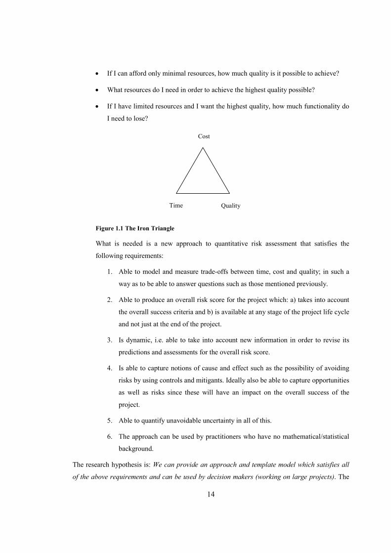
The criteria against which a project’s success or failure can be measured are cost, time

and quality, often referred to as The Iron Triangle, see Figure 1.1. Ideally, every project manager

would like their projects to satisfy all three of the above criteria. However, the reality is that due

to project constraints, trade-offs need to be made which usually result in only two of the three

criteria being met, as implied by the Iron Triangle. Many factors need to be considered when

deciding whether to compromise on time, cost and/or quality. The problem is that it is not always

possible to amend one of these factors without having an impact on one or more of the other

factors. For example, reducing the time could have a serious impact on cost and/or quality. The

key point is that it is possible to trade-off quality for lesser time spent, but also less cost.

Currently project management literature only covers the theory behind the classic ‘trade-

off’ problem between cost, time and quality but it does not provide a decision-support system for

trade-off analysis, in such a way that project managers can monitor and see which projects are on

target in different phases of a project. This thesis is interested in providing a decision-support

system motivated by the real problems and questions that face real project managers:

14

• If I can afford only minimal resources, how much quality is it possible to achieve?

• What resources do I need in order to achieve the highest quality possible?

• If I have limited resources and I want the highest quality, how much functionality do

I need to lose?

Figure 1.1 The Iron Triangle

What is needed is a new approach to quantitative risk assessment that satisfies the

following requirements:

1. Able to model and measure trade-offs between time, cost and quality; in such a

way as to be able to answer questions such as those mentioned previously.

2. Able to produce an overall risk score for the project which: a) takes into account

the overall success criteria and b) is available at any stage of the project life cycle

and not just at the end of the project.

3. Is dynamic, i.e. able to take into account new information in order to revise its

predictions and assessments for the overall risk score.

4. Is able to capture notions of cause and effect such as the possibility of avoiding

risks by using controls and mitigants. Ideally also be able to capture opportunities

as well as risks since these will have an impact on the overall success of the

project.

5. Able to quantify unavoidable uncertainty in all of this.

6. The approach can be used by practitioners who have no mathematical/statistical

background.

The research hypothesis is: We can provide an approach and template model which satisfies all

of the above requirements and can be used by decision makers (working on large projects). The

Time

Cost

Quality

15

approach is based on Bayesian Networks (BNs). BNs will be used because they provide effective

decision-support for problems involving uncertainty and probabilistic reasoning, since they are

able to combine diverse data.

In addition to satisfying the above requirements the proposed approach has the following benefits

inherited from the BNs methodology:

a. Handle and make predictions with incomplete data sets

b. Combine diverse types of data sets including both subjective beliefs and objective data

c. Overturn previous beliefs in light of new evidence

d. Learn and explicitly model causal factors and their relationships

e. Reason from effect to cause and vice versa

f. Arrive at decision based on visible auditable reasoning and improve decision making for

managers

The thesis is organised into eight chapters as follows.

Chapter 2 discusses the background and overview of project risk management. Project risk

management is introduced together with project risk management standards. This is followed by a

comprehensive list of risk factors for large projects with a discussion of the reasons for project

failure and project success. The chapter finishes with a comprehensive review of state-of-the-art

project risk management tools.

Chapter 3 provides the necessary background on BNs including their theoretical and technical

framework. This provides sufficient information to discuss the advantages of BNs when applied

to project risk management modelling.

Chapter 4 gives a detailed description of existing BN project risk models and their limitations.

Models that include trade-off analysis as well as models that cover other aspects of project risk

management are examined.

Chapter 5 is one of the main new contributions of this thesis and it argues that standard project

risk quantification framework is inadequate. Overview of the risk definitions and how they have

evolved to include opportunities are included. We present a new causal risk framework and

models created to demonstrate it.

This is the original work and an earlier version of this work has been published: Fineman,

M. and Fenton N. E., Quantifying Risks Using Bayesian Networks, IASTED Int. Conf. Advances

16

in Management Science and Risk Assessment (MSI 2009), Beijing, China, 2009, IASTED 662-219

[65]. I discussed the fundamental problems with a classical risk register and proposed a solution

based on Bayesian Networks that incorporates opportunities into modelling.

Chapter 6 is one of the main contributions to this thesis and it describes a Causal Risk Register

Model that implements risk taxonomy presented in chapter 5. The model is validated internally

and externally. The model addresses key limitations of classical risk register approach.

Chapter 7 is one of the main contributions to this thesis and it describes Generic Trade-off Model

that provides trade-offs between time, cost and quality. It includes requirements for the new

template model and covers structure of this model. The model is an improvement on models

discussed in chapter 4. The model is validated internally and externally.

This is the original work and an earlier version of this work has been published: Fineman

M., Radlinski L. and Fenton N. E., Modelling Project Trade-off Using Bayesian Networks, IEEE

Int. Conf. Computational Intelligence and Software Engineering. Wuhan, China, 2009, IEEE

Computer Society [64]. I developed a generic BN model for analysis of trade-offs between time,

cost and quality in large projects. I also proposed a set of assumed rules that the model had to

satisfy and demonstrated how the model can be used to support decision making by the managers

in some typical scenarios. The new research content of the paper is almost entirely my own work,

with contributions from the co-authors on presentation and accuracy.

Chapter 8 summarises the main points of the research undertaken for the thesis drawing

conclusions.

Appendix A, Risk Factors for Large Projects

Appendix B, Risk Factors for Large Projects as Attributes

17

2. Overview of Project Risk Management

To understand the requirements and research hypothesis it is crucial to review and

provide the background information on project risk management. In this chapter we discuss

project risk management standards, since we believe risk definitions from various standards could

be improved. We discuss the project risk management process and general risk issues for large

projects. Numerous works have been conducted on how project success can be measured. Project

success is usually defined as meeting time, cost and quality objectives. Key project factors

identified will be used in the quantitative models developed and described in the subsequent

chapters.

In the second part of this chapter we examine current state-of-the-art models. These vary

in focus from the ones that concentrate on planning and scheduling to risk register through to

alternative approaches. We first cover the planning and scheduling group of models including

critical path method, PERT and Monte Carlo simulation techniques. We then cover classical risk

register, followed by alternative techniques including fault trees, cognitive mapping methods and

decision trees.

The new contribution of this chapter is the analysis of risk factors and improvement on

how they can be phrased as attributes (Appendix B) and the analysis of the suitability of various

modelling approaches to risk analysis for large projects.

2.1 Background of Project Risk Management

The first formalized project risk management approach started in the 1950s. An important

milestone for indicating the beginning of quantitative project risk management was the

development of scheduling techniques such as the Critical Path Method (CPM) [96] and the

Program Evaluation and Review Technique (PERT) [119] which deal with risks implicitly. The

main focus of those approaches was project scheduling This is a reasonably well researched area

and it is not a major focus of this thesis, except if scheduling is in the context of quantifying risk

assessment (tools such as the CPM and PERT, along with other project risk management tools are

discussed in section 2.7).

The first article on project risk management was published by the Harvard Business

Review [68]. In the beginning, the main focus was on planning, procurement and administrative

functions. By the 1980’s, project risk management had already become a well-recognized area in

project management literature consisting of: risk identification, estimation, risk response

18

development and risk control. Its applications in industries were mainly time and cost risk

analysis [78].

During the 1990’s the focus of project risk management has changed and it began to turn

from developing the quantitative side into developing and understanding the risk management

process. New project risk management focus areas were cooperation and networking approaches,

and managing business processes as projects. The rapid development of technology has enabled

the application of project risk management in a geographically distributed business environment.

Furthermore, an increasing number of risk management studies were carried out in the 1990’s

which report on project failures. Hence, practitioners are paying attention on learning from

experience and introducing experience-based solutions of how risks could be avoided.

Companies are developing knowledge bases associated with project risk management

[123]. The knowledge bases contain the descriptions of risks, but can also offer other valuable

data such as suggestions for how to respond to risk. These risk knowledge bases can thus be used

as organizational memory banks where experience about risks and potential risk responses are

continuously recorded during project execution. It seems likely that changes and developments,

such as these, in project risk management will continue.

2.2 Project Risk Management Standards

The first risk related standard ever published was Norsk Standard NS5814:1991: Krav til

risikoanalyser in 1991 [143]. This standard only addressed risk analysis and it did not cover the

other parts of risk assessment.

The first project risk management standard was BS 6079-3:2000: Project Management –

Part 3: Guide to the Management of Business – related Project Risk by British Standards

Institution in 2000 [24]. The International Electrotechnical Commission in Switzerland launched

CEI/IEC 62198:2001: International Standard, Project Risk Management: Application Guidelines

in 2001 [86]. In its scope section is stated that: “This International Standard is applicable to any

project with technological content. It may also apply to other projects.” In general it is easy to

classify the standards according to their scope. The exception to this is the IEEE Standard 1540-

2001: Standard for Software Life Cycle Processes – Risk Management by Institute of Electrical

and Electronic Engineers in USA in 2001 [84], which states in its introduction that: “The risk

management process defined in this standard can be adapted for use at an organisation level or

project level.”

19

The Risk Management Guide for DoD Acquisition by the US Department of Defence

published in 2002 [182] has a limited scope of application to US defence acquisition projects.

Two project risk management standards appeared in quick succession in 2004. The

Association for Project Management in the UK launched the Project Risk Analysis and

Management Guide [7]; and the Project Management Institute in USA introduced the Guide to

the Project Management Body of Knowledge (PMBoK): Chapter 11, Project Risk Management

[151].

The focus on various standards was to create process consistency. All standards identified

describe the following process steps: planning, identification, analysis, treatment and control.

Terminology differs between the standards, but the process structure is similar in all of them.

In the analysis step, there seems to be a dominant distinction between the two following main

activities:

1. Risk estimation, which refers to an assessment of the likelihood of occurrence and

possible consequences of the risks identified in the previous step.

2. Risk assessment, which refers to an evaluation of the assessed risk by comparison with

the criteria and thresholds of the decision makers in order to determine the priority for

treatment.

The above six standards limit their scope of application, as indicated by their title, to project

risk management. However, it may be worth looking at other standards, defined in general terms

since there are no significant differences in terms of the structure of the processes and the

contents of the various stages. Thus it seems reasonable to also consult the following general

scope standards, i.e. organisational standards:

• CAN/CSA-Q850-97: Risk Management: Guideline for Decision-Makers

launched by Canadian Standards Association in 1997 [27].

• JIS Q2001: 2001(E): Guidelines for Development and Implementation of Risk

Management System launched by Japanese Standards Association in 2001 [88].

• Risk Management Standard published by Institute of Risk Management/National

Forum for Risk Management in the Public Sector/Association of Insurance and

Risk Mangers in UK in 2002 [85].

• AS/NZS 4360:2004: Risk Management published by Standards

Australia/Standards New Zealand in 2004 [9].

In subsequent discussions about risk definition and processes the following standards

have been used: Risk Management Standard published by Institute of Risk Management/National

Forum for Risk Management in the Public Sector/Association of Insurance and Risk Mangers in

20

UK in 2002, AS/NZS 4360:2004: Risk Management published by Standards Australia/Standards

New Zealand in 2004, the Project Management Institute in USA introduced Guide to the Project

Management Body of Knowledge (PMBoK): Chapter 11, Project Risk Management.

2.3 Project Risk Management Process

In advocating the use of project risk management, Wideman [189] observed that:

“Experience on many projects reveals poor performance in terms of reaching scope, quality, time

and cost objectives. Many of these shortcomings are attributed either to unforeseen events which

might or might not have been anticipated by more experienced project management, or to

foreseen events for which the risks were not fully accommodated.”

Wideman’s observation manages to encapsulate three central ideas in project risk management

practice:

1. Identifying events with negative consequences

2. Estimating their probability and impact

3. Responding appropriately

Wideman’s process requires that we first identify ‘risk events’. We then estimate the probability

that each risk will occur, and the impact on the project if it does occur. Thirdly we determine an

appropriate response to the risk.

Research of failed software projects showed that “their problems could have been avoided or

strongly reduced if there had been an explicit early concern with identifying and resolving their

high-risk elements” (Boehm [19]). Hence, Boehm [19] suggested a process consisting of two

main phases:

1. Risk assessment, which includes identification, analysis and prioritization.

2. Risk control, which includes risk management planning, risk resolution and risk

monitoring planning, tracking and corrective action.

Fairley [53] proposes about seven steps:

1. Identify the risk factors

2. Assess risk probabilities and effects

3. Develop strategies to mitigate the identified risks

4. Monitor the risk factors

5. Invoke a contingency plan

6. Manage the crisis

7. Recover from the crisis

21

The Software Engineering Institute [168], a leading source of methodologies for managing

software development projects, looks at project risk management as consisting of five distinct

phases: identification, analysis, response planning, tracking and control. In its Guide to the

Project Management Body of Knowledge, the Project Management Institute [151] gives a good

overview of typical PRM processes consisting of four phases: identification, quantification,

response development and control.

Kliem and Ludin [103] present a four phases process: identification, analysis, control and

reporting. Chapman and Ward [32] outline a generic PRM process consisting of nine phases:

define the key aspects of the project, focus on a strategic approach to risk management, identify

where the risks might arise, structure the information about the risk assumptions and

relationships, assign ownership of the risks and responses, estimate the extent of the uncertainty,

evaluate the relative magnitude of the various risks, plan the responses and manage by monitoring

and controlling the execution. From this brief review it is noticeable that there is general

agreement regarding what is included in the process, with the differences depending on variations

in the level of detail and on the assignment of activities to steps and phases.

It is in response to the risk stage that project risk management lays a claim to rationality. The

expected value of the risk can be calculated as first described by Bernoulli in 1738 [16]:

“If the utility of each possible profit expectation is multiplied by the number of ways in which can

it occur, and we then divide the sum of these products by the total number of possible cases, a

mean utility will be obtained, and the profit which corresponds to this utility will equal the value

of risk in question.”

This concept of expected value allows us to evaluate risk responses. Let net response gain

for a given risk response be defined as the gain in expected value less the cost of applying the risk

response. The rational risk treatment is then the response among all possible alternatives that has

the greatest net response gain.

The risk response planning process prescribed in the PMBOK offers a number of

categories of risk treatments. If the expected value of the untreated risk is sufficiently high, one

might decide to accept the risk (pg. 263). Otherwise, one might treat the risk by transferring it, for

example, by insuring against it. Alternatively, one could avoid the risk by adopting a new course

of action through which the risk cannot occur, or one could mitigate the risk by taking action to

reduce its probability or impact (pg. 261-2). Techniques based on the traditional expected utility

theory do not accurately describe human decision making and techniques based on expected

monetary value raise even more concerns [101]. Review of multiple criteria decision analysis

(MCDA) indicates popularity of multiattribute utility theory [50].

22

2.4 General Risk Issues for Major Large Scale Projects

Risks differ according to the type of project. For example, oil platforms are technically

difficult, but they typically face few institutional risks since they are socially desired because of

the high revenues they bring to communities and countries [94, 174]. Nuclear-power projects also

pose high technical risks, however, they have higher social and institutional risks.

It is often said that the real risks in any project are the ones that you fail to recognise.

This would imply that when identifying potential sources of risk, a broad scope should be

adopted, thereby reducing the chances of overlooking important areas of risk. The emphasis

should therefore be on generating a comprehensive list of risks rather than prematurely

identifying a limited set of key risks. During the identification of risks there is a natural tendency

to simply omit recording some risks because their impacts are immediately considered to be of a

minor nature. This has obvious dangers in that omitting seemingly minor problems can mean that

the combined effect of large numbers of apparently minor risks may be underestimated. In

addition, there is also a tendency to omit recording risks where an effective response cannot be

attributed to it, and this too has an obvious danger since potentially some risks are overlooked.

First it is important to be able to identify:

• new risks

• risks of which the scale may have changed, for instance, because of a context that has

developed

• long known risks that have not been studied in depth

• risks of which social awareness has grown, for example, it may be that a risk that has

been dominant in the past has been eliminated or reduced which creates new priorities.

2.5 What is a successful project?

Project success is a core concept of project management. Therefore, it is important that

success objectives are defined and specified [87, 105, 112, 196, 159]. Oisen [144] in the 1970s

suggested cost, time and quality as the success criteria for project management and the success of

projects. Since then these criteria are usually included in the description of project management.

Many other writers Turner [181], Morris and Hough [130], Wateridge [185, 186], deWitt [41,

42], McCoy [129], Pinto and Slevin [150], Babu and Suresh [9], Saarinen [167], Khang et al.

[99], Ballantine et al. [12] and Kerzner [97, 98] all agree cost, time and quality should be used as

success criteria. Some authors suggest that other criteria in addition to cost, time and quality

could be used to assess projects [169, 175].

23

In the early 1980s more comprehensive definitions were developed. Baker et al. defined

project success as follows: “If the project meets the technical performance specifications and/or

mission to be performed and if there is a high level of satisfaction concerning the project outcome

among: key people in the parent organisation, key people in the client organisation, key people in

the project team and key users or clientele of the project effort, the project is considered an

overall success.” [11]

Freeman and Beale [67] concluded that success means different things to each

professional. An architect may consider success in terms of aesthetic appearance, an engineer in

terms of technical competence, an accountant in terms of pounds spent under budget, a human

resource manager in terms of employee satisfaction, etc. The importance of the concept of project

success was reflected by the Project Management Institute devoting its 1986 Annual Seminar and

Symposium to this topic.

It is important to understand the concept of project success in order to explore it further.

Time, cost and quality are the basic criteria to project success and they are identified and

discussed in almost every article on project success [8]. Atkinson [8] called these three criteria the

“Iron Triangle”. He further suggested that while other definitions on project management success

have developed, the iron triangle is always included in the alternative definitions.

The study performed by Crawford et al. [36] during the period of 1994–2003 confirms

the fact that project management places great emphasis on ensuring conformance to time, budget

and quality constraints. All projects are, to a certain degree, unique complex undertakings.

However, there are significant similarities - most projects have restrictions in time and costs as

well as certain demands for quality. As a result the project manager may find it extremely

difficult to stay within the Iron Triangle. Kohrs and Welngarten [105] reported trade-offs that

project manager must make: “Good! Fast! Cheap! Pick any two.” The Iron Triangle is the ‘magic

combination’ that is continuously pursued by the project manager throughout the life cycle of the

project [25, 78, 92, 72, 113, 130, 155, 165].

If the project were to flow smoothly, according to plan, there might not be a need for

trade-off analysis. Unfortunately, most projects eventually get into crises such that it is no longer

possible to maintain the delicate balance necessary to attain the desired performance within time

and cost [101]. The deviations are normally overruns, in the case of time and cost, whereas the

quality deviation is usually a shortfall. No two projects are ever exactly alike, and trade-off

analysis would be an ongoing effort throughout the life of the project, continuously influenced by

both the internal and external environment. Experienced project managers may have planned

24

trade-offs in reserve in the event that anticipated crises arise hence recognising that trade-offs are

essential in effective project risk management.

For example, if we can achieve high quality this may compensate for cost and time. Or if

there is timely delivery which enables a ‘first-to-market’ advantage (Microsoft products for

example), then we may be willing to compromise with a low quality end-product. In the case of

software projects we include functionality as part of quality and by doing this we can compare

success. For example, how many function points [157] you deliver with how many defects at

what cost and time. This means we can measure functionality objectively.

There are many reports on project overruns and it would be a conservative estimate to

state that approximately 50% of construction projects overrun [130] and approximately 63% of all

information systems projects encounter substantial budget overrun [130], with overrun values

“typically between 40 and 200 percent” [130]. Project sponsors claim that although, “most

projects are eventually completed more or less to specification”, they are “seldom on time and

within budget” [196]. It has even been suggested that a “good rule of thumb is to add a minimum

of 50% to every time estimate, and 50% to the first estimate of the budget” [196].

At first glance, a project that does not meet the three success factors of time, cost and

quality would appear to be a failure, but this is not necessarily so. It is ‘perceived’ success or

failure that is important and provided a project achieves a satisfactory level of technical

performance, in retrospect it may be considered a success by the parties involved, despite

exceeding its cost and time targets. This of course depends on whether cost and time targets were

fixed or not. In addition, although the project cost more and took longer than the client originally

perceived, the client may accept that this was unavoidable, was for good reason, that it received

value for money, and the project was still a commercial success. The criterion of success or

failure is whether the project sponsor, owner, client and other parties concerned, including the

project manager’s parent company, are satisfied with the final outcome of the project.

2.6 Factors affecting success or failure of projects

The identification of project success factors can be used to analyse the reasons for project

success and failure. Since the 1960s, many theoretical and empirical studies have been completed

on success factors of a project.

The success and failure factors were first introduced by Rubin and Seeling [164]. They

investigated the impact of a project manager’s experience on the project’s success and failure.

They concluded that the number of projects previously managed by a project manager has

25

minimal impact on the project’s performance, whereas the size of the previously managed

projects does affect the project’s performance.

Pinto and Selvin [150] reported that the critical success of a project depends on ten

factors. These are: project mission, top management support, project schedules, client

consultation, personnel recruitment, technical tasks, client acceptance, monitoring and feedback,

communication and trouble-shooting. Anton listed six factors to enhance project success. These

factors are: planning effort in design and implementation, project manager goal commitment,

project team motivation, project manager technical capabilities, scope and work definition and

control system.

Belassi and Tukel [14] categorised these factors into four main groups. These are factors

relating to: the project managers, the project, the organisation and the external environment.

UK experience

In the UK, two studies identified the factors leading to the failure of projects. Duffy and Thomas

[49] identified the following reasons for the failure of projects:

• Project management in the client, consultant, contractor and supplier organisations is

an important factor in poor project performance.

• Inappropriate project organisation is usually the key to an unsuccessful project. Here

the roles and responsibilities in the project parties have not been clearly defined.

• Lack of direction and control in the project team often results in low productivity and

a failure to meet delivery dates.

• On many projects consideration of an appropriate contract strategy is left until late in

the project, when the full range of options available to the client cannot be

considered.

• Often the scope of work is not defined adequately to those participating in the

project.

• Frequently the level of planning is inappropriate to the scope of the project. Project

stages are not clearly identified with agreed deliverables.

US experience

The major research work on the subject was carried out in the USA by Baker, Murphy and Fisher

[11], who studied 650 projects. They identified a large number of factors which affected the

26

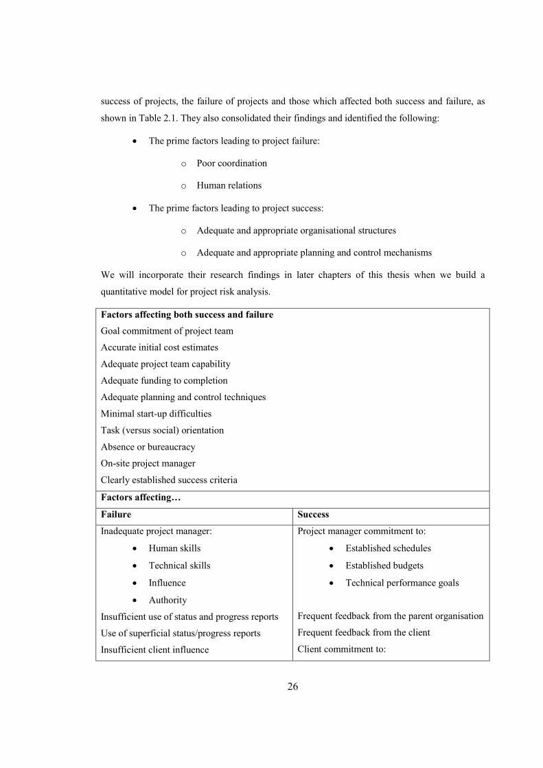
success of projects, the failure of projects and those which affected both success and failure, as

shown in Table 2.1. They also consolidated their findings and identified the following:

• The prime factors leading to project failure:

o Poor coordination

o Human relations

• The prime factors leading to project success:

o Adequate and appropriate organisational structures

o Adequate and appropriate planning and control mechanisms

We will incorporate their research findings in later chapters of this thesis when we build a

quantitative model for project risk analysis.

Factors affecting both success and failure

Goal commitment of project team

Accurate initial cost estimates

Adequate project team capability

Adequate funding to completion

Adequate planning and control techniques

Minimal start-up difficulties

Task (versus social) orientation

Absence or bureaucracy

On-site project manager

Clearly established success criteria

Factors affecting…

Failure Success

Inadequate project manager:

• Human skills

• Technical skills

• Influence

• Authority

Insufficient use of status and progress reports

Use of superficial status/progress reports

Insufficient client influence

Project manager commitment to:

• Established schedules

• Established budgets

• Technical performance goals

Frequent feedback from the parent organisation

Frequent feedback from the client

Client commitment to:

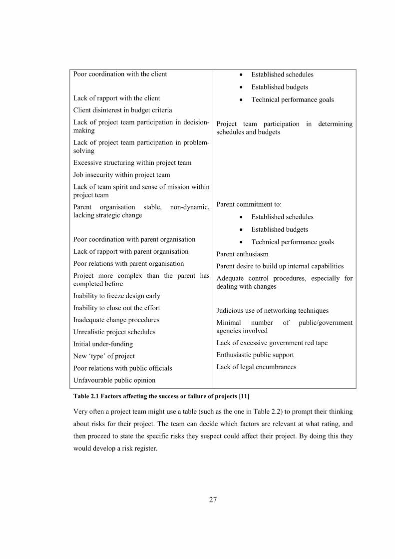
27

Poor coordination with the client

Lack of rapport with the client

Client disinterest in budget criteria

Lack of project team participation in decision-making

Lack of project team participation in problem-solving

Excessive structuring within project team

Job insecurity within project team

Lack of team spirit and sense of mission within project team

Parent organisation stable, non-dynamic, lacking strategic change

Poor coordination with parent organisation

Lack of rapport with parent organisation

Poor relations with parent organisation

Project more complex than the parent has completed before

Inability to freeze design early

Inability to close out the effort

Inadequate change procedures

Unrealistic project schedules

Initial under-funding

New ‘type’ of project

Poor relations with public officials

Unfavourable public opinion




Project team participation in determining schedules and budgets

Parent commitment to:




Parent enthusiasm

Parent desire to build up internal capabilities

Adequate control procedures, especially for dealing with changes

Judicious use of networking techniques

Minimal number of public/government agencies involved

Lack of excessive government red tape

Enthusiastic public support

Lack of legal encumbrances

Table 2.1 Factors affecting the success or failure of projects [11]

Very often a project team might use a table (such as the one in Table 2.2) to prompt their thinking

about risks for their project. The team can decide which factors are relevant at what rating, and

then proceed to state the specific risks they suspect could affect their project. By doing this they

would develop a risk register.

28

When the project completes, the team should review its performance against the risk

management documentation to see if there are factors to add to this table or if there are cues that

should be changed to help future projects in the organization better identify their risks.

Rating (check one)

Factor

ID

Risk Factors Low Risk Cues Medium Risk

Cues

High Risk

Cues L M H NA NI TBD

Notes

Mission and Goals

1 Project Fit to

Customer

Organization

directly

supports

customer

organization

mission and/or

goals

indirectly

impacts one or

more goals of

customer

does not

support or

relate to

customer

organization

mission or

goals

2 Project Fit to

Provider

Organization

directly

supports

provider

organization

mission and/or

goals

indirectly

impacts one or

more goals of

provider

does not

support or

relate to

provider

organization

mission or

goals

3 Customer

Perception

customer

expects this

organization to

provide this

product

organization is

working on

project in area

not expected by

customer

project is

mismatch with

prior products

or services of

this

organization

4 Work Flow little or no

change to work

flow

will change

some aspect or

have small

affect on work

flow

significantly

changes the

work flow or

method of

organization

Table 2.2 Sample risk factors for large projects [45]

29

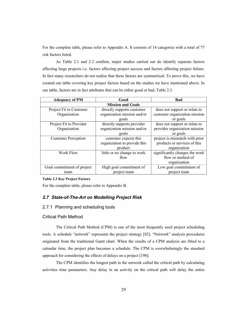
For the complete table, please refer to Appendix A. It consists of 14 categories with a total of 77

risk factors listed.

As Table 2.1 and 2.2 confirm, major studies carried out do identify separate factors

affecting large projects i.e. factors affecting project success and factors affecting project failure.

In fact many researchers do not realise that these factors are symmetrical. To prove this, we have

created our table covering key project factors based on the studies we have mentioned above. In

our table, factors are in fact attributes that can be either good or bad, Table 2.3.

Adequacy of PM Good Bad

Mission and Goals Project Fit to Customer

Organization directly supports customer

organization mission and/or goals

does not support or relate to customer organization mission

or goals

Project Fit to Provider Organization

directly supports provider organization mission and/or

goals

does not support or relate to provider organization mission

or goals

Customer Perception customer expects this organization to provide this

product

project is mismatch with prior products or services of this

organization

Work Flow little or no change to work flow

significantly changes the work flow or method of

organization

Goal commitment of project team

High goal commitment of project team

Low goal commitment of project team

Table 2.3 Key Project Factors

For the complete table, please refer to Appendix B.

2.7 State-of-The-Art on Modelling Project Risk

2.7.1 Planning and scheduling tools

Critical Path Method

The Critical Path Method (CPM) is one of the most frequently used project scheduling

tools. A schedule “network” represents the project strategy [82]. “Network” analysis procedures

originated from the traditional Gantt chart. When the results of a CPM analysis are fitted to a

calendar time, the project plan becomes a schedule. The CPM is overwhelmingly the standard

approach for considering the effects of delays on a project [190].

The CPM identifies the longest path in the network called the critical path by calculating

activities time parameters. Any delay in an activity on the critical path will delay the entire

30

project. The paths that are not critical can be delayed, if they have scheduling flexibility, without

necessarily delaying the project.

The CPM models the activities and their dependency. Hence, it is not possible to start

some activities until others are finished. These activities need to be completed in a sequence, with

each stage being completed before the next stage can begin. Since real projects do not work this

way, the CPM is just the beginning of project schedule management. Some key reservations

about the standard CPM:

• It is based on single-point estimates and therefore gives a false notion that the future can

be predicted precisely. One common misconception is that since estimates are based on

most likely estimates, things will even out by the law of averages [90]. In almost all

cases, the CPM completion date is not the most likely. [82]

• The activities on the critical path may not be the most likely to delay the project. Tasks

not on the critical path can, due to deviations from the plan, end up on the critical path.

The use of the CPM can therefore direct management’s attention to activities not likely

to delay the project. The duration of each task is an estimate subject to uncertainty [90].

The critical path may vary and single tasks may or may not be on the critical path when

randomness is accounted for.

• Project duration is probabilistic and therefore predictions of completion dates should be

accompanied by probabilities. The duration calculated by the CPM is simply an addition

of the most likely estimates, which is only accurate if everything goes according to plan.

[82] The CPM date is rarely a good approximation of the most likely date. Even with a

single path project, the CPM date is almost always far too optimistic [71].

• The CPM does not account for path convergence and therefore tends to underestimate

the duration of the project. For example, if three parallel activities all have an estimated

duration of 10 days, the CPM calculated duration will be 10 days. However, if any one

of the activities is delayed, this estimation will not hold. The likelihood of meeting the

predicted merge date is the product of the probabilities of each of the joining paths [71].

• The project duration calculated by the CPM is accurate only if everything goes

according to plan. This is rare in real projects.

• In many cases the completion dates the CPM produces are unrealistically optimistic and

highly likely to be overrun, even if the schedule logic and duration estimates are

accurately implemented.

31

• The CPM completion date is not even the most likely project completion date, in almost

all cases.

• The path identified as the “critical path” using traditional CPM techniques may not be

the one that will be most likely to delay the project and which may need management

attention.

PERT

The PERT (Program Evaluation and Review Technique) is a variation on Critical Path

Analysis developed in the 1950’s. It was able to incorporate uncertainty in activity duration by

making it possible to schedule a project while not knowing precisely the details and durations of

all the activities [40, 119, 130, 132]. For each activity PERT gives three estimations: optimistic,

most likely and pessimistic times. Also, it identifies the minimum time needed to complete the

total project.

In the 1960s PERT was a great success. However, in the 1970s doubts were raised about

the theoretical assumptions of PERT and its practicality. The assumption of independence

between activities and also assumption that all estimates have a Beta distribution are not practical.

More importantly the PERT assumes that the probability distribution of the project completion

time is the same as that of the critical path. The possibility that the critical path identified may not

end up being the critical path is ignored. Hence, the PERT consistently underestimates the

expected project completion time and produces overly optimistic estimates for the project

duration.

Monte Carlo Simulation Tools

Monte Carlo simulation (MCS) can be used to overcome some challenges associated with

CPM and PERT. It was first proposed for project scheduling in the early 1960s. The technique

became dominant only in 1980s when sufficient computer power became available. Each

simulation is generated by randomly pulling a sample value for each input variable. These input

sample values are then used to calculate the results, i.e. total project duration, total project cost,

project finish time. The duration of each activity is estimated by shortest, most likely and longest

duration and also the shape of the distribution (Normal, Beta etc.). Then critical path calculation

is repeated several times. A sufficient number of runs provide a probability distribution for the

possible results (i.e. time, cost) [91].

The following project risk management tools apply Monte Carlo analysis:

32

• Pertmaster Project Risk [149]

• @Risk [1]

• Deltek Risk+ [43]

• Risk+ from S/C Solutions Inc. [161]

• Crystall Ball [38]

• Risky Project Professional 2.1[162]

• PROAct [152]

• Project Risk Analysis [154]

Each MCS tool has its own specific functionalities. The following features are common

to all of them:

• Assign different statistical distributions including custom distributions to project

inputs (task duration, cost, etc.)

• Output results in different formats.

MCS can also provide a sensitivity analysis by measuring the correlation between the

project inputs (task duration, finish time etc.) and the project outputs (project duration, cost etc.).

This gives an indication of how much the duration of each task affects completion of other tasks

and also the tasks that are most likely to cause delay on the project.

The classic Monte Carlo simulation method has a number of limitations. The serious flaw

in traditional MCS is the assumption of statistical independence for individual activities which

share risk factors in common with other activities [183]. MCS tools assume that the marginal

distribution of uncertainty for individual activities in the project completely define the

multivariate distribution for project schedule. Van Dorp and Duffey [183] demonstrated that

failure to model such dependence during MCS can result in the underestimation of total

uncertainty in project schedule. Statistical distributions of project inputs such as task durations

should be obtained based on reliable historical data. In most large, novel projects this information

is not available and using the MCS may not improve estimations [183].

2.7.2 Risk Register Approach

The standard tool for project risk management is the so-called risk register [33, 184, 29,

37, 191, 193]. Many organisations store their risks in undisclosed forms of registers [146, 34]. A

risk register is a list of the typical risk factors of project failure compiled based on the experiences

33

from past projects. A risk register usually takes the form of a questionnaire or a risk list. The

questionnaire consists of a set of questions that ask about the current state of the project. The

questions directly indicate the existing risk factors and also guide towards some potential risk

factors. The risk factors are identified usually by negative answers. Research conducted by the

Design Information Group at Bristol University found that 67% of questionnaire respondents

documented their risks on either paper or a computer based risk register [37].

There are various statements in the literature describing the role of a risk register.

Williams [193] states that a risk register has two main roles:

1. To serve as a repository of knowledge

2. To begin analysis and plans that flow from it.

As such, the risk register should be used to keep log of the risks to a project. Chapman and Ward

state that, to enable the documentation of the sources of the risk and their responses, as well as

their classification, “the risk register identify phase involves compiling a list, a log or register”

[33]. Within this, they identify that the documentation produced through the utilisation of project

risk management can be regarded as a “by-product…rather than a central concern” [33].

Furthermore Ward states that “the purpose of the summary risk register is to help the project team

review project risks on a regular basis throughout the project” [184]. The risk register is used as a

formal method of identifying, quantifying and categorising the risks, as well as providing the

means of developing a cost-effective method of controlling them [71].

The risk register consists of three entities. A register of the risks itself as suggested by the

title, which is the main focus of the system, and two supporting documents, to include

information on the risk owner and risk reduction and mitigation plans. Once the risks have been

identified, assessed and possibly analysed, they are placed into the risk register. Additional

information about the risks to the project can be held within the risk owner and risk reduction and

mitigation plans entities.

Williams [193], Carter et al. [29] and Ward [184] all give examples of the type of

information or items which can be stored in the risk register. Their general consensus is that the

risk register should contain a description of the risk, its impact and probability. Hence, risk is

decomposed into two components:

• Probability of the risk

• Impact the risk can cause.

34

Risk is then quantified as the measure:

risk = probability x impact

Many additional items that could potentially be included within the risk register.

A risk register involves a considerable dose of subjectivity especially where the project

state is being assessed. A common technique to reduce the subjectivity in a risk register is to

gather the answers from different sources.

The publicly available risk identification risk registers are particularly useful in practice

because of their accessibility and comprehensiveness. Some public risk registers currently

available are:

• Taxonomy-Based Questionnaire [28] – not very detailed, but wide-ranging questionnaire

proposed by SEI in 1993. It consists of 194 mostly yes-no questions (some with sub-

questions) arranged in 3 risk taxonomy classes (product engineering, development

environment and program constraints) divided further into 3 to 5 elements each with 3 to

8 attributes.

• Risk Assessment Checklist [179] – general questionnaire proposed by Rob Thomsett in

1992 to assess risk in the very early stages of a project. It consists of 64 test questions in

3 risk areas (user environment, team environment, system complexity). Coverage of the

user environment is quite unique to this risk register. The questionnaire is supplemented

with a method to assess the overall level of project risk, which evaluates each answer

with a given number of points. The total number of points is then compared against a

predefined scale, which assigns a risk level (high, medium or low) to a given range of

points.

• Software Development Checklist [127] – very detailed technically oriented questionnaire

proposed by Steve McConnell in 1993. It consists of 511 yes-no questions in 5 major

areas (requirements, design, construction, quality assurance, outsourcing). This checklist

is exceptionally detailed and comprehensive with regard to the implementation practices

(371 questions).

• Complete List of Schedule Risks [128] – comprehensive list of risk factors for the

exceeded schedule risk compiled by Steve McConnell in 1996. It consists of 109 risk

factors in 12 areas (e.g. requirements, design, customer, end-user, personnel,

35

management). This risk list is also published on the Internet. It is quite well known and

used in the industry.

• Capers Jones’ 60 Risk Factors [90] – list of 60 common risk factors for the general risk of

project failure compiled by Capers Jones in 1994. Each risk factor is extensively

described in a 20-point text structure including severity and frequency, root causes,

methods of prevention and control, as well as effectiveness and cost of known therapies.

Information on known remedies, support, and references for each risk factor makes this

risk list especially useful.

2.7.3 Alternative general graphical tools

This thesis proposes the use of graphical methods [113], namely Bayesian Networks

(BNs), for project risk management. However, there are alternative graphical tools and that is

what we will review next.

Fault trees

Fault tree analysis was developed by Bell Telephone Laboratories in 1962 for the US Air

Force for use with the Minuteman system. It was later adopted and extensively applied by the

Boeing Company [72, 160]. This is a graphical technique that provides a systematic description

of the combinations of possible occurrences in a system, which can result in a system failure [14].

Fault tree analysis is a top-down method of analysing an undesirable event to determine all the

ways that the event can happen, based on the behaviour of the components, lower-level

assemblies, and interfaces.

The most serious outcome is selected as the Top Event. A fault tree is then constructed by

relating the sequences of events with AND and OR logical gates, which individually or in

combination, could lead to the Top Event. Probabilities are assigned to each event and at an OR

gate the probabilities must be added to give the probability of the next event, whereas at an AND

gate, the probabilities are multiplied. Therefore it is possible to identify the failures that have the

greatest influence on the End Event.

Advantages of fault tree analysis are:

• Provides insight into the system behaviour

• A graphic aid for management

• Identifies failures deductively

• Handles complex systems more easily

36

• Provides options for management and others to perform either qualitative or quantitative

reliability analysis

• Allows concentration on one particular failure at a time

In contrast, some of the disadvantages are as follows:

• Independence assumption between the causes

• A time consuming approach

• A costly method

• It considers components in either a working or failed state. More specifically, the

components partial failure states are difficult to handle

• Difficult to use for large projects

• The end results are difficult to check.

Cognitive Mapping Methodologies

Cognitive mapping methods have been applied in research in a project context by Eden et

al. [50] to study disruption and delays in projects; Williams [194] proposes using causal mapping

and system dynamics to model complex projects; Williams et al. [194] used causal mapping to

explore risks in projects; Maytorena et al. [124] employed causal mapping to explore the process

of risk identification in projects and Klein proposed cognitive mapping to model project trade-

offs [101], to name a few. In a broader management science context cognitive mapping methods

could be combined with other methodologies such as MCDM [16].

The cognitive mapping methodology is built on the premise that all individuals gain an

understanding of the world they inhabit through developing a set of beliefs, assumptions, and a

knowledge base that is used to make sense of the world around them. The decision makers use

“personal models” when making decisions and it is through the dissection of their explanations

using cognitive mapping techniques that researchers are able to gain greater insight into the

perceived complexities of the issues.

Cognitive mapping techniques are used to identify an individual’s beliefs about a

particular domain and to depict these diagrammatically. Swan [175] in her review of cognitive

mapping as a management research tool highlights that the product of these mapping techniques,

although typically referred to as cognitive maps, are not cognitive maps in the “psychological

sense”. It is not “an internal mental representation” but a visual representation of an individual’s

subjective data which helps in the understanding and analysis of specific elements of an

individual’s thoughts rather than thinking [175].

37

The maps are a network of nodes and arrows as links where the direction of the arrow

implies believed causality. Hence, when constructed by group cognitive maps are known as

‘cause maps’. Cognitive maps are usually derived through interviews and they are intended to

represent the subjective world of the interviewee. Cognitive mapping is a formal modelling

technique with rules for its development. Cognitive maps are characterised by an hierarchical

structure which is most often in the form of a means/ends graph with goal type statements at the

top of the hierarchy.

Eden’s causal mapping is an interactive decision-support tool used to capture and analyse

complex problems and decision making [52]. Eden’s mapping approach is based on Kelly’s

Personal Construct Theory [95], which provides a sound basis for understanding how individuals

make sense of their experiences. This focus on problem solving and action makes it appropriate

for ‘problem structuring’ and uncovering solution options. Kelly’s theory provides the rules for

mapping.

For representational purposes a cognitive map is drawn as short pieces of text linked with

arrows. Generally a statement at the tail of an arrow is taken to cause, or influence, the statement

at the arrowhead. An important aspect of Kelly’s theory argues that we make sense of situations

through similarities and differences. Hence, we seek to identify each statement as having two

contrasting poles. For cognitive maps the causality relates the first phrase of the bi-polar

statement to the first phrase of the second statement. When an arrow head is shown with a

negative sign attached then the first pole of the tail statement implies the second pole of the head

statement. Typically a concept which has no implication is referred as a ‘head’ and a node which

has no in-arrows is referred to as a ‘tail’.

It is a well-founded methodology with a limited number of usable analysis software

packages that allow for a detailed analysis of individual maps. One of the most advanced software

packages is Decision Explorer™ [13]. In practice, the maps are built out of concepts linked to

each other by arrows in a hierarchical form that indicate the nature of the linkage. From this the

structure of the map has the potential of being analysed in a number of ways. Its disadvantage is

that it does not allow for content analysis to be carried out easily. However, it can be used in

combination with other specialist software packages for this purpose.

This technique provides clear procedures for collecting data, and it allows for a

systematic analysis of that data and is supported by a software package, which increases the

reliability of the analysis. However, it does not provide the full use of causal modelling i.e.

building quantitative models. We will provide this with using Bayesian Networks.

38

Decision Tree

A decision tree is a graphical diagram consisting of nodes and branches used to model

and evaluate a decision process which consists of an alternating sequence of actions and

uncertainty consequences [30, 80]. There are two node types:

• Rectangle represents the decision to be made. The branches from decision nodes are the

alternative choices. The manager can implement only one alternative.

• Circle represents chance node. The branches from chance nodes have some element of

uncertainty as to whether or not they will occur.

The core of the decision tree is aggregating the payoff values and their associated

probabilities into a single quantity that can be compared with each other. The aggregation

procedure is repeated until the decision maker can identify the action to be chosen at the initial

node and the subsequent decision nodes. The most commonly used method for the decision tree is

the expected monetary value (EMV), which maximises the expected payoff as the evaluation

criteria. If the monetary value is replaced with utility, which measures the decision maker’s

preference in an interval scale, the EMV decision rule would become the maximising expected

utility (EU). The utility analysis is a powerful framework for decisions involving risk, but it has

some limitations. As discussed in [20], it cannot include the portfolio effect of the decision

maker’s attitude, as the decision maker’s attitude changes dynamically. Another limitation is the

famous Allais paradox [101], where people sometimes violate the basic assumptions on which the

utility approach is based. So in most cases it is usual to use only the EMV rule. However, this

might not produce the best result since the EMV rule does not consider the decision maker’s

attitude. Yager pointed out the shortcomings of the EMV rule [199, 201, 200] such as the use of

the expected values that associate a neutral attitude to the decision maker.

For the solutions of constructing decision functions which allow for the inclusion of

decision attitude and probabilistic information in uncertainty, Yager comprehensively

investigated this problem in various conditions, and proposed a mechanism for combining

probabilistic information about the state of nature with information about the decision maker’s

attitude.

39

2.8 Discussion

Every project involves some degree of risk, but that risk can be controlled with careful

analysis. One of the key responsibilities of a project manager is to anticipate project risks, and

then to devise the means for controlling those risks before they can get out of hand. This is where

the risk management process comes in. Risk is a complex notion and it is very difficult to capture

all major aspects of project risk. The fast changing environment and the complexity of projects

has increased risk exposure.

Project risk management operates in a complex and dynamic environment that is

constantly confronted with various risks. It is therefore imperative that project managers should

consider all possible risk factors affecting a given project. Furthermore, they should take

corrective actions to control and manage the identified risks. An effective risk management

approach can provide a framework for project mangers which enables them to identify and assess

potential risk factors and to then take the necessary actions in order to achieve the desired

objectives of a given project.

Risk management can be a challenging process because it requires anticipating future

events. However, instead of only trying to look into the future, we can manage risk by looking at

the past. By examining prior project experiences, you can get a better insight into risk

probabilities and if you can anticipate an event, you should be able to weigh up the consequences,

and control the outcome.

All novel projects are risky and once a project has started even experienced project

managers can make ineffective choices. Hence, we need project risk analysis and project risk

management tools in order to help us with decision making.

We have reviewed the techniques currently in use within the area of project risk

management. Furthermore, we have established the requirements which must be satisfied and, as

we can see in Table 2.4, there is no current state-of-the-art tool which satisfies all the

requirements. Even what is considered as standard to project risk management (the risk register)

does not satisfy two of the criteria. We believe it is possible to develop a tool which satisfies all

the requirements using BNs. In the next chapter we introduce the BN technique.

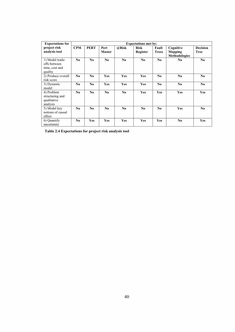
40

Expectations for project risk

analysis tool

Expectations met by:

CPM PERT Pert

Master

@Risk Risk

Register

Fault

Trees

Cognitive

Mapping

Methodologies

Decision

Tree

1) Model trade-offs between time, cost and quality

No No No No No No No No

2) Produce overall risk score

No No Yes Yes Yes No No No

3) Dynamic model

No No Yes Yes Yes No No No

4) Problem structuring and qualitative analysis

No No No No Yes Yes Yes Yes

5) Model key notions of causal effect

No No No No No No Yes No

6) Quantify uncertainty

No Yes Yes Yes Yes Yes No Yes

Table 2.4 Expectations for project risk analysis tool

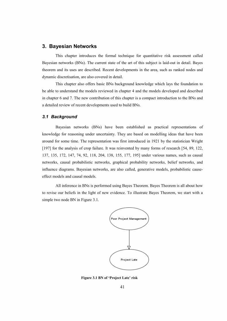
41

3. Bayesian Networks

This chapter introduces the formal technique for quantitative risk assessment called

Bayesian networks (BNs). The current state of the art of this subject is laid-out in detail. Bayes

theorem and its uses are described. Recent developments in the area, such as ranked nodes and

dynamic discretisation, are also covered in detail.

This chapter also offers basic BNs background knowledge which lays the foundation to

be able to understand the models reviewed in chapter 4 and the models developed and described

in chapter 6 and 7. The new contribution of this chapter is a compact introduction to the BNs and

a detailed review of recent developments used to build BNs.

3.1 Background

Bayesian networks (BNs) have been established as practical representations of

knowledge for reasoning under uncertainty. They are based on modelling ideas that have been

around for some time. The representation was first introduced in 1921 by the statistician Wright

[197] for the analysis of crop failure. It was reinvented by many forms of research [54, 89, 122,

137, 135, 172, 147, 74, 92, 118, 204, 138, 155, 177, 195] under various names, such as causal

networks, causal probabilistic networks, graphical probability networks, belief networks, and

influence diagrams. Bayesian networks, are also called, generative models, probabilistic cause-

effect models and causal models.

All inference in BNs is performed using Bayes Theorem. Bayes Theorem is all about how

to revise our beliefs in the light of new evidence. To illustrate Bayes Theorem, we start with a

simple two node BN in Figure 3.1.

Figure 3.1 BN of ‘Project Late’ risk

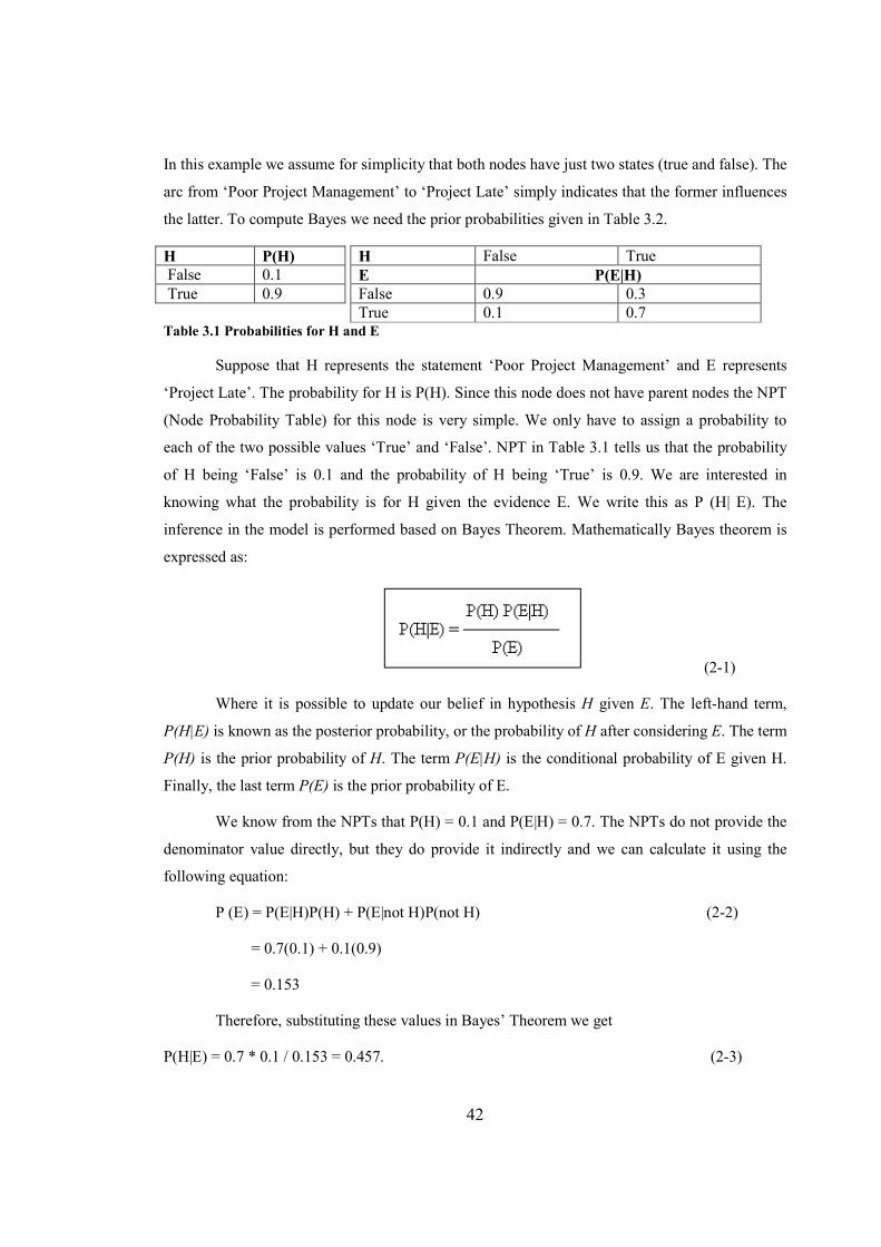
42

In this example we assume for simplicity that both nodes have just two states (true and false). The

arc from ‘Poor Project Management’ to ‘Project Late’ simply indicates that the former influences

the latter. To compute Bayes we need the prior probabilities given in Table 3.2.

H False True

E P(E|H)

False 0.9 0.3

True 0.1 0.7 Table 3.1 Probabilities for H and E

Suppose that H represents the statement ‘Poor Project Management’ and E represents

‘Project Late’. The probability for H is P(H). Since this node does not have parent nodes the NPT

(Node Probability Table) for this node is very simple. We only have to assign a probability to

each of the two possible values ‘True’ and ‘False’. NPT in Table 3.1 tells us that the probability

of H being ‘False’ is 0.1 and the probability of H being ‘True’ is 0.9. We are interested in

knowing what the probability is for H given the evidence E. We write this as P (H| E). The

inference in the model is performed based on Bayes Theorem. Mathematically Bayes theorem is

expressed as:

(2-1)

Where it is possible to update our belief in hypothesis H given E. The left-hand term,

P(H|E) is known as the posterior probability, or the probability of H after considering E. The term

P(H) is the prior probability of H. The term P(E|H) is the conditional probability of E given H.

Finally, the last term P(E) is the prior probability of E.

We know from the NPTs that P(H) = 0.1 and P(E|H) = 0.7. The NPTs do not provide the

denominator value directly, but they do provide it indirectly and we can calculate it using the

following equation:

P (E) = P(E|H)P(H) + P(E|not H)P(not H) (2-2)

= 0.7(0.1) + 0.1(0.9)

= 0.153

Therefore, substituting these values in Bayes’ Theorem we get

P(H|E) = 0.7 * 0.1 / 0.153 = 0.457. (2-3)

H P(H)

False 0.1

True 0.9

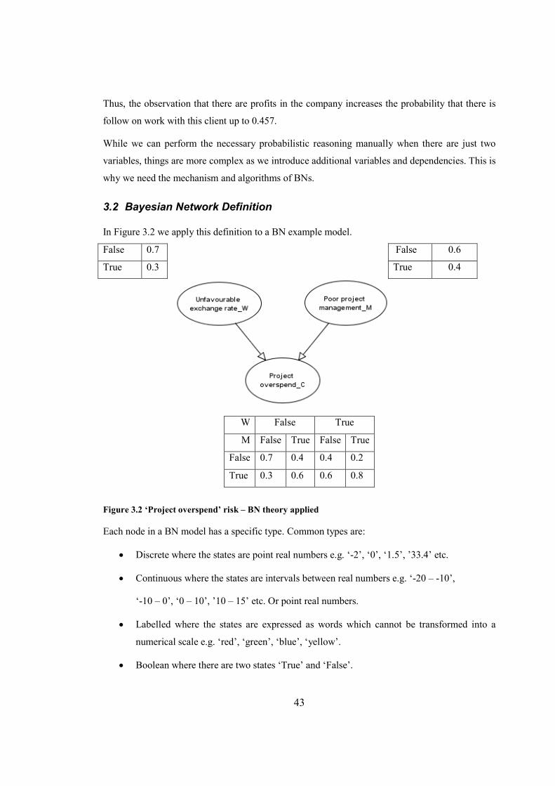
43

Thus, the observation that there are profits in the company increases the probability that there is

follow on work with this client up to 0.457.

While we can perform the necessary probabilistic reasoning manually when there are just two

variables, things are more complex as we introduce additional variables and dependencies. This is

why we need the mechanism and algorithms of BNs.

3.2 Bayesian Network Definition

In Figure 3.2 we apply this definition to a BN example model.

False 0.6

True 0.4

W False True

M False True False True

False 0.7 0.4 0.4 0.2

True 0.3 0.6 0.6 0.8

Figure 3.2 ‘Project overspend’ risk – BN theory applied

Each node in a BN model has a specific type. Common types are:

• Discrete where the states are point real numbers e.g. ‘-2’, ‘0’, ‘1.5’, ’33.4’ etc.

• Continuous where the states are intervals between real numbers e.g. ‘-20 – -10’,

‘-10 – 0’, ‘0 – 10’, ’10 – 15’ etc. Or point real numbers.

• Labelled where the states are expressed as words which cannot be transformed into a

numerical scale e.g. ‘red’, ‘green’, ‘blue’, ‘yellow’.

• Boolean where there are two states ‘True’ and ‘False’.

False 0.7

True 0.3

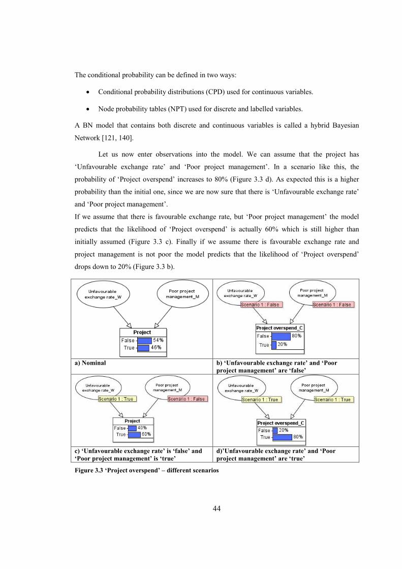
44

The conditional probability can be defined in two ways:

• Conditional probability distributions (CPD) used for continuous variables.

• Node probability tables (NPT) used for discrete and labelled variables.

A BN model that contains both discrete and continuous variables is called a hybrid Bayesian

Network [121, 140].

Let us now enter observations into the model. We can assume that the project has

‘Unfavourable exchange rate’ and ‘Poor project management’. In a scenario like this, the

probability of ‘Project overspend’ increases to 80% (Figure 3.3 d). As expected this is a higher

probability than the initial one, since we are now sure that there is ‘Unfavourable exchange rate’

and ‘Poor project management’.

If we assume that there is favourable exchange rate, but ‘Poor project management’ the model

predicts that the likelihood of ‘Project overspend’ is actually 60% which is still higher than

initially assumed (Figure 3.3 c). Finally if we assume there is favourable exchange rate and

project management is not poor the model predicts that the likelihood of ‘Project overspend’

drops down to 20% (Figure 3.3 b).

a) Nominal b) ‘Unfavourable exchange rate’ and ‘Poor

project management’ are ‘false’

c) ‘Unfavourable exchange rate’ is ‘false’ and

‘Poor project management’ is ‘true’

d)’Unfavourable exchange rate’ and ‘Poor

project management’ are ‘true’

Figure 3.3 ‘Project overspend’ – different scenarios

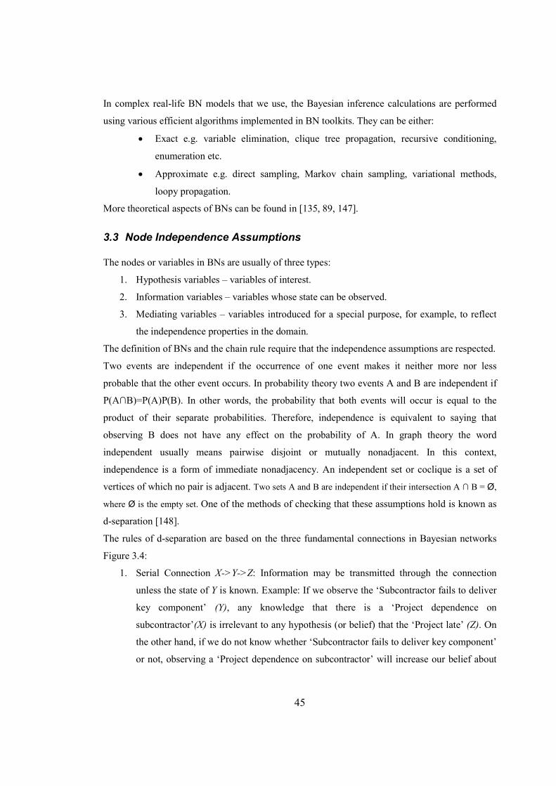
45

In complex real-life BN models that we use, the Bayesian inference calculations are performed

using various efficient algorithms implemented in BN toolkits. They can be either:

• Exact e.g. variable elimination, clique tree propagation, recursive conditioning,

enumeration etc.

• Approximate e.g. direct sampling, Markov chain sampling, variational methods,

loopy propagation.

More theoretical aspects of BNs can be found in [135, 89, 147].

3.3 Node Independence Assumptions

The nodes or variables in BNs are usually of three types:

1. Hypothesis variables – variables of interest.

2. Information variables – variables whose state can be observed.

3. Mediating variables – variables introduced for a special purpose, for example, to reflect

the independence properties in the domain.

The definition of BNs and the chain rule require that the independence assumptions are respected.

Two events are independent if the occurrence of one event makes it neither more nor less

probable that the other event occurs. In probability theory two events A and B are independent if

P(A∩B)=P(A)P(B). In other words, the probability that both events will occur is equal to the

product of their separate probabilities. Therefore, independence is equivalent to saying that

observing B does not have any effect on the probability of A. In graph theory the word

independent usually means pairwise disjoint or mutually nonadjacent. In this context,

independence is a form of immediate nonadjacency. An independent set or coclique is a set of

vertices of which no pair is adjacent. Two sets A and B are independent if their intersection A ∩ B = Ø,

where Ø is the empty set. One of the methods of checking that these assumptions hold is known as

d-separation [148].

The rules of d-separation are based on the three fundamental connections in Bayesian networks

Figure 3.4:

1. Serial Connection X->Y->Z: Information may be transmitted through the connection

unless the state of Y is known. Example: If we observe the ‘Subcontractor fails to deliver

key component’ (Y), any knowledge that there is a ‘Project dependence on

subcontractor’(X) is irrelevant to any hypothesis (or belief) that the ‘Project late’ (Z). On

the other hand, if we do not know whether ‘Subcontractor fails to deliver key component’

or not, observing a ‘Project dependence on subcontractor’ will increase our belief about

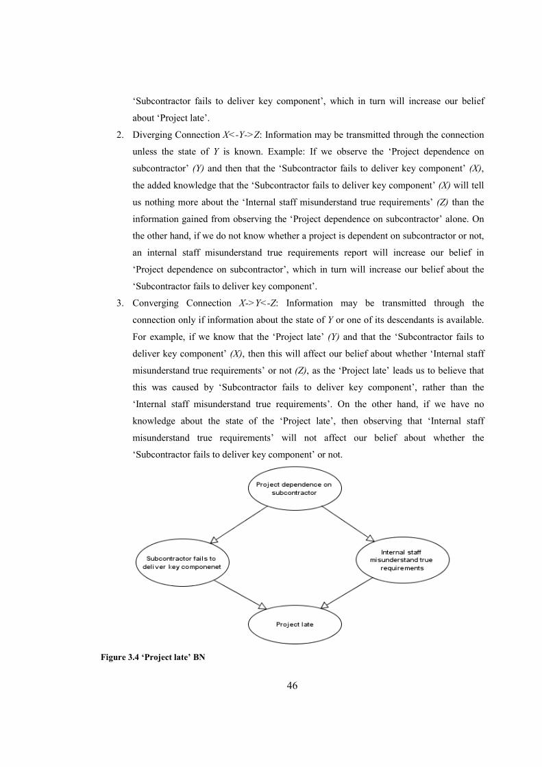
46

‘Subcontractor fails to deliver key component’, which in turn will increase our belief

about ‘Project late’.

2. Diverging Connection X<-Y->Z: Information may be transmitted through the connection

unless the state of Y is known. Example: If we observe the ‘Project dependence on

subcontractor’ (Y) and then that the ‘Subcontractor fails to deliver key component’ (X),

the added knowledge that the ‘Subcontractor fails to deliver key component’ (X) will tell

us nothing more about the ‘Internal staff misunderstand true requirements’ (Z) than the

information gained from observing the ‘Project dependence on subcontractor’ alone. On

the other hand, if we do not know whether a project is dependent on subcontractor or not,

an internal staff misunderstand true requirements report will increase our belief in

‘Project dependence on subcontractor’, which in turn will increase our belief about the

‘Subcontractor fails to deliver key component’.

3. Converging Connection X->Y<-Z: Information may be transmitted through the

connection only if information about the state of Y or one of its descendants is available.

For example, if we know that the ‘Project late’ (Y) and that the ‘Subcontractor fails to

deliver key component’ (X), then this will affect our belief about whether ‘Internal staff

misunderstand true requirements’ or not (Z), as the ‘Project late’ leads us to believe that

this was caused by ‘Subcontractor fails to deliver key component’, rather than the

‘Internal staff misunderstand true requirements’. On the other hand, if we have no

knowledge about the state of the ‘Project late’, then observing that ‘Internal staff

misunderstand true requirements’ will not affect our belief about whether the

‘Subcontractor fails to deliver key component’ or not.

Figure 3.4 ‘Project late’ BN

47

Two variables X and Z are d-separated if for all paths between X and Z there is an intermediate

variable such as Y that either

• The connection is serial or diverging and Y is instantiated (i.e. its value is known), or

• The connection is converging and neither Y nor any of its descendants have received

evidence.

In the example of Figure 3.4, the set of nodes {Subcontractor fails to deliver key

component, Internal staff misunderstand true requirements} d-separates {Project dependence on

subcontractor} and {Project late}, because ‘Subcontractor fails to deliver key component’ blocks

the path (Project dependence on subcontractor, Subcontractor fails to deliver key component,

Project late) and ‘Internal staff misunderstand true requirements’ blocks the path (Project

dependence on subcontractor, Internal staff misunderstand true requirements, Project late). In

both cases, the blocking node is linear on the path. Furthermore, {Project dependence on

subcontractor} d-separates {Subcontractor fails to deliver key component} and {Internal staff

misunderstand true requirements}, where ‘Project dependence on subcontractor’ is diverging on

the only path between them, (Subcontractor fails to deliver key component, Project dependence

on subcontractor, Internal staff misunderstand true requirements).

If X and Z are not d-separated, they are d-connected. Dependence and independence relies

on what you know (and do not know). In other words, the available evidence plays a significant

role when determining the dependence and independence relations.

We can distinguish various patterns of plausible common sense reasoning that are

supported by BNs. These patterns can be explained using the example network in Figure 3.5; to

ensure that the example is as simple as possible we assume that all nodes are discrete, having the

two possible states ‘true’ and ‘false’:

• Predictive: If we believe that ‘Unfavourable exchange rate’, then it becomes more

plausible for us that the ‘Project overspend’. If we find out that ‘Unfavourable exchange

rate’ is true, the ‘Project overspend’ has become more plausible for us. We can also

observe predictive pattern in the example in Figure 3.4.

• Diagnostic: Suppose we observe that ‘Project overspend’ is true then both ‘Unfavourable

exchange rate’ and ‘Poor project management’ become more likely as shown in Figure

3.6.

• Explaining away:

48

Figure 3.5 ‘Project overspend’ BN

Figure 3.6 ‘Project overspend’ is ‘true’

If we observe ‘Project overspend’ is true (Figure 3.6) then the most likely explanation is

‘Unfavourable exchange rate’ while revised probability for ‘Poor project management’ is still

low. However, if we observe that the ‘Project late’ is also true (Figure 3.7) then we see that

‘Project overspend’ is most likely caused by ‘Poor project management’ and not ‘Unfavourable

exchange rate’. Hence, the ‘Project overspend’ is explained away by the observation that the

project is late.

Figure 3.7 ‘Project overspend’ is ‘true’ and ‘Project late’ is ‘false’

49

3.4 Bayesian Network Modelling Techniques

Usually domain experts can determine the important variables which need to be included

in the model and the links between them. Specifying unconditional and conditional probabilities

for each node is not an easy task. In models where there are many states per variable and nodes

with many parents it is a very complex task to elicit consistent NPTs or CPDs manually. In this

study we used a BN tool called AgenaRisk which supports defining NPTs and CPDs using

expressions which often simplify the task of model preparation and reduce the time needed to

build a model.

One of the biggest challenges in BNs is completing NPTs [48]. For example, if a node

with 5 states has two parents each with 5 states then the child node NPT has 125 cells to

complete. This section introduces different ways of making that task easier. Another challenge is

continuous nodes. In section 3.5.3 we discuss how to handle continuous nodes.

3.4.1 Noisy OR

For Boolean Nodes with multiple parents, noisyOR allows us to quickly model a range of

complex situations that would be far too difficult to do by manually completing an NPT [44, 173,

203]. Therefore, the NoisyOR operator is one of the most powerful operators. Let us observe an

example where we are trying to predict whether a project is going to run over schedule. Assume

the node F is the node ‘Schedule overrun’. Suppose we decide that we identify five factors that

can influence F, namely:

• Poor management (A)

• Requirements creep (B)

• Process inefficiencies (C)

• Inadequate business environment (D)

• Lack of project commitment (E)

The structure of such a model is shown in Figure 3.8. For simplicity, in this example, let

us assume that the nodes A to E are independent and they all influence the node F. In this case we

cannot use a Boolean expression, because there will always be uncertainty about F. For example,

even if all the parents are ‘True’ we cannot say with certainty that F will be ‘True’. On the other

hand, if we try to complete the NPT for node F manually we have 64 entries to complete which

would be extremely tedious and prone to error. Moreover, imagine trying to complete any such

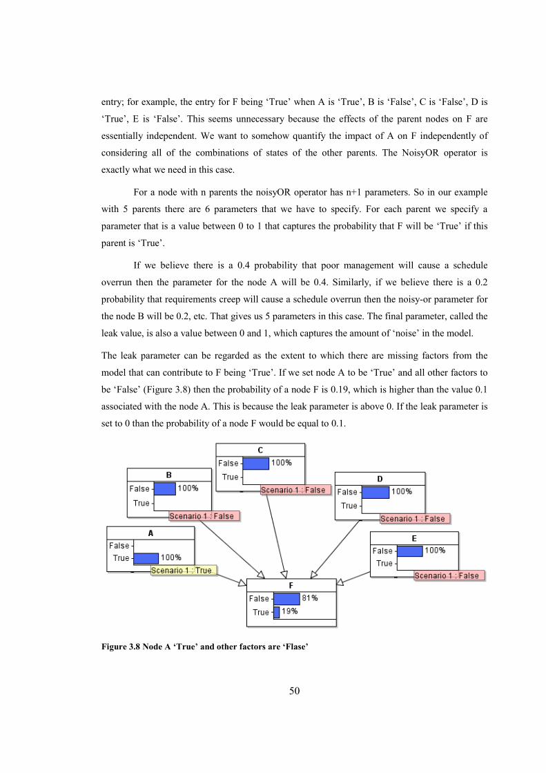
50

entry; for example, the entry for F being ‘True’ when A is ‘True’, B is ‘False’, C is ‘False’, D is

‘True’, E is ‘False’. This seems unnecessary because the effects of the parent nodes on F are

essentially independent. We want to somehow quantify the impact of A on F independently of

considering all of the combinations of states of the other parents. The NoisyOR operator is

exactly what we need in this case.

For a node with n parents the noisyOR operator has n+1 parameters. So in our example

with 5 parents there are 6 parameters that we have to specify. For each parent we specify a

parameter that is a value between 0 to 1 that captures the probability that F will be ‘True’ if this

parent is ‘True’.

If we believe there is a 0.4 probability that poor management will cause a schedule

overrun then the parameter for the node A will be 0.4. Similarly, if we believe there is a 0.2

probability that requirements creep will cause a schedule overrun then the noisy-or parameter for

the node B will be 0.2, etc. That gives us 5 parameters in this case. The final parameter, called the

leak value, is also a value between 0 and 1, which captures the amount of ‘noise’ in the model.

The leak parameter can be regarded as the extent to which there are missing factors from the

model that can contribute to F being ‘True’. If we set node A to be ‘True’ and all other factors to

be ‘False’ (Figure 3.8) then the probability of a node F is 0.19, which is higher than the value 0.1

associated with the node A. This is because the leak parameter is above 0. If the leak parameter is

set to 0 than the probability of a node F would be equal to 0.1.

Figure 3.8 Node A ‘True’ and other factors are ‘Flase’

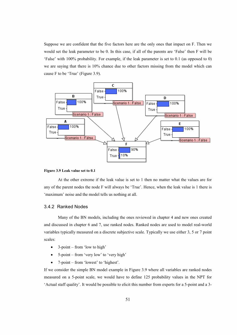
51

Suppose we are confident that the five factors here are the only ones that impact on F. Then we

would set the leak parameter to be 0. In this case, if all of the parents are ‘False’ then F will be

‘False’ with 100% probability. For example, if the leak parameter is set to 0.1 (as opposed to 0)

we are saying that there is 10% chance due to other factors missing from the model which can

cause F to be ‘True’ (Figure 3.9).

Figure 3.9 Leak value set to 0.1

At the other extreme if the leak value is set to 1 then no matter what the values are for

any of the parent nodes the node F will always be ‘True’. Hence, when the leak value is 1 there is

‘maximum’ noise and the model tells us nothing at all.

3.4.2 Ranked Nodes

Many of the BN models, including the ones reviewed in chapter 4 and new ones created

and discussed in chapter 6 and 7, use ranked nodes. Ranked nodes are used to model real-world

variables typically measured on a discrete subjective scale. Typically we use either 3, 5 or 7 point

scales:

• 3-point – from ‘low to high’

• 5-point – from ‘very low’ to ‘very high’

• 7-point – from ‘lowest’ to ‘highest’.

If we consider the simple BN model example in Figure 3.9 where all variables are ranked nodes

measured on a 5-point scale, we would have to define 125 probability values in the NPT for

‘Actual staff quality’. It would be possible to elicit this number from experts for a 5-point and a 3-

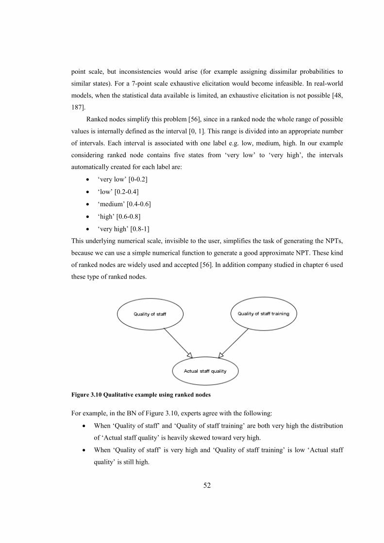
52

point scale, but inconsistencies would arise (for example assigning dissimilar probabilities to

similar states). For a 7-point scale exhaustive elicitation would become infeasible. In real-world

models, when the statistical data available is limited, an exhaustive elicitation is not possible [48,

187].

Ranked nodes simplify this problem [56], since in a ranked node the whole range of possible

values is internally defined as the interval [0, 1]. This range is divided into an appropriate number

of intervals. Each interval is associated with one label e.g. low, medium, high. In our example

considering ranked node contains five states from ‘very low’ to ‘very high’, the intervals

automatically created for each label are:

• ‘very low’ [0-0.2]

• ‘low’ [0.2-0.4]

• ‘medium’ [0.4-0.6]

• ‘high’ [0.6-0.8]

• ‘very high’ [0.8-1]

This underlying numerical scale, invisible to the user, simplifies the task of generating the NPTs,

because we can use a simple numerical function to generate a good approximate NPT. These kind

of ranked nodes are widely used and accepted [56]. In addition company studied in chapter 6 used

these type of ranked nodes.

Figure 3.10 Qualitative example using ranked nodes

For example, in the BN of Figure 3.10, experts agree with the following:

• When ‘Quality of staff’ and ‘Quality of staff training’ are both very high the distribution

of ‘Actual staff quality’ is heavily skewed toward very high.

• When ‘Quality of staff’ is very high and ‘Quality of staff training’ is low ‘Actual staff

quality’ is still high.

53

• When ‘Quality of staff’ is low and ‘Quality of staff training’ is high ‘Actual staff quality’

is skewed toward low.

• When ‘Quality of staff’ and ‘Quality of staff training’ are both very low the distribution

of ‘Actual staff quality’ is heavily skewed toward very low.

Such relations suggest ‘Actual staff quality’ is a distribution whose mean is a weighted sum

of the parents. Hence, various weighted expressions significantly simplify the process of defining

NPTs. In equation (2-4) we have used a weighted expression to define the NPT for ‘Actual staff

quality’ from Figure 3.12:

AS = wmean (2, SQ, 1, ST) (2-4)

This expression tells us that ‘Actual staff quality’ is a weighted mean of ‘Staff quality’ and ‘Staff

training quality’, with the former having twice the impact than the latter.

Ranked nodes very often use Truncated Normal (TNormal) distribution [56]. This is a Gaussian

distribution that has been truncated at both ends. Considering it is a Gaussian distribution, it has

to specify the mean (µ) and the standard deviation (σ). The difference between Normal and

TNormal is that TNormal has finite end points, hence the range (a and b) of the distribution must

also be specified. This range is always [0, 1] in ranked nodes.

To demonstrate this we would have to add a variance (σ2) of 0.001 to our earlier example:

AS = TNormal (wmean(2, SQ, 1, ST), 0.001, 0, 1) (2-5)

When we run this model for the following two scenarios the result achieved is presented in Figure

3.11 :

• Scenario 1: ‘Quality of staff’ = ‘very high’ and ‘Quality of staff training’ = ‘very low’

• Scenario 2: ‘Quality of staff’ = ‘very low’ and ‘Quality of staff training’ = ‘very high’.

Figure 3.11 Predicted ‘Actual staff quality’

Figure 3.12 shows the result of defining different variance in a ranked node.

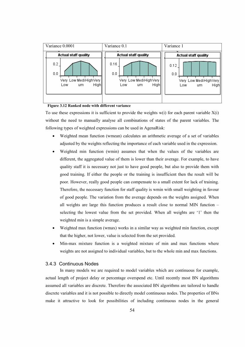
54

Variance 0.0001 Variance 0.1 Variance 1

Figure 3.12 Ranked node with different variance

To use these expressions it is sufficient to provide the weights w(i) for each parent variable X(i)

without the need to manually analyse all combinations of states of the parent variables. The

following types of weighted expressions can be used in AgenaRisk:

• Weighted mean function (wmean) calculates an arithmetic average of a set of variables

adjusted by the weights reflecting the importance of each variable used in the expression.

• Weighted min function (wmin) assumes that when the values of the variables are

different, the aggregated value of them is lower than their average. For example, to have

quality staff it is necessary not just to have good people, but also to provide them with

good training. If either the people or the training is insufficient then the result will be

poor. However, really good people can compensate to a small extent for lack of training.

Therefore, the necessary function for staff quality is wmin with small weighting in favour

of good people. The variation from the average depends on the weights assigned. When

all weights are large this function produces a result close to normal MIN function –

selecting the lowest value from the set provided. When all weights are ‘1’ then the

weighted min is a simple average.

• Weighted max function (wmax) works in a similar way as weighted min function, except

that the higher, not lower, value is selected from the set provided.

• Min-max mixture function is a weighted mixture of min and max functions where

weights are not assigned to individual variables, but to the whole min and max functions.

3.4.3 Continuous Nodes

In many models we are required to model variables which are continuous for example,

actual length of project delay or percentage overspend etc. Until recently most BN algorithms

assumed all variables are discrete. Therefore the associated BN algorithms are tailored to handle

discrete variables and it is not possible to directly model continuous nodes. The properties of BNs

make it attractive to look for possibilities of including continuous nodes in the general

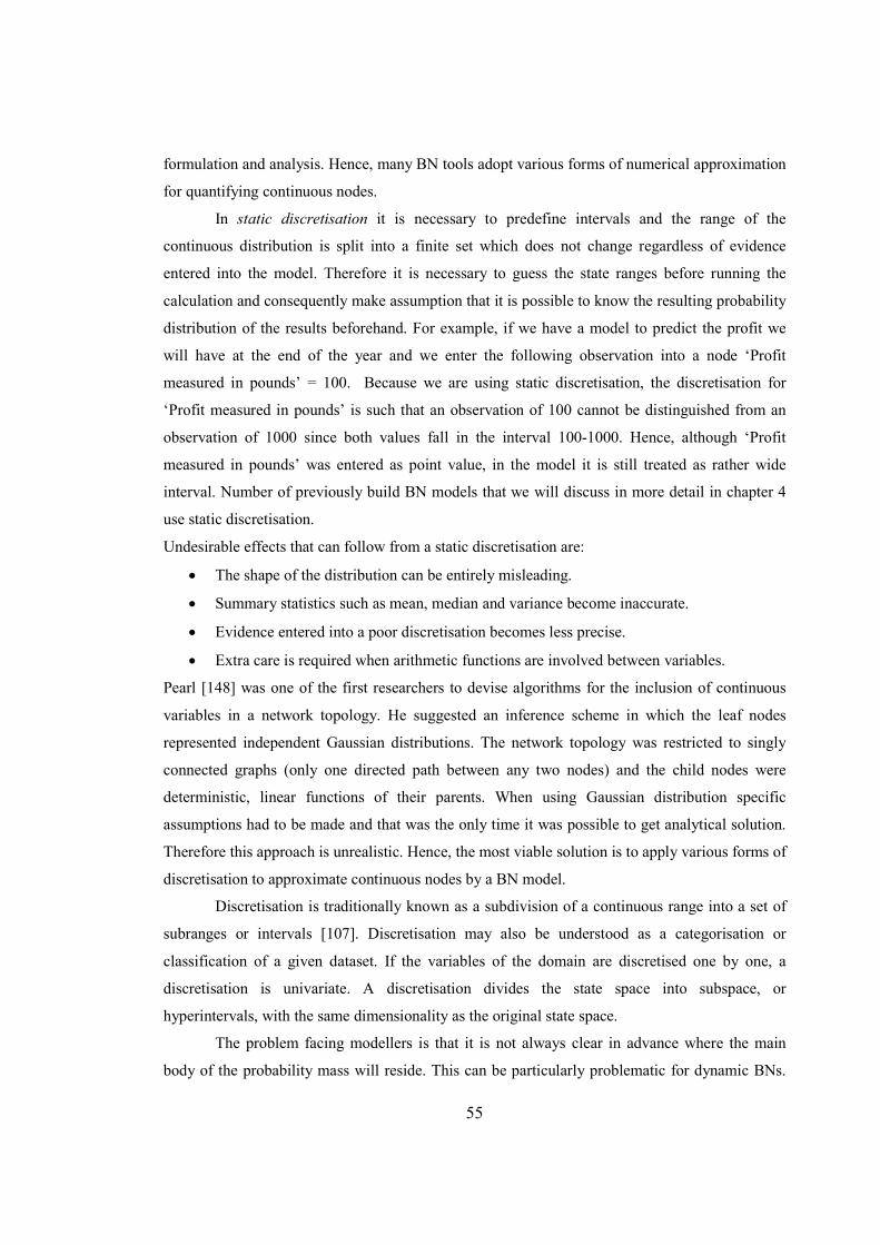
55

formulation and analysis. Hence, many BN tools adopt various forms of numerical approximation

for quantifying continuous nodes.

In static discretisation it is necessary to predefine intervals and the range of the

continuous distribution is split into a finite set which does not change regardless of evidence

entered into the model. Therefore it is necessary to guess the state ranges before running the

calculation and consequently make assumption that it is possible to know the resulting probability

distribution of the results beforehand. For example, if we have a model to predict the profit we

will have at the end of the year and we enter the following observation into a node ‘Profit

measured in pounds’ = 100. Because we are using static discretisation, the discretisation for

‘Profit measured in pounds’ is such that an observation of 100 cannot be distinguished from an

observation of 1000 since both values fall in the interval 100-1000. Hence, although ‘Profit

measured in pounds’ was entered as point value, in the model it is still treated as rather wide

interval. Number of previously build BN models that we will discuss in more detail in chapter 4

use static discretisation.

Undesirable effects that can follow from a static discretisation are:

• The shape of the distribution can be entirely misleading.

• Summary statistics such as mean, median and variance become inaccurate.

• Evidence entered into a poor discretisation becomes less precise.

• Extra care is required when arithmetic functions are involved between variables.

Pearl [148] was one of the first researchers to devise algorithms for the inclusion of continuous

variables in a network topology. He suggested an inference scheme in which the leaf nodes

represented independent Gaussian distributions. The network topology was restricted to singly

connected graphs (only one directed path between any two nodes) and the child nodes were

deterministic, linear functions of their parents. When using Gaussian distribution specific

assumptions had to be made and that was the only time it was possible to get analytical solution.

Therefore this approach is unrealistic. Hence, the most viable solution is to apply various forms of

discretisation to approximate continuous nodes by a BN model.

Discretisation is traditionally known as a subdivision of a continuous range into a set of

subranges or intervals [107]. Discretisation may also be understood as a categorisation or

classification of a given dataset. If the variables of the domain are discretised one by one, a

discretisation is univariate. A discretisation divides the state space into subspace, or

hyperintervals, with the same dimensionality as the original state space.

The problem facing modellers is that it is not always clear in advance where the main

body of the probability mass will reside. This can be particularly problematic for dynamic BNs.

56

In this case, the probability mass will often move across timeslices, so that a discretisation which

is appropriate for one timeslice turns out to be inappropriate for another.

A solution, involving dynamic discretisation, has been proposed by Neil, Tailor and

Marquez [141]. The dynamic discretisation algorithm outline is as follows:

1. Calculate the current marginal probability distribution for a node given its current

discretisation.

2. Split the discrete state with the highest entropy error into two equally sized states.

3. Repeat steps 1 and 2 until converged to an acceptable level of accuracy.

4. Repeat steps 1, 2 and 3 for all nodes in the BN.

This algorithm has been implemented into the AgenaRisk toolset. Hence, we can simply set a

numeric node as a simulation node without having to worry about pre-defined intervals. It is

sufficient to define a single interval [x, y] for any variable that is bounded below by x and above

by y, while for infinite bounds we only need introduce one extra interval. This is the approach

that has been adopted in the subsequent models.

3.4.4 Object Oriented Bayesian Networks

Object Oriented Bayesian Networks (OOBN) were introduced to help model large and

complex systems [106]. The idea of OOBNs was based on the object-oriented programming

languages and they provide a robust, flexible and efficient framework. It is possible to build

complex models by using OOBNs. With objects we can modularise the model into chunks

representing logical groupings of risks or time dependencies between objects. In an OOBN we are

essentially modelling sequential time series processes where each ‘time-slice’ in the time series is

modelled as BN. OOBNs are used in some example models discussed in the next chapter as well

as the model developed in this thesis.

The basic element in an OOBN is an object. For multiple objects we can define classes.

Classes of objects provide the ability to describe a general and reusable network that can be used

in many different contexts. Figure 3.13 shows a model composed of two risk objects. Each object

is linked to the network with reference link that connects an output node in one object to an input

node in other object (dashed link in Figure 3.13).

57

Figure 3.13 OOBN – structural representation

Figure 3.14 shows how objects are linked in AgenaRisk to build a large BN.

Figure 3.14 OOBN in AgenaRisk

Important advantages of OOBN are [106]:

• Natural representation of objects that are composed of lower level objects.

• Classes of objects explicitly represented which allows the incorporation of inheritance.

• Natural model fragment reuse.

• Ability to speed up the inference process by encapsulation of objects within other objects

and the code reuse.

• Ability to support a natural framework for abstraction and refinement.

3.5 Strengths and Limitations of Bayesian Networks

The strengths of BNs over alternative techniques are:

• Explicit incorporation of uncertainty

• BNs, in contrast to classical statistics, can model causal factors explicitly. This makes

them an ideal tool for predicting the future.

• The graphical nature of a BN makes it a powerful communication tool. Causal

relationships among the variables or nodes can be seen easily without the need to

compute probabilities.

58

• BNs are intuitive, conceptual and easily understandable. This helps at the development

stage when the model is being discussed between the project manager and the various

parties.

• Ability to combine subjective data (expert knowledge) and objective data. This is a great

advantage especially when objective data is scarce or when there is the need to

incorporate expert opinion in the model.

• A BN will update the probability distribution for every unknown variable whenever an

observation is entered into any node i.e. reason from effect to cause and vice versa.

• The model can be easily updated or previous beliefs modified in light of new evidence,

for example the notion of explaining away evidence.

• BNs can be used to perform sensitivity or "what-if" analyses to examine the sensitivity of

predictions, or conclusions against initial assumptions.

• BNs can make predictions with incomplete data. If no observation is entered then the

model assumes prior distribution.

• BNs are capable of modelling highly complex systems. The areas of application

mentioned earlier demonstrate this.

Bayesian networks do have some limitations. Originally BNs were constructed based on

human heuristics and thus have been subject to human biases. The fact is that a BN model is only

as good as the modeller and experts who produced it, since it is a representation of the modeller

and the experts' perceptions of reality. Therefore best fit is chosen given the modeller and experts.

Another limitation centres on the extent of the quality of the prior beliefs used in Bayesian

inference processing. The usefulness of a BN is based on the reliability of its prior knowledge. An

excessively optimistic or pessimistic expectation of the quality of these prior beliefs will either

distort the entire network or invalidate the results. Hence, it is difficult to empirically validate

model estimates in models built only on expert knowledge.

3.6 Application of Bayesian Networks

Bayesian networks have had considerable applications in many fields both in academia

and industry. Hundreds of publications have described BNs application in various fields [61]. In

the academic field, Nikovski [142] applied BNs to problems in medical diagnosis, Hansson and

Mayer [77], Ames et al. [5] in heuristic search, Marcot et al. [120] in ecology, Heckermann [75]

in data mining and Breese and Heckerman [22] in intelligent trouble shooting systems, Xenos

[197] to predict and assess students’ behavior, Rodin et al. [163] in biology, Andradottir [6] in

simulation.

59

The industrial application of Bayesian technology spans several fields: Fenton et al. [61,

57, 55, 58] applied BNs to software quality measurement, Neil et al. [136, 137] in financial

operational risk scenarios, Langseth and Lindqvist [110] in software maintenance modeling,

Bobbio et al. [18]; Langseth [111]; Ingleby and West [83] in general software reliability

modeling, Lucas et al. [116] in biomedicine and health-care, Hackerman et al. [76] in medical

diagnosis, Borsuk et al. [21] in environmental science.

3.7 Summary

In this chapter we have reviewed Bayes Theorem and how it is used when building BNs.

Also we have looked at the advantages and the disadvantages of BNs. This chapter has provided

an introduction to BNs and the different types of BN structure in order to enable the reader to

understand the models developed later in the thesis.

In the next chapter, we will look at BN models which address project trade-off analysis;

as well as BN models that address and support different features of project risk management

(SIMP, MODIST and Productivity model). Later in the chapter, we will look at construction

projects BNs, Khodakarami’s model and operational risk models.

60

4. Existing BN Project Risk Management Models

This chapter focuses on the review of existing BN models. The models to which the

author had access have been extensively tested. BN models that address trade-offs are reviewed

as well as a group of other BN models related to project risk management and relevant to this

thesis. It is demonstrated how such models can be used to provide useful information for decision

makers, and the advantages and disadvantages of these models are discussed. The new

contribution of this chapter is a thorough analysis, some of it (SIMP model) which was not

displayed before in public domain, of selected existing BN models for project risk management.

4.1 Introduction to Bayesian Net Modelling

We will specifically look at BN models which address project trade-off analysis. These

models are: SIMP [3], MODIST [4, 63] and Productivity model [157]. SIMP and MODIST

attempted for the first time ever to look at project risk management trade-off issues, and are of

particular interest in this thesis, since the author has drawn motivation for analysing trade-offs

from these models. In the second part of this chapter, we will look at construction projects BNs,

Khodakarami’s model and operational risk models. These models address and support different

features of project risk management. All of the models were used to provide improved methods of

risk analysis and assessment for project managers in different areas and are discussed in more

detail in the sections that follow.

4.2 BN models addressing trade-off analysis

4.2.1 SIMP – Major Projects BN

Model background

The SIMP project was based on the practices of a major international defence company

for risk and risk criteria. SIMP project objective was to determine whether BNs can model

defence system engineering processes and derive predictions about risk and uncertainty for

decision support. The project aimed to develop methods and tools for quantitative risk assessment

and requirements analysis in complex systems engineering domains. The motivation for this

research lay in systems cost over-runs, delayed delivery and inadequate performance of complex

systems in the military and civil sectors. Trade-offs addressed between these variables served as

inspiration for the author’s focus on modelling trade-offs in large projects. These problems were

61

caused by poor organisation of the systems engineering process, weak risk assessment, inability

to manage risk and poor requirements analysis. Since this is a commercial model it provides the

basis for commercial application of trade-off analysis and models that implement it. The SIMP

project focused on improving the systems engineering process and the quality of the system’s

products, in particular to enhance the requirements capture to make systems fit for purpose.

Model structure

The aim of the SIMP model was to predict and assess overall risk status of large and

complex systems engineering projects. The SIMP model is aimed at project managers. There are

six sub-nets in the model:

• Resource performance – variables capturing the quality of the contribution that the

resources make to the project (e.g. subcontract management, procurement, information,

planning, organisation effectiveness, motivation, staff, facilities)

• Technical quality – variables capturing the quality of the contribution that the technical

parts make to the project (e.g. interfacing, design solution, key subsystems, obsolescence,

technical facilities)

• Schedule – variables capturing the ‘real’ schedule that is suggested by the project risk

attributes (e.g. budget constraints, process efficiency, requirements, business

environment) and variables capturing current schedule of the project (e.g. actual schedule

differential above agreed) The schedule is expressed as the deviation from that of the

nominal project.

• Cost – variables capturing the ‘real’ cost that is suggested by the project risk attributes

(e.g. process efficiency, requirements, business environment) and variables capturing the

current cost of the project (e.g. actual cost differential above agreed). The cost is

expressed as the deviation from that of the nominal project.

• Performance – represents the overall performance of the system being built. It is directly

influenced by two variables: actual schedule differential and actual cost differential.

• Reputation – variables capture the reputation in the commercial environment (e.g. actual

schedule differential above agreed, actual cost differential above agreed)

Figure 4.1 shows the key part of the model that enables managers to perform trade-off

analysis between:

• Time – represented by schedule differential implied by project attributes and

actual schedule differential

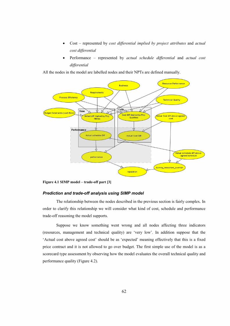
62

• Cost – represented by cost differential implied by project attributes and actual

cost differential

• Performance – represented by actual schedule differential and actual cost

differential

All the nodes in the model are labelled nodes and their NPTs are defined manually.

Figure 4.1 SIMP model – trade-off part [3]

Prediction and trade-off analysis using SIMP model

The relationship between the nodes described in the previous section is fairly complex. In

order to clarify this relationship we will consider what kind of cost, schedule and performance

trade-off reasoning the model supports.

Suppose we know something went wrong and all nodes affecting three indicators

(resources, management and technical quality) are ‘very low’. In addition suppose that the

‘Actual cost above agreed cost’ should be as ‘expected’ meaning effectively that this is a fixed

price contract and it is not allowed to go over budget. The first simple use of the model is as a

scorecard type assessment by observing how the model evaluates the overall technical quality and

performance quality (Figure 4.2).

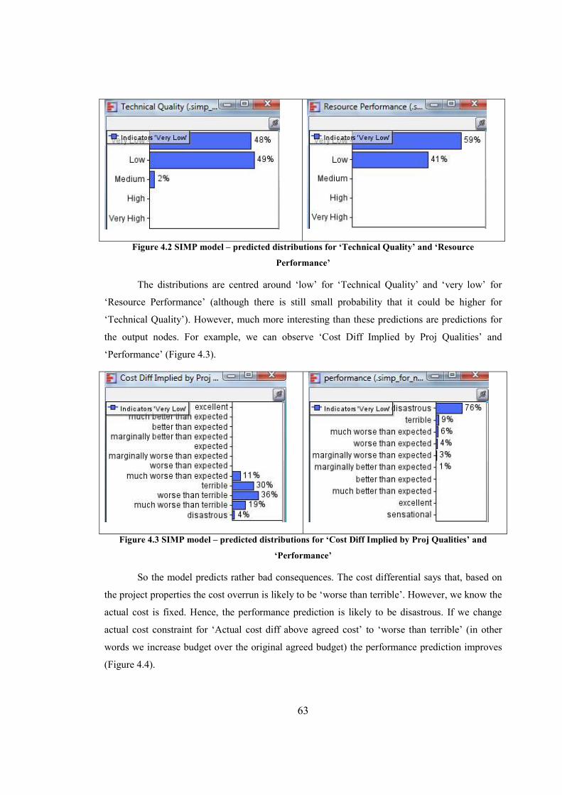
63


Performance’

The distributions are centred around ‘low’ for ‘Technical Quality’ and ‘very low’ for

‘Resource Performance’ (although there is still small probability that it could be higher for

‘Technical Quality’). However, much more interesting than these predictions are predictions for

the output nodes. For example, we can observe ‘Cost Diff Implied by Proj Qualities’ and

‘Performance’ (Figure 4.3).

Figure 4.3 SIMP model – predicted distributions for ‘Cost Diff Implied by Proj Qualities’ and

‘Performance’

So the model predicts rather bad consequences. The cost differential says that, based on

the project properties the cost overrun is likely to be ‘worse than terrible’. However, we know the

actual cost is fixed. Hence, the performance prediction is likely to be disastrous. If we change

actual cost constraint for ‘Actual cost diff above agreed cost’ to ‘worse than terrible’ (in other

words we increase budget over the original agreed budget) the performance prediction improves

(Figure 4.4).

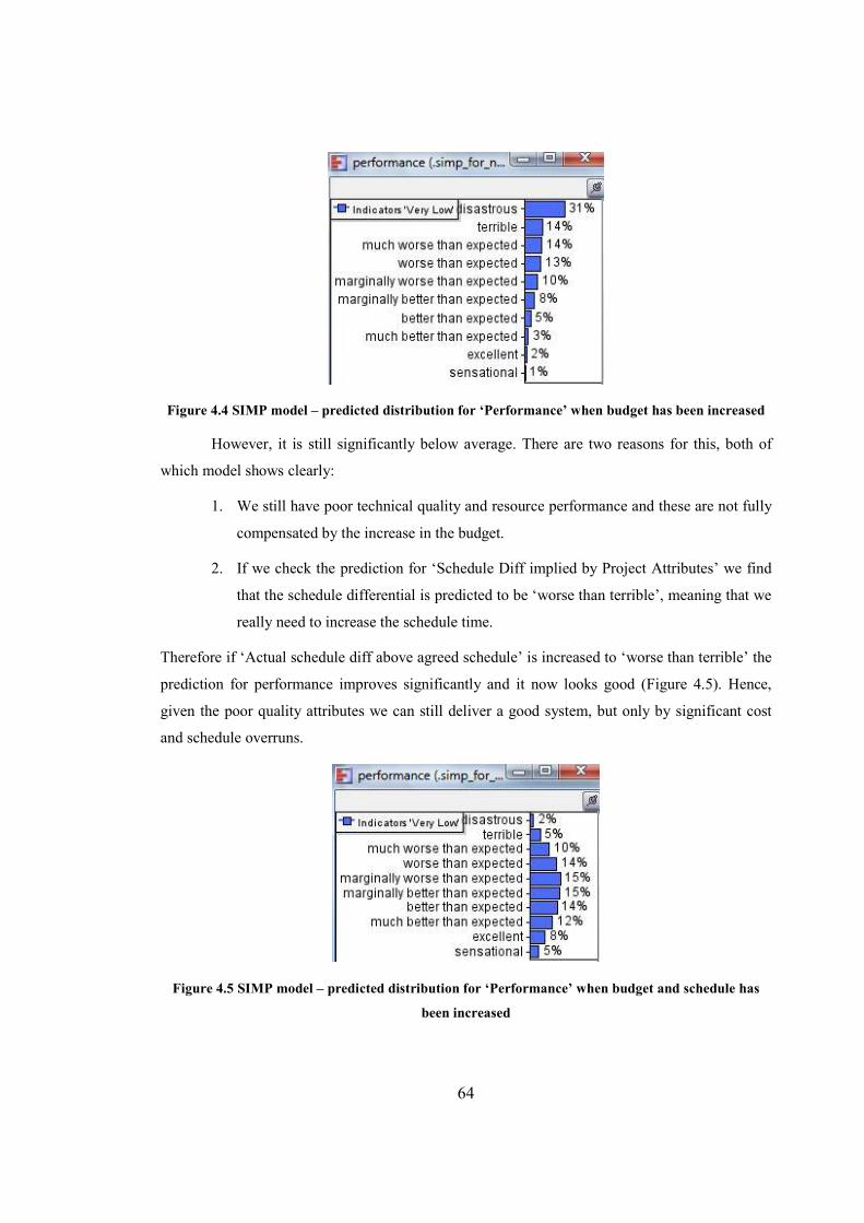
64

Figure 4.4 SIMP model – predicted distribution for ‘Performance’ when budget has been increased

However, it is still significantly below average. There are two reasons for this, both of

which model shows clearly:

1. We still have poor technical quality and resource performance and these are not fully

compensated by the increase in the budget.

2. If we check the prediction for ‘Schedule Diff implied by Project Attributes’ we find

that the schedule differential is predicted to be ‘worse than terrible’, meaning that we

really need to increase the schedule time.

Therefore if ‘Actual schedule diff above agreed schedule’ is increased to ‘worse than terrible’ the

prediction for performance improves significantly and it now looks good (Figure 4.5). Hence,

given the poor quality attributes we can still deliver a good system, but only by significant cost

and schedule overruns.

Figure 4.5 SIMP model – predicted distribution for ‘Performance’ when budget and schedule has

been increased

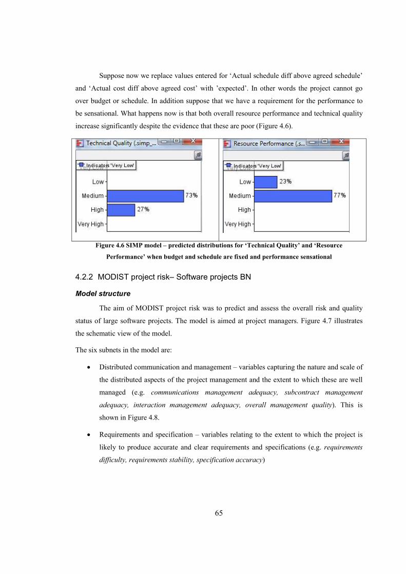
65

Suppose now we replace values entered for ‘Actual schedule diff above agreed schedule’

and ‘Actual cost diff above agreed cost’ with ’expected’. In other words the project cannot go

over budget or schedule. In addition suppose that we have a requirement for the performance to

be sensational. What happens now is that both overall resource performance and technical quality

increase significantly despite the evidence that these are poor (Figure 4.6).


Performance’ when budget and schedule are fixed and performance sensational

4.2.2 MODIST project risk– Software projects BN

Model structure

The aim of MODIST project risk was to predict and assess the overall risk and quality

status of large software projects. The model is aimed at project managers. Figure 4.7 illustrates

the schematic view of the model.

The six subnets in the model are:

• Distributed communication and management – variables capturing the nature and scale of

the distributed aspects of the project management and the extent to which these are well

managed (e.g. communications management adequacy, subcontract management

adequacy, interaction management adequacy, overall management quality). This is

shown in Figure 4.8.

• Requirements and specification – variables relating to the extent to which the project is

likely to produce accurate and clear requirements and specifications (e.g. requirements

difficulty, requirements stability, specification accuracy)

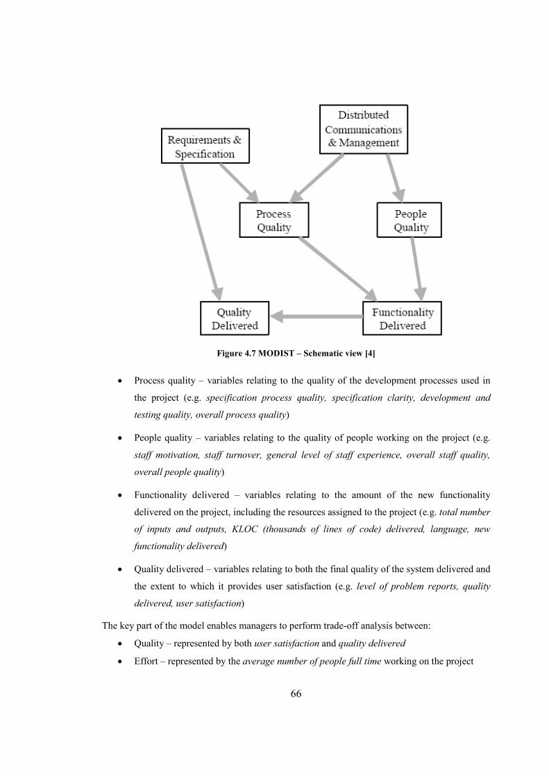
66

Figure 4.7 MODIST – Schematic view [4]

• Process quality – variables relating to the quality of the development processes used in

the project (e.g. specification process quality, specification clarity, development and

testing quality, overall process quality)

• People quality – variables relating to the quality of people working on the project (e.g.

staff motivation, staff turnover, general level of staff experience, overall staff quality,

overall people quality)

• Functionality delivered – variables relating to the amount of the new functionality

delivered on the project, including the resources assigned to the project (e.g. total number

of inputs and outputs, KLOC (thousands of lines of code) delivered, language, new

functionality delivered)

• Quality delivered – variables relating to both the final quality of the system delivered and

the extent to which it provides user satisfaction (e.g. level of problem reports, quality

delivered, user satisfaction)

The key part of the model enables managers to perform trade-off analysis between:

• Quality – represented by both user satisfaction and quality delivered

• Effort – represented by the average number of people full time working on the project

67

• Time – represented by the project duration

• Functionality – meaning functionality delivered

One of the main limitations of MODIST trade-off analysis is the fact that it applies only to

software engineering projects. Functionality in the MODIST model is based on function points

which are a well known measure of software output. This is built into NPTs for functionality and

therefore it is specific to software engineering projects and not easily extendable.

Management and Communication Subnet

We will show this subnet (Figure 4.8) in more detail in order to examine some of the

techniques used. This subnet models the size of a project team, its geographical diversity, the

amount of work that has been subcontracted and the quality of the subcontracted work.

Ranked nodes discussed in section 3.4.2 are used extensively in this subnet and

throughout the entire model. In Figure 4.7 nodes with symbol are ranked nodes and 10 out of

12 nodes in this subnet are ranked nodes. The dominance of the ranked nodes indicates the scale

of expert judgement required in this subnet and indeed the model. This model focuses on

quantifying aspects of software projects which are often omitted due to the lack of data.

This subnet also makes extensive use of the TNormal expression discussed in section

3.5.2. All the nodes in Figure 4.8 with symbol have their NPTs defined using TNormal

expression. For example, NPT for Communications management adequacy node is:

Communications management adequacy = TNormal (wmax(2.0, sdc, 5.0, cmq), 0.005, 0.0, 1.0)

i.e. it is a TNormal whose mean is a weighted maximum of its two parent nodes and whose

variance is 0.005.

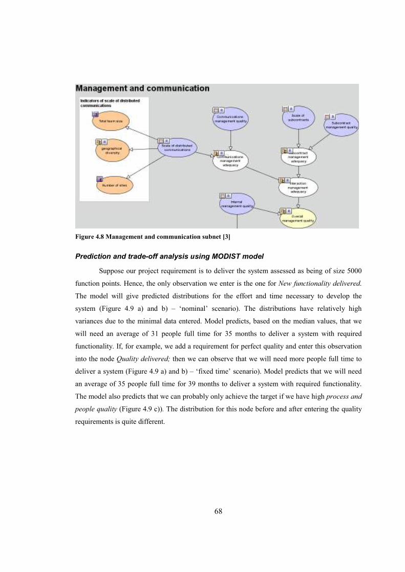
68

Figure 4.8 Management and communication subnet [3]

Prediction and trade-off analysis using MODIST model

Suppose our project requirement is to deliver the system assessed as being of size 5000

function points. Hence, the only observation we enter is the one for New functionality delivered.

The model will give predicted distributions for the effort and time necessary to develop the

system (Figure 4.9 a) and b) – ‘nominal’ scenario). The distributions have relatively high

variances due to the minimal data entered. Model predicts, based on the median values, that we

will need an average of 31 people full time for 35 months to deliver a system with required

functionality. If, for example, we add a requirement for perfect quality and enter this observation

into the node Quality delivered; then we can observe that we will need more people full time to

deliver a system (Figure 4.9 a) and b) – ‘fixed time’ scenario). Model predicts that we will need

an average of 35 people full time for 39 months to deliver a system with required functionality.

The model also predicts that we can probably only achieve the target if we have high process and

people quality (Figure 4.9 c)). The distribution for this node before and after entering the quality

requirements is quite different.

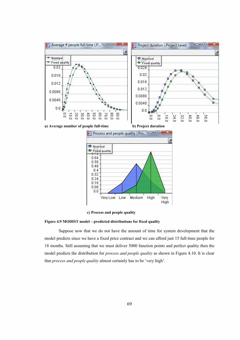
69

a) Average number of people full-time b) Project duration

c) Process and people quality

Figure 4.9 MODIST model – predicted distributions for fixed quality

Suppose now that we do not have the amount of time for system development that the

model predicts since we have a fixed price contract and we can afford just 15 full-time people for

18 months. Still assuming that we must deliver 5000 function points and perfect quality then the

model predicts the distribution for process and people quality as shown in Figure 4.10. It is clear

that process and people quality almost certainly has to be ‘very high’.

70

Figure 4.10 MODIST model – prediction distribution for fixed quality, schedule and effort

If for example, we know that process and people quality is only average then we can look

at possible trade-offs between functionality and quality. If we still insist on 5000 function points

and remove the quality requirement the model predicts the quality very likely to be abysmal. If

we keep the perfect quality requirement, but remove the functionality delivered requirement, the

model predicts a vastly reduced number of function points with the median of 566 compared to

the original 5000.

4.2.3 Radlinski’s “Productivity” Model

The MODIST project risk model discussed in the previous section is one part of the

MODIST toolset. Another part is the MODIST phase model. The Phase Model enables detailed

defect prediction to be performed at a lower level i.e. not for the whole project but for individual

teams. A single-phase model enables predictions for a single software development phase. It is

possible to join together copies of the phase-based model to form complex multi-phase models

that reflect any particular lifecycle used. Radlinski’s model is an extension to the MODIST phase

model and an attempt to have a unified model. A high level overview of Radlinski’s Productivity

Model [157] is shown in Figure 4.11. Its aim is to model software risk assessment at the project

level. The model is too large to be considered all at once. Therefore it is natural to breakdown the

model into smaller subnets.

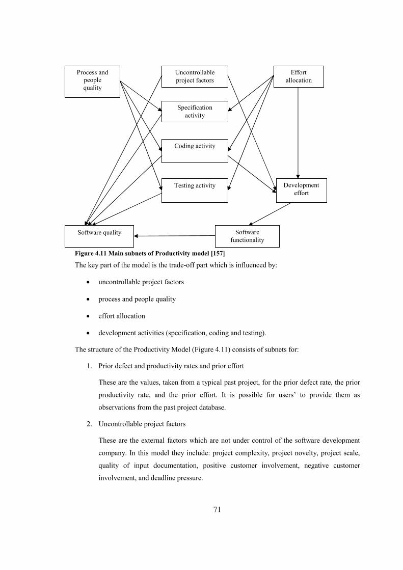
71

Figure 4.11 Main subnets of Productivity model [157]

The key part of the model is the trade-off part which is influenced by:

• uncontrollable project factors

• process and people quality

• effort allocation

• development activities (specification, coding and testing).

The structure of the Productivity Model (Figure 4.11) consists of subnets for:

1. Prior defect and productivity rates and prior effort

These are the values, taken from a typical past project, for the prior defect rate, the prior

productivity rate, and the prior effort. It is possible for users’ to provide them as

observations from the past project database.

2. Uncontrollable project factors

These are the external factors which are not under control of the software development

company. In this model they include: project complexity, project novelty, project scale,

quality of input documentation, positive customer involvement, negative customer

involvement, and deadline pressure.

Process and people

quality

Uncontrollable

project factors

Effort

allocation

Specification

activity

Coding activity

Testing activity Development

effort

Software quality Software

functionality

72

3. Development activities:

a. Specification and documentation

This subnet contains variables related to requirements quality, specification process

and people quality and change of effort on specification which altogether influence the

specification and documentation process effectiveness.

b. Coding

This subnet contains variables related to coding process and people quality, change of

effort on coding and the influence on coding effectiveness caused by the

documentation quality.

c. Testing

This subnet contains variables related to testing process and people quality, change of

effort on testing and the influence on testing effectiveness caused by the documentation

quality and coding effectiveness.

4. Revised defect and productivity rates

These are the rates adjusted by: uncontrollable project factors, documentation quality,

coding effectiveness and testing effectiveness. The adjusted rates influence the

relationships between variables in the trade-off component.

5. Trade-off component

Software functionality is calculated as the product of revised effort and revised

productivity rate. Similarly, the number of defects is calculated as the product of

delivered number of units and revised defect rate.

The Productivity Model provides the following distinctive features which were not available in

previous models:

1. Allows the user to enter custom prior productivity rate and prior defect rate.

Companies normally keep records and analyse data from their past projects. Productivity and

defect rates are among the easiest to be extracted from such databases. Even if a company does

not collect effort data [158], they are often easy to estimate post hoc.

2. Enables the user to perform trade-off analysis with variables expressed on a numeric scale.

73

3. Enables the user to apply different units of measurement up to the extent where the users

perform the analysis using their custom units.

4. The impact of qualitative factors can be easily changed by changing the weights in the node

expressions. A questionnaire is provided which can help determine users’ opinions on the

relationships between various model variables.

5. Allows target values for numeric variables to be defined as intervals, not just as point values.

For example, this model can answer questions such as: how can we achieve a defect rate

between 0.04 and 0.07 defects/function points for a project of a specific size with other

possible constraints.

Other features of the Productivity Model, which were partially available in the past models,

include:

1. The model can be easily extended by adding other qualitative factors.

2. Numeric variables in this model are dynamically discretised.

However, there are also several places where enhancements could be made for Productivity

Model:

1. Causal framework for risk compatibility

The structure of the Productivity Model can be improved. The model should be

compatible with the causal framework for risk. Uncontrollable project factors directly

influence revised productivity and defect rates; and not any of the development

activities. Hence, the Productivity Model is not causal model.

2. Incorporating code reuse

The Productivity Model assumes that there is no code reused from past projects. To make

the model more realistic, code reuse may be incorporated into the model. To model this

properly more details are required about the reused code; for example whether the reused

code is a complete module or rather smaller pieces of code from various modules, how

good was the development process when the reused code was originally written and

tested and what is the typical proportion of reused code out of the total code delivered.

3. Integrating detailed defect prediction with trade-off analysis

The Productivity Model is an integrated model in the sense that it can predict both effort

and quality (revised defect rate, number of defects). However, the prediction for the

74

number of defects is less detailed i.e. detailed data on the potential number of defects

depending on project size, potential number of defects adjusted by specification and

documentation adequacy, number of defects inserted as a result of imperfect coding

process, number of defects found, number of defects fixed, number of defects in the

reused code (Revised Defect Prediction Model only).

4. User satisfaction

The Productivity Model captures software quality as the number of defects, which can be

objectively counted by testers or managers. It does not refer in any way to how future

users will perceive software quality. User satisfaction could for example capture

adequacy of the software to meet user needs, appearance of the interface, software

performance and level of training and quality of documentation.

4.3 Other BN PRM models

4.3.1 BN models in construction projects

One of the early efforts of applying BNs to project performance were carried out by

McCabe et al. in 1998 [126, 125]. They developed a BN to improve an approach for modelling of

construction performance (Figure 4.12). The BN is used to evaluate the performance at each

resource interaction/queuing location based on performance indices. Five performance indices

have been developed: queue length index, queue wait time index, customer delay index, server

utilisation index and server quantity index. The indices are effect variables in the BN model and

they are evaluated at each queuing location. If the value of any of the performance indices does

not fall between the lower and upper bounds for that index then a remedial action needs to be

performed. The cost and duration nodes were added to allow the improvement process to take

different approaches to diagnosing the performance. For example, if performance indices provide

evidence that the queue wait time is too long; depending on where the focus has been placed there

can be two outcomes:

• If the focus is placed on a shortened duration, then the action would be to increase the

number of servers.

• If cost is the major factor, then action would be to reduce the number of customers.

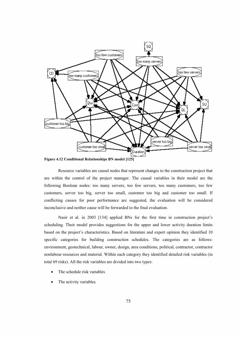
75

Figure 4.12 Conditional Relationships BN model [125]

Resource variables are causal nodes that represent changes to the construction project that

are within the control of the project manager. The causal variables in their model are the

following Boolean nodes: too many servers, too few servers, too many customers, too few

customers, server too big, server too small, customer too big and customer too small. If

conflicting causes for poor performance are suggested, the evaluation will be considered

inconclusive and neither cause will be forwarded to the final evaluation.

Nasir et al. in 2003 [134] applied BNs for the first time in construction project’s

scheduling. Their model provides suggestions for the upper and lower activity duration limits

based on the project’s characteristics. Based on literature and expert opinion they identified 10

specific categories for building construction schedules. The categories are as follows:

environment, geotechnical, labour, owner, design, area conditions, political, contractor, contractor

nonlabour resources and material. Within each category they identified detailed risk variables (in

total 69 risks). All the risk variables are divided into two types:

• The schedule risk variables

• The activity variables.

76

The first type of variables are input nodes where the evidence may describe the project condition.

The second type of variables are output nodes.

Activity variables were divided into 8 groups that represent all the types of activities

in a construction schedule. The groups were as follows: mobilization/demobilization,

foundation/piling, labour intensive, equipment intensive, mechanical/electrical, roof/external,

demolition and commissioning. Each group was modelled with two nodes where one node

represented the pessimistic value and the other node represented the optimistic value.

Both BN models reviewed in this section provided a flexible modelling environment.

However, the models have the following limitations:

• They are specific to building construction projects. Therefore the models cannot be

applied to other industries and different type of projects.

• They make an assumption about the input data i.e. the models assume that most likely

duration is already known and takes it as an input to the model.

• The output of the model needs another approach to calculate results such as the expected

project duration, the probability of delay/completion etc.

• Pre-defined values for the upper and lower bounds of activity duration i.e. the pessimistic

side for the percent increase of activity duration is limited to 10%, 25%, 50% and 100%.

• All the risk variables were binary nodes; therefore many variables with more than two

states were not modelled properly.

• Overly complex and unstructured models that are difficult to follow and understand.

• Diagnostic analysis (i.e. reasoning from effect to cause) which is a very powerful BN

feature not used in the models.

Luu et al. in 2009 [117] continued Nasir et al. work of applying BNs to quantifying the

schedule risk in construction projects. They adopted and adjusted McCabe et al.’s BN model to

construction projects in Vietnam. The sixteen most significant causes of schedule delay in

construction projects in Vietnam were identified. Following this, based on expert survey, 18

cause and effect relationships were established. The BN model developed was applied to two case

studies. The model performed well in predicting the probability of the construction schedule

delay in both studies.

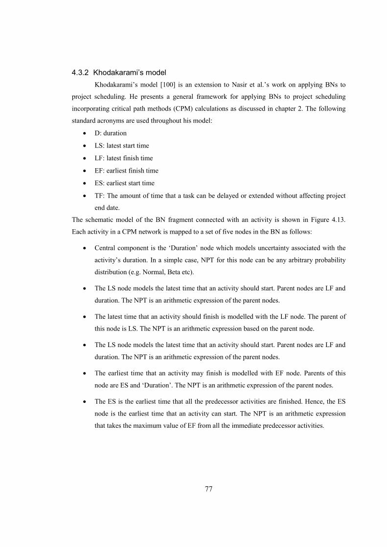
77

4.3.2 Khodakarami’s model

Khodakarami’s model [100] is an extension to Nasir et al.’s work on applying BNs to

project scheduling. He presents a general framework for applying BNs to project scheduling

incorporating critical path methods (CPM) calculations as discussed in chapter 2. The following

standard acronyms are used throughout his model:

• D: duration

• LS: latest start time

• LF: latest finish time

• EF: earliest finish time

• ES: earliest start time

• TF: The amount of time that a task can be delayed or extended without affecting project

end date.

The schematic model of the BN fragment connected with an activity is shown in Figure 4.13.

Each activity in a CPM network is mapped to a set of five nodes in the BN as follows:

• Central component is the ‘Duration’ node which models uncertainty associated with the

activity’s duration. In a simple case, NPT for this node can be any arbitrary probability

distribution (e.g. Normal, Beta etc).

• The LS node models the latest time that an activity should start. Parent nodes are LF and

duration. The NPT is an arithmetic expression of the parent nodes.

• The latest time that an activity should finish is modelled with the LF node. The parent of

this node is LS. The NPT is an arithmetic expression based on the parent node.

• The LS node models the latest time that an activity should start. Parent nodes are LF and

duration. The NPT is an arithmetic expression of the parent nodes.

• The earliest time that an activity may finish is modelled with EF node. Parents of this

node are ES and ‘Duration’. The NPT is an arithmetic expression of the parent nodes.

• The ES is the earliest time that all the predecessor activities are finished. Hence, the ES

node is the earliest time that an activity can start. The NPT is an arithmetic expression

that takes the maximum value of EF from all the immediate predecessor activities.

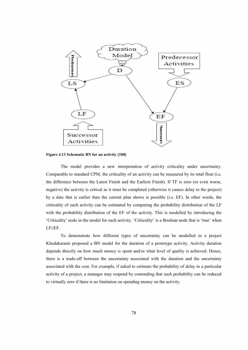
78

Figure 4.13 Schematic BN for an activity [100]

The model provides a new interpretation of activity criticality under uncertainty.

Comparable to standard CPM, the criticality of an activity can be measured by its total float (i.e.

the difference between the Latest Finish and the Earliest Finish). If TF is zero (or even worse,

negative) the activity is critical as it must be completed (otherwise it causes delay to the project)

by a date that is earlier than the current plan shows is possible (i.e. EF). In other words, the

criticality of each activity can be estimated by comparing the probability distribution of the LF

with the probability distribution of the EF of the activity. This is modelled by introducing the

‘Criticality’ node in the model for each activity. ‘Criticality’ is a Boolean node that is ‘true’ when

LF≤EF.

To demonstrate how different types of uncertainty can be modelled in a project

Khodakarami proposed a BN model for the duration of a prototype activity. Activity duration

depends directly on how much money is spent and/or what level of quality is achieved. Hence,

there is a trade-off between the uncertainty associated with the duration and the uncertainty

associated with the cost. For example, if asked to estimate the probability of delay in a particular

activity of a project, a manager may respond by contending that such probability can be reduced

to virtually zero if there is no limitation on spending money on the activity.

79

The limitations of the Khodakarami’s model are:

• The model is far more complex than Monte Carlo based techniques.

• Efficient application of the model requires a well-established risk management process

especially in identifying different sources of uncertainty and also in the data acquisition

process.

• For large size BNs that contain continuous nodes exact inference is infeasible. Therefore,

the model is not applicable for large-scale projects.

4.3.3 BN models in Operational Risk

Risk in large-scale projects is very similar to operational risk in finance, particularly the

way the risk events are represented. In addition even some of the risk factors are same. Neil,

Fenton et al. [137] have shown how Bayesian models can be used to improve operational risk

modelling. These authors first explored the use of BNs to model statistical loss distributions in

financial operational risk scenarios focusing on modelling ‘long’ tail or unexpected loss events.

One of the first models they developed was risk control self assessment model. This model was

able to do the following:

• Quantified and rated qualitative and quantitative risks

• Used Risk Maps to rate the risk contribution of each element in a COSO complaint risk

structure (Business/ Process/ Activity/ Risk Control)

• Mixed loss distribution derived from internal and external loss databases and embeds

these in a Risk Map.

• Forecasted the capital charge in a form of value at risk (VaR) or any other statistic.

• Coped with missing audit/assessment data and accommodates differences in expert

opinions.

The model uses issues and action plans to predict the reliability of the controls being

modelled. The reliability of these processes is then combined to predict the reliability of the

overall task and ultimately the information predicts process reliability and the loss distribution

[3]. We are in particular interested in the structure of this model and how risk events are

represented. We will use and develop this structure further in chapter 5.

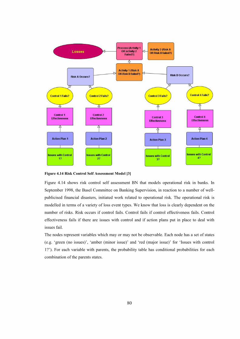
80

Figure 4.14 Risk Control Self Assessment Model [3]

Figure 4.14 shows risk control self assessment BN that models operational risk in banks. In

September 1998, the Basel Committee on Banking Supervision, in reaction to a number of well-

publicised financial disasters, initiated work related to operational risk. The operational risk is

modelled in terms of a variety of loss event types. We know that loss is clearly dependent on the

number of risks. Risk occurs if control fails. Control fails if control effectiveness fails. Control

effectiveness fails if there are issues with control and if action plans put in place to deal with

issues fail.

The nodes represent variables which may or may not be observable. Each node has a set of states

(e.g. ‘green (no issues)’, ‘amber (minor issue)’ and ‘red (major issue)’ for ‘Issues with control

1?’). For each variable with parents, the probability table has conditional probabilities for each

combination of the parents states.

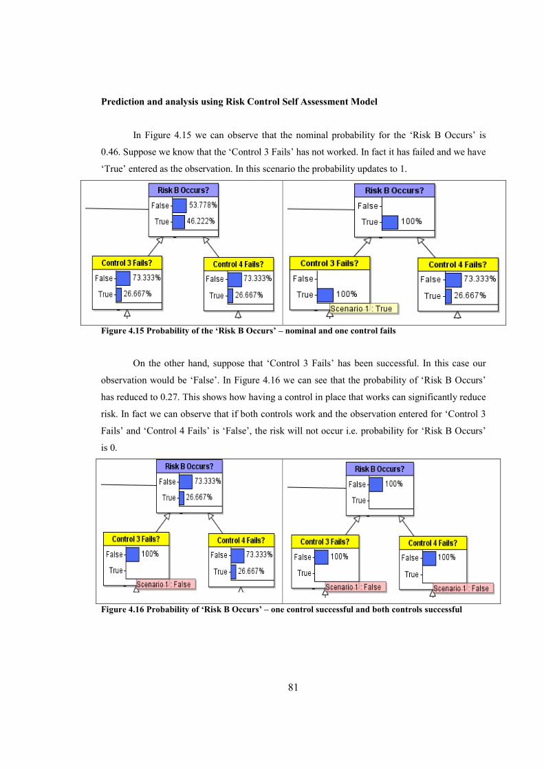
81

Prediction and analysis using Risk Control Self Assessment Model

In Figure 4.15 we can observe that the nominal probability for the ‘Risk B Occurs’ is

0.46. Suppose we know that the ‘Control 3 Fails’ has not worked. In fact it has failed and we have

‘True’ entered as the observation. In this scenario the probability updates to 1.

Figure 4.15 Probability of the ‘Risk B Occurs’ – nominal and one control fails

On the other hand, suppose that ‘Control 3 Fails’ has been successful. In this case our

observation would be ‘False’. In Figure 4.16 we can see that the probability of ‘Risk B Occurs’

has reduced to 0.27. This shows how having a control in place that works can significantly reduce

risk. In fact we can observe that if both controls work and the observation entered for ‘Control 3

Fails’ and ‘Control 4 Fails’ is ‘False’, the risk will not occur i.e. probability for ‘Risk B Occurs’

is 0.

Figure 4.16 Probability of ‘Risk B Occurs’ – one control successful and both controls successful

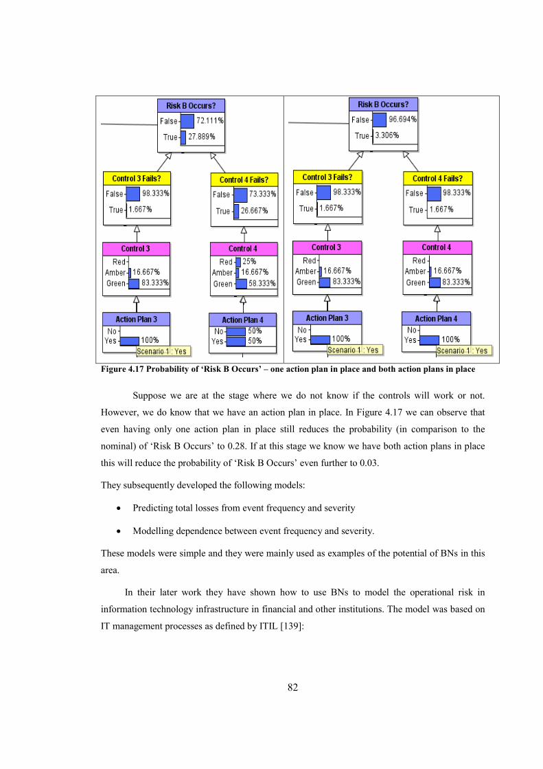
82

Figure 4.17 Probability of ‘Risk B Occurs’ – one action plan in place and both action plans in place

Suppose we are at the stage where we do not know if the controls will work or not.

However, we do know that we have an action plan in place. In Figure 4.17 we can observe that

even having only one action plan in place still reduces the probability (in comparison to the

nominal) of ‘Risk B Occurs’ to 0.28. If at this stage we know we have both action plans in place

this will reduce the probability of ‘Risk B Occurs’ even further to 0.03.

They subsequently developed the following models:

• Predicting total losses from event frequency and severity

• Modelling dependence between event frequency and severity.

These models were simple and they were mainly used as examples of the potential of BNs in this

area.

In their later work they have shown how to use BNs to model the operational risk in

information technology infrastructure in financial and other institutions. The model was based on

IT management processes as defined by ITIL [139]:

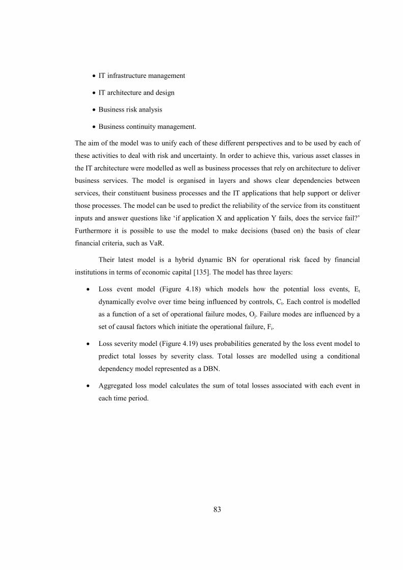
83

• IT infrastructure management

• IT architecture and design

• Business risk analysis

• Business continuity management.

The aim of the model was to unify each of these different perspectives and to be used by each of

these activities to deal with risk and uncertainty. In order to achieve this, various asset classes in

the IT architecture were modelled as well as business processes that rely on architecture to deliver

business services. The model is organised in layers and shows clear dependencies between

services, their constituent business processes and the IT applications that help support or deliver

those processes. The model can be used to predict the reliability of the service from its constituent

inputs and answer questions like ‘if application X and application Y fails, does the service fail?’

Furthermore it is possible to use the model to make decisions (based on) the basis of clear

financial criteria, such as VaR.

Their latest model is a hybrid dynamic BN for operational risk faced by financial

institutions in terms of economic capital [135]. The model has three layers:

• Loss event model (Figure 4.18) which models how the potential loss events, Et

dynamically evolve over time being influenced by controls, Ct. Each control is modelled

as a function of a set of operational failure modes, Oj. Failure modes are influenced by a

set of causal factors which initiate the operational failure, Fi.

• Loss severity model (Figure 4.19) uses probabilities generated by the loss event model to

predict total losses by severity class. Total losses are modelled using a conditional

dependency model represented as a DBN.

• Aggregated loss model calculates the sum of total losses associated with each event in

each time period.

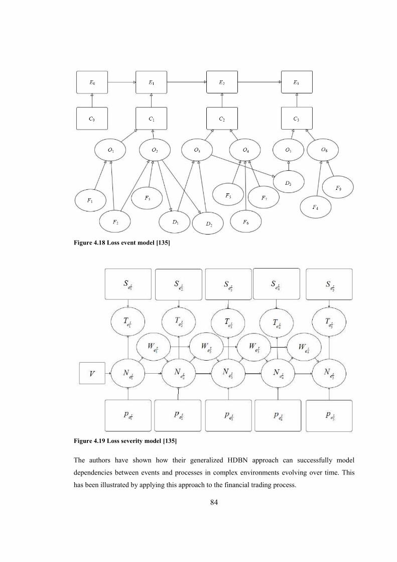
84

Figure 4.18 Loss event model [135]

Figure 4.19 Loss severity model [135]

The authors have shown how their generalized HDBN approach can successfully model

dependencies between events and processes in complex environments evolving over time. This

has been illustrated by applying this approach to the financial trading process.

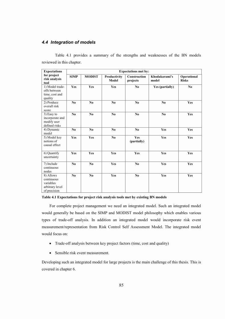
85

4.4 Integration of models

Table 4.1 provides a summary of the strengths and weaknesses of the BN models

reviewed in this chapter.

Expectations

for project

risk analysis

tool

Expectations met by:

SIMP MODIST Productivity

Model

Construction

projects

Khodakarami’s

model

Operational

Risks

1) Model trade-offs between time, cost and quality

Yes Yes Yes No Yes (partially) No

2) Produce overall risk score

No No No No No Yes

3) Easy to incorporate and modify user defined risks

No No No No No Yes

4) Dynamic model

No No No No Yes Yes

5) Model key notions of causal effect

Yes Yes No Yes

(partially)

Yes Yes

6) Quantify uncertainty

Yes Yes Yes Yes Yes Yes

7) Include continuous nodes

No No Yes No Yes Yes

8) Allows continuous variables arbitrary level of precision

No No Yes No Yes Yes

Table 4.1 Expectations for project risk analysis tools met by existing BN models

For complete project management we need an integrated model. Such an integrated model

would generally be based on the SIMP and MODIST model philosophy which enables various

types of trade-off analysis. In addition an integrated model would incorporate risk event

measurement/representation from Risk Control Self Assessment Model. The integrated model

would focus on:

• Trade-off analysis between key project factors (time, cost and quality)

• Sensible risk event measurement.

Developing such an integrated model for large projects is the main challenge of this thesis. This is

covered in chapter 6.

86

4.5 Summary

We have seen that it is possible to use BNs to build models that are proved to be

successful in both research and industry. However, the existing models have some limitations

discussed in this chapter. These limitations raise the number of well defined research challenges.

Some of these challenges are addressed using relatively simple solutions. However, the most

important challenges cannot be solved by extending existing models and they require building

new models. These new BN models are discussed in the chapters that follow.

87

5. New structured approach for BN risk models

A major objective in the field of risk analysis is the development of a uniform definition

of risk. In this chapter we briefly review and compare the most common risk definitions. Risk has

different meanings to different people. Risks are not always associated with negative outcomes

and they may represent opportunities as well. Taking big risks can be beneficial to a party that is

able to accept them because it enables opportunity.

Generally risk is seen as an abstract concept whose measurement is very difficult. Based

on current risk definitions we propose the causal risk framework for risk quantification, which we

see as an improvement of the standard risk measure: Risk = Probability x Impact. By using the

causal risk framework we improve the modelling approach in order to help develop better

decision support systems. Improvement of the causal risk framework and its application are some

of the main contributions of the whole thesis. The earlier version of this work has been

published [65].

5.1 Background

It is clear that if/when risk strikes, it can have a range of effects on the achievement of

project objectives, from total failure to a surprisingly good/better than expected outcome. The

inability of project managers to deal with competing views can affect the quality and acceptability

of their projects. The confusions and delays in developing, for example, product strategies and

information systems to support projects can mean that opportunities can be lost.

Despite this, the traditional project risk management process as practised by the majority

of project managers tends to concentrate almost exclusively on the potential negative effects of

risks. As a result of this focus, considerable effort is spent on identifying and managing risks,

while opportunities tend to be overlooked. We argue that if the synergy between risks and

opportunities is recognised and properly managed, it can ensure that unwelcome negative effects

are minimised while at the same time maximising the chances of exploiting unexpected positive

effects.

Entrepreneurs, for example, perceive risk differently from project managers. Shane and

Venkatraman [168] suggest that entrepreneurs who identify an opportunity sooner appear to

accept greater amounts of risk because others lack the knowledge to properly understand (and

assess) the opportunity. Therefore, asymmetry in knowledge will lead to differing perceptions of

risk regarding a given decision.

88

5.2 Identification of Risks

There are many techniques for risk identification, such as brainstorming and workshops,

questionnaires and interviews. The appropriate combination of techniques should be used, since

there isn’t a single best method. Each of the commonly used risk identification techniques listed

could be used equally effectively to identify opportunities as well as risks. To demonstrate this we

will first list illustrative examples of common risks in large projects [60]. In the next section we

will use the same technique to list potential opportunities in large projects.

Typical risks

• ‘Insufficient use of status and progress reports’

• ‘Insufficient client influence’

• ‘Poor rapport/coordination with the client’

• ‘Lack of project team participation in decision-making/problem-solving’

• ‘Job insecurity within the project team’

• ‘Lack of team spirit and sense of mission within project team’

• ‘Parent organization stable, non-dynamic, lacking strategic change’

• ‘Poor rapport/coordination with the parent organization’

• ‘Poor relations with the parent organization’

• ‘Project more complex than the parent has completed before’

• ‘Inability to freeze design early

• ‘Inability to close out the effort’

• ‘Unrealistic project schedules’

• ‘Initial under-funding’

• ‘New ‘type’ of project’

• ‘Poor relations with public officials’

• ‘Unfavourable public opinion’

• ‘The company’s reputation is damaged’

89

• ‘Poor staff performance’

• ‘Poor quality of the delivered system’

5.3 Identification of Opportunities

If risk is defined as entirely negative and opportunity as entirely positive then naturally we would

need to look at project risk management and project opportunity management. Risk practitioners

often find it easier to identify potential problems than to look for hidden advantages and upsides.

Here indeed we list illustrative examples of common opportunities in large projects [60].

Typical opportunities

• ‘There is commitment of the project team to a goal’

• ‘The initial cost estimates are accurate’

• ‘Project team has exceptional capability’

• ‘There is exceptional funding to completion’

• ‘There are exceptional planning and control techniques’

• ‘There are minimal start-up difficulties’

• ‘Absence of bureaucracy’

• ‘There is an on-site project manager’

• ‘There are clearly established success criteria’

• ‘There is project manager commitment to: established schedules, budgets and technical

performance goals’

• ‘There is frequent feedback from the parent organization’

• ‘There is frequent feedback from the client’

• ‘There is client and parent commitment to: established schedules, budgets and technical

performance goals’

• ‘There is project team participation in determining schedules and budgets’

• ‘There is slack in the schedule’

• ‘There is slack in the budget’

90

• ‘There is company enthusiasm’

• ‘There are exceptional control procedures, especially for dealing with changes’

• ‘Judicious use of networking techniques’

• ‘Lack of excessive government red tape’

5.4 Definition of Risk includes Opportunities

Issues involving risk are often difficult to distinguish and misunderstood by those making

vital decisions for projects. Risk is not tangible or visible, therefore, a manager’s risk perceptions

in a particular project vary by risk characteristics and the project’s internal and external

environment [47]. Are people more risk taking for risks or for opportunities? Indeed, what makes

a risk risky is the possibility of loss, whether it be loss of current assets or loss of opportunity for

more assets. However, few people could be expected to take risks if they did not perceive some

element of opportunity associated with risk-taking behaviour. Thus, it seems clear that the degree

to which people will engage in risk-taking behaviour is related to the degree to which they

perceive risk taking as an opportunity for something. Therefore, it is important to first define risk.

The word risk generally has implications of negative or adverse results from an event [66,

174, 188, 25]. Therefore, there is no doubt that common usage of the word risk sees only the

downside. Asking a man in the street if he would be willing to take a risk, will almost always

result in a negative response. This is reflected in the traditional definitions of the word, both in

standard dictionaries and some technical definitions. One dictionary defines ‘risk’ as: “a situation

involving exposure to danger, the possibility that something unpleasant will happen, loss,

exposure to chance of injury or loss. ” [145].

However, some professional bodies and standards organisations have gradually

developed their definitions of risk to include both the upside and the downside. COSO [34]

defines a risk as an event that can have negative impact. Equally an event that can have a positive

impact is an opportunity. A guide published by the UK Association for Project Management has

adopted a broad view of risk. Their definition of risk is: “Risk – an uncertain event or set of

circumstances that, should it occur, will have an effect on the achievement of the project’s

objectives. “ [7] In this definition, the nature of the effect is undefined and could therefore

implicitly include both positive and negative effects. The Australian/New Zealand Standard has a

similar risk definition where once again the nature of the effect is undefined and hence could

implicitly include both positive and negative effects. Others, for example, a guide published by

91

the US Project Management Institute, are explicit naming both positive and negative effects on

the project objectives within their definition of risk. The PMBOK definition states: “Project risk

is an uncertain event or condition that, if it occurs, has a positive or a negative effect on a project

objective … Project risk includes both risks to the project’s objectives and opportunities to

improve on those objectives.”[151]

In traditional behavioural decision theory, the term risk is used interchangeably with the

term uncertainty [115, 23, 46]. Decision makers are said to be risk-averse if they prefer a sure

thing to an option whose outcome is uncertain (i.e. a risky option). Yates and Stone’s [202]

review of risk definitions in various arenas reveals that definitions of risk range from emphasis on

risk of personal harm, found in medical and hazard research, to emphasis on possible

opportunities, found in economic and business literature. A common theme in most definitions of

risk is still the possibility of loss. However, each conceptualisation of risk also contains some

component of opportunity, even if it is only the opportunity to avoid loss.

The fact that recent documentation now incorporates both opportunities and risks within

their definition for risk, it is a clear recognition that both are equally important influences over

project success [81].

5.5 Problems with the standard measure of risk

As discussed in 2.7.2 in organisations where risk is treated seriously, it is a standard that

at the start of every project, managers discuss and list risks. Project managers are often expecting

a number of risks to occur, which will be similar from project to project. Project managers can

employ experiences gained through the course of one project to the next one.

When managers think about the risks that might cause the next project to fail, such as the

risks listed in section 5.2; whether deliberately or not, they will have measured such risks. A

liquidity crisis that destroys their company and forces it into administration would probably not

appear on their list. Although its impact is more devastating than any of the others, the chances of

it actually happening are so low that a project manager would probably have discounted it.

As discussed in 2.7.2 the probability x impact measure of risk is quite useful for

prioritising risks (the bigger the number the ‘greater’ the risk). The problem is that, it is normally

not possible to get the numbers needed to calculate it [59, 192, 31]:

• We cannot get the Probability number. It is only natural to be worried if, for example,

we know there have been bad investments in mortgage back securities. This increases the

risk of ‘Liquidity crisis’ and could result in the company going into administration. Does

this make the probability of the liquidity crisis equal to one? Clearly not, because if it was

92

one then there would have been no point in trying to properly evaluate assets. The

probability of the liquidity crisis is conditional on a number of other control events (like

practising proper asset valuation to avoid the liquidity crisis) and trigger events (like bad

investments in mortgage back securities). It makes no sense to assign a direct probability

without considering the events it is conditional on. In general, it makes no sense (and

would in any case be too difficult) for a risk manager to give the unconditional

probability of every ‘risk’ irrespective of relevant controls, triggers and mitigants. This is

especially significant when there are, for example, controls that are not used very often

(like implementing proper asset valuation globally).

• We cannot get the Impact number. Just as it makes little sense to attempt to assign an

(unconditional) probability to the event ‘Liquidity crisis’, so it makes little sense to assign

an (unconditional) number to the impact of company goes into administration. This can

literally mean anything from, for example, no job losses to 100% job losses. Apart from

the obvious question “impact on what”, we cannot say what the impact is without

considering the possible mitigating events such as company searching for bailout. Hence,

we simply discard having 1 – 10 point scale for impact. Mitigants can not only avoid the

worst case scenario, but can even avoid administration altogether.

• Risk score is meaningless. Even if we could get round the two problems above what

exactly does the resulting number mean? Suppose the (conditional) probability of the

liquidity risk is 0.95 and, on a scale of 1 to 10, the impact of the crisis is 10 (even

accounting for mitigants). The liquidity crisis ‘risk’ is 9.5, which is a number close to the

highest possible 10. But it does not measure anything in a meaningful sense.

• It does not tell us what we really need to know. What we really need to know is the

probability, given our current state of knowledge that the company will go into

administration.

Shortcomings of probability x impact measure are discussed further in section 6.9.

5.6 Getting sensible risk measures with causal models (risk maps)

The rational way to think of risks is in terms of causal models (BNs) with trigger events,

control events, risk events, mitigant events and consequence events. In the next section we will

explain this in more detail. For the liquidity crisis risk, the relevant causal model is shown in

Figure 5.1.

A risk is therefore characterised by a set of uncertain events. Each of these events has a

set of outcomes. For simplicity here we will assume that these events have two outcomes — true

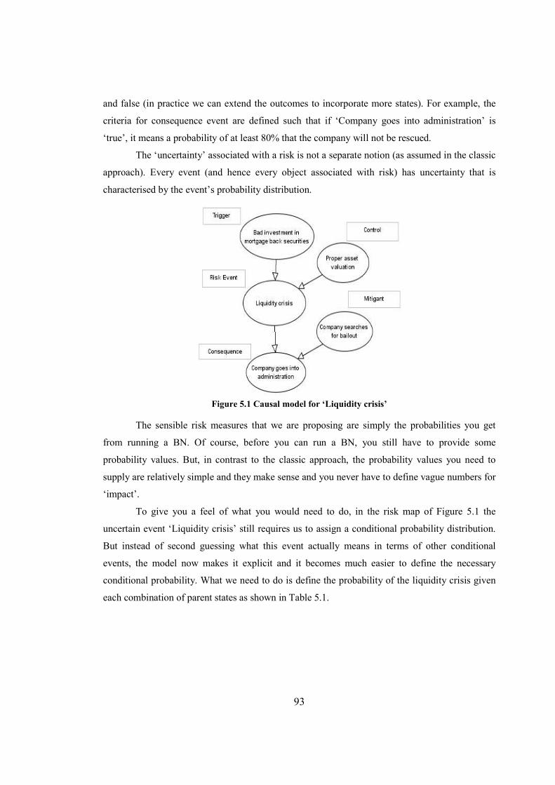
93

and false (in practice we can extend the outcomes to incorporate more states). For example, the

criteria for consequence event are defined such that if ‘Company goes into administration’ is

‘true’, it means a probability of at least 80% that the company will not be rescued.

The ‘uncertainty’ associated with a risk is not a separate notion (as assumed in the classic

approach). Every event (and hence every object associated with risk) has uncertainty that is

characterised by the event’s probability distribution.

Figure 5.1 Causal model for ‘Liquidity crisis’

The sensible risk measures that we are proposing are simply the probabilities you get

from running a BN. Of course, before you can run a BN, you still have to provide some

probability values. But, in contrast to the classic approach, the probability values you need to

supply are relatively simple and they make sense and you never have to define vague numbers for

‘impact’.

To give you a feel of what you would need to do, in the risk map of Figure 5.1 the

uncertain event ‘Liquidity crisis’ still requires us to assign a conditional probability distribution.

But instead of second guessing what this event actually means in terms of other conditional

events, the model now makes it explicit and it becomes much easier to define the necessary

conditional probability. What we need to do is define the probability of the liquidity crisis given

each combination of parent states as shown in Table 5.1.

94

Bad investment in mortgage back securities False True

Proper asset valuation False True False True

False 1.0 1.0 0.0 0.8

True 0.0 0.0 1.0 0.2

Table 5.1 Conditional probability table for ‘Liquidity crisis’

For example, if there are bad investments in mortgage back securities then the probability

of liquidity crisis is 1, if there was no proper asset valuation, and 0.2, if there was proper asset

valuation. In filling in such a table, we no longer have to try to ‘factor in’ any implicit

conditioning events like investment type.

There are some events in the BN for which we do need to assign unconditional

probability values. These are the nodes that have no parents; it makes sense to get unconditional

probabilities for these because, by definition, they are not restricted by any conditions. Such

nodes can generally be only triggers, controls or mitigants. An example is shown in Table 5.2.

False 0.05

True 0.95

Table 5.2 Probability table for ‘Bad investment in mortgage back securities’

As discussed in chapter 3, we are not suggesting that assigning the probability tables in a

BN is always easy. You will generally require expert judgement or data to do it properly. What is

important is that it is easier than the classic alternative. At worse, when you have no data, purely

subjective values can be supplied.

Once you have supplied the prior probability values a BN tool will run the model and

generate all the measures of risk that you need. For example, when you run the model using only

the prior probabilities i.e. no observations entered, the model computes the probability of the

liquidity crises as just under 0.8 and the probability of company going into administration

(meaning at least 80% chance that the company will not be rescued) is about 0.75 (Figure 5.2).

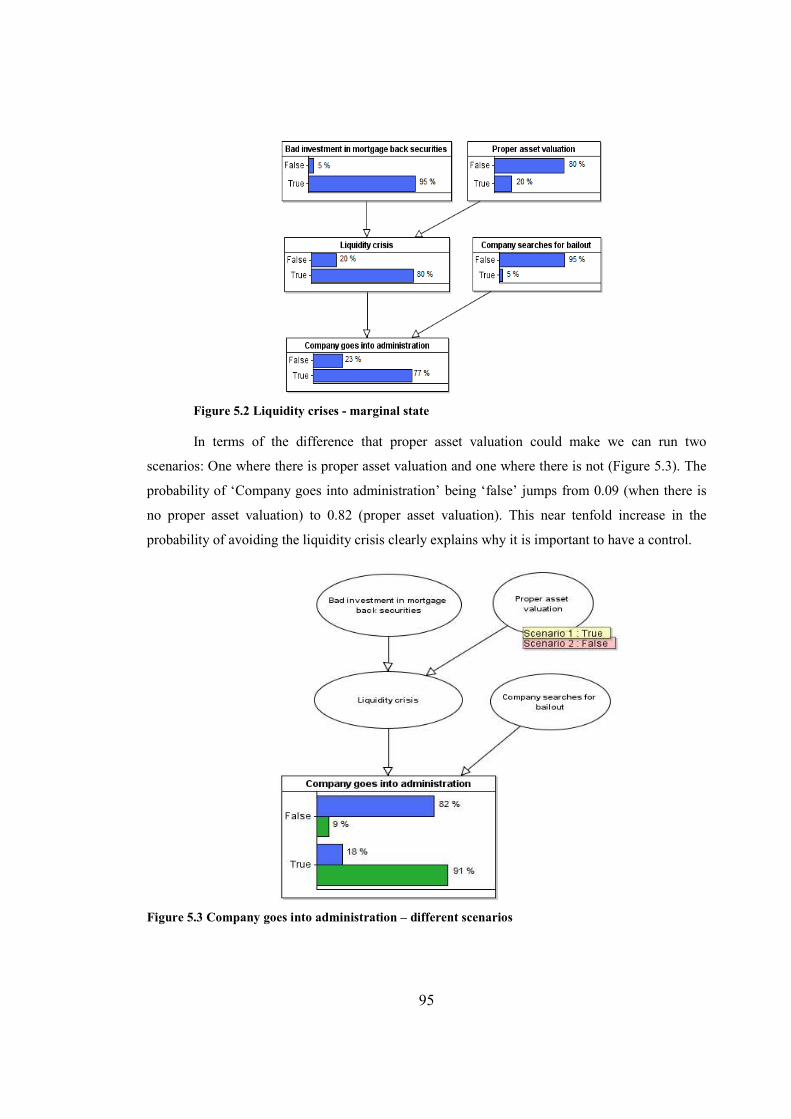
95

Figure 5.2 Liquidity crises - marginal state

In terms of the difference that proper asset valuation could make we can run two

scenarios: One where there is proper asset valuation and one where there is not (Figure 5.3). The

probability of ‘Company goes into administration’ being ‘false’ jumps from 0.09 (when there is

no proper asset valuation) to 0.82 (proper asset valuation). This near tenfold increase in the

probability of avoiding the liquidity crisis clearly explains why it is important to have a control.

Figure 5.3 Company goes into administration – different scenarios

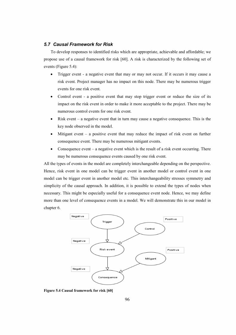
96

5.7 Causal Framework for Risk

To develop responses to identified risks which are appropriate, achievable and affordable; we

propose use of a causal framework for risk [60]. A risk is characterized by the following set of

events (Figure 5.4):

• Trigger event - a negative event that may or may not occur. If it occurs it may cause a

risk event. Project manager has no impact on this node. There may be numerous trigger

events for one risk event.

• Control event - a positive event that may stop trigger event or reduce the size of its

impact on the risk event in order to make it more acceptable to the project. There may be

numerous control events for one risk event.

• Risk event – a negative event that in turn may cause a negative consequence. This is the

key node observed in the model.

• Mitigant event – a positive event that may reduce the impact of risk event on further

consequence event. There may be numerous mitigant events.

• Consequence event – a negative event which is the result of a risk event occurring. There

may be numerous consequence events caused by one risk event.

All the types of events in the model are completely interchangeable depending on the perspective.

Hence, risk event in one model can be trigger event in another model or control event in one

model can be trigger event in another model etc. This interchangeability stresses symmetry and

simplicity of the causal approach. In addition, it is possible to extend the types of nodes when

necessary. This might be especially useful for a consequence event node. Hence, we may define

more than one level of consequence events in a model. We will demonstrate this in our model in

chapter 6.

Figure 5.4 Causal framework for risk [60]

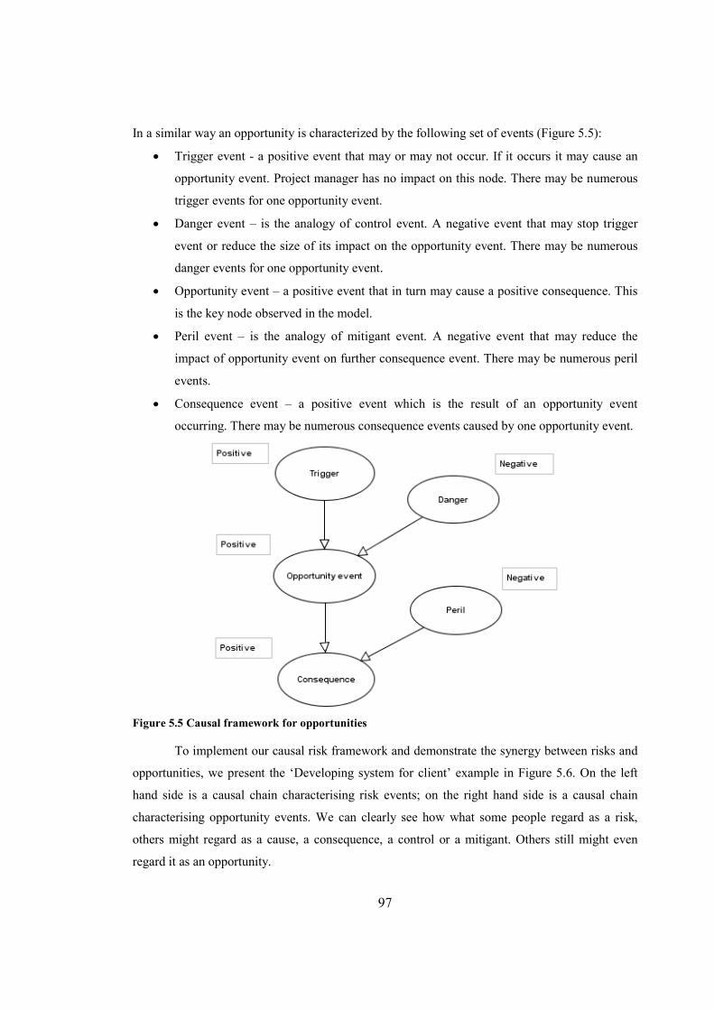
97

In a similar way an opportunity is characterized by the following set of events (Figure 5.5):

• Trigger event - a positive event that may or may not occur. If it occurs it may cause an

opportunity event. Project manager has no impact on this node. There may be numerous

trigger events for one opportunity event.

• Danger event – is the analogy of control event. A negative event that may stop trigger

event or reduce the size of its impact on the opportunity event. There may be numerous

danger events for one opportunity event.

• Opportunity event – a positive event that in turn may cause a positive consequence. This

is the key node observed in the model.

• Peril event – is the analogy of mitigant event. A negative event that may reduce the

impact of opportunity event on further consequence event. There may be numerous peril

events.

• Consequence event – a positive event which is the result of an opportunity event

occurring. There may be numerous consequence events caused by one opportunity event.

Figure 5.5 Causal framework for opportunities

To implement our causal risk framework and demonstrate the synergy between risks and

opportunities, we present the ‘Developing system for client’ example in Figure 5.6. On the left

hand side is a causal chain characterising risk events; on the right hand side is a causal chain

characterising opportunity events. We can clearly see how what some people regard as a risk,

others might regard as a cause, a consequence, a control or a mitigant. Others still might even

regard it as an opportunity.

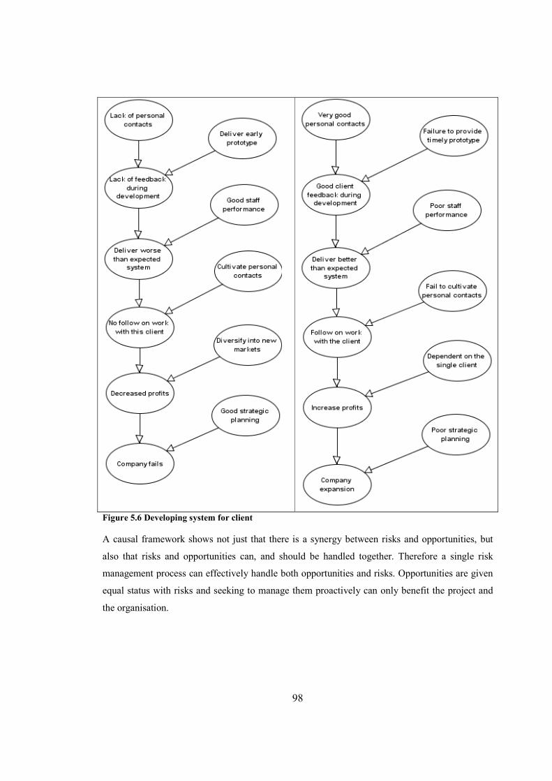
98

Figure 5.6 Developing system for client

A causal framework shows not just that there is a synergy between risks and opportunities, but

also that risks and opportunities can, and should be handled together. Therefore a single risk

management process can effectively handle both opportunities and risks. Opportunities are given

equal status with risks and seeking to manage them proactively can only benefit the project and

the organisation.

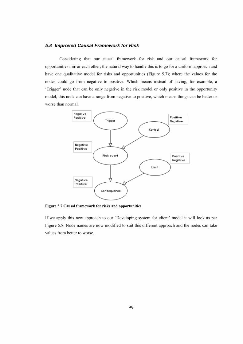
99

5.8 Improved Causal Framework for Risk

Considering that our causal framework for risk and our causal framework for

opportunities mirror each other; the natural way to handle this is to go for a uniform approach and

have one qualitative model for risks and opportunities (Figure 5.7); where the values for the

nodes could go from negative to positive. Which means instead of having, for example, a

‘Trigger’ node that can be only negative in the risk model or only positive in the opportunity

model, this node can have a range from negative to positive, which means things can be better or

worse than normal.

Figure 5.7 Causal framework for risks and opportunities

If we apply this new approach to our ‘Developing system for client’ model it will look as per

Figure 5.8. Node names are now modified to suit this different approach and the nodes can take

values from better to worse.

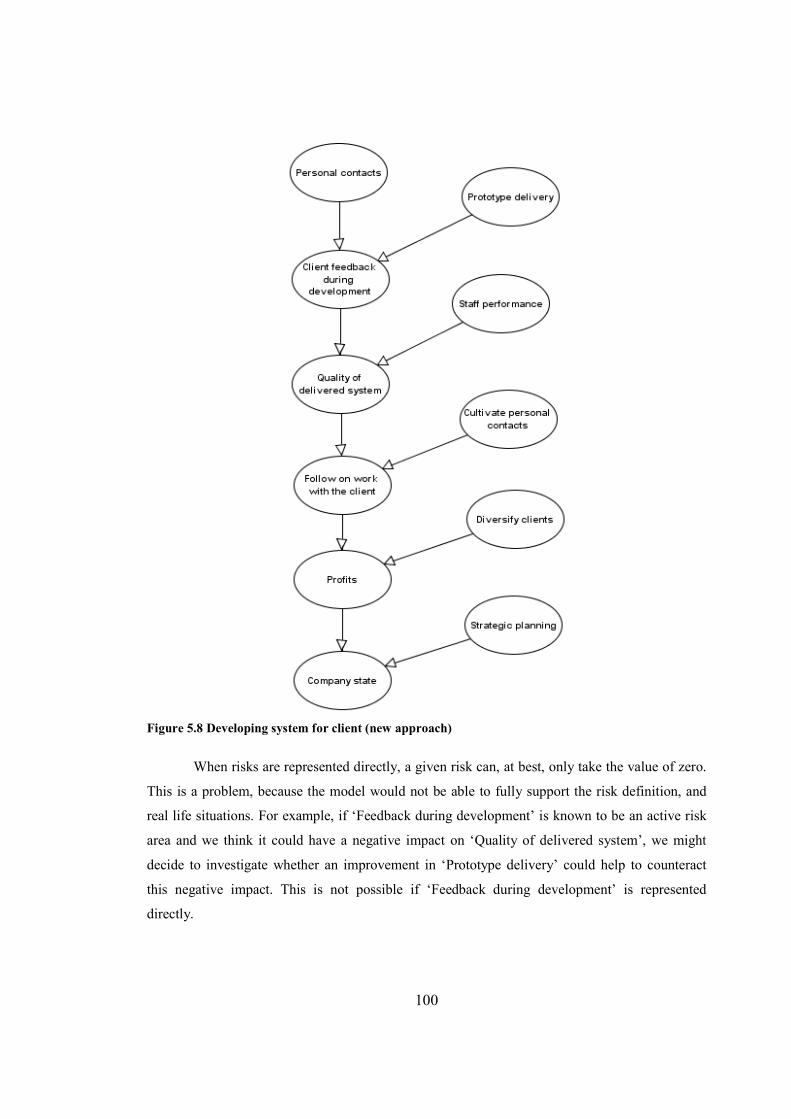
100

Figure 5.8 Developing system for client (new approach)

When risks are represented directly, a given risk can, at best, only take the value of zero.

This is a problem, because the model would not be able to fully support the risk definition, and

real life situations. For example, if ‘Feedback during development’ is known to be an active risk

area and we think it could have a negative impact on ‘Quality of delivered system’, we might

decide to investigate whether an improvement in ‘Prototype delivery’ could help to counteract

this negative impact. This is not possible if ‘Feedback during development’ is represented

directly.

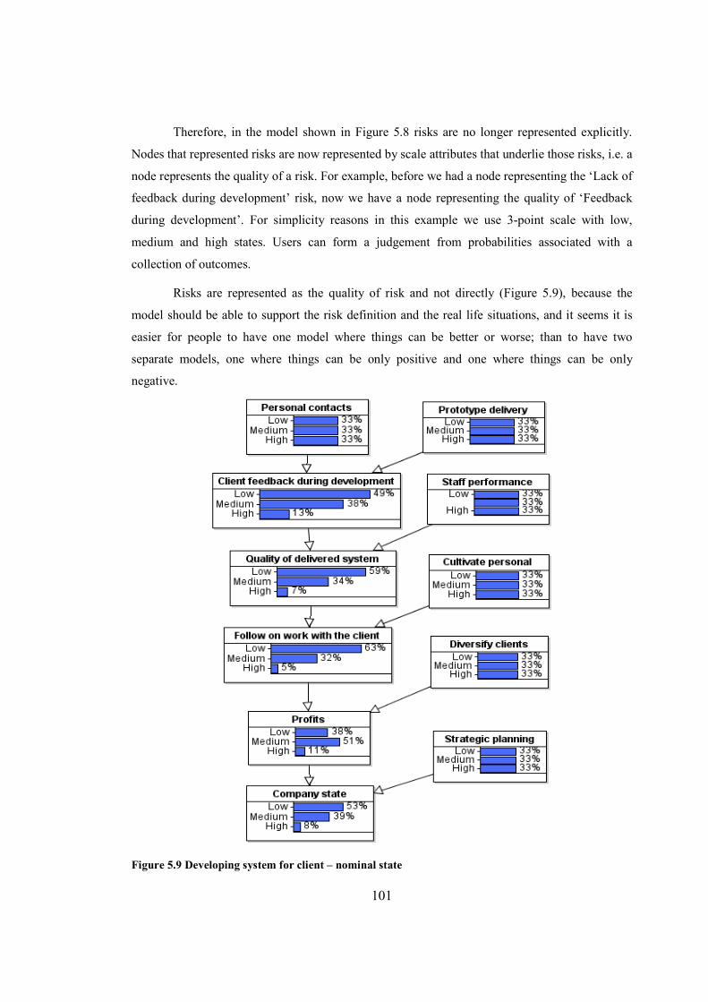
101

Therefore, in the model shown in Figure 5.8 risks are no longer represented explicitly.

Nodes that represented risks are now represented by scale attributes that underlie those risks, i.e. a

node represents the quality of a risk. For example, before we had a node representing the ‘Lack of

feedback during development’ risk, now we have a node representing the quality of ‘Feedback

during development’. For simplicity reasons in this example we use 3-point scale with low,

medium and high states. Users can form a judgement from probabilities associated with a

collection of outcomes.

Risks are represented as the quality of risk and not directly (Figure 5.9), because the

model should be able to support the risk definition and the real life situations, and it seems it is

easier for people to have one model where things can be better or worse; than to have two

separate models, one where things can be only positive and one where things can be only

negative.

Figure 5.9 Developing system for client – nominal state

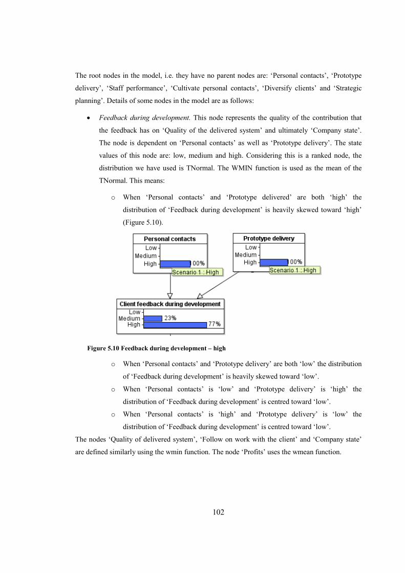
102

The root nodes in the model, i.e. they have no parent nodes are: ‘Personal contacts’, ‘Prototype

delivery’, ‘Staff performance’, ‘Cultivate personal contacts’, ‘Diversify clients’ and ‘Strategic

planning’. Details of some nodes in the model are as follows:

• Feedback during development. This node represents the quality of the contribution that

the feedback has on ‘Quality of the delivered system’ and ultimately ‘Company state’.

The node is dependent on ‘Personal contacts’ as well as ‘Prototype delivery’. The state

values of this node are: low, medium and high. Considering this is a ranked node, the

distribution we have used is TNormal. The WMIN function is used as the mean of the

TNormal. This means:

o When ‘Personal contacts’ and ‘Prototype delivered’ are both ‘high’ the

distribution of ‘Feedback during development’ is heavily skewed toward ‘high’

(Figure 5.10).

Figure 5.10 Feedback during development – high

o When ‘Personal contacts’ and ‘Prototype delivery’ are both ‘low’ the distribution

of ‘Feedback during development’ is heavily skewed toward ‘low’.

o When ‘Personal contacts’ is ‘low’ and ‘Prototype delivery’ is ‘high’ the

distribution of ‘Feedback during development’ is centred toward ‘low’.

o When ‘Personal contacts’ is ‘high’ and ‘Prototype delivery’ is ‘low’ the

distribution of ‘Feedback during development’ is centred toward ‘low’.

The nodes ‘Quality of delivered system’, ‘Follow on work with the client’ and ‘Company state’

are defined similarly using the wmin function. The node ‘Profits’ uses the wmean function.

103

5.9 Summary

In this chapter, we have identified some problems with the term risk as well as problems

with how risk is quantified. Traditional definitions illustrate the term risk as negative. In any

given decision situation both risks and opportunities are usually involved, and both should be

managed. Relatively recent risk definitions incorporate opportunities into their risk definition.

To manage risk we propose a causal framework for risk. Risks and opportunities can

sometimes be treated separately, but it is important to understand that they are not independent.

Hence we use this framework to develop qualitative models where risks are no longer represented

explicitly, but nodes that represent risk are now represented by scale attributes that underlie those

risks. With this type of model, it is possible to fully support the risk definition and real life

situations.

104

6. The Causal Risk Register Model

In chapter 2 we analysed standard project risk management tools; why they were often

inadequate and provided no natural measure for risk analysis. We then went on to describe

Bayesian nets in chapter 3 and explained why they provided a better platform for project risk

analysis. Chapter 4 demonstrated the current BN project risk models and their limitations. New

risk taxonomy was then presented in chapter 5. This chapter introduces the ‘Causal Risk Register

Model’, a new model for large projects at the overall project level.

The main novel contribution of this chapter, and consequently of the whole thesis, is to

implement and validate new risk framework using the Bayesian net model. This new model

adopts the basic philosophy from the existing models whilst overcoming certain limitations. The

model implicitly considers the trade-offs that may be made in the risk model, specifically time,

cost and quality. We discussed project success and failure in section 2.5. At the end, the model

gives a risk score in the form of the probability of the project failing.

6.1 Overview of the Causal Risk Register Model

The main goal of the Causal Risk Register Model (CRRM) is to offer an improvement on

the standard risk measurement (Risk = Probability x Impact) and therefore enable improved

project risk analysis. It captures the basic philosophy of the standard project risk analysis tool i.e.

the risk register, but structurally it is very different.

As discussed previously, there are many problems with the standard measure of risk

using the risk register. In chapter 5 we explained the rational way to think about risks in terms of

causal models with trigger events, control events, risk events, mitigant events and consequence

events. We have applied the causal framework to general top level risks and developed the risk

model for an international leading defence company which we will refer to as ‘company X’.

Figure 6.1 shows the CRRM which is an improvement to the original model developed for

‘company X’. This model illustrates how these risks affect ‘Project Failure’.

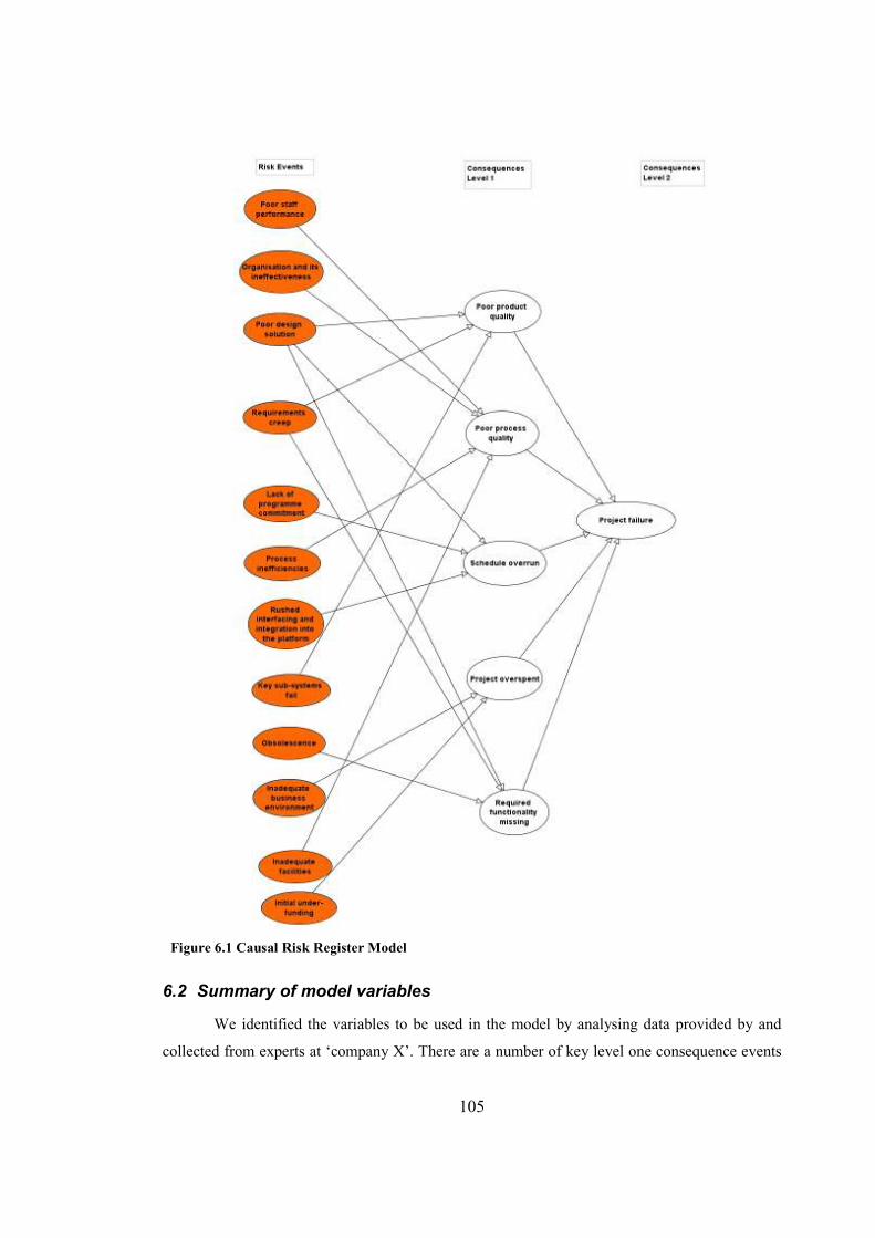
105

Figure 6.1 Causal Risk Register Model

6.2 Summary of model variables

We identified the variables to be used in the model by analysing data provided by and

collected from experts at ‘company X’. There are a number of key level one consequence events

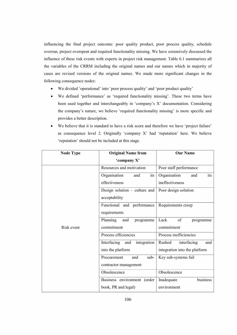
106

influencing the final project outcome: poor quality product, poor process quality, schedule

overrun, project overspent and required functionality missing. We have extensively discussed the

influence of these risk events with experts in project risk management. Table 6.1 summarizes all

the variables of the CRRM including the original names and our names which in majority of

cases are revised versions of the original names. We made more significant changes in the

following consequence nodes:

• We divided ‘operational’ into ‘poor process quality’ and ‘poor product quality’

• We defined ‘performance’ as ‘required functionality missing’. These two terms have

been used together and interchangeably in ‘company’s X’ documentation. Considering

the company’s nature, we believe ‘required functionality missing’ is more specific and

provides a better description.

• We believe that it is standard to have a risk score and therefore we have ‘project failure’

as consequence level 2. Originally ‘company X’ had ‘reputation’ here. We believe

‘reputation’ should not be included at this stage.

Node Type Original Name from

‘company X’

Our Name

Risk event

Resources and motivation Poor staff performance

Organisation and its

effectiveness

Organisation and its

ineffectiveness

Design solution – culture and

acceptability

Poor design solution

Functional and performance

requirements

Requirements creep

Planning and programme

commitment

Lack of programme

commitment

Process efficiencies Process inefficiencies

Interfacing and integration

into the platform

Rushed interfacing and

integration into the platform

Procurement and sub-

contractor management

Key sub-systems fail

Obsolescence Obsolescence

Business environment (order

book, PR and legal)

Inadequate business

environment

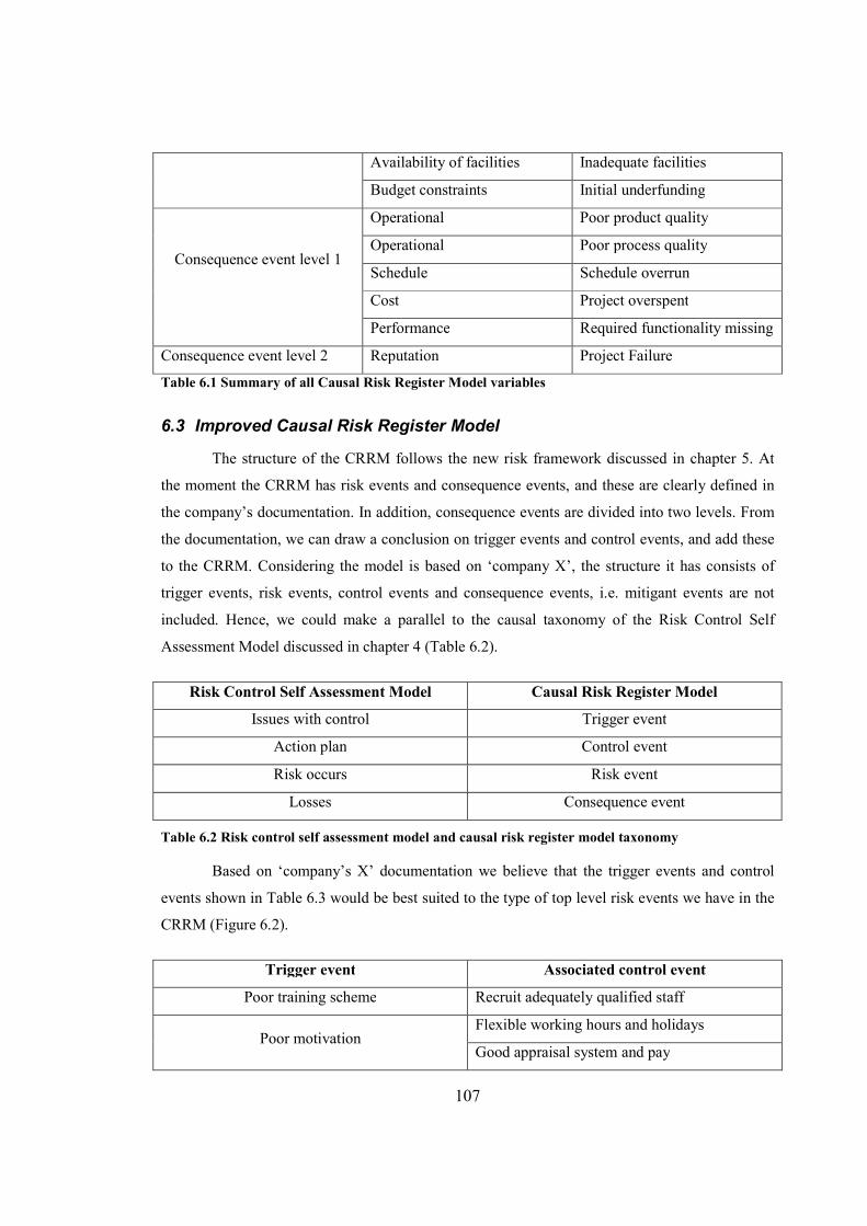
107

Availability of facilities Inadequate facilities

Budget constraints Initial underfunding

Consequence event level 1

Operational Poor product quality

Operational Poor process quality

Schedule Schedule overrun

Cost Project overspent

Performance Required functionality missing

Consequence event level 2 Reputation Project Failure

Table 6.1 Summary of all Causal Risk Register Model variables

6.3 Improved Causal Risk Register Model

The structure of the CRRM follows the new risk framework discussed in chapter 5. At

the moment the CRRM has risk events and consequence events, and these are clearly defined in

the company’s documentation. In addition, consequence events are divided into two levels. From

the documentation, we can draw a conclusion on trigger events and control events, and add these

to the CRRM. Considering the model is based on ‘company X’, the structure it has consists of

trigger events, risk events, control events and consequence events, i.e. mitigant events are not

included. Hence, we could make a parallel to the causal taxonomy of the Risk Control Self

Assessment Model discussed in chapter 4 (Table 6.2).

Risk Control Self Assessment Model Causal Risk Register Model

Issues with control Trigger event

Action plan Control event

Risk occurs Risk event

Losses Consequence event

Table 6.2 Risk control self assessment model and causal risk register model taxonomy

Based on ‘company’s X’ documentation we believe that the trigger events and control

events shown in Table 6.3 would be best suited to the type of top level risk events we have in the

CRRM (Figure 6.2).

Trigger event Associated control event

Poor training scheme Recruit adequately qualified staff

Poor motivation Flexible working hours and holidays

Good appraisal system and pay

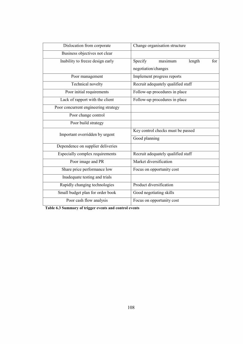
108

Dislocation from corporate Change organisation structure

Business objectives not clear

Inability to freeze design early Specify maximum length for

negotiation/changes

Poor management Implement progress reports

Technical novelty Recruit adequately qualified staff

Poor initial requirements Follow-up procedures in place

Lack of rapport with the client Follow-up procedures in place

Poor concurrent engineering strategy

Poor change control

Poor build strategy

Important overridden by urgent Key control checks must be passed

Good planning

Dependence on supplier deliveries

Especially complex requirements Recruit adequately qualified staff

Poor image and PR Market diversification

Share price performance low Focus on opportunity cost

Inadequate testing and trials

Rapidly changing technologies Product diversification

Small budget plan for order book Good negotiating skills

Poor cash flow analysis Focus on opportunity cost

Table 6.3 Summary of trigger events and control events

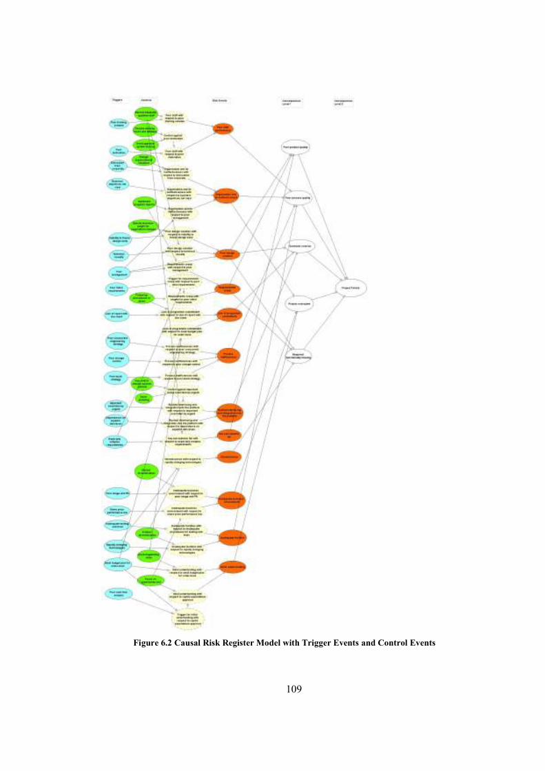
109

Figure 6.2 Causal Risk Register Model with Trigger Events and Control Events

110

As established in chapter 5, it is possible for each risk event to have more than one trigger

event and control event. If we observe the Causal Risk Register Model segment for ‘Poor staff

performance’ risk event (Figure 6.3), we can see there are two trigger events (‘Poor motivation’

and ‘Poor training scheme’) and three control events (‘Recruit adequately qualified staff’,

‘Flexible working hours and holidays’ and ‘Good appraisal system and pay’). Considering there

are five parent nodes, we need to be careful not to end up with very complex NPTs.

To keep ease of use throughout the model and simple NPTs, we have taken the following

steps: firstly, we introduced two dummy nodes for each of the trigger events, i.e. ‘Poor staff

performance with respect to training scheme’ and ‘Poor staff performance with respect to poor

motivation’. Secondly, since there are two control events for ‘Poor motivation’, we introduced

additional dummy node ‘Control against poor motivation’. This node represents the combined

contribution that all the control events put together have on the risk event with respect to a

particular trigger event. For simplicity, this node is a Boolean node and we have used a noisyor

comparative expression to define the NPT.

‘Poor staff with respect to poor motivation’ node is dependent on ‘Poor motivation’ and

‘Control against poor motivation’. This node represents the impact that ‘Poor motivation’ has on

‘Poor staff performance’ when ‘Control against poor motivation’ taken into account. This is a

Boolean node and the NPT is defined manually.

‘Poor staff performance’ node represents a risk event. It is dependent on ‘Poor staff with

respect to poor motivation’ and ‘Poor staff with respect to poor training scheme’. It directly

influences ‘Poor process quality’ which is a consequence level 1 event. Hence, we could say

‘Poor staff performance’ is a trigger event for the ‘Poor process quality’ risk event. Hence, we

can see how the types of events in the causal taxonomy of risk are all completely interchangeable.

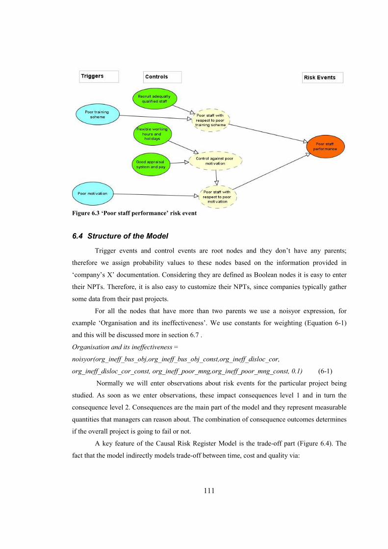
111

Figure 6.3 ‘Poor staff performance’ risk event

6.4 Structure of the Model

Trigger events and control events are root nodes and they don’t have any parents;

therefore we assign probability values to these nodes based on the information provided in

‘company’s X’ documentation. Considering they are defined as Boolean nodes it is easy to enter

their NPTs. Therefore, it is also easy to customize their NPTs, since companies typically gather

some data from their past projects.

For all the nodes that have more than two parents we use a noisyor expression, for

example ‘Organisation and its ineffectiveness’. We use constants for weighting (Equation 6-1)

and this will be discussed more in section 6.7 .

Organisation and its ineffectiveness =

noisyor(org_ineff_bus_obj,org_ineff_bus_obj_const,org_ineff_disloc_cor,

org_ineff_disloc_cor_const, org_ineff_poor_mng,org_ineff_poor_mng_const, 0.1) (6-1)

Normally we will enter observations about risk events for the particular project being

studied. As soon as we enter observations, these impact consequences level 1 and in turn the

consequence level 2. Consequences are the main part of the model and they represent measurable

quantities that managers can reason about. The combination of consequence outcomes determines

if the overall project is going to fail or not.

A key feature of the Causal Risk Register Model is the trade-off part (Figure 6.4). The

fact that the model indirectly models trade-off between time, cost and quality via:

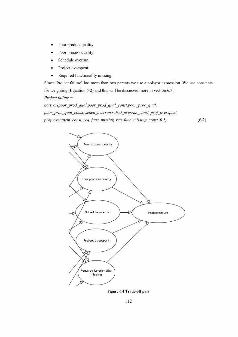
112

• Poor product quality

• Poor process quality

• Schedule overrun

• Project overspent

• Required functionality missing.

Since ‘Project failure’ has more than two parents we use a noisyor expression. We use constants

for weighting (Equation 6-2) and this will be discussed more in section 6.7 .

Project failure =

noisyor(poor_prod_qual,poor_prod_qual_const,poor_proc_qual,

poor_proc_qual_const, sched_overrun,sched_overrun_const, proj_overspent,

proj_overspent_const, req_func_missing, req_func_missing_const, 0.1) (6-2)

Figure 6.4 Trade-off part

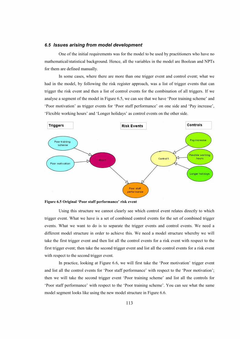
113

6.5 Issues arising from model development

One of the initial requirements was for the model to be used by practitioners who have no

mathematical/statistical background. Hence, all the variables in the model are Boolean and NPTs

for them are defined manually.

In some cases, where there are more than one trigger event and control event; what we

had in the model, by following the risk register approach, was a list of trigger events that can

trigger the risk event and then a list of control events for the combination of all triggers. If we

analyse a segment of the model in Figure 6.5, we can see that we have ‘Poor training scheme’ and

‘Poor motivation’ as trigger events for ‘Poor staff performance’ on one side and ‘Pay increase’,

‘Flexible working hours’ and ‘Longer holidays’ as control events on the other side.

Figure 6.5 Original ‘Poor staff performance’ risk event

Using this structure we cannot clearly see which control event relates directly to which

trigger event. What we have is a set of combined control events for the set of combined trigger

events. What we want to do is to separate the trigger events and control events. We need a

different model structure in order to achieve this. We need a model structure whereby we will

take the first trigger event and then list all the control events for a risk event with respect to the

first trigger event; then take the second trigger event and list all the control events for a risk event

with respect to the second trigger event.

In practice, looking at Figure 6.6, we will first take the ‘Poor motivation’ trigger event

and list all the control events for ‘Poor staff performance’ with respect to the ‘Poor motivation’;

then we will take the second trigger event ‘Poor training scheme’ and list all the controls for

‘Poor staff performance’ with respect to the ‘Poor training scheme’. You can see what the same

model segment looks like using the new model structure in Figure 6.6.

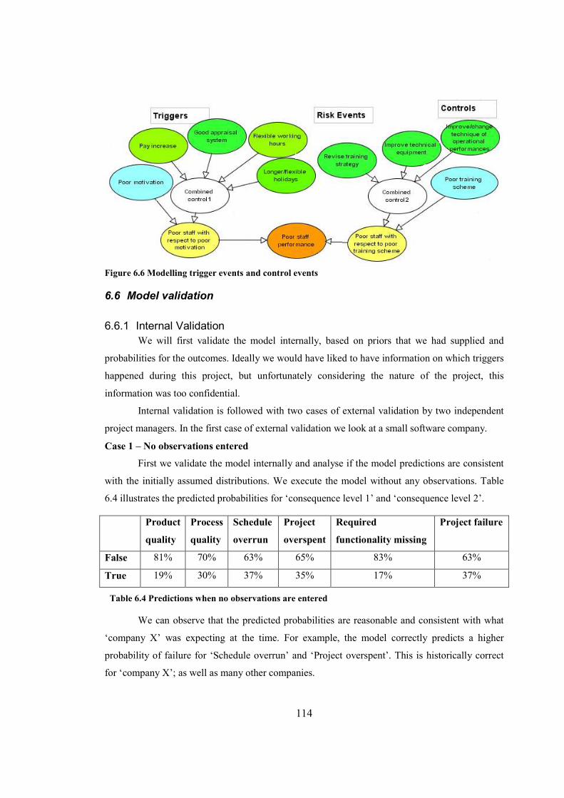
114

Figure 6.6 Modelling trigger events and control events

6.6 Model validation

6.6.1 Internal Validation

We will first validate the model internally, based on priors that we had supplied and

probabilities for the outcomes. Ideally we would have liked to have information on which triggers

happened during this project, but unfortunately considering the nature of the project, this

information was too confidential.

Internal validation is followed with two cases of external validation by two independent

project managers. In the first case of external validation we look at a small software company.

Case 1 – No observations entered

First we validate the model internally and analyse if the model predictions are consistent

with the initially assumed distributions. We execute the model without any observations. Table

6.4 illustrates the predicted probabilities for ‘consequence level 1’ and ‘consequence level 2’.

Product

quality

Process

quality

Schedule

overrun

Project

overspent

Required

functionality missing

Project failure

False 81% 70% 63% 65% 83% 63%

True 19% 30% 37% 35% 17% 37%

Table 6.4 Predictions when no observations are entered

We can observe that the predicted probabilities are reasonable and consistent with what

‘company X’ was expecting at the time. For example, the model correctly predicts a higher

probability of failure for ‘Schedule overrun’ and ‘Project overspent’. This is historically correct

for ‘company X’; as well as many other companies.

115

Case 2 – Observation ‘false’ is entered for ‘Project failure’

We execute the model when observation ‘false’ is entered for ‘Project failure’. This

results in back propagation and Table 6.5 illustrates the revised probabilities for ‘consequence

level 1’ nodes.

Product

quality

Process

quality

Schedule

overrun

Project

overspent

Required


False 87% 77% 69% 71% 88%

True 13% 23% 31% 29% 12%

Table 6.5 Predictions when observation ‘false’ is entered for ‘Project failure’

The model correctly revises probability distributions and predicts a higher probability of

‘consequence level 1’ nodes being ‘false’. For example, the probability for ‘Product quality’

being ‘false’ is revised and it increases from 81% (Figure 6.4) to 87% (Figure 6.5).

Case 3 – Observation ‘false’ is entered for ‘Schedule overrun’

We execute the model when observation ‘false’ is entered for ‘Schedule overrun’. This

results in back propagation and Table 6.6 illustrates the revised probabilities for relevant risk

event nodes.

Poor design

solution

Lack of programme

commitment



False 92% 93% 91%

True 8% 7% 9%

Table 6.6 Predictions when observation ‘false’ is entered for ‘Schedule overrun’

The model correctly revises probability distributions and predicts a higher probability of

relevant risk events being ‘false’. For example, the probability for ‘Poor design solution’ being

‘false’ is revised and it increases from 77% (Figure 6.7) to 92% (Figure 6.6).

Poor design

solution

Lack of programme

commitment



False 77% 87% 84%

True 23% 13% 16%

Table 6.7 Predictions when no observations are entered

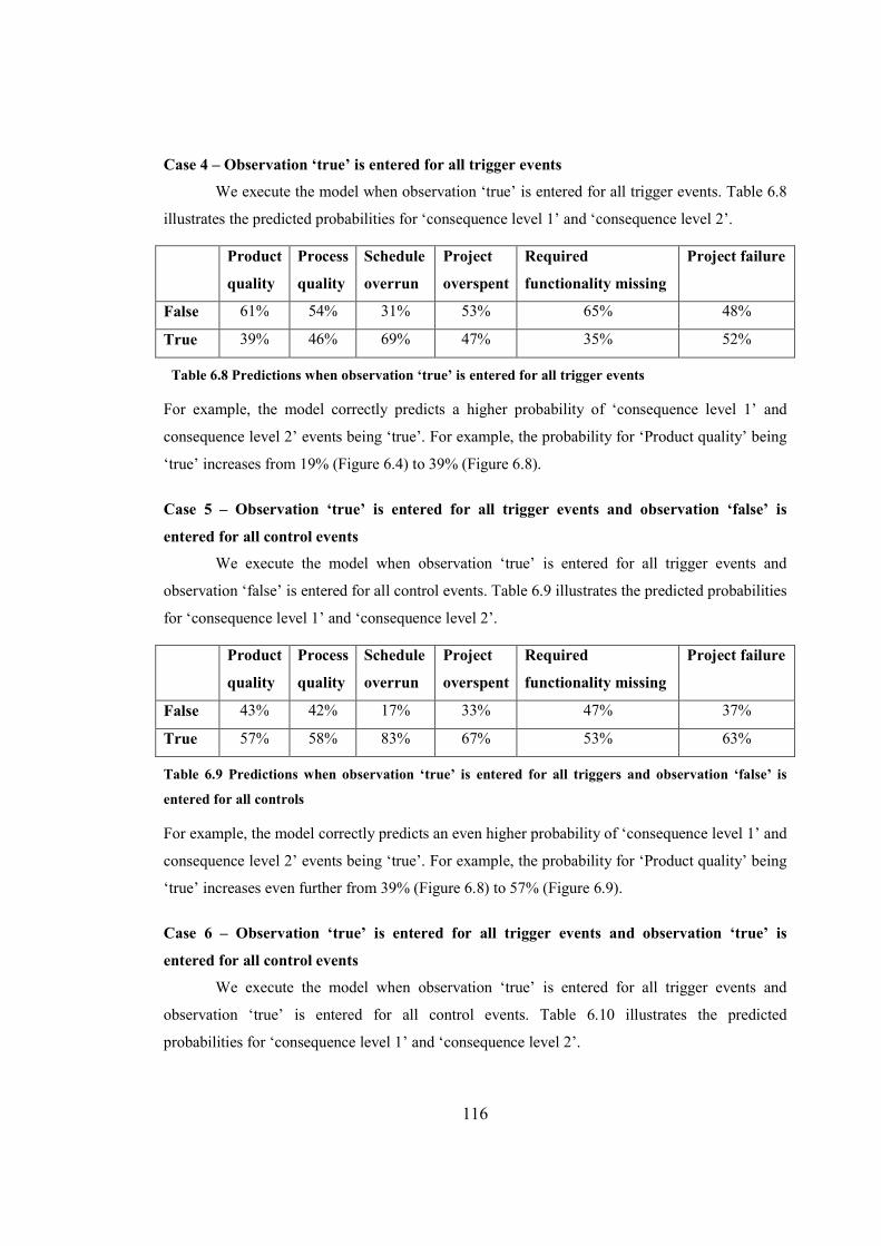
116

Case 4 – Observation ‘true’ is entered for all trigger events

We execute the model when observation ‘true’ is entered for all trigger events. Table 6.8

illustrates the predicted probabilities for ‘consequence level 1’ and ‘consequence level 2’.

Product

quality

Process

quality

Schedule

overrun

Project

overspent

Required


Project failure

False 61% 54% 31% 53% 65% 48%

True 39% 46% 69% 47% 35% 52%

Table 6.8 Predictions when observation ‘true’ is entered for all trigger events

For example, the model correctly predicts a higher probability of ‘consequence level 1’ and

consequence level 2’ events being ‘true’. For example, the probability for ‘Product quality’ being

‘true’ increases from 19% (Figure 6.4) to 39% (Figure 6.8).

Case 5 – Observation ‘true’ is entered for all trigger events and observation ‘false’ is

entered for all control events

We execute the model when observation ‘true’ is entered for all trigger events and

observation ‘false’ is entered for all control events. Table 6.9 illustrates the predicted probabilities

for ‘consequence level 1’ and ‘consequence level 2’.

Product

quality

Process

quality

Schedule

overrun

Project

overspent

Required


Project failure

False 43% 42% 17% 33% 47% 37%

True 57% 58% 83% 67% 53% 63%

Table 6.9 Predictions when observation ‘true’ is entered for all triggers and observation ‘false’ is

entered for all controls

For example, the model correctly predicts an even higher probability of ‘consequence level 1’ and


‘true’ increases even further from 39% (Figure 6.8) to 57% (Figure 6.9).

Case 6 – Observation ‘true’ is entered for all trigger events and observation ‘true’ is

entered for all control events

We execute the model when observation ‘true’ is entered for all trigger events and

observation ‘true’ is entered for all control events. Table 6.10 illustrates the predicted

probabilities for ‘consequence level 1’ and ‘consequence level 2’.

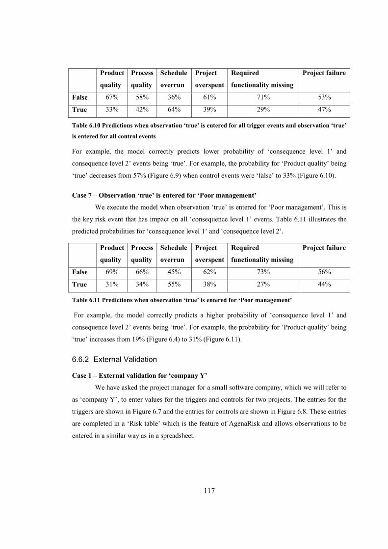
117

Product

quality

Process

quality

Schedule

overrun

Project

overspent

Required


Project failure

False 67% 58% 36% 61% 71% 53%

True 33% 42% 64% 39% 29% 47%

Table 6.10 Predictions when observation ‘true’ is entered for all trigger events and observation ‘true’

is entered for all control events

For example, the model correctly predicts lower probability of ‘consequence level 1’ and


‘true’ decreases from 57% (Figure 6.9) when control events were ‘false’ to 33% (Figure 6.10).

Case 7 – Observation ‘true’ is entered for ‘Poor management’

We execute the model when observation ‘true’ is entered for ‘Poor management’. This is

the key risk event that has impact on all ‘consequence level 1’ events. Table 6.11 illustrates the

predicted probabilities for ‘consequence level 1’ and ‘consequence level 2’.

Product

quality

Process

quality

Schedule

overrun

Project

overspent

Required


Project failure

False 69% 66% 45% 62% 73% 56%

True 31% 34% 55% 38% 27% 44%

Table 6.11 Predictions when observation ‘true’ is entered for ‘Poor management’

For example, the model correctly predicts a higher probability of ‘consequence level 1’ and


‘true’ increases from 19% (Figure 6.4) to 31% (Figure 6.11).

6.6.2 External Validation

Case 1 – External validation for ‘company Y’

We have asked the project manager for a small software company, which we will refer to

as ‘company Y’, to enter values for the triggers and controls for two projects. The entries for the

triggers are shown in Figure 6.7 and the entries for controls are shown in Figure 6.8. These entries

are completed in a ‘Risk table’ which is the feature of AgenaRisk and allows observations to be

entered in a similar way as in a spreadsheet.

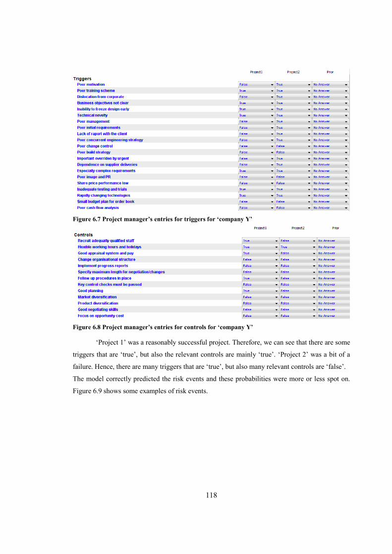
118

Figure 6.7 Project manager’s entries for triggers for ‘company Y’

Figure 6.8 Project manager’s entries for controls for ‘company Y’

‘Project 1’ was a reasonably successful project. Therefore, we can see that there are some

triggers that are ‘true’, but also the relevant controls are mainly ‘true’. ‘Project 2’ was a bit of a

failure. Hence, there are many triggers that are ‘true’, but also many relevant controls are ‘false’.

The model correctly predicted the risk events and these probabilities were more or less spot on.

Figure 6.9 shows some examples of risk events.

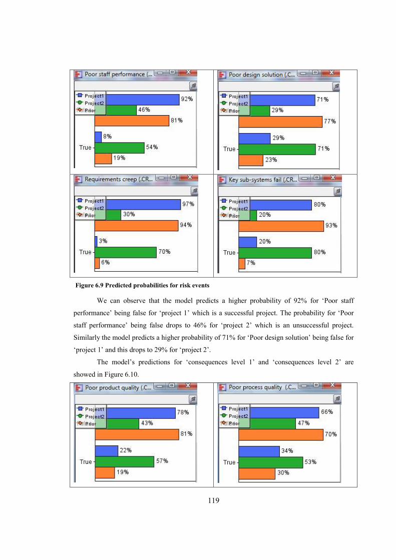
119

Figure 6.9 Predicted probabilities for risk events

We can observe that the model predicts a higher probability of 92% for ‘Poor staff

performance’ being false for ‘project 1’ which is a successful project. The probability for ‘Poor

staff performance’ being false drops to 46% for ‘project 2’ which is an unsuccessful project.

Similarly the model predicts a higher probability of 71% for ‘Poor design solution’ being false for

‘project 1’ and this drops to 29% for ‘project 2’.

The model’s predictions for ‘consequences level 1’ and ‘consequences level 2’ are

showed in Figure 6.10.

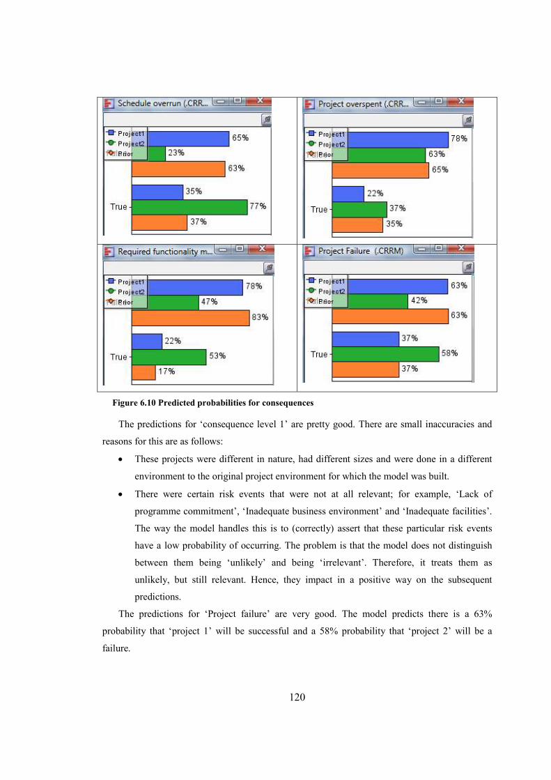
120

Figure 6.10 Predicted probabilities for consequences

The predictions for ‘consequence level 1’ are pretty good. There are small inaccuracies and

reasons for this are as follows:

• These projects were different in nature, had different sizes and were done in a different

environment to the original project environment for which the model was built.

• There were certain risk events that were not at all relevant; for example, ‘Lack of

programme commitment’, ‘Inadequate business environment’ and ‘Inadequate facilities’.

The way the model handles this is to (correctly) assert that these particular risk events

have a low probability of occurring. The problem is that the model does not distinguish

between them being ‘unlikely’ and being ‘irrelevant’. Therefore, it treats them as

unlikely, but still relevant. Hence, they impact in a positive way on the subsequent

predictions.

The predictions for ‘Project failure’ are very good. The model predicts there is a 63%

probability that ‘project 1’ will be successful and a 58% probability that ‘project 2’ will be a

failure.

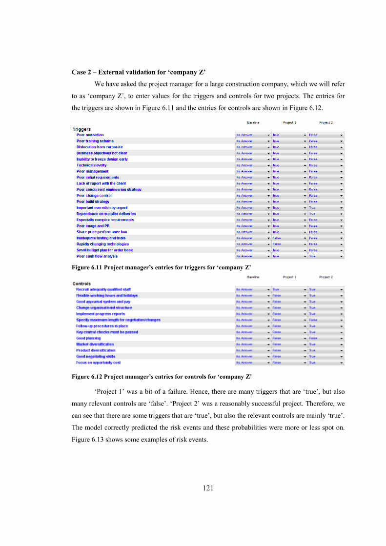
121

Case 2 – External validation for ‘company Z’

We have asked the project manager for a large construction company, which we will refer

to as ‘company Z’, to enter values for the triggers and controls for two projects. The entries for

the triggers are shown in Figure 6.11 and the entries for controls are shown in Figure 6.12.

Figure 6.11 Project manager’s entries for triggers for ‘company Z’

Figure 6.12 Project manager’s entries for controls for ‘company Z’

‘Project 1’ was a bit of a failure. Hence, there are many triggers that are ‘true’, but also

many relevant controls are ‘false’. ‘Project 2’ was a reasonably successful project. Therefore, we

can see that there are some triggers that are ‘true’, but also the relevant controls are mainly ‘true’.

The model correctly predicted the risk events and these probabilities were more or less spot on.

Figure 6.13 shows some examples of risk events.

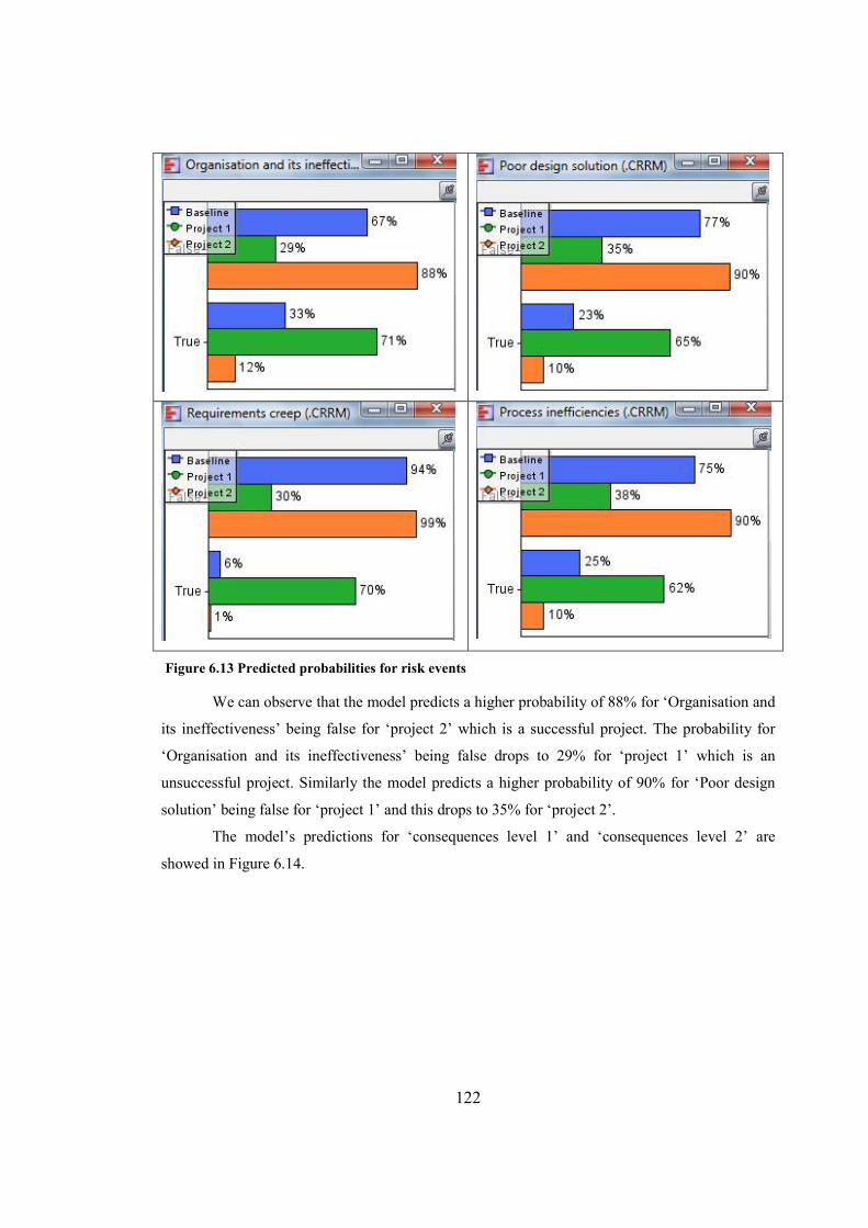
122

Figure 6.13 Predicted probabilities for risk events

We can observe that the model predicts a higher probability of 88% for ‘Organisation and

its ineffectiveness’ being false for ‘project 2’ which is a successful project. The probability for

‘Organisation and its ineffectiveness’ being false drops to 29% for ‘project 1’ which is an

unsuccessful project. Similarly the model predicts a higher probability of 90% for ‘Poor design

solution’ being false for ‘project 1’ and this drops to 35% for ‘project 2’.

The model’s predictions for ‘consequences level 1’ and ‘consequences level 2’ are

showed in Figure 6.14.

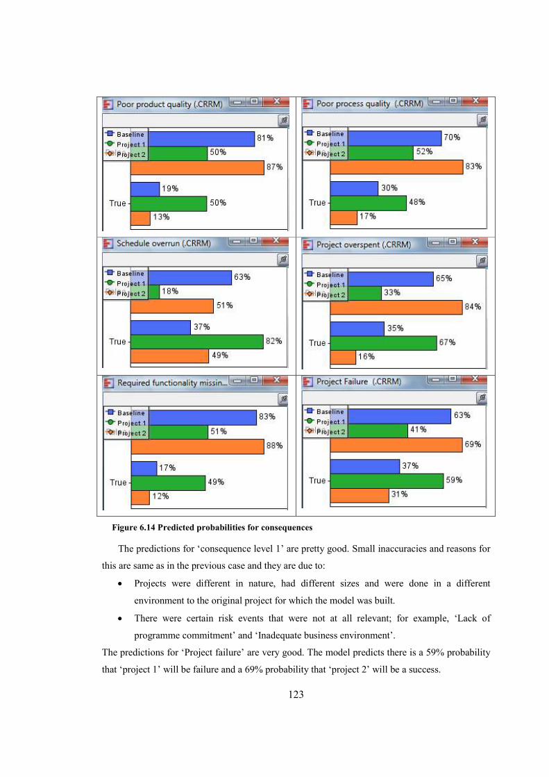
123

Figure 6.14 Predicted probabilities for consequences

The predictions for ‘consequence level 1’ are pretty good. Small inaccuracies and reasons for

this are same as in the previous case and they are due to:

• Projects were different in nature, had different sizes and were done in a different

environment to the original project for which the model was built.

• There were certain risk events that were not at all relevant; for example, ‘Lack of

programme commitment’ and ‘Inadequate business environment’.

The predictions for ‘Project failure’ are very good. The model predicts there is a 59% probability

that ‘project 1’ will be failure and a 69% probability that ‘project 2’ will be a success.

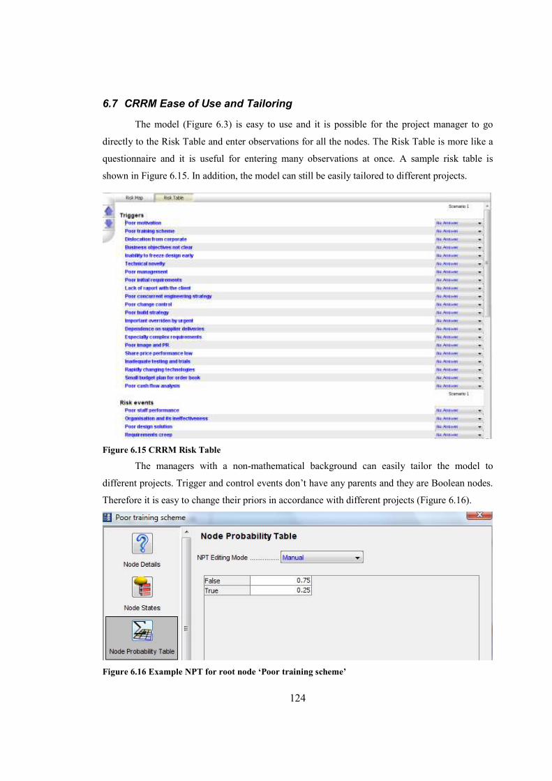
124

6.7 CRRM Ease of Use and Tailoring

The model (Figure 6.3) is easy to use and it is possible for the project manager to go

directly to the Risk Table and enter observations for all the nodes. The Risk Table is more like a

questionnaire and it is useful for entering many observations at once. A sample risk table is

shown in Figure 6.15. In addition, the model can still be easily tailored to different projects.

Figure 6.15 CRRM Risk Table

The managers with a non-mathematical background can easily tailor the model to

different projects. Trigger and control events don’t have any parents and they are Boolean nodes.

Therefore it is easy to change their priors in accordance with different projects (Figure 6.16).

Figure 6.16 Example NPT for root node ‘Poor training scheme’

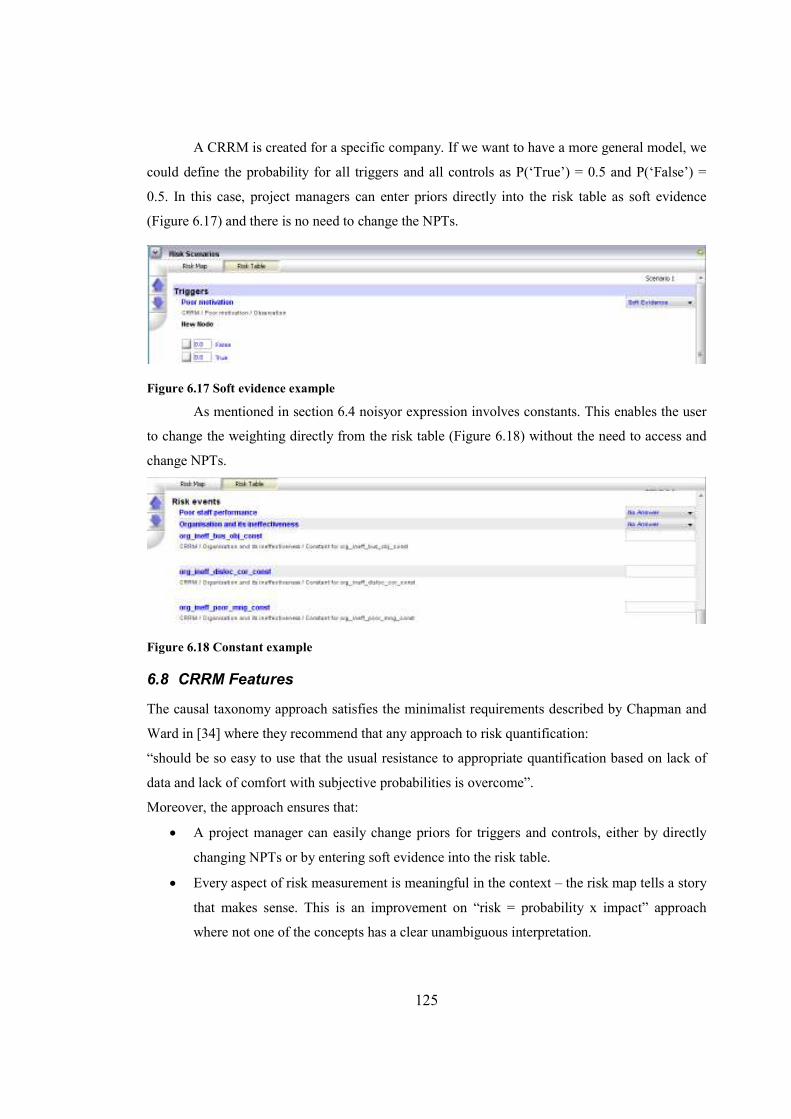
125

A CRRM is created for a specific company. If we want to have a more general model, we

could define the probability for all triggers and all controls as P(‘True’) = 0.5 and P(‘False’) =

0.5. In this case, project managers can enter priors directly into the risk table as soft evidence

(Figure 6.17) and there is no need to change the NPTs.

Figure 6.17 Soft evidence example

As mentioned in section 6.4 noisyor expression involves constants. This enables the user

to change the weighting directly from the risk table (Figure 6.18) without the need to access and

change NPTs.

Figure 6.18 Constant example

6.8 CRRM Features

The causal taxonomy approach satisfies the minimalist requirements described by Chapman and

Ward in [34] where they recommend that any approach to risk quantification:

“should be so easy to use that the usual resistance to appropriate quantification based on lack of

data and lack of comfort with subjective probabilities is overcome”.

Moreover, the approach ensures that:

• A project manager can easily change priors for triggers and controls, either by directly

changing NPTs or by entering soft evidence into the risk table.

• Every aspect of risk measurement is meaningful in the context – the risk map tells a story

that makes sense. This is an improvement on “risk = probability x impact” approach

where not one of the concepts has a clear unambiguous interpretation.

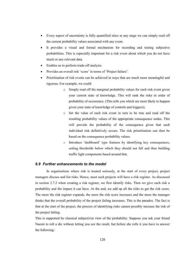
126

• Every aspect of uncertainty is fully quantified since at any stage we can simply read off

the current probability values associated with any event.

• It provides a visual and formal mechanism for recording and testing subjective

probabilities. This is especially important for a risk event about which you do not have

much or any relevant data.

• Enables us to perform trade-off analysis.

• Provides an overall risk ‘score’ in terms of ‘Project failure’.

• Prioritisation of risk events can be achieved in ways that are much more meaningful and

rigorous. For example, we could:

o Simply read off the marginal probability values for each risk event given

your current state of knowledge. This will rank the risks in order of

probability of occurrence. (This tells you which are most likely to happen

given your state of knowledge of controls and triggers);

o Set the value of each risk event in turn to be true and read off the

resulting probability values of the appropriate consequence nodes. This

will provide the probability of the consequence given that each

individual risk definitively occurs. The risk prioritisation can then be

based on the consequence probability values.

o Introduce ‘dashboard’ type features by identifying key consequences,

setting thresholds below which they should not fall and then building

traffic light components based around that.

6.9 Further enhancements to the model

In organisations where risk is treated seriously, at the start of every project, project

managers discuss and list risks. Hence, most such projects will have a risk register. As discussed

in section 2.7.2 when creating a risk register, we first identify risks. Then we give each risk a

probability and the impact it can have. At the end, we add up all the risks to get the risk score.

The more the risk register expands, the more the risk score increases and the more the manager

thinks that the overall probability of the project failing increases. This is the paradox. The fact is

that at the start of the project, the process of identifying risks cannot possibly increase the risk of

the project failing.

This is supported by classical subjectivist view of the probability. Suppose you ask your friend

Naomi to roll a die without letting you see the result, but before she rolls it you have to answer

the following:

127

Question 1: What is the probability the number rolled will be a 4?

Having rolled the die Naomi must write down the number rolled on a piece of paper (without

showing you) and place it in an envelope.

Now answer:

Question 2: What is the probability the number written down is a 4 (i.e. was the number rolled a

4)?

From your perspective it is rational to answer 1/6 in both cases. If Naomi informs Hannah that the

number written down is even, then the rational answer to Question 2 from Hannah's perspective is

1/3. So different information about the same unkown event can rationally lead to different

subjective probabilities about that event. But from Naomi's perspective there is no uncertainty at

all about the event. The answer to question 2 is either 1 (if it is a 4) or 0 (if it is not) and it is this

situation that leads (wrongly) to the 'no such thing as probability' argument. This argument says

that there is no uncertainty about the number because it is a ‘fact’ - it is even written down (and is

known to Naomi). But, if YOUR knowledge about the number after it is thrown (i.e. if you are

not Naomi or even Hannah) is as incomplete as it was before, then your uncertainty about it

remains the same. Hence it is irrational to argue that the probability has changed from your

perspective.

For example, we could look at the probability of a terrorist attack from two perspectives

[2]; the perspective of a random school child and the perspective of an MI5 officer. Imagine they

were both given authority to make decision about the risk of a terrorist attack. We can say that

what is known to the decision maker in the first case will be less than what is known to the

decision maker in the second case (at least we hope this would be the case). However, the

probability of the terrorist attack is clearly independent of probability assign to it by decision

makers.

Therefore, the key in this example is that the probability of the ‘terrorist attack’ is the

same in both cases. This probability does not change. What changes is that the random school

child will probably know less ‘known terrorist groups’ than the MI5 officer who will hopefully

know more. The fact that the MI5 officer will simply list many more ‘known terrorist groups’

does not increase the probability of a ‘terrorist attack’. Hence, the prior for ‘terrorist attack’

should not change, because what changes is only our knowledge about the risks and not the risks

themselves. Following the risk register approach, the random school child and the MI5 officer

would end up with two different risk scores. The MI5 officer would end up with a higher risk

score, because he would simply list many more terrorist groups; and the random school child

128

would end up with a lower risk score, because he/she would list less terrorist groups. This is the

paradox.

However, there has been little discussion about this paradox. Therefore, we need a new

approach to improve risk classification. The key point is that in the beginning when we do a risk

assessment, the probability of a project failing does not change. However, the probability margins

between the known knowns and the known unknown are probably different. This is the key

technical point that most project managers miss out on. We will discuss risk classification more in

the next section.

6.9.1 The Risk Classification Framework

The United States military was the first one to use the term ‘unknown unknowns’. The

earliest use comes from a paper entitled ‘Clausewitz and Modern War Gaming: losing can be

better than winning’ [68]. Almost a decade later, the software engineering community has

adopted the term and used it as basis to propose one of the ways to classify risks. A 1993 paper

by Carnegie Mellon’s Software Engineering Institute proposed grouping risks into three basic

categories. Risks can be known, unknown or unknowable. “Known risks are those that one or

more project personnel are aware of – if not explicitly as risks, at least as concerns. The unknown

risks are those that would surface (i.e. become known), if the project personnel were given the

right opportunity, cues, and information. The unknowable risks are those that, even in principle,

“none could foresee.” [169] In 1997 Chapman and Ward’s [32] text book on project management

adopted this approach of classifying risk. In 2002 Donald Rumsfeld [165], the American secretary

of defence at the time, was ridiculed by media for his famous ‘known unknowns’ remark, then

defended as clear. Media coverage did not reveal he was simply quoting accepted project

management theory.

Most commonly used standards for project risk management in organisations e.g. Project

Management Institute, Project Management Body of Knowledge, Chapter 11 [151], UK

Association for Project Management Project Risk Analysis and Management (PRAM) Guide [7],

AS/NZS 4360 Standard [9]; do not at all mention known, unknown and unknowable risk. The

World Economic Forum 2006 [179] Global risk report’s suggestion is to classify risks into three

categories: known, unknown and unknowable. Clearly there are ambiguities here; the cases of

tsunamis, hurricanes, the severity of an epidemic, terrorism attacks are a few to mention.

Let us take, for example, the terrorist attacks in the United States on September 11th

2001. Here we can identify the risk event as “Terrorists hijack and crash large civilian aircraft

into major buildings”. The question now is whether this risk event was known, unknown or

129

unknowable. We can certainly say that it was definitely not an unknowable risk event, because

there were many examples before whereby terrorists have hijacked planes. The real question is

whether this risk event was known or unknown. We are not able to answer this question using the

classification framework proposed in 1993 and still in use. The reason for this is that the risk

event in question was known to the US intelligence, but it was unknown to the key decision

makers at the time. Using this example we can clearly see what is wrong with the risk

classification framework currently in use. It fails to account for information and knowledge

available to particular decision makers.

Part of the initial purpose of our new risk classification framework was to define known,

unknown and unknowable in more detail and to provide simple descriptions and terminology to

fit these ambiguities. The key is that these ambiguities do not fit in the World Economic Forum

2006 Global risk report framework, because the risk event from the above example is not just

unknown. Generally speaking people knew about it, but the problem was that at the time decision

makers did not know. Hence, in our new risk event classification framework, we will introduce

this new idea of the decision maker and the information and knowledge available to them (Table

6.12).

There are known knowns; these are things we know we know. A known known is when

we know the risk and we have seen it happen sufficiently many times before. Hence, we are able

to make an empirical probabilistic judgement of the risk occurring and its consequence. We also

know there are known unknowns; that is to say we know there are some things we do not know.

A known unknown is when we know the risk event, but we have rarely observed it or we have

never had the opportunity to observe it. Hence, we can only make a subjective probabilistic

judgement about it and we are not able to make an empirical probabilistic judgement. Hence, the

probability of the risk occurring and its consequence is based only on our subjective probabilistic

judgement.

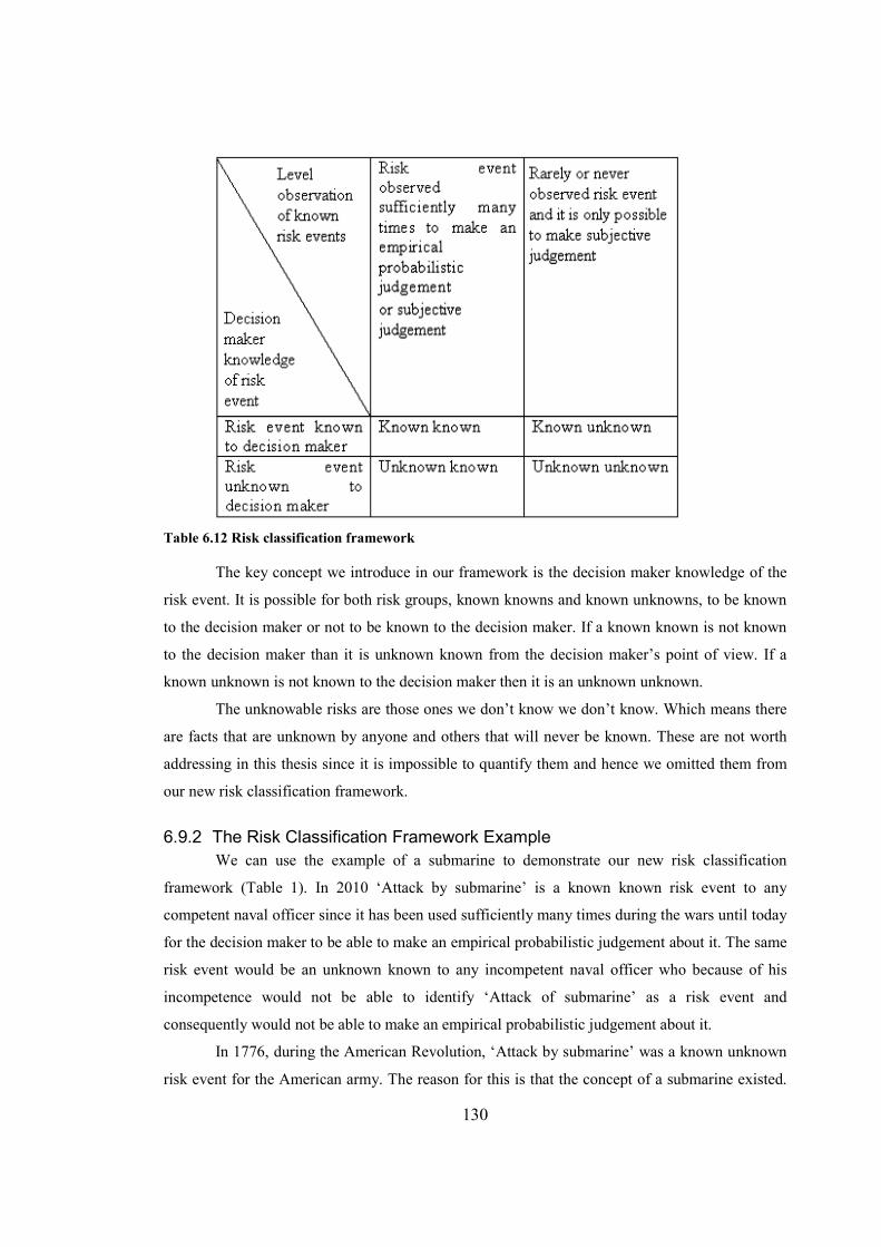
130

Table 6.12 Risk classification framework

The key concept we introduce in our framework is the decision maker knowledge of the

risk event. It is possible for both risk groups, known knowns and known unknowns, to be known

to the decision maker or not to be known to the decision maker. If a known known is not known

to the decision maker than it is unknown known from the decision maker’s point of view. If a

known unknown is not known to the decision maker then it is an unknown unknown.

The unknowable risks are those ones we don’t know we don’t know. Which means there

are facts that are unknown by anyone and others that will never be known. These are not worth

addressing in this thesis since it is impossible to quantify them and hence we omitted them from

our new risk classification framework.

6.9.2 The Risk Classification Framework Example

We can use the example of a submarine to demonstrate our new risk classification

framework (Table 1). In 2010 ‘Attack by submarine’ is a known known risk event to any

competent naval officer since it has been used sufficiently many times during the wars until today

for the decision maker to be able to make an empirical probabilistic judgement about it. The same

risk event would be an unknown known to any incompetent naval officer who because of his

incompetence would not be able to identify ‘Attack of submarine’ as a risk event and

consequently would not be able to make an empirical probabilistic judgement about it.

In 1776, during the American Revolution, ‘Attack by submarine’ was a known unknown

risk event for the American army. The reason for this is that the concept of a submarine existed.

131

The fact that it had not been used in warfare before meant that the decision makers at the time

were not able to make an empirical probabilistic judgement. However, they were still able to

make a subjective probabilistic judgement about it. Since the decision makers were able to make

a subjective judgement about the risk event, we can put the above risk event into the known

unknown category.

The first published description for the submarine was in 1578. William Bourne, a former

Royal Navy gunner, designed a completely enclosed boat that could be submerged and rowed

beneath the surface. His creation was a wooden framework bound in waterproofed leather. It was

to be submerged by using hand vices to contract the sides and decrease the volume. In 1776, the

submarine was used in warfare for the first time. Because of this we can say that before 1776

‘Attack by submarine’ was an unknown unknown risk event.

The key to improving the risk register is using our new risk classification framework and

looking at how dividing line between the known knowns, known unknowns, unknown knowns

and unknown unknowns changes. As the project progresses what changes is our knowledge about

risks and not the risk events themselves. What is a known unknown can become a known known.

In some situations, the list of things that are known knowns and known unknowns can be altered.

There are some things that could be known knowns, but sometimes the costs of knowing them

may exceed the potential benefits. Risk management in general tries to shift risks that are

considered known unknowns into the category of known knowns and tries to mitigate the costs

associated with things that remain known unknowns. Known unknowns can appear at any time

during the execution of the project. We need to create a strategy to deal with such possibilities.

The real dilemma is what to do with risks that seem unknowable. In a crisis, information

inevitably will be highly imperfect. The very nature of a crisis means that the ratio of the

unknown and unknowable will be especially large relative to the known, and this, in turn, can

influence how decision makers judge risks. It is important to mention that the only way for the

overall probability of failure to change is if an unknowable risk becomes at least an unknown

unknown.

The challenge is how to complete priors for this type of model. Maybe it would be

possible to elicit them from experienced managers. We would have to ask them to say something

about what they don’t know. An unknowable risk cannot be modelled. The only way to

incorporate unknowable risks is to add additional nodes when unknowable risks become at least

unknown unknowns. Hence, in terms of quantitative project risk management, it would be

possible to concentrate on known knowns and known unknowns.

132

Ideally what we would like to achieve in a model is to somehow automatically change

between known knowns and known unknowns without changing the overall probability. This

complex causal relationship is important, but it is beyond the scope of this thesis.

6.10 Summary

The new Causal Risk Register Model discussed in this chapter applies risk framework

developed in chapter 5. The model is developed based on top level risks provided by an

international leading defence company. The internal and external validation performed on the

CRRM showed its great potential in providing useful information for project risk assessment. The

model provides reasonable explanations in a number of different scenarios. We identified some

issues and possible future improvements notably the risk classification framework. The next

chapter discusses the extension to the model in order to explicitly address project trade-offs.

133

7. Generic Trade-off Model

In chapter 4 we provided examples of previous BN models and how they indirectly

addressed trade-offs. The Causal Risk Register Model developed in chapter 6 also addresses

trade-offs indirectly. Therefore, this chapter focuses on extending the Causal Risk Register Model

with a sub-model able to explicitly model trade-offs. The Generic Trade-off Model considers the

trade-offs that may be made during a project, specifically time, cost and quality. For example, if

asked to estimate the probability of a project overrunning by various lengths of time, a manager

may respond by contending that such a risk can be reduced to virtually zero if he is given a larger

budget. This implies that, in such a case, there is a trade-off between the time and the cost.

Novel contributions of this chapter include a list of assumed rules that satisfy project

trade-offs and reflect relationships between key project variables and the BN model that satisfies

all the assumed rules identified. The Generic Trade-off Model is one of the main contributions to

the whole thesis. The earlier version of this work has been published [64].

7.1 The Project Trade-offs

As mentioned in section 2.5, successful project risk management attempts to control

resources within the constraints of time, cost and quality. In the traditional cost, time and quality

model; quality is a euphemism for the features of the end project which is delivered. This clearly

has two attributes: functionality (amount of useful features delivered to end users) [107] and

product quality (how good is the product delivered) [104]. Clearly it is possible to deliver less or

more functionality; and lower or higher product quality. This breakdown of quality is really

important, since it brings the causal aspect into the model. In addition, we introduce a new

dimension – process quality (how good is the process during delivery). This is important because

from a risk management perspective this is something the project manager can control/improve.

For the purpose of assumed rules simplification, we have grouped cost and time into

resources. If cost and time are observed independently, then anything that applies to resources

applies to cost and time. The model itself preserves cost and time separately; considers process

quality and both attributes for quality.

Trade-offs are always determined by the constraints of the project. The types of

constraints commonly imposed are illustrated in Table 7.1 [97]. Situations with one or two

elements fixed at a given time are the typical trade-offs encountered in project management.

Situations where three elements are fixed or variable portray some research and development

projects. The quality of research and development projects, for example, is usually well defined,

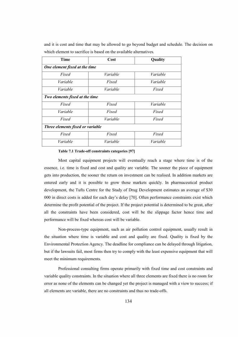
134

and it is cost and time that may be allowed to go beyond budget and schedule. The decision on

which element to sacrifice is based on the available alternatives.

Time Cost Quality

One element fixed at the time

Fixed Variable Variable

Variable Fixed Variable

Variable Variable Fixed

Two elements fixed at the time

Fixed Fixed Variable

Variable Fixed Fixed

Fixed Variable Fixed

Three elements fixed or variable

Fixed Fixed Fixed

Variable Variable Variable

Table 7.1 Trade-off constraints categories [97]

Most capital equipment projects will eventually reach a stage where time is of the

essence, i.e. time is fixed and cost and quality are variable. The sooner the piece of equipment

gets into production, the sooner the return on investment can be realised. In addition markets are

entered early and it is possible to grow those markets quickly. In pharmaceutical product

development, the Tufts Centre for the Study of Drug Development estimates an average of $30

000 in direct costs is added for each day’s delay [70]. Often performance constraints exist which

determine the profit potential of the project. If the project potential is determined to be great, after

all the constraints have been considered, cost will be the slippage factor hence time and

performance will be fixed whereas cost will be variable.

Non-process-type equipment, such as air pollution control equipment, usually result in

the situation where time is variable and cost and quality are fixed. Quality is fixed by the

Environmental Protection Agency. The deadline for compliance can be delayed through litigation,

but if the lawsuits fail, most firms then try to comply with the least expensive equipment that will

meet the minimum requirements.

Professional consulting firms operate primarily with fixed time and cost constraints and

variable quality constraints. In the situation where all three elements are fixed there is no room for

error as none of the elements can be changed yet the project is managed with a view to success; if

all elements are variable, there are no constraints and thus no trade-offs.

135

7.2 Assumed rules for Generic Trade-off Model

Before discussing the assumed rules we make a number of simplifying assumptions:

1. Cost and time are combined into resources in order to keep the assumed rules simple.

Resources represent total effort allocated for a project.

2. Quality is separated into:

a) process quality – overall measure of process quality aggregating various

organizational factors,

b) functionality – size or quantity of a product,

c) product quality – how good the delivered product is.

With these assumptions, we propose the following assumed rules summarised in Table 7.2.

Assumed rule No.

Observed variables*

Expected outcome*

1 if R↑ then F↑ or Q↑

2 if P↑ then F↑ or Q↑

3 if F↑ then P↑ or R↑

4 if Q↑ then P↑ or R↑

5 if F↑ and R= then P↑ or Q↓

6 if F↑ and P= then R↑ or Q↓

7 if Q↑ and R= then P↑ or F↓

8 if Q↑ and P= then R↑ or F↓

* ‘R’ – resources, ‘P’ – process quality, ‘F’ – functionality, ‘Q’ – project quality

‘↑’ – increase, ‘↓’ – decrease, ‘=’ – no change

Table 7.2 Summary of assumed rules in project management

Assumed rule 1. If the only information that we have about the project is that the resources have

increased (i.e. more time and budget allocated to the project), then it is reasonable for us to expect

that either the functionality delivered and/or the product quality will increase.

Assumed rule 2. If the only information that we have about the project is that the process quality

has increased, then it is reasonable for us to expect that either the functionality delivered or the

product quality will increase.

Assumed rule 3. If the only information that we have about the project is that the functionality

delivered has increased, then it is reasonable for us to expect that this increase was an effect of the

increase in either the process quality and/or the resources being allocated to the project.

136

Assumed rule 4. If the only information that we have about the project is that the project quality

has increased, then it is reasonable for us to expect that this increase was an effect of the increase

in either the process quality and/or the resources being allocated to the project.

Assumed rule 5. If the functionality delivered increases and if the resources being allocated for

the project remain unchanged, then it is reasonable for us to expect either:

1) If the process quality increases the project quality remains unchanged.

2) If the process quality remains unchanged the project quality will decrease.

Assumed rule 6. If the functionality delivered increases and if the process quality remains

unchanged, then it is reasonable for us to expect either:

1) If the resources being allocated for the project increase the project quality will remain

unchanged.

2) If the resources being allocated for the project remain unchanged the project quality will

decrease.

Assumed rule 7. If the quality of the project increases and if the resources allocated for the

project remain unchanged, then it is reasonable for us to expect that either:

1) If the process quality increases the functionality will remain unchanged.

2) If the process quality remains unchanged the functionality will decrease.

Assumed rule 8. If the quality of the project increases and if the process quality remains

unchanged, then it is reasonable for us to expect that either:

1) Functionality delivered will decrease if the resources being allocated for the project

remain unchanged.

2) If functionality delivered remains unchanged then the resources being allocated for the

project will increase.

While these assumed rules are uncontroversial, it turns out that it is remarkably difficult to

construct a causal BN model in which they are all satisfied. A major challenge therefore was to

consider how and why previous attempts failed to preserve all the assumed rules and how we

built a model that satisfied them.

7.3 Issues arising from model development

7.3.1 Modelling trade-off based on SIMP model

Initially we looked at the SIMP model discussed in chapter 4. We concentrated on

percentage increase or decrease in cost, schedule and performance based on the risk score. The

reason being, as previously mentioned in chapter 4, the project manager can determine percentage

increase or decrease when analysing the trade-off between budget and time. Therefore in order to

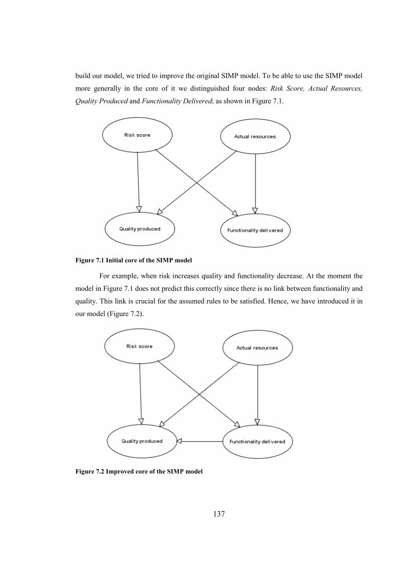
137

build our model, we tried to improve the original SIMP model. To be able to use the SIMP model

more generally in the core of it we distinguished four nodes: Risk Score, Actual Resources,

Quality Produced and Functionality Delivered; as shown in Figure 7.1.

Figure 7.1 Initial core of the SIMP model

For example, when risk increases quality and functionality decrease. At the moment the

model in Figure 7.1 does not predict this correctly since there is no link between functionality and

quality. This link is crucial for the assumed rules to be satisfied. Hence, we have introduced it in

our model (Figure 7.2).

Figure 7.2 Improved core of the SIMP model

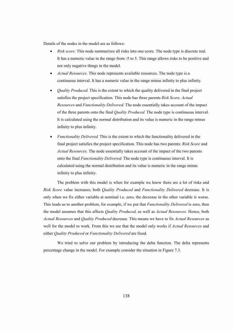
138

Details of the nodes in the model are as follows:

• Risk score. This node summarizes all risks into one score. The node type is discrete real.

It has a numeric value in the range from -5 to 5. This range allows risks to be positive and

not only negative things in the model.

• Actual Resources. This node represents available resources. The node type is a

continuous interval. It has a numeric value in the range minus infinity to plus infinity.

• Quality Produced. This is the extent to which the quality delivered in the final project

satisfies the project specification. This node has three parents Risk Score, Actual

Resources and Functionality Delivered. The node essentially takes account of the impact

of the three parents onto the final Quality Produced. The node type is continuous interval.

It is calculated using the normal distribution and its value is numeric in the range minus

infinity to plus infinity.

• Functionality Delivered. This is the extent to which the functionality delivered in the

final project satisfies the project specification. This node has two parents: Risk Score and

Actual Resources. The node essentially takes account of the impact of the two parents

onto the final Functionality Delivered. The node type is continuous interval. It is

calculated using the normal distribution and its value is numeric in the range minus

infinity to plus infinity.

The problem with this model is when for example we know there are a lot of risks and

Risk Score value increases; both Quality Produced and Functionality Delivered decrease. It is

only when we fix either variable at nominal i.e. zero, the decrease in the other variable is worse.

This leads us to another problem, for example, if we put that Functionality Delivered is zero, then

the model assumes that this affects Quality Produced, as well as Actual Resources. Hence, both

Actual Resources and Quality Produced decrease. This means we have to fix Actual Resources as

well for the model to work. From this we see that the model only works if Actual Resources and

either Quality Produced or Functionality Delivered are fixed.

We tried to solve our problem by introducing the delta function. The delta represents

percentage change in the model. For example consider the situation in Figure 7.3.

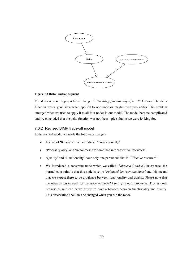
139

Figure 7.3 Delta function segment

The delta represents proportional change in Resulting functionality given Risk score. The delta

function was a good idea when applied to one node or maybe even two nodes. The problem

emerged when we tried to apply it to all four nodes in our model. The model became complicated

and we concluded that the delta function was not the simple solution we were looking for.

7.3.2 Revised SIMP trade-off model

In the revised model we made the following changes:

• Instead of ‘Risk score’ we introduced ‘Process quality’.

• ‘Process quality’ and ‘Resources’ are combined into ‘Effective resources’.

• ‘Quality’ and ‘Functionality’ have only one parent and that is ‘Effective resources’.

• We introduced a constraint node which we called ‘balanced f and q’. In essence, the

normal constraint is that this node is set to ‘balanced between attributes’ and this means

that we expect there to be a balance between functionality and quality. Please note that

the observation entered for the node balanced f and q is both attributes. This is done

because as said earlier we expect to have a balance between functionality and quality.

This observation shouldn’t be changed when you run the model.

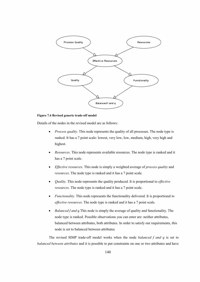
140

Figure 7.4 Revised generic trade-off model

Details of the nodes in the revised model are as follows:

• Process quality. This node represents the quality of all processes. The node type is

ranked. It has a 7 point scale: lowest, very low, low, medium, high, very high and

highest.

• Resources. This node represents available resources. The node type is ranked and it

has a 7 point scale.

• Effective resources. This node is simply a weighted average of process quality and

resources. The node type is ranked and it has a 7 point scale.

• Quality. This node represents the quality produced. It is proportional to effective

resources. The node type is ranked and it has a 7 point scale.

• Functionality. This node represents the functionality delivered. It is proportional to

effective resources. The node type is ranked and it has a 7 point scale.

• Balanced f and q.This node is simply the average of quality and functionality. The

node type is ranked. Possible observations you can enter are: neither attributes,

balanced between attributes, both attributes. In order to satisfy our requirements, this

node is set to balanced between attributes.

The revised SIMP trade-off model works when the node balanced f and q is set to

balanced between attributes and it is possible to put constraints on one or two attributes and have

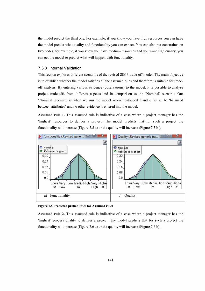
141

the model predict the third one. For example, if you know you have high resources you can have

the model predict what quality and functionality you can expect. You can also put constraints on

two nodes, for example, if you know you have medium resources and you want high quality, you

can get the model to predict what will happen with functionality.


This section explores different scenarios of the revised SIMP trade-off model. The main objective

is to establish whether the model satisfies all the assumed rules and therefore is suitable for trade-

off analysis. By entering various evidence (observations) to the model, it is possible to analyse

project trade-offs from different aspects and in comparison to the ‘Nominal’ scenario. Our

‘Nominal’ scenario is when we run the model where ‘balanced f and q’ is set to ‘balanced

between attributes’ and no other evidence is entered into the model.

Assumed rule 1. This assumed rule is indicative of a case where a project manager has the

‘highest’ resources to deliver a project. The model predicts that for such a project the

functionality will increase (Figure 7.5 a) or the quality will increase (Figure 7.5 b ).

a) Functionality b) Quality

Figure 7.5 Predicted probabilities for Assumed rule1


‘highest’ process quality to deliver a project. The model predicts that for such a project the

functionality will increase (Figure 7.6 a) or the quality will increase (Figure 7.6 b).

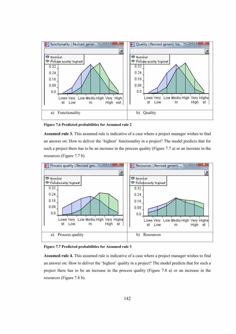
142


Figure 7.6 Predicted probabilities for Assumed rule 2

Assumed rule 3. This assumed rule is indicative of a case where a project manager wishes to find

an answer on: How to deliver the ‘highest’ functionality in a project? The model predicts that for

such a project there has to be an increase in the process quality (Figure 7.7 a) or an increase in the

resources (Figure 7.7 b).

a) Process quality b) Resources



an answer on: How to deliver the ‘highest’ quality in a project? The model predicts that for such a

project there has to be an increase in the process quality (Figure 7.8 a) or an increase in the

resources (Figure 7.8 b).

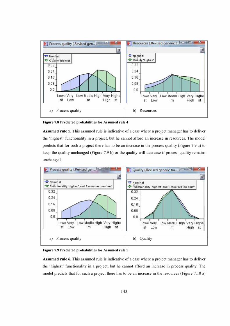
143



Assumed rule 5. This assumed rule is indicative of a case where a project manager has to deliver

the ‘highest’ functionality in a project, but he cannot afford an increase in resources. The model

predicts that for such a project there has to be an increase in the process quality (Figure 7.9 a) to

keep the quality unchanged (Figure 7.9 b) or the quality will decrease if process quality remains

unchanged.

a) Process quality b) Quality



the ‘highest’ functionality in a project, but he cannot afford an increase in process quality. The

model predicts that for such a project there has to be an increase in the resources (Figure 7.10 a)

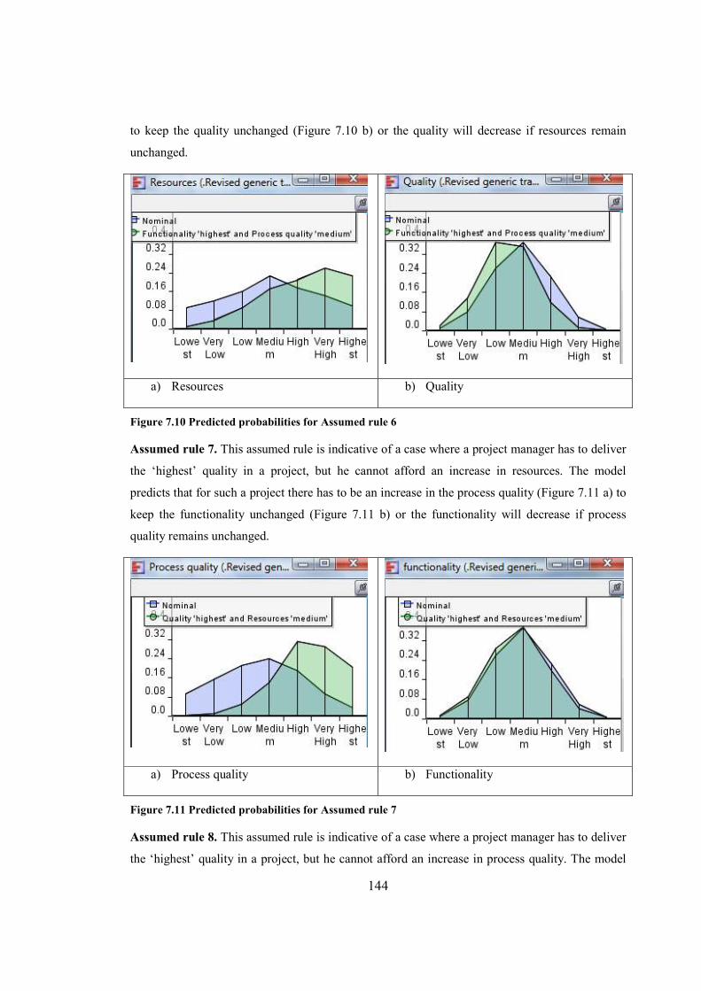
144

to keep the quality unchanged (Figure 7.10 b) or the quality will decrease if resources remain

unchanged.

a) Resources b) Quality



the ‘highest’ quality in a project, but he cannot afford an increase in resources. The model

predicts that for such a project there has to be an increase in the process quality (Figure 7.11 a) to

keep the functionality unchanged (Figure 7.11 b) or the functionality will decrease if process

quality remains unchanged.

a) Process quality b) Functionality



the ‘highest’ quality in a project, but he cannot afford an increase in process quality. The model

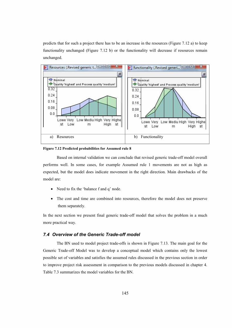
145

predicts that for such a project there has to be an increase in the resources (Figure 7.12 a) to keep

functionality unchanged (Figure 7.12 b) or the functionality will decrease if resources remain

unchanged.

a) Resources b) Functionality


Based on internal validation we can conclude that revised generic trade-off model overall

performs well. In some cases, for example Assumed rule 1 movements are not as high as

expected, but the model does indicate movement in the right direction. Main drawbacks of the

model are:

• Need to fix the ‘balance f and q’ node.

• The cost and time are combined into resources, therefore the model does not preserve

them separately.

In the next section we present final generic trade-off model that solves the problem in a much

more practical way.

7.4 Overview of the Generic Trade-off model

The BN used to model project trade-offs is shown in Figure 7.13. The main goal for the

Generic Trade-off Model was to develop a conceptual model which contains only the lowest

possible set of variables and satisfies the assumed rules discussed in the previous section in order

to improve project risk assessment in comparison to the previous models discussed in chapter 4.

Table 7.3 summarizes the model variables for the BN.

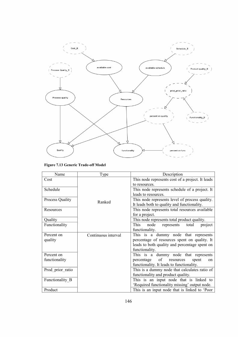
146

Figure 7.13 Generic Trade-off Model

Name Type Description

Cost

Ranked

This node represents cost of a project. It leads to resources.

Schedule This node represents schedule of a project. It leads to resources.

Process Quality This node represents level of process quality. It leads both to quality and functionality.

Resources This node represents total resources available for a project.

Quality This node represents total product quality.

Functionality This node represents total project functionality.

Percent on quality

Continuous interval

This is a dummy node that represents percentage of resources spent on quality. It leads to both quality and percentage spent on functionality.

Percent on functionality

This is a dummy node that represents percentage of resources spent on functionality. It leads to functionality.

Prod_prior_ratio This is a dummy node that calculates ratio of functionality and product quality.

Functionality_B This is an input node that is linked to ‘Required functionality missing’ output node.

Product This is an input node that is linked to ‘Poor

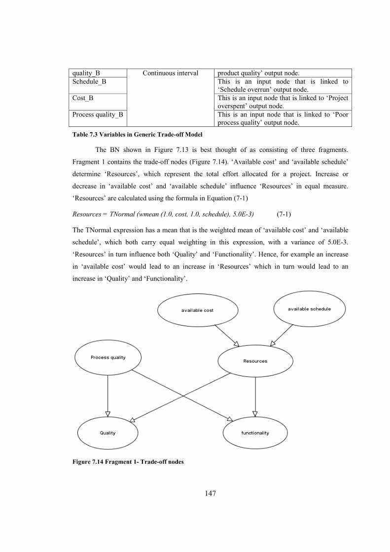
147

quality_B Continuous interval

product quality’ output node.

Schedule_B This is an input node that is linked to ‘Schedule overrun’ output node.

Cost_B This is an input node that is linked to ‘Project overspent’ output node.

Process quality_B This is an input node that is linked to ‘Poor process quality’ output node.

Table 7.3 Variables in Generic Trade-off Model

The BN shown in Figure 7.13 is best thought of as consisting of three fragments.

Fragment 1 contains the trade-off nodes (Figure 7.14). ‘Available cost’ and ‘available schedule’

determine ‘Resources’, which represent the total effort allocated for a project. Increase or

decrease in ‘available cost’ and ‘available schedule’ influence ‘Resources’ in equal measure.

‘Resources’ are calculated using the formula in Equation (7-1)

Resources = TNormal (wmean (1.0, cost, 1.0, schedule), 5.0E-3) (7-1)

The TNormal expression has a mean that is the weighted mean of ‘available cost’ and ‘available

schedule’, which both carry equal weighting in this expression, with a variance of 5.0E-3.

‘Resources’ in turn influence both ‘Quality’ and ‘Functionality’. Hence, for example an increase

in ‘available cost’ would lead to an increase in ‘Resources’ which in turn would lead to an

increase in ‘Quality’ and ‘Functionality’.

Figure 7.14 Fragment 1- Trade-off nodes

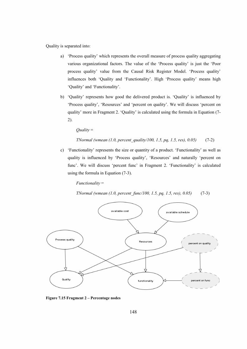
148

Quality is separated into:

a) ‘Process quality’ which represents the overall measure of process quality aggregating

various organizational factors. The value of the ‘Process quality’ is just the ‘Poor

process quality’ value from the Causal Risk Register Model. ‘Process quality’

influences both ‘Quality and ‘Functionality’. High ‘Process quality’ means high

‘Quality’ and ‘Functionality’.

b) ‘Quality’ represents how good the delivered product is. ‘Quality’ is influenced by

‘Process quality’, ‘Resources’ and ‘percent on quality’. We will discuss ‘percent on

quality’ more in Fragment 2. ‘Quality’ is calculated using the formula in Equation (7-

2).

Quality =

TNormal (wmean (1.0, percent_quality/100, 1.5, pq, 1.5, res), 0.05) (7-2)

c) ‘Functionality’ represents the size or quantity of a product. ‘Functionality’ as well as

quality is influenced by ‘Process quality’, ‘Resources’ and naturally ‘percent on

func’. We will discuss ‘percent func’ in Fragment 2. ‘Functionality’ is calculated

using the formula in Equation (7-3).

Functionality =

TNormal (wmean (1.0, percent_func/100, 1.5, pq, 1.5, res), 0.05) (7-3)

Figure 7.15 Fragment 2 – Percentage nodes

149

Fragment 2 contains the “percentage” nodes that are lightly shaded in Figure 7.15. There

are two “percentage” nodes and they are dummy nodes in the BN model. It is impossible to build

the model satisfying all the assumed rules without introducing the “percentage” nodes. It is

reasonable to assume if resources need to be divided between quality and functionality then there

should be an equitable distribution of resources. The model shown in Fragment 1 works based on

this principle. The problem arises when we would like to specify that we want to spend more

resources on, for example, quality. Therefore, we want to have high quality.

To achieve this it is necessary to introduce “percentage” nodes:

1. ‘Percent on quality’ represents percentage of resources out of 100% spent on quality. Quality

can be viewed as time spent on testing.

2. ‘Percent on func’ represents percentage of resources out of 100% spent on functionality.

Functionality can be viewed as time spent on development.

For any project time spent on development and time spent on testing can be checked from time

sheets. Using “percentage” nodes that are hidden from the user is really crucial in making the

model work. They allow us to allocate a certain percentage of total resources we would like to

spend on quality and functionality. For example, if we would like to achieve very high quality,

we may wish to spend 70% of resources on quality. In that case, we have only 30% left for

functionality assuming we are not going over resources. Hence, we would have to be satisfied

with low to medium functionality. Hence, percentage spent on functionality is calculated using

the formula in Equation (7-4).

Percentage spent on functionality = Max (0, 100 – percent_quality) (7-4)

We are using the maximum arithmetic function and simply saying that the value for functionality

is 100% minus the percentage we spent on quality.

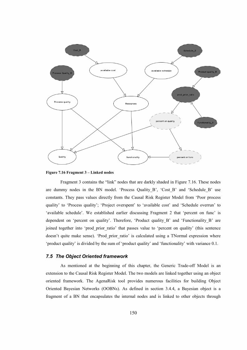
150

Figure 7.16 Fragment 3 – Linked nodes

Fragment 3 contains the “link” nodes that are darkly shaded in Figure 7.16. These nodes

are dummy nodes in the BN model. ‘Process Quality_B’, ‘Cost_B’ and ‘Schedule_B’ use

constants. They pass values directly from the Causal Risk Register Model from ‘Poor process

quality’ to ‘Process quality’; ‘Project overspent’ to ‘available cost’ and ‘Schedule overrun’ to

‘available schedule’. We established earlier discussing Fragment 2 that ‘percent on func’ is

dependent on ‘percent on quality’. Therefore, ‘Product quality_B’ and ‘Functionality_B’ are

joined together into ‘prod_prior_ratio’ that passes value to ‘percent on quality’ (this sentence

doesn’t quite make sense). ‘Prod_prior_ratio’ is calculated using a TNormal expression where

‘product quality’ is divided by the sum of ‘product quality’ and ‘functionality’ with variance 0.1.

7.5 The Object Oriented framework

As mentioned at the beginning of this chapter, the Generic Trade-off Model is an

extension to the Causal Risk Register Model. The two models are linked together using an object

oriented framework. The AgenaRisk tool provides numerous facilities for building Object

Oriented Bayesian Networks (OOBNs). As defined in section 3.4.4, a Bayesian object is a

fragment of a BN that encapsulates the internal nodes and is linked to other objects through

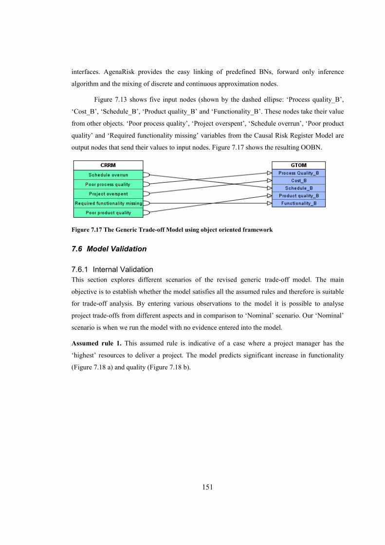
151

interfaces. AgenaRisk provides the easy linking of predefined BNs, forward only inference

algorithm and the mixing of discrete and continuous approximation nodes.

Figure 7.13 shows five input nodes (shown by the dashed ellipse: ‘Process quality_B’,

‘Cost_B’, ‘Schedule_B’, ‘Product quality_B’ and ‘Functionality_B’. These nodes take their value

from other objects. ‘Poor process quality’, ‘Project overspent’, ‘Schedule overrun’, ‘Poor product

quality’ and ‘Required functionality missing’ variables from the Causal Risk Register Model are

output nodes that send their values to input nodes. Figure 7.17 shows the resulting OOBN.

Figure 7.17 The Generic Trade-off Model using object oriented framework

7.6 Model Validation


This section explores different scenarios of the revised generic trade-off model. The main

objective is to establish whether the model satisfies all the assumed rules and therefore is suitable

for trade-off analysis. By entering various observations to the model it is possible to analyse

project trade-offs from different aspects and in comparison to ‘Nominal’ scenario. Our ‘Nominal’

scenario is when we run the model with no evidence entered into the model.


‘highest’ resources to deliver a project. The model predicts significant increase in functionality

(Figure 7.18 a) and quality (Figure 7.18 b).

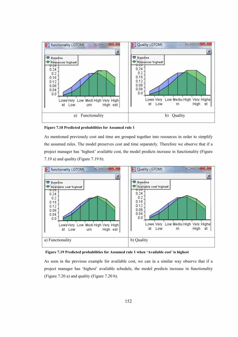
152



As mentioned previously cost and time are grouped together into resources in order to simplify

the assumed rules. The model preserves cost and time separately. Therefore we observe that if a

project manager has ‘highest’ available cost, the model predicts increase in functionality (Figure

7.19 a) and quality (Figure 7.19 b).


Figure 7.19 Predicted probabilities for Assumed rule 1 when ‘Available cost’ is highest

As seen in the previous example for available cost, we can in a similar way observe that if a

project manager has ‘highest’ available schedule, the model predicts increase in functionality

(Figure 7.20 a) and quality (Figure 7.20 b).

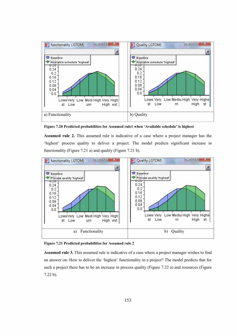
153


Figure 7.20 Predicted probabilities for Assumed rule1 when ‘Available schedule’ is highest


‘highest’ process quality to deliver a project. The model predicts significant increase in

functionality (Figure 7.21 a) and quality (Figure 7.21 b).




an answer on: How to deliver the ‘highest’ functionality in a project? The model predicts that for

such a project there has to be an increase in process quality (Figure 7.22 a) and resources (Figure

7.22 b).

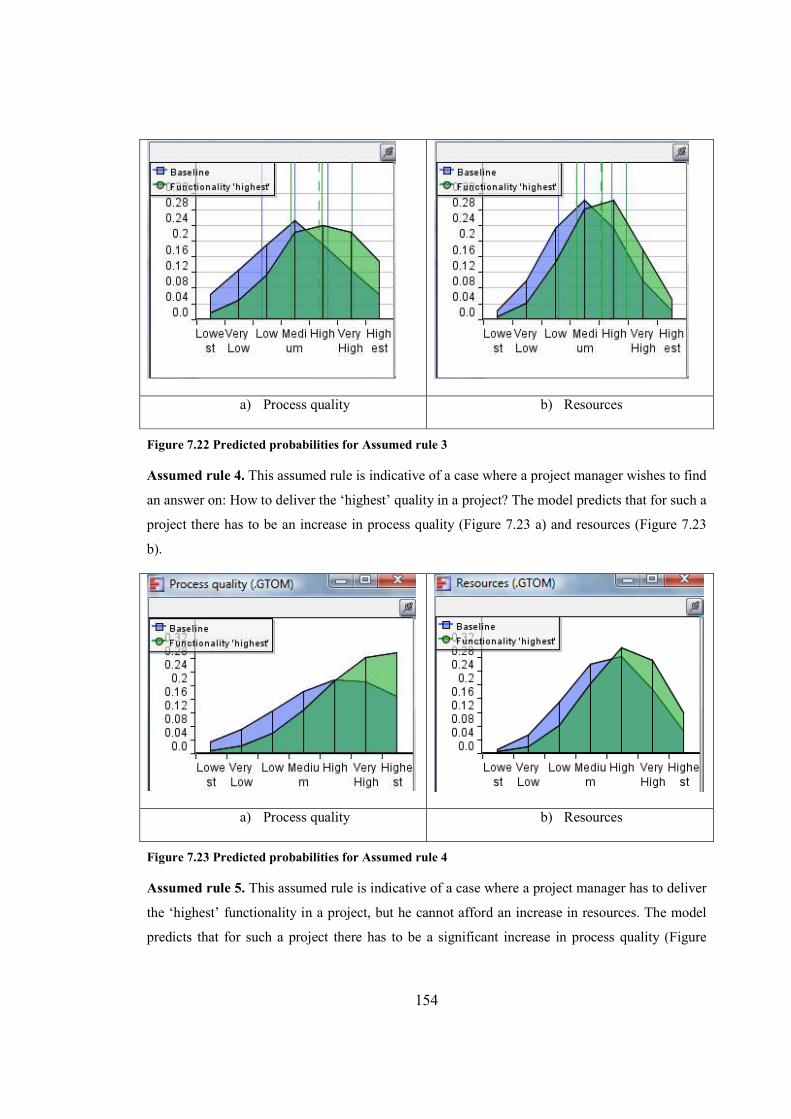
154




an answer on: How to deliver the ‘highest’ quality in a project? The model predicts that for such a

project there has to be an increase in process quality (Figure 7.23 a) and resources (Figure 7.23

b).




the ‘highest’ functionality in a project, but he cannot afford an increase in resources. The model

predicts that for such a project there has to be a significant increase in process quality (Figure

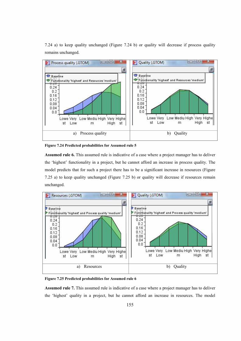
155

7.24 a) to keep quality unchanged (Figure 7.24 b) or quality will decrease if process quality

remains unchanged.

a) Process quality b) Quality



the ‘highest’ functionality in a project, but he cannot afford an increase in process quality. The

model predicts that for such a project there has to be a significant increase in resources (Figure

7.25 a) to keep quality unchanged (Figure 7.25 b) or quality will decrease if resources remain

unchanged.

a) Resources b) Quality



the ‘highest’ quality in a project, but he cannot afford an increase in resources. The model

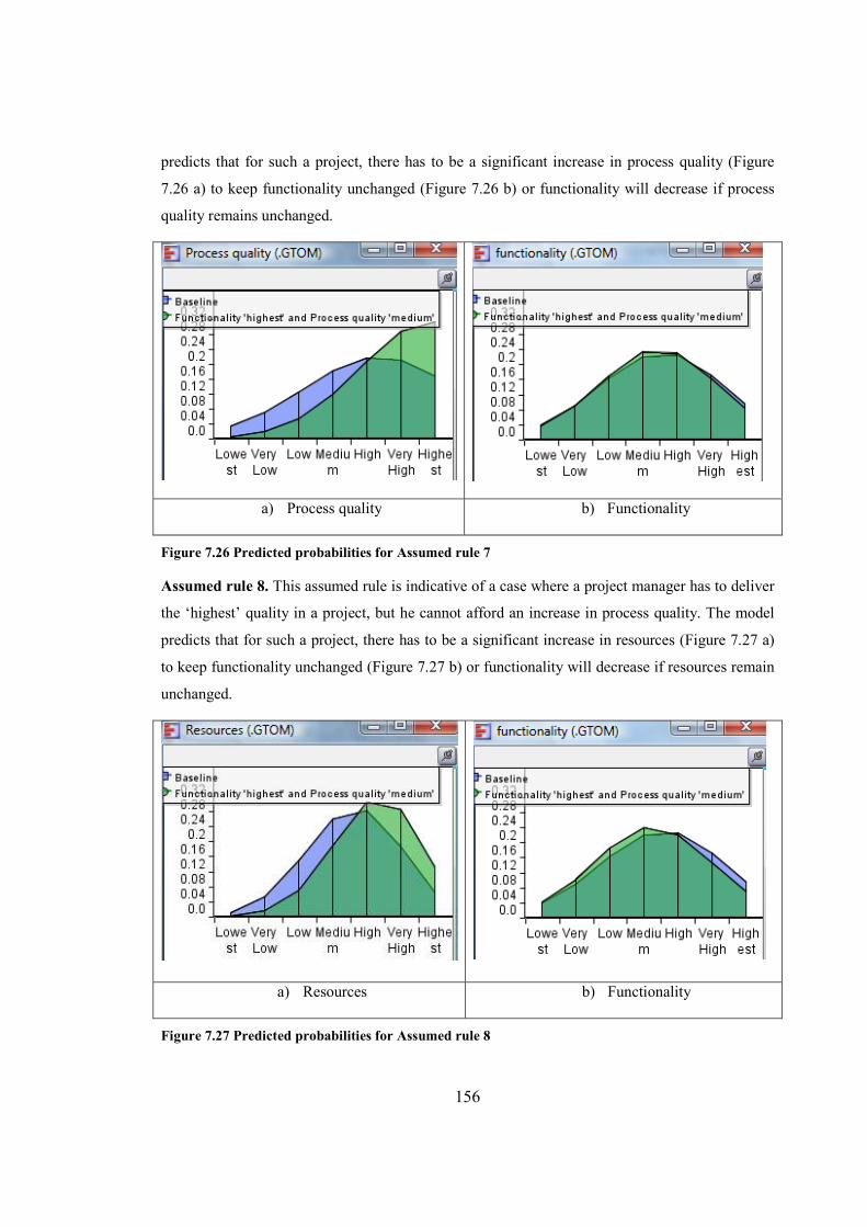
156

predicts that for such a project, there has to be a significant increase in process quality (Figure

7.26 a) to keep functionality unchanged (Figure 7.26 b) or functionality will decrease if process

quality remains unchanged.

a) Process quality b) Functionality



the ‘highest’ quality in a project, but he cannot afford an increase in process quality. The model

predicts that for such a project, there has to be a significant increase in resources (Figure 7.27 a)

to keep functionality unchanged (Figure 7.27 b) or functionality will decrease if resources remain

unchanged.

a) Resources b) Functionality


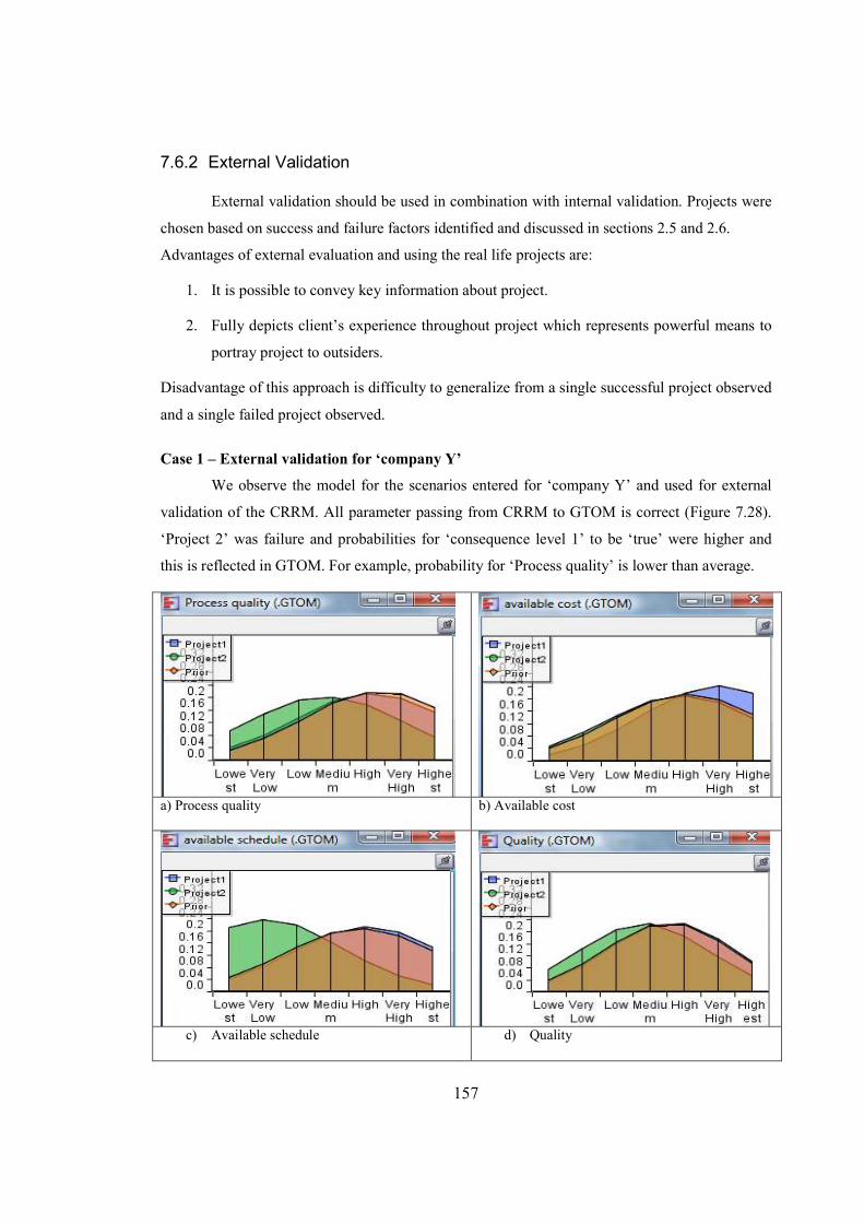
157

7.6.2 External Validation

External validation should be used in combination with internal validation. Projects were

chosen based on success and failure factors identified and discussed in sections 2.5 and 2.6.

Advantages of external evaluation and using the real life projects are:

1. It is possible to convey key information about project.

2. Fully depicts client’s experience throughout project which represents powerful means to

portray project to outsiders.

Disadvantage of this approach is difficulty to generalize from a single successful project observed

and a single failed project observed.

Case 1 – External validation for ‘company Y’

We observe the model for the scenarios entered for ‘company Y’ and used for external

validation of the CRRM. All parameter passing from CRRM to GTOM is correct (Figure 7.28).

‘Project 2’ was failure and probabilities for ‘consequence level 1’ to be ‘true’ were higher and

this is reflected in GTOM. For example, probability for ‘Process quality’ is lower than average.

a) Process quality b) Available cost

c) Available schedule d) Quality

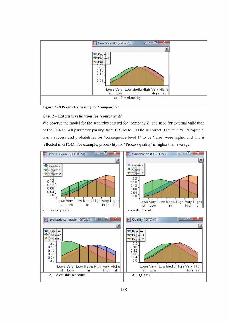
158

e) Functionality

Figure 7.28 Parameter passing for ‘company Y’

Case 2 – External validation for ‘company Z’

We observe the model for the scenarios entered for ‘company Z’ and used for external validation

of the CRRM. All parameter passing from CRRM to GTOM is correct (Figure 7.29). ‘Project 2’

was a success and probabilities for ‘consequence level 1’ to be ‘false’ were higher and this is

reflected in GTOM. For example, probability for ‘Process quality’ is higher than average.

a) Process quality b) Available cost

c) Available schedule d) Quality

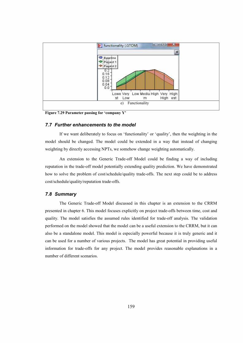
159

e) Functionality

Figure 7.29 Parameter passing for ‘company Y’

7.7 Further enhancements to the model

If we want deliberately to focus on ‘functionality’ or ‘quality’, then the weighting in the

model should be changed. The model could be extended in a way that instead of changing

weighting by directly accessing NPTs, we somehow change weighting automatically.

An extension to the Generic Trade-off Model could be finding a way of including

reputation in the trade-off model potentially extending quality prediction. We have demonstrated

how to solve the problem of cost/schedule/quality trade-offs. The next step could be to address

cost/schedule/quality/reputation trade-offs.

7.8 Summary

The Generic Trade-off Model discussed in this chapter is an extension to the CRRM

presented in chapter 6. This model focuses explicitly on project trade-offs between time, cost and

quality. The model satisfies the assumed rules identified for trade-off analysis. The validation

performed on the model showed that the model can be a useful extension to the CRRM, but it can

also be a standalone model. This model is especially powerful because it is truly generic and it

can be used for a number of various projects. The model has great potential in providing useful

information for trade-offs for any project. The model provides reasonable explanations in a

number of different scenarios.

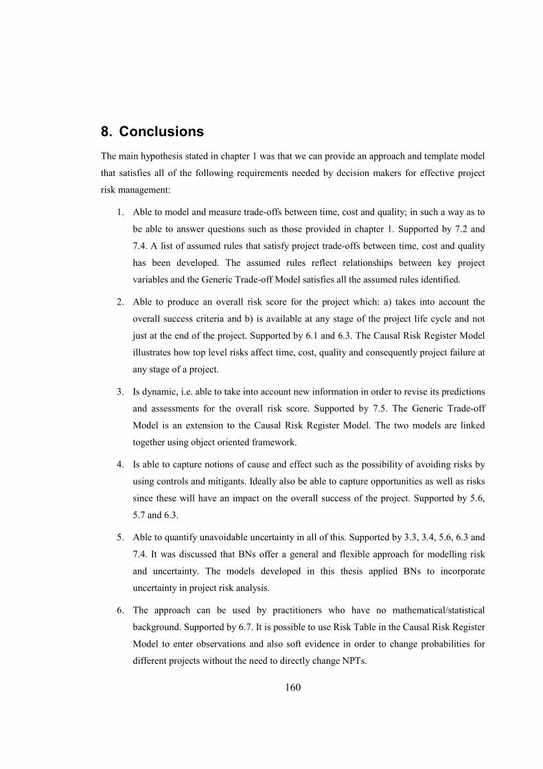
160

8. Conclusions

The main hypothesis stated in chapter 1 was that we can provide an approach and template model

that satisfies all of the following requirements needed by decision makers for effective project

risk management:

1. Able to model and measure trade-offs between time, cost and quality; in such a way as to

be able to answer questions such as those provided in chapter 1. Supported by 7.2 and

7.4. A list of assumed rules that satisfy project trade-offs between time, cost and quality

has been developed. The assumed rules reflect relationships between key project

variables and the Generic Trade-off Model satisfies all the assumed rules identified.

2. Able to produce an overall risk score for the project which: a) takes into account the

overall success criteria and b) is available at any stage of the project life cycle and not

just at the end of the project. Supported by 6.1 and 6.3. The Causal Risk Register Model

illustrates how top level risks affect time, cost, quality and consequently project failure at

any stage of a project.

3. Is dynamic, i.e. able to take into account new information in order to revise its predictions

and assessments for the overall risk score. Supported by 7.5. The Generic Trade-off

Model is an extension to the Causal Risk Register Model. The two models are linked

together using object oriented framework.

4. Is able to capture notions of cause and effect such as the possibility of avoiding risks by

using controls and mitigants. Ideally also be able to capture opportunities as well as risks

since these will have an impact on the overall success of the project. Supported by 5.6,

5.7 and 6.3.

5. Able to quantify unavoidable uncertainty in all of this. Supported by 3.3, 3.4, 5.6, 6.3 and

7.4. It was discussed that BNs offer a general and flexible approach for modelling risk

and uncertainty. The models developed in this thesis applied BNs to incorporate

uncertainty in project risk analysis.

6. The approach can be used by practitioners who have no mathematical/statistical

background. Supported by 6.7. It is possible to use Risk Table in the Causal Risk Register

Model to enter observations and also soft evidence in order to change probabilities for

different projects without the need to directly change NPTs.

161

I claim novelty for the models developed in points 1 and 2. They are a significant

improvement on the previous BN models that are already in use in the commercial environment.

Although, there is still room for further improvements, I discussed the need to extend the causal

risk register to deal with the issue of unknown knowns in 6.8 and the scope for improving the

trade-off model in 7.7, I believe that the contributions provided by the new models will lead to a

better understanding of project trade-offs between time, cost and quality; better project risk

analysis and consequently better project delivery.

The best (and possibly only realistic) way to ensure proper practical use and exploitation

of this model is to make it web enabled, with different users having access to the parts of the

model relevant to them. Different users would enter evidence into the model on one or more

nodes during project duration. This would enable the model to be used for bottom-up as well as

top-down reasoning. The users could find out the reasoning behind the model outputs as

interactions between variables are clearly displayed. This would provide clarity to users and

increase the transparency of project risk management decision making. In addition it may be

appropriate to link a database to the system and store different scenarios in order to enhance

future forecasts and analysis for different projects. This would show that it is possible to deploy

large and complex probabilistic models in practice.

162

Bibliography

1. @Risk, http://www.palisade.com

2. Adams J., Risk (Routledge, 2005)

3. Agena, AgenaRisk: Advanced risk analysis for important decisions.

http://www.agenarisk.com (2007)

4. Agena, Software Project Risk Models Manual, Version 01.00, 2004

5. Ames D.P., Neilson B. T., Stevens D. K. and Lall U., Using Bayesian networks to model

watershed management decisions: an East Canyon creek case study, World Wide Web,

http://www.hydromap.com/papers/ames_ecc.pdf, 2003, Visited July, 2005

6. Andradottir, S. and Bier V. M., Applying Bayesian ideas in simulation, Elsevier, 2000

7. Association for Project Management, Project risk analysis and management (PRAM)

Guide, 2nd ed., APM Publishing, High Wycombe, 2004

8. Atkinson R., Project management: cost, time and quality, two best guesses and

phenomenon, its time to accept other success criteria, International Journal of Project

Management, 17 (6), 337-342, 1999

9. Australian/New Zealand Standard AS/NZS 4360:2004, Risk Management, Homebush

NSW 2140: Standards Australia and Wellington 6001: Standards New Zealand, 2004

10. Babu A. J. G. and Suresh N., Project management with time, cost, and quality

considerations, Euro. J. of Op. Res., 320-327, 1996

11. Baker B. N., Murphy D. C. and Fisher D., Factors affecting project success, Project

management handbook 2nd Ed., Cleland D. I. and King W. R. Ed., John Wiley, New

York, 1998

12. Ballantine J., Bonner M., Levy M., Martin A., Munro I. and Powell P. L., The 3-D model

of information systems successes: the search for the dependent variable continues,

Information Resources Management Journal, 9(4), 5-14, 1996

13. Banxia, http://www.banxia.com/dexplore/index.html

163

14. Barlow R. E. and Lambert H. E., Introduction to fault tree analysis, In Richard E. Barlow,

Jerry B. Fussell and Nozer Singpurwalla, Reliability and Fault Tree Analysis, Society for

Industrial and Applied Mathematics, 1975

15. Belassi W. and Tukel O.I., A new framework for determining critical success/failure

factors in projects, International Journal of Project Management, 14(3), 141-151, 1996

16. Belton V. and Stewart T., Multiple Criteria Decision Analysis: An Integrated Approach,

Kluwer Academic Publishers, Boston, 2002

17. Bernoulli D., Exposition of a New Theory on the Measurement of Risk, Econometrica, 22

(1), 23-36, 1738/1954

18. Bobbio A., Portinale L., Minichino M. and Ciancamerla E., Improving the analysis of

dependable systems by mapping fault trees into Bayesian networks, Reliability

Engineering and System Safety, 71 (3), 249-260, 2001

19. Boehm, B. W., Software risk management principles and practices, IEEE Software, 8(1),

32-41, 1991

20. Bonini C. P., Hausman W. H. and Bierman H., Quantitative Analysis for Management,

9th Ed., McGraw-Hill Companies, New York, 319, 1997

21. Borsuk M. E., Stowl C. A. and Reckhow K. H., A Bayesian network of eutrophication

models for synthesis, prediction ,and uncertainty analysis, division of environmental

science and policy, Nicholas School of the Environment and Earth Sciences, Duke

University, Durham, USA, 2003

22. Breese J.S. and Heckerman D., Decision theoretical troubleshooting, IEEE Trans-actions

on Systems, Man and Cybernetics, Part A (Systems and Human), 26 (6):838-842, 1999

23. Brehmer, B., The Psychology of Risk: Risk and Decisions, John Wiley and Sons Ltd,

1987

24. British Standards Institute, BS6079-3:2000: Project Management – Part : Guide to the

Management of Business-related Project Risk, London: BSI, 2000

25. Calantone R.J., Di Benedetto C.A., Performance and time to market: accelerating cycle

time with overlapping stages, IEEE Transactions on Engeneering Management, 27 (2),

232-244, 2000

26. Cambridge Dictionaries Online, http://dictionary.cambridge.org/

164

27. Canadian Standards Association, CAN/CSA-Q850-97: Risk Management: Guideline for

Decision makers, Mississauga, Ont: Canadian Standards Association, 2002

28. Carr, Marvin, Konda, Suresh, Monarch, Ira, Urlich, Carol, Walker, Clay, Taxonomy

based risk identification (CMU/SEI-93-TR-6, ADA266992), Software Engineering

Institute, Carnegie Mellon University, Pittsburgh, PA, 1993

29. Carter R., Hancock T., Morin J. M. and Robins N., Introducing RISKMAN

Methodology, NNC Blackwell Ltd, UK, 1995

30. Chankong V. and Haimes Y. Y., Multiobjective Decision Making: Theory and

Methodology, Elsevier Science, Amsterdam, 1983

31. Chapman C. and Ward S., Managing Project Risk and Uncertainty, Chichester, England,

John Wiley & Sons, 2002

32. Chapman C. B. and Ward S. C., Project risk management: Processes, Techniques and

Insights, John Wiley and Sons, Chichester, 1997

33. Chapman C., Project risk analysis and management – PRAM the generic process,

International Journal of Project Management, 15 (5), 273-281, 1997

34. Chapman C.B. and Ward S. C., Estimation and evaluation of uncertainty: a minimalist

first pass approach, International Journal of Project Management, 18, 369-383, 2000

35. COSO (Committee of Sponsoring Organisations of the Treadway Commission),

Enterprise Risk Management: Integrated Framework, www.coso.org/publications.htm,

2004

36. Crawford L., Pollack J. and England D., Uncovering the trends in project management:

journal emphases over the last 10 years, Int. J. Proj. Mgmt., pp. 175-184, 2006

37. Crossland R., McMahon C. A. and Williams J. H., Survey of current practices in

managing design risk, Design Information Group, University of Bristol, 1998

38. Crystall Ball, http://www.decisioneering.com

39. Davies A., Brady T. and Hobday M., Charting a path toward integrated solutions, MIT

Sloan Mgmt. Rev., 39-48, 2006

40. Dawson R. J. And Dawson C. W., Practical proposals for managing uncertainty and risk

in project planning, International Journal of Project Management, 16(5), 299-310, 1998

165

41. De Witt A., Measurement of project management success, International Journal of

Project Management, 6(3), 164-170, 1988

42. De Witt A., Measuring project success, Project management Institute

Seminar/Symposium Montreal Canada, 13-21, Sep 1987

43. Deltek Risk+, http://www.deltek.com

44. Diez F. J., Parameter Adjustment in Bayes Networks: The Generalized Noisy OR-Gate,

Proceedings 9th Conference Uncertainty in Artificial Intelligence, 99-105, 1993

45. DIR, Risk List, http://www.dir.state.tx.us/eod/qa/risk/risklist.htm

46. Douglas, M., Risk acceptability according to social sciences, Russell Sage Foundation,

1985

47. Douglas, M., Understanding the enterprise culture: Themes in the work of Mary Douglas,

Edinburgh University Press, 1990

48. Druzdzel M. K. and van der Gaag L. C., Building Probabilistic Networks: Where Do the

Numbers Come From?, IEEE Transactions on Knowledge and Data Engineering, 12 (4),

481-486, 2000

49. Duffy P. J. and Thomas R. D., Project performance auditing, International Journal of

Project Management, 7 (2), 101-104, 1989

50. Durbach I. N. and Stewart T., Using expected values to simplify decision making under

uncertainty, OMEGA: International Journal of Management Science, 37, 312-330, 2009

51. Eden C., Ackermann F. and Cropper S., The Analysis of Cause Maps, Journal of

Management Studies, 29, 309-324, 1992

52. Eden C., On the Nature of Cognitive Maps, Journal of Management Studies, 29 (3), 261-

165, 1992

53. Fairley R., Risk Management for Software Projects, IEEE Software, 57–67, 1994

54. Fenton N. E. and Neil M., Making Decisions: Using Bayesian Nets and MCDA,

Knowledge-Based Systems, 14, 2001, 307-325

55. Fenton N. E. and Neil M., Software metrics, failures and new directions, J. of Systems

and Software, 47, 1999, 149-157

166

56. Fenton N. E., Neil M. and Caballero J. G., Using Ranked nodes to model qualitative

judgements in Bayesian Networks, IEEE Transactions on Knowledge and Data

Engineering, 2007

57. Fenton N. E., Neil M. and Marquez D., Using Bayesian Networks to Predict Software

Defects and Reliability, 5th International Mathematical Methods in Reliability Conference

MMR 07), Glasgow, 2007

58. Fenton N. E., Neil M., Hearty P., Marsh W., Marquez D., Krause P. and Mishra R.,

Predictiong Software defects in Varying Development Lifecycles Using Bayesian Nets,

Information and Software Technology, vol. 49, no. 1, 32-43, 2007

59. Fenton N. Neil M., Measuring your risks, Agena White Paper, 2005, www.agenarisk.com

60. Fenton N. Neil M., Visualising your Risks, Agena White Paper, 2005,

www.agenarisk.com

61. Fenton N., Bayesian Net References: A Comprehensive Listing, From

http://www.agenarisk.com/resources/BN_refs.doc.

62. Fenton N., Krause P. and Neil M., Probabilistic Modelling for Software Quality Control,

Journal of Applied Non-Classical Logics, 12 (2), 173-188, 2002

63. Fenton N., Marsh W., Neil M., Cates P., Forey S., Tailor M., Making Resource Decisions

for Software Projects, Proc. 26th Int. Conf. on Software Engineering (May 23–28 2004),

IEEE Computer Society, Washington, DC, 397–406, 2004

64. Fineman M., Radlinski L. and Fenton N. E., Modelling Project Trade-off Using Bayesian

Networks, IEEE Int. Conf. Computational Intelligence and Software Engineering.

Wuhan, China, IEEE Computer Society, 2009

65. Fineman, M. and Fenton N. E., Quantifying Risks Using Bayesian Networks, IASTED

Int. Conf. Advances in Management Science and Risk Assessment (MSI 2009), Beijing,

China, IASTED 662-219, 2009

66. Fishburn P. C., Foundations of risk measurement, I. Risk as probable loss, Management

Science, 30 (4), 396-406, 1984

67. Freeman M. and Beale P., Measuring project success, Project Management Journal,

23(1), 8-17, 1992

167

68. Furlong R., ‘Clausewitz and Modern War Gaming: losing can be better than winning’,

Air University Review, 1984

69. Gaddis P. O., The Project Manager, Harvard Business Review, May-June 89-97, 1959

70. Getz K.A. and de Bruin A., Speed demons of drug development, Pharm. Exect., 78-84,

July 2000

71. Godfrey P. S., Sir Halcrow W. and Partners Ltd., Control Of Risk – A Guide to the

Systematic Management of Risk from Construction, CIRIA, 1996

72. Graves S. B., Why costs increase when projects accelerate, Research Technology

Management, 32 (2), 16–18, 1989

73. Haasl D. F., Advanced concepts in fault tree analysis, In System Safety Symposium,

University of Washington, 1965

74. Hackerman D. and Wellman M. P., Bayesian Networks, Communications of the ACM,

38 (3), 1995, 27-30

75. Hackerman D., Bayesian networks for data mining, Data Mining and Knowledge

Discovery, 1 (1), 1997, 79-119

76. Hackerman D., Horvitz E. and Nathwani B., Towards normative expert systems: Part I.

The Pathfinder project, Methods of Information in Medicine, 31 (2), 90-105, 1992

77. Hansson O. and Mayer A., Heuristic search as evidential reasoning, Proceedings of the

5th Workshop on Uncertainty in Artificial Intelligence, 1989.

78. Harter D.E., Krishnan M.S., Slaughter S.A., Effects of process maturity on quality, cycle

time, and effort in software product development, Management Science, 46 (4), 451–466,

2000

79. Hayes R., An introduction to project planning and costing risk management, Risk

Analysis and Management Conference, Chartered Institute of Management Accountants

and the Operational Research Society, 1987

80. Heidenberger K., Dynamic project selection and funding under risk: a decision tree based

MILP approach, European Journal of Operational Research, 95 (2), 284-298, 1995

81. Hillson D., Extending the risk process to manage opportunities, International Journal of

Project Management, 2002

168

82. Hulett D., Schedule Risk Analysis Simplified, PM Network, Project Management

Institute, 23-30, 1996

83. Ingleby M. and West M., Causal influence coefficients: A localised maximum entrpy

approach to Bayesian inference, Doksum K. and Lindqvist B. H. eds., Mathematical and

Statistical Methods in Reliability, Quality, Reliability and Engineering Statistics, World

Scientific Publishing Co., Singapore, Ch. 4, 45-56, 2003

84. Institute of Electrical and Electronic Engineers, IEEE Standard 1540-2001: Standard for

Software Life Cycle Process – Risk Management, New York: IEEE, 2001

85. Institute of Risk Management/National Forum for Risk Management in the Public

Sector/Association of Insurance and Risk Managers, A Risk Management Standard,

London: IRM/ALARM/AIRMIC, 2002

86. International Electrotechnical Commission, CEI/IEC 62198:2001 International Standard:

Project Risk Management: Application Guidelines, Geneva: IEC, 2001

87. Ireland L. R. and Shirely V. D., Measuring risk in the project environment, Proceedings

of the 18th Annual Seminar/Symposium of the Project Management Institute, Montreal,

Cnada, pp 150-156, 1986

88. Japanese Standards Association, JIS Q2001:2001(E): Guidelines for Development and

Implementation of Risk Management System, Tokyo:JSA, 2001

89. Jensen F. V., An Introduction to Bayesian Networks, Springer-Verlag, New York, 1996

90. Jones C., Assessment and Control of Software Risks, Prentice Hall, 1994

91. Kandaswamy S., The Basic of Monte Carlo Simulation: A Tutorial, Proceedings of the

31st Annual Project Management Institute 2001 Seminars and Symposium, Nashville,

Tennessee, USA, 2001

92. Karlsson C. and Ahlstrom P., Technological level and product development cycle time,

Journal of Product Innovation Management, 16 (4), 352–362, 1999

93. Karni E., Foundations of Bayesian theory, Elsevier, 2005

94. Kasperson A. and Stallen P., Communicating risks to the public: Technology, risk and

society, Kluwer Academic Publishers, 1991

95. Kelly G. A., The Psychology of Personal Constructs, New York: Norton & Company

Inc., 1995

169

96. Kelly J. E., Critical-Path Planning and Scheduling: Mathematical Basis, Operations

Research, 9:290-320, 1961

97. Kerzner H., Project management, Van Nostrand Reinhold, New York, 1992, 875-879.

98. Kerzner H., Project Management: A Systems Approach to Planning, Scheduling and

Controlling, John Wiley, 2001

99. Khang D. B. and Myint Y. M., Time, cost and quality trade-off in project management: a

case study, International Journal of Project Management, 249-256, 1999

100. Khodakarami V., Applying Bayesian Networks to Model Uncertainty in Project

Scheduling, PhD Thesis, Queen Mary University Of London, 2009

101. Klein J. H., Modelling Risk Trade-off, The Journal of the Operational Research

Society, 44 (5), 445-460, 1993

102. Kleindorfer P. R., Kunreuther H. C. and Schoemaker P. J. H., Decision Sciences,

Cambridge University Press, Cambridge, Chapter 4, 1993

103. Kliem R. L. and Ludin I. S., Reducing Project Risk, Gower, 1997

104. Knoepfel H., Cost and quality control in the project cycle, International Journal

of Project Management, 7(4), 229-235, 1990

105. Kohrs R. H. and Welngarten G. C., Measuring successful technical performance

– A cost/schedule/technical control system, Proceedings of the 18th Annual

Seminar/Symposium of the Project Management Institute, Montreal, Canada, 158-164,

1986

106. Koller, D. and Pfeffer, A., Object-Oriented Bayesian Networks, In Proceeding of

the Thirteenth Annual Conference on Uncertainty in Artificial Intelligence, San

Francisco, Morgan Kaufmann, 1997

107. Kometa S., Olomolaiye P. O. and Harris F. C., An Evaluation of Clients’ needs

and Responsibilities in the Construction Process, Engineering, Construction and

Architectural Management, 2 (1), 45-56, 1995

108. Kozlov D. and Koller D., Nonuniform Dynamic Discretization in Hybrid

Networks, Proceedings 13th Conference on Uncertainty in Artificial Intelligence,

Stanford, 1997

170

109. Kumar R. L., Managing risks in IT projects: an options perspective, Information

& Management, 40, 63-74, 2002

110. Langseth H. and Lindqvist B. H., A maintenance model for componenets

exposed to several failure mechanisms and imperfect repair, Mathematical and Statistical

Methods in Reliability, Lindqvist B. H. and Doksum K. A. ed., World Scientific, River

Edge, NJ, 415-430, 2003

111. Langseth H., Bayesian networks with applications in reliability analysis, PhD

thesis Department of Mathematical Sciences, Norwegian University of Science and

Technology, 2002

112. Larson E. W. and Gobeli D. H., Significance of project management structure on

development success, IEEE Transactions on Engineering Management, 36(2), 119-125,

1989

113. Laslo Z., Activity time-cost tradeoffs under time and cost chance constraints,

Computers and Industrial Engineering, 44 (3), 365–384, 2003

114. Lauritzen S. L., Graphical Models, Clarendon Press, Oxford, 1996

115. Lopes L. L., Some thoughts on the psychological concept of risk, Journal of

Experimental Psychology: Human Perception and Performance, 9, 137-144, 1983

116. Lucas P., van der Gaag and Abu-Hanna A., Bayesian networks in biomedicine

and health-care, Artificial Intelligence in Medicine, 2004

117. Luu V. T., Kim S., Tuan N. V. and Ogunlana S. O., Quantifying schedule risk in

construction projects using Bayesian Networks, International Journal of Project

Management, 27 (1), 2007, 39-50

118. Majumdar D., An axiomatic characterization of Bayes’ Rule, Elsevier, 2003

119. Malcolm D. G., Roseboom J. H., Clark C. E. and Fazer W., Application of a

Technique for Research and Development Program Evaluation, Operations Research, 7

(5): 646-669, 1959

120. Marcot B.G., Holthausen R. S., Raphael M. G., Rowland M. and Wisdom M.,

Using bayesian belief networks to evaluate fish and wildlife population viability under

land management alternatives from an environmental impact statement, Forest Ecology

and Management, 153:29-42, 2001

171

121. Marquez D., Neil M. and Fenton N., Solving Dynamic Fault Trees using a New

Hybrid Bayesian Network Inference Algorithm, 16th Mediterranean Conference on

Control and Automation, Ajaccio, France, 2008

122. Marsh W. and Bearfield G., Merging Event Trees Using Bayesian Networks, in

Proceedings of ESREL 2007, Stavanger, Norway, Springer-Verlag, 2007

123. Maylor H., Project management, Prentice Hall, Harlow, England, 2003

124. Maytorena E., Winch G. M., Kiely T., Clarke S. and Dalton M., Identifying

Project Risks: A Cognitive Approach, In: Slevin D. P., Cleland, D. I. and Pinto J. K.

(Eds.), Innovations: Project Management Research, Pennsylvania, USA: Project

Management Institute Inc., 465-80, 2004

125. McCabe, B., AbouRizk, S.M. and Goebel, R., Belief Networks for Construction

Performance Diagnostics, Journal of Computing in Civil Engineering, Vol. 12, No. 2, 93-

100, 1998

126. McCabe, B., Belief Networks in Construction Simulation, Proceedings of the

30th conference on Winter simulation. Washington, D.C., United States, IEEE Computer

Society Press, 1998.

127. McConnell S., Code Complete, Microsoft Press, 1993

128. McConnell S., Rapid Development, Microsoft Press, 1996

129. McCoy F. A., Measuring Success: Establishing and Maintaining A Baseline,

Project management Institute Seminar/Symposium Montreal Canada, 47-52, Sep 1987

130. Miller, R. W., How to Plan and Control with Pert, Harvard Business Review, 93–

104, 1962

131. Mockus A., Weiss D.M. and Zhang P., Understanding and Predicting Effort in

Software Projects, Proc. 25th Int. Conf. on Software Engineering (Portland, OR, May 3–

10 2003), IEEE Computer Society, Washington, DC, 274–284, 2003

132. Moder, J., Network Techniques in Project Management. Project Management

Handbook, New York, Van Nostrand Reinhold, 1988

133. Morris P. W. G. and Hough G. H., The anatomy of major projects, John Wiley,

1987

172

134. Nasir, D. et al., Evaluating Risk in Construction-Schedule Model (Eric-S):

Construction Schedule Risk Model, Journal of Construction Engineering & Management,

129(5): 518, 2003

135. Neapolitan R. E., Learning Bayesian Networks, Pearson Prentice Hall, 2004

136. Neil M., Andersen L. B. and Hager D., Modelling Operational Risk in Financial

Institutions using Hybrid Bayesian Networks, The Journal of Operational Risk, 2009

137. Neil M., Fenton N. E., and Tailor M., Using Bayesian Networks to Model

Expected and Unexpected Operational Losses, Risk Analysis: An International Journal,

vol. 25, no. 4, 963-972, 2005

138. Neil M., Fenton N. E., Forey S., and Harris R., Using Bayesian Belief Networks

to Predict the Reliability of Military Vehicles, IEE Computing and Control Engineering,

12(1), 11-20, 2002

139. Neil M., Marquez D. and Fenton N., Using Bayesian networks to model the

operational risk to information technology infrastructure in financial institutions, Journal

of Financial Transformation, 2008

140. Neil M., Marquez D., Fenton N., Tailor M. and Hearty P., Modelling Dependable

Systems using Hybrid Bayesian Networks, First International Conference on Availability,

Reliability and Security (ARES 2006), Vienna, Austria, 2006

141. Neil M., Tailor M. and Marquez D., Inference in Bayesian networks using

dynamic discretisation, Statistics and Computing, 17:3, 2007

142. Nikovski D., Constructing Bayesian Networks for Medical Diagnosis from

Incomplete and Partially Correct Statistics, IEEE Transactions on Knowledge and Data

Engineering, 12 (4), 509-516, 2000

143. Norges Standardiseringsforbound, Norsk Standard NS5814:1991: Krav til

risikoanalyser. Lysaker: NSF, 1991

144. Oisen R. P., Can project management be defined?, Project Management

Quarterly, 2(1), pp 12-14, 1971

145. Oxford dictionary, http://www.askoxford.com/?view=uk

173

146. Patterson F. D. and Neailey K., A Risk Register Database System to aid the

management of project risk, International Journal of Project Management, 19, 139-145,

2002

147. Pearl J. and Russell S., Bayesian Networks, In Michael A. Arbib, Ed., The

Handbook of Brain Theory and Neural Networks, 2nd ed., MIT Press, 2003

148. Pearl J., Probabilistic reasoning in intelligent systems: Networks of Plausible

Inference, Morgan-Kaufmann, San Mateo, CA, 1988

149. Pertmaster Project Risk, http://www.pertmaster.com

150. Pinto J. K. and Sevin D. P., Critical success factors across the project life cycle’,

Project Management Journal, 19 3, pp 67-75, 1988

151. PMI (Project Management Institute), A guide to the project management book of

knowledge: PMBOK (project management book of knowledge) guide, Upper Darby,

PA:PMI, 2004

152. Pollack-Johnson B. and Liberatore M.J., Incorporating Quality Considerations

Into Project Time/Cost Tradeoff Analysis and Decision Making, IEEE Transactions on

Engineering Management, 53 (4), 534–542, 2006

153. PROAct, http://www.noweco.com

154. Project Risk Analysis, http://www.katmarsoftware.com

155. Pulat P.S. and Horn S.J., Time-Resource Tradeoff Problem, IEEE Transactions

on Engineering Management, 43 (4), 411–417, 1996.

156. Radlinski L., Fenton N., Neil M., and Marquez D., Modelling Prior Productivity

and Defect Rates in Causal Model for Software Project Risk Assessment, Polish Journal

of Environmental Studies, Vol. 16, No. 4A, 256-260, 2007

157. Radlinski L., Improved Software Project Risk Assessment Using Bayesian Nets,

PhD Thesis, Queen Mary University of London, 2008

158. Rainer A. and Hall T., Identifying the causes of poor progress in software

projects, Proc. 10th Int. Symposium on Software Metrics, 184–195, 2004

159. Raz T., Shenhar A. J. and Dvir D., Risk Management, Project Success, and

Technological Uncertainty, R&D Manag., 101-109, 2002

160. Recht J. L., System safety analysis: The fault Tree, National Safety News, 1996

174

161. Risk+ from S/C Solutions Inc., www.cs-solutions.com

162. Risky Project Professional 2.1, http://www.intaver.com

163. Rodin A., Mosley T. H., Clark A. G., Sing C. F., Boerwinkle E., Mining genetic

epidemiology data with Bayesian networks application to APOE gene variation and

plasma lipid levels, Journal of Computational Biology, 12 (1), 2005, 1-11

164. Rubin I. M. and Seeling W., Experience as a factor in the selection and

performance of project managers, IEEE Trans Eng Management, 14(3), 131-134, 1967

165. Ruhe G., Eberlein A. and Pfahl D., Trade-off Analysis for Requirements

Selection, International Journal on Software Engineering and Knowledge Engineering, 13

(4), 345–366, 2003

166. Rumsfeld D. H., Transforming the Military, Foreign Affairs, 81 (3), 20-32, 2002

167. Saarinen T., Systems development methodology and project success, Information

and Management, 19, 183-193, 1990

168. Shane S. and Venkataraman S., The promise of entrepreneurship as a field of

research, Academy of Management Review, 25 (1), 217-26, 2000

169. Smith P.G. and Reinertsen D. G., Developing Products in Half the Time: New

Rules, New Tools, John Wiley & Sons Inc., New York, 1998

170. Software Engineering Institute, Carnegie Mellon SEI Annual Report, 1993

171. Software Engineering Institute, Carnegie Mellon SEI Annual Report, 2001

172. Spiegelhalter D., Dawid A., Lauritzen S. and Cowell R., Bayesian analysis in

expert systems, Statistical Science, 8 (3), 219-283, 1993

173. Srinivas S., A Generalization of the Noisy-OR Model, Proceedings 9th

Conference Uncertainty in Artificial Intelligence, 208-215, 1993

174. Statman M. and Tyebjee T. T., The risk of investment in technological

innovation, IEEE Transactions on Engineering Management, 31 (4), 165-171, 1984

175. Struckenbruck L., Who determines project success, Project Management Institute

Seminar/Symposium Montreal Canada, 85-93, 1987

176. Swan J., Using cognitive mapping in management research: Decision about

technical innovation, British Journal of Management, 8 (183-198), 1997

175

177. Swink M., Talluri S., Pandejpong T., Faster, better, cheaper: A study of NPD

project efficiency and performance tradeoffs, Journal of Operations Management, 24,

542–562, 2006.

178. Taroni F., Biedermann A., Garbolino P. and Aitken C. G., A general approach to

Bayesian networks for the interpretation of evidence, Forensic Science International, 139,

2004, 5-16

179. The Economist, 2006

http://www.economist.com/science/displaystory.cfm?story_id=5354696&no_na_tran=1

180. Thomsett R., Third Wave Project Management, Englewood Cliffs, N. J., Prentice

Hall, 1992

181. Turner J. R., Editorial: Project management: a profession based on knowledge or

faith, International Journal of Project Management, 17(6), 329-30, 1999

182. US Department of Defense, Risk Management Guide for DoD Acquisition,

Defense Acquisition University, Defense Systems Management College, 5th end. Fort

Belvoir, VA: DSMC, 2002

183. Van Dorp J.R. and Duffey M. R., Statistical Dependence in Risk Analysis for

Project Networks Using Monte Carlo Methods, International Journal of Production

Economics, 58 (1), 17-29, 1999

184. Ward S. C., Assessing and managing important risks, International Journal of

Project Management, Volume 17, Issue 6, 331-336, Dec 1999

185. Wateridge J., How can IS/IT projects be measured for success?, International

Journal of Project Management, 16(1), 59-63, 1998

186. Wateridge J., IT projects: a basis for success, International Journal of Project

Management, 13(3), 169-172, 1995

187. Wellman M. P., Fundamental Concepts of Qualitative Probabilistic Networks,

Artificial Intelligence, 44 (3), 257-303, 1990

188. Wharton F., Risk management: Basic concepts and general principles, in: Ansell

J. and Wharton F. (eds.), Risk: Analysis, Assessment and Management, Wiley, New

York, 1-14, 1992

176

189. Wideman R. M., Risk Management Handbook, Project Management Institute,

Newtown Square, PA, 1992

190. Williams T. M., Assessing Extension of Time delays on major projects,

International Journal of Project Management, 21, 19-26, 2001

191. Williams T. M., Risk-management infrastructures, International Journal of

Project Management, 11, 5-10, 1993

192. Williams T. M., Two-dimensionality of project risk, International Journal of

Project Management, 14 (3), 185-186, 1996

193. Williams T. M., Using a Risk Register to integrate Risk Management in Project

Definition, International Journal of Project Management, 12, 17-22, 1994

194. Williams T., Ackermann F. and Eden C., Structuring a delay and disruption

claim: An application of cause-mapping and system dynamics, European Journal of

Operations Research, 148 (1), 192-204, 2003

195. Winkler R.L., An Introduction to Bayesian Inference and Decision. Second

Edition, Probabilistic Publishing, Gainsville, FL, 2003.

196. Wright J.N., Time and budget: the twin imperatives of a project sponsor,

International Journal of Project Management, 15(3), 181-186, 1997

197. Wright S., Correlation and causation, Journal of Agricultural Research, 20:557-

585, 1921

198. Xenos M., Prediction and assessment of student behaviour in open and distance

education in computers using Bayesian Networks, Computers and Education, 43 (4), 345-

359, 2003

199. Yager R. R., Including decision attitude in probabilistic decision making,

International Journal Approximate Reasoning, 21(1), 1-21, 1999

200. Yager R. R., On the valuation of alternatives for decision-making under

uncertainty, International Journal of Intelligent Systems, 17, 687-707, 2002

201. Yager R.R., Fuzzy modelling for intelligent decision making under uncertainty,

IEEE Transactions Systems Man Cybernet, Part B 30 (1), 60-70, 2000

202. Yates F. J. And Stone E. R. The risk construct, Risk taking behaviour, J. F.

Yates Ed., John Wiley, New York, 1992

177

203. Zagorecki A. and Druzdzel M., An Empirical Study of Probability Elicitation

under Noisy-OR Assumption, In Proceedings of the 17th International Florida Artificial

Intelligence Research Society Conference, Barr V. and Markov Z. (eds), 880-885, 2004

204. Ziv H. and Richardson D. J., Bayesian-network confirmation of software testing

uncertainties, ESEC, 1997

178

Appendix A, Risk Factors for Large Projects

Project

Domain

Name for an area in which projects might be done, with risk factors in this table generally

found in this type of project.

Factor ID A sequentially assigned number for risk factors in this domain. When new factors are

added, they get the next available sequential number, thus items within a category may not

be in numerical order.

Risk

Category

Header that names the category in which the following risk factors belong.

Risk Factors Named areas of potential risk to projects in this domain.

Low Risk

Cues

Characteristics of this factor when it can be considered low risk to a project.

Medium

Risk Cues

Characteristics of this factor when it provides a medium risk to a project.

High Risk

Cues

Characteristics of this factor when it should be considered high risk to a project.

Rating Level of risk you think is true of this project.

Low (L) This project exhibits the low risk cue, or appears to have no risk in this area.

Medium (M) This project exhibits the medium risk cue, or something similar in threat.

High (H) This project exhibits the high risk cue, or something similar in threat.

Not Applic

(NA) This factor is not applicable to this project.

Need Info

(NI) We need information from someone else (perhaps an expert) to make a judgment.

TBD The project is not far enough along to make a rating; we need to review this later.

Notes Space for notes during rating, for later reference on reasons a rating was chosen.

Rating (check one)

Factor Risk Factors Low Risk Cues Medium Risk High Risk L M H NA NI TBD Notes

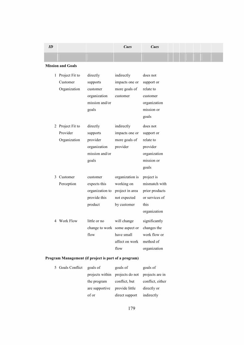
179

ID Cues Cues

Mission and Goals

1 Project Fit to

Customer

Organization

directly

supports

customer

organization

mission and/or

goals

indirectly

impacts one or

more goals of

customer

does not

support or

relate to

customer

organization

mission or

goals

2 Project Fit to

Provider

Organization

directly

supports

provider

organization

mission and/or

goals

indirectly

impacts one or

more goals of

provider

does not

support or

relate to

provider

organization

mission or

goals

3 Customer

Perception

customer

expects this

organization to

provide this

product

organization is

working on

project in area

not expected

by customer

project is

mismatch with

prior products

or services of

this

organization

4 Work Flow little or no

change to work

flow

will change

some aspect or

have small

affect on work

flow

significantly

changes the

work flow or

method of

organization

Program Management (if project is part of a program)

5 Goals Conflict goals of

projects within

the program

are supportive

of or

goals of

projects do not

conflict, but

provide little

direct support

goals of

projects are in

conflict, either

directly or

indirectly

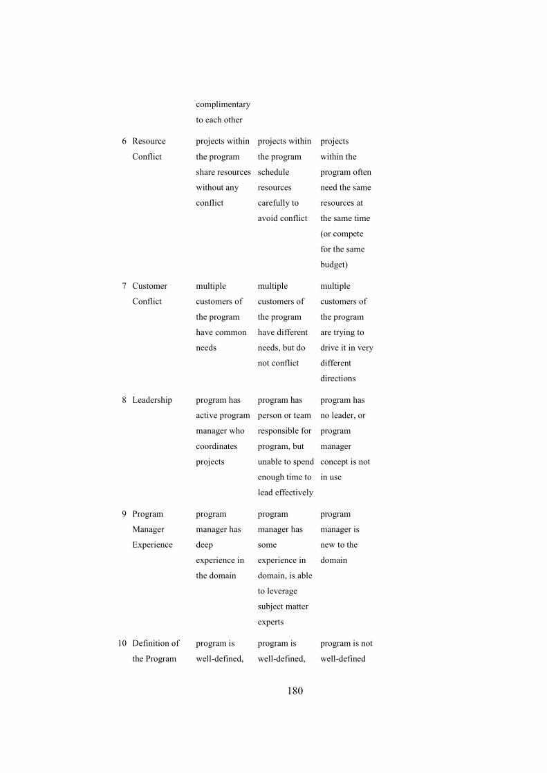
180

complimentary

to each other

6 Resource

Conflict

projects within

the program

share resources

without any

conflict

projects within

the program

schedule

resources

carefully to

avoid conflict

projects

within the

program often

need the same

resources at

the same time

(or compete

for the same

budget)

7 Customer

Conflict

multiple

customers of

the program

have common

needs

multiple

customers of

the program

have different

needs, but do

not conflict

multiple

customers of

the program

are trying to

drive it in very

different

directions

8 Leadership program has

active program

manager who

coordinates

projects

program has

person or team

responsible for

program, but

unable to spend

enough time to

lead effectively

program has

no leader, or

program

manager

concept is not

in use

9 Program

Manager

Experience

program

manager has

deep

experience in

the domain

program

manager has

some

experience in

domain, is able

to leverage

subject matter

experts

program

manager is

new to the

domain

10 Definition of

the Program

program is

well-defined,

program is

well-defined,

program is not

well-defined

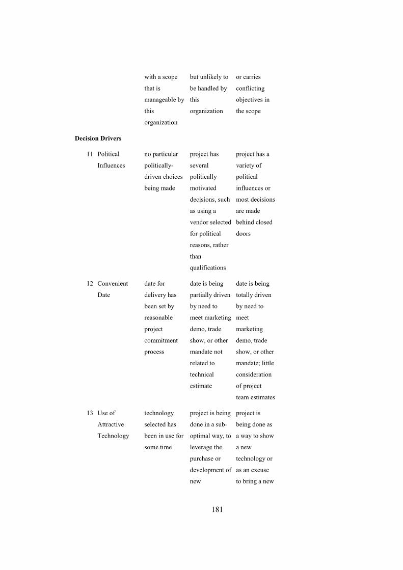
181

with a scope

that is

manageable by

this

organization

but unlikely to

be handled by

this

organization

or carries

conflicting

objectives in

the scope

Decision Drivers

11 Political

Influences

no particular

politically-

driven choices

being made

project has

several

politically

motivated

decisions, such

as using a

vendor selected

for political

reasons, rather

than

qualifications

project has a

variety of

political

influences or

most decisions

are made

behind closed

doors

12 Convenient

Date

date for

delivery has

been set by

reasonable

project

commitment

process

date is being

partially driven

by need to

meet marketing

demo, trade

show, or other

mandate not

related to

technical

estimate

date is being

totally driven

by need to

meet

marketing

demo, trade

show, or other

mandate; little

consideration

of project

team estimates

13 Use of

Attractive

Technology

technology

selected has

been in use for

some time

project is being

done in a sub-

optimal way, to

leverage the

purchase or

development of

new

project is

being done as

a way to show

a new

technology or

as an excuse

to bring a new

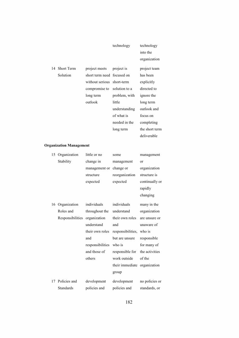
182

technology technology

into the

organization

14 Short Term

Solution

project meets

short term need

without serious

compromise to

long term

outlook

project is

focused on

short-term

solution to a

problem, with

little

understanding

of what is

needed in the

long term

project team

has been

explicitly

directed to

ignore the

long term

outlook and

focus on

completing

the short term

deliverable

Organization Management

15 Organization

Stability

little or no

change in

management or

structure

expected

some

management

change or

reorganization

expected

management

or

organization

structure is

continually or

rapidly

changing

16 Organization

Roles and

Responsibilities

individuals

throughout the

organization

understand

their own roles

and

responsibilities

and those of

others

individuals

understand

their own roles

and

responsibilities,

but are unsure

who is

responsible for

work outside

their immediate

group

many in the

organization

are unsure or

unaware of

who is

responsible

for many of

the activities

of the

organization

17 Policies and

Standards

development

policies and

development

policies and

no policies or

standards, or

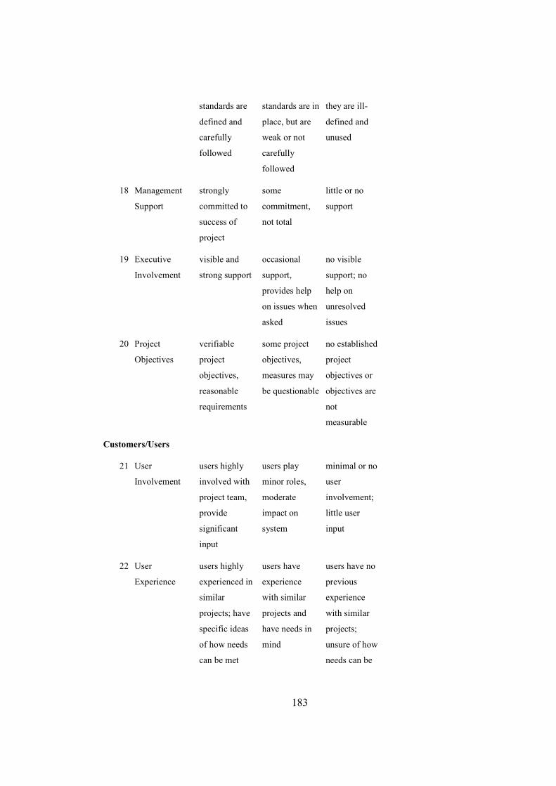
183

standards are

defined and

carefully

followed

standards are in

place, but are

weak or not

carefully

followed

they are ill-

defined and

unused

18 Management

Support

strongly

committed to

success of

project

some

commitment,

not total

little or no

support

19 Executive

Involvement

visible and

strong support

occasional

support,

provides help

on issues when

asked

no visible

support; no

help on

unresolved

issues

20 Project

Objectives

verifiable

project

objectives,

reasonable

requirements

some project

objectives,

measures may

be questionable

no established

project

objectives or

objectives are

not

measurable

Customers/Users

21 User

Involvement

users highly

involved with

project team,

provide

significant

input

users play

minor roles,

moderate

impact on

system

minimal or no

user

involvement;

little user

input

22 User

Experience

users highly

experienced in

similar

projects; have

specific ideas

of how needs

can be met

users have

experience

with similar

projects and

have needs in

mind

users have no

previous

experience

with similar

projects;

unsure of how

needs can be

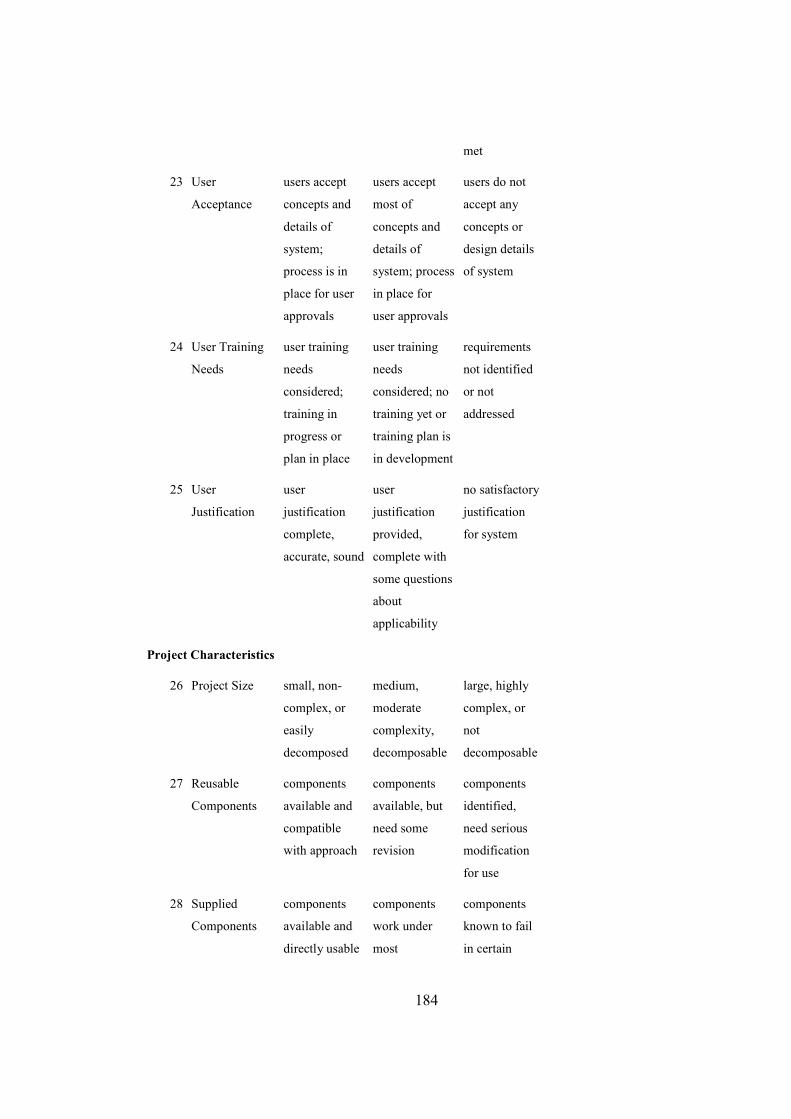
184

met

23 User

Acceptance

users accept

concepts and

details of

system;

process is in

place for user

approvals

users accept

most of

concepts and

details of

system; process

in place for

user approvals

users do not

accept any

concepts or

design details

of system

24 User Training

Needs

user training

needs

considered;

training in

progress or

plan in place

user training

needs

considered; no

training yet or

training plan is

in development

requirements

not identified

or not

addressed

25 User

Justification

user

justification

complete,

accurate, sound

user

justification

provided,

complete with

some questions

about

applicability

no satisfactory

justification

for system

Project Characteristics

26 Project Size small, non-

complex, or

easily

decomposed

medium,

moderate

complexity,

decomposable

large, highly

complex, or

not

decomposable

27 Reusable

Components

components

available and

compatible

with approach

components

available, but

need some

revision

components

identified,

need serious

modification

for use

28 Supplied

Components

components

available and

directly usable

components

work under

most

components

known to fail

in certain

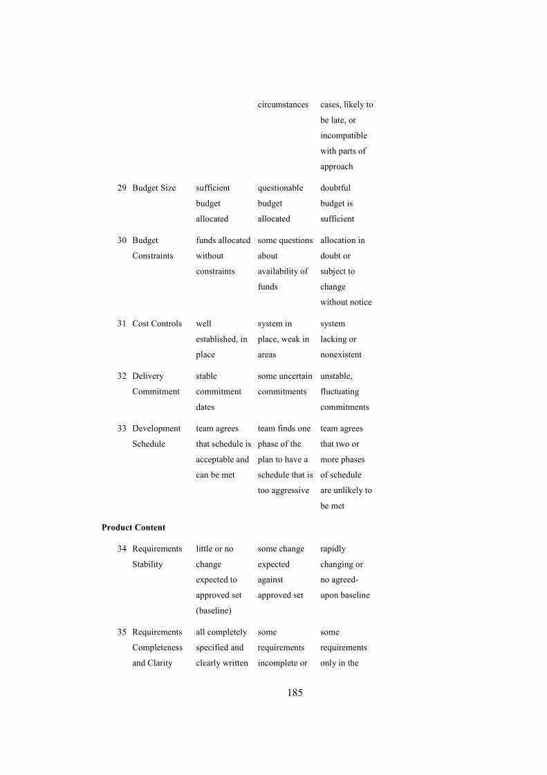
185

circumstances cases, likely to

be late, or

incompatible

with parts of

approach

29 Budget Size sufficient

budget

allocated

questionable

budget

allocated

doubtful

budget is

sufficient

30 Budget

Constraints

funds allocated

without

constraints

some questions

about

availability of

funds

allocation in

doubt or

subject to

change

without notice

31 Cost Controls well

established, in

place

system in

place, weak in

areas

system

lacking or

nonexistent

32 Delivery

Commitment

stable

commitment

dates

some uncertain

commitments

unstable,

fluctuating

commitments

33 Development

Schedule

team agrees

that schedule is

acceptable and

can be met

team finds one

phase of the

plan to have a

schedule that is

too aggressive

team agrees

that two or

more phases

of schedule

are unlikely to

be met

Product Content

34 Requirements

Stability

little or no

change

expected to

approved set

(baseline)

some change

expected

against

approved set

rapidly

changing or

no agreed-

upon baseline

35 Requirements

Completeness

and Clarity

all completely

specified and

clearly written

some

requirements

incomplete or

some

requirements

only in the

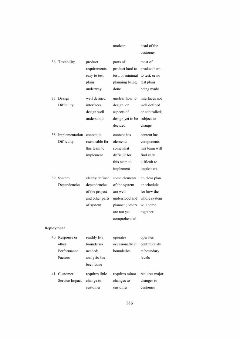
186

unclear head of the

customer

36 Testability product

requirements

easy to test,

plans

underway

parts of

product hard to

test, or minimal

planning being

done

most of

product hard

to test, or no

test plans

being made

37 Design

Difficulty

well defined

interfaces;

design well

understood

unclear how to

design, or

aspects of

design yet to be

decided

interfaces not

well defined

or controlled;

subject to

change

38 Implementation

Difficulty

content is

reasonable for

this team to

implement

content has

elements

somewhat

difficult for

this team to

implement

content has

components

this team will

find very

difficult to

implement

39 System

Dependencies

clearly defined

dependencies

of the project

and other parts

of system

some elements

of the system

are well

understood and

planned; others

are not yet

comprehended

no clear plan

or schedule

for how the

whole system

will come

together

Deployment

40 Response or

other

Performance

Factors

readily fits

boundaries

needed;

analysis has

been done

operates

occasionally at

boundaries

operates

continuously

at boundary

levels

41 Customer

Service Impact

requires little

change to

customer

requires minor

changes to

customer

requires major

changes to

customer

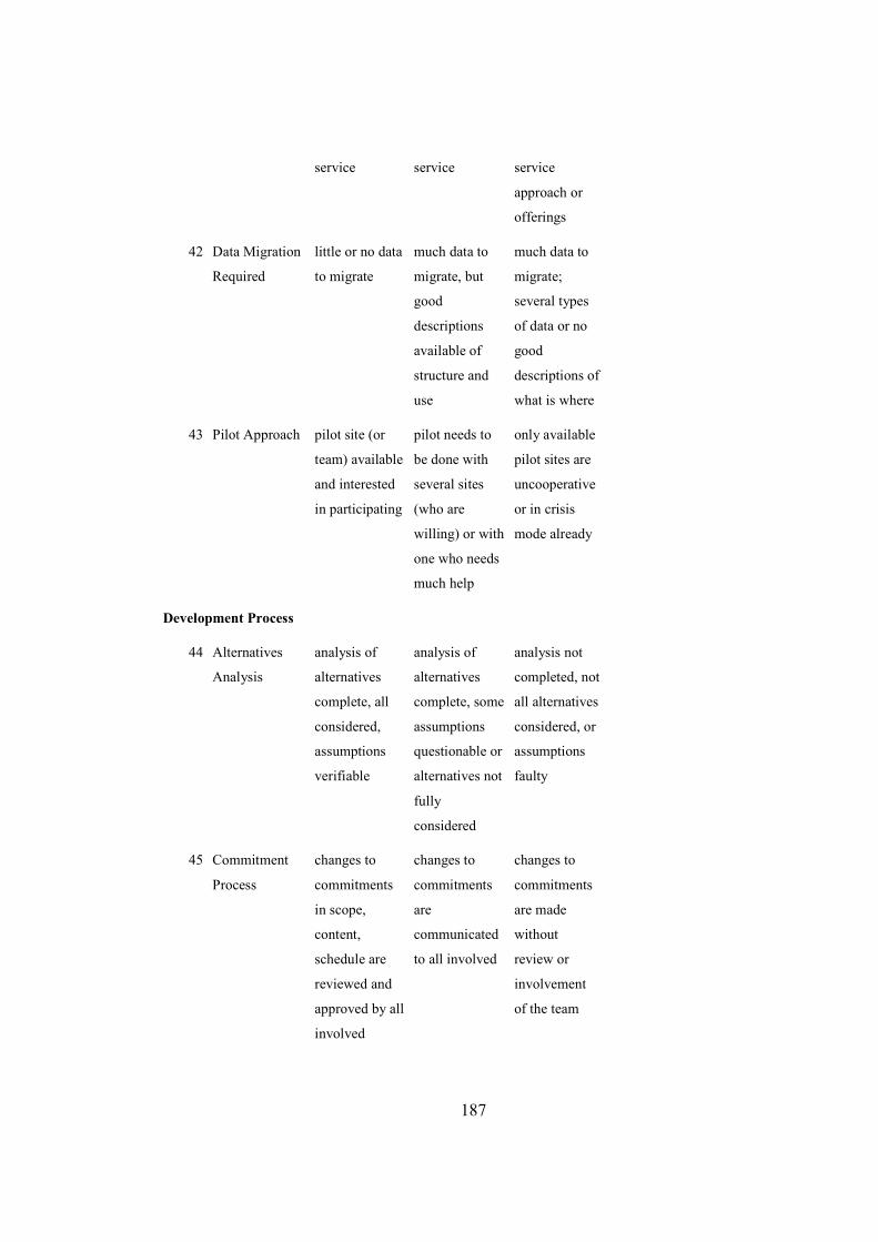
187

service service service

approach or

offerings

42 Data Migration

Required

little or no data

to migrate

much data to

migrate, but

good

descriptions

available of

structure and

use

much data to

migrate;

several types

of data or no

good

descriptions of

what is where

43 Pilot Approach pilot site (or

team) available

and interested

in participating

pilot needs to

be done with

several sites

(who are

willing) or with

one who needs

much help

only available

pilot sites are

uncooperative

or in crisis

mode already

Development Process

44 Alternatives

Analysis

analysis of

alternatives

complete, all

considered,

assumptions

verifiable

analysis of

alternatives

complete, some

assumptions

questionable or

alternatives not

fully

considered

analysis not

completed, not

all alternatives

considered, or

assumptions

faulty

45 Commitment

Process

changes to

commitments

in scope,

content,

schedule are

reviewed and

approved by all

involved

changes to

commitments

are

communicated

to all involved

changes to

commitments

are made

without

review or

involvement

of the team

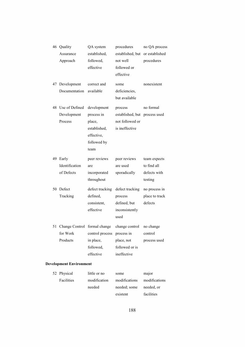
188

46 Quality

Assurance

Approach

QA system

established,

followed,

effective

procedures

established, but

not well

followed or

effective

no QA process

or established

procedures

47 Development

Documentation

correct and

available

some

deficiencies,

but available

nonexistent

48 Use of Defined

Development

Process

development

process in

place,

established,

effective,

followed by

team

process

established, but

not followed or

is ineffective

no formal

process used

49 Early

Identification

of Defects

peer reviews

are

incorporated

throughout

peer reviews

are used

sporadically

team expects

to find all

defects with

testing

50 Defect

Tracking

defect tracking

defined,

consistent,

effective

defect tracking

process

defined, but

inconsistently

used

no process in

place to track

defects

51 Change Control

for Work

Products

formal change

control process

in place,

followed,

effective

change control

process in

place, not

followed or is

ineffective

no change

control

process used

Development Environment

52 Physical

Facilities

little or no

modification

needed

some

modifications

needed; some

existent

major

modifications

needed, or

facilities

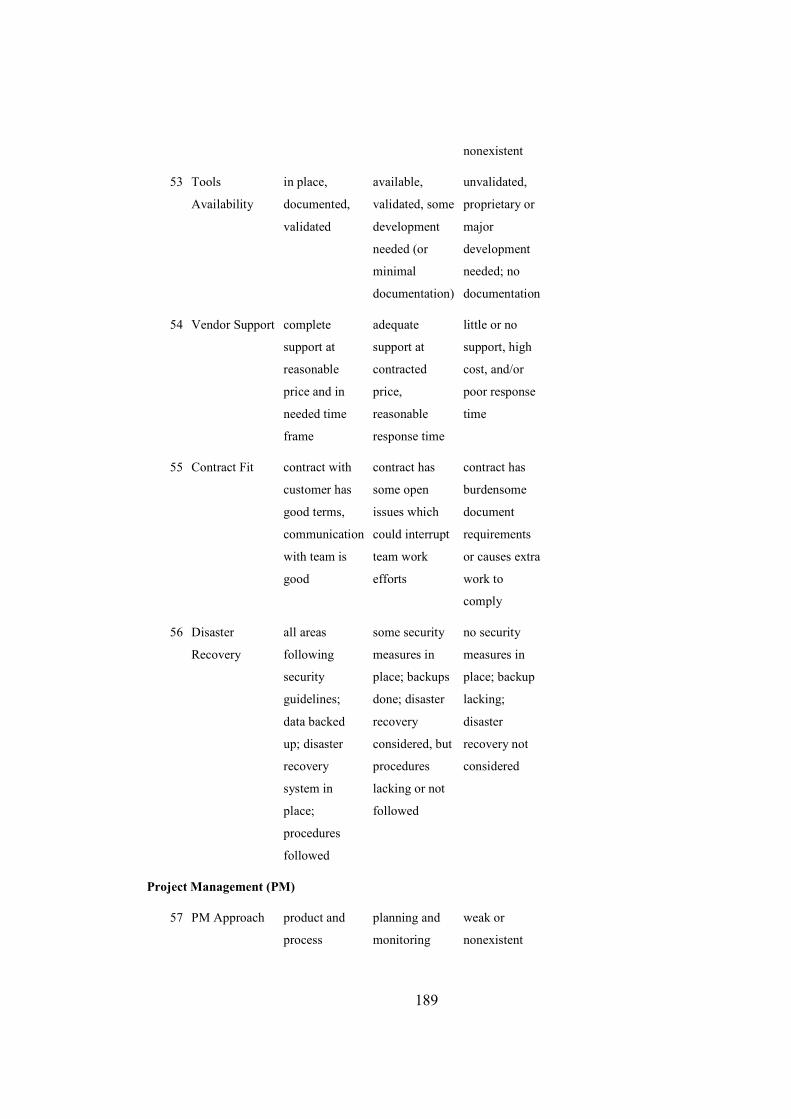
189

nonexistent

53 Tools

Availability

in place,

documented,

validated

available,

validated, some

development

needed (or

minimal

documentation)

unvalidated,

proprietary or

major

development

needed; no

documentation

54 Vendor Support complete

support at

reasonable

price and in

needed time

frame

adequate

support at

contracted

price,

reasonable

response time

little or no

support, high

cost, and/or

poor response

time

55 Contract Fit contract with

customer has

good terms,

communication

with team is

good

contract has

some open

issues which

could interrupt

team work

efforts

contract has

burdensome

document

requirements

or causes extra

work to

comply

56 Disaster

Recovery

all areas

following

security

guidelines;

data backed

up; disaster

recovery

system in

place;

procedures

followed

some security

measures in

place; backups

done; disaster

recovery

considered, but

procedures

lacking or not

followed

no security

measures in

place; backup

lacking;

disaster

recovery not

considered

Project Management (PM)

57 PM Approach product and

process

planning and

monitoring

weak or

nonexistent

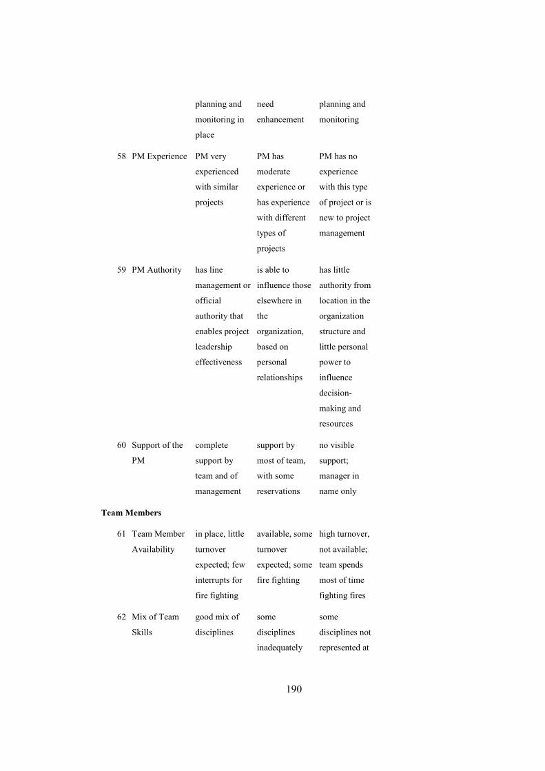
190

planning and

monitoring in

place

need

enhancement

planning and

monitoring

58 PM Experience PM very

experienced

with similar

projects

PM has

moderate

experience or

has experience

with different

types of

projects

PM has no

experience

with this type

of project or is

new to project

management

59 PM Authority has line

management or

official

authority that

enables project

leadership

effectiveness

is able to

influence those

elsewhere in

the

organization,

based on

personal

relationships

has little

authority from

location in the

organization

structure and

little personal

power to

influence

decision-

making and

resources

60 Support of the

PM

complete

support by

team and of

management

support by

most of team,

with some

reservations

no visible

support;

manager in

name only

Team Members

61 Team Member

Availability

in place, little

turnover

expected; few

interrupts for

fire fighting

available, some

turnover

expected; some

fire fighting

high turnover,

not available;

team spends

most of time

fighting fires

62 Mix of Team

Skills

good mix of

disciplines

some

disciplines

inadequately

some

disciplines not

represented at

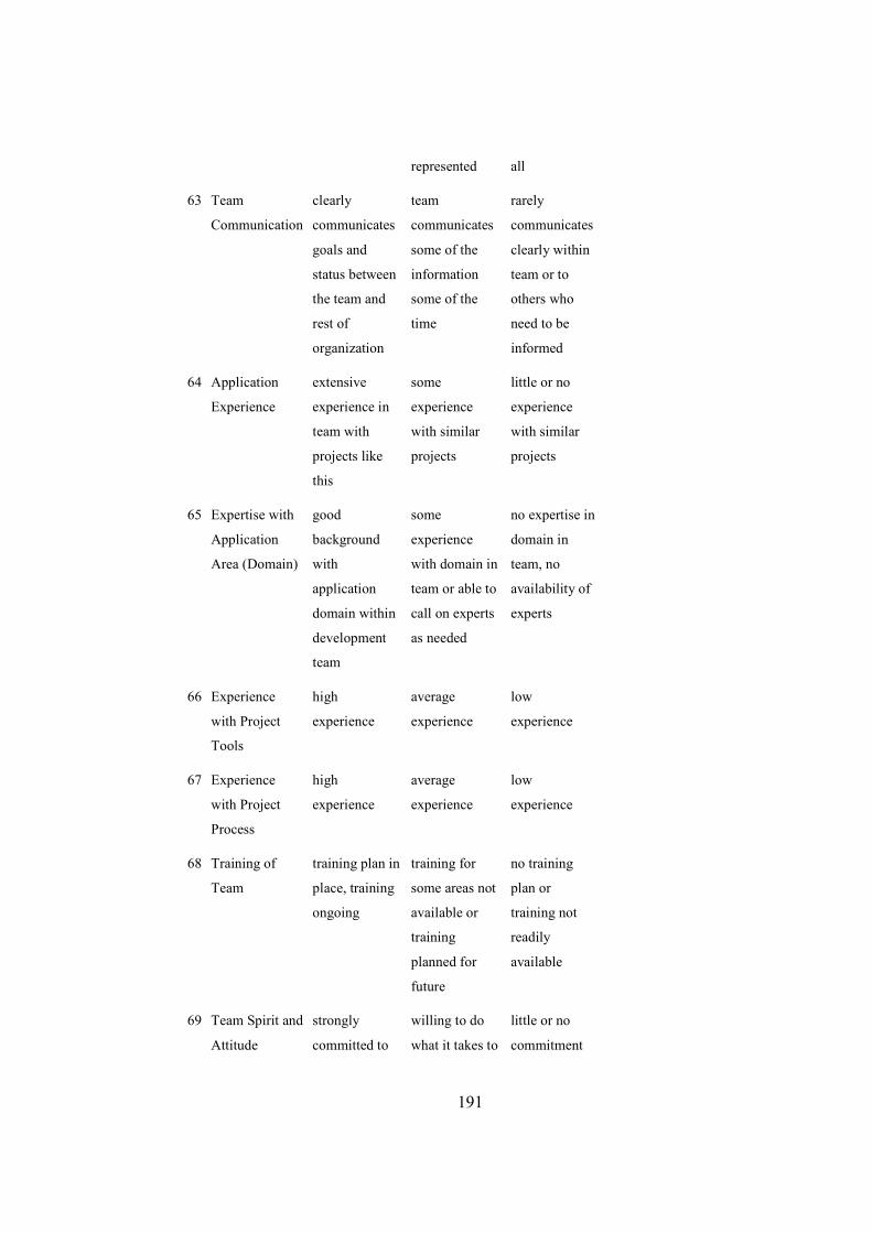
191

represented all

63 Team

Communication

clearly

communicates

goals and

status between

the team and

rest of

organization

team

communicates

some of the

information

some of the

time

rarely

communicates

clearly within

team or to

others who

need to be

informed

64 Application

Experience

extensive

experience in

team with

projects like

this

some

experience

with similar

projects

little or no

experience

with similar

projects

65 Expertise with

Application

Area (Domain)

good

background

with

application

domain within

development

team

some

experience

with domain in

team or able to

call on experts

as needed

no expertise in

domain in

team, no

availability of

experts

66 Experience

with Project

Tools

high

experience

average

experience

low

experience

67 Experience

with Project

Process

high

experience

average

experience

low

experience

68 Training of

Team

training plan in

place, training

ongoing

training for

some areas not

available or

training

planned for

future

no training

plan or

training not

readily

available

69 Team Spirit and

Attitude

strongly

committed to

willing to do

what it takes to

little or no

commitment

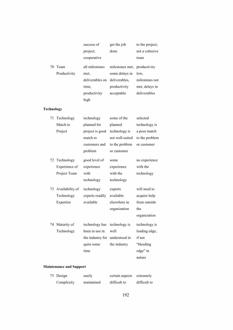
192

success of

project;

cooperative

get the job

done

to the project;

not a cohesive

team

70 Team

Productivity

all milestones

met,

deliverables on

time,

productivity

high

milestones met,

some delays in

deliverables,

productivity

acceptable

productivity

low,

milestones not

met, delays in

deliverables

Technology

71 Technology

Match to

Project

technology

planned for

project is good

match to

customers and

problem

some of the

planned

technology is

not well-suited

to the problem

or customer

selected

technology is

a poor match

to the problem

or customer

72 Technology

Experience of

Project Team

good level of

experience

with

technology

some

experience

with the

technology

no experience

with the

technology

73 Availability of

Technology

Expertise

technology

experts readily

available

experts

available

elsewhere in

organization

will need to

acquire help

from outside

the

organization

74 Maturity of

Technology

technology has

been in use in

the industry for

quite some

time

technology is

well

understood in

the industry

technology is

leading edge,

if not

"bleeding

edge" in

nature

Maintenance and Support

75 Design

Complexity

easily

maintained

certain aspects

difficult to

extremely

difficult to

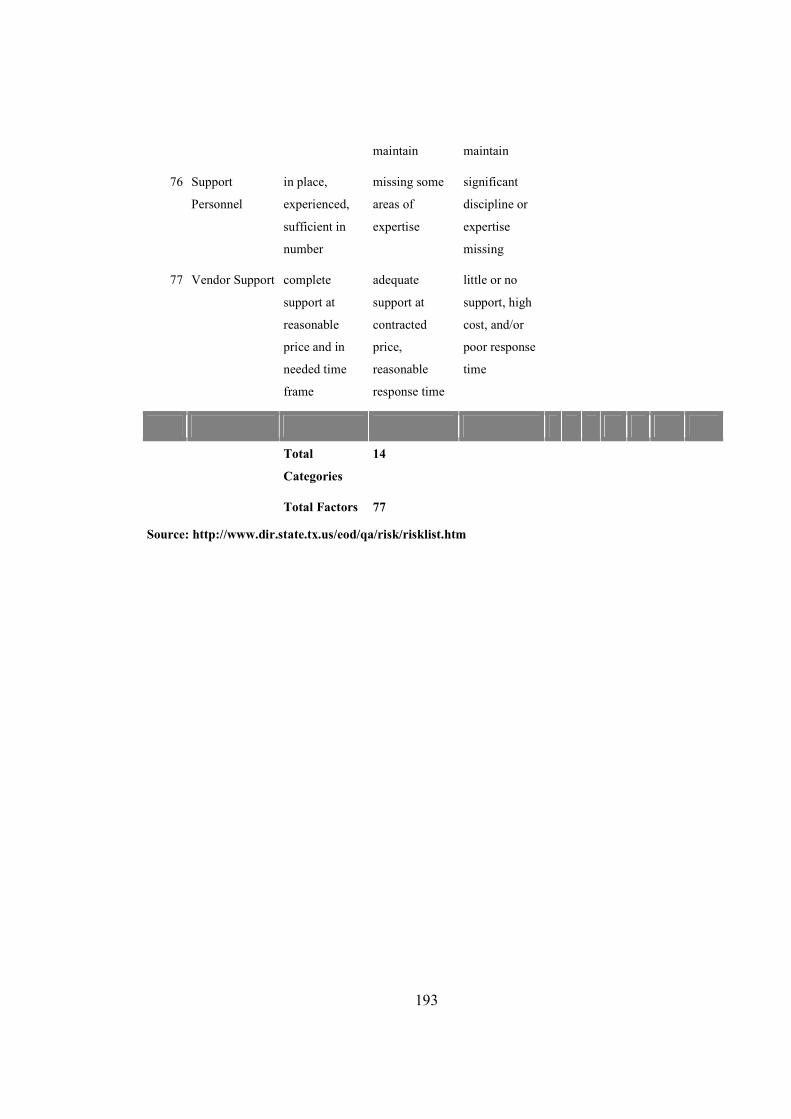
193

maintain maintain

76 Support

Personnel

in place,

experienced,

sufficient in

number

missing some

areas of

expertise

significant

discipline or

expertise

missing

77 Vendor Support complete

support at

reasonable

price and in

needed time

frame

adequate

support at

contracted

price,

reasonable

response time

little or no

support, high

cost, and/or

poor response

time

Total

Categories

14

Total Factors 77

Source: http://www.dir.state.tx.us/eod/qa/risk/risklist.htm

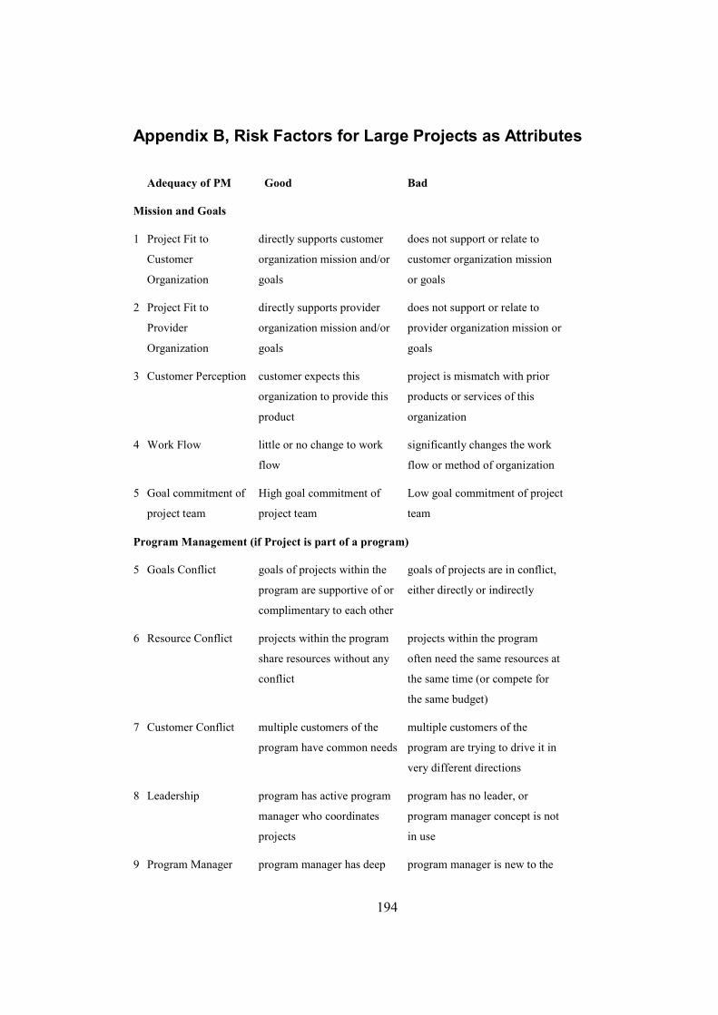
194

Appendix B, Risk Factors for Large Projects as Attributes

Adequacy of PM Good Bad

Mission and Goals

1 Project Fit to

Customer

Organization

directly supports customer

organization mission and/or

goals

does not support or relate to

customer organization mission

or goals

2 Project Fit to

Provider

Organization

directly supports provider

organization mission and/or

goals

does not support or relate to

provider organization mission or

goals

3 Customer Perception customer expects this

organization to provide this

product

project is mismatch with prior

products or services of this

organization

4 Work Flow little or no change to work

flow

significantly changes the work

flow or method of organization

5 Goal commitment of

project team

High goal commitment of

project team

Low goal commitment of project

team

Program Management (if Project is part of a program)

5 Goals Conflict goals of projects within the

program are supportive of or

complimentary to each other

goals of projects are in conflict,

either directly or indirectly

6 Resource Conflict projects within the program

share resources without any

conflict

projects within the program

often need the same resources at

the same time (or compete for

the same budget)

7 Customer Conflict multiple customers of the

program have common needs

multiple customers of the

program are trying to drive it in

very different directions

8 Leadership program has active program

manager who coordinates

projects

program has no leader, or

program manager concept is not

in use

9 Program Manager program manager has deep program manager is new to the

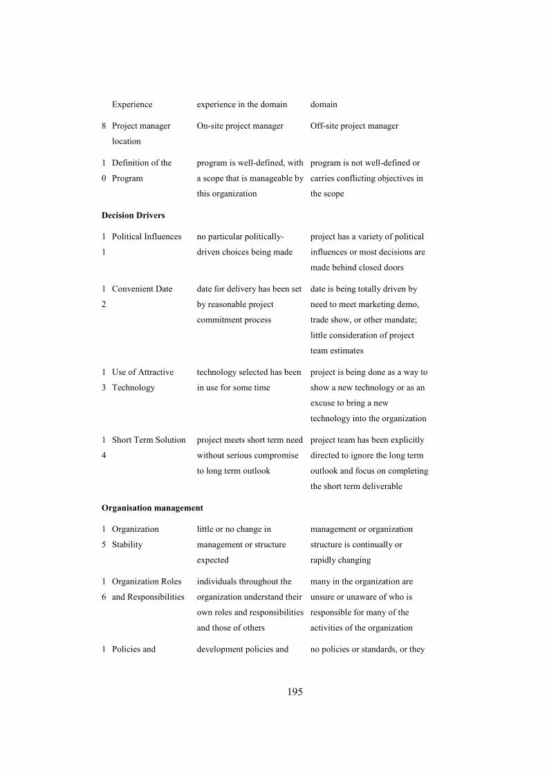
195

Experience experience in the domain domain

8 Project manager

location

On-site project manager Off-site project manager

1

0

Definition of the

Program

program is well-defined, with

a scope that is manageable by

this organization

program is not well-defined or

carries conflicting objectives in

the scope

Decision Drivers

1

1

Political Influences no particular politically-

driven choices being made

project has a variety of political

influences or most decisions are

made behind closed doors

1

2

Convenient Date date for delivery has been set

by reasonable project

commitment process

date is being totally driven by

need to meet marketing demo,

trade show, or other mandate;

little consideration of project

team estimates

1

3

Use of Attractive

Technology

technology selected has been

in use for some time

project is being done as a way to

show a new technology or as an

excuse to bring a new

technology into the organization

1

4

Short Term Solution project meets short term need

without serious compromise

to long term outlook

project team has been explicitly

directed to ignore the long term

outlook and focus on completing

the short term deliverable

Organisation management

1

5

Organization

Stability

little or no change in

management or structure

expected

management or organization

structure is continually or

rapidly changing

1

6

Organization Roles

and Responsibilities

individuals throughout the

organization understand their

own roles and responsibilities

and those of others

many in the organization are

unsure or unaware of who is

responsible for many of the

activities of the organization

1 Policies and development policies and no policies or standards, or they

196

7 Standards standards are defined and

carefully followed

are ill-defined and unused

1

8

Management Support strongly committed to

success of project

little or no support

1

9

Executive

Involvement

visible and strong support no visible support; no help on

unresolved issues

2

0

Project Objectives verifiable project objectives,

reasonable requirements

no established project objectives

or objectives are not measurable

Customers/Users

2

1

User Involvement users highly involved with

project team, provide

significant input

minimal or no user involvement;

little user input

2

2

User Experience users highly experienced in

similar projects; have specific

ideas of how needs can be

met

users have no previous

experience with similar projects;

unsure of how needs can be met

2

3

User Acceptance users accept concepts and

details of system; process is

in place for user approvals

users do not accept any concepts

or design details of system

2

4

User Training Needs user training needs

considered; training in

progress or plan in place

requirements not identified or

not addressed

2

5

User Justification user justification complete,

accurate, sound

no satisfactory justification for

system

Project Characteristics

2

6

Project Size small, non-complex, or easily

decomposed

large, highly complex, or not

decomposable

2

7

Reusable

Components

components available and

compatible with approach

components identified, need

serious modification for use

2

8

Supplied

Components

components available and

directly usable

components known to fail in

certain cases, likely to be late, or

incompatible with parts of

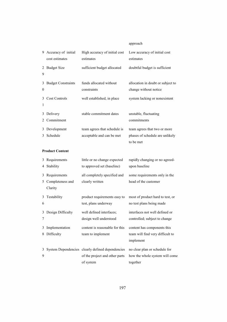
197

approach

9 Accuracy of initial

cost estimates

High accuracy of initial cost

estimates

Low accuracy of initial cost

estimates

2

9

Budget Size sufficient budget allocated doubtful budget is sufficient

3

0

Budget Constraints funds allocated without

constraints

allocation in doubt or subject to

change without notice

3

1

Cost Controls well established, in place system lacking or nonexistent

3

2

Delivery

Commitment

stable commitment dates unstable, fluctuating

commitments

3

3

Development

Schedule

team agrees that schedule is

acceptable and can be met

team agrees that two or more

phases of schedule are unlikely

to be met

Product Content

3

4

Requirements

Stability

little or no change expected

to approved set (baseline)

rapidly changing or no agreed-

upon baseline

3

5

Requirements

Completeness and

Clarity

all completely specified and

clearly written

some requirements only in the

head of the customer

3

6

Testability product requirements easy to

test, plans underway

most of product hard to test, or

no test plans being made

3

7

Design Difficulty well defined interfaces;

design well understood

interfaces not well defined or

controlled; subject to change

3

8

Implementation

Difficulty

content is reasonable for this

team to implement

content has components this

team will find very difficult to

implement

3

9

System Dependencies clearly defined dependencies

of the project and other parts

of system

no clear plan or schedule for

how the whole system will come

together

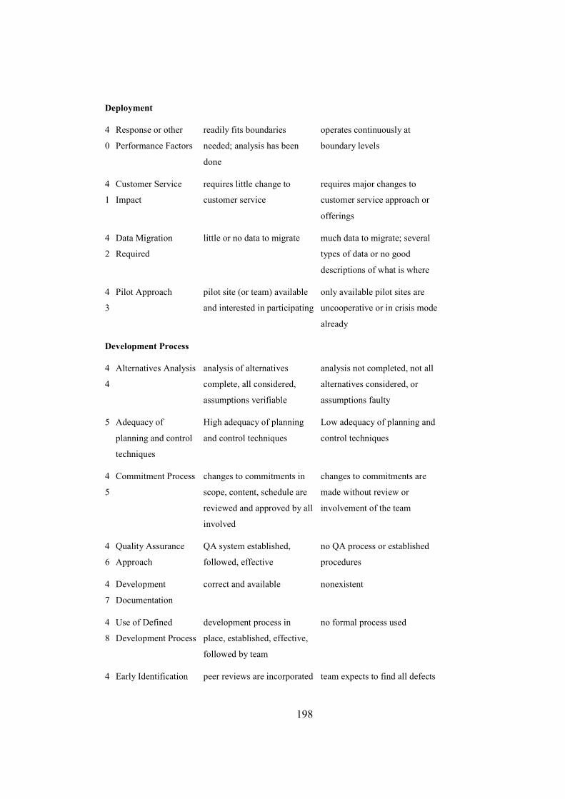
198

Deployment

4

0

Response or other

Performance Factors

readily fits boundaries

needed; analysis has been

done

operates continuously at

boundary levels

4

1

Customer Service

Impact

requires little change to

customer service

requires major changes to

customer service approach or

offerings

4

2

Data Migration

Required

little or no data to migrate much data to migrate; several

types of data or no good

descriptions of what is where

4

3

Pilot Approach pilot site (or team) available

and interested in participating

only available pilot sites are

uncooperative or in crisis mode

already

Development Process

4

4

Alternatives Analysis analysis of alternatives

complete, all considered,

assumptions verifiable

analysis not completed, not all

alternatives considered, or

assumptions faulty

5 Adequacy of

planning and control

techniques

High adequacy of planning

and control techniques

Low adequacy of planning and

control techniques

4

5

Commitment Process changes to commitments in

scope, content, schedule are

reviewed and approved by all

involved

changes to commitments are

made without review or

involvement of the team

4

6

Quality Assurance

Approach

QA system established,

followed, effective

no QA process or established

procedures

4

7

Development

Documentation

correct and available nonexistent

4

8

Use of Defined

Development Process

development process in

place, established, effective,

followed by team

no formal process used

4 Early Identification peer reviews are incorporated team expects to find all defects

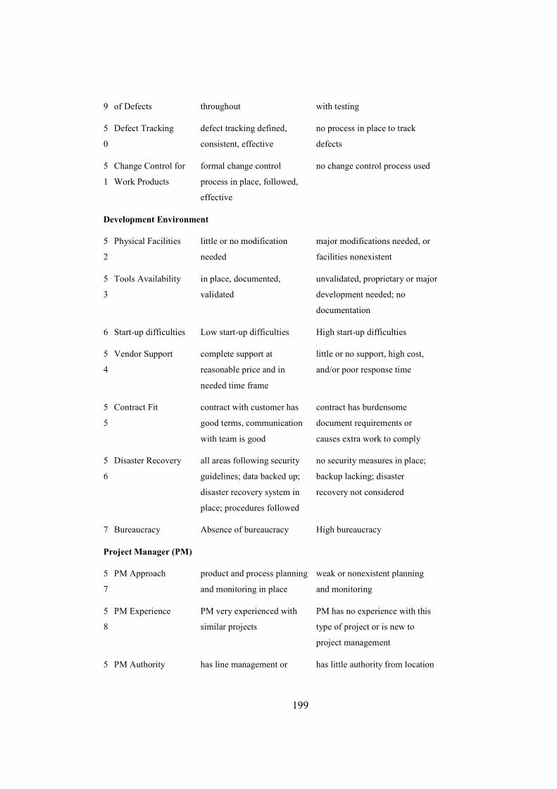
199

9 of Defects throughout with testing

5

0

Defect Tracking defect tracking defined,

consistent, effective

no process in place to track

defects

5

1

Change Control for

Work Products

formal change control

process in place, followed,

effective

no change control process used

Development Environment

5

2

Physical Facilities little or no modification

needed

major modifications needed, or

facilities nonexistent

5

3

Tools Availability in place, documented,

validated

unvalidated, proprietary or major

development needed; no

documentation

6 Start-up difficulties Low start-up difficulties High start-up difficulties

5

4

Vendor Support complete support at

reasonable price and in

needed time frame

little or no support, high cost,

and/or poor response time

5

5

Contract Fit contract with customer has

good terms, communication

with team is good

contract has burdensome

document requirements or

causes extra work to comply

5

6

Disaster Recovery all areas following security

guidelines; data backed up;

disaster recovery system in

place; procedures followed

no security measures in place;

backup lacking; disaster

recovery not considered

7 Bureaucracy Absence of bureaucracy High bureaucracy

Project Manager (PM)

5

7

PM Approach product and process planning

and monitoring in place

weak or nonexistent planning

and monitoring

5

8

PM Experience PM very experienced with

similar projects

PM has no experience with this

type of project or is new to

project management

5 PM Authority has line management or has little authority from location

200

9 official authority that enables

project leadership

effectiveness

in the organization structure and

little personal power to influence

decision-making and resources

7 PM Influence High PM influence Low PM influence

8 PM Technical skills High PM technical skills Low PM technical skills

9 PM Human skills High PM human skills Low PM human skills

6

0

Support of the PM complete support by team

and of management

no visible support; manager in

name only

1 Project manager

commitment to

established schedules

1 Project manager

commitment to

established budgets

1 Project manager

commitment to

technical

performance goals

Team Members

6

1

Team Member

Availability

in place, little turnover

expected; few interrupts for

fire fighting

high turnover, not available;

team spends most of time

fighting fires

6

2

Mix of Team Skills good mix of disciplines some disciplines not represented

at all

6

3

Team

Communication

clearly communicates goals

and status between the team

and rest of organization

rarely communicates clearly

within team or to others who

need to be informed

6

4

Application

Experience

extensive experience in team

with projects like this

little or no experience with

similar projects

6

5

Expertise with

Application Area

(Domain)

good background with

application domain within

development team

no expertise in domain in team,

no availability of experts

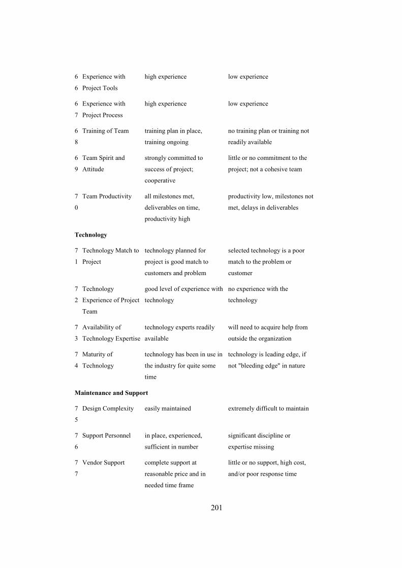
201

6

6

Experience with

Project Tools

high experience low experience

6

7

Experience with

Project Process

high experience low experience

6

8

Training of Team training plan in place,

training ongoing

no training plan or training not

readily available

6

9

Team Spirit and

Attitude

strongly committed to

success of project;

cooperative

little or no commitment to the

project; not a cohesive team

7

0

Team Productivity all milestones met,

deliverables on time,

productivity high

productivity low, milestones not

met, delays in deliverables

Technology

7

1

Technology Match to

Project

technology planned for

project is good match to

customers and problem

selected technology is a poor

match to the problem or

customer

7

2

Technology

Experience of Project

Team

good level of experience with

technology

no experience with the

technology

7

3

Availability of

Technology Expertise

technology experts readily

available

will need to acquire help from

outside the organization

7

4

Maturity of

Technology

technology has been in use in

the industry for quite some

time

technology is leading edge, if

not "bleeding edge" in nature

Maintenance and Support

7

5

Design Complexity easily maintained extremely difficult to maintain

7

6

Support Personnel in place, experienced,

sufficient in number

significant discipline or

expertise missing

7

7

Vendor Support complete support at

reasonable price and in

needed time frame

little or no support, high cost,

and/or poor response time