Download - Improved kernel estimation of copulas: Weak convergence and goodness-of-fit testing

arX

iv:0

908.

4530

v1 [

mat

h.ST

] 3

1 A

ug 2

009

The Annals of Statistics

2009, Vol. 37, No. 5B, 3023–3058DOI: 10.1214/08-AOS666c© Institute of Mathematical Statistics, 2009

IMPROVED KERNEL ESTIMATION OF COPULAS: WEAK

CONVERGENCE AND GOODNESS-OF-FIT TESTING1

By Marek Omelka, Irene Gijbels and Noel Veraverbeke

Charles University Prague, Katholieke Universiteit Leuvenand Hasselt University

We reconsider the existing kernel estimators for a copula func-tion, as proposed in Gijbels and Mielniczuk [Comm. Statist. TheoryMethods 19 (1990) 445–464], Fermanian, Radulovic and Wegkamp[Bernoulli 10 (2004) 847–860] and Chen and Huang [Canad. J. Statist.35 (2007) 265–282]. All of these estimators have as a drawback thatthey can suffer from a corner bias problem. A way to deal with this isto impose rather stringent conditions on the copula, outruling as suchmany classical families of copulas. In this paper, we propose improvedestimators that take care of the typical corner bias problem. For Gij-bels and Mielniczuk [Comm. Statist. Theory Methods 19 (1990) 445–464] and Chen and Huang [Canad. J. Statist. 35 (2007) 265–282], theimprovement involves shrinking the bandwidth with an appropriatefunctional factor; for Fermanian, Radulovic and Wegkamp [Bernoulli10 (2004) 847–860], this is done by using a transformation. The theo-retical contribution of the paper is a weak convergence result for thethree improved estimators under conditions that are met for mostcopula families. We also discuss the choice of bandwidth parame-ters, theoretically and practically, and illustrate the finite-sample be-haviour of the estimators in a simulation study. The improved esti-mators are applied to goodness-of-fit testing for copulas.

1. Introduction. Consider a random vector X = (X1, . . . ,Xd)T with joint

cumulative distribution function H and marginal distribution functions F1, . . . ,

Received July 2008; revised October 2008.1Supported by the IAP Research Network P6/03 of the Belgian State (Belgian Science

Policy). This work was done while the first author was a postdoctoral researcher at theKatholieke Universiteit Leuven and the Universiteit Hasselt within the IAP ResearchNetwork. Support of the Research Project LC06024 is also highly appreciated.

AMS 2000 subject classifications. Primary 62G07; secondary 62G20.Key words and phrases. Copula, Cramer–von Mises statistics, Gaussian process,

goodness-of-fit, Kendall’s tau, Kolmogorov–Smirnov statistics, parametric bootstrap,pseudo-observations, weak convergence.

This is an electronic reprint of the original article published by theInstitute of Mathematical Statistics in The Annals of Statistics,2009, Vol. 37, No. 5B, 3023–3058. This reprint differs from the original inpagination and typographic detail.

1

http://arxiv.org/abs/0908.4530v1

http://www.imstat.org/aos/

http://dx.doi.org/10.1214/08-AOS666

http://www.imstat.org

http://www.ams.org/msc/

http://www.imstat.org

http://www.imstat.org/aos/

http://dx.doi.org/10.1214/08-AOS666

2 M. OMELKA, I. GIJBELS AND N. VERAVERBEKE

Fd. According to Sklar’s theorem [see, e.g., Nelsen (2006)], there exists a d-variate function C such that

H(x1, . . . , xd) = C(F1(x1), . . . , Fd(xd)).(1)

The function C is called a copula, and it is, in itself, a joint cumulative distri-bution function on [0,1]d with uniform marginals. If the marginal distribu-tion functions F1, . . . , Fd are continuous, then the function C is unique andC(u1, . . . , ud) = H(F−1

1 (u1), . . . , F−1d (ud)), where, for j = 1, . . . , d, F−1

j (u) =

inf{x :Fj(x) ≥ u}, with u ∈ [0,1], is the quantile function of Fj . The copulaC “couples” the joint distribution function H to its univariate marginals,capturing as such the dependence structure between the components ofX = (X1, . . . ,Xd)

T.Methods for estimation of copulas usually depend on how much we are

willing to assume about the joint distribution function H . In fully para-metric approaches with parametric models for both the copula and themarginals, maximum likelihood estimation may be used. Nowadays semi-parametric estimation is quite popular, in which one specifies a parametriccopula and estimates the marginals nonparametrically. In this paper, we fo-cus on nonparametric estimation of the copula making as such no restrictivedistributional assumptions on the copula nor on the marginals.

For simplicity of the presentation, we will restrict to the case d = 2, andconsider an independent and identically distributed sample (X1, Y1)

T, . . . ,(Xn, Yn)T of a bivariate random vector (X,Y )T with joint distribution func-tion H and marginal distribution functions F and G.

Nonparametric estimation of copulas goes back to Deheuvels (1979) whoproposed, in order to test for independence, the following empirical copulaestimator:

Cn(u, v) =1

n

n∑

i=1

I{Ui ≤ u, Vi ≤ v} with Ui = Fn(Xi), Vi = Gn(Yi),

where Fn and Gn are the empirical cumulative distribution functions of themarginals, and where I{A} denotes the indicator of a set A. This estimatoris asymptotically equivalent [up to a term O(n−1)] with the estimator baseddirectly on Sklar’s theorem given by

Cn(u, v) = Hn(F−1n (u),G−1

n (v))(2)

with Hn the empirical joint distribution function. Weak convergence studiesof this estimator can be found in Ganssler and Stute (1987), Fermanian,Radulovic and Wegkamp (2004) and Tsukuhara (2005). Our Monte Carloexperiments showed that it is better to use the following (asymptotically

IMPROVED KERNEL ESTIMATION OF COPULAS 3

equivalent) modification of the empirical copula:

C(E)n (u, v) =

1

n

n∑

i=1

I{U (E)i ≤ u, V

(E)i ≤ v}

(3)

with U(E)i =

n

n + 1Fn(Xi), V

(E)i =

n

n + 1Gn(Yi),

which shifts the pseudo-observations Fn(Xi) and Gn(Yi) a bit closer to theleft corner of the unit interval [0,1] [see, e.g., Genest, Ghoudi and Rivest(1995)].

Fermanian, Radulovic and Wegkamp (2004) also proposed a smoothedversion of the empirical copula. Their proposal is a straightforward modifi-cation of (3) and the estimator is defined as

C(SE)n (u, v) = Hn(F−1

n (u), G−1n (v)),(4)

where the quantities Hn, Fn and Gn are given by

Hn(x, y) =1

n

n∑

i=1

Kn(x−Xi, y − Yi), Fn(x) = Hn(x,+∞),

(5)Gn(x) = Hn(+∞, y)

with

Kn(x, y) = K

(

x

bn,

y

bn

)

, K(x, y) =

∫ x

−∞

∫ y

−∞k(s, t)dsdt,

where k(s, t) is a given bivariate kernel density function, and bn is a band-width sequence tending to zero with n. Fermanian, Radulovic and Wegkamp(2004) proved weak convergence of this estimator.

There are two kernel type estimators in the literature that pay specialattention to the correction of the boundary bias. This typical bias associ-ated with kernel estimation is present since a copula has its support on thebounded set [0,1]2. The first reference is the mirror-reflection type estima-tor originating from the work of Gijbels and Mielniczuk (1990) on copuladensity estimation. They take care of boundary bias correction through data-augmentation obtained by reflecting the original data with respect to theedges and the corners of the unit square. The second reference is the esti-mator of Chen and Huang (2007), who proposed to use a local linear kernelin order to deal with the bias near the boundaries of the unit square.

A first goal of the present paper is to prove the weak convergence of theestimators of Gijbels and Mielniczuk (1990) and Chen and Huang (2007)under the assumption that C has bounded second order partial deriva-tives on [0,1]2 (see Theorem 1 in Section 2). It turns out, however, that

https://www.researchgate.net/publication/227633507_Nonparametric_Estimation_of_Copula_Functions_For_Dependence_Modeling?el=1_x_8&enrichId=rgreq-f3adcd47-d76e-4151-b175-70c156cbaca8&enrichSource=Y292ZXJQYWdlOzQ1ODY5ODgyO0FTOjEwNDQ2MjEzNTg1NzE2NUAxNDAxOTE3MTIyNjg3



for many commonly-used families of copulas (e.g., Clayton, Gumbel, nor-mal, Student), the latter condition is not satisfied and the bias behavior atthe corners of the unit square precludes the weak convergence on the whole[0,1]2. We therefore propose improved “shrinked” versions of the estimatorsof Gijbels and Mielniczuk (1990) and Chen and Huang (2007). This shrink-ing is done by including a weight function which removes the corner bias. Inthe same spirit, we also suggest a modification of the copula estimator (4)of Fermanian, Radulovic and Wegkamp (2004). In Theorem 2 we estab-lish weak convergence for all newly proposed estimators. The finite-sampleperformance of the estimators is demonstrated via a simulation study. Wediscuss optimal bandwidth selection and compare the performances of theestimators using various well-known distance measures.

The second goal of the paper is to discuss the use of the various estimatorsof copulas in goodness-of-fit testing problems.

The paper is organized as follows. In Section 2, we introduce the im-proved kernel estimators and state the main theoretical results on weakconvergence. In Section 3, we investigate the finite-sample performance ofthe newly-proposed estimators and compare these with performances of ex-isting estimators. In Section 4, simulation results are reported for goodness-of-fit testing. The proofs of the weak convergence results are given in theAppendix.

2. Nonparametric kernel estimators of a copula. In this section, we brieflydiscuss existing kernel estimators and propose important modifications. Wealso state the weak convergence results.

2.1. Local linear kernel estimator. Chen and Huang (2007) constructedtheir estimator in the following way. In the first stage, they estimate marginalsby

Fn(x) =1

n

n∑

i=1

K

(

x−Xi

bn1

)

, Gn(y) =1

n

n∑

i=1

K

(

y − Yi

bn2

)

(6)

with K the integral of a symmetric bounded kernel function k supported on[−1,1]. In the second stage, the pseudo-observations Ui = Fn(Xi) and Vi =

Gn(Yi) are used to estimate the joint distribution function of the unobservedF (Xi) and G(Yi), which gives the estimate of the unknown copula C. Toprevent boundary bias, Chen and Huang (2007) suggested using a locallinear version of the kernel k given by

ku,h(x) =k(x){a2(u,h)− a1(u,h)x}a0(u,h)a2(u,h)− a2

1(u,h)I

{

u− 1

h< x <

u

h

}

,(7)




where

al(u,h) =

∫ u/h

(u−1)/htlk(t)dt for l = 0,1,2.

Finally, the local linear type estimator of the copula is given by

C(LL)n (u, v) =

1

n

n∑

i=1

Ku,hn

(

u− Ui

hn

)

Kv,hn

(

v − Vi

hn

)

,(8)

where Ku,h(x) =∫ x−∞ ku,h(s)ds. Chen and Huang (2007) derived expres-

sions for asymptotic bias, variance and mean squared error for this estima-tor and showed that a proper choice of the second stage smoothing con-stants h = hn may considerably decrease variance and mean squared errorof the copula estimate. Moreover, their Monte Carlo experiments showed

that the estimator C(LL)n is quite insensitive to the choice of the constants

b1n and b2n used for smoothing the marginals in the first stage. Varianceconsiderations provided by the authors even showed that it is reasonableto take b1n and b2n as small as possible. Note that strong undersmooth-ing in the first stage, recommended in Chen and Huang (2007), results in

using the pseudo-observations (Ui, Vi)T = (2nFn(Xi)−1

2n , 2nGn(Yi)−12n )T, which is

asymptotically equivalent to the mostly-used pseudo-observations defined in(3).

As already mentioned in the Introduction, the theoretical inconvenience ofthe estimator (8) is that for many common families of copulas (e.g., Clayton,Gumbel, normal, Student) the bias of the estimator at some of the cornersof the unit square is only of order O(hn). As the optimal bandwidth fordistribution function estimation is of order O(n−1/3), this violates the n1/2-order weak convergence on the whole [0,1]2.

The problem is caused by unboundedness of second order partial deriva-tives of many copula families. Although parametric models with unboundeddensities are rather rare in “standard” parametric models, copula familieswith unbounded densities are quite common. As a benchmark, we can takethe normal bivariate density, which is usually supposed to be a well-behavedmodel. But the resulting normal copula density is unbounded.

To overcome this difficulty, we propose a method of shrinking the band-width when coming close to the borders of the unit square. The proposedmethod is based on the observation that, when calculating the bias of the es-timator (8), we have to deal with terms of the form h2Cuu(u, v), h2Cuv(u, v)and h2Cvv(u, v), where Cuu(u, v), Cuv(u, v) and Cvv(u, v) are the second or-der partial derivatives of C; that is, Cuu(u, v) = ∂2C(u, v)/∂u2 and, similarly,for Cuv(u, v), Cvv(u, v). The problem is that, for many common families ofcopulas, these second order partial derivatives are not bounded, and, in fact,


a closer inspection of them shows that

Cuu(u, v) = O

(

1

u(1− u)

)

, Cvv(u, v) = O

(

1

v(1− v)

)

,

(9)

Cuv(u, v) = O

(

1√

uv(1− u)(1− v)

)

.

This is shown in Appendix D for Clayton, Gumbel, normal and Student cop-ulas. In order to keep the bias bounded, we suggest an improved “shrinked”version of (8), which is given by

C(LLS)n (u, v) =

1

n

n∑

i=1

Ku,hn

(

u− Ui

b(u)hn

)

Kv,hn

(

v − Vi

b(v)hn

)

(10)with b(w) = min(

√w,

√1−w),

where the constant bandwidth hn is replaced by a bandwidth function b(u)hn

that “shrinks” the value of the bandwidth close to zero at the corners of theunit square. A straightforward adaptation of the result of Chen and Huang(2007) gives that, for (u/b(u), v/b(v)) ∈ [hn,1 − hn]2 (and no smoothing ofthe marginals in the first stage),

Bias{C(LLS)n (u, v)}

(11)

=σ2

K

2h2

n{b2(u)Cuu(u, v) + b2(v)Cvv(u, v)}+ o(h2n),

Var{C(LLS)n (u, v)}

=1

nVar[I{U ≤ u,V ≤ v} −Cu(u, v)I{U ≤ u} −Cv(u, v)I{V ≤ v}]

(12)

− hnbK

n[b(u)Cu(u, v)(1−Cu(u, v))

+ b(v)Cv(u, v)(1−Cv(u, v))] + o

(

hn

n

)

with σ2K =

∫ 1−1 t2k(t)dt, bK = 2

∫ 1−1 tk(t)K(t)dt and b(·) as defined in (10).

Taking b(w) = 1 gives back the bias and variance expressions for C(LL)n in

Chen and Huang (2007) (in case of no smoothing at the first stage).The improvements are obtained by shrinking the bandwidth through the

function b(α,w) = min{wα, (1 − w)α}. Different choices of α or differentchoices of shrinking factors are possible, but our extensive investigations

showed that b(w) = min{√w,√

1−w} is overall a very good choice. Thechoice of a possible optimal shrinking factor is an open question.


2.2. Mirror-reflection kernel estimator. Another version of a kernel es-timator for the copula might be obtained by integration of the estimator ofthe density of the copula introduced and studied in Gijbels and Mielniczuk(1990). This estimator deals with the boundary problem by the techniqueknown as mirror-reflection. If a multiplicative kernel k(x, y) = k(x)k(y) isused, then the mirror-reflection estimate of the copula has a simple form

C(MR)n (u, v) =

1

n

n∑

i=1

9∑

ℓ=1

[

K

(

u− U(ℓ)i

hn

)

−K

(−U(ℓ)i

hn

)]

(13)

×[

K

(

v − V(ℓ)i

hn

)

−K

(−V(ℓ)i

hn

)]

,

where {(U (ℓ)i , V

(ℓ)i ), i = 1, . . . , n, ℓ = 1, . . . ,9} = {(±Ui,±Vi), (±Ui,2 − Vi),

(2− Ui,±Vi), (2− Ui,2− Vi), i = 1, . . . , n}.The mirror-type estimator (13) faces the same “corner bias” problem as

the local linear estimator (8). To prevent this problem, we can “shrink” thebandwidth similarly as in (10) and propose

C(MRS)n (u, v) =

1

n

n∑

i=1

9∑

ℓ=1

[

K

(

u− U(ℓ)i

b(u)hn

)

−K

( −U(ℓ)i

b(u)hn

)]

(14)

×[

K

(

v − V(ℓ)i

b(v)hn

)

−K

( −V(ℓ)i

b(v)hn

)]

.

2.3. Transformation estimator. The unboundedness of the densities ofmany copula families brings us back to Sklar’s theorem in (1) and to theestimator (4) proposed in Fermanian, Radulovic and Wegkamp (2004).

To control the bias of this estimator in order to achieve weak conver-gence, we need the boundedness of the second order partial derivatives ofthe original joint distribution H . As the bivariate normal benchmark exam-ple shows, this condition may be considerably weaker than the requirementof the bounded second order derivatives of the underlying copula C.

A possible methodological objection to the estimator C(SE)n , defined in

(4), may be its dependence on the marginal distributions. This is confirmedby Monte Carlo simulations which show that, for a given copula, the successof this estimator depends on the marginals crucially.

As the copula function is invariant to increasing transformations of themargins, it is possible to transform the original data to X ′

i = T1(Xi) andY ′

i = T2(Yi), where T1 and T2 are increasing functions, and then use (X ′i, Y

′i )

instead of the original observations (Xi, Yi) in the estimator C(SE)n . The

aim of the transformation is to simplify the kernel estimation of the joint


distribution. As the direct choice of functions T1, T2 is difficult, we pro-pose the following procedure. Let us first construct the uniform pseudo-

observations U(E)i = n

n+1Fn(Xi) and V(E)i = n

n+1Gn(Yi). Then, for a given

distribution function Φ, put Si = Φ−1(U(E)i ) and Ti = Φ−1(V

(E)i ). Finally,

use these transformed pseudo-observations (Si, Ti) instead of the originalobservations (Xi, Yi) in the estimator (5) of the joint distribution function.As we know, the marginals to be given by the function Φ, the suggested esti-mator has, in the case of multiplicative kernel, the following simple formula:

C(T)n (u, v) =

1

n

n∑

i=1

K

(

Φ−1(u)−Φ−1(U(E)i )

hn

)

(15)

×K

(

Φ−1(v)−Φ−1(V(E)i )

hn

)

.

The advantage of this estimator is that it is not affected by the marginaldistributions. Further bias calculations show that, if we choose Φ, such thatΦ′(x)2

Φ(x) is bounded, we take care of the “corner bias problem” that is present

if we try to estimate the joint distribution of pseudo-observations directly.The above condition is satisfied, for example, for Φ the normal cumulativedistribution function.

2.4. Main results. The main theoretical contribution of this paper is the

weak convergence of the kernel estimators C(LL)n , C

(LLS)n , C

(MR)n , C

(MRS)n and

C(T)n .For notational convenience, let us denote Fn and Gn the estimates of the

marginals that are used to construct pseudo-observations; that is, in thefollowing we will write Ui = Fn(Xi) and Vi = Gn(Yi). For the weak conver-gence results we need these functions to be asymptotically equivalent to theempirical cumulative distribution functions Fn, Gn; that is,

supx

|Fn(x)−Fn(x)| = op

(

1√n

)

,

(16)

supy

|Gn(y)−Gn(y)| = op

(

1√n

)

,

which further implies the standard weak convergence of the processes√

n(Fn−F ) and

√n(Gn −G) to particular Brownian bridges. For technical reasons,

we will also suppose that the functions Fn and Gn are nondecreasing, whichexcludes higher order kernels (taking negative values) for the estimation ofthe marginals.


It is easy to see that (16) is satisfied if we define pseudo-observations as

Ui = 2nFn(Xi)−12n , Vi = 2nGn(Yi)−1

2n , or in a way given in (3).

If we decide for kernel smoothing of the marginals given in (6), then itis well known [see, e.g., Lemma 7 of Fermanian, Radulovic and Wegkamp(2004)] that assumption (16) is met if there exists α > 0 such that, uniformlyin x,

F (x + b1n) = F (x) + b1nf(x) + o(b1+α1n ) with

√nb1+α

1n → 0,

where f denotes the derivative of F and, similarly, for G involving b2n.

Let C(LL)n , C

(LLS)n , C

(MR)n , C

(MRS)n , C

(T)n be suitably normalized empirical

copula processes; that is, for (u, v) ∈ [0,1]2,

C(·)n =

√n{C(·)

n −C(u, v)}.

The proof of the following theorem is given in Appendix A. The termini-nology on stochastic processes (e.g., pinned C-Brownian sheet) is taken fromTsukuhara (2005). We refer the reader to this reference for details on theconcepts used.

Theorem 1. Suppose that H has continuous marginal distribution func-tions and that the underlying copula function C has bounded second orderpartial derivatives on [0,1]2. If hn = O(n−1/3) and (16) is satisfied, then

the (kernel) copula processes C(LL)n , C

(MR)n converge weakly to the Gaussian

process GC in ℓ∞([0,1]2), having representation

GC(u, v) = BC(u, v)−Cu(u, v)BC(u,1)−Cv(u, v)BC(1, v),(17)

where Cu and Cv denote the first order partial derivatives of C, and BC is atwo-dimensional pinned C-Brownian sheet on [0,1]2; that is, it is a centeredGaussian process with covariance function

E[BC(u, v)BC(u′, v′)] = C(u∧ u′, v ∧ v′)−C(u, v)C(u′, v′).(18)

While Theorem 1 requires boundedness of the second order partial deriva-tives of the copula C, the weak convergence result of Fermanian, Radulovic

and Wegkamp (2004) for the estimator C(SE)n given by (4) requires bounded-

ness of the second order derivatives of the original joint distribution functionH . This may or may not be more stringent, depending on the marginals. Un-fortunately, Theorem 1 excludes many commonly-used families of copulas.The next theorem and Appendix D guarantee that the weak convergence of

the proposed improved estimators C(LLS)n , C

(MRS)n , C

(T)n holds for commonly-

used copulas such as Clayton, Gumbel, normal and Student copulas.


Remark. A careful reader may find out that all the published weakconvergence results for the empirical estimator (2) or the smoothed empiricalestimator (4) require smoothness of the first order partial derivatives Cu andCv of the copulas C on [0,1]2. But this smoothness assumption usually isnot true for the families which do not have bounded second order partialderivatives (e.g., Clayton, Gumbel, normal and Student). For instance, thefirst order partial derivatives of the Clayton copula are not continuous inthe corner point (0,0). The second step of our proof given in Appendix Bshows that it is sufficient to assume that

Cu,Cv are continuous in [0,1]2 \ {(0,0), (0,1), (1,0), (1,1)}.(19)

Theorem 2. Suppose that H has continuous marginal distribution func-tions and that the copula C has bounded second order partial derivatives on(0,1)2 and satisfies (9) and (19). If hn = O(n−1/3) and (16) is satisfied,

then the (kernel) copula processes C(LLS)n and C

(MRS)n converge weakly to the

Gaussian process GC in ℓ∞([0,1]2) given in Theorem 1.

Moreover, if the functions Φ′ and Φ′(x)2

Φ(x) are bounded, then the above state-

ment holds also for the process C(T)n .

3. Finite sample comparisons.

3.1. Set up and performed comparisons. In our simulation study, we al-ways use the Epanechnikov kernel k(x) = 3

4(1−x2)I{|x| ≤ 1} and the bivari-ate multiplicative kernel k(x, y) = k(x)k(y). The optimality of the Epanech-nikov kernel in kernel density estimation was proven in Epanechnikov (1969).For background information on multivariate kernels see, for example, Wandand Jones (1995) and Fan and Gijbels (1996).

We investigate the performances of the estimators C(E)n , C

(T)n , C

(LL)n , C

(MR)n

and C(LLS)n . We do not include the estimator C

(SE)n , defined in (4), because

this estimator is too strongly influenced by the marginals, which makesthe comparison difficult. For example, for a normal copula with normal

marginals, the estimator C(SE)n usually does slightly better than its com-

petitors. But, for a normal copula with, for example, exponential marginals,

the performance of C(SE)n is considerably worse than its competitors. We do

not present results for the modification of the mirror-type estimator C(MRS)n

either, since its performance was found to be close to that of the estimator

C(LLS)n .The performances of the various estimators were evaluated using two crite-

ria: a Kolmogorov–Smirnov distance KSn and a Cramer–von Mises distance


CMn; that is,

KSn = supu,v

|Cn(u, v)−C(u, v)|,

CMn =n

∑

i=1

[Cn(Ui, Vi)−C(Ui, Vi)]2,

where Cn stands for any of the investigated estimators, for example, C(E)n .

The corresponding statistics are denoted accordingly, for example, KS(E)n and

CM(E)n . Originally, we included the mean integrated asymptotic error Qn =

n∫∫

[Cn(u, v)−C(u, v)]2 dudv as well. Not surprisingly, this measure behaves

similarly to the Cramer–von Mises distance, since CMn ≈ n∫∫

(Cn −C)2 dC,but it is not so sensitive to the bias of the underlying copula estimator. Seealso Section 4.

For computational reasons, the supremum in the Kolmogorov–Smirnovdistance KSn was replaced by a maximum over a grid of 101× 101 points.

3.2. Bandwidth choice. The estimator C(LL)n involves bandwidths bn1

and bn2 (for estimation of the marginals) as well as a bandwidth hn whenusing local linear fitting to estimate the copula. Preliminary simulation re-sults confirmed the results of Chen and Huang (2007), that the estimator

C(LL)n [as well as its modification C

(LLS)n ] cannot be improved by smooth-

ing the marginals. Therefore, we simply work with the pseudo-observations

U(E)i = n

n+1Fn(Xi) and V(E)i = n

n+1Gn(Yi), with Fn and Gn the empiricalcumulative distribution functions. This slightly differs from the strategy ofstrong undersmoothing recommended in Chen and Huang (2007), which

more or less results in taking Ui = 2nFn(Xi)−12n and Vi = 2nGn(Yi)−1

2n . Never-theless, the behavior of the resulting estimators is very similar.

For choosing the bandwidth hn for C(LL)n and C

(LLS)n , we rely on the

expressions for asymptotic bias, variance and MISE derived in Chen andHuang (2007). From the main (Asymptotic) terms in (11) and (12), wederive the asymptotic mean squared error of the copula estimator in a givenpoint (u, v)

AMSE{Cn(u, v)} = AVar{Cn(u, v)}+ [ABias{Cn(u, v)}]2.(20)

An optimal bandwidth is obtained by minimization of∫∫

AMSE{Cn(u,v)}dC(u, v). As the true copula is unknown, this minimization cannot becarried out. A possible approach is then to consider a so-called referencecopula. Chen and Huang (2007) proposed using a t-copula as a referencecopula. But, as the second derivatives of the t-copula are not bounded, weexperienced numerical difficulties and instabilities trying to apply this ref-erence rule. We therefore decided to use Frank’s copula, which has bounded


second derivatives. The unknown parameter in Frank’s copula family is es-timated by inversion of Kendall’s tau. The computational simplicity of thisapproach also makes the goodness-of-fit testing procedures, presented inSection 4, much more feasible.

Since the shrinkage of the bandwidth in the estimator C(LLS)n removes the

problem of possible unboundedness of the second order partial derivatives,there are plenty of families of copulas to use as a reference copula for thisestimator. For simplicity and for more appropriate comparisons, we also use

Frank’s copula as a reference for C(LLS)n .

The asymptotic expansions (11) and (12) hold for the mirror-type kernel

estimators C(MR)n and C

(MRS)n as well; hence we also rely here on the same

choice for hn.For the two improved estimators, a Frank copula based reference selection

rule seems to give quite good performance (see Sections 3 and 4). A normalcopula based reference rule tends to result in a too large bandwidth, whereasa Clayton copula based reference rule tends to give, on average, too smallbandwidths. Thus Frank’s reference rule seems to be a good compromise.

More problematic is the bandwidth choice for C(T)n , as we do not have

asymptotic expressions for bias and variance here. We tried to minimize theexpected mean squared integrated error

∫ +∞

−∞

∫ +∞

−∞[Hn(x, y)−H(x, y)]2h(x, y)dxdy(21)

taking a bivariate normal distribution H , with corresponding density h, as areference distribution [see Jin and Shao (1999)]. However, the resulting band-width selector turned out to be too big. A possible explanation is that such aselection rule does not take into account that we rely on pseudo-observations(Ui, Vi) instead of on the unobservable (Ui, Vi). In our simulation study, wethen used the above mentioned bandwidth divided by a factor two. Thisseems to be a reasonable ad-hoc solution. To further investigate the band-

width selection problem, for C(T)n , we calculated the ratio of the bandwidth

selected via (21) to the one selected via searching for a bandwidth that min-imizes the criterion KSn(h) [resp., CMn(h)] over a grid of h-values. Table 1summarizes the obtained average ratios, for various values of Kendall’s taufrom 2000 simulated samples. Note that the ratios stay quite stable acrossdifferent families of copulas as well as for different sample sizes. This sug-

gests that it may be possible to find a reliable reference-based rule for C(T)n

as well.The simulation studies reported below showed a promising performance

for the transformation estimator C(T)n . A good bandwidth selection rule is

missing, for the moment, and is subject of further research.


Table 1Average ratios of bandwidths for C

(T)n selected from minimizing (21) and from criteria

KSn(h) and CMn(h), respectively, for different Kendall’s τ and sample sizes n

Clayton Frank Normal

τ = 0.25 τ = 0.75 τ = 0.25 τ = 0.75 τ = 0.25 τ = 0.75

KSn CMn KSn CMn KSn CMn KSn CMn KSn CMn KSn CMn

n = 50 1.20 1.28 1.53 2.00 1.23 1.38 1.53 2.04 1.28 1.37 1.26 1.62n = 150 1.13 1.27 1.38 2.08 1.21 1.47 1.55 2.07 1.20 1.36 1.24 1.60

3.3. Simulation results. An extensive simulation study was carried out tocompare the performances of all estimators using the performance measuresKSn (the Kolmogorov–Smirnov distance) and CMn (the Cramer–von Misesdistance). To illustrate our main findings, we only report on results obtainedfor the following two simulation models:

Model 1. Frank copula with Kendall’s τ = 0.25;

Model 2. Clayton copula with Kendall’s τ = 0.75.

Models 1 and 2 represent very different copula functions. The copula inmodel 1 has bounded second order partial derivatives and presents a caseof mild dependence, whereas the copula in model 2 has unbounded secondorder partial derivatives and shows a strong dependence between X and Y .From each model, we simulated 10,000 samples of sample size n = 150.

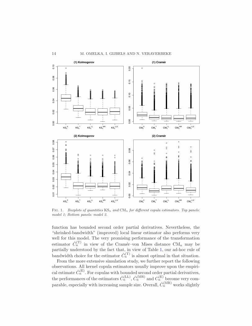
Figure 1 shows the boxplots of the performance measures KSn and CMn

for model 1 (top panels) and model 2 (bottom panels). Note that, for model

1, the estimators C(LL)n , C

(MR)n , C

(LLS)n and C

(T)n perform very comparable

for the Cramer–von Mises distance measure. For the Kolmogorov–Smirnov

performance measure, the estimator C(T)n performs slightly but significantly

worse than the three other estimators. The latter is likely caused by the usageof a too small bandwidth, as can be anticipated by looking at the differentresults for the two performance measures and Table 1. For model 2 (bottompanels), one clearly sees a better performance of the improved estimators

C(LLS)n and C

(T)n , especially when looking at the performance measure CMn.

This is as to be expected, since the copula in model 2 has unbounded secondorder partial derivatives and the measure CMn ≈ n

∫∫

(Cn −C)2 dC is mostaffected by points with higher values of the copula density c(u, v) (whichusually correspond with points with higher values of the second order partialderivatives Cuu and Cvv). In other words, the performance measure CMn

is more sensitive to the corner bias problem than the measure KSn. Formodel 1, there was no need for “shrinking” the bandwidth since the copula

14 M. OMELKA, I. GIJBELS AND N. VERAVERBEKE0.0

00.0

20.0

40.0

60.0

80.1

0

(1) Kolmogorov

KSnE

KSnT

KSnLL

KSnMR

KSnLLS

0.0

00.0

50.1

00.1

50.2

0

(1) Cramér

CMnE

CMnT

CMnLL

CMnMR

CMnLLS

0.0

10.0

20.0

30.0

40.0

50.0

60.0

70.0

8

(2) Kolmogorov

KSnE

KSnT

KSnLL

KSnMR

KSnLLS

0.0

00.0

20.0

40.0

60.0

8

(2) Cramér

CMnE

CMnT

CMnLL

CMnMR

CMnLLS

Fig. 1. Boxplots of quantities KSn and CMn for different copula estimators. Top panels:model 1; Bottom panels: model 2.

function has bounded second order partial derivatives. Nevertheless, the“shrinked-bandwidth” (improved) local linear estimator also performs verywell for this model. The very promising performance of the transformation

estimator C(T)n in view of the Cramer–von Mises distance CMn may be

partially understood by the fact that, in view of Table 1, our ad-hoc rule of

bandwidth choice for the estimator C(T)n is almost optimal in that situation.

From the more extensive simulation study, we further report the followingobservations. All kernel copula estimators usually improve upon the empiri-

cal estimate C(E)n . For copulas with bounded second order partial derivatives,

the performances of the estimators C(LL)n , C

(MR)n and C

(E)n become very com-

parable, especially with increasing sample size. Overall, C(MR)n works slightly


better for copulas with bounded second order partial derivatives [e.g., Frank,Farlie–Gumbel–Morgenstern, Ali–Mikhail–Haq; see Nelson (2006)] and milddependence, with a significant improvement for copulas very close to inde-

pendence copulas. On the other hand, the local linear kernel estimator C(LL)n

is preferable [compared to C(MR)n ] in the remaining cases.

To gain further insights in the kernel estimators, we examined the depen-dence of these estimators on the bandwidth. We again use models 1 and 2to illustrate our findings. For brevity, we present results only for the esti-

mator C(LL)n , since similar findings can be reported on for the other kernel

estimators.Figure 2 illustrates the performance of the copula C

(LL)n with a fixed

bandwidth h, in view of the performance measures KSn and CMn, for models1 and 2 (top and bottom panels, resp.). For comparison purposes, we alsoinclude (at the far left of the horizontal axis) the boxplot summarizing the

results for the empirical copula C(E)n . In addition, we provide in each picture

a (vertical) boxplot that indicates the bandwidths selected for C(LL)n via

(20).Note that the effect of bandwidth choice is most noticeable from the

Kolmogorov–Smirnov quantity KSn. This is particularly true for the Clay-

ton copula, model 2. For model 1, the estimator C(LL)n improves upon the

empirical copula C(E)n for almost all h-values in the considered range of val-

ues. For model 2, however, which presents a case of stronger dependence, akernel estimator comes with a gain, but only for a carefully selected band-width.

From the vertically displayed boxplots of bandwidths selected, we canfurther remark that a bandwidth selected via (20) works in fact quite satis-factory. This is particularly true in case of mild dependence and for copulaswith bounded second derivatives (such as model 1). It may lead to a slightoversmoothing in a situation of strong dependence and for copulas with un-bounded second derivatives (cf. model 2). It is worth mentioning though,that the presented results for model 2 are almost among the “worst-case”scenarios here.

4. Goodness-of-fit tests for copulas. When modelling multivariate datausing copulas, a popular method is to estimate marginals nonparametricallyand the copula in a parametric way. This requires choosing a suitable familyof copulas for the data at hand, which is not an easy task. In this section,we focus on testing the null hypothesis

H0 :C ∈ C0,

where C0 = {Cθ, θ ∈ Θ} is a given parametric family of copulas.

16 M. OMELKA, I. GIJBELS AND N. VERAVERBEKE0.0

00.0

20.0

40.0

60.0

8

(1) Kolmogorov

h

hplug

0.1 0.2 0.3 0.4KSnE

00.0

00.0

50.1

00.1

5

(1) Cramér

h

0.1 0.2 0.3 0.4CMnE

0

hplug

0.0

00.0

10.0

20.0

30.0

40.0

50.0

60.0

7

(2) Kolmogorov

h

0.04 0.08 0.12 0.16 0.2KSnE

0

hplug

0.0

00.0

20.0

40.0

60.0

80.1

00.1

2

(2) Cramér

h

0.04 0.08 0.12 0.16 0.2CMnE

0

hplug

Fig. 2. Boxplots of the quantities KSn and CMn for different values of fixed bandwidthsfor the estimator C

(LL)n , and boxplot (far left) for the estimator C

(E)n . Top panels: model

1; Bottom panels: model 2.

Many testing methods have been proposed. See, for example, Chen andHuang (2007) and the review paper of Genest, Remillard and Beaudoin(2008). The latter paper included a simulation study on classical goodness-of-fit measures such as the Kolmogorov–Smirnov and the Cramer–von Misesstatistics, which we denote by (allowing a small abuse of previous notation)

KS(E)n = sup

u,v|C(E)

n (u, v)−Cθn(u, v)|,

(22)

CM(E)n =

n∑

i=1

[C(E)n (Ui, Vi)−Cθn

(Ui, Vi)]2,


where θn is an estimate of the unknown parameter θ0 based on the inversionof the observed Kendall’s tau.

The aim of this section is to investigate the size and power properties

for testing procedures based on the test statistics KS(LL)n , KS

(LLS)n , CM

(LL)n

CM(LLS)n computed by replacing C

(E)n in (22) with C

(LL)n or C

(LLS)n . In addi-

tion, we consider here the test statistic

Q(E)n =

∫ ∫

[C(E)n (u, v)−Cθn

(u, v)]2 dudv

and its C(LL)n and C

(LLS)n versions. The double integral in the definition of

Q(·)n was approximated by a double sum over a grid of 101× 101 points.Since the asymptotic distributions of these test statistics are too complex,

a parametric bootstrap is used. This procedure runs as follows:

(1) By inversion of the empirical Kendall’s τ , estimate the unknown param-

eter θ of the null hypothesis family by θn and compute the test statistic

KS(·)n [where the superscript (·) refers to any of the considered estimators

of the copula];(2) Generate {(U∗

i , V ∗i )}n

i=1 from the copula Cθnand use them as original

observations to compute θ∗n and KS∗(·)n ;

(3) Repeat step (2) B-times;(4) Estimate the p-values as

pKS

(·)n

=1 + #{KS

∗(·)n ≥KS

(·)n }

B + 1.

See Davison and Hinkley (1997).

For any of the other test statistics, we proceed similarly, replacing KS(·)n by

CM(·)n or Q

(·)n .

According to Genest and Remillard (2008), the validity of this bootstrap

procedure requires the weak convergence of the copula processes C(LL)n and

C(LLS)n . For the latter process, the weak convergence is justified for all copula

families considered in our simulation study, by Theorem 2. In contrast, onlyfor Frank’s copula the condition of Theorem 1 is satisfied when dealing with

the weak convergence of the process C(LL)n . Lemma C.1 of Appendix C shows

that the test based on C(LL)n holds asymptotically the level even for the other

families C0 appearing in the simulation study.The setup of our simulation study closely follows that of Genest, Remillard

and Beaudoin (2008). The sample size is n = 150, and we take 999 num-ber of bootstrap samples. Three values of Kendal’s tau are considered,namely τ = 0.25,0.50,0.75, for the following copula families: Clayton, Gum-bel, Frank, normal and Student with four degrees of freedom (df). We use


the R-computing environment, version 2.5.0 [see R Development Core Team(2007)], with copula package [see Yan (2007)]. For approximating the levelof the test (i.e., under the null hypothesis) we use 6000 repetitions. Theestimated powers of the test statistics are based on 1500 repetitions.

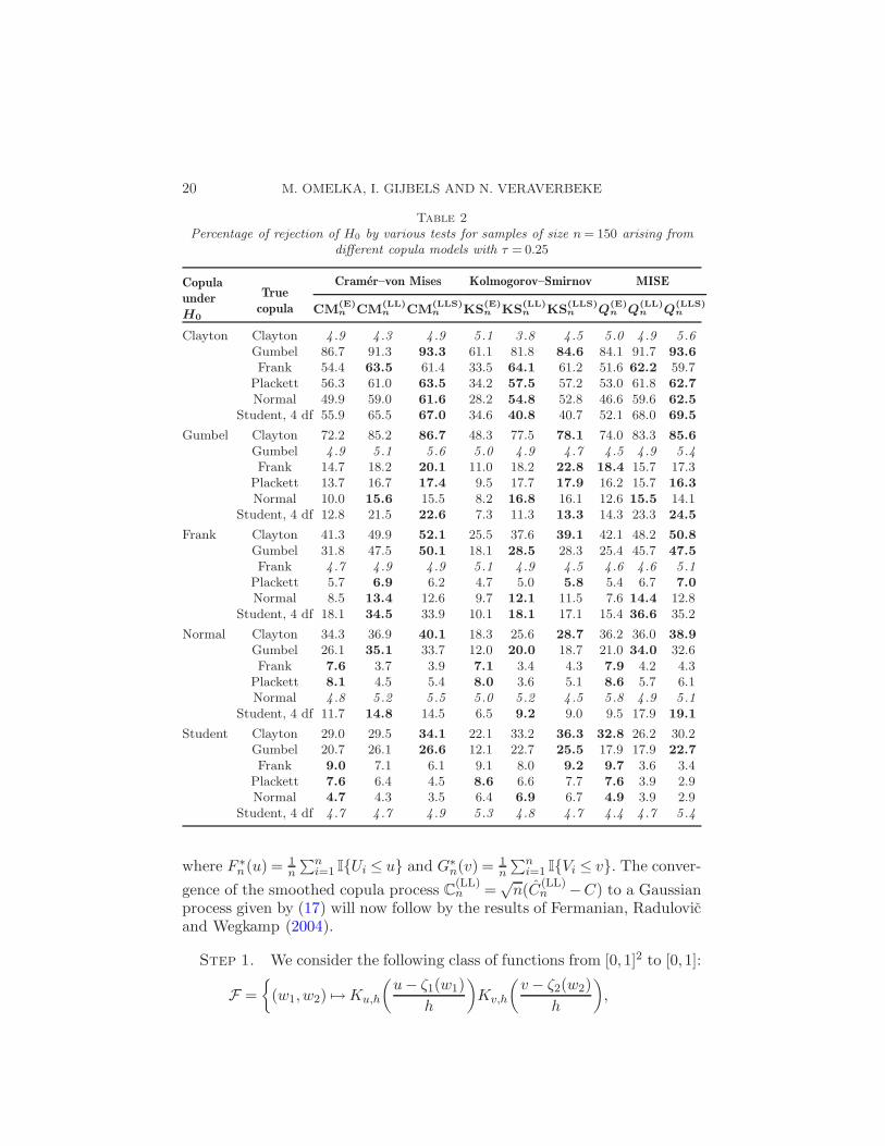
The results of the simulations are presented in Tables 2, 3 and 4. Forease of the reader, the estimated values for the size of the test statistics arepresented in italics. Furthermore, for each testing problem, we highlightedthe “best” power performances using bold characters. Readers should beaware of the fact that these estimated powers and sizes (using, resp., 1500and 6000 repetitions) are of course subject to Monte Carlo approximationerrors. A conservative upper bound (relying on a binomial distribution withparameters B and p) for these approximations errors (in terms of standarddeviation) is for the size estimates 0.28% (using B = 6000 and p = 0.05) andfor the power estimates 1.29% (using B = 1500 and p = 0.5, for getting toan upper bound).

A summary of conclusions from the simulations results is as follows:

• The use of a kernel estimator [e.g., C(LLS)n ] in goodness-of-fit testing seems

to be promising in case true copulas are in the Clayton, Gumbel and Frankfamilies, and we consistently improve upon the power for the Kolmogorov–Smirnov test;

• If a kernel estimator improves upon the power, it is most noticeable whenthe dependence is weaker, and is greatest for the Kolmogorov–Smirnovtest;

• The power of the test statistics Qn is usually somewhere between thepower of Kolmogorov–Smirnov and the Cramer–von Mises test statistics;

• The power of the test statistics based on the improved estimator C(LLS)n is

usually higher than this for test statistics based on C(LL)n for alternatives

with unbounded second order partial derivatives;• For a true Frank copula and a Cramer–von Mises test statistic, the esti-

mator C(LLS)n is usually the best choice;

• The use of kernel estimators seems to be promising for Archimedean fam-ilies of copulas (Clayton, Frank, Gumbel) but is somewhat questionablefor elliptical families of copulas (normal, Student). Although kernel esti-mators may improve the power against Clayton and Gumbel alternatives,a loss in power is noticed for Frank alternatives. This holds in particular

for C(LLS)n -based statistics.

APPENDIX A: PROOF OF THEOREM 1

For simplicity, we will suppress the dependence on n in the notation ofpseudo-observations (Ui, Vi)

T and write, simply, Ui = Fn(Xi) = Fn(F−1(Ui))


and Vi = Gn(Yi) = Gn(G−1(Vi)), where (Ui, Vi) have a joint distributionfunction given by the copula C.

As our proof is a straightforward adaptation of the ideas used in vander Vaart and Wellner (2007), we would like to clarify one point. In the

following, we will encounter the expectations of the form Eg(U , V ), where g

is a measurable function on [0,1]2 and U = Fn(F−1(U)), V = Gn(G−1(V )).In these types of expectations, the estimators of the marginal distributionfunctions Fn, Gn are considered to be fixed (nonrandom) functions, and theexpectation is taken only with respect to (U,V ) with joint distribution givenby the copula C. Formally,

Eg(U , V ) = EU,V [g(U , V )|(X1, Y1), . . . , (Xn, Yn)],

whenever the integral on the right-hand side exists.

A.1. Weak convergence of the process C(LL)n

. In view of the previousremark, we decompose

√n(C(LL)

n (u, v)−C(u, v))

=1√n

[

n∑

i=1

Ku,hn

(

u− Ui

hn

)

Kv,hn

(

v − Vi

hn

)

−C(u, v)

]

(23)

= Ahn

n (u, v) + Bn(u, v) + Chn

n (u, v),

where

Ahn

n (u, v) =1√n

[

n∑

i=1

Ku,hn

(

u− Ui

hn

)

Kv,hn

(

v − Vi

hn

)

− I{Ui ≤ u,Vi ≤ v}(24)

−E

(

Ku,hn

(

u− U

hn

)

Kv,hn

(

v − V

hn

)

−C(u, v)

)

]

and

Bn(u, v) =1√n

n∑

i=1

[I{Ui ≤ u,Vi ≤ v} −C(u, v)],(25)

Chn

n (u, v) =√

nE

[

Ku,hn

(

u− U

hn

)

Kv,hn

(

v − V

hn

)

−C(u, v)

]

.(26)

Our proof will be divided into two steps. First, we will show, in Step 1,that supu,v |Ahn

n |= op(1). Then, we will prove, in Step 2, that

supu,v

|Chn

n (u, v)− ∂1C(u, v)√

n[F ∗n(u)− u]− ∂2C(u, v)

√n[G∗

n(v)− v]|= oP (1),


Table 2Percentage of rejection of H0 by various tests for samples of size n = 150 arising from

different copula models with τ = 0.25

Copula

under

H0

True

copula

Cramer–von Mises Kolmogorov–Smirnov MISE

CM(E)n CM

(LL)n CM

(LLS)n KS

(E)n KS

(LL)n KS

(LLS)n Q

(E)n Q

(LL)n Q

(LLS)n

Clayton Clayton 4 .9 4 .3 4 .9 5 .1 3 .8 4 .5 5 .0 4 .9 5 .6Gumbel 86.7 91.3 93.3 61.1 81.8 84.6 84.1 91.7 93.6

Frank 54.4 63.5 61.4 33.5 64.1 61.2 51.6 62.2 59.7Plackett 56.3 61.0 63.5 34.2 57.5 57.2 53.0 61.8 62.7

Normal 49.9 59.0 61.6 28.2 54.8 52.8 46.6 59.6 62.5

Student, 4 df 55.9 65.5 67.0 34.6 40.8 40.7 52.1 68.0 69.5

Gumbel Clayton 72.2 85.2 86.7 48.3 77.5 78.1 74.0 83.3 85.6

Gumbel 4 .9 5 .1 5 .6 5 .0 4 .9 4 .7 4 .5 4 .9 5 .4Frank 14.7 18.2 20.1 11.0 18.2 22.8 18.4 15.7 17.3

Plackett 13.7 16.7 17.4 9.5 17.7 17.9 16.2 15.7 16.3

Normal 10.0 15.6 15.5 8.2 16.8 16.1 12.6 15.5 14.1Student, 4 df 12.8 21.5 22.6 7.3 11.3 13.3 14.3 23.3 24.5

Frank Clayton 41.3 49.9 52.1 25.5 37.6 39.1 42.1 48.2 50.8

Gumbel 31.8 47.5 50.1 18.1 28.5 28.3 25.4 45.7 47.5

Frank 4 .7 4 .9 4 .9 5 .1 4 .9 4 .5 4 .6 4 .6 5 .1Plackett 5.7 6.9 6.2 4.7 5.0 5.8 5.4 6.7 7.0

Normal 8.5 13.4 12.6 9.7 12.1 11.5 7.6 14.4 12.8Student, 4 df 18.1 34.5 33.9 10.1 18.1 17.1 15.4 36.6 35.2

Normal Clayton 34.3 36.9 40.1 18.3 25.6 28.7 36.2 36.0 38.9

Gumbel 26.1 35.1 33.7 12.0 20.0 18.7 21.0 34.0 32.6Frank 7.6 3.7 3.9 7.1 3.4 4.3 7.9 4.2 4.3

Plackett 8.1 4.5 5.4 8.0 3.6 5.1 8.6 5.7 6.1Normal 4 .8 5 .2 5 .5 5 .0 5 .2 4 .5 5 .8 4 .9 5 .1

Student, 4 df 11.7 14.8 14.5 6.5 9.2 9.0 9.5 17.9 19.1

Student Clayton 29.0 29.5 34.1 22.1 33.2 36.3 32.8 26.2 30.2Gumbel 20.7 26.1 26.6 12.1 22.7 25.5 17.9 17.9 22.7

Frank 9.0 7.1 6.1 9.1 8.0 9.2 9.7 3.6 3.4Plackett 7.6 6.4 4.5 8.6 6.6 7.7 7.6 3.9 2.9Normal 4.7 4.3 3.5 6.4 6.9 6.7 4.9 3.9 2.9

Student, 4 df 4 .7 4 .7 4 .9 5 .3 4 .8 4 .7 4 .4 4 .7 5 .4

where F ∗n(u) = 1

n

∑ni=1 I{Ui ≤ u} and G∗

n(v) = 1n

∑ni=1 I{Vi ≤ v}. The conver-

gence of the smoothed copula process C(LL)n =

√n(C

(LL)n −C) to a Gaussian

process given by (17) will now follow by the results of Fermanian, Radulovicand Wegkamp (2004).

Step 1. We consider the following class of functions from [0,1]2 to [0,1]:

F =

{

(w1,w2) 7→ Ku,h

(

u− ζ1(w1)

h

)

Kv,h

(

v − ζ2(w2)

h

)

,




Copula

under

H0

True

copula


CM(E)n CM

(LL)n CM

(LLS)n KS

(E)n KS

(LL)n KS

(LLS)n Q

(E)n Q

(LL)n Q

(LLS)n

Clayton Clayton 5 .3 5 .2 5 .4 5 .5 5 .3 5 .7 4 .8 5 .6 5 .8Gumbel 99.9 100.0 99.9 98.9 99.5 99.9 100.0 100.0 99.9Frank 95.9 96.4 96.2 82.5 98.3 95.6 91.1 93.3 92.3

Plackett 95.6 96.7 96.0 75.3 94.7 89.7 92.3 95.7 94.5Normal 94.4 96.3 96.9 75.0 91.9 91.1 89.9 94.5 94.9

Student, 4 df 94.9 96.7 97.2 77.9 86.4 88.2 92.7 96.2 96.3

Gumbel Clayton 99.6 99.7 99.7 94.3 98.7 98.8 98.9 99.3 99.1Gumbel 4 .5 4 .7 4.9 5 .0 4 .9 5 .4 4 .8 3 .9 4 .6Frank 40.5 48.2 39.7 29.6 48.1 40.4 41.1 35.3 30.6

Plackett 29.4 33.3 30.7 18.9 26.5 22.8 31.0 30.0 27.6Normal 18.8 26.4 25.1 14.6 25.3 23.8 22.3 22.1 21.8

Student, 4 df 22.3 27.8 29.2 11.7 19.1 16.5 23.6 28.5 29.0

Frank Clayton 89.6 88.9 91.9 68.1 72.7 75.5 85.1 86.3 85.5Gumbel 63.8 71.0 74.1 39.3 44.6 47.3 50.5 68.9 65.7Frank 5 .3 4 .9 5 .2 5 .1 5 .2 5 .0 5 .1 4 .9 5 .0

Plackett 8.4 10.4 12.1 5.4 6.9 6.7 8.3 15.2 8.5Normal 19.6 26.0 29.5 17.6 26.9 25.5 16.5 25.7 17.5

Student, 4 df 35.0 44.9 52.8 17.9 27.8 29.4 29.0 51.0 46.2

Normal Clayton 83.0 78.3 82.9 55.8 66.6 66.1 79.6 76.1 79.4Gumbel 41.7 39.5 44.3 18.3 22.7 26.6 32.4 39.6 41.2

Frank 21.2 20.1 14.9 15.1 11.8 11.0 19.3 14.4 10.5Plackett 12.0 7.4 7.8 7.7 5.8 4.5 13.4 11.9 9.9Normal 4 .8 5 .1 5 .5 4 .7 5 .0 5 .4 5 .8 4 .5 4 .6

Student, 4 df 8.1 6.4 8.3 4.0 4.5 4.8 7.6 11.5 12.5



Student, 4 df 4 .7 4 .9 5 .1 4 .9 5 .0 4 .9 5 .2 4 .1 4 .7

(27)

(u, v) ∈ [0,1]2, h ∈[

0,1

4

]

, ζ1, ζ2 : [0,1] → [0,1] nondecreasing

}

.

As each function f from F is characterized by a quintuple (u, v,h, ζ1, ζ2),the empirical process indexed by F can be written as

Zn(f) = Zn(u, v,h, ζ1, ζ2)




Copula

under

H0

True

copula


CM(E)n CM

(LL)n CM

(LLS)n KS

(E)n KS

(LL)n KS

(LLS)n Q

(E)n Q

(LL)n Q

(LLS)n

Clayton Clayton 5 .3 5 .6 5 .3 5 .1 4 .9 4 .6 3 .3 4 .6 4 .0Gumbel 100.0 100.0 100.0 99.9 100.0 100.0 100.0 100.0 100.0Frank 98.8 98.3 98.5 83.7 98.1 97.2 94.0 95.4 95.1

Plackett 99.5 99.2 99.9 85.1 90.6 93.9 97.0 98.3 99.1

Normal 99.8 99.5 99.9 90.5 93.6 96.8 98.0 98.4 99.2

Student, 4 df 99.9 99.7 100.0 92.7 91.4 97.7 98.5 99.5 99.5

Gumbel Clayton 99.9 99.5 99.9 95.8 98.5 98.5 99.6 99.1 99.0Gumbel 4 .5 4 .6 4 .8 4 .7 4 .6 4 .9 5 .0 3 .2 3 .7Frank 53.3 54.5 47.0 25.6 38.1 38.3 40.7 26.6 23.7

Plackett 24.3 23.5 19.1 6.6 9.3 9.3 29.5 24.9 25.1Normal 12.4 13.1 13.9 11.3 13.6 13.3 12.3 8.3 7.7

Student, 4 df 15.6 15.7 20.1 8.5 10.4 10.8 16.2 15.1 14.9

Frank Clayton 96.7 91.3 96.9 57.6 63.7 64.9 90.8 86.2 89.0Gumbel 81.6 80.5 87.8 36.9 41.7 39.7 61.1 73.7 75.3

Frank 4 .4 4 .6 4 .4 4 .7 4 .5 4 .8 4 .7 3 .0 3 .7Plackett 19.6 20.7 27.5 5.9 8.7 7.5 34.5 45.7 48.3

Normal 40.7 41.1 52.7 28.5 33.3 30.2 31.9 38.7 42.9

Student, 4 df 58.4 57.9 72.6 26.7 33.6 30.3 50.6 63.1 64.6

Normal Clayton 93.4 88.9 90.5 66.7 77.9 79.7 88.4 83.3 82.6Gumbel 41.1 38.3 43.4 13.0 19.6 20.9 24.3 33.5 35.0

Frank 46.1 46.7 37.7 17.5 18.2 22.9 31.0 24.1 18.4Plackett 15.2 11.6 9.2 3.1 3.1 4.0 24.4 27.7 23.7Normal 4 .7 4 .8 4 .4 4 .4 4 .6 4 .7 5 .2 3 .5 3 .5

Student, 4 df 6.9 6.3 6.8 4.7 3.9 4.2 7.0 10.1 9.6



Student, 4 df 4 .3 4 .9 4 .4 4 .7 5 .1 4 .9 4 .8 3 .6 3 .1

=1√n

n∑

i=1

Ku,h

(

u− ζ1(Ui)

h

)

Kv,h

(

v − ζ2(Vi)

h

)

.

Put Zn = Zn −EZn and note that

Ahn

n (u, v) = Zn(fn1 )− Zn(f2),

(28)where fn

1 = (u, v,hn, Fn(F−1),Gn(F−1)), f2 = (u, v,0, I, I)

with I being the identity function on the interval [0,1].


Lemma A.1, which is given below, states that the set of functions Fis Donsker. Indeed, F is a subset of F∗ in Lemma A.1, taking b(·) = 1and u0 = u and v0 = v. This implies the weak convergence of the processZn(f), f ∈ F , which further implies that the process Zn is asymptoticallyuniformly ρ-equicontinuous in probability [see pages 37–41 of van der Vaartand Wellner (1996)] with semimetric ρ given by

ρ(f, f ′) = E

[

Ku,h

(

u− ζ1(U)

h

)

Kv,h

(

v − ζ2(V )

h

)

−Ku′,h′

(

u′ − ζ ′1(U)

h′

)

Kv′,h′

(

v′ − ζ ′2(V )

h′

)]2

.

Using this asymptotic uniform ρ-equicontinuity and (28), we get thatsupu,v |Ahn

n |= op(1), provided that supu,v ρ(fn1 , f2) converges to zero in prob-

ability, where fn1 and f2 are given in (28) [for details consult the proof in

van der Vaart (1994)].Put M = supu,h,x |ku,h(x)|, where ku,h is defined in (7), and denote

Aε = {|U −U |> ε or |V − V |> ε}.The consistency of Fn and Gn yields that, for every ε > 0, for all sufficientlylarge n,

P[

max{

supx∈R

|Fn(x)− F (x)|, supy∈R

|Gn(y)−G(y)|}

> ε]

< ε,

which further implies that, for all sufficiently large n,

P (Aε) = P [max{|Fn(X)−F (X)|, |Gn(Y )−G(Y )|} > ε] < ε.(29)

Now, we can bound

ρ(fn1 , f2) = E

[

Ku,hn

(

u− U

hn

)

Kv,hn

(

v − V

hn

)

− I{U ≤ u,V ≤ v}]2

≤ E

[

Ku,h

(

u− U

h

)

Kv,h

(

v − V

h

)

− I{U ≤ u,V ≤ v}]2

IAcε+ IAε

≤ M4E[|I{U ≤ u− hn} − I{U ≤ u}|+ |I{U ≤ u + hn} − I{U ≤ u}|+ |I{V ≤ v − hn} − I{V ≤ v}|+ |I{V ≤ v + hn} − I{V ≤ v}|]IAc

ε+ IAε

≤ 4M4(ε + hn) + IAε.

As the above bound holds uniformly in (u, v) and by (29), for all sufficientlylarge n, we have P (Aε) < ε. Since ε can be arbitrarily small, this impliessupu,v ρ(fn

1 , f2) = op(1).


Lemma A.1. Suppose that the function k is of bounded variation and∫

k(x)dx = 1. Then, the set of functions from [0,1]2 to [0,1]

F∗ =

{

(w1,w2) 7→ Ku0,h

(

u− ζ1(w1)

b(u0)h

)

Kv0,h

(

v − ζ2(w2)

b(v0)h

)

,

(u0, v0), (u, v) ∈ [0,1]2,

h ∈[

0,1

4

]

, ζ1, ζ2 : [0,1] → [0,1] nondecreasing

}

,

where b(w) = 1 or b(w) = min{√w,√

1−w}, is Donsker.Consequently, the family F in (27) is Donsker.

Proof. Note that the class of functions

G1 = {(w1,w2) 7→ I{ζ1(w1)≤ a, ζ2(w2)≤ b},a, b ∈ R, ζ1, ζ2 : [0,1] → [0,1] nondecreasing}

is a subset of the class of indicators

G2 = {(w1,w2) 7→ I{w1 < (≤)a,w2 < (≤)b}, a, b ∈ R}.But this implies that G1 is a Donsker class [see Example 2.5.4 of van derVaart and Wellner (1996)].

As the set G1 is closed under translation, we know by the beginning ofthe proof of van der Vaart (1994) that the set of functions

H =

{∫

f(x + y)dµ(y), f ∈ G1, µ ∈MB

}

(30)

is a Donsker class, where MB is a family of all signed measures (on R2) of

total mass bounded by a fixed constant B.Let us introduce the set of signed measures

M0 =

{

(−∞,w1]× (−∞,w2] 7→ Ku0,h

(

w1

b(u0)h

)

Kv0,h

(

w2

b(v0)h

)

,

(u0, v0) ∈ [0,1]2, h ∈[

0,1

4

]}

.

If k is of bounded variation, then, by taking sufficiently large B, we ensurethat M0 ⊂MB . Further, if x stands for (w1,w2) and y for (y1, y2), then,for f ∈ G1 and µ ∈M0, we get

∫

f(x + y)dµ(y)

=

∫ ∫

I{ζ1(w1) + y1 ≤ u,


ζ2(w2) + y2 ≤ v}d

(

Ku0,h

(

y1

b(u0)h

)

Kv0,h

(

y2

b(v0)h

))

= Ku0,h

(

u− ζ1(w1)

b(u0)h

)

Kv0,h

(

v − ζ2(w2)

b(v0)h

)

,

which is a Donsker class. As F∗ includes F of (27) (consider u0 = u andv0 = v), the family F is a Donsker class as well. �

Step 2. Now, we can turn our attention to the process Chn

n given by(26). For (u, v) ∈ R

2, define

C∗F ,G

(u, v) = C(F (F−1(u∗)),G(G−1(v∗))),

where w∗ = max{min{w,1},0}. Note that

EI{U ≤ u, V ≤ v} = EI{U ≤ F (F−1n (u)), V ≤G(G−1

n (u))}+ O(n−1)

= C∗Fn,Gn

(u, v) + O(n−1),

where the remainder term O(n−1) disappears if we do some smoothing onthe first stage; that is, if b1n, b2n > 0. As

EKu,h

(

u− U

h

)

Kv,h

(

v − V

h

)

= E

∫ 1

−1

∫ 1

−1I{Ui ≤ u− thn, Vi ≤ u− shn}ku,h(s)kv,h(t)dt ds

=

∫ 1

−1

∫ 1

−1C∗

Fn,Gn

(u− thn, v − shn)ku,h(s)kv,h(t)dt ds + O(n−1),

it will be useful to have a closer look at the process {C∗Fn,Gn

(u, v) ∈ [0,1]2}.In the following, we will prove that, uniformly in (u, v),

√n(C∗

Fn,Gn

(u, v)−C(u, v))

=−Cu(u, v)1√n

n∑

i=1

[I{Ui ≤ u} − u](31)

−Cv(u, v)1√n

n∑

i=1

[I{Vi ≤ v} − v] + op(1).

Let D[a, b] be the Banach space of all cadlag functions on an interval [a, b]equipped with the uniform norm.

Lemma A.2. Let F be a continuous distribution function. Then, themap F 7→ F ◦ F−1 as a map D[0,1] 7→ ℓ∞[0,1] is Hadamard-differentiable atF = F tangentially to the set of functions

α ∈EF = {α(x) = β(F (x)), x ∈ R, β ∈ C[0,1], β(0) = β(1) = 0}.


The derivative is given by −α ◦ F−1.

Proof. Let αt converge uniformly to α ∈ EF . Put Ft = F + tαt. As

supu∈[0,1]

|Ft(F−1t (u))− u| = sup

u∈[0,1]|Ft(u+)−Ft(u−)|,

the function F is continuous and the function αt converges uniformly to abounded and continuous function, we get that Ft(F

−1t (u)) − u = o(t) uni-

formly in u.Thus, we can calculate

1

t[F (F−1

t )(u)− F (F−1(u)) + tα(F−1(u))]

= α(F−1(u))−αt(F−1t (u)) + o(1)

= [α(F−1(u))−α(F−1t (u))] + [α(F−1

t (u))− αt(F−1t (u))] + o(1).

As αt → α uniformly, the second term converges to zero uniformly in u. Byusing the representation α(x) = β(F (x)), we see that, to ensure a uniformconvergence of the first term to zero, we need to show that F (F−1

t (u)) → uuniformly. But this follows by a simple calculation, which yields

|F (F−1t (u))−F (F−1(u))|= |tαt(F

−1t (u))|+ o(t)

≤ |t||αt(F−1t (u))− α(F−1

t (u))|+ |t||α(F−1t (u))|+ o(t) = O(t),

uniformly in u. �

Remark. As (16) implies that√

n(Fn − F ) converges in distributionto a Gaussian process B ◦ F , where B is a standard Brownian motion onthe interval [0,1], the Hadamard-differentiability tangentially to EF givenin Lemma A.2 is exactly what is needed to derive asymptotic distributionof the process

√n(F (F−1

n (u))− u).

Similarly, we can prove that the mapping G 7→ G ◦ G−1 is Hadamard-differentiable at G = G tangentially to the set of functions

EG = {α(x) = β(G(x)), x ∈ R, β ∈ C[0,1], β(0) = β(1) = 0}.The proof of the following lemma follows easily by applying Lemma A.2

and the chain rule.

Lemma A.3. Let the copula C have continuous partial derivatives on[a, b]× [c, d] ⊂ [0,1]2, and F,G are continuous; then, the map (F , G) 7→ C∗

F ,G

as a map D[a, b]× D[a, b] 7→ ℓ∞([a, b] × [c, d]) is Hadamard-differentiable at


the point (F , G) = (F,G) tangentially to the set of functions (α1, α2) ∈EF ×EG. The derivative is given by

φ′(α1, α2) =−Cu ◦ α1 ◦ F−1 −Cv ◦ α2 ◦G−1 = −Cu ◦ β1 −Cv ◦ β2,(32)

where β1 = α1 ◦ F−1 and β2 = α2 ◦G−1.

Lemma A.3, together with Theorem 3.9.4 of van der Vaart and Wellner(1996), imply that representation (31) holds uniformly for (u, v) ∈ [a, b] ×[c, d]. Unfortunately, many of the most popular families (e.g., Clayton, Gum-bel, normal) do not have continuous Cu and Cv at some of the points{(0,0), (0,1), (1,0), (1,1)}. The following lemma takes care of this situation.

Lemma A.4. Let the distribution H have continuous margins F,G and acopula function whose first derivatives are continuous on [0,1]2 \{(0,0), (0,1),(1,0), (1,1)}. Then, representation (31) holds uniformly in (u, v) ∈ [0,1]2.

Proof. Suppose, for simplicity, that the point of discontinuity is onlyat (0,0) [other points (0,1), (1,0), (1,1) might be handled in a similar way].Let us denote

Zn(u, v) =√

n(C∗Fn,Gn

(u, v)−C(u, v))

+ Cu(u, v)1√n

n∑

i=1

[I{Ui ≤ u} − u](33)

+ Cv(u, v)1√n

n∑

i=1

[I{Vi ≤ v} − v].

Let ε > 0 be given. As all the process

X1n(u) =

√n[F (F−1

n (u))− u], X3n(u) =

1√n

n∑

i=1

[I{Ui ≤ u} − u],

X2n(u) =

√n[G(G−1

n (u))− u], X4n(u) =

1√n

n∑

i=1

[I{Vi ≤ u} − u]

converge to a Brownian motion, we can find δε and nε such that, for alln > nε,

P

(

supu≤δε

|Xjn(u)| ≥ ε

4

)

<ε

4, j = 1, . . . ,4.

As Cu,Cv are bounded by 1, the triangular inequality implies that, for alln > nε,

P(

supu,v≤δε

|Zn(u, v)| ≥ ε)

≤4

∑

j=1

P

(

supu≤δε

|Xjn(u)| ≥ ε

4

)

< ε.


Next, the existence of n′ε such that, for all n > n′

ε,

P(

supu,v∈Aε

|Zn(u, v)| ≥ ε)

< ε with Aε = [0,1]2 \ [0, δε]2,

follows by Lemma A.3 applied to rectangles [0, δε]× [δε,1] and [δε,1]× [0,1].Thus, for n > max{nε, n

′ε} :P (supu,v |Zn(u, v)| ≥ ε) < ε, which proves the

lemma. �

Combining (31), Lemma A.4, the fact that hn → 0 and asymptotic equicon-tinuity of the processes Un(u) = 1√

n

∑ni=1[I{Ui ≤ u} − u], Vn(v) =

1√n

∑ni=1[I{Vi ≤ v} − v] yields

Chn

n (u, v) =√

nE

[

Ku,hn

(

u− U

hn

)

Kv,hn

(

v − V

hn

)

−C(u, v)

]

(34)= −Cu(u, v)Un(u)−Cv(u, v)Vn(v) +

√nDn(u, v) + oP (1),

where the bias term Dn is given by

Dn(u, v) =

∫ 1

−1

∫ 1

−1

√n[C(u− thn, v − shn)−C(u, v)]

(35)× ku,h(s)kv,h(t)dt ds.

If copula C has bounded second order partial derivatives on [0,1]2, then

√n sup

u,v|Dn(u, v)| = O(n1/2h2

n) = o(1).(36)

Finally, combining (23), (25), (26), (34) and (36) yields

√n(C(LL)

n (u, v)−C(u, v))

=1√n

n∑

i=1

[I{Ui ≤ u,Vi ≤ v} −C(u, v)]

(37)

−Cu(u, v)1√n

n∑

i=1

[I{Ui ≤ u} − u]

−Cv(u, v)1√n

n∑

i=1

[I{Vi ≤ v} − v] + oP (1).

A.2. Weak convergence of the process C(MR)n

. Here, we adapt the fore-

going proof for the mirrored-type kernel estimator C(MR)n given in (13).


Step 1. At first, we rewrite

C(MR)n =

9∑

ℓ=1

[Zn(ℓ, u, v)−Zn(ℓ, u,0)−Zn(ℓ,0, v) + Zn(ℓ,0,0)],(38)

where

Zn(ℓ, u, v) =1

n

n∑

i=1

K

(

u− U(ℓ)i

hn

)

K

(

v − V(ℓ)i

hn

)

.

Let us define

Z0n(ℓ, u, v) =1

n

n∑

i=1

I{U (ℓ)i ≤ u,V

(ℓ)i ≤ v}.

Similarly as in Step 1 of the proof of Appendix A.1 [weak convergence of

C(LL)n ], we can show that, for each ℓ = 1, . . . ,9,

supu,v

|√

n(Zn(ℓ, u, v)−EZn(ℓ, u, v))

(39)−√

n(Z0n(ℓ, u, v)−EZ0n(ℓ, u, v))|= op(1).

Further, note that

9∑

ℓ=1

Z0n(ℓ, u, v) =1

n

n∑

i=1

I{Ui ≤ u,Vi ≤ v}+ F ∗n(u) + G∗

n(v) + 1.(40)

Combining (38), (39) and (40), implies that, uniformly in (u, v),√

n(C(MR)n (u, v)−C(u, v)) = Bn(u, v) + Chn

n (u, v) + op(1),

where Bn is given by (25) and

Chn

n (u, v) =√

n

{

9∑

ℓ=1

E

[

K

(

u− U (ℓ)

hn

)

−K

(−U (ℓ)

hn

)]

×[

K

(

v − V (ℓ)

hn

)

−K

(−V (ℓ)

hn

)]

−C(u, v)

}

.

Step 2. Now, similarly as in Step 2 of the proof in Appendix A.1, wederive that, uniformly in (u, v),

Chn

n (u, v) =−Cu(u, v)Un(u)−Cv(u, v)Vn(v) +√

nDn(u, v) + oP (1),(41)

with the bias term Dn(u, v) given by

Dn(u, v) =9

∑

ℓ=1

E

[

K

(

u−U(ℓ)1

hn

)

−K

(−U(ℓ)1

hn

)]

(42)

×[

K

(

v − V(ℓ)1

hn

)

−K

(−V(ℓ)1

hn

)]

−C(u, v).


To show that this bias term is uniformly O(h2n) is straightforward but te-

dious. The most simple case is if (u, v) ∈ [hn,1−hn]2. Then, (42) boils downto

Dn(u, v) = EK

(

u−U1

hn

)

K

(

v − V1

hn

)

−C(u, v)

=

∫ 1

−1

∫ 1

−1C(u− thn, v − shn)k(t)k(s)dt ds−C(u, v)

and the assertion follows simply by Taylor expansion.Regarding the remaining cases, we will be dealing explicitly only with

(u, v) ∈ [1− hn,1]2. The other cases may be handled in a similar way.Note that Taylor expansion together with the assumptions of the theorem

imply C(u, v) = u+v−1+O(h2n) uniformly in (u, v) ∈ [1−2hn,1]2. Further,

routine algebra shows that (42) simplifies to

Dn(u, v) = EK

(

u−U1

hn

)

K

(

v − V1

hn

)

+ EK

(

u + U1 − 2

hn

)

K

(

v − V1

hn

)

(43)

+ EK

(

u−U1

hn

)

K

(

v + V1 − 2

hn

)

+ EK

(

u + U1 − 2

hn

)

K

(

v + V1 − 2

hn

)

−C(u, v).

Let us compute

EK

(

u−U1

hn

)

K

(

v − V1

hn

)

=

∫ 1

(u−1)/hn

∫ 1

(v−1)/hn

C(u− thn, v − shn)k(t)k(s)dt ds

+

∫ 1

(u−1)/hn

∫ (v−1)/hn

−1(u− thn)k(t)k(s)dt ds

+

∫ (u−1)/hn

−1

∫ 1

(v−1)/hn

(v − shn)k(t)k(s)dt ds(44)

+

∫ (u−1)/hn

−1

∫ (v−1)/hn

−11k(t)k(s)dt ds

=

∫ 1

(u−1)/hn

∫ 1

(v−1)/hn

(u− thn + v − shn − 1)k(t)k(s)dt ds

+

∫ 1

(u−1)/hn

(u− thn)k(t)dtK

(

u− 1

hn

)


+

∫ 1

(v−1)/hn

(v − shn)k(s)dsK

(

v − 1

hn

)

+ K

(

u− 1

hn

)

K

(

v − 1

hn

)

+ O(h2n)

= · · ·

= (u + v − 1) + K

(

u− 1

hn

)

(1− u) + K

(

v − 1

hn

)

(1− v)

− hn

∫ 1

(u−1)/hn

tk(t)dt− hn

∫ 1

(v−1)/hn

tk(t)dt + O(h2n).

Similarly,

EK

(

u + U1 − 2

hn

)

K

(

v − V1

hn

)

=

∫ (u−1)/hn

−1

∫ 1

(v−1)/hn

P (U1 > 2 + thn − u,

V1 ≤ v − shn)k(t)k(s)dt ds(45)

+

∫ (u−1)/hn

−1

∫ (v−1)/hn

−1(1− 2− thn + u)k(t)k(s)dt ds

= · · ·= (u− 1)K

(

u− 1

hn

)

− hn

∫ (u−1)/hn

−1tk(t)dt + O(h2

n),

EK

(

v + V1 − 2

hn

)

K

(

u−U1

hn

)

(46)

= (v − 1)K

(

v − 1

hn

)

− hn

∫ (v−1)/hn

−1tk(t)dt + O(h2

n),

EK

(

u + U1 − 2

hn

)

K

(

v + V1 − 2

hn

)

(47)= O(h2

n).

Combining (43) with (44), (45), (46) and (47) gives us

Dn(u, v) = u + v − 1 + O(h2n)−C(u, v) = O(h2

n),

which was to be proved.

APPENDIX B: PROOF OF THEOREM 2

B.1. Weak convergence of the processes C(LLS)n

and C(MRS)n

. The proofof Theorem 2 for these estimators goes completely along the lines of the proofof Theorem 1, apart from a small difference in Step 2.


This difference is in calculating the bias term Dn given by (35) for C(LL)n

and by (42) for C(MR)n . The shrinking of the bandwidths by the function

b(w) = min{√w,√

1−w}, together with condition (9), guarantees that theTaylor expansion

C(u− shnb(u), v − thnb(v))

= C(u, v)− shnb(u)Cu(u, v)− thnb(v)Cv(u, v) + O(h2n)

holds uniformly in (u, v) ∈ [0,1]2 and (s, t) ∈ [−1,1]2. Applying the aboveexpansion in the bias calculations completes the proof.

B.2. Weak convergence of the process C(T)n

. The proof is completely

analogous to (and simpler than) the proof of Theorem 1 for C(LL)n . The only

difference is in calculating the bias Dn, which is for the estimator C(T)n given

by

Dn(u, v) =

∫ 1

−1

∫ 1

−1C(Φ(Φ−1(u)− shn),Φ(Φ−1(v)− thn))k(s)k(t)dsdt.

As all the second order partial derivatives of C(Φ(Φ−1(u)−shn),Φ(Φ−1(v)−thn)) taken as a function of (s, t) are bounded by the assumptions of thetheorem, Taylor expansion gives us Dn(u, v) = O(h2

n) uniformly in (u, v)which proves the statement.

APPENDIX C: JUSTIFICATION OF BOOTSTRAP TESTS BASED ONC

(LL)N

Denote the process underlying the goodness-of-fit statistics as Gn =√

n×(C

(LL)n −Cθn

) and G∗n =

√n(C

(LL)∗n − Cθ∗n

) for its bootstrap version. In the

following lemma, we will suppose that the true copula C belongs to a knownparametric family of copulas C0 = {Cθ, θ ∈Θ}.

Lemma C.1. Assume that the parametric family of copulas C0 satisfiesthe assumptions of Theorem 1 of Genest and Remillard (2008) and, more-over, the derivative of the true copula Cθ0 with respect to θ is continuous asa function of (u, v) in [0,1]2. Then, there exists a “nonstochastic” sequenceof functions an from [0,1]2 to [0,1], such that (Gn − an,G∗

n − an) convergesin distribution to two independent copies of the same process.

Proof. From the proof of Theorem 1 of this paper, it follows that

√nC(LL)

n =√

nC(E)n +

√nDθ0

n + op(1),


where

Dθn(u, v) =

∫ 1

−1

∫ 1

−1[Cθ(u− thn, v − shn)−Cθ(u, v)]ku,h(s)kv,h(t)dt ds.

(48)Thus, the processes Gn and G∗

n might be rewritten as

Gn =√

n(C(E)n −Cθn

) +√

nDθ0n + op(1),(49)

G∗n =

√n(C(E)∗

n −Cθ∗n) +

√nDθn

n + op(1).(50)

As the empirical copula process√

n(C(E)n −Cθ0) converges weakly, Theorem

1 of Genest and Remillard (2008) implies that the first terms on the right-hand sides of (49) and (50) converge jointly in distribution to independentcopies of the same process. Thus, defining an(u, v) as

√nDθ0

n (u, v), it remainsto show that

supu,v

|Dθ0n (u, v)−Dθn

n (u, v)| = op

(

1√n

)

.

But this follows directly from (48), the first order Taylor expansion of Cθn

around the true value of the parameter θ0 and the assumptions of the lemma.�

APPENDIX D: VERIFICATION OF (9) FOR SOME FAMILIES OFCOPULAS

We will verify assumption (9) only for Cuu. The assumptions about Cuv ,Cvv may be checked analogously.

Clayton and Gumbel copulas. Clayton and Gumbel copulas belong toan Archimedean family of copulas given by

C(u, v) = φ−1(φ(u) + φ(v)),(51)

where the function φ is called a generator of the copula. The generator ofa Clayton copula is given by φ(t) = 1

θ (t−θ − 1) with θ ≥ 0 and that of a

Gumbel copula by φ(t) = (− log t)θ with θ ≥ 1.Direct differentiaton of (51) yields

Cu(u, v) =φ′(u)

φ′(C(u, v)),

(52)

Cuu(u, v) =φ′′(u)

φ′(C(u, v))− [φ′(u)]2φ′′(C(u, v))

[φ′(C(u, v))]3.


For a Clayton and a Gumbel copula, it is easy to verify that φ′′(u)φ′(u) = O( 1

u(1−u)).

Hence, we can bound the first term on the right-hand side of the expressionfor Cuu(u, v) in (52) uniformly in v by

∣

∣

∣

∣

φ′′(u)

φ′(C(u, v))

∣

∣

∣

∣

≤∣

∣

∣

∣

φ′′(u)

φ′(u)

∣

∣

∣

∣

∣

∣

∣

∣

φ′(u)

φ′(C(u, v))

∣

∣

∣

∣

≤∣

∣

∣

∣

φ′′(u)

φ′(u)

∣

∣

∣

∣

|Cu(u, v)|(53)

= O

(

1

u(1− u)

)

.

The second term on the right-hand side of the expression for Cuu(u, v) in(52) is a more delicate one. For a Clayton copula, we have φ′(t) = −t−θ−1

and φ′′(t) = (θ + 1)t−θ−2, which implies∣

∣

∣

∣

[φ′(u)]2φ′′(C(u, v))

[φ′(C(u, v))]3

∣

∣

∣

∣

=

∣

∣

∣

∣

(θ + 1)[C(u, v)]3θ+3

u2θ+2[C(u, v)]θ+2

∣

∣

∣

∣

=

∣

∣

∣

∣

(θ + 1)[C(u, v)]2θ+1

u2θ+2

∣

∣

∣

∣

(54)

≤ θ + 1

u= O

(

1

u

)

,

using the Frechet–Hoeffding upper bound for a copula [see Nelsen (2006)].Combining (53) and (54) verifies (9) for Cuu of a Clayton copula.

For a Gumbel copula we have

φ′(u) = θ(− logu)θ−1(−1

u

)

,

φ′′(u) = θ(θ − 1)(− logu)θ−2(

1

u2

)

+ θ(− logu)θ−1(

1

u2

)

,

which implies

[φ′(u)]2φ′′(C(u, v))

[φ′(C(u, v))]3

=

(

θ2(− logu)2θ−2[

θ(θ − 1)(− logC(u, v))θ−2 1

[C(u, v)]2

+ θ(− logC(u, v))θ−1 1

[C(u, v)]2

])

(55)

×(

u2[

θ(− logC(u, v))θ−1 −1

C(u, v)

]3)−1

=−(− logu)2θ−2C(u, v)

u2

× [(θ − 1)(− logC(u, v))1−2θ + (− logC(u, v))2−2θ ].


When u → 0+, the key fact is that

C(u, v)

u2

(− logu)2θ−2

(− logC(u, v))2θ−2≤ u

u2

(− logu)2θ−2

(− logu)2θ−2=

1

u,(56)

and, when u → 1−,

(− logu)2θ−2

(− logC(u, v))2θ−1≤ (− logu)2θ−2

(− logu)2θ−1=

1

− logu= O

(

1

1− u

)

.(57)

Combining (53), (55), (56) and (56) verifies (9) for Cuu of a Gumbel copula.

Normal copula. The normal copula is given by

C(u, v) =

∫ Φ−1(u)

−∞

∫ Φ−1(v)

−∞

1

2π√

1− ρ2exp

{

s2 − 2ρst + t2

2(1− ρ2)

}

dsdt,

ρ ∈ (−1,1),

where Φ is the cumulative distribution function of a standard normal vari-able.

By a direct computation (or with the help of properties of a conditionalnormal distribution), we get

Cu(u, v) = Φ

(

Φ−1(v)− ρΦ−1(u)√

1− ρ2

)

,

whose derivative with respect to u is given by

Cuu(u, v) =−ρ

√

1− ρ2φ

(

Φ−1(v)− ρΦ−1(u)√

1− ρ2

)

1

φ(Φ−1(u)),(58)

where φ = Φ′. As φ is bounded, it is sufficient to deal with [φ(Φ−1(u))]−1.L’Hopital’s rule yields

u(1− u)

φ(Φ−1(u))∼ 1− 2u

Φ−1(u)= o(1), for u → 0+ (u → 1−),

which, together with (58), verifies (9) for Cuu of a normal copula.

Student copula. The Student copula (with m degrees of freedom) is givenby

C(u, v) =

∫ t−1m (u)

−∞

∫ t−1m (v)

−∞

1

2π√

1− ρ2

(

1 +s2 − 2ρst + t2

m(1− ρ2)

)−(m+2)/2

dsdt,

ρ ∈ (−1,1),

where t−1m (·) is the quantile function of the Student distribution with m

degrees of freedom.


Direct calculation shows that

Cu(u, v) =d(m+2)/2

fm(t−1m (u))

1

(c + d)(m+1)/2

(59)

×∫ (t−1

m (v)−ρt−1m (u))/

√d+c

−∞(1 + x2)−(m+2)/2 dx,

where c = [t−1m (u)]2, d = m(1 − ρ2) and fm is the density of the Student

distribution with m degrees of freedom. Assumption (9) for Cuu of a Studentcopula can be verified by differentiating (59) with respect to u. The usefulfacts (which follow by l’Hopital’s rule or properties of the density fm) are

t−1m (u)

u∼ 1

fm(t−1m (u))

,

f ′m(t−1

m (u))

fm(t−1m (u))

= O

(

1

t−1m (u)

)

for u → 0+ (u → 1−),

where f ′m is the derivative of fm.

Acknowledgments. The authors are grateful to the co-Editor, an Associate-Editor and two reviewers for their very helpful comments, which led to aconsiderable improvement of the original version of the paper.

REFERENCES

Chen, S. X. and Huang, T.-M. (2007). Nonparametric estimation of copula functionsfor dependence modelling. Canad. J. Statist. 35 265–282. MR2393609

Davison, A. C. and Hinkley, D. V. (1997). Bootstrap Methods and Their Application.Cambridge Univ. Press, New York. MR1478673

Deheuvels, P. (1979). La fonction de dependance empirique et ses proprietes. Acad. Roy.Belg. Bull. Cl. Sci. 65 274–292. MR0573609

Epanechnikov, V. (1969). Nonparametric estimation of a multidimensional probabilitydensity. Theory Probab. Appl. 14 153–158. MR0250422

Fan, J. and Gijbels, I. (1996). Local Polynomial Modelling and Its Applications. Chap-man & Hall, London. MR1383587

Fermanian, J.-D., Radulovic, D. and Wegkamp, M. (2004). Weak convergence ofempirical copula processes. Bernoulli 10 847–860. MR2093613

Ganssler, P. and Stute, W. (1987). Seminar on Empirical Processes. Birkhauser, Basel.MR0902803

Genest, C., Ghoudi, K. and Rivest, L.-P. (1995). A semiparametric estimation proce-dure of dependence parameters in multivariate families of distributions. Biometrika 82

543–552. MR1366280Genest, C. and Remillard, B. (2008). Validity of the parametric bootstrap for goodness-

of-fit testing in semiparametric models. Ann. Inst. H. Poincare Probab. Statist. 44

1096–1127. MR2469337Genest, C., Remillard, B. and Beaudoin, D. (2009). Goodness-of-fit tests for copu-

las: A review and a power study. Insurance: Mathematics and Economics. To appear.Available at DOI: 10.1016/j.insmatheco.2007.10.005.

http://www.ams.org/mathscinet-getitem?mr=2393609









http://dx.doi.org/10.1016/j.insmatheco.2007.10.005


Gijbels, I. and Mielniczuk, J. (1990). Estimating the density of a copula function.Comm. Statist. Theory Methods 19 445–464. MR1067582

Jin, Z. and Shao, Y. (1999). On kernel estimation of a multivariate distribution function.Statist. Probab. Lett. 41 163–168. MR1665267

Nelsen, R. B. (2006). An Introduction to Copulas, 2nd ed. Springer, New York.MR2197664

R Development Core Team (2007). R: A Language and Environment for StatisticalComputing. R Foundation for Statistical Computing, Vienna, Austria.

Tsukuhara, H. (2005). Semiparametric estimation in copula models. Canad. J. Statist.33 357–375. MR2193980

van der Vaart, A. W. (1994). Weak convergence of smoothed empirical processes. Scand.J. Statist. 21 501–504. MR1310093

van der Vaart, A. W. and Wellner, J. A. (1996). Weak Convergence and EmpiricalProcesses. Springer, New York. MR1385671

van der Vaart, A. W. and Wellner, J. A. (2007). Empirical processes indexed byestimated functions. In Asymptotics: Particles, Processes and Inverse Problems. IMSLecture Notes Monograph Series 55 234–252. Inst. Math. Statist., Beachwood, OH.MR2459942

Wand, M. and Jones, M. (1995). Kernel Smoothing. Chapman & Hall, London.MR1319818

Yan, J. (2007). Enjoy the joy of copulas: With a package copula. J. Statist. Software 21

1–21.

M. OmelkaJaroslav Hajek Center for Theoretical

and Applied StatisticsCharles University PragueSokolovska 83, 186 75 Praha 8Czech RepublicE-mail: [email protected]

I. GijbelsDepartment of Mathematics

and Leuven StatisticsResearch Center (LStat)

Katholieke Universiteit LeuvenCelestijnenlaan 200BB-3001 Leuven (Heverlee)BelgiumE-mail: [email protected]

N. VeraverbekeCenter for StatisticsHasselt UniversityAgoralaan—building DB-3590 DiepenbeekBelgiumE-mail: [email protected]









mailto:[email protected]

