Impact of UK Low Carbon Energy Scenarios on Transmission Network Protection Policies

2019

Melake Kuflom

A thesis submitted to The University of Manchester for the degree of

Doctor of Philosophy

in the Faculty of Science and Engineering

School of Electrical and Electronic Engineering

2

Table of Contents

Table of Contents ......................................................................................................................................... 2

List of Figures ................................................................................................................................................. 6

List of Tables ................................................................................................................................................... 9

List of Abbreviations .................................................................................................................................. 10

Abstract ........................................................................................................................................................... 12

Declaration ..................................................................................................................................................... 13

Copyright Statement.................................................................................................................................. 14

Acknowledgment ......................................................................................................................................... 15

Chapter 1: Introduction............................................................................................................................. 16

1.1 Power System Protection and Control ................................................................... 16

1.1.1 Electrical power system fault types and causes ........................................................... 18

1.1.2 Development of protective relay technology ................................................................. 20

1.1.3 Role of protection and zone of protection ..................................................................... 23

1.1.4 Overview of GB transmission line protection system .................................................... 23

1.1.5 Impact of fault level reduction on protection schemes .................................................. 25

1.2 Project Aims & Objectives ..................................................................................... 25

1.3 Structure of the Thesis .......................................................................................... 27

Chapter 2: Review into fault level and protection system studies ....................................... 28

2.1. Motivation of fault level analysis ........................................................................... 28

2.2. Short circuit current analysis ................................................................................. 28

2.3. Review on relay scheme selection issues caused by inverter based sources ....... 35

2.4. Short circuit analysis from synchronous generator & inverter based sources ........ 36

2.5. Review on protection challenges in converter dominated power system ............... 44

2.6. Protection challenges with respect to the declining fault levels in the UK .............. 45

2.6.1 Fault level analysis for protection setting requirements ................................................ 51

2.6.2 Protection policy on performing short circuit levels ....................................................... 54

2.7. Physical relay injection and simulation test methods ............................................. 55

2.8. Summary .............................................................................................................. 59

3

Chapter 3: Sensitivity Analysis of Distance Protection Schemes ........................................ 60

3.1. Concept of distance protection scheme ................................................................ 60

1.1.1 Distance relay and zone setting calculations ................................................................ 60

1.1.2 Distance protection with signalling channels ................................................................ 62

3.2 Distance relay protection....................................................................................... 66

3.3 Fault types and calculations .................................................................................. 67

3.4 Relationship between relay voltage and source impedance ratio (SIR) ................. 72

3.5 Effect of remote fault in-feed current on distance zone setting .............................. 74

3.6 Effect of parallel line outage on distance protection and setting implications ......... 76

3.7 Three ended feeder protection (Teed feeder) and setting considerations .............. 77

3.8 Performance assessment on distance protection of transmission line ................... 80

3.9 The influence of resistive faults on reach setting of distance protection ................ 83

3.10 The effect of mutual coupling on the ground distance reach setting ...................... 85

3.11 Summary .............................................................................................................. 88

Chapter 4: Sensitivity Analysis of Differential Protection Schemes .................................... 89

4.1 Concept of line current differential protection ........................................................ 89

4.1.1 Mode of operation, selectivity, and application of current differential protection .......... 89

4.1.2 Basic principles of feeder line differential protection ..................................................... 90

4.1.3 Operating characteristics of differential feeder protection............................................. 91

4.1.4 Performance assessment on line current differential protection ................................... 94

4.2 Current Transformer (CT) ..................................................................................... 98

4.2.1 Dimensioning of CTs ................................................................................................... 101

4.3 Protection signalling and intertripping.................................................................. 104

4.4 Busbar protection ................................................................................................ 106

4.5 Feeder transformer protection ............................................................................. 108

4.5.1 Setting of transformer biased differential protection ................................................... 110

4.6 Generator protection ........................................................................................... 110

4.7 Summary ............................................................................................................ 112

Chapter 5: Sensitivity Analysis of Overcurrent Protection ................................................... 113

5.1 Review on sensitivity analysis of overcurrent protection ...................................... 113

5.2 Grading of overcurrent relays .............................................................................. 117

4

5.3 The role of backup overcurrent protection applied in National Grid ..................... 119

5.3.1 Backup overcurrent protection for outgoing feeders ................................................... 121

5.3.2 Backup earth fault (IDMT) protection for outgoing feeders ......................................... 125

5.4 Summary ............................................................................................................ 130

Chapter 6: Role of Backup Protection under Low Fault Level ........................................... 131

6.1 Role of back-up protection .................................................................................. 131

6.2 Limitation of current differential protection under low fault level .......................... 132

6.2.1 Feeder protection ........................................................................................................ 132

6.3 Limitation of distance protection under low fault level .......................................... 140

6.3.1 The Great Britain electricity transmission system protection ...................................... 140

6.4 Limitation of backup overcurrent protection under low fault level ......................... 158

6.4.1 Feeder backup overcurrent protection ........................................................................ 158

6.4.2 Feeder backup earth IDMT fault protection ................................................................ 163

6.5 Summary ............................................................................................................ 168

Chapter 7: Impact of low fault level & alternative protection strategy ............................. 169

7.1 Review into the impact of low fault levels on feeder protection ............................ 169

7.1.1 Unit differential protection ........................................................................................... 169

7.1.2 Non-unit distance protection ....................................................................................... 170

7.1.3 Backup overcurrent protection .................................................................................... 172

7.1.4 Backup earth fault (IDMT) protection .......................................................................... 174

7.2 Application of protection schemes under low fault levels ..................................... 175

7.2.1 Unit protection ............................................................................................................. 175

7.2.2 Non-unit distance protection ....................................................................................... 176

7.2.3 Backup overcurrent protection .................................................................................... 177

7.2.4 Backup earth fault protection ...................................................................................... 177

7.3 Implications for future protection strategy under low fault level............................ 177

7.3.1 Identifying alternative protection methodologies and their suitability for transmission

systems under the various future scenarios ............................................................................... 177

7.4 The impact of new technology on fault clearing times ......................................... 179

7.5 Summary ............................................................................................................ 180

Chapter 8: The Role & Impact of IEC 61850 protocols for Future Protection

Development .............................................................................................................................................. 181

8.1 Motivation of IEC 61850 Protection Development ............................................... 181

5

8.2 Implementation of IEC61850 IEDs ...................................................................... 181

8.2.1 Sampling values configuration (SV) ............................................................................ 182

8.2.2 Goose Message Configuration .................................................................................... 184

8.3 Implementation of IEC 61850 Process Bus Architecture for secondary system ... 185

8.3.1 The role of Merging Unit in digital substations ............................................................ 186

8.4 Summary ............................................................................................................ 187

Chapter 9: Conclusion and Future work ....................................................................................... 189

References .................................................................................................................................................. 191

List of Publication ..................................................................................................................................... 196

Appendix: 1 ................................................................................................................................................. 197

Appendix: 2 ................................................................................................................................................. 198

Word count: 53,317

6

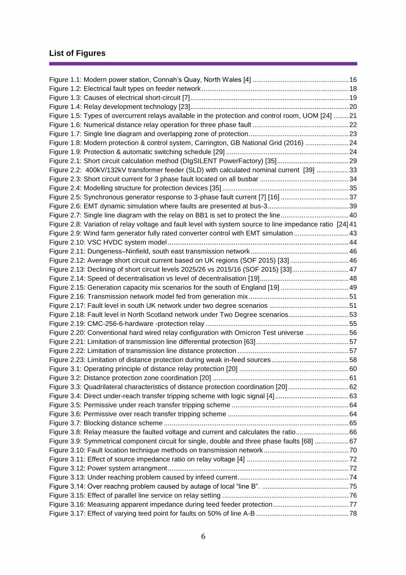
List of Figures

Figure 1.1: Modern power station, Connah’s Quay, North Wales [4] ................................................... 16 Figure 1.2: Electrical fault types on feeder network .............................................................................. 18 Figure 1.3: Causes of electrical short-circuit [7] .................................................................................... 19 Figure 1.4: Relay development technology [23].................................................................................... 20 Figure 1.5: Types of overcurrent relays available in the protection and control room, UOM [24] ........ 21 Figure 1.6: Numerical distance relay operation for three phase fault ................................................... 22 Figure 1.7: Single line diagram and overlapping zone of protection ..................................................... 23 Figure 1.8: Modern protection & control system, Carrington, GB National Grid (2016) ....................... 24 Figure 1.9: Protection & automatic switching schedule [29] ................................................................. 24 Figure 2.1: Short circuit calculation method (DIgSILENT PowerFactory) [35] ...................................... 29 Figure 2.2: 400kV/132kV transformer feeder (SLD) with calculated nominal current [39] ................. 33 Figure 2.3: Short circuit current for 3 phase fault located on all busbar ............................................... 34 Figure 2.4: Modelling structure for protection devices [35] ................................................................... 35 Figure 2.5: Synchronous generator response to 3-phase fault current [7] [16] .................................... 37 Figure 2.6: EMT dynamic simulation where faults are presented at bus-3 ........................................... 39 Figure 2.7: Single line diagram with the relay on BB1 is set to protect the line .................................... 40 Figure 2.8: Variation of relay voltage and fault level with system source to line impedance ratio [24] 41 Figure 2.9: Wind farm generator fully rated converter control with EMT simulation ............................. 43 Figure 2.10: VSC HVDC system model ................................................................................................ 44 Figure 2.11: Dungeness–Ninfield, south east transmission network .................................................... 46 Figure 2.12: Average short circuit current based on UK regions (SOF 2015) [33] ............................... 46 Figure 2.13: Declining of short circuit levels 2025/26 vs 2015/16 (SOF 2015) [33].............................. 47 Figure 2.14: Speed of decentralisation vs level of decentralisation [19] ............................................... 48 Figure 2.15: Generation capacity mix scenarios for the south of England [19] .................................... 49 Figure 2.16: Transmission network model fed from generation mix ..................................................... 51 Figure 2.17: Fault level in south UK network under two degree scenarios .......................................... 51 Figure 2.18: Fault level in North Scotland network under Two Degree scenarios................................ 53 Figure 2.19: CMC-256-6-hardware -protection relay ............................................................................ 55 Figure 2.20: Conventional hard wired relay configuration with Omicron Test universe ....................... 56 Figure 2.21: Limitation of transmission line differential protection [63] ................................................. 57 Figure 2.22: Limitation of transmission line distance protection ........................................................... 57 Figure 2.23: Limitation of distance protection during weak in-feed sources ......................................... 58 Figure 3.1: Operating principle of distance relay protection [20] .......................................................... 60 Figure 3.2: Distance protection zone coordination [20] ........................................................................ 61 Figure 3.3: Quadrilateral characteristics of distance protection coordination [20] ................................ 62 Figure 3.4: Direct under-reach transfer tripping scheme with logic signal [4] ....................................... 63 Figure 3.5: Permissive under reach transfer tripping scheme .............................................................. 64 Figure 3.6: Permissive over reach transfer tripping scheme ................................................................ 64 Figure 3.7: Blocking distance scheme .................................................................................................. 65 Figure 3.8: Relay measure the faulted voltage and current and calculates the ratio............................ 66 Figure 3.9: Symmetrical component circuit for single, double and three phase faults [68] .................. 67 Figure 3.10: Fault location technique methods on transmission network ............................................. 70 Figure 3.11: Effect of source impedance ratio on relay voltage [4] ...................................................... 72 Figure 3.12: Power system arrangment ................................................................................................ 72 Figure 3.13: Under reaching problem caused by infeed current........................................................... 74 Figure 3.14: Over reachng problem caused by autage of local “line B”. .............................................. 75 Figure 3.15: Effect of parallel line service on relay setting ................................................................... 76 Figure 3.16: Measuring apparent impedance during teed feeder protection ........................................ 77 Figure 3.17: Effect of varying teed point for faults on 50% of line A-B ................................................. 78

7

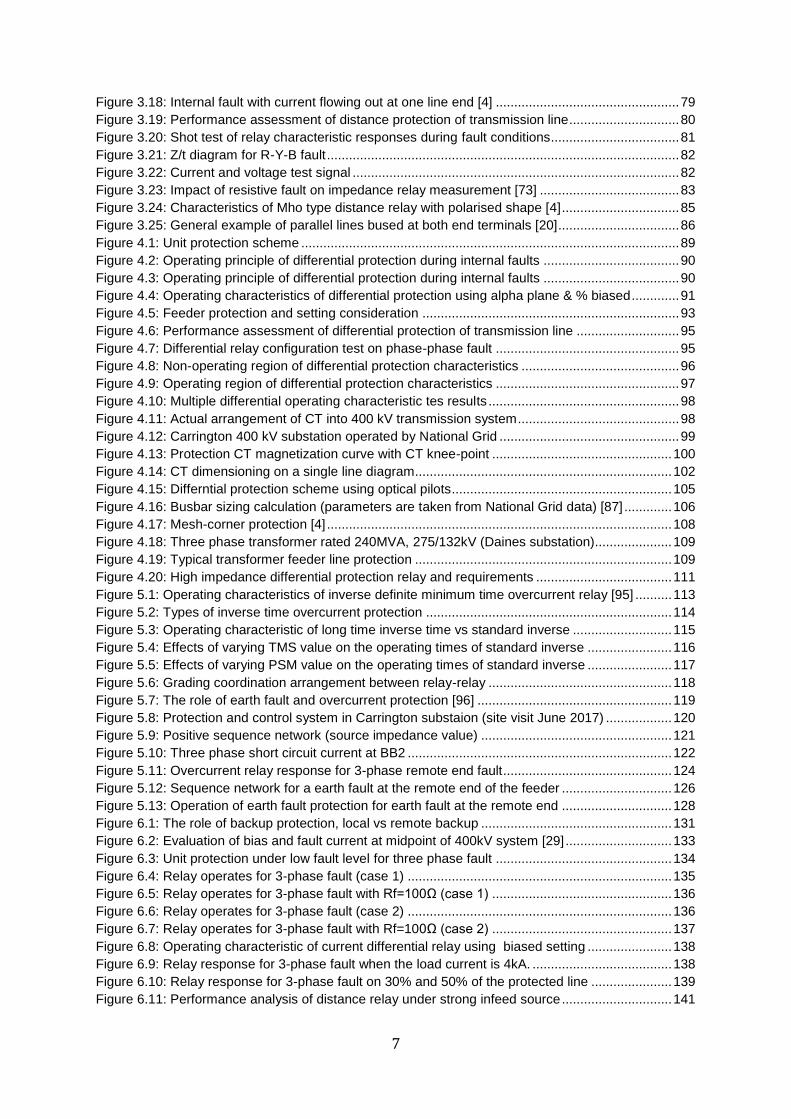
Figure 3.18: Internal fault with current flowing out at one line end [4] .................................................. 79 Figure 3.19: Performance assessment of distance protection of transmission line .............................. 80 Figure 3.20: Shot test of relay characteristic responses during fault conditions ................................... 81 Figure 3.21: Z/t diagram for R-Y-B fault ................................................................................................ 82 Figure 3.22: Current and voltage test signal ......................................................................................... 82 Figure 3.23: Impact of resistive fault on impedance relay measurement [73] ...................................... 83 Figure 3.24: Characteristics of Mho type distance relay with polarised shape [4] ................................ 85 Figure 3.25: General example of parallel lines bused at both end terminals [20] ................................. 86 Figure 4.1: Unit protection scheme ....................................................................................................... 89 Figure 4.2: Operating principle of differential protection during internal faults ..................................... 90 Figure 4.3: Operating principle of differential protection during internal faults ..................................... 90 Figure 4.4: Operating characteristics of differential protection using alpha plane & % biased ............. 91 Figure 4.5: Feeder protection and setting consideration ...................................................................... 93 Figure 4.6: Performance assessment of differential protection of transmission line ............................ 95 Figure 4.7: Differential relay configuration test on phase-phase fault .................................................. 95 Figure 4.8: Non-operating region of differential protection characteristics ........................................... 96 Figure 4.9: Operating region of differential protection characteristics .................................................. 97 Figure 4.10: Multiple differential operating characteristic tes results .................................................... 98 Figure 4.11: Actual arrangement of CT into 400 kV transmission system ............................................ 98 Figure 4.12: Carrington 400 kV substation operated by National Grid ................................................. 99 Figure 4.13: Protection CT magnetization curve with CT knee-point ................................................. 100 Figure 4.14: CT dimensioning on a single line diagram ...................................................................... 102 Figure 4.15: Differntial protection scheme using optical pilots ............................................................ 105 Figure 4.16: Busbar sizing calculation (parameters are taken from National Grid data) [87] ............. 106 Figure 4.17: Mesh-corner protection [4] .............................................................................................. 108 Figure 4.18: Three phase transformer rated 240MVA, 275/132kV (Daines substation)..................... 109 Figure 4.19: Typical transformer feeder line protection ...................................................................... 109 Figure 4.20: High impedance differential protection relay and requirements ..................................... 111 Figure 5.1: Operating characteristics of inverse definite minimum time overcurrent relay [95] .......... 113 Figure 5.2: Types of inverse time overcurrent protection ................................................................... 114 Figure 5.3: Operating characteristic of long time inverse time vs standard inverse ........................... 115 Figure 5.4: Effects of varying TMS value on the operating times of standard inverse ....................... 116 Figure 5.5: Effects of varying PSM value on the operating times of standard inverse ....................... 117 Figure 5.6: Grading coordination arrangement between relay-relay .................................................. 118 Figure 5.7: The role of earth fault and overcurrent protection [96] ..................................................... 119 Figure 5.8: Protection and control system in Carrington substaion (site visit June 2017) .................. 120 Figure 5.9: Positive sequence network (source impedance value) .................................................... 121 Figure 5.10: Three phase short circuit current at BB2 ........................................................................ 122 Figure 5.11: Overcurrent relay response for 3-phase remote end fault .............................................. 124 Figure 5.12: Sequence network for a earth fault at the remote end of the feeder .............................. 126 Figure 5.13: Operation of earth fault protection for earth fault at the remote end .............................. 128 Figure 6.1: The role of backup protection, local vs remote backup .................................................... 131 Figure 6.2: Evaluation of bias and fault current at midpoint of 400kV system [29] ............................. 133 Figure 6.3: Unit protection under low fault level for three phase fault ................................................ 134 Figure 6.4: Relay operates for 3-phase fault (case 1) ........................................................................ 135 Figure 6.5: Relay operates for 3-phase fault with Rf=100Ω (case 1) ................................................. 136 Figure 6.6: Relay operates for 3-phase fault (case 2) ........................................................................ 136 Figure 6.7: Relay operates for 3-phase fault with Rf=100Ω (case 2) ................................................. 137 Figure 6.8: Operating characteristic of current differential relay using biased setting ....................... 138 Figure 6.9: Relay response for 3-phase fault when the load current is 4kA. ...................................... 138 Figure 6.10: Relay response for 3-phase fault on 30% and 50% of the protected line ...................... 139 Figure 6.11: Performance analysis of distance relay under strong infeed source .............................. 141

8

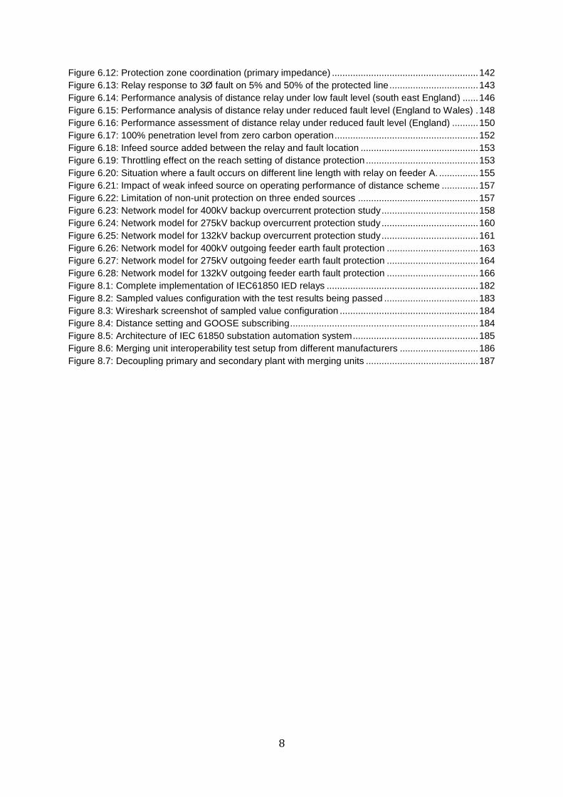
Figure 6.12: Protection zone coordination (primary impedance) ........................................................ 142 Figure 6.13: Relay response to 3Ø fault on 5% and 50% of the protected line .................................. 143 Figure 6.14: Performance analysis of distance relay under low fault level (south east England) ...... 146 Figure 6.15: Performance analysis of distance relay under reduced fault level (England to Wales) . 148 Figure 6.16: Performance assessment of distance relay under reduced fault level (England) .......... 150 Figure 6.17: 100% penetration level from zero carbon operation ....................................................... 152 Figure 6.18: Infeed source added between the relay and fault location ............................................. 153 Figure 6.19: Throttling effect on the reach setting of distance protection ........................................... 153 Figure 6.20: Situation where a fault occurs on different line length with relay on feeder A. ............... 155 Figure 6.21: Impact of weak infeed source on operating performance of distance scheme .............. 157 Figure 6.22: Limitation of non-unit protection on three ended sources .............................................. 157 Figure 6.23: Network model for 400kV backup overcurrent protection study ..................................... 158 Figure 6.24: Network model for 275kV backup overcurrent protection study ..................................... 160 Figure 6.25: Network model for 132kV backup overcurrent protection study ..................................... 161 Figure 6.26: Network model for 400kV outgoing feeder earth fault protection ................................... 163 Figure 6.27: Network model for 275kV outgoing feeder earth fault protection ................................... 164 Figure 6.28: Network model for 132kV outgoing feeder earth fault protection ................................... 166 Figure 8.1: Complete implementation of IEC61850 IED relays .......................................................... 182 Figure 8.2: Sampled values configuration with the test results being passed .................................... 183 Figure 8.3: Wireshark screenshot of sampled value configuration ..................................................... 184 Figure 8.4: Distance setting and GOOSE subscribing ........................................................................ 184 Figure 8.5: Architecture of IEC 61850 substation automation system ................................................ 185 Figure 8.6: Merging unit interoperability test setup from different manufacturers .............................. 186 Figure 8.7: Decoupling primary and secondary plant with merging units ........................................... 187

9

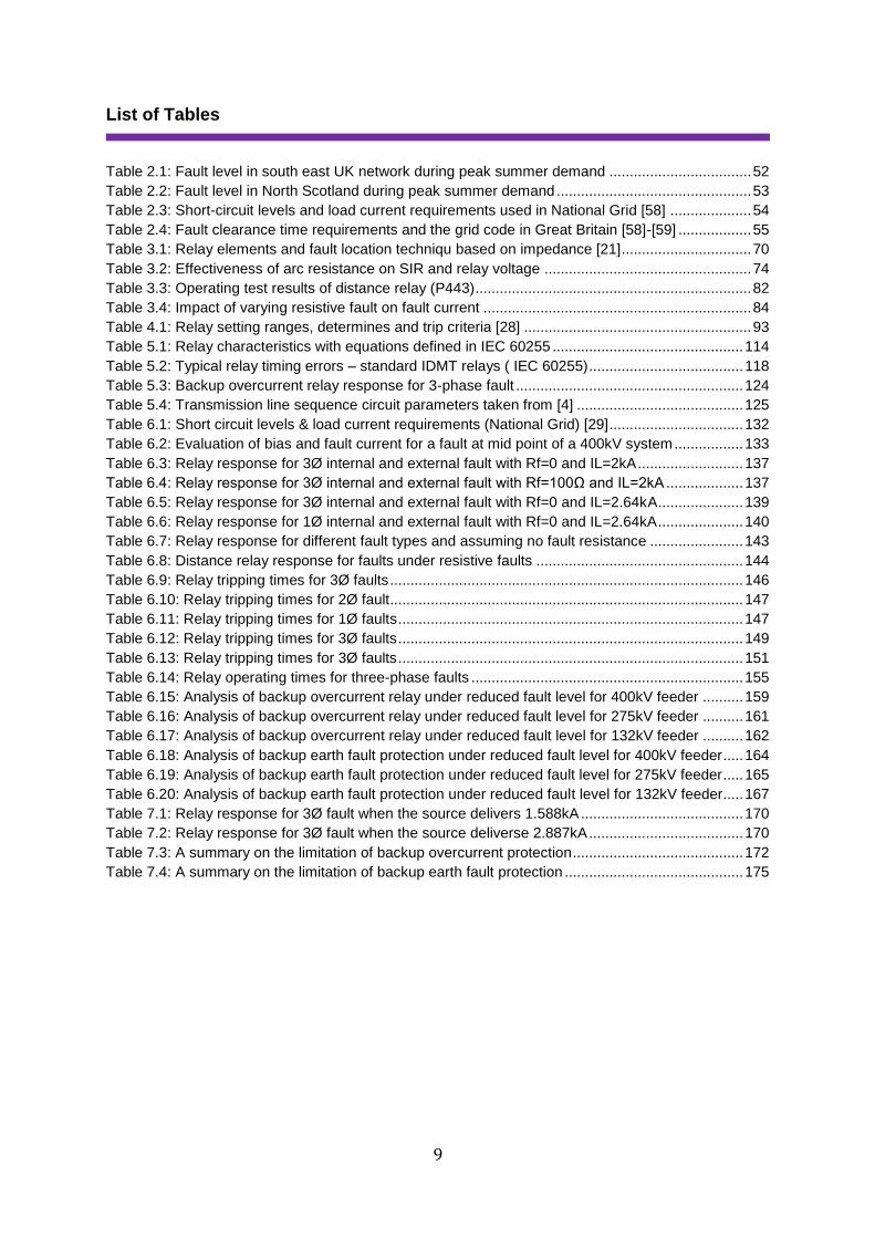
List of Tables

Table 2.1: Fault level in south east UK network during peak summer demand ................................... 52 Table 2.2: Fault level in North Scotland during peak summer demand ................................................ 53 Table 2.3: Short-circuit levels and load current requirements used in National Grid [58] .................... 54 Table 2.4: Fault clearance time requirements and the grid code in Great Britain [58]-[59] .................. 55

Table 3.1: Relay elements and fault location techniqu based on impedance [21]................................ 70 Table 3.2: Effectiveness of arc resistance on SIR and relay voltage ................................................... 74 Table 3.3: Operating test results of distance relay (P443) .................................................................... 82 Table 3.4: Impact of varying resistive fault on fault current .................................................................. 84 Table 4.1: Relay setting ranges, determines and trip criteria [28] ........................................................ 93

Table 5.1: Relay characteristics with equations defined in IEC 60255 ............................................... 114 Table 5.2: Typical relay timing errors – standard IDMT relays ( IEC 60255) ...................................... 118 Table 5.3: Backup overcurrent relay response for 3-phase fault ........................................................ 124 Table 5.4: Transmission line sequence circuit parameters taken from [4] ......................................... 125

Table 6.1: Short circuit levels & load current requirements (National Grid) [29] ................................. 132 Table 6.2: Evaluation of bias and fault current for a fault at mid point of a 400kV system ................. 133 Table 6.3: Relay response for 3Ø internal and external fault with Rf=0 and IL=2kA .......................... 137 Table 6.4: Relay response for 3Ø internal and external fault with Rf=100Ω and IL=2kA ................... 137 Table 6.5: Relay response for 3Ø internal and external fault with Rf=0 and IL=2.64kA ..................... 139 Table 6.6: Relay response for 1Ø internal and external fault with Rf=0 and IL=2.64kA ..................... 140 Table 6.7: Relay response for different fault types and assuming no fault resistance ....................... 143 Table 6.8: Distance relay response for faults under resistive faults ................................................... 144 Table 6.9: Relay tripping times for 3Ø faults ....................................................................................... 146 Table 6.10: Relay tripping times for 2Ø fault....................................................................................... 147 Table 6.11: Relay tripping times for 1Ø faults ..................................................................................... 147 Table 6.12: Relay tripping times for 3Ø faults ..................................................................................... 149 Table 6.13: Relay tripping times for 3Ø faults ..................................................................................... 151 Table 6.14: Relay operating times for three-phase faults ................................................................... 155 Table 6.15: Analysis of backup overcurrent relay under reduced fault level for 400kV feeder .......... 159 Table 6.16: Analysis of backup overcurrent relay under reduced fault level for 275kV feeder .......... 161 Table 6.17: Analysis of backup overcurrent relay under reduced fault level for 132kV feeder .......... 162 Table 6.18: Analysis of backup earth fault protection under reduced fault level for 400kV feeder..... 164 Table 6.19: Analysis of backup earth fault protection under reduced fault level for 275kV feeder..... 165 Table 6.20: Analysis of backup earth fault protection under reduced fault level for 132kV feeder..... 167

Table 7.1: Relay response for 3Ø fault when the source delivers 1.588kA ........................................ 170 Table 7.2: Relay response for 3Ø fault when the source deliverse 2.887kA ...................................... 170 Table 7.3: A summary on the limitation of backup overcurrent protection .......................................... 172 Table 7.4: A summary on the limitation of backup earth fault protection ............................................ 175

10

List of Abbreviations

Alternating Current AC

Direct Current DC

High Voltage HV

Extra-High Voltage EHV

High Voltage Direct Current HVDC

Flexible Alternating Current Transmission Systems FACTS

Voltage Source Converter based generations VSC

Single Line Diagram SLD

Kilo-volts kV

Kilo-amperes kA

Second s

Milliseconds ms

Hertz Hz

Decibels dB

Resistance R

Reactance X

Line impedance Z

Source impedance Zs

Positive, negative and zero-sequence voltage at the relay location V1, V2, V0

Positive, negative and zero-sequence current at the relay location I1, I2, I0

Voltage input signal in the distance relay comparator Vr

Current input signal in the distance relay comparator Ir

Angle in which the voltage r ϕ

Renewable Energy Sources RES

General Object Oriented Substation Event GOOSE

Merging Unit MU

Sampled Value SV

Ethernet Switch ES

11

One pulse per second 1-PPS

Supervisory control and data acquisition SCADA

Inter Range Instrumentation Group B IRIG-B

Global Positioning System GPS

Simplified Network Time Protocol SNTP

Local Area Network LAN

Medium Access Control MAC

Virtual Local Area Network VLAN

Real Time Digital Simulator RTDS

Giga-Transceiver Analogue Output Card (V/I) GTAO

Gigabit-Transceiver Front Panel Interface for trip signals GTFPI

Great Britain GB

United Kingdom UK

Electricity Ten Year Statement ETYS

System Operating Framework SOF

National Grid NG

12

Abstract

Name of University: The University of Manchester

Candidate Name: Melake Kuflom

Degree Title: The Degree of Doctor of Philosophy

Title: Impact of UK Low Carbon Energy Scenarios on Transmission Network Protection Policies Date: June 2019

Traditional UK power stations operate using synchronous generators which ensures they deliver a

high fault level, are the main source of system inertia and provides the control of the power frequency.

Recently, the percentage of demand satisfied by large synchronous generators has significantly

reduced, as more wind farms, photo voltaic sources, power electronic converters, storage and HVDC

links are integrated within the power system. Increasing deployment of converter based generation

within the distribution networks and the decline in large scale traditional synchronous power

generation at transmission level results in a fault level reduction across Great Britain network and

severe implications for the effectiveness of existing protection relaying performance. The reduction in

inertia also poses a challenge for power system stabilises, especially following a disturbance such as

the tripping of a large synchronous generation or a major interconnector to a region with synchronous

generation.

This project studies the behaviour of existing protection relaying scheme as related to the future

power system protection strategies of Great Britain and to establish how adaptive the relay can be to

the future generation mix and changes in summer minimum demand. This project also presents the

protection setting strategy used on the existing GB transmission network and to assess the limitation

of exiting protection schemes as related to the future protection setting strategy when the source

delivers a fault level that changes from a high level (strong source) to a low level (weak source).

From the research outcome, the performance of overcurrent protection is the most affected scheme

whereas unit protection is the least affected scheme during low fault level conditions. The proposed

alternative transmission protection strategies are configuring distance protection with weak infeed

logic, overcurrent protection with voltage restraint, and deploy two unit protections as main 1 & 2 with

distance protection as backup in condition when distance protection is not suitable. Other

recommended scheme includes unblocking distance schemes with weak infeed, wide area protection

and travelling wave based protection.

This thesis introduces briefly the aim & scope of the project, and then reviews the key papers in the

field as well as existing protection schemes as used in the GB transmission system. Following this, a

review into fault level, sensitivity of protection schemes, and challenges as related to the future

scenarios are discussed. The impact of low fault level on existing protection schemes, alternative

protection strategies, overview on the role & impact of IEC61850 protocol for future protection

development, and conclusions are provided at the end.

13

Declaration

No portion of the work referred to in the thesis has been submitted in support of an application for

another degree or qualification of this or any other university or other institute of learning.

14

Copyright Statement

i. The author of this thesis (including any appendices and/or schedules to this thesis) owns certain

copyright or related rights in it (the “Copyright”) and s/he has given The University of Manchester

certain rights to use such Copyright, including for administrative purposes.

ii. Copies of this thesis, either in full or in extracts and whether in hard or electronic copy, may be

made only in accordance with the Copyright, Designs and Patents Act 1988 (as amended) and

regulations issued under it or, where appropriate, in accordance with licensing agreements which the

University has from time to time. This page must form part of any such copies made.

iii. The ownership of certain Copyright, patents, designs, trademarks and other intellectual property

(the “Intellectual Property”) and any reproductions of copyright works in the thesis, for example graphs

and tables (“Reproductions”), which may be described in this thesis, may not be owned by the author

and may be owned by third parties. Such Intellectual Property and Reproductions cannot and must

not be made available for use without the prior written permission of the owner(s) of the relevant

Intellectual Property and/or Reproductions.

iv. Further information on the conditions under which disclosure, publication and commercialisation of

this thesis, the Copyright and any Intellectual Property and/or Reproductions described in it may take

place is available in the University IP Policy (see

http://documents.manchester.ac.uk/DocuInfo.aspx?DocID=24420), in any relevant Thesis restriction

declarations deposited in the University Library, The University Library’s regulations (see

https://www.library.manchester.ac.uk/aboutus/regulations) and in The University’s policy on

Presentation of Theses.

15

Acknowledgment

This project research is made in collaboration with the School of Electrical and Electronic

Engineering, the EPSRC Centre for Doctoral Training in Power Networks, University of Manchester,

and National Grid.

Firstly, I would like to express my sincere gratitude to my supervisor, Professor Peter Crossley. His

invaluable guidance, encouragement, constructive feedback, positive attitude and recommendations

to available technology throughout my research were countless. His wide knowledge, great

experience, logical way of thinking and networks he linked has been of great value for me. It would be

impossible to finish this report without his supervision and I wish him a joyful life.

I would also like to thank my co-supervisor, Dr Victor Levi and Dr Mark Osborne from National Grid,

for their guidance, constructive advices and suggestions.

Many thanks to the CDT administrative managers, staff members of University of Manchester and

those who have encouraged me during my studies.

Last but not least, sincere thanks to my beloved parents, my lovely wife and little daughter, and my

siblings for their moral support and encouragements throughout this work.

16

Chapter 1: Introduction

1.1 Power System Protection and Control

ower system engineering deals with the generation, transmission and distribution of electrical

energy [1]. At the end of 19th century, UK’s first AC coal-fired power station (i.e. 10kV 800kW)

was built in Deptford, south-east London [2]. Rapid developments of technology and an improvement

in quality of life have resulted in a massive increase in power demand over the 20th century. Building

power stations, operating at higher voltage is one possible solution to satisfy the maximum power

demand and to enhance the power transfer capabilities of transmission feeders [3]. As a part of this

process, and as an example of development, a 400kV grid system was implemented in the UK in the

1960’s.

Power system protection is a sub-division of power system engineering involved with electrical faults

[4]-[5]. The main concern of electrical network is to maintain continuity of supply, especially when

electrical faults or random failure of devices have occurred. This is because the consequence of

power outage and/or blackout is significant. In history, the largest blackout occurred in India in July

2012, and this affected about 630 million people [6]. Therefore, in transmission system protection,

technical aspects of design are crucial in related to health and safety. If protection fails, a person

could be killed or injured and financial cost for the Grid Company is very high. In addition, mal-

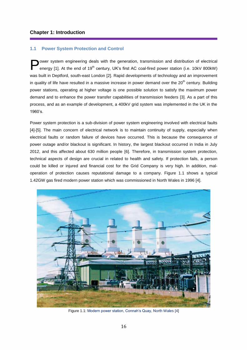
operation of protection causes reputational damage to a company. Figure 1.1 shows a typical

1.42GW gas fired modern power station which was commissioned in North Wales in 1996 [4].

Figure 1.1: Modern power station, Connah’s Quay, North Wales [4]

P

17

The role of power system protection is to minimize the damage caused by electrical faults, maintain

security of supply and ensure the safety of personnel [7]. Transmission lines in the UK are often lightly

loaded for most of the year, this means they are not thermally stressed and have been continued to

operate in a reliable and stable manner for 50 to 60 years. In addition to this, traditional power system

generations have been providing a strong fault level and are capable of contributing sufficient short

circuit current during fault conditions [8] [9] and [10]. This enables the protective devices to provide

correct operation during fault conditions.

However, due to the move towards low carbon technology [11] [12] [13], many existing UK

generations are recently being shut down, including Cottam, Aberthaw and Fiddlers Ferry coal fired

power stations, whereas Dungeness power station is also expected to close down by 2027/28 or

earlier. Hence, future UK generation to demand is expected to be satisfied by green energy sources

such as nuclear power, hydro, biomass and renewables [14] [15]. From protection prospective, if the

closure of coal fired power station is replaced with nuclear power, the fault level remains high. In

comparison, the challenge is use of renewables interfaced to power grid by power electronics which

resulted a substantial fault level reduction, difference in short circuit characteristics and their capacity

ratings [16] [17].

As part of this, the research is focused on the impact of UK low carbon energy scenarios on

transmission network protection policies. A recent report from National Grid’s System Operating

Framework and Future Energy Scenario documents [18]-[19] identified the low fault levels and

reduction in system synchronous inertia as problem for the future. These issues are associated with

increasing changes of equipment connected to the transmission network and the issues faced by the

existing protection control systems due to these changes. The dynamic characteristic response of

static power electronic of synchronous generators is starting to show a profound impact on the

continuity and reliability of power systems with high penetration of renewable generation levels.

The scope and key study area of concern in particular is for the reliable & secure operation of

protection relays including:

The impact of low fault currents on the operation of existing protection systems,

The impact of green or low carbon energy on the protection & control systems & practice

Alternative protection strategy as related to the future energy scenarios

Note, reliability is associated with dependability and security [20]. Dependability depends on which

relay can operate as expected, whereas security is a measure of a relay that will not operate if not

required. Selectivity or discrimination is dealt with by tripping the correct circuit breaker [20]-[21]. This

includes whether the operation is required to isolate the fault or not. Relay operating speed is critical

in a protection scheme, since it is necessary to detect a fault and isolate the faulted system as fast as

possible and avoided the possibilities of a wide area disturbance or a power system collapse.

The main contribution of this research is highlighted in chapter 7 and 8, where the limitations of exiting

protections are identified and alternative protection strategies are also proposed. For example, the

18

performance of overcurrent protection (i.e. accuracy relay reach and operating time) under reduced

fault level is the most affected scheme whereas unit protection is the least. The solutions being

considered as an alternative transmission network protection strategy includes configuring distance

protection with weak infeed logic to cope with extremely weak infeed conditions and configuring

overcurrent protection with voltage restraint control system to speed up the operating time. Utilising

two unit differential protection as first main with distance protection as backup in condition when

distance protection is not suitable is also highly considered in this thesis. Other recommended

alternative protection schemes includes unblocking distance schemes with weak infeed, wide area

protection and travelling wave based protection.

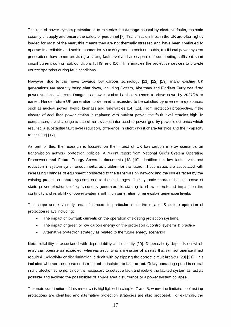
1.1.1 Electrical power system fault types and causes

Most power systems are exposed to various kinds of faults, where a fault is considered as any

abnormal condition that affects the flow of electrical power [22]. The common types of faults are short

circuits between phases and/or ground, open-circuits, simultaneous flashovers at multiple location,

and winding faults. Balanced three-phase short-circuited faults are mostly used for a standard fault

level study. In general, there are 10 different short circuit type faults:

Symmetrical/balanced fault

1x three phase faults; with or without earth connection

Unsymmetrical/unbalanced fault

3x single phase-to-ground faults

3x double phase faults

3x double phase-to-ground faults

Source

G1

Transformer

LV/HV

1Φ-e

F

2Φ

F

F

F

F

F

3Φ 2Φ-e

F

F

F = Fault Rf = resistive fault

Rf

L 1

L 2

L 3

Bus 1

Figure 1.2: Electrical fault types on feeder network

Figure 1.2 shows the typical short circuit fault types presented in HV system, where most faults on

overhead lines fall into transient, semi-transient and permanent fault [4].

Transient faults: a fault that lasts for a very short time often caused by lighting which induces a

fashover between conductors. Most overhead line faults are transient faults, typically 80%-90%

of all faults. Tranisient faults can be cleared by immediate tripping of a circuit breaker and

subsequent re-energizing of transmission line via auto-reclose. The role of auto-reclose is to re-

19

energise and restoration of supply the line after the fault trip and this allows a successful re-

energisation of the line [4].

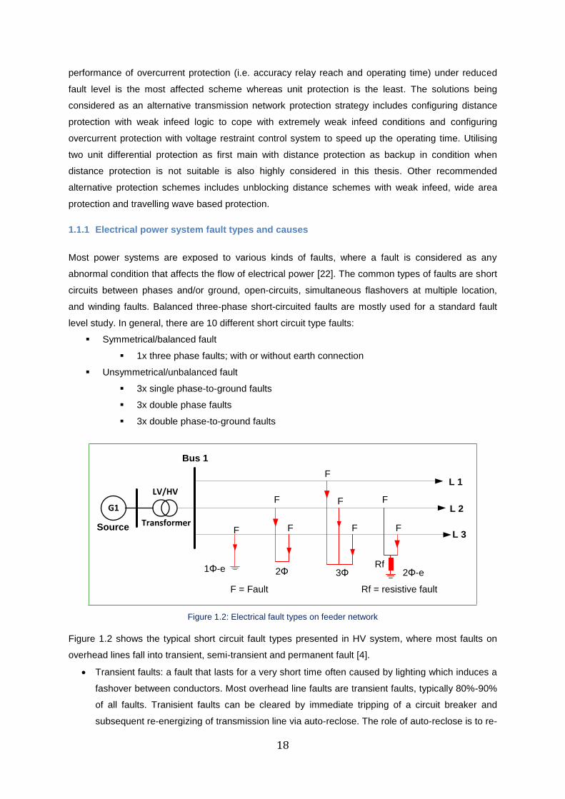
Semi-transient/semi-permanent faults:- happens when an

external object such as a small tree branch touches an

overhead line causing a semi permanent fault. In this case,

faults can be cleared by initiating a delayed trip time or multiple

trip-reclose cycles. Providing a delayed trip time will normally

allow the object to burn away before the line is re-energised

using a delayed automatic reclose (DAR). The use of delayed

trip time is often used in distribution system.

Permanent faults:- caused as a result of an insulation failure which mostly appeared on

underground cables, a single or two phase broken conductors that can produce the unbalanced

voltage of the power system causing a damage to the equipment, and or a short circuit faults

causing a permanent fault. In this case the faulted item must be repaired before restoration of

the supply.

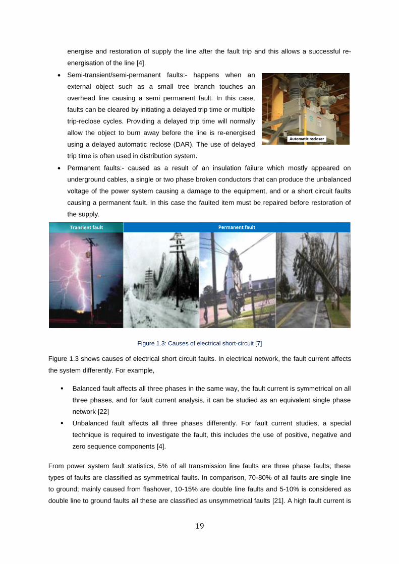
Transient fault Permanent fault

Figure 1.3: Causes of electrical short-circuit [7]

Figure 1.3 shows causes of electrical short circuit faults. In electrical network, the fault current affects

the system differently. For example,

Balanced fault affects all three phases in the same way, the fault current is symmetrical on all

three phases, and for fault current analysis, it can be studied as an equivalent single phase

network [22]

Unbalanced fault affects all three phases differently. For fault current studies, a special

technique is required to investigate the fault, this includes the use of positive, negative and

zero sequence components [4].

From power system fault statistics, 5% of all transmission line faults are three phase faults; these

types of faults are classified as symmetrical faults. In comparison, 70-80% of all faults are single line

to ground; mainly caused from flashover, 10-15% are double line faults and 5-10% is considered as

double line to ground faults all these are classified as unsymmetrical faults [21]. A high fault current is

Automatic recloser

20

the most severe type of fault and therefore a balanced three phase solid fault is the most severe,

whereas, a single line to ground fault is less severe, but if the fault is resistive or the network has

impedance in the grounding.

1.1.2 Development of protective relay technology

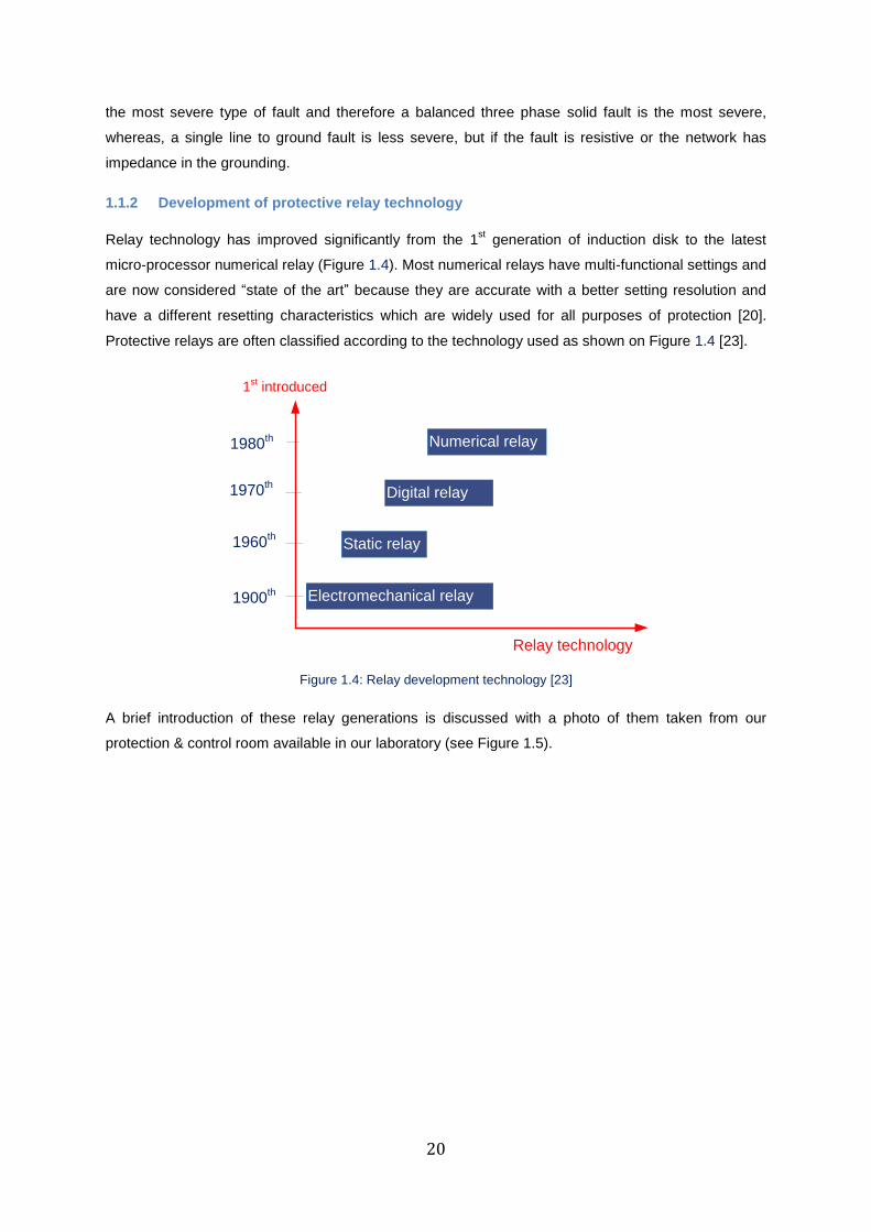
Relay technology has improved significantly from the 1st generation of induction disk to the latest

micro-processor numerical relay (Figure 1.4). Most numerical relays have multi-functional settings and

are now considered “state of the art” because they are accurate with a better setting resolution and

have a different resetting characteristics which are widely used for all purposes of protection [20].

Protective relays are often classified according to the technology used as shown on Figure 1.4 [23].

1st introduced

1900th

1960th

1970th

1980th

Electromechanical relay

Static relay

Digital relay

Numerical relay

Relay technology

Figure 1.4: Relay development technology [23]

A brief introduction of these relay generations is discussed with a photo of them taken from our

protection & control room available in our laboratory (see Figure 1.5).

21

B. Static relay

D. Numerical relay

A. Electromechanical relay

C. Digital relay

PC

Omicron

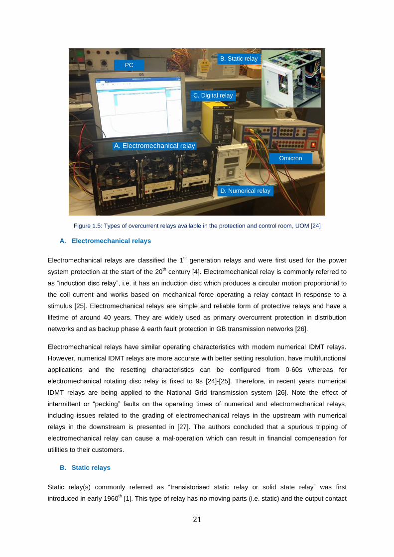
Figure 1.5: Types of overcurrent relays available in the protection and control room, UOM [24]

A. Electromechanical relays

Electromechanical relays are classified the 1st generation relays and were first used for the power

system protection at the start of the 20th century [4]. Electromechanical relay is commonly referred to

as “induction disc relay”, i.e. it has an induction disc which produces a circular motion proportional to

the coil current and works based on mechanical force operating a relay contact in response to a

stimulus [25]. Electromechanical relays are simple and reliable form of protective relays and have a

lifetime of around 40 years. They are widely used as primary overcurrent protection in distribution

networks and as backup phase & earth fault protection in GB transmission networks [26].

Electromechanical relays have similar operating characteristics with modern numerical IDMT relays.

However, numerical IDMT relays are more accurate with better setting resolution, have multifunctional

applications and the resetting characteristics can be configured from 0-60s whereas for

electromechanical rotating disc relay is fixed to 9s [24]-[25]. Therefore, in recent years numerical

IDMT relays are being applied to the National Grid transmission system [26]. Note the effect of

intermittent or “pecking” faults on the operating times of numerical and electromechanical relays,

including issues related to the grading of electromechanical relays in the upstream with numerical

relays in the downstream is presented in [27]. The authors concluded that a spurious tripping of

electromechanical relay can cause a mal-operation which can result in financial compensation for

utilities to their customers.

B. Static relays

Static relay(s) commonly referred as “transistorised static relay or solid state relay” was first

introduced in early 1960th [1]. This type of relay has no moving parts (i.e. static) and the output contact

22

to trip the CB is achieved with the attracted armature principle. The design of this relays uses

analogue electronic devices and the average useful life time is about 30 years.

C. Digital relays

Digital relays were first introduced in 1980’s and are a step change in technology as compared to

static or electro-mechanical relays. Microprocessors and microcontrollers replaced the analogue

circuits used in static relays to implement relay functions [4]. They often copy the behaviour of

electromechanical relays and have similar or the same performance as electromechanical relays

which are still the current technology for many relay applications. Compared to an electromechanical

or static relays, digital relays have a wider range of settings, great accuarcy, and a communication

link to a remote computer. Similar to static relays, the usefull life time is about 30 years.

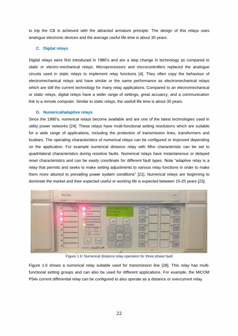
D. Numerical/adaptive relays

Since the 1980’s, numerical relays become available and are one of the latest technologies used in

utility power networks [24]. These relays have multi-functional setting resolutions which are suitable

for a wide range of applications, including the protection of transmission lines, transformers and

busbars. The operating characteristics of numerical relays can be configured or improved depending

on the application. For example numerical distance relay with Mho characteristic can be set to

quadrilateral characteristics during resistive faults. Numerical relays have instantaneous or delayed

reset characteristics and can be easily coordinate for different fault types. Note “adaptive relay is a

relay that permits and seeks to make setting adjustments to various relay functions in order to make

them more attuned to prevailing power system conditions” [21]. Numerical relays are beginning to

dominate the market and their expected useful or working life is expected between 15-20 years [23].

Figure 1.6: Numerical distance relay operation for three phase fault

Figure 1.6 shows a numerical relay suitable used for transmission line [28]. This relay has multi-

functional setting groups and can also be used for different applications. For example, the MiCOM

P54x current differential relay can be configured to also operate as a distance or overcurrent relay.

23

1.1.3 Role of protection and zone of protection

The primary aim of protection is to clear faults as fast as possible and limit further damage to the

equipment and the system. The application of protection is based on the fault level of the system and

may also differ according to the system topology. A Unit or differential protection scheme is suitable to

protect a specific item of plant including transmission lines, bus-bars, motors, transformers and

generators, whereas non-unit distance protection schemes are mainly used for transmission and sub-

transmission line protection, and over-current relays are commonly used as main protection for a

radial distribution network or as backup protection in a transmission network.

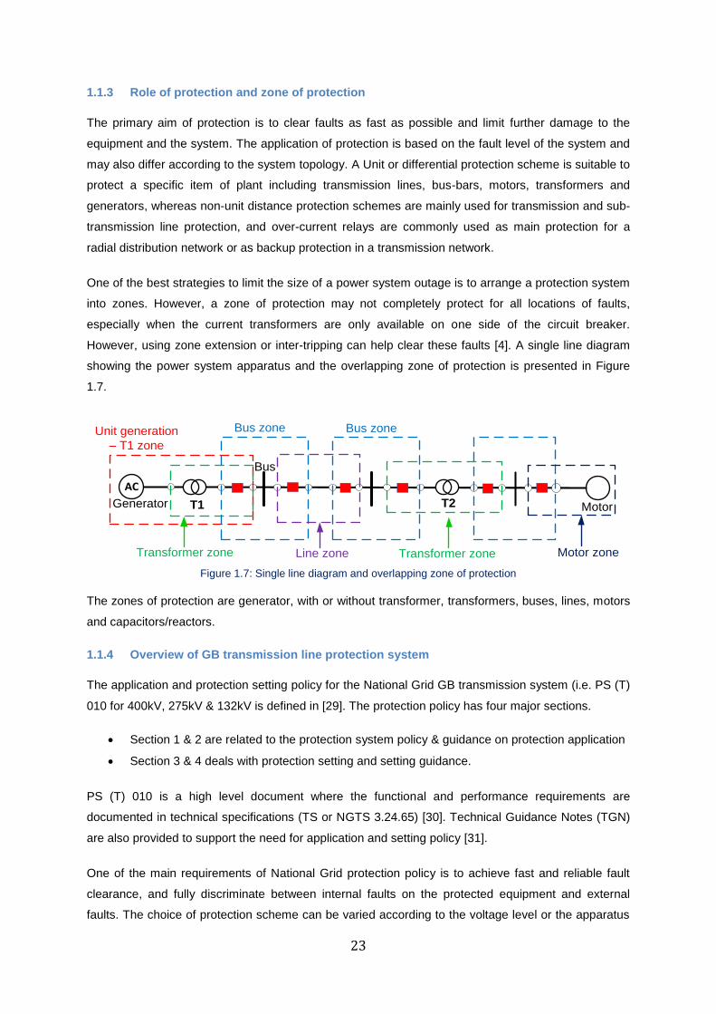
One of the best strategies to limit the size of a power system outage is to arrange a protection system

into zones. However, a zone of protection may not completely protect for all locations of faults,

especially when the current transformers are only available on one side of the circuit breaker.

However, using zone extension or inter-tripping can help clear these faults [4]. A single line diagram

showing the power system apparatus and the overlapping zone of protection is presented in Figure

1.7.

AC

T1 T2

Bus zone Bus zoneUnit generation

– T1 zone

Transformer zone Line zone Transformer zone

Motor

Motor zone

Generator

Bus

Figure 1.7: Single line diagram and overlapping zone of protection

The zones of protection are generator, with or without transformer, transformers, buses, lines, motors

and capacitors/reactors.

1.1.4 Overview of GB transmission line protection system

The application and protection setting policy for the National Grid GB transmission system (i.e. PS (T)

010 for 400kV, 275kV & 132kV is defined in [29]. The protection policy has four major sections.

Section 1 & 2 are related to the protection system policy & guidance on protection application

Section 3 & 4 deals with protection setting and setting guidance.

PS (T) 010 is a high level document where the functional and performance requirements are

documented in technical specifications (TS or NGTS 3.24.65) [30]. Technical Guidance Notes (TGN)

are also provided to support the need for application and setting policy [31].

One of the main requirements of National Grid protection policy is to achieve fast and reliable fault

clearance, and fully discriminate between internal faults on the protected equipment and external

faults. The choice of protection scheme can be varied according to the voltage level or the apparatus

24

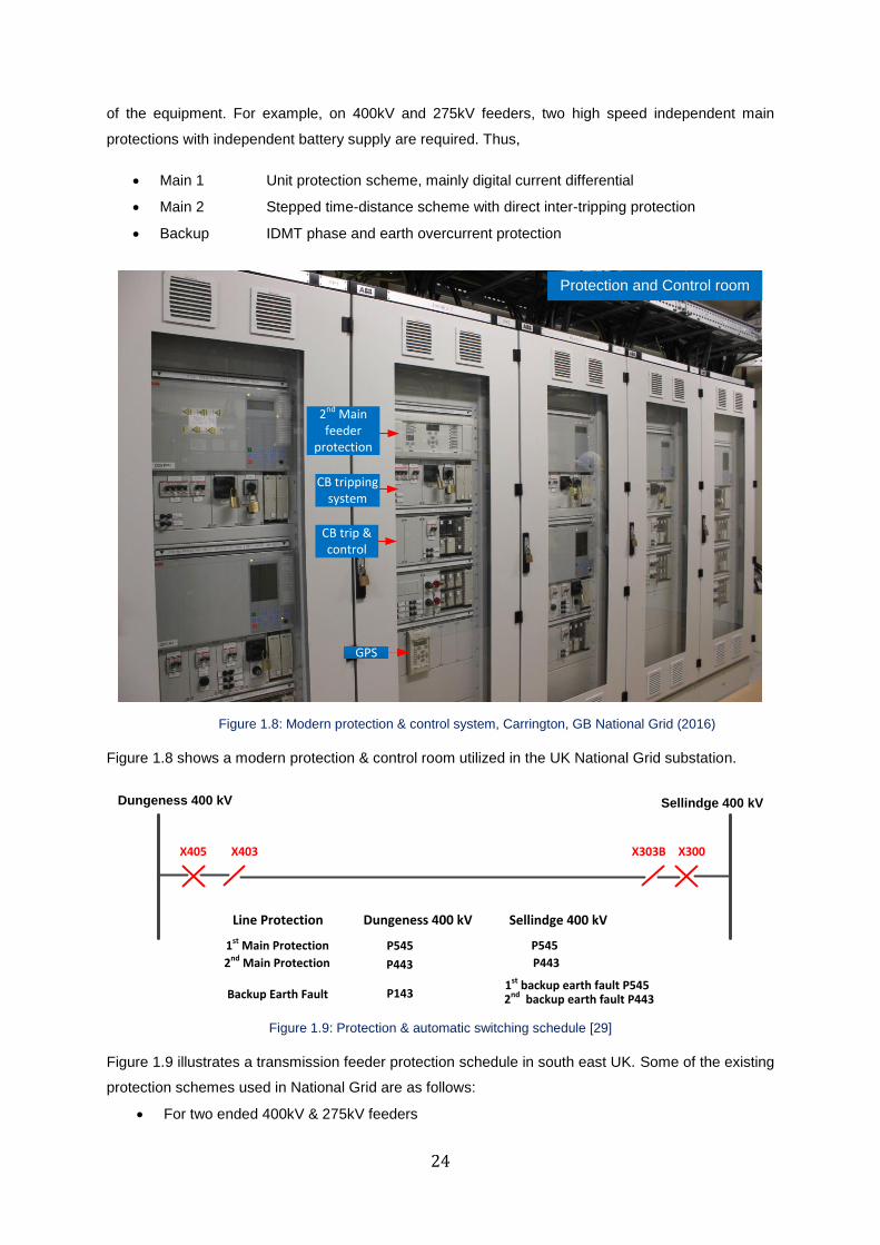
of the equipment. For example, on 400kV and 275kV feeders, two high speed independent main

protections with independent battery supply are required. Thus,

Main 1 Unit protection scheme, mainly digital current differential

Main 2 Stepped time-distance scheme with direct inter-tripping protection

Backup IDMT phase and earth overcurrent protection

GPS

Protection and Control room

CB tripping system

CB trip & control

2nd Main feeder

protection

Figure 1.8: Modern protection & control system, Carrington, GB National Grid (2016)

Figure 1.8 shows a modern protection & control room utilized in the UK National Grid substation.

Dungeness 400 kV Sellindge 400 kV

Line Protection Dungeness 400 kV Sellindge 400 kV

1st Main Protection

2nd Main Protection

Backup Earth Fault

P545

P443

P143

P545

P443

1st backup earth fault P5452nd backup earth fault P443

X405 X403 X303B X300

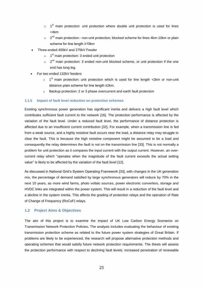
Figure 1.9: Protection & automatic switching schedule [29]

Figure 1.9 illustrates a transmission feeder protection schedule in south east UK. Some of the existing

protection schemes used in National Grid are as follows:

For two ended 400kV & 275kV feeders

25

o 1st main protection: unit protection where double unit protection is used for lines

<4km

o 2nd

main protection:- non-unit protection; blocked scheme for lines 4km-10km or plain

scheme for line length ≥10km

Three-ended 400kV and 275kV Feeder

o 1st main protection: 3 ended unit protection

o 2nd

main protection: 3 ended non-unit blocked scheme, or unit protection if the one

end has long leg.

For two ended 132kV feeders

o 1st main protection: unit protection which is used for line length <2km or non-unit

distance plain scheme for line length ≥2km.

o Backup protection: 2 or 3 phase overcurrent and earth fault protection

1.1.5 Impact of fault level reduction on protection schemes

Existing synchronous power generation has significant inertia and delivers a high fault level which

contributes sufficient fault current to the network [16]. The protection performance is affected by the

variation of the fault level. Under a reduced fault level, the performance of distance protection is

affected due to an insufficient current contribution [32]. For example, when a transmission line is fed

from a weak source, and a highly resistive fault occurs near the load, a distance relay may struggle to

clear the fault. This is because the high resistive component might be assumed to be a load and

consequently the relay determines the fault is not on the transmission line [33]. This is not normally a

problem for unit protection as it compares the input current with the output current. However, an over-

current relay which “operates when the magnitude of the fault current exceeds the actual setting

value” is likely to be affected by the variation of the fault level [12].

As discussed in National Grid’s System Operating Framework [33], with changes in the UK generation

mix, the percentage of demand satisfied by large synchronous generators will reduce by 70% in the

next 10 years, as more wind farms, photo voltaic sources, power electronic converters, storage and

HVDC links are integrated within the power system. This will result in a reduction of the fault level and

a decline in the system inertia. This affects the grading of protection relays and the operation of Rate

of Change of Frequency (RoCoF) relays.

1.2 Project Aims & Objectives

The aim of this project is to examine the impact of UK Low Carbon Energy Scenarios on

Transmission Network Protection Policies. The analysis includes evaluating the behaviour of existing

transmission protection scheme as related to the future power system strategies of Great Britain. If

problems are likely to be experienced, the research will propose alternative protection methods and

operating schemes that would satisfy future network protection requirements. The thesis will assess

the protection performance with respect to declining fault levels; increased penetration of renewable

26

generation, decreased generation from synchronous sources and changes in the source impedance

ratio.

The main objectives of this thesis are to:

1. Assess the impact of low fault level on the operation of existing protection systems such as

a. Line protection schemes

Unit differential protection

Non-unit distance protection

Backup overcurrent protection

Back up earth fault (IDMT) protection

2. Establish the limitation of existing protection policy to cater for future scenarios

Assess the limitation of existing protection under varying fault level

3. Consider how faults can be differentiated from heavy loading conditions during low short circuit

Fault current vs load current

4. Provide an alternative protection methodologies for transmission network with low inertia and

low fault current analysis that includes

Protection philosophy

Time scale

5. Consider the impact of new technology on fault clearing times and recommended protection &

control coordination strategies

27

1.3 Structure of the Thesis

The outline of the remaining chapters is organised as follows:

Chapter 2 details the fault level analysis, protection studies and provides a review on the selection of

a relay scheme. Then an evaluation of existing & future fault level analysis on the Great Britain

transmission network and the protection challenges with respect to the declining fault levels is

explored. The impact on protection policy of declining short circuit levels is also investigated.

Chapter 3 shows the concept and sensitivity analysis of distance protection and the associated zone

setting methodology. Various parameters that influence the performance of time stepped distance

protection are discussed.

Chapter 4 shows the concept and sensitivity analysis of differential protection. Issues related to the

dimensioning of current transformers, protection signalling and the application of unit scheme are also

highlighted.

Chapter 5 identifies the concept, sensitivity analysis of backup overcurrent phase and earth fault

protection. The focus is put on the impact of fault level reduction on the backup overcurrent protection

and an implication on the limitation of backup overcurrent protection.

Chapter 6 explores the role of backup protection and identifies the key strategy for evaluating the

impact of low fault level on the limitation of existing protection schemes as related to the future

protection strategy and this is one of the most significant parts of this thesis.

As fault level reduces, the effectiveness of existing protection schemes used in the UK transmission

network is assessed. The assessment process is based on National Grid reports, i.e. System

Operating Framework (SOF) and Electricity Ten Year Statement (ETYS). Chapter 7 identifies the

impact of low fault levels on the capability of conventional protection schemes. This has the

implications for the future protection application and setting strategy.

The drive towards decarbonisation, decentralisation and digitalisation; means future digital substation

will use smart IEDs operating in line with IEC61850 protocols, GOOSE, Sampling Values and real

time synchronisation. Chapter 8 evaluates the role, benefit & impact of IEC 61850 protocols for future

protection development.

A conclusion of the thesis and implications for future work is discussed in chapter 9. A summary of

operating characteristics of distance relay types and their applications can be found in appendix 1

whereas a postscript on the UK blackout incident is also provided in appendix 2.

28

Chapter 2: Review into fault level and protection system studies

2.1. Motivation of fault level analysis

This chapter will focus on fault level studies and the key protection challenges associated with a

converter dominated power system. Firstly, the standard methods of fault level calculation will be

discussed. Then, fault current contribution from traditional synchronous generations and converter

based generations will be evaluated. Next, the impact of declining fault levels and increased

penetration of renewable generations on existing protection schemes, including in the GB

transmission system will be highlighted. Finally, the short circuit analysis simulation test results will be

presented. The summary will describe how adequate handling of short circuit and protection policy

can be applied to the calculated short circuit levels.

2.2. Short circuit current analysis

Short circuit current is an excessive form of current flowing into an item of power system plant that

has been affected by a short circuit. In a power system, adequate handling of a short circuit current is

vital to the design of an optimal network [22]. The main reasons for fault current study are

Calculate the rating of circuit breaker: must be able to make or break a very large current.

Design protection system: to distinguish if the fault current is large enough to be detected

because undetected faults are a safety hazards

Check system stability: faults can cause large system disturbances

Power quality: faults create voltage sags in other parts of the network

Generally, if the short circuit current is not properly detected & cleared; it may result in equipment

damage, the interruption of power in large parts of the network including the healthy system and a

health risk to utility personnel or the general public.

The causes of short circuit current are generally the following:

Lightning discharge on transmission lines/live conductors

Insulation failure causing a contact between live conductors

Failure of equipment; acting as a fault point which draws large amount of fault current

Incorrect system operation caused by human error that may result in a short circuit current

In power system protection, the maximum, minimum current flowing into a fault within the protected

object or zone and the through fault current is required to determine the relay setting necessary to

provide correct operation [5]. Thus, the common methods of fault analysis are thevenin equivalent

and superposition (complete) method [22]. According [17] [34], the most common methods used to

calculate short circuit currents are IEC 60909 and complete methods, where DIgSILENT Power-

Factory simulator has modules that implement both IEC 60909 and complete methods as shown in

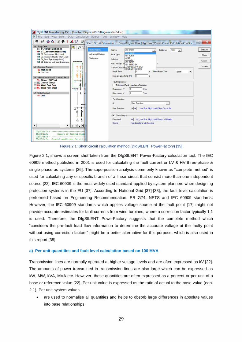
Figure 2.1.

29

Figure 2.1: Short circuit calculation method (DIgSILENT PowerFactory) [35]

Figure 2.1, shows a screen shot taken from the DIgSILENT Power-Factory calculation tool. The IEC

60909 method published in 2001 is used for calculating the fault current or LV & HV three-phase &

single phase ac systems [36]. The superposition analysis commonly known as “complete method” is

used for calculating any or specific branch of a linear circuit that consist more than one independent

source [22]. IEC 60909 is the most widely used standard applied by system planners when designing

protection systems in the EU [37]. According to National Grid [37]-[38], the fault level calculation is

performed based on Engineering Recommendation, ER G74, NETS and IEC 60909 standards.

However, the IEC 60909 standards which applies voltage source at the fault point [17] might not

provide accurate estimates for fault currents from wind turbines, where a correction factor typically 1.1

is used. Therefore, the DIgSILENT PowerFactory suggests that the complete method which

“considers the pre-fault load flow information to determine the accurate voltage at the faulty point

without using correction factors” might be a better alternative for this purpose, which is also used in

this report [35].

a) Per unit quantities and fault level calculation based on 100 MVA

Transmission lines are normally operated at higher voltage levels and are often expressed as kV [22].

The amounts of power transmitted in transmission lines are also large which can be expressed as

kW, MW, kVA, MVA etc. However, these quantities are often expressed as a percent or per unit of a

base or reference value [22]. Per unit value is expressed as the ratio of actual to the base value (eqn.

2.1). Per unit system values

are used to normalise all quantities and helps to obsorb large differences in absolute values

into base relationships

30

provides the system to become more uniform in more meaningfull data

The ratio in percent is 100 times the per unit values. For example, when a system voltage is 420kV

and if the chosen base voltage is 400kV; this can be transferred to 420/400=1.05 per unit or

1.05×100=105%.

per unit of an element =actual value

base value eqn. 2.1

The conversion of actual value of current (A), voltage (kV), apparent power (kVA or MVA) and

impedance (Ω) on chosen base value to per unit or vice versa can be performed using eqn. 2.1. The

basic conversations are provided as follows:

For single phase power (1∅),

Base current, A = Sbase

Vbase

= base MVA1∅

base voltage, kVLN

eqn. 2.2

Base impedance, Ω = Vbase

Ibase

=base voltage VLN

base current, A eqn. 2.3

Base impedance, Ω =𝑉𝑏𝑎𝑠𝑒

2

Sbase

=(base voltage, kVLN)2

base MVA1∅ eqn. 2.4

Base power, MW1∅ = base MVA1∅ eqn. 2.5

For three phase power, the power is 3 times the single phase power. The line voltage is also √3 times

the phase voltage. For instance, if the 3-phase power and line-line voltage is given as:

Base power, MVA3∅ = 100 MVA and base kVLL = 400 kV

The single phase power and phase voltage will be:

Base power, MVA1∅ =100

3= 33.33MVA

Base voltage, kVLL =400

√3= 230.94kV

If the actual line to line voltage in a balanced 3-phase is 390kV, the phase voltage will be 390/√3 =

225.167kV.

Per unit voltage =390

400= 0.975p. u.

If the actual power is 75 MVA (i.e. the single phase power is 25MVA), the power in per unit will be:

Per unit power =75

100= 0.75 p. u.

31

Similarly, the base element in three phase system can be obtained as follows:

Base current, A = Sbase

Vbase

= base MVA3∅

base voltage, kVLL

eqn. 2.6

Where kVLL = √3 × kVLN

Base impedance, Ω = Vbase

Ibase

=base voltage VLL

base current, A eqn. 2.7

Base impedance =(base voltage, kVLL)2

base MVA3∅

eqn. 2.8

For example, using 100MVA base (eqn. 2.8), the base impedance on 400kV feeder line will be:

Base impedance =kV2

MVA =

4002

100 = 1600 Ω

In a power system, the system fault level at each voltage level is constrained within the design limits.

Thus, the fault current at any point of a system is determined by the source impedance value.

According to National Grid, the technical data of the system parameter are given as R and X (% on

100 MVA). Hence, it’s important to note the basic conversation methods in transferring from % to

MVA or ohmic values and vice versa.

If the reactance of generator or transformer is given in % based on the name plate ratings, it

can be converted into a 100MVA base using:

X% on 100 MVAbase =X % at name plate rated MVA × 100

normal rating (MVA) eqn. 2.9

For instance, if a 400/275kV feeder transformer supplied at 400kV with a fault level at the 275kV

busbar is 750MVA, the % reactance on 100MVA base will be:

%X on 100MVA = Base MVA

Fault level, MVA× 100 =

100 MVA

750MVA× 100 = 13.33%

Assume a transformer with a reactance of 10% on 10MVA. On 100MVA base, this translates to:

% X = X% × Base MVA

Fault level, MVA× 100 = 10% ×

100

10 × 100 = 100% at 100MVA rating

Similarly, if the fault infeed of 40kA at the 275kV busbar is considered in the UK, the % sources

impedance will be:

Fault MVA = √3 × 275kV × 40kA = 19050MVA

% Zs =Base MVA × 100

Fault MVA=

100 × 100

19050 = j0.525%

32

i. e. Zs (p. u) =j0.525%

100 = j0.00525 p. u.

The normal rating fault level (MVA) can be rearranged from eqn. 2.9:

Fault Level (MVA) =Base MVA × 100

X (% on 100 MVA) eqn 2.10

Example, if the percentage source impedance of a generator is 0.525%, the fault level on 100MVA

base will be

e. g Fault level on 100 MVAbase =100MVA × 100

0.525%= 19047MVA = 19.05GVA

i. e the lower % source impedance implies the stronger fault level of the system

If the resistance and reactance values are given in %, the ohmic values can be obtained as:

𝑅(Ω) =%R × kV2

100 × 100MVA 𝑎𝑛𝑑 𝑋(Ω) =

%X × kV2

100 × 100MVA eqn. 2.11

Example, the percentage values for 400kV transmission line i.e. from Dungeness to Ninfield

substation are given as Z = 0.0391 + j0.7567Ω i. e Z = 0.7577∠96Ω) (% on 100MVA); the ohmic

values based on eqn. 2.11 will be:

𝑅(Ω) =0.0391 × 4002

100 × 100= 0.6256Ω 𝑎𝑛𝑑 𝑋(Ω) =

0.7567 × 4002

100 × 100 = 12.107Ω

i. e Z (% on 100 MVA) = 0.7577∠96 (i. e 0.00757 p. u. ) translates to Z = 12.116∠87Ω

From, eqn. 2.8, on 100MVA base, the base impedance for 400kV line is 1600Ω whereas the ohmic

impedance from eqn. 2.11 is 12.116Ω. The per unit impedance on 100MVA base will be

Z (per unit) =Zactual/ohmic

Zbase

=12.116 Ω

1600 Ω= 0.00757 p. u.

In addition to the above conversion of per unit to fault level or percentage calculations, normal rating

current and CT selection can be obtained. For example, let’s consider a 400kV source that delivers

63kA or 43,648MVA (Figure 2.2) that stepped down to transfer electricity to the 132kV transmission

feeder line, with a given transformer leakage reactance of 8% on 240MVA rating, then the CT ratio

can be determined by obtaining the corresponding nominal currents as follows:

Nominal current, In(400kV side) =240MVA

√3 × 400kV= 346.4A use CT ratio > In i. e. 600/1A

Nominal current, In(132kV side) =240MVA

√3 × 132kV= 1049.72A use CT ratio > In i. e. 1200/1A

33

Daines Cellarhead 400/132kV

PsT: 240MVA

X=8%

346.4A 1049.72A

AC

400kV

SCC’’

43648MVA

CT1

400/1A

F1

CT2

1200/1A

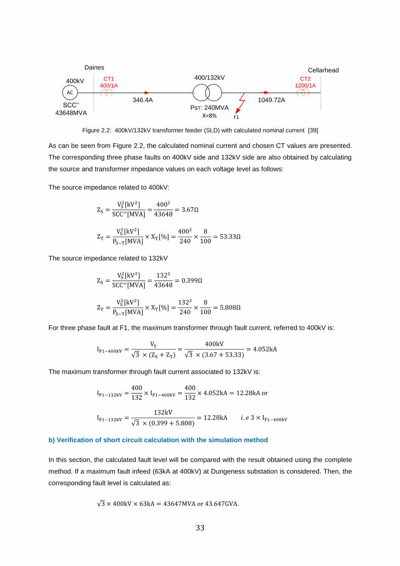
Figure 2.2: 400kV/132kV transformer feeder (SLD) with calculated nominal current [39]

As can be seen from Figure 2.2, the calculated nominal current and chosen CT values are presented.

The corresponding three phase faults on 400kV side and 132kV side are also obtained by calculating

the source and transformer impedance values on each voltage level as follows:

The source impedance related to 400kV:

ZS =VS

2[kV2]

SCC′′[MVA]=

4002

43648= 3.67Ω

ZT =VS

2[kV2]

PS−T[MVA]× XT[%] =

4002

240×

8

100= 53.33Ω

The source impedance related to 132kV

ZS =VS

2[kV2]

SCC′′[MVA]=

1322

43648= 0.399Ω

ZT =VS

2[kV2]

PS−T[MVA]× XT[%] =

1322

240×

8

100= 5.808Ω

For three phase fault at F1, the maximum transformer through fault current, referred to 400kV is:

IF1−400kV =VS

√3 × (ZS + ZT)=

400kV

√3 × (3.67 + 53.33)= 4.052kA

The maximum transformer through fault current associated to 132kV is:

IF1−132kV =400

132× IF1−400kV =

400

132× 4.052kA = 12.28kA or

IF1−132kV =132kV

√3 × (0.399 + 5.808)= 12.28kA 𝑖. 𝑒 3 × IF1−400kV

b) Verification of short circuit calculation with the simulation method

In this section, the calculated fault level will be compared with the result obtained using the complete

method. If a maximum fault infeed (63kA at 400kV) at Dungeness substation is considered. Then, the

corresponding fault level is calculated as:

√3 × 400kV × 63kA = 43647MVA or 43.647GVA.

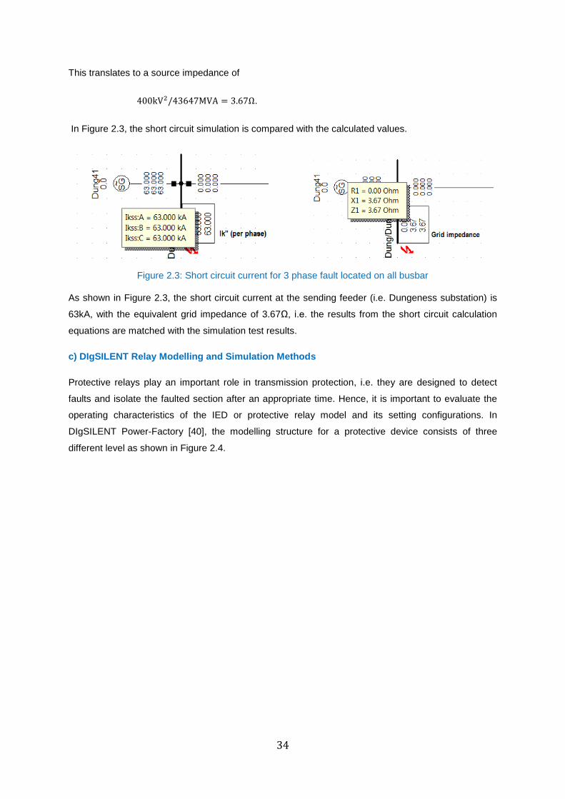
34

This translates to a source impedance of

400kV2/43647MVA = 3.67Ω.

In Figure 2.3, the short circuit simulation is compared with the calculated values.

Figure 2.3: Short circuit current for 3 phase fault located on all busbar

As shown in Figure 2.3, the short circuit current at the sending feeder (i.e. Dungeness substation) is

63kA, with the equivalent grid impedance of 3.67Ω, i.e. the results from the short circuit calculation

equations are matched with the simulation test results.

c) DIgSILENT Relay Modelling and Simulation Methods

Protective relays play an important role in transmission protection, i.e. they are designed to detect

faults and isolate the faulted section after an appropriate time. Hence, it is important to evaluate the

operating characteristics of the IED or protective relay model and its setting configurations. In

DIgSILENT Power-Factory [40], the modelling structure for a protective device consists of three

different level as shown in Figure 2.4.

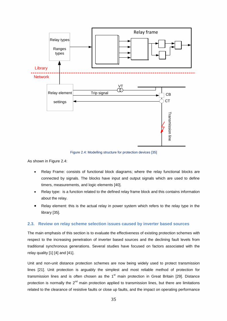
35

Library

Network

Relay element

settings

Trip signal CB

CT

VT

Relay types

Ranges

types

Relay frame

Tra

nsm

issio

n lin

e

Figure 2.4: Modelling structure for protection devices [35]

As shown in Figure 2.4:

Relay Frame: consists of functional block diagrams; where the relay functional blocks are

connected by signals. The blocks have input and output signals which are used to define

timers, measurements, and logic elements [40].

Relay type: is a function related to the defined relay frame block and this contains information

about the relay.

Relay element: this is the actual relay in power system which refers to the relay type in the

library [35].

2.3. Review on relay scheme selection issues caused by inverter based sources

The main emphasis of this section is to evaluate the effectiveness of existing protection schemes with

respect to the increasing penetration of inverter based sources and the declining fault levels from

traditional synchronous generations. Several studies have focused on factors associated with the

relay quality [1] [4] and [41].

Unit and non-unit distance protection schemes are now being widely used to protect transmission

lines [21]. Unit protection is arguably the simplest and most reliable method of protection for

transmission lines and is often chosen as the 1st main protection in Great Britain [29]. Distance

protection is normally the 2nd

main protection applied to transmission lines, but there are limitations

related to the clearance of resistive faults or close up faults, and the impact on operating performance

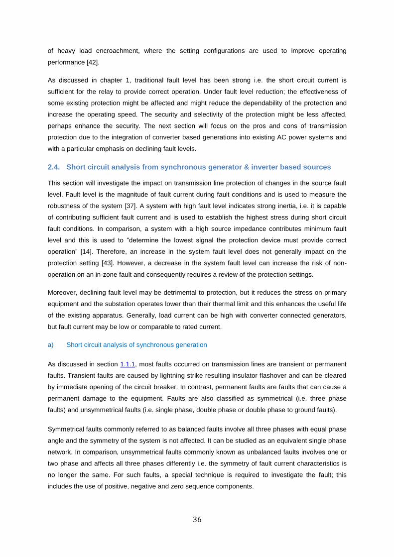
36

of heavy load encroachment, where the setting configurations are used to improve operating

performance [42].

As discussed in chapter 1, traditional fault level has been strong i.e. the short circuit current is

sufficient for the relay to provide correct operation. Under fault level reduction; the effectiveness of

some existing protection might be affected and might reduce the dependability of the protection and

increase the operating speed. The security and selectivity of the protection might be less affected,

perhaps enhance the security. The next section will focus on the pros and cons of transmission

protection due to the integration of converter based generations into existing AC power systems and

with a particular emphasis on declining fault levels.

2.4. Short circuit analysis from synchronous generator & inverter based sources

This section will investigate the impact on transmission line protection of changes in the source fault

level. Fault level is the magnitude of fault current during fault conditions and is used to measure the

robustness of the system [37]. A system with high fault level indicates strong inertia, i.e. it is capable

of contributing sufficient fault current and is used to establish the highest stress during short circuit

fault conditions. In comparison, a system with a high source impedance contributes minimum fault

level and this is used to “determine the lowest signal the protection device must provide correct

operation” [14]. Therefore, an increase in the system fault level does not generally impact on the

protection setting [43]. However, a decrease in the system fault level can increase the risk of non-

operation on an in-zone fault and consequently requires a review of the protection settings.

Moreover, declining fault level may be detrimental to protection, but it reduces the stress on primary

equipment and the substation operates lower than their thermal limit and this enhances the useful life

of the existing apparatus. Generally, load current can be high with converter connected generators,

but fault current may be low or comparable to rated current.

a) Short circuit analysis of synchronous generation

As discussed in section 1.1.1, most faults occurred on transmission lines are transient or permanent

faults. Transient faults are caused by lightning strike resulting insulator flashover and can be cleared

by immediate opening of the circuit breaker. In contrast, permanent faults are faults that can cause a

permanent damage to the equipment. Faults are also classified as symmetrical (i.e. three phase

faults) and unsymmetrical faults (i.e. single phase, double phase or double phase to ground faults).

Symmetrical faults commonly referred to as balanced faults involve all three phases with equal phase

angle and the symmetry of the system is not affected. It can be studied as an equivalent single phase

network. In comparison, unsymmetrical faults commonly known as unbalanced faults involves one or

two phase and affects all three phases differently i.e. the symmetry of fault current characteristics is

no longer the same. For such faults, a special technique is required to investigate the fault; this

includes the use of positive, negative and zero sequence components.

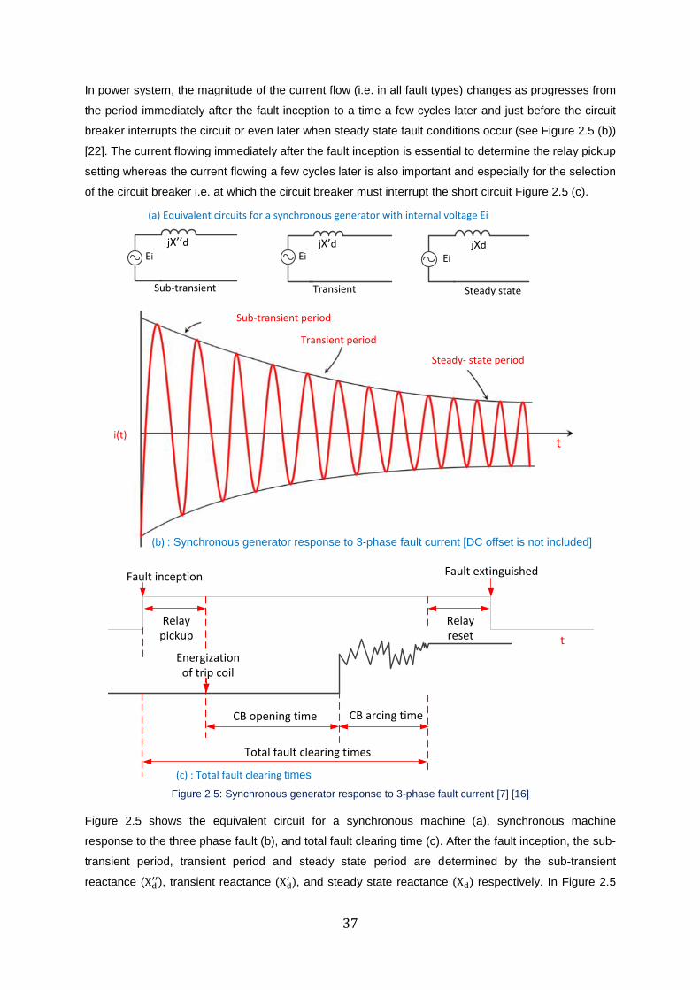
37

In power system, the magnitude of the current flow (i.e. in all fault types) changes as progresses from

the period immediately after the fault inception to a time a few cycles later and just before the circuit

breaker interrupts the circuit or even later when steady state fault conditions occur (see Figure 2.5 (b))

[22]. The current flowing immediately after the fault inception is essential to determine the relay pickup

setting whereas the current flowing a few cycles later is also important and especially for the selection

of the circuit breaker i.e. at which the circuit breaker must interrupt the short circuit Figure 2.5 (c).

(a) Equivalent circuits for a synchronous generator with internal voltage Ei

Relay pickup

Relay reset

Fault inception Fault extinguished

Total fault clearing times

CB opening time CB arcing time

Transient period

Sub-transient period

Steady- state period

i(t)t

jX’’d jX’d jXdEi Ei Ei

Sub-transient Transient Steady state

(b) : Synchronous generator response to 3-phase fault current [DC offset is not included]

(c) : Total fault clearing times

t

Energization of trip coil

Figure 2.5: Synchronous generator response to 3-phase fault current [7] [16]

Figure 2.5 shows the equivalent circuit for a synchronous machine (a), synchronous machine

response to the three phase fault (b), and total fault clearing time (c). After the fault inception, the sub-

transient period, transient period and steady state period are determined by the sub-transient

reactance (Xd′′), transient reactance (Xd

′ ), and steady state reactance (Xd) respectively. In Figure 2.5

38

(b), the fault current magnitude decreases as a function of time. The sub-transient current commonly

referred to as the initial symmetrical rms current is much larger than the steady state because the

sub-transient reactance (Xd′′) is much smaller than the steady state reactance (Xd). The transient

current is also smaller than the sub-transient, but larger than the steady state current (i.e. |Id′′| > |Id

′ | >

|Id| or Xd′′ < Xd

′ < Xd ).

According to [16], synchronous generation is capable of providing fault current up to 6 times its rated

current immediately after the fault, but a few cycles later it will have it reduced to 400%-200% of rated

current. From [16], the sub-transient period is the first few cycles or after the fault when the fault

current is very large & falls rapidly whereas the transient period is when the fault current falls at a

slower rate. Steady state period on the other hand is when a fault current reaches the steady value. In

Figure 2.5 (c), the circuit breaker must withstand the maximum instantaneous current and interrupt

the total short circuit current. The basic definitions and assumptions during the fault conditions are

provided as follows:

Initial peak short circuit current (ip) or asymmetrical peak which is the 1st peak and the largest

current after fault inception. 𝑖𝑝 = 𝑘 × √2 × 𝐼𝑘 𝑤ℎ𝑒𝑟𝑒 𝑘 = 1.02 + 0.98𝑒−3𝑅

𝑋. This is the short

circuit current where the circuit breaker must be able to close onto the event.

Ik = steady state current which is a symmetrical fault current

Peak make current: is the maximum possible instantaneous value of the prospective short

circuit current. Normally, peak make occurs at the first ac peak after fault inception. Due to the

the short time has elapsed; since the fault occurred there is minimum decay of the dc

component [22] [36].

Ib = peak break current,: is the largest instantaneous short circuit current the circuit breaker

may be required to extinguish during the arcing period, taking account the protection

operating time.

RMS break current, Ib: is the RMS value of the ac component of the short circuit current at the

instant when the circuit breaker is required to open and this takes no account of the dc

component. This is effectively the nominal rating of the equipment and can be calculated

using the break time (i.e. the break time for 275kV and 400kV is 50ms, and for 132kV is 70ms

on the GB network) [44]. Transient faults are used for protection study. In addition, the making

capacity of switchboard is 2.5 times the breaking capacity of the switchboard (i.e specified in

BS EN 62271-100 standard for High-voltage switchgear and control gear) [9].

Total fault clearing time: is the time from the fault occurrence to CB opening. The protection

trip contacts normally close 40-60ms before CB opens.

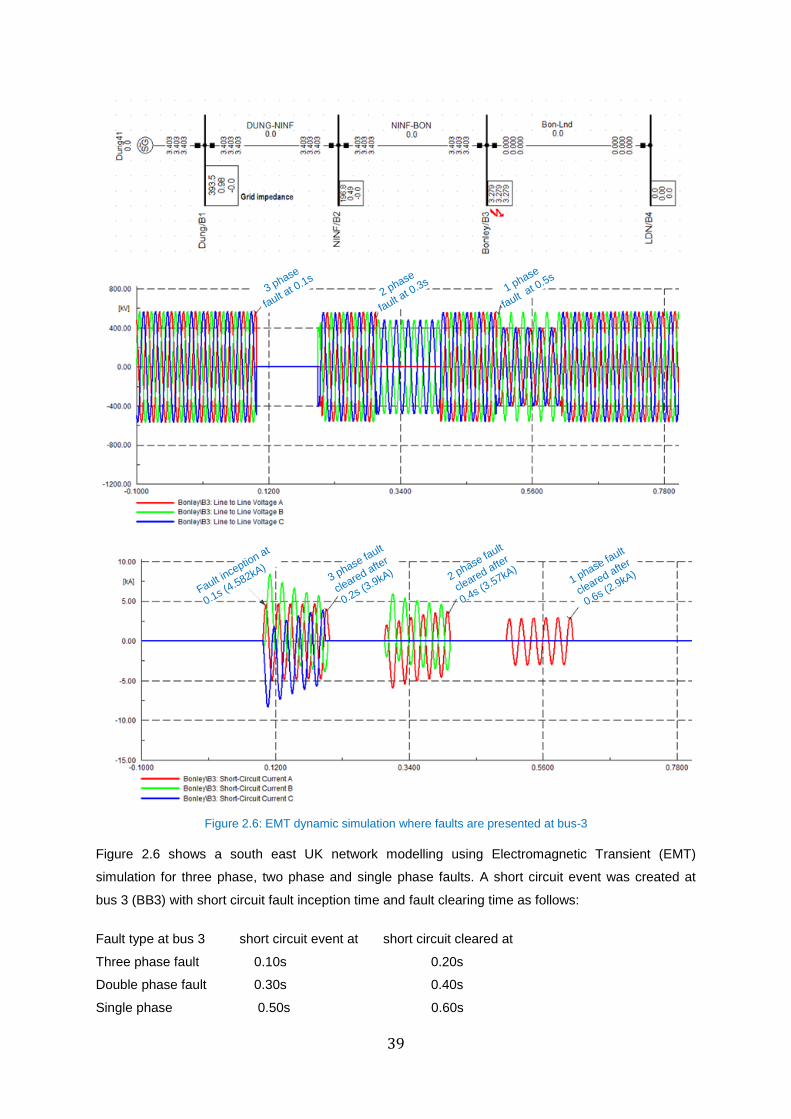
39

3 phase fault

cleared after

0.2s (3.9kA) 2 phase fa

ult

cleared after

0.4s (3.57kA)

1 phase fault

cleared after

0.6s (2.9kA)

Fault inceptio

n at

0.1s (4.582kA)

3 phase

fault at 0

.1s

2 phase

fault at 0

.3s1 phase

fault at 0

.5s

Figure 2.6: EMT dynamic simulation where faults are presented at bus-3

Figure 2.6 shows a south east UK network modelling using Electromagnetic Transient (EMT)

simulation for three phase, two phase and single phase faults. A short circuit event was created at

bus 3 (BB3) with short circuit fault inception time and fault clearing time as follows:

Fault type at bus 3 short circuit event at short circuit cleared at

Three phase fault 0.10s 0.20s

Double phase fault 0.30s 0.40s

Single phase 0.50s 0.60s

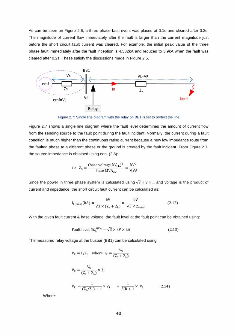
40

As can be seen on Figure 2.6, a three phase fault event was placed at 0.1s and cleared after 0.2s.

The magnitude of current flow immediately after the fault is larger than the current magnitude just

before the short circuit fault current was cleared. For example, the initial peak value of the three

phase fault immediately after the fault inception is 4.582kA and reduced to 3.9kA when the fault was

cleared after 0.2s. These satisfy the discussions made in Figure 2.5.

emf

Relay

ZLZs

BB1

IR

VL=VRVs

emf=Vs VR IR=If

Figure 2.7: Single line diagram with the relay on BB1 is set to protect the line

Figure 2.7 shows a single line diagram where the fault level determines the amount of current flow

from the sending source to the fault point during the fault incident. Normally, the current during a fault

condition is much higher than the continuous rating current because a new low impedance route from

the faulted phase to a different phase or the ground is created by the fault incident. From Figure 2.7,

the source impedance is obtained using eqn. (2.8):

i. e ZS =(base voltage, kVLL)2

base MVA3∅

=kV2

MVA

Since the power in three phase system is calculated using √3 × V × I, and voltage is the product of

current and impedance; the short circuit fault current can be calculated as:

If (rms)(kA) =kV

√3 × (Zs + ZL)=

kV

√3 × Ztotal

(2.12)

With the given fault current & base voltage, the fault level at the fault point can be obtained using:

Fault level, 𝑆𝐶𝐶𝑀𝑉𝐴 = √3 × kV × kA (2.13)

The measured relay voltage at the busbar (BB1) can be calculated using:

VR = IRZL where IR =VS

(Zs + ZL)

VR =VS

(Zs + ZL)× ZL

VR =1

(Zs/ZL) + 1× VS =

1

SIR + 1× VS (2.14)

Where:

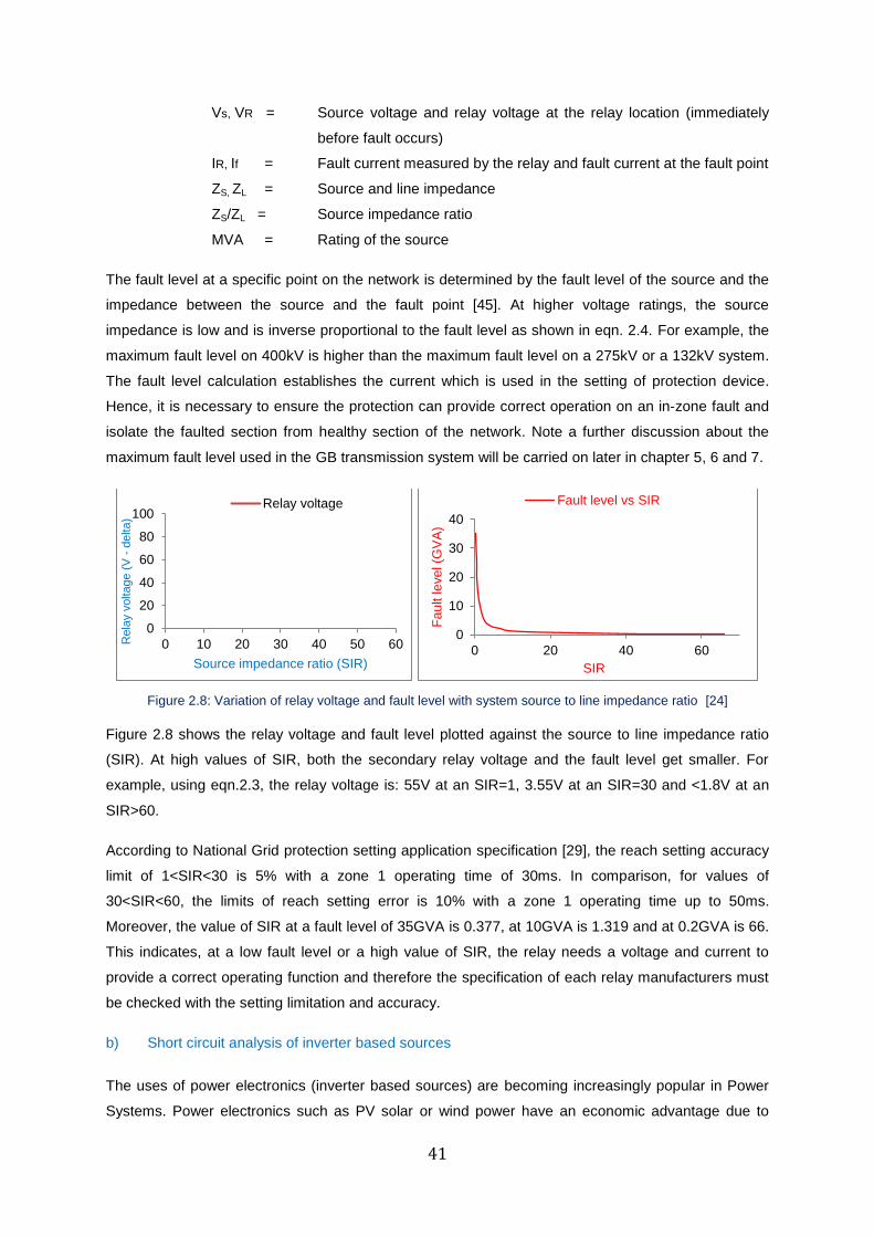
41

Vs, VR = Source voltage and relay voltage at the relay location (immediately

before fault occurs)

IR, If = Fault current measured by the relay and fault current at the fault point

ZS, ZL = Source and line impedance

ZS/ZL = Source impedance ratio

MVA = Rating of the source

The fault level at a specific point on the network is determined by the fault level of the source and the

impedance between the source and the fault point [45]. At higher voltage ratings, the source

impedance is low and is inverse proportional to the fault level as shown in eqn. 2.4. For example, the

maximum fault level on 400kV is higher than the maximum fault level on a 275kV or a 132kV system.

The fault level calculation establishes the current which is used in the setting of protection device.

Hence, it is necessary to ensure the protection can provide correct operation on an in-zone fault and

isolate the faulted section from healthy section of the network. Note a further discussion about the

maximum fault level used in the GB transmission system will be carried on later in chapter 5, 6 and 7.

Figure 2.8: Variation of relay voltage and fault level with system source to line impedance ratio [24]

Figure 2.8 shows the relay voltage and fault level plotted against the source to line impedance ratio

(SIR). At high values of SIR, both the secondary relay voltage and the fault level get smaller. For

example, using eqn.2.3, the relay voltage is: 55V at an SIR=1, 3.55V at an SIR=30 and <1.8V at an

SIR>60.

According to National Grid protection setting application specification [29], the reach setting accuracy

limit of 1<SIR<30 is 5% with a zone 1 operating time of 30ms. In comparison, for values of

30<SIR<60, the limits of reach setting error is 10% with a zone 1 operating time up to 50ms.

Moreover, the value of SIR at a fault level of 35GVA is 0.377, at 10GVA is 1.319 and at 0.2GVA is 66.

This indicates, at a low fault level or a high value of SIR, the relay needs a voltage and current to

provide a correct operating function and therefore the specification of each relay manufacturers must

be checked with the setting limitation and accuracy.

b) Short circuit analysis of inverter based sources

The uses of power electronics (inverter based sources) are becoming increasingly popular in Power

Systems. Power electronics such as PV solar or wind power have an economic advantage due to

0

20

40

60

80

100

0 10 20 30 40 50 60Rela

y v

oltage (

V -

delta)

Source impedance ratio (SIR)

Relay voltage

0

10

20

30

40

0 20 40 60

Fa

ult le

ve

l (G

VA

)

SIR

Fault level vs SIR

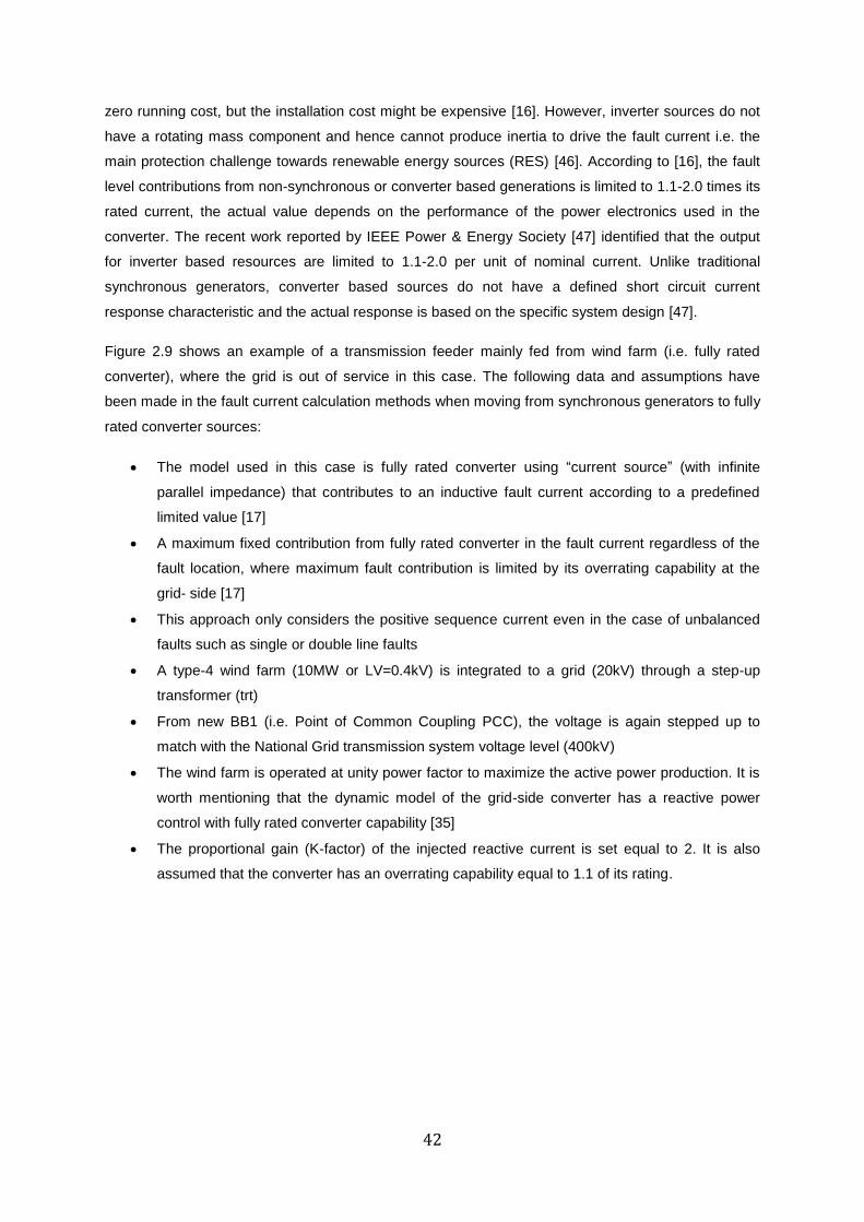
42

zero running cost, but the installation cost might be expensive [16]. However, inverter sources do not

have a rotating mass component and hence cannot produce inertia to drive the fault current i.e. the

main protection challenge towards renewable energy sources (RES) [46]. According to [16], the fault

level contributions from non-synchronous or converter based generations is limited to 1.1-2.0 times its

rated current, the actual value depends on the performance of the power electronics used in the

converter. The recent work reported by IEEE Power & Energy Society [47] identified that the output

for inverter based resources are limited to 1.1-2.0 per unit of nominal current. Unlike traditional

synchronous generators, converter based sources do not have a defined short circuit current

response characteristic and the actual response is based on the specific system design [47].

Figure 2.9 shows an example of a transmission feeder mainly fed from wind farm (i.e. fully rated

converter), where the grid is out of service in this case. The following data and assumptions have

been made in the fault current calculation methods when moving from synchronous generators to fully

rated converter sources:

The model used in this case is fully rated converter using “current source” (with infinite

parallel impedance) that contributes to an inductive fault current according to a predefined

limited value [17]

A maximum fixed contribution from fully rated converter in the fault current regardless of the

fault location, where maximum fault contribution is limited by its overrating capability at the

grid- side [17]

This approach only considers the positive sequence current even in the case of unbalanced

faults such as single or double line faults

A type-4 wind farm (10MW or LV=0.4kV) is integrated to a grid (20kV) through a step-up

transformer (trt)

From new BB1 (i.e. Point of Common Coupling PCC), the voltage is again stepped up to

match with the National Grid transmission system voltage level (400kV)

The wind farm is operated at unity power factor to maximize the active power production. It is

worth mentioning that the dynamic model of the grid-side converter has a reactive power

control with fully rated converter capability [35]

The proportional gain (K-factor) of the injected reactive current is set equal to 2. It is also

assumed that the converter has an overrating capability equal to 1.1 of its rating.

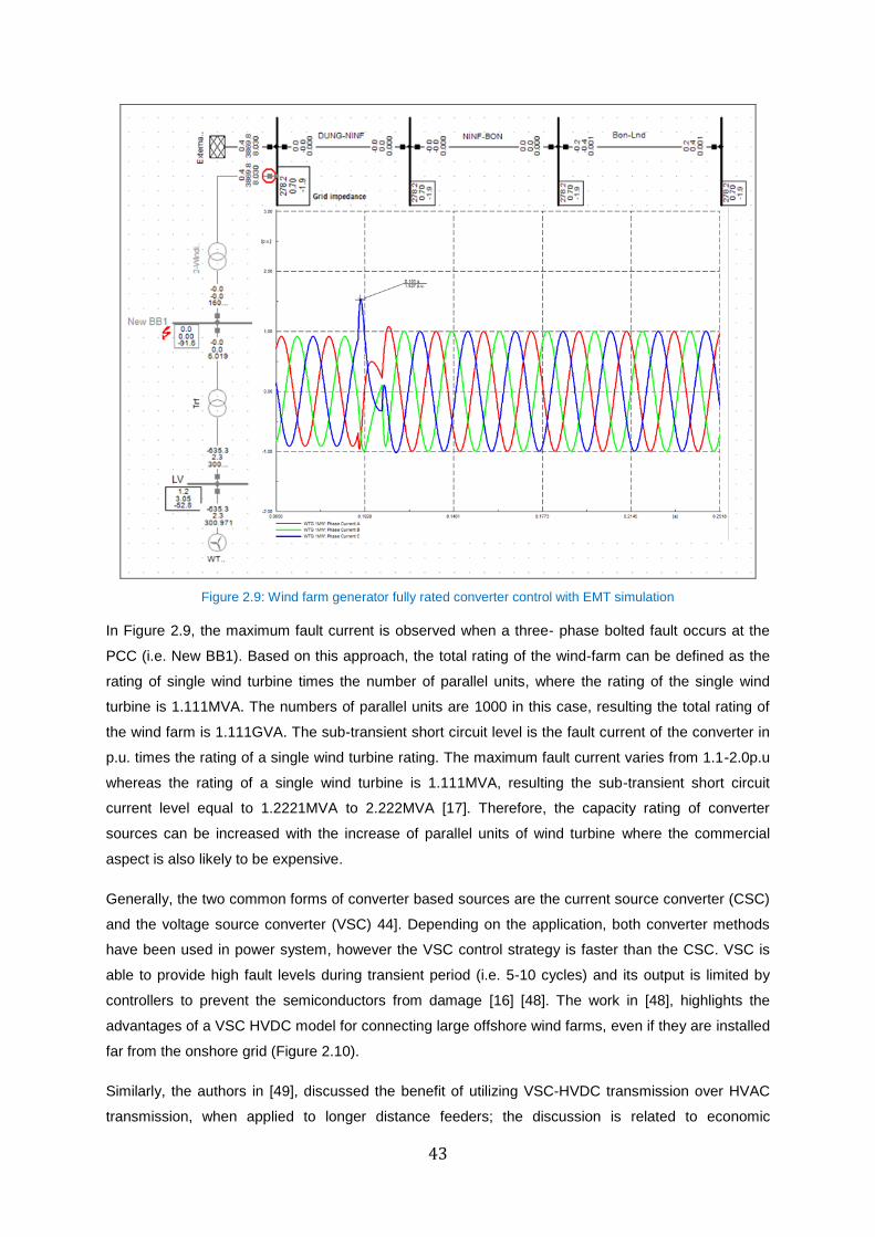
43

Figure 2.9: Wind farm generator fully rated converter control with EMT simulation

In Figure 2.9, the maximum fault current is observed when a three- phase bolted fault occurs at the

PCC (i.e. New BB1). Based on this approach, the total rating of the wind-farm can be defined as the

rating of single wind turbine times the number of parallel units, where the rating of the single wind

turbine is 1.111MVA. The numbers of parallel units are 1000 in this case, resulting the total rating of

the wind farm is 1.111GVA. The sub-transient short circuit level is the fault current of the converter in

p.u. times the rating of a single wind turbine rating. The maximum fault current varies from 1.1-2.0p.u

whereas the rating of a single wind turbine is 1.111MVA, resulting the sub-transient short circuit

current level equal to 1.2221MVA to 2.222MVA [17]. Therefore, the capacity rating of converter

sources can be increased with the increase of parallel units of wind turbine where the commercial

aspect is also likely to be expensive.

Generally, the two common forms of converter based sources are the current source converter (CSC)

and the voltage source converter (VSC) 44]. Depending on the application, both converter methods

have been used in power system, however the VSC control strategy is faster than the CSC. VSC is

able to provide high fault levels during transient period (i.e. 5-10 cycles) and its output is limited by

controllers to prevent the semiconductors from damage [16] [48]. The work in [48], highlights the

advantages of a VSC HVDC model for connecting large offshore wind farms, even if they are installed

far from the onshore grid (Figure 2.10).

Similarly, the authors in [49], discussed the benefit of utilizing VSC-HVDC transmission over HVAC

transmission, when applied to longer distance feeders; the discussion is related to economic

44

advantages, and the freedom of control by allowing independent control of active and reactive power.

However, the limitation of VSCs includes sensitivity during grid voltage dips and unbalanced current

injection [50].

Transformer

Converter

- DC

HVDC line to

wind farm

+ DC

BusbarBusbar

AC grid

Reactance

Figure 2.10: VSC HVDC system model

The system shown in Figure 2.10 represents a VSC HVDC system model which can be modelled in

DIgSILENT PowerFactory. In power system analysis, power flow or load flow studies are of great

importance in planning and designing the future expansion of systems [22]. Hence, load flow

calculation is used to determine the voltage magnitude (V), angle of the nodes (θ), active power (P),

and reactive power (Q). The document in [35] defines the different types of network nodes used for

load flow calculations. These are:

i. PV nodes: where the active power and voltage magnitude are known, and are used to

represent generators and synchronouse condensers.

ii. PQ nodes: the active and reactive power are specified, and are used to represent loads and

machines with fixed values. PQ control method is widely used to calculate initial conditions

for a fast current-controller.

iii. Slack node: where the voltage magnitude and angle are fixed (i.e. external grid)

iv. Device node: special nodes used to represent devices such as HVDC converters and SVCs;

these have specific control conditions such as the control of active power flow at a certain

MW threshold in an HVDC converter.

2.5. Review on protection challenges in converter dominated power system

In future energy scenarios, the system strength will be determined by the a large penetration of

renewable generation, and this resulted in a low fault level or reduced inertia [18]. Consequently, this

has a negative impact on system stability and protection settings [46]. The latter is the main focus of

this thesis.

Numerous research has been completed on the protection challenges associated with a high

penetration of converter based generation. The authors in [13] highlights the impact of converter

dominated power systems on existing protection challenges. The author’s main finding includes an

increase in the operating time of zone 1 distance relays when the penetration level of converter

source increases from 0% to 100%. The increase is from 15.4ms to 31ms for three phase faults

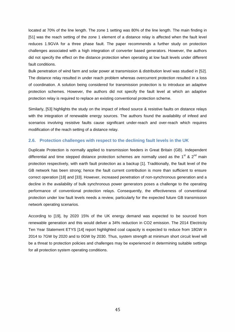
45

located at 70% of the line length. The zone 1 setting was 80% of the line length. The main finding in

[51] was the reach setting of the zone 1 element of a distance relay is affected when the fault level

reduces 1.9GVA for a three phase fault. The paper recommends a further study on protection

challenges associated with a high integration of converter based generators. However, the authors

did not specify the effect on the distance protection when operating at low fault levels under different

fault conditions.

Bulk penetration of wind farm and solar power at transmission & distribution level was studied in [52].

The distance relay resulted in under reach problem whereas overcurrent protection resulted in a loss

of coordination. A solution being considered for transmission protection is to introduce an adaptive

protection schemes. However, the authors did not specify the fault level at which an adaptive

protection relay is required to replace an existing conventional protection scheme.

Similarly, [53] highlights the study on the impact of infeed source & resistive faults on distance relays

with the integration of renewable energy sources. The authors found the availability of infeed and

scenarios involving resistive faults cause significant under-reach and over-reach which requires

modification of the reach setting of a distance relay.

2.6. Protection challenges with respect to the declining fault levels in the UK

Duplicate Protection is normally applied to transmission feeders in Great Britain (GB). Independent

differential and time stepped distance protection schemes are normally used as the 1st & 2

nd main

protection respectively, with earth fault protection as a backup [1]. Traditionally, the fault level of the

GB network has been strong; hence the fault current contribution is more than sufficient to ensure

correct operation [18] and [33]. However, increased penetration of non-synchronous generation and a

decline in the availability of bulk synchronous power generators poses a challenge to the operating

performance of conventional protection relays. Consequently, the effectiveness of conventional

protection under low fault levels needs a review, particularly for the expected future GB transmission

network operating scenarios.

According to [19], by 2020 15% of the UK energy demand was expected to be sourced from

renewable generation and this would deliver a 34% reduction in CO2 emission. The 2014 Electricity

Ten Year Statement ETYS [14] report highlighted coal capacity is expected to reduce from 18GW in

2014 to 7GW by 2020 and to 0GW by 2030. Thus, system strength at minimum short circuit level will

be a threat to protection policies and challenges may be experienced in determining suitable settings

for all protection system operating conditions.

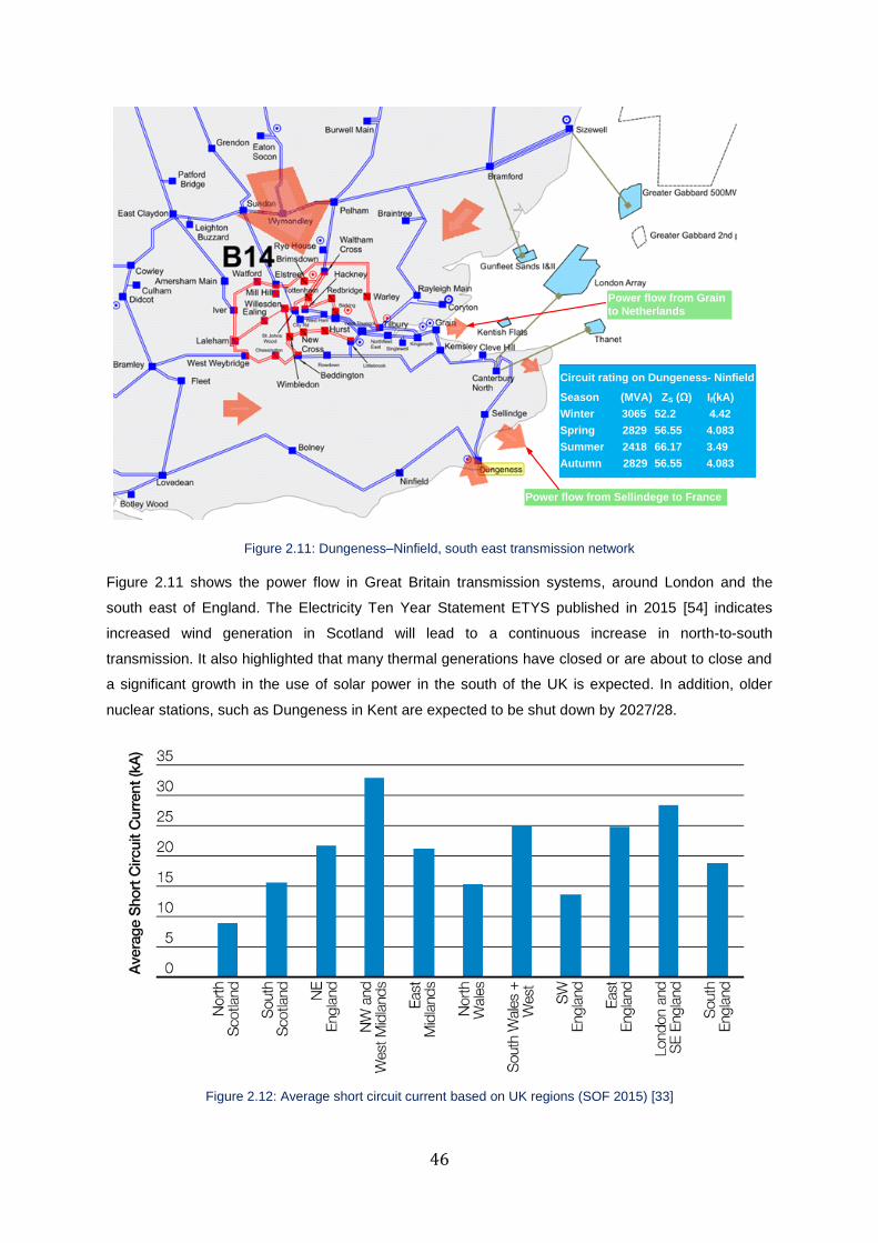
46

Season (MVA) ZS (Ω) If(kA)

Winter 3065 52.2 4.42

Spring 2829 56.55 4.083

Summer 2418 66.17 3.49

Autumn 2829 56.55 4.083

Circuit rating on Dungeness- Ninfield

Power flow from Sellindege to France

Power flow from Grain

to Netherlands

Figure 2.11: Dungeness–Ninfield, south east transmission network

Figure 2.11 shows the power flow in Great Britain transmission systems, around London and the

south east of England. The Electricity Ten Year Statement ETYS published in 2015 [54] indicates

increased wind generation in Scotland will lead to a continuous increase in north-to-south

transmission. It also highlighted that many thermal generations have closed or are about to close and

a significant growth in the use of solar power in the south of the UK is expected. In addition, older

nuclear stations, such as Dungeness in Kent are expected to be shut down by 2027/28.

Figure 2.12: Average short circuit current based on UK regions (SOF 2015) [33]

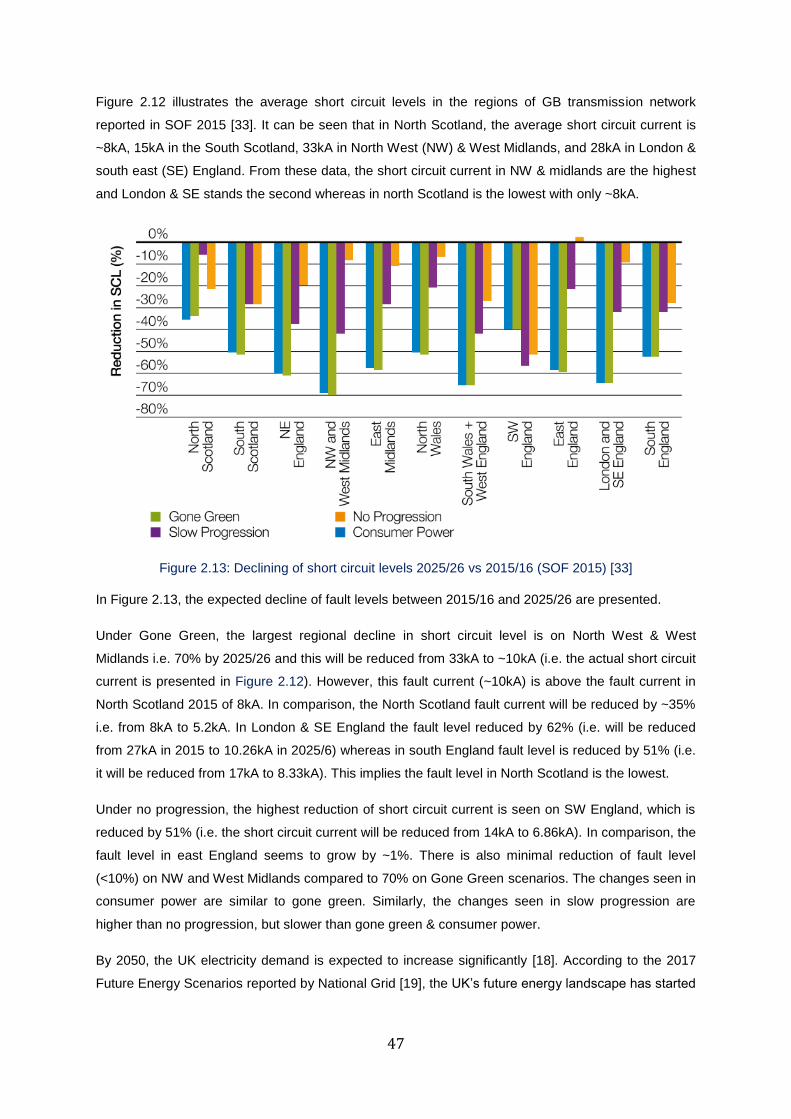
47

Figure 2.12 illustrates the average short circuit levels in the regions of GB transmission network

reported in SOF 2015 [33]. It can be seen that in North Scotland, the average short circuit current is

~8kA, 15kA in the South Scotland, 33kA in North West (NW) & West Midlands, and 28kA in London &

south east (SE) England. From these data, the short circuit current in NW & midlands are the highest

and London & SE stands the second whereas in north Scotland is the lowest with only ~8kA.

Figure 2.13: Declining of short circuit levels 2025/26 vs 2015/16 (SOF 2015) [33]

In Figure 2.13, the expected decline of fault levels between 2015/16 and 2025/26 are presented.

Under Gone Green, the largest regional decline in short circuit level is on North West & West

Midlands i.e. 70% by 2025/26 and this will be reduced from 33kA to ~10kA (i.e. the actual short circuit

current is presented in Figure 2.12). However, this fault current (~10kA) is above the fault current in

North Scotland 2015 of 8kA. In comparison, the North Scotland fault current will be reduced by ~35%

i.e. from 8kA to 5.2kA. In London & SE England the fault level reduced by 62% (i.e. will be reduced

from 27kA in 2015 to 10.26kA in 2025/6) whereas in south England fault level is reduced by 51% (i.e.

it will be reduced from 17kA to 8.33kA). This implies the fault level in North Scotland is the lowest.

Under no progression, the highest reduction of short circuit current is seen on SW England, which is

reduced by 51% (i.e. the short circuit current will be reduced from 14kA to 6.86kA). In comparison, the

fault level in east England seems to grow by ~1%. There is also minimal reduction of fault level

(<10%) on NW and West Midlands compared to 70% on Gone Green scenarios. The changes seen in

consumer power are similar to gone green. Similarly, the changes seen in slow progression are

higher than no progression, but slower than gone green & consumer power.

By 2050, the UK electricity demand is expected to increase significantly [18]. According to the 2017

Future Energy Scenarios reported by National Grid [19], the UK’s future energy landscape has started

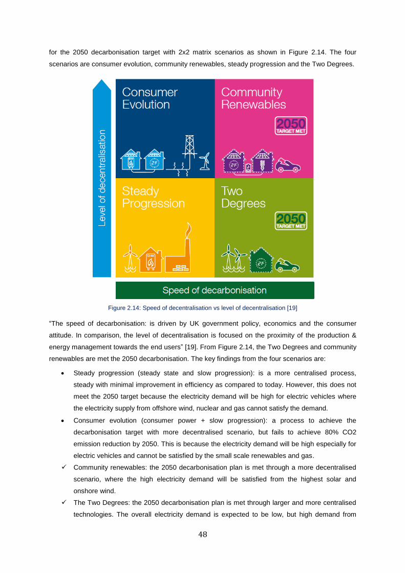
48

for the 2050 decarbonisation target with 2x2 matrix scenarios as shown in Figure 2.14. The four

scenarios are consumer evolution, community renewables, steady progression and the Two Degrees.

Figure 2.14: Speed of decentralisation vs level of decentralisation [19]

“The speed of decarbonisation: is driven by UK government policy, economics and the consumer

attitude. In comparison, the level of decentralisation is focused on the proximity of the production &

energy management towards the end users” [19]. From Figure 2.14, the Two Degrees and community

renewables are met the 2050 decarbonisation. The key findings from the four scenarios are:

Steady progression (steady state and slow progression): is a more centralised process,

steady with minimal improvement in efficiency as compared to today. However, this does not

meet the 2050 target because the electricity demand will be high for electric vehicles where

the electricity supply from offshore wind, nuclear and gas cannot satisfy the demand.

Consumer evolution (consumer power + slow progression): a process to achieve the

decarbonisation target with more decentralised scenario, but fails to achieve 80% CO2

emission reduction by 2050. This is because the electricity demand will be high especially for

electric vehicles and cannot be satisfied by the small scale renewables and gas.

Community renewables: the 2050 decarbonisation plan is met through a more decentralised

scenario, where the high electricity demand will be satisfied from the highest solar and

onshore wind.

The Two Degrees: the 2050 decarbonisation plan is met through larger and more centralised

technologies. The overall electricity demand is expected to be low, but high demand from

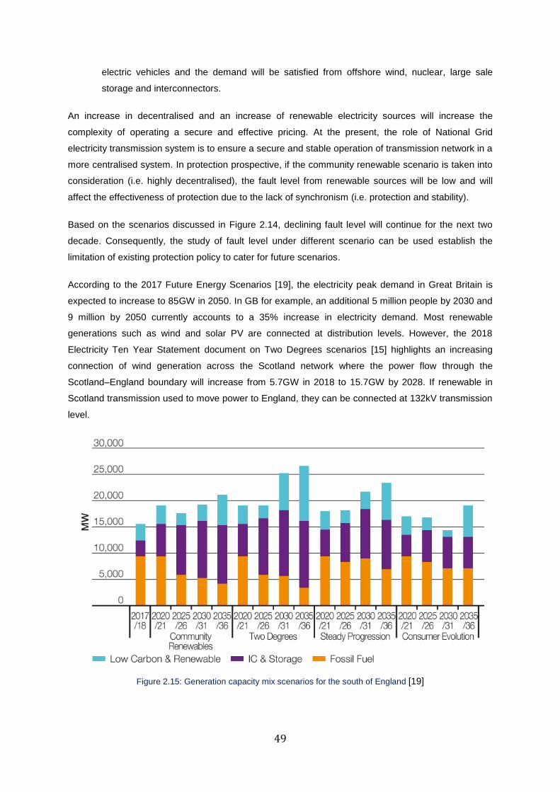
49

electric vehicles and the demand will be satisfied from offshore wind, nuclear, large sale

storage and interconnectors.

An increase in decentralised and an increase of renewable electricity sources will increase the

complexity of operating a secure and effective pricing. At the present, the role of National Grid

electricity transmission system is to ensure a secure and stable operation of transmission network in a

more centralised system. In protection prospective, if the community renewable scenario is taken into

consideration (i.e. highly decentralised), the fault level from renewable sources will be low and will

affect the effectiveness of protection due to the lack of synchronism (i.e. protection and stability).

Based on the scenarios discussed in Figure 2.14, declining fault level will continue for the next two

decade. Consequently, the study of fault level under different scenario can be used establish the

limitation of existing protection policy to cater for future scenarios.

According to the 2017 Future Energy Scenarios [19], the electricity peak demand in Great Britain is

expected to increase to 85GW in 2050. In GB for example, an additional 5 million people by 2030 and

9 million by 2050 currently accounts to a 35% increase in electricity demand. Most renewable

generations such as wind and solar PV are connected at distribution levels. However, the 2018

Electricity Ten Year Statement document on Two Degrees scenarios [15] highlights an increasing

connection of wind generation across the Scotland network where the power flow through the

Scotland–England boundary will increase from 5.7GW in 2018 to 15.7GW by 2028. If renewable in

Scotland transmission used to move power to England, they can be connected at 132kV transmission

level.

Figure 2.15: Generation capacity mix scenarios for the south of England [19]

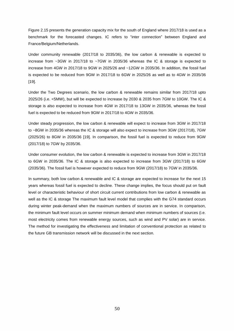
50

Figure 2.15 presents the generation capacity mix for the south of England where 2017/18 is used as a

benchmark for the forecasted changes. IC refers to “inter connection” between England and

France/Belgium/Netherlands.

Under community renewable (2017/18 to 2035/36), the low carbon & renewable is expected to

increase from ~3GW in 2017/18 to ~7GW in 2035/36 whereas the IC & storage is expected to

increase from 4GW in 2017/18 to 9GW in 2025/26 and ~12GW in 2035/36. In addition, the fossil fuel

is expected to be reduced from 9GW in 2017/18 to 6GW in 2025/26 as well as to 4GW in 2035/36

[19].

Under the Two Degrees scenario, the low carbon & renewable remains similar from 2017/18 upto

2025/26 (i.e. <5MW), but will be expected to increase by 2030 & 2035 from 7GW to 10GW. The IC &

storage is also expected to increase from 4GW in 2017/18 to 13GW in 2035/36, whereas the fossil

fuel is expected to be reduced from 9GW in 2017/18 to 4GW in 2035/36.

Under steady progression, the low carbon & renewable will expect to increase from 3GW in 2017/18

to ~8GW in 2035/36 whereas the IC & storage will also expect to increase from 3GW (2017/18), 7GW

(2025/26) to 8GW in 2035/36 [19]. In comparison, the fossil fuel is expected to reduce from 9GW

(2017/18) to 7GW by 2035/36.

Under consumer evolution, the low carbon & renewable is expected to increase from 3GW in 2017/18

to 6GW in 2035/36. The IC & storage is also expected to increase from 3GW (2017/18) to 6GW

(2035/36). The fossil fuel is however expected to reduce from 9GW (2017/18) to 7GW in 2035/36.

In summary, both low carbon & renewable and IC & storage are expected to increase for the next 15

years whereas fossil fuel is expected to decline. These change implies, the focus should put on fault

level or characteristic behaviour of short circuit current contributions from low carbon & renewable as

well as the IC & storage The maximum fault level model that complies with the G74 standard occurs

during winter peak-demand when the maximum numbers of sources are in service. In comparison,

the minimum fault level occurs on summer minimum demand when minimum numbers of sources (i.e.

most electricity comes from renewable energy sources, such as wind and PV solar) are in service.

The method for investigating the effectiveness and limitation of conventional protection as related to

the future GB transmission network will be discussed in the next section.

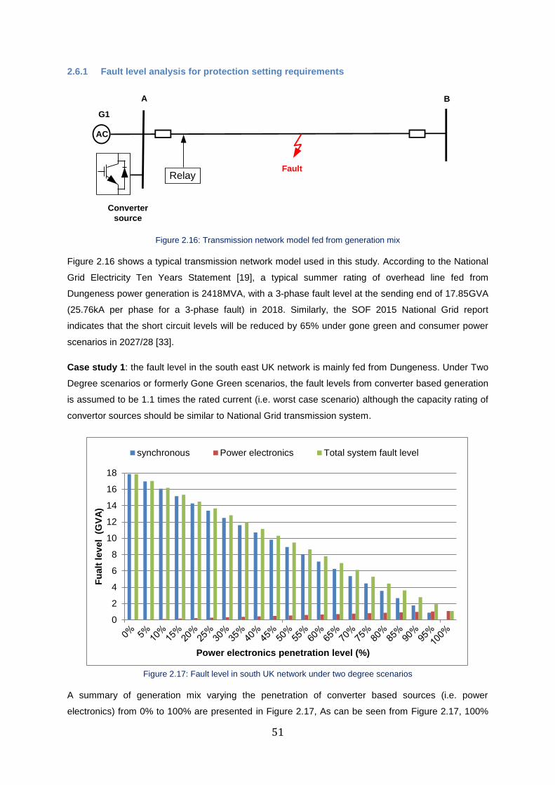
51

2.6.1 Fault level analysis for protection setting requirements

G1

AC

A B

Fault

Converter

source

Relay

Figure 2.16: Transmission network model fed from generation mix

Figure 2.16 shows a typical transmission network model used in this study. According to the National

Grid Electricity Ten Years Statement [19], a typical summer rating of overhead line fed from

Dungeness power generation is 2418MVA, with a 3-phase fault level at the sending end of 17.85GVA

(25.76kA per phase for a 3-phase fault) in 2018. Similarly, the SOF 2015 National Grid report

indicates that the short circuit levels will be reduced by 65% under gone green and consumer power

scenarios in 2027/28 [33].

Case study 1: the fault level in the south east UK network is mainly fed from Dungeness. Under Two

Degree scenarios or formerly Gone Green scenarios, the fault levels from converter based generation

is assumed to be 1.1 times the rated current (i.e. worst case scenario) although the capacity rating of

convertor sources should be similar to National Grid transmission system.

Figure 2.17: Fault level in south UK network under two degree scenarios

A summary of generation mix varying the penetration of converter based sources (i.e. power

electronics) from 0% to 100% are presented in Figure 2.17, As can be seen from Figure 2.17, 100%

0

2

4

6

8

10

12

14

16

18

Fu

alt

lev

el

(G

VA

)

Power electronics penetration level (%)

synchronous Power electronics Total system fault level

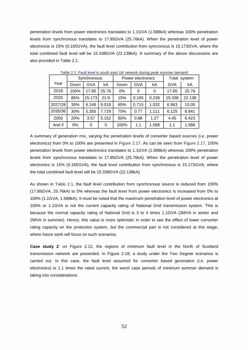
52

penetration levels from power electronics translates to 1.1GVA (1.588kA) whereas 100% penetration

levels from synchronous translates to 17.85GVA (25.76kA). When the penetration level of power

electroncis is 15% (0.165GVA), the fault level contribution from syncronous is 15.173GVA, where the

total combined fault level will be 15.338GVA (22.138kA). A summary of the above discussions are

also provided in Table 2.1.

Table 2.1: Fault level in south east UK network during peak summer demand

Year

Synchronous Power electronics Total system

Given GVA kA Given GVA kA GVA kA

2018 100% 17.85 25.76 0% 0 0 17.85 25.76

2020 85% 15.173 21.9 15% 0.165 0.238 15.338 22.138

2027/28 35% 6.248 9.018 65% 0.715 1.032 6.963 10.05

2035/36 30% 5.355 7.729 70% 0.77 1.111 6.125 8.841

2050 20% 3.57 5.152 80% 0.88 1.27 4.45 6.423

And if 0% 0 0 100% 1.1 1.588 1.1 1.588

A summary of generation mix, varying the penetration levels of converter based sources (i.e. power

electronics) from 0% to 100% are presented in Figure 2.17. As can be seen from Figure 2.17, 100%

penetration levels from power electronics translates to 1.1GVA (1.588kA) whereas 100% penetration

levels from synchronous translates to 17.85GVA (25.76kA). When the penetration level of power

electronics is 15% (0.165GVA), the fault level contribution from synchronous is 15.173GVA, where

the total combined fault level will be 15.338GVA (22.138kA)

As shown in Table 2.1, the fault level contribution from synchronous source is reduced from 100%

(17.85GVA, 25.76kA) to 0% whereas the fault level from power electronics is increased from 0% to

100% (1.1GVA, 1.588kA). It must be noted that the maximum penetration level of power electronics at

100% or 1.1GVA is not the current capacity rating of National Grid transmission system. This is

because the normal capacity rating of National Grid is 3 to 4 times 1.1GVA (3MVA in winter and

2MVA in summer). Hence, this value is more optimistic in order to see the effect of lower converter

rating capacity on the protection system, but the commercial part is not considered at this stage,

where future work will focus on such scenarios.

Case study 2: on Figure 2.12, the regions of minimum fault level in the North of Scotland

transmission network are presented. In Figure 2.18, a study under the Two Degree scenarios is

carried out. In this case, the fault level assumed for converter based generation (i.e. power

electronics) is 1.1 times the rated current, the worst case periods of minimum summer demand is

taking into considerations.

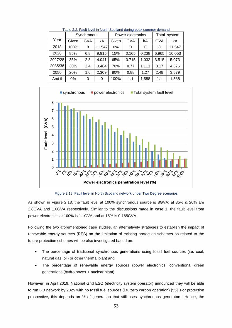
53

Table 2.2: Fault level in North Scotland during peak summer demand

Year

Synchronous Power electronics Total system

Given GVA kA Given GVA kA GVA kA

2018 100% 8 11.547 0% 0 0 8 11.547

2020 85% 6.8 9.815 15% 0.165 0.238 6.965 10.053

2027/28 35% 2.8 4.041 65% 0.715 1.032 3.515 5.073

2035/36 30% 2.4 3.464 70% 0.77 1.111 3.17 4.576

2050 20% 1.6 2.309 80% 0.88 1.27 2.48 3.579

And if 0% 0 0 100% 1.1 1.588 1.1 1.588

Figure 2.18: Fault level in North Scotland network under Two Degree scenarios

As shown in Figure 2.18, the fault level at 100% synchronous source is 8GVA; at 35% & 20% are

2.8GVA and 1.6GVA respectively. Similar to the discussions made in case 1, the fault level from

power electronics at 100% is 1.1GVA and at 15% is 0.165GVA.

Following the two aforementioned case studies, an alternatively strategies to establish the impact of

renewable energy sources (RES) on the limitation of existing protection schemes as related to the

future protection schemes will be also investigated based on:

The percentage of traditional synchronous generations using fossil fuel sources (i.e. coal,

natural gas, oil) or other thermal plant and

The percentage of renewable energy sources (power electronics, conventional green

generations (hydro power + nuclear plant)

However, in April 2019, National Grid ESO (electricity system operator) announced they will be able

to run GB network by 2025 with no fossil fuel sources (i.e. zero carbon operation) [55]. For protection

prospective, this depends on % of generation that still uses synchronous generators. Hence, the

0

1

2

3

4

5

6

7

8

Fu

alt

lev

el

(G

VA

)

Power electronics penetration level (%)

synchronous power electronics Total system fault level

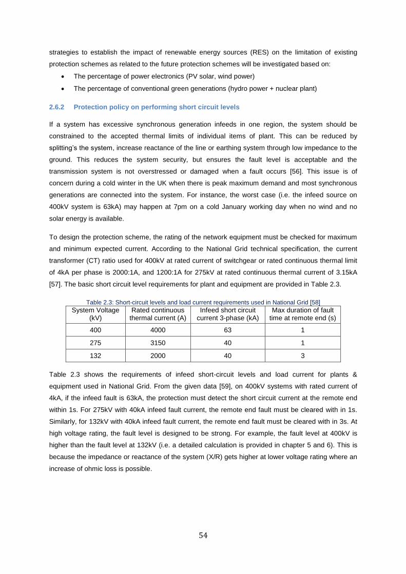
54

strategies to establish the impact of renewable energy sources (RES) on the limitation of existing

protection schemes as related to the future protection schemes will be investigated based on:

The percentage of power electronics (PV solar, wind power)

The percentage of conventional green generations (hydro power + nuclear plant)

2.6.2 Protection policy on performing short circuit levels

If a system has excessive synchronous generation infeeds in one region, the system should be

constrained to the accepted thermal limits of individual items of plant. This can be reduced by

splitting’s the system, increase reactance of the line or earthing system through low impedance to the

ground. This reduces the system security, but ensures the fault level is acceptable and the

transmission system is not overstressed or damaged when a fault occurs [56]. This issue is of

concern during a cold winter in the UK when there is peak maximum demand and most synchronous

generations are connected into the system. For instance, the worst case (i.e. the infeed source on

400kV system is 63kA) may happen at 7pm on a cold January working day when no wind and no

solar energy is available.

To design the protection scheme, the rating of the network equipment must be checked for maximum

and minimum expected current. According to the National Grid technical specification, the current

transformer (CT) ratio used for 400kV at rated current of switchgear or rated continuous thermal limit

of 4kA per phase is 2000:1A, and 1200:1A for 275kV at rated continuous thermal current of 3.15kA

[57]. The basic short circuit level requirements for plant and equipment are provided in Table 2.3.

Table 2.3: Short-circuit levels and load current requirements used in National Grid [58]

System Voltage (kV)

Rated continuous thermal current (A)

Infeed short circuit current 3-phase (kA)

Max duration of fault time at remote end (s)

400 4000 63 1

275 3150 40 1

132 2000 40 3

Table 2.3 shows the requirements of infeed short-circuit levels and load current for plants &

equipment used in National Grid. From the given data [59], on 400kV systems with rated current of

4kA, if the infeed fault is 63kA, the protection must detect the short circuit current at the remote end

within 1s. For 275kV with 40kA infeed fault current, the remote end fault must be cleared with in 1s.

Similarly, for 132kV with 40kA infeed fault current, the remote end fault must be cleared with in 3s. At

high voltage rating, the fault level is designed to be strong. For example, the fault level at 400kV is

higher than the fault level at 132kV (i.e. a detailed calculation is provided in chapter 5 and 6). This is

because the impedance or reactance of the system (X/R) gets higher at lower voltage rating where an

increase of ohmic loss is possible.

55

Table 2.4: Fault clearance time requirements and the grid code in Great Britain [58]-[59]

System Voltage (kV)

Great Britain Protection fault

clearance time (ms) Generator fault ride through time (ms)

400 England & Wales 80 140

275 England & Wales 100 140

132 England & Wales 120 140

132 Scotland 140 140

Table 2.4 provides the minimum requirements for protection fault clearance and ride through

generator time in Great Britain transmission system. According to [59], “fault ride through is defined as

the ability of generating units and power park modules to ride through supergrid transmission system

faults and disturbances whilst connected to a healthy system circuit. As shown in Table 2.4, the

protection fault clearance times are lower than the generator fault ride through time. This implies, the

protection system has to operate within the generator fault ride through time.

2.7. Physical relay injection and simulation test methods

In this report, all physical relay injection and simulation test methods were carried out using Omicron

Test Universe (CMC-256-6) and DIgSILENT Power-Factory software packages.

Omicron Test Universe is universal solution used as secondary injection test set [60]. It can be

configured to provide for testing overcurrent relays, distance relays, and differential relays.

Figure 2.19: CMC-256-6-hardware -protection relay

As shown on Figure 2.19, the omicron test universe equipment has 10 x multifunctional binary inputs,

wide ranges of voltage and current generators, 4 x binary outputs, where the test universe software is

used to configure relay characteristic setting and provide test results. P543/P545 relay family have

multifunctional setting groups and can be set for distance or differential relay where settings are

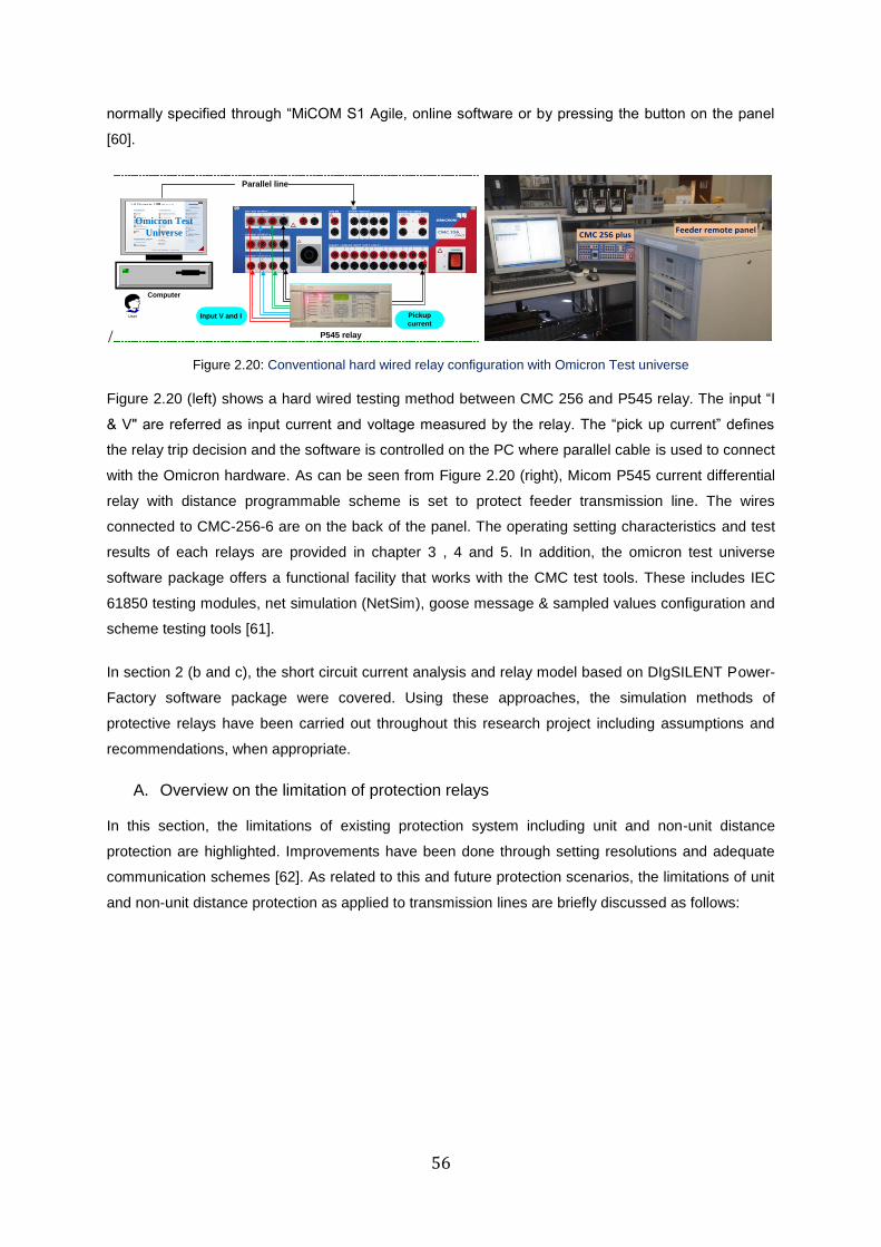
56

normally specified through “MiCOM S1 Agile, online software or by pressing the button on the panel

[60].

/

Input V and IUser

Computer

Parallel line

Pickup

current

P545 relay

Omicron Test

Universe

Input V and I

Feeder remote panel CMC 256 plus

Figure 2.20: Conventional hard wired relay configuration with Omicron Test universe

Figure 2.20 (left) shows a hard wired testing method between CMC 256 and P545 relay. The input “I

& V" are referred as input current and voltage measured by the relay. The “pick up current” defines

the relay trip decision and the software is controlled on the PC where parallel cable is used to connect

with the Omicron hardware. As can be seen from Figure 2.20 (right), Micom P545 current differential

relay with distance programmable scheme is set to protect feeder transmission line. The wires

connected to CMC-256-6 are on the back of the panel. The operating setting characteristics and test

results of each relays are provided in chapter 3 , 4 and 5. In addition, the omicron test universe

software package offers a functional facility that works with the CMC test tools. These includes IEC

61850 testing modules, net simulation (NetSim), goose message & sampled values configuration and

scheme testing tools [61].

In section 2 (b and c), the short circuit current analysis and relay model based on DIgSILENT Power-

Factory software package were covered. Using these approaches, the simulation methods of

protective relays have been carried out throughout this research project including assumptions and

recommendations, when appropriate.

A. Overview on the limitation of protection relays

In this section, the limitations of existing protection system including unit and non-unit distance

protection are highlighted. Improvements have been done through setting resolutions and adequate

communication schemes [62]. As related to this and future protection scenarios, the limitations of unit

and non-unit distance protection as applied to transmission lines are briefly discussed as follows:

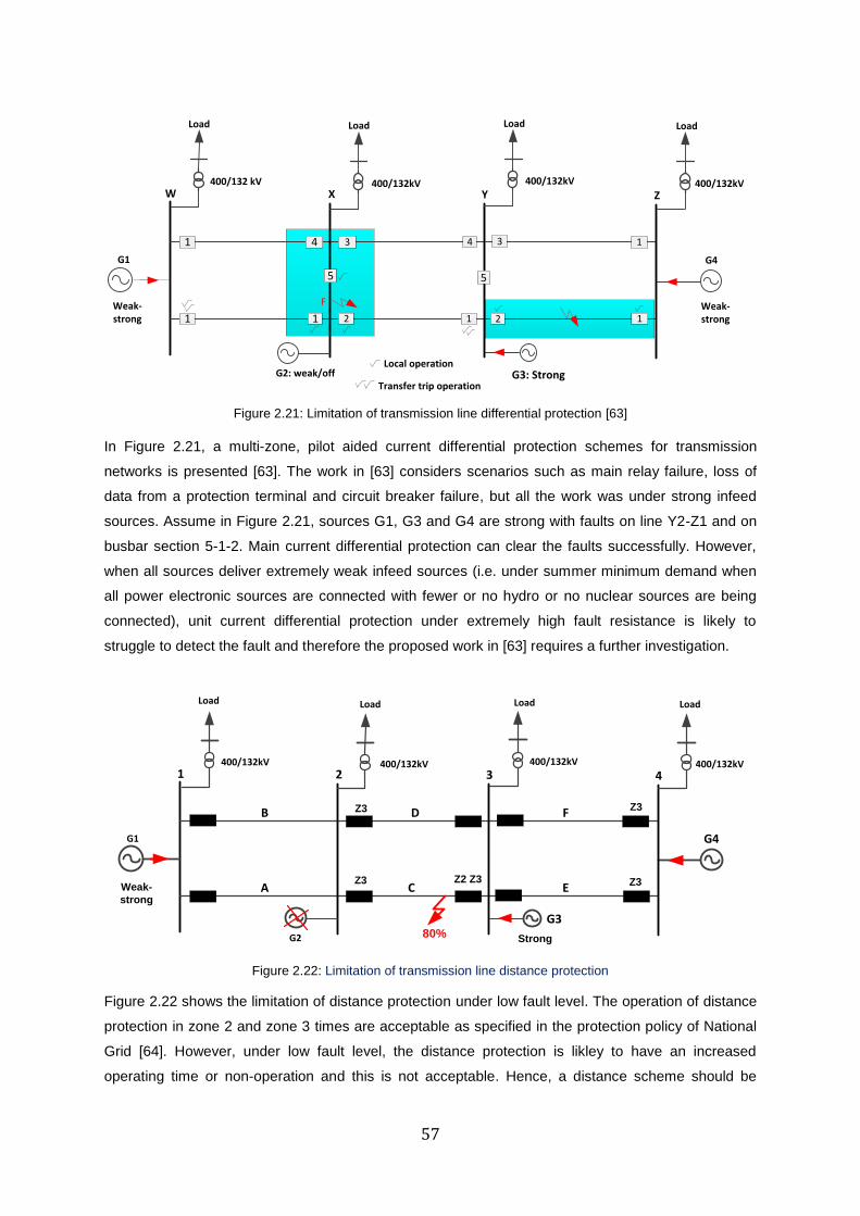
57

Weak-strong

G1 G4

G3: StrongG2: weak/off

W

Load

F

X Y Z

21

31 14

11

400/132 kV 400/132kV 400/132kV 400/132kV

Load Load Load

3

21

4

55

Local operation

Transfer trip operation

Weak-strong

Figure 2.21: Limitation of transmission line differential protection [63]

In Figure 2.21, a multi-zone, pilot aided current differential protection schemes for transmission

networks is presented [63]. The work in [63] considers scenarios such as main relay failure, loss of

data from a protection terminal and circuit breaker failure, but all the work was under strong infeed

sources. Assume in Figure 2.21, sources G1, G3 and G4 are strong with faults on line Y2-Z1 and on

busbar section 5-1-2. Main current differential protection can clear the faults successfully. However,

when all sources deliver extremely weak infeed sources (i.e. under summer minimum demand when

all power electronic sources are connected with fewer or no hydro or no nuclear sources are being

connected), unit current differential protection under extremely high fault resistance is likely to

struggle to detect the fault and therefore the proposed work in [63] requires a further investigation.

G1 G4

CA

B D

E

F

G3

G2

1

Load

80%

2 3 4400/132kV 400/132kV 400/132kV 400/132kV

Load Load Load

Z3

Z3 Z3

Z3Weak-

strong

Strong

Z2 Z3

Figure 2.22: Limitation of transmission line distance protection

Figure 2.22 shows the limitation of distance protection under low fault level. The operation of distance

protection in zone 2 and zone 3 times are acceptable as specified in the protection policy of National

Grid [64]. However, under low fault level, the distance protection is likley to have an increased

operating time or non-operation and this is not acceptable. Hence, a distance scheme should be

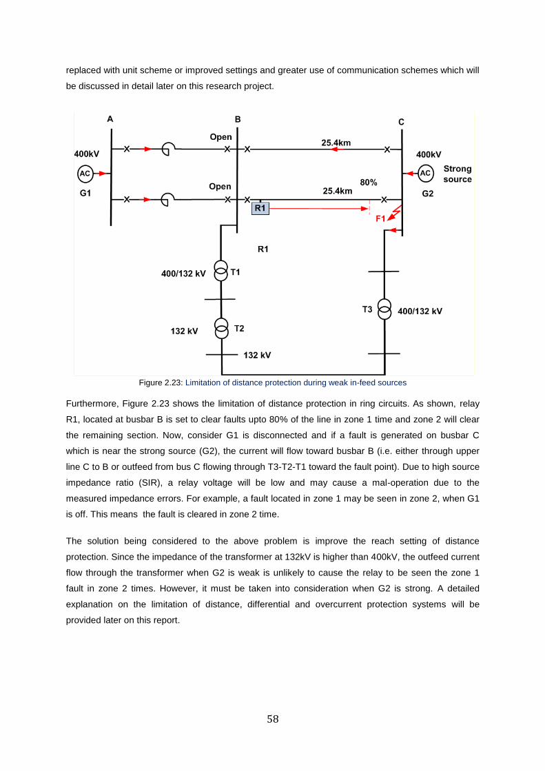
58

replaced with unit scheme or improved settings and greater use of communication schemes which will

be discussed in detail later on this research project.

Figure 2.23: Limitation of distance protection during weak in-feed sources

Furthermore, Figure 2.23 shows the limitation of distance protection in ring circuits. As shown, relay

R1, located at busbar B is set to clear faults upto 80% of the line in zone 1 time and zone 2 will clear

the remaining section. Now, consider G1 is disconnected and if a fault is generated on busbar C

which is near the strong source (G2), the current will flow toward busbar B (i.e. either through upper

line C to B or outfeed from bus C flowing through T3-T2-T1 toward the fault point). Due to high source

impedance ratio (SIR), a relay voltage will be low and may cause a mal-operation due to the

measured impedance errors. For example, a fault located in zone 1 may be seen in zone 2, when G1

is off. This means the fault is cleared in zone 2 time.

The solution being considered to the above problem is improve the reach setting of distance

protection. Since the impedance of the transformer at 132kV is higher than 400kV, the outfeed current

flow through the transformer when G2 is weak is unlikely to cause the relay to be seen the zone 1

fault in zone 2 times. However, it must be taken into consideration when G2 is strong. A detailed

explanation on the limitation of distance, differential and overcurrent protection systems will be

provided later on this report.

59

2.8. Summary

The fault level calculation was discussed in this chapter. The issues associated with declining fault

level and their impacts on existing protection schemes are highlighted. From a fault level analysis

perspective, the minimum fault level is normally seen during minimum summer demand. Utility

concern about protection performance as the penetration of non- synchronous generation increases

was reviewed in this chapter.

A review of the literature indicates, overcurrent protection is most likely to be affected during low short

circuit fault levels whereas differential protection is the least affected. Distance protection also shows

an increase in operating times. However, there is limited information on the protection setting strategy

at different fault level conditions.

According to the system operating framework published by National Grid, the largest decline in the

fault level provides a benchmark for establishing the limitation of existing protection and their settings.

In the GB transmission network, the average lowest short current level is seen during the summer

minimum demand period whereas the maximum fault level is seen during winter maximum demand.

Based on the Two Degree scenario, the expected fault level calculations used for the assessment of

protection performance in 2020, 2028, 2036 and 2050 are presented on Table 2.1.

The protection policy on performing short circuit levels, overview on the limitation of existing

protection systems and test methods used in this research are also discussed. The short circuit

calculation is performed based on complete method, incapable of providing exact values without

approximation.

The key strengths of this study are to increase understanding on the concept of fault level and issues

associated with the setting of protection when significant renewable generation is operational and

minimal synchronous generation is being used. The objective is to understand the impact of

protection performance of declining fault levels on the Great Britain networks.

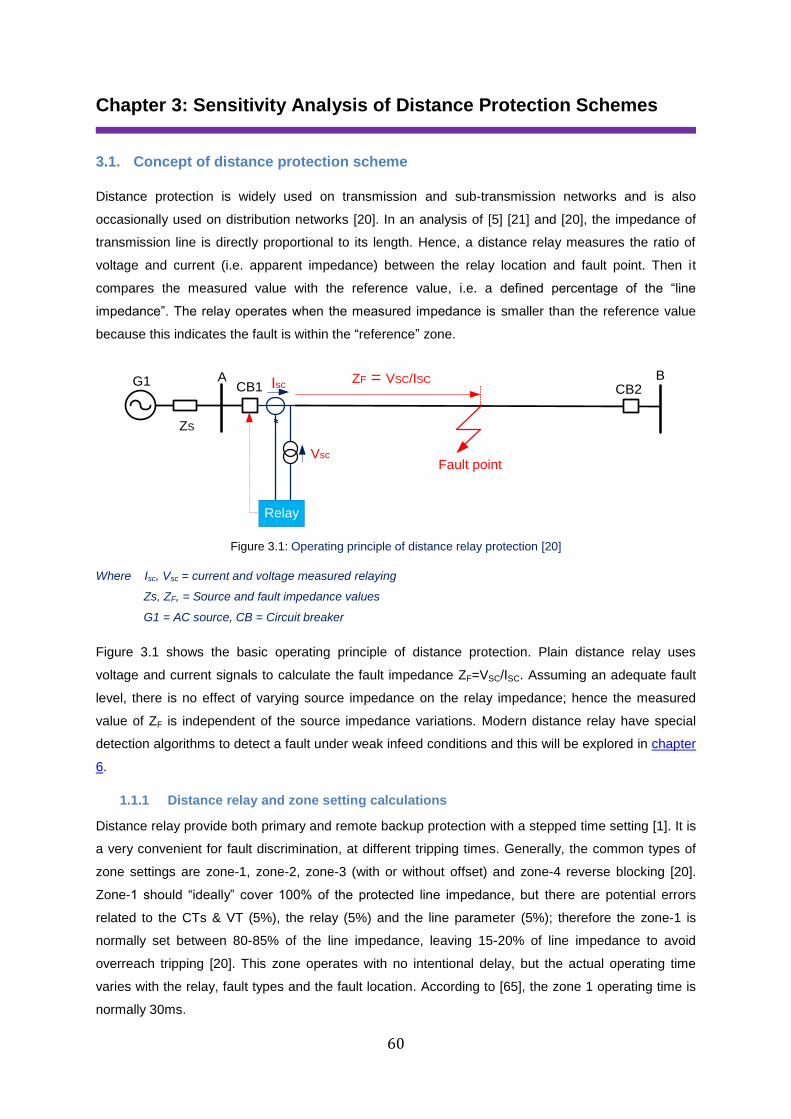
60

Chapter 3: Sensitivity Analysis of Distance Protection Schemes

3.1. Concept of distance protection scheme

Distance protection is widely used on transmission and sub-transmission networks and is also

occasionally used on distribution networks [20]. In an analysis of [5] [21] and [20], the impedance of

transmission line is directly proportional to its length. Hence, a distance relay measures the ratio of

voltage and current (i.e. apparent impedance) between the relay location and fault point. Then it

compares the measured value with the reference value, i.e. a defined percentage of the “line

impedance”. The relay operates when the measured impedance is smaller than the reference value

because this indicates the fault is within the “reference” zone.

B

Relay

ACB1 Isc

ZF = VSC/ISC

ZS

Fault point

CB2G1

Vsc

Figure 3.1: Operating principle of distance relay protection [20]

Where Isc, Vsc = current and voltage measured relaying

Zs, ZF, = Source and fault impedance values

G1 = AC source, CB = Circuit breaker

Figure 3.1 shows the basic operating principle of distance protection. Plain distance relay uses

voltage and current signals to calculate the fault impedance ZF=VSC/ISC. Assuming an adequate fault

level, there is no effect of varying source impedance on the relay impedance; hence the measured

value of ZF is independent of the source impedance variations. Modern distance relay have special

detection algorithms to detect a fault under weak infeed conditions and this will be explored in chapter

6.

1.1.1 Distance relay and zone setting calculations

Distance relay provide both primary and remote backup protection with a stepped time setting [1]. It is

a very convenient for fault discrimination, at different tripping times. Generally, the common types of

zone settings are zone-1, zone-2, zone-3 (with or without offset) and zone-4 reverse blocking [20].

Zone-1 should “ideally” cover 100% of the protected line impedance, but there are potential errors

related to the CTs & VT (5%), the relay (5%) and the line parameter (5%); therefore the zone-1 is

normally set between 80-85% of the line impedance, leaving 15-20% of line impedance to avoid

overreach tripping [20]. This zone operates with no intentional delay, but the actual operating time

varies with the relay, fault types and the fault location. According to [65], the zone 1 operating time is

normally 30ms.

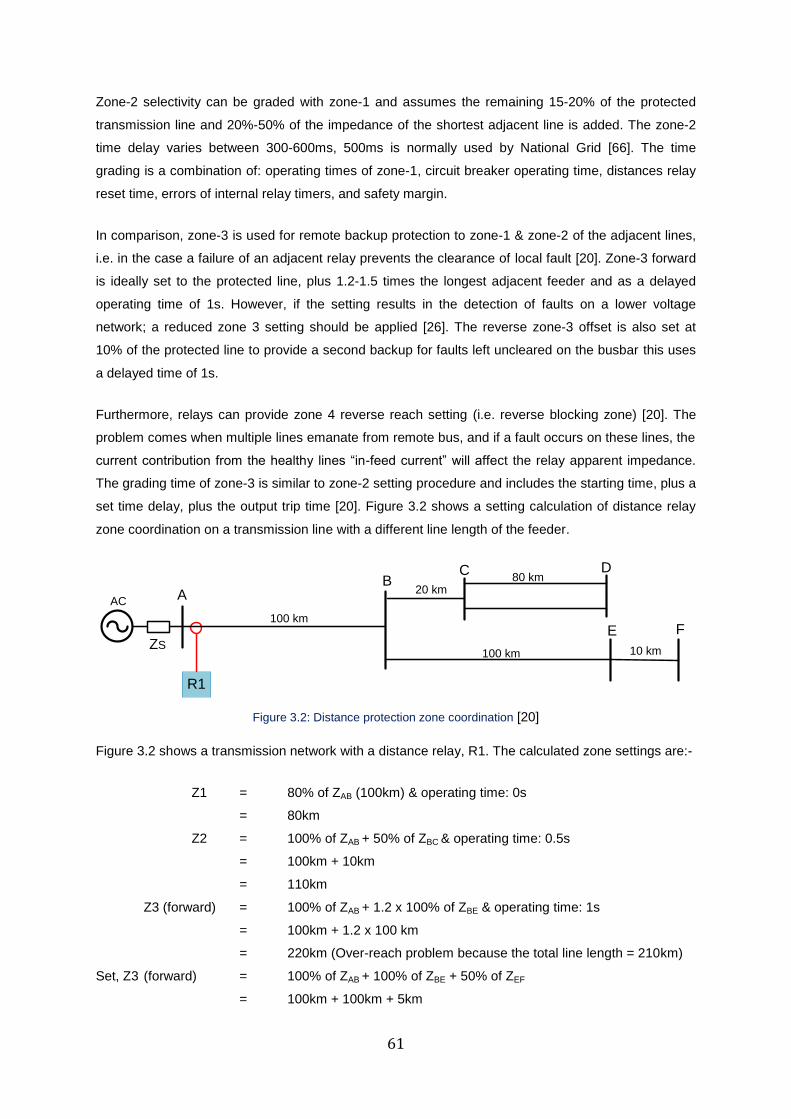
61

Zone-2 selectivity can be graded with zone-1 and assumes the remaining 15-20% of the protected

transmission line and 20%-50% of the impedance of the shortest adjacent line is added. The zone-2

time delay varies between 300-600ms, 500ms is normally used by National Grid [66]. The time

grading is a combination of: operating times of zone-1, circuit breaker operating time, distances relay

reset time, errors of internal relay timers, and safety margin.

In comparison, zone-3 is used for remote backup protection to zone-1 & zone-2 of the adjacent lines,

i.e. in the case a failure of an adjacent relay prevents the clearance of local fault [20]. Zone-3 forward

is ideally set to the protected line, plus 1.2-1.5 times the longest adjacent feeder and as a delayed

operating time of 1s. However, if the setting results in the detection of faults on a lower voltage

network; a reduced zone 3 setting should be applied [26]. The reverse zone-3 offset is also set at

10% of the protected line to provide a second backup for faults left uncleared on the busbar this uses

a delayed time of 1s.

Furthermore, relays can provide zone 4 reverse reach setting (i.e. reverse blocking zone) [20]. The

problem comes when multiple lines emanate from remote bus, and if a fault occurs on these lines, the

current contribution from the healthy lines “in-feed current” will affect the relay apparent impedance.

The grading time of zone-3 is similar to zone-2 setting procedure and includes the starting time, plus a

set time delay, plus the output trip time [20]. Figure 3.2 shows a setting calculation of distance relay

zone coordination on a transmission line with a different line length of the feeder.

A

ZS

BC D

100 km

AC

R1

100 km

20 km

10 km

E F

80 km

Figure 3.2: Distance protection zone coordination [20]

Figure 3.2 shows a transmission network with a distance relay, R1. The calculated zone settings are:-

Z1 = 80% of ZAB (100km) & operating time: 0s

= 80km

Z2 = 100% of ZAB + 50% of ZBC & operating time: 0.5s

= 100km + 10km

= 110km

Z3 (forward) = 100% of ZAB + 1.2 x 100% of ZBE & operating time: 1s

= 100km + 1.2 x 100 km

= 220km (Over-reach problem because the total line length = 210km)

Set, Z3 (forward) = 100% of ZAB + 100% of ZBE + 50% of ZEF

= 100km + 100km + 5km

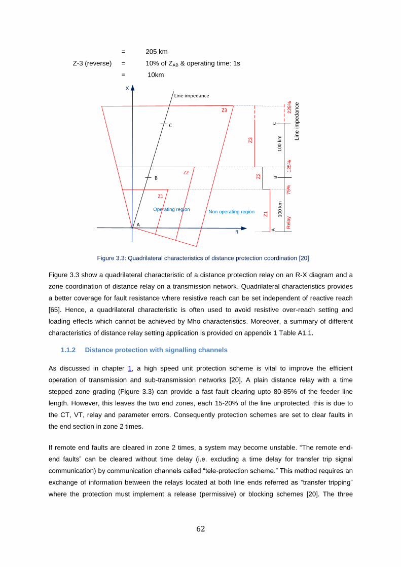
62

= 205 km

Z-3 (reverse) = 10% of ZAB & operating time: 1s

= 10km

Non operating regionOperating region

R

X

Line impedance

Z3

Z2

Z1

A

B

C

Z2

Z1

Z3

75

%1

25

%

AB

C

Re

lay

Lin

e im

pe

da

nce

10

0 k

m1

00

km

22

5%

Figure 3.3: Quadrilateral characteristics of distance protection coordination [20]

Figure 3.3 show a quadrilateral characteristic of a distance protection relay on an R-X diagram and a

zone coordination of distance relay on a transmission network. Quadrilateral characteristics provides

a better coverage for fault resistance where resistive reach can be set independent of reactive reach

[65]. Hence, a quadrilateral characteristic is often used to avoid resistive over-reach setting and

loading effects which cannot be achieved by Mho characteristics. Moreover, a summary of different

characteristics of distance relay setting application is provided on appendix 1 Table A1.1.

1.1.2 Distance protection with signalling channels

As discussed in chapter 1, a high speed unit protection scheme is vital to improve the efficient

operation of transmission and sub-transmission networks [20]. A plain distance relay with a time

stepped zone grading (Figure 3.3) can provide a fast fault clearing upto 80-85% of the feeder line

length. However, this leaves the two end zones, each 15-20% of the line unprotected, this is due to

the CT, VT, relay and parameter errors. Consequently protection schemes are set to clear faults in

the end section in zone 2 times.

If remote end faults are cleared in zone 2 times, a system may become unstable. “The remote end-

end faults” can be cleared without time delay (i.e. excluding a time delay for transfer trip signal

communication) by communication channels called “tele-protection scheme.” This method requires an

exchange of information between the relays located at both line ends referred as “transfer tripping”

where the protection must implement a release (permissive) or blocking schemes [20]. The three

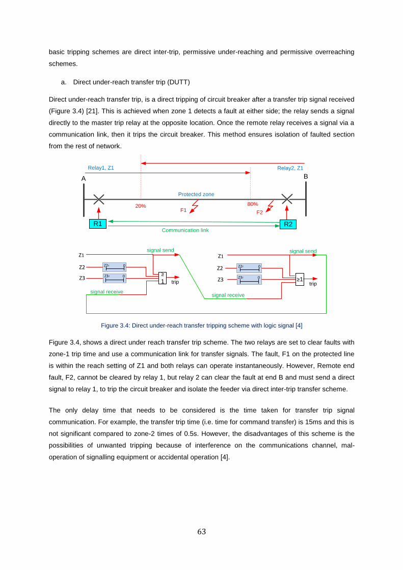
63

basic tripping schemes are direct inter-trip, permissive under-reaching and permissive overreaching

schemes.

a. Direct under-reach transfer trip (DUTT)

Direct under-reach transfer trip, is a direct tripping of circuit breaker after a transfer trip signal received

(Figure 3.4) [21]. This is achieved when zone 1 detects a fault at either side; the relay sends a signal

directly to the master trip relay at the opposite location. Once the remote relay receives a signal via a

communication link, then it trips the circuit breaker. This method ensures isolation of faulted section

from the rest of network.

Z1signal send

trip

signal receive

Z2

Z3

Z2T 0

Z3T 0 ≥1

Z1signal send

trip

signal receive

Z2

Z3

Z2T 0

Z3T 0 ≥1

A B

20% 80%

R1 R2Communication link

Protected zone

Relay2, Z1Relay1, Z1

F1 F2

Figure 3.4: Direct under-reach transfer tripping scheme with logic signal [4]

Figure 3.4, shows a direct under reach transfer trip scheme. The two relays are set to clear faults with

zone-1 trip time and use a communication link for transfer signals. The fault, F1 on the protected line

is within the reach setting of Z1 and both relays can operate instantaneously. However, Remote end

fault, F2, cannot be cleared by relay 1, but relay 2 can clear the fault at end B and must send a direct

signal to relay 1, to trip the circuit breaker and isolate the feeder via direct inter-trip transfer scheme.

The only delay time that needs to be considered is the time taken for transfer trip signal

communication. For example, the transfer trip time (i.e. time for command transfer) is 15ms and this is

not significant compared to zone-2 times of 0.5s. However, the disadvantages of this scheme is the

possibilities of unwanted tripping because of interference on the communications channel, mal-

operation of signalling equipment or accidental operation [4].

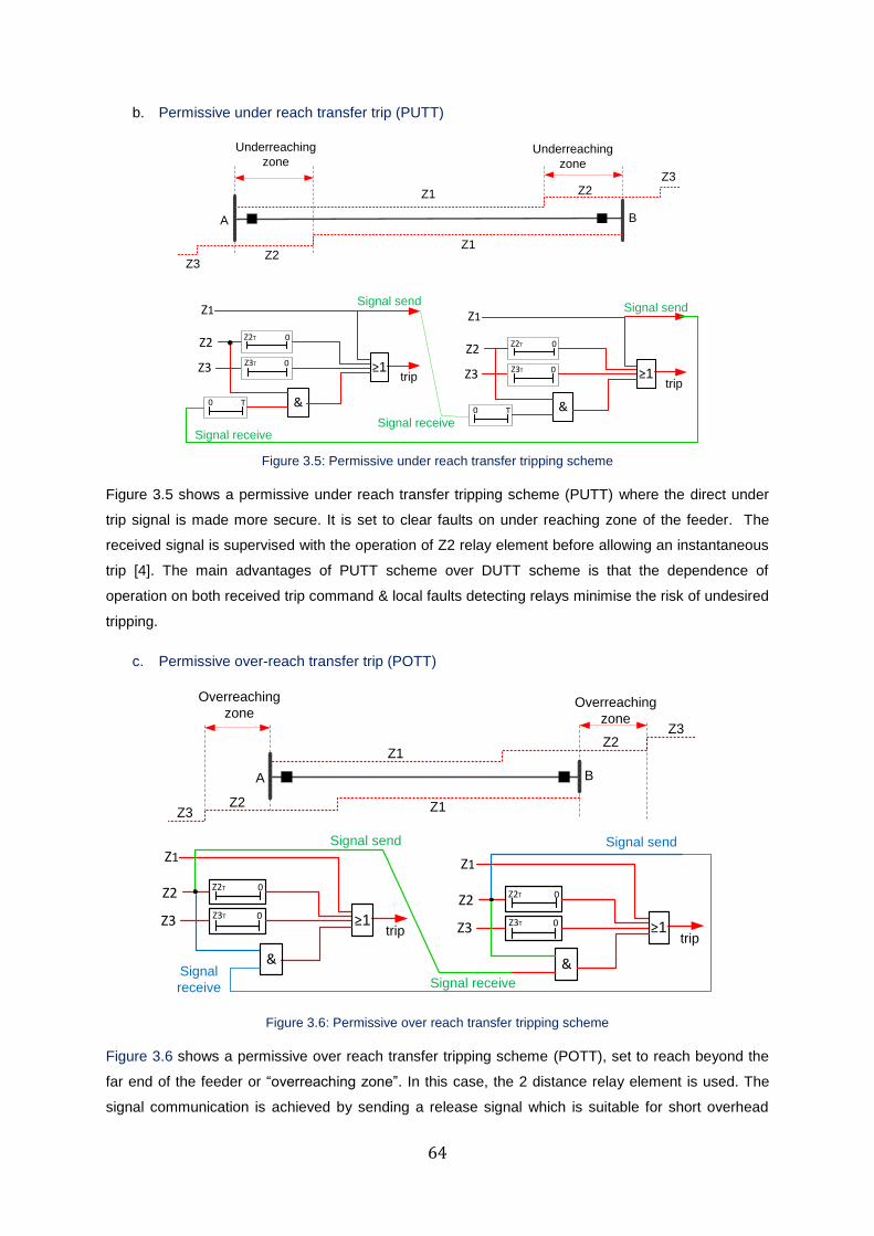
64

b. Permissive under reach transfer trip (PUTT)

&

Z1Signal send

trip

Signal receive

Z2

Z3

Z2T 0

Z3T 0

0 T

≥1

&

Z1Signal send

trip

Signal receive

Z2

Z3

Z2T 0

Z3T 0

0 T

≥1

Z1

Z1

Z2Z3

Z2Z3

Underreaching

zoneUnderreaching

zone

A B

Figure 3.5: Permissive under reach transfer tripping scheme

Figure 3.5 shows a permissive under reach transfer tripping scheme (PUTT) where the direct under

trip signal is made more secure. It is set to clear faults on under reaching zone of the feeder. The

received signal is supervised with the operation of Z2 relay element before allowing an instantaneous

trip [4]. The main advantages of PUTT scheme over DUTT scheme is that the dependence of

operation on both received trip command & local faults detecting relays minimise the risk of undesired

tripping.

c. Permissive over-reach transfer trip (POTT)

Z1

Z1

Z2Z3

Z2Z3

Overreaching

zoneOverreaching

zone

A B

Z1Signal send

trip

Signal

receive

Z2

Z3

Z2T 0

Z3T 0 ≥1

&

Z1

Signal send

trip

Signal receive

Z2

Z3

Z2T 0

Z3T 0 ≥1

&

Figure 3.6: Permissive over reach transfer tripping scheme

Figure 3.6 shows a permissive over reach transfer tripping scheme (POTT), set to reach beyond the

far end of the feeder or “overreaching zone”. In this case, the 2 distance relay element is used. The

signal communication is achieved by sending a release signal which is suitable for short overhead

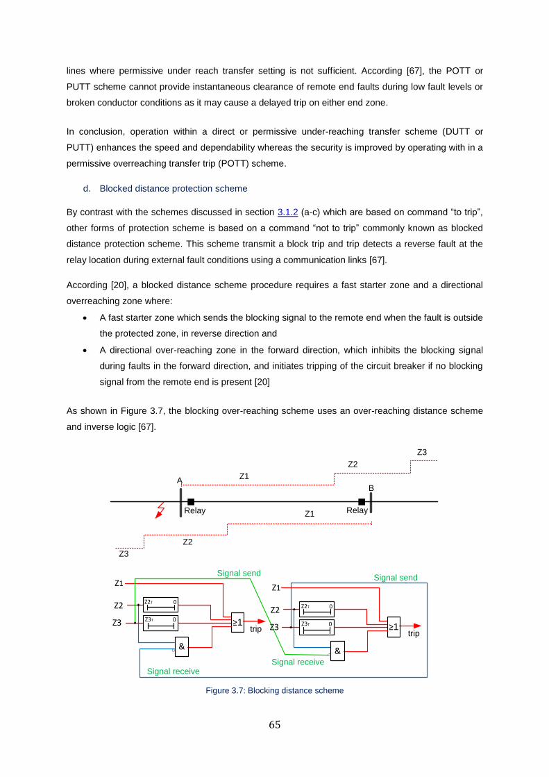
65

lines where permissive under reach transfer setting is not sufficient. According [67], the POTT or

PUTT scheme cannot provide instantaneous clearance of remote end faults during low fault levels or

broken conductor conditions as it may cause a delayed trip on either end zone.

In conclusion, operation within a direct or permissive under-reaching transfer scheme (DUTT or

PUTT) enhances the speed and dependability whereas the security is improved by operating with in a

permissive overreaching transfer trip (POTT) scheme.

d. Blocked distance protection scheme

By contrast with the schemes discussed in section 3.1.2 (a-c) which are based on command “to trip”,

other forms of protection scheme is based on a command “not to trip” commonly known as blocked

distance protection scheme. This scheme transmit a block trip and trip detects a reverse fault at the

relay location during external fault conditions using a communication links [67].

According [20], a blocked distance scheme procedure requires a fast starter zone and a directional

overreaching zone where:

A fast starter zone which sends the blocking signal to the remote end when the fault is outside

the protected zone, in reverse direction and

A directional over-reaching zone in the forward direction, which inhibits the blocking signal

during faults in the forward direction, and initiates tripping of the circuit breaker if no blocking

signal from the remote end is present [20]

As shown in Figure 3.7, the blocking over-reaching scheme uses an over-reaching distance scheme

and inverse logic [67].

Z1

Z2

AB

Z1Signal send

trip

Z2

Z3

Z2T 0

Z3T 0 ≥1

Signal receive

&

Z1Signal send

trip

Signal receive

Z2

Z3

Z2T 0

Z3T 0 ≥1

&

Z3

Z1

Z2

Z3

Relay Relay

Figure 3.7: Blocking distance scheme

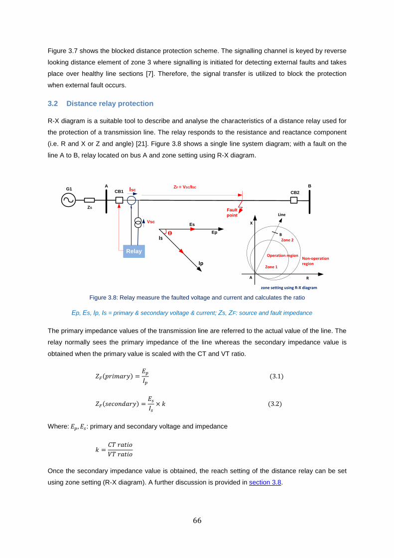
66

Figure 3.7 shows the blocked distance protection scheme. The signalling channel is keyed by reverse

looking distance element of zone 3 where signalling is initiated for detecting external faults and takes

place over healthy line sections [7]. Therefore, the signal transfer is utilized to block the protection

when external fault occurs.

3.2 Distance relay protection

R-X diagram is a suitable tool to describe and analyse the characteristics of a distance relay used for

the protection of a transmission line. The relay responds to the resistance and reactance component

(i.e. R and X or Z and angle) [21]. Figure 3.8 shows a single line system diagram; with a fault on the

line A to B, relay located on bus A and zone setting using R-X diagram.

Es

Ip

Ep

Isө

B

Relay

A

CB1 IscZF = VSC/ISC

ZSFault

point

CB2G1

Vsc

A

B

Zone 1

Non-operation region

Operation region

Zone 2

Line

X

R

zone setting using R-X diagram Figure 3.8: Relay measure the faulted voltage and current and calculates the ratio

Ep, Es, Ip, Is = primary & secondary voltage & current; Zs, ZF: source and fault impedance

The primary impedance values of the transmission line are referred to the actual value of the line. The

relay normally sees the primary impedance of the line whereas the secondary impedance value is

obtained when the primary value is scaled with the CT and VT ratio.

𝑍𝐹(𝑝𝑟𝑖𝑚𝑎𝑟𝑦) =𝐸𝑝

𝐼𝑝

(3.1)

𝑍𝐹(𝑠𝑒𝑐𝑜𝑛𝑑𝑎𝑟𝑦) =𝐸𝑠

𝐼𝑠

× 𝑘 (3.2)

Where: 𝐸𝑝, 𝐸𝑠: primary and secondary voltage and impedance

𝑘 =𝐶𝑇 𝑟𝑎𝑡𝑖𝑜

𝑉𝑇 𝑟𝑎𝑡𝑖𝑜

Once the secondary impedance value is obtained, the reach setting of the distance relay can be set

using zone setting (R-X diagram). A further discussion is provided in section 3.8.

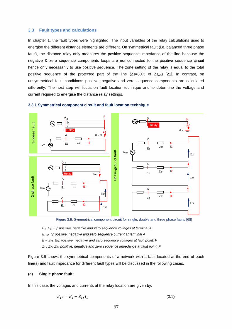
67

3.3 Fault types and calculations

In chapter 1, the fault types were highlighted. The input variables of the relay calculations used to

energise the different distance elements are different. On symmetrical fault (i.e. balanced three phase

fault), the distance relay only measures the positive sequence impedance of the line because the

negative & zero sequence components loops are not connected to the positive sequence circuit

hence only necessarily to use positive sequence. The zone setting of the relay is equal to the total

positive sequence of the protected part of the line (Z1=80% of Z1AB) [21]. In contrast, on

unsymmetrical fault conditions: positive, negative and zero sequence components are calculated

differently. The next step will focus on fault location technique and to determine the voltage and

current required to energise the distance relay settings.

3.3.1 Symmetrical component circuit and fault location technique

Ph

ase

-gro

un

d f

au

lt

2-p

ha

se f

au

lt3

-ph

ase

fa

ult

a

A

VTH E1 Z1f

A

E2 Z2f

I1

I2E2f

E1f

A

Relay

a

bc

b-c

A

F

VTH

E1Z1f

A

E2Z2f

A

E0Z0f

I1

I2

I0

E0f

E2f

E1f

A

Relay

a-g

A

VTHE1 Z1f I1

F

a-b-c

A

Relay

a

b

c

Figure 3.9: Symmetrical component circuit for single, double and three phase faults [68]

E1, E2, E0: positive, negative and zero sequence voltages at terminal A

I1, I2, I0: positive, negative and zero sequence current at terminal A

E1f, E2f, E0f: positive, negative and zero sequence voltages at fault point, F

Z1f, Z2f, Z0f: positive, negative and zero sequence impedance at fault point, F

Figure 3.9 shows the symmetrical components of a network with a fault located at the end of each

line(s) and fault impedance for different fault types will be discussed in the following cases.

(a) Single phase fault:

In this case, the voltages and currents at the relay location are given by:

𝐸1𝑓 = 𝐸1 − 𝑍1𝑓𝐼1 (3.1)

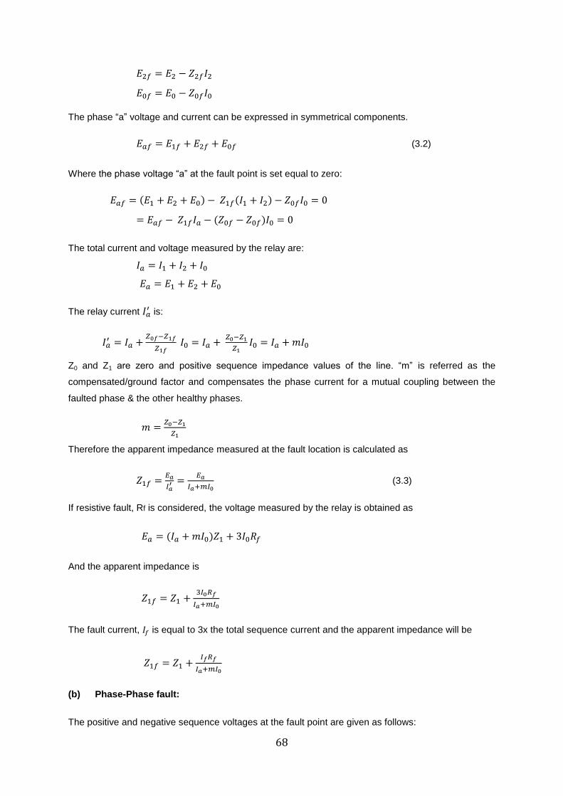
68

𝐸2𝑓 = 𝐸2 − 𝑍2𝑓𝐼2

𝐸0𝑓 = 𝐸0 − 𝑍0𝑓𝐼0

The phase “a” voltage and current can be expressed in symmetrical components.

𝐸𝑎𝑓 = 𝐸1𝑓 + 𝐸2𝑓 + 𝐸0𝑓 (3.2)

Where the phase voltage “a” at the fault point is set equal to zero:

𝐸𝑎𝑓 = (𝐸1 + 𝐸2 + 𝐸0) − 𝑍1𝑓(𝐼1 + 𝐼2) − 𝑍0𝑓𝐼0 = 0

= 𝐸𝑎𝑓 − 𝑍1𝑓𝐼𝑎 − (𝑍0𝑓 − 𝑍0𝑓)𝐼0 = 0

The total current and voltage measured by the relay are:

𝐼𝑎 = 𝐼1 + 𝐼2 + 𝐼0

𝐸𝑎 = 𝐸1 + 𝐸2 + 𝐸0

The relay current 𝐼𝑎′ is:

𝐼𝑎′ = 𝐼𝑎 +

𝑍0𝑓−𝑍1𝑓

𝑍1𝑓 𝐼0 = 𝐼𝑎 +

𝑍0−𝑍1

𝑍1𝐼0 = 𝐼𝑎 + 𝑚𝐼0

Z0 and Z1 are zero and positive sequence impedance values of the line. “m” is referred as the

compensated/ground factor and compensates the phase current for a mutual coupling between the

faulted phase & the other healthy phases.

𝑚 =𝑍0−𝑍1

𝑍1

Therefore the apparent impedance measured at the fault location is calculated as

𝑍1𝑓 =𝐸𝑎

𝐼𝑎′ =

𝐸𝑎

𝐼𝑎+𝑚𝐼0 (3.3)

If resistive fault, Rf is considered, the voltage measured by the relay is obtained as

𝐸𝑎 = (𝐼𝑎 + 𝑚𝐼0)𝑍1 + 3𝐼0𝑅𝑓

And the apparent impedance is

𝑍1𝑓 = 𝑍1 +3𝐼0𝑅𝑓

𝐼𝑎+𝑚𝐼0

The fault current, 𝐼𝑓 is equal to 3x the total sequence current and the apparent impedance will be

𝑍1𝑓 = 𝑍1 +𝐼𝑓𝑅𝑓

𝐼𝑎+𝑚𝐼0

(b) Phase-Phase fault:

The positive and negative sequence voltages at the fault point are given as follows:

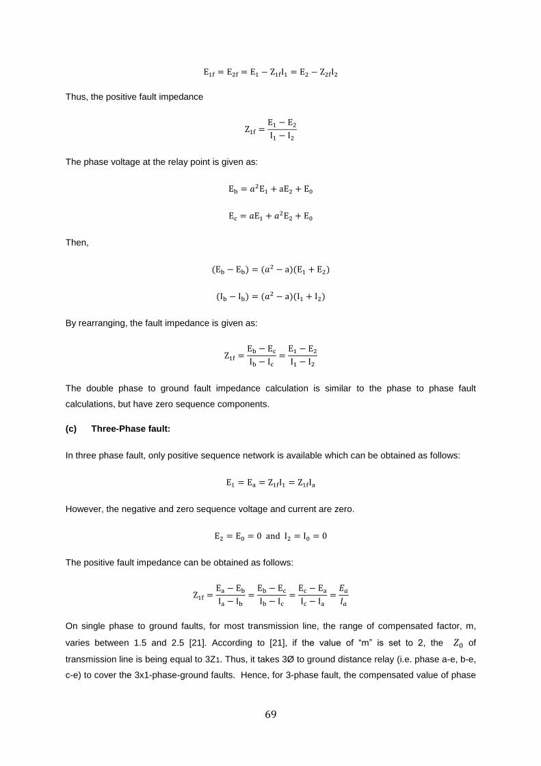
69

E1f = E2f = E1 − Z1fI1 = E2 − Z2fI2

Thus, the positive fault impedance

Z1f =E1 − E2

I1 − I2

The phase voltage at the relay point is given as:

Eb = 𝑎2E1 + aE2 + E0

Ec = 𝑎E1 + 𝑎2E2 + E0

Then,

(Eb − Eb) = (𝑎2 − a)(E1 + E2)

(Ib − Ib) = (𝑎2 − a)(I1 + I2)

By rearranging, the fault impedance is given as:

Z1f =Eb − Ec

Ib − Ic

=E1 − E2

I1 − I2

The double phase to ground fault impedance calculation is similar to the phase to phase fault

calculations, but have zero sequence components.

(c) Three-Phase fault:

In three phase fault, only positive sequence network is available which can be obtained as follows:

E1 = Ea = Z1fI1 = Z1fIa

However, the negative and zero sequence voltage and current are zero.

E2 = E0 = 0 and I2 = I0 = 0

The positive fault impedance can be obtained as follows:

Z1f =Ea − Eb

Ia − Ib

=Eb − Ec

Ib − Ic

=Ec − Ea

Ic − Ia

=𝐸𝑎

𝐼𝑎

On single phase to ground faults, for most transmission line, the range of compensated factor, m,

varies between 1.5 and 2.5 [21]. According to [21], if the value of “m” is set to 2, the 𝑍0 of

transmission line is being equal to 3Z1. Thus, it takes 3Ø to ground distance relay (i.e. phase a-e, b-e,

c-e) to cover the 3x1-phase-ground faults. Hence, for 3-phase fault, the compensated value of phase

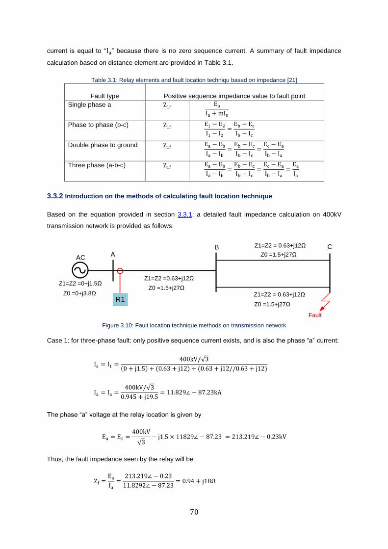
70

current is equal to “Ia” because there is no zero sequence current. A summary of fault impedance

calculation based on distance element are provided in Table 3.1.

Table 3.1: Relay elements and fault location techniqu based on impedance [21]

Fault type Positive sequence impedance value to fault point

Single phase a Z1f Ea

Ia + mI0

Phase to phase (b-c) Z1f E1 − E2

I1 − I2

=Eb − Ec

Ib − Ic

Double phase to ground Z1f Ea − Eb

Ia − Ib

=Eb − Ec

Ib − Ic

=Ec − Ea

Ib − Ia

Three phase (a-b-c) Z1f Ea − Eb

Ia − Ib

=Eb − Ec

Ib − Ic

=Ec − Ea

Ib − Ia

=Ea

Ia

3.3.2 Introduction on the methods of calculating fault location technique

Based on the equation provided in section 3.3.1; a detailed fault impedance calculation on 400kV

transmission network is provided as follows:

Z1=Z2 = 0.63+j12Ω

Z0 =0+j3.8Ω

AB

AC

R1

Fault

Z1=Z2 =0.63+j12Ω

Z0 =1.5+j27Ω Z1=Z2 = 0.63+j12Ω

Z0 =1.5+j27Ω

Z0 =1.5+j27Ω

C

Z1=Z2 =0+j1.5Ω

Figure 3.10: Fault location technique methods on transmission network

Case 1: for three-phase fault: only positive sequence current exists, and is also the phase “a” current:

Ia = I1 =400kV/√3

(0 + j1.5) + (0.63 + j12) + (0.63 + j12//0.63 + j12)

Ia = Ia =400kV/√3

0.945 + j19.5= 11.829∠ − 87.23kA

The phase “a” voltage at the relay location is given by

Ea = E1 =400kV

√3− j1.5 × 11829∠ − 87.23 = 213.219∠ − 0.23kV

Thus, the fault impedance seen by the relay will be

Zf =Ea

Ia

=213.219∠ − 0.23

11.8292∠ − 87.23= 0.94 + j18Ω

71

Case 2: for phase “a” to ground fault, the three symmetrical components of the current is equal:

I1 = I0 = I2 =Ea

Z0 + Z1 + Z2

=400kV/√3

(0 + j3.8) + (1.5 + j27) + (0.75 + 13.5j) + 2(0 + 1.5j) + 2(0.63 + 12j) + 2(0.315 + 6j)

I1 = I0 = I2 = 2.769∠ − 87.15 kA

The symmetric components of the voltages at the relay location are:

E1 =400kV

√3− j1.5 × 2769∠ − 87.15° = 226791.745 − j206.5177 V

E2 = −(0 + j1.5) × 2769∠ − 87.15° = −4148.36265 − j206.5177 V

E0 = −(0 + j3.8) × 2769∠ − 87.15° = −10509.1854 − 523.1782 V

And, the phase “a” voltage and current at the relay location are:

Ea = E1 + E2 + E0 = 212136.2629∠ − 0.25 V

Ia = I1 + I2 + I0 = 3 × 2.769∠ − 87.15° kA = 8307∠ − 87.15A

The zero sequence current compensation factor m is given by

m =Z0 − Z1

Z1

=(1.5 + j27) − (0.63 + j12)

(0.63 + j12)= 1.25∠ − 0.31

And the compensated phase a current 𝐼𝑎′ is

Ia′ = Ia + mI0 = 8307∠ − 87.15° + 1.25∠ − 0.31 × 2769∠ − 87.15

= 11.768214∠ − 87.24kA

Finally, the fault impedance seen by the relay in this case with reference to eqn. 3.3 is

Z1f =Ea

Ia + mI0

=Ea

Ia′

=212.1362629∠ − 0.25° k V

11.768214∠ − 87.24° kA= 0.94 + j18Ω

Thus, if the distance relay is energized with the phase “a” voltage and the compensated phase “a"

current, it also measures the positive sequence impedance to the fault. Finally, it can be concluded

that, based on the equations derived in section 3.2, the fault detection technique calculation on

transmission network is valid and justified.

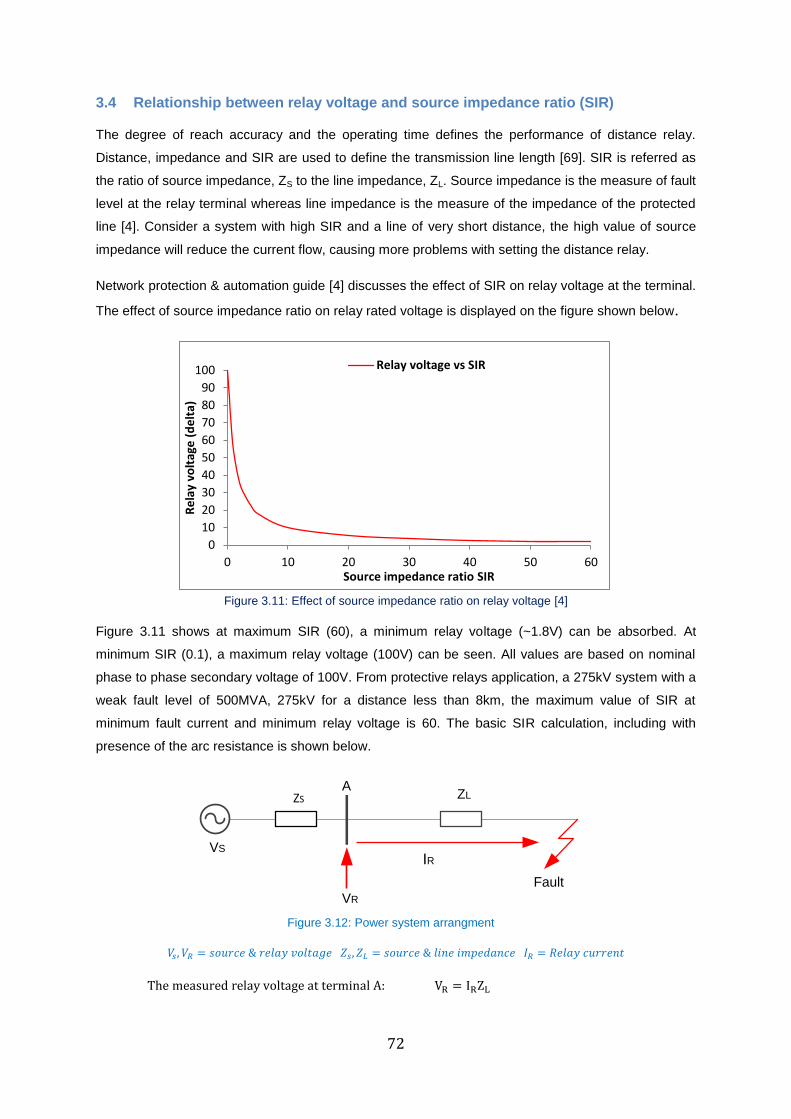
72

3.4 Relationship between relay voltage and source impedance ratio (SIR)

The degree of reach accuracy and the operating time defines the performance of distance relay.

Distance, impedance and SIR are used to define the transmission line length [69]. SIR is referred as

the ratio of source impedance, ZS to the line impedance, ZL. Source impedance is the measure of fault

level at the relay terminal whereas line impedance is the measure of the impedance of the protected

line [4]. Consider a system with high SIR and a line of very short distance, the high value of source

impedance will reduce the current flow, causing more problems with setting the distance relay.

Network protection & automation guide [4] discusses the effect of SIR on relay voltage at the terminal.

The effect of source impedance ratio on relay rated voltage is displayed on the figure shown below.

Figure 3.11: Effect of source impedance ratio on relay voltage [4]

Figure 3.11 shows at maximum SIR (60), a minimum relay voltage (~1.8V) can be absorbed. At

minimum SIR (0.1), a maximum relay voltage (100V) can be seen. All values are based on nominal

phase to phase secondary voltage of 100V. From protective relays application, a 275kV system with a

weak fault level of 500MVA, 275kV for a distance less than 8km, the maximum value of SIR at

minimum fault current and minimum relay voltage is 60. The basic SIR calculation, including with

presence of the arc resistance is shown below.

AZL

IRVS

ZS

VR

Fault

Figure 3.12: Power system arrangment

𝑉𝑠, 𝑉𝑅 = 𝑠𝑜𝑢𝑟𝑐𝑒 & 𝑟𝑒𝑙𝑎𝑦 𝑣𝑜𝑙𝑡𝑎𝑔𝑒 𝑍𝑠, 𝑍𝐿 = 𝑠𝑜𝑢𝑟𝑐𝑒 & 𝑙𝑖𝑛𝑒 𝑖𝑚𝑝𝑒𝑑𝑎𝑛𝑐𝑒 𝐼𝑅 = 𝑅𝑒𝑙𝑎𝑦 𝑐𝑢𝑟𝑟𝑒𝑛𝑡

The measured relay voltage at terminal A: VR = IRZL

0

10

20

30

40

50

60

70

80

90

100

0 10 20 30 40 50 60

Re

lay

volt

age

(d

elt

a)

Source impedance ratio SIR

Relay voltage vs SIR

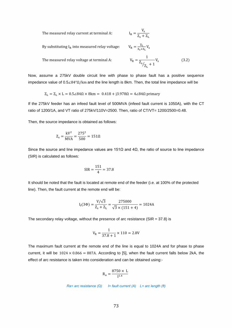
73

The measured relay current at terminal A: IR =Vs

Zs + ZL

By substituting IR into measured relay voltage: VR =ZL

Zs+ZLVs

The measured relay voltage at terminal A: VR =1

ZsZL

⁄ + 1Vs (3.2)

Now, assume a 275kV double circuit line with phase to phase fault has a positive sequence

impedance value of 0.5∠84°Ω/km and the line length is 8km. Then, the total line impedance will be

ZL = ZL × L = 0.5∠84Ω × 8km = 0.418 + j3.978Ω = 4∠84Ω primary

If the 275kV feeder has an infeed fault level of 500MVA (infeed fault current is 1050A), with the CT

ratio of 1200/1A, and VT ratio of 275kV/110V=2500. Then, ratio of CT/VT= 1200/2500=0.48.

Then, the source impedance is obtained as follows:

Zs =kV2

MVA=

2752

500= 151Ω

Since the source and line impedance values are 151Ω and 4Ω, the ratio of source to line impedance

(SIR) is calculated as follows:

SIR =151

4= 37.8

It should be noted that the fault is located at remote end of the feeder (i.e. at 100% of the protected

line). Then, the fault current at the remote end will be:

If(3Φ) =V/√3

Zs + ZL

=275000

√3 × (151 + 4)= 1024A

The secondary relay voltage, without the presence of arc resistance (SIR = 37.8) is

VR =1

37.8 + 1× 110 = 2.8V

The maximum fault current at the remote end of the line is equal to 1024A and for phase to phase

current, it will be 1024 × 0.866 = 887A. According to [5], when the fault current falls below 2kA, the

effect of arc resistance is taken into consideration and can be obtained using:-

Ra =8750 × L

I1.4

Ra= arc resistance (Ω) I= fault current (A) L= arc length (ft)

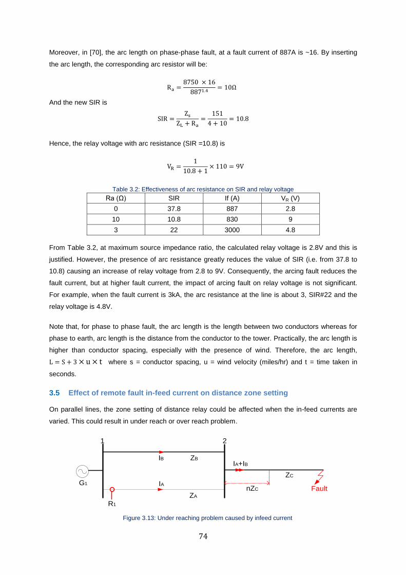
74

Moreover, in [70], the arc length on phase-phase fault, at a fault current of 887A is ~16. By inserting

the arc length, the corresponding arc resistor will be:

Ra =8750 × 16

8871.4= 10Ω

And the new SIR is

SIR =Zs

ZL + Ra

=151

4 + 10= 10.8

Hence, the relay voltage with arc resistance (SIR =10.8) is

VR =1

10.8 + 1× 110 = 9V

Table 3.2: Effectiveness of arc resistance on SIR and relay voltage

Ra (Ω) SIR If (A) VR (V)

0 37.8 887 2.8

10 10.8 830 9

3 22 3000 4.8

From Table 3.2, at maximum source impedance ratio, the calculated relay voltage is 2.8V and this is

justified. However, the presence of arc resistance greatly reduces the value of SIR (i.e. from 37.8 to

10.8) causing an increase of relay voltage from 2.8 to 9V. Consequently, the arcing fault reduces the

fault current, but at higher fault current, the impact of arcing fault on relay voltage is not significant.

For example, when the fault current is 3kA, the arc resistance at the line is about 3, SIR#22 and the

relay voltage is 4.8V.

Note that, for phase to phase fault, the arc length is the length between two conductors whereas for

phase to earth, arc length is the distance from the conductor to the tower. Practically, the arc length is

higher than conductor spacing, especially with the presence of wind. Therefore, the arc length,

L = S + 3 × u × t where s = conductor spacing, u = wind velocity (miles/hr) and t = time taken in

seconds.

3.5 Effect of remote fault in-feed current on distance zone setting

On parallel lines, the zone setting of distance relay could be affected when the in-feed currents are

varied. This could result in under reach or over reach problem.

IB

G1

ZB

IA

R1

ZA

ZC

nZC

IA+IB

Fault

1 2

Figure 3.13: Under reaching problem caused by infeed current

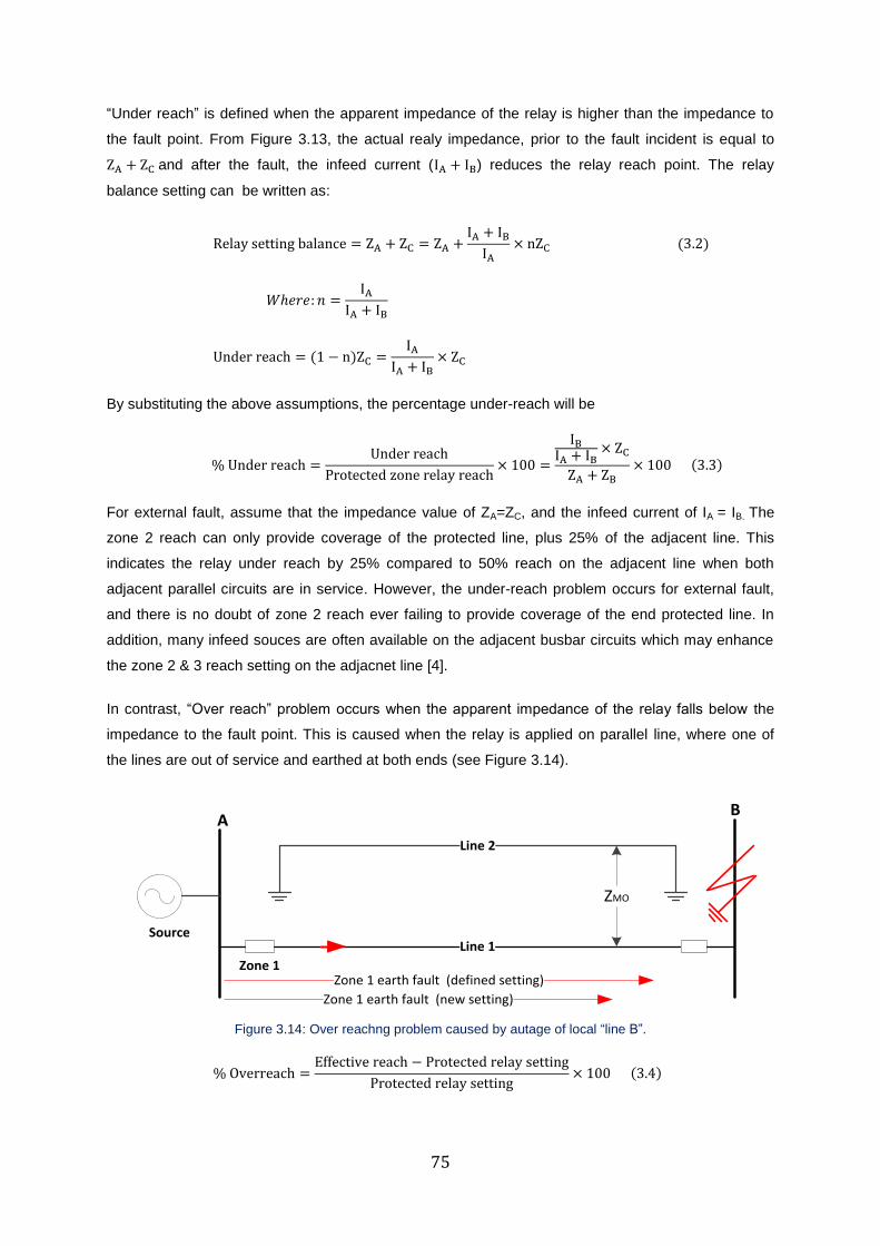
75

“Under reach” is defined when the apparent impedance of the relay is higher than the impedance to

the fault point. From Figure 3.13, the actual realy impedance, prior to the fault incident is equal to

ZA + ZC and after the fault, the infeed current (IA + IB) reduces the relay reach point. The relay

balance setting can be written as:

Relay setting balance = ZA + ZC = ZA +IA + IB

IA

× nZC (3.2)

𝑊ℎ𝑒𝑟𝑒: 𝑛 =IA

IA + IB

Under reach = (1 − n)ZC =IA

IA + IB

× ZC

By substituting the above assumptions, the percentage under-reach will be

% Under reach =Under reach

Protected zone relay reach× 100 =

IB

IA + IB× ZC

ZA + ZB

× 100 (3.3)

For external fault, assume that the impedance value of ZA=ZC, and the infeed current of IA = IB. The

zone 2 reach can only provide coverage of the protected line, plus 25% of the adjacent line. This

indicates the relay under reach by 25% compared to 50% reach on the adjacent line when both

adjacent parallel circuits are in service. However, the under-reach problem occurs for external fault,

and there is no doubt of zone 2 reach ever failing to provide coverage of the end protected line. In

addition, many infeed souces are often available on the adjacent busbar circuits which may enhance

the zone 2 & 3 reach setting on the adjacnet line [4].

In contrast, “Over reach” problem occurs when the apparent impedance of the relay falls below the

impedance to the fault point. This is caused when the relay is applied on parallel line, where one of

the lines are out of service and earthed at both ends (see Figure 3.14).

SourceLine 1

Line 2

ZMO

AB

Zone 1 earth fault (defined setting)

Zone 1 earth fault (new setting)

Zone 1

Figure 3.14: Over reachng problem caused by autage of local “line B”.

% Overreach =Effective reach − Protected relay setting

Protected relay setting× 100 (3.4)

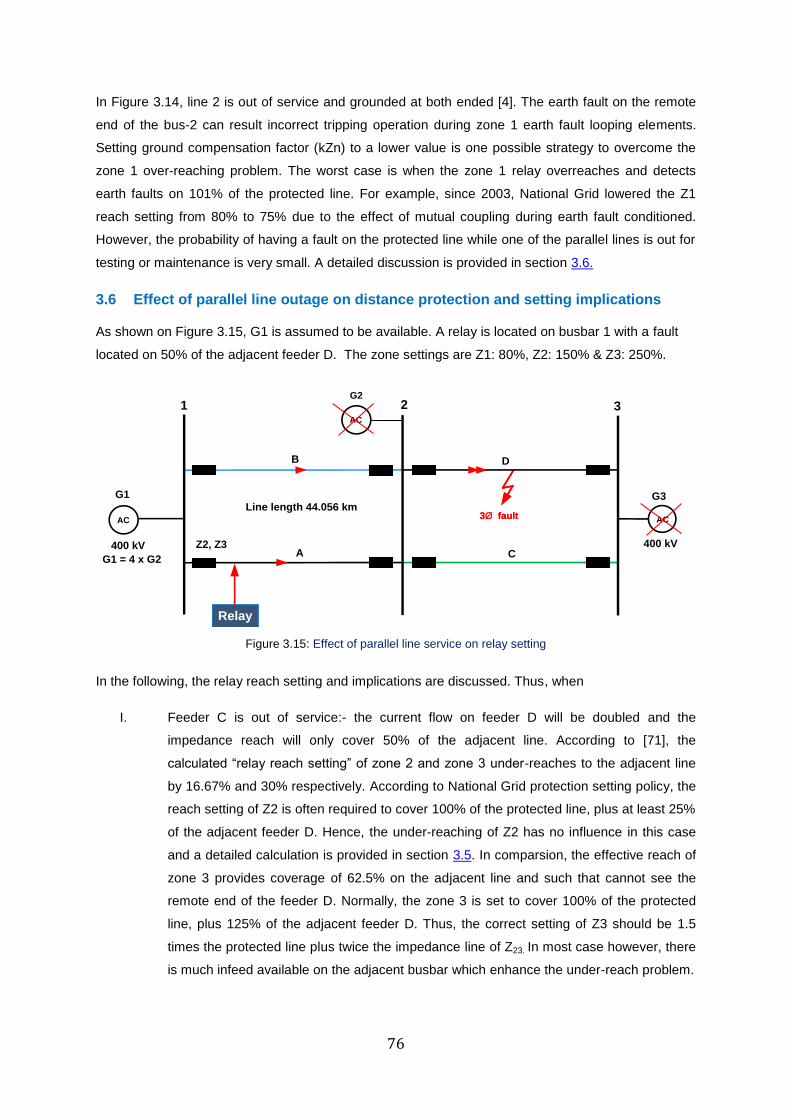
76

In Figure 3.14, line 2 is out of service and grounded at both ended [4]. The earth fault on the remote

end of the bus-2 can result incorrect tripping operation during zone 1 earth fault looping elements.

Setting ground compensation factor (kZn) to a lower value is one possible strategy to overcome the

zone 1 over-reaching problem. The worst case is when the zone 1 relay overreaches and detects

earth faults on 101% of the protected line. For example, since 2003, National Grid lowered the Z1

reach setting from 80% to 75% due to the effect of mutual coupling during earth fault conditioned.

However, the probability of having a fault on the protected line while one of the parallel lines is out for

testing or maintenance is very small. A detailed discussion is provided in section 3.6.

3.6 Effect of parallel line outage on distance protection and setting implications

As shown on Figure 3.15, G1 is assumed to be available. A relay is located on busbar 1 with a fault

located on 50% of the adjacent feeder D. The zone settings are Z1: 80%, Z2: 150% & Z3: 250%.

G1

G1 = 4 x G2

400 kV 400 kV

3

AC

B D

Relay

A C

1 2

AC

G3

AC

G2

Z2, Z3

Line length 44.056 km3Ø fault3Ø fault

Figure 3.15: Effect of parallel line service on relay setting

In the following, the relay reach setting and implications are discussed. Thus, when

I. Feeder C is out of service:- the current flow on feeder D will be doubled and the

impedance reach will only cover 50% of the adjacent line. According to [71], the

calculated “relay reach setting” of zone 2 and zone 3 under-reaches to the adjacent line

by 16.67% and 30% respectively. According to National Grid protection setting policy, the

reach setting of Z2 is often required to cover 100% of the protected line, plus at least 25%

of the adjacent feeder D. Hence, the under-reaching of Z2 has no influence in this case

and a detailed calculation is provided in section 3.5. In comparsion, the effective reach of

zone 3 provides coverage of 62.5% on the adjacent line and such that cannot see the

remote end of the feeder D. Normally, the zone 3 is set to cover 100% of the protected

line, plus 125% of the adjacent feeder D. Thus, the correct setting of Z3 should be 1.5

times the protected line plus twice the impedance line of Z23. In most case however, there

is much infeed available on the adjacent busbar which enhance the under-reach problem.

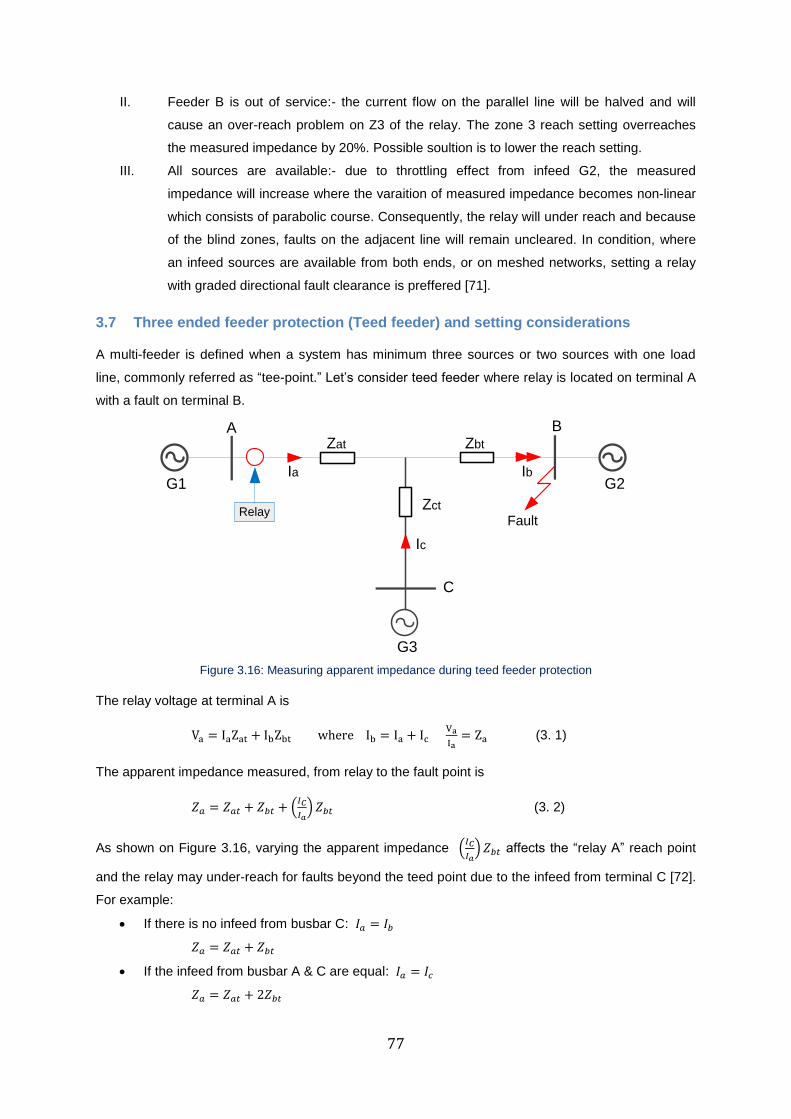
77

II. Feeder B is out of service:- the current flow on the parallel line will be halved and will

cause an over-reach problem on Z3 of the relay. The zone 3 reach setting overreaches

the measured impedance by 20%. Possible soultion is to lower the reach setting.

III. All sources are available:- due to throttling effect from infeed G2, the measured

impedance will increase where the varaition of measured impedance becomes non-linear

which consists of parabolic course. Consequently, the relay will under reach and because

of the blind zones, faults on the adjacent line will remain uncleared. In condition, where

an infeed sources are available from both ends, or on meshed networks, setting a relay

with graded directional fault clearance is preffered [71].

3.7 Three ended feeder protection (Teed feeder) and setting considerations

A multi-feeder is defined when a system has minimum three sources or two sources with one load

line, commonly referred as “tee-point.” Let’s consider teed feeder where relay is located on terminal A

with a fault on terminal B.

A

Ia

Zat

G1

RelayFault

B

C

Zct

Zbt

Ic

IbG2

G3

Figure 3.16: Measuring apparent impedance during teed feeder protection

The relay voltage at terminal A is

Va = IaZat + IbZbt where Ib = Ia + Ic Va

Ia= Za (3. 1)

The apparent impedance measured, from relay to the fault point is

𝑍𝑎 = 𝑍𝑎𝑡 + 𝑍𝑏𝑡 + (𝐼𝐶

𝐼𝑎) 𝑍𝑏𝑡 (3. 2)

As shown on Figure 3.16, varying the apparent impedance (𝐼𝐶

𝐼𝑎) 𝑍𝑏𝑡 affects the “relay A” reach point

and the relay may under-reach for faults beyond the teed point due to the infeed from terminal C [72].

For example:

If there is no infeed from busbar C: 𝐼𝑎 = 𝐼𝑏

𝑍𝑎 = 𝑍𝑎𝑡 + 𝑍𝑏𝑡

If the infeed from busbar A & C are equal: 𝐼𝑎 = 𝐼𝑐

𝑍𝑎 = 𝑍𝑎𝑡 + 2𝑍𝑏𝑡

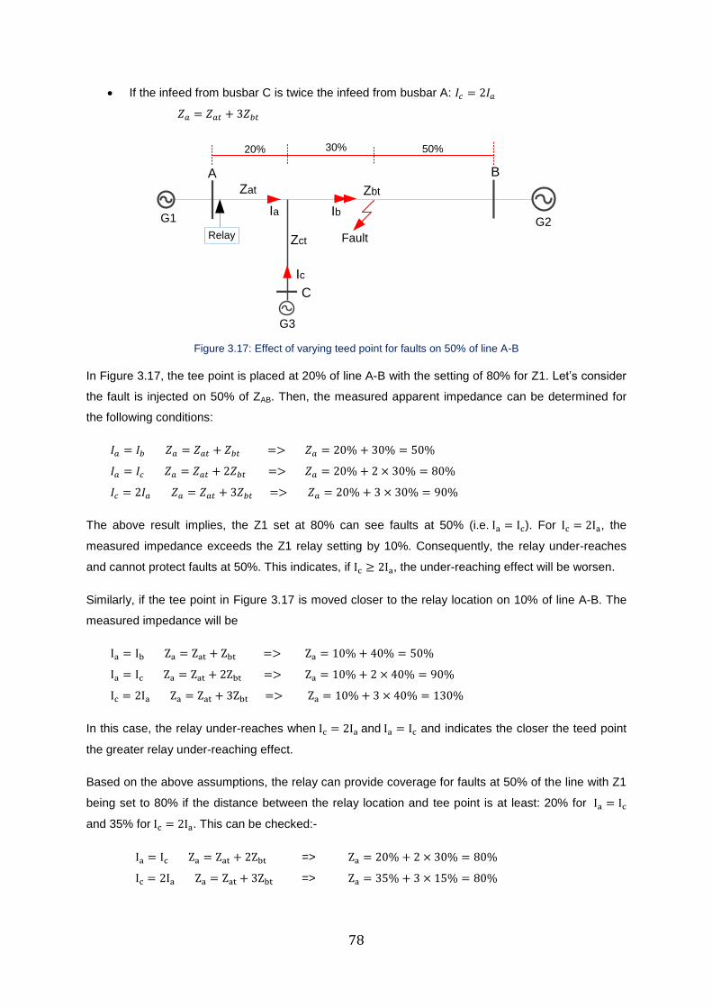
78

If the infeed from busbar C is twice the infeed from busbar A: 𝐼𝑐 = 2𝐼𝑎

𝑍𝑎 = 𝑍𝑎𝑡 + 3𝑍𝑏𝑡

A

Ia

Zat

G1

Relay Fault

B

C

Zct

Zbt

Ic

Ib

G3

G2

20% 50%30%

Figure 3.17: Effect of varying teed point for faults on 50% of line A-B

In Figure 3.17, the tee point is placed at 20% of line A-B with the setting of 80% for Z1. Let’s consider

the fault is injected on 50% of ZAB. Then, the measured apparent impedance can be determined for

the following conditions:

𝐼𝑎 = 𝐼𝑏 𝑍𝑎 = 𝑍𝑎𝑡 + 𝑍𝑏𝑡 => 𝑍𝑎 = 20% + 30% = 50%

𝐼𝑎 = 𝐼𝑐 𝑍𝑎 = 𝑍𝑎𝑡 + 2𝑍𝑏𝑡 => 𝑍𝑎 = 20% + 2 × 30% = 80%

𝐼𝑐 = 2𝐼𝑎 𝑍𝑎 = 𝑍𝑎𝑡 + 3𝑍𝑏𝑡 => 𝑍𝑎 = 20% + 3 × 30% = 90%

The above result implies, the Z1 set at 80% can see faults at 50% (i.e. Ia = Ic). For Ic = 2Ia, the

measured impedance exceeds the Z1 relay setting by 10%. Consequently, the relay under-reaches

and cannot protect faults at 50%. This indicates, if Ic ≥ 2Ia, the under-reaching effect will be worsen.

Similarly, if the tee point in Figure 3.17 is moved closer to the relay location on 10% of line A-B. The

measured impedance will be

Ia = Ib Za = Zat + Zbt => Za = 10% + 40% = 50%

Ia = Ic Za = Zat + 2Zbt => Za = 10% + 2 × 40% = 90%

Ic = 2Ia Za = Zat + 3Zbt => Za = 10% + 3 × 40% = 130%

In this case, the relay under-reaches when Ic = 2Ia and Ia = Ic and indicates the closer the teed point

the greater relay under-reaching effect.

Based on the above assumptions, the relay can provide coverage for faults at 50% of the line with Z1

being set to 80% if the distance between the relay location and tee point is at least: 20% for Ia = Ic

and 35% for Ic = 2Ia. This can be checked:-

Ia = Ic Za = Zat + 2Zbt => Za = 20% + 2 × 30% = 80%

Ic = 2Ia Za = Zat + 3Zbt => Za = 35% + 3 × 15% = 80%

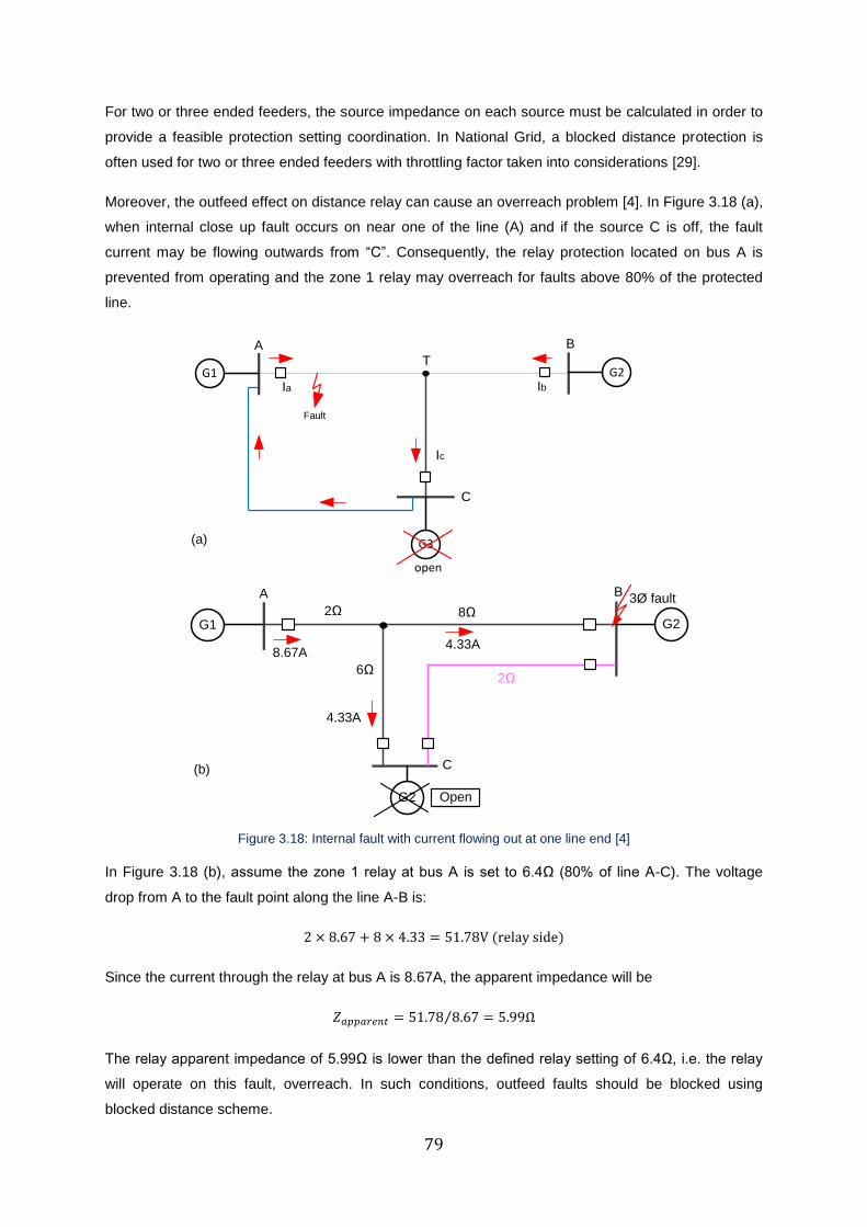
79

For two or three ended feeders, the source impedance on each source must be calculated in order to

provide a feasible protection setting coordination. In National Grid, a blocked distance protection is

often used for two or three ended feeders with throttling factor taken into considerations [29].

Moreover, the outfeed effect on distance relay can cause an overreach problem [4]. In Figure 3.18 (a),

when internal close up fault occurs on near one of the line (A) and if the source C is off, the fault

current may be flowing outwards from “C”. Consequently, the relay protection located on bus A is

prevented from operating and the zone 1 relay may overreach for faults above 80% of the protected

line.

A

Ia

B

C

Ic

Ib

Fault

TG1

G3

G2

open

A B

C

G1 G2

G2 Open

2Ω 8Ω

2Ω 6Ω

4.33A

8.67A4.33A

3Ø fault

(a)

(b)

Figure 3.18: Internal fault with current flowing out at one line end [4]

In Figure 3.18 (b), assume the zone 1 relay at bus A is set to 6.4Ω (80% of line A-C). The voltage

drop from A to the fault point along the line A-B is:

2 × 8.67 + 8 × 4.33 = 51.78V (relay side)

Since the current through the relay at bus A is 8.67A, the apparent impedance will be

𝑍𝑎𝑝𝑝𝑎𝑟𝑒𝑛𝑡 = 51.78 8.67⁄ = 5.99Ω

The relay apparent impedance of 5.99Ω is lower than the defined relay setting of 6.4Ω, i.e. the relay

will operate on this fault, overreach. In such conditions, outfeed faults should be blocked using

blocked distance scheme.

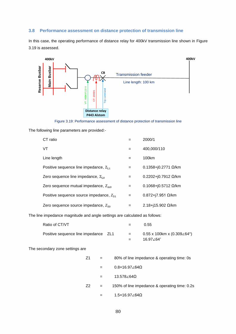
80

3.8 Performance assessment on distance protection of transmission line

In this case, the operating performance of distance relay for 400kV transmission line shown in Figure

3.19 is assessed.

Re

se

rve

Bu

sb

ar

Ma

in B

us

ba

r

Distance relay P443 Alstom

CB

400kV400kV

Transmission feeder

Line length: 100 km

CT

: 2

00

0/1

VT

: 4

00

kV

/11

0 V

Trip

co

mm

an

d

Figure 3.19: Performance assessment of distance protection of transmission line

The following line parameters are provided:-

CT ratio = 2000/1

VT = 400,000/110

Line length = 100km

Positive sequence line impedance, ZL1 = 0.1358+j0.2771 Ω/km

Zero sequence line impedance, ZL0 = 0.2202+j0.7912 Ω/km

Zero sequence mutual impedance, 𝑍m0 = 0.1068+j0.5712 Ω/km

Positive sequence source impedance, 𝑍S1 = 0.872+j7.951 Ω/km

Zero sequence source impedance, 𝑍S0 = 2.18+j15.902 Ω/km

The line impedance magnitude and angle settings are calculated as follows:

Ratio of CT/VT = 0.55

Positive sequence line impedance ZL1 = 0.55 x 100km x (0.309∠64°)

= 16.97∠64˚

The secondary zone settings are

Z1 = 80% of line impedance & operating time: 0s

= 0.8×16.97∠64Ω

= 13.578∠64Ω

Z2 = 150% of line impedance & operating time: 0.2s

= 1.5×16.97∠64Ω

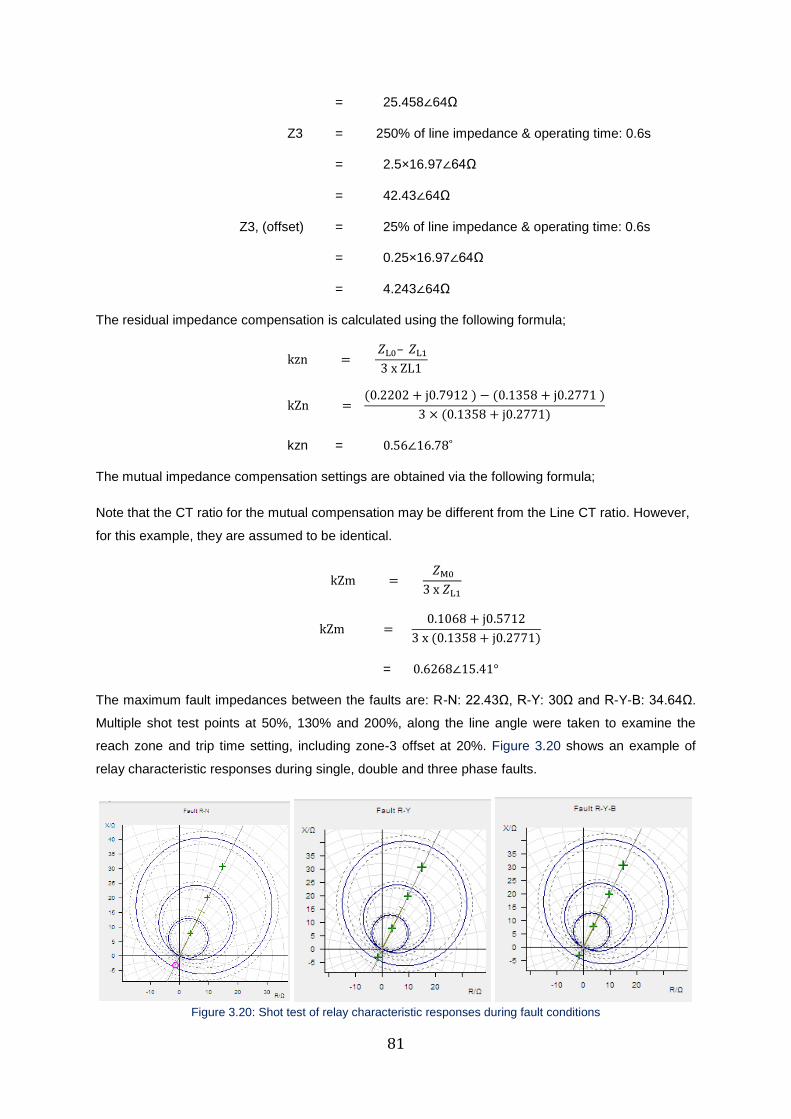
81

= 25.458∠64Ω

Z3 = 250% of line impedance & operating time: 0.6s

= 2.5×16.97∠64Ω

= 42.43∠64Ω

Z3, (offset) = 25% of line impedance & operating time: 0.6s

= 0.25×16.97∠64Ω

= 4.243∠64Ω

The residual impedance compensation is calculated using the following formula;

kzn = 𝑍L0– 𝑍L1

3 x ZL1

kZn = (0.2202 + j0.7912 ) − (0.1358 + j0.2771 )

3 × (0.1358 + j0.2771)

kzn = 0.56∠16.78˚

The mutual impedance compensation settings are obtained via the following formula;

Note that the CT ratio for the mutual compensation may be different from the Line CT ratio. However,

for this example, they are assumed to be identical.

kZm = 𝑍M0

3 x 𝑍L1

kZm = 0.1068 + j0.5712

3 x (0.1358 + j0.2771)

= 0.6268∠15.41°

The maximum fault impedances between the faults are: R-N: 22.43Ω, R-Y: 30Ω and R-Y-B: 34.64Ω.

Multiple shot test points at 50%, 130% and 200%, along the line angle were taken to examine the

reach zone and trip time setting, including zone-3 offset at 20%. Figure 3.20 shows an example of

relay characteristic responses during single, double and three phase faults.

Figure 3.20: Shot test of relay characteristic responses during fault conditions

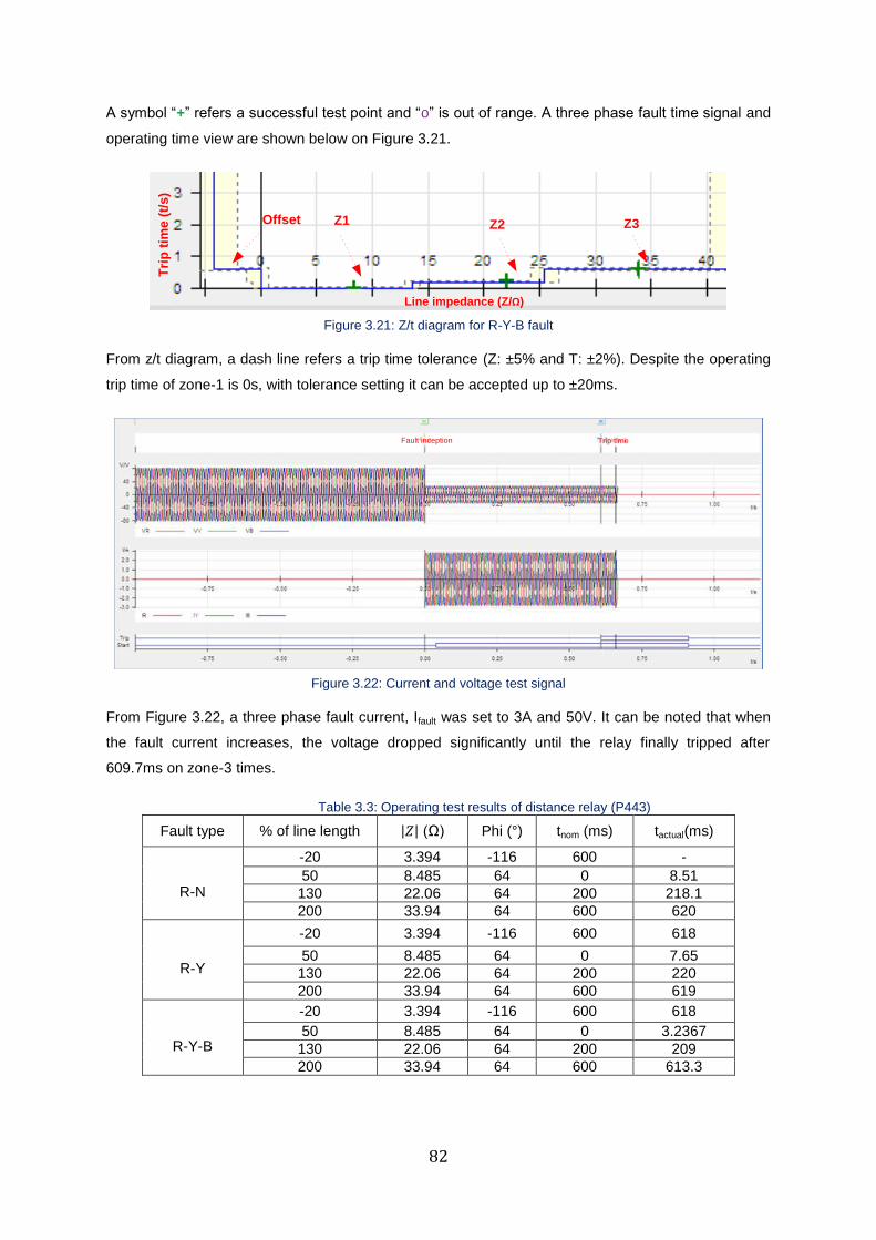
82

A symbol “+” refers a successful test point and “o” is out of range. A three phase fault time signal and

operating time view are shown below on Figure 3.21.

Tri

p t

ime

(t/

s)

Line impedance (Z/Ω)

Offset Z1 Z2 Z3

Figure 3.21: Z/t diagram for R-Y-B fault

From z/t diagram, a dash line refers a trip time tolerance (Z: ±5% and T: ±2%). Despite the operating

trip time of zone-1 is 0s, with tolerance setting it can be accepted up to ±20ms.

Fault inception Trip time

Figure 3.22: Current and voltage test signal

From Figure 3.22, a three phase fault current, Ifault was set to 3A and 50V. It can be noted that when

the fault current increases, the voltage dropped significantly until the relay finally tripped after

609.7ms on zone-3 times.

Table 3.3: Operating test results of distance relay (P443)

Fault type % of line length |𝑍| (Ω) Phi (°) tnom (ms) tactual(ms)

R-N

-20 3.394 -116 600 -

50 8.485 64 0 8.51

130 22.06 64 200 218.1

200 33.94 64 600 620

R-Y

-20 3.394 -116 600 618

50 8.485 64 0 7.65

130 22.06 64 200 220

200 33.94 64 600 619

R-Y-B

-20 3.394 -116 600 618

50 8.485 64 0 3.2367

130 22.06 64 200 209

200 33.94 64 600 613.3

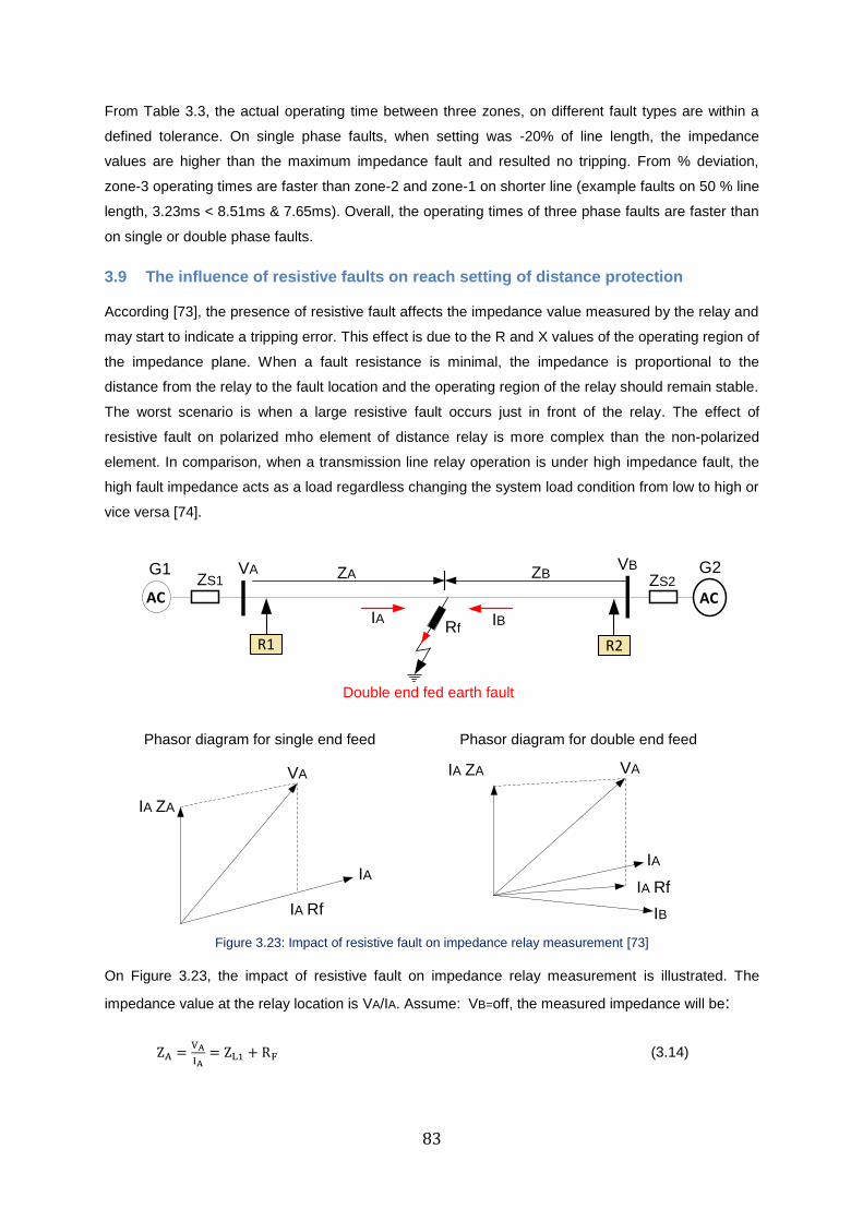
83

From Table 3.3, the actual operating time between three zones, on different fault types are within a

defined tolerance. On single phase faults, when setting was -20% of line length, the impedance

values are higher than the maximum impedance fault and resulted no tripping. From % deviation,

zone-3 operating times are faster than zone-2 and zone-1 on shorter line (example faults on 50 % line

length, 3.23ms < 8.51ms & 7.65ms). Overall, the operating times of three phase faults are faster than

on single or double phase faults.

3.9 The influence of resistive faults on reach setting of distance protection

According [73], the presence of resistive fault affects the impedance value measured by the relay and

may start to indicate a tripping error. This effect is due to the R and X values of the operating region of

the impedance plane. When a fault resistance is minimal, the impedance is proportional to the

distance from the relay to the fault location and the operating region of the relay should remain stable.

The worst scenario is when a large resistive fault occurs just in front of the relay. The effect of

resistive fault on polarized mho element of distance relay is more complex than the non-polarized

element. In comparison, when a transmission line relay operation is under high impedance fault, the

high fault impedance acts as a load regardless changing the system load condition from low to high or

vice versa [74].

G1

AC

R1

IA

ZS1

AC

R2

IB

ZA ZB G2 ZS2

VA VB

Double end fed earth fault

VAVA

IB

IAIA

IA ZA

IA ZA

IA Rf

IA Rf

Phasor diagram for single end feed Phasor diagram for double end feed

Rf

Figure 3.23: Impact of resistive fault on impedance relay measurement [73]

On Figure 3.23, the impact of resistive fault on impedance relay measurement is illustrated. The

impedance value at the relay location is VA/IA. Assume: VB=off, the measured impedance will be:

ZA =VA

IA= ZL1 + RF (3.14)

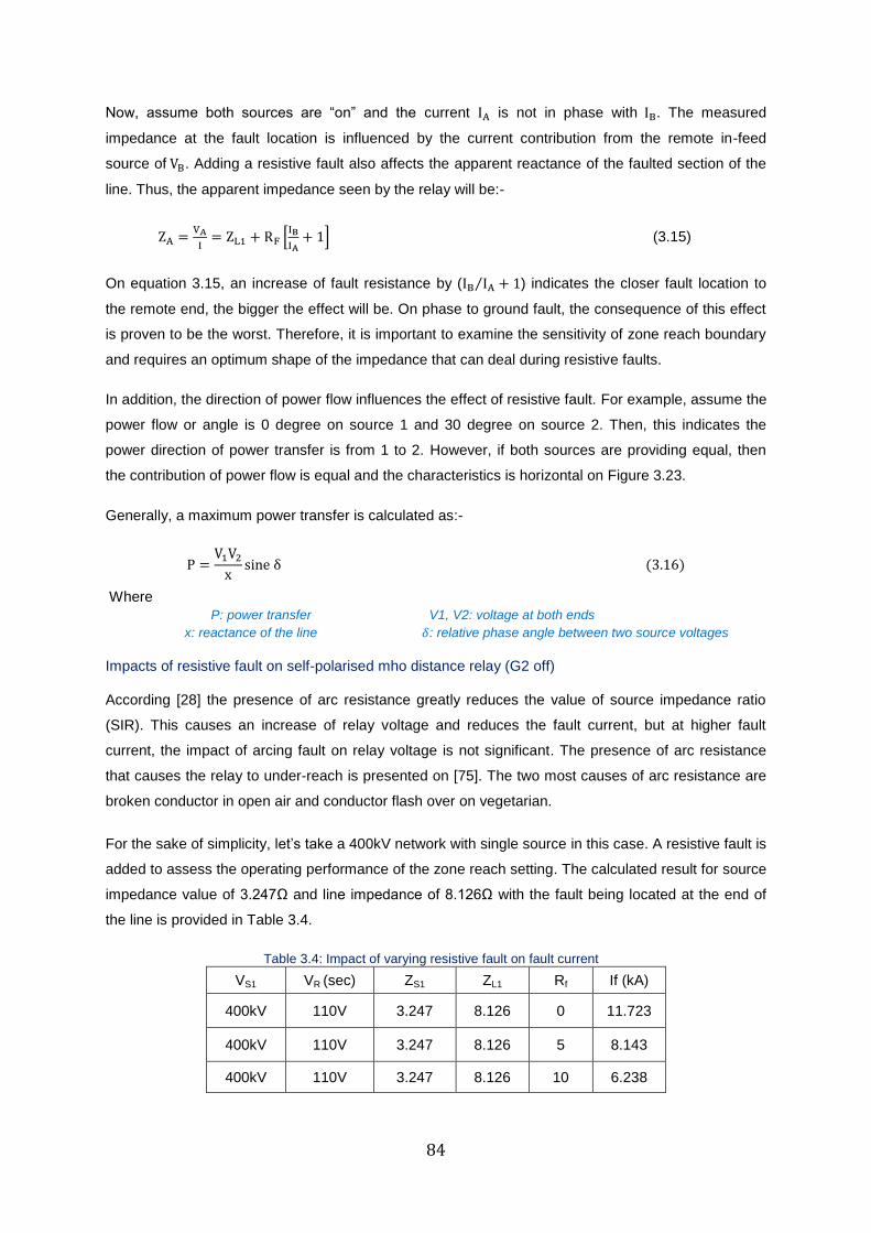
84

Now, assume both sources are “on” and the current IA is not in phase with IB. The measured

impedance at the fault location is influenced by the current contribution from the remote in-feed

source of VB. Adding a resistive fault also affects the apparent reactance of the faulted section of the

line. Thus, the apparent impedance seen by the relay will be:-

ZA =VA

I= ZL1 + RF [

IB

IA+ 1] (3.15)

On equation 3.15, an increase of fault resistance by (IB IA⁄ + 1) indicates the closer fault location to

the remote end, the bigger the effect will be. On phase to ground fault, the consequence of this effect

is proven to be the worst. Therefore, it is important to examine the sensitivity of zone reach boundary

and requires an optimum shape of the impedance that can deal during resistive faults.

In addition, the direction of power flow influences the effect of resistive fault. For example, assume the

power flow or angle is 0 degree on source 1 and 30 degree on source 2. Then, this indicates the

power direction of power transfer is from 1 to 2. However, if both sources are providing equal, then

the contribution of power flow is equal and the characteristics is horizontal on Figure 3.23.

Generally, a maximum power transfer is calculated as:-

P =V1V2

xsine δ (3.16)

Where

P: power transfer V1, V2: voltage at both ends

x: reactance of the line 𝛿: relative phase angle between two source voltages

Impacts of resistive fault on self-polarised mho distance relay (G2 off)

According [28] the presence of arc resistance greatly reduces the value of source impedance ratio

(SIR). This causes an increase of relay voltage and reduces the fault current, but at higher fault

current, the impact of arcing fault on relay voltage is not significant. The presence of arc resistance

that causes the relay to under-reach is presented on [75]. The two most causes of arc resistance are

broken conductor in open air and conductor flash over on vegetarian.

For the sake of simplicity, let’s take a 400kV network with single source in this case. A resistive fault is

added to assess the operating performance of the zone reach setting. The calculated result for source

impedance value of 3.247Ω and line impedance of 8.126Ω with the fault being located at the end of

the line is provided in Table 3.4.

Table 3.4: Impact of varying resistive fault on fault current

VS1 VR (sec) ZS1 ZL1 Rf If (kA)

400kV 110V 3.247 8.126 0 11.723

400kV 110V 3.247 8.126 5 8.143

400kV 110V 3.247 8.126 10 6.238

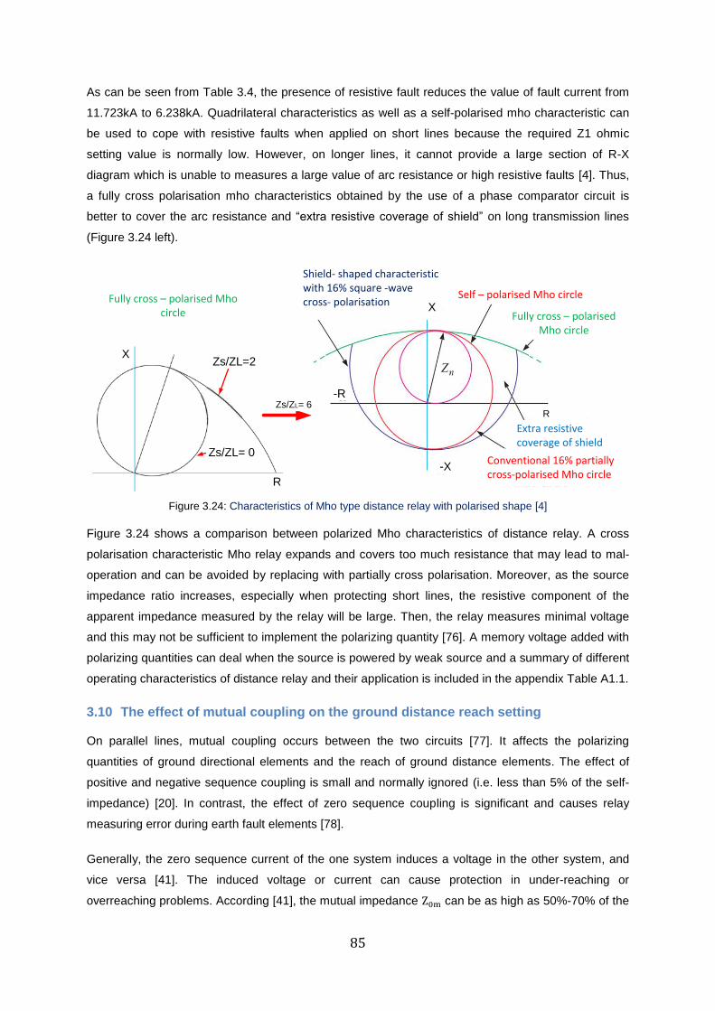
85

As can be seen from Table 3.4, the presence of resistive fault reduces the value of fault current from

11.723kA to 6.238kA. Quadrilateral characteristics as well as a self-polarised mho characteristic can

be used to cope with resistive faults when applied on short lines because the required Z1 ohmic

setting value is normally low. However, on longer lines, it cannot provide a large section of R-X

diagram which is unable to measures a large value of arc resistance or high resistive faults [4]. Thus,

a fully cross polarisation mho characteristics obtained by the use of a phase comparator circuit is

better to cover the arc resistance and “extra resistive coverage of shield” on long transmission lines

(Figure 3.24 left).

Fully cross – polarised Mho circle

Zs/ZL= 25Zs/ZL=2

Zs/ZL= 0

R

Zs/

ZL=

25

X

Shield- shaped characteristic with 16% square -wave cross- polarisation

Self – polarised Mho circle

Fully cross – polarisedMho circle

Extra resistive coverage of shield

Conventional 16% partially cross-polarised Mho circle

Zs/ZL= 6R

-R

-X

X

Figure 3.24: Characteristics of Mho type distance relay with polarised shape [4]

Figure 3.24 shows a comparison between polarized Mho characteristics of distance relay. A cross

polarisation characteristic Mho relay expands and covers too much resistance that may lead to mal-

operation and can be avoided by replacing with partially cross polarisation. Moreover, as the source

impedance ratio increases, especially when protecting short lines, the resistive component of the

apparent impedance measured by the relay will be large. Then, the relay measures minimal voltage

and this may not be sufficient to implement the polarizing quantity [76]. A memory voltage added with

polarizing quantities can deal when the source is powered by weak source and a summary of different

operating characteristics of distance relay and their application is included in the appendix Table A1.1.

3.10 The effect of mutual coupling on the ground distance reach setting

On parallel lines, mutual coupling occurs between the two circuits [77]. It affects the polarizing

quantities of ground directional elements and the reach of ground distance elements. The effect of

positive and negative sequence coupling is small and normally ignored (i.e. less than 5% of the self-

impedance) [20]. In contrast, the effect of zero sequence coupling is significant and causes relay

measuring error during earth fault elements [78].

Generally, the zero sequence current of the one system induces a voltage in the other system, and

vice versa [41]. The induced voltage or current can cause protection in under-reaching or

overreaching problems. According [41], the mutual impedance Z0m can be as high as 50%-70% of the

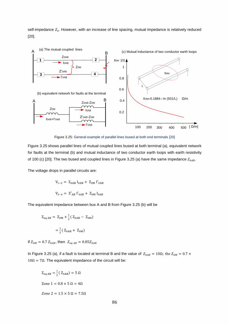
86

self-impedance 𝑍0. However, with an increase of line spacing, mutual impedance is relatively reduced

[20].

L

X0M

100 200 300 400 500

0.2

0.4

0.6

0.8

1

X0M=0.1884 × ln (931/L) Ω/m

[ Ω/m]

X0M [Ω]

(c) Mutual inductance of two conductor earth loops

A B

Z0M

I0AB+I’0ABZ’0AB-Z0M

Z0AB-Z0M

I0AB

I’0AB

A B

1

Z0M

I0AB

I’0AB

Z0AB

Z’0AB

3

2

4

(a) The mutual coupled lines

(b) equivalent network for faults at the terminal

Figure 3.25: General example of parallel lines bused at both end terminals [20]

Figure 3.25 shows parallel lines of mutual coupled lines bused at both terminal (a), equivalent network

for faults at the terminal (b) and mutual inductance of two conductor earth loops with earth resistivity

of 100 (c) [20]. The two bused and coupled lines in Figure 3.25 (a) have the same impedance 𝑍0𝐴𝐵.

The voltage drops in parallel circuits are:

V1−2 = Z0AB I0AB + Z0M I′0AB

V3−4 = Z′AB I′0AB + Z0M I0AB

The equivalent impedance between bus A and B from Figure 3.25 (b) will be

Zeq AB = Z0M +1

2( Z0AB − Z0M)

=1

2( Z0AB + Z0M)

If 𝑍0𝑀 = 0.7 𝑍0𝐴𝐵, then 𝑍𝑒𝑞 𝐴𝐵 = 0.85𝑍0𝐴𝐵

In Figure 3.25 (a), if a fault is located at terminal B and the value of 𝑍0𝐴𝐵 = 10Ω; the 𝑍0𝑀 = 0.7 ×

10Ω = 7Ω. The equivalent impedance of the circuit will be:

Zeq AB =1

2( Z0AB) = 5 Ω

Zone 1 = 0.8 × 5 Ω = 4Ω

𝑍𝑜𝑛𝑒 2 = 1.5 × 5 Ω = 7.5Ω

87

Now, if the zero sequence mutual coupling is considered, the apparent impedance and zone setting

would be

𝑍𝑒𝑞 𝐴𝐵 =1

2(10 + 7) = 8.5Ω

𝑍𝑜𝑛𝑒 1 = 0.8 × 8.5 Ω = 6.8Ω

𝑍𝑜𝑛𝑒 2 = 1.5 × 8.5 Ω = 12.5Ω

Thus, when the currents are flowing in the same direction, the mutual increases the line impedance

between the two buses from 5Ω to 8.5Ω (i.e. 0.5 times 𝑍0𝐴𝐵 without the mutual coupling). Hence, the

rising of mutual coupling affects the inductive reactance of the protected circuit especially during

uncertainties associated with the data model (i.e. an accurate value of the zero sequence impedance

to which the relay must be set), changes in earth resistivity, or by the change of mutual coupling due

to availability of infeed sources [20].

The impact of mutual coupling on the ground distance element includes

Zone 1 over-reach: happened when the zero sequence currents in the protected line and the

coupled line flow in opposite directions (i.e when one of the parallel lines is out of service and

grounded at both end with fault on the remote bus). This can be resolved by altering the zone

1 earth loop reach where the residual compensation factor is set to a lower value than normal

[78].

Zone 2 and 3: under-reach: happened when the current flow in the same direction (i.e. both

parallel line in service with fault on remote bus) [78]. This can be resolved by increasing the

setting of the earth fault elements such that it will have a comparable reach to the phase fault

elements [72]. However, the reach setting of residual compensation factor has to consider the

effects of mutual coupling and provide a relay with correct data model of the zero sequence

current of the coupled line [20].

In UK National Grid, the zero sequence impedance of a double circuit (Z0DC ) is 180 -200% of 𝑍0 [29].

In order to avoid the overreaching operation, the positive sequence impedance of a double circuit is

set lower by 5% than a single circuit positive sequence when the same current is flowing in the same

direction. Thus, the current policy of National Grid reduced the zone 1 setting in 2004 from 80% to

75% Z1DC for 400 kV and 275 kV. If the residual compensation factor is given, the phase and earth

fault Zone 1 reaches is set using the following equation [29]:

Zone 1earth fault = Zone 1phase fault (1 + kZn); kZn =1

3(

Z0

Z1

− 1)

Z1, Z0= positive and zero sequence impedance for the protected line

The recent paper presented by National Grid [43] identified the risk for protection mal-operation for

out-of-zone faults during transmission system reinforcements. The authors have recommended

protection setting re-calculation for earth fault reach up to the acceptable level.

88

3.11 Summary

In this chapter, the operating behaviour and setting application of distance protection is discussed.

Distance relay measures the impedance of the line and operates when the measured value is less

than the reference value. The role of distance protection scheme is designed to provide a high speed

protection for faults within the protected line. If a measuring element of a distance relay is set to cover

100% of the protected line, without considering the errors generated from CT and VT, relay

measurements (i.e.15%-20%), and data obtained from the primary values; it would be difficult to

ensure relay operation does not trip for an external fault beyond the remote end of the protected line.

Hence, the accepted Zone 1 setting of a distance protection is 75%-85% of protected line impedance,

and this is configured for an instantaneous trip with no intentional delay time. The minimum Zone 2

setting covers 120% of the protected line and the maximum setting covers the protected line, plus

50% of the shortest adjacent line, operating at a delayed time of 0.5s. The Zone 3 forward setting

covers 100% of the protected line, plus 125%-150% of the adjacent line and provides a backup

protection for zone 1 and 2 at a delayed time of 1s. The Zone 3 reverse looking setting covers part of

the adjacent line, and looks in a reverse direction, it is normally set to impedance equal to 10% of the

protected line. The reach setting of distance protection can be affected by the presence of resistive

fault, mutual coupling effect, fault location on parallel lines, especially if one of the lines is

disconnected, the ratio of source to line impedance, and the availability of fault level.

However, with aid of a communication channel, a distance protection scheme can provide 100% fault

coverage of the protected line. The common types of communication schemes are direct inter-trip,

permissive and blocking schemes. However, the performance of these schemes may be affected

during weak infeed conditions, on varying source impedance ratio or during a failure of signal

communication channels. In the GB transmission system operated by National Grid, distance

protection is the 2nd

main protection used for 400 kV or 275 kV feeder protections. On feeders with

purely cable section where double unit protection is used, the integral distance protection is set to

provide backup protection. The sensitivity analysis of reach setting of distance relay and setting

consideration of distance protection of a double circuit transmission line is highlighted in this chapter.

The key strengths of this study are to widen understanding on the concept and application of distance

protection. To validate this, a simulation testing of distance protection relay on a 400kV double circuit

transmission feeder was performed. Thus, the physical relay was tested using the Omicron test

universe (secondary injection static test). During these experimental tests, three phase, double phase

and single phase fault tests were conducted.

The 1st technical paper entitled < Impact of Weak In-feed Tripping Performance on Distance Protection

Schemes> was published and presented based on this work at the HubNet Smart Grids Symposium annual show

case. The Symposium was held on Sep 13-14, 2016 at the University of Strathclyde, Glasgow, UK.

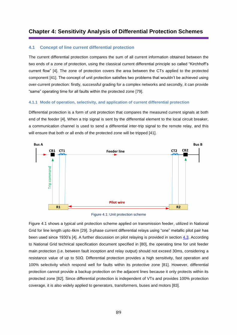
89

Chapter 4: Sensitivity Analysis of Differential Protection Schemes

4.1 Concept of line current differential protection

The current differential protection compares the sum of all current information obtained between the

two ends of a zone of protection, using the classical current differential principle so called “Kirchhoff’s

current flow” [4]. The zone of protection covers the area between the CTs applied to the protected

component [41]. The concept of unit protection satisfies two problems that wouldn’t be achieved using

over-current protection: firstly, successful grading for a complex networks and secondly, it can provide

“same” operating time for all faults within the protected zone [79].

4.1.1 Mode of operation, selectivity, and application of current differential protection

Differential protection is a form of unit protection that compares the measured current signals at both

end of the feeder [4]. When a trip signal is sent by the differential element to the local circuit breaker,

a communication channel is used to send a differential inter-trip signal to the remote relay, and this

will ensure that both or all ends of the protected zone will be tripped [41].

R1

CB1 CB2CT1 CT2

Pilot wire

Feeder line

Bus A Bus B

Trip

co

mm

and

R2

Figure 4.1: Unit protection scheme

Figure 4.1 shows a typical unit protection scheme applied on transmission feeder, utilized in National

Grid for line length upto 4km [29]. 3-phase current differential relays using “one” metallic pilot pair has

been used since 1930’s [4]. A further discussion on pilot relaying is provided in section 4.3. According

to National Grid technical specification document specified in [80], the operating time for unit feeder

main protection (i.e. between fault inception and relay output) should not exceed 30ms, considering a

resistance value of up to 50Ω. Differential protection provides a high sensitivity, fast operation and

100% selectivity which respond well for faults within its protective zone [81]. However, differential

protection cannot provide a backup protection on the adjacent lines because it only protects within its

protected zone [82]. Since differential protection is independent of VTs and provides 100% protection

coverage, it is also widely applied to generators, transformers, buses and motors [83].

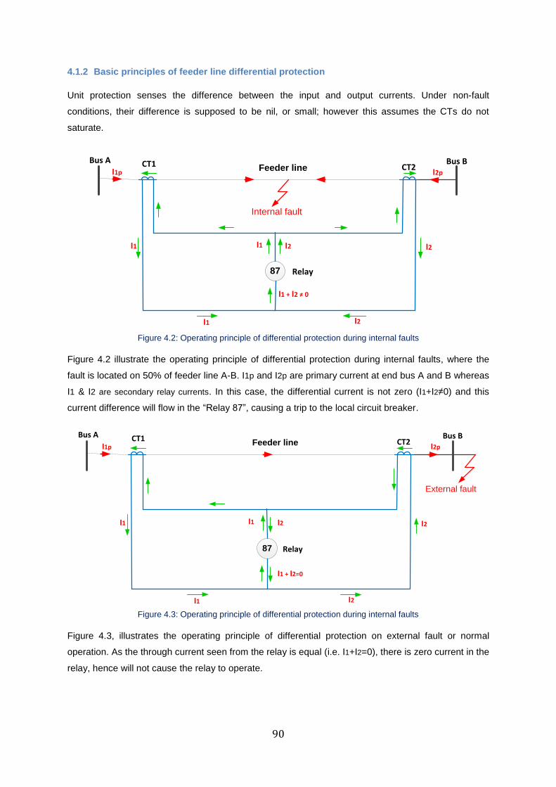
90

4.1.2 Basic principles of feeder line differential protection

Unit protection senses the difference between the input and output currents. Under non-fault

conditions, their difference is supposed to be nil, or small; however this assumes the CTs do not

saturate.

Bus A Bus BCT1 CT2Feeder line

87 Relay

Internal fault

I1p

I1 I2

I2I1

I1 + I2 ≠ 0

I1 I2

I2p

Figure 4.2: Operating principle of differential protection during internal faults

Figure 4.2 illustrate the operating principle of differential protection during internal faults, where the

fault is located on 50% of feeder line A-B. I1p and I2p are primary current at end bus A and B whereas

I1 & I2 are secondary relay currents. In this case, the differential current is not zero (I1+I2≠0) and this

current difference will flow in the “Relay 87”, causing a trip to the local circuit breaker.

External fault

Bus A Bus BCT1 CT2Feeder line

87 Relay

I1p I2p

I1 I2

I2I1

I1 + I2=0

I1 I2

Figure 4.3: Operating principle of differential protection during internal faults

Figure 4.3, illustrates the operating principle of differential protection on external fault or normal

operation. As the through current seen from the relay is equal (i.e. I1+I2=0), there is zero current in the

relay, hence will not cause the relay to operate.

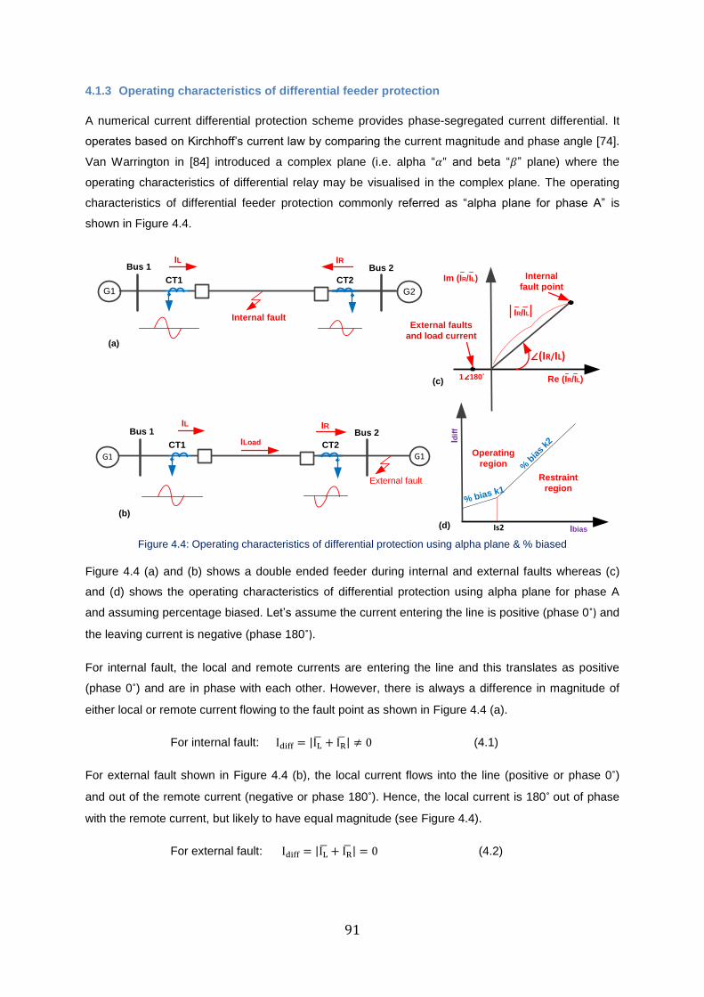
91

4.1.3 Operating characteristics of differential feeder protection

A numerical current differential protection scheme provides phase-segregated current differential. It

operates based on Kirchhoff’s current law by comparing the current magnitude and phase angle [74].

Van Warrington in [84] introduced a complex plane (i.e. alpha “𝛼" and beta “𝛽” plane) where the

operating characteristics of differential relay may be visualised in the complex plane. The operating

characteristics of differential feeder protection commonly referred as “alpha plane for phase A” is

shown in Figure 4.4.

Idif

f

Ibias

Restraint

region

Operating

region

Is2

% bias k1

% b

ias

k2

(d)

Bus 1 Bus 2

CT1 CT2

IL IR

G1 G2

Bus 1 Bus 2

CT1 CT2

IL IR

G1 G1

ILoad

Internal fault

External fault

(a)

(b)

Internal

fault point

External faults

and load current

Re (IR/IL)1 180˚

(IR/IL)

IR/IL

Im (IR/IL)

(c)

Figure 4.4: Operating characteristics of differential protection using alpha plane & % biased

Figure 4.4 (a) and (b) shows a double ended feeder during internal and external faults whereas (c)

and (d) shows the operating characteristics of differential protection using alpha plane for phase A

and assuming percentage biased. Let’s assume the current entering the line is positive (phase 0˚) and

the leaving current is negative (phase 180˚).

For internal fault, the local and remote currents are entering the line and this translates as positive

(phase 0˚) and are in phase with each other. However, there is always a difference in magnitude of

either local or remote current flowing to the fault point as shown in Figure 4.4 (a).

For internal fault: Idiff = |IL + IR| ≠ 0 (4.1)

For external fault shown in Figure 4.4 (b), the local current flows into the line (positive or phase 0˚)

and out of the remote current (negative or phase 180˚). Hence, the local current is 180˚ out of phase

with the remote current, but likely to have equal magnitude (see Figure 4.4).

For external fault: Idiff = |IL + IR| = 0 (4.2)

92

Figure 4.4 (c) shows the complex plane called “alpha plane”, where the relay operates by checking

the vector ratio of the local and remote current [85]. From [84], plane 𝛼 = IR/IL = 𝑎 + 𝑗𝑏 = r = 𝑟𝑒𝑗𝜃

and 𝛽 = IL/IR. For external fault or normal operation, let’s assume the magnitude of line current is “I”

and the ratio of remote to local current will be as follows:

Phase A =IRA

ILA

=1∠180°

1∠0°= 1∠180° or − 1 + j0 i. e the same rule for phase B and C.

This indicates, the ratio of remote to local current is out of phase and the relay will not trip as shown

on the left of the origin on the alpha plane or X axis (Figure 4.4 (c)). The alpha plane can be modified

to accumulate the errors caused by line charging current, CT saturation, channel time-delay

compensation errors and other related errors. Therefore, internal fault will be appeared in the 1st and

4th quadrant whereas external fault will be appeared in the 2

nd and 3

rd quadrant.

A good sensitivity of the relay is ensured by making the differential current almost proportional to the

fault current. Hence, the operating current is the magnitude phasor sum of local and remote current

and is given by:

Idiff = |IL + IR| (4.3)

The restraint or bias current is the ratio of differential or spill current to the mean through fault current.

Since the restraint or bias current is a function of the total current where the function is often constant

“k”, it is given by:

Irestriant = k(|IL| + |IR|) (4.4)

The minimum operating criterion is:

Iop > Imin + Irestriant (4.5)

Where:

𝐼𝑜𝑝 = |𝐼 𝑚𝑖𝑛 + 𝐼 𝑚𝑖𝑛| (4.6)

𝐼𝑚𝑖𝑛 = 𝑀𝑖𝑛𝑖𝑚𝑢𝑚 𝑟𝑒𝑙𝑎𝑦 𝑝𝑖𝑐𝑘𝑢𝑝 𝑙𝑒𝑣𝑒𝑙 𝑜𝑓 𝑡ℎ𝑒 𝑟𝑒𝑙𝑎𝑦 𝑎𝑛𝑑

𝐼𝑟𝑒𝑠𝑡𝑟𝑖𝑎𝑛𝑡 = 𝑓(𝐼 𝑚𝑖𝑛 , 𝐼 𝑚𝑖𝑛)

Alternatively, as shown on Figure 4.4 (d), for percentage biased characteristic, the tripping criterion is

given by:

For |Ibias| < Is2 |Idiff| > k1 × |Ibias| + Is1 (4.7)

For |Ibias| > Is2 |Idiff| > k2 × |Ibias| − (k2 − k1) × Is2 + Is1 (4.8)

The basic relay setting ranges[28], the operating criteria of differential protection is summarised in

Table 4.1.

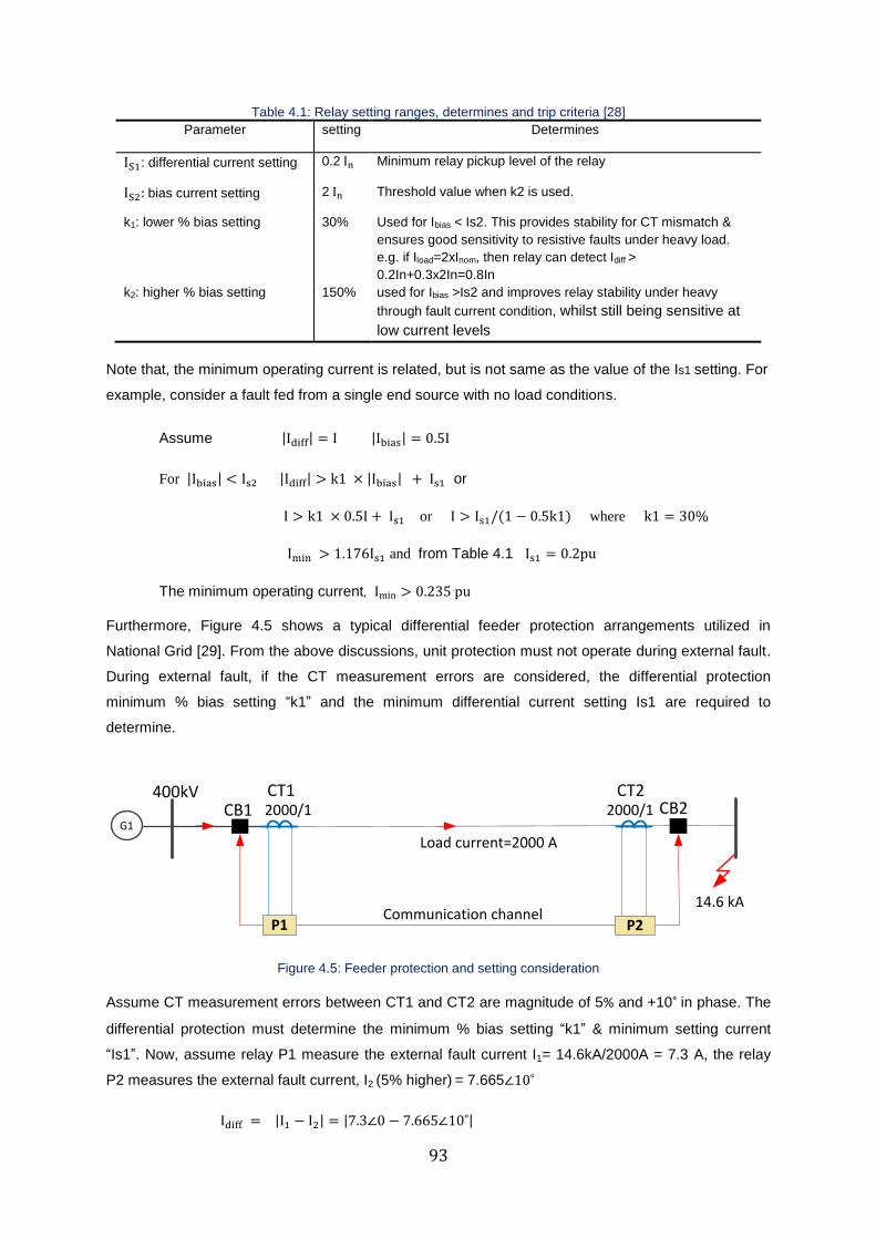
93

Table 4.1: Relay setting ranges, determines and trip criteria [28]

Parameter setting Determines

IS1: differential current setting 0.2 In Minimum relay pickup level of the relay

IS2: bias current setting 2 In Threshold value when k2 is used.

k1: lower % bias setting 30% Used for Ibias < Is2. This provides stability for CT mismatch &

ensures good sensitivity to resistive faults under heavy load.

e.g. if Iload=2xInom, then relay can detect Idiff >

0.2In+0.3x2In=0.8In

k2: higher % bias setting 150% used for Ibias >Is2 and improves relay stability under heavy

through fault current condition, whilst still being sensitive at

low current levels

Note that, the minimum operating current is related, but is not same as the value of the Is1 setting. For

example, consider a fault fed from a single end source with no load conditions.

Assume |Idiff| = I |Ibias| = 0.5I

For |Ibias| < Is2 |Idiff| > k1 × |Ibias| + Is1 or

I > k1 × 0.5I + Is1 or I > Is1/(1 − 0.5k1) where k1 = 30%

Imin > 1.176Is1 and from Table 4.1 Is1 = 0.2pu

The minimum operating current, Imin > 0.235 pu

Furthermore, Figure 4.5 shows a typical differential feeder protection arrangements utilized in

National Grid [29]. From the above discussions, unit protection must not operate during external fault.

During external fault, if the CT measurement errors are considered, the differential protection

minimum % bias setting “k1” and the minimum differential current setting Is1 are required to

determine.

P1

CB1 CB2CT12000/1 2000/1

CT2400kV

P2

Load current=2000 A

14.6 kA

G1

Communication channel

Figure 4.5: Feeder protection and setting consideration

Assume CT measurement errors between CT1 and CT2 are magnitude of 5% and +10˚ in phase. The

differential protection must determine the minimum % bias setting “k1” & minimum setting current

“Is1”. Now, assume relay P1 measure the external fault current I1= 14.6kA/2000A = 7.3 A, the relay

P2 measures the external fault current, I2 (5% higher) = 7.665∠10˚

Idiff = |I1 − I2| = |7.3∠0 − 7.665∠10˚|

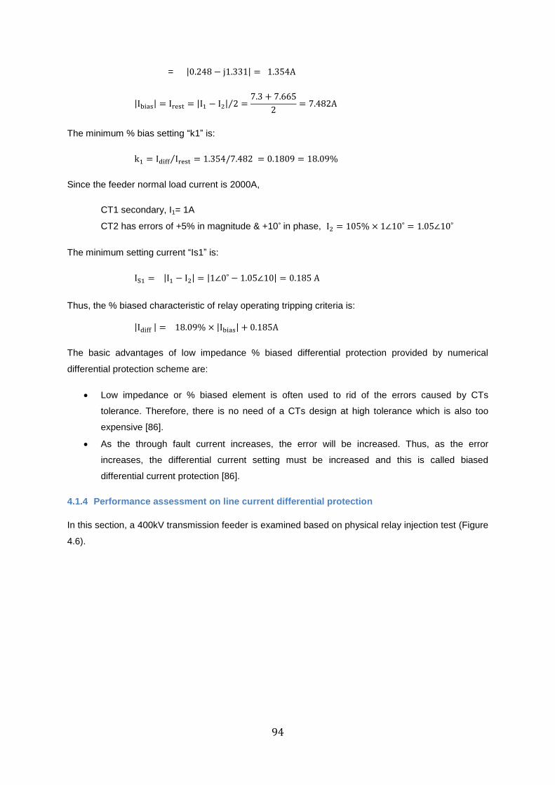
94

= |0.248 − j1.331| = 1.354A

|Ibias| = Irest = |I1 − I2| 2⁄ =7.3 + 7.665

2= 7.482A

The minimum % bias setting “k1” is:

k1 = Idiff Irest = 1.354/7.482 = 0.1809 = 18.09%⁄

Since the feeder normal load current is 2000A,

CT1 secondary, I1= 1A

CT2 has errors of +5% in magnitude & +10˚ in phase, I2 = 105% × 1∠10˚ = 1.05∠10˚

The minimum setting current “Is1” is:

IS1 = |I1 − I2| = |1∠0˚ − 1.05∠10| = 0.185 A

Thus, the % biased characteristic of relay operating tripping criteria is:

|Idiff | = 18.09% × |Ibias| + 0.185A

The basic advantages of low impedance % biased differential protection provided by numerical

differential protection scheme are:

Low impedance or % biased element is often used to rid of the errors caused by CTs

tolerance. Therefore, there is no need of a CTs design at high tolerance which is also too

expensive [86].

As the through fault current increases, the error will be increased. Thus, as the error

increases, the differential current setting must be increased and this is called biased

differential current protection [86].

4.1.4 Performance assessment on line current differential protection

In this section, a 400kV transmission feeder is examined based on physical relay injection test (Figure

4.6).

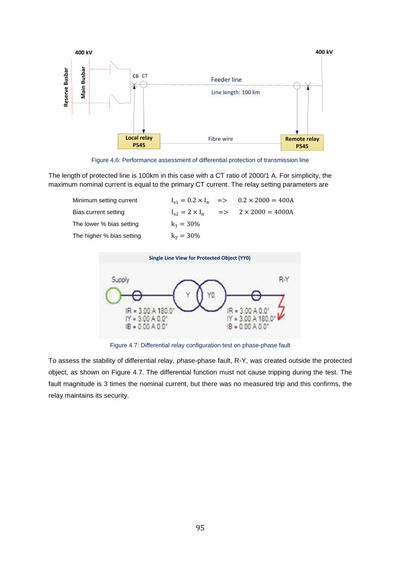
95

Re

serv

e B

usb

ar

Mai

n B

usb

ar

Local relayP545

CTCB

400 kV400 kV

Feeder line

Line length: 100 km

Remote relayP545

Fibre wire

Figure 4.6: Performance assessment of differential protection of transmission line

The length of protected line is 100km in this case with a CT ratio of 2000/1 A. For simplicity, the

maximum nominal current is equal to the primary CT current. The relay setting parameters are

Minimum setting current Is1 = 0.2 × In => 0.2 × 2000 = 400A

Bias current setting Is2 = 2 × In => 2 × 2000 = 4000A

The lower % bias setting k1 = 30%

The higher % bias setting k2 = 30%

Single Line View for Protected Object (YY0)

Figure 4.7: Differential relay configuration test on phase-phase fault

To assess the stability of differential relay, phase-phase fault, R-Y, was created outside the protected

object, as shown on Figure 4.7. The differential function must not cause tripping during the test. The

fault magnitude is 3 times the nominal current, but there was no measured trip and this confirms, the

relay maintains its security.

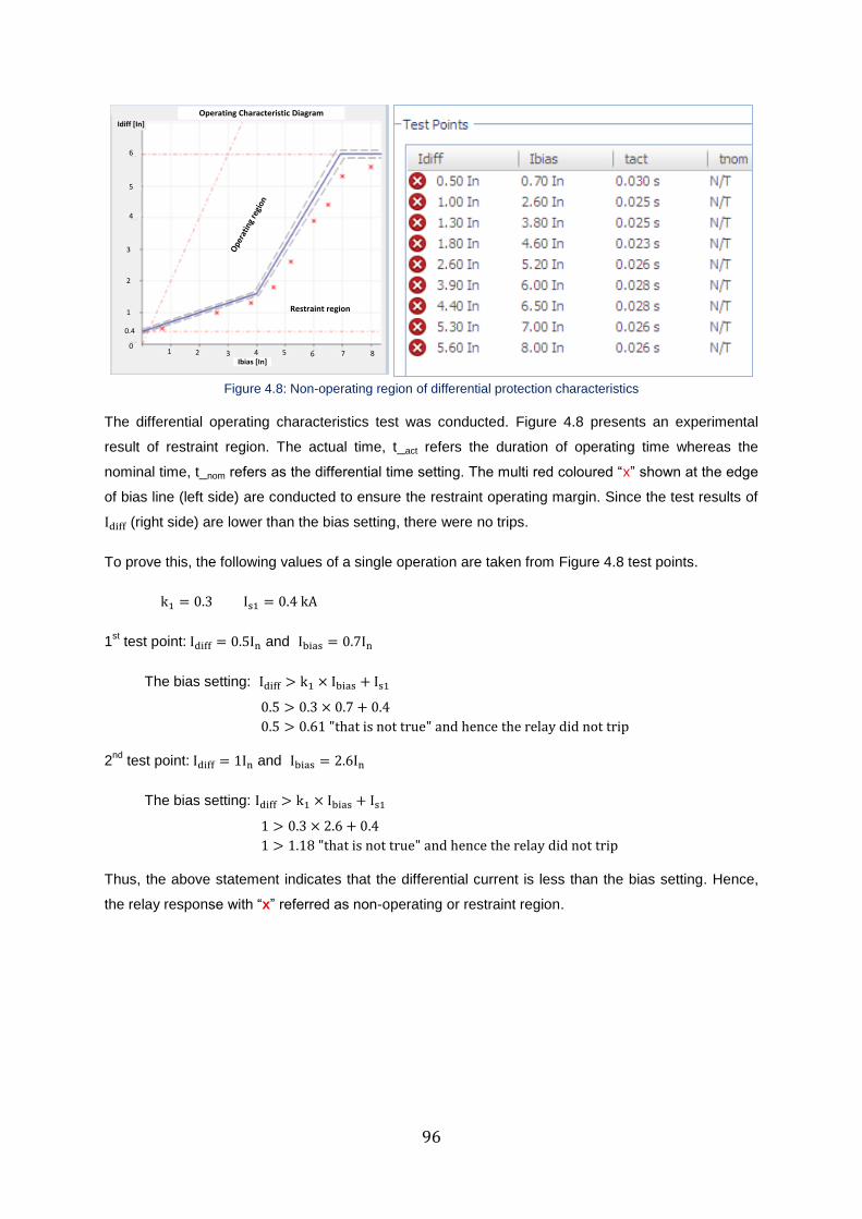
96

Ibias

Operating Characteristic DiagramIdiff [In]

6

5

4

3

2

1

0

Restraint region

Ope

rati

ng re

gion

1 2 3 4Ibias [In]

5 6 7 8

0.4

Figure 4.8: Non-operating region of differential protection characteristics

The differential operating characteristics test was conducted. Figure 4.8 presents an experimental

result of restraint region. The actual time, t_act refers the duration of operating time whereas the

nominal time, t_nom refers as the differential time setting. The multi red coloured “x” shown at the edge

of bias line (left side) are conducted to ensure the restraint operating margin. Since the test results of

Idiff (right side) are lower than the bias setting, there were no trips.

To prove this, the following values of a single operation are taken from Figure 4.8 test points.

k1 = 0.3 Is1 = 0.4 kA

1st test point: Idiff = 0.5In and Ibias = 0.7In

The bias setting: Idiff > k1 × Ibias + Is1

0.5 > 0.3 × 0.7 + 0.4

0.5 > 0.61 "that is not true" and hence the relay did not trip

2nd

test point: Idiff = 1In and Ibias = 2.6In

The bias setting: Idiff > k1 × Ibias + Is1

1 > 0.3 × 2.6 + 0.4

1 > 1.18 "that is not true" and hence the relay did not trip

Thus, the above statement indicates that the differential current is less than the bias setting. Hence,

the relay response with “x” referred as non-operating or restraint region.

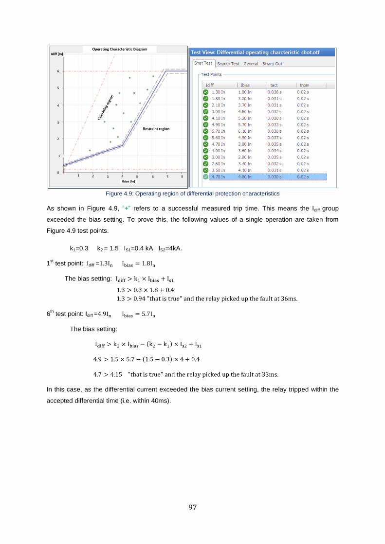
97

Operating Characteristic DiagramIdiff [In]

6

5

4

3

2

1

0

Restraint region

Ope

rati

ng r

egio

n

1 2 3 4

Ibias [In]

5 6 7 8

Figure 4.9: Operating region of differential protection characteristics

As shown in Figure 4.9, “+” refers to a successful measured trip time. This means the Idiff group

exceeded the bias setting. To prove this, the following values of a single operation are taken from

Figure 4.9 test points.

k1=0.3 k2 = 1.5 IS1=0.4 kA IS2=4kA.

1st test point: Idiff =1.3In Ibias = 1.8In

The bias setting: Idiff > k1 × Ibias + Is1

1.3 > 0.3 × 1.8 + 0.4

1.3 > 0.94 "that is true" and the relay picked up the fault at 36ms.

6th test point: Idiff =4.9In Ibias = 5.7In

The bias setting:

Idiff > k2 × Ibias − (k2 − k1) × Is2 + Is1

4.9 > 1.5 × 5.7 − (1.5 − 0.3) × 4 + 0.4

4.7 > 4.15 "that is true" and the relay picked up the fault at 33ms.

In this case, as the differential current exceeded the bias current setting, the relay tripped within the

accepted differential time (i.e. within 40ms).

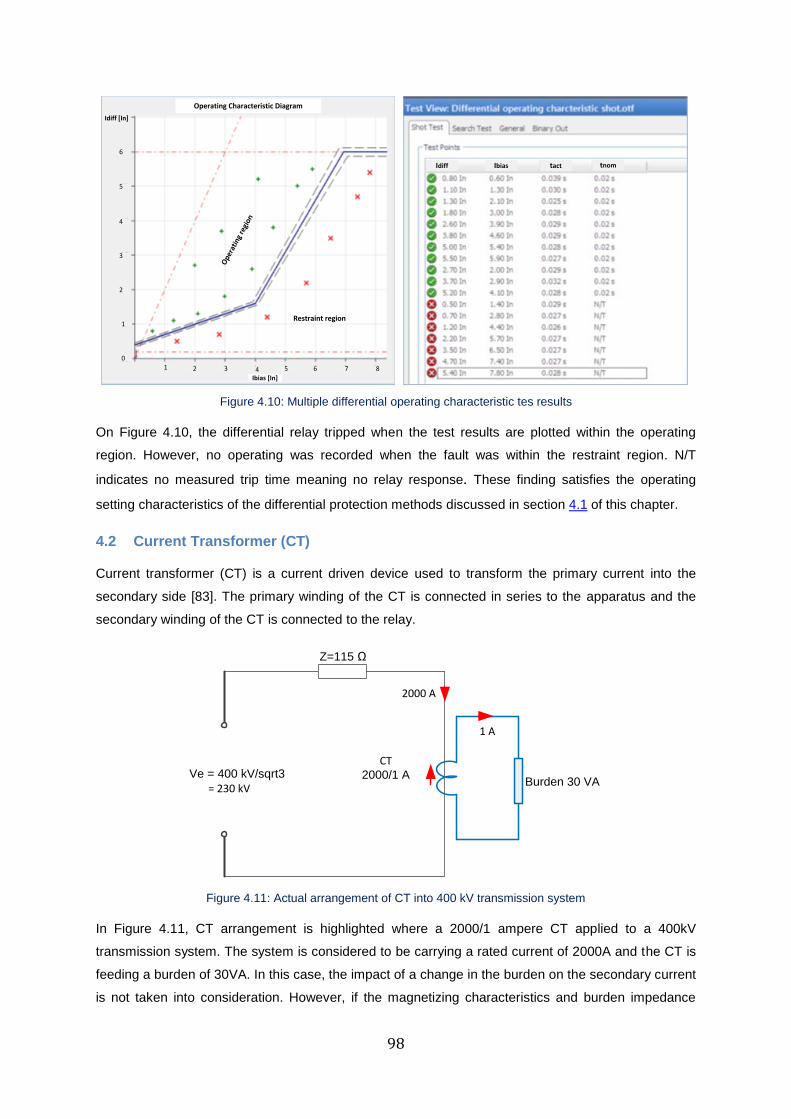
98

Restraint region

Ope

rati

ng r

egio

n

Operating Characteristic Diagram

Idiff [In]

6

5

4

3

2

1

0

1 2 3 4Ibias [In]

5 6 7 8

IbiasIdiff tact tnom

Figure 4.10: Multiple differential operating characteristic tes results

On Figure 4.10, the differential relay tripped when the test results are plotted within the operating

region. However, no operating was recorded when the fault was within the restraint region. N/T

indicates no measured trip time meaning no relay response. These finding satisfies the operating

setting characteristics of the differential protection methods discussed in section 4.1 of this chapter.

4.2 Current Transformer (CT)

Current transformer (CT) is a current driven device used to transform the primary current into the

secondary side [83]. The primary winding of the CT is connected in series to the apparatus and the

secondary winding of the CT is connected to the relay.

Ve = 400 kV/sqrt3

= 230 kV

CT2000/1 A

Burden 30 VA

Z=115 Ω

2000 A

1 A

Figure 4.11: Actual arrangement of CT into 400 kV transmission system

In Figure 4.11, CT arrangement is highlighted where a 2000/1 ampere CT applied to a 400kV

transmission system. The system is considered to be carrying a rated current of 2000A and the CT is

feeding a burden of 30VA. In this case, the impact of a change in the burden on the secondary current

is not taken into consideration. However, if the magnetizing characteristics and burden impedance

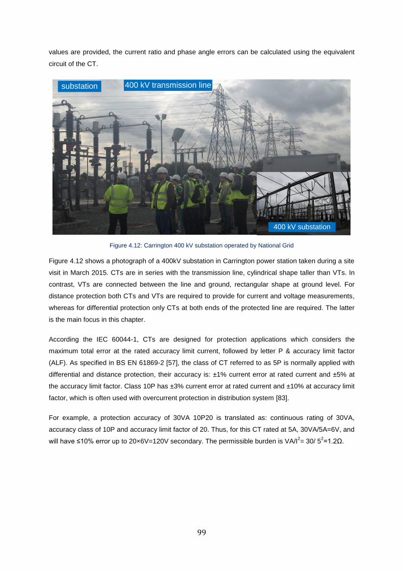
99

values are provided, the current ratio and phase angle errors can be calculated using the equivalent

circuit of the CT.

400 kV transmission linesubstation

400 kV substation

Figure 4.12: Carrington 400 kV substation operated by National Grid

Figure 4.12 shows a photograph of a 400kV substation in Carrington power station taken during a site

visit in March 2015. CTs are in series with the transmission line, cylindrical shape taller than VTs. In

contrast, VTs are connected between the line and ground, rectangular shape at ground level. For

distance protection both CTs and VTs are required to provide for current and voltage measurements,

whereas for differential protection only CTs at both ends of the protected line are required. The latter

is the main focus in this chapter.

According the IEC 60044-1, CTs are designed for protection applications which considers the

maximum total error at the rated accuracy limit current, followed by letter P & accuracy limit factor

(ALF). As specified in BS EN 61869-2 [57], the class of CT referred to as 5P is normally applied with

differential and distance protection, their accuracy is: ±1% current error at rated current and ±5% at

the accuracy limit factor. Class 10P has ±3% current error at rated current and ±10% at accuracy limit

factor, which is often used with overcurrent protection in distribution system [83].

For example, a protection accuracy of 30VA 10P20 is translated as: continuous rating of 30VA,

accuracy class of 10P and accuracy limit factor of 20. Thus, for this CT rated at 5A, 30VA/5A=6V, and

will have ≤10% error up to 20×6V=120V secondary. The permissible burden is VA/I2= 30/ 5

2=1.2Ω.

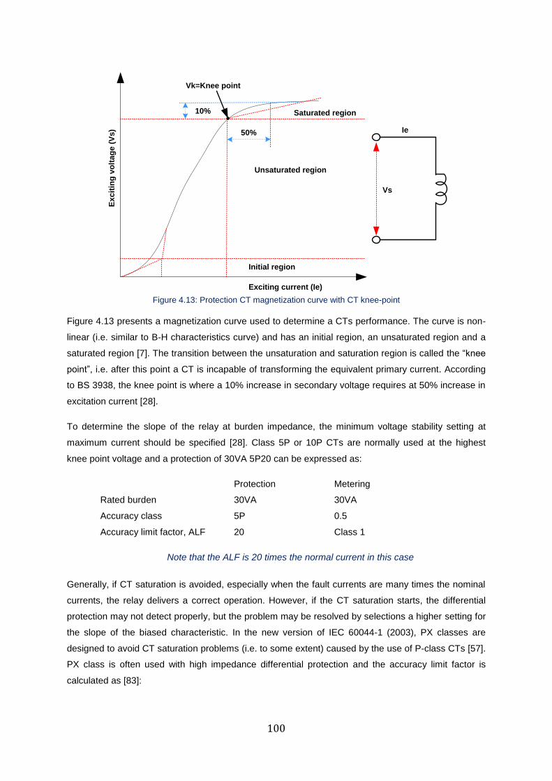
100

Vk=Knee point

Exciting current (Ie)

Ex

cit

ing

vo

lta

ge

(V

s) 50%

10% Saturated region

Unsaturated region

Ie

Initial region

Vs

Figure 4.13: Protection CT magnetization curve with CT knee-point

Figure 4.13 presents a magnetization curve used to determine a CTs performance. The curve is non-

linear (i.e. similar to B-H characteristics curve) and has an initial region, an unsaturated region and a

saturated region [7]. The transition between the unsaturation and saturation region is called the “knee

point”, i.e. after this point a CT is incapable of transforming the equivalent primary current. According

to BS 3938, the knee point is where a 10% increase in secondary voltage requires at 50% increase in

excitation current [28].

To determine the slope of the relay at burden impedance, the minimum voltage stability setting at

maximum current should be specified [28]. Class 5P or 10P CTs are normally used at the highest

knee point voltage and a protection of 30VA 5P20 can be expressed as:

Protection Metering

Rated burden 30VA 30VA

Accuracy class 5P 0.5

Accuracy limit factor, ALF 20 Class 1

Note that the ALF is 20 times the normal current in this case

Generally, if CT saturation is avoided, especially when the fault currents are many times the nominal

currents, the relay delivers a correct operation. However, if the CT saturation starts, the differential

protection may not detect properly, but the problem may be resolved by selections a higher setting for

the slope of the biased characteristic. In the new version of IEC 60044-1 (2003), PX classes are

designed to avoid CT saturation problems (i.e. to some extent) caused by the use of P-class CTs [57].

PX class is often used with high impedance differential protection and the accuracy limit factor is

calculated as [83]:

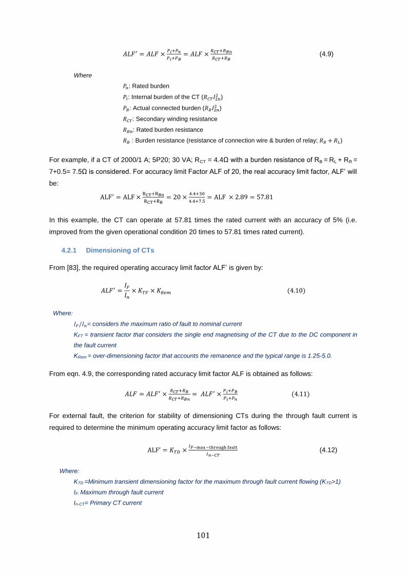
101

𝐴𝐿𝐹′ = 𝐴𝐿𝐹 ×𝑃𝑖+𝑃𝑛

𝑃𝑖+𝑃𝐵= 𝐴𝐿𝐹 ×

𝑅𝐶𝑇+𝑅𝐵𝑛

𝑅𝐶𝑇+𝑅𝐵 (4.9)

Where

𝑃𝑛: Rated burden

𝑃𝑖: Internal burden of the CT (𝑅𝐶𝑇𝐼2𝑛2 )

𝑃𝐵: Actual connected burden (𝑅𝐵𝐼2𝑛2 )

𝑅𝐶𝑇: Secondary winding resistance

𝑅𝐵𝑛: Rated burden resistance

𝑅𝐵 : Burden resistance (resistance of connection wire & burden of relay; 𝑅𝑅 + 𝑅𝐿)

For example, if a CT of 2000/1 A; 5P20; 30 VA; RCT = 4.4Ω with a burden resistance of RB = RL + RR =

7+0.5= 7.5Ω is considered. For accuracy limit Factor ALF of 20, the real accuracy limit factor, ALF’ will

be:

ALF′ = ALF ×RCT+RBn

RCT+RB= 20 ×

4.4+30

4.4+7.5= ALF × 2.89 = 57.81

In this example, the CT can operate at 57.81 times the rated current with an accuracy of 5% (i.e.

improved from the given operational condition 20 times to 57.81 times rated current).

4.2.1 Dimensioning of CTs

From [83], the required operating accuracy limit factor ALF’ is given by:

𝐴𝐿𝐹′ =𝐼𝐹

𝐼𝑛

× 𝐾𝑇𝐹 × 𝐾𝑅𝑒𝑚 (4.10)

Where:

𝐼𝐹/𝐼𝑛= considers the maximum ratio of fault to nominal current

KFT = transient factor that considers the single end magnetising of the CT due to the DC component in

the fault current

KRem = over-dimensioning factor that accounts the remanence and the typical range is 1.25-5.0.

From eqn. 4.9, the corresponding rated accuracy limit factor ALF is obtained as follows:

𝐴𝐿𝐹 = 𝐴𝐿𝐹′ ×𝑅𝐶𝑇+𝑅𝐵

𝑅𝐶𝑇+𝑅𝐵𝑛= 𝐴𝐿𝐹′ ×

𝑃𝑖+𝑃𝐵

𝑃𝑖+𝑃𝑛 (4.11)

For external fault, the criterion for stability of dimensioning CTs during the through fault current is

required to determine the minimum operating accuracy limit factor as follows:

ALF’ = 𝐾𝑇𝐷 ×𝐼𝐹−max −through fault

𝐼𝑛−𝐶𝑇 (4.12)

Where:

KTD =Minimum transient dimensioning factor for the maximum through fault current flowing (KTD>1)

IF: Maximum through fault current

In-CT= Primary CT current

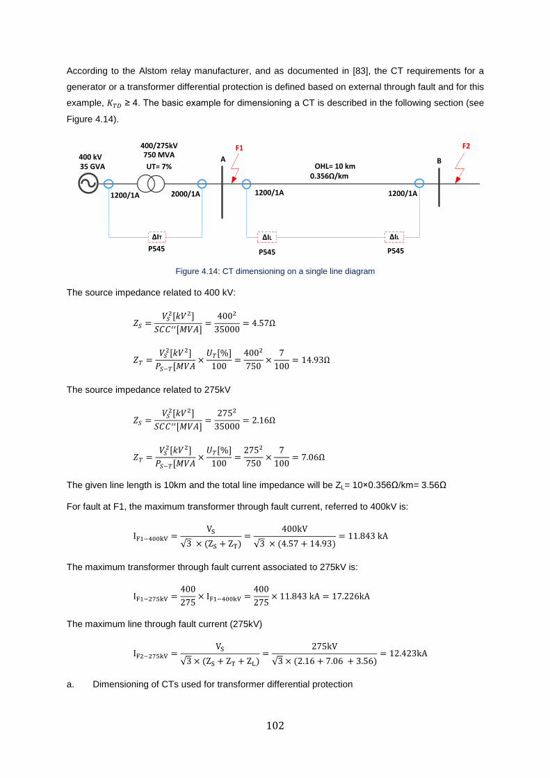
102

According to the Alstom relay manufacturer, and as documented in [83], the CT requirements for a

generator or a transformer differential protection is defined based on external through fault and for this

example, 𝐾𝑇𝐷 ≥ 4. The basic example for dimensioning a CT is described in the following section (see

Figure 4.14).

BA

F2F1750 MVA

400/275kV

35 GVA400 kV

1200/1A 2000/1A 1200/1A 1200/1A

OHL= 10 km0.356Ω/km

ΔIT ΔIL

UT= 7%

P545 P545 P545

ΔIL

Figure 4.14: CT dimensioning on a single line diagram

The source impedance related to 400 kV:

𝑍𝑆 =𝑉𝑆

2[𝑘𝑉2]

𝑆𝐶𝐶′′[𝑀𝑉𝐴]=

4002

35000= 4.57Ω

𝑍𝑇 =𝑉𝑆

2[𝑘𝑉2]

𝑃𝑆−𝑇[𝑀𝑉𝐴×

𝑈𝑇[%]

100=

4002

750×

7

100= 14.93Ω

The source impedance related to 275kV

𝑍𝑆 =𝑉𝑆

2[𝑘𝑉2]

𝑆𝐶𝐶′′[𝑀𝑉𝐴]=

2752

35000= 2.16Ω

𝑍𝑇 =𝑉𝑆

2[𝑘𝑉2]

𝑃𝑆−𝑇[𝑀𝑉𝐴×

𝑈𝑇[%]

100=

2752

750×

7

100= 7.06Ω

The given line length is 10km and the total line impedance will be ZL= 10×0.356Ω/km= 3.56Ω

For fault at F1, the maximum transformer through fault current, referred to 400kV is:

IF1−400kV =VS

√3 × (ZS + ZT)=

400kV

√3 × (4.57 + 14.93)= 11.843 kA

The maximum transformer through fault current associated to 275kV is:

IF1−275kV =400

275× IF1−400kV =

400

275× 11.843 kA = 17.226kA

The maximum line through fault current (275kV)

IF2−275kV =VS

√3 × (ZS + ZT + ZL)=

275kV

√3 × (2.16 + 7.06 + 3.56)= 12.423kA

a. Dimensioning of CTs used for transformer differential protection

103

CTs on 400kV-side:

The accuracy limit factor in operation:

ALF’ = KTD ×IF1−400kV

In−CT= 4 ×

11843

1200= 39.477

Note that according to [83], the Siemens manufacturer recommended value of 𝐾𝑇𝐷 for generator and transformer

differential protection during external fault is ≥4.

If the CT design data are 1200/1A, 30VA, 5P, internal burden of 4.5VA and the connection burden

resistance of 5 VA (i.e. the CT secondary cable and relay).

Then, the required rated accuracy limit factor will be

𝐴𝐿𝐹 ≥𝑃𝑖 + 𝑃𝐵

𝑃𝑖 + 𝑃𝑛

× 𝐴𝐿𝐹′ =4.5 + 5

4.5 + 30× 39.477 = 10.87

The following CT type is selected (choose higher than the calculate value):

1200/1 A, 30 VA class1 5P20, RCT ≤ 4.5 Ω (Pi ≤ 4.5VA)

CTs on 275 kV side:

The accuracy limit factor

ALF’ = 𝐾𝑇𝐷 ×𝐼𝐹1−275𝑘𝑉

𝐼𝑛−𝐶𝑇

= 4 ×17226

2000= 34.45

For CT design data with 2000/1A, 30VA, 5P, an internal burden of 8VA and a connection burden

resistance of 8.5 VA (i.e. the CT secondary cable and relay). The required rated accuracy limit factor

will be

𝐴𝐿𝐹 ≥𝑃𝑖 + 𝑃𝐵

𝑃𝑖 + 𝑃𝑛

× 𝐴𝐿𝐹′ =8 + 8.5

8 + 30× 34.45 = 14.96

The following CT type is selected (choose higher than the calculate value):

2000/1 A, 30VA, 5P20, RCT ≤ 8 Ω (Pi ≤ 8VA)

b. Dimensioning of the CTs for feeder differential protection

The accuracy limit factor,

ALF’ = 𝐾𝑇𝐷 ×𝐼𝐹2−275𝑘𝑉

𝐼𝑛−𝐶𝑇

= 2 ×12423

1200= 20.71

Note that according to [83], the Siemens manufacturer recommended value of 𝐾𝑇𝐷 for feeder differential

protection during external fault is ≥ 1.2 and in this case the value of 𝐾𝑇𝐷 = 2 is assumed.

Assume the data for each CT are 1200/1 A, 30VA, 5P, internal burden ≤ 12VA and connection burden

resistance of 12.5 VA. Hence,

104

𝐴𝐿𝐹 ≥𝑃𝑖 + 𝑃𝐵

𝑃𝑖 + 𝑃𝑛

× 𝐴𝐿𝐹′ =12 + 12.5

12 + 30× 20.71 = 12.08

The following CT type at both ends is selected:

1200/1 A, 30 VA, class1 5P20, RCT ≤ 12 Ω (Pi ≤ 12VA)

4.3 Protection signalling and intertripping

Generally, the term “signalling” is the transfer of information between separate locations which

represents the information to be transferred using a signal or message [83]. The communication

facilities required to trip the remote circuit breaker due to the local event is known as “inter-tripping”

[4]. According to [70] [83], the common signal transmission channels used for differential relaying are:

Pilot wire: is a twisted pair of wire designed to transmit 50/60 Hz

Power line carrier: signals are transmitted over high voltage transmission lines (30kHz to

300kHz)

Digital microwave/Radio: signals are transmitted by light of sight between terminals ( 2 to

12GHz, band width of 64kbit/s)

Fibre optic cable: is used to transmit signals by light modulation via electrical non conducting

cable and has a band width of 64kbits/s.

A pilot wire has many interconnections between CTs [83]. For example, the three phases requires at

least 6 pilot wires and is not economic for longer distance. Hence, it is often used for very short line

length, typically less than 15km. Power line carrier uses analogue or digital communication where

digital communication up to 128kbits/s is achieved using a 16kHz bandwidth [83]. Unlike pilot wires,

power line carrier is economic and may use for long transmission line.

A direct fibre optic cable is a wideband channel with channel capacity of 64kbits/s at a baud rate >4

kHz. This enhances the performance of the existing pilot wires which allows the sampled current

signal at both terminals to be converted into a digital signal and often used for upto 150km [72].

According to [83], pilot wires, power line carrier and radio links have been the mostly used in

transmission communication links. However, the use of fibre optic cable i.e. capable of monitoring the

power system is getting popularity.

When operating with switched communications, it is important to assess the tolerance of the relay

related to changes between the go and return links. For example, PT and PR are power in decibels per

mW (dBm) for transmit and receive signals. Signal to noise ratio (S/N) determines the data rate of the

transmitted signals and the sensitivity required for the receiving signal. The discussion are

summarised as follows:

a. Modem transmitter power (dBm): 10 log 𝑃𝑇

b. Modem receiver noise level (dBm): 10 log 𝑃𝑅

c. Channel loss: signal attenuation × length of fiber optic

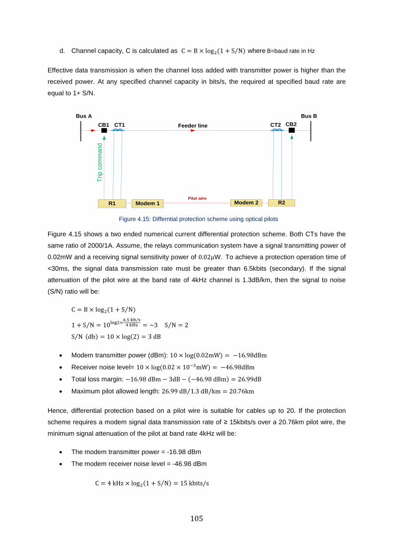
105

d. Channel capacity, C is calculated as C = B × log2(1 + S N⁄ ) where B=baud rate in Hz

Effective data transmission is when the channel loss added with transmitter power is higher than the

received power. At any specified channel capacity in bits/s, the required at specified baud rate are

equal to 1+ S/N.

CB1 CB2CT1 CT2

Pilot wire

Feeder line

Bus A Bus B

Trip

co

mm

an

d

Modem 1 Modem 2 R2R1

Figure 4.15: Differntial protection scheme using optical pilots

Figure 4.15 shows a two ended numerical current differential protection scheme. Both CTs have the

same ratio of 2000/1A. Assume, the relays communication system have a signal transmitting power of

0.02mW and a receiving signal sensitivity power of 0.02μW. To achieve a protection operation time of

<30ms, the signal data transmission rate must be greater than 6.5kbits (secondary). If the signal

attenuation of the pilot wire at the band rate of 4kHz channel is 1.3dB/km, then the signal to noise

(S/N) ratio will be:

C = B × log2(1 + S N⁄ )

1 + S N⁄ = 10log2×6.5 kb/s

4 kHz = ~3 S N⁄ = 2

S N⁄ (db) = 10 × log(2) = 3 dB

Modem transmitter power (dBm): 10 × log (0.02mW) = −16.98dBm

Receiver noise level= 10 × log (0.02 × 10−3mW) = −46.98dBm

Total loss margin: −16.98 dBm − 3dB − (−46.98 dBm) = 26.99dB

Maximum pilot allowed length: 26.99 dB 1.3 dB/km⁄ = 20.76km

Hence, differential protection based on a pilot wire is suitable for cables up to 20. If the protection

scheme requires a modem signal data transmission rate of ≥ 15kbits/s over a 20.76km pilot wire, the

minimum signal attenuation of the pilot at band rate 4kHz will be:

The modem transmitter power = -16.98 dBm

The modem receiver noise level = -46.98 dBm

C = 4 kHz × log2(1 + S N⁄ ) = 15 kbits/s

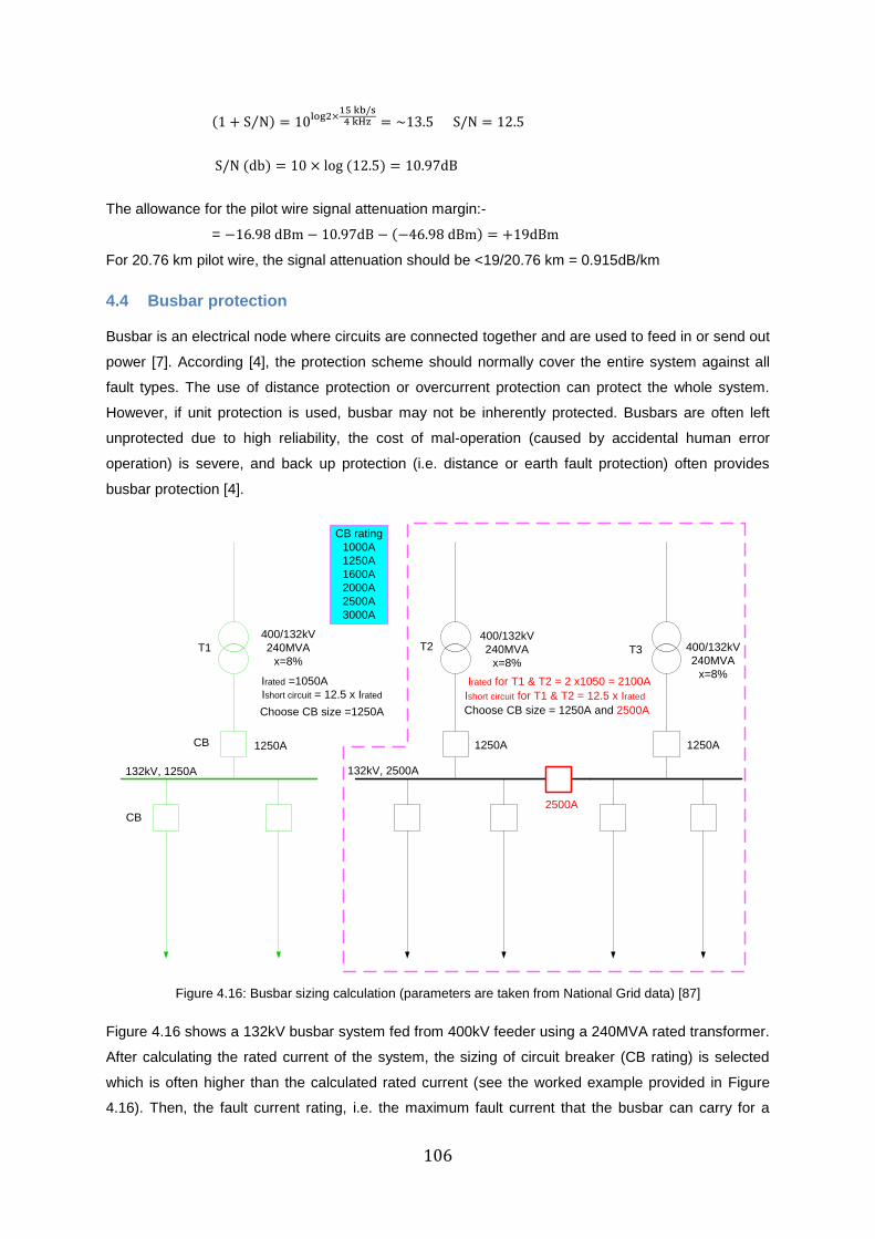
106

(1 + S N⁄ ) = 10log2×15 kb/s

4 kHz = ~13.5 S/N = 12.5

S/N (db) = 10 × log (12.5) = 10.97dB

The allowance for the pilot wire signal attenuation margin:-

= −16.98 dBm − 10.97dB − (−46.98 dBm) = +19dBm

For 20.76 km pilot wire, the signal attenuation should be <19/20.76 km = 0.915dB/km

4.4 Busbar protection

Busbar is an electrical node where circuits are connected together and are used to feed in or send out

power [7]. According [4], the protection scheme should normally cover the entire system against all

fault types. The use of distance protection or overcurrent protection can protect the whole system.

However, if unit protection is used, busbar may not be inherently protected. Busbars are often left

unprotected due to high reliability, the cost of mal-operation (caused by accidental human error

operation) is severe, and back up protection (i.e. distance or earth fault protection) often provides

busbar protection [4].

400/132kV

240MVA

x=8%

400/132kV

240MVA

x=8%

400/132kV

240MVA

x=8%

Irated =1050A

1250A

132kV, 1250A

1250A

132kV, 2500A

2500A

1250A

Irated for T1 & T2 = 2 x1050 = 2100A

Choose CB size =1250A Choose CB size = 1250A and 2500A

CB

CB

T1 T2 T3

Ishort circuit = 12.5 x Irated Ishort circuit for T1 & T2 = 12.5 x Irated

CB rating

1000A

1250A

1600A

2000A

2500A

3000A

Figure 4.16: Busbar sizing calculation (parameters are taken from National Grid data) [87]

Figure 4.16 shows a 132kV busbar system fed from 400kV feeder using a 240MVA rated transformer.

After calculating the rated current of the system, the sizing of circuit breaker (CB rating) is selected

which is often higher than the calculated rated current (see the worked example provided in Figure

4.16). Then, the fault current rating, i.e. the maximum fault current that the busbar can carry for a

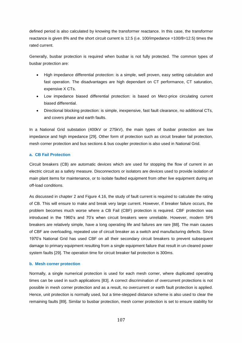
107

defined period is also calculated by knowing the transformer reactance. In this case, the transformer

reactance is given 8% and the short circuit current is 12.5 (i.e. 100/impedance =100/8=12.5) times the

rated current.

Generally, busbar protection is required when busbar is not fully protected. The common types of

busbar protection are:

High impedance differential protection: is a simple, well proven, easy setting calculation and

fast operation. The disadvantages are high dependant on CT performance, CT saturation,

expensive X CTs.

Low impedance biased differential protection: is based on Merz-price circulating current

biased differential.

Directional blocking protection: is simple, inexpensive, fast fault clearance, no additional CTs,

and covers phase and earth faults.

In a National Grid substation (400kV or 275kV), the main types of busbar protection are low

impedance and high impedance [29]. Other form of protection such as circuit breaker fail protection,

mesh corner protection and bus sections & bus coupler protection is also used in National Grid.

a. CB Fail Protection

Circuit breakers (CB) are automatic devices which are used for stopping the flow of current in an

electric circuit as a safety measure. Disconnectors or isolators are devices used to provide isolation of

main plant items for maintenance, or to isolate faulted equipment from other live equipment during an

off-load conditions.

As discussed in chapter 2 and Figure 4.16, the study of fault current is required to calculate the rating

of CB. This will ensure to make and break very large current. However, if breaker failure occurs, the

problem becomes much worse where a CB Fail (CBF) protection is required. CBF protection was

introduced in the 1960’s and 70’s when circuit breakers were unreliable. However, modern SF6

breakers are relatively simple, have a long operating life and failures are rare [88]. The main causes

of CBF are overloading, repeated use of circuit breaker as a switch and manufacturing defects. Since

1970’s National Grid has used CBF on all their secondary circuit breakers to prevent subsequent

damage to primary equipment resulting from a single equipment failure that result in un-cleared power

system faults [29]. The operation time for circuit breaker fail protection is 300ms.

b. Mesh corner protection

Normally, a single numerical protection is used for each mesh corner, where duplicated operating

times can be used in such applications [83]. A correct discrimination of overcurrent protections is not

possible in mesh corner protection and as a result, no overcurrent or earth fault protection is applied.

Hence, unit protection is normally used, but a time-stepped distance scheme is also used to clear the

remaining faults [89]. Similar to busbar protection, mesh corner protection is set to ensure stability for

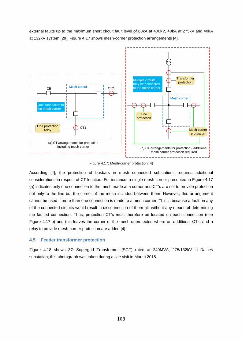
108

external faults up to the maximum short circuit fault level of 63kA at 400kV, 40kA at 275kV and 40kA

at 132kV system [29]. Figure 4.17 shows mesh-corner protection arrangements [4].

Mesh corner

Line

protection

Transformer

protection

Mesh corner

protection

Multiple circuits

may be connected

to the mesh corner

(b) CT arrangements for protection - additional

mesh corner protection required

CB

Line protection

relayCT1

CT2Mesh corner

One connection to

the mesh corner

(a) CT arrangements for protection

including mesh corner

Figure 4.17: Mesh-corner protection [4]

According [4], the protection of busbars in mesh connected substations requires additional

considerations in respect of CT location. For instance, a single mesh corner presented in Figure 4.17

(a) indicates only one connection to the mesh made at a corner and CT’s are set to provide protection

not only to the line but the corner of the mesh included between them. However, this arrangement

cannot be used if more than one connection is made to a mesh corner. This is because a fault on any

of the connected circuits would result in disconnection of them all, without any means of determining

the faulted connection. Thus, protection CT’s must therefore be located on each connection (see

Figure 4.17,b) and this leaves the corner of the mesh unprotected where an additional CT’s and a

relay to provide mesh-corner protection are added [4].

4.5 Feeder transformer protection

Figure 4.18 shows 3Ø Supergrid Transformer (SGT) rated at 240MVA, 275/132kV in Daines

substation; this photograph was taken during a site visit in March 2015.

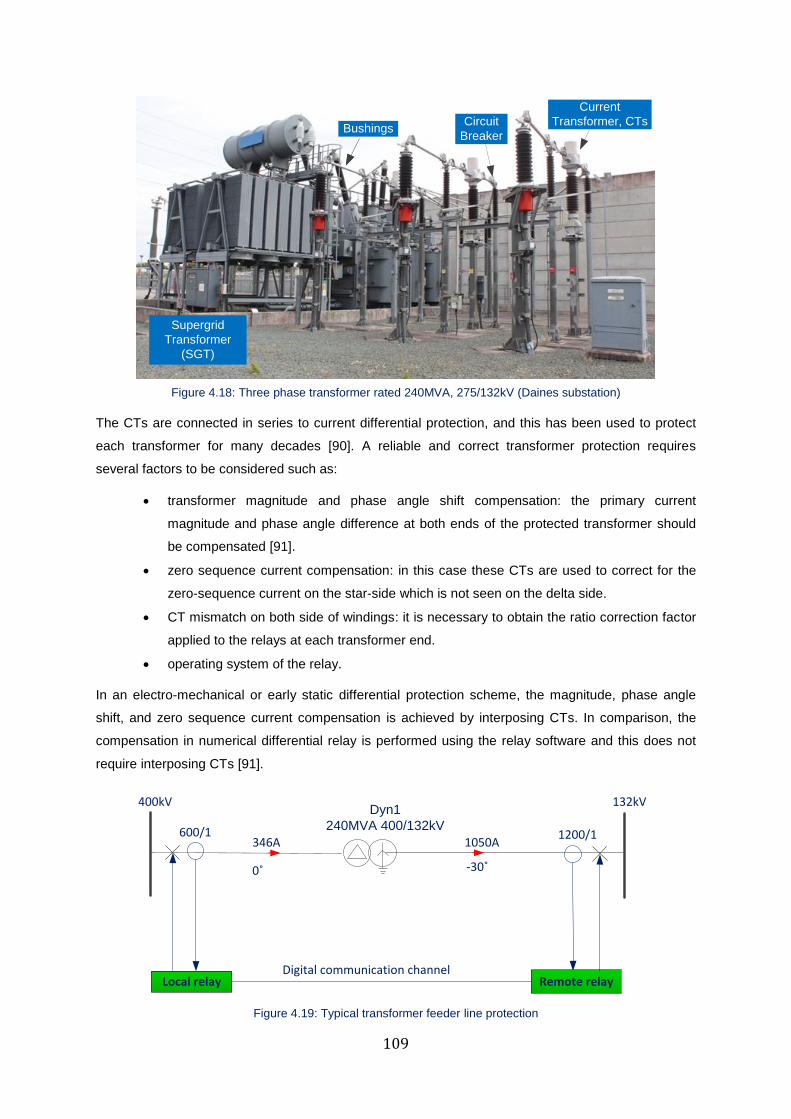
109

Bushings

Supergrid

Transformer

(SGT)

Circuit

Breaker

Current

Transformer, CTs

Figure 4.18: Three phase transformer rated 240MVA, 275/132kV (Daines substation)

The CTs are connected in series to current differential protection, and this has been used to protect

each transformer for many decades [90]. A reliable and correct transformer protection requires

several factors to be considered such as:

transformer magnitude and phase angle shift compensation: the primary current

magnitude and phase angle difference at both ends of the protected transformer should

be compensated [91].

zero sequence current compensation: in this case these CTs are used to correct for the

zero-sequence current on the star-side which is not seen on the delta side.

CT mismatch on both side of windings: it is necessary to obtain the ratio correction factor

applied to the relays at each transformer end.

operating system of the relay.

In an electro-mechanical or early static differential protection scheme, the magnitude, phase angle

shift, and zero sequence current compensation is achieved by interposing CTs. In comparison, the

compensation in numerical differential relay is performed using the relay software and this does not

require interposing CTs [91].

Local relay

600/1

Dyn1

240MVA 400/132kV

Remote relay

1200/1346A 1050A

0˚ -30˚

400kV 132kV

Digital communication channel

Figure 4.19: Typical transformer feeder line protection

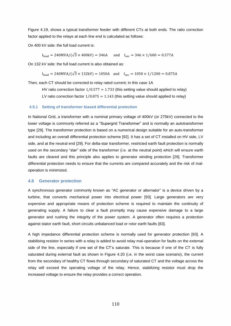
110

Figure 4.19, shows a typical transformer feeder with different CTs at both ends. The ratio correction

factor applied to the relays at each line end is calculated as follows:

On 400 kV side: the full load current is:

Iload = 240MVA/(√3 × 400kV) = 346A and Isec = 346 × 1 600⁄ = 0.577A

On 132 kV side: the full load current is also obtained as:

Iload = 240MVA/(√3 × 132kV) = 1050A and Isec = 1050 × 1 1200⁄ = 0.875A

Then, each CT should be corrected to relay rated current; in this case 1A

HV ratio correction factor 1 0.577⁄ = 1.733 (this setting value should applied to relay)

LV ratio correction factor 1 0.875⁄ = 1.143 (this setting value should applied to relay)

4.5.1 Setting of transformer biased differential protection

In National Grid, a transformer with a nominal primary voltage of 400kV (or 275kV) connected to the

lower voltage is commonly referred as a “Supergrid Transformer” and is normally an autotransformer

type [29]. The transformer protection is based on a numerical design suitable for an auto-transformer

and including an overall differential protection scheme [92]. It has a set of CT installed on HV side, LV

side, and at the neutral end [29]. For delta-star transformer, restricted earth fault protection is normally

used on the secondary “star” side of the transformer (i.e. at the neutral point) which will ensure earth

faults are cleared and this principle also applies to generator winding protection [29]. Transformer

differential protection needs to ensure that the currents are compared accurately and the risk of mal-

operation is minimized.

4.6 Generator protection

A synchronous generator commonly known as “AC generator or alternator” is a device driven by a

turbine, that converts mechanical power into electrical power [93]. Large generators are very

expensive and appropriate means of protection scheme is required to maintain the continuity of

generating supply. A failure to clear a fault promptly may cause expensive damage to a large

generator and rushing the integrity of the power system. A generator often requires a protection

against stator earth fault, short circuits unbalanced load or rotor earth faults [83].

A high impedance differential protection scheme is normally used for generator protection [93]. A

stabilising resistor in series with a relay is added to avoid relay mal-operation for faults on the external

side of the line, especially if one set of the CT’s saturate. This is because if one of the CT is fully

saturated during external fault as shown in Figure 4.20 (i.e. in the worst case scenario), the current

from the secondary of healthy CT flows through secondary of saturated CT and the voltage across the

relay will exceed the operating voltage of the relay. Hence, stabilizing resistor must drop the

increased voltage to ensure the relay provides a correct operation.

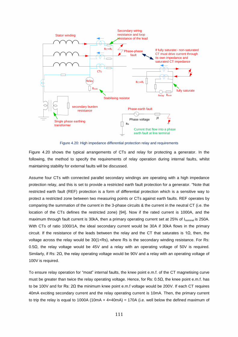
111

CTs

Relay

Stabilising resistor

secondary burden

resistance

RCT+RL

Secondary wiring

resistance and loop

resistance of the lead

Rstab

Stator winding

Single phase earthing

transformer

Phase-phase

fault

RstabRelay

RCT+RL

If fully saturate:- non-saturated

CT must drive current through

its own impedance and

saturated CT impedance

Phase-earth fault

Phase voltage

RN

jX

Current that flow into a phase

earth fault at line terminal

fully saturate

Figure 4.20: High impedance differential protection relay and requirements

Figure 4.20 shows the typical arrangements of CTs and relay for protecting a generator. In the

following, the method to specify the requirements of relay operation during internal faults, whilst

maintaining stability for external faults will be discussed.

Assume four CTs with connected parallel secondary windings are operating with a high impedance

protection relay, and this is set to provide a restricted earth fault protection for a generator. "Note that

restricted earth fault (REF) protection is a form of differential protection which is a sensitive way to

protect a restricted zone between two measuring points or CTs against earth faults. REF operates by

comparing the summation of the current in the 3-phase circuits & the current in the neutral CT (i.e. the

location of the CTs defines the restricted zone) [94]. Now if the rated current is 1000A, and the

maximum through fault current is 30kA, then a primary operating current set at 25% of Inominal is 250A.

With CTs of ratio 1000/1A, the ideal secondary current would be 30A if 30kA flows in the primary

circuit. If the resistance of the leads between the relay and the CT that saturates is 1Ω, then, the

voltage across the relay would be 30(1+Rs), where Rs is the secondary winding resistance. For Rs:

0.5Ω, the relay voltage would be 45V and a relay with an operating voltage of 50V is required.

Similarly, if Rs: 2Ω, the relay operating voltage would be 90V and a relay with an operating voltage of

100V is required.

To ensure relay operation for “most” internal faults, the knee point e.m.f. of the CT magnetising curve

must be greater than twice the relay operating voltage. Hence, for Rs: 0.5Ω, the knee point e.m.f. has

to be 100V and for Rs: 2Ω the minimum knee point e.m.f voltage would be 200V. If each CT requires

40mA exciting secondary current and the relay operating current is 10mA. Then, the primary current

to trip the relay is equal to 1000A (10mA + 4×40mA) = 170A (i.e. well below the defined maximum of

112

250A). Appropriate choice of stabilising resistor will ensure the relay does not operate on the worse-

case external fault (highest possible fault current). However, it requires to be ensured the relay can

detect an earth fault located at any point on the stator winding. In practise this is impossible, since the

fault current seen when a fault occurs near the neutral point is very small. Hence it is required to

determine the percentage of the winding protected by the relay, i.e. often between 80% and 95% [93].

4.7 Summary

The basic principles, operating characteristics and application of current differential protection were

studied in this chapter. Unit protection is set to provide fault clearance for a protected line or

transformer under all minimum and maximum fault level operating conditions and the setting must

ensure stability is maintained for external faults up to the switchgear rated fault current capacity. CTs

are normally used to provide current information between the protected object and the relay, whereas

communication channel is used to transfer information between two locations via a signal or

message.

In comparison to distance & overcurrent protection; unit protection has better selectivity, is more

secure, has higher sensitivity, does not over reach and is not influenced by the load or power swings.

However, it has limitations as it fully dependant on the communication channel and cannot provide

backup protection. In addition, concerns related to CT saturation must be noted. The influence of CT

mismatch and saturation reduces the sensitivity of differential protection. However, this can be

overcome by configuring “lower & higher” bias setting. A CT fully saturates when the secondary

excitation voltage exceeds the CT knee point voltage and this affects the relay performance.

In many transmission networks including the UK, unit protection is often used as 1st main protection

for feeder protection. In National Grid, unit protection is also used as the 2nd

main protection when

utilizing distance protection scheme is not possible. However, blocked or plain distance protections

are normally used as the 2nd

main protection. Generally, unit protection is widely used to protect

transmission feeders, transformers, generators, busbars and motors. A double unit protection is used

on cables or on situations when utilizing a voltage transformer becomes difficult. In addition, REF is

used to protect a zone of generator or transformer against internal earth faults.

The key strengths of this study are to increase understanding on the concept and application of

current differential protection. The objective is to understand the operating characteristics and setting

calculation of unit protection. The impact of low fault level on the operating performance of unit

protection and setting implication will be discussed in chapter 6.

The 2nd

technical paper entitled < Impact on Transmission Line Protection of future changes in the UK Energy

landscape > was published and presented based on this work on 7th

International conference on Advanced

Power System Automation and Protection (APAP 2017). The conference was held on October 16-18, 2017, Jeju,

Korea.

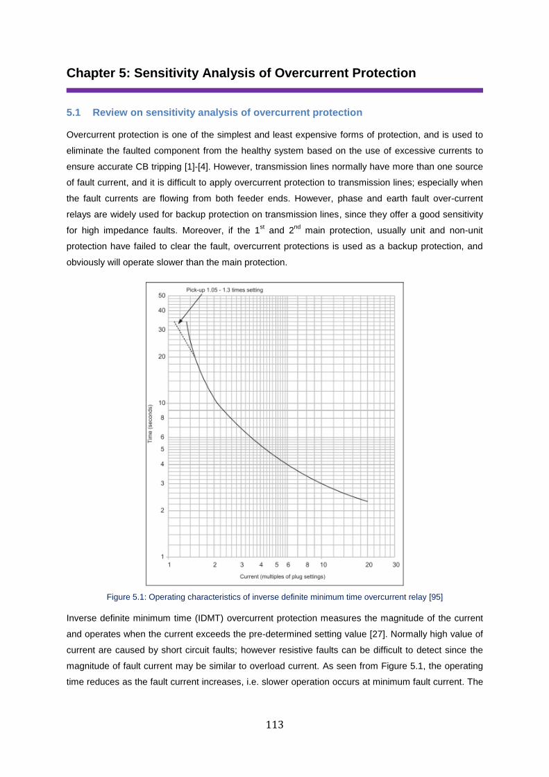
113

Chapter 5: Sensitivity Analysis of Overcurrent Protection

5.1 Review on sensitivity analysis of overcurrent protection

Overcurrent protection is one of the simplest and least expensive forms of protection, and is used to

eliminate the faulted component from the healthy system based on the use of excessive currents to

ensure accurate CB tripping [1]-[4]. However, transmission lines normally have more than one source

of fault current, and it is difficult to apply overcurrent protection to transmission lines; especially when

the fault currents are flowing from both feeder ends. However, phase and earth fault over-current

relays are widely used for backup protection on transmission lines, since they offer a good sensitivity

for high impedance faults. Moreover, if the 1st and 2

nd main protection, usually unit and non-unit

protection have failed to clear the fault, overcurrent protections is used as a backup protection, and

obviously will operate slower than the main protection.

Figure 5.1: Operating characteristics of inverse definite minimum time overcurrent relay [95]

Inverse definite minimum time (IDMT) overcurrent protection measures the magnitude of the current

and operates when the current exceeds the pre-determined setting value [27]. Normally high value of

current are caused by short circuit faults; however resistive faults can be difficult to detect since the

magnitude of fault current may be similar to overload current. As seen from Figure 5.1, the operating

time reduces as the fault current increases, i.e. slower operation occurs at minimum fault current. The

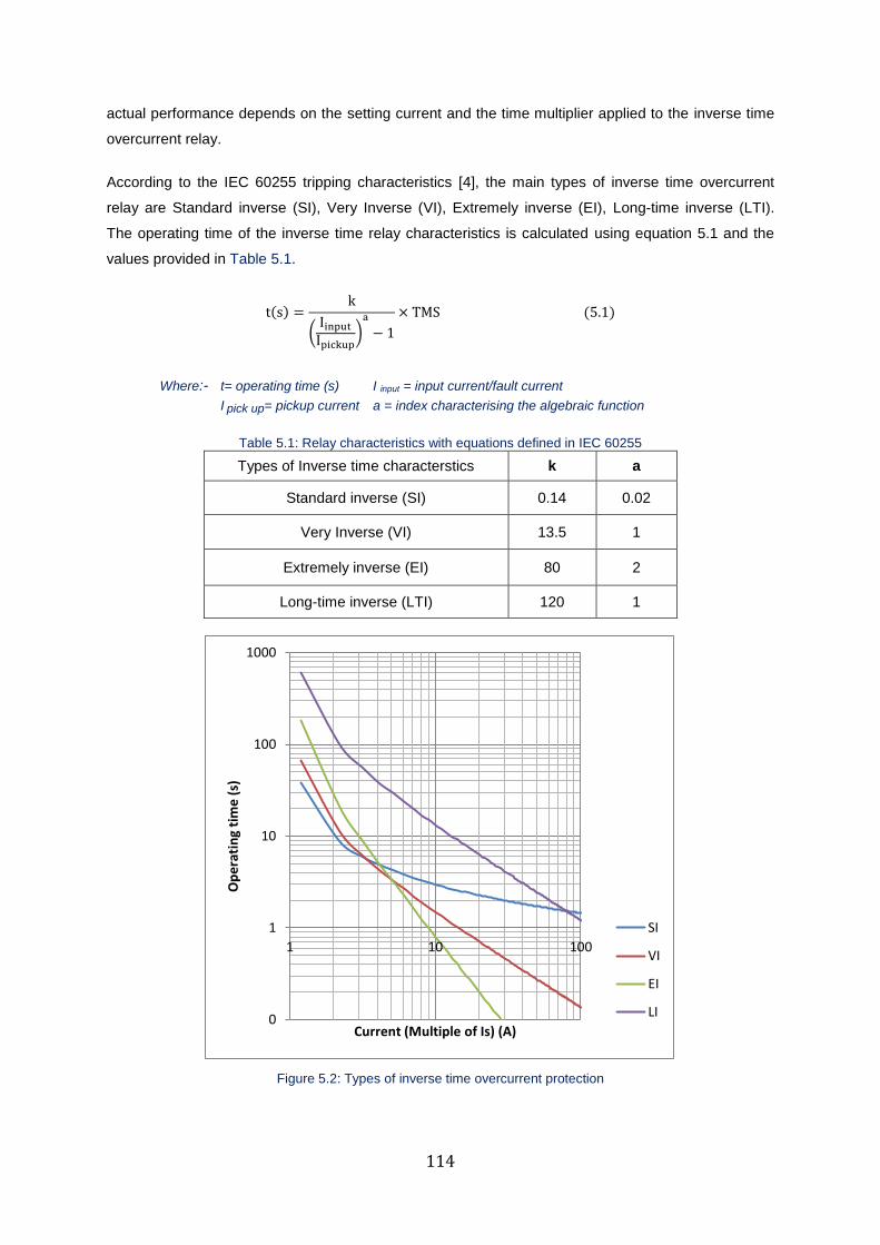
114

actual performance depends on the setting current and the time multiplier applied to the inverse time

overcurrent relay.

According to the IEC 60255 tripping characteristics [4], the main types of inverse time overcurrent

relay are Standard inverse (SI), Very Inverse (VI), Extremely inverse (EI), Long-time inverse (LTI).

The operating time of the inverse time relay characteristics is calculated using equation 5.1 and the

values provided in Table 5.1.

t(s) =k

(Iinput

Ipickup)

a

− 1

× TMS (5.1)

Where:- t= operating time (s) I input = input current/fault current

I pick up= pickup current a = index characterising the algebraic function

Table 5.1: Relay characteristics with equations defined in IEC 60255

Types of Inverse time characterstics k a

Standard inverse (SI) 0.14 0.02

Very Inverse (VI) 13.5 1

Extremely inverse (EI) 80 2

Long-time inverse (LTI) 120 1

Figure 5.2: Types of inverse time overcurrent protection

0

1

10

100

1000

1 10 100

Op

era

tin

g ti

me

(s)

Current (Multiple of Is) (A)

SI

VI

EI

LI

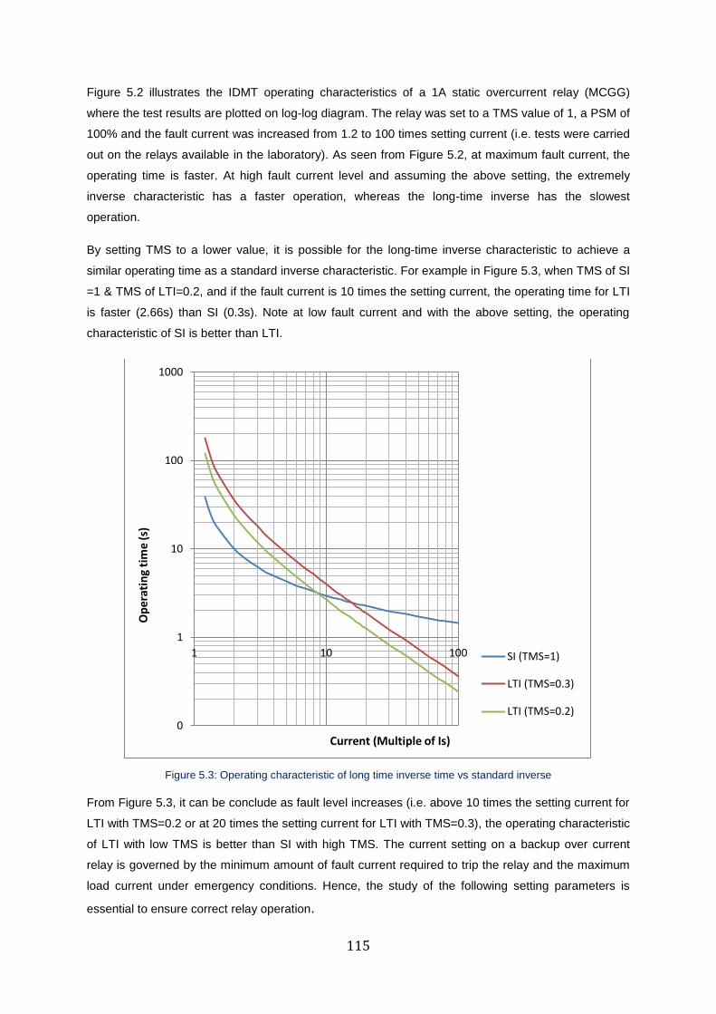
115

Figure 5.2 illustrates the IDMT operating characteristics of a 1A static overcurrent relay (MCGG)

where the test results are plotted on log-log diagram. The relay was set to a TMS value of 1, a PSM of

100% and the fault current was increased from 1.2 to 100 times setting current (i.e. tests were carried

out on the relays available in the laboratory). As seen from Figure 5.2, at maximum fault current, the

operating time is faster. At high fault current level and assuming the above setting, the extremely

inverse characteristic has a faster operation, whereas the long-time inverse has the slowest

operation.

By setting TMS to a lower value, it is possible for the long-time inverse characteristic to achieve a

similar operating time as a standard inverse characteristic. For example in Figure 5.3, when TMS of SI

=1 & TMS of LTI=0.2, and if the fault current is 10 times the setting current, the operating time for LTI

is faster (2.66s) than SI (0.3s). Note at low fault current and with the above setting, the operating

characteristic of SI is better than LTI.

Figure 5.3: Operating characteristic of long time inverse time vs standard inverse

From Figure 5.3, it can be conclude as fault level increases (i.e. above 10 times the setting current for

LTI with TMS=0.2 or at 20 times the setting current for LTI with TMS=0.3), the operating characteristic

of LTI with low TMS is better than SI with high TMS. The current setting on a backup over current

relay is governed by the minimum amount of fault current required to trip the relay and the maximum

load current under emergency conditions. Hence, the study of the following setting parameters is

essential to ensure correct relay operation.

0

1

10

100

1000

1 10 100

Op

erat

ing

tim

e (s

)

Current (Multiple of Is)

SI (TMS=1)

LTI (TMS=0.3)

LTI (TMS=0.2)

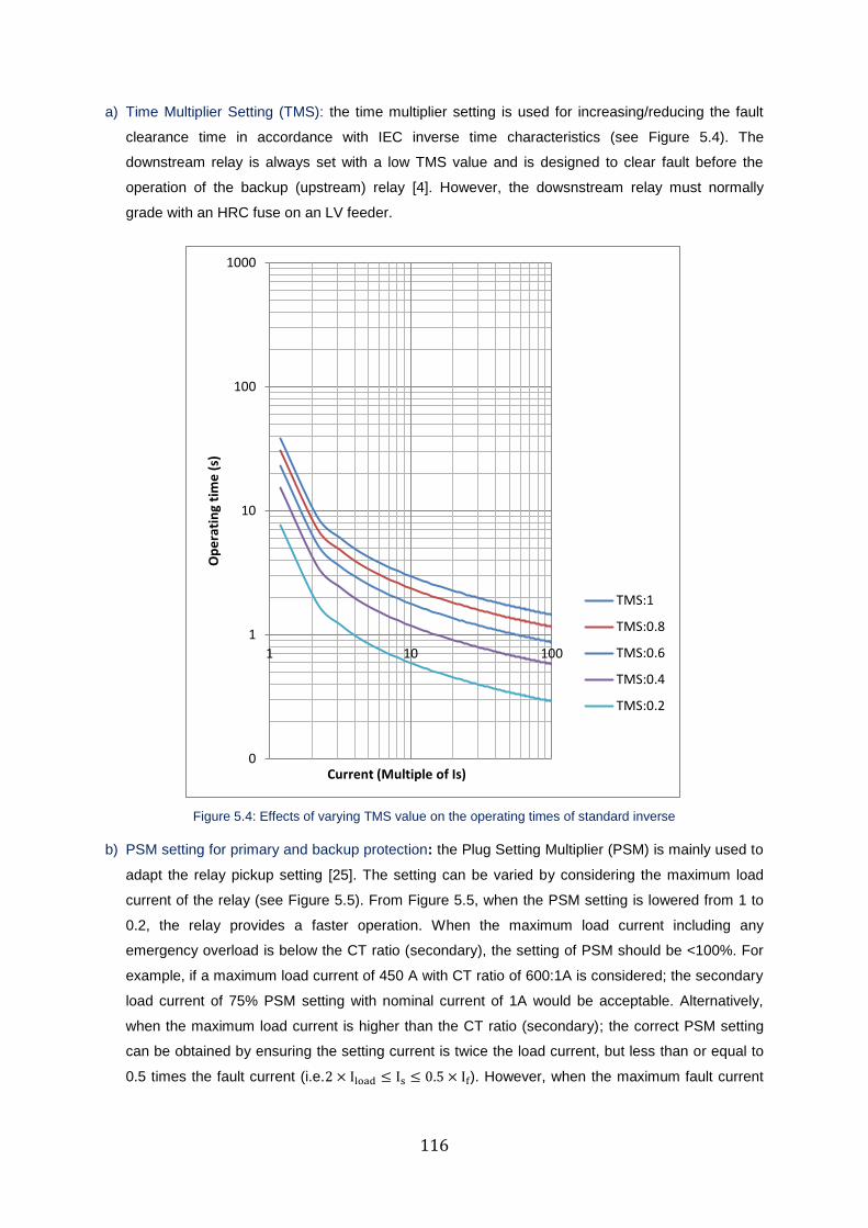
116

a) Time Multiplier Setting (TMS): the time multiplier setting is used for increasing/reducing the fault

clearance time in accordance with IEC inverse time characteristics (see Figure 5.4). The

downstream relay is always set with a low TMS value and is designed to clear fault before the

operation of the backup (upstream) relay [4]. However, the dowsnstream relay must normally

grade with an HRC fuse on an LV feeder.

Figure 5.4: Effects of varying TMS value on the operating times of standard inverse

b) PSM setting for primary and backup protection: the Plug Setting Multiplier (PSM) is mainly used to

adapt the relay pickup setting [25]. The setting can be varied by considering the maximum load

current of the relay (see Figure 5.5). From Figure 5.5, when the PSM setting is lowered from 1 to

0.2, the relay provides a faster operation. When the maximum load current including any

emergency overload is below the CT ratio (secondary), the setting of PSM should be <100%. For

example, if a maximum load current of 450 A with CT ratio of 600:1A is considered; the secondary

load current of 75% PSM setting with nominal current of 1A would be acceptable. Alternatively,

when the maximum load current is higher than the CT ratio (secondary); the correct PSM setting

can be obtained by ensuring the setting current is twice the load current, but less than or equal to

0.5 times the fault current (i.e.2 × Iload ≤ Is ≤ 0.5 × If). However, when the maximum fault current

0

1

10

100

1000

1 10 100

Op

era

tin

g ti

me

(s)

Current (Multiple of Is)

TMS:1

TMS:0.8

TMS:0.6

TMS:0.4

TMS:0.2

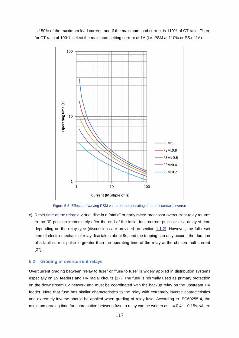
117

is 150% of the maximum load current, and if the maximum load current is 110% of CT ratio. Then,

for CT ratio of 100:1, select the maximum setting current of 1A (i.e. PSM at 110% or PS of 1A).

Figure 5.5: Effects of varying PSM value on the operating times of standard inverse

c) Reset time of the relay: a virtual disc in a “static” or early micro-processor overcurrent relay returns

to the “0” position immediately after the end of the initial fault current pulse or at a delayed time

depending on the relay type (discussions are provided on section 1.1.2). However, the full reset

time of electro-mechanical relay disc takes about 9s, and the tripping can only occur if the duration

of a fault current pulse is greater than the operating time of the relay at the chosen fault current

[27].

5.2 Grading of overcurrent relays

Overcurrent grading between “relay to fuse” or “fuse to fuse” is widely applied in distribution systems

especially on LV feeders and HV radial circuits [27]. The fuse is normally used as primary protection

on the downstream LV network and must be coordinated with the backup relay on the upstream HV

feeder. Note that fuse has similar characteristics to the relay with extremely inverse characteristics

and extremely inverse should be applied when grading of relay-fuse. According to IEC60255-4, the

minimum grading time for coordination between fuse to relay can be written as t' = 0.4t + 0.15s, where

1

10

100

1 10 100

Op

era

tin

g ti

me

(s)

Current (Multiple of Is)

PSM:1

PSM:0.8

PSM: 0.6

PSM:0.4

PSM:0.2

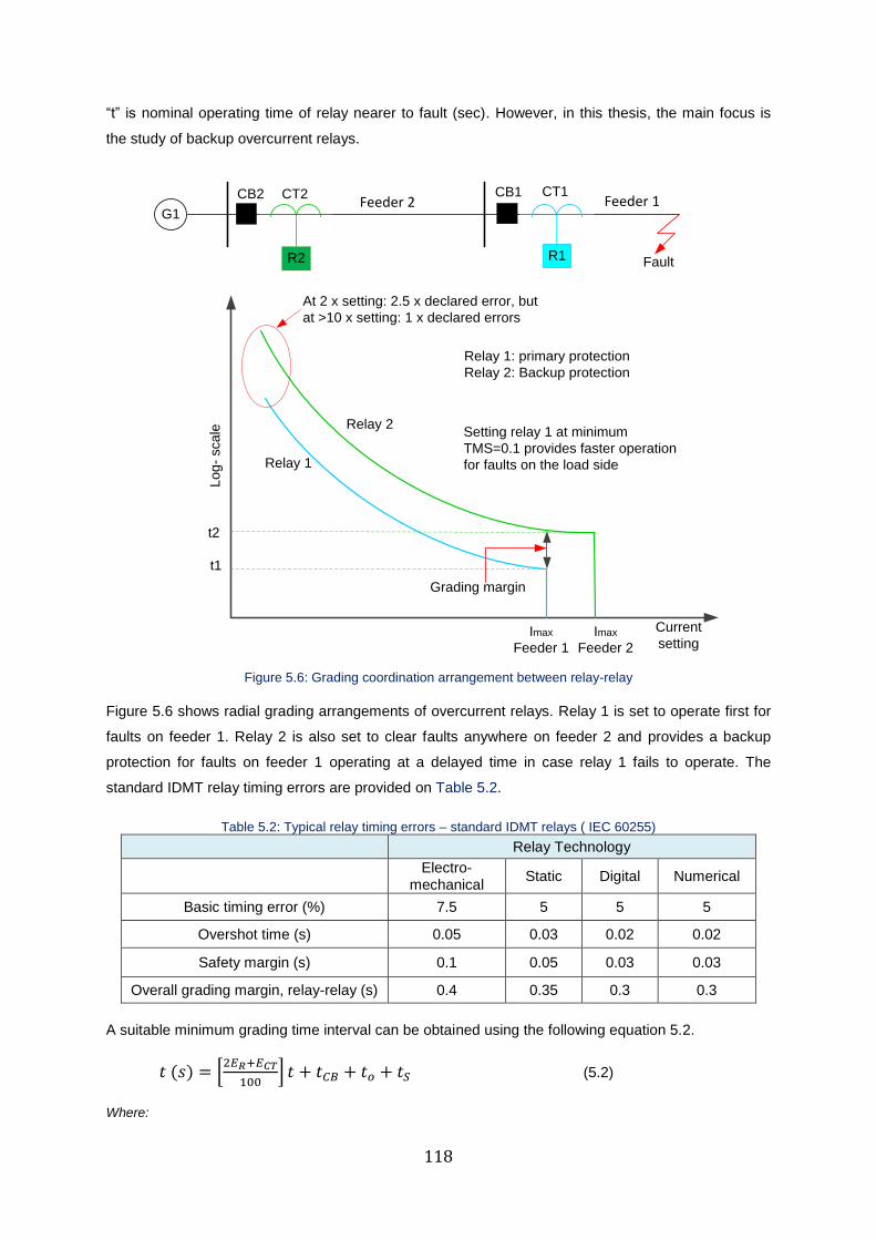
118

“t” is nominal operating time of relay nearer to fault (sec). However, in this thesis, the main focus is

the study of backup overcurrent relays.

G1

R2 R1 Fault

Relay 2

Relay 1

Grading margin

Relay 1: primary protection

Relay 2: Backup protection

CT2 CT1CB1CB2

Lo

g-

sca

le

Imax

Feeder 1

t1

t2

Setting relay 1 at minimum

TMS=0.1 provides faster operation

for faults on the load side

Feeder 2 Feeder 1

At 2 x setting: 2.5 x declared error, but

at >10 x setting: 1 x declared errors

Imax

Feeder 2

Current

setting

Figure 5.6: Grading coordination arrangement between relay-relay

Figure 5.6 shows radial grading arrangements of overcurrent relays. Relay 1 is set to operate first for

faults on feeder 1. Relay 2 is also set to clear faults anywhere on feeder 2 and provides a backup

protection for faults on feeder 1 operating at a delayed time in case relay 1 fails to operate. The

standard IDMT relay timing errors are provided on Table 5.2.

Table 5.2: Typical relay timing errors – standard IDMT relays ( IEC 60255)

Relay Technology

Electro-

mechanical Static Digital Numerical

Basic timing error (%) 7.5 5 5 5

Overshot time (s) 0.05 0.03 0.02 0.02

Safety margin (s) 0.1 0.05 0.03 0.03

Overall grading margin, relay-relay (s) 0.4 0.35 0.3 0.3

A suitable minimum grading time interval can be obtained using the following equation 5.2.

𝑡 (𝑠) = [2𝐸𝑅+𝐸𝐶𝑇

100] 𝑡 + 𝑡𝐶𝐵 + 𝑡𝑜 + 𝑡𝑆 (5.2)

Where:

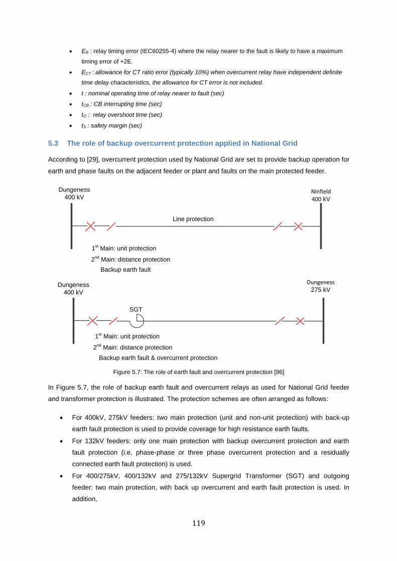
119

ER : relay timing error (IEC60255-4) where the relay nearer to the fault is likely to have a maximum

timing error of +2E.

ECT : allowance for CT ratio error (typically 10%) when overcurrent relay have independent definite

time delay characteristics, the allowance for CT error is not included.

t : nominal operating time of relay nearer to fault (sec)

tCB : CB interrupting time (sec)

tO : relay overshoot time (sec)

tS : safety margin (sec)

5.3 The role of backup overcurrent protection applied in National Grid

According to [29], overcurrent protection used by National Grid are set to provide backup operation for

earth and phase faults on the adjacent feeder or plant and faults on the main protected feeder.

Dungeness

400 kV

Ninfield 400 kV

1st Main: unit protection

2nd

Main: distance protection

Backup earth fault & overcurrent protection

SGT

Dungeness

400 kV

Dungeness 275 kV

1st Main: unit protection

2nd

Main: distance protection

Backup earth fault

Line protection

Figure 5.7: The role of earth fault and overcurrent protection [96]

In Figure 5.7, the role of backup earth fault and overcurrent relays as used for National Grid feeder

and transformer protection is illustrated. The protection schemes are often arranged as follows:

For 400kV, 275kV feeders: two main protection (unit and non-unit protection) with back-up

earth fault protection is used to provide coverage for high resistance earth faults.

For 132kV feeders: only one main protection with backup overcurrent protection and earth

fault protection (i.e. phase-phase or three phase overcurrent protection and a residually

connected earth fault protection) is used.

For 400/275kV, 400/132kV and 275/132kV Supergrid Transformer (SGT) and outgoing

feeder: two main protection, with back up overcurrent and earth fault protection is used. In

addition,

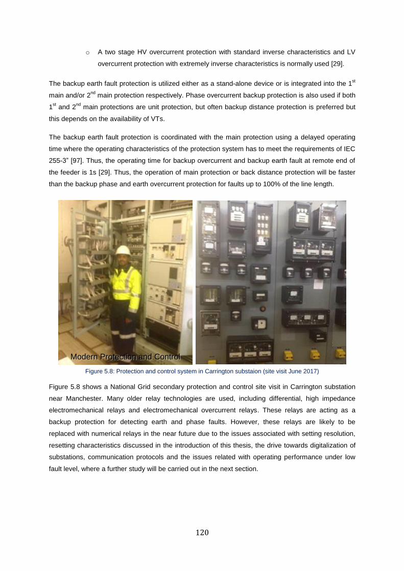
120

o A two stage HV overcurrent protection with standard inverse characteristics and LV

overcurrent protection with extremely inverse characteristics is normally used [29].

The backup earth fault protection is utilized either as a stand-alone device or is integrated into the 1st

main and/or 2nd

main protection respectively. Phase overcurrent backup protection is also used if both

1st and 2

nd main protections are unit protection, but often backup distance protection is preferred but

this depends on the availability of VTs.

The backup earth fault protection is coordinated with the main protection using a delayed operating

time where the operating characteristics of the protection system has to meet the requirements of IEC

255-3” [97]. Thus, the operating time for backup overcurrent and backup earth fault at remote end of

the feeder is 1s [29]. Thus, the operation of main protection or back distance protection will be faster

than the backup phase and earth overcurrent protection for faults up to 100% of the line length.

Modern Protection and ControlModern Protection and Control

High Impedance

Electromechanical Relays

Figure 5.8: Protection and control system in Carrington substaion (site visit June 2017)

Figure 5.8 shows a National Grid secondary protection and control site visit in Carrington substation

near Manchester. Many older relay technologies are used, including differential, high impedance

electromechanical relays and electromechanical overcurrent relays. These relays are acting as a

backup protection for detecting earth and phase faults. However, these relays are likely to be

replaced with numerical relays in the near future due to the issues associated with setting resolution,

resetting characteristics discussed in the introduction of this thesis, the drive towards digitalization of

substations, communication protocols and the issues related with operating performance under low

fault level, where a further study will be carried out in the next section.

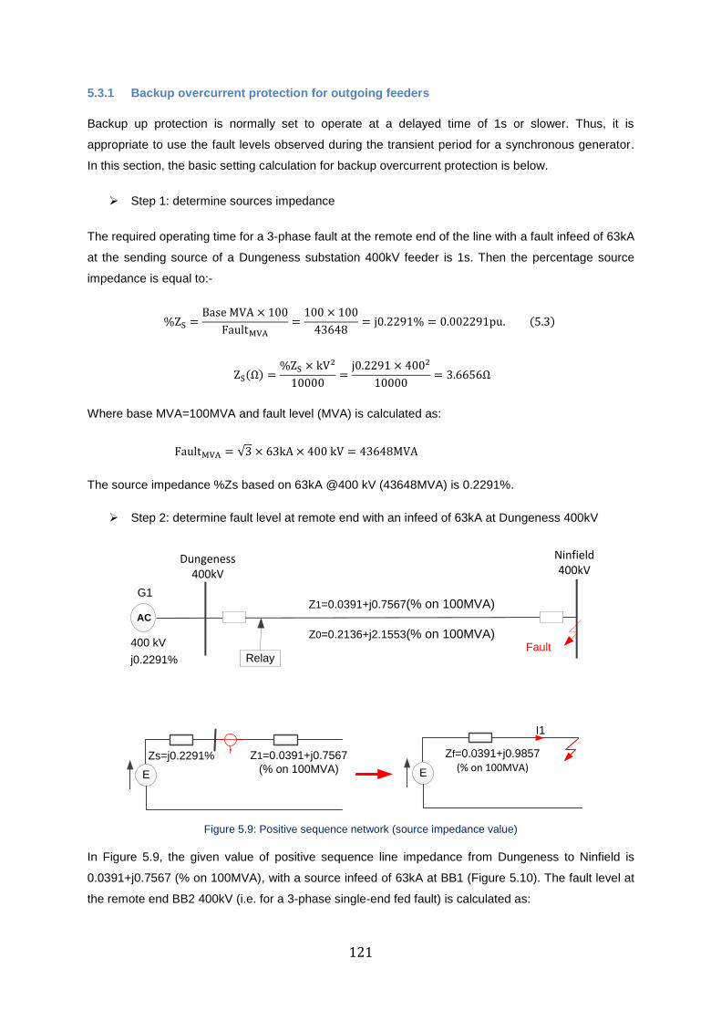
121

5.3.1 Backup overcurrent protection for outgoing feeders

Backup up protection is normally set to operate at a delayed time of 1s or slower. Thus, it is

appropriate to use the fault levels observed during the transient period for a synchronous generator.

In this section, the basic setting calculation for backup overcurrent protection is below.

Step 1: determine sources impedance

The required operating time for a 3-phase fault at the remote end of the line with a fault infeed of 63kA

at the sending source of a Dungeness substation 400kV feeder is 1s. Then the percentage source

impedance is equal to:-

%ZS =Base MVA × 100

FaultMVA

=100 × 100

43648= j0.2291% = 0.002291pu. (5.3)

ZS(Ω) =%ZS × kV2

10000=

j0.2291 × 4002

10000= 3.6656Ω

Where base MVA=100MVA and fault level (MVA) is calculated as:

FaultMVA = √3 × 63kA × 400 kV = 43648MVA

The source impedance %Zs based on 63kA @400 kV (43648MVA) is 0.2291%.

Step 2: determine fault level at remote end with an infeed of 63kA at Dungeness 400kV

Z1=0.0391+j0.7567

(% on 100MVA)

Dungeness 400kV

E

Zs=j0.2291% Zf=0.0391+j0.9857

(% on 100MVA) E

I1

G1

AC

Ninfield 400kV

Fault

Z1=0.0391+j0.7567(% on 100MVA)

Relay

400 kV

j0.2291%

Z0=0.2136+j2.1553(% on 100MVA)

Figure 5.9: Positive sequence network (source impedance value)

In Figure 5.9, the given value of positive sequence line impedance from Dungeness to Ninfield is

0.0391+j0.7567 (% on 100MVA), with a source infeed of 63kA at BB1 (Figure 5.10). The fault level at

the remote end BB2 400kV (i.e. for a 3-phase single-end fed fault) is calculated as:

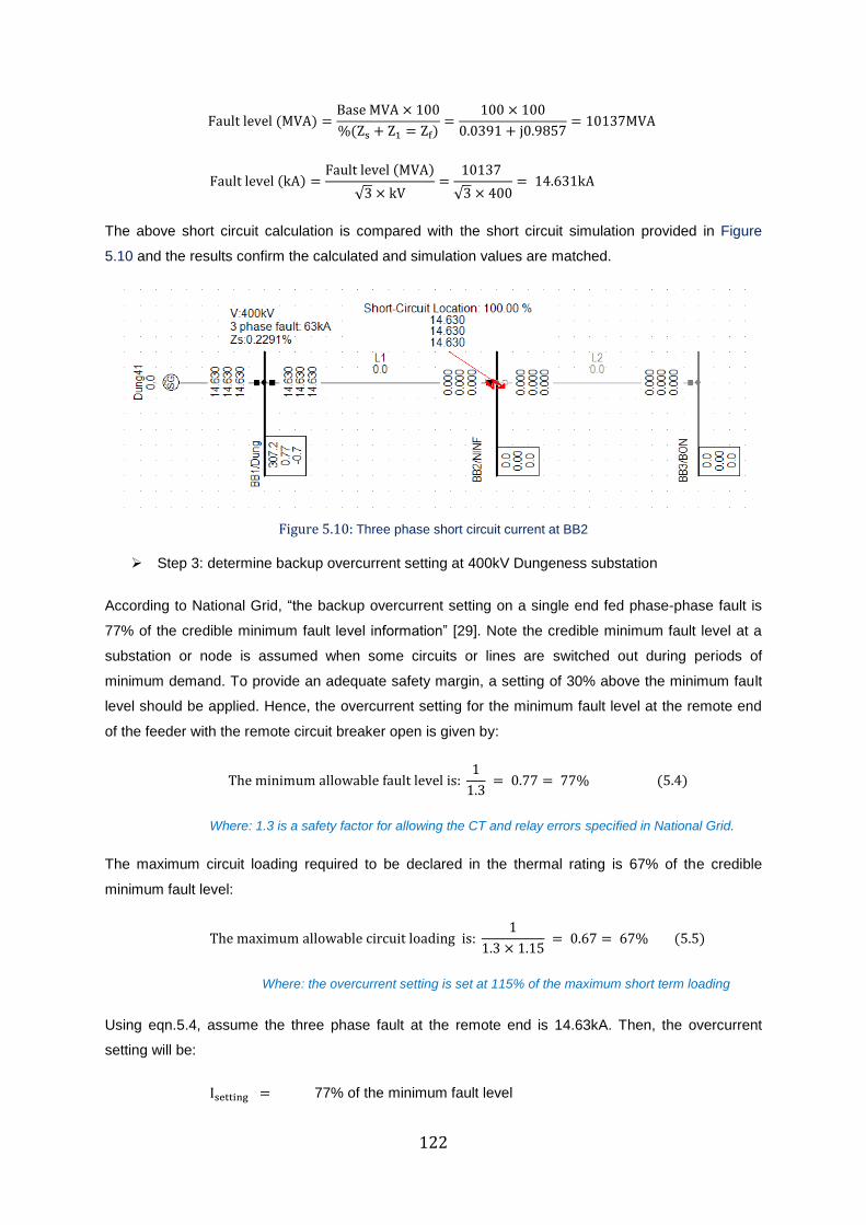
122

Fault level (MVA) =Base MVA × 100

%(Zs + Z1 = Zf)=

100 × 100

0.0391 + j0.9857= 10137MVA

Fault level (kA) =Fault level (MVA)

√3 × kV=

10137

√3 × 400= 14.631kA

The above short circuit calculation is compared with the short circuit simulation provided in Figure

5.10 and the results confirm the calculated and simulation values are matched.

Figure 5.10: Three phase short circuit current at BB2

Step 3: determine backup overcurrent setting at 400kV Dungeness substation

According to National Grid, “the backup overcurrent setting on a single end fed phase-phase fault is

77% of the credible minimum fault level information” [29]. Note the credible minimum fault level at a

substation or node is assumed when some circuits or lines are switched out during periods of

minimum demand. To provide an adequate safety margin, a setting of 30% above the minimum fault

level should be applied. Hence, the overcurrent setting for the minimum fault level at the remote end

of the feeder with the remote circuit breaker open is given by:

The minimum allowable fault level is: 1

1.3 = 0.77 = 77% (5.4)

Where: 1.3 is a safety factor for allowing the CT and relay errors specified in National Grid.

The maximum circuit loading required to be declared in the thermal rating is 67% of the credible

minimum fault level:

The maximum allowable circuit loading is: 1

1.3 × 1.15 = 0.67 = 67% (5.5)

Where: the overcurrent setting is set at 115% of the maximum short term loading

Using eqn.5.4, assume the three phase fault at the remote end is 14.63kA. Then, the overcurrent

setting will be:

Isetting = 77% of the minimum fault level

123

= 77% × 14.63kA

= 11265 A (primary)

= √3 × 400kV × 11265 A = 7804.62MVA

= 5.63A (secondary) for 2000:1 CT ratio (i.e. 11265 A/2000=5.63A)

Note: the CT ratio is 2000/1A whereas the relay rating is 1A. Using eqn. 5.5, assume the minimum

fault level at the remote end of the feeder is 14.63 kA. The maximum circuit loading that is required to

be declared in the thermal rating will be:

Imax load = 67% of the minimum fault level

= 67% × 14.63kA

= 9802 A (primary)

= √3 × 400 kV × 9802 A = 6791MVA

= 4.9 A (secondary) for 2000:1 CT ratio (i.e. 9802A/2000=4.9A)

The overcurrent setting is set higher than the maximum loading current and this ensures the relay will

not trip for loaded circuits. In National Grid, the backup overcurrent setting for 400kV, 275kV, and

132kV feeders is set at 15% above the required maximum system loading. Since the maximum short

term loading requirements for 400kV feeders is 7600A, an overcurrent setting above (7600 × 1.15 =

8740A) would not restrict the required maximum circuit loading. The required setting to clear a

minimum phase to phase fault at the remote end under worst conditions (i.e. the setting should not be

below the maximum loading) can be calculated as follows:

I selected setting = 1.15 × 7600A

= 8740A

= √3 × 400 kV × 8740 A = 6055MVA

= 4.37A (secondary) for 2000:1 CT ratio (i.e. 8740A/2000=4.37A)

If 77% of the minimum fault level fed from Dungeness falls below 8740A, it would restrict the required

maximum loading of 7600A.

Step 4: determine backup overcurrent Time Multiplier Setting (TMS value)

In this case, the TMS value is calculated to ensure a fault clearance time of 1s.

top =0.14

(Iremote end fault

PSM × Iset)

0.02

− 1

× TMS = 1s; (5.6)

TMS = 1 ×(

101376055

)0.02

− 1

0.14 or 1 ×

(146318740

)0.02

− 1

0.14= 0.0734 (5.7)

Note: set the TMS value to the nearest available setting; where 0.075 is chosen in this case.

The actual operating time at chosen TMS is

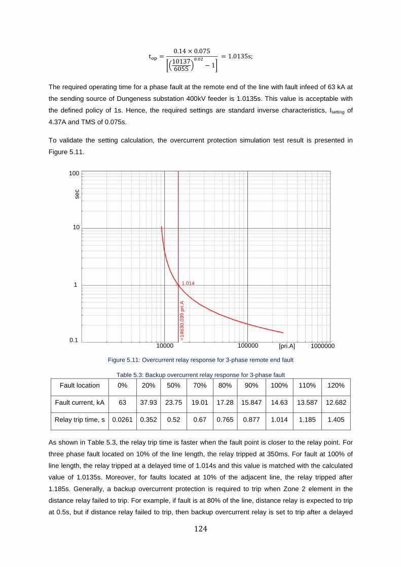
124

top =0.14 × 0.075

[(101376055

)0.02

− 1]

= 1.0135s;

The required operating time for a phase fault at the remote end of the line with fault infeed of 63 kA at

the sending source of Dungeness substation 400kV feeder is 1.0135s. This value is acceptable with

the defined policy of 1s. Hence, the required settings are standard inverse characteristics, Isetting of

4.37A and TMS of 0.075s.

To validate the setting calculation, the overcurrent protection simulation test result is presented in

Figure 5.11.

0.1

1

10

se

c

100

10000 100000 1000000[pri.A]

1.014

=1

46

30

.03

9 p

ri.A

Figure 5.11: Overcurrent relay response for 3-phase remote end fault

Table 5.3: Backup overcurrent relay response for 3-phase fault

Fault location 0% 20% 50% 70% 80% 90% 100% 110% 120%

Fault current, kA 63 37.93 23.75 19.01 17.28 15.847 14.63 13.587 12.682

Relay trip time, s 0.0261 0.352 0.52 0.67 0.765 0.877 1.014 1.185 1.405

As shown in Table 5.3, the relay trip time is faster when the fault point is closer to the relay point. For

three phase fault located on 10% of the line length, the relay tripped at 350ms. For fault at 100% of

line length, the relay tripped at a delayed time of 1.014s and this value is matched with the calculated

value of 1.0135s. Moreover, for faults located at 10% of the adjacent line, the relay tripped after

1.185s. Generally, a backup overcurrent protection is required to trip when Zone 2 element in the

distance relay failed to trip. For example, if fault is at 80% of the line, distance relay is expected to trip

at 0.5s, but if distance relay failed to trip, then backup overcurrent relay is set to trip after a delayed

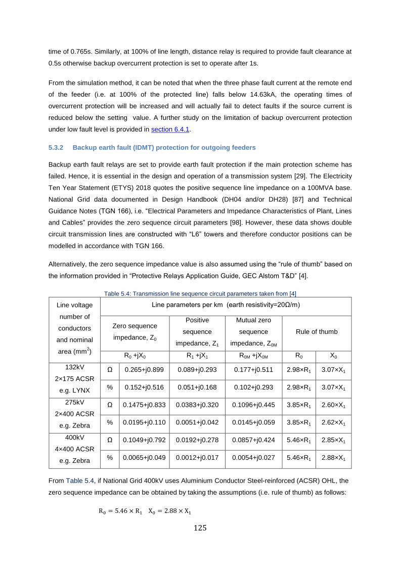
125

time of 0.765s. Similarly, at 100% of line length, distance relay is required to provide fault clearance at

0.5s otherwise backup overcurrent protection is set to operate after 1s.

From the simulation method, it can be noted that when the three phase fault current at the remote end

of the feeder (i.e. at 100% of the protected line) falls below 14.63kA, the operating times of

overcurrent protection will be increased and will actually fail to detect faults if the source current is

reduced below the setting value. A further study on the limitation of backup overcurrent protection

under low fault level is provided in section 6.4.1.

5.3.2 Backup earth fault (IDMT) protection for outgoing feeders

Backup earth fault relays are set to provide earth fault protection if the main protection scheme has

failed. Hence, it is essential in the design and operation of a transmission system [29]. The Electricity

Ten Year Statement (ETYS) 2018 quotes the positive sequence line impedance on a 100MVA base.

National Grid data documented in Design Handbook (DH04 and/or DH28) [87] and Technical

Guidance Notes (TGN 166), i.e. “Electrical Parameters and Impedance Characteristics of Plant, Lines

and Cables” provides the zero sequence circuit parameters [98]. However, these data shows double

circuit transmission lines are constructed with “L6” towers and therefore conductor positions can be

modelled in accordance with TGN 166.

Alternatively, the zero sequence impedance value is also assumed using the “rule of thumb” based on

the information provided in “Protective Relays Application Guide, GEC Alstom T&D” [4].

Table 5.4: Transmission line sequence circuit parameters taken from [4]

Line voltage

number of

conductors

and nominal

area (mm2)

Line parameters per km (earth resistivity=20Ω/m)

Zero sequence

impedance, Z0

Positive

sequence

impedance, Z1

Mutual zero

sequence

impedance, Z0M

Rule of thumb

R0 +jX0 R1 +jX1 R0M +jX0M R0 X0

132kV

2×175 ACSR

e.g. LYNX

Ω 0.265+j0.899 0.089+j0.293 0.177+j0.511 2.98×R1 3.07×X1

% 0.152+j0.516 0.051+j0.168 0.102+j0.293 2.98×R1 3.07×X1

275kV

2×400 ACSR

e.g. Zebra

Ω 0.1475+j0.833 0.0383+j0.320 0.1096+j0.445 3.85×R1 2.60×X1

% 0.0195+j0.110 0.0051+j0.042 0.0145+j0.059 3.85×R1 2.62×X1

400kV

4×400 ACSR

e.g. Zebra

Ω 0.1049+j0.792 0.0192+j0.278 0.0857+j0.424 5.46×R1 2.85×X1

% 0.0065+j0.049 0.0012+j0.017 0.0054+j0.027 5.46×R1 2.88×X1

From Table 5.4, if National Grid 400kV uses Aluminium Conductor Steel-reinforced (ACSR) OHL, the

zero sequence impedance can be obtained by taking the assumptions (i.e. rule of thumb) as follows:

R0 = 5.46 × R1 X0 = 2.88 × X1

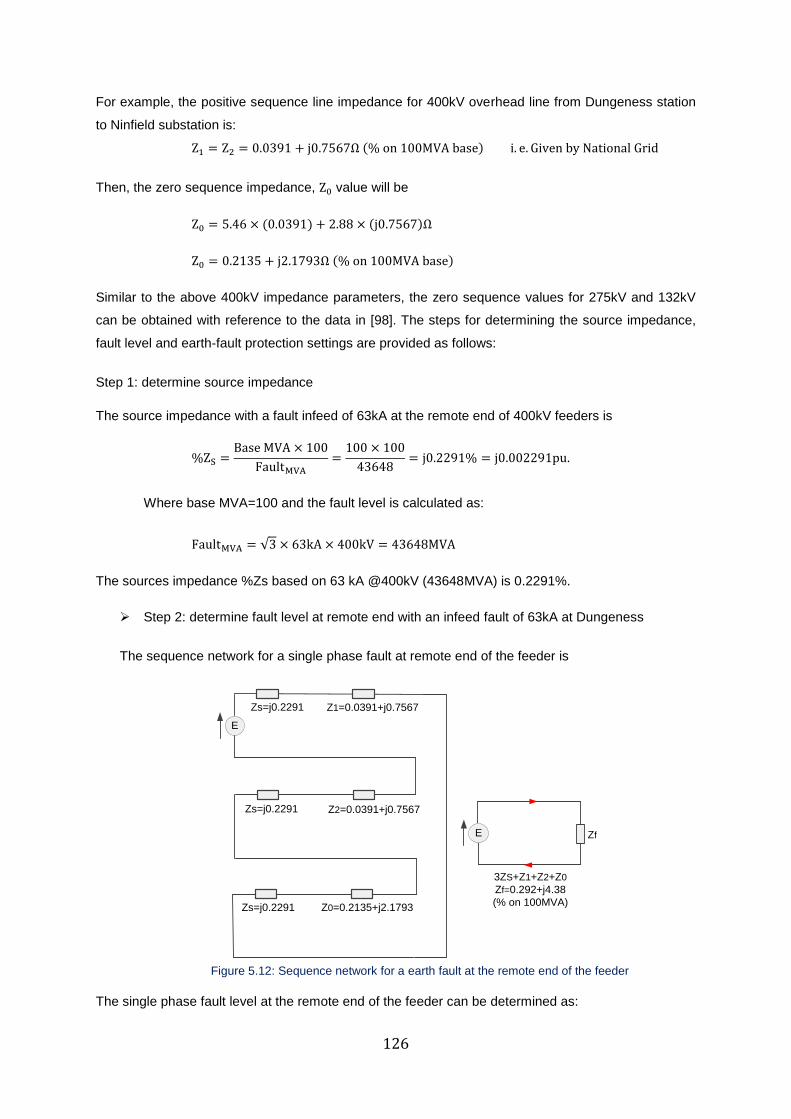
126

For example, the positive sequence line impedance for 400kV overhead line from Dungeness station

to Ninfield substation is:

Z1 = Z2 = 0.0391 + j0.7567Ω (% on 100MVA base) i. e. Given by National Grid

Then, the zero sequence impedance, Z0 value will be

Z0 = 5.46 × (0.0391) + 2.88 × (j0.7567)Ω

Z0 = 0.2135 + j2.1793Ω (% on 100MVA base)

Similar to the above 400kV impedance parameters, the zero sequence values for 275kV and 132kV

can be obtained with reference to the data in [98]. The steps for determining the source impedance,

fault level and earth-fault protection settings are provided as follows:

Step 1: determine source impedance

The source impedance with a fault infeed of 63kA at the remote end of 400kV feeders is

%ZS =Base MVA × 100

FaultMVA

=100 × 100

43648= j0.2291% = j0.002291pu.

Where base MVA=100 and the fault level is calculated as:

FaultMVA = √3 × 63kA × 400kV = 43648MVA

The sources impedance %Zs based on 63 kA @400kV (43648MVA) is 0.2291%.

Step 2: determine fault level at remote end with an infeed fault of 63kA at Dungeness

The sequence network for a single phase fault at remote end of the feeder is

Z1=0.0391+j0.7567

E

Zs=j0.2291

ZfE

Z2=0.0391+j0.7567Zs=j0.2291

Z0=0.2135+j2.1793Zs=j0.2291

3ZS+Z1+Z2+Z0

Zf=0.292+j4.38

(% on 100MVA)

Figure 5.12: Sequence network for a earth fault at the remote end of the feeder

The single phase fault level at the remote end of the feeder can be determined as:

127

I0(MVA) =Base MVA × 100

%(Zf)=

100 × 100

0.292 + j4.38= 2278MVA

I0(kA) =Fault level (MVA)

√3 × kV=

2278

√3 × 400= 3.288kA

Note the zero sequence data is normally given from the data of the plant, where the earth fault current

may vary significant. As shown in Figure 5.12, the earth fault current is lowered due to the high zero

sequence impedance value. With comments in chapter 1, the zero sequence components are not

available in phase fault currents or normal load currents. Overall, the sensitivity of earth fault

protection is greatly improved using the zero sequence current instead of phase current. According to

National Grid system design specified in [29], the maximum level of zero phase sequence current is

3.3%, where the current seen by earth fault protection is 10% (i. e. 3I0 = 9.9%).

The maximum fault level at the remote end of the feeder will be:

Fault MVA = 3I0(MVA) = 3 × 2278 = 6834MVA (5.8)

Fault kA =3I0(MVA)

√3 × kV=

6834

√3 × 400= 9.86kA or 3I0(kA) = 9.86kA

Step 3: determine backup earth fault setting at 400kV Dungeness substation

If the earth fault protection is required to detect up to 100Ω resistive faults, the fault current will be

If(400kV) = kV

√3 × Rf

=400kV

√3 × 100Ω= 2309.4A = 2.309kA (5.9)

The fault current at the midpoint for equally fed from two sources will be 2309.4/2=1154.7A. If the

relay pickup safety factor of 1.3 is assumed. The required earth fault setting is:

I setting = 1154.7 1.3⁄

= 888A (primary)

= √3 × 400 kV × 888A = 615MVA

= 0.444 A (secondary) for 2000:1 CT ratio (i.e. 888A/2000=0.444A)

To prevent unwanted operation, the earth fault relay pickup is set to 115% of the maximum

overloading circuit, and the earth fault relay should not trip for the imbalance current, i.e. 10% of the

full load current. Hence, the earth fault pickup setting can be given by:

I selected setting = Irated load (max) × 10% × 1.15 (5.10)

= 7600 × 10% × 1.15 = 874A, ~880A

= 880A primary

= √3 × 400 kV × 880A = 610MVA

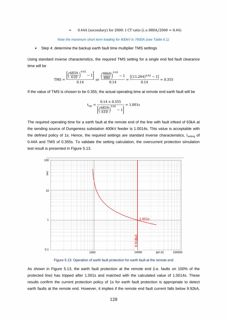
128

= 0.44A (secondary) for 2000: 1 CT ratio (i. e. 880A/2000 = 0.44)

Note the maximum short term loading for 400kV is 7600A (see Table 6.1).

Step 4: determine the backup earth fault time multiplier TMS settings

Using standard inverse characteristics, the required TMS setting for a single end fed fault clearance

time will be

TMS =[(

6834 610

)0.02

− 1]

0.14 or

(9860880

)0.02

− 1

0.14=

[(11.204)0.02 − 1]

0.14= 0.355

If the value of TMS is chosen to be 0.355, the actual operating time at remote end earth fault will be

top =0.14 × 0.355

[(6834610

)0.02

− 1]

= 1.001s

The required operating time for a earth fault at the remote end of the line with fault infeed of 63kA at

the sending source of Dungeness substation 400kV feeder is 1.0014s. This value is acceptable with

the defined policy of 1s. Hence, the required settings are standard inverse characteristics, Isetting of

0.44A and TMS of 0.355s. To validate the setting calculation, the overcurrent protection simulation

test result is presented in Figure 5.13.

Earth fault protection

0.1

1

10

se

c

100

1000 10000 100000[pri.A]

1.001s

9.9

18

kA

Figure 5.13: Operation of earth fault protection for earth fault at the remote end

As shown in Figure 5.13, the earth fault protection at the remote end (i.e. faults on 100% of the

protected line) has tripped after 1.001s and matched with the calculated value of 1.0014s. These

results confirm the current protection policy of 1s for earth fault protection is appropriate to detect

earth faults at the remote end. However, it implies if the remote end fault current falls below 9.92kA,

129

the operating times of earth fault protection will be increased and may fail to provide adequate earth

fault protection. This will occur if the infeed fault current is reduced substantially. The impact of low

fault level on the limitation of backup earth fault protections will be carried out in section 6.4.2.

5.3.3 Setting implications for 400/275 kV Auto Transformer

In this case, a phase overcurrent and earth fault protection scheme will be discussed. It is essential to

ensure the TMS value for feeder backup protection (overcurrent and earth fault) provides adequate

grading with the SGT HV overcurrent and LV earth fault protection.

a. 400/275 kV high set overcurrent (HSOC)/ HV three phase overcurrent protection

High set overcurrent protection is normally used on the HV side of the transformer to provide fast

instantaneous operation for faults on the terminal ends of the transformer HV winding or on the

bushing, whilst time-delayed overcurrent protection detects faults on the LV side of the transformer

[7]. Since the operation of HSOC is fast, the sub-transient fault current values must be used.

To ensure the HSOC must not operate for a fault on the LV side of the transformer, the current

settings, used by National Grid, are as follows [29]:

Isetting: ≥150% of the fault current supplied to a 3-phase fault on the LV windings when the

fault level is a maximum

Isetting: ≤50% of the fault current supplied to a 2-phase fault on the HV bushing under

minimum fault level conditions.

5.3.4 Review on setting requirements for supergrid/132 kV auto-transformers

Earth fault protection is set to provide both current and time grading with residual connected earth

fault protection applied to the 132kV side of the super grid 400/132kV auto-transformers [90]. Similarly

to the protection setting applied for 400/275kV transformer, in this case will be:

a. High set overcurrent protection: settings are similar to 400/275kV

b. 2 Stage HV three phase Overcurrent protection

Stage 1: is set to provide backup protection for faults left detected in the LV of the

transformer.

Stage 2: is set to provide backup protection for faults left undetected on the transformer.

c. LV three phase overcurrent

This form of protection is set to provide a backup protection for faults left undetected on

the LV conncetions of the transformer when faults are fed from the LV side [21].

d. LV earth fault

Earth fault protection is set to provide backup protection for earth faults left undetected on

the DNO feeders operating at 132 kV.

130

5.4 Summary

The basic principles, operating characteristics and application of overcurrent protection were studied

in this chapter. An over-current protection operates when the magnitude of the fault current caused by

short circuit exceeds a pre-determined setting current. Overcurrent relays are used for backup

protection of transmission system and the sub-transmission network (132kV in UK), and are the main

types of protection used in distribution networks (11kV in UK).

Unlike differential and distance protection; overcurrent protection is the simplest and least expensive

form of protection. However, overcurrent coordination is difficult to achieve when transmission system

have more than one source, especially when the fault currents are flowing from both sides of the

terminal.

At present, backup overcurrent and backup earth fault protection are widely used by National Grid.

The role of backup protection is to clear a fault, only if the first and second main protection schemes

failed to detect faults. The operation is set to achieve 1s for faults on the remote end of the feeder.

The operation time is normally calculated based on the fault level of the system where TMS is used to

adjust the trip time of the relay. In UK National Grid, backup overcurrent or backup earth fault

protection operation is normally slower than the zone 2 distance protection (0.5s) and this ensures the

coordination between the main and backup protection is adequate.

The key strengths of this chapter are to widen understanding on the concept and application of

overcurrent protection. The objective is to understand the operating characteristics and setting

calculation of overcurrent protection. The impact of low fault level on the operating performance of

overcurrent and setting implication will be discussed in chapter 6.

The 3rd

technical paper entitled < Impact of Pecking Faults on the Operating Times of Numerical and

Electromechanical Over-current Relays> was published and presented based on grading of overcurrent

protection on 13th

International conference on Development in Power System Protection (DPSP2016). The

conference was held on March 7-10, 2016, Edinburgh, UK.

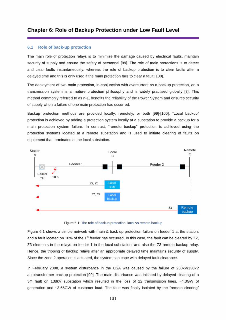
131

Chapter 6: Role of Backup Protection under Low Fault Level

6.1 Role of back-up protection

The main role of protection relays is to minimize the damage caused by electrical faults, maintain

security of supply and ensure the safety of personnel [99]. The role of main protections is to detect

and clear faults instantaneously, whereas the role of backup protection is to clear faults after a

delayed time and this is only used if the main protection fails to clear a fault [100].

The deployment of two main protection, in-conjunction with overcurrent as a backup protection, on a

transmission system is a mature protection philosophy and is widely practised globally [7]. This

method commonly referred to as n-1, benefits the reliability of the Power System and ensures security

of supply when a failure of one main protection has occurred.

Backup protection methods are provided locally, remotely, or both [99]-[100]. “Local backup”

protection is achieved by adding a protection system locally at a substation to provide a backup for a

main protection system failure. In contrast, “remote backup” protection is achieved using the

protection systems located at a remote substation and is used to initiate clearing of faults on

equipment that terminates at the local substation.

Feeder 2Feeder 1

Local

B

Remote

CStation

A

10%

Remote

backup

Local

relay

Local

backup

Failed

CB

Z3

Z2, Z3

Z2, Z3

Figure 6.1: The role of backup protection, local vs remote backup

Figure 6.1 shows a simple network with main & back up protection failure on feeder 1 at the station,

and a fault located on 10% of the 1st feeder has occurred. In this case, the fault can be cleared by Z2,

Z3 elements in the relays on feeder 1 in the local substation, and also the Z3 remote backup relay.

Hence, the tripping of backup relays after an appropriate delayed time maintains security of supply.

Since the zone 2 operation is actuated, the system can cope with delayed fault clearance.

In February 2008, a system disturbance in the USA was caused by the failure of 230kV/138kV

autotransformer backup protection [99]. The main disturbance was initiated by delayed clearing of a

3Φ fault on 138kV substation which resulted in the loss of 22 transmission lines, ~4.3GW of

generation and ~3.65GW of customer load. The fault was finally isolated by the “remote clearing”

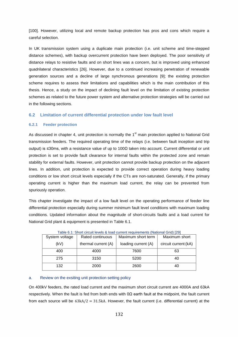
132

[100]. However, utilizing local and remote backup protection has pros and cons which require a

careful selection.

In UK transmission system using a duplicate main protection (i.e. unit scheme and time-stepped

distance schemes), with backup overcurrent protection have been deployed. The poor sensitivity of

distance relays to resistive faults and on short lines was a concern, but is improved using enhanced

quadrilateral characteristics [26]. However, due to a continued increasing penetration of renewable

generation sources and a decline of large synchronous generations [9]; the existing protection

scheme requires to assess their limitations and capabilities which is the main contribution of this

thesis. Hence, a study on the impact of declining fault level on the limitation of existing protection

schemes as related to the future power system and alternative protection strategies will be carried out

in the following sections.

6.2 Limitation of current differential protection under low fault level

6.2.1 Feeder protection

As discussed in chapter 4, unit protection is normally the 1st main protection applied to National Grid

transmission feeders. The required operating time of the relays (i.e. between fault inception and trip

output) is ≤30ms, with a resistance value of up to 100Ω taken into account. Current differential or unit

protection is set to provide fault clearance for internal faults within the protected zone and remain

stability for external faults. However, unit protection cannot provide backup protection on the adjacent

lines. In addition, unit protection is expected to provide correct operation during heavy loading

conditions or low short circuit levels especially if the CTs are non-saturated. Generally, if the primary

operating current is higher than the maximum load current, the relay can be prevented from

spuriously operation.

This chapter investigate the impact of a low fault level on the operating performance of feeder line

differential protection especially during summer minimum fault level conditions with maximum loading

conditions. Updated information about the magnitude of short-circuits faults and a load current for

National Grid plant & equipment is presented in Table 6.1.

Table 6.1: Short circuit levels & load current requirements (National Grid) [29]

System voltage

(kV)

Rated continuous

thermal current (A)

Maximum short term

loading current (A)

Maximum short

circuit current (kA)

400 4000 7600 63

275 3150 5200 40

132 2000 2600 40

a. Review on the exsiting unit protection setting policy

On 400kV feeders, the rated load current and the maximum short circuit current are 4000A and 63kA

respectively. When the fault is fed from both ends with 0Ω earth fault at the midpoint, the fault current

from each source will be 63kA/2 = 31.5kA. However, the fault current (i.e. differential current) at the

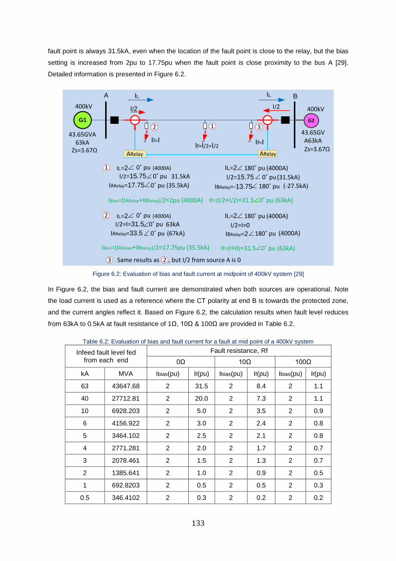
133

fault point is always 31.5kA, even when the location of the fault point is close to the relay, but the bias

setting is increased from 2pu to 17.75pu when the fault point is close proximity to the bus A [29].

Detailed information is presented in Figure 6.2.

G1

I/2

ILA IL

G2

ARelay

I/2

2 1

If=I/2+I/2If=I

43.65GVA 63kA

400kV

43.65GVA63kA

400kV

B

1 IL=2 (4000A)0˚ pu IL=2 (4000A)180˚ puI/2=15.75 31.5kA0˚ pu I/2=15.75 (31.5kA)0˚ pu

IARelay=17.75 (35.5kA)0˚ pu (-27.5kA)180˚ pu

ARelay

IBRelay=-13.75

IBias=(IARelay+IBRelay)/2=2pu (4000A)

Zs=3.67Ω

If=(I/2+I/2)=31.5 0˚ pu (63kA)

Zs=3.67Ω

3

If=I

23 Same results as , but I/2 from source A is 0

2 IL=2 (4000A)0˚ pu IL=2 (4000A)180˚ puI/2=I=31.5 63kA0˚ pu I/2=I=0

IARelay=33.5 (67kA)0˚ pu (4000A)180˚ puIBRelay=2

IBias=(IARelay+IBRelay)/2=17.75pu (35.5kA) If=(I+0)=31.5 0˚ pu (63kA)

Figure 6.2: Evaluation of bias and fault current at midpoint of 400kV system [29]

In Figure 6.2, the bias and fault current are demonstrated when both sources are operational. Note

the load current is used as a reference where the CT polarity at end B is towards the protected zone,

and the current angles reflect it. Based on Figure 6.2, the calculation results when fault level reduces

from 63kA to 0.5kA at fault resistance of 1Ω, 10Ω & 100Ω are provided in Table 6.2.

Table 6.2: Evaluation of bias and fault current for a fault at mid point of a 400kV system

Infeed fault level fed from each end

Fault resistance, Rf

0Ω 10Ω 100Ω

kA MVA Ibias(pu) If(pu) Ibias(pu) If(pu) Ibias(pu) If(pu)

63 43647.68 2 31.5 2 8.4 2 1.1

40 27712.81 2 20.0 2 7.3 2 1.1

10 6928.203 2 5.0 2 3.5 2 0.9

6 4156.922 2 3.0 2 2.4 2 0.8

5 3464.102 2 2.5 2 2.1 2 0.8

4 2771.281 2 2.0 2 1.7 2 0.7

3 2078.461 2 1.5 2 1.3 2 0.7

2 1385.641 2 1.0 2 0.9 2 0.5

1 692.8203 2 0.5 2 0.5 2 0.3

0.5 346.4102 2 0.3 2 0.2 2 0.2

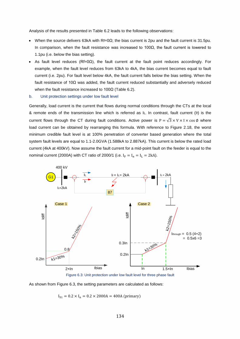
134

Analysis of the results presented in Table 6.2 leads to the following observations:

When the source delivers 63kA with Rf=0Ω; the bias current is 2pu and the fault current is 31.5pu.

In comparison, when the fault resistance was increased to 100Ω, the fault current is lowered to

1.1pu (i.e. below the bias setting).

As fault level reduces (Rf=0Ω), the fault current at the fault point reduces accordingly. For

example, when the fault level reduces from 63kA to 4kA, the bias current becomes equal to fault

current (i.e. 2pu). For fault level below 4kA, the fault current falls below the bias setting. When the

fault resistance of 10Ω was added, the fault current reduced substantially and adversely reduced

when the fault resistance increased to 100Ω (Table 6.2).

b. Unit protection settings under low fault level

Generally, load current is the current that flows during normal conditions through the CTs at the local

& remote ends of the transmission line which is referred as IL. In contrast, fault current (If) is the

current flows through the CT during fault conditions. Active power is P = √3 × V × I × cos ∅ where

load current can be obtained by rearranging this formula. With reference to Figure 2.18, the worst

minimum credible fault level is at 100% penetration of converter based generation where the total

system fault levels are equal to 1.1-2.0GVA (1.588kA to 2.887kA). This current is below the rated load

current (4kA at 400kV). Now assume the fault current for a mid-point fault on the feeder is equal to the

nominal current (2000A) with CT ratio of 2000/1 (i.e. IF = In = IL = 2kA).

Ithrough = 0.5 (4+2)

= 0.5x6 =3

G1

87

If = IL= 2kA

If

0.2In

0.3In

In 1.5×In

Idiff

Ibias

IL

400 kV

0.2In

2×In

Idiff

Ibias

k1=30%

k2=150%

0.8

k2=

150%

k1=30%

Case 1 Case 2

IL = 2kA

IL=2kA

Figure 6.3: Unit protection under low fault level for three phase fault

As shown from Figure 6.3, the setting parameters are calculated as follows:

IS1 = 0.2 × In = 0.2 × 2000A = 400A (primary)

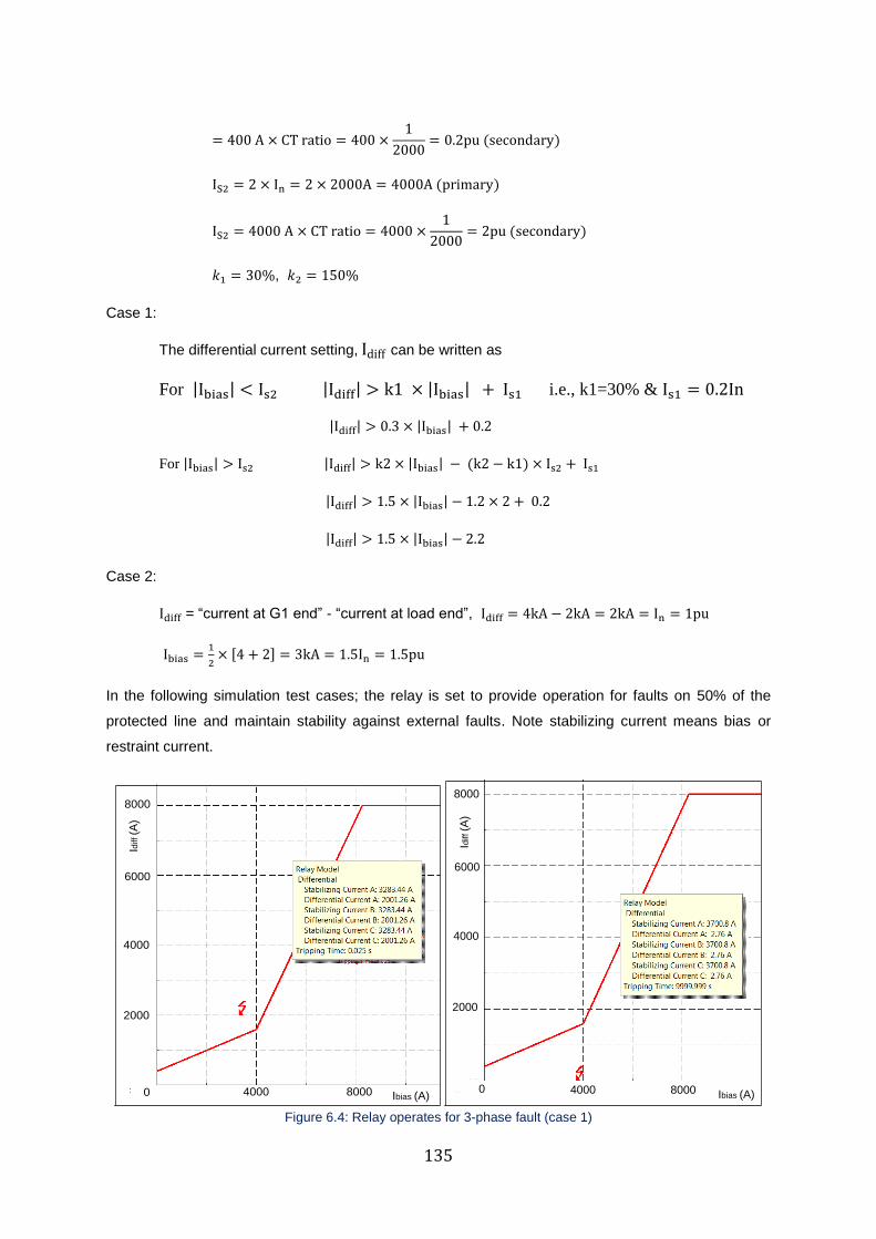
135

= 400 A × CT ratio = 400 ×1

2000= 0.2pu (secondary)

IS2 = 2 × In = 2 × 2000A = 4000A (primary)

IS2 = 4000 A × CT ratio = 4000 ×1

2000= 2pu (secondary)

𝑘1 = 30%, 𝑘2 = 150%

Case 1:

The differential current setting, Idiff can be written as

For |Ibias| < Is2 |Idiff| > k1 × |Ibias| + Is1 i.e., k1=30% & Is1 = 0.2In

|Idiff| > 0.3 × |Ibias| + 0.2

For |Ibias| > Is2 |Idiff| > k2 × |Ibias| − (k2 − k1) × Is2 + Is1

|Idiff| > 1.5 × |Ibias| − 1.2 × 2 + 0.2

|Idiff| > 1.5 × |Ibias| − 2.2

Case 2:

Idiff = “current at G1 end” - “current at load end”, Idiff = 4kA − 2kA = 2kA = In = 1pu

Ibias =1

2× [4 + 2] = 3kA = 1.5In = 1.5pu

In the following simulation test cases; the relay is set to provide operation for faults on 50% of the

protected line and maintain stability against external faults. Note stabilizing current means bias or

restraint current.

Idiff (A

)

8000

6000

4000

2000

4000 8000 12000 160000 Ibias (A)

Idiff (A

)

8000

6000

4000

2000

4000 8000 12000 16000Ibias (A)0

Figure 6.4: Relay operates for 3-phase fault (case 1)

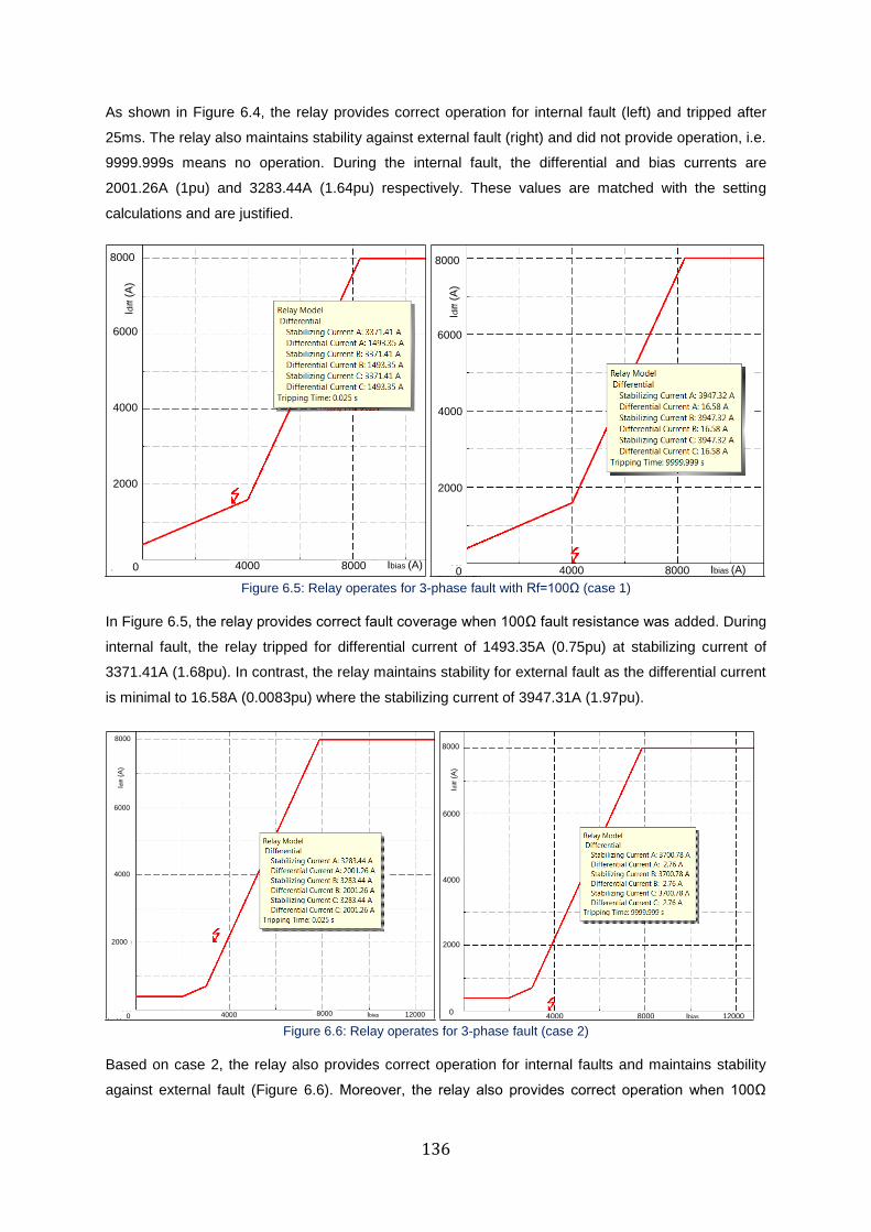
136

As shown in Figure 6.4, the relay provides correct operation for internal fault (left) and tripped after

25ms. The relay also maintains stability against external fault (right) and did not provide operation, i.e.

9999.999s means no operation. During the internal fault, the differential and bias currents are

2001.26A (1pu) and 3283.44A (1.64pu) respectively. These values are matched with the setting

calculations and are justified.

0Ibias (A)4000 8000 12000

8000

6000

4000

2000

0

Idiff (A

)

0

Ibias (A)4000 8000 12000

8000

6000

4000

2000

0

Idiff (A

)

Figure 6.5: Relay operates for 3-phase fault with Rf=100Ω (case 1)

In Figure 6.5, the relay provides correct fault coverage when 100Ω fault resistance was added. During

internal fault, the relay tripped for differential current of 1493.35A (0.75pu) at stabilizing current of

3371.41A (1.68pu). In contrast, the relay maintains stability for external fault as the differential current

is minimal to 16.58A (0.0083pu) where the stabilizing current of 3947.31A (1.97pu).

8000

6000

4000

2000

0 Ibias4000 8000

Idiff (A

)

12000 12000Ibias800040000

2000

4000

6000

Idiff (A

)

8000

Figure 6.6: Relay operates for 3-phase fault (case 2)

Based on case 2, the relay also provides correct operation for internal faults and maintains stability

against external fault (Figure 6.6). Moreover, the relay also provides correct operation when 100Ω

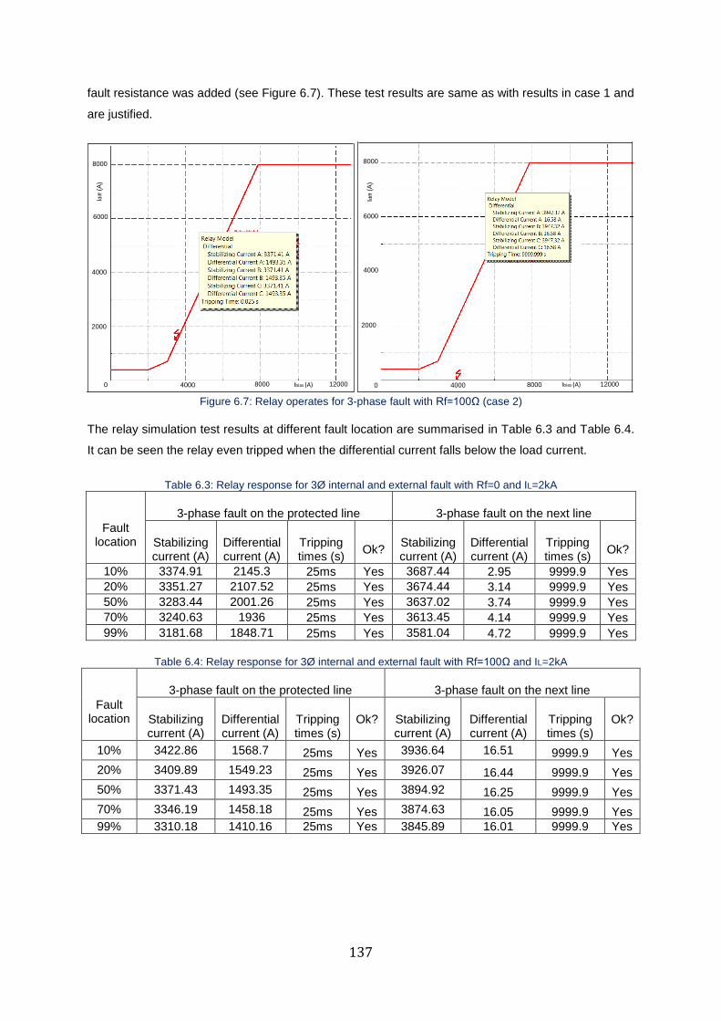
137

fault resistance was added (see Figure 6.7). These test results are same as with results in case 1 and

are justified.

6000

4000

2000

0 Ibias (A)4000 8000

Idiff (A

)

12000

8000

8000

6000

4000

2000

0 Ibias (A)4000 8000

Idiff (A

)

12000 Figure 6.7: Relay operates for 3-phase fault with Rf=100Ω (case 2)

The relay simulation test results at different fault location are summarised in Table 6.3 and Table 6.4.

It can be seen the relay even tripped when the differential current falls below the load current.

Table 6.3: Relay response for 3Ø internal and external fault with Rf=0 and IL=2kA

Fault location

3-phase fault on the protected line 3-phase fault on the next line

Stabilizing current (A)

Differential current (A)

Tripping times (s)

Ok? Stabilizing current (A)

Differential current (A)

Tripping times (s)

Ok?

10% 3374.91 2145.3 25ms Yes 3687.44 2.95 9999.9 Yes

20% 3351.27 2107.52 25ms Yes 3674.44 3.14 9999.9 Yes 50% 3283.44 2001.26 25ms Yes 3637.02 3.74 9999.9 Yes 70% 3240.63 1936 25ms Yes 3613.45 4.14 9999.9 Yes 99% 3181.68 1848.71 25ms Yes 3581.04 4.72 9999.9 Yes

Table 6.4: Relay response for 3Ø internal and external fault with Rf=100Ω and IL=2kA

Fault location

3-phase fault on the protected line 3-phase fault on the next line

Stabilizing current (A)

Differential current (A)

Tripping times (s)

Ok? Stabilizing current (A)

Differential current (A)

Tripping times (s)

Ok?

10% 3422.86 1568.7 25ms Yes 3936.64 16.51 9999.9 Yes

20% 3409.89 1549.23 25ms Yes 3926.07 16.44 9999.9 Yes

50% 3371.43 1493.35 25ms Yes 3894.92 16.25 9999.9 Yes

70% 3346.19 1458.18 25ms Yes 3874.63 16.05 9999.9 Yes 99% 3310.18 1410.16 25ms Yes 3845.89 16.01 9999.9 Yes

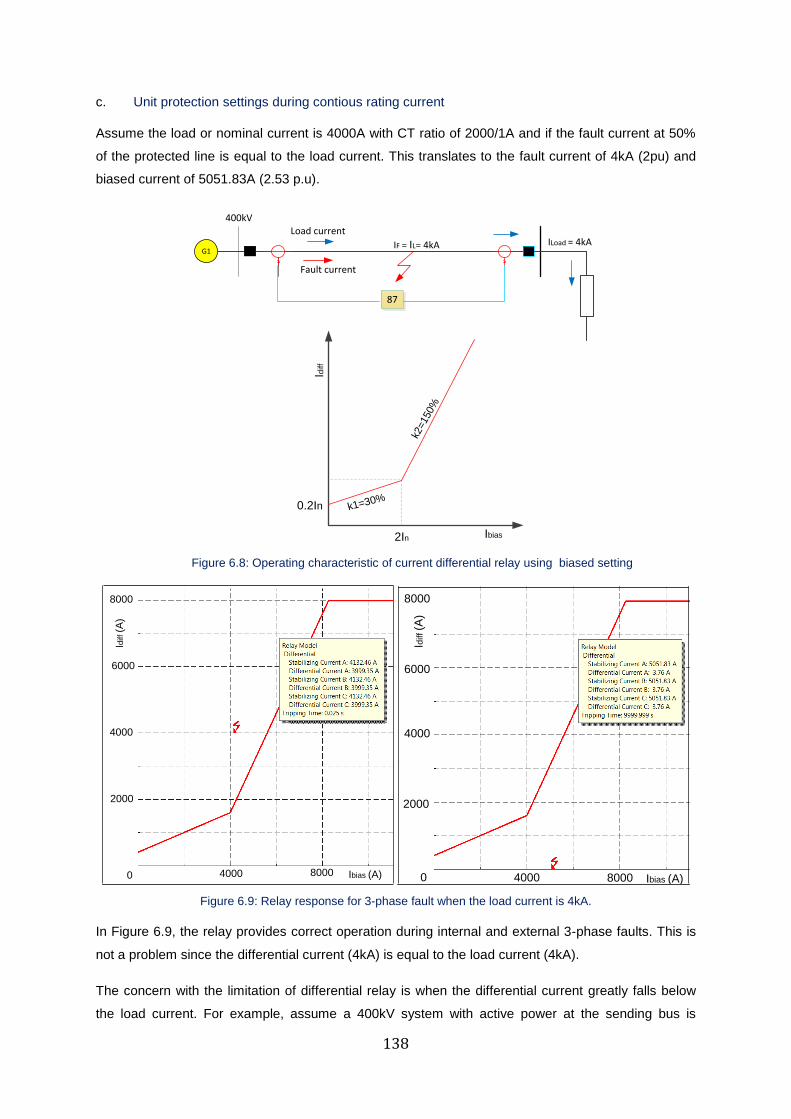
138

c. Unit protection settings during contious rating current

Assume the load or nominal current is 4000A with CT ratio of 2000/1A and if the fault current at 50%

of the protected line is equal to the load current. This translates to the fault current of 4kA (2pu) and

biased current of 5051.83A (2.53 p.u).

G1IF = IL= 4kA ILoad = 4kA

Load current

Fault current

87

400kV

0.2In

2In

Idiff

Ibias

k1=30%

k2=150%

Figure 6.8: Operating characteristic of current differential relay using biased setting

2000

0 4000 8000 Ibias (A)

4000

6000

8000

Idiff (A

)

Ibias (A)80004000 0

2000

4000

6000

Idiff (A

)

8000

Figure 6.9: Relay response for 3-phase fault when the load current is 4kA.

In Figure 6.9, the relay provides correct operation during internal and external 3-phase faults. This is

not a problem since the differential current (4kA) is equal to the load current (4kA).

The concern with the limitation of differential relay is when the differential current greatly falls below

the load current. For example, assume a 400kV system with active power at the sending bus is

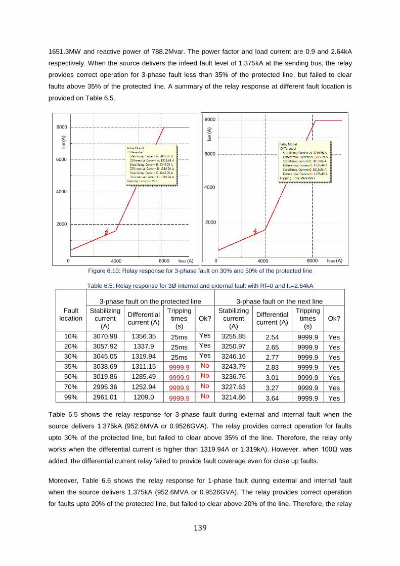
139

1651.3MW and reactive power of 788.2Mvar. The power factor and load current are 0.9 and 2.64kA

respectively. When the source delivers the infeed fault level of 1.375kA at the sending bus, the relay

provides correct operation for 3-phase fault less than 35% of the protected line, but failed to clear

faults above 35% of the protected line. A summary of the relay response at different fault location is

provided on Table 6.5.

Ibias (A)80004000 0

2000

4000

6000

Idiff (A

)

8000

Ibias (A)80004000 0

2000

4000

6000

Idiff (A

)

8000

Figure 6.10: Relay response for 3-phase fault on 30% and 50% of the protected line

Table 6.5: Relay response for 3Ø internal and external fault with Rf=0 and IL=2.64kA

Fault location

3-phase fault on the protected line 3-phase fault on the next line

Stabilizing current

(A)

Differential current (A)

Tripping times

(s) Ok?

Stabilizing current

(A)

Differential current (A)

Tripping times

(s) Ok?

10% 3070.98 1356.35 25ms Yes 3255.85 2.54 9999.9 Yes

20% 3057.92 1337.9 25ms Yes 3250.97 2.65 9999.9 Yes

30% 3045.05 1319.94 25ms Yes 3246.16 2.77 9999.9 Yes

35% 3038.69 1311.15 9999.9 No 3243.79 2.83 9999.9 Yes

50% 3019.86 1285.49 9999.9 No 3236.76 3.01 9999.9 Yes

70% 2995.36 1252.94 9999.9 No 3227.63 3.27 9999.9 Yes

99% 2961.01 1209.0 9999.9 No 3214.86 3.64 9999.9 Yes

Table 6.5 shows the relay response for 3-phase fault during external and internal fault when the

source delivers 1.375kA (952.6MVA or 0.9526GVA). The relay provides correct operation for faults

upto 30% of the protected line, but failed to clear above 35% of the line. Therefore, the relay only

works when the differential current is higher than 1319.94A or 1.319kA). However, when 100Ω was

added, the differential current relay failed to provide fault coverage even for close up faults.

Moreover, Table 6.6 shows the relay response for 1-phase fault during external and internal fault

when the source delivers 1.375kA (952.6MVA or 0.9526GVA). The relay provides correct operation

for faults upto 20% of the protected line, but failed to clear above 20% of the line. Therefore, the relay

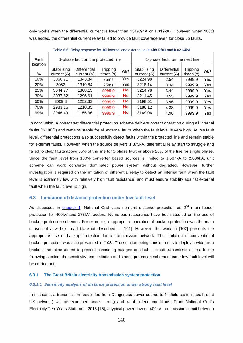
140

only works when the differential current is lower than 1319.94A or 1.319kA). However, when 100Ω

was added, the differential current relay failed to provide fault coverage even for close up faults.

Table 6.6: Relay response for 1Ø internal and external fault with Rf=0 and IL=2.64kA

Fault location

%

1-phase fault on the protected line 1-phase fault on the next line

Stabilizing current (A)

Differential current (A)

Tripping times (s)

Ok? Stabilizing current (A)

Differential current (A)

Tripping times (s)

Ok?

10% 3066.71 1343.84 25ms Yes 3224.98 2.54 9999.9 Yes 20% 3052 1319.84 25ms Yes 3218.14 3.34 9999.9 Yes 25% 3044.77 1308.13 9999.9 No 3214.78 3.44 9999.9 Yes 30% 3037.62 1296.61 9999.9 No 3211.45 3.55 9999.9 Yes 50% 3009.8 1252.33 9999.9 No 3198.51 3.96 9999.9 Yes 70% 2983.16 1210.85 9999.9 No 3186.12 4.38 9999.9 Yes 99% 2946.49 1155.36 9999.9 No 3169.06 4.96 9999.9 Yes

In conclusion, a correct set differential protection scheme delivers correct operation during all internal

faults (0-100Ω) and remains stable for all external faults when the fault level is very high. At low fault

level, differential protections also successfully detect faults within the protected line and remain stable

for external faults. However, when the source delivers 1.375kA, differential relay start to struggle and

failed to clear faults above 35% of the line for 3-phase fault or above 20% of the line for single phase.

Since the fault level from 100% converter based sources is limited to 1.587kA to 2.886kA, unit

scheme can work converter dominated power system without degraded. However, further

investigation is required on the limitation of differential relay to detect an internal fault when the fault

level is extremely low with relatively high fault resistance, and must ensure stability against external

fault when the fault level is high.

6.3 Limitation of distance protection under low fault level

As discussed in chapter 1, National Grid uses non-unit distance protection as 2nd

main feeder

protection for 400kV and 275kV feeders. Numerous researches have been studied on the use of

backup protection schemes. For example, inappropriate operation of backup protection was the main

causes of a wide spread blackout described in [101]. However, the work in [102] presents the

appropriate use of backup protection for a transmission network. The limitation of conventional

backup protection was also presented in [103]. The solution being considered is to deploy a wide area

backup protection aimed to prevent cascading outages on double circuit transmission lines. In the

following section, the sensitivity and limitation of distance protection schemes under low fault level will

be carried out.

6.3.1 The Great Britain electricity transmission system protection

6.3.1.1 Sensitivity analysis of distance protection under strong fault level

In this case, a transmission feeder fed from Dungeness power source to Ninfield station (south east

UK network) will be examined under strong and weak infeed conditions. From National Grid’s

Electricity Ten Years Statement 2018 [15], a typical power flow on 400kV transmission circuit between

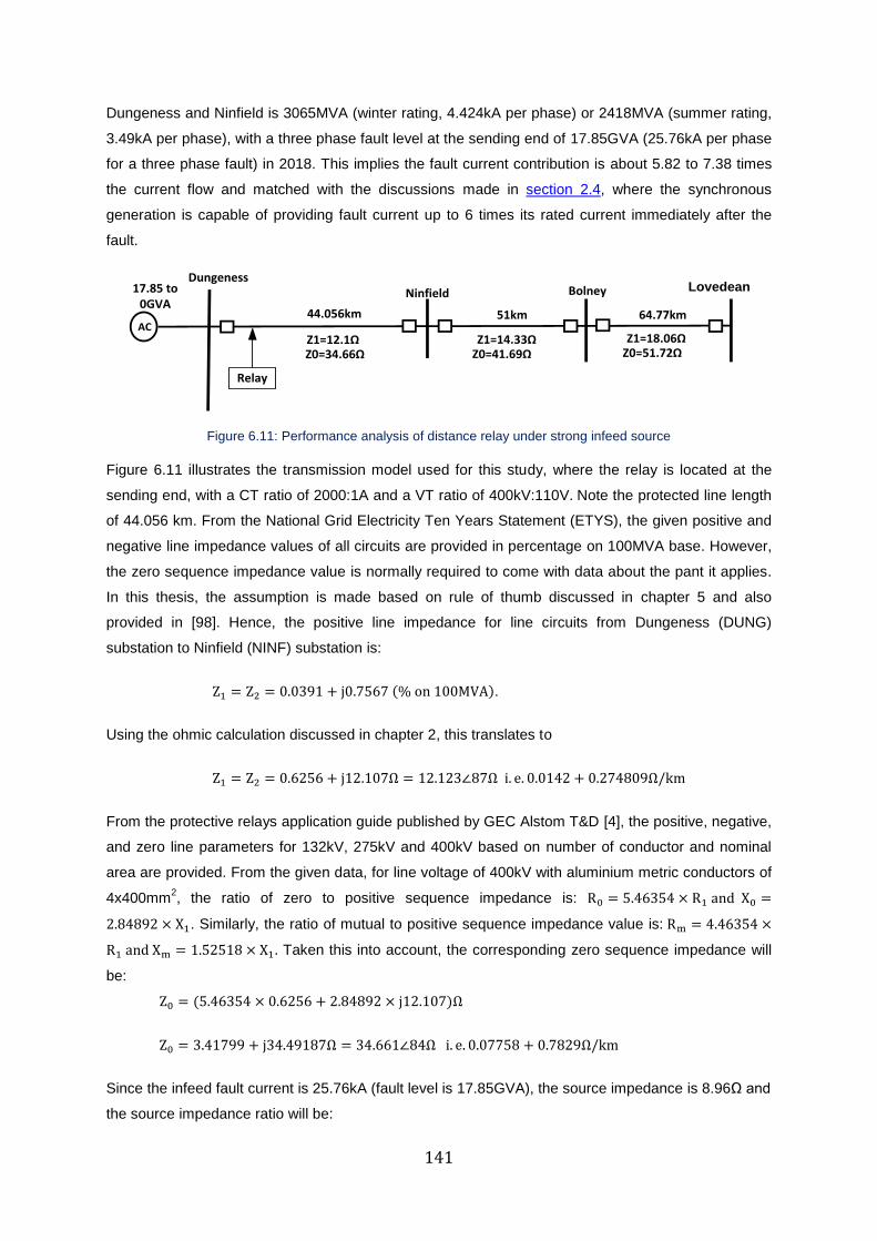
141

Dungeness and Ninfield is 3065MVA (winter rating, 4.424kA per phase) or 2418MVA (summer rating,

3.49kA per phase), with a three phase fault level at the sending end of 17.85GVA (25.76kA per phase

for a three phase fault) in 2018. This implies the fault current contribution is about 5.82 to 7.38 times

the current flow and matched with the discussions made in section 2.4, where the synchronous

generation is capable of providing fault current up to 6 times its rated current immediately after the

fault.

Lovedean17.85 to 0GVA

AC

DungenessNinfield

44.056km

Relay

Bolney

51km 64.77km

Z1=14.33Ω Z0=41.69Ω

Z1=18.06Ω Z0=51.72Ω

Z1=12.1Ω Z0=34.66Ω

Figure 6.11: Performance analysis of distance relay under strong infeed source

Figure 6.11 illustrates the transmission model used for this study, where the relay is located at the

sending end, with a CT ratio of 2000:1A and a VT ratio of 400kV:110V. Note the protected line length

of 44.056 km. From the National Grid Electricity Ten Years Statement (ETYS), the given positive and

negative line impedance values of all circuits are provided in percentage on 100MVA base. However,

the zero sequence impedance value is normally required to come with data about the pant it applies.

In this thesis, the assumption is made based on rule of thumb discussed in chapter 5 and also

provided in [98]. Hence, the positive line impedance for line circuits from Dungeness (DUNG)

substation to Ninfield (NINF) substation is:

Z1 = Z2 = 0.0391 + j0.7567 (% on 100MVA).

Using the ohmic calculation discussed in chapter 2, this translates to

Z1 = Z2 = 0.6256 + j12.107Ω = 12.123∠87Ω i. e. 0.0142 + 0.274809Ω/km

From the protective relays application guide published by GEC Alstom T&D [4], the positive, negative,

and zero line parameters for 132kV, 275kV and 400kV based on number of conductor and nominal

area are provided. From the given data, for line voltage of 400kV with aluminium metric conductors of

4x400mm2, the ratio of zero to positive sequence impedance is: R0 = 5.46354 × R1 and X0 =

2.84892 × X1. Similarly, the ratio of mutual to positive sequence impedance value is: Rm = 4.46354 ×

R1 and Xm = 1.52518 × X1 . Taken this into account, the corresponding zero sequence impedance will

be:

Z0 = (5.46354 × 0.6256 + 2.84892 × j12.107)Ω

Z0 = 3.41799 + j34.49187Ω = 34.661∠84Ω i. e. 0.07758 + 0.7829Ω/km

Since the infeed fault current is 25.76kA (fault level is 17.85GVA), the source impedance is 8.96Ω and

the source impedance ratio will be:

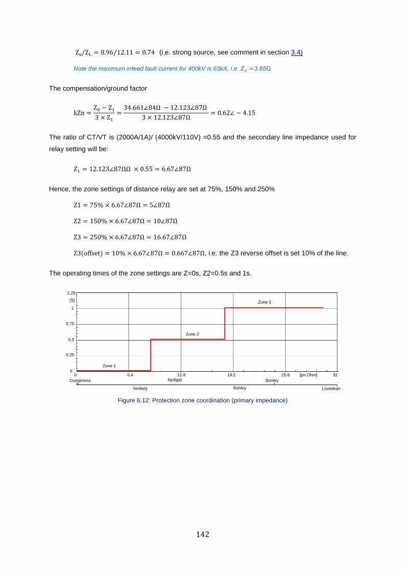
142

Zs/ZL = 8.96/12.11 = 0.74 (i.e. strong source, see comment in section 3.4)

Note the maximum infeed fault current for 400kV is 63kA, i.e. 𝑍𝑠 =3.65Ω

The compensation/ground factor

kZn =Z0 − Z1

3 × Z1

=34.661∠84Ω − 12.123∠87Ω

3 × 12.123∠87Ω= 0.62∠ − 4.15

The ratio of CT/VT is (2000A/1A)/ (4000kV/110V) =0.55 and the secondary line impedance used for

relay setting will be:

𝑍1 = 12.123∠87ΩΩ × 0.55 = 6.67∠87Ω

Hence, the zone settings of distance relay are set at 75%, 150% and 250%

Z1 = 75% × 6.67∠87Ω = 5∠87Ω

Z2 = 150% × 6.67∠87Ω = 10∠87Ω

Z3 = 250% × 6.67∠87Ω = 16.67∠87Ω

Z3(offset) = 10% × 6.67∠87Ω = 0.667∠87Ω, i.e. the Z3 reverse offset is set 10% of the line.

The operating times of the zone settings are Z=0s, Z2=0.5s and 1s.

Zone 1

Zone 2

Zone 3

6.4 12.8 19.2 25.6 [pri.Ohm] 320

1

0.75

0.5

0.25

0

Dungeness

Ninfield

Ninfield

Bonley

Bonley

Lovedean

[S]

1.25

Figure 6.12: Protection zone coordination (primary impedance)

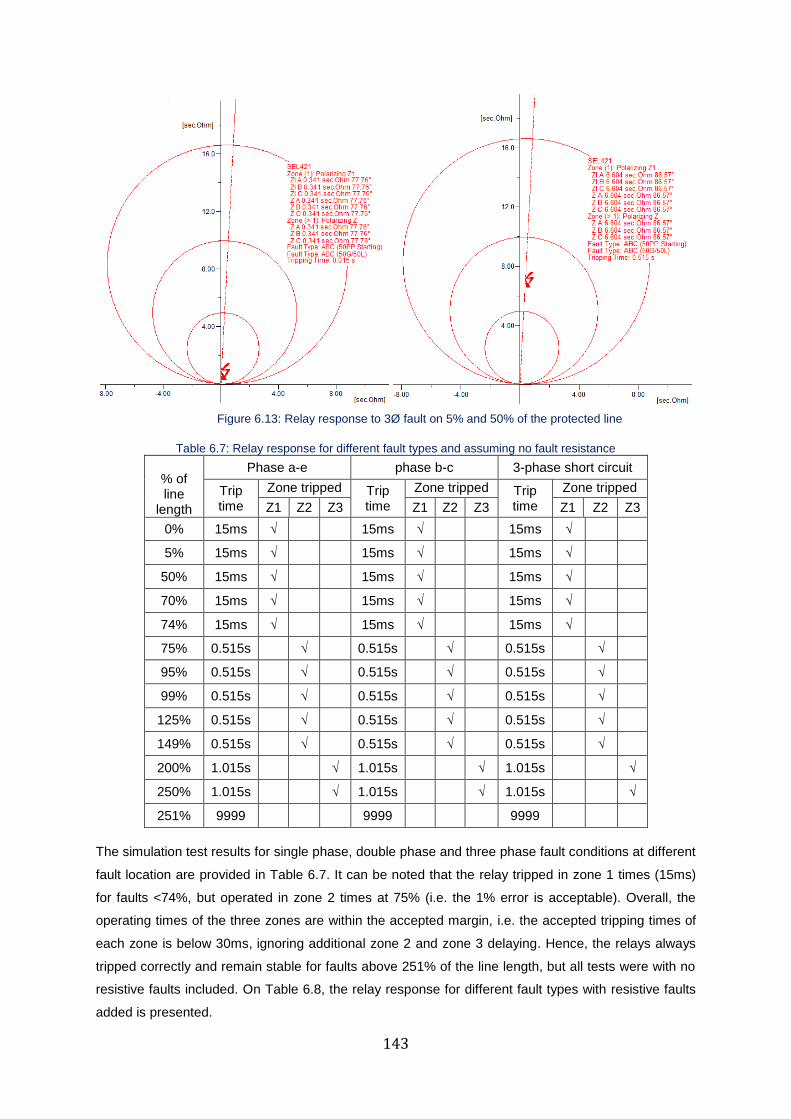
143

Figure 6.13: Relay response to 3Ø fault on 5% and 50% of the protected line

Table 6.7: Relay response for different fault types and assuming no fault resistance

% of line

length

Phase a-e phase b-c 3-phase short circuit

Trip time

Zone tripped Trip time

Zone tripped Trip time

Zone tripped

Z1 Z2 Z3 Z1 Z2 Z3 Z1 Z2 Z3

0% 15ms √ 15ms √ 15ms √

5% 15ms √ 15ms √ 15ms √

50% 15ms √ 15ms √ 15ms √

70% 15ms √ 15ms √ 15ms √

74% 15ms √ 15ms √ 15ms √

75% 0.515s √ 0.515s √ 0.515s √

95% 0.515s √ 0.515s √ 0.515s √

99% 0.515s √ 0.515s √ 0.515s √

125% 0.515s √ 0.515s √ 0.515s √

149% 0.515s √ 0.515s √ 0.515s √

200% 1.015s √ 1.015s √ 1.015s √

250% 1.015s √ 1.015s √ 1.015s √

251% 9999 9999 9999

The simulation test results for single phase, double phase and three phase fault conditions at different

fault location are provided in Table 6.7. It can be noted that the relay tripped in zone 1 times (15ms)

for faults <74%, but operated in zone 2 times at 75% (i.e. the 1% error is acceptable). Overall, the

operating times of the three zones are within the accepted margin, i.e. the accepted tripping times of

each zone is below 30ms, ignoring additional zone 2 and zone 3 delaying. Hence, the relays always

tripped correctly and remain stable for faults above 251% of the line length, but all tests were with no

resistive faults included. On Table 6.8, the relay response for different fault types with resistive faults

added is presented.

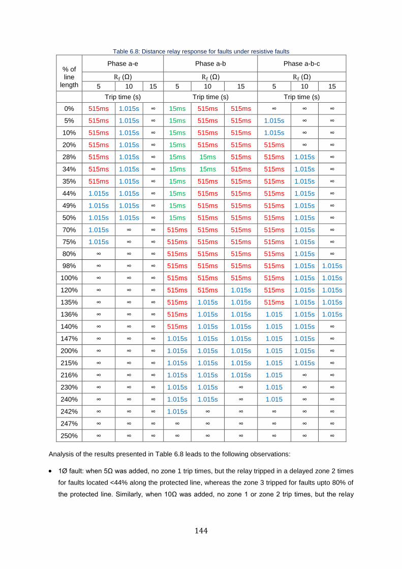
144

Table 6.8: Distance relay response for faults under resistive faults

% of line

length

Phase a-e Phase a-b Phase a-b-c

Rf (Ω) Rf (Ω) Rf (Ω)

5 10 15 5 10 15 5 10 15

Trip time (s) Trip time (s) Trip time (s)

0% 515ms 1.015s ∞ 15ms 515ms 515ms ∞ ∞ ∞

5% 515ms 1.015s ∞ 15ms 515ms 515ms 1.015s ∞ ∞

10% 515ms 1.015s ∞ 15ms 515ms 515ms 1.015s ∞ ∞

20% 515ms 1.015s ∞ 15ms 515ms 515ms 515ms ∞ ∞

28% 515ms 1.015s ∞ 15ms 15ms 515ms 515ms 1.015s ∞

34% 515ms 1.015s ∞ 15ms 15ms 515ms 515ms 1.015s ∞

35% 515ms 1.015s ∞ 15ms 515ms 515ms 515ms 1.015s ∞

44% 1.015s 1.015s ∞ 15ms 515ms 515ms 515ms 1.015s ∞

49% 1.015s 1.015s ∞ 15ms 515ms 515ms 515ms 1.015s ∞

50% 1.015s 1.015s ∞ 15ms 515ms 515ms 515ms 1.015s ∞

70% 1.015s ∞ ∞ 515ms 515ms 515ms 515ms 1.015s ∞

75% 1.015s ∞ ∞ 515ms 515ms 515ms 515ms 1.015s ∞

80% ∞ ∞ ∞ 515ms 515ms 515ms 515ms 1.015s ∞

98% ∞ ∞ ∞ 515ms 515ms 515ms 515ms 1.015s 1.015s

100% ∞ ∞ ∞ 515ms 515ms 515ms 515ms 1.015s 1.015s

120% ∞ ∞ ∞ 515ms 515ms 1.015s 515ms 1.015s 1.015s

135% ∞ ∞ ∞ 515ms 1.015s 1.015s 515ms 1.015s 1.015s

136% ∞ ∞ ∞ 515ms 1.015s 1.015s 1.015 1.015s 1.015s

140% ∞ ∞ ∞ 515ms 1.015s 1.015s 1.015 1.015s ∞

147% ∞ ∞ ∞ 1.015s 1.015s 1.015s 1.015 1.015s ∞

200% ∞ ∞ ∞ 1.015s 1.015s 1.015s 1.015 1.015s ∞

215% ∞ ∞ ∞ 1.015s 1.015s 1.015s 1.015 1.015s ∞

216% ∞ ∞ ∞ 1.015s 1.015s 1.015s 1.015 ∞ ∞

230% ∞ ∞ ∞ 1.015s 1.015s ∞ 1.015 ∞ ∞

240% ∞ ∞ ∞ 1.015s 1.015s ∞ 1.015 ∞ ∞

242% ∞ ∞ ∞ 1.015s ∞ ∞ ∞ ∞ ∞

247% ∞ ∞ ∞ ∞ ∞ ∞ ∞ ∞ ∞

250% ∞ ∞ ∞ ∞ ∞ ∞ ∞ ∞ ∞

Analysis of the results presented in Table 6.8 leads to the following observations:

1Ø fault: when 5Ω was added, no zone 1 trip times, but the relay tripped in a delayed zone 2 times

for faults located <44% along the protected line, whereas the zone 3 tripped for faults upto 80% of

the protected line. Similarly, when 10Ω was added, no zone 1 or zone 2 trip times, but the relay

145

tripped in a delayed zone 3 times for faults upto 70% of the protected line. When 15Ω was added,

the protection did not operate.

2Ø fault: when 5Ω was added, the relay tripped in zone 1 times for faults less than 70% of the

protected line and the zone 2 tripped for faults less than 47% of the adjacent line. The zone 3 also

tripped for faults below 42% of the third line. With 10Ω added, the relay tripped in a delayed zone 2

times for faults from 0% to 28% of the protected line, but tripped in zone 1 times for faults from

28% to 35% of the protected line. For faults from 35% of the protected line to 35% of the adjacent

line, the relay tripped in a delayed zone 2 times and tripped in a delayed zone 3 times for faults

from 35% of the adjacent line to 40% of the third line. When 15Ω was added, the relay provides

operation in a delayed zone 2 times for faults on the protected line, plus 20% of the adjacent line.

Moreover, the relay tripped in a delayed zone 3 times for faults from 20% of the adjacent line to

16% of the third line.

3Ø fault: when 5Ω was added, the relay initially did not provide a trip for close up faults <5% of the

line (i.e. this could be due to measuring error), but then tripped in delayed zone 3 times for faults

from 5% to 10% of the protected line. For faults from 10% of the protected line to 35% of the

adjacent line, the relay tripped in a delayed zone 2 times. Then, for faults from 35% of the adjacent

line to 40% of the third line, the relay tripped in delayed zone 3 times, but failed to provide

operation for faults from 40%-50% of the third line. When 10Ω was added, the relay seriously

affected, where the relay only provide operation at a delayed zone 3 times for faults from 44% of

the protected line to 115% of the adjacent line. Similarly, when 15Ω was added, the relays

significantly affected and only provide operation in zone 3 times for faults from 98% of the

protected line to 36% of the adjacent line.

From the observation, the effect of fault resistance, when a fault occurs on a on short line is significant

and prevented the relay operating correctly. As the line length increase, the effect of resistive faults

resulted in a delayed operation of the relay (i.e. as the line length increases, the line impedance also

increases and the effect of resistive faults is less significant as compared to the faults on short lines).

However, at higher line length, the effect of resistive fault seriously affects the relay response and

resulted in no operation. Since, the zone operation of a distance relay with Mho characteristics is

affected when resistive faults were added; a solution to consider is to replace Mho characteristic with

quadrilateral type characteristics.

6.3.1.2 Sensitivity analysis of distance protection under low fault level

Case-1: Impact of increasing penetration levels of power electronics on the operating

performance of distance scheme as used in the Great Britain transmission system.

In Figure 6.14, the source from G1 was reduced from 100% to 0% (i.e. fault level was reduced from

17.85GVA to 0GVA) whereas the converter source at the grid was increased from 0% to 100% (i.e.

fault level was increased from 0GVA to 1.1GVA). With the relay settings defined in section 6.3.1.1, the

relay response test results are provided in Table 6.9.

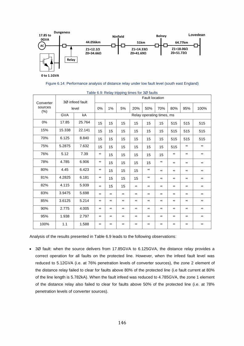
146

Lovedean17.85 to 0GVA

AC

DungenessNinfield

44.056km

0 to 1.1GVA

Relay

Bolney

51km 64.77km

Z1=14.33Ω Z0=41.69Ω

Z1=18.06Ω Z0=51.72Ω

Z1=12.1Ω Z0=34.66Ω

Figure 6.14: Performance analysis of distance relay under low fault level (south east England)

Table 6.9: Relay tripping times for 3Ø faults

Converter sources

(%)

3Ø infeed fault

level

Fault location

0% 1% 5% 20% 50% 70% 80% 95% 100%

GVA kA Relay operating times, ms

0% 17.85 25.764 15 15 15 15 15 15 515 515 515

15% 15.338 22.141 15 15 15 15 15 15 515 515 515

70% 6.125 8.840 15 15 15 15 15 15 515 515 515

75% 5.2875 7.632 15 15 15 15 15 15 515 ∞ ∞

76% 5.12 7.39 ∞ 15 15 15 15 15 ∞ ∞ ∞

78% 4.785 6.906 ∞ 15 15 15 15 ∞ ∞ ∞ ∞

80% 4.45 6.423 ∞ 15 15 15 ∞ ∞ ∞ ∞ ∞

81% 4.2825 6.181 ∞ 15 15 15 ∞ ∞ ∞ ∞ ∞

82% 4.115 5.939 ∞ 15 15 ∞ ∞ ∞ ∞ ∞ ∞

83% 3.9475 5.698 ∞ ∞ ∞ ∞ ∞ ∞ ∞ ∞ ∞

85% 3.6125 5.214 ∞ ∞ ∞ ∞ ∞ ∞ ∞ ∞ ∞

90% 2.775 4.005 ∞ ∞ ∞ ∞ ∞ ∞ ∞ ∞ ∞

95% 1.938 2.797 ∞ ∞ ∞ ∞ ∞ ∞ ∞ ∞ ∞

100% 1.1 1.588 ∞ ∞ ∞ ∞ ∞ ∞ ∞ ∞ ∞

Analysis of the results presented in Table 6.9 leads to the following observations:

3Ø fault: when the source delivers from 17.85GVA to 6.125GVA, the distance relay provides a

correct operation for all faults on the protected line. However, when the infeed fault level was

reduced to 5.12GVA (i.e. at 76% penetration levels of converter sources), the zone 2 element of

the distance relay failed to clear for faults above 80% of the protected line (i.e fault current at 80%

of the line length is 5.782kA). When the fault infeed was reduced to 4.785GVA, the zone 1 element

of the distance relay also failed to clear for faults above 50% of the protected line (i.e. at 78%

penetration levels of converter sources).

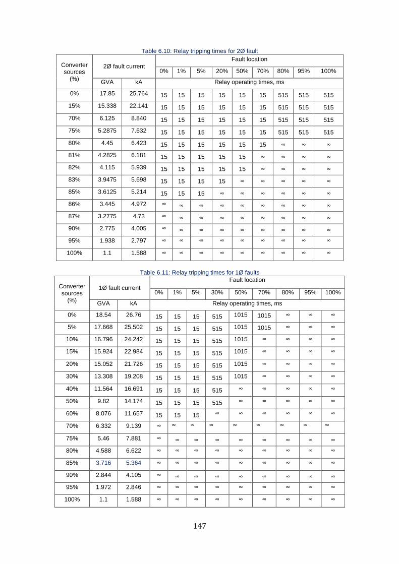
147

Table 6.10: Relay tripping times for 2Ø fault

Converter sources

(%)

2Ø fault current

Fault location

0% 1% 5% 20% 50% 70% 80% 95% 100%

GVA kA Relay operating times, ms

0% 17.85 25.764 15 15 15 15 15 15 515 515 515

15% 15.338 22.141 15 15 15 15 15 15 515 515 515

70% 6.125 8.840 15 15 15 15 15 15 515 515 515

75% 5.2875 7.632 15 15 15 15 15 15 515 515 515

80% 4.45 6.423 15 15 15 15 15 15 ∞ ∞ ∞

81% 4.2825 6.181 15 15 15 15 15 ∞ ∞ ∞ ∞

82% 4.115 5.939 15 15 15 15 15 ∞ ∞ ∞ ∞

83% 3.9475 5.698 15 15 15 15 ∞ ∞ ∞ ∞ ∞

85% 3.6125 5.214 15 15 15 ∞ ∞ ∞ ∞ ∞ ∞

86% 3.445 4.972 ∞ ∞ ∞ ∞ ∞ ∞ ∞ ∞ ∞

87% 3.2775 4.73 ∞ ∞ ∞ ∞ ∞ ∞ ∞ ∞ ∞

90% 2.775 4.005 ∞ ∞ ∞ ∞ ∞ ∞ ∞ ∞ ∞

95% 1.938 2.797 ∞ ∞ ∞ ∞ ∞ ∞ ∞ ∞ ∞

100% 1.1 1.588 ∞ ∞ ∞ ∞ ∞ ∞ ∞ ∞ ∞

Table 6.11: Relay tripping times for 1Ø faults

Converter sources

(%)

1Ø fault current

Fault location

0% 1% 5% 30% 50% 70% 80% 95% 100%

GVA kA Relay operating times, ms

0% 18.54 26.76 15 15 15 515 1015 1015 ∞ ∞ ∞

5% 17.668 25.502 15 15 15 515 1015 1015 ∞ ∞ ∞

10% 16.796 24.242 15 15 15 515 1015 ∞ ∞ ∞ ∞

15% 15.924 22.984 15 15 15 515 1015 ∞ ∞ ∞ ∞

20% 15.052 21.726 15 15 15 515 1015 ∞ ∞ ∞ ∞

30% 13.308 19.208 15 15 15 515 1015 ∞ ∞ ∞ ∞

40% 11.564 16.691 15 15 15 515 ∞ ∞ ∞ ∞ ∞

50% 9.82 14.174 15 15 15 515 ∞ ∞ ∞ ∞ ∞

60% 8.076 11.657 15 15 15 ∞ ∞ ∞ ∞ ∞ ∞

70% 6.332 9.139 ∞ ∞ ∞ ∞ ∞ ∞ ∞ ∞ ∞

75% 5.46 7.881 ∞ ∞ ∞ ∞ ∞ ∞ ∞ ∞ ∞

80% 4.588 6.622 ∞ ∞ ∞ ∞ ∞ ∞ ∞ ∞ ∞

85% 3.716 5.364 ∞ ∞ ∞ ∞ ∞ ∞ ∞ ∞ ∞

90% 2.844 4.105 ∞ ∞ ∞ ∞ ∞ ∞ ∞ ∞ ∞

95% 1.972 2.846 ∞ ∞ ∞ ∞ ∞ ∞ ∞ ∞ ∞

100% 1.1 1.588 ∞ ∞ ∞ ∞ ∞ ∞ ∞ ∞ ∞

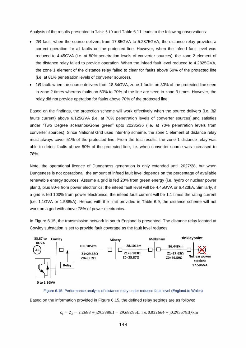
148

Analysis of the results presented in Table 6.10 and Table 6.11 leads to the following observations:

2Ø fault: when the source delivers from 17.85GVA to 5.2875GVA, the distance relay provides a

correct operation for all faults on the protected line. However, when the infeed fault level was

reduced to 4.45GVA (i.e. at 80% penetration levels of converter sources), the zone 2 element of

the distance relay failed to provide operation. When the infeed fault level reduced to 4.2825GVA,

the zone 1 element of the distance relay failed to clear for faults above 50% of the protected line

(i.e. at 81% penetration levels of converter sources).

1Ø fault: when the source delivers from 18.54GVA, zone 1 faults on 30% of the protected line seen

in zone 2 times whereas faults on 50% to 70% of the line are seen in zone 3 times. However, the

relay did not provide operation for faults above 70% of the protected line.

Based on the findings, the protection scheme will work effectively when the source delivers (i.e. 3Ø

faults current) above 6.125GVA (i.e. at 70% penetration levels of converter sources).and satisfies

under “Two Degree scenarios/Gone green” upto 20235/36 (i.e. at 70% penetration levels from

converter sources). Since National Grid uses inter-trip scheme, the zone 1 element of distance relay

must always cover 51% of the protected line. From the test results, the zone 1 distance relay was

able to detect faults above 50% of the protected line, i.e. when converter source was increased to

78%.

Note, the operational licence of Dungeness generation is only extended until 2027/28, but when

Dungeness is not operational, the amount of infeed fault level depends on the percentage of available

renewable energy sources. Assume a grid is fed 20% from green energy (i.e. hydro or nuclear power

plant), plus 80% from power electronics; the infeed fault level will be 4.45GVA or 6.423kA. Similarly, if

a grid is fed 100% from power electronics, the infeed fault current will be 1.1 times the rating current

(i.e. 1.1GVA or 1.588kA). Hence, with the limit provided in Table 6.9, the distance scheme will not

work on a grid with above 78% of power electronics.

In Figure 6.15, the transmission network in south England is presented. The distance relay located at

Cowley substation is set to provide fault coverage as the fault level reduces.

Hinkleypoint33.87 to 0GVA

Cowley Minety

100.105km

0 to 1.1GVA

Relay

Melksham

28.101km 86.448km

Z1=8.983Ω Z0=25.87Ω

Z1=27.63Ω Z0=79.59Ω

Z1=29.68Ω Z0=85.2Ω

AC AC

Nuclear power station:

17.58GVA

Figure 6.15: Performance analysis of distance relay under reduced fault level (England to Wales)

Based on the information provided in Figure 6.15, the defined relay settings are as follows:

Z1 = Z2 = 2.2688 + j29.5888Ω = 29.68∠85Ω i. e. 0.022664 + j0.295578Ω/km

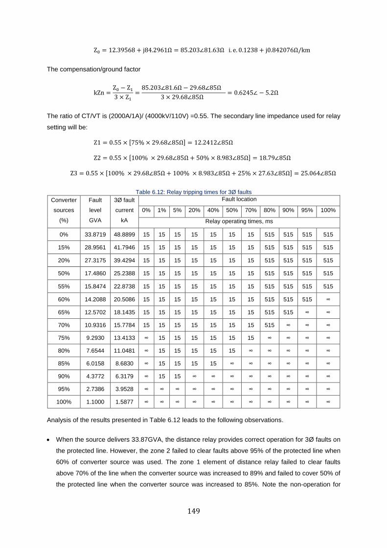
149

Z0 = 12.39568 + j84.2961Ω = 85.203∠81.63Ω i. e. 0.1238 + j0.842076Ω/km

The compensation/ground factor

kZn =Z0 − Z1

3 × Z1

=85.203∠81.6Ω − 29.68∠85Ω

3 × 29.68∠85Ω = 0.6245∠ − 5.2Ω

The ratio of CT/VT is (2000A/1A)/ (4000kV/110V) =0.55. The secondary line impedance used for relay

setting will be:

Z1 = 0.55 × [75% × 29.68∠85Ω] = 12.2412∠85Ω

Z2 = 0.55 × [100% × 29.68∠85Ω + 50% × 8.983∠85Ω] = 18.79∠85Ω

Z3 = 0.55 × [100% × 29.68∠85Ω + 100% × 8.983∠85Ω + 25% × 27.63∠85Ω] = 25.064∠85Ω

Table 6.12: Relay tripping times for 3Ø faults

Converter

sources

(%)

Fault

level

GVA

3Ø fault

current

kA

Fault location

0% 1% 5% 20% 40% 50% 70% 80% 90% 95% 100%

Relay operating times, ms

0% 33.8719 48.8899 15 15 15 15 15 15 15 515 515 515 515

15% 28.9561 41.7946 15 15 15 15 15 15 15 515 515 515 515

20% 27.3175 39.4294 15 15 15 15 15 15 15 515 515 515 515

50% 17.4860 25.2388 15 15 15 15 15 15 15 515 515 515 515

55% 15.8474 22.8738 15 15 15 15 15 15 15 515 515 515 515

60% 14.2088 20.5086 15 15 15 15 15 15 15 515 515 515 ∞

65% 12.5702 18.1435 15 15 15 15 15 15 15 515 515 ∞ ∞

70% 10.9316 15.7784 15 15 15 15 15 15 15 515 ∞ ∞ ∞

75% 9.2930 13.4133 ∞ 15 15 15 15 15 15 ∞ ∞ ∞ ∞

80% 7.6544 11.0481 ∞ 15 15 15 15 15 ∞ ∞ ∞ ∞ ∞

85% 6.0158 8.6830 ∞ 15 15 15 15 ∞ ∞ ∞ ∞ ∞ ∞

90% 4.3772 6.3179 ∞ 15 15 ∞ ∞ ∞ ∞ ∞ ∞ ∞ ∞

95% 2.7386 3.9528 ∞ ∞ ∞ ∞ ∞ ∞ ∞ ∞ ∞ ∞ ∞

100% 1.1000 1.5877 ∞ ∞ ∞ ∞ ∞ ∞ ∞ ∞ ∞ ∞ ∞

Analysis of the results presented in Table 6.12 leads to the following observations.

When the source delivers 33.87GVA, the distance relay provides correct operation for 3Ø faults on

the protected line. However, the zone 2 failed to clear faults above 95% of the protected line when

60% of converter source was used. The zone 1 element of distance relay failed to clear faults

above 70% of the line when the converter source was increased to 89% and failed to cover 50% of

the protected line when the converter source was increased to 85%. Note the non-operation for

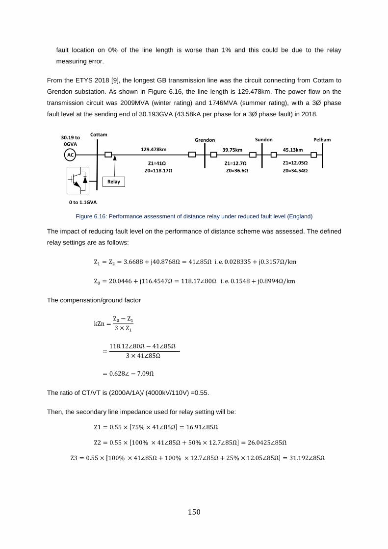
150

fault location on 0% of the line length is worse than 1% and this could be due to the relay

measuring error.

From the ETYS 2018 [9], the longest GB transmission line was the circuit connecting from Cottam to

Grendon substation. As shown in Figure 6.16, the line length is 129.478km. The power flow on the

transmission circuit was 2009MVA (winter rating) and 1746MVA (summer rating), with a 3Ø phase

fault level at the sending end of 30.193GVA (43.58kA per phase for a 3Ø phase fault) in 2018.

0 to 1.1GVA

30.19 to 0GVA

AC

CottamGrendon

129.478km

Relay

Sundon Pelham

39.75km 45.13km

Z1=12.05Ω Z1=12.7Ω Z1=41Ω

Z0=118.17Ω Z0=36.6Ω Z0=34.54Ω

Figure 6.16: Performance assessment of distance relay under reduced fault level (England)

The impact of reducing fault level on the performance of distance scheme was assessed. The defined

relay settings are as follows:

Z1 = Z2 = 3.6688 + j40.8768Ω = 41∠85Ω i. e. 0.028335 + j0.3157Ω/km

Z0 = 20.0446 + j116.4547Ω = 118.17∠80Ω i. e. 0.1548 + j0.8994Ω/km

The compensation/ground factor

kZn =Z0 − Z1

3 × Z1

=118.12∠80Ω − 41∠85Ω

3 × 41∠85Ω

= 0.628∠ − 7.09Ω

The ratio of CT/VT is (2000A/1A)/ (4000kV/110V) =0.55.

Then, the secondary line impedance used for relay setting will be:

Z1 = 0.55 × [75% × 41∠85Ω] = 16.91∠85Ω

Z2 = 0.55 × [100% × 41∠85Ω + 50% × 12.7∠85Ω] = 26.0425∠85Ω

Z3 = 0.55 × [100% × 41∠85Ω + 100% × 12.7∠85Ω + 25% × 12.05∠85Ω] = 31.192∠85Ω

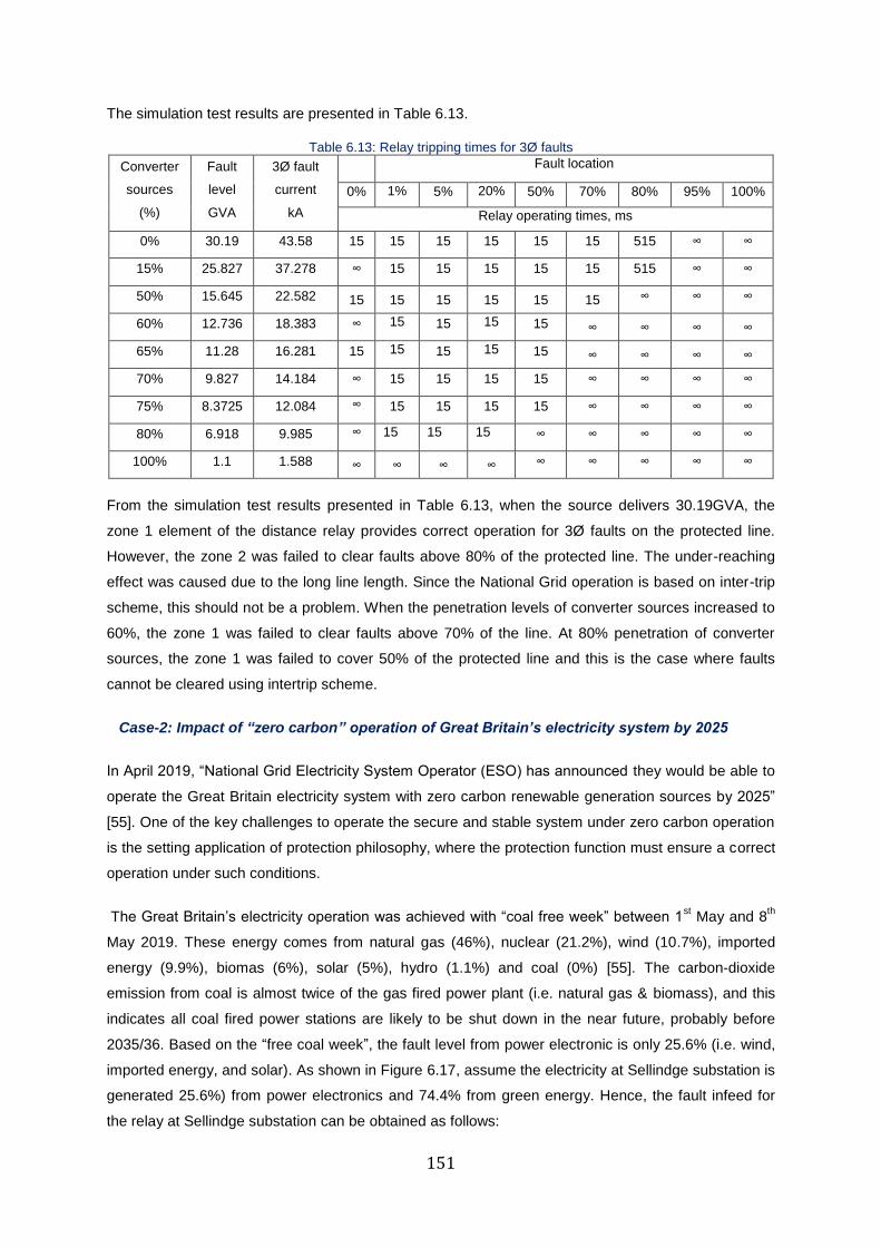
151

The simulation test results are presented in Table 6.13.

Table 6.13: Relay tripping times for 3Ø faults

Converter

sources

(%)

Fault

level

GVA

3Ø fault

current

kA

Fault location

0% 1% 5% 20% 50% 70% 80% 95% 100%

Relay operating times, ms

0% 30.19 43.58 15 15 15 15 15 15 515 ∞ ∞

15% 25.827 37.278 ∞ 15 15 15 15 15 515 ∞ ∞

50% 15.645 22.582 15 15 15 15 15 15 ∞ ∞ ∞

60% 12.736 18.383 ∞ 15 15 15 15 ∞ ∞ ∞ ∞

65% 11.28 16.281 15 15 15 15 15 ∞ ∞ ∞ ∞

70% 9.827 14.184 ∞ 15 15 15 15 ∞ ∞ ∞ ∞

75% 8.3725 12.084 ∞ 15 15 15 15 ∞ ∞ ∞ ∞

80% 6.918 9.985 ∞ 15 15 15 ∞ ∞ ∞ ∞ ∞

100% 1.1 1.588 ∞ ∞ ∞ ∞ ∞ ∞ ∞ ∞ ∞

From the simulation test results presented in Table 6.13, when the source delivers 30.19GVA, the

zone 1 element of the distance relay provides correct operation for 3Ø faults on the protected line.

However, the zone 2 was failed to clear faults above 80% of the protected line. The under-reaching

effect was caused due to the long line length. Since the National Grid operation is based on inter-trip

scheme, this should not be a problem. When the penetration levels of converter sources increased to

60%, the zone 1 was failed to clear faults above 70% of the line. At 80% penetration of converter

sources, the zone 1 was failed to cover 50% of the protected line and this is the case where faults

cannot be cleared using intertrip scheme.

Case-2: Impact of “zero carbon” operation of Great Britain’s electricity system by 2025

In April 2019, “National Grid Electricity System Operator (ESO) has announced they would be able to

operate the Great Britain electricity system with zero carbon renewable generation sources by 2025”

[55]. One of the key challenges to operate the secure and stable system under zero carbon operation

is the setting application of protection philosophy, where the protection function must ensure a correct

operation under such conditions.

The Great Britain’s electricity operation was achieved with “coal free week” between 1st May and 8

th

May 2019. These energy comes from natural gas (46%), nuclear (21.2%), wind (10.7%), imported

energy (9.9%), biomas (6%), solar (5%), hydro (1.1%) and coal (0%) [55]. The carbon-dioxide

emission from coal is almost twice of the gas fired power plant (i.e. natural gas & biomass), and this

indicates all coal fired power stations are likely to be shut down in the near future, probably before

2035/36. Based on the “free coal week”, the fault level from power electronic is only 25.6% (i.e. wind,

imported energy, and solar). As shown in Figure 6.17, assume the electricity at Sellindge substation is

generated 25.6%) from power electronics and 74.4% from green energy. Hence, the fault infeed for

the relay at Sellindge substation can be obtained as follows:

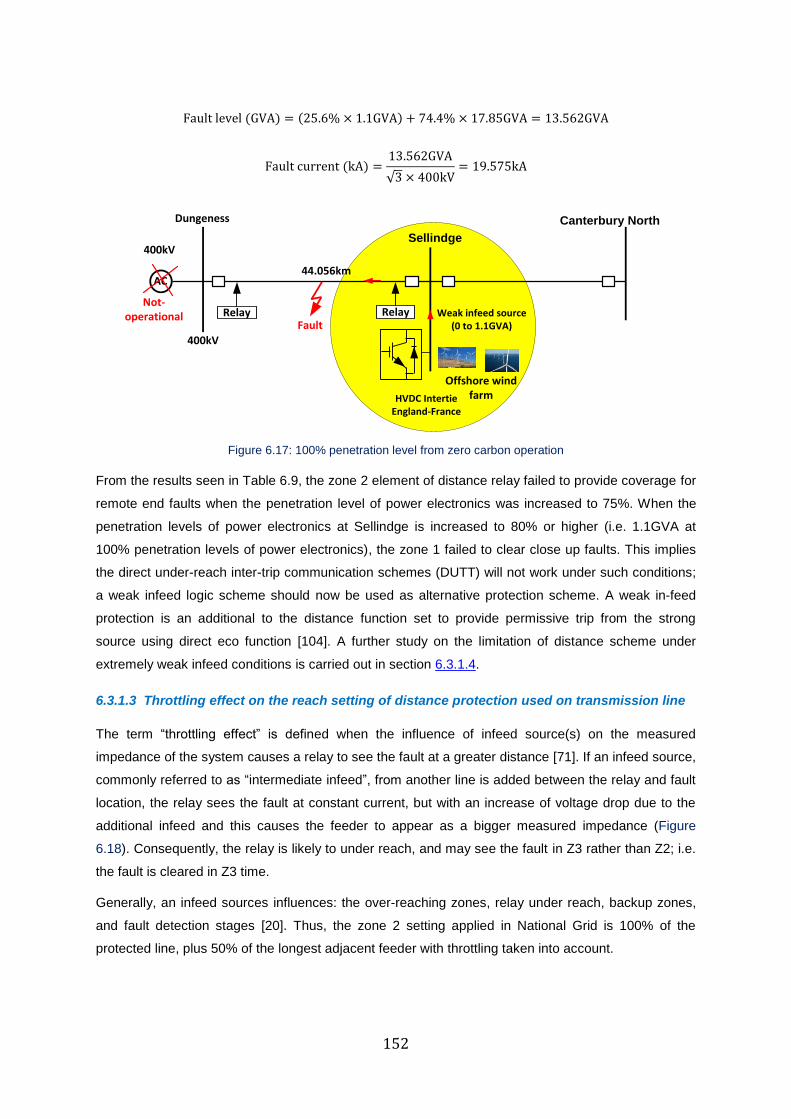
152

Fault level (GVA) = (25.6% × 1.1GVA) + 74.4% × 17.85GVA = 13.562GVA

Fault current (kA) =13.562GVA

√3 × 400kV= 19.575kA

400kV

AC

Dungeness

Sellindge

Fault

44.056km

Relay

Canterbury North

HVDC IntertieEngland-France

RelayNot-

operational Weak infeed source (0 to 1.1GVA)

Offshore wind farm

400kV

Figure 6.17: 100% penetration level from zero carbon operation

From the results seen in Table 6.9, the zone 2 element of distance relay failed to provide coverage for

remote end faults when the penetration level of power electronics was increased to 75%. When the

penetration levels of power electronics at Sellindge is increased to 80% or higher (i.e. 1.1GVA at

100% penetration levels of power electronics), the zone 1 failed to clear close up faults. This implies

the direct under-reach inter-trip communication schemes (DUTT) will not work under such conditions;

a weak infeed logic scheme should now be used as alternative protection scheme. A weak in-feed

protection is an additional to the distance function set to provide permissive trip from the strong

source using direct eco function [104]. A further study on the limitation of distance scheme under

extremely weak infeed conditions is carried out in section 6.3.1.4.

6.3.1.3 Throttling effect on the reach setting of distance protection used on transmission line

The term “throttling effect” is defined when the influence of infeed source(s) on the measured

impedance of the system causes a relay to see the fault at a greater distance [71]. If an infeed source,

commonly referred to as “intermediate infeed”, from another line is added between the relay and fault

location, the relay sees the fault at constant current, but with an increase of voltage drop due to the

additional infeed and this causes the feeder to appear as a bigger measured impedance (Figure

6.18). Consequently, the relay is likely to under reach, and may see the fault in Z3 rather than Z2; i.e.

the fault is cleared in Z3 time.

Generally, an infeed sources influences: the over-reaching zones, relay under reach, backup zones,

and fault detection stages [20]. Thus, the zone 2 setting applied in National Grid is 100% of the

protected line, plus 50% of the longest adjacent feeder with throttling taken into account.

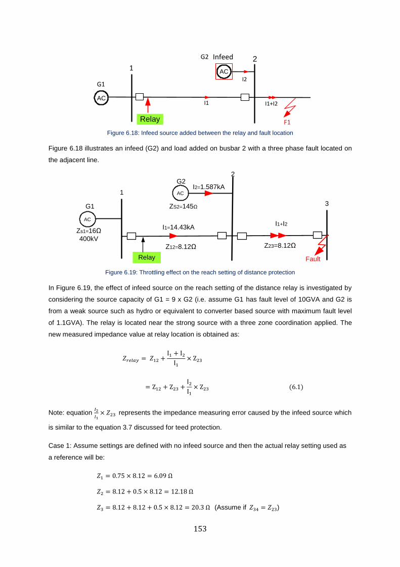
153

G1

AC

2

1AC

F1

G2 Infeed

I1

I2

I1+I2

Relay

Figure 6.18: Infeed source added between the relay and fault location

Figure 6.18 illustrates an infeed (G2) and load added on busbar 2 with a three phase fault located on

the adjacent line.

2

Zs1=16Ω

400kV

Fault

I2=1.587kA

ZS2=145Ω

1

3

Z12=8.12Ω

Relay

AC

I1+I2

G2

I1=14.43kA

Z23=8.12Ω

AC

G1

Figure 6.19: Throttling effect on the reach setting of distance protection

In Figure 6.19, the effect of infeed source on the reach setting of the distance relay is investigated by

considering the source capacity of G1 = 9 x G2 (i.e. assume G1 has fault level of 10GVA and G2 is

from a weak source such as hydro or equivalent to converter based source with maximum fault level

of 1.1GVA). The relay is located near the strong source with a three zone coordination applied. The

new measured impedance value at relay location is obtained as:

𝑍𝑟𝑒𝑙𝑎𝑦 = 𝑍12 +I1 + I2

I1

× Z23

= Z12 + Z23 +I2

I1

× Z23 (6.1)

Note: equation 𝐼2

𝐼1× 𝑍23 represents the impedance measuring error caused by the infeed source which

is similar to the equation 3.7 discussed for teed protection.

Case 1: Assume settings are defined with no infeed source and then the actual relay setting used as

a reference will be:

𝑍1 = 0.75 × 8.12 = 6.09 Ω

𝑍2 = 8.12 + 0.5 × 8.12 = 12.18 Ω

𝑍3 = 8.12 + 8.12 + 0.5 × 8.12 = 20.3 Ω (Assume if 𝑍34 = 𝑍23)

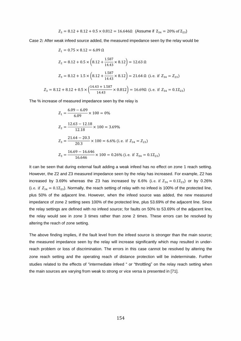
154

𝑍3 = 8.12 + 8.12 + 0.5 × 0.812 = 16.646Ω (Assume if Z34 = 20% of Z23)

Case 2: After weak infeed source added, the measured impedance seen by the relay would be

𝑍1 = 0.75 × 8.12 = 6.09 Ω

𝑍2 = 8.12 + 0.5 × (8.12 +1.587

14.43× 8.12) = 12.63 Ω

𝑍3 = 8.12 + 1.5 × (8.12 +1.587

14.43× 8.12) = 21.64 Ω (i. e. if 𝑍34 = 𝑍23)

𝑍3 = 8.12 + 8.12 + 0.5 × (14.43 + 1.587

14.43× 0.812) = 16.69Ω (i. e. if 𝑍34 = 0.1Z23)

The % increase of measured impedance seen by the relay is

𝑍1 =6.09 − 6.09

6.09× 100 = 0%

𝑍2 =12.63 − 12.18

12.18× 100 = 3.69%

𝑍3 =21.64 − 20.3

20.3× 100 = 6.6% (i. e. if 𝑍34 = 𝑍23)

𝑍3 =16.69 − 16.646

16.646× 100 = 0.26% (i. e. if Z34 = 0.1Z23)

It can be seen that during external fault adding a weak infeed has no effect on zone 1 reach setting.

However, the Z2 and Z3 measured impedance seen by the relay has increased. For example, Z2 has

increased by 3.69% whereas the Z3 has increased by 6.6% (i. e. if 𝑍34 = 0.1Z23) or by 0.26%

(i. e. if 𝑍34 = 0.1Z23). Normally, the reach setting of relay with no infeed is 100% of the protected line,

plus 50% of the adjacent line. However, when the infeed source was added, the new measured

impedance of zone 2 setting sees 100% of the protected line, plus 53.69% of the adjacent line. Since

the relay settings are defined with no infeed source; for faults on 50% to 53.69% of the adjacent line,

the relay would see in zone 3 times rather than zone 2 times. These errors can be resolved by

altering the reach of zone setting.

The above finding implies, if the fault level from the infeed source is stronger than the main source;

the measured impedance seen by the relay will increase significantly which may resulted in under-

reach problem or loss of discrimination. The errors in this case cannot be resolved by altering the

zone reach setting and the operating reach of distance protection will be indeterminate. Further

studies related to the effects of “intermediate infeed “ or “throttling” on the relay reach setting when

the main sources are varying from weak to strong or vice versa is presented in [71].

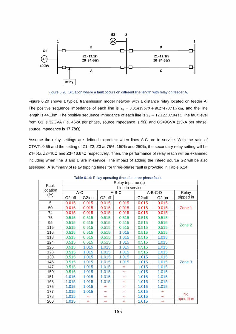
155

G1

AC

Relay

400kV

A

D

Z1=12.1Ω Z0=34.66Ω

AC

G2

1

Z1=12.1Ω Z0=34.66Ω

C

B

2

3

Figure 6.20: Situation where a fault occurs on different line length with relay on feeder A.

Figure 6.20 shows a typical transmission model network with a distance relay located on feeder A.

The positive sequence impedance of each line is Z1 = 0.01419679 + j0.274737 Ω/km, and the line

length is 44.1km. The positive sequence impedance of each line is Z1 = 12.12∠87.04 Ω. The fault level

from G1 is 32GVA (i.e. 46kA per phase, source impedance is 5Ω) and G2=9GVA (13kA per phase,

source impedance is 17.78Ω).

Assume the relay settings are defined to protect when lines A-C are in service. With the ratio of

CT/VT=0.55 and the setting of Z1, Z2, Z3 at 75%, 150% and 250%, the secondary relay setting will be

Z1=5Ω, Z2=10Ω and Z3=16.67Ω respectively. Then, the performance of relay reach will be examined

including when line B and D are in-service. The impact of adding the infeed source G2 will be also

assessed. A summary of relay tripping times for three-phase fault is provided in Table 6.14.

Table 6.14: Relay operating times for three-phase faults

Fault location

(%)

Relay trip time (s)

Line in service

A-C A-B-C A-B-C-D Relay tripped in G2:off G2:on G2:off G2:off G2:on

5 0.015 0.015 0.015 0.015 0.015 0.015

Zone 1 50 0.015 0.015 0.015 0.015 0.015 0.015

74 0.015 0.015 0.015 0.015 0.015 0.015

75 0.515 0.515 0.515 0.515 0.515 0.515

Zone 2 95 0.515 0.515 0.515 0.515 0.515 0.515

115 0.515 0.515 0.515 0.515 0.515 0.515

116 0.515 0.515 0.515 1.015 0.515 0.515

118 0.515 0.515 0.515 1.015 0.515 1.015

Zone 3

124 0.515 0.515 0.515 1.015 0.515 1.015

126 0.515 1.015 1.015 1.015 0.515 1.015

128 0.515 1.015 1.015 1.015 0.515 1.015

130 0.515 1.015 1.015 1.015 1.015 1.015

146 0.515 1.015 1.015 1.015 1.015 1.015

147 0.515 1.015 1.015 ∞ 1.015 1.015

150 0.515 1.015 1.015 ∞ 1.015 1.015

151 1.015 1.015 1.015 ∞ 1.015 1.015

168 1.015 1.015 1.015 ∞ 1.015 1.015

175 1.015 1.015 ∞ ∞ 1.015 1.015

177 1.015 1.015 ∞ ∞ 1.015 ∞ No

operation 178 1.015 ∞ ∞ ∞ 1.015 ∞

200 1.015 ∞ ∞ ∞ 1.015 ∞

156

Test 1: when lines A-C are in service with G2 off (i.e. the defined relay settings), the relay provides

correct tripping for all faults on the protected line and the adjacent line within the expected tripping

times. With G2 on, the Z2 covers up to 24% of the adjacent line, but under-reached by 26% due to the

throttling. The Z3 tripped for faults up to 77% of the adjacent line and failed to see faults above 77%

of the adjacent line because the measured impedance error caused by the G2 infeed is high.

Consequently, the relay under-reached and failed to clear faults at the remote end of the adjacent

line.

Test 2: when lines A-B-C are in-service with G2 off; the Z1 tripped correctly whereas Z2 tripped upto

24% of the adjacent line. The Z3 also covers up to 68% of the adjacent line, but failed to see remote

end faults. With G2 on, the Z2 only covers 15% of the adjacent line whereas the Z3 covers up to 46%

of the adjacent line and failed to the fault on remote end of the adjacent line (i.e. relay under-reach

due to the throttling effect).

Test 3: when lines A-B-C-D are in-service with G2 off, the Z1 tripped correctly within the Z1 operating

times. The zone 2 also covers the protected line plus 30% of the adjacent line. The Z3 is able to see

100% faults on remote end of the adjacent line. With G2 on, the Z2 covers only 16% of the adjacent

line whereas the Z3 sees faults up to 75% of the adjacent line, but failed to see faults on the remote

end (i.e. due to the throttling effect). In conclusion, the Zone 3 failed to faults remote end of the

adjacent line due to the line D outage or throttling. These results satisfy the operating principle and

setting calculation of distance protection discussed in chapter 3.

In UK National Grid transmission system, the worst-case for throttling effect is when a fault presents

on three ended infeed [26]. The current National Grid policy on setting of distance protection specifies

the zone 2 distance relay must provide coverage for busbar or mesh corner faults at the furthest

remote end without throttling taken into account [29].

6.3.1.4 Limitation of distance protection on complex network under low fault level

Case-1: Limitation of distance protection on two ended sources

Normally, when a standard permissive overreach distance scheme operates in conjunction with a

permissive under-reach scheme, instantaneous fault clearance can be obtained. In National Grid,

instantaneous fault clearance is achieved using permissive direct transfer trip schemes. The problem

occurs when a weak infeed or open breaker condition is present, where instantaneous fault clearance

cannot be achieved for close up faults.

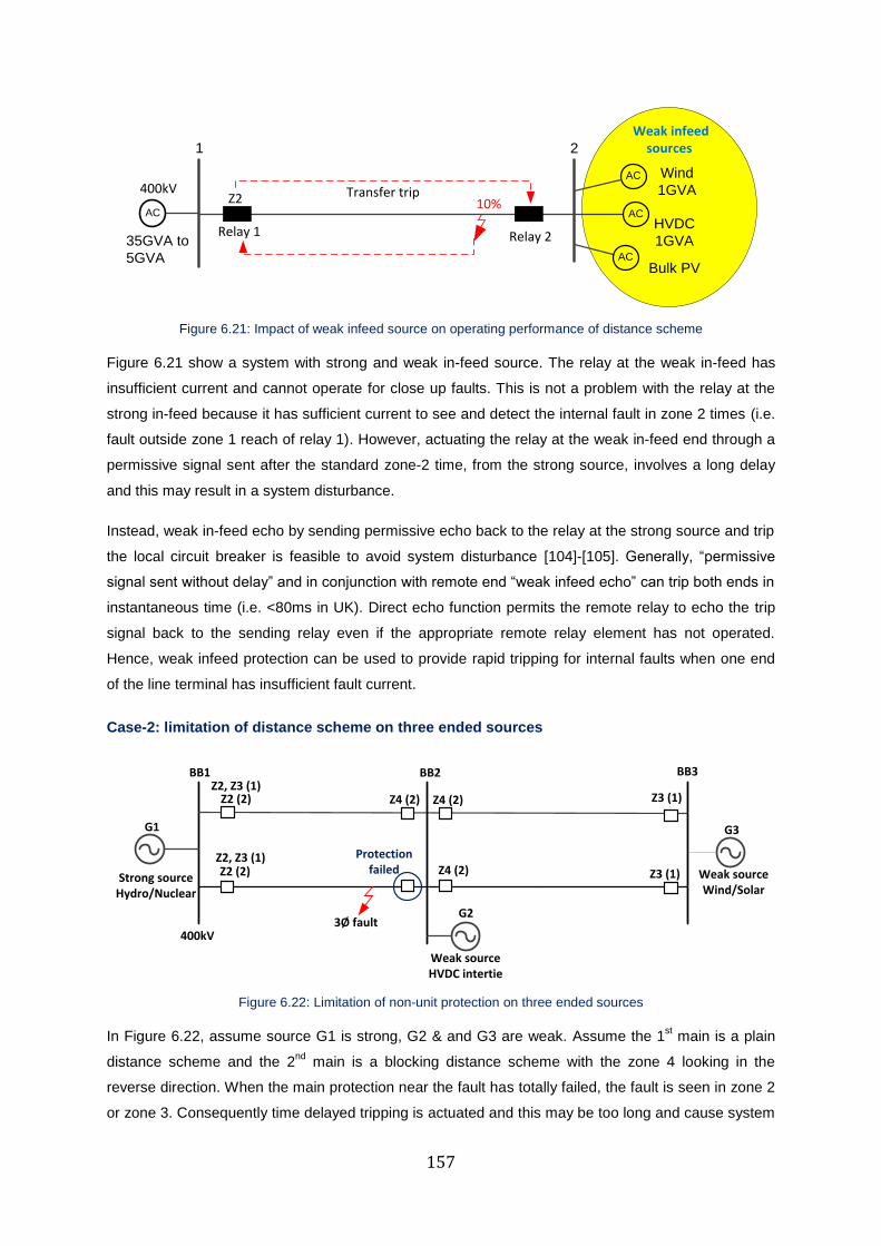
157

AC

10%

1 2

400kV

AC

35GVA to

5GVA

Relay 1

AC

ACBulk PV

HVDC

1GVA

Wind

1GVA

Relay 2

Transfer tripZ2

Weak infeed sources

Figure 6.21: Impact of weak infeed source on operating performance of distance scheme

Figure 6.21 show a system with strong and weak in-feed source. The relay at the weak in-feed has

insufficient current and cannot operate for close up faults. This is not a problem with the relay at the

strong in-feed because it has sufficient current to see and detect the internal fault in zone 2 times (i.e.

fault outside zone 1 reach of relay 1). However, actuating the relay at the weak in-feed end through a

permissive signal sent after the standard zone-2 time, from the strong source, involves a long delay

and this may result in a system disturbance.

Instead, weak in-feed echo by sending permissive echo back to the relay at the strong source and trip

the local circuit breaker is feasible to avoid system disturbance [104]-[105]. Generally, “permissive

signal sent without delay” and in conjunction with remote end “weak infeed echo” can trip both ends in

instantaneous time (i.e. <80ms in UK). Direct echo function permits the remote relay to echo the trip

signal back to the sending relay even if the appropriate remote relay element has not operated.

Hence, weak infeed protection can be used to provide rapid tripping for internal faults when one end

of the line terminal has insufficient fault current.

Case-2: limitation of distance scheme on three ended sources

Strong source Hydro/Nuclear

G1

Weak source HVDC intertie

BB2

Weak source Wind/Solar

G3

BB1 BB3

G2

400kV3Ø fault

Protection failed

Z2, Z3 (1)

Z2, Z3 (1)Z4 (2)Z2 (2)

Z2 (2) Z4 (2)

Z4 (2) Z3 (1)

Z3 (1)

Figure 6.22: Limitation of non-unit protection on three ended sources

In Figure 6.22, assume source G1 is strong, G2 & and G3 are weak. Assume the 1st main is a plain

distance scheme and the 2nd

main is a blocking distance scheme with the zone 4 looking in the

reverse direction. When the main protection near the fault has totally failed, the fault is seen in zone 2

or zone 3. Consequently time delayed tripping is actuated and this may be too long and cause system

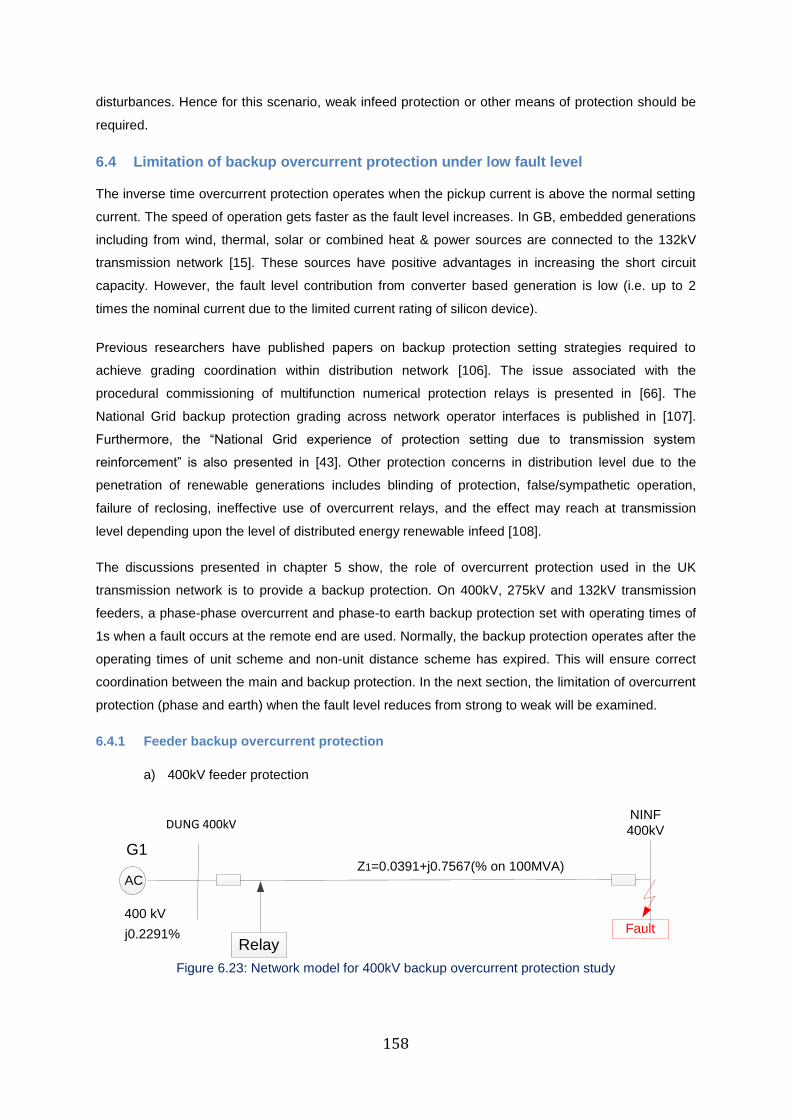
158

disturbances. Hence for this scenario, weak infeed protection or other means of protection should be

required.

6.4 Limitation of backup overcurrent protection under low fault level

The inverse time overcurrent protection operates when the pickup current is above the normal setting

current. The speed of operation gets faster as the fault level increases. In GB, embedded generations

including from wind, thermal, solar or combined heat & power sources are connected to the 132kV

transmission network [15]. These sources have positive advantages in increasing the short circuit

capacity. However, the fault level contribution from converter based generation is low (i.e. up to 2

times the nominal current due to the limited current rating of silicon device).

Previous researchers have published papers on backup protection setting strategies required to

achieve grading coordination within distribution network [106]. The issue associated with the

procedural commissioning of multifunction numerical protection relays is presented in [66]. The

National Grid backup protection grading across network operator interfaces is published in [107].

Furthermore, the “National Grid experience of protection setting due to transmission system

reinforcement” is also presented in [43]. Other protection concerns in distribution level due to the

penetration of renewable generations includes blinding of protection, false/sympathetic operation,

failure of reclosing, ineffective use of overcurrent relays, and the effect may reach at transmission

level depending upon the level of distributed energy renewable infeed [108].

The discussions presented in chapter 5 show, the role of overcurrent protection used in the UK

transmission network is to provide a backup protection. On 400kV, 275kV and 132kV transmission

feeders, a phase-phase overcurrent and phase-to earth backup protection set with operating times of

1s when a fault occurs at the remote end are used. Normally, the backup protection operates after the

operating times of unit scheme and non-unit distance scheme has expired. This will ensure correct

coordination between the main and backup protection. In the next section, the limitation of overcurrent

protection (phase and earth) when the fault level reduces from strong to weak will be examined.

6.4.1 Feeder backup overcurrent protection

a) 400kV feeder protection

G1

AC

DUNG 400kVNINF

400kV

Fault

Z1=0.0391+j0.7567(% on 100MVA)

Relay

400 kV

j0.2291%

Figure 6.23: Network model for 400kV backup overcurrent protection study

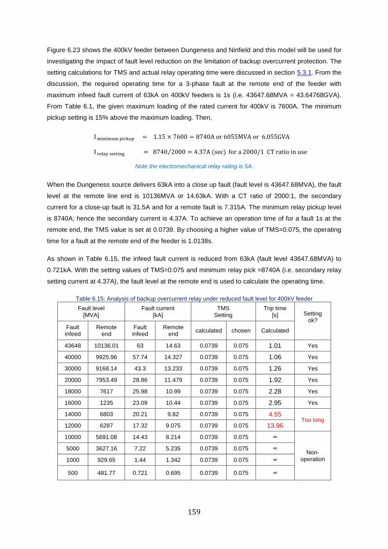
159

Figure 6.23 shows the 400kV feeder between Dungeness and Ninfield and this model will be used for

investigating the impact of fault level reduction on the limitation of backup overcurrent protection. The

setting calculations for TMS and actual relay operating time were discussed in section 5.3.1. From the

discussion, the required operating time for a 3-phase fault at the remote end of the feeder with

maximum infeed fault current of 63kA on 400kV feeders is 1s (i.e. 43647.68MVA = 43.64768GVA).

From Table 6.1, the given maximum loading of the rated current for 400kV is 7600A. The minimum

pickup setting is 15% above the maximum loading. Then,

I minimum pickup = 1.15 × 7600 = 8740A or 6055MVA or 6.055GVA

I relay setting = 8740 2000 = 4.37A (sec)⁄ for a 2000/1 CT ratio in use

Note the electromechanical relay rating is 5A.

When the Dungeness source delivers 63kA into a close up fault (fault level is 43647.68MVA), the fault

level at the remote line end is 10136MVA or 14.63kA. With a CT ratio of 2000:1, the secondary

current for a close-up fault is 31.5A and for a remote fault is 7.315A. The minimum relay pickup level

is 8740A; hence the secondary current is 4.37A. To achieve an operation time of for a fault 1s at the

remote end, the TMS value is set at 0.0739. By choosing a higher value of TMS=0.075, the operating

time for a fault at the remote end of the feeder is 1.0138s.

As shown in Table 6.15, the infeed fault current is reduced from 63kA (fault level 43647.68MVA) to

0.721kA. With the setting values of TMS=0.075 and minimum relay pick =8740A (i.e. secondary relay

setting current at 4.37A), the fault level at the remote end is used to calculate the operating time.

Table 6.15: Analysis of backup overcurrent relay under reduced fault level for 400kV feeder

Fault level [MVA]

Fault current [kA]

TMS Setting

Trip time [s] Setting

ok? Fault

infeed Remote

end Fault infeed

Remote end

calculated chosen Calculated

43648 10136.01 63 14.63 0.0739 0.075 1.01 Yes

40000 9925.96 57.74 14.327 0.0739 0.075 1.06 Yes

30000 9168.14 43.3 13.233 0.0739 0.075 1.26 Yes

20000 7953.49 28.86 11.479 0.0739 0.075 1.92 Yes

18000 7617 25.98 10.99 0.0739 0.075 2.28 Yes

16000 1235 23.09 10.44 0.0739 0.075 2.95 Yes

14000 6803 20.21 9.82 0.0739 0.075 4.55 Too long

12000 6287 17.32 9.075 0.0739 0.075 13.96

10000 5691.08 14.43 8.214 0.0739 0.075 ∞

Non- operation

5000 3627.16 7.22 5.235 0.0739 0.075 ∞

1000 929.65 1.44 1.342 0.0739 0.075 ∞

500 481.77 0.721 0.695 0.0739 0.075 ∞

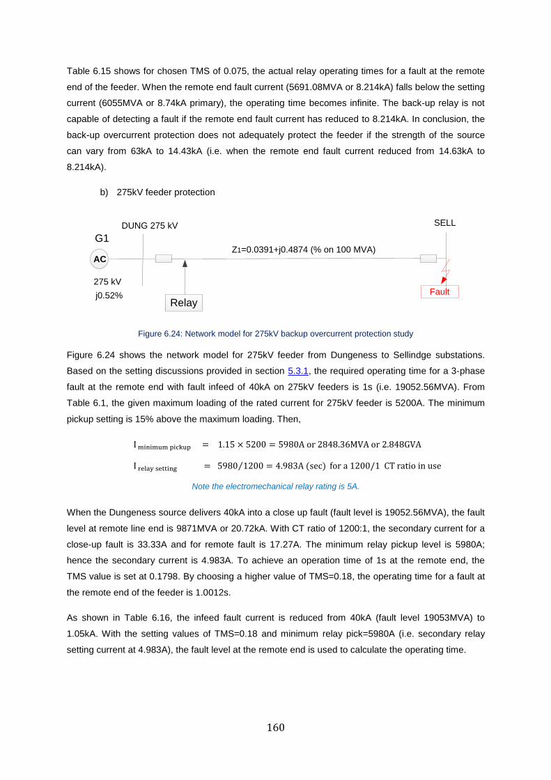
160

Table 6.15 shows for chosen TMS of 0.075, the actual relay operating times for a fault at the remote

end of the feeder. When the remote end fault current (5691.08MVA or 8.214kA) falls below the setting

current (6055MVA or 8.74kA primary), the operating time becomes infinite. The back-up relay is not

capable of detecting a fault if the remote end fault current has reduced to 8.214kA. In conclusion, the

back-up overcurrent protection does not adequately protect the feeder if the strength of the source

can vary from 63kA to 14.43kA (i.e. when the remote end fault current reduced from 14.63kA to

8.214kA).

b) 275kV feeder protection

G1

AC

DUNG 275 kV SELL

Fault

Z1=0.0391+j0.4874 (% on 100 MVA)

Relay

275 kV

j0.52%

Figure 6.24: Network model for 275kV backup overcurrent protection study

Figure 6.24 shows the network model for 275kV feeder from Dungeness to Sellindge substations.

Based on the setting discussions provided in section 5.3.1, the required operating time for a 3-phase

fault at the remote end with fault infeed of 40kA on 275kV feeders is 1s (i.e. 19052.56MVA). From

Table 6.1, the given maximum loading of the rated current for 275kV feeder is 5200A. The minimum

pickup setting is 15% above the maximum loading. Then,

I minimum pickup = 1.15 × 5200 = 5980A or 2848.36MVA or 2.848GVA

I relay setting = 5980 1200 = 4.983A (sec)⁄ for a 1200/1 CT ratio in use

Note the electromechanical relay rating is 5A.

When the Dungeness source delivers 40kA into a close up fault (fault level is 19052.56MVA), the fault

level at remote line end is 9871MVA or 20.72kA. With CT ratio of 1200:1, the secondary current for a

close-up fault is 33.33A and for remote fault is 17.27A. The minimum relay pickup level is 5980A;

hence the secondary current is 4.983A. To achieve an operation time of 1s at the remote end, the

TMS value is set at 0.1798. By choosing a higher value of TMS=0.18, the operating time for a fault at

the remote end of the feeder is 1.0012s.

As shown in Table 6.16, the infeed fault current is reduced from 40kA (fault level 19053MVA) to

1.05kA. With the setting values of TMS=0.18 and minimum relay pick=5980A (i.e. secondary relay

setting current at 4.983A), the fault level at the remote end is used to calculate the operating time.

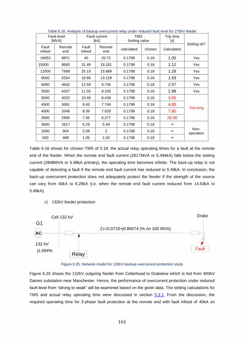
161

Table 6.16: Analysis of backup overcurrent relay under reduced fault level for 275kV feeder

Fault level [MVA]

Fault current [kA]

TMS Setting value

Trip time [s]

Setting ok? Fault infeed

Remote end

Fault infeed

Remote end

calculated chosen Calculated

19053 9871 40 20.72 0.1798 0.18 1.00 Yes

15000 8660 31.49 18.181 0.1798 0.18 1.12 Yes

12000 7568 25.19 15.889 0.1798 0.18 1.28 Yes

9000 6254 18.89 13.129 0.1798 0.18 1.59 Yes

6000 4642 12.59 9.746 0.1798 0.18 2.57 Yes

5500 4337 11.55 9.105 0.1798 0.18 2.98 Yes

5000 4020 10.49 8.439 0.1798 0.18 3.65

Too long 4500 3691 9.45 7.749 0.1798 0.18 4.85

4000 3348 8.39 7.029 0.1798 0.18 7.80

3500 2990 7.35 6.277 0.1798 0.18 26.00

3000 2617 6.29 5.49 0.1798 0.18 ∞ Non-

operation 1000 954 2.09 2 0.1798 0.18 ∞

500 488 1.05 1.02 0.1798 0.18 ∞

Table 6.16 shows for chosen TMS of 0.18, the actual relay operating times for a fault at the remote

end of the feeder. When the remote end fault current (2617MVA or 5.494kA) falls below the setting

current (2848MVA or 5.98kA primary), the operating time becomes infinite. The back-up relay is not

capable of detecting a fault if the remote end fault current has reduced to 5.49kA. In conclusion, the

back-up overcurrent protection does not adequately protect the feeder if the strength of the source

can vary from 40kA to 6.29kA (i.e. when the remote end fault current reduced from 14.63kA to

5.49kA).

c) 132kV feeder protection

G1

AC

Cell 132 kV Drake

Fault

Z1=0.0719+j0.86574 (% on 100 MVA)

Relay

132 kV

j1.094%

Figure 6.25: Network model for 132kV backup overcurrent protection study

Figure 6.25 shows the 132kV outgoing feeder from Cellarhead to Drakelow which is fed from 400kV

Daines substation near Manchester. Hence, the performance of overcurrent protection under reduced

fault level from “strong to weak” will be examined based on the given data. The setting calculations for

TMS and actual relay operating time were discussed in section 5.3.1. From the discussion, the

required operating time for 3-phase fault protection at the remote end with fault infeed of 40kA on

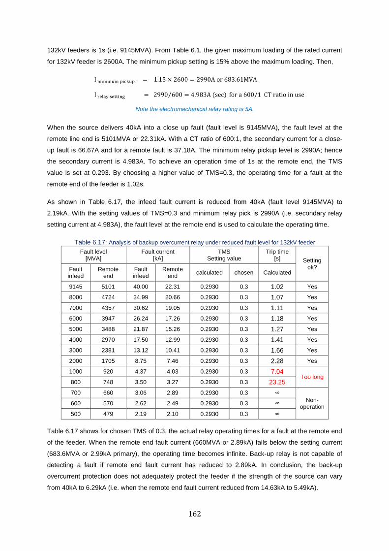
162

132kV feeders is 1s (i.e. 9145MVA). From Table 6.1, the given maximum loading of the rated current

for 132kV feeder is 2600A. The minimum pickup setting is 15% above the maximum loading. Then,

I minimum pickup = 1.15 × 2600 = 2990A or 683.61MVA

I relay setting = 2990 600 = 4.983A (sec)⁄ for a 600/1 CT ratio in use

Note the electromechanical relay rating is 5A.

When the source delivers 40kA into a close up fault (fault level is 9145MVA), the fault level at the

remote line end is 5101MVA or 22.31kA. With a CT ratio of 600:1, the secondary current for a close-

up fault is 66.67A and for a remote fault is 37.18A. The minimum relay pickup level is 2990A; hence

the secondary current is 4.983A. To achieve an operation time of 1s at the remote end, the TMS

value is set at 0.293. By choosing a higher value of TMS=0.3, the operating time for a fault at the

remote end of the feeder is 1.02s.

As shown in Table 6.17, the infeed fault current is reduced from 40kA (fault level 9145MVA) to

2.19kA. With the setting values of TMS=0.3 and minimum relay pick is 2990A (i.e. secondary relay

setting current at 4.983A), the fault level at the remote end is used to calculate the operating time.

Table 6.17: Analysis of backup overcurrent relay under reduced fault level for 132kV feeder

Fault level [MVA]

Fault current [kA]

TMS Setting value

Trip time [s] Setting

ok? Fault infeed

Remote end

Fault infeed

Remote end

calculated chosen Calculated

9145 5101 40.00 22.31 0.2930 0.3 1.02 Yes

8000 4724 34.99 20.66 0.2930 0.3 1.07 Yes

7000 4357 30.62 19.05 0.2930 0.3 1.11 Yes

6000 3947 26.24 17.26 0.2930 0.3 1.18 Yes

5000 3488 21.87 15.26 0.2930 0.3 1.27 Yes

4000 2970 17.50 12.99 0.2930 0.3 1.41 Yes

3000 2381 13.12 10.41 0.2930 0.3 1.66 Yes

2000 1705 8.75 7.46 0.2930 0.3 2.28 Yes

1000 920 4.37 4.03 0.2930 0.3 7.04 Too long

800 748 3.50 3.27 0.2930 0.3 23.25

700 660 3.06 2.89 0.2930 0.3 ∞ Non-

operation 600 570 2.62 2.49 0.2930 0.3 ∞

500 479 2.19 2.10 0.2930 0.3 ∞

Table 6.17 shows for chosen TMS of 0.3, the actual relay operating times for a fault at the remote end

of the feeder. When the remote end fault current (660MVA or 2.89kA) falls below the setting current

(683.6MVA or 2.99kA primary), the operating time becomes infinite. Back-up relay is not capable of

detecting a fault if remote end fault current has reduced to 2.89kA. In conclusion, the back-up

overcurrent protection does not adequately protect the feeder if the strength of the source can vary

from 40kA to 6.29kA (i.e. when the remote end fault current reduced from 14.63kA to 5.49kA).

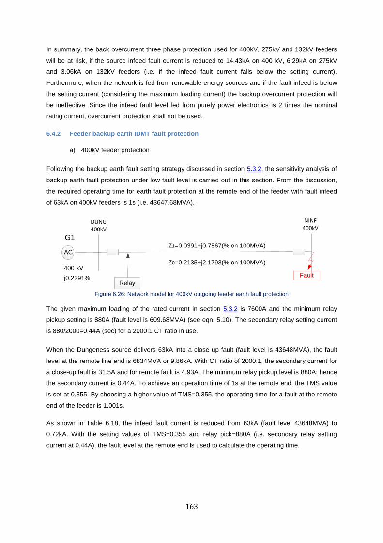
163

In summary, the back overcurrent three phase protection used for 400kV, 275kV and 132kV feeders

will be at risk, if the source infeed fault current is reduced to 14.43kA on 400 kV, 6.29kA on 275kV

and 3.06kA on 132kV feeders (i.e. if the infeed fault current falls below the setting current).

Furthermore, when the network is fed from renewable energy sources and if the fault infeed is below

the setting current (considering the maximum loading current) the backup overcurrent protection will

be ineffective. Since the infeed fault level fed from purely power electronics is 2 times the nominal

rating current, overcurrent protection shall not be used.

6.4.2 Feeder backup earth IDMT fault protection

a) 400kV feeder protection

Following the backup earth fault setting strategy discussed in section 5.3.2, the sensitivity analysis of

backup earth fault protection under low fault level is carried out in this section. From the discussion,

the required operating time for earth fault protection at the remote end of the feeder with fault infeed

of 63kA on 400kV feeders is 1s (i.e. 43647.68MVA).

G1

AC

DUNG 400kV

NINF 400kV

Fault

Z1=0.0391+j0.7567(% on 100MVA)

Relay

400 kV

j0.2291%

Z0=0.2135+j2.1793(% on 100MVA)

Figure 6.26: Network model for 400kV outgoing feeder earth fault protection

The given maximum loading of the rated current in section 5.3.2 is 7600A and the minimum relay

pickup setting is 880A (fault level is 609.68MVA) (see eqn. 5.10). The secondary relay setting current

is 880/2000=0.44A (sec) for a 2000:1 CT ratio in use.

When the Dungeness source delivers 63kA into a close up fault (fault level is 43648MVA), the fault

level at the remote line end is 6834MVA or 9.86kA. With CT ratio of 2000:1, the secondary current for

a close-up fault is 31.5A and for remote fault is 4.93A. The minimum relay pickup level is 880A; hence

the secondary current is 0.44A. To achieve an operation time of 1s at the remote end, the TMS value

is set at 0.355. By choosing a higher value of TMS=0.355, the operating time for a fault at the remote

end of the feeder is 1.001s.

As shown in Table 6.18, the infeed fault current is reduced from 63kA (fault level 43648MVA) to

0.72kA. With the setting values of TMS=0.355 and relay pick=880A (i.e. secondary relay setting

current at 0.44A), the fault level at the remote end is used to calculate the operating time.

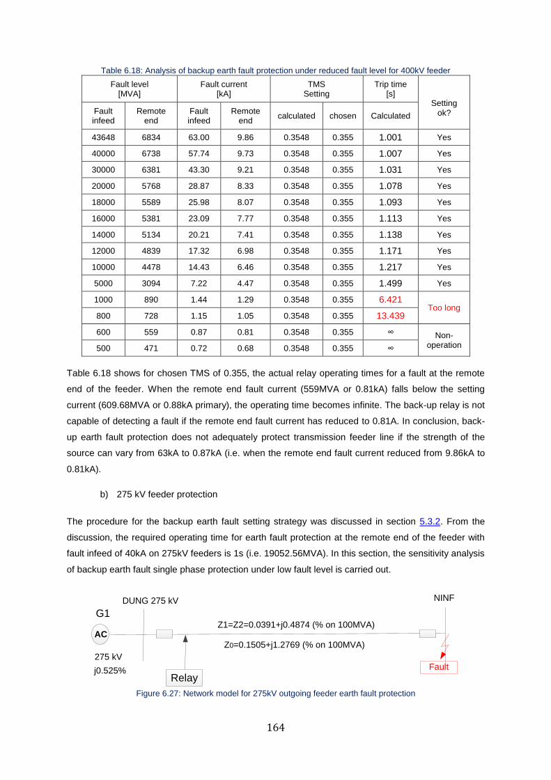
164

Table 6.18: Analysis of backup earth fault protection under reduced fault level for 400kV feeder

Fault level [MVA]

Fault current [kA]

TMS Setting

Trip time [s]

Setting ok? Fault

infeed Remote

end Fault infeed

Remote end

calculated chosen Calculated

43648 6834 63.00 9.86 0.3548 0.355 1.001 Yes

40000 6738 57.74 9.73 0.3548 0.355 1.007 Yes

30000 6381 43.30 9.21 0.3548 0.355 1.031 Yes

20000 5768 28.87 8.33 0.3548 0.355 1.078 Yes

18000 5589 25.98 8.07 0.3548 0.355 1.093 Yes

16000 5381 23.09 7.77 0.3548 0.355 1.113 Yes

14000 5134 20.21 7.41 0.3548 0.355 1.138 Yes

12000 4839 17.32 6.98 0.3548 0.355 1.171 Yes

10000 4478 14.43 6.46 0.3548 0.355 1.217 Yes

5000 3094 7.22 4.47 0.3548 0.355 1.499 Yes

1000 890 1.44 1.29 0.3548 0.355 6.421 Too long

800 728 1.15 1.05 0.3548 0.355 13.439

600 559 0.87 0.81 0.3548 0.355 ∞ Non-operation 500 471 0.72 0.68 0.3548 0.355 ∞

Table 6.18 shows for chosen TMS of 0.355, the actual relay operating times for a fault at the remote

end of the feeder. When the remote end fault current (559MVA or 0.81kA) falls below the setting

current (609.68MVA or 0.88kA primary), the operating time becomes infinite. The back-up relay is not

capable of detecting a fault if the remote end fault current has reduced to 0.81A. In conclusion, back-

up earth fault protection does not adequately protect transmission feeder line if the strength of the

source can vary from 63kA to 0.87kA (i.e. when the remote end fault current reduced from 9.86kA to

0.81kA).

b) 275 kV feeder protection

The procedure for the backup earth fault setting strategy was discussed in section 5.3.2. From the

discussion, the required operating time for earth fault protection at the remote end of the feeder with

fault infeed of 40kA on 275kV feeders is 1s (i.e. 19052.56MVA). In this section, the sensitivity analysis

of backup earth fault single phase protection under low fault level is carried out.

G1

AC

DUNG 275 kV NINF

Fault

Z1=Z2=0.0391+j0.4874 (% on 100MVA)

Relay

275 kV

j0.525%

Z0=0.1505+j1.2769 (% on 100MVA)

Figure 6.27: Network model for 275kV outgoing feeder earth fault protection

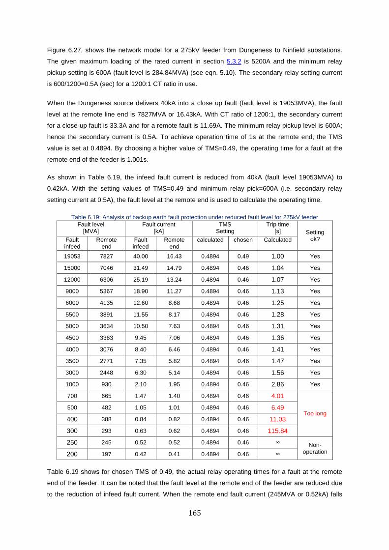
165

Figure 6.27, shows the network model for a 275kV feeder from Dungeness to Ninfield substations.

The given maximum loading of the rated current in section 5.3.2 is 5200A and the minimum relay

pickup setting is 600A (fault level is 284.84MVA) (see eqn. 5.10). The secondary relay setting current

is 600/1200=0.5A (sec) for a 1200:1 CT ratio in use.

When the Dungeness source delivers 40kA into a close up fault (fault level is 19053MVA), the fault

level at the remote line end is 7827MVA or 16.43kA. With CT ratio of 1200:1, the secondary current

for a close-up fault is 33.3A and for a remote fault is 11.69A. The minimum relay pickup level is 600A;

hence the secondary current is 0.5A. To achieve operation time of 1s at the remote end, the TMS

value is set at 0.4894. By choosing a higher value of TMS=0.49, the operating time for a fault at the

remote end of the feeder is 1.001s.

As shown in Table 6.19, the infeed fault current is reduced from 40kA (fault level 19053MVA) to

0.42kA. With the setting values of TMS=0.49 and minimum relay pick=600A (i.e. secondary relay

setting current at 0.5A), the fault level at the remote end is used to calculate the operating time.

Table 6.19: Analysis of backup earth fault protection under reduced fault level for 275kV feeder

Fault level [MVA]

Fault current [kA]

TMS Setting

Trip time [s] Setting

ok?

Fault infeed

Remote end

Fault infeed

Remote end

calculated chosen Calculated

19053 7827 40.00 16.43 0.4894 0.49 1.00 Yes

15000 7046 31.49 14.79 0.4894 0.46 1.04 Yes

12000 6306 25.19 13.24 0.4894 0.46 1.07 Yes

9000 5367 18.90 11.27 0.4894 0.46 1.13 Yes

6000 4135 12.60 8.68 0.4894 0.46 1.25 Yes

5500 3891 11.55 8.17 0.4894 0.46 1.28 Yes

5000 3634 10.50 7.63 0.4894 0.46 1.31 Yes

4500 3363 9.45 7.06 0.4894 0.46 1.36 Yes

4000 3076 8.40 6.46 0.4894 0.46 1.41 Yes

3500 2771 7.35 5.82 0.4894 0.46 1.47 Yes

3000 2448 6.30 5.14 0.4894 0.46 1.56 Yes

1000 930 2.10 1.95 0.4894 0.46 2.86 Yes

700 665 1.47 1.40 0.4894 0.46 4.01

Too long 500 482 1.05 1.01 0.4894 0.46 6.49

400 388 0.84 0.82 0.4894 0.46 11.03

300 293 0.63 0.62 0.4894 0.46 115.84

250 245 0.52 0.52 0.4894 0.46 ∞ Non-operation 200 197 0.42 0.41 0.4894 0.46 ∞

Table 6.19 shows for chosen TMS of 0.49, the actual relay operating times for a fault at the remote

end of the feeder. It can be noted that the fault level at the remote end of the feeder are reduced due

to the reduction of infeed fault current. When the remote end fault current (245MVA or 0.52kA) falls

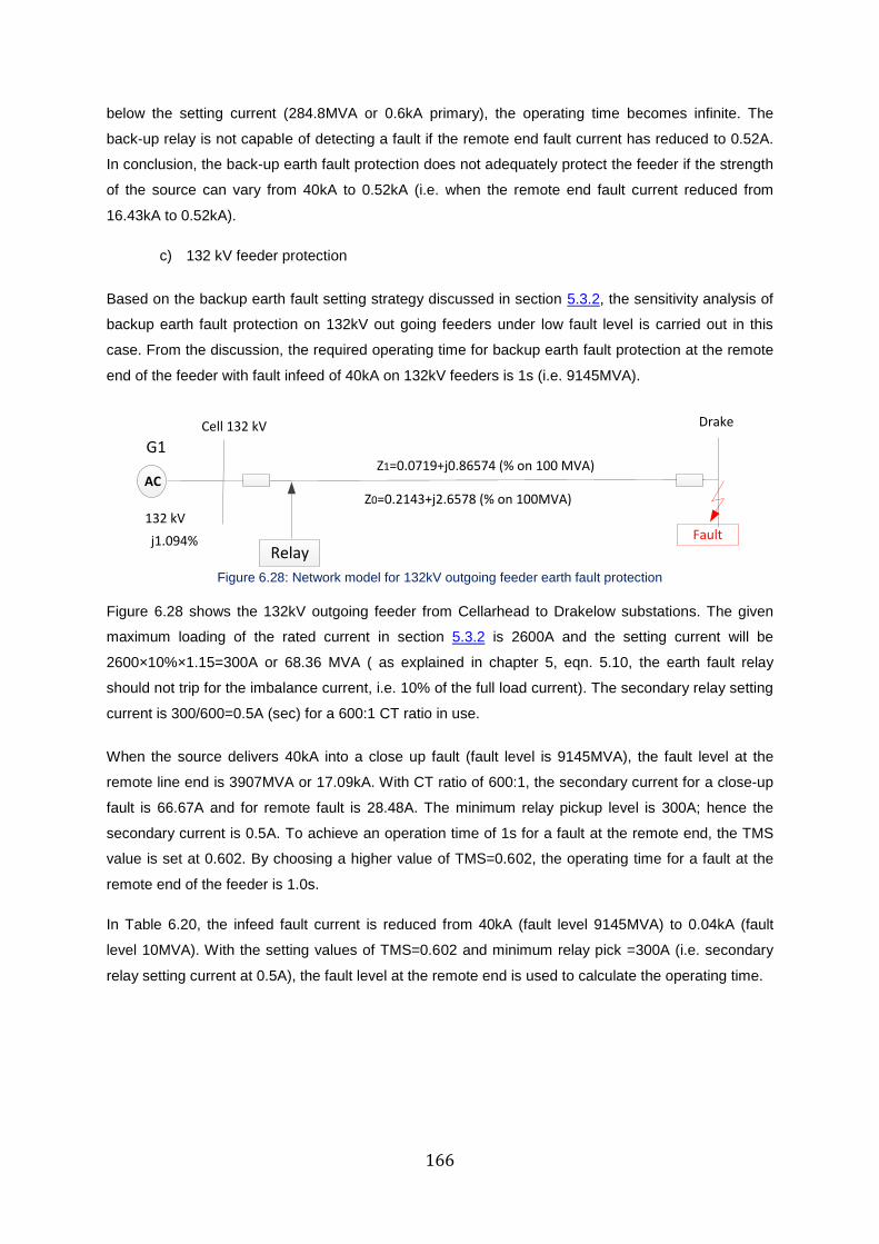
166

below the setting current (284.8MVA or 0.6kA primary), the operating time becomes infinite. The

back-up relay is not capable of detecting a fault if the remote end fault current has reduced to 0.52A.

In conclusion, the back-up earth fault protection does not adequately protect the feeder if the strength

of the source can vary from 40kA to 0.52kA (i.e. when the remote end fault current reduced from

16.43kA to 0.52kA).

c) 132 kV feeder protection

Based on the backup earth fault setting strategy discussed in section 5.3.2, the sensitivity analysis of

backup earth fault protection on 132kV out going feeders under low fault level is carried out in this

case. From the discussion, the required operating time for backup earth fault protection at the remote

end of the feeder with fault infeed of 40kA on 132kV feeders is 1s (i.e. 9145MVA).

G1

AC

Cell 132 kV Drake

Fault

Z1=0.0719+j0.86574 (% on 100 MVA)

Relay

132 kV

j1.094%

Z0=0.2143+j2.6578 (% on 100MVA)

Figure 6.28: Network model for 132kV outgoing feeder earth fault protection

Figure 6.28 shows the 132kV outgoing feeder from Cellarhead to Drakelow substations. The given

maximum loading of the rated current in section 5.3.2 is 2600A and the setting current will be

2600×10%×1.15=300A or 68.36 MVA ( as explained in chapter 5, eqn. 5.10, the earth fault relay

should not trip for the imbalance current, i.e. 10% of the full load current). The secondary relay setting

current is 300/600=0.5A (sec) for a 600:1 CT ratio in use.

When the source delivers 40kA into a close up fault (fault level is 9145MVA), the fault level at the

remote line end is 3907MVA or 17.09kA. With CT ratio of 600:1, the secondary current for a close-up

fault is 66.67A and for remote fault is 28.48A. The minimum relay pickup level is 300A; hence the

secondary current is 0.5A. To achieve an operation time of 1s for a fault at the remote end, the TMS

value is set at 0.602. By choosing a higher value of TMS=0.602, the operating time for a fault at the

remote end of the feeder is 1.0s.

In Table 6.20, the infeed fault current is reduced from 40kA (fault level 9145MVA) to 0.04kA (fault

level 10MVA). With the setting values of TMS=0.602 and minimum relay pick =300A (i.e. secondary

relay setting current at 0.5A), the fault level at the remote end is used to calculate the operating time.

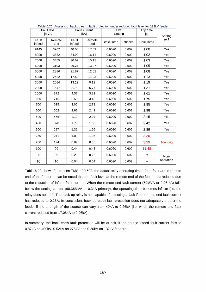
167

Table 6.20: Analysis of backup earth fault protection under reduced fault level for 132kV feeder

Fault level [MVA]

Fault current [kA]

TMS Setting

Trip time [s]

Setting ok?

Fault infeed

Remote end

Fault infeed

Remote end

calculated chosen Calculated

9145 3907 40.00 17.09 0.6020 0.602 1.00 Yes

8000 3682 34.99 16.11 0.6020 0.602 1.02 Yes

7000 3455 30.62 15.11 0.6020 0.602 1.03 Yes

6000 3193 26.24 13.97 0.6020 0.602 1.05 Yes

5000 2886 21.87 12.62 0.6020 0.602 1.08 Yes

4000 2522 17.50 11.03 0.6020 0.602 1.13 Yes

3000 2084 13.12 9.12 0.6020 0.602 1.19 Yes

2000 1547 8.75 6.77 0.6020 0.602 1.31 Yes

1000 872 4.37 3.82 0.6020 0.602 1.61 Yes

800 716 3.50 3.13 0.6020 0.602 1.75 Yes

700 635 3.06 2.78 0.6020 0.602 1.85 Yes

600 552 2.62 2.41 0.6020 0.602 1.98 Yes

500 466 2.19 2.04 0.6020 0.602 2.15 Yes

400 378 1.75 1.65 0.6020 0.602 2.42 Yes

300 287 1.31 1.26 0.6020 0.602 2.89 Yes

250 241 1.09 1.05 0.6020 0.602 3.30

Too long 200 194 0.87 0.85 0.6020 0.602 3.99

100 99 0.44 0.43 0.6020 0.602 11.48

60 59 0.26 0.26 0.6020 0.602 ∞ Non-operation 10 10 0.04 0.04 0.6020 0.602 ∞

Table 6.20 shows for chosen TMS of 0.602, the actual relay operating times for a fault at the remote

end of the feeder. It can be noted that the fault level at the remote end of the feeder are reduced due

to the reduction of infeed fault current. When the remote end fault current (59MVA or 0.26 kA) falls

below the setting current (68.36MVA or 0.3kA primary), the operating time becomes infinite (i.e. the

relay does not trip). The back-up relay is not capable of detecting a fault if the remote end fault current

has reduced to 0.26A. In conclusion, back-up earth fault protection does not adequately protect the

feeder if the strength of the source can vary from 40kA to 0.26kA (i.e. when the remote end fault

current reduced from 17.08kA to 0.26kA).

In summary, the back earth fault protection will be at risk, if the source infeed fault current falls to

0.87kA on 400kV, 0.52kA on 275kV and 0.26kA on 132kV feeders.

168

6.5 Summary

The operating performances of transmission feeder protection were studied in this chapter. The

protection schemes used in this chapter are unit scheme, non-unit distance scheme and backup

phase and earth protection scheme. Under strong infeed conditions, unit scheme works correctly and

cope with resistive fault or high level of loading conditions. However, the operating performance of

unit scheme under low fault level with relatively high fault resistance is a concern and may require

establishing correct setting limitations during minimum credible fault levels.

In contrast, the non-unit distance scheme operating using Mho characteristics works correctly under

strong infeed conditions, but there are limitations when resistive faults are included or during short

lines. However, the operating performance of distance scheme can be improved by setting to a

quadrilateral and polarization characteristics. As fault level reduces, the operating performance of

non-unit scheme was influenced with changes in line length, fault location and percentage levels of

power electronic and resulted in an increase of operating times or non-operation. Hence, the distance

scheme operating using a permissive direct transfer scheme should be replaced with a weak infeed

protection. Moreover, the operating performance of backup overcurrent (phase and earth) protection

was examined under reduced fault level. Under low fault level, overcurrent back-up protection is

severely affected by low fault currents whereas the backup earth fault protection is less affected.

The key strengths of this study are to increase understanding on the impact of low fault level on the

operating performance of unit protection, distance protection, overcurrent and their setting

implications. The objective is to investigate the performances of protection schemes under low fault

level and establish their limitation. Further discussions related to the impact of low fault level on future

protection performances and alternative protection strategy is provided in chapter 7.

The 4th

technical paper entitled < Impact of Intermediate Sources on Distance Protection of Transmission Lines >

was published and presented based on this work on 14th

International Conference on Development in Power

System Protection (DPSP 2018). The conference was held at the Europa Hotel on March 12-15, 2018, Belfast,

UK.

169

Chapter 7: Impact of low fault level & alternative protection strategy

7.1 Review into the impact of low fault levels on feeder protection

In chapter 6, the strategies to evaluate the impact of fault level reduction on performance assessment

of unit scheme protection, non-unit distance scheme protection and backup overcurrent or earth fault

protection were studied in depth based on the following three conditions:

a) strong fault level

b) reduced fault level.

c) converter dominated power system

7.1.1 Unit differential protection

Case (a): strong fault level

As discussed in section 6.2.1(a), when a system is fed from a strong source, a unit protection is

capable of providing a correct operation and resistive faults were cleared successfully within the

expected operating region (i.e. <30ms).

Case (b): reduced fault level

When a weak infeed source was added to the network, the sensitivity of unit protection adapted to the

change in fault level, but sensitivity check of the unit scheme is required under extremely low fault

level. For instance, during internal fault with relatively high fault resistance (i.e. when fault current falls

below 1.375kA), a part of the load current may still be flowing through the protected item during the

fault period, and the through flowing load current is superimposed onto the fault currents flowing into

the protected item.

Case (c): converter dominated power systems

Renewable energy or green energy sources are a form of electrical generation produced from power

electronics (i.e. wind power or solar panel) and synchronous generation (i.e. hydropower, nuclear

power). When a system is fed from generation mix, the amount of % generation determines the

system fault level. For example, the electricity minimum demand is normally seen in summer when all

power electronic sources are in service with fewer synchronous generations such as nuclear or hydro

power being in service.

If a system is fed 80%-90% from power electronics and 10%-20% of synchronous generation (i.e.

fault level is 4.45GVA to 2.77GVA), unit protection can provide correct operation (see section 6.2.1).

Moreover, when the penetration level from power electronics is 100% (i.e. fault level is 1.1GVA-

2.0GVA or 1.588kA to 2.886kA), the sensitivity of unit scheme also works perfect. However, the relay

struggle to detect when a large fault resistance values were added. For example, if the worst case

scenario is considered, i.e. the converter source delivers 1.1pu per unit of nominal current (1.587kA)

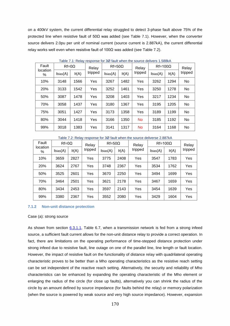
170

on a 400kV system, the current differential relay struggled to detect 3-phase fault above 75% of the

protected line when resistive fault of 50Ω was added (see Table 7.1). However, when the converter

source delivers 2.0pu per unit of nominal current (source current is 2.887kA), the current differential

relay works well even when resistive fault of 100Ω was added (see Table 7.2).

Table 7.1: Relay response for 3Ø fault when the source delivers 1.588kA

Fault location

%

Rf=0Ω Relay tripped

Rf=50Ω Relay tripped

Rf=100Ω Relay tripped Ibias(A) If(A) Ibias(A) If(A) Ibias(A) If(A)

10% 3148 1566 Yes 3267 1482 Yes 3262 1294 No

20% 3133 1542 Yes 3252 1461 Yes 3250 1278 No

50% 3087 1478 Yes 3208 1403 Yes 3217 1234 No

70% 3058 1437 Yes 3180 1367 Yes 3195 1205 No

75% 3051 1427 Yes 3173 1358 Yes 3189 1199 No

80% 3044 1418 Yes 3166 1350 No 3185 1192 No

99% 3018 1383 Yes 3141 1317 No 3164 1168 No

Table 7.2: Relay response for 3Ø fault when the source deliverse 2.887kA

Fault location

%

Rf=0Ω Relay tripped

Rf=50Ω Relay tripped

Rf=100Ω Relay tripped Ibias(A) If(A) Ibias(A) If(A) Ibias(A) If(A)

10% 3659 2827 Yes 3775 2408 Yes 3547 1783 Yes

20% 3624 2767 Yes 3748 2367 Yes 3534 1762 Yes

50% 3525 2601 Yes 3670 2250 Yes 3494 1699 Yes

70% 3464 2501 Yes 3621 2178 Yes 3467 1659 Yes

80% 3434 2453 Yes 3597 2143 Yes 3454 1639 Yes

99% 3380 2367 Yes 3552 2080 Yes 3429 1604 Yes

7.1.2 Non-unit distance protection

Case (a): strong source

As shown from section 6.3.1.1, Table 6.7, when a transmission network is fed from a strong infeed

source, a sufficient fault current allows for the non-unit distance relay to provide a correct operation. In

fact, there are limitations on the operating performance of time-stepped distance protection under

strong infeed due to resistive fault, line outage on one of the parallel line, line length or fault location.

However, the impact of resistive fault on the functionality of distance relay with quadrilateral operating

characteristic proves to be better than a Mho operating characteristics as the resistive reach setting

can be set independent of the reactive reach setting. Alternatively, the security and reliability of Mho

characteristics can be enhanced by expanding the operating characteristic of the Mho element or

enlarging the radius of the circle (for close up faults), alternatively you can shrink the radius of the

circle by an amount defined by source impedance (for faults behind the relay) or memory polarization

(when the source is powered by weak source and very high source impedance). However, expansion

171

of the Mho element during weak source conditions will result in operation over a much larger area in

the resistive direction and this may cause mal-operation.

Case (b): reduced fault level

As fault level reduces, the source impedance ratio increases, and the reach setting error increases. At

higher value of SIR or extremely low fault level, the specification of each relay manufacturers must be

checked with the setting limitation and accuracy. With the comments made in section 3.4, most

conventional relays stop working if the source impedance ratio exceeds 60-65.

Under low fault level, the distance relay has issues with the measured impedance error which

increases the operating times of zone 2 and zone 3. This error leads to an under-reach problem and

may be partially resolved by changing the reach of zone settings. However, as the fault level reduces,

the operating reach of a distance relay may change and in extreme cases become inadequate. For

example, based on the data from the Electricity Ten Year Statement 2018 Appendix B, the impact of

fault level reduction with the increase in penetration of renewable energy sources on the operating

performance of protection schemes was examined. Note the fault level from power electronics varies

between 1.1-2.0pu. However, in this study, 1.1 times the rated current is considered (i.e. in the worst

case scenario).

As fault level reduces, the distance scheme starts to under reach and resulting in an increase of

operating times or non-operation. For example in section 6.3.1.2 Table 6.9, when the infeed fault level

was reduced from 17.85GVA to 5.12GVA (i.e. at 76% penetration levels of converter sources), the

zone 2 element of the distance relay failed to clear for faults above 80% of the protected line. When

the fault infeed was reduced to 4.785GVA, the zone 1 element of the distance relay also failed to

clear for faults above 50% of the protected line (i.e. at 78% penetration levels of converter sources).

Based on the findings, the protection scheme will work effectively when the source delivers (i.e. 3Ø

faults current) above 6.125GVA (i.e. at 70% penetration levels of converter sources) and satisfies

under “Two Degree scenarios/gone green” upto 2035/36 (i.e. at 70% penetration levels from

converter sources). Since National Grid uses inter-trip scheme, the zone 1 element of distance relay

must ensure to cover 51% of the protected line. From the test results, the zone 1 distance relay was

able to detect faults above 50% of the protected line, i.e. when converter source was increased to

78%.

Case (c): converter dominated power systems

As fault level reduces, the limitation of distance scheme reduces and resulted in an increase of

operating times. Assume Dungeness power station is not operational and if a grid is fed 20% from

green energy, plus 80% from power electronics; the infeed fault level will be 4.45GVA or 6.423kA.

Similarly, if a grid is fed 100% from power electronics, the infeed fault current will be 1.1GVA to

2.0GVA times the rating current (i.e. 1.588kA to 2.886kA). However, the distance scheme will not

work if the power electronics exceeds 78%.

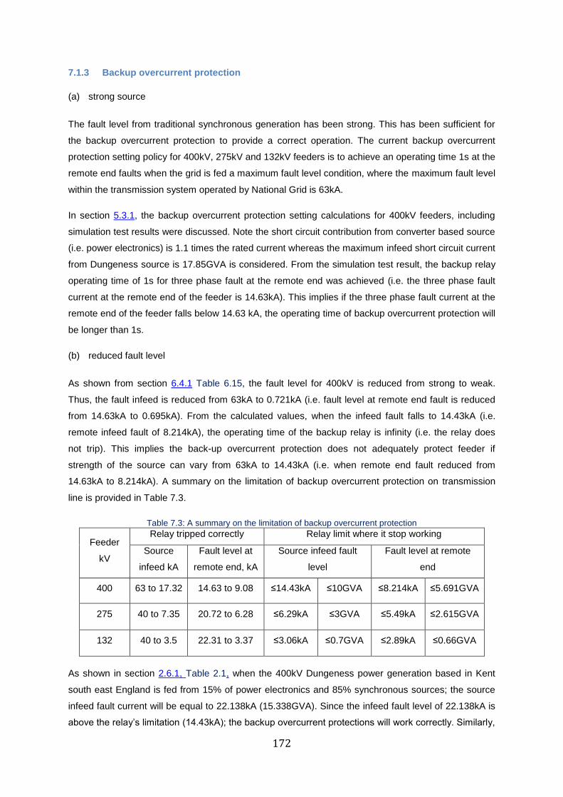
172

7.1.3 Backup overcurrent protection

(a) strong source

The fault level from traditional synchronous generation has been strong. This has been sufficient for

the backup overcurrent protection to provide a correct operation. The current backup overcurrent

protection setting policy for 400kV, 275kV and 132kV feeders is to achieve an operating time 1s at the

remote end faults when the grid is fed a maximum fault level condition, where the maximum fault level

within the transmission system operated by National Grid is 63kA.

In section 5.3.1, the backup overcurrent protection setting calculations for 400kV feeders, including

simulation test results were discussed. Note the short circuit contribution from converter based source

(i.e. power electronics) is 1.1 times the rated current whereas the maximum infeed short circuit current

from Dungeness source is 17.85GVA is considered. From the simulation test result, the backup relay

operating time of 1s for three phase fault at the remote end was achieved (i.e. the three phase fault

current at the remote end of the feeder is 14.63kA). This implies if the three phase fault current at the

remote end of the feeder falls below 14.63 kA, the operating time of backup overcurrent protection will

be longer than 1s.

(b) reduced fault level

As shown from section 6.4.1 Table 6.15, the fault level for 400kV is reduced from strong to weak.

Thus, the fault infeed is reduced from 63kA to 0.721kA (i.e. fault level at remote end fault is reduced

from 14.63kA to 0.695kA). From the calculated values, when the infeed fault falls to 14.43kA (i.e.

remote infeed fault of 8.214kA), the operating time of the backup relay is infinity (i.e. the relay does

not trip). This implies the back-up overcurrent protection does not adequately protect feeder if

strength of the source can vary from 63kA to 14.43kA (i.e. when remote end fault reduced from

14.63kA to 8.214kA). A summary on the limitation of backup overcurrent protection on transmission

line is provided in Table 7.3.

Table 7.3: A summary on the limitation of backup overcurrent protection

Feeder

kV

Relay tripped correctly Relay limit where it stop working

Source

infeed kA

Fault level at

remote end, kA

Source infeed fault

level

Fault level at remote

end

400 63 to 17.32 14.63 to 9.08 ≤14.43kA ≤10GVA ≤8.214kA ≤5.691GVA

275 40 to 7.35 20.72 to 6.28 ≤6.29kA ≤3GVA ≤5.49kA ≤2.615GVA

132 40 to 3.5 22.31 to 3.37 ≤3.06kA ≤0.7GVA ≤2.89kA ≤0.66GVA

As shown in section 2.6.1, Table 2.1, when the 400kV Dungeness power generation based in Kent

south east England is fed from 15% of power electronics and 85% synchronous sources; the source

infeed fault current will be equal to 22.138kA (15.338GVA). Since the infeed fault level of 22.138kA is

above the relay’s limitation (14.43kA); the backup overcurrent protections will work correctly. Similarly,

173

when the penetration of power electronics was increased to 45% with 55% from synchronous source

(see Figure 2.17), the fault infeed will be 14.88kA (10.313GVA), i.e. just above the limitation of relay

setting of 14.43kA and the backup relay will work correctly. However, if the penetration of power

electronics was increased to 46% with 54% from synchronous sources, the fault infeed will be

14.627kA (10.134GVA), i.e. just below the limitation of relay setting (14.63kA) and this indicates the

backup relay will no longer work.

In longer term: with the discussions made in section 2.6.1, Figure 2.17, the UK and EU have a long

term agreement on the reduction of CO2 emission where 80% penetration of renewable generation

was set to achieve by 2050. If a grid is fed 20% from thermal nuclear & hydro sources (3.57GVA),

20% from thermal coal fired generation (3.57GVA), and 60% from power electronics (0.66GVA) are

assumed. The total infeed fault level will be 7.8GVA (11.258kA), i.e. below the backup relay limit

(infeed fault level of 10GVA or 14.43kA). Thus, the relay will not work under such conditions and shall

not be used by 2050. In conclusion, under the condition considered, the backup overcurrent relay will

not work if the penetration of power electronics (i.e. converted based sources) is ≥45%.

In short term; with the discussions made in section 2.6.1, Figure 2.17, the UK has a short and long

term agreement. For example, National Grid proposed a penetration of 15% (case1), 65% (case2)

and 70% (case3) renewable energy sources by 2020 and 2027/8 and 2035/36 respectively.

Case 1: assume a grid is fed 15% (0.165GVA) from power electronics and 85% (15.173GVA)

from traditional synchronous sources. The total infeed fault level will be 15.338GVA

(22.138kA) and this value is higher than the relay limit (14.43kA or 10GVA). Hence, the

operating performance of backup overcurrent protection will not be affected by 2020.

Case 2: assume a grid is fed 45% (0.495GVA) from power electronics, 20% (3.57GVA) from

hydro & nuclear power plant, and 35% (6.248GVA) from traditional synchronous sources, the

total infeed fault level will be 10.313GVA (14.885kA), i.e. slightly higher than the relay

minimum pickup current (14.43kA or 10GVA). The effectiveness of backup overcurrent

protection may not be affected by 2027/8. However, if the penetration of power electronics is

above 45%, the operating performance of the protection will be at risk.

Case 3: assume a grid is fed 50% (0.55GVA) from power electronics (i.e. in the worst case for

the protection), 20% (3.57GVA) from hydro & nuclear power plant and 30% (5.355GVA) from

traditional synchronous sources. The total infeed fault level is 9.475GVA (13.678 kA) and this

is below the relay limit (10GVA or 14.43kA). Hence, the effectiveness of backup overcurrent

protection will be at risk by 2035/36. Thus, the maximum penetration of power electronics

should not exceed 45% (i.e.the rating of power electronics was assumed 1.1pu). However, if

assuming the rating of power electrocnics is 2pu, the limitation of the relay may increase.

(c) converter dominated power systems

As discussed in the above case (2) and section 2.6.1, Table 2.1, for a system fed 45% from power

electronics and 55% from traditional synchronous sources, the total infeed fault level is 10.313GVA

(14.885kA), i.e. slightly above the relay limit (10GVA). This implies the 400kV backup overcurrent

174

protection is at risk if more than 45% of power electronics is added into the grid. Thus, if a system is

fed from 100% of renewable generation (let say 80%-90% of power electronics, and 10%-20% from

hydro & nuclear power), the total fault infeed will be 2.775GVA to 4.45GVA. This implies backup

overcurrent protection will not work and should not be used.

Moreover, the Great Britain’s electricity operation was achieved recently with “coal free week”

between 1st May and 8th May 2019. These energy were a generation mix from natural gas (46%),

nuclear (21.2%), wind (10.7%), imported energy (9.9%), biomas (6%), solar (5%), hydro (1.1%) and

coal (0%). This means, the penetration of power electronics is 25.6% (i.e. 10.7% wind, 9.9% imported

energy & 5% solar), with 74.4% from gas fired power plant and green energy (i.e. nuclear, biomass &

hydro). Hence, the total infeed fault current is 13.562GVA (i.e. 19.575kA). As the infeed fault current

level is above the relay minimum pickup level (14.63kA), it can be said the backup relay is not at risk

by the operation of the Great Britain’s electricity with coal free week.

Furthermore, National Grid ESO (electricity system operator) has announced in April 2019 they would

be able to run the GB network by 2025 with no fossil fuel sources (i.e. zero carbon operation) [55]. As

discussed earlier, if the penetration level from power electronics increased above 45%, the backup

relay will be at risk.

7.1.4 Backup earth fault (IDMT) protection

(a) strong source

The fault level from traditional synchronous generation has been strong. This has been sufficient for

the backup earth fault protection to provide a correct operation. The current backup overcurrent

protection setting policy for 400kV, 275kV and 132kV feeders is to achieve an operating time of 1s for

a fault at the remote feeder end when the grid operates under maximum fault level condition; the

maximum fault level on a 400kV National Grid feeder is 63kA whereas 40kA on 275kV and 132kV

feeder.

In section 5.3.2, the backup earth fault protection setting calculations for 400kV feeders, including

simulation test results were discussed. Note the short circuit contribution from converter based source

(i.e. power electronics) is 1.1 times the rated current whereas the maximum infeed short circuit current

from Dungeness source is 17.85GVA is considered. From the simulation test result, the backup relay

operating time of 1s for three phase fault at the remote end was achieved (i.e. the three phase fault

current at the remote end of the feeder is 9.86kA). This implies if the three phase fault current at the

remote end of the feeder falls below 9.86kA, the operating time of backup overcurrent protection will

be longer than 1s. A further discussion is provided below in case (b).

(b) reduced fault level

As shown in section 6.4.1 Table 6.18, the infeed fault level for 400kV is reduced from 63kA to 0.72kA

(i.e. the fault level at remote end is reduced from 9.86kA to 0.68kA). However, when the infeed fault

falls from 63kA to 0.87kA (i.e. remote infeed fault of 0.81kA), the operating time of the relay is infinity.

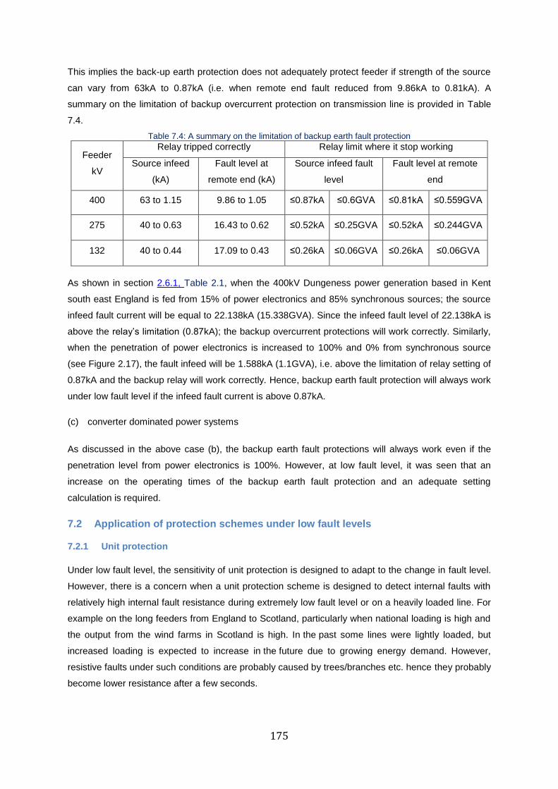
175

This implies the back-up earth protection does not adequately protect feeder if strength of the source

can vary from 63kA to 0.87kA (i.e. when remote end fault reduced from 9.86kA to 0.81kA). A

summary on the limitation of backup overcurrent protection on transmission line is provided in Table

7.4.

Table 7.4: A summary on the limitation of backup earth fault protection

Feeder

kV

Relay tripped correctly Relay limit where it stop working

Source infeed

(kA)

Fault level at

remote end (kA)

Source infeed fault

level

Fault level at remote

end

400 63 to 1.15 9.86 to 1.05 ≤0.87kA ≤0.6GVA ≤0.81kA ≤0.559GVA

275 40 to 0.63 16.43 to 0.62 ≤0.52kA ≤0.25GVA ≤0.52kA ≤0.244GVA

132 40 to 0.44 17.09 to 0.43 ≤0.26kA ≤0.06GVA ≤0.26kA ≤0.06GVA

As shown in section 2.6.1, Table 2.1, when the 400kV Dungeness power generation based in Kent

south east England is fed from 15% of power electronics and 85% synchronous sources; the source

infeed fault current will be equal to 22.138kA (15.338GVA). Since the infeed fault level of 22.138kA is

above the relay’s limitation (0.87kA); the backup overcurrent protections will work correctly. Similarly,

when the penetration of power electronics is increased to 100% and 0% from synchronous source

(see Figure 2.17), the fault infeed will be 1.588kA (1.1GVA), i.e. above the limitation of relay setting of

0.87kA and the backup relay will work correctly. Hence, backup earth fault protection will always work

under low fault level if the infeed fault current is above 0.87kA.

(c) converter dominated power systems

As discussed in the above case (b), the backup earth fault protections will always work even if the

penetration level from power electronics is 100%. However, at low fault level, it was seen that an

increase on the operating times of the backup earth fault protection and an adequate setting

calculation is required.

7.2 Application of protection schemes under low fault levels

7.2.1 Unit protection

Under low fault level, the sensitivity of unit protection is designed to adapt to the change in fault level.

However, there is a concern when a unit protection scheme is designed to detect internal faults with

relatively high internal fault resistance during extremely low fault level or on a heavily loaded line. For

example on the long feeders from England to Scotland, particularly when national loading is high and

the output from the wind farms in Scotland is high. In the past some lines were lightly loaded, but

increased loading is expected to increase in the future due to growing energy demand. However,

resistive faults under such conditions are probably caused by trees/branches etc. hence they probably

become lower resistance after a few seconds.

176

It must be noted that during internal fault with a high fault resistance, a part of the load current may

still be flowing through the protected item during the fault period, and the through flowing load current

is superimposed onto the fault currents flowing into the protected item [83] . Hence, the limitation of

unit scheme under heavy loading conditions with relatively high faults resistance, plus when the fault

current falls below the load current needs further investigation. Further, there is no clear information

about the nominal current currently used in National Grid. For example, if the maximum fault current

from power electronics is limited to 1.1pu-2.0pu, a further emphasis on the use of nominal current of

2000A (i.e. used on 400kV or 275kV system) may need a review.

7.2.2 Non-unit distance protection

(a) strong source

As discussed in section 7.1.2, distance protection works effectively under strong source. The

limitations of distance protection have been already known for decades and can be resolved using

different setting configuration such as Quadrilateral for resistive faults. Hence, if a system has strong

infeed, distance protection can be used as 1st or 2

nd main protection depends on the application and

protection policy of the utilities.

(b) reduced fault level

As fault level reduces, the distance scheme starts to under-reach, resulting in an increase in operating

times or non-operation. When the source delivers extremely low fault level, the ratio of source to line

impedance on short feeders is very large. The relay with mho characteristics may struggle to detect

close up faults and a relay with quadrilateral characteristics should be used. Similarly, as the fault

level reduces, the reach setting of distance scheme on long feeders is adversely affected (i.e. the

delayed time distance scheme likely to fail to clear remote end faults on the next line).

(c) under converter dominated power systems

National Grid Electric System Operator has recently announced to be able to run the GB network by

2025 with no fossil fuel sources. From the results seen in Table 6.9, the zone 2 element of distance

relay failed to provide coverage remote end faults when the penetration level of power electronics was

increased to 75%. When the power electronic source was increased to 80% or higher, the zone 1

failed to clear close up faults. This implies, the direct under-reach inter-trip communication schemes

(DUTT) will not work under such conditions where weak infeed logic scheme should be used as an

alternative means of protection scheme. A weak in-feed protection is an additional to the distance

function set to provide permissive trip from the strong source using direct eco function [100]. Direct

echo function permits the remote relay to echo the trip signal back to the sending relay even if the

appropriate remote relay element has not operated. Hence, weak infeed protection can be used to

provide rapid tripping for internal faults when one end of the line terminal has insufficient fault current.

177

7.2.3 Backup overcurrent protection

A backup overcurrent protection shall not be used if the infeed fault current falls to 14.43kA or lower.

According to National Grid, when 45% of the energy supplied to a system is fed from power

electronics, backup overcurrent protection will be at risk and should be replaced with voltage

controlled overcurrent protection of over-reaching distance protection.

7.2.4 Backup earth fault protection

A backup earth fault protection shall not be used if the infeed fault current falls to 0.87kA or lower.

However, earth fault protection shall be used even under 100% penetration from converted based

sources (i.e. 100% power electronics).

7.3 Implications for future protection strategy under low fault level

7.3.1 Identifying alternative protection methodologies and their suitability for transmission

systems under the various future scenarios

Based on the length of the feeders, availability of VTs, and infeed source; the application of

protection scheme may vary. For example, on some feeders when unit protection is not possible

to use, a double distance scheme is used, with one configured in a blocking scheme. However,

when one of the schemes is out for maintenance or needs to be tested, and if high internal

resistive fault occurs, the second main distance scheme might struggle to provide a correct

operation, especially during weak infeed conditions (i.e. resistive faults in zone 1 may be cleared

in zone 2 or zone 3 times or the relay may not provide operation depending on percentage levels

of power electronics, the line length or fault location).

In future National Grid should consider “unblocking” schemes and “unblocking with weak infeed”

to cope with extremely weak infeed conditions. More advanced distance schemes are now being

used in countries with complex transmission networks. For example, SEL distance relays, but

most existing National Grid protection schemes do not apply weak infeed logic schemes and may

need to configure differently to cope with extremely weak infeed conditions, especially when the

zone 1 distance relay cannot provide 50% fault coverage of the protected line. Based on the

information from National Grid protection schedule and site network documents, protection relays

used by National Grid that have the option of weak infeed logic are P54x distance relays,

REC561 relays, REL531 high speed distance relays or 7SA522 distance relays [65].

The main benefit of weak infeed logic scheme is to enhance the operation of direct under-reach

inter-trip communication schemes (DUTT). Weak infeed logic is used when the relay near the

weak infeed source cannot clear close up faults, where the relay near the strong source is

permitted to provide operation.

178

a) What is the need for 2 main protection schemes, if one protection system is more

relaible than the other

Under low fault level; the dependability of distance and backup overcurrent protection were

degraded and this reduces the dependability of the protection schemes and increased the

operating time. Since the National Grid transmission network are mainly double circuits, a solo

main protection may not be able to provide local backup operation in the events of communication

failure (i.e. assume unit scheme was used). Alternatively, when a smart and high reliable distance

relay is used to protect the system, the system may be left unprotected if the relay is out for

maintenance or if a relay needs to be tested and only one scheme is applied. The need for 2 main

protections, even if one protection system becomes more reliable than the other is for redundancy

purpose. Hence, if one main protection will be used in the future, the redundancy of the system

will be reduced, but solutions depend on governmental and regulatory requirements and needs

further investigation.

b) What is the role for backup protection if the main protections do not work properly?

At present, the role of backup protection used in National Grid is to provide fault coverage in case

the main protection does not work properly. For example, in the event of unit scheme

communication failure, the task of main protection can be achieved using a backup distance

scheme (i.e. under-reaching zone 1 element using inter-trip scheme). Then, the delayed zone 2

and 3 elements of distance relay can provide fault coverage on the remote end of the line, plus

the next lines. Backup overcurrent protection is also set to provide phase and earth fault

protection at a delayed time (1s at the remote end fault) in case the main scheme fails.

Under low fault level, the role of backup should be also considered, especially on local protection.

Assume on extremely weak infeed conditions, only unit protection scheme is used, and if the unit

scheme failed to see internal faults with relatively high fault resistance. Since the fault level is low,

the risk of damage to the primary equipment might not be severe, but a health and safety risk still

exists. Hence, it’s essential to clear the fault with a delayed backup scheme. Moreover, when the

main protection failed to clear the fault and if faults are not cleared within the defined National

Grid’s “Grid code” (i.e. where the generator is required to ride through grid faults during voltage

dips without being disconnected), a blackout may occur if the generator that feed the fault current

is disconnected.

c) Will voltage be a better parameter to monitor than current as fault level reduces?

Monitoring voltage signal is essential during weak in-feed conditions. In weak in-feed conditions;

the zero sequence current which dominates in the phase currents overshadows the fault

signature which makes difficult to identify [20]. If the actual voltage can be read by distance relay

for example, the relay will use this for the directional comparison. If there is no voltage present,

the relay will use the recorded voltage before the fault known as memory voltage. Moreover, if the

source impedance is high, fault current is low, but voltage on a large part of network drops to a

179

low value. Concern that during a fault, if measured voltage at multiple relays on the faulted line

and adjacent lines is very low, monitoring voltage to decide where the fault is located may not be

the best option. Hence, a wide area protection scheme, or perhaps travelling wave based

protection should be used.

d) How faults can be differentiated from heavy loading conditions during low short circuit

When the maximum possible fault current in a system is close to the rated load current; the problem

of distinguishing between a fault and a load arises. Load current usually does not exceed 30˚ from the

reference voltage at the worst power factor, i.e. cos (30) = 0.866. Since transmission lines are highly

inductive circuits where most faults occur on inductive lines; the angle between voltage and current is

much greater than 30 degree and usually start above 70 degree. This method can help to differentiate

the fault current from load current. Other method is to consider the analysis of zero sequence

impedance (Z0) value of the source. As discussed in chapter 5, the earth/ground fault setting is

normally much lower than the rated current (For example 5%, 10%, 15% or 20% etc.) and there is no

problem, but when the source is grounded through impedance the maximum possible earth fault

current also becomes lower.

Inverter-based generation or micro-grids only provides about 1.1 – 2.0 times rated current during a

fault conditions. Differential line protection can easily solve the issues related to distinguishing fault

from load current. An alternative protection strategy to resolve the impact of low fault level on backup

overcurrent protection is to use a voltage controlled/voltage constrained over current protection in

places where the fault current is equal or lower than the load current which uses the measured

voltage to differentiate load from fault currents. According to [5], voltage-controlled type prevents the

overcurrent scheme from operation until the fault reduces the system voltage to the minimum

acceptable value (let say 80% to 85%) of the nominal voltage depending on the utilities voltage limit.

e) Is Circuit Breaker Failure (CBF) protection required as switchgear performance reliability improves

Circuit breaker failure (CBF) protection was introduced in the 1960’s and 70’s when circuit

breakers were unreliable, air blast breakers had many operating parts [29]. However, modern

SF6 breakers are relatively simple, have a long operating life and failures are rare. However,

need to check how often CBF is needed in UK at transmission levels, suspect very few (or even

no) failures in last 10 years. Hence, it is unclear and needs further investigation.

7.4 The impact of new technology on fault clearing times

Due to the drive towards digitalisation and decarbonisation or possibly decentralization, the traditional

equipment used in secondary substation including protection and control system devices are likely to

be replaced with IEDs based on IEC 61850 protocols [55] [109]. For example, National Grid has an

intention to replace all transmission substations to digital technology in the future [89]. To achieve

this, National Grid and The University of Manchester have been working on a joint project involved on

the digital substation more focus on testing performance of IEC61850 process bus, interoperability of

180

multi-vendor bay solutions in a fully digital substation. From protection prospective, the impact of new

technology may have less impact on the fault clearing times, especially if the reliability of new

technology is improved. A review on the operating performance of IEC 61850 IEDs, GOOSE

message and sampling value is provided in chapter 8.

7.5 Summary

The impact of low fault level on the operating performance of unit protection, distance protection,

overcurrent and their setting implications were discussed in this chapter. Under strong infeed

conditions, unit scheme works correctly and cope with resistive faults or high level of loading

conditions. However, the operating performance of unit scheme under extremely low fault level with

relatively high fault resistance is a concern in the future and may require establishing correct setting

limitations during minimum credible fault levels.

In contrast, the non-unit distance scheme operating using Mho characteristics works correctly under

strong infeed conditions, but there are limitations in detecting resistive faults or when protecting short

lines. However, the operating performance of distance scheme can be improved by using a relay with

a quadrilateral or a polarized Mho characteristic. As fault level reduces, the operating performance of

non-unit distance scheme was affected and resulted in an increase of operating times or non-

operation. The performance of distance scheme also greatly influenced with changes in the line

length, fault location, fault resistance and percentage level of power electronics. For example, as fault

level reduces a distance scheme applied to a short feeder works better than one applied to a long

feeder. The limitation of distance scheme as related to the future energy scenarios is discussed in

section 7.1 and 7.2. The implications of future protection strategy are also covered in section 7.3.

Moreover, the operating performance of backup overcurrent (phase and earth) protection was

examined under reduced fault level. Under low fault level, overcurrent back-up protection is severely

affected by low fault currents.

Generally, distance scheme under extremely low fault level or when the transmission is fully powered

by converter based generation is unlikely to provide correct operation. The solution being

recommended to National Grid is to use weak infeed protection instead of DUTT scheme.

Alternatively, a duplicated unit scheme should be used when distance protection is not suitable. In a

long term, National Grid may even need to consider superimposed directional comparison protection

and perhaps wide area protection with local functionality.

181

Chapter 8: The Role & Impact of IEC 61850 protocols for Future Protection Development

8.1 Motivation of IEC 61850 Protection Development

The operational life for primary plant, CTs & VTs used in transmission network substation is 40-60

years and generally they are replaced if they are physically damaged or their asset life ends [109]. In

comparison, the useful life time of the secondary systems including protection and control is about 25

years where the replacement time scale is faster than the primary plant [110]. In the UK National Grid,

the current time scale for replacement of a single protection device is 6-7 weeks and this requires a

primary network outage [111].

Due to the drive towards digitalisation and issues associated with maintenance & installation cost, the

use of a new architecture interface based on IEC 61850 standards is getting popularity. The IEC

61850 protocol is international standard “Communication Networks & Systems” used in substations

where the protection and control signals and commands are transmitted via a single Ethernet network

[112]. Thus, the use of new digital substation architecture and substation equipment based on IEC

61850 tools has technical and economic advantages over traditional protection and control systems

[113].

The scope of this chapter will focus on IEC 61850 IED tools, and discuss the benefits over

conventional IED devices. The study on the implementation and operating performance of IEC61850

IED device with associated tools such as merging unit (MU), GOOSE messaging and sampling values

(SV) will be the main emphasis of this section. The main objectives of this chapter is to investigate the

setting of IEC61850 IED devices on the secondary system protocol, evaluate the operating

performance of protection schemes and highlight the reliability & cost effectiveness.

8.2 Implementation of IEC61850 IEDs

As discussed in the introduction, the main advantages of utilizing IEC 61850 standard offers cost

minimizing, reliable operation [112] [114]. The IEC 61850 process bus enables the use of digital

communication between merging units (MU), CT/VT, switchgear, and IEDs [113]. As can be seen

from Figure 2.20, the conventional hardwired omicron test method is achieved by injecting secondary

analogue input from the omicron to the IEDs and digital output. In comparison, Figure 8.1 shows a

complete implementation of IED relay with IEC 61850 9-2LE interfaces, where the input signal is

acquired using sampled values and the trip signal is sent to the CB via a goose trip message.

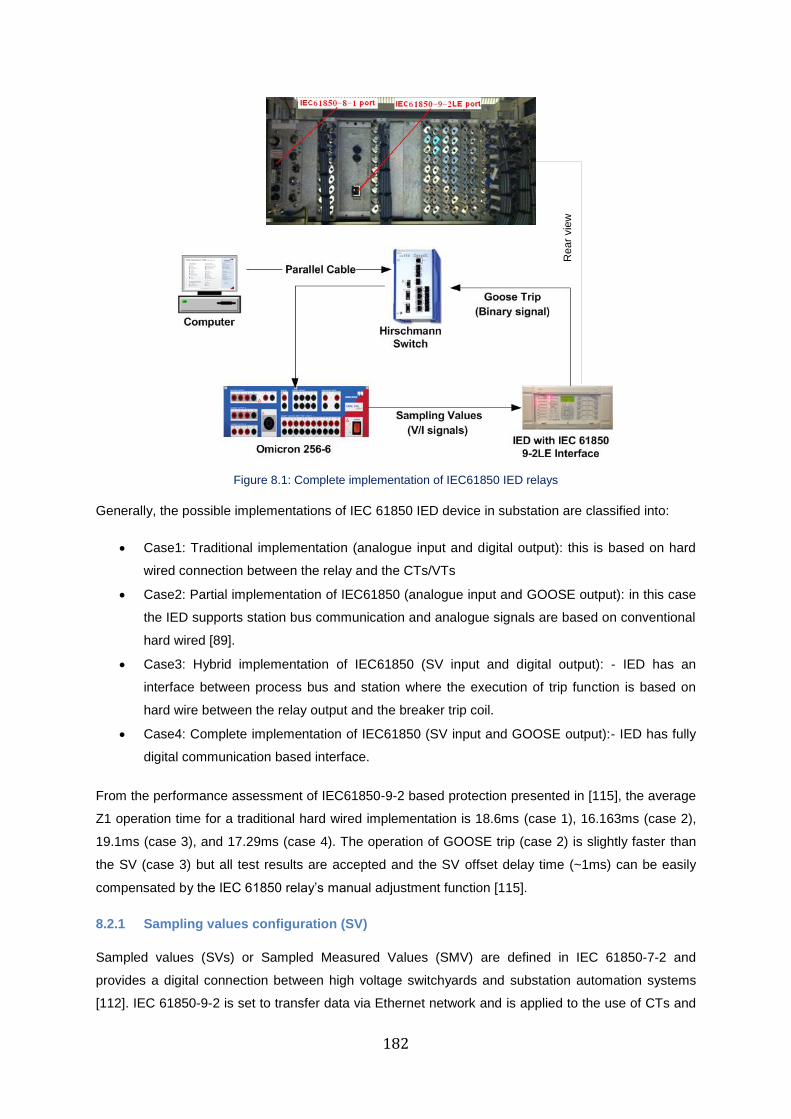
182

Re

ar

vie

w

Figure 8.1: Complete implementation of IEC61850 IED relays

Generally, the possible implementations of IEC 61850 IED device in substation are classified into:

Case1: Traditional implementation (analogue input and digital output): this is based on hard

wired connection between the relay and the CTs/VTs

Case2: Partial implementation of IEC61850 (analogue input and GOOSE output): in this case

the IED supports station bus communication and analogue signals are based on conventional

hard wired [89].

Case3: Hybrid implementation of IEC61850 (SV input and digital output): - IED has an

interface between process bus and station where the execution of trip function is based on

hard wire between the relay output and the breaker trip coil.

Case4: Complete implementation of IEC61850 (SV input and GOOSE output):- IED has fully

digital communication based interface.

From the performance assessment of IEC61850-9-2 based protection presented in [115], the average

Z1 operation time for a traditional hard wired implementation is 18.6ms (case 1), 16.163ms (case 2),

19.1ms (case 3), and 17.29ms (case 4). The operation of GOOSE trip (case 2) is slightly faster than

the SV (case 3) but all test results are accepted and the SV offset delay time (~1ms) can be easily

compensated by the IEC 61850 relay’s manual adjustment function [115].

8.2.1 Sampling values configuration (SV)

Sampled values (SVs) or Sampled Measured Values (SMV) are defined in IEC 61850-7-2 and

provides a digital connection between high voltage switchyards and substation automation systems

[112]. IEC 61850-9-2 is set to transfer data via Ethernet network and is applied to the use of CTs and

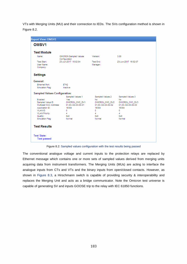
183

VTs with Merging Units (MU) and their connection to IEDs. The SVs configuration method is shown in

Figure 8.2.

Figure 8.2: Sampled values configuration with the test results being passed

The conventional analogue voltage and current inputs to the protection relays are replaced by

Ethernet message which contains one or more sets of sampled values derived from merging units

acquiring data from instrument transformers. The Merging Units (MUs) are acting to interface the

analogue inputs from CTs and VTs and the binary inputs from open/closed contacts. However, as

shown in Figure 8.3, a Hirschmann switch is capable of providing security & interoperability and

replaces the Merging Unit and acts as a bridge communicator. Note the Omicron test universe is

capable of generating SV and inputs GOOSE trip to the relay with IEC 61850 functions.

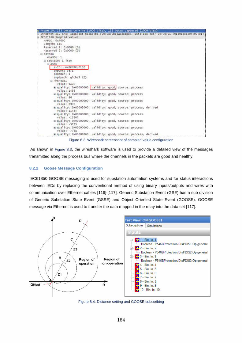
184

Figure 8.3: Wireshark screenshot of sampled value configuration

As shown in Figure 8.3, the wireshark software is used to provide a detailed view of the messages

transmitted along the process bus where the channels in the packets are good and healthy.

8.2.2 Goose Message Configuration

IEC61850 GOOSE messaging is used for substation automation systems and for status interactions

between IEDs by replacing the conventional method of using binary inputs/outputs and wires with

communication over Ethernet cables [116]-[117]. Generic Substation Event (GSE) has a sub division

of Generic Substation State Event (GSSE) and Object Oriented State Event (GOOSE). GOOSE

message via Ethernet is used to transfer the data mapped in the relay into the data set [117].

Figure 8.4: Distance setting and GOOSE subscribing

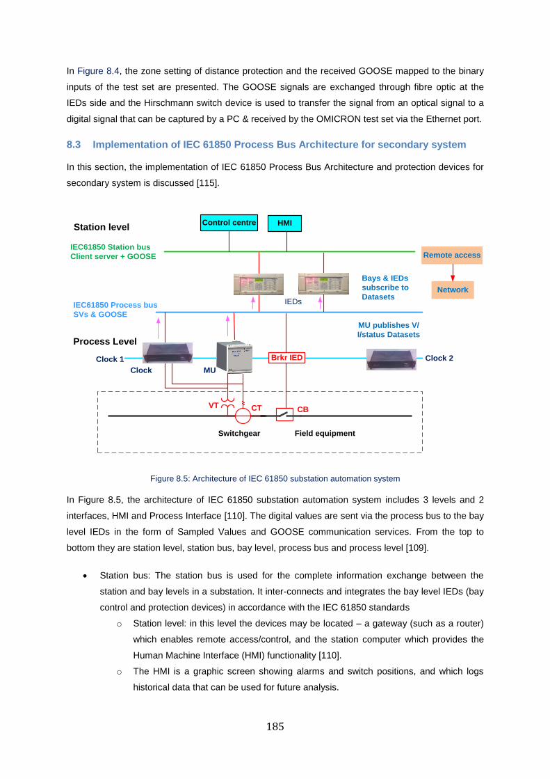
185

In Figure 8.4, the zone setting of distance protection and the received GOOSE mapped to the binary

inputs of the test set are presented. The GOOSE signals are exchanged through fibre optic at the

IEDs side and the Hirschmann switch device is used to transfer the signal from an optical signal to a

digital signal that can be captured by a PC & received by the OMICRON test set via the Ethernet port.

8.3 Implementation of IEC 61850 Process Bus Architecture for secondary system

In this section, the implementation of IEC 61850 Process Bus Architecture and protection devices for

secondary system is discussed [115].

CBCTVT

MU publishes V/

I/status Datasets

Bays & IEDs

subscribe to

Datasets

Station level HMIControl centre

Switchgear Field equipment

IEC61850 Station bus

Client server + GOOSE

IEC61850 Process bus

SVs & GOOSE

Clock 1 Clock 2

Process Level

Brkr IED

MUClock

Remote access

IEDs

Network

Figure 8.5: Architecture of IEC 61850 substation automation system

In Figure 8.5, the architecture of IEC 61850 substation automation system includes 3 levels and 2

interfaces, HMI and Process Interface [110]. The digital values are sent via the process bus to the bay

level IEDs in the form of Sampled Values and GOOSE communication services. From the top to

bottom they are station level, station bus, bay level, process bus and process level [109].

Station bus: The station bus is used for the complete information exchange between the

station and bay levels in a substation. It inter-connects and integrates the bay level IEDs (bay

control and protection devices) in accordance with the IEC 61850 standards

o Station level: in this level the devices may be located – a gateway (such as a router)

which enables remote access/control, and the station computer which provides the

Human Machine Interface (HMI) functionality [110].

o The HMI is a graphic screen showing alarms and switch positions, and which logs

historical data that can be used for future analysis.

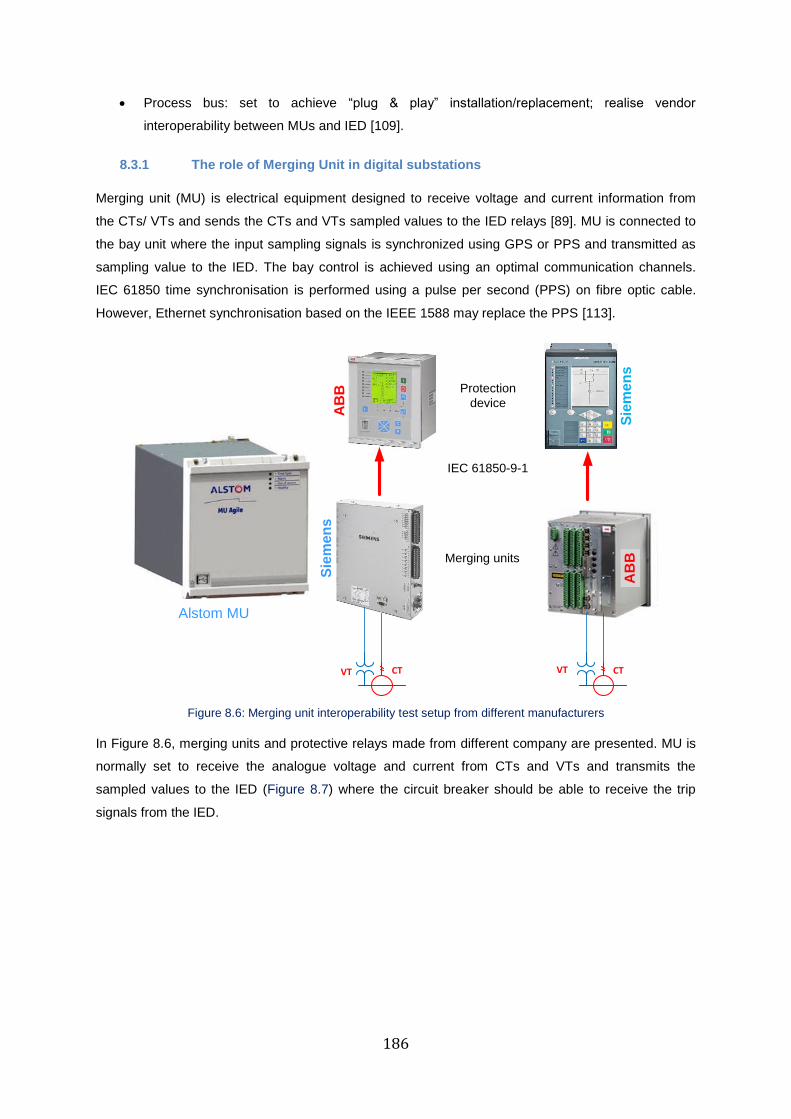
186

Process bus: set to achieve “plug & play” installation/replacement; realise vendor

interoperability between MUs and IED [109].

8.3.1 The role of Merging Unit in digital substations

Merging unit (MU) is electrical equipment designed to receive voltage and current information from

the CTs/ VTs and sends the CTs and VTs sampled values to the IED relays [89]. MU is connected to

the bay unit where the input sampling signals is synchronized using GPS or PPS and transmitted as

sampling value to the IED. The bay control is achieved using an optimal communication channels.

IEC 61850 time synchronisation is performed using a pulse per second (PPS) on fibre optic cable.

However, Ethernet synchronisation based on the IEEE 1588 may replace the PPS [113].

Protection

device

IEC 61850-9-1

Merging units

Sie

me

ns

Sie

me

ns

A

BB

AB

B

CTVT CT

Alstom MU

VT

Figure 8.6: Merging unit interoperability test setup from different manufacturers

In Figure 8.6, merging units and protective relays made from different company are presented. MU is

normally set to receive the analogue voltage and current from CTs and VTs and transmits the

sampled values to the IED (Figure 8.7) where the circuit breaker should be able to receive the trip

signals from the IED.

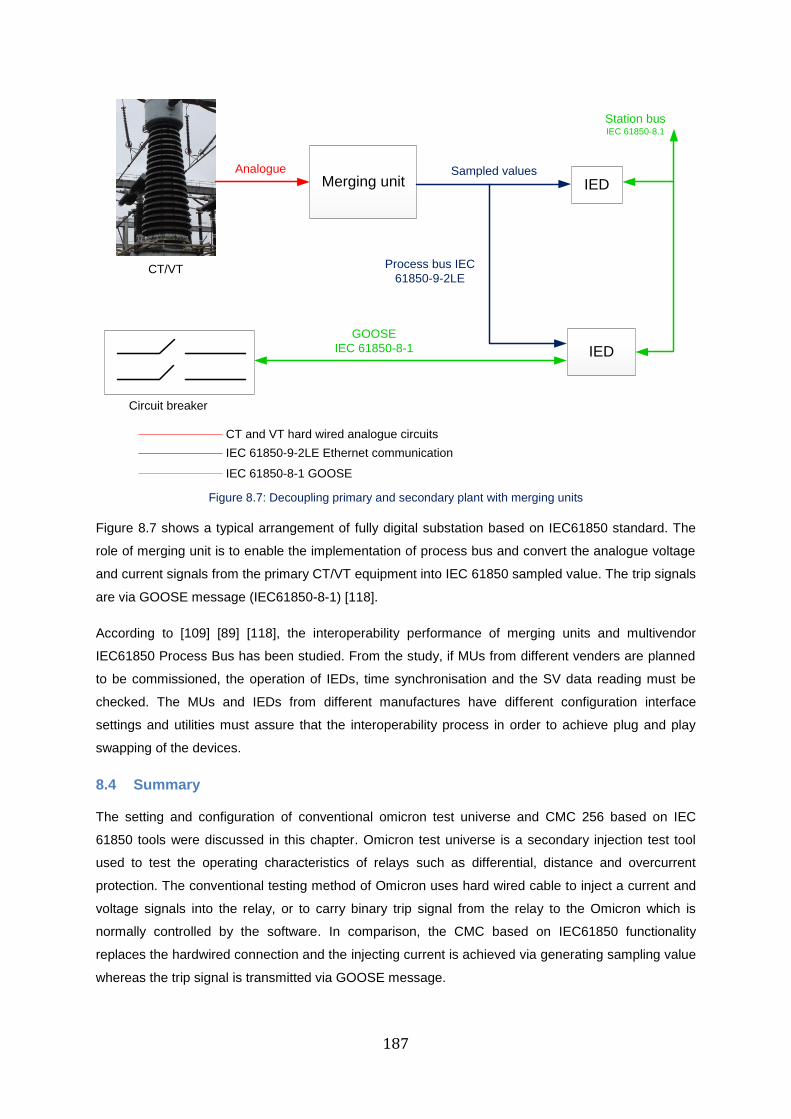
187

CT/VT

Merging unit IED

IED

Circuit breaker

GOOSE

IEC 61850-8-1

Process bus IEC

61850-9-2LE

Analogue Sampled values

Station busIEC 61850-8.1

CT and VT hard wired analogue circuits

IEC 61850-9-2LE Ethernet communication

IEC 61850-8-1 GOOSE

Figure 8.7: Decoupling primary and secondary plant with merging units

Figure 8.7 shows a typical arrangement of fully digital substation based on IEC61850 standard. The

role of merging unit is to enable the implementation of process bus and convert the analogue voltage

and current signals from the primary CT/VT equipment into IEC 61850 sampled value. The trip signals

are via GOOSE message (IEC61850-8-1) [118].

According to [109] [89] [118], the interoperability performance of merging units and multivendor

IEC61850 Process Bus has been studied. From the study, if MUs from different venders are planned

to be commissioned, the operation of IEDs, time synchronisation and the SV data reading must be

checked. The MUs and IEDs from different manufactures have different configuration interface

settings and utilities must assure that the interoperability process in order to achieve plug and play

swapping of the devices.

8.4 Summary

The setting and configuration of conventional omicron test universe and CMC 256 based on IEC

61850 tools were discussed in this chapter. Omicron test universe is a secondary injection test tool

used to test the operating characteristics of relays such as differential, distance and overcurrent

protection. The conventional testing method of Omicron uses hard wired cable to inject a current and

voltage signals into the relay, or to carry binary trip signal from the relay to the Omicron which is

normally controlled by the software. In comparison, the CMC based on IEC61850 functionality

replaces the hardwired connection and the injecting current is achieved via generating sampling value

whereas the trip signal is transmitted via GOOSE message.

188

The different implementation methods between the IEC 61850 relay and omicron test universe are

partial, hybrid and complete method. The main advantages of complete method (i.e. fully digitalisation

communication) between the CT and IEC61850 IED relays over conventional hardwired connection

are eliminating copper wires, cost minimizing, easy flexible of coper wiring, easy of configuration plug

and play swapping devices. The goal of IEC 61850 standard is to contribute a viable solution to future

smart network based on optical fibre and digital communications. However, a compressive

interoperability testing of Merging Units and IEDs from different manufactures is required to improve

reliable operation of secondary systems.

The 5th

technical paper entitled < Performance Testing of Distance Protection under Weak in-feed Sources based

on IEC61850 standard tools > was published and presented based on this work at the 9th

Protection, Automation

& Control World (PACWorld 2018). The Conference was held on June 25-28, 2018 at Grand hotel, Sofia,

Bulgaria.

189

Chapter 9: Conclusion and Future work

The thesis first introduces a background study into the role of existing transmission protection and

control system. Traditional power system with synchronous generators are capable of contributing

sufficient short circuit current during fault conditions and this enables the protective relays to provide

correct operation. However, due to the move towards low carbon technology, many existing UK

generation sources are shut down; including Cottam, Aberthaw and Fiddlers Ferry coal fired power

stations. Thus, increasing levels of demand will be satisfied by green energy sources such as by

hydro, biomass and renewable sources and low carbon energy such as nuclear power. The closure of

coal fired power station as replaced with nuclear and renewables have many challenges including

fault level reduction, difference in short circuit characteristics or behaviour due to declining inertia and

stability issues. As part of this, the research has been focused on the impact of UK low carbon energy

scenarios on transmission network protection policies.

The literature review into fault level, protection system studies as well as the methodology used in this

thesis is highlighted in chapter 2. This includes the operating principles of protection systems, short

circuit current types & calculation methods, sizing CTs & VTs, and physical relay testing procedures &

configurations.

Then, the impact of a low fault level on the operating performance of unit protection, distance

protection, and backup overcurrent relays were discussed thoroughly in this research project, which

are the main contribution of this research outcome. Under strong infeed conditions, unit scheme

works correctly and copes with resistive faults or a high level of loading. However, the operating

performance of unit scheme under extremely low fault level when a relatively high resistive fault

occurs is a concern. In the future, it may be necessary to re-establish correct setting limitations during

minimum credible fault levels.

In contrast, the distance protection operating using Mho characteristics works correctly under strong

infeed conditions, but there are limitations when resistive faults are included or during closed up faults

on short lines. However, the operating performance of distance scheme can be improved by the

utilisation of quadrilateral or cross polarised Mho characteristic. As fault level reduces, the operating

performance of non-unit distance protection was affected and resulted in an increase of operating

times or non-operation. However, factors such as line length, fault location, fault resistance and

percentage level of power electronics are also greatly influences the performance of distance

protection scheme. For example, as fault level reduces the distance scheme on short feeders works

better than on long feeders. The limitation of distance scheme as related to the future energy

scenarios is discussed in section 7.1 and 7.2.

One of the main challenges of this research project was the strategy to examine the impact of short

circuit contribution from renewable energy sources and synchronous sources, especially on the

operating performance of existing protection system in order to adapt the future power system

protection. As part of this, the implications of future protection strategy are also covered in section 7.3.

190

Moreover, the operating performance of backup overcurrent (phase and earth) protection was

examined under reduced fault level. Under low fault level, overcurrent back-up protection is severely

affected by low fault currents and should be replaced with voltage controlled overcurrent protection.

Based on the finding, distance scheme under extremely low fault level or when the transmission is

fully powered by converter based generation is unlikely to provide correct operation. The solution

being recommended to National Grid is to replace DUTT scheme with weak infeed protection.

Alternatively, a double unit scheme should be used when distance protection is not suitable, but unit

scheme cannot provide backup protection.

From the finding of the project National Grid should consider “unblocking” schemes and “unblocking

with weak infeed” to cope with extremely weak infeed conditions especially when differential

protection is not used. More advanced distance schemes are now being used in countries with

complex transmission networks. For example, SEL distance relays, but most existing National Grid

protection schemes do not apply weak infeed logic schemes and may need to configure differently to

cope with extremely weak infeed conditions, especially when the zone 1 distance relay cannot provide

50% fault coverage of the protected line. In a long term, National Grid may even need to consider

superimposed directional comparison protection and perhaps wide area protection with local

functionality.

The setting and testing of IED relays with IEC 61850 protocols is also covered. The goal of IEC 61850

standard is to contribute a viable solution to future smart network based on optical fibre and digital

communications. From physical relay testing results and previous research studies, the operating

times of IED relays using IEC 61850 protocols is similar to the traditional protection trip times and

have no impact on the existing National Grid protection operating times.

The future work will focus on establishing the limitations of unit scheme and non-unit distance scheme

when a source delivers an extremely weak infeed condition. These includes the setting configurations

of distance scheme using weak infeed conditions, impact of new technology on fault clearing times

and or design a relay algorithm that adapts the change of low fault levels. Moreover, studies on the

setting and testing of voltage controlled protection for transmission and distribution system will be

covered.

Furthermore, future work will focus on innovation research ideas to emphasise on suitability of future

transmission and distribution protection systems. The idea of having zero carbon smart cities are not

far from reality which will enable future smart cities to power with clean energy and be able to use

efficient and less energy. Thus, the overall future work will focus on the study of protection system

studies that can adapt for the future flexible smart grids.

191

References

[1] P. M. Anderson, Power System Protection. New York: A John Wiley & Sons, Inc, 1999. [2] Jonathan Clarke, “20th-century coal and oil-fired electric power generation,” Introductions to

Heritage Assets, Historic England, England, UK, 2015. Available at https://historicengland.org.uk/images-books/publications/iha-20thcentury-coal-oil-fired-electric-power-generation/heag056-electric-power-generation-iha.

[3] R. Bhattarai, A. Haddad, H. Griffiths, and N. Harid, “Voltage uprating of overhead transmission lines,” in Proceedings of the Universities Power Engineering Conference, 2010, pp. 1–6.

[4] Network Protection & Automation Guide, Protective Relays, Measurement & Control. Stafford, UK: Alstom Grid, 2011.

[5] J. Lewis Blackburn. and Thomas J. Domin, Protective Relaying Principles and Applications, 3rd ed. ISBN: 9781574447163, New York, USA, 2007.

[6] Joshua J. Romero, “Blackouts illuminate India’s power problems,” IEEE Spectrum, vol. 49, no. 10, 2012.

[7] L. G. Hewitson, M. Brown, and R. Balakrishnan, Practical power system protection, vol. 22, no. 4. IDC Technologies, ISBN:9780080455983, Elsevier, London, England, 2006.

[8] S. M. Blair, N. K. Singh, C. D. Booth, and G. M. Burt, “Operational control and protection implications of fault current limitation in distribution networks,” Univ. Power Eng. Conf., pp. 1–5, 2009.

[9] “Fault level, Electricity Ten Year Statement (ETYS), National Grid, UK,” 2018. [10] P. System, R. Committee, I. Power, and E. Society, IEEE Guide for Determining Fault Location

on AC Transmission and Distribution Lines, vol. 2014. 2014. [11] Julian Leslie, “Zero Carbon Operation 2025,” National Grid ESO, UK. [12] “System Operability Framework,” Electricity Tranmission, National Grid, UK. [Online].

Available: https://www.nationalgrideso.com/sites/eso/files/documents/35435-SOF%202014%20Final.pdf. [Accessed: 5-Jan-2015], 2014.

[13] Ruiqi Li, Campbell Booth, Adam Dyko, Andrew Roscoe, Jiebei Zhu, and Helge Urda, “Protection challenges in future converter dominated power systems,” in 6th Protection, Automation and Control World Conference (PAC), 2015.

[14] “Electricity Ten Year Statement,” Electricity Transmission, National Grid, UK. [Online]. Available: https://www.nationalgrideso.com/sites/eso/files/documents/37790-ETYS%202014.pdf. [Accessed: 10-Feb-2016], 2014.

[15] “Electricity Ten Year Statement,” National Grid, UK. Available at https://www.nationalgrideso.com/insights/electricity-ten-year-statement-etys, 2018.

[16] J. Keller and B. Kroposki, “Understanding Fault Characteristics of Inverter-Based Distributed Energy Resources,” 2010.

[17] R. Aljarrah, H. Marzooqhi, V. Terzija, and J. Yu, “Issues and challenges of steady-state fault calculation methods in power systems with a high penetration of non-synchronous generation,” in 2019 IEEE Milan PowerTech, PowerTech 2019, 2019, vol. 691800, no. 691800, pp. 1–6.

[18] “System Operability Framework,” Electricity Transmission, National Grid, UK. Available at https://www.nationalgrideso.com/insights/system-operability-framework-sof, 2016.

[19] “Future Energy Scenarios,” National Grid, UK. Available at http://fes.nationalgrid.com/fes-document/fes-archives/, 2017.

[20] G. Ziegler, Numerical Distance Protection, Principle and Application, ISBN:9788578110796, SIEMENS, 4th ed., vol. 53, no. 9. Berlin, 2011.

[21] Stanley H. Horowitz and Arun G. Phadke, Power System Relaying, 3rd ed. ISBN 978-0-470-05712-4, USA, 2008.

[22] P. S. R. Murty, Power System Analysis. 2007. [23] A. Abdelmoumene and H. Bentarzi, “A review on protective relays’ developments and trends,”

in Journal of Energy in Southern Africa, 2014, vol. 25, no. 2, pp. 91–95. [24] “Feeder Management IED Platform, P40 Agile P14N, Technical Manual,” Alstom Grid, UK,

2012. [25] G. Benmouyal, M. Meisinger, J. Burnworth, and W.A. Elmore, “IEEE Standard Inverse-Time

Characteristic Equations for Overcurrent Relays,” IEEE Trans. Power Deliv., vol. 14, no. 3, pp. 868–872, 1999.

[26] “A Review of Transmission System Back-up Protection,” Technical Report TR(E)339, National Grid, UK, 2000.

[27] M. Kuflom, P. A. Crossley, and N. Liu, “Impact of Pecking Faults on the Operating Times of

192

Numerical and Electromechanical Over-current Relays,” pp. 1–6, 2016. [28] “Current Differential Protection Relay,” Technical Manual, MiCOM P54x/EN M/Mc5, Schneider

Electric. Available at https://www.schneider-electric.co.uk/en/download/document/P54x_EN_M_Mc5__VC0%252BVD0_M/, 2013.

[29] I. Sokhey, “Application and Protection Setting for the National Grid UK Transmission System,” Transmission System, National Grid, UK, Policy Statement PS(T) 010, Warwick Technology Park, Gallows Hill, Warwick CV34 6DA, UK, 2015.

[30] “Overall Protection,” National Grid Technical Specification, NGTS 3.24.65, National grid, UK, National Grid Technical Specification NGTS 3.24.65, Warwick Technology Park, Gallows Hill, Warwick CV34 6DA, UK, 2000.

[31] “Protection and Control Equipment Meeting the Requirements of TPS 5/33.” National Grid Technical Guidance Note NGT (E) 15, Warwick Technology Park, Gallows Hill, Warwick CV34 6DA, UK, 2000.

[32] M. Singh, T. Vishnuvardhan, and S. G. Srivani, “Adaptive protection coordination scheme for power networks under penetration of distributed energy resources,” IET Gener. Transm. Distrib., vol. 10, no. 15, pp. 3919–3929, 2016.

[33] National Grid, “System Operability Framework,” UK Electricity Transmission, 2015. [34] Francisco M. Gonzalez and Longatt José Luis Rueda, PowerFactory Applications for Power

System Analysis. ISBN 978-3-319-12958-7: Springer Berlin Heidelberg, 2014. [35] “DIgSILENT PowerFactory 15, Integrated Power System Analysis Software user Manual,”

Gomaringen, Germany, 2015. [36] J.C. Das, Power system analysis, vol. 22, no. 12. ISBN: 0-8247-0737-0, New York, 2002. [37] National Grid UK, “Electricity Ten Year Statement (ETYS) - Appendix D - Fault Levels,”

National Grid UK. Available at https://www.nationalgrideso.com/insights/electricity-ten-year-statement-etys, 2015.

[38] A. Kazerooni, S. Jupe, N. Murdoch, and J. Berry, “Sensitivity Analysis of Fault level Assesments in HV Networks,” 2014, no. 0200, pp. 11–12.

[39] “Guidance on Requirements for Protection Setting Re-calculation due to changes in Feeder Impedance or Fault level,” no. 1. National Grid Capital Delivery Design Handbook DH29, pp. 1–19, 2014.

[40] “DigSILENT PowerFactory, Advanced Tutorial Distance Protection.” DIgSILENT GmbH, Gomaringen, Germany, 2017.

[41] J. Lewis Blackburn Thomas J. Domin, Protective Relaying, Principles and Applications, Electrical Engineering and Electronics, New York, USA, 3rd ed., vol. 18, no. 37. 1987.

[42] Filipe Faria da Silva and Claus L. Bak, “Distance protection of multiple-circuit shared tower transmission lines with different voltages - Part I: Fault current magnitude,” IET Gener. Transm. Distrib., vol. 11, no. 10, 2017.

[43] S. Dhakshinamurthi, I. Sokhey, J. Singh, N. Tart, and A. Sharman, “National Grid Experience of Protection Setting Re-Calculation Due to Transmission System Reinforcements,” in 13th IET International Conference on Development in Power System Protection (DPSP), Edinburgh UK, 2016, pp. 1–5.

[44] “Short Circuit, Electricity Ten Year Statement (ETYS),” National Grid UK. Available at https://www.nationalgrideso.com/insights/electricity-ten-year-statement-etys, 2018.

[45] I. Hernando-Gil, H. Shi, F. Li, S. Djokic, and M. Lehtonen, “Evaluation of Fault Levels and Power Supply Network Impedances in 230/400 v 50 Hz Generic Distribution Systems,” IEEE Trans. Power Deliv., vol. 32, no. 2, pp. 768–777, 2017.

[46] Helge Urdal, Richard lerna, Jiebei Zhu, Chavdar Ivanov, Amir Dahresobh, and Djaved Rostom, “System strength considerations in a converter dominated power system,” in IET Renewable Power Generation, 2015, vol. 9, no. 1, pp. 10–17.

[47] IEEE PES, “Impact of Inverter Based Generation on Bulk Power System Dynamics and Short-Circuit Performance,” 2018.

[48] B. Rios and R. Garcia-Valle, “Dynamic modelling of VSC-HVDC for connection of offshore wind farms,” in 9th IET International Conference on AC and DC Power Transmission (ACDC 2010), 2010, pp. P22–P22.

[49] J. Zhu, C. D. Booth, G. P. Adam, A. J. Roscoe, and C. G. Bright, “Inertia Emulation Control Strategy for VSC-HVDC Transmission Systems,” IEEE Trans. POWER Syst., vol. 28, no. 2, pp. 1277–1287, 2013.

[50] J. Jia, G. Yang, S. Merner, A. H. Nielsen, and S. Merner, “Investigation of Grid-connected Voltage Source Converter Performance under Unbalanced Faults,” 2016, no. 12196, pp. 609–613.

193

[51] Ruiqi Li, Campbell Booth, Adam Dyśko, Andrew Roscoe, Helge Urdal, and Jiebei Zhu, “A systematic evaluation of network protection responses in future converter-dominated power systems,” 2016.

[52] Vishnuvardhan Telukunta, Janmejaya Pradhan, Anubha Agrawal, Manohar Singh, and Sankighatta Garudachar Srivani, “Protection Challenges Under Bulk Penetration of Renewable Energy Resources in Power Systems,” CSEE J. Power Energy Syst., vol. 3, no. 4, pp. 365–379, 2017.

[53] Vassilis C. Nikolaidis, Aristotelis M. Tsimtsi, and Anastasia S. Safigianni, “Investigating Particularities of Infeed and Fault Resistance Effect on Distance Relays Protecting Radial Distribution Feeders with DG,” IEEE Access, vol. 6, pp. 11301–11312, 2018.

[54] “Electricity Ten Year Statement,” Electricity Transmission, National Grid, UK. Available at https://www.nationalgrideso.com/insights/electricity-ten-year-statement-etys, 2015.

[55] Julian Leslie, “Zero Carbon Operation 2025,” Electricity System Operator, National Grid, UK. [Online]. Available: https://www.nationalgrideso.com/document/141031/download. [Accessed: 5-April-2019], 2019.

[56] X. Wu, J. Mutale, N. Jenkins, and G. Strbac, “An investigation of Network Splitting for Fault Level Reduction,” no. January, pp. 1–30, 2003.

[57] “Current transformers for protection and general use,” no. 6. National Grid Technical Specification NGTS 3.02.04, Warwick Technology Park, Gallows Hill, Warwick CV34 6DA, UK, pp. 1–36, 2015.

[58] “Rating and General Requirements for plant, equipment and apparatus for the National Grid System,” no. 3. National Grid plc, Thorpe Park 1100 Century Way, Leeds, LS15 8TU, National Grid Technical Specification NGTS1, pp. 1–6, 2007.

[59] Andrew Hemus, “The Grid Code,” National Grid, Warwick Technology Park, Gallows Hill, Warwick CV34 6DA, UK. Available at https://www.nationalgrideso.com/codes/grid-code, 2018.

[60] OMICRON CMC 256plus -, “Protection relay test set and universal calibrator,” 2006. [61] O. Gmbh, “Application-oriented testing of a distance teleprotection function end to end in the

field using the corresponding RelaySimTest template Author,” pp. 1–25, 2015. [62] A. A. Omicron, D. T. A. T, and D. Automation, “Protection of Double Circuit Transmission

Lines.” [63] K. Kangvansaichol and P. A. Crossley, “Multi-zone Current Differential Protection For

Transmission Networks,” in PES Transmission and Distribution Conference and Exposition, 2003, pp. 359–364.

[64] I. Sokhey, “Application and Protection Setting for the National Grid UK Transmission System,” no. 3, 2015.

[65] “Non-Unit Feeder Protection,” Technical Specification NGTS 3.24.35, National Grid, Warwick Technology Park, Gallows Hill, Warwick CV34 6DA, UK, 2000.

[66] A. Sharman, I. Sokhey, B. Chong, J. Watson, and S. Dhakshinamurthi, “National Grid procedural test requirements for commissioning of multifunction numerical protection relays,” in 13th International Conference on Development in Power System Protection (DPSP), IET, Edinburgh, UK, 2016, pp. 1–6.

[67] “Distance Protection Scheme,” in Network Protection & Automation Guide, 2011, pp. 170–191. [68] S. H. Horowitz and A. G. Phadke, Power System Relaying: Third Edition. 2008. [69] M. J. Thompson and A. Somani, “A Tutorial on Calculating Source Impedance Ratios for

Determining Line Length.” p. 9, 2015. [70] J. L. Blackburn and T. . Domin, Protective Relaying, Principle and Application, vol. 18, no. 37.

1987. [71] M. Kuflom, P. A. Crossley, and M. Osborne, “Impact of ‘ Intermediate ’ Sources on Distance

Protection of Transmission Lines,” in 14th International Conference on Developments in Power System Protection DPSP, 2018, pp. 1–6.

[72] “Current differential Protection relays, Technical Guide, MiCOM P54x/EN T/I53,” Alstom Grid, UK, 2012.

[73] M. E. Erezzaghi and P. A. Crossley, “The Effect Of High Resistance Faults On A Distance Relay,” in IEEE Power Engineering Society General Meeting (IEEE Cat. No.03CH37491), 2003, pp. 2128–2133.

[74] J. B. Lee, I. D. Kim, and Y. K. Baek, “Protective Relay Testing and Characteristic Analysis for High Impedance Faults in Transmission Lines,” pp. 1076–1081, 1999.

[75] A. a Abdlrahem and H. H. Sherwali, “Modelling of Numerical Distabce Relays Using MATLAB,” in IEEE Symposium on Industrial Electronics and Applications (ISIEA), 2009, no. Isiea, pp. 389–392.

194

[76] Bogdan Kasztenny and Dale Finney, “Fundamentals of Distance Protection,” in 61st IEEE Annual Conference for Protective Relay Engineers, 2008.

[77] A. Apostolov, D. Tholomier, S. Sambasivan, and S. Richards, “Protection of Double Circuit Transmission Lines,” in 60th IEEE Annual Conference for Protective Relay Engineers, 2007, pp. 1–17.

[78] Demetrios A. Tziouvaras, Héctor J. Altuve, and Fernando Calero, “Protecting mutually coupled transmission lines: Challenges and solutions,” in 67th Annual Conference for Protective Relay Engineers, 2014, pp. 30–49.

[79] H. Y. Li, E. P. Southern, and P. A. Crossley, “A new type of differential feeder protection relay using the global positioning system for data synchronization,” IEEE Trans. Power Deliv., vol. 12, no. 3, pp. 1090–1097, 1997.

[80] “Unit Feeder Main Protection,” National Grid Technical Specification NGTS 3.24.18, Warwick Technology Park, Gallows Hill, Warwick CV34 6DA, UK, 2011.

[81] S. Dambhare, S. A. Soman, and M. C. Chandorkar, “Novel sensitive current differential protection of transmission line,” pp. 1–6, 2008.

[82] Jingham He, Tony Yip, Yupeng Huang, Ziqi Wang, and Lin Liu, “Digital Substation Backup Protection using a Multi-Agent System Approach,” in 13th International Conference on Development in Power System Protection (DPSP), Edinburgh UK, 2016, pp. 1–6.

[83] Gerhard Ziegler, Numerical Differential Protection, Principles and Application, 2nd ed. SIEMENS, Germany, 2012.

[84] H. Altuve, G. Benmouyal, J. Roberts, and D.A. Tziouvaras, “Transmission line differential protection with an enhanced characteristic,” in 8th IET International Conference on Developments in Power System Protection, 2004, pp. 1–8.

[85] Tarangini Karoor Subrahmanyam, “Design of a differential protection scheme fo a 345 kV transmission line using SEL 311L relays,” Manhattan, Kansas, 2014.

[86] “Current Differential Protection Relay, Technical Manual, MiCOM P54x/EN M/Ka4+Kb4, Schneider Electric,” 2010.

[87] “Guidance on Policy Application and Setting of Feeder Backup Protection,” National Grid Capital Delivery Design Handbook DH04, Warwick Technology Park, Gallows Hill, Warwick CV34 6DA, UK.

[88] “Circuit Breaker Fail Protection,” National Grid, Technical Specification NGTS 3.24.39, Warwick Technology Park, Gallows Hill, Warwick CV34 6DA, UK., 2000.

[89] P. A. Crossley, L. Yang, H. Y. Li, U. Anombem, and A. Wen, “Performance assessment of an IEC 61850-9-2 based protection scheme for the mesh corner of a 400kV transmission substation,” in CIGRE, B5, 2012, vol. B5-118, pp. 1–11.

[90] J. Rushton and K. G. M. Mewes, “Protection of generators , transformers , generator-transformer units and transformer feeders,” .

[91] Lubomir Sevov, Zhiying Zhang, and Ilia Voloh, “Differential Protection for Power Transformers With Non-Standard Phase Shifts,” in 64th Annual Conference for Protective Relay Engineers, 2011, pp. 1–10.

[92] “Strategic Spares Policy for Supergrid Transformers,” Supporting Statement for Transmission System PS(T) 029, National Grid, Warwick Technology Park, Gallows Hill, Warwick CV34 6DA, UK., 2011.

[93] “IEEE Guide for AC Generator Protection, The Institute of Electrical and Electronics Engineers, IEEE C37.102-1987,” New York, USA, 1995.

[94] E. Khan, A. Biswas, and R. Islam, “Restricted Earth Fault Protection with Superconducting Fault Current Limiter for 100 % Stator Winding,” 2013.

[95] Network Protection & Automation Guide, Protection Relays, Measurments & Control. Alstom Grid: Alstom Grid, 2011.

[96] “Guidance on Policy Application & Setting of Feeder Backup Protection,” no. 2. National Grid Capital Delivery Design Handbook DH04, pp. 1–20, 2011.

[97] S. Sip and E. No, “Overcurrent protection,” pp. 1–5. [98] “Electrical Parameters and Impedance Characteristics of Plant, Lines and Cables,” National

Grid Technical Guidance Note TGN (E) 166, Warwick Technology Park, Gallows Hill, Warwick CV34 6DA, UK, 2002.

[99] R. Guideline, “Transmission System Phase Backup Protection,” no. June, 2011. [100] “Local Back-up Protection for an Electric Power System, GE Power Management, GER-3178.” [101] Arun G. Phadke, Peter Wall, Lei Ding, and Vladmir Terzija, “Improving the performance of

power system protection using wide area monitoring systems,” Mod. Power Syst. Clean Energy, vol. 4, no. 3, pp. 319–331, 2016.

195

[102] J. C. Tan, P. A. Crossley, D. Kirschen, J. Goody, and J. A. Downes, “An expert system for the back-up protection of a transmission network,” IEEE Trans. Power Deliv., vol. 15, no. 2, pp. 508–514, 2000.

[103] J. C. Tan, P. A. Crossley, P. G. Mclaren, P. F. Gale, I. Hall, and J. Farrell, “Application of a Wide Area Backup Protection Expert System to Prevent Cascading Outages,” vol. 17, no. 2, pp. 375–380, 2002.

[104] A. Bartylak, “Evaluation of weak infeed tripping technique on the ESKOM transmission network,” CIGRE, Study Committee B5 Colloquium 2005 September 14-16 Calgary, CANADA, 2005.

[105] Mark Wang and Yong Chen, “Weak Infeed Study and Protection Solution,” in 38 th Annual Western Protection Relay Conferenceth Annual Western Protection Relay Conference, 2011.

[106] B. Chong, A. Sharman, I. Sokhey, and S. Dhakshinamurithi, “National Grid Back-up Protection Setting Tool for Grading Coordination across Distribution Network Operators / Third Party Interfaces,” in 13th International Conference on Development in Power System Protection (DPSP), IET, Edinburgh, UK, 2016, pp. 1–6.

[107] “Back-up Protection Grading Across Network Operator Interfaces,” National Grid Policy Statement, UK, 2014.

[108] Edward Coster, Johanna Myrzik, and Wil Kling, “Effect of DG on distribution grid protection,” in Distributed Generation, 2010, pp. 93–118.

[109] X. Chen, H. Guo, and P. Crossley, “Interoperability Performance Assessment of Multivendor IEC61850 Process Bus,” IEEE Trans. Power Deliv., vol. 31, no. 4, pp. 1934–1944, 2016.

[110] D. Otto, R. Zhang, and H. Li, “IEC 61850 configuration strategy for substation control and protection,” Dev. Power Syst. Prot. (DPSP 2010). Manag. Chang. 10th IET Int. Conf., pp. 1–4, 2010.

[111] H.Y. Li, P.A. Crossley, and J. Fitch, “Development of IEC61850 Hardware Laboratory Platform for Substation Protection and Control integration,” in 9th International Conference on Developments in Power System Protection, 2008, pp. 501–505.

[112] X. Chen, P. A. Crossley, and H. Guo, “Design, construction and validation of a next generation protection and control system based on IEC61850 standards,” in Developments in Power System Protection (DPSP 2014), 12th IET International Conference on, 2014, pp. 1–6.

[113] Xi Chen, Hao Guo, and Peter Crossley, “Performance Testing of IEC 61850 Based Architecture for UK National Grid Standardised Substation Automation Solutions,” in IEEE Power & Energy Society General Meeting, 2015, pp. 1–5.

[114] A. C. Adewole and R. Tzoneva, Impact of IEC 61850-9-2 standard-based process bus on the operating performance of protection IEDS: Comparative study, vol. 19, no. 3. IFAC, 2014.

[115] L. Yang, P. A. Crossley, A. Wen, R. Chatfield, and J. Wright, “Performance assessment of a IEC 61850-9-2 based protection scheme for a transmission substation,” IEEE PES Innov. Smart Grid Technol. Conf. Eur., pp. 1–5, 2011.

[116] C. Mctaggart and D. Adam, “A Multilevel System Integrity Protection Scheme Based on GOOSE Messaging,” pp. 1–5, 2017.

[117] P. Franco, G. Rocha, and D. Dolezilek, “Improving reliability and security of protection algorithms via signal message supervision,” pp. 1–6.

[118] Anombem Uzoamaka, LI Haiyu, Peter A. Crossley, AN Wen, Zhan Ray, and Mctaggart Craig, “Performance testing and assessment of Merging Units using IEC61850,” in APAP 2011 - Proceedings: 2011 International Conference on Advanced Power System Automation and Protection, 2011, vol. 2, pp. 1252–1257.

[119] “Appendices to the Technical Report on the events of 9 August 2019,” 2019. [120] “Technical Report on the events of 9 August 2019,” National Grid Capital Delivery Design

Handbook DH05, 2019.

196

List of Publication

1. M. Kuflom; P. A Crossley, “Performance Assessment of Protection Schemes under Low Fault Level for GB Transmission Networks”, to be submitted to IEEE Transactions on Power Delivery

2. M. Kuflom; P. A Crossley, “Reliable Grading Strategy for Overcurrent Relays during “Pecking” Faults” in IEEE Transactions on Power Delivery, to be submitted to IEEE Transactions on Power Delivery

3. M. Kuflom; P. A Crossley and Mark Osborne, “Performance Testing of Distance Protection under Weak in-feed Sources based on IEC61850 standard tools”, 9th Protection, Automation & Control World (PACWorld) conference, Sofia, Bulgaria, June 25-28, 2018

4. M. Kuflom; P. A Crossley; M. Osborne, “Impact of Intermediate Sources on Distance Protection of Transmission Lines” 14th International Conference on Development in Power System Protection (DPSP) pp 1-6, dio: 10.1049/joe.2018.0239; Belfast, UK, March 12-15, 2018

5. M. Kuflom; P. A Crossley; M. Osborne, “Impact on Transmission Line Protection of future changes in the UK Energy landscape” 7th International conference on Advanced Power System Automation and Protection (APAP), Jeju, Korea, October 16 -18, 2017

6. M. Kuflom; P. A Crossley, “Impact of weak In-feed Tripping Performance on Distance Protection Schemes” HubNet Smart Grids Symposium, University of Strathclyde, Glasgow, UK, Sep 13-14, 2016

7. M. Kuflom; P. A Crossley and Nan. Liu, “Impact of pecking faults on the operating times of numerical and electromechanical over-current relays” 13th International Conference on Development in Power System Protection (DPSP) pp 1-6; doi:10.1049/cp.2016.0046, Edinburgh,UK, March 7-10, 2016

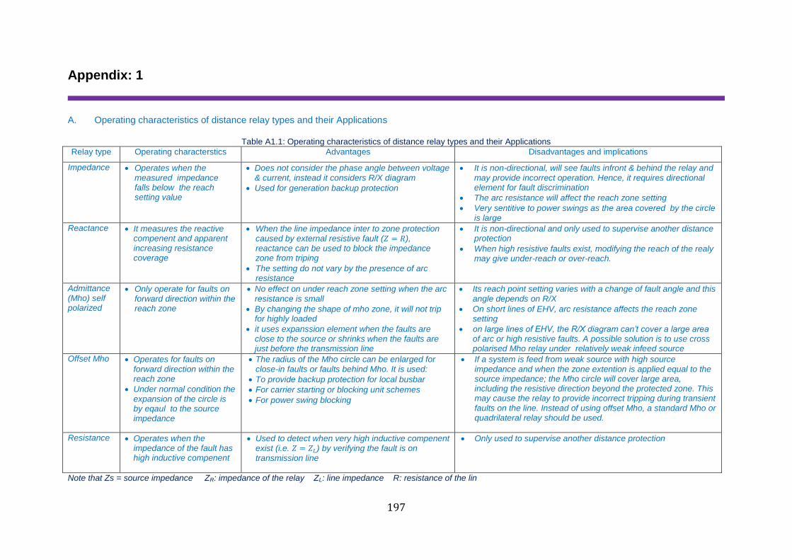
197

Appendix: 1

A. Operating characteristics of distance relay types and their Applications

Table A1.1: Operating characteristics of distance relay types and their Applications

Relay type Operating characterstics Advantages Disadvantages and implications

Impedance Operates when the measured impedance falls below the reach setting value

Does not consider the phase angle between voltage & current, instead it considers R/X diagram

Used for generation backup protection

It is non-directional, will see faults infront & behind the relay and may provide incorrect operation. Hence, it requires directional element for fault discrimination

The arc resistance will affect the reach zone setting

Very sentitive to power swings as the area covered by the circle is large

Reactance It measures the reactive compenent and apparent increasing resistance coverage

When the line impedance inter to zone protection caused by external resistive fault (𝑍 = 𝑅), reactance can be used to block the impedance zone from triping

The setting do not vary by the presence of arc resistance

It is non-directional and only used to supervise another distance protection

When high resistive faults exist, modifying the reach of the realy may give under-reach or over-reach.

Admittance (Mho) self polarized

Only operate for faults on forward direction within the reach zone

No effect on under reach zone setting when the arc resistance is small

By changing the shape of mho zone, it will not trip for highly loaded

it uses expanssion element when the faults are close to the source or shrinks when the faults are just before the transmission line

Its reach point setting varies with a change of fault angle and this angle depends on R/X

On short lines of EHV, arc resistance affects the reach zone setting

on large lines of EHV, the R/X diagram can’t cover a large area of arc or high resistive faults. A possible solution is to use cross polarised Mho relay under relatively weak infeed source

Offset Mho Operates for faults on forward direction within the reach zone

Under normal condition the expansion of the circle is by eqaul to the source impedance

The radius of the Mho circle can be enlarged for close-in faults or faults behind Mho. It is used:

To provide backup protection for local busbar

For carrier starting or blocking unit schemes

For power swing blocking

If a system is feed from weak source with high source impedance and when the zone extention is applied equal to the source impedance; the Mho circle will cover large area, including the resistive direction beyond the protected zone. This may cause the relay to provide incorrect tripping during transient faults on the line. Instead of using offset Mho, a standard Mho or quadrilateral relay should be used.

Resistance Operates when the impedance of the fault has high inductive compenent

Used to detect when very high inductive compenent exist (i.e. 𝑍 = 𝑍𝐿) by verifying the fault is on transmission line

Only used to supervise another distance protection

Note that Zs = source impedance ZR: impedance of the relay ZL: line impedance R: resistance of the lin

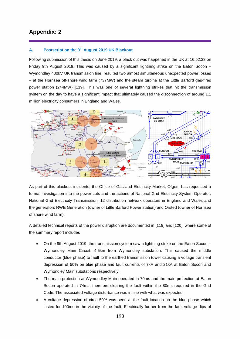
198

Appendix: 2

A. Postscript on the 9th

August 2019 UK Blackout

Following submission of this thesis on June 2019, a black out was happened in the UK at 16:52:33 on

Friday 9th August 2019. This was caused by a significant lightning strike on the Eaton Socon –

Wymondley 400kV UK transmission line, resulted two almost simultaneous unexpected power losses

– at the Hornsea off-shore wind farm (737MW) and the steam turbine at the Little Barford gas-fired

power station (244MW) [119]. This was one of several lightning strikes that hit the transmission

system on the day to have a significant impact that ultimately caused the disconnection of around 1.1

million electricity consumers in England and Wales.

Circuit fault

As part of this blackout incidents, the Office of Gas and Electricity Market, Ofgem has requested a

formal investigation into the power cuts and the actions of National Grid Electricity System Operator,

National Grid Electricity Transmission, 12 distribution network operators in England and Wales and

the generators RWE Generation (owner of Little Barford Power station) and Orsted (owner of Hornsea

offshore wind farm).

A detailed technical reports of the power disruption are documented in [119] and [120], where some of

the summary report includes

On the 9th August 2019, the transmission system saw a lightning strike on the Eaton Socon –

Wymondley Main Circuit, 4.5km from Wymondley substation. This caused the middle

conductor (blue phase) to fault to the earthed transmission tower causing a voltage transient

depression of 50% on blue phase and fault currents of 7kA and 21kA at Eaton Socon and

Wymondley Main substations respectively.

The main protection at Wymondley Main operated in 70ms and the main protection at Eaton

Socon operated in 74ms, therefore clearing the fault within the 80ms required in the Grid

Code. The associated voltage disturbance was in line with what was expected.

A voltage depression of circa 50% was seen at the fault location on the blue phase which

lasted for 100ms in the vicinity of the fault. Electrically further from the fault voltage dips of

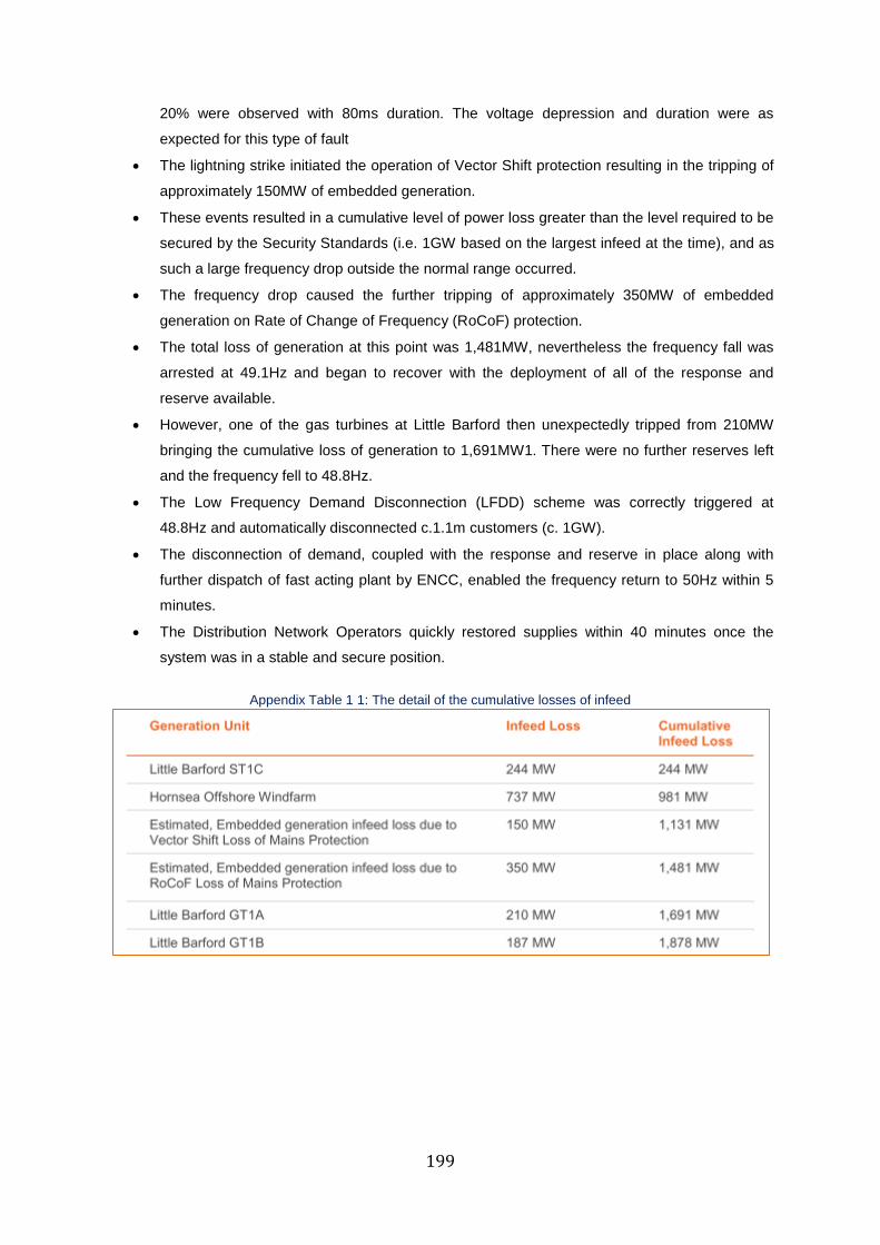
199

20% were observed with 80ms duration. The voltage depression and duration were as

expected for this type of fault

The lightning strike initiated the operation of Vector Shift protection resulting in the tripping of

approximately 150MW of embedded generation.

These events resulted in a cumulative level of power loss greater than the level required to be

secured by the Security Standards (i.e. 1GW based on the largest infeed at the time), and as

such a large frequency drop outside the normal range occurred.

The frequency drop caused the further tripping of approximately 350MW of embedded

generation on Rate of Change of Frequency (RoCoF) protection.

The total loss of generation at this point was 1,481MW, nevertheless the frequency fall was

arrested at 49.1Hz and began to recover with the deployment of all of the response and

reserve available.

However, one of the gas turbines at Little Barford then unexpectedly tripped from 210MW

bringing the cumulative loss of generation to 1,691MW1. There were no further reserves left

and the frequency fell to 48.8Hz.

The Low Frequency Demand Disconnection (LFDD) scheme was correctly triggered at

48.8Hz and automatically disconnected c.1.1m customers (c. 1GW).

The disconnection of demand, coupled with the response and reserve in place along with

further dispatch of fast acting plant by ENCC, enabled the frequency return to 50Hz within 5

minutes.

The Distribution Network Operators quickly restored supplies within 40 minutes once the

system was in a stable and secure position.

Appendix Table 1 1: The detail of the cumulative losses of infeed

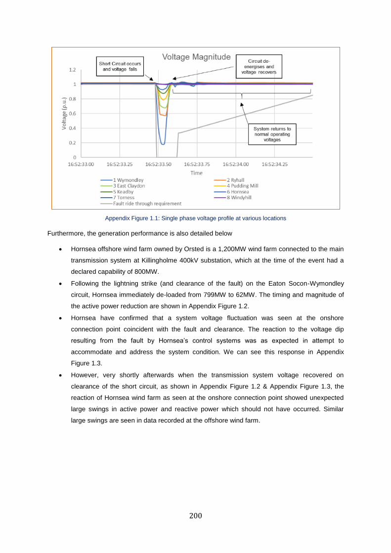
200

Appendix Figure 1.1: Single phase voltage profile at various locations

Furthermore, the generation performance is also detailed below

Hornsea offshore wind farm owned by Orsted is a 1,200MW wind farm connected to the main

transmission system at Killingholme 400kV substation, which at the time of the event had a

declared capability of 800MW.

Following the lightning strike (and clearance of the fault) on the Eaton Socon-Wymondley

circuit, Hornsea immediately de-loaded from 799MW to 62MW. The timing and magnitude of

the active power reduction are shown in Appendix Figure 1.2.

Hornsea have confirmed that a system voltage fluctuation was seen at the onshore

connection point coincident with the fault and clearance. The reaction to the voltage dip

resulting from the fault by Hornsea’s control systems was as expected in attempt to

accommodate and address the system condition. We can see this response in Appendix

Figure 1.3.

However, very shortly afterwards when the transmission system voltage recovered on

clearance of the short circuit, as shown in Appendix Figure 1.2 & Appendix Figure 1.3, the

reaction of Hornsea wind farm as seen at the onshore connection point showed unexpected

large swings in active power and reactive power which should not have occurred. Similar

large swings are seen in data recorded at the offshore wind farm.

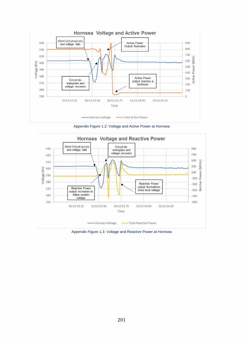
201

Appendix Figure 1.2: Voltage and Active Power at Hornsea

Appendix Figure 1.3: Voltage and Reactive Power at Hornsea

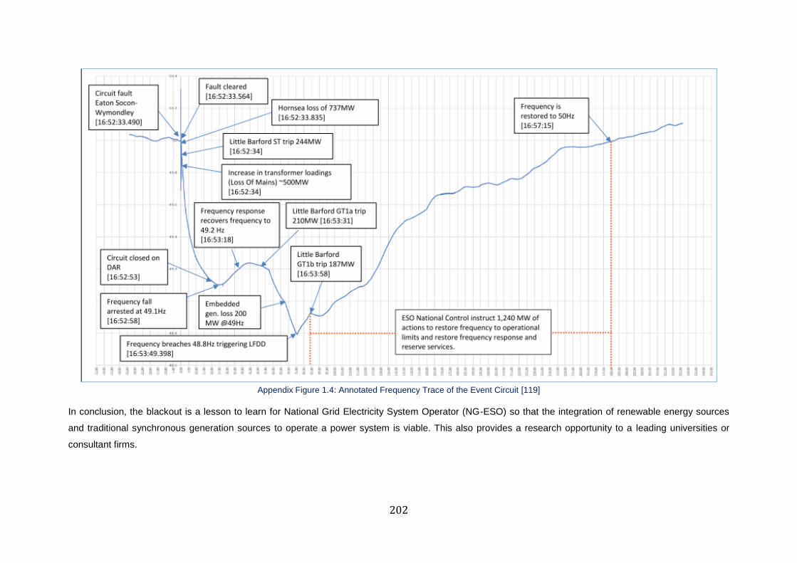
202

Appendix Figure 1.4: Annotated Frequency Trace of the Event Circuit [119]

In conclusion, the blackout is a lesson to learn for National Grid Electricity System Operator (NG-ESO) so that the integration of renewable energy sources

and traditional synchronous generation sources to operate a power system is viable. This also provides a research opportunity to a leading universities or

consultant firms.