How To Address Data Gaps in Life Cycle Inventories: A Case Study onEstimating CO2 Emissions from Coal-Fired Electricity Plants on aGlobal ScaleZoran J. N. Steinmann,† Aranya Venkatesh,*,‡ Mara Hauck,† Aafke M. Schipper,† Ramkumar Karuppiah,‡

Ian J. Laurenzi,‡ and Mark A. J. Huijbregts†

†Department of Environmental Science, Radboud University Nijmegen, Toernooiveld 1, 6525 ED Nijmegen, Netherlands‡ExxonMobil Research and Engineering Company, 1545 Route 22 East, Annandale, New Jersey 08801-3059, United States

*S Supporting Information

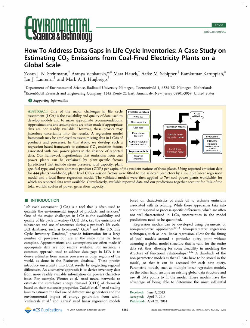
ABSTRACT: One of the major challenges in life cycleassessment (LCA) is the availability and quality of data used todevelop models and to make appropriate recommendations.Approximations and assumptions are often made if appropriatedata are not readily available. However, these proxies mayintroduce uncertainty into the results. A regression modelframework may be employed to assess missing data in LCAs ofproducts and processes. In this study, we develop such aregression-based framework to estimate CO2 emission factorsassociated with coal power plants in the absence of reporteddata. Our framework hypothesizes that emissions from coalpower plants can be explained by plant-specific factors(predictors) that include steam pressure, total capacity, plantage, fuel type, and gross domestic product (GDP) per capita of the resident nations of those plants. Using reported emission datafor 444 plants worldwide, plant level CO2 emission factors were fitted to the selected predictors by a multiple linear regressionmodel and a local linear regression model. The validated models were then applied to 764 coal power plants worldwide, forwhich no reported data were available. Cumulatively, available reported data and our predictions together account for 74% of thetotal world’s coal-fired power generation capacity.

■ INTRODUCTION

Life cycle assessment (LCA) is a tool that is often used toquantify the environmental impact of products and services.1

One of the major challenges in LCA is the availability andquality of life cycle inventory (LCI) data, i.e., the emissions ofsubstances and use of resources during a product’s life cycle.LCI databases, such as Ecoinvent,2 GaBi,3 and the U.S. LifeCycle Inventory Database,4 provide information for a largenumber of processes but are at the same time far fromcomplete. Approximations and assumptions are often made ifappropriate data are not readily available. For instance, acommon approach used to address data gaps in LCA is toderive estimates from similar processes in other regions of theworld, as done in the Ecoinvent database.2 These proxiesintroduce uncertainty into LCA results by neglecting regionaldifferences. An alternative approach is to derive inventory datafrom more readily available information on process character-istics. For example, Wernet et al.5 used neural networks toestimate the cumulative energy demand (CED) of chemicalsbased on their molecular properties. Caduff et al.6,7 used scalinglaws to estimate the fuel use of different size generators and theenvironmental impact of energy generation from wind.Venkatesh et al.8 and Karras9 used linear regression models

based on characteristics of crude oil to estimate emissionsassociated with its refining. While these approaches take intoaccount regional or process-specific differences, which are oftennot well-characterized in LCA, uncertainties in the modelpredictions need to be quantified.Regression models can be developed using parametric or

non-parametric approaches10.11 Non-parametric regressiontechniques, such as local linear regression, allow for the fittingof local models around a particular query point withoutassuming a global model structure that is valid for the entiredata set, thus allowing for some flexibility in modeling thestructure of functional relationships.11,12 A drawback of thenon-parametric models is that all data have to be stored in themodel, so that it can be accessed for each new query.Parametric models, such as multiple linear regression models,on the other hand, assume an existing global data structure anduse all data points to fit the model. These models have theadvantage of being able to determine the most influential

Received: June 7, 2013Accepted: April 7, 2014Published: April 21, 2014

Article

pubs.acs.org/est

© 2014 American Chemical Society 5282 dx.doi.org/10.1021/es500757p | Environ. Sci. Technol. 2014, 48, 5282−5289

parameters easily, and they are easily transferred to otherapplications (only the model parameters need to be known).Fossil energy demand constitutes one of largest sources of

environmental impacts for many products and processes.13,14 Inparticular, coal power plants are among the highest emitters ofgreenhouse gases (GHGs) per kWh of electricity compared toother sources of electricity.15 Coal is also the dominant sourceof electricity generation; i.e., 42% of all electricity generated inthe world in 2011 was produced by coal plants.16 Coal powerplant efficiencies and, therefore, their CO2 emissions varygreatly across the world. For example, the average thermalefficiency of Japanese plants is around 42%, while plants fromIndia have an average efficiency of about 30%.17 Hence,approximations of power generation models using “typical”values from other contexts (for example, assuming Indianpower plants have impacts similar to U.S. power plants) maysignificantly influence an assessment of environmental impactsover a product’s life cycle. Quantifying emission factors of coal-fired electricity as accurately as possible could thereforesignificantly improve the performance of life cycle modelsthat include electricity generation as a major component. Aconsiderable effort has been made by Dones et al.,18 whodeveloped coal power plant emission factors for China, theUnited States, and 19 different European countries/regionsbased on reported data for coal use and electricity generation.However, coal-fired electricity generation is widespread, andemission data are not reported for many other countries in theworld. Moreover, Steinmann et al.19 demonstrated that there isconsiderable variability in life cycle GHG emissions betweenindividual power plants, implying that there is added value inplant-based emission models compared to country-basedapproaches.We are aware of one study by the Center for Global

Development,20,21 called Carbon Monitoring in Action(CARMA), where combustion-phase CO2 emissions fromthermal power plants across the world were estimated with aglobal regression model based solely on the design character-istics of the plants. As far as we know, no other efforts havebeen made to estimate power plant emissions on a global scale.We predict CO2 combustion emissions per kWh (from hereonward referred to as emission factors) from coal power plantson a global scale and quantify uncertainty in the predictions.We employ two predictive regression models: a parametric anda non-parametric model. After fitting and validating bothmodels, we use these to predict CO2 emission factors for 764coal-fired power plants worldwide. These predictions can beused to supplement information in life cycle modeling effortswherever the required data are unavailable.Similar to the Center for Global Development approach, we

include power plant design characteristics as explanatoryvariables within the regression models. There are, however,some notable differences between the two approaches. Thequantification of statistical uncertainty is one of the advantagesof our model framework. Quantifying the uncertainty that arisesfrom using a predictive model is important because it can bepropagated to the final output of any LCA that uses electricityfrom one of these coal plants as input. Another difference isthat our model can distinguish between lignite and non-ligniteplants, whereas the CARMA model cannot. Also, thedifferences between countries were made explicit in ourmodel by including per capita gross domestic product (GDP)as a predictor. Finally, we explored various types of parametric

and non-parametric model approaches and settings to findoptimal model predictions.

■ METHODSRegression models using reported emission data weredeveloped and validated to predict CO2 emission factorsfrom coal-fired power plants across the world. In this section,we describe the data used to develop the regression models,model structures, metrics to evaluate the performance of themodels, and application of the models.

Emission Data. Reported CO2 emissions from individualpower plants were obtained from databases published bygovernmental agencies, such as the U.S. Energy InformationAdministration (EIA), or from reports by private powercompanies. A more extensive discussion on how the CO2emissions per kWh were derived from reported data can befound in SI1 of the Supporting Information.If emission data were available for multiple years, the most

recent year was used. Only plants with a capacity greater than100 MW were included in the analysis to ensure that the dataset was not confounded by very small autonomous producers(for example, a power plant belonging to a paper mill). In total,emissions were reported for 444 plants with a total capacity of494 GW (Table 1).

Predictor Variables and Data. To estimate power-plant-specific CO2 emission factors, a number of potentiallyimportant predictor variables were identified (Table 2). Forour models to be applicable to coal-fired plants throughout theworld, we selected predictors that were available from publicdata sources. Plant age, total capacity, steam pressure, and coaltype were all expected to influence CO2 emissions and werederived from the World Electric Power Plant (WEPP)database.22 The plant age was calculated by taking thecapacity-weighted average of the age of all active generators

Table 1. Characteristics of Individual Coal-Fired PowerPlants by Country Used for Model Validation

countrynumberof plants

sumcapacity(MW) year source

United States 310 288689 2010 Steinmann et al.19

based on EIA38

India 59 64623 2010−2011 Central ElectricAuthority39

Australia 24 27494 2010 AEMO40

South Africa 13 37678 2011 Eskom41

China(includingHong Kong)

2 5368 2011 CLP group42

Canada 4 4221 2010 OPG43

Bulgaria 1 908 2010 Enel44

Greece 4 3977 2006 Kavouridis45

WWF46

England andWales

8 17884 2006 WWF46

Germany 10 22324 2006 WWF46

Poland 4 10905 2006 WWF46

Czech Republic 1 1490 2006 WWF46

Italy 1 2640 2006 WWF46

Spain 1 140 2006 WWF46

Portugal 1 1250 2006 WWF46

Scotland 1 2400 2006 WWF46

total 444 493586

Environmental Science & Technology Article

dx.doi.org/10.1021/es500757p | Environ. Sci. Technol. 2014, 48, 5282−52895283

at a plant. The GDP per capita of the resident nations of thepower plants was also chosen as a predictor because wehypothesized that it correlates with the GHG emission policiesand/or power plant maintenance in those nations, which, inturn, affects the efficiency (and therefore the CO2 emissions) ofthe plants. The 2011 GDP per capita [in purchasing powerparity (PPP)] for each country was obtained from theInternational Monetary Fund’s World Economic Outlook.23

Figure S1 of the Supporting Information shows how theemission factors and predictor variables relate to each other.Model Fitting. Two different modeling approaches were

employed, i.e., a multiple linear regression model and a locallinear regression. Because the models derived in this study wereused to predict CO2 emission factors for a large number ofunknown plants, a thorough assessment of the predictive powerof the model is required. Therefore, prior to model fitting, thedata set (444 plants) was split into a training set and a test set.The training set consisted of 311 of 444 plants (approximately70%), while the remaining 133 plants in the test set were usedfor validation of the models.Multiple Linear Regression. A multiple linear regression

model can be used to predict the value of a response variablebased on a linear relation to any number of predictor variables.The CO2 emission factor associated with a power plant isinversely related to its generation efficiency. We hypothesizethat the selected predictors are linearly related to the efficiencyof the power plant and, therefore, inversely related to its CO2emission factor (eq 1)

β β == +z

yX

10

(1)

where y is a vector representing an estimate of the emissionfactor for all plants, X is the matrix where each columncorresponds to individual predictor variables (Table 2), β is avector of coefficients, and β0 represents the intercept of themodel.Ordinary least-squares (OLS) fitting was used to calculate

the model coefficients. The need for log transformation (with10 as a base) of the predictor variables, total capacity, plant age,steam pressure, and GDP per capita, was assessed, given theskewed distribution of the predictor variables (see SI2 of theSupporting Information). Prior to the log transformation, 1year was added to the plant age because some plants that wereless than 1 year old were assigned a plant age of 0. We used thepackage MuMIn in the statistical program R24 to generate allpossible models using any combination of the predictorvariables (both log-transformed and non-transformed). To

find the optimum between model complexity and the accuracyof the predictions, we calculated Akaike’s Information Criterion(AIC) for all 162 possible combinations. AIC gives a bonus forthe goodness of fit [the log likelihood function, ln(L)] and apenalty for the number of predictors k (eq 2). The model withthe lowest AIC value was considered to be the best model.

= −k LAIC 2 ln( ) (2)

The best model was subsequently checked for multicollinearityin its predictor variables by calculating variance inflation factors(VIFs). Typically, predictors with a VIF > 10 indicatemulticollinearity in the inputs and need to be excluded fromthe model.25 No predictor variables were excluded from ourmodel based on this threshold because the highest observedVIF was below 2 (see Table S1 of the Supporting Information).Furthermore, 95% prediction intervals (as a function of thestandard error in the model fit and the deviation of eachpredictor from its mean value) were calculated by the Rfunction predict.lm.Furthermore, leave-one-out cross-validation (LOOCV) was

performed, which is a procedure in which a model is fitted withall power plants but one. The fitted model is then used topredict the emission factor of the power plant that was left out,and this procedure is repeated until a prediction is obtained forevery single power plant. These estimates were used to assessthe predictive power of the model.To determine the relative importance of each of the

predictor variables for the best model (that is, the modelwith the lowest AIC), we performed a separate analysis basedon standardized predictor variables. Because all of the inputvariables are measured in different units (e.g., age in years,capacity in MW, etc.), they were first standardized to z scores.Regression coefficients resulting from the standardized fitdirectly reflect the relative importance of each predictorvariable.

Local Linear Regression Model. In locally weightedpolynomial regression, a low-degree polynomial is fitted locallyaround a query point using a weighted least-squares approach,where observations near the query point are assigned higherweights.26 In this study, we used an implementation of a localfirst-order (linear) regression by Kalnins et al.,27 developed byJekabsons,28 detailed as follows.Assume that yp is a vector that represents emission factors

and Xp represents a matrix of d columns corresponding to theindividual predictor variables; these represent the training set.The training set includes n observations (Xi

p, yip); i = 1, ..., n.

The predicted emission factor of a particular (query) plant j,

Table 2. Range of Predictor Variables

variablerange used inmodel fitting

total range inWEPP database

and IMF notes

plant age 0−60 years 0−70 years in the case of multiple generators, a weighted average age is used; the ages of the generators were calculatedby subtracting the operation year from the year for which the data were reported; the weights were basedon the generator capacity as a proportion of the total plant capacity

coal type lignite ornon-lignitea

lignite ornon-lignite

plants that did not report their fuel type or that report a combination of fuel types, such aslignite/bituminous, were excluded from the analysis

steampressure

35−293 bar 17−286 bar the average steam pressure of all operational generators per plant

totalcapacity

100−4440 MW 100−5500 MW total capacity of all operational generators per plant; only plants of >100 MW were included

GDP percapita

$3694−48387 $487−48387 GDP per capita in $ of PPP

aNon-lignite plants are modeled as 0, while lignite plants were assigned a value of 1.

Environmental Science & Technology Article

dx.doi.org/10.1021/es500757p | Environ. Sci. Technol. 2014, 48, 5282−52895284

with characteristics described by Xjq, is estimated by performing

a linear regression locally in the neighborhood of query plant j.The linear model to be used locally can be represented as

shown in eq 3.

∑= +=

F X a a X( )id

m

m i0

1

m(3)

The coefficients a in eq 3 are calculated using a weighted least-squares method, as shown in eq 4. In this method, theneighbors nearest to query point Xj

q are assigned higherweights.

∑= −=

a w X X F X yarg min ( , )( ( ) )n

i

jq

ip

ip

ip

12

(4)

The weighting function w used in eq 4 is a function of thedistance between observations Xp and query point Xj

q. While anumber of different weighting functions, such as theEpanechnikov quadratic weighting, tri-cube, and Gaussianweighting can be used, it has been shown that the choice ofthe weighting function does not significantly affect the results.29

We used the Gaussian weighting function, implemented byKalnins et al.27, as follows. In this implementation, μi refers tothe scaled distance from the query point j to the ith plant in thetraining set, as shown in eq 5.

μ =|| − ||

|| − ||X X

X Xij j

qip

jq p

farthest (5)

The Gaussian weight function is then calculated as a function ofthe scaled distance μi and coefficient α, as shown in eq 6. Thiscoefficient controls the linear approximation, by defining theextent of the neighborhood around a query point that isweighted strongly in the approximation.

αμ= −w X X( , ) exp( )jq

ip

ij

(6)

Before being used to estimate weights, all predictors in thetraining set (without log transformation) were first transformedto z scores. Furthermore, Gower’s dissimilarity metric was usedto transform the binary coal-type variable (by multiplying the zscores of the binary coal-type variable by a factor of 1/√2, assuggested by Sigovini30). The coefficient α was tuned usingLOOCV, suggested as a widely accepted method to measurethe goodness of fit of the local model.31 In this approach, for aspecific value of α, a prediction was made for a single powerplant based on a fitted model that included all other powerplants in the training set. This was performed for each powerplant in the training data set, resulting in emission factorestimates for every single plant that was used to evaluate themodel mean square error for that specific value of α. Theoptimal value of the coefficient α was determined using asimple stepwise search algorithm presented by Kalnins et al.,27

which resulted in the lowest LOOCV mean square error.The optimal coefficient α, thus determined, was then used in

conjunction with the training set data to estimate the emissionfactors of all plants in the test set.Finally, bootstrap sampling was used to develop pointwise

prediction interval estimates for all power plants, as shown byAneiros-Perez et al.32 The training data residuals, calculatedusing the local linear regression model, were used to estimate1000 bootstrapped residuals for each data point in the test set.

The 95% prediction intervals for new plants were based onthese 1000 bootstrapped residuals.

Model Evaluation. We analyzed the R2 for the cross-validated training set (311 plants) and the R2 for the 133 plantsin the test set to obtain an indication of the predictive power ofthe models.33 These R2 metrics have values that are between−∞ and 1. A value of 1 reflects a perfect prediction, while anymodel with a R2 value below 0 has no added value compared tousing the average of the data set.34,35

In addition to the R2 metrics for the training and test sets, wecalculated relative prediction errors for each power plant, as thedifference between the reported and predicted emission factors,represented as a fraction of the reported emission factor. Wealso plotted relative prediction errors for all plants against theindividual predictors to identify predictor ranges for which theestimates are particularly uncertain. To check the influence ofthe relatively large number of U.S. plants in the training data set(223 of 311) on the global multiple linear regression model, anadditional multiple regression fit was performed where 135 ofthe U.S. plants were removed from the training data set toobtain a data set with an equal number of U.S. and non-U.S.plants (88 each).

Model Application. The multiple linear regression modelwith the lowest AIC value and the local linear regression modelwere applied to coal-fired power plants in the WEPP database,for which all predictors listed in Table 2 were available and forwhich no reported emission data were available. In total, theWEPP database includes 1974 coal plants with a capacity of>100 MW (cumulative capacity of 1687 GW) in 72 countries,with at least one operational generator in the year 2012.Emissions were reported for 444 of these plants (494 GW),contributing to 29% of the total capacity of the world (see theEmission Data section). Of the remaining 1540 plants, allpredictor data were available for 764 plants with a total capacityof 760 GW (45% of the total capacity of the world).

■ RESULTSMultiple Linear Regression Model. The AIC values of all

possible multiple regression models (see Table S2 of theSupporting Information) showed that the model with the log-transformed values of the four continuous predictors and thecategorical fuel type (lignite or non-lignite) was the best model.The coefficients for this model are shown in Table 3. The

normalized model coefficients, indicating influence of eachpredictor, are shown in Table S3 of the SupportingInformation. The log-transformed steam pressure has thehighest normalized coefficient value, indicating that it is themost important predictor. The coefficients of the model thatused an equal number of U.S. plants and non-U.S. plants arewell within 50% of coefficients of the model fitted to thetraining data, for all predictors except for plant age, for which

Table 3. Coefficients of the Best Multiple Linear RegressionModel

predictor name coefficient p value

intercept −3.65 × 10−1 9.7 × 10−5

log[capacity (in MW)] 6.38 × 10−2 9.8 × 10−6

log[age + 1 (in years)] −8.69 × 10−2 2.7 × 10−4

log[steam pressure (in bar)] 3.46 × 10−1 8.8 × 10−14

log[GDP (in $PPP) per capita] 1.20 × 10−1 3.7 × 10−17

fuel type (1, lignite; 0, non-lignite) −1.49 × 10−1 3.5 × 10−17

Environmental Science & Technology Article

dx.doi.org/10.1021/es500757p | Environ. Sci. Technol. 2014, 48, 5282−52895285

the coefficient almost doubles because of the removal of theU.S. plants (see Table S4 of the Supporting Information). Thepredictions from this model are consistent with the predictionsfrom the model based on the entire training data set; onaverage, these differ by 1.5%.The cross-validated R2 value based on the training set fit is

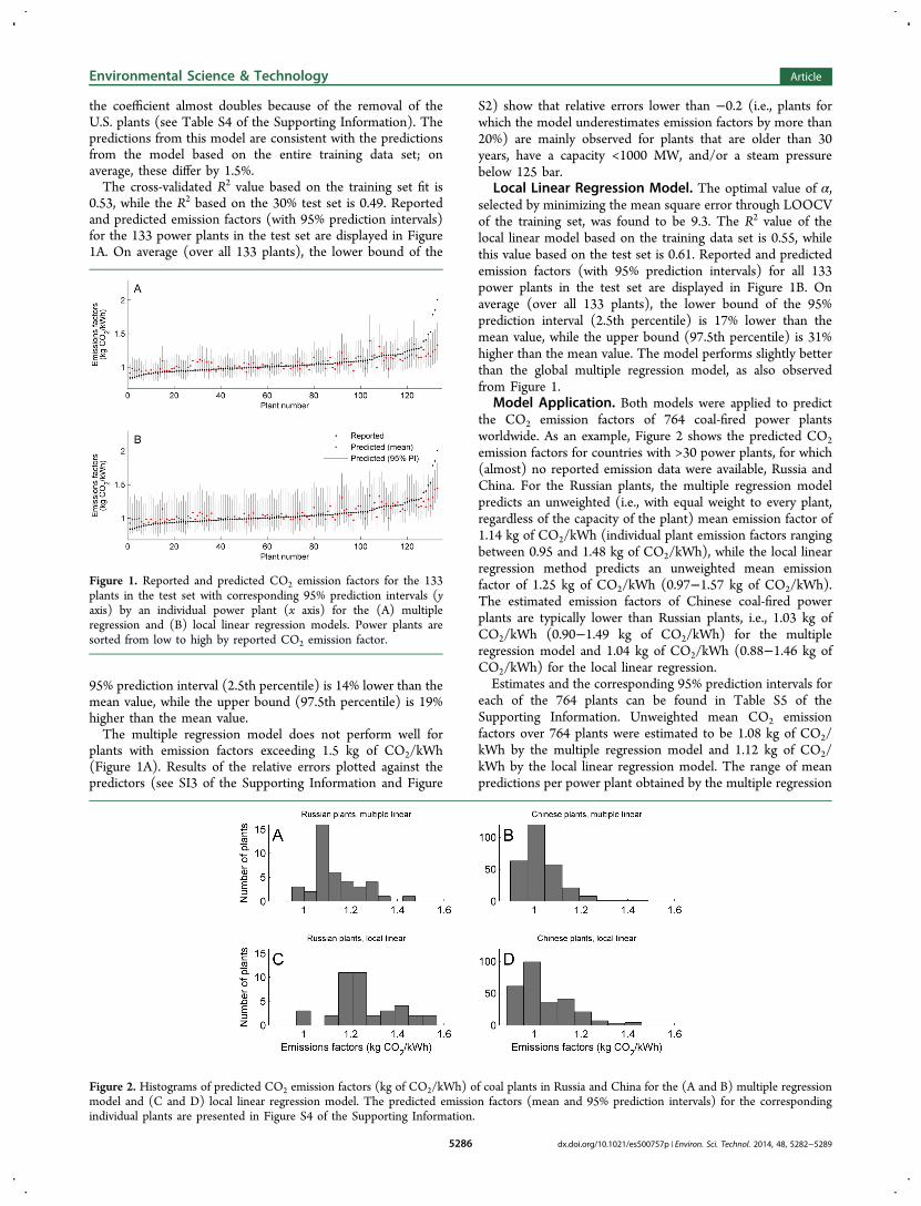
0.53, while the R2 based on the 30% test set is 0.49. Reportedand predicted emission factors (with 95% prediction intervals)for the 133 power plants in the test set are displayed in Figure1A. On average (over all 133 plants), the lower bound of the

95% prediction interval (2.5th percentile) is 14% lower than themean value, while the upper bound (97.5th percentile) is 19%higher than the mean value.The multiple regression model does not perform well for

plants with emission factors exceeding 1.5 kg of CO2/kWh(Figure 1A). Results of the relative errors plotted against thepredictors (see SI3 of the Supporting Information and Figure

S2) show that relative errors lower than −0.2 (i.e., plants forwhich the model underestimates emission factors by more than20%) are mainly observed for plants that are older than 30years, have a capacity <1000 MW, and/or a steam pressurebelow 125 bar.

Local Linear Regression Model. The optimal value of α,selected by minimizing the mean square error through LOOCVof the training set, was found to be 9.3. The R2 value of thelocal linear model based on the training data set is 0.55, whilethis value based on the test set is 0.61. Reported and predictedemission factors (with 95% prediction intervals) for all 133power plants in the test set are displayed in Figure 1B. Onaverage (over all 133 plants), the lower bound of the 95%prediction interval (2.5th percentile) is 17% lower than themean value, while the upper bound (97.5th percentile) is 31%higher than the mean value. The model performs slightly betterthan the global multiple regression model, as also observedfrom Figure 1.

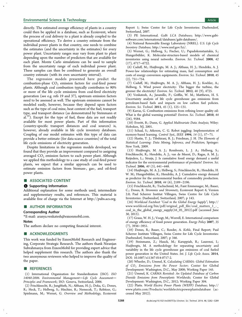
Model Application. Both models were applied to predictthe CO2 emission factors of 764 coal-fired power plantsworldwide. As an example, Figure 2 shows the predicted CO2emission factors for countries with >30 power plants, for which(almost) no reported emission data were available, Russia andChina. For the Russian plants, the multiple regression modelpredicts an unweighted (i.e., with equal weight to every plant,regardless of the capacity of the plant) mean emission factor of1.14 kg of CO2/kWh (individual plant emission factors rangingbetween 0.95 and 1.48 kg of CO2/kWh), while the local linearregression method predicts an unweighted mean emissionfactor of 1.25 kg of CO2/kWh (0.97−1.57 kg of CO2/kWh).The estimated emission factors of Chinese coal-fired powerplants are typically lower than Russian plants, i.e., 1.03 kg ofCO2/kWh (0.90−1.49 kg of CO2/kWh) for the multipleregression model and 1.04 kg of CO2/kWh (0.88−1.46 kg ofCO2/kWh) for the local linear regression.Estimates and the corresponding 95% prediction intervals for

each of the 764 plants can be found in Table S5 of theSupporting Information. Unweighted mean CO2 emissionfactors over 764 plants were estimated to be 1.08 kg of CO2/kWh by the multiple regression model and 1.12 kg of CO2/kWh by the local linear regression model. The range of meanpredictions per power plant obtained by the multiple regression

Figure 1. Reported and predicted CO2 emission factors for the 133plants in the test set with corresponding 95% prediction intervals (yaxis) by an individual power plant (x axis) for the (A) multipleregression and (B) local linear regression models. Power plants aresorted from low to high by reported CO2 emission factor.

Figure 2. Histograms of predicted CO2 emission factors (kg of CO2/kWh) of coal plants in Russia and China for the (A and B) multiple regressionmodel and (C and D) local linear regression model. The predicted emission factors (mean and 95% prediction intervals) for the correspondingindividual plants are presented in Figure S4 of the Supporting Information.

Environmental Science & Technology Article

dx.doi.org/10.1021/es500757p | Environ. Sci. Technol. 2014, 48, 5282−52895286

model (0.84−2.34 kg of CO2/kWh) is larger than the range forthe local linear model (0.87−1.89 kg of CO2/kWh). It shouldbe noted, however, that the maximum value predicted by themultiple regression model refers to a plant with extremecharacteristics (old plants with small capacity and low steampressure) located in a country with low GDP per capita(Zimbabwe). The characteristics of this plant are outside therange of predictors used to train the model. When the 95%prediction intervals are considered, we observe a smaller rangefor the multiple regression model (0.90−1.42 kg of CO2/kWh)compared to the range (0.90−1.57 kg of CO2/kWh) found forthe local linear regression.

■ DISCUSSION

Model Performance. We employed two regressiontechniques (multiple linear regression and local linearregression) to estimate the CO2 emission factors of coal-firedpower plants on a global scale. Predictions obtained by the locallinear regression model show a slightly better performance, asdemonstrated by the higher R2 of the test set (0.61 for locallinear regression versus 0.49 for the multiple linear regression).We also tested a number of alternate non-parametric regressionapproaches, including k-nearest neighbors and kernel regression(see Table S6 of the Supporting Information). However, thelocal linear regression was found to perform better than thesemethods based on the training and test set R2 values.Both regression models have a relative error of less than 20%

for more than 95% of the power plants based on the test setwith 30% of the plants. A direct comparison of these values tothe findings by Ummel in the CARMA model21 is impossiblebecause the results were not provided separately for coal-firedplants; CO2 emissions from all thermal power plants (includingother generation types, such as natural gas plants) wereestimated in that study. As noted, our multiple regressionmodel, in particular, underestimates the highest reportedemission factors (>1.5 kg of CO2/kWh). A similar effect canbe observed in the CARMA model.21 The highest predictions(for any fuel type) from that study were approximately 1.5 kg ofCO2/kWh, while the highest reported emission factors wereclose to 2.0 kg of CO2/kWh.A possible limitation of our models is that they do not

address temporal variability in the emission factors. Because ofdata limitations, it was not possible to obtain reportedemissions and generation data for multiple years for all powerplants in the data set. We did, however, assess the temporalvariability in the emission factors of a subset of U.S. coal plantsfor which data were available (see SI4 of the SupportingInformation). Even though the total annual CO2 emissions andthe net generation were found to fluctuate over the years (aspresented in the CARMA report21), our results show thatemission factors appear to be relatively stable. For the 306plants with an emission factor of <1.5 kg of CO2/kWh, thedifference between extreme values observed over a 3 year timeperiod was, on average, 3.1% of the mean value. Additionally,the highest temporal variability was found for plants with highCO2 emission factors. The four plants with an average emissionfactor of >1.5 kg of CO2/kWh show an average difference of33% between the extreme values. This finding indicates that theCO2 emission factors of the plants with relatively high CO2emission factors are inherently variable over time. This findingmay also help explain why our models make less accuratepredictions for plants with high emission factors.

Analysis of the relative errors in the training set and the testset (see SI3 of the Supporting Information) shows that themodel fit is not as good for plants that are over 30 years old,have a capacity below 1000 MW, or especially, have steampressures below 125 bar. Therefore, we suggest caution whenapplying our model to plants with characteristics in this range,especially if a plant has all three characteristics in the criticalrange.

Number of Predictors. A limited number of readilyavailable predictors was included in our models, because theaim was to develop models to predict emission factors for alarge number of power plants. On the basis of AIC, we foundthat the best model included all predictors, indicating that noneof these predictors were redundant. However, several otherpredictors may influence plant efficiencies and, therefore, CO2emission factors, such as the cooling processes of the plant, thepresence of SO2 and NOx control equipment, and plantcapacity factor. Furthermore, the grid stability of a country mayinfluence the performance of a power plant as well. If the gridlacks stability, plants have to stop and start relatively often,which lowers the average plant efficiency. We were, however,not able to add the regional grid stability as an extra predictorbecause of the lack of data.Lam and Shiu36 found that the capacity factor strongly

influences power plant efficiency. As part of a sensitivityanalysis, we included the plant capacity factor as an additionalpredictor (see SI5 of the Supporting Information). Thepredictive power of both models increased as a result ofincluding the capacity factor as an additional predictor.However, both models were not able to make accuratepredictions for plants with high emission factors, even whenincluding the capacity factor as a predictor variable. It was alsofound that estimates for plants with capacity factors higher than50%, in general, have lower relative errors (as shown in SI5 ofthe Supporting Information). It should be noted, however, thatfor the external application of our models, the capacity factorhas no added value because net electricity generation istypically not known for plants that do not report CO2emissions.

Model Application. The applicability domain of a modelrefers to the range of predictor values in which a model can beapplied. The observed ranges of predictors in the applicationset were similar to or within the range of the modeldevelopment set. From this, we conclude that the plants inthe application set were within the applicability domain of ourmodels. One exception is the per capita GDP, which rangesbetween $3700 and $48 000 per capita in the model trainingset. A total of 11 plants in the application set are situated incountries with GDP below $3700 per capita. Extrapolationoutside the original range causes the predictions for these plantsto be more uncertain, such as for the prediction for the coalplant in Zimbabwe, which should be interpreted with caution.The uncertainties that are introduced by predictive modeling

are around 8 times larger than the uncertainty that was foundfor measured emissions in the United States by Steinmann etal.19 Their study showed that it is possible to reduce uncertaintyin the emissions from individual power plants to a muchsmaller range with full disclosure of power plant fuel use andelectricity generation data. In the absence of more data,however, a modeling approach for calculating the CO2 emissionfactors of individual power plants could help address data gapsin life cycle inventories. With small adaptations to our modelframework, it is possible to estimate power plant efficiencies

Environmental Science & Technology Article

dx.doi.org/10.1021/es500757p | Environ. Sci. Technol. 2014, 48, 5282−52895287

directly. The estimated average efficiency of plants in a countrycould then be applied in a database, such as Ecoinvent, wherethe process of coal delivery to a plant is already coupled to theoperational efficiency. To derive a country estimate from theindividual power plants in that country, one needs to combinethe estimates (and the uncertainty in the estimates) for everypower plant. Uncertainty ranges may vary from plant to plantdepending upon the number of predictors that are available foreach plant. Monte Carlo simulations can be used to samplefrom the uncertainty range of each individual power plant.These samples can then be combined to generate an overallcountry estimate (with its own uncertainty interval).The regression models presented here predict the

combustion-phase CO2 emission factors for coal-fired powerplants. Although coal combustion typically contributes to 90%or more of the life cycle emissions from coal-fired electricitygeneration (see e.g. refs 19 and 37), upstream emission factorsneed to be assessed as well. The upstream emissions cannot bemodeled easily, however, because they depend upon factorssuch as the type of coal mine, heat content of the fuel, transporttype, and transport distance (as demonstrated by Steinmann etal.19). Except for the type of fuel, these data are not readilyavailable for most power plants. Part of this information(country-specific transport distances and coal sources) is,however, already available in life cycle inventory databases.Coupling of our model estimates with this type of data canprovide a better estimate (for data-scarce countries) of the totallife cycle emissions of electricity generation.Despite limitations in the regression models developed, we

found that they provide an improvement compared to assigningaveraged CO2 emission factors to each power plant. Althoughwe applied this methodology to a case study of coal-fired powerplants, we expect that a similar approach can be used toestimate emission factors from biomass-, gas-, and oil-firedpower plants.

■ ASSOCIATED CONTENT*S Supporting InformationAdditional explanation for some methods used, intermediateand supplementary results, and references. This material isavailable free of charge via the Internet at http://pubs.acs.org.

■ AUTHOR INFORMATIONCorresponding Author*E-mail: aranya.venkatesh@exxonmobil.com.NotesThe authors declare no competing financial interest.

■ ACKNOWLEDGMENTSThis work was funded by ExxonMobil Research and Engineer-ing, Corporate Strategic Research. The authors thank NiranjanSubrahmanya from ExxonMobil for providing expert advice thathelped supplement this research. The authors also thank thetwo anonymous reviewers who helped to improve the quality ofthe paper.

■ REFERENCES(1) International Organization for Standardization (ISO). ISO14040:2006. Environmental ManagementLife Cycle AssessmentPrinciples and Framework; ISO: Geneva, Switzerland, 2006.(2) Frischknecht, R.; Jungbluth, N.; Althaus, H.-J.; Doka, G.; Dones,R.; Heck, T.; Hellweg, S.; Hischier, R.; Nemecek, T.; Rebitzer, G.;Spielmann, M.; Wernet, G. Overview and Methodology, Ecoinvent

Report 1; Swiss Centre for Life Cycle Inventories: Duebendorf,Switzerland, 2007.(3) PE International. GaBi LCA Databases; http://www.gabi-software.com/international/databases/gabi-databases/.(4) National Renewable Energy Laboratory (NREL). U.S. Life CycleInventory Database; http://www.nrel.gov/lci/.(5) Wernet, G.; Hellweg, S.; Fischer, U.; Papadokonstantakis, S.;Hungerbuhler, K. Molecular-structure-based models of chemicalinventories using neural networks. Environ. Sci. Technol. 2008, 42(17), 6717−6722.(6) Caduff, M.; Huijbregts, M. A. J.; Althaus, H. J.; Hendriks, A. J.Power-law relationships for estimating mass, fuel consumption andcosts of energy conversion equipments. Environ. Sci. Technol. 2010, 45(2), 751−754.(7) Caduff, M.; Huijbregts, M. A. J.; Althaus, H. J.; Koehler, A.;Hellweg, S. Wind power electricity: The bigger the turbine, thegreener the electricity? Environ. Sci. Technol. 2012, 46 (9), 4725.(8) Venkatesh, A.; Jaramillo, P.; Griffin, W. M.; Matthews, H. S.Uncertainty analysis of life cycle greenhouse gas emissions frompetroleum-based fuels and impacts on low carbon fuel policies.Environ. Sci. Technol. 2011, 45 (1), 125−131.(9) Karras, G. Combustion emissions from refining lower quality oil:What is the global warming potential? Environ. Sci. Technol. 2010, 44(24), 9584.(10) Everitt, B.; Dunn, G. Applied Multivariate Data Analysis; Wiley:Hoboken, NJ, 2001.(11) Schaal, S.; Atkeson, C. G. Robot juggling: Implementation ofmemory-based learning. Control Syst., IEEE 1994, 14 (1), 57−71.(12) Hastie, T. J.; Tibshirani, R. J.; Friedman, J. H. The Elements ofStatistical Learning: Data Mining, Inference, and Prediction; Springer:New York, 2009.(13) Huijbregts, M. A. J.; Rombouts, L. J. A.; Hellweg, S.;Frischknecht, R.; Hendriks, A. J.; van de Meent, D.; Ragas, A. M. J.;Reijnders, L.; Struijs, J. Is cumulative fossil energy demand a usefulindicator for the environmental performance of products? Environ. Sci.Technol. 2006, 40 (3), 641−648.(14) Huijbregts, M. A. J.; Hellweg, S.; Frischknecht, R.; Hendriks, H.W. M.; Hungerbuhler, K.; Hendriks, A. J. Cumulative energy demandas predictor for the environmental burden of commodity production.Environ. Sci. Technol. 2010, 44 (6), 2189−2196.(15) Frischknecht, R.; Tuchschmid, M.; Faist Emmeneger, M.; Bauer,C.; Dones, R. Strommix und Stromnetz, Ecoinvent Report 6, Version2.0; Paul Scherrer Institut Villingen, Swiss Centre for Life CycleInventories: Duebendorf, Switzerland, 2007; p 143.(16) Worldcoal Factsheet “Coal in the Global Energy Supply”; http://www.worldcoal.org/bin/pdf/original_pdf_file/coal_matters_1_-_coal_in_the_global_energy_supply(16_05_2012).pdf (accessed June30, 2013).(17) Graus, W. H. J.; Voogt, M.; Worrell, E. International comparisonof energy efficiency of fossil power generation. Energy Policy 2007, 35(7), 3936−3951.(18) Dones, R.; Bauer, C.; Roeder, A. Kohle, Final Report; PaulScherrer Institute Villingen, Swiss Centre for Life Cycle Inventories:Duebendorf, Switzerland, 2007; p 346.(19) Steinmann, Z.; Hauck, M.; Karuppiah, R.; Laurenzi, I.;Huijbregts, M. A methodology for separating uncertainty andvariability in the life cycle greenhouse gas emissions of coal fueledpower generation in the United States. Int. J. Life Cycle Assess. 2014,DOI: 10.1007/s11367-014-0717-2.(20) Wheeler, D.; Ummel, K. Calculating CARMA: Global Estimationof CO2 Emissions from the Power Sector; Center for GlobalDevelopment: Washington, D.C., May 2008; Working Paper 145.(21) Ummel, K. CARMA Revisited: An Updated Database of CarbonDioxide Emissions from Powerplants Worldwide; Center for GlobalDevelopment: Washington, D.C., 2012; Working Paper 304.(22) Platts. World Electric Power Plants (WEPP) Database; http://www.platts.com/Products/worldelectricpowerplantsdatabase (ac-cessed May 2012).

Environmental Science & Technology Article

dx.doi.org/10.1021/es500757p | Environ. Sci. Technol. 2014, 48, 5282−52895288

(23) International Monetary Fund (IMF). World Economic Outlook;http://www.imf.org/external/pubs/ft/weo/2012/01/weodata/download.aspx.(24) R Foundation for Statistical Computing. R Core Team R: ALanguage and Environment for Statistical Computing; R Foundation forStatistical Computing: Vienna, Austria, 2012.(25) Field, A. Discovering Statistics Using SPSS; Sage PublicationsLimited: Thousand Oaks, CA, 2009.(26) Cleveland, W. S. Robust locally weighted regression andsmoothing scatterplots. J. Am. Stat. Assoc. 1979, 74 (368), 829−836.(27) Kalnins, K.; Ozolins, O.; Jekabsons, G. Metamodels in design ofGFRP composite stiffened deck structure. Proceedings of 7th ASMO-UK/ISSMO International Conference on Engineering Design Optimiza-tion; Association for Structural and Multidisciplinary Optimization inthe UK (ASMO-UK): Bath, U.K., 2008; p 11.(28) Jekabsons, G. Locally Weighted Polynomials for Matlab, 2010;http://www.cs.rtu.lv/jekabsons.(29) Chu, C. K.; Marron, J. S. Choosing a kernel regressionestimator. Stat. Sci. 1991, 6 (4), 404−419.(30) Sigovini, M. Multiscale dynamics of zoobenthic communitiesand relationships with environmental factors in the Lagoon of Venice.Doctoral dissertation, Universita Ca’Foscari Venezia, Dorsoduro, Italy,2011; http://dspace.unive.it/handle/10579/1092.(31) Schaal, S.; Atkeson, C. G. Assessing the quality of learned localmodels. Adv. Neural Inf. Process. Syst. 1994, 1−8.(32) Aneiros-Perez, G.; Cao, R.; Vilar-Fernandez, J. M. Functionalmethods for time series prediction: A nonparametric approach. J.Forecasting 2010, 30 (4), 377−392.(33) Schuurmann, G.; Ebert, R.-U.; Chen, J.; Wang, B.; Kuhne, R.External validation and prediction employing the predictive squaredcorrelation coefficientTest set activity mean vs training set activitymean. J. Chem. Inf. Model. 2008, 48 (11), 2140−2145.(34) Legates, D. R.; McCabe, G. J., Jr. Evaluating the use of“goodness-of-fit” measures in hydrologic and hydroclimatic modelvalidation. Water Resour. Res. 1999, 35 (1), 233−241.(35) Todeschini, R. Tutorial 5, Useful and Unuseful Summaries ofRegression Models; http://www.moleculardescriptors.eu/tutorials/tutorials.htm.(36) Lam, P. L.; Shiu, A. A data envelopment analysis of theefficiency of China’s thermal power generation. Util. Policy 2001, 10(2), 75−83.(37) Littlefield, J.; Bhander, R.; Bennett, B.; Davis, T.; Draucker, L.;Eckard, R.; Ellis, W.; Kauffman, J.; Malone, A.; Munson, R.; Nippert,M.; Ramezan, M.; Bromiley, R. Life Cycle Analysis: Existing PulverizedCoal (EXPC) Power Plant; National Energy Technology Laboratory(NETL): Pittsburgh, PA, 2010; 110809, p 112.(38) U.S. Energy Information Administration (EIA). Form EIA-923Detailed Data; http://www.eia.gov/electricity/data/eia923/.(39) Central Electric Authority. Baseline Carbon Dioxide Emissionsfrom Power Sector; http://www.cea.nic.in/reports/planning/cdm_co2/cdm_co2.htm (accessed June 2012).(40) Australian Energy Market Operator (AEMO). NationalTransmission Network Development Plan, Supply Input Spreadsheets;http://www.aemo.com.au/Consultations/National-Electricity-Market/Closed/∼/media/Files/Other/planning/0410-0029%20zip.ashx (accessed June 2012).(41) Eskom. CDM Calculations; http://www.eskom.co.za/c/article/236/cdm-calculations/ (accessed June 2012).(42) CLP Group. Facility Performance Statistics for Fangchenggang andCastle Peak; https://www.clpgroup.com/ourvalues/report/Pages/sustainabilityreport.aspx (accessed June 2012).(43) Ontario Power Generation. Sustainable Development Report2010; Ontario Power Generation: Toronto, Ontario, Canada, 2011.(44) Enel. Sustainability Report 2010; http://www.enel.com/en-GB/doc/report2010/Sustainability_report_2010_30_06_2011.pdf (ac-cessed June 2012).(45) Kavouridis, K. Lignite industry in Greece within a worldcontext: Mining, energy supply and environment. Energy Policy 2008,36 (4), 1257−1272.

(46) World Wide Fund for Nature (WWF). Dirty Thirty, Ranking ofthe Most Polluting Power Stations in Europe; http://wwf.panda.org/?100140/Europes-Dirty-30 (accessed July 2012).

Environmental Science & Technology Article

dx.doi.org/10.1021/es500757p | Environ. Sci. Technol. 2014, 48, 5282−52895289