Higher-order (2 1 4) Korteweg-de Vries-like equation for interfacial wavesin a symmetric three-layer fluid

O. E. Kurkina,1,2,3 A. A. Kurkin,3 T. Soomere,1 E. N. Pelinovsky,2,3,4

and E. A. Rouvinskaya2,4

1Wave Engineering Laboratory, Institute of Cybernetics, Tallinn University of Technology, Tallinn, Estonia2Department of Mathematics, National Research University Higher School of Economics,Nizhny Novgorod Branch, Nizhny Novgorod, Russia3Department of Applied Mathematics, Nizhny Novgorod State Technical University, Nizhny Novgorod, Russia4Department of Nonlinear Geophysical Processes, Institute of Applied Physics of Russian Academy ofSciences, Nizhny Novgorod, Russia

(Received 25 March 2011; accepted 26 September 2011; published online 18 November 2011)

We address a specific but possible situation in natural water bodies when the three-layer stratification

has a symmetric nature, with equal depths of the uppermost and the lowermost layers. In such case,

the coefficients at the leading nonlinear terms of the modified Korteweg-de Vries (mKdV) equation

vanish simultaneously. It is shown that in such cases there exists a specific balance between the

leading nonlinear and dispersive terms. An extension to the mKdV equation is derived by means of

combination of a sequence of asymptotic methods. The resulting equation contains a cubic and a

quintic nonlinearity of the same magnitude and possesses solitary wave solutions of different polarity.

The properties of smaller solutions resemble those for the solutions of the mKdV equation, whereas

the height of the taller solutions is limited and they become table-like. It is demonstrated numerically

that the collisions of solitary wave solutions to the resulting equation are weakly inelastic: the basic

properties of the counterparts experience very limited changes but the interactions are certainly

accompanied by a certain level of radiation of small-amplitude waves. VC 2011 American Institute ofPhysics. [doi:10.1063/1.3657816]

I. INTRODUCTION

Internal gravity waves serve as one of the most impor-

tant constituent of nonlinear wave motions in stratified envi-

ronment.1 Internal waves often play the decisive role in

various processes in geophysical and other similar media

where they may serve as major agents carrying energy from

remote areas to specific domains in the ocean. For example,

energy release into local turbulent motions and subsequent

mixing caused by internal waves apparently is an important

source of the potential energy that is needed to bring deep,

dense bottom water to the surface.2–4 Their impact on the

functioning of the ocean has been relatively well understood

in shelf regions where high-amplitude, nonlinear, or breaking

internal waves frequently contribute to localized highly ener-

getic motions that not only are able to substantially affect

offshore engineering activities5 but also cause resuspension

and transport of bottom sediments6 or release of nutrients

and pollution into the water column. Extensive patches of

turbulence associated with propagation and breaking of such

waves are hypothesized to be an important source of vertical

mixing of water masses and, consequently, a key mechanism

supporting penetration of various substances (including

adverse impacts) from bottom layers up to the ocean surface.

Changes to the properties of water at some depths may sub-

stantially modify acoustic properties of the environment.

The most interesting phenomena in this respect are inter-

nal solitons—localized, long-living disturbances that can carry

wave energy and momentum far from the place of their gener-

ation, survive collisions with similar entities along their

journey, and release the energy in certain specific conditions.

The existence such phenomena has been recognized for a long

time and their generic representatives have received a lot of

attention.7,8 Still there are major gaps in our understanding of

the conditions of existence, properties, appearance, and dy-

namics of long-living solitonic internal waves and wave pack-

ets. Most of the relevant research has addressed their

properties in a greatly simplified environment; usually in the

framework of different versions of the two-layer fluid and/or

solitonic solutions of integrable evolution equations. The sim-

plest equation of this class is the well-known Korteweg-de

Vries (KdV) equation that describes the motion of weakly

nonlinear internal waves in the long-wave limit.9 Later on, a

variety of its extensions have been introduced, for example,

the modified Korteweg-de Vries (mKdV) equation10,11 and

Gardner equation (sometimes called the KdV equation with

combined nonlinearity12–14 as it accounts for both quadratic

and cubic nonlinearity).

The need for systematically accounting for higher nonli-

nearities stems from the nature of these equations. While the

coefficients of similar equations in some other environments

can be expressed in terms of simple combinations of govern-

ing scales for the particular problem,15,16 the coefficients of

nonlinear evolution equations for internal waves are defined

by the particular vertical distribution of water density, proper-

ties of shear flow, and boundary conditions at the water

surface.17–20 A specific property of such equations is that

some coefficients at the nonlinear terms may vanish for cer-

tain symmetric situations.10,21 In such cases, it is necessary to

account for higher-order nonlinearities to adequately describe

1070-6631/2011/23(11)/116602/13/$30.00 VC 2011 American Institute of Physics23, 116602-1

PHYSICS OF FLUIDS 23, 116602 (2011)

Author complimentary copy. Redistribution subject to AIP license or copyright, see http://phf.aip.org/phf/copyright.jsp

the motion. This process not only leads to the necessity of

inclusion of some additional terms in the governing equations

but also naturally highlights a variety of qualitatively new

phenomena in the dynamics of localized, solitonic (non-radi-

ating) internal waves – solutions to such equations.12–14,22,23

In this paper, we shall analyze properties of internal soli-

tons in the framework of the widely used concept of layered

fluid. Models of wave motion for such environments are

attractive for both theoretical research and applications

because of their ability to mirror the basic properties of the

actual internal wave systems using model equations of strati-

fied media containing small number parameters and in many

cases allowing for extensive analytical studies of the proper-

ties of solutions. As mentioned above, the simplest system

basically representing the key properties of internal waves is

the two-layer model. Various properties of internal waves in

this approximation have been addressed in numerous analyti-

cal and numerical studies as well as by means of in situobservations and laboratory experiments.17,21,24–33 These

studies cover a wide range of different regimes of wave

motion, from ideally linear systems and weakly nonlinear

models up to fully nonlinear phenomena.

The two-layer model and the family of the KdV equa-

tion and its generalizations have been used as a simple but

instructive model to demonstrate the richness of internal

wave phenomena compared to long weakly nonlinear surface

waves. Namely, for internal waves, the coefficient at the

quadratic nonlinearity in the KdV equation vanishes for the

naturally occurring symmetric situation when the layers have

equal thicknesses in Boussinesq approximation. The leading

nonlinear term in almost symmetric situations is the cubic

one and the Gardner equation (or its generalizations) has to

be used to describe the wave motion.21,24,25,34–37 The inclu-

sion of only one (cubic) nonlinear term gives rise to several

principally new phenomena that do not occur in the KdV

environment. For example, if the coefficient at the cubic

term is negative (this is the case for the two-layer fluid), the

amplitude of solitons has an upper limit. While the increase

in the energy for the KdV soliton is associated with a higher

and narrower wave profile, the similar process for the rele-

vant class of solutions of the Gardner equation results in a

widening of the wave profile and formation of a plateau-like

entity with steep front and back and very gently sloping

upper part. Such appearance of large-amplitude solitary

waves has been repeatedly observed in both laboratory and

field conditions.11,38,39

The two-layer fluid is, in fact, quite a simplified repre-

sentation of the natural stratified flows. For example, in

many areas of the World Ocean, the vertical stratification

has a clearly pronounced three-layer structure, with well-

defined seasonal thermocline at a depth of �100 m and the

main thermocline at much larger depths.40,41 Several basins

such as the Baltic Sea host more or less continuously three-

layer vertical structure.42 In order to reveal the basic features

of the internal wave field in such environments it is neces-

sary to introduce a three-layer model. Such models are con-

siderably more complex than the two-layer systems;

however, they allow for much more analytical progress com-

pared to the fully stratified situation.

In this paper, we address a generalization of the mKdV

equation for the three-layer stratification. This procedure is

basically straightforward, albeit cumbersome and technically

complicated. The resulting equation admits solitary wave

solutions for a certain range of parameters. The focus of the

study is almost symmetric situations in which the lower-

order nonlinear terms vanish, and the higher-order contribu-

tions govern the behavior of wave phenomena in the system.

A simple symmetric situation corresponds to the equal thick-

nesses of the uppermost and the lowermost layers provided

the density differences between the layers are also equal.

This situation can naturally occur in shallow strongly strati-

fied seas as the Baltic Sea where the interplay of fresh water

discharge to the surface and irregular salt water intrusion in

the bottom layers frequently give rise to two density jumps

of comparable size and sharpness and an almost symmetric

three-layer structure and may lead to vanishing of several

interactions between baroclinic Rossby waves.42,43 The key

development through the research into such an environment

(that is impossible in the two-layer medium) is the possibility

of having the cubic nonlinearity with a positive coefficient.

Moreover, this coefficient may change its sign in different

domains and may even vanish under certain conditions.10 As

a result, the dynamics of internal waves in such environ-

ments is much richer in content and reveals several features

that cannot become evident in two-layer flows. In particular,

the possibility of simultaneous vanishing of the coefficients

at both the quadratic and cubic nonlinear terms makes it pos-

sible to naturally generalize the mKdV equation towards

accounting for the quadric nonlinearity and towards even

more detailed analytical description of the properties of in-

ternal wave dynamics in layered fluids.

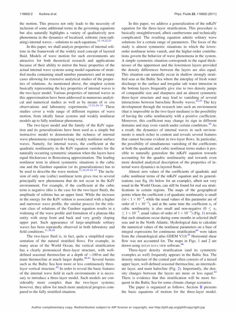
Almost zero values of the coefficients of quadratic and

cubic nonlinear terms of the mKdV equation and its general-

izations (see Eq. (6) below for an example), albeit not very

usual in the World Ocean, can still be found for real sea strati-

fications in certain regions. The maps of the geographical

points where the coefficient a of quadratic nonlinearity is small

(|a|< 1� 10�4, while the usual values of this parameter are of

order of 1� 10�2), and at the same time the coefficient a1 of

cubic nonlinearity is also small and non-negative (0 � a1

� 1� 10�5, usual values of order of 1� 10�3) (Fig. 1) reveals

that such situations occur during some months in selected shelf

seas and in the North Atlantic. Hydrological data to calculate

the numerical values of the nonlinear parameters on a base of

integral expressions for continuous stratification44 were taken

from the climatological atlas GDEM V3.0.45 Horizontal shear

flow was not accounted for. The maps in Figs. 1 and 2 are

drawn using OCEAN DATA VIEW software.46

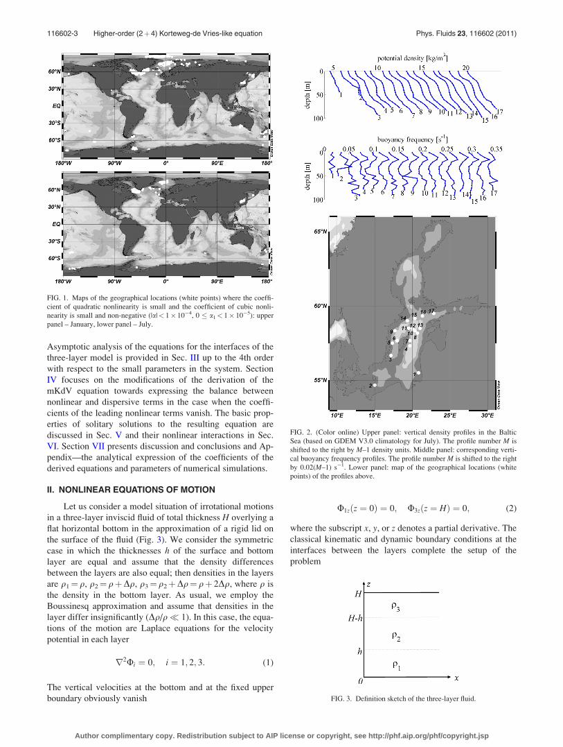
Three-layer density stratification (and its symmetric

examples as well) frequently appears in the Baltic Sea. The

density structure of the central part often consists of a mixed

upper layer, well-defined seasonal thermocline, an intermedi-

ate layer, and main halocline (Fig. 2). Importantly, the den-

sity changes between the layers are more or less equal.42

There is evidence that this stratification will be more fre-

quent in the Baltic Sea for some climate change scenarios.

The paper is organized as follows. Section II presents

the basic equations of motion for the three-layer model.

116602-2 Kurkina et al. Phys. Fluids 23, 116602 (2011)

Author complimentary copy. Redistribution subject to AIP license or copyright, see http://phf.aip.org/phf/copyright.jsp

Asymptotic analysis of the equations for the interfaces of the

three-layer model is provided in Sec. III up to the 4th order

with respect to the small parameters in the system. Section

IV focuses on the modifications of the derivation of the

mKdV equation towards expressing the balance between

nonlinear and dispersive terms in the case when the coeffi-

cients of the leading nonlinear terms vanish. The basic prop-

erties of solitary solutions to the resulting equation are

discussed in Sec. V and their nonlinear interactions in Sec.

VI. Section VII presents discussion and conclusions and Ap-

pendix—the analytical expression of the coefficients of the

derived equations and parameters of numerical simulations.

II. NONLINEAR EQUATIONS OF MOTION

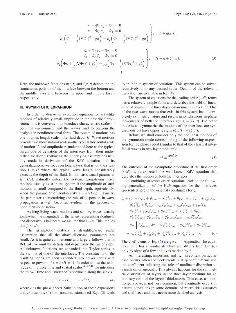
Let us consider a model situation of irrotational motions

in a three-layer inviscid fluid of total thickness H overlying a

flat horizontal bottom in the approximation of a rigid lid on

the surface of the fluid (Fig. 3). We consider the symmetric

case in which the thicknesses h of the surface and bottom

layer are equal and assume that the density differences

between the layers are also equal; then densities in the layers

are q1¼ q, q2¼qþDq, q3¼q2þDq¼ qþ 2Dq, where q is

the density in the bottom layer. As usual, we employ the

Boussinesq approximation and assume that densities in the

layer differ insignificantly (Dq/q� 1). In this case, the equa-

tions of the motion are Laplace equations for the velocity

potential in each layer

r2Ui ¼ 0; i ¼ 1; 2; 3: (1)

The vertical velocities at the bottom and at the fixed upper

boundary obviously vanish

U1zðz ¼ 0Þ ¼ 0; U3zðz ¼ HÞ ¼ 0; (2)

where the subscript x, y, or z denotes a partial derivative. The

classical kinematic and dynamic boundary conditions at the

interfaces between the layers complete the setup of the

problem

FIG. 1. Maps of the geographical locations (white points) where the coeffi-

cient of quadratic nonlinearity is small and the coefficient of cubic nonli-

nearity is small and non-negative (|a|< 1� 10�4, 0 � a1< 1� 10�5): upper

panel – January, lower panel – July.

FIG. 2. (Color online) Upper panel: vertical density profiles in the Baltic

Sea (based on GDEM V3.0 climatology for July). The profile number M is

shifted to the right by M–1 density units. Middle panel: corresponding verti-

cal buoyancy frequency profiles. The profile number M is shifted to the right

by 0.02(M–1) s�1. Lower panel: map of the geographical locations (white

points) of the profiles above.

FIG. 3. Definition sketch of the three-layer fluid.

116602-3 Higher-order (2þ4) Korteweg-de Vries-like equation Phys. Fluids 23, 116602 (2011)

Author complimentary copy. Redistribution subject to AIP license or copyright, see http://phf.aip.org/phf/copyright.jsp

gt þ U1xgx � U1z

¼ 0

gt þ U2xgx � U2z

¼ 0

q1 U1t þ1

2rU1ð Þ2þ gg

� �¼ q2 U2t þ

1

2rU2ð Þ2þ gg

� �9>>=>>;z ¼ hþ gðx; tÞ;

ft þ U2xfx � U2z

¼ 0

ft þ U3xfx � U3z

¼ 0

q2 U2t þ1

2rU2ð Þ2þ gf

� �¼ q3 U3t þ

1

2rU3ð Þ2þ gf

� �9>>=>>;z ¼ H � hþ fðx; tÞ: (3)

Here, the unknown functions g(x, t) and f(x, t) denote the in-

stantaneous position of the interface between the bottom and

the middle layer and between the upper and middle layer,

respectively.

III. ASYMPTOTIC EXPANSION

In order to derive an evolution equation for wavelike

motions of relatively small amplitude in the described envi-

ronment, it is convenient to introduce characteristic scales of

both the environment and the waves, and to perform the

analysis in nondimensional form. The system of motions has

one obvious length scale—the fluid depth H. Wave motions

provide two more natural scales—the typical horizontal scale

of motions L and amplitude a (understood here as the typical

magnitude of deviation of the interfaces from their undis-

turbed location). Following the underlying assumptions usu-

ally made in derivation of the KdV equation and its

generalizations, we focus on long waves, that is, on the situa-

tion L� H where the typical wave length considerably

exceeds the depth of the fluid. In this case, small parameter

�l ¼ H=L naturally enters the system. Long-living wave

motions usually exist in the system if the amplitude of such

motions is small compared to the fluid depth, equivalently,

when the parameter of nonlinearity e ¼ a=H � 1. Finally,

the parameter characterizing the role of dispersion in wave

propagation l ¼ �l2 becomes evident in the process of

nondimensionalisation.

As long-living wave motions and solitary waves usually

exist when the magnitude of the terms representing nonlinear

and dispersive is balanced, we assume that e� l. This implies

that �l �ffiffiep

.

The asymptotic analysis is straightforward under

assumption that all the above-discussed parameters are

small. As it is quite cumbersome and largely follows that in

Ref. 24, we omit the details and depict only the major steps.

All unknown functions are expanded into Taylor series in

the vicinity of one of the interfaces. The constituents of the

resulting series are then expanded into power series with

respect to powers of e ¼ a=H � 1. In order to use the tech-

nique of multiple time and spatial scales,43,47,48 we introduce

the “slow” time and “stretched” coordinate along the x-axis

n ¼ e1=2ðx� ctÞ; s ¼ e3=2t; (4)

where c is the phase speed. Substitution of these expansions

and expressions (4) into nondimensionalised Eqs. (3) leads

to an infinite system of equations. This system can be solved

recursively until any desired order. Details of the relevant

derivation are available in Ref. 49.

The system of equations for the leading order (�e0) terms

has a relatively simple form and describes the field of linear

internal waves in the three-layer environment in question. One

of the two wave modes that exist in this system has a com-

pletely symmetric nature and results in synchronous in-phase

movements of both the interfaces g(x, t)¼ f(x, t). The other

mode is antisymmetric: the motions of the interfaces are syn-

chronous but have opposite signs g(x, t)¼ – f(x, t).Below, we shall consider only the nonlinear motions of

the symmetric mode corresponding to the following expres-

sion for the phase speed (similar to that of the classical inter-

facial waves in two-layer medium):

c2 ¼ ghDqq

: (5)

The outcome of the asymptotic procedure at the first order

(�e1) is, as expected, the well-known KdV equation that

describes the motion of both the interfaces.

Combining of lower-order equations leads to the follow-

ing generalization of the KdV equation for the interfaces

(presented here in the original coordinates for f):

ft þ cfx þ affx þ bfxxx þ a1f2fx þ b1f5x þ c1ffxxx þ c�2fxfxx

þ a�2f3fx þ b2f7x þ c21fxxfxxx þ c22fxfxxxx þ c23ff5x

þ c31f3x þ c32ffxfxx þ c33f

2fxxx þ a3f4fx þ b3f9x

þ c�41fxf6x þ c�42fxxf5x þ c�42fxxxfxxxx þ c51ffxxfxxx

þ c52

ðfxfxxfxxxdxþ c53ffxfxxxx þ c54f

2f5x þ c55f2x fxxx

þ c56fxf2xx þ c�61ff

3x þ c�62f

2fxfxx þ c�63f3fxxx ¼ 0: (6)

The coefficients of Eq. (6) are given in Appendix. The equa-

tion for g has a similar structure and differs from Eq. (6)

only by signs of a few additives marked by *.

An interesting, important, and rich in content particular

case occurs when the coefficients a at quadratic terms and

the coefficient reflecting the role of nonlinear dispersion c1

vanish simultaneously. This always happens for the symmet-

ric distribution of layers in the three-layer medium for an

arbitrary ratio of the layers’ thicknesses. This case, as men-

tioned above, is not very common, but eventually occurs in

natural conditions in some domains of micro-tidal estuaries

and shelf seas and thus needs more detailed analysis.

116602-4 Kurkina et al. Phys. Fluids 23, 116602 (2011)

Author complimentary copy. Redistribution subject to AIP license or copyright, see http://phf.aip.org/phf/copyright.jsp

IV. MODIFIED KdV EQUATION (mKdV)

In essence, the vanishing of the coefficient a at quadratic

terms in the resulting evolution equations means that some

other terms largely govern the motion and that the straight-

forward asymptotic expansion introduced above becomes in-

valid. It is easy to see that, formally, the reason for the

failure is that the assumption of equivalence of the contribu-

tions of nonlinearity and dispersion (e� l) to the formation

of motion patterns is no more valid. In such situations, it is

first necessary to establish which from the higher-order terms

provides the largest contribution to the motion. As the pres-

ence of solitonic solutions in the system in question normally

is associated with a specific balance of nonlinear and disper-

sive terms, it is natural to keep this balance also in the

higher-order modifications to the KdV equation. The appear-

ance of Eqs. (6) suggests that such a balance in symmetric

stratified media is possible if e2� l. This property actually

means that the higher-order nonlinear terms provide a rela-

tively large contribution to the governing equation compared

with the dispersive terms.

Introducing variables g ¼ e~g, f ¼ e~f, ~x ¼ �lx, ~t ¼ �lt, Eq.

(6) can be presented as follows (for simplicity we omit

tildes):

ft þ cfx þ eaffx þ lbfxxx þ e2a1f2fx þ l2b1f5x

þ el c1ffxxx þ c�2fxfxx

� �þ e3a�2f

3fx þ l3b2f7x

þ el2 c21fxxfxxx þ c22fxfxxxx þ c23ff5xð Þþ e2l c31f

3x þ c32ffxfxx þ c33f

2fxxx

� �þ e4a3f

4fx þ l4b3f9x

þ el3 c�41fxf6x þ c�42fxxf5x þ c�43fxxxfxxxx

� �þ e2l2 c51ffxxfxxx þ c52

ðfxfxxfxxxdxþ c53ffxfxxxx

�

þ c54f2f5x þ c55f

2x fxxxþc56fxf

2xx

�þ e3l c�61ff

3x þ c�62f

2fxfxx þ c�63f3fxxx

� �¼ 0: (7)

Making Making use of assumption e2¼ l leads to the follow-

ing equation:

ft þ cfx þ a1f2fx þ bfxxx þ e a�2f

3fx þ c�2fxfxx

� �þ e2 a3f

4fx þ c31f3x þ c32ffxfxx þ c33f

2fxxx þ b1f5x

� �þ O e3

� �¼ 0; (8)

where the analytical expressions for the coefficients are pre-

sented in Appendix and, as above, in the equation for g(x, t)the signs of coefficients a�2 and c�2 are reversed. The lowest

order terms in Eq. (8) form well-known modified KdV equa-

tion (mKdV) that are complemented with terms describing

the contribution of higher-order (O(e) and O(e2)) nonlinear-

ities, nonlinear dispersion and also linear dispersion b1f5x.

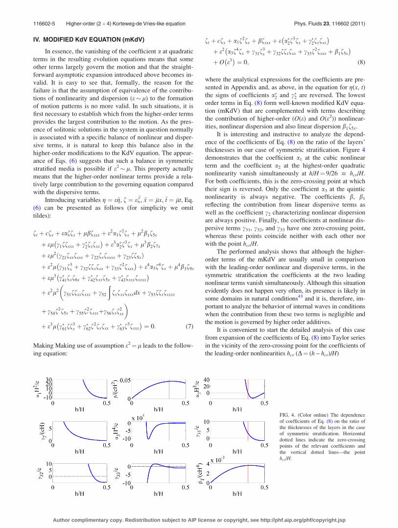
It is interesting and instructive to analyze the depend-

ence of the coefficients of Eq. (8) on the ratio of the layers’

thicknesses in our case of symmetric stratification. Figure 4

demonstrates that the coefficient a1 at the cubic nonlinear

term and the coefficient a2 at the highest-order quadratic

nonlinearity vanish simultaneously at h/H¼ 9/26 : hcr/H.

For both coefficients, this is the zero-crossing point at which

their sign is reversed. Only the coefficient a3 at the quintic

nonlinearity is always negative. The coefficients b, b1

reflecting the contribution from linear dispersive terms as

well as the coefficient c2 characterizing nonlinear dispersion

are always positive. Finally, the coefficients at nonlinear dis-

persive terms c31, c32, and c33 have one zero-crossing point,

whereas these points coincide neither with each other nor

with the point hcr/H.

The performed analysis shows that although the higher-

order terms of the mKdV are usually small in comparison

with the leading-order nonlinear and dispersive terms, in the

symmetric stratification the coefficients at the two leading

nonlinear terms vanish simultaneously. Although this situation

evidently does not happen very often, its presence is likely in

some domains in natural conditions43 and it is, therefore, im-

portant to analyze the behavior of internal waves in conditions

when the contribution from these two terms is negligible and

the motion is governed by higher order additives.

It is convenient to start the detailed analysis of this case

from expansion of the coefficients of Eq. (8) into Taylor series

in the vicinity of the zero-crossing point for the coefficients of

the leading-order nonlinearities hcr (D¼ (h – hcr)/H)

FIG. 4. (Color online) The dependence

of coefficients of Eq. (8) on the ratio of

the thicknesses of the layers in the case

of symmetric stratification. Horizontal

dotted lines indicate the zero-crossing

points of the relevant coefficients and

the vertical dotted lines—the point

hcr/H.

116602-5 Higher-order (2þ4) Korteweg-de Vries-like equation Phys. Fluids 23, 116602 (2011)

Author complimentary copy. Redistribution subject to AIP license or copyright, see http://phf.aip.org/phf/copyright.jsp

a1 ¼ �c

H2

57122

243Dþ O D2

� �¼ ~a1Dþ O D2

� �;

b ¼ cH2 63

1352þ 1

52D

� �þ O D2

� �¼ ~bþ O Dð Þ;

a�2 ¼c

H3

5940688

6561Dþ O D2

� �¼ ~a2Dþ O D2

� �;

c�2cH¼ 7

13� 115

18Dþ O D2

� �;

a3H4

c¼ � 47411260

59049þ 12084101978

531441Dþ O D2

� �;

c31

c¼ 1483

486� 298285

2916Dþ O D2

� �;

c32

c¼ 2341

486� 641017

2916Dþ O D2

� �;

c33

c¼ � 109

243� 30589

2916Dþ O D2

� �;

b1

cH4¼ 66291

18279040þ 1099

1054560Dþ O D2

� �:

The extension of the mKdV equation towards inclusion of

the higher-order terms for small values of D (equivalently, in

the vicinity of the point hcr) is as follows:

ft þ cfx þ ~a1Df2fx þ ~bfxxx þ e ~a�2Df3fx þ ~c�2fxfxx

� �þ e2 ~a3f

4fx þ ~c31f3x þ ~c32ffxfxx þ ~c33f

2fxxx þ ~b1f5x

� �þ O e3

� �¼ 0: (9)

It is easy to see that in this particular case of the symmetric

three-layer stratification a balance between nonlinear and

dispersive effects exists when the small parameters D and eare related as follows D� e2. After performing rescaling

x_ ¼ �lx, t

_ ¼ �lt and removing the “hats,” we have

ft þ e2 ~a1f2fx þ ~a3f

4fx

� �þ l~bfxxx þ el~c�2fxfxx

þ e2l ~c31f3x þ ~c32ffxfxx þ ~c33f

2fxxx

� �þ l2 ~b1f5x

þ O e3; l3; el2� �

¼ 0;

where, as above, the equation for g(x, t) only differs from the

above one by the reversed sign of the coefficient ~c�2.

Summarizing the above considerations, in this particular

case the balance between the leading (nonzero) dispersive

and nonlinear terms occurs when e2¼ l. In the coordinate

system consisting of slow time and stretched x-axis

x ¼ x� ct, t_ ¼ e2t, the relevant equation for any of the inter-

faces is (the “hats” omitted)

ft þ ~a1f2fx þ ~a3f

4fx þ ~bfxxx ¼ 0: (10)

Equation (10) provides a description of motions and phe-

nomena occurring in situations when the leading-order non-

linear and dispersive terms of the mKdV equation are

negligible. In this case, the resulting equation contains two

leading nonlinear terms of the same magnitude: the cubic

and quintic nonlinearities. Both the terms consist of the prod-

uct of a power (2nd or 4th) of the unknown function and its

first-order spatial derivative. The resulting equation differs

from the classical Gardner equation (that is frequently used

for motions in situations containing zero-crossing of the

coefficient at the quadratic nonlinearity, for example, in two-

layer media with almost equal layers) by the presence of the

quintic nonlinearity. This equation, obviously, belongs to the

family of generalized Gardner equations50,51 used to describe

different properties of internal waves. Following the nomen-

clature of different extensions of the KdV equation, Eq. (10)

may be called 2þ 4 Korteweg-de Vries-like equation, abbre-

viated 2þ 4 KdV.

The above has shown that auxiliary equations derived in

the process of the asymptotic analysis had different appear-

ances for different interfaces. Remarkably, Eq. (10) is uni-

versal in the sense that it is identical for both the upper and

the lower interfaces. This feature is not completely unex-

pected as the classical mKdV equation is also universal for

both the interfaces. Therefore, we can analyze only one

equation (10) without the loss of generality. We shall do this

for the upper interface f(x, t).As equations ftþ fnfxþ fxxx¼ 0 with n> 2 are non-

integrable (in particular, with respect to the Zakharov-Shabat

method52,53), it is likely that Eq. (10) is also non-integrable.

The question about its integrability is, however, out of the

scope of the current study.

Differently from Eq. (8), Eq. (10) has two conservation

laws of mass and energy

M ¼ð1�1

fdx; E ¼ð1�1

f2dx: (11)

The decisive parameters for wave motion in media described

by Eq. (10) are the signs of the coefficients at its nonlinear

terms. As mentioned above, the coefficient a1 at the cubic

nonlinearity is sign-variable in the vicinity of hcr/H. The

coefficient a3 at the quintic nonlinearity is negative in this

region but may change its sign at h/H< (423 – 3ffiffiffiffiffiffiffiffiffiffi6641p

)/

1324 0.1348. The analysis of the stratification correspond-

ing to these values of the layers’ thicknesses is out of the

scope of this paper, mostly because it corresponds to quite

large values of D but Eq. (10) is valid in the neighborhood of

D¼ 0.

An important feature of Eq. (10) is that it has solitary

wave solutions. The relevant analysis of their existence and

appearance (including the impact of the quintic nonlinearity

on their shape compared to that of the classical mKdV equa-

tion) is presented in the following sections. It is well-known

that solitons of the extensions of KdV equations of the form

ftþ fnfxþ fxxx¼ 0 with n 4 are unstable,53 and that for such

equations both smooth and localized initial conditions develop

singularities within finite time (or at finite distances). To our

knowledge, neither integrability of Eq. (10) nor stability of

solitary wave solutions for Eq. (10) (or its analogues with

combined (cubic and quintic) nonlinearity) has been addressed

in literature. But all our numerical simulations of the initial

problem for Eq. (10) with smooth and localized initial condi-

tions showed a stable wave dynamics, with no evidence of

instabilities or collapses even in interactions. Therefore, it

seems plausible that the cubic nonlinearity plays a stabilizing

116602-6 Kurkina et al. Phys. Fluids 23, 116602 (2011)

Author complimentary copy. Redistribution subject to AIP license or copyright, see http://phf.aip.org/phf/copyright.jsp

role. This conjecture, however, requires a more detailed study,

which is out of scope of this paper.

V. SOLITARY WAVE SOLUTIONS

Let us consider steady-state (in a properly chosen mov-

ing coordinate system) localized solutions fs(x – Vt) to Eq.

(10). Such solutions can be expressed in implicit form in

terms of the integral

Y � Y0 ¼ffiffiffib

p ðvS

v0

Vf2 � a1

6f4 � e

a3

15f6

� ��1=2

df; (12)

where V is the propagation speed of the disturbance and

Y¼ x – Vt. The substitution A¼ f2 would reduce Eq. (12) to

a similar expression for the Gardner equation, and the soli-

tary wave solutions can be derived. For a1> 0 these solu-

tions can be expressed explicitly

fðYÞ ¼ 6

ffiffiffiffiffiffiffiffiffiffiffiffiffiffiffiffiffiffiffiffiffiffiffiffiffiffiffiffiffiffiffiffiffiffiffiffiffiffiffiffiffiffiffiffiffiffiffiffiffiffiffiffiffiffiffiffiffiffiffiffiffiffiffiffiffiffiffiffiffiffiffiffiffiffi60V

5a1 þffiffiffiffiffiffiffiffiffiffiffiffiffiffiffiffiffiffiffiffiffiffiffiffiffiffiffiffiffiffi25a2

1 þ 240a3Vp

cosh 2YffiffiffiVb

q� �vuut : (13)

It is easy to demonstrate that Eq. (13) describes localized sol-

utions to Eq. (10). The maximum amplitude a of the excur-

sions of the interface is obviously

a ¼ffiffiffiffiffiffiffiffiffiffiffiffiffiffiffiffiffiffiffiffiffiffiffiffiffiffiffiffiffiffiffiffiffiffiffiffiffiffiffiffiffiffiffiffiffiffiffiffi

60V

5a1 þffiffiffiffiffiffiffiffiffiffiffiffiffiffiffiffiffiffiffiffiffiffiffiffiffiffiffiffiffiffi25a2

1 þ 240a3Vp

s: (14)

Similarly to the solutions of the Gardner equation, the propa-

gation speed of such solutions depends on their amplitude a

V ¼ a1

6a2 þ a3

15a4:

The natural limit for the wave speed stems from the request

that expressions under the square root in Eqs. (13) and (14)

must be non-negative for physically meaningful solutions.

This condition means that the wave speed V has an upper

limit

Vlim ¼ �5a2

1

48a3

: (15)

Consequently, the amplitude of solutions is also limited by

the following value:

alim ¼1

2

ffiffiffiffiffiffiffiffiffi5a1

�a3

s: (16)

The limiting amplitude in Eq. (16) can be expressed using

the relative thickness of the lower and upper layers (equiva-

lently, using the ratio l¼ h/H):

alim

H¼ 2

3l2ffiffiffiffiffi15p ffiffiffiffiffiffiffiffiffiffiffiffiffiffiffiffiffiffiffiffiffiffiffiffiffiffiffiffiffiffiffiffiffiffiffiffiffiffiffiffiffiffiffiffiffiffiffiffiffiffiffiffiffiffiffiffiffi

9� 26l

1324l3 � 1508l2 þ 513l� 45

r: (17)

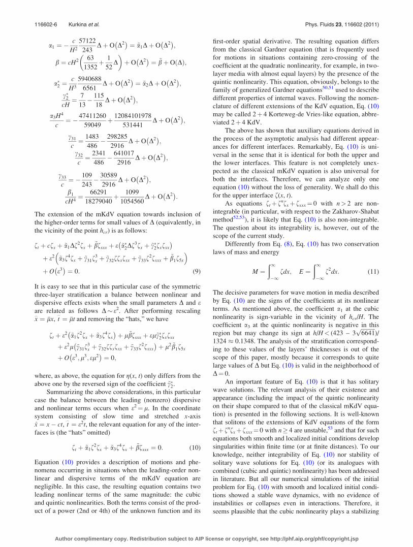
The limiting amplitude reaches its maximum values alim

0.0864 H at h/H 0.286. This corresponds to the highest

possible location hþ alim 0.397 H of the lower interface,

whereas the relevant h 0.3243 H insignificantly differs

from hcr.

The dependence of the limiting amplitude alim on the rel-

ative thickness of layers h/H has quite a complicated appear-

ance (Fig. 5). This amplitude increases slowly with the

increase in h/H and reveals a very gently sloping maximum at

h/H 0.286. Further increase in h/H is first accompanied

with a gentle decrease in alim that is replaced by almost explo-

sive decrease in the limiting amplitude near the zero-crossing

point h/H¼ 9/26.

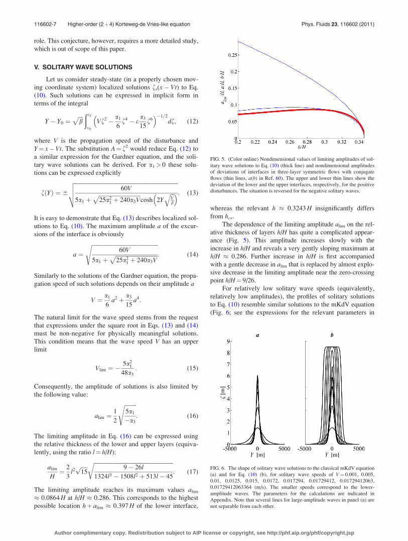
For relatively low solitary wave speeds (equivalently,

relatively low amplitudes), the profiles of solitary solutions

to Eq. (10) resemble similar solutions to the mKdV equation

(Fig. 6; see the expressions for the relevant parameters in

FIG. 5. (Color online) Nondimensional values of limiting amplitudes of sol-

itary wave solutions to Eq. (10) (thick line) and nondimensional amplitudes

of deviations of interfaces in three-layer symmetric flows with conjugate

flows (thin lines, a(b) in Ref. 60). The upper and lower thin lines show the

deviation of the lower and the upper interfaces, respectively, for the positive

disturbances. The situation is reversed for the negative solitary waves.

FIG. 6. The shape of solitary wave solutions to the classical mKdV equation

(a) and for Eq. (10) (b), for solitary wave speeds of V¼ 0.001, 0.005,

0.01, 0.0125, 0.015, 0.0172, 0.017294, 0.01729412, 0.01729412063,

0.01729412063364 (m/s). The smaller speeds correspond to the lower-

amplitude waves. The parameters for the calculations are indicated in

Appendix. Note that several lines for large-amplitude waves in panel (a) are

not separable from each other.

116602-7 Higher-order (2þ4) Korteweg-de Vries-like equation Phys. Fluids 23, 116602 (2011)

Author complimentary copy. Redistribution subject to AIP license or copyright, see http://phf.aip.org/phf/copyright.jsp

Appendix). For larger wave speeds (larger amplitudes), the

two sets of solutions considerable differ from each other.

The key difference is that large-amplitude solutions to Eq.

(10) form a table-like wide signal that may, theoretically,

infinitely widen in the process V ! Vlim whereas their ampli-

tude asymptotically tends to alim. Both positive and negative

solitary wave solutions are possible for each combination of

the signs of the coefficients of Eq. (10).

Similar table-like solutions are characteristic for some

other equations containing higher-order nonlinear terms, for

example, they exist for the Gardner equation that describes

motions in the two-layer fluid and where the cubic nonlinearity

is of the leading order. The existence of such wide table-like

solitons and the possibility of their propagation in combina-

tions with other solitons have been demonstrated for several

other classes of nonlinear wave models.27,38,54,55

The solutions in question have several features similar

to Gardner solitons; in particular, their amplitude is limited

and the increase in the amplitude is accompanied by virtually

unlimited widening of the wave profile. The set of Gardner

solitons has much more rich in content variety of properties

compared to the KdV and mKdV solitons. For example, this

set allows for propagation of smaller solitons along the wide

table-like crest of large solitons the amplitude of which is

close to the limiting one, or the possibility of formation of

two trains of solitons of different polarity during the process

of dispersion of disturbances with amplitudes exceeding the

limiting amplitude. Moreover, the development of the sys-

tem of solitons is very much different for rectangular and

smooth initial pulses of otherwise equivalent properties. It is

natural to expect that the set of solutions to Eq. (10) also pos-

sesses a larger variety of different features compared to the

ensembles of KdV or mKdV solitons.

The described table-like appearance of solutions for the

relatively large-amplitude and rapidly moving disturbances

with steep fronts may have substantial consequences in prac-

tical applications. The propagation of such disturbances is

similar to the motion of smooth bores that possess consider-

able danger for objects on their way. Such horizontal

motions (smooth bores, sometimes called conjugate flows)

are frequent in vertically inhomogeneous fluids.56–58 The

performed analysis shows that such flows can naturally occur

in three-layer fluids for some combinations of the layers’

thicknesses and density variations.

Numerical simulations of flows in media with continu-

ous vertical stratification with two pycnoclines and with a

simplified three-layer model have been performed by several

authors.59–61 A comparison of the results of the theory of

conjugate fluxes in symmetric three-layer environment with

the values of the limiting amplitude based on Eqs. (16) and

(17) is presented in Fig. 5. For the situations in which the

thicknesses of the upper and lower layers are close to hcr, the

amplitudes of deviations of the interfaces from their undis-

turbed locations are relatively small and almost equal for all

the presented cases, for conjugate fluxes in the nonlinear

model and for the above derived estimate of alim in the

weakly nonlinear model. If the thicknesses of the layers are

considerably different from hcr, the amplitudes of deviations

of the upper and lower interfaces become substantially

different. It is remarkable that the estimate of the deviation

alim in the weakly nonlinear framework practically coincides

with one of those for the fully nonlinear case for a wide

range of h/H. The similarity occurs for the deviation of the

interface that bends into the thinner outer (the uppermost or

the lowermost) layer.

For the range of layers’ depths h> hcr (D> 0), a solution

exists neither for our weakly nonlinear approach nor in the

theory of conjugate flows.

VI. INTERACTIONS OF SOLITARY SOLUTIONSOF THE 2 1 4 KdV EQUATION

Generally speaking, interactions and collisions of soli-

tary solutions to non-integrable evolution equations are

inelastic. It is, therefore, not unexpected that solitary solu-

tions to Eq. (10) interact inelastically with each other and

with the background wave fields. As a demonstration of this

feature, we present an example of numerically simulated col-

lision of two solitonic solutions corresponding to the values

of coefficients given in Appendix.

The numerical code used in integration of Eq. (10)

employs an implicit pseudo-spectral method62 that conserves

the integrals presented in Eq. (11). The spatial domain was

chosen based on the analytically estimated propagation speed

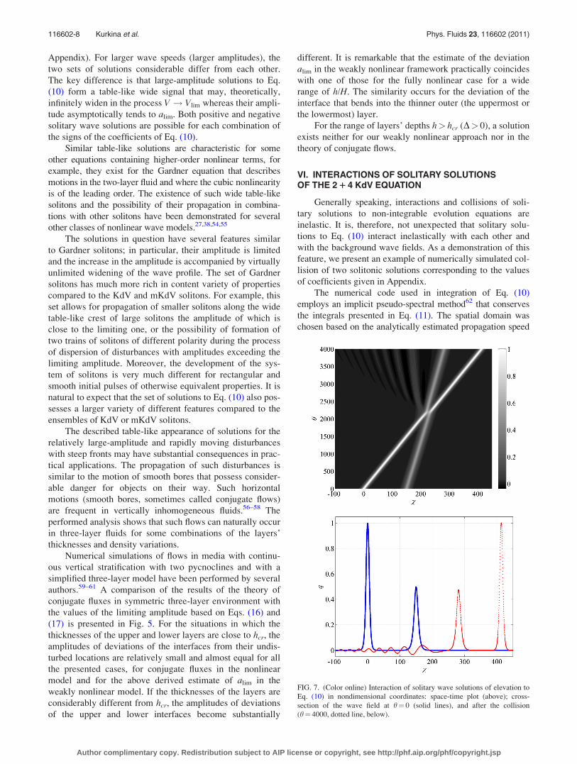
FIG. 7. (Color online) Interaction of solitary wave solutions of elevation to

Eq. (10) in nondimensional coordinates: space-time plot (above); cross-

section of the wave field at h¼ 0 (solid lines), and after the collision

(h¼ 4000, dotted line, below).

116602-8 Kurkina et al. Phys. Fluids 23, 116602 (2011)

Author complimentary copy. Redistribution subject to AIP license or copyright, see http://phf.aip.org/phf/copyright.jsp

of solitons and interaction time and was extended as occasion

required. The numerical code was tested against exact analyti-

cal multisoliton solutions to the classical mKdV equation and

by means of long-term tracking of propagation of exact soli-

tary solutions to Eq. (10) in the absence of other disturbances.

In particular, the results of the latter test did not change when

the spatial step was decreased by a factor of two. For simplic-

ity, we use the nondimensional form of Eq. (10)

qh þ q2qv � q4qv þ qvvv ¼ 0; (18)

where

h ¼ a31

a3

3=4

ðbÞ�1=2t; v ¼ a31

a3

1=4

ðbÞ�1=2x; q ¼ a1

a3

1=2

1:

(19)

The step in the x-direction was set to 0.2 and the step in time

to 0.1. The performed tests indicated that the numerical inac-

curacies for this choice of parameters is of the order of 10�6

whereas the value of the small parameter l > 0.04.

The initial state was composed from two solitary

waves with nondimensional amplitudes of 1 and 60.5. The

nondimensional limiting amplitude for the parameters in use

isffiffiffi5p

=2 1:118. The corresponding dimensional ampli-

tudes would have been 7.62 m and 63.81 m, respectively.

Before integrating this constellation, evolution of each of the

counterparts was integrated until h¼ 4000. During this inter-

val, the total error of the numerical solution (caused, e.g., by

small distortions of the amplitude of the numerical solution

owing to its discrete representation and by radiation of wave

energy) did not exceed 1� 10�6.

The initial state for studies of interaction of these soli-

tary waves was composed simply as a linear superposition of

the counterparts. The smaller wave was placed ahead of the

larger one, at a distance (counted as the distance between the

relevant maxima) of 150 nondimensional units of length.

The simulation was performed until h¼ 4000, that is, quite a

long time after the interaction of the highest parts of the

waves was terminated (Fig. 7).

The evolution of solitary waves of elevation resembled

the typical scenarios for soliton interactions of similar type

in the classical KdV and mKdV frameworks in which the

taller wave overtakes the smaller one.63,64 In such interac-

tions, the counterparts usually lose their identity and merge

into a composite structure at a certain instant. After a while,

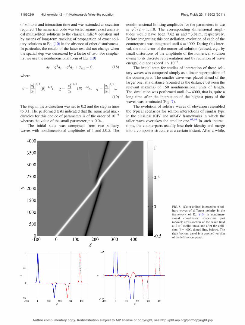
FIG. 8. (Color online) Interaction of sol-

itary waves of different polarity in the

framework of Eq. (10) in nondimen-

sional coordinates: space-time plot

(above); cross-section of the wave field

at h¼ 0 (solid lines), and after the colli-

sion (h¼ 4000, dotted line, below). The

right bottom panel is a zoomed version

of the left bottom panel.

116602-9 Higher-order (2þ4) Korteweg-de Vries-like equation Phys. Fluids 23, 116602 (2011)

Author complimentary copy. Redistribution subject to AIP license or copyright, see http://phf.aip.org/phf/copyright.jsp

the counterparts emerge again whereas one cannot say

whether the counterparts propagate through each other as

waves do or collide as particles do. The interaction process

is accompanied, as in the case of KdV solitons, by a clear

decrease of the amplitude of the composite structure during

the merging phase and by a substantial phase shift.

Differently from processes governed by integrable equa-

tions, the collision was accompanied by generation of very

long and almost stationary localized depression area. The

entire process was also accompanied by a modest radiation

of wave energy from the interaction region. The amplitude

of wavelike disturbances was about 4� 10�2, that is, by sev-

eral orders of magnitude larger than the level of numerical

errors (<1� 10�6). This level of wave generation signifies

the effects of dispersion on the evolution of the system. Note

that the amplitude of the disturbances matches the magnitude

of the relevant dispersive terms O(l)¼O(D) that also is

about 4� 10–2.

The collision of solitary waves of different polarities has

a similar appearance. Both the counterparts largely survive the

collision but the phase shift for the wave of depression is

more pronounced (Fig. 8). The amplitude of radiated waves

is, however, much smaller than in the above case and does not

exceed 1� 10�2. Test simulations with a twice higher spatial

resolution led to practically identical results. Therefore, the

described side effects such as wave radiation in both cases

and the formation of a long depression area in the collision of

waves of elevation evidently are an inherent part of interac-

tions of solitary waves in the framework of Eq. (10).

Consequently, collisions of solitary wave solutions of

Eq. (10) basically have inelastic nature although both the in-

tensity of wave radiation and changes to the amplitudes of

the solitons are fairly minor. For example, the collision of

waves of elevation led to the increase in the amplitude of the

taller soliton from 1 to 1.002 and an accompanying decrease

in the smaller solution from 0.5 to 0.477. The collision of

waves of different polarity led to much smaller changes: the

post-collision amplitudes of the waves were 1.001 and

�0.499, respectively. Note that this effect also does not

exceed the order of O(l). The effects caused by interactions

of different solitary waves with similar entities and with the

wave background could, of course, be much larger during

longer time intervals and/or caused by multiple collisions.

As expected for non-integrable equations, such interactions

should finally lead to damping of solitary waves to a level of

magnitude at which they are either practically linear or are

governed by a different balance of nonlinear and dispersive

terms.

VII. CONCLUSIONS AND DISCUSSION

Although contemporary numerical methods and fully

nonlinear approaches such as the method of conjugate flows

allow for extensive studies into properties of highly nonlin-

ear internal waves, many specific features can still be recog-

nized, analyzed, and understood using classical methods for

analytical studies into internal waves in ideal layered fluids

and in the weakly nonlinear framework. Such fully analytical

methods make it possible to exactly establish qualitative

appearance of disturbances of different shapes and ampli-

tudes, and, more importantly, to understand the specific fea-

tures of the behavior of waves corresponding to situation

where a substantial change in the overall regime of wave

propagation is possible.

The performed analytical investigation of different

regimes of wave propagation in a relatively simple but fre-

quently occurring in nature symmetric three-layer environ-

ment reveals several interesting feature of wave shapes that

are usually hidden in the analysis of non-symmetric situa-

tions. The key development is the derivation of a new non-

linear evolution equation that describes the wave motion in

situations where all the leading-order nonlinear terms in the

classical modified Korteweg-de Vries (mKdV) equation van-

ish simultaneously. Such situations may happen quite fre-

quently in relatively shallow non-tidal strongly stratified

basins such as the Baltic Sea. In this case, the evolution

equation governing wave motion contains two nonlinear

terms (cubic and quintic nonlinearities) of the same magni-

tude. This equation is obtained using the basically standard

asymptotic procedure that is widely used in similar problems

and is of the second order of accuracy as the mKdV equation

for the non-symmetric situation.

The resulting equation differs from the mKdV equation

in two important aspects. First, it reflects a different balance

between the (higher-order) nonlinear terms and the disper-

sive terms compared to that exploited in the mKdV equation.

More importantly, this equation contains two nonlinear terms

of the same magnitude—the cubic and quintic nonlinearities,

the latter one distinguishing the resulting equation from the

mKdV equation. The resulting equation has solitary wave

solutions. As this equation probably is not integrable, the

possible solitonic nature of these solutions, the persistence of

these solutions in interactions and the existence of multisoli-

ton solutions is a subject of further research.

The presence of the quintic nonlinearity does not sub-

stantially modify the shape of the solitons of relatively small

amplitude but leads to radical changes in the appearance of

larger-amplitude solitary waves. Their amplitude and propa-

gation speed are limited. Larger-amplitude solitons have a

table-like shape with very steep fronts. The motion of such

solitary waves may be accompanied by high water speeds

and strong hydrodynamic loads in the areas where the struc-

ture of medium is favorable for their existence. It is likely

that the classical solitary solutions to the mKdV equation are

transformed into such structures when they approach sea

areas where the coefficients at the lower-order nonlinear

terms vanish.

ACKNOWLEDGMENTS

The research is partially supported by Russian Founda-

tions for Basic Research grants (10-05-00199, 09-05-00204,

11-02-00483, and 11-05-00216), Estonian Science Founda-

tion (Grant No. 7413), the BONUSþ BalticWay project and

the targeted financing by the Estonian Ministry of Education

and Science (Grant No. SF0140007s11). O.K., A.K., and

E.R. acknowledge as well RF President grant for young

researchers MD-99.2010.5.

116602-10 Kurkina et al. Phys. Fluids 23, 116602 (2011)

Author complimentary copy. Redistribution subject to AIP license or copyright, see http://phf.aip.org/phf/copyright.jsp

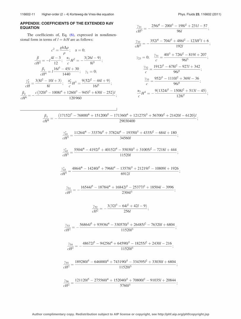
APPENDIX: COEFFICIENTS OF THE EXTENDED KdVEQUATION

The coefficients of, Eq. (6), expressed in nondimen-

sional form in terms of l ¼ h/H are as follows:

c2 ¼ ghDqq

; a ¼ 0;

bcH2¼ �l

4l� 3

12;

a1

cH2 ¼ � 3 26l� 9ð Þ

8l3;

b1

cH4¼ l

16l3 � 45lþ 30

1440; c1 ¼ 0;

c�2cH¼ 3 8l2 � 10lþ 3ð Þ

8l;

a�2c

H3 ¼ 9 52l2 � 44lþ 9ð Þ16l5

;

b2

cH6¼�

c 320l5� 1008l4þ 1260l3� 945l2þ 630l� 252� �

l

120 960;

c21

cH3¼ � 256l4 � 200l3 � 198l2 þ 231l� 57

96l;

c22

cH3¼ � 352l4 � 704l3 þ 486l2 � 123H3lþ 6

192l;

c23 ¼ 0;c31

c¼ 40l3 þ 726l2 � 819lþ 207

96l3;

c32

c¼ 1912l3 � 678l2 � 927lþ 342

96l3;

c33

c¼ 952l3 � 1110l2 þ 369l� 36

96l3;

a3

cH4 ¼ � 9 1324l3 � 1508l2 þ 513l� 45ð Þ

128l7;

b3

cH8¼ �

17152l7 � 76800l6 þ 151200l5 � 171360l4 þ 121275l3 þ 56700l2 þ 21420l� 6120� �

l

29030400;

c�41

cH5¼ 11264l6 � 33376l5 þ 37824l4 � 19350l3 þ 4335l2 � 684lþ 180

34560l;

c�42

cH5¼ 5504l6 � 4192l5 þ 40152l4 � 55030l3 þ 31005l2 � 7218lþ 444

11520l;

c�43

cH5¼ 4864l6 � 14240l5 þ 7968l4 � 13578l3 þ 21219l2 � 10809lþ 1926

6912l;

c51

cH2¼ � 16544l5 � 18784l4 þ 16842l3 � 25377l2 þ 18504l� 3996

2304l3;

c52

cH2¼ � 3 32l3 � 64l2 þ 42l� 9ð Þ

256l;

c53

cH2¼ � 56864l5 þ 93936l4 � 330570l3 þ 26485l2 � 76320lþ 6804

11520l3;

c54

cH2¼ � 48672l5 � 94256l4 þ 64590l3 � 18255l2 þ 2430l� 216

11520l3;

c55

cH2¼ 189280l5 � 646880l4 þ 743190l3 � 334395l2 þ 33030lþ 6804

11520l3;

c56

cH2¼ 121120l5 � 275560l4 þ 152040l3 þ 70800l2 � 91035lþ 20844

5760l3;

116602-11 Higher-order (2þ4) Korteweg-de Vries-like equation Phys. Fluids 23, 116602 (2011)

Author complimentary copy. Redistribution subject to AIP license or copyright, see http://phf.aip.org/phf/copyright.jsp

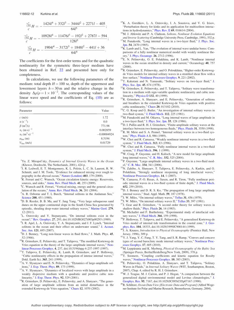
c�61

cH ¼ � 1424l4 þ 332l3 � 3444l2 þ 2271l� 405

64l5;

c�62

cH ¼ � 10928l4 � 11476l3 � 192l2 þ 2787l� 594

128l5;

c�63

cH ¼ � 1904l4 � 3172l3 þ 1848l2 � 441lþ 36

64l5:

The coefficients for the first-order terms and for the quadratic

nonlinearity for the symmetric three-layer medium have

been obtained in Ref. 22 and presented here only for

completeness.

In calculations, we use the following parameters of the

medium: total depth H¼ 100 v, depth of the uppermost and

lowermost layers h¼ 30 m and the relative change in the

density Dq/q¼ 1� 10�2. The corresponding values of the

linear wave speed and the coefficients of Eq. (10) are as

follows:

Parameter Value

c (m/s) 1.72

a (s�1) 0.0

b (m3/s) 771.98

a1 (m�s)�1 0.002859

a3 (m3�s)�1 �0.00004924

alim (m) 8.5194

Vlim (m/s) 0.01729

1Yu. Z. Miropol’sky, Dynamics of Internal Gravity Waves in the Ocean(Kluwer, Dordrecht, The Netherlands, 2001), 424 p.

2J. R. Ledwell, E. T. Montgomery, K. L. Polzin, L. C. St. Laurent, R. W.

Schmitt, and J. M. Toole, “Evidence for enhanced mixing over rough to-

pography in the abyssal ocean,” Nature (London) 403, 179 (2000).3R. Ferrari and C. Wunsch, “Ocean circulation kinetic energy: Reservoirs,

sources, and sinks,” Annu. Rev. Fluid Mech. 41, 253 (2009).4C. Wunsch and R. Ferrari, “Vertical mixing, energy and the general circu-

lation of the oceans,” Annu. Rev. Fluid Mech. 36, 281 (2004).5A. R. Osborne and T. L Burch, “Internal solitons in the Andaman Sea,”

Science 208, 451 (1980).6D. B. Reeder, B. B. Ma, and Y. Jang Yang, “Very large subaqueous sand

dunes on the upper continental slope in the South China Sea generated by

episodic, shoaling deep-water internal solitary waves,” Marine Geol. 279,

12 (2011).7L. Ostrovsky and Y. Stepanyants, “Do internal solitons exist in the

ocean?,” Rev. Geophys. 27, 293, doi:10.1029/RG027i003p00293 (1989).8J. R. Apel, L. A. Ostrovsky, Y. A. Stepanyants, and J. F. Lynch, “Internal

solitons in the ocean and their effect on underwater sound,” J. Acoust.

Soc. Am. 121, 695 (2007).9D. J. Benney, “Long non-linear waves in fluid flows,” J. Math. Phys. 45,

52 (1966).10R. Grimshaw, E. Pelinovsky, and T. Talipova, “The modified Korteweg-de

Vries equation in the theory of the large–amplitude internal waves,” Non-

linear Processes Geophys. 4, 237, doi:10.5194/npg-4-237-1997 (1997).11T. Talipova, E. Pelinovsky, K. Lamb, R. Grimshaw, and P. Holloway,

“Cubic nonlinearity effects in the propagation of intense internal waves,”

Dokl. Earth Sci. 365, 241 (1999).12A. V. Slyunyaev and E. N. Pelinovsky, “Dynamics of large-amplitude sol-

itons,” J. Exp. Theor. Phys. 89, 173 (1999).13A. V. Slyunyaev, “Dynamics of localized waves with large amplitude in a

weakly dispersive medium with a quadratic and positive cubic non-

linearity,” J. Exp. Theor. Phys. 92, 529 (2001).14R. Grimshaw, D. Pelinovsky, E. Pelinovsky, and A. Slunyaev, “The gener-

ation of large amplitude solitons from an initial disturbance in the

extended Korteweg-de Vries equation,” Chaos 12, 1070 (2002).

15K. A. Gorshkov, L. A. Ostrovsky, I. A. Soustova, and V. G. Irisov,

“Perturbation theory for kinks and its application for multisoliton interac-

tions in hydrodynamics,” Phys. Rev. E 69, 016614 (2004).16M. J. Ablowitz and P. A. Clarkson, Solitons, Nonlinear Evolution Equations

and Inverse Scattering (Cambridge University Press, Cambridge, 1991), 532 p.17M. Funakoshi, “Long internal waves in a two-layer fluid,” J. Phys. Soc.

Jpn. 54, 2470 (1985).18K. Lamb and L. Yan, “The evolution of internal wave undular bores: Com-

parisons of a fully nonlinear numerical model with weakly nonlinear the-

ory,” J. Phys. Oceanogr. 26, 2712 (1996).19E. N. Pelinovsky, O. E. Polukhina, and K. Lamb, “Nonlinear internal

waves in the ocean stratified in density and current,” Oceanology 40, 757

(2000).20R. Grimshaw, E. Pelinovsky, and O. Poloukhina, “Higher-order Korteweg-

de Vries models for internal solitary waves in a stratified shear flow with a

free surface,” Nonlinear Processes Geophys. 9, 221 (2002).21T. Kakutani and N. Yamasaki, “Solitary waves on two-layer fluid,” J.

Phys. Soc. Jpn. 45, 674 (1978).22R. Grimshaw, E. Pelinovsky, and T. Talipova, “Solitary wave transforma-

tion in a medium with sign-variable quadratic nonlinearity and cubic non-

linearity,” Physica D 132, 40 (1999).23R. Grimshaw, A. Slunyaev, and E. Pelinovsky, “Generation of solitons

and breathers in the extended Korteweg-de Vries equation with positive

cubic nonlinearity,” Chaos 20, 013102 (2010).24C. G. Koop and G. Butler, “An investigation of internal solitary waves in

two-fluid system,” J. Fluid Mech. 112, 225 (1981).25M. Funakoshi and M. Oikawa, “Long internal waves of large amplitude in

a two-layer fluid,” J. Phys. Soc. Jpn. 55, 128 (1986).26D. I. Pullin and R. H. J. Grimshaw, “Finite-amplitude solitary waves at the

interface between two homogeneous fluids,” Phys. Fluids 31, 3550 (1998).27R. M. Mirie and S. A. Pennel, “Internal solitary waves in a two-fluid sys-

tem,” Phys. Fluids A 1, 986 (1989).28W. Choi and R. Camassa, “Weakly nonlinear internal waves in a two-fluid

system,” J. Fluid Mech. 313, 83 (1996).29W. Choi and R. Camassa, “Fully nonlinear internal waves in a two-fluid

system,” J. Fluid Mech. 396, 1 (1999).30W. Craig, P. Guyenne, and H. Kalisch, “A new model for large amplitude

long internal waves,” C. R. Mec. 332, 525 (2004).31P. Guyenne, “Large-amplitude internal solitary waves in a two-fluid mod-

el,” C. R. Mec. 334, 341 (2006).32N. Zahibo, A. Slunyaev, T. Talipova, E. Pelinovsky, A. Kurkin, and O.

Polukhina, “Strongly nonlinear steepening of long interfacial waves,”

Nonlinear Processes Geophys. 14, 1 (2007).33R. Camassa, P.-O. Rusas, A. Saxen, and R. Tiron, “Fully nonlinear peri-

odic internal waves in a two-fluid system of finite depth,” J. Fluid Mech.

652, 259 (2010).34D. J. Benney and D. R. S. Ko, “The propagation of long large amplitude

internal waves,” Stud. Appl. Math. 59, 187 (1978).35J. W. Miles, “On internal solitary waves,” Tellus 31, 456 (1979).36J. W. Miles, “On internal solitary waves II,” Tellus 33, 397 (1981).37J. Gear and R. Grimshaw, “A second order theory for solitary waves in

shallow fluids,” Phys. Fluids 26, 14 (1983).38H. Michallet and F. Barthelemy, “Experimental study of interfacial soli-

tary waves,” J. Fluid Mech. 366, 159 (1998).39P. Holloway, T. Talipova, and E. Pelinovsky, “A generalised Korteweg-de

Vries model of internal tide transformation in the coastal zone,” J. Geo-

phys. Res. 104, 18333, doi:10.1029/1999JC900144 (1999).40J. A. Knauss, Introduction to Physical Oceanography (Prentice Hall, New

Jersey, 1996), 309 p.41Y. J. Yang, Y. C. Fang, T. Y. Tang, and S. R. Ramp, “Convex and concave

types of second baroclinic mode internal solitary waves,” Nonlinear Proc-

esses Geophys. 17, 605 (2010).42M. Lepparanta and K. Myrberg, Physical Oceanography of the Baltic Sea

(Springer Praxis, Berlin/Heidelberg/New York, 2009), 378 p.43T. Soomere, “Coupling coefficients and kinetic equation for Rossby

waves,” Nonlinear Processes Geophys. 10, 385 (2003).44E. Pelinovsky, O. Polukhina, A. Slunyaev, and T. Talipova, “Solitary

Waves in Fluids,” in Internal Solitary Waves (WIT, Southampton, Boston,

2007), Chap. 4, edited by R. H. J. Grimshaw.45W. J. Teague, M. J. Carron, and P. J. Hogan, “A comparison between the

generalized digital environmental model and Levitus climatologies,” J.

Geophys. Res. 95, 7167, doi:10.1029/JC095iC05p07167 (1990).46R. Schlitzer, Ocean Data View [Electronic Data and Program] (Alfred Wege-

ner Institute for Polar and Marine Research, Bremerhaven, Germany, 2004).

116602-12 Kurkina et al. Phys. Fluids 23, 116602 (2011)

Author complimentary copy. Redistribution subject to AIP license or copyright, see http://phf.aip.org/phf/copyright.jsp

47A. Nayfeh, Perturbation Methods (Wiley, New York, 2000), 437 p.48J. K. Engelbrecht, V. E. Fridman, and E. N. Pelinovsky, Nonlinear Evolu-

tion Equations, Pitman Research Notes in Mathematics Series, 180 (Long-

man, London, 1988), 122 p.49E. A. Ruvinskaya, O. E. Kurkina, and A. A. Kurkin, “A modified nonlinear

evolution equation for internal gravity waves in a three-layer symmetric flu-

id,” (in Russian) Transactions of the Nizhny Novgorod R. E. Alekseev State

Technical University, 4(83), 30 (2010), ISSN 1816-210X. (October 2011,

available at website http://www1.nntu.ru/trudy/2010/04/030-039.htm).50S. Hamdi, B. Morse, B. Halphen, and W. Schiesser, “Analytical

solutions of long nonlinear internal waves: Part I,” Nat. Hazards 57, 597

(2011).51S. Hamdi, B. Morse, B. Halphen, and W. Schiesser, “Conservation laws

and invariants of motion for nonlinear internal waves: Part II,” Nat. Haz-

ards 57, 609 (2011).52S. P. Novikov, V. E. Zakharov, S. V. Manakov, and L. V. Pitaevsky, Soli-

ton Theory (Plenum, New York, 1984).53M. Ablowitz and H. Segur, Solitons and Inverse Scattering Transform

(SIAM, Philadelphia, 2000), 425 p.54M. Miyata, “Long internal waves of large amplitude,” in Nonlinear Water

Waves edited by K. Horikawa and H. Maruo (Springer-Verlag, Berlin,

1988), p. 399.

55M. Miyata, “A note on broad and narrow solitary waves,” IPRC Report

00-01 SOEST 00-05 (Honolulu, Hawaii, 2000), 47 p.56T. B. Benjamin, “A unified theory of conjugate flows,” Philos. Trans. R.

Soc. London 269, 587 (1971).57N. I. Makarenko, “On the non-uniqueness of conjugate flows,” J. Appl. Mech.

Technol. Phys. 45, 204, doi: 10.1023/B:JAMT.0000017583.02455.94 (2004).58N. I. Makarenko, Zh. L. Maltseva, and A. Yu Kazakov, “Conjugate flows

and amplitude bounds for internal solitary waves,” Nonlinear Processes

Geophys. 16, 169 (2009).59K. G. Lamb and B. Wan, “Conjugate flows and flat solitary waves for a

continuously stratified fluid,” Phys. Fluids 10, 2061 (1998).60K. G. Lamb, “Conjugate flows for a three-layer fluid,” Phys. Fluids 12,

2169 (2000).61P.-O. Rusas and J. Grue, “Solitary waves and conjugate flows in a three-

layer fluid,” Euro. J. Mech. B/Fluids 21, 185 (2002).62B. Fornberg, A Practical Guide to Pseudospectral Methods (Cambridge

University Press, Cambridge/New York/Melbourne 1998), 231 p.63T. Soomere, “Solitons interactions,” in Encyclopedia of Complexity and

Systems Science, edited by R. A. Meyers (Springer, New York, 2009),

Vol. 9, p. 8479.64P. G. Drazin and R. S. Johnson, Solitons: An Introduction (Cambridge

University Press, Cambridge/New York, 1989), 226 p.

116602-13 Higher-order (2þ4) Korteweg-de Vries-like equation Phys. Fluids 23, 116602 (2011)

Author complimentary copy. Redistribution subject to AIP license or copyright, see http://phf.aip.org/phf/copyright.jsp