


Bahasa
Halaman
Hukum


INTERNATIONAL AMERICAN STUDIES ASSOCIATION 2007 Lisbon September 20-23, 2007
Gun-control Public Policy in the U.S.
Trend of gun-related incidences in the U.S. from 1976 – 2004.
With National Data and Fifty-State Panel Data
Ikuro Fujiwara QMSS, Graduate School, Columbia University
Part-time Lecturer Osaka University of Foreign Studies
Summary
The number of homicide by gun decreases dramatically during the 1990's. No
researchers had predicted the trend (Levitt 2004). Lott and Mustard (1997) explained it by
the increase of “shall issue” states since 1986. On the other hand, Ludwig (1998) describes
the curtailing trend has been derived from Brady Handgun Violence Prevention Act, and
further turned the public to heed the social cost of gun-related homicide and incidences: the
estimate of social cost of gun-related incidences exceeds $100 billion per year. In this thesis,
three regression models and Difference-in-Difference analysis are applied to show how the
number of "shall issue" states and gun-control laws have affected from 1976 to 2004, using
the aggregate national data as well as 50-state panel date. To measure the effectiveness of
these policies, treatment dummy variables, TDV, are used. First, with national data, the
results show that gun-control policies affect the decrease of gun-related homicide with
statistically significance, while "shall issue" law does not hold the significance, but attribute
to the increase trend. With 50-state panel data analysis, a Least-Square-Dummy- Variable,
LSDV, and Difference-in-Difference methods are applied. The results are of the same as
the national data: the models observe the same effects of gun-control and “shall-issue."
Brady Law and its successor, National Instant Check System, hold significant direct effects
on the gun-homicide rate in regression models with national and fifty-state panel data, and
gun-control policy could save social cost, expending minimum institutional cost in “waiting
period” and “background check.”

- 2 -
Introduction
The Bureau of Justice Statistics record of the ratio of homicide and overall
gun-related crimes per 100,000 from 1976 to 2004 dramatically decreased during the
1990’s as Figure 1 shows. The drastic decrease began in 1994 to last through 1990’s,
and since 2000 the gun homicide rate is rising slightly. The ratio of Gun-use in
homicide varies in years and among states, but it was 63.98 percent from 1976 to 2004
with data given by FBI Uniform Crime Data.1)
No researchers predicted this drastic change of homicide casualties before 1990 (Levitt
2004). Researchers analyze factors to explain why gun-crime rate began declining in
1994 and lasted during the 1990’s. Lott and Mustard maintain the deterrence effect of
0
50
100
150
200
250
1976
1978
1980
1982
1984
1986
1988
1990
1992
1994
1996
1998
2000
2002
2004
○: Overall gun crime rate
7.32
5.85
4.39
2.93
1.46
0
Overall Gun Crime Rate & Gun Homicide Rate ( per 100,000 )
◆: Homicide by gun rate
Year 1976 - 2004
Figure 1 Peak in 1993 in Gun-related Crime RateSource: FBI Uniform Crime Report, January 2007

- 3 -
carrying concealed weapons, CCW, has affected the decreasing number of gun-related
crimes and homicide after 1994 (Lott and Mustard 1997; Lott 2000). The number of
those states has increased up to be thirty-six as of 2004 from only one before 1986.
Those states allow citizens to carry concealed weapons when they are given permission:
the permission “shall issue” to all the applicants without discretion if they pass the test
of criminal history, age, and mental disorder. Before 1986, only the state of Vermont
allowed its citizens to hold the right to carry concealed weapons state-widely, but in
1986, nine new states passed the “shall-issue” law, which Lott and Mustard describe the
year of beginning of “shall-issue” deterrence (Lott and Mustard 1997). The deterrence
effect of carrying concealed handguns have been supported by other researchers, using
quantitative and qualitative methodologies (Jongyeon and Kleck 1997; Kleck 1998,
2004; Malcom 2002 and the like).
On the other hand, Cook and Ludwig present social cost of handguns and carrying
them in public (Cook and Ludwig 1997, 2000, 2006; Cook 1998, Ludwig 2001). They
maintain that the substantial costs of gun violence to society exceeds around $1 million
per injury (Cook and Ludwig, 2000; Ludwig and Cook, 2001). Gun crimes account for
around 80% of the $100 billion in social costs that gun violence imposes on American
society each year (Cook and Ludwig, 2000; Ludwig 2006). From the view of public

- 4 -
health, gun-related incidences cause enormous negative effects on not only family, but
also society at large. Bereaved families suffer from lack of their beloved ones
financially and psychologically. Urgent medical care and thereafter rehabilitation cost
the injured by gun as well as those firms they work for, deteriorating general conditions
of working environments in society. To combat such gun-related cost and tragedies, the
Federal Government has been engaged in Project Safe Neighborhoods, PSN2), in which
gun locks, child-proof devices, and other measures should reduce gun incidences.
However, Ludwig emphasizes that PSN’s budget has been expended more on
punishment, resulting in less effective on street-level law-enforcement: i.e., gun
carrying or use in crime (Ludwig 2005).
In this thesis, regression models are constructed with national data and fifty-state
panel data. It is fundamentally important and necessary to assess the effectiveness of
policy by Federal, State, and municipal governments. Social science researchers have
improved the methodology to measure the level of policy effectiveness. This thesis
adopts Treatment Dummy Variable, TDV, in Ordinal Least-Squared, OLS, regression
models and a Difference-in-Difference, DID, regression model, whose estimator is
equivalent to GLS (Housman and Kuersteiner). The models show that CCW has not
directly contributed to the curtailment of homicide cases by gun in the regression

- 5 -
models, but gun-control measures effectively relates to the reduction of gun-homicide
and overall gun-related cases.
Methodology
Ratio Variable to Measure Policy Effectiveness
In general, measuring policy is difficult to work out. When a certain law or
direction is given, it depends on community, society, state, or nation to determine how
much the law precisely exerts the effects.
First, in this thesis, policy implementation is measured by numerical ratio. For
example, the waiting period is a policy which each state takes on since 1999. If one
wants to estimate the relation between waiting period and gun-related homicide, it is
highly common to use the number of days in waiting period relating with the homicide
rate by gun. In another instance, the ratio between national population and the
population of some states, which have adopted a certain law such as “shall issue” law,
could be a variable to show the implementation as nation. The implementation of
“shall-issue” law is measured by the ratio between the summed population of
“shall-issue” states and the national population. Brady Handgun Violence Prevention
Act is also measured as a policy variable, in which “5” is given to the years from 1994 to

- 6 -
1998 during the law implementation. After 1998 when the law expired, the Brady law
is measured by two variables: “waiting period” and National Instant Check System,
NICS. “Waiting period” is shown the number of days which requires purchasers in a
state to wait. To measure the aggregated measurement of “waiting period,” the ratio
between state population times “waiting period” days and 5 times the national
population from 1999 to 2004. There are only eighteen states, which impose “waiting
period” after the Brady law.3) New York requires 180-day waiting period, which might
cause a bias if 180 times the population of state of New York. Therefore, the multiplier
of “2” is assigned to all the waiting period more than 10 days.4)
Introducing TDV to Measure Policy as Treatment
Although the OLS regression model with policy variables mentioned above holds
good index and passes most test. However, the ratio, which is 0 to 1, causes the
multicolinearity shown as VIF value more than 10.5) To avoid multicolinearity, policy
dummy variables are generated. For example, the shall-issue law began its trend in
1986. Before 1986, there was only one “shall-issue” state. As of 2004, however,
thirty-six states adopted the law.6) In some years, no sates did not adopt the shall-issue
law, but it is highly reasonable and possible to use a dummy variable of “1” from 1986 to
2004 and “0” from 1976 to 1985 as Treatment Variable of “shall issue” law.
- 7 -
As for gun-control factors, they are divided into two factors: one is Brady Act and
the other is NICS, National Instant Check System. Brady Act was implemented in
February 18, 1994 nation-widely, and expired on December 30, 1998, in accord with the
provision in itself. Since the beginning of 1999, NICS began its background check on
all the purchasers through internet or calling. NICS serves only for the background
check and the waiting periods were discretionally determined by each state. However,
most states changed the waiting period since NICS began at the beginning of 1999.
Before 1994, only very few states adopted state-wide waiting period for purchasers: in
most states, city- or county-level discretion was effective to impose waiting period or not.
Since 1999, however, seventeen states impose state-wide waiting period.7) Even after
Brady Act expiration in 1998, its policy of uniform state period could be considered a
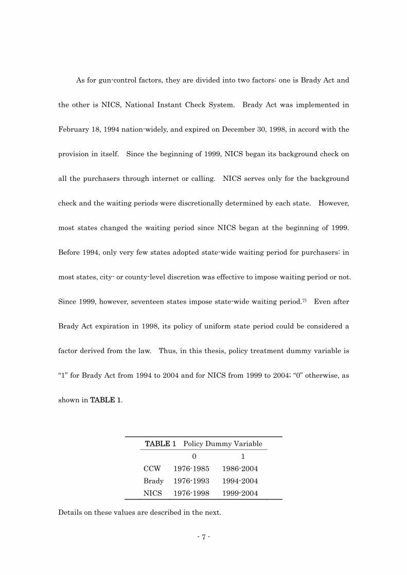
factor derived from the law. Thus, in this thesis, policy treatment dummy variable is
“1” for Brady Act from 1994 to 2004 and for NICS from 1999 to 2004; “0” otherwise, as
shown in TABLE 1.
TABLE 1 Policy Dummy Variable 0 1 CCW 1976-1985 1986-2004 Brady 1976-1993 1994-2004 NICS 1976-1998 1999-2004
Details on these values are described in the next.
- 8 -
Regression Models
Using aggregate national data, the following three models are constructed to
measure how CCW and gun-control factors affect the ratio of homicide by gun.
-t 0 1 t 2 t 3 t 4
Model - 1 : Y = + ×CCW + × Brady + × ptv NICS trendβ β β β β+ ×
-
- - -t 0 1 t 2 t 3 t 4
Model - 2 : Policy Treatment -Variable Model :Y = + × ptv CCW + × ptv Brady + × ptv NICS trendβ β β β β+ ×
0 1 2 3 4 5 6
- - - - -t t t t t t t
Model - 3 : Policy Treatmet Variable Model with economic indexY ptv CCW ptv Brady ptv NICS unemploy GDPchange inflationβ β β β β β β= + + + + + +
Furthermore, fifty-state panel data are constructed with the year of “shall issue”
adoption, waiting period, Gross State Product per person change, State unemployment
rate, and disposable personal income per person. The regression models are tested in
the following Least-Squared-Dummy-Variable, model and Difference-in-Difference
model. In panel model, the fixed-effect and random-effect models are usually created
to test.8) In this thesis, these models are tested, but the R-squared or the ratio of
explaining the variance of the dependent variable is too small to explain. Therefore,
the LSDV and DID models are constructed to explain the effect of CCW, Brady Act, and
NICS.
- 9 -
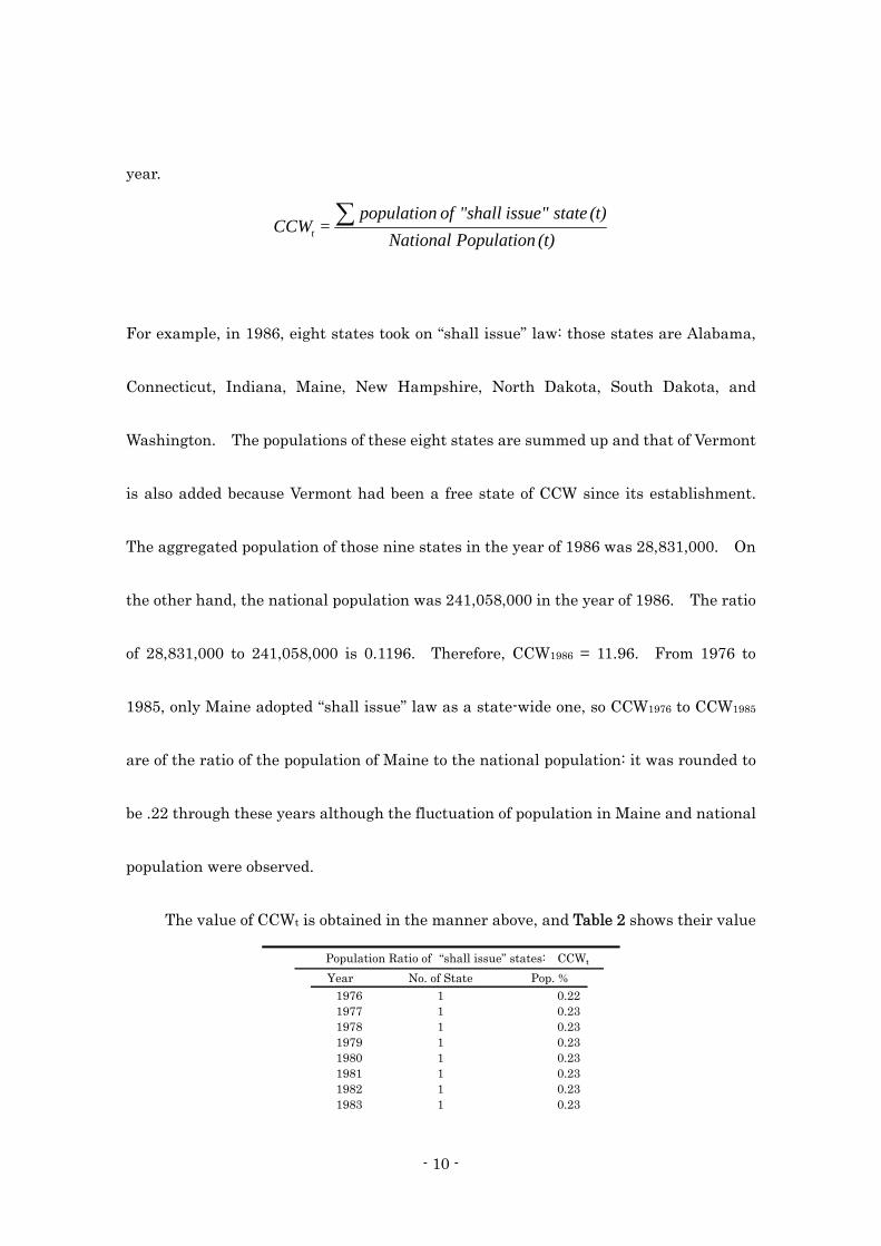
Fifty-State Data Treatment-Dummy Variable Model: Yt =β0 + β1CCWt + β2Bradyt + β3NICSt + β4log (state unemployment) + β5
log (GSPchange) + β6 (Disposable Income) + β7-58 ( Least Squared Treatment Variables, LSTV, of States1 to States51)
Difference-in-Difference Model: Yt = β0×Treatment+β1 AfterTreatment +β2 Treatment*AfterTreatment
Detail Description of Each Variables
Yt : the explained variable
In all three models, Yt denotes the number of cases of homicide with gun per
100,000 population in the year of t from 1976 to 2004:
tY = Rate of homicide with gun each year per 100,000 ( from 1976 to 2004) 9)
CCWt and ptv-CCWt : a measurement variable of “shall issue” law states
There are three basic explanatory variables: CCWt, Bradyt, and ptvNICSt to
assess how these variables affect the ratio of gun-homicide cases yearly. Among them,
CCWt shows the ratio of aggregated state population, which adopted the right to carry
concealed handguns in the year of t and then divided by the national population of that
- 10 -
year.
t
population of "shall issue" state (t)CCW =
National Population (t)∑
For example, in 1986, eight states took on “shall issue” law: those states are Alabama,
Connecticut, Indiana, Maine, New Hampshire, North Dakota, South Dakota, and
Washington. The populations of these eight states are summed up and that of Vermont
is also added because Vermont had been a free state of CCW since its establishment.
The aggregated population of those nine states in the year of 1986 was 28,831,000. On
the other hand, the national population was 241,058,000 in the year of 1986. The ratio
of 28,831,000 to 241,058,000 is 0.1196. Therefore, CCW1986 = 11.96. From 1976 to
1985, only Maine adopted “shall issue” law as a state-wide one, so CCW1976 to CCW1985
are of the ratio of the population of Maine to the national population: it was rounded to
be .22 through these years although the fluctuation of population in Maine and national
population were observed.
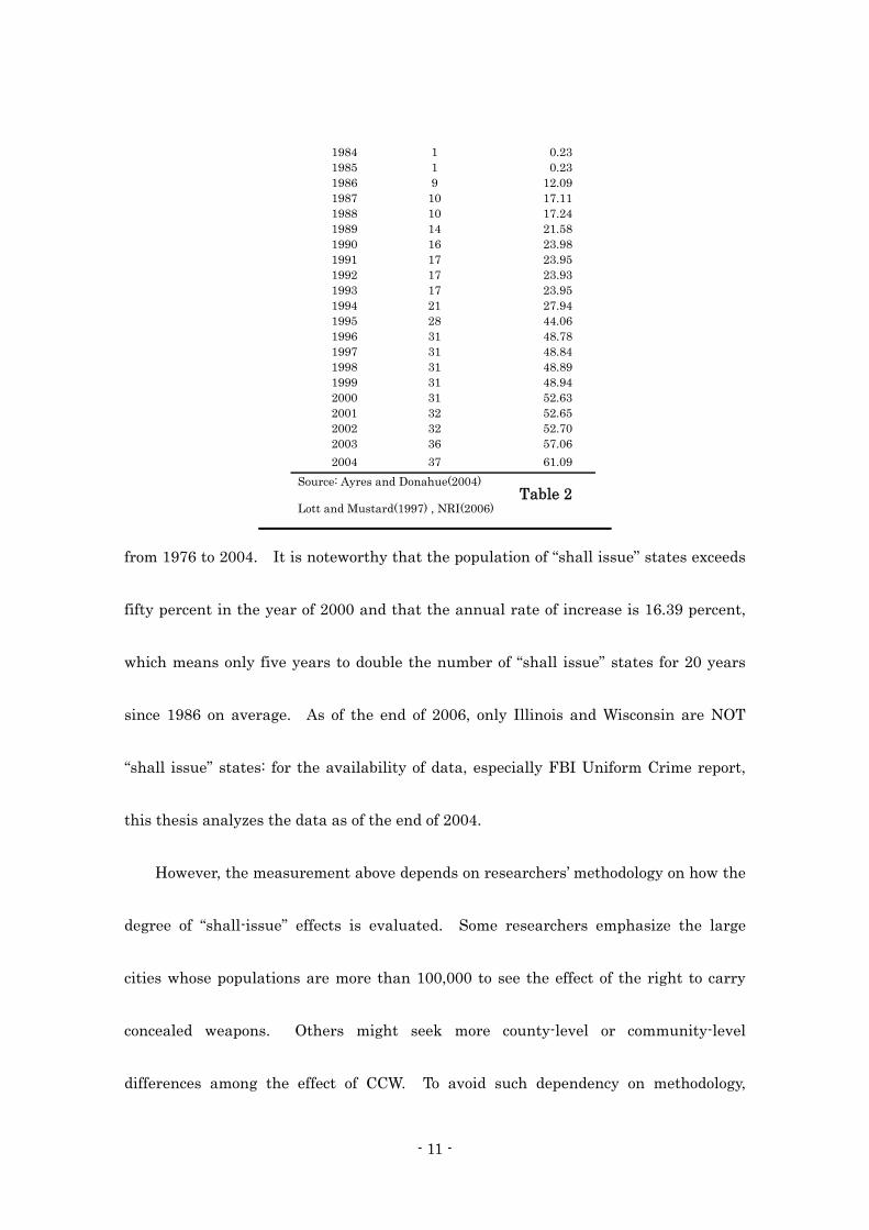
The value of CCWt is obtained in the manner above, and Table 2 shows their value
Population Ratio of “shall issue” states: CCWt Year No. of State Pop. %
1976 1 0.22 1977 1 0.23 1978 1 0.23 1979 1 0.23 1980 1 0.23 1981 1 0.23 1982 1 0.23 1983 1 0.23
- 11 -
1984 1 0.23 1985 1 0.23 1986 9 12.09 1987 10 17.11 1988 10 17.24 1989 14 21.58 1990 16 23.98 1991 17 23.95 1992 17 23.93 1993 17 23.95 1994 21 27.94 1995 28 44.06 1996 31 48.78 1997 31 48.84 1998 31 48.89 1999 31 48.94 2000 31 52.63 2001 32 52.65 2002 32 52.70 2003 36 57.06 2004 37 61.09 Source: Ayres and Donahue(2004)
Table 2
Lott and Mustard(1997) , NRI(2006)
from 1976 to 2004. It is noteworthy that the population of “shall issue” states exceeds
fifty percent in the year of 2000 and that the annual rate of increase is 16.39 percent,
which means only five years to double the number of “shall issue” states for 20 years
since 1986 on average. As of the end of 2006, only Illinois and Wisconsin are NOT
“shall issue” states: for the availability of data, especially FBI Uniform Crime report,
this thesis analyzes the data as of the end of 2004.
However, the measurement above depends on researchers’ methodology on how the
degree of “shall-issue” effects is evaluated. Some researchers emphasize the large
cities whose populations are more than 100,000 to see the effect of the right to carry
concealed weapons. Others might seek more county-level or community-level
differences among the effect of CCW. To avoid such dependency on methodology,

- 12 -
Treatment Dummy Variable, TDV, of policy is introduced in this thesis. TDV in policy
is consisted only with “0” or “1,” and “0” is assigned to the year before the specific policy
was adopted and “1” is for the years after the policy implementation.
Policy treatment dummy variable holds rather interesting characters. In national
data models, TDV holds the good R-squared and adjusted R-squared index and residual
normality test such as the Shapiro-Wilk W residual test and the inter-quartile test for
outliers. However, if a “trend” variable is included, the value of “trend” cause
multicolinearity (VIF test) and autocorrelation (Durbin-Watson test) in the model.
Therefore, trend is omitted when economic variables are included.
The problem of endogenous propensities in independent variables can be solved in
several ways such as Simultaneous Equation Model10), Two-Stage-Least-Squared Model,
2SLS, Instrumental Variable, IV, and others. In this thesis, the problem is dealt by
Difference-in-Difference methodology in fifty-state panel data. However, in national
data, the endogeneity supposition among variables are not treated, but high value of
adjusted R-squared and Model 3 shows sufficient indices in the hypothesis tests of
collinearity, autocorrelation, model specificity, the heterogeneity, skewness, kurtosis of
and of residuals.
In OLS regression model with national data, TDV models do not fail in

- 13 -
multicollinearity and autocorrelation tests. Non-linear problem is solved by taking
logarithm of variables. TDV is effective to analyze with logarithmic values possibly
because the value of all the other variables are logarithmically distributed and curtailed
into power index of small numbers.
Bradyt and ptv-Bradyt : a measurement variable of Brady Act
Bradyt is a variable to show the implementation of Brady Handgun Control Law,
which includes “waiting period” and “background check.” Although forty-one states
adopted some waiting period before 1994, there was no “federal” law to mandate
“waiting period” uniformly. Before 1994, each state had its discretion, and waiting
period was mostly not state-widely, but rather on county-level discretion by sheriffs and
police officers as mentioned above. Therefore, the value of Brady1t before 1994 were
all “0.”
To measure the value of uniform state-wide waiting period and background check
of Brady Act, “0” is assigned from 1976 to 1993, “1” is given from 1994 to 1998. From
1999 to 2004, the values are measured by the following methodology. The weight is
generated by the ratio of the days divided by 5, which was the mandatory waiting period
of Brady Act from 1994 to 1998. The basic idea of this weight is derived from the fact

- 14 -
that if waiting period of Brady Act had been 10 days, Bradyt could be twice as much.
Furthermore, if the size of national population were doubled, the value of Bradyt would
be “2.” This assessment might also provoke a polemic discussion, but the problem is
also dealt in Treatment-Variable Model. Treatment Variable Model is useful to
countermeasure the problems on the ratio numeralization of policy. Basic idea of
Treatment-Variable Model comes from differentiating policy period against non-policy
period by allocating the value of “1” and “0” and compares the values with control
samples. If a law is not adopted by all fifty states, control is used without difficulties.
Measuring “shall issue” policy can be controlled by 14 states which did not adopt it as of
2004. “Waiting period” is also controlled by 18 states which did not impose any of it as
of 2004. NICS is nation-wide policy, so it actually cannot be controlled. However, if
combining with waiting period, it could be controlled.
Introducing treatment variables will make the model more appropriate to assess
the direct effect of each variable on the dependent variable as shown later.
01
t
1,t
(t = 1976 -1993) before Brady LawBrady = (t = 1994 -1998) During Brady Law period
a state pop. with weight (0 - 2 : days/5, 2 : otherwise)(t = 1999 - 2004)
National Population (t)
⎧⎪⎨⎪⎩ ∑
- 15 -
The calculation of α(1,t) is as follows. Since 1999, each state has set its waiting
period. For example, New York extends it to six months, and Massachusetts, New
Jersey, and North Carolina require the 30-day waiting period. Hawaii 15 days, and
Connecticut 14 days. All the other states require less than or equal to 10 days.
Hereby, if the waiting period extends 10 days, 2 is given as weight, otherwise the ratio of
waiting period divided by 2 is used as Brady1t variable. The ratio is multiplied by the
population of each state in each year, and then divided by the national population at the
year to calculate the value.
tvNICSt : a treatment variable to measure background check in NICS
As discussed above, Brady Act held two different gun-control implementations:
federally uniform 5-day waiting period and background check on purchasers.
0 (1976 1998)
1 (1999 2004)t
tNICS =
t= −⎧
⎨ = −⎩
After Brady Act waiting period expired on December 30, 1998, National Instant
Check System, NICS, replaced it. NICS is a computerized background check system,
and each state has discretion to check the background of purchaser by the data in state
or federal.
- 16 -
In 1997, the Supreme Court verified that federal background check is illegal from
the view of Tenth Amendment in the case of Printz v. the U.S.11) Brady Act includes
computerization of checking background, so it originally set the expiration date in five
years when it was passed in the Congress. Thereafter, National Instant Check System
began working on the background check, but the system is said to hold some loophole
problems such as fraudulent identification of applicants through the Internet.
Therefore, differentiating waiting periods succeeding Brady Act, the effect of NICS is
evaluated by a different explanatory variable as a policy treatment variable of
ptv-NICSt, in which “0” is assigned from 1976 to 1998 and “1” from 1999 to 2004.
trendt and lgtrendt : a trend variable from 1 to 29 and log of it, from 1976 to 2004
This variable is used to measure time series data. Although trendt, from 1 to 29,
causes multicolinearity problem, the VIF value will be improved enough by taking its
logarithmic value. Policy Treatment Variables can be used in the form of be
time-series variables by lgtrendt. However, in Model 3, VIF of lgtrendt exceeds 10, so it
is omitted to obtain the sufficient values to pass the tests mentioned above.
lgunemt, lgGDPchanget, and lginft : aggregated logarithmic economic variables

- 17 -
Unemployment rate in each year is denoted unemt. and its logarithmic value is
lgunemt. In the same way, the percent change of national GDP per capita is denoted as
gdpct with the log value, lggdpct. Annual inflation rate is inft and lginft is the value of
logarithmic inflation rate.
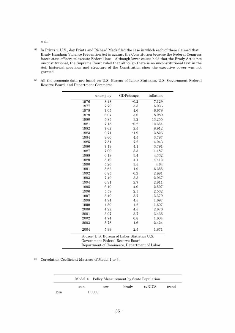
These three variables are introduced to show how much gun-homicide and
gun-crimes are related with aggregated economic conditions. Intuitively,
unemployment rate and inflation would positively affect gun-related crimes and GDP
annual rate change would negatively affect them. All the data used are shown at the
endnote.12)
Lott maintains that unemployment rate positively affect the decrease of
gun-related crimes and homicides (Lott 2000), but the models here show that more
unemployment results in more gun crimes. It seems that Lott’s assessment implies
the indirect effects of “shall issue” .law with other variables such as unemployment, but
this issue will be further evaluated in discussion.
Results of TDV Model with National Data
The results of coefficients and other indices of the regression Model 1 to 3 are
shown in Table 3. It is noteworthy that all the values become better from Model 1 to
- 18 -
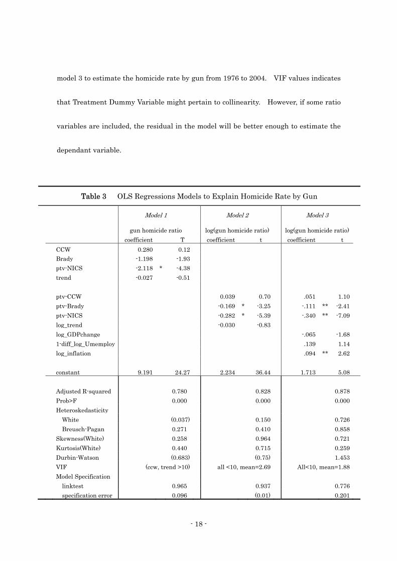
model 3 to estimate the homicide rate by gun from 1976 to 2004. VIF values indicates
that Treatment Dummy Variable might pertain to collinearity. However, if some ratio
variables are included, the residual in the model will be better enough to estimate the
dependant variable.
Table 3 OLS Regressions Models to Explain Homicide Rate by Gun
Model 1 Model 2 Model 3 gun homicide ratio log(gun homicide ratio) log(gun homicide ratio) coefficient T coefficient t coefficient t CCW 0.280 0.12 Brady -1.198 -1.93 ptv-NICS -2.118 * -4.38 trend -0.027 -0.51 ptv-CCW 0.039 0.70 .051 1.10 ptv-Brady -0.169 * -3.25 -.111 ** -2.41 ptv-NICS -0.282 * -5.39 -.340 ** -7.09 log_trend -0.030 -0.83 log_GDPchange -.065 -1.68 1-diff_log_Umemploy .139 1.14 log_inflation .094 ** 2.62 constant 9.191 24.27 2.234 36.44 1.713 5.08 Adjusted R-squared 0.780 0.828 0.878 Prob>F 0.000 0.000 0.000 Heteroskedasticity White (0.037) 0.150 0.726 Breusch-Pagan 0.271 0.410 0.858 Skewness(White) 0.258 0.964 0.721 Kurtosis(White) 0.440 0.715 0.259 Durbin-Watson (0.683) (0.75) 1.453 VIF (ccw, trend >10) all <10, mean=2.69 All<10, mean=1.88 Model Specification linktest 0.965 0.937 0.776 specification error 0.096 (0.01) 0.201
- 19 -
* 95 percent ( ) shows the value does not pass the test ** 99 percent Correlation matrices are shown in endnote13)
The results show interesting characters in measuring policy implementation in
aggregated data. The state population weights in CCW are not so fit as the policy
treatment dummy variables. The precision of policy measurement does not construct
better regression models which evaluate how much each variable directly affect the
explained variable.
The model explains more than ninety percent of the changing in the number of
homicide by gun. Two variables of Brady Act affect negatively with statistically
significant level of 94 percent. As for NICS, its statistical significance is more than 99
percent. On the other hand, CCW shows positive effects on the ratio of gun-homicide
per 100,000. It is statistically significant in this model.
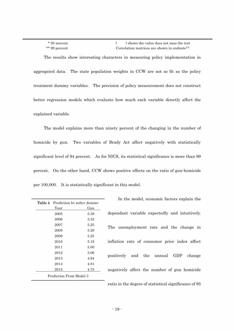
In the model, economic factors explain the
dependant variable expectedly and intuitively.
The unemployment rate and the change in
inflation rate of consumer price index affect
positively and the annual GDP change
negatively affect the number of gun homicide
ratio in the degree of statistical significance of 95
Table 4 Prediction by policy dummy Year Gun 2005 5.38 2006 5.32 2007 5.25 2008 5.29 2009 5.25 2010 5.19 2011 5.00 2012 5.06 2013 4.94 2014 4.81 2015 4.75
Prediction From Model 3

- 20 -
percent.
Policy dummy variable is useful in the regression model, so it could be used as
predictor to the explained variable. Table 4 shows the point estimator of the gun
homicide rates in 10 years, and the trend is negative, but its annual rate is rather slow.
Further discussion will be given later.
Fifty State Panel Data Analysis
To construct panel data for
fifty states, the following data are
used. From 1976 to 2004, CCW is
created for each state. When a
state passed and implemented
“shall-issue” law, “1” is assigned to
the value of CCW in that year and
after. Before the year, all the
values of CCW are “0” in the state.
Brady Handgun Violence
Prevention Act is uniformly adopted by fifty states with 5-day waiting period during
Table 5
Waiting Period after Brady Handgun Violence
State Waiting
Period State
Waiting
Period State
Waiting
Period
AL 0 LA 0 OH 0AK 0 ME 0 OK 0AZ 0 MD 7 OR 0AR 0 MA 30 PA 0CA 10 MI 1* RI 7CO 0 MN 7 SC 0CT 14 MS 0 SD 0DE 0 MO 7 TN 0FL 3 MT 0 TX 0GA 0 NE 2 UT 0HI 15 NV 0 VT 0ID 0 NH 0 VA 0IL 3 NJ 30 WA 5IN 0 NM 0 WV 0IA 3 NY 180 WI 2KS 0 NC 30 WY 0KY 0 ND 0 DC 2
* Michigan varies in waiting period

- 21 -
1994 to 1998, so all the states are given “5” to the independent value of “Brady” during
the period. Before 1994, all the states are given “0.” However, from 1999 to 2004, the
value depends on each state in accord with the state waiting period. Table 5 shows
fifty-state waiting periods after 1998.
The waiting period is complicated because some states require to create
identification cards for purchasers when they purchase guns for the first time in the
state. Once ID cards are created, some states do not require any waiting periods, but
others do. Each value of the waiting period above is given to the Brady variable of each
state after 1999.
The fixed-effect, FE, model and radon-effect, RE, model are usually used in panel
data analyses. However, R-squared value of FE and RE models are less than .084
within and less than 0.16 between variances to be explained.14) Therefore, the both
models cannot explain enough residual fluctuation, so this thesis does not facilitate FE
or RE model to analyze the effect of policy on gun-homicide rate.
In the analysis of Difference-in-Difference, these CCW and Brady variables are
used although they are not only “0” and “1.” How to construct the variables in DID
using these variables are described later.
The index of Gross State Product per capita, Disposable Income per capita , and

- 22 -
unemployment rate in each state are obtained from Bureau of Economic Analysis,
Department of Commerce.15)
Results of Panel Data Analysis by LSDV and DID
The panel data analyses on fifty states from 1976 to 2004 are as follows. The
coefficients or slope of each state on the increase of gun-homicide rate is from 1.27
(South Dakota) to 7.3 (California). As long as considering the ratio, the model holds
significance in practical and statistical implication.
Table 6 Least-Squared-Treatment-Variable Regression Model in Fifty-State Panel Data
lggun Coef. t lggun Coef. t Lggun Coef. t
ccw 0.0250 0.90 Illinois 6.3314 18.97 * New York 6.7642 20.30 *
brady -0.0024 -3.11 * Indiana 5.3405 16.73 * North Carolina 5.7497 17.88 *
nics -0.2372 -9.25 * Iowa 3.0700 9.57 * North Dakota 1.2798 4.10 *
lgpdi 0.0360 1.22 Kansas 4.1212 12.76 * Ohio 5.7229 17.39 *
lgsune -0.0451 -1.19 Kentucky 4.9928 15.42 * Oklahoma 4.7550 14.82 *
lggspch -0.0046 -0.33 Louisiana 5.9423 18.26 * Oregon 3.8944 11.86 *
Alabama 5.4348 16.93 * Maine 2.2563 7.07 * Pennsylvania 5.8090 17.79 *
Alaska 3.1095 9.11 * Maryland 5.4829 16.58 * Rhode Island 2.6196 7.97 *
Arizona 5.0455 15.47 * Massachusetts 4.2554 12.89 * South Carolina 5.1582 16.01 *
Arkansas 4.7465 14.75 * Michigan 6.1417 18.48 * South Dakota 1.2732 4.05 *
California 7.3035 21.72 * Minnesota 3.8102 11.70 * Tennessee 5.5380 17.02 *
Colorado 4.3838 13.32 * Mississippi 5.1387 15.91 * Texas 6.8787 21.02 *
Connecticut 4.1575 12.73 * Missouri 5.4449 16.91 * Utah 3.1018 9.73 *
Delaware 2.4741 7.32 * Montana 2.6963 8.35 * Vermont 1.6694 5.26 *
DC 4.9310 14.82 * Nebraska 3.0526 9.65 * Virginia 5.4982 16.99 *
Florida 6.3154 19.31 * Nevada 4.1284 12.42 * Washington 4.5094 13.65 *
Georgia 5.9098 18.35 * New Hampshire 1.8797 5.87 * West Virginia 3.9052 12.06 *
- 23 -
Hawaii 2.5776 7.93 * New Jersey 4.9970 14.90 * Wisconsin 4.3643 13.41 *
Idaho 2.7134 8.49 * New Mexico 4.1859 12.79 * Wyoming 1.9381 6.00 *
* p>.99 Adjusted R-squared 0.9608
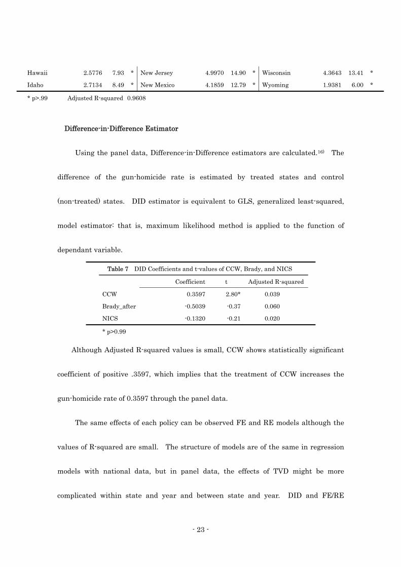
Difference-in-Difference Estimator
Using the panel data, Difference-in-Difference estimators are calculated.16) The
difference of the gun-homicide rate is estimated by treated states and control
(non-treated) states. DID estimator is equivalent to GLS, generalized least-squared,
model estimator: that is, maximum likelihood method is applied to the function of
dependant variable.
Table 7 DID Coefficients and t-values of CCW, Brady, and NICS
Coefficient t Adjusted R-squared CCW 0.3597 2.80* 0.039 Brady_after -0.5039 -0.37 0.060 NICS -0.1320 -0.21 0.020 * p>0.99
Although Adjusted R-squared values is small, CCW shows statistically significant
coefficient of positive .3597, which implies that the treatment of CCW increases the
gun-homicide rate of 0.3597 through the panel data.
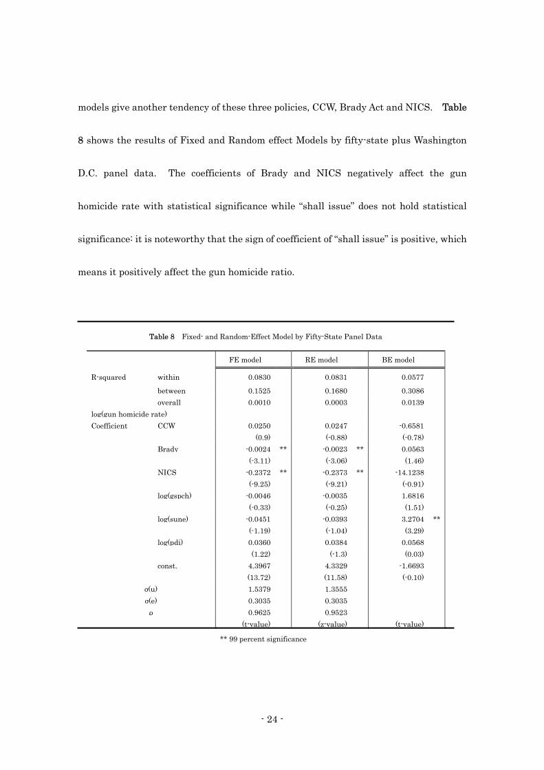
The same effects of each policy can be observed FE and RE models although the
values of R-squared are small. The structure of models are of the same in regression
models with national data, but in panel data, the effects of TVD might be more
complicated within state and year and between state and year. DID and FE/RE
- 24 -
models give another tendency of these three policies, CCW, Brady Act and NICS. Table
8 shows the results of Fixed and Random effect Models by fifty-state plus Washington
D.C. panel data. The coefficients of Brady and NICS negatively affect the gun
homicide rate with statistical significance while “shall issue” does not hold statistical
significance: it is noteworthy that the sign of coefficient of “shall issue” is positive, which
means it positively affect the gun homicide ratio.
Table 8 Fixed- and Random-Effect Model by Fifty-State Panel Data
FE model RE model BE model
R-squared within 0.0830 0.0831 0.0577
between 0.1525 0.1680 0.3086 overall 0.0010 0.0003 0.0139 log(gun homicide rate) Coefficient CCW 0.0250 0.0247 -0.6581 (0.9) (-0.88) (-0.78) Brady -0.0024 ** -0.0023 ** 0.0563 (-3.11) (-3.06) (1.46) NICS -0.2372 ** -0.2373 ** -14.1238 (-9.25) (-9.21) (-0.91) log(gspch) -0.0046 -0.0035 1.6816 (-0.33) (-0.25) (1.51) log(sune) -0.0451 -0.0393 3.2704 ** (-1.19) (-1.04) (3.29) log(pdi) 0.0360 0.0384 0.0568 (1.22) (-1.3) (0.03) const. 4.3967 4.3329 -1.6693 (13.72) (11.58) (-0.10) σ(u) 1.5379 1.3555 σ(e) 0.3035 0.3035 ρ 0.9625 0.9523 (t-value) (z-value) (t-value)
** 99 percent significance

- 25 -
Discussion
The trend of homicide by guns or gun-related crimes are not controlled by the
increase of “shall issue” states in the regression models constructed above. Brady Act
and its successor public policy of NICS are more effective to reduce the trend. From
the view of public policy, “shall issue” states give more permission to carry concealed
handguns, but the decrease trend of gun homicide and gun-using crimes has been on the
same level since 1999, and in the year of 2004, it is rising a little.
Brady Act was replaced by NICS, but its implementation of “waiting period” and
“background check” should be implemented continuously. Lott explains that even
unemployment rate affect negatively the handgun crimes (Lott and Mustard 1997, Lott
2000; Lott 2004). However, the model shows unemployment rate plausibly, positively
shows the positive effect on the homicide rate. It is said that the handgun incidences
cost more than$100 billion per year (Ludwig 1997; Cook 2000), and to reduce it,
gun-control public policy should be implemented continuously. As Webster et al.
present that radar-detective scanner is now being developed to search concealed guns in
public. In addition, manufacturers’ efforts should take responsibility to produce
reliable products and child proof and safe devices should be more strengthened.
Lott and Mustard maintains that if all the states adopted “shall issue” in

- 26 -
handgun policy, at least $5.74 billion would be gained in public expenditure (Lott and
Mustard 1998). However, Black and Nagin reexamined the data Lott and Mustard
used and concluded that Lott and Mustard model is highly sensitive to a small change
without Florida cases and that no impact can be found on the decrease of homicide and
rape (Black and Nagin 1998).
The debate is followed by many researchers. Webster et al. maintain that Lott
and Mustard model holds systematic error missing drug markets and/or police practices
and that the effect appears in 4 to 7 years later, which mislead the treatment year or
point (Webseter et al. 1998). Hemenway also points out the lack of those variables and
criticize their results that the increasing the rate of unemployment and reducing
income reduce the rate of violent crimes (Hemenway 1998). The reason why drug
problems are brought about to criticize Lott and Mustard is that their data covers 1977
to 1992 to show how 10 states, which adopted “shall issue” law in late 1980’s, decrease
the number of crimes, but crack cocaine are dramatically introduced in 1980’s at large
and these 10 states had LESS of a crack problem (Donohue 2003). Although Ayres and
Donahue praise the data collection efforts by Lott and Mustard, their findings collapse
when the more completely country data is subjected to less-constrained
jurisdiction-specific specification (Ayres and Donohue 2003a: 1296).

- 27 -
This thesis shows that TDV, treatment dummy variables, are useful to evaluate
how much policy affects the explained variable in both aggregated national data and
fifty-state panel data. CCW affects positively on gun-homicide rate while Brady and
NICS do negatively effects on it. To discuss the issue more, not only direct effect, but
also indirect effect should be considered because the correlation coefficient between
CCW and the decrease of gun homicide rate is negative because the “shall issue” states
began increasing right before 1994 when homicide and crimes rates dramatically
decreased.
Negative correlation coefficient, but positive coefficient in regression models
means that indirect effect of CCW is quite large: that is, CCW must have high
correlation coefficient with other social and economic factors. To discuss the issue, we
need to clarify the relations among variables and direct and indirect effects, and in
Addendum in this thesis gives the proof of it.
So-called deterrence effect must need to be correlated with social, economic, and
psychological factors, which can explain why CCW has a negative correlation coefficient
and positive coefficient in regression models to gun-homicide ratio. The social,
economic, and psychological complexity is required to establish deterrence effect, if
possible.

- 28 -
Last but not least, DID analysis in panel data shows significant effects of CCW to
gun-homicide rate. This can be interpreted that CCW positively related among fifty
states to increase the gun-homicide rate significantly from 1976 to 2004, but Brady Act
and NICS do not significantly affect the decrease of it although the sign of both
coefficients are negative. In aggregate national data, Brady Act and NICS show
significantly negative effect of the increase of gun-homicide rate, but the difference in
state shows no significance: that is, state difference holds large factor in gun-control.
Some states impose strict “waiting periods” and “background check.” In “background
check,” some state use Federal records, but such records allegedly lack of details
comparing with State criminal records. Therefore, DID panel data analysis implies
that the difference of state policy in gun-control contribute sufficiently to show the
significance in aggregate national data and insignificance in fifty-state panel data. In
this respect, some states which are too lenient on gun-control law should consider more
restrict on gun-control laws.

- 29 -
a 1, 2
a 2, n-1
Addendum
Direct and Indirect Effects in a Standardized Regression Model
First, this thesis gives a proof of the relations between direct effect and indirect
effect from a independent variable to dependant variable. Suppose the following
generalized regression model in the form of pass analysis.
e : error term Zn : dependent variable Z1, Z 2, … , Z n : independent variables A 1, n, A 2, n, …, A n-1, n : Coefficients in Regression Model denoted by
e
Z n
Z 1
Z 2
Z n-1
A 1, n
A 2, n
A 3, n
a 1, n-1

- 30 -
a 1, 2, a 2, n-1, …, a n-2, n-1 : Correlation Coefficients among independent variables
denoted by
In standardized regression models, direct effects and indirect effects hold the
following relation.
n-1
i n n, 1 i, j i j n , j j=1
Cor ( Z , Z ) = A + ( 1 - ) { Cor ( Z , Z ) × A }
Total Effect Direct Effect Indirect Effect
δ ∑
Where Cor ( Zi, Zn) denotes the correlation coefficients between Z i and Z n, and δi, j
signifies Kronecker’s Delta, in which δ i, j = 1 when i=j and δ i, j =0 otherwise. The
equation means that the correlation coefficient between the dependent variable and an
independent variable is the sum of Direct Effect and Indirect Effect. Direct Effect is
the coefficient of an independent variable in the regression. On the other hand,
Indirect Effect is complicated. Given an independent variable of Z k ( 1 ≤ k ≤ n-1 ),
Indirect Effect of Z k to Z n is denoted by:
A1 ×a(1,k) + A2 ×a(2,k) + … Ak-1×a(k-1,k) + Ak+1, k×a(k+1,k) + … + An-1 × a(k, n-1)
All the sum of the multiples between the other coefficients of independent variables, i.e.,
A1, A2, … A n-1 except for A k itself, in the regression model and the correlation
coefficient among the independent variables and the independent variable of Z k. The

- 31 -
proof is given at the endnote.17)
Endnote 1) Bureau of Justice Department, Department of Justice, provides FBI Uniform Crime Report on
line: http://www.ojp.usdoj.gov/bjs/welcome.html 2) Project Neighborhood Safety is provided by Department of Justice in order to make citizens life
safer. The project main target is to reduce gun crimes. Structural activities are linked among federal, state, and local law enforcements, prosecutors, and community leaders. 10,841 federal firearms cases were filed in 2005 and 73% were related with PNS. http://www.psn.gov/default.aspx
3) The following states require some kind of safety training before a person can buy a handgun: California, Connecticut, Hawaii, Massachusetts and Michigan. Nov. 30, 1998, the background check is shifted to computerized National Instant Check System.
State BC, Background Check WP, Waiting Period BC times WP Federal=0 State=1
AL 0 0 0 AK 0 0 0 AZ 1 0 0 AR 0 0 0 CA 1 10 10 CO 1 0 0 CT 1 14 14 DE 0 0 0 FL 1 3 3 GA 1 0 0 HI 1 15 15 ID 0 0 0 IL 1 3 3 IN 1 0 0 IA 1 3 3 KS 0 0 0 KY 0 0 0 LA 0 0 0 ME 0 0 0 MD 1 7 7 MA 0 30 0 MI 1 1 1 MN 0 7 0 MS 0 0 0 MO 0 7 0 MT 0 0 0 NE 1 2 2 NV 1 0 0

- 32 -
NH 1 0 0 NJ 1 30 30 NM 0 0 0 NY 1 180 180 NC 1 30 30 ND 0 0 0 OH 0 0 0 OK 0 0 0 OR 1 0 0 PA 1 0 0 RI 0 7 0 SC 0 0 0 SD 0 0 0 TN 1 0 0 TX 0 0 0 UT 1 0 0 VT 1 0 0 VA 1 0 0 WA 1 5 5 WV 0 0 0 WI 1 2 2 WY 0 0 0
Data: Jan. 2003. Brady Campaign http://www.bradycampaign.org/facts/issues/?page=waitxstate
State backgournd check is favorable because the state data of purchasers are more complihensible than that of Federal. In this sense, codifying background check by giving “1” to State Background check and “0” to Federal Background check, the index of BC times WP could the detail-background check with waiting period. The rightest colum above shows that there are twelve states with such state-background with waiting period.
Note: As of the end of 2006, forty-eight states adopted “shall-issue” law. However, the data of
FBI Uniform Crime report is available until the year of 2004 on gun-related incidences and homicide rates to date.
4) The multiplier depends on researchers. To find out the proper weights in waiting period, it is
necessary to research on it differently: how the weights in wiating period affects the estimator of gn-homicide and gun-incidence ratios.
5) VIF values in the OLS regression model are as follows: CCW Brady NICS unemploy inflation GDPpc
coefficient 0.970 -1.046 -3.030 0.128 0.134 -0.202
p-value 0.577 0.048 0.000 0.399 0.023 0.004
VIF 13.32* 4.51 4.23 3.24 2.56 1.32
White p-value
Heteroskedasticity 0.273
Skewness 0.130
Kurtosis 0.306
Durbin-Watson 1.269
Ramsey p-value 0.251
Model Specification 0.951
- 33 -
As shown above, CCW’s VIF value indicates the policy variable holds multicolinearity. It is concered to calculate the measurement value of policy from 0 to 1. To avoid this, policy dummy variables are generated in this thesis.
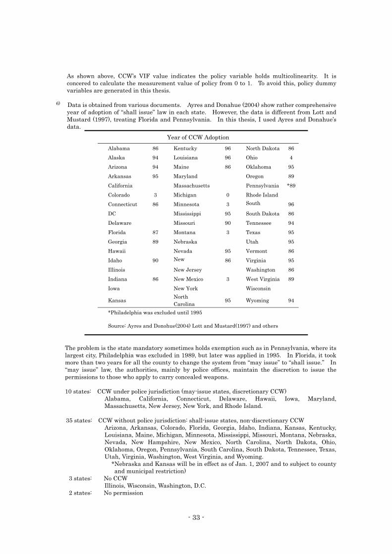
6) Data is obtained from various documents. Ayres and Donahue (2004) show rather comprehensive
year of adoption of “shall issue” law in each state. However, the data is different from Lott and Mustard (1997), treating Florida and Pennsylvania. In this thesis, I used Ayres and Donahue’s data.
Year of CCW Adoption
Alabama 86 Kentucky 96 North Dakota 86 Alaska 94 Louisiana 96 Ohio 4 Arizona 94 Maine 86 Oklahoma 95 Arkansas 95 Maryland Oregon 89 California Massachusetts Pennsylvania *89 Colorado 3 Michigan 0 Rhode Island Connecticut 86 Minnesota 3 South
C li96
DC Mississippi 95 South Dakota 86 Delaware Missouri 90 Tennessee 94 Florida 87 Montana 3 Texas 95 Georgia 89 Nebraska Utah 95 Hawaii Nevada 95 Vermont 86 Idaho 90 New
H hi86 Virginia 95
Illinois New Jersey Washington 86 Indiana 86 New Mexico 3 West Virginia 89 Iowa New York Wisconsin
Kansas North Carolina 95 Wyoming 94
*Philadelphia was excluded until 1995
Source: Ayres and Donohue(2004) Lott and Mustard(1997) and others
The problem is the state mandatory sometimes holds exemption such as in Pennsylvania, where its
largest city, Philadelphia was excluded in 1989, but later was applied in 1995. In Florida, it took more than two years for all the county to change the system from “may issue” to “shall issue.” In “may issue” law, the authorities, mainly by police offices, maintain the discretion to issue the permissions to those who apply to carry concealed weapons.
10 states: CCW under police jurisdiction (may-issue states, discretionary CCW)
Alabama, California, Connecticut, Delaware, Hawaii, Iowa, Maryland, Massachusetts, New Jersey, New York, and Rhode Island.
35 states: CCW without police jurisdiction: shall-issue states, non-discretionary CCW Arizona, Arkansas, Colorado, Florida, Georgia, Idaho, Indiana, Kansas, Kentucky, Louisiana, Maine, Michigan, Minnesota, Mississippi, Missouri, Montana, Nebraska, Nevada, New Hampshire, New Mexico, North Carolina, North Dakota, Ohio, Oklahoma, Oregon, Pennsylvania, South Carolina, South Dakota, Tennessee, Texas, Utah, Virginia, Washington, West Virginia, and Wyoming.
*Nebraska and Kansas will be in effect as of Jan. 1, 2007 and to subject to county and municipal restriction)
3 states: No CCW Illinois, Wisconsin, Washington, D.C.
2 states: No permission
- 34 -
Vermont and Alaska Open carry law has not been developed enough, but it is said that there are 10 states which allow
“open carry” handguns in public. Alaska, Arizona, Idaho, Kentucky, Montana, New Mexico, Ohio, South Dakota, Vermont, Virginia, West Virginia, and Wyoming
7) The following states require some kind of safety training before a person can buy a handgun: California, Connecticut, Hawaii, Massachusetts and Michigan. The facts show the difficulty to measure the policy by ratio variables.
8) Although the FE model and RE model show almost the same coefficients and other numerical values, the models do not fit very well. The reason might be derived from the similarity structure of CCW and Brady. CCW began in 1986 and has increased its state through 2004, and Brady Act began in 1994 and has been effective even after its expiration due to federal program such as PNS and state government requirements. NICS treatment periods are only six year in the model among 29-year observational periods, which might be too small to observe the contribution to the fluctuation of homicide ratio in each state.
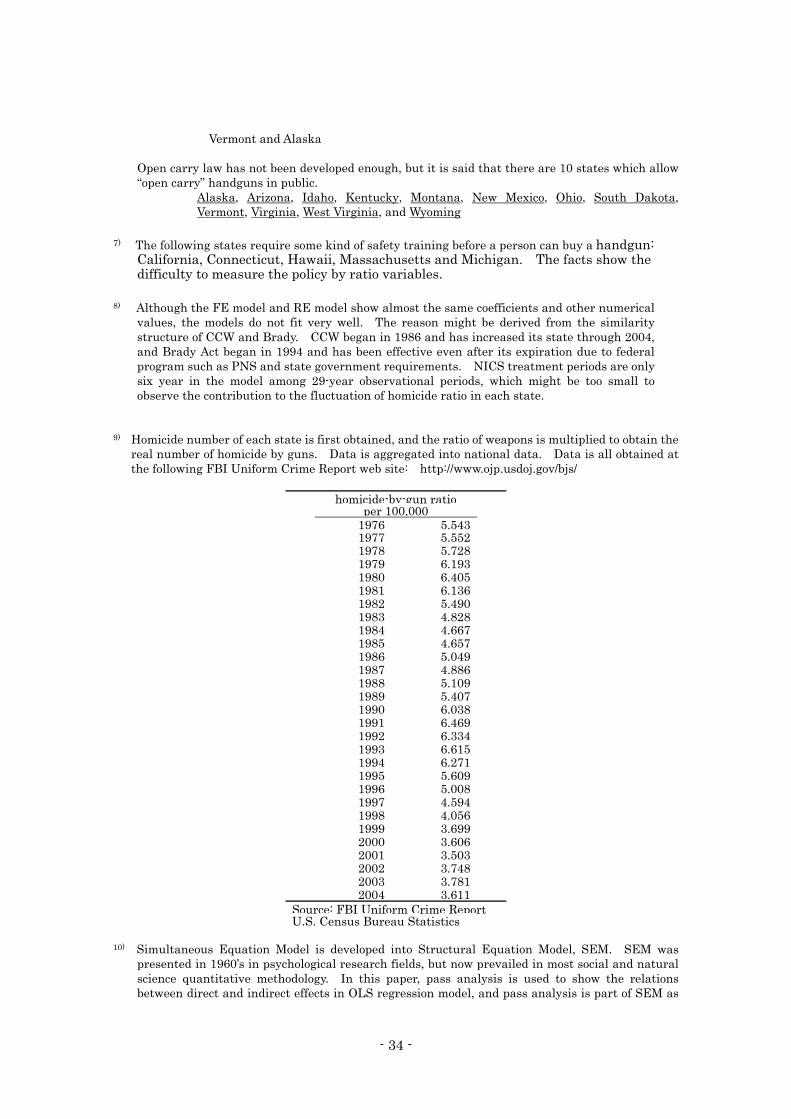
9) Homicide number of each state is first obtained, and the ratio of weapons is multiplied to obtain the
real number of homicide by guns. Data is aggregated into national data. Data is all obtained at the following FBI Uniform Crime Report web site: http://www.ojp.usdoj.gov/bjs/
homicide-by-gun ratio per 100,000 1976 5.543 1977 5.552 1978 5.728 1979 6.193 1980 6.405 1981 6.136 1982 5.490 1983 4.828 1984 4.667 1985 4.657 1986 5.049 1987 4.886 1988 5.109 1989 5.407 1990 6.038 1991 6.469 1992 6.334 1993 6.615 1994 6.271 1995 5.609 1996 5.008 1997 4.594 1998 4.056 1999 3.699 2000 3.606 2001 3.503 2002 3.748 2003 3.781 2004 3.611 Source: FBI Uniform Crime ReportU.S. Census Bureau Statistics
10) Simultaneous Equation Model is developed into Structural Equation Model, SEM. SEM was
presented in 1960’s in psychological research fields, but now prevailed in most social and natural science quantitative methodology. In this paper, pass analysis is used to show the relations between direct and indirect effects in OLS regression model, and pass analysis is part of SEM as
- 35 -
well. 11) In Printz v. U.S., Jay Printz and Richard Mack filed the case in which each of them claimed that
Brady Handgun Violence Prevention Act is against the Constitution because the Federal Congress forces state officers to execute Federal law. Although lower courts held that the Brady Act is not unconstitutional, the Supreme Court ruled that although there is no unconstitutional text in the Act, historical provision and structure of the Constitution show the executive power was not granted.
12) All the economic data are based on U.S. Bureau of Labor Statistics, U.S. Government Federal
Reserve Board, and Department Commerce.
unemploy GDPchange inflation 1976 8.48 -0.2 7.129 1977 7.70 5.3 5.036 1978 7.05 4.6 6.678 1979 6.07 5.6 8.989 1980 5.85 3.2 13.255 1981 7.18 -0.2 12.354 1982 7.62 2.5 8.912 1983 9.71 -1.9 3.826 1984 9.60 4.5 3.787 1985 7.51 7.2 4.043 1986 7.19 4.1 3.791 1987 7.00 3.5 1.187 1988 6.18 3.4 4.332 1989 5.49 4.1 4.412 1990 5.26 3.5 4.64 1991 5.62 1.9 6.255 1992 6.85 -0.2 2.981 1993 7.49 3.3 2.967 1994 6.91 2.7 2.811 1995 6.10 4.0 2.597 1996 5.59 2.5 2.532 1997 5.40 3.7 3.379 1998 4.94 4.5 1.697 1999 4.50 4.2 1.607 2000 4.22 4.5 2.676 2001 3.97 3.7 3.436 2002 4.74 0.8 1.604 2003 5.78 1.6 2.424
2004 5.99 2.5 1.871
Source: U.S. Bureau of Labor Statistics U.S. Government Federal Reserve Board Department of Commerce, Department of Labor
13) Correlation Coefficient Matrices of Model 1 to 3.
Model 1: Policy Measurement by State Population
gun ccw brady tvNICS trend gun 1.0000

- 36 -
ccw -0.7985 1.0000 brady -0.7217 0.8555 1.0000 tvNICS -0.8274 0.6979 0.5063 1.0000 trend -0.8012 0.9545 0.8113 0.7132 1.0000
Model 2: Policy Treatment Variable model with trend
Gun tvccw tvbrady tvNICS trend Gun 1.000
Tvccw -0.447 1.000 Tvbrady -0.806 0.567 1.000 tvNICS -0.827 0.371 0.653 1.000
trend -0.801 0.783 0.861 0.713 1.000
Model 3: Policy Dummy with Economic Index
lggun tv1ccw tv1brady tvNICS lgunem lggdpc lginf
lggun 1.0000
Tv1ccw -0.4144 1.0000
Tv1brady -0.7917 0.5528 1.0000
tvNICS -0.8688 0.3504 0.6340 1.0000
lgunem(D1) -0.0651 0.0154 -0.0200 0.2198 1.0000
lggdpc 0.2229 -0.3713 -0.2515 -0.4087 -0.2167 1.0000
lginf 0.5544 -0.6558 -0.5820 -0.3342 -0.1175 0.2207 1.0000
14) R-squared is the ratio of the difference between mean value and estimated values to the difference between mean value and actual dependent values. In statistical models, R-squared show the fitness of the model, but still the model holds some significance even if R-squared is small. In this respect, the consistency of the effect in DID and FE/ME models are important to explain policy effect on the dependent variable.
15) Bureau of Economic Analysis shows the state compensation for unemployment, so unemployment rates are gathered from various souses such as Department of Labor and others.
Bureau of Economic Analysis: http://bea.gov/beahome.html Department of Labor: http://www.dol.gov/
16) Three estimators of Difference-in-Difference are calculated: CCW, Post-Brady, and NICS. Here is the example to calculate CCW in STATA.
gen treatBrady = sid if ( ccw==1) gen afterBrady = year if (ccw==1) gen treatafterBrady = treatBrady*afterBrady reg gun treatBrady afterBrady treatafterBrady
- 37 -
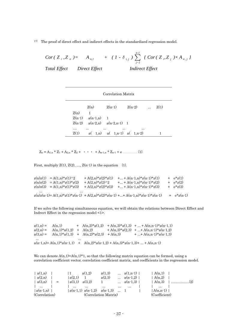
17) The proof of direct effect and indirect effects in the standardized regression model.
Correlation Matrix
Z(n) Z(n-1) Z(n-2) ... Z(1) Z(n) 1 Z(n-1) a(n-1,n) 1 Z(n-2) a(n-2,n) a(n-2,n-1) 1 .... ... ... ... ... Z(1) a( 1,n) a( 1,n-1) a( 1,n-2) 1
Zn = A1,n * Z1 + A2,n * Z2 + ・・・ + An-1,n * Zn-1 + e {1} First, multiply Z(1), Z(2), …, Z(n-1) in the equation {1}. z(n)z(1) = A(1,n)*z(1)^2 + A(2,n)*z(2)*z(1) +... + A(n-1,n)*z(n-1)*z(1) + e*z(1) z(n)z(2) = A(1,n)*z(1)*z(2) + A(2,n)*z(2)^2 +... + A(n-1,n)*z(n-1)*z(2) + e*z(2) z(n)z(3) = A(1,n)*z(1)*z(3) + A(2,n)*z(2)*z(3) +... + A(n-1,n)*z(n-1)*z(3) + e*z(3) ... ... z(n)z(n-1)= A(1,n)*z(1)*z(n-1) + A(2,n)*z(2)*z(n-1) +...+ A(n-1,n)*z(n-1)*z(n-1) + e*z(n-1) If we solve the following simaltaneous equation, we will obtain the relations between Direct Effect and Indrect Effect in the regression model <1>. a(1,n) = A(n,1) + A(n,2)*a(1,2) + A(n,3)*a(1,3) + ... + A(n,n-1)*a(n-1,1) a(2,n) = A(n,1)*a(1,2) + A(n,2) + A(n,3)*a(2,3) + ...+ A(n,n-1)*a(n-1,2) a(3,n) = A(n,1)*a(1,3) + A(n,2)*a(2,3) + A(n,3) + ...+ A(n,n-1)*a(n-1,3) ... ... a(n-1,n)= A(n,1)*a(n-1,1) + A(n,2)*a(n-1,2) + A(n,3)*a(n-1,3)+ ... + A(n,n-1) We can denote A(n,1)=A(n,1)*1, so that the following matrix equation can be formed, using a correlation coefficient vector, correlation coefficient matrix, and coefficients in the regression model. | a(1,n) | |1 a(1,2) a(1,3) ... a(1,n-1) | | A(n,1) | | a(2,n) | |a(2,1) 1 a(2,3) ... a(n-1,2) | | A(n,2) | | a(3,n) | = |a(3,1) a(3,2) 1 ... a(n-1,3) | | A(n,3) | ..................{2} | ... | | ... ... ... ... ... | | ... | |a(n-1,n) | |a(n-1,1) a(n-1,2) a(n-1,3) ... 1 | |A(n,n-1) | (Correlation) (Correlation Matrix) (Coefficient)
n-1
i n n, 1 i, j i j n , j j=1
Cor ( Z , Z ) = A + ( 1 - ) { Cor ( Z , Z ) × A }
Total Effect Direct Effect Indirect Effect
δ ∑

- 38 -
Carefully consider the relation of a(1,n) = CORR(x1,xn) and replace all the a(1,2), a(1,3), …, a(n-1, 1) with Cor(Z1, Z2), Cor(Z1, Z2), …, Cor(Z(n-1), Z(1), we will obtain the following equation:
Cor(Z1,Zn) = A(n,1)+Cor(Z1,Z2)*A(n,2)+Cor(Z1,Z3)*A(n,3) +...+ Cor(Z(n-1),1) *A(n,n-1)
Therefore,
CORR(X1,Xn) = A(1,n) + ∑{ CORR(X1,Xj)*A(n,j) } ............................. {3}
Applying {3} to all the other variables, we can obtain {1}.
CORR(Xi,Xn) = A(i,n) + ∑ {CORR (Xi,Xj)* A(j,n)} ( i ≠j ) [end of proof]
- 39 -
Main References
Ayres, Ian and John J. Donohue III. (2003) “Shooting Down the ‘More Guns, Less Crime’ Hypothesis.” Stanford Law Review. Vol. 55. 4: 1193-1312.
Ayres, Ian and John J. Donohue III. (2003) “The Latest Misfires in Support of the ‘More
Gun, Less Crime’ Hypothesis. Stanford Law Review. Vol. 55. 4: 1371-1399. Bruce-Briggs, B. (1976) “The Great American Gun War” Public Interest, vol. 45: 37-62. Brown, Peter Harry and Daniel G. Abel. (2003) Outgunned: Up Against the NRA, the
First Complete Inside Account of the Battle Over Gun Control. New York: The Free Press.
Cook, Philip J. and Jens Ludwig. (2000) Gun Violence: The Real Cost. New York:
Oxford University Press. Cook, Philip J. and Jens Ludwig. (2006) “The social costs of gun ownership.” Journal of
Public Economics. Vol. 90: 379-391. Courtwright, David T. (1998) Violent Land: Single Men nd Social Disorder from the
Frontier to the Inner City. Donohue, John J. (2003) “The final bullet in the body of the more guns, less crime
hypothesis.” Criminology & Public Policy. Jul. 2003; 2, 3: pp. 397-409. Duggan, Mark (2001) “More Guns, More Crime,” Journal of Political Economy
109(5):1086–1114.
FBI Uniform Crime Reports
- 40 -
Gottfredson, Michael R. and Travis Hirschi. (1990) A General Theory of Crime. Stanford: Stanford University Press
Gusfields J.R. (1986). Symbolic Crusade. 2nd edition. Urbana: University of Illinois
Press Housman Jerry, and Guido Kuersteiner. (2004) “Difference-in-Difference Meets
Generalized Least Squares: Higher Order Prperties of Hypotheses Test.” Hays, Stuart R. (1960) “The Right to Bear Arms, A Study in Judicial Misinterpretation.”
William & Mary Law Review Vol. 381: 381-406. Hemenway, David. (1998) “More Guns, Less Crime: Understanding crime and
gun-control laws / Making A Killing: The business of guns in American.” The New England Journal of Medicine. Boston. Vol. 339. Iss. 27: pp 2029-2030.
Kaplan, J. (1979). Controlling firearms. Cleveland State Law Review, 28, 1-28. Kleck Gary. (1999) “There are no lessons to be learned from Littleton.” Criminal
Justice Ethics. Winter; 18, 1: 2-6. --------, and Jongyeon Tark. (2004) “Resisting Crime: The Effects of Victim Action on the
Outcomes of Crimes.” Criminology. vol. 42. Iss. 4: 861-509. --------, Brion Sever, Spencer Li, and Marc Gertz. (2005) “The Missing Link in General
Deterrence Research.” Criminology. vol. 43. 3: 623-659. Kopel, Davd B. (1995) Guns: Who Should Have Them? New York: Prometheus Books. Kruschk, Earl R. (1995) Gun Control: A Reference Handbook. Santa Barbara:
ABC-CLIO. Levitt, Steven D. (2004) “Understanding Why Crime Fell in the 1990s: Four Factors
that Explain the Decline and Six that Do Not.” Journal of Economic Perspectives. Vol. 18, 1:163-190.
Ludwig, Jens. (1998) “Concealed-Gun-Carrying Laws and Violent Crime: Evidence from

- 41 -
State Panel Data.” International Review of Law and Economics. 18:239-254: 239-254.
--------. and Philip J. Cook. (2000) “Homicide and Suicide Rates Associated With
Implementation of the Brady Handgun Violence Prevention Act.” Journal of American Medical Association. Vol. 284, 5: 585-591.
--------. (2005) “Better Gun Enforcement, Less Crime.” Criminology & Public Policy. Vol4,
4: 677-716. Lott, John R., Jr. (2000) More Guns, Less Crime: Understanding Crime and
Gun-Control Laws. 2nd ed. Chicago: The University of Chicago Press. Lott, John R. and David B. Mustard. (1997) “Crime, Deterrence, and Right-to-Carry
Concealed Handguns.” The Journal of Legal Studies. Vol. 26-1: 1-68. Malcolm, Joyce Lee. (2002) Guns and Violence: The English Experience. Boston:
Harvard University Press. Nisbet, Lee. (Ed) (2001) The Gun Control Debate: You Decide. 2nd ed. New York:
Prometheus Books. Polsby, Daniel D. (1996) “Second Reading: Treating the Second Amendment as
Normal Constitutional Law.” Reason on Line. March. http://www.reason.com/news/show/29865.html
Spitzer, Robert J. (1995) The Politics of Gun Control. Chatham House Publisher, Inc.:
New Jersey. U.S. Bureau of Justice Statistics. http://bjsdata.ojp.usdoj.gov/dataonline/ U.S. Department of Commerce. Bureau of Economic Analysis, BEA. http://bea.gov/beahome.html U.S. Department of Labor. http://www.dol.gov/ U.S. Project Neighborhood Safety. Department of Justice.

- 42 -
http://www.psn.gov/default.aspx Vermick, Jon. Mathew W Pierce, Daniel W. Webster, Sara B. Johnson. Shannon Frattori.
(2003) “Technologies to Detect Concealed Weapons: Fourth Amendment Limits on a New Public Health and Law Enforcement Tool.” The Journal of Law, Medicine, and Ethics. Boston: Winter 2003. Vol.31. Iss. 4: 567-579.
Webster, D.W., J.S. Vernice, J. Ludwig, and K.J. Lester. (1997) “Flawed Gun Policy
Research Could Endanger Public Safety.” American Journal of Public Health 87 (6):918-921.
Webster, Daniel W., Jon S. Vermick, and Jens Ludwig. (1998) “Webster and Colleagues
Respond: No Proof That Shall-Issue Laws Reduce Violence.” American Journal of Public Health. Vol.88, 6: 982-983.
Top Related
Copyright © 2022 FDOKUMEN

