ORIGINAL RESEARCH PAPER

Global forecasting of thermal health hazards: the skillof probabilistic predictions of the Universal Thermal ClimateIndex (UTCI)

F. Pappenberger & G. Jendritzky & H. Staiger & E. Dutra &

F. Di Giuseppe & D. S. Richardson & H. L. Cloke

Received: 30 October 2013 /Revised: 30 April 2014 /Accepted: 1 May 2014# The Author(s) 2014. This article is published with open access at Springerlink.com

Abstract Although over a hundred thermal indices can be usedfor assessing thermal health hazards, many ignore the humanheat budget, physiology and clothing. The Universal ThermalClimate Index (UTCI) addresses these shortcomings by using anadvanced thermo-physiological model. This paper assesses thepotential of using the UTCI for forecasting thermal healthhazards. Traditionally, such hazard forecasting has had twofurther limitations: it has been narrowly focused on a particularregion or nation and has relied on the use of single ‘determin-istic’ forecasts. Here, the UTCI is computed on a global scale,which is essential for international health-hazard warnings anddisaster preparedness, and it is provided as a probabilistic fore-cast. It is shown that probabilistic UTCI forecasts are superior inskill to deterministic forecasts and that despite global variations,the UTCI forecast is skilful for lead times up to 10 days. Thepaper also demonstrates the utility of probabilistic UTCI fore-casts on the example of the 2010 heat wave in Russia.

Keywords Universal Thermal Climate Index (UTCI) .

Ensemble forecasting . Temperature forecasting . Thermalcomfort . Thermal stress . NWP

Introduction

The extreme heat wave that affected Russia in June 2010killed over 55,000 people. In China, extreme winter

conditions in January 2008 affected 77million people, leadingto costs of over 21 billion USD (Em-Dat 2014). During the hotsummer of 2003 in western and southern parts of Europe,55,000 deaths were attributed as heat related (Koppe et al.2004), 35,000 of which were during the hottest period in earlyAugust. An early understanding of the thermal health hazardsassociated with extreme heat or cold can serve to minimize theimpact by increasing preparedness in the affected region. Forthis reason forecasting of thermal indices is routinely carriedout by national weather services (Staiger et al. 1997) usuallybased on high-resolution numerical weather prediction(NWP) forecasts.

In order to determine thermal stress, several factors, includ-ing air temperature, wind velocity, water vapour pressure,short- and long-wave radiant fluxes, physiological strain, be-haviour and the autonomous human thermoregulatory system,need to be considered (Havenith 2001; Jendritzky et al. 2009;Parsons 2003). There are more than 100 indices used to assessthermal health hazards. The first indices to be widely usedwere based on a simple two-parameter combination of airtemperature and humidity for ‘warm’ indices and air temper-ature and wind speed (wind chill) for ‘cold’ indices(Blazejczyk et al. 2012). Over the last 30–40 years, a secondgeneration of still relatively simple human heat budget modelshave been developed which consider the core and the shell ofthe human body known as 2-node (core/shell of the humanbody), and these have improved the assessment of the thermalenvironment. Examples are the ‘physiological equivalent tem-perature PET’ (Hoeppe 1999; VDI 2008), and OUT-SET*(Pickup and de Dear 2000), with further examples describedin Blazejczyk et al. (2012). One of the earliest simple heatbudget models was the Klima-Michel model developed by theGerman national weather service, Deutscher Wetterdienst(DWD) (Jendritzky et al. 1979), which translated Fanger’s(1970) predicted mean vote (PMV) equation to outdoor con-ditions. This was mainly achieved by writing a radiation

F. Pappenberger (*) : E. Dutra : F. Di Giuseppe :D. S. RichardsonForecast Department, European Centre for Medium-Range WeatherForecasts, Reading, UKe-mail: florian.pappenberger@ecmwf.int

G. Jendritzky :H. StaigerUniversity of Freiburg, Freiburg, Germany

H. L. ClokeUniversity of Reading, Reading, UK

Int J BiometeorolDOI 10.1007/s00484-014-0843-3

scheme in order to calculate the mean radiant temperature Tmrt(by which short- and long-wave radiant fluxes refer to anupright standing human being) and was based on easily avail-able meteorological data. The outcome is ‘perceived temper-ature PT’ that relates in its development to an improvedradiation scheme and the 2-node thermo-physiology outsideof the PMV comfort region (Staiger et al. 1997; VDI 2008;Staiger et al. 2012). The radiation scheme for calculating Tmrtbased on NWP meteorological data in our paper is currentlyused by the DWD.

To calculate the entire heat exchange between the humanbody and its environment, 2-m air temperature (Ta), windvelocity at body height derived from 10-m wind speed (v),2-m water vapour pressure (e) and Tmrt are needed as meteo-rological input variables. The limitations of the two-parameterindices are obvious because they do not consider the humanheat budget and hence ignore issues such as physiology andclothing. Although the 2-node heat budget models representan improvement over the simple indices, they still makeseveral simplifications considering thermo-physiology andheat exchange theory (for example, the effects of clothing).To exploit more recent scientific developments and to mini-mize the various shortcomings of the former assessment pro-cedures (Jendritzky et al. 2012), the Universal Thermal Cli-mate Index (UTCI) was developed using one of the mostadvanced and comprehensively validated (Psikuta et al.2012) multi-node models of human heat transfer andthermo-regulation (Fiala et al. 2012; Fiala et al. 2001). TheUTCI development was performed by a multidisciplinaryexpert team in the framework of a commission of the Interna-tional Society of Biometeorology (ISB) and of COSTAction730 (Jendritzky et al. 2009) under the ‘umbrella’ of the WorldMeteorological Organisation Commission for Climatology(WMO-CCl). The UTCI can be applied to key applicationsin human biometeorology, such as daily forecasting and warn-ings, urban and regional planning, environmental epidemiol-ogy and climate impact research; it is applicable for allclimates.

Forecasts of thermal indices have to rely on NWP modelsto provide the required meteorological input at future times.The quality of the thermal index forecast will be dependent onthe quality of the meteorological forcing as well as on thedefinition of the index itself. Forecasts of thermal indices areusually made using single (deterministic) runs of NWPmodels. However, recent advances in NWP indicate thatensemble prediction systems (EPS) have higher skill thandeterministic forecasts in forecasting meteorological variablesover the medium term of 3 to 10 days (Bartholmes et al. 2009;Pappenberger et al. 2011b; Richardson 2000; Roulin 2007).Ensembles account for the unavoidable uncertainties inweather forecasting by providing multiple future weatherscenarios, allowing the forecast to be expressed in terms ofprobabilities. This probabilistic information allows

assessment of the most likely and extreme scenarios, facilitat-ing better preparedness for any stakeholders involved (Pitt2008). In addition, the potential costs and losses of precau-tionary actions, such as early warning provision to fuel sup-pliers, water resources and health care providers can be care-fully assessed (Richardson 2000).

The UTCI was designed to be applicable in all climateregions, and global NWP ensembles can be used to forecastthe UTCI anywhere in the world. However, before suchforecasts can be used, it is essential to assess their skill overthe area of interest. For a comprehensive evaluation, observa-tions must be available on a global scale and be comparable interms of error structure to the forecasts. Whilst direct obser-vational measurements are inhomogeneously distributed glob-ally (very sparse in some regions) and need careful qualitycontrol, recently developed reanalyses provide consistent,quality-controlled historical analysis of the state-of-the-globalatmosphere based on a wealth of ground, atmospheric andsatellite observational data. Here, the ERA-Interim reanalysis(Dee et al. 2011) is used as a global observation proxy.

Global ensemble forecasts from the integrated forecastingsystem (IFS) of the European Centre for Medium-RangeWeather Forecasts (ECMWF) are used to provide the meteo-rological input required for the UTCI. The skill of the UTCIforecasts will depend on the quality of this meteorologicalforcing. The meteorological performance of the ECMWFensemble forecasts is evaluated in detail elsewhere(Hagedorn et al. 2008, 2012; Hamill et al. 2008; Pinson andHagedorn 2012; Richardson et al. 2013), and only a briefdiscussion is included here.

This paper provides an assessment of the UTCI usingprobabilistic NWP forcing on a global scale, demonstratingthat the UTCI can be readily combined with forecast data. Theobjectives of this paper are to analyze the global behaviour ofthe UTCI using ECMWF reanalysis data and to assess thepredictability of the UTCI using medium-range (10-day)probabilistic forecasts. The added value of these global prob-abilistic UTCI predictions will be assessed. This evaluation,using ECMWF ensembles as the meteorological forcing, pro-vides a benchmark against which other forecasting systemscan be compared.

Methodology

The UTCI is calculated globally using meteorological inputfrom ECMWFs high-resolution and ensemble forecasts. Thequality of these forecasts is assessed by comparing the pre-dicted UTCI against analyzed values computed using reanal-ysis data (as a proxy for the truth, in the absence of globalobservational data). Both deterministic and probabilistic eval-uation scores are used.

Int J Biometeorol

The Universal Thermal Climate Index (UTCI)

The UTCI is the result of an approach which developed morethan a decade ago in the International Society of Biometeo-rology (ISB) Commission 6 and was later reinforced byCOSTAction 730 (Jendritzky et al. 2009). The various aspects ofUTCI are comprehensively described in the final report ofCOSTAction 730 (Jendritzky et al. 2009) and by 10 papers ina UTCI special issue on of Int J Biometeorol (56; 2012). Thedevelopment pooled the resources of multidisciplinary expertsin the fields of thermo-physiology, biology, mathematicalmodelling, occupational and environmental medicine, cloth-ing research and meteorological data handling.

The UTCI is based on Fiala et al.’s (2012, 2001) advancedmulti-node model of thermo-regulation. Thermo-regulation isthe ability of an organism to keep its body temperature withincertain boundaries, even when the surrounding temperature isvery different (Eq. 1).

UTCI∼ f Ta; Tmrt; v; eð Þ ð1Þ

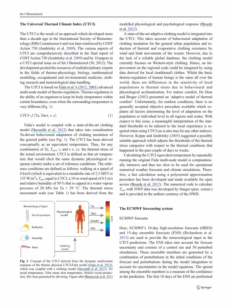
Fiala’s model is coupled with a state-of-the-art clothingmodel (Havenith et al. 2012) that takes into considerationTa-driven behavioural adaptation of clothing insulation ofthe general public (see Fig. 1). The UTCI has been derivedconceptually as an equivalent temperature. Thus, for anycombination of Ta, Tmrt, v, and e v, i.e. the thermal stress ofthe actual environment, UTCI is defined as that air tempera-ture that would elicit the same dynamic physiological re-sponse (strain) under a set of reference conditions. The refer-ence conditions are defined as follows: walking at a speed of4 km/h (which is equivalent to a metabolic rate of 2.3 METor135W/m2), Tmrt equal to UTCI, a 10-mwind speed of 0.5 m/sand relative humidity of 50 % that is capped at a water vapourpressure of 20 hPa for Ta > 29 °C. The thermal stressassessment scale (see Table 1) has been derived from the

modelled physiological and psychological response (Broedeet al. 2012).

A state-of-the-art adaptive clothing model is integrated intothe UTCI. This takes account of behavioural adaptation ofclothing insulation for the general urban population and re-duction of thermal and evaporative clothing resistance bywind and limb movements of the wearer. However, due tothe lack of a reliable global database, the clothing modelcurrently focuses on Western-style clothing. Hence, an im-provement on the regional scale could be imagined by usingdata derived for local (traditional) clothes. Whilst the basicthermo-regulation of human beings is the same all over theworld, there are differences in the sensitivity of localpopulations to thermal stress due to behavioural andphysiological acclimatization. For indoor comfort, De Dearand Brager (2002) presented an ‘adaptive model of thermalcomfort’. Unfortunately, for outdoor conditions, there is nogenerally accepted objective procedure available which ex-plains all factors determining the level of adaptation on thepopulation or individual level in all regions and scales. Withrespect to this issue, a meaningful interpretation of the stan-dard thresholds to be tailored to the local experience is re-quired when using UTCI (as is also true for any other indices).However, Koppe and Jendritzky (2005) suggested a possiblysuitable approach which adjusts the thresholds of the thermalstress categories with respect to the thermal conditions thathappened in the past couple of days to weeks.

Calculating the UTCI equivalent temperature by repeatedlyrunning the original Fiala multi-node model is computation-ally intensive and thus too slow to be used for operationalnumerical weather forecasts and climate simulations. There-fore, a fast calculation using a polynomial approximationprocedure has been developed and made available for openaccess (Broede et al. 2012). The numerical code to calculateTmrt with NWP data was developed by Staiger (pers. comm.)and is provided to the authors courtesy of the DWD.

The ECMWF forecasting system

ECMWF forecasts

Here, ECMWF’s 10-day high-resolution forecasts (HRES)and 15-day ensemble forecasts (ENS) (Richardson et al.2013) are used to provide the meteorological input to theUTCI predictions. The ENS takes into account the forecastuncertainty and consists of a control run and 50 perturbedsimulations. These ensemble members are generated by acombination of perturbations in the initial conditions of theforecast and perturbations during the model integration toaccount for uncertainties in the model equations. The spreadamong the ensemble members is a measure of the confidencein the prediction. The first 10 days of the ENS are performed

Fig. 1 Concept of the UTCI derived from the dynamic multivariateresponse of the thermo physical UTCI-Fiala model (Fiala et al. 2012),which was coupled with a clothing model (Havenith et al. 2012). Trerectal temperature, Tskm mean skin temperature, Mskdot sweat produc-tion, Shiv heat generated by shivering. Figure after Błażejczyk et al. 2013

Int J Biometeorol

at a spatial resolution of approximately 32 km×32 km forcedby persisted sea surface temperature (SST) anomalies (up-dated every 24 h). After day 10, the model is coupled to theocean model and has a spatial resolution of roughly 64×64 km. The 10-day high-resolution forecast uses the samemodel version as the ENS system, but runs are performed ata much higher horizontal (roughly 16×16 km) and verticalresolution.

ECMWF reanalysis: observation proxy

Reanalysis involves reprocessing observational dataspanning an extended historical period, incorporating avery large number of ground-based, ocean-, atmosphere-and satellite-based observations. A data assimilation sys-tem is used to transform these millions of observationsinto the model space to produce a dataset that can beregarded as a proxy for observations but with the ad-vantage of providing spatio-temporal resolution unob-tainable with a normal observational network. It shouldbe noted that reanalyses, although constrained by theobservations and data assimilation system, may sufferfrom effects of model errors; these impacts are discussed in thedocumentation of the reanalysis datasets (Dee et al. 2011). Thelatest global atmospheric reanalysis produced by ECMWF isERA-Interim (ERA-I), which extends from 1 January 1979 tothe present date (Dee et al. 2011). Gridded data productsinclude a large variety of 3-hourly surface parameters,describing weather as well as ocean-wave and land-surface conditions, and 6-hourly upper-air parameterscovering the troposphere and stratosphere. In this study,we use ERA-Interim as a proxy for global observationsto generate an analysis of UTCI which will be used as abenchmark for forecast skill calculations.

To evaluate the skill of UTCI forecasts, 4 years of data wereprocessed. A UTCI forecast was computed every day (with alead time of 10 days) from 1 January 2009 to 31 December2012 using both the high-resolution and 51-member ENSforecast.

Evaluation scores

A set of well-established skill scores is used to assess the skillof the UTCI predictions. Deterministic forecasts from both

HRES and ENS were evaluated using the anomaly correlationcoefficient (ACC). The Brier skill score (BSS) and the con-tinuous rank probability skill score (CRPSS) were used toevaluate the ENS probabilistic forecasts.

Anomaly correlation coefficient (ACC)

The anomaly correlation coefficient is a measure of the sim-ilarity between two signals or patterns (ignoring any potentialoffsets or biases). Both forecasts and observations are firstexpressed as anomalies from climatology before computingthe correlation between them. This minimizes the seasonaleffect (Stevenson 2006).

ACC ¼∑m

i¼1bx0i− bx0−Þðx0

i−x0̄� �

Msbx 0sxið2Þ

xi' and bx0

i are the observed and forecast anomalies, respec-tively. sbx0 and sxi are the standard deviations of the anomalies.

M being the number of cells and the overbar expressing themean.

The higher the anomaly correlation, the better is theperformance of a forecast system. The ACC, whilst agood measure of forecast skill, is not sensitive to bias,and hence, a good correlation should not be used inisolation to assess a forecast if bias is important. TheACC is used to assess deterministic forecast skill. How-ever, it does not provide information on the range ofpossibilities or uncertainty in the forecast, which isprovided by an ensemble of forecasts. Two probabilisticscores are therefore also used; the continuous rankprobability skill score (CRPSS) (Hersbach 2000) andthe Brier skill score (BSS) (Murphy 1973).

Brier skill score (BSS)

The Brier score measures the mean squared probability errorfor binary events (e.g. UTCI greater than 32 °C, see Eq. 3).The climatological probability of the event can be consideredas a no-skill reference forecast. The Brier skill score measuresthe improvement of the ECMWF forecasts with respect to thisreference. The Brier skill score has a maximum of 1(indicating a perfect deterministic forecast; Murphy 1973),

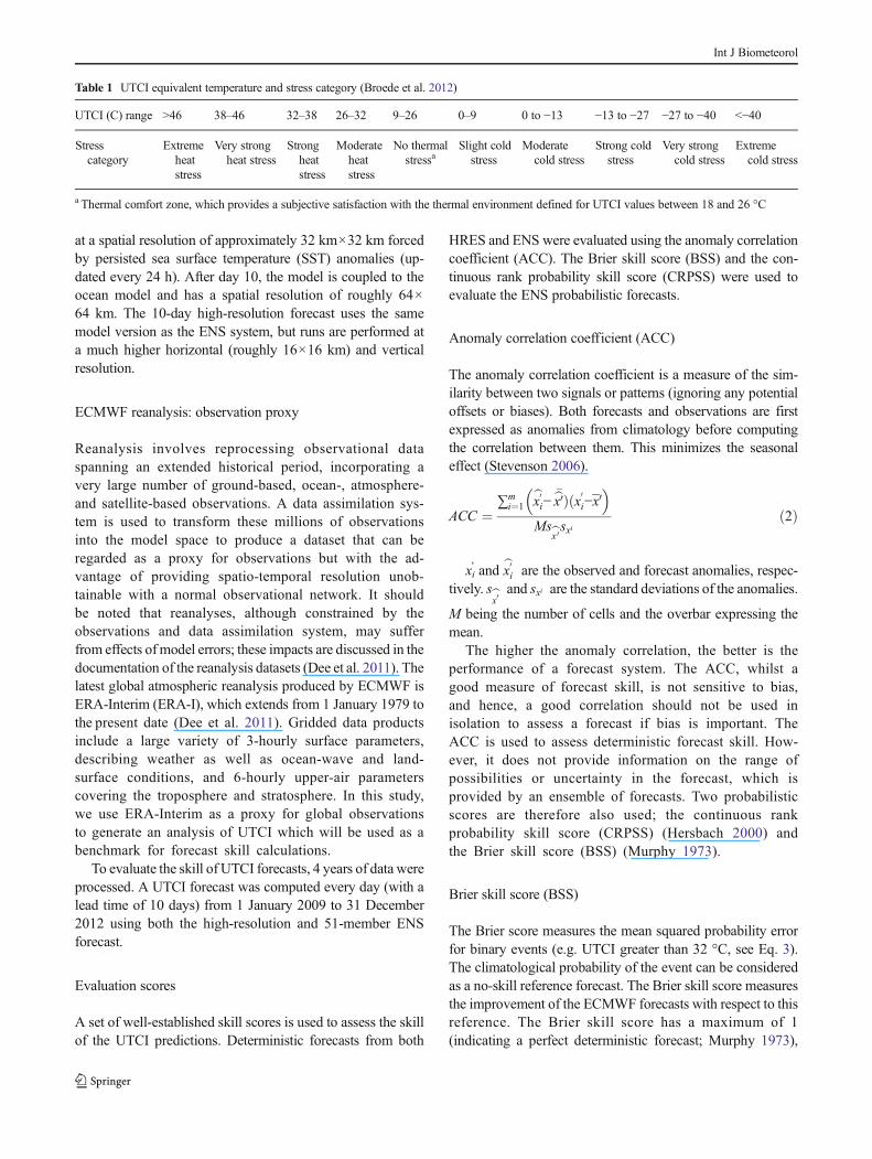
Table 1 UTCI equivalent temperature and stress category (Broede et al. 2012)

UTCI (C) range >46 38–46 32–38 26–32 9–26 0–9 0 to −13 −13 to −27 −27 to −40 <−40

Stresscategory

Extremeheatstress

Very strongheat stress

Strongheatstress

Moderateheatstress

No thermalstressa

Slight coldstress

Moderatecold stress

Strong coldstress

Very strongcold stress

Extremecold stress

a Thermal comfort zone, which provides a subjective satisfaction with the thermal environment defined for UTCI values between 18 and 26 °C

Int J Biometeorol

whilst positive values indicate higher skill than the climatebenchmark.

BSS ¼ 1−

1

n

Xn

t¼1bpt−yt

� �2

1

n

Xn

t¼1c−ytð Þ2

ð3Þ

BSS Brier skill scorebpt Probability assigned to the event by the tth forecastyt Equals 1 if the tth observation corresponds to an event,

0 otherwisec Climatological probability of the event (here, based on

a 30-year record)n Number of cases

Continuous rank probability skill score (CRPSS)

The continuous rank probability score (CRPS) is calculated asthe square differences in the cumulative probability spacebetween a probabilistic forecast and observation (see Eq. 4).It is transformed into a skill score (CRPSS) by comparing it toa climatological forecast based on a 30-year record. Seasonalmeans derived from the reanalysis data are used to provide thereference climate. The higher the CRPSS, the better the fore-cast, with a maximum value of 1 and positive values indicat-ing skill with respect to the climate benchmark.

CRPS ¼ ∫∞−∞ P xð Þ−H x−xað Þ½ �dx ð4Þ

where x is the forecast variable, xa is the observed value, P(x)is the cumulative distribution function of x and H(x−xα) is the

Heaviside function which is 0 when (x−xα)<0 and 1otherwise.

Results

Performance of ECMWF NWP forecasts

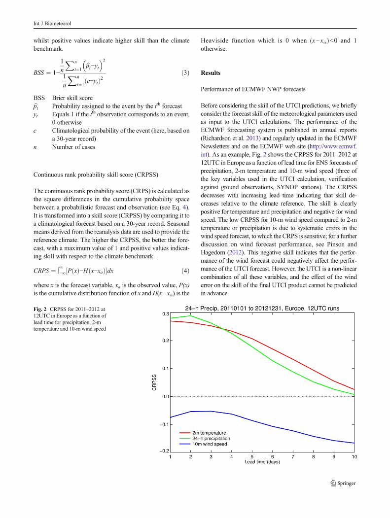
Before considering the skill of the UTCI predictions, we brieflyconsider the forecast skill of the meteorological parameters usedas input to the UTCI calculations. The performance of theECMWF forecasting system is published in annual reports(Richardson et al. 2013) and regularly updated in the ECMWFNewsletters and on the ECMWF web site (http://www.ecmwf.int). As an example, Fig. 2 shows the CRPSS for 2011–2012 at12UTC in Europe as a function of lead time for ENS forecasts ofprecipitation, 2-m temperature and 10-m wind speed (three ofthe key variables used in the UTCI calculation, verificationagainst ground observations, SYNOP stations). The CRPSSdecreases with increasing lead time indicating that skill de-creases relative to the climate reference. The skill is clearlypositive for temperature and precipitation and negative for windspeed. The low CRPSS for 10-m wind speed compared to 2-mtemperature or precipitation is due to systematic errors in thewind speed forecast, towhich the CRPS is sensitive; for a furtherdiscussion on wind forecast performance, see Pinson andHagedorn (2012). This negative skill indicates that the perfor-mance of the wind forecast could negatively affect the perfor-mance of the UTCI forecast. However, the UTCI is a non-linearcombination of all these variables, and the effect of the winderror on the skill of the final UTCI product cannot be predictedin advance.

Fig. 2 CRPSS for 2011–2012 at12UTC in Europe as a function oflead time for precipitation, 2-mtemperature and 10-m wind speed

Int J Biometeorol

Statistical post-processing of the ensemble forecast can, inprinciple, correct systematic errors in the meteorological pa-rameters used by the UTCI. Indeed, studies have demonstrat-ed substantial improvements in ECMWF probabilistic fore-casts for 10-m wind (Courtney et al. 2013) as well as for 2-mtemperature (Hagedorn et al. 2008, 2012) and precipitation(Hamill et al. 2008). However, in the present study, theECMWF forecast data is used directly with no attempt toaccount for systematic errors in the model. The skill of theresulting UTCI forecasts can therefore be considered as alower bound to what may be achievable with appropriatecalibration.

Global UTCI climatology

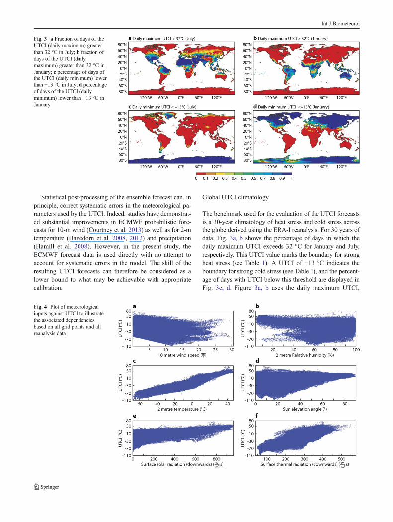
The benchmark used for the evaluation of the UTCI forecastsis a 30-year climatology of heat stress and cold stress acrossthe globe derived using the ERA-I reanalysis. For 30 years ofdata, Fig. 3a, b shows the percentage of days in which thedaily maximum UTCI exceeds 32 °C for January and July,respectively. This UTCI value marks the boundary for strongheat stress (see Table 1). A UTCI of −13 °C indicates theboundary for strong cold stress (see Table 1), and the percent-age of days with UTCI below this threshold are displayed inFig. 3c, d. Figure 3a, b uses the daily maximum UTCI,

Fig. 3 a Fraction of days of theUTCI (daily maximum) greaterthan 32 °C in July; b fraction ofdays of the UTCI (dailymaximum) greater than 32 °C inJanuary; c percentage of days ofthe UTCI (daily minimum) lowerthan −13 °C in July; d percentageof days of the UTCI (dailyminimum) lower than −13 °C inJanuary

Fig. 4 Plot of meteorologicalinputs against UTCI to illustratethe associated dependenciesbased on all grid points and allreanalysis data

Int J Biometeorol

whereas Fig. 3c, d is calculated using the daily minimumUTCI. As expected, the index shows a clear seasonalpattern. Strong heat stress affects almost all southernhemisphere land areas in January, northern hemisphere(especially equatorwards of 40 N) in July and tropicalregions in both months. In addition, there are significant

regional variations, mainly related to orography. Strongcold stress mainly affects the winter-time northern hemi-sphere (Fig. 3c, d), with notable longitudinal gradientsacross Europe and western North America, consistentwith the climatological temperature patterns. However,it should be noted that there is not a 1:1 correspondencewith temperature: as expected, the UTCI is providingadditional information (as discussed in the next section).Some regions are subject to stress over 90 % of days inthese months, for example, large parts of Australia areunder permanent strong heat stress in January, whereaslarge parts of Asia and North America are under almostconstant strong cold stress in January.

Sensitivity to NWP forecast variables

In order to understand the relationship between the NWPforecast variables used to generate the UTCI and the UTCIvalues themselves, sensitivity plots were constructed(Fig. 4). These show the relationship between computedUTCI values and each meteorological input variable for theentire reanalysis period and all grid points. Although theUTCI has some linear dependencies on air temperature, agiven temperature can lead to a wide range of UTCIvalues. This underlines the value of calculating the UTCIrather than relying only on temperature forecasts as anindicator of potential heat stress. The UTCI also showssensitivity to wind, which shows a distinct lower boundary.The UTCI is more sensitive to wind than previous indicesbecause it accounts for changes in clothing insulation andvapour resistance caused by wind and body movement(Havenith et al. 2012). Figure 4a shows a distinctive tailingbehaviour at wind speeds of over 17 m/s; this is because ofthe polynomial approximation for the UTCI used in this

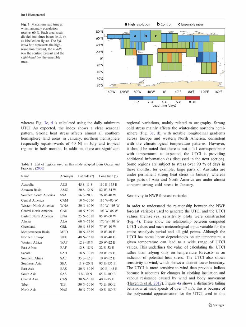
Fig. 5 Maximum lead time atwhich anomaly correlationreaches 60 %. Each area is sub-divided into three boxes (a, b, c)as labelled on figure. The left-hand box represents the high-resolution forecast, the middlebox the control forecast and theright-hand box the ensemblemean

Table 2 List of regions used in this study adapted from Giorgi andFrancisco (2000)

Name Acronym Latitude (°) Longitude (°)

Australia AUS 45 S–11 S 110 E–155 E

Amazon Basin AMZ 20 S–12 N 82 W–34 W

Southern South America SSA 56 S–20 S 76 W–40 W

Central America CAM 10 N–30 N 116 W–83 W

Western North America WNA 30 N–60 N 130 W–103 W

Central North America CAN 30 N–50 N 103 W–85 W

Eastern North America ENA 25 N–50 N 85 W–60 W

Alaska ALA 60 N–72 N 170 W–103 W

Greenland GRL 50 N–85 N 77 W–10 W

Mediterranean Basin MED 30 N–48 N 10 W–40 E

Northern Europe NEU 48 N–75 N 10 W–40 E

Western Africa WAF 12 S–18 N 20 W–22 E

East Africa EAF 12 S–18 N 22 E–52 E

Sahara SAH 18 N–30 N 20 W–65 E

Southern Africa SAF 35 S–12 S 10 W–52 E

Southeast Asia SEA 11 S–20 N 95 E–155 E

East Asia EAS 20 N–50 N 100 E–145 E

South Asia SAS 5 N–30 N 65 E–100 E

Central Asia CAS 30 N–50 N 40 E–75 E

Tibet TIB 30 N–50 N 75 E–100 E

North Asia NAS 50 N–70 N 40 E–180 E

Int J Biometeorol

study which has not been optimized beyond this range. Alimit of a maximum wind speed of 17 m/s should thus beconsidered in the future. This is responsible for the ex-tremely low UTCI values. The solar elevation angle clearlyinfluences the lower bound for the UTCI, as do the solarand thermal radiation. These input variables are themselvescorrelated. This makes a full interpretation more difficult ashigher order dependencies (dependencies on more than oneinput variable) cannot be determined from this one-dimensional analysis (Cloke et al. 2008).

UTCI forecast

A UTCI forecast was calculated every day (with a lead time of10 days) from 1 January 2009 to 31 December 2012 using

both the HRES and 51-member ENS inputs. The skill isassessed for these 4 years of data using ACC, BSS andCRPSS.

Similarity between forecast and observed UTCI

The deterministic high-resolution, control and ensemble meanforecasts of UTCI are compared with observations using theACC. In Fig. 5, the maximum lead time for which ACC isabove 60 % is shown for a list of regions across the globe (seeTable 2). The skill is shown for each of the three availableforecasts: the left-hand box of each box indicates the skill ofthe high-resolution forecast, the middle box the skill of thecontrol forecast and the right-hand box the skill of the ensem-ble mean. For example, the colour green indicates that the

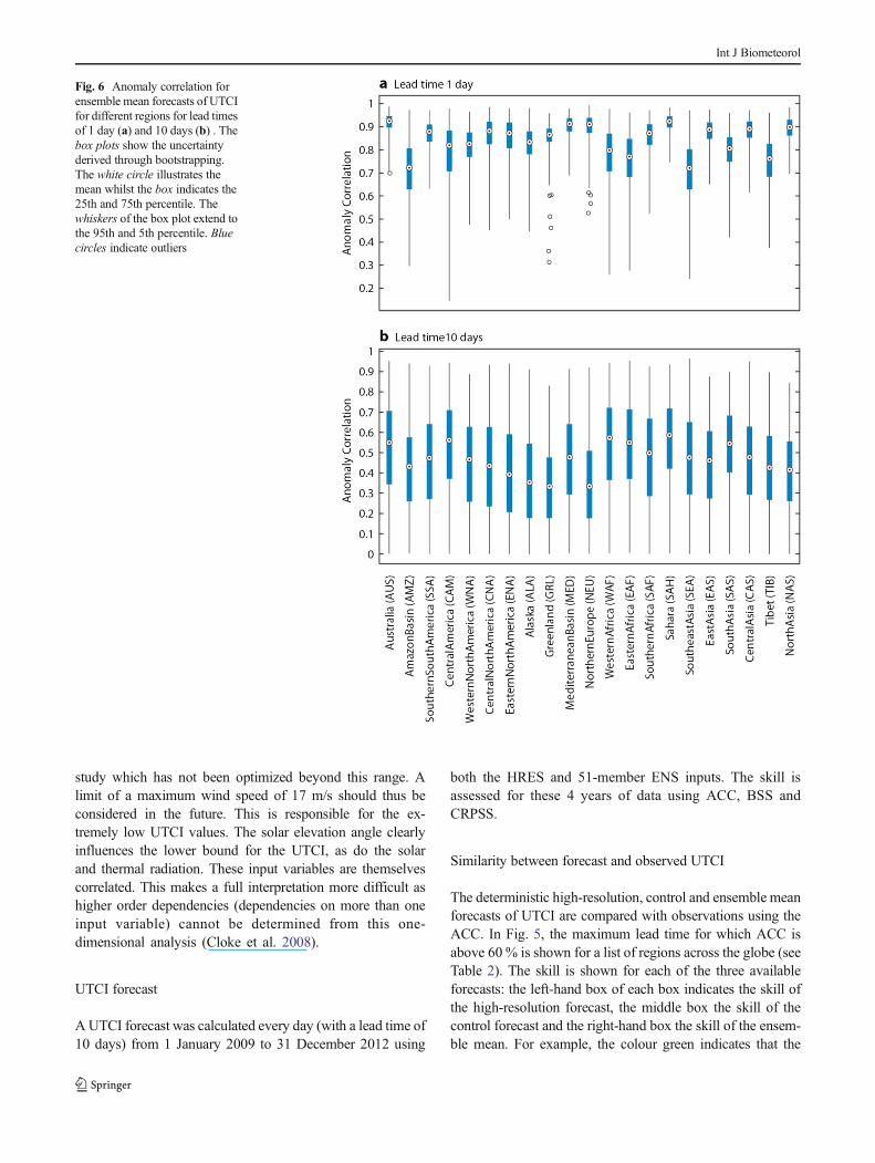
Fig. 6 Anomaly correlation forensemble mean forecasts of UTCIfor different regions for lead timesof 1 day (a) and 10 days (b) . Thebox plots show the uncertaintyderived through bootstrapping.The white circle illustrates themean whilst the box indicates the25th and 75th percentile. Thewhiskers of the box plot extend tothe 95th and 5th percentile. Bluecircles indicate outliers

Int J Biometeorol

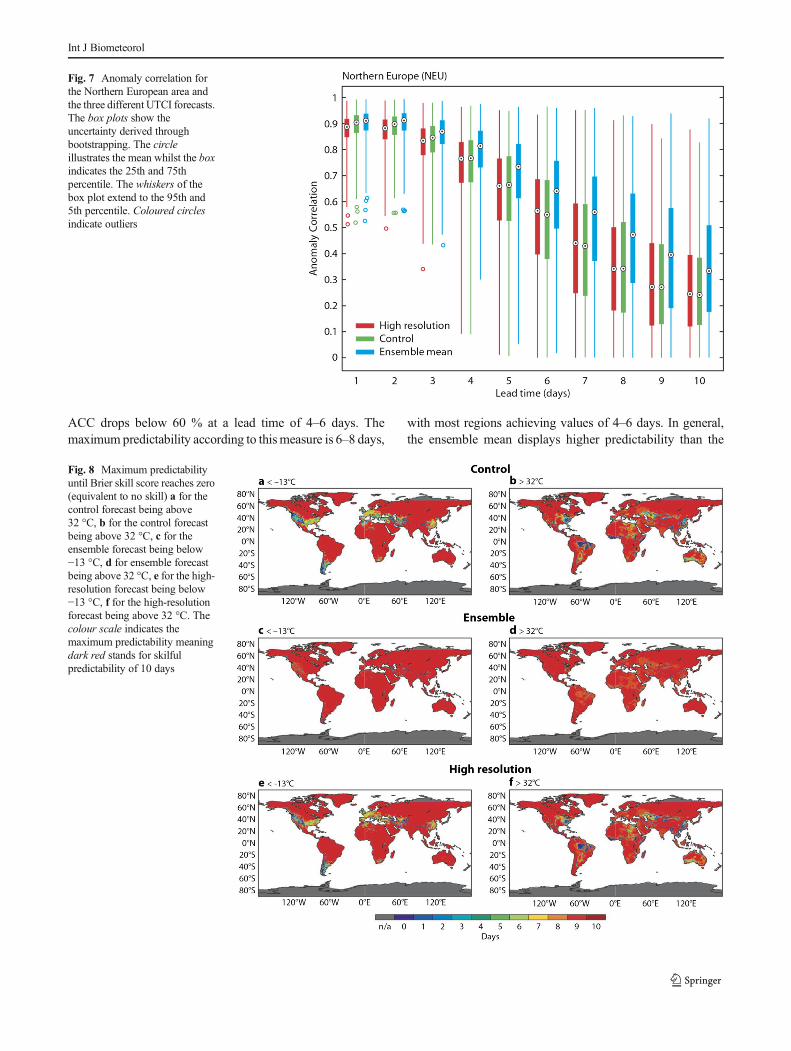
ACC drops below 60 % at a lead time of 4–6 days. Themaximum predictability according to thismeasure is 6–8 days,

with most regions achieving values of 4–6 days. In general,the ensemble mean displays higher predictability than the

Fig. 7 Anomaly correlation forthe Northern European area andthe three different UTCI forecasts.The box plots show theuncertainty derived throughbootstrapping. The circleillustrates the mean whilst the boxindicates the 25th and 75thpercentile. The whiskers of thebox plot extend to the 95th and5th percentile. Coloured circlesindicate outliers

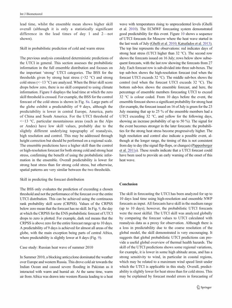
Fig. 8 Maximum predictabilityuntil Brier skill score reaches zero(equivalent to no skill) a for thecontrol forecast being above32 °C, b for the control forecastbeing above 32 °C, c for theensemble forecast being below−13 °C, d for ensemble forecastbeing above 32 °C, e for the high-resolution forecast being below−13 °C, f for the high-resolutionforecast being above 32 °C. Thecolour scale indicates themaximum predictability meaningdark red stands for skilfulpredictability of 10 days

Int J Biometeorol

other two forecasts. The results in Fig. 5 are veryencouraging in terms of forecast skill but give littleindication about the uncertainty and spread of theACC. The uncertainty is shown using box plots of theanomaly correlation for the different regions for leadtimes of 1 day (Fig. 6a) and 10 days (Fig. 6b) for theensemble mean. The uncertainty is derived bybootstrapping the sample using 80 % of available datapoints. Uncertainty increases with lead time, and thedifferent regions exhibit varying spread. For example,

the Mediterranean Basin, Sahara and Northern Europeshow comparatively small variation compared to CentralAmerica for day 1, which reflects the distribution alsofound through the verification of the meteorologicalforecasts (not shown). At the lead time of 10 days,none of the distributions for the different regions aresignificantly different. In Fig. 7, the ACC for the high-resolution, control and ensemble mean forecasts areplotted for the Northern European area for all lead timesfrom 1 to 10 days. There is a clear drop of ACC with

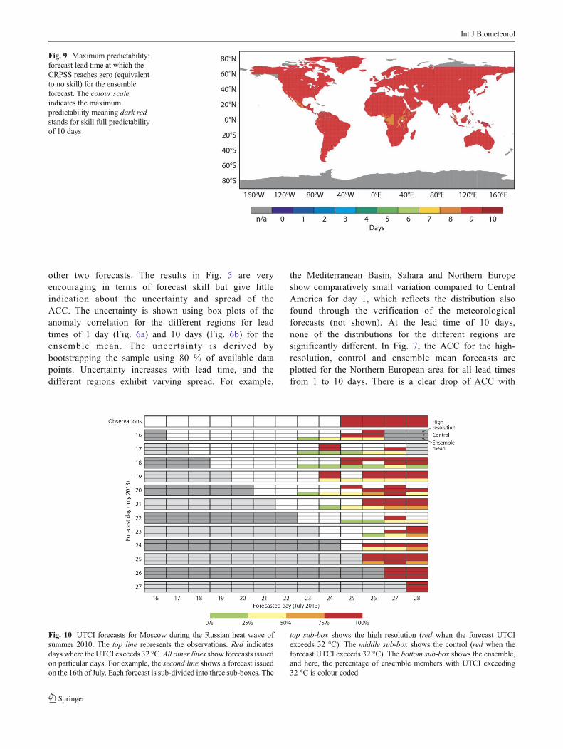
Fig. 9 Maximum predictability:forecast lead time at which theCRPSS reaches zero (equivalentto no skill) for the ensembleforecast. The colour scaleindicates the maximumpredictability meaning dark redstands for skill full predictabilityof 10 days

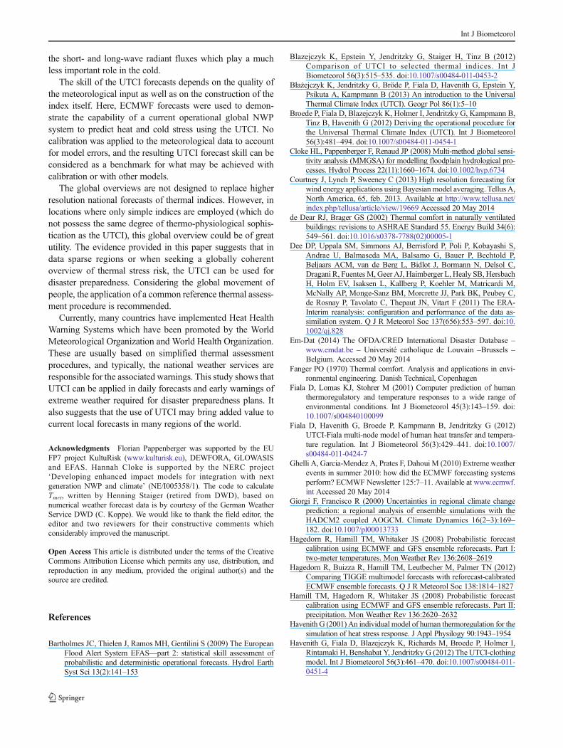
Fig. 10 UTCI forecasts for Moscow during the Russian heat wave ofsummer 2010. The top line represents the observations. Red indicatesdays where the UTCI exceeds 32 °C. All other lines show forecasts issuedon particular days. For example, the second line shows a forecast issuedon the 16th of July. Each forecast is sub-divided into three sub-boxes. The

top sub-box shows the high resolution (red when the forecast UTCIexceeds 32 °C). The middle sub-box shows the control (red when theforecast UTCI exceeds 32 °C). The bottom sub-box shows the ensemble,and here, the percentage of ensemble members with UTCI exceeding32 °C is colour coded

Int J Biometeorol

lead time, whilst the ensemble mean shows higher skilloverall (although it is only a statistically significantdifference in the lead times of day 1 and 2—notshown).

Skill in probabilistic prediction of cold and warm stress

The previous analysis considered deterministic predictions ofthe UTCI in general. This section assesses the probabilisticinformation in the full ensemble distribution and focuses onthe important ‘strong’ UTCI categories. The BSS for thethresholds given by strong heat stress (>32 °C) and strongcold stress (<−13 °C) are analyzed. When the Brier skill scoredrops below zero, there is no skill compared to using climateinformation. Figure 8 displays the lead time at which the zeroskill threshold is crossed. For example, the BSS for the controlforecast of the cold stress is shown in Fig. 8a. Large parts ofthe globe exhibit a predictability of 9 days, although thepredictability is lower in central Europe, America, partsof China and South America. For the UTCI threshold of<−13 °C, particular mountainous areas (such as the Alpsor Andes) have low skill values, probably due to theslightly different underlying topography of reanalysis,high resolution and control. This may be addressed throughheight correction but should be performed on a regional scale.The ensemble predictions have a higher skill than the controlor high-resolution forecast for both strong cold and strong heatstress, confirming the benefit of using the probabilistic infor-mation in the ensemble. Overall predictability is lower forstrong heat stress than for strong cold stress, but otherwise,spatial patterns are very similar between the two thresholds.

Skill in predicting the forecast distribution

The BSS only evaluates the prediction of exceeding a chosenthreshold and not the performance of the forecast over the entireUTCI distribution. This can be achieved using the continuousrank probability skill score (CRPSS). Values of the CRPSSbelow zero mean that the forecast has no skill. In Fig. 9, the dayat which the CRPSS for the ENS probabilistic forecast of UTCIdrops to zero is plotted. For example, dark red means that theCRPSS is above zero for the entire forecast range up to 10 days.A predictability of 9 days is achieved for almost all areas of theglobe, with the main exception being parts of central Africa,where predictability is slightly lower at 8 days (Fig. 9).

Case study: Russian heat wave of summer 2010

In Summer 2010, a blocking anticyclone dominated the weatherover Europe andwestern Russia. This drove cold air towards theIndian Ocean and caused severe flooding in Pakistan as itinteracted with warm and humid air. At the same time, warmair from Africa was drawn into western Russia leading to a heat

wave with temperatures rising to unprecedented levels (Ghelliet al. 2010). The ECMWF forecasting system demonstratedgood predictability for this event. Figure 10 shows a sequenceof UTCI forecasts for Moscow where the heat wave started inthe last week of July (Ghelli et al. 2010; Katsafados et al. 2013).The top line represents the observations: red indicates days ofstrong heat stress (UTCI higher than 32 °C). The second rowshows the forecasts issued on 16 July; rows below show subse-quent forecasts, with the last row showing the forecasts from 27July. Each forecast row is sub-divided into three sub-boxes. Thetop sub-box shows the high-resolution forecast (red when theforecast UTCI exceeds 32 °C). The middle sub-box shows thecontrol (red when the forecast UTCI exceeds 32 °C). Thebottom sub-box shows the ensemble forecast, and here, thepercentage of ensemble members forecasting UTCI to exceed32 °C is colour coded. From 10 days before the event, theensemble forecast shows a significant probability for strong heat(for example, the forecast issued on 16 of July is green for the 23July meaning that up to 25 % of the ensemble members had aUTCI exceeding 32 °C, and yellow for the following days,showing an increase probability of up to 50 %). The signal forthe event becomes stronger in the later forecasts: the probabili-ties for the strong heat stress become progressively higher. Thehigh resolution and control also indicate a possible event, al-though at the longer range, the timing of this is not consistentfrom day to day (the signal flip-flops, or changes) (Pappenbergeret al. 2011a). These results indicate that a UTCI forecast couldhave been used to provide an early warning of the onset of thisheat wave.

Conclusion

The skill in forecasting the UTCI has been analyzed for up to10 days lead time using high-resolution and ensemble NWPforecasts as input. All forecasts have skill in the medium range(up to 10 days); however, the probabilistic UTCI forecastswere the most skilful. The UTCI skill was analyzed globallyby comparing the forecast values to UTCI calculated withreanalysis data as a proxy for observation. Although there isa loss in predictability due to the coarse resolution of theglobal model, the skill demonstrated is very encouraging. Itsuggests that global probabilistic UTCI predictions can pro-vide a useful global overview of thermal health hazards. Theskill of the UTCI predictions shows some regional variations,for example, it is lower in some high altitude areas, and has astrong sensitivity to wind, in particular in coastal regions,which may be related to a maximum wind speed limit underwhich the UTCI is applicable in this study. Overall, predict-ability is slightly lower for heat stress than for cold stress. Thismay be explained by forecast model errors in forecasting of

Int J Biometeorol

the short- and long-wave radiant fluxes which play a muchless important role in the cold.

The skill of the UTCI forecasts depends on the quality ofthe meteorological input as well as on the construction of theindex itself. Here, ECMWF forecasts were used to demon-strate the capability of a current operational global NWPsystem to predict heat and cold stress using the UTCI. Nocalibration was applied to the meteorological data to accountfor model errors, and the resulting UTCI forecast skill can beconsidered as a benchmark for what may be achieved withcalibration or with other models.

The global overviews are not designed to replace higherresolution national forecasts of thermal indices. However, inlocations where only simple indices are employed (which donot possess the same degree of thermo-physiological sophis-tication as the UTCI), this global overview could be of greatutility. The evidence provided in this paper suggests that indata sparse regions or when seeking a globally coherentoverview of thermal stress risk, the UTCI can be used fordisaster preparedness. Considering the global movement ofpeople, the application of a common reference thermal assess-ment procedure is recommended.

Currently, many countries have implemented Heat HealthWarning Systems which have been promoted by the WorldMeteorological Organization and World Health Organization.These are usually based on simplified thermal assessmentprocedures, and typically, the national weather services areresponsible for the associated warnings. This study shows thatUTCI can be applied in daily forecasts and early warnings ofextreme weather required for disaster preparedness plans. Italso suggests that the use of UTCI may bring added value tocurrent local forecasts in many regions of the world.

Acknowledgments Florian Pappenberger was supported by the EUFP7 project KultuRisk (www.kulturisk.eu), DEWFORA, GLOWASISand EFAS. Hannah Cloke is supported by the NERC project‘Developing enhanced impact models for integration with nextgeneration NWP and climate’ (NE/I005358/1). The code to calculateTmrt, written by Henning Staiger (retired from DWD), based onnumerical weather forecast data is by courtesy of the German WeatherService DWD (C. Koppe). We would like to thank the field editor, theeditor and two reviewers for their constructive comments whichconsiderably improved the manuscript.

Open Access This article is distributed under the terms of the CreativeCommons Attribution License which permits any use, distribution, andreproduction in any medium, provided the original author(s) and thesource are credited.

References

Bartholmes JC, Thielen J, Ramos MH, Gentilini S (2009) The EuropeanFlood Alert System EFAS—part 2: statistical skill assessment ofprobabilistic and deterministic operational forecasts. Hydrol EarthSyst Sci 13(2):141–153

Blazejczyk K, Epstein Y, Jendritzky G, Staiger H, Tinz B (2012)Comparison of UTCI to selected thermal indices. Int JBiometeorol 56(3):515–535. doi:10.1007/s00484-011-0453-2

Błażejczyk K, Jendritzky G, Bröde P, Fiala D, Havenith G, Epstein Y,Psikuta A, Kampmann B (2013) An introduction to the UniversalThermal Climate Index (UTCI). Geogr Pol 86(1):5–10

Broede P, Fiala D, Blazejczyk K, Holmer I, Jendritzky G, Kampmann B,Tinz B, Havenith G (2012) Deriving the operational procedure forthe Universal Thermal Climate Index (UTCI). Int J Biometeorol56(3):481–494. doi:10.1007/s00484-011-0454-1

Cloke HL, Pappenberger F, Renaud JP (2008) Multi-method global sensi-tivity analysis (MMGSA) for modelling floodplain hydrological pro-cesses. Hydrol Process 22(11):1660–1674. doi:10.1002/hyp.6734

Courtney J, Lynch P, Sweeney C (2013) High resolution forecasting forwind energy applications using Bayesian model averaging. TellusA,North America, 65, feb. 2013. Available at http://www.tellusa.net/index.php/tellusa/article/view/19669 Accessed 20 May 2014

de Dear RJ, Brager GS (2002) Thermal comfort in naturally ventilatedbuildings: revisions to ASHRAE Standard 55. Energy Build 34(6):549–561. doi:10.1016/s0378-7788(02)00005-1

Dee DP, Uppala SM, Simmons AJ, Berrisford P, Poli P, Kobayashi S,Andrae U, Balmaseda MA, Balsamo G, Bauer P, Bechtold P,Beljaars ACM, van de Berg L, Bidlot J, Bormann N, Delsol C,Dragani R, FuentesM, Geer AJ, Haimberger L, Healy SB, HersbachH, Holm EV, Isaksen L, Kallberg P, Koehler M, Matricardi M,McNally AP, Monge-Sanz BM, Morcrette JJ, Park BK, Peubey C,de Rosnay P, Tavolato C, Thepaut JN, Vitart F (2011) The ERA-Interim reanalysis: configuration and performance of the data as-similation system. Q J R Meteorol Soc 137(656):553–597. doi:10.1002/qj.828

Em-Dat (2014) The OFDA/CRED International Disaster Database –www.emdat.be – Université catholique de Louvain –Brussels –Belgium. Accessed 20 May 2014

Fanger PO (1970) Thermal comfort. Analysis and applications in envi-ronmental engineering. Danish Technical, Copenhagen

Fiala D, Lomas KJ, Stohrer M (2001) Computer prediction of humanthermoregulatory and temperature responses to a wide range ofenvironmental conditions. Int J Biometeorol 45(3):143–159. doi:10.1007/s004840100099

Fiala D, Havenith G, Broede P, Kampmann B, Jendritzky G (2012)UTCI-Fiala multi-node model of human heat transfer and tempera-ture regulation. Int J Biometeorol 56(3):429–441. doi:10.1007/s00484-011-0424-7

Ghelli A, Garcia-Mendez A, Prates F, Dahoui M (2010) Extreme weatherevents in summer 2010: how did the ECMWF forecasting systemsperform? ECMWF Newsletter 125:7–11. Available at www.ecmwf.int Accessed 20 May 2014

Giorgi F, Francisco R (2000) Uncertainties in regional climate changeprediction: a regional analysis of ensemble simulations with theHADCM2 coupled AOGCM. Climate Dynamics 16(2–3):169–182. doi:10.1007/pl00013733

Hagedorn R, Hamill TM, Whitaker JS (2008) Probabilistic forecastcalibration using ECMWF and GFS ensemble reforecasts. Part I:two-meter temperatures. Mon Weather Rev 136:2608–2619

Hagedorn R, Buizza R, Hamill TM, Leutbecher M, Palmer TN (2012)Comparing TIGGE multimodel forecasts with reforecast-calibratedECMWF ensemble forecasts. Q J R Meteorol Soc 138:1814–1827

Hamill TM, Hagedorn R, Whitaker JS (2008) Probabilistic forecastcalibration using ECMWF and GFS ensemble reforecasts. Part II:precipitation. Mon Weather Rev 136:2620–2632

Havenith G (2001) An individual model of human thermoregulation for thesimulation of heat stress response. J Appl Physilogy 90:1943–1954

Havenith G, Fiala D, Blazejczyk K, Richards M, Broede P, Holmer I,Rintamaki H, Benshabat Y, Jendritzky G (2012) The UTCI-clothingmodel. Int J Biometeorol 56(3):461–470. doi:10.1007/s00484-011-0451-4

Int J Biometeorol

Hersbach H (2000) Decomposition of the continuous ranked probabilityscore for ensemble prediction systems.Weather Forecast 15(5):559–570. doi:10.1175/1520-0434(2000) 015

Hoeppe P (1999) The physiological equivalent temperature—a universalindex for the biometeorological assessment of the thermal environ-ment. Int J Biometeorol 43(2):71–75

Jendritzky G, Sönning W, Swantes HJ (1979) Ein objektivesBewertungsverfahren zur Beschreibung des thermischenMilieus in der Stadt-und Landschaftsplanung ("Klima-Michel-Modell"). Beitr. Akad. f. Raumforschung u. Landesplanung 28,85 S

Jendritzky G, Havenith G, Weihs P, Batchvarova E (eds) (2009) Towardsa Universal Thermal Climate Index (UTCI) for assessing the thermalenvironment of the human being. Final Report, COST ActionBrusseles. Available at http://w3.cost.eu/fileadmin/domain_files/ESSEM/Action_730/final_report/final_report-730.pdf Accessed 20May 2014

JendritzkyG, deDear R, HavenithG (2012)UTCI—why another thermalindex? Int J Biometeorol 56(3):421–428. doi:10.1007/s00484-011-0513-7

Katsafados P, Papadopoulos A, Varlas G, Papadopoulou E,Mavromatidis E (2013) Seasonal predictability of the 2010Russian heat wave. Nat Hazards Earth Syst Sci Discuss 1:5057–5086

Koppe C, Jendritzky G (2005) Inclusion of short-term adaptation tothermal stresses in a heat load warning procedure. Meteorol Z14(2):271–278. doi:10.1127/0941-2948/2005/0030

Koppe C, Kovats S, Jendritzky G, Menne B, Breuer DJ, Wetterdienst D(2004) Heat waves: risks and responses. Regional Office for Europe,World Health Organization

Murphy AH (1973) A new vector partition of the probability score. JAppl Meteorol 12(4):595–600

Pappenberger F, Cloke HL, Persson A, Demeritt D (2011a) HESS opin-ions “On forecast (in)consistency in a hydro-meteorological chain:curse or blessing?”. Hydrol Earth Syst Sci 8:1225–1245

Pappenberger F, Thielen J, Del Medico M (2011b) The impact of weatherforecast improvements on large scale hydrology: analysing a decadeof forecasts of the European Flood Alert System. Hydrol Process25(7):1091–1113. doi:10.1002/hyp.7772

Parsons KC (2003) Human thermal environments: the effect of hot,moderate and cold environments on human health, comfort andperformance. Taylor & Francis, New York

Pickup J, de Dear R (2000) An Outdoor Thermal Comfort Index(OUT_SET*)—part I—the model and its assumptions. In: de DearR, Kalma J, Oke T, Auliciems A (eds) Conference ICB-ICUC'99(Sydney, 8-12 Nov. 1999), Biometeorology and Urban Climatologyat the Turn of the Millenium, Geneva, 2000. WMO, pp 279-283

Pinson P, Hagedorn R (2012) Verification of the ECMWF ensem-ble forecasts of wind speed against analyses and observa-tions. Meteorol Appl 19(4):484–500. doi:10.1002/met.283

Pitt M (2008) The Pitt review: learning lessons from the 2007 floods[online]. Available from http://archive.cabinetoffice.gov.uk/pittreview/thepittreview/final_report.html Accessed 20 May 2014

Psikuta A, Fiala D, Laschewski G, Jendritzky G, Richards M, BlazejczykK, Mekjavic I, Rintamaki H, de Dear R, Havenith G (2012)Validation of the Fiala multi-node thermophysiological model forUTCI application. International Journal of Biometeorology 56(3):443–460. doi:10.1007/s00484-011-0450-5

Richardson DS (2000) Skill and relative economic value of the ECMWFensemble prediction system. Quarterly Journal of the RoyalMeteorological Society 126(563):649–667. doi:10.1256/smsqj.56312

Richardson D, Bidlot J, Ferranti L, Haiden T, Hewson T, Janousek M,Prates F, Vitart F (2013) Evaluation of ECMWF forecasts, including2012-2013 upgrades, ECMWF Technical Memorandum710,ECMWF, Reading, http://www.ecmwf.int/publications/library/ecpublications/_pdf/tm/701-800/tm710.pdf, last accessed: 25.02.2014

Roulin E (2007) Skill and relative economic value of medium-rangehydrological ensemble predictions. Hydrology and Earth SystemSciences 11(2):725–737

Staiger H, Bucher K, Jendritzky G (1997) Gefühlte Temperatur Diephysiologisch gerechte Bewertung von Wärmebelastung undKältestress beim Aufenthalt im Freien in der Maßzahl GradCelsius. Annalen der Meteorologie 33:100–107

Staiger H, Laschewski G, Grätz A (2012) The perceived temperature - aversatile index for the assessment of the human thermal environ-ment. Part A: scientific basics. Int J Biometeorol 56:165–176

Stevenson M (2006) Forecast verification: a practitioner’s guide in atmo-spheric science. International Journal of Forecasting 22(2):403–405.doi:10.1016/j.ijforecast.2005.11.002

VDI (2008) VDI guideline 3787/part 2:environmental meteorology:methods for the human biometeorological evaluation of climateand air quality for urban and regional planning at regional level.Verein Deutscher Ingenieure VDI, Beuth, Berlin, pp 1–31

Int J Biometeorol