Download - Gentile and Argano 2005

ORIGINALARTICLE

Island biogeography of theMediterranean sea: the species–arearelationship for terrestrial isopods

Gabriele Gentile1* and Roberto Argano2

1Dipartimento di Biologia, Universita Tor

Vergata and 2Dipartimento di Biologia

Animale e dell’Uomo, Universita La Sapienza,

Rome, Italy

*Correspondence: Gabriele Gentile,

Dipartimento di Biologia, Via della Ricerca

Scientifica, 00133 Rome, Italy.

E-mail: [email protected]

ABSTRACT

Aim We looked at the biogeographical patterns of Oniscidean fauna from the

small islands of the Mediterranean Sea in order to investigate the species–area

relationship and to test for area-range effects.

Location The Mediterranean Sea.

Methods We compiled from the literature a data set of 176 species of Oniscidea

(terrestrial isopods) distributed over 124 Mediterranean islands. Jaccard’s index

was used as input for a UPGMA cluster analysis. The species–area relationship

was investigated by applying linear, semi-logarithmic, logarithmic and sigmoid

models. We also investigated a possible ‘small island effect’ (SIE) by performing

breakpoint regression. We used a cumulative and a sliding-window approach to

evaluate scale-dependent area-range effects on the log S/log A regression

parameters.

Results Based on similarity indexes, results indicated that small islands of the

Mediterranean Sea can be divided into two major groups: eastern and western. In

general, islands from eastern archipelagos were linked together at similarity values

higher than those observed for western Mediterranean islands. This is consistent

with a more even distribution of species in the eastern Mediterranean islands.

Separate archipelagos in the western Mediterranean could be discriminated, with

the exception of islets, which tended to group together at the lowest similarity

values regardless of the archipelago to which they belong. Islets were characterized

by a few common species with large ranges. The species–area logarithmic model

did not always provide the best fit. Most continental archipelagos showed very

similar intercepts, higher than the intercept for the Canary island oceanic

archipelago. Sigmoid regression returned convex curves. Evidence for a SIE was

found, whereas area-range effects that are dependent on larger scale analyses were

not unambiguously supported.

Main conclusions The Oniscidea fauna from small islands of the Mediterranean

Sea is highly structured, with major and minor geographical patterns being

identifiable. Some but not all of the biogeographical complexity can be explained

by interpreting the different shapes of species–area curves. Despite its flexibility,

the sigmoid model tested did not always provide the best fit. Moreover, when the

model did provide a good fit the curves looked convex, not sigmoid. We found

evidence for a SIE, and minor support for scale-dependent area-range effects.

Keywords

Breakpoint analysis, cluster analysis, island biogeography, isopods, Mediterra-

nean, Oniscidea, similarity index, small island effect, species–area relationship.

Journal of Biogeography (J. Biogeogr.) (2005) 32, 1715–1726

ª 2005 Blackwell Publishing Ltd www.blackwellpublishing.com/jbi doi:10.1111/j.1365-2699.2005.01329.x 1715

INTRODUCTION

Of all the Crustaceans, the Oniscidea is undoubtedly the group

that has been most successful in colonizing terrestrial envi-

ronments. Although these isopods are found in a variety of

different habitats, they are characterized by low dispersal

ability and a high degree of stenoecy. A combination of these

characteristics is often a determinant of the high degree of

morphological and/or genetic variation exhibited by species of

this suborder over time and space, at both micro- and macro-

scales (Gentile & Sbordoni, 1998; Sarbu et al., 2000). Oniscidea

are also very sensitive to habitat heterogeneity. Recent studies

of Oniscidea from Mediterranean islands have shown that the

number of species is directly proportional to habitat hetero-

geneity, which may also influence community structure

(Sfenthourakis, 1996a; G. Gentile and R. Argano, unpubl.

data). As a result of these characteristics, Oniscidea are a

valuable tool when investigating the evolutionary dynamics of

insular biota, and represent a good biological model for the

study of colonization processes.

Many studies of the Oniscidea of Mediterranean islands

have been carried out, primarily focusing on local faunas

(Arcangeli, 1953; Ferrara & Taiti, 1978; Taiti & Ferrara, 1980,

1989; Caruso et al., 1987; Argano & Manicastri, 1996;

Sfenthourakis, 1996a,b; G. Gentile & R. Argano, unpubl.

data). Up until now, with the exception of the work by

Sfenthourakis (1996a,b), there has been little use made of the

available data, despite their biogeographical relevance. In fact,

these data could prove very useful, not only to investigate

general biogeographical patterns of the Mediterranean area,

but also to address the species–area issue, a topic of renewed

interest among biogeographers.

In this study, numerical taxonomic techniques were applied

to the data in order to perform an analysis of the Oniscidea

fauna from a large sample of islands within the Mediterranean

Sea. We use the species–area relationship to compare five

continental archipelagos of the Mediterranean Sea and the

oceanic archipelago of the Canary Islands. A range of linear

and nonlinear models were used to verify the findings of

Sfenthourakis (1996a), who investigated which model (linear,

logarithmic or semi-logarithmic) should be applied to Onisc-

idea of the Canary, Aegean and Tuscanian islands. We also

considered the biological relevance of the slope and intercept

of the species–area relationship for Oniscidea of the islands of

the Mediterranean Sea.

In general, estimates of slopes and intercepts can be affected

by bias introduced by the area-range effect. Martin (1981) has

shown that slope estimates may vary when the smallest and

largest island ranges of some archipelagos are examined

separately or cumulatively. In particular, he observed that

slope estimates would be higher if based on ranges of small

islands, whereas they would be lower when considering ranges

of larger islands. Additionally, if the areas of two archipelagos

overlap, but the range of one is extended to include larger or

smaller islands, then the slope of the log S/log A curve would

be lower or higher respectively. The influence of spatial and

temporal scale on the nature of the species–area relationship,

in relation to speciation, has been discussed by Lomolino

(2000).

We also consider the ‘small island effect’ (SIE). The SIE

refers to the existence of two different patterns in the species–

area curve, whereas traditional models, such as the log S/log A

model, can usually describe only one pattern. The SIE shows

that below a certain threshold value, the number of species can

vary independently of area and that in this case, a sigmoid

curve describes better the species–area relationship (Lomolino,

2000). To address this issue, Lomolino & Weiser (2001) used

simple linear regression with a breakpoint transformation

(McGee & Carleton, 1970; Besier & Sugihara, 1997). For the

estimation of the breakpoint, which is the upper limit of the

SIE, they used the equation:

log S ¼ b0 þ b1½ðlogA � TÞðlogA � TÞ�; ðeqn 1Þ

where S and A are species richness and area respectively. T is

the upper limit of the SIE and (log A ‡ T) is a logical variable

that returns 1 or 0 if true or false respectively. Parameters of

the equations were estimated by iteration, with T (in units of

log A) being incremented at each iteration. In this equation,

x-values of islands smaller than T are reduced to 0, whereas

x-values of islands larger or equal to T are decreased by the

amount T.

With respect to the traditional models, the equation

proposed by Lomolino & Weiser (2001) has the advantage

that it describes in more detail the species–area relationship

when a SIE exists. However, the equation is not very

appropriate to assess whether or not a SIE exists in a certain

data set because it a priori assumes a SIE and imposes it on the

model. In fact, x-values are reduced to 0 when islands are

smaller than T so that log S is estimated as a constant (b0).

We used our data to compare slopes and intercepts for six

archipelagos that differ in island size. We also investigated the

possible occurrence of the SIE on the shape of the species–area

curve by using both the model proposed by Lomolino &

Weiser (2001) and a more general model of piecewise

regression that does not assume a priori the existence of a

SIE. Lastly, we investigated the possible occurrence of an area

effect, as reported by Martin (1981), by estimating determina-

tion coefficients (R2), slopes (z) and intercepts (k) by both

adding islands of increasing/decreasing size, and using sliding-

windows that encompassed islands of increasing size. Although

the SIE effect exists in nature, it is still debated how common it

is (Lomolino, 2000, 2002; Williamson et al., 2001; Barrett

et al., 2003). In this regard, the inclusion of a disproportion-

ately high number of large islands in biogeographical surveys

could be one of the reasons why many studies failed to detect

the effect (Lomolino, 2000; Lomolino & Weiser, 2001). In the

present study, the island size distributions for each archipelago

always showed a leptokurtic, right-skewed pattern, thus

removing this bias.

Additionally, to gather more information from the data,

we looked for possible covariation patterns between

regression parameters and area distribution skewness, when

G. Gentile and R. Argano

1716 Journal of Biogeography 32, 1715–1726, ª 2005 Blackwell Publishing Ltd

the area-range effect was investigated. Thus, at each step in the

cumulative and sliding-window analyses the skewness of the

area distribution was also calculated.

METHODS

Data set

Data for this study have been obtained from the literature.

Additions and corrections have been performed whenever

possible based on new data and personal communications.

Although we have reviewed the specialized literature critically,

these data could still suffer from an uneven sampling bias

especially with respect to the inclusion or exclusion of

troglobitic species, which are very narrowly distributed and

are often limited to only a few islands. However, we are

confident that the errors involved are small. Indeed, the

presence/absence of these species from the data set did not

seriously affect the estimation of z and k parameters, as shown

in a test for the Sardinian islands (z ¼ 0.227, k ¼ 1.052 and

z ¼ 0.221, k ¼ 1.029 when troglobitic species were included or

removed respectively).

The Oniscidean data collected for analysis comprised

176 species and 124 islands from the Mediterranean Sea.

Our data set comprises islands that range in area from small

to relatively large, but does not include major Mediterranean

islands such as Sardinia, Sicily, Corsica, Crete and Cyprus.

Islands with areas around 0.1 km2 or smaller (22.3%) are

defined as islets, whereas the term ‘small islands’ refers to

islands with areas from 0.1 up to about 10 km2 (41.2%).

Islands larger than 10 km2 (35.5%) are here considered as

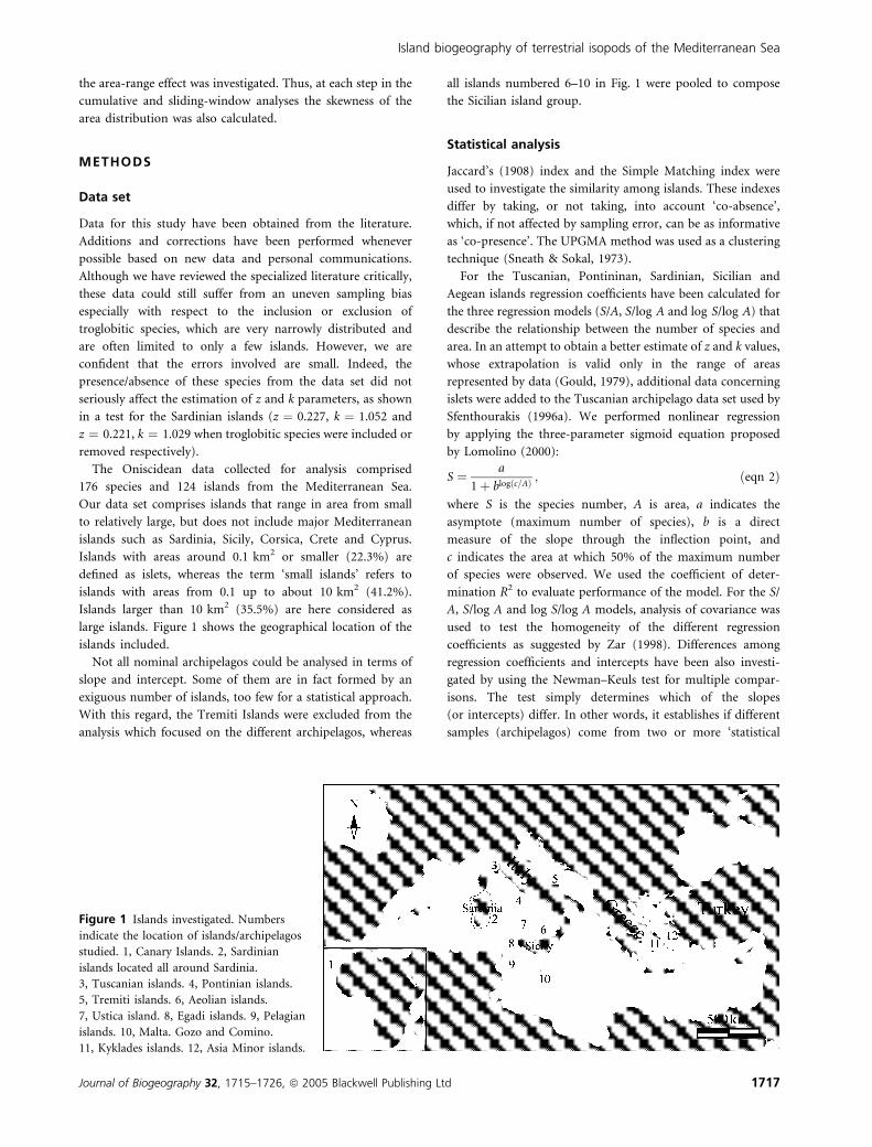
large islands. Figure 1 shows the geographical location of the

islands included.

Not all nominal archipelagos could be analysed in terms of

slope and intercept. Some of them are in fact formed by an

exiguous number of islands, too few for a statistical approach.

With this regard, the Tremiti Islands were excluded from the

analysis which focused on the different archipelagos, whereas

all islands numbered 6–10 in Fig. 1 were pooled to compose

the Sicilian island group.

Statistical analysis

Jaccard’s (1908) index and the Simple Matching index were

used to investigate the similarity among islands. These indexes

differ by taking, or not taking, into account ‘co-absence’,

which, if not affected by sampling error, can be as informative

as ‘co-presence’. The UPGMA method was used as a clustering

technique (Sneath & Sokal, 1973).

For the Tuscanian, Pontininan, Sardinian, Sicilian and

Aegean islands regression coefficients have been calculated for

the three regression models (S/A, S/log A and log S/log A) that

describe the relationship between the number of species and

area. In an attempt to obtain a better estimate of z and k values,

whose extrapolation is valid only in the range of areas

represented by data (Gould, 1979), additional data concerning

islets were added to the Tuscanian archipelago data set used by

Sfenthourakis (1996a). We performed nonlinear regression

by applying the three-parameter sigmoid equation proposed

by Lomolino (2000):

S ¼ a

1þ blogðc=AÞ ; ðeqn 2Þ

where S is the species number, A is area, a indicates the

asymptote (maximum number of species), b is a direct

measure of the slope through the inflection point, and

c indicates the area at which 50% of the maximum number

of species were observed. We used the coefficient of deter-

mination R2 to evaluate performance of the model. For the S/

A, S/log A and log S/log A models, analysis of covariance was

used to test the homogeneity of the different regression

coefficients as suggested by Zar (1998). Differences among

regression coefficients and intercepts have been also investi-

gated by using the Newman–Keuls test for multiple compar-

isons. The test simply determines which of the slopes

(or intercepts) differ. In other words, it establishes if different

samples (archipelagos) come from two or more ‘statistical

Figure 1 Islands investigated. Numbers

indicate the location of islands/archipelagos

studied. 1, Canary Islands. 2, Sardinian

islands located all around Sardinia.

3, Tuscanian islands. 4, Pontinian islands.

5, Tremiti islands. 6, Aeolian islands.

7, Ustica island. 8, Egadi islands. 9, Pelagian

islands. 10, Malta. Gozo and Comino.

11, Kyklades islands. 12, Asia Minor islands.

Island biogeography of terrestrial isopods of the Mediterranean Sea

Journal of Biogeography 32, 1715–1726, ª 2005 Blackwell Publishing Ltd 1717

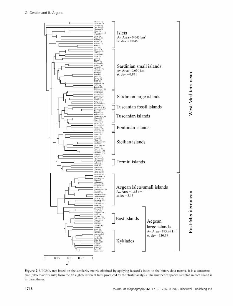
Figure 2 UPGMA tree based on the similarity matrix obtained by applying Jaccard’s index to the binary data matrix. It is a consensus

tree (50% majority rule) from the 32 slightly different trees produced by the cluster analysis. The number of species sampled in each island is

in parentheses.



populations’ (of islands) that differ in terms of slope (or

intercept) (Zar, 1998).

To investigate the existence of a SIE, we performed

breakpoint regression analyses by using both the model

proposed by Lomolino & Weiser (2001) and the following

discontinuous model, which combines two linear relationships

into a single equation:

log S ¼ ðb0 þ b1 logAÞðlogA � TÞ þ ðb2 þ b3 logAÞðlogA > TÞðeqn 3Þ

In this equation, variables S, A and parameter T are defined

as above, (log A £ T) and (log A > T) are logical variables that

return 1 or 0 if true or false respectively. This model does not

assume a priori the existence of a SIE. If a breakpoint is found,

the correlation between log S and log A to the left to the

breakpoint can still be evaluated, whereas this is not possible if

equation 1 is used. The parameters were estimated by using

nonlinear estimation procedures based on iteration. As in

Lomolino & Weiser (2001), we incremented the breakpoint

values by 0.1. Values of all parameters were chosen on the basis

of the amount of variance explained (maximum R2 value).

Before performing the cumulative and the sliding-windows

analysis, we pooled together islands based on results from the

cluster analysis. Islands below the breakpoint value, from

archipelagos exhibiting a SIE, were removed from the data set.

In the cumulative analysis the width of the starting window

was set to 1.5 (log A), to include a minimum of 10 islands. The

window was increased by increments of 0.1. The same width

was also used in the sliding-window analysis and was also

shifted by increments of 0.1.

The statistical programs ntsys (version 2.1; Exeter Software,

Setauket, NY, USA) and statistica (version 5.1; StatSoft, Inc.,

Tulsa, OK, USA) were used. The original data set is available at

the website http://www.biogeography.org.

RESULTS AND DISCUSSION

Island biogeography

The two similarity indexes provided similar results, thus, only

the Jaccard’s index results are presented. Figure 2 shows the

UPGMA consensus tree (50% majority rule) from the

32 slightly different trees produced by the cluster analysis.

This tree describes the similarity between the major Mediter-

ranean archipelagos and it is geographically structured. Three

different levels of similarity can be recognized, although clear

thresholds in the similarity values cannot be easily established.

According to this tree, Mediterranean islands can first be split

into two distinct major faunal and geographical areas: western

and eastern. In this tree, islands belonging to the Aegean

archipelago form a distinct cluster, which can be divided into

two groups: islets/small islands and large islands. The latter

group can be further subdivided into central Aegean islands

(Kyklades) and eastern islands (Asia Minor group) with

different biogeographical histories. The topology of this cluster

is consistent with Sfenthourakis (1996a; see this publication for

a discussion of the biogeography of Aegean islands), and is not

affected by the addition of the western archipelagos, which

have their own identity. At a second level of differentiation,

within the western Mediterranean group, islands belonging to

the same archipelago were clustered together for the major

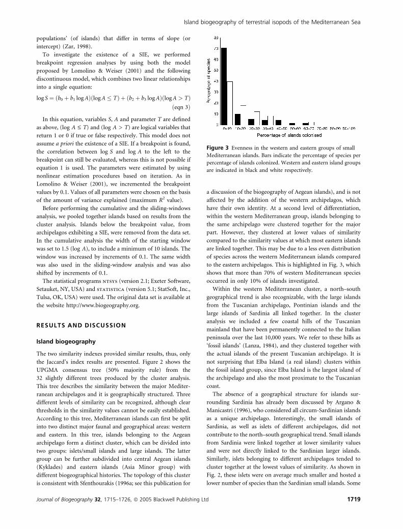
part. However, they clustered at lower values of similarity

compared to the similarity values at which most eastern islands

are linked together. This may be due to a less even distribution

of species across the western Mediterranean islands compared

to the eastern archipelagos. This is highlighted in Fig. 3, which

shows that more than 70% of western Mediterranean species

occurred in only 10% of islands investigated.

Within the western Mediterranean cluster, a north–south

geographical trend is also recognizable, with the large islands

from the Tuscanian archipelago, Pontinian islands and the

large islands of Sardinia all linked together. In the cluster

analysis we included a few coastal hills of the Tuscanian

mainland that have been permanently connected to the Italian

peninsula over the last 10,000 years. We refer to these hills as

‘fossil islands’ (Lanza, 1984), and they clustered together with

the actual islands of the present Tuscanian archipelago. It is

not surprising that Elba Island (a real island) clusters within

the fossil island group, since Elba Island is the largest island of

the archipelago and also the most proximate to the Tuscanian

coast.

The absence of a geographical structure for islands sur-

rounding Sardinia has already been discussed by Argano &

Manicastri (1996), who considered all circum-Sardinian islands

as a unique archipelago. Interestingly, the small islands of

Sardinia, as well as islets of different archipelagos, did not

contribute to the north–south geographical trend. Small islands

from Sardinia were linked together at lower similarity values

and were not directly linked to the Sardinian larger islands.

Similarly, islets belonging to different archipelagos tended to

cluster together at the lowest values of similarity. As shown in

Fig. 2, these islets were on average much smaller and hosted a

lower number of species than the Sardinian small islands. Some

Figure 3 Evenness in the western and eastern groups of small

Mediterranean islands. Bars indicate the percentage of species per

percentage of islands colonized. Western and eastern island groups

are indicated in black and white respectively.



geographical ‘signal’ was still detectable in the case of the small

islands of Sardinia, which still grouped together. However, this

‘signal’ was completely lost in the case of islets. A similar

pattern was observed by Sfenthourakis (1996b) who found that

islets/very small island clusters from the Central Aegean Sea did

not follow any geographical or palaeogeographical pattern, and

instead were influenced by vegetation and other ecological

variables. Although it is possible that the grouping of islets may

have been a statistical artefact to some extent, some faunal

affinity among islets/very small islands is not surprising because

Oniscidea species that inhabit very small islands are relatively

more common and have broader distributions than those

restricted to larger islands.

On the whole, the results confirmed Oniscidea as a good

biogeographical indicator and justifies the consideration of

separate archipelagos in the species–area analysis.

Island model: linear, semi-logarithmic, logarithmic

and sigmoid regressions

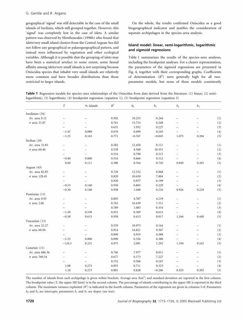
Table 1 summarizes the results of the species–area analyses,

including the breakpoint analyses. For a clearer representation,

the parameters of the sigmoid regressions are presented in

Fig. 4, together with their corresponding graphs. Coefficients

of determination (R2) were generally high for all two-

parameter models, but none of these models consistently

Table 1 Regression models for species–area relationships of the Oniscidea from data derived from the literature: (1) linear; (2) semi-

logarithmic; (3) logarithmic; (4) breakpoint regression (equation 1); (5) breakpoint regression (equation 3)

T % islands R2 b0 b1 b2 b3

Sardinian (34)

Av. area 8.12

r area 21.87

– – 0.502 10.253 0.244 – – (1)

– – 0.761 13.714 6.248 – – (2)

– – 0.631 1.052 0.227 – – (3)

)1.47 0.088 0.670 0.690 0.245 – – (4)

)1.25 0.163 0.771 )0.767 )0.845 1.075 0.204 (5)

Sicilian (18)

Av. area 33.85

r area 60.46

– – 0.582 12.450 0.111 – – (1)

– – 0.538 4.568 10.351 – – (2)

– – 0.516 0.790 0.312 – – (3)

)0.40 0.000 0.516 0.666 0.312 – – (4)

0.60 0.111 0.580 0.764 0.720 0.849 0.265 (5)

Aegean (43)

Av. area 82.85

r area 120.45

– – 0.720 12.332 0.068 – – (1)

– – 0.820 10.630 7.004 – – (2)

– – 0.920 0.977 0.199 – – (3)

)0.53 0.140 0.930 0.805 0.229 – – (4)

)0.30 0.140 0.938 1.048 0.210 0.926 0.229 (5)

Pontinian (13)

Av. area 0.93

r area 2.06

– – 0.803 4.787 4.219 – – (1)

– – 0.742 16.439 7.311 – – (2)

– – 0.789 1.083 0.354 – – (3)

)1.20 0.538 0.932 0.369 0.612 – – (4)

)0.50 0.615 0.958 0.413 0.017 1.166 0.440 (5)

Tuscanian (13)

Av. area 22.27

r area 60.94

– – 0.570 10.973 0.164 – – (1)

– – 0.914 14.821 9.307 – – (2)

– – 0.890 0.919 0.388 – – (3)

)1.53 0.000 0.890 0.326 0.388 – – (4)

)1/0.3 0.231 0.973 2.091 1.292 1.194 0.162 (5)

Canarian (11)

Av. area 686.36

r area 760.54

– – 0.746 7.977 0.011 – – (1)

– – 0.677 0.173 7.227 – – (2)

– – 0.752 0.568 0.247 – – (3)

1.08 0.273 0.855 0.711 0.323 – – (4)

1.10 0.273 0.881 0.828 )0.206 0.423 0.303 (5)

The number of islands from each archipelago is given within brackets. Average area (km2) and standard deviation are reported in the first column.

The breakpoint value (T, the upper SIE limit) is in the second column. The percentage of islands contributing to the upper SIE is reported in the third

column. The maximum variance explained (R2) is indicated in the fourth column. Parameters of the regression are given in columns 5–8. Parameters

b0 and b2 are intercepts, parameters b1 and b3 are slopes (see text).



provided the best fit. In particular, as already pointed out by

Sfenthourakis (1996a), the logarithmic model did not always

provide the best fit. A possible explanation is that the linear

model may better approximate the species–area relationship

when dealing with sets of data distributed in narrow size

ranges. This could be because a logarithmic curve may be

approximated by a linear curve when narrow intervals are

considered and also because a logarithmic transformation is

less sensitive to the heteroscedasticity expected when wider

ranges of area are considered (Sfenthourakis, 1996a).

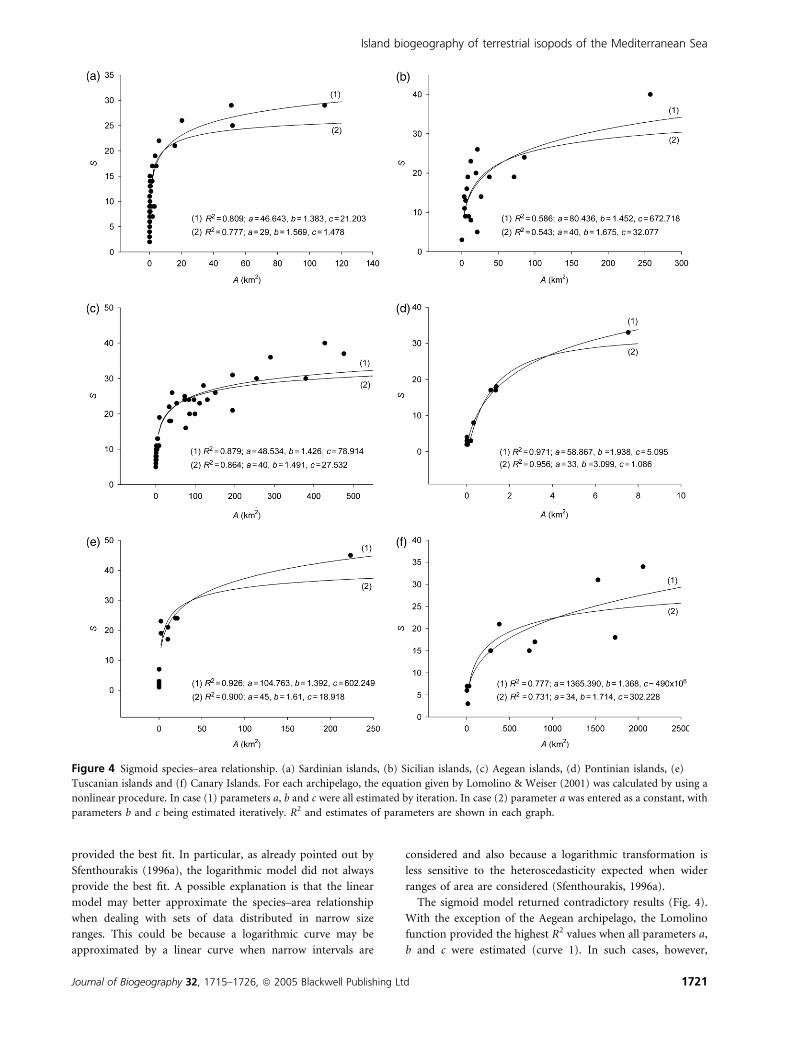
The sigmoid model returned contradictory results (Fig. 4).

With the exception of the Aegean archipelago, the Lomolino

function provided the highest R2 values when all parameters a,

b and c were estimated (curve 1). In such cases, however,

Figure 4 Sigmoid species–area relationship. (a) Sardinian islands, (b) Sicilian islands, (c) Aegean islands, (d) Pontinian islands, (e)

Tuscanian islands and (f) Canary Islands. For each archipelago, the equation given by Lomolino & Weiser (2001) was calculated by using a

nonlinear procedure. In case (1) parameters a, b and c were all estimated by iteration. In case (2) parameter a was entered as a constant, with

parameters b and c being estimated iteratively. R2 and estimates of parameters are shown in each graph.



estimates of parameters a and c returned unrealistic values for

most of the archipelagos. When parameter a was entered as a

constant (curve 2), parameter c became more reliable, but the

amount of variance explained decreased and the sigmoid

model was not the best fit. We also note that, even when it did

provide the best fit, parameter b estimates were so small that

the inflection point was virtually undetectable.

Island models: slopes and intercepts in the

Mediterranean archipelagos

Analysis of covariance showed that the islands from the

Mediterranean archipelagos cannot be treated as belonging to

the same pool (F ¼ 6.642, P(2),4,111 > 0.001). Table 2 shows

results of the Newman–Keuls test for multiple comparisons

among slopes. Data regarding the archipelago of the Canary

Islands, although available, have not been included in this test.

This is because the Canary Islands are on average much larger

than Mediterranean islands, and their inclusion is expected to

greatly increase the variance of the data set. The Newman–

Keuls test allowed us to determine which archipelagos differ in

terms of slope and intercept. In terms of slope, two sets of

similarities could be distinguished. The Sardinian and the

Aegean archipelagos were assigned to one set. The slopes of

these archipelagos were not statistically different, while their

intercepts were (t(2)74 ¼ 2.317, P ¼ 0.023). Pontinian and

Tuscanian archipelagos were assigned to the second set. Their

slopes were not statistically different, whereas their intercepts

were (t(2)23 ¼ 22.495, P > 0.0001).

Slopes for the Tuscanian and Pontinian archipelagos have

higher values than the Sardinian and Aegean archipelagos. It is

instructive to note that the inclusion of six additional small

islands (ranging from 0.03 to 0.1 km2) to the Tuscanian data

set produced a slope estimate much higher than previously

observed (Sfenthourakis, 1996a). In general, the effect of the

very small islands or islets on the outcome is important

because it can influence the shape and the goodness-of-fit of

the species–area relationship. In general, the first part of the

curve, which is important in order to detect the correct

approximation, is in most cases extrapolated either because

many archipelagos lack very small islands or because the

authors do not include them.

The slope for the Sicilian islands had an intermediate value

and could not be assigned to any of the two sets. This is

because the variance explained by the regression is very poor

(R2 ¼ 0.52). These results were partly expected as they

possibly reflected the different degrees of isolation of the

different archipelagos from their species source pools. It was

reasonable to expect that geographical distance should have

been related to both the species number and the rate at

which species colonize islands. The last is in part reflected by

the slope in the log S/log A relationship (Rosenzweig, 1995),

since intercept indicates the logarithm of the average number

of species that can be found in an island of unitary area.

However, for Oniscidea from the Mediterranean archipelagos

studied, distance does not seem to have a great impact on

species richness (Sfenthourakis, 1996a; G. Gentile &

R. Argano, unpubl. data). Consistent with this view,

intercepts were very similar (although their differences were

statistically significant), showing values of around 1–0.9, with

the only exception being the Sicilian archipelago. We do not

want to over-emphasize the few statistical differences between

archipelagos; however, it should be noted that the intercepts

of all the continental Mediterranean archipelagos studied are

higher than the intercept value of the oceanic archipelago of

the Canary Islands (k ¼ 0.57, Sfenthourakis, 1996a). It seems

that geographical distance influences the rate at which the

log S/log A relationship increases. Although all of them are

continental archipelagos, the Aegean islands, which exhibit

the lowest regression coefficient, are on average further from

the mainland than the Sicilian, and particularly the Pontinian

and Tuscanian islands. The low regression coefficient

observed for the Sardinian archipelago is difficult to explain.

These islands are very distant from the continental mainland

and this would be consistent with the low value of the slope.

However, they are also extremely proximate to Sardinia, one

of the largest islands of the Mediterranean Sea. Thus, a high

rate of colonization could be expected from Sardinia,

whereas the slope value (0.23) did not indicate this. This is

most likely to be related to the number of species occurring

in Sardinia (72; Argano & Manicastri, 1996), which is much

smaller than the number of species that occur in the Italian

mainland (c. 350; Argano et al., 1995). It has been proposed

that, for islands of equal area, slopes tend to decrease when

the number of species in the original source pool (mainland)

decreases (Martin, 1981). Interestingly, the z-value observed

for Sardinian islands was similar to the value predicted by

Schoener (1976) who, based on the observation that species

differ in their dispersal and colonizing abilities and in the

intensity of their interactions, provided a model to estimate z

when the number of species in the mainland is known.

Area-range effects

A breakpoint was found for all archipelagos (Fig. 5). Both

equations 1 and 3 provided similar breakpoint values for the

Table 2 Newman–Keuls test for multiple comparisons among

slopes of the species–area relationships for Oniscidea

Sardinian Aegean Sicilian Pontinian

Aegean tot. 1.166

(n.s.)

Sicilian 1.771

(n.s.)

2.427

(n.s.)

Pontinian 3.708

(P > 0.05)

4.834

(P > 0.01)

0.805

(n.s.)

Tuscanian 5.269

(P > 0.01)

6.742

(P > 0.001)

1.526

(n.s.)

0.908

(n.s.)

The value of the observed statistic q is reported in the first row.

Residual pooled DF is equal to 111. The probability that the observed

q > expected q is reported in the second row (see Zar, 1998).



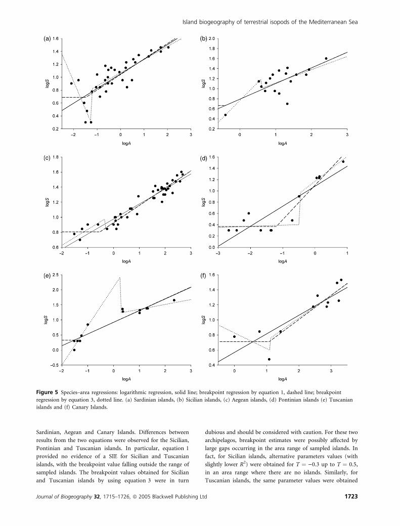
Sardinian, Aegean and Canary Islands. Differences between

results from the two equations were observed for the Sicilian,

Pontinian and Tuscanian islands. In particular, equation 1

provided no evidence of a SIE for Sicilian and Tuscanian

islands, with the breakpoint value falling outside the range of

sampled islands. The breakpoint values obtained for Sicilian

and Tuscanian islands by using equation 3 were in turn

dubious and should be considered with caution. For these two

archipelagos, breakpoint estimates were possibly affected by

large gaps occurring in the area range of sampled islands. In

fact, for Sicilian islands, alternative parameters values (with

slightly lower R2) were obtained for T ¼ )0.3 up to T ¼ 0.5,

in an area range where there are no islands. Similarly, for

Tuscanian islands, the same parameter values were obtained

Figure 5 Species–area regressions: logarithmic regression, solid line; breakpoint regression by equation 1, dashed line; breakpoint

regression by equation 3, dotted line. (a) Sardinian islands, (b) Sicilian islands, (c) Aegean islands, (d) Pontinian islands (e) Tuscanian

islands and (f) Canary Islands.



from T ¼ )1 up to T ¼ 0.3 due to the lack of islands in the

corresponding interval. Thus, for these two archipelagos we

prefer to consider the SIE issue as unresolved.

In general, for continental archipelagos, the breakpoint

seems to occur for A smaller than 1 km2, as Lomolino &

Weiser (2001) showed for terrestrial isopods from the

Aegean, by using data from Sfenthourakis (1996a). A

breakpoint occurs at a higher value (c. 12 km2) for the

oceanic archipelago of the Canary Islands. More data

regarding small islands and islets from this archipelago

could help clarify if the higher breakpoint value observed is

simply due to lack of data or if it could be an echo of

the greater distance of the Canary Islands from the

mainland.

Our data offer little evidence of a scale effect within the

species–area relationship (Martin, 1981), although a general

trend could be recognized at the inter-archipelago level

(Table 1). In fact, with the evident exception only of the

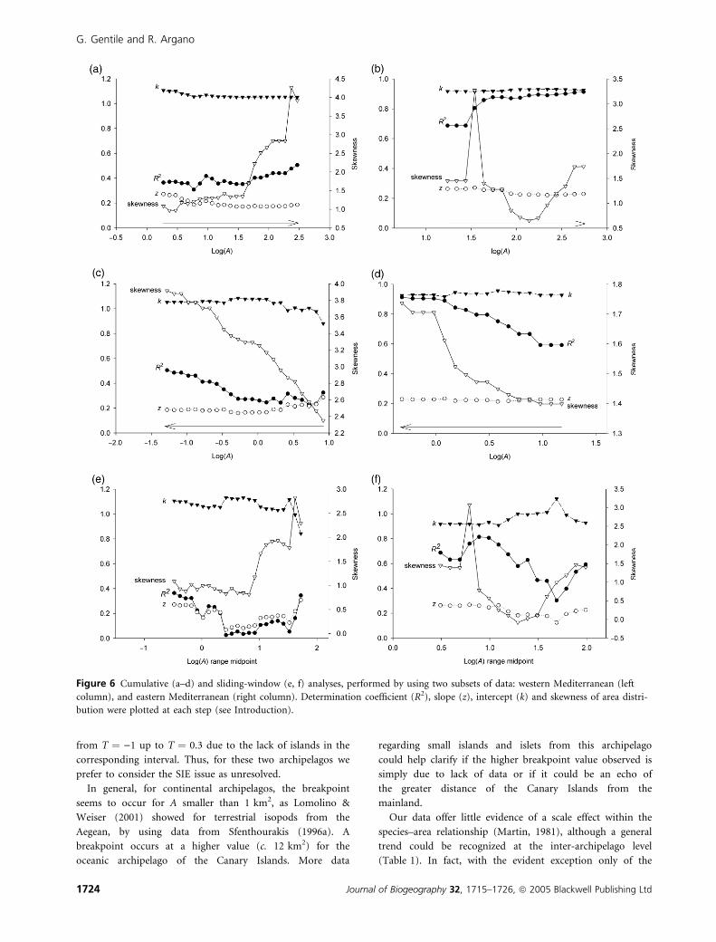
Figure 6 Cumulative (a–d) and sliding-window (e, f) analyses, performed by using two subsets of data: western Mediterranean (left

column), and eastern Mediterranean (right column). Determination coefficient (R2), slope (z), intercept (k) and skewness of area distri-

bution were plotted at each step (see Introduction).



Sardinian islands (which represent a special case), it seems that

all the archipelagos including larger islands tend to have lower

regression coefficients. If islands are included in the analysis

from left to right (smaller to larger), it would be expected that

z should decrease, whereas z would be expected to increase if

islands are added to the analysis from right to left (larger to

smaller), as in Martin (1981). Additionally, the sliding-window

approach should lead to decreasing z-values when moving

from left to right. The expected patterns from these analyses

are poorly reflected in the results obtained (Fig. 5a–d). This

approach suggests that R2 and skewness (always positive) of

the area distribution may vary independently of the slope and

intercept of the species–area relationships, which in turn

exhibits a flattened trend for both western Mediterranean and

Aegean islands. As expected, the sliding-windows analysis

depicted a more accentuated trend (Fig. 6e–f), in part

consistent with expectation, with R2 and skewness showing

some correlation with slopes and intercepts. However, this

should be taken with caution because confidence limits of

values observed at each iteration partly overlap (not shown in

Fig. 6 for clarity).

CONCLUSIONS

The terrestrial isopod fauna from islands of the Mediterranean

Sea can be divided into two major groups: the eastern and

western Mediterranean. In general, there is a high degree of

structure observed in Oniscidea assemblages from Mediterra-

nean islands. The structure reflects evolutionary events acting

at a local scale and the faunal inter-connectivity between

archipelagos and the most proximate mainland. As a conse-

quence, single archipelagos may be discriminated at different

similarity values. In part, the complex biogeographical pattern

may be explained by interpreting the different shapes of the

species–area curves. Slopes and intercepts provide helpful hints

to highlight major trends, but these data show a degree of

complexity that cannot be completely explained by the models

considered here. Besides the possibility that the interpretation

of slopes may reflect an artefact of the regression system

(Engen, 1977; Connor & McCoy, 1979; Sugihara, 1981; Keith

& McGuinnes, 1984), we note that several different factors may

interact and eventually contribute to the values of z

(MacArthur & Wilson, 1967; Karr & Roth, 1971; Willson,

1974; Gilbert, 1980). These factors make different contributions

to the species–area correlation and are difficult to distinguish

in most cases. In our case, some variables (latitude, number of

species and species vagility) may be assumed to be acting

equally on the different archipelagos, whilst others factors may

not. For example, evidence was provided for a linear decrease

(regressed on longitude) in the number of endemic species

of reptiles from western to eastern Mediterranean islands

(Mylonas & Valakos, 1990). Additionally, historical factors

may play an important role in determining the colonization

patterns of these archipelagos. On the whole, the effective

contribution of such factors to the species–area relationship

changes from case to case and cannot be easily quantified.

On the whole, area-range effects exist, although our data

offered poor support for scale-dependent effects such as

those discussed by Martin (1981) and Lomolino (2000).

Nevertheless, most continental archipelagos considered here

exhibit a SIE, with the upper limit being lower than 1 km2.

Despite the occurrence of a SIE, a sigmoid model did not

provide the best representation of our data. Even when the

sigmoid regression returned the best fit, the inflection point

was virtually undetectable. It is conceivable that in cases like

this, ‘the better fit of sigmoid curves does not necessarily prove

sigmoid relationships’ (Tjørve, 2003), with the better fit simply

being a reflection of the flexibility of a model with a higher

number of parameters.

ACKNOWLEDGEMENTS

We gratefully thank the two anonymous referees whose

valuable and constructive criticism helped us to improve this

paper. We also wish to thank N. Ellwood, E. Fresi, M.V.

Lomolino and M. Scardi for their interest in our work. This

work was financially supported by the National Research

Council (CNR), with the grant ‘Ricerche sulle popolazioni

insulari promosse e finanziate dal Consiglio Nazionale delle

Ricerche. Isole Ponziane: 50’.

REFERENCES

Arcangeli, A. (1953) La fauna isopodologica terrestre della

Puglia e delle isole Tremiti e la sua probabile origine in

rapporto alla diffusione transadriatica di specie. Memorie di

Biogeografica Adriatica, 2, 109–175.

Argano, R., Ferrara, F., Guglielmo, L., Riggio, S. & Ruffo, S.

(1995) Crustacea Malacostraca II (Tanaidacea, Isopoda,

Amphipoda, Euphausiacea). Checklist delle specie della fauna

italiana (ed. by A. Minelli, S. Ruffo and S. La Posta), pp. 1–

52. Calderini, Bologna.

Argano, R. & Manicastri, C. (1996) Gli Isopodi terrestri delle

piccole isole circumsarde (Crustacea, Oniscidea). Biogeo-

graphia, 18, 283–298.

Barrett, K., Wait, D.A. & Anderson, W.B. (2003) Small island

biogeography in the Gulf of California: lizards, the sub-

sidized island biogeography hypothesis, and the small island

effect. Journal of Biogeography, 30, 1575–1581.

Besier, L. & Sugihara, G. (1997) Scaling regions for food web

properties. Proceedings of the National Academy of Sciences of

the United States of America, 94, 1247–1251.

Caruso, D., Baglieri, C., Di Maio, M.C. & Lombardo,

B.M. (1987) Isopodi terrestri di Sicilia ed isole circum-

siciliane (Crustacea, Isopoda, Oniscoidea). Animalia, 14,

5–211.

Connor, E.F. & McCoy, E.D. (1979) The statistics and biology

of the species–area relationship. The American Naturalist,

113, 791–833.

Engen, S. (1977) Exponential and logarithmic species–area

curves. The American Naturalist, 111, 591–594.



Ferrara, F. & Taiti, S. (1978) Gli Isopodi terrestri dell’Arci-

pelago Toscano. Studio sistematico e biogeografico. Redia,

61, 1–106.

Gentile, G. & Sbordoni, V. (1998) Indirect methods to estimate

gene flow in cave and surface populations of Androniscus

dentiger (Isopoda: Oniscidea). Evolution, 52, 432–442.

Gilbert, F.S. (1980) The equilibrium theory of island biogeo-

graphy: fact or fiction? Journal of Biogeography, 7, 209–235.

Gould, S.J. (1979) An allometric interpretation of species–area

curves: the meaning of the coefficient. The American Nat-

uralist, 114, 335–343.

Jaccard, P. (1908) Nouvelles recherches sur la distribution

floral. Bulletin de la Societe Vaudoise des Sciences Naturelles,

44, 223–270.

Karr, J.R. & Roth, R.R. (1971) Vegetation structure and avian

diversity in several new world areas. The American Nat-

uralist, 105, 423–435.

Keith, A. & McGuinnes, A. (1984) Equations and explanations

in the study of species–area curves. Biological Reviews, 59,

423–440.

Lanza, B. (1984) Sul significato delle isole fossili, con parti-

colare riferimento all’Arcipelago pliocenico della Toscana.

Atti Societa Italiana Scienze Naturali, 125, 145–158.

Lomolino, M.V. (2000) Ecology’s most general, yet Protean

pattern: the species–area relationship. Journal of Biogeogra-

phy, 27, 17–26.

Lomolino, M.V. (2002) ‘… there are areas too small, and areas

too large to show clear diversity patterns…’ R. H. Mac-

Arthur (1972: 191). Journal of Biogeography, 29, 555–557.

Lomolino, M.V. & Weiser, M.D. (2001) Towards a more

general species–area relationship: diversity on all islands,

great and small. Journal of Biogeography, 28, 431–445.

MacArthur, R.H. & Wilson, E.O. (1967) The theory of island

biogeography. Princeton University Press, Princeton.

Martin, T.E. (1981) Species–area slopes and coefficients: a

caution on their interpretation. The American Naturalist,

118, 823–837.

McGee, V.E. & Carleton, W.T. (1970) Piecewise regression.

Journal of the American Statistical Association, 65, 1109–

1125.

Mylonas, M. & Valakos, E.D. (1990) Contribution to the

biogeographical analysis of the reptiles distribution in the

Mediterranean islands. Revista Espanola de Herpetologıa, 4,

101–107.

Rosenzweig, M.L. (1995) Species diversity in space and time.

Cambridge University Press, Cambridge, UK.

Sarbu, S.M., Galdenzi, S., Menichetti, M. & Gentile, G. (2000)

Geology and biology of the Frasassi Caves in central Italy: an

ecological multi-disciplinary study of a hypogenic under-

ground karst system. Ecosystems of the world – subterranean

ecosystems (ed. by H. Wilkens, D.C. Culver and W.F.

Humphreys), pp. 359–378. Elsevier, Amsterdam.

Schoener, T.W. (1976) The species–area relation within

archipelagos: models and evidence from island land birds.

Proceedings of the 16th International Ornithology Congress

(ed. by H.J. Firth and J.H. Calaby), pp. 629–642. Canberra,

ACT, Australian Academy of Science.

Sfenthourakis, S. (1996a) The species–area relationship of

terrestrial isopods (Isopoda; Oniscidea) from the Aegean

archipelago (Greece): a comparative study. Global Ecology

and Biogeography Letters, 5, 149–157.

Sfenthourakis, S. (1996b) A biogeographical analysis of terrest-

rial isopods (Isopoda, Oniscidea) from the central Aegean

islands (Greece). Journal of Biogeography, 23, 687–698.

Sneath, P.H.A. & Sokal, R.R. (1973) Numerical taxonomy.

W.H. Freeman & Co., San Francisco.

Sugihara, G. (1981) S ¼ CAz, z ¼ 1/4: a reply to Connor and

McCoy. The American Naturalist, 117, 790–793.

Taiti, S. & Ferrara, F. (1980) Nuovi studi sugli Isopodi terrestri

dell’Arcipelago Toscano. Redia, 63, 249–300.

Taiti, S. & Ferrara, F. (1989) Biogeography and ecology

of terrestrial isopods from Tuscany. Monitore Zoologico

Italiano, 4, 75–101.

Tjørve, E. (2003) Shapes and functions of species–area curves:

a review of possible models. Journal of Biogeography, 30,

827–835.

Williamson, M., Gaston, K.J. & Lonsdale, W.M. (2001) The

species–area relationship does not have an asymptote!

Journal of Biogeography, 28, 827–830.

Willson, M.F. (1974) Avian community organization and

habitat structure. Ecology, 55, 1017–1029.

Zar, J.H. (1998) Biostatistical analysis, 4th edn. Prentice-Hall,

New Jersey.

BIOSKETCHES

Gabriele Gentile has taught for 5 years a course entitled

Principles of Molecular, Cellular and Developmental Biology at

Yale University, USA. He is currently teaching a course

entitled Conservation of Nature and Conservation Genetics at

the University of Rome ‘Tor Vergata’, Italy. He is interested in

the ecology, genetics and evolution of subterranean organisms,

island biogeography, molecular phylogeny and systematics,

and conservation genetics of endangered species (invertebrates

and vertebrates).

Roberto Argano is a full Professor of Zoology. He teaches a

course entitled Adaptive Zoology, Evolutionary Zoology and

Animal Biodiversity at the University of Rome ‘La Sapienza’,

Italy. His interests are in the ecology, systematics, phylogeny

and biogeography of Isopoda, the biology and ecology of

aquatic communities, and the conservation of the sea turtle

Caretta caretta in the Mediterranean.

Editors: Jon Sadler and Robert Whittaker

