


Bahasa
Halaman
Hukum


Edifici B – Campus de Bellaterra 08193 Cerdanyola del Vallès, Barcelona, Spain Tel.:(+34) 935811203; Fax: (+34) 935812012 http://www.h-economica.uab.es
Departament d’Economia i d’Història Econòmica, Universitat Autònoma de Barcelona, Edifici B, 08193, Bellaterra (Cerdanyola), Spain
E-mail: [email protected]
04/11/2013
Unitat d’Història Econòmica UHE Working Paper 2013_06
GDP and life expectancy in Italy and Spain over the long-run (1861-2008): insights from a time-
series approach
Emanuele Felice, Josep Pujol Andreu

Emanuele Felice, Josep Pujol Andreu, 2013 GDP and life expectancy in Italy and Spain over the long-run (1861-2008): insights from a time-series approach UHE Working Paper 2013_06 http://www.h-economica.uab.es/wps/2013_06.pdf Unitat d’Història Econòmica Departament d’Economia i Història Econòmica Edifici B, Campus UAB 08193 Cerdanyola del Vallès, Spain Tel: (+34) 935811203 http://www.h-economica.uab.es © 2013 by Emanuele Felice, Josep Pujol Andreu and UHE-UAB
1
GDP and life expectancy in Italy and Spain
over the long-run (1861-2008): insights from a time-series approach1
Emanuele Felice, Josep Pujol Andreu
Departament d’Economia i d’Història Econòmica, Universitat Autònoma de Barcelona, Edifici B, 08193, Bellaterra (Cerdanyola), Spain E-mail: [email protected]
Abstract: The article presents and discusses long-run series of per capita GDP and life expectancy for Italy and Spain (1861-2008). After refining the available estimates in order to make them comparable and with the avail of the most up-to-date researches, the main changes in the international economy and in technological and socio-biological regimes are used as analytical frameworks to re-assess the performances of the two countries; then structural breaks are searched for and Granger causality between the two variables is investigated. The long-run convergence notwithstanding, significant cyclical differences between the two countries can be detected: Spain began to modernize later in GDP, with higher volatility in life expectancy until recent decades; by contrast, Italy showed a more stable pattern of life expectancy, following early breaks in per capita GDP, but also a negative GDP break in the last decades. Our series confirm that, whereas at the early stages of development differences in GDP tend to mirror those in life expectancy, this is no longer true at later stages of development, when, if any, there seems to be a negative correlation between GDP and life expectancy: this finding is in line with the thesis of a non-monotonic relation between life expectancy and GDP and is supported by tests of Granger causality. Keywords: Italy, Spain, GDP, life expectancy, unified growth theory, demographic transition JEL codes: N13, N14, N33, N34, O47, O52.
1. Introduction
When dealing with the long-run determinants of economic growth at the national
level, i.e. with macro-economic history, from quantitative grounds two are the most
1 Acknowledgements: helpful advice has come from Antonio Escudero, Francesco Gallio, Roser Nicolau; the usual disclaimers apply. The authors gratefully acknowledge financial support from the Spanish Ministry for Science and Innovation, project HAR2010-20684-C02-01.

2
popular approaches: cross-country studies, usually with the avail of cross-section data,
or country-specific studies, usually with the avail of time series.2 In cross-country
studies, the data at hand are usually limited to a few benchmark years, or to short
periods of time; although a wide range of countries and indicators may be included and
discussed, the lack of time-series may prevent from dealing efficaciously with
endogeneity, even when instrumental variables are used.3 Time-series macroeconomic
analyses of specific countries or regions are of course much more complete in
historical coverage and usually make use of updated and refined data,4 but this usually
comes at the cost of international comparisons.5
In this article, we extend time-series econometrics to a comparison between two or
more countries: our goal is to maintain some degree of generalization (l’espris de
geometrie), without losing in accuracy (l’espris de finesse). Namely, we present long-
run time-series comparisons between the two most important countries of Southern
Europe, Italy and Spain − which are usually regarded similar for culture and values, for
some key institutional features and even for economic performance6 − and compare
them with France, their main neighbouring country to which both have often looked up
as a proper term of evaluation. Our analysis focuses on economic monetary indicators
(GDP at constant prices) and social no-monetary ones (life expectancy), running from
the year of Italy’s Unification (1861) until the outbreak of the present economic crisis
(2008). The long-run convergence notwithstanding, are there significant cyclical
differences between the two countries, and how “exceptional” is their performance, for
instance when compared with their most important neighbour? Furthermore, are there
some common features of the patterns of GDP and life expectancy, and of their
relationship, which can be observed in both Italy and Spain? There is a growing
literature about the relation between improvements in life expectancy and the growth of
GDP per capita, mostly based on contributions from the unified growth theory, where
the demographic transition plays a crucial role in the transition from stagnation to
growth (Galor and Weil, 2000; Galor 2012). A number of cross-country studies have
found a positive effect of life expectancy, or a negative effect of mortality, on income
2 Some combination of the two may also be used: Prados de la Escosura (2007) provides a long-run comparisons among European countries via combining cross-section and time series data. 3 For an extended overview of cross-country studies with instrumental variables, see Durlauf et al. (2005). 4 For Italy, see Fenoaltea (2003, 2005) and, more recently, Felice and Vecchi (2012). For Spain, see among the others Pons and Tirado (2006), Prados de la Escosura (2010a), Sabaté, Fillat and Gracia (2011), Prados de la Escosura, Rosés and Sanz-Villarroya (2012). For other countries, see for instance the remarkable study on Turkey: Altug et al. (2008). 5 Unless of course the well-known series by Maddison (2010) are used, but when it comes to a detailed scrutiny of national cases Maddison’s estimates not always are reliable. For a criticism of Maddison’s Italian estimates, see Fenoaltea (2011). Fort time-series analysis using Maddison’s figures, see for instance Ben-David and Papell (2000). Time-series analysis with alternative estimates are usually limited to the industrial output: Crafts, Leyborne and Mills (1990); see also the Williamson project (Williamson, 2011). 6 At least in four important aspects: both are catholic countries, share the Latin heritage (from neo-Latin language to the codified law), are late-comers in the European industrialization, and are medium-big sized countries with significant regional differences.

3
per capita (Bloom and Sachs, 1998; Gallup et al., 1999; Lorentzen et al., 2008), but the
debate is still open: Acemoglu and Johnson (2007) have found no evidence of an
impact of life expectancy on income growth, while more recent studies have suggested
that the causal effect of life expectancy on growth is non-monotonic, i.e., it is negative
although insignificant before the onset of the demographic transition, positive after that
(Cervellati and Sunde, 2011). All these studies are based on cross-section comparison,
and we believe that an important contribution to the debate may come from a time-
series approach.
For our analysis, we work upon recent advancements in the historical research,
which make possible to review and discuss the most updated series of GDP, as well as
to present new long-run series of life expectancy for both Italy and Spain. In the case of
GDP, we make use of the new series at constant prices for Italy (Baffigi, 2011; Felice
and Vecchi, 2012), by many standards more reliable than the previous one included in
Maddison (1991, 2010), and compare it with the one available for Spain produced by
Prados de la Escosura (2003), which is incorporated in Maddison (2010) and unlike
others (Maluquer de Motes, 2009a) looks more similar to the Italian one in its
methodological approach. In the case of life expectancy, we link the most updated
estimates, for Italy in benchmark years (Felice and Vasta, 2012) and for Spain (Blanes
Llorens, 2007), with previously available information on life expectancy or mortality, in
order to produce long-run comparable series running from 1861 to 2008. All these
series are then confronted with those available for France, from well-known
international database (Maddison, 2010; HDM, 2011a).
For both the indicators, comparisons are made through simple quantitative tools
such as graphs and growth rates, and more refined ones such as econometric testing.
After presenting the new series, the main changes in the international economy, as well
as in technological and socio-biological regimes, are introduced and employed as
analytical grids to re-assess the performances of the two countries. As a further step,
through time-series econometrics structural breaks in the series of per capita GDP and
life expectancy are searched for, identified and discussed.
The article is organized as follows. In section §2 we present our updated series of
GDP and life expectancy for Italy and Spain, either if they are mostly new (per-capita
GDP for Italy, life expectancy for Italy and Spain) or a simple refinement of the previous
series to make the two countries more properly comparable (per-capita GDP for
Spain). In §3 we present the results and introduce the discussion by way of two-pairs
comparisons between Italy and Spain. In §4 we enter into a more detailed analysis, by
way of historical grids based on the main international changes in the world economic
history, as well as in technological and socio-biological regimes. Section §5 is

4
dedicated to discussing differences in structural breaks between the two countries and
to the issue of (Granger) causality between life expectancy and GDP. Section §6
concludes, by providing some answers to the abovementioned research questions.
2. The data
2.1. GDP per capita
As known GDP was invented in the 1930s, in the US, and only after world war II it
was progressively adopted by other countries, in primis those of western Europe. This
is the reason why GDP figures for periods previous world war II are always the product
of reconstruction by economic historians or statisticians. The Italian Istituto Nazionale
di Statistica was one of the first institutions to engage itself in the task of providing a
long-run series of Italy’s GDP, spanning from Unification (1861) until the 1950s (Istat,
1957), but the results were on the whole disappointing, not least due to the opacity of
sources and methods (e.g. Fenoaltea, 2010). Since the 1950s (Gerschenkron, 1955;
Fenoaltea, 1969) until our days (Fenoealtea, 2003, 2005; Carreras and Felice, 2010;
Battilani, Felice and Zamagni 2012), economic historians have tried to amend the main
flaws by providing their own indices of national production, for specific sectors or
periods. Only recently, under the joint auspices of Bank of Italy, Istat, and the
University of Rome II, these efforts have been unified into a long-run series of Italy’s
GDP, both at current and constant prices and spanning over 150 years, whose
procedure and sources are fully verifiable (Baffigi, 2011; Brunetti, Felice and Vecchi,
2011). Soon after it was released, the brand-new series has been updated (Felice and
Vecchi, 2012), to include the last advancements in the literature covering the interwar
years (Felice and Carreras, 2012). We make use of this latest series, after revising the
per-capita figures in order to consider the population de facto, rather than the resident
population, as should be “by the book” with Gross Domestic Product.7 In order to have
the revised series, however, first we must estimate a series of the Italian de facto
population at present boundaries; this is done through a few simple steps using the
data of population de facto at historical borders, from official censuses in benchmark
years, and the long-run series of resident population at historical and at present
boundaries, from Istat (2012a).8
7 By definition, per-capita Gross National Product should be based on resident population, per-capita Gross Domestic Product on present population. 8 In more detail, as a first step the benchmarks of the population de facto at historical borders (referring to the years: 1861, 1871, 1881, 1901, 1911, 1921, 1931, 1931, 1936, 1951, 1961, 1971, 1981, 1991, 2001, 2011) are interpolated, with geometric average using the cycles of the resident population at historical borders; this way, a series of the population de facto at historical borders is obtained. As a second step, the series of the population de facto at historical borders is converted into the series of the population de facto at present borders, using for each year the coefficient “population at historical borders / population at current borders” from the series of resident population.

5
In the case of Spain, we have resorted to the estimate by Leandro Prados de la
Escosura (2003), which was incorporated in Maddison (2010). This was not the only
available series, however. Recently, Jordi Maluquer de Motes (2009a) has published in
Revista de Economía Aplicada an alternative estimate of Spanish GDP at current and
constant prices; the reply by Prados de la Escosura (2009) and a further clarification by
Maluquer de Motes (2009b) were jointly published in the same journal. The two series
are indeed quite different: for the years 1850 to 1970, the one by Maluquer is on
average 24,5% higher than the one by Prados, and thus Spain’s backwardness as
compared to the rest of Europe is significantly reduced (Escudero and Simón, 2010, p.
234). The main reason of this discrepancy is due to the way different series at constant
prices, based on different base years, are linked in 1958, that is in the year when the
reconstruction by economic historians (1850-1958) and the one by the official national
accounts (1958 to date) meet. Since the value from this latter is higher,9 a major
problem is how to bridge this difference. Maluquer chooses to consider superior the
new estimate from national accounts: therefore he accepts the difference, which is then
rescaled to the historical series from 1958 backward.10 Prados’ alternative strategy is
instead to consider the historical estimate made at historical prices more reliable than
the new estimate made with a more recent price system, and thus to refuse the
difference for 1958 (i.e, to take as good the lower value): the difference is then
distributed onward until the next base year for the constant-price series, in this case
1995; more specifically, it is allocated from 1958 to 1995 with weights increasing with
the distance from 1958 (Prados de la Escosura, 2009, pp. 12-14). As a consequence,
Prados’ series remains unchanged from 1958 backward, although the growth rate from
1958 to 1995 is probably artificially increased. One second source of discrepancy is
due to the fact that Maluquer uses one single deflator for all the series, the consumer
price index, rather than implicit sectoral deflators as Prados does.
Surely Prados’ approach pays more attention to the actual value of production in
the past, by assuming that historical estimates in the base year at historical prices are
more reliable than subsequent estimates made with different price systems (although
there might be some reason for preferring instead Maluquer’s index, for instance the
use of some updated historical information).11 Since we are interested in a comparison
with Italy, we choose with little doubt Prados’ estimate, essentially because both its
9 As usual, and mostly due to the different price-basis used. This happens because, when prices and quantities are inversely correlated, late-weight indices, such as those of national accounts, tend to grow slower than early-weight ones (e.g. Gerschenkron, 1947). 10 Namely, for 1958 Maluquer enlaces his series to the official accounts produced by Uriel, Moltó and Cucarella (2000), which in 1958 has a GDP higher by 10.7% than the one estimated by Prados (Maluquer de Motes, 2009b, p. 35). 11 The new series of population estimated by Maluquer himself (Maluquer de Motes, 2008) and the series about prices and consumption also reconstructed by Maluquer (Maluquer de Motes, 2005): as we are going to explain, the former is here incorporated in Prados’ index, since this can be done at no risk of weakening the consistency of Prados’ estimates.

6
deflation system based on implicit deflators, and the redistributing rule used to link
deflators with different base years, are conceptually similar to the methods used for
reconstructing the Italian series (and they are also in line with Maddison’s approach).12
However, we find no reason for distrusting Maluquer’s new estimate of the Spanish
population (Maluquer de Motes, 2008): the author provides a series which is for the first
time geographically and methodologically consistent through the different periods of
Spanish history, and always refers to the population de facto, the one which should be
used for per capita GDP (as mentioned). Therefore, we incorporate these data in order
to produce up-to-date estimates of per capita GDP based on the population de facto,13
which is comparable to the one we have produced for Italy. The differences between
the old and the new population series are noteworthy above all for the years following
the 1929 crisis, where Maluquer’s new data for the first time include the emigrants
returning from abroad: this results in higher estimates for the population and lower
ones for GDP per capita and, as we will see (section §5), this change has some impact
when it comes to search for structural breaks in the Spanish series.14
Both series are expressed in a common unit of measure, 1990 international Geary-
Khamis purchasing power parity dollars (1990 G-K dollars, thereafter). For Spain, in
Maddison (2010) Prados’ series of total GDP is already expressed in 1990 G-K dollars.
For Italy, we have had to transform the new series by Felice and Vecchi (2012) from
constant 2011 euros to constant 1990 liras, using the standard deflator for the Italian
cost of living, from Istat (2012b); after this, Italian 1990 liras were converted in 1990 G-
K dollars, using the coefficient for Italy (1384.11 liras for 1 G-K dollar) reported in
Maddison (2006, p. 189).
The results are displayed in table 1.
12 For Italy, see Baffigi, 2011, pp. 56-59; Brunetti, Felice and Vecchi, 2011, p. 234. See also Maddison (1991). 13 We divide Prados’ series of total GDP by Maluquer’s series of population de facto. We use the population de facto at the 1st of July. 14 The series of the population de facto for Italy and Spain are presented in the Appendix.

7
Table 1. GDP per capita (1990 K-S dollars) in Italy and Spain, 1861-2008
Italy Spain Italy Spain Italy Spain 1861 1,556 1,246 1911 2,403 2,011 1961 6,401 3,452 1862 1,576 1,243 1912 2,410 1,984 1962 6,782 3,805 1863 1,614 1,263 1913 2,520 2,052 1963 7,137 4,148 1864 1,616 1,258 1914 2,385 2,004 1964 7,348 4,504 1865 1,714 1,215 1915 2,250 2,014 1965 7,607 4,747 1866 1,711 1,273 1916 2,427 2,086 1966 8,045 5,044 1867 1,562 1,263 1917 2,435 2,043 1967 8,596 5,321 1868 1,594 1,133 1918 2,377 2,011 1968 9,153 5,580 1869 1,615 1,170 1919 2,293 2,031 1969 9,688 6,029 1870 1,654 1,198 1920 2,330 2,165 1970 10,207 6,328 1871 1,618 1,290 1921 2,233 2,203 1971 10,333 6,633 1872 1,581 1,465 1922 2,400 2,272 1972 10,664 7,109 1873 1,573 1,590 1923 2,594 2,281 1973 11,335 7,666 1874 1,654 1,454 1924 2,640 2,326 1974 11,878 8,155 1875 1,663 1,493 1925 2,814 2,448 1975 11,554 8,350 1876 1,621 1,517 1926 2,816 2,414 1976 12,301 8,602 1877 1,631 1,667 1927 2,724 2,595 1977 12,554 8,835 1878 1,672 1,617 1928 2,863 2,578 1978 12,908 9,029 1879 1,677 1,518 1929 2,984 2,731 1979 13,625 9,066 1880 1,703 1,643 1930 2,825 2,610 1980 14,052 9,191 1881 1,754 1,673 1931 2,764 2,510 1981 14,149 9,167 1882 1,777 1,684 1932 2,795 2,524 1982 14,194 9,269 1883 1,794 1,714 1933 2,743 2,435 1983 14,346 9,448 1884 1,769 1,709 1934 2,716 2,491 1984 14,803 9,535 1885 1,796 1,658 1935 2,847 2,507 1985 15,206 9,683 1886 1,837 1,616 1936 2,723 1,923 1986 15,634 9,961 1887 1,885 1,584 1937 3,010 1,757 1987 16,127 10,487 1888 1,877 1,641 1938 3,111 1,752 1988 16,790 11,022 1889 1,821 1,633 1939 3,230 1,908 1989 17,341 11,568 1890 1,824 1,632 1940 3,081 2,073 1990 17,678 12,050 1891 1,850 1,666 1941 2,970 2,026 1991 17,929 12,319 1892 1,851 1,784 1942 2,779 2,133 1992 18,090 12,382 1893 1,879 1,714 1943 2,342 2,196 1993 17,944 12,206 1894 1,889 1,727 1944 1,925 2,278 1994 18,348 12,453 1895 1,904 1,708 1945 1,740 2,104 1995 18,901 12,756 1896 1,932 1,570 1946 2,361 2,178 1996 19,141 13,026 1897 1,934 1,645 1947 2,779 2,195 1997 19,512 13,490 1898 1,926 1,754 1948 2,993 2,179 1998 19,812 14,055 1899 1,946 1,761 1949 3,190 2,143 1999 20,123 14,660 1900 1,997 1,786 1950 3,444 2,193 2000 20,880 15,377 1901 2,029 1,899 1951 3,751 2,396 2001 21,284 15,882 1902 2,064 1,828 1952 3,904 2,576 2002 21,233 16,107 1903 2,086 1,817 1953 4,166 2,547 2003 20,971 16,333 1904 2,126 1,795 1954 4,295 2,718 2004 20,993 16,595 1905 2,173 1,758 1955 4,562 2,805 2005 20,849 16,912 1906 2,250 1,838 1956 4,760 3,009 2006 21,070 17,322 1907 2,294 1,885 1957 5,006 3,080 2007 21,154 17,623 1908 2,345 1,947 1958 5,262 3,183 2008 20,608 17,501
1909 2,368 1,967 1959 5,603 3,078 1910 2,374 1,887 1960 5,963 3,094
Sources and notes: see the text.

8
2.2. Life expectancy
Measures based on GDP are not, of course, the only indicators of economic
growth, not to mention of human welfare. A wide range of social indicators, from per
capita calories to average heights, to life expectancy, can be used to supplement or
integrate GDP − not only because of the lack of GDP historical figures (Steckel, 2009)
− combined in composite indicators (among which the Human development index, HDI,
is now by far the most successful one),15 or considered individually in a “dashboard”
approach.16 Although estimating social indicators for past periods is in principle not
more difficult than reconstructing GDP − on the contrary, this latter poses by far greater
conceptual problems17 − international historical series of social indicators are badly
lacking; nothing comparable with the impressive reach of the Maddison project,
criticisable as it is. Before 1950, usually only benchmark estimates are available for
education, heights, and nutrition. Things are a bit better for life expectancy: here some
consistent series have been published, mostly thanks to the efforts by the Max Planck
Institute for Demographic Research of the University of California (i.e., the Human
Mortality Database, HMD hereafter);18 however, their database does not always include
home-made research made by economic historians in specific countries and which, if
properly assessed and possibly incorporated, could be useful to enlarge both the
international scope and the historical coverage of the database. For Italy, a wide range
of social indicators has been published in the recent book by Giovanni Vecchi (2011),
in benchmark years; in the case of life expectancy, an alternative and more recent
estimate has also been published, in benchmark years from 1871 to our days (Felice
and Vasta, 2012). For Spain, the Nisal research project has now made available on-
line an impressive range of social and well-being indicators, including historical
estimates of life expectancy previously published by Roser Nicolau (2005);19
furthermore, for this country we now have very accurate new estimates of life
expectancy in benchmark years (Cabré et al., 2002) and even in a yearly series from
1911 to 2004 (Blanes Llorens, 2007), both of them thus far not considered by HMD.
Thanks to this information, and to the available historical series published in the
HMD, it is now possible to produce historical and consistent series of such an important
social indicator as life expectancy, for both Italy and Spain spanning from 1861 until
2008, which are therefore directly comparable with the GDP series of the previous
15 UNDP (2010). For historical cross-country estimates, see Crafts (1997, 2002) and Prados de la Escosura (2010b); for Italy, see Brandolini and Vecchi (2011), Felice and Vasta (2012); for Spain, see Escudero and Simón (2010). 16 Ravallion (2012). For Italy, see Vecchi (2011). 17 Cfr. Boldizzoni, 2011, pp. 81-86. 18 Freely available at: http://www.mortality.org/. 19 Freely available at: http://www.proyectonisal.org/.

9
section. These new series of life expectancy are here presented and discussed for the
first time.
For Italy, the basic reference are the estimates recently published in Felice and
Vasta (2012), in benchmark years spanning from 1871 to 2007: from 1911 these
estimates are roughly the same as those published in the HMD;20 differences between
the two are present for the early period, when, however, HMD’s researchers
themselves consider their figures far less trustworthy.21 All these estimates − those by
Felice and Vasta as well as those by HMD and even the Vecchi’s ones − are at
historical borders and thus, for a proper time-series analysis, they need to be converted
to current borders. This conversion is made possible thanks to the fact that Felice and
Vasta report life expectancy data also for the Italian regions, at historical borders: we
make the conversion under the hypothesis that the ratio between life expectancy in
Trentino-Alto Adige and a part of what is now Friuli-Venezia Giulia (including Trieste)
on the one side, and the rest of Italy on the other side, has remained unchanged from
the liberal age (when Trentino-Alto Adige and a part of Friuli-Venezia Giulia were not
part of the Italian Reign) to the interwar years (when following World War I these
provinces were annexed). Once we have estimated the new benchmarks at current
borders (for 1871, 1891, 1911, 1931, 1938, 1951, 1961, 1971, 1981, 1991, 2001,
2007), the yearly series is constructed by interpolating through the benchmarks the
yearly series of HMD (2011b), through a geometric average; from 1861 to 1870, the
series is produced by projecting backward the value of life expectancy in 1871, with the
inverse of the mortality rate on resident population for the years 1862 to 1871.22
If for Italy we have three sources of historical data for life expectancy, for Spain the
sources are four. First, there are the benchmark figures published by Roser Nicolau
(2005), mostly based on the estimates by the Spanish Instituto Nacional de Estadística
(INE), running every ten years from 1900 to 1970, every five years from 1970 onwards,
and with a last benchmark in 1998. Second, for the years 1908 to 2008 there is the
yearly series by HDM (2011c). As expected, for corresponding years there are some
differences between the benchmarks in Nicolau and the HDM series, which are due to
different procedures of computing the population of Ceuta and Melilla and to the
changes from the population de facto to the resident population; it is worth noticing,
20 The Human mortality database provides an yearly series, at historical borders, from 1871 to 2008. Both Felice-Vasta and HMD differ from the benchmark estimates (which also are at historical borders) published in Vecchi (2011, p. 419), but to know the reasons of this discrepancy is impossible, at the present, because in the explanatory notes in Vecchi (2011, pp. 128-9) reference is made to an unpublished graduate thesis; in the case of Felice and Vasta, see the discussion at p. 35. 21 Since “deaths counts are available only by five-year age groups (i.e., 0-4, 5-9,…, 65-74, 75+)” and “the data for 1883-84 demonstrate clear patterns of age heaping” (Glei, 2011, p. 3). 22 The series of the mortality rate is available from Istat (2012c), for all the years 1862 to 2009; as expected, the correlation between mortality and life expectancy, for the years 1871 to 2009, is very high: Pearson coefficient of -0.955, with R2 of 0.911. The value for 1861 is linearly interpolated, through a linear regression for the years 1862-1880, where year is the independent variable and life expectancy the dependent one.
10
however, that the HDM researchers do not seem aware of the previous work by Roser
Nicolau,23 therefore they do not raise this issue (Glei et al., 2012). This is little harm,
since both works should by now be considered mostly outdated, thanks to the research
carried out by Anna Cabrè and her co-authors, and more recently by Amand Blanes
Llorens, who was a PhD student of Cabrè. At first, Cabré et al. (2002, p. 127) have
published five years estimates of life expectancy in Spain, beginning as early as 1860,
and running until 1995. A few years after, a PhD student of Cabré has published yearly
series of life expectancy in Spain, from 1911 until 2004, as part of his PhD thesis
(Blanes Llorens, 2007). This work is truly impressive, boasting a level of accuracy and
detail with no parallels in other previous and subsequent researches, including the one
by HDM (apparently unaware of this work too, unlike Blanes Llorens who discusses
their work);24 moreover, the results have never been published outside of the PhD
thesis, and are here presented for the first time to a wider public.
The higher level of accuracy of the work by Blanes Llorens can be exemplified by
the way of coping with under-registration of infant mortality, an issue which had indeed
some impact on the overall trend of life expectancy in Spain when compared to Italy, as
we are going to see in the next section. According to the Spanish laws, until 1974 the
newborns who died within the first 24 hours of life were counted in the official censuses
as aborted foetuses, or stillbirths, while from 1975 onwards they were included in the
mortality tables. Therefore, deaths were under-registered until 1974. In order to
estimate life expectancy, Blanes Llorens has recounted the number of these “false”
stillbirths from the demographic statistics (Movimiento Natural de la Población) of INE
from 1911 to 1975, and has accordingly modified his tables for those years to make
them fully comparable with the following period (Blanes Llorens, 2007, pp. 57-59).
HDM researchers also had coped with this problem, but had corrected infant death
counts only from 1930 onwards (Glei et al., 2012, pp. 3-5).
Once we have accepted the new figures as superior, the only (minor) problem is
that both the estimated series by Blanes Llorens, and the benchmark data by Cabré et
al. are reported by sex, with no averages for the whole population; averages must
therefore be calculated via the series of the population by sex, which is reconstructed
from the data of official censuses for benchmark years (see Nicolau, 2004).25 At this
point, the different data of life expectancy for the whole population can be linked and
unified, with the aim of producing the most updated and at the same time coherent
23 Whose first version was published as early as 1989 (Nicolau, 1989). 24 For a full description of sources and methods, see Blanes Llorens, 2007, pp. 43-114. 25 Namely, historical data of population by sex are available for the following benchmarks: 1860, 1877, 1887, 1897, 1900, 1910, 1920, 1930, 1940, 1950, 1960, 1970, 1981, 1991, 2001, plus 2010. The annual series of the shares of female (and male) population is constructed via linearly interpolating the shares of the benchmarks, through the continuous compounded annual rate.

11
series of life expectancy for Spain.26 To this scope, for the years 1911 to 2004 we use
the series from Blanes Llorens (2007); these are in turn linked to the five-years
estimates by Cabré et al. (2002) from 1861 to 1910.27 In order to complete the cycle
from 1861 to 1910, these are interpolated every five years, through geometric average,
using the series of the inverse of mortality rates until 1907,28 from Nicolau (2005), then
using for the last two years, 1908 and 1909, the life expectancy series from HDM
(2011c). For the very last stretch (2005-2008), we link the estimates by Blanes Llorens
to the series by HDM; needless to say, in the overlapping years of the last period their
figures are practically identical.
The new series are displayed in table 2.
26 When it comes to econometrics, however, an alternative series constructed via linking the Nicolau data through the HDM estimates will also be tested, arguing that it shows statistical discrepancies that make us doubt of its reliability; alternatively, if the HDM series must be believed, it would reinforce rather than weaken the main results of the article. 27 It is worth noticing that for the following period 5-years estimates by Cabré et al. are very close to the new figures by Blanes Llorens. 28 Also in the case of Spain, for those years when it is possible to check for (i.e., from 1908 to 2001), we register a high correlation between mortality rates and life expectancy: Pearson coefficient of -0.958, R2 of 0.918. In the series of mortality rates the years 1871 to 1876 are missing, and they should be reconstructed via linear interpolation through the continuous compounded annual rate, from 1870 to 1877; since, however, we have an estimate of life expectancy for 1875, the years of linear interpolation are indeed only four (1871 to 1874), plus one (1876).

12
Table 2. Life expectancy at birth (years) in Italy and Spain, 1861-2008
Italy Spain Italy Spain Italy Spain 1861 32.1 30.3 1911 44.2 42.2 1961 70.1 69.7 1862 32.0 31.0 1912 48.4 45.2 1962 69.4 69.7 1863 31.9 30.4 1913 47.9 43.7 1963 69.5 69.8 1864 33.1 29.7 1914 49.3 43.8 1964 70.6 70.6 1865 33.0 29.1 1915 41.9 43.6 1965 70.5 71.0 1866 33.9 34.1 1916 38.8 44.6 1966 71.2 71.2 1867 33.1 32.6 1917 37.3 43.3 1967 71.2 71.4 1868 32.4 28.7 1918 25.4 30.7 1968 71.0 71.7 1869 35.5 28.3 1919 41.7 41.9 1969 71.1 71.2 1870 33.1 30.1 1920 45.1 40.8 1970 71.8 72.2 1871 33.2 30.3 1921 48.8 43.9 1971 72.1 71.8 1872 33.6 30.5 1922 49.6 45.6 1972 72.3 73.0 1873 35.5 30.7 1923 51.1 45.6 1973 72.2 72.8 1874 35.4 30.9 1924 51.2 47.1 1974 72.8 73.1 1875 34.7 31.1 1925 51.0 47.6 1975 72.7 73.6 1876 36.9 31.2 1926 50.7 48.3 1976 73.0 73.9 1877 38.1 31.3 1927 52.4 49.0 1977 73.3 74.3 1878 37.2 31.5 1928 52.5 49.1 1978 73.6 74.5 1879 36.5 32.0 1929 52.2 50.1 1979 73.8 75.0 1880 35.0 32.1 1930 55.1 51.0 1980 73.7 75.5 1881 36.3 31.4 1931 54.8 50.9 1981 74.0 75.7 1882 36.2 30.5 1932 55.0 52.3 1982 74.5 76.3 1883 37.0 32.1 1933 56.8 52.4 1983 74.4 76.1 1884 38.4 28.3 1934 57.7 52.9 1984 75.2 76.5 1885 38.5 31.7 1935 57.3 53.1 1985 75.3 76.4 1886 36.6 32.9 1936 58.2 51.7 1986 75.7 76.7 1887 37.3 33.5 1937 57.2 48.1 1987 76.2 77.0 1888 38.2 34.9 1938 58.1 48.3 1988 76.4 76.9 1889 40.3 34.1 1939 59.5 47.9 1989 76.8 77.0 1890 39.5 34.1 1940 58.7 49.9 1990 76.9 77.0 1891 39.4 34.4 1941 56.1 48.9 1991 76.9 77.1 1892 39.5 34.7 1942 53.8 53.2 1992 77.3 77.5 1893 40.1 34.6 1943 50.3 55.2 1993 77.6 77.7 1894 39.9 34.1 1944 53.4 56.6 1994 77.8 78.1 1895 39.3 35.0 1945 55.8 58.1 1995 78.0 78.2 1896 40.1 34.5 1946 59.9 57.7 1996 78.4 78.3 1897 42.4 35.6 1947 62.0 59.4 1997 78.6 78.8 1898 41.1 35.6 1948 64.1 61.3 1998 78.7 78.9 1899 42.1 34.7 1949 64.6 61.0 1999 79.1 78.9 1900 39.9 34.5 1950 66.1 62.3 2000 79.5 79.4 1901 41.3 35.8 1951 65.5 61.9 2001 79.8 79.7 1902 41.0 38.0 1952 66.1 65.0 2002 80.0 79.8 1903 41.3 39.6 1953 66.8 65.7 2003 80.1 79.7 1904 42.7 38.4 1954 68.1 66.9 2004 80.9 80.2 1905 42.4 38.1 1955 68.5 66.7 2005 80.9 80.2 1906 43.7 38.0 1956 67.9 66.7 2006 81.3 80.8 1907 44.2 40.5 1957 68.0 66.6 2007 81.4 80.8 1908 42.1 42.0 1958 69.1 68.8 2008 81.6 81.1
1909 43.8 41.6 1959 69.5 68.7 1910 46.0 41.5 1960 69.4 69.4
Sources and notes: see the text.

13
3. How close, how far? A comparison by pairs of indicators (1861-2008)
The Italian and the Spanish series of GDP per capita, at constant prices (1990 K-S
dollars), are displayed in the left side of figure 1, while in the right side the two series
are confronted with the one available for France (the main neighbouring country of both
Italy and Spain).
Figure 1. Per capita GDP in Italy and Spain, 1861-2008
Sources and notes: table 1; data for France are from Maddison (2010).
The story of the “race” between Italy and Spain can be summarized as follows: Italy
began at a higher level, but lost some ground in the first decade following Unification;
from the 1870s until the mid of the 1930s there was a slight ledge in favour of Italy,
more or less unchanged through the ups and down from the end of the nineteenth
century until the Spanish Civil War; after World War II, for fifteen years (1946-1961) the
Italian gap toward Spain dramatically enlarged, but since the early 1960s Spain began
to converge. From this outline we may therefore identify four phases: 1) the first
decade (1861-1871), following Italy’s Unification, when Italy had a lead in per capita
GDP between 20 and 40% over Spain; 2) the following longer phase (1872-1935), until
the Spanish civil war, when the difference between the two countries was relatively
mild, between 0 and 20% in favour of Italy; 3) a third phase (1946-1960), characterized
by a growing gap in favour of Italy, from 6% in 1946 to a remarkable 91% in 1960; 4)
then the final period when, although through ups and downs, Spain has converged
towards Italy, reducing that gap down to 17-18% in 2008 − that is, to around the level
which had characterized the second phase.

14
Further insights come from a comparison with France, as from the right side of the
figure. Until the second half of the XX century, both Italy and Spain are declining
relatively to France: Italy indeed was falling behind only until 1899, thereafter remaining
more or less stable (although, again, through ups and downs); Spain instead continued
to lose ground as late as until 1960. In the second half of the XX century, however, the
two countries began steadily to converge, first Italy and later Spain. At the end of the
1980s Italy indeed even overcame France29, but then from 2001 it has fallen behind
again; conversely, Spain has continued to converge until 2008.
In short, Italy has passed from the status of European periphery to which it was
confined until World War II, much closer to Spain than to France, to the one of
European core in the second half of the twentieth century, but this status is now in
doubt. Instead Spain began to converge later towards the European core, but its
catching-up has not yet come to a halt (at least, not until 2008).
It is interesting to see as this evidence compares with the one we now have for life
expectancy, whose new series for Italy and Spain are displayed in figure 2. Unlike with
GDP, here at the beginning Italy’s gap towards Spain enlarged, throughout the first
decades following Unification up to the end of the XIX century; however, Spain began
to converge at the beginning of the XX century, to reach Italy in the 1960s. There is
here some discrepancy with the previous life expectancy data available for Spain,
according to which the convergence of Spain began fifteen years earlier, around the
second half of the 1880s, and closed some years before, in the decade following world
war II; the discrepancy is indeed due to the fact that official censuses, and even HDM
until 1930, underreported infant mortality, as we have seen in the previous section.
Lastly, it is worth stressing as in terms of life expectancy in the second half of the
1990s there was a new «reversal of fortunes», with Italy once again taking the lead.
29 The surpass is confirmed by GDP figures based on resident population. It should be remember that all these comparisons are at 1990 purchasing power parity (PPP), i.e., based on the differences in the cost of living observed in 1990.

15
Figure 2. Life expectancy in Italy and Spain, 1861-2008
Sources and notes: elaborations from table 2; data for France are from HDM (2011a).
In broad terms, we can say that there are two important similarities between the
patterns of GDP per capita and life expectancy: the initial advantage of Italy; the
convergence of Spain over the long-run. It is worth reminding that the convergence of
Spain is confirmed by a wide range of other indicators of well-being, from heights,30 to
per capita calories,31 to composite indicators such as the Human Development Index,
which a part from income and life expectancy includes education and where Spain has
indeed overtaken Italy in the last years.32
At a closer inspection, however, it is also clear how the two indicators differ in at
least two more important respects: first, in life expectancy Spain began to converge in
advance and even overtook Italy as early as the 1960s, i.e., when its convergence in
per capita GDP had only begun; secondly, in life expectancy Italy in turn overtook
Spain again in the late 1990s, i.e., at the same time when Spanish convergence in per
capita GDP remarkably accelerated. Indeed, in the patterns of life expectancy we can
also detect four phases, but this are significantly different from those of GDP: the first
phase, 1861-1899, is one of growing divergence in favour of Italy; the second is the
one of Spanish convergence, from 1900 to 1961, some ups and downs
notwithstanding; a third phase, from 1962 to 1998, shows indeed a slight edge in
favour of Spain; then comes a fourth final phase (1999 to date), which shows a new
slight edge in favour of Italy.
30 For Italy, see A’Hearn and Vecchi (2011, p. 57); for Spain, see María-Dolores and Martínez-Carrión, (2011, p. 35) and Martínez-Carrión and Puche-Gil (2011, pp. 444 and 447). 31 For Italy, see Sorrentino and Vecchi (2011, p. 417); for Spain, see Cussó Segura (2005). 32 For Italy, see Felice and Vasta (2012); for Spain, see Prados de la Escosura (2010b).

16
As for per capita GDP, also for life expectancy we can compare Spain and Italy with
France (right side of figure 2). Here around 1861 France has a lead over Italy even
higher than the one in GDP. Italy, however, began to converge soon, starting in 1863,
and practically reached France around the mid of the 1950s; soon after convergence in
GDP had begun, and well before it was completed. This is similar to what we have
seen for Spain in comparison with Italy. During the last decades, Italy is improving its
position in life expectancy also with respect to France, which by 1999 has been
surpassed. Conversely Spain passed through more ups and downs and began to
steadily converge towards France later than Italy, in the last years of the XIX century; it
reached the same level of France roughly a decade after Italy, in the middle of the
1960s. At the beginning of the 1970s, Spain indeed overtook France as well, and
managed to maintain such a lead throughout the 1980s. During the last two decades
Spain and France rank practically at the same level, although Spain is slightly falling
behind − once again, in sharp contrast with GDP.
From these comparisons, in the patterns of GDP and life expectancy some
regularities or common features come out, which are worth being discussed. The first
common feature is about the starting point: differences in GDP mirror those in life
expectancy at lower levels of development; in these early stages, a clear lead in GDP
results into a clear lead in life expectancy, and viceversa. This finding is not new: in the
contemporary world, there is a strong correlation between life expectancy and income
in poor countries, as displayed for example by the well-known Preston (1975) curve,
and the same can be said for historical periods when material conditions were low (e.g.
Fogel, 2004). By analysing the historical data for 16 western countries, in benchmark
years from 1870 to 2000, Livi Bacci (2012, p. 125) has efficaciously simplified the
reasons: “more food, better clothing, better houses, and more medical care have a
notable effect on those who are malnourished, badly clothed, poorly housed, and
forced to trust fate in case of sickness.”
The second regularity concerns the trend, i.e. the pattern of convergence: we
observe that convergence in life expectancy begins earlier than the one in GDP. On
this, we can say something more: we have convergence in life expectancy when the
leading country (France in the case of Italy, or Italy in the case of Spain) is in the rising
bend of its industrial transformation (which at the early stages may well have some
negative consequences on life expectancy), while at the same time the follower is
benefitting from a decline in mortality coming from breakthroughs in medicine and
social conditions, but has not undertaken yet its industrial transformation. Although
some tests of causality are needed (see further, section §5), this finding appears to be
in line with recent results stemming from unified growth theory, which stress a positive

17
impact of improvement in life expectancy upon economic growth, after the onset of the
demographic transition (Galor and Weil, 2000; Cervellati and Sunde, 2011).
Finally, the third regularity we observe concerns the last period: at higher levels of
development, further advancements in GDP may not result into advancement in life
expectancy: the two indicators are no longer necessarily correlated. Indeed, it even
seems that, if at this stage any correlation between the two can be established, this
would be of a negative sign: countries falling behind in life expectancy may forge ahead
in GDP, and viceversa. This result may be true well beyond the three countries here
under investigation − think of the opposite evidence of the United States (forging ahead
in GDP but falling behind in life expectancy) and Japan (similar instead to Italy) − and
can be of some interest in order to re-model growth economics for nowadays rich and
ageing countries. Demographers and economists have only begun to address this
point. Concerning the impact of GDP on life expectancy, we may quote again Livi Bacci
(2012, p. 125): “When increased production benefits already prosperous population the
effects are minimal or nonexistent, if not negative, as may be the case with overeating
and environmental deterioration.” The opposite impact of increased life expectancy on
GDP growth also deserves some attention: in the context of the “second demographic
transition” (Lestaeghe and Van de Kaa, 1986; Lestaeghe, 2000), when fertility has
gone below the replacement level, or the so-called “longevity transition” (Eggleston and
Fuchs, 2012), when the most part of additional years in life are realized late in life, very
high life expectancy may result into a disproportionately old population, which hampers
economic growth. In this respect our findings are thus in line with those recently
proposed by Eggleston and Fuchs (2012) for the United States.
4. Historical periodizations
After presenting the new series, we now analyse the growth rates of Italy and Spain
according to the different historical ages.33 In the left column of table 3 we can see the
main ages of (economic and political) world contemporary history: the first globalization
era (ca. 1861-1914), the break-up of the system and the autarky going from world war I
to world war II (ca. 1914-1948), then the golden age (ca. 1948-1973), the end of
Bretton Woods and the oil shocks (ca. 1973-1985), finally the second globalization era
(beginning roughly in 1985, the year of the counter-shock in oil prices).34 This broad
33 In order to smooth the consequences of specific yearly shocks, we make use of (3-period) simple moving averages. For the first and the last years of the series, data are from a 2-period simple moving average, using the subsequent (1862) or the previous (2007) year respectively. 34 E.g. Hobsbawm (1987, 1994). According to Hobsbawm, the last period should begin with the fall of the Berlin Wall (1989). We prefer 1985 because this was the year when the trend in oil prices changed, which ultimately contributed also to the fall of the Soviet Union; 1985 was also the year when Mikhail Gorbachev came to power in Soviet Union,

18
historical framework is useful to discuss both GDP per capita and life expectancy,
prima facie at least.
Table 3. Growth rates in GDP per capita and life expectancy, by historical periods
GDP per capita Life expectancy Italy Spain France Italy Spain France 1861‐1914 0.80 0.92 1.12 0.70 0.67 0.23 1914‐1948 0.66 0.21 0.89 0.93 0.96 0.93 1948‐1973 5.46 5.16 4.26 0.52 0.75 0.45 1973‐1985 2.52 2.03 1.70 0.34 0.40 0.33 1985‐2008 1.39 2.60 1.56 0.34 0.25 0.32
1861‐2008 1.78 1.82 1.71 0.64 0.66 0.46
Sources: elaborations from tables 1 and 2. Notes: see text.
For what concerns GDP, Spain grew more than Italy in the liberal age, but Italy
outperformed Spain in the interwar years; Italy again grew more rapidly than Spain in
the golden age and the following period; Spain, at last, grew more rapidly than Italy in
the last stretch, after joining the European Community in 1986. If we look at life
expectancy, however, we have exactly opposite results: that is, Italy grew more rapidly
than Spain in the first period, but then more slowly in the following three periods; it
grew again more rapidly in the last period. When including France in our analysis, this
sort of negative correlation is partly confirmed: in GDP per capita, France outperformed
both Italy and Spain in the first two periods, when indeed it lagged behind in life
expectancy; although in the third and fourth phases both Italy and Spain converged in
GDP and life expectancy, then again in the last stretch France outgrew Spain in life
expectancy although was losing ground in GDP, and it outgrew Italy in GDP per capita
but was losing ground in life expectancy.
In light of what we have seen in the previous section, these different performances
do not come as a surprise. Indeed, they can be seen as qualifications of two out of the
three main results from the previous section: convergence in life expectancy began
earlier than the one in GDP (thus during the liberal age Italy outperformed in life
expectancy Spain and France, whereas in the following phase Spain outperformed
both Italy and France); at later stages of development, further advancements in GDP
did not result into advancements in life expectancy, and viceversa. It is also worth
noticing that these different cycles took place within similar trends over the long-run: for
both GDP and life expectancy, highest growth of Spain, the less advanced country,
lowest growth of France, the most advanced one, with Italy in the middle. In other
words, there is a common trend of convergence, which is in part the product of the fact beginning a series of reforms which were to change the world in a handful of years. Furthermore, in 1985 agreement among the EEC members was reached on the Single European Act (SEA); the SEA was signed one year later, the same year when Spain joined the EEC.

19
that in terms of backwardness in each country the initial conditions were similar for
GDP per capita and life expectancy − the third of our results from the previous section.
A different kind of periodization focuses on the international changes in
technological regimes for GDP per capita, in socio-biological regimes for life
expectancy; that is, on those conditions which may specifically have an impact either
upon GDP per capita, or upon life expectancy. With reference to technological regimes,
a well-established literature (Freeman and Perez, 1988; Perez, 2002, 2010) considers
four different ages: steam engine and railways (from the end of the nineteenth century
until 1875, i.e. for our purposes from 1861 to 1875), steel and electricity (1875-1908),
the era of combustion engine, oil, and mass production (1908-1971), then telematics
and the new economy (1971 to date).
A periodization through technological regimes would makes little sense for life
expectancy, since these affect mostly GDP;35 in this case, we should rather look at
changes which affect specifically this variable, related to scientific, socio-demographic
and biological advancements and which we may call socio-biological regimes. The
main issue is mortality reduction. In a recent article, Cutler et al. (2006) have reviewed
the determinants of mortality reduction over the long-run, identifying three main
phases: the first one, roughly from the mid-XVIII century to the mid-XIX century, when
improvements in nutrition played the major role; a second one, from the mid-XIX
century to the 1930s, when the reduction in mortality rates was driven by public health
measures, the construction of urban infrastructures allowing for running water with
indoor plumbing (which provided clean water and the removal of waste), and good
advice about personal health practices; a third phase, starting in the 1930s, when the
main determinant was the advent of modern medicine, to begin with vaccination and
antibiotics. This framework is here partly refined and enlarged. Concerning the
refinement, the dividing line between the first two phases is postponed to the last
decade of the XIX century; the authors themselves recognize that “big public health did
not fully come into its own until the acceptance of the germ theory of disease in the
1880s and 1890s, which led to a wave of new public health initiatives and the
conveyance of safe health practices to individuals” (Cutler at al., 2006, p. 102; Mokyr,
2002; Tomes, 1998).36 Concerning the enlargement, a fourth phase going from the
35 This is not necessarily always true, however. An alternative and more inclusive periodization of technological regimes considers running water with indoor plumbing as one of the three central innovations − together with electricity and the internal combustion engine − of the second industrial revolution, which accordingly began in 1870 and lasted for about a century (Gordon, 2012). Running water with indoor plumbing had a huge impact upon the standard of living and life expectancy, and is here considered in our periodization specific for life expectancy (see forward). 36 More specifically, we should talk of infectious diseases (measles, scarlet fever, diphtheria), respiratory diseases (bronchitis, pneumonia, influenza), and intestinal diseases (diarrhea, enteritis) (Livi Bacci, 2012, p. 122). The germ theory was fully accepted only after Robert Kock published its postulates in 1890, although these were partly known from 1875 (Madigan and Martinko, 2005). It should be added that the decision by Cutler et al. about the dividing line in

20
1960s until our days is here added: thanks to the development of modern medicine
(mostly antibiotics in the 1930s and 1940s), in fact, by 1960 “mortality from infectious
diseases had declined to its current level” (Cutler at al., 2006, p. 103); furthermore,
from the 1960s the main driver for the decrease of mortality, at least in the advanced
countries,37 had become the reduction in cardiovascular disease mortality and the
decline in infant mortality (Cutler at al., 2006, p. 104), the latter also due to the
improvements in neonatal medical care for low birth-weight infants; at the same time,
from the 1960s the demographic transition is by now completed or under completion,38
while also the role of nutrition changed, from quantity to quality.
In view of this, in the case of life expectancy we propose the following periodization
for «socio-biological» regimes: a) from the mid XVIII century until 1890, i.e. in our case
1861-1890, when improvements in nutrition are the main determinants of the reduction
in mortality; b) 1890-1935, when the main drivers are hygienic health practices and the
construction of health and hydraulic infrastructures, in part following the application of
the germ theory; c) 1935-1960, when the reduction in mortality was driven by modern
medicine, to fight against infectious diseases; d) 1960-2008, characterized by on-going
improvements in the reduction of the death toll of cardio-vascular diseases and
neonatal mortality, as well as by the completion of the demographic transition.
The results according to the two periodizations, technological regimes for GDP per
capita and socio-biological regimes for life expectancy, are displayed in table 4. Once
again, we record contrasting results according to the indicator used. In GDP per capita,
Spain performs better than Italy in the (last stretch of the) first technological regime,
while performs clearly worst in the following two regimes; Spain again performs better
in the age of telematics (which for Spain is also the age of constructions). In life
expectancy, on the contrary, Italy performs better in the first socio-biological regime,
while it is outperformed by Spain in the following two; in the last period, life expectancy
has on average the same growth rate in both countries. These differences are a
consequence of the fact that Italy began to improve in life expectancy before than in
GDP per capita, and earlier than Spain; when Spain was converging in life expectancy,
Italy was forging ahead in GDP per capita, as we have seen; after both countries had
reached very high levels of life expectancy, their growth rates became similar.
the mid of the XIX century was based upon the experience of England, which at that time was the most advanced country: for a comparison between the causes of death in England and Italy, see Caselli (1991). 37 In Italy, from Unification until the mid-1950s infant mortality reduced by 226‰ to 51‰, thus by a ratio of more than four times; however, in the following half a century it would have further collapsed by a ratio of more than ten times, down to 4,4‰ by 1999-2002 (Felice, 2007, p. 115). In Spain, convergence in infant mortality took place after 1960 (Nicolau, 1989, pp. 57 and 70-72.) 38 Some differences among countries notwithstanding: in Spain, the demographic transition was completed later than in other countries, during the 1980s (Carreras and Tufanell, 2004, p. 38). In Italy, it lasted from 1876 to 1965, as in other European countries such as Germany (Livi Bacci, 2012, p. 118; Chesnay, 1986, pp. 294 and 301).

21
A part from confirmations, when looking at France there is another important result
coming out of table 4. In life expectancy France was the leading country at the
beginning of the period, but in terms of growth rates it was outperformed by both Italy
and Spain in all the four socio-biological regimes; conversely, in GDP per capita France
− although here too it was ahead of both Italy and Spain at the beginning of the period
− in some technological regimes performed better than either Italy (the first regime),
Spain (the third one), or even both (the second one). This evidence suggests that
convergence in GDP per capita should not be taken for granted, unlike the case of life
expectancy, where instead convergence through different regimes seems to be less
reversible. The fact that convergence in life expectancy can be more permanent does
not mean, however, that it is more stable, as we are going to see in the next section.
Table 4. Growth rates in GDP per capita and life expectancy, by technological and
socio-biological regimes
Techno-logical
regimes
GDP per capita Socio-biological regimes
Life expectancy Italy Spain France Italy Spain France
1861‐1875 0.36 1.28 1.06 1861-1890 0.75 0.38 0.22
1875‐1908 1.07 0.80 1.13 1890-1935 0.83 0.96 0.62
1908‐1971 2.40 1.99 2.15 1935-1960 0.75 1.11 0.75
1971‐2008 1.90 2.64 1.72 1960-2008 0.33 0.33 0.29
1861‐2008 1.78 1.82 1.71 1861-2008 0.64 0.66 0.46
Sources: elaborations from tables 1 and 2. Notes: see text.
5. Structural breaks and (Granger) causality
5.1. Structural breaks
Thus far, we have compared growth rates at different ages, in order to discuss as
exogenous changes may have impacted upon domestic performance. In the above
framework, the historical ages have been defined through the evolution of the
international scenario and of technological and socio-biological regimes, both of them
exogenous to the national context. It is now time to turn to time series analysis, in order
to detect if there are some breaks in the series which can be referable not only to
external shocks (such as World War II) and exogenous changes, but also to internal
and country-specific breaks, whether or not they are in response to exogenous
changes. On this, a time-series analysis has the advantage of not imposing any ex-
ante periodization, thus being useful to see as the international context interacts with
the evolution of domestic scenario.39
39 Moreover, in terms of clarity at this point a time-series analysis is far more efficacious than further comparisons of growth rates based on more historical ages, this time defined in terms of national and country-specifics changes (which

22
In order to search for structural breaks in the series, we run the Quandt Likelihood
Ratio (Quandt, 1960) or QLR test, which is a modified Chow test used to identify
unknown structural breaks (Andrews, 1993). We follow the procedure presented in
Stock and Watson (2007), here adapted from an autoregressive distributed lag (ADL)
model in levels, with one lag, to a first-differenced autoregressive (AR) model, with two
lags (Torres-Reyna, 2012).
First, let’s have a first-differenced autoregressive model with two lags, AR(2):
[1] yt = β0 + β1yt-1 + β2yt-2 + γ0Dt(τ) + γ1[Dt(τ)*yt-1] + γ2[Dt(τ)*yt-2] + εt;
where Dt(τ) is a binary variable, which equals 0 before the break (τ), 1 after:
[2] Dt(τ) = 0, if t ≤ τ; Dt(τ) = 1, if t ˃ τ;
in absence of break, the regression function is the same before and after τ, thus γ0
= γ1 = γ2 = 0. Accordingly, we test:
H0 γ0 = γ1 = γ2 = 0
H1 not H0
i.e., under the null hypothesis (H0) we have no break, while under the alternative
hypothesis (H1) we have break, since at least one γ is different from zero. Let’s F(τ) be
the F-statistics testing H0. If the break date τ is unknown, as in our case, the QLR test
calculates the highest value of F(τ) in the interval τ0 ≤ τ ≤ τ1:
[3] QLR = max [F(τ0), F(τ0 + 1), … , F(τ1)]
This QLR statistic may identify one single structural break, several structural
breaks, or even a slower evolution of the regression function. For our tests, we set τ0 =
0.1*T, τ1 = 0.9*T, which results in a 10% trimming from each tail. Although 0.15*T and
0.85*T are more commonly used for τ0 and τ1 respectively, we prefer a shorter trimming
since it allows us to identify more structural breaks around the extremes of the
distribution, as we will see, whereas the results for the central years of the distribution
would be the subject of endless discussion and would take this article far astray from its promised goals): to define international ages was relatively easy, given the wide (but not unanimous) consensus about the main epochs of world contemporary history, not only in terms of broad geopolitical scenarios, but also for what concerns technological and socio-political standards; historical grids resulting from domestic changes, specific for Italy and Spain, would be far less undisputed, while any comparison would be blurred by the fact that the historical grids would not be the same between Italy and Spain.

23
remain unchanged.40 Two more caveats are warranted: 1) to have comparable results,
we always use log transformation for both GDP and life expectancy; 2) in order to
ensure that possible differences are not the product of different methodologies
estimates, for each function we test two different series, our new one (Tables 1 and 2),
and the main alternative available series. The tests are displayed in figure 5 (GDP per
capita) and 6 (life expectancy).
From figure 3, the main result is that in the Italian series GDP many more structural
breaks can be observed than in the Spanish series.41 For Italy, there are a number of
breaks from 1877 to 1888, a period roughly coinciding with the rise to power of what is
called the Historical Left (1876) and the first protectionist and pro-industrialist policies
pursued by those governments.42 The second break, which is visible with the lower
threshold (6.02) from the 15% trimming, comes at the end of the century, in 1899, and
marks the beginning of the Giolitt’s age (1900-13) and the take-off of the Italian
industry.43 Then comes the biggest break, the one at the end of world war II, with the
beginning of unprecedented growth – the economic miracle − which would have
brought back the country “from the periphery to the centre” (Zamagni, 1993), as the
sixth world economic power. Finally, a fourth and negative break can be noticed, in
1993, coinciding with an economic recession and the first significant austerity
measures to join the euro, and which marks the beginning of Italy’s economic decline
(Felice and Vecchi, 2013).
Confronted with this story, the series of Spanish GDP looks much flatter: the breaks
come in the second half of the 1950s and reach the highest value in 1960, following the
Franco’s liberalization and the end of autarchy. The 1960 maximum marks the
beginning of the Spanish economic miracle, with a fifteen-years delay on Italy.44 In
other words, in terms of GDP Spain did not experience the breaks Italy lived through in
the second half of the nineteenth century, i.e., Italy’s early ruptures towards higher
economic growth: Spanish modernization in GDP began later and took place all at
once. This results is significantly different from the one found by Molinas and Prados
de la Escosura, with previous series for Italy and Spain, and benchmark comparisons
between the two: according to them Spain and Italy would have attained similar levels
of per capita income at around the same historical dates, but Spain converged later
40 Critical values of the QLR statistics with a 10% trimming are from Andrews, 2003. 41 The QLR test has been run also for France, but no significant breaks have been found (the highest observed break is in 1959); this is probably due to the higher level of GDP boasted by that country. Results will be provided on request to anyone interested. 42 The first trade protections were introduced in 1878, significantly reinforced in 1887, while the first Italian enterprise of the second industrial revolution (steel, electricity) were born in the first half of the 1880s, even with the help of the state (as in the case of Terni, in steel). For extensive discussion on these topics, see Toniolo (1990), Zamagni (1993), Federico and Tena-Junguito (1998), Fenoaltea (2011). 43 For a recent reappraisal, see Felice and Carreras (2012). 44 Or a bit less, since in Italy’s high growth rates of the early years following World War II were can be regarded as the “backlash” of world war II destruction − i.e., the product of the Reconstruction.

24
than Italy in structural change (Molinas and Prados de la Escosura, 1989). Such a
discrepancy was only apparent: indeed, also in per capita GDP Spain began to
modernize later than Italy.
Limitedly to Spain, our finding is in line with the results by Pons and Tirado (2006),
who making use of a variant of Andrews (1993) methodology45 also had found the lack
of breaks in the Spanish (Prados’) GDP series before the civil war, with a positive
break as late as 1960.46 Pons and Tirado also found two negative breaks in 1936 and
1940, the difference with us being due to the fact that we use the updated population
series by Maluquer: via counting the returns of Spanish emigrants after the 1929 crisis,
Maluquer finds higher numbers for the population de facto in the first half of the 1930s
(Maluquer de Motes, 2008) and correspondingly reduces the level of GDP per capita
for the same period; as a consequence, in our estimates the percentage decrease due
to the civil war is also reduced.
Our results are also consistent with an earlier vast literature stressing the missed
opportunities of the Spanish economy from the last decades of the XIX century until the
Franco’s liberalization policies in 1959: there was an essential continuity, characterized
by sluggish economic growth and international isolation, from the Bourbon Restoration
(1874-1923), to the dictatorship of Primo De Rivera and the short-lived Second
Republic (1923-1939), to the first phase of Franchism (1939-1959) (Fraile, 1991; Nadal
and Sudrià, 1993; Carreras 1990, 1997; Velarde, 1999). Accordingly, the first phase of
Franchism, negative as it was (Carreras 1989; Comín, 1995; Prados de la Escosura,
1997), should be seen not so much as an interlude, but rather as an enduring
constraint which delayed of about fifteen years the modernization of the Spanish
economy.
45 The Sup Wald test by Vogelsang (1997), extended by Ben-David and Papell (2000) to estimate multiple break-points. Unlike us, Pons and Tirado use an auto-regressive model in levels. 46 For a pioneering application of Andrews methodology to the Spanish historical series of GDP, again with analogous results, see also Cubel and Palafox (1998).
25
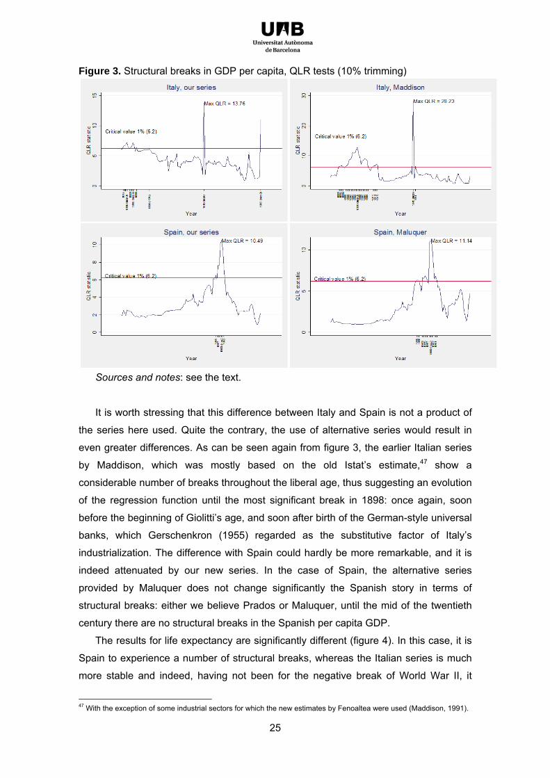
Figure 3. Structural breaks in GDP per capita, QLR tests (10% trimming)
Sources and notes: see the text.
It is worth stressing that this difference between Italy and Spain is not a product of
the series here used. Quite the contrary, the use of alternative series would result in
even greater differences. As can be seen again from figure 3, the earlier Italian series
by Maddison, which was mostly based on the old Istat’s estimate,47 show a
considerable number of breaks throughout the liberal age, thus suggesting an evolution
of the regression function until the most significant break in 1898: once again, soon
before the beginning of Giolitti’s age, and soon after birth of the German-style universal
banks, which Gerschenkron (1955) regarded as the substitutive factor of Italy’s
industrialization. The difference with Spain could hardly be more remarkable, and it is
indeed attenuated by our new series. In the case of Spain, the alternative series
provided by Maluquer does not change significantly the Spanish story in terms of
structural breaks: either we believe Prados or Maluquer, until the mid of the twentieth
century there are no structural breaks in the Spanish per capita GDP.
The results for life expectancy are significantly different (figure 4). In this case, it is
Spain to experience a number of structural breaks, whereas the Italian series is much
more stable and indeed, having not been for the negative break of World War II, it
47 With the exception of some industrial sectors for which the new estimates by Fenoaltea were used (Maddison, 1991).

26
would have experienced no break at all. Once again, it should be emphasized as this
discrepancy is not a result of the series we use: as it can be seen, the Italian data do
not change significantly when passing from ours figures to the HDM’s,48 and in the
case of Spain we have indeed a higher (not a lower) number of breaks with the old
series: as with GDP, the differences between Italy and Spain are softened rather than
reinforced by the use of the new series.
How can this discrepancy between GDP and life expectancy be explained? From
what we have seen thus far, one could be tempted to say that this is simply the result
of the fact that in Spain convergence in life expectancy began earlier. But at a closer
inspection this does not seem to be the case. For what concerns life expectancy, in
fact, the break in the Spanish series are of negative sign, which means that they are
due to an abrupt rise of mortality in specific years. This higher sensitiveness to
mortality is indeed a product of backwardness, not of modernization, and can even be
seen as the other face of the delayed Spanish modernization in GDP: although Spain
tends to converge earlier in life expectancy than in GDP, thanks to the spread of
modern medicine and basic infrastructures, due to its delay in GDP it remains a poorer
country with a larger agricultural sector, well up to the 1960s. As a result, although life
expectancy is on average relatively high, in specific years it can remarkably fall from its
heights: because of the longer permanence of poverty and malnutrition, which make a
higher share of the population weaker in the face of other calamities, such as the 1918
Spanish flu pandemic.49
48 With no surprise, given that the cycles are the same and only the benchmarks differ. 49 We can have many confirmations of this, from different indicators which are not necessarily average growth of GDP. For example, we may look at the regional dispersion of industrialization and economic growth: in Spain, during the first century of our series industrialization interested regions with a fraction of population minor than in the case of Italy; i.e., in Spain the agrarian regions where in demographic terms more important than in Italy. In Spain, the population of Catalonia, Madrid and the Basque Country, the three most industrialized regions of the countries, passed from 16% in 1857 to 22% in 1950. At the same time, in Italy the population of the regions of the industrial triangle (Piedmont, Liguria, and Lombardy) was always above 25%; if we include the region of Rome, which had services more than industry, the population was around 30-32%. For Spain, see the estimates in Rosés et al. (2010) and population figures in Nicolau (2005); for Italy, see the estimates in Felice (2010, 2011) and population figures in Felice (2007, p. 16).

27
Figure 4. Structural breaks in life expectancy, QLR tests (10% trimming)
Sources and notes: see the text.
To sum up, in both Italy and Spain life expectancy tends to move along a positive
rising trend, with no structural positive breaks (unlike GDP per capita, where instead
we have one or more breaks which mark the beginning of modern economic growth);
but life expectancy still is characterized by negative breaks, which are stronger where
modernization in GDP is delayed − in Spain − and weaker when modernization in GDP
is more advanced − in Italy (and in France, whose results from QLR test in life
expectancy are analogous to those for Italy).50
This result is an important qualification of the last finding from the end of the
previous section: even though the pattern of convergence through different periods is
much less reversible in life expectancy than in GDP, since convergence begins earlier
in life expectancy, it is also more subject to temporary turbulences, or specific yearly
shocks; precisely because of the lack of modernization in GDP. Although in life
expectancy there is a positive trend of convergence which begins earlier and over the
long run is less reversible than in the case of GDP, the cycle of life expectancy is more
unstable, at least until the advent of a positive trend of convergence also in GDP.
50 Results will be provided on request.

28
5.2. Granger causality
We may now turn to the correlation between life expectancy and GDP per capita.
We test if there is some impact of the growth of life expectancy on the growth of GDP,
or viceversa, and if this impact changes with the level of development. A first
approximation is by way of cross-correlograms, a visual tool commonly used in
descriptive statistics to estimate the degree to which two stationary time series are
correlated and if one anticipates the other.51 As can be seen from figure 5, over the
long run it is life expectancy which anticipates GDP, not viceversa, and this effect is
stronger in Italy and Spain, than it is in France. These two results are in turn the
product of two findings from the previous sections: the fact that in both Italy and Spain
convergence in life expectancy began earlier than convergence in GDP, from which the
anticipation of life expectancy on GDP; and even the fact that as both GDP and life
expectancy grow their link becomes weaker, which may explain why the anticipation
looks milder in the case of France, the most advanced country.
Figure 5. Cross-correlograms of life expectancy and per capita GDP
Sources and notes: see the text.
Tests of Granger causality confirm only in part the results from descriptive statistics,
but this is because of the differences between countries we have detailed thus far: Italy
fits the expectations, but Spain and France don’t, either because too backward (Spain)
or too advanced (France). A variable x is said to Granger-cause another y, if the latter
51 Given two series x(i) and y(i), with i = 1, 2, … N-1, the cross-correlation r at delay d is defined as:
[4]
)()(
)]()[(22
1
1
yyxx
yyxx
dii
diir
N
i
where x and y are the means of the corresponding series which, in our case, are logarithm of life expectancy and
GDP per capita (log transformation is employed to ensure stationarity). Correlation series, as those displayed in Figure 7, result from computing [4] for a certain number of delays d. For an introduction to this method, see Chatfield (1980, pp. 169-174).

29
can be better predicted using past values of both x and y, than it can by using past
values of y alone; it is worth reminding that this doesn’t mean that a change in x will
cause a change in y, but only that past values of x contain useful information to foresee
the changes in y, besides the information contained in past values of y (for example,
because the two series are co-integrated) (Granger, 1969).52 One way of testing for
Granger causality is through OLS, by regressing y on lagged values of y and x: if the
coefficients of the lagged x are statistically significantly different from 0, then it can be
argued that x Granger-causes y (Stock and Watson, 2007). Let’s have an
autoregressive distributed lag model, ADL(4,4), in levels:
[5] yt = β0 + β1yt-1 + β2yt-2 + β3yt-3 + β4yt-4 + δ1xt-1 + δ2xt-2 + δ3xt-3 + δ4xt-4 + εt;
we test
H0 δ1,… δ4 = 0
H1 not H0
i.e., under the null hypothesis (H0) we have no Granger causality, while under the
alternative hypothesis (H1) we have it.
The F-statistics of the coefficients of the lagged x are displayed in table 5, either
when the dependent variable is life expectancy, and thus x is GDP per capita, or when
the dependent variable is GDP per capita, and thus x is life expectancy.53 We also
introduce a break in the series, corresponding to the maximum value from the QLR
tests in the series of GDP series, 1945 for Italy and 1960 for Spain, which is intended
to be a threshold between a less advanced and a more advanced economic status:
accordingly, we test Granger regressions for three model, the long-term one (1861-
2008), the one for the years before the GDP break, and the one for the years after that.
52 The presence of Granger causality is a necessary but not sufficient condition of co-integration: the lack of Granger causality ensures that the two series are not co-integrated, whereas the presence of Granger causality does not necessarily mean that the two series are co-integrated. We have co-integration when the difference between a pair of integrated series is stationary. An “internal visualization way” of explaining co-integration is the one provided by Granger himself, in his Nobel lecture: “Suppose that we had two similar chains of pearls and we threw each on the table separately, but for ease of visualization, they do not cross one another. Each would represent smooth series but would follow different shapes and have no relationship. The distances between the two sets of pearls would also give a smooth series if you plotted it. However, if the pearls were set in small but strong magnets, it is possible that there would be an attraction between the two chains, and that they would have similar, but not identical, smooth shapes. In that case, the distance between the two sets of pearls would give a stationary series and this would give an example of cointegration” (Granger 2004, p. 422). 53 In all these cases, we use log transformation to ensure that the series are stationary.

30
Table 5. Granger causality via OLS: F statistics of the coefficients of the lagged x
x: life expectancy x: GDP per capita F Prob > F F Prob > F Italy 1861-2008 3.55 0.0087*** 1.59 0.1807 1861-1945 2.63 0.0414** 4.82 0.0017** 1946-2008 1.09 0.3693 1.59 0.1924 Spain 1861-2008 1.61 0.1745 1.47 0.2144 1861-1960 1.18 0.3272 1.51 0.2062 1961-2008 0.56 0.6935 1.91 0.1298 France 1861-2008 1.47 0.2135 1.44 0.2255
Sources and notes: see the text. *** Significant at the 0.01 level. ** Significant at the 0.05
level.
The results indicate the presence of Granger causality only in the case of Italy.
Here, on the long-run life expectancy Granger-causes GDP per capita; moreover,
Granger causality is concentrated in the first part of the series (1861-1945), as
expected, when both life expectancy and GDP per capita are lower; in this first part,
also GDP per capita in turn Granger-causes life expectancy. The lack of Granger
causality in the Spanish series can be explained with the higher volatility of the Spanish
series of life expectancy, which is subject to negative shocks well up to the second half
of the twentieth century. In the case of France, the lack of Granger causality can
instead be referable to the higher development of this country, which in fact according
to QLR tests does not even experience a significant break in the series of GDP per
capita.
6. Conclusions
After reviewing and updating the available estimates, and in some cases by taking
advantage of unpublished material, this article has presented and discussed long-run
series of GDP per capita and life expectancy for Italy and Spain (1861-2008). Our goal
was not only to briefly reconsider the economic history of both countries by the light of
the new evidence, but also to investigate the long-run evolution of GDP per capita and
life expectancy, and their mutual relationship, by way of country comparisons and a
time-series approach. After contrasting the series for Spain and Italy with the available
series for their most important (and common) neighbour, France, the new data have
been analysed through historical periodization and time-series econometrics.

31
Generally speaking, over the long-run convergence is confirmed for both the
indicators: at the beginning of the period, Spain is the country most backward in life
expectancy and GDP, but over the entire period it is also the country converging at the
highest average rate; Italy ranks in the middle between Spain and France. The long-run
convergence notwithstanding, significant cyclical differences between the two countries
can be observed. Namely, Spain began to modernize later in GDP, which may have
had as a consequence higher volatility in life expectancy until recent decades. Italy, by
contrast, showed a more stable pattern of life expectancy, following early breaks in the
GDP series; but it also showed a significant and negative GDP break in the last
decades, a result which reinforces worries about its recent economic decline.
A part from the common convergence process, we find evidence or confirmation for
four more major features in the patterns of GDP per capita and life expectancy. First, at
the early stages of development, when both GDP and life expectancy are low,
differences in GDP mirror those in life expectancy: a clear lead in GDP results into a
clear lead in life expectancy. Second, convergence in life expectancy tends to begin
earlier than convergence in GDP: in line with results from unified growth theory, after
the onset of the demographic transition the growth of life expectancy seems to
anticipate and may even cause the growth of GDP. Third, at later stages of
development, when both GDP and life expectancy are higher, further advancements in
GDP may not necessarily result into advancements in life expectancy, and viceversa: if
any, there may be even a negative correlation between the two variables. Lastly, we
observe that in life expectancy there is a positive trend of convergence which over the
long run is less reversible than in the case of GDP, but the cycle is more unstable, until
the advent of a positive trend of convergence also in GDP: since in the less advanced
country convergence in life expectancy begins earlier than in GDP, here the former is
also more subject to temporary turbulences, or specific yearly shocks, perhaps
precisely because of the lack of modernization in GDP.
When tests of causality are run, because of the four common features we have
recalled above, it results that the growth of life expectancy anticipates the growth of
GDP, but life expectancy Granger-causes GDP only in the case of Italy; furthermore,
this is true only for the first part of the period, before the maximum break in the series
of GDP in the middle of the twentieth century. For Spain and France we do not have
Granger causality, either because the country is too backward, such as Spain with a
much higher volatility in life expectancy, or too advanced, such as France. These
results confirm that the relation between life expectancy and income is non-monotonic
and may be subject to many historical qualifications, as suggested also by a recent
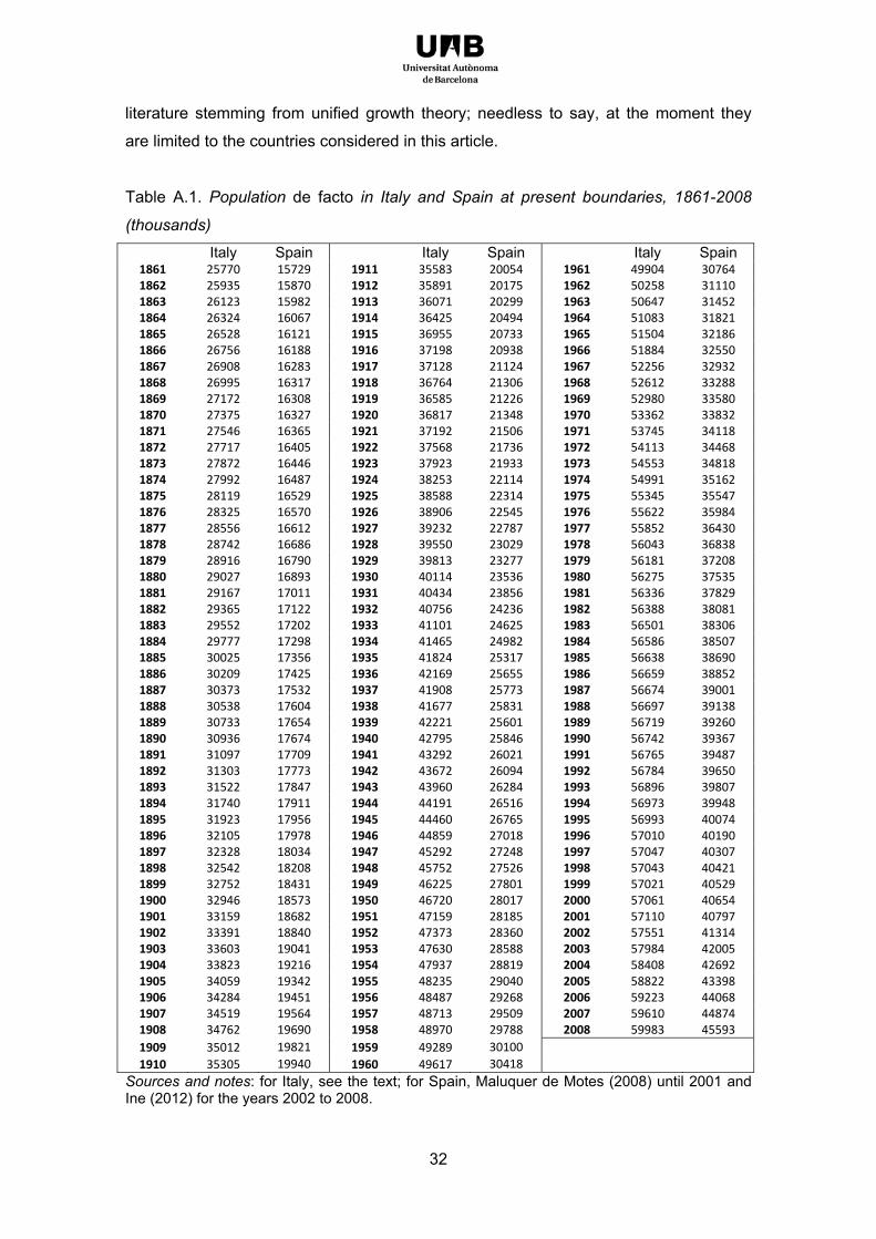
32
literature stemming from unified growth theory; needless to say, at the moment they
are limited to the countries considered in this article.
Table A.1. Population de facto in Italy and Spain at present boundaries, 1861-2008
(thousands)
Italy Spain Italy Spain Italy Spain 1861 25770 15729 1911 35583 20054 1961 49904 30764 1862 25935 15870 1912 35891 20175 1962 50258 31110 1863 26123 15982 1913 36071 20299 1963 50647 31452 1864 26324 16067 1914 36425 20494 1964 51083 31821 1865 26528 16121 1915 36955 20733 1965 51504 32186 1866 26756 16188 1916 37198 20938 1966 51884 32550 1867 26908 16283 1917 37128 21124 1967 52256 32932 1868 26995 16317 1918 36764 21306 1968 52612 33288 1869 27172 16308 1919 36585 21226 1969 52980 33580 1870 27375 16327 1920 36817 21348 1970 53362 33832 1871 27546 16365 1921 37192 21506 1971 53745 34118 1872 27717 16405 1922 37568 21736 1972 54113 34468 1873 27872 16446 1923 37923 21933 1973 54553 34818 1874 27992 16487 1924 38253 22114 1974 54991 35162 1875 28119 16529 1925 38588 22314 1975 55345 35547 1876 28325 16570 1926 38906 22545 1976 55622 35984 1877 28556 16612 1927 39232 22787 1977 55852 36430 1878 28742 16686 1928 39550 23029 1978 56043 36838 1879 28916 16790 1929 39813 23277 1979 56181 37208 1880 29027 16893 1930 40114 23536 1980 56275 37535 1881 29167 17011 1931 40434 23856 1981 56336 37829 1882 29365 17122 1932 40756 24236 1982 56388 38081 1883 29552 17202 1933 41101 24625 1983 56501 38306 1884 29777 17298 1934 41465 24982 1984 56586 38507 1885 30025 17356 1935 41824 25317 1985 56638 38690 1886 30209 17425 1936 42169 25655 1986 56659 38852 1887 30373 17532 1937 41908 25773 1987 56674 39001 1888 30538 17604 1938 41677 25831 1988 56697 39138 1889 30733 17654 1939 42221 25601 1989 56719 39260 1890 30936 17674 1940 42795 25846 1990 56742 39367 1891 31097 17709 1941 43292 26021 1991 56765 39487 1892 31303 17773 1942 43672 26094 1992 56784 39650 1893 31522 17847 1943 43960 26284 1993 56896 39807 1894 31740 17911 1944 44191 26516 1994 56973 39948 1895 31923 17956 1945 44460 26765 1995 56993 40074 1896 32105 17978 1946 44859 27018 1996 57010 40190 1897 32328 18034 1947 45292 27248 1997 57047 40307 1898 32542 18208 1948 45752 27526 1998 57043 40421 1899 32752 18431 1949 46225 27801 1999 57021 40529 1900 32946 18573 1950 46720 28017 2000 57061 40654 1901 33159 18682 1951 47159 28185 2001 57110 40797 1902 33391 18840 1952 47373 28360 2002 57551 41314 1903 33603 19041 1953 47630 28588 2003 57984 42005 1904 33823 19216 1954 47937 28819 2004 58408 42692 1905 34059 19342 1955 48235 29040 2005 58822 43398 1906 34284 19451 1956 48487 29268 2006 59223 44068 1907 34519 19564 1957 48713 29509 2007 59610 44874 1908 34762 19690 1958 48970 29788 2008 59983 45593
1909 35012 19821 1959 49289 30100 1910 35305 19940 1960 49617 30418
Sources and notes: for Italy, see the text; for Spain, Maluquer de Motes (2008) until 2001 and Ine (2012) for the years 2002 to 2008.
33
References
Acemoglu, Daron, and Simon Johnson (2007). “Disease and development: The effect of life expectancy on economic growth.” Journal of Political Economy, 115, no. 6: 925-985.
A’Hearn, Brian, and Giovanni Vecchi (2011). “Statura.” In In ricchezza e in povertà. Il benessere degli italiani dall’Unità a oggi, by Giovanni Vecchi: 37-72 and 418-419. Bologna: Il Mulino.
Altug, Sumru, Filiztekin, Alpay, and Şevket Pamuk (2008). “Sources of long-term economic growth for Turkey, 1880–2005.” European Review of Economic History, 12, no. 3: 393-430
Andrews, Donald W.K. (1993). “Tests of Parameter Instability and Structural Change with Unknown Change Point.” Econometrica, 59, no. 3: 821-856.
Andrews, Donald W.K. (2003). “Tests of Parameter Instability and Structural Change with Unknown Change Point: A Corrigendum.” Econometrica, 71, no. 1: 395-397.
Baffigi, Alberto (2011). Italian National Accounts, 1861-2011. Banca d’Italia − Quaderni di Storia Economica, no. 18, October.
Battilani, Patrizia, Felice, Emanuele, and Vera Zamagni (2012). “Il valore aggiunto dei servizi a prezzi correnti (1861-1951).” Rome: Banca d’Italia, mimeo.
Ben David, Dan and David H. Papell (2000). “Some evidence on the continuity of the growth process among the G7 countries.” Economic Inquiry, 38, no. 2: 320-330.
Blanes Llorens, Amand (2007). La mortalidad en la España del siglo XX. Análisis demográfico y territorial. Tesis doctoral dirigida por Dra. Anna Cabré Pla. Bellaterra (Cerdanyola del Vallès), Barcelona: Department de Geografia, Facultat de Filosofia i Lletres, Universitat Autònoma de Barcelona.
Bloom, David E. and & Jeffrey D. Sachs (1998). “Geography, demography, and economic growth in Africa.” Brookings Papers on Economic Activity, 2: 207-273.
Boldizzoni, Francesco (2011). The Poverty of Clio. Resurrecting Economic History. Princeton: Princeton University Press.
Brandolini, Andrea, and Giovanni Vecchi (2011). The Well-Being of Italians: A Comparative Historical Approach. Banca d’Italia − Quaderni di Storia Economica, no. 19, October.
Brunetti, Alessandro, Felice, Emanuele, and Giovanni Vecchi (2011). “Reddito.” In In ricchezza e in povertà. Il benessere degli italiani dall’Unità a oggi, by Giovanni Vecchi: 209-234 and 427-429. Bologna: Il Mulino.
Cabré, Anna, Domingo, Andreu, and Teresa Menacho (2002). “Demografía y crecimiento de la población española durante el siglo XX.” In Mediterráneo Económico, 1. Monogràfic: Procesos Migratorios, economía y personas, ed. by Manuel Pimentel Siles: 121-138. Almeria: Caja Rural Intermediterránea Cajamar.
Carreras, Albert (1989). “La industrialización española en el marco de la historia económica europea: ritmos y caracteres comparados.” In España, economía, ed. José Luis García Delgado: 79-115. Madrid: Espasa Calpe.
Carreras, Albert (1990). Industrialización española: estudios de historia cuantitativa. Madrid: Espasa Calpe.
Carreras, Albert (1997). “La industrialización: una perspectiva de largo plazo.” Papeles de Economía Española, no. 73: 35-60.
Carreras, Albert, and Xavier Tafunell (2004). Historia económica de la España contemporánea. Barcelona: Crítica.
Carreras, Albert, and Emanuele Felice (2010). “L’industria italiana dal 1911 al 1938: ricostruzione della serie del valore aggiunto e interpretazioni.” Rivista di Storia Economica 26, no. 3: 285-333.
Caselli, Graziella (1991). “Health Transition and Cause-Specific Mortality.” In The Decline of Mortality in Europe, eds. by Roger Schofield, David Reher, and Alain Bideau: 68-96. Oxford, Oxford University Press.
Cervellati, Matteo, and Uwe Sunde (2011). “Life expectancy and economic growth: the role of the demographic transition”. Journal of Economic Growth, 16, no. 2: 99-133.
Chatfield, Christopher (1980). The Analysis of Time Series: An Introduction. Second Edition. London: Chapman and Hall.
Chesnay, Jean-Claude (1986). La transition démographique. Etapes, formes e implications économiques. Étude de series temporelles (1720-1984) relatives a 67 país. Paris: PUF.
Comín, Francisco (1995). “La difícil convergencia de la economía española: un problema histórico.” Papeles de Economía Española, no. 63: 78-92.
Crafts, Nicholas F.R. (1997). “The human development index and changes in standards of living: some historical comparisons.” European Review of Economic History, 1, no. 3: 299-322.
Crafts, Nicholas F.R. (2002). “The human development index, 1870-1999: some revised estimates.” European Review of Economic History, 6, no. 3: 395-405.
Crafts, Nicholas F.R., Leybourne, Stephen J. and Terence C. Mills (1990). “Measurement of trend growth in European industrial output before 1914: Methodological issues and new estimates.” Explorations in Economic History, 27, no. 4: 442-467.
Cubel, Antonio, and Jordi Palafox (1998). “La continuidad del crecimiento económico en España, 1850-1935.” Revista de Historia Económica, 16, no. 3: 619-644.

34
Cussó Segura, Xavier (2005). “El estado nutritivo de la población española 1900-1970. Análisis de las necesidades y disponibilidades de nutrientes.” Historia Agraria, 36: 329-358.
Cutler, David, Deaton, Angus and Adriana Lleras-Muney (2006). “The Determinants of Mortality.” Journal of Economic Perspectives, 20, no. 3: 97-120.
Durlauf, Steven N., Johnson, Paul A., and Jonathan R.W. Temple (2005). “Growth Econometrics.” In Handbook of Economic Growth, Volume 1A, eds. by Philippe Aghion and Steven N. Durlauf: 555-677. Amsterdam: Elsevier.
Eggleston, Karen N. and R. Fuchs, Victor (2012). “The New Demographic Transition: Most Gains in Life Expectancy Now Realized Late in Life.” Journal of Economic Perspectives, 26, no. 3: 137-156.
Escudero, Antonio, and Hipólito Simón (2010). “Nuevos datos sobre el bienestar en España (1850-1993).” In Los niveles de vida en España y Francia (siglos XVIII-XX). In memoriam Gérard Gayot, eds. by Gerard Chastagnaret, Jean Calude Daumas, Antonio Escudero, and Olivier Raveux: 213-252. San Vicente del Raspeig: Publicaciones de la Universidad de Alicante.
Federico, Giovanni and Antonio Tena-Junguito (1998). “Was Italy a protectionist country?”. European Review of Economic History, 2, no. 1: 73-97.
Felice, Emanuele (2007). Divari regionali e intervento pubblico. Per una rilettura dello sviluppo in Italia. Bologna: il Mulino.
Felice, Emanuele (2010). “Regional Development: Reviewing the Italian Mosaic.” Journal of Modern Italian Studies, 15, no. 1: 64-80.
Felice, Emanuele (2011). “Regional value added in Italy, 1891-2001, and the foundation of a long-term picture.” Economic History Review, 64, no. 3: 929-950.
Felice, Emanuele, and Albert Carreras (2012). “When did modernization begin? Italy’s industrial growth reconsidered in light of new value-added series, 1911−1951.” Explorations in Economic History, 49, no. 4: 443-460. DOI 10.1016/j.eeh.2012.07.004.
Felice, Emanuele, and Michelangelo Vasta (2012). Passive modernization? The new Human development index and its components in Italy’s regions (1871-2007). Universitat Autònoma de Barcelona. Departament d’Economia i d’Història Econòmica. UHE Working Paper 2012_10.
Felice, Emanuele, and Giovanni Vecchi (2012). Italy’s modern economic growth, 1861-2011. Quaderni del Dipartimento di Economia Politica e Statistica, Università di Siena, no. 663.
Felice, Emanuele, and Giovanni Vecchi (2013). Italy’s Growth and Decline, 1861-2011. CEIS Tor Vergata. Research Paper Series, vol. 11, Issue 13, No. 293 − October 2013
Fenoaltea, Stefano (1969). “Public Policy and Italian Industrial Development, 1861–1913.” Journal of Economic History 29, no. 1: 176-179 [summary of a doctoral dissertation, Harvard University, 1967].
Fenoaltea, Stefano (2003). “Notes on the Rate of Industrial Growth in Italy, 1861–1913.” Journal of Economic History 63, no. 3: 695-735.
Fenoaltea, Stefano (2005). “The growth of the Italian economy, 1861-1913: Preliminary second-generation estimates.” European Review of Economic History 9, no. 3: 273-312.
Fenoaltea, Stefano (2010). “The Reconstruction of historical national accounts: the case of Italy.” PSL Quarterly Review 63, no. 252: 77-96.
Fenoaltea, Stefano (2011). “On the Structure of the Italian Economy, 1861-1913.” Rivista di Storia Economica 27, no. 1: 61-72.
Fenoaltea, Stefano (2011). The Reinterpretation of Italian Economic History: From Unification to the Great War. Cambridge: Cambridge University Press.
Fogel, Robert W. (2004). The Escape from Hunger and Premature Death, 1700-2100: Europe, America and the Third World. Cambridge: Cambridge University Press.
Fraile, Pedro (1991). Industrialización y grupos de presión. La economía política de la protección en España. Madrid: Alianza.
Freeman, Christopher and Perez, Carlota (1988), “Structural crises of adjustment, business cycles and investment behaviour”. In Technical Change and Economic Theory, eds. by Giovanni Dosi, Christopher Freeman, Richard Nelson, Gerald Silverberg, and Luc Soete: 38-66. London: Pinter.
Gallup, John Luke, Jeffrey D. Sachs, and Andrew D. Mellinger (1999). “Geography and economic development.” International Regional Science Review, 22, no. 2: 179-232.
Galor, Oded, and David N. Weil (2000). “Population, Technology, and Growth: From Malthusian Stagnation to the Demographic Transition and Beyond”. American Economic Review 90, no. 4: 806-828.
Galor, Oded (2012). “The Demographic Transition: Causes and Consequences”. Cliometrica 6, no. 1: 1-28.
Gerschenkron, Alexander (1947). “The Soviet Indices of Industrial Production.” Review of Economics and Statistics 29, no. 4: 217–26.
Gerschenkron, Alexander (1955). “Notes on the Rate of Industrial Growth in Italy, 1881–1913.” Journal of Economic History 15, no. 4: 360-375
Glei, Dana A. (2011). About mortality data for Italy. Max Planck Institute for Demographic Research of the University of California, Human Mortality Database: http://www.mortality.org/.
Glei, Dana A., Gómez Redondo, Rosa, Argüeso, Antonio and Vladimir Canudas-Romo (2011). About mortality data for Spain. Max Planck Institute for Demographic Research of the University of California, Human Mortality Database: http://www.mortality.org/.
Gordon, Robert J. (2012). Is US economic growth over? Faltering innovation confronts the six headwinds. Center for Economic Policy Research, Policy insight no. 63, September.
35
Granger, Clive W.J. (1969). “Investigating Causal Relations by Econometric Models and Cross-Spectral Methods.” Econometrica, 37, no. 3: 424-438.
Granger, Clive W.J. (2004). “Time Series Analysis, Cointegration, and Applications.” American Economic Review, 94, no. 3: 421-425.
HDM, Human Mortality Database (2011a). France, Total Population, Life expectancy at birth (period, 1x1). Last modified: 23-Mar-2011. Max Planck Institute for Demographic Research of the University of California, Human Mortality Database: http://www.mortality.org/.
HDM, Human Mortality Database (2011b). Italy, Life expectancy at birth (period, 1x1). Last modified: 29-Mar-2011. Max Planck Institute for Demographic Research of the University of California, Human Mortality Database: http://www.mortality.org/.
HDM, Human Mortality Database (2011c). Spain, Life expectancy at birth (period, 1x1). Last modified: 13-Jul-2011. Max Planck Institute for Demographic Research of the University of California, Human Mortality Database: http://www.mortality.org/.
Hobsbawm, Eric J. (1987). The Age of Empire: 1875-1914. New York: Vintage Books. Hobsbawm, Eric J. (1994). The Age of Extremes: the short twentieth century, 1914-1991. New York:
Vintage Books. Ine, Institudo Nacional de Estadística (2012). Estimaciones de Población Actual de España.
Resultados Nacionales. Madrid: http://www.ine.es/jaxiBD/tabla.do?per=01&type=db&divi=EPOB&idtab=2. (last access in October 2013).
Istat, Istituto Centrale di Statistica (1957). Indagine statistica sullo sviluppo del reddito nazionale dell’Italia dal 1861 al 1956. Annali di Statistica, Serie 8, vol. 9. Rome: Istat.
Istat, Istituto Centrale di Statistica (2012a). Ricostruzione della popolazione residente e del bilancio demografico. Rome: Istat. www.seriestoricheistat.it.
Istat, Istituto Centrale di Statistica (2012b). Indice dei prezzi al consumo per le rivalutazioni monetarie. Rome: Istat. www.istat.it.
Istat, Istituto Centrale di Statistica (2012c). Morti ed età mediana alla morte, per sesso − Anni 1862-2009. Rome: Istat. www.seriestoricheistat.it.
Lestaeghe, Ron J. and Dirk J. Van de Kaa (1986). “Twee demografische transitie?” In Bevolking: groei en krimp, eds. by Dirk J. Van de Kaa and Ron J. Lestaeghe: 9-24. Deventer: Van Loghum Slaterus.
Lestaeghe, Ron J. (2000). “Recent trends in fertility and household formation in the industrialized World”. Review of Population and Social Policy, 9: 121-170.
Livi Bacci, Massimo (2012). A concise history of world population. Fifth edition. Oxford: Blackwell. Lorentzen, Peter, McMillan, John, and Romain Wacziarg (2008). “Death and development.” Journal of
Economic Growth, 13, no. 2: 81-124. Maddison, Angus (1991). “A Revised Estimate of Italian Economic Growth, 1861-1989.” BNL
Quarterly Review, no. 177: 225-241. Maddison, Angus (2006). The World Economy: Volume 1. A Millennial Perspective. Paris: OECD. Maddison, Angus (2010). Historical Statistics of the World Economy: 1-2008 AD. Paris: OECD,
www.ggdc.net/maddison/content/shtml. Madigan, Michael T. and John M. Martinko, eds. (2005). Brock Biology of Microorganisms (11th ed.).
Upper Saddle River, NJ: Prentice Hall. Maluquer de Motes, Jordi (2005). “Consumo y precios.” In Estadísticas históricas de España. Siglos
XIX y XX, vol. III, eds. by Albert Carreras and Xavier Tafunell: 1247-1296. Madrid: Fundación BBVA. Maluquer de Motes, Jordi (2008). “El crecimiento moderno de la población de España de 1850 a
2001: una serie homogénea anual.” Investigaciones de Historia Económica, 10: 129-162. Maluquer de Motes, Jordi (2009a). “Del caos al cosmos: una nueva serie enlazada del producto
interior bruto de España entre 1850 y 2000.” Revista de Economía Aplicada, 17, no. 49: 5-45. Maluquer de Motes, Jordi (2009b). “Viajar a través del cosmos: la medida de la creación de la riqueza
y la serie histórica del producto interior bruto de España (1850-2008).” Revista de Economía Aplicada, 17, no. 51: 25-54.
María-Dolores, Ramón and José Miguel Martínez Carrión (2011). “The relationship between height and economic development in Spain, 1850-1958.” Economics and Human Biology, 9, no. 1: 30-44.
Martínez Carrión, José Miguel and Javier Puche-Gil (2011). “La evolución de la estatura en Francia y en España, 1770-2000: balnce historiográfico y nuevas evidencias.” Dynamis, 31, no. 2: 429-452.
Mokyr, Joel (2002). The Gifts of Athena: Historical Origins of the Knowledge Economy. Princeton: Princeton University Press.
Molinas, César and Prados de la Escosura, Leandro (1989). “Was Spain Different? Spanish Historical Backwardness Revisited.” Explorations in Economic History, 26, no. 4: 385-402.
Nadal, Jordi and Carles Sudrià (1993): “La controversia en torno al atraso económico español en la segunda mitad del siglo XIX (1860-1913).” Revista de Historia Industrial, no. 3: 199-227.
Nicolau, Roser (1989). “La población.” In Estadísticas históricas de España. Siglos XIX y XX, ed. by Albert Carreras: 49-90. Madrid: Fundación Banco Exterior.
Nicolau, Roser (2005). “Población, salud y actividad.” In Estadísticas históricas de España. Siglos XIX y XX, vol. I, eds. by Albert Carreras and Xavier Tafunell: 77-154. Madrid: Fundación BBVA.
Perez, Carlota (2002). Technological Revolutions and Financial Capital: the Dynamics of Bubbles and Golden Ages. Cheltenham: Elgar.

36
Perez, Carlota (2010). “Technological revolutions and techno-economic paradigms.” Cambridge Journal of Economics, 34, no. 1: 185-202.
Prados de la Escosura, Leandro (1997). “Política Económica liberal y crecimiento en la España contemporánea: un argumento contrafactual.” Papeles de Economía Española, no. 73: 83-98.
Prados de la Escosura, Leandro (2003). El Progreso Económico de España (1850-2000). Bilbao: Fundación BBVA.
Prados de la Escosura, Leandro (2007). “European Patterns of Development in Historical Perspective”. Scandinavian Economic History Review, 55, no. 3: 187-221.
Prados de la Escosura, Leandro (2009). “Del cosmos al caos: la serie del PIB de Maluquer de Motes”. Revista de Economía Aplicada, 17, no. 51: 5-23.
Prados de la Escosura, Leandro (2010a). “Spain’s international position, 1850-1913”. Revista de Historia Económica / Journal of Iberian and Latin American Economic History, 28, no. 1: pp. 173-215.
Prados de la Escosura, Leandro (2010b). “Improving human development: a long-run view”. Journal of Economic Surveys, 24, no. 5: 841-894.
Prados de la Escosura, Leandro, Rosés, Joan R. and Isabel Sanz-Villarroya (2012). “Economic reforms and growth in Franco’s Spain”. Revista de Historia Económica, 30, no. 1: 45-89.
Preston, Samuel H. (1975). “The Changing Relation Between Mortality and Level of Economic Development.” Population Studies, 29, no. 2: 231-248.
Quandt, Richard (1960). “Tests of the Hypothesis That a Linear Regression System Obeys Two Separate Regimes”. Journal of the American Statistical Association, 55, no. 290: 324-330.
Ravallion, Martin (2012). “Mashup Indices of Development.” The World Bank Research Observer, 27, no. 1: 1-32.
Rosés, Joan Ramon, Martínez-Galarraga, Julio and Daniel Tirado (2010). “The upswing of regional income inequality in Spain (1860–1930).” Explorations in Economic History, 47, no. 2: 244-257.
Sabaté, Marcela, Fillat, Carmen and Ana Belén Gracia (2011). “The peripheral protectionist backlash in the First Globalization: Spain (1870-1913)”. Revista de Historia Económica, 29, no. 1: 95-121
Sorrentino, Marina, and Giovanni Vecchi (2011). “Nutrizione.” In In ricchezza e in povertà. Il benessere degli italiani dall’Unità a oggi, by Giovanni Vecchi: 3-36 and 417. Bologna: Il Mulino.
Steckel, Richard H. (2009). “Heights and human welfare: Recent developments and new directions”. Explorations in Economic History, 46, no. 1: 1-23.
Stock, James and Watson, Mark (2007). Introduction to Econometrics, 2nd edition. Boston: Pearson Addison Wesley.
Pons, Jordi and Daniel Tirado (2006). “Discontinuidades en el crecimiento económico en el período 1870-1994: España en perspectiva comparada.” Revista de Economía Aplicada, 40, Spring: 137-156.
Tomes, Nancy (1998). The Gospel of Germs: Men, Women, and the Microbe in American Life. Cambridge, MA: Harvard University Press.
Toniolo, Gianni (1990). An Economic History of Liberal Italy, 1850–1918. London: Routledge. Torres-Reyna, Oscar (2012). Getting Started in Data Analysis. Data Analysis 101 workshops. Time
Series (ver. 1.5). Princeton: Princeton University Library. http://libguides.princeton.edu/profile.php?uid=762 (last access in October, 2012). UNDP (United Nations Development Programme) (2010). Human Development Report 2010. 20th
Anniversary Edition. The Real Wealth of Nations: Pathways to Human Development. New York: Palgrave Macmillan for the UNDP.
Uriel, Ezequiel, Moltó, María Luisa and Vicent Cucarella (2000). Contabilidad Nacional de España. Series enlazadas 1954-1967 (CNEe-86). Bilbao: Fundación BBV.
Vecchi, Giovanni (2011). In ricchezza e in povertà. Il benessere degli italiani dall’Unità a oggi. Bologna: Il Mulino.
Velarde, Juan (1999). “La economía española de 1914 a 1931.” In Historia Económica de España. Siglos XIX y XX, ed. by Gonzalo Anes: 470-524. Barcelona: Galaxia Gutemberg-Círculo de Lectores.
Vogelsang, Timothy J. (1997). “Wald-Type tests for detecting shifts in the trend function of a dynamic time series.” Econometric Theory, 13, no. 6: 818-849.
Williamson, Jeffrey G. (2011). Industrial Catching Up in the Poor Periphery 1870-1975. CEPR Discussion Paper No. DP8335. Available at SSRN: http://ssrn.com/abstract=1810298.
Zamagni, Vera (1993). The Economic History of Italy, 1860-1990. Recovery after Decline. Oxford: Oxford University Press.
Top Related
Copyright © 2022 FDOKUMEN

