


Bahasa
Halaman
Hukum

Free Volume and Storage Stability of One-component Epoxy Nanocomposites
Dissertation
zur Erlangung des akademischen Grades
Doktor der Ingenieurwissenschaften
(Dr.-Ing.)
der Technischen Fakultät
der Christian-Albrechts-Universität zu Kiel
Muhammad Qasim Shaikh
Kiel
2010

1. Gutachter: Prof. Dr. Klaus Rätzke
2. Gutachter: Prof. Dr. Wolfgang Jäger
Datum der mündlichen Prüfung: 11.11.2010

Dedicated to my parents and my wife

i
Table of Contents
1. Introduction ...............................................................................................................................1
2. Positrons and Positronium Annihilation .................................................................................5
2.1 Introduction ................................................................................................................................ 5
2.2 Positrons and Positronium........................................................................................................... 5
2.2.1 Self Annihilation of Positrons and Positronium........................................................... 6
2.2.2 Pick-off Annihilation of ortho-Positronium................................................................ 6
2.2.3 Theoretical models for Positronium formation ........................................................... 7
2.3 Positrons sources for PALS......................................................................................................... 8
2.4 Positrons Annihilation Techniques (PATs).................................................................................. 9
2.4.1 Positron Annihilation Lifetime Spectroscopy (PALS)............................................... 10
2.4.1.1 Scintillator-Photomultiplier Detectors.......................................................... 11
2.4.1.2 Constant Fraction Diffraction Discriminators (CFDD)................................. 12
2.4.1.3 Time to Amplitude Converter (TAC)........................................................... 13
2.4.1.4 Multi-Channel Analyzer (MCA).................................................................. 13
2.5 Data Analysis of PALS spectrum .............................................................................................. 14
2.5.1 Analysis with LifeTime routine LT 9.0..................................................................... 14
2.5.1.1 Finite lifetime analysis ................................................................................ 15
2.5.1.2 Continuous term analysis (with distribution)................................................ 16
2.6 Tao-Eldrup Model for calculating the free volume in polymers ................................................. 18
2.7 PALS studies on epoxy precursors ............................................................................................ 20
2.8 PALS studies on cured epoxy composites ................................................................................. 21
2.9 PALS related to this thesis ........................................................................................................ 21
3. Free Volume in Polymers ........................................................................................................23
3.1 Introduction .............................................................................................................................. 23
3.2 Basic concept of the free volume............................................................................................... 23
3.3 Definitions of the free volume................................................................................................... 24
3.3.1 Empty volume ......................................................................................................... 25
3.3.2 Excess free volume.................................................................................................. 25
3.3.3 Accessible free volume............................................................................................ 26
3.4 Fractional free volume and related theories ............................................................................... 27
3.5 Experimental techniques to determine free volume.................................................................... 28
3.6 Polymer properties characterized by the free volume................................................................. 29
3.6.1 Glass-Transition temperature.................................................................................... 30
3.6.2 Physical Ageing ....................................................................................................... 31
3.7 Summary of this chapter ........................................................................................................... 31
Table of Contents
ii
4. Johnson-Mehl-Avrami-Kohlmogorov Theory ......................................................................33
4.1 Introduction .............................................................................................................................. 33
4.2 Basics of phase transformations ................................................................................................ 33
4.2.1 Nucleation and growth............................................................................................. 33
4.3 Phase transformation Kinetics ................................................................................................... 36
4.4 Transformation mechanisms ..................................................................................................... 37
4.5 Johnson-Mehl-Avrami-Kohlmogorov (JMAK) theory............................................................... 38
4.5.1 Important assumptions............................................................................................. 39
4.5.2 Derivation of Avrami equation................................................................................. 39
4.5.3 Avrami exponent ‘n’................................................................................................ 43
4.6 Time-Temperature Superposition.............................................................................................. 45
4.7 Summary of this chapter ........................................................................................................... 46
5. One-component Epoxy Resin formulations...........................................................................47
5.1 Epoxy Resins: An Introduction ................................................................................................. 47
5.1.1 Industrial applications of epoxy resin formulations .................................................. 47
5.2 Current state of art and aim of this project ................................................................................. 48
5.3 Basic principles of formulation ................................................................................................. 49
5.3.1 Epoxy resins ............................................................................................................ 50
5.3.1.1 Diglycidyl ether of bisphenol A (DGEBA) .................................................. 51
5.3.1.2 Bisphenol F Epoxy resin ............................................................................. 52
5.3.2 Hardeners (Curing agents) ....................................................................................... 53
5.3.2.1 Amine curing .............................................................................................. 54
5.3.2.1.1 Dicyandiamide (DICY)................................................................... 55
5.3.2.2 Anhydride curing ........................................................................................ 56
5.3.2.2.1 Methyl hexahydrophthalic anhydride (MHHPA)............................. 58
5.3.3 Accelerators............................................................................................................. 58
5.3.4 Fillers ...................................................................................................................... 59
5.3.5 Micro and Nano/Encapsulation of Accelerators........................................................ 59
5.4 Epoxy curing process and TTT diagram.................................................................................... 60
5.5 Characterization of epoxy curing and cured epoxy networks ..................................................... 61
5.5.1 Traditional off-line methods..................................................................................... 62
5.5.2 Modern in-situ methods ........................................................................................... 62
5.6 Summary of this chapter ........................................................................................................... 63
6. Shelf life of one-component epoxy-resin formulation...........................................................65
6.1 Introduction .............................................................................................................................. 65
6.1.1 One-component formulation .................................................................................... 65
6.1.2 Shelf-life and the curing mechanism ........................................................................ 66
6.1.3 Transformed fraction and the JMAK theory ............................................................. 66
6.1.4 Free volume and PALS............................................................................................ 67
6.2 Experimental ............................................................................................................................ 68
Table of Contents
iii
6.3 Results and Discussions ............................................................................................................ 69
6.3.1 Analysis of Lifetime Spectra.................................................................................... 69
6.3.2 Curing Kinetics and Avrami equation ...................................................................... 71
6.4 Conclusion................................................................................................................................ 75
7. Free and encapsulated accelerator formulations ..................................................................77
7.1 Introduction .............................................................................................................................. 77
7.2 Experimental ............................................................................................................................ 79
7.2.1 Preparation of the epoxies........................................................................................ 79
7.2.2 Modulated DSC....................................................................................................... 80
7.2.3 IR Spectroscopy ...................................................................................................... 80
7.2.4 PALS ...................................................................................................................... 80
7.3 Results and Discussions ............................................................................................................ 81
7.3.1 Part I: Precursor series (IR, PALS and JMAK)........................................................ 81
7.3.1.1 Shelf calculated by IR Spectroscopy and PALS data at 60 °C ...................... 81
7.3.1.2 JMAK fits to PALS data.............................................................................. 82
7.3.2 Part II: Cured series (PALS and DSC)..................................................................... 85
7.3.2.1 Analysis of Positron Lifetime Spectra.......................................................... 85
7.3.2.2 Micro-volumetric Tg and the co-efficient of thermal expansion .................... 88
7.3.2.3 Fractional hole free volume fg (at Tg) ........................................................... 89
7.3.2.4 Effect of cross-linking on Tg ........................................................................ 89
7.3.2.5 No effect of Positron irradiation .................................................................. 90
7.3.2.6 The ortho-Positronium Inhibition ................................................................ 91
7.4 Conclusions .............................................................................................................................. 91
8. The effect of encapsulation on activation energy ..................................................................93
8.1 Introduction .............................................................................................................................. 93
8.2 Experimental ............................................................................................................................ 94
8.2.1 Material ................................................................................................................... 94
8.2.2 Analysis and Measurement ...................................................................................... 94
8.3 Results and Discussions ............................................................................................................ 95
8.3.1 The o-Ps lifetime and the storage time ..................................................................... 95
8.3.2 Transformed fraction and the JMAK fits .................................................................. 97
8.3.3 Avrami exponent and the Activation energies .......................................................... 99
8.4 Summary & Conclusions ........................................................................................................ 102
9. Zeolite and Pyrogenic Silica filled Nanocomposites ...........................................................105
9.1 Introduction ............................................................................................................................ 105
9.2 Experimental .......................................................................................................................... 107
9.2.1 Synthesis of Micro and Nano-sized encapsulations ................................................ 107
9.3 Accelerator encapsulation in Zeolite carriers ........................................................................... 107
9.3.1 Effects of varying accelerator concentration in µ-Zeolite carriers ........................... 107
Table of Contents
iv
9.3.2 Single-step micro and nano-sized encapsulations ................................................... 111
9.3.3 Multi-stage micro and nano-Zeolite encapsulations ................................................ 113
9.4 Accelerator encapsulation on Pyrogenic Silica carriers ............................................................ 116
9.4.1 Effects of varying accelerator concentration in 1K-formulations ............................ 117
9.5 Summary & Conclusions ........................................................................................................ 121
10. Summary & Outlook ...........................................................................................................123
11. Bibliography... ......................................................................................................................127
AppendicesAppendix A ........................................................................................................................ 135
Appendix B ........................................................................................................................ 137
Appendix C ......................................................................................................................... 139
Acknowledgments
List of Publications
Chapter 1: Introduction
1
1. Introduction
Epoxy resins are firmly established in a number of important applications, such as adhesives,
protective coatings, laminates, and a variety of uses in building and construction.1 The
chemistry of epoxies and the range of modifications that are commercially available, allow
cured polymers to be produced with a very broad range of properties. Successful performance
of epoxy-based systems depends on proper selection and formulation of components. The
components that have the most significant influence on the curing behavior and the network
structure are the epoxy resin and the curing agents. As epoxy resins are converted into solid,
infusible, and insoluble three-dimensional thermosetting networks for their applications, by
curing with cross-linkers. Optimum performance properties are obtained by cross-linking the
right epoxy resins with the proper cross-linkers, often called hardeners or curing agents.
Selection of curing agent depends on various considerations, such as cost, ease of handling,
pot life, cure rates, and the mechanical, electrical, or thermal properties required in the final
resin. In order to lower the energy cost its important to achieve low temperature hardening
and for this reason an accelerator must be added to speed up the reaction.
A single batch formulation is relevant for industrial applications, as for large scale
applications, mixing the components directly before usage is not practical in industrial
surrounding. As compared to a two-component epoxy-resin system, there is a limitation of
shelf life when it comes to one-component systems, since the resin, hardener, accelerator,
fillers and additives are all mixed together in one package. Therefore, a considerable shelf
life of such ready to use one-component formulations is required. The epoxy curing process is
an important factor affecting the performance of cured epoxies. To obtain desirable network
structure and performance, it is imperative to understand the curing process and its kinetics to
design the proper cure schedule. Epoxy curing process can be monitored by a number of
experimental techniques and indirect estimation of cure conversion as a function of time is
done with a combination of several experimental techniques and the available theoretical
models. However, considering the product development in view it is still of utmost relevance,
to establish reliable means of experimentally predicting the shelf life of new formulations of
one-component epoxies, which is usually guessed from accelerated tests at elevated
temperatures relying on selected reference measurements. In order to achieve predictability it
is important to understand the complete curing mechanism of epoxies, so that the reaction
Chapter 1: Introduction
2
kinetics can be further elaborated in light of available standard models and further
extrapolated to shelf life at storage temperatures.
Positron Annihilation Lifetime Spectroscopy (PALS), is presented here as a useful technique
to study the curing kinetics of one-component epoxy resin formulations. Chapter 2 of this
thesis discusses in detail the basics of positrons and positronium (Ps) formation in amorphous
polymers. A brief overview of several positron annihilation techniques (PATs), is followed by
an in-depth study of PALS technique, which is eventually the main focus of this PhD thesis. It
is shown how a general setup of fast-fast coincidence functions and what information is
experimentally obtained. Furthermore, data analysis of PALS by LifeTime routine 9.0
(LT9.0)2 in its different modes is presented for the calculation of ortho-Positronium (o-Ps)
lifetime τ3 = τo-Ps. It is also shown that how this information can be correlated to the free
volume in amorphous polymers, using a semi-empirical Tao-Eldrup model.3-4
Chapter 3 of this thesis stresses the importance of free volume and the characteristic
properties of polymers directly affected by the free volume. It starts with the basic definition
of the free volume and is followed by different ways of calculating the occupied volume. On
one hand the change in free volume of the epoxy resin formulations, during the isothermal
runs at elevated temperatures, is used to calculate the extent of curing i.e. the transformed
fraction X. On the other hand, for a series of cured epoxy composites the temperature
dependence of the free volume is used to calculate the glass-transition temperature (Tg) and
the co-efficient of thermal expansion in the glassy and the rubbery phase.
The most significant achievement of this work is to study the curing kinetics of one-
component epoxy resin formulations, using PALS data i.e. the change in free volume, in
combination with Johnson-Mehl-Avrami-Kolmogorov (JMAK) equation,5-7 as discussed in
Chapter 4. Isothermal and non-isothermal curing behaviors of epoxy resins has already been
studied in the light of the Avrami equation in past, but only for high curing temperatures and
neither growth exponent nor reaction constant have been interpreted or extrapolated to room
temperature. This is of great importance for predicting storage stability of industrial one
component formulations at room temperature. The origin of Avrami equation from metal
physics, studied in the light of nucleation and growth theory for a liquid to solid phase
transformation is also discussed in this chapter. This is followed by the derivation of Avrami
Chapter 1: Introduction
3
equation for a case of site-saturated homogenous nucleation. Furthermore, the Avrami
exponent ‘n’ and the reaction constant ‘k’ are also discussed.
The composition of one-component epoxy resin formulations used in this work is discussed in
Chapter 5 of this thesis. The basic rules of formulations, importance of maintaining the
stoichiometric ratio of resin and hardener, the choice of accelerators and fillers are listed here.
Please note that respecting the non-disclosure agreements concerning this work, the names of
accelerators and the micro and nano-carriers used for encapsulation, will be treated as
classified information.
The first results on the state of art one-component epoxy resin formulations, used as the
benchmark system are mentioned in Chapter 6. It is shown that, how with increasing
temperatures the reaction constant ‘k’ varies and at the same time the Avrami exponent ‘n’
remains constant. The boundary conditions for the fulfillment of JMAK equation are
discussed and with the help of Arrhenius equation the shelf-life of epoxy resin formulation is
extrapolated to storage temperatures.
Chapter 7 shows the results of PALS and IR-spectroscopy techniques, used for a series of
one-component epoxy resin formulations in their precursor state. The affect of adding free
and micro or nano-encapsulated accelerator on the shelf life is reported. The curing kinetics of
one-component epoxy-resin systems is also discussed in the light of Avrami parameters and
concluded with the possible reasons for the observed differences. Furthermore, the
temperature dependence of the free volume for their cured composites is also studied in
combination with PALS and DSC techniques.
The effect of accelerator encapsulation on curing kinetics and the activation energy is
discussed in Chpater 8. Finally, a selected series of 1K-formulation containing Zeolite and
nanosilica encapsulated accelerator are discussed in Chapter 9. Please note that the complete
list of one-component epoxy resin formulations investigated during the course of this PhD
thesis consists of 80 different formulations, with approximately 100 spectrums measured per
sample on average, which is approximately 3 years of just the measuring time alone. Off
course, this was possible due to the availability of three PALS machines at the Institute for
Material Science, Multi-component Materials, University of Kiel. The data analysis includes
the JMAK fits to the PALS data and tstorage from PALS in comparison to IR spectroscopy for
Chapter 1: Introduction
4
selected samples. Furthermore, the release behavior of accelerators is discussed in the light of
Avrami parameters and compared with the hardening temperatures measured with DSC
technique for selected samples.
The main aim of this PhD thesis on one hand, is to present the Positron Annihilation Lifetime
Spectroscopy (PALS) as one of the state of art technique to characterize the in-situ curing
kinetics of one-component epoxy resin formulations, by using the change in free volume as
the measure of extent of curing in combination with the JMAK equation. On the other hand it
is shown that PALS is also very useful when it comes to the characterization of the cured
epoxy composites. This can give information about the interesting properties of cured
composites, such as the temperature dependence of the free volume(Vf), the fractional free
volume (FFV), glass-transition temperature(Tg), the thermal expansion co-efficient in the
glassy and the rubbery phase.
Chapter 2: Positrons and Positronium Annihilation
2. Positrons and Positronium Annihilation
2.1 Introduction
Positrons are excellent probe particles to characterize defects of condensed matter. Upon
annihilation with its anti-particle, the electron, they provide an indirect image of the structure,
such as the concentration of vacancies and defect concentration in metals and semiconductors,
sub-nanometre level free volume holes in polymers and they are even handy when it comes to
characterization of larger pore diameters in highly porous materials. Positron annihilation has
been, and continues to be, exploited in the study of structural changes associated with phase
transitions, precipitation, deformation and physical ageing in various materials. The recent
appearance of brilliant, reactor-based positron beams add a new dimension for the
characterization and development of new thin-film probes, providing the research community
with views on nature and possibilities in the development of advanced materials for future
applications in everyday life.
The group of Prof. Dr. Franz Faupel at the Institute for Material Science – Multicomponent
Materials, Engineering department of the Christian-Albrechts University of Kiel is involved
in materials research with Positron Annihilation Lifetime Spectroscopy (PALS), since more
than a decade. Some of the most noticeable works include free volume in bulk metallic
glasses,8-10 amorphous alloys,11 polyimides,12 polymeric membranes with high
permeability,12-13 Polymers of intrinsic micro-porosity,14 epoxy thin films15 and low molecular
weight glass formers.16 In this chapter the basics of positrons and their detection as it relates
to the sub-nanometre level free volume in bulk polymers are discussed, which is characterized
in particular by the PALS.
2.2 Positrons and Positronium
In 1930 Paul AM Dirac 17 postulated that a subatomic particle existed which was equivalent in
mass to an electron but carried a positive charge. Carl Anderson observed these particles,
which he named as the positrons, in cosmic ray research using cloud chambers in 1933.18 The
positrons observed by Anderson were produced naturally in the upper atmosphere by the
conversion of high-energy cosmic radiation into an electron–positron pair. Soon after this it
5
Chapter 2: Positrons and Positronium Annihilation
was shown that when positrons interact with matter they give rise to two photons which, are
emitted simultaneously in almost opposed directions.
Positrons (e+ or β+) are the anti-particles of electrons (e-), with a mass equal to that of
electrons but having a positive charge. A positron in matter, can pick up an electron and this
reaction of positron with an electron can lead to a meta-stable state called Positronium,
abbreviated as (Ps).19 Positronium particles are similar to hydrogen atom in terms of size, but
have a mass equivalent to two electrons.
2.2.1 Self Annihilation of Positrons and Positronium
The Ps annihilation events are governed by a selection rule resulting from charged parity (CP)
invariance. The parity of the γ–photons is (-1)n, and for ground-state Ps it is (-1)S, where S is
the total spin angular momentum of the Ps atom. If the positron and electron in the Ps have
opposing spins (the singlet state, para-Ps or p-Ps) then the total S = 0 and consequently n has
to be an even number, but if the positron and electron spins are parallel and S = 1 (the triplet
state, ortho-Ps or o-Ps) then n has to be odd. The p-Ps principally decays into two 511 keV
anti-parallel γ–rays, whereas o-Ps decays into three γ–rays whose total energy is 2mc2 or 1022
keV.20
2.2.2 Pick-off annihilation of ortho-Positronium
The intrinsic lifetimes in vacuum for p-Ps and o-Ps are 0.125 ns and 142 ns, respectively (see
Fig. 2.1). In ordinary molecular media, the electron density is low enough so that o-Ps can
pick off electrons from the media that have anti-parallel spin to that of the positron, and
undergo two-photon annihilation. The pick-off annihilation of o-Ps not only occurs in the
form of two-photon annihilation, but it also shortens the o-Ps lifetime from 142 ns (self-
annihilating o-Ps) to approximately ~1 to 10 ns in polymers.21
Experimental determination of o-Ps lifetime is one of the most useful methods for positron
and positronium research. This is because o-Ps lifetime contains information about electron
density, which governs the basic properties of chemical bonding in molecules and it is also
controlled by the physical structure of molecules.
6
Chapter 2: Positrons and Positronium Annihilation
22Na Source
Free positrons
1.2
7 M
eV
e+
Zerotime
e+
e-
e-e+
e+
e-e-
e+
e-e+
p-PsIntrinsic
annihilation
o-PsPick-off
annihilation
Lifetime t (ns)
0.125 0.4 1 10 142
o-PsSelf annihilation
22Na Source
Free positrons
1.2
7 M
eV
e+e+
Zerotime
e+e+
e-e-
e-e-e+e+
e+e+
e-e-e-e-
e+e+
e-e+ e-e-e+e+
p-PsIntrinsic
annihilation
o-PsPick-off
annihilation
Lifetime t (ns)
0.125 0.4 1 10 142
o-PsSelf annihilation
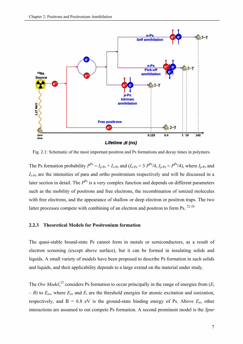
Fig. 2.1: Schematic of the most important positron and Ps formations and decay times in polymers.
The Ps formation probability PPs = Ip-Ps + Io-Ps and (Io-Ps = 3 PPs/4, Ip-Ps = PPs/4), where Ip-Ps and
Io-Ps are the intensities of para and ortho positronium respectively and will be discussed in a
later section in detail. The PPs is a very complex function and depends on different parameters
such as the mobility of positrons and free electrons, the recombination of ionized molecules
with free electrons, and the appearance of shallow or deep electron or positron traps. The two
latter processes compete with combining of an electron and positron to form Ps. 22-24
2.2.3 Theoretical Models for Positronium formation
The quasi-stable bound-state Ps cannot form in metals or semiconductors, as a result of
electron screening (except above surface), but it can be formed in insulating solids and
liquids. A small variety of models have been proposed to describe Ps formation in such solids
and liquids, and their applicability depends to a large extend on the material under study.
The Ore Model,25 considers Ps formation to occur principally in the range of energies from (Ei
– B) to Eex, where Eex and Ei are the threshold energies for atomic excitation and ionization,
respectively, and B = 6.8 eV is the ground-state binding energy of Ps. Above Eex other
interactions are assumed to out compete Ps formation. A second prominent model is the Spur
7
Chapter 2: Positrons and Positronium Annihilation
Model, due to Mogensen26, in which the positron binds to an electron released in a spur during
the slowing-down process, under conditions of small relative momentum. An extension of this
model is to consider the end of the positron track to be a Blob, rather than a spur27. A third,
particularly considered with respect to Ps in polymers, involves the formation of Ps in open
volumes or holes, the electron being picked up from the surface,28 if the positron is not
completely thermalized, then the Ps atom may undergo thermalizing collisions with hole
walls.
2.3 Positron sources for PALS
There are many radioactive isotopes which decay under β+ emission of positrons, a process
which is often used to produce positrons. In the laboratory environment the choice of
radioactive sources for positron experiments has always been a compromise between
application and cost. At the Isotope lab, Institute for Material Science, Engineering
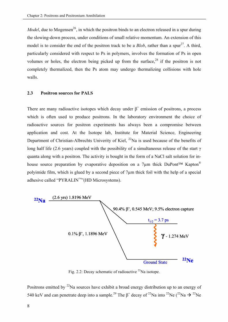
Department of Christian-Albrechts Univerity of Kiel, 22Na is used because of the benefits of
long half life (2.6 years) coupled with the possibility of a simultaneous release of the start γ
quanta along with a positron. The activity is bought in the form of a NaCl salt solution for in-
house source preparation by evaporative deposition on a 7µm thick DuPont™ Kapton®
polyimide film, which is glued by a second piece of 7µm thick foil with the help of a special
adhesive called “PYRALINTM”(HD Microsystems).
(2.6 yrs) 1.8196 MeV
90.4% β+, 0.545 MeV; 9.5% electron capture
γ - 1.274 MeV0.1% β+, 1.1896 MeV
22Na
22NeGround State
t1/2 = 3.7 ps
(2.6 yrs) 1.8196 MeV
90.4% β+, 0.545 MeV; 9.5% electron capture
γ - 1.274 MeV0.1% β+, 1.1896 MeV
22Na
22NeGround State
t1/2 = 3.7 ps
Fig. 2.2: Decay schematic of radioactive 22Na isotope.
Positrons emitted by 22Na sources have exhibit a broad energy distribution up to an energy of
540 keV and can penetrate deep into a sample.29 The β+ decay of 22Na into 22Ne (22Na 22Ne
8
Chapter 2: Positrons and Positronium Annihilation
+ ν + γ), as shown in Fig. 2.2., is the most commonly used process for the emission of
positrons, where 22Na isotope gives a relatively high positron yield of 90.4%. It is observed
that 22Na decays by positron emission and electron capture, to the first excited state of neon
nucleus (22Ne) by the emission of an energetic positron and an electron neutrino. This excited
state quickly de-excites to the ground state by the emission of a 1.274 MeV γ-ray with half-
life t1/2 of 3.7 ps. Approximately 9.5 % of the 22Na will decay by electron capture, but it may
also decay (0.1 %) directly to the ground state of Ne via the emission of a more energetic
positron.
The decay of 22Na results in the emission of the positrons (e+) and a simultaneous release of a
1.27 MeV γ - quantum, which is often called the “birth” or “start” quantum of a positron. The
lifetime of a positron is determined by the time between the birth quantum and its
“annihilation” or the “stop” quanta. The half life of 22Na is 2.6 years and the rate of its
positron emission depends on the activity of the source. The higher the activity of a source,
the shorter the time needed to complete the measurement of one spectrum. But too high
activity can result in high background,30 which can be problematic for analysis of long
lifetimes, but are of no worry when analyzing polymers. The sources used throughout this
thesis were approximately ~1 MBq, with a count rate of 400-500 counts per second. This
means the time required to measure a spectrum of 5x10⁶ annihilating events was in the range
of 2-4 hours. This high number of total counts is important when analyzing the PALS
spectrum with routine LT 9.0 software in its distribution mode and is discussed in detail in
section 2.7.1.2.
2.4 Positron Annihilation Techniques (PATs)
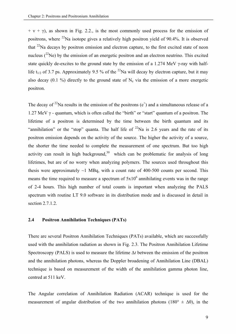
There are several Positron Annihilation Techniques (PATs) available, which are successfully
used with the annihilation radiation as shown in Fig. 2.3. The Positron Annihilation Lifetime
Spectroscopy (PALS) is used to measure the lifetime Δt between the emission of the positron
and the annihilation photons, whereas the Doppler broadening of Annihilation Line (DBAL)
technique is based on measurement of the width of the annihilation gamma photon line,
centred at 511 keV.
The Angular correlation of Annihilation Radiation (ACAR) technique is used for the
measurement of angular distribution of the two annihilation photons (180° ± Δθ), in the
9
Chapter 2: Positrons and Positronium Annihilation
direction transverse to the gamma emission, which directly yields information on the
component of momentum of the annihilating pair. The Coincidence Doppler Broadening
Spectroscopy (CDBS) can be used to investigate annihilations with core electrons to identify
the chemical environment in which the positron decays.
E1 - DBAL
22Na Source
Sample
- 511 keV (E2)
e+e+
AgedMOmentumCorrelation
CoincidenceDopplerBroadeningSpectroscopy
DopplerBroadening ofAnnihilationLine
e-
AngularCorrelation ofAnnihilationRadiation
PositronAnnihilationLifetimeSpectroscopy
t
E1 + E2 - CDBS
t, E1 - AMOC
thermalization
diffusion ~ 100 nm
- ACARt - PALS
- 511 keV (E1)
- 1.27 MeV
E1 - DBAL
22Na Source
Sample
- 511 keV (E2)
e+e+e+e+
AgedMOmentumCorrelation
CoincidenceDopplerBroadeningSpectroscopy
DopplerBroadening ofAnnihilationLine
e-e-
AngularCorrelation ofAnnihilationRadiation
PositronAnnihilationLifetimeSpectroscopy
t
E1 + E2 - CDBS
t, E1 - AMOC
thermalization
diffusion ~ 100 nm
- ACARt - PALS
- 511 keV (E1)
- 1.27 MeV
Fig. 2.3: Positron annihilation techniques.
The simultaneous measurement of positron lifetime and the momentum of the annihilating
pair (i.e. PALS + DBAL) can give information on thermalization and transitions between
positron states (and hence on chemical reactions of positrons or Ps, this technique is known as
the Age-Momentum Correlation (AMOC). As mentioned earlier, the experimental technique
used throughout this thesis was PALS, therefore in the following sections only the PALS
technique is discussed in detail.
2.4.1 Positron Annihilation Lifetime Spectroscopy (PALS)
The positron lifetime of a single event can be measured by detecting the time difference
between the birth γ-quantum of the β+-decay in the source and one of the annihilation γ-
quanta with energy of 511 keV. The activity of the source must be sufficiently low in order to
ensure that on average only one positron is in the sample. This avoids the intermixing of start
and stop quanta originating from different annihilation events. A special “sandwich”
10
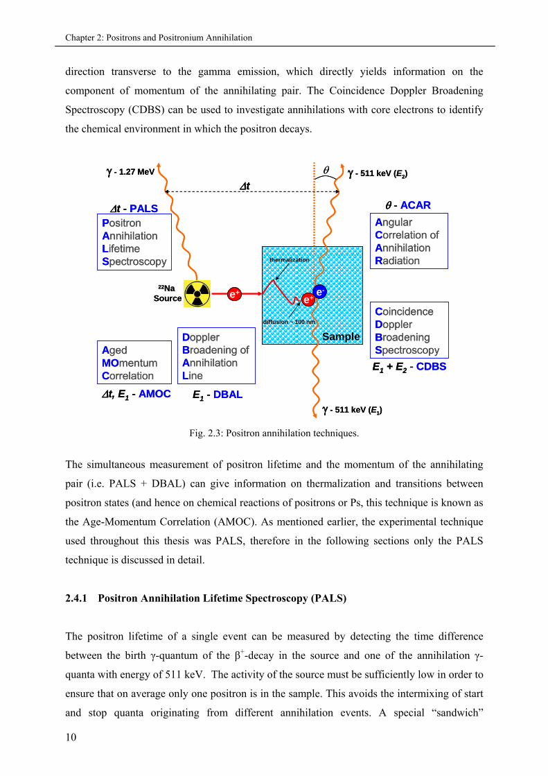
Chapter 2: Positrons and Positronium Annihilation
arrangement of 22Na source, two identical samples, and detectors guarantees that all positrons
emitted from the source are penetrating the sample material.
start
stop
delay
CFD1.27 MeV
CFD511 keV
TAC
MCA
HV1.91 kV
HV1.91 kV
Ph
oto
mu
ltip
lier
tub
e
Scintillator
22Na Sourcee+ e-
e+
Sample
511 keV
511 keV
1.27 MeV
start
stop
delay
CFD1.27 MeV
CFD511 keV
TAC
MCAMCA
HV1.91 kVHV
1.91 kV
HV1.91 kVHV
1.91 kV
Ph
oto
mu
ltip
lier
tub
e
Scintillator
22Na Sourcee+e+ e-e-
e+e+
Sample
511 keV
511 keV
1.27 MeV
Fig. 2.4: Illustration of the experimental setup of positron annihilation lifetime spectroscopy (PALS), showing high voltage (HV) suppliers, photo-multiplier tubes (PMTs), constant fraction discriminators (CFDs), time to amplitude converter (TAC) and the multi-channel analyzer (MCA).
The experimental arrangement as shown in Fig. 2.4 is known as the “fast–fast coincidence”
setup. The term is related to the fact that the time measurement as well as the energy selection
is performed in a fast channel. A slow channel was used for energy selection when fast
differential discriminators were not available at the beginning of positron lifetime
experiments; this arrangement was called a fast–slow setup.29
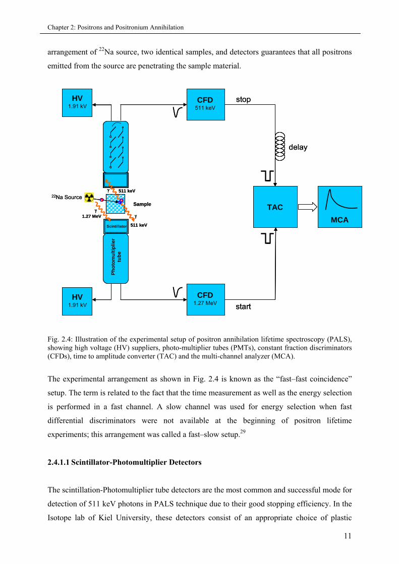
2.4.1.1 Scintillator-Photomultiplier Detectors
The scintillation-Photomultiplier tube detectors are the most common and successful mode for
detection of 511 keV photons in PALS technique due to their good stopping efficiency. In the
Isotope lab of Kiel University, these detectors consist of an appropriate choice of plastic
11
Chapter 2: Positrons and Positronium Annihilation
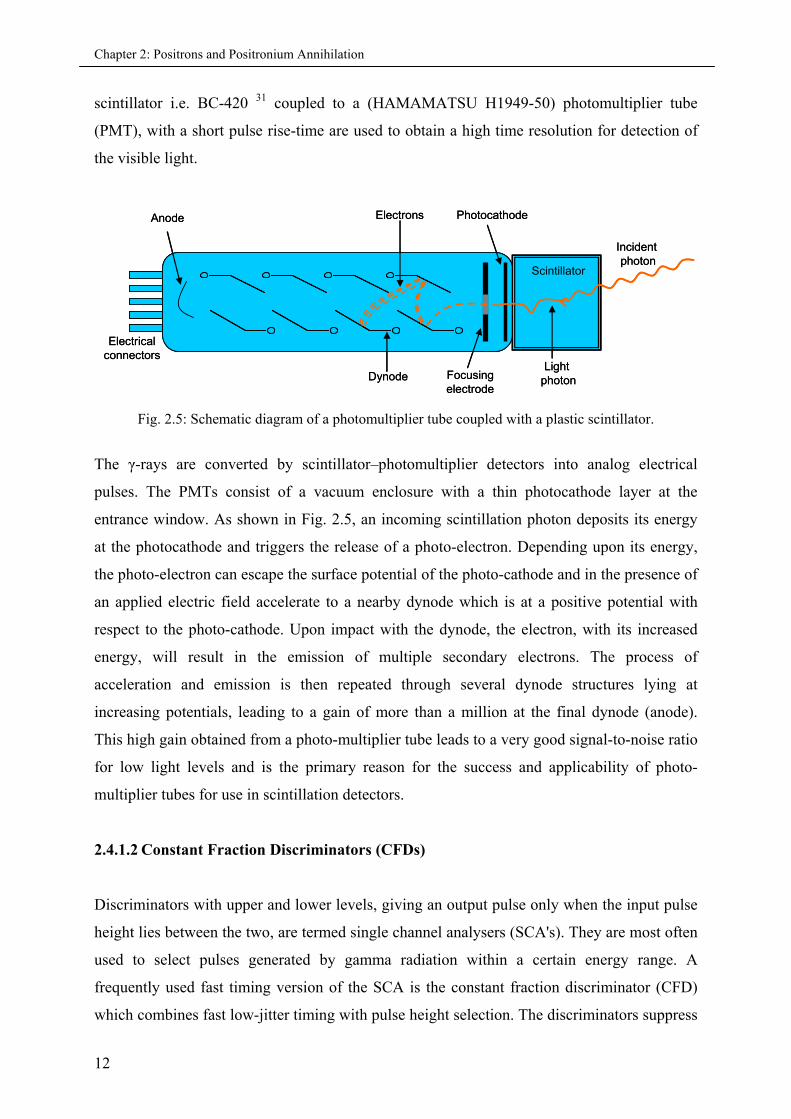
scintillator i.e. BC-420 31 coupled to a (HAMAMATSU H1949-50) photomultiplier tube
(PMT), with a short pulse rise-time are used to obtain a high time resolution for detection of
the visible light.
Light photon
Incident photon
Scintillator
PhotocathodeElectrons
Focusingelectrode
Dynode
Anode
Electricalconnectors
Light photon
Incident photon
Scintillator
PhotocathodeElectrons
Focusingelectrode
Dynode
Anode
Electricalconnectors
Fig. 2.5: Schematic diagram of a photomultiplier tube coupled with a plastic scintillator.
The γ-rays are converted by scintillator–photomultiplier detectors into analog electrical
pulses. The PMTs consist of a vacuum enclosure with a thin photocathode layer at the
entrance window. As shown in Fig. 2.5, an incoming scintillation photon deposits its energy
at the photocathode and triggers the release of a photo-electron. Depending upon its energy,
the photo-electron can escape the surface potential of the photo-cathode and in the presence of
an applied electric field accelerate to a nearby dynode which is at a positive potential with
respect to the photo-cathode. Upon impact with the dynode, the electron, with its increased
energy, will result in the emission of multiple secondary electrons. The process of
acceleration and emission is then repeated through several dynode structures lying at
increasing potentials, leading to a gain of more than a million at the final dynode (anode).
This high gain obtained from a photo-multiplier tube leads to a very good signal-to-noise ratio
for low light levels and is the primary reason for the success and applicability of photo-
multiplier tubes for use in scintillation detectors.
2.4.1.2 Constant Fraction Discriminators (CFDs)
Discriminators with upper and lower levels, giving an output pulse only when the input pulse
height lies between the two, are termed single channel analysers (SCA's). They are most often
used to select pulses generated by gamma radiation within a certain energy range. A
frequently used fast timing version of the SCA is the constant fraction discriminator (CFD)
which combines fast low-jitter timing with pulse height selection. The discriminators suppress
12
Chapter 2: Positrons and Positronium Annihilation
noise and generate standard timing pulses by the constant-fraction discrimination principle.
Another task is to guarantee that the 1.27-MeV and 511-keV quanta are accepted only in the
appropriate channels. Their output pulses start and stop a time-to-amplitude converter as an
“electronic stopwatch”. The stop pulse is coax-cable delayed in order to shift the time
spectrum into a linear region of the TAC.
2.4.1.3 Time to Amplitude Converter (TAC)
The amplitude of the output pulse is proportional to the time difference between the birth and
the annihilation γ-quanta and thus, represents a measure of the positron lifetime. The timing
pulses are used to start and stop the charging of a capacitor in the time-to-amplitude converter
(TAC). The time linearity is ensured there by constant-current charging that is stopped at the
arrival of the stop pulse originating from the annihilation γ-quantum.
2.4.1.4 Multi-Channel Analyzer (MCA):
The final signal, whose amplitude is proportional to the lifetime of the positron is then fed
into a multi-channel buffer (MCB) which records this in a histogram which, over time,
describes the positron lifetime spectrum. An ORTEC® 919A multi-channel analyzer with
about 16000 channels is used for storing the spectra. The multi-channel analyser (MCA), sorts
pulses according to their height into several thousand channels or bins. MCAs can be multi-
parameter, collecting for example spectra simultaneously in two dimensions and storing
intensity contour plots.32 A single annihilation event is stored after analog–digital conversion
in the memory of a multi-channel analyzer. Here the channel numbers represent the time
scale, which can be easily converted by multiplying by the channel width. The three PALS
instruments in the Isolab at the University of Kiel are configured to use 4096 channels each.
The channel width used for the major part of this work was 25 ps, which is completely
acceptable given that polymers have an o-Ps lifetime in the range of 1-10 ns. The time
resolution of the spectrometer is determined mainly by the scintillator–multiplier part and is
approximately 285 ps. The practical consequence of this relatively poor resolution is the
limitation of the determination of positron lifetime components larger than about 50 ns. In
order to obtain the lifetime spectrum with good statistics, more than 5x10⁶ annihilation events
were recorded.
13
Chapter 2: Positrons and Positronium Annihilation
2.5 Data analysis of PALS spectrum
The MCA builds a histogram over the probability P(t), such that the annihilation of a single
positron at a time t is registered. The spectrum S is a function of the total counts Index n, each
of which represents a channel number in MCA, with the peak of spectrum coming from the
maximum number of annihilation events. This gives the spectrum S(n) with total number of
coincidence counts N0, as follows:
tt
t
n
n
dttPNnS )()( 0 (2.1)
where tn+1 = tn + Δt, with Δt being the channel width of the spectrometer and tn being the
incident time of particular stop signal in addition to the channel width. The time dependent
coincidence probability P(t) can be summarize as;
BtNtRtP )()()( (2.2)
with N(t) being the decay function, B is the signal background, and R(t) is the resolution
function of the instrument, generally determined by measuring a reference sample. For this
purpose, Cu (τr = 122 ps), Al (τr= 169 ps), Si (τr= 219 ps) or Kapton® (τav = 370 ps)33 can be
used, where τr and τav are the reference and average lifetime values. The PALS spectrum for
the reference must be obtained under the same experimental conditions and configurations as
used in the samples in order to preserve the same instrument resolution.
2.5.1 Analysis with LifeTime routine LT 9.0
The positron lifetime spectrum must be analyzed by assuming a certain model spectrum, in
order to obtain information about the properties of the inspected material. Positrons can
annihilate in a crystal lattice in defect-free regions or after being trapped in the free volume
holes of a polymer. Each of which gives a characteristic annihilation rate λi and characteristic
lifetime τi = 1/λi, respectively. In practice the lifetime distributions are usually obtained using
a computer program such as the PATFIT,34 CONTIN,35 or MELT programs.36 The reliability
of these programs for measuring the o-Ps lifetime distribution in polymers was shown by Cao
et al.37 A detailed description of these methods of data analysis is already presented in
literature.32 In PALS studies of polymers the decay function N(t) of PALS spectrum can also
14
Chapter 2: Positrons and Positronium Annihilation
be analyzed by LifeTime routine LT 9.0.2 The advantage of LT 9.0 over the other programs is
that it can be easily used in a windows environment (except VISTA) and there is also a
possibility of analyzing in two ways i.e. a finite lifetime analysis (discrete) or continuous
lifetime analysis (with distribution).
2.5.1.1 Finite lifetime analysis
The life of a single positron has a well defined value between 0 and ∞, if N number of
positrons annihilate from a single state, they will have their lifetimes distributed according to
Eq. (2.3)
( ) expN
N t
t (2.3)
but in reality positrons will usually annihilate from more than one state, each with its own
individual lifetime. In the finite lifetime analysis the PALS spectrum are resolved into a finite
number of negative exponentials decays. The experimental data P(t) is expressed as a
convoluted expression (by a symbol *) of the instrument resolution function R(t) and a finite
number of negative exponentials. So the decay function N(t) is given as;
1 1
i = 1 i = 1
( ) exp expk k
ii i i
i i
I tN t I t
(2.4)
Substituting this value in Eq. 2.2, one gets;
1
i = 1
( ) expk
i
i i
I tP t R t B
(2.5)
where, λi, is the inverse of the i-th lifetime component (τi) and Ii, is its intensity. The LT 9.0 is
a routine that performs a weighted non-linear least square fit of Eq. 2.5 to the experimental
spectrum. The user defines, the number of component i, to be fitted as well as initial guesses
of the starting values. In polymers it is usually found that the spectra can be best resolved into
three components. Where each lifetime corresponds to the average annihilation rate of a
positron in different state. The shortest lifetime (τ1 ~ 0.125ns) is due to singlet para-
positronium (p-Ps). The intermediate lifetime (τ2 ~ 0.40 ns) is due to positrons and positron-
molecule species. The longest lifetime (τ3 > 1 ns) is due to the o-Ps localized in the free-
volumes holes.
15
Chapter 2: Positrons and Positronium Annihilation
2.5.1.2 Continuous term analysis
The finite term analysis was basically developed for materials such as metals and
semiconductors, which have often a single lifetime or a possibility of a number of discrete
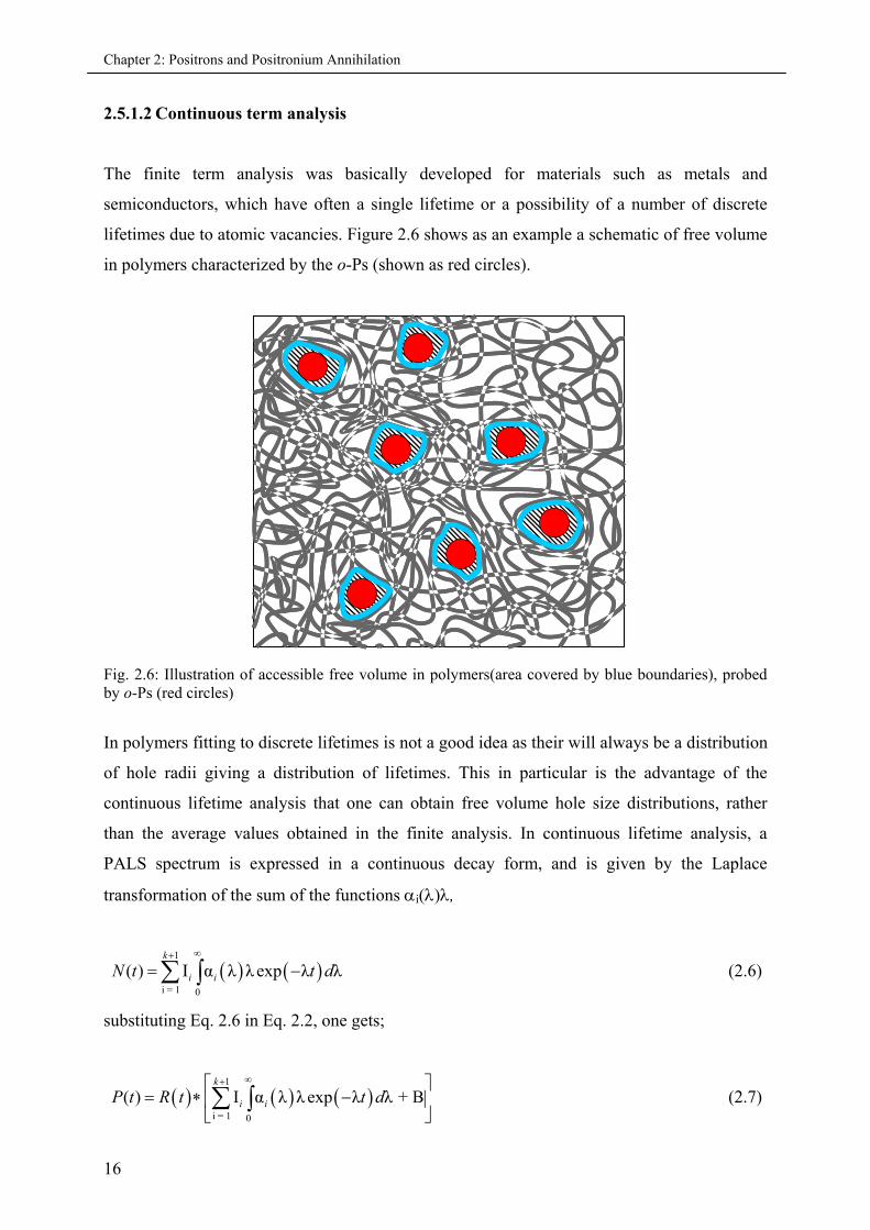
lifetimes due to atomic vacancies. Figure 2.6 shows as an example a schematic of free volume
in polymers characterized by the o-Ps (shown as red circles).
Fig. 2.6: Illustration of accessible free volume in polymers(area covered by blue boundaries), probed by o-Ps (red circles)
In polymers fitting to discrete lifetimes is not a good idea as their will always be a distribution
of hole radii giving a distribution of lifetimes. This in particular is the advantage of the
continuous lifetime analysis that one can obtain free volume hole size distributions, rather
than the average values obtained in the finite analysis. In continuous lifetime analysis, a
PALS spectrum is expressed in a continuous decay form, and is given by the Laplace
transformation of the sum of the functions i(),
1
i = 1 0
( ) I α λ λ exp λ λk
i iN t t d
(2.6)
substituting Eq. 2.6 in Eq. 2.2, one gets;
1
i = 1 0
( ) I α λ λ exp λ λ + Bk
i iP t R t t d
(2.7)
16
Chapter 2: Positrons and Positronium Annihilation
Here i() is the distribution (probability density function, pdf) of the annihilation rate = 1/
of the decay channel i, and LT 9.0 describes i() by log normal functions;
1
2
1lnln
exp2
12
2
0
ii
i (2.8)
where τ0 is the inverse of the mean log normal annihilation rate distribution and σi is the
standard deviation related to the finite width of the distribution comes from the size (and
shape) distribution of holes. So the continuous component depends on three model parameters
i.e. the component intensity I, the mean-lifetime of each channel τi,
2
1 00
0
exp2i i d
(2.9)
and the standard deviation from the mean-lifetime σi;
2 2 2 2 2 20 0 0 0exp exp 1 exp 1i i (2.10)
The time resolution is characterized by the full width at half maximum, FWHM, that is:
2ln2FWHM (2.11)
0 5 10 15 20 2510
100
1000
10000
100000
Num
ber
of C
ount
s
Lifetime (ns)
Experimental curve Background
1 = 1/
1
3 = 1/
3
2 = 1/
2
0 5 10 15 20 2510
100
1000
10000
100000
Num
ber
of C
ount
s
Lifetime (ns)
Experimental curve Background
1 = 1/
1
2 = 1/
2
3 = 1/
3
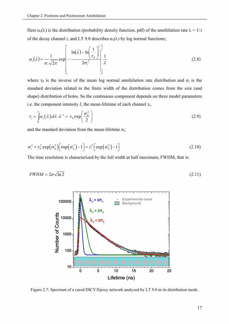
Figure 2.7: Spectrum of a cured DICY/Epoxy network analyzed by LT 9.0 in its distribution mode.
17
Chapter 2: Positrons and Positronium Annihilation
As an example, a typical positron lifetime spectra obtained from a cured DGEBA/Epoxy
network is shown in Fig. (2.7). The experimentally obtained spectrum is analyzed with the
help of LT 9.0 in its distribution mode. This continuous lifetime analysis approach was used
throughout this thesis, which as explained above is of benefit to obtain free volume hole size
distributions as compared to the discrete lifetime values obtained by the finite analysis.
It is generally observed that by increasing the number of parameters to be fitted one can
reduce the χ2 for a particular fit. To decompose a lifetime spectrum, the determination of the
number of components in samples with unknown free volume distribution is started by a
three-component fit of the spectrum. Additional components such as standard deviation σi (i =
1,2,3) and a second resolution function are added until the variance of the fit χ2 is in the range
of 1.0 to 1.15.
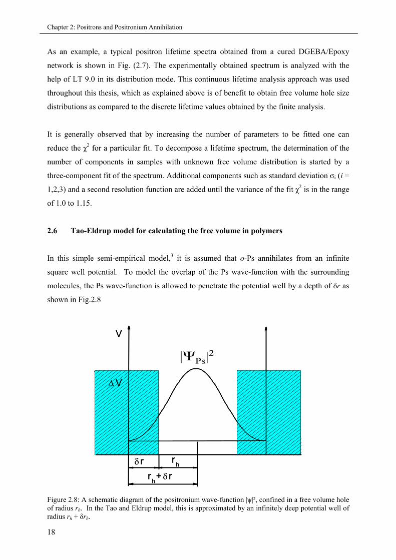
2.6 Tao-Eldrup model for calculating the free volume in polymers
In this simple semi-empirical model,3 it is assumed that o-Ps annihilates from an infinite
square well potential. To model the overlap of the Ps wave-function with the surrounding
molecules, the Ps wave-function is allowed to penetrate the potential well by a depth of δr as
shown in Fig.2.8
rh r
P s
V
V
rh+ r
|ΨPs|2
rh r
P s
V
V
rh+ r
|ΨPs|2
Figure 2.8: A schematic diagram of the positronium wave-function |ψ|², confined in a free volume hole of radius rh. In the Tao and Eldrup model, this is approximated by an infinitely deep potential well of radius rh + δrh.
18
Chapter 2: Positrons and Positronium Annihilation
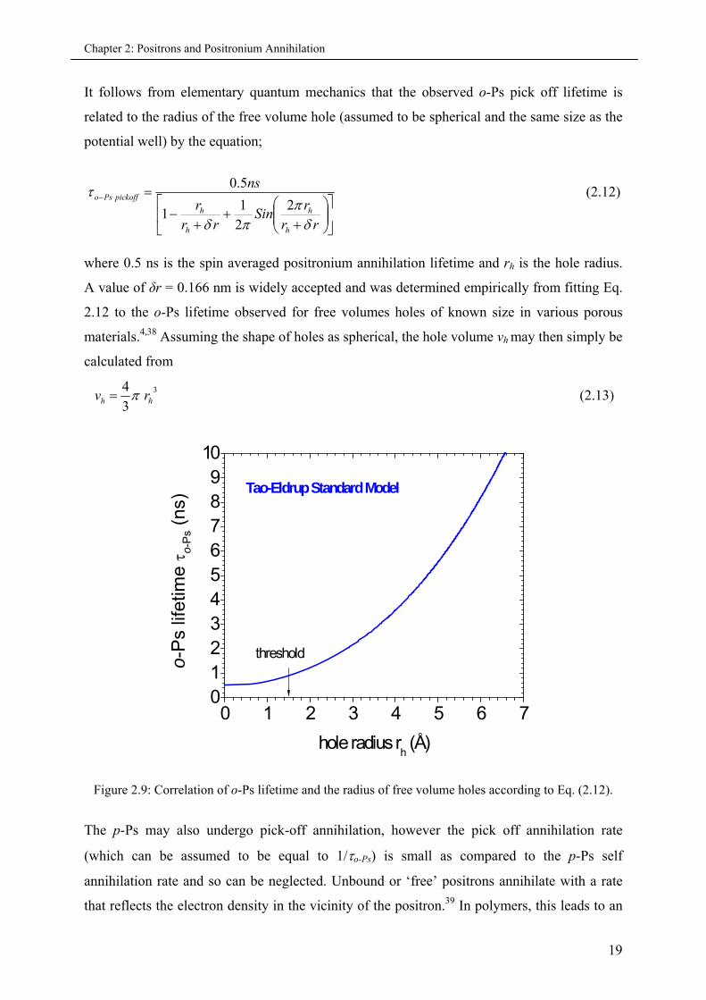
It follows from elementary quantum mechanics that the observed o-Ps pick off lifetime is
related to the radius of the free volume hole (assumed to be spherical and the same size as the
potential well) by the equation;
rrr
Sinrr
r
ns
h
h
h
h
pickoffPso
2
21
1
5.0 (2.12)
where 0.5 ns is the spin averaged positronium annihilation lifetime and rh is the hole radius.
A value of δr = 0.166 nm is widely accepted and was determined empirically from fitting Eq.
2.12 to the o-Ps lifetime observed for free volumes holes of known size in various porous
materials.4,38 Assuming the shape of holes as spherical, the hole volume vh may then simply be
calculated from
3
3
4hh rv (2.13)
0 1 2 3 4 5 6 70123456789
10
o-P
s lif
etim
e o
-Ps
(ns)
hole radius rh (Å)
Tao-Eldrup Standard Model
threshold
Figure 2.9: Correlation of o-Ps lifetime and the radius of free volume holes according to Eq. (2.12).
The p-Ps may also undergo pick-off annihilation, however the pick off annihilation rate
(which can be assumed to be equal to 1/o-Ps) is small as compared to the p-Ps self
annihilation rate and so can be neglected. Unbound or ‘free’ positrons annihilate with a rate
that reflects the electron density in the vicinity of the positron.39 In polymers, this leads to an
19
Chapter 2: Positrons and Positronium Annihilation
average free positron lifetime of ~ 350 to 500 ps. It is conventionally assumed that the free
positron lifetime is fixed for a given polymer. The free positrons may be trapped and
annihilate in free volume holes and that the average free positron lifetime may also reflect the
size of these holes.
To summarize, the average positron and positronium lifetimes in a polymer sample may be
expressed as;
PsppoPsp
Psp 11
125 to 200 ps (2.14)
psfree
free 5003501
(2.15)
1 1
1 10o Ps
o Ps po po
ns
(2.16)
where λp-Ps and λo-Ps are the intrinsic annihilation rates of p-Ps and o-Ps respectively. λpo is the
pickoff rate and is assumed to be the same for both p-Ps and o-Ps. The value η is the relative
contact density and reflects the change in the overlap of the electron-position wave-functions
compared to their state in vacuum.40
2.7 PALS studies on epoxy precursors
Characterization of precursors or cured epoxy resin formulations by PALS, has been reported
by various groups. For example, in-situ investigations on the cross-linking process of the
epoxy resin system DGEBA and diethylenetriamine (DETA) in comparison with infrared (IR)
spectroscopy was reported by J. Kanzow et al.41 The decrease in free volume of epoxy resin
system is strongly connected with the cross-linking process of resin and hardener. It was
observed that the free volume is dependent on the composition of the resin and the hardener.
The isothermal curing of several epoxy-resin systems was studied by T. Suzuki et al.42-44 The
decrease in o-Ps lifetime and simultaneous increase in its intensity were reported as the
commencement of polymerization of the epoxy formulation, whereas the lower values of τ3
were referred to as the termination of polymerization, these observations were supported by
the higher values of I3 with reached the saturation limits.
20
Chapter 2: Positrons and Positronium Annihilation
2.8 PALS studies on cured epoxy composites
Nanohole volume dependence on the cure schedule in epoxy thermosetting networks was
reported by A. Somoza et al.45 A strong dependence of the pre-cure temperature on the
structure of amine cured epoxies was reported and it was suggested that the epoxy composites
must be treated under similar conditions, specially when it comes to a comparison of PALS
data with other techniques. Free volume changes with respect to the change in thermoplastic
composition were reported by A.J. MacKinnon et al,46 the change in the thermoset matrix
material is termed as the major factor contributing to the phase structure of the cured
composites, which eventually effects the mechanical properties. Pressure dependence of
amine-cured epoxy polymers was studied above and below their glass-transition temperatures
by Y.Y. Wang et al,47 both o-Ps lifetime and its intensity decreases with increasing pressure.
A second run with decreasing pressure was performed and the results were reproducible for
the temperature above Tg, but this was not the case for the sample below Tg. This difference
was attributed to the time scale for molecular relaxation below Tg, being lower than the
experimental time scale of a few hours.
2.9 PALS related to this thesis
The work reported in this thesis is one step forward and the storage stability of one-
component epoxy resin formulations is determined with the help of Johnson-Mehl-Avrami-
Kolmogorov equation (JMAK) and Arrhenius law in combination with PALS data, the JMAK
theory is discussed in Chapter 4 of this work. The effect of change in activation energies is
also studied for free-accelerator and encapsulated accelerator formulations. Furthermore, the
change in free volume, thermal expansion co-efficient and the glass-transition temperatures
for several dicyandiamide (DICY) cured diglycidyl ether of bisphenol-A (DGEBA)
formulations are studied, for an details of these formulations the reader is referred to the
Chapter 5 of this thesis..
21

Chapter 2: Positrons and Positronium Annihilation
22
Chapter 3: Free Volume in Polymers
23
3. Free Volume in Polymers
3.1 Introduction
Free volume is an important characteristic property of polymeric materials which influences
their numerous properties, such as viscoelasticity,48-50 diffusivity and permeability,51
penetration by solvents,52 impact properties53 and the physical aging.54 However, in contrast
to other properties of polymers, free volume can be regarded as a complex physical object
within polymers that can be characterized by the size and size distribution of micro-cavities or
free volume element (FVE) that forms it. Initially, free volume was merely regarded as a
theoretical concept that could explain many aspects of polymer behavior but could not be
determined experimentally. Later, much attention was drawn to the problem of experimental
evaluation of free volume in polymers and attempts to characterize the free volume resulted in
development of various methods. In this chapter a quantitative discussion of various free
volume definitions is done and compared with the hole free volume as characterized by
positron annihilation lifetime spectroscopy (PALS).
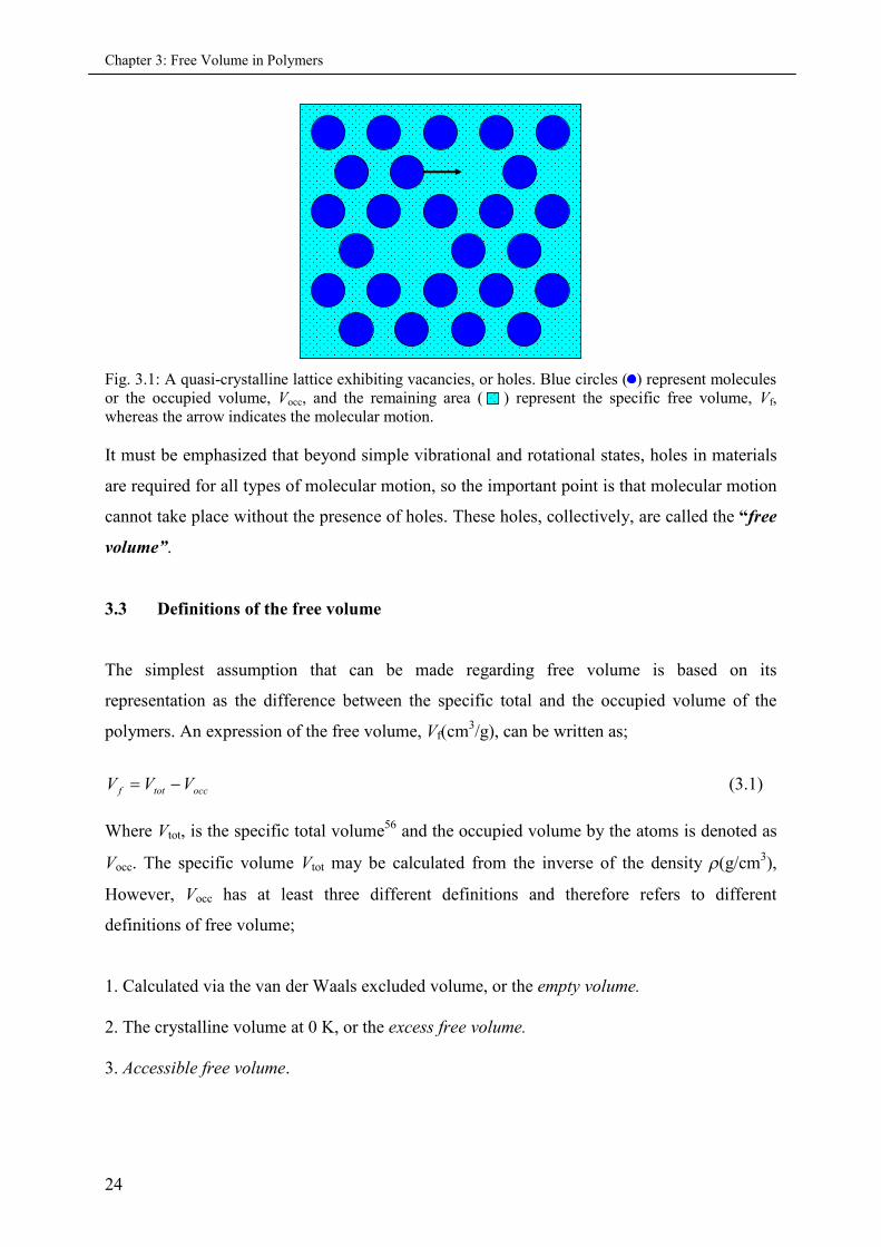
3.2 Basic concept of the Free Volume
According to the free volume theory as first developed by Eyring55 and others, molecular
motion in the bulk state depends on the presence of holes, or places where there are vacancies
or voids. When a molecule moves into a hole, obviously the hole also exchange places with
the molecule, as illustrated by the motion indicated in Fig. 3.1.
Although Fig. 3.1 assumes small molecules, a similar model can be constructed for the motion
of polymer chains, the main difference being that more than one “hole” may be required to be
in the same locality, as cooperative motions are required. Thus, for a polymeric segment to
move from its present position to an adjacent site, a critical void volume must first exist
before the segment can jump.
Chapter 3: Free Volume in Polymers
24
Fig. 3.1: A quasi-crystalline lattice exhibiting vacancies, or holes. Blue circles ( ) represent moleculesor the occupied volume, Vocc, and the remaining area ( ) represent the specific free volume, Vf,whereas the arrow indicates the molecular motion.
It must be emphasized that beyond simple vibrational and rotational states, holes in materials
are required for all types of molecular motion, so the important point is that molecular motion
cannot take place without the presence of holes. These holes, collectively, are called the “free
volume”.
3.3 Definitions of the free volume
The simplest assumption that can be made regarding free volume is based on its
representation as the difference between the specific total and the occupied volume of the
polymers. An expression of the free volume, Vf(cm3/g), can be written as;
occtotf VVV (3.1)
Where Vtot, is the specific total volume56 and the occupied volume by the atoms is denoted as
Vocc. The specific volume Vtot may be calculated from the inverse of the density (g/cm3),
However, Vocc has at least three different definitions and therefore refers to different
definitions of free volume;
1. Calculated via the van der Waals excluded volume, or the empty volume.
2. The crystalline volume at 0 K, or the excess free volume.
3. Accessible free volume.
Chapter 3: Free Volume in Polymers
25
3.3.1 Empty volume
An approach to find the occupied volume of polymers was proposed by Bondi,57 who
suggested calculation of the van der Waals volume VW, of repeat units of polymers by using
the tabulated increments in VW for smaller groups, which gives;
Wtotf VVV (3.2)
In this model, the van der Waals volume is assumed to consist of a number of interpenetrating
spheres. The radii of these spheres are equal to the van der Waals radii of the corresponding
atoms and the separation of the centre of the spheres is equal to the bond lengths. Tabulated
values of the van der Waals volumes of many of the most commonly occurring groups of
atoms can be found in literature,58 allowing the van der Waals volume of most polymers to be
easily calculated. The free volume calculated as the difference between the total volume and
the van der Waals volume represents the total free volume of the sample, which is often
termed as the empty volume. It should be noted however, that not all of the total free volume
defined in this way is available for the motion of the polymer chain segments.
3.3.2 Excess free volume
The concept of excess free volume is generally described as the free volume in the sample in
excess of the volume occupied by the densest packing of molecules. According to this
definition, the occupied volume consists of the van der Waals volume and the intrinsic
interstitial free volume that occurs as a result of the equilibrium packing coefficient. Defining
the free and occupied volume in this way acknowledges that the molecules can never fill the
volume of the entire sample, so there must always be free volume analogous to the interstitial
free volume in a crystal. Initially, in this model the crystal packing itself is used as the
occupied volume and Bondi equated this occupied volume with the crystal polymer’s volume
at absolute zero, Vc(0), and then postulated an empirical relation;
Vocc = Vc(0) ≈ 1.3Vw (3.3)
Connecting Vocc with the van der Waals volume.
)0()()( ctotf VTVTV (3.4)
Chapter 3: Free Volume in Polymers
26
Wtotf VVV 3.1 (3.5)
The tabulated values of Vc determined experimentally for a large number of common
polymers can be found in literature.58 The factor of 1.3 is due to the packing densities of
polymeric crystals at absolute zero. This approach therefore describes the excess free volume
as the volume that appears as a result of the irregular packing of the molecules. Clearly this
approach represents a major simplification for defining the occupied volume as it assumes
exactly the same packing efficiency for all polymers, and the assumption that the occupied
volume doesn’t change with temperature is not true. Furthermore, if Vc cannot be measured
directly, an approximate value may be calculated using the van der Waals volume. As it is
shown58 for a large series of polymers, the crystalline volume at 298 K may be closely
approximated by;
wcocc VKVV 45.1)298( (3.6)
Another advantage of this excess free volume is that, it directly represents the volume
available for motion of the polymer chain segments and is expected to be related to the
physical and rheological properties of the polymer.
3.3.3 Accessible free volume
The accessible volume for a given penetrant molecule is the volume of the domain composed
of points that can be occupied by the center of mass of the penetrant without any overlap
between the van der Waals spheres of the polymer and that of the penetrant. For a spherical
penetrant, accessible volume is most easily obtained by augmenting the radii of all polymer
atoms and calculating the unoccupied volume. For a given matrix and a range of spherical
probe molecules of progressively increasing radius, the accessible volume falls quasi-
exponentially.59-60
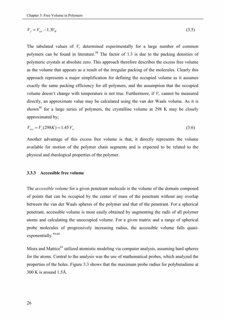
Misra and Mattice61 utilized atomistic modeling via computer analysis, assuming hard spheres
for the atoms. Central to the analysis was the use of mathematical probes, which analyzed the
properties of the holes. Figure 3.3 shows that the maximum probe radius for polybutadiene at
300 K is around 1.5Å.
Chapter 3: Free Volume in Polymers
27
Fig 3.3: Theoretical free volume fraction as a function of the probe sized for polybutadiene.61
3.4 Fractional free volume and related theories
In most cases, a dimensionless, reduced value of the free volume, called the fractional free
volume f, gives better correlations than Vf with transport properties within a family of
polymers and is also a good measure of the openness of a polymer matrix. The fractional free
volume is defined as the ratio of the specific free volume Vf, to the total volume Vtot;
tot
f
V
Vf (3.7)
Because of the different ways of defining the free volume, it is clear that the magnitude of the
specific free volume and the free volume fraction will depend crucially on exactly how the
occupied volume is defined. This difficulty is demonstrated by the wide range of values
calculated by different free volume theories for the same polymer at the same temperature.
Table 3.1 - The free volume fraction f of PMMA at T = Tg calculated from various freevolume theories.62
Method f (Tg)
Simha-Somcynsky EOS theory 0.081
Simha-Boyer 0.137
Boyer-Spencer 0.235
Hirai-Eyring 0.056
Williams-Landel-Ferry (Doolittle) 0.013
Miller (Cohen – Turnbull) 0.032
Chapter 3: Free Volume in Polymers
28
An example is highlighted in table 3.1 which shows the fractional free volume of
poly(methylmethacrylate) PMMA calculated at the glass transition temperature by various
free volume theories. Since the above mentioned free volume theories are beyond the scope of
this work, for this reason they are not discussed in detail.
3.5 Experimental Techniques to determine the free volume
Free volume distributions have been studied using kinetic theories(as briefly named in the
previous section) and molecular dynamic simulations.63 The attempts to characterize free
volume resulted in development of various methods that are often united by the term “probe
methods”. A common feature of these methods is that probes of different nature and size
(atoms or molecules) are introduced into a polymer and observation of their behaviour, which
is sensitive to free volume, makes it possible to deduce some information on nano-structure of
free volume.
Just to name a few of these techniques, the experimental probes for free volume at molecular
and atomic scales is possible using small-angle X-ray diffraction(SAXS),64 inverse gas
chromatography,65 129Xe NMR spectroscopy,66 spin-probe measurements,67 wide-angle X-ray
scattering(WAXS), photo-chromic and fluorescence techniques.68
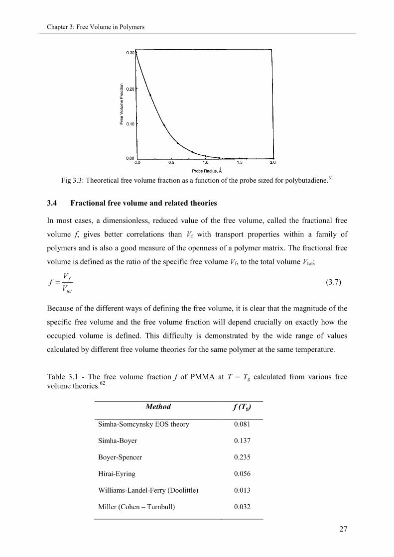
Fig. 3.2: Typical accessible free volume ( ) sites in a polymeric structure due to the disorderedpackaging. The mean volume of these individual nanoscopic holes is determined by PALS and thetotal sum of all the free volumes can be obtained if number density N, of holes is known.
Positron annihilation lifetime spectroscopy has emerged as the unique method providing
resolution of a few Angstroms in size and it has been shown that a good correlation exists
Chapter 3: Free Volume in Polymers
29
between the lifetime of ortho-Positronium (o-Ps) atoms and the free volume for not only
polymers, but also applied to simple liquids as well.69-70 However, PALS calculate the hole
free volume Vh, and the total free volume cannot be estimated directly with this method. In
addition, it is important to realize that PALS is a dynamic method of measurement with a time
scale of 10-9s. The molecular vibrations with a frequency higher than 109 Hz will therefore
contribute to the occupied volume.71 This thesis is based on experimental data obtained from
the PALS technique only, which is already discussed quantitatively in Chapter 2.
Table 3.2 Methods used for probing free volumes in Polymers72
Method Probe Size InformationPositron AnnihilationLifetime Spectroscopy
o-Ps 1.06 Å Size, size distribution,concentration of the FVE anddependence of the size of theFVE on temperature andpressure
Inverse gaschromatography
Organic Vapors > 5 Å (>C3) Temperature-averaged meansize of the FVE
129Xe NMR 129Xe ca. 4 Å Size of the FVE and itstemperature dependence
Spin probe method 2,2,6,6-tetra-methylpyperidine-1-oxyl(TEMPO) and
other stable nitroxylradicals
> 100 Å3 Information on the part of thesize distribution of the freevolume which corresponds tolarger holes; temperaturedependence of larger hole sizes
Photochromic probemethod
Stilben andazobenzenederivatives
120-600 Å3
Electrochromic probemethod
Azo-dyes > 100 Å3
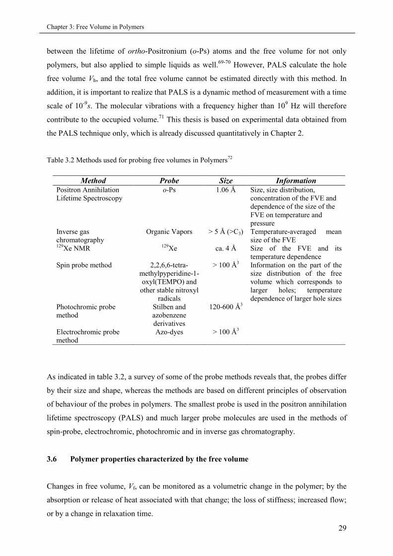
As indicated in table 3.2, a survey of some of the probe methods reveals that, the probes differ
by their size and shape, whereas the methods are based on different principles of observation
of behaviour of the probes in polymers. The smallest probe is used in the positron annihilation
lifetime spectroscopy (PALS) and much larger probe molecules are used in the methods of
spin-probe, electrochromic, photochromic and in inverse gas chromatography.
3.6 Polymer properties characterized by the free volume
Changes in free volume, Vf, can be monitored as a volumetric change in the polymer; by the
absorption or release of heat associated with that change; the loss of stiffness; increased flow;
or by a change in relaxation time.
Chapter 3: Free Volume in Polymers
30
3.6.1 Glass-Transition temperature
One of the most suitable approximations for analyzing the glass transition concerns the free
volume.73 As explained earlier, the free volume is the space in a solid or liquid not occupied
by molecules; i.e., it is the empty space existing between molecules. In the liquid state the free
volume is large, so molecular movements occur easily (the unoccupied volume facilitates the
mobility of the molecules), and the molecules are therefore able to change their conformation
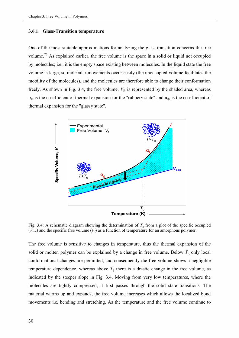
freely. As shown in Fig. 3.4, the free volume, Vf, is represented by the shaded area, whereas
αr, is the co-efficient of thermal expansion for the "rubbery state" and αg, is the co-efficient of
thermal expansion for the "glassy state".
T<Tg
T>Tg
Temperature (K)
Specifiv
Volu
me,V
ExperimentalFree Volume, Vf
Vocc
αr
αg
Physical Ageing
Tg
Fig. 3.4: A schematic diagram showing the determination of Tg from a plot of the specific occupied(Vocc) and the specific free volume (Vf) as a function of temperature for an amorphous polymer.
The free volume is sensitive to changes in temperature, thus the thermal expansion of the
solid or molten polymer can be explained by a change in free volume. Below Tg only local
conformational changes are permitted, and consequently the free volume shows a negligible
temperature dependence, whereas above Tg there is a drastic change in the free volume, as
indicated by the steeper slope in Fig. 3.4. Moving from very low temperatures, where the
molecules are tightly compressed, it first passes through the solid state transitions. The
material warms up and expands, the free volume increases which allows the localized bond
movements i.e. bending and stretching. As the temperature and the free volume continue to
Chapter 3: Free Volume in Polymers
31
increase, the whole side chains and localized groups of four to eight backbone atoms begin to
have enough space to move.
Furthermore, as the heating continues, the Tg or the glass transition temperature is reached,
where the chains in the amorphous regions begin to coordinate long-range cooperative
motions. One classical description of this region is that the amorphous regions have begun to
melt, since the Tg only occurs in amorphous material, in a 100% crystalline material one does
not see a Tg. Finally, the melt temperature Tm is reached, where large-scale chain slippage
occurs and the material flows (not shown here). For a cured thermoset, nothing happens after
the Tg until the sample begins to burn and degrade because the cross-links prevent the chains
from slipping past each other.
3.6.2 Physical Ageing
While the molecular motion in the rubbery and liquid states involves 10 to 50 carbon atoms,
molecular motion in the glassy state is restricted to vibrations, rotations, and motions by
relatively short segments of the chains. As explained before, the extent of molecular motion
depends on the free volume. In the glassy state, the free volume depends on the thermal
history of the polymer. When a sample is cooled from the melt to some temperature below Tg
and held at constant temperature, its volume will decrease (see Figure 3.4). Because of the
lower free volume, the rate of stress relaxation, creep, and related properties will decrease.74
This phenomenon is sometimes called physical aging, although the sample ages in the sense
not of degradation or oxidation but rather of an approach to the equilibrium state in the glass.
3.7 Summary of this chapter
The glass-transition and physical ageing properties of some of the cured epoxy resin systems
are studied with the help of the hole free volume obtained from PALS experiments and these
results will be discussed in a later part (Chapter 7) of this thesis.But the major part of this
work is focused on the investigation of the storage stability of single-component epoxy resin
precursors as shown in Chapter 6, which are also studied with the help of Johnson-Mehl-
Avrami-Kolmogorov (JMAK) equation and the transformed fraction calculated from the
change in o-Ps lifetime, which in turn is the measure of hole free volume Vh. The JMAK
Chapter 3: Free Volume in Polymers
32
equation of phase transformations is discussed in the next chapter, whereas the PALS
technique, as mentioned earlier is quantitatively discussed in Chapter 5.
Chapter 4: Johnson-Mehl-Avrami-Kolmogorov Theory
33
4. Johnson-Mehl-Avrami-Kolmogorov Theory
4.1 Introduction
The main aim of this thesis is to provide industry with some more reliable and efficient means
of determining the shelf-life of single-component epoxy-resin systems. In order to achieve
this, it is necessary to understand the curing kinetics of these systems. This can be explained
by the phase transformation from the precursor to the solid phase. In general, the theoretical
basis for the overall transformation kinetics comes from the metal physics. The most
important of them being the Avrami theory, also known as JMAK equation, named after
Johnson and Mehl,75 Avrami5-7 and Kolmogorov,76 who significantly contributed to this
equation. The Avrami theory is a widely accepted model to study the phase transformations,
e.g. crystallization or austenite-to-martensite transformations.77 In this chapter, the Avrami
theory for the crystalline phase transformations is discussed. Here, this theory is applied for
the first time to study the curing of epoxies, with the help of PALS data.
4.2 Basics of Phase Transformations
The emergence of a new phase within a parent phase, such as a solid within a liquid, involves
the birth of a phase and its subsequent development. Normally with phase transformations, at
least one new phase is formed that has different physical or chemical characteristics, with a
possibility of a different crystallographic structure than the parent phase. Furthermore, most
phase transformations do not occur instantaneously. In fact, they begin by the formation of
numerous small particles of the new phase, which increase in size until the transformation has
reached its completion. The progress of a phase transformation can be divided into two
distinct stages: nucleation and growth.
4.2.1 Nucleation and Growth
Discussion of the theory of nucleation involves a thermodynamic parameter called free energy
(or Gibbs free energy, G). A transformation will occur spontaneously only when ΔG has a
negative value, where ΔG is the change in free energy. There are two types of nucleation i.e.
homogeneous and heterogeneous. The distinction between them is made according to the site
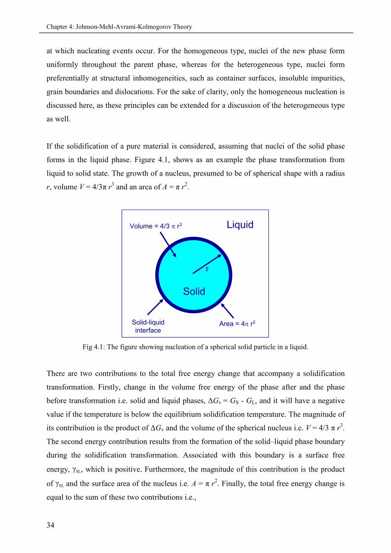
Chapter 4: Johnson-Mehl-Avrami-Kolmogorov Theory
34
at which nucleating events occur. For the homogeneous type, nuclei of the new phase form
uniformly throughout the parent phase, whereas for the heterogeneous type, nuclei form
preferentially at structural inhomogeneities, such as container surfaces, insoluble impurities,
grain boundaries and dislocations. For the sake of clarity, only the homogeneous nucleation is
discussed here, as these principles can be extended for a discussion of the heterogeneous type
as well.
If the solidification of a pure material is considered, assuming that nuclei of the solid phase
forms in the liquid phase. Figure 4.1, shows as an example the phase transformation from
liquid to solid state. The growth of a nucleus, presumed to be of spherical shape with a radius
r, volume V = 4/3π r3 and an area of A = π r2.
Solid
Liquid
r
Volume = 4/3 r3
Area = 4 r2Solid-liquidinterface
Solid
Liquid
r
Volume = 4/3 r3
Area = 4 r2Solid-liquidinterface
Fig 4.1: The figure showing nucleation of a spherical solid particle in a liquid.
There are two contributions to the total free energy change that accompany a solidification
transformation. Firstly, change in the volume free energy of the phase after and the phase
before transformation i.e. solid and liquid phases, ΔGv = GS - GL, and it will have a negative
value if the temperature is below the equilibrium solidification temperature. The magnitude of
its contribution is the product of ΔGv and the volume of the spherical nucleus i.e. V = 4/3 π r3.
The second energy contribution results from the formation of the solid–liquid phase boundary
during the solidification transformation. Associated with this boundary is a surface free
energy, γSL, which is positive. Furthermore, the magnitude of this contribution is the product
of γSL and the surface area of the nucleus i.e. A = π r2. Finally, the total free energy change is
equal to the sum of these two contributions i.e.,
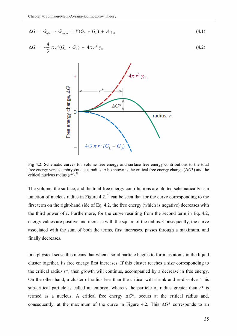
Chapter 4: Johnson-Mehl-Avrami-Kolmogorov Theory
35
- ( - )after before S L SLG G G V G G A (4.1)
3 24- ( - ) 4
3L S SLG r G G r (4.2)
4π r2 SL
4/3 π r3 GL – GS)
4π r2 SL
4/3 π r3 GL – GS)
Fig 4.2: Schematic curves for volume free energy and surface free energy contributions to the totalfree energy versus embryo/nucleus radius. Also shown is the critical free energy change (ΔG*) and thecritical nucleus radius (r*).78
The volume, the surface, and the total free energy contributions are plotted schematically as a
function of nucleus radius in Figure 4.2.78 can be seen that for the curve corresponding to the
first term on the right-hand side of Eq. 4.2, the free energy (which is negative) decreases with
the third power of r. Furthermore, for the curve resulting from the second term in Eq. 4.2,
energy values are positive and increase with the square of the radius. Consequently, the curve
associated with the sum of both the terms, first increases, passes through a maximum, and
finally decreases.
In a physical sense this means that when a solid particle begins to form, as atoms in the liquid
cluster together, its free energy first increases. If this cluster reaches a size corresponding to
the critical radius r*, then growth will continue, accompanied by a decrease in free energy.
On the other hand, a cluster of radius less than the critical will shrink and re-dissolve. This
sub-critical particle is called an embryo, whereas the particle of radius greater than r* is
termed as a nucleus. A critical free energy ΔG*, occurs at the critical radius and,
consequently, at the maximum of the curve in Figure 4.2. This ΔG* corresponds to an
Chapter 4: Johnson-Mehl-Avrami-Kolmogorov Theory
36
activation free energy, which is the free energy required for the formation of a stable nucleus
or it may be considered an energy barrier to the nucleation process.
Since r* and ΔG* appear at the maximum on the free energy-versus-radius curve of Figure
4.2, derivation of expressions for these two parameters is a simple matter. For r*, the ΔG
equation (Equation 4.2) is differentiated with respect to r, the resulting expression is set equal
to zero, and then solved for (r = r*). That is,
2( ) 4( - )(3 ) 4 (2 ) 0
3L S SL
d GG G r r
dr
(4.3)
this leads to the result,
2*
( - )SL
S L
rG G
(4.4)
Now, substituting this expression for r* into Equation 4.2, yields the following expression for
ΔG*: (with ΔG = ΔG*)
3
2
16*
3 ( - )SL
L S
GG G
(4.5)
During the growth stage these nuclei increase in size, which results in the disappearance of
some or all of the parent phase. The transformation reaches completion if the growth of these
new phase particles is allowed to proceed until the equilibrium fraction is attained. Note that
nucleation will continue to occur simultaneously with growth of the new phase particles. Off
course, nucleation cannot occur in regions that have already transformed to the new phase.
Furthermore, the growth process will cease in any region where particles of the new phase
meet, as the transformation should have reached completion in these regions.79
4.3 Phase Transformation Kinetics
The amount of material transformed can be calculated, subject to the restraints that are
imposed on the kinetic process. The time dependence of rate, which is often termed as the
kinetics of a transformation, is an important factor widely used in the study of numerous
materials. The rate of transformation and the time required for the transformation to proceed
to some degree of completion (e.g., time to 50% reaction completion, t1/2) are inversely
proportional to each other (Equation 4.6).78
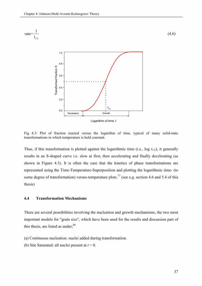
Chapter 4: Johnson-Mehl-Avrami-Kolmogorov Theory
37
1/2
1rate=
t(4.6)
0.2
0.4
0.6
0.8
1.0
Growth
Tra
nsfo
rme
dfr
act
ion
X
Logarithim of time, t
t1/2
Nucleation0.0
Fig 4.3: Plot of fraction reacted versus the logarithm of time, typical of many solid-statetransformations in which temperature is held constant.
Thus, if this transformation is plotted against the logarithmic time (i.e., log t1/2), it generally
results in an S-shaped curve i.e. slow at first, then accelerating and finally decelerating (as
shown in Figure 4.3). It is often the case that the kinetics of phase transformations are
represented using the Time-Temperature-Superposition and plotting the logarithmic time- (to
some degree of transformation) versus-temperature plots.77 (see e.g. section 4.6 and 5.4 of this
thesis)
4.4 Transformation Mechanisms
There are several possibilities involving the nucleation and growth mechanisms, the two most
important models for "grain size", which have been used for the results and discussion part of
this thesis, are listed as under;80
(a) Continuous nucleation: nuclei added during transformation.
(b) Site Saturated: all nuclei present at t = 0.
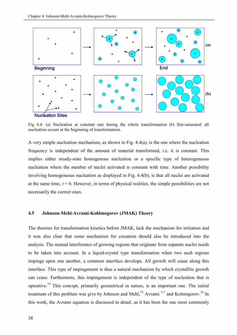
Chapter 4: Johnson-Mehl-Avrami-Kolmogorov Theory
38
Beginning EndBeginning End
Nucleation SitesNucleation Sites
Fig 4.4: (a) Nucleation at constant rate during the whole transformation (b) Site-saturated: allnucleation occurs at the beginning of transformation.
A very simple nucleation mechanism, as shown in Fig. 4.4(a), is the one where the nucleation
frequency is independent of the amount of material transformed, i.e. it is constant. This
implies either steady-state homogenous nucleation or a specific type of heterogeneous
nucleation where the number of nuclei activated is constant with time. Another possibility
involving homogeneous nucleation as displayed in Fig. 4.4(b), is that all nuclei are activated
at the same time, t = 0. However, in terms of physical realities, the simple possibilities are not
necessarily the correct ones.
4.5 Johnson-Mehl-Avrami-Kohlmogorov (JMAK) Theory
The theories for transformation kinetics before JMAK, lack the mechanism for initiation and
it was also clear that some mechanism for cessation should also be introduced into the
analysis. The mutual interference of growing regions that originate from separate nuclei needs
to be taken into account. In a liquid-crystal type transformation when two such regions
impinge upon one another, a common interface develops. All growth will cease along this
interface. This type of impingement is thus a natural mechanism by which crystallite growth
can cease. Furthermore, this impingement is independent of the type of nucleation that is
operative.79 This concept, primarily geometrical in nature, is an important one. The initial
treatment of this problem was give by Johnson and Mehl,75 Avrami 5-7 and Kolmogorov.76 In
this work, the Avrami equation is discussed in detail, as it has been the one most commonly
(a)
(b)
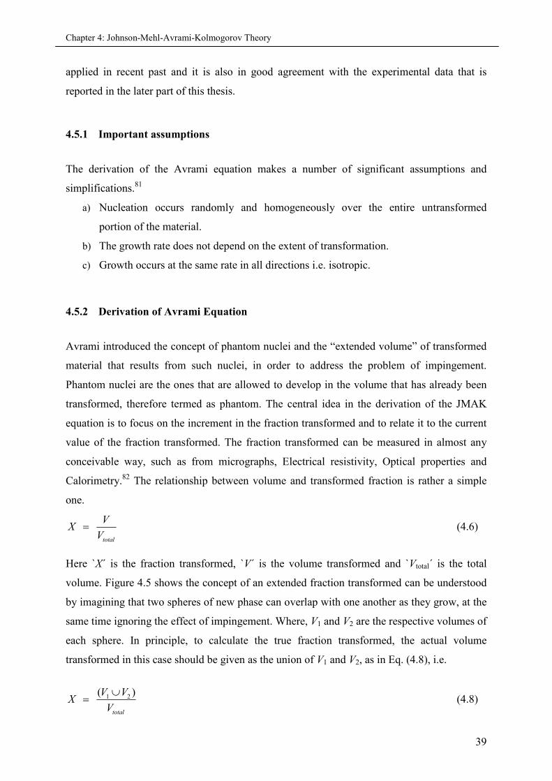
Chapter 4: Johnson-Mehl-Avrami-Kolmogorov Theory
39
applied in recent past and it is also in good agreement with the experimental data that is
reported in the later part of this thesis.
4.5.1 Important assumptions
The derivation of the Avrami equation makes a number of significant assumptions and
simplifications.81
a) Nucleation occurs randomly and homogeneously over the entire untransformed
portion of the material.
b) The growth rate does not depend on the extent of transformation.
c) Growth occurs at the same rate in all directions i.e. isotropic.
4.5.2 Derivation of Avrami Equation
Avrami introduced the concept of phantom nuclei and the “extended volume” of transformed
material that results from such nuclei, in order to address the problem of impingement.
Phantom nuclei are the ones that are allowed to develop in the volume that has already been
transformed, therefore termed as phantom. The central idea in the derivation of the JMAK
equation is to focus on the increment in the fraction transformed and to relate it to the current
value of the fraction transformed. The fraction transformed can be measured in almost any
conceivable way, such as from micrographs, Electrical resistivity, Optical properties and
Calorimetry.82 The relationship between volume and transformed fraction is rather a simple
one.
total
VX
V (4.6)
Here `X´ is the fraction transformed, `V´ is the volume transformed and `Vtotal´ is the total
volume. Figure 4.5 shows the concept of an extended fraction transformed can be understood
by imagining that two spheres of new phase can overlap with one another as they grow, at the
same time ignoring the effect of impingement. Where, V1 and V2 are the respective volumes of
each sphere. In principle, to calculate the true fraction transformed, the actual volume
transformed in this case should be given as the union of V1 and V2, as in Eq. (4.8), i.e.
1 2( )
total
V VX
V
(4.8)
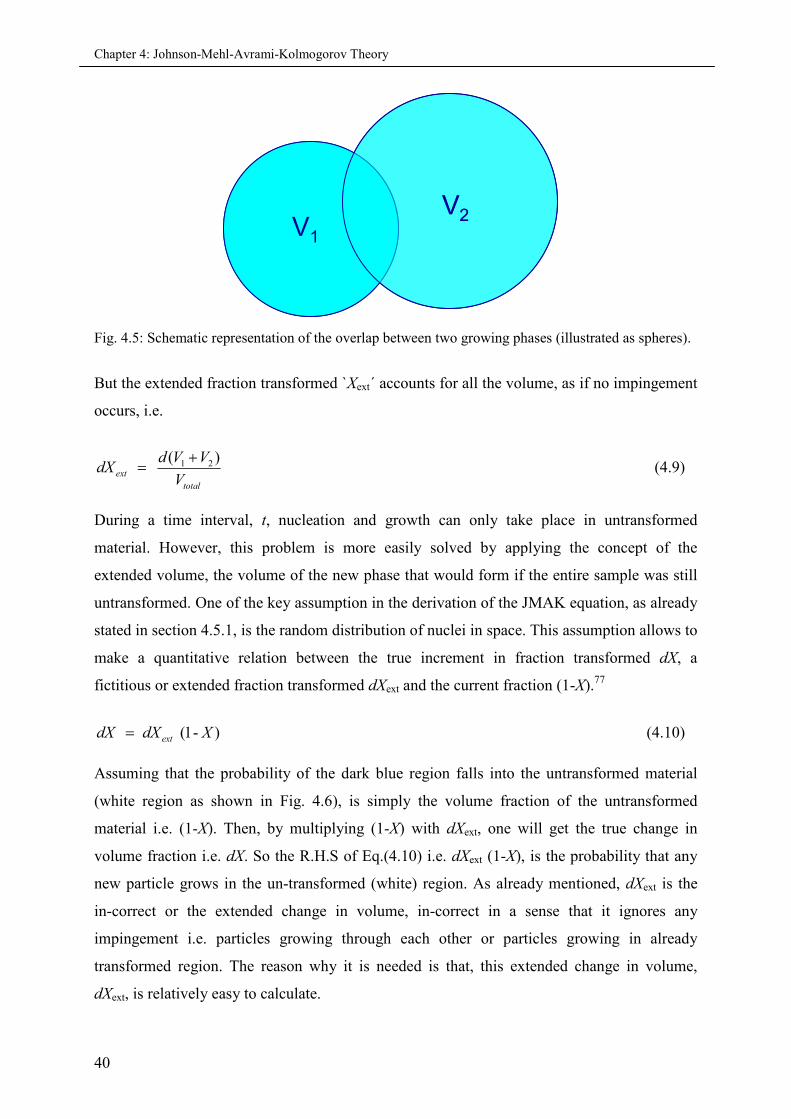
Chapter 4: Johnson-Mehl-Avrami-Kolmogorov Theory
40
V1
V2V1
V2
Fig. 4.5: Schematic representation of the overlap between two growing phases (illustrated as spheres).
But the extended fraction transformed `Xext´ accounts for all the volume, as if no impingement
occurs, i.e.
1 2( )ext
total
d V VdX
V
(4.9)
During a time interval, t, nucleation and growth can only take place in untransformed
material. However, this problem is more easily solved by applying the concept of the
extended volume, the volume of the new phase that would form if the entire sample was still
untransformed. One of the key assumption in the derivation of the JMAK equation, as already
stated in section 4.5.1, is the random distribution of nuclei in space. This assumption allows to
make a quantitative relation between the true increment in fraction transformed dX, a
fictitious or extended fraction transformed dXext and the current fraction (1-X).77
(1- )extdX dX X (4.10)
Assuming that the probability of the dark blue region falls into the untransformed material
(white region as shown in Fig. 4.6), is simply the volume fraction of the untransformed
material i.e. (1-X). Then, by multiplying (1-X) with dXext, one will get the true change in
volume fraction i.e. dX. So the R.H.S of Eq.(4.10) i.e. dXext (1-X), is the probability that any
new particle grows in the un-transformed (white) region. As already mentioned, dXext is the
in-correct or the extended change in volume, in-correct in a sense that it ignores any
impingement i.e. particles growing through each other or particles growing in already
transformed region. The reason why it is needed is that, this extended change in volume,
dXext, is relatively easy to calculate.
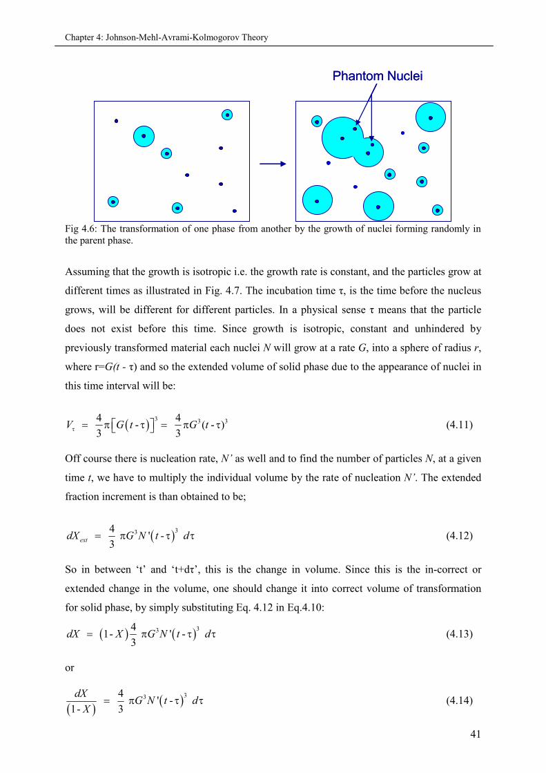
Chapter 4: Johnson-Mehl-Avrami-Kolmogorov Theory
41
Phantom NucleiPhantom Nuclei
Fig 4.6: The transformation of one phase from another by the growth of nuclei forming randomly inthe parent phase.
Assuming that the growth is isotropic i.e. the growth rate is constant, and the particles grow at
different times as illustrated in Fig. 4.7. The incubation time τ, is the time before the nucleus
grows, will be different for different particles. In a physical sense τ means that the particle
does not exist before this time. Since growth is isotropic, constant and unhindered by
previously transformed material each nuclei N will grow at a rate G, into a sphere of radius r,
where r=G(t - τ) and so the extended volume of solid phase due to the appearance of nuclei in
this time interval will be:
3 3 34 4
- ( - )3 3
V G t G t (4.11)
Off course there is nucleation rate, N’ as well and to find the number of particles N, at a given
time t, we have to multiply the individual volume by the rate of nucleation N’. The extended
fraction increment is than obtained to be;
334
' -3
extdX G N t d (4.12)
So in between ‘t’ and ‘t+dτ’, this is the change in volume. Since this is the in-correct or
extended change in the volume, one should change it into correct volume of transformation
for solid phase, by simply substituting Eq. 4.12 in Eq.4.10:
334
1- ' -3
dX X G N t d (4.13)
or
334' -
1- 3
dXG N t d
X (4.14)
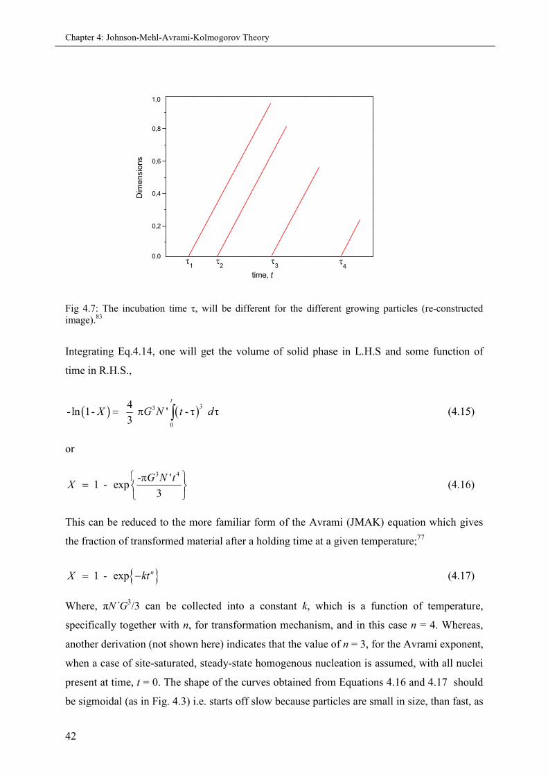
Chapter 4: Johnson-Mehl-Avrami-Kolmogorov Theory
42
0,2
0,4
0,6
0,8
4
3
2
1.0
Dim
en
sio
ns
time, t
0.0
1
Fig 4.7: The incubation time τ, will be different for the different growing particles (re-constructedimage).83
Integrating Eq.4.14, one will get the volume of solid phase in L.H.S and some function of
time in R.H.S.,
33
0
4-ln 1- ' -
3
t
X G N t d (4.15)
or
3 4- '1 - exp
3
G N tX
(4.16)
This can be reduced to the more familiar form of the Avrami (JMAK) equation which gives
the fraction of transformed material after a holding time at a given temperature;77
1 - exp nX kt (4.17)
Where, πN´G3/3 can be collected into a constant k, which is a function of temperature,
specifically together with n, for transformation mechanism, and in this case n = 4. Whereas,
another derivation (not shown here) indicates that the value of n = 3, for the Avrami exponent,
when a case of site-saturated, steady-state homogenous nucleation is assumed, with all nuclei
present at time, t = 0. The shape of the curves obtained from Equations 4.16 and 4.17 should
be sigmoidal (as in Fig. 4.3) i.e. starts off slow because particles are small in size, than fast, as
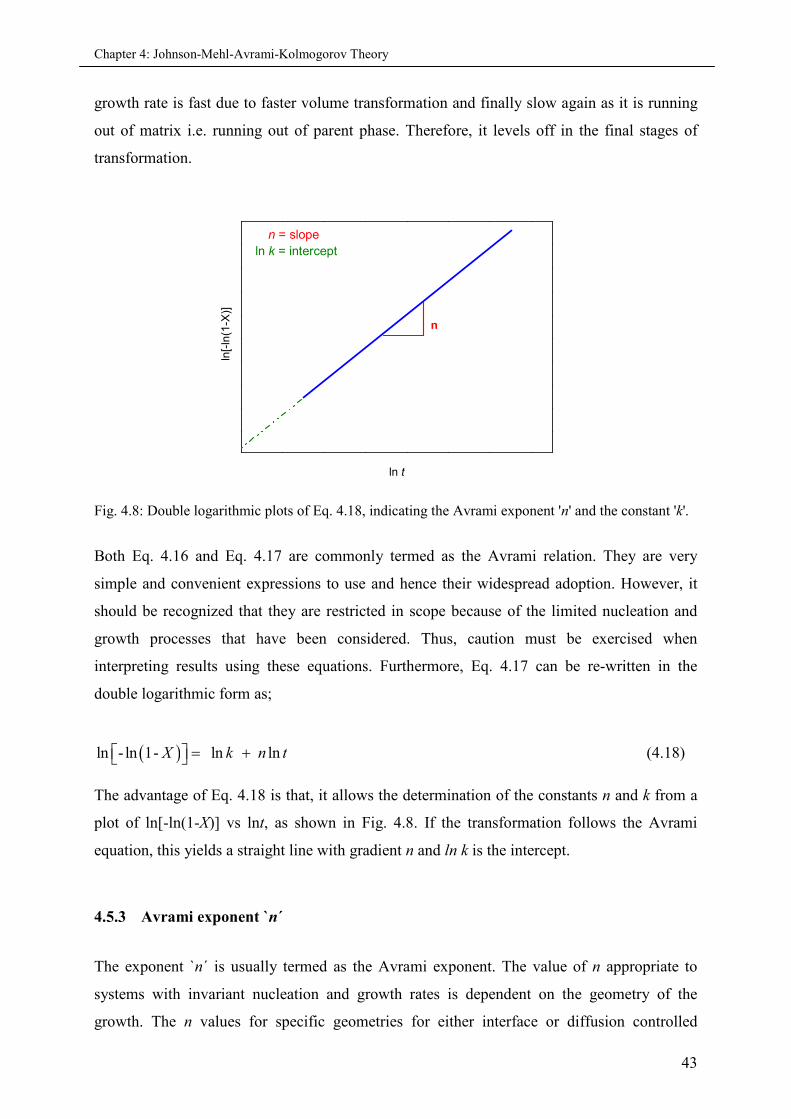
Chapter 4: Johnson-Mehl-Avrami-Kolmogorov Theory
43
growth rate is fast due to faster volume transformation and finally slow again as it is running
out of matrix i.e. running out of parent phase. Therefore, it levels off in the final stages of
transformation.
ln[-
ln(1
-X)]
ln t
n
ln k = intercept
n = slope
Fig. 4.8: Double logarithmic plots of Eq. 4.18, indicating the Avrami exponent 'n' and the constant 'k'.
Both Eq. 4.16 and Eq. 4.17 are commonly termed as the Avrami relation. They are very
simple and convenient expressions to use and hence their widespread adoption. However, it
should be recognized that they are restricted in scope because of the limited nucleation and
growth processes that have been considered. Thus, caution must be exercised when
interpreting results using these equations. Furthermore, Eq. 4.17 can be re-written in the
double logarithmic form as;
ln - ln 1- ln lnX k n t (4.18)
The advantage of Eq. 4.18 is that, it allows the determination of the constants n and k from a
plot of ln[-ln(1-X)] vs lnt, as shown in Fig. 4.8. If the transformation follows the Avrami
equation, this yields a straight line with gradient n and ln k is the intercept.
4.5.3 Avrami exponent `n´
The exponent `n´ is usually termed as the Avrami exponent. The value of n appropriate to
systems with invariant nucleation and growth rates is dependent on the geometry of the
growth. The n values for specific geometries for either interface or diffusion controlled
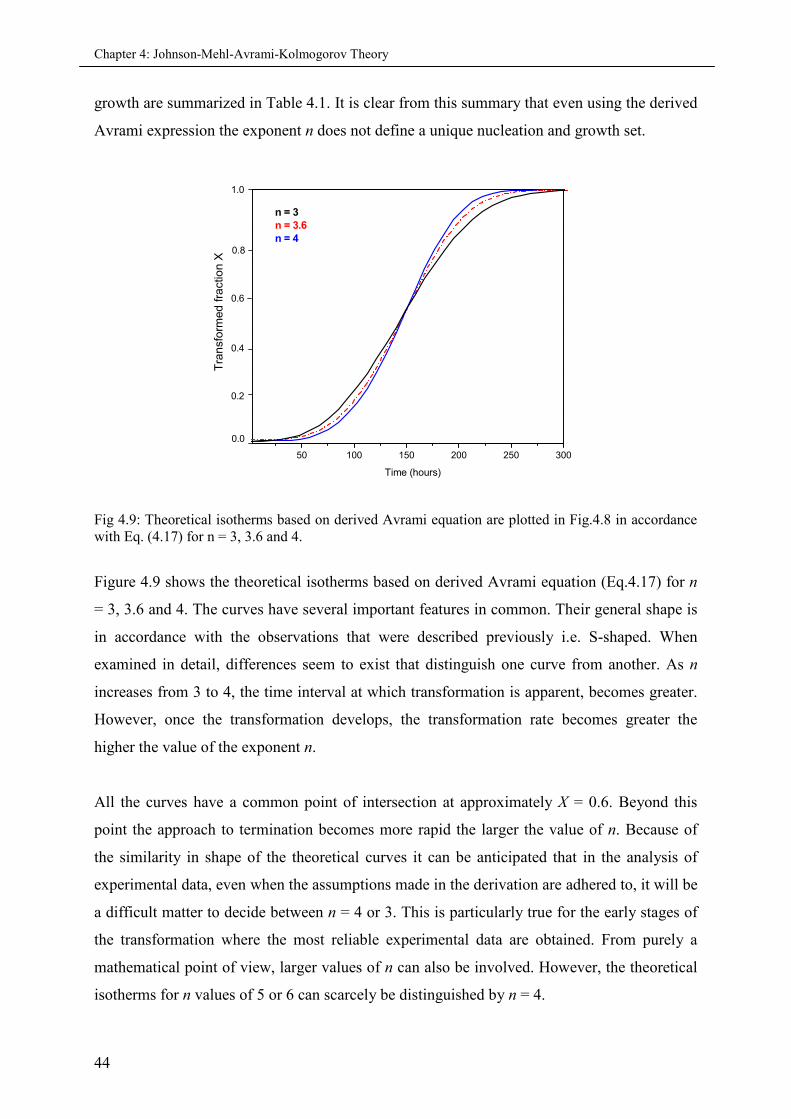
Chapter 4: Johnson-Mehl-Avrami-Kolmogorov Theory
44
growth are summarized in Table 4.1. It is clear from this summary that even using the derived
Avrami expression the exponent n does not define a unique nucleation and growth set.
50 100 150 200 250 300
0.6
0.4
0.2
0.8
Time (hours)
n = 3n = 3.6n = 4
1.0
Tra
nsf
orm
ed
fra
ctio
nX
0.0
Fig 4.9: Theoretical isotherms based on derived Avrami equation are plotted in Fig.4.8 in accordancewith Eq. (4.17) for n = 3, 3.6 and 4.
Figure 4.9 shows the theoretical isotherms based on derived Avrami equation (Eq.4.17) for n
= 3, 3.6 and 4. The curves have several important features in common. Their general shape is
in accordance with the observations that were described previously i.e. S-shaped. When
examined in detail, differences seem to exist that distinguish one curve from another. As n
increases from 3 to 4, the time interval at which transformation is apparent, becomes greater.
However, once the transformation develops, the transformation rate becomes greater the
higher the value of the exponent n.
All the curves have a common point of intersection at approximately X = 0.6. Beyond this
point the approach to termination becomes more rapid the larger the value of n. Because of
the similarity in shape of the theoretical curves it can be anticipated that in the analysis of
experimental data, even when the assumptions made in the derivation are adhered to, it will be
a difficult matter to decide between n = 4 or 3. This is particularly true for the early stages of
the transformation where the most reliable experimental data are obtained. From purely a
mathematical point of view, larger values of n can also be involved. However, the theoretical
isotherms for n values of 5 or 6 can scarcely be distinguished by n = 4.
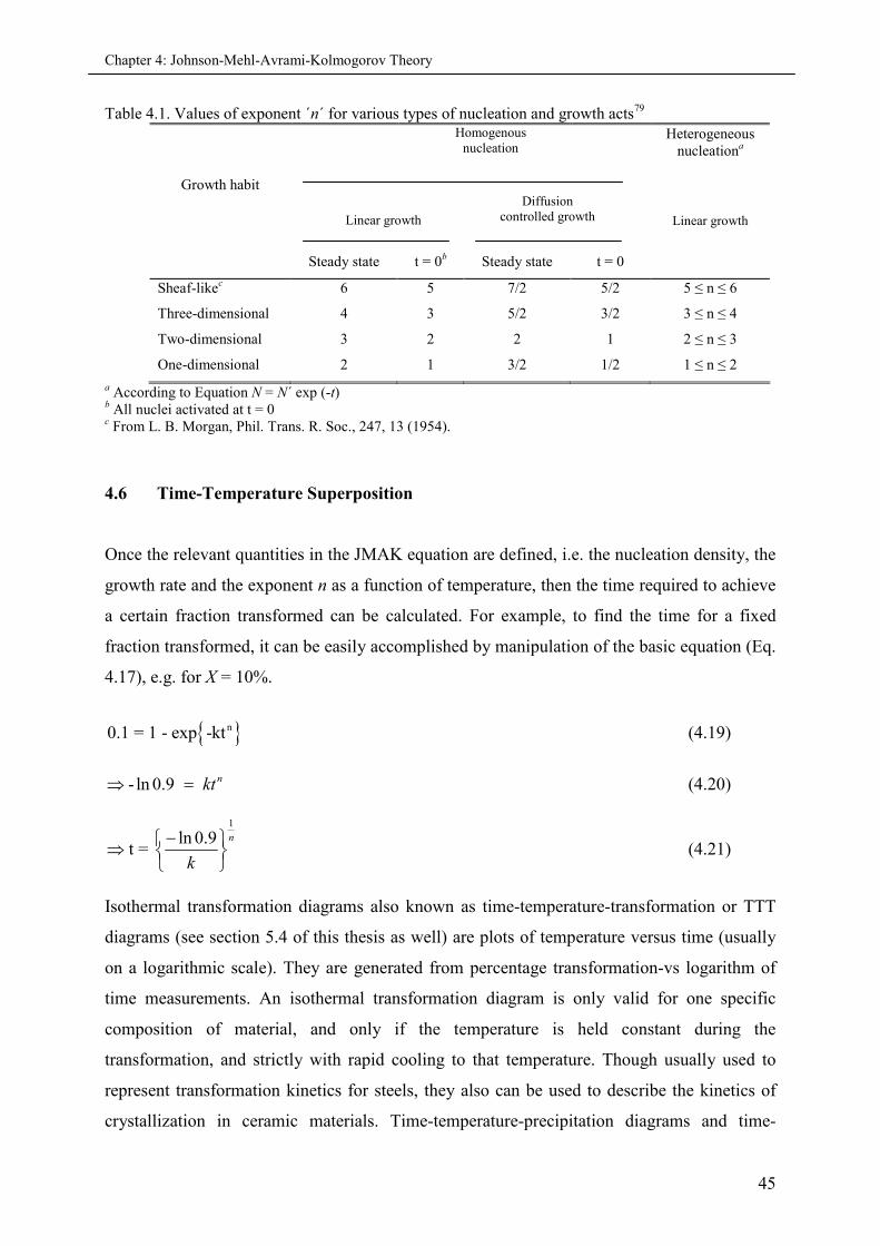
Chapter 4: Johnson-Mehl-Avrami-Kolmogorov Theory
45
Table 4.1. Values of exponent ´n´ for various types of nucleation and growth acts79
Growth habit
Steady state t = 0b Steady state t = 0
Heterogeneousnucleationa
Sheaf-likec
Three-dimensional
Two-dimensional
One-dimensional
6
4
3
2
5
3
2
1
7/2
5/2
2
3/2
5/2
3/2
1
1/2
5 ≤ n ≤ 6
3 ≤ n ≤ 4
2 ≤ n ≤ 3
1 ≤ n ≤ 2
a According to Equation N = N´ exp (-t)b All nuclei activated at t = 0c From L. B. Morgan, Phil. Trans. R. Soc., 247, 13 (1954).
4.6 Time-Temperature Superposition
Once the relevant quantities in the JMAK equation are defined, i.e. the nucleation density, the
growth rate and the exponent n as a function of temperature, then the time required to achieve
a certain fraction transformed can be calculated. For example, to find the time for a fixed
fraction transformed, it can be easily accomplished by manipulation of the basic equation (Eq.
4.17), e.g. for X = 10%.
n0.1 = 1 - exp -kt (4.19)
- ln 0.9 nkt (4.20)
1
ln 0.9t =
n
k
(4.21)
Isothermal transformation diagrams also known as time-temperature-transformation or TTT
diagrams (see section 5.4 of this thesis as well) are plots of temperature versus time (usually
on a logarithmic scale). They are generated from percentage transformation-vs logarithm of
time measurements. An isothermal transformation diagram is only valid for one specific
composition of material, and only if the temperature is held constant during the
transformation, and strictly with rapid cooling to that temperature. Though usually used to
represent transformation kinetics for steels, they also can be used to describe the kinetics of
crystallization in ceramic materials. Time-temperature-precipitation diagrams and time-
Linear growth
Homogenousnucleation
Diffusioncontrolled growth Linear growth
Chapter 4: Johnson-Mehl-Avrami-Kolmogorov Theory
46
temperature-embrittlement diagrams have also been used to represent kinetic changes in
steels.
4.7 Summary of this chapter
In this Chapter the JMAK theory of phase transformation is discussed in detail. Furthermore,
a derivation of Avrami equation for the case of continuous nucleation is mentioned, where
nuclei are constantly added during transformation. This results in a value of n = 4 for the
Avrami exponent. Similarly, the value of n = 3 is found for the case of site-saturated
homogenous nucleation, where all nuclei are present at the start of the transformation (i.e t =
0). The hole free volume measured from the PALS and the Tao-Eldrup model, will be used as
a measure of the transformed fraction X and the obtained information will be used to discuss
the curing kinetics of the one-component epoxy resin formulations, in combination with the
JMAK equation. In the next section of this thesis (Chapter 5), the principles of choosing the
proper resin and hardener for the formulations are discussed, followed by the results and
discussions in Chapter 6, 7 and 8.
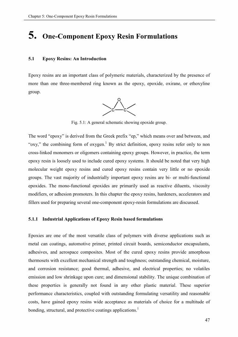
Chapter 5: One-Component Epoxy Resin Formulations
47
5. One-Component Epoxy Resin Formulations
5.1 Epoxy Resins: An Introduction
Epoxy resins are an important class of polymeric materials, characterized by the presence of
more than one three-membered ring known as the epoxy, epoxide, oxirane, or ethoxyline
group.
Fig. 5.1: A general schematic showing epoxide group.
The word “epoxy” is derived from the Greek prefix “ep,” which means over and between, and
“oxy,” the combining form of oxygen.1 By strict definition, epoxy resins refer only to non
cross-linked monomers or oligomers containing epoxy groups. However, in practice, the term
epoxy resin is loosely used to include cured epoxy systems. It should be noted that very high
molecular weight epoxy resins and cured epoxy resins contain very little or no epoxide
groups. The vast majority of industrially important epoxy resins are bi- or multi-functional
epoxides. The mono-functional epoxides are primarily used as reactive diluents, viscosity
modifiers, or adhesion promoters. In this chapter the epoxy resins, hardeners, accelerators and
fillers used for preparing several one-component epoxy-resin formulations are discussed.
5.1.1 Industrial Applications of Epoxy Resin based formulations
Epoxies are one of the most versatile class of polymers with diverse applications such as
metal can coatings, automotive primer, printed circuit boards, semiconductor encapsulants,
adhesives, and aerospace composites. Most of the cured epoxy resins provide amorphous
thermosets with excellent mechanical strength and toughness; outstanding chemical, moisture,
and corrosion resistance; good thermal, adhesive, and electrical properties; no volatiles
emission and low shrinkage upon cure; and dimensional stability. The unique combination of
these properties is generally not found in any other plastic material. These superior
performance characteristics, coupled with outstanding formulating versatility and reasonable
costs, have gained epoxy resins wide acceptance as materials of choice for a multitude of
bonding, structural, and protective coatings applications.1
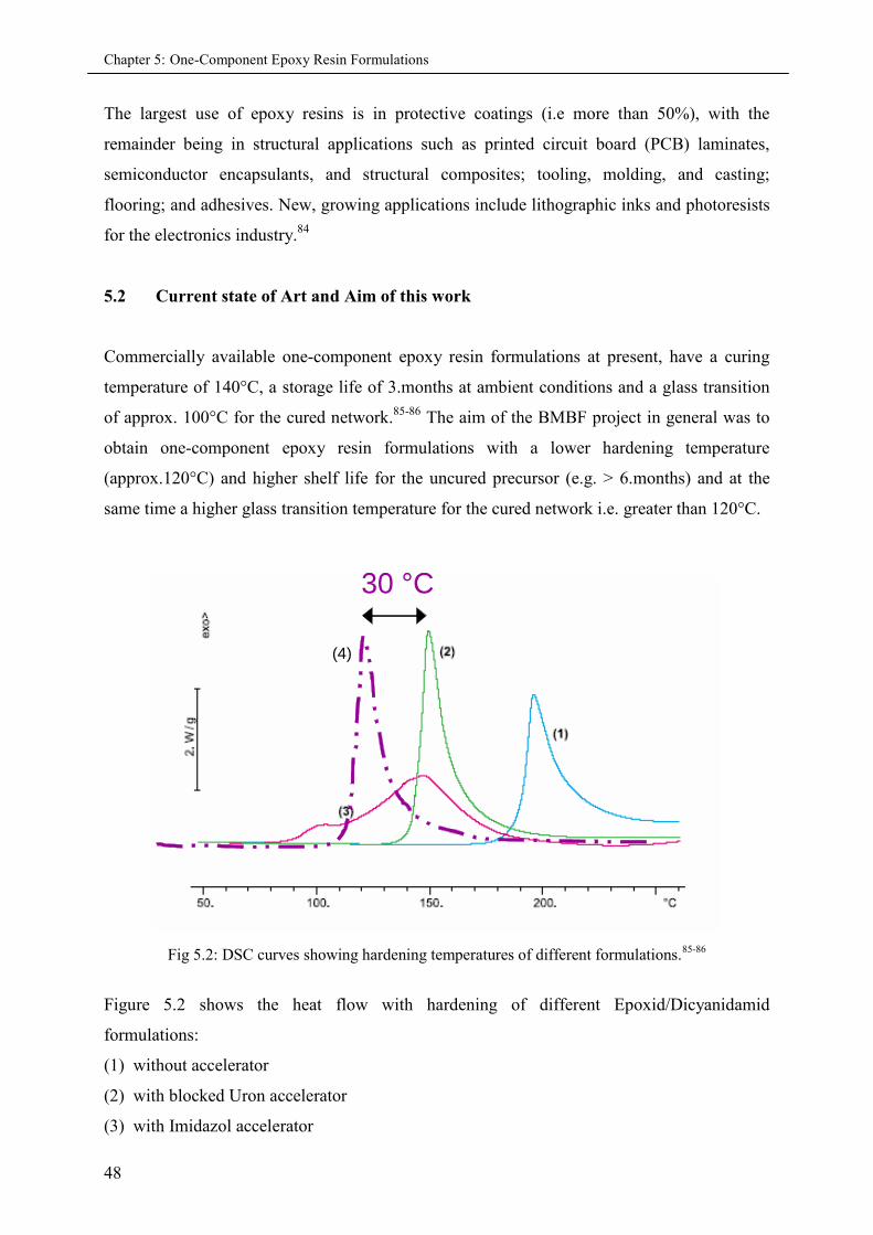
Chapter 5: One-Component Epoxy Resin Formulations
48
The largest use of epoxy resins is in protective coatings (i.e more than 50%), with the
remainder being in structural applications such as printed circuit board (PCB) laminates,
semiconductor encapsulants, and structural composites; tooling, molding, and casting;
flooring; and adhesives. New, growing applications include lithographic inks and photoresists
for the electronics industry.84
5.2 Current state of Art and Aim of this work
Commercially available one-component epoxy resin formulations at present, have a curing
temperature of 140°C, a storage life of 3.months at ambient conditions and a glass transition
of approx. 100°C for the cured network.85-86 The aim of the BMBF project in general was to
obtain one-component epoxy resin formulations with a lower hardening temperature
(approx.120°C) and higher shelf life for the uncured precursor (e.g. > 6.months) and at the
same time a higher glass transition temperature for the cured network i.e. greater than 120°C.
(4)
30 °C
(4)(4)
30 °C
(4)
(4)
30 °C
(4)(4)
30 °C
(4)
Fig 5.2: DSC curves showing hardening temperatures of different formulations.85-86
Figure 5.2 shows the heat flow with hardening of different Epoxid/Dicyanidamid
formulations:
(1) without accelerator
(2) with blocked Uron accelerator
(3) with Imidazol accelerator
Chapter 5: One-Component Epoxy Resin Formulations
49
(4) with accelerator from multi-functional nano-modules, which as stated earlier was the
general motivation for this particular BMBF project.
In particular, the main aim of this work is to characterize epoxy based polymer nano-
composites, primarily with PALS technique for both precursor and cured systems. The results
which will be discussed in Chapters 6, 7 and 8 of this thesis, proved really important to
understand on one hand the curing kinetics of epoxy precursors and on the other the release
behaviour of accelerator(encapsulated in micro and nano sized carriers), in the epoxy-
hardener matrix.
5.3 Basic principles of formulation
The capability of the highly strained epoxy ring to react with a wide variety of curing agents
under diverse conditions and temperatures gives additional versatility to the epoxies. The
major industrial utility of epoxy resins is in thermosetting applications. Treatment with curing
agents gives insoluble and intractable thermoset polymers.
The most important step in using epoxy resins is to develop the appropriate epoxy formulation
since most of them are used as precursors for a three-dimensional cross-linked network. With
the exception of the very high Mw phenoxy resins and the epoxy based thermoplastics, epoxy
resins are rarely used by themself. It is usually formulated with modifiers such as fillers and
used in composite structures with glass fiber or metal substrates (for coatings). To design a
successful epoxy formulation that will give optimum processability and performance, the
following factors must be carefully considered:
Selection of the proper combination of epoxy resins and structures of curing agents.
Stoichiometric ratio of epoxy and the curing agent.
Selection of catalyst or accelerator.
Curing/post-curing processes and conditions.
Formulation modifiers such as fillers, diluents, toughening agents, etc
Interactions among the formulation ingredients and with the composite materials (e.g.
fibers, metals) on the system chemistry, adhesion, rheology, morphology, and
performance.
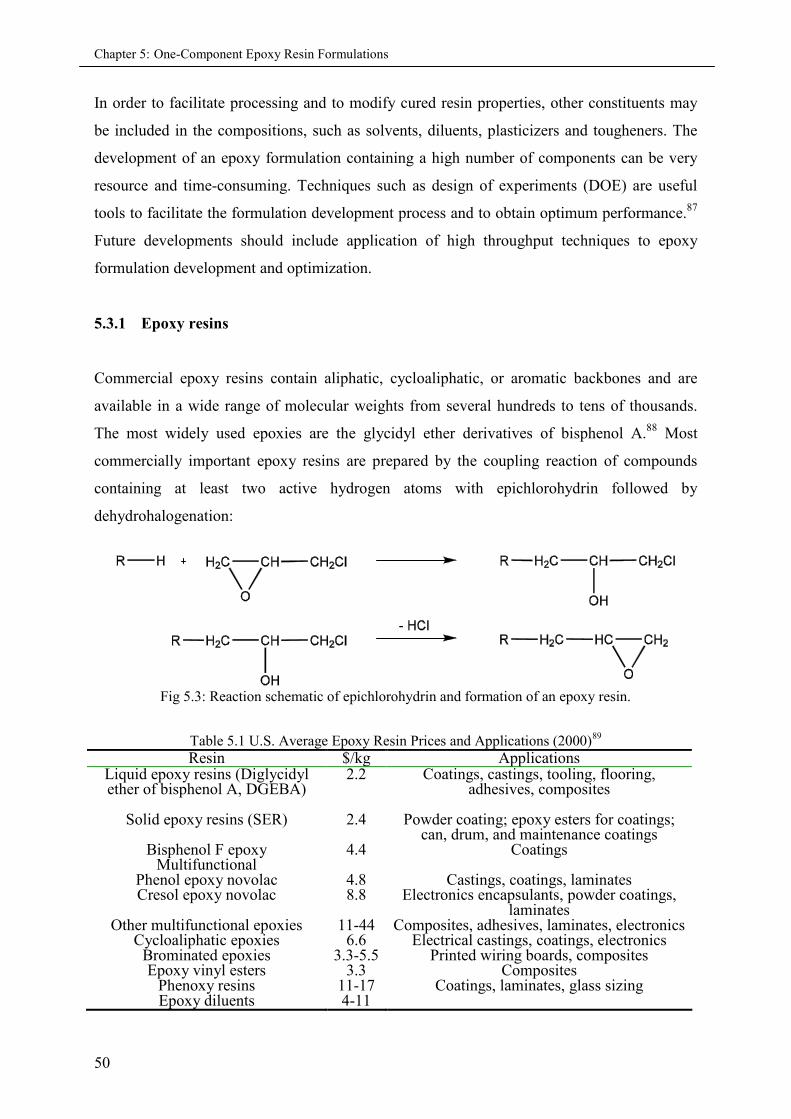
Chapter 5: One-Component Epoxy Resin Formulations
50
In order to facilitate processing and to modify cured resin properties, other constituents may
be included in the compositions, such as solvents, diluents, plasticizers and tougheners. The
development of an epoxy formulation containing a high number of components can be very
resource and time-consuming. Techniques such as design of experiments (DOE) are useful
tools to facilitate the formulation development process and to obtain optimum performance.87
Future developments should include application of high throughput techniques to epoxy
formulation development and optimization.
5.3.1 Epoxy resins
Commercial epoxy resins contain aliphatic, cycloaliphatic, or aromatic backbones and are
available in a wide range of molecular weights from several hundreds to tens of thousands.
The most widely used epoxies are the glycidyl ether derivatives of bisphenol A.88 Most
commercially important epoxy resins are prepared by the coupling reaction of compounds
containing at least two active hydrogen atoms with epichlorohydrin followed by
dehydrohalogenation:
Fig 5.3: Reaction schematic of epichlorohydrin and formation of an epoxy resin.
Table 5.1 U.S. Average Epoxy Resin Prices and Applications (2000)89
Resin $/kg ApplicationsLiquid epoxy resins (Diglycidylether of bisphenol A, DGEBA)
2.2 Coatings, castings, tooling, flooring,adhesives, composites
Solid epoxy resins (SER) 2.4 Powder coating; epoxy esters for coatings;can, drum, and maintenance coatings
Bisphenol F epoxy 4.4 CoatingsMultifunctional
Phenol epoxy novolacCresol epoxy novolac
4.88.8
Castings, coatings, laminatesElectronics encapsulants, powder coatings,
laminatesOther multifunctional epoxies 11-44 Composites, adhesives, laminates, electronics
Cycloaliphatic epoxies 6.6 Electrical castings, coatings, electronicsBrominated epoxies 3.3-5.5 Printed wiring boards, compositesEpoxy vinyl esters 3.3 Composites
Phenoxy resins 11-17 Coatings, laminates, glass sizingEpoxy diluents 4-11
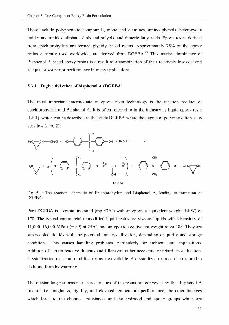
Chapter 5: One-Component Epoxy Resin Formulations
51
These include polyphenolic compounds, mono and diamines, amino phenols, heterocyclic
imides and amides, aliphatic diols and polyols, and dimeric fatty acids. Epoxy resins derived
from epichlorohydrin are termed glycidyl-based resins. Approximately 75% of the epoxy
resins currently used worldwide, are derived from DGEBA.89 This market dominance of
Bisphenol A based epoxy resins is a result of a combination of their relatively low cost and
adequate-to-superior performance in many applications
5.3.1.1 Diglycidyl ether of bisphenol A (DGEBA)
The most important intermediate in epoxy resin technology is the reaction product of
epichlorohydrin and Bisphenol A. It is often referred to in the industry as liquid epoxy resin
(LER), which can be described as the crude DGEBA where the degree of polymerization, n, is
very low (n ≈0.2):
Fig. 5.4: The reaction schematic of Epichlorohydrin and Bisphenol A, leading to formation ofDGEBA.
Pure DGEBA is a crystalline solid (mp 43°C) with an epoxide equivalent weight (EEW) of
170. The typical commercial unmodified liquid resins are viscous liquids with viscosities of
11,000–16,000 MPa·s (= cP) at 25°C, and an epoxide equivalent weight of ca 188. They are
supercooled liquids with the potential for crystallization, depending on purity and storage
conditions. This causes handling problems, particularly for ambient cure applications.
Addition of certain reactive diluents and fillers can either accelerate or retard crystallization.
Crystallization-resistant, modified resins are available. A crystallized resin can be restored to
its liquid form by warming.
The outstanding performance characteristics of the resins are conveyed by the Bisphenol A
fraction i.e. toughness, rigidity, and elevated temperature performance, the ether linkages
which leads to the chemical resistance, and the hydroxyl and epoxy groups which are
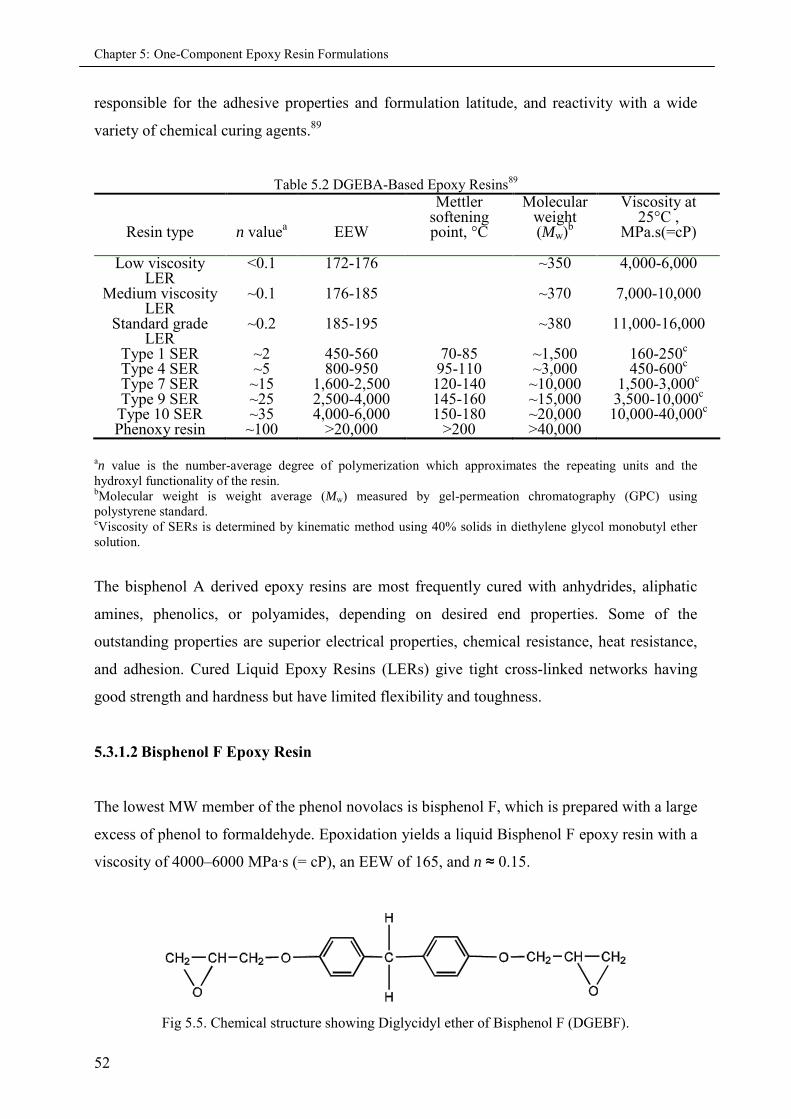
Chapter 5: One-Component Epoxy Resin Formulations
52
responsible for the adhesive properties and formulation latitude, and reactivity with a wide
variety of chemical curing agents.89
Table 5.2 DGEBA-Based Epoxy Resins89
Resin type n valuea EEW
Mettlersofteningpoint, °C
Molecularweight(Mw)b
Viscosity at25°C ,
MPa.s(=cP)
Low viscosityLER
<0.1 172-176 ~350 4,000-6,000
Medium viscosityLER
~0.1 176-185 ~370 7,000-10,000
Standard gradeLER
~0.2 185-195 ~380 11,000-16,000
Type 1 SER ~2 450-560 70-85 ~1,500 160-250c
Type 4 SER ~5 800-950 95-110 ~3,000 450-600c
Type 7 SER ~15 1,600-2,500 120-140 ~10,000 1,500-3,000c
Type 9 SER ~25 2,500-4,000 145-160 ~15,000 3,500-10,000c
Type 10 SER ~35 4,000-6,000 150-180 ~20,000 10,000-40,000c
Phenoxy resin ~100 >20,000 >200 >40,000
an value is the number-average degree of polymerization which approximates the repeating units and thehydroxyl functionality of the resin.bMolecular weight is weight average (Mw) measured by gel-permeation chromatography (GPC) usingpolystyrene standard.cViscosity of SERs is determined by kinematic method using 40% solids in diethylene glycol monobutyl ethersolution.
The bisphenol A derived epoxy resins are most frequently cured with anhydrides, aliphatic
amines, phenolics, or polyamides, depending on desired end properties. Some of the
outstanding properties are superior electrical properties, chemical resistance, heat resistance,
and adhesion. Cured Liquid Epoxy Resins (LERs) give tight cross-linked networks having
good strength and hardness but have limited flexibility and toughness.
5.3.1.2 Bisphenol F Epoxy Resin
The lowest MW member of the phenol novolacs is bisphenol F, which is prepared with a large
excess of phenol to formaldehyde. Epoxidation yields a liquid Bisphenol F epoxy resin with a
viscosity of 4000–6000 MPa·s (= cP), an EEW of 165, and n ≈ 0.15.
Fig 5.5. Chemical structure showing Diglycidyl ether of Bisphenol F (DGEBF).
Chapter 5: One-Component Epoxy Resin Formulations
53
This unmodified, low viscosity liquid resin exhibits slightly higher functionality than
unmodified bisphenol A liquid resins. Crystallization, often a problem with liquid bisphenol
A resins, is reduced with bisphenol F resin. Consequently, noncrystallizing LERs which are
blends of DGEBA and Bisphenol F epoxy are available. Epoxy resins based on bisphenol F
are used primarily as functional diluents in applications requiring a low viscosity, high
performance resin system (eg, solvent-free coatings). Higher filler levels and faster bubble
release are possible because of the low viscosity. The higher epoxy content and functionality
of Bisphenol F epoxy resins provide improved chemical resistance compared to conventional
Bisphenol A epoxies. Bisphenol F epoxy resins are used in high solids, high build systems
such as tank and pipe linings, industrial floors, road and bridge deck toppings, structural
adhesives, grouts, coatings, and electrical varnishes.90
Interestingly, all epoxides contain aromatic rings in their structures. An aromatic ring confers
mechanical rigidity and thermal stability to the cross-linked network. It is also worth noting
that some of the epoxides in the Tab. 5.2 have two epoxide functional groups, while others
have three or four or more. Irrespective of whether a network is developed by mixing the
epoxide with a curing agent or is developed from epoxide alone by catalytic homo-
polymerization, a large number of the molecules in a given formulation must be able to react
with more than two other molecules in order to form a cross-linked network instead of merely
forming linear chains.89 For the sake of clarity, only the experimentally used epoxy resins are
discussed in this thesis.
5.3.2 Hardeners (Curing agents)
Epoxide molecules in the pure state at room temperature normally do not react with each
other and can stay for years in a dry container without mutual reaction. The types of
chemicals added to the epoxide to effect network formation fall into two categories: curing
agents and catalysts. Curing agents, sometimes called hardeners, are added in significant
amounts (i.e. stoichiometric ratios) to the epoxide and react with it to become a part of the
cross-linked network. These curing agents can be aliphatic amines, aromatic amines, or
anhydrides. Curing agents are either catalytic or co-reactive. A catalytic curing agent
functions as an initiator for epoxy resin homo-polymerization or as an accelerator for other
curing agents, whereas the co-reactive curing agent acts as a co-monomer in the
polymerization process. The most important groups of co-reactive curing agents are those
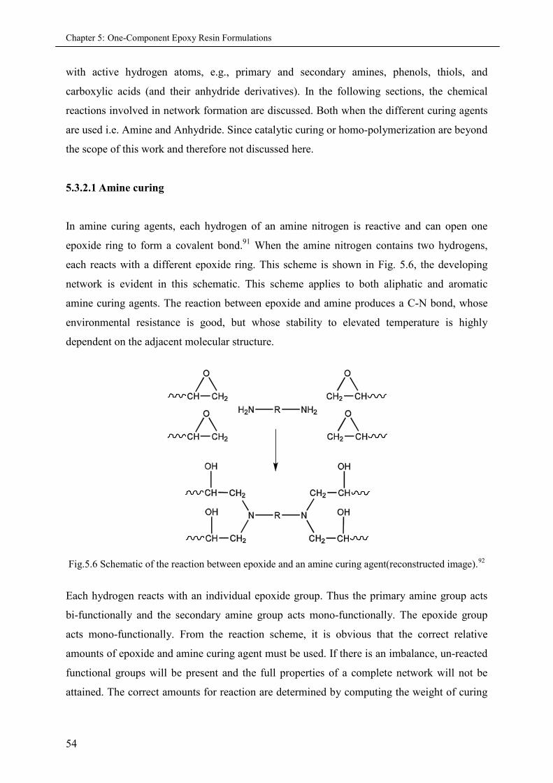
Chapter 5: One-Component Epoxy Resin Formulations
54
with active hydrogen atoms, e.g., primary and secondary amines, phenols, thiols, and
carboxylic acids (and their anhydride derivatives). In the following sections, the chemical
reactions involved in network formation are discussed. Both when the different curing agents
are used i.e. Amine and Anhydride. Since catalytic curing or homo-polymerization are beyond
the scope of this work and therefore not discussed here.
5.3.2.1 Amine curing
In amine curing agents, each hydrogen of an amine nitrogen is reactive and can open one
epoxide ring to form a covalent bond.91 When the amine nitrogen contains two hydrogens,
each reacts with a different epoxide ring. This scheme is shown in Fig. 5.6, the developing
network is evident in this schematic. This scheme applies to both aliphatic and aromatic
amine curing agents. The reaction between epoxide and amine produces a C-N bond, whose
environmental resistance is good, but whose stability to elevated temperature is highly
dependent on the adjacent molecular structure.
Fig.5.6 Schematic of the reaction between epoxide and an amine curing agent(reconstructed image).92
Each hydrogen reacts with an individual epoxide group. Thus the primary amine group acts
bi-functionally and the secondary amine group acts mono-functionally. The epoxide group
acts mono-functionally. From the reaction scheme, it is obvious that the correct relative
amounts of epoxide and amine curing agent must be used. If there is an imbalance, un-reacted
functional groups will be present and the full properties of a complete network will not be
attained. The correct amounts for reaction are determined by computing the weight of curing
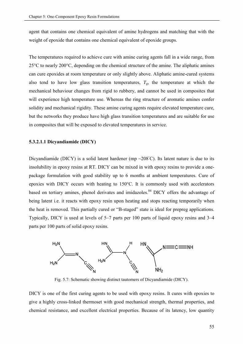
Chapter 5: One-Component Epoxy Resin Formulations
55
agent that contains one chemical equivalent of amine hydrogens and matching that with the
weight of epoxide that contains one chemical equivalent of epoxide groups.
The temperatures required to achieve cure with amine curing agents fall in a wide range, from
25°C to nearly 200°C, depending on the chemical structure of the amine. The aliphatic amines
can cure epoxides at room temperature or only slightly above. Aliphatic amine-cured systems
also tend to have low glass transition temperatures, Tg, the temperature at which the
mechanical behaviour changes from rigid to rubbery, and cannot be used in composites that
will experience high temperature use. Whereas the ring structure of aromatic amines confer
solidity and mechanical rigidity. These amine curing agents require elevated temperature cure,
but the networks they produce have high glass transition temperatures and are suitable for use
in composites that will be exposed to elevated temperatures in service.
5.3.2.1.1 Dicyandiamide (DICY)
Dicyandiamide (DICY) is a solid latent hardener (mp ~208◦C). Its latent nature is due to its
insolubility in epoxy resins at RT. DICY can be mixed in with epoxy resins to provide a one-
package formulation with good stability up to 6 months at ambient temperatures. Cure of
epoxies with DICY occurs with heating to 150°C. It is commonly used with accelerators
based on tertiary amines, phenol derivates and imidazoles.84 DICY offers the advantage of
being latent i.e. it reacts with epoxy resin upon heating and stops reacting temporarily when
the heat is removed. This partially cured or “B-staged” state is ideal for prepreg applications.
Typically, DICY is used at levels of 5–7 parts per 100 parts of liquid epoxy resins and 3–4
parts per 100 parts of solid epoxy resins.
Fig. 5.7: Schematic showing distinct tautomers of Dicyandiamide (DICY).
DICY is one of the first curing agents to be used with epoxy resins. It cures with epoxies to
give a highly cross-linked thermoset with good mechanical strength, thermal properties, and
chemical resistance, and excellent electrical properties. Because of its latency, low quantity
Chapter 5: One-Component Epoxy Resin Formulations
56
requirements and excellent balance of properties, DICY is a widely used curing agent in
powder coating and electrical laminate applications. These two applications account for 85%
of DICY consumption as epoxy curing agent.84
To sum up the epoxy–DICY systems offer the following advantages:
Cost effectiveness (DICY is a low equivalent weight, multifunctional curing agent)
Stable formulations
Excellent adhesion to copper and glass
Good moisture and solder resistance
Good processability
The primary disadvantage of the standard epoxy–DICY systems is their relatively low thermal
performance (Tg < 140°C, Td = 300°C), which limits their uses in more demanding
applications such as the FR-5 boards and other high density circuit boards. Speciality epoxy–
DICY systems are available with Tg approaching 190ºC, but at higher costs.93
5.3.2.2 Anhydride curing
In anhydride curing agents, the anhydride groups themselves must be cleaved asymmetrically
to start the reaction.91 The initial cleavage, is accomplished with the help of a small amount of
accelerator, which is a chemical that functions as a catalyst to speed up the epoxide curing
agent reaction. Accelerators will be discussed later in section 5.3.3 of this chapter. Figure 5.8
shows an idealized scheme, where the cleaved anhydride reacts with an epoxide ring carbon,
opening the ring in the process. The negatively charged oxygen formed by the opening of the
epoxide ring can proceed to react with a different anhydride group, perpetuating the reaction.
In this idealized developing network, each anhydride group is bi-functional, i.e. it links to two
different epoxide molecules. In practice, the high temperatures required for anhydride cure,
plus the presence of accelerator, provides conditions for some extent of epoxide homo-
polymerization to take place, making the actual curing reaction much more complex than
depicted in Fig. 5.8. The reaction between epoxide and anhydride produces primarily ester
linkages, which have good stability to elevated temperatures and to most hostile environments
except bases.
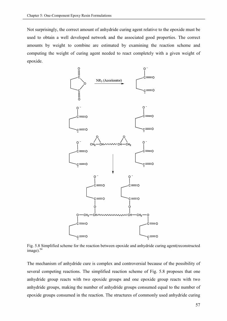
Chapter 5: One-Component Epoxy Resin Formulations
57
Not surprisingly, the correct amount of anhydride curing agent relative to the epoxide must be
used to obtain a well developed network and the associated good properties. The correct
amounts by weight to combine are estimated by examining the reaction scheme and
computing the weight of curing agent needed to react completely with a given weight of
epoxide.
Fig. 5.8 Simplified scheme for the reaction between epoxide and anhydride curing agent(reconstructedimage).94
The mechanism of anhydride cure is complex and controversial because of the possibility of
several competing reactions. The simplified reaction scheme of Fig. 5.8 proposes that one
anhydride group reacts with two epoxide groups and one epoxide group reacts with two
anhydride groups, making the number of anhydride groups consumed equal to the number of
epoxide groups consumed in the reaction. The structures of commonly used anhydride curing
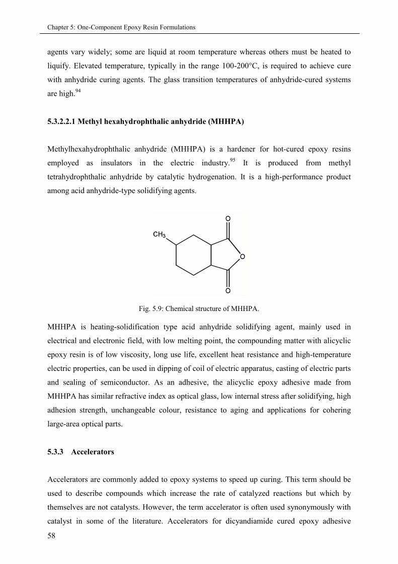
Chapter 5: One-Component Epoxy Resin Formulations
58
agents vary widely; some are liquid at room temperature whereas others must be heated to
liquify. Elevated temperature, typically in the range 100-200°C, is required to achieve cure
with anhydride curing agents. The glass transition temperatures of anhydride-cured systems
are high.94
5.3.2.2.1 Methyl hexahydrophthalic anhydride (MHHPA)
Methylhexahydrophthalic anhydride (MHHPA) is a hardener for hot-cured epoxy resins
employed as insulators in the electric industry.95 It is produced from methyl
tetrahydrophthalic anhydride by catalytic hydrogenation. It is a high-performance product
among acid anhydride-type solidifying agents.
Fig. 5.9: Chemical structure of MHHPA.
MHHPA is heating-solidification type acid anhydride solidifying agent, mainly used in
electrical and electronic field, with low melting point, the compounding matter with alicyclic
epoxy resin is of low viscosity, long use life, excellent heat resistance and high-temperature
electric properties, can be used in dipping of coil of electric apparatus, casting of electric parts
and sealing of semiconductor. As an adhesive, the alicyclic epoxy adhesive made from
MHHPA has similar refractive index as optical glass, low internal stress after solidifying, high
adhesion strength, unchangeable colour, resistance to aging and applications for cohering
large-area optical parts.
5.3.3 Accelerators
Accelerators are commonly added to epoxy systems to speed up curing. This term should be
used to describe compounds which increase the rate of catalyzed reactions but which by
themselves are not catalysts. However, the term accelerator is often used synonymously with
catalyst in some of the literature. Accelerators for dicyandiamide cured epoxy adhesive
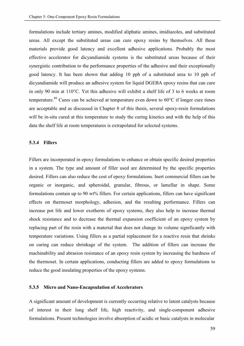
Chapter 5: One-Component Epoxy Resin Formulations
59
formulations include tertiary amines, modified aliphatic amines, imidiazoles, and substituted
ureas. All except the substituted ureas can cure epoxy resins by themselves. All these
materials provide good latency and excellent adhesive applications. Probably the most
effective accelerator for dicyandiamide systems is the substituted ureas because of their
synergistic contribution to the performance properties of the adhesive and their exceptionally
good latency. It has been shown that adding 10 pph of a substituted urea to 10 pph of
dicyandiamide will produce an adhesive system for liquid DGEBA epoxy resins that can cure
in only 90 min at 110°C. Yet this adhesive will exhibit a shelf life of 3 to 6 weeks at room
temperature.89 Cures can be achieved at temperature even down to 60°C if longer cure times
are acceptable and as discussed in Chapter 8 of this thesis, several epoxy-resin formulations
will be in-situ cured at this temperature to study the curing kinetics and with the help of this
data the shelf life at room temperatures is extrapolated for selected systems.
5.3.4 Fillers
Fillers are incorporated in epoxy formulations to enhance or obtain specific desired properties
in a system. The type and amount of filler used are determined by the specific properties
desired. Fillers can also reduce the cost of epoxy formulations. Inert commercial fillers can be
organic or inorganic, and spheroidal, granular, fibrous, or lamellar in shape. Some
formulations contain up to 90 wt% fillers. For certain applications, fillers can have significant
effects on thermoset morphology, adhesion, and the resulting performance. Fillers can
increase pot life and lower exotherm of epoxy systems, they also help to increase thermal
shock resistance and to decrease the thermal expansion coefficient of an epoxy system by
replacing part of the resin with a material that does not change its volume significantly with
temperature variations. Using fillers as a partial replacement for a reactive resin that shrinks
on curing can reduce shrinkage of the system. The addition of fillers can increase the
machinability and abrasion resistance of an epoxy resin system by increasing the hardness of
the thermoset. In certain applications, conducting fillers are added to epoxy formulations to
reduce the good insulating properties of the epoxy systems.
5.3.5 Micro and Nano-Encapsulation of Accelerators
A significant amount of development is currently occurring relative to latent catalysts because
of interest in their long shelf life, high reactivity, and single-component adhesive
formulations. Present technologies involve absorption of acidic or basic catalysts in molecular
Chapter 5: One-Component Epoxy Resin Formulations
60
sieves, formation of Lewis acid salts or other amine salts, micro-encapsulation of amines, and
other novel segregation methods. As will be shown in the results section of this thesis
(Chpaters 7 and 8), the accelerator used throughout this work is encapsulated in micro and
nano-size carriers. But both the accelerator and the carrier used for encapsulation will be
treated as classified information, due to the non-disclosure agreements concerning this
research.
5.4 Epoxy curing process and TTT diagram
The thermosetting or the curing reaction is the joining of many small molecules by chemical
reaction to produce an extended network structure. Although this process is a polymerization,
it is distinct from the type of polymerization that forms many individual long chains. The
thermosetting reaction unifies all the constituent monomers into a single large molecule
extending to the boundaries of the material. Since the epoxy curing process is an important
factor affecting the cured epoxy performance. Therefore, it is important to understand the
curing process and its kinetics to design the proper cure schedule to obtain optimum structure
and performance. Excellent reviews on this topic are available in the literature.96
ResinTg0
∞
GelTgCuri
ng
tem
pe
ratu
re
time
Tg∞
Degradation
Vitrification
Gelled-glass region
Ungelled-glass region
Rubberregion
Liquidregion
Gelation
ResinTg0
∞
GelTgCuri
ng
tem
pe
ratu
re
time
Tg∞
Degradation
Vitrification
Gelled-glass region
Ungelled-glass region
Rubberregion
Liquidregion
Gelation
Fig 5.10 : A general schematic of the time-temperature-transformation (TTT diagram) forepoxies(reconstructed image).97-98
The curing of a thermoset epoxy resin can be expressed in terms of a time-temperature-
transformation (TTT) diagram as shown in Fig (5.10).97-98 In the TTT diagram, the time to
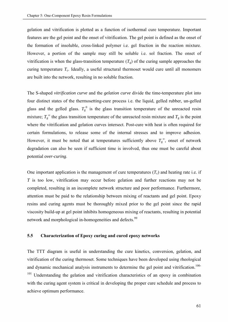
Chapter 5: One-Component Epoxy Resin Formulations
61
gelation and vitrification is plotted as a function of isothermal cure temperature. Important
features are the gel point and the onset of vitrification. The gel point is defined as the onset of
the formation of insoluble, cross-linked polymer i.e. gel fraction in the reaction mixture.
However, a portion of the sample may still be soluble i.e. sol fraction. The onset of
vitrification is when the glass-transition temperature (Tg) of the curing sample approaches the
curing temperature Tc. Ideally, a useful structural thermoset would cure until all monomers
are built into the network, resulting in no soluble fraction.
The S-shaped vitrification curve and the gelation curve divide the time-temperature plot into
four distinct states of the thermosetting-cure process i.e. the liquid, gelled rubber, un-gelled
glass and the gelled glass. Tg0 is the glass transition temperature of the unreacted resin
mixture; Tg∞ the glass transition temperature of the unreacted resin mixture and Tg is the point
where the vitrification and gelation curves intersect. Post-cure with heat is often required for
certain formulations, to release some of the internal stresses and to improve adhesion.
However, it must be noted that at temperatures sufficiently above Tg∞, onset of network
degradation can also be seen if sufficient time is involved, thus one must be careful about
potential over-curing.
One important application is the management of cure temperatures (Tc) and heating rate i.e. if
T is too low, vitrification may occur before gelation and further reactions may not be
completed, resulting in an incomplete network structure and poor performance. Furthermore,
attention must be paid to the relationship between mixing of reactants and gel point. Epoxy
resins and curing agents must be thoroughly mixed prior to the gel point since the rapid
viscosity build-up at gel point inhibits homogeneous mixing of reactants, resulting in potential
network and morphological in-homogeneities and defects.99
5.5 Characterization of Epoxy curing and cured epoxy networks
The TTT diagram is useful in understanding the cure kinetics, conversion, gelation, and
vitrification of the curing thermoset. Some techniques have been developed using rheological
and dynamic mechanical analysis instruments to determine the gel point and vitrification.100-
101 Understanding the gelation and vitrification characteristics of an epoxy in combination
with the curing agent system is critical in developing the proper cure schedule and process to
achieve optimum performance.
Chapter 5: One-Component Epoxy Resin Formulations
62
The degree of cure can be defined in terms of any one of a large number of chemical or
physical (including mechanical) properties that change continuously during the curing
reaction and reach a constant value at end of the cure. Evaluation of the degree of cure is
usually based on one of these properties and full cure is then defined as the point at which this
selected property reaches a constant value.
5.5.1 Traditional off-line methods
Intermittent off-line methods include chemical titration of the unreacted epoxide groups
present,102 specific gravity to measure densification103 and differential scanning calorimetry
(DSC) to measure the residual cure exotherm.104 Continuous off-line methods include infrared
spectroscopy (IR),105 parallel plate-type bulk dielectrornetry106 and dynamic mechanical
analysis (DMA).97 The off-line methods, real time or not, are useful for developing a cure
schedule for a new epoxy resin formulation, for optimizing processing variables and for
quality control of incoming resins or prepregs. They have also been used successfully for the
development of mathematical models of cure kinetics. However, because they are off-line,
they cannot be used for process control.
5.5.2 Modern in-situ methods
In-situ methods for cure monitoring are real time methods that require sensors small enough
to implant and leave in the composite itself. When the information from in situ monitoring is
used as continuous input to an appropriate process model, it can be used in process control
loops that adjust the processing conditions automatically.
One example of an in-situ method is low frequency dielectrometry using a very small
assembly of inter-digitated electrodes called a fringe field sensor. This technique measures
changes in ability of permanent dipoles within the resin chemical structure to align themselves
with the applied oscillating electric field and also measures changes in the mobility of ions
present as impurities in the resin.107 Both of these quantities correlate with resin viscosity in
the early stages of cure and with mechanical rigidity in the later stages of cure.108
Other examples of in-situ monitoring are based on fluorescence spectroscopy of tag molecules
in the resin109 and on infrared110 and Raman111 spectroscopies of the resin molecules
Chapter 5: One-Component Epoxy Resin Formulations
63
themselves. In these methods, optical fibres are the sensors that transmit the appropriate
wavelength of light into the curing resin and also transmit the spectral information back
out.112 The spectral changes relate directly to the chemical changes that occur as the curing
reaction progresses to completion.
5.6 Summary of this Chapter
Positron annihilation lifetime spectroscopy (PALS) is another addition to the in-situ curing
measurement techniques, as already discussed in detail in Chapter 2 of this thesis. Although,
this technique has been already used to characterize the cured epoxy composites in past. But
in this thesis it will be shown that how Johnson-Mehl-Avrami-Kolmogorov (JMAK) or
Avrami equation (discussed in Chapter 4) can be used to fit the experimental data observed
from PALS and the obtained Avrami parameters gives us information about the curing
kinetics of one-component epoxy resin formulations.

Chapter 5: One-Component Epoxy Resin Formulations
64
Chapter 6: Shelf life of one-component epoxy-resin formulation
65
6. Shelf life of one-component epoxy-resin formulation
In this section the first results of the state of art benchmark system are discussed, please note
that these results are already published.113 It is shown how PALS can be used to study the
curing behavior of epoxy resins of DGEBA with a hardener of dicyandiamide, from the initial
viscous state of the formulation to the cured polymer. Isothermal measurements are done in
range from 50°C to 80°C, in steps of 10°C. Onset of gelation is indicated by an increase in the
ortho-positronium (o-Ps) intensity and a sharp decrease in the lifetime. Change of o-Ps
lifetime was used as a measure for the degree of curing i.e. the transformed fraction X.
Applying the Johnson-Mehl-Avrami-Kolmogorov approach, these changes can be
characterized and the growth exponent ‘n’ and the reaction constant ‘k’ are determined.
Furthermore, the shelf life of this one component epoxy formulation is extrapolated to room
temperature with the help of Avrami parameters.
6.1 Introduction
There are numerous choices of epoxy resins and curing agents, presenting a wide variety of
structure and functionality. These details are already discussed in Chapter 5, but for the sake
of clarity the following sequence of sub-sections will help the reader to understand the link
between the curing of one-component epoxy resin formulations and the JMAK theory of
curing kinetics, where the transformed fraction is followed by the sub-nanometer level hole
free volume measured from the PALS technique.
6.1.1 One-component formulation
The one-component epoxy resin formulation used here is based on the diglycidyl ether of
Bisphenol-A (DGEBA), which is cured with Dicyandiamide (DICY). Curing of epoxies with
DICY occurs only while heating to temperatures at least 150°C. DICY may react with epoxy
resin upon heating and stops reacting temporarily when the heat is removed. The resulting
partially cured or “B-staged” state is ideal for prepreg applications.84 Typically, DICY is used
at levels of 5–7 parts per 100 parts of liquid epoxy resins and 3-4 parts per 100 parts of solid
epoxy resins by weight. In order to achieve low temperature curing a block Uron (U500)
accelerator is also used.
Chapter 6: Shelf life of one-component epoxy-resin formulation
66
6.1.2 Shelf-life and the curing mechanism
The epoxy curing process is an important factor affecting the cured epoxy performance. As
stated in the earlier Chapters of this thesis, to obtain optimum network structure and
performance, it is imperative to understand the curing process and its kinetics to design the
proper cure schedule. A good number of reviews on this topic are already available in the
literature.96,114 However, from the industrial point of view it is still of utmost relevance, to
establish reliable means of experimentally predicting the shelf life of new formulations of
one-component epoxies, which is usually guessed from accelerated tests at elevated
temperatures relying on selected reference measurements. In order to achieve predictability it
is important to understand the complete curing mechanism of epoxies, so that the reaction
kinetics can be further elaborated in light of available standard models and further
extrapolated to shelf life at storage temperatures.
The curing mechanism of DGEBA/DICY and similar systems is rather complex, involving
several simultaneous reactions. There are a number of different mechanisms proposed in the
literature.115-116 Indirect estimation of cure conversion as a function of time is done with a
combination of several experimental techniques and the available theoretical models. This
work is one step ahead and proposes the use of PALS in combination with the JMAK theory
of transformation kinetics.
6.1.3 Transformed fraction and the JMAK theory
As already discussed in the Chapter 4 of this thesis, the Avrami equation, is a widely accepted
model to study phase transformations, e.g. crystallization or austenite-to-martensite
transformations.77 According to the this equation117 (Eq. 4.17, Section 4.5.2 of this thesis), for
solid-state transformations displaying the kinetic behavior, the fraction of transformation X is
a function of time t.117 Where, ‘n’ is termed as the Avrami exponent, which is characteristic
for the type of transformation e.g. diffusion or reaction controlled, quenched in nuclei or
random nucleation or the shape of the particles of the new phase, The constant ‘k’ is named
the reaction constant, which is in turn temperature dependent, often via a simple Arrhenius
law. In such cases, by performing several isothermal experiments at different temperatures,
the activation energy Ea of the rate determining step can be extracted by plotting the reaction
constant ‘k’ on a logarithmic scale as a function of the reciprocal temperature.
Chapter 6: Shelf life of one-component epoxy-resin formulation
67
Assuming that the type of reaction and the rate determining step do not change with
temperature (i.e. the exponent ‘n’ stays constant for different temperatures), the Avrami
equation can be used to extrapolate the transformation behavior to other temperatures at least
in the early stages of transformation, i.e. for transformed fractions X ≤ 0.5. The boundary
conditions underlying the Avrami equation are not fulfilled for the larger fractions. The basic
idea of this research is to apply this model to the curing of the epoxide system, i.e. the
nucleation period of crystallization is attributed to the initial period of reaction and the
diffusional part to the proceeding of the reaction until saturation is reached. This is in contrast
to usual reaction kinetic models, which are of first or second order and do not include any
incubation time.
Isothermal and non-isothermal curing behaviors of epoxy resins have already been studied in
the light of the Avrami equation in past,118-122 but only for high curing temperatures and
neither the growth exponent nor the reaction constant has been interpreted or extrapolated to
the storage temperatures. However, this is of major importance for predicting storage stability
of the one component formulations at room temperature.
6.1.4 Free Volume and PALS
It is generally accepted that a key property for all amorphous polymers is the available
microscopic free volume, which can be detected by several atomic probes and described by
molecular dynamic simulations. Positron Annihilation Lifetime Spectroscopy (PALS) is a
widely accepted experimental tool to characterize the free volume in amorphous
polymers12,123-125 and has been used for epoxy resins126 and epoxy based polymers as
well.44,127-128 For details of PALS technique please refer to the Chapter 2 of this thesis.
In order to apply PALS parameters in combination with the JMAK equation to the curing
kinetics, several boundary conditions need to be fulfilled. Firstly, it is possible to correlate the
PALS parameters (i.e. o-Ps lifetime and intensity) and the cured or the transformed fraction X.
Since there is a good correlation between the shrinkage of epoxy during curing,128 with the
changes in macroscopic volume measured by Pressure-Volume-Temperature measurements
(PVT)) and the microscopic free volume measured by PALS. Secondly, in order to make a
reliable extrapolation from the experimentally covered temperature range it is necessary that
the reaction pathway does not change with temperature. If the growth exponent ‘n’ is found to
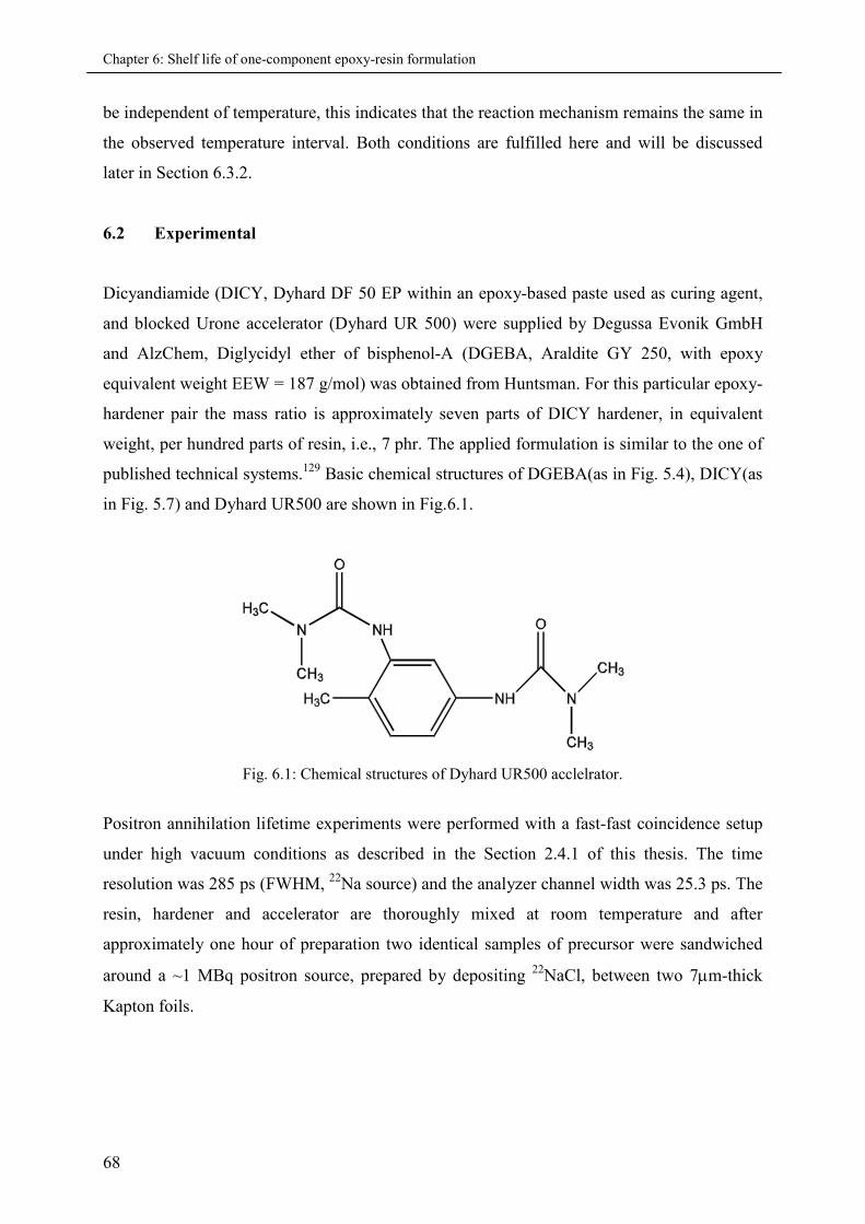
Chapter 6: Shelf life of one-component epoxy-resin formulation
68
be independent of temperature, this indicates that the reaction mechanism remains the same in
the observed temperature interval. Both conditions are fulfilled here and will be discussed
later in Section 6.3.2.
6.2 Experimental
Dicyandiamide (DICY, Dyhard DF 50 EP within an epoxy-based paste used as curing agent,
and blocked Urone accelerator (Dyhard UR 500) were supplied by Degussa Evonik GmbH
and AlzChem, Diglycidyl ether of bisphenol-A (DGEBA, Araldite GY 250, with epoxy
equivalent weight EEW = 187 g/mol) was obtained from Huntsman. For this particular epoxy-
hardener pair the mass ratio is approximately seven parts of DICY hardener, in equivalent
weight, per hundred parts of resin, i.e., 7 phr. The applied formulation is similar to the one of
published technical systems.129 Basic chemical structures of DGEBA(as in Fig. 5.4), DICY(as
in Fig. 5.7) and Dyhard UR500 are shown in Fig.6.1.
Fig. 6.1: Chemical structures of Dyhard UR500 acclelrator.
Positron annihilation lifetime experiments were performed with a fast-fast coincidence setup
under high vacuum conditions as described in the Section 2.4.1 of this thesis. The time
resolution was 285 ps (FWHM, 22Na source) and the analyzer channel width was 25.3 ps. The
resin, hardener and accelerator are thoroughly mixed at room temperature and after
approximately one hour of preparation two identical samples of precursor were sandwiched
around a ~1 MBq positron source, prepared by depositing 22NaCl, between two 7m-thick
Kapton foils.
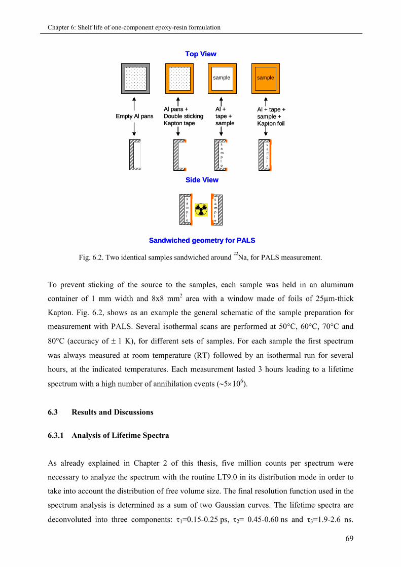
Chapter 6: Shelf life of one-component epoxy-resin formulation
69
sample
sample
sample sample
sample
sample
Top View
Side View
Sandwiched geometry for PALS
Empty Al pansAl pans +Double stickingKapton tape
Al +tape +sample
Al + tape +sample +Kapton foil
sample
sample
sample
sample
sample sample
sample
sample
Top View
Side View
Sandwiched geometry for PALS
Empty Al pansAl pans +Double stickingKapton tape
Al +tape +sample
Al + tape +sample +Kapton foil
Fig. 6.2. Two identical samples sandwiched around22
Na, for PALS measurement.
To prevent sticking of the source to the samples, each sample was held in an aluminum
container of 1 mm width and 8x8 mm2 area with a window made of foils of 25µm-thick
Kapton. Fig. 6.2, shows as an example the general schematic of the sample preparation for
measurement with PALS. Several isothermal scans are performed at 50°C, 60°C, 70°C and
80°C (accuracy of 1 K), for different sets of samples. For each sample the first spectrum
was always measured at room temperature (RT) followed by an isothermal run for several
hours, at the indicated temperatures. Each measurement lasted 3 hours leading to a lifetime
spectrum with a high number of annihilation events (5106).
6.3 Results and Discussions
6.3.1 Analysis of Lifetime Spectra
As already explained in Chapter 2 of this thesis, five million counts per spectrum were
necessary to analyze the spectrum with the routine LT9.0 in its distribution mode in order to
take into account the distribution of free volume size. The final resolution function used in the
spectrum analysis is determined as a sum of two Gaussian curves. The lifetime spectra are
deconvoluted into three components: 1=0.15-0.25 ps, 2= 0.45-0.60 ns and 3=1.9-2.6 ns.

Chapter 6: Shelf life of one-component epoxy-resin formulation
70
Here, 1 is the shortest lifetime component, which is attributed to the annihilation of para-
positronium (p-Ps). The intermediate lifetime component 2 is attributed to annihilation of
free-positrons (e+) and the component 3 is attributed to the ortho-positronium (o-Ps). This is
the relevant quantity for the free volume and for the investigation of curing here.
Figure 6.3 shows the most important results obtained from the PALS technique i.e. 3 and the
I3. The plateau of the o-Ps lifetime 3 observed in the early stages of the lower temperature
investigations shows that the mixture is still in its precursor state. The following sharp
decrease in o-Ps lifetime indicates that the curing sets in. Finally, the cured state is achieved,
which is indicated by reaching the saturation limit. One should note that in the course of the
process 3 is decreasing, reflecting a decrease in hole size, as expected for shrinkage during
curing.128 The slight reduction in the intensity during curing may be an indication that there
are reactive groups inhibiting Ps formation. The half-life of the curing process is also
indicated.
0 50 100 150 200 250 300 350 400 450 500 550
1.8
2.0
2.2
2.4
2.6
12
14
16
18
o-P
sIn
ten
sity
(%)
o-Ps lifetime
o-P
slif
etim
e(n
s)
annealing time (hours)
reference system (ex-situ cured)
o-Ps intensity
Fig. 6.3: o-Ps lifetime, dispersion and intensity as function of curing time at 50 °C. Also shownreference values (ex-situ cured @ 150 °C)
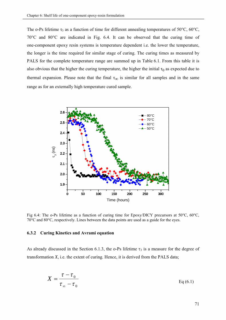
Chapter 6: Shelf life of one-component epoxy-resin formulation
71
The o-Ps lifetime τ3 as a function of time for different annealing temperatures of 50°C, 60°C,
70°C and 80°C are indicated in Fig. 6.4. It can be observed that the curing time of
one-component epoxy resin systems is temperature dependent i.e. the lower the temperature,
the longer is the time required for similar stage of curing. The curing times as measured by
PALS for the complete temperature range are summed up in Table 6.1. From this table it is
also obvious that the higher the curing temperature, the higher the initial τ0 as expected due to
thermal expansion. Please note that the final τ∞ is similar for all samples and in the same
range as for an externally high temperature cured sample.
0 50 100 150 200 250 300
1.9
2.0
2.1
2.2
2.3
2.4
2.5
2.6
0 50 100 150 200 250 300
1.9
2.0
2.1
2.2
2.3
2.4
2.5
2.6
0 50 100 150 200 250 300
1.9
2.0
2.1
2.2
2.3
2.4
2.5
2.6
0 50 100 150 200 250 300
1.9
2.0
2.1
2.2
2.3
2.4
2.5
2.680°C
3(n
s)
Time (hours)
70°C
50°C
60°C
Fig 6.4: The o-Ps lifetime as a function of curing time for Epoxy/DICY precursors at 50°C, 60°C,70°C and 80°C, respectively. Lines between the data points are used as a guide for the eyes.
6.3.2 Curing Kinetics and Avrami equation
As already discussed in the Section 6.1.3, the o-Ps lifetime 3 is a measure for the degree of
transformation X, i.e. the extent of curing. Hence, it is derived from the PALS data;
0
0
XEq (6.1)
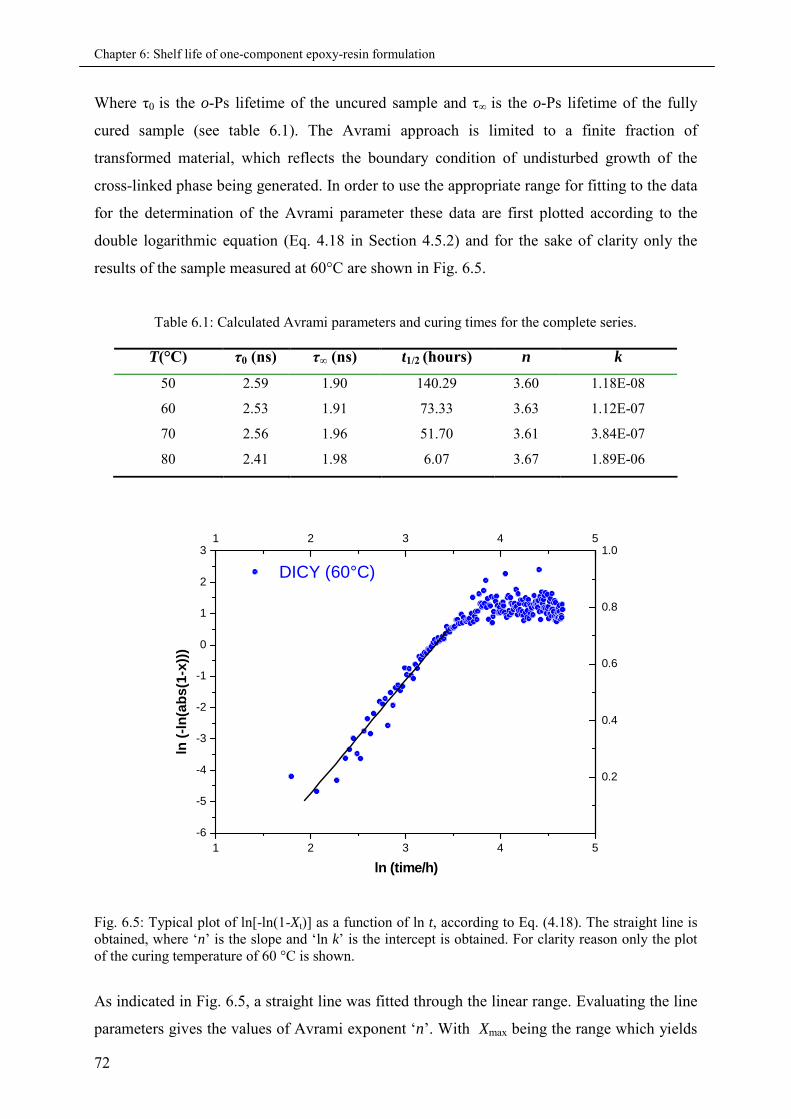
Chapter 6: Shelf life of one-component epoxy-resin formulation
72
Where τ0 is the o-Ps lifetime of the uncured sample and τ∞ is the o-Ps lifetime of the fully
cured sample (see table 6.1). The Avrami approach is limited to a finite fraction of
transformed material, which reflects the boundary condition of undisturbed growth of the
cross-linked phase being generated. In order to use the appropriate range for fitting to the data
for the determination of the Avrami parameter these data are first plotted according to the
double logarithmic equation (Eq. 4.18 in Section 4.5.2) and for the sake of clarity only the
results of the sample measured at 60°C are shown in Fig. 6.5.
Table 6.1: Calculated Avrami parameters and curing times for the complete series.
1 2 3 4 5
-6
-5
-4
-3
-2
-1
0
1
2
31 2 3 4 5
0.2
0.4
0.6
0.8
1.0
DICY (60°C)
ln(-
ln(a
bs
(1-x
)))
ln (time/h)
Fig. 6.5: Typical plot of ln[-ln(1-Xt)] as a function of ln t, according to Eq. (4.18). The straight line isobtained, where ‘n’ is the slope and ‘ln k’ is the intercept is obtained. For clarity reason only the plotof the curing temperature of 60 °C is shown.
As indicated in Fig. 6.5, a straight line was fitted through the linear range. Evaluating the line
parameters gives the values of Avrami exponent ‘n’. With Xmax being the range which yields
T(°C) τ0 (ns) τ∞ (ns) t1/2 (hours) n k
50 2.59 1.90 140.29 3.60 1.18E-08
60 2.53 1.91 73.33 3.63 1.12E-07
70 2.56 1.96 51.70 3.61 3.84E-07
80 2.41 1.98 6.07 3.67 1.89E-06
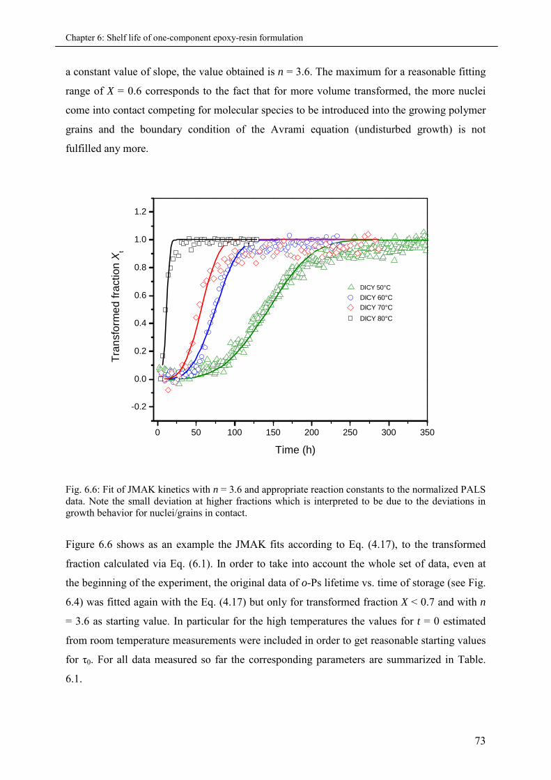
Chapter 6: Shelf life of one-component epoxy-resin formulation
73
a constant value of slope, the value obtained is n = 3.6. The maximum for a reasonable fitting
range of X = 0.6 corresponds to the fact that for more volume transformed, the more nuclei
come into contact competing for molecular species to be introduced into the growing polymer
grains and the boundary condition of the Avrami equation (undisturbed growth) is not
fulfilled any more.
0 50 100 150 200 250 300 350
-0.2
0.0
0.2
0.4
0.6
0.8
1.0
1.2
Time (h)
Tra
nsfo
rme
dfr
actio
nX
t
DICY 50°C
DICY 60°C
DICY 70°C
DICY 80°C
Fig. 6.6: Fit of JMAK kinetics with n = 3.6 and appropriate reaction constants to the normalized PALSdata. Note the small deviation at higher fractions which is interpreted to be due to the deviations ingrowth behavior for nuclei/grains in contact.
Figure 6.6 shows as an example the JMAK fits according to Eq. (4.17), to the transformed
fraction calculated via Eq. (6.1). In order to take into account the whole set of data, even at
the beginning of the experiment, the original data of o-Ps lifetime vs. time of storage (see Fig.
6.4) was fitted again with the Eq. (4.17) but only for transformed fraction X < 0.7 and with n
= 3.6 as starting value. In particular for the high temperatures the values for t = 0 estimated
from room temperature measurements were included in order to get reasonable starting values
for τ0. For all data measured so far the corresponding parameters are summarized in Table.
6.1.
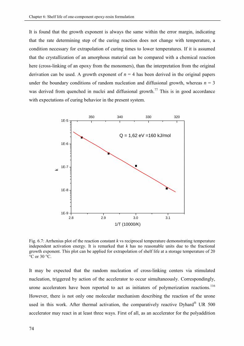
Chapter 6: Shelf life of one-component epoxy-resin formulation
74
It is found that the growth exponent is always the same within the error margin, indicating
that the rate determining step of the curing reaction does not change with temperature, a
condition necessary for extrapolation of curing times to lower temperatures. If it is assumed
that the crystallization of an amorphous material can be compared with a chemical reaction
here (cross-linking of an epoxy from the monomers), than the interpretation from the original
derivation can be used. A growth exponent of n = 4 has been derived in the original papers
under the boundary conditions of random nucleation and diffusional growth, whereas n = 3
was derived from quenched in nuclei and diffusional growth.77 This is in good accordance
with expectations of curing behavior in the present system.
2.8 2.9 3.0 3.1
1E-9
1E-8
1E-7
1E-6
1E-5350 340 330 320
k
1/T (10000/K)
Q = 1,62 eV =160 kJ/mol
Fig. 6.7: Arrhenius plot of the reaction constant k vs reciprocal temperature demonstrating temperatureindependent activation energy. It is remarked that k has no reasonable units due to the fractionalgrowth exponent. This plot can be applied for extrapolation of shelf life at a storage temperature of 20°C or 30 °C.
It may be expected that the random nucleation of cross-linking centers via stimulated
nucleation, triggered by action of the accelerator to occur simultaneously. Correspondingly,
urone accelerators have been reported to act as initiators of polymerization reactions.116
However, there is not only one molecular mechanism describing the reaction of the urone
used in this work. After thermal activation, the comparatively reactive Dyhard® UR 500
accelerator may react in at least three ways. First of all, as an accelerator for the polyaddition
Chapter 6: Shelf life of one-component epoxy-resin formulation
75
reaction, between DGEBA and DICY. Secondly, as a catalyst for the epoxy homo-
polymerisation reaction and finally as a curative which is consumed during the polyreaction.
The formulation used for the present investigation is not completely optimised with respect to
a consumption of all the DICY in the reactive mixture within the curing schedule applied.
Assuming thermally activated behavior, the reaction constant k can reasonably be plotted on a
logarithmic scale versus the reciprocal temperature in order to verify an Arrhenius-type
activation behavior as shown in Fig. 6.7. The slope directly yields activation energy of
approximately 160 kJ/mol. This corresponds to the energy of the rate limiting step of the
reaction. This value is distinctly larger than values usually given for the reaction of various
epoxides130 and the calculated activation energies are termed as model dependent. In this
work not only the mere chemical reaction, but also the change in the mobility of molecular
species due to increased cross-linking and the transport effects in the system during curing are
taken into account.
The chemical reactions occurring during storage at room temperature as compared to curing at
temperatures of up to 180°C, it may be expected that according to the latency of the DICY
hardener at room temperature its influence on the network forming reaction will increase with
increasing temperatures.116 Finally for the present system the shelf life time is extrapolated to
storage temperature (T = 20°C) and an upper limit of 850 h (T = 30°C, t = 500 h) is estimated,
which could be compared to nearly three months (2000 h) of storage of the sample at the same
temperature. Hence, the model seems to be useful to give at least lower limits of storage
stability.
6.4 Conclusion
PALS have been applied to observe in-situ curing of a typical epoxide with high accuracy and
time resolution for the first time. Based on transformed fractions of reactive species calculated
from characteristic reference values for o-Ps lifetime 3 within the reactive system, shrinkage
and a decreased molecular mobility within the forming network are monitored, following the
chemical reactions limiting the storage stability of the formulations. Applying the
Johnson-Mehl-Avrami-Kolmogorov equation to the curing data, appropriate kinetic
parameters could be derived. Such proceeding allows extrapolation of the shelf life of
one-component epoxy systems at room temperature.

Chapter 6: Shelf life of one-component epoxy-resin formulation
76
Chapter 7: Free and encapsulated accelerator formulations
77
7. Free and encapsulated accelerator formulations
One-component epoxy resin composites are an important class of adhesive materials,
especially when it comes to high temperature applications. It is of utmost importance to not
only modify the chemical constituents to achieve a higher shelf life of these materials in
precursor state, but at the same time making sure that the properties of the cured polymers are
not compromised. Even from the product development point of view, it is necessary to study
the curing kinetics of these systems and also the characteristic properties of their cured epoxy
composites for better understanding and further modification or development. In this section a
comparison of IR-spectroscopy and PALS data is presented, which is used to study the effect
of free and encapsulated accelerator on the curing times of epoxy precursors at elevated
temperature of 60 °C. Furthermore, PALS and differential scanning calorimetry (DSC) are
used as the experimental techniques to characterize all together, six different DGEBA–DICY
cured epoxy composites. It is remarked that IR-spectroscopy and DSC experiments were
performed at the University of Saarland in Saarbrücken and the results are only used for
comparison with PALS data.
7.1 Introduction
One-component epoxy resin systems remain the most widely-used adhesives in structural
applications,131 with ease of usage,132 good environmental stability,133 and adequate creep
resistance.134 The storage stability of the one-component epoxy precursors is very important
parameter as far as research and development of such formulations is concerned. On one hand
a higher shelf life can be obtained by encapsulating the accelerator in a carrier material which
delays the reaction with epoxy matrix, increasing the shelf life of one-component epoxy resin
formulations and at the same time making sure that hardening temperatures are in acceptable
range. But on the other hand, it is also very important not to compromise on the characteristic
properties of the cured composites.
Glass-transition temperature Tg, is a critical property of these composites when it comes to
high temperature applications. The Tg can change with different combinations of resin,
hardener and accelerators and its important to maintain a higher Tg and at the same time
having a longer storage life. The properties of epoxy composites are influenced by factors at
the molecular level, such as backbone structures of epoxy resin and curing agent; nature of the
Chapter 7: Free and encapsulated accelerator formulations
78
covalent bond developed between the epoxy resin and the curing agent during the cross-
linking; and the density and the extent of cross-linking i.e. degree of cure.89 This class of
cured thermosetting polymers are more difficult to analyse as compared to the thermoplastics,
as they are insoluble and generally intractable
Free volume is an interesting approach to study not only the precursor state of these
epoxies,135 but also the Tg and other related properties of their cured composites. In a
qualitative sense, free volume may be considered simply as the volume unoccupied by the
atomic species of the material. This unoccupied volume has a strong influence on the mobility
of segments of polymer molecules, and on the permeability of the polymer to gaseous or
liquid penetrants.136 The concept of free volume may be considered as rather simplistic in the
light of advances in modern polymer physics, but it has the advantage of ease of visualization
and, in this particular case, lends itself to quantitative analysis.
Over the past decade Positron annihilation lifetime spectroscopy (PALS) has emerged as one
of the entrusted tools to characterize the free volume in amorphous polymers.137 The Positron
group at the University of Kiel, have used PALS technique to identify changes of free volume
in various membranes, nano-composites and low-molecular-weight substances 124,138-139. In
this study PALS is evaluated as a method to detect free volume in a series of DGEBA-
dicyandiamide precursors and their cured epoxy composites, which differs in terms of their
chemical constituents.
As shown in Chapter 6 of this thesis, JMAK fits are applied to the experimental data
measured by PALS technique. This is helpful to understand the reaction kinetics of the
formulations with micro and nano-ecapsulated accelerator, in comparison to the system with
free accelerator. In this section it is shown that not only the curing times observed by PALS
are in good agreement with the IR-spectroscopy data, but at the same time PALS is also
suitable for the investigation of holes of sub-nanometre size in their cured composites. The
temperature dependence of the hole free volumes, calculated using the Tao-Eldrup model,3-4
will be presented for the complete series of samples. Apart from that the glass-transition
temperatures, Tg and the temperature at which the extrapolated free volume goes to zero, T0,
and the thermal expansion coefficients of the glassy (αg) and the rubbery (αr) phases are also
compared. Furthermore, the glass-transition temperatures calculated from the PALS and DSC
experiments are compared and discussed.
Chapter 7: Free and encapsulated accelerator formulations
79
7.2. Experimental
7.2.1 Preparation of the epoxies
The EP consists of diglycidylether of bisphenol A (DGEBA, CAS-Nr. 1675-54-3; DOW,
DER 332) and dicyandiamide (DICY, Dyhard®100SF, CAS-Nr. 461-58-5, Alzchem
Trostberg GmbH, Germany) in the mass ratio 100 : 6.7. In order to avoid sedimentation of the
solid DICY particles, the mixture is pre-cured at 150 °C for 1 h. This step partially dissolves
the DICY and increases viscosity due to the formation of oligomers. The corresponding IR
spectroscopic oxirane conversion is 15 %. This pre-polymer is degassed in vacuum and
homogenised (3200 min-1, 2 x 30 s) by a Speedmixer® (Hauschild Engineering, DAC 150 FV,
Germany) in normal air at 40 °C. EPaccel is made of the pre-polymer and the accelerator
(0.5 weight-%, substance not revealed for proprietary reasons) by mixing in the Speedmixer
under the same conditions. In a similar manner, EPµ-zeolite, EPn-zeolite, EPµ-filler and EPn-filler are
obtained by dispersing the micro-zeolites (2.4 weight-%), the nano-zeolites (2.4 weight-%),
the loaded micro-zeolite fillers (2.9 weight-%, corresponding to 0.5 weight-% of accelerator)
or the loaded nano-zeolite fillers (2.9 weight-%, corresponding to 0.5 weight-% of
accelerator) in the pre-polymer.
For the sake of clarity the six different samples are abbreviated as follow;
BK1 = Pre-polymerized DGEBA and DICY system with a stoichiometric ratio of 100:6.7
BK2 = BK1 + Accelerator (0.5 wt%)
BK3 = BK1 + unloaded μ-Zeolite
BK4 = BK1 + micromodule (0.5 wt% Accelerator encapsulated in μ-Zeolite)
BK5 = BK1 + unloaded n-Zeolite
BK6 = BK1 + nanomodule (0.5 wt% Accelerator encapsulated in nano-Zeolite)
7.2.2 Modulated DSC
MDSC investigations done by the calorimeter Q100 (TA Instruments) at a heating rate of
β = 10 K min-1 are carried out with sinusoidal modulation at f = 1 / 60 Hz and a temperature
amplitude of T = ± 1 K. The measuring cycle for network formation starts by heating the
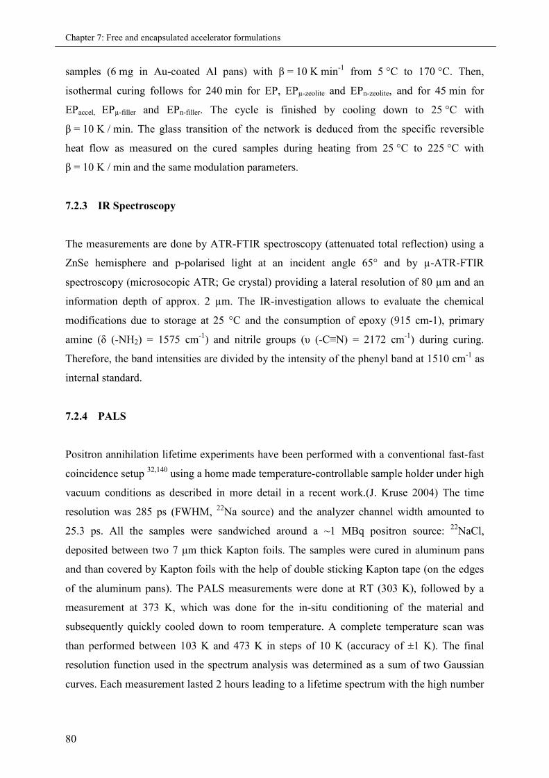
Chapter 7: Free and encapsulated accelerator formulations
80
samples (6 mg in Au-coated Al pans) with β = 10 K min-1 from 5 °C to 170 °C. Then,
isothermal curing follows for 240 min for EP, EPµ-zeolite and EPn-zeolite, and for 45 min for
EPaccel, EPµ-filler and EPn-filler. The cycle is finished by cooling down to 25 °C with
β = 10 K / min. The glass transition of the network is deduced from the specific reversible
heat flow as measured on the cured samples during heating from 25 °C to 225 °C with
β = 10 K / min and the same modulation parameters.
7.2.3 IR Spectroscopy
The measurements are done by ATR-FTIR spectroscopy (attenuated total reflection) using a
ZnSe hemisphere and p-polarised light at an incident angle 65° and by µ-ATR-FTIR
spectroscopy (microsocopic ATR; Ge crystal) providing a lateral resolution of 80 µm and an
information depth of approx. 2 µm. The IR-investigation allows to evaluate the chemical
modifications due to storage at 25 °C and the consumption of epoxy (915 cm-1), primary
amine (δ (-NH2) = 1575 cm-1) and nitrile groups (υ (-C≡N) = 2172 cm-1) during curing.
Therefore, the band intensities are divided by the intensity of the phenyl band at 1510 cm-1 as
internal standard.
7.2.4 PALS
Positron annihilation lifetime experiments have been performed with a conventional fast-fast
coincidence setup 32,140 using a home made temperature-controllable sample holder under high
vacuum conditions as described in more detail in a recent work.(J. Kruse 2004) The time
resolution was 285 ps (FWHM, 22Na source) and the analyzer channel width amounted to
25.3 ps. All the samples were sandwiched around a ~1 MBq positron source: 22NaCl,
deposited between two 7 μm thick Kapton foils. The samples were cured in aluminum pans
and than covered by Kapton foils with the help of double sticking Kapton tape (on the edges
of the aluminum pans). The PALS measurements were done at RT (303 K), followed by a
measurement at 373 K, which was done for the in-situ conditioning of the material and
subsequently quickly cooled down to room temperature. A complete temperature scan was
than performed between 103 K and 473 K in steps of 10 K (accuracy of ±1 K). The final
resolution function used in the spectrum analysis was determined as a sum of two Gaussian
curves. Each measurement lasted 2 hours leading to a lifetime spectrum with the high number
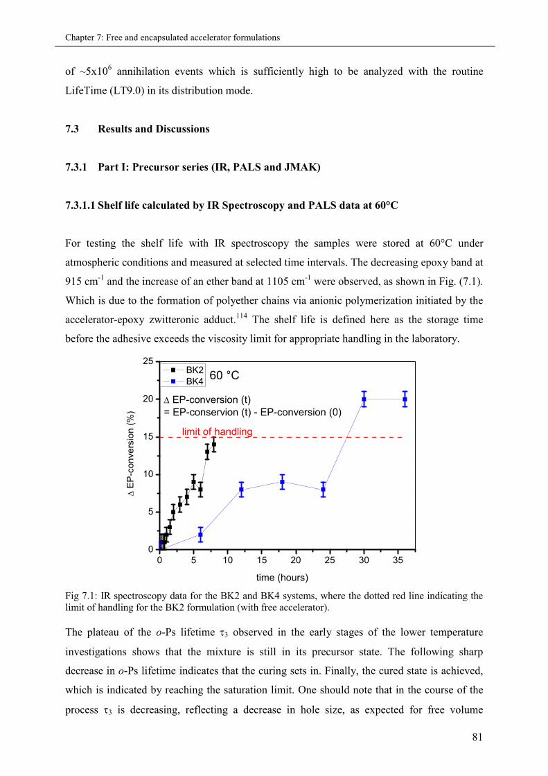
Chapter 7: Free and encapsulated accelerator formulations
81
of ~5x10⁶ annihilation events which is sufficiently high to be analyzed with the routine
LifeTime (LT9.0) in its distribution mode.
7.3 Results and Discussions
7.3.1 Part I: Precursor series (IR, PALS and JMAK)
7.3.1.1 Shelf life calculated by IR Spectroscopy and PALS data at 60°C
For testing the shelf life with IR spectroscopy the samples were stored at 60°C under
atmospheric conditions and measured at selected time intervals. The decreasing epoxy band at
915 cm-1 and the increase of an ether band at 1105 cm-1 were observed, as shown in Fig. (7.1).
Which is due to the formation of polyether chains via anionic polymerization initiated by the
accelerator-epoxy zwitteronic adduct.114 The shelf life is defined here as the storage time
before the adhesive exceeds the viscosity limit for appropriate handling in the laboratory.
0 5 10 15 20 25 30 350
5
10
15
20
25
E
P-c
on
ve
rsio
n(%
)
time (hours)
BK2BK4
EP-conversion (t)= EP-conservion (t) - EP-conversion (0)
60 °C
limit of handling
Fig 7.1: IR spectroscopy data for the BK2 and BK4 systems, where the dotted red line indicating thelimit of handling for the BK2 formulation (with free accelerator).
The plateau of the o-Ps lifetime 3 observed in the early stages of the lower temperature
investigations shows that the mixture is still in its precursor state. The following sharp
decrease in o-Ps lifetime indicates that the curing sets in. Finally, the cured state is achieved,
which is indicated by reaching the saturation limit. One should note that in the course of the
process 3 is decreasing, reflecting a decrease in hole size, as expected for free volume
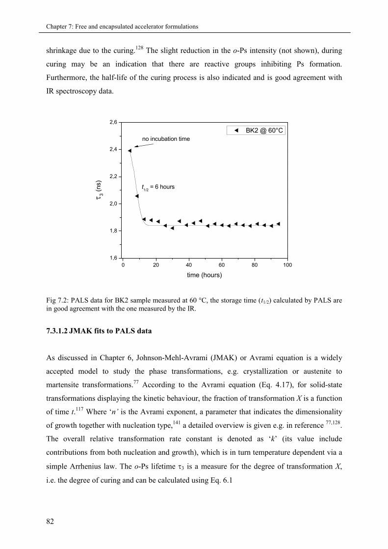
Chapter 7: Free and encapsulated accelerator formulations
82
shrinkage due to the curing.128 The slight reduction in the o-Ps intensity (not shown), during
curing may be an indication that there are reactive groups inhibiting Ps formation.
Furthermore, the half-life of the curing process is also indicated and is good agreement with
IR spectroscopy data.
0 20 40 60 80 100
1,6
1,8
2,0
2,2
2,4
2,6
BK2 @ 60°C
3(n
s)
time (hours)
no incubation time
t1/2
= 6 hours
Fig 7.2: PALS data for BK2 sample measured at 60 °C, the storage time (t1/2) calculated by PALS arein good agreement with the one measured by the IR.
7.3.1.2 JMAK fits to PALS data
As discussed in Chapter 6, Johnson-Mehl-Avrami (JMAK) or Avrami equation is a widely
accepted model to study the phase transformations, e.g. crystallization or austenite to
martensite transformations.77 According to the Avrami equation (Eq. 4.17), for solid-state
transformations displaying the kinetic behaviour, the fraction of transformation X is a function
of time t.117 Where ‘n’ is the Avrami exponent, a parameter that indicates the dimensionality
of growth together with nucleation type,141 a detailed overview is given e.g. in reference 77,128.
The overall relative transformation rate constant is denoted as ‘k’ (its value include
contributions from both nucleation and growth), which is in turn temperature dependent via a
simple Arrhenius law. The o-Ps lifetime 3 is a measure for the degree of transformation X,
i.e. the degree of curing and can be calculated using Eq. 6.1
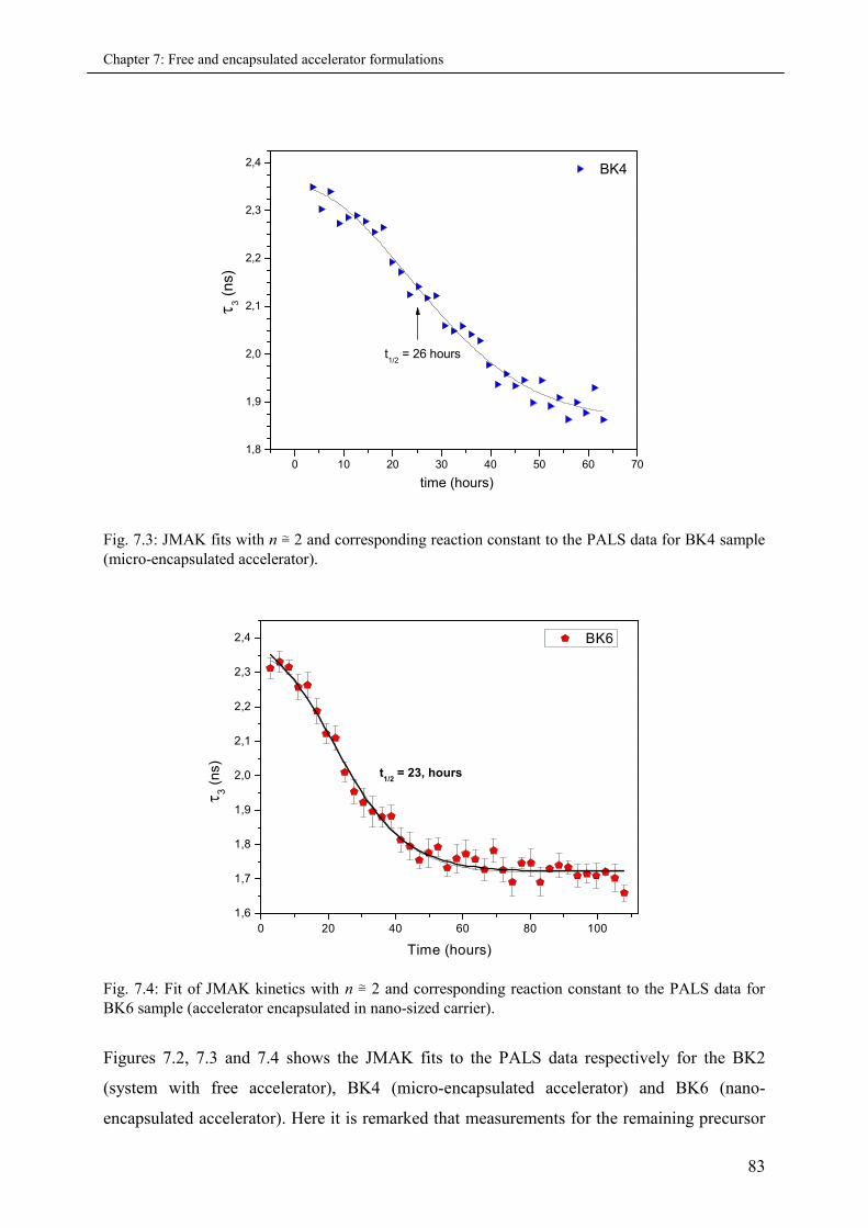
Chapter 7: Free and encapsulated accelerator formulations
83
0 10 20 30 40 50 60 70
1,8
1,9
2,0
2,1
2,2
2,3
2,4BK4
t1/2
= 26 hours
3(n
s)
time (hours)
Fig. 7.3: JMAK fits with n ≅ 2 and corresponding reaction constant to the PALS data for BK4 sample(micro-encapsulated accelerator).
0 20 40 60 80 100
1,6
1,7
1,8
1,9
2,0
2,1
2,2
2,3
2,4 BK6
3(n
s)
Time (hours)
t1/2
= 23, hours
Fig. 7.4: Fit of JMAK kinetics with n ≅ 2 and corresponding reaction constant to the PALS data forBK6 sample (accelerator encapsulated in nano-sized carrier).
Figures 7.2, 7.3 and 7.4 shows the JMAK fits to the PALS data respectively for the BK2
(system with free accelerator), BK4 (micro-encapsulated accelerator) and BK6 (nano-
encapsulated accelerator). Here it is remarked that measurements for the remaining precursor
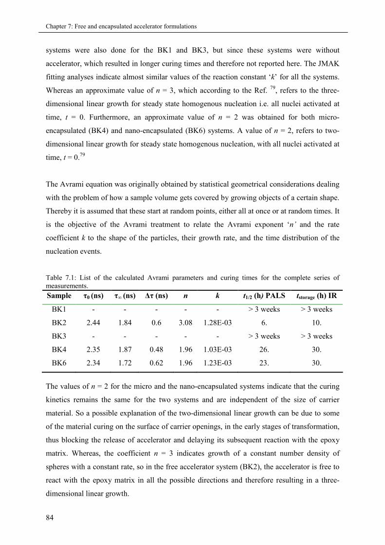
Chapter 7: Free and encapsulated accelerator formulations
84
systems were also done for the BK1 and BK3, but since these systems were without
accelerator, which resulted in longer curing times and therefore not reported here. The JMAK
fitting analyses indicate almost similar values of the reaction constant ‘k’ for all the systems.
Whereas an approximate value of n = 3, which according to the Ref. 79, refers to the three-
dimensional linear growth for steady state homogenous nucleation i.e. all nuclei activated at
time, t = 0. Furthermore, an approximate value of n = 2 was obtained for both micro-
encapsulated (BK4) and nano-encapsulated (BK6) systems. A value of n = 2, refers to two-
dimensional linear growth for steady state homogenous nucleation, with all nuclei activated at
time, t = 0.79
The Avrami equation was originally obtained by statistical geometrical considerations dealing
with the problem of how a sample volume gets covered by growing objects of a certain shape.
Thereby it is assumed that these start at random points, either all at once or at random times. It
is the objective of the Avrami treatment to relate the Avrami exponent ‘n’ and the rate
coefficient k to the shape of the particles, their growth rate, and the time distribution of the
nucleation events.
Table 7.1: List of the calculated Avrami parameters and curing times for the complete series ofmeasurements.
Sample τ0 (ns) τ∞ (ns) Δτ (ns) n k t1/2 (h) PALS tstorage (h) IR
BK1 - - - - - > 3 weeks > 3 weeks
BK2 2.44 1.84 0.6 3.08 1.28E-03 6. 10.
BK3 - - - - - > 3 weeks > 3 weeks
BK4 2.35 1.87 0.48 1.96 1.03E-03 26. 30.
BK6 2.34 1.72 0.62 1.96 1.23E-03 23. 30.
The values of n = 2 for the micro and the nano-encapsulated systems indicate that the curing
kinetics remains the same for the two systems and are independent of the size of carrier
material. So a possible explanation of the two-dimensional linear growth can be due to some
of the material curing on the surface of carrier openings, in the early stages of transformation,
thus blocking the release of accelerator and delaying its subsequent reaction with the epoxy
matrix. Whereas, the coefficient n = 3 indicates growth of a constant number density of
spheres with a constant rate, so in the free accelerator system (BK2), the accelerator is free to
react with the epoxy matrix in all the possible directions and therefore resulting in a three-
dimensional linear growth.
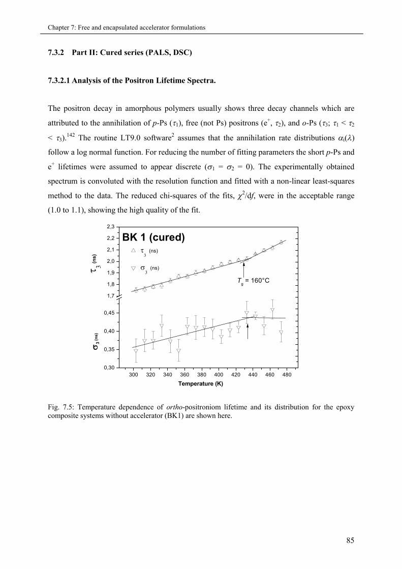
Chapter 7: Free and encapsulated accelerator formulations
85
7.3.2 Part II: Cured series (PALS, DSC)
7.3.2.1 Analysis of the Positron Lifetime Spectra.
The positron decay in amorphous polymers usually shows three decay channels which are
attributed to the annihilation of p-Ps (1), free (not Ps) positrons (e+, 2), and o-Ps (3; 1 < 2
< 3).142 The routine LT9.0 software2 assumes that the annihilation rate distributions i()
follow a log normal function. For reducing the number of fitting parameters the short p-Ps and
e+ lifetimes were assumed to appear discrete (1 = 2 = 0). The experimentally obtained
spectrum is convoluted with the resolution function and fitted with a non-linear least-squares
method to the data. The reduced chi-squares of the fits, 2/df, were in the acceptable range
(1.0 to 1.1), showing the high quality of the fit.
300 320 340 360 380 400 420 440 460 480
0,30
0,35
0,40
0,45
1,7
1,8
1,9
2,0
2,1
2,2
2,3
Temperature (K)
(n
s)
(ns)
(ns)
Tg
= 160°C
BK 1 (cured)
3
(ns)
Fig. 7.5: Temperature dependence of ortho-positroniom lifetime and its distribution for the epoxycomposite systems without accelerator (BK1) are shown here.
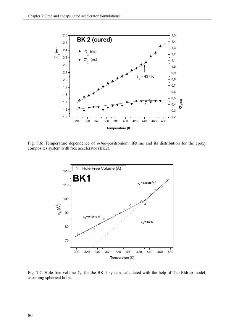
Chapter 7: Free and encapsulated accelerator formulations
86
300 320 340 360 380 400 420 440 460 480
1,5
1,6
1,7
1,8
1,9
2,0
2,1
2,2
2,3
2,4
2,5
2,6
0,2
0,3
0,4
0,5
0,6
0,7
0,8
0,9
1,0
1,1
1,2
1,3
1,4
1,5
(ns)
3
(ns)
(n
s)
Temperature (K)
Tg
= 437 K
BK 2 (cured)
(ns)
Fig. 7.6: Temperature dependence of ortho-positroniom lifetime and its distribution for the epoxycomposites system with free accelerator (BK2).
300 320 340 360 380 400 420 440 460 480
70
80
90
100
110
120
BK1r = 3,56x10
-2K
-1
Hole Free Volume (Å)
v h(Å
3)
Temperature (K)
Tg = 432 K
g = 9,12x10⁻³K
-1
Fig. 7.7: Hole free volume Vh, for the BK 1 system, calculated with the help of Tao-Eldrup model,assuming spherical holes.
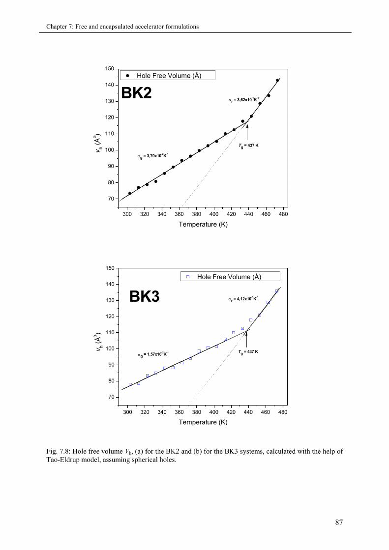
Chapter 7: Free and encapsulated accelerator formulations
87
300 320 340 360 380 400 420 440 460 480
70
80
90
100
110
120
130
140
150
BK2r = 3,62x10
-1K
-1
Hole Free Volume (Å)
vh
(Å3)
Temperature (K)
Tg = 437 K
g = 3,70x10⁻²K
-1
300 320 340 360 380 400 420 440 460 480
70
80
90
100
110
120
130
140
150
r = 4,12x10⁻¹K
-1
Hole Free Volume (Å)
vh
(Å3)
Temperature (K)
Tg = 437 Kg = 1,57x10
-2K
-1
BK3
Fig. 7.8: Hole free volume Vh, (a) for the BK2 and (b) for the BK3 systems, calculated with the help ofTao-Eldrup model, assuming spherical holes.
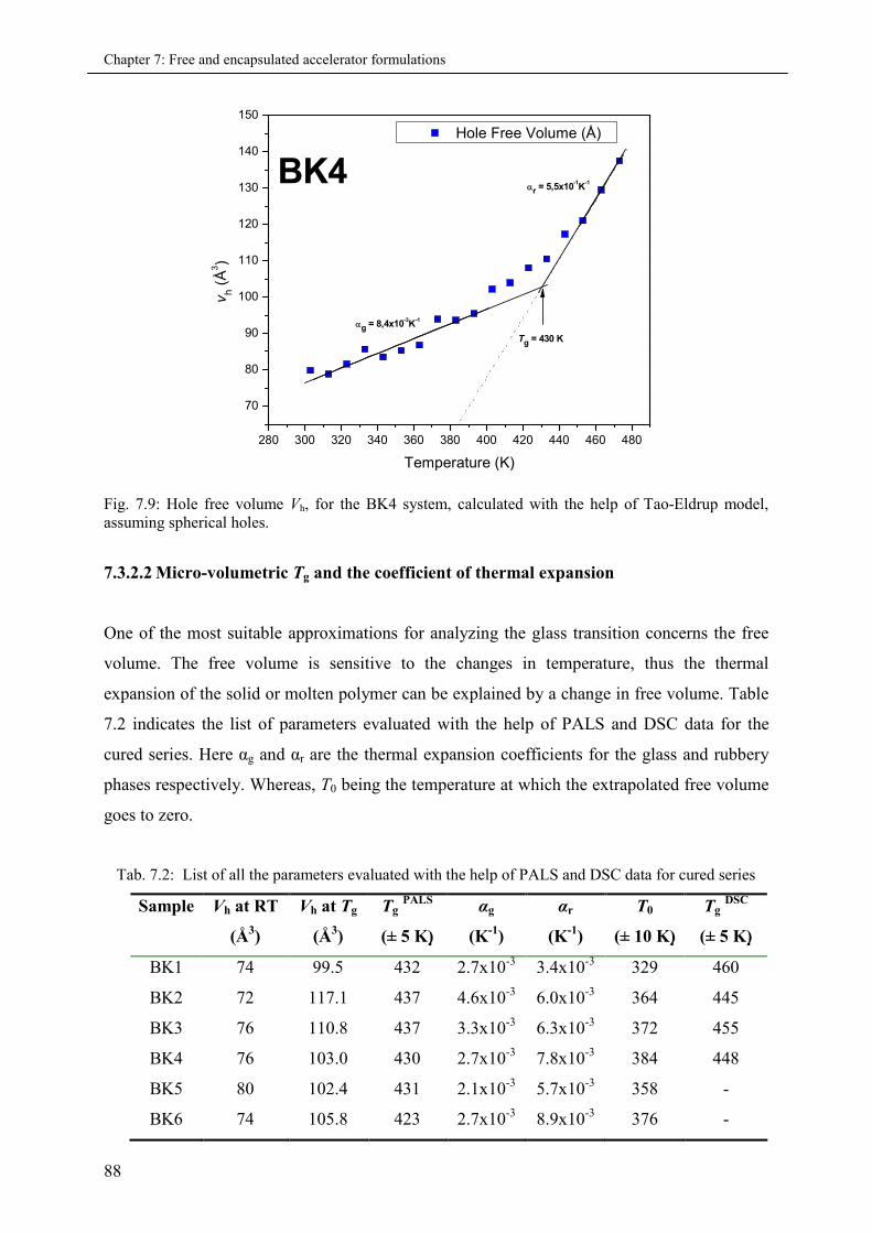
Chapter 7: Free and encapsulated accelerator formulations
88
280 300 320 340 360 380 400 420 440 460 480
70
80
90
100
110
120
130
140
150
BK4r = 5,5x10
-1K
-1
Hole Free Volume (Å)
vh
(Å3)
Temperature (K)
Tg = 430 K
g = 8,4x10⁻³K
-1
Fig. 7.9: Hole free volume Vh, for the BK4 system, calculated with the help of Tao-Eldrup model,assuming spherical holes.
7.3.2.2 Micro-volumetric Tg and the coefficient of thermal expansion
One of the most suitable approximations for analyzing the glass transition concerns the free
volume. The free volume is sensitive to the changes in temperature, thus the thermal
expansion of the solid or molten polymer can be explained by a change in free volume. Table
7.2 indicates the list of parameters evaluated with the help of PALS and DSC data for the
cured series. Here αg and αr are the thermal expansion coefficients for the glass and rubbery
phases respectively. Whereas, T0 being the temperature at which the extrapolated free volume
goes to zero.
Tab. 7.2: List of all the parameters evaluated with the help of PALS and DSC data for cured series
Sample Vh at RT
(Å3)
Vh at Tg
(Å3)
TgPALS
(± 5 K)
αg
(K-1)
αr
(K-1)
T0
(± 10 K)
TgDSC
(± 5 K)
BK1 74 99.5 432 2.7x10⁻³ 3.4x10⁻³ 329 460
BK2 72 117.1 437 4.6x10⁻³ 6.0x10⁻³ 364 445
BK3 76 110.8 437 3.3x10⁻³ 6.3x10⁻³ 372 455
BK4 76 103.0 430 2.7x10⁻³ 7.8x10⁻³ 384 448
BK5 80 102.4 431 2.1x10⁻³ 5.7x10⁻³ 358 -
BK6 74 105.8 423 2.7x10⁻³ 8.9x10⁻³ 376 -
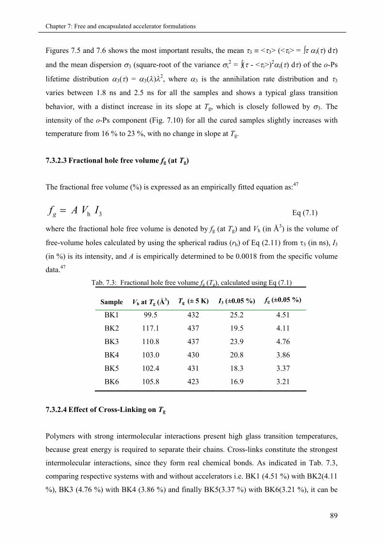
Chapter 7: Free and encapsulated accelerator formulations
89
Figures 7.5 and 7.6 shows the most important results, the mean 3 <3> (<i> = i() d)
and the mean dispersion 3 (square-root of the variance i2 = ( - <i>)2i() d) of the o-Ps
lifetime distribution 3() = 3()2, where 3 is the annihilation rate distribution and 3
varies between 1.8 ns and 2.5 ns for all the samples and shows a typical glass transition
behavior, with a distinct increase in its slope at Tg, which is closely followed by 3. The
intensity of the o-Ps component (Fig. 7.10) for all the cured samples slightly increases with
temperature from 16 % to 23 %, with no change in slope at Tg.
7.3.2.3 Fractional hole free volume fg (at Tg)
The fractional free volume (%) is expressed as an empirically fitted equation as:47
h 3gf A V I Eq (7.1)
where the fractional hole free volume is denoted by fg (at Tg) and Vh (in Å3) is the volume of
free-volume holes calculated by using the spherical radius (rh) of Eq (2.11) from 3 (in ns), I3
(in %) is its intensity, and A is empirically determined to be 0.0018 from the specific volume
data.47
Tab. 7.3: Fractional hole free volume fg (Tg), calculated using Eq (7.1)
Sample Vh at Tg (Å3) Tg (± 5 K) I3 (±0.05 %) fg (±0.05 %)
BK1 99.5 432 25.2 4.51
BK2 117.1 437 19.5 4.11
BK3 110.8 437 23.9 4.76
BK4 103.0 430 20.8 3.86
BK5 102.4 431 18.3 3.37
BK6 105.8 423 16.9 3.21
7.3.2.4 Effect of Cross-Linking on Tg
Polymers with strong intermolecular interactions present high glass transition temperatures,
because great energy is required to separate their chains. Cross-links constitute the strongest
intermolecular interactions, since they form real chemical bonds. As indicated in Tab. 7.3,
comparing respective systems with and without accelerators i.e. BK1 (4.51 %) with BK2(4.11
%), BK3 (4.76 %) with BK4 (3.86 %) and finally BK5(3.37 %) with BK6(3.21 %), it can be
Chapter 7: Free and encapsulated accelerator formulations
90
seen that every time the accelerator is introduced in the epoxy resin formulation, the ortho-
Positronium intensity (I3) and eventually the fractional hole free volume at Tg is also
decreased. This can be attributed to the effect of highly reactive accelerator, resulting in
higher degree of cross-linking and therefore a lower fractional hole free volume, as compared
to the systems without accelerator. It is known that if the cross-link density increases, then the
free volume should decrease, and this consequently gives rise to the Tg, because the molecular
mobility is more hindered.143 However, only the comparison of BK1 and BK2 agrees with this
theoretical interpretation and it is not clear as to why the systems with encapsulated
accelerators (i.e. BK4 and BK6) have a lower Tg, although they have lower values of the
fractional hole free volumes. For the complete series of cured composites the number density
of holes is also estimated, by taking certain assumptions into account, but since there was no
significant difference observed and therefore these results will not be reported here.
7.3.2.5 No effect of positron irradiation
A minimum in I3 near Tg has been reported for several polymers and is generally agreed to be
the result of cumulative irradiation.144 The effect of long-term exposure to the positron source
during positron annihilation lifetime measurements was explored by monitoring any change in
the o-Ps intensity (I3) as a function of exposure time and temperature.
20 40 60 80 100 120 140 160 180 200 220
14
16
18
20
22
24
26
28
30
32 BK1BK2BK3BK4
I 3(%
)
Temperature (°C)
Fig. 7.10: Plots of ortho-positronium intensities (I3) for all the samples, indicating that there is no realtemperature dependence, but definitely the intensities of BK1 and BK3 are relatively higher ascompared to other samples. For the sake of clarity data for BK5 and BK6 are not shown here.
Chapter 7: Free and encapsulated accelerator formulations
91
For the complete series of cured samples, the o-Ps intensity within the error bars remains
more or less unchanged, which suggest no real irradiation effects. However, as shown in
Fig.6, the intensities of BK1 and BK3 are higher as compared to the other samples, for the
sake of clarity the intensity data of BK5 and BK6 systems is not shown here.
7.3.2.6 The ortho-Positronium Inhibition
Furthermore, it was observed that every time the accelerator is introduced into the
formulation, it lowers the intensity of ortho-positronium, this effect is attributed to the process
of “ortho-Positronium inhibition”. Although this interpretation eventually means that the
values obtained for the fractional hole free volume, fh are not reliable, but for the scientific
understanding of these results its very important to discuss each and every aspect of the
available data. Since the dicyandiamide hardener already have N-atoms in its structure and
even the accelerator used here also have Nitrogen in its structure, so due to higher
concentration of N-atoms Ps inhibition occurs in the formulations with accelerator, which
reduces the intensity of o-Ps formation as compared to the systems without accelerators,
whereas on the contrary there is no real effect on the o-Ps lifetimes.
7.4 Conclusions
An in-depth analysis for the precursor and the cured series of one-component epoxy resin
formulations is reported. The shelf-life calculated from PALS is in good agreement with the
ones observed by the IR spectroscopy. JMAK fits to the PALS data indicates that the micro
(BK4) and the nano-encapsulated (BK6) systems show the same reaction kinetics, with
Avrami exponent having an approximate value of n = 2, whereas the system with free
accelerator (BK2) does not show any incubation time and a higher value of n = 3.
Furthermore, the cured series of their epoxy composites indicate no real change in the hole
free volume at room temperature of 300 K and even other parameters does not indicate any
systemic behaviour. The values of Tg calculated by PALS are a bit lower as compared to the
ones observed by DSC, which is due to the longer annealing times of PALS technique.
However, the ortho-Positronium intensity and the fractional hole free volume at the Tg is
lowered, every time the accelerator is introduced into the system.

Chapter 7: Free and encapsulated accelerator formulations
92
Chapter 8: The effect of encapsulation on activation energy
93
8. The effect of encapsulation on activation energy
It is also very important to investigate the kinetic parameters such as the apparent activation
energy (Ea) for understanding the mechanism for the curing of epoxy resins. The Ea
determines whether the curing reaction of epoxy resin will be carried out smoothly.145 By
using PALS, an activation energy of 160 kJ/mole is observed for the state of the art
dicyandiamide cured 1K-DGEBA benchmark formulation,113 where block uron is used as an
accelerator (see for example Chapter 6 of this thesis). The results presented in this section will
show how the activation energy for the 1K formulation with free accelerator vary, as
compared to the epoxy-resin formulation with the same accelerator, but encapsulated in a
micro-sized Zeolite carrier. The details of the accelerator and the carrier material will be
treated as classified.
8.1 Introduction
The relative reaction rates are often expressed in terms of the activation energy, Ea (Arrhenius
type relationship). Ea allows comparisons of reaction rates at different temperatures and is
influenced by the type of chemical reactions involved in the cure. The epoxy cures are known
to involve multiple steps that are likely to have different activation energies. There are two
major approaches to kinetic analysis.130 Firstly, the reaction complexity can be accounted by
using complex models,146 and secondly, based on fitting of kinetic data to assumed reaction
models. In the later, data are fitted to a single-step reaction model that obviously yields a
single averaged value of the activation energy for the overall cure process. The resulting value
does not reflect changes in the reaction mechanism and kinetics with the temperature and the
extent of conversion. However, as the main aim of this work is to predict the shelf-life of 1K
epoxy resin formulations with the help of accelerated tests at elevated temperatures, therefore,
the JMAK approach used in this work is acceptable.
In the case of hot-curing systems, isothermal kinetics approach is adopted where the reaction
kinetics change from being chemically controlled in the liquid state to diffusion controlled in
the glassy state as a function of time at a given temperature. The cross-linking reduces
molecular mobility and results in the process changing from being kinetically controlled to
diffusion controlled.147 After vitrification, the reaction becomes diffusion controlled and then
Chapter 8: The effect of encapsulation on activation energy
94
practically stops at a maximum conversion, a greater conversion can only be reached by
raising the reaction temperature,148 or increasing time by multiples of 10.
Curing of epoxy resins with phenols or aromatic and aliphatic amines proceeds with fairly
low activation energy of 50–58.5 kJ/mol.149 Activation energies are higher when epoxy
compounds having low hydroxyl content are cured alone in the presence of catalysts (92
kJ/mol) or with dicyandiamide (125.5 kJ/mol).149 Horie et al.150 reported an activation energy
of 53.9 kJ/mol for the system DGEBA-EDA determined by DSC. Gupta et al.151 found a
value of 56 kJ/mol, observing that the activation energy hardly changes with the hardener
used. Independent of the sample and the technique used for the kinetic analysis, no variation
of the activation energy of the epoxy curing reaction was found, which suggests that there are
no changes in the mechanism of the reaction along the process.152
8.2 Experimental
8.2.1 Material
Diglycidyl ether of bisphenol-A (DGEBA, Araldite GY 250, with epoxy equivalent weight
EEW = 187 g/mol) was obtained from Huntsman. Dicyandiamide (DICY, Dyhard DF 50 EP
within an epoxy-based paste used as curing agent. For this particular epoxy-hardener pair the
mass ratio is approximately seven parts of DICY hardener, in equivalent weight, per hundred
parts of resin, i.e. 7 phr. The applied formulation is similar to one of the published technical
systems.129 As explained earlier the details of accelerator and the carrier material used for
micro-encapsulation of the accelerator are treated as classified information and won’t be
mentioned here.
8.2.2 Analysis and measurement
Positron annihilation lifetime experiments were performed with a fast-fast coincidence setup
under high vacuum conditions as described in the Sections (2.4.1 and 6.2) of this thesis. The
time resolution was 285 ps (FWHM, 22Na source) and the analyzer channel width was 25.3
ps. The resin, hardener and accelerator are thoroughly mixed at room temperature and after
approximately one hour of preparation two identical samples of precursor were sandwiched
around a ~1 MBq positron source, prepared by depositing 22NaCl, between two 7μm-thick
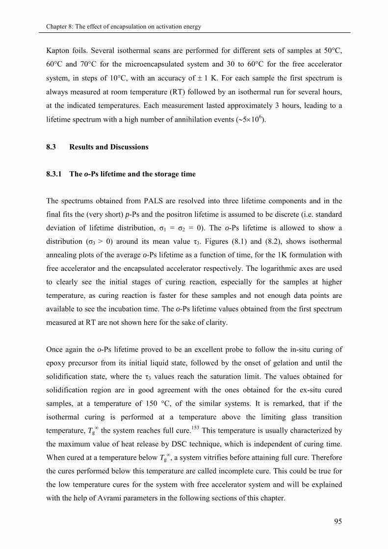
Chapter 8: The effect of encapsulation on activation energy
95
Kapton foils. Several isothermal scans are performed for different sets of samples at 50°C,
60°C and 70°C for the microencapsulated system and 30 to 60°C for the free accelerator
system, in steps of 10°C, with an accuracy of 1 K. For each sample the first spectrum is
always measured at room temperature (RT) followed by an isothermal run for several hours,
at the indicated temperatures. Each measurement lasted approximately 3 hours, leading to a
lifetime spectrum with a high number of annihilation events (5106).
8.3 Results and Discussions
8.3.1 The o-Ps lifetime and the storage time
The spectrums obtained from PALS are resolved into three lifetime components and in the
final fits the (very short) p-Ps and the positron lifetime is assumed to be discrete (i.e. standard
deviation of lifetime distribution, σ1 = σ2 = 0). The o-Ps lifetime is allowed to show a
distribution (σ3 > 0) around its mean value τ3. Figures (8.1) and (8.2), shows isothermal
annealing plots of the average o-Ps lifetime as a function of time, for the 1K formulation with
free accelerator and the encapsulated accelerator respectively. The logarithmic axes are used
to clearly see the initial stages of curing reaction, especially for the samples at higher
temperature, as curing reaction is faster for these samples and not enough data points are
available to see the incubation time. The o-Ps lifetime values obtained from the first spectrum
measured at RT are not shown here for the sake of clarity.
Once again the o-Ps lifetime proved to be an excellent probe to follow the in-situ curing of
epoxy precursor from its initial liquid state, followed by the onset of gelation and until the
solidification state, where the τ3 values reach the saturation limit. The values obtained for
solidification region are in good agreement with the ones obtained for the ex-situ cured
samples, at a temperature of 150 °C, of the similar systems. It is remarked, that if the
isothermal curing is performed at a temperature above the limiting glass transition
temperature, Tg∞ the system reaches full cure.153 This temperature is usually characterized by
the maximum value of heat release by DSC technique, which is independent of curing time.
When cured at a temperature below Tg∞, a system vitrifies before attaining full cure. Therefore
the cures performed below this temperature are called incomplete cure. This could be true for
the low temperature cures for the system with free accelerator system and will be explained
with the help of Avrami parameters in the following sections of this chapter.
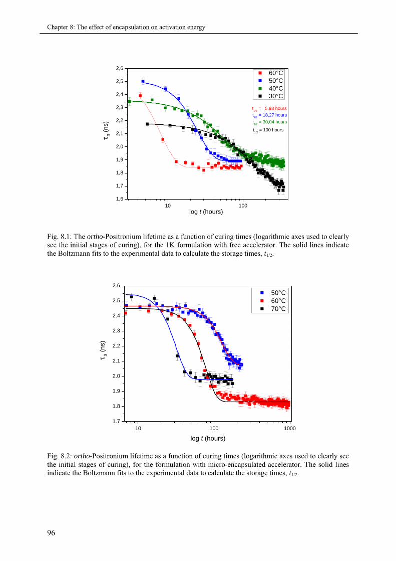
Chapter 8: The effect of encapsulation on activation energy
96
10 100
1,6
1,7
1,8
1,9
2,0
2,1
2,2
2,3
2,4
2,5
2,6
t1/2
= 100 hours
t1/2
= 30,04 hours
t1/2
= 5,98 hours
60°C50°C40°C30°C
3(n
s)
log t (hours)
t1/2
= 18,27 hours
Fig. 8.1: The ortho-Positronium lifetime as a function of curing times (logarithmic axes used to clearlysee the initial stages of curing), for the 1K formulation with free accelerator. The solid lines indicatethe Boltzmann fits to the experimental data to calculate the storage times, t1/2.
10 100 1000
1.7
1.8
1.9
2.0
2.1
2.2
2.3
2.4
2.5
2.6
50°C60°C70°C
3(n
s)
log t (hours)
Fig. 8.2: ortho-Positronium lifetime as a function of curing times (logarithmic axes used to clearly seethe initial stages of curing), for the formulation with micro-encapsulated accelerator. The solid linesindicate the Boltzmann fits to the experimental data to calculate the storage times, t1/2.
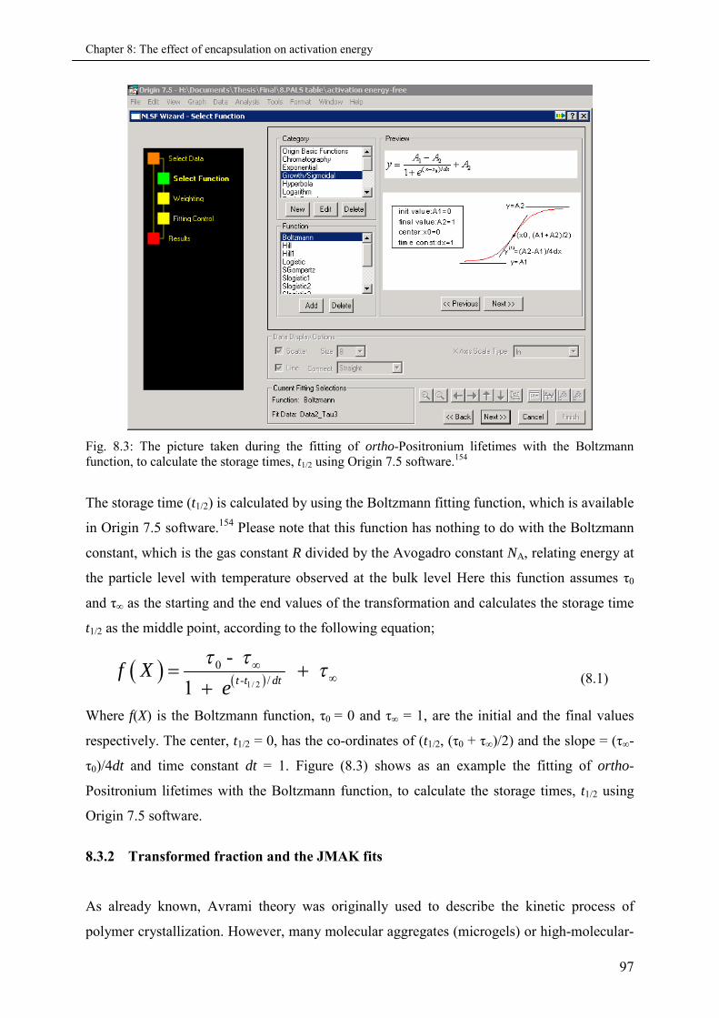
Chapter 8: The effect of encapsulation on activation energy
97
Fig. 8.3: The picture taken during the fitting of ortho-Positronium lifetimes with the Boltzmannfunction, to calculate the storage times, t1/2 using Origin 7.5 software.154
The storage time (t1/2) is calculated by using the Boltzmann fitting function, which is available
in Origin 7.5 software.154 Please note that this function has nothing to do with the Boltzmann
constant, which is the gas constant R divided by the Avogadro constant NA, relating energy at
the particle level with temperature observed at the bulk level Here this function assumes τ0
and τ∞ as the starting and the end values of the transformation and calculates the storage time
t1/2 as the middle point, according to the following equation;
1/ 2
0
- /
-
1t t dt
f Xe
(8.1)
Where f(X) is the Boltzmann function, τ0 = 0 and τ∞ = 1, are the initial and the final values
respectively. The center, t1/2 = 0, has the co-ordinates of (t1/2, (τ0 + τ∞)/2) and the slope = (τ∞-
τ0)/4dt and time constant dt = 1. Figure (8.3) shows as an example the fitting of ortho-
Positronium lifetimes with the Boltzmann function, to calculate the storage times, t1/2 using
Origin 7.5 software.
8.3.2 Transformed fraction and the JMAK fits
As already known, Avrami theory was originally used to describe the kinetic process of
polymer crystallization. However, many molecular aggregates (microgels) or high-molecular-
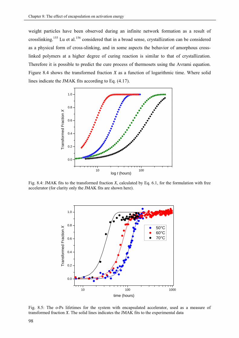
Chapter 8: The effect of encapsulation on activation energy
98
weight particles have been observed during an infinite network formation as a result of
crosslinking.155 Lu et al.156 considered that in a broad sense, crystallization can be considered
as a physical form of cross-slinking, and in some aspects the behavior of amorphous cross-
linked polymers at a higher degree of curing reaction is similar to that of crystallization.
Therefore it is possible to predict the cure process of thermosets using the Avrami equation.
Figure 8.4 shows the transformed fraction X as a function of logarithmic time. Where solid
lines indicate the JMAK fits according to Eq. (4.17).
10 100
0.0
0.2
0.4
0.6
0.8
1.0
log t (hours)
Tra
nsf
orm
ed
Fra
ction
X
Fig. 8.4: JMAK fits to the transformed fraction X, calculated by Eq. 6.1, for the formulation with freeaccelerator (for clarity only the JMAK fits are shown here).
10 100 1000
0.0
0.2
0.4
0.6
0.8
1.0
50°C60°C70°C
Tra
nsfo
rme
dF
ractio
nX
time (hours)
Fig. 8.5: The o-Ps lifetimes for the system with encapsulated accelerator, used as a measure oftransformed fraction X. The solid lines indicates the JMAK fits to the experimental data
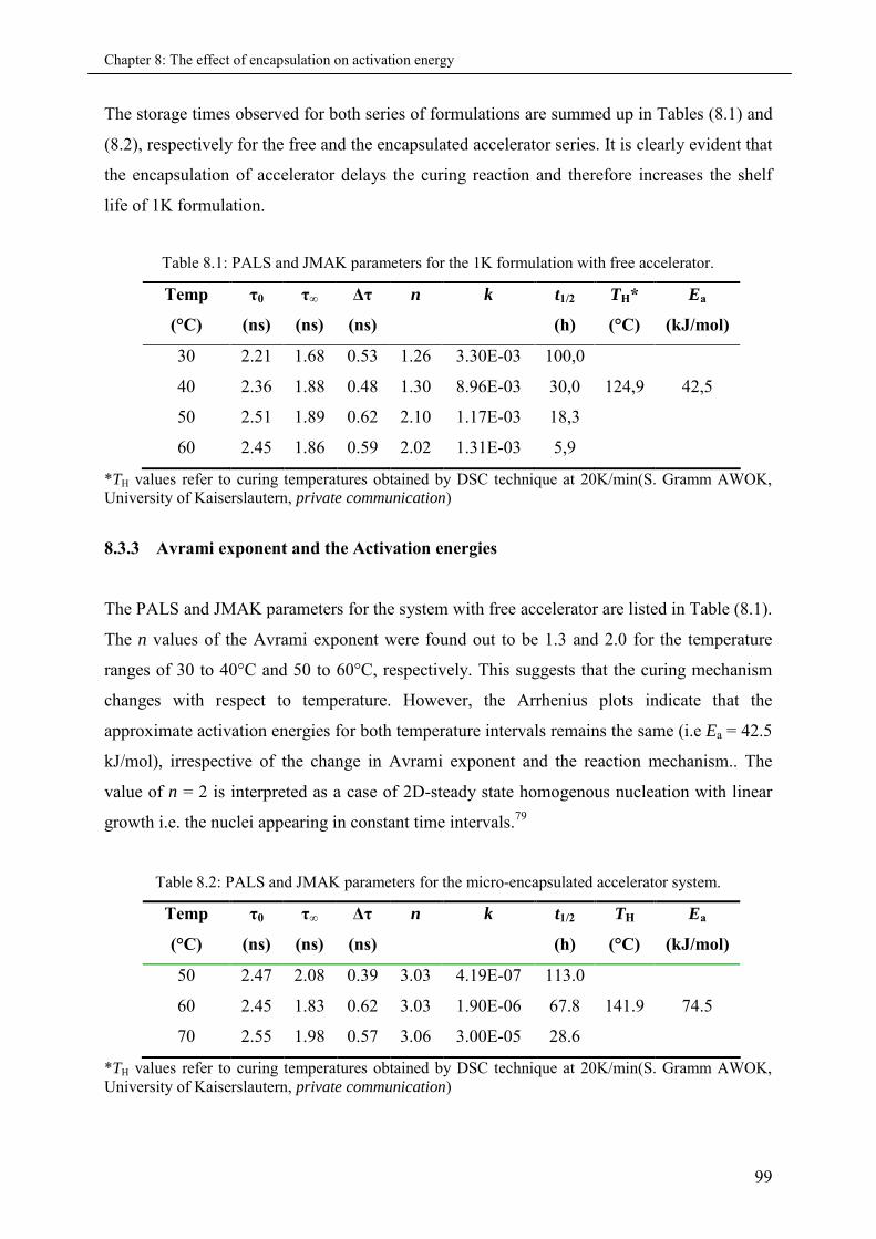
Chapter 8: The effect of encapsulation on activation energy
99
The storage times observed for both series of formulations are summed up in Tables (8.1) and
(8.2), respectively for the free and the encapsulated accelerator series. It is clearly evident that
the encapsulation of accelerator delays the curing reaction and therefore increases the shelf
life of 1K formulation.
Table 8.1: PALS and JMAK parameters for the 1K formulation with free accelerator.
Temp
(°C)
τ0
(ns)
τ∞
(ns)
Δτ
(ns)
n k t1/2
(h)
TH*
(°C)
Ea
(kJ/mol)
30 2.21 1.68 0.53 1.26 3.30E-03 100,0
40 2.36 1.88 0.48 1.30 8.96E-03 30,0 124,9 42,5
50 2.51 1.89 0.62 2.10 1.17E-03 18,3
60 2.45 1.86 0.59 2.02 1.31E-03 5,9
*TH values refer to curing temperatures obtained by DSC technique at 20K/min(S. Gramm AWOK,University of Kaiserslautern, private communication)
8.3.3 Avrami exponent and the Activation energies
The PALS and JMAK parameters for the system with free accelerator are listed in Table (8.1).
The n values of the Avrami exponent were found out to be 1.3 and 2.0 for the temperature
ranges of 30 to 40°C and 50 to 60°C, respectively. This suggests that the curing mechanism
changes with respect to temperature. However, the Arrhenius plots indicate that the
approximate activation energies for both temperature intervals remains the same (i.e Ea = 42.5
kJ/mol), irrespective of the change in Avrami exponent and the reaction mechanism.. The
value of n = 2 is interpreted as a case of 2D-steady state homogenous nucleation with linear
growth i.e. the nuclei appearing in constant time intervals.79
Table 8.2: PALS and JMAK parameters for the micro-encapsulated accelerator system.
Temp
(°C)
τ0
(ns)
τ∞
(ns)
Δτ
(ns)
n k t1/2
(h)
TH
(°C)
Ea
(kJ/mol)
50 2.47 2.08 0.39 3.03 4.19E-07 113.0
60 2.45 1.83 0.62 3.03 1.90E-06 67.8 141.9 74.5
70 2.55 1.98 0.57 3.06 3.00E-05 28.6
*TH values refer to curing temperatures obtained by DSC technique at 20K/min(S. Gramm AWOK,University of Kaiserslautern, private communication)
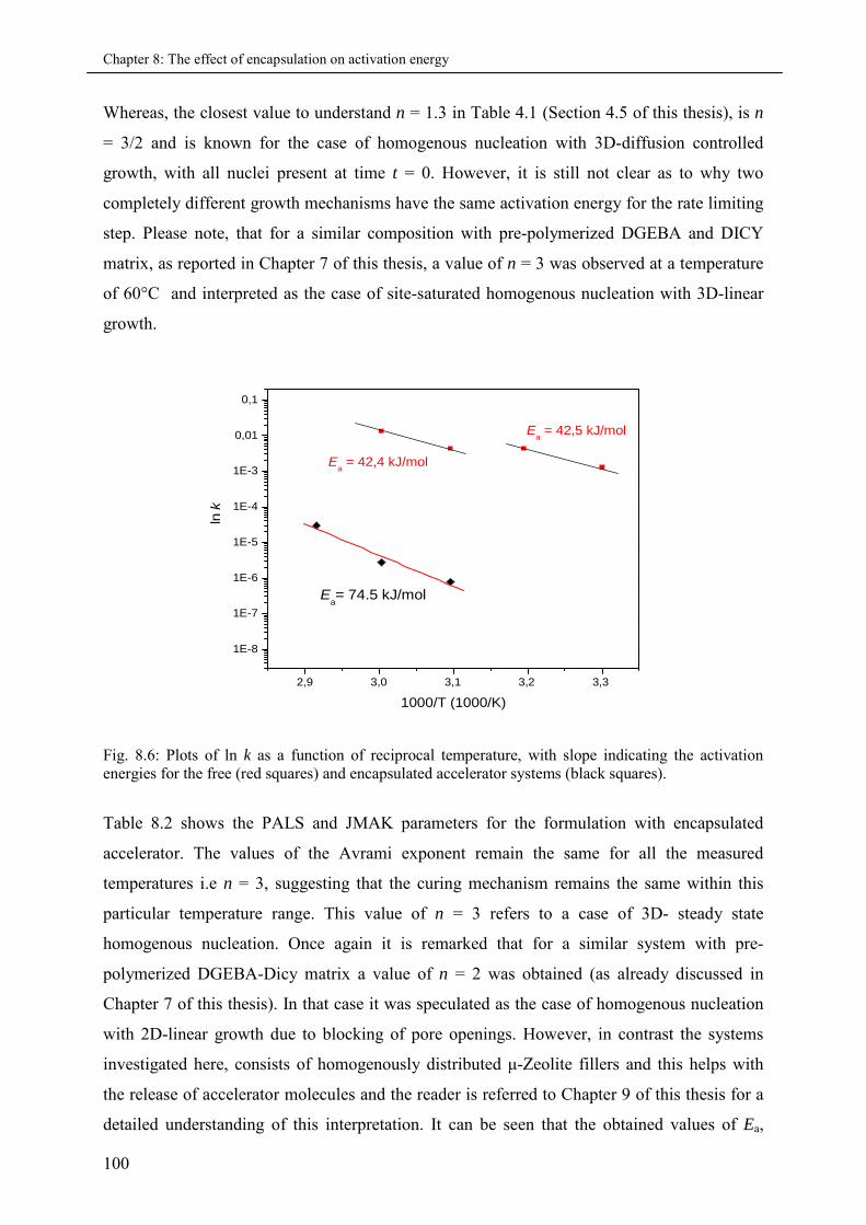
Chapter 8: The effect of encapsulation on activation energy
100
Whereas, the closest value to understand n = 1.3 in Table 4.1 (Section 4.5 of this thesis), is n
= 3/2 and is known for the case of homogenous nucleation with 3D-diffusion controlled
growth, with all nuclei present at time t = 0. However, it is still not clear as to why two
completely different growth mechanisms have the same activation energy for the rate limiting
step. Please note, that for a similar composition with pre-polymerized DGEBA and DICY
matrix, as reported in Chapter 7 of this thesis, a value of n = 3 was observed at a temperature
of 60°C and interpreted as the case of site-saturated homogenous nucleation with 3D-linear
growth.
2,9 3,0 3,1 3,2 3,3
1E-8
1E-7
1E-6
1E-5
1E-4
1E-3
0,01
0,1
lnk
1000/T (1000/K)
Ea= 74.5 kJ/mol
Ea
= 42,5 kJ/mol
Ea
= 42,4 kJ/mol
Fig. 8.6: Plots of ln k as a function of reciprocal temperature, with slope indicating the activationenergies for the free (red squares) and encapsulated accelerator systems (black squares).
Table 8.2 shows the PALS and JMAK parameters for the formulation with encapsulated
accelerator. The values of the Avrami exponent remain the same for all the measured
temperatures i.e n = 3, suggesting that the curing mechanism remains the same within this
particular temperature range. This value of n = 3 refers to a case of 3D- steady state
homogenous nucleation. Once again it is remarked that for a similar system with pre-
polymerized DGEBA-Dicy matrix a value of n = 2 was obtained (as already discussed in
Chapter 7 of this thesis). In that case it was speculated as the case of homogenous nucleation
with 2D-linear growth due to blocking of pore openings. However, in contrast the systems
investigated here, consists of homogenously distributed μ-Zeolite fillers and this helps with
the release of accelerator molecules and the reader is referred to Chapter 9 of this thesis for a
detailed understanding of this interpretation. It can be seen that the obtained values of Ea,
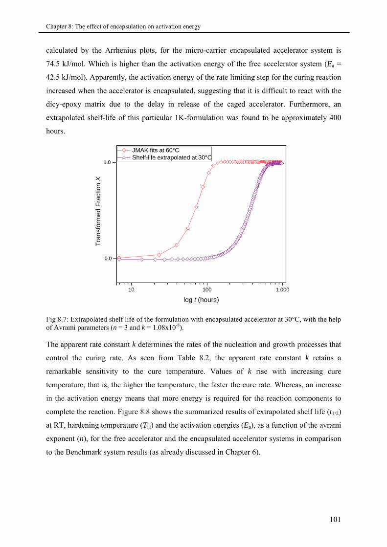
Chapter 8: The effect of encapsulation on activation energy
101
calculated by the Arrhenius plots, for the micro-carrier encapsulated accelerator system is
74.5 kJ/mol. Which is higher than the activation energy of the free accelerator system (Ea =
42.5 kJ/mol). Apparently, the activation energy of the rate limiting step for the curing reaction
increased when the accelerator is encapsulated, suggesting that it is difficult to react with the
dicy-epoxy matrix due to the delay in release of the caged accelerator. Furthermore, an
extrapolated shelf-life of this particular 1K-formulation was found to be approximately 400
hours.
10 100 1.000
1.0
JMAK fits at 60°CShelf-life extrapolated at 30°C
Tra
nsf
orm
ed
Fra
ctio
nX
log t (hours)
0.0
Fig 8.7: Extrapolated shelf life of the formulation with encapsulated accelerator at 30°C, with the helpof Avrami parameters (n = 3 and k = 1.08x10⁻⁸).
The apparent rate constant k determines the rates of the nucleation and growth processes that
control the curing rate. As seen from Table 8.2, the apparent rate constant k retains a
remarkable sensitivity to the cure temperature. Values of k rise with increasing cure
temperature, that is, the higher the temperature, the faster the cure rate. Whereas, an increase
in the activation energy means that more energy is required for the reaction components to
complete the reaction. Figure 8.8 shows the summarized results of extrapolated shelf life (t1/2)
at RT, hardening temperature (TH) and the activation energies (Ea), as a function of the avrami
exponent (n), for the free accelerator and the encapsulated accelerator systems in comparison
to the Benchmark system results (as already discussed in Chapter 6).
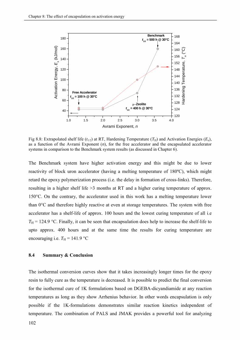
Chapter 8: The effect of encapsulation on activation energy
102
1.0 1.5 2.0 2.5 3.0 3.5 4.0
40
60
80
100
120
140
160
180
120
124
128
132
136
140
144
148
152
156
160
164
168
Free Acceleratort
1/2= 100 h @ 30°C
Zeolitet
1/2= 400 h @ 30°C
Hard
enin
gT
em
pe
ratu
re,T
H(°
C)
Activ
ation
Ene
rgy,E
a(k
J/m
ol)
Avrami Exponent, n
Benchmarkt1/2
= 500 h @ 30°C
Fig 8.8: Extrapolated shelf life (t1/2) at RT, Hardening Temperature (TH) and Activation Energies (Ea),as a function of the Avrami Exponent (n), for the free accelerator and the encapsulated acceleratorsystems in comparison to the Benchmark system results (as discussed in Chapter 6).
The Benchmark system have higher activation energy and this might be due to lower
reactivity of block uron accelerator (having a melting temperature of 180ºC), which might
retard the epoxy polymerization process (i.e. the delay in formation of cross-links). Therefore,
resulting in a higher shelf life >3 months at RT and a higher curing temperature of approx.
150°C. On the contrary, the accelerator used in this work has a melting temperature lower
than 0°C and therefore highly reactive at even at storage temperatures. The system with free
accelerator has a shelf-life of approx. 100 hours and the lowest curing temperature of all i.e
TH = 124.9 °C. Finally, it can be seen that encapsulation does help to increase the shelf-life to
upto approx. 400 hours and at the same time the results for curing temperature are
encouraging i.e. TH = 141.9 °C
8.4 Summary & Conclusion
The isothermal conversion curves show that it takes increasingly longer times for the epoxy
resin to fully cure as the temperature is decreased. It is possible to predict the final conversion
for the isothermal cure of 1K formulations based on DGEBA-dicyandiamide at any reaction
temperatures as long as they show Arrhenius behavior. In other words encapsulation is only
possible if the 1K-formulations demonstrates similar reaction kinetics independent of
temperature. The combination of PALS and JMAK provides a powerful tool for analyzing
Chapter 8: The effect of encapsulation on activation energy
103
cure and cross-linking reactions associated with thermosetting materials. It provides valuable
information on the cure characteristics of 1K formulations, which in turn can be helpful to
produce formulations with higher shelf-life and at the same time with lower hardening
temperatures. The changes in the quantity or chemical constituents of the epoxy system
significantly affect the reaction rate and the degree of cross-linking. Accelerants, retardants,
and other additives affect the reaction process as well. This data of curing kinetics provides
yet another tool for quantifying parameters of 1K-formulations, such as predicting process
rates and estimating product lifetimes. The same approach should be equally useful in
characterizing B-stage prepregs and other curing, vulcanizing, and polymerizing reaction
systems.

Chapter 8: The effect of encapsulation on activation energy
104
Chapter 9: Zeolite and Pyrogenic Silica filled Nanocomposites
105
9. Zeolite and Pyrogenic Silica filled Nanocomposites
In the previous sections of this thesis it was shown that how the hole free volume obtained
from PALS is used as a measure of the transformed fraction of curing. It is also emphasized
that this information can be used to study the curing kinetics of 1K-epoxy formulations with
the help of JMAK theory of phase transformation. Now that the PALS is already established
as a suitable technique to follow the in-situ curing and the shelf-life prediction of one-
component epoxy resin formulations. In this Chapter a brief overview is given on various
series of 1K-formulations, studied by PALS and the JMAK. There were three different types
of carrier materials proposed for the encapsulation of accelerator i.e. Zeolites, pyrogenic silica
and the layered silicates. In the following sections of this thesis only the selected formulations
with Zeolites and pyrogenic silica carriers will be discussed, as due to the time constraints it
was not possible to do the complete research with the layered silicate carriers within the scope
of this PhD thesis. For example, to understand the release behaviour of accelerator, the
concentration of accelerator is varied in a µ-Zeolite carrier and the curing kinetics studied for
constant accelerator concentrations in DICY/EP formulation Furthermore, the effect of micro
and nano-Zeolite encapsulated accelerator as compared to the similar fillers with multi-stage
encapsulation, on the shelf-life at elevated temperatures, the curing kinetics and the hole free
volume is discussed. Whereas, for a constant concentration of accelerator encapsulated in an
pyrogenic silica carrier, the curing kinetics are studied by varying the concentration of the
accelerator in the dicyandiamide cured 1K-formulation.
9.1 Introduction
The term nano-composites means to distribute appropriate amounts of nanoparticles in a
polymer matrix.157 Nanotechnology means that one has to deal with huge surface areas, vast
amounts of nano-fillers, and a small distance between them. Polymeric nano-composites can
be considered as an important category of organic-inorganic hybrid materials, in which
inorganic nanoscale building blocks (e.g., nanoparticles, nanotubes, or nanometer-thick
sheets) are dispersed in an organic polymer matrix.158 They represent the current trend in
developing novel nanostructured materials. When compared to conventional composites
based on micrometer-sized fillers, the interface between the filler particles and the matrix in a
polymer nanocomposite constitutes a much greater area within the bulk material, and hence
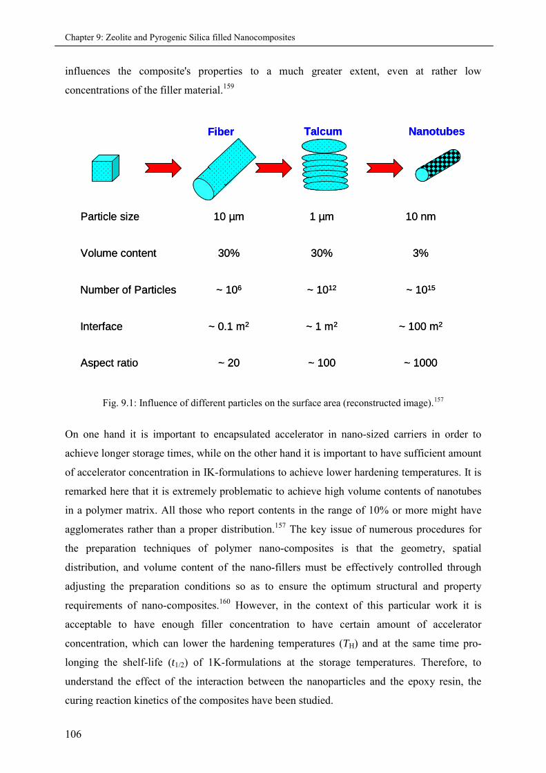
Chapter 9: Zeolite and Pyrogenic Silica filled Nanocomposites
106
influences the composite's properties to a much greater extent, even at rather low
concentrations of the filler material.159
Fiber Talcum NanotubesFiber Talcum Nanotubes
~ 1000~ 100~ 20Aspect ratio
~ 100 m2~ 1 m2~ 0.1 m2Interface
~ 1015~ 1012~ 106Number of Particles
3%30%30%Volume content
10 nm1 µm10 µmParticle size
~ 1000~ 100~ 20Aspect ratio
~ 100 m2~ 1 m2~ 0.1 m2Interface
~ 1015~ 1012~ 106Number of Particles
3%30%30%Volume content
10 nm1 µm10 µmParticle size
Fig. 9.1: Influence of different particles on the surface area (reconstructed image).157
On one hand it is important to encapsulated accelerator in nano-sized carriers in order to
achieve longer storage times, while on the other hand it is important to have sufficient amount
of accelerator concentration in IK-formulations to achieve lower hardening temperatures. It is
remarked here that it is extremely problematic to achieve high volume contents of nanotubes
in a polymer matrix. All those who report contents in the range of 10% or more might have
agglomerates rather than a proper distribution.157 The key issue of numerous procedures for
the preparation techniques of polymer nano-composites is that the geometry, spatial
distribution, and volume content of the nano-fillers must be effectively controlled through
adjusting the preparation conditions so as to ensure the optimum structural and property
requirements of nano-composites.160 However, in the context of this particular work it is
acceptable to have enough filler concentration to have certain amount of accelerator
concentration, which can lower the hardening temperatures (TH) and at the same time pro-
longing the shelf-life (t1/2) of 1K-formulations at the storage temperatures. Therefore, to
understand the effect of the interaction between the nanoparticles and the epoxy resin, the
curing reaction kinetics of the composites have been studied.
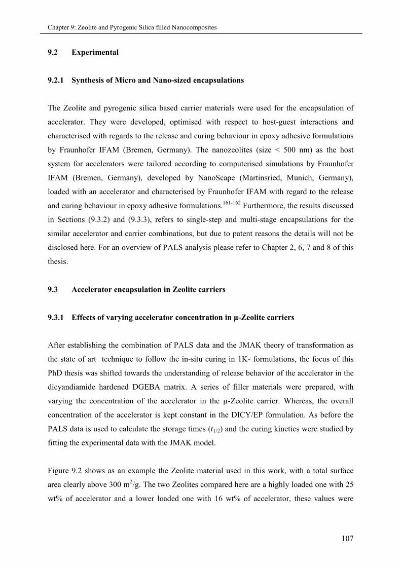
Chapter 9: Zeolite and Pyrogenic Silica filled Nanocomposites
107
9.2 Experimental
9.2.1 Synthesis of Micro and Nano-sized encapsulations
The Zeolite and pyrogenic silica based carrier materials were used for the encapsulation of
accelerator. They were developed, optimised with respect to host-guest interactions and
characterised with regards to the release and curing behaviour in epoxy adhesive formulations
by Fraunhofer IFAM (Bremen, Germany). The nanozeolites (size < 500 nm) as the host
system for accelerators were tailored according to computerised simulations by Fraunhofer
IFAM (Bremen, Germany), developed by NanoScape (Martinsried, Munich, Germany),
loaded with an accelerator and characterised by Fraunhofer IFAM with regard to the release
and curing behaviour in epoxy adhesive formulations.161-162 Furthermore, the results discussed
in Sections (9.3.2) and (9.3.3), refers to single-step and multi-stage encapsulations for the
similar accelerator and carrier combinations, but due to patent reasons the details will not be
disclosed here. For an overview of PALS analysis please refer to Chapter 2, 6, 7 and 8 of this
thesis.
9.3 Accelerator encapsulation in Zeolite carriers
9.3.1 Effects of varying accelerator concentration in µ-Zeolite carriers
After establishing the combination of PALS data and the JMAK theory of transformation as
the state of art technique to follow the in-situ curing in 1K- formulations, the focus of this
PhD thesis was shifted towards the understanding of release behavior of the accelerator in the
dicyandiamide hardened DGEBA matrix. A series of filler materials were prepared, with
varying the concentration of the accelerator in the µ-Zeolite carrier. Whereas, the overall
concentration of the accelerator is kept constant in the DICY/EP formulation. As before the
PALS data is used to calculate the storage times (t1/2) and the curing kinetics were studied by
fitting the experimental data with the JMAK model.
Figure 9.2 shows as an example the Zeolite material used in this work, with a total surface
area clearly above 300 m2/g. The two Zeolites compared here are a highly loaded one with 25
wt% of accelerator and a lower loaded one with 16 wt% of accelerator, these values were
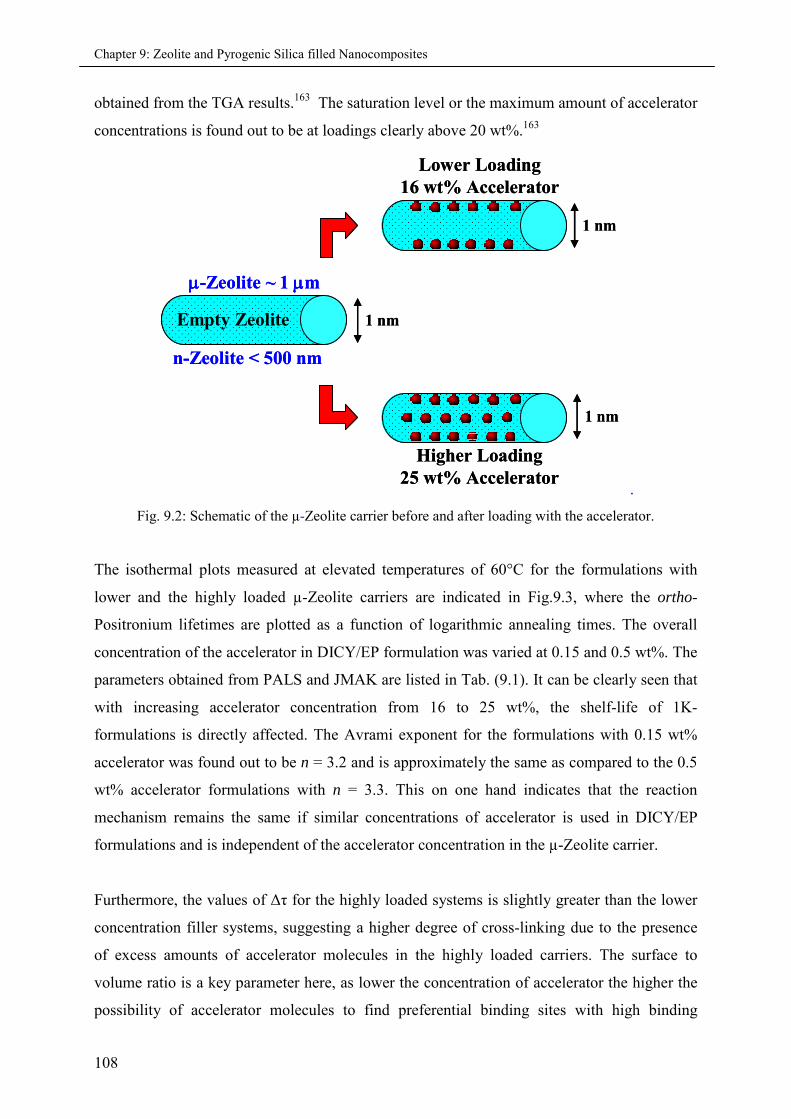
Chapter 9: Zeolite and Pyrogenic Silica filled Nanocomposites
108
obtained from the TGA results.163 The saturation level or the maximum amount of accelerator
concentrations is found out to be at loadings clearly above 20 wt%.163
Lower Loading16 wt% Accelerator
Higher Loading25 wt% Accelerator
n-Zeolite < 500 nm
Empty Zeolite 1 nm
1 nm
1 nm
-Zeolite ~ 1 m
Lower Loading16 wt% Accelerator
Higher Loading25 wt% Accelerator
n-Zeolite < 500 nm
Empty Zeolite 1 nm
1 nm
1 nm
-Zeolite ~ 1 m
.
Fig. 9.2: Schematic of the µ-Zeolite carrier before and after loading with the accelerator.
The isothermal plots measured at elevated temperatures of 60°C for the formulations with
lower and the highly loaded µ-Zeolite carriers are indicated in Fig.9.3, where the ortho-
Positronium lifetimes are plotted as a function of logarithmic annealing times. The overall
concentration of the accelerator in DICY/EP formulation was varied at 0.15 and 0.5 wt%. The
parameters obtained from PALS and JMAK are listed in Tab. (9.1). It can be clearly seen that
with increasing accelerator concentration from 16 to 25 wt%, the shelf-life of 1K-
formulations is directly affected. The Avrami exponent for the formulations with 0.15 wt%
accelerator was found out to be n = 3.2 and is approximately the same as compared to the 0.5
wt% accelerator formulations with n = 3.3. This on one hand indicates that the reaction
mechanism remains the same if similar concentrations of accelerator is used in DICY/EP
formulations and is independent of the accelerator concentration in the µ-Zeolite carrier.
Furthermore, the values of Δτ for the highly loaded systems is slightly greater than the lower
concentration filler systems, suggesting a higher degree of cross-linking due to the presence
of excess amounts of accelerator molecules in the highly loaded carriers. The surface to
volume ratio is a key parameter here, as lower the concentration of accelerator the higher the
possibility of accelerator molecules to find preferential binding sites with high binding
Chapter 9: Zeolite and Pyrogenic Silica filled Nanocomposites
109
energies, within the carrier material. As for the case of highly loaded Zeolite carrier with 25
wt% of accelerator concentration, the excess molecules of accelerator are free to react with
the DICY/EP matrix once the filler material is dispersed in the matrix. This has two
disadvantages, firstly there is no controlled release and secondly this will reduced the shelf-
life of the 1K-formulations, as indicated by the results in Tab. 9.1.
10 100
1,8
2,0
2,2
2,4
2,6
10 10010 10010 100
(n
s)
log t (hours)
0.15wt% Acc. in DICY/EP (fully loaded) at 60°C
0.5wt% Acc. in DICY/EP (fully loaded) at 60°C0.15wt% Acc. in DICY/EP (partially loaded) at 60°C
Fig. 9.3: The ortho-Positronium lifetime as a function of isothermal annealing time for the partiallyand the fully loaded accelerator in µ-Zeolite carrier at elevated temperatures of 60 °C.
Table 9.1: PALS and JMAK parameters for the partially and the fully loaded µ-Zeolite carriers.
Accelerator in
µ-Zeolite
Accelerator in
DICY/EP
τ0 τ∞ Δτ n k t1/2
(h)
16 wt% 0.15 wt% 2.48 1.94 0.54 3.20 2.29E-08 218,
16 wt% 0.5 wt% 2.48 1.95 0.53 3.30 1.35E-08 38,
25 wt% 0.15 wt% 2.59 2.01 0.58 3.21 1.44E-08 243,
25 wt% 0.5 wt% 2.56 1.95 0.61 3.29 2.00E-05 24,
Furthermore, a series of experiments were performed to understand the release behavior of the
accelerator with respect to different loading concentrations of accelerator in the µ-Zeolite
carrier. Once again isothermal annealing is done at elevated temperature of 60 °C and in order to have
a better comparison the concentration of accelerator was kept constant at 0.5 wt% in the DICY/EP
formulations. Figure 9.4 shows the o-Ps lifetime as a function of annealing time for the complete
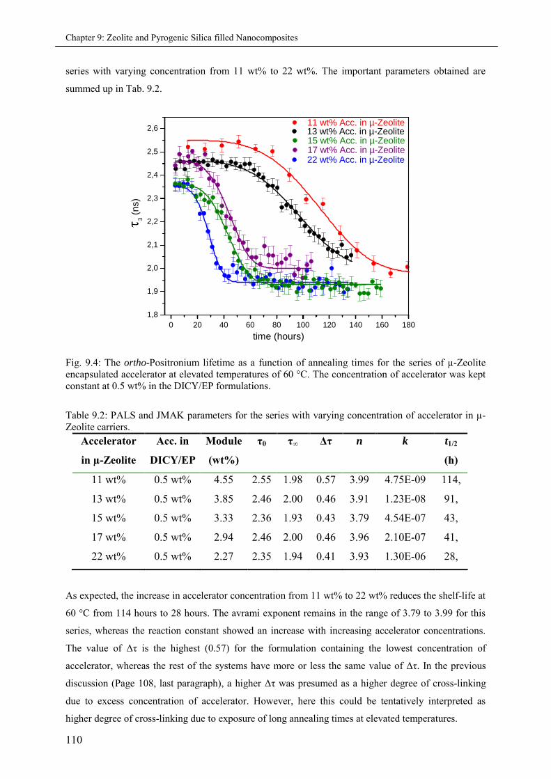
Chapter 9: Zeolite and Pyrogenic Silica filled Nanocomposites
110
series with varying concentration from 11 wt% to 22 wt%. The important parameters obtained are
summed up in Tab. 9.2.
0 20 40 60 80 100 120 140 160 180
1,8
1,9
2,0
2,1
2,2
2,3
2,4
2,5
2,6 3
(ns)
time (hours)
11 wt% Acc. in µ-Zeolite13 wt% Acc. in µ-Zeolite
22 wt% Acc. in µ-Zeolite17 wt% Acc. in µ-Zeolite15 wt% Acc. in µ-Zeolite
Fig. 9.4: The ortho-Positronium lifetime as a function of annealing times for the series of µ-Zeoliteencapsulated accelerator at elevated temperatures of 60 °C. The concentration of accelerator was keptconstant at 0.5 wt% in the DICY/EP formulations.
Table 9.2: PALS and JMAK parameters for the series with varying concentration of accelerator in µ-Zeolite carriers.
Accelerator
in µ-Zeolite
Acc. in
DICY/EP
Module
(wt%)
τ0 τ∞ Δτ n k t1/2
(h)
11 wt% 0.5 wt% 4.55 2.55 1.98 0.57 3.99 4.75E-09 114,
13 wt% 0.5 wt% 3.85 2.46 2.00 0.46 3.91 1.23E-08 91,
15 wt% 0.5 wt% 3.33 2.36 1.93 0.43 3.79 4.54E-07 43,
17 wt% 0.5 wt% 2.94 2.46 2.00 0.46 3.96 2.10E-07 41,
22 wt% 0.5 wt% 2.27 2.35 1.94 0.41 3.93 1.30E-06 28,
As expected, the increase in accelerator concentration from 11 wt% to 22 wt% reduces the shelf-life at
60 °C from 114 hours to 28 hours. The avrami exponent remains in the range of 3.79 to 3.99 for this
series, whereas the reaction constant showed an increase with increasing accelerator concentrations.
The value of Δτ is the highest (0.57) for the formulation containing the lowest concentration of
accelerator, whereas the rest of the systems have more or less the same value of Δτ. In the previous
discussion (Page 108, last paragraph), a higher Δτ was presumed as a higher degree of cross-linking
due to excess concentration of accelerator. However, here this could be tentatively interpreted as
higher degree of cross-linking due to exposure of long annealing times at elevated temperatures.
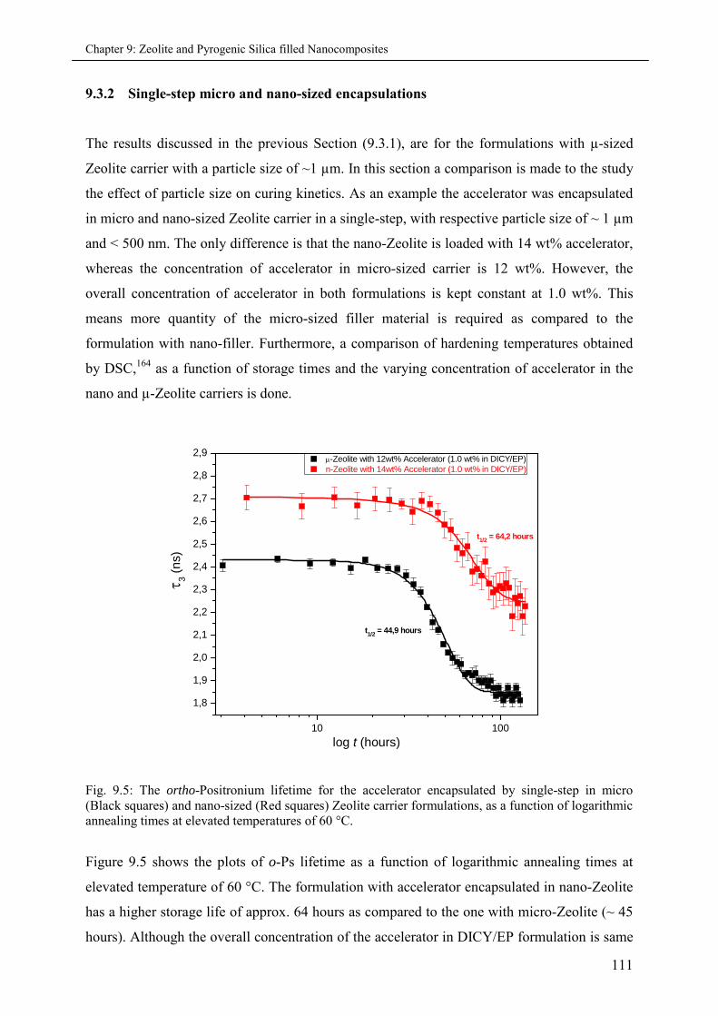
Chapter 9: Zeolite and Pyrogenic Silica filled Nanocomposites
111
9.3.2 Single-step micro and nano-sized encapsulations
The results discussed in the previous Section (9.3.1), are for the formulations with µ-sized
Zeolite carrier with a particle size of ~1 µm. In this section a comparison is made to the study
the effect of particle size on curing kinetics. As an example the accelerator was encapsulated
in micro and nano-sized Zeolite carrier in a single-step, with respective particle size of ~ 1 µm
and < 500 nm. The only difference is that the nano-Zeolite is loaded with 14 wt% accelerator,
whereas the concentration of accelerator in micro-sized carrier is 12 wt%. However, the
overall concentration of accelerator in both formulations is kept constant at 1.0 wt%. This
means more quantity of the micro-sized filler material is required as compared to the
formulation with nano-filler. Furthermore, a comparison of hardening temperatures obtained
by DSC,164 as a function of storage times and the varying concentration of accelerator in the
nano and µ-Zeolite carriers is done.
10 100
1,8
1,9
2,0
2,1
2,2
2,3
2,4
2,5
2,6
2,7
2,8
2,9
t1/2
= 64,2 hours
-Zeolite with 12wt% Accelerator (1.0 wt% in DICY/EP)n-Zeolite with 14wt% Accelerator (1.0 wt% in DICY/EP)
3(n
s)
log t (hours)
t1/2
= 44,9 hours
Fig. 9.5: The ortho-Positronium lifetime for the accelerator encapsulated by single-step in micro(Black squares) and nano-sized (Red squares) Zeolite carrier formulations, as a function of logarithmicannealing times at elevated temperatures of 60 °C.
Figure 9.5 shows the plots of o-Ps lifetime as a function of logarithmic annealing times at
elevated temperature of 60 °C. The formulation with accelerator encapsulated in nano-Zeolite
has a higher storage life of approx. 64 hours as compared to the one with micro-Zeolite (~ 45
hours). Although the overall concentration of the accelerator in DICY/EP formulation is same
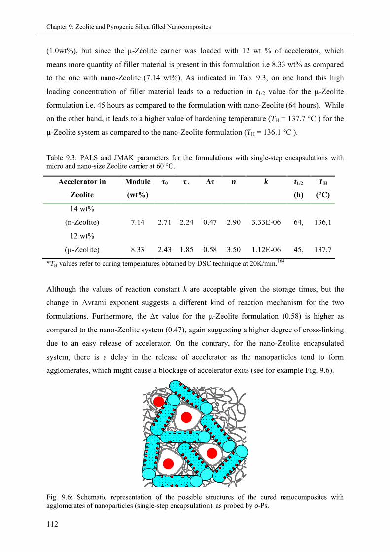
Chapter 9: Zeolite and Pyrogenic Silica filled Nanocomposites
112
(1.0wt%), but since the µ-Zeolite carrier was loaded with 12 wt % of accelerator, which
means more quantity of filler material is present in this formulation i.e 8.33 wt% as compared
to the one with nano-Zeolite (7.14 wt%). As indicated in Tab. 9.3, on one hand this high
loading concentration of filler material leads to a reduction in t1/2 value for the µ-Zeolite
formulation i.e. 45 hours as compared to the formulation with nano-Zeolite (64 hours). While
on the other hand, it leads to a higher value of hardening temperature (TH = 137.7 °C ) for the
µ-Zeolite system as compared to the nano-Zeolite formulation (TH = 136.1 °C ).
Table 9.3: PALS and JMAK parameters for the formulations with single-step encapsulations withmicro and nano-size Zeolite carrier at 60 °C.
*TH values refer to curing temperatures obtained by DSC technique at 20K/min.164
Although the values of reaction constant k are acceptable given the storage times, but the
change in Avrami exponent suggests a different kind of reaction mechanism for the two
formulations. Furthermore, the Δτ value for the µ-Zeolite formulation (0.58) is higher as
compared to the nano-Zeolite system (0.47), again suggesting a higher degree of cross-linking
due to an easy release of accelerator. On the contrary, for the nano-Zeolite encapsulated
system, there is a delay in the release of accelerator as the nanoparticles tend to form
agglomerates, which might cause a blockage of accelerator exits (see for example Fig. 9.6).
Fig. 9.6: Schematic representation of the possible structures of the cured nanocomposites withagglomerates of nanoparticles (single-step encapsulation), as probed by o-Ps.
Accelerator in
Zeolite
Module
(wt%)
τ0 τ∞ Δτ n k t1/2
(h)
TH
(°C)
14 wt%
(n-Zeolite) 7.14 2.71 2.24 0.47 2.90 3.33E-06 64, 136,1
12 wt%
(µ-Zeolite) 8.33 2.43 1.85 0.58 3.50 1.12E-06 45, 137,7
Chapter 9: Zeolite and Pyrogenic Silica filled Nanocomposites
113
Interestingly, the τ0 and τ∞ values for the system with nano-Zeolite are considerably higher as
compared to the formulation with µ-Zeolite. This reconfirms the above-mentioned
interporetation, that the nano-filler particles tend to form agglomerates when dispersed in the
epoxy matrix and therefore resulting in higher τ0 and τ∞ values. It is noteworthy that the
problem with dispersive mixing is that the nanoparticles commercially available usually exist
in the form of agglomerates, which are difficult to disconnect by the limited shear force
during mixing. This is true even when a coupling agent is used,165 since it can only react with
the nanoparticles on the surface of the agglomerates. The latter will maintain their friable
structure in the composite and can hardly provide property improvements at all. Even the
higher value of storage time t1/2, for the nano-Zeolite based formulation as compared to the µ-
Zeolite system, agrees with this speculation of agglomerates formation. Since their will be a
delay in the release of accelerator due to blockage of pore openings and therefore results in an
increased shelf-life.
9.3.3 Multi-stage micro and nano-Zeolite encapsulations
Another possibility of achieving even higher storage life is by closing the pore mouths of the
Zeolite carrier with the help of multi-stage encapsulations. Even the positive effects of
nanoparticles can be brought into play if nanoparticle agglomerates themselves are reinforced
prior to the compounding procedure, since a further promotion of the dispersion by existing
methods might be too ideal to be realized. Nanoparticles can be pretreated to introduce
grafting polymers onto their surface not only outside but also inside the particle agglomerates.
Owing to their low molecular weight, the monomers can penetrate into the agglomerated
nanoparticles easily and react with the activated sites of the latters. The interstitial volume
inside the nanoparticle agglomerates will be partly filled with grafting macromolecular
chains, and the agglomerated nanoparticles will be even closer, therefore reducing the size of
big voids between them. In addition, the surface of the nanoparticles will also become
"hydrocarbonated" due to an increased hydrophobicity resulting from the grafting polymer.
This is beneficial for the filler/matrix miscibility and hence for the ultimate properties.166
When the pre-grafted nanoparticles are mixed with the melt of a thermoplastic polymer, the
filler/matrix interfacial adhesion can be improved by the grafting polymers chemically bonded
onto the nanoparticles, in particular by creating entanglements with the matrix molecules
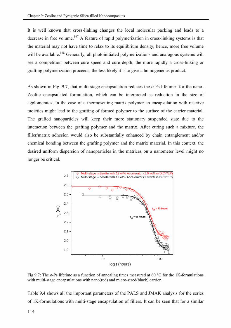
Chapter 9: Zeolite and Pyrogenic Silica filled Nanocomposites
114
It is well known that cross-linking changes the local molecular packing and leads to a
decrease in free volume.167 A feature of rapid polymerization in cross-linking systems is that
the material may not have time to relax to its equilibrium density; hence, more free volume
will be available.168 Generally, all photoinitiated polymerizations and analogous systems will
see a competition between cure speed and cure depth; the more rapidly a cross-linking or
grafting polymerization proceeds, the less likely it is to give a homogeneous product.
As shown in Fig. 9.7, that multi-stage encapsulation reduces the o-Ps lifetimes for the nano-
Zeolite encapsulated formulation, which can be interpreted as reduction in the size of
agglomerates. In the case of a thermosetting matrix polymer an encapsulation with reactive
moieties might lead to the grafting of formed polymer to the surface of the carrier material.
The grafted nanoparticles will keep their more stationary suspended state due to the
interaction between the grafting polymer and the matrix. After curing such a mixture, the
filler/matrix adhesion would also be substantially enhanced by chain entanglement and/or
chemical bonding between the grafting polymer and the matrix material. In this context, the
desired uniform dispersion of nanoparticles in the matrices on a nanometer level might no
longer be critical.
10 100
1,9
2,0
2,1
2,2
2,3
2,4
2,5
2,6
2,7Multi-stage n-Zeolite with 12 wt% Accelerator (1.0 wt% in DICY/EP)Multi-stage -Zeolite with 12 wt% Accelerator (1.0 wt% in DICY/EP)
log t (hours)
t1/2
= 65 hours
t1/2
= 70 hours
3(n
s)
Fig 9.7: The o-Ps lifetime as a function of annealing times measured at 60 °C for the 1K-formulationswith multi-stage encapsulations with nano(red) and micro-sized(black) carrier.
Table 9.4 shows all the important parameters of the PALS and JMAK analysis for the series
of 1K-formulations with multi-stage encapsulation of fillers. It can be seen that for a similar
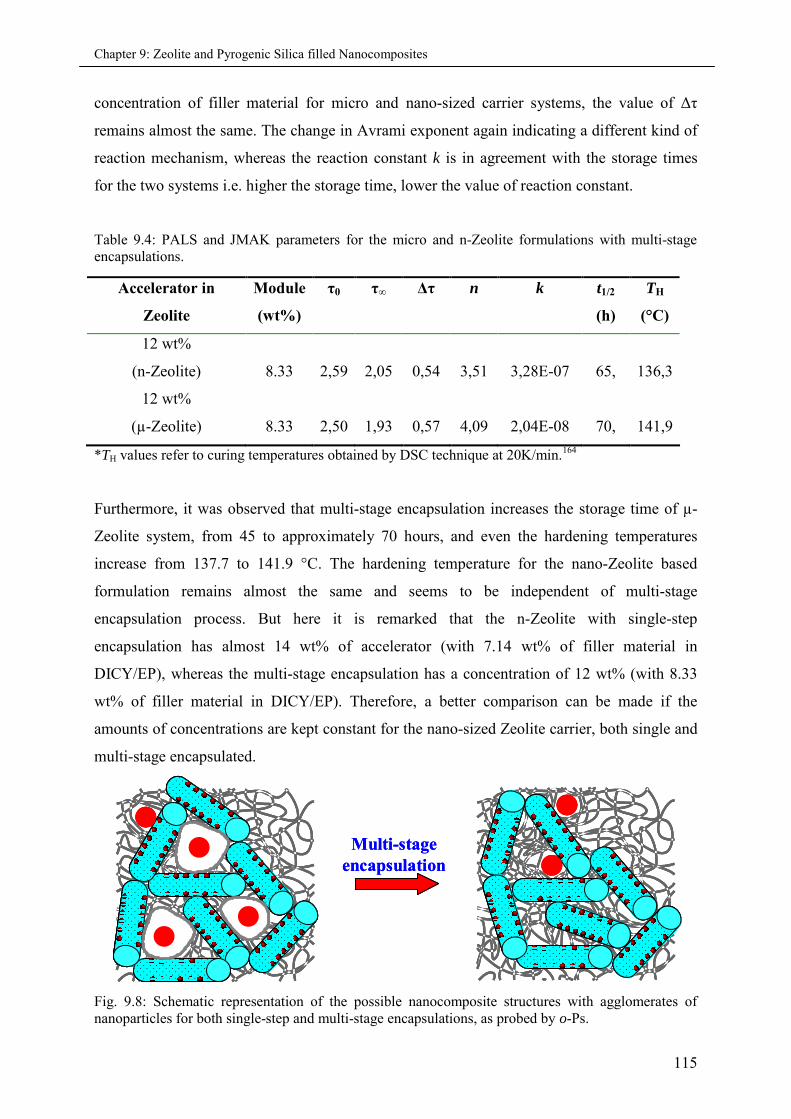
Chapter 9: Zeolite and Pyrogenic Silica filled Nanocomposites
115
concentration of filler material for micro and nano-sized carrier systems, the value of Δτ
remains almost the same. The change in Avrami exponent again indicating a different kind of
reaction mechanism, whereas the reaction constant k is in agreement with the storage times
for the two systems i.e. higher the storage time, lower the value of reaction constant.
Table 9.4: PALS and JMAK parameters for the micro and n-Zeolite formulations with multi-stageencapsulations.
*TH values refer to curing temperatures obtained by DSC technique at 20K/min.164
Furthermore, it was observed that multi-stage encapsulation increases the storage time of µ-
Zeolite system, from 45 to approximately 70 hours, and even the hardening temperatures
increase from 137.7 to 141.9 °C. The hardening temperature for the nano-Zeolite based
formulation remains almost the same and seems to be independent of multi-stage
encapsulation process. But here it is remarked that the n-Zeolite with single-step
encapsulation has almost 14 wt% of accelerator (with 7.14 wt% of filler material in
DICY/EP), whereas the multi-stage encapsulation has a concentration of 12 wt% (with 8.33
wt% of filler material in DICY/EP). Therefore, a better comparison can be made if the
amounts of concentrations are kept constant for the nano-sized Zeolite carrier, both single and
multi-stage encapsulated.
Multi-stageencapsulation
Multi-stageencapsulation
Fig. 9.8: Schematic representation of the possible nanocomposite structures with agglomerates ofnanoparticles for both single-step and multi-stage encapsulations, as probed by o-Ps.
Accelerator in
Zeolite
Module
(wt%)
τ0 τ∞ Δτ n k t1/2
(h)
TH
(°C)
12 wt%
(n-Zeolite) 8.33 2,59 2,05 0,54 3,51 3,28E-07 65, 136,3
12 wt%
(µ-Zeolite) 8.33 2,50 1,93 0,57 4,09 2,04E-08 70, 141,9
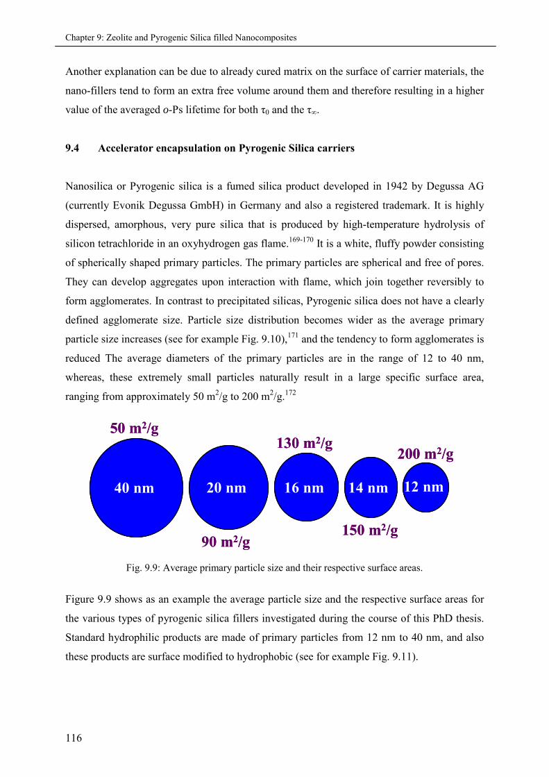
Chapter 9: Zeolite and Pyrogenic Silica filled Nanocomposites
116
Another explanation can be due to already cured matrix on the surface of carrier materials, the
nano-fillers tend to form an extra free volume around them and therefore resulting in a higher
value of the averaged o-Ps lifetime for both τ0 and the τ∞.
9.4 Accelerator encapsulation on Pyrogenic Silica carriers
Nanosilica or Pyrogenic silica is a fumed silica product developed in 1942 by Degussa AG
(currently Evonik Degussa GmbH) in Germany and also a registered trademark. It is highly
dispersed, amorphous, very pure silica that is produced by high-temperature hydrolysis of
silicon tetrachloride in an oxyhydrogen gas flame.169-170 It is a white, fluffy powder consisting
of spherically shaped primary particles. The primary particles are spherical and free of pores.
They can develop aggregates upon interaction with flame, which join together reversibly to
form agglomerates. In contrast to precipitated silicas, Pyrogenic silica does not have a clearly
defined agglomerate size. Particle size distribution becomes wider as the average primary
particle size increases (see for example Fig. 9.10),171 and the tendency to form agglomerates is
reduced The average diameters of the primary particles are in the range of 12 to 40 nm,
whereas, these extremely small particles naturally result in a large specific surface area,
ranging from approximately 50 m2/g to 200 m2/g.172
40 nm 20 nm 16 nm 14 nm 12 nm
50 m2/g
90 m2/g
130 m2/g
150 m2/g
200 m2/g
40 nm 20 nm 16 nm 14 nm 12 nm
50 m2/g
90 m2/g
130 m2/g
150 m2/g
200 m2/g
Fig. 9.9: Average primary particle size and their respective surface areas.
Figure 9.9 shows as an example the average particle size and the respective surface areas for
the various types of pyrogenic silica fillers investigated during the course of this PhD thesis.
Standard hydrophilic products are made of primary particles from 12 nm to 40 nm, and also
these products are surface modified to hydrophobic (see for example Fig. 9.11).
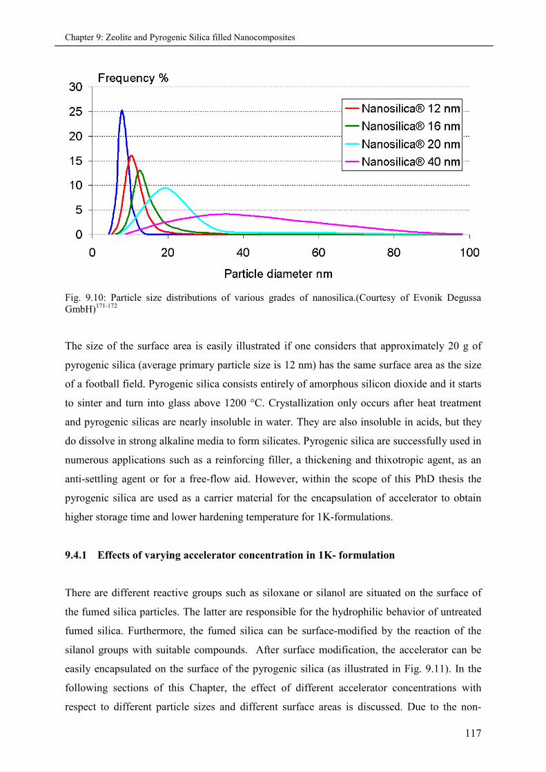
Chapter 9: Zeolite and Pyrogenic Silica filled Nanocomposites
117
Fig. 9.10: Particle size distributions of various grades of nanosilica.(Courtesy of Evonik DegussaGmbH)171-172
The size of the surface area is easily illustrated if one considers that approximately 20 g of
pyrogenic silica (average primary particle size is 12 nm) has the same surface area as the size
of a football field. Pyrogenic silica consists entirely of amorphous silicon dioxide and it starts
to sinter and turn into glass above 1200 °C. Crystallization only occurs after heat treatment
and pyrogenic silicas are nearly insoluble in water. They are also insoluble in acids, but they
do dissolve in strong alkaline media to form silicates. Pyrogenic silica are successfully used in
numerous applications such as a reinforcing filler, a thickening and thixotropic agent, as an
anti-settling agent or for a free-flow aid. However, within the scope of this PhD thesis the
pyrogenic silica are used as a carrier material for the encapsulation of accelerator to obtain
higher storage time and lower hardening temperature for 1K-formulations.
9.4.1 Effects of varying accelerator concentration in 1K- formulation
There are different reactive groups such as siloxane or silanol are situated on the surface of
the fumed silica particles. The latter are responsible for the hydrophilic behavior of untreated
fumed silica. Furthermore, the fumed silica can be surface-modified by the reaction of the
silanol groups with suitable compounds. After surface modification, the accelerator can be
easily encapsulated on the surface of the pyrogenic silica (as illustrated in Fig. 9.11). In the
following sections of this Chapter, the effect of different accelerator concentrations with
respect to different particle sizes and different surface areas is discussed. Due to the non-
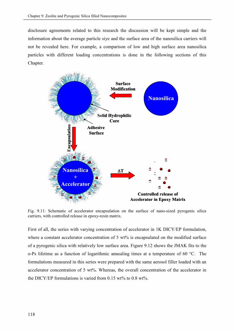
Chapter 9: Zeolite and Pyrogenic Silica filled Nanocomposites
118
disclosure agreements related to this research the discussion will be kept simple and the
information about the average particle siye and the surface area of the nanosilica carriers will
not be revealed here. For example, a comparison of low and high surface area nanosilica
particles with different loading concentrations is done in the following sections of this
Chapter.
Solid HydrophilicCore
AdhesiveSurface
Nanosilica+
Accelerator
T
Controlled release ofAccelerator in Epoxy Matrix
SurfaceModification
En
cap
sula
tio
n
Nanosilica
Solid HydrophilicCore
AdhesiveSurface
Nanosilica+
Accelerator
T
Controlled release ofAccelerator in Epoxy Matrix
SurfaceModification
En
cap
sula
tio
n
Nanosilica
Fig. 9.11: Schematic of accelerator encapsulation on the surface of nano-sized pyrogenic silicacarriers, with controlled release in epoxy-resin matrix.
First of all, the series with varying concentration of accelerator in 1K DICY/EP formulation,
where a constant accelerator concentration of 5 wt% is encapsulated on the modified surface
of a pyrogenic silica with relatively low surface area. Figure 9.12 shows the JMAK fits to the
o-Ps lifetime as a function of logarithmic annealing times at a temperature of 60 °C. The
formulations measured in this series were prepared with the same aerosol filler loaded with an
accelerator concentration of 5 wt%. Whereas, the overall concentration of the accelerator in
the DICY/EP formulations is varied from 0.15 wt% to 0.8 wt%.
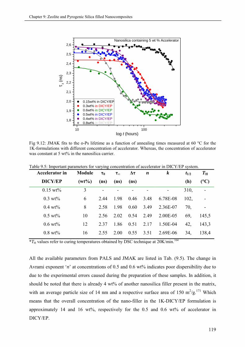
Chapter 9: Zeolite and Pyrogenic Silica filled Nanocomposites
119
10 100
1,8
1,9
2,0
2,1
2,2
2,3
2,4
2,5
2,6
0.15wt% in DICY/EP0.3wt% in DICY/EP0.6wt% in DICY/EP0.5wt% in DICY/EP0.4wt% in DICY/EP0.8wt% in DICY/EP
3(n
s)
log t (hours)
Nanosilica containing 5 wt % Accelerator
Fig 9.12: JMAK fits to the o-Ps lifetime as a function of annealing times measured at 60 °C for the1K-formulations with different concentration of accelerator. Whereas, the concentration of acceleratorwas constant at 5 wt% in the nanosilica carrier.
Table 9.5: Important parameters for varying concentration of accelerator in DICY/EP system.
Accelerator in
DICY/EP
Module
(wt%)
τ0
(ns)
τ∞
(ns)
Δτ
(ns)
n k t1/2
(h)
TH
(°C)
0.15 wt% 3 - - - - - 310, -
0.3 wt% 6 2.44 1.98 0.46 3.48 6.78E-08 102, -
0.4 wt% 8 2.58 1.98 0.60 3.49 2.36E-07 70, -
0.5 wt% 10 2.56 2.02 0.54 2.49 2.00E-05 69, 145,5
0.6 wt% 12 2.37 1.86 0.51 2.17 1.50E-04 42, 143,3
0.8 wt% 16 2.55 2.00 0.55 3.51 2.69E-06 34, 138,4
*TH values refer to curing temperatures obtained by DSC technique at 20K/min.164
All the available parameters from PALS and JMAK are listed in Tab. (9.5). The change in
Avrami exponent ‘n’ at concentrations of 0.5 and 0.6 wt% indicates poor dispersibility due to
due to the experimental errors caused during the preparation of these samples. In addition, it
should be noted that there is already 4 wt% of another nanosilica filler present in the matrix,
with an average particle size of 14 nm and a respective surface area of 150 m2/g.171 Which
means that the overall concentration of the nano-filler in the 1K-DICY/EP formulation is
approximately 14 and 16 wt%, respectively for the 0.5 and 0.6 wt% of accelerator in
DICY/EP.
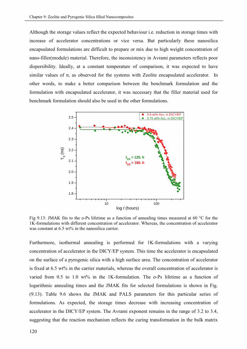
Chapter 9: Zeolite and Pyrogenic Silica filled Nanocomposites
120
Although the storage values reflect the expected behaviour i.e. reduction in storage times with
increase of accelerator concentrations or vice versa. But particularly these nanosilica
encapsulated formulations are difficult to prepare or mix due to high weight concentration of
nano-filler(module) material. Therefore, the inconsistency in Avrami parameters reflects poor
dispersibility. Ideally, at a constant temperature of comparison, it was expected to have
similar values of n, as observed for the systems with Zeolite encapsulated accelerator. In
other words, to make a better comparison between the benchmark formulation and the
formulation with encapsulated accelerator, it was necessary that the filler material used for
benchmark formulation should also be used in the other formulations.
10 100
1.8
1.9
2.0
2.1
2.2
2.3
2.4
2.5
t1/2
= 125. h
t1/2
= 160. h
0.6 wt% Acc. in DICY/EP0.75 wt% Acc. in DICY/EP
3(n
s)
log t (hours)
Fig 9.13: JMAK fits to the o-Ps lifetime as a function of annealing times measured at 60 °C for the1K-formulations with different concentration of accelerator. Whereas, the concentration of acceleratorwas constant at 6.5 wt% in the nanosilica carrier.
Furthermore, isothermal annealing is performed for 1K-formulations with a varying
concentration of accelerator in the DICY/EP system. This time the accelerator is encapsulated
on the surface of a pyrogenic silica with a high surface area. The concentration of accelerator
is fixed at 6.5 wt% in the carrier materials, whereas the overall concentration of accelerator is
varied from 0.5 to 1.0 wt% in the 1K-formulation. The o-Ps lifetime as a function of
logarithmic annealing times and the JMAK fits for selected formulations is shown in Fig.
(9.13). Table 9.6 shows the JMAK and PALS parameters for this particular series of
formulations. As expected, the storage times decrease with increasing concentration of
accelerator in the DICY/EP system. The Avrami exponent remains in the range of 3.2 to 3.4,
suggesting that the reaction mechanism reflects the curing transformation in the bulk matrix
Chapter 9: Zeolite and Pyrogenic Silica filled Nanocomposites
121
and remains independent of the accelerator and the overall nano-filler concentrations in the
DICY/EP. Whereas, the reaction constant ‘k’ shows a behavior similar to the previous results
i.e. higher the storage times, lower the value of reaction constant.
Table 9.6: Important parameters for varying concentration of accelerator in DICY/EP system.
Accelerator in
DICY/EP
Filler
(wt%)
τ0
(ns)
τ∞
(ns)
Δτ
(ns)
n k t1/2 (h) TH
(°C)
0.5 wt% 7.7 - - - - - > 200. 148.
0.6 wt% 9.2 2,41 1,91 0,50 3,40 2,56E-08 160. 153.3
0.75 wt% 11.2 2,39 1,87 0,52 3,20 1,63E-07 125. 149.7
0.8 wt% 12. 60. 149.
1.0 wt% 15. 2,55 2,05 0,55 3,20 1,67E-06 61. -
*TH values refer to curing temperatures obtained by DSC technique at 20K/min.164
The data for the hardening temperatures obtained from DSC experiments does not show any
particular trend. The values of Δτ remains more or less constant for all the available
formulations. But interestingly, the τ0 and the τ∞ values for the system with higher weight
concentration are relatively higher as compared to the other formulations. This on one hand
can be tentatively interpreted as the formation of agglomerates and therefore results in an
increase of the averaged o-Ps lifetimes, while on the other hand it re-confirms that the Avrami
exponent and the Δτ reflects the curing transformation of the bulk matrix alone.
9.5 Summary & Conclusions
It is shown that the combination of PALS and JMAK theory of transformation is a sensitive
tool to follow not only the in-situ curing of 1K-formulations, but also to understand the effect
of different loading concentrations of the accelerator and the nano-filler on the release
behavior. However, as an outlook it would make complete sense if the benchmark system
should be dispersed with the same type of nano-filler, which will be used later on for the
encapsulation of accelerator. This on one hand will solve the problem of dispersibility due to
high concentrations of nano-fillers and on the other hand when compared with the system in
which encapsulated accelerator is used, it will only give information about the release
behavior of the accelerator in the epoxy matrix. This in turn will be helpful to further tune up
the optimum loading concentration of accelerator in the filler material to achieve a higher
storage life and at the same time reducing the hardening temperatures.

Chapter 9: Zeolite and Pyrogenic Silica filled Nanocomposites
122
Chapter 10: Summary & Outlook
123
10. Summary & Outlook
The investigation of the curing kinetics for the state of the art one-component dicyandiamide
cured DGEBA formulation, at elevated temperatures is reported for the first time, in terms of
the experimental data obtained from the PALS technique combined with the JMAK theory of
transformation. It allows to estimate the shelf-life of these formulations at storage
temperatures, which otherwise is being done with time consuming methods and techniques.
The results are detailed in Chapters 6, 7, 8 and 9 of this thesis, it can be seen that the curing
kinetics and storage times at elevated temperatures for a large number of one-component
epoxy resin formulations is studied with the help of PALS. The storage times obtained from
the PALS data were compared for some of the formulations with the IR-Spectroscopy data,
which showed a good correlation.
Furthermore, the accelerator is encapsulated in the micro and nano-carriers to increase the
shelf life of epoxy formulations. But at the same time it was important from the industrial
applications point of view, to decrease the hardening temperature, so that the energy costs can
be reduced. Therefore, to understand the release behavior of the accelerator, firstly the
concentration of accelerator in the micro and nano carriers was varied, whereas the
concentration of the accelerator in DICY/Epoxy formulations was constant. Secondly, at a
constant concentration of the accelerator in the micro and nano-carriers, the curing kinetics
are studied by varying the concentration of the accelerator in the DICY/Epoxy formulations.
The results indicate that the change in accelerator concentration directly effects the storage
time and hardening temperature for the one-component epoxy-resin formulation. Furthermore,
it is observed for a series of samples that the avarami exponent is independent of the change
in concentration of accelerator and remains the same within the experimental accuracy.
It is also shown that PALS is a very useful technique, when it comes to the characterization of
cured epoxy composites. A comparison of PALS with DSC technique was dome for a selected
series of cured composites, which indicates the glass-transition Tg obtained from the two
techniques was in good correlation. Furthermore, with the help of PALS data in combination
with the Tao-Eldrup model, the temperature dependence of the hole free volume, the
fractional free volume (FFV) and the thermal expansion co-efficients in the glassy and the
rubbery phase were also estimated.
Chapter 10: Summary & Outlook
124
During the major part of this work, the main focus was on providing the industrial partners
with the shelf-life information for the one-component epoxy-resin formulations, as obtained
from PALS data at elevated temperatures. This information was really helpful in developing
new synthesis approaches for the encapsulation of accelerator in micro and nano-sized
carriers. But as an outlook, purely from the academic research point of view, still there
appears to be a lot of open questions. The paragraphs to follow, will be used to throw a light
on these topics of purely academic interest.
The effect of the particle size on the storage time and the curing kinetics can be studied by the
combination of PALS and the JMAK theory of phase transformation. For example, the DICY
is commercially available with particle sizes in the range of 5 to 40 μm and it will be really
interesting to see the effect of particle size on the shelf-life and the hardening temperatures of
one-component formulations. This will in turn help with the choice of material used in DICY
cured one-component formulations. Another possible theme concerning the particle size could
be to study the effect of temperature on the final structure of the cured composites. This in
turn can be compared with the atomic force microscopy (AFM) or other imaging techniques
and these results could be helpful to understand the effect of temperature on the extent of
cured fraction and the type of structure formed.
The accelerator used throughout this work for encapsulation purpose, to lower the hardening
temperature, has a melting temperature (Tm) of less than 0°C. This makes the accelerator
highly reactive not only at the elevated temperatures but even at the storage conditions as
well. Since accelerators with melting temperatures higher than storage temperatures are
commercially available, so it will be better to use one with Tm above room temperature. It is
expected that this will increase the shelf life of the formulation and at the same time it can be
useful in achieving low temperature curing. Since no incubation time was observed for the
free accelerator systems (as reported in Chapter 7 of this thesis), it will be interesting to study
a comparison of free and encapsulated accelerator on the activation energies for such an
accelerator (with Tm > RT).
There was already a nanosilica filler material used for all the dicyandiamide cured
formulations to control the viscosity, which is acceptable as long as formulations with the free
accelerator or the Zeolite encapsulated accelerator are concerned. But the precursor was
difficult to prepare or mix, when this nanosilica filler was used in combination with the
Chapter 10: Summary & Outlook
125
accelerator encapsulated on pyrogenic silica based carriers, as the viscosity is apparently
affected by high weight concentration of fumed silica particles. Therefore, a benchmark
system should be the one containing the same filler material as the one which is later on
supposed to be used as the carrier material for accelerator encapsulation. Furthermore, the
accelerator was mostly encapsulated in Nanosilica and Zeolite based carriers, it will be
interesting to see the effect of other carrier materials (such as layered silicates) e.g., on one
hand the curing kinetics of one-component formulations and on the other hand, how it affects
the properties of their cured composites.
To the best of knowledge the reaction chemistry of such one-component formulations is not
known and even it is impossible to simulate the cured structure of such formulations.
Therefore, a comparison of PALS data can be studied in combination with the pressure-
volume-temperature (PVT) experiments. This will give complete structural information such
as, the temperature dependence of the hole free volume, the specific total, the occupied and
the specific free volume along with fractional free volume and the number density of holes.
This will enable to calculate the cross-linking density, which will be of great help in
simulating such complex structures.

Chapter 10: Summary & Outlook
126
Chapter 11: Bibliography
127
11. Bibliography
1 M.A. Clayton. Epoxy resins: chemistry and technology. 2nd Edition edn, (Marcel DekkerInc., 1987).
2 J. Kansy. Microcomputer program for analysis of positron annihilation lifetime spectra.Nuclear Instruments and Methods in Physics Research Section A: Accelerators,Spectrometers, Detectors and Associated Equipment 374 (2), 1996, 235–244 374, 235-244(1996).
3 S. J. Tao. Positronium annihilation in molecular substances. Journal of Chemical Physics 56,5499–5510 (1972).
4 M. Eldrup, D. Lightbody & Sherwood, J. N. The temperature dependence of positron lifetimein solid pivalic acid. Chemical Physics 63, 51-58 (1981).
5 M. Avrami. Kinetics of Phase Change. I: General Theory. J. Chem. Phys. 7, 1103 (1939).6 M. Avrami. Kinetics of phase change II. Transformation-time relations for random
distribution of nuclei. J. Chem. Phys. 8, 212-224 (1940).7 M. Avrami. Granulation, phase change and microstructure Kinetics of phase change. III.
Journal of Chemical Physics 9, 177-184 (1941).8 B.S.S. Daniel et al. Free volume evolution in bulk metallic glass during high temperature
creep. MRS Symp. Proc. CC 11.16, 754 (2003).9 C. Nagel et al. Free volume changes in the bulk metallic glass Zr47Ti8Cu7,5Ni10Be27,5 and the
undercooled liquid. Phys. Rev. B 57, 10224 (1998).10 C. Nagel, K. Rätzke, E. Schmidtke, F. Faupel & Ulfert, W. Positron annihilation studies of
free volume changes in the bulk metallic glass Zr65Al7.5Ni10Cu17.5 during structural relaxationand at the glass transition. Phys. Rev. B 60, 9212 (1999).
11 C. Nagel, K. Rätzke, E. Schmidtke & Faupel, F. Free volume changes in bulk amorphousalloys during structural relaxation and in the supercooled liquid state. MRS Symp. Proc. 75,554 (1999).
12 J. Kruse et al. Free Volume in Polyimides: Positron Annihilation Experiments and MolecularModelling. Macromolecules 38, 9638 (2005).
13 J. Kruse et al. Free volume in polymeric membranes: Experiment and simulation. MembraneNews 66, 51 (2004).
14 R.De.Miranda, J. K., K.Rätzke, F.Faupel, D.Fritsch, V.Abetz, P.M.Budd, J.D.Selbie,N.B.McKeown, B S.Ghanem. Unusual temperature dependence of positron lifetime in apolymer of intrinsic microporosity. Phys. Stat. Sol. Rapid Res. Lett., 5, 190 (2007).
15 J.Kanzow, V. Z., H.Nabika, M.Mizuhata, S.Deki, F Faupel,. In-situ investigations on thecross-linking process of the epoxy resin system DGEBA-DETA by means of positronannihilation lifetime spectroscopy in comparison with infrared spectroscopy. Mat. Sci. Forum445-446, 313 (2004).
16 G.Dlubek, M. Q. S., K.Rätzke, F.Faupel, J Pionteck, M. Paluch. The temperature dependenceof free volume in phenyl salicylate and its relation to structural dynamics: A positronannihilation lifetime and pressure-volume-temperature study. J. Chem. Phys. 130, 144906(2009).
17 P. A. M. Dirac. in Proc. Cambridge Phil. Soc. 361-375.18 C.D. Anderson. The positive electron. Phys. Rev. 43, 491-498 (1933).19 A.E. Ruark. Positronium. Physical Review 68, 278 (1945).20 P. G. Coleman. in Encyclopedia of Applied Spectroscopy (ed D. L. Andrews) Ch. 5,
(WILEY-VCH Verlag GmbH, 2009).21 J. Kruse. Freies Volumen in Membranpolymeren –
Positronenannihilationslebensdauerspektroskopie an ausgewählten Systemen PhD thesis,Christian-Albrechts University of Kiel, (2007).
22 O.E. Mogensen. (Springer-Verlag, Berlin, Heidelberg, 1995).
Chapter 11: Bibliography
128
23 C. Dauwe, B. Van Waeyenberge & N. Balcaen. Positronium formation in poly(methylmethacrylate). Phys. Rev. B 68, 1322021-1322024 (2003).
24 T. Hirade, F.H. Maurer & M. Eldrup. Positronium formation at low temperatures: the role oftrapped electrons. Rad. Phys. Chem. 58, 465-471 (2000).
25 A. Ore. Universitetet i Bergen Arbok, (1949).26 O.Mogensen. in Springer Series in Chemical Physics Vol. 58 (Springer-Verlag, 1995).27 S.V.Stepanov, V. M. B. Electric field effect on Ps formation in liquids. Journal of Chemical
Physics 116, 6718-6195 (2002).28 W.Brandt, S.Berko & W.W.Walker. Positronium Decay in Molecular Substances. Physical
Review 120, 1289 (1960).29 R. Krause-Rehberg & H. S. Leipner. in Springer series in solid-state sciences Vol. 127
(Springer, Berlin, 1999).30 S. Thraenert, E. Hassan & R. Krause-Rehberg. Ortho-positronium lifetime measurement –
positron source activity and statistics Nuclear Instruments and Methods in Physics ResearchSection B: Beam Interactions with Materials and Atoms 248, 336–339 (2006).
31 C. Nagel. Freies Volumen und Transporteigenschaften in hochselektiven Polymermembranenund metallischen Massivgläsern, Christian-Albrechts-Universität zu Kiel, 1999, (1999).
32 Y.C. Jean, P. E. Mallon & Schrader, D. M. (World Scientific Publishing Co. Pte. Ltd.,,Singapore, 2003).
33 S. McGuire & D. J. Keeble. Positron lifetime and implantation in Kapton. Journal of PhysicsD: Applied Physics 39, 3388-3393 (2006).
34 P. Kirkegaard, M. Eldrup, O. E. Mogensen & Pedersen, N. J. Computer PhysicsCommunications 23, 307-335 (1981).
35 S. W. Provencher. Computer Physics Communications 27, 229-242 (1982).36 A. Shukla, M. Peter & Hoffmann, L. Nuclear Instruments and Methods A 335, 310 (1993).37 H. Cao, G.H. Dai, J.P. Yuan & Jean, Y. C. Reliability of ortho-Positronium Lifetime
distribution dnalysis in Polymers by using CONTIN program. Materials Science Forum 255-257, 238-242 (1997).
38 H. Nakanishi, S. Wang & Y.C. Jean. in Positron Annihilation Studies of Fluids (ed S.Sharama) 292–298 (World Scientific, 1988).
39 G. Ferrante. Annihilation of Positrons from Positronium Negative Ion e-e+e-. Physical Review170, 76 (1968).
40 A. Dupasquier, P. De Natale & Rolando, A. Formal calculation of the pick-off annihilationrate for ortho- and parapositronium. Physical Review B 43, 10036 (1991).
41 J. Kanzow et al. In-situ investigations on the cross-linking process of the epoxy resin systemDGEBA-DETA by means of positron annihilation lifetime spectroscopy in comparison withinfrared spectroscopy. Mat. Sci. Forum 445-446, 313 (2004).
42 T. Suzuki, Y. Oki, M. Numajiri, K. Kondo & Y. Ito. Positron annihilation and polymerizationof epoxy resins. Polymer, 7, 1361-1365 (1993).
43 T. Suzuki et al. Polymerization of bisphenol-A dicyanate studied by positron annihilation.Materials science forum 175-178, 785-788 (1995).
44 T. Suzuki, T. Hayashi & Y. Ito. Polymerization of epoxy resins studied by positronannihilation. Mat. Res. Innovat 4, 273-277 (2001).
45 W. Salgueiro, J. Ramos, A. Somoza, S. Goyanes & I. Mondragon. Nanohole volumedependence on the cure schedule in epoxy thermosetting networks: A PALS study. Polymer47, 5066-5070 (2006).
46 A.J. MacKinnon, R.A. Pethrick, S.D. Jenkins & P.T. McGrail. Investigation of thermoplastic-modified thermosets: positron annihilation and related studies of an amine-cured epoxy resin.Polymer 35, 5319-5326 (1994).
47 Y.Y. Wang, H. Nakanishi & Jean, Y. C. Positron annihilation in amine-cured epoxy polymers- pressure depedence. Journal of Polymer Science Part B: Polymer Physics 28, 1431-1441(1990).
48 J.D.Ferry. (Wiley, New York, 1980).49 W.J.McKnight, J. J. A. a. (Wiley, New York, 1983).50 M.L.Williams, R. F. L., and J.D.Ferry. J. Am. Chem. Soc., 77, 3701 (1955).
Chapter 11: Bibliography
129
51 W.W.Lee. Selection of barrier materials from molecular structure. Polym. Eng. Sci. 20, 65-68(1980).
52 J.D.Vrentas, J. L. D., and J.W.Huang. Macromolecules 19, 1718 (1986).53 W.Brostow & M.A.Macip. Macromolecules 22, 2761 (1989).54 S.Matsuoka. (Hanser, New York, 1992).55 H.Eyring. J. Chem. Phys. 4, 283 (1936).56 J.Liu, Q. D., and Y.C.Jean. Macromolecules 26, 7149 (1993).57 A.Bondi. (John Wiley & Sons, Inc.,, New York, 1968).58 vanKrevelen, D. W. (Elsevier, Amsterdam, 1990).59 D.N.Theodorou. (ed P. Neogi) 67-142 (Marcel Dekker, New York, 1996).60 M.L. Greenfield & D.N.Theodorou. Geometric analysis of diffusion pathways in glassy and
melt atactic polypropylene. Macromolecules 36, 5461-5672 (1993).61 W.L.Mattice, S. M. a. Macromolecules 26, 7274 (1993).62 D.Bamford. PhD thesis, University of Bristol, (2003).63 R.J.Roe, D. R. a. Macromolecules 23, 5312 (1990).64 V.I.Betekhtin, E. L. G., A.G.Kadomtsev, A.Yu.Kipyatkova and O.V.Tolochko. Effect of
annealing on the excess free volume and strength of amorphous alloys. Physics of the SolidState 42, 1460-1464 (2000).
65 A.Y.Alentiev, V. P. S., T.C.Merkel, V.I.Bondar, B.D.Freeman and Y.P.Yampolski. Gas andvapor sorption, permeation and diffusion in glassy amorphous Teflon AF1600.Macromolecules 35, 9513-9522 (2002).
66 B.Nagasaka, T. E., H.Nakayama, N.Nakamura, Y.Ito. Positron annihilation and 129Xe NMRstudies of free volume in polymers. Radiation Physics and Chemistry 58, 581-585 (2000).
67 H.Vajdlenková, J. B. Spin probe mobility in relation to free volume and relaxation dynamicsof glass-formers: A series of spin probes in poly(isobutylene). Journal of Polymer SciencePart B: Polymer Physics 47, 1058-1068 (2009).
68 J.M.Torkelson, J. S. R. a. Photochromic and fluorescent probe studies in glassy polymeratrices. 5. Effects of physical aging on bisphenol-A polycarbonate and poly(viny1 acetate) assensed by a size distribution of photochromic probes. Macromolecules 25, 4792-4796 (1992).
69 T.S.Chow. Macrom. Theory Simul. 4, 397-404 (1995).70 Y.C Jean, J.-P. Y., J.LIU, Q.DENG and H.Yang. Correlations between gas permeation and
free-volume hole properties probed by positron annihilation spectroscopy. Journal of PolymerScience: Part B: Polymer Physics 33, 2365-2371 (1995).
71 R.M.Dammert, S. L. M., F.H.J.Maurer, I.M.Neelow, S.Niemelä, F.Sundholm and C.Wästlund.Free volume and tacticity in polystyrenes. Macromolecules 32, 1930-1938 (1999).
72 V.Shantarovich, Y. Y. a. in Materials Science of Membranes: for Gas and Vapor separation(ed I.Pinnai and B.D.Freeman Y.Yampolski) (John Wiley & Sons Ltd.,, UK, 2006).
73 R.S.Spencer, R. F. B. a. J. Appl. Phys. 15, 398 (1944).74 F.H.J.Maurer, J.H.M. Palmen & H.C.Booij. Generalized stress relaxation behaviour and
physical aging in heterogeneous amorphous polyblends Rheologiea Acta 24, 243-249 (1985).75 W.A. Johnson & R.F. Mehl. Trans. Am. Inst. Min. Metall. Eng., 135, 416 (1939).76 A.N. Kolmogorov. Statistical theory of crystallization of metals.(in russian). Izvestia
Akademia Nauk SSSR Ser. Mathematica 1, 355–359 (1937).77 J.W. Christian. The theory of transformations in metals and alloys. Part I, Equilibrium and
general kinetic theory. (Pergamon, 1975).78 W.D. Callister Jr. Materials Science and Engineering: An Introduction. 5th edn, (John Wiley
and Sons Inc., 2000).79 L. Mandelkern. Crystallization of Polymers: Kinetics and Mechanisms, Volume 2. 2nd edn,
Vol. 2 (Cambridge University Press, 2004).80 D.A. Porter & K.E. Easterling. Phase Transformations in Metals and Alloys. (Chapman and
Hall, 1991).81 A.K. Jena & M.C. Chaturvedi. Phase Transformations in Materials. . 243 (Prentice Hall,
1992).82 Prof. A.D. Rollett. Microstructure Properties II: The KJMA Equation (Department of
Materials Science and Engineering; Carnegie Mellon University Pittsburgh, USA, 2009).83 Prof. H.K.D.H. Bhadesia. Kinetics and Microstructure Modelling. (2010).
Chapter 11: Bibliography
130
84 E.M. Petrie. Epoxy Adhesive Formulations. (MacGraw Hill, 2006).85 Dyhard Booklet. (ed Degussa Fine Chemicals) (March 2003).86 BMBF Projekt. Entwicklung vernetzungssteuernder Nanomodule mit controlled Release-
function für Polymerharz-Systeme mit erhöhter Lagerstabilität und reduzierterHärtungstemperatur (www.nanomodule.de) (NANOMODULE, 2006).
87 G.K. Noren. Cationic UV Curable Formulations Containing Hydroxy FunctionalFluoropolymer Resins. Journal of Coatings Technology 72, 53-59 (2000).
88 Herman F. Mark. (John Wiley & Sons, 2004).89 H. F. Mark. in Encyclopedia of polymer science and technology. Vol. 9, Epoxy resins. (John
Wiley & Sons, 2004).90 Dow Chemical Company USA. Liquid Epoxy Resin - DGEBF (2010).91 Y. Tanaka. in Epoxy Resins: Chemistry and Technology (ed M.A. Clayton) pp.969 (Marcel
Dekker Inc., 1988).92 Prof. Dr. Franz Faupel. Lecture notes "Polymer-I". (2010).93 Hexion Speciality Chemicals - USA. Electrical Laminating Resins. (www.hexion.com)
(2010).94 L.S. Penn & H. Wang. in Handbook of Composites (ed S.T. Peters) (Chapman and Hall,
London, 1998).95 P. Pfäffli, M. Hämeilä, R. Riala, J. Tornaeus & R. Wirmoila. Exposure to
methylhexahydrophthalic anhydride (MHHPA) in two workplaces of the electric industry.Journal of Environmental Monitoring 6, 295-299 (2004).
96 J.P. Pascault, H. Sauterau, J. Verdu & R.J.J. Williams. Thermosetting polymers. (MarcelDekker, 2002).
97 J.B. Enns & J.K. Gillham. The time-temperature transformation (TTT) cure diagram:modeling the cure behavior of thermosets. Journal of Applied Polymer Science 28, 2567-2591(1983).
98 G. Wisanrakkit & J. K. Gillham. The Glass Transition Temperature (Tg) as an Index ofChemical Conversion for a High-Tg Amine/Epoxy System: Chemical and Diffusion-Controlled Reaction Kinetics. Journal of Applied Polymer Science 41, 2885-2929 (1990).
99 K. Dusek. in Epoxy Resins and Composites III, Advances in Polymer Science Vol. 78 (ed K.Dusek) pp. 1-59 (Springer-Verlag, Berlin, 1986).
100 C. M. Tung & J. P. Dynes. Journal of Applied Polymer Science 27, 569-574 (1982).101 M. E. Smith & H. Ishida. Journal of Applied Polymer Science 73, 593-600 (1999).102 H. Jahn & P. Goetzky. in Epoxy Resins: Chemistry and Technology, (ed C.A. May) pp.
1049-1087 (Marcel Dekker, Inc. New York, , 1988).103 C.T. Chou & L.S. Penn. Mechanism by which an orthocarbonate reduces residual stress in a
composite. Journal of Composite Materials 26, 171-184 (1992).104 J. Mijovic & H.T. Wang. Cure kinetics of neat and graphite-fiber-reinforced epoxy
formulations. Journal of Applied Polymer Science 37, 2661-2673 (1989).105 R. Morgan. Structure-property relations of epoxies used as composite matrices. Advances in
Polymer Science 72, 143 (1985).106 S. Yalof & W. Wrasidlo. Crosschecking between dielectric measurements, DTA, and other
methods of thermal analysis in research and production. Journal of Applied Polymer Science16, 2159-2173 (1972).
107 S.D. Senturia & N.F. Sheppard. Dielectric analysis of thermoset cure. Advances in PolymerScience 80, 147 (1986).
108 P.R. Ciriscioli & G.S. Springer. Dielectric cure monitoring - a critical review. SAMPE J. 25,3542 (1989).
109 C.S.P. Sung & R. Mathisen. Cure characterization of an epoxy network by fluorescencebehavior of trans-diaminostilbene. Polymer 28, 941-945 (1987).
110 P.R. Young, M.A. Druy, W.A. Stevenson & D.A. Compton. In-situ composite monitoringusing infrared-transmitting optical fibers. SAMPE J. 25, 11-16 (1989).
111 M.L. Myrick, S.M. Angel, R.E. Lyon & T.M. Vess. Epoxy cure monitoring using fiber-opticRaman spectroscopy. SAMPE J. 28, 3742 (1992).
112 J. Mijovic, J.M. Kenny, L. Nicolais & S. Pejanovic. Present and future trends in insitumonitoring of processing of advanced composites. SAMPE J. 28, 3946 (1992).
Chapter 11: Bibliography
131
113 K. Raetzke, M.Q. Shaikh, F. Faupel & P.-L.M. Noeske. Shelf stability of reactive adhesiveformulations: A case study for dicyandiamide-cured epoxy systems International Journal ofAdhesion and Adhesives 30, 105-110 (2010).
114 B. Ellis. Chemistry and Technology of Epoxy Resins. 1st ed. edn, 72, 116 (Blackie Academic& Professional, 1993).
115 J. Kanzow et al. Applied Surface Science 239, 227 (2005).116 S.A. Zahir. in Advances in Organic Coatings Science and Technology, Vol. IV: Sixth
International Conference in Organic Coatings Science and Technology Vol. 4 eds G.D.Parfitt & A. V. Patsis) pp.83 (Technomic Publishing Co. Inc., 1982).
117 L.H. Sperling. Introduction to Physical Polymer Science. (Wiley, 2005).118 M. Cao et al. Journal of Applied Polymer Science 85, 873 (2002).119 M. Pollard & J.L. Kardos. Polymer Engineering and Science, 27, 829 (1987).120 M.G. Lu, M.J. Shim & S.W. Kim. Journal Thermal Analysis and Calorimetry 58, 701 (1999).121 D.Z. Chen, P.S. He & L.J. Pan. Polymer Testing 22, 689 (2003).122 X.H. Zhang, Y.Q. Min, H. Zhao, H.M. Wan & G.R. Qi. Journal of Applied Polymer Science
100, 3483 (2006).123 R.De. Miranda et al. Unusual temperature dependence of positron lifetime in a polymer of
intrinsic microporosity. Phys. Stat. Sol. Rapid Res. Lett., 5, 190 (2007).124 J. Kruse et al. Free volume in C-60 modified PPO polymer membranes by positron
annihilation lifetime spectroscopy. J Phys Chem B 111, pp. 13914–13918. (2007).125 G. Dlubek, J. Pionteck, M.Q. Shaikh, E.M. Hassan & R. Krause-Rehberg. Physical Review E
75, 021802 (2007).126 G. Dlubek, M.Q. Shaikh, R. Krause-Rehberg & M. Paluch. J. Chem. Phys. 126, 024906
(2007).127 J. Kanzow et al. in Adhesion - Current research and applications (ed W. Possart) 465
(Wiley-VCH, 2005).128 A. Somoza, W. Salgueiro, S. Goyanes, J. Ramos & Mondragon, I. Volume changes at macro-
and nano-scale in epoxy resins studied by PALS and PVT experimental techniques RadiationPhysics and Chemistry 76, 118-122 (2007).
129 Dyhard Booklet. (ed by Degussa Fine Chemicals) (2005).130 S. Vyazovkin & N. Sbirrazzuoli. Macromol. Chem. Phys. 200, 2294-2303 (1999).131 T. M. Goulding. Handbook of Adhesive Technology. 2nd Ed. edn, (Marcel Dekker, Inc.,
2003).132 G. Webster. Chemistry & Technology of UV & EB Formulation for Coatings, Inks & Paints.
Vol. 2 (John Wiley & Sons, Inc., 1997).133 E.W. Flick. Contemporary Industrial Coatings, Enviromentally Safe Formulations. (Noyes
Publishers, 1985).134 W.K. Goertzen & Kessler, M. R. Creep behavior of carbon fiber/epoxy matrix composites.
Materials Science and Engineering: A. 421, 217-225 (2006).135 G. Dlubek, J. Pointeck, M.Q. Shaikh, E. M. Hassan & Krause-Rehberg, R. Free volume of an
oligomeric epoxy resin and its relation to structural relaxation: Evidence from positronlifetime and pressure-volume-temperature experiments. Phys. Rev. E 75, 021802-02180213(2007).
136 M. Rudel et al. Temperature dependence of positron annihilation lifetimes in highpermeability polymers: amorphous Teflons AF. Macromolecules 41, 788 (2008).
137 G. Dlubek et al. The free volume in two untreated, pressure-densified, and CO2 gas exposedpolymers from positron lifetime and pressure-volume-temperature experiments. e-Polymers108, 1 (2007).
138 M. Rudel et al. Temperature dependence of positron annihilation lifetimes in highpermeability polymers: amorphous Teflons AF. Macromolecules 41, 788 (2008).
139 G. Dlubek et al. The temperature dependence of free volume in phenyl salicylate and itsrelation to structural dynamics: A positron annihilation lifetime and pressure-volume-temperature study. J. Chem. Phys. 130, 144906 (2009).
140 O. Mogensen. in Springer Series in Chemical Physics Vol. 58 (Springer-Verlag, 1995).141 V. Abetz. Advances in Polymer Science. Block Copolymers II. (Springer-Verlag, 2005).
Chapter 11: Bibliography
132
142 G. Dlubek, M.Q. Shaikh, R. Krause-Rehberg & M. Paluch. Effect of free volume andtemperature on the structural relaxation in polymethylphenylsiloxane: A positron lifetime andpressure-volume-temperature study. J. Chem. Phys. 126, 024906 (2007).
143 E. Riande, R. Diaz-Calleja, M.G. Prolongo, R.M. Masegosa & Salom., C. PolymerViscoelasticity: Stress and Strain in practice, . 71-72 (Marcel Dekker Inc., 2000).
144 R. Srithawatpong et al. Positron annihilation lifetime studies of changes in free volume oncross-linking cis-polyisoprene, high-vinyl polybutadiene, and their miscible blends. Journal ofpolymer science. Part B. Polymer physics 37, pp. 2754-2770 (1999).
145 C. Lianxi, T. Hua, L. Quanwen & W. Jun. Curing Reaction Kinetics of Epoxy Resin UsingDicyandiamide Modified by Aromatic Amines. Wuhan University Journal of Natural Sciences12, 1105-1108 (2007).
146 M.R. Kamal. Polym. Eng. Sci. 14, 231 (1974).147 Jürgen Schawe. Kinetic studies of complex reactions Part 1: model free kinetics Usercom -
Mettler Toledo 2, 13-16 (2003).148 J. Schawe. Kinetic studies of complex reactions, Part 2:Description of diffusion control,.
Usercom- Mettler Toledo 1, 8-12 (2004).149 H. F. Mark. in Encyclopedia of polymer science and technology. Vol. 9, Epoxy resins. (ed H.
F. Mark) pp.757 (John Wiley & Sons, 2004).150 K. Horie, H. Hiura, M. Sawada, L.Mita & H. Kambe. Calorimetric investigation of
polymerization reactions. III. Curing reaction of epoxides with amines. J. Polym. Sci. (Part A-1) 8, 1357-1372 (1970).
151 N. Gupta & I.K. Varma. Effect of structure of aromatic diamines on curing characteristics,thermal stability, and mechanical properties of epoxy resins. I. Journal of Applied PolymerScience 68, 1759-1766 (1998).
152 D. Olmos, A.J Aznar, J. Baselga & J. González-Benito. Kinetic study of epoxy curing in theglass fiber/epoxy interface using dansyl fluorescence Journal of Colloid and Interface Science267, 117–126 (2003).
153 J.K. Gillham. in Encyclopedia of Polymer Science and Engineering Vol. 4 p. 519 (Wiley,New York, 1989).
154 Boltzmann Function. Microcal Origin 7.5. (2010).155 M. Pollard & J.L. Kardos. Analysis of epoxy resin curing kinetics using the Avrami theory of
phase change. Polym. Eng. Sci. 27, 829-836 (1987).156 M.G. Lu, M.J. Shim & S.W. Kim. The macrokinetic model of thermosetting polymers by
phase-change theory. Mater. Sci. Commun. 56, 193-197 (1998).157 K. Schulte, F.H. Gojny & B. Fiedler. in Polymer Composites: From Nano to Macro Scale
(ed S. Fakirov K. Friedrich, Z. Zhang) 3-22 (Springer, 2005).158 R. Dagani. Nanostructured materials promise to advance range of technologies. C&EN 70, 18
(1992).159 M. Z. Rong, M. Q. Zhang, Y. X. Zheng, H. M. Zeng & K. Friedrich. Improvement of tensile
properties of nano-Si0,PP composites in relation to percolation mechanism. Polymer 42, 3301(2001).
160 M. Q. Zhang, M. Z. Rong & K. Friedrich. in Polymer Composites: From Nano to Macro Scale(ed S. Fakirov K. Friedrich, Z. Zhang) 25-43 (2005).
161 J. Ch. Gaukler & W. Possart. Functional Nano fillers in hot curing epoxies for prolongedshelf life and reduced curing temperature. (2009).
162 M. Noeske, P. Schiffels & J. Trautmann. Jahresbericht 2007/2008. (Fraunhofer Institut fürFertigungstechnik und Angewandte Materialforschung (IFAM), Bremen, Germany, March2008).
163 P.L.M. Noeske. (Private Communication, Fraunhofer Institute for ManufacturingTechnology and Applied Materials Research in Bremen, 2010).
164 S. Gramm. (Private Communication, AWOK University of Kaiserslautern, 2010).165 W. Xu, R. Huang, B. Cai & W. Fan. Nano-CaCO3 filled HDPE composites. China Plastics 12,
30-34 (1998).166 L.S. Schadler, K.O. Laul, R.W. Smith & E. Petrovicova. Microstructure and mechanical
properties of thermally sprayed silica/nylon nanocomposites. Journal of Thermal SprayTechnology 6, 475 (1997).
Chapter 11: Bibliography
133
167 A. Bhattacharya, J. W. Rawlins & P. Ray. Polymer Grafting and Crosslinking. (John Wiley &Sons Inc., 2009).
168 C.N. Bowman & N.A. Peppas. Development of a novel kinetic gelation method for thesimulation of free radical polymerizations. Chemical Engineering Science 47, 1411-1419(1992).
169 Degussa AG. in Technical Bulletin Free Particles No. 56, Highly Dispersed Metallic OxidesProduced by the AEROSIL Process, 4th ed. (D-40402 Düsseldorf, 1989).
170 Degussa AG. in Technical Bulletin Fine Particles No. 27, AEROSIL® Fumed Silica forSolvent-Free Epoxy Resins (D-40402 Düsseldorf, 2009).
171 T. Schlosser & R. Nowak. (Evonik Degussa GmbH, personal communication, 60287Frankfurt am Main, G ermany, 2010).
172 J.H. Koo. in Polymer Nanocomposites: Processing, Characterization, and Applications (edJ.H. Koo) pp. 38-40 (McGraw-Hill Professional, 2006).
173 H. Nakanishi & Y.C. Jean. in Studies in Physical Theoretical Chemistry Vol. 57 eds D.M.Schrader & Y.C. Jean) pp. 159-192 (Elsevier, 1988).
174 T. Goworek, B. Jasinska, J. Wawryszczuk, K. Ciesielski & J. Goworek. in Studies in SurfaceScience and Catalysis Vol. 128 eds V.K.K. Unger, G. Kreysa, & J.P. Baselt) pp. 557-564(Elsevier, 2000).
175 B. Nagasaka, T. Eguchi, H. Nakayama, N. Nakamura & Ito, Y. Positron annihilation and 129XeNMR studies of free volume in polymers. Radiation Physics and Chemistry 58, 581-585(2000).
176 W.R. Ashcroft. in Chemistry and Technology of Epoxy Resins, 1st ed. (ed B. Ellis) pp. 37,71 (Blackie Academic & Professional, 1993).
177 M.D. Gilbert, N.S. Schneider & W.J. McKnight. Mechanism of the dicyandiamide/epoxidereaction. Macromolecules 24, 360-369 (1991).
178 S.A. Zahir. in Advances in Organic Coatings Science and Technology, Vol. IV: SixthInternational Conference in Organic Coatings Science and Technology eds G.D. Parfitt & A.V. Patsis) pp.83 (Technomic Publishing Co. Inc., 1982).

Chapter 11: Bibliography
134
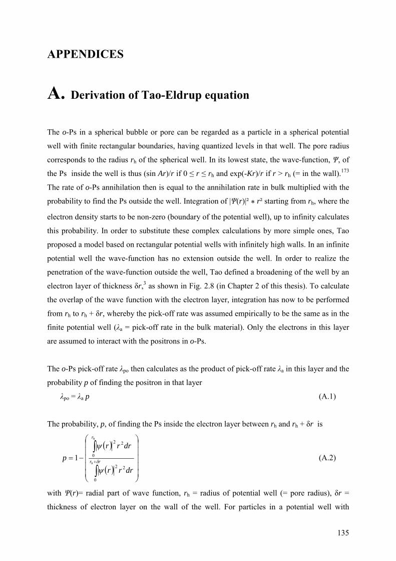
135
APPENDICES
A. Derivation of Tao-Eldrup equation
The o-Ps in a spherical bubble or pore can be regarded as a particle in a spherical potential
well with finite rectangular boundaries, having quantized levels in that well. The pore radius
corresponds to the radius rh of the spherical well. In its lowest state, the wave-function, Ψ, of
the Ps inside the well is thus (sin Ar)/r if 0 ≤ r ≤ rh and exp(-Kr)/r if r > rh (= in the wall).173
The rate of o-Ps annihilation then is equal to the annihilation rate in bulk multiplied with the
probability to find the Ps outside the well. Integration of |Ψ(r)|² * r² starting from rh, where the
electron density starts to be non-zero (boundary of the potential well), up to infinity calculates
this probability. In order to substitute these complex calculations by more simple ones, Tao
proposed a model based on rectangular potential wells with infinitely high walls. In an infinite
potential well the wave-function has no extension outside the well. In order to realize the
penetration of the wave-function outside the well, Tao defined a broadening of the well by an
electron layer of thickness δr,3 as shown in Fig. 2.8 (in Chapter 2 of this thesis). To calculate
the overlap of the wave function with the electron layer, integration has now to be performed
from rh to rh + δr, whereby the pick-off rate was assumed empirically to be the same as in the
finite potential well (λa = pick-off rate in the bulk material). Only the electrons in this layer
are assumed to interact with the positrons in o-Ps.
The o-Ps pick-off rate λpo then calculates as the product of pick-off rate λa in this layer and the
probability p of finding the positron in that layer
λpo = λa p (A.1)
The probability, p, of finding the Ps inside the electron layer between rh and rh + δr is
rr
r
h
h
drrr
drrr
p
0
22
0
22
1 (A.2)
with Ψ(r)= radial part of wave function, rh = radius of potential well (= pore radius), δr =
thickness of electron layer on the wall of the well. For particles in a potential well with
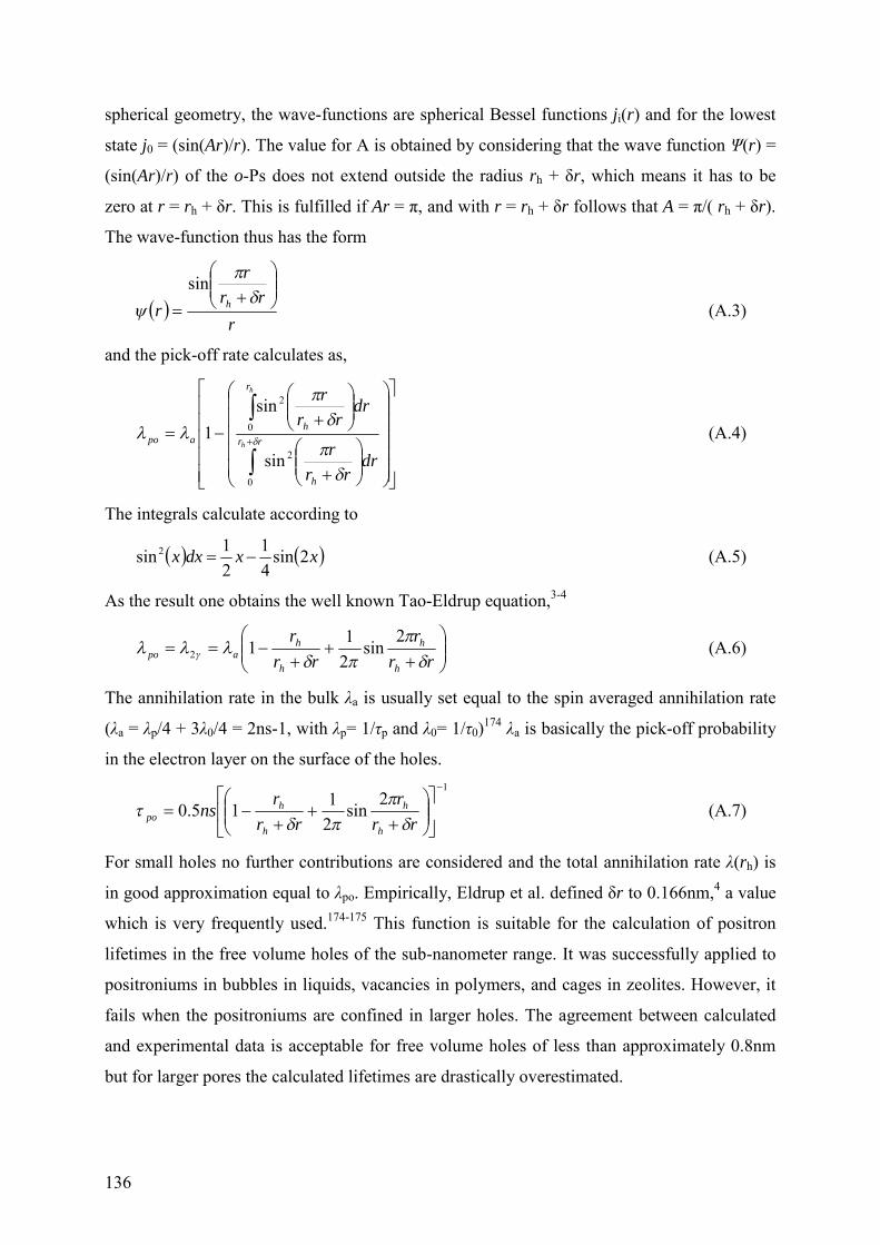
136
spherical geometry, the wave-functions are spherical Bessel functions ji(r) and for the lowest
state j0 = (sin(Ar)/r). The value for A is obtained by considering that the wave function Ψ(r) =
(sin(Ar)/r) of the o-Ps does not extend outside the radius rh + δr, which means it has to be
zero at r = rh + δr. This is fulfilled if Ar = π, and with r = rh + δr follows that A = π/( rh + δr).
The wave-function thus has the form
r
rr
r
rh
sin
(A.3)
and the pick-off rate calculates as,
rr
h
r
h
apoh
h
drrr
r
drrr
r
0
2
0
2
sin
sin
1 (A.4)
The integrals calculate according to
xxdxx 2sin4
1
2
1sin 2 (A.5)
As the result one obtains the well known Tao-Eldrup equation,3-4
rr
r
rr
r
h
h
h
hapo
2sin
2
112 (A.6)
The annihilation rate in the bulk λa is usually set equal to the spin averaged annihilation rate
(λa = λp/4 + 3λ0/4 = 2ns-1, with λp= 1/τp and λ0= 1/τ0)174 λa is basically the pick-off probability
in the electron layer on the surface of the holes.
1
2sin
2
115.0
rr
r
rr
rns
h
h
h
hpo
(A.7)
For small holes no further contributions are considered and the total annihilation rate λ(rh) is
in good approximation equal to λpo. Empirically, Eldrup et al. defined δr to 0.166nm,4 a value
which is very frequently used.174-175 This function is suitable for the calculation of positron
lifetimes in the free volume holes of the sub-nanometer range. It was successfully applied to
positroniums in bubbles in liquids, vacancies in polymers, and cages in zeolites. However, it
fails when the positroniums are confined in larger holes. The agreement between calculated
and experimental data is acceptable for free volume holes of less than approximately 0.8nm
but for larger pores the calculated lifetimes are drastically overestimated.
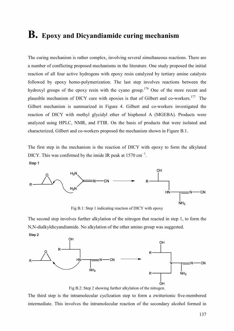
137
B. Epoxy and Dicyandiamide curing mechanism
The curing mechanism is rather complex, involving several simultaneous reactions. There are
a number of conflicting proposed mechanisms in the literature. One study proposed the initial
reaction of all four active hydrogens with epoxy resin catalyzed by tertiary amine catalysts
followed by epoxy homo-polymerization. The last step involves reactions between the
hydroxyl groups of the epoxy resin with the cyano group.176 One of the more recent and
plausible mechanism of DICY cure with epoxies is that of Gilbert and co-workers.177 The
Gilbert mechanism is summarized in Figure 4. Gilbert and co-workers investigated the
reaction of DICY with methyl glycidyl ether of bisphenol A (MGEBA). Products were
analyzed using HPLC, NMR, and FTIR. On the basis of products that were isolated and
characterized, Gilbert and co-workers proposed the mechanism shown in Figure B.1.
The first step in the mechanism is the reaction of DICY with epoxy to form the alkylated
DICY. This was confirmed by the imide IR peak at 1570 cm−1.
Fig B.1: Step 1 indicating reaction of DICY with epoxy
The second step involves further alkylation of the nitrogen that reacted in step 1, to form the
N,N-dialkyldicyandiamide. No alkylation of the other amino group was suggested.
Fig B.2: Step 2 showing further alkylation of the nitrogen.
The third step is the intramolecular cyclization step to form a zwitterionic five-membered
intermediate. This involves the intramolecular reaction of the secondary alcohol formed in
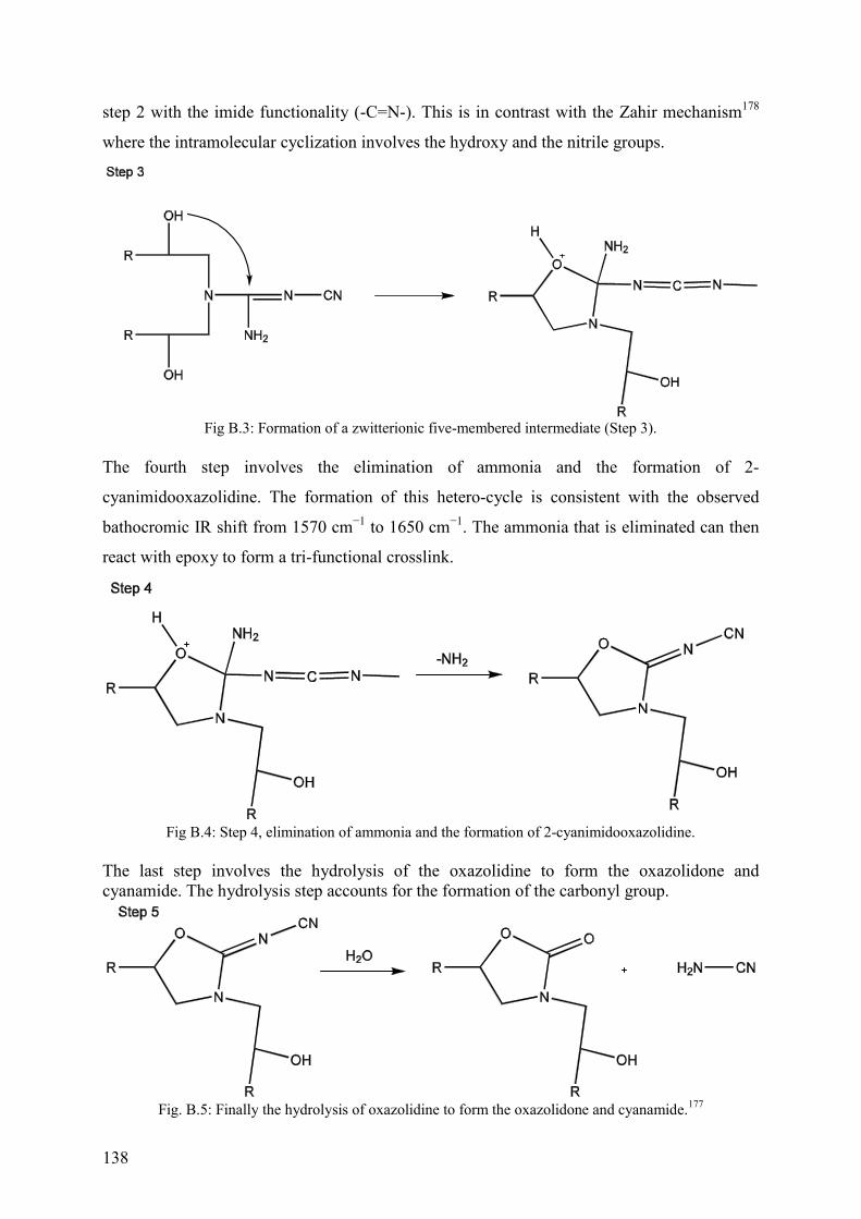
138
step 2 with the imide functionality (-C=N-). This is in contrast with the Zahir mechanism178
where the intramolecular cyclization involves the hydroxy and the nitrile groups.
Fig B.3: Formation of a zwitterionic five-membered intermediate (Step 3).
The fourth step involves the elimination of ammonia and the formation of 2-
cyanimidooxazolidine. The formation of this hetero-cycle is consistent with the observed
bathocromic IR shift from 1570 cm−1 to 1650 cm−1. The ammonia that is eliminated can then
react with epoxy to form a tri-functional crosslink.
Fig B.4: Step 4, elimination of ammonia and the formation of 2-cyanimidooxazolidine.
The last step involves the hydrolysis of the oxazolidine to form the oxazolidone andcyanamide. The hydrolysis step accounts for the formation of the carbonyl group.
Fig. B.5: Finally the hydrolysis of oxazolidine to form the oxazolidone and cyanamide.177
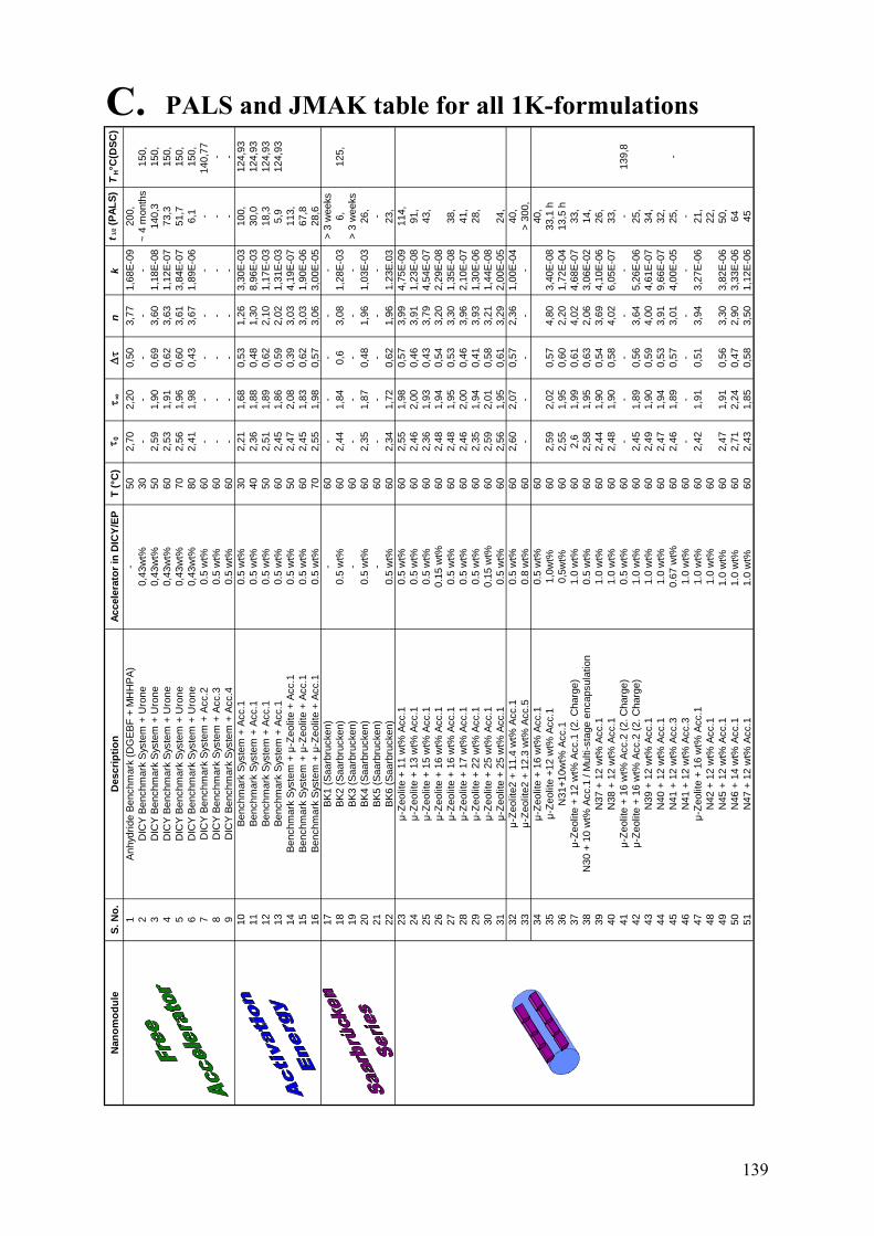
Nan
om
od
ule
S.N
o.
Descri
pti
on
Accele
rato
rin
DIC
Y/E
PT
(°C
)t 0
t ∞D
tn
kt
1/2
(PA
LS
)T
H°C
(DS
C)
1A
nhyd
ride
Benchm
ark
(DG
EB
F+
MH
HP
A)
-50
2,7
02,2
00,5
03,7
71,6
8E
-09
200,
2D
ICY
Benchm
ark
Sys
tem
+U
rone
0,4
3w
t%30
--
--
-~
4m
onth
s150,
3D
ICY
Benchm
ark
Sys
tem
+U
rone
0,4
3w
t%50
2,5
91,9
00,6
93,6
01,1
8E
-08
140,3
150,
4D
ICY
Benchm
ark
Sys
tem
+U
rone
0,4
3w
t%60
2,5
31,9
10,6
23,6
31,1
2E
-07
73,3
150,
5D
ICY
Benchm
ark
Sys
tem
+U
rone
0,4
3w
t%70
2,5
61,9
60,6
03,6
13,8
4E
-07
51,7
150,
6D
ICY
Benchm
ark
Sys
tem
+U
rone
0,4
3w
t%80
2,4
11,9
80,4
33,6
71,8
9E
-06
6,1
150,
7D
ICY
Benchm
ark
Sys
tem
+A
cc.2
0.5
wt%
60
--
--
--
140,7
78
DIC
YB
enchm
ark
Sys
tem
+A
cc.3
0.5
wt%
60
--
--
--
-9
DIC
YB
enchm
ark
Sys
tem
+A
cc.4
0.5
wt%
60
--
--
--
-10
Benchm
ark
Sys
tem
+A
cc.1
0.5
wt%
30
2,2
11,6
80,5
31,2
63,3
0E
-03
100,
124,9
311
Benchm
ark
Sys
tem
+A
cc.1
0.5
wt%
40
2,3
61,8
80,4
81,3
08,9
6E
-03
30,0
124,9
312
Benchm
ark
Sys
tem
+A
cc.1
0.5
wt%
50
2,5
11,8
90,6
22,1
01,1
7E
-03
18,3
124,9
313
Benchm
ark
Sys
tem
+A
cc.1
0.5
wt%
60
2,4
51,8
60,5
92,0
21,3
1E
-03
5,9
124,9
314
Benchm
ark
Sys
tem
+μ
-Zeolit
e+
Acc.1
0.5
wt%
50
2,4
72,0
80,3
93,0
34,1
9E
-07
113,
15
Benchm
ark
Sys
tem
+μ
-Zeolit
e+
Acc.1
0.5
wt%
60
2,4
51,8
30,6
23,0
31,9
0E
-06
67,8
16
Benchm
ark
Sys
tem
+μ
-Zeolit
e+
Acc.1
0.5
wt%
70
2,5
51,9
80,5
73,0
63,0
0E
-05
28,6
17
BK
1(S
aarb
rucke
n)
-60
--
--
->
3w
eeks
18
BK
2(S
aarb
rucke
n)
0.5
wt%
60
2,4
41,8
40,6
3,0
81,2
8E
-03
6,
125,
19
BK
3(S
aarb
rucke
n)
-60
--
--
->
3w
eeks
20
BK
4(S
aarb
rucke
n)
0.5
wt%
60
2,3
51,8
70,4
81,9
61,0
3E
-03
26,
21
BK
5(S
aarb
rucke
n)
-60
--
--
--
22
BK
6(S
aarb
rucke
n)
0.5
wt%
60
2,3
41,7
20,6
21,9
61.2
3E
.03
23,
23
μ-Z
eolit
e+
11
wt%
Acc.1
0.5
wt%
60
2,5
51,9
80,5
73,9
94,7
5E
-09
114,
24
μ-Z
eolit
e+
13
wt%
Acc.1
0.5
wt%
60
2,4
62,0
00,4
63,9
11,2
3E
-08
91,
25
μ-Z
eolit
e+
15
wt%
Acc.1
0.5
wt%
60
2,3
61,9
30,4
33,7
94,5
4E
-07
43,
26
μ-Z
eolit
e+
16
wt%
Acc.1
0.1
5w
t%60
2,4
81,9
40,5
43,2
02,2
9E
-08
27
μ-Z
eolit
e+
16
wt%
Acc.1
0.5
wt%
60
2,4
81,9
50,5
33,3
01,3
5E
-08
38,
28
μ-Z
eolit
e+
17
wt%
Acc.1
0.5
wt%
60
2,4
62,0
00,4
63,9
62,1
0E
-07
41,
29
μ-Z
eolit
e+
22
wt%
Acc.1
0.5
wt%
60
2,3
51,9
40,4
13,9
31,3
0E
-06
28,
30
μ-Z
eolit
e+
25
wt%
Acc.1
0.1
5w
t%60
2,5
92,0
10,5
83,2
11,4
4E
-08
31
μ-Z
eolit
e+
25
wt%
Acc.1
0.5
wt%
60
2,5
61,9
50,6
13,2
92,0
0E
-05
24,
32
μ-Z
eolit
e2
+11.4
wt%
Acc.1
0.5
wt%
60
2,6
02,0
70,5
72,3
61,0
0E
-04
40,
33
μ-Z
eolit
e2
+12.3
wt%
Acc.5
0.8
wt%
60
--
--
->
300,
34
μ-Z
eolit
e+
16
wt%
Acc.1
0.5
wt%
60
40,
35
μ-Z
eolit
e+
12
wt%
Acc.1
1,0
wt%
60
2,5
92,0
20,5
74,8
03,4
0E
-08
33,1
h36
N31+
10w
t%A
cc.1
0,5
wt%
60
2,5
51,9
50,6
02,2
01,7
2E
-04
13,5
h37
μ-Z
eolit
e+
12
wt%
Acc.1
(2.C
harg
e)
1.0
wt%
60
2,6
1,9
90,6
14,0
24,6
8E
-07
33,
38
N30
+10
wt%
Acc.1
/M
ulti-
sta
ge
encapsula
tion
0.5
wt%
60
2,5
81,9
50,6
32,0
63,0
6E
-02
14,
39
N37
+12
wt%
Acc.1
1.0
wt%
60
2,4
41,9
00,5
43,6
94,1
0E
-06
26,
40
N38
+12
wt%
Acc.1
1.0
wt%
60
2,4
81,9
00,5
84,0
26,0
5E
-07
33,
41
μ-Z
eolit
e+
16
wt%
Acc.2
(2.C
harg
e)
0.5
wt%
60
--
--
--
139,8
42
μ-Z
eolit
e+
16
wt%
Acc.2
(2.C
harg
e)
1.0
wt%
60
2,4
51,8
90,5
63,6
45,2
6E
-06
25,
43
N39
+12
wt%
Acc.1
1.0
wt%
60
2,4
91,9
00,5
94,0
04,6
1E
-07
34,
44
N40
+12
wt%
Acc.1
1.0
wt%
60
2,4
71,9
40,5
33,9
19,6
6E
-07
32,
45
N41
+12
wt%
Acc.3
0.6
7w
t%60
2,4
61,8
90,5
73,0
14,0
0E
-05
25,
-46
N41
+12
wt%
Acc.3
1.0
wt%
60
--
--
--
47
μ-Z
eolit
e+
16
wt%
Acc.1
1.0
wt%
60
2,4
21,9
10,5
13,9
43,2
7E
-06
21,
48
N42
+12
wt%
Acc.1
1.0
wt%
60
22,
49
N45
+12
wt%
Acc.1
1.0
wt%
60
2,4
71,9
10,5
63,3
03,8
2E
-06
50,
50
N46
+14
wt%
Acc.1
1.0
wt%
60
2,7
12,2
40,4
72,9
03,3
3E
-06
64
51
N47
+12
wt%
Acc.1
1.0
wt%
60
2,4
31,8
50,5
83,5
01,1
2E
-06
45
C. PALS and JMAK table for all 1K-formulations
139
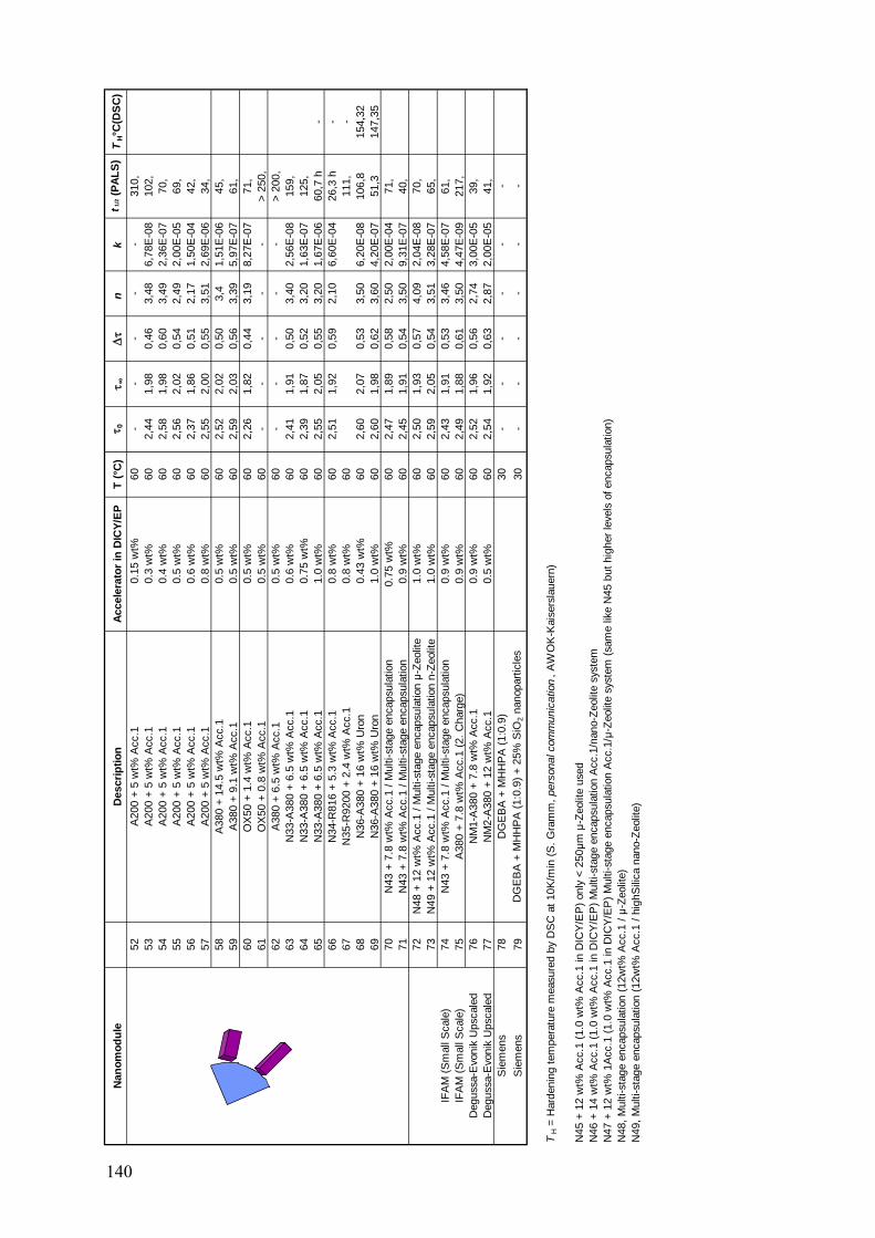
Nan
om
od
ule
Descri
pti
on
Accele
rato
rin
DIC
Y/E
PT
(°C
)t 0
t ∞D
tn
kt1
/2(P
AL
S)
TH°C
(DS
C)
52
A200
+5
wt%
Acc.1
0.1
5w
t%60
--
--
-310,
53
A200
+5
wt%
Acc.1
0.3
wt%
60
2,4
41,9
80,4
63,4
86,7
8E
-08
102,
54
A200
+5
wt%
Acc.1
0.4
wt%
60
2,5
81,9
80,6
03,4
92,3
6E
-07
70,
55
A200
+5
wt%
Acc.1
0.5
wt%
60
2,5
62,0
20,5
42,4
92,0
0E
-05
69,
56
A200
+5
wt%
Acc.1
0.6
wt%
60
2,3
71,8
60,5
12,1
71,5
0E
-04
42,
57
A200
+5
wt%
Acc.1
0.8
wt%
60
2,5
52,0
00,5
53,5
12,6
9E
-06
34,
58
A380
+14.5
wt%
Acc.1
0.5
wt%
60
2,5
22,0
20,5
03,4
1,5
1E
-06
45,
59
A380
+9.1
wt%
Acc.1
0.5
wt%
60
2,5
92,0
30,5
63,3
95,9
7E
-07
61,
60
OX
50
+1.4
wt%
Acc.1
0.5
wt%
60
2,2
61,8
20,4
43,1
98,2
7E
-07
71,
61
OX
50
+0.8
wt%
Acc.1
0.5
wt%
60
--
--
->
250,
62
A380
+6.5
wt%
Acc.1
0.5
wt%
60
--
--
->
200,
63
N33-A
380
+6.5
wt%
Acc.1
0.6
wt%
60
2,4
11,9
10,5
03,4
02,5
6E
-08
159,
64
N33-A
380
+6.5
wt%
Acc.1
0.7
5w
t%60
2,3
91,8
70,5
23,2
01,6
3E
-07
125,
65
N33-A
380
+6.5
wt%
Acc.1
1.0
wt%
60
2,5
52,0
50,5
53,2
01,6
7E
-06
60,7
h-
66
N34-R
816
+5.3
wt%
Acc.1
0.8
wt%
60
2,5
11,9
20,5
92,1
06,6
0E
-04
26,3
h-
67
N35-R
9200
+2.4
wt%
Acc.1
0.8
wt%
60
111,
-
68
N36-A
380
+16
wt%
Uro
n0.4
3w
t%60
2,6
02,0
70,5
33,5
06,2
0E
-08
106,8
154,3
2
69
N36-A
380
+16
wt%
Uro
n1.0
wt%
60
2,6
01,9
80,6
23,6
04,2
0E
-07
51,3
147,3
5
70
N43
+7.8
wt%
Acc.1
/M
ulti-st
age
encapsu
lation
0.7
5w
t%60
2,4
71,8
90,5
82,5
02,0
0E
-04
71,
71
N43
+7.8
wt%
Acc.1
/M
ulti-st
age
encapsu
lation
0.9
wt%
60
2,4
51,9
10,5
43,5
09,3
1E
-07
40,
72
N48
+12
wt%
Acc.1
/M
ulti-st
age
encapsu
lationμ
-Zeolit
e1.0
wt%
60
2,5
01,9
30,5
74,0
92,0
4E
-08
70,
73
N49
+12
wt%
Acc.1
/M
ulti-st
age
encapsu
lation
n-Z
eolit
e1.0
wt%
60
2,5
92,0
50,5
43,5
13,2
8E
-07
65,
IFA
M(S
mall
Scale
)74
N43
+7.8
wt%
Acc.1
/M
ulti-st
age
encapsu
lation
0.9
wt%
60
2,4
31,9
10,5
33,4
64,5
8E
-07
61,
IFA
M(S
mall
Scale
)75
A380
+7.8
wt%
Acc.1
(2.
Charg
e)
0.9
wt%
60
2,4
91,8
80,6
13,5
04,4
7E
-09
217,
Deguss
a-E
vonik
Upsc
ale
d76
NM
1-A
380
+7.8
wt%
Acc.1
0.9
wt%
60
2,5
21,9
60,5
62,7
43,0
0E
-05
39,
Deguss
a-E
vonik
Upsc
ale
d77
NM
2-A
380
+12
wt%
Acc.1
0.5
wt%
60
2,5
41,9
20,6
32,8
72,0
0E
-05
41,
Sie
mens
78
DG
EB
A+
MH
HP
A(1
:0.9
)30
--
--
--
Sie
mens
79
DG
EB
A+
MH
HP
A(1
:0.9
)+
25%
SiO
2nanopart
icle
s30
--
--
--
TH
=H
ard
enin
gte
mpera
ture
measu
red
by
DS
Cat
10K
/min
(S.
Gra
mm
,pers
onalcom
munic
ation
,A
WO
K-K
ais
ers
lauern
)
N45
+12
wt%
Acc.1
(1.0
wt%
Acc.1
inD
ICY
/EP
)only
<250μ
mμ
-Zeolit
euse
d
N46
+14
wt%
Acc.1
(1.0
wt%
Acc.1
inD
ICY
/EP
)M
ulti-st
age
encapsu
lation
Acc.1
/nano-Z
eolit
esy
stem
N47
+12
wt%
1A
cc.1
(1.0
wt%
Acc.1
inD
ICY
/EP
)M
ulti-st
age
encapsu
lation
Acc.1
/μ-Z
eolit
esy
stem
(sam
elik
eN
45
but
hig
her
leve
lsofencapsu
lation)
N48,
Multi-st
age
encapsu
lation
(12w
t%A
cc.1
/μ
-Zeolit
e)
N49,
Multi-st
age
encapsu
lation
(12w
t%A
cc.1
/hig
hS
ilica
nano-Z
eolit
e)
140
Acknowledgements
I am deeply grateful to Prof. Dr. Franz Faupel for accepting me as a PhD candidate in his
group at the Institute for Material Science, Multi-component Materials, Christian-Albrechts
University of Kiel and the German Ministry of Education and Research (BMBF) for the
financial support under the Project No.:03X0026F “Nanomodule”. The last four years of my
life have been no less than a roller coaster ride, both in terms of the academics and my
personal life. But before going into details I would like to thank one of the most important
person, who’s scientific knowledge and discussions helped me to finally complete my PhD
thesis, my mentor, my guide and my “Doktorpapa”; Prof. Dr. Klaus Rätzke. It was an honor
learning under his supervision, not just the academic part but also the social part i.e.
punctuality, good sense of humor and team skills. I’m sure all these qualities will go a long
way in building my personality as a qualified researcher and most important of all a more
responsible individual.
Special thanks for Emeritus Prof. Dr. Günter Dlubek from the Institute for Innovative
Technologies (ITA), in Halle (Saale). He is the “See of Knowledge” when it comes to
positron annihilation science and I consider myself really lucky to grab a few buckets of
knowledge for myself. Dr. Michael Noeske and collegues from Fraunhofer Institute for
Manufacturing Technology and Applied Materials Research (IFAM) in Bremen, Prof. Dr.
Wulff Possart and Dipl.-Ing. Jan Gaukler from the University of Saarland in Saarbruecken
were really cordial with their expert opinions and the scientific discussions during the half
yearly meetings within the framework of the BMBF project, along with other industrial and
academic partners.
It’s never easy to settle in a completely new environment, but thanks to Dr. Ing. Jan Kruse and
Dr. Ing. Alexandar Bartsch for not only a smooth transition into the “Kieler Positronerei”, but
also for the scientific knowledge and healthy discussions. Dipl.-Ing. Rainer Kloth made sure
that my PC kept running and the huge data analysis in my work was not possible without his
technical assistance. Dipl. Ing. Stefan Rehders is simply the best when it comes to the
engineering skills and knowledge. It was always relaxing to know that he is on the standby,
whenever it comes to troubleshooting. Another Stephan I would like to thank is my lab mate,
Dipl. Phys. Stephan Harms, we always had a very good level of understanding when it comes
to sharing not only the three PALS machines but also our lab duties. It was the same case
when I use to share the lab with Dipl. Ing. Dennis Ehlers. There was a time when the three of
us worked together to assemble the new PALS baby “MCB4”, it was an interesting phase of
my thesis, as I never thought that learning can be so fun, I think we were a great team.
The “Chair Symposiums” together with the groups of Prof. Dr. Rainer Adelung and Prof. Dr.
Mady Elbahry helped a lot in increasing the general scientific knowledge and also improved
my presentation skills. The famous “Two Questions” of Dr. Vladimir Zaporojtchenko are
particularly appreciated for the gain in scientific knowledge, although most of the times one
used to ask “and what was the other question please?”
My “Mittags Gruppe”, including Dr. Ing. Seid Jebril, M.Sc Arfat Pradana, M.Sc Dawit
Gedamu and M.Sc Ahmed Fazir, deserve a big thank for all the politically in-correct
discussions. Dr. rer. nat. Ulrich Schürmann, Dr. Ing. Sebastian Wille, Dr. Ing. Christian
Hanisch, Dr. Ing. Henry Greeve, M.Sc Sören Kaps, Dipl. Phys. Tomislav Hrkac and Dipl.
Chem. Christina Pakula made sure that living in Kiel was fun. My “Kicker” mates and the
“WM-2010” group, for giving me such wonderful memories to cheer, it would have been
great if the “Nationalmannschaft” were the champions. M.Sc Chakravadhanula Venkata Sai
Kiran was really helpful for all the tips regarding the loopholes in the German bureaucratic
system. Big thanks to all the significant members of the AG Faupel, AG Adelung and AG
Elbahry for the coffee and cake parties.
I would also like to thank my family back in Pakistan, for their continued support and prayers.
Last but definitely not the least; I would like to thank my wife Ayesha for her continued
support and love, which helped a lot even through some of the darkest and the lowest phases
of my life. She always believed that I can do it and her love gave me strength to keep striving
for the best, which eventually resulted in achieving this work.
Curriculum Vitae
Name: Muhammad Qasim Shaikh
Address: Preetzer Str. 64, 24143 Kiel
Born: 14.November 1977 in Karachi
Parents: Muhammad Shamim Shaikh
Feroza Nigar
School Education
1991 Secondary School Certificate
1993 Higher Secondary School Certificate (Graduation)
Academic Education
01/1994 - 08/1998 Bachelors of Mechanical Engineering (B.E.)
at the N.E.D University of Engineering and Technology, Karachi
10/2004 - 09/2006 Masters in Applied Polymer Science (M.Sc)
at the Martin-Luther University of Halle-Wittenberg
09/2006 Master Thesis: "Investigation of Free Volume in Polymers by PositronAnnihilation Lifetime Spectroscopy (PALS)"'
Occupational History
09/1998 - 09/2004 Manager Production and Quality control
at Nasarun Exports, Karachi
09/2006 - Scientific Researcher
at the Institute of Material Science, Multicomponent Materials
Engineering Department, Christian-Albrechts University of Kiel

List of Publications
Publications related to this work:
1. "Shelf stability of reactive adhesive formulations: A case study for dicyandiamide-cured epoxysystems". K. Raetzke, M.Q. Shaikh, F. Faupel, P.-L.M. Noeske, International Journal ofAdhesion and Adhesives, Vol. 30, Issue 2, 105-110, (2010).
2. "Effect of accelerator encapsulation on the curing kinetics and the activation energies of one-component epoxy-resin formulations". M.Q. Shaikh, K. Raetzke, F. Faupel, P.-L.M. Noeske, inpreparation.
3. "IR-spectroscopy, DSC and PALS studies of several epoxy precursors and their curedcomposites”. M.Q. Shaikh, K. Rätzke, J. Ch. Gaukler, W. Possart, F. Faupel, in preparation.
Other Publications:
4. “Positron Annihilation studies on Metal Organic Frameworks”. M.Q. Shaikh, K. Raetzke, F.Faupel, I. Senkovska and S. Kaskel, in preparation.
5. "From small molecules to polymers: The free volume from PALS and PVT experiments inrelation to the dynamics", G. Dlubek, M.Q. Shaikh, Y. Yu, J. Pionteck, M. Paluch, K. Rätzke,F. Faupel, R. Krause-Rehberg, 14th International Conference Polymeric Materials´2010(P2010), Halle (Saale), Sept. 15-17, 2010. Submitted.
6. "Open volume in bioadhesive detected by positron annihilation lifetime spectroscopy ". K.Raetzke, M. Wiegemann, M.Q. Shaikh, S. Harms, R. Adelung, W. Egger and P. Sperr, ActaBiomaterialia Vol. 6, 2690-2694, (2010).
7. "Free volume from positron lifetime and pressure–volume–temperature experiments in relationto structural relaxation of van der Waals molecular glass-forming liquids". G. Dlubek, M.Q.Shaikh, K. Raetzke, M. Paluch and F. Faupel, Journal of Physics: Condensed Matter, Vol. 22,235104, (2010).
8. "Subnanometre size free volumes in amorphous Verapamil hydrochloride: A positron lifetimeand PVT study through Tg in comparison with dielectric relaxation spectroscopy". G. Dlubek,M.Q. Shaikh, K. Rätzke, J. Pionteck, M. Paluch, F. Faupel, European Journal of PharmaceuticalSciences. Vol. 41, 388–398 (2010).
9. "Molecular Dynamics Approach to Structure-Property Correlation in Epoxy Resins for Thermo-Mechanical Lifetime Modeling" B. Wunderle, E. Dermitzaki, O. Hoelck, J. Bauer, H. Walter,M.Q. Shaikh, K. Raetzke, F. Faupel, B. Michel, H. Reich; The 59th Electronic Components andTechnology Conference (ECTC), San Diego, California USA, May (2009).
10. “The temperature dependence of free volume in phenyl salicylate and its relation to structuraldynamics: A positron annihilation lifetime and pressure-volume-temperature study” G. Dlubek,M.Q. Shaikh, K. Raetzke, F. Faupel, J. Pionteck, and M. Paluch; Journal of Chemical Physics130, 144906 (2009).
11. “Gas permeability and free volume in poly(amide-b-ethylene oxide)/polyethylene glycol blendmembranes” W. Yave, A. Car, K.V. Peinemann, M.Q. Shaikh, K. Rätzke, F. Faupel; Journal ofMembrane Science 339, 177 (2009).
12. "Molecular Dynamics Simulation and Mechanical Characterization for the Establishment ofStructure-Property Correlations for Epoxy Resins in Microelectronics Packaging Applications"B. Wunderle, E. Dermitzaki, O. Hoelck, J. Bauer, H. Walter, M.Q. Shaikh, K. Raetzke, F.Faupel, B. Michel; Proceedings of the 10th EuroSimE, Delft, The Netherlands, April (2009).
13. “Differences in Free Volume Elements of the Carrier Matrix Affect the Stability ofMicroencapsulated Lipophilic Food Ingredients” S. Drusch, K. Raetzke, M.Q. Shaikh, Y.Serfert, H. Steckel, M. Scampicchio, I. Voigt, K. Schwarz, S. Mannino; Food Biophysics 4, 42(2009).
14. “Temperature dependence of the free volume from positron lifetime experiments and its relationto structural dynamics: Phenylphthalein-dimethylether” G. Dlubek, M.Q. Shaikh, K. Raetzke,F. Faupel, M. Paluch; Physical Review E 78, 051505 (2008).
15. “Free volume of an oligomeric epoxy resin and its relation to structural relaxation: Evidencefrom positron lifetime and pressure-volume-temperature experiments” G. Dlubek, J. Pointeck,M.Q. Shaikh, E.M. Hassan, R. Krause-Rehberg; Physical Review E 75, 021802 (2007).
16. “The free volume in two untreated, pressure-densified, and CO2 gas exposed polymers frompositron lifetime and pressure-volume-temperature experiments” G. Dlubek, J. Pionteck, M.Q.Shaikh, L. Häußler, S. Thraenert, E. M. Hassan, R. Krause-Rehberg; e-Polymers no.108, 1(2007).
17. “Effect of free volume and temperature on the structural relaxation inpolymethylphenylsiloxane: A positron lifetime and pressure-volume-temperature study” G.Dlubek, M.Q. Shaikh, R. Krause-Rehberg, M. Paluch; Journal of Chemical Physics 126,024906 (2007).
Declaration
I hereby declare that this thesis entitled "Free Volume and Storage Stability of One-
component Epoxy Nanocomposites" is an authentic record of research work carried out by
me and coworkers under the supervision of Prof. Dr. Klaus Rätzke, Multicomponent
Materials, at Institute for Materials Science and Engineering, Christian Albrechts University
of Kiel, Germany.
In keeping with the general practice of reporting scientific works, due acknowledgement has
been made whenever work discussed has been based on the finding of other investigators.
Any oversight due to error of judgment is regretted.
Muhammad Qasim Shaikh
Kiel, 2011
Top Related
Copyright © 2022 FDOKUMEN

