ARTICLE

Force-directed layout of origin-destination flow mapsBernhard Jenny a,b,c, Daniel M. Stephen c, Ian Muehlenhaus d,Brooke E. Marstonc, Ritesh Sharma e, Eugene Zhange and Helen Jennyc

aFaculty of Information Technology, Monash University, Melbourne, Australia; bSchool of Science –Geospatial Sciences, RMIT University, Melbourne, Australia; cCollege of Earth, Ocean, and AtmosphericSciences, Oregon State University, Corvallis, OR, USA; dDepartment of Geography, University of WisconsinMadison, Madison, WI, USA; eSchool of Electrical Engineering and Computer Science, Oregon StateUniversity, Corvallis, OR, USA

ABSTRACTThis paper introduces a force-directed layout method for creatingorigin-destination flow maps. Design principles derived from man-ual cartography and automated graph drawing to increase read-ability of flow maps and graph layouts are taken into account. Theorigin-destination flow maps produced with our algorithm showflows with quadratic Bézier curves that reduce flow-on-flow andflow-on-node overlaps, and avoid sharp or irregular bends in flowlines. A survey of expert cartographers found that flow mapscreated with our automated method are similar in quality tomanually produced flow maps.

ARTICLE HISTORYReceived 7 November 2016Accepted 13 March 2017

KEYWORDSOrigin-destination flowmaps; graph drawing;cartographic designprinciples; map design

1. Introduction

Flow maps visualize movement and not only demonstrate which places have beenaffected by movement but also the type, direction, and volume of movement. Theyare efficient tools for identifying spatial patterns and answer questions about geo-graphic phenomena. Geographic flow mapping is an underdeveloped subfield of infor-mation visualization and geographic information science (Rae 2011). Legible flow mapsare labor intensive to create manually and require a high level of cartographic expertise.As map automation and map services become more common methods of making maps,well-designed flow maps are increasingly rare. Despite efforts to develop specializedsoftware (Tobler 1987, Rae 2011, Kim et al. 2012, Gerlt 2013) and web map services (Guo2012), flow map functionality is limited and cumbersome to use in current geographicinformation systems and web mapping software.

Our computational flow mapping method takes cartographic design principles intoaccount. It creates non-branching origin-destination flow maps where the curvature ofthe flows can be adjusted freely because the geometry of the flow path is unknown orirrelevant for the visualization.

CONTACT Bernhard Jenny bernie.jenny@monash.edu

INTERNATIONAL JOURNAL OF GEOGRAPHICAL INFORMATION SCIENCE, 2017http://dx.doi.org/10.1080/13658816.2017.1307378

© 2017 Informa UK Limited, trading as Taylor & Francis Group

2. Related work

2.1. Design principles for flow maps

Cartographic design principles are guidelines that help cartographers to create legibleand aesthetically pleasing maps. One of the primary goals for designing origin-destina-tion flow maps is to reduce overlaps between flows because flow-on-flow and flow-on-node overlaps often create ambiguous maps that are difficult to read accurately. Jennyet al. (2016) compiled cartographic design principles for origin-destination flow mapsfrom cartographic literature (Imhof 1972, Dent et al. 2008, Slocum et al. 2009) and graphdrawing, a discipline in computer science concerned with generating diagram layoutsfor graphs.

Graph drawing is relevant to mapping origin-destination flows because flows onmaps form a graph; the graph nodes are the starts and ends of flows and the graphedges are the connecting flows. In graph drawing, as in flow mapping, the geometry ofedges is adjusted to reduce the number of flow-on-flow and flow-on-node overlaps.Because graph drawing and flow mapping share similar design characteristics, userstudies evaluating design principles for graph drawing are relevant to the design ofcartographic flow maps. However, principles from graph drawing need to be adapted toflow mapping because unlike graph drawing, the starts and ends of flows in maps aregeographically constrained and cannot be freely positioned.

A number of design principles for the design of flow geometry and the arrangement offlow lines were verified by user studies. These user studies show that applying designprinciples decreases error rates and reading time. Before developing our automatedmethod, we completed a content analysis with 97 manually created flow maps to identifydesign principles applied by professional cartographers. We also conducted a user studyto test additional design options. The results of the user study led us to recommend thefollowing set of design principles for flow maps (Figure 1) (Jenny et al. 2016).

The number of flows overlapping should be minimized (Purchase et al. 1996, Wareet al. 2002, Huang et al. 2008). Curving flows can reduce overlaps (Figure 1(a)). Sharpbends should be avoided (Purchase et al. 1996), and symmetrically curved flows arepreferable to asymmetric flows (Figure 1(b)) (Jenny et al. 2016). Acute-angle crossings of

eAngular

Distribution

bCurve Shape

aIntersectionsand Overlap

Avoided

Preferred

cIntersection

Angles

d

NodesUnconnected

Figure 1. Design principles for origin-destination flow maps: preferred (top) and avoided (bottom)arrangements (from Jenny et al. 2016).

2 B. JENNY ET AL.

flows should also be avoided (Figure 1(c)) (Huang et al. 2008, 2014). Flows must not passunder unconnected nodes (Figure 1(d)) (Wong et al. 2003). Flows should be radiallydistributed around nodes (Figure 1(e)) (Huang 2007). Small flows are placed on top oflarge flows (Dent et al. 2009).

Design principles for indicating flow quantity and direction are well established incartography. Quantity is best represented by adjusting the width of flows (Dent et al.2009). Arrowheads are the best indication for direction on flow maps (Jenny et al. 2016).

2.2. Automated creation of origin-destination flow maps

The first automated methods for creating flow maps used straight bands to connectstart and end positions. Tobler (1987) dates the earliest example of a digitally generatedflow map to 1959. Kern and Rushton (1969) used thin straight lines to connect origins todestinations. Kadmon (1971) introduced digital flow lines with varying widths to indicatequantities, and Wittick (1976) extended these digital methods to map quantitative flowsin networks, and others (Evatt et al. 1981, Tobler 1981, 1987) later refined and extendedthese digital approaches.

Bézier curves (Brandes et al. 2000, Guo 2009, Wood et al. 2011, Guo and Zhu 2014)and sections of circles (Ho et al. 2011) have been used for automated origin-destinationflow maps. In these digital applications, the geometric arrangement of flows is neitheroptimized to minimize the number of intersections among flow lines, nor reduce thenumber of overlaps between flows.

A few authors explore methods for the automated creation of branching flow maps(Phan et al. 2005, Verbeek et al. 2011, Nocaj and Brandes 2013, Debiasi et al. 2014a,2014b). Complementary approaches for flow clustering (Zhu and Guo 2014) and edgebundling are also explored. Zhou et al. (2013) present an overview of edge bundlingapplied to flow visualization.

In graph drawing, curved edges are used for node-link diagrams (Riche et al. 2012, Xuet al. 2012). The reasoning behind using curved lines in graph drawing can also beapplied to flow mapping: better use of canvas space and reduced visual clutter becausefewer edges overlap or intersect.

3. Force-directed layout method

We develop a force-directed layout method to automate the creation of non-branchingorigin-destination flow maps. Flows are modeled with quadratic Bézier curves that useone control point, which is placed off the line. Quadratic Bézier curves are an appropriatechoice for origin-destination flow maps because they cannot have loops, are neverS-shaped, and are included in common graphics libraries and exchange formats. Ifnecessary, they can be converted to cubic curves for editing in vector graphics software.

The control point of each quadratic Bézier curve is attached to a spring (Figure 2). Theopposing end of the spring is attached to the midpoint of the line between the start andend points of the flow. Other flows exert repulsing forces onto the control point of thequadratic Bézier curve. Inspired by methods for force-directed graph drawing (Brandesand Wagner 2000, Kobourov 2012, Fink 2013), an iterative process computes theequilibrium state between the retracting forces of the springs and the repulsing forces

INTERNATIONAL JOURNAL OF GEOGRAPHICAL INFORMATION SCIENCE 3

of other flows. We develop a series of refinements to this algorithm (discussed below).For example, spring stiffness is adjusted for peripheral flows, excessively asymmetricflows are avoided, flows are moved away from overlapping nodes, and control pointsare constrained to a bounding rectangle to avoid excessive curvature. Our method iscontrolled by a set of parameters. We provide default parameter values that can beadjusted using a graphical user interface.

The pseudo-code below provides an outline of the method. On each iteration, foreach flow f, five forces are computed: Fflows is the total repulsing force exerted by allother flow curves; Fnodes is the total repulsing force exerted by all other flow nodes;FantiTorsion is a force countering asymmetric distortion of the flow; Fspring is the forceexerted by the spring on the Bézier control point; and FangRes is a force improving theangular resolution of flows around nodes. Each of the five forces is scaled by anindividual, user-defined weight. An additional weight w is applied to the first four forces.This weight linearly decreases from 1 to 0 to decrease the energy in the system towardthe end of the iterative computations. The stabilizing weight for FangRes is w − w2. We usethis weight instead of w to reduce the influence of the angular adjustments during theinitial phase of computations. We use the following default values for the five weights:wflows = 1; wnodes = 0.5; wantiTorsion = 0.8; wspring = 1; and wangRes = 3.75. The default is 100iterations for small flow data sets. For complex or large flow maps, a larger number ofiterations is necessary for the layout to converge to a stable equilibrium.

Ftotal is the sum of the five weighted forces and is applied to the Bézier control pointof f to compute a new translated control point position. The translated control points areconstrained to stay within a rectangle aligned with the start-to-end line of the flow. Theyare also constrained to stay within a rectangle aligned with the canvas space. After thecontrol points of all flows have been translated, intersecting flows and flows that overlapunconnected nodes or arrowheads are moved.

Input: Flows in map MOutput: An improved layout of Mj = 0for i in 0 .. #iterations – 1 do

// forces exerting on Bézier control pointsw = 1 – i/#iterationsfor each flow f in M do

Fflows ← force of flows in M against f (Section 3.1.1)Fnodes ← force of nodes in M against f (Section 3.1.2)

Fspring

Figure 2. Quadratic Bézier curve modeling a flow with a spring pulling the control point toward themidpoint between start and end points.

4 B. JENNY ET AL.

FantiTorsion ← anti-torsion force of f (Section 3.1.3)

Fspring ← spring force of f (Section 3.1.4)FangRes ← angular resolution force of f (Section 3.1.5)Ftotal = w · (wflows · Fflows + wnodes · Fnodes + wantiTorsion · FantiTorsion +wspring · Fspring) + (w – w2) · wangRes · FangRes

pf ← copy control point of f and translate by FtotalConstrain pf to rectangle aligned with f (Section 3.2.1)Constrain pf to canvas rectangle (Section 3.2.1)

end forfor each flow f in M do

Assign control point pf to fend for

// reducing flow intersections (Section 3.2.2)P ← pairs of intersecting flows connected to a shared nodefor each pair p in P do

Move control points of both flows of pend for

// moving flows off nodes and arrowheads (Section 3.2.3)if (i > 10% of #iterations and j ≤ 0) then

N ← flows overlapping nodes and arrowheadsj ← number of iterations until next flow is moved off nodesn ← number of flows to move off nodesfor each flow f in N do

if (geometry for f without overlap exists) thenMove control point pf of fbreak for loop if n flows have been moved

end ifend for

elsej = j – 1

end ifend for

3.1. Forces exerting on Bézier control points

3.1.1. Curving flows with flows-against-flow forcesFlows on the map exert repulsing forces against the control points of all other flows,which curve the flows. The purpose of the flows-against-flow force is to spread flowsapart to reduce overlap and avoid intersections between flows.

We calculate the force Fflows exerted on the control point of flow f by all other flowson the map by first locating evenly spaced points along all flows (Figure 3). Points along

INTERNATIONAL JOURNAL OF GEOGRAPHICAL INFORMATION SCIENCE 5

all other flows emit a repelling force against each point of f. The repelling forces areinterpolated for each point of f using Shepard’s (1968) inverse distance weighting. Theresulting force for point p on f is: Fp ¼

Pdi " wi=

Pwi, with wi ¼ 1= dij jα, where dij j is the

distance between p and another point not on f, and α is a parameter. The final forceFflows is the sum of the forces exerted onto all points of f divided by the number ofpoints n on f: Fflows ¼

PpFp=n. Fflows is applied on the control point of f. The default value

for parameter α is 4.

3.1.2. Curving flows with nodes-against-flow forcesNodes exert a repelling force that moves flows apart to prevent flows from touchingunconnected nodes. To compute the repelling force Fnodes for flow f, for each node ni notconnected to f, we compute the vector di between node ni and the closest point on f(Figure 4). Fnodes is computed with inverse distance weighting: Fnodes ¼

Pdi " wi=

Pwi,

with wi ¼ 1= dij jβ, where dij j is the length of di, and β is a parameter. Fnodes is applied tothe control point of f. The default value for parameter β is four. Figure 5 shows the effectof the nodes-against-flow forces.

F

Figure 3. Flow-against-flow forces are the distance-weighted sum of forces between points onflows. The forces of only one flow exerting on a second flow are shown.

d1d2

Fnodes

Figure 4. Nodes-against-flow forces by the nodes of the black flow on the gray flow.

6 B. JENNY ET AL.

3.1.3. Anti-torsion to counter asymmetric flowsThe force FantiTorsion reduces Bézier curve asymmetry by pushing the control point towardthe perpendicular bisector of the line between the start and end points (Figure 6). Thelength of FantiTorsion equals the distance between the control point and the perpendicularbisector, which is computed with γ. Figure 7 shows the effect of the anti-torsion forces.

3.1.4. Spring force to reduce curvatureThe spring force Fspring of each flow pulls the control point of the curve toward the basepoint, the point halfway along a line between the start and end points of the flow(Figure 2). This results in a straight flow if no external force is exerted. The purpose ofthe spring force is to oppose external forces that are causing the flow to curve, therebypreventing the flow from curving too much and creating equilibrium with external forces.

The spring force Fspring is computed with Hooke’s law: Fspring = k · L, where k is the springconstant and L is the length of the spring. The spring constant k varies with the length ofthe flow. The spring constant for a flow with zero length is defined by parameter kshort.

Before After

Figure 5. Before (left) and after (right) applying nodes-against-flow forces.

Controlpoint

β

β

γ α

γ = – α – βπ2

fx

fyFantiTorsion

Figure 6. Calculation of the anti-torsion force pulling the Bézier control point toward the perpendi-cular bisector of the start–end line.

Before After

Figure 7. Before (left) and after (right) applying anti-torsion forces.

INTERNATIONAL JOURNAL OF GEOGRAPHICAL INFORMATION SCIENCE 7

Parameter klong is the spring constant for the longest flow on themap. The spring constantfor flow f is linearly interpolated with k = (klong−kshort) · (B/Bmax) + kshort, where B is thedistance between the start and end points of flow f, and Bmax is the longest B of all flows inthe map.

Peripheral flows are made straighter by increasing their spring constant. This countersthe tendency of peripheral flows to curve in an asymmetric way, which is caused by theunilateral distribution of external forces for peripheral flows. The peripherality of flow f iscomputed by dividing the Bézier curve into straight-line segments. For each line segment,we compute the force Fs that all other flows exert with the method for computing flow-against-flow forces outlined in 3.1.1. We sum the force vectors,

PFs, and the length of the

force vectors,P

Fsj j. For a flow surrounded on both sides by other flows, the ratioPFs=

PFsj j is close to 0 because the opposing forces

PFs exerted by surrounding flows

tend to compensate each other. For a peripheral flow, the ratio will be close to 1. The springconstant k is multiplied by

PFs=

PFsj j " Cp þ 1 to increase the spring constant for periph-

eral flows. Parameter Cp adjusts the amount of correction for peripheral flows. We use thefollowing default values for the three parameters: kshort = 0.5; klong = 0.05; and Cp = 2.5.

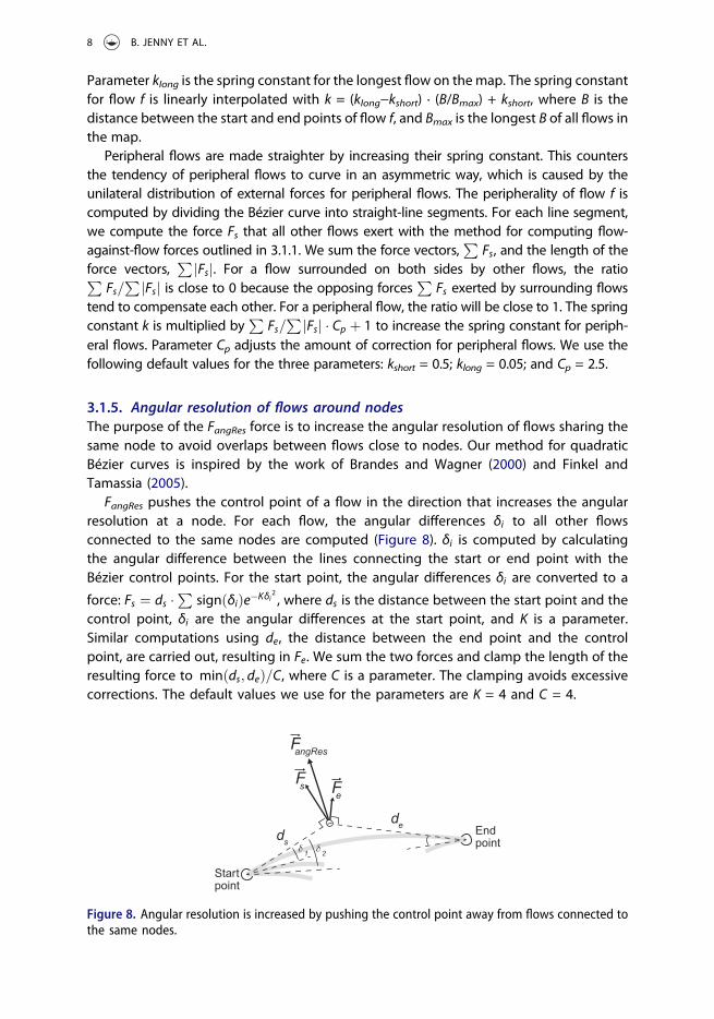
3.1.5. Angular resolution of flows around nodesThe purpose of the FangRes force is to increase the angular resolution of flows sharing thesame node to avoid overlaps between flows close to nodes. Our method for quadraticBézier curves is inspired by the work of Brandes and Wagner (2000) and Finkel andTamassia (2005).

FangRes pushes the control point of a flow in the direction that increases the angularresolution at a node. For each flow, the angular differences δi to all other flowsconnected to the same nodes are computed (Figure 8). δi is computed by calculatingthe angular difference between the lines connecting the start or end point with theBézier control points. For the start point, the angular differences δi are converted to a

force: Fs ¼ ds "P

sign δið Þe&Kδi2, where ds is the distance between the start point and the

control point, δi are the angular differences at the start point, and K is a parameter.Similar computations using de, the distance between the end point and the controlpoint, are carried out, resulting in Fe. We sum the two forces and clamp the length of theresulting force to min ds; deð Þ=C, where C is a parameter. The clamping avoids excessivecorrections. The default values we use for the parameters are K = 4 and C = 4.

FangRes

Fs Fede

ds

Startpoint

Endpointδ 1 δ 2

Figure 8. Angular resolution is increased by pushing the control point away from flows connected tothe same nodes.

8 B. JENNY ET AL.

3.2. Layout constraints

The forces described above are applied to all flows in the map. We apply additionalconstraints to the geometry of flows to adjust strongly asymmetric or curved flows,reduce the number of intersections, and move overlapping flows away from nodes toimprove legibility.

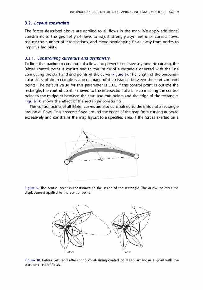
3.2.1. Constraining curvature and asymmetryTo limit the maximum curvature of a flow and prevent excessive asymmetric curving, theBézier control point is constrained to the inside of a rectangle oriented with the lineconnecting the start and end points of the curve (Figure 9). The length of the perpendi-cular sides of the rectangle is a percentage of the distance between the start and endpoints. The default value for this parameter is 50%. If the control point is outside therectangle, the control point is moved to the intersection of a line connecting the controlpoint to the midpoint between the start and end points and the edge of the rectangle.Figure 10 shows the effect of the rectangle constraints.

The control points of all Bézier curves are also constrained to the inside of a rectanglearound all flows. This prevents flows around the edges of the map from curving outwardexcessively and constrains the map layout to a specified area. If the forces exerted on a

Figure 9. The control point is constrained to the inside of the rectangle. The arrow indicates thedisplacement applied to the control point.

AfterBefore

Figure 10. Before (left) and after (right) constraining control points to rectangles aligned with thestart–end line of flows.

INTERNATIONAL JOURNAL OF GEOGRAPHICAL INFORMATION SCIENCE 9

flow push the control point outside the canvas, the same method for rectangles aroundflows is applied. The canvas size can be increased if desired. The default canvas size istwice the length and width of the bounding box around all flows.

3.2.2. Reducing flow intersectionsAcute-angle intersections often occur for flows connected to a shared node. For exam-ple, in Figure 11, two intersecting flows represented as dashed gray lines are bothconnected to the shared node S. We identify pairs of intersecting flows connected toa shared node, then adjust the position of the Bézier control points M and N of the twointersecting flows. Control point M is moved along a line connecting the control point Mand the non-shared node A (Figure 11) to position M̄. The new position is the intersec-tion of the line through A and M with the line through S and N. Control point N is movedto N̄, which is the intersection of the line through N and B and the line through S and M.These adjustments to the Bézier control points are applied at each iteration after theforces described in Section 3.1 have been applied to the control points of all flows (seethe pseudo-code at the beginning of Section 3). The control points are constrained tolay within the limiting rectangles described in Section 3.2.1. Figure 12 (center and right)shows the effect of moving control points to avoid intersections. In the center ofFigure 12, the following flow pairs intersect: from Germany to Austria and Turkey,from Great Britain to Greece and Italy, from Great Britain to Germany and Turkey.

A

S

B

N

M

N

M

Figure 11. Displacement of Bézier control points of intersecting flows connected to the same nodeS. Control points M and N are moved to M̄ and N̄, respectively. Gray dashed lines indicate the initialintersecting flows defined by M and N; solid lines indicate the amended flows defined by M̄ and N̄.

Figure 12. Initial layout (left), layout after moving flows off nodes (center), and layout after reducingintersections (right). The map at the center is Map 6 for the expert study. (Map after TelegeographyInc. (2000))

10 B. JENNY ET AL.

After applying the method described in this section, these flow pairs do not intersect(right of Figure 12).

3.2.3. Moving flows off nodes and arrowheadsThe nodes-against-flow forces described in Section 3.1.2 do not guarantee that maps willnot have flows overlapping nodes or arrowheads of other flows. In dense areas, it is stillpossible for flows to overlap nodes and arrowheads they are not connected to, causingsignificant ambiguity. To avoid this, flows are moved to create a minimum distancebetween flows and obstacles (unconnected nodes or arrowheads). The default para-meter value for the minimum distance of flows from obstacles is four pixels. Figure 12(left and center) shows the effect of moving flows off nodes. In the map on the left ofFigure 12, flows between Germany and Turkey, Germany and Croatia, Great Britain andGermany, Great Britain and Greece, and France and the Netherlands intersect nodes.After applying the method described in this section, these flows do not intersect anynodes (center of Figure 12). The pseudo-code at the beginning of Section 3 is anoverview of the algorithm; details are included below.

If a flow overlaps an obstacle, the control point of the Bézier curve is moved along anArchimedean spiral centered on the initial location of the control point until the curve isa minimum distance from all obstacles (Figure 13). Once a flow is moved away fromobstacles, its control point location cannot be changed in subsequent iterations. Thisprevents the control point from moving back to the same location and the flow fromoverlapping the same obstacle. Because a control point can move a relatively largedistance, additional conflicts with neighboring flows can result. Ideally, each movementaway from an obstacle is followed by a few iterations without similar movements inorder to give neighboring flows the opportunity to stabilize their geometry. Similarly, noflows are moved away from obstacles during the first 10% of iterations to let the flowsfind a roughly stable geometry. When iteration i after 10% of all iterations is reached, thefollowing algorithm is applied.

All flows overlapping obstacles are identified and stored in set N. We compute twovalues from the number of overlapping flows. The first value is the number of iterationsbefore the next flow is moved off obstacles: j = (#iterations – i)/(|N| + 1)/2, where |N| isthe number of flows in N, and the division by 2 is heuristic to increase the number of

Figure 13. The dashed flow overlaps an unconnected node. The overlap area is illustrated in black.Its control point (square symbol) is moved along an Archimedean spiral until there is a minimumdistance between the flow and all obstacles. Sampling points along the spiral are marked withcircles.

INTERNATIONAL JOURNAL OF GEOGRAPHICAL INFORMATION SCIENCE 11

iterations without flows overlapping obstacles. The second value is the number of flowsto be moved in the current iteration: n = ceil(|N|/(#iterations – i – 1)). The value of n isusually 1, unless there are more flows overlapping obstacles than remaining iterations.An attempt is then made to move n flows away from all obstacles. Once n flows aremoved away from obstacles, the next force iteration is started. This algorithm is repeatedafter j iterations.

To find a control point location that does not result in an overlap with any obstacle, wecreate and test candidate positions for the control point along an Archimedean spiral(Figure 13). The spiral is centered on the initial control point location. The windings of anArchimedean spiral are separated by a constant distance, which we set to the minimumdistance parameter with a default value of four pixels. The candidate positions are separatedby the same minimum distance parameter along the spiral. Candidate points outside of theconstraining rectangle described in Section 3.2.1 are not considered. We sequentially placethe Bézier control point on each candidate position, moving along the spiral, until a positionfor the control point is found that results in a curve with a minimum distance from allobstacles. If, after checking all possible positions, no position is found where the flow is notthe minimum distance from other points, the flow remains in its original position.

3.3. Arrowheads

The lengths and widths of arrowheads are scaled to the width of the flows throughlinear interpolation, but the smallest arrowheads are increased for better visibility(Figure 14). The default enlargement factor for the thinnest flow line is 20%. The defaultlength and width parameters of arrowheads are 1.6 times the flow width.

4. Expert evaluation

To evaluate our force-directed layout method for origin-destination flow maps, wecreated six maps (Figure 12 center, and Figures 15–19) with our method and invitedprofessional cartographers to provide feedback. We conducted this study with experts inflow mapping instead of general user subjects to more easily and quickly identify designissues and to simplify the study setup. Our study was not designed to assess theeffectiveness of flow map design principles. Instead, our study uses the experts tocritique the results of our automated flow mapping method. The goals of the survey

1 5 10

Linear

Enlarged(preferred)

Flow widthmin max

k

Flow width

Arr

owhe

ad s

ize

20%k

LinearEnlarged

Figure 14. The size of arrowheads is enlarged for thin flows to increase readability.

12 B. JENNY ET AL.

were to (1) collect qualitative feedback on the curvature, distribution, and intersection offlows, and the design of arrowheads and (2) learn whether additional design aspectshould be added to the automated method.

The maps, modeled after existing origin-destination flow maps, contained between27 and 56 flows and 10 and 32 nodes. Only one of the six maps indicated flow direction(Figure 15) using arrowheads of varying size. We assumed that a single map witharrowheads would be sufficient to judge the size and design of arrowheads. All mapshad a title, but did not include legends, toponyms, details about the represented data,or additional information because we were not seeking feedback on the design of these

Map 1: Telecommunications (with arrows)

Figure 15. Map 1 for the expert evaluation (after Telegeography Inc. (2000)). This is a variant of Map6 (Figure 12 center) with arrowheads.

Map 2: South African Flights

Figure 16. Map 2 for the expert evaluation (after Board et al. (1970)).

INTERNATIONAL JOURNAL OF GEOGRAPHICAL INFORMATION SCIENCE 13

elements. Parameters for the automated method were adjusted to arrange flows in away we found aesthetically pleasing.

All components of the force-directed layout method described in the previous sectionwere used to create the six maps with two exceptions. First, the number of intersections

Map 3: International Investments

Figure 17. Map 3 for the expert evaluation (after Roxburgh et al. (2009, p. 18)).

in Zürich

Figure 18. Map 4 for the expert evaluation (after Baudirektion Kanton Zürich (2003, p. 10)).

14 B. JENNY ET AL.

between flows connected to shared nodes was not reduced (Section 3.2.2). This resulted ina few acute-angle intersections. In Figure 15, for example, the flows from Germany toGreece and from Germany to Serbia intersect at an acute angle. Second, while we treatednodes as obstacles that flows should not cross, we did not treat arrowheads as obstacles(Section 3.2.3). This resulted in a few arrowheads partially covered by other flows. Forexample, in Figure 15, the arrowhead for the flow from Spain to France is partially coveredby another flow. We added these two components to the force-directed layout methodafter the expert evaluation to address comments received from survey participants.

We solicited comments on features that the automated method handled well andthat could be improved. The following question was asked: ‘We are looking for feedbackon aspects that the method handles well and aspects that need to be improved. Pleasecomment on:

● Curvature of flows● Distribution of flows around points● Intersections and overlaps among flows● Design of arrows● Any other design-related aspects’

We asked experts not to compare our maps with the original maps, because we didnot want experts to identify differences between automated and original maps. Instead

Map 5: Merchandise Exchangein France

Figure 19. Map 5 for the expert evaluation (after Atlas de France (2000, p. 73)).

INTERNATIONAL JOURNAL OF GEOGRAPHICAL INFORMATION SCIENCE 15

we wanted them to evaluate automated maps based on their individual expertise andpreference. We also asked experts to ignore the lack of legends and other map elements.

We received feedback from nine experienced cartographers who produce flow mapsfor different media outlets, teach courses in thematic mapping, or have publishedcartographic textbooks discussing flow map design (for names and affiliations, see theAcknowledgments section).

General comments: All cartographers commented positively on the design of mapscreated with our method. Six cartographers provided very positive general feedback andwere surprised by the impressive quality of the maps: ‘Overall (and especially for anautomated process) excellent’, ‘generally, the aspects you’ve asked for feedback on seemto work well for the examples’, ‘great work’, ‘I don’t really see any issues’, ‘overall I thinkthe maps are clear’, and ‘I really don’t have anything negative to say. I like the overalldesign of the maps and the manner in which the flows are depicted’.

Curvature: Five cartographers provided feedback on the level and type of curvature,and comments were encouraging: ‘In terms of the line curvature [. . .], I think [the maps]are excellent’, ‘you’ve got the [. . .] curvature well scaled’, ‘I appreciate that the lines arecurved’, ‘good; with clear arcs that are generally easy to follow’, and ‘curvature in generallooks good’. Three cartographers pointed out that straight flows should be avoided bycurving all flows for aesthetic reasons. Cartographer 1: ‘Some [curved lines] appear“stiffer” than others. In Map 3 [Figure 17], for example, the flow from Australia toEurope is nearly straight, while several other flows are much more curved. Sometimesthis appears to be a matter of necessity, but other times it looks like there’s flexibility inhow curved the lines could be, and there’s a bit of disharmony. It’s not severe, but it’ssomething that I noticed’. Cartographer 2: ‘I wonder if all lines should be curved as thereis sometimes a visual dissonance between straight lines and curves when there is nointended significance behind this difference in form’. Cartographer 3: ‘Because of (carto)graphic reasons, there should be no straight line in these maps. Even “direct connec-tions” without obstacles in between should be slightly bowed’. One cartographerrecommended more variety in curvature: ‘Curvature [. . .] is more consistent than Iwould expect in a nicely design[ed] flow arrow map; [maps] would look better withmore variety in the radius of curves and with more curves that are based on asymme-trical radii’. One cartographer recommended avoiding short flows with strong curvature:‘There are a couple of awkward short paths with high curvature in Map 6 [Figure 12center] that tend to coalesce with other lines but it’s a minor issue’.

Angular resolution: Three cartographers commented that the angular resolution offlows around nodes could be improved for some nodes. Cartographer 1: ‘I probablywouldn’t have paid much mind to the way the flows are distributed around the points, ifyou hadn’t called attention to it. But now that you mention it, they could sometimes bea little more even. On Map 3 [Figure 17], for example, there are a series of lines comingoff of North America that could be spaced a bit better’. Cartographer 2: ‘[I try to avoid]lines twisting around each other (e.g. on map 3 [Figure 17] the lines from USA to CentralAsia and East Asia intersect each other over Europe)’. Cartographer 3: ‘Need better radialseparation around origin and destination points’.

Overlaps and intersections: Comments on the number of overlaps and intersectionswere positive overall: ‘avoidance [is] excellent’, and ‘for an automated method, I amimpressed with its ability to minimize overlaps and intersections’. Five cartographers

16 B. JENNY ET AL.

identified intersections and overlaps they would improve. Cartographer 1: ‘On Map 1, forexample, the line from Athens to London is partly covered by the line from London toParis. There are still a few situations like that’. Cartographer 2: ‘Graphically, there is aproblem around Nice [in Map 5, Figure 19]: lines are overlapping, and they are changing“curvature direction”’. Cartographer 3: ‘Some potential for improvement here. Wherethinner and thicker lines overlap it can be difficult to see the paths of the thinner lines.[. . .] I would also try to minimize all overlaps – sometimes the flow lines can take a slightlylonger path to avoid crossing each other’. Cartographer 4: ‘[Map 6 (Figure 12 center)]seems to have a couple of links which follow sibling links in parallel for some distance, forexample, Germany–Austria and Germany–Turkey. I think it would be nice if a one-pixel linecould be drawn to separate these parallel bands’. Cartographer 5: ‘Lines twisting aroundeach other (e.g. on Map 3 [Figure 17] the lines from USA to Central Asia and East Asiaintersect each other over Europe)‘. One cartographer suggested distributing intersections(“junctions”) more evenly: ’some of the junctions could be clearer – perhaps either getlines to cross exactly at the same zone or space out the junctions more”.

Arrowheads: Overall, the cartographers liked the arrowhead design. Two cartogra-phers criticized overlaps between arrowheads and flows, and one suggested taperedlines: ‘Arrow design (map 1 [Figure 15]) generally OK, but you get a funky effect inSweden and Italy where lots of them collide. I might look at a simple taper to a point,but that not communicate direction as well’. One cartographer commented positively onthe size of arrowheads, which were scaled non-linearly, and two recommended increas-ing the size of large arrowheads. One cartographer suggested adding empty spacebetween nodes and arrowheads: ‘The arrows seem to come a little closer to the circlesthan I’d recommend. Instead of touching them exactly, [you] might want to push themback a short distance’.

Other suggestions: Two cartographers expressed interest in seeing maps withdenser and more complex flow patterns. Two cartographers suggested using visualmethods such as transparency and breaking lines to clarify intersections. One cartogra-pher suggested varying color and transparency: ‘Many of the problems of overlapping orcoalescing could be dealt with by simply using color or changing the transparency ofthe line symbols so they visually disentangle a little’. One cartographer suggested theuse of branching lines. Two cartographers noted it was unclear on some maps whetherflows were between cities or countries because point symbols typically communicatepoint locations: ‘For true point-to-point data (flights in particular), the whole thing workswell. The circles do really communicate as single points, so where they are meant toindicate whole countries or regions, the net result is less clear’.

In summary, the nine professional cartographers generally liked the curvature offlows. The automated method could be extended to avoid straight flows by curving allflows, a suggestion offered by a few cartographers; however, there is no indication fromuser studies that curving all flows would increase readability. Cartographers suggestedreducing the number of intersections, which we addressed after the survey by develop-ing the method described in Section 3.2.2 for reducing intersections of flows connectedto a shared node. This addition reduced the number of acute-angle intersectionsconsiderably (Figure 12 center and right). Another post-survey addition was treatingarrowheads as obstacles that should not be crossed by flows (Section 3.2.3). Thisaddressed comments by two cartographers.

INTERNATIONAL JOURNAL OF GEOGRAPHICAL INFORMATION SCIENCE 17

5. Conclusion

Information in flow maps is often dense and visual clutter is difficult to resolve becausenodes can only be moved within small geographical limits. We introduce a force-directed method for creating non-branching origin-destination flow maps that takecartographic design principles into account. Our method can be applied to a varietyof small- and medium-sized flow data sets. Computation times are modest. For example,the creation of an origin-destination flow map with up to 200 flows and 40 nodesrequires 3.5 s with our single-threaded Java implementation using a 2.3 MHz Intel Corei7 CPU. It is likely that limiting the inverse distance weighting to local neighborhoodsand using a spatial index for spatial queries could accelerate the algorithm. Our methodis fast enough to implement in web maps for automated on-the-fly flow mapping inweb browsers, as demonstrated by Stephen and Jenny (submitted).

Feedback from nine professional cartographers is very positive or positive. Mostcartographers identified various design aspects that could be improved. Three carto-graphers suggested extending the automated method to avoid straight flows and curveall flows. Improvements to the angular distribution of flows around nodes and improve-ments to overlaps and intersections are also suggested.

Our method could be extended to handle more complex flow map data. For example,our method does not handle branching or merging flows. Our method currently requirestrial and error to find a parameter combination that will result in a map where designprinciples are applied appropriately. Further research could integrate aesthetic metricsto automate the selection of suitable parameters.

Our research focused on the optimization of the geometric layout of non-branchingorigin-destination flows. While the resulting layouts are satisfactory for flow data sets ofsmall and medium size, it is often impossible to find a layout without intersecting oroverlapping flows for large, dense, or complex flow maps. The readability of flowmaps canbe further improved by applying other design options, such as varying visual variables(color, transparency), animating flow lines, or exploring flows with interactive tools.

Acknowledgments

The authors thank the anonymous reviewers for their comments, and Nat Case (Incase LLC), KenField (Esri Inc.), Daniel Huffman (University of Wisconsin Madison), Alex Kent (Canterbury ChristChurch University), Charles Preppernau (National Geographic), René Sieber (ETH Zurich), Terry A.Slocum (University of Kansas), Alex Tait (International Mapping, National Geographic), Hans vander Maarel (Red Geographics) for providing feedback for the expert evaluation.

Disclosure statement

No potential conflict of interest was reported by the authors.

Funding

This work was supported by grant 1438417 from the US National Science Foundation NSF.

18 B. JENNY ET AL.

ORCID

Bernhard Jenny http://orcid.org/0000-0001-6101-6100Daniel M. Stephen http://orcid.org/0000-0001-9106-5130Ian Muehlenhaus http://orcid.org/0000-0001-7016-1238Ritesh Sharma http://orcid.org/0000-0003-1160-3918

References

Atlas de France, 2000. Transports et énergie. Montpellier: RECLUS.Baudirektion Kanton Zürich, 2003. Raumbeobachtung Kanton Zürich: Verkehrsentwicklung, vol. 23.

Zürich: ARV, Amt für Raumordnung und Vermessung.Board, C., Davies, R.J., and Fair, T., 1970. The structure of the South African space economy: an

integrated approach. Regional Studies, 4 (3), 367–392.Brandes, U., Shubina, G., and Tamassia, R., Improving angular resolution in visualizations of

geographic networks. Data Visualization 2000: Joint Eurographics and IEEE TCVG Symposium onVisualization, 2000 Amsterdam, NL, 23–32.

Brandes, U. and Wagner, D., 2000. Using graph layout to visualize train interconnection data.Journal of Graph Algorithms and Applications, 4 (3), 135–155. doi:10.7155/jgaa.00028

Debiasi, A., Simões, B., and De Amicis, R., 2014a. Force directed flow map layout. InformationVisualization Theory and Applications (IVAPP), 2014 International Conference on. 170–177.

Debiasi, A., Simões, B., and De Amicis, R., Supervised force directed algorithm for the generation offlow maps. WSCG 2014 22nd International Conference on Computer Graphics, Visualization andComputer Vision 2014b Plzen, Czech Republic.

Dent, B., Hodler, T., and Torguson, J., 2009. Cartography: thematic map design. New York: McGraw-Hill Education.

Evatt, B., et al., FLOWMAP: an interactive graphic mapping program for displaying patient origin-destination patterns in space and time. Fifth Annual Symposium on Computer Application inMedical Care November 1–4 1981 Washington, D.C., 1072–1077.

Fink, M. 2013. Drawing metro maps using Bézier curves. In: W. Didimo, et al. eds. Graph drawing:20th international symposium, GD 2012, Redmond, WA, USA, 2012. Berlin, Heidelberg: SpringerBerlin Heidelberg, 463–474.

Finkel, B. and Tamassia, R., 2005. Curvilinear graph drawing using the force-directed method. In: J.Pach, ed. Graph drawing: 12th international symposium, GD 2004, New York, NY, USA, 2004. Berlin,Heidelberg: Springer, 448–453.

Gerlt, B., 2013. Distributive flow maps – more raster, more faster [online]. Available from: https://blogs.esri.com/esri/apl/2013/08/26/flow-map-version-2/.

Guo, D., 2009. Flow mapping and multivariate visualization of large spatial interaction data. IEEETransactions on Visualization and Computer Graphics, 15 (6), 1041–1048. doi:10.1109/TVCG.2009.143

Guo, D., et al., WMS-based flow mapping services. Services (SERVICES), 2012 IEEE Eighth WorldCongress on, 2012, 234–241.

Guo, D. and Zhu, X., 2014. Origin-destination flow data smoothing and mapping. IEEE Transactionson Visualization and Computer Graphics, 20 (12), 2043–2052. doi:10.1109/TVCG.2014.2346271

Ho, Q., et al., 2011. Implementation of a flow map demonstrator for analyzing commuting andmigration flow statistics data. Procedia - Social and Behavioral Sciences, 21, 157–166.doi:10.1016/j.sbspro.2011.07.029

Huang, W., Using eye tracking to investigate graph layout effects. APVIS ‘07 6th International Asia-Pacific Symposium on Visualization, 2007 Sydney, 97–100.

Huang, W., Eades, P., and Hong, S.-H., 2014. Larger crossing angles make graphs easier to read.Journal of Visual Languages & Computing, 25 (4), 452–465. doi:10.1016/j.jvlc.2014.03.001

Huang, W., Hong, S.-H., and Eades, P., Effects of crossing angles. Visualization Symposium, PacificVIS‘08. IEEE Pacific, 2008, 41–46.

INTERNATIONAL JOURNAL OF GEOGRAPHICAL INFORMATION SCIENCE 19

Imhof, E., 1972. Thematische Kartographie. Berlin: Walter de Gruyter.Jenny, B., et al., 2016. Design principles for origin-destination flow maps. Cartography and

Geographic Information Science, 1–15. doi:10.1080/15230406.2016.1262280Kadmon, N., 1971. KOMPLOT “Do-it-yourself” computer cartography. The Cartographic Journal, 8

(2), 139–144. doi:10.1179/caj.1971.8.2.139Kern, R. and Rushton, G., 1969. MAPIT: A computer program for production of flow maps, dot maps

and graduated symbol maps. The Cartographic Journal, 6 (2), 131–137.Kim, K., et al., 2012. Developing a flow mapping module in a GIS environment. The Cartographic

Journal, 49 (2), 164–175.Kobourov, S.G., 2012. Spring embedders and force directed graph drawing algorithms. arXiv.org,

1201.3011. [online].Nocaj, A. and Brandes, U., 2013. Stub bundling and confluent spirals for geographic networks.

Lecture Notes in Computer Science, 8242, 388–399.Phan, D., et al., 2005. Flow map layout. INFOVIS ‘05 Proceedings of the 2005 IEEE Symposium on

Information Visualization. 219–224.Purchase, H.C., Cohen, R.F., and James, M., 1996. Validating graph drawing aesthetics. In Graph

Drawing, GD 1995, vol. 1027. Berlin, Heidelberg: Springer, 435–446.Rae, A., 2011. Flow-data analysis with geographical information systems: a visual approach.

Environment and Planning B: Planning and Design, 38 (5), 776–794.Riche, N.H., et al., Exploring the design space of interactive link curvature in network diagrams. AVI

‘12 International Working Conference on Advanced Visual Interfaces, 2012, 506–513.Roxburgh, C., et al., 2009. Global capital markets: entering a new era. McKinsey Global Institute.Shepard, D., A two-dimensional interpolation function for irregularly-spaced data. Proceedings of

the 23rd ACM National Conference, 1968, 517–524.Slocum, T.A., et al., 2009. Thematic cartography and geovisualization. Upper Saddle River, NJ:

Pearson/Prentice-Hall.Stephen, D.M. and Jenny, B. submitted. Automated layout of origin-destination flow maps: U.S.

county-to-county migration 2009–2013. Journal of Maps.Telegeography Inc., 2000. Telecommunications [map]. Telegeography, Inc.Tobler, W.R., 1981. A model of geographical movement. Geographical Analysis, 13 (1), 1–20.Tobler, W.R., 1987. Experiments in migration mapping by computer. The American Cartographer, 14

(2), 155–163. doi:10.1559/152304087783875273Verbeek, K., Buchin, K., and Speckmann, B., 2011. Flow map layout via spiral trees. IEEE Transactions

on Visualization and Computer Graphics, 17 (12), 2536–2544.Ware, C., et al., 2002. Cognitive measurements of graph aesthetics. Information Visualization, 1 (2),

103–110.Wittick, R.I., 1976. A computer system for mapping and analyzing transportation networks.

Southeastern Geographer, 16 (1), 74–81.Wong, N., Carpendale, S., and Greenberg, S., EdgeLens: an interactive method for managing edge

congestion in graphs. Ninth Annual IEEE Conference on Information Visualization, INFOVIS’03,2003 Seattle, Washington, 51–58.

Wood, J., Slingsby, A., and Dykes, J., 2011. Visualizing the dynamics of London’s bicycle-hirescheme. Cartographica, 46 (4), 239–251. doi:10.3138/carto.46.4.239

Xu, K., et al., 2012. A user study on curved edges in graph visualization. IEEE Transactions onVisualization and Computer Graphics, 18 (12), 2449–2456. doi:10.1109/TVCG.2012.189

Zhou, H., et al., 2013. Edge bundling in information visualization. Tsinghua Science and Technology,18 (2), 145–156.

Zhu, X. and Guo, D., 2014. Mapping large spatial flow data with hierarchical clustering. Transactionsin GIS, 18 (3), 421–435. doi:10.1111/tgis.2014.18.issue-3

20 B. JENNY ET AL.