arX

iv:c

ond-

mat

/020

5285

v1 [

cond

-mat

.sta

t-m

ech]

14

May

200

2

Fluctuation-Dissipation Ratio for Compacting Granular Media

Alain Barrat1, Vittoria Colizza2,3 and Vittorio Loreto3

1 Laboratoire de Physique Theorique, Unite Mixte de Recherche UMR 8627,Batiment 210, Universite de Paris-Sud, 91405 Orsay Cedex, France

2 International School for Advanced Studies (SISSA), via Beirut 4, 34014 Trieste, Italy3 “La Sapienza” University in Rome, Physics Department, P.le A. Moro 5, 00185 Rome,

Italy and INFM, Center for Statistical Mechanics and Complexity, Rome, Italy(Dated: February 1, 2008)

In this paper we investigate the possibility of a dynamical definition of an effective temperaturefor compacting granular media in the framework of the Fluctuation-Dissipation (FD) relations. Wehave studied two paradigmatic models for the compaction of granular media, which consider particlesdiffusing on a lattice, with either geometrical (Tetris model) or dynamical (Kob-Andersen model)constraints. Idealized compaction without gravity has been implemented for the Tetris model, andcompaction with a preferential direction imposed by gravity has been studied for both models.In the ideal case of an homogeneous compaction, the obtained FD ratio is clearly shown to be inagreement with the prediction of Edwards’ measure at various densities. Similar results are obtainedwith gravity only when the homogeneity of the bulk is imposed. In this case the FD ratio obtaineddynamically for horizontal displacements and mobility and from Edwards’ measure coincide. Finally,we propose experimental tests for the validity of the Edwards’ construction through the comparisonof various types of dynamical measurements. (PACS: 05.70.Ln, 05.20.-y, 45.70.Cc)

I. INTRODUCTION

Granular materials [1, 2, 3] play a very important rolein many fields of human life and industrial activities, likeagriculture, building, chemistry, etc. Their properties areinteresting not only for practical reasons, but also fromthe point of view of fundamental physics. In fact, in spiteof their apparent simplicity, they display a wide varietyof behaviours that is only partially understood in termsof general physical principles.

A. Typical problems to face in the study ofcompact granular matter

The common wisdom about granular materials definesthem as non-thermal systems, since thermal energy canbe generally neglected if compared to mechanical energydue to gravity and other external energy sources usuallyacting on these systems. In addition, a fundamental rolein the dynamics is played by the mechanical energy dissi-pation due to friction and collisions among the grains andwith the container walls: motion can take place only bycontinuously feeding energy into the system, that oth-erwise would get stuck into some metastable state, nolonger exploring spontaneously the configuration space.Consequently, as a matter of fact, the dynamics of gran-ular matter is always a response to an external pertur-bation and in general the response will depend in a non-trivial way on the rheological properties of the medium,on the boundaries, on the driving procedure and, last butnot the least, on the past history of the system.

From the non-thermal character of these systems a lotof consequences can be drawn. The first one concerns thelack of any ergodicity principles: a granular media is notable to freely explore its phase space and the dynamical

equations do not leave the microcanonical or any otherknown ensemble invariant. Moreover, just as in the caseof aging glasses, the compaction dynamics [4, 5, 6] doesnot approach any stationary state on experimental timescales (at least at small enough forcing) and these sys-tems exhibit aging [7, 8, 9] and memory [10, 11, 12]. Agranular media lives then always in non-equilibrium con-ditions. Even when one observes some stationary stateas the result of a specific dynamics (energy injection)imposed to the system, one is never able to establishsome sort of equipartition principle ruling how the en-ergy injected is redistributed among the different degreesof freedom of the system.

Despite all these difficulties, since granular systems in-volve a large number of particles, one is always natu-rally inclined to treat them with methods of statisticalmechanics. In particular one of the main questions con-cerns the very possibility to construct a coherent ther-modynamics and on this point the debate is wide open.The construction of a thermodynamics would imply theidentification of a suitable distribution that is left invari-ant by the dynamics (e.g. the microcanonical ensemble),and then the assumption that this distribution will bereached by the system, under suitable conditions of ’er-godicity’. As already mentioned since in granular mediaenergy is lost through internal friction, and gained bya non-thermal source such as tapping or shearing, thisapproach seems doomed from the outset. Neverthelessone could ask whether some elementary thermodynamicquantities are well defined and what is their meaning. Itis in this spirit that in this paper we address the questionof the definition of an effective temperature for compactgranular media. Before going in the details let us brieflyreview the state of the art on these subjects.

2

B. State of the art

A lot of approaches [13]-[22] have been devised in thelast years to provide a coherent scenario but till now thesituation is quite uncertain mainly because at a funda-mental level there is no general argument showing thata particular construction should lead to the relevant dis-tribution for the dynamics (as one does in the case ofconservative dynamics, leading to thermodynamics).

Many models have been proposed in order to reproducethe rich phenomenology observed in granular compactionexperiments [4, 5], but a general thermodynamical-likeframework, based on the idea of describing granular ma-terial with a small number of parameters, is however stilllacking.

A very ambitious approach, aiming at such a descrip-tion of dense granular matter has been put forward by S.Edwards and co-workers [18, 19], by proposing an equiv-alent of the microcanonical ensemble: macroscopic quan-tities in a jammed situation should be obtained by a flataverage over all blocked configurations (i.e. in which ev-ery grain is unable to move) of given volume, energy, etc..The strong assumption is here that all blocked configura-tions are treated as equivalent and have the same weightin the measure.

Very recently, important progresses in this directionhave been reported in various contexts: a tool to system-atically construct Edwards’ measure, defined as the setof blocked configurations of a given model, was proposedin [23, 24]; it was used to show that the outcome of theaging dynamics of the Kob-Andersen (KA) [25] model (akinetically constrained lattice gas model) was correctlypredicted by Edwards’ measure. Moreover, the validityand relevance of Edwards’ measure have been demon-strated [26] for the Tetris model [21], for one-dimensionalphenomenological models [27], for spin models with “tap-ping” dynamics [28], and for sheared hard spheres [29].

At the time being however, the correspondence be-tween Edwards’ distribution and long-time dynamics isat best checked but does not follow from any principle. Itis therefore important to continue to explore its range ofvalidity and therefore to test its applicability to variouskinds of models.

Another important message emerging from these stud-ies concerns the link between Edwards’ approach andthe outcomes of the measurements of the Fluctuation-Dissipation relations. In [23, 24, 26] it has been shown inthe framework of two non-mean field models, the Kob-Andersen model and the Tetris model, that the so-calledEdwards’ ratio (see below for its precise definition) coin-cides on a wide range of densities with the Fluctuation-Dissipation Ratio (FDR) in homogeneous systems, i.e. insystems without any preferential direction. This paperextends those results providing a series of new evidencesfor the validity of Edwards’ approach in two main direc-tions. (i) First of all we focus on more realistic situationsby considering the case of granular packings subject togravity: this is an important example to test the role of

large scale inhomogeneities, such as the density profilesalong the preferential direction, whose treatment has tobe performed very carefully in order to avoid apparentlynon-physical results [30]. (ii) We present new resultsconcerning the independence of the FD ratio of the ob-servables used for its definition.

It should be noted that previous measurements of FDRin the presence of gravity (and thus heterogeneities) havebeen attempted in [30, 31]. However, the negative re-sponse functions observed in [30] was subsequently shownin [8, 11] to be linked to memory effects [10], and not toEdwards’ measure. Moreover, the measures of [30, 31]were flawed by an incorrect definition of the correlationpart of the Fluctuation-Dissipation ratio, due to the factthat one-time quantities are still evolving (see section Vfor a detailed discussion). The conclusion of [31] aboutthe existence of a dynamical temperature was thus pre-mature.

The link established between Edwards’ approach andthe Fluctuation-Dissipation relations could open newperspectives from two different points of view. Firstof all from the experimental point of view where pos-sibilities are open to (i) check the Edwards’ measure bymeans of dynamical measurements; (ii) perform dynam-ical measurements (through the Fluctuation-Dissipationrelations) of a “temperature” which should only dependon the density. This could allow for an at least partialequilibration of the disproportion existing between thehuge number of theoretical/numerical works (and thispaper contributes to this number) and the few experi-mental results. Moreover very focused experimental re-sults could help in discriminating between the differentmodels proposed in literature. On the other hand, fromthe theoretical point of view one is left with several ques-tions: why Edwards’ measure seems to be correct in awide range of situations? Is it possible to identify somefirst principles justifications or derivations for it? Whythe outcomes of the Edwards’ approach seem to coin-cide with the results of Fluctuation-Dissipation measure-ments?

This paper, far from being able to address all thesequestions, tries to make the link between Edwards’ ap-proach and the Fluctuation-Dissipation measurementsfirmer in several realistic situations and propose somepossible experimental paths for its checking. The outlineof the paper is as follows: we first recall in section IIthe definition of the models under consideration, andin section III how to construct Edwards’ measure. Thecase of homogeneous compaction for the Tetris model isdescribed in section IV, while fluctuation-dissipation ra-tios during a gravity-driven compaction are measured forboth KA and Tetris models in section V. Finally, possibleexperiments are proposed in section VI, and conclusionsare drawn.

3

II. MODELS DEFINITION

The models we consider are lattice models, and in thissense are not realistic microscopic models of granular ma-terials. However, they are worth investigating: on theone hand, they have been shown to reproduce the com-plex phenomenology of granular media (see [7, 8, 11, 21]and [33, 35]); on the other hand, the validity of Edwards’measure for some observables has already been shownin an ideal case of homogeneous compaction [23, 24],making these finite-dimensional models good candidatesfor further investigations in more realistic situations, i.e.with heterogeneities induced by gravity and the existenceof a preferential direction.

A. Tetris model

Under the denomination of “tetris” falls a class of lat-tice [21] models whose basic ingredient is the geometricalfrustration. The models are defined on a two-dimensionalsquare lattice with particles of randomly chosen shapesand sizes. The only constraint in the system is that par-ticles cannot overlap: for two nearest-neighbor particles,the sum of the arms oriented along the bond connectingthe two particles has to be smaller than the bond length.The interactions are hence not spatially quenched butdetermined in a self-consistent way by local particle con-figurations.

In the version we use (see [24]), the particles have a“T”-shape (three arms of length 3

4d, where d sets thebond size on the square lattice). The maximum densityallowed is then ρmax = 2/3.

B. Kob-Andersen model

The other model we consider is the so-called Kob-Andersen (KA) model [25], first studied in the contextof Mode-Coupling theories [32] as a finite dimensionalmodel exhibiting a divergence of the relaxation time at afinite value of the control parameter (here the density);this divergence is due to the presence in this model ofthe formation of “cages” around particles at high den-sity (the model was indeed devised to reproduce the cageeffect existing in super-cooled liquids).

Though very schematic, it has then been shown to re-produce rather well several aspects of glasses [33], likethe aging behaviour with violation of FDT [34], and ofgranular compaction [35].

The successful comparison of aging dynamics and pre-dictions of Edwards’ measure was moreover shown forthe first time for this model, in [23, 24], in the idealizedcase of homogeneous compaction. On the other hand, astudy of the violation of the FDT during the compactionprocess (under gravity) was undertaken in [31], and theexistence of a dynamical temperature was advocated [45].

The model is defined as a lattice gas on a three dimen-sional lattice, with at most one particle per site. Thedynamical rule is as follows: a particle can move to aneighboring empty site, only if it has strictly less than νneighbours in the initial and in the final position.

Following [25], we take ν = 5: this ensures that thesystem is still ergodic at low densities, while displaying asharp increase in relaxation times at a density well below1. The dynamic rule guarantees that the equilibriumdistribution is trivially simple since all the configurationsof a given density are equally probable: the Hamiltonianis just 0 since no static interactions exist.

Moreover, it is also easy to consider a mixture of twotypes of particles, by considering particles of type 1 witha certain value ν1 for the dynamical constraint, and par-ticles of type 2 with ν2 6= ν1 [35].

III. EDWARDS’ MEASURE

Edwards’ approach is based on a flat sampling overall the blocked configurations, i.e. configurations withall particles unable to move. This definition thereforedepends on the model and of the type of dynamics. Forexample, a particle is more easily blocked in presence ofan imposed drift, e.g. gravity.

This approach, based on the idea of describing granularmaterial with a small number of parameters, leads to theintroduction of an entropy SEdw, given by the logarithmof the number of blocked configurations of given vol-ume, energy, etc., and its corresponding density sEdw ≡SEdw/N . Associated with this entropy are the state vari-ables such as ‘compactivity’ X−1

Edw = ∂∂V

SEdw(V ) and

‘temperature’ T−1Edw = ∂

∂ESEdw(E).

The explicit construction of Edwards’ measure, as wellas of the equilibrium measure, has been described in de-tail in [23, 24] for the Tetris and the KA models. In par-ticular, Edwards’ measure is obtained with an annealingprocedure at fixed density. In order to select only the sub-set of configurations contributing to the Edwards’ mea-sure we introduce an auxiliary temperature Taux (andthe corresponding βaux = 1/Taux) and, associated to it,an auxiliary energy Eaux which, for each configuration,is equal to the number of mobile particles. A particleis defined as mobile if it can be moved according to thedynamic rules of the original model.

In particular one measures Eaux(βaux, ρ), i.e. the de-crease of the auxiliary energy at fixed density, perform-ing an annealing procedure increasing progressively βaux.From this measure one can compute the Edwards’ en-tropy density defined by:

sEdw(ρ) ≡ saux(βaux = ∞, ρ) =

sequil(ρ) −

∫ ∞

0

eaux(βaux, ρ)dβaux (1)

where eaux(βaux, ρ) is the auxiliary Edwards’ energy den-sity and saux(βaux = 0, ρ) = sequil(ρ) is the equilibrium

4

entropy of the model.For the KA model, the equilibrium entropy is sim-

ply the entropy of a lattice gas. It is worth howeverrecalling that, for the Tetris model (and in general whenthe equilibrium measure is not known analytically), theequilibrium measure can also be obtained with an an-nealing procedure: also in this case one introduces anauxiliary temperature T ′

aux = 1/β′aux associated with an

auxiliary energy E′aux defined as the total particle over-

laps existing in a certain configuration. For each valueof T ′

aux one allows the configurations with a probabil-

ity given by e(−β′

auxE′

aux). Starting with a large tem-perature T ′

aux one samples the allowed configurations byprogressively decreasing T ′

aux. As T ′aux is reduced E′

aux

decreases and only at T ′aux = 0 (no violation of con-

straints allowed) the auxiliary energy is precisely zero.The exploration of the configuration space can be per-formed working at constant density by interchanging thepositions of couples of particles. This procedure is usedto compute E′

aux(β′aux, ρ) and e′aux(β′

aux, ρ) (energy perparticle), from which one can compute the equilibriumentropy per particle by the expression:

sequil(ρ) ≡ sequil(β′aux = ∞, ρ) =

= sequil(β′aux = 0, ρ) −

∫ ∞

0

e′aux(β′aux, ρ)dβ′

aux

where e′aux(β′aux, ρ) is the auxiliary energy per particle.

For the choice made for the particles one has

sequil(β′aux = 0, ρ) = −ρ lnρ − (1 − ρ) ln(1 − ρ)

+ρ ln 4, (2)

which is easily obtained by counting the number of waysin which one can arrange ρL2 particles of four differenttypes on L2 sites.

0 0.2 0.4 0.6 0.8ρ

0.4

0.6

0.8

1

s edw(ρ

) , s

equi

l(ρ)

sedw(ρ)sequil(ρ)

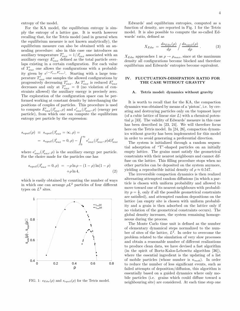
FIG. 1: sEdw(ρ) and sequil(ρ) for the Tetris model.

Edwards’ and equilibrium entropies, computed as afunction of density, are reported in Fig. 1 for the Tetrismodel. It is also possible to compute the so-called Ed-wards’ ratio, defined as

XEdw =dsEdw(ρ)

dρ

/ dsequil(ρ)

dρ. (3)

XEdw approaches 1 as ρ → ρmax, since at the maximumdensity all configurations become blocked and thereforeequilibrium and Edwards’ entropies become equivalent.

IV. FLUCTUATION-DISSIPATION RATIO FORTHE CASE WITHOUT GRAVITY

A. Tetris model: dynamics without gravity

It is worth to recall that for the KA, the compactiondynamics was obtained by means of a ‘piston’, i.e. by cre-ating and destroying particles only on the topmost layer(of a cubic lattice of linear size L) with a chemical poten-tial µ [33]. The validity of Edwards’ measure in this casehas been described in [23, 24]. We will therefore focushere on the Tetris model. In [24, 26], compaction dynam-ics without gravity has been implemented for this modelin order to avoid generating a preferential direction.

The system is initialized through a random sequen-tial adsorption of “T”-shaped particles on an initiallyempty lattice. The grains must satisfy the geometricalconstraints with their nearest neighbours and cannot dif-fuse on the lattice. This filling procedure stops when noother particles can be deposited on the system anymore,yielding a reproducible initial density of ρ ≈ 0.547.

The irreversible compaction dynamics is then realizedalternating attempted random diffusions (in which a par-ticle is chosen with uniform probability and allowed tomove toward one of its nearest-neighbours with probabil-ity p = 1

4 , only if all the possible geometrical constraintsare satisfied), and attempted random depositions on thelattice (an empty site is chosen with uniform probabil-ity and a grain is then adsorbed on the lattice only ifno violation of the geometrical constraints occurs). Theglobal density increases, the system remaining homoge-neous during the process.

The Monte Carlo time unit is defined as the numberof elementary dynamical steps normalized to the num-ber of sites of the lattice, L2. In order to overcome theproblem related to the simulation of very slow processesand obtain a reasonable number of different realizationsto produce clean data, we have devised a fast algorithm(in the spirit of Bortz-Kalos-Lebowitz algorithm [36]),where the essential ingredient is the updating of a listof mobile particles (whose number is nmob). In orderto reduce the number of less significant events, such asfailed attempts of deposition/diffusion, this algorithm isessentially based on a guided dynamics where only mo-bile particles (i.e. grains which could diffuse toward aneighbouring site) are considered. At each time step one

5

mobile particle is chosen with uniform probability and al-lowed to move if all the geometrical constraints are satis-fied. If the attempt has been successful, the list of mobileparticles is then updated, performing a local control ofgrains’ mobility. This procedure therefore introduces atemporal bias in the evolution of the system, which hasto be taken into account by incrementing the time of anamount ∆t = 1/nmob, after each guided elementary step.This algorithm becomes very efficient as the density ofthe system increases, since the number of mobile parti-cles reduces drastically.

During the compaction, we measure the density ρ(t)of particles, the density ρmob(t) of mobile particles, the

mobility χ(tw, tw + t) = 1dN

∑

a

∑Nk=1

δ〈(rak(tw+t)−ra

k(tw))〉δf

obtained by the application of a random forceto the particles between tw and tw + t, andthe mean square displacement B(tw, tw + t) =1

dN

∑

a

∑Nk=1

⟨

(rak(tw + t) − ra

k(tw))2⟩

(N is the numberof particles; a = 1, · · · , d runs over the spatial dimen-sions: d = 2 for Tetris, d = 3 for KA; ra

k is measured inunits of the bond size d of the square lattice). Indeed, thequantities χ(tw, tw + t) and B(tw, tw + t), at equilibrium,are linearly related (and actually depend only on t sincetime-translation invariance holds) by

2χ(t) =X

T eqd

B(t), (4)

where X is the so-called Fluctuation-Dissipation ratio(FDR) which is unitary in equilibrium. Any deviationsfrom this linear law signals a violation of the Fluctuation-Dissipation Theorem (FDT). Nevertheless it has beenshown, first in mean-field models [37], then in various nu-merical simulations of finite dimensional models [38, 39]how in several aging systems violations from (4) reduceto the occurrence of two regimes: a quasi-equilibriumregime with X = 1 (and time-translation invariance)for “short” time separations (t ≪ tw), and the agingregime with a constant X ≤ 1 for large time separations.This second slope is typically referred to as a dynam-ical temperature Tdyn ≥ T eq

d such that X = Xdyn =T eq

d /Tdyn [40].We have simulated lattices of linear size L =

50, 100, 200, in order to ensure that finite-size effectswere irrelevant. We have chosen periodic boundary con-ditions on the lattice, having checked that other typesof boundary conditions (e.g. closed ones) gave the sameresults. We have investigated the irreversible compactiondynamics of the system up to times of 2 × 105 MCsteps, realizing a large number of different runs (Nruns ≃8000÷ 9000), in order to obtain clean data. The randomperturbation is realized by varying the diffusion proba-bility of each particle from the initial value p = 1

4 to the

value pǫ = 14 +f r

i · ǫ, where f ri = ±1 is a random variable

associated to each grain independently for each possibledirection (r = x, y), and ǫ represents the perturbationstrength. The results presented here are obtained with aperturbation strength ǫ = 0.005, having checked that for0.002 < ǫ < 0.01 non-linear effects are absent.

B. Interrupted aging regime

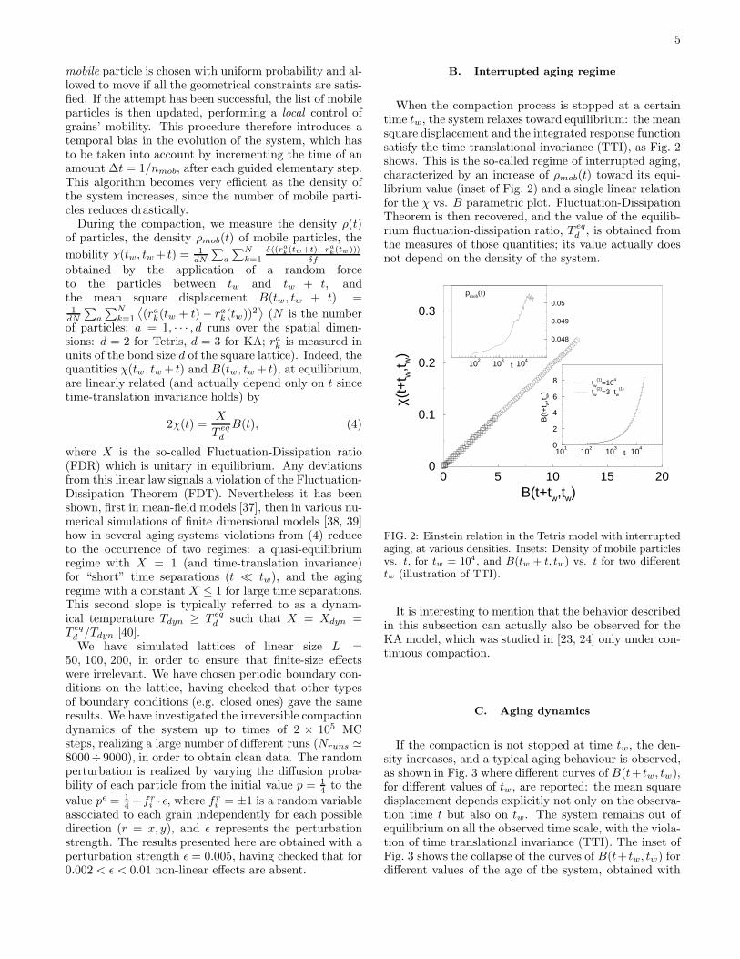
When the compaction process is stopped at a certaintime tw, the system relaxes toward equilibrium: the meansquare displacement and the integrated response functionsatisfy the time translational invariance (TTI), as Fig. 2shows. This is the so-called regime of interrupted aging,characterized by an increase of ρmob(t) toward its equi-librium value (inset of Fig. 2) and a single linear relationfor the χ vs. B parametric plot. Fluctuation-DissipationTheorem is then recovered, and the value of the equilib-rium fluctuation-dissipation ratio, T eq

d , is obtained fromthe measures of those quantities; its value actually doesnot depend on the density of the system.

0 5 10 15 20B(t+tw,tw)

0

0.1

0.2

0.3

χ(t+

t w,t w

)

101

102

103

104

t0

2

4

6

8

B(t

+t w

,t w)

tw

(1)=10

4

tw

(2)=3 tw

(1)

102

103

104

t

0.048

0.049

0.05

ρmob(t)

FIG. 2: Einstein relation in the Tetris model with interruptedaging, at various densities. Insets: Density of mobile particlesvs. t, for tw = 104, and B(tw + t, tw) vs. t for two differenttw (illustration of TTI).

It is interesting to mention that the behavior describedin this subsection can actually also be observed for theKA model, which was studied in [23, 24] only under con-tinuous compaction.

C. Aging dynamics

If the compaction is not stopped at time tw, the den-sity increases, and a typical aging behaviour is observed,as shown in Fig. 3 where different curves of B(t+ tw, tw),for different values of tw, are reported: the mean squaredisplacement depends explicitly not only on the observa-tion time t but also on tw. The system remains out ofequilibrium on all the observed time scale, with the viola-tion of time translational invariance (TTI). The inset ofFig. 3 shows the collapse of the curves of B(t+ tw, tw) fordifferent values of the age of the system, obtained with

6

the following scaling function

B(t + tw, tw) = c ·

[

ln(

t+tw+ts

τ

)

ln(

tw+ts

τ

) − 1

]

(5)

where c, ts and τ are fit parameters. Our results show alinear dependence of the parameters ts and τ on the ageof the system, while the coefficient c is nearly constant.

101

102

103

104

105

106

t

0

2

4

6

8

B(t

+t w

,t w)

0 2 4 6rescaled time

0

2

4

6

B(t

+t w

,t w)

FIG. 3: Evolution of B(t+tw, tw) for various tw (from bottomto top, 5 × 103, 104, 3 × 104 and 5 × 104); inset: collapse ofB; for the collapse, we have not taken into account the finalportion of each curve, because of a saturation of B due tofinite-size effects.

Moreover, we observe the density of mobile particlesρmob(t) getting smaller than the corresponding value atequilibrium [24], as another evidence of the out of equi-librium behaviour of the system during the compactionprocess.

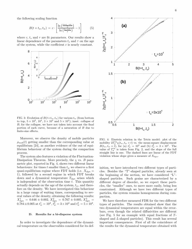
The system also features a violation of the Fluctuation-Dissipation Theorem. More precisely, the χ vs. B para-metric plot, reported in Fig. 4, shows two different linearbehaviours: for times t smaller than tw we observe a firstquasi-equilibrium regime where FDT holds (i.e. Xdyn =1), followed by a second regime in which FDT breaksdown and a dynamical temperature Tdyn arises whichis independent of the observation time t. This quantityactually depends on the age of the system, tw, and there-fore on the density. We have investigated this behaviourin a large range of waiting times, corresponding to sev-eral values of the density, obtaining the following results:X1

dyn = 0.646 ± 0.002, X2dyn = 0.767 ± 0.005, X3

dyn =

0.784±0.005 at t1w = 104, t2w = 3×104 and t3w = 5×104.

D. Results for a bi-disperse system

In order to investigate the dependence of the dynami-cal temperature on the observables considered for its def-

1 2 3 4 5B(t+tw,,tw)

1

2

3

4

2χ(t

+t w

,t w)T

deq

tw=104

(a)

0.5 1 1.5 2B(t+tw,,tw)

0.5

1

1.5

2χ(t

+t w

,t w)T

deq

tw=3x104

(b)

FIG. 4: Einstein relation in the Tetris model: plot of themobility 2T eq

d χ(tw, tw + t) vs. the mean-square displacementB(tw, tw + t), for (a) t1w = 104 and (b) t2w = 3 × 104. Thevalue of T eq

d is taken from Fig. 2, and the slope of the fullstraight line is one. The dashed lines are linear of the FDTviolation whose slope gives a measure of Xdyn.

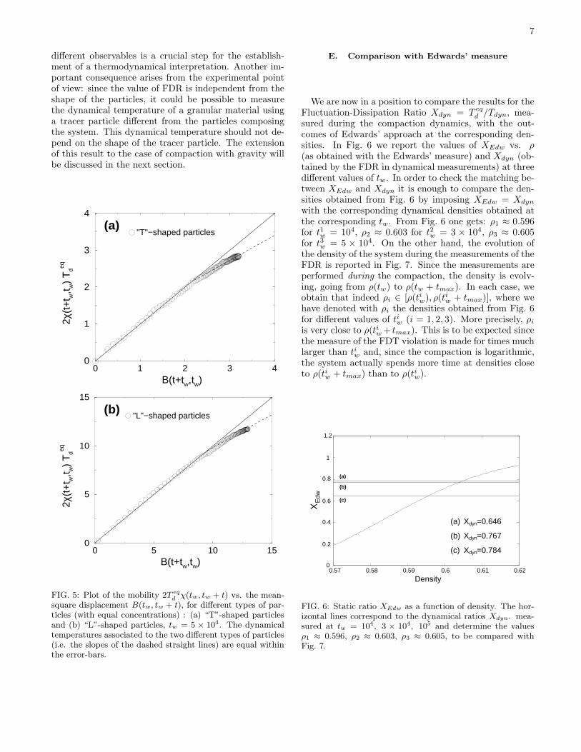
inition, we have introduced two different types of parti-cles. Besides the “T”-shaped particles, already seen atthe beginning of the section, we have considered “L”-shaped particles. Such grains are characterized by adifferent degree of disorder, so we expect these parti-cles, the “smaller” ones, to move more easily, being lessconstrained. Although we have two different types ofparticles, the system remains homogeneous during com-paction.

We have therefore measured FDR for the two differenttypes of particles. The results obtained show that thetwo dynamical temperatures are equal within the error-bars, even though the related diffusivities are different(see Fig. 5 for an example with equal fractions of T -shaped and L-shaped particles). This result has severalimportant consequences. First of all the coincidence ofthe results for the dynamical temperature obtained with

7

different observables is a crucial step for the establish-ment of a thermodynamical interpretation. Another im-portant consequence arises from the experimental pointof view: since the value of FDR is independent from theshape of the particles, it could be possible to measurethe dynamical temperature of a granular material usinga tracer particle different from the particles composingthe system. This dynamical temperature should not de-pend on the shape of the tracer particle. The extensionof this result to the case of compaction with gravity willbe discussed in the next section.

0 1 2 3 4B(t+tw,tw)

0

1

2

3

4

2χ(t

+tw,t w

) T

deq

"T"−shaped particles(a)

0 5 10 15B(t+tw,tw)

0

5

10

15

2χ(t

+tw,t w

) T

deq

"L"−shaped particles(b)

FIG. 5: Plot of the mobility 2T eq

d χ(tw, tw + t) vs. the mean-square displacement B(tw, tw + t), for different types of par-ticles (with equal concentrations) : (a) “T”-shaped particlesand (b) “L”-shaped particles, tw = 5 × 104. The dynamicaltemperatures associated to the two different types of particles(i.e. the slopes of the dashed straight lines) are equal withinthe error-bars.

E. Comparison with Edwards’ measure

We are now in a position to compare the results for theFluctuation-Dissipation Ratio Xdyn = T eq

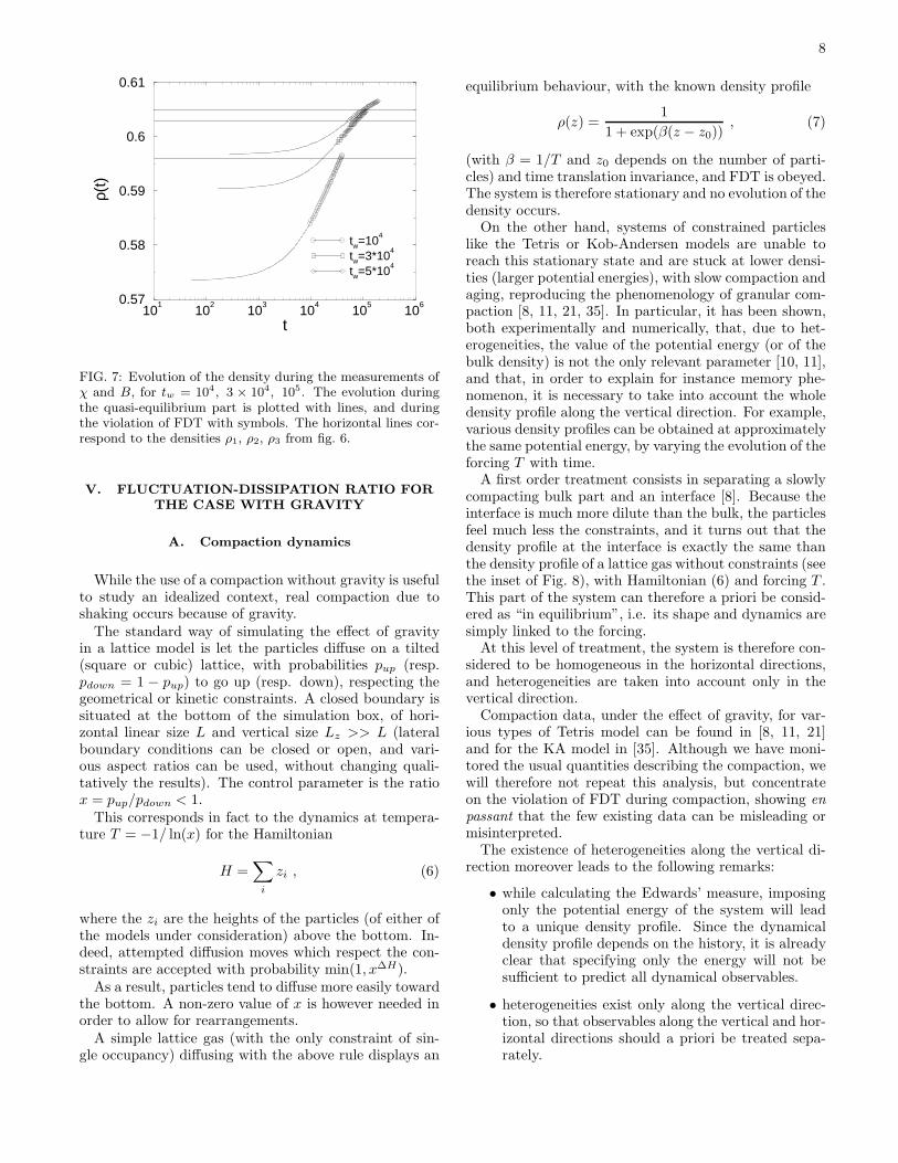
d /Tdyn, mea-sured during the compaction dynamics, with the out-comes of Edwards’ approach at the corresponding den-sities. In Fig. 6 we report the values of XEdw vs. ρ(as obtained with the Edwards’ measure) and Xdyn (ob-tained by the FDR in dynamical measurements) at threedifferent values of tw. In order to check the matching be-tween XEdw and Xdyn it is enough to compare the den-sities obtained from Fig. 6 by imposing XEdw = Xdyn

with the corresponding dynamical densities obtained atthe corresponding tw. From Fig. 6 one gets: ρ1 ≈ 0.596for t1w = 104, ρ2 ≈ 0.603 for t2w = 3 × 104, ρ3 ≈ 0.605for t3w = 5 × 104. On the other hand, the evolution ofthe density of the system during the measurements of theFDR is reported in Fig. 7. Since the measurements areperformed during the compaction, the density is evolv-ing, going from ρ(tw) to ρ(tw + tmax). In each case, weobtain that indeed ρi ∈ [ρ(tiw), ρ(tiw + tmax)], where wehave denoted with ρi the densities obtained from Fig. 6for different values of tiw (i = 1, 2, 3). More precisely, ρi

is very close to ρ(tiw + tmax). This is to be expected sincethe measure of the FDT violation is made for times muchlarger than tiw and, since the compaction is logarithmic,the system actually spends more time at densities closeto ρ(tiw + tmax) than to ρ(tiw).

0

0.2

0.4

0.6

0.8

1

1.2

0.57 0.58 0.59 0.6 0.61 0.62

X

X

X

X

Density

dyn=0.646

dyn=0.767

dyn=0.784

(a)

(b)

(c)

Edw (c)

(b)

(a)

FIG. 6: Static ratio XEdw as a function of density. The hor-izontal lines correspond to the dynamical ratios Xdyn. mea-sured at tw = 104, 3 × 104, 105 and determine the valuesρ1 ≈ 0.596, ρ2 ≈ 0.603, ρ3 ≈ 0.605, to be compared withFig. 7.

8

101

102

103

104

105

106

t

0.57

0.58

0.59

0.6

0.61ρ(

t)

tw=104

tw=3*104

tw=5*104

FIG. 7: Evolution of the density during the measurements ofχ and B, for tw = 104, 3 × 104, 105. The evolution duringthe quasi-equilibrium part is plotted with lines, and duringthe violation of FDT with symbols. The horizontal lines cor-respond to the densities ρ1, ρ2, ρ3 from fig. 6.

V. FLUCTUATION-DISSIPATION RATIO FORTHE CASE WITH GRAVITY

A. Compaction dynamics

While the use of a compaction without gravity is usefulto study an idealized context, real compaction due toshaking occurs because of gravity.

The standard way of simulating the effect of gravityin a lattice model is let the particles diffuse on a tilted(square or cubic) lattice, with probabilities pup (resp.pdown = 1 − pup) to go up (resp. down), respecting thegeometrical or kinetic constraints. A closed boundary issituated at the bottom of the simulation box, of hori-zontal linear size L and vertical size Lz >> L (lateralboundary conditions can be closed or open, and vari-ous aspect ratios can be used, without changing quali-tatively the results). The control parameter is the ratiox = pup/pdown < 1.

This corresponds in fact to the dynamics at tempera-ture T = −1/ ln(x) for the Hamiltonian

H =∑

i

zi , (6)

where the zi are the heights of the particles (of either ofthe models under consideration) above the bottom. In-deed, attempted diffusion moves which respect the con-straints are accepted with probability min(1, x∆H).

As a result, particles tend to diffuse more easily towardthe bottom. A non-zero value of x is however needed inorder to allow for rearrangements.

A simple lattice gas (with the only constraint of sin-gle occupancy) diffusing with the above rule displays an

equilibrium behaviour, with the known density profile

ρ(z) =1

1 + exp(β(z − z0)), (7)

(with β = 1/T and z0 depends on the number of parti-cles) and time translation invariance, and FDT is obeyed.The system is therefore stationary and no evolution of thedensity occurs.

On the other hand, systems of constrained particleslike the Tetris or Kob-Andersen models are unable toreach this stationary state and are stuck at lower densi-ties (larger potential energies), with slow compaction andaging, reproducing the phenomenology of granular com-paction [8, 11, 21, 35]. In particular, it has been shown,both experimentally and numerically, that, due to het-erogeneities, the value of the potential energy (or of thebulk density) is not the only relevant parameter [10, 11],and that, in order to explain for instance memory phe-nomenon, it is necessary to take into account the wholedensity profile along the vertical direction. For example,various density profiles can be obtained at approximatelythe same potential energy, by varying the evolution of theforcing T with time.

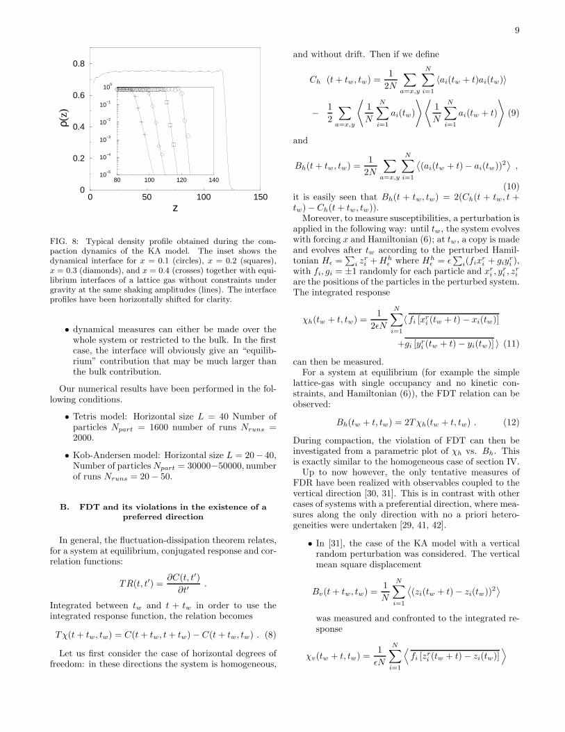
A first order treatment consists in separating a slowlycompacting bulk part and an interface [8]. Because theinterface is much more dilute than the bulk, the particlesfeel much less the constraints, and it turns out that thedensity profile at the interface is exactly the same thanthe density profile of a lattice gas without constraints (seethe inset of Fig. 8), with Hamiltonian (6) and forcing T .This part of the system can therefore a priori be consid-ered as “in equilibrium”, i.e. its shape and dynamics aresimply linked to the forcing.

At this level of treatment, the system is therefore con-sidered to be homogeneous in the horizontal directions,and heterogeneities are taken into account only in thevertical direction.

Compaction data, under the effect of gravity, for var-ious types of Tetris model can be found in [8, 11, 21]and for the KA model in [35]. Although we have moni-tored the usual quantities describing the compaction, wewill therefore not repeat this analysis, but concentrateon the violation of FDT during compaction, showing en

passant that the few existing data can be misleading ormisinterpreted.

The existence of heterogeneities along the vertical di-rection moreover leads to the following remarks:

• while calculating the Edwards’ measure, imposingonly the potential energy of the system will leadto a unique density profile. Since the dynamicaldensity profile depends on the history, it is alreadyclear that specifying only the energy will not besufficient to predict all dynamical observables.

• heterogeneities exist only along the vertical direc-tion, so that observables along the vertical and hor-izontal directions should a priori be treated sepa-rately.

9

80 100 120 14010

−5

10−4

10−3

10−2

10−1

100

0 50 100 150z

0

0.2

0.4

0.6

0.8ρ(

z)

FIG. 8: Typical density profile obtained during the com-paction dynamics of the KA model. The inset shows thedynamical interface for x = 0.1 (circles), x = 0.2 (squares),x = 0.3 (diamonds), and x = 0.4 (crosses) together with equi-librium interfaces of a lattice gas without constraints undergravity at the same shaking amplitudes (lines). The interfaceprofiles have been horizontally shifted for clarity.

• dynamical measures can either be made over thewhole system or restricted to the bulk. In the firstcase, the interface will obviously give an “equilib-rium” contribution that may be much larger thanthe bulk contribution.

Our numerical results have been performed in the fol-lowing conditions.

• Tetris model: Horizontal size L = 40 Number ofparticles Npart = 1600 number of runs Nruns =2000.

• Kob-Andersen model: Horizontal size L = 20− 40,Number of particles Npart = 30000−50000, numberof runs Nruns = 20 − 50.

B. FDT and its violations in the existence of apreferred direction

In general, the fluctuation-dissipation theorem relates,for a system at equilibrium, conjugated response and cor-relation functions:

TR(t, t′) =∂C(t, t′)

∂t′.

Integrated between tw and t + tw in order to use theintegrated response function, the relation becomes

Tχ(t + tw, tw) = C(t + tw, t + tw) − C(t + tw, tw) . (8)

Let us first consider the case of horizontal degrees offreedom: in these directions the system is homogeneous,

and without drift. Then if we define

Ch (t + tw, tw) =1

2N

∑

a=x,y

N∑

i=1

〈ai(tw + t)ai(tw)〉

−1

2

∑

a=x,y

⟨

1

N

N∑

i=1

ai(tw)

⟩ ⟨

1

N

N∑

i=1

ai(tw + t)

⟩

(9)

and

Bh(t + tw, tw) =1

2N

∑

a=x,y

N∑

i=1

⟨

(ai(tw + t) − ai(tw))2⟩

,

(10)it is easily seen that Bh(t + tw, tw) = 2(Ch(t + tw, t +tw) − Ch(t + tw, tw)).

Moreover, to measure susceptibilities, a perturbation isapplied in the following way: until tw, the system evolveswith forcing x and Hamiltonian (6); at tw, a copy is madeand evolves after tw according to the perturbed Hamil-tonian Hǫ =

∑

i zri + Hh

ǫ where Hhǫ = ǫ

∑

i(fixri + giy

ri ),

with fi, gi = ±1 randomly for each particle and xri , y

ri , z

ri

are the positions of the particles in the perturbed system.The integrated response

χh(tw + t, tw) =1

2ǫN

N∑

i=1

〈 fi [xri (tw + t) − xi(tw)]

+gi [yri (tw + t) − yi(tw)] 〉 (11)

can then be measured.For a system at equilibrium (for example the simple

lattice-gas with single occupancy and no kinetic con-straints, and Hamiltonian (6)), the FDT relation can beobserved:

Bh(tw + t, tw) = 2Tχh(tw + t, tw) . (12)

During compaction, the violation of FDT can then beinvestigated from a parametric plot of χh vs. Bh. Thisis exactly similar to the homogeneous case of section IV.

Up to now however, the only tentative measures ofFDR have been realized with observables coupled to thevertical direction [30, 31]. This is in contrast with othercases of systems with a preferential direction, where mea-sures along the only direction with no a priori hetero-geneities were undertaken [29, 41, 42].

• In [31], the case of the KA model with a verticalrandom perturbation was considered. The verticalmean square displacement

Bv(t + tw, tw) =1

N

N∑

i=1

⟨

(zi(tw + t) − zi(tw))2⟩

was measured and confronted to the integrated re-sponse

χv(tw + t, tw) =1

ǫN

N∑

i=1

⟨

fi [zri (tw + t) − zi(tw)]

⟩

10

to a perturbation Hvǫ = ǫ

∑

i fizri (fi = ±1 ran-

domly). The existence of a dynamical temperaturewas inferred from the observed linear relation be-tween Bv and χv, with a slope different from theapplied temperature.

• In [30], a perturbation in the forcing was applied,and confronted to the following mean-square dis-placement:

Bv(t + tw, tw) =⟨

(h(tw + t) − h(tw))2⟩

with h(t) =∑

i zi(t)/N . The perturbation in theforcing lead to the observation of negative responsefunctions (χv(t + tw, tw) = hr(t + tw) − h(t + tw),where hr is the mean height of the perturbed sys-tem, the perturbation being applied after tw), in-terpreted as the signature of a “negative dynamicaltemperature”. This case was investigated in [8, 11]where this result was shown to be linked to theexistence of memory effects, as also confirmed inexperiments [10].

In both cases however, the existence of a downwarddrift, due to compaction, was not taken into accountfor the correct definition of the correlation part of thefluctuation-dissipation relation: indeed, in the first case,the correlation being

Cv (t + tw, tw) =1

N

N∑

i=1

〈zi(tw + t)zi(tw)〉

−

⟨

1

N

N∑

i=1

zi(tw)

⟩ ⟨

1

N

N∑

i=1

zi(tw + t)

⟩

, (13)

Bv(t + tw, tw) is not proportional to Cv(t + tw, t + tw) −Cv(t + tw, tw) as in the homogeneous case. This is evenmore easily seen in the second case, where the correlationconjugated to the response to a change in the driving isCv(t + tw, tw) = 〈h(t + tw)h(tw)〉 − 〈h(t + tw)〉〈h(tw)〉.Indeed

Bv(t+tw , tw) = 〈h2(t+tw)+h2(tw)〉−2〈h(t+tw)h(tw)〉 ,

and

Cv (t + tw, t + tw) − Cv(t + tw, tw) =

〈h2(t + tw)〉 − 〈h(t + tw)h(tw)〉

− 〈h(t + tw)〉〈h(t + tw) − h(tw)〉 (14)

are not simply related since 〈h(t + tw)〉 6= 〈h(tw)〉 and〈h2(t + tw)〉 6= 〈h2(tw)〉 (see also a similar discussion, onthe case of one-time quantities changing with time, in[43]).

It turns therefore out that the results of [30, 31] are apriori flawed from an incorrect measure of the correlationpart of FDR.

We will see in the next subsections how measures ofcorrelation and response functions along the horizontaldirections lead to sensible results, whereas all measures ofvertical correlations or response lead to the impossibilityof defining effective temperatures.

C. FDR in the aging (compacting) regime

1. Vertical observables?

Two sets of response and correlation functions can apriori be measured: the incoherent ones (Cv, χv) as in

[31] or the coherent ones (Cv, χv) as in [30].If we write

Cv (t + tw, t + tw) − Cv(t + tw, tw) =

=

⟨

1

N

N∑

i=1

zi(t + tw)(zi(t + tw) − zi(tw))

⟩

+1

N

⟨

N∑

i=1

zi(t + tw)

⟩ ⟨

1

N

N∑

i=1

(zi(tw) − zi(t + tw))

⟩

=

⟨

1

N

N∑

i=1

(zi(tw) − zi(t + tw)) (〈h(t + tw)〉 − zi(t + tw))

⟩

we can observe that generically zi(tw + t) ≤ zi(tw) sincethe system is compacting, so that two opposite contribu-tions can be distinguished in Cv(t + tw, t + tw) − Cv(t +tw, tw): the particles such that zi(t + tw) < h(t + tw)give a positive contribution, those such that zi(t + tw) >h(t + tw) give a negative one. At short and interme-diate times, the particles closer to the surface movemore than those in the bulk and therefore the nega-tive contribution dominates. This leads to a negativeCv(t + tw, t + tw) − Cv(t + tw, tw). At very long timesCv(t + tw, t + tw)−Cv(t + tw, tw) has to become positiveby definition, but such times may not be reachable in anumerical simulation.

This peculiar behaviour comes from the fact that thedrift is not homogeneous in the system: some regions arecompacting more than others. Local drifts should thenbe taken into account. However this is numerically (andalso experimentally) too difficult to measure.

On the other hand, the coherent correlation and re-sponse Cv, χv can also be measured. The difficultyarises from the measure of the coherent correlation func-tion Cv, of order 1/N for N particles: relatively smallsystems have to be simulated with a large number ofrealizations. For an equilibrium lattice gas without ki-netic constraints, FDT is then recovered: N(Cv(t +

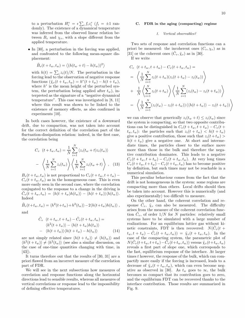
tw, t + tw) − Cv(t + tw, tw)) = χv(t + tw, tw). In thecase of the compacting system, the parametric plot ofN(Cv(t+ tw, t+ tw)− Cv(t+ tw, tw)) versus χv(t+ tw, tw)reveals a first part of slope one, which corresponds tothe fast, equilibrium response of the interface. At largertimes t however, the response of the bulk, which can com-pactify more easily if the forcing is increased, leads to adecrease of χv(t + tw, tw), which can even become neg-ative as observed in [30]. As tw goes to ∞, the bulkbecomes so compact that its contribution goes to zero,and the equilibrium FDT can be recovered thanks to theinterface contribution. Those results are summarized inFig. 9.

11

0 10 20N(Cv(t+tw,t+tw)−Cv(t+tw,tw))

−1

1

3χ v(

t+t w

,t w)

FIG. 9: χv(t+tw, tw) vs. N(Cv(t+tw, t+tw)−Cv(t+tw, tw))for the KA model, with L = 20, Npart = 4000, Nrun = 500,x = 0.8 (circles) and x = 0.5 (squares); tw = 214 andt = 2, · · · , 216. The first equilibrium part corresponds to theinterface dynamics, while at longer times χv decreases be-cause of the bulk response. The diamonds correspond to asimulation with no kinetic constraint and Npart = 4000 par-ticles: only equilibrium FDT is then observed. The straightline has slope 1.

The previous investigations shows that no definition ofan effective temperature can be inferred from dynami-cal measures correlated with the preferred directions inwhich heterogeneities occur.

Note that this kind of situation also arises in the studyof effective temperatures in driven vortex lattices withrandom pinning: while an effective temperature can bedefined and measured for degrees of freedom perpendicu-lar to the drive, problems are encountered when dealingwith longitudinal observables [44].

We now turn to horizontal observables.

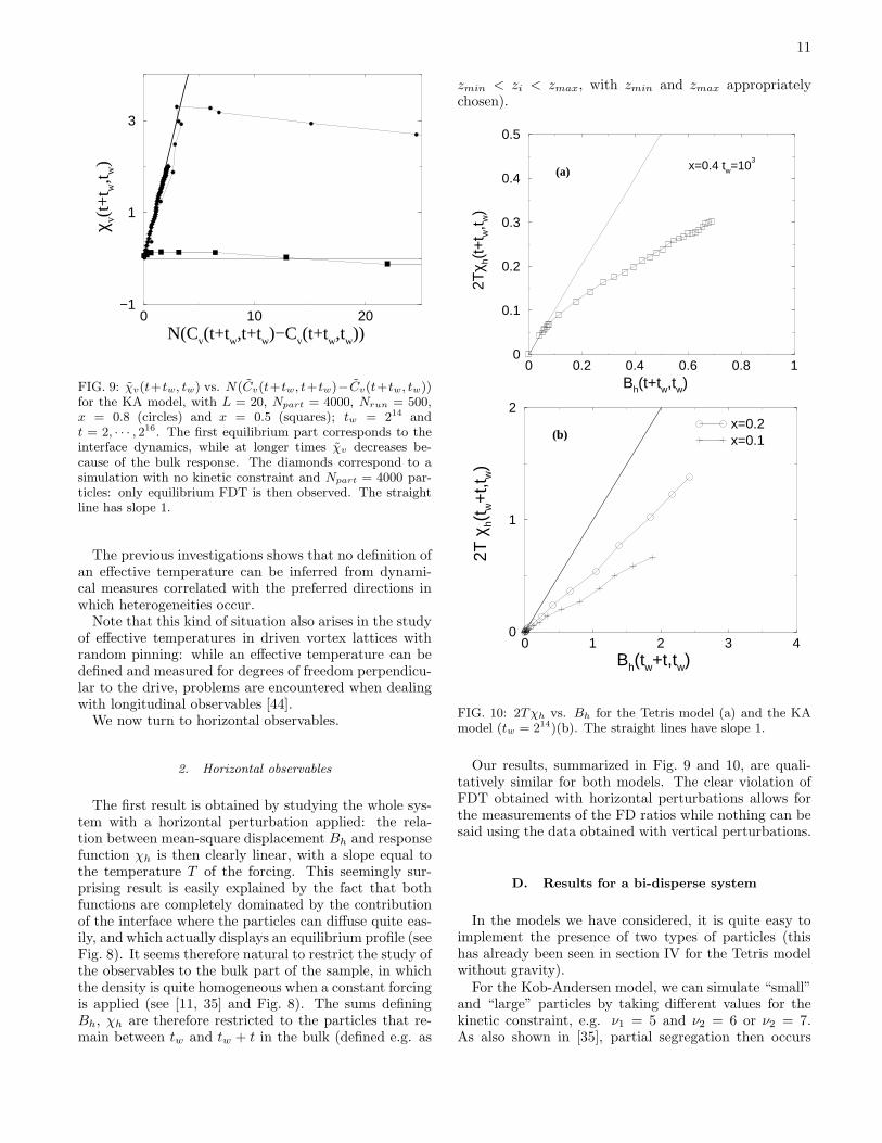
2. Horizontal observables

The first result is obtained by studying the whole sys-tem with a horizontal perturbation applied: the rela-tion between mean-square displacement Bh and responsefunction χh is then clearly linear, with a slope equal tothe temperature T of the forcing. This seemingly sur-prising result is easily explained by the fact that bothfunctions are completely dominated by the contributionof the interface where the particles can diffuse quite eas-ily, and which actually displays an equilibrium profile (seeFig. 8). It seems therefore natural to restrict the study ofthe observables to the bulk part of the sample, in whichthe density is quite homogeneous when a constant forcingis applied (see [11, 35] and Fig. 8). The sums definingBh, χh are therefore restricted to the particles that re-main between tw and tw + t in the bulk (defined e.g. as

zmin < zi < zmax, with zmin and zmax appropriatelychosen).

0 0.2 0.4 0.6 0.8 1Bh(t+tw,tw)

0

0.1

0.2

0.3

0.4

0.5

2Tχ h(

t+t w

,t w)

(a) x=0.4 tw=103

0 1 2 3 4Bh(tw+t,tw)

0

1

2

2T χ

h(t w

+t,t

w)

x=0.2x=0.1(b)

FIG. 10: 2Tχh vs. Bh for the Tetris model (a) and the KAmodel (tw = 214)(b). The straight lines have slope 1.

Our results, summarized in Fig. 9 and 10, are quali-tatively similar for both models. The clear violation ofFDT obtained with horizontal perturbations allows forthe measurements of the FD ratios while nothing can besaid using the data obtained with vertical perturbations.

D. Results for a bi-disperse system

In the models we have considered, it is quite easy toimplement the presence of two types of particles (thishas already been seen in section IV for the Tetris modelwithout gravity).

For the Kob-Andersen model, we can simulate “small”and “large” particles by taking different values for thekinetic constraint, e.g. ν1 = 5 and ν2 = 6 or ν2 = 7.As also shown in [35], partial segregation then occurs

12

because the particle with larger ν are less constrainedand can move more easily toward the bottom.

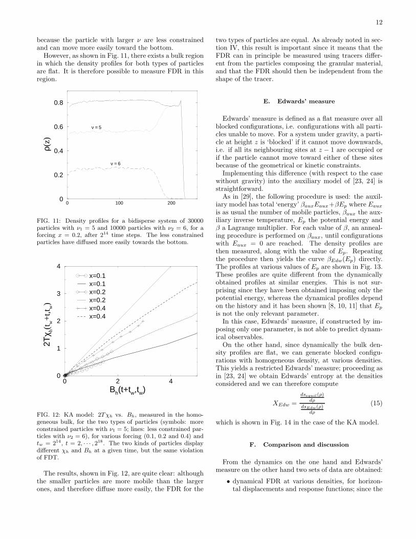
However, as shown in Fig. 11, there exists a bulk regionin which the density profiles for both types of particlesare flat. It is therefore possible to measure FDR in thisregion.

0 100 2000

0.2

0.4

0.6

0.8

ρ(z)

ν = 6

ν = 5

FIG. 11: Density profiles for a bidisperse system of 30000particles with ν1 = 5 and 10000 particles with ν2 = 6, for aforcing x = 0.2, after 214 time steps. The less constrainedparticles have diffused more easily towards the bottom.

0 2 4Bh(t+tw,tw)

0

1

2

3

4

2Tχ h(

t w+

t,tw)

x=0.1x=0.1 x=0.2 x=0.2x=0.4 x=0.4

FIG. 12: KA model: 2Tχh vs. Bh, measured in the homo-geneous bulk, for the two types of particles (symbols: moreconstrained particles with ν1 = 5; lines: less constrained par-ticles with ν2 = 6), for various forcing (0.1, 0.2 and 0.4) andtw = 214, t = 2, · · · , 218. The two kinds of particles displaydifferent χh and Bh at a given time, but the same violationof FDT.

The results, shown in Fig. 12, are quite clear: althoughthe smaller particles are more mobile than the largerones, and therefore diffuse more easily, the FDR for the

two types of particles are equal. As already noted in sec-tion IV, this result is important since it means that theFDR can in principle be measured using tracers differ-ent from the particles composing the granular material,and that the FDR should then be independent from theshape of the tracer.

E. Edwards’ measure

Edwards’ measure is defined as a flat measure over allblocked configurations, i.e. configurations with all parti-cles unable to move. For a system under gravity, a parti-cle at height z is ‘blocked’ if it cannot move downwards,i.e. if all its neighbouring sites at z − 1 are occupied orif the particle cannot move toward either of these sitesbecause of the geometrical or kinetic constraints.

Implementing this difference (with respect to the casewithout gravity) into the auxiliary model of [23, 24] isstraightforward.

As in [29], the following procedure is used: the auxil-iary model has total ‘energy’ βauxEaux+βEp where Eaux

is as usual the number of mobile particles, βaux the aux-iliary inverse temperature, Ep the potential energy andβ a Lagrange multiplier. For each value of β, an anneal-ing procedure is performed on βaux, until configurationswith Eaux = 0 are reached. The density profiles arethen measured, along with the value of Ep. Repeatingthe procedure then yields the curve βEdw(Ep) directly.The profiles at various values of Ep are shown in Fig. 13.These profiles are quite different from the dynamicallyobtained profiles at similar energies. This is not sur-prising since they have been obtained imposing only thepotential energy, whereas the dynamical profiles dependon the history and it has been shown [8, 10, 11] that Ep

is not the only relevant parameter.In this case, Edwards’ measure, if constructed by im-

posing only one parameter, is not able to predict dynam-ical observables.

On the other hand, since dynamically the bulk den-sity profiles are flat, we can generate blocked configu-rations with homogeneous density, at various densities.This yields a restricted Edwards’ measure; proceeding asin [23, 24] we obtain Edwards’ entropy at the densitiesconsidered and we can therefore compute

XEdw =

dsequil(ρ)dρ

dsEdw(ρ)dρ

(15)

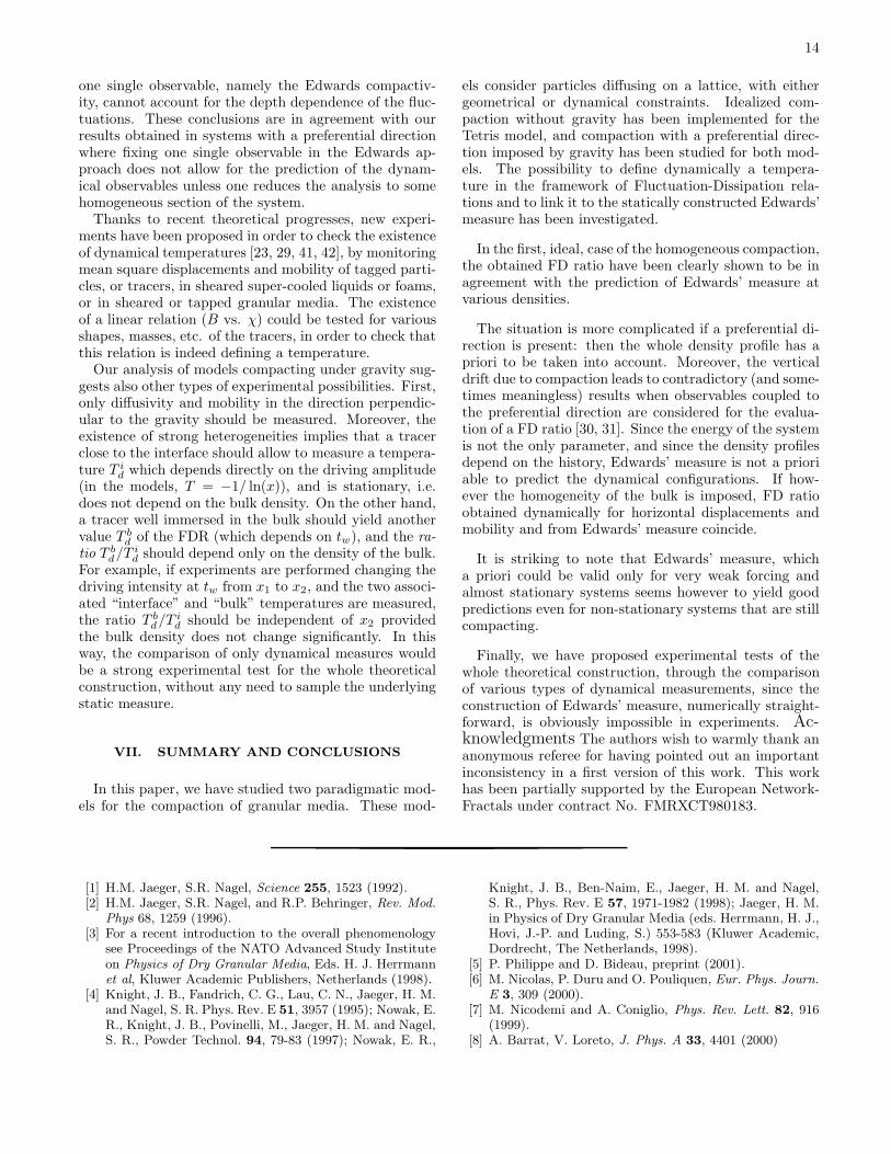
which is shown in Fig. 14 in the case of the KA model.

F. Comparison and discussion

From the dynamics on the one hand and Edwards’measure on the other hand two sets of data are obtained:

• dynamical FDR at various densities, for horizon-tal displacements and response functions; since the

13

0 50 100 150z

0

0.2

0.4

0.6

0.8

1ρ(

z)

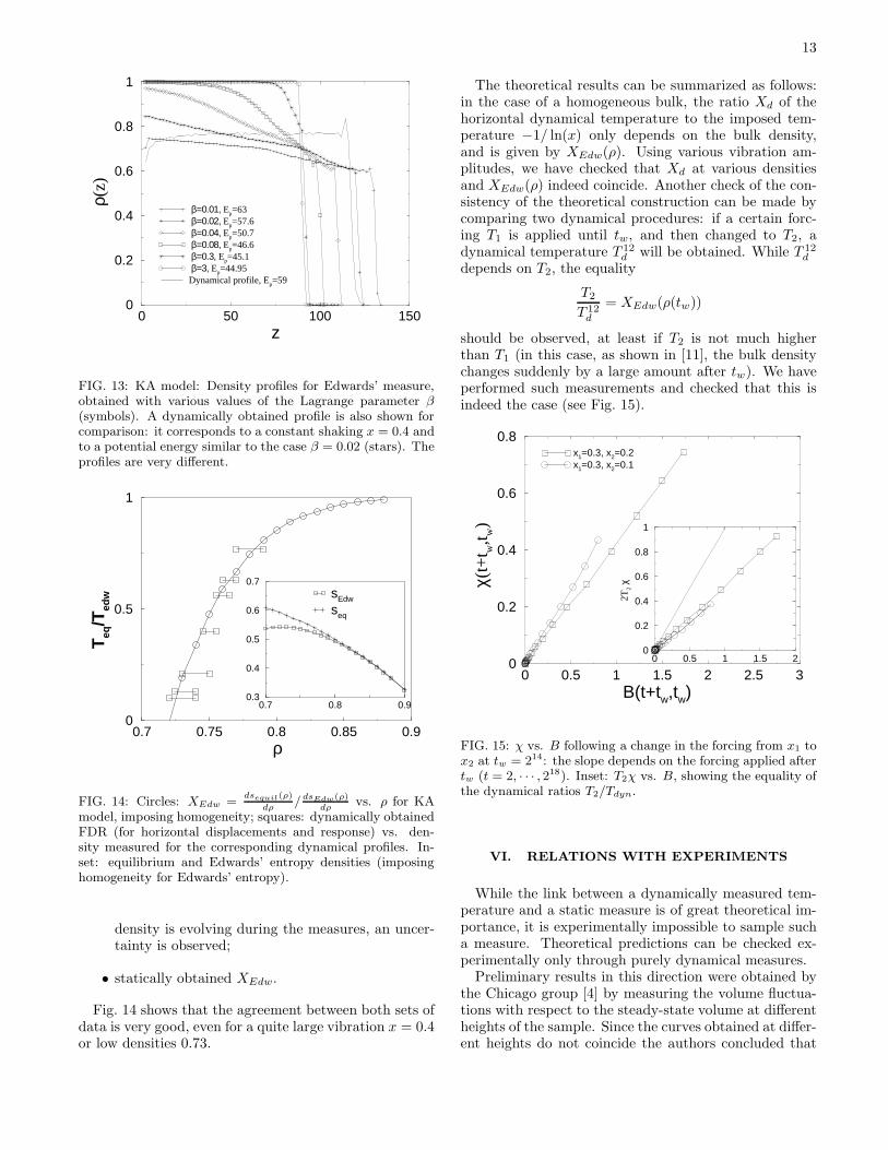
β=0.01, Ep=63 β=0.02, Ep=57.6 β=0.04, Ep=50.7 β=0.08, Ep=46.6 β=0.3, Ep=45.1 β=3, Ep=44.95Dynamical profile, Ep=59

FIG. 13: KA model: Density profiles for Edwards’ measure,obtained with various values of the Lagrange parameter β(symbols). A dynamically obtained profile is also shown forcomparison: it corresponds to a constant shaking x = 0.4 andto a potential energy similar to the case β = 0.02 (stars). Theprofiles are very different.

0.7 0.75 0.8 0.85 0.9ρ

0

0.5

1

Teq

/Ted

w

0.7 0.8 0.90.3

0.4

0.5

0.6

0.7sEdw

seq

FIG. 14: Circles: XEdw =dsequil(ρ)

dρ/dsEdw(ρ)

dρvs. ρ for KA

model, imposing homogeneity; squares: dynamically obtainedFDR (for horizontal displacements and response) vs. den-sity measured for the corresponding dynamical profiles. In-set: equilibrium and Edwards’ entropy densities (imposinghomogeneity for Edwards’ entropy).

density is evolving during the measures, an uncer-tainty is observed;

• statically obtained XEdw.

Fig. 14 shows that the agreement between both sets ofdata is very good, even for a quite large vibration x = 0.4or low densities 0.73.

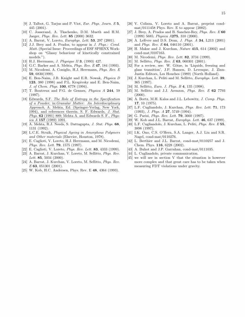
The theoretical results can be summarized as follows:in the case of a homogeneous bulk, the ratio Xd of thehorizontal dynamical temperature to the imposed tem-perature −1/ ln(x) only depends on the bulk density,and is given by XEdw(ρ). Using various vibration am-plitudes, we have checked that Xd at various densitiesand XEdw(ρ) indeed coincide. Another check of the con-sistency of the theoretical construction can be made bycomparing two dynamical procedures: if a certain forc-ing T1 is applied until tw, and then changed to T2, adynamical temperature T 12

d will be obtained. While T 12d

depends on T2, the equality

T2

T 12d

= XEdw(ρ(tw))

should be observed, at least if T2 is not much higherthan T1 (in this case, as shown in [11], the bulk densitychanges suddenly by a large amount after tw). We haveperformed such measurements and checked that this isindeed the case (see Fig. 15).

0 0.5 1 1.5 20

0.2

0.4

0.6

0.8

1

2T2 χ

x1=0.3, x2=0.2x1=0.3, x2=0.1

0 0.5 1 1.5 2 2.5 3B(t+tw,tw)

0

0.2

0.4

0.6

0.8

χ(t+

t w,t w

)

FIG. 15: χ vs. B following a change in the forcing from x1 tox2 at tw = 214: the slope depends on the forcing applied aftertw (t = 2, · · · , 218). Inset: T2χ vs. B, showing the equality ofthe dynamical ratios T2/Tdyn.

VI. RELATIONS WITH EXPERIMENTS

While the link between a dynamically measured tem-perature and a static measure is of great theoretical im-portance, it is experimentally impossible to sample sucha measure. Theoretical predictions can be checked ex-perimentally only through purely dynamical measures.

Preliminary results in this direction were obtained bythe Chicago group [4] by measuring the volume fluctua-tions with respect to the steady-state volume at differentheights of the sample. Since the curves obtained at differ-ent heights do not coincide the authors concluded that

14

one single observable, namely the Edwards compactiv-ity, cannot account for the depth dependence of the fluc-tuations. These conclusions are in agreement with ourresults obtained in systems with a preferential directionwhere fixing one single observable in the Edwards ap-proach does not allow for the prediction of the dynam-ical observables unless one reduces the analysis to somehomogeneous section of the system.

Thanks to recent theoretical progresses, new experi-ments have been proposed in order to check the existenceof dynamical temperatures [23, 29, 41, 42], by monitoringmean square displacements and mobility of tagged parti-cles, or tracers, in sheared super-cooled liquids or foams,or in sheared or tapped granular media. The existenceof a linear relation (B vs. χ) could be tested for variousshapes, masses, etc. of the tracers, in order to check thatthis relation is indeed defining a temperature.

Our analysis of models compacting under gravity sug-gests also other types of experimental possibilities. First,only diffusivity and mobility in the direction perpendic-ular to the gravity should be measured. Moreover, theexistence of strong heterogeneities implies that a tracerclose to the interface should allow to measure a tempera-ture T i

d which depends directly on the driving amplitude(in the models, T = −1/ ln(x)), and is stationary, i.e.does not depend on the bulk density. On the other hand,a tracer well immersed in the bulk should yield anothervalue T b

d of the FDR (which depends on tw), and the ra-

tio T bd/T i

d should depend only on the density of the bulk.For example, if experiments are performed changing thedriving intensity at tw from x1 to x2, and the two associ-ated “interface” and “bulk” temperatures are measured,the ratio T b

d/T id should be independent of x2 provided

the bulk density does not change significantly. In thisway, the comparison of only dynamical measures wouldbe a strong experimental test for the whole theoreticalconstruction, without any need to sample the underlyingstatic measure.

VII. SUMMARY AND CONCLUSIONS

In this paper, we have studied two paradigmatic mod-els for the compaction of granular media. These mod-

els consider particles diffusing on a lattice, with eithergeometrical or dynamical constraints. Idealized com-paction without gravity has been implemented for theTetris model, and compaction with a preferential direc-tion imposed by gravity has been studied for both mod-els. The possibility to define dynamically a tempera-ture in the framework of Fluctuation-Dissipation rela-tions and to link it to the statically constructed Edwards’measure has been investigated.

In the first, ideal, case of the homogeneous compaction,the obtained FD ratio have been clearly shown to be inagreement with the prediction of Edwards’ measure atvarious densities.

The situation is more complicated if a preferential di-rection is present: then the whole density profile has apriori to be taken into account. Moreover, the verticaldrift due to compaction leads to contradictory (and some-times meaningless) results when observables coupled tothe preferential direction are considered for the evalua-tion of a FD ratio [30, 31]. Since the energy of the systemis not the only parameter, and since the density profilesdepend on the history, Edwards’ measure is not a prioriable to predict the dynamical configurations. If how-ever the homogeneity of the bulk is imposed, FD ratioobtained dynamically for horizontal displacements andmobility and from Edwards’ measure coincide.

It is striking to note that Edwards’ measure, whicha priori could be valid only for very weak forcing andalmost stationary systems seems however to yield goodpredictions even for non-stationary systems that are stillcompacting.

Finally, we have proposed experimental tests of thewhole theoretical construction, through the comparisonof various types of dynamical measurements, since theconstruction of Edwards’ measure, numerically straight-forward, is obviously impossible in experiments. Ac-knowledgments The authors wish to warmly thank ananonymous referee for having pointed out an importantinconsistency in a first version of this work. This workhas been partially supported by the European Network-Fractals under contract No. FMRXCT980183.

[1] H.M. Jaeger, S.R. Nagel, Science 255, 1523 (1992).[2] H.M. Jaeger, S.R. Nagel, and R.P. Behringer, Rev. Mod.

Phys 68, 1259 (1996).[3] For a recent introduction to the overall phenomenology

see Proceedings of the NATO Advanced Study Instituteon Physics of Dry Granular Media, Eds. H. J. Herrmannet al, Kluwer Academic Publishers, Netherlands (1998).

[4] Knight, J. B., Fandrich, C. G., Lau, C. N., Jaeger, H. M.and Nagel, S. R. Phys. Rev. E 51, 3957 (1995); Nowak, E.R., Knight, J. B., Povinelli, M., Jaeger, H. M. and Nagel,S. R., Powder Technol. 94, 79-83 (1997); Nowak, E. R.,

Knight, J. B., Ben-Naim, E., Jaeger, H. M. and Nagel,S. R., Phys. Rev. E 57, 1971-1982 (1998); Jaeger, H. M.in Physics of Dry Granular Media (eds. Herrmann, H. J.,Hovi, J.-P. and Luding, S.) 553-583 (Kluwer Academic,Dordrecht, The Netherlands, 1998).

[5] P. Philippe and D. Bideau, preprint (2001).[6] M. Nicolas, P. Duru and O. Pouliquen, Eur. Phys. Journ.

E 3, 309 (2000).[7] M. Nicodemi and A. Coniglio, Phys. Rev. Lett. 82, 916

(1999).[8] A. Barrat, V. Loreto, J. Phys. A 33, 4401 (2000)

15

[9] J. Talbot, G. Tarjus and P. Viot, Eur. Phys. Journ. E 5,445 (2001).

[10] C. Josserand, A. Tkachenko, D.M. Mueth and H.M.Jaeger, Phys. Rev. Lett. 85 (2000) 3632.

[11] A. Barrat, V. Loreto, Europhys. Lett. 53, 297 (2001).[12] J.J. Brey and A. Prados, to appear in J. Phys.: Cond.

Matt. (Special Issue: Proceedings of ESF SPHINX Work-shop on “Glassy behaviour of kinetically constrainedmodels.”).

[13] H.J. Herrmann, J. Physique II 3, (1993) 427.[14] G.C. Barker and A. Mehta, Phys. Rev. E 47, 184 (1993).[15] M. Nicodemi, A. Coniglio, H.J. Herrmann, Phys. Rev. E

59, 6830(1999).[16] E. Ben-Naim, J.B. Knight and E.R. Nowak, Physica D

123, 380 (1998) and P.L. Krapivsky and E. Ben-Naim,J. of Chem. Phys. 100, 6778 (1994).

[17] T. Boutreux and P.G. de Gennes, Physica A 244, 59(1997).

[18] Edwards, S.F. The Role of Entropy in the Specificationof a Powder, in:Granular Matter: An InterdisciplinaryApproach, A. Mehta, Ed. (Springer-Verlag, New York,1994), and references therein. S. F. Edwards, J. Stat.Phys. 62 (1991) 889; Mehta A. and Edwards S. F., Phys-ica A 157 (1989) 1091.

[19] A. Mehta, R.J. Needs, S. Dattagupta, J. Stat. Phys. 68,1131 (1992).

[20] L.C.E. Struik, Physical Ageing in Amorphous Polymersand Other materials (Elsevier, Houston, 1978).

[21] E. Caglioti, V. Loreto, H.J. Herrmann, and M. Nicodemi,Phys. Rev. Lett. 79, 1575 (1997).

[22] E. Caglioti, V. Loreto, Phys. Rev. Lett. 83, 4333 (1999).[23] A. Barrat, J. Kurchan, V. Loreto, M. Sellitto, Phys. Rev.

Lett. 85, 5034 (2000).[24] A. Barrat, J. Kurchan, V. Loreto, M. Sellitto, Phys. Rev.

E 63, 051301 (2001).[25] W. Kob, H.C. Andersen, Phys. Rev. E 48, 4364 (1993).

[26] V. Colizza, V. Loreto and A. Barrat, preprint cond-mat/0111458 Phys. Rev. E to appear (2002).

[27] J. Brey, A. Prados and B. Sanchez-Rey, Phys. Rev. E 60(1999) 5685; Physica A275, 310 (2000).

[28] A. Lefevre and D.S. Dean, J. Phys. A 34, L213 (2001)and Phys. Rev. E 64, 046110 (2001).

[29] H. Makse and J. Kurchan, Nature 415, 614 (2002) andcond-mat/0107163.

[30] M. Nicodemi, Phys. Rev. Lett. 82, 3734 (1999).[31] M. Sellitto, Phys. Rev. E 63, 060301 (2001).[32] For a review, see: W. Gotze, in ‘Liquids, freezing and

glass transition’, J.P. Hansen, D. Levesque, J. Zinn-Justin Editors, Les Houches (1989) (North Holland).

[33] J. Kurchan, L. Peliti and M. Sellitto, Europhys. Lett. 39,365 (1997).

[34] M. Sellitto, Euro. J. Phys. B 4, 135 (1998).[35] M. Sellitto and J.J. Arenzon, Phys. Rev. E 62 7793

(2000).[36] A. Bortz, M.H. Kalos and J.L. Lebowitz, J. Comp. Phys.

17, 10 (1975).[37] L.F. Cugliandolo, J. Kurchan, Phys. Rev. Lett. 71, 173

(1993), J. Phys. A 27, 5749 (1994).[38] G. Parisi, Phys. Rev. Lett. 79, 3660 (1997).[39] W. Kob and J.L. Barrat, Europhys. Lett. 46, 637 (1999).[40] L.F. Cugliandolo, J. Kurchan, L. Peliti, Phys. Rev. E 55,

3898 (1997).[41] I.K. Ono, C.S. O’Hern, S.A. Langer, A.J. Liu and S.R.

Nagel, cond-mat/0110276.[42] L. Berthier and J.L. Barrat, cond-mat/0110257 and J.

Chem. Phys. 116, 6228 (2002).[43] A. Buhot and J.P. Garrahan, cond-mat/0111035.[44] L. Cugliandolo, private communication.[45] we will see in section V that the situation is however

more complex and that great care has to be taken whenmeasuring FDT violations under gravity.