


Bahasa
Halaman
Hukum


SCHAUM’S OUTLINE OF
FINANCIALMANAGEMENT
Third Edition
�
JAE K. SHIM, Ph.D.Professor of Business Administration
California State University at Long Beach
JOEL G. SIEGEL, Ph.D., CPAProfessor of Finance and Accounting
Queens College
City University of New York
�
SCHAUM’S OUTLINE SERIES
New York Chicago San Francisco Lisbon London Madrid
Mexico City Milan New Delhi San Juan Seoul
Singapore Sydney Toronto

Copyright © 2007, 1998, 1986 by The McGraw-Hill Companies, Inc. All rights reserved. Manufactured in the United States of America.
Except as permitted under the United States Copyright Act of 1976, no part of this publication may be reproduced or distributed in any
form or by any means, or stored in a database or retrieval system, without the prior written permission of the publisher.
0-07-150940-2
The material in this eBook also appears in the print version of this title: 0-07-148128-1.
All trademarks are trademarks of their respective owners. Rather than put a trademark symbol after every occurrence of a trademarked
name, we use names in an editorial fashion only, and to the benefit of the trademark owner, with no intention of infringement of the trade-
mark. Where such designations appear in this book, they have been printed with initial caps.
McGraw-Hill eBooks are available at special quantity discounts to use as premiums and sales promotions, or for use in corporate training
programs. For more information, please contact George Hoare, Special Sales, at [email protected] or (212) 904-4069.
TERMS OF USE
This is a copyrighted work and The McGraw-Hill Companies, Inc. (“McGraw-Hill”) and its licensors reserve all rights in and to the work.
Use of this work is subject to these terms. Except as permitted under the Copyright Act of 1976 and the right to store and retrieve one copy
of the work, you may not decompile, disassemble, reverse engineer, reproduce, modify, create derivative works based upon, transmit, dis-
tribute, disseminate, sell, publish or sublicense the work or any part of it without McGraw-Hill’s prior consent. You may use the work for
your own noncommercial and personal use; any other use of the work is strictly prohibited. Your right to use the work may be terminated
if you fail to comply with these terms.
THE WORK IS PROVIDED “AS IS.” McGRAW-HILL AND ITS LICENSORS MAKE NO GUARANTEES OR WARRANTIES AS TO
THE ACCURACY, ADEQUACY OR COMPLETENESS OF OR RESULTS TO BE OBTAINED FROM USING THE WORK, INCLUD-
ING ANY INFORMATION THAT CAN BE ACCESSED THROUGH THE WORK VIA HYPERLINK OR OTHERWISE, AND
EXPRESSLY DISCLAIM ANY WARRANTY, EXPRESS OR IMPLIED, INCLUDING BUT NOT LIMITED TO IMPLIED WAR-
RANTIES OF MERCHANTABILITY OR FITNESS FOR A PARTICULAR PURPOSE. McGraw-Hill and its licensors do not warrant or
guarantee that the functions contained in the work will meet your requirements or that its operation will be uninterrupted or error free.
Neither McGraw-Hill nor its licensors shall be liable to you or anyone else for any inaccuracy, error or omission, regardless of cause, in the
work or for any damages resulting therefrom. McGraw-Hill has no responsibility for the content of any information accessed through the
work. Under no circumstances shall McGraw-Hill and/or its licensors be liable for any indirect, incidental, special, punitive, consequential
or similar damages that result from the use of or inability to use the work, even if any of them has been advised of the
possibility of such damages. This limitation of liability shall apply to any claim or cause whatsoever whether such claim or cause arises in
contract, tort or otherwise.
DOI: 10.1036/0071481281

Preface
Financial Management, designed for finance and business students, presents
the theory and application of corporate finance. As in the preceding volumes
in the Schaum’s Outline Series in Accounting, Business, and Economics, the
solved-problems approach is used, with emphasis on the practical application of
principles, concepts, and tools of financial management. Although an elementary
knowledge of accounting, economics, and statistics is helpful, it is not required for
using this book since the student is provided with the following:
1. Definitions and explanations that are clear and concise.
2. Examples that illustrate the concepts and techniques discussed in
each chapter.
3. Review questions and answers.
4. Detailed solutions to representative problems covering the subject matter.
5. Comprehensive examinations, with solutions, to test the student’s
knowledge of each chapter; the exams are representative of those
used by 2- and 4-year colleges and M.B.A. programs.
In line with the development of the subject, two professional designations
are noted. One is the Certificate in Management Accounting (CMA)/Certified
in Financial Management (CFM) which is a recognized certificate for both
management accountants and financial managers. The other is the Chartered
Financial Analyst (CFA), established by the Institute of Chartered Financial
Analysts. Students who hope to be certified by either of these organizations
may find this outline particularly useful.
This book was written with the following objectives in mind:
1. To supplement formal training in financial management courses
at the undergraduate and graduate levels. It therefore serves as an
excellent study guide.
2. To enable students to prepare for the business finance portion of such
professional examinations as the CMA/CFM and CFA examinations.
Hence it is a valuable reference source for review and self-testing.
This edition expands in scope to cover new developments in finance such as
real options and the Sarbanes-Oxley Act.
Financial Management was written to cover the common denominator of
managerial finance topics after a thorough review was made of the numerous
managerial finance, financial management, corporate finance, and business
finance texts currently available. It is, therefore, comprehensive in coverage and
presentation. In an effort to give readers a feel for the types of questions asked on
the CMA/CFM and CFA examinations, problems from those exams have been
incorporated within this book.
‘‘Permission has been received from the Institute of Certified Management
Accountants to use questions and/or unofficial answers from past CMA/CFM
examinations.’’
Finally, we would like to thank our assistant Allison Slim for her assistance.
JAE K. SHIM
JOEL G. SIEGEL
iii
Copyright © 2007, 1998, 1986 by The McGraw-Hill Companies, Inc. Click here for terms of use.

This page intentionally left blank

Contents
Chapter 1 INTRODUCTION . . . . . . . . . . . . . . . . . . . . . . . . . . . . . . . . . . . . . . . . . . . . . . . . . . . . . . . . . . . 1
1.1 The Goals of Financial Management in the New Millennium . . . . . . . . . . . . . . . . . . . . . . 1
1.2 The Role of Financial Managers . . . . . . . . . . . . . . . . . . . . . . . . . . . . . . . . . . . . . . . . . . . . . . . . . . 2
1.3 Agency Problems . . . . . . . . . . . . . . . . . . . . . . . . . . . . . . . . . . . . . . . . . . . . . . . . . . . . . . . . . . . . . . . . . 3
1.4 Financial Decisions and Risk-Return Trade-Off . . . . . . . . . . . . . . . . . . . . . . . . . . . . . . . . . . . 3
1.5 Basic Forms of Business Organization . . . . . . . . . . . . . . . . . . . . . . . . . . . . . . . . . . . . . . . . . . . . 4
1.6 The Financial Institutions and Markets . . . . . . . . . . . . . . . . . . . . . . . . . . . . . . . . . . . . . . . . . . . 6
1.7 Corporate Tax Structure . . . . . . . . . . . . . . . . . . . . . . . . . . . . . . . . . . . . . . . . . . . . . . . . . . . . . . . . . . 6
1.8 The Sarbanes–Oxley Act and Corporate Governance . . . . . . . . . . . . . . . . . . . . . . . . . . . . 10
Chapter 2 ANALYSIS OF FINANCIAL STATEMENTS AND CASH FLOW . . . . . . . . . . . . 17
2.1 The Scope and Purpose of Financial Analysis . . . . . . . . . . . . . . . . . . . . . . . . . . . . . . . . . . . . . . 17
2.2 Financial Statement Analysis . . . . . . . . . . . . . . . . . . . . . . . . . . . . . . . . . . . . . . . . . . . . . . . . . . . . . . 17
2.3 Horizontal Analysis . . . . . . . . . . . . . . . . . . . . . . . . . . . . . . . . . . . . . . . . . . . . . . . . . . . . . . . . . . . . . . . . 18
2.4 Vertical Analysis . . . . . . . . . . . . . . . . . . . . . . . . . . . . . . . . . . . . . . . . . . . . . . . . . . . . . . . . . . . . . . . . . . . 21
2.5 Ratio Analysis . . . . . . . . . . . . . . . . . . . . . . . . . . . . . . . . . . . . . . . . . . . . . . . . . . . . . . . . . . . . . . . . . . . . . 22
2.6 Summary and Limitations of Ratio Analysis . . . . . . . . . . . . . . . . . . . . . . . . . . . . . . . . . . . . . . . 34
2.7 The Sustainable Rate of Growth . . . . . . . . . . . . . . . . . . . . . . . . . . . . . . . . . . . . . . . . . . . . . . . . . . . 35
2.8 Economic Value Added (Eva�) . . . . . . . . . . . . . . . . . . . . . . . . . . . . . . . . . . . . . . . . . . . . . . . . . . . . 35
2.9 Cash Basis of Preparing the Statement of Changes in Financial Position . . . . . . . . . . . . 37
2.10 The Statement of Cash Flows . . . . . . . . . . . . . . . . . . . . . . . . . . . . . . . . . . . . . . . . . . . . . . . . . . . . . . 38
Chapter 3 FINANCIAL FORECASTING, PLANNING, AND BUDGETING . . . . . . . . . . . . . 71
3.1 Financial Forecasting . . . . . . . . . . . . . . . . . . . . . . . . . . . . . . . . . . . . . . . . . . . . . . . . . . . . . . . . . . . . . . 71
3.2 Percent-of-Sales Method of Financial Forecasting . . . . . . . . . . . . . . . . . . . . . . . . . . . . . . . . . . 71
3.3 The Budget, or Financial Plan . . . . . . . . . . . . . . . . . . . . . . . . . . . . . . . . . . . . . . . . . . . . . . . . . . . . . 73
3.4 The Structure of the Budget . . . . . . . . . . . . . . . . . . . . . . . . . . . . . . . . . . . . . . . . . . . . . . . . . . . . . . . 73
3.5 A Shortcut Approach to Formulating the Budget . . . . . . . . . . . . . . . . . . . . . . . . . . . . . . . . . . 81
3.6 Computer-Based Models for Financial Planning and Budgeting . . . . . . . . . . . . . . . . . . . . 82
Chapter 4 THE MANAGEMENT OF WORKING CAPITAL . . . . . . . . . . . . . . . . . . . . . . . . . . . 100
4.1 Managing Net Working Capital . . . . . . . . . . . . . . . . . . . . . . . . . . . . . . . . . . . . . . . . . . . . . . . . . . 100
4.2 Current Assets . . . . . . . . . . . . . . . . . . . . . . . . . . . . . . . . . . . . . . . . . . . . . . . . . . . . . . . . . . . . . . . . . . . . 101
4.3 Cash Management . . . . . . . . . . . . . . . . . . . . . . . . . . . . . . . . . . . . . . . . . . . . . . . . . . . . . . . . . . . . . . . . 101
4.4 Management of Accounts Receivable . . . . . . . . . . . . . . . . . . . . . . . . . . . . . . . . . . . . . . . . . . . . . 107
4.5 Inventory Management . . . . . . . . . . . . . . . . . . . . . . . . . . . . . . . . . . . . . . . . . . . . . . . . . . . . . . . . . . . 112
Chapter 5 SHORT-TERM FINANCING . . . . . . . . . . . . . . . . . . . . . . . . . . . . . . . . . . . . . . . . . . . . . . . . 133
5.1 Introduction . . . . . . . . . . . . . . . . . . . . . . . . . . . . . . . . . . . . . . . . . . . . . . . . . . . . . . . . . . . . . . . . . . . . . . 133
5.2 Trade Credit . . . . . . . . . . . . . . . . . . . . . . . . . . . . . . . . . . . . . . . . . . . . . . . . . . . . . . . . . . . . . . . . . . . . . . 133
5.3 Bank Loans . . . . . . . . . . . . . . . . . . . . . . . . . . . . . . . . . . . . . . . . . . . . . . . . . . . . . . . . . . . . . . . . . . . . . . 134
5.4 Bankers’ Acceptances . . . . . . . . . . . . . . . . . . . . . . . . . . . . . . . . . . . . . . . . . . . . . . . . . . . . . . . . . . . . . 136
5.5 Commercial Finance Company Loans . . . . . . . . . . . . . . . . . . . . . . . . . . . . . . . . . . . . . . . . . . . . . 137
5.6 Commercial Paper . . . . . . . . . . . . . . . . . . . . . . . . . . . . . . . . . . . . . . . . . . . . . . . . . . . . . . . . . . . . . . . . 137
5.7 Receivable Financing . . . . . . . . . . . . . . . . . . . . . . . . . . . . . . . . . . . . . . . . . . . . . . . . . . . . . . . . . . . . . 138
v
For more information about this title, click here

5.8 Inventory Financing . . . . . . . . . . . . . . . . . . . . . . . . . . . . . . . . . . . . . . . . . . . . . . . . . . . . . . . . . . . . . . 141
5.9 Other Assets . . . . . . . . . . . . . . . . . . . . . . . . . . . . . . . . . . . . . . . . . . . . . . . . . . . . . . . . . . . . . . . . . . . . . . 143
Examination I: Chapters 1–5 . . . . . . . . . . . . . . . . . . . . . . . . . . . . . . . . . . . . . . . . . . . . . . . . . . . . . . . . . . . . . . . . . . 156
Chapter 6 TIME VALUE OF MONEY . . . . . . . . . . . . . . . . . . . . . . . . . . . . . . . . . . . . . . . . . . . . . . . . . 160
6.1 Introduction . . . . . . . . . . . . . . . . . . . . . . . . . . . . . . . . . . . . . . . . . . . . . . . . . . . . . . . . . . . . . . . . . . . . . . 160
6.2 Future Values – Compounding . . . . . . . . . . . . . . . . . . . . . . . . . . . . . . . . . . . . . . . . . . . . . . . . . . . 160
6.3 Present Value – Discounting . . . . . . . . . . . . . . . . . . . . . . . . . . . . . . . . . . . . . . . . . . . . . . . . . . . . . . 162
6.4 Applications of Future Values and Present Values . . . . . . . . . . . . . . . . . . . . . . . . . . . . . . . . . 163
Chapter 7 RISK, RETURN, AND VALUATION . . . . . . . . . . . . . . . . . . . . . . . . . . . . . . . . . . . . . . . . 174
7.1 Risk Defined . . . . . . . . . . . . . . . . . . . . . . . . . . . . . . . . . . . . . . . . . . . . . . . . . . . . . . . . . . . . . . . . . . . . . 174
7.2 Portfolio Risk and Capital Asset Pricing Model (CAPM) . . . . . . . . . . . . . . . . . . . . . . . . . . 177
7.3 Bond and Stock Valuation . . . . . . . . . . . . . . . . . . . . . . . . . . . . . . . . . . . . . . . . . . . . . . . . . . . . . . . . 181
7.4 Determining Interest-Rate Risk . . . . . . . . . . . . . . . . . . . . . . . . . . . . . . . . . . . . . . . . . . . . . . . . . . . 186
Chapter 8 CAPITAL BUDGETING (INCLUDING LEASING) . . . . . . . . . . . . . . . . . . . . . . . . . . 205
8.1 Capital Budgeting Decisions Defined . . . . . . . . . . . . . . . . . . . . . . . . . . . . . . . . . . . . . . . . . . . . . . 205
8.2 Measuring Cash Flows . . . . . . . . . . . . . . . . . . . . . . . . . . . . . . . . . . . . . . . . . . . . . . . . . . . . . . . . . . . 205
8.3 Capital Budgeting Techniques . . . . . . . . . . . . . . . . . . . . . . . . . . . . . . . . . . . . . . . . . . . . . . . . . . . . . 207
8.4 Mutually Exclusive Investments . . . . . . . . . . . . . . . . . . . . . . . . . . . . . . . . . . . . . . . . . . . . . . . . . . . 212
8.5 The Modified Internal Rate of Return (MIRR) . . . . . . . . . . . . . . . . . . . . . . . . . . . . . . . . . . . 213
8.6 Comparing Projects with Unequal Lives . . . . . . . . . . . . . . . . . . . . . . . . . . . . . . . . . . . . . . . . . . 214
8.7 Real Options . . . . . . . . . . . . . . . . . . . . . . . . . . . . . . . . . . . . . . . . . . . . . . . . . . . . . . . . . . . . . . . . . . . . . 215
8.8 The Concept of Abandonment Value . . . . . . . . . . . . . . . . . . . . . . . . . . . . . . . . . . . . . . . . . . . . . 216
8.9 Capital Rationing . . . . . . . . . . . . . . . . . . . . . . . . . . . . . . . . . . . . . . . . . . . . . . . . . . . . . . . . . . . . . . . . 216
8.10 How Does Income Taxes Affect Investment Decisions? . . . . . . . . . . . . . . . . . . . . . . . . . . . . 217
8.11 Capital Budgeting Decisions and the Modified Accelerated
Cost Recovery System (MACRS) . . . . . . . . . . . . . . . . . . . . . . . . . . . . . . . . . . . . . . . . . . . . . . . . . 218
8.12 Leasing . . . . . . . . . . . . . . . . . . . . . . . . . . . . . . . . . . . . . . . . . . . . . . . . . . . . . . . . . . . . . . . . . . . . . . . . . . . 221
8.13 Capital Budgeting and Inflation . . . . . . . . . . . . . . . . . . . . . . . . . . . . . . . . . . . . . . . . . . . . . . . . . . . 223
Chapter 9 CAPITAL BUDGETING UNDER RISK . . . . . . . . . . . . . . . . . . . . . . . . . . . . . . . . . . . . . 256
9.1 Introduction . . . . . . . . . . . . . . . . . . . . . . . . . . . . . . . . . . . . . . . . . . . . . . . . . . . . . . . . . . . . . . . . . . . . . . 256
9.2 Measures of Risk . . . . . . . . . . . . . . . . . . . . . . . . . . . . . . . . . . . . . . . . . . . . . . . . . . . . . . . . . . . . . . . . . 256
9.3 Risk Analysis in Capital Budgeting . . . . . . . . . . . . . . . . . . . . . . . . . . . . . . . . . . . . . . . . . . . . . . . 257
9.4 Correlation of Cash Flows Over Time . . . . . . . . . . . . . . . . . . . . . . . . . . . . . . . . . . . . . . . . . . . . 260
9.5 Normal Distribution and NPV Analysis: Standardizing the Dispersion . . . . . . . . . . . . . 261
9.6 Portfolio Risk and the Capital Asset Pricing Model (CAPM) . . . . . . . . . . . . . . . . . . . . . . 263
Chapter 10 COST OF CAPITAL . . . . . . . . . . . . . . . . . . . . . . . . . . . . . . . . . . . . . . . . . . . . . . . . . . . . . . . . . 282
10.1 Cost of Capital Defined . . . . . . . . . . . . . . . . . . . . . . . . . . . . . . . . . . . . . . . . . . . . . . . . . . . . . . . . . . 282
10.2 Computing Individual Costs of Capital . . . . . . . . . . . . . . . . . . . . . . . . . . . . . . . . . . . . . . . . . . . 282
10.3 Measuring the Overall Cost of Capital . . . . . . . . . . . . . . . . . . . . . . . . . . . . . . . . . . . . . . . . . . . . 285
10.4 Level of Financing and the Marginal Cost of Capital (MCC) . . . . . . . . . . . . . . . . . . . . . . 287
vi CONTENTS

Chapter 11 LEVERAGE AND CAPITAL STRUCTURE . . . . . . . . . . . . . . . . . . . . . . . . . . . . . . . . . 306
11.1 Leverage Defined . . . . . . . . . . . . . . . . . . . . . . . . . . . . . . . . . . . . . . . . . . . . . . . . . . . . . . . . . . . . . . . . 306
11.2 Break-Even Point, Operating Leverage, and Financial Leverage . . . . . . . . . . . . . . . . . . 306
11.3 The Theory of Capital Structure . . . . . . . . . . . . . . . . . . . . . . . . . . . . . . . . . . . . . . . . . . . . . . . . . 308
11.4 EBIT-EPS Analysis . . . . . . . . . . . . . . . . . . . . . . . . . . . . . . . . . . . . . . . . . . . . . . . . . . . . . . . . . . . . . . 313
Examination II: Chapters 6–11 . . . . . . . . . . . . . . . . . . . . . . . . . . . . . . . . . . . . . . . . . . . . . . . . . . . . . . . . . . . . . . . . 331
Chapter 12 DIVIDEND POLICY . . . . . . . . . . . . . . . . . . . . . . . . . . . . . . . . . . . . . . . . . . . . . . . . . . . . . . . . 337
12.1 Introduction . . . . . . . . . . . . . . . . . . . . . . . . . . . . . . . . . . . . . . . . . . . . . . . . . . . . . . . . . . . . . . . . . . . . . 337
12.2 Dividend Policy . . . . . . . . . . . . . . . . . . . . . . . . . . . . . . . . . . . . . . . . . . . . . . . . . . . . . . . . . . . . . . . . . 338
12.3 Factors that Influence Dividend Policy . . . . . . . . . . . . . . . . . . . . . . . . . . . . . . . . . . . . . . . . . . . 339
12.4 Stock Dividends . . . . . . . . . . . . . . . . . . . . . . . . . . . . . . . . . . . . . . . . . . . . . . . . . . . . . . . . . . . . . . . . . 340
12.5 Stock Split . . . . . . . . . . . . . . . . . . . . . . . . . . . . . . . . . . . . . . . . . . . . . . . . . . . . . . . . . . . . . . . . . . . . . . 340
12.6 Stock Repurchases . . . . . . . . . . . . . . . . . . . . . . . . . . . . . . . . . . . . . . . . . . . . . . . . . . . . . . . . . . . . . . 341
Chapter 13 TERM LOANS AND LEASING . . . . . . . . . . . . . . . . . . . . . . . . . . . . . . . . . . . . . . . . . . . . . 349
13.1 Intermediate-Term Bank Loans . . . . . . . . . . . . . . . . . . . . . . . . . . . . . . . . . . . . . . . . . . . . . . . . . . 349
13.2 Insurance Company Term Loans . . . . . . . . . . . . . . . . . . . . . . . . . . . . . . . . . . . . . . . . . . . . . . . . 350
13.3 Equipment Financing . . . . . . . . . . . . . . . . . . . . . . . . . . . . . . . . . . . . . . . . . . . . . . . . . . . . . . . . . . . . 350
13.4 Leasing . . . . . . . . . . . . . . . . . . . . . . . . . . . . . . . . . . . . . . . . . . . . . . . . . . . . . . . . . . . . . . . . . . . . . . . . . . 351
Chapter 14 LONG-TERM DEBT . . . . . . . . . . . . . . . . . . . . . . . . . . . . . . . . . . . . . . . . . . . . . . . . . . . . . . . . . 357
14.1 Introduction . . . . . . . . . . . . . . . . . . . . . . . . . . . . . . . . . . . . . . . . . . . . . . . . . . . . . . . . . . . . . . . . . . . . . 357
14.2 Mortgages . . . . . . . . . . . . . . . . . . . . . . . . . . . . . . . . . . . . . . . . . . . . . . . . . . . . . . . . . . . . . . . . . . . . . . . 357
14.3 Bonds Payable . . . . . . . . . . . . . . . . . . . . . . . . . . . . . . . . . . . . . . . . . . . . . . . . . . . . . . . . . . . . . . . . . . 357
14.4 Debt Financing . . . . . . . . . . . . . . . . . . . . . . . . . . . . . . . . . . . . . . . . . . . . . . . . . . . . . . . . . . . . . . . . . . 360
14.5 Bond Refunding . . . . . . . . . . . . . . . . . . . . . . . . . . . . . . . . . . . . . . . . . . . . . . . . . . . . . . . . . . . . . . . . . 362
Chapter 15 PREFERRED AND COMMON STOCK . . . . . . . . . . . . . . . . . . . . . . . . . . . . . . . . . . . . . 372
15.1 Introduction . . . . . . . . . . . . . . . . . . . . . . . . . . . . . . . . . . . . . . . . . . . . . . . . . . . . . . . . . . . . . . . . . . . . . 372
15.2 Investment Banking . . . . . . . . . . . . . . . . . . . . . . . . . . . . . . . . . . . . . . . . . . . . . . . . . . . . . . . . . . . . . 372
15.3 Public Versus Private Placement of Securities . . . . . . . . . . . . . . . . . . . . . . . . . . . . . . . . . . . . 373
15.4 Going Public – About an Initial Public Offering (IPO) . . . . . . . . . . . . . . . . . . . . . . . . . . . 373
15.5 Venture Capital Financing . . . . . . . . . . . . . . . . . . . . . . . . . . . . . . . . . . . . . . . . . . . . . . . . . . . . . . . 373
15.6 Preferred Stock . . . . . . . . . . . . . . . . . . . . . . . . . . . . . . . . . . . . . . . . . . . . . . . . . . . . . . . . . . . . . . . . . . 374
15.7 Common Stock . . . . . . . . . . . . . . . . . . . . . . . . . . . . . . . . . . . . . . . . . . . . . . . . . . . . . . . . . . . . . . . . . . 376
15.8 Stock Rights . . . . . . . . . . . . . . . . . . . . . . . . . . . . . . . . . . . . . . . . . . . . . . . . . . . . . . . . . . . . . . . . . . . . 380
15.9 Stockholders’ Equity Section of the Balance Sheet . . . . . . . . . . . . . . . . . . . . . . . . . . . . . . . 381
15.10 Governmental Regulation . . . . . . . . . . . . . . . . . . . . . . . . . . . . . . . . . . . . . . . . . . . . . . . . . . . . . . . 382
15.11 Financing Strategy . . . . . . . . . . . . . . . . . . . . . . . . . . . . . . . . . . . . . . . . . . . . . . . . . . . . . . . . . . . . . . 382
Examination III: Chapters 12–15 . . . . . . . . . . . . . . . . . . . . . . . . . . . . . . . . . . . . . . . . . . . . . . . . . . . . . . . . . . . . . . 397
CONTENTS vii

Chapter 16 HYBRIDS, DERIVATIVES, AND RISK MANAGEMENT . . . . . . . . . . . . . . . . . . . 401
16.1 Introduction . . . . . . . . . . . . . . . . . . . . . . . . . . . . . . . . . . . . . . . . . . . . . . . . . . . . . . . . . . . . . . . . . . . . . 401
16.2 Warrants . . . . . . . . . . . . . . . . . . . . . . . . . . . . . . . . . . . . . . . . . . . . . . . . . . . . . . . . . . . . . . . . . . . . . . . . 401
16.3 Convertible Securities . . . . . . . . . . . . . . . . . . . . . . . . . . . . . . . . . . . . . . . . . . . . . . . . . . . . . . . . . . . . 403
16.4 Options . . . . . . . . . . . . . . . . . . . . . . . . . . . . . . . . . . . . . . . . . . . . . . . . . . . . . . . . . . . . . . . . . . . . . . . . . 406
16.5 The Black–Scholes Option Pricing Model (OPM) . . . . . . . . . . . . . . . . . . . . . . . . . . . . . . . . 409
16.6 Futures . . . . . . . . . . . . . . . . . . . . . . . . . . . . . . . . . . . . . . . . . . . . . . . . . . . . . . . . . . . . . . . . . . . . . . . . . . 410
16.7 Risk Management and Analysis . . . . . . . . . . . . . . . . . . . . . . . . . . . . . . . . . . . . . . . . . . . . . . . . . 411
Chapter 17 MERGERS AND ACQUISITIONS . . . . . . . . . . . . . . . . . . . . . . . . . . . . . . . . . . . . . . . . . . 418
17.1 Introduction . . . . . . . . . . . . . . . . . . . . . . . . . . . . . . . . . . . . . . . . . . . . . . . . . . . . . . . . . . . . . . . . . . . . . 418
17.2 Mergers . . . . . . . . . . . . . . . . . . . . . . . . . . . . . . . . . . . . . . . . . . . . . . . . . . . . . . . . . . . . . . . . . . . . . . . . . 418
17.3 Acquisition Terms . . . . . . . . . . . . . . . . . . . . . . . . . . . . . . . . . . . . . . . . . . . . . . . . . . . . . . . . . . . . . . . 420
17.4 Merger Analysis . . . . . . . . . . . . . . . . . . . . . . . . . . . . . . . . . . . . . . . . . . . . . . . . . . . . . . . . . . . . . . . . . 421
17.5 The Effect of a Merger on Earnings Per Share and Market Price
Per Share of Stock . . . . . . . . . . . . . . . . . . . . . . . . . . . . . . . . . . . . . . . . . . . . . . . . . . . . . . . . . . . . . . 423
17.6 Holding Company . . . . . . . . . . . . . . . . . . . . . . . . . . . . . . . . . . . . . . . . . . . . . . . . . . . . . . . . . . . . . . . 425
17.7 Tender Offer . . . . . . . . . . . . . . . . . . . . . . . . . . . . . . . . . . . . . . . . . . . . . . . . . . . . . . . . . . . . . . . . . . . . 427
17.8 Leverage Buyout (LBO) . . . . . . . . . . . . . . . . . . . . . . . . . . . . . . . . . . . . . . . . . . . . . . . . . . . . . . . . . 427
17.9 Divestiture . . . . . . . . . . . . . . . . . . . . . . . . . . . . . . . . . . . . . . . . . . . . . . . . . . . . . . . . . . . . . . . . . . . . . . 428
Chapter 18 FAILURE AND REORGANIZATION . . . . . . . . . . . . . . . . . . . . . . . . . . . . . . . . . . . . . . . 435
18.1 Introduction . . . . . . . . . . . . . . . . . . . . . . . . . . . . . . . . . . . . . . . . . . . . . . . . . . . . . . . . . . . . . . . . . . . . . 435
18.2 Voluntary Settlement . . . . . . . . . . . . . . . . . . . . . . . . . . . . . . . . . . . . . . . . . . . . . . . . . . . . . . . . . . . . 435
18.3 Bankruptcy Reorganization . . . . . . . . . . . . . . . . . . . . . . . . . . . . . . . . . . . . . . . . . . . . . . . . . . . . . . 437
18.4 Liquidation Due to Bankruptcy . . . . . . . . . . . . . . . . . . . . . . . . . . . . . . . . . . . . . . . . . . . . . . . . . . 439
18.5 The Z Score Model: Forecasting Business Failures . . . . . . . . . . . . . . . . . . . . . . . . . . . . . . . 444
Chapter 19 MULTINATIONAL FINANCE . . . . . . . . . . . . . . . . . . . . . . . . . . . . . . . . . . . . . . . . . . . . . . 454
19.1 Special Features of a Multinational Corporation (MNC) . . . . . . . . . . . . . . . . . . . . . . . . . 454
19.2 Financial Goals of MNCs . . . . . . . . . . . . . . . . . . . . . . . . . . . . . . . . . . . . . . . . . . . . . . . . . . . . . . . 454
19.3 Types of Foreign Operations . . . . . . . . . . . . . . . . . . . . . . . . . . . . . . . . . . . . . . . . . . . . . . . . . . . . 454
19.4 Functions of an MNC’s Financial Manager . . . . . . . . . . . . . . . . . . . . . . . . . . . . . . . . . . . . . . 455
19.5 The Foreign Exchange Market . . . . . . . . . . . . . . . . . . . . . . . . . . . . . . . . . . . . . . . . . . . . . . . . . . . 455
19.6 Spot and Forward Foreign Exchange Rates . . . . . . . . . . . . . . . . . . . . . . . . . . . . . . . . . . . . . . 455
19.7 Currency Risk Management . . . . . . . . . . . . . . . . . . . . . . . . . . . . . . . . . . . . . . . . . . . . . . . . . . . . . 457
19.8 Forecasting Foreign Exchange Rates . . . . . . . . . . . . . . . . . . . . . . . . . . . . . . . . . . . . . . . . . . . . . 461
19.9 Analysis of Foreign Investments . . . . . . . . . . . . . . . . . . . . . . . . . . . . . . . . . . . . . . . . . . . . . . . . . 462
19.10 International Sources of Financing . . . . . . . . . . . . . . . . . . . . . . . . . . . . . . . . . . . . . . . . . . . . . . . 463
Examination IV: Chapters 16–19 . . . . . . . . . . . . . . . . . . . . . . . . . . . . . . . . . . . . . . . . . . . . . . . . . . . . . . . . . . . . . . 470
Appendix A . . . . . . . . . . . . . . . . . . . . . . . . . . . . . . . . . . . . . . . . . . . . . . . . . . . . . . . . . . . . . . . . . . . . . . . . . . . . . . . . . . 476
Appendix B . . . . . . . . . . . . . . . . . . . . . . . . . . . . . . . . . . . . . . . . . . . . . . . . . . . . . . . . . . . . . . . . . . . . . . . . . . . . . . . . . . 477
Appendix C . . . . . . . . . . . . . . . . . . . . . . . . . . . . . . . . . . . . . . . . . . . . . . . . . . . . . . . . . . . . . . . . . . . . . . . . . . . . . . . . . . 478
Appendix D . . . . . . . . . . . . . . . . . . . . . . . . . . . . . . . . . . . . . . . . . . . . . . . . . . . . . . . . . . . . . . . . . . . . . . . . . . . . . . . . . . 479
Appendix E . . . . . . . . . . . . . . . . . . . . . . . . . . . . . . . . . . . . . . . . . . . . . . . . . . . . . . . . . . . . . . . . . . . . . . . . . . . . . . . . . . 480
INDEX . . . . . . . . . . . . . . . . . . . . . . . . . . . . . . . . . . . . . . . . . . . . . . . . . . . . . . . . . . . . . . . . . . . . . . . . . . . . . . . . . . . . . . 481
viii CONTENTS

We hope you enjoy this
McGraw-Hill eBook! If
you’d like more information about this book,
its author, or related books and websites,
please click here.
Professional
Want to learn more?

Chapter 1
Introduction
1.1 THE GOALS OF FINANCIAL MANAGEMENT IN THE NEW MILLENNIUM
Typical goals of the firm include (1) stockholder wealth maximization; (2) profit maximization;
(3) managerial reward maximization; (4) behavioral goals; and (5) social responsibility. Modern
managerial finance theory operates on the assumption that the primary goal of the firm is to maximize
the wealth of its stockholders, which translates into maximizing the price of the firm’s common
stock. The other goals mentioned above also influence a firm’s policy but are less important than
stock price maximization. Note that the traditional goal frequently stressed by economists—profit
maximization—is not sufficient for most firms today. The focus on wealth maximization continues
in the new millennium. Two important trends—the globalization of business and the increased use
of information technology—are providing exciting challenges in terms of increased profitability and
new risks.
Profit Maximization versus Stockholder Wealth Maximization
Profit maximization is basically a single-period or, at the most, a short-term goal. It is
usually interpreted to mean the maximization of profits within a given period of time. A firm
may maximize its short-term profits at the expense of its long-term profitability and still realize
this goal. In contrast, stockholder wealth maximization is a long-term goal, since stockholders
are interested in future as well as present profits. Wealth maximization is generally preferred
because it considers (1) wealth for the long term; (2) risk or uncertainty; (3) the timing of returns;
and (4) the stockholders’ return. Table 1-1 provides a summary of the advantages and disadvantages
of these two often conflicting goals.
Table 1-1. Profit Maximization versus Stockholder Wealth Maximization
Goal Objective Advantages Disadvantages
Profit
maximization
Large amount
of profits
1. Easy to calculate
profits
2. Easy to determine
the link between
financial decisions
and profits
1. Emphasizes the
short term
2. Ignores risk
or uncertainty
3. Ignores the timing
of returns
4. Requires immediate
resources
Stockholder wealth
maximization
Highest market
value of
common stock
1. Emphasizes the
long term
2. Recognizes risk or
uncertainty
3. Recognizes the
timing of returns
4. Considers stockholders’
return
1. Offers no
clear relationship between
financial decisions
and stock price
2. Can lead to
management anxiety
and frustration
3. Can promote aggressive
and creative accounting
practices
1
Copyright © 2007, 1998, 1986 by The McGraw-Hill Companies, Inc. Click here for terms of use.

EXAMPLE 1.1 Profit maximization can be achieved in the short term at the expense of the long-term goal,
that is, wealth maximization. For example, a costly investment may experience losses in the short term but
yield substantial profits in the long term. Also, a firm that wants to show a short-term profit may, for
example, postpone major repairs or replacement, although such postponement is likely to hurt its long-term
profitability.
EXAMPLE 1.2 Profit maximization does not consider risk or uncertainty, whereas wealth maximization
does. Consider two products, A and B, and their projected earnings over the next 5 years, as shown below.
Year
Product
A
Product
B
1 $10,000 $11,000
2 10,000 11,000
3 10,000 11,000
4 10,000 11,000
5 10,000 11,000
$50,000 $55,000
A profit maximization approach would favor product B over product A. However, if product B is more risky
than product A, then the decision is not as straightforward as the figures seem to indicate. It is important to realize
that a trade-off exists between risk and return. Stockholders expect greater returns from investments of higher risk
and vice versa. To choose product B, stockholders would demand a sufficiently large return to compensate for the
comparatively greater level of risk.
1.2 THE ROLE OF FINANCIAL MANAGERS
The financial manager of a firm plays an important role in the company’s goals, policies, and
financial success. The financial manager’s responsibilities include:
1. Financial analysis and planning: Determining the proper amount of funds to employ in the firm,
i.e., designating the size of the firm and its rate of growth
2. Investment decisions: The efficient allocation of funds to specific assets
3. Financing and capital structure decisions: Raising funds on as favorable terms as possible, i.e.,
determining the composition of liabilities
4. Management of financial resources (such as working capital)
5. Risk management: protecting assets by buying insurance or by hedging.
In a large firm, these financial responsibilities are carried out by the treasurer, controller,
and financial vice president (chief financial officer). The treasurer is responsible for managing
corporate assets and liabilities, planning the finances, budgeting capital, financing the business,
formulating credit policy, and managing the investment portfolio. He or she basically handles
external financing matters. The controller is basically concerned with internal matters, namely,
financial and cost accounting, taxes, budgeting, and control functions. The chief financial
officer (CFO) supervises all phases of financial activity and serves as the financial adviser to
the board of directors.
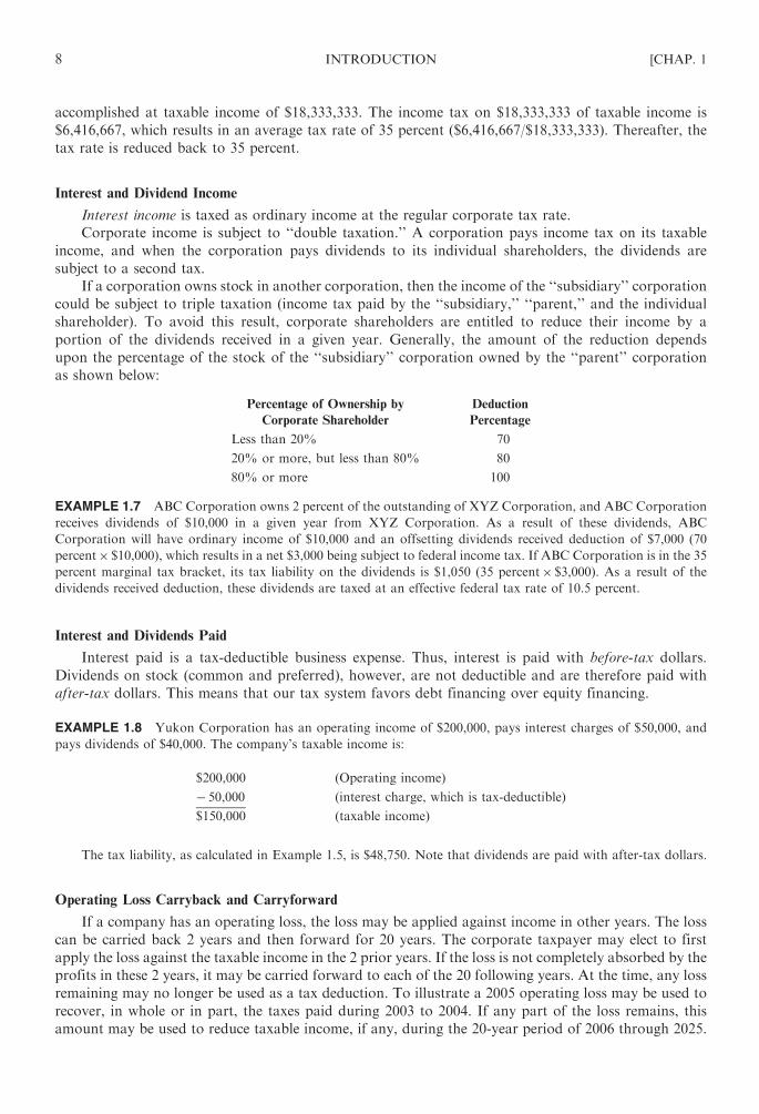
The Financial Executives Institute (www.fei.org), an association of corporate treasurers and
controllers, distinguishes their functions as shown in Table 1-2. (For a typical organization chart
highlighting the structure of financial activity within a firm, see Problem 1.4.)
2 INTRODUCTION [CHAP. 1

The financial manager can affect stockholder wealth maximization by influencing
1. Present and future earnings per share (EPS)
2. The timing, duration, and risk of these earnings
3. Dividend policy
4. The manner of financing the firm
1.3 AGENCY PROBLEMS
An agency relationship exists when one or more persons (called principals) employ one or more
other persons (called agents) to perform some tasks. Primary agency relationships exist (1) between
shareholders and managers and (2) between creditors and shareholders. They are the major source of
agency problems.
Shareholders versus Managers
The agency problem arises when a manager owns less than 100 percent of the company’s ownership.
As a result of the separation between the managers and owners, managers may make decisions
that are not in line with the goal of maximizing stockholder wealth. For example, they may work
less eagerly and benefit themselves in terms of salary and perks. The costs associated with the
agency problem, such as a reduced stock price and various ‘‘perks,’’ is called agency costs.
Several mechanisms are used to ensure that managers act in the best interests of the shareholders:
(1) golden parachutes or severance contracts; (2) performance-based stock option plans; (3) the threat
of firing; and (4) the threat of takeover.
Creditors versus Shareholders
Conflicts develop if (1) managers, acting in the interest of shareholders, take on projects with greater
risk than creditors anticipated and (2) raise the debt level higher than was expected. These actions tend to
reduce the value of the debt outstanding.
1.4 FINANCIAL DECISIONS AND RISK-RETURN TRADE-OFF
Integral to the theory of finance is the concept of a risk-return trade-off. All financial decisions
involve some sort of risk-return trade-off. The greater the risk associated with any financial decision, the
Table 1-2. Functions of Controller and Treasurer
Controller Treasurer
Planning for control Provision of capital
Reporting and interpreting Investor relations
Evaluating and consulting Short-term financing
Tax administration Banking and custody
Government reporting Credits and collections
Protection of assets Investments
Economic appraisal Insurance
CHAP. 1] INTRODUCTION 3

greater the return expected from it. Proper assessment and balance of the various risk-return trade-offs
available is part of creating a sound stockholder wealth maximization plan.
EXAMPLE 1.3 In the case of investment in stock, the investor would demand higher return from a speculative
stock to compensate for the higher level of risk.
In the case of working capital management, the less inventory a firm keeps, the higher the expected return (since
less of the firm’s current assets is tied up), but also the greater the risk of running out of stock and thus losing
potential revenue.
A financial manager’s role is delineated in part by the financial environment in which he or she
operates. Three major aspects of this environment are (1) the organization form of the business; (2) the
financial institutions and markets; and (3) the tax structure. In this book, we limit the discussion of tax
structure to that of the corporation.
1.5 BASIC FORMS OF BUSINESS ORGANIZATION
Finance is applicable both to all economic entities such as business firms and nonprofit organiza-
tions such as schools, governments, hospitals, churches, and so on. However, this book will focus
on finance for business firms organized as three basic forms of business organizations. These forms
are (1) the sole proprietorship; (2) the partnership; and (3) the corporation.
Sole Proprietorship
This is a business owned by one individual. Of the three forms of business organizations, sole
proprietorships are the greatest in number. The advantages of this form are:
1. No formal charter required
2. Less regulation and red tape
3. Significant tax savings
4. Minimal organizational costs
5. Profits and control not shared with others
The disadvantages are:
1. Limited ability to raise large sums of money
2. Unlimited liability for the owner
3. Limited to the life of the owner
4. No tax deductions for personal and employees’ health, life, or disability insurance
Partnership
This is similar to the sole proprietorship except that the business has more than one owner. Its
advantages are:
1. Minimal organizational effort and costs
2. Less governmental regulations
Its disadvantages are:
1. Unlimited liability for the individual partners
2. Limited ability to raise large sums of money
3. Dissolved upon the death or withdrawal of any of the partners
4 INTRODUCTION [CHAP. 1

There is a special form of partnership, called a limited partnership, where one or more partners, but not
all, have limited liability up to their investment in the event of business failure.
1. The general partner manages the business
2. Limited partners are not involved in daily activities. The return to limited partners is in the form
of income and capital gains
3. Often, tax benefits are involved
Examples of limited partnerships are in real estate and oil and gas exploration.
Corporation
This is a legal entity that exists apart from its owners, better known as stockholders. Ownership
is evidenced by possession of shares of stock. In terms of types of businesses, the corporate form is not
the greatest in number, but the most important in terms of total sales, assets, profits, and contribution
to national income. Corporations are governed by a distinct set of state or federal laws and come in two
forms: a state C Corporation or federal Subchapter S.
The advantages of a C corporation are:
1. Unlimited life
2. Limited liability for its owners, as long as no personal guarantee on a business-related obligation
such as a bank loan or lease
3. Ease of transfer of ownership through transfer of stock
4. Ability to raise large sums of capital
Its disadvantages are:
1. Difficult and costly to establish, as a formal charter is required
2. Subject to double taxation on its earnings and dividends paid to stockholders
3. Bankruptcy, even at the corporate level, does not discharge tax obligations
Subchapter S Corporation
This is a form of corporation whose stockholders are taxed as partners. To qualify as an S
corporation, the following is necessary:
1. A corporation cannot have more than 75 shareholders
2. It cannot have any nonresident foreigners as shareholders
3. It cannot have more than one class of stock
4. It must properly elect Subchapter S status
The S corporation can distribute its income directly to shareholders and avoid the corporate income
tax while enjoying the other advantages of the corporate form. Note: not all states recognize Subchapter
S corporations.
Limited Liability Company
Limited Liability Companies (LLCs) are a relatively recent development. Most states permit
the establishment of LLCs. LLCs are typically not permitted to carry on certain service businesses
(e.g., law, medicine, and accounting). An LLC provides limited personal liability, as does a corporation.
Owners, who are called members, can be other corporations. The members run the company or they may
hire an outside management group. The LLC can choose whether to be taxed as a regular corporation
or pass through to members. Profits and losses can be split among members in any way they choose.
Note: LLC rules vary by state.
CHAP. 1] INTRODUCTION 5

1.6 THE FINANCIAL INSTITUTIONS AND MARKETS
A healthy economy depends heavily on efficient transfer of funds from savers to individuals,
businesses, and governments who need capital. Most transfers occur through specialized financial
institutions (see Fig. 1-1), which serve as intermediaries between suppliers and users of funds.
It is in the financial markets that entities demanding funds are brought together with those having
surplus funds. Financial markets provide a mechanism through which the financial manager may obtain
funds from a wide range of sources, including financial institutions. The financial markets are composed
of money markets and capital markets. Figure 1-1 depicts the general flow of funds among financial
institutions and markets.
Money markets are the markets for short-term (less than 1 year) debt securities. Examples of money
market securities include U.S. Treasury bills, federal agency securities, bankers’ acceptances, commercial
paper, and negotiable certificates of deposit issued by government, business, and financial institutions.
Capital markets are the markets for long-term debt and corporate stocks. The New York Stock
Exchange, which handles the stocks of many of the larger corporations, is a prime example of a capital
market. The American Stock Exchange and the regional stock exchanges are still another example.
In addition, securities are traded through the thousands of brokers and dealers on the over-the-counter
market, a term used to denote all buying and selling activities in securities that do not take place on an
organized stock exchange.
1.7 CORPORATE TAX STRUCTURE
In order to make sound financial and investment decisions, a corporation’s financial manager
must have a general understanding of the corporate tax structure, which includes the following:
1. Corporate tax rate schedule
2. Interest and dividend income
3. Interest and dividends paid by a corporation
Fig. 1-1 General flow of funds among financial institutions and financial markets
6 INTRODUCTION [CHAP. 1

4. Operating loss carryback and carry forward
5. Capital gains and losses
6. Alternative ‘‘pass-through’’ entities
Corporate Tax Rate Schedule
Corporations pay federal income tax on their taxable income, which is the corporation’s gross
income reduced by the deductions’ permitted under the Internal Revenue Code of 1986. Federal
income taxes are imposed at the following tax rates:
15% on the first $50,000
25% on the next $25,000
34% on the next $25,000
39% on the next $235,000
34% on the next $9,665,000
35% on the next $5,000,000
38% on the next $3,333,333
35% on the remaining income
EXAMPLE 1.4 If a firm has $20,000 in taxable income, the tax liability is $3,000 ($20,000� 15 percent)
EXAMPLE 1.5 If a firm has $20,000,000 in taxable income, the tax is calculated as follows:
Income ($) � Marginal Tax Rate (%) = Taxes ($)
50,000 15 7,500
25,000 25 6,250
25,000 34 8,500
235,000 39 91,650
9,665,000 34 3,286,100
5,000,000 35 1,750,000
3,333,333 38 1,266,667
1,666,667 35 583,333
20,000,000 7,000,000
Financial managers often refer to the federal tax rate imposed on the next dollar of income as the
‘‘marginal tax rate’’ of the taxpayer. Because of the fluctuations in the corporate tax rates, financial
managers also talk in terms of the ‘‘average tax rate’’ of a corporation. Average tax rates are computed
as follows:
Average Tax Rate ¼ Tax Due=Taxable Income
EXAMPLE 1.6 The average tax rate for the corporation in Example 1.5 is 35 percent (7,000,000/20,000,000).
The marginal tax rate for the corporation in Example 1.5 is 35 percent.
As suggested in Example 1.6, at taxable incomes beyond $18,333,333, corporations pay a tax of
35 percent on all of their taxable income. This fact demonstrates the reasoning behind the patch-quilt of
corporate tax rates. The 15 percent–25 percent–34 percent tax brackets demonstrate the intent that there
should be a graduated tax rate for small corporate taxpayers. The effect of the 39 percent tax bracket is
to wipe out the early low tax brackets. At $335,000 of corporate income, the cumulative income tax is
$113,900, which results in an average tax rate of 34 percent ($113,900/$335,000). The income tax rate
increases to 35 percent at taxable incomes of $10,000,000. The purpose of the 38 percent tax bracket is to
wipe out the effect of the 34 percent tax bracket and to raise the average tax rate to 35 percent. This is
CHAP. 1] INTRODUCTION 7
accomplished at taxable income of $18,333,333. The income tax on $18,333,333 of taxable income is
$6,416,667, which results in an average tax rate of 35 percent ($6,416,667/$18,333,333). Thereafter, the
tax rate is reduced back to 35 percent.
Interest and Dividend Income
Interest income is taxed as ordinary income at the regular corporate tax rate.
Corporate income is subject to ‘‘double taxation.’’ A corporation pays income tax on its taxable
income, and when the corporation pays dividends to its individual shareholders, the dividends are
subject to a second tax.
If a corporation owns stock in another corporation, then the income of the ‘‘subsidiary’’ corporation
could be subject to triple taxation (income tax paid by the ‘‘subsidiary,’’ ‘‘parent,’’ and the individual
shareholder). To avoid this result, corporate shareholders are entitled to reduce their income by a
portion of the dividends received in a given year. Generally, the amount of the reduction depends
upon the percentage of the stock of the ‘‘subsidiary’’ corporation owned by the ‘‘parent’’ corporation
as shown below:
Percentage of Ownership by
Corporate Shareholder
Deduction
Percentage
Less than 20% 70
20% or more, but less than 80% 80
80% or more 100
EXAMPLE 1.7 ABC Corporation owns 2 percent of the outstanding of XYZ Corporation, and ABC Corporation
receives dividends of $10,000 in a given year from XYZ Corporation. As a result of these dividends, ABC
Corporation will have ordinary income of $10,000 and an offsetting dividends received deduction of $7,000 (70
percent� $10,000), which results in a net $3,000 being subject to federal income tax. If ABC Corporation is in the 35
percent marginal tax bracket, its tax liability on the dividends is $1,050 (35 percent� $3,000). As a result of the
dividends received deduction, these dividends are taxed at an effective federal tax rate of 10.5 percent.
Interest and Dividends Paid
Interest paid is a tax-deductible business expense. Thus, interest is paid with before-tax dollars.
Dividends on stock (common and preferred), however, are not deductible and are therefore paid with
after-tax dollars. This means that our tax system favors debt financing over equity financing.
EXAMPLE 1.8 Yukon Corporation has an operating income of $200,000, pays interest charges of $50,000, and
pays dividends of $40,000. The company’s taxable income is:
$200,000 (Operating income)
� 50,000 (interest charge, which is tax-deductible)
$150,000 (taxable income)
The tax liability, as calculated in Example 1.5, is $48,750. Note that dividends are paid with after-tax dollars.
Operating Loss Carryback and Carryforward
If a company has an operating loss, the loss may be applied against income in other years. The loss
can be carried back 2 years and then forward for 20 years. The corporate taxpayer may elect to first
apply the loss against the taxable income in the 2 prior years. If the loss is not completely absorbed by the
profits in these 2 years, it may be carried forward to each of the 20 following years. At the time, any loss
remaining may no longer be used as a tax deduction. To illustrate a 2005 operating loss may be used to
recover, in whole or in part, the taxes paid during 2003 to 2004. If any part of the loss remains, this
amount may be used to reduce taxable income, if any, during the 20-year period of 2006 through 2025.
8 INTRODUCTION [CHAP. 1

The corporation may choose to forgo the loss carryback, and to instead carry the net operating loss to
future years only.
EXAMPLE 1.9 The Loyla Company’s taxable income and associated tax payments for the years 2003 through
2010 are presented below:
Year Taxable Income ($) Tax Payments ($)
2003 100,000 22,250
2004 100,000 22,250
2005 (700,000) 0
2006 100,000 22,250
2007 100,000 22,250
2008 100,000 22,250
2009 100,000 22,250
2010 100,000 22,250
In 2005, Loyla Company had an operating loss of $700,000. By carrying the loss back 2 years and then forward,
the firm was able to ‘‘zero-out’’ its before-tax income as follows:
Year Income
Reduction ($)
Remaining 2005 Net
Operating Loss ($)
Tax Savings ($)
2003 100,000 600,000 22,250
2004 100,000 500,000 22,250
2005 0 500,000 0
2006 100,000 400,000 22,250
2007 100,000 300,000 22,250
2008 100,000 200,000 22,250
2009 100,000 100,000 22,250
2010 100,000 0 22,250
As soon as the company recognized the loss of $700,000 in 2005, it was able to file for a tax refund of $44,500
($22,250+$22,250) for the years 2003 through 2004. It then carried forward the portion of the loss not used to
offset past income and applied it against income for the next 5 years, 2006 through 2010.
Capital Gains and Losses
Capital gains and losses are a major form of corporate income and loss (see also Chapter 8). They
may result when a corporation sells investments and/or business property (not inventory). If depreciation
has been taken on the asset sold, then part or all of the gain from the sale may be taxed as ordinary
income.
Like all taxpayers, corporations net any capital gains and capital losses that they have. Corporations
include any net capital gains as part of their taxable income. Individuals pay tax on their capital gains at
reduced rates.
Modified Accelerated Cost Recovery System (MACRS)
For all assets acquired after 1986, depreciation for tax purposes (‘‘cost recovery’’) is calculated
using the Modified Accelerated Cost Recovery System (‘‘MACRS’’). MACRS is discussed in depth in
Chapter 8.
Alternative ‘‘Pass-Through’’ Tax Entities
As noted above, a disadvantage of corporations, compared to other forms of doing business (e.g.,
general partnerships), is double taxation. The net income of a corporation is taxed to the corporation.
Later, should the corporation distribute that income to its shareholders, the distribution is taxed a
CHAP. 1] INTRODUCTION 9

second time to the recipient shareholders. Despite this disadvantage, corporations are popular because
they have many advantages, including the fact that the liability of their shareholders, who are active in
their business, for corporate debts is generally limited to the shareholders’ investment in the corporation.
Two entities have developed (S Corporation and LLCs), which allow investors limited liability and
yet avoid double taxation. With these entities, owners of the entities are taxed on their share of the
entities’ income. Later, when that income is distributed to the owners, the distribution can be tax-free.
The importance of avoiding double taxation can be seen in the following example. Assume that a
business has $100,000 of net income, and it has one shareholder, who is in the 28 percent marginal tax
bracket. Assume that the business is either a corporation or a pass-through entity:
Corporation Pass-Through Entity
Entity’s Taxable Income: $100,000 $100,000
Tax on Entity Level: (22,250) (0)
Distribution to Owner: $ 77,750 $100,000
Tax on Owner: (21,770) (28,000)
After-tax Distribution: $ 55,980 $ 72,000
Double taxation costs the investor $16,020 or approximately 16 percent in the above example. This
percentage increases as the corporation’s marginal tax rate increases.
Generally, the pass-through entity merely files an informational tax return with the Internal Revenue
Service, and informs its owners of their share of the entity’s taxable income or loss. The owners will be
taxed on their share of the corporation’s income. Afterwards, the distribution of any accrued income to
the owners generally is tax-free.
1.8 THE SARBANES–OXLEY ACT AND CORPORATE GOVERNANCE
Section 404 of the Sarbanes–Oxley Act—‘‘Enhanced Financial Disclosures, Management
Assessment of Internal Control’’—mandates sweeping changes. Section 404, in conjunction with the
related Securities and Exchange Commission (SEC) rules and Auditing Standard No. 2 established by
the Public Company Accounting Oversight Board (PCAOB), requires management of a public company
and the company’s independent auditor to issue two new reports at the end of every fiscal year. These
reports must be included in the company’s annual report filed with the SEC.
� Management must report annually on the effectiveness of the company’s internal control over
financial reporting.
� In conjunction with the audit of the company’s financial statements, the company’s independent
auditor must issue a report on internal control over financial reporting, which includes both an
opinion on management’s assessment and an opinion on the effectiveness of the company’s internal
control over financial reporting.
In the past, a company’s internal controls were considered in the context of planning the audit but
were not required to be reported publicly, except in response to the SEC’s Form 8-K requirements when
related to a change in auditor. The new audit and reporting requirements have drastically changed the
situation and have brought the concept of internal control over financial reporting to the forefront for
audit committees, management, auditors, and users of financial statements.
The new requirements also highlight the concept of a material weakness in internal control over
financial reporting, and mandate that both management and the independent auditor publicly report any
material weaknesses in internal control over financial reporting that exist as of the fiscal-year-end
assessment date. Under both PCAOB Auditing Standard No. 2 and the SEC rules implementing
Section 404, the existence of a single material weakness requires management and the independent
auditor conclude that internal control over financial reporting is not effective.
10 INTRODUCTION [CHAP. 1

Review Questions
1. Modern financial theory assumes that the primary goal of the firm is the maximization of
stockholder , which translates into maximizing the of the
firm’s common stock.
2. is a short-term goal. It can be achieved at the expense of the firm and its
stockholders.
3. A firm’s stock price depends on such factors as present and future earnings per share, the
timing, duration, and of these earnings, and .
4. A major disadvantage of the corporation is the on its earnings and
the paid to its owners (stockholders).
5. A is the largest form of business organization with respect to the number of
such businesses in existence. However, the corporate form is the most important with respect to
the total amount of , assets, , and contribution
to .
6. A corporation is a(n) that exists separately from its owners, better known
as .
7. A partnership is dissolved upon the or of any one of
the .
8. The sole proprietorship is easily established with no and does not have to
share or with others.
9. Corporate financial functions are carried out by the , ,
and .
10. The financial markets are composed of money markets and .
11. Money markets are the markets for short-term (less than 1 year) .
12. The is the term used for all trading activities in securities that do not take
place on an organized stock exchange.
13. Commercial banks and credit unions are two examples of .
14. represent the distribution of earnings to the stockholders of a corporation.
15. are the rates applicable for the next dollar of taxable income.
16. In order to avoid triple taxation, corporations may be entitled to deduct a portion of
the that they receive.
17. If a corporation has a net operating loss, the loss may be and
then .
CHAP. 1] INTRODUCTION 11

18. Unlike individuals, corporations are taxed on their capital gains at the same
as other income.
19. A corporation is entitled to carryback any operating loss years and/or
carryforward that loss years.
20. Two entities that offer active investors limited liability and avoid double taxation
are and .
21. Risk management involves protecting assets by purchasing or
by .
22. Under the Act, management must report annually on the effectiveness of the
company’s .
Answers: (1) wealth, market price; (2) Profit maximization; (3) risk, dividend policy; (4) double taxation,
dividends; (5) sole proprietorship, sales, profits, national income; (6) legal entity, stockholders; (7) withdrawal,
death, partners; (8) formal charter, profits, control; (9) treasurer, controller, financial vice-president; (10)
capital markets; (11) debt securities; (12) over-the-counter market; (13) financial institutions (or intermedi-
aries); (14) Dividends; (15) Marginal tax rates; (16) dividends; (17) carried back, carried forward; (18)
income tax rates; (19) 2 years, 20 years; (20) S Corporations, Limited Liability Companies; (21) insurance,
hedging; (22) Sarbanes–Oxley, internal control over financial reporting.
Solved Problems
1.1 Profit Maximization versus Stockholder Wealth Maximization. What are the disadvantages of
profit maximization and stockholder wealth maximization as the goals of the firm?
SOLUTION
The disadvantages are
Profit Maximization Stockholder Wealth Maximization
Emphasizes the short run Offers no clear link between
financial decisions and stock priceIgnores risk
Ignores the timing of returns Can lead to management anxiety
and frustrationIgnores the stockholders’ return
1.2 The Role of Financial Managers. What are the major functions of the financial manager?
SOLUTION
The financial manager performs the following functions:
1. Financial analysis, forecasting, and planning
(a) Monitors the firm’s financial position
(b) Determines the proper amount of funds to employ in the firm
2. Investment decisions
(a) Makes efficient allocations of funds to specific assets
(b) Makes long-term capital budget and expenditure decisions
12 INTRODUCTION [CHAP. 1
3. Financing and capital structure decisions
(a) Determines both the mix of short-term and long-term financing and equity/debt financing
(b) Raises funds on the most favorable terms possible
4. Management of financial resources
(a) Manages working capital
(b) Maintains optimal level of investment in each of the current assets
1.3 Stock Price Maximization. What are the factors that affect the market value of a firm’s common
stock?
SOLUTION
The factors that influence a firm’s stock price are:
1. Present and future earnings
2. The timing and risk of earnings
3. The stability and risk of earnings
4. The manner in which the firm is financed
5. Dividend policy
1.4 Organizational Chart of the Finance Function. Depict a typical organizational chart highlighting
the finance function of the firm.
SOLUTION
See Fig. 1-2.
1.5 Tax Liability and Average Tax Rate. A corporation has a taxable income of $15,000. What is its
tax liability and average tax rate?
SOLUTION
The company’s tax liability is $2,250 ($15,000� 15%). The company’s average tax rate is 15
percent.
1.6 Tax Liability. A corporation has $120,000 in taxable income. What is its tax liability?
Fig. 1-2
CHAP. 1] INTRODUCTION 13

SOLUTION
Income ($) � Marginal Tax Rate (%) = Taxes ($)
50,000 15 7,500
25,000 25 6,250
25,000 34 8,500
20,000 39 7,800
120,000 30,050
The company’s total tax liability is $30,050.
1.7 Average Tax Rate. In Problem 1.6, what is the average tax rate of the corporation?
SOLUTION
Average tax rate ¼ total tax liability� taxable income ¼ $30;050=$120;000 ¼ 25:04%:
1.8 Dividends Received Deduction. Rha Company owns 30 percent of the stock in Aju Corporation
and receives dividends of $20,000 in a given year. Assume that Rha Company is in the 35 percent
tax bracket. What is the company’s tax liability?
SOLUTION
Rha Company will include the $20,000 in its income, but generally, will receive an offsetting deduction
equal to 80 percent of the dividends received (80%� $20,000=$16,000). As a result of this deduction, Rha
Company will be taxed on a net amount of $4,000.
1.9 Dividends Received Deduction. Yousef Industries had operating income of $200,000 in 2005. In
addition, it received $12,500 in interest income from investment and another $10,000 in dividends
from a wholly owned subsidiary. What is the company’s total tax liability for the year?
SOLUTION
Taxable income:
$ 20,000 (operating income)
12,500 (interest income)
10,000 (dividend income)
(10,000) (100% dividend received deduction for 100% subsidiary)
$212,500 (taxable income)
The company’s total tax liability is computed as follows:
Income ($) � Marginal Tax Rate (%) = Taxes ($)
50,000 15 7,500
25,000 25 6,250
25,000 34 8,500
112,500 39 43,875
212,500 66,125
1.10 Interest and Dividends Paid. Johnson Corporation has operating income of $120,000, pays interest
charges of $60,000, and pays dividends of $20,000. What is the company’s tax liability?
14 INTRODUCTION [CHAP. 1

SOLUTION
The company’s taxable income is:
$120,000 (operating income)
�60,000 (interest charge)
$ 60,000 (taxable income)
The tax liability is then calculated as follows:
Income ($) � Marginal Tax Rate (%) = Taxes ($)
50,000 15 7,500
10,000 25 2,500
60,000 10,000
Note that since dividends of $20,000 are paid out of after-tax income, the dividend amount is not
included in the computation.
1.11 Net Operating Loss Carryback and Carryforward. The Kenneth Parks Company’s taxable
income and tax payments/liability for the years 2003 through 2008 are given below.
Year Taxable Income ($) Tax Payments ($)
2003 100,000 22,250
2004 50,000 7,500
2005 (150,000) 0
2006 100,000 22,250
2007 50,000 7,500
2008 50,000 7,500
Compute the Company’s tax refund in 2005.
SOLUTION
Year Income
Reduction ($)
Remaining 2005 Net
Operating Loss ($)
Tax Savings ($)
2003 100,000 50,000 22,250
2004 50,000 0 7,500
Total 150,000 29,750
As soon as the corporation recognizes the $150,000 loss in 2005, it may file for a tax refund of $29,750
($7,500+$22,250) for the years 2003 and 2004.
1.12 Net Operating Loss Carryback and Carryforward. Assume that the Kenneth Parks Company
anticipates that corporate tax rates will decline in future years, and, therefore, elects to forgo
the carryback and to instead carry the net operating loss forward. Calculate the company’s tax
benefit in the future years assuming no change in tax rates.
SOLUTION
Year Income
Reduction ($)
Remaining 2005 Net
Operating Loss ($)
Tax Savings ($)
2006 100,000 100,000 22,250
2007 50,000 50,000 7,500
Total 150,000 29,750
CHAP. 1] INTRODUCTION 15

1.13 Capital Gain–Maximum Tax Rate. The Theisman Company and its sole shareholder John
Theisman each have a net capital gain of $100,000. John Theisman is in the maximum individual
capital gain tax bracket (28 percent) and the Theisman Company is in the maximum corporate tax
bracket (35 percent). What is the tax liability resulting from the capital gain?
SOLUTION
The Theisman Company: 35%� $100,000=$35,000
John Theisman: 28%� $100,000=$28,000
1.14 Alternative ‘‘Pass-Through’’ Tax Entities. Davidson Company is a limited liability company. It
earned $100,000 in its first year of operation. It may elect to be taxed as a corporation or as a
pass-through entity. Davidson Company intends to distribute all of its earnings to its sole share-
holder David Davidson, who is in the 39.6 percent tax bracket. Should it elect to be taxed as a
corporation or as a pass through entity in its first year?
SOLUTION
Corporation Pass-Through Entity
Entity’s Taxable Income: $100,000 $100,000
Tax on Entity Level: (22,250) (0)
Distribution to Owner: $ 77,750 $100,000
Tax on Owner: (30,789) (39,600)
After-tax Distribution: $ 46,961 $ 60,400
Focusing only on the first year, the sole shareholder will receive a larger after-tax distribution if it elects
to be taxed as a pass-through entity.
1.15 Alternative ‘‘Pass-Through’’ Tax Entities. Assume that in Problem 1.15, the Davidson Company
intends to use its earnings in the business and will not distribute any earnings to its shareholder.
Under these circumstances, should it elect to be taxed as a corporation or as a pass-through entity
in its first year?
SOLUTION
Corporation Pass-Through Entity
Entity’s Taxable Income: $100,000 $100,000
Tax on Entity Level: (22,250) (0)
Distribution to Owner: $ 0 $ 39,600
Tax on Owner: (39,600)
Total Retained by Entity: $ 77,750 $ 61,400
Focusing only on the first year, if no distributions are anticipated, the entity can retain more of its
earnings if it elects to be taxed as a corporation.
16 INTRODUCTION [CHAP. 1

Chapter 2
Analysis of Financial Statements and Cash Flow
2.1 THE SCOPE AND PURPOSE OF FINANCIAL ANALYSIS
Financial analysis is an evaluation of both a firm’s past financial performance and its prospects for
the future. Typically, it involves an analysis of the firm’s financial statements and its cash flows. Financial
statement analysis involves the calculation of various ratios. It is used by such interested parties as
creditors, investors, and managers to determine the firm’s financial position relative to that of others.
The way in which an entity’s financial position and operating results are viewed by investors and
creditors will have an impact on the firm’s reputation, price/earnings ratio, and effective interest rate.
Cash flow analysis is an evaluation of the firm’s statement of cash flows in order to determine
the impact that its sources and uses of cash have on the firm’s operations and financial condition.
It is used in decisions that involve corporate investments, operations, and financing.
2.2 FINANCIAL STATEMENT ANALYSIS
The financial statements of an enterprise present the summarized data of its assets, liabilities,
and equities in the balance sheet and its revenue and expenses in the income statement. If not analyzed,
such data may lead one to draw erroneous conclusions about the firm’s financial condition. Various
measuring instruments may be used to evaluate the financial health of a business, including horizontal,
vertical, and ratio analyses. A financial analyst uses the ratios to make two types of comparisons:
1. Industry comparison. The ratios of a firm are compared with those of similar firms or with
industry averages or norms to determine how the company is faring relative to its competitors.
Industry average ratios are available from a number of sources, including:
a. Risk Management Association (RMA). RMA (formerly known as Robert Morris
Associate) has been compiling statistical data on financial statements for more than 75
years. The RMA Annual Statement Studies provide statistical data from more than 150,000
actual companies on many key financial ratios, such as gross margin, operating margins,
and return on equity and assets. If you are looking to put real authority into the ‘‘industry
average’’ numbers that your company is beating, the Statement Studies are the way to go.
They are organized by SIC codes, and you can buy the financial statement studies for your
industry in report form or over the Internet (www.rmahq.org).
b. Dun and Bradstreet. Dun and Bradstreet publishes Industry Norms and Key Business
Ratios, which covers over 1 million firms in over 800 lines of business.
c. Value Line. Value Line Investment Service provides financial data and rates stocks of over
1,700 firms.
d. The Department of Commerce. The Department of Commerce Financial Report provides
financial statement data and includes a variety of ratios and industrywide common-size
vertical financial statements.
e. Others. Standard and Poor’s, Moody’s Investment Service, and various brokerate compile
industry studies. Further, numerous online services such as Yahoo! and MSN Money
Central, to name a few, also provide these data.
2. Trend analysis. A firm’s present ratio is compared with its past and expected future ratios to
determine whether the company’s financial condition is improving or deteriorating over time.
17
Copyright © 2007, 1998, 1986 by The McGraw-Hill Companies, Inc. Click here for terms of use.

After completing the financial statement analysis, the firm’s financial analyst will consult with
management to discuss their plans and prospects, any problem areas identified in the analysis, and
possible solutions.
2.3 HORIZONTAL ANALYSIS
Horizontal analysis is used to evaluate the trend in the accounts over the years. A $3 million profit
year looks very good following a $1 million profit year, but not after a $4 million profit year. Horizontal
analysis is usually shown in comparative financial statements (Examples 2.1, 2.2, and 2.3). Companies
often show comparative financial data for 5 years in annual reports.
EXAMPLE 2.1
The Ratio Company
Comparative Balance Sheet (in Thousands of Dollars)
December 31, 20X3, 20X2, and 20X1
Increase or (Decrease)
Percentage
Increase or (Decrease)
20X3 20X2 20X1 20X3 – 20X2 20X2 – 20X1 20X3 – 20X2 20X2 – 20X1
ASSETS
Current assets:
Cash $30.0 $35.0 $35.0 (5.00) 0.00 (0.1) 0.0
Short-term investments $20.0 $15.0 $5.0 5.00 10.00 0.3 2.0
Accounts receivable $20.0 $15.0 $10.0 5.00 5.00 0.3 0.5
Inventory $50.0 $45.0 $50.0 5.00 (5.00) 0.1 (0.1)
Total current assets $120.0 $110.0 $100.0 10.00 10.00 0.1 0.1
Plant assets $110.0 $97.0 $91.0 13.00 6.00 0.1 0.1
Accumulated depreciation ($10.0) ($7.0) ($6.0) (3.00) (1.00) 0.4 0.2
Plant assets, net $100.0 $90.0 $85.0 10.00 5.00 0.1 0.1
Total assets $220.0 $200.0 $185.0 20.00 15.00 0.1 0.1
LIABILITIES
Current liabilities-accounts payable $55.4 $50.0 $51.0 5.40 (1.00) 0.1 (0.0)
Long-term debt $80.0 $75.0 $70.0 5.00 5.00 0.1 0.1
Total liabilities $135.4 $125.0 $121.0 10.40 4.00 0.1 0.0
STOCKHOLDERS’ EQUITY
Common stock, $10 par, 4,500 shares $45.0 $45.0 $45.0 0.00 0.00 0.0 0.0
Retained earnings $39.6 $30.0 $18.0 9.60 12.00 0.3 0.7
Total stockholders’ equity $84.6 $75.0 $63.0 9.60 12.00 0.1 0.2
Total liability and stockholders’ equity $220.0 $200.0 $184.0 $20.00 $16.00 0.1 0.1
18 ANALYSIS OF FINANCIAL STATEMENTS AND CASH FLOW [CHAP. 2

EXAMPLE 2.2
The Ratio Company
Comparative Income Statement (in Thousands of Dollars)
December 31, 20X3, 20X2, 20X1
Increase or (Decrease)
Percentage
Increase or (Decrease)
20X3 20X2 20X1 20X3 – 20X2 20X2 – 20X1 20X3 – 20X2 or 20X2 – 20X1
Sales $100.0 $110.0 $50.0 (10.0) 60.0 �9.1 120.0
Sales return and allowances $20.0 $8.0 $3.0 12.0 5.0 150.0 166.7
Net sales $80.0 $102.0 $47.0 (22.0) 55.0 �21.6 117.0
Cost of goods sold $50.0 $60.0 $25.0 (10.0) 35.0 �16.7 140.0
Gross profit $30.0 $42.0 $22.0 (12.0) 20.0 �28.6 90.9
Operating expenses
Selling expenses $5.0 $12.0 $7.0 (7.0) 5.0 �58.3 71.4
General expenses $4.0 $7.0 $4.0 (3.0) 3.0 �42.9 75.0
Total operating expenses $9.0 $19.0 $11.0 (10.0) 8.0 �52.6 72.7
Earnings before interest, taxes and depreciation (EBITD) $21.0 $23.0 $11.0 (2.0) 12.0 �8.7 109.1
Depreciation $3.0 $1.0 $0.0 2.0 1.0 200.0
Earnings before interest and taxes (EBIT)=operating income $18.0 $22.0 $11.0 (4.0) 11.0 �18.2 100.0
Interest expense $2.0 $2.0 $1.0 0.0 1.0 0.0 100.0
Earnings before taxes (EBT) $16.0 $20.0 $10.0 (4.0) 10.0 �20.0 100.0
Income taxes (40%) $6.4 $8.0 $4.0 (1.6) 4.0 �20.0 100.0
Net income $9.6 $12.0 $6.0 (2.4) 6.0 �20.0 100.0
CHAP.2]
ANALYSIS
OF
FIN
ANCIA
LSTATEMENTSAND
CASH
FLOW
19

EXAMPLE 2.3
The Ratio Company
Statement of Cash Flows
(in Thousands of Dollars)
For the Year Ended December 31, 20X2 and 20X3
20X3 20X2
Cash flows from operating activities:
Net income $9.6 $12.0
Add (deduct) to reconcile net income to net cash flow
Depreciation 3.0 1.0
Increase in current liabilities 5.4 (2.0)
Increase in accounts receivable (5.0) (5.0)
Increase in inventory (5.0) (1.6) 5.0 (1.0)
Net cash flow from operating activities 8.0 11.0
Cash flows from investing activities:
Cash paid to purchase marketable securities (13.0) (6.0)
Cash paid to purchase fixed assets (5.0) (10.0)
Net cash flow used for investing activities (18.0) (16.0)
Cash flows from financing activities:
Issuance of long-term debt 5.0 5.0
Net cash flow used in financing activities 5.0 5.0
Net decrease in cash and cash equivalents (5.0) 0.0
Cash and cash equivalents at the beginning of the year 35.0 35.0
Cash and cash equivalents at the end of the year $30.0 $35.0
Because horizontal analysis stresses the trends of the various accounts, it is relatively easy
to identify areas of wide divergence that require further attention. In the income statement
shown in Example 2.2, the large increase in sales returns and allowances coupled with the
decrease in sales for the period 20X2 to 20X3 should cause concern. One might compare these
results with those of competitors to determine whether the problem is industry wide or just within the
company.
Note that it is important to show both the dollar amount of change and the percentage of
change, because either one alone might be misleading. For example, although the interest
expense from 20X1 to 20X2 increased 100 percent (Example 2.2), it probably does not require further
investigation since the dollar amount of increase is only $1,000. Similarly, a large change in dollar
amount might result in only a small percentage change and therefore not be a cause for concern.
When an analysis covers a span of many years comparative financial statements may become
cumbersome. To avoid this, the results of horizontal analysis may be presented by showing trends
relative to a base year. In this method, a year representative of the firm’s activity is chosen as the
base. Each account of the base year is assigned an index of 100. The index for each respective account
in succeeding years is found by dividing the account’s amount by the base year amount and multiplying
by 100. For example, if we let 20X1 be the base year in the balance sheet of Examples 2.1, Accounts
Receivable would be given an index of 100. In 20X2, the index would be 150 [(15/10)� 100], and in 20X3
it would be 200 [(20/10)� 100]. A condensed form of the balance sheet using trend analysis is shown in
Example 2.4.
20 ANALYSIS OF FINANCIAL STATEMENTS AND CASH FLOW [CHAP. 2
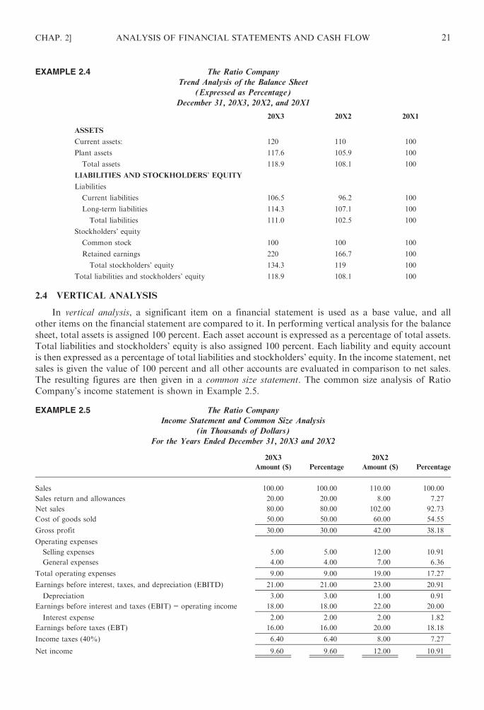
EXAMPLE 2.4 The Ratio Company
Trend Analysis of the Balance Sheet
(Expressed as Percentage)
December 31, 20X3, 20X2, and 20X1
20X3 20X2 20X1
ASSETS
Current assets: 120 110 100
Plant assets 117.6 105.9 100
Total assets 118.9 108.1 100
LIABILITIES AND STOCKHOLDERS’ EQUITY
Liabilities
Current liabilities 106.5 96.2 100
Long-term liabilities 114.3 107.1 100
Total liabilities 111.0 102.5 100
Stockholders’ equity
Common stock 100 100 100
Retained earnings 220 166.7 100
Total stockholders’ equity 134.3 119 100
Total liabilities and stockholders’ equity 118.9 108.1 100
2.4 VERTICAL ANALYSIS
In vertical analysis, a significant item on a financial statement is used as a base value, and all
other items on the financial statement are compared to it. In performing vertical analysis for the balance
sheet, total assets is assigned 100 percent. Each asset account is expressed as a percentage of total assets.
Total liabilities and stockholders’ equity is also assigned 100 percent. Each liability and equity account
is then expressed as a percentage of total liabilities and stockholders’ equity. In the income statement, net
sales is given the value of 100 percent and all other accounts are evaluated in comparison to net sales.
The resulting figures are then given in a common size statement. The common size analysis of Ratio
Company’s income statement is shown in Example 2.5.
EXAMPLE 2.5 The Ratio Company
Income Statement and Common Size Analysis
(in Thousands of Dollars)
For the Years Ended December 31, 20X3 and 20X2
20X3
Amount ($) Percentage
20X2
Amount ($) Percentage
Sales 100.00 100.00 110.00 100.00
Sales return and allowances 20.00 20.00 8.00 7.27
Net sales 80.00 80.00 102.00 92.73
Cost of goods sold 50.00 50.00 60.00 54.55
Gross profit 30.00 30.00 42.00 38.18
Operating expenses
Selling expenses 5.00 5.00 12.00 10.91
General expenses 4.00 4.00 7.00 6.36
Total operating expenses 9.00 9.00 19.00 17.27
Earnings before interest, taxes, and depreciation (EBITD) 21.00 21.00 23.00 20.91
Depreciation 3.00 3.00 1.00 0.91
Earnings before interest and taxes (EBIT)=operating income 18.00 18.00 22.00 20.00
Interest expense 2.00 2.00 2.00 1.82
Earnings before taxes (EBT) 16.00 16.00 20.00 18.18
Income taxes (40%) 6.40 6.40 8.00 7.27
Net income 9.60 9.60 12.00 10.91
CHAP. 2] ANALYSIS OF FINANCIAL STATEMENTS AND CASH FLOW 21

Vertical analysis is used to disclose the internal structure of an enterprise. It indicates the existing relationship
between each income statement account and revenue. It shows the mix of assets that produces the income and
the mix of the sources of capital, whether by current or long-term liabilities or by equity funding. In addition to
making such internal evaluation possible, the results of vertical analysis are also used to further asses the firm’s
relative position in the industry.
As with horizontal analysis, vertical analysis is not the end of the process. The financial analyst must
be prepared to probe deeper into those areas that either horizontal or vertical analysis, or both, indicate to be
possible problem areas.
2.5 RATIO ANALYSIS
Horizontal and vertical analyses compare one figure to another within the same category. It is also
essential to compare figures from different categories. This is accomplished through ratio analysis.
There are many ratios that an analyst can use, depending upon what he or she considers to be important
relationships.
Financial ratios can be classified into five groups:
1. Liquidity ratios
2. Activity ratios
3. Leverage ratios
4. Profitability ratios
5. Market value ratios
Some of the most useful ones in each category are discussed next.
Liquidity Ratios
Liquidity is a company’s ability to meet its maturing short-term obligations. Liquidity is essential
to conducting business activity, particularly in times of adversity, such as when a business is shut down
by a strike or when operating losses ensue due to an economic recession or a steep rise in the price
of a raw material or part. If liquidity is insufficient to cushion such losses, serious financial difficulty
may result. Poor liquidity is analogous to a person having a fever — it is a symptom of a fundamental
problem.
Analyzing corporate liquidity is especially important to creditors. If a company has a poor liquidity
position, it may be a poor credit risk, perhaps unable to make timely interest and principal payments.
Liquidity ratios are static in nature as of year-end. Therefore, it is also important for management
to look at expected future cash flows. If future cash outflows are expected to be high relative to inflows,
the liquidity position of the company will deteriorate.
A description of various liquidity measures follows.
Net Working Capital. Net working capital1 is equal to current assets less current liabilities.
Current assets are those assets that are expected to be converted into cash or used up within 1 year.
Current liabilities are those liabilities that must be paid with in 1 year; they are paid out of current assets.
Net working capital is a safety cushion to creditors. A large balance is required when the entity has
difficulty borrowing on short notice.
Net working captial ¼ current assets� current liabilities
1Some textbooks define working capital as current assets less current liabilities. Therfore, the terms net working capital and working
capital are often used interchangeably throughout those books.
22 ANALYSIS OF FINANCIAL STATEMENTS AND CASH FLOW [CHAP. 2

The net working capital for the Ratio Company for 20X3 is:
$120,000� $55,400 ¼ $64,600
In 20X2, net working capital was $60,000. The increase in net working capital is a favorable sign.
Current Ratio. The current ratio is equal to current assets divided by current liabilities. This
ratio, which is subject to seasonal fluctuations, is used to measure the ability of an enterprise to meet
its current liabilities out of current assets. A high ratio is needed when the firm has difficulty
borrowing on short notice. A limitation of this ratio is that it may rise just prior to financial
distress because of a company’s desire to improve its cash position by, for example, selling fixed
assets. Such dispositions have a detrimental effect upon productive capacity. Another limitation of
the current ratio is that it will be excessively high when inventory is carried on the last-in, first-out
(LIFO) basis.
Current ratio ¼ current assets
current liabilities
The Ratio Company’s current ratio for 20X3 is:
$120,000
$55,400¼ 2:17
In 20X2, the current ratio was 2.2. The ratio showed a slight decline over the year.
Quick (Acid-Test) Ratio. The quick ratio, also known as the acid-test ratio, is a stringent test of
liquidity. It is found by dividing the most liquid current assets (cash, marketable securities, and accounts
receivable) by current liabilities. Inventory is not included because of the length of time needed to
convert inventory into cash. Prepaid expenses are also not included because they are not convertible
into cash and so are not capable of covering current liabilities.
Quick ratio ¼ cashþmarketable securitiesþ accounts receivable
current liabilties
The quick ratio for the Ratio Company in 20X3 is:
$30,000þ $20,000þ $20,000
$55,400¼ 1:26
The ratio was 1.3 in 20X2. The ratio went down slightly over the year.
Other Liquidity Ratios. Two other popular liquidity ratios that a short-term creditor might be
interested in are: the cash ratio and cash burn rate. The cash ratio (or doomsday ratio) is:
cash
current liabilities
For the Ratio Company, the cash ratio is:
20X3 20X2 Trend
$30,000/$55,400=0.54 $35,000/$50,000=0.70 Deteriorated
Note: This ratio is most relevant for companies in financial distress. The name doomsday ratio comes
from the worst-case assumption that the business ceases to exist and only the cash on hand is available to
meet credit obligations.
Suppose that a company is facing a strike and cash inflows begin to dry up. How long could the
company keep running? One answer is given by the cash burn rate:
Cash burn rate ¼ current assets
average daily operating expenses
CHAP. 2] ANALYSIS OF FINANCIAL STATEMENTS AND CASH FLOW 23

In 20X3, total operating expenses were $70,000 ($50,000 cost of goods sold+$12,000 operating
expenses). The daily average expense was $72,000/365=$197.26 per day. The burn rate is
thus=$120,000/$197.26=608 days. Based on this, the Ratio Company could hang on for about
20 months. It was 508 days in 20X2, which suggests that the burn rate is improving. Note: This ratio
is most relevant for start-up companies that often have little in the way of revenues.
The overall liquidity trend shows a slight deterioration as reflected in the lower current, quick,
and cash ratios. But a mitigating factor is the increase in net working capital and cash burn rate.
Activity (Asset Utilization) Ratios
Activity ratios are used to determine how quickly various accounts are converted into sales or cash.
Overall liquidity ratios generally do not give an adequate picture of a company’s real liquidity, due to
differences in the kinds of current assets and liabilities the company holds. Thus, it is necessary to
evaluate the activity or liquidity of specific current accounts. Various ratios exist to measure the activity
of receivables, inventory, and total assets.
Accounts Receivable Ratios. Accounts receivable ratios consist of the accounts receivable turnover
ratio and the average collection period. The accounts receivable turnover ratio gives the number of times
accounts receivable is collected during the year. It is found by dividing net credit sales (if not available,
then total sales) by the average accounts receivable. Average accounts receivable is typically found by
adding the beginning and ending accounts receivable and dividing by 2. Although average accounts
receivable may be computed annually, quarterly, or monthly, the ratio is most accurate when the shortest
period available is used. In general, the higher the accounts receivable turnover, the better since
the company is collecting quickly from customers and these funds can then be invested. However,
an excessively high ratio may indicate that the company’s credit policy is too stringent, with
the company not tapping the potential for profit through sales to customers in higher risk classes.
Note that here, too, before changing its credit policy, a company has to weigh the profit potential
against the risk inherent in selling to more marginal customers.
Accounts receivable turnover ¼ net credit sales
average accounts receivable
The Ratio Company’s average accounts receivable for 20X2 is:
$15,000þ $20,000
2¼ $17,500
The accounts receivable turnover ratio for 20X3 is:
$80,000
$17,500¼ 4:57 times
In 20X2, the accounts receivable turnover ratio was 8.16. The drop in this ratio in 20X3 is significant
and indicates a serious problem in collecting from customers. The company needs to reevaluate its credit
policy, which may be too lax, or its billing and collection practices, or both.
The collection period (days sales in receivables) is the number of days it takes to collect on
receivables.
Average collection period ¼ 365
accounts receivable turnover
The Ratio Company’s average collection period for 20X3 is:
365
4:57¼ 79:9 days
This means that it takes almost 80 days for a sale to be converted into cash. In 20X2, the average
collection period was 44.7 days. With the substantial increase in collection days in 20X3, there exists
a danger that customer balances may become uncollectible. One possible cause for the increase may
24 ANALYSIS OF FINANCIAL STATEMENTS AND CASH FLOW [CHAP. 2

be that the company is now selling to highly marginal customers. The analyst should compare the
company’s credit terms with the extent to which customer balances are delinquent. An aging schedule,
which lists the accounts receivable according to the length of time they are outstanding, would be helpful
for this comparison.
Inventory Ratios. If a company is holding excess inventory, it means that funds which could
be invested elsewhere are being tied up in inventory. In addition, there will be high carrying cost
for storing the goods, as well as the risk of obsolescence. On the other hand, if inventory is too low,
the company may lose customers because it has run out of merchandise. Two major ratios for
evaluating inventory are inventory turnover and average age of inventory.
Inventory turnover is computed as:
Inventory turnover ¼ cost of goods sold
average inventory
Average inventory is determined by adding the beginning and ending inventories and dividing by 2.
For the Ratio Company, the inventory turnover in 20X3 is:
$50,000
$47,500¼ 1:05 times
In 20X2, the inventory turnover was 1.26 times.
The decline in the inventory turnover indicates the stocking of goods. An attempt should be made
to determine whether specific inventory categories are not selling well and if this is so, the reasons
therefore. Perhaps there are obsolete goods on hand not actually worth their stated value. However,
a decline in the turnover rate would not cause concern if it were primarily due to the introduction of
a new product line for which the advertising effects have not been felt yet.
Average age of inventory is computed as follows:
Average age of inventory ¼ 365
inventory turnover
The average age of inventory in 20X3 is:
365
1:05¼ 347:6 days
In 20X2, the average age was 289.7 days. The lengthening of the holding period shows a potentially
greater risk of obsolescence.
Operating Cycle
The operating cycle of a business is the number of days it takes to convert inventory and receivables
to cash. Hence, a short operating cycle is desirable.
Operating cycle ¼ average collection periodþ average age of inventory
The operating cycle for the Ratio Company in 20X3 is:
79:9 daysþ 347:6 days ¼ 427:5 days
In 20X2, the operating cycle was 334.4 days. This is an unfavorable trend since an increased amount
of money is being tied up in noncash assets.
Cash Conversion Cycle
Noncash working capital consists of current assets and liabilities other than cash. One way to view
noncash working capital efficiency is to view operations as a cycle—from initial purchase of inventory to
the final collection upon sale. The cycle begins with a purchase of inventory on account followed
by the account payment, after which the item is sold and the account collected. These three balances
CHAP. 2] ANALYSIS OF FINANCIAL STATEMENTS AND CASH FLOW 25

can be translated into days of sales and used to measure how well a company efficiently manages
noncash working capital. This measure is termed the cash conversion cycle or cash cycle. This is the
number of days that pass before we collect the cash from a sale, measured from when we actually pay
for the inventory. The cash conversion cycle is:
Cash conversion cycle ¼ operating cycle� accounts payable period,
where
Accounts payables turnover ¼ cost of goods sold
average accounts payableand
Accounts payable period ¼ 365
accounts payable turnover
In 20X3, Accounts payables turnover ¼ $50,000
$50,400þ $50,000ð Þ=2 ¼ 0:95 times
Accounts payable period ¼ 365
0:95¼ 384:2 days
(Note that current liabilities for the Ratio Company are all accounts payable.)
In 20X3 for the Ratio Company, the cash conversion cycle=427.5 days� 384.2 days=43.3 days.
Thus, on average, there is a 43-day delay between the time the company pays for merchandise and the
time it collects on the sale. In 20X2, the ratio was 25.1 days. This is an unfavorable sign since an
increased cycle implies that more money is being tied up in inventories and receivables.
Total Asset Turnover. The total asset turnover ratio is helpful in evaluating a company’s ability
to use its asset base efficiently to generate revenue. A low ratio may be due to many factors, and
it is important to identify the underlying reasons. For example, is investment in assets excessive
when compared to the value of the output being produced? If so, the company might want to
consolidate its present operation, perhaps by selling some of its assets and investing the proceeds for
a higher return or using them to expand into a more profitable area.
Total asset turnover ¼ net sales
average total assets
In 20X3 the total asset turnover ratio for the Ratio Company is:
$80,000
$210,000¼ 0:381
In 20X2, the ratio was 0.530 ($102,000/$192,500). The company’s use of assets declined
significantly, and the reasons need to be pinpointed. For example, are adequate repairs being made?
Or are the assets getting old and do they need replacing?
Interrelationship of Liquidity and Activity to Earnings. A trade-off exists between liquidity risk
and return. Liquidity risk is minimized by holding greater current assets than noncurrent assets.
However, the rate of return will decline because the return on current assets (i.e., marketable securities)
is typically less than the rate earned on productive fixed assets. Also, excessively high liquidity may
mean that management has not aggressively searched for desirable capital investment opportunities.
Maintaining a proper balance between liquidity and return is important to the overall financial health
of a business.
It must be pointed out that high profitability does not necessarily infer a strong cash flow position.
Income may be high but cash problems may exist because of maturing debt and the need to replace
assets, among other reasons. For example, it is possible that a growth company may experience a decline
in liquidity since the net working capital needed to support the expanding sales is tied up in assets
that cannot be realized in time to meet the current obligations. The impact of earning activities on
liquidity is highlighted by comparing cash flow from operations to net income.
26 ANALYSIS OF FINANCIAL STATEMENTS AND CASH FLOW [CHAP. 2
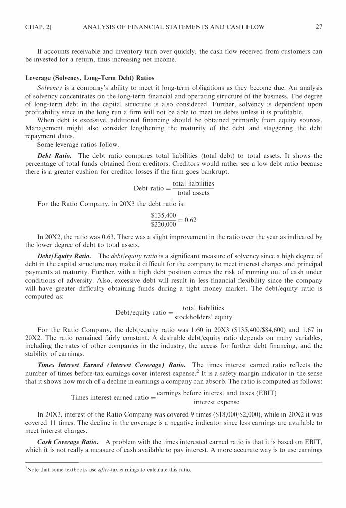
If accounts receivable and inventory turn over quickly, the cash flow received from customers can
be invested for a return, thus increasing net income.
Leverage (Solvency, Long-Term Debt) Ratios
Solvency is a company’s ability to meet it long-term obligations as they become due. An analysis
of solvency concentrates on the long-term financial and operating structure of the business. The degree
of long-term debt in the capital structure is also considered. Further, solvency is dependent upon
profitability since in the long run a firm will not be able to meet its debts unless it is profitable.
When debt is excessive, additional financing should be obtained primarily from equity sources.
Management might also consider lengthening the maturity of the debt and staggering the debt
repayment dates.
Some leverage ratios follow.
Debt Ratio. The debt ratio compares total liabilities (total debt) to total assets. It shows the
percentage of total funds obtained from creditors. Creditors would rather see a low debt ratio because
there is a greater cushion for creditor losses if the firm goes bankrupt.
Debt ratio ¼ total liabilities
total assets
For the Ratio Company, in 20X3 the debt ratio is:
$135,400
$220,000¼ 0:62
In 20X2, the ratio was 0.63. There was a slight improvement in the ratio over the year as indicated by
the lower degree of debt to total assets.
Debt/Equity Ratio. The debt/equity ratio is a significant measure of solvency since a high degree of
debt in the capital structure may make it difficult for the company to meet interest charges and principal
payments at maturity. Further, with a high debt position comes the risk of running out of cash under
conditions of adversity. Also, excessive debt will result in less financial flexibility since the company
will have greater difficulty obtaining funds during a tight money market. The debt/equity ratio is
computed as:
Debt=equity ratio ¼ total liabilities
stockholders’ equity
For the Ratio Company, the debt/equity ratio was 1.60 in 20X3 ($135,400/$84,600) and 1.67 in
20X2. The ratio remained fairly constant. A desirable debt/equity ratio depends on many variables,
including the rates of other companies in the industry, the access for further debt financing, and the
stability of earnings.
Times Interest Earned (Interest Coverage) Ratio. The times interest earned ratio reflects the
number of times before-tax earnings cover interest expense.2 It is a safety margin indicator in the sense
that it shows how much of a decline in earnings a company can absorb. The ratio is computed as follows:
Times interest earned ratio ¼ earnings before interest and taxes ðEBITÞinterest expense
In 20X3, interest of the Ratio Company was covered 9 times ($18,000/$2,000), while in 20X2 it was
covered 11 times. The decline in the coverage is a negative indicator since less earnings are available to
meet interest charges.
Cash Coverage Ratio. A problem with the times interested earned ratio is that it is based on EBIT,
which it is not really a measure of cash available to pay interest. A more accurate way is to use earnings
2Note that some textbooks use after-tax earnings to calculate this ratio.
CHAP. 2] ANALYSIS OF FINANCIAL STATEMENTS AND CASH FLOW 27
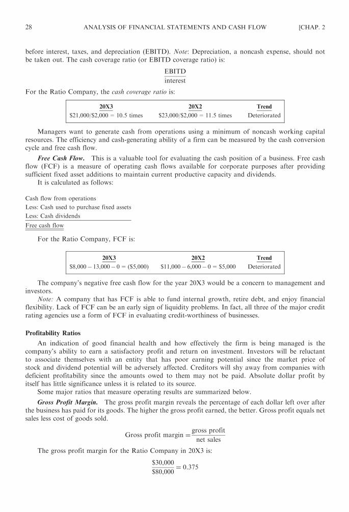
before interest, taxes, and depreciation (EBITD). Note: Depreciation, a noncash expense, should not
be taken out. The cash coverage ratio (or EBITD coverage ratio) is:
EBITD
interest
For the Ratio Company, the cash coverage ratio is:
20X3 20X2 Trend
$21,000/$2,000=10.5 times $23,000/$2,000=11.5 times Deteriorated
Managers want to generate cash from operations using a minimum of noncash working capital
resources. The efficiency and cash-generating ability of a firm can be measured by the cash conversion
cycle and free cash flow.
Free Cash Flow. This is a valuable tool for evaluating the cash position of a business. Free cash
flow (FCF) is a measure of operating cash flows available for corporate purposes after providing
sufficient fixed asset additions to maintain current productive capacity and dividends.
It is calculated as follows:
Cash flow from operations
Less: Cash used to purchase fixed assets
Less: Cash dividends
Free cash flow
For the Ratio Company, FCF is:
20X3 20X2 Trend
$8,000� 13,000� 0= ($5,000) $11,000� 6,000� 0=$5,000 Deteriorated
The company’s negative free cash flow for the year 20X3 would be a concern to management and
investors.
Note: A company that has FCF is able to fund internal growth, retire debt, and enjoy financial
flexibility. Lack of FCF can be an early sign of liquidity problems. In fact, all three of the major credit
rating agencies use a form of FCF in evaluating credit-worthiness of businesses.
Profitability Ratios
An indication of good financial health and how effectively the firm is being managed is the
company’s ability to earn a satisfactory profit and return on investment. Investors will be reluctant
to associate themselves with an entity that has poor earning potential since the market price of
stock and dividend potential will be adversely affected. Creditors will shy away from companies with
deficient profitability since the amounts owed to them may not be paid. Absolute dollar profit by
itself has little significance unless it is related to its source.
Some major ratios that measure operating results are summarized below.
Gross Profit Margin. The gross profit margin reveals the percentage of each dollar left over after
the business has paid for its goods. The higher the gross profit earned, the better. Gross profit equals net
sales less cost of goods sold.
Gross profit margin ¼ gross profit
net sales
The gross profit margin for the Ratio Company in 20X3 is:
$30,000
$80,000¼ 0:375
28 ANALYSIS OF FINANCIAL STATEMENTS AND CASH FLOW [CHAP. 2
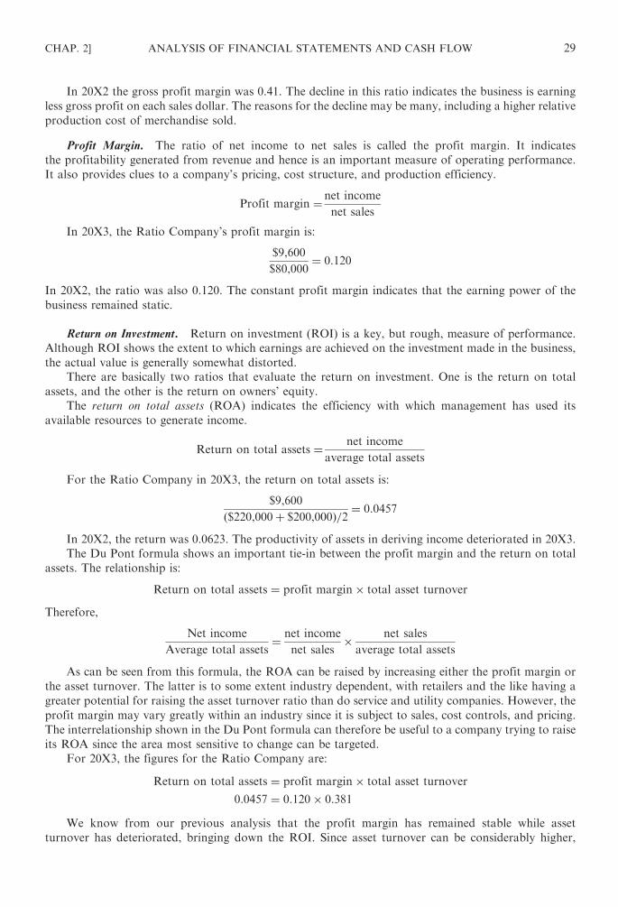
In 20X2 the gross profit margin was 0.41. The decline in this ratio indicates the business is earning
less gross profit on each sales dollar. The reasons for the decline may be many, including a higher relative
production cost of merchandise sold.
Profit Margin. The ratio of net income to net sales is called the profit margin. It indicates
the profitability generated from revenue and hence is an important measure of operating performance.
It also provides clues to a company’s pricing, cost structure, and production efficiency.
Profit margin ¼ net income
net sales
In 20X3, the Ratio Company’s profit margin is:
$9,600
$80,000¼ 0:120
In 20X2, the ratio was also 0.120. The constant profit margin indicates that the earning power of the
business remained static.
Return on Investment. Return on investment (ROI) is a key, but rough, measure of performance.
Although ROI shows the extent to which earnings are achieved on the investment made in the business,
the actual value is generally somewhat distorted.
There are basically two ratios that evaluate the return on investment. One is the return on total
assets, and the other is the return on owners’ equity.
The return on total assets (ROA) indicates the efficiency with which management has used its
available resources to generate income.
Return on total assets ¼ net income
average total assets
For the Ratio Company in 20X3, the return on total assets is:
$9,600
ð$220,000þ $200,000Þ=2 ¼ 0:0457
In 20X2, the return was 0.0623. The productivity of assets in deriving income deteriorated in 20X3.
The Du Pont formula shows an important tie-in between the profit margin and the return on total
assets. The relationship is:
Return on total assets ¼ profit margin� total asset turnover
Therefore,
Net income
Average total assets¼ net income
net sales� net sales
average total assets
As can be seen from this formula, the ROA can be raised by increasing either the profit margin or
the asset turnover. The latter is to some extent industry dependent, with retailers and the like having a
greater potential for raising the asset turnover ratio than do service and utility companies. However, the
profit margin may vary greatly within an industry since it is subject to sales, cost controls, and pricing.
The interrelationship shown in the Du Pont formula can therefore be useful to a company trying to raise
its ROA since the area most sensitive to change can be targeted.
For 20X3, the figures for the Ratio Company are:
Return on total assets ¼ profit margin� total asset turnover
0:0457 ¼ 0:120� 0:381
We know from our previous analysis that the profit margin has remained stable while asset
turnover has deteriorated, bringing down the ROI. Since asset turnover can be considerably higher,
CHAP. 2] ANALYSIS OF FINANCIAL STATEMENTS AND CASH FLOW 29

the Ratio Company might first focus on improving this ratio while at the same time reevaluating its
pricing policy, cost controls, and sales practices.
The return on common equity (ROE) measures the rate of return earned on the common
stockholders’ investment.
Return on common equity ¼ earnings available to common stockholders
average stockholders’ equity
In 20X3, the Ratio Company’s return on equity is:
$9,600
ð$84,600þ $75,000Þ=2 ¼ 0:1203
In 20X2, the ROE was 0.17. There has been a significant drop in the return earned by the owners
of the business.
ROE and ROA are closely related through what is known as the equity multiplier (leverage, or debt
ratio) as follows:
ROE ¼ ROA� equity multiplier
¼ ROA� total assets
common equity
or
¼ ROA
1� debt ratio
In 20X3, the Ratio Company’s debt ratio was 0.62. Thus,
ROE ¼ 0:0457
1� 0:62¼ 0:1203
Note that ROA=0.0457 and ROE=0.1203. This means that through the favorable use of leverage
(debt), the Ratio Company was able to increase the stockholders’ return significantly.
Market Value Ratios
A final group of ratios relates the firm’s stock price to its earnings (or book value) per share. It also
includes dividend-related ratios.
Earnings per Share. Earnings per share indicates the amount of earnings for each common share
held. When preferred stock is included in the capital structure, net income must be reduced by the
preferred dividends to determine the amount applicable to common stock. When preferred stock
does not exist, as is the case with the Ratio Company, earnings per share is equal to net income divided
by common shares outstanding. Earnings per share is a useful indicator of the operating performance
of the company as well as of the dividends that may be expected.
Earnings per share ¼ net income� preferred dividends
common stock outstanding
In 20X3, earnings per share is:
$9,600
4,500 shares¼ $2:13
30 ANALYSIS OF FINANCIAL STATEMENTS AND CASH FLOW [CHAP. 2

In 20X2, earnings per share was $2.67. The decline in earnings per share should be of concern
to investors.
Almost all of the Ratio Company’s profitability ratios have declined in 20X3 relative to 20X2.
This is a very negative sign.
Price/Earnings Ratio (Multiple). Some ratios evaluate the enterprise’s relationship with its
stockholders. The often quoted price/earnings (P/E) ratio is equal to the market price per share of
stock divided by the earnings per share. A high P/E multiple is good because it indicates that
the investing public considers the company in a favorable light.
P=E ratio ¼ market price per share
earnings per share
Let us assume that the market price per share of Ratio Company stock was $20 on December 31,
20X3, and $22 on December 31, 20X2. Therefore, the P/E ratio in 20X3 is:
$20
$2:13¼ 9:39
The ratio in 20X2 was 8.24 ($22/$2.67). The rise in the P/E multiple indicates that the stock
market has a favorable opinion of the company.
Book Value per Share. Book value per share is net assets available to common stockholders
divided by shares outstanding, where net assets is stockholders’ equity minus preferred stock.
Comparing book value per share with market price per share gives another indication of how investors
regard the firm.
The Ratio Company book value per share in 20X3 equals:
Book value per share ¼ total stockholders’ equity� preferred stock
shares outstanding
¼ $84,600� 0
4,500¼ $18:80
The book value per share in 20X2 was $16.67.
If we assume the stock market has a market price of $20 per share, then the Ratio Company’s stock
is favorably regarded by investors since its market price exceeds book value.
Market Value Added. The major goal of a firm is to maximize wealth maximization. This goal is
maximized by maximizing the difference between the market value of the firm’s stock and the amount
of equity capital supplied by shareholders. The difference is called the market value added (MVA).
MVA=market value of the firm’s stock� equity capital supplied by shareholders= (stock price�shares outstanding)� total common equity.
In 20X3, the Ratio Company’s MVA is ($20� 4,500 shares)� $84,500=$5,500. It was $24,000 in
20X2, which indicates a substantial reduction. The higher its MVA, the better the job management is
doing for the company’s shareholders.
Dividend Ratios. Many stockholders are primarily interested in receiving dividends. The two
pertinent ratios are dividend yield and dividend payout:
Dividend yield ¼ dividends per share
market price per share
Dividend payout ¼ dividends per share
earnings per share
Obviously, a decline in these ratios signals a decline in the value of dividends and would cause
concern on the part of stockholders. (See Problem 2.12 for a computation of the dividend ratios.)
CHAP. 2] ANALYSIS OF FINANCIAL STATEMENTS AND CASH FLOW 31

EXAMPLE 2.6
Ratio Company
Summary of Financial Ratios — Trend and Industry Comparisons
(a) (b) Evaluation
Ratios Definitions 20X2 20X3 Industry Industry Trend Overall
LIQUIDITY
Net working capital Current assets� current liabilities $60,000 $64,600 $56,000 Good Improving Good
Current Ratio Current assets/current liabilities 2.2 2.17 2.05 OK Deteriorated OK
Quick (Acid-test)
ratio
(Cash+marketable securities+
accounts receivable)/current
liabilities
1.3 1.26 1.11 OK Deteriorated OK
Cash Ratio Cash/current liabilities 0.7 0.4 N/A N/A Deteriorated Poor
Cash burn rate Current assets/average daily
operating expenses
508
days
608
days
N/A N/A Deteriorated Poor
ASSET UTILIZATION
Accounts receivable turnover Net credit sales/average accounts
receivable
8.16 4.57 5.5 OK Deteriorated Poor
Average collection
period
365 days/accounts receivable
turnover
44.7
days
79.9
days
66.4
days
OK Deteriorated Poor
Inventory turnover Cost of goods sold/average
inventory
1.26 1.05 1.2 OK Deteriorated Poor
Average age of
inventory
365 days/Inventory turnover 289.7
days
347.6
days
N/A N/A Deteriorated Poor
Operating cycle Average collection period+
average age of inventory
334.4
days
427.5
days
N/A N/A Deteriorated Poor
Cash conversion cycle Operating cycle� average
payable period
25.1
days
43.3
days
N/A N/A Deteriorated Poor
Total asset turnover Net sales/average total assets 0.53 0.381 0.44 OK Deteriorated Poor
32
ANALYSIS
OF
FIN
ANCIA
LSTATEMENTSAND
CASH
FLOW
[CHAP.2
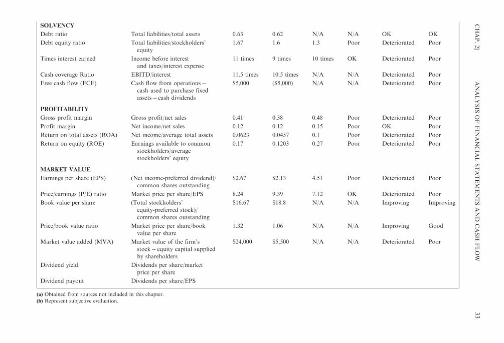
SOLVENCY
Debt ratio Total liabilities/total assets 0.63 0.62 N/A N/A OK OK
Debt equity ratio Total liabilities/stockholders’
equity
1.67 1.6 1.3 Poor Deteriorated Poor
Times interest earned Income before interest
and taxes/interest expense
11 times 9 times 10 times OK Deteriorated Poor
Cash coverage Ratio EBITD/interest 11.5 times 10.5 times N/A N/A Deteriorated Poor
Free cash flow (FCF) Cash flow from operations�cash used to purchase fixed
assets� cash dividends
$5,000 ($5,000) N/A N/A Deteriorated Poor
PROFITABILITY
Gross profit margin Gross profit/net sales 0.41 0.38 0.48 Poor Deteriorated Poor
Profit margin Net income/net sales 0.12 0.12 0.15 Poor OK Poor
Return on total assets (ROA) Net income/average total assets 0.0623 0.0457 0.1 Poor Deteriorated Poor
Return on equity (ROE) Earnings available to common
stockholders/average
stockholders’ equity
0.17 0.1203 0.27 Poor Deteriorated Poor
MARKET VALUE
Earnings per share (EPS) (Net income-preferred dividend)/
common shares outstanding
$2.67 $2.13 4.51 Poor Deteriorated Poor
Price/earnings (P/E) ratio Market price per share/EPS 8.24 9.39 7.12 OK Deteriorated Poor
Book value per share (Total stockholders’
equity-preferred stock)/
common shares outstanding
$16.67 $18.8 N/A N/A Improving Improving
Price/book value ratio Market price per share/book
value per share
1.32 1.06 N/A N/A Improving Good
Market value added (MVA) Market value of the firm’s
stock� equity capital supplied
by shareholders
$24,000 $5,500 N/A N/A Deteriorated Poor
Dividend yield Dividends per share/market
price per share
Dividend payout Dividends per share/EPS
(a) Obtained from sources not included in this chapter.
(b) Represent subjective evaluation.
CHAP.2]
ANALYSIS
OF
FIN
ANCIA
LSTATEMENTSAND
CASH
FLOW
33

Collective Inference of All the Ratios
By examining the trend in the company’s ratios from 20X2 to 20X3, shown in Example 2.6,
we find from the decline in the current and quick ratios that there has been a slight deterioration
in liquidity. However, net working capital has improved. A significant deterioration in the activity
ratios has taken place, indicating that better credit and inventory policies are needed. The Ratio
Company should improve its collection efforts. The increased age in inventory may point to obsolescence
problems. On a positive note, the company’s leverage has improved, so it is generally better able to
meet long-term debt. However, less earnings are available to meet interest charges. The Ratio
Company’s profitability has worsened over the year. As a result, the return on the owner’s investment
and the return on assets have gone down. Part of the reason for the earnings decrease may be
the company’s higher cost of short-term financing. The higher costs may have come about because
of the problems with receivables and inventory that forced a decline in the liquidity and activity
ratios. Also, as receivables and inventory turn over fewer times per year, earnings will drop from
a lack of sales and the costs associated with holding higher current asset balances.
2.6 SUMMARY AND LIMITATIONS OF RATIO ANALYSIS
Financial statement analysis is an attempt to work with the reported financial figures in order to
asses the entity’s financial strengths and weaknesses.
Most analysts tend to favor certain ratios. They may leave out some of those mentioned in this
chapter and include some not mentioned. Although other ratios may be of interest, depending on one’s
perspective (i.e., manager, stockholder, investor, or creditor), there is no use in computing ratios
of unrelated items such as sales returns to income taxes.
A banker, for example, is concerned with the firm’s liquidity position in deciding whether to
extend a short-term loan. On the other hand, a long-term creditor has more interest in the entity’s
earning power and operating efficiency as a basis to pay off the debt at maturity. Stockholders are
interested in the long-run profitability of the firm since that will be the basis for dividends and apprecia-
tion in the market price of stock. Management, naturally, is interested in all aspects of financial analysis
since they are concerned with how the firm looks to both the investment and credit communities.
Once a ratio is computed, it is compared with related ratios of the company, the same ratios
from previous years, and the ratios of competitors. The comparisons show trends over a period of
time and hence the ability of an enterprise to compete with others in the industry. Ratio comparisons
do not mark the end of the analysis of the company, but rather indicate areas needing further attention.
Although ratio analysis is useful, it does have its limitations, some of which are listed below.
1. Many large firms are engaged in multiple lines of business, so that it is difficult to identify
the industry group to which the firm belongs. Comparing their ratios with those of other
corporations may be meaningless.
2. Operating and accounting practices differ from firm to firm, which can distort the ratios
and make comparisons meaningless. For example, the use of different inventory valuation
methods (LIFO versus FIFO) and different depreciation methods would affect inventory and
asset turnover ratios.
3. Published industry average ratios are only approximations. Therefore, the company may have to
look at the ratios of its major competitors, if such ratios are available.
4. Financial statements are based on historical costs and do not take inflation into account.
5. Management may hedge or exaggerate their financial figures; thus, certain ratios will not be
accurate indicators.
6. A ratio does not describe the quality of its components. For example, the current ratio may be
high but inventory may consist of obsolete goods.
7. Ratios are static and do not consider future trends.
34 ANALYSIS OF FINANCIAL STATEMENTS AND CASH FLOW [CHAP. 2

2.7 THE SUSTAINABLE RATE OF GROWTH
The sustainable rate of growth (g*) represents the rate at which a firm’s sales can grow if it wants
to maintain its present financial ratios and does not want to resort to the sale of new equity shares.
A simple formula can be derived for g*, where we assume that a firm’s assets and liabilities all grow
at the same rate as its sales, that is,
Sustainable rate of growth ðgÞ ¼ ROE ð1� bÞ
Recall that ROE is the firm’s return on equity:
ROE ¼ earnings available to common stockholders
average stockholders’ equity
and b is the firm’s dividend payout ratio, that is,
b ¼ dividends per share
earnings per share
The term (1� b) is sometimes referred to as the plowback ratio since it indicates the fraction of earnings
that are reinvested or plowed back into the firm. Consequently, a firm’s sustainable rate of growth is
determined by its ROE (i.e., its anticipated net profit margin, asset turnover, and capital structure), as
well as its dividend policy.
EXAMPLE 2.7 Consider the three firms:
Firm ROI (%) Equity Multiplier ROE (%)
Plowback Ratio (%)
(1�b) g* (%)
A 10 3.33 33.33 50 16.65
B 10 3.33 33.33 100 33.30
C 10 2.00 20.00 100 20.00
Comparing firms A and B, we see that the only difference is that firm A pays out half its earnings in
common dividends (i.e., plows back half its earnings), whereas firm B retains or plows back all of its earnings.
The net result is that firm B, with its added source of internal equity financing, can grow at twice the rate of firm A
(33.30 percent compared to 16.65 percent). Likewise, comparing firms B and C, we note that they differ only in
that Firm B finances only 30 percent (1/3.33) of its assets with equity, whereas firm C finances 50 percent (1/2.00)
of its assets with equity. The result is that firm C’s sustainable rate of growth is 20 percent compared to 33.30 percent
for firm B. This example indicates that firm B was using leverage (debt) favorably.
For this equation to accurately depict a firm’s sustainable rate of growth, the following assumptions
must hold: First, the firm’s assets must vary as a constant percent of sales (i.e., even fixed assets expand
and contract directly with the level of firm sales). Second, the firm’s liabilities must all vary directly with
firm sales. This means that the firm’s management will expand its borrowing (both spontaneous and
discretionary) in direct proportion with sales to maintain its present ratio of debt to assets. Finally, the
firm pays out a constant proportion of its earnings in common stock dividends regardless of the level of
firm sales. Since all three of these assumptions are only rough approximations to the way that firms
actually behave, the equation provides crude approximation of the firm’s actual sustainable rate of
growth. However, an estimate of g* using this equation can be a very useful first step in the firm’s
financial planning process.
2.8 ECONOMIC VALUE ADDED (EVA�)
EVA is a concept similar to residual income, but often applied at the overall firm level as well as
at the departmental level. It is a registered trademark of Stern Stewart & Co. (www.sternsteward.com/),
which developed the concept.
CHAP. 2] ANALYSIS OF FINANCIAL STATEMENTS AND CASH FLOW 35

EVA is a measure of economic profit, but not the accounting profit we are accustomed to seeing
in a corporate profit and loss statement. It is a measure of an operation’s true profitability. The cost
of debt capital (interest expense) is deducted when calculating net income, but no cost is deducted
to account for the cost of common equity. Hence, in an economic sense, net income overstates ‘‘true’’
income. EVA overcomes this flaw in conventional accounting.
EVA is found by taking the net operating profit after taxes (NOPAT) for a particular period
(such as a year) and subtracting the annual cost of all the capital a firm uses. EVA recognizes all capital
costs, including the opportunity cost of the shareholder funds. It is a business’s true economic profit.
Such economic profits are the basis of shareholder value creation. Note: The calculation of EVA can
be complex because it makes various cost of capital and accounting principles adjustments.
The formula is:
EVA ¼ NOPAT� after-tax cost of total capital
¼ earnings before interest and taxes ðEBITÞ ð1� tax rateÞ
� ðtotal capitalÞ ðafter-tax cost of capitalÞ
Total capital used here is total assets minus current liabilities. Hence, it is long-term liabilities plus
equity (preferred stock and common equity). Thus, EVA is an estimate of a business’s true economic
profit for the year, and it differs sharply from accounting profit. EVA represents the residual income
that remains after the cost of all capital, including equity capital, has been deducted, whereas accounting
profit is determined without imposing a charge for equity capital. Equity capital has a cost because
funds provided by shareholders could have been invested elsewhere where they would have earned
a return. In other words, shareholders give up the opportunity to invest funds elsewhere when they
provide capital to the firm. The return they could earn elsewhere in investments of equal risk represents
the cost of equity capital. This cost is an opportunity cost rather than an accounting cost, but it is quite
real nevertheless.
The following example illustrates how an operation’s economic profit differs from its accounting
profit.
EXAMPLE 2.8 A company with $100,000 in equity capital (stated at fair value) and $100,000 in 8 percent debt
(also at fair value) had $60,000 in earnings before interest and taxes (EBIT). Assume also that $200,000 equals
capital employed. The corporate tax rate is 40 percent. If that company’s weighted-average after-tax cost of capital is
14 percent, the EVA is $2,000, calculated as follows:
EBIT $60,000
Minus taxes (40%� $60,000) (24,000)
NOPAT $36,000
Capital charge (14%� $200,000) (28,000)
EVA $ 8,000
The company’s traditional income statement reports income of $31,200, calculated as follows:
EBIT $60,000
Minus interest (8%� $100,000) (8,000)
Income before taxes 52,000
Income taxes (40%� $52,000) (20,800)
Net income after taxes $31,200
Initially, a 31.2 percent return on equity ($31,200 of net income/$100,000 of equity capital) seems favorable,
but what is the cost of that equity capital? Given equal amounts of debt and equity, the cost of the equity capital
must be 23.2 percent because the after-tax weighted-average cost of capital was 14 percent, and the after-tax cost of
debt capital was 4.8%=8% (1.0–40%). Note: Since 14%=(4.8%)(1/2)+X(1/2), X=23.2%.
36 ANALYSIS OF FINANCIAL STATEMENTS AND CASH FLOW [CHAP. 2

Thus $23,200 of the $31,200 of net income is nothing more than the opportunity cost of equity capital.
The $8,000 of EVA is the only portion of earnings that has created value for the shareholders. Accordingly,
if income after taxes had been only $20,000 (a 20 percent return on equity), shareholder value would have been
reduced because the cost equity capital would have exceeded the return.
EVA and Value Creation. In the previous example, the $2,000 of EVA is the only portion of
earnings that has created value for the shareholders. EVA provides a good measure of whether the
firm has added to shareholder value. Therefore, if managers focus on EVA, this will help to ensure that
they operate in a manner that is consistent with maximizing shareholder value. Note also that EVA can
be determined for divisions—it is more often called residual income—as well as for the company as a
whole, so it provides a useful basis for determining managerial compensation at all levels.
Although most companies adopt EVA for purposes of internal reporting and for calculating
bonuses, some publish the results in the corporate annual reports. For example, Eli Lilly reports
EVA in the Financial Highlights section of the annual report. Companies like SPX made it clear
in their 1998 annual report: ‘‘EVA is the foundation of everything we do . . . It is a common language,
a mindset, and the way we do business.’’
2.9 CASH BASIS OF PREPARING THE STATEMENT OF CHANGES
IN FINANCIAL POSITION
The statement of changes in financial position prepared on the cash basis typically provides more
information for financial analysis. Its preparation is shown in the following example.
EXAMPLE 2.9 In addition to the information presented in the following balance sheet for the beginning and
end of 20X1, Long Beach Corporation had a net income after taxes of $182 million and paid out $40 million
in cash dividends.
Long Beach Corporation
Balance Sheet
(in Millions of Dollars)
January 1, 20X1 December 31, 20X1 Source Use
ASSETS
Cash $ 51 $ 27 $ 24
Marketable securities 30 2 28
Receivables 62 97 $ 35
Inventories 125 211 86
Total current assets $268 $337
Gross fixed assets $225 $450 225
Less: Accumulated depreciation (62) (85) 23
Net fixed assets $163 $365
Total Assets $431 $702
LIABILITIES AND EQUITY
Accounts payable $ 65 $ 74 9
Notes payable 45 9 36
Other current liabilities 21 45 24
Long-term debt 24 78 54
Common stock 114 192 78
Retained earnings 162 304 142
Total liabilities and equity $431 $702 $382 $382
Note the purchase of fixed assets in the amount of $225 million and depreciation expense of $23 million. The
statement of changes in financial position (or statement of cash flows) is prepared as follows.
CHAP. 2] ANALYSIS OF FINANCIAL STATEMENTS AND CASH FLOW 37

Long Beach Corporation
Statement of Changes in Financial Position
(in Millions of Dollars)
Amount Percentage of Total
SOURCES
From operations
Net income $182 45.73%
Depreciation 23 5.78
Sale of marketable securities 28 7.04
Increase in accounts payable 9 2.26
Increase in other liabilities 24 6.03
Issuance of long-term debt 54 13.57
Sale of common stock 78 19.60
Total sources $398 100.00%
USES
Payment of dividends $ 40 9.48%
Increase in receivables 35 8.29
Increase in inventories 86 20.38
Decrease in notes payable 36 8.53
Purchase of fixed assets 225 53.32
Total uses $422 100.00%
Decrease in cash $ 24
An analysis of the statement of changes in financial position shows the following information. Large
investments were made in fixed assets and inventories (53.32 percent and 20.38 percent, respectively). Cash was
also used to reduce outstanding notes payable and to increase accounts receivable. The uses of cash were met
from internal sources, which provided 51.51 percent of the cash used (45.73 percent from retained earnings
and 5.78 percent from depreciation), while another 33.17 percent of the total cash was raised through new issues
of long-term debt and common stock (33.17%=13.57%+19.60%).
2.10 THE STATEMENT OF CASH FLOWS
The statement of cash flows shows the sources and uses of cash, which is a basis for cash flow
analysis for financial managers. The statement aids him/her in answering vital questions like ‘‘where
was money obtained?’’ and ‘‘where was money put and for what purpose?’’ The following provides a list
of more specific questions that can be answered by the statement of cash flows and cash flow analysis:
1. Is the company growing or just maintaining its competitive position?
2. Will the company be able to meet its financial obligations?
3. Where did the company obtain funds?
4. What use was made of net income?
5. How much of the required capital has been generated internally?
6. How was the expansion in plant and equipment financed?
7. Is the business expanding faster than it can generate funds?
8. Is the company’s dividend policy in balance with its operating policy?
9. Is the company’s cash position sound and what effect will it have on the market price of stock?
Cash is vital to the operation of every business. How management utilizes the flow of cash
can determine a firm’s success or failure. Financial managers must control their company’s cash
flow so that bills can be paid on time and extra dollars can be put into the purchase of inventory
and new equipment or invested to generate additional earnings.
38 ANALYSIS OF FINANCIAL STATEMENTS AND CASH FLOW [CHAP. 2

FASB Requirements
Management and external interested parties have always recognized the need for a cash flow
statement. Therefore, in recognition of the fact that cash flow information is an integral part of both
investment and credit decisions, the Financial Accounting Standards Board (FASB) has issued Statement
No. 95, ‘‘Statement of Cash Flows.’’ This pronouncement requires that enterprises include a statement
of cash flows as part of the financial statements. A statement of cash flows reports the cash receipts,
payments, and net change in cash on hand resulting from the operating, investing, and financing activities of
an enterprise during a given period. The presentation reconciles beginning and ending cash balances.
Accrual Basis of Accounting
Under Generally Accepted Accounting Principles (GAAP), most companies use the accrual
basis of accounting. This method requires that revenue be recorded when earned and the expenses
be recorded when incurred. Revenue may include credit sales that have not yet been collected in cash
and expenses incurred that may not have been paid in cash. Thus, under the accrual basis of accounting,
net income will generally not indicate the net cash flow from operating activities. To arrive at net
cash flow from operating activities, it is necessary to report revenues and expenses on a cash basis.
This is accomplished by eliminating those transactions that did not result in a corresponding increase
or decrease in cash on hand.
EXAMPLE 2.10 During 20X1, the Eastern Electric Supply Corporation earned $2,100,000 in credit sales, of which
$100,000 remained uncollected as of the end of the calendar year. Cash that was actually collected by the corpora-
tion in 20X1 can be calculated as follows:
Credit sales $2,100,000
Less: Credit sales uncollected at year end 100,000
Actual cash collected $2,000,000
A statement of cash flows focuses only on transactions involving the cash receipts and disbursements of a
company.
As previously stated, the statement of cash flows classifies cash receipts and cash payments into operating,
investing, and financing activities.
Operating Activities
Operating activities include all transactions that are not investing or financial activities. They only
relate to income statement items. Thus cash received from the sale of goods or services, including
the collection or sale of trade accounts and notes receivable from customers, interest received on
loans, and dividend income are to be treated as cash from operating activities. Cash paid to
acquire materials for the manufacture of goods for resale, rental payments to landlords, payments
to employees as compensation, and interest paid to creditors are classified as cash outflows for
operating activities.
Investing Activities
Investing activities include cash inflows from the sale of property, plant, and equipment used
in the production of goods and services, debt instruments or equity or other entities, and the collection
of principal on loans made to other enterprises. Cash outflows under this category may result form
the purchase of plant and equipment and other productive assets, debt instruments or equity of other
entities, and the making of loans to other enterprises.
Financing Activities
The financing activities of an enterprise involve the sale of a company’s own preferred and
common stock, bonds, mortgages, notes, and other short- or long-term borrowings. Cash outflows
CHAP. 2] ANALYSIS OF FINANCIAL STATEMENTS AND CASH FLOW 39

classified as financing activities include the repayment or short- and long-term debt, the reacquisition of
treasury stock, and the payment of cash dividends.
EXAMPLE 2.11 The basic form of the statement of cash flows for Long Beach Corporation in Example 2.6
is illustrated below.
Long Beach Corporation
Statement of Cash Flows
For the Year Ended December 31, 20X1
(in Millions of Dollars)
Cash flows from operating activities:
Net income 182
Add (deduct) to reconcile net
income to net cash flow
Depreciation 23
Increase in accounts payable 9
Increase in other liabilities 24
Increase in accounts receivable (35)
Increase in inventory (86)
Net cash provided by
operating activities 117
Cash flows from investing activities:
Cash paid to purchase fixed assets (225)
Sale of marketable securities 28 (197)
Net cash provided by
investing activities
Cash flows from financing activities:
Decrease in notes payable (36)
Issuance of long-term debt 54
Sale of common stock 78
Cash paid for dividends (40)
Net cash used in financing
activities 56
Net decrease in cash and
cash equivalents (24)
Cash and cash equivalents at the
beginning of the year 51
Cash and cash equivalents at the
end of the year 27
Review Questions
1. Comparing an account to the same account in a prior year is known as .
2. In a common size income statement, is given the value of 100 percent.
3. is the ability of a company to meet its current liabilities out of current assets.
4. The current ratio is equal to divided by .
40 ANALYSIS OF FINANCIAL STATEMENTS AND CASH FLOW [CHAP. 2

5. is included in computing the current ratio but not the quick ratio.
6. Accounts receivable turnover is equal to divided by .
7. The number of days for converting inventory sold on credit into cash is found by adding
the to the .
8. The ratio of total liabilities to is used to determine the degree of debt in the
capital structure.
9. The number of times interest is earned is equal to divided by .
10. Return on owners’ equity is found by dividing by .
11. The price/earnings ratio is equal to the per share divided by
the per share.
12. Two measures that are of interest to stockholders in evaluating the dividend policy of a firm are
the dividend and the dividend ratios.
13. When the comparison of ratios indicates a significant change in a company’s financial position,
the analyst should investigate further: (a) true; (b) false.
14. The Statement of Cash Flows seeks to explain the changes in
and , rather than ambiguous terms such as .
15. The is the breakdown of the return on total assets into the profit margin
and .
16. Depreciation expense is one of the items that must be to net income to
determine the cash flows from .
17. The three major categories of the Statement of Cash Flows are cash flows associated
with activities, investing activities, and activities.
18. The return on equity is the return on total assets multiplied by .
19. A stock dividend (is/is not) shown in the Statement of Cash Flows.
20. Financial statement analysis should combine and industry comparisons.
21. Free cash flow (FCF) is cash flow from operations minus cash used to purchase fixed assets
minus .
22. Market value added (MVA) is minus equity capital supplied by shareholders.
Answers: (1) horizontal analysis; (2) net sales; (3) Liquidity; (4) current assets, current liabilities;
(5) Inventory;(6) net credit sales, average accounts receivable; (7) collection period, average age of inventory;
(8) stockholders’equity; (9) income before interest and taxes, interest expense; (10) net income, average stock-
holders’ equity; (11) market price, earnings; (12) yield, payout; (13) (a); (14) cash, cash equivalents,
funds; (15) Du Pont formula, total asset turnover; (16) added back, operating activities; (17) operating,
financing; (18) equity multiplier; (19) is not; (20) trend analysis; (21) cash dividends; (22) market value of
the firm’s stock.
CHAP. 2] ANALYSIS OF FINANCIAL STATEMENTS AND CASH FLOW 41

Solved Problems
2.1 Horizontal Analysis. Smith Corporation provides the following comparative income statement:
Smith Corporation
Comparative Income Statement
For the Years Ended December 31, 20X3 and 20X2
20X3 20X2
Sales $570,000 $680,000
Cost of goods sold 200,000 170,000
Gross profit $370,000 $510,000
Operating expenses 100,000 210,000
EBIT $270,000 $300,000
(a) Calculate the percentage change using horizontal analysis and (b) evaluate the results.
SOLUTION
(a) Smith Corporation
Comparative Income Statement
For the Years Ended December 31, 20X3 and 20X2
20X3 20X2
Percentage Increase
or (Decrease)
Sales $570,000 $680,000 (16.2)
Cost of goods sold 200,000 170,000 17.6
Gross profit $370,000 $510,000 (27.5)
Operating expenses 100,000 210,000 (52.4)
EBIT $270,000 $300,000 (10.0)
(b) Gross profit declined 27.5 percent due to the combined effects of lower sales and higher cost of sales.
However, operating expenses were sharply cut. This kept the decline in net income to only 10 percent.
2.2 Index Numbers. Jones Corporation reports the following for the period 20X1 to 20X3:
20X3 20X2 20X1
Current liabilities $34,000 $25,000 $20,000
Long-term liabilities $60,000 $45,000 $50,000
The base year is 20X1. Using trend analysis, determine the appropriate index numbers.
SOLUTION
20X3 20X2 20X1
Current liabilities 170 125 100
Long-term liabilities 120 90 100
2.3 Vertical Analysis. The Lyons Corporation reported the following income statement data:
20X2 20X1
Net sales $400,000 $250,000
Cost of goods sold $280,000 $160,000
Operating expenses $75,000 $56,000
42 ANALYSIS OF FINANCIAL STATEMENTS AND CASH FLOW [CHAP. 2

(a) Prepare a comparative income statement for 20X2 and 20X1 using vertical analysis, and (b)
evaluate the results.
SOLUTION
(a) The Lyons Corporation
Income Statement and
Common Size Analysis
For the Years Ended December 31, 20X2 and 20X1
20X2 20X1
Amount Percentage Amount Percentage
Net sales $400,000 100 $250,000 100
Cost of goods sold 280,000 70 160,000 64
Gross profit $120,000 30 $ 90,000 36
Operating expenses 75,000 18.8 56,000 22.4
EBIT $ 45,000 11.2% $ 34,000 13.6%
(b) Cost of goods sold may have increased because of higher costs in buying merchandise. Expenses may
have dropped due to better cost control. However, the drop in expenses has not offset the rise in the
cost of goods sold and so the company’s profits have declined from 20X1 to 20X2.
2.4 Net Working Capital, Current Ratio, and Quick Ratio. Charles Corporation’s balance sheet
at December 31, 20X7, shows the following:
Current assets
Cash $4,000
Marketable securities 8,000
Accounts receivable 100,000
Inventories 120,000
Prepaid expenses 1,000
Total current assets $233,000
Current liabilities
Notes payable $5,000
Accounts payable 150,000
Accrued expenses 20,000
Income taxes payable 1,000
Total current liabilities $176,000
Long-term liabilities $340,000
Determine the following: (a) net working capital; (b) current ratio; and (c) quick ratio.
SOLUTION
(a) Net working capital ¼ current assets� current liabilities
¼ $223,000� $176,000 ¼ $57,000
(b)Current ratio ¼ current assets
current liabilities¼ $233,000
$176,000¼ 1:32
(c)Quick ratio ¼ cashþmarketable securitiesþ accounts receivable
current liabilities
$4,000þ $8,000þ $100,000
$176,000¼ $112,000
$176,000¼ 0:64
CHAP. 2] ANALYSIS OF FINANCIAL STATEMENTS AND CASH FLOW 43

2.5 Liquidity Position. Based upon the answer to Problem 2.4, does Charles Corporation have
good or poor liquidity if industry average for current ratio is 1.29 and quick ratio is 1.07?
SOLUTION
While the company’s current ratio is slightly better than the industry norm, its quick ratio is signifi-
cantly below the norm. Charles Corporation has more current liabilities than highly liquid assets and so has
a poor liquidity position.
2.6 Accounts Receivable. The Rivers Company reports the following data relative to accounts
receivable:20X2 20X1
Average accounts receivable $ 400,000 $ 416,000
Net credit sales $2,600,000 $3,100,000
The terms of sale are net 30 days. (a) Compute the accounts receivable turnover and the
collection period, and (b) evaluate the results.
SOLUTION
(a) Accounts receivable turnover ¼ net credit sales
average accounts receivable
For 20X2:$2,600,000
$400,000¼ 6:5 times
For 20X1:$3,100,000
$416,000¼ 7:45 times
Collection period ¼ 365
accounts receivable turnover
For 20X2:365
6:5¼ 56:2 days
For 20X1:365
7:45¼ 49 days
(b) The company’s management of accounts receivable is poor. In both years, the collection period
exceeded the terms of net 30 days. The situation getting worse, as is indicated by the significant
increase in the collection period in 20X2 relative to 20X1. The company has significant funds tied
up in accounts receivable that otherwise could be invested for a return. A careful evaluation of the
credit policy is needed; perhaps too many sales are being made to marginal customers.
2.7 Net Sales. Utica Company’s net accounts receivable were $250,000 as of December 31, 20X8, and
$300,000 as of December 31, 20X9. Net cash sales for 20X9 were $100,000. The accounts receiv-
able turnover for 20X9 was 5.0. What were Utica’s total net sales for 20X9?
SOLUTION
Average accounts receivable ¼ beginning accounts receivableþ ending accounts receivable
2$250,000þ $300,000
2¼ $275,000
Accounts receivable turnover ¼ net credit sales
average accounts receivable
5 ¼ net credit sales
$275,000
Net credit sales ¼ 5� $275,000 ¼ $1,375,000
Since the cash sales were $100,000, the total net sales must be $1,475,000.
44 ANALYSIS OF FINANCIAL STATEMENTS AND CASH FLOW [CHAP. 2

2.8 Inventory. On January 1, 20X6, the River Company’s beginning inventory $400,000. During
20X6, River purchased $1,900,000 of additional inventory. On December 31, 20X6, River’s
ending inventory was $500,000. (a) What is the inventory turnover and the age of inventory
for 20X6? (b) If the inventory turnover in 20X5 was 3.3 and the average age of the inventory
was 100.6 days, evaluate the results 20X6.
SOLUTION
(a) First determine the cost of goods sold:
Beginning inventory $ 400,000
Purchases 1,900,000
Cost of goods available $2,300,000
Ending inventory 500,000
Cost of goods sold $1,800,000
Average inventory ¼ beginning inventoryþ ending inventory
2¼ $400,000þ $500,000
2¼ $450,000
Inventory turnover ¼ cost of goods sold
average inventory¼ $1,800,000
$450,000¼ 4
Average age of inventory ¼ 365
inventory turnover¼ 365
4¼ 91:3 days
(b) River Company’s inventory management improved in 20X6, as evidenced by the higher turnover rate
and the decrease in the number of days that inventory was held. As a result, there is less liquidity risk
and the company’s profitability will benefit from the increased turnover of merchandise. Note that this
is only a conjecture, based on an evaluation of two ratios in isolation; keep in mind that if the rapid
turnover was accomplished by offering excessive discounts, for example, profitability ratios may not
show an improvement.
2.9 Operating Cycle. Based on your answer to Problem 2.8, what is the River Company’s operating
cycle in 20X6 if it is assumed that the average collection period is 42 days?
SOLUTION
Average age of inventory 91.3
Average collection period 42.0
Operating cycle 133.3 days
2.10 Operating and Cash Conversion Cycles. Consider the following selected financial data for the
Cloud 9 Retailer:
Item Beginning Ending
Inventory $5,000 $7,000
Accounts receivable 1,600 2,400
Accounts payable 2,700 4,800
Net credit sales $50,000
Cost of goods sold 30,000
Calculate the operating and cash conversion cycles (CFM adapted).
CHAP. 2] ANALYSIS OF FINANCIAL STATEMENTS AND CASH FLOW 45

SOLUTION
First, calculate three turnover ratios, as follows.
Average inventory turnover ¼ $30,000
ð5,000þ 7,000Þ=2 ¼ 5 times
Average receivable turnover ¼ $50,000
ð1,600þ 2,400Þ=2 ¼ 25 times
Average payable turnover ¼ $30,000
ð2,700þ 4,800Þ=2 ¼ 8 times
Next, calculate three average periods:
Average age of inventory ¼ 365=5 ¼ 73 days
Average collection period ¼ 365=25 ¼ 14:6 days
Average payable period ¼ 365=8 ¼ 45:6 days
The time it takes to acquire inventory and sell it is about 73 days. Collection takes another 14.6 days,
and the operating cycle is thus 73+14.6=87.6 days. The cash conversion cycle is 87.6 days less 45.6
days=42 days.
2.11 Financial Ratios. A condensed balance sheet and other financial data for the Alpha Company
appear below.
Alpha Company
Balance Sheet
December 31, 20X1
ASSETS
Current assets $100,000
Plant assets 150,000
Total assets $250,000
LIABILITIES AND
STOCKHOLDERS’ EQUITY
Current liabilities $100,000
Long-term liabilities 75,000
Total liabilities $175,000
Stockholders’ equity 75,000
Total liabilities and stockholders’ equity $250,000
Income statement data appear below.
Net sales $375,000
Interest expense 4,000
Net income 22,500
The following account balances existed at December 31, 20X0:
Total assets $200,000
Stockholders’ equity $65,000
The tax rate is 35 percent. Industry norms as of December 31, 20X1, are:
Debt/equity ratio 1.75
Profit margin 0.12
Return on total assets 0.15
Return on stockholders’ equity 0.30
Total asset turnover 1.71
46 ANALYSIS OF FINANCIAL STATEMENTS AND CASH FLOW [CHAP. 2
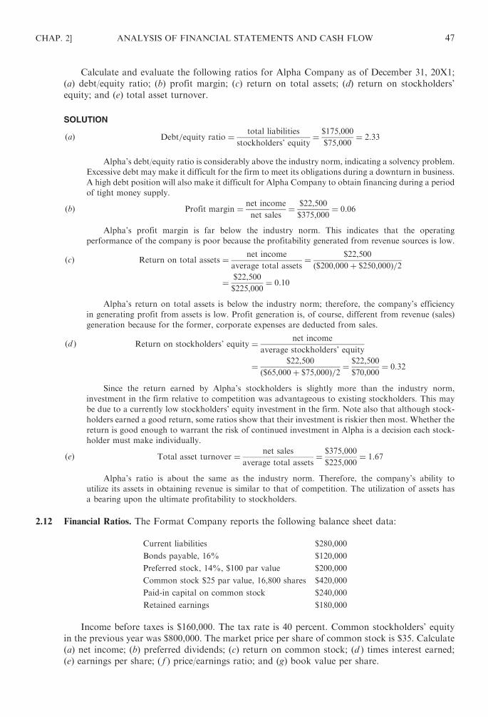
Calculate and evaluate the following ratios for Alpha Company as of December 31, 20X1;
(a) debt/equity ratio; (b) profit margin; (c) return on total assets; (d) return on stockholders’
equity; and (e) total asset turnover.
SOLUTION
(a) Debt=equity ratio ¼ total liabilities
stockholders’ equity¼ $175,000
$75,000¼ 2:33
Alpha’s debt/equity ratio is considerably above the industry norm, indicating a solvency problem.
Excessive debt may make it difficult for the firm to meet its obligations during a downturn in business.
A high debt position will also make it difficult for Alpha Company to obtain financing during a period
of tight money supply.
(b) Profit margin ¼ net income
net sales¼ $22,500
$375,000¼ 0:06
Alpha’s profit margin is far below the industry norm. This indicates that the operating
performance of the company is poor because the profitability generated from revenue sources is low.
(c) Return on total assets ¼ net income
average total assets¼ $22,500
ð$200,000þ $250,000Þ=2
¼ $22,500
$225,000¼ 0:10
Alpha’s return on total assets is below the industry norm; therefore, the company’s efficiency
in generating profit from assets is low. Profit generation is, of course, different from revenue (sales)
generation because for the former, corporate expenses are deducted from sales.
(d ) Return on stockholders’ equity ¼ net income
average stockholders’ equity
¼ $22,500
ð$65,000þ $75,000Þ=2 ¼$22,500
$70,000¼ 0:32
Since the return earned by Alpha’s stockholders is slightly more than the industry norm,
investment in the firm relative to competition was advantageous to existing stockholders. This may
be due to a currently low stockholders’ equity investment in the firm. Note also that although stock-
holders earned a good return, some ratios show that their investment is riskier then most. Whether the
return is good enough to warrant the risk of continued investment in Alpha is a decision each stock-
holder must make individually.
(e) Total asset turnover ¼ net sales
average total assets¼ $375,000
$225,000¼ 1:67
Alpha’s ratio is about the same as the industry norm. Therefore, the company’s ability to
utilize its assets in obtaining revenue is similar to that of competition. The utilization of assets has
a bearing upon the ultimate profitability to stockholders.
2.12 Financial Ratios. The Format Company reports the following balance sheet data:
Current liabilities $280,000
Bonds payable, 16% $120,000
Preferred stock, 14%, $100 par value $200,000
Common stock $25 par value, 16,800 shares $420,000
Paid-in capital on common stock $240,000
Retained earnings $180,000
Income before taxes is $160,000. The tax rate is 40 percent. Common stockholders’ equity
in the previous year was $800,000. The market price per share of common stock is $35. Calculate
(a) net income; (b) preferred dividends; (c) return on common stock; (d ) times interest earned;
(e) earnings per share; ( f ) price/earnings ratio; and (g) book value per share.
CHAP. 2] ANALYSIS OF FINANCIAL STATEMENTS AND CASH FLOW 47
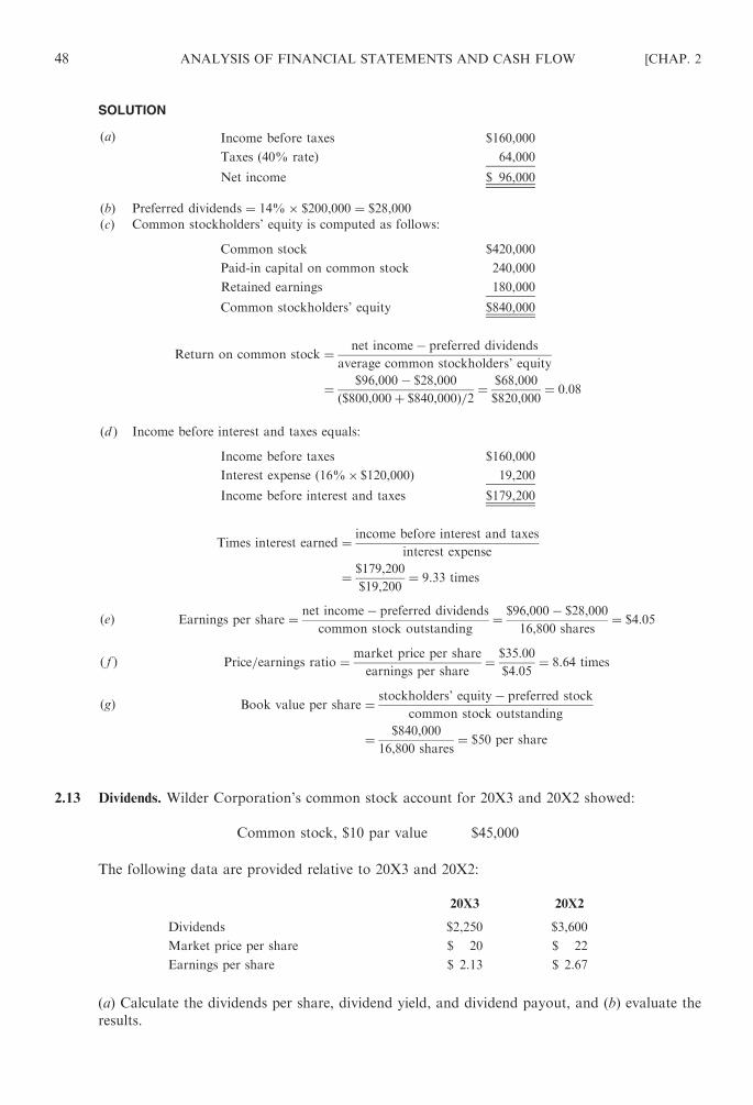
SOLUTION
(a) Income before taxes $160,000
Taxes (40% rate) 64,000
Net income $ 96,000
(b) Preferred dividends ¼ 14%� $200,000 ¼ $28,000
(c) Common stockholders’ equity is computed as follows:
Common stock $420,000
Paid-in capital on common stock 240,000
Retained earnings 180,000
Common stockholders’ equity $840,000
Return on common stock ¼ net income� preferred dividends
average common stockholders’ equity
¼ $96,000� $28,000
ð$800,000þ $840,000Þ=2 ¼$68,000
$820,000¼ 0:08
(d ) Income before interest and taxes equals:
Income before taxes $160,000
Interest expense (16%� $120,000) 19,200
Income before interest and taxes $179,200
Times interest earned ¼ income before interest and taxes
interest expense
¼ $179,200
$19,200¼ 9:33 times
(e) Earnings per share ¼ net income� preferred dividends
common stock outstanding¼ $96,000� $28,000
16,800 shares¼ $4:05
( f ) Price=earnings ratio ¼ market price per share
earnings per share¼ $35:00
$4:05¼ 8:64 times
(g) Book value per share ¼ stockholders’ equity� preferred stock
common stock outstanding
¼ $840,000
16,800 shares¼ $50 per share
2.13 Dividends. Wilder Corporation’s common stock account for 20X3 and 20X2 showed:
Common stock, $10 par value $45,000
The following data are provided relative to 20X3 and 20X2:
20X3 20X2
Dividends $2,250 $3,600
Market price per share $ 20 $ 22
Earnings per share $ 2.13 $ 2.67
(a) Calculate the dividends per share, dividend yield, and dividend payout, and (b) evaluate the
results.
48 ANALYSIS OF FINANCIAL STATEMENTS AND CASH FLOW [CHAP. 2

SOLUTION
(a)Dividends per share ¼ dividends
outstanding shares
For 20X3:$2,250
4,500 shares¼ $0:50
For 20X2:$3,600
4,500 shares¼ $0:80
Dividend yield ¼ dividends per share
market price per share
For 20X3:$0:50
$20:00¼ 0:025
For 20X2:$0:80
$22:00¼ 0:036
Dividend payout ¼ dividends per share
earnings per share
For 20X3:$0:50
$2:13¼ 0:23
For 20X2:$0:80
$2:67¼ 0:30
(b) The decline in dividends per share, dividend yield, and dividend payout from 20X2 to 20X3 will cause
concern to both stockholders and management.
Stockholders will want to determine the reason for the decline. For example, do they know that
the company is investing heavily to reposition itself for greater competitiveness in the future? Has the
entire industry suffered a decline or only Wilder? Is the company on solid financial footing or is it
borderline? What is the company’s—and the industry’s—potential for the future?
Management will want to deal with similar questions and find solutions to other problems, such
as how to manage their finances so as not to lose investors in the short term while ensuring financial
health in the long term. Whatever the reasons for the decline in the ratios, this is a situation where
management cannot safely ignore the short term and may therefore choose to sacrifice some long-term
goals in order to turn the ratios around. The extent to which a company may choose to do this
depends on many factors, including its relative financial health, its reputation in the financial
world, how much risk managers are willing (or able) to take, what the actual problems are, and
what options are available as solutions.
2.14 Financial Ratios. Jones Corporation’s financial statements appear below.
Jones Corporation
Balance Sheet
December 31, 20X1
ASSETS
Current assets
Cash $100,000
Marketable securities 200,000
Inventory 300,000
Total current assets $ 600,000
Plant assets 500,000
Total assets $1,100,000
CHAP. 2] ANALYSIS OF FINANCIAL STATEMENTS AND CASH FLOW 49

LIABILITIES AND
STOCKHOLDERS’ EQUITY
Liabilities
Current liabilities $200,000
Long-term liabilities 100,000
Total liabilities $ 300,000
Stockholders’ equity
Common stock, $1 par value,
100,000 shares $100,000
Premium on common stock 500,000
Retained earnings 200,000
Total stockholders’ equity 800,000
Total liabilities and stockholders’ equity $1,100,000
Jones Corporation
Income Statement
For the Year Ended December 31, 20X1
Net sales $10,000,000
Cost of goods sold 6,000,000
Gross profit $ 4,000,000
Operating expenses 1,000,000
Income before taxes $ 3,000,000
Income taxes (50% rate) 1,500,000
Net income $ 1,500,000
Additional information includes a market price of $150 per share of stock, total dividends of
$600,000 for 20X1, and $250,000 of inventory as of December 31, 20X0.
Compute the following ratios; (a) current ratio; (b) quick ratio; (c) inventory turnover; (d )
average age of inventory; (e) debt/equity ratio; ( f ) book value per share; (g) earnings per share;
(h) price/earnings ratio; (i) dividends per share; and ( j) dividend payout.
SOLUTION
(a) Current ratio ¼ current assets
current liabilities¼ $600,000
$200,000¼ 3:0
(b) Quick ratio ¼ cashþmarketable securities
current liabilities¼ $300,000
$200,000¼ 1:5
(c) Inventory turnover ¼ cost of goods sold
average inventory¼ $6,000,000
ð$250,000þ $300,000Þ=2 ¼ 21:82
(d ) Average age of inventory ¼ 365
inventory turnover¼ 365
21:82¼ 16:7 days
(e) Debt=equity ratio ¼ total liabilities
stockholders’ equity¼ $300,000
$800,000¼ 0:375
( f ) Book value per share ¼ stockholders’ equity� preferred stock
common shares outstanding¼ $800,000
100,000 shares¼ $8
(g) Earnings per share ¼ net income
outstanding common shares¼ $1,500,000
100,000 shares¼ $15
50 ANALYSIS OF FINANCIAL STATEMENTS AND CASH FLOW [CHAP. 2

(h) Price=earnings ratio ¼ market price per share
earnings per share¼ $150
$15¼ 10
(i) Dividends per share ¼ dividends
outstanding shares¼ $600,000
100,000 shares¼ $6
( j ) Dividend payout ¼ dividends per share
earnings per share¼ $6
$15¼ 0:4
2.15 Financial Ratios. The 20X9 financial statements for Johanson Co. are reproduced below.
Johanson Co.
Statement of Financial Position
(in Thousands of Dollars)
December 31, 20X8 and 20X9
20X8 20X9
ASSETS
Current assets
Cash and temporary investments $ 380 $ 400
Accounts receivable (net) 1,500 1,700
Inventories 2,120 2,200
Total current assets $4,000 $4,300
Long-term assets
Land $ 500 $ 500
Building and equipment (net) 4,000 4,700
Total long-term assets $4,500 $5,200
Total assets $8,500 $9,500
LIABILITIES AND
STOCKHOLDERS’ EQUITY
Liabilities
Current liabilities
Accounts payable $ 700 $1,400
Current portion of long-term
debt 500 1,000
Total current liabilities $1,200 $2,400
Long-term debt 4,000 3,000
Total liabilities $5,200 $5,400
Stockholders’ equity
Common stock $3,000 $3,000
Retained earnings 300 1,100
Total stockholders’ equity $3,300 $4,100
Total liabilities and stockholders’
equity $8,500 $9,500
CHAP. 2] ANALYSIS OF FINANCIAL STATEMENTS AND CASH FLOW 51

Johanson Company
Statement of Income and Retained Earnings
(in Thousands of Dollars) For the Year Ended December 31, 20X1
Net sales $28,800
Less: Cost of goods sold $15,120
Selling expenses 7,180
Administrative expenses 4,100
Interest 400
Income taxes 800 27,600
Net income $ 1,200
Retained earnings January 1 300
Subtotal $ 1,500
Cash dividends declared and paid 400
Retained earnings December 31 $ 1,100
For 20X9, find (a) the acid-test ratio; (b) the average number of days sales were outstanding;
(c) the times interest earned ratio; (d ) the asset turnover; (e) the inventory turnover; ( f ) the
operating income margin; and (g) the dividend payout ratio. (CMA, adapted.)
SOLUTION
(a) Acid-test ratio ¼ cashþ net receivablesþmarketable securities
current liabilities¼ $400þ $1,700
$2,400¼ 0:875 ffi 0:9
(b) Accounts receivable turnover ratio ¼ net credit sales
average accounts receivable¼ $28,000
ð$1,500þ $1,700Þ=2 ¼ 18
Number of days sales outstanding ¼ 365
accounts receivable turnover ratio¼ 365
18¼ 20:3
(c) Times interest earned ratio ¼ net incomeþ taxesþ interest expense
interest expense¼ $1,200þ $800þ $400
$400¼ 6:0
(d) Asset turnover ratio ¼ sales
average assets during year¼ $28,000
ð$8,500þ $9,500Þ=2 ¼ 3:2
(e) Inventory turnover ratio ¼ cost of sales
average inventory¼ $15,120
ð$2,120þ $2,200Þ=2 ¼ 7:0
(f) Operating income margin ¼ net income from operations before taxes
net sales
¼ $1,200þ $800þ $400
$28,800¼ 8:3%
(g) Dividend payout ratio ¼ dividends
net income¼ $400
$1,200¼ 33:3%
2.16 Financial Ratios. Warford Corporation was formed 5 years ago through a public subscription
of common stock. Lucinda Street, who owns 15 percent of the common stock, was one of
the organizers of Warford and is its current president. The company has been successful,
but it is currently experiencing a shortage of funds. On June 10, Street approached the Bell
National Bank, asking for a 24-month extension of two $30,000 notes, which are due on
52 ANALYSIS OF FINANCIAL STATEMENTS AND CASH FLOW [CHAP. 2

June 30, 20X2, and September 30, 20X2. Another note of $7,000 is due on December 31,
20X2, but Street expects to have no difficulty in paying this note on its due date. Street
explained that Warford’s cash flow problems are primarily due to the company’s desire to
finance a $300,000 plant expansion over the next two fiscal years through internally generated
funds.
The commercial loan officer of Bell National Bank requested financial reports for the last
two fiscal years. These reports are reproduced below.
Warford Corporation
Income Statement
For the Fiscal Years Ended March 31, 20X1 and 20X2
20X1 20X2
Sales $2,700,000 $3,000,000
Cost of goods solda 1,720,000 1,902,500
Gross margin $ 980,000 $1,097,500
Operating expenses 780,000 845,000
Net income before taxes $ 200,000 $ 252,500
Income taxes (40%) 80,000 101,000
Income after taxes $ 120,000 $ 151,500
a Depreciation charges of $100,000 on the plant and equipment and $102,500 for
fiscal years ended March 31, 20X1 and 20X2, respectively, are included in cost of
goods sold.
Warford Corporation
Statement of Financial Position
March 31, 20X1 and 20X2
20X1 20X2
ASSETS
Cash $ 12,500 $ 16,400
Notes receivable 104,000 112,000
Accounts receivable (net) 68,500 81,600
Inventories (at cost) 50,000 80,000
Plant and equipment (net of depreciation) 646,000 680,000
Total assets $881,000 $970,000
LIABILITIES AND
OWNERS’ EQUITY
Accounts payable $ 72,000 $ 69,000
Notes payable 54,500 67,000
Accrued liabilities 6,000 9,000
Common stock (60,000 shares, $10 par) 600,000 600,000
Retained earningsa 148,500 225,000
Total liabilities and owners’ equity $881,000 $970,000
a Cash dividends were paid at the rate of $1 per share in fiscal year 20X1 and $1.25
per share in fiscal year 20X2.
CHAP. 2] ANALYSIS OF FINANCIAL STATEMENTS AND CASH FLOW 53

Calculate the following items for Warford Corporation: (a) current ratio for fiscal years 20X1
and 20X2; (b) quick (acid-test) ratio for fiscal years 20X1 and 20X2; (c) inventory turnover for
fiscal year 20X2; (d ) return on assets for fiscal years 20X1 and 20X2; and (e) percentage change in
sales, cost of goods sold, gross margin, and net income after taxes from fiscal year 20X1 to 20X2.
(CMA, adapted).
SOLUTION
(a) Current ratio ¼ current assets
current liabilities
For 20X1:$235,000
$132,500¼ 1:77
For 20X2:$290,000
$145,000¼ 2:00
(b) Quick ratio ¼ current assets� inventories
current liabilities
For 20X1:$185,000
$132,500¼ 1:40
For 20X2:$210,000
$145,000¼ 1:45
(c) Inventory turnover ¼ cost of goods sold
average inventory
For 20X2:$1,902,500
ð$50,000þ $80,000Þ=2 ¼ 29 times
(d ) Return on assets ¼ net income
total assets
For 20X1:$120,000
$881,500¼ 13:6%
For 20X2:$151,500
$970,000¼ 15:6%
(e) Percent changes are as follows (in thousands of dollars):
Amounts
20X2 20X1 Percentage increase
Sales $3,000.0 $2,700.0 $300:0
$2,700:0¼ 11:11
Cost of goods sold $1,902.5 $1,720.0 $182:5
$1,720:0¼ 10:61
Gross margin $1.097.5 $ 980.0 $117:5
$980:0¼ 11:99
Net income after taxes $ 151.5 $ 120.0 $31:5
$120:0¼ 26:25
2.17 Financial Ratios. Ratio analysis is employed to gain insight into the financial character of a firm.
The calculation of ratios can often lead to a better understanding of a firm’s financial position
and performance. A specific ratio or a number of selected ratios can be calculated and used to
measure or evaluate a specific financial or operating characteristic of a firm. (a) Identify and
54 ANALYSIS OF FINANCIAL STATEMENTS AND CASH FLOW [CHAP. 2

explain what financial characteristic of a firm would be measured by an analysis in which the
following four ratios were calculated: (1) current ratio; (2) acid-test ratio; (3) accounts receivable
turnover ratio; and (4) inventory turnover ratio. (b) Do the ratios in part (a) provide adequate
information to measure this characteristic or are additional data needed? If so, provide two
examples of other data that would be required. (c) Identify and explain what specific character-
istic regarding a firm’s operations would be measured by an analysis in which the following three
ratios were calculated: (1) gross profit margin; (2) operating income margin; and (3) net income to
sales (profit margin). (d ) Do these ratios provide adequate information to measure this charac-
teristic or are additional data needed? If so, provide two examples of other data that would be
required.
SOLUTION
(a) These four ratios are used to measure short-term liquidity and to evaluate the management of
net working capital of a firm, i.e., the ability to meet financial obligations in the near future.
(b) For a thorough analysis of the firm’s ability to meet its financial obligations in the near future,
we would also need to know the normal and/or industry standards for these ratios in order
to have a basis of comparison. In addition, we would need to know if any current assets
are pledged or restricted for any reason, if open lines of credit are available to the firm,
the firm’s credit rating, and any capital investment plans that might require an inordinate amount
of cash.
(c) These three ratios are used to measure the profitability of a firm; respectively, each ratio relates sales
revenue with (1) the cost of goods or services sold; (2) the costs of operating the business, which
would include the cost of goods sold, the marketing expenses, the administrative expenses, and other
general operating expenses; and (3) the final net result of all the corporate financial activity for the
accounting period.
(d ) These ratios do provide an indication of the firm’s profitability. However, to complete a thorough
analysis, it would be necessary to determine the return on investment, earnings per share, inventory
valuation methods, depreciation methods, and any nonrecurring items included in the statement.
In addition, data about the cost/volume/profit relationships would be useful. All this information
should be evaluated while considering industry averages, results of prior periods, and future
projections.
2.18 The Du Pont Formula and Return on Total Assets. Industry A has three companies whose income
statements and balance sheets are summarized below.
Company X Company Y Company Z
Sales $500,000 (d ) (g)
Net income $ 25,000 $30,000 (h)
Total assets $100,000 (e) $250,000
Total asset turnover (a) ( f ) 0.4
Profit margin (b) 0.4% 5%
Return on total assets (ROA) (c) 2% (i)
First supply the missing data in the table above. Then comment on the relative performance
of each company.
SOLUTION
(a) Total asset turnover ¼ sales
average total assets¼ $500,000
$100,000¼ 5 times
(b) Profit margin ¼ net income
sales¼ $25,000
$500,000¼ 5%
CHAP. 2] ANALYSIS OF FINANCIAL STATEMENTS AND CASH FLOW 55

(c) ROA ¼ net income
average total assets
If we multiply both the numerator and denominator by sales, we get
ROA ¼ net income
sales� sales
average total assets
¼ profit margin� total asset turnover
¼ 5% ½from ðbÞ� � 5 ½from ðaÞ� ¼ 25%
(d ) Profit margin ¼ net income
sales
Sales ¼ net income
profit margin¼ $30,000
0:004¼ $7,500,000
(e) ROA ¼ net income
average total assets
Average total assets ¼ net income
ROA¼ $30,000
0:02¼ $1,500,000
( f ) Total asset turnover ¼ sales
average total assets
¼ $7,500,000 ½from ðdÞ�$1,500,000 ½from ðeÞ� ¼ 5 times
(g) Total asset turnover ¼ sales
average total assets
Sales ¼ total asset turnover� average total assets
¼ 0:4� $250,000 ¼ $100,000
(h) Profit margin ¼ net income
sales
Net income ¼ profit margin� sales
¼ 5%� $100,000 ½from ðgÞ� ¼ $5,000
(i) ROA ¼ total asset turnover� profit margin
¼ 0:4� 5% ¼ 2%
or
ROA ¼ net income
average total assets
¼ $5,000 ½from ðhÞ�$250,000
¼ 2%
Summarizing the results of (a) through (i) gives:
Company X Company Y Company Z
Total asset turnover 5 times 5 times 0.4 times
Profit margin 5% 0.4% 5%
ROA 25% 2% 2%
Company X performed best. It appears that companies Y and Z are in trouble. Company Y turns over
its assets as often as company X, but Y’s margin on sales is much lower. Thus, company Y must work on
improving its margin. The following questions may be raised about company Y: Is the low margin due to
inefficiency? Is it due to excessive material, labor, or overhead, or all three?
Company Z, on the other hand, does just as well as company X in terms of profit margin but has a
much lower turnover of capital than X. Therefore, company Z should take a close look at its investments. Is
there too much tied up in inventories and receivables? Are there unused fixed assets? Is there idle cash sitting
around?
56 ANALYSIS OF FINANCIAL STATEMENTS AND CASH FLOW [CHAP. 2

2.19 ROA and ROE. The following ratios have been computed for Los Alamitos Company and are
compared with the industry averages:Los Alamitos Industry
Return on total assets (ROA) 6.2% 6.0%
Return on common equity (ROE) 16.5% 8.5%
Comment on the comparison of the company to the industry.
SOLUTION
Los Alamitos Company shows a satisfactory return on total investment (6.20 percent versus 6 percent
for the industry). The company’s 16.5 percent return on common stockholders’ investment compares very
favorably with that of the industry (16.5 percent versus 8.5 percent). This higher-than-average return reflects
the firm’s above-average use of financial leverage. Through the favorable use of debt, the firm was able to
increase significantly the return earned on the stockholders’ investment which would favorably affect its
stock price.
2.20 Financial Statement Analysis and Loan Decision. The Konrath Company, a wholesaler in the
midwest, is considering extending credit to the Hawk Company, a retail chain operation that
has a number of stores in the midwest. The Konrath Company has had a gross margin of
approximately 60 percent in recent years and expects to have a similar gross margin on the
Hawk Company order, which is estimated at $2 million per year. The Hawk Company’s order
is approximately 15 percent of the Konrath Company’s present sales. Recent statements of the
Hawk Company are given below.
Hawk Company
Balance Sheet
(in Millions of Dollars)
As of December 31, 20X1, 20X2, and 20X3
20X1 20X2 20X3
ASSETS
Current assets
Cash $ 2.6 $ 1.8 $ 1.6
Government securities (cost) 0.4 0.2
Accounts and notes receivable (net) 8.0 8.5 8.5
Inventories 2.8 3.2 2.8
Prepaid assets 0.7 0.6 0.6
Total current assets $14.5 $14.3 $13.5
Property, plant, and equipment (net) 4.3 5.4 5.9
Total Assets $18.8 $19.7 $19.4
LIABILITIES AND STOCKHOLDERS’ EQUITY
Liabilities
Current liabilities
Notes payable $ 3.2 $ 3.7 $ 4.2
Accounts payable 2.8 3.7 4.1
Accrued expenses and taxes 0.9 1.1 1.0
Total current liabilities $ 6.9 $ 8.5 $ 9.3
Long-term debt, 6% 3.0 2.0 1.0
Total liabilities $ 9.9 $10.5 $10.3
Stockholders’ equity 8.9 9.2 9.1
Total liabilities and stockholders’ equity $18.8 $19.7 $19.4
CHAP. 2] ANALYSIS OF FINANCIAL STATEMENTS AND CASH FLOW 57

Hawk Company
Income Statement
(in Millions of Dollars)
For the Years Ended December 31, 20X1, 20X2, and 20X3
20X1 20X2 20X3
Net sales $24.2 $24.5 $24.9
Cost of goods sold 16.9 17.2 18.0
Gross margin $ 7.3 $ 7.3 $ 6.9
Selling expenses $ 4.3 $ 4.4 $ 4.6
Administrative expenses 2.3 2.4 2.7
Total expenses $ 6.6 $ 6.8 $ 7.3
Earning (loss) before taxes $ 0.7 $ 0.5 $ (0.4)
Income taxes 0.3 0.2 (0.2)
Net income $ 0.4 $ 0.3 $ (0.2)
Hawk Company
Statement of Changes in Financial Positions
(in Millions of Dollars)
For the Years Ended December 31, 20X1, 20X2, and 20X3
20X1 20X2 20X3
Sources of funds
Net income (loss) $ 0.4 $ 0.3 $(0.2)
Depreciation 0.4 0.5 0.5
Funds from operations $ 0.8 $ 0.8 $ 0.3
Sale of building 0.2
Sale of treasury stock 0.1 0.1
Total sources $ 1.0 $ 0.9 $ 0.4
Uses of funds
Purchase of property, plant,
and equipment $ 1.2 $ 1.6 $ 1.0
Dividends 0.1 0.1
Retirement of long-term debt 1.0 1.0
Total uses $ 1.3 $ 2.7 $ 2.0
Net increase (decrease) in net
working capital $(0.3) $(1.8) $(1.6)
(a) Calculate for the year 20X3 the following ratios: (1) return on total assets; (2) acid-test ratio;
(3) profit margin; (4) current ratio; and (5) inventory turnover.
(b) As part of the analysis to determine whether or not Konrath should extend credit to Hawk,
assume the ratios below were calculated from Hawk Co. statements. For each ratio indicate
whether it is a favorable, unfavorable, or neutral statistic in the decision to grant Hawk
credit. Briefly explain your choice in each case.
58 ANALYSIS OF FINANCIAL STATEMENTS AND CASH FLOW [CHAP. 2
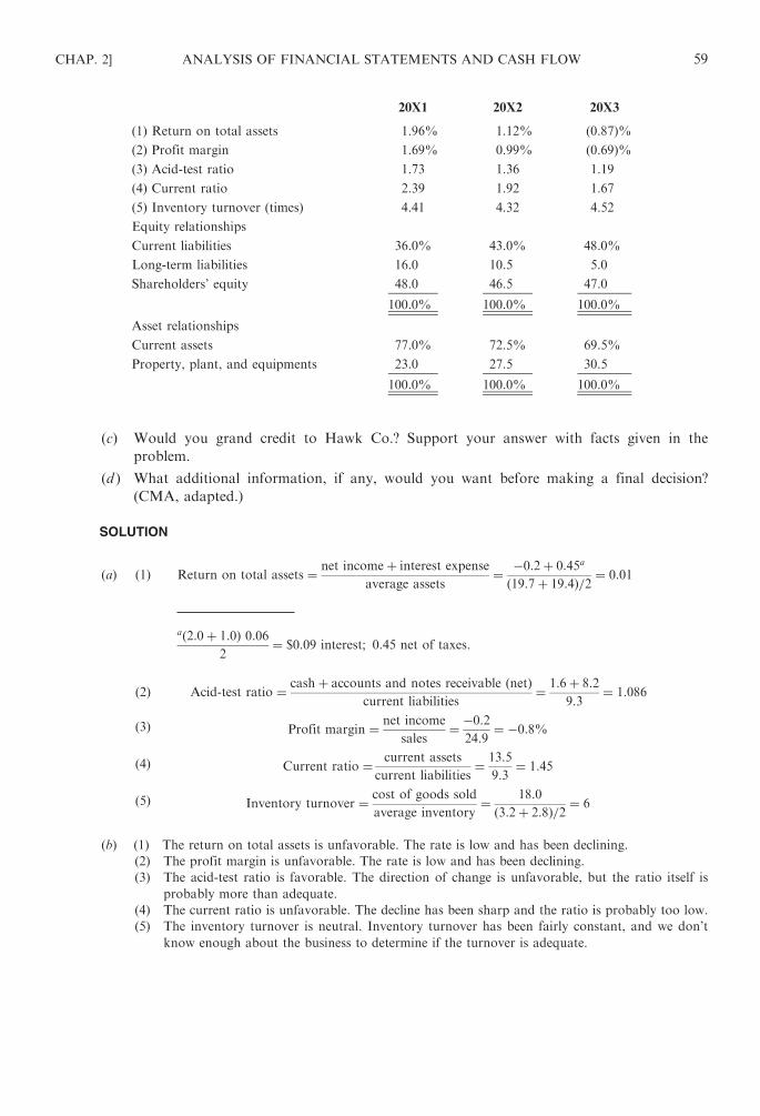
20X1 20X2 20X3
(1) Return on total assets 1.96% 1.12% (0.87)%
(2) Profit margin 1.69% 0.99% (0.69)%
(3) Acid-test ratio 1.73 1.36 1.19
(4) Current ratio 2.39 1.92 1.67
(5) Inventory turnover (times) 4.41 4.32 4.52
Equity relationships
Current liabilities 36.0% 43.0% 48.0%
Long-term liabilities 16.0 10.5 5.0
Shareholders’ equity 48.0 46.5 47.0
100.0% 100.0% 100.0%
Asset relationships
Current assets 77.0% 72.5% 69.5%
Property, plant, and equipments 23.0 27.5 30.5
100.0% 100.0% 100.0%
(c) Would you grand credit to Hawk Co.? Support your answer with facts given in the
problem.
(d ) What additional information, if any, would you want before making a final decision?
(CMA, adapted.)
SOLUTION
ðaÞ ð1Þ Return on total assets ¼ net incomeþ interest expense
average assets¼ �0:2þ 0:45a
ð19:7þ 19:4Þ=2 ¼ 0:01
að2:0þ 1:0Þ 0:062
¼ $0:09 interest; 0:45 net of taxes:
ð2Þ Acid-test ratio ¼ cashþ accounts and notes receivable ðnetÞcurrent liabilities
¼ 1:6þ 8:2
9:3¼ 1:086
ð3Þ Profit margin ¼ net income
sales¼ �0:2
24:9¼ �0:8%
ð4Þ Current ratio ¼ current assets
current liabilities¼ 13:5
9:3¼ 1:45
ð5Þ Inventory turnover ¼ cost of goods sold
average inventory¼ 18:0
ð3:2þ 2:8Þ=2 ¼ 6
(b) (1) The return on total assets is unfavorable. The rate is low and has been declining.
(2) The profit margin is unfavorable. The rate is low and has been declining.
(3) The acid-test ratio is favorable. The direction of change is unfavorable, but the ratio itself is
probably more than adequate.
(4) The current ratio is unfavorable. The decline has been sharp and the ratio is probably too low.
(5) The inventory turnover is neutral. Inventory turnover has been fairly constant, and we don’t
know enough about the business to determine if the turnover is adequate.
CHAP. 2] ANALYSIS OF FINANCIAL STATEMENTS AND CASH FLOW 59

(c) The facts available from the problem are inadequate to make a final judgment; additional information
would be necessary. However, the facts given do not present a good overall picture of Hawk. The
company doesn’t appear to be in serious trouble at the moment, but most of the trends reflected in the
ratios are unfavorable. The company appears to be developing liquidity problems: cash and securities
are declining; inventories and plant and equipment are an increasing portion of the assets; and current
liabilities are an increasing portion of capital.
The operations of the company also show unfavorable trends: cost of goods sold is
increasing as a percentage of sales; administrative expenses are increasing as a percent sales; and if
we recognize that prices have risen, it appears that physical volume at Hawk might have actually
decreased.
On the basis of these observations and the fact that Hawk would be a very large customer (thus
a potentially large loss if the accounts became uncollectible), credit should be extended to Hawk only
under carefully controlled and monitored conditions.
(d ) For a final decision on whether to grant credit to Hawk, the additional information needed is:
quality of management of the Hawk Company, locations of the Hawk stores, current activities
of Hawk that have increased plant and equipment but not inventories, industry position
of the Hawk Company, credit rating of the Hawk Company, current economic conditions,
capacity of the Konrath Company to handle such a large single account, and normal ratios for the
industry.
2.21 Corporate and Economic Factors. What factors (a) within the company and (b) within the
economy have affected and are likely to affect the degree of variability in the (1) earnings per
share; (2) dividends per share; and (3) market price per share of common stock?
SOLUTION
(a) Within the company
(1) Earnings
a. accounting policies
b. sales volume
c. new product introduction
(2) Dividends
a. capital expenditure
b. stability of earnings
c. replacement of fixed assets
(3) Market price
a. management quality
b. growth in earnings
c. financial leverage
(b) Economy
(1) Earnings
a. trend in economy
b. governmental regulation
c. labor relations
(2) Dividends
a. tax law
b. recessionary conditions
(3) Market price
a. investor confidence
b. cyclical charges
60 ANALYSIS OF FINANCIAL STATEMENTS AND CASH FLOW [CHAP. 2

2.22 Transactions and the Statement of Cash Flows. Classify each transaction in the first three columns
by its correct cash flow activity.Type of activity
Operating Investing Financing
(a) Issued common stock for cash
(b) Purchased treasury stock
(c) Paid an account payable
(d) Declared a cash dividend
(e) Issued a bond payable
(f) Purchased land
(g) Sold a machine at book value
SOLUTION
Operating Investing Financing
(a) Issued common stock for cash X
(b) Purchased treasury stock X
(c) Paid an account payable X
(d) Declared a cash dividend X
(e) Issued a bond payable X
(f) Purchased land X
(g) Sold a machine at book value X
2.23 Activity Classification. Classify each of the following transactions as an operating activity, an
investing activity, or a financing activity. Also indicate whether the activity is a source of cash or a
use of cash.
1. A plant was sold for $550,000.
2. A profit of $75,000 was reported.
3. Long-term bonds were retired.
4. Cash dividends of $420,000 were paid.
5. Four hundred thousand share of preferred stock were sold.
6. A new high-tech robotics was purchased.
7. A long-term note payable was issued.
8. A 50 percent interest in a company was purchased.
9. A loss for the year was reported.
10. Additional common stock was sold.
SOLUTION
1. Investing—source of cash
2. Operating—source of cash
3. Financing—use of cash
4. Financing—use of cash
5. Financing—source of cash
6. Investing—use of cash
7. Financing—source of cash
8. Investing—use of cash
9. Operating—use of cash
10. Financing—source of cash
CHAP. 2] ANALYSIS OF FINANCIAL STATEMENTS AND CASH FLOW 61

2.24 Statement Analysis of Financial Position. The financial statements for XYZ Company for the
years 20X1 and 20X2 are given below.
XYZ Company
Balance Sheet
December 31, 20X1 and 20X2
20X2 20X1
ASSETS
Current assets
Cash $ 200 $ 500
Accounts receivable 600 300
Inventory 600 700
Total current assets $1,400 $1,150
Fixed assets
Plant and equipment $ 900 $ 700
Less: Accumulated depreciation (200) (150)
Net fixed assets $ 700 $ 550
Long-term investments $ 300 $ 400
Total assets $2,400 $2,100
LIABILITIES AND
STOCKHOLDERS’ EQUITY
Current liabilities
Accounts payable $ 800 $ 400
Taxes payable 50 100
Total current liabilities $ 850 $ 500
Bonds payable $ 150 $ 500
Stockholders’ equity
Capital stock $ 800 $ 700
Retained earnings 600 400
Total stockholders’ equity $1,400 $1,100
Total liabilities and
stockholders’ equity $2,400 $2,100
XYZ Company
Income Statement
For the Years Ended December 31, 20X2
Sales $900
Cost of goods sold 200
Gross margin $700
Operating expenses
Selling expense $100
Administrative expense 150
Depreciation expense 50
Total expenses 300
Net income $400
62 ANALYSIS OF FINANCIAL STATEMENTS AND CASH FLOW [CHAP. 2

XYZ Company
Statement of Retained Earnings
For the Year Ended December 31, 20X2
Retained earnings, December 31, 20X1 $400
Add: Net income 400
$800
Deduct: Dividends paid 200
Retained earnings, December 31, 20X2 $600
Prepare (a) the statement of changes in financial position on a net working capital basis, and
(b) the statement of changes in financial position on a cash basis with percentages. (c) Briefly
summarize your findings.
SOLUTION
(a) XYZ Company
Statement of Changes in Financial Position
For the Year Ended December 31, 20X2
Sources of net working capital
From operations
Net income $ 400
Add: Depreciation 50
Total funds from operations $ 450
From sale of long-term investments 100
From sale of capital stock 100
Total sources $ 650
Uses of net working capital
To pay dividends $ 200
To purchase plant and equipments 200
To retire bonds payable 350
Total uses $ 750
Decrease in net working capital $(100)
(b) XYZ Company
Statement of Changes in Financial Position (Cash Basis)
For the Year Ended December 31, 20X2
Dollars Percentage
Sources
From operations
Net income $ 400 34.78%
Depreciation 50 4.35
Decrease in inventory 100 8.7
Increase in accounts payable 400 34.78
From sale of long-term investments 100 8.7
From sale of capital stock 100 8.7
Total sources $1,150 100.00%
CHAP. 2] ANALYSIS OF FINANCIAL STATEMENTS AND CASH FLOW 63

Uses
Increase in accounts receivable $ 300 27.27%
Decrease in taxes payable 50 4.55
Payment of dividends 200 18.18
Purchase plant and equipment 200 18.18
Retire bonds payable 350 31.82
Total uses $1,100 100.00%
Increase in cash $ 50
(c) Major sources for the XYZ Company during 20X2 were internal (39.13 percent) and an increase
in accounts payable (34.78 percent). External sources accounted for 17.4 percent of XYZ’s funds
through the sale of long-term investments and capital stock. The largest uses of funds were for the
retirement of long-term bonds (31.82 percent) and an increase in accounts receivable (27.27 percent).
There were also additions to plant and equipment (18.18 percent).
2.25 Statement of Changes in Financial Position. The consolidated balance sheets for CSULB
Seasonal Products, Inc., at the beginning and end of 20X1 are presented below (in millions of
dollars).
January 1,
20X1
December 31,
20X1
ASSETS
Cash $ 12 $ 9
Accounts receivable 14 24
Inventories 4 12
Total current assets $ 30 $ 45
Gross fixed assets $120 $145
Less: Accumulated depreciation 45 55
Net fixed assets $ 75 $ 90
Total assets $105 $135
LIABILITIES AND EQUITY
Accounts payable $ 14 $ 11
Notes payable 10 10
Long-term debt 10 25
Common stock 30 30
Retained earnings 41 59
Total liabilities and equity $105 $135
CSULB earned $20 million after taxes during the year and paid cash dividends of $2 million.
The annual depreciation expense during 20X1 was $10 million. The company purchased $25
million of fixed assets.
(a) Add source and use column to the balance sheet; (b) prepare a statement of changes in
financial position on the cash basis, and include percentage computations; and (c) summarize
your findings.
64 ANALYSIS OF FINANCIAL STATEMENTS AND CASH FLOW [CHAP. 2
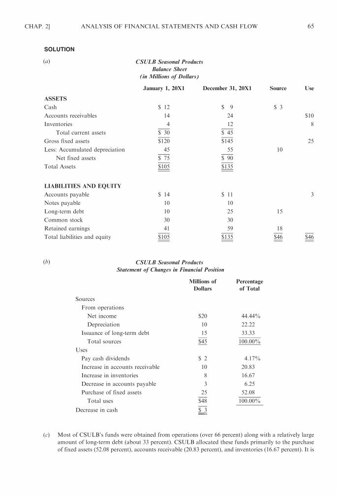
SOLUTION
(a) CSULB Seasonal Products
Balance Sheet
(in Millions of Dollars)
January 1, 20X1 December 31, 20X1 Source Use
ASSETS
Cash $ 12 $ 9 $ 3
Accounts receivables 14 24 $10
Inventories 4 12 8
Total current assets $ 30 $ 45
Gross fixed assets $120 $145 25
Less: Accumulated depreciation 45 55 10
Net fixed assets $ 75 $ 90
Total Assets $105 $135
LIABILITIES AND EQUITY
Accounts payable $ 14 $ 11 3
Notes payable 10 10
Long-term debt 10 25 15
Common stock 30 30
Retained earnings 41 59 18
Total liabilities and equity $105 $135 $46 $46
(b) CSULB Seasonal Products
Statement of Changes in Financial Position
Millions of
Dollars
Percentage
of Total
Sources
From operations
Net income $20 44.44%
Depreciation 10 22.22
Issuance of long-term debt 15 33.33
Total sources $45 100.00%
Uses
Pay cash dividends $ 2 4.17%
Increase in accounts receivable 10 20.83
Increase in inventories 8 16.67
Decrease in accounts payable 3 6.25
Purchase of fixed assets 25 52.08
Total uses $48 100.00%
Decrease in cash $ 3
(c) Most of CSULB’s funds were obtained from operations (over 66 percent) along with a relatively large
amount of long-term debt (about 33 percent). CSULB allocated these funds primarily to the purchase
of fixed assets (52.08 percent), accounts receivable (20.83 percent), and inventories (16.67 percent). It is
CHAP. 2] ANALYSIS OF FINANCIAL STATEMENTS AND CASH FLOW 65

important to realize that the company does not have an optimal mix of financing since a relatively
large portion of long-term debt went toward the purchase of short-term assets, namely accounts
receivable and inventories. Furthermore, since the company’s sales are seasonal, it could end
up with rather costly excess cash on hand if the additional investment in inventories and accounts
receivable is not needed.
2.26 Adjustments to Net Income. Indicate whether each of the events described below will be added
to or deducted from net income in order to compute cash flow from operations.
1. Gain on sale of an asset
2. Increase in accounts receivable
3. Decrease in prepaid insurance
4. Depreciation expense
5. Increase in accounts payable
6. Uncollectible accounts expense
7. Decrease in wages payable
8. Increase in inventory
9. Amortization of a patent
SOLUTION
1. Deducted from
2. Deducted from
3. Added to
4. Added to
5. Added to
6. Added to
7. Deducted from
8. Deducted from
9. Added to
2.27 Statement of Cash Flows. Acme Manufacturing has provided the following financial statements:
Acme Manufacturing
Comparative Balance Sheets
For the years Ended December 31, 20X4 and 20X5
20X4 20X5
ASSETS
Cash $ 112,500 $ 350,000
Accounts receivable 350,000 281,250
Inventories 125,000 150,000
Plant and equipment 1,000,000 1,025,000*
Accumulated depreciation (500,000) (525,000)
Land 500,000 718,750
Total assets $1,587,500 $2,000,000
* Beginning equipment $1,000,000
Purchases 250,000
Less sales (225,000)
Ending equipment $1,025,000
66 ANALYSIS OF FINANCIAL STATEMENTS AND CASH FLOW [CHAP. 2
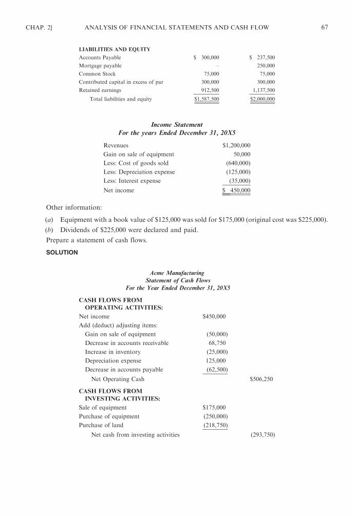
LIABILITIES AND EQUITY
Accounts Payable $ 300,000 $ 237,500
Mortgage payable – 250,000
Common Stock 75,000 75,000
Contributed capital in excess of par 300,000 300,000
Retained earnings 912,500 1,137,500
Total liabilities and equity $1,587,500 $2,000,000
Income Statement
For the years Ended December 31, 20X5
Revenues $1,200,000
Gain on sale of equipment 50,000
Less: Cost of goods sold (640,000)
Less: Depreciation expense (125,000)
Less: Interest expense (35,000)
Net income $ 450,000
Other information:
(a) Equipment with a book value of $125,000 was sold for $175,000 (original cost was $225,000).
(b) Dividends of $225,000 were declared and paid.
Prepare a statement of cash flows.
SOLUTION
Acme Manufacturing
Statement of Cash Flows
For the Year Ended December 31, 20X5
CASH FLOWS FROM
OPERATING ACTIVITIES:
Net income $450,000
Add (deduct) adjusting items:
Gain on sale of equipment (50,000)
Decrease in accounts receivable 68,750
Increase in inventory (25,000)
Depreciation expense 125,000
Decrease in accounts payable (62,500)
Net Operating Cash $506,250
CASH FLOWS FROM
INVESTING ACTIVITIES:
Sale of equipment $175,000
Purchase of equipment (250,000)
Purchase of land (218,750)
Net cash from investing activities (293,750)
CHAP. 2] ANALYSIS OF FINANCIAL STATEMENTS AND CASH FLOW 67
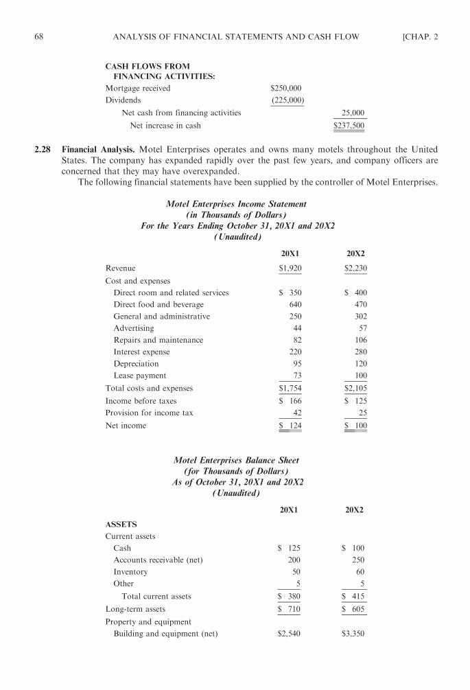
CASH FLOWS FROM
FINANCING ACTIVITIES:
Mortgage received $250,000
Dividends (225,000)
Net cash from financing activities 25,000
Net increase in cash $237,500
2.28 Financial Analysis. Motel Enterprises operates and owns many motels throughout the United
States. The company has expanded rapidly over the past few years, and company officers are
concerned that they may have overexpanded.
The following financial statements have been supplied by the controller of Motel Enterprises.
Motel Enterprises Income Statement
(in Thousands of Dollars)
For the Years Ending October 31, 20X1 and 20X2
(Unaudited)
20X1 20X2
Revenue $1,920 $2,230
Cost and expenses
Direct room and related services $ 350 $ 400
Direct food and beverage 640 470
General and administrative 250 302
Advertising 44 57
Repairs and maintenance 82 106
Interest expense 220 280
Depreciation 95 120
Lease payment 73 100
Total costs and expenses $1,754 $2,105
Income before taxes $ 166 $ 125
Provision for income tax 42 25
Net income $ 124 $ 100
Motel Enterprises Balance Sheet
(for Thousands of Dollars)
As of October 31, 20X1 and 20X2
(Unaudited)
20X1 20X2
ASSETS
Current assets
Cash $ 125 $ 100
Accounts receivable (net) 200 250
Inventory 50 60
Other 5 5
Total current assets $ 380 $ 415
Long-term assets $ 710 $ 605
Property and equipment
Building and equipment (net) $2,540 $3,350
68 ANALYSIS OF FINANCIAL STATEMENTS AND CASH FLOW [CHAP. 2

Land 410 370
Construction in progress 450 150
Total property and equipment $3,400 $3,870
Other assets $ 110 $ 110
Total assets $4,600 $5,000
LIABILITIES AND
STOCKHOLDERS’ EQUITY
Liabilities
Current liabilities
Accounts payable $30 $ 40
Accrued liabilities 190 190
Notes payable to bank 10 30
Current portion of long-term notes 50 80
Total current liabilities $ 280 $ 340
Long-term debt
Long-term notes $2,325 $2,785
Subordinated debentures 800 800
Total long-term debt $3,125 $3,585
Total liabilities $3,405 $3,925
Stockholders’ equity
Common stock ($1 par) $ 300 $ 300
Paid-in capital in excess of par 730 730
Net unrealized loss on long-term
investments (105)
Retained earnings 165 150
Total stockholders’ equity $1,195 $1,075
Total liabilities and stockholders’
equity $4,600 $5,000
(a) Compute the following ratios for 20X1 and 20X2: (1) debt/equity ratio; (2) times interest
earned; (3) return on total assets; (4) current ratio; (5) return on common stock equity; and
(6) accounts receivable turnover.
(b) Evaluate the financial condition based on the trend analysis. (CMA, adapted.)
SOLUTION
(a) 1. Debt=equity ratio ¼ total liabilities
stockholders’ equity
For 20X1:$3,405
$1,075¼ 3:17
For 20X2:$3,925
$1,195¼ 3:28
2. Times interest earned ¼ EBIT
interest expense
For 20X1:$386
$220¼ 1:75
For 20X2:$405
$280¼ 1:45
CHAP. 2] ANALYSIS OF FINANCIAL STATEMENTS AND CASH FLOW 69

3. Return on total assets ¼ net income
average total assets
For 20X1:$124
$4,600¼ 2:7%
For 20X2:$100
ð$4,600þ $5,000Þ=2 ¼ 2:1%
4. Current ratio ¼ current assets
current liabilties
For 20X1:$380
$280¼ 1:36
For 20X2:$415
$340¼ 1:22
5. Return on common stock equity ¼ earnings available to common stockholders
average stockholders’ equity
For 20X1 estimated:$124
$1,195¼ 10:4%
For 20X2:$100
ð$1,195þ $1,075Þ=2 ¼ 8:8%
6. Accounts receivable turnover ¼ net credit sales
average accounts receivable
For 20X1 estimated:$1,920
$200¼ 9:6 ðevery 38 daysÞ
For 20X2:$2,230
ð$200þ $250Þ=2 ¼ 9:91 ðevery 37 daysÞ
(b) Based on the trend analysis for 20X1 and 20X2, the company’s financial condition has deteriorated
to some degree in this period, and there is going to be a serious liquidity problem as is evidenced by
the decline in the current ratio and the decline of net working capital.
In addition, the company’s interest coverage has declined and large amounts of debt are coming
due in the near future. The statement of changes in financial position shows that a large portion of
capital expenditures were financed through long-term debt.
70 ANALYSIS OF FINANCIAL STATEMENTS AND CASH FLOW [CHAP. 2

Chapter 3
Financial Forecasting, Planning, and Budgeting
3.1 FINANCIAL FORECASTING
Financial forecasting, an essential element of planning, is the basis for budgeting activities and
estimating future financing needs. Financial forecasts begin with forecasting sales and their related
expenses. The basic steps involved in projecting financing needs are:
1. Project the firm’s sales. Most other forecasts (budgets) follow the sales forecast. The statistical
methods of forecasting sales include:
(a) Time-series analysis
(b) Exponential smoothing
(c) Regression analysis
(d) Box–Jenkins method
(These methods are discussed in other disciplines such as managerial economics and statistics
and are not covered here.)
2. Project variables such as expenses.
3. Estimate the level of investment in current and fixed assets that is required to support the
projected sales.
4. Calculate the firm’s financing needs.
3.2 PERCENT-OF-SALES METHOD OF FINANCIAL FORECASTING
When constructing a financial forecast, the sales forecast is used traditionally to estimate various
expenses, assets, and liabilities. The most widely used method for making these projections is the percent-
of-sales method, in which the various expenses, assets, and liabilities for a future period are estimated
as a percentage of sales. These percentages, together with the projected sales, are then used to construct
pro forma (planned or projected) balance sheets.
The calculations for a pro forma balance sheet are as follows:
1. Express balance sheet items that vary directly with sales as a percentage of sales. Any item that
does not vary directly with sales (such as long-term debt) is designated not applicable (n.a.).
2. Multiply the percentages determined in step 1 by the sales projected to obtain the amounts for
the future period.
3. Where no percentage applies (such as for long-term debt, common stock, and capital surplus),
simply insert the figures from the present balance sheet in the column for the future period.
4. Compute the projected retained earnings as follows:
Projected retained earnings ¼ present retained earnings
þ projected net income� cash dividends paid
(You will need to know the percentage of sales that constitutes net income and the dividend
payout ratio.)
5. Sum the asset accounts to obtain a total projected assets figure. Then add the projected liabilities
and equity accounts to determine the total financing provided. Since liability plus equity must
balance the assets when totaled, any difference is a shortfall, which is the amount of external
financing needed.
71
Copyright © 2007, 1998, 1986 by The McGraw-Hill Companies, Inc. Click here for terms of use.
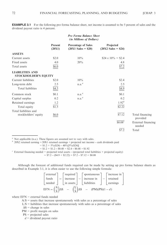
EXAMPLE 3.1 For the following pro forma balance sheet, net income is assumed to be 5 percent of sales and the
dividend payout ratio is 4 percent.
Pro Forma Balance Sheet
(in Millions of Dollars)
Present
(20X1)
Percentage of Sales
(20X1 Sales=$20)
Projected
(20X2 Sales=$24)
ASSETS
Current assets $2.0 10% $24� 10%=$2.4
Fixed assets 4.0 20% 4.8
Total assets $6.0 $7.2
LIABILITIES AND
STOCKHOLDER’S EQUITY
Current liabilities $2.0 10% $2.4
Long-term debt 2.5 n.a.a 2.5
Total liabilities $4.5 $4.9
Common stock $0.1 n.a.a $0.1
Capital surplus 0.2 n.a.a 0.2
Retained earnings 1.2 1.92b
Total equity $1.5 $2.22
Total liabilities and
stockholders’ equity $6.0 $7.12 Total financing
provided
$0.08c External financing
needed
$7.2 Total
a Not applicable (n.a.). These figures are assumed not to vary with sales.b 20X2 retained earning=20X1 retained earnings+projected net income� cash dividends paid
=$1.2+5%($24)� 40%[5%($24)]
=$1.2+$1.2� $0.48=$2.4� $0.48=$1.92c External financing needed=projected total assets� (projected total liabilities+projected equity)
=$7.2� ($4.9+$2.22)=$7.2� $7.12=$0.08
Although the forecast of additional funds required can be made by setting up pro forma balance sheets as
described in Example 3.1, it is often easier to use the following simple formula:
external
funds
needed
2
6
4
3
7
5¼
required
increase
in assets
2
6
4
3
7
5�
spontaneous
increase in
liabilities
2
6
4
3
7
5�
increase in
retained
earnings
2
6
4
3
7
5
EFN ¼ A
S
� �
DS � L
S
� �
DS � ðPMÞðPSÞð1� d Þ
where EFN=external funds needed
A/S=assets that increase spontaneously with sales as a percentage of sales
L/S= liabilities that increase spontaneously with sales as a percentage of sales
DS=change in sales
PM=profit margin on sales
PS=projected sales
d=dividend payout ratio
72 FINANCIAL FORECASTING, PLANNING, AND BUDGETING [CHAP. 3

EXAMPLE 3.2 From Example 3.1:
A
S¼ $6
$20¼ 30%
L
S¼ $2
$20¼ 10%
DS ¼ $24� $20 ¼ $4
PM ¼ 5% on sales
PS ¼ $24
d ¼ 40%
Inserting these figures into the formula, we get
EFN ¼ A
S
� �
DS� L
S
� �
DS� ðPMÞðPSÞð1� d Þ
¼ 0:3ð$4Þ � 0:1ð$4Þ � ð0:05Þð$24Þð1� 0:4Þ
¼ $1:2� $0:4� $0:72 ¼ $0:08
The $80,000 in external financing can be raised by issuing notes payable, bonds, or stocks, singly or in
combination.
One important limitation of the percent-of-sales method is that the firm is assumed to be operating
at full capacity. On the basis of this assumption, the firm does not have sufficient productive capacity to
absorb projected increases in sales and thus requires an additional investment in assets.
The major advantage of the percent-of-sales method of financial forecasting is that it is simple and
inexpensive to use. To obtain a more precise projection of the firm’s future financing needs, however, the
preparation of a cash budget is required (see the following sections).
3.3 THE BUDGET, OR FINANCIAL PLAN
A company’s annual financial plan is called a budget. The budget is a set of formal (written)
statements of management’s expectations regarding sales, expenses, production volume, and various
financial transactions of the firm for the coming period. Simply put, a budget is a set of pro forma
statements about the company’s finances and operations. A budget is a tool for both planning and
control. At the beginning of the period, the budget is a plan or standard; at the end of the period, it
serves as a control device to help management measure the firm’s performance against the plan so that
future performance may be improved.
3.4 THE STRUCTURE OF THE BUDGET
The budget is classified broadly into two categories: the operational budget, which reflects the results
of operating decisions; and the financial budget, which reflects the financial decisions of the firm.
The operating budget consists of:
1. Sales budget, including a computation of expected cash receipts
2. Production budget
3. Ending inventory budget
4. Direct materials budget, including a computation of expected cash disbursements for materials
5. Direct labor budget
6. Factory overhead budget
7. Selling and administrative expense budget
8. Pro forma income statement
CHAP. 3] FINANCIAL FORECASTING, PLANNING, AND BUDGETING 73

The financial budget consists of:
1. Cash budget
2. Pro forma balance sheet
The major steps in preparing the budget are:
1. Prepare a sales forecast
2. Determine production volume
3. Estimate manufacturing costs and operating expenses
4. Determine cash flow and other financial effects
5. Formulate projected financial statements
Follow the illustration of the Johnson Company (Examples 3.3 to 3.12), a manufacturer of a single
product, as its annual budget is created for the year 20X2. The company develops its budget on a
quarterly basis. The example will highlight the variable cost–fixed cost breakdown throughout.
The Sales Budget
The sales budget is the starting point in preparing the operating budget, since estimated sales volume
influences almost all other items appearing throughout the annual budget. The sales budget gives the
quantity of each product expected to be sold. (For the Johnson Company, there is only one product.)
Basically, there are three ways of making estimates for the sales budget:
1. Make a statistical forecast (using any one or a combination of the methods mentioned in Section
3.1) on the basis of an analysis of general business conditions, market conditions, product
growth curves, etc.
2. Make an internal estimate by collecting the opinions of executives and sales staff.
3. Analyze the various factors that affect sales revenue and then predict the future behavior of each
of those factors.
After sales volume has been estimated, the sales budget is constructed by multiplying the estimated
number of units by the expected unit price. Generally, the sales budget includes a computation
of cash collections anticipated from credit sales, which will be used later for cash budgeting.
See Example 3.3.
EXAMPLE 3.3 Assume that of each quarter’s sales, 70 percent is collected in the first quarter of the sale; 28 percent
is collected in the following quarter; and 2 percent is uncollectible.
The Johnson Company
Sales Budget
For the Year Ended December 31, 20X2
Quarter
1 2 3 4 Total
Expected sales in units 800 700 900 800 3,200
Unit sales price ($) �80 �80 �80 �80 �80Total sales $64,000 $56,000 $72,000 $64,000 $256,000
74 FINANCIAL FORECASTING, PLANNING, AND BUDGETING [CHAP. 3

Schedule of Expected Cash Collections
Quarter
1 2 3 4 Total
Accounts receivable,
December 31, 20X1
$ 9,500 $ 9,500
1st-quarter sales ($64,000) 44,800a $17,920b 62,720
2nd-quarter sales ($56,000) 39,200 $15,680 54,880
3rd-quarter sales ($72,000) 50,400 $20,160 70,560
4th-quarter sales ($64,000) 44,800 44,800
Total cash collections $54,300 $57,120 $66,080 $64,960 $242,460
a $64,000� 0.70=$44,800b $64,000� 0.28=$17,920
The Production Budget
After sales are budgeted, the production budget can be determined. The number of units expected to
be manufactured to meet budgeted sales and inventory is set forth. The expected volume of production is
determined by subtracting the estimated inventory at the beginning of the period from the sum of units
to be sold plus desired ending inventory. See Example 3.4.
EXAMPLE 3.4 Assume that ending inventory is 10 percent of the next quarter’s sales and that the ending
inventory for the fourth quarter is 100 units.
The Johnson Company
Production Budget
For the Year Ended December 31, 20X2
Quarter
1 2 3 4 Total
Planned sales (Example 3.3) 800 700 900 800 3,200
Desired ending inventory 70 90 80 100 100
Total needs 870 790 980 900 3,300
Less beginning inventorya 80 70 90 80 80
Units to be produced 790 720 890 820 3,220
a The same amount as the previous quarter’s ending inventory.
The Direct Materials Budget
When the level of production has been computed, a direct materials budget is constructed
to show how much material will be required and how much of it must be purchased to meet
CHAP. 3] FINANCIAL FORECASTING, PLANNING, AND BUDGETING 75

production requirements. The purchase will depend on both expected usage of materials and inventory
levels. The formula for computing the purchase is
amount of materials
to be purchased
in units
2
4
3
5 ¼materials needed
for production
in units
2
4
3
5þdesired ending
material inventory
in units
2
4
3
5�beginning
material inventory
in units
2
4
3
5
The direct materials budget is usually accompanied by a computation of expected cash payments for the
purchased materials.
EXAMPLE 3.5 Assume that ending inventory is 10 percent of the next quarter’s production needs; the ending
materials inventory for the fourth quarter is 250 units; and 50 percent of each quarter’s purchases are paid in that
quarter, with the remainder being paid in the following quarter. Also, 3 pounds of materials are needed per unit of
product at a cost of $2 per pound.
The Johnson Company
Direct Material Budget
For the Year Ended December 31, 20X2
Quarter
1 2 3 4 Total
Units to be produced (Example 3.4) 790 720 890 820 3,220
Material needs per unit (pounds) �3 �3 �3 �3 �3Material needs for production 2,370 2,160 2,670 2,460 9,660
Desired ending inventory of materials 216 267 246 250 250
Total needs 2,586 2,427 2,916 2,710 9,910
Less: Beginning inventory of materialsa 237 216 267 246 237
Materials to be purchased 2,349 2,211 2,649 2,464 9,673
Unit price ($) �2 �2 �2 �2 �2Purchase cost $4,698 $4,422 $5,298 $4,928 $19,346
Schedule of Expected Cash Disbursements
Accounts payable,
December 31, 20X1 $2,200 $2,200
1st-quarter purchases ($4,698) 2,349 $2,349 4,698
2nd-quarter purchases ($4,422) 2,211 $2,211 4,422
3rd-quarter purchases ($5,298) 2,469 $2,649 5,298
4th-quarter purchases ($4,928) 2,464 2,464
Total disbursements $4,549 $4,560 $4,860 $5,113 $19,082
a The same amount as the prior quarter’s ending inventory.
The Direct Labor Budget
The production budget also provides the starting point for the preparation of the direct labor cost
budget. The direct labor hours necessary to meet production requirements multiplied by the estimated
hourly rate yields the total direct labor cost.
76 FINANCIAL FORECASTING, PLANNING, AND BUDGETING [CHAP. 3

EXAMPLE 3.6 Assume that 5 hours of labor are required per unit of product and that the hourly rate is $5.
The Johnson Company
Direct Labor Budget
For the Year Ended December 31, 20X2
Quarter
1 2 3 4 Total
Units to be produced (Example 3.4) 790 720 890 820 3,220
Direct labor hours per unit �5 �5 �5 �5 �5Total hours 3,950 3,600 4,450 4,100 16,100
Direct labor cost per hour ($) �5 �5 �5 �5 �5Total direct labor cost $19,750 $18,000 $22,250 $20,500 $80,500
The Factory Overhead Budget
The factory overhead budget is a schedule of all manufacturing costs other than direct materials and
direct labor. Using the contribution approach to budgeting requires the development of a predetermined
overhead rate for the variable portion of the factory overhead. In developing the cash budget, remember
that depreciation does not entail a cash outlay and therefore must be deducted from the total factory
overhead in computing cash disbursements for factory overhead.
EXAMPLE 3.7 For the following factory overhead budget, assume that:
1. Total factory overhead is budgeted at $6,000 per quarter plus $2 per hour of direct labor.
2. Depreciation expenses are $3,250 per quarter.
3. All overhead costs involving cash outlays are paid in the quarter in which they are incurred.
The Johnson Company
Factory Overhead Budget
For the Year Ended December 31, 20X2
Quarter
1 2 3 4 Total
Budgeted direct labor hours
(Example 3.6) 3,950 3,600 4,450 4,100 16,100
Variable overhead rate ($) �2 �2 �2 �2 �2Variable overhead budgeted $ 7,900 $ 7,200 $ 8,900 $ 8,200 $32,000
Fixed overhead budgeted 6,000 6,000 6,000 6,000 24,000
Total budgeted overhead $13,900 $13,200 $14,900 $14,200 $56,200
Less: Depreciation 3,250 3,250 3,250 3,250 13,000
Cash disbursements for overhead $10,650 $ 9,950 $11,650 $10,950 $43,200
The Ending Inventory Budget
The ending inventory budget provides the information required for constructing budgeted financial
statements. First, it is useful for computing the cost of goods sold on the budgeted income statement.
Second, it gives the dollar value of the ending materials and finished goods inventory that will appear on
the budgeted balance sheet.
CHAP. 3] FINANCIAL FORECASTING, PLANNING, AND BUDGETING 77

EXAMPLE 3.8 For the ending inventory budget, we first need to compute the unit variable cost for finished goods,
as follows:
Units Cost Units Total
Direct materials $2 3 pounds $ 6
Direct labor $5 5 hours 25
Variable overhead $2 5 hours 10
Total variable manufacturing cost $41
The Johnson Company
Ending Inventory Budget
For the Year Ended December 31, 20X2
Ending Inventory
Units Unit Costs Total
Direct materials 250 pounds $ 2 $500
Finished goods 100 units $41 $4,100
The Selling and Administrative Expense Budget
The selling and administrative expense budget lists the operating expenses involved in selling the
products and in managing the business.
EXAMPLE 3.9 The variable selling and administrative expenses amount of $4 per unit of sale, including commis-
sions, shipping, and supplies; expenses are paid in the same quarter in which they are incurred, with the exception of
$1,200 in income tax, which is paid in the third quarter.
The Johnson Company
Selling and Administrative Expense Budget
For the Year Ended December 31, 20X2
Quarter
1 2 3 4 Total
Expected sales in units 800 700 900 800 3,200
Variable selling and administrative expense per unit ($) �4 �4 �4 �4 �4Budgeted variable expense $ 3,200 $ 2,800 $ 3,600 $ 3,200 $12,800
Fixed selling and administrative expenses
Advertising 1,100 1,100 1,100 1,100 4,400
Insurance 2,800 2,800
Office salaries 8,500 8,500 8,500 8,500 34,000
Rent 350 350 350 350 1,400
Taxes 1,200 1,200
Total budgeted selling and administrative expenses $15,950 $12,750 $14,750 $13,150 $56,600
The Cash Budget
The cash budget is prepared in order to forecast the firm’s future financial needs. It is also a tool for
cash planning and control. Because the cash budget details the expected cash receipts and disbursements
for a designated time period, it helps avoid the problem of either having idle cash on hand or suffering a
cash shortage. However, if a cash shortage is experienced, the cash budget indicates whether the shortage
is temporary or permanent, that is, whether short-term or long-term borrowing is needed.
78 FINANCIAL FORECASTING, PLANNING, AND BUDGETING [CHAP. 3

The cash budget typically consists of four major sections:
1. The receipts section, which gives the beginning cash balance, cash collections from customers,
and other receipts
2. The disbursements section, which shows all cash payments made, listed by purpose
3. The cash surplus or deficit section, which simply shows the difference between the cash receipts
section and the cash disbursements section
4. The financing section, which provides a detailed account of the borrowings and repayments
expected during the budget period
EXAMPLE 3.10 For this example, assume the following:
1. The company desires to maintain a $5,000 minimum cash balance at the end of each quarter.
2. All borrowing and repayment must be in multiples of $500 at an interest rate of 10 percent per annum.
Interest is computed and paid as the principal is repaid. Borrowing takes place at the beginning and
repayments at the end of each quarter.
3. The cash balance at the beginning of the first quarter is $10,000.
4. A sum of $24,300 is to be paid in the second quarter for machinery purchases.
5. Income tax of $4,000 is paid in the first quarter.
The Johnson Company
Cash Budget
For the Year Ended December 31, 20X2
Quarter
From Example 1 2 3 4 Total
Cash balance, beginning Given $10,000 $ 9,401 $ 5,461 $ 9,106 $ 10,000
Add receipts
Collection from customers 3.3 54,300 57,120 66,080 64,960 242,460
Total cash available $64,300 $ 66,521 $ 71,541 $74,066 $252,460
Less disbursements
Direct materials 3.5 $ 4,549 $ 4,560 $ 4,860 $ 5,113 $ 19,082
Direct labor 3.6 19,750 18,000 22,250 20,500 80,500
Factory overhead 3.7 10,650 9,950 11,650 10,950 43,200
Selling and administrative 3.9 15,950 12,750 14,750 13,150 56,600
Machinery purchase Given 24,300 24,300
Income tax Given 4,000 4,000
Total disbursements $54,899 $ 69,560 $ 53,510 $49,713 $227,682
Cash surplus (deficit) $ 9,401 $(3,039) $ 18,031 $24,353 $ 24,778
Financing
Borrowing $ 8,500 $ 8,500
Repayment (8,500) (8,500)
Interest (425) (425)
Total financing $ 8,500 $ (8,925) $ (425)
Cash balance, ending $ 9,401 $ 5,461 $ 9,106 $24,353 $ 24,353
The Budgeted Income Statement
The budgeted income statement summarizes the various component projections of revenue and
expenses for the budgeting period. For control purposes, the budget can be divided into quarters, for
example, depending on the need.
CHAP. 3] FINANCIAL FORECASTING, PLANNING, AND BUDGETING 79

EXAMPLE 3.11
The Johnson Company
Budgeted Income Statement
For the Year Ended December 31, 20X2
From
Example
Sales (3,200 units @ $80) 3.3 $256,000
Less: Variable expenses
Variable cost of goods sold (3,200 units @ $41) 3.8 $131,200
Variable selling and administrative 3.9 12,800 144,000
Contribution margin $112,000
Less: Fixed expenses
Factory overhead 3.7 $ 24,000
Selling and administrative 3.9 43,800 67,800
Net operating income $ 44,200
Less: Interest expense 3.10 425
Net income before taxes $ 43,775
Less: Income taxes (20%) 8,755
Net income $ 35,020
The Budgeted Balance Sheet
The budgeted balance sheet is developed by beginning with the balance sheet for the year just ended
and adjusting it, using all the activities that are expected to take place during the budget period. Some of
the reasons why the budgeted balance sheet must be prepared are:
1. To disclose any potentially unfavorable financial conditions
2. To serve as a final check on the mathematical accuracy of all the other budgets
3. To help management perform a variety of ratio calculations
4. To highlight future resources and obligations
EXAMPLE 3.12
The Johnson Company
Balance sheet
For the Year Ended December 31, 20X1
ASSETS LIABILITIES AND
STOCKHOLDERS’ EQUITY
Current assets Current liabilities
Cash $ 10,000 Accounts payable $ 2,200
Accounts receivable 9,500 Income tax payable 4,000
Materials inventory 474 Stockholders’ equity
Finished goods inventory 3,280 Common stock, no par 70,000
$ 23,254 Retained earnings 37,054
Fixed assets
Land $ 50,000
Building and equipment 100,000
Accumulated depreciation (60,000)
$ 90,000
Total assets $113,254 Total liabilities and stockholders’ equity $113,254
80 FINANCIAL FORECASTING, PLANNING, AND BUDGETING [CHAP. 3

The Johnson Company
Budgeted Balance sheet
For the Year Ended December 31, 20X2
ASSETS LIABILITIES AND
STOCKHOLDERS’ EQUITY
Current assets Current liabilities
Cash $ 24,353a Account payable $ 2,464g
Accounts receivable 23,040b Income tax payable 8,755h
Materials inventory 500c
Finished goods inventory 4,100c Stockholders’ equity
$ 51,993 Common stock, no par 70,000i
Retained earnings 72,074j
Fixed assets
Land $ 50,000d
Buildings and equipment 124,300e
Accumulated depreciation (73,000)f
$101,300
Total assets $153,293 Total liabilities and stockholders’ equity $153,293
a From Example 3.10 (cash budget).b From Example 3.3 (sales budget).
Accounts receivable ¼ Beginning balanceþ sales� receipts
¼ $9,500þ $256,000� $242,460 ¼ $23,040
c From Example 3.8 (ending inventory budget).d Unchanged from 20X1 balance sheet.e $100,000 (from 20X1 balance sheet)+$24,300 (from Example 3.10)=$124,300f $60,000 (from 20X1 balance sheet)+$13,000 (from Example 3.7)=$73,000g Accounts payable=beginning balance+purchase cost� disbursements for materials
=$2,200+$19,346 (Example 3.5)� $19,082 (Example 3.5)=$2,464
or 50% of 4th-quarter purchase=50% ($4,928)=$2,464.h From Example 3.11 (budgeted income statement).i Unchanged from 20X1 balance sheet.j $37,054 (from 20X1 balance sheet)+$35,020 (from net income, Example 3.11)=$72,074
3.5 A SHORTCUT APPROACH TO FORMULATING THE BUDGET
Examples 3.3 to 3.12 show a detailed procedure for formulating a budget. However, in practice a
shortcut approach to budgeting is quite common and may be summarized as follows:
1. A pro forma income statement is developed using past percentage relationships between
relevant expense and cost items and the firm’s sales. These percentages are then applied to
the firm’s forecasted sales. This is a version of the percent-of-sales method discussed in
Section 3.2.
2. A pro forma balance sheet is estimated by determining the desired level of certain balance sheet
items, then making additional financing conform to those desired figures. The remaining items,
thus, are estimated to make the balance sheet balance.
There are two basic assumptions underlying this approach:
1. The firm’s past financial condition is an accurate predictor of its future condition.
2. The value of certain variables such as cash, inventory, and accounts receivable can be forced to
take on specified desired values.
CHAP. 3] FINANCIAL FORECASTING, PLANNING, AND BUDGETING 81

3.6 COMPUTER-BASED MODELS FOR FINANCIAL PLANNING AND BUDGETING
More and more companies are developing computer-based quantitative models for constructing
a profit planning budget. The models help managerial decision makers answer a variety of what-if
questions. The resultant calculations provide a basis for choice among alternatives under conditions
of uncertainty. There are primarily two approaches to modeling the corporate budgeting process:
simulation and optimization.
Review Questions
1. , an essential element of planning, is the basis for budgeting activities.
2. The most widely used method for forecasting future financing needs is .
3. In a forecast of additional funds, external funds needed equal required increase in assets minus
the sum of plus .
4. Budgeting is a tool for and .
5. The cash budget contains four major sections. They are the
section, section, section, and the financing section.
6. How much to produce is contingent upon expected sales in units and the
and inventories of finished goods.
7. Production budget is prepared after the budget is completed. It is prepared
in .
8. Cash budgets should include noncash charges such as depreciation: (a) true; (b) false.
9. Cash budgets are prepared on a short-term basis such as on a monthly, quarterly, or even
weekly basis: (a) true; (b) false.
10. Operating budgets would include cash budgets: (a) true; (b) false.
11. The pro forma shows the expected operating results for the budgeting year,
while the pro forma shows the expected financial condition at the end of
budgeting period.
12. Desired ending inventory figures appear on both budgeted
and .
13. The idea behind preparing cash budgets is to avoid unnecessary cash
and .
14. are often used to develop budgets in order to evaluate alternative courses of
action.
15. A shortcut approach to formulating a budget uses a version of the .
82 FINANCIAL FORECASTING, PLANNING, AND BUDGETING [CHAP. 3

Answers: (1) Financial forecasting; (2) the percent-of-sales method; (3) spontaneous increase in liabilities,
increase in retained earnings; (4) planning, control; (5) cash receipt, cash disbursement, cash surplus (or defi-
cit); (6) beginning, ending; (7) sales, physical units; (8) (b); (9) (a); (10) (b); (11) income statement, balance
sheet; (12) income statement (or cost of goods sold), balance sheet; (13) surplus, deficit; (14) Computer-based
financial planning models; (15) percent-of-sales method.
Solved Problems
3.1 Behavior of Balance Sheet Items. Which of the following balance sheet items generally vary
directly with sales?
(a) Common stock ( f ) Marketable securities
(b) Accounts payable (g) Debentures
(c) Retained earnings (h) Accrued wages
(d ) Inventory (i) Preferred stock
(e) Taxes payable ( j) Mortgage bonds
SOLUTION
(b), (d ), (e), ( f ), (h)
3.2 Financial Forecasting and External Funds Needed. The following financial data pertain to Barret
Company:
Income Statement
(in Millions of Dollars)
Sales $16.0
Cost of goods sold 13.0
Gross profit $ 3.0
Operating expenses 1.0
Net profit before taxes $ 2.0
Tax 1.0
Profit after taxes $ 1.0
Dividends 0.7
Retentions $ 0.3
Balance Sheet
(in Millions of Dollars)
ASSETS
Current assets
Cash $ 2.0
Receivables 2.0
Inventories 4.0
Total current assets $ 8.0
Fixed assets 8.0
Total assets $16.0
CHAP. 3] FINANCIAL FORECASTING, PLANNING, AND BUDGETING 83

LIABILITIES AND NET WORTH
Current liabilities $ 5.0
Long-term debt 2.0
Total debt $ 7.0
Common stock 7.0
Retained earnings $ 2.0
Total liabilities and net worth $16.0
Barret expects its sales to increase by $2,000,000 next year. In this problem, all the asset
accounts (including fixed assets) and current liabilities vary with sales. Barret is operating at full
capacity. (a) Forecast Barret’s need for external funds by (1) constructing a pro forma balance
sheet and (2) using the simple formula. (b) Discuss the limitation of the percent-of-sales method.
SOLUTION
(a) (1) Pro Forma Balance Sheet
(in Millions of Dollars)
Present
Percentage
of Sales
(Sales=$16.0)
Next Year
(Projected
Sales=$18.0)
ASSETS
Current assets $ 8.0 50 $ 9.0000
Fixed assets 8.0 50 9.0000
Total assets $16.0 $18.0000
LIABILITIES AND NET WORTH
Current liabilities $ 5.0 31.25 $ 5.6250
Long-term debt 2.0 n.a. 2.0000
Total liabilities $ 7.0 $ 7.6250
Common stock $ 7.0 n.a. $ 7.0000
Retained earnings 2.0 2.3375a
Total net worth $ 9.0 $ 9.3375
Total liabilities and net worth $16.0
$16.9625 Total financing
provided
$ 1.0375b External financing
needed
$18.0000 Total
a Next year’s retained earnings=present year’s retained earnings+projected net income (after taxes)� cash dividends
paid. Note that after-tax net income=$1.0/$16.0=6.25% and dividend payout ratio=0.7/1.0=7%. Therefore
Next year’s retained earnings ¼ $2:0þ 6:25%ð$18:0Þ � 0:7½6:25%ð$18Þ� ¼ $2:0þ $1:125� $0:7875 ¼ $2:3375:b External funds needed=projected total assets� (projected total liabilities+projected equity)=$18.0� $16.9625=
$1.0375
84 FINANCIAL FORECASTING, PLANNING, AND BUDGETING [CHAP. 3

ð2Þ EFN ¼ A
S
� �
DS� L
S
� �
DS� ðPMÞðPSÞð1� d Þ
whereA
S¼ $16:0
$16:0¼ 100%
L
S¼ $5:0
$16:0¼ 31:25%
DS ¼ $18:0� $16:0 ¼ $2:0
PM ¼ $1:0=$16:0 ¼ 6:25%
PS ¼ $18:0
d ¼ $0:7=$1:0 ¼ 70%; or 1� d ¼ 30%
Thus,
EFN ¼ 100%ð$2Þ � 31:25%ð$2Þ � ð6:25%Þð$18Þð1� 0:7Þ¼ $2� $0:625� $0:3375 ¼ $1:0375
(b) The calculations for both the pro forma balance sheet and the simple formula are based on percentage
of sales. The limitations of the percent-of-sales method are (1) the relationship between sales and the
expense item, asset, or liability being projected is assumed to be pure, that is, free of any other
influences; and (2) the method does not provide accurate forecasts when a firm has extra capacity
to absorb all or a portion of the projected increase in sales and the related investment in assets.
3.3 Determination of External Funds Needed. Ina Corporation is thinking of purchasing a new
machine. With this new machine, the company expects sales to increase from $8,000,000 to
$10,000,000.
The company knows that its assets, accounts payable, and accrued expenses vary directly with
sales. The company’s profit margin on sales is 8 percent, and the company plans to pay 40 percent
of its after-tax earnings in dividends, The company’s current balance sheet is given below.
Balance Sheet
Current assets $ 3,000,000
Fixed assets 12,000,000
Total assets $15,000,000
Accounts payable $ 4,000,000
Accrued expenses 1,000,000
Long-term debt 3,000,000
Common stock 2,000,000
Retained earnings 5,000,000
Total liabilities and net worth $15,000,000
(a) Prepare a pro forma balance sheet.
(b) Use the simple formula to determine the external funds needed by the company based on the answer in
part (a).
(c) Determine, using the simple formula, the external funds needed under each of the following
conditions:
1. The profit margin rises from 8 percent to 10 percent.
2. The profit margin is 8 percent, but the dividend payout ratio is reduced from 40 percent to 20
percent.
(d ) Comment on the results from part (c).
CHAP. 3] FINANCIAL FORECASTING, PLANNING, AND BUDGETING 85
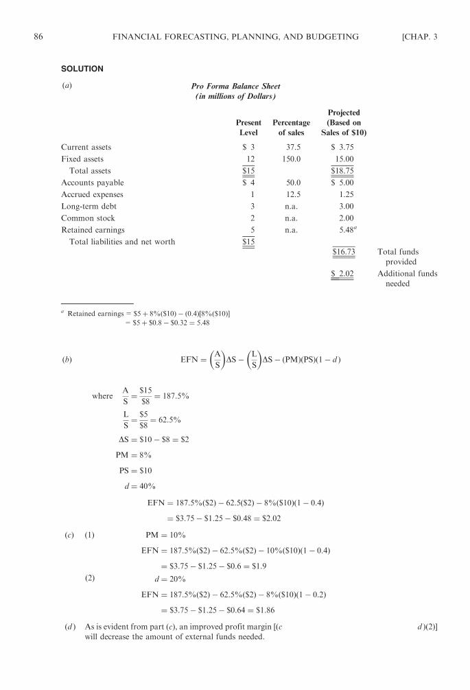
SOLUTION
(a) Pro Forma Balance Sheet
(in millions of Dollars)
Present
Level
Percentage
of sales
Projected
(Based on
Sales of $10)
Current assets $ 3 37.5 $ 3.75
Fixed assets 12 150.0 15.00
Total assets $15 $18.75
Accounts payable $ 4 50.0 $ 5.00
Accrued expenses 1 12.5 1.25
Long-term debt 3 n.a. 3.00
Common stock 2 n.a. 2.00
Retained earnings 5 n.a. 5.48a
Total liabilities and net worth $15
$16.73 Total funds
provided
$ 2.02 Additional funds
needed
a Retained earnings=$5þ 8%ð$10Þ � ð0:4Þ½8%ð$10Þ�= $5þ $0:8� $0:32 ¼ 5:48
(b) EFN ¼ A
S
� �
DS� L
S
� �
DS� ðPMÞðPSÞð1� d Þ
whereA
S¼ $15
$8¼ 187:5%
L
S¼ $5
$8¼ 62:5%
DS ¼ $10� $8 ¼ $2
PM ¼ 8%
PS ¼ $10
d ¼ 40%
EFN ¼ 187:5%ð$2Þ � 62:5ð$2Þ � 8%ð$10Þð1� 0:4Þ
¼ $3:75� $1:25� $0:48 ¼ $2:02
(c) (1) PM ¼ 10%
EFN ¼ 187:5%ð$2Þ � 62:5%ð$2Þ � 10%ð$10Þð1� 0:4Þ
¼ $3:75� $1:25� $0:6 ¼ $1:9
(2) d ¼ 20%
EFN ¼ 187:5%ð$2Þ � 62:5%ð$2Þ � 8%ð$10Þð1� 0:2Þ
¼ $3:75� $1:25� $0:64 ¼ $1:86
(d ) As is evident from part (c), an improved profit margin [(c)(1)] or a lower dividend payout ratio [(d )(2)]
will decrease the amount of external funds needed.
86 FINANCIAL FORECASTING, PLANNING, AND BUDGETING [CHAP. 3

3.4 Filling in Blanks and Financial Forecasting. The following data pertain to ABC Company:
Balance Sheet Items
on December 31, 20X1
(in Thousands of Dollars)
20X1
Percentage of Sales
(20X1 Sales=$400)
Pro Forma Balance Sheet on
December 31, 20X2
(Projected Sales=$600)
Cash $ 10 2.5 $ 15
Receivables 90 22.5 135
Inventories 200 50.0 300
Total current assets $300 75.0 $450
Net fixed assets 300 75.0 450
Total assets $600 150.0 $900
Accounts payable $ 40 10.0 $ 60
Notes payable 20 n.a. (c)
Accrued wages and taxes 40 10.0 60
Total current liabilities $100 (b)
Mortgage bonds $140 n.a. (d )
Common stock 60 n.a. ( f )
Retained earnings 300 n.a. 324
Total $600 (e) Funds provided
(a) Additional funds needed
In addition, ABC Company must maintain a total debt/total assets ratio at or below
40 percent and a current ratio at or above 2.5. Within these constraints, ABC would prefer to
finance using short-term rather than long-term debt or long-term debt rather than equity.
Fill in the missing terms on the December 31, 20X2, pro forma balance sheet.
SOLUTION
(a) external
funds
needed
2
6
4
3
7
5¼
required
increase
in assets
2
6
4
3
7
5�
spontaneous
increase in
liabilities
2
6
4
3
7
5�
increase in
retained
earnings
2
6
4
3
7
5
¼ ð$900� $600Þ �
increase in
accounts
payable
accrued wages
and taxes
2
6
6
6
6
6
6
4
3
7
7
7
7
7
7
5
� ð$324� $300Þ
¼ $300� ð$60� $40Þ þ ð$60� $40Þ½ � � $24
¼ $300� $40� $24 ¼ $236
(b) Current ratio ¼ current assets
current liabilities
2:5 ðminimumÞ ¼ $450
current liabilities
Current liabilities ¼ $180, which is the maximum allowed:
(c) Notes payable ¼ current liabilities� ðaccounts payableþ accrued wages and taxesÞ¼ $180� ð$60þ $60Þ ¼ $180� $120 ¼ $60
CHAP. 3] FINANCIAL FORECASTING, PLANNING, AND BUDGETING 87
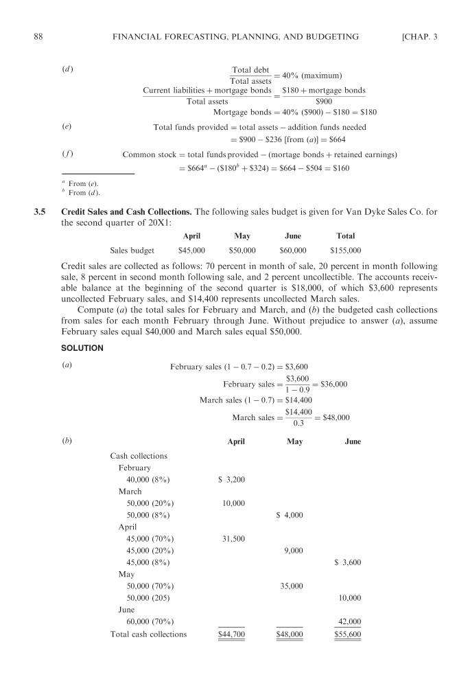
(d ) Total debt
Total assets¼ 40% ðmaximumÞ
Current liabilitiesþmortgage bonds
Total assets¼ $180þmortgage bonds
$900
Mortgage bonds ¼ 40% ð$900Þ � $180 ¼ $180
(e) Total funds provided ¼ total assets� addition funds needed
¼ $900� $236 ½from ðaÞ� ¼ $664
( f ) Common stock ¼ total funds provided� ðmortage bondsþ retained earningsÞ¼ $664a � ð$180b þ $324Þ ¼ $664� $504 ¼ $160
a From (e).b From (d ).
3.5 Credit Sales and Cash Collections. The following sales budget is given for Van Dyke Sales Co. for
the second quarter of 20X1:
April May June Total
Sales budget $45,000 $50,000 $60,000 $155,000
Credit sales are collected as follows: 70 percent in month of sale, 20 percent in month following
sale, 8 percent in second month following sale, and 2 percent uncollectible. The accounts receiv-
able balance at the beginning of the second quarter is $18,000, of which $3,600 represents
uncollected February sales, and $14,400 represents uncollected March sales.
Compute (a) the total sales for February and March, and (b) the budgeted cash collections
from sales for each month February through June. Without prejudice to answer (a), assume
February sales equal $40,000 and March sales equal $50,000.
SOLUTION
(a) February sales ð1� 0:7� 0:2Þ ¼ $3,600
February sales ¼ $3,600
1� 0:9¼ $36,000
March sales ð1� 0:7Þ ¼ $14,400
March sales ¼ $14,400
0:3¼ $48,000
(b) April May June
Cash collections
February
40,000 (8%) $ 3,200
March
50,000 (20%) 10,000
50,000 (8%) $ 4,000
April
45,000 (70%) 31,500
45,000 (20%) 9,000
45,000 (8%) $ 3,600
May
50,000 (70%) 35,000
50,000 (205) 10,000
June
60,000 (70%) 42,000
Total cash collections $44,700 $48,000 $55,600
88 FINANCIAL FORECASTING, PLANNING, AND BUDGETING [CHAP. 3

3.6 Cash Collections. The following data are given for Erich From Stores:
September
Actual ($)
October
Actual ($)
November
Estimated ($)
December
Estimated ($)
Cash sales 7,000 6,000 8,000 6,000
Credit sales 50,000 48,000 62,000 80,000
Total sales 57,000 54,000 70,000 86,000
Past experience indicates net collections normally occur in the following pattern:
No collections are made in the month of sale, 80 percent of the sales of any month are collected
in the following month, 19 percent of sales are collected in the second following month, and
1 percent of sales are uncollectible.
Compute (a) total cash receipts for November and December, and (b) accounts receivable
balance at November 30 if the October 31 balance is $50,000.
SOLUTION
(a) November December
Cash receipts
Cash sales $ 8,000 $ 6,000
Cash collections
September sales
50,000 (19%) 9,500
October sales
48,000 (80%) 38,400
48,000 (19%) 9,120
November sales
62,000 (80%) 49,600
Total cash receipts $55,900 $64,720
(b) Accounts receivable (November 30)=$50,000+$62,000� $9,500� $38,400=$64,100
3.7 Cash Collections and Discount Policy. The treasurer of John Loyde Co. plans for the company to
have a cash balance of $91,000 on March 1. Sales during March are estimated at $900,000.
February sales amounted to $600,000, and January sales amounted to $500,000. Cash payments
for March have been budgeted at $580,000. Cash collections have been estimated as follows:
60 percent of the sales for the month to be collected during the month, 30 percent of the sales for
the preceding month to be collected during the month, and 8 percent of the sales for the second
preceding month to be collected during the month.
The treasurer plans to accelerate collections by allowing a 2 percent discount for
prompt payment. With the discount policy, she expects to collect 70 percent of the current
sales and will permit the discount reduction on these collections. Sales of the preceding
month will be collected to the extent of 15 percent with no discount allowed, and 10 percent
of the sales of the second preceding month will be collected with no discount allowed.
This pattern of collection can be expected in subsequent months. During the transitional
month of March, collections may run somewhat higher. However, the treasurer prefers to
estimate collections on the basis of the new pattern so that the estimates will be somewhat
conservative.
Estimate (a) cash collections for March and the cash balance at March 31 under the present
policy, and (b) cash collections for March and the cash balance at March 31 according to the new
policy of allowing discounts. (c) Is the discount policy desirable?
CHAP. 3] FINANCIAL FORECASTING, PLANNING, AND BUDGETING 89

SOLUTION
(a) and (b)
(a)
Cash Collection
under the Present Policy:
(b)
Cash Collection
under the Discount Policy:
Balance, March 1
Collections
$ 91,000 $ 91,000
From March sales 540,000 ($900,000� 60%) 617,400a
From February sales 180,000 ($600,000� 30%) 90,000 ($600,000� 15%)
From January sales 40,000 ($500,000� 8%) 50,000 ($500,000� 10%)
Total cash available $851,000 $848,400
Less: Disbursements 580,000 580,000
Balance, March 31 $271,000 $268,400
a $900,000� 70%� 98%=$617,400
(c) No, the discount policy is not, since, under the discount policy, the March 31 cash balance will be
smaller.
3.8 Cash Payments. Hello Wheels purchases bicycle components in the month prior to assembling
them into bicycles. Assembly is scheduled one month prior to budgeted sales. Rolling pays
75 percent of component costs in the month of purchase and 25 percent of the costs in the
following month. Component costs included in budgeted cost of sales are:
April May June July August
$5,000 $6,000 $7,000 $8,000 $8,000
What are Hello’s budgeted cash payments for components in May? (CFM adapted)
SOLUTION
The bicycle components purchased by Hello Wheels in May will be included in bicycles sold in
July. The components are purchased one month prior to assembly and assembled one month prior to
sale. Hello will pay 75 percent of June’s $8,000 budgeted cost of sales in May and the remaining
25 percent in June. Moreover, 25 percent of June’s $7,000 budgeted cost of sales is paid for in May.
Consequently, Hello’s budgeted cash payments for components in May are $7,750 [($8,000� 0.75)+
($7,000� 0.25)].
3.9 Cash Disbursements. Eastmark Stores wants to estimate cash disbursements for cash budgeting
purposes for the first 3 months of 20X2 from the data given below.
1. Cost of merchandise sold, estimated:
20X1: December $225,000
20X2: January $250,000
February $280,000
March $210,000
The cost of merchandise is to be paid for as follows: 35 percent in the month of sale and
65 percent in the following month.
90 FINANCIAL FORECASTING, PLANNING, AND BUDGETING [CHAP. 3
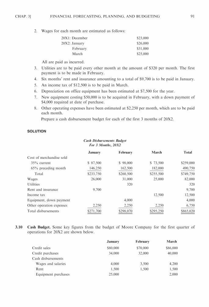
2. Wages for each month are estimated as follows:
20X1: December $23,000
20X2: January $26,000
February $31,000
March $25,000
All are paid as incurred.
3. Utilities are to be paid every other month at the amount of $320 per month. The first
payment is to be made in February.
4. Six months’ rent and insurance amounting to a total of $9,700 is to be paid in January.
5. An income tax of $12,500 is to be paid in March.
6. Depreciation on office equipment has been estimated at $7,500 for the year.
7. New equipment costing $50,000 is to be acquired in February, with a down payment of
$4,000 required at date of purchase.
8. Other operating expenses have been estimated at $2,250 per month, which are to be paid
each month.
Prepare a cash disbursement budget for each of the first 3 months of 20X2.
SOLUTION
Cash Disbursements Budget
For 3 Months, 20X2
January February March Total
Cost of merchandise sold
35% current $ 87,500 $ 98,000 $ 73,500 $259,000
65% preceding month 146,250 162,500 182,000 490,750
Total $233,750 $260,500 $255,500 $749,750
Wages 26,000 31,000 25,000 82,000
Utilities 320 320
Rent and insurance 9,700 9,700
Income tax 12,500 12,500
Equipment, down payment 4,000 4,000
Other operation expenses 2,250 2,250 2,250 6,750
Total disbursements $271,700 $298,070 $295,250 $865,020
3.10 Cash Budget. Some key figures from the budget of Moore Company for the first quarter of
operations for 20X2 are shown below.
January February March
Credit sales $80,000 $70,000 $86,000
Credit purchases 34,000 32,000 40,000
Cash disbursements
Wages and salaries 4,000 3,500 4,200
Rent 1,500 1,500 1,500
Equipment purchases 25,000 2,000
CHAP. 3] FINANCIAL FORECASTING, PLANNING, AND BUDGETING 91

The company estimates that 10 percent of its credit sales will never be collected. Of those that
will be collected, 50 percent will be collected in the month of sale and the remainder will be
collected in the following month. Purchases on account will all be paid for in the month following
purchase. 20X2 December sales were $90,000.
Using the preceding information, complete the following cash budget.
January February March
Beginning cash balance $100,000 —–—— —–——
Cash receipts
Cash collections from credit sales —–—— —–—— —–——
Total cash available —–—— —–—— —–——
Cash disbursements
Purchases —–—— —–—— —–——
Wages and salaries —–—— —–—— —–——
Rent —–—— —–—— —–——
Equipment purchases —–—— —–—— —–——
Total disbursements —–—— —–—— —–——
Ending cash balance
SOLUTION
January February March
Beginning cash balance $100,000 $146,000 $174,500
Cash receipts
Cash collections from credit sales 76,500a 67,500b 70,200c
Total cash available $176,500 $213,500 $244,700
Cash disbursements
Purchases $ 34,000 $ 32,000
Salaries $ 4,000 3,500 4,200
Rent 1,500 1,500 1,500
Fixed assets 25,000 2,000
Total disbursements $ 30,500 $ 39,000 $ 39,700
Ending cash balance $146,000 $174,500 $205,000
a From December sales: $90,000� ð$90,000� 0:1Þ2
¼ $40,500
January sales: $80,000� ð$80,000� 0:1Þ2
¼ 36,000
$76,500
b From January sales:
February sales: $70,000� ð$70,000� 0:1Þ2
¼ 31; 500
$67,500
$31,500
c From February sales:
March sales: $86,00� ð$86,000� 0:1Þ2
¼ 38,700
$70,200
3.11 Incomplete Data on Sales. The following information pertains to merchandise purchased by
Westwood Plumbing Co. for July, August, September, and October. During any month, 60
percent of the merchandise to be sold in the following month is purchased. The balance of the
merchandise is purchased during the month of sale. Gross margin averages 20 percent of sales.
92 FINANCIAL FORECASTING, PLANNING, AND BUDGETING [CHAP. 3
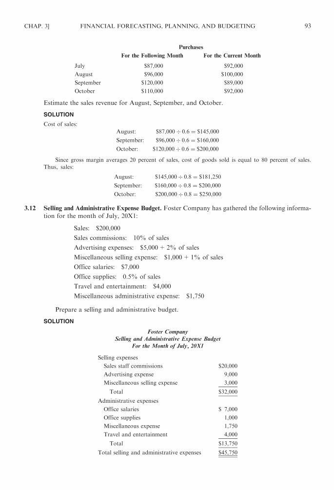
Purchases
For the Following Month For the Current Month
July $87,000 $92,000
August $96,000 $100,000
September $120,000 $89,000
October $110,000 $92,000
Estimate the sales revenue for August, September, and October.
SOLUTION
Cost of sales:
August: $87,000� 0:6 ¼ $145,000
September: $96,000� 0:6 ¼ $160,000
October: $120,000� 0:6 ¼ $200,000
Since gross margin averages 20 percent of sales, cost of goods sold is equal to 80 percent of sales.
Thus, sales:
August: $145,000� 0:8 ¼ $181,250
September: $160,000� 0:8 ¼ $200,000
October: $200,000� 0:8 ¼ $250,000
3.12 Selling and Administrative Expense Budget. Foster Company has gathered the following informa-
tion for the month of July, 20X1:
Sales: $200,000
Sales commissions: 10% of sales
Advertising expenses: $5,000+2% of sales
Miscellaneous selling expense: $1,000+1% of sales
Office salaries: $7,000
Office supplies: 0.5% of sales
Travel and entertainment: $4,000
Miscellaneous administrative expense: $1,750
Prepare a selling and administrative budget.
SOLUTION
Foster Company
Selling and Administrative Expense Budget
For the Month of July, 20X1
Selling expenses
Sales staff commissions $20,000
Advertising expense 9,000
Miscellaneous selling expense 3,000
Total $32,000
Administrative expenses
Office salaries $ 7,000
Office supplies 1,000
Miscellaneous expense 1,750
Travel and entertainment 4,000
Total $13,750
Total selling and administrative expenses $45,750
CHAP. 3] FINANCIAL FORECASTING, PLANNING, AND BUDGETING 93

3.13 Budgeted Income Statement. In the fiscal quarter ended December 31, 20X1, Eric Wills Lumber
Company plans to sell 52,000 board feet lumber at a price of $125 per board foot. There are to be
5,500 board feet on hand October 1, with a cost of $65 per board foot. The company plans to
manufacture 53,000 board feet of lumber during the quarter, with the following manufacturing
costs:
Direct materials: $971,500
Direct labor: $2,000,000
Factory overhead: (25% of direct labor costs)
The company uses the last-in, first-out (LIFO) method of inventory costing. Selling expenses
are estimated at 25 percent of sales, and administrative expenses are expected to be 10 percent
more than the previous quarter’s $950,000.
Prepare a budgeted income statement.
SOLUTION
Eric Wills Lumber Co.
Budgeted Income statement
For the Quarter Ended December 31, 20X1
Sales (52,000 @ $125) $6,500,000
Less: Cost of goods sold
Beginning inventory
(5,500 @ $65) $ 357,500
Direct materials 971,500
Direct labor 2,000,000
Factory overhead
(25% of $2,000,000) 500,000
Cost of goods available for sale $3,829,000
Less: Ending inventory
(6,500 units)a423,000b 3,406,000
Gross profit $3,094,000
Less operating expenses
Selling expenses
(25% of $6,500,000) $1,625,000
Administrative expenses
(110% of $950,000) 1,045,000 2,670,000
Net income $ 424,000
a5,500 unitsþ 53,000 units� x ¼ 52,000 units
x ¼ 6,500 units
b The unit cost for the last quarter of 20X1 is calculated as follows:
Unit cost ¼ cost of goods manufactured=number of units
¼ ð$971,500þ $2,000,000þ $500,000Þ=53,000 board feet ¼ $65:50
Then,
5,500 units @ $65.00 $357,500
1,000 units @ $65.50 65,500
6,500 units $423,000
3.14 Budgeted Income Statement. The Moore Distributor, Inc., has just received a franchise
to distribute dishwashers. The company started business on January 1, 20X1, with the
94 FINANCIAL FORECASTING, PLANNING, AND BUDGETING [CHAP. 3

following assets:
Cash $45,000
Inventory $94,000
Warehouse, office, and delivery facilities and equipment $800,000
All facilities and equipment have a useful life of 20 years and no residual value. First-quarter
sales are expected to be $360,000 and should be doubled in the second quarter. Third-quarter
sales are expected to be $1,080,000. One percent of sales are considered to be uncollectible. The
gross profit margin should be 30 percent. Variable selling expenses (except uncollectible accounts)
are budgeted at 12 percent of sales and fixed selling expenses at $48,000 per quarter, exclusive of
depreciation. Variable administrative expenses are expected to be 3 percent of sales, and fixed
administrative expenses should total $34,200 per quarter, exclusive of depreciation.
Prepare a budgeted income statement for the second quarter, 20X1.
SOLUTION
The Moore Distributor, Inc.
Budgeted Income Statement
For the Second Quarter, 20X1
Sales $720,000
Cost of goods sold (70%) 504,000
Gross profit (30%) $216,000
Operating expenses
Uncollectible accounts (1%) $7,200
Depreciationa 10,000
Selling
Variable (12%) 86,400
Fixed 48,000
Administrative
Variable (3%) 21,600
Fixed 34,200 207,400
Income before income tax $ 8,600
a 14ð$800,000Þ � 20 years ¼ $10,000
3.15 Pro Forma Balance Sheet.Given the following data on the Dunes Corporation, project its balance
sheet for the coming year:
Present sales: $500,000
Next year’s sales: $800,000
After-tax profits: 5% of sales
Dividend payout ratio: 40%
Present retained earnings: $200,000
Cash as a percent of sales: 4%
Accounts receivable as a percent of sales: 10%
Inventory as a percent of sales: 30%
Net fixed assets as a percent of sales: 35%
Accounts payable as a percent of sales: 7%
Accruals as a percent of sales: 15%
Next year’s common stock: $200,000
CHAP. 3] FINANCIAL FORECASTING, PLANNING, AND BUDGETING 95
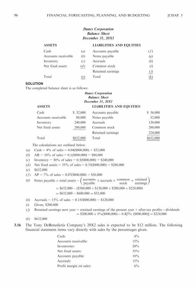
Dunes Corporation
Balance Sheet
December 31, 20X1
ASSETS LIABILITIES AND EQUITIES
Cash (a) Accounts payable ( f )
Accounts receivable (b) Notes payable (g)
Inventory (c) Accruals (h)
Net fixed assets (d ) Common stock (i)
Retained earnings ( j)
Total (e) Total (k)
SOLUTION
The completed balance sheet is as follows:
Dunes Corporation
Balance Sheet
December 31, 20X1
ASSETS LIABILITIES AND EQUITIES
Cash $ 32,000 Accounts payable $ 56,000
Accounts receivable 80,000 Notes payable 32,000
Inventory 240,000 Accruals 120,000
Net fixed assets 280,000 Common stock 200,000
Retained earnings 224,000
Total $632,000 Total $632,000
The calculations are outlined below.
(a) Cash=4% of sales=0.04($800,000)=$32,000
(b) AR=10% of sales=0.1($800,000)=$80,000
(c) Inventory=30% of sales=0.3($800,000)=$240,000
(d ) Net fixed assets=35% of sales=0.35($800,000)=$280,000
(e) $632,000
( f ) AP=7% of sales=0.07($800,000)=$56,000
(g) Notes payable ¼ total assets� accountspayable
þ accrualsþ commonstock
þ retainedearnings
� �
¼ $632,000� ð$560,000þ $120,000þ $200,000þ $224,000Þ¼ $632,000� $600,000 ¼ $32,000
(h) Accruals=15% of sales=0.15($800,000)=$120,000
(i) Given, $200,000
( j) Retained earnings next year=retained earnings of the present year+after-tax profits� dividends
¼ $200,000þ 5%ð$800,000Þ � 0:4½5% ð$800,000Þ� ¼ $224,000
(k) $632,000
3.16 The Tony DeBenedictis Company’s 20X2 sales is expected to be $12 million. The following
financial statement items vary directly with sales by the percentages given.
Cash: 4%
Accounts receivable: 15%
Inventories: 20%
Net fixed assets: 35%
Accounts payable: 18%
Accruals: 15%
Profit margin on sales: 6%
96 FINANCIAL FORECASTING, PLANNING, AND BUDGETING [CHAP. 3
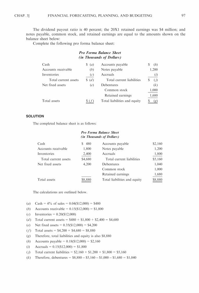
The dividend payout ratio is 40 percent; the 20X1 retained earnings was $4 million; and
notes payable, common stock, and retained earnings are equal to the amounts shown on the
balance sheet below:
Complete the following pro forma balance sheet:
Pro Forma Balance Sheet
(in Thousands of Dollars)
Cash $ (a) Accounts payable $ (h)
Accounts receivable (b) Notes payable 1,200
Inventories (c) Accruals (i)
Total current assets $ (d ) Total current liabilities $ ( j)
Net fixed assets (e) Debentures (k)
Common stock 1,000
Retained earnings 1,680
Total assets $ ( f ) Total liabilities and equity $ (g)
SOLUTION
The completed balance sheet is as follows:
Pro Forma Balance Sheet
(in Thousands of Dollars)
Cash $ 480 Accounts payable $2,160
Accounts receivable 1,800 Notes payable 1,200
Inventories 2,400 Accruals 1,800
Total current assets $4,680 Total current liabilities $5,160
Net fixed assets 4,200 Debentures 1,040
Common stock 1,000
Retained earnings 1,680
Total assets $8,880 Total liabilities and equity $8,880
The calculations are outlined below.
(a) Cash=4% of sales=0.04($12,000)=$480
(b) Accounts receivable=0.15($12,000)=$1,800
(c) Inventories=0.20($12,000)
(d ) Total current assets=$480+$1,800+$2,400=$4,680
(e) Net fixed assets=0.35($12,000)=$4,200
( f ) Total assets=$4,200+$4,680=$8,880
(g) Therefore, total liabilities and equity is also $8,880
(h) Accounts payable=0.18($12,000)=$2,160
(i) Accruals=0.15($12,000)=$1,800
( j) Total current liabilities=$2,160+$1,200+$1,800=$5,160
(k) Therefore, debentures=$8,880� $5,160� $1,000� $1,680=$1,040
CHAP. 3] FINANCIAL FORECASTING, PLANNING, AND BUDGETING 97

3.17 Budgeted Income Statement and Balance Sheet. A budget is being prepared for the first and second
quarters of 20X2 for Aggarwal Retail Stores, Inc. The balance sheet as of December 31, 20X1 is
given below
Aggarwal Retail Stores, Inc.
Balance Sheet December 31, 20X1
ASSETS LIABILITIES AND EQUITIES
Cash $ 65,000 Accounts payable $ 83,000
Accounts receivable 52,000 Income tax payable 20,000
Merchandise inventory 75,000 Capital stock 70,000
Retained earnings 19,000
Total assets $192,000 Total liabilities and equities $192,000
Actual and projected sales are:
20X1, 3rd quarter (actual): $250,000
20X1, 4th quarter (actual): $300,000
20X2, 1st quarter (estimated): $200,000
20X2, 2nd quarter (estimated): $230,000
20X2, 3nd quarter (estimated): $220,000
Experience has shown that 60 percent of sales will be collected during the first quarter of sales
and 35 percent of sales will be collected in the following quarter. Gross profit averages 30 percent
of sales. There is a basic inventory of $20,000. The policy is to purchase in each quarter the
additional inventory needed for the following quarter’s sales; payments are made in the quarter
following the quarter of purchase. Selling and administrative expenses for each quarter are
estimated at 4 percent of sales plus $15,000 and are paid as incurred. Income tax is equal to
40 percent of taxable income. The income tax liability as of December 31, 20X1, is to be paid
during the first quarter of 20X2.
Prepare (a) a budgeted income statement for the first and second quarter of 20X2 and (b) a
budgeted balance sheet as of June 30, 20X2.
SOLUTION
(a)
Aggarwal Retail Stores, Inc.
Budgeted Income Statement
For the 6 Months Ended June 30, 20X2
Quarter
1 2 Total
Sales $200,000 $230,000 $430,000
Less: Cost of goods sold (70%) 140,000 161,000 301,000
Gross margin $ 60,000 $ 69,000 $129,000
Less: Selling and administrative expenses
($15,000+4% of sales) 23,000 24,200 47,200
Net income before tax $ 37,000 $ 44,800 $ 81,800
Income tax (40%) 14,800 17,920 32,720
Net income $ 22,200 $ 26,880 $ 49,080
98 FINANCIAL FORECASTING, PLANNING, AND BUDGETING [CHAP. 3

(b) Aggarwal Retail Stores, Inc.
Budgeted Balance Sheet as of June 30, 20X2
ASSETS LIABILITIES AND EQUITIES
Cash $ 89,800a Accounts payable $ 97,000d
Accounts receivable 49,000b Income tax payable 32,720e
Merchandise inventory 129,000c Capital stock 70,000
Retained earnings 68,080 f
Total assets $267,800 Total liabilities and equity $267,800
The supporting calculations for the balance sheet are as follows:
Quarter
1 2 Total
CASH RECEIPTS
60% of current sales $120,000 $138,000 $258,000
35% of prior quarter’s sales 105,000 70,000 175,000
Total receipts $225,000 $208,000 $433,000
CASH DISBURSEMENTS
Merchandise purchasesg $160,000 $181,000 $341,000
Selling and administrative expenses
($15,000 +4% of sales per month)
23,000 24,200 47,200
Income tax (for previous quarter) 20,000 20,000
Total disbursements $203,000 $205,200 $408,200
aCash ¼ beginning balanceþ cash receipts� disbursements
¼ $65; 000þ $433,000� $408,200 ¼ $89,800b
Accounts receivable ¼ beginning balanceþ sales� cash receipts
¼ $52,000þ ð$200,000þ $230,000Þ � $433,000 ¼ $49,000cMerchandise inventory ¼ beginning balanceþ purchases� cost of goods sold
¼ $75,000þ ð$181,000þ $174,000Þ � 70%ð$430,000Þ ¼ $129,000d
Accounts payable ¼ Beginning balanceþ purchasesþ selling and administrative expenses
� disbursements ðfor purchases and selling and administrative expensesÞ¼ $83,000þ $355,000þ $47,200� ð$341,000þ $47,200Þ ¼ $97,000
eIncome tax payable ¼ beginning balanceþ net income after tax� income tax payment
¼ $20,000þ $32,720� $20,000 ¼ $32,720f Retained earnings=beginning balance+net income=$19,000+$49,080=$68,080
Quarter
Merchandise 4 1 2 Total
Purchases
($20,000 basic+70%
of the quarter’s sales)
$160,000 $181,000 $174,000 $515,000
Cash disbursements for
merchandise purchases
$160,000 $181,000 $341,000
CHAP. 3] FINANCIAL FORECASTING, PLANNING, AND BUDGETING 99

Chapter 4
The Management of Working Capital
4.1 MANAGING NET WORKING CAPITAL
Working capital is equal to current assets. Net working capital is equal to current assets less current
liabilities.
EXAMPLE 4.1 Ace Company has the following selected assets and liabilities:
Cash $10,000
Accounts receivable $30,000
Inventory $42,000
Machinery $90,000
Long-term investments $36,000
Patent $4,000
Accounts payable $12,000
Taxes payable $3,000
Accrued expenses payable $5,000
Bonds payable $50,000
Common stock $70,000
The net working capital is:
CURRENT ASSETS
Cash $10,000
Accounts receivable 30,000
Inventory 42,000 $82,000
CURRENT LIABILITIES
Accounts payable $12,000
Taxes payable 3,000
Accrued expenses payable 5,000 20,000
Net working capital $62,000
Management of net working capital involves regulating the various types of current assets and
current liabilities. Management of net working capital also requires decisions about how current
assets should be financed, for example, through short-term debt, long-term debt, or equity. Net working
capital is increased when current assets are financed through noncurrent sources.
The liquidity of current assets will affect the terms and availability of short-term credit. The greater
the liquidity, the easier it becomes, generally, to obtain a short-term loan at favorable terms. Short-term
credit, in turn, affects the amount of cash balance held by a firm.
Working Capital Management and Risk-Return Trade-Off
The management of net working capital requires consideration for the trade-off between return and
risk. Holding more current than fixed assets means a reduced liquidity risk. It also means greater
flexibility, since current assets may be modified easily as sales volume changes. However, the rate of
return will be less with current assets than with fixed assets. Fixed assets typically earn a greater return
than current assets. Long-term financing has less liquidity risk associated with it than short-term debt,
but it also carries a higher cost.
100
Copyright © 2007, 1998, 1986 by The McGraw-Hill Companies, Inc. Click here for terms of use.

For example, when a company needs funds to purchase seasonal or cyclical inventory, it uses short-
term, not long-term financing. The short-term debt gives the firm flexibility to meet its seasonal needs
within its ability to repay the loan. On the other hand, the company’s permanent assets should be
financed with long-term debt. Because the assets last longer, the financing can be spread over a
longer time. Liquidity risk may be reduced by using the hedging approach to financing, in which
assets are financed by liabilities with similar maturity.
4.2 CURRENT ASSETS
By optimally managing cash, receivables, and inventory, a company can maximize its rate of return
and minimize its liquidity and business risk. The financial manager should determine the amount to be
invested in a given current asset. The amount invested may vary from day to day and require close
evaluation of the account balances. Current assets are improperly managed if funds tied up in an asset
could be used more productively elsewhere. Financing such assets with debt incurs unnecessary interest
expense. Also, large account balances indicate risk since, for example, inventory may not be saleable
and/or accounts receivable may not be collectible. On the other hand, inadequate current asset levels
may be costly as, for example, when business is lost because lack of inventory does not permit the timely
fulfillment of customer orders.
4.3 CASH MANAGEMENT
Cash refers to currency and demand deposits. Cash management involves having the optimum,
neither excessive nor deficient, amount of cash on hand at the right time. Proper cash management
requires that the company know how much cash it needs, as well as how much it has and where that cash
is at all times. This is especially essential in an inflationary environment.
The objective of cash management is to invest excess cash for a return while retaining sufficient
liquidity to satisfy future needs. The financial manager must plan when to have excess funds available for
investment and when money needs to be borrowed.
The amount of cash to be held depends upon the following factors:
1. Cash management policies
2. Current liquidity position
3. Management’s liquidity risk preferences
4. Schedule of debt maturity
5. The firm’s ability to borrow
6. Forecasted short- and long-term cash flow
7. The probabilities of different cash flows under varying circumstances
The company should not have an excessive cash balance since no return is being earned upon it.
The least amount of cash a firm should hold is the greater of (1) compensating balances (a deposit held
by a bank to compensate it for providing services) or (2) precautionary balances (money held for
emergency purposes) plus transaction balances (money needed to cover checks outstanding).
Cash management also requires knowing the amount of funds available for investment and the
length of time for which they can be invested. A firm may invest its funds in the following:
1. Time deposits, including savings accounts earning daily interest, long-term savings accounts,
and certificates of deposit
2. Money market funds, which are managed portfolios of short-term, high-grade debt instruments
such as Treasury bills and commercial paper
3. Demand deposits that pay interest
4. U.S. Treasury securities
CHAP. 4] THE MANAGEMENT OF WORKING CAPITAL 101

When cash receipts and disbursements are highly synchronized and predictable, a firm may keep
a small cash balance. The financial manager must accurately forecast the amount of cash needed,
its source, and its destination. These data are needed on both a short- and a long-term basis.
Forecasting assists the manager in properly timing financing, debt repayment, and the amount to be
transferred between accounts.
In deciding whether to adopt a cash management system, the financial manager should consider its
associated costs versus the return earned from implementation of the system. Costs related to cash
management systems include bank charges, financial manager’s time, and office employee salaries.
Some cash management systems use the firm’s computer to make transactions with the computers of
banks and money market funds. Computer systems are also useful for purchasing and selling securities in
the money market.
Companies with many bank accounts should guard against accumulating excessive balances.
Less cash needs to be kept on hand when a company can borrow quickly from a bank, such
as under a line of credit agreement, which permits a firm to borrow instantly up to a specified
maximum amount. A company may also find some cash unnecessarily tied up in other accounts,
such as advances to employees. Excess cash should be invested in marketable securities for a return.
Note, however, that cash in some bank accounts may not be available for investment. For instance,
when a bank lends money to a company, the bank often requires the company to keep funds on
hand as collateral. This deposit is called a compensating balance, which in effect represents restricted
cash for the company.
Holding marketable securities serves as protection against cash shortages. Companies
with seasonal operations may buy marketable securities when they have excess funds and then sell
the securities when cash deficits occur. A firm may also invest in marketable securities
when funds are being held temporarily in anticipation of short-term capital expansion. In selecting
an investment portfolio, consideration should be given to return, default risk, marketability, and
maturity date.
The thrust of cash management is to accelerate cash receipts and delay cash payments. Each bank
account should be analyzed as to its type, balance, and cost so that corporate return is maximized.
Acceleration of Cash Inflow
To accelerate cash inflow, the financial manager must (1) know the bank’s policy regarding fund
availability; (2) know the source and location of company receipts; and (3) devise procedures for quick
deposit of checks received and quick transfer of receipts in outlying accounts into the main corporate
account.
The various types of check processing delays that must be analyzed are: (1) mail float—the time
required for a check to move from a debtor to a creditor; (2) processing float—the time it takes for a
creditor to deposit the check after receipt; and (3) deposit collection float—the time required for a check
to clear.
Note: Electronic data exchange (EDI), or financial EDI (FEDI), significantly reduces or eliminates
a float. EDI refers to the growing practice of direct, electronic information exchange between all
types of businesses, thereby shortening the length of time required to initiate and complete a business
transaction.
Mail float can be minimized by having the collection center located near the customer. Local
banks should be selected to speed the receipt of funds for subsequent transfer to the central corporate
account. As an alternative, strategic post office lockboxes may be used for customer remissions.
The local bank collects from these boxes periodically during the day and deposits the funds in
the corporate account. The bank also furnishes the company with a computer listing of payments
received by account and a daily total. Because the lockbox system has a significant per-item cost, it
is most cost-effective with low-volume, high-dollar remissions. However, the system is becoming
increasingly more available to companies with high-volume, low-dollar deposits as technological
advances (such as machine-readable documents) lower the per-item cost of lockboxes.
102 THE MANAGEMENT OF WORKING CAPITAL [CHAP. 4
Before a lockbox system is implemented, the company should make a cost–benefit analysis that
considers the average dollar amount of checks received, the costs saved by having lockboxes, the
reduction in mailing time per check, and the processing cost.
EXAMPLE 4.2 Chaset Corporation obtains average cash receipts of $200,000 per day. It usually takes 5 days from
the time a check is mailed to its availability for use. The amount tied up by the delay is:
5 days� $200,000 ¼ $1,000,000
EXAMPLE 4.3 It takes Travis Corporation about 7 days to receive and deposit payments from customers.
Therefore, a lockbox system is being considered. It is expected that the system will reduce the float time to
5 days. Average daily collections are $500,000. The rate of return is 12 percent.
The reduction in outstanding cash balances arising from implementing the lockbox system is:
2 days� $500,000 ¼ $1,000,000
The return that could be earned on these funds is:
$1,000,000� 0:12 ¼ $120,000
The maximum monthly charge the company should pay for this lockbox arrangement is therefore:
$120,000
12¼ $10,000
EXAMPLE 4.4 Charles Corporation is exploring the use of a lockbox system that will cost $100,000 per year.
Daily collections average $350,000. The lockbox arrangement will reduce the float period by 2 days. The firm’s rate
of return is 15 percent.
The cost–benefit analysis is shown below.
Return on early collection of cash
0.15� 2� $350,000 $105,000
Cost 100,000
Advantage of lockbox $ 5,000
A corporate financial manager should determine whether it would be financially advantageous to
split a geographic collection region into a number of parts.
EXAMPLE 4.5 Travis Company has an agreement with Charter Bank in which the bank handles $3 million in
collections a day and requires a $700,000 compensating balance. Travis is thinking of canceling the agreement and
dividing its western region so that two other banks will handle its business instead. Bank A will handle $1 million a
day of collections, requiring a compensating balance of $300,000, and bank B will handle the other $2 million a day,
asking for a compensating balance of $500,000. Travis’s financial manager anticipates that collections will be
accelerated 14day if the western region is divided. The company’s rate of return is 14 percent.
The financial manager decided that the new arrangement should be implemented, based on the following
analysis:
Acceleration in cash receipts
$3 million per day � 14day
$750,000
Additional compensating balance required 100,000
Increased cash flow $650,000
Rate of return � 0.14
Net annual savings $ 91,000
Concentration banking should also be considered for use. With this method funds are collected by
several local banks and transferred to a main concentration account in another bank. The transfer of
CHAP. 4] THE MANAGEMENT OF WORKING CAPITAL 103

funds between banks should be accomplished through the use of depository transfer checks (DTCs) or
wire transfers. In the DTC arrangement, there exists a resolution statement with the bank in which
signatureless checks are allowed to be deposited. As the initial banks collect the funds, information is
immediately transferred to the concentration bank, which then issues a DTC to collect the outlying
funds. The funds may be available the same day.
Once remissions have been accelerated, freed cash should be used for investment in marketable
securities or to pay off short-term debt. Thus, the freed cash will generate interest revenue to the
business. The revenue derived can be determined for a given month by multiplying the monthly average
accounts receivable balance times the associated monthly interest rate (i.e., the interest rate on market-
able securities or the interest rate applicable to short-term debt).
EXAMPLE 4.6 A firm’s weekly average cash balances are as follows:
Week Average Cash Balance
1 $12,000
2 17,000
3 10,000
4 15,000
Total $54,000
The monthly average cash balance is:
$54,000
4¼ $13,500
If the annual interest rate is approximated at 12 percent, the monthly return earned on the average cash
balance is:
$13,500� 0:1 ¼ $135
For a cash acceleration system to be feasible, the return earned on the freed cash must exceed the
cost of the system.
Delay of Cash Outflow
There are various ways to delay cash disbursements, including:
1. Using drafts to pay bills since drafts are not due on demand. When a bank receives a draft
it must return the draft to the issuer for acceptance prior to payment. When the company
accepts the draft, it then deposits the required funds with the bank; hence, a smaller average
checking balance is maintained.
2. Mailing checks from post offices having limited service or from locations where the mail must
go through several handling points, lengthening the payment period.
3. Drawing checks on remote banks or establishing cash disbursement centers in remote locations
so that the payment period is lengthened. For example, someone in New York can be paid with
a check drawn on a California bank.
4. Using credit cards and charge accounts in order to lengthen the time between the acquisition
of goods and the date of payment for those goods.
5. Disbursing sales commissions when the receivables are collected rather than when the sales
are made.
6. Maintaining a zero balance account (ZBA) where zero balances are established for all
of the company’s disbursing units. These accounts are in the same concentration bank.
Checks are drawn against these accounts, with the balance in each account never
104 THE MANAGEMENT OF WORKING CAPITAL [CHAP. 4

exceeding $0. Divisional disbursing authority is thus maintained at the local level of
management. The advantages of zero balance accounts are better control over cash payments,
reduction in excess cash balances held in regional banks, and a possible increase in
disbursing float.
7. Using a controlled disbursement account. With this system, almost all payments that must be
made are known in the morning. The bank informs the firm of the total, and the firm transfers
(usually by wire) the amount needed.
EXAMPLE 4.7 Every 2 weeks, company X disburses checks that average $500,000 and take 3 days to clear. How
much money can the company save annually if it delays transfer of funds from an interest-bearing account that pays
0.0384 percent per day (annual rate of 14 percent) for those 3 days?
The interest for 3 days is:
$500,000� 0:000384� 3ð Þ ¼ $576
The number of 2-week periods in a year is:
52 weeks
2 weeks¼ 26
The savings per year is:
$576� 26 ¼ $14,976
Opportunity Cost of Forgoing a Cash Discount
An opportunity cost is the net revenue lost by rejecting an alternative action. A firm should
typically take advantage of a discount offered by a creditor because of the associated high
opportunity cost. For example, if the terms of sale are 2/10, net/30, the customer has 30 days to pay
the bill but will get a 2 percent discount if he or she pays in 10 days. Some companies use seasonal datings
such as 2/10, net/30, July 1 dating. Here, with an invoice dated July 1, the discount can be taken until
July 10.
The following formula may be used to compute the opportunity cost in percentage, on an annual
basis, of not taking a discount:
Opportunity cost ¼ discount percent
100� discount percent� 360
N
where N=the number of days payment can be delayed by forgoing the cash discount
=days credit is outstanding�discount period
The numerator of the first term (discount percent) is the cost per dollar of credit, whereas the
denominator (100� discount percent) represents the money made available by forgoing the cash dis-
count. The second term represents the number of times this cost is incurred in a year.
EXAMPLE 4.8 The opportunity cost of not taking a discount when the terms are 3/15, net/60 is computed as
follows:
Opportunity cost ¼ 3
100� 3� 360
60� 15¼ 3
97� 360
45¼ 24:7%
Determination of the Optimal Cash Balance
There are two techniques for deciding how much cash to maintain at any given point, considering
that both holding cash and investing it have both advantages and disadvantages. The purpose of cash
models is to satisfy cash requirements at the least cost.
CHAP. 4] THE MANAGEMENT OF WORKING CAPITAL 105
Baumol’s Model
It attempts to determine the optimum cash balance under conditions of certainty. The objective is to
minimize the sum of the fixed costs of transactions and the opportunity cost of holding cash balances.
These costs are expressed as:
b� Tð ÞCþ i Cð Þ
2
where b=the fixed cost of a transaction, T= the total cash needed for the time period involved, i=the
interest rate on marketable securities, and C=cash balance.
The optimal level of cash or the optimal cash balance is determined using the following formula:
C ¼ffiffiffiffiffiffiffiffiffi
2bT
i
r
EXAMPLE 4.9 You estimate a cash need for $4,000,000 over a 1-month period where the cash account is expected
to be disbursed at a constant rate. The opportunity interest rate is 6 percent per annum or 0.5 percent for a 1-month
period. The transaction cost each time you borrow or withdraw is $100.
The optimal cash balance and the number of transactions you should make during the month follow:
C ¼ffiffiffiffiffiffiffiffi
2bT
i
r
¼ffiffiffiffiffiffiffiffiffiffiffiffiffiffiffiffiffiffiffiffiffiffiffiffiffiffiffiffiffiffiffiffiffiffiffiffi
2 100ð Þ 4,000,000ð Þ0:005
r
¼ $400,000
The optimal cash balance is $400,000. The average cash balance is:
C
2¼ $400,000
2¼ $200,000
The number of transactions required are:
$4,000,000
$400,000¼ 10 transactions during the month:
The Miller–Orr Model
The Miller–Orr model is a stochastic model for cash management where uncertainty exists for
cash payments. In other words, there is irregularity of cash payments. The Miller–Orr model places
an upper and lower limit for cash balances. When the upper limit is reached a transfer of cash to
marketable securities or other suitable investments is made. When the lower limit is reached a transfer
from securities to cash occurs. A transaction will not occur as long as the cash balance falls within the
limits.
The Miller–Orr model takes into account the fixed costs of a securities transaction (b), assumed to
be the same for buying as well as selling, the daily interest rate on marketable securities (i), and
the variance of daily net cash flows (s2). A major assumption is the randomness of cash flows. The
two control limits in the Miller–Orr model may be specified as ‘‘h’’ dollars as an upper limit and zero
dollars at the lower limit. When the cash balance reaches the upper level, h less z dollars of securities are
bought and the new balance equals zero, and z dollars of securities are sold and the new balance again
reaches z.
The optimal cash balance z is computed as follows:
z ¼ffiffiffiffiffiffiffiffiffi
3bs2
4i
3
r
The optimal value for h is computed as 3z. The average cash balance will approximate (z+h)/3.
106 THE MANAGEMENT OF WORKING CAPITAL [CHAP. 4

EXAMPLE 4.10 Delta Inc. has experienced a stochastic demand for its product, which results in fluctuating cash
balances randomly. The following information supplied:
Fixed cost of a securities transaction $10
Variance of daily net cash flows $50
Daily interest rate on securities (10%/360) 0.0003
The optimal cash balance, the upper limit of cash needed, and the average cash balance follow:
z ¼
ffiffiffiffiffiffiffiffiffiffiffiffiffiffiffiffiffiffiffi
3 10ð Þ 50ð Þ4 0:0003ð Þ
3
s
¼ffiffiffiffiffiffiffiffiffiffiffiffiffiffiffiffiffiffiffi
3 10ð Þ 50ð Þ0:0012
3
r
¼ffiffiffiffiffiffiffiffiffiffiffiffiffiffi
1:500
0:0012
3
r
¼ffiffiffiffiffiffiffiffiffiffiffiffiffiffiffiffiffiffiffiffi
1,250,0003p
¼ $102
The optimal cash balance is $102. The upper limit is $306(3� $102). The average cash balance is
$102þ $306ð Þ3
¼ $136
When the upper limit of $306 is reached, $204 of securities ($306� $102) will be purchased to bring you to the
optimal cash balance of $102. When the lower limit of zero dollars is reached, $102 of securities will be sold to again
bring you to the optimal cash balance of $102.
4.4 MANAGEMENT OF ACCOUNTS RECEIVABLE
Consideration should be given to the company’s investment in accounts receivable since there
is an opportunity cost associated with holding receivable balances. The major decision regarding
accounts receivable is the determination of the amount and terms of credit to extend to
customers. The credit terms offered have a direct bearing on the associated costs and revenue to
be generated from receivables. For example, if credit terms are tight, there will be less of an
investment in accounts receivable and less bad debt losses, but there will also be lower sales and reduced
profits.
In evaluating a potential customer’s ability to pay, consideration should be given to the firm’s
integrity, financial soundness, collateral to be pledged, and current economic conditions. A customer’s
credit soundness may be evaluated through quantitative techniques such as regression analysis. Such
techniques are most useful when a large number of small customers are involved. Bad debt losses can be
estimated reliably when a company sells to many customers and when its credit policies have not changed
for a long period of time.
The collection period for accounts receivable partly depends on the firm’s credit policy and
economic conditions, such as a recessionary environment, a period of limited or tight credit, or both.
In managing accounts receivable, the following procedures are recommended. First, establish a
credit policy:
1. A detailed review of a potential customer’s soundness should be made prior to extending credit.
Procedures such as a careful review of the customer’s financial statements and credit rating, as
well as a review of financial service reports (e.g., Dun & Bradstreet), are common.
2. As customer financial health changes, credit limits should be revised.
3. Marketing factors must be noted since an excessively restricted credit policy will lead to lost
sales.
4. If seasonal datings are used, the firm may offer more liberal payments than usual during slow
periods in order to stimulate business by selling to customers who are unable to pay until later in
the season. This policy is financially appropriate when the return on the additional sales plus the
CHAP. 4] THE MANAGEMENT OF WORKING CAPITAL 107

lowering in inventory costs is greater than the incremental cost associated with the additional
investment in accounts receivable.
Second, establish a policy concerning billing:
1. Customer statements should be sent within 1 day subsequent to the close of the period.
2. Large sales should be billed immediately.
3. Customers should be invoiced for goods when the order is processed rather than when it is
shipped.
4. Billing for services should be done on an interim basis or immediately prior to the actual
services. The billing process will be more uniform if cycle billing is employed.
5. The use of seasonal datings should be considered. (See item 4, concerning credit policy.)
Finally, establish a policy concerning collection:
1. Accounts receivable should be aged in order to identify delinquent and high-risk customers.
The aging should be compared to industry norms.
2. Collection efforts should be undertaken at the very first sign of customer financial
unsoundness.
EXAMPLE 4.11 Jones Corporation sells on terms of net/60. Its accounts are on the average 30 days past due.
Annual credit sales are $500,000. The investment in accounts receivable is:
90
360� $500,000 ¼ $125,000
EXAMPLE 4.12 The cost of a given product is 40 percent of selling price, and carrying cost is 12 percent of selling
price. On average, accounts are paid 90 days subsequent to the sale date. Sales average $40,000 per month.
The investment in accounts receivable from this product is:
Accounts receivable:
3 months� $40,000 sales = $120,000
Investment in accounts receivable:
$120,000� (0.40+0.12) = $ 62,400
EXAMPLE 4.13 A company has accounts receivable of $700,000. The average manufacturing cost is 40 percent of
the sales price. The before-tax profit margin is 10 percent. The carrying cost of inventory is 3 percent of selling price.
The sales commission is 8 percent of sales. The investment in accounts receivable is:
$700,000 0:40þ 0:03þ 0:08ð Þ ¼ $700,000 0:51ð Þ ¼ $357,000
EXAMPLE 4.14 If a company’s credit sales are $120,000, the collection period is 60 days, and the cost is 80 percent
of sales price, what are (a) the average accounts receivable balance and (b) the average investment in accounts
receivable?
(a)Accounts receivable turnover:
360
60¼ 6
Average accounts receivable ¼ credit sales
turnover¼ $120,000
6¼ $20,000
(b) Average investment in accounts receivable ¼ $20,000� 0:80 ¼ $16,000
It pays for a firm to give a discount for early payment by customers when the return on the funds
received early is greater than the cost of the discount.
108 THE MANAGEMENT OF WORKING CAPITAL [CHAP. 4

EXAMPLE 4.15 Lakeside Corporation provides the following data:
Current annual credit sales $12,000,000
Collection period 2 months
Terms net/30
Rate of return 15%
Lakeside proposes to offer a 3/10, net/30 discount. The corporation anticipates 25 percent of its customers will
take advantage of the discount. As a result of the discount policy, the collection period will be reduced to 112months.
Should Lakeside offer the new terms?
The discount policy is disadvantageous, as indicated below.
Current average accounts receivable
balance ($12,000,000/6) $2,000,000
Average accounts receivable
balance—after policy change
($12,000,000/8) 1,500,000
Reduction in average accounts
receivable $ 500,000
Rate of return �0.15Dollar return earned $ 75,000
Cost of discount
(0.25� $12,000,000� 0.03) $ 90,000
Disadvantage of discount policy
($90,000� $75,000) $ 15,000
A firm may consider offering credit to customers with a higher-than-normal risk rating. Here, the
profitability on additional sales generated must be compared with the amount of additional bad debts
expected, higher investing and collection costs, and the opportunity cost of tying up funds in receivables
for a longer period of time. When idle capacity exists, the additional profitability represents the incre-
mental contribution margin (sales less variable costs) since fixed costs remain the same. The incremental
investment in receivables represents the average accounts receivable multiplied by the ratio of per-unit
cost to selling price.
EXAMPLE 4.16 Joseph Corporation, which has idle capacity, provides the following data:
Selling price per unit $80
Variable cost per unit $50
Fixed cost per unit $10
Annual credit sales 300,000 units
Collection period 2 months
Rate of return 16%
The corporation is considering a change in policy that will relax its credit standards. The following information
applies to the proposal:
1. Sales will increase by 20 percent.
2. Collection period will go to 3 months.
3. Bad debt losses are expected to be 3 percent of the increased sales.
4. Collection costs are expected to increase by $20,000.
The analysis of its proposed credit policy change follows:
Concerning incremental profitability:
Increased unit sales (300,000� 0.20) 60,000
Per-unit contribution margin ($80� $50) �$30Incremental profit $1,800,000
CHAP. 4] THE MANAGEMENT OF WORKING CAPITAL 109

Concerning additional bad debts:
Incremental dollar sales (60,000� $80) $4,800,000
Bad debt percentage �0.03Additional bad debts $ 144,000
New average unit cost is:
Units Unit Cost Total Cost
Current 300,000 $60 $18,000,000
Increment 60,000 $50a 3,000,000
Total 360,000 $21,000,000
New average unit cost ¼ $21,000,000
360,000¼ $58:33
aSince idle capacity exists, the per-unit cost on the incremental sales is solely the variable cost
of $50.
Additional cost of higher investment in average accounts receivable is:
Investment in average accounts
receivable after the change in
policy $5,249,700a
Current investment in average accounts
receivable 3,000,000b
Incremental investment in
average accounts receivable $ 2,249,700
Rate of return �0.16Additional cost $ 359,952
a Credit sales
turnover� unit cost
selling price¼ $28,800,000
4� $58:33
$80:00¼ $5,249,700
b$24,000,000
6� $60
$80¼ $3,000,000
The net advantage/disadvantage is:
Incremental profitability $1,800,000
Less: Additional bad debts $144,000
Additional collection costs 20,000
Opportunity cost 359,952 523,952
Net advantage/disadvantage $1,276,048
Since the net advantage is considerable, Joseph Corporation should relax its credit policy.
EXAMPLE 4.17 Wise Corporation is considering liberalizing its credit policy to encourage more customers to
purchase on credit. Currently, 80 percent of sales are on credit and there is a gross margin of 30 percent. Other
relevant data are:
Currently Proposal
Sales $300,000 $450,000
Credit sales $240,000 $360,000
Collection expenses 4% of credit sales 5% of credit sales
Accounts receivable turnover 4.5 3
110 THE MANAGEMENT OF WORKING CAPITAL [CHAP. 4

An analysis of the proposal yields the following results:
Average accounts receivable balance (credit sales/accounts receivable turnover)
Expected average accounts receivable ($360,000/3) $120,000
Current average accounts receivable ($240,000/4.5) 53,333
Increase $ 66,667
Gross profit
Expected increase in credit sales ($360,000� $240,000) $120,000
Gross profit rate 0.30
Increase $ 36,000
Collection expenses
Expected collection expenses (0.05� $360,000) $ 18,000
Current collection expenses (0.04� $240,000) 9,600
Increase $ 8,400
Wise Corporation would benefit from a more liberal credit policy.
When a company is considering initiating a sales campaign in order to improve income, incremental
profitability is compared to the cost of the discount and the opportunity cost associated with the higher
investment in accounts receivable.
EXAMPLE 4.18 Drake Company is planning a sales campaign, during which Drake will offer credit terms of 4/20,
net/60. Drake anticipates its collection period will rise from 70 days to 90 days. Data for the contemplated
campaign are:
Percentage of Sales
Prior to Campaign
Percentage of Sales
During Campaign
Cash sales 30 20
Payment from
1–20 50 45
21–100 20 35
The proposed sales strategy will likely increase sales from $6 million to $7 million. The gross profit rate is 20
percent, and the rate of return is 12 percent. Sales discounts are given on cash sales.
An analysis of the proposed sales campaign is as follows:
Sales Campaign
Without Campaign With Campaign
Gross profit $1,200,000 $1,400,000
Sales subject to discount
0.8� $6,000,000 $4,800,000
0.65� $7,000,000 $4,550,000
Sales discount �0.4 �192,000 �0.04 �182,000Investment in average accounts receivable
70/360� $6,000,000� 0.8 $ 933,333
90/360� $7,000,000� 0.8 $1,400,000
Rate of return �0.12 �112,000 �0.12 �168,000Net profit $ 896,000 $1,050,000
Drake should initiate the sales program since it will generate an additional profit of $154,000.
CHAP. 4] THE MANAGEMENT OF WORKING CAPITAL 111

A business may wish to evaluate a credit policy that would extend credit to currently limited-credit
or no-credit customers. Full credit should only be given to a customer category if net earnings ensue.
EXAMPLE 4.19 TGD Corporation has three credit categories (X, Y, Z) and is considering changing its credit
policy for categories Y and Z. The pertinent data are:
Category
Bad Debt
(%)
Collection
Period (days) Credit Terms
Additional Annual
Sales if Credit
Restrictions Are Eased
X 2 30 Full $100,000
Y 5 50 Restricted $400,000
Z 13 80 No credit $900,000
Gross profit approximates 15 percent of sales. The rate of return is 16 percent.
Analysis of the data yields the following results:
Category Y Category Z
Gross profit
$400,000� 0.15 $60,000
$900,000� 0.15 $135,000
Increment in bad debts
$400,000� 0.05 �20,000$900,000� 0.13 �117,000
Incremental average in accounts receivable
50/360� 0.85� $400,000 $47,222
80/360� 0.85� $900,000 $170,000
Rate of return �0.16 �0.16Additional cost �7,556 �27,200Net profitability $32,444 $�9,200
Credit should be eased only for category Y. Extending credit to category Z is likely to incur a loss for the
company.
4.5 INVENTORY MANAGEMENT
The three types of inventory are: (1) raw materials, which are materials acquired from a supplier that
will be used in the manufacture of goods; (2) work-in-process, which is partially completed goods at the
end of the accounting period; and (3) finished goods, which are completed goods awaiting sale.
Inventory management involves a trade-off between the costs associated with keeping inventory
versus the benefits of holding inventory. Higher inventory levels result in increased costs from storage,
insurance, spoilage, and interest on borrowed funds needed to finance inventory acquisition. However,
an increase in inventory lowers the possibility of lost sales from stockouts and the incidence of
production slowdowns from inadequate inventory. Further, large volume purchases will result in greater
purchase discounts. Inventory levels are also influenced by short-term interest rates. For example,
as short-term interest rates increase, the optimum level of holding inventory will be reduced.
Inventory should be counted at regular, cyclic intervals because this provides the ability to check
inventory on an ongoing basis as well as to reconcile the book and physical amounts. Cyclic counting has
the following advantages:
1. It allows for an efficient use of a few full-time experienced counters throughout the year.
2. It enables the timely detection and correction of the causes of inventory error.
3. It does not require a plant shutdown, as does a year-end count.
4. It facilitates the modification of computer inventory programs if needed.
112 THE MANAGEMENT OF WORKING CAPITAL [CHAP. 4
A quantity discount may be received when purchasing large orders. The discount serves as a reduc-
tion of the acquisition cost of materials.
EXAMPLE 4.20 A company purchases 1,000 units of an item having a list price of $10 each. The quantity discount
is 5 percent. The net cost of the item is:
Acquisition cost (1,000� $10) $10,000
Less: Discount (0.05� $10,000) 500
Net cost $ 9,500
The average investment in inventory should be considered.
EXAMPLE 4.21 Savon Corporation places an order for 5,000 units at the beginning of the year. Each unit costs
$10. The average investment is:
Average inventorya 2,500 units
Unit cost, $ �$10Average investment $25,000
aQuantity Qð Þ
2¼ 5,000
2
The more frequently a company places an order, the lower will be the average investment.
Carrying and Ordering Costs
Inventory carrying costs include those for warehousing, handling, insurance, and property taxes. A
provisional cost for spoilage and obsolescence should also be included in an analysis of inventory. In
addition, the opportunity cost of holding inventory balances must be considered. Assuming that the
carrying cost per unit is constant, then
Carrying cost ¼ Q
2� C
where Q/2 represents average quantity and C is the carrying cost per unit.
Inventory order costs are the costs of placing an order and receiving the merchandise. They include
freight charges and the clerical costs to place an order. In the case of produced items, they also include
the scheduling cost. The ordering cost per unit is assumed to be constant.
Ordering cost ¼ S
Q� P
where S=total usage
Q=quantity per order
P=cost of placing an order
The total inventory cost is therefore:
QC
2þ SP
C
CHAP. 4] THE MANAGEMENT OF WORKING CAPITAL 113

A trade-off exists between ordering and carrying costs. A greater order quantity will increase
carrying costs but lower ordering costs.
Economic Order Quantity (EOQ)
The economic order quantity (EOQ) is the optimum amount of goods to order each time an order is
placed so that total inventory costs are minimized.
EOQ ¼ffiffiffiffiffiffiffiffiffi
2SP
C
r
The number of orders to be made for a period is the usage (S) divided by the EOQ.
EXAMPLE 4.22 Winston Corporation needs to know how frequently to place their orders. They provide the
following information:
S ¼ 500 units per month
P ¼ $40 per order
C ¼ $4 per unit
EOQ ¼ffiffiffiffiffiffiffiffiffi
2SP
C
r
¼ffiffiffiffiffiffiffiffiffiffiffiffiffiffiffiffiffiffiffiffiffi
2 500ð Þ 40ð Þ4
r
¼ffiffiffiffiffiffiffiffiffiffiffiffiffiffi
10,000p
¼ 100 units
The number of orders required each month is:
S
EOQ¼ 500
100¼ 5
Therefore, an order should be placed about every 6 days (31/5).
EXAMPLE 4.23 Apex Appliance Store is determining its frequency of orders for toasters. Each toaster costs $15.
The annual carrying costs are approximated at $200. The ordering cost is $10. Apex expects to sell 50 toasters each
month. Its desired average inventory level is 40.
S ¼ 50� 12 ¼ 600
P ¼ $10
C ¼ purchase price� carrying cost
average investment¼ $15� $200
40� $15¼ $5
EOQ ¼ffiffiffiffiffiffiffiffiffi
2SP
C
r
¼ffiffiffiffiffiffiffiffiffiffiffiffiffiffiffiffiffiffiffiffiffi
2 600ð Þ 10ð Þ5
r
¼ffiffiffiffiffiffiffiffiffiffiffiffiffiffi
12,000
5
r
¼ffiffiffiffiffiffiffiffiffiffiffi
2,400p
¼ 49 roundedð Þ
The number of orders per year is:
S
EOQ¼ 600
49¼ 12 orders roundedð Þ
Apex Appliance should place an order about every 30 days (365/12).
During periods of inflation and tight credit, a company should be flexible in its inventory manage-
ment policies. For example, its EOQ model will have to be modified to reflect rising costs.
Stockouts
Stockout of raw materials or work-in-process can result in a shutdown or slowdown in the
production process. In order to avoid a stockout situation, a safety stock level should be maintained.
114 THE MANAGEMENT OF WORKING CAPITAL [CHAP. 4

Safety stock is the minimum inventory amount needed for an item, based on anticipated usage and the
expected delivery time of materials. This cushion guards against unusual product demand or unexpected
delivery problems.
EXAMPLE 4.24 Winston Corporation places an order when its inventory level reaches 210 rather than 180 units.
Its safety stock is 30 units. In other words, the company expects to be stocked with 30 units when the new order is
received.
The optimum safety stock level is the point where the increased carrying cost equals the opportunity
cost associated with a potential stockout. The increased carrying cost is equal to the carrying cost per
unit multiplied by the safety stock.
Stockout cost ¼ number of ordersusage
order quantity
� �
� stockout units
� unit stockout cost� probability of a stockout
EXAMPLE 4.25 Tristar Corporation uses 100,000 units annually. Each order placed is for 10,000 units. Stockout
is 1,000 units; this amount is the difference between the maximum daily usage during the lead time less the reorder
point, ignoring a safety stock factor. The stockout probability management wishes to take is 30 percent. The per-unit
stockout cost is $2.30. The carrying cost per unit is $5. The inventory manager must determine (a) the stockout cost
and (b) the amount of safety stock to keep on hand.
(a) Stockout cost ¼ usage
order quantity� stockout units� unit stockout cost� probability of a stockout
¼ 100,000
10,000� 1,000� $2:30� 0:3 ¼ $6,900
(b) Let X=safety stock
Stockout cost ¼ carrying cost of safety stock
$6,900 ¼ $5X
1,380 units ¼ X
Economic Order Point (EOP)
The economic order point is the inventory level that signals the time to reorder merchandise at the
EOQ amount. Safety stock is provided for in the computation.
EOP ¼ SLþ zffiffiffiffiffiffiffiffiffiffiffiffiffiffiffiffiffiffiffiffiffiffiffiffi
S EOQð Þ Lð Þp
where L=the lead time
z=the stockout acceptance factor
EXAMPLE 4.26 Blake Corporation provides the following data:
S ¼ 2,000 units per month
EOQ ¼ 75 units
L ¼ 14of a month
z ¼ 1:29;which represents the acceptable stockout level of 10 percent
ðfrom normal probability distribution table in Appendix EÞ
CHAP. 4] THE MANAGEMENT OF WORKING CAPITAL 115

EOP ¼ SLþ zffiffiffiffiffiffiffiffiffiffiffiffiffiffiffiffiffiffiffiffiffiffiffiffi
S EOQð Þ Lð Þp
¼ 2,000ð Þ 14
� �
þ 1:29
ffiffiffiffiffiffiffiffiffiffiffiffiffiffiffiffiffiffiffiffiffiffiffiffiffi
2,000 75ð Þ 14
� �
q
¼ 500þ 1:29ffiffiffiffiffiffiffiffiffiffiffiffiffiffi
37,500p
¼ 500þ 1:29 193:6ð Þ ¼ 750 roundedð Þ
The financial manager should attempt to determine the inventory level that results in the greatest
savings.
EXAMPLE 4.27 Frost Corporation is thinking of revising its inventory policy. The current inventory turnover is
16 times. Variable costs are 70 percent of sales. If inventory levels are increased, Frost anticipates additional sales
generated and less of an incidence of inventory stockouts. The rate of return is 17 percent.
Actual and estimated sales and inventory turnover are as follows:
Sales ($) Turnover
700,000 16
780,000 14
850,000 11
940,000 7
Frost’s financial manager can now compute the inventory level that will result in the highest net savings.
A B C D E F
Sales ($) Turnover
Average Inventory
(A7B) ($)
Opportunity Cost Associated
with Additional Inventorya ($)
Additional
Profitabilityb ($)
Net Savings
(E–D) ($)
700,000 16 43,750
780,000 14 55,714 2,034 24,000 21,966
850,000 11 77,273 3,665 21,000 17,335
940,000 7 134,286 9,692 27,000 17,308
a Incremental average inventory balance� 0.17 (the rate of return).b Incremental sales� 0.30 (contribution margin).
The best inventory level is 55,714 units, since the greatest savings result at this point.
ABC Inventory Control Method
The ABC method of inventory control requires the classification of inventory into one of three
groups, A, B, or C. Group A items are most expensive, group B less expensive, and group C the least
expensive. The higher the value of the inventory items, the more control should be exercised over them.
Inventory should be analyzed frequently when using the ABC method. The procedure for construct-
ing an ABC analysis follows:
1. Separate each type of inventory, such as finished goods, work-in-process, and raw materials.
2. Calculate the annual dollar usage for each type of inventory by multiplying the unit cost times
the expected future annual usage.
3. Rank each inventory type from high to low, based on annual dollar usage.
4. Classify the inventory as A, B, or C, based on the top 20 percent, the next 30 percent, and the
last 50 percent valuation, respectively.
5. Tag the inventory with ABC classifications and record those classifications in the item inventory
master records.
Figure 4-1 illustrates the ABC distribution.
The ABC analysis become a tool with the materials manger checks the accuracy of his or her records.
More time is spent cheking A category items than B and C items. The financial manager should establish
an audit program for those records and items that have the greatest impact on profitability based on the
ABC analysis.
116 THE MANAGEMENT OF WORKING CAPITAL [CHAP. 4
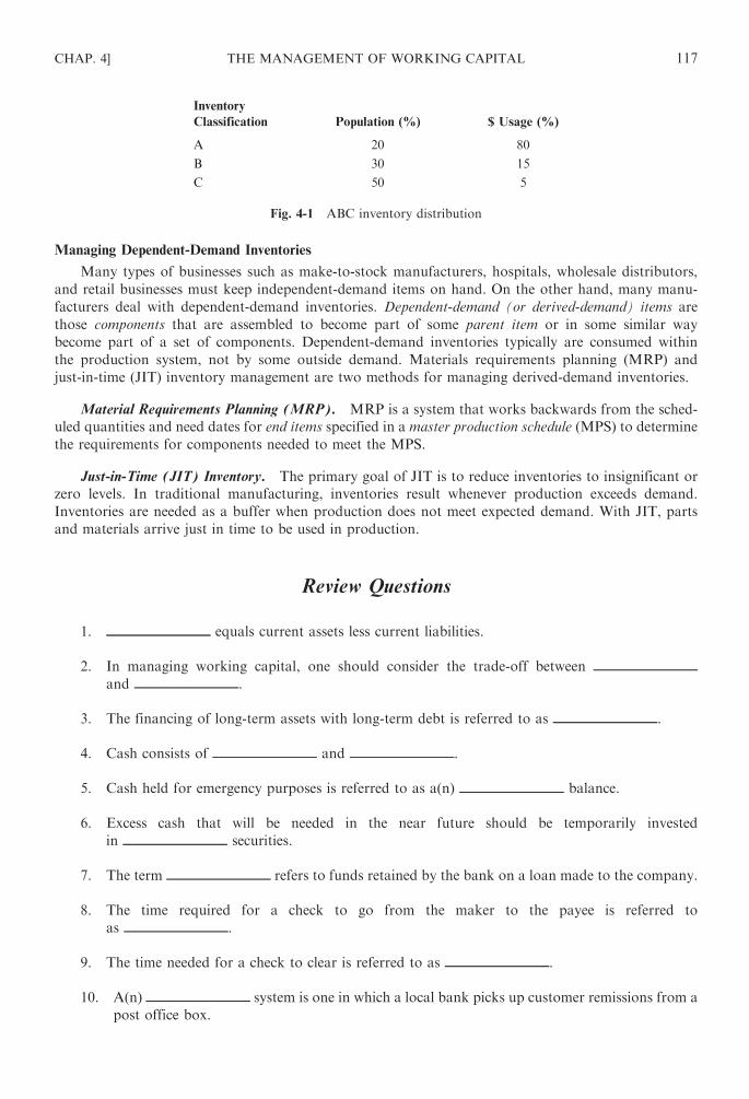
Managing Dependent-Demand Inventories
Many types of businesses such as make-to-stock manufacturers, hospitals, wholesale distributors,
and retail businesses must keep independent-demand items on hand. On the other hand, many manu-
facturers deal with dependent-demand inventories. Dependent-demand (or derived-demand) items are
those components that are assembled to become part of some parent item or in some similar way
become part of a set of components. Dependent-demand inventories typically are consumed within
the production system, not by some outside demand. Materials requirements planning (MRP) and
just-in-time (JIT) inventory management are two methods for managing derived-demand inventories.
Material Requirements Planning (MRP). MRP is a system that works backwards from the sched-
uled quantities and need dates for end items specified in a master production schedule (MPS) to determine
the requirements for components needed to meet the MPS.
Just-in-Time (JIT) Inventory. The primary goal of JIT is to reduce inventories to insignificant or
zero levels. In traditional manufacturing, inventories result whenever production exceeds demand.
Inventories are needed as a buffer when production does not meet expected demand. With JIT, parts
and materials arrive just in time to be used in production.
Review Questions
1. equals current assets less current liabilities.
2. In managing working capital, one should consider the trade-off between
and .
3. The financing of long-term assets with long-term debt is referred to as .
4. Cash consists of and .
5. Cash held for emergency purposes is referred to as a(n) balance.
6. Excess cash that will be needed in the near future should be temporarily invested
in securities.
7. The term refers to funds retained by the bank on a loan made to the company.
8. The time required for a check to go from the maker to the payee is referred to
as .
9. The time needed for a check to clear is referred to as .
10. A(n) system is one in which a local bank picks up customer remissions from a
post office box.
Inventory
Classification Population (%) $ Usage (%)
A 20 80
B 30 15
C 50 5
Fig. 4-1 ABC inventory distribution
CHAP. 4] THE MANAGEMENT OF WORKING CAPITAL 117
11. is a system of collection in which a local bank receives funds and transfers
them to a main concentration bank account.
12. One way to defer a cash payment is by the use of a(n) , because the bank must
first secure approval from the company before the instrument is paid.
13. The terms of a $1,000 sale are 3/20, net/40. If collection is received in 14 days, the amount
received is $ .
14. Partially completed merchandise at year-end is referred to as inventory.
15. Inventory consisting of fashionable merchandise has high risk.
16. refers to the cost of holding inventory.
17. As the order size increases, carrying cost and ordering cost .
18. The optimum amount to order each time is referred to as the .
19. The optimum inventory level requiring a reorder of goods is referred to as the .
20. The method requires that greater control be exercised over higher-valued
merchandise.
Answers: (1) Net working capital; (2) risk, return; (3) hedging; (4) currency, demand deposits; (5) precau-
tionary; (6) marketable; (7) compensating balance; (8) mail float; (9) deposit collection float; (10) lock-
box; (11) Concentration banking; (12) draft; (13) 970; (14) work-in-process; (15) realization; (16) Carrying
cost; (17) increases, decreases; (18) economic order quantity (EOQ); (19) economic order point (EOP); (20)
ABC.
Solved Problems
4.1 Net Working Capital. Winston Corporation has the following selected assets and liabilities:
Cash $15,000
Accounts receivable $20,000
Inventory $37,000
Land $70,000
Building $190,000
Goodwill $26,000
Accounts payable $13,000
Salaries payable $7,000
Taxes payable $19,000
Mortgage payable $80,000
Common stock $100,000
Retained earnings $82,000
Determine the company’s net working capital.
118 THE MANAGEMENT OF WORKING CAPITAL [CHAP. 4

SOLUTION
CURRENT ASSETS
Cash $15,000
Accounts receivable 20,000
Inventory 37,000 $72,000
CURRENT LIABILITIES
Accounts payable $13,000
Salaries payable 7,000
Taxes payable 19,000 39,000
Net working capital $33,000
4.2 Delay in Cash Receipt. Blake Corporation receives average daily cash receipts of $140,000.
The finance manager has determined that the time period between the mailing of a check and
its actual availability for corporate use is 4 days. What is the amount of cash being tied up
because of the delay?
SOLUTION
4 days� $140; 000 ¼ $560,000
4.3 Float Measurement. On a typical day, ABC Company writes checks totaling $3,000. These checks
clear in 7 days. Simultaneously, the company receives $1,700. The cash is available in 2 days on
average. (1) Calculate the disbursement, the collection, and the net floats and (2) interpret the
result (CFM adapted).
SOLUTION
(1) The disbursement float is 7 days� $3,000=$21,000. The collection float is 2 days� (�$1,700)=� $3,400. The net float is $21,000+ (�3,400)=$17,600.
(2) At any given time, the firm typically has uncashed checks outstanding of $21,000. At the same
time, it has uncollected receipts of $3,400. Thus, the firm’s book balance is typically $17,600 less
than its available balance for a positive $17,600 net float.
4.4 Lockbox. It typically takes Lawrence Corporation 8 days to receive and deposit customer
remissions. Lawrence is considering a lockbox system and anticipates that the system will
reduce the float time to 5 days. Average daily cash receipts are $220,000. The rate of return is
10 percent.
(a) What is the reduction in cash balances associated with implementing the system? (b)
What is the rate of return associated with the earlier receipt of the funds? (c) What should be
the maximum monthly charge associated with the lockbox proposal?
SOLUTION
(a) $220,000� 3 days ¼ $660,000
(b) 0:10� $660,000 ¼ $66,000
(c) $66,000
12¼ $5,500
CHAP. 4] THE MANAGEMENT OF WORKING CAPITAL 119

4.5 Lockbox. Doral Corporation is considering a lockbox arrangement that will cost $216,000 per
year. Average daily collections are $450,000. As a result of the system, the float time will
be reduced by 3 days. The rate of return is 14 percent. Should the lockbox arrangement be
instituted?
SOLUTION
Cost $216,000
Return on freed cash (0.14� 3� $450,000) 189,000
Disadvantage of lockbox $ 27,000
The lockbox should not be used.
4.6 Dividing of Region. Boston Corporation has an arrangement with XYZ Bank in which the bank
handles $5 million a day in collections but requires a $420,000 compensating balance. The
company is considering withdrawing from the arrangement and dividing its southern region so
that two other banks will handle the business instead. Bank S will handle $3 million a day of
collections and require a $450,000 compensating balance, and bank T will handle the other $2
million a day and require a compensating balance of $350,000. By dividing the southern region,
collections will be accelerated by 12day. The rate of return is 17 percent. Should the southern
region be divided?
SOLUTION
Accelerated cash inflow $5 million per day� 12day $2,500,000
Incremental compensating balance required 380,000
Increased cash flow $2,120,000
Rate of return �0.17Net annual savings $ 360,400
Yes, the southern region should be divided, as doing so will save the company $360,400 per year.
4.7 Average Cash Balance. Dane Company’s weekly average cash balances are:
Week Average Cash Balance
1 $15,000
2 19,000
3 12,000
4 17,000
Total $63,000
(a) What is the monthly average cash balance? (b) Assuming an annual interest rate 15
percent, what is the monthly rate of return earned on the average cash balance?
SOLUTION
(a) $63,000
4¼ $15,750
(b) $15,750� 0:15� 12ð Þ ¼ $196:88
4.8 Book Balance versus Bank Balance. Company P writes checks averaging $30,000 per day that
require 4 days to clear. By what amount will its book balance be less than its bank balance?
120 THE MANAGEMENT OF WORKING CAPITAL [CHAP. 4

SOLUTION
$30,000� 4 days ¼ $120,000
4.9 Opportunity Cost of Not Taking Discount. What is the opportunity cost of not taking a discount
when the terms are 2/20, net/45?
SOLUTION
Opportunity cost ¼ discount percent
100� discount percent� 360
N¼ 2
98� 360
25¼ 29:4%
4.10 Baumol Model. The following formula is used in determining its optimal level of cash:
C ¼ffiffiffiffiffiffiffiffiffi
2bT
i
r
where b=the fixed cost of a transaction
T=the total cash needed for the time period involved
i=the interest rate on marketable securities
C=cash balance
C*=optimal level of cash
Assume that the fixed cost of selling marketable securities is $10 per transaction and the interest
rate on marketable securities is 6% per year. The company estimates that it will make cash
payments of $12,000 over a 1-month period. What is the average cash balance (rounded to the
nearest dollar)? (CFM adapted.)
SOLUTION
A model developed by William Baumol can determine the optimum amount of cash for a company to hold
under conditions of certainty. The objective is to minimize the sum of the fixed costs of transactions and the
opportunity cost (return forgone) of holding cash balances that do not yield a return. Substituting in the
formula as shown below yields an optimal cash balance of about $6,928. Thus, the average cash balance is
$3,464 ð$6,928� 2Þ:
C ¼ffiffiffiffiffiffiffiffi
2bT
i
r
¼
ffiffiffiffiffiffiffiffiffiffiffiffiffiffiffiffiffiffiffiffiffiffiffiffiffiffiffiffiffiffiffiffi
2ð$10Þð$12,000Þ5%=12 months
s
¼ $6,928
4.11 Optimal Cash Balance. Green Corporation anticipates a cash requirement of $1,000 over a 1-
month period. It is expected that cash will be paid uniformly. The annual interest rate is 24
percent. The transaction cost of each borrowing or withdrawal is $30. (a) What is the optimal
cash balance? (b) What is the average cash balance?
SOLUTION
(a) The optimum cash balance is:
C ¼ffiffiffiffiffiffiffiffi
2bT
i
r
¼ffiffiffiffiffiffiffiffiffiffiffiffiffiffiffiffiffiffiffiffiffiffiffiffiffi
2 30ð Þ 1,000ð Þ0:24� 12a
r
¼ffiffiffiffiffiffiffiffiffiffiffiffiffiffi
60,000
0:02
r
¼ $1,732:05
(b) The average cash balance is:
C
2¼ $1,732:05
2¼ $866:03
a Monthly interest rate ¼ 0:24 annual interest rate
12 months¼ 0:02
CHAP. 4] THE MANAGEMENT OF WORKING CAPITAL 121
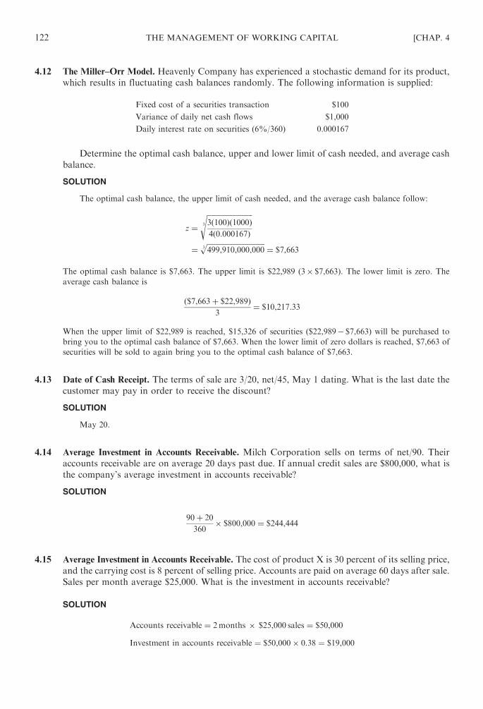
4.12 The Miller–Orr Model. Heavenly Company has experienced a stochastic demand for its product,
which results in fluctuating cash balances randomly. The following information is supplied:
Fixed cost of a securities transaction $100
Variance of daily net cash flows $1,000
Daily interest rate on securities (6%/360) 0.000167
Determine the optimal cash balance, upper and lower limit of cash needed, and average cash
balance.
SOLUTION
The optimal cash balance, the upper limit of cash needed, and the average cash balance follow:
z ¼
ffiffiffiffiffiffiffiffiffiffiffiffiffiffiffiffiffiffiffiffiffiffiffiffiffiffi
3 100ð Þ 1000ð Þ4 0:000167ð Þ
3
s
¼ffiffiffiffiffiffiffiffiffiffiffiffiffiffiffiffiffiffiffiffiffiffiffiffiffiffiffiffiffiffiffiffiffi
499,910,000,0003p
¼ $7,663
The optimal cash balance is $7,663. The upper limit is $22,989 (3� $7,663). The lower limit is zero. The
average cash balance is
$7,663þ $22,989ð Þ3
¼ $10,217:33
When the upper limit of $22,989 is reached, $15,326 of securities ($22,989� $7,663) will be purchased to
bring you to the optimal cash balance of $7,663. When the lower limit of zero dollars is reached, $7,663 of
securities will be sold to again bring you to the optimal cash balance of $7,663.
4.13 Date of Cash Receipt. The terms of sale are 3/20, net/45, May 1 dating. What is the last date the
customer may pay in order to receive the discount?
SOLUTION
May 20.
4.14 Average Investment in Accounts Receivable. Milch Corporation sells on terms of net/90. Their
accounts receivable are on average 20 days past due. If annual credit sales are $800,000, what is
the company’s average investment in accounts receivable?
SOLUTION
90þ 20
360� $800,000 ¼ $244,444
4.15 Average Investment in Accounts Receivable. The cost of product X is 30 percent of its selling price,
and the carrying cost is 8 percent of selling price. Accounts are paid on average 60 days after sale.
Sales per month average $25,000. What is the investment in accounts receivable?
SOLUTION
Accounts receivable ¼ 2months � $25,000 sales ¼ $50,000
Investment in accounts receivable ¼ $50,000� 0:38 ¼ $19,000
122 THE MANAGEMENT OF WORKING CAPITAL [CHAP. 4
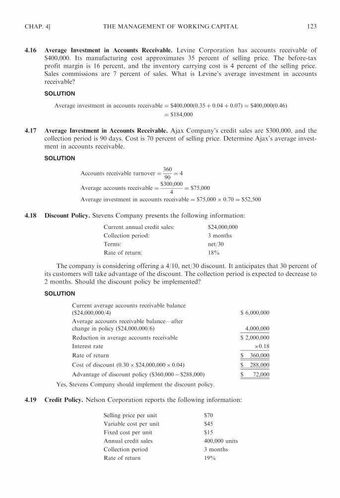
4.16 Average Investment in Accounts Receivable. Levine Corporation has accounts receivable of
$400,000. Its manufacturing cost approximates 35 percent of selling price. The before-tax
profit margin is 16 percent, and the inventory carrying cost is 4 percent of the selling price.
Sales commissions are 7 percent of sales. What is Levine’s average investment in accounts
receivable?
SOLUTION
Average investment in accounts receivable ¼ $400,000 0:35þ 0:04þ 0:07ð Þ ¼ $400,000 0:46ð Þ¼ $184,000
4.17 Average Investment in Accounts Receivable. Ajax Company’s credit sales are $300,000, and the
collection period is 90 days. Cost is 70 percent of selling price. Determine Ajax’s average invest-
ment in accounts receivable.
SOLUTION
Accounts receivable turnover ¼ 360
90¼ 4
Average accounts receivable ¼ $300,000
4¼ $75,000
Average investment in accounts receivable ¼ $75,000� 0:70 ¼ $52,500
4.18 Discount Policy. Stevens Company presents the following information:
Current annual credit sales: $24,000,000
Collection period: 3 months
Terms: net/30
Rate of return: 18%
The company is considering offering a 4/10, net/30 discount. It anticipates that 30 percent of
its customers will take advantage of the discount. The collection period is expected to decrease to
2 months. Should the discount policy be implemented?
SOLUTION
Current average accounts receivable balance
($24,000,000/4) $ 6,000,000
Average accounts receivable balance—after
change in policy ($24,000,000/6) 4,000,000
Reduction in average accounts receivable $ 2,000,000
Interest rate �0.18Rate of return $ 360,000
Cost of discount (0.30� $24,000,000� 0.04) $ 288,000
Advantage of discount policy ($360,000� $288,000) $ 72,000
Yes, Stevens Company should implement the discount policy.
4.19 Credit Policy. Nelson Corporation reports the following information:
Selling price per unit $70
Variable cost per unit $45
Fixed cost per unit $15
Annual credit sales 400,000 units
Collection period 3 months
Rate of return 19%
CHAP. 4] THE MANAGEMENT OF WORKING CAPITAL 123

The company is considering easing its credit standards. If it does, the following is expected to
result: Sales will increase by 25 percent; collection period will increase to 4 months; bad debt
losses are anticipated to be 4 percent on the incremental sales; and collection costs will increase by
$34,000.
Should the proposed relaxation in credit standards be implemented?
SOLUTION
Incremental profitability:
Increased unit sales (400,000� 0.25) 100,000
Contribution margin per unit ($70� $45) �$25Incremental profit $2,500,000
Increased bad debts:
Incremental dollar sales (100,000� $70) $7,000,000
Uncollectibility percentage �0.04Additional bad debts $ 280,000
To determine the opportunity cost of the increased investment in accounts receivable, we first need to
calculate the new average unit cost, as follows:
Units Unit Cost Total Cost
Present 400,000 $60 $24,000,000
Increment 100,000 $45 4,500,000
Total 500,000 $28,500,000
New average unit cost ¼ $28,500,000
500,000¼ $57
Additional cost:
Investment in average accounts receivable
[(credit sales/turnover)� (unit cost/selling price)]
After change in policy
[($35,000,000/3)� ($57/$70)] $9,500,000
Current
[($28,000,000/4)� ($60/$70)] 6,000,000
Incremental $3,500,000
Rate of return �0.19Opportunity cost $ 665,000
Net advantage/disadvantage of proposal:
Additional profitability $2,500,000
Less: Increased bad debts $280,000
Increased collection costs 34,000
Opportunity cost 665,000 979,000
Net advantage $1,521,000
Thus, the Nelson Corporation would benefit from relaxing its credit policy as proposed.
4.20 Credit Policy. Simon Corporation is evaluating a relaxation of its credit policy. At present, 70
percent of sales are on credit and there is a gross margin of 20 percent. Additional data are:
Current Anticipated
Sales $500,000 $640,000
Credit sales $410,000 $520,000
Collection expenses 3% of credit sales 4% of credit sales
Collection period 72 days 90 days
124 THE MANAGEMENT OF WORKING CAPITAL [CHAP. 4

Using 360 days in a year, answer the following questions: (a) What is the change in gross
profit associated with the proposal? (b) What is the incremental change in collection expenses? (c)
What is the change in average accounts receivable?
SOLUTION
(a) Incremental credit sales $110,000
Gross profit rate �0.20Increase in gross profit $ 22,000
(b) Collection expenses with proposal
(0.04� $520,000) $20,800
Collection expenses currently
(0.03� $410,000) 12,300
Increase in collection expenses $ 8,500
(c) Average accounts receivable after change in policy are:
Credit sales/accounts receivable turnover
($520,000/4) $130,000
Current average accounts receivable
($410,000/5) 82,000
Increase in average accounts receivable $ 48,000
4.21 Sales Campaign. Jones Corporation is considering a sales campaign in which it will offer credit
terms of 3/15, net/80. The finance manager expects that the collection period will increase from 90
days to 110 days. Information before and during the proposed campaign follows:
Percentage of Sales
before Campaign
Percentage of Sales
during Campaign
Cash sales 20 10
Payment from
1–15 35 25
16–120 45 65
The sales campaign is expected to raise sales from $5 million to $6 million. The gross profit
rate is 30 percent and the rate of return is 16 percent. Sales discounts are given on cash sales.
Should the sales campaign be initiated?
SOLUTION
Without Sales Campaign With Sales Campaign
Gross profit $1,500,000 $1,800,000
Sales subject to discount
0.55� $5,000,000 $2,750,000
0.35� $6,000,000 $2,100,000
Sales discount �0.03 �82,500 �0.03 �63,000Investment in average accounts
receivable
(90/360)� $5,000,000� 0.7 $ 875,000
(110/360)� $6,000,000� 0.7 $1,283,333
Rate of return �0.16 �140,000 �0.16 �205,333Net profit $1,277,500 $1,531,667
The sales campaign should be implemented because it results in an incremental profit of $254,167.
CHAP. 4] THE MANAGEMENT OF WORKING CAPITAL 125

4.22 Credit Policy. Wilder Corporation is considering granting credit to currently limited customers or
no-credit customers. The following information is given:
Category
Bad Debt
Percentage
Collection
Period Credit Terms
Incremental Annual Sales
Accompanying
Relaxation in Credit
Standards ($)
A 3 20 days Full 250,000
B 6 45 days Restricted 540,000
C 10 90 days No credit 800,000
Gross profit approximates 12 percent of sales. The rate of return is 18 percent.
Should credit be extended to categories B and C?
SOLUTION
Category B Category C
Gross profit
$540,000� 0.12
$800,000� 0.12 $64,800 $96,000
Less: Increased bad debts
$540,000� 0.06 �32,400$800,000� 0.10 �80,000
Incremental investment in average
accounts receivable
(45/360)� 0.88� $540,000 $59,400
(90/360)� 0.88� $800,000 $176,000
Rate of return �0.18 �0.18Opportunity cost �10,692 �31,680
Net profit $21,708 �$15,680
Credit should be extended only to category B.
4.23 Materials Cost. Grason Corporation purchases 3,000 units of a raw material at a list price of $5
each. The supplier offers a quantity discount of 4 percent. What is the material cost of the item?
SOLUTION
Acquisition cost (3,000� $5) $15,000
Less: Discount (0.04� $15,000) 600
Net cost $14,400
4.24 Average Investment in Inventory. West Corporation orders 4,000 units of a product at the begin-
ning of the period for $7 each. What is West Corporation’s average investment in inventory?
SOLUTION
Average inventory (Q/2=4,000/2) 2,000 units
Unit cost ($) �7Average investment $14,000
4.25 Ordering Cost. Charles Corporation uses 8,500 units per year. Each order is for 200 units. The
cost per order is $13. What is the total ordering cost for the year?
126 THE MANAGEMENT OF WORKING CAPITAL [CHAP. 4

SOLUTION
8,500
200� $13 ¼ $552:50
4.26 Economic Order Quantity. Luster Corporation presents the following data: Usage is 400 units per
month, cost per order is $20, and carrying cost per unit is $6.
Given these data, answer the following questions: (a) What is the economic order quantity?
(b) How many orders are required each month? (c) How often should each order be placed?
SOLUTION
(a) EOQ ¼ffiffiffiffiffiffiffiffiffi
2SP
C
r
¼ffiffiffiffiffiffiffiffiffiffiffiffiffiffiffiffiffiffiffiffiffi
2 400ð Þ 20ð Þ6
r
¼ffiffiffiffiffiffiffiffiffiffiffiffiffiffi
16,000
6
r
¼ 52 ðroundedÞ
(b)S
EOQ¼ 400
52¼ 8 roundedð Þ
(c)31
8¼ every 4 days
4.27 Stockout Cost. Boston Corporation uses 30,000 units. Each order placed is for 1,500 units. The
stockout units is 300. Management is willing to accept a stockout probability of 40 percent.
The stockout cost per unit is $3.20. What is the total stockout cost?
SOLUTION
Stockout cost ¼ usage
order quantity� stockout units� unit stockout cost� probability of stockout
¼ 30,000
1,500� 300� $3:20� 0:4 ¼ $7,680
4.28 Economic Order Point. Met Corporation reports the following data regarding one of its
inventory items: Usage is 5,000 units per month, EOQ is units, and lead time is 12month.
The stockout acceptance factor is 1.29, which represents an acceptable stockout percentage of
10 percent.
Determine the economic order point.
SOLUTION
EOP ¼ SLþ zffiffiffiffiffiffiffiffiffiffiffiffiffiffiffiffiffiffiffiffiffiffiffiffi
S EOQð Þ Lð Þp
¼ 5,000ð Þ 12
� �
þ 1:29
ffiffiffiffiffiffiffiffiffiffiffiffiffiffiffiffiffiffiffiffiffiffiffiffiffiffiffi
5,000 100ð Þ 12
� �
q
¼ 2,500þ 1:29ffiffiffiffiffiffiffiffiffiffiffiffiffiffiffiffi
250,000p
¼ 2,500þ 1:29 500ð Þ ¼ 3,145
4.29 Inventory Management. XYZ Appliance Store sells an average of 160 units per month. Each
order the store places is for 300 units. The cost per unit is $5. The cost per order is $12.
Carrying cost is $0.15 per dollar invested per year. The rate of return is 18 percent. The tax
rate is 46 percent.
CHAP. 4] THE MANAGEMENT OF WORKING CAPITAL 127
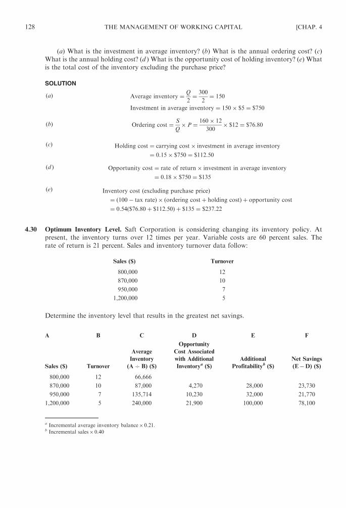
(a) What is the investment in average inventory? (b) What is the annual ordering cost? (c)
What is the annual holding cost? (d ) What is the opportunity cost of holding inventory? (e) What
is the total cost of the inventory excluding the purchase price?
SOLUTION
(a) Average inventory ¼ Q
2¼ 300
2¼ 150
Investment in average inventory ¼ 150� $5 ¼ $750
(b) Ordering cost ¼ S
Q� P ¼ 160� 12
300� $12 ¼ $76:80
(c) Holding cost ¼ carrying cost� investment in average inventory
¼ 0:15� $750 ¼ $112:50
(d ) Opportunity cost ¼ rate of return� investment in average inventory
¼ 0:18� $750 ¼ $135
(e) Inventory cost excluding purchase priceð Þ¼ 100� tax rateð Þ � ordering costþ holding costð Þ þ opportunity cost
¼ 0:54 $76:80þ $112:50ð Þ þ $135 ¼ $237:22
4.30 Optimum Inventory Level. Saft Corporation is considering changing its inventory policy. At
present, the inventory turns over 12 times per year. Variable costs are 60 percent sales. The
rate of return is 21 percent. Sales and inventory turnover data follow:
Sales ($) Turnover
800,000 12
870,000 10
950,000 7
1,200,000 5
Determine the inventory level that results in the greatest net savings.
A B C D E F
Sales ($) Turnover
Average
Inventory
(A7B) ($)
Opportunity
Cost Associated
with Additional
Inventorya ($)
Additional
Profitabilityb ($)
Net Savings
(E�D) ($)
800,000 12 66,666
870,000 10 87,000 4,270 28,000 23,730
950,000 7 135,714 10,230 32,000 21,770
1,200,000 5 240,000 21,900 100,000 78,100
a Incremental average inventory balance� 0.21.b Incremental sales� 0.40
128 THE MANAGEMENT OF WORKING CAPITAL [CHAP. 4

The inventory level that results in the greatest net savings is 240,000 units.
4.31 Lockbox System. Tunequip, Inc., is a wholesale distributor of specialized audio equipment,
tapes, and records. Annual sales are projected at $27 million for the 20X1 fiscal year, and the
average accounts receivable balance is estimated at $2.5 million. The average invoice size is
$1,000. Customers pay their accounts by check, which are mailed to corporate headquarters in
Florida.
The finance manager of Tunequip is examining the firm’s cash-handling techniques to find
ways to reduce borrowing requirements and financing costs. One alternative under consideration
is the establishment of a lockbox system to handle collections from customers in the western
United States, Those customers are expected to account for $10.8 million of Tunequip’s total
projected sales in 20X1. Tunequip could acquire the use of the funds a day earlier if the western
customers mailed their checks to a post office box in Utah. The Utah National Bank would
process the payments mailed to the post office box; they would deposit the checks in Tunequip’s
account in Utah National, wire transfer the money to the Florida National Bank (Tunequip’s
primary bank), and send the payment information by mail. Utah National Bank’s charge for
operating the lockbox system would be a flat fee of $80 per month plus $0.10 for each paid invoice
handled; in addition the Utah bank would require Tunequip to maintain a $5,000 minimum cash
balance with the bank.
There would be no change in Tunequip’s relationship with Florida National Bank. The
finance manager estimates that Tunequip would be able to borrow funds from Florida
National Bank during 20X1 at an interest rate of 9 percent.
(a) If Tunequip, Inc., established the lockbox system for its western customers, calculate (1) the
annual cost of operating the lockbox system, and (2) the dollar amount of the change in the
level of accounts receivable and the reduction in borrowing which will result from this
system.
(b) What factors other than those referred to in (a) should Tunequip consider in its evaluation
of the lockbox system?
(c) Do your calculations support the establishment of a lockbox system for Tunequip’s western
customers? Explain your answer. (CMA, adapted.)
SOLUTION
(a) (1) The annual cost of operating the lockbox system is:
Estimated number of invoices ¼ western sales
average invoice size
¼ $10,800,000
$1,000=invoice¼ 10,800 invoices
Estimated handling fee (10,800� $0.10) $1,080
Fixed fee (12 months� $80) 960
Cost of compensating balance ($5,000� 0.09) 450
Estimated annual operating cost $2,490
(2) The use of the lockbox will permit Tunequip to acquire the use of the funds 1 day earlier. This
will have the effect of reducing the average accounts receivable by 1 day’s sales and reduce the
need for borrowing by the same amount. This amounts to $30,000 as is shown below.
Reduction in average accounts receivable ¼ western sales
days in year¼ $10,800,000
360¼ $30,000
CHAP. 4] THE MANAGEMENT OF WORKING CAPITAL 129

(b) Other factors to be considered when changing to the lockbox system include the following:
What is the cost of the wire transfers? Will there be a delay in recording receivables thus
affecting customer attitudes? Will customers be upset because their lockbox checks will be cashed
earlier? What is the impact of changes on costs on the main office? What other alternatives, such as
tightening credit terms and slowing payments, of cash management can be used to reduce borrowing
needs?
(c) The financial manager makes the following recommendation:
Reduction in borrowing $30,000
Interest rate 0.09
Annual savings $ 2,700
Estimated annual operating cost 2,490
Estimated savings $ 210
These projections give marginal support for the establishment of a lockbox because annual
savings exceed costs by $210. However, the other items outlined in (b) should be considered in arriving
at a final decision.
4.32 Credit Policy. The Heap Corporation finds itself with excess manufacturing capacity.
The company has lost a portion of its share of the market over the past several years. This,
in part, may be due to Heap having a more conservative credit policy than is common in the
industry.
Heap
Corporation Industry
Terms 2/10, net/30 (%) 2/10, net/30 (%)
Credit granted as
percent of applicants
by credit class
A 100 100
B 100 100
C 25 70
D 11 40
E 2 20
F 0 5
Average collection period 30 days 60 days
The vice-president for finance recommends that Heap Corporation relax its credit
standards, with the expectation that sales and profitability will increase. Staff studies show
that credit sales can be expected to increase to $92 million, bad debt losses will be
approximately $2.4 million, inventory will need to be increased by $5.67 million, and
average collection of accounts receivable will be 60 days. The 20X2 Heap income statement is
given below.
130 THE MANAGEMENT OF WORKING CAPITAL [CHAP. 4

Heap Corporation
Income Statement
(in Thousands of Dollars)
For Year Ended December 31, 20X2
Revenue
Credit sales $ 72
Cash sales 8 $80
Costs and other charges
Manufacturing expensesa $57.4
Administrative expensesb 3.0
Selling expensesc 9.6 70
Net income before taxes $10
Federal income tax 5
Net income $ 5
aMaterials and supplies $ 10.0
Labor 40.0
Fixed overhead 7.4
$57.4bAll fixed $ 3.0cSelling expenses
Variable expense $ 8.0
Bad debt loss estimate 1.6
$ 9.6
(a) Estimate the accounts receivable balance at December 31, 20X2. (b) Assuming total assets at
December 31, 20X2 equal 40 million dollars: (1) What is Heap Corporation’s return on corporate assets?
(2) What is the asset turnover? (c) What profit margin will Heap Corporation earn if the predictions are
correct? (d ) What return should be expected on corporate assets if the policy is adopted and the predictions
are correct? (e) Will the company be better off financially if the proposed change in credit policy is made?
Explain your answer. (CMA, adapted.)
SOLUTION
(a) Credit sales $72,000,000
Allowance for bad debts $ 1,600,000
Net credit sales $70,400,000
Average collection period 30 days
Accounts receivable turnover 12 times
Net receivables balance; December 31; 20X2 ¼ $70,400,000
12¼ $5,866,667
(b) (1) Return on corporate assets ¼ net income
total assets¼ 5,000,000
40,000,000¼ 12:5%
CHAP. 4] THE MANAGEMENT OF WORKING CAPITAL 131

(2) Asset turnover ¼ sales
assets¼ 80,000,000
40,000,000¼ 2
(c) Heap Corporation
Pro Forma Income Statement
(in Millions of Dollars)
For Year Ended December 31, 20X2
Credit sales $92.00
Cash sales 8.00 $100.00
Manufacturing expense
Materials and supplies $12.50
Labor 50.00
Fixed overhead 7.40 $69.90
Administrative expense 3.00
Selling expense
Variable $10.00
Bad debt loss estimate 2.40 12.40 85.30
Net income before taxes $ 14.70
Federal income tax 7.35
Net income $ 7.35
(d )
Total assets
Prior assets $40,000,000
Increase in receivablesa 9,066,666
Increase in inventory 5,670,000
$54,736,666
a $92,000,000 credit salesð Þ2,400,00
89,600,000
bad debtð Þnet credit salesð Þ
360
60¼ 6 receivable turnoverð Þ
$89; 600; 000
6¼ $14,933,333
Change in receivables ¼ $14,933,333� $5,866,667 ¼ $9,066,666
Return on assets ¼ $7,350,000
$54,736,666¼ 13:4%
(e) Since the overall return on assets has increased after the credit policy change, the company may be
considered to be in better financial condition. However, it should be noted that the nature and cost
of financing the current asset expansion have not been considered. If the incremental financing is
available only at a comparatively high cost, the change in credit policy may not be desirable.
132 THE MANAGEMENT OF WORKING CAPITAL [CHAP. 4

Chapter 5
Short-term Financing
5.1 INTRODUCTION
This chapter discusses the advantages and disadvantages of the various short-term financing sources.
‘‘Short term’’ refers to financing that will be repaid in 1 year or less. Short-term financing may be used to
meet seasonal and temporary fluctuations in a company’s funds position as well as to meet permanent
needs of the business. For example, short-term financing may be used to provide extra net working
capital, finance current assets, or provide interim financing for a long-term project.
When compared to long-term financing, short-term financing has several advantages; for example,
it is easier to arrange, it is less expensive, and it affords the borrower more flexibility. The drawbacks
of short-term financing are that interest rates fluctuate more often, refinancing is frequently needed,
and delinquent repayment may be detrimental to the credit rating of a borrower who is experiencing
a liquidity problem.
The sources of short-term financing are trade credit, bank loans, bankers’ acceptances, finance
company loans, commercial paper, receivable financing, and inventory financing.
The merits of the different alternative sources of short-term financing are usually considered care-
fully before a firm borrows money. The factors bearing upon the selection of the source of short-term
financing include:
1. Cost.
2. Effect on credit rating. Some sources of short-term financing may negatively affect the firm’s
credit rating.
3. Risk. The firm must consider the reliability of the source of funds for future borrowing.
4. Restrictions. Certain lenders may impose restrictions, such as requiring a minimum level of net
working capital.
5. Flexibility. Certain lenders are more willing than others to work with the borrower, for example,
to periodically adjust the amount of funds needed.
6. Expected money market conditions.
7. The inflation rate.
8. Corporate profitability and liquidity positions.
9. The stability of the firm’s operations.
5.2 TRADE CREDIT
Trade credit (accounts payable) refers to balances owed to suppliers. It is a spontaneous financing
source since it comes from normal business operations. Trade credit is the least expensive form of financing
inventory. The benefits of trade credit are: It is readily available, since suppliers want business; collateral is
not required; interest is typically not demanded or, if so, the amount is minimal; it is convenient; and trade
creditors are frequently lenient in the event of corporate financial problems. A company having liquidity
problems may stretch its accounts payable; however, among the disadvantages of doing so are the giving
up of any cash discount offered and the probability of lowering the firm’s credit rating.
EXAMPLE 5.1 Tristar Corporation purchases $475 worth of merchandise per day from suppliers. The terms of
purchase are net/45, and the company pays on time. How much is Tristar’s accounts payable balance?
$475 per day� 45 days ¼ $21,375
133
Copyright © 2007, 1998, 1986 by The McGraw-Hill Companies, Inc. Click here for terms of use.

5.3 BANK LOANS
To be eligible for a bank loan, a company must have sufficient equity and good liquidity. When
a short-term bank loan is taken, the debtor usually signs a note, which is a written statement that
the borrower agrees to repay the loan at the due date. A note payable may be paid at maturity or
in installments.
Bank loans are not spontaneous financing as is trade credit. Borrowers must apply for loans, and
lenders must grant them. Without additional funds, a firm may have to restrict its plans; therefore, as a
company’s need for funds changes, it alters its borrowings from banks. One example is a self-liquidating
(seasonal) loan which is used to pay for a temporary increase in accounts receivable or inventory.
As soon as the assets realize cash, the loan is repaid.
Loans, of course, earn interest, and the prime interest rate is the lowest interest rate applied to short-
term loans from a bank. Banks charge only their most creditworthy clients the prime rate; other
borrowers are charged higher interest rates.
Bank financing may take any of the following forms:
1. Unsecured loans
2. Secured loans
3. Lines of credit
4. Installment loans
Unsecured Loans
Most short-term unsecured loans are self-liquidating. This kind of loan is recommended for use
by companies with excellent credit ratings for financing projects that have quick cash flows. They are
appropriate when the firm must have immediate cash and can either repay the loan in the near future or
quickly obtain longer-term financing. The disadvantages of this kind of loan are that, because it is made
for the short term, it carries a higher interest rate than a secured loan and payment in a lump sum
is required.
Secured Loans
If a borrower’s credit rating is deficient, the bank may lend money only on a secured basis, that is,
with some form of collateral behind the loan. Collateral may take many forms including inventory,
accounts receivable, or fixed assets. In some cases, even though the company is able to obtain an
unsecured loan, it may still give collateral in exchange for a lowest interest rate.
Lines of Credit
Under a line of credit, the bank agrees to lend money to the borrower on a recurring basis up to a
specified amount. Credit lines are typically established for a 1-year period and may be renewed annually.
Construction companies often use such an arrangement because they usually receive only minimal
payments from their clients during construction, being compensated primarily at the end of a job.
The advantages of a line of credit for a company are the easy and immediate access to funds during
tight money market conditions and the ability to borrow only as much as needed and repay immediately
when cash is available. The disadvantages relate to the collateral requirements and the additional
financial information that must be presented to the bank. Also, the bank may place restrictions upon
the company, such as ceiling on capital expenditures or the maintenance of a minimum level of working
capital. Further, the bank will charge a commitment fee on the amount of the unused credit line.
When a company borrows under a line of credit, it may be required to maintain a deposit with
the bank that does not earn interest. This deposit is referred to as a compensating balance and is stated
as a percentage of the loan. The compensating balance effectively increases the cost of the loan.
A compensating balance may also be placed on the unused portion of a line of credit, in which case
the interest rate would be reduced.
134 SHORT-TERM FINANCING [CHAP. 5

EXAMPLE 5.2 A company borrows $200,000 and is required to keep a 12 percent compensating balance. It also
has an unused line of credit in the amount of $100,000, for which a 10 percent compensating balance is required.
What amount is the maximum balance that the business must maintain?
ð$200,000� 0:12Þ þ ð$100,000� 0:10Þ ¼ $24,000þ $10,000 ¼ $34,000
The bank may test a borrower’s financial capability by requiring the borrower to ‘‘clean up,’’ that is,
repay the loan for a brief time during the year (e.g., for 1 month). A company that is unstable to repay a
short-term loan should probably finance with long-term funds. The payment shows the bank that the
loan is actually seasonal rather than permanent financing.
Installment Loans
An installment loan requires monthly payments. When the principal on the loan decreases
sufficiently, refinancing can take place at lower interest rates. The advantage of this kind of loan is
that it may be tailored to satisfy a company’s seasonal financing needs.
Computation of Interest
Interest on a loan may be paid either at maturity (ordinary interest) or in advance (discounting
the loan). When interest is paid in advance, the proceeds from the loan are reduced and the effective
(true) interest cost is increased.
EXAMPLE 5.3 Acme Company borrows $30,000 at 16 percent interest per annum and repays the loan 1 year
hence. The interest paid is $30,000� 0.16=$4,800. The effective interest rate is 16 percent.
EXAMPLE 5.4 Assume the same facts as in Example 5.3, except the note is discounted. The proceeds of this loan
are smaller than in the previous example.
Proceeds ¼ principal� interest ¼ $30,000� $4,800 ¼ $25,200
The true interest rate for this discounted loan is:
Effective interest rate ¼ interest
proceeds¼ $4,800
$25,000¼ 19%
EXAMPLE 5.5 Prestige Bank will give a company a 1-year loan at an interest rate of 20 percent payable
at maturity, while Heritage Bank will lend on a discount basis at a 19 percent interest rate. Which bank charges
the lowest effective rate?
Prestige Bank 20%
Heritage Bank19%
81%¼ 23:5%
The loan from Prestige Bank has the better interest rate.
When a loan has a compensating balance requirement associated with it, the proceeds received by
the borrower are decreased by the amount of the balance. The compensating balance will increase the
effective interest rate.
EXAMPLE 5.6 The effective interest rate associated with a 1-year, $600,000 loan that has a nominal interest rate of
19 percent, with interest due at maturity and requiring a 15 percent compensating balance is computed as follows:
Effective interest rate ðwith compensating balanceÞ ¼ interest rate� principal
proceeds, %� principal
¼ 0:19� $600,000
ð1:00� 0:15Þ � $600,000¼ $114,000
$510,000¼ 22:4%
CHAP. 5] SHORT-TERM FINANCING 135

EXAMPLE 5.7 Assume the same facts as in Example 5.6, except that the loan is discounted. The effective interest
rate is:
Effective interest rate ðwith discountÞ ¼ interest rate� principal
ðproceeds, %� principalÞ � interest
¼ 0:19� $600,000
ð0:85� $600,000Þ � $114,000¼ $114,000
$396,000¼ 28:8%
EXAMPLE 5.8 Jones Company has a line of credit in the amount of $400,000 from its bank, but it must maintain
a compensating balance of 13 percent on outstanding loans and a compensating balance of 10 percent on the unused
credit. The interest rate on the loan is 18 percent. The company borrows $275,000. What is the effective interest rate
on the loan?
The required compensating balance is:
0:13� $275,000 $35,750
0:10� 125,000 12,500
$48,250
Effective interest rate ðwith line of creditÞ ¼ interest rate ðon loanÞ � principal
principal� compensating balance
¼ 0:18� $275,000
$275,000� $48,250¼ $49,500
$226,750¼ 21:8%
On an installment loan, the effective interest rate computation is more involved. Assuming a 1-year
loan is to be paid in equal monthly installments, the effective rate must be based on the average amount
outstanding for the year. The interest to be paid is computed on the face amount of the loan.
EXAMPLE 5.9 A company borrows $40,000 at an interest rate of 10 percent to be paid in 12 monthly installments.
The average loan balance is $40,000/2=$20,000. The effective interest rate is $4,000/$20,000=20%.
EXAMPLE 5.10 Assume the same facts as in Example 5.9, except that the loan is discounted. The interest of
$4,000 is deducted in advance so the proceeds received are $40,000� $4,000=$36,000. The average loan balance
is $36,000/2=$18,000. The effective interest rate is $4,000/$18,000=22.2%.
5.4 BANKERS’ ACCEPTANCES
A banker’s acceptance is a draft, drawn by an individual and accepted by a bank, that orders
payment to a third party at a later date. The creditworthiness of the draft is of good quality because
it has the backing of the bank, not the drawer. It is, in essence, a debt instrument created by the
creditor out of a self-liquidating business transaction. Bankers’ acceptances are often used to
finance the shipment and handling of both domestic and foreign merchandise. Acceptances are classed
as short-term financing because they typically have maturities of less than 180 days.
EXAMPLE 5.11 A United States oil refiner arranges with its United States commercial bank for a letter of credit
to a Saudi Arabian exporter with whom the United States refiner has undertaken a transaction. The letter of credit
provides the information regarding the shipment and states that the exporter can draw a time draft for a given
amount on the United States bank. Because of the letter of credit, the exporter draws a draft on the bank and
negotiates it with a local Saudi Arabian bank, receiving immediate payment. The Saudi Arabian bank sends the
draft to the United States bank and when the latter accepts the draft, there is an acceptance to meet the obligation on
the maturity date.
136 SHORT-TERM FINANCING [CHAP. 5
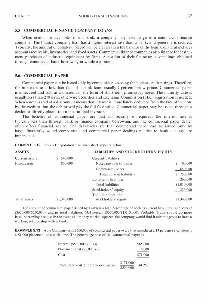
5.5 COMMERCIAL FINANCE COMPANY LOANS
When credit is unavailable from a bank, a company may have to go to a commercial finance
company. The finance company loan has a higher interest rate than a bank, and generally is secured.
Typically, the amount of collateral placed will be greater than the balance of the loan. Collateral includes
accounts receivable, inventories, and fixed assets. Commercial finance companies also finance the install-
ment purchases of industrial equipment by firms. A portion of their financing is sometimes obtained
through commercial bank borrowing at wholesale rates.
5.6 COMMERCIAL PAPER
Commercial paper can be issued only by companies possessing the highest credit ratings. Therefore,
the interest rate is less than that of a bank loan, usually 12percent below prime. Commercial paper
is unsecured and sold at a discount in the form of short-term promissory notes. The maturity date is
usually less than 270 days, otherwise Securities and Exchange Commission (SEC) registration is needed.
When a note is sold at a discount, it means that interest is immediately deducted from the face of the note
by the creditor, but the debtor will pay the full face value. Commercial paper may be issued through a
dealer or directly placed to an institutional investor.
The benefits of commercial paper are that no security is required, the interest rate is
typically less than through bank or finance company borrowing, and the commercial paper dealer
often offers financial advice. The drawbacks are that commercial paper can be issued only by
large, financially sound companies, and commercial paper dealings relative to bank dealings are
impersonal.
EXAMPLE 5.12 Travis Corporation’s balance sheet appears below.
ASSETS LIABILITIES AND STOCKHOLDERS’ EQUITY
Current assets $ 540,000 Current liabilities
Fixed assets 800,000 Notes payable to banks $ 100,000
Commercial paper 650,000
Total current liabilities $ 750,000
Long-term liabilities 260,000
Total liabilities $1,010,000
Stockholders’ equity 330,000
Total assets $1,340,000
Total liabilities and
stockholders’ equity $1,340,000
The amount of commercial paper issued by Travis is a high percentage of both its current liabilities, 86.7 percent
($650,000/$750,000), and its total liabilities, 64.4 percent ($650,000/$1,010,000). Probably Travis should do more
bank borrowing because in the event of a money market squeeze, the company would find it advantageous to have a
working relationship with a bank.
EXAMPLE 5.13 Able Company sells $500,000 of commercial paper every two months at a 13 percent rate. There is
a $1,000 placement cost each time. The percentage cost of the commercial paper is:
Interest ($500,000� 0.13) $65,000
Placement cost ($1,000� 6) 6,000
Cost $71,000
Percentage cost of commerical paper ¼ $ 71,000
$500,000¼ 14:2%
CHAP. 5] SHORT-TERM FINANCING 137

EXAMPLE 5.14 Ajax Corporation issues $300,000 worth of 18 percent, 90-day commercial paper. However, the
funds are needed for only 70 days. The excess funds can be invested in securities earning 17 percent. The brokerage
fee associated with the marketable security transaction is 1.5 percent. The dollar cost to the company in issuing the
commercial paper is:
Interest expense
[0.18� $300,000� (90/360)]
$13,500
Brokerage fee (0.015� $300,000) 4,500
Total cost $18,000
Less: Return on marketable securities
[0.17� $300,000� (20/360)] 2,833
Net cost $15,167
EXAMPLE 5.15 Charles Corporation anticipates it will need $500,000 cash for February 20X2 in order to
purchase inventory. There are three ways to finance this purchase, as follows:
(a) Set up a 1-year credit line for $500,000. The bank requires a 1 percent commitment fee. The interest rate
is 18 percent on borrowed funds. Funds are needed for 30 days.
(b) Do not take advantage of a 1/10, net/40 discount on a $500,000 credit purchase.
(c) Issue $500,000 of commercial paper for 30 days at 17 percent.
Which is the least expensive method of financing?
(a) Set up a credit line:
Commitment fee
[0.01� $500,000� (11/12)]
$ 4,583
Interest [0.18� $500,000� (1/12)] 7,500
$12,083
(b) Do not take advantage of discount:
0:01� $500,000 ¼ $5,000
(c) Issue commercial paper:
0:17� $500,000� ð1=12Þ ¼ $7,083
The financing with the least dollar cost is to not take the discount, as specified in (b).
5.7 RECEIVABLE FINANCING
Receivable financing has several advantages, including avoiding the need for long-term financing
and obtaining a recurring cash flow base. Accounts receivable financing has the drawback of high
administrative costs when there are many small accounts. However, with the use of computers these
costs can be curtailed.
Accounts receivable may be financed under either a factoring or assignment arrangement. Factoring
refers to the outright sale of accounts receivable to a bank or finance company without recourse.
The purchaser takes all credit and collection risks. The proceeds received by the selling company
are equal to the face value of the receivables less the commission charge, which is typically 2 to
4 percent higher than the prime interest rate. The cost of the factoring arrangement is the factor’s
commission for credit investigation, interest on the unpaid balance of advanced funds, and a discount
from the face value of the receivables where high credit risks exist. Remissions by customers are made
directly to the factor.
138 SHORT-TERM FINANCING [CHAP. 5
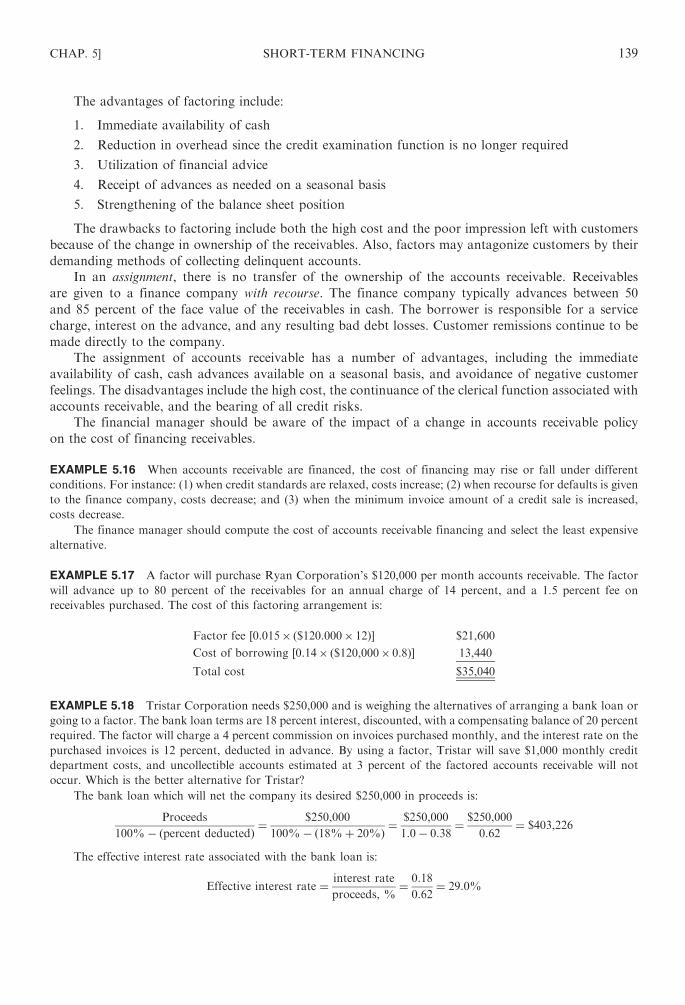
The advantages of factoring include:
1. Immediate availability of cash
2. Reduction in overhead since the credit examination function is no longer required
3. Utilization of financial advice
4. Receipt of advances as needed on a seasonal basis
5. Strengthening of the balance sheet position
The drawbacks to factoring include both the high cost and the poor impression left with customers
because of the change in ownership of the receivables. Also, factors may antagonize customers by their
demanding methods of collecting delinquent accounts.
In an assignment, there is no transfer of the ownership of the accounts receivable. Receivables
are given to a finance company with recourse. The finance company typically advances between 50
and 85 percent of the face value of the receivables in cash. The borrower is responsible for a service
charge, interest on the advance, and any resulting bad debt losses. Customer remissions continue to be
made directly to the company.
The assignment of accounts receivable has a number of advantages, including the immediate
availability of cash, cash advances available on a seasonal basis, and avoidance of negative customer
feelings. The disadvantages include the high cost, the continuance of the clerical function associated with
accounts receivable, and the bearing of all credit risks.
The financial manager should be aware of the impact of a change in accounts receivable policy
on the cost of financing receivables.
EXAMPLE 5.16 When accounts receivable are financed, the cost of financing may rise or fall under different
conditions. For instance: (1) when credit standards are relaxed, costs increase; (2) when recourse for defaults is given
to the finance company, costs decrease; and (3) when the minimum invoice amount of a credit sale is increased,
costs decrease.
The finance manager should compute the cost of accounts receivable financing and select the least expensive
alternative.
EXAMPLE 5.17 A factor will purchase Ryan Corporation’s $120,000 per month accounts receivable. The factor
will advance up to 80 percent of the receivables for an annual charge of 14 percent, and a 1.5 percent fee on
receivables purchased. The cost of this factoring arrangement is:
Factor fee [0.015� ($120.000� 12)] $21,600
Cost of borrowing [0.14� ($120,000� 0.8)] 13,440
Total cost $35,040
EXAMPLE 5.18 Tristar Corporation needs $250,000 and is weighing the alternatives of arranging a bank loan or
going to a factor. The bank loan terms are 18 percent interest, discounted, with a compensating balance of 20 percent
required. The factor will charge a 4 percent commission on invoices purchased monthly, and the interest rate on the
purchased invoices is 12 percent, deducted in advance. By using a factor, Tristar will save $1,000 monthly credit
department costs, and uncollectible accounts estimated at 3 percent of the factored accounts receivable will not
occur. Which is the better alternative for Tristar?
The bank loan which will net the company its desired $250,000 in proceeds is:
Proceeds
100%� ðpercent deductedÞ ¼$250,000
100%� ð18%þ 20%Þ ¼$250,000
1:0� 0:38¼ $250,000
0:62¼ $403,226
The effective interest rate associated with the bank loan is:
Effective interest rate ¼ interest rate
proceeds, %¼ 0:18
0:62¼ 29:0%
CHAP. 5] SHORT-TERM FINANCING 139

The amount of accounts receivable that should be factored to net the firm $250,000 is:
$250,000
1:0� 0:16¼ $250,000
0:84¼ $297,619
The total annual cost of the bank arrangement is:
Interest ($250,000� 0.29) $72,500
Additional cost of not using a factor:
Credit costs ($1,000� 12) 12,000
Uncollectible accounts ($297,619� 0.03) 8,929
Total cost $93,429
The effective interest rate associated with factoring accounts receivable is:
Effective interest rate ¼ interest rate
proceeds,%¼ 12%
100%� ð12%þ 4%Þ ¼0:12
0:84¼ 14:3%
The total annual cost of the factoring alternative is:
Interest ($250,000� 0.143) $35,750
Factoring ($297,619� 0.04) 11,905
Total cost $47,655
Factoring should be used since it will cost almost half as much as the bank loan.
EXAMPLE 5.19 System Corporation’s factor charges a 3 percent fee per month. The factor lends the firm up to
75 percent of receivables purchased for an additional 1 percent per month. The company’s credit sales are $400,000
per month. As a result of the factoring arrangement, the company saves $6,500 per month in credit costs and a bad
debt expense of 2 percent of credit sales.
XYZ Bank has offered an arrangement where it will lend the firm up to 75 percent of the receivables. The bank
will charge 2 percent per month interest plus a 4 percent processing charge on receivable lending.
The collection period is 30 days. If System Corporation borrows the maximum allowed per month, should
the firm stay with the factor or switch to XYZ Bank?
Cost of factor:
Purchased receivables (0.03� $400,000) $12,000
Lending fee (0.01� $300,000) 3,000
Total cost $15,000
Cost of bank financing:
Interest (0.20� $300,000) $ 6,000
Processing charge (0.04� $300,000) 12,000
Additional cost of not using the factor:
Credit costs 6,500
Bad debts (0.02� $400,000) 8,000
Total cost $32,500
System Corporation should stay with the factor.
EXAMPLE 5.20 Davis Company is considering a factoring arrangement. The company’s sales are $2,700,000,
accounts receivable turnover is 9 times, and a 17 percent reserve on accounts receivable is required by the factor.
The factor’s commission charge on average accounts receivable payable at the point of receivable purchase is
2.0 percent. The factor’s interest charge is 16 percent on receivable after subtracting the commission charge
140 SHORT-TERM FINANCING [CHAP. 5

and reserve. The interest charge reduces the advance. What is the annual effective cost under the factoring
arrangement?
Average accounts receivable ¼ credit sales
turnover¼ $2,700,000
9¼ $300,000
Davis will receive the following amount by factoring its accounts receivable:
Average accounts receivable $300,000
Less: Reserve ($300,000� 0.17) �51,000Commission ($300,000� 0.02) �6,000
Net prior to interest $243,000
Less: Interest [$243,000� (16%/9)] 4,320
Proceeds received $238,680
The annual cost of the factoring arrangement is:
Commission ($300,000� 0.02) $ 6,000
Interest [$243,000� (16%/9)] 4,320
Cost each 40 days (360/9) $10,320
Turnover � 9
Total annual cost $92,880
The annual effective cost under the factoring arrangement based on the amount received is:
Annual cost
Average amount received¼ $92,880
$238,680¼ 38:9%
5.8 INVENTORY FINANCING
Financing inventory typically occurs when a company has fully used its borrowing capacity on
receivables. Inventory financing requires the existence of marketable, nonperishable, and standardized
goods that have quick turnover. The merchandise should not be subject to rapid obsolescence. Good
collateral inventory is that which can be marketed apart from the borrower’s marketing organization.
Inventory financing should take into account the price stability of the inventory and the expenses
associated with selling it.
The disadvantages of inventory financing include the high interest rate and the restrictions on some
of the company’s inventory.
The vehicles of inventory financing include a floating (blanket) lien, warehouse receipt, and trust
receipt. In the case of a floating lien, the creditor’s security lies in the aggregate inventory rather than in
its components. Even though the borrower sells and restocks, the lender’s security interest continues.
With a warehouse receipt, the lender receives an interest in the borrower’s inventory stored at a public
warehouse; however, the fixed costs of this arrangement are quite high. There may be a field warehouse
arrangement where the warehouser sets up a secured area directly at the debtor’s location. The debtor
has access to the goods but must continually account for them. With a trust receipt loan, the creditor
has title to given goods but releases them to the borrower to sell on the creditor’s behalf. As goods are
sold, the borrower remits the funds to the lender. A good example of trust receipt use is in automobile
dealer financing. The drawback of the trust receipt arrangement is that a trust receipt must be given
for specific items.
A collateral certificate may be issued by a third party to the lender guaranteeing the existence
of pledged inventory. The advantage of a collateral certificate is flexibility since merchandise does not
have to be segregated or possessed by the lender.
CHAP. 5] SHORT-TERM FINANCING 141

EXAMPLE 5.21 Jackson Corporation wishes to finance its $500,000 inventory. Funds are needed for 3 months.
A warehouse receipt loan may be taken at 16 percent with a 90 percent advance against the inventory’s value.
The warehousing cost is $4,000 for the 3-month period. The cost of financing the inventory is:
Interest [0.16� 0.90� $500,000� (3/12)] $ 18,000
Warehousing cost 4,000
Total cost $22,0000
EXAMPLE 5.22 Hardy Corporation has been showing growth in its operations but is currently experiencing
liquidity problems. Six large financially sound companies are Hardy customers, being responsible for 75 percent
of Hardy’s sales. On the basis of the following information for 20X1, would Hardy Corporation be able to borrow
on receivables or inventory?
Balance sheet data are as follows:
ASSETS
Current assets
Cash $ 27,000
Receivables 380,000
Inventory (consisting of 55%
of work-in-process) 320,000
Total current assets $727,000
Fixed assets 250,000
Total assets $977,000
LIABILITIES AND
STOCKHOLDERS’ EQUITY
Current liabilities
Accounts payable $260,000
Loans payable 200,000
Accrued expenses 35,000
Total current liabilities $495,000
Bonds payable $110,000
Total liabilities $605,000
Stockholders’ equity
Common stock $250,000
Retained earnings 122,000
Total stockholders’ equity 372,000
Total liabilities and
stockholders’ equity $977,000
Selected income statement data are as follows:
Sales $1,800,000
Net income $ 130,000
Receivable financing can be expected since a high percentage of sales are made to only six large financially
healthy firms. Receivables will therefore show good collectibility. It is also easier to control a few large customer
accounts.
Inventory financing is not likely, due to the high percentage of partially completed items. Lenders are reluctant
to finance inventory when a large work-in-process balance exists since the goods will be difficult to further process
and sell by lenders.
142 SHORT-TERM FINANCING [CHAP. 5

5.9 OTHER ASSETS
Assets other than inventory and receivables may be used as security for short-term bank loans such
as real estate, plant and equipment, cash surrender value of life insurance policies, and securities. Also,
lenders are usually willing to advance a high percentage of the market value of bonds. The owner’s
personal assets may be pledged when the company’s financial position is very weak. In addition,
loans may be made based on a guaranty of a third party.
Review Questions
1. Short-term financing refers to the issuance of debt having a maturity of less
than .
2. Short-term financing makes the borrower more susceptible to fluctuations.
3. The least expensive source of short-term financing is .
4. Accounts payable is a(n) financing source.
5. Accounts payable should not be stretched too far because of a possible reduction in the
firm’s .
6. A note payable may be payable at or in .
7. loans are those in which the loan is paid as soon as the financed assets
realize cash.
8. The rate charged by banks to their best clients is called the interest rate.
9. loans require no collateral.
10. When a(n) is given, the bank agrees to lend the borrower money on a
continual basis up to a given amount.
11. A(n) refers to the deposit, which does not earn interest, that a company must
maintain at the bank as collateral for a loan.
12. In a(n) loan, monthly payments are required.
13. Interest on a loan may be paid at or .
14. When a loan is discounted, the interest rate will be higher.
15. A(n) is a draft drawn by an individual and accepted by the bank requiring
future payment to a third party.
16. The interest rate on is less than the interest rate on a bank loan.
17. The outright sale of accounts receivable to a third party is called .
CHAP. 5] SHORT-TERM FINANCING 143

18. In a(n) , accounts receivable are transferred to a third party with recourse.
19. In the case of inventory financing, a(n) lien applies to the aggregate
inventory rather than the components.
20. In a(n) loan, the creditor has title to goods but releases them to the borrower
to sell on the creditor’s behalf.
Answers: (1) 1 year; (2) interest rate; (3) trade credit; (4) spontaneous; (5) credit rating; (6) maturity, install-
ments; (7) Self-liquidating; (8) prime; (9) Unsecured; (10) line of credit; (11) compensating balance; (12)
installment; (13) maturity, in advance; (14) effective; (15) bankers’ acceptance; (16) commercial paper; (17)
factoring; (18) assignment; (19) floating (blanket); (20) trust receipt.
Solved Problems
5.1 Accounts Payable. James Corporation purchases $750 per day from suppliers on terms of net/30.
Determine the accounts payable balance.
SOLUTION
$750 per day� 30 days ¼ $22,500
5.2 Compensating Balance. Carl Corporation borrows $150,000 from a bank. A 10 percent
compensating balance is required. What is the amount of the compensating balance?
SOLUTION
$150,000� 0:10 ¼ $15,000
5.3 Compensating Balance. Wilson Company borrows $500,000 from the bank and is required
to maintain a 15 percent compensating balance. Further, Wilson has an unused line of
credit of $200,000, with a required 11 percent compensating balance. What is the total required
compensating balance the firm must maintain?
SOLUTION
ð$500,000� 0:15Þ þ ð$200,000� 0:11Þ ¼ $97,000
5.4 Effective Interest Rate. Charles Corporation borrows $70,000 at 19 percent annual interest.
Principal and interest is due in 1 year. What is the effective interest rate?
SOLUTION
The effective interest rate is 19 percent.
5.5 Proceeds of Loan. Assume the same information as in Problem 5.4, except that interest is
deducted in advance. (a) What is the amount of proceeds the company will receive at the time
of the loan? (b) What is the effective interest rate?
144 SHORT-TERM FINANCING [CHAP. 5

SOLUTION
(a) Interest ¼ $70,000� 0:19 ¼ $13,300
Proceeds ¼ principal� interest ¼ $70,000� $13,300 ¼ $56,700
(b)Effective interest rate ¼ interest
proceeds¼ $13,300
$56,700¼ 23:5%
5.6 Interest Cost. Ajax Corporation is deciding which of two banks to borrow from on a 1-year basis.
Bank A charges an 18 percent interest rate payable at maturity. Bank B charges a 17 percent
interest rate on a discount basis. Which loan is cheaper?
SOLUTION
Bank A 18%
Bank B17%
83%¼ 20:5%
Ajax should borrow from bank A since the effective interest rate is lower.
5.7 Effective Interest Rate. Tech Corporation takes out a $70,000 loan having a nominal interest rate
of 22 percent payable at maturity. The required compensating balance is 12 percent. What is the
effective interest rate?
SOLUTION
Effective interest rate ¼ interest rate
proceeds, %¼ 0:22
1:00� 0:12¼ 0:22
0:88¼ 25%
5.8 Effective Interest Rate. Assume the same information as in Problem 5.7 except that interest is
payable in advance. What is the effective interest rate?
SOLUTION
Effective rate ¼ interest rate
proceeds, %¼ 0:22
0:88� 0:22¼ 0:22
0:66¼ 33:3%
5.9 Effective Interest Rate and Compensating Balance. Wilson Corporation has a credit line
of $800,000. The compensating balance requirement on outstanding loans is 14 percent, and
8 percent on the unused credit line. The company borrows $500,000 at a 20 percent interest
rate. (a) What is the required compensating balance? (b) What is the effective interest rate?
SOLUTION
(a) The required compensating balance is:
Loan 0.14� $500,000 $70,000
Unused credit 0.08� $300,000 24,000
$94,000
(b)Effective interest rate ¼ interest
proceeds¼ 0:20� $500,000
$500,000� $94,000¼ $100,000
$406,000¼ 24:6%
CHAP. 5] SHORT-TERM FINANCING 145
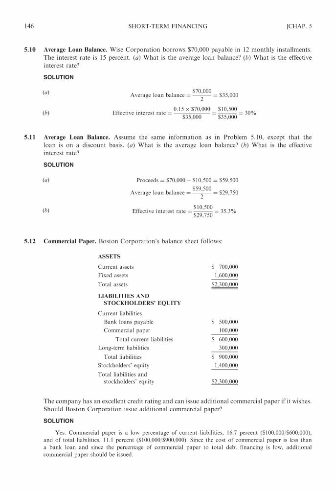
5.10 Average Loan Balance. Wise Corporation borrows $70,000 payable in 12 monthly installments.
The interest rate is 15 percent. (a) What is the average loan balance? (b) What is the effective
interest rate?
SOLUTION
(a)Average loan balance ¼ $70,000
2¼ $35,000
(b) Effective interest rate ¼ 0:15� $70,000
$35,000¼ $10,500
$35,000¼ 30%
5.11 Average Loan Balance. Assume the same information as in Problem 5.10, except that the
loan is on a discount basis. (a) What is the average loan balance? (b) What is the effective
interest rate?
SOLUTION
(a) Proceeds ¼ $70,000� $10,500 ¼ $59,500
Average loan balance ¼ $59,500
2¼ $29,750
(b) Effective interest rate ¼ $10,500
$29,750¼ 35:3%
5.12 Commercial Paper. Boston Corporation’s balance sheet follows:
ASSETS
Current assets $ 700,000
Fixed assets 1,600,000
Total assets $2,300,000
LIABILITIES AND
STOCKHOLDERS’ EQUITY
Current liabilities
Bank loans payable $ 500,000
Commercial paper 100,000
Total current liabilities $ 600,000
Long-term liabilities 300,000
Total liabilities $ 900,000
Stockholders’ equity 1,400,000
Total liabilities and
stockholders’ equity $2,300,000
The company has an excellent credit rating and can issue additional commercial paper if it wishes.
Should Boston Corporation issue additional commercial paper?
SOLUTION
Yes. Commercial paper is a low percentage of current liabilities, 16.7 percent ($100,000/$600,000),
and of total liabilities, 11.1 percent ($100,000/$900,000). Since the cost of commercial paper is less than
a bank loan and since the percentage of commercial paper to total debt financing is low, additional
commercial paper should be issued.
146 SHORT-TERM FINANCING [CHAP. 5

5.13 Cost of Commercial Paper. Nelson Corporation issues $800,000 of commercial paper every
3 months at a 16 percent rate. Each issuance involves a placement cost of $2,000. What is the
annual percentage cost of the commercial paper?
SOLUTION
Interest ($800,000� 0.16) $128,000
Placement cost ($2,000� 4) 8,000
Total cost $136,000
Cost of commercial paper ¼ $136,000
$800,000¼ 17:0%
5.14 Cost of Commercial Paper. Cho Corporation issues $500,000, 20 percent, 120-day commercial
paper. However, the funds are needed for only 90 days. The excess funds can be invested in
securities earning 19 percent. The brokerage fee for the marketable security transaction is 1.0
percent. What is the net cost to the company for issuing the commercial paper?
SOLUTION
Interest [0.20� $500,000� (120/360)] $33,333
Brokerage fee (0.01� $500,000) 5,000
Total cost $38,333
Less: Return on marketable securities
[0.19� $500,000� (30/360)]
7,917
Net cost $30,416
5.15 Financing Strategy. Johnson Company expects that it will need $600,000 cash for March 20X2.
Possible means of financing are: (a) Establish a 1-year credit line for $600,000. The bank requires
a 2 percent commitment fee. The interest rate is 21 percent. Funds are needed for 30 days. (b) Fail
to take a 2/10, net/40 discount on a $600,000 credit purchase. (c) Issue $600,000, 20 percent
commercial paper for 30 days. Which financing strategy should be selected?
SOLUTION
(a) The credit line cost is:
Commitment fee [0.02� $600,000� (11/12)] $11,000
Interest [0.21� $600,000� (1/12)] 10,500
Total cost $21,500
(b) The cost of not taking discount is:
0:02� $600,000 ¼ $12,000
(c) The cost of commercial paper is:
0:20� $600,000� 112¼ $10,000
Strategy (c) is best since issuance of commercial paper involves the least cost.
5.16 Cost of Accounts Receivable Financing.What is the effect of the following situations on the cost of
accounts receivable financing? (a) A more thorough credit check is undertaken. (b) Receivables
are sold without recourse. (c) The minimum invoice amount for a credit sale is decreased.
(d ) Credit standards are tightened.
CHAP. 5] SHORT-TERM FINANCING 147

SOLUTION
(a) Decrease (c) Increase
(b) Increase (d ) Decrease
5.17 Cost of Factoring. Drake Company is contemplating factoring its accounts receivable. The factor
will acquire $250,000 of the company’s accounts receivable every 2 months. An advance of
75 percent is given by the factor on receivables at an annual charge of 18 percent. There is a
2 percent factor fee associated with receivables purchased. What is the cost of the factoring
arrangement?
SOLUTION
Factor fee (0.02� $250,000� 6) $30,000
Cost of advance (0.18� $250,000� 0.75) 33,750
Total cost $63,750
5.18 Bank versus Factor. Forest Corporation needs $400,000 additional financing. The company is
considering the choice of financing with a bank or a factor. The bank loan carries a 20 percent
interest rate on a discount basis with a required compensating balance of 16 percent. The factor
charges a 3 percent commission on invoices purchased monthly. The interest rate associated with
these invoices is 11 percent with interest deductible in advance. If a factor is used, there will be
a monthly savings of $1,500 per month in credit department costs. Further, an uncollectible
accounts expense of 2 percent on the factored receivables will not exist.
(a) What amount of principal must the company borrow from the bank to receive $400,000
in proceeds? (b) What amount of accounts receivable must be factored to net the firm $400,000?
(c) What is the effective interest rate on the bank loan? (d ) What is the total annual cost of
the bank arrangement? (e) What is the effective interest rate associated with the factoring arrange-
ment? ( f ) What is the total annual cost of factoring?
SOLUTION
(a) Principal
Proceeds¼ 1:00
1:00� ð0:20þ 0:16ÞPrincipal
$400,000¼ 1
1:0� 0:36Therefore
$400,000
1:0� 0:36¼ $400,000
0:64¼ $625,000
(b) Accounts receivables to factor ¼ $400,000
1:0� 0:14¼ $400,000
0:86¼ $465,116
(c) Effective interest rate of bank loan ¼ interest rate
proceeds %¼ 0:20
0:64¼ 31:3%
(d ) The cost of the bank loan is:
Interest ($400,000� 0.313) $125,200
Credit costs ($1,500� 12) 18,000
Uncollectible accounts ($465,116� 0.02) 9,302
Total annual cost $152,502
(e) The effective interest rate of factoring is:
0:11
0:86¼ 12:8%
148 SHORT-TERM FINANCING [CHAP. 5

( f ) The cost of factoring is:
Interest ($400,000� 0.128) $51,200
Factoring ($465,116� 0.03) 13,953
Total annual cost $65,153
5.19 Bank versus Factor.Wayne Corporation’s factor charges a 4 percent monthly fee. The factor lends
Wayne up to 85 percent of receivables purchased for an additional 112percent per month. The
monthly credit sales are $350,000. With the factoring arrangement, there is a savings in corporate
credit checking costs of $4,200 per month and in bad debts of 3 percent on credit sales.
Trust Bank has offered to lend Wayne up to 85 percent of the receivables, at an interest
charge of 2.5 percent per month plus a 5 percent processing charge on receivable lending.
The collection period is 30 days, and Wayne borrows the maximum amount permitted each
month. Should Wayne Corporation accept the bank’s offer?
SOLUTION
Cost of factor:
Purchased receivables (0.04� $350,000) $14,000
Lending fee (0.015� $350,000� 0.85) 4,463
Total cost $18,463
Cost of bank financing:
Interest (0.025� $350,000� 0.85) $ 7,438
Processing charge (0.05� $350,000� 0.85) 14,875
Additional cost of not using factor
Credit costs 4,200
Bad debts (0.03�$350,000) 10,500
Total Cost $37,013
Wayne Corporation should stay with the factor, since the cost of the bank’s offer is more than twice the
cost of factoring.
5.20 Factoring Accounts Receivable. Grafton Corporation is considering factoring its accounts
receivable. Its sales are $3,600,000, and accounts receivable turnover is two times. The factor
requires: (1) an 18 percent reserve on accounts receivable; (2) a commission charge of 2.5 percent
on average accounts receivable, payable when receivables are purchased; and (3) an interest
charge of 19 percent on receivables after deducting the commission charge and reserve.
The interest charge reduces the advance.
Given the facts, answer the following questions: (a) What is the average accounts receivable?
(b) How much will Grafton receive by factoring its accounts receivable? (c) What is the annual
cost of the factoring arrangement? (d ) What is the effective annual cost of factoring?
SOLUTION
(a)Average accounts receivable ¼ credit sales
turnover¼ $3,600,000
2¼ $1,800,000
CHAP. 5] SHORT-TERM FINANCING 149

(b) The proceeds from factoring are:
Average accounts receivable $1,800,000
Less: Reserve ($1,800,000� 0.18) �324,000Commission ($1,800,000� 0.025) �45,000
Net prior to interest $1,431,000
Less: Interest [$1,431,000� (19%/2)] 135,945
Proceeds received $1,295,055
(c) The cost of factoring is:
Commission ($1,800,000� 0.025) $ 45,000
Interest [$1,431,000� (19%/2)] 135,945
Cost each 180 days (360/2) $180,945
Turnover � 2
Total annual cost $361,890
(d ) Effective annual cost of factoring ¼ annual cost
average amount received¼ $361,890
$1,295,055¼ 27:9%
5.21 Financing Cost of Inventory. Blake Company desires to finance its $300,000 inventory. Funds
are required for 4 months. Under consideration is a warehouse receipt loan at an annual interest
rate of 17 percent, with an 85 percent advance against the inventory’s value. The warehousing cost
is $5,000 for the 4-month period. Determine the financing cost.
SOLUTION
Interest [0.17� 0.85� $300,000� (4/12)] $14,450
Warehousing cost 5,000
Total cost $19,450
5.22 Receivable Financing or Inventory Financing. Large Corporation has liquidity problems. Most
of its sales are made to small customer accounts. Relevant balance sheet data for 20X1 are:
ASSETS
Current assets
Cash $ 35,000
Receivables 410,000
Inventory (primarily consisting
of finished goods and
raw materials) 360,00
Total current assets $ 805,000
Fixed assets 600,000
Total assets $1,405,000
150 SHORT-TERM FINANCING [CHAP. 5

LIABILITIES AND STOCKHOLDERS’ EQUITY
Current liabilities
Accounts payable $350,000
Loans payable 320,000
Accrued expenses 56,000
Total current liabilities $ 726,000
Bonds payable 225,000
Total liabilities $ 951,000
Stockholders’ equity
Common stock $300,000
Retained earnings
Total stockholders’ equity 154,000 454,000
Total liabilities and
stockholders’ equity $1,405,000
Relevant income statement data are:
Sales $2,400,000
Net income $480,000
Given the balance sheet and income statement data: (a) Is receivable financing likely? (b) Is
inventory financing likely?
SOLUTION
(a) No, receivable financing is not likely since receivables are made to many small customer accounts.
Control over receivables will therefore be a problem. (b) Yes, inventory financing is likely since inventory
consists of a large proportion of finished goods and raw materials which are readily saleable.
5.23 Cost of Issuing the Commercial Paper. Cartele, Inc., will need $4 million over the next year to
finance its short-term requirements. The company is considering financing alternatives—bank
financing and the sale of commercial paper.
Addison Union Bank is willing to loan Cartele the necessary funds providing the company
maintains a 20 percent compensating balance. The effective cost of the bank loan, considering the
compensating balance requirement, is 10.4 percent on a pretax basis.
Under the other alternative Cartele would sell $4 million of 90-day maturity commercial
paper every 3 months. The commercial paper will carry a rate of 734percent; the interest rate is
expected to remain at this level throughout the year. The commercial paper dealer’s fee to place
the issue would be a one-time charge of 18percent. The commercial paper dealer will require
Cartele to establish a $400,000 compensating balance.
Management prefers the flexibility of bank financing. However, if the cost of bank financing
should exceed the cost of the commercial paper by more than 1 percent, Cartele plans to issue the
commercial paper.
(a) Calculate the effective cost on a pretax basis of issuing the commercial paper and, based
solely upon your cost calculations, recommend the method of financing Cartele, Inc., should
select. (b) Identify the characteristics Cartele should possess in order to deal regularly in the
commercial paper market. (CMA, adapted.)
CHAP. 5] SHORT-TERM FINANCING 151

SOLUTION
(a)Cost of commercial paper ¼ costs incurred by using commercial paper
net funds available from commercial paper
The cost of commercial paper in the first quarter is:
Cost of issuing commercial paper
Interest ð$4,000,000� 0:0775� 14Þ $ 77,500
Placement fee ($4,000,000� 0.00125) 5,000
1st-quarter cost $ 82,500
Funds available for use
Funds raised $4,000,000
Less: Compensating balance $400,000
Interest and placement 82,500 482,500
Net funds available in the 1st quarter $3,517,500
Cost of commerical paper in the 1st quarter ¼ $82,500
$3,517,500¼ 2:345%
Cost of issuing commercial paper per quarter
Interest ð$4,000,000� 0:0775� 14Þ $ 77,500
Funds available for use
Funds raised $4,000,000
Less: Compensating balance $400,000
Interest 77,500 477,500
Net funds available per quarter $3,522,500
Cost of commercial paper per quarter ¼ $77,500
$3,522,500¼ 2:20%
The total annual effective cost of commercial paper is:
Effective cost ¼ 1st-quarter costþ 3ðcost per quarter� for 2nd, 3rd, 4th quartersÞ¼ 0:02345þ 3ð0:02200Þ ¼ 0:02345þ 0:06600 ¼ 0:089545 ¼ 8:95%
Cartele, Inc., should choose commercial paper because the cost of bank financing (10.4 percent)
exceeds the cost of commercial paper (8.95 percent) by greater than 1 percent.
(b) The characteristics Cartele, Inc., should possess in order to deal regularly in the commercial
paper market include the following:
1. Have a prestigious reputation, be financially strong, and have a high credit rating.
2. Have flexibility to arrange for large amounts of funds through regular banking channels.
3. Have large and frequently recurring short-term or seasonal needs for funds.
4. Have the ability to deal in large denominations of funds for periods of 1 to 9 months and be willing
to accept the fact that commercial paper cannot be paid prior to maturity.
5.24 Establishing a Line of Credit. Luther Company produces and sells a complete line of infant and
toddler toys. Its sales, characteristic of the entire toy industry, are very seasonal. The company
offers favorable credit to those customers who will place their Christmas orders early and who
will accept a shipment schedule arranged to fit the production schedules of Luther. The customer
must place orders by May 15 and be willing to accept shipments beginning August 15; Luther
guarantees shipment no later than October 15. Customers willing to accept these conditions are
not required to pay for their Christmas purchases until January 30.
152 SHORT-TERM FINANCING [CHAP. 5

The suppliers of the raw materials used by Luther in the manufacture of toys offer more
normal credit terms. The usual terms for the raw materials are 2/10, net/30. Luther Company
makes payment within the 10-day discount period during the first 6 months of the year;
however, in the summer and fall, it does not even meet the 30-day terms. The company regularly
pays invoices for raw materials 80 to 90 days after the invoice date during this latter period.
Suppliers have come to accept this pattern because it has existed for many years. In addition,
this payment pattern has not affected Luther’s credit rating or ability to acquire the necessary
raw materials.
Luther recently hired a new financial vice-president. He feels quite uncomfortable with the
unusually large accounts receivable and payable balances in the fall and winter and with the poor
payment practice of Luther. He would like to consider alternatives to the present method of
financing the accounts receivable.
One proposal being considered is to establish a line of credit at a local bank. The company
could then draw against this line of credit in order to pay the invoices within the 10-day discount
period and pay off the debt in February when the accounts receivable are collected. The effective
interest rate for this arrangement would be 12 percent.
(a) Would establishing a line of credit reduce Luther’s cost of doing business? Support your
answer with appropriate calculations. (b) Would long-term financing (debt and common stock) be
a sound alternative means of financing Luther’s generous accounts receivable terms?
(CMA, adapted.)
SOLUTION
(a) No, the line of credit alternative would not reduce Luther Company’s cost of doing business. The cost
of not taking the cash discount is calculated as follows:
Cost ¼ discount percent
ð1:00� discount percentÞ �360
payment date� discount period
If Luther pays its invoices within 80 days, the cost of the cash discount forgone is 10.5 percent as shown
below.
Cost ¼ 0:02
ð1:00� 0:02Þ �360
ð80� 10Þ ¼0:02
0:98� 360
70¼ 10:5%
Therefore, given the assumptions that Luther Company’s credit rating or supply sources would not
suffer due to late payment, the cost of the trade credit and forgoing the cash discount is lower than the
12 percent effective cost of the line of credit arrangement that would be used to take advantage of the 2
percent cash discounts.
(b) No, long-term financing is not an appropriate financing alternative to either the present method or the
proposed line of credit for Luther Company.
Luther’s financing need is primarily short term and seasonal. If long-term financing is employed,
Luther would probably have excess funds for 6 months of each year. The use of long-term financing to
meet seasonal needs usually is impractical and can affect the company’s profits and financing flexibility
adversely. Generally, the matching of asset lives and liability maturity provides less risk because the
return on and proceeds from the sale of the assets provide the funds necessary to pay off the debt when
due. For example, noncurrent assets should be financed with long-term debt rather than short-term
obligations.
5.25 Costs of Alternative Sources of Short-term Financing. On March 1, 20X1, National Corporation
purchased $100,000 worth of inventory on credit with terms of 1/20, net/60. In the past, National
has always followed the policy of making payment 1 month (30 days) after the goods are
purchased.
A new member of National’s staff has indicated that the company she had previously worked
for never passed up its cash discounts, and she wonders if that is not a sound policy. She has also
pointed out to National that if it does not take advantage of the cash discount, it should wait the
entire 60-day period to pay the full bill rather than paying within 30 days.
CHAP. 5] SHORT-TERM FINANCING 153

If National were to take advantage of the discount and pay the bill on March 20 rather than
on March 30, the firm would have to borrow the necessary funds for the 10 extra days. National’s
borrowing terms with a local bank are estimated to be at 812percent (annual rate), with a
15 percent compensating balance for the term of the loan. Most members of National’s
staff feel that it makes little sense to take out an 812percent loan with a compensating balance
of 15 percent in order to save 1 percent on its $100,000 by paying the account 10 days earlier
than it had planned.
(a) Just in terms of true interest cost, would it be to National’s advantage to take the 1 percent
discount by paying the bill 10 days earlier than usual if to do this it borrowed the necessary
amount on the above-mentioned terms? (b) If National ordinarily paid 60 days after purchase
(instead of 30 days); would the company benefit by taking the discount if it had to borrow
the money on the above-mentioned terms? (c) Compare your answers to (a) and (b) and explain
what makes the discount more (less) desirable under the conditions stated in (b) than in (a).
(CMA, adapted.)
SOLUTION
(a) The cost of not paying by the twentieth day is $1,000. The company pays on the thirtieth day; thus, it is
paying $1,000 to borrow $99,000 for 10 days. The annual interest cost is:
$1,000
$99,000� 360
10¼ 36:36%
It would be necessary to borrow $116,471 from the bank to satisfy the 15 percent compensating balance
and pay $99,000 to the suppliers ($99,000� 0.85). The interest charges for the 10-day period would be
$116,471� 0.085� 10/360=$275.00. The interest rate on the $99,000 would be:
$275
$99,000� 360
10¼ 10:00%
It is to National’s advantage to borrow from the bank in order to earn the discount.
(b) Waiting 40 days past the discount date to pay the bill changes the annual interest cost of the discount to
9.09 percent.
$1,000
$99,000� 360
40¼ 9:09%
The interest charges at the bank would be $116,471� 0.085� 40/360=$1,100.
The interest rate on the $99,000 would be:
$1,100
$99,000� 360
40¼ 10:00%
It is not in National’s best Interest to borrow from the bank in this case.
(c) The reason the borrowing alternative is no longer desirable in (b) is the change in the number of days
that the borrowing covers. The $1,000 discount is a fixed charge for the 40-day period; it is unchanged
by the number of days that lapse between the twentieth day and the day of payment. However, the
interest charges vary with the number of days. Changing the borrowing period from 10 to 40 days
increases the interest charges from $275 to $1,100.
5.26 Factoring. The Jackson Company has been negotiating with the Wright Bank with the hope of
finding a cheaper source of funds than their current factoring arrangements. Forecasts indicate
that, on average, they will need to borrow $180,000 per month this year–which is approximately
30 percent more than they have been borrowing on their receivables during the past year. Sales
are expected to average $900,000 per month, of which 70 percent are on credit.
As an alternative to the present arrangements, Wright Bank has offered to lend the company
up to 75 percent of the face value of the receivables shown on the schedule of accounts. The bank
would charge 15 percent per annum interest plus a 2 percent processing charge per dollar of
154 SHORT-TERM FINANCING [CHAP. 5

receivables assigned to support the loans. Jackson Company extends terms of net 30 days, and all
customers who pay their bills do so by the 30th of the month.
The company’s present factoring arrangement costs them a 212percent factor fee plus an
additional 112percent per month on advances up to 90 percent of the volume of credit sales.
Jackson Company saves $2,500 per month that would be required to support a credit department
and a 134percent bad debt expense on credit sales.
(a) Calculate the expected monthly cost of the bank financing proposal. (b) Calculate the
expected monthly cost of factoring (c) Discuss three advantages of factoring. (d ) Discuss three
disadvantages of factoring (e) Would you recommend that the firm discontinue or reduce its
factoring arrangement in favor of Wright Bank’s financing plan? Explain your answer. (CMA,
adapted.)
SOLUTION
(a) The expected monthly cost of bank financing is the sum of the interest cost, processing cost, bad debt
expense, and credit department cost. The calculations are as follows:
Interest [(0.15/12)� $180,000] $ 2,250
Processing [0.02� ($180,000/0.75)] 4,800
Additional cost of not using factor:
credit department 2,500
Bad debt expense
(0.0175� 0.7� $900,000)
11,025
Expected monthly cost of bank financing $20,575
(b) The expected monthly cost of factoring is the sum of the interest cost and the factor cost. The
calculations are as follows:
Interest (0.015� $180,000) $ 2,700
Factor (0.025� 0.7� $900,000) 15,750
Expected monthly cost of factoring $18,450
(c) The following are possible advantages of factoring: (1) Using a factor eliminates the need to carry a
credit department. (2) Factoring is a flexible source of financing because as sales increase, the amount
of readily available financing increases. (3) Factors specialize in evaluating and diversifying credit risks.
(d ) The following are possible disadvantages of factoring: (1) The administrative costs may be excessive
when invoices are numerous and relatively small in dollar amount. (2) Factoring removes one of the
most liquid of the firm’s assets and weakens the position of creditors. It may mar the firm’s credit
rating and increase the cost of other borrowing arrangements. (3) Customers could react unfavorably
to a firm’s factoring their accounts receivable.
(e) Based upon the calculations in parts (a) and (b), the factoring arrangement should be continued. The
disadvantages of factoring are relatively unimportant in this case, especially since Jackson Company
has been using the factor in the past. Before arriving at a final decision, the other services offered by the
factor and bank would have to be evaluated, as well as the margin of error inherent in the estimation of
the source data used in the calculations for parts (a) and (b). The additional borrowing capacity needed
by Jackson Company is irrelevant because the firm needs only $180,000, the bank will loan $472,500
($900,000� 0.70� 0.75), and the factor will lend $567,000 ($900,000� 0.70� 0.90).
CHAP. 5] SHORT-TERM FINANCING 155

Examination I
Chapters 1–5
1. What are the principal functions of the financial manager?
2. Charles Corporation reports the following for 20X1:
Accounts—receivable Jan. 1 $100,000
Accounts—receivable Dec. 31 $150,000
Inventory—Jan. 1 $40,000
Inventory—Dec. 31 $55,000
Net credit sales $800,000
Cost of goods sold $450,000
Compute: (a) accounts receivable turnover; (b) collection period; (c) inventory turnover; (d ) age
of inventory; and (e) operating cycle.
3. Column A lists the name of a ratio and column B indicates how the ratio is computed. For each
ratio name given in column A identify the ratio computation from column B.
Column A Column B
(1) Profit margin ðaÞ Net income� preferred dividends
common stock outstanding
(2) Dividend payout ðbÞ Market price per share
Earnings per share
(3) Earnings per share ðcÞ Net income
Sales
(4) Dividend yield ðd Þ Dividends per share
Earnings per share
(5) Quick ratio ðeÞ Current assets
Current liabilities
(6) Interest coverage ð f Þ Cashþmarketable securitiesþ accounts receivable
Current liabilities
(7) Current ratio ðgÞ Dividends per share
Market price per share
(8) Price/earnings ratio ðhÞ Income before interest and taxes
Interest expense
156
Copyright © 2007, 1998, 1986 by The McGraw-Hill Companies, Inc. Click here for terms of use.
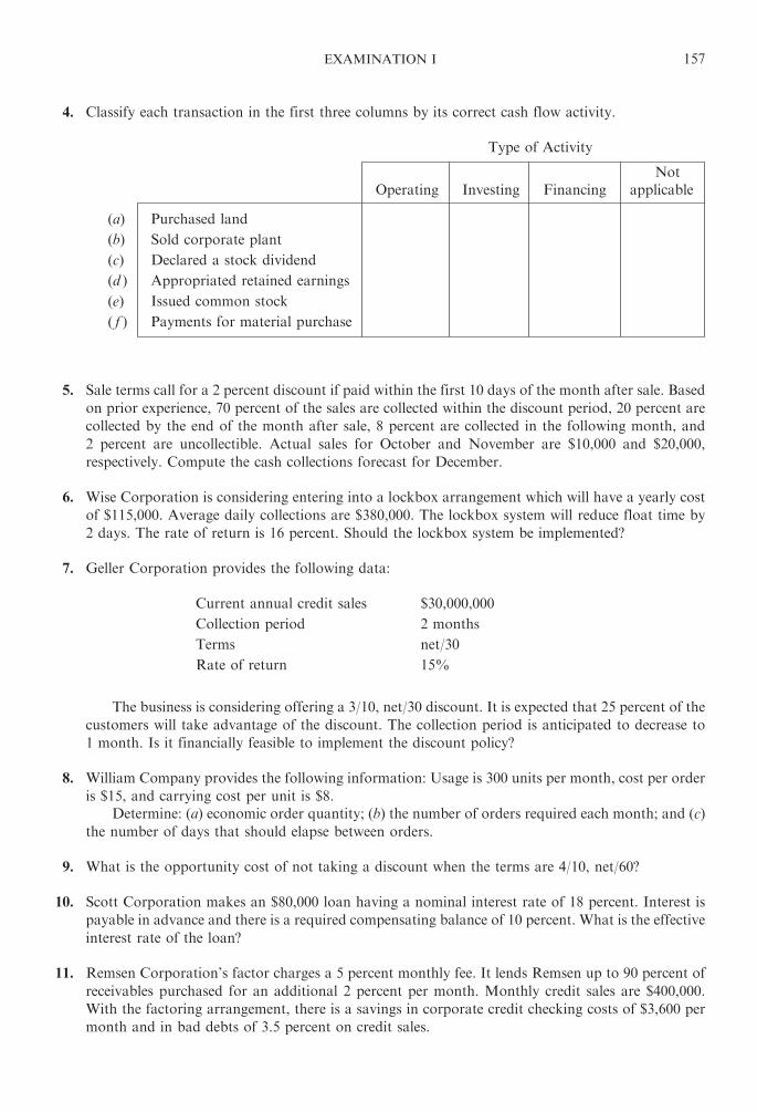
4. Classify each transaction in the first three columns by its correct cash flow activity.
Type of Activity
Operating Investing Financing
Not
applicable
(a) Purchased land
(b) Sold corporate plant
(c) Declared a stock dividend
(d ) Appropriated retained earnings
(e) Issued common stock
( f ) Payments for material purchase
5. Sale terms call for a 2 percent discount if paid within the first 10 days of the month after sale. Based
on prior experience, 70 percent of the sales are collected within the discount period, 20 percent are
collected by the end of the month after sale, 8 percent are collected in the following month, and
2 percent are uncollectible. Actual sales for October and November are $10,000 and $20,000,
respectively. Compute the cash collections forecast for December.
6. Wise Corporation is considering entering into a lockbox arrangement which will have a yearly cost
of $115,000. Average daily collections are $380,000. The lockbox system will reduce float time by
2 days. The rate of return is 16 percent. Should the lockbox system be implemented?
7. Geller Corporation provides the following data:
Current annual credit sales $30,000,000
Collection period 2 months
Terms net/30
Rate of return 15%
The business is considering offering a 3/10, net/30 discount. It is expected that 25 percent of the
customers will take advantage of the discount. The collection period is anticipated to decrease to
1 month. Is it financially feasible to implement the discount policy?
8. William Company provides the following information: Usage is 300 units per month, cost per order
is $15, and carrying cost per unit is $8.
Determine: (a) economic order quantity; (b) the number of orders required each month; and (c)
the number of days that should elapse between orders.
9. What is the opportunity cost of not taking a discount when the terms are 4/10, net/60?
10. Scott Corporation makes an $80,000 loan having a nominal interest rate of 18 percent. Interest is
payable in advance and there is a required compensating balance of 10 percent. What is the effective
interest rate of the loan?
11. Remsen Corporation’s factor charges a 5 percent monthly fee. It lends Remsen up to 90 percent of
receivables purchased for an additional 2 percent per month. Monthly credit sales are $400,000.
With the factoring arrangement, there is a savings in corporate credit checking costs of $3,600 per
month and in bad debts of 3.5 percent on credit sales.
EXAMINATION I 157
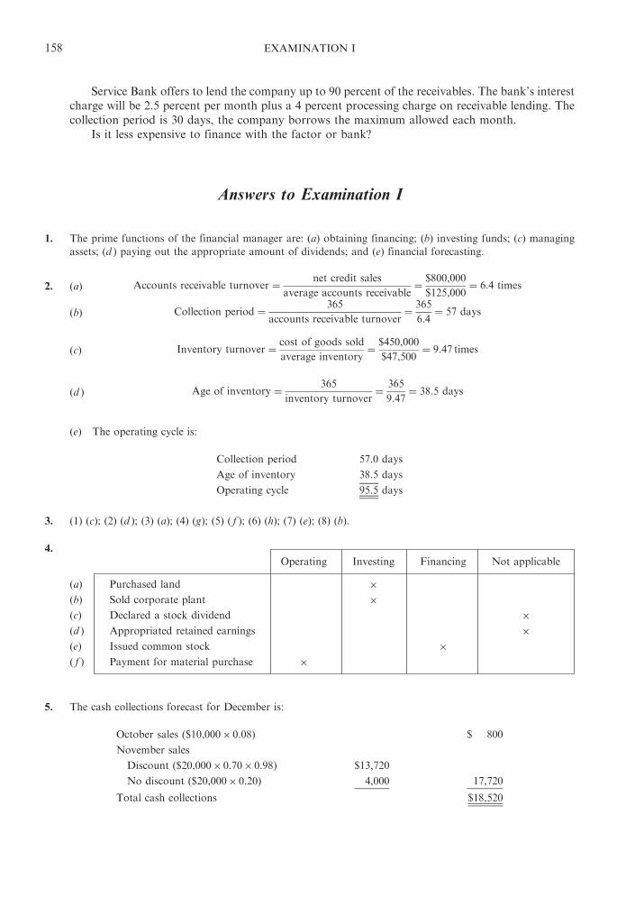
Service Bank offers to lend the company up to 90 percent of the receivables. The bank’s interest
charge will be 2.5 percent per month plus a 4 percent processing charge on receivable lending. The
collection period is 30 days, the company borrows the maximum allowed each month.
Is it less expensive to finance with the factor or bank?
Answers to Examination I
1. The prime functions of the financial manager are: (a) obtaining financing; (b) investing funds; (c) managing
assets; (d ) paying out the appropriate amount of dividends; and (e) financial forecasting.
2. (a) Accounts receivable turnover ¼ net credit sales
average accounts receivable¼ $800,000
$125,000¼ 6:4 times
(b) Collection period ¼ 365
accounts receivable turnover¼ 365
6:4¼ 57 days
(c) Inventory turnover ¼ cost of goods sold
average inventory¼ $450,000
$47,500¼ 9:47 times
(d ) Age of inventory ¼ 365
inventory turnover¼ 365
9:47¼ 38:5 days
(e) The operating cycle is:
Collection period 57.0 days
Age of inventory 38.5 days
Operating cycle 95.5 days
3. (1) (c); (2) (d ); (3) (a); (4) (g); (5) ( f ); (6) (h); (7) (e); (8) (b).
4.
Operating Investing Financing Not applicable
(a) Purchased land �(b) Sold corporate plant �(c) Declared a stock dividend �(d ) Appropriated retained earnings �(e) Issued common stock �( f ) Payment for material purchase �
5. The cash collections forecast for December is:
October sales ($10,000� 0.08) $ 800
November sales
Discount ($20,000� 0.70� 0.98) $13,720
No discount ($20,000� 0.20) 4,000 17,720
Total cash collections $18,520
158 EXAMINATION I

6. The proposed lockbox arrangement for Wise Corporation is:
Cost $115,000
Return on freed cash (0.16� 2� $380,000) 121,600
$ 6,600
The lockbox system would save the company $6,000 and should be implemented.
7. Current average accounts receivable
balance ($30,000,000/6) $5,000,000
Average accounts receivable
balance—after change in policy
($30,000,000/12) 2,500,000
Reduction in average accounts receivable $2,500,000
Rate of return �0.15Dollar return $ 375,000
Cost of discount
(0.25� $30,000,000� 0.03) $ 225,000
Advantage to discount policy
($375,000 � $225,000) $ 150,000
The discount policy is financially feasible.
8. (a) EOQ ¼ffiffiffiffiffiffiffiffiffi
2SP
C
r
¼ffiffiffiffiffiffiffiffiffiffiffiffiffiffiffiffiffiffiffiffiffi
2ð300Þð15Þ8
r
¼ffiffiffiffiffiffiffiffiffiffiffi
9,000
8
r
¼ 34 ðroundedÞ
(b)S
EOQ¼ 300
34¼ 9 ðroundedÞ
(c)31
9¼ every 3 days ðroundedÞ
9. Opportunity cost of not taking discount ¼ discount percent
100� discount percent� 360
N¼ 4
96� 360
50¼ 30:0%
10. Effective interest rate ¼ interest rate� principal
ðproceeds, %� principalÞ � interest
¼ 18%� $80,000
ð90%� $80,000Þ � $14,400¼ $14,400
$57,600¼ 25%
11. The cost of financing with a factor is:
Purchased receivable (0.05� $400,000) $20,000
Lending fee (0.02� $400,000� 0.90) 7,200
Total cost $27,200
The cost of financing with a bank is:
Interest (0.025� $400,000� 0.90) $ 9,000
Processing charge (0.04� $400,000� 0.90) 14,400
Additional cost of not using factor
Credit costs 3,600
Bad debts (0.035� $400,000) 14,000
Total cost $41,000
It is less expensive to use the factor.
EXAMINATION I 159
Chapter 6
Time Value of Money
6.1 INTRODUCTION
Time value of money is a critical consideration in financial and investment decisions. For example,
compound interest calculations are needed to determine future sums of money resulting from an invest-
ment. Discounting, or the calculation of present value, which is inversely related to compounding, is used
to evaluate future cash flow associated with capital budgeting projects. There are plenty of applications
of time value of money in finance. The chapter discusses the concepts, calculations, and applications of
future values and present values.
6.2 FUTURE VALUES—COMPOUNDING
A dollar in hand today is worth more than a dollar to be received tomorrow because of the interest it
could earn from putting it in a savings account or placing it in an investment account. Compounding
interest means that interest earns interest. For the discussion of the concepts of compounding and time
value, let us define:
Fn ¼ future value ¼ the amount of money at the end of year n
P ¼ principal
i ¼ annual interest rate
n ¼ number of years
Then,
F1 ¼ the amount of money at the end of year 1
¼ principal and interest ¼ Pþ iP ¼ Pð1þ iÞF2 ¼ the amount of money at the end of year 2
¼ F1ð1þ iÞ ¼ Pð1þ iÞð1þ iÞ ¼ Pð1þ iÞ2
The future value of an investment compounded annually at rate i for n years is
Fn ¼ Pð1þ iÞn ¼ P �FVIFi;n
where FVIFi,n is the future value interest factor for $1 and can be found in Appendix A.
EXAMPLE 6.1 George Jackson placed $1,000 in a savings account earning 8 percent interest compounded
annually. How much money will he have in the account at the end of 4 years?
Fn ¼ Pð1þ iÞn
F4 ¼ $1,000ð1þ 0:08Þ4 ¼ $1,000 �FVIF8;4
From Appendix A, the FVIF for 4 years at 8 percent is 1.3605. Therefore,
F4 ¼ $1,000ð1:3605Þ ¼ $1,360:50
EXAMPLE 6.2 Rachael Kahn invested a large sum of money in the stock of TLC Corporation. The company paid
a $3 dividend per share. The dividend is expected to increase by 20 percent per year for the next 3 years. She wishes
to project the dividends for years 1 through 3.
160
Copyright © 2007, 1998, 1986 by The McGraw-Hill Companies, Inc. Click here for terms of use.

Fn ¼ Pð1þ iÞn
F1 ¼ $3ð1þ 0:2Þ1 ¼ $3ð1:2000Þ ¼ $3:60
F2 ¼ $3ð1þ 0:2Þ2 ¼ $3ð1:4400Þ ¼ $4:32
F3 ¼ $3ð1þ 0:2Þ3 ¼ $3ð1:7280Þ ¼ $5:18
Intrayear Compounding
Interest is often compounded more frequently than once a year. Banks, for example, compound
interest quarterly, daily, and even continuously. If interest is compounded m times a year, then the
general formula for solving for the future value becomes
Fn ¼ P 1þ i
m
� �n �m¼ P �FVIFi=m;n �m
The formula reflects more frequent compounding ðn �mÞ at a smaller interest rate per period (i/m).
For example, in the case of semiannual compounding (m=2), the above formula becomes
Fn ¼ P 1þ i
2
� �n � 2¼ P �FVIFi=2;n � 2
As m approaches infinity, the term (1+ i/m)n �m approaches ei � n, where e is approximately 2.71828,
and Fn becomes
Fn ¼ P � ei � n
The future value increases as m increases. Thus, continuous compounding results in the maximum
possible future value at the end of n periods for a given rate of interest.
EXAMPLE 6.3 Assume that P=$100, i=12% and n=3 years. Then for
Annual compounding ðm ¼ 1Þ: F3 ¼ $100ð1þ 0:12Þ3 ¼ $100ð1:404Þ3 ¼ $140:49
Semiannual compounding ðm ¼ 2Þ: F3 ¼ $100 1þ 0:12
2
� �3 � 2
¼ $100ð1þ 0:06Þ6 ¼ $100ð1:4185Þ ¼ $141:85
Quarterly compounding ðm ¼ 4Þ: F3 ¼ $100 1þ 0:12
4
� �3 � 4¼ $100ð1þ 0:03Þ12
¼ $100ð1:4257Þ ¼ $142:57
Monthly compounding ðm ¼ 12Þ: F3 ¼ $100 1þ 0:12
12
� �3 � 12
¼ $100ð1þ 0:01Þ36 ¼ $100ð1:4307Þ ¼ $143:07
Continuous compounding ðei � nÞ : F3 ¼ $100 � eð0:12 � 3Þ ¼ $100ð2:71828Þ0:36
¼ $100ð1:4333Þ ¼ $143:33
Future Value of an Annuity
An annuity is defined as a series of payments (or receipts) of a fixed amount for a specified number of
periods. Each payment is assumed to occur at the end of the period. The future value of an annuity is a
compound annuity which involves depositing or investing an equal sum of money at the end of each year
for a certain number of years and allowing it to grow.
Let Sn=the future value of an n-year annuity
A=the amount of an annuity
CHAP. 6] TIME VALUE OF MONEY 161

Then we can write
Sn ¼ Að1þ iÞn�1 þ Að1þ iÞn�2 þ � � � þ Að1þ iÞ0
¼ A½ðiþ IÞn�1 þ ð1þ iÞn�2 þ � � � þ ð1þ iÞ0�
¼ A �X
n�1
t¼0ð1þ iÞt ¼ A �FVIFAi;n
where FVIFAi,n represents the future value interest factor for an n-year annuity compounded at i percent
and can be found in Appendix B.
EXAMPLE 6.4 Jane Oak wishes to determine the sum of money she will have in her savings account at the end of
6 years by depositing $1,000 at the end of each year for the next 6 years. The annual interest rate is 8 percent.
The FVIEA8%,6 years is given in Appendix B as 7.336. Therefore,
S6 ¼ $1,000ðFVIFA8;6Þ ¼ $1,000ð7:336Þ ¼ $7,336
6.3 PRESENT VALUE—DISCOUNTING
Present value is the present worth of future sums of money. The process of calculating present
values, or discounting, is actually the opposite of finding the compounded future value. In connection
with present value calculations, the interest rate i is called the discount rate.
Recall that
Fn ¼ Pð1þ iÞn
Therefore,
P ¼ Fn
ð1þ iÞn ¼ Fn
1
ð1þ iÞn�
¼ Fn �PVIFi;n
Where PVIFi,n represents the present value interest factor for $1 and is given in Appendix C.
EXAMPLE 6.5 Ron Jaffe has been given an opportunity to receive $20,000 6 years from now. If he can earn
10 percent on his investments, what is the most he should pay for this opportunity? To answer this question, one
must compute the present value of $20,000 to be received 6 years from now at a 10 percent rate of discount. F6 is
$20,000, i is 10 percent, which equals 0.1, and n is 6 years. PVIF10,6 from Appendix C is 0.5645.
P ¼ $20,0001
ð1þ 0:1Þ6�
¼ $20,000ðPVIF10;6Þ ¼ $20,000ð0:5645Þ ¼ $11,290
This means that Ron Jaffe, who can earn 10 percent on his investment, could be indifferent to the choice between
receiving $11,290 now or $20,000 6 years from now since the amounts are time equivalent In other words, he could
invest $11,290 today at 10 percent and have $20,000 in 6 years.
Present Value of Mixed Streams of Cash Flows
The present value of a series of mixed payments (or receipts) is the sum of the present value of each
individual payment. We know that the present value of each individual payment is the payment times the
appropriate PVIF.
EXAMPLE 6.6 Candy Parker has been offered an opportunity to receive the following mixed stream of revenue
over the next 3 years:
Year Revenue
1 $1,000
2 $2,000
3 $500
162 TIME VALUE OF MONEY [CHAP. 6

If she must earn a minimum of 6 percent on her investment, what is the most she should pay today? The present
value of this series of mixed streams of revenue is as follows:
Year Revenue ($) � PVIF = Present Value
1 1,000 0.943 $ 943
2 2,000 0.890 1,780
3 500 0.840 420
$3,143
Present Value of an Annuity
Interest received from bonds, pension funds, and insurance obligations all involve annuities. To
compare these financial instruments, we need to know the present value of each. The present value of an
annuity (Pn) can be found by using the following equation:
Pn ¼ A � 1
ð1þ iÞ1þ A � 1
ð1þ iÞ2þ � � � þ A � 1
ð1þ iÞn
¼ A1
ð1þ iÞ1þ 1
ð1þ iÞ2þ � � � þ 1
ð1þ iÞn�
¼ A �X
n
t¼1
1
ð1þ iÞt¼ A �PVIFAi;n
where PVIFAi,n represents the appropriate value for the present value interest factor for a $1 annuity
discounted at i percent for n years and is found in Appendix D.
EXAMPLE 6.7 Assume that the revenues in Example 6.6 form an annuity of $1,000 for 3 years. Then the present
value isPn ¼ A �PVIFAi;n
P3 ¼ $1,000ðPVIFA6;3Þ ¼ $1,000ð2:6730Þ ¼ $2,673
Perpetuities
Some annuities go on forever. Such annuities are called perpetuities. An example of a perpetuity is
preferred stock which yields a constant dollar dividend indefinitely. The present value of a perpetuity is
found as follows:
Present value of a perpetuity ¼ receipt
discount rate¼ A
i
EXAMPLE 6.8 Assume that a perpetual bond has an $80-per-year interest payment and that the discount rate is
10 percent. The present value of this perpetuity is:
P ¼ A
i¼ $80
0:10¼ $800
6.4 APPLICATIONS OF FUTURE VALUES AND PRESENT VALUES
Future and present values have numerous applications in financial and investment decisions, which
will be discussed throughout the book. Five of these applications are presented below.
Deposits to Accumulate a Future Sum (or Sinking Fund)
An individual might wish to find the annual deposit (or payment) that is necessary to accumulate a
future sum. To find this future amount (or sinking fund) we can use the formula for finding the future
value of an annuity.
Sn ¼ A �FVIFAi;n
CHAP. 6] TIME VALUE OF MONEY 163

Solving for A, we obtain:
Sinking fund amount ¼ A ¼ Sn
FVIFAi;n
EXAMPLE 6.9 Mary Czech wishes to determine the equal annual end-of-year deposits required to accumulate
$5,000 at the end of 5 years when her son enters college. The interest rate is 10 percent. The annual deposit is:
S5 ¼ $5,000
FVIFA10;5 ¼ 6:1051 ðfrom Appendix BÞ
A ¼ $5,000
6:1051¼ $818:99 ffi $819
In other words, if she deposits $819 at the end of each year for 5 years at 10 percent interest, she will have
accumulated $5,000 at the end of the fifth year.
Amortized Loans
If a loan is to be repaid in equal periodic amounts, it is said to be an amortized loan. Examples
include auto loans, mortgage loans, and most commercial loans. The periodic payment can easily be
computed as follows:
Pn ¼ A �PVIFAi;n
Solving for A, we obtain:
Amount of loan ¼ A ¼ Pn
PVIFAi;n
EXAMPLE 6.10 Jeff Balthness has a 40-month auto loan of $5,000 at a 12 percent annual interest rate. He wants
to find out the monthly loan payment amount.
i ¼ 12%� 12 months ¼ 1%
P40 ¼ $5,000
PVIFA1;40 ¼ 32:8347 ðfrom Appendix DÞ
Therefore,
A ¼ $5; 000
32:8347¼ $152:28
So, to repay the principal and interest on a $5,000,12 percent, 40-month loan, Jeff Balthness has to pay $152,28
a month for the next 40 months.
Note: The annual interest rate can be calculated by
PVIFAi;n ¼Pn
A
EXAMPLE 6.11 Assume that a firm borrows $2,000 to be repaid in three equal installments at the end of each of
the next 3 years. The bank wants 12 percent interest. Compute the amount of each payment.
P3 ¼ $2,000
PVIFA12;3 ¼ 2:4018
Therefore,
A ¼ $2,000
2,4018¼ $832:71
164 TIME VALUE OF MONEY [CHAP. 6

Each loan payment consists partly of interest and partly of principal. The breakdown is often displayed in a loan
amortization schedule. The interest component is largest in the first period and subsequently declines, whereas the
principal portion is smallest in the first period and increases thereafter, as shown in the following example.
EXAMPLE 6.12 Using the same data as in Example 6.11, we set up the following amortization schedule:
Year Payment Interest
Repayment
of Principal
Remaining
Balance
1 $832.71 $240,00a $592.71 $1,407.29
2 $832.71 $168.88 $663.83 $ 743.46
3 $832.68b $ 89.22 $743.46c
a Interest is computed by multiplying the loan balance at the beginning
of the year by the interest rate. Therefore, interest in year 1 is
$2,000(0.12)=$240; in year 2 interest is $1,407.29(0.12)=$168.88; and
in year 3 interest is $743.46(0.12)=$89.22. All figures are rounded.b Last payment is adjusted downward.c Not exact because of accumulated rounding errors.
Annual Percentage Rate (APR)
Different types of investments use different compounding periods. For example, most bonds pay
interest semiannually; banks generally pay interest quarterly. If an investor wishes to compare invest-
ments with different compounding periods, he or she needs to put them on a common basis. The annual
percentage rate (APR), or effective annual rate, is used for this purpose and is computed as follows:
APR ¼ 1þ r
m
�m
� 1:0
where r=the stated, nominal or quoted rate and m=the number of compounding periods per year.
EXAMPLE 6.13 If the nominal rate is 6 percent, compounded quarterly, the APR is
APR ¼ 1þ r
m
�m
� 1:0 ¼ 1þ 0:06
4
� �4
� 1:0 ¼ ð1:015Þ4 � 1:0 ¼ 1:0614� 1:0 ¼ 0:0614 ¼ 6:14%
This means that if one bank offered 6 percent with quarterly compounding, while another offered 6.14 percent with
annual compounding, they would both be paying the same effective rate of interest.
Rates of Growth
In finance, it is necessary to calculate the compound annual interest rate, or rate of growth, associated
with a stream of earnings.
EXAMPLE 6.14 Assume that the Geico Company has earnings per share of $2.50 in 20X1, and 10 years later the
earnings per share has increased to $3.70. The compound annual rate of growth of the earnings per share can be
computed as follows:
Fn ¼ P �FVIFi;n
Solving this for FVIF, we obtain:
FVIFi;n ¼Fn
P
FVIFi;10 ¼$3:70
$2:50¼ 1:48
From Appendix A an FVIF of 1.48 at 10 years is at i=4%. The compound annual rate of growth is therefore
4 percent.
CHAP. 6] TIME VALUE OF MONEY 165
Bond Values
Bonds call for the payment of a specific amount of interest for a stated number of years and the
repayment of the face value at the bond’s maturity. Thus, a bond represents an annuity plus a lump sum.
Its value is found as the present value of this payment stream. The interest is usually paid semiannually.
V ¼X
n
t¼1
I
ð1þ rÞtþ M
ð1þ rÞn
¼ IðPVIFAr;nÞ þMðPVIFr;nÞ
where I=interest payment per period
M=par value, or maturity value, usually $1,000
r=investor’s required rate of return
n=number of periods
This topic is covered in more detail in Chapter 7, ‘‘Risk, Return, and Valuation.’’
EXAMPLE 6.15 Assume there is a 10-year bond with a 10 percent coupon, paying interest semiannually and
having a face value of $1,000. Since interest is paid semiannually, the number of periods involved is 20 and the
semiannual cash inflow is $100/2=$50.
Assume that investors have a required rate of return of 12 percent for this type of bond. Then, the present value
(V ) of this bond is:
V ¼ $50ðPVIFA6;20Þ þ $1,000ðPVIF6;20Þ¼ $50ð11:4699Þ þ $1,000ð0:3118Þ ¼ $573:50þ $311:80 ¼ $885:30
Note that the required rate of return (12 percent) is higher than the coupon rate of interest (10 percent),
and so the bond value (or the price investors are willing to pay for this particular bond) is less than its $1,000
face value.
Review Questions
1. is a critical consideration in many financial and investment decisions.
2. The process of determining present value is often called and is the reverse of
the process.
3. Fn ¼ Pð1þ i=mÞn �m is a general formula used for .
4. results in the maximum possible future value at the end of n periods for a given
rate of interest.
5. A(n) is a series of payments (or receipts) of a fixed amount for a specified
number of periods.
6. The , or effective annual rate, is used to compare investments with differ-
ent on a common basis.
7. The present value of a mixed stream of payments (or receipts) is the of present
values of .
8. A(n) is an annuity in which payments go on forever.
166 TIME VALUE OF MONEY [CHAP. 6
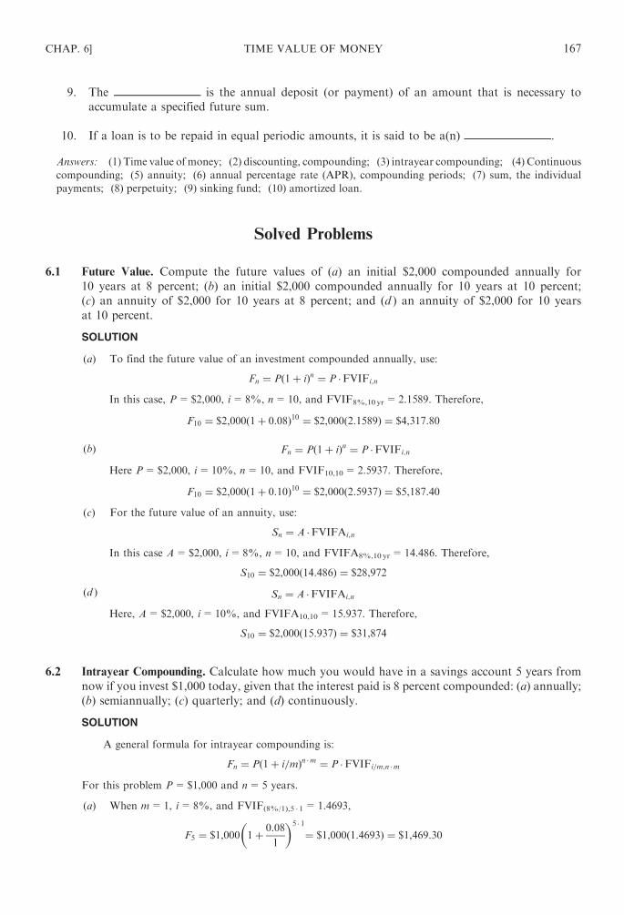
9. The is the annual deposit (or payment) of an amount that is necessary to
accumulate a specified future sum.
10. If a loan is to be repaid in equal periodic amounts, it is said to be a(n) .
Answers: (1) Time value of money; (2) discounting, compounding; (3) intrayear compounding; (4) Continuous
compounding; (5) annuity; (6) annual percentage rate (APR), compounding periods; (7) sum, the individual
payments; (8) perpetuity; (9) sinking fund; (10) amortized loan.
Solved Problems
6.1 Future Value. Compute the future values of (a) an initial $2,000 compounded annually for
10 years at 8 percent; (b) an initial $2,000 compounded annually for 10 years at 10 percent;
(c) an annuity of $2,000 for 10 years at 8 percent; and (d ) an annuity of $2,000 for 10 years
at 10 percent.
SOLUTION
(a) To find the future value of an investment compounded annually, use:
Fn ¼ Pð1þ iÞn ¼ P �FVIFi;n
In this case, P=$2,000, i=8%, n=10, and FVIF8%,10 yr=2.1589. Therefore,
F10 ¼ $2,000ð1þ 0:08Þ10 ¼ $2,000ð2:1589Þ ¼ $4,317:80
(b) Fn ¼ Pð1þ iÞn ¼ P �FVIFi;n
Here P=$2,000, i=10%, n=10, and FVIF10,10=2.5937. Therefore,
F10 ¼ $2,000ð1þ 0:10Þ10 ¼ $2,000ð2:5937Þ ¼ $5,187:40
(c) For the future value of an annuity, use:
Sn ¼ A �FVIFAi;n
In this case A=$2,000, i=8%, n=10, and FVIFA8%,10 yr=14.486. Therefore,
S10 ¼ $2,000ð14:486Þ ¼ $28,972
(d ) Sn ¼ A �FVIFAi;n
Here, A=$2,000, i=10%, and FVIFA10,10=15.937. Therefore,
S10 ¼ $2,000ð15:937Þ ¼ $31,874
6.2 Intrayear Compounding. Calculate how much you would have in a savings account 5 years from
now if you invest $1,000 today, given that the interest paid is 8 percent compounded: (a) annually;
(b) semiannually; (c) quarterly; and (d) continuously.
SOLUTION
A general formula for intrayear compounding is:
Fn ¼ Pð1þ i=mÞn �m ¼ P �FVIFi=m;n �m
For this problem P=$1,000 and n=5 years.
(a) When m=1, i=8%, and FVIF(8%/1),5 � 1=1.4693,
F5 ¼ $1,000 1þ 0:08
1
� �5 � 1¼ $1,000ð1:4693Þ ¼ $1,469:30
CHAP. 6] TIME VALUE OF MONEY 167

(b) When m=2 and FVIF(8%/2),5 � 2=FVIF4,10=1.4802,
F5 ¼ $1,000ð1:4802Þ ¼ $1,480:20
(c) m=4 and FVIF(8%/4),5 � 4=FVIF2,20=1.4859,
F5 ¼ $1,000ð1:4859Þ ¼ $1,485:90
(d) For continuous compounding, use:
Fn ¼ P � ei � n
F5 ¼ $1,000ð2:71828Þ0:08 � 5 ¼ $1,000ð2:71828Þ0 � 4
¼ $1,000ð1:4918Þ ¼ $1,491:80
6.3 Present Value. Calculate the present value, discounted at 10 percent, of receiving: (a) $800 at the
end of year 4; (b) $200 at the end of year 3 and $300 at the end of year 5; (c) $500 at the end of
year 4 and $300 at the end of year 6; and (d) $500 a year for the next 10 years.
SOLUTION
(a) P ¼ Fn
1
ð1þ iÞn�
¼ Fn �PVIFi;n
Here n=4, F4=$800, and i=10%.
PVIF10;4 ¼ 0:6830
P ¼ $800ð0:6830Þ ¼ $546:40
(b) P ¼ $200ðPVIF10;3Þ þ $300ðPVIF10;5Þ¼ $200ð0:7513Þ þ $300ð0:6209Þ ¼ $150:26þ $186:27 ¼ $336:53
(c) P ¼ $500ðPVIF10;4Þ þ $300ðPVIF10;6Þ ¼ $500ð0:6830Þ þ $300ð0:5645Þ¼ $341:50þ $169:35 ¼ $510:85
(d) For the present value of an annuity, use:
Pn ¼ A �PVIFAi;n
Here A=$500, n=10, and i=10%. Therefore,
P10 ¼ $500ðPVIFA10;10Þ ¼ $500ð6:1446Þ ¼ $3,072:30
6.4 Present Value. Calculate the present value of the following future cash inflows discounted at 10
percent: (a) $1,000 a year for years 1 through 10; (b) $1,000 a year for years 5 through 10; and
(c) $1,000 a year for years 1 through 3, nothing in years 4 through 5, then $2,000 a year for years
6 through 10.
SOLUTION
(a) Pn ¼ A �PVIFAi;n
Here A=$1,000, i=10%, and n=10 years. Therefore,
P10 ¼ $1,000ðPVIFA10;10Þ ¼ $1,000ð6:1446Þ ¼ $6,144:60
(b) P ¼ $1,000ðPVIFA10;10Þ � $1,000ðPVIFA10;4Þ¼ $1,000ð6:1446Þ � $1,000ð3:1699Þ ¼ $6,144:60� $3,169:90 ¼ $2,974:70
This type of annuity is called a deferred annuity.
168 TIME VALUE OF MONEY [CHAP. 6

(c) P ¼ $1,000ðPVIFA10;3Þ þ ½$2,000ðPVIFA10;10Þ � $2,000ðPVIFA10;5Þ�¼ $1,000ð2:4869Þ þ ½$2,000ð6:1446Þ � $2,000ð3:7908Þ�¼ $2,486:90þ ½$12,289:2� $7,581:60� ¼ $2,466:90þ $4,707:60 ¼ $7,194:5
6.5 Present Value. Your favorite uncle has offered you the choice of the following options. He will
give you either $2,000 1 year from now or $3,000 4 years from now. Which would you choose if
the discount rate is (a) 10 percent? (b) 20 percent?
SOLUTION
P ¼ Fn �PVIFi;n
(a) Option 1: $2,000 one year from now. In this case i=10%, n=1, F1=$2,000, and PVIF10,1=0.9091.
Therefore,
P ¼ $2,000ð0:9091Þ ¼ $1,818:20
Option 2: $3,000 four years from now. In this case i=10%, n=4, F4=$3,000, and
PVIF10,4=0.6830.
Therefore,
P ¼ $3,000ð0:6830Þ ¼ $2,049
At 10 percent, the best choice is $3,000 four years from now.
(b) Option 1: $2,000 one year from now. In this case i=20%, n=1, F1=$2,000, and PVIF20,1=0.8333.
Therefore,
P ¼ $2,000ð0:8333Þ ¼ $1,666:60
Option 2: $3,000 four years from now. In this case i=20%, n=4, F4=$3,000, and
PVIF20,4=0.4823.
Therefore,
P ¼ $3,000ð0:4823Þ ¼ $1,446:9
At 20 percent, the best choice is $2,000 one year from now.
6.6 Present value. A 55-year-old executive will retire at age 65 and expects to live to age 75. Assuming
a 10 percent rate of return, calculate the amount he must have available at age 65 in order to
receive $10,000 annually from retirement until death. (CFA, adapted.)
SOLUTION
This problem involves finding the present value of an annuity. The executive must have $61,446 avail-
able at age 65, calculated as follows:
Pn ¼ A �PVIFAi,n
Here A=$10,000, n=10, i=10%, and PVIFA10,10=6.1446. Therefore,
P10 ¼ $10,000ð6:1446Þ ¼ $61,446
6.7 Present Value. Your father is about to retire. His firm has given him the option of retiring with a
lump sum of $20,000 or an annuity of $2,500 for 10 years. Which is worth more now, if an interest
rate of 6 percent is used for the annuity?
SOLUTION
Pn ¼ A �PVIFi,n
CHAP. 6] TIME VALUE OF MONEY 169
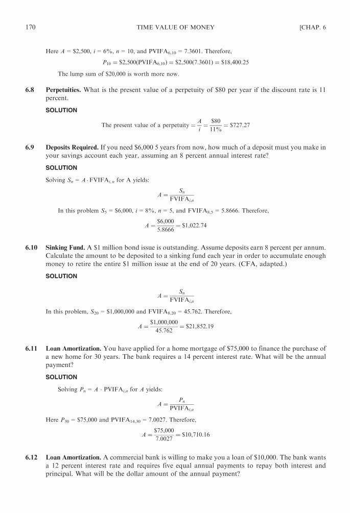
Here A=$2,500, i=6%, n=10, and PVIFA6,10=7.3601. Therefore,
P10 ¼ $2,500ðPVIFA6,10Þ ¼ $2,500ð7:3601Þ ¼ $18,400:25
The lump sum of $20,000 is worth more now.
6.8 Perpetuities. What is the present value of a perpetuity of $80 per year if the discount rate is 11
percent.
SOLUTION
The present value of a perpetuity ¼ A
i¼ $80
11%¼ $727:27
6.9 Deposits Required. If you need $6,000 5 years from now, how much of a deposit must you make in
your savings account each year, assuming an 8 percent annual interest rate?
SOLUTION
Solving Sn=A �FVIFAi, n for A yields:
A ¼ Sn
FVIFAi,n
In this problem S5=$6,000, i=8%, n=5, and FVIFA8,5=5.8666. Therefore,
A ¼ $6,000
5:8666¼ $1,022:74
6.10 Sinking Fund. A $1 million bond issue is outstanding. Assume deposits earn 8 percent per annum.
Calculate the amount to be deposited to a sinking fund each year in order to accumulate enough
money to retire the entire $1 million issue at the end of 20 years. (CFA, adapted.)
SOLUTION
A ¼ Sn
FVIFAi,n
In this problem, S20=$1,000,000 and FVIFA8,20=45.762. Therefore,
A ¼ $1,000,000
45:762¼ $21,852:19
6.11 Loan Amortization. You have applied for a home mortgage of $75,000 to finance the purchase of
a new home for 30 years. The bank requires a 14 percent interest rate. What will be the annual
payment?
SOLUTION
Solving Pn=A � PVIFAi,n for A yields:
A ¼ Pn
PVIFAi;n
Here P30=$75,000 and PVIFA14,30=7.0027. Therefore,
A ¼ $75,000
7:0027¼ $10,710:16
6.12 Loan Amortization. A commercial bank is willing to make you a loan of $10,000. The bank wants
a 12 percent interest rate and requires five equal annual payments to repay both interest and
principal. What will be the dollar amount of the annual payment?
170 TIME VALUE OF MONEY [CHAP. 6

SOLUTION
A ¼ Pn
PVIFAi,n
Here P5=$10,000 and PVIFA12,5=3.6048. Therefore,
A ¼ $10,000
3:6048¼ $2,774:08
6.13 Loan Amortization Schedule. Set up an amortization schedule for a $5,000 loan to be repaid in
equal installments at the end of each of the next 3 years. The interest rate is 15 percent.
SOLUTION
First, find the amount of equal installment by using the following formula:
A ¼ Pn
PVIFAi,n
In this problem P3=$5,000 and PVIFA15,3=2.2832. Therefore,
A ¼ $5,000
2:2832¼ $2,189:91
The amortization schedule is as follows:
Year Payment InterestaRepayment
of Principal
Remaining
Balance
1 $2,189.91 $750 $1,439.91 $3,560.09
2 $2,189.91 $534.01 $1,655.90 $1,904.19
3 $2,189.82b $285.63 $1,904.19c
a Interest is computed by multiplying the loan balance at the beginning
of the year by the interest rate. Therefore, interest in year 1 is
$5,000(0.15)=$750; in year 2 interest is $3,560.09(0.15)=$534.01; etc.b Last payment is adjusted downward.c Not exact because of accumulated rounding errors.
6.14 Annual Percentage Rate (APR). Suppose that a company borrows $20,000 for 1 year at a stated
rate of interest of 9 percent. What is the annual percentage rate (APR) if interest is paid to the
lender (a) annually? (b) semiannually? (c) quarterly?
SOLUTION
APR ¼ 1þ r
m
�m
� 1:0
In this problem r=9%=0.09.
(a) If interest is paid at the end of the year, m=1 and
APR ¼ 1þ 0:09
1
� �1
� 1:0 ¼ 1:09� 1:0 ¼ 0:09 ¼ 9:0%
(b) If the interest is paid at the end of each 6-month period, m=2 and
APR ¼ 1þ 0:09
2
� �2
� 1:0 ¼ ð1:045Þ2 � 1:0
¼ 1:092� 1:0 ¼ 0:092 ¼ 9:2%
CHAP. 6] TIME VALUE OF MONEY 171

(c) If interest is paid at the end of each quarter, m=4 and
APR ¼ 1þ 0:09
4
� �4
� 1:0 ¼ ð1:0225Þ4 � 1:0
¼ 1:093� 1:0 ¼ 0:093 ¼ 9:3%
More frequent payment of interest increases the effective annual cost paid by the company.
6.15 Rate of Growth. If a firm’s earnings increase from $3.00 per share to $4.02 over a 6-year period,
what is the rate of growth?
SOLUTION
Solving Fn ¼ P �FVIFi,n for FVIF yields:
FVIFi,n ¼Fn
P
Here, P=$3.00 and F6=$4.02. Therefore,
FVIFi,6 ¼$4:02
$3:00¼ 1:340
From Appendix A, an FVIF of 1.340 at 6 years is at i=5%. The rate of growth of earnings is therefore
5 percent.
6.16 Annual Interest Rate. You borrowed $20,000, to be repaid in 12 monthly installments of
$1,891.20. What is the annual interest rate?
SOLUTION
Solving Pn ¼ A �PVIFAi,n for PVIFA yields:
PVIFAi,n ¼Pn
A
In this problem P12=$20,000 and A=$1,891.20. Therefore,
PVIFAi,12 ¼$20,000
$1,891:20¼ 10:5753
From Appendix D, a PVIFA of 10.5753 for 12 periods is at i=2%. The annual interest rate is therefore
2%� 12=24%.
6.17 Bond Value. What amount should an investor be willing to pay for a $1,000, 5-year United States
government bond which pays $50 interest semiannually and is sold to yield 8 percent?
SOLUTION
The semiannual interest is 4 percent. The value of the bond is:
V ¼ IðPVIFAr,nÞ þMðPVIFr,nÞ¼ $50ðPVIFA4,10Þ þ $1,000ðPVIF4,10Þ¼ $50ð8:1109Þ þ $1,000ð0:6756Þ ¼ $405:55þ $675:60 ¼ $1,081:15
6.18 Bond Values. Calculate the value of a bond with a face value of $1,000, a coupon interest rate of
8 percent paid semiannually, and a maturity of 10 years. Assume the following discount rates:
(a) 6 percent; (b) 8 percent; and (c) 10 percent.
172 TIME VALUE OF MONEY [CHAP. 6

SOLUTION
Semiannual interest ¼ 8%ð$1,000Þ2
¼ $40
Number of periods ¼ 10� 2 ¼ 20 periods
(a) V ¼ IðPVIAr,nÞ þMðPVIFr,nÞ¼ $40ðPVIFA3,20Þ þ $1,000ðPVIF3,20Þ¼ $40ð14:8775Þ þ $1,000ð0:5537Þ ¼ $595:10þ $553:7 ¼ $1,148:80
(b) V ¼ $40ðPVIFA4,20Þ þ $1,000ðPVIF4,20Þ¼ $40ð13:5903Þ þ $1,000ð0:4564Þ ¼ $543:61þ $456:40 ¼ $1,000 ðroundedÞ
(c) V ¼ $40ðPVIFA5,20Þ þ $1,000ðPVIF5,20Þ¼ $40ð12,4622Þ þ $1,000ð0:3769Þ ¼ $498:49þ $376:90 ¼ $875:37
CHAP. 6] TIME VALUE OF MONEY 173
Chapter 7
Risk, Return, and Valuation
7.1 RISK DEFINED
Risk (or uncertainty) refers to the variability of expected returns associated with a given investment.
Risk, along with the concept of return, is a key consideration in investment and financial decisions. This
chapter will discuss procedures for measuring risk and investigate the relationship between risk, returns,
and security valuation.
Probability Distributions
Probabilities are used to evaluate the risk involved in a security. The probability of an event taking
place is defined as the chance that the event will occur. It may be thought of as the percentage chance of a
given outcome.
EXAMPLE 7.1 A weather forecaster may state, ‘‘There is a 30 percent chance of rain tomorrow and a 70 percent
chance of no rain.’’ Then we could set up the following probability distribution:
Outcome Probability
Rain 30%=0.3
No rain 70%=0.7
100%=1.00
Expected Rate of Return
Expected rate of return ð�rÞ is the weighted average of possible returns from a given investment,
weights being probabilities. Mathematically,
�r ¼X
n
i¼1ripi
where ri= ith possible return
pi= probability of the ith return
n=number of possible returns
EXAMPLE 7.2 Consider the possible rates of return that you might earn next year on a $50,000 investment in
stock A or on a $50,000 investment in stock B, depending upon the states of the economy: recession, normal, and
prosperity.
For stock A:
State of Economy Return (ri) Probability (pi)
Recession �5% 0.2
Normal 20% 0.6
Prosperity 40% 0.2
For stock B:
State of Economy Return (ri) Probability (pi)
Recession 10% 0.2
Normal 15% 0.6
Prosperity 20% 0.2
174
Copyright © 2007, 1998, 1986 by The McGraw-Hill Companies, Inc. Click here for terms of use.

Then the expected rate of return (�r) for stock A is computed as follows:
�r ¼X
n
i¼1ripi ¼ ð�5%Þð0:2Þ þ ð20%Þð0:6Þ þ ð40%Þð0:2Þ ¼ 19%
Stock B’s expected rate of return is:
�r ¼ ð10%Þð0:2Þ þ ð15%Þð0:6Þ þ 20%ð0:2Þ ¼ 15%
Measuring Risk: The Standard Deviation
The standard deviation (�), which is a measure of dispersion of the probability distribution, is
commonly used to measure risk. The smaller the standard deviation, the tighter the probability distribu-
tion and, thus, the lower the risk of the investment.
Mathematically,
� ¼ffiffiffiffiffiffiffiffiffiffiffiffiffiffiffiffiffiffiffiffiffiffiffiffiffiffiffi
X
n
i¼1ðri � �rÞ2pi
s
To calculate �, take the following steps:
Step 1. Compute the expected rate of return ð�rÞ.Step 2. Subtract each possible return from �r to obtain a set of deviations ðri � �rÞ.Step 3. Square each deviation, multiply the squared deviation by the probability of occurrence for its
respective return, and sum these products to obtain the variance (�2):
�2 ¼X
n
i¼1ðri � �r Þ2pi
Step 4. Finally, take the square root of the variance to obtain the standard deviation (�).
To follow this step-by-step approach, it is convenient to set up a table.
EXAMPLE 7.3 Using the data given in Example 7.2, compute the standard deviation for each stock and set up the
tables as follows for stock A:
Step 1 Step 2 Step 3
Return (ri) (%) Probability (pi) rip (%) ðri � �rÞð%Þ ðri��rÞ2 ðri��rÞ2pið%Þ
�5 0.2 �1 �24 576 115.2
20 0.6 12 1 1 0.6
40 0.2 8 21 441 88.2
�r ¼ 19 �2=204
Knowing �2=204, we proceed with Step 4 and
� ¼ffiffiffiffiffiffiffiffi
204p
¼ 14:28%
CHAP. 7] RISK, RETURN, AND VALUATION 175

For stock B:
Step 1 Step 2 Step 3
Return (ri) (%) Probability (pi) rip (%) ðri � �rÞð%Þ ðri��rÞ2 ðri��rÞ2pið%Þ10 0.2 2 �5 25 5
15 0.6 9 0 0 0
20 0.2 4 5 25 5
�r ¼ 15 �2=10
Knowing �2=10, we take Step 4 and
� ¼ffiffiffiffiffi
10p¼ 3:16%
Statistically, if the probability distribution is normal, 68 percent of the returns will lie in ±1 standard deviation,
95 percent of all observations will lie between ±2 standard deviations, and 99 percent of all observations will lie
between ±3 standard deviations of the expected value.
EXAMPLE 7.4 Using the results from Example 7.3,
Stock A Stock B
Expected return ð�rÞ 19% 15%
Standard deviation (�) 14.28% 3.16%
For stock A, there is a 68 percent probability that the actual return will be in the range of 19 percent plus or
minus 14.28 percent or from 4.72 percent to 33.28 percent. Since the range is so great, stock A is risky; it is likely to
either fall far below its expected rate of return or far exceed the expected return. For stock B, the 68 percent range is
15 percent plus or minus 3.16 percent or from 11.84 percent to 18.16 percent. With such a small �, there is only a
small probability that stock B’s return will be far less or greater than expected; hence, stock B is not very risky.
Measure of Relative Risk: Coefficient of Variation
One must be careful when using the standard deviation to compare risk since it is only an absolute
measure of dispersion (risk) and does not consider the dispersion of outcomes in relationship to an
expected value (return). Therefore, when comparing securities that have different expected returns, use
the coefficient of variation. The coefficient of variation is computed simply by dividing the standard
deviation for a security by expected value: �=�r. The higher the coefficient, the more risky the security.
EXAMPLE 7.5 Again, using the results from Example 7.3:
Stock A Stock B
�r 19% 15%
� 14.28% 3.16%
�=�r 0.75 0.21
Although stock A is expected to produce a considerably higher return than stock B, stock A is overall more
risky than stock B, based on the computed coefficient of variation.
176 RISK, RETURN, AND VALUATION [CHAP. 7
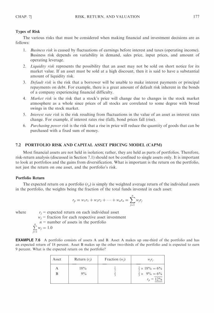
Types of Risk
The various risks that must be considered when making financial and investment decisions are as
follows:
1. Business risk is caused by fluctuations of earnings before interest and taxes (operating income).
Business risk depends on variability in demand, sales price, input prices, and amount of
operating leverage.
2. Liquidity risk represents the possibility that an asset may not be sold on short notice for its
market value. If an asset must be sold at a high discount, then it is said to have a substantial
amount of liquidity risk.
3. Default risk is the risk that a borrower will be unable to make interest payments or principal
repayments on debt. For example, there is a great amount of default risk inherent in the bonds
of a company experiencing financial difficulty.
4. Market risk is the risk that a stock’s price will change due to changes in the stock market
atmosphere as a whole since prices of all stocks are correlated to some degree with broad
swings in the stock market.
5. Interest rate risk is the risk resulting from fluctuations in the value of an asset as interest rates
change. For example, if interest rates rise (fall), bond prices fall (rise).
6. Purchasing power risk is the risk that a rise in price will reduce the quantity of goods that can be
purchased with a fixed sum of money.
7.2 PORTFOLIO RISK AND CAPITAL ASSET PRICING MODEL (CAPM)
Most financial assets are not held in isolation; rather, they are held as parts of portfolios. Therefore,
risk-return analysis (discussed in Section 7.1) should not be confined to single assets only. It is important
to look at portfolios and the gains from diversification. What is important is the return on the portfolio,
not just the return on one asset, and the portfolio’s risk.
Portfolio Return
The expected return on a portfolio (rp) is simply the weighted average return of the individual assets
in the portfolio, the weights being the fraction of the total funds invested in each asset:
rp ¼ w1r1 þ w2r2 þ � � � þ wnrn ¼X
n
j¼1wjrj
where rj=expected return on each individual asset
wj=fraction for each respective asset investment
n=number of assets in the portfolioP
n
j¼1wj ¼ 1:0
EXAMPLE 7.6 A portfolio consists of assets A and B. Asset A makes up one-third of the portfolio and has
an expected return of 18 percent. Asset B makes up the other two-thirds of the portfolio and is expected to earn
9 percent. What is the expected return on the portfolio?
Asset Return (rj) Fraction (wj) wjrj
A 18% 13
13� 18% ¼ 6%
B 9% 23
23� 9% ¼ 6%
rp=12%
CHAP. 7] RISK, RETURN, AND VALUATION 177

Portfolio Risk
Unlike returns, the risk of a portfolio (�p) is not simply the weighted average of the standard
deviations of the individual assets in the contribution, for a portfolio’s risk is also dependent on the
correlation coefficients of its assets. The correlation coefficient (�) is a measure of the degree to which
two variables ‘‘move’’ together. It has a numerical value that ranges from �1.0 to 1.0. In a two-asset
(A and B) portfolio, the portfolio risk is defined as:
�p ¼ffiffiffiffiffiffiffiffiffiffiffiffiffiffiffiffiffiffiffiffiffiffiffiffiffiffiffiffiffiffiffiffiffiffiffiffiffiffiffiffiffiffiffiffiffiffiffiffiffiffiffiffiffiffiffiffiffiffiffiffiffiffiffiffiffiffiffiffiffiffi
w2A�
2A þ w2
B�2B þ 2wAwB � �AB�A�B
q
where �A and �B=standard deviations of assets A and B, respectively
wA and wB=weights, or fractions, of total funds invested in assets A and B
�AB=the correlation coefficient between assets A and B
Portfolio risk can be minimized by diversification, or by combining assets in an appropriate manner.
The degree to which risk is minimized depends on the correlation between the assets being combined. For
example, by combining two perfectly negative correlated assets (�=�1), the overall portfolio risk can be
completely eliminated. Combining two perfectly positive correlated assets (�=+1) does nothing to help
reduce risk. (See Example 7.7.) An example of the latter might be ownership of two automobile stocks or
two housing stocks.
EXAMPLE 7.7 Assume the following:
Asset r W
A 20% 13
B 10% 23
The portfolio risk then is:
�p ¼ffiffiffiffiffiffiffiffiffiffiffiffiffiffiffiffiffiffiffiffiffiffiffiffiffiffiffiffiffiffiffiffiffiffiffiffiffiffiffiffiffiffiffiffiffiffiffiffiffiffiffiffiffiffiffiffiffiffiffiffiffiffiffiffiffiffiffiffiffiffi
w2A�
2A þ w2
B�2B þ 2wAwB � �AB�A�B
q
¼ffiffiffiffiffiffiffiffiffiffiffiffiffiffiffiffiffiffiffiffiffiffiffiffiffiffiffiffiffiffiffiffiffiffiffiffiffiffiffiffiffiffiffiffiffiffiffiffiffiffiffiffiffiffiffiffiffiffiffiffiffiffiffiffiffiffiffiffiffiffiffiffiffiffiffiffiffiffiffiffiffiffiffiffiffiffiffi
ð13Þ2ð0:2Þ2 þ ð2
3Þ2ð0:1Þ2 þ 2�ABð13Þð23Þð0:2Þð0:1Þ
q
¼ffiffiffiffiffiffiffiffiffiffiffiffiffiffiffiffiffiffiffiffiffiffiffiffiffiffiffiffiffiffiffiffiffiffiffiffiffiffiffiffiffi
0:0089þ 0:0089�AB
p
(a) Now assume that the correlation coefficient between A and B is +1 (a perfectly positive correlation).
This means that when the value of asset A increases in response to market conditions, so does the
value of asset B, and it does so at exactly the same rate as A. The portfolio risk when �=+1 then
becomes:
�p ¼ffiffiffiffiffiffiffiffiffiffiffiffiffiffiffiffiffiffiffiffiffiffiffiffiffiffiffiffiffiffiffiffiffiffiffiffiffiffiffiffiffi
0:0089þ 0:0089�AB
p
¼ffiffiffiffiffiffiffiffiffiffiffiffiffiffiffiffiffiffiffiffiffiffiffiffiffiffiffiffiffiffiffiffiffiffiffiffiffiffiffi
0:0089þ 0:0089ð1Þp
¼ffiffiffiffiffiffiffiffiffiffiffiffiffiffi
0:0178p
¼ 0:1334 ¼ 13:34%
(b) If �=0, the assets lack correlation and the portfolio risk is simply the risk of the expected returns on the
assets, i.e., the weighted average of the standard deviations of the individual assets in the portfolio.
Therefore, when �AB=0, the portfolio risk for this example is:
�p ¼ffiffiffiffiffiffiffiffiffiffiffiffiffiffiffiffiffiffiffiffiffiffiffiffiffiffiffiffiffiffiffiffiffiffiffiffiffiffiffiffiffi
0:0089þ 0:0089�AB
p
¼ffiffiffiffiffiffiffiffiffiffiffiffiffiffiffiffiffiffiffiffiffiffiffiffiffiffiffiffiffiffiffiffiffiffiffiffiffiffiffi
0:0089þ 0:0089ð0Þp
¼ffiffiffiffiffiffiffiffiffiffiffiffiffiffi
0:0089p
¼ 0:0943 ¼ 9:43%
(c) If �=�1 (a perfectly negative correlation coefficient), then as the price of A rises, the price of B declines
at the very same rate. In such a case, risk would be completely eliminated. Therefore, when �AB=�1, theportfolio risk is
�p ¼ffiffiffiffiffiffiffiffiffiffiffiffiffiffiffiffiffiffiffiffiffiffiffiffiffiffiffiffiffiffiffiffiffiffiffiffiffiffiffiffiffi
0:0089þ 0:0089�AB
p
¼ffiffiffiffiffiffiffiffiffiffiffiffiffiffiffiffiffiffiffiffiffiffiffiffiffiffiffiffiffiffiffiffiffiffiffiffiffiffiffiffiffiffi
0:0089þ 0:0089ð�1Þp
¼ffiffiffiffiffiffiffiffiffiffiffiffiffiffiffiffiffiffiffiffiffiffiffiffiffiffiffiffiffiffiffiffiffi
0:0089� 0:0089p
¼ffiffiffi
0p¼ 0
178 RISK, RETURN, AND VALUATION [CHAP. 7

When we compare the results of (a); (b); and (c), we see that a positive correlation between assets increases a
portfolio’s risk above the level found at zero correlation, while a perfectly negative correlation eliminates that risk.
EXAMPLE 7.8 To illustrate the point of diversification, assume the data on the following three securities are as
follows:
Year Security X (%) Security Y (%) Security Z (%)
20X1 10 50 10
20X2 20 40 20
20X3 30 30 30
20X4 40 20 40
20X5 50 10 50
rj 30 30 30
�j 14.14 14.14 14.14
Note here that securities X and Y have a perfectly negative correlation, and securities X and Z have a perfectly
positive correlation. Notice what happens to the portfolio risk when X and Y, and X and Z are combined. Assume
that funds are split equally between the two securities in each portfolio.
Year
Portfolio XY
(50%–50%)
Portfolio XZ
(50%–50%)
20X1 30 10
20X2 30 20
20X3 30 30
20X4 30 40
20X5 30 50
rp 30 30
�p 0 14.14
Again, see that the two perfectly negative correlated securities (XY) result in a zero overall risk.
Capital Asset Pricing Model (CAPM)
A security risk consists of two components—diversifiable risk and nondiversifiable risk. Diversifiable
risk, sometimes called controllable risk or unsystematic risk, represents the portion of a security’s risk that
can be controlled through diversification. This type of risk is unique to a given security. Business,
liquidity, and default risks fall into this category. Nondiversifiable risk, sometimes referred to as non-
controllable risk or systematic risk, results from forces outside of the firm’s control and is therefore not
unique to the given security. Purchasing power, interest rate, and market risks fall into this category.
Nondiversifiable risk is assessed relative to the risk of a diversified portfolio of securities, or the market
portfolio. This type of risk is measured by the beta coefficient.
The capital asset pricing model (CAPM) relates the risk measured by beta to the level of expected or
required rate of return on a security. The model, also called the security market line (SML), is given as
follows:
rj ¼ rf þ bðrm � rfÞ
where rj=the expected (or required) return on security j
rf=the risk-free security (such as a T-bill)
rm=the expected return on the market portfolio (such as Standard & Poor’s 500 Stock
Composite Index or Dow Jones 30 Industrials)
b=beta, an index of nondiversifiable (noncontrollable, systematic) risk
CHAP. 7] RISK, RETURN, AND VALUATION 179

The key component in the CAPM, beta (b), is a measure of the security’s volatility relative to that of
an average security. For example: b=0.5 means the security is only half as volatile, or risky, as the
average security; b=1.0 means the security is of average risk; and b=2.0 means the security is twice as
risky as the average risk.
The whole term b(rm� rf) represents the risk premium, the additional return required to compensate
investors for assuming a given level of risk.
Thus, in words, the CAPM (or SML) equation shows that the required (expected) rate of return on a
given security (rj) is equal to the return required for securities that have no risk (rf) plus a risk premium
required by investors for assuming a given level of risk. The higher the degree of systematic risk (b), the
higher the return on a given security demanded by investors. Figure 7.1 graphically illustrates the CAPM
as the security market line.
EXAMPLE 7.9 Assuming that the risk-free rate (rf) is 8 percent, and the expected return for the market (rm) is
12 percent, then if
b ¼ 0 (risk-free security) rj ¼ 8%þ 0ð12%� 8%Þ ¼ 8%
b ¼ 0:5 rj ¼ 8%þ 0:5ð12%� 8%Þ ¼ 10%
b ¼ 1:0 ðmarket portfolioÞ rj ¼ 8%þ 1:0ð12%� 8%Þ ¼ 12%
b ¼ 2:0 rj ¼ 8%þ 2:0ð12%� 8%Þ ¼ 16%
The Arbitrage Pricing Model (APM)
The CAPM assumes that required rates of return depend only on one risk factor, the stock’s beta.
The Arbitrage Pricing Model (APM) disputes this and includes any number of risk factors:
r ¼ rf þ b1RP1 þ b2RP2 þ � � � þ bnRPn
where r=the expected return for a given stock or portfolio
rf=the risk-free rate
bi=the sensitivity (or reaction) of the returns of the stock to unexpected changes in economic
forces i (i= 1,. . ., n)
RPi= the market risk premium associated with an unexpected change in the ith economic force
n=the number of relevant economic forces
Roll and Ross suggest the following five economic forces:
1. Changes in expected inflation
2. Unanticipated changes in inflation
Fig. 7-1 CAPM as security market line
180 RISK, RETURN, AND VALUATION [CHAP. 7
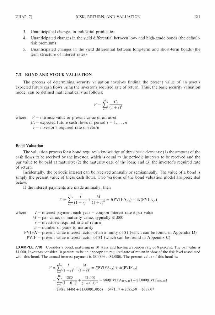
3. Unanticipated changes in industrial production
4. Unanticipated changes in the yield differential between low- and high-grade bonds (the default-
risk premium)
5. Unanticipated changes in the yield differential between long-term and short-term bonds (the
term structure of interest rates)
7.3 BOND AND STOCK VALUATION
The process of determining security valuation involves finding the present value of an asset’s
expected future cash flows using the investor’s required rate of return. Thus, the basic security valuation
model can be defined mathematically as follows:
V ¼X
n
t¼1
Ct
ð1þ rÞt
where V=intrinsic value or present value of an asset
Ct=expected future cash flows in period t=1, . . . , n
r=investor’s required rate of return
Bond Valuation
The valuation process for a bond requires a knowledge of three basic elements: (1) the amount of the
cash flows to be received by the investor, which is equal to the periodic interests to be received and the
par value to be paid at maturity; (2) the maturity date of the loan; and (3) the investor’s required rate
of return.
Incidentally, the periodic interest can be received annually or semiannually. The value of a bond is
simply the present value of these cash flows. Two versions of the bond valuation model are presented
below:
If the interest payments are made annually, then
V ¼X
n
t¼1
I
ð1þ rÞtþ M
ð1þ rÞn ¼ IðPVIFAr,nÞ þMðPVIFr,nÞ
where I=interest payment each year=coupon interest rate� par value
M=par value, or maturity value, typically $1,000
r=investor’s required rate of return
n=number of years to maturity
PVIFA=present value interest factor of an annuity of $1 (which can be found in Appendix D)
PVIF=present value interest factor of $1 (which can be found in Appendix C)
EXAMPLE 7.10 Consider a bond, maturing in 10 years and having a coupon rate of 8 percent. The par value is
$1,000. Investors consider 10 percent to be an appropriate required rate of return in view of the risk level associated
with this bond. The annual interest payment is $80(8%� $1,000). The present value of this bond is:
V ¼X
n
t¼1
I
ð1þ rÞtþ M
ð1þ rÞn ¼ IðPVIFAr,nÞ þMðPVIFr,nÞ
¼X
10
t¼1
$80
ð1þ 0:1Þtþ $1,000
ð1þ 0:1Þ10¼ $80ðPVIFA10%,10Þ þ $1,000ðPVIF10%,10Þ
¼ $80ð6:1446Þ þ $1,000ð0:3855Þ ¼ $491:57þ $385:50 ¼ $877:07
CHAP. 7] RISK, RETURN, AND VALUATION 181

If the interest is paid semiannually, then
V ¼X
2n
t¼1
I=2
ð1þ r=2Þtþ M
ð1þ r=2Þ2n¼ I
2ðPVIFAr=2,2nÞ þMðPVIFr=2,2nÞ
EXAMPLE 7.11 Assume the same data as in Example 7.10, except the interest is paid semiannually.
V ¼X
2n
t¼1
I=2
ð1þ r=2Þtþ M
ð1þ r=2Þ2n¼ I
2ðPVIFAn=2,2nÞ þMðPVIFr=2,2nÞ
¼X
20
t¼1
$40
ð1þ 0:05Þtþ $1,000
ð1þ 0:05Þ20
¼ $40ðPVIFA5%,20Þ þ $1,000ðPVIF5%,20Þ ¼ $40ð12:4622Þ þ $1,000ð0:3769Þ ¼ $498:49þ $376:90 ¼ $875:39
Common Stock Valuation
Like bonds, the value of a common stock is the present value of all future cash inflows expected to be
received by the investor. The cash inflows expected to be received are dividends and the future price at
the time of the sale of the stock. For an investor holding a common stock for only 1 year, the value of the
stock would be the present value of both the expected cash dividend to be received in 1 year (D1) and the
expected market price per share of the stock at year-end (P1). If r represents an investor’s required rate of
return, the value of common stock (P0) would be:
P0 ¼D1
ð1þ rÞ1þ P1
ð1þ rÞ1
EXAMPLE 7.12 Assume an investor is considering the purchase of stock A at the beginning of the year. The
dividend at year-end is expected to be $1.50, and the market price by the end of the year is expected to be $40. If the
investor’s required rate of return is 15 percent, the value of the stock would be:
P0 ¼D1
ð1þ rÞ1þ P1
ð1þ rÞ1¼ $1:50
ð1þ 0:15Þ þ$40
ð1þ 0:15Þ ¼ $1:50ð0:870Þ þ $40ð0:870Þ ¼ $1:31þ $34:80 ¼ $36:11
Since common stock has no maturity date and is held for many years, a more general, multiperiod
model is needed. The general common stock valuation model is defined as follows:
P0 ¼X
1
t¼1
Dt
ð1þ rÞt
There are three cases of growth in dividends. They are (1) zero growth; (2) constant growth; and
(3) nonconstant, or supernormal, growth.
In the case of zero growth, if
D0 ¼ D1 ¼ � � � ¼ D1
then the valuation model
P0 ¼X
1
t¼1
Dt
ð1þ rÞt
182 RISK, RETURN, AND VALUATION [CHAP. 7

reduces to the formula:
P0 ¼Dt
r
EXAMPLE 7.13 Assuming D equals $2.50 and r equals 10 percent, then the value of the stock is:
P0 ¼$2:50
0:1¼ $25
In the case of constant growth, if we assume that dividends grow at a constant rate of g every year
[i.e., Dt=D0(1+ g)t], then the above model is simplified to:
P0 ¼D1
r� g
This formula is known as the Gordon growth model.
EXAMPLE 7.14 Consider a common stock that paid a $3 dividend per share at the end of the last year and is
expected to pay a cash dividend every year at a growth rate of 10 percent. Assume the investor’s required rate of
return is 12 percent. The value of the stock would be:
D1 ¼ D0ð1þ gÞ ¼ $3ð1þ 0:10Þ ¼ $3:30
P0 ¼D1
r� g¼ $3:30
0:12� 0:10¼ $165
Finally, consider the case of nonconstant, or supernormal, growth. Firms typically go through life
cycles, during part of which their growth is faster than that of the economy and then falls sharply. The
value of stock during such supernormal growth can be found by taking the following steps: (1) Compute
the dividends during the period of supernormal growth and find their present value; (2) find the price of
the stock at the end of the supernormal growth period and compute its present value; and (3) add these
two PV figures to find the value (P0) of the common stock.
EXAMPLE 7.15 Consider a common stock whose dividends are expected to grow at a 25 percent rate for 2 years,
after which the growth rate is expected to fall to 5 percent. The dividend paid last period was $2. The investor desires
a 12 percent return. To find the value of this stock, take the following steps:
1. Compute the dividends during the supernormal growth period and find their present value. Assuming D0
is $2, g is 15 percent, and r is 12 percent:
D1 ¼ D0ð1þ gÞ ¼ $2ð1þ 0:25Þ ¼ $2:50
D2 ¼ D0ð1þ gÞ2 ¼ $2ð1:563Þ ¼ $3:125
or D2 ¼ D1ð1þ gÞ ¼ $2:50ð1:25Þ ¼ $3:125
PV of dividends ¼ D1
ð1þ rÞ1þ D2
ð1þ rÞ2¼ $2:50
ð1þ 0:12Þ þ$3:125
ð1þ 0:12Þ2
¼ $2:50ðPVIF12%,1Þ þ $3:125ðPVIF12%,2Þ
¼ $2:50ð0:8929Þ þ $3:125ð0:7972Þ ¼ $2:23þ $2:49 ¼ $4:72
2. Find the price of the stock at the end of the supernormal growth period. The dividend for the third year is:
D3 ¼ D2ð1þ g0Þ, where g0 ¼ 5%
¼ $3:125ð1þ 0:05Þ ¼ $3:28
CHAP. 7] RISK, RETURN, AND VALUATION 183
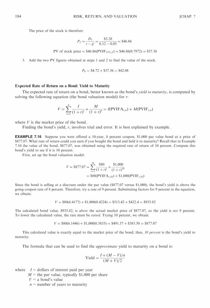
The price of the stock is therefore:
P2 ¼D3
r� g0¼ $3:28
0:12� 0:05¼ $46:86
PV of stock price ¼ $46:86ðPVIF12%,2Þ ¼ $46:86ð0:7972Þ ¼ $37:36
3. Add the two PV figures obtained in steps 1 and 2 to find the value of the stock.
P0 ¼ $4:72þ $37:36 ¼ $42:08
Expected Rate of Return on a Bond: Yield to Maturity
The expected rate of return on a bond, better known as the bond’s yield to maturity, is computed by
solving the following equation (the bond valuation model) for r:
V ¼X
n
t¼1
I
ð1þ rÞtþ M
ð1þ rÞn ¼ IðPVIFAr,nÞ þMðPVIFr,nÞ
where V is the market price of the bond.
Finding the bond’s yield, r, involves trial and error. It is best explained by example.
EXAMPLE 7.16 Suppose you were offered a 10-year, 8 percent coupon, $1,000 par value bond at a price of
$877.07. What rate of return could you earn if you bought the bond and held it to maturity? Recall that in Example
7.10 the value of the bond, $877.07, was obtained using the required rate of return of 10 percent. Compute this
bond’s yield to see if it is 10 percent.
First, set up the bond valuation model:
V ¼ $877:07 ¼X
10
t¼1
$80
ð1þ rÞtþ $1,000
ð1þ rÞ10
¼ $80ðPVIFAr,10Þ þ $1,000ðPVIFr,10Þ
Since the bond is selling at a discount under the par value ($877.07 versus $1,000), the bond’s yield is above the
going coupon rate of 8 percent. Therefore, try a rate of 9 percent. Substituting factors for 9 percent in the equation,
we obtain:
V ¼ $80ð6:4177Þ þ $1,000ð0:4224Þ ¼ $513:42þ $422:4 ¼ $935:82
The calculated bond value, $935.82, is above the actual market price of $877.07, so the yield is not 9 percent.
To lower the calculated value, the rate must be raised. Trying 10 percent, we obtain:
V ¼ $80ð6:1446Þ þ $1,000ð0:3855Þ ¼ $491:57þ $385:50 ¼ $877:07
This calculated value is exactly equal to the market price of the bond; thus, 10 percent is the bond’s yield to
maturity.
The formula that can be used to find the approximate yield to maturity on a bond is:
Yield ¼ Iþ ðM� VÞ=nðMþ VÞ=2
where I=dollars of interest paid per year
M=the par value, typically $1,000 per share
V= a bond’s value
n=number of years to maturity
184 RISK, RETURN, AND VALUATION [CHAP. 7

This formula can also be used to obtain a starting point for the trial-and-error method discussed in
Example 7.16.
EXAMPLE 7.17 Using the same data as in Example 7.16 and the shortcut method, the rate of return on the
bond is:
Yield ¼ Iþ ðM� VÞ=nðMþ VÞ=2 ¼ $80þ ð$1,000� $877:60Þ=10
ð$1,000þ $877:60Þ=2 ¼ $80þ $12:24
$938:80¼ $92:24
$938:80¼ 9:8%
which is very close to the exact rate of 10 percent.
Expected Rate of Return on Common Stock
The formula for computing the expected rate of return on common stock can be derived easily from
the valuation models.
The single-period return formula is derived from:
P0 ¼D1
ð1þ rÞ þP1
ð1þ rÞ
Solving for r gives:
r ¼ D1 þ ðP1 � P0ÞP0
In words,
Rate of return ¼ dividendsþ capital gain
beginning price
¼ dividend yieldþ capital gain yield
EXAMPLE 7.18 Consider a stock that sells for $50. The company is expected to pay a $3 cash dividend at the end
of the year, and the stock’s market price at the end of the year is expected to be $55 a share. Thus, the expected
return would be:
r ¼ D1 þ ðP1 � P0ÞP0
¼ $3:00þ ð$55� $50Þ$50
¼ $3:00þ $5:00
$50¼ 16%
or:
Dividend yield ¼ $3:00
$50¼ 6%
Capital gain yield ¼ $5:00
$50¼ 10%
r ¼ dividend yieldþ capital gain yield
¼ 6%þ 10% ¼ 16%
Assuming a constant growth in dividend, the formula for the expected rate of return on an invest-
ment in stock can be derived as follows:
P0 ¼D1
r� g
r ¼ D1
P0
þ g
CHAP. 7] RISK, RETURN, AND VALUATION 185

EXAMPLE 7.19 Suppose that ABC Company’s dividend per share was $4.50, expected to grow at a constant rate
of 6 percent. The current market price of the stock is $30. Then the expected rate of return is:
r ¼ D1
P0
þ g ¼ $4:50
$30þ 6% ¼ 15%þ 6% ¼ 21%
7.4 DETERMINING INTEREST-RATE RISK
Interest-rate risk of a debt instrument such as a bond can be determined in two ways. One way is to
look at the term structure of a debt security by measuring its average term to maturity — a duration. The
other way is to measure the sensitivity of changes in a debt security’s price associated with changes in its
yield to maturity. We will discuss two measurement approaches: Macaulay’s duration coefficient and the
interest elasticity.
Duration
Duration (D), more exactly known asMacaulay’s Duration Coefficient, is an attempt to measure risk
in a bond by considering the maturity and the time pattern of cash inflows (i.e., interest payments and
principal). It is defined as the number of years until a bond pays back its principal.
EXAMPLE 7.20 A bond pays a 7 percent coupon rate annually on its $1,000 face value if it has 3 years until its
maturity and has a YTM of 6 percent. The computation of duration involves the following three steps:
Step 1 Calculate the present value of the bond for each year.
Step 2 Express present values as proportions of the price of the bond.
Step 3 Multiply proportions by years’ digits to obtain the weighted average time.
(Step 1) (Step 2) (Step 3)
(1) (2) (3) (4) (5) (6)
Year Cash flow
PV factor
@ 6%
PV of
Cashflow
PV as proportion
of price of bond
(6)= (1)� (5)
Column (5)
1 $70 0.9434 $ 66.04 0.0643 0.0643
2 70 0.8900 62.30 0.0607 0.1214
3 1,070 0.8396 898.39 0.8750 2.6250
$1,026.73 1.0000 2.8107
This 3-year bond’s duration is a little over 2.8 years. Although duration is expressed in years, think of it
as a percentage change. Thus, 2.8 years means this particular bond will gain (lose) 2.8 percent of its value
for each 1 percentage drop (rise) in interest rates. Note, however, that duration will not tell you anything
about the credit quality or yield of your bonds.
Interest Rate Elasticity
A bond’s interest rate elasticity (E) is defined as
E ¼ Percentage change in bond price
Percentage change in YTM
Since bond prices and YTMs always move inversely, the elasticity will always be a negative number.
Any bond’s elasticity can be determined directly with the above formula. Knowing the duration
coefficient (D), we can calculate the E using the following simple formula:
ð�1ÞE ¼ DYTM
ð1þYTMÞ
186 RISK, RETURN, AND VALUATION [CHAP. 7

EXAMPLE 7.21 Using the same date in Example 7.20, the elasticity is calculated as follows:
(�1) E=2.8107 [0.06/(1.06)]=0.1591, which means that the bond will lose or gain 15.91% of principal value
for each 1 percentage point move in interest rates.
Review Questions
1. refers to the variability of associated with a given
investment.
2. Expected rate of return is the of possible returns from a given investment,
with the weights being .
3. The smaller the standard deviation, the ‘‘tighter’’ the and, thus, the lower
the of the investment.
4. The higher the coefficient of , the greater the risk of the security.
5. depends on in demand, sales price, input prices, and so on.
6. refers to the change in a stock’s price that results from changes in the stock
market as a whole.
7. Total risk is the sum of and .
8. Portfolio risk can be reduced by .
9. �AB=�1.0 means that assets A and B have a(n) .
10. The , or , equation shows that the required rate of return on a
security is equal to the risk-free rate plus .
11. The valuation process involves finding the of an asset’s expected future cash
flows using the investor’s required rate of return.
12. The expected rate of return on a stock is the sum of yield and
yield.
13. The computes the value of a common stock when dividends are expected to
grow at a constant rate.
14. The three cases of dividend growth are: , ,
and .
15. The one-period return on stock investment is dividends plus , divided by the
beginning price.
16. is an index of systematic risk.
17. Unlike the Capital Asset Pricing Model (CAPM), the includes any number of
risk factors.
CHAP. 7] RISK, RETURN, AND VALUATION 187
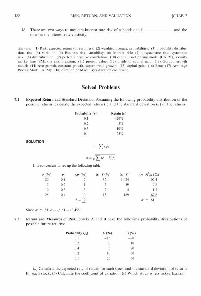
18. There are two ways to measure interest rate risk of a bond: one is and the
other is the interest rate elasticity.
Answers: (1) Risk, expected return (or earnings); (2) weighted average, probabilities; (3) probability distribu-
tion, risk; (4) variation; (5) Business risk, variability; (6) Market risk; (7) unsystematic risk, systematic
risk; (8) diversification; (9) perfectly negative correlation; (10) capital asset pricing model (CAPM), security
market line (SML), a risk premium; (11) present value; (12) dividend, capital gain; (13) Gordon growth
model; (14) zero growth, constant growth, supernormal growth; (15) capital gain; (16) Beta; (17) Arbitrage
Pricing Model (APM); (18) duration or Macaulay’s duration coefficient.
Solved Problems
7.1 Expected Return and Standard Deviation. Assuming the following probability distribution of the
possible returns, calculate the expected return ð�rÞ and the standard deviation (�) of the returns.
Probability (pi) Retain (ri)
0.1 �20%0.2 5%
0.3 10%
0.4 25%
SOLUTION
r ¼X
ripi
� ¼ffiffiffiffiffiffiffiffiffiffiffiffiffiffiffiffiffiffiffiffiffiffiffiffiffiffiffi
X
ðri � �rÞ2piq
It is convenient to set up the following table:
ri (%) pi ripi (%) ðri��rÞð%Þ ðri��rÞ2 ðri��rÞ2pi ð%Þ�20 0.1 �2 �32 1,024 102.4
5 0.2 1 �7 49 9.8
10 0.3 3 �2 4 1.2
25 0.4 10 13 169 67.6
�r ¼ 12 �2=181
Since �2=181, � ¼
ffiffiffiffiffiffiffiffi
181p
¼ 13:45%.
7.2 Return and Measures of Risk. Stocks A and B have the following probability distributions of
possible future returns:
Probability (pi) A (%) B (%)
0.1 �15 �200.2 0 10
0.4 5 20
0.2 10 30
0.1 25 50
(a) Calculate the expected rate of return for each stock and the standard deviation of returns
for each stock, (b) Calculate the coefficient of variation, (c) Which stock is less risky? Explain.
188 RISK, RETURN, AND VALUATION [CHAP. 7

SOLUTION
(a) For stock A:
ri (%) pi ripi (%) ðri��rÞð%Þ ðri��rÞ2 ðri��rÞ2pi ð%Þ�15 0.1 �1.5 �20 400 40
0 0.2 0 �5 25 5
5 0.4 2 0 0 0
10 0.2 2 5 25 5
25 0.1 2.5 20 400 40
�r ¼ 5.0 �2 ¼ 90
Since �2=90, � ¼
ffiffiffiffiffi
90p¼ 9:5%.
For stock B:
ri (%) pi ripi (%) ðri��rÞð%Þ ðri��rÞ2 ðri��rÞ2pi ð%Þ�20 0.1 �2 �39 1,521 152.1
10 0.2 2 �9 81 16.2
20 0.4 8 1 1 0.4
30 0.2 6 11 121 24.2
50 0.1 5 31 961 96.1
�r ¼ 19 �2 ¼ 289
Since �2=289, � ¼
ffiffiffiffiffiffiffiffi
289p
¼ 17%.
(b) The coefficient of variation is �=�r. Thus, for stock A:
9:5%
5%¼ 1:9
For stock B:
17:0%
19%¼ 0:89
(c) Stock B is less risky than stock A since the coefficient of variation (a measure of relative risk) is smaller
for stock B.
7.3 Absolute and Relative Risk. Ken Parker must decide which of two securities is best for him.
By using probability estimates, he computed the following statistics:
Statistic Security X Security Y
Expected return ð�rÞ 12% 8%
Standard deviation (�) 20% 10%
(a) Compute the coefficient of variation for each security, and (b) explain why the standard
deviation and coefficient of variation give different rankings of risk. Which method is superior
and why?
SOLUTION
(a) For the X coefficient of variation ð�=�rÞ is 20/12=1.67. For Y it is 10/8=1.25.
(b) Unlike the standard deviation, the coefficient of variation considers the standard deviation of secu-
rities relative to their average return. The coefficient of variation is therefore the more useful measure
of relative risk. The lower the coefficient of variation, the less risky the security relative to the expected
return. Thus, in this problem, security Y is relatively less risky than security X.
CHAP. 7] RISK, RETURN, AND VALUATION 189

7.4 Diversification Effects. The securities of firms A and B have the expected return and standard
deviations given below; the expected correlation between the two stocks (�AB) is 0.1.
�r r
A 14% 20%
B 9% 30%
Compute the return and risk for each of the following portfolios: (a) 100 percent A; (b) 100
percent B; (c) 60 percent A – 40 percent B; and (d ) 50 percent A–50 percent B.
SOLUTION
(a) 100 percent A: �r ¼ 14%; � ¼ 20%; �=�r ¼ 20
14¼ 1:43
(b) 100 percent B: �r ¼ 9%; � ¼ 30%; �=�r ¼ 30
9¼ 3:33
(c) 60 percent A� 40 percent B:
rp ¼ wArA þ wBrB ¼ ð0:6Þð14%Þ þ ð0:4Þð9%Þ ¼ 12%
�p ¼ffiffiffiffiffiffiffiffiffiffiffiffiffiffiffiffiffiffiffiffiffiffiffiffiffiffiffiffiffiffiffiffiffiffiffiffiffiffiffiffiffiffiffiffiffiffiffiffiffiffiffiffiffiffiffiffiffiffiffiffiffiffiffiffiffiffi
w2A�
2B þ w2
B�2B þ 2wAwB�AB�A�B
q
¼ffiffiffiffiffiffiffiffiffiffiffiffiffiffiffiffiffiffiffiffiffiffiffiffiffiffiffiffiffiffiffiffiffiffiffiffiffiffiffiffiffiffiffiffiffiffiffiffiffiffiffiffiffiffiffiffiffiffiffiffiffiffiffiffiffiffiffiffiffiffiffiffiffiffiffiffiffiffiffiffiffiffiffiffiffiffiffiffiffiffiffiffiffiffiffiffiffiffiffiffiffiffiffiffi
ð0:6Þ2ð0:2Þ2 þ ð0:4Þ2ð0:3Þ2 þ 2ð0:6Þð0:4Þ�ABð0:2Þð0:3Þq
¼ffiffiffiffiffiffiffiffiffiffiffiffiffiffiffiffiffiffiffiffiffiffiffiffiffiffiffiffiffiffiffiffiffiffiffiffiffiffiffiffiffiffiffiffiffiffiffiffiffiffiffiffiffiffiffiffiffiffiffiffi
0:0144þ 0:0144þ 0:0288�AB
p
¼ffiffiffiffiffiffiffiffiffiffiffiffiffiffiffiffiffiffiffiffiffiffiffiffiffiffiffiffiffiffiffiffiffiffiffiffiffiffiffiffiffiffi
0:0288þ 0:0288ð0:1Þp
¼ffiffiffiffiffiffiffiffiffiffiffiffiffiffiffiffi
0:03168p
¼ 0:1780 ¼ 17:8%
(d ) 50 percent A� 50 percent B:
rp ¼ ð0:5Þð14%Þ þ ð0:5Þð9%Þ ¼ 11:5%
�p ¼ffiffiffiffiffiffiffiffiffiffiffiffiffiffiffiffiffiffiffiffiffiffiffiffiffiffiffiffiffiffiffiffiffiffiffiffiffiffiffiffiffiffiffiffiffiffiffiffiffiffiffiffiffiffiffiffiffiffiffiffiffiffiffiffiffiffiffiffiffiffiffiffiffiffiffiffiffiffiffiffiffiffiffiffiffiffiffiffiffiffiffiffiffiffiffiffiffiffiffiffiffiffiffiffi
ð0:5Þ2ð0:2Þ2 þ ð0:5Þ2ð0:3Þ2 þ 2ð0:5Þð0:5Þ�ABð0:2Þð0:3Þq
¼ffiffiffiffiffiffiffiffiffiffiffiffiffiffiffiffiffiffiffiffiffiffiffiffiffiffiffiffiffiffiffiffiffiffiffiffiffiffiffiffiffiffiffiffiffiffiffiffiffiffi
0:01þ 0:0225þ 0:03�AB
p
¼ffiffiffiffiffiffiffiffiffiffiffiffiffiffiffiffiffiffiffiffiffiffiffiffiffiffiffiffiffiffiffiffiffiffiffiffi
0:0325þ 0:03�AB
p
¼ffiffiffiffiffiffiffiffiffiffiffiffiffiffiffiffiffiffiffiffiffiffiffiffiffiffiffiffiffiffiffiffiffiffiffiffiffi
0:0325þ 0:03ð0:1Þp
¼ffiffiffiffiffiffiffiffiffiffiffiffiffiffi
0:0355p
¼ 0:1884 ¼ 18:84%
7.5 Diversification Effects. Use the same facts as for Problem 7.4, except for this problem assume the
expected correlation between the two stocks (�AB)=�1.0.
SOLUTION
(a) and (b) The answers are the same as in Problem 7.4.
(c) rp ¼ 12%
�p ¼ffiffiffiffiffiffiffiffiffiffiffiffiffiffiffiffiffiffiffiffiffiffiffiffiffiffiffiffiffiffiffiffiffiffiffiffiffiffiffiffiffiffiffiffiffiffi
0:0288þ 0:0288ð�1:0Þp
¼ffiffiffi
0p¼ 0%
(d ) rp ¼ 11:5%
�p ¼ffiffiffiffiffiffiffiffiffiffiffiffiffiffiffiffiffiffiffiffiffiffiffiffiffiffiffiffiffiffiffiffiffiffiffiffiffiffiffiffiffi
0:0325þ 0:03ð�1:0Þp
¼ffiffiffiffiffiffiffiffiffiffiffiffiffiffi
0:0025p
¼ 0:05 ¼ 5%
7.6 Portfolio Risk. What is the standard deviation of the following two-stock portfolio?
Weighting
Standard
Deviation Correlation
Stock A 60% 11% 0.7
Stock B 40% 14%
(CFM adapted.)
190 RISK, RETURN, AND VALUATION [CHAP. 7
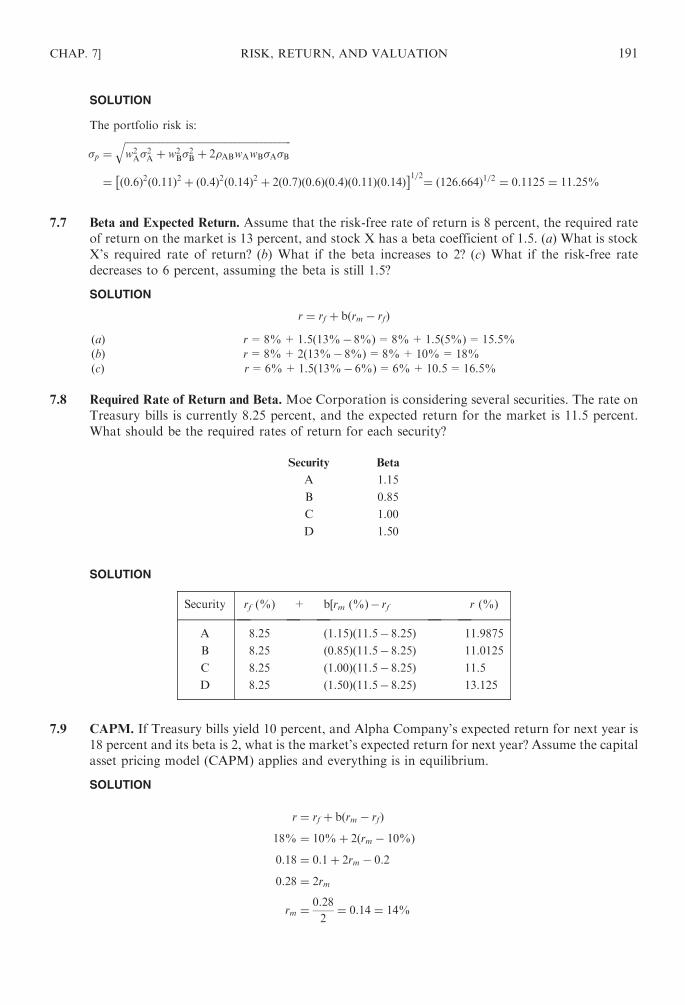
SOLUTION
The portfolio risk is:
�p ¼ffiffiffiffiffiffiffiffiffiffiffiffiffiffiffiffiffiffiffiffiffiffiffiffiffiffiffiffiffiffiffiffiffiffiffiffiffiffiffiffiffiffiffiffiffiffiffiffiffiffiffiffiffiffiffiffiffiffiffiffiffiffiffiffiffiffiffi
w2A�
2A þ w2
B�2B þ 2�ABwAwB�A�B
q
¼ ð0:6Þ2ð0:11Þ2 þ ð0:4Þ2ð0:14Þ2 þ 2ð0:7Þð0:6Þð0:4Þð0:11Þð0:14Þ� �1=2¼ ð126:664Þ1=2 ¼ 0:1125 ¼ 11:25%
7.7 Beta and Expected Return. Assume that the risk-free rate of return is 8 percent, the required rate
of return on the market is 13 percent, and stock X has a beta coefficient of 1.5. (a) What is stock
X’s required rate of return? (b) What if the beta increases to 2? (c) What if the risk-free rate
decreases to 6 percent, assuming the beta is still 1.5?
SOLUTION
r ¼ rf þ bðrm � rfÞ
(a) r=8%+1.5(13%� 8%)=8%+1.5(5%)=15.5%
(b) r=8%+2(13%� 8%)=8%+10%=18%
(c) r=6%+1.5(13%� 6%)=6%+10.5=16.5%
7.8 Required Rate of Return and Beta. Moe Corporation is considering several securities. The rate on
Treasury bills is currently 8.25 percent, and the expected return for the market is 11.5 percent.
What should be the required rates of return for each security?
Security Beta
A 1.15
B 0.85
C 1.00
D 1.50
SOLUTION
Security rf (%) + b[rm (%)� rf (%)] = r (%)
A 8.25 (1.15)(11.5� 8.25) 11.9875
B 8.25 (0.85)(11.5� 8.25) 11.0125
C 8.25 (1.00)(11.5� 8.25) 11.5
D 8.25 (1.50)(11.5� 8.25) 13.125
7.9 CAPM. If Treasury bills yield 10 percent, and Alpha Company’s expected return for next year is
18 percent and its beta is 2, what is the market’s expected return for next year? Assume the capital
asset pricing model (CAPM) applies and everything is in equilibrium.
SOLUTION
r ¼ rf þ bðrm � rfÞ
18% ¼ 10%þ 2ðrm � 10%Þ
0:18 ¼ 0:1þ 2rm � 0:2
0:28 ¼ 2rm
rm ¼0:28
2¼ 0:14 ¼ 14%
CHAP. 7] RISK, RETURN, AND VALUATION 191

7.10 Beta. Assuming the CAPM applies, if the market’s expected return is 13 percent, the risk-free
rate is 8 percent, and stock A’s required rate of return is 16 percent, what is the stock’s beta
coefficient?
SOLUTION
r ¼ rf þ bðrm � rfÞ16% ¼ 8%þ bð13%� 8%Þ0:16 ¼ 0:08þ bð0:05Þ0:08 ¼ bð0:05Þ
b ¼ 1:6
7.11 Security Market Line (SML). The risk-free rate is 7 percent, and the expected return on the
market portfolio is 12 percent. (a) What is the equation for the security market line (SML)?
(b) Graph the SML.
SOLUTION
(a) The SML equation is:
r ¼ rf þ bðrm � rfÞ ¼ 7%þ bð12%� 7%Þ ¼ 7%þ bð5%Þ
(b) See Fig. 7-2.
7.12 CAPM. Assume the following: the risk-free rate is 8 percent, and the market portfolio expected
return is 12 percent.Portfolio Beta
A 0.6
B 1.0
C 1.4
(a) Calculate for each of the three portfolios the expected return consistent with the capital
asset pricing model. (b) Show graphically the expected portfolio returns in (a). (c) Indicate what
would happen to the capital market line if the expected return on the market portfolio were 10
percent (CFA, adapted.)
SOLUTION
(a) Portfolio A: r ¼ 8%þ 0:6ð12%� 8%Þ ¼ 10:4%
Portfolio B: r ¼ 8%þ 1:0ð12%� 8%Þ ¼ 12:0%
Portfolio C: r ¼ 8%þ 1:4ð12%� 8%Þ ¼ 13:6%
Fig. 7-2
192 RISK, RETURN, AND VALUATION [CHAP. 7

(b) See Fig. 7-3.
(c) A lower expected return for the market portfolio would change the slope of the market line downward,
as is shown in Fig. 7-4.
7.13 CAPM. During a 5-year period, the relevant results for the aggregate market are that the rf(risk-free rate) is 8 percent and the rm (return on market) is 14 percent. For that period, the
results of four portfolio managers are as follows:
Portfolio Manager Average Return (%) Beta
A 13 0.80
B 14 1.05
C 17 1.25
D 13 0.90
(a) Calculate the expected rate of return for each portfolio manager and compare the actual
returns with the expected returns. (b) Based upon your calculations, select the manager with the
best performance. (c) What are the critical assumptions in the capital asset pricing model
(CAPM)? What are the implications of relaxing these assumptions? (CFA, adapted.)
SOLUTION
(a) Use the CAPM equation:
rj ¼ rf þ bðrm � rfÞ
Fig. 7-3
Fig. 7-4
CHAP. 7] RISK, RETURN, AND VALUATION 193

The expected rates of return are as follows:
Portfolio
Manager
Average
Return (%) Expected Return (%)
Actual
Return (%)
Difference
between
Actual and
Expected
Returns (%)
A 13 rA=8%+0.80(14%� 8%)=12.8 13 +0.2
B 14 rB=8%+1.05(14%� 8%)=14.3 14 �0.3C 17 rC=8%+1.25(14%� 8%)=15.5 17 +1.5
D 13 rD=8%+0.90(14%� 8%)=13.4 13 �0.4
(b) Portfolio managers A and C did better than expected, since A exceeded the expected return by 1.56
percent (0.2% 7 12.8%) and C bettered the expected return by 9.68 percent (1.5% 7 15.5%).
C therefore showed the best performance.
(c) The critical assumptions in CAPM are perfect capital markets and homogeneous expectations.
Relaxation of the perfect capital markets assumption results in limitations to the effectiveness of
predicting and computing expected return on stock. Certain securities may have values and expected
returns that are not entirely explained by the security market line. Residual risk may be important,
particularly where bankruptcy costs are significant. When expectations of market participants are
not homogeneous, each investor has his or her own capital market line. The important thing to
stress, however, is that in market equilibrium, there still will exist an implied risk-return trade-
off for securities where risk is represented by the undiversifiable risk, as opposed to the total risk of the
security.
7.14 Value of Bond. Trooper Corporation has a bond issue with a coupon rate of 10 percent per year
and 5 years remaining until maturity. The par value of the bond is $1,000. What is the value of the
bond when the going rate of interest is (a) 6 percent; (b) 10 percent; and (c) 12 percent? The bond
pays interest annually.
SOLUTION
Annual interest ¼ 10%� $1,000 ¼ $100
V ¼X
n
i¼1
I
ð1þ rÞtþ M
ð1þ rÞn ¼$100
ð1þ rÞ1þ $100
ð1þ rÞ2þ � � � þ $100
ð1þ rÞ5þ $1,000
ð1þ rÞ5
¼ $100ðPVIFAr,nÞ þ $1,000ðPVIFr,nÞ
(a) Value ¼ $100ðPVIFA6%,5Þ þ $1,000ðPVIF6%,5Þ¼ $100ð4:2124Þ þ $1,000ð0:7473Þ ¼ $421:24þ $747:30 ¼ $1,168:54
(b) Value ¼ $100ðPVIFA10%,5Þ þ $1,000ðPVIF10%,5Þ¼ $100ð3:7908Þ þ $1,000ð0:6209Þ ¼ $379:08þ $620:90 ¼ $999:98
(c) Value ¼ $100ðPVIFA12%,5Þ þ $1,000ðPVIF12%,5Þ¼ $100ð3:6048Þ þ $1,000ð0:5674Þ ¼ $360:48þ $567:40 ¼ $927:88
7.15 Value of Bond. Assume the same data and questions as in Problem 7.13, except that in this
problem, the bond pays interest semiannually.
SOLUTION
Semiannual interest ¼ $100
2¼ $50
Number of periods ¼ 5 years� 2 ¼ 10 periods
194 RISK, RETURN, AND VALUATION [CHAP. 7

V ¼X
2n
t¼1
I=2
ð1þ r=2Þtþ M
ð1þ r=2Þ2n
¼ $50
ð1þ r=2Þ þ$50
ð1þ r=2Þ2� � � $50
ð1þ r=2Þ10þ $1,000
ð1þ r=2Þ10
¼ $50ðPVIFAr=2,10Þ þ $1,000ðPVIFr=2,10Þ
(a) V ¼ $50ðPVIFA3%,10Þ þ $1,000ðPVIF3%,10Þ¼ $50ð8:5302Þ þ $1,000ð0:7441Þ ¼ $426:51þ $744:10 ¼ $1,170:61
(b) V ¼ $50ðPVIFA5%,10Þ þ $1,000ðPVIF5%,10Þ¼ $50ð7:7217Þ þ $1,000ð0:6139Þ ¼ $386:09þ $613:90 ¼ $999:99
(c) V ¼ $50ðPVIFA6%,10Þ þ $1,000ðPVIF6%,10Þ¼ $50ð7:3601Þ þ $1,000ð0:5584Þ ¼ $368:01þ $558:40 ¼ $926:41
7.16 Stock Valuation—Single Period. Mary Czech is considering the purchase of stock X at the
beginning of the year. The dividend at year-end is expected to be $3.25, and the market price
by the end of the year is expected to be $25. If she requires a rate of return of 12 percent, what is
the value of the stock?
SOLUTION
P0 ¼D1
ð1þ rÞ þP1
ð1þ rÞ ¼$3:25
ð1þ 0:12Þ þ$25
ð1þ 0:12Þ¼ $3:25ð0:893Þ þ $25ð0:893Þ ¼ $2:90þ $22:33 ¼ $25:23
7.17 Stock Valuation—Finite Periods. The Ohm Company paid a $2.50 dividend per share at the end
of the year. The dividend is expected to grow by 10 percent each year for the next 3 years, and the
stock’s market price per share is expected to be $50 at the end of the third year. Investors require a
rate of return of 14 percent. At what price per share should the Ohm stock sell?
SOLUTION
P0 ¼X
3
t¼1
Dt
ð1þ rÞtþ P3
ð1þ rÞ3
Note that
D0 ¼ $2:50
D1 ¼ $2:50ð1þ 0:10Þ ¼ $2:50ð1:10Þ ¼ $2:75
D2 ¼ $2:50ð1þ 0:10Þ2 ¼ $2:50ð1:21Þ ¼ $3:03
D3 ¼ $2:50ð1þ 0:10Þ3 ¼ $2:50ð1:331Þ ¼ $3:33
P0 ¼$2:75
ð1þ 0:14Þ þ$3:03
ð1þ 0:14Þ2þ $3:33
ð1þ 0:14Þ3þ $50
ð1þ 0:14Þ3
¼ $2:75ð0:877Þ þ $3:03ð0:770Þ þ $3:33ð0:675Þ þ $50ð0:675Þ¼ $2:41þ $2:33þ $2:25þ $33:75 ¼ $40:74
The stock should sell for $40.74 per share.
7.18 Stock Valuation—No Growth in Dividends. Susan O’Reilly invests in a stock of company X which
expects no growth in dividends. The company paid a $2.75 dividend per share. If Susan requires a
rate of return of 10 percent, what would be the value of the stock?
CHAP. 7] RISK, RETURN, AND VALUATION 195

SOLUTION
If D0 ¼ D1 ¼ D2 ¼ � � � ¼ D1, then
P0 ¼D
r
Therefore,
P0 ¼$2:75
0:1¼ $27:50
7.19 The Gordon Dividend Growth Model. Develop the Gordon growth model, assuming constant
growth of dividends, i.e., Dt ¼ D0ð1þ gÞt.
SOLUTION
Since Dt ¼ D0ð1þ gÞt
P0 ¼D0ð1þ gÞð1þ rÞ þ
D0ð1þ gÞ2
ð1þ rÞ2þ � � � þD0ð1þ gÞ1
ð1þ rÞ1
If both sides of this expression are multiplied by (1+ r)/(1+ g) and then this is subtracted from the
product, the result is:
P0ð1þ rÞð1þ gÞ � P0 ¼ D0 �
D0ð1þ gÞ1
ð1þ rÞ1
If r> g, which should normally be true, the term on the far right-hand side approaches zero. As a result,
P0ð1þ rÞð1þ gÞ � P0 ¼ D0
P0
1þ r
1þ g
� �
� P0
1þ g
1þ g
� �
¼ D0
P0
ð1þ rÞ � ð1� gÞð1þ gÞ
�
¼ D0
P0ðr� gÞ ¼ D0ð1þ gÞ
If we assume dividends grow at a constant rate g, then
Dt ¼ D0ð1þ gÞt and t ¼ 1
and
P0 ¼D1
r� g
7.20 Stock Valuation. Investors require a rate of return of 12 percent. At what price will the stock sell if
the next expected dividend D1 is $1 per share and investors expect the dividends and earnings to
grow (a) at 8 percent; (b) at 10 percent; (c) at 12 percent; and (d ) at 14 percent?
SOLUTION
P0 ¼D1
r� g
(a) P0 ¼$1
0:12� 0:08¼ $25
(b) P0 ¼$1
0:12� 0:1¼ $50
196 RISK, RETURN, AND VALUATION [CHAP. 7

(c) P0 ¼$1
0:12� 0:12¼ undefined
The formula is invalid since a necessary condition is r > g.
(d )P0 ¼
$1
0:12� 0:14¼ undefined
7.21 Beta and Stock Valuation. The risk-free rate is 6 percent, the required rate of return on the market
is 12 percent, and stock A has a beta coefficient of 1.2. If the dividend expected during the coming
year is $2 and the growth rate of dividends and earnings is 7 percent, at what price should stock A
sell?
SOLUTION
r ¼ rf þ bðrm � rfÞ ¼ 6%þ 1:2ð12%� 6%Þ ¼ 6%þ 7:2% ¼ 13:2%
Therefore,
P0 ¼D1
r� g¼ $2
13:2%� 7%¼ $2
0:062¼ $32:26
7.22 Stock Valuation. Investors require a 20 percent per year return on the stock of M Company.
Yesterday M Company paid a $2 dividend (dividends are paid annually). The dividend is
expected to grow 30 percent per year for the next 2 years and at 8 percent per year thereafter.
At what price should the stock sell?
SOLUTION
D0 ¼ $2
D1 ¼ $2ð1þ 0:3Þ ¼ $2:60
D2 ¼ $2ð1þ 0:3Þ2 ¼ $2ð1:69Þ ¼ $3:38
D3 ¼ $3:38ð1þ 0:08Þ ¼ $3:65
Present value of dividends for the first 2 years are:
$2:60
ð1þ 0:2Þ þ$3:38
ð1þ 0:2Þ2¼ $2:60ðPVIF20%,1Þ þ $3:38ðPVIF20%,2Þ
¼ $2:60ð0:8333Þ þ $3:38ð0:6944Þ ¼ $2:17þ $2:35 ¼ $4:52
Find P2:
P2 ¼D3
r� g¼ $3:65
0:2� 0:08¼ $30:42
Present value of $30.42 is:
$30:42
ð1þ 0:2Þ2¼ $30:42ðPVIF20%,2Þ ¼ $30:42ð0:6944Þ ¼ $21:12
Add these two PV figures to obtain P0:
P0 ¼ $4:52þ $21:12 ¼ $25:64
7.23 Stock Valuation. Investors require a 10 percent per year return on the stock of the Take-Two
Corporation, which anticipates a nonconstant growth pattern for dividends. The company paid a
$2 per share dividend. The dividend is expected to grow by 15 percent per year until the end of
year 4 (i.e., for the next 3 years) and 7 percent thereafter.
CHAP. 7] RISK, RETURN, AND VALUATION 197

(a) Project dividends for years 1 through 4. (b) Compute the present value of the dividends in
part (a). (c) Project the dividend for the fifth year (D5). (d ) Find the present value of all future
dividends beginning with the fifth year’s dividend. The present value you find will be at the end of
the fourth year. Use the formula P4=D5/(r� g). (e) Discount back the value found in part (d ) for
4 years at 10 percent. ( f ) Determine the value of the stock P0.
SOLUTION
(a) D0ðgivenÞ ¼ $2
D1 ¼ $2ð1þ 0:15Þ ¼ $2:30
D2 ¼ $2:30ð1þ 0:15Þ ¼ $2:65
D3 ¼ $2:65ð1þ 0:15Þ ¼ $3:05
D4 ¼ $3:05ð1þ 0:15Þ ¼ $3:51
(b) PV of dividends ¼ $2:30
ð1þ 0:1Þ þ$2:65
ð1þ 0:1Þ2þ $3:05
ð1þ 0:1Þ3þ $3:51
ð1þ 0:1Þ4
¼ $2:30ðPVIF10%,1Þ þ $2:65ðPVIF10%,2Þ þ $3:05ðPVIF10%,3Þ þ $3:51ðPVIF10%,4Þ
¼ $2:30ð0:9091Þ þ $2:65ð0:8264Þ þ $3:05ð0:7513Þ þ $3:51ð0:6830Þ
¼ $2:09þ $2:19þ $2:29þ $2:40 ¼ $8:97
(c) D5 ¼ $3:51ð1þ 0:15Þ ¼ $4:04
(d )P4 ¼
D5
r� g¼ $4:04
0:1� 0:07¼ $4:04
0:03¼ $134:67
(e) Therefore,
$134:67
ð1þ 0:1Þ4¼ $134:67ðPVIF10%,4Þ ¼ $134:67ð0:6830Þ ¼ $91:98
( f ) The value of the stock, P0, is:
P0 ¼ $8:97þ $91:98 ¼ $100:95
7.24 Stock Valuation. On December 31, 20X2, the shares of Amacom, Inc., closed at $20. The com-
pany subsequently paid a year-end dividend in each of the years 20X3 through 20X7 as follows:
20X3: $1.00 20X6: $1.25
20X4: $1.00 20X7: $1.25
20X5: $1.10
Suppose you had purchased a share of Amacom stock on December 31, 20X2. Find the price at
which you must sell your share at 20X7 year-end in order to realize an annual compounded total
rate of return of 10 percent on your initial investment (before commissions and taxes). (CFA,
adapted.)
SOLUTION
P0 ¼X
5
t¼1
Dt
ð1þ rÞtþ P5
ð1þ rÞ5
Substituting the value given yields:
$20 ¼X
5
t¼1
Dt
ð1þ 0:1Þtþ P5
ð1þ 0:1Þ5
198 RISK, RETURN, AND VALUATION [CHAP. 7

First compute the present value of dividends for the years 20X3 through 20X7.
$1:00
ð1þ 0:1Þ1þ $1:00
ð1þ 0:1Þ2þ $1:10
ð1þ 0:1Þ3þ $1:25
ð1þ 0:1Þ4þ $1:25
ð1þ 0:1Þ5
¼ $1:00ð0:9091Þ þ $1:00ð0:8264Þ þ $1:10ð0:7513Þ þ $1:25ð0:6830Þ þ $1:25ð0:6209Þ
¼ $0:91þ $0:83þ $0:83þ $0:85þ $0:78 ¼ $4:20
Therefore,
$20 ¼ $4:20þ P5
ð1þ 0:1Þ5
$20 ¼ $4:20þ P5ðPVIF10%,5Þ
$20 ¼ $4:20þ P5ð0:6209Þ
P5ð0:6209Þ ¼ $20� $4:20
P5ð0:6209Þ ¼ $51:80
P5 ¼$15:80
0:6209¼ $25:45
7.25 Yield to Maturity. The Rite Company’s bonds have 3 years remaining until maturity. Interest is
paid annually, the bonds have a $1,000 par value, and the coupon interest rate is 10 percent. What
is the yield to maturity at a current market price of: (a) $1,052; (b) $1,000; and (c) $935?
SOLUTION
Annual interest ¼ $100 ð10%� $1,000Þ
V ¼X
n
t¼1
I
ð1þ rÞtþ M
ð1þ rÞn
¼ IðPVIFAr,nÞ þMðPVIFr,nÞ
(a) $1,052 ¼ $100
ð1þ rÞ1þ $100
ð1þ rÞ2þ � � � þ $100
ð1þ rÞ3þ $1,000
ð1þ rÞ3
$1,052 ¼ $100ðPVIFAr,3Þ þ $1,000ðPVIFr,3Þ
Since the bond is selling above par value, the bond’s yield is below the coupon rate of 10 percent. At
r=8%:
V ¼ $100ð2:5771Þ þ $1,000ð0:7938Þ ¼ $257:71þ $793:80 ¼ $1,051:51
Therefore, the annual yield to maturity of the bond is 8 percent.
Alternatively, the shortcut formula yields:
Yield to maturity of a bond ¼ Iþ ðM� VÞ=nðMþ VÞ=2
¼ $100þ ð$1,000� $1,052Þ=3ð$1,000þ $1,052Þ=2 ¼ $82:67
$1,026¼ 8:05%
(b) $1,000 ¼ $100ðPVIFAr,3Þ þ $1,000ðPVIFr,3Þ
Since the bond is selling at par value, the bond’s yield should be the same as the coupon rate. At
r=10%:
V ¼ $100ð2:4869Þ þ $1,000ð0:7513Þ ¼ $248:69þ $751:30 ¼ $999:99
CHAP. 7] RISK, RETURN, AND VALUATION 199

Or, using the shortcut formula:
Yield ¼ $100þ ð$1,000� $1,000Þ=3ð$1,000þ $1,000Þ=2 ¼ $100
$1,000¼ 10%
(c) $935 ¼ $100ðPVIFAr,3Þ þ $1,000ðPVIFAr,3Þ
Since the bond is selling at a discount under the par value, the bond’s yield is above the going coupon
rate of 10 percent. At r=12%:
V ¼ $100ð2:4018Þ þ $1,000ð0:7118Þ ¼ $240:18þ $711:80 ¼ $951:98
At 10 percent, the bond’s value is above the actual market value of $935, so we must raise the rate. At
r=13%:
V ¼ $100ð2:361Þ þ $1,000ð0:693Þ ¼ $236:10þ $693 ¼ $929:10
Since the bond value of $935 falls between 12 percent and 13 percent, find the yield by interpolation, as
follows:
Bond Value
12% $951.18 $951.18
True yield 935.00
13% 929.10
Difference $ 16.18 $ 22.08
Yield ¼ 12%þ 16:18
22:08ð1%Þ ¼ 12%þ 0:73ð1%Þ ¼ 12:73%
Alternatively, using the shortcut method:
Yield ¼ $100þ ð$1,000� $935Þ=3ð$1,000þ $935Þ=2 ¼ $121:67
$967:5¼ 12:58%
7.26 Yield to Maturity. Assume a bond has 4 years remaining until maturity and that it pays interest
semiannually (the most recent payment was yesterday). (a) What is the yield to maturity of the
bond if its maturity value is $1,000, its coupon yield is 8 percent, and it currently sells for $821?
(b) What if it currently sells for $1,070?
SOLUTION
V ¼X
2n
t¼1
I=2
ð1þ r=2Þtþ M
ð1þ r=2Þ2n
¼ I=2ðPVIFAr=2,2nÞ þMðPVIFr=2,2nÞ
(a)Semiannual interest ¼ 8%ð$1,000Þ
2¼ $40
$821 ¼ $40
ð1þ r=2Þ1þ 40
ð1þ r=2Þ2þ � � � þ 40
ð1þ r=2Þ8þ $1,000
ð1þ r=2Þ8
$821 ¼ $40ðPVIFAr=2,8Þ þ $1,000ðPVIFr=2,8Þ
By trial and error, we find that when r/2=7%:
V ¼ $40ð5:9713Þ þ $1,000ð0:5820Þ ¼ $238:85þ $582 ¼ $820:85
Therefore, the annual yield is 7%� 2=14%.
Using the shortcut formula:
Yield ¼ Iþ ðM� VÞ=nðMþ VÞ=2 ¼ $80þ ð$1,000� $821Þ=4
ð$1,000þ $821Þ=2 ¼ $124:75
$910:5¼ 13:7%
200 RISK, RETURN, AND VALUATION [CHAP. 7

(b)$1,070 ¼ $40
ð1þ r=2Þ1þ 40
ð1þ r=2Þ2þ � � � þ 40
ð1þ r=2Þ8þ $1,000
ð1þ r=2Þ8
$1,070 ¼ $40ðPVIFAr=2,8Þ þ $1,000ðPVIFr=2,8Þ
By trial and error, we get the semiannual interest of 3 percent:
V ¼ $40ð7:0197Þ þ $1,000ð0:7894Þ ¼ $280:79þ $789:40 ¼ $1,070:19
Therefore, the annual yield is 3%� 2=6%.
Alternatively, using the shortcut method:
Yield ¼ $80þ ð$1,000� $1,070Þ=4ð$1,000þ $1,070Þ=2 ¼ $62:5
$1,035¼ 6%
7.27 Yield of a Note. You can buy a note at a price of $13,500. If you buy the note, you will receive
10 annual payments of $2,000, the first payment to be made immediately. What rate of return,
or yield, does the note offer?
SOLUTION
V ¼X
n
t¼1
Ct
ð1þ rÞt
$13,500 ¼ $2,000þ $2,000
ð1þ rÞ1þ $2,000
ð1þ rÞ2þ � � � þ $2,000
ð1þ rÞ9
$13,500 ¼ $2,000ð1þ PVIFAr,9Þ
ð1þ PVIFAr,9Þ ¼$13,500
$2,000¼ 6:75
PVIFAr,9=6.75� 1=5.75, which is very close to 10 percent as found in Appendix D.
7.28 Expected Return on Stock Investment. You are considering the purchase of a share of stock in a
firm for $40. The company is expected to pay a $2.50 dividend at the end of the year, and its
market price after the payment of the dividend is expected to be $45 a share. What is the expected
return on the investment in this stock?
SOLUTION
r ¼ dividendsþ ðending price� beginning priceÞbeginning price
¼ D1 þ ðP1 � P0ÞP0
¼ $2:50þ ð$45� $40Þ$40
¼ 18:75%
Alternatively, we set the current market price equal to the present value of the dividend, plus the
expected market price, as follows:
$40 ¼ $2:50
ð1þ rÞ þ$45
ð1þ rÞ
Solving this equation for r:
$40ð1þ rÞ ¼ $2:50þ $45
1þ r ¼ $2:50þ $45
$40
r ¼ $2:50þ $45
$40� 1 ¼ $47:50
40� 1 ¼ 1:1975� 1 ¼ 18:75%
7.29 Expected Return on Stock Investment. Tom Laboratory’s common stock is currently selling at $60
per share. The next annual dividend is expected to be $3 per share, and the earnings, dividends,
CHAP. 7] RISK, RETURN, AND VALUATION 201

and stock prices are expected to grow at a rate, of: (a) 0 percent; (b) 4 percent; and (c) 6 percent.
What is the expected total return in each case from the purchase of the common stock?
SOLUTION
r ¼ D1
P0
þ g
(a)r ¼ $3
$60þ 0 ¼ 5%
(b)r ¼ $3
$60þ 4% ¼ 5%þ 4% ¼ 9%
(c)r ¼ $3
$60þ 6% ¼ 5%þ 6% ¼ 11%
7.30 Expected Return on Stock Investment. By using the dividend growth model, estimate the cost of
equity capital for a firm with a stock price of $30, an estimated dividend at the end of the first year
of $3.00 per share, and an expected growth rate of 10 percent. (CFM adapted.)
SOLUTION
The Gordon’s dividend growth model estimates the cost of equity capital using the dividends per share, the
expected growth rate, and the market price.
r ¼ D1
P0
þ g ¼ $3
$30þ 10% ¼ 10%þ 10% ¼ 20%
The cost of equity capital is 20%. This model assumes that the payout ratio, retention rate, and the earnings
per share growth rate are all constant.
7.31 Expected Return on Stock Investment. The common stock of the Nicolas Corporation is currently
selling at $80 per share. The leadership of the company intends to pay a $4 per share dividend
next year. With the expectation that the dividend will grow at 5% perpetually, what will the
market’s required return on investment be for Nicolas common stock? (CFM adapted.)
SOLUTION
The Gordon’s dividend growth model estimates the required rate of return on common stock using the
dividends per share, the expected growth rate, and the market price.
r ¼ D1
P0
þ g ¼ $4
$80þ 5% ¼ 5%þ 5% ¼ 10%
The current dividend yield is 5% ($47 $80). Adding the growth rate of 5% to the yield of 5% results in a
required return of 10%.
7.32 Dividend Yield and Capital Gain Yield. N Company’s last dividend, D0, was $1. Earnings and
dividends are expected to grow at a 5 percent rate. The required rate of return on the stock is
13 percent. The current stock price is $25. What is the expected dividend yield and expected
capital gains yield for the coming year?
SOLUTION
Dividend yield ¼ $1:00ð1þ 0:05Þ$25
¼ $1:05
$25¼ 4:2%
Capital gain yield ¼ rate of return� dividend yield ¼ 13%� 4:2% ¼ 8:8%
202 RISK, RETURN, AND VALUATION [CHAP. 7

7.33 The Arbitrage Pricing Model (APM). Suppose a three-factor APM holds and the risk-free rate
is 6 percent. You are interested in two particular stocks: A and B. The returns on both stocks are
related to factors 1 and 2 as follows:
r ¼ 0:06þ b1ð0:09Þ � b2ð0:03Þ þ b3ð0:04Þ
The sensitivity coefficients for the two stocks are given below.
Stock b1 b2 b3
A 0.70 0.80 0.20
B 0.50 0.04 0.20
Calculate the expected returns on both stocks. Which stock requires a higher return?
SOLUTION
For stock A: r ¼ 0:06þ ð0:70Þð0:09Þ � ð0:80Þð0:03Þ þ ð0:20Þð0:04Þ¼ 10:70%
For stock B: r ¼ 0:06þ ð0:50Þð0:09Þ � ð0:40Þð0:03Þ þ ð0:20Þð0:04Þ¼ 14:10%
Stock B requires a higher return, indicating it is the riskier of the two. Part of the reason is that its return is
substantially more sensitive to the third economic force than stock A’s is.
7.34 Duration. You have a 9 percent bond with 4 years to maturity paid interest annually.
Its YTM is 10 percent and its market value is $968.29 per bond. What is the duration of
the bond?
SOLUTION
The computation of duration involves the following three steps:
Step 1 Calculate the present value of the bond for each year.
Step 2 Express present values as proportions of the price of the bond.
Step 3 Multiply proportions by years’ digits to obtain the weighted average time.
(Step 1) (Step 2) (Step 3)
(3) (4) (5) (6)
(1)
Year
(2)
Cash flow
PV factor
@10%
PV of
Cash flow
PV as proportion
of price of bond
Column (1)�Column (5)
1 $ 90 0.9091 $ 81.82 0.0845 0.0845
2 90 0.8264 74.38 0.0768 0.1536
3 90 0.7513 67.62 0.0698 0.2094
4 1,090 0.6830 744.47 0.7689 3.0756
$968.29 1.0000 3.5231
The duration of the bond is 3.52 years.
7.35 Interest Rate Sensitivity. What is the interest rate elasticity of the bond in Problem 7.31? What
does that mean?
CHAP. 7] RISK, RETURN, AND VALUATION 203

SOLUTION
The formula is:
ð�1ÞE ¼ DYTM
ð1þYTMÞ
ð�1ÞE ¼ 3:5231ð0:10=1:10Þ ¼ 0:3203, which means that the bond will lose or gain 32.03% of principal value
for each 1 percentage point move in interest rates.
204 RISK, RETURN, AND VALUATION [CHAP. 7

Chapter 8
Capital Budgeting
(Including Leasing)
8.1 CAPITAL BUDGETING DECISIONS DEFINED
Capital budgeting is the process of making long-term planning decisions for investments. There are
typically two types of investment decisions: (1) selection decisions concerning proposed projects (for
example, investments in long-term assets such as property, plant, and equipment, or resource commit-
ments in the form of new product development, market research, re-funding of long-term debt, intro-
duction of a computer, etc.) and (2) replacement decisions (for example, replacement of existing facilities
with new facilities).
8.2 MEASURING CASH FLOWS
The incremental (or relevant) after-tax cash flows that occur with an investment project are the ones
that are measured. In general the cash flows of a project fall into the following three categories: (1) the
initial investment; (2) the incremental (relevant) cash inflows over the life of the project; and (3) the
terminal cash flow.
Initial Investment
The initial investment (I) is the initial cash outlay necessary to purchase the asset and put it in
operating order. It is determined as follows:
Initial investment ¼ cost of assetþ installation cost
þ working capital investments� proceeds from
sale of old asset� taxes on sale
of old asset
The proceeds from the sale of old assets are subject to some type of tax. There are three possibilities:
1. The asset is sold for more than its book value.
2. The asset is sold for its book value.
3. The asset is sold for less than its book value.
Additional working capital (in the form of increased inventory, cash, and receivables) is usually
required to support a new investment project. This should be included in the project’s initial outlay.
At the end of the project’s life, it should be recaptured as part of the project’s terminal cash flow.
EXAMPLE 8.1 Assume that an asset has a book value of $60,000 and initially cost $100,000. Assume further that
the firm’s ordinary marginal tax rate is 34 percent. Consider each of the three possible tax situations dealing with the
sale of the old asset.
1. The old asset is sold for $80,000. In this case, the total gain is simply recapture of depreciation and taxed
at the ordinary rate. Therefore,
ð$80,000� $60,000Þð0:34Þ ¼ $6,800
2. The old asset is sold for $60,000. In this case, no taxes result since there is neither a gain nor a loss on
the sale.
3. The old asset is sold for $50,000. In this case there is a loss, which results in tax savings. The tax savings are
as follows:
ð$60,000� $50,000Þð0:34Þ ¼ $3,400
205
Copyright © 2007, 1998, 1986 by The McGraw-Hill Companies, Inc. Click here for terms of use.

Taxes on the gain from the sale of an old asset or the tax savings on a loss must be considered when determining
the amount of the initial investment of a new asset.
EXAMPLE 8.2 XYZ Corporation is considering the purchase of a new machine for $250,000, which will
be depreciated on a straight-line basis over 5 years with no salvage value. In order to put this machine in
operating order, it is necessary to pay installation charges of $50,000. The new machine will replace an existing
machine, purchased 3 years ago at a cost of $240,000, that is depreciated on a straight-line basis (with no salvage
value) over its 8-year life (i.e., $30,000 per year depreciation). The old machine can be sold for $255,000 to a
scrap dealer. The company is in the 34 percent tax bracket. The machine will require an increase investment in
inventory of $5,000.
The key calculation of the initial investment is the taxes on the sale of the old machine. The total gain, which
is the difference between the selling price and the book value, is $105,000 ($255,000� $150,000). The tax on this
$105,000 total gain is $35,700 (34%� $105,000). Therefore, the amount of initial investment is:
Purchase price of the machine $250,000
+ Installation cost 50,000
+ Increased investment in inventory 5,000
�Proceeds from sales of old machine 255,000
+Taxes on sale of old machine 35,700
Initial investment $ 85,700
Incremental (Relevant) Cash Inflows
The relevant cash inflows over a project’s expected life involve the incremental after-tax cash flows
resulting from increased revenues and/or savings in cash operating costs. Cash flows are not the same as
accounting income, which is not usually available for paying the firms’ bills. The differences between
accounting income and cash flows are such noncash charges as depreciation expense and amortization
expense.
The computation of relevant or incremental cash inflows after taxes involves the following two
steps:
1. Compute the after-tax cash flows of each proposal by adding back any noncash charges, which
are deducted as expenses on the firm’s income statement, to net profits (earnings) after taxes;
that is:
After-tax cash inflows ¼ net profits ðor earningsÞ after taxesþ depreciation
2. Subtract the cash inflows after taxes resulting from use of the old asset from the
cash inflows generated by the new asset to obtain the relevant (incremental) cash inflows
after taxes.
EXAMPLE 8.3 XYZ Corporation has provided its revenues and cash operating costs (excluding depreciation)
for the old and the new machine, as follows:
AnnualNet Profits before
Depreciation and TaxesRevenue Cash Operating Costs
Old machine $150,000 $70,000 $ 80,000
New machine $180,000 $60,000 $120,000
Recall from Example 8.2 that the annual depreciation of the old machine and the new machine will be $30,000
and $50,000, respectively.
206 CAPITAL BUDGETING (INCLUDING LEASING) [CHAP. 8

To arrive at net profits after taxes, we first have to deduct depreciation expenses from the net profits before
depreciation and taxes, as follows:
Net Profits after Taxes Add Depreciation
After-Tax
Cash Inflows
Old machine ($80,000� $30,000)(1� 0.46)=$27,000 $30,000 $57,000
New machine ($120,000� $50,000)(1� 0.46)=$37,800 $50,000 $87,800
Subtracting the after-tax cash inflows of the old machine from the cash inflows of the new machine results in the
relevant, or incremental, cash inflows for each year.
Therefore, in this example, the relevant or incremental cash inflows for each year are $87,800� $57,000=
$30,800.
Alternatively, the incremental cash inflows after taxes can be computed, using the following simple
formula:
After-tax incremental cash inflows ¼ ðincrease in revenuesÞð1� tax rateÞ� ðincrease in cash changesÞð1� tax rateÞþ ðincrease in depreciation expensesÞðtax rateÞ
EXAMPLE 8.4 Using the data in Example 8.3, after-tax incremental cash inflows for each year are:
Increase in revenue� (1� tax rate):
($180,000� $150,000)(1� 0.46) $16,200
� Increase in cash charges� (1� tax rate):
($60,000� $70,000)(1� 0.46) � (� 5,400)
+ Increase in depreciation expense�tax rate: ($50,000� $30,000)(0.46) 9,200
$30,800
Terminal Cash Flow
Cash flows associated with a project’s termination generally include the disposal value of the project
plus or minus any taxable gains or losses associated with its sale. The way in which to compute these
gains or losses is very similar to the method for computing the taxes on the sale of an old asset. In most
cases, the disposal value at the end of the project’s useful life results in a taxable gain since its book value
(or undepreciated value) is usually zero. The terminal cash flow must include the recapture of working
capital investments required in the initial outlay.
8.3 CAPITAL BUDGETING TECHNIQUES
Several methods of evaluating investment projects are as follows:
1. Payback period
2. Discounted payback period
3. Accounting rate of return (ARR)
4. Net present value (NPV)
5. Internal rate of return (IRR)
6. Profitability index (or benefit/cost ratio)
The NPV method and the IRR method are called discounted cash flow (DCF) methods. Each of these
methods is discussed below.
CHAP. 8] CAPITAL BUDGETING (INCLUDING LEASING) 207
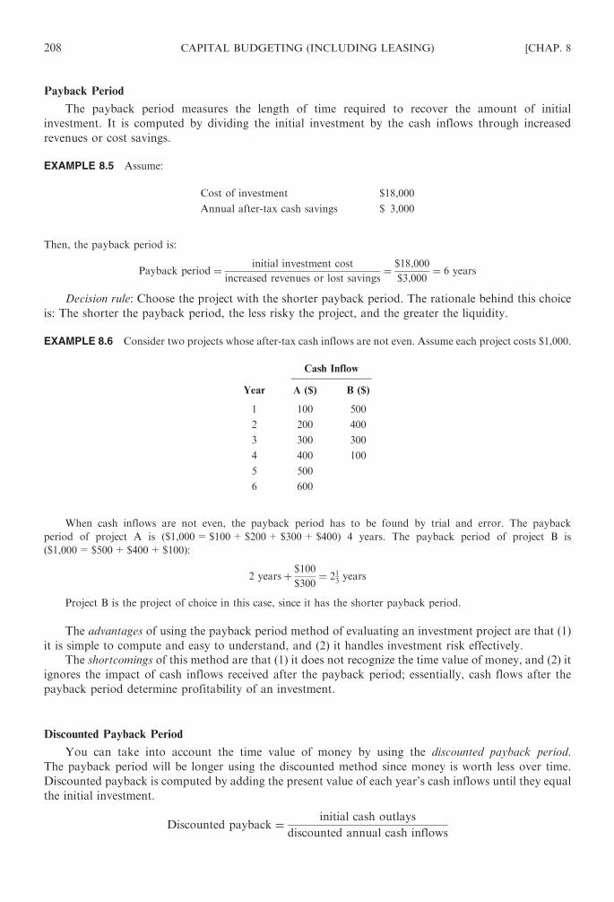
Payback Period
The payback period measures the length of time required to recover the amount of initial
investment. It is computed by dividing the initial investment by the cash inflows through increased
revenues or cost savings.
EXAMPLE 8.5 Assume:
Cost of investment $18,000
Annual after-tax cash savings $ 3,000
Then, the payback period is:
Payback period ¼ initial investment cost
increased revenues or lost savings¼ $18,000
$3,000¼ 6 years
Decision rule: Choose the project with the shorter payback period. The rationale behind this choice
is: The shorter the payback period, the less risky the project, and the greater the liquidity.
EXAMPLE 8.6 Consider two projects whose after-tax cash inflows are not even. Assume each project costs $1,000.
Cash Inflow
Year A ($) B ($)
1 100 500
2 200 400
3 300 300
4 400 100
5 500
6 600
When cash inflows are not even, the payback period has to be found by trial and error. The payback
period of project A is ($1,000=$100+$200+$300+$400) 4 years. The payback period of project B is
($1,000=$500+$400+$100):
2 yearsþ $100
$300¼ 21
3years
Project B is the project of choice in this case, since it has the shorter payback period.
The advantages of using the payback period method of evaluating an investment project are that (1)
it is simple to compute and easy to understand, and (2) it handles investment risk effectively.
The shortcomings of this method are that (1) it does not recognize the time value of money, and (2) it
ignores the impact of cash inflows received after the payback period; essentially, cash flows after the
payback period determine profitability of an investment.
Discounted Payback Period
You can take into account the time value of money by using the discounted payback period.
The payback period will be longer using the discounted method since money is worth less over time.
Discounted payback is computed by adding the present value of each year’s cash inflows until they equal
the initial investment.
Discounted payback ¼ initial cash outlays
discounted annual cash inflows
208 CAPITAL BUDGETING (INCLUDING LEASING) [CHAP. 8

EXAMPLE 8.7 You invest $40,000 and receive the following cash inflows.
Year Cash Inflow PV Factor Present Value
Accumulated
Present Value
1 $15,000 0.909 $13,635 $13,635
2 20,000 0.826 16,520 30,155
3 28,000 0.751 21,028 51,183
The discounted payback period is calculated as follows:
$30,155þ $40,000� $30,155
$51,183� $40,000¼ 2 yearsþ 0:47 years ¼ 2:47 years
Accounting Rate of Return
Accounting rate of return (ARR) measures profitability from the conventional accounting stand-
point by relating the required investment—or sometimes the average investment—to the future annual
net income.
Decision rule: Under the ARR method, choose the project with the higher rate of return.
EXAMPLE 8.8 Consider the following investment:
Initial investment $6,500
Estimated life 20 years
Cash inflows per year $1,000
Depreciated per year (using straight line) $325
The accounting rate of return for this project is:
ARR ¼ net income
investment¼ $1,000� $325
$6,500¼ 10:4%
If average investment (usually assumed to be one-half of the original investment) is used, then:
ARR ¼ $1,000� $325
$3,250¼ 20:8%
The advantages of this method are that it is easily understandable, simple to compute, and recognizes
the profitability factor.
The shortcomings of this method are that it fails to recognize the time value of money, and its uses
accounting data instead of cash flow data.
Net Present Value
Net present value (NPV) is the excess of the present value (PV) of cash inflows generated by the
project over the amount of the initial investment (I):
NPV ¼ PV� I
The present value of future cash flows is computed using the so-called cost of capital (or minimum
required rate of return) as the discount rate. In the case of an annuity, the present value would be
PV ¼ A � PVIFA
where A is the amount of the annuity. The value of PVIFA is found in Appendix D.
Decision rule: If NPV is positive, accept the project. Otherwise, reject it.
CHAP. 8] CAPITAL BUDGETING (INCLUDING LEASING) 209

EXAMPLE 8.9 Consider the following investment:
Initial investment $12,950
Estimated life 10 years
Annual cash inflows $3,000
Cost of capital
(minimum required rate of return) 12%
Present value of the cash inflows is
PV=A�PVIFA=$3,000�PVIFA12%,10
=$3,000 (5.6502) $16,950.60
Initial investment (I) 12,950.00
Net present value (NPV=PV� I) $ 4,000.60
Since the NPV of the investment is positive, the investment should be accepted.
The advantages of the NPV method are that it obviously recognizes the time value of money and it is
easy to compute whether the cash flows form an annuity or vary from period to period.
Internal Rate of Return
Internal rate of return (IRR) is defined as the rate of interest that equates I with the PV of future
cash inflows. In other words, at IRR,
I ¼ PV
or
NPV ¼ 0
Decision rule: Accept the project if the IRR exceeds the cost of capital. Otherwise, reject it.
EXAMPLE 8.10 Assume the same data given in Example 8.8, and set the following equality (I=PV):
$12,950 ¼ $3,000� PVIFA
PVIFA ¼ $12,950
$3,000¼ 4:317
which stands somewhere between 18 percent and 20 percent in the 10-year line of Appendix D. The interpolation
follows:
PV Factor
18% 4.494 4.494
IRR 4.317
20% 4.192
Difference 0.177 0.302
Therefore,
IRR ¼ 18%þ 0:177
0:302ð20%� 18%Þ
¼ 18%þ 0:586ð2%Þ ¼ 18%þ 1:17% ¼ 19:17%
Since the IRR of the investment is greater than the cost of capital (12 percent) accept the project.
The advantage of using the IRR method is that it does consider the time value of money and,
therefore, is more exact and realistic than the ARR method.
210 CAPITAL BUDGETING (INCLUDING LEASING) [CHAP. 8

The shortcomings of this method are that (1) it is time-consuming to compute, especially when the
cash inflows are not even, although most business calculators and spreadsheet software have a program
to calculate IRR, and (2) it fails to recognize the varying sizes of investment in competing projects and
their respective dollar profitabilities.
Use of Spreadsheet Software
Spreadsheet programs can be used in making IRR calculations. For example, Excel has a function
IRR (values, guess). Excel considers negative numbers as cash outflows such as the initial investment,
and positive numbers as cash inflows. Many financial calculators have similar features. As in Example
8.8, suppose you want to calculate the IRR of a $12,950 investment (the value 12950 entered in year 0 is
followed by 10 monthly cash inflows of $3,000). Using a guess of 12% (the value of 0.12), which is in
effect the cost of capital, your formula would be @IRR (values, 0.12), and Excel would return 19.15%,
as shown below.
Year 0 1 2 3 4 5 6 7 8 9 10
$ (12,950) 3,000 3,000 3,000 3,000 3,000 3,000 3,000 3,000 3,000 3,000
IRR=19.15%
NPV=$4,000.67
Note: The Excel formula for NPV is NPV (discount rate, cash inflow values)+ I, where I is given as a
negative number.
Summary of Decision Rules Using Both IRR and NPV Methods
International Rate of Return (IRR)
� Using the present-value tables, financial calculator, or Excel, compute the IRR.
� If the IRR exceeds the cost of capital, accept the project; if not, reject the project.
Net Present Value (NPV)
� Calculate the NPV using the cost of capital as the discount rate.
� If the NPV is positive, accept the project; otherwise, reject the project.
Multiple Internal Rates of Return
In nonconventional (mixed) projects that have one or more periods of cash outflows (inflows) with
periods of cash inflows (outflows), there may be multiple internal rates of return.
EXAMPLE 8.11 Consider a strip-mining project with the following cash flows:
0 1 2
ð$60,000Þ 155,000 ð100,000Þ
This project yields two IRRs=25% and 33.33%. Unfortunately, financial calculators and spreadsheet software
are not aware of this problem and just report the first IRR. Descartes’ rule of signs states that in a capital-budgeting
context, the number of IRRs is equal to the number of variations in the sign of the cash flow series or is less than that
number by an even integer. According to the rule, for example, if the series of cash flows has three variations in sign,
this series must have either three or one value of IRR.
CHAP. 8] CAPITAL BUDGETING (INCLUDING LEASING) 211

Profitability Index (Benefit/Cost Ratio)
The profitability index is the ratio of the total PV of future cash inflows to the initial investment, that
is, PV/I. This index is used as a means of ranking projects in descending order of attractiveness. If the
profitability index is greater than 1, then accept the project.
Decision rule: If the profitability index is greater than 1, then accept the project.
EXAMPLE 8.12 Using the data in Example 8.8, the profitability index is
PV
I¼ $16,950
$12,950¼ 1:31
Since this project generates $1.31 for each dollar invested (i.e., its profitability index is greater than 1), accept the
project.
8.4 MUTUALLY EXCLUSIVE INVESTMENTS
A project is said to be mutually exclusive if the acceptance of one project automatically excludes the
acceptance of one or more other projects. In the case where one must choose between mutually exclusive
investments, the NPV and IRR methods may result in contradictory indications. The conditions under
which contradictory rankings can occur are:
1. Projects that have different life expectancies.
2. Projects that have different sizes of investment.
3. Projects whose cash flows differ over time. For example, the cash flows of one project increase
over time, while those of another decrease.
The contradictions result from different assumptions with respect to the reinvestment rate on cash
flows from the projects.
1. The NPV method discounts all cash flows at the cost of capital, thus implicitly assuming that
these cash flows can be reinvested at this rate.
2. The IRR method implies a reinvestment rate at IRR. Thus, the implied reinvestment rate will
differ from project to project.
The NPV method generally gives correct ranking, since the cost of capital is a more realistic
reinvestment rate.
EXAMPLE 8.13 Assume the following:
Cash Flows
0 1 2 3 4 5
A (100) 120
B (100) 201.14
Computing IRR and NPV at 10 percent gives the following different rankings:
IRR NPV at 10%
A 20% 9.08
B 15% 24.90
The NPVs plotted against the appropriate discount rates form a graph called a NPV profile
(Fig. 8-1).
212 CAPITAL BUDGETING (INCLUDING LEASING) [CHAP. 8

At a discount rate larger than 14 percent, A has a higher NPV than B. Therefore, A should be
selected. At a discount rate less than 14 percent, B has the higher NPV than A, and thus should be
selected. The correct decision is to select the project with the higher NPV, since the NPV method assumes
a more realistic reinvestment rate, that is, the cost of capital.
8.5 THE MODIFIED INTERNAL RATE OF RETURN (MIRR)
When the IRR and NPV methods produce a contradictory ranking for mutual exclusive projects, the
modified IRR, or MIRR, overcomes the disadvantage of IRR.
The MIRR is defined as the discount rate which forces
I ¼ PV of terminal ðfutureÞ value compounded at the cost of capital
The MIRR forces cash flow reinvestment at the cost of capital rather than the project’s own IRR, which
was the problem with the IRR.
1. MIRR avoids the problem of multiple IRRs.
2. Conflicts can still occur in ranking mutually exclusive projects with differing sizes. NPV should
again be used in such a case.
EXAMPLE 8.14 In Example 18.12, Project A’s MIRR is:
First, compute the project’s terminal value at a 10% cost of capital.
120 FVIF10,4 ¼ 120� 1:4641 ¼ 175:69
Next, find the IRR by setting:
100 ¼ 175:69 PVIFMIRR,5
PVIF ¼ 100=175:69 ¼ 0:5692, which gives MIRR ¼ about 12%
Now we see the consistent ranking from both the NPV and MIRR methods.
Fig. 8-1 NPV profile
CHAP. 8] CAPITAL BUDGETING (INCLUDING LEASING) 213

MIRR NPV at 10%
A 12% $ 9.08
B 15 $24.90
8.6 COMPARING PROJECTS WITH UNEQUAL LIVES
A replacement decision typically involving two mutually exclusive projects. When these two
mutually exclusive projects have significantly different lives, an adjustment would be necessary. We
discuss two approaches: (1) the replacement chain (common life) approach and (2) the equivalent
annual annuity approach.
The Replacement Chain (Common Life) Approach
This procedure extends one, or both, projects until an equal life is achieved. For example, Project A
has a 6-year life, while Project B has a 3-year life. Under this approach, the projects would be extended to
a common life of 6 years. Project B would have an adjusted NPV equal to the NPVB plus the NPVB
discounted for 3 years at the project’s cost of capital. Then the project with the higher NPV would be
chosen.
EXAMPLE 8.15 Sims Industries, Inc. is considering two machines to replace an old machine. Machine A has a life
of 10 years, will cost $24,500, and will produce net cash savings of $4,800 per year. Machine B has an expected life of
5 years, will cost $20,000, and will produce net cash savings in operating costs of $6,000 per year. The company’s
cost of capital is 14 percent. Project A’s NPV is
NPVA ¼ PV� I ¼ $4,800 PVIFA10,14 � $24,500
¼ $4,800ð5:2161Þ � $24,500 ¼ $25,037:28� $24,500
¼ $537:28
Project B’s extended time line can be set up as follows:
0 1 2 3 4 5 6 7 8 9 10
�200 60 60 60 60 60
�20060 60 60 60 60 (in hundredths)
Adjusted NPVB ¼ PV� I ¼ $6,000 PVIFA10,14 � $20,000 PVIF5,14 � $20,000
¼ $6,000ð5:2161Þ � $20,000ð0:5194Þ � $20,000
¼ $31,296:60� $10,388:00� $20,000
¼ $908:60
Or, alternatively,
NPVB ¼ PV� I ¼ $6,000 PVIFA5,14 � $20,000
¼ $6,000ð3:4331Þ � $20,000
¼ $20,598:60� $20,000
¼ $598:60
Adjusted NPVB ¼ NPVB þNPVB discounted for 5 years
¼ $598:60þ $598:60 PVIF5,14
¼ $598:60þ $598:60ð0:5194Þ¼ $598:60þ $310:91
¼ $909:51 ðdue to rounding errorsÞ
214 CAPITAL BUDGETING (INCLUDING LEASING) [CHAP. 8

The Equivalent Annual Annuity (EAA) Approach
It is often cumbersome to compare projects with different lives. For example, one project might
have a 4-year life versus a 10-year life for the other. This would require a replacement chain analysis over
20 years, the lowest common denominator of the two lives. In such a case, it is often simpler to use
an alternative approach, the equivalent annual annuity method.
This procedure involves three steps:
1. Determine each project’s NPV over its original life.
2. Find the constant annuity cash flow or EAA, using
NPV of each project
PVIFAn,i
3. Assuming infinite replacement, find the infinite horizon (or perpetuity) NPV of each project, using
EAA of each
cost of capital
EXAMPLE 8.16 From Example 8.14, NPVA=$537.28 and NPVB=$598.60.
To obtain the constant annuity cash flow or EAA, we do the following:
EAAA ¼ $537:28=PVIFA10,14 ¼ $537:28=5:2161 ¼ $103:00
EAAB ¼ $598:60=PVIFA5,14 ¼ $598:60=3:4331 ¼ $174:36
Thus, the infinite horizon NPVs are as follows:
Infinite horizon NPVA ¼ $103:00=0:14 ¼ $735:71
Infinite horizon NPVB ¼ $174:36=0:14 ¼ $1,245:43
8.7 REAL OPTIONS
Almost all capital budgeting proposals can be viewed as real options. Also, projects and operations
contain implicit options, such as the option as to when to take a project, the option to expand, the option
to abandon, and the option to suspend or contract operations. Deciding when to take a project is called
the investment timing option.
Example 8.17 A project costs $100 and has a single future cash flow. If we take it today, the cash flow will be $120
in 1 year. If we wait 1 year, the project will still cost $100, but the cash flow the following year (i.e., 2 years from
now) will be $130 because the potential market is bigger. If these are only two options, and the relevant discount rate
is 10 percent, what should we do? To answer this question, we need to compute the two NPVs. If we take it today,
the NPV=�$100+120/1.1=$9.09. If we wait 1 year from now, the NPV at that time would be:
NPV=� $100+130/1.1=$18.18. Here, $18.18 is the NPV 1 year from now. We need the value today, so we
discount back $18.18/11.1=$16.53.
If we wait, the NPV is $16.53 today compared to $9.09 if we start immediately, so the optimal time to begin the
project is 1 year from now. The fact that we do not have to take a project immediately is often called the ‘‘option to
wait.’’ In this example, the value of the option to wait is the difference in NPVs, $16.53� 9.09=$7.44. This $7.44 is
the extra value created by deferring the start of the act as opposed to taking it today.
Example 8.18 A project costs $200 and has a future cash flow of $42 per year forever. If we wait 1 year, the
project will cost $240 because of inflation, but the cash flows will be $48 per year forever. If these are the only two
options, and the relevant discount rate is 12 percent, what should we do? What is the value of the option to wait?
In this case, the project is a simple perpetuity. If we take it today, the NPV is:
NPV ¼ �$200þ 42=1:12 ¼ $150
If we wait 1 year, the NFV at that time would be:
NPV ¼ �$240þ 48=1:12 ¼ $160
CHAP. 8] CAPITAL BUDGETING (INCLUDING LEASING) 215
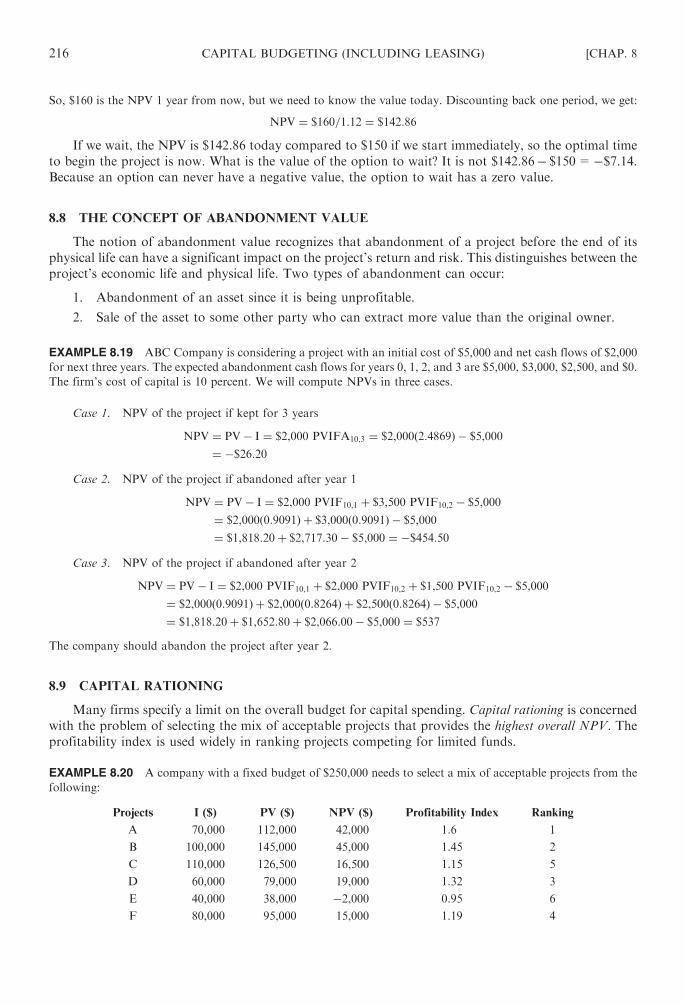
So, $160 is the NPV 1 year from now, but we need to know the value today. Discounting back one period, we get:
NPV ¼ $160=1:12 ¼ $142:86
If we wait, the NPV is $142.86 today compared to $150 if we start immediately, so the optimal time
to begin the project is now. What is the value of the option to wait? It is not $142.86� $150=�$7.14.Because an option can never have a negative value, the option to wait has a zero value.
8.8 THE CONCEPT OF ABANDONMENT VALUE
The notion of abandonment value recognizes that abandonment of a project before the end of its
physical life can have a significant impact on the project’s return and risk. This distinguishes between the
project’s economic life and physical life. Two types of abandonment can occur:
1. Abandonment of an asset since it is being unprofitable.
2. Sale of the asset to some other party who can extract more value than the original owner.
EXAMPLE 8.19 ABC Company is considering a project with an initial cost of $5,000 and net cash flows of $2,000
for next three years. The expected abandonment cash flows for years 0, 1, 2, and 3 are $5,000, $3,000, $2,500, and $0.
The firm’s cost of capital is 10 percent. We will compute NPVs in three cases.
Case 1. NPV of the project if kept for 3 years
NPV ¼ PV� I ¼ $2,000 PVIFA10,3 ¼ $2,000ð2:4869Þ � $5,000
¼ �$26:20
Case 2. NPV of the project if abandoned after year 1
NPV ¼ PV� I ¼ $2,000 PVIF10,1 þ $3,500 PVIF10,2 � $5,000
¼ $2,000ð0:9091Þ þ $3,000ð0:9091Þ � $5,000
¼ $1,818:20þ $2,717:30� $5,000 ¼ �$454:50
Case 3. NPV of the project if abandoned after year 2
NPV ¼ PV� I ¼ $2,000 PVIF10,1 þ $2,000 PVIF10,2 þ $1,500 PVIF10,2 � $5,000
¼ $2,000ð0:9091Þ þ $2,000ð0:8264Þ þ $2,500ð0:8264Þ � $5,000
¼ $1,818:20þ $1,652:80þ $2,066:00� $5,000 ¼ $537
The company should abandon the project after year 2.
8.9 CAPITAL RATIONING
Many firms specify a limit on the overall budget for capital spending. Capital rationing is concerned
with the problem of selecting the mix of acceptable projects that provides the highest overall NPV. The
profitability index is used widely in ranking projects competing for limited funds.
EXAMPLE 8.20 A company with a fixed budget of $250,000 needs to select a mix of acceptable projects from the
following:
Projects I ($) PV ($) NPV ($) Profitability Index Ranking
A 70,000 112,000 42,000 1.6 1
B 100,000 145,000 45,000 1.45 2
C 110,000 126,500 16,500 1.15 5
D 60,000 79,000 19,000 1.32 3
E 40,000 38,000 �2,000 0.95 6
F 80,000 95,000 15,000 1.19 4
216 CAPITAL BUDGETING (INCLUDING LEASING) [CHAP. 8

The ranking resulting from the profitability index shows that the company should select projects A, B, and D:
I PV
A $ 70,000 $112,000
B 100,000 145,000
D 60,000 79,000
$230,000 $336,000
Therefore,
NPV ¼ $336,000� $230,000 ¼ $106,000
Unfortunately, the profitability index method has some limitations. One of the more serious is that it
breaks down whenever more than one resource is rationed.
A more general approach to solving capital rationing problems is the use of mathematical (or
zero-one) programming.1 Here the objective is to select the mix of projects that maximizes the NPV
subject to a budget constraint.
EXAMPLE 8.21 Using the data given in Example 8.13 set up the problem as a mathematical programming
problem. First label project A as X1, B as X2, and so on; the problem can be stated as follows: Maximize
NPV ¼ $42,000X1 þ $45,000X2 þ $16,500X3 þ $19,000X4 � $2,000X5 þ $15,000X6
subject to
$70,000X1 þ $100,000X2 þ $110,000X3 þ $60,000X4 þ $40,000X5 þ $80,000X6 % $250,000
Xt ¼ 0, 1 ði ¼ 1, 2, . . . ,6Þ
Using the mathematical program solution routine, the solution to this problem is:
X1 ¼ 1, X2 ¼ 1, X4 ¼ 1
and the NPV is $106,000. Thus, projects A, B, and D should be accepted.
8.10 HOW DOES INCOME TAXES AFFECT INVESTMENT DECISIONS?
Income taxes make a difference in many capital budgeting decisions. In other words, the project that
is attractive on a before-tax basis may have to be rejected on an after-tax basis. Income taxes typically
affect both the amount and the timing of cash flows. Since net income, not cash inflows, is subject to tax,
after-tax cash inflows are not usually the same as after-tax net income.
Let us define:
S=Sales
E=Cash operating expenses
d=Depreciation
t=Tax rate
Then, before-tax cash inflows (or before-tax cash savings)=S�E and net income=S�E� d.
By definition,
After-tax cash inflows ¼ before-tax cash inflows� taxes
¼ ðS� E Þ � ðS� E� d Þ ðtÞ
1 A Comprehensive treatment of the problem appears in H. Martin Weingartner, ‘‘Capital Budgeting of Interrelated
Projects—Survey and Synthesis,’’ Management Science, vol. 12, March 1966, pp. 485–516.
CHAP. 8] CAPITAL BUDGETING (INCLUDING LEASING) 217

Rearranging gives the short-cut formula:
After-tax cash inflows ¼ ðS� E Þ ð1� t Þ þ ðd ÞðtÞ
As can be seen, the deductibility of depreciation from sales in arriving at net income subject to taxes
reduces income tax payments and thus serves as a tax shield:
Tax shield ¼ tax saving on depreciation ¼ ðd ÞðtÞ
Example 8.22 Assume:
S=$12,000
E=$10,000
d=$500 per year using the straight line method
t=30%
Then,
After-tax cash inflow ¼ ð$12,000� $10,000Þ ð1� 0:3Þ þ ð$500Þð0:3Þ¼ ð$2,000Þð0:7Þ þ ð$500Þð0:3Þ¼ $1,400þ $150 ¼ $1,550
Note that a tax shield ¼ tax savings on depreciation ¼ ðd ÞðtÞ¼ ($500)(0:3Þ ¼ $150
Since the tax shield is dt, the higher the depreciation deduction, the higher the tax savings on depreciation.
Therefore, an accelerated depreciation method (such as double-declining balance) produces higher tax savings than
the straight-line method. Accelerated methods produce higher present values for the tax savings, which may make a
given investment more attractive.
8.11 CAPITAL BUDGETING DECISIONS AND THE MODIFIED ACCELERATED
COST RECOVERY SYSTEM (MACRS)
Although the traditional depreciation methods still can be used for computing depreciation for book
purposes, 1981 saw a new way of computing depreciation deductions for tax purposes. The current rule
is called the Modified Accelerated Cost Recovery System (MACRS) rule, as enacted by Congress in 1981
and then modified somewhat in 1986 under the Tax Reform Act of 1986. This rule is characterized as
follows:
1. It abandons the concept of useful life and accelerates depreciation deductions by placing all
depreciable assets into one of eight age property classes. It calculates deductions, based on an
allowable percentage of the asset’s original cost (see Tables 8-1 and 8-2).
With a shorter asset tax life than useful life, the company would be able to deduct depreciation
more quickly and save more in income taxes in the earlier years, thereby making an investment
more attractive. The rationale behind the system is that this way the government encourages the
company to invest in facilities and increase its productive capacity and efficiency. (Remember
that the higher d, the larger the tax shield (d )(t).)
2. Since the allowable percentages in Table 8-1 add up to 100%, there is no need to consider the
salvage value of an asset in computing depreciation.
3. The company may elect the straight-line method. The straight-line convention must follow what
is called the half-year convention. This means that the company can deduct only half of the
regular straight-line depreciation amount in the first year. The reason for electing to use the
MACRS optional straight-line method is that some firms may prefer to stretch out depreciation
deductions using the straight-line method rather than to accelerate them. Those firms are the
218 CAPITAL BUDGETING (INCLUDING LEASING) [CHAP. 8

ones that just start out or have little or no income and wish to show more income on their
income statements.
4. If an asset is disposed of before the end of its class life, the half-year convention allows half the
depreciation for that year (early disposal rule).
EXAMPLE 8.23 Assume that a machine falls under a 3-year property class costs $3,000 initially. The straight-line
option under MACRS differs from the traditional straight-line method in that under this method the company
would deduct only $500 depreciation in the first year and the fourth year ($3,000/3 years=$1,000; $1,000/2=$500).
The table below compares the straight-line with half-year convention with the MACRS.
Straight-line
(half-year) MACRS
Year Depreciation Cost MACRS (%) Deduction
1 $ 500 $3,000 � 33.3 $ 999
2 1,000 3,000 � 44.5 1,335
3 1,000 3,000 � 14.8 444
4 500 3,000 � 7.4 222
$3,000 $3,000
Table 8-1. Modified accelerated cost recovery system classification of assets
Property class
Year 3-year 5-year 7-year 10-year 15-year 20-year
1 33.3% 20.0% 14.3% 10.0% 5.0% 3.8%
2 44.5 32.0 24.5 18.0 9.5 7.2
3 14.8a 19.2 17.5 14.4 8.6 6.7
4 7.4 11.5a 12.5 11.5 7.7 6.2
5 11.5 8.9a 9.2 6.9 5.7
6 5.8 8.9 7.4 6.2 5.3
7 8.9 6.6a 5.9a 4.9
8 4.5 6.6 5.9 4.5a
9 6.5 5.9 4.5
10 6.5 5.9 4.5
11 3.3 5.9 4.5
12 5.9 4.5
13 5.9 4.5
14 5.9 4.5
15 5.9 4.5
16 3.0 4.4
17 4.4
18 4.4
19 4.4
20 4.4
21 2.2
Total 100% 100% 100% 100% 100% 100%
a Denotes the year of changeover to straight-line depreciation.
CHAP. 8] CAPITAL BUDGETING (INCLUDING LEASING) 219

Table 8.2. MACRS tables by property class
MACRS Property Class
& Depreciation Method
Useful Life
(ADR Midpoint Life) a
Examples of Assets
3-year property 200%
declining balance
4 years or less Most small tools are
included; the law
specifically excludes
autos and light trucks
from this property class.
5-year property 200%
declining balance
More than 4 years to
less than 10 years
Autos and light trucks,
computers, typewriters,
copiers, duplicating
equipment, heavy
general-purpose trucks,
and research and
experimentation
equipment are included.
7-year property 200%
declining balance
10 years or more to less
than 16 years
Office furniture and
fixtures and most items
of machinery and
equipment used in
production are included.
10-year property 200%
declining balance
16 years or more to less
than 20 years
Various machinery and
equipment, such as that
used in petroleum
distilling and refining
and in the milling of
grain, are included.
15-year property 150%
declining balance
20 years or more to less
than 25 years
Sewage treatment plants,
telephone and electrical
distribution facilities,
and land improvements
are included.
20-year property 150%
declining balance
25 years or more Service stations and
other real property with
an ADR midpoint life of
less than 27.5 years are
included.
27.5-year property
straight-line
Not applicable All residential rental
property is included.
31.5-year property
straight-line
Not applicable All nonresidential real
property is included.
a The term ADR midpoint life means the ‘‘useful life’’ of an asset in a business sense; the appropriate ADR
midpoint lives for assets are designated in the Tax Regulations.
220 CAPITAL BUDGETING (INCLUDING LEASING) [CHAP. 8

EXAMPLE 8.24 A machine costs $10,000. Annual cash inflows are expected to be $5,000. The machine
will be depreciated using the MACRS rule and will fall under the 3-year property class. The cost of capital after
taxes is 10%. The estimated life of the machine is 5 years. The salvage value of the machine at the end of the
fifth year is expected to be $1,200. The tax rate is 30%. Should you buy the machine? The formula for computation
of after-tax cash inflows (S�E )(1� t)+ (d )(t) needs to be computed separately. The NPV analysis can be
performed as follows:
Present value
Factor @ 10%
Present
value
(S�E)(1� t): $5,000 $5,000
(1� 0.3) = $3,500
For 5 years for 5 years $3,500 3.719a $13,268.50
(d )(t):
Year Cost MACRS(%) d (d)(t)
1 $10,000� 33.3 $3,330 $999 0.909b 908.09
2 $10,000� 44.5 4,450 1,335 0.826b 1,102.71
3 $10,000� 14.8 1,480 444 0.751b 333.44
4 $10,000� 7.4 740 222 0.683b 151.63
Salvage
value:
$1,200 $1,200(1� 0.3)= $840c $840 0.621b 521.64
in year 5: in year 5
Present value (PV) $16,286.01
a T4 (10%, 4 years)=3.170 (from Table 4).b T3 values (year 1, 2, 3, 4, 5) obtained from Table 3.c Any salvage value received under the MACRS rules is a taxable gain (the excess of the selling price over book value, $1,200 in this
example), since the book value will be zero at the end of the life of the machine.
Since NPV=PV� I=$16,286.01� $10,000=$6,286.01 is positive, the machine should be bought.
8.12 LEASING
Leasing provides an alternative to purchasing an asset in order to acquire its services without
directly incurring any fixed debt obligation. There are two basic types of leases available to the
business firm:
1. An operating lease is basically a short-term lease. It is cancelable at the option of the firm leasing
the asset (the lessee). Such leases are commonly used for leasing such items as computer hard-
ware, cash registers, vehicles, and equipment.
2. A financial (capital) lease is a longer-term lease than an operating lease. It constitutes a non-
cancelable contractual commitment on the part of the lessee to make a series of payments to the
firm that actually owns the asset (the lessor) for the use of the asset.
Accounting for Leases
Prior to 1977, most financial (capital) leases were not included in the balance sheets of the lessee.
Instead, they were reported in the footnotes of the balance sheet. However, in November 1976, the
Financial Accounting Standards Board (FASB), which is a part of the American Institute of Certified
Public Accountants, issued a statement that requires any lease meeting one or more of the following
criteria2 to be included in the body of the balance sheet of the lessor.
2 Financial Accounting Standards Board, Statement of Accounting Standards No. 13, ‘‘Accounting for Leases,’’ November 1976,
Stamford, CN.
CHAP. 8] CAPITAL BUDGETING (INCLUDING LEASING) 221

1. The lease transfers ownership of the property to the lessee by the end of the lease term.
2. The lease contains a bargain repurchase option.
3. The lease term is equal to 75 percent or more of the estimated economic life of the leased
property.
4. The present value of the minimum lease payments equals or exceeds 90 percent of the
excess of the fair value of the property over any related investment tax credit retained by the
lessor.
The Lease-Purchase Decision
The lease-purchase decision is a decision that commonly confronts firms considering the acquisition
of new assets. It is a hybrid capital budgeting decision which forces a company to compare the leasing
and purchasing alternatives. To make an intelligent decision, an after-tax, cash outflow, present value
comparison is needed. There are special steps to take when making this comparison.
When considering a lease, take the following steps:
1. Find the annual lease payment. Since the annual lease payment is typically made in advance, the
formula to be used is:
Amount of lease ¼ Aþ AðPVIFAi,n�1Þ or A ¼ amount of lease
1þ PVIFAi,n�1
Notice we use n – 1 rather than n.
2. Find the after-tax cash outflows.
3. Find the present value of the after-tax cash outflows.
When considering a purchase, take the following steps:
1. Find the annual loan amortization by using:
A ¼ amount of loan for the purchase
PVIFAi,n
This step may not be necessary since this amount is usually available.
2. Calculate the interest. The interest is segregated from the principal in each of the annual loan
payments because only the interest is tax-deductible.
3. Find the cash outflows by adding interest and depreciation (plus and maintenance costs), and
then compute the after-tax outflows.
4. Find the present value of the after-tax cash outflows, using Appendix C.
EXAMPLE 8.25 A firm has decided to acquire an asset costing $100,000 that has an expected life of 5 years, after
which the asset is not expected to have any residual value. The asset can be purchased by borrowing or it can be
leased. If leasing is used, the lessor requires a 12 percent return. As is customary, lease payments are to be made in
advance, that is, at the end of the year prior to each of the 10 years. The tax rate is 50 percent and the firm’s cost of
capital, or after-tax cost of borrowing, is 8 percent.
First compute the present value of the after-tax cash outflows associated with the leasing alternative.
1. Find the annual lease payment:
A ¼ amount of lease
1þ PVIFAi,n�1
¼ $100,000
1þ PVIFA12%,4 years
¼ $100,000
1þ 3:3073¼ $100,000
4:3073¼ $23:216 ðroundedÞ
Steps 2 and 3 can be done in the same schedule, as follows:
222 CAPITAL BUDGETING (INCLUDING LEASING) [CHAP. 8
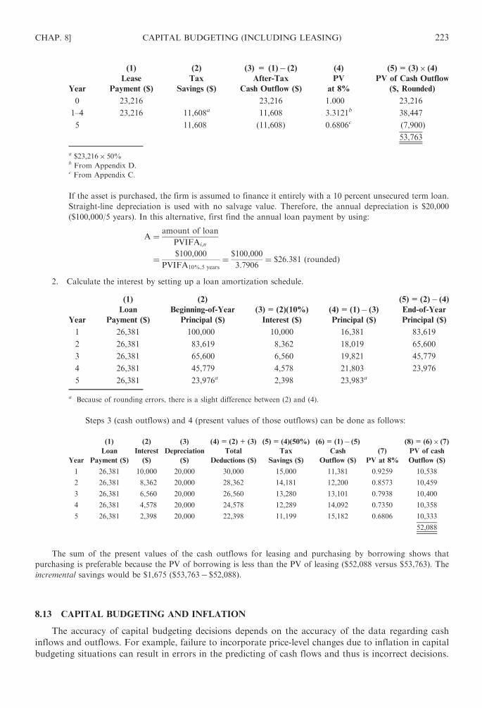
Year
(1)
Lease
Payment ($)
(2)
Tax
Savings ($)
(3) = (1)� (2)
After-Tax
Cash Outflow ($)
(4)
PV
at 8%
(5)= (3)� (4)
PV of Cash Outflow
($, Rounded)
0 23,216 23,216 1.000 23,216
1–4 23,216 11,608a 11,608 3.3121b 38,447
5 11,608 (11,608) 0.6806c (7,900)
53,763
a $23,216� 50%b From Appendix D.c From Appendix C.
If the asset is purchased, the firm is assumed to finance it entirely with a 10 percent unsecured term loan.
Straight-line depreciation is used with no salvage value. Therefore, the annual depreciation is $20,000
($100,000/5 years). In this alternative, first find the annual loan payment by using:
A ¼ amount of loan
PVIFAi,n
¼ $100,000
PVIFA10%,5 years
¼ $100,000
3:7906¼ $26:381 ðroundedÞ
2. Calculate the interest by setting up a loan amortization schedule.
Year
(1)
Loan
Payment ($)
(2)
Beginning-of-Year
Principal ($)
(3)= (2)(10%)
Interest ($)
(4)= (1)� (3)
Principal ($)
(5)= (2)� (4)
End-of-Year
Principal ($)
1 26,381 100,000 10,000 16,381 83,619
2 26,381 83,619 8,362 18,019 65,600
3 26,381 65,600 6,560 19,821 45,779
4 26,381 45,779 4,578 21,803 23,976
5 26,381 23,976a 2,398 23,983a
a Because of rounding errors, there is a slight difference between (2) and (4).
Steps 3 (cash outflows) and 4 (present values of those outflows) can be done as follows:
Year
(1)
Loan
Payment ($)
(2)
Interest
($)
(3)
Depreciation
($)
(4)= (2)+ (3)
Total
Deductions ($)
(5)= (4)(50%)
Tax
Savings ($)
(6)= (1)� (5)
Cash
Outflow ($)
(7)
PV at 8%
(8)= (6)� (7)
PV of cash
Outflow ($)
1 26,381 10,000 20,000 30,000 15,000 11,381 0.9259 10,538
2 26,381 8,362 20,000 28,362 14,181 12,200 0.8573 10,459
3 26,381 6,560 20,000 26,560 13,280 13,101 0.7938 10,400
4 26,381 4,578 20,000 24,578 12,289 14,092 0.7350 10,358
5 26,381 2,398 20,000 22,398 11,199 15,182 0.6806 10,333
52,088
The sum of the present values of the cash outflows for leasing and purchasing by borrowing shows that
purchasing is preferable because the PV of borrowing is less than the PV of leasing ($52,088 versus $53,763). The
incremental savings would be $1,675 ($53,763� $52,088).
8.13 CAPITAL BUDGETING AND INFLATION
The accuracy of capital budgeting decisions depends on the accuracy of the data regarding cash
inflows and outflows. For example, failure to incorporate price-level changes due to inflation in capital
budgeting situations can result in errors in the predicting of cash flows and thus is incorrect decisions.
CHAP. 8] CAPITAL BUDGETING (INCLUDING LEASING) 223

Typically, an analyst has two options dealing with a capital budgeting situation with inflation: Either
restate the cash flows in nominal terms and discount them at a nominal cost of capital (minimum
required rate of return) or restate both the cash flows and cost of capital in constant terms and discount
the constant cash flows at a constant cost of capital. The two methods are basically equivalent.
EXAMPLE 8.26 A company has the following projected cash flows estimated in real terms:
Real Cash Flows (000s)
Period 0 1 2 3
� 100 35 50 30
The nominal cost of capital is 15 percent. Assume that inflation is projected at 10 percent a year. Then the first cash
flows for year 1, which is $35,000 in current dollars, will be 35,000� 1.10=$38,500 in year-1 dollars. Similarly the
cash flow for year 2 will be 50,000� (1.10)2=$60,500 in year-2 dollars, so on. If we discount these nominal cash
flows at the 15 percent nominal cost of capital, we have the following net present value (NPV):
Period
Cash
Flows
PVIF
(Appendix C)
Present
Values
0 � 100 1.000 � 100
1 38.5 0.870 33.50
2 60.5 0.756 45.74
3 39.9 0.658 26.25
NPV= 5.49 or $5,490
Instead of converting the cash-flow forecasts into nominal terms, we could convert the cost of capital into real
terms by using the following formula:
Real cost of capital ¼ 1þ nominal cost of capital
1þ inflation rate� 1
In the example, this gives
Real cost of capital ¼ ð1þ 0:15Þ=ð1þ 0:10Þ � 1
¼ 1:15=1:101� 1
¼ 1:045� 1
¼ 0:045 or 4:5%
We will obtain the same answer except for rounding errors ($5,490 versus $5,580).
Period
Cash
Flows PVIF=1/(1+0.045)n Present Values
0 � 100 1.000 � 100
1 35 1/(1+0.045)=0.957 33.50
2 50 1/(1.045)2=0.916 45.80
3 30 1/(1.045)3=0.876 26.28
NPV= 5.58 or $5,580
224 CAPITAL BUDGETING (INCLUDING LEASING) [CHAP. 8

Review Questions
1. The initial investment is plus installation cost minus plus or
minus .
2. The total gain is split into and . These breakdowns are
subject to tax rates.
3. After-tax cash inflows equal net profits after taxes plus .
4. The NPV method and the IRR method are called methods.
5. is the process of making decisions.
6. is the divided by the cash inflow through increased revenues
or cash savings in operating expenses.
7. The shorter the , the less risky the project and the greater the .
8. Accounting rate of return does not recognize the .
9. Internal rate of return is the rate at which equals .
10. Accept the investment if its IRR exceeds .
11. IRR is difficult to compute when the cash flows are .
12. In , the NPV and the IRR methods may produce .
13. is used widely in ranking the investments competing for limited funds.
14. The method discounts all cash flows at the , thus implicitly
assuming that these cash flows can be reinvested at this rate.
15. MACRS rules abandon the concept of .
16. is taken in the year in which an asset is first placed into service.
17. The straight-line depreciation method with allows the company to deduct
only half of the regular straight-line deduction amount in the year.
18. Immediate disposal of an old machine usually results in that is fully deduc-
tible from current income for tax purposes.
19. The FASB requires firms to certain financial (capital) leases and to restate
their .
20. Lease payments represent a desired rate of return to the .
21. If two mutually exclusive projects have unequal lives, either of the two methods may be used
for the analysis: the and the .
CHAP. 8] CAPITAL BUDGETING (INCLUDING LEASING) 225

22. The overcomes many of the IRR’s disadvantages.
23. Real options involve the right to buy or sell , not .
Answers: (1) cost (purchase price) of the asset, the proceeds from sale of the old asset, taxes on the sale of old
asset; (2) a capital gain, recapture of depreciation, different; (3) depreciation; (4) discounted cash flow
(DCF); (5) Capital budgeting, long-term investment; (6) Payback period, initial amount of investment; (7)
payback period, liquidity; (8) time value of money; (9) present value of cash inflows, the initial investment; (10)
the cost of capital; (11) not even; (12) mutually exclusive investments, conflicting rankings; (13) Profitability
index (or benefit/cost ratio); (14) NPV, cost of capital; (15) useful life; (16) Investment tax credit (ITC); (17)
the half-year convention, first; (18) a loss; (19) capitalize, balance sheets; (20) lessor; (21) replacement chain
(common life) approach, equivalent annual annuity (EAA); (22) modified internal rate of return (MIRR); (23)
real assets, financial assets.
Solved Problems
8.1 Capital Gain (Loss) and Recapture of Depreciation. For each of the following cases, compute
the total taxes resulting from the sale of the asset. Assume a 34 percent ordinary tax rate.
The asset was purchased for $75,000 3 years ago and has a book value (undepreciated value)
of $40,000. (a) The asset is sold for $80,000. (b) The asset is sold for $70,000. (c) The asset is sold
for $40,000. (d ) The asset is sold for $38,000.
SOLUTION
(a) Total gain ¼ selling price� book value
¼ $80,000� $40,000 ¼ $40,000
Total taxes are: $13,600 (34%� $40,000)
(b) Gain: $70,000� $40,000 ¼ $30,000
Tax: $30,000� 0:34 ¼ $10,200
(c) No Tax:
(d ) Loss: $38,000� $40,000 ¼ $2,000
Tax saving: $2,000� 0:34 ¼ $680
8.2 Calculation of Initial Investment. A firm is considering replacing an old machine with another.
The new machine costs $90,000 plus $10,000 to install. For each of the four cases given in
Problem 8.1, calculate the initial investment of the replacement.
SOLUTION
(a) (b) (c) (d )
Cost of new machine $90,000 $90,000 $90,000 $90,000
+ Installation cost 10,000 10,000 10,000 10,000
�Proceeds from sale of old machine 80,000 70,000 40,000 38,000
+Taxes on sale of old machine 17,500 13,800 0 (920)
Invalid investment $37,500 $43,800 $60,000 $61,080
8.3 Incremental Cash Inflows. National Bottles Corporation is contemplating the replacement of one
of its bottling machines with a new one that will increase revenue from $25,000 to $31,000 per
year and reduce cash operating costs from $12,000 to $10,000 per year. The new machine will cost
$48,000 and have an estimated life of 10 years with no salvage value. The firm uses straight-line
depreciation and is subject to a 46 percent tax rate. The old machine has been fully depreciated
226 CAPITAL BUDGETING (INCLUDING LEASING) [CHAP. 8
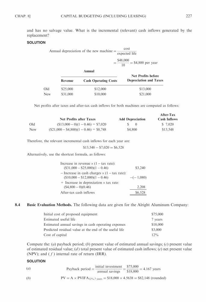
and has no salvage value. What is the incremental (relevant) cash inflows generated by the
replacement?
SOLUTION
Annual depreciation of the new machine ¼ cost
expected life
¼ $48,000
10¼ $4,800 per year
Annual
Net Profits before
Depreciation and TaxesRevenue Cash Operating Costs
Old $25,000 $12,000 $13,000
New $31,000 $10,000 $21,000
Net profits after taxes and after-tax cash inflows for both machines are computed as follows:
Net Profits after Taxes Add Depreciation
After-Tax
Cash Inflows
Old ($13,000� 0)(1� 0.46)=$7,020 $ 0 $ 7,020
New ($21,000� $4,800)(1� 0.46)=$8,748 $4,800 $13,548
Therefore, the relevant incremental cash inflows for each year are:
$13,548� $7,020 ¼ $6,528
Alternatively, use the shortcut formula, as follows:
Increase in revenue� (1� tax rate):
($31,000� $25,000)(1� 0.46) $3,240
� Increase in cash charges� (1� tax rate):
($10,000� $12,000)(1� 0.46) �(� 1,080)
+ Increase in depreciation� tax rate:
($4,800� 0)(0.46) 2,208
After-tax cash inflows $6,528
8.4 Basic Evaluation Methods. The following data are given for the Alright Aluminum Company:
Initial cost of proposed equipment $75,000
Estimated useful life 7 years
Estimated annual savings in cash operating expenses $18,000
Predicted residual value at the end of the useful life $3,000
Cost of capital 12%
Compute the: (a) payback period; (b) present value of estimated annual savings; (c) present value
of estimated residual value; (d ) total present value of estimated cash inflows; (e) net present value
(NPV); and ( f ) internal rate of return (IRR).
SOLUTION
(a) Payback period ¼ initial investment
annual savings¼ $75,000
$18,000¼ 4:167 years
(b) PV ¼ A� PVIFA12%,7 years ¼ $18,000� 4:5638 ¼ $82,148 ðroundedÞ
CHAP. 8] CAPITAL BUDGETING (INCLUDING LEASING) 227

(c) PV ¼ $3,000� PVIF12%,7 years ¼ $3,000� 0:4523 ¼ $1,357 ðroundedÞ
(d ) Total PV ¼ $82,148þ $1,357 ¼ $83,505
(e) NPV ¼ PV� I ¼ $83,505� $75,000 ¼ $8,505
( f ) At IRR, I=PV. Thus,
$75,000 ¼ $18,000� PVIFAr,7
PVIFAr,7 ¼$75,000
$18,000¼ 4:1667
which is somewhere between 14 percent and 15 percent in the 7-year line.
Using interpolation,
PVIFA
14% 4.2883 4.2883
True rate 4.1667
15% 4.1604
Difference 0.1216 0.1279
IRR ¼ 14%þ 4:2883� 4:1667
4:2883� 4:1604ð15%� 14%Þ
¼ 14%þ 0:1216
0:1279ð1%Þ ¼ 14%þ 0:95% ¼ 14:95%
8.5 Payback Period and ARR. The John-in-the-Box Store is a fast food restaurant chain. Potential
franchisees are given the following revenue and cost information:
Building and equipment $490,000
Annual revenue $520,000
Annual cash operating costs $380,000
The building and equipment have a useful life of 20 years. The straight-line method for
depreciation is used. The income tax is 40 percent. Given these facts: (a) What is the payback
period? (b) What is the accounting rate of return?
SOLUTION
Net profits before depreciation and taxes ¼ $520,000� $380,000 ¼ $140,000
Annual depreciation ¼ $490,000
20 years¼ $24,500
Therefore,
Net profit after taxes ¼ ð$140,000� $24,5000Þð1� 0:4Þ ¼ $69,300
After-tax cash inflows ¼ $69,300þ $24,500 ¼ $93,800
(a) Payback period ¼ Initial investment
annual cash flow¼ $490,000
$93,800¼ 5:22 years
(b) Accounting rate of return ¼ net income
investment¼ $69,300
$490,000¼ 14:14%
or using average investment in the denominator gives:
ARR ¼ $69,300
$490,000=2¼ 28:28%
8.6 Basic Evaluation Methods. The Rango Company is considering a capital investment for which
the initial outlay is $20,000. Net annual cash inflows (before taxes) are predicted to be $4,000
228 CAPITAL BUDGETING (INCLUDING LEASING) [CHAP. 8

for 10 years. Straight-line depreciation is to be used, with an estimated salvage value of zero.
Ignore income taxes. Compute the: (a) payback period; (b) accounting rate of return (ARR); (c)
net present value (NPV), assuming a cost of capital (before tax) of 12 percent; and (d ) internal
rate of return (IRR).
SOLUTION
(a) Payback period ¼ initial investment
annual cash flow¼ $20,000
$4,000=year¼ 5 years
(b) Accounting rate of return ðARRÞ ¼ net income
initial investment
Depreciation ¼ $20,000
10 years¼ $2,000=year
Accounting rate of return ¼ ð$4,000� $2,000Þ=year$20,000
¼ 0:10 ¼ 10%
(c) Net present value ðNPVÞ ¼ PV of cash inflows ½discounted at the cost of capital ð12%Þ�� initial investment
$4,000� ðPVIFA12%,10Þ � $20,000 ¼ $4,000ð5:6502Þ � $20,000 ¼ $2,600:80
(d ) Internal rate of return (IRR) is the rate which equates the amount invested with the present value of
cash inflows generated by the project.
$20,000 ¼ $4,000ðPVIFAr,10Þ
PVIFAr,10 ¼$20,000
$4,000¼ 5
which is between 15 percent and 16 percent in Appendix D. Using interpolation,
PVIFA
15% 5.0188 5.0188
True rate 5.0000
16% 4.8332
Difference 0.0188 0.1856
IRR ¼ 15%þ 5:0188� 5:0000
5:0188� 4:8332
� �
ð16%� 15%Þ ¼ 15%þ 0:0188
0:1856ð1%Þ
¼ 15%þ 0:101% ¼ 15:101%
8.7 Basic Capital Budgeting Decisions. Consider an investment which has the following cash flows:
Year Cash Flow ($)
0 (31,000)
1 10,000
2 20,000
3 10,000
4 10,000
5 5,000
(a) Compute the: (1) payback period; (2) net present value (NPV) at 14 percent cost of capital;
and (3) internal rate of return (IRR).
(b) Based on (2) and (3) in part (a), make a decision about the investment. Should it be accepted
or not?
CHAP. 8] CAPITAL BUDGETING (INCLUDING LEASING) 229

SOLUTION
(a) (1) The payback period is computed as follows:
Recovery of Initial Outlay
Year Cash Flow Needed Balance Payback Period
1 $10,000 $31,000 $21,000 1.00
2 $20,000 $21,000 $ 1,000 1.00
3 $10,000 $ 1,000 0.10
2.1a
a Payback period in years.
(2) NPV is computed as follows:
Year Cash Flow ($) PV Factor at 14% PV ($)
0 (31,000) 1.000 (31,000)
1 10,000 0.8772 8,772
2 20,000 0.7695 15,390
3 10,000 0.6750 6,750
4 10,000 0.5921 5,921
5 5,000 0.5194 2,597
NPV 8,430
(3) By definition, IRR is the rate at which PV=I or NPV=0. From part (2), NPV at 14%=
$8,430. Try 30 percent to determine what happens to NPV.
Year Cash Flow ($) PV Factor at 30% PV ($)
0 (31,000) 1.000 (31,000)
1 10,000 0.7694 7,694
2 20,000 0.5921 11,842
3 10,000 0.4558 4,558
4 10,000 0.3509 3,509
5 5,000 0.2702 1,351
(2,046)
True IRR is somewhere between 14 percent and 30 percent. Use interpolation to determine the
amount.
NPV
14% $8,430 $8,430
True rate 0
30% �(� 2,046)
Difference $8,430 $10,476
Therefore,
IRR ¼ 14%þ $8,430
$8,430� ð�$2,046Þ ð30%� 14%Þ
¼ 14%þ $8,430
$10,476ð16%Þ ¼ 14%þ 12:875% ¼ 26:875%
230 CAPITAL BUDGETING (INCLUDING LEASING) [CHAP. 8

(b) Under the NPV method, accept the project since the NPV is positive ($8,430). Under the IRR method,
accept the project since the IRR of 26.875 percent exceeds the cost of capital of 14 percent.
8.8 Comprehensive Capital Budgeting Decision. The Chellin Company purchased a special machine
1 year ago at a cost of $12,000. At that time the machine was estimated to have a useful life of
6 years and no salvage value. The annual cash operating cost is approximately $20,000. A new
machine has just come on the market which will do the same job but with an annual cash
operating cost of only $17,000. This new machine costs $21,000 and has an estimated life of 5
years with zero salvage value. The old machine can be sold for $10,000 to a scrap dealer. Straight-
line depreciation is used, and the company’s income tax rate is 40 percent.
Assuming a cost of capital of 8 percent after taxes, calculate: (a) the initial investment; (b) the
incremental cash inflow after taxes; (c) the NPV of the new investment; and (d ) the IRR on the
new investment.
SOLUTION
(a) The initial investment is:
Cost of new machine $21,000
�Proceeds from sale of old machine 10,000
$11,000
Since the selling price ($10,000) is the same as the book value ($12,000� $2,000=$10,000), no taxable
gain or loss results.
(b) The incremental cash inflow may be computed by using the shortcut formula:
Annual cash savings
[$3,000� (1� 0.4)] $1,800
+ Increase in depreciation� tax rate
[($4,200+$2,000)(0.4)] 880
After-tax cash inflow $2,680
(c) NPV ¼ PV� I
¼ $2,680ðPVIFA8,5Þ � $11,000 ¼ $2,680ð3:9927Þ � $11,000
¼ $10,700� $11,000 ¼ �$300 ðroundedÞ
(d ) IRR is the rate at which I=PV. Thus,
I ¼ PV
$11,000 ¼ $2,680 PVIFAr, 5 years
PVIFAr,5 ¼$11,000
$2,680¼ 4:1045
which is about 7 percent in the 5-year line of Appendix D.
8.9 Supplying Missing Data. Fill in the blanks for each of the following independent cases. Assume in
all cases the investment has a useful life of 10 years.
Annual Cash
Inflow Investment
Cost of
Capital IRR NPV
$100,000 $449,400 14% (a) (b)
$70,000 (c) 14% 20% (d )
(e) $200,000 ( f ) 14% $35,624
(g) $300,000 12% (h) $39,000
CHAP. 8] CAPITAL BUDGETING (INCLUDING LEASING) 231

SOLUTION
(a) I ¼ PV
$449,400 ¼ $100,000 PVIFAr,10
PVIFAr,10 ¼$449,400
$100,000¼ 4:494
From Appendix D, the present value factor of 4.494 at 10 years gives a rate of 18%.
(b) NPV ¼ PV� I
¼ $100,000 PVIFA14,10 � $449,400
¼ $100,000ð5:2161Þ � $449,400 ¼ $521,610� $449,400 ¼ $72,210
(c) I ¼ PV
¼ $70,000 PVIFA20,10 ¼ $70,000ð4:1925Þ ¼ $293,475
(d ) NPV ¼ PV� I
¼ $70,000 PVIFA14,10 � $293,475
¼ $70,000ð5:2161Þ � $293,475 ¼ $365,127� $293,475 ¼ $71,652
(e) At IRR 14%, PV=I.
Cash inflow� PVIFA14,10 ¼ investment
Cash inflow ¼ investment
PVIFA14,10
¼ $200,000
5:2161¼ $38,343 ðroundedÞ
( f ) NPV ¼ PV� I
$35,624 ¼ PV� $200,000
$35,624þ $200,000 ¼ PV ¼ cash inflow ðPVIFAr,10Þ
$235,624 ¼ $38,343 PVIFAr,10
$235,624
$38,343¼ PVIFAr,10
6:1451 ¼ PVIFAr,10
Since this is the present value factor for 10 percent at 10 years, the cost of capital is 10 percent.
(g) PV ¼ NPVþ 1
Cash inflow ðPVIFA12,10Þ ¼ NPVþ I ¼ $39,000þ $300,000 ¼ $339,000
Cash inflow ¼ $339,000
PVIFA12,10
¼ $339,000
5:6502¼ $59,998 ðroundedÞ
(h) I ¼ PV
$300,000 ¼ $59,998 PVIFAr,10
PVIFAr,10 ¼$300,000
$59,998¼ 5:0002
Since this PVIFA value is about halfway between 15 percent and 16 percent at 10 years, IRR is
estimated at about 15.5 percent.
232 CAPITAL BUDGETING (INCLUDING LEASING) [CHAP. 8

8.10 NPV Analysis. Kim Corporation invested in a 4-year project. Kim’s cost of capital is 8 percent.
Additional information on the project follows:
Year After-Tax Cash Inflow
Present Value
of $1 at 8%
1 $2,000 0.926
2 $2,200 0.857
3 $2,400 0.794
4 $2,600 0.735
Assuming an NPV of $700, what was the initial investment?
SOLUTION
Year Cash Inflow PV Total PV
1 $2,000 0.926 $1,852
2 $2,200 0.857 1,885
3 $2,400 0.794 1,906
4 $2,600 0.735 1,911
$7,554
NPV ¼ PV� I
I ¼ PV�NPV
¼ $7,554� $700 ¼ $6,854
8.11 IRR. XYZ, Inc., invested in a machine with a useful life of 6 years and no salvage value. The
machine was depreciated using the straight-line method and it was expected to produce annual
cash inflow from operations, net of income taxes, of $2,000. The present value of an ordinary
annuity of $1 for six periods at 10 percent is 4.3553. The present value of $1 for six periods at
10 percent is 0.5645. Assuming that XYZ used an internal rate of return of 10 percent, what was
the amount of the original investment?
SOLUTION
By definition, at IRR, PV=I or NPV=0.
To obtain the amount of initial investment find the present value of $2,000 a year for 6 periods.
PV ¼ $2,000� 4:3553 ¼ $8,710:60
8.12 Ranking. Data relating to three investment projects are given below.
A B C
Investment (I) $30,000 $20,000 $50,000
Useful life 10 years 4 years 20 years
Annual cash savings $6,207 $7,725 $9,341
Rank the projects according to their attractiveness using the: (a) payback period; (b) IRR; and
(c) NPV at 14 percent cost of capital.
SOLUTION
(a)Payback period ¼ initial investment
increased revenue or savings
CHAP. 8] CAPITAL BUDGETING (INCLUDING LEASING) 233

Project Payback Period Rank
A$30,000
$6,207¼ 4:833 years 2
B$20,000
$7,725¼ 2:588 years 1
C$50,000
$9,341¼ 5:353 years 3
(b) The IRR ranking is:
Project Closed Ratea Rank
A 16% 3
B 20% 1
C 18% 2
a PV=I
Cash inflow� PVIFA ¼ I
PVIFA ¼ I
Cash inflow
For A: PVIFAr,10 ¼$30,000
$6,207¼ 4:8333
For B: PVIFAr,4 ¼$20,000
$7,725¼ 2:589
For C: PVIFAr,20 ¼$50,000
$9,341¼ 5:3527
(c) NPV at 14 percent is:
Project Annual Savings PV Factor Total PV I
NPV
(PV� I) Rank
A $6,207 5.2161 $32,376 $30,000 $ 2,376 3
B $7,725 2.9137 $22,508 $20,000 $ 2,508 2
C $9,341 6.6231 $61,866 $50,000 $11,866 1
8.13 Capital Rationing. Rand Corporation is considering five different investment opportunities.
The company’s cost of capital is 12 percent. Data on these opportunities under consideration
are given below.
Project Investment ($) PV at 12% ($) NPV ($) IRR (%)
Profitability Index
(Rounded)
1 35,000 39,325 4,325 16 1.12
2 20,000 22,930 2,930 15 1.15
3 25,000 27,453 2,453 14 1.10
4 10,000 10,854 854 18 1.09
5 9,000 8,749 (251) 11 0.97
Based on these data: (a) rank these five projects in the descending order of preference, accord-
ing to NPV, IRR, and profitability index (or benefit/cost ratio). (b) Which ranking would you
prefer? (c) Based on your answer to part (b), which projects would you select if $55,000 is the limit
to be spent?
234 CAPITAL BUDGETING (INCLUDING LEASING) [CHAP. 8

SOLUTION
(a) Order of Preference
Project NPV IRR
Profitability
Index
1 1 2 2
2 2 3 1
3 3 4 3
4 4 1 4
5 5 5 5
(b) The profitability index approach is generally considered the most dependable method of ranking
projects competing for limited funds. It is an index of relative attractiveness, measured in terms of
how much is returned for each dollar invested.
(c) Based on the answer in part (b), choose projects (2) and (1), for which the combined NPV would be
$7,255 ($2,930+$4,325) with the limited budget of $55,000.
8.14 Capital Rationing and Mathematical Programming. Express the capital rationing problem given
in Problem 8.13 as a mathematical programming problem.
SOLUTION
Labeling project (1) as X1, project (2) as X2, and so on, the problem can be stated as follows:
Maximize
NPV ¼ $4,325X1 þ $2,930X2 þ $2,453X3 þ $854X4 � $251X5
subject to
$35,000X1 þ $20,000X2 þ $25,000X3 þ $10,000X4 þ $9,000X5 $55,000
Xi ¼ 0, 1 ði ¼ 1, 2, . . . ,5Þ
8.15 NPV Analysis. In Problem 8.3, should National Bottles Corporation buy the new machine?
Base your answer on the NPV method, assuming that the cost of capital is 8 percent after taxes.
SOLUTION
From Problem 8.3,
I ¼ $48,000
n ¼ 10 years
A ¼ $6,528=year
Therefore,
NPV ¼ PV� I ¼ A � PVIFA� I
¼ $6,528ð6:7101Þ � $48,000 ¼ $43,804� $48,000 ¼ �$4,196 ðroundedÞ
National Bottles Corporation should not purchase the machine, because the NPV is negative.
8.16 Replacement Decision. Wisconsin Products Company manufactures several different products.
One of the firm’s principal products sells for $20 per unit. The sales manager of Wisconsin
Products has stated repeatedly that he could sell more units of this product if they were available.
In an attempt to substantiate his claim the sales manager conducted a market research study last
year at a cost of $44,000 to determine potential demand for this product. The study indicated that
Wisconsin Products could sell 18,000 units of this product annually for the next 5 years.
CHAP. 8] CAPITAL BUDGETING (INCLUDING LEASING) 235

The equipment currently in use has the capacity to produce 11,000 units annually. The
variable production costs are $9 per unit. The equipment has a book value of $60,000 and a
remaining useful life of 5 years. The salvage value of the equipment is negligible now and will be
zero in 5 years.
A maximum of 20,000 units could be produced annually on new machinery. The new equip-
ment costs $300,000 and has an estimated useful life of 5 years, with no salvage value at the end of
5 years. Wisconsin Products’ production manager has estimated that the new equipment,
if purchased, would provide increased production efficiencies that would reduce the variable
production costs to $7 per unit.
Wisconsin Products Company uses straight-line depreciation on all its equipment for
tax purposes. The firm is subject to a 40 percent tax rate, and its after-tax cost of capital is
15 percent.
The sales manager felt so strongly about the need for additional capacity that he attempted
to prepare an economic justification for the equipment although this was not one of his
responsibilities. His analysis, presented below and on the next page, disappointed him because
it did not justify acquisition of the equipment.
He computed the required investment as follows:
Purchase price of new equipment $300,000
Disposal of existing equipment
Loss on disposal $60,000
Less tax benefit (40%) 24,000 36,000
Cost of market research study 44,000
Total investment $380,000
He computed the annual returns as follows:
Contribution margin from product
Using the new equipment
[18,000� ($20� $7)] $234,000
Using the existing equipment
[11,000� ($20� $9)] 121,000
Increase in contribution margin $113,000
Less depreciation 60,000
Increase in before-tax income $53,000
Income tax (40%) 21,200
Increase in income $31,800
Less 15% cost of capital on the
additional investment required
(0.15� $380,000) 57,000
Net annual return on proposed
investment in new equipment $(25,200)
The controller of Wisconsin Products Company plans to prepare a discounted cash
flow analysis for this investment proposal. The controller has asked you to prepare corrected
calculations of (a) the required investment in the new equipment and (b) the recurring annual cash
flows. Explain why your corrected calculations differ from the original analysis prepared by the
sales manager. (c) Calculate the net present value of the proposed investment in the new
equipment.
236 CAPITAL BUDGETING (INCLUDING LEASING) [CHAP. 8

SOLUTION
(a) The initial investment is:
Purchase price of new equipment $300,000
�Tax savings from loss on disposala 24,000
$276,000
a Tax savings are computed as follows:
Loss= selling price� book value
=($0� $60,000)=$60,000
Tax rate 0.4
Tax savings $24,000
(b) Using the shortcut method, the annual cash flows are computed by first determining the increased cash
flows resulting from change in contribution margin:
Using new equipment
[18,000 ($20� $7)]a $234,000
Using existing equipment
[11,000 ($20� $9)] 121,000
Increased cash flows $113,000
Taxes (0.40� $113,000) 45,200
Increased cash flows after taxes $67,800
Next, compute the increase in depreciation:
Depreciation on new equipment
($300,000U 5) $60,000
Depreciation on existing equipment
($60,000U 5) 12,000
Increased depreciation charge $48,000
Tax rate 0.4 19,200
Recurring annual cash flows $87,000
a The new equipment is capable of producing 20,000 units, but Wisconsin Products
can sell only 18,000 units annually.
The sales manager made several errors in his calculations of required investment and annual cash
flows.
Concerning the required investment, the sales manager made two errors: First, the cost of the
market research study ($44,000) is a sunk cost because it was incurred last year and will not change
regardless of whether the investment is made or not. Second, the loss on the disposal of the existing
equipment does not result in an actual cash cost as shown by the sales manager. The loss on disposal
results in a reduction of taxes which reduces the cost of the new equipment.
In computing the annual cash flows, the sales manager made three errors: First, he considered
only the depreciation on the new equipment rather than just the additional depreciation which would
result from the acquisition of the new equipment. Second, he failed to consider that the depreciation is
a noncash expenditure which provides a tax shield. Third, the sales manager’s use of the discount rate
(i.e., cost of capital) was incorrect. The discount rate should be used to reduce the value of future cash
flows to their current equivalent at time period zero.
(c) NPV ¼ PV� I ¼ cash flow ðPVIFA15,5Þ � I
¼ ð$87,000� 3:3522Þ � $276,000 ¼ $291,641� $276,000 ¼ $15,641
CHAP. 8] CAPITAL BUDGETING (INCLUDING LEASING) 237

8.17 Mutually Exclusive Investments. The Wan-Ki Manufacturing Company must decide between
investment projects A and B, which are mutually exclusive. The data on these projects are as
follows (in thousands of dollars):
Cash Flows, per Year
Project 0 1 2 3 4
A (100) $120.00
B (100) $193.80
(a) For each project, compute the NPV at 12 percent cost of capital, and the IRR. (b) Explain
why the rankings conflict. Recommend which project should be chosen.
SOLUTION
(a) The NPV at 12 percent is:
Project Cash Inflow PV at $1a PV NPV (PV� I)
A $120.00 0.8929 $107.15 $ 7.15
B $193.80 0.6355 $123.16 $23.16
a PVIF12,1 for A and PVIF12,4 for B; both from Appendix C.
The IRR is:
Project I/Cash Flow PVIF IRR
A$100
$120:00¼ 0:8333 (at 1 year) 20%
B$100
$193:80¼ 0:516 (at 4 year) 18%
(b) The conflicting ranking results from different assumptions regarding the reinvestment rate on the cash
inflows released by the project. The NPV method assumes the cost of capital (12 percent in this
problem) as the rate for reinvestment, whereas the IRR method assumes the cash inflows are reinvested
at their own internal rate of return (20 percent in the case of project A). The use of NPV for ranking
mutually exclusive investments is recommended since the cost of capital is a more realistic reinvestment
rate. Therefore, project B should be chosen.
8.18 NPV, IRR, and Mutually Exclusive Investments. The Bitter Almond Company was confronted
with the two mutually exclusive investment projects, A and B, which have the following after-tax
cash flows:
Cash Flows, per Year ($)
Project 0 1 2 3 4
A (12,000) 5,000 5,000 5,000 5,000
B (12,000) 25,000
Based on these cash flows: (a) Calculate each project’s NPV and IRR. (Assume that the firm’s
cost of capital after taxes is 10 percent.) (b) Which of the two projects would be chosen according
to the IRR criterion? (c) How can you explain the differences in rankings given by the NPV and
IRR methods in this case?
238 CAPITAL BUDGETING (INCLUDING LEASING) [CHAP. 8

SOLUTION
(a) The NPV for project A is:
Year
Cash (Outflow)
or Inflow
Present Value of $1
at 10%
Net Present Value
of Cash Flow
0 $(12,000) 1.000 $(12,000)
1–4 $5,000 3.1699 15,850
$ 3,850
The NPV for project B is:
Year
Cash (Outflow)
or Inflow
Present Value of $1
at 10%
Net Present Value
of Cash Flow
0 $(12,000) 1.000 $(12,000)
4 $25,000 0.6830 17,075
$ 5,075
The IRR for project A is:
$12,000 ¼ $5,000 ðPVIFAr,4Þ
PVIFAr,4 ¼$12,000
$5000¼ 2:4
Using interpolation:
PV
24% 2.4043 2.4043
True rate 2.4000
28% 2.2410
Difference 0.0043 0.1633
IRR ¼ 24%þ 0:0043
0:1633ð4%Þ ¼ 24%þ 0:11% ¼ 24:11%
The IRR for project B is:
Year
Cash
(outflow)
Inflow
Present
Value of $1
at 20%
Net Present
Value of
Cash Flow
Present
Value of $1
at 22%
Net Present
Value of
Cash Flow
0 $(12,000) 1.000 $(12,000) 1.000 $(12,000)
4 $ 25,000 0.4823 12,058 0.4526� 11,315
$ 58 $ (685)
NPV
20% $50 $ 50
True rate 0
22% �(� 685)
Difference $50 $735
IRR ¼ 20%þ $50
$735ð2%Þ ¼ 20%þ 0:14% ¼ $20:14
(b) In summary,
Projects NPV IRR
A $3,850 24.11%
B $5,075 20.14%
Under the NPV method, choose B over A. Under the IRR method, choose A over B.
CHAP. 8] CAPITAL BUDGETING (INCLUDING LEASING) 239

(c) The decision of which project to choose hinges on assumptions made about reinvestment of
cash inflow. Theory suggests resorting to the NPV method because the cost of capital reinvestment
assumption implicit in this method is considered to be a more realistic assumption than the IRR,
where a reinvestment at the IRR is assumed. Therefore, choose B rather than A, using the NPV
ranking.
8.19 The Modified Internal Rate of Return (MIRR). Refer to Problem 8.18. Compute MIRRs for
projects A and B. Compare the ranking by MIRR with the one by NPV.
SOLUTION
First, compute the terminal value (TV) compounded at the cost of capital 10 percent.
A: TV ¼ 5,000 FVIFA10,3 ¼ 5,000� 3:3100 ¼ 16,550:00
Next, find the IRR by setting:
12,000 ¼ 16,390:50 PVIFMIRR,4
PVIF ¼ 12000=16,390:50 ¼ 0:7321, which gives MIRR ¼ about 12%
Now we see the consistent ranking from both the NPV and MIRR methods.
MIRR NPV at 10%
A 12% $3,850
B 20.14 5,075
8.20 Replacement Decisions with Unequal Lives. Consider two projects, X and Y:
Project Cost Life Annual After-Tax Cash Inflow
X $50,000 10 years $9,000
Y 50,000 15 7,500
The company’s cost of capital is 10 percent.
1. Determine the adjusted NPV for each project, using the replacement chain procedure.
2. Determine the equivalent annual annuity for each project.
3. Which project should be taken?
SOLUTION
1. First, determine each project’s original NPV as follows:
NPVX ¼ $9,000 PVIFA10,10 � $50,000
¼ $9,000ð6:1446Þ � $50,000
¼ $55,301:40� $50,000
¼ $5,301:40
NPVY ¼ $7,500 PVIFA15,10�$50,000
¼ $7,500ð7:6061Þ � $50,000
¼ $57,045:75� $50,000
¼ $7,045:75
240 CAPITAL BUDGETING (INCLUDING LEASING) [CHAP. 8
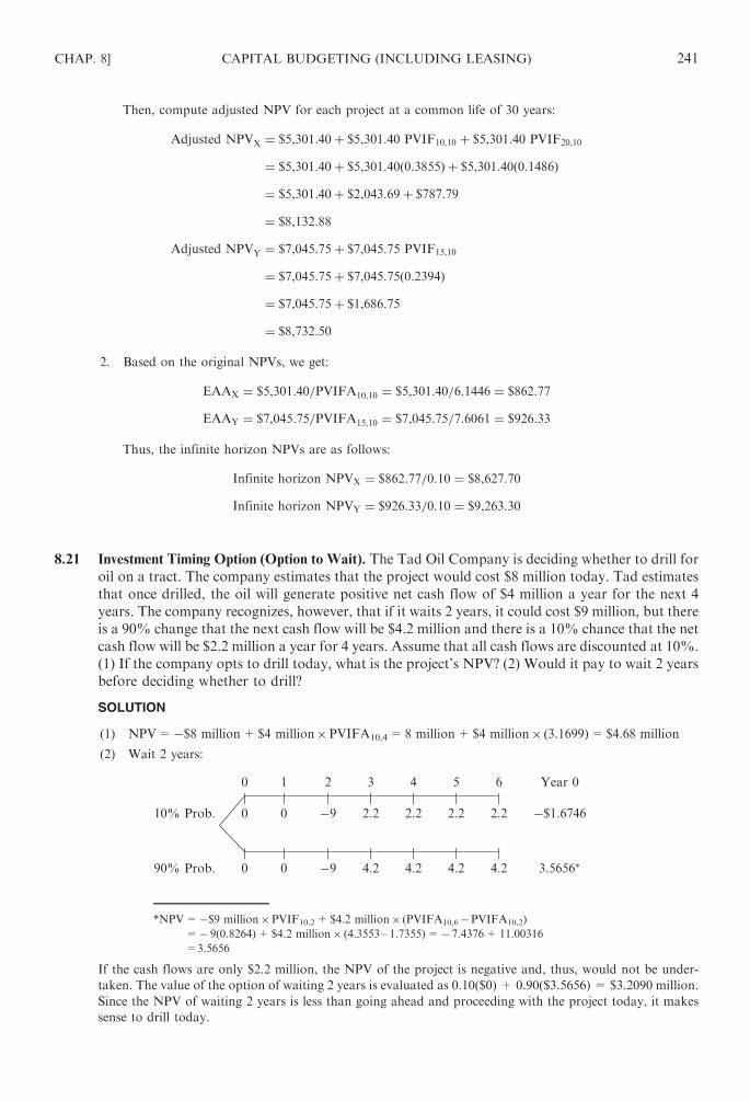
Then, compute adjusted NPV for each project at a common life of 30 years:
Adjusted NPVX ¼ $5,301:40þ $5,301:40 PVIF10,10 þ $5,301:40 PVIF20,10
¼ $5,301:40þ $5,301:40ð0:3855Þ þ $5,301:40ð0:1486Þ
¼ $5,301:40þ $2,043:69þ $787:79
¼ $8,132:88
Adjusted NPVY ¼ $7,045:75þ $7,045:75 PVIF15,10
¼ $7,045:75þ $7,045:75ð0:2394Þ
¼ $7,045:75þ $1,686:75
¼ $8,732:50
2. Based on the original NPVs, we get:
EAAX ¼ $5,301:40=PVIFA10,10 ¼ $5,301:40=6:1446 ¼ $862:77
EAAY ¼ $7,045:75=PVIFA15,10 ¼ $7,045:75=7:6061 ¼ $926:33
Thus, the infinite horizon NPVs are as follows:
Infinite horizon NPVX ¼ $862:77=0:10 ¼ $8,627:70
Infinite horizon NPVY ¼ $926:33=0:10 ¼ $9,263:30
8.21 Investment Timing Option (Option to Wait). The Tad Oil Company is deciding whether to drill for
oil on a tract. The company estimates that the project would cost $8 million today. Tad estimates
that once drilled, the oil will generate positive net cash flow of $4 million a year for the next 4
years. The company recognizes, however, that if it waits 2 years, it could cost $9 million, but there
is a 90% change that the next cash flow will be $4.2 million and there is a 10% chance that the net
cash flow will be $2.2 million a year for 4 years. Assume that all cash flows are discounted at 10%.
(1) If the company opts to drill today, what is the project’s NPV? (2) Would it pay to wait 2 years
before deciding whether to drill?
SOLUTION
(1) NPV=�$8 million+$4 million�PVIFA10,4=8 million+$4 million� (3.1699)=$4.68 million
(2) Wait 2 years:
0 1 2 3 4 5 6 Year 0
j j j j j j j10% Prob: 0 0 �9 2:2 2:2 2:2 2:2 �$1:6746
j j j j j j j90% Prob: 0 0 �9 4:2 4:2 4:2 4:2 3:5656
*NPV=�$9 million�PVIF10,2+$4.2 million� (PVIFA10,6�PVIFA10,2)
=� 9(0.8264)+$4.2 million� (4.3553 – 1.7355)=� 7.4376+11.00316
=3.5656
If the cash flows are only $2.2 million, the NPV of the project is negative and, thus, would not be under-
taken. The value of the option of waiting 2 years is evaluated as 0.10($0) + 0.90($3.5656) = $3.2090 million.
Since the NPV of waiting 2 years is less than going ahead and proceeding with the project today, it makes
sense to drill today.
CHAP. 8] CAPITAL BUDGETING (INCLUDING LEASING) 241
8.22 Abandonment. Henteleff, Inc. is considering a project with the following data:
Year
Initial Investment
and Net Cash Flow
Abandonment
Value in Year t
0 ($8,000) $8,000
1 4,000 4,500
2 4,000 3,000
3 4,000 0
The firm’s cost of capital is 10 percent. What should the company do?
SOLUTION
We will compute NPVs in three cases.
Case 1. NPV of the project if kept for 3 years
NPV ¼ PV� I ¼ $4,000 PVIFA10,3 ¼ $4,000ð2:4869Þ � $8,000
¼ $1,947:60
Case 2. NPV of the project if abandoned after Year 1
NPV ¼ PV� I ¼ $4,000 PVIF10,1 þ $4,500 PVIF10,2 � $8,000
¼ $4,000ð0:9091Þ þ $4,500ð0:9091Þ � $8,000
¼ $3,636:40þ $4,090:95� $8,000 ¼ �$272:65
Case 3. NPV of the project if abandoned after Year 2
NPV ¼ PV� I ¼ $4,000 PVIF10,1 þ $4,000 PVIF10,2 þ $3,000 PVIF10,2 � $8,000
¼ $4,000ð0:9091Þ þ $4,000ð0:8264Þ þ $3,000ð0:8264Þ � $8,000
¼ $3,636:40þ $3,305:60þ $2,479:20� $8,000 ¼ $1,421:20
The company should keep the project for 3 years.
8.23 NPV Analysis. Two new machines are being evaluated for possible purchase. Forecasts related
to the machines are:
Machine 1 Machine 2
Purchased price $50,000 $60,000
Estimated life (straight-line depreciation) 4 years 4 years
Estimated scrap value None None
Annual cash benefits before income tax:
Year 1 $25,000 $45,000
Year 2 25,000 19,000
Year 3 25,000 25,000
Year 4 25,000 25,000
Income tax rate 40% 40%
Compute the net present value of each machine. Assume a cost of capital of 8%.
242 CAPITAL BUDGETING (INCLUDING LEASING) [CHAP. 8

SOLUTION
After-tax cash benefit:
Cash
Benefit
Year (a) Depreciation
Taxable
Income
Income
Tax (b)
Net After-Tax
Cash Inflow
(a)–(b)
Machine 1
1 $25,000 $12,500 $12,500 $5,000 $20,000
2 25,000 12,500 12,500 5,000 20,000
3 25,000 12,500 12,500 5,000 20,000
4 25,000 12,500 12,500 5,000 20,000
Machine 2
1 $45,000 $15,000 $30,000 $12,000 $33,000
2 19,000 15,000 4,000 1,600 17,400
3 25,000 15,000 10,000 4,000 21,000
4 25,000 15,000 10,000 4,000 21,000
Net present value:
Year
Cash (Outflow)
Inflow
Present Value of
$1 8 Percent
Net Present Value
of Cash Flow
Machine 1
0 $(50,000) 1.000 $(50,000)
1–4 20,000 3.312 66,240
Net present value $ 16,240
Machine 2
0 $(60,000) 1.000 $(60,000)
1 33,000 0.926 30,558
2 17,400 0.857 14,912
3 21,000 0.794 16,674
4 21,000 0.735 15,435
Net present value $ 17,579
8.24 IRR. The Michener Company purchased a special machine 1 year ago at a cost of $12,000.
At that time, the machine was estimated to have a useful life of 6 years and no disposal value.
The annual cash operating cost is approximately $20,000.
A new machine that has just come on the market will do the same job but with an annual cash
operating cost of only $17,000. This new machine costs $15,000 and has an estimated life of
5 years with no disposal value. The old machine could be used as a trade-in at an allowance
of $5,000. Straight-line depreciation is used and the company’s income tax rate is 40 percent.
Compute the internal rate of return on the new investment.
CHAP. 8] CAPITAL BUDGETING (INCLUDING LEASING) 243
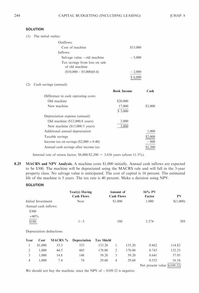
SOLUTION
(1) The initial outlay:
Outflows:
Cost of machine $15,000
Inflows:
Salvage value� old machine � 5,000
Tax savings from loss on sale
of old machine
($10,000� $5,000)(0.4) � 2,000
$ 8,000
(2) Cash savings (annual):
Book Income Cash
Difference in cash operating costs:
Old machine $20,000
New machine 17,000 $3,000
$ 3,000
Depreciation expense (annual):
Old machine ($12,000/6 years) 2,000
New machine ($15,000/5 years) 3,000
Additional annual depreciation 1,000
Taxable savings $2,000
Income tax on savings ($2,000� 0.40) � 800
Annual cash savings after income tax $2,200
Internal rate of return factor; $8,000/$2,200 = 3.636 years (about 11.5%).
8.25 MACRS and NPV Analysis. A machine costs $1,000 initially. Annual cash inflows are expected
to be $300. The machine will be depreciated using the MACRS rule and will fall in the 3-year
property class. No salvage value is anticipated. The cost of capital is 16 percent. The estimated
life of the machine is 5 years. The tax rate is 40 percent. Make a decision using NPV.
SOLUTION
Year(s) Having
Cash Flows
Amount of
Cash Flows
16% PV
Factor PV
Initial Investment Now $1,000 1.000 $(1,000)
Annual cash inflows:
$300
�60%$180 1�5 180 3.274 589
Depreciation deductions:
Year Cost MACRS % Depreciation Tax Shield
1 $1,000 33.3 333 133.20 1 133.20 0.862 114.82
2 1,000 44.5 445 178.00 2 178.00 0.743 132.25
3 1,000 14.8 148 59.20 3 59.20 0.641 37.95
4 1,000 7.4 74 29.60 4 29.60 0.552 16.34
Net present value $(109.32)
We should not buy the machine, since the NPV of � $109.32 is negative.
244 CAPITAL BUDGETING (INCLUDING LEASING) [CHAP. 8

8.26 MACRS and NPV Analysis. A firm is considering the purchase of an automatic machine for
$6,200. The machine has an installation cost of $800 and zero salvage value at the end of its
expected life of 5 years. Depreciation is by the straight-line method with the half-year convention.
The machine is considered a 5-year property. Expected cash savings before tax is $1,800 per year
over the 5 years. The firm is in the 40 percent tax bracket. The firm has determined the cost of
capital (or minimum required rate of return) of 10 percent after taxes. Should the firm purchase
the machine? Use the NPV method.
SOLUTION
Year(s) Having
Cash Flows
Amount of
Cash Flows
10% PV
Factor PV
Initial investment Now $(7,000) 1.000 $(7,000)
Annual cash inflows:
$1,800
�60%$1,080 1–5 1,080 3.791 4,094
Depreciation deductions:
Year Depreciation
Tax
Shield
at 40%
1 $ 700 $280 1 $280 0.909 $255
2 1,400 560 2 560 0.826 463
3 1,400 560 3 560 0.751 421
4 1,400 560 4 560 0.683 382
5 1,400 560 5 560 0.621 348
6 700 280 6 280 0.564 158
Net present value $(879)
The firm should not buy the automatic machine since its NPV is negative.
8.27 MACRS and NPV Analysis. The Wessels Corporation is considering installing a new conveyor
for materials handling in a warehouse. The conveyor will have an initial cost of $75,000 and an
installation cost of $5,000. Expected benefits of the conveyor are: (a) Annual labor cost will be
reduced by $16,500, and (b) breakage and other damages from handling will be reduced by $400
per month. Some of the firm’s costs are expected to increase as follows: (a) Electricity cost will rise
by $100 per month, and (b) annual repair and maintenance of the conveyor will amount to $900.
Assume the firm uses the MACRS rules for depreciation in the 5-year property class. No
salvage value will be recognized for tax purposes. The conveyor has an expected useful life of 8
years and a projected salvage value of $5,000. The tax rate is 40 percent.
1. Estimate future cash inflows for the proposed project.
2. Determine the projects NPV at 10 percent. Should the firm buy the conveyor?
SOLUTION
1. Annual cash inflow:
$16,500 Reduction in labor cost
4,800 Reduction in breakage
� 1,200 Increase in electricity costs
� 900 Increase in repair and maintenance cost
$19,200
CHAP. 8] CAPITAL BUDGETING (INCLUDING LEASING) 245

2. Initial amount of investment is:
$75,000þ $5,000 ¼ $80,000
Year(s)
Having
Cash Flows
Amount
of Cash
Flows
10% PV
Factor PV
Initial investment Now $(80,000) 1.000 $(80,000)
Annual cash inflows: $19,200
� 60%
After-tax cash inflow: $11,520 1–8 11,520 5.335 61,459.20
Depreciation deductions:
Year Cost MACRS
(%)
Depreciation
Tax
Shield
1 $80,000 20.0 $16,000 $6,400 0.909 $ 5,817.60
2 80,000 32.0 25,600 10,240 0.826 8,458.24
3 80,000 19.2 15,360 6,144 0.751 4,614.14
4 80,000 11.5 9,200 3,680 0.683 2,513.44
5 80,000 11.5 9,200 3,680 0.621 2,285.28
6 80,000 5.8 4,640 1,856 0.564 1,046.78
$24,735.48
Salvage value, fully taxable since book value will be zero:
$5,000
� 60% 8 3,000 0.467 1,401.00
$3,000 Net present value $7,595.68
The JKS Corporation should buy and install the conveyor, since it brings a positive NPV.
8.28 NPV Analysis. The JS Company is considering buying a machine at a cost of $800,000,
which has the following cash flow pattern. No residual value is expected. Depreciation is
by straight-line. Assume that the income tax rate is 40%, and the after-tax cost of capital
(minimum required rate of return) is 10%. Should the company buy the machine? Use the
NPV method.
Year
Cash
Inflow,
(1)
Cash
Outflow,
(2)
1 $800,000 $550,000
2 $790,000 $590,000
3 $920,000 $600,000
4 $870,000 $610,000
5 $650,000 $390,000
246 CAPITAL BUDGETING (INCLUDING LEASING) [CHAP. 8

SOLUTION
Net cash flow after taxes calculation
Year
Cash
Inflow,
(1)
Cash
Outflow,
(2)
Net Cash
Flow Before
Taxes,
(3)=(1)�(2)
Depreciation
(Noncash
Expense)
(4)=0.2�,800,000
Net Income
Before Taxes,
(5)=(3)�(4)
Income
Taxes
(6)=0.4�,(5)
Net Income
After Taxes,
(7)=(5)�(6)
Net Cash
Flow After
Taxes,
(8)=(3)�(6)or (7)+(4)
1 $800,000 $550,000 $250,000 $160,000 $ 90,000 $36,000 $54,000 $214,000
2 $790,000 $590,000 $200,000 $160,000 $ 40,000 $16,000 $24,000 $184,000
3 $920,000 $600,000 $320,000 $160,000 $160,000 $64,000 $96,000 $256,000
4 $870,000 $610,000 $260,000 $160,000 $100,000 $40,000 $60,000 $220,000
5 $650,000 $390,000 $260,000 $160,000 $100,000 $40,000 $60,000 $220,000
The Net Present Value (NPV) is computed as follows:
Year
Net
Cash Flow
After
Taxes,
10% PV
Table Value,
Present
Value,
0 $(800,000) 1.000 $(800,000)
1 $ 214,000 0.909 $ 194,526
2 $ 184,000 0.826 $ 151,984
3 $ 256,000 0.751 $ 192,256
4 $ 220,000 0.683 $ 150,260
5 $ 220,000 0.621 $ 136,620
NPV= $ 25,646
The company should buy the machine, since NPV is positive ($25,646).
8.29 Payback Period, ARR, and NPV. The Baxter Company manufactures toys and short-
lived-fad-type items. The research and development department came up with an item that
would make a good promotion gift for office equipment dealers. Aggressive and effective
effort by Baxter’s sales personnel has resulted in almost firm commitments for this product for
the next 3 years. It is expected that the product’s value will be exhausted by that time.
In order to produce the quality demanded Baxter will need to buy additional machinery and
rent some additional space. It appears that about 25,000 square feet will be needed: 12,500 square
feet of presently unused, but leased, space is available now. (Baxter’s present lease with 10 years
to run costs $3.00 a square foot.) There is another 12,500 square feet adjoining the Baxter
facility which Baxter will rent for 3 years at $4.00 per square foot per year if it decides to
make this product.
The equipment will be purchased for about $900,000. It will require $30,000 in modifica-
tions, $60,000 for installation, and $90,000 for testing: all of these activities will be done
by a firm of engineers hired by Baxter. All of the expenditures will be paid for on January 1,
20X1.
The equipment should have a salvage value of about $180,000 at the end of the third year.
No additional general overhead costs are expected to be incurred.
The following estimates of revenues and expenses for this product for the 3 years have been
developed.
CHAP. 8] CAPITAL BUDGETING (INCLUDING LEASING) 247

20X1 20X2 20X3
Sales $1,000,000 $1,600,000 $800,000
Material, labor, and incurred overhead $ 400,000 $ 750,000 $350,000
Assigned general overhead 40,000 75,000 35,000
Rent 87,500 87,500 87,500
Depreciation 450,000 300,000 150,000
$ 977,500 $1,212,500 $622,500
Income before tax $ 22,500 $ 387,500 $117,500
Income tax (40%) 9,000 155,000 71,000
$ 13,500 $ 232,500 $106,500
1. Prepare a schedule which shows the incremental after-tax cash flows for this project.
2. If the company requires a 2-year payback period for its investment, would it undertake
this project? Show your supporting calculations clearly.
3. Calculate the after-tax accounting rate of return for the project.
4. A newly hired business-school graduate recommends that the company consider the use
of net present value analysis to study this project. If the company sets a required rate of
return of 20 percent after taxes, will this project be accepted? Show your supporting
calculations clearly. (Assume all operating revenues and expenses occur at the end of
the year.)
SOLUTION
1. Incremental After-Tax Cash Flow (000 omitted)
20X1 20X2 20X3
Sales $1,000 $1,600 $800
Material, labor, overhead $ 400 $ 750 $350
Added rent 50 50 50
Depreciation 450 300 150
Incremental costs $ 900 $1,100 $550
Incremental income $ 100 $ 500 $250
Incremental taxes 40 200 100
Incremental income after taxes $ 60 $ 300 $150
Add back depreciation 450 300 150
Incremental operation cash flow $ 510 $ 600 $300
Salvage value 180
Net incremental after-tax cash flow $ 510 $ 600 $480
Initial investment for project:
Purchase price $ 900
Modification 30
Installation 60
Testing 90
Total $1,080
248 CAPITAL BUDGETING (INCLUDING LEASING) [CHAP. 8

2. The project should be undertaken if the criterion is a 2-year payback.
20X1 $ 510,000
20X2 600,000
$1,110,000
Payback is in 2 years, which is greater than cost of $1,080,000.
The payback period is:
ð510=510Þ þ ð570=600Þ ¼ 1:95 years
3. 20X1 income $ 13,500
20X2 income 232,500
20X3 income 106,500
$352,500
Average income: $117,500 ($352,500/3)
Accounting rate of return: $117,500/$1,080,000=10.88%
4. The project should be adopted if a 20 percent after-tax rate of return is required.
Present Value of Cash Flows at 20%
20X1 0.83� 510,000=$ 423,300
20X2 0.69� 600,000= 414,000
20X3 0.58� 480,000= 278,400
Present Value $1,115,700
The present value of $1,115,700 is greater than the initial outlay of $1,080,000; therefore, the project
more than satisfies the 20 percent requirement.
8.30 Income Tax Factors. R. Jack and J. Jill have formed a corporation to franchise a quick food
system for shopping malls. They have just completed experiments with a prototype machine
which will serve as the basis of the operation. Because the system is new and untried, they
have decided to conduct a pilot operation in a nearby mall. When it proves successful, they
will aggressively market the franchises.
The income statements below represent Jack and Jill’s best estimates of income from the mall
operation for the next 4 years. At the end of the 4-year period they intend to sell the operation and
concentrate on the sale of and supervision of franchises. Based upon the income stream projected,
they believe the operation can be sold for $190,000; the income tax liability from the sale will be
$40,000.
1. Calculate the cash flow for the mall operation for the 4-year period beginning January 1,
20X6, ignoring tax implications.
2. Adjust the cash flows for tax consequences as appropriate.
CHAP. 8] CAPITAL BUDGETING (INCLUDING LEASING) 249
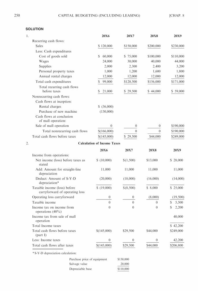
SOLUTION
1. 20X6 20X7 20X8 20X9
Recurring cash flows:
Sales $ 120,000 $150,000 $200,000 $230,000
Less: Cash expenditures
Cost of goods sold $ 60,000 $ 75,000 $100,000 $110,000
Wages 24,000 30,000 40,000 44,000
Supplies 2,000 2,300 2,400 3,200
Personal property taxes 1,000 1,200 1,600 1,800
Annual rental charges 12,000 12,000 12,000 12,000
Total cash expenditures $ 99,000 $120,500 $156,000 $171,000
Total recurring cash flows
before taxes $ 21,000 $ 29,500 $ 44,000 $ 59,000
Nonrecurring cash flows:
Cash flows at inception:
Rental charges $ (36,000)
Purchase of new machine (130,000)
Cash flows at conclusion
of mall operation:
Sale of mall operation 0 0 0 $190,000
Total nonrecurring cash flows $(166,000) 0 0 $190,000
Total cash flows before taxes $(145,000) $ 29,500 $44,000 $249,000
2. Calculation of Income Taxes
20X6 20X7 20X8 20X9
Income from operations:
Net income (loss) before taxes as
stated
$ (10,000) $(1,500) $13,000 $ 28,000
Add: Amount for straight-line
depreciation
11,000 11,000 11,000 11,000
Deduct: Amount of S-Y-D
depreciation*
(20,000) (18,000) (16,000) (14,000)
Taxable income (loss) before
carryforward of operating loss
$ (19,000) $(8,500) $ 8,000 $ 25,000
Operating loss carryforward 0 0 (8,000) (19,500)
Taxable income 0 0 0 $ 5,500
Income tax on income from
operations (40%)
0 0 0 $ 2,200
Income tax from sale of mall
operation
40,000
Total Income taxes $ 42,200
Total cash flows before taxes
(part I)
$(145,000) $29,500 $44,000 $249,000
Less: Income taxes 0 0 0 42,200
Total cash flows after taxes $(145,000) $29,500 $44,000 $206,800
* S-Y-D depreciation calculation:
Purchase price of equipment $130,000
Salvage value 20,000
Depreciable base $110,000
250 CAPITAL BUDGETING (INCLUDING LEASING) [CHAP. 8
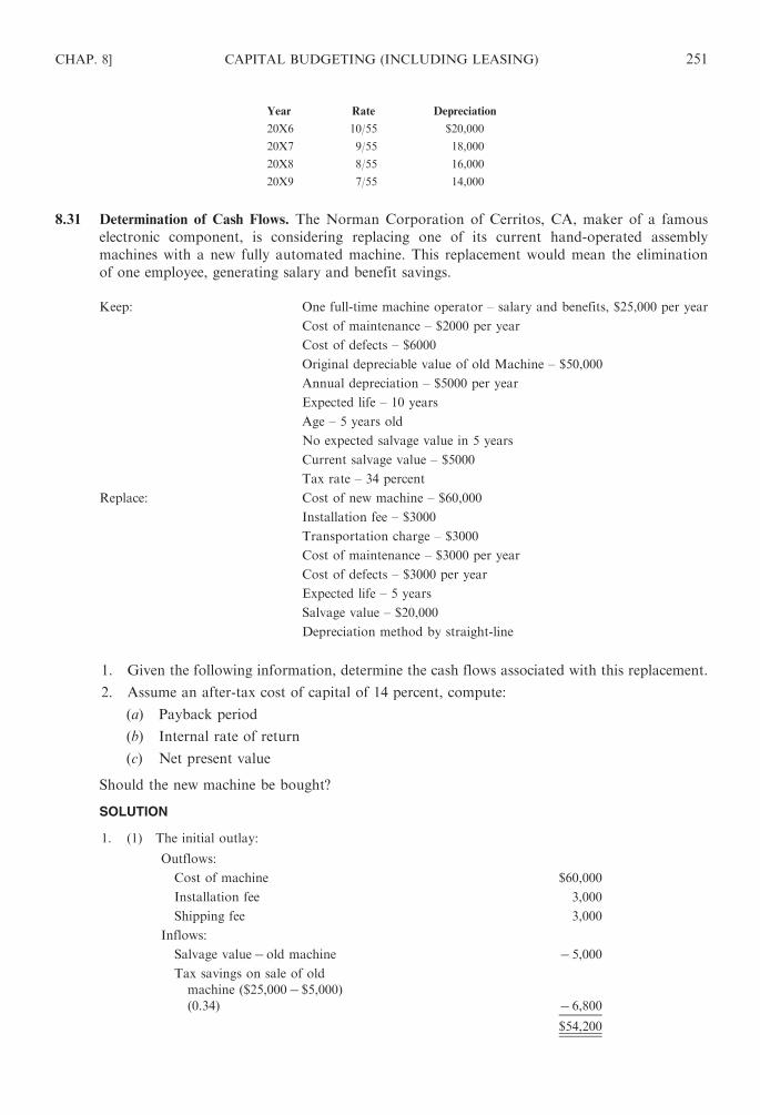
Year Rate Depreciation
20X6 10/55 $20,000
20X7 9/55 18,000
20X8 8/55 16,000
20X9 7/55 14,000
8.31 Determination of Cash Flows. The Norman Corporation of Cerritos, CA, maker of a famous
electronic component, is considering replacing one of its current hand-operated assembly
machines with a new fully automated machine. This replacement would mean the elimination
of one employee, generating salary and benefit savings.
Keep: One full-time machine operator – salary and benefits, $25,000 per year
Cost of maintenance – $2000 per year
Cost of defects – $6000
Original depreciable value of old Machine – $50,000
Annual depreciation – $5000 per year
Expected life – 10 years
Age – 5 years old
No expected salvage value in 5 years
Current salvage value – $5000
Tax rate – 34 percent
Replace: Cost of new machine – $60,000
Installation fee – $3000
Transportation charge – $3000
Cost of maintenance – $3000 per year
Cost of defects – $3000 per year
Expected life – 5 years
Salvage value – $20,000
Depreciation method by straight-line
1. Given the following information, determine the cash flows associated with this replacement.
2. Assume an after-tax cost of capital of 14 percent, compute:
(a) Payback period
(b) Internal rate of return
(c) Net present value
Should the new machine be bought?
SOLUTION
1. (1) The initial outlay:
Outflows:
Cost of machine $60,000
Installation fee 3,000
Shipping fee 3,000
Inflows:
Salvage value� old machine � 5,000
Tax savings on sale of old
machine ($25,000� $5,000)
(0.34) � 6,800
$54,200
CHAP. 8] CAPITAL BUDGETING (INCLUDING LEASING) 251

(2) The differential cash flows over the project’s life.
Book Income Cash Flow
Savings: Reduced salary $25,000 $25,000
Reduced defects 3,000 3,000
Costs: Increased maintenance (1,000) (1,000)
Increased depreciation
($13,200� $5000)* (8,200)
Net savings before taxes $18,800 $27,000
Taxes (0.34) (6,392) (6,392)
Annual net cash flow after taxes $20,608
*Annual depreciation on the new machine = ($60,000+$3,000+$3,000)/5=$13,200.
(3) The terminal cash flow:
Salvage value� new machine $20,000
Less: Taxes on gain:
($20,000� 0)� 0.34 6,800
$13,200
Thus the cash flow in the final year will be equal to the annual net cash flow in that year of
$20,608 plus the terminal cash flow of $13,200 for a total of $33,808.
2. (1) Payback period=$54,200/$20,608=2.63 years
(2) IRR by trial and error=about 30 percent
$54,200=$20,608 PVIFA1,5+$13,200 PVIF1,5
(3) NPV ¼ $20,608 PVIFA14%,5 þ $13,200 PVIF14%,5 � $54,200
¼ $20,608ð3:433Þ þ $13,200ð0:519Þ � $54,200
¼ $70,726� $6,850� $54,200 ¼ $23,376
The machine should be bought since the IRR is greater than 14% and the NPV is positive.
8.32 Annual Lease Payments. Fairchild Leasing Company is setting up a capital lease with Gemi
Trucking, Inc. The lease will cover a $36,000 delivery truck. The terms of the lease call for a
12 percent return to the truck lessor. The lease is to run for 5 years.
Based on these data, determine (a) the annual lease payment and (b) the annual lease payment
if the lessor desires 10 percent on its lease.
SOLUTION
(a) Annual lease payment ¼ A ¼ amount
PVIFA12%,5
¼ $36,000
3:6048¼ $9,987 ðroundedÞ
(b) A ¼ $36,000
PVIFA10%,5
¼ $36,000
3:7908¼ $9,497 ðroundedÞ
8.33 Annual Lease Payments. Star Wars Leasing, Inc., is setting up a financial lease covering a $36,000
truck. The lease arrangement requires beginning-of-year payments and the life of the lease is
5 years. The company wants equal annual lease payments that will allow it to earn 12 percent on
its investment.
Based on these data, determine (a) the annual lease payment and (b) the annual lease payment
if the desired rate of return is only 10 percent.
252 CAPITAL BUDGETING (INCLUDING LEASING) [CHAP. 8

SOLUTION
(a) Since the lease payment is made in advance, the straightforward application of the formula
(i.e., A=amount/PVIFA) does not work. The equation can be set up as follows:
$36,000 ¼ AþA � PVIFA12%,4
$36,000 ¼ Að1þ PVIFF12%,4Þ
A ¼ $36,000
1þ PVIFA12%,4
¼ $36,000
1þ 3:0373¼ $36,000
4:0373¼ $8,917 ðroundedÞ
(b) A ¼ $36,000
1þ PVIFA10%,4
¼ $36,000
1þ 3:1699¼ $36,000
4:1699¼ $8,633 ðroundedÞ
8.34 Lease versus Purchase Decision. Carter Company wishes to expand its productive capacity.
In order to do so it must acquire a new tractor costing $40,000. The machine can be purchased
or leased. The firm is in the 40 percent tax bracket and its after-tax cost of debt is currently
6 percent.
If the firm purchased the machine, the purchase would be totally financed with a 10 percent
loan requiring equal annual end-of-year payments over 5 years. The machine would be depre-
ciated straight-line over its 5-year life. A salvage value of zero is anticipated. The life of a lease
would be 5 years. The lessor intends to charge equal annual lease payments that will enable it to
earn 15 percent on its investment. In doing the following calculations, round your answers to the
nearest dollar.
(a) Calculate the annual lease payment required in order to give the lessor its desired return.
(b) Calculate the annual loan payment paying 10 percent interest. (c) Determine the after-tax cash
outflows associated with each alternative. (d ) Find the present value of the after-tax cash outflows
using the after-tax cost of debt. (e)Which alternative (i.e., lease or purchase) would you recom-
mend? Why?
SOLUTION
(a) Annual lease payment ¼ $40,000
1þ PVIFA15%, 5
¼ $40,000
3:3522¼ $11,932
(b) Annual loan payment ¼ A ¼ $40,000
PVIFA10%, 5
¼ $40,000
3:7908¼ $10,552
(c) and (d ) Data pertaining to a lease agreement are as follows:
Year Payment After-Tax Cost PV Factor at 6% PV of Outflow
1–5 $11,932 $7,159 4.2124 $30,157
Data pertaining to a purchase agreement are as follows:
Year Payment ($) Interest ($) Principal ($) Balance ($) Depreciation ($)
1 10,552 4,000 6,552 33,448 8,000
2 10,552 3,345 7,207 26,241 8,000
3 10,552 2,624 7,928 18,313 8,000
4 10,552 1,831 8,721 9,592 8,000
5 10,552 959 9,593 8,000
CHAP. 8] CAPITAL BUDGETING (INCLUDING LEASING) 253
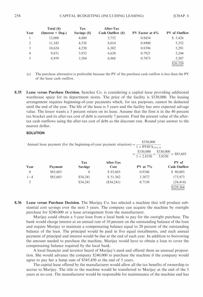
Year
Total ($)
(Interest+Dep.)
Tax
Savings ($)
After-Tax
Cash Outflow ($) PV Factor at 6% PV of Outflow
1 12,000 4,800 5,752 0.9434 $ 5,426
2 11,345 4,538 6,014 0.8900 5,352
3 10,624 4,250 6,302 0.8396 5,291
4 9,831 3,932 6,620 0.7921 5,244
5 8,959 3,584 6,968 0.7473 5,207
$26,520
(e) The purchase alternative is preferable because the PV of the purchase cash outflow is less than the PV
of the lease cash outflow.
8.35 Lease versus Purchase Decision. Sanchez Co. is considering a capital lease providing additional
warehouse space for its department stores. The price of the facility is $330,000. The leasing
arrangement requires beginning-of-year payments which, for tax purposes, cannot be deducted
until the end of the year. The life of the lease is 5 years and the facility has zero expected salvage
value. The lessor wants a 5 percent return on its lease. Assume that the firm is in the 40 percent
tax bracket and its after-tax cost of debt is currently 7 percent. Find the present value of the after-
tax cash outflows using the after-tax cost of debt as the discount rate. Round your answer to the
nearest dollar.
SOLUTION
Annual lease payment ðfor the beginning-of-year payment situationÞ ¼ $330,000
1þ PVIFA15%, 4
¼ $330,000
1þ 2:8550¼ $330,000
3:8550¼ $85,603
Year Payment
Tax
Savings
After-Tax
Cost PV at 7%
PV of
Cash Outflow
0 $85,603 0 $ 85,603 0.9346 $ 80,005
1�4 $85,603 $34,241 $ 51,362 3.3872 173,973
5 $34,241 ($34,241) 0.7130 (24,414)
$229,564
8.36 Lease versus Purchase Decision. The Marijay Co. has selected a machine that will produce sub-
stantial cost savings over the next 5 years. The company can acquire the machine by outright
purchase for $240,000 or a lease arrangement from the manufacturer.
Marijay could obtain a 5-year loan from a local bank to pay for the outright purchase. The
bank would charge interest at an annual rate of 10 percent on the outstanding balance of the loan
and require Marijay to maintain a compensating balance equal to 20 percent of the outstanding
balance of the loan. The principal would be paid in five equal installments, and each annual
payment of principal and interest would be due at the end of each year. In addition to borrowing
the amount needed to purchase the machine, Marijay would have to obtain a loan to cover the
compensating balance required by the local bank.
A local financier and investor heard of Marijay’s need and offered them an unusual proposi-
tion. She would advance the company $240,000 to purchase the machine if the company would
agree to pay her a lump sum of $545,450 at the end of 5 years.
The capital lease offered by the manufacturer would allow all the tax benefits of ownership to
accrue to Marijay. The title to the machine would be transferred to Marijay at the end of the 5
years at no cost. The manufacturer would be responsible for maintenance of the machine and has
254 CAPITAL BUDGETING (INCLUDING LEASING) [CHAP. 8

included $8,000 per year in the lease payment to cover the maintenance cost. Marijay would pay
$70,175 to the manufacturer at the beginning of each year for 5-year period.
(a) Calculate the before-tax interest rate for each of the three alternatives.
(b) Without prejudice to your answer to (a), what arguments would you present to justify a lease
financing alternative even if that arrangement turned out to have a higher interest cost than a
regular loan?
(c) Compare the relative effect that the three financing alternatives would have on Marijay’s
current ratio at the end of the first year. (CMA, adapted.)
SOLUTION
(a) The before-tax interest rates of return for each of the three alternatives are shown below.
For a local financier
PVIFr,5 ¼principal
total payment¼ $240,000
$545,450¼ 0:44
The before-tax interest rate is 18 percent, which is determined by finding the rate for a PVIF of 0.44 for
year 5 in Appendix C.
For a lease:
Annual payment for leasing=$70,175 yearly payment� $8,000 maintenance=$62,175
To find the principal, subtract the first annual payment from the price of the machine, since this
payment is made at the beginning of the year. Therefore,
PVIFAr,4 ¼principal
annual payment
¼ $240,000� $62,175
$62,175¼ 2:8601
From Appendix D, the before-tax interest rate is 15 percent for a PVIFA of 2.8601 at 4 years (4 years,
not 5, since payments are made at the beginning of each year).
For a purchase:
Beginning
of Year
Principal
Borrowed ($)aCompensating
Balance (20%) ($)
(1)
Principal
for Use (80%) ($)
(2)
Interest
(10%) on
Borrowings ($)
(2U 1)
Effective
Rate (%)
1 300,000 60,000 240,000 30,000 1212
2 240,000 48,000 192,000 24,000 1212
3 180,000 36,000 144,000 18,000 1212
4 120,000 24,000 96,000 12,000 1212
5 60,000 12,000 48,000 60,000 1212
a One-fifth of loan repaid each year at the end of the year.
(b) Arguments justifying leases are as follows: The commitment for maintenance is limited, the cash
budgeting impact of maintenance is known, manufacturer may exchange the machine for improved
model at reduced rates, and financing alternatives are expanded.
(c) The effect on the current ratio at the end of the first year differs according to the financing alternative.
For the financier there is no effect because the entire transaction is recorded as a long-term debt and
there is no current asset or current liability until the end of the fourth year. With a loan, the current
ratio will be lower than with the financier arrangement because there will be net cash outlays in the
first year and a current liability recorded at the end of the first year. If a lease is chosen, the current
ratio will be lower than both prior alternatives. There will be a greater net cash outlay in the first year
and a larger current liability recorded at the end of the first year.
CHAP. 8] CAPITAL BUDGETING (INCLUDING LEASING) 255
Chapter 9
Capital Budgeting Under Risk
9.1 INTRODUCTION
Risk analysis is important in making capital investment decisions because of the large amount of
capital involved and the long-term nature of the investments being considered. The higher the risk
associated with a proposed project, the greater the rate of return that must be earned on the project
to compensate for that risk.
9.2 MEASURES OF RISK
Risk, a measure of the dispersion around a probability distribution, is defined as the variability of
cash flow around the expected value. Risk can be measured in either absolute or relative terms. First, the
expected value, �A, is
�A ¼X
n
i¼1Aipi
where Ai=the value of the ith possible outcome
pi=the probability that the ith outcome will occur
n=the number of possible outcomes
Then, the absolute risk is measured by the standard deviation:
� ¼ffiffiffiffiffiffiffiffiffiffiffiffiffiffiffiffiffiffiffiffiffiffiffiffiffiffiffiffiffiffiffi
X
n
i¼1Ai � �A� �2
pi
s
The relative risk is measured by the coefficient of variation, which is �/ �A. (These three statistics were
also discussed in Chapter 7.)
EXAMPLE 9.1 The ABC Corporation is considering investment in one of two mutually exclusive projects.
Depending on the state of the economy, the projects would provide the following cash inflows in each of the
next 5 years:
State Probability Proposal A Proposal B
Recession 0.3 $1,000 $ 500
Normal 0.4 $2,000 $2,000
Boom 0.3 $3,000 $5,000
To compute the expected value ( �A), the standard deviation (�), and the coefficient of variation, it is convenient
to set up the following tables:
For proposal A:
Ai ($) pi Ai pi ($) (Ai� �A) ($) (Ai� �A)2 pi
1,000 0.3 300 � 1,000 300,000
2,000 0.4 800 0 0
3,000 0.3 900 1,000 300,000
�A=2,000 �2=600,000
256
Copyright © 2007, 1998, 1986 by The McGraw-Hill Companies, Inc. Click here for terms of use.

Since �2=600,000, �=775. Thus
�
�A¼ $775
$2,000¼ 0:39
For proposal B:
Ai ($) pi Ai pi ($) (Ai� �A) ($) (Ai� �A)2 ($) (Ai� �A)2 pi
500 0.3 150 � 1,950 3,802,500 1,140,750
2,000 0.4 800 � 450 202,500 81,000
5,000 0.3 1,500 2,550 6,502,500 1,950,750
2,450 �2=3,172,500
Since �2=$3,172,500, �=$1781. Thus
�
�A¼ $1,781
$2,450¼ 0:73
Therefore, proposal A is relatively less risky than proposal B, as indicated by the lower coefficient of variation.
9.3 RISK ANALYSIS IN CAPITAL BUDGETING
Since different investment projects involve different risks, it is important to incorporate risk into the
analysis of capital budgeting. There are several methods for incorporating risk, including:
1. Probability distributions
2. Risk-adjusted discount rate
3. Certainty equivalent
4. Simulation
5. Sensitivity analysis
6. Decision trees (or probability trees)
Probability Distributions
Expected values of a probability distribution may be computed. Before any capital budgeting
method is applied, compute the expected cash inflows or, in some cases, the expected life of the asset.
EXAMPLE 9.2 A firm is considering a $30,000 investment in equipment that will generate cash savings from
operating costs. The following estimates regarding cash savings and useful life, along with their respective prob-
abilities of occurrence, have been made:
Annual Cash Savings ($) Useful Life
6,000 0.2 4 years 0.2
8,000 0.5 5 years 0.6
10,000 0.3 6 years 0.2
Then, the expected annual saving is:
$6,000(0.2)=$1,200
$8,000(0.5)= 4,000
$10,000(0.3)= 3,000
$8,200
CHAP. 9] CAPITAL BUDGETING UNDER RISK 257
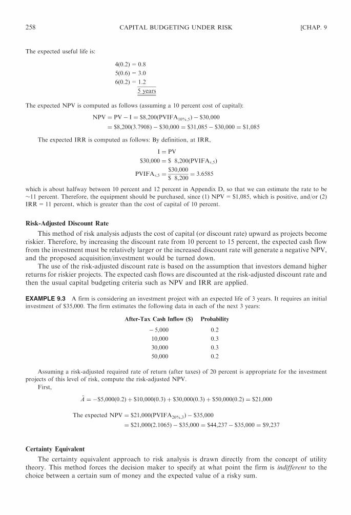
The expected useful life is:
4(0.2)=0.8
5(0.6)=3.0
6(0.2)=1.2
5 years
The expected NPV is computed as follows (assuming a 10 percent cost of capital):
NPV ¼ PV� I ¼ $8,200ðPVIFA10%,5Þ � $30,000
¼ $8,200ð3:7908Þ � $30,000 ¼ $31,085� $30,000 ¼ $1,085
The expected IRR is computed as follows: By definition, at IRR,
I ¼ PV
$30,000 ¼ $ 8,200ðPVIFAv,5Þ
PVIFAv,5 ¼$30,000
$ 8,200¼ 3:6585
which is about halfway between 10 percent and 12 percent in Appendix D, so that we can estimate the rate to be
�11 percent. Therefore, the equipment should be purchased, since (1) NPV=$1,085, which is positive, and/or (2)
IRR=11 percent, which is greater than the cost of capital of 10 percent.
Risk-Adjusted Discount Rate
This method of risk analysis adjusts the cost of capital (or discount rate) upward as projects become
riskier. Therefore, by increasing the discount rate from 10 percent to 15 percent, the expected cash flow
from the investment must be relatively larger or the increased discount rate will generate a negative NPV,
and the proposed acquisition/investment would be turned down.
The use of the risk-adjusted discount rate is based on the assumption that investors demand higher
returns for riskier projects. The expected cash flows are discounted at the risk-adjusted discount rate and
then the usual capital budgeting criteria such as NPV and IRR are applied.
EXAMPLE 9.3 A firm is considering an investment project with an expected life of 3 years. It requires an initial
investment of $35,000. The firm estimates the following data in each of the next 3 years:
After-Tax Cash Inflow ($) Probability
� 5,000 0.2
10,000 0.3
30,000 0.3
50,000 0.2
Assuming a risk-adjusted required rate of return (after taxes) of 20 percent is appropriate for the investment
projects of this level of risk, compute the risk-adjusted NPV.
First,
�A ¼ �$5,000ð0:2Þ þ $10,000ð0:3Þ þ $30,000ð0:3Þ þ $50,000ð0:2Þ ¼ $21,000
The expected NPV ¼ $21,000ðPVIFA20%,3Þ � $35,000
¼ $21,000ð2:1065Þ � $35,000 ¼ $44,237� $35,000 ¼ $9,237
Certainty Equivalent
The certainty equivalent approach to risk analysis is drawn directly from the concept of utility
theory. This method forces the decision maker to specify at what point the firm is indifferent to the
choice between a certain sum of money and the expected value of a risky sum.
258 CAPITAL BUDGETING UNDER RISK [CHAP. 9

Once certainty equivalent coefficients are obtained, they are multiplied by the original cash flow to
obtain the equivalent certain cash flow. Then, the accept-or-reject decision is made, using the normal
capital budgeting criteria. The risk-free rate of return is used as the discount rate under the NPV method
and as the cutoff rate under the IRR method.
EXAMPLE 9.4 XYZ, Inc., with a 14 percent cost of capital after taxes is considering a project with an expected life
of 4 years. The project requires an initial certain cash outlay of $50,000. The expected cash inflows and certainty
equivalent coefficients are as follows:
Year After-Tax Cash Flow ($) Certainty Equivalent Coefficient
1 10,000 0.95
2 15,000 0.80
3 20,000 0.70
4 25,000 0.60
The risk-free rate of return is 5 percent; compute the NPV and IRR.
The equivalent certain cash inflows are obtained as follows:
Year
After-Tax
Cash Inflow ($)
Certainty Equivalent
Coefficient
Equivalent Certain
Cash Inflow ($) PV at 5% PV ($)
1 10,000 0.95 9,500 0.9524 9,048
2 15,000 0.80 12,000 0.9070 10,884
3 20,000 0.70 14,000 0.8638 12,093
4 25,000 0.60 15,000 0.8227 12,341
44,366
NPV ¼ $44,366� $50,000 ¼ �$5,634
By trial and error, we obtain 4 percent as the IRR. Therefore, the project should be rejected, since (1)
NPV=� 5,634, which is negative and/or (2) IRR=4 percent is less than the risk-free rate of 5 percent.
Simulation
This risk analysis method is frequently called the Monte Carlo simulation. It requires that a prob-
ability distribution be constructed for each of the important variables affecting the project’s cash flows.
Thanks to computer software, project simulation is easily affordable.
Sensitivity Analysis
Forecasts of many calculated NPVs under various alternative functions are compared to see how
sensitive NPV is to changing conditions. It may be found that a certain variable or group of variables,
once their assumptions are changed or relaxed, drastically alters the NPV. This results in a much riskier
asset than was originally forecast.
Decision Trees
Some firms use decision trees (probability trees) to evaluate the risk of capital budgeting proposals.
A decision tree is a graphical method of showing the sequence of possible outcomes. A capital budgeting
tree would show the cash flows and NPV of the project under different possible circumstances. The
decision tree method has the following advantages: (1) It visually lays out all the possible outcomes of the
proposed project and makes management aware of the adverse possibilities, and (2) the conditional
nature of successive years’ cash flows can be expressly depicted. The primary disadvantage is that most
problems are too complex to permit a year-by-year depiction. For example, for a 3-year project with
three possible outcomes following each year, there are 27 paths. For a 10-year project (again with three
possible outcomes following each year) there will be about 60,000 paths.
CHAP. 9] CAPITAL BUDGETING UNDER RISK 259

EXAMPLE 9.5 A firm has an opportunity to invest in a machine which will last 2 years, initially cost $125,000,
and has the following estimated possible after-tax cash inflow pattern: In year 1, there is a 40 percent chance
that the after-tax cash inflow will be $45,000, a 25 percent chance that it will be $65,000, and a 35 percent
chance that it will be $90,000. In year 2, the after-tax cash inflow possibilities depend on the cash inflow that
occurs in year 1; that is, the year 2 after-tax cash inflows are conditional probabilities. Assume that the firm’s after-tax
cost of capital is 12 percent. The estimated conditional after-tax cash inflows (ATCI) and probabilities are given
below.
If ATCI1=$45,000 If ATCI1=$65,000 If ATCI1=$90,000
ATCI2 ($) Probability ATCI2 ($) Probability ATCI2 ($) Probability
30,000 0.3 80,000 0.2 90,000 0.1
60,000 0.4 90,000 0.6 100,000 0.8
90,000 0.3 100,000 0.2 110,000 0.1
Then the decision tree which shows the possible after-tax cash inflow in each year, including the conditional nature
of the year 2 each cash inflow and its probabilities, can be depicted as follows:
a NPV ¼ PV� I ¼ $45,000
1þ 0:12ð Þ þ$30,000
1þ 0:12ð Þ2� $125,000
¼ $45,000 PVIF12%,1
� �
þ $30,000 PVIF12%,2
� �
� $125,000
¼ $45,000 0:893ð Þ þ $30,000 0:797ð Þ � $125,000 ¼ $40,185þ $23,910� $125,000 ¼� $60,905
b Joint probability= (0.4)(0.3)=0.120
The last column shows the calculation of expected NPV, which is the weighted average of the individual path NPVs
where the weights are the path probabilities. In this example, the expected NPV of the project is � $1,330, and the
project should be rejected.
9.4 CORRELATION OF CASH FLOWS OVER TIME
When cash inflows are independent from period to period, it is fairly easy to measure the overall
risk of an investment proposal. In some cases, however, especially with the introduction of a new
product, the cash flows experienced in early years affect the size of the cash flows in later years.
This is called the time dependence of cash flows, and it has the effect of increasing the risk of the project
over time.
260 CAPITAL BUDGETING UNDER RISK [CHAP. 9

EXAMPLE 9.6 Jandy Corporation’s after-tax cash inflows (ATCI) are time-dependent, so that year 1 results
(ATCI1) affect the flows in year 2 (ATCI2) as follows:
If ATCI1 is $8,000 with a 40 percent probability, the distribution for ATCI2 is:
0.3 $ 5,000
0.5 $10,000
0.2 $15,000
If ATCI1 is $15,000 with a 50 percent probability, the distribution for ATCI2 is:
0.3 $10,000
0.6 $20,000
0.1 $30,000
If ATCI1 is $20,000 with a 10 percent chance, the distribution for ATCI2 is
0.1 $15,000
0.8 $40,000
0.1 $50,000
The project requires an initial investment of $20,000, and the risk-free rate of capital is 10 percent.
The company uses the expected NPV from decision tree analysis to determine whether the project should be
accepted. The analysis is as follows:
aNPV ¼ PV� I ¼ $8,000 PVIF10,1 þ $5,000 PVIF10,2 � $20,000
¼ $8,000ð0:9091Þ þ $5,000ð0:8264Þ � $20,000 ¼ �$8,595b Joint probability of first path= (0.4)(0.3)=0.12
Since the NPV is positive ($5,306), Jandy Corporation should accept the project.
9.5 NORMAL DISTRIBUTION AND NPV ANALYSIS: STANDARDIZING
THE DISPERSION
With the assumption of independence of cash flows over time, the expected NPV would be
NPV ¼ PV� I
¼X
n
t¼1
�At
1þ rð Þt� I
CHAP. 9] CAPITAL BUDGETING UNDER RISK 261

The standard deviation of NPVs is
� ¼ffiffiffiffiffiffiffiffiffiffiffiffiffiffiffiffiffiffiffiffiffiffiffiffi
X
n
t¼1
�2t
ð1þ rÞ2t
s
The expected value ( �A) and the standard deviation (�) give a considerable amount of information by
which to assess the risk of an investment project. If the probability distribution is normal, some prob-
ability statement regarding the project’s NPV can be made. For example, the probability of a project’s
NPV providing an NPV of less or greater than zero can be computed by standardizing the normal variate
x as follows:
z ¼ x�NPV
�
where x=the outcome to be found
NPV=the expected NPV
z=the standardized normal variate whose probability value can be found in Appendix E.
EXAMPLE 9.7 Assume an investment with the following data:
Period 1 ($) Period 2 ($) Period 3 ($)
Expected cash inflow ( �A) 5,000 4,000 3,000
Standard deviation (�) 1,140 1,140 1,140
Assume that the firm’s cost of capital is 8 percent and the initial investment is $9,000. Then the expected NPV is:
NPV ¼ PV� I
¼ $5,000
ð1þ 0:08Þ þ$4,000
ð1þ 0:08Þ2þ $3,000
ð1þ 0:08Þ3� $9,000
¼ $5,000ðPVIF8,1Þ þ $4,000ðPVIF8,2Þ þ $3,000ðPVIF8,3Þ � $9,000
¼ $5,000ð0:9259Þ þ $4,000ð0:8573Þ þ $3,000ð0:7938Þ � $9,000
¼ $4,630 þ $3,429 þ $2,381 � $9,000 ¼ $1,440
The standard deviation about the expected NPV is
� ¼ffiffiffiffiffiffiffiffiffiffiffiffiffiffiffiffiffiffiffiffiffiffiffiffiffiffiffi
X
n
t¼1
�2t
ð1 þ rÞ2t
s
¼ffiffiffiffiffiffiffiffiffiffiffiffiffiffiffiffiffiffiffiffiffiffiffiffiffiffiffiffiffiffiffiffiffiffiffiffiffiffiffiffiffiffiffiffiffiffiffiffiffiffiffiffiffiffiffiffiffiffiffiffiffiffiffiffiffiffiffiffiffiffiffiffiffiffiffiffiffiffi
$1,1402
ð1þ 0:08Þ2þ $1,1402
ð1þ 0:08Þ4þ $1,1402
ð1þ 0:08Þ6
s
¼ffiffiffiffiffiffiffiffiffiffiffiffiffiffiffiffiffiffiffiffiffiffi
$2,888,411p
¼ $1,670
The probability that the NPV is less than zero is then:
z ¼ x�NPV
�
¼ 0� $1,440
$1,670¼ �0:862
The area of normal distribution that is z standard deviations to the left or right of the mean may be found in
Appendix E. A value of z equal to �0.862 falls in the area between 0.1949 and 0.1922 in Appendix E. Therefore,
there is approximately a 19 percent chance that the project’s NPV will be zero or less. Putting it another way, there is
a 19 percent chance that the IRR of the project will be less than the risk-free rate.
262 CAPITAL BUDGETING UNDER RISK [CHAP. 9
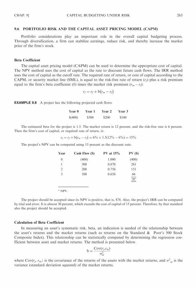
9.6 PORTFOLIO RISK AND THE CAPITAL ASSET PRICING MODEL (CAPM)
Portfolio considerations play an important role in the overall capital budgeting process.
Through diversification, a firm can stabilize earnings, reduce risk, and thereby increase the market
price of the firm’s stock.
Beta Coefficient
The capital asset pricing model (CAPM) can be used to determine the appropriate cost of capital.
The NPV method uses the cost of capital as the rate to discount future cash flows. The IRR method
uses the cost of capital as the cutoff rate. The required rate of return, or cost of capital according to the
CAPM, or security market line (SML), is equal to the risk-free rate of return (rf) plus a risk premium
equal to the firm’s beta coefficient (b) times the market risk premium (rm� rf):
rf ¼ rf þ b rm � rf� �
EXAMPLE 9.8 A project has the following projected cash flows:
Year 0 Year 1 Year 2 Year 3
$(400) $300 $200 $100
The estimated beta for the project is 1.5. The market return is 12 percent, and the risk-free rate is 6 percent.
Then the firm’s cost of capital, or required rate of return, is:
rf ¼ rf þ b rm � rf� �
¼ 6%þ 1:5 12%� 6%ð Þ ¼ 15%
The project’s NPV can be computed using 15 percent as the discount rate:
Year Cash Flow ($) PV at 15% PV ($)
0 (400) 1.000 (400)
1 300 0.870 261
2 200 0.756 151
3 100 0.658 66
78a
a NPV.
The project should be accepted since its NPV is positive, that is, $78. Also, the project’s IRR can be computed
by trial and error. It is almost 30 percent, which exceeds the cost of capital of 15 percent. Therefore, by that standard
also the project should be accepted.
Calculation of Beta Coefficient
In measuring an asset’s systematic risk, beta, an indication is needed of the relationship between
the asset’s returns and the market returns (such as returns on the Standard & Poor’s 500 Stock
Composite Index). This relationship can be statistically computed by determining the regression coe-
fficient between asset and market returns. The method is presented below.
b ¼ Covðrj,rmÞ�2m
where Cov(rj, rm) is the covariance of the returns of the assets with the market returns, and �2m is the
variance (standard deviation squared) of the market returns.
CHAP. 9] CAPITAL BUDGETING UNDER RISK 263

An easier way to compute beta is to determine the slope of the least-squares linear regression line
(rj� rf), where the excess return of the asset (rj� rf) is regressed against the excess return or the market
portfolio (rm� rf). The formula for b is:
b ¼P
MK� n �M �KP
M2 � n �M2
where M=(rm� rf)
K= (rj� rf)
n=number of years�M=average of M�K=average of K
EXAMPLE 9.9 Compute the beta coefficient, b, using the following data for stock x and the market portfolio:
Historic Rates of Return
Year rf (%) rm (%)
20X1 � 5 10
20X2 4 8
20X3 7 12
20X4 10 20
20X5 12 15
Assume that the risk-free rate is 6 percent. For easy computation, it is convenient to set up the following table:
Year
Stock Return,
rj
Market Return,
rm
Risk-free Rate,
rf (rj� rf)=K (rm� rj)=M M2 MK
20X1 � 0.05 0.10 0.06 � 0.11 0.04 0.0016 � 0.0044
20X2 0.04 0.08 0.06 � 0.02 0.02 0.0004 � 0.0004
20X3 0.07 0.12 0.06 0.01 0.06 0.0036 0.0006
20X4 0.10 0.20 0.06 0.04 0.14 0.0196 0.0056
20X5 0.12 0.15 0.06 0.06 0.09 0.0081 0.0054
– 0.02 0.35 0.0333 0.0068
�K=�0.004 �M=�0.07
Therefore, beta is:
b ¼P
MK� n �M �KP
M2 � n �M2¼ 0:0068� ð5Þð�0:004Þð0:07Þ
0:0333� ð5Þð0:07Þ2¼ 0:0082
0:0088¼ 0:93
Note: Using Excel regression yields the following:
Regression Statistics
Multiple R 0.65666
R Square 0.431203
Adjusted R Square 0.241603
Standard Error 5.796289
Observation 5
264 CAPITAL BUDGETING UNDER RISK [CHAP. 9

Coefficients
Intercept � 6.51364
X Variable 1 0.931818 � beta
Review Questions
1. is important in the capital budgeting process.
2. Risk can be measured in either or terms .
3. The use of is based on the concept that investors demand
for riskier projects.
4. The certainty equivalent approach is directly drawn from the concept of .
5. Under the certainty equivalent approach, is used as the discount rate under
the NPV method and as the cutoff rate under the IRR method.
6. Simulation is often called simulation.
7. attempts to determine how sensitive NPV or IRR is to changing conditions.
8. A(n) is a graphical exposition of the of possible outcomes.
9. If the probability distribution is , the expected value and the
may be used to compute the probability of a project’s providing an NPV of less or greater
than zero.
10. The required rate of return on a company’s security is equal to the plus a
.
11. Riskier projects should be evaluated with a higher discount rate, called a .
12. An easier way to determine beta is to determine the of the least-squares linear
regression line, where the of the security is regressed against the
of the .
13. Relative risk is measured by the .
14. is an index of risk.
Answers: (1) Risk analysis; (2) absolute, relative; (3) risk-adjusted rates of return, higher returns; (4) utility
theory; (5) the risk-free rate; (6) Monte Carlo; (7) Sensitivity analysis; (8) decision tree (or probability tree),
sequence; (9) normal, standard deviation; (10) risk-free rate, risk premium; (11) risk-adjusted discount
rate; (12) slope, excessive return, excessive return, market portfolio; (13) coefficient of variation; (14) Beta,
systematic (noncontrollable, nondiversifiable).
CHAP. 9] CAPITAL BUDGETING UNDER RISK 265

Solved Problems
9.1 Expected Value and Standard Deviation. The Lendal Company is considering investment in one
of two mutually exclusive projects. They have the following cash inflows for each of the next
3 years:Cash Inflows ($)
Probability Project A Project B
0.10 3,000 3,000
0.25 3,500 4,000
0.30 4,000 5,000
0.25 4,500 6,000
0.10 5,000 7,000
Calculate (a) the expected value (expected cash inflow) of each project; (b) the standard
deviation of each project; and (c) the coefficient of variation. (d ) Which Project has the greater
degree of risk? Why?
SOLUTION
(a) and (b) �A ¼X
n
i¼1Aipi � ¼
ffiffiffiffiffiffiffiffiffiffiffiffiffiffiffiffiffiffiffiffiffiffiffiffiffiffiffiffiffiffiffi
X
n
i¼1ðAi � �AÞ2pi
s
For project A:
Ai ($) pi Aipi ($) (Ai� �A) ($) (Ai� �A)2 ($) (Ai� �A)2 pi
3,000 0.10 300 � 1,000 1,000,000 100,000
3,500 0.25 875 � 500 250,000 62,500
4,000 0.30 1,200 0 0 0
4,500 0.25 1,125 500 250,000 62,500
5,000 0.10 500 1,000 1,000,000 100,000
�A=4,000 �2=325,000
Since �2=325,000, �=$570.09
For project B:
Ai ($) pi Ai pi ($) (Ai� �A) ($) (Ai� �A)2 ($) (Ai� �A)2pi ($)
3000 0.10 300 � 2,000 4,000,000 400,000
4,000 0.25 1,000 � 1,000 1000,000 250,000
5000 0.30 1,500 0 0 0
6,000 0.25 1,500 1,000 1,000,000 250,000
7,000 0.10 700 2,000 4,000,000 400,000
�A=5,000 �2=1,300,000
Since �2=1,300,000, �=$1,140.18.
(c) The coefficient of variation is:
A B
�
�A
$570:09
$4,000¼ 0:14
$1,140:18
$5,000¼ 0:23
(d ) Project B is riskier, since it has the greater coefficient of variation (i.e., 0.23 versus 0.14).
266 CAPITAL BUDGETING UNDER RISK [CHAP. 9

9.2 Coefficient of Variation. McEnro wishes to decide between two projects, X and Y. By using
probability estimates, he has determined the following statistics:
Project X ($) Project Y ($)
Expected NPV 35,000 20,000
� 22,000 20,000
(a) Compute the coefficient of variation for each project, and (b) explain why � and the
coefficient of variation give different rankings of risk. Which method is better?
SOLUTION
(a) Project X Project Y
�= �A $22,000
35,000¼ 0:63
$20,000
20,000¼ 1:00
(b) The coefficient of variation is a superior measure of risk because it is a relative measure, giving the
degree of dispersion relative to the expected value.
9.3 NPV Analysis Under Risk. The Connors Company is considering a $60,000 investment in a
machine that will reduce operating costs. The following estimates regarding cash savings, along
with their probabilities of occurrence, have been made:
Annual Cash Savings Useful Life
Event Probability Event Probability
$20,000 0.30 9 years 0.40
$14,000 0.30 8 years 0.40
$12,000 0.40 6 years 0.20
(a) Compute the expected annual cash savings and useful life. Determine whether the machine
should be purchased, using the NPV method.
(b) The company wishes to see whether the machine would be a good investment if each of its
most pessimistic estimates, but not both at the same time, came true. Determine whether the
investment would be desirable if: (1) the useful life is the expected value computed in part (a),
and annual cash flows are only $12,000; (2) the annual cash flows are equal to the expected
value computed in part (a) and the useful life is only 6 years.
SOLUTION
(a) Determine of expected annual cash savings is:
Event (Ai) Probabilities (pi) Expected Value
$20,000 0.30 $ 6,000
$14,000 0.30 4,200
$12,000 0.40 4,800
1.00 $15,000
CHAP. 9] CAPITAL BUDGETING UNDER RISK 267

Determination of useful life is:
Event Probability Useful Life
9 years 0.40 3.6 years
8 years 0.40 3.2 years
6 years 0.20 1.2 years
1.00 8.0 years
Expected annual cash savings $15,000
Present value factor for 8-year
annuity at 16% (PVIFA16%,8) � 4.344
Present value of future flows (PV) $65,160
Less cost of machine (I) 60,000
Net present value (NPV) $ 5,160
The purchase of the machine would appear to be wise because of its positive net present value.
(b) (1) The present value of the future cash savings ($52,128) is less than the purchase price ($60,000) and
the machine should not be purchased.
Annual cash savings, pessimistic
estimate $12,000
Present value factor, 8-year annuity
at 16% (PVIFA16%,8) 4.344
Present value of future cash flows $52,128
(2) The present value of the future cash savings ($55,275) is less than the purchase price ($60,000) and
the machine should not be purchased.
Annual cash savings, expected value $15,000
Present value factor, 6-year annuity
at 16% (PVIFA16%,6) 3.685
Present value of future cash flows $55,275
9.4 Expected NPV and Risk. The administrator of ABC Hospital is considering the purchase of new
operating room equipment at a cost of $7,500. The surgical staff has furnished the following
estimates of useful life and cost savings. Each useful life estimate is independent of each cost
savings estimate.
Years of
Estimated
Useful Life
Probability of
Occurrence
Estimated Cost
Savings
Probability of
Occurrence
4 0.25 $1.900 0.30
5 0.50 $2,000 0.40
6 0.25 $2,100 0.30
1.00 1.00
Calculate (a) the expected net present value, allowing for risk and uncertainty and using a 10
percent discount rate, and (b) the standard deviation and coefficient of variation for the present
value calculations of estimated cost savings before deducting the investment.
268 CAPITAL BUDGETING UNDER RISK [CHAP. 9
SOLUTION
(a)
(1) (2) (3) (4) (5) (6) (7) (8)
Estimated
Useful Life
Estimated
Cost Savings Combined
Probability Present Value
Present Value ($)
(Conditional
Value)
Expected
Present
Value ($)
Years Probability $ Probability (2)� (4) Factor 10% (3) � (6) (5) � (7)
0.25 1,900 0.30 0.075 3.170 6,023 452
4 0.25 2,000 0.40 0.100 3.170 6,340 634
0.25 2,100 0.30 0.075 3.170 6,657 499
0.50 1,900 0.30 0.150 3.791 7,203 1,080
5 0.50 2,000 0.40 0.200 3.791 7,582 1,516
0.50 2,100 0.30 0.150 3.791 7,961 1,194
0.25 1,900 0.30 0.075 4.355 8,275 621
6 0.25 2,000 0.40 0.100 4.355 8,710 871
0.25 2,100 0.30 0.075 4.355 9.146 686
1.000 7,553
Total expected present value $7,553
Less investment in equipment 7,500
Expected net present value $ 53
(b)
(1) (2) (3) (4) (5)
Present Value ($)
(Conditional
Value)
Difference from
Expected Value ($)
($7,553)
(2) Squared
($) Probability (3)� (4) ($)
6,023 � 1,530 2,340,900 0.075 175,568
6,340 � 1,213 1,471,369 0.100 147,137
6,657 � 896 802,816 0.075 60,211
7,203 � 350 122,500 0.150 18,375
7,582 29 841 0.200 168
7,961 408 166,464 0.150 24,970
8,275 722 521,28 0.075 39,096
8,710 1,157 1,338,649 0.100 133,865
9,146 1,593 2,537,649 0.075 190,324
�2=$789,714
� ¼ffiffiffiffiffiffiffiffiffiffiffiffiffiffiffiffiffiffiffi
$789,714p
¼ $889
Coefficient of variation ¼ �
�A¼ $889
$7,553¼ 0:12
9.5 Risk-Adjusted NPV and Decision. Vilas Corporation is considering two mutually exclusive
projects, both of which require an initial investment of $4,500 and an expected life of
CHAP. 9] CAPITAL BUDGETING UNDER RISK 269

10 years. The probability distribution for the cash inflows are as follows (for years 1
through 10):
Project A Project B
Cash Inflow Probability Cash Inflow Probability
$700 0.10 $ 550 0.2
900 0.80 800 0.3
1,000 0.10 1,000 0.3
1,400 0.2
The company has decided that the project with higher relative risk should have a required
rate of return of 16 percent, whereas the less risky project’s required rate of return should be 14
percent.
Compute (a) the coefficient of variation as a measure of relative risk, and (b) the risk-adjusted
NPV of each project. Which project should be chosen? (c) What factors other than NPV should
be considered when deciding between these two projects?
SOLUTION
(a) For project A:
�A ¼X
n
i¼1Aipi ¼ $700ð0:1Þ þ $900ð0:8Þ þ $1,000ð0:1Þ
¼ $70þ $720þ $100 ¼ $890
� ¼ffiffiffiffiffiffiffiffiffiffiffiffiffiffiffiffiffiffiffiffiffiffiffiffiffiffiffiffiffiffiffi
X
n
i¼1ðAi � �AÞ2pi
s
¼ffiffiffiffiffiffiffiffiffiffiffiffiffiffiffiffiffiffiffiffiffiffiffiffiffiffiffiffiffiffiffiffiffiffiffiffiffiffiffiffiffiffiffiffiffiffiffiffiffiffiffiffiffiffiffiffiffiffiffiffiffiffiffiffiffiffiffiffiffiffiffiffiffiffiffiffiffiffiffiffiffiffiffiffiffiffiffiffiffiffiffiffiffiffiffiffiffiffiffiffiffiffiffiffiffiffiffiffiffiffiffiffiffiffiffiffiffiffiffiffiffiffiffiffiffiffiffiffiffiffiffiffiffiffi
ð$700� $890Þ2ð0:1Þ þ ð$900� $890Þ2ð0:8Þ þ ð$1,000� $890Þ2ð0:1Þq
¼ffiffiffiffiffiffiffiffiffiffiffiffiffiffiffiffiffiffiffiffiffiffiffiffiffiffiffiffiffiffiffiffiffiffiffiffiffiffiffiffiffiffiffiffiffiffi
$3,610þ $80þ $1,210p
¼ffiffiffiffiffiffiffiffiffiffiffiffiffiffi
$4,900p
¼ $70
�
�A¼ $70
$890¼ 0:079
For project B:
�A ¼ $550ð0:2Þ þ $800ð0:3Þ þ $1,000ð0:3Þ þ $1,400ð0:2Þ¼ $110þ $240þ $300þ $280 ¼ $930
� ¼ffiffiffiffiffiffiffiffiffiffiffiffiffiffiffiffiffiffiffiffiffiffiffiffiffiffiffiffiffiffiffiffiffiffiffiffiffiffiffiffiffiffiffiffiffiffiffiffiffiffiffiffiffiffiffiffiffiffiffiffiffiffiffiffiffiffiffiffiffiffiffiffiffiffiffiffiffiffiffiffiffiffiffiffiffiffiffiffiffiffiffiffiffiffiffiffiffiffiffiffiffiffiffiffiffiffiffiffiffiffiffiffiffiffiffiffiffiffiffiffiffiffiffiffiffiffiffiffiffiffiffiffiffiffiffiffiffiffiffiffiffiffiffiffiffiffiffiffiffiffiffiffiffiffiffiffiffiffiffiffiffiffiffiffiffiffiffiffiffiffiffiffiffiffiffiffiffiffiffiffiffiffiffi
ð$550� $930Þ2ð0:2Þ þ ð$800� $930Þ2ð0:3Þ þ ð$1,000� $930Þ2ð0:3Þ þ ð$1,400� $930Þ2ð0:2Þq
¼ffiffiffiffiffiffiffiffiffiffiffiffiffiffiffiffiffiffiffiffiffiffiffiffiffiffiffiffiffiffiffiffiffiffiffiffiffiffiffiffiffiffiffiffiffiffiffiffiffiffiffiffiffiffiffiffiffiffiffiffiffiffiffiffiffiffiffiffiffiffiffiffiffiffiffiffi
$28,880þ $5,070þ $1,470þ $44,180p
¼ffiffiffiffiffiffiffiffiffiffiffiffiffiffiffiffi
$79,600p
¼ $282:13
�
�A¼ $282:13
$930¼ 0:30
(b) Project A is relatively less risky than project B. Therefore, Project A’s expected cash inflow is
discounted at 14 percent, while project B’s expected cash inflow is discounted at 16 percent.
For project A:
Expected NPV ¼ PV� I ¼ $890ðPVIFA14%,10Þ � $4,500 ¼ $890ð5:216Þ � $4,500
¼ $4,642:24� $4,500 ¼ $142:24
For project B:
Expected NPV ¼ $930ðPVIFA16%,10Þ � $4,500 ¼ $930ð4:833Þ � $4,500
¼ $4,494:69� $4,500 ¼ �$5:31
Because project A has a positive NPV, project A should be chosen.
270 CAPITAL BUDGETING UNDER RISK [CHAP. 9

(c) The company should also consider the potential diversification effect associated with these projects.
If the project’s cash inflow patterns are negatively correlated with those of the company, the overall
risk of the company may be significantly reduced.
9.6 Risk-Adjusted NPV. Kyoto Laboratories, Inc., is contemplating a capital investment project with
an expected useful life of 10 years that requires an initial cash outlay of $225,000. The company
estimates the following data:
Annual Cash
Inflows ($) Probabilities
0 0.10
50,000 0.20
65,000 0.40
70,000 0.20
90,000 0.10
(a) Assuming a risk-adjusted required rate of return of 25 percent is appropriate for projects
of this level of risk, calculate the risk-adjusted NPV of the project. (b) Should the project
be accepted?
SOLUTION
(a) �A ¼X
n
i¼1Aipi ¼ $0ð0:10Þ þ $50,000ð0:2Þ þ $65,000ð0:4Þ þ $70,000ð0:2Þ þ $90,000ð0:1Þ
¼ $0þ $10,000þ $26,000þ $14,000þ $9,000 ¼ $59,000
Expected NPV ¼ PV� I
¼ $59,000ðPVIFA25%,10Þ � $225,000 ¼ $210,689� $225,000 ¼ �$14,311
(b) Reject the project, since the expected NPV is negative.
9.7 Certainty Equivalent NPV. Rush Corporation is considering the purchase of a new machine that
will last 5 years and require a cash outlay of $300,000. The firm has a 12 percent cost of capital
rate and its after-tax risk-free rate is 9 percent. The company has expected cash inflows and
certainty equivalents for these cash inflows, as follows:
Year
After-Tax
Cash Inflows ($)
Certainty
Equivalent
1 100,000 1.00
2 100,000 0.95
3 100,000 0.90
4 100,000 0.80
5 100,000 0.70
Calculate (a) the unadjusted NPV, and (b) the certainty equivalent NPV. (c) Determine if the
machine should be purchased.
SOLUTION
(a) NPV ¼ PV� I ¼ $100,000ðPVIFA12%,5Þ � $300,000
¼ $100,000ð3:605Þ � $300,000 ¼ $360,500� $300,000 ¼ $60,500
CHAP. 9] CAPITAL BUDGETING UNDER RISK 271

(b)
Year
After-Tax
Cash Inflows ($)
Certainty
Equivalents
Certain
Cash Inflows ($) PV at 9% PV ($)
1 100,000 1.00 100,000 0.917 91,700
2 100,000 0.95 95,000 0.842 79,990
3 100,000 0.90 90,000 0.772 69,480
4 100,000 0.80 80,000 0.708 56,640
5 100,000 0.70 70,000 0.650 45,500
343,310
Certainty equivalent NPV ¼ $343,310� $300,000 ¼ $43,310
(c) Because of a positive NPV, the machine should be purchased.
9.8 Decision Tree. The Summerall Corporation wishes to introduce one of two products to the market
this year. The probabilities and present values of projected cash inflows are given below.
Products
Initial
Investment ($)
PV of
Cash Inflows ($) Probabilities
A 225,000 1.00
450,000 0.4
200,000 0.5
�100,000 0.1
B 80,000 1.00
320,000 0.2
100,000 0.6
�150,000 0.2
(a) Construct a decision tree to analyze the two products. (b) Which product would you
introduce? Comment on your decision.
SOLUTION
(a)
For product A:
Expected NPV ¼ expected PV� I ¼ $270,000� $225,000 ¼ $45,000
For product B:
Expected NPV ¼ $94,000� $80,000 ¼ $14,000
272 CAPITAL BUDGETING UNDER RISK [CHAP. 9
(b) Based on the expected NPV, choose product A over product B; however, this analysis fails to recognize
the risk factor in project analysis.
9.9 Dependent Cash Inflows and Expected NPV. The Newcome Corporation has determined that
its after-tax cash inflow (ATCI) distributions are not independent. Further, the company has
estimated that the year 1 results (ATCI1) will affect the year 2 flows (ATCI2) as follows:
If ATCI1=$40,000 with a 30 percent chance, the distribution for ATCI2 is:
0.2 $20,000
0.6 $50,000
0.2 $80,000
If ATCI1=$60,000 with a 40 percent chance, the distribution for ATCI2 is:
0.3 $70,000
0.4 $80,000
0.3 $90,000
If ATCI1=$80,000 with a 30 percent chance, the distribution for ATCI2 is:
0.1 $ 80,000
0.8 $100,000
0.1 $120,000
Assume that the project’s initial investment is $100,000.
(a) Set up a decision tree to depict the above cash flow possibilities, and calculate an expected
NPV for each 2-year possibility using a risk-free rate of 15 percent. (b) Determine if the project
should be accepted.
SOLUTION
(a)
a NPV ¼ PV� I ¼ $40,000
ð1þ 0:15Þ þ$20,000
ð1þ 0:15Þ2� $100,000
¼ $40,000ðPVIF15%, 1Þ þ $20,000ðPVIF15%;2Þ � $100,000
¼ $40,000ð0:87Þ þ $20,000ð0:756Þ � $100,000 ¼ $34,800þ $15,120� $100,000 ¼ �$50,080b Joint probability of the first path= (0.3)(0.2)=0.6
The expected NVP is $10,431.
(b) Accept the project, since the expected NPV is positive.
CHAP. 9] CAPITAL BUDGETING UNDER RISK 273

9.10 Decision Tree Analysis. The Drysdale Corporation is contemplating the development of a
new product. The initial investment required to purchase the necessary equipment is
$200,000. There is a 60 percent chance that demand will be high in year 1. If it is high, there
is an 80 percent chance that it will continue high indefinitely. If demand is low in year 1, there
is a 60 percent chance that it will continue to be low indefinitely. If demand is high, forecasted
cash inflow (before taxes) is $90,000 a year; if demand is low, forecasted cash inflow is $30,000
a year.
The corporate income tax rate is 40 percent. The company uses straight-line depreciation
and will depreciate the equipment over 10 years with no salvage value.
(a) Determine the after-tax cash inflows. (b) Set up a decision tree representing all possible
outcomes, and compute the expected NPV using a 10 percent risk-free rate of return.
SOLUTION
(a) First, compute the annual depreciation.
Depreciation ¼ price=useful life ¼ $200,000
10 years¼ $20,000=year
After-tax cash inflow ¼ after-tax net profitsþ depreciation
Therefore, when demand is high:
After-tax cash inflow ¼ ð$90,000� $20,000Þð1� 0:4Þ þ $20,000 ¼ $62,000
When demand is low:
After-tax cash inflow ¼ ð$30,000� $20,000Þð1� 0:4Þ þ $20,000 ¼ $26,000
(b)
a NPV ¼ PV� I ¼ $62,000
ð1þ 0:1Þ þ$62,000
ð1þ 0:1Þ2þ � � � þ $62,000
ð1þ 0:1Þ10� $200,000
¼ $62,000ðPVIF10%;1Þ þ $62,000ðPVIFA10%;10 � PVIFA10%1Þ � $200,000
¼ $62,000ð0:909Þ þ $62,000ð6:145� 0:909Þ � $200,000
¼ $56,358þ $324,632� $200,000 ¼ $180,990
b Joint probability= (0.6)(0.8)=0.48
The expected NPV is $100,042.
274 CAPITAL BUDGETING UNDER RISK [CHAP. 9

9.11 Decision Tree Analysis and Expected IRR. The NFL Systems, Inc., is considering the purchase of
a minicomputer using the following decision tree:
(a) Complete the decision tree by computing IRR, joint probability, and the expected IRR (round to the
nearest whole percent of IRR). (b) Should this computer be purchased? (Assume the company’s cost of
capital is 16 percent.)
SOLUTION
(a)
a By definition, at IRR, I=PV.
Thus,
$17,500 ¼ $10,000ðPVIFAr,2Þ
PVIFAr,2 ¼$17,500
$10,000¼ 1:75
From Appendix D this value is close to 9 percent.
b Joint probability= (0.4)(1.0)=0.4
c I=PV($17,500)=$12,500(PVIFr,1)+$13,500(PVIFr,2)
By trial and error, IRR is approximately 30 percent. In other words, at r=30 percent:
I ¼ PV
¼ $12,500ð0:769Þ þ $13,500ð0:592Þ ¼ $9,613þ $7,992 ¼ $17,605
(b) The expected IRR is 20.1 percent, which exceeds the cost of capital of 16 percent. Therefore, the
computer should be purchased.
CHAP. 9] CAPITAL BUDGETING UNDER RISK 275

9.12 Normal Distribution and NPV Analysis. The probability distribution of possible NPVs for project
A has an expected cash inflow of $30,000 and a standard deviation of $15,000. Assuming a
normal distribution, compute the probability that: (a) the NPV will be zero or less; (b) the
NPV will be greater than $45,000; and (c) the NPV will be less than $7,500.
SOLUTION
The standardized normal variate is:
z ¼ x�NPV
�
(a) For NPV of zero or less:
z ¼ 0� $30,000
$15,000¼ �2
From Appendix E, z=� 2 corresponds to a probability of 0.0228 or 2.28 percent.
(b) For NPV of $45,000 or more:
z ¼ $45,000� $30,000
$15,000¼ 1:0
From Appendix E, the probability for this value of z is 15.77 percent.
(c) For NPV of $7,500 or less:
z ¼ $7,500� $30,000
$15,000¼ �1:5
From Appendix E, the probability for z=� 1.5 is 6.68 percent.
9.13 Normal Distribution and NPV Analysis. The Halo Shipping Company is considering an invest-
ment in a project that requires an investment of $6,000, with a projected after-tax cash inflow
generated over the next 3 years as follows:
Period 1 Period 2 Period 3
Probability Cash Flow ($) Probability Cash Flow ($) Probability Cash Flow ($)
0.10 1,000 0.2 1,000 0.3 1,000
0.30 2,000 0.4 2,000 0.4 2,000
0.20 3,000 0.3 3,000 0.1 3,000
0.40 4,000 0.1 4,000 0.2 4,000
Assume that probability distributions are independent and the after-tax risk-free rate of
return is 6 percent. Calculate: (a) the expected NPV of the project; (b) the standard deviation
of the expected NPV; (c) the probability that the NPV will be zero or less (assume
that the probability distribution is normal and continuous); (d ) the probability that the
NPV will be greater than zero; and (e) the probability that the NPV will be greater than the
expected value.
SOLUTION
(a)
Period 1 Period 2 Period 3
$1,000(0.1)= $ 100 $1,000(0.2)=$ 200 $1,000(0.3)=$ 300
$2,000(0.3)= 600 $2,000(0.4)= 800 $2,000(0.4)= 800
$3,000(0.2)= 600 $3,000(0.3)= 900 $3,000(0.1)= 300
$4,000(0.4)= 1,600 $4,000(0.1)= 400 $4,000(0.2)= 800
$2,900 $2,300 $2,200
276 CAPITAL BUDGETING UNDER RISK [CHAP. 9

NPV ¼ PV� I
¼ $2,900
ð1þ 0:06Þ þ$2,300
ð1þ 0:06Þ2þ $2,200
ð1þ 0:06Þ3� $6,000
¼ $2,900ðPVIF6%, 1Þ þ $2,300ðPVIF6%, 2Þþ$2,200ðPVIF6%, 3Þ � $6,000
¼ $2,900ð0:943Þ þ $2,300ð0:89Þþ$2,200ð0:84Þ � $6,000
¼ $2,735þ $2,047þ $1,848� $6,000 ¼ $6,630� $6,000 ¼ $630
(b) Calculations for standard deviation of NPV are as follows:
For period 1:
A ($) p (A� �A) ($) (A� �A)2 ($) (A� �A)2 p
1,000 0.1 �1,900 3,610,000 $ 361,000
2,000 0.3 �900 810,000 243,000
3,000 0.2 100 10,000 2,000
4,000 0.4 1,100 1,210,000 484,000
$1,090,000a
$ 1,044b
a $1,090,000= �2
b $1,044= �
For period 2:
A ($) p (A� �A) ($) (A� �A)2 ($) (A� �A)2 p ($)
1,000 0.2 � 1,300 1,690,000 338,000
2,000 0.4 � 300 90,000 36,000
3,000 0.3 700 490,000 147,000
4,000 0.1 1,100 2,890,000 289,000
�2=810,000
�=$ 900
For period 3:
A ($) p (A� �A) ($) (A� �A)2 ($) (A� �A)2 p ($)
1,000 0.3 � 1,200 1,440,000 432,000
2,000 0.4 � 200 40,000 16,000
3,000 0.1 800 640,000 64,000
4,000 0.2 1,800 3,240,000 648,000
�2=1,160,000
�=$ 1,077
The standard deviation of the expected NPV is:
�NPV ¼
ffiffiffiffiffiffiffiffiffiffiffiffiffiffiffiffiffiffiffiffiffiffiffiffiffiffiffiffiffiffiffiffiffiffiffiffiffiffiffiffiffiffiffiffiffiffiffiffiffiffiffiffiffiffiffiffiffiffiffiffiffiffiffiffiffiffiffiffiffiffiffiffiffiffiffiffiffiffi
ð$1,044Þ2
ð1þ 0:06Þ2þ ð$900Þ2
ð1þ 0:06Þ4þ ð$1,077Þ
2
ð1þ 0:06Þ6
s
¼ffiffiffiffiffiffiffiffiffiffiffiffiffiffiffiffiffiffiffiffiffiffiffiffiffiffiffiffiffiffiffiffiffiffiffiffiffiffiffiffiffiffiffiffiffiffiffiffiffiffiffiffiffiffiffiffiffiffiffiffiffiffiffiffiffiffi
$970,039þ $642,857þ $727,776p
¼ffiffiffiffiffiffiffiffiffiffiffiffiffiffiffiffiffiffiffiffiffiffi
$2,340,672p
¼ $1,530
(c) z ¼ x�NPV
�¼ 0� $630
$1,530¼ �0:41176
From the normal distribution table Appendix E, this value of z gives a probability of 0.3409, or
approximately a 34 percent chance that NPV will be zero or less.
CHAP. 9] CAPITAL BUDGETING UNDER RISK 277

(d ) The probability of the NPV being greater than zero is the compliment of 34 percent, or 66 percent.
(e) z ¼ $630� $630
$1,530¼ 0
Reading from Appendix E, at z=0, there is 50 percent probability that the NPV will be greater than
the expected value.
9.14 Portfolio Effects. The projected cash inflows of three projects—X, Y, and Z—for the period 20X1
to 20X5 are given below.
Year Project X ($) Project Y ($) Project Z ($)
20X1 2,000 6,000 1,000
20X2 3,000 4,000 2,000
20X3 4,000 3,000 3,000
20X4 5,000 2,000 3,000
20X5 7,000 1,000 6,000
Project X ($) Project Y ($) Project Z ($)
�A 4,200 3,200 3,000
� 3,847 3,847 3,742
(a) Calculate the expected cash inflows and standard deviation of cash inflows for project
combinations XY and XZ, and (b) determine the portfolio effects of the above combinations of
projects upon the portfolio risk.
SOLUTION
Since the probabilities associated with the cash inflows are not given (in fact, their cash inflows are equally
likely), the formulas for �A and � are
�A ¼X
Ai=n and � ¼ffiffiffiffiffiffiffiffiffiffiffiffiffiffiffiffiffiffiffiffiffiffiffiffiffiffiffiffiffiffiffiffi
X
n
i¼1ðAi � �AÞ2=n
s
where n is the number of terms.
(a) For projects XY:
Cash Inflow (A) ($) (A� �A) ($) (A� �A)2 ($)
8,000 600 360,000
7,000 � 400 160,000
7,000 � 400 160,000
7,000 � 400 160,000
8,000 600 360,000
37,000 1,200,000
�A ¼ $37,000
5¼ $7,400
�2 ¼ $1,200,000
5¼ $240,000
Thus
� ¼ $490
278 CAPITAL BUDGETING UNDER RISK [CHAP. 9

For projects XZ:
Cash Inflow (A) ($) (A� �A) ($) (A� �A)2 ($)
3,000 � 4,200 17,640,000
5,000 � 2,200 4,840,000
7,000 � 200 40,000
8,000 800 640,000
13,000 5,800 33,640,000
36,000 56,800,000
�A ¼ $36,000
5¼ $7,200
�2 ¼ $56,800,000
5¼ $11,360,000
Thus
� ¼ $3,370
(b) The greatest reduction in overall risk occurs when the portfolio combines projects which are negatively
correlated such as projects XY (i.e., �XY=$490).
9.15 CAPM and Capital Budgeting Decision. The Taylor Corporation is evaluating some new capital
budgeting projects. Their evaluation method involves comparing each project’s risk-adjusted
return obtained from the capital asset pricing model (CAPM) with the project’s average rate of
return. The following data are provided:
Projects Beta
A � 0.5
B 0.8
C 1.2
D 2.0
Possible rates of return and associated probabilities are:
Rates of Return (%)
(0.4) (0.5) (0.1)
A 4 2 5
B 2 6 12
C 10 15 20
D � 8 25 50
Assume that the risk-free rate of return is 6 percent and the market rate of return is 12
percent. Which projects should be selected?
SOLUTION
Use the CAPM equation to compute:
Projects r= rf+ b(rm – rf)
A rA=6%+(� 0.5)(12%� 6%)=3%
B rB=6%+(0.8)(12%� 6%)=10.8%
C rC=6%+(1.2)(12%� 6%)=13.2%
D rD=6%+(2.0)(12%� 6%)=18%
CHAP. 9] CAPITAL BUDGETING UNDER RISK 279
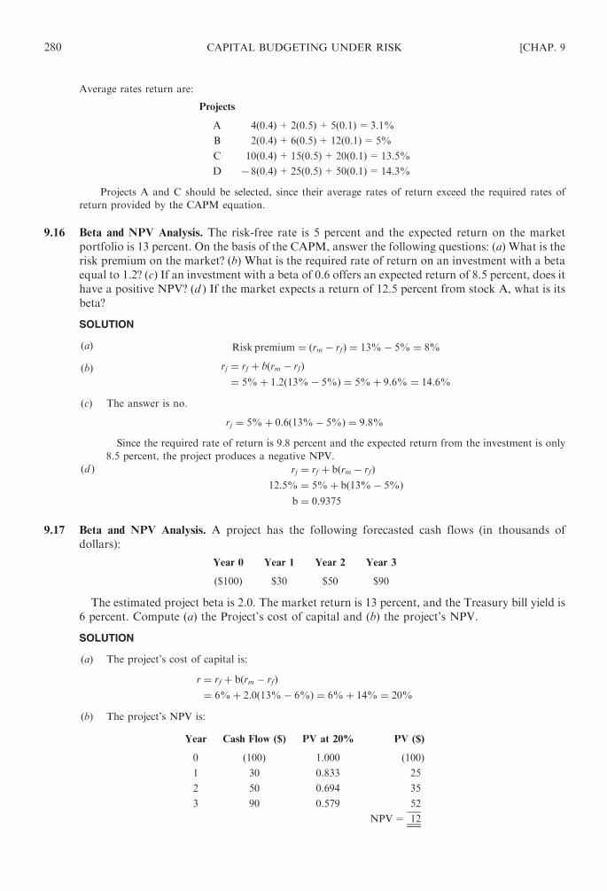
Average rates return are:
Projects
A 4(0.4)+2(0.5)+5(0.1)=3.1%
B 2(0.4)+6(0.5)+12(0.1)=5%
C 10(0.4)+15(0.5)+20(0.1)=13.5%
D � 8(0.4)+25(0.5)+50(0.1)=14.3%
Projects A and C should be selected, since their average rates of return exceed the required rates of
return provided by the CAPM equation.
9.16 Beta and NPV Analysis. The risk-free rate is 5 percent and the expected return on the market
portfolio is 13 percent. On the basis of the CAPM, answer the following questions: (a) What is the
risk premium on the market? (b) What is the required rate of return on an investment with a beta
equal to 1.2? (c) If an investment with a beta of 0.6 offers an expected return of 8.5 percent, does it
have a positive NPV? (d ) If the market expects a return of 12.5 percent from stock A, what is its
beta?
SOLUTION
(a) Risk premium ¼ ðrm � rfÞ ¼ 13%� 5% ¼ 8%
(b) rj ¼ rf þ bðrm � rfÞ¼ 5%þ 1:2ð13%� 5%Þ ¼ 5%þ 9:6% ¼ 14:6%
(c) The answer is no.
rj ¼ 5%þ 0:6ð13%� 5%Þ ¼ 9:8%
Since the required rate of return is 9.8 percent and the expected return from the investment is only
8.5 percent, the project produces a negative NPV.
(d ) rj ¼ rf þ bðrm � rfÞ12:5% ¼ 5%þ bð13%� 5%Þ
b ¼ 0:9375
9.17 Beta and NPV Analysis. A project has the following forecasted cash flows (in thousands of
dollars):
Year 0 Year 1 Year 2 Year 3
($100) $30 $50 $90
The estimated project beta is 2.0. The market return is 13 percent, and the Treasury bill yield is
6 percent. Compute (a) the Project’s cost of capital and (b) the project’s NPV.
SOLUTION
(a) The project’s cost of capital is:
r ¼ rf þ bðrm � rfÞ¼ 6%þ 2:0ð13%� 6%Þ ¼ 6%þ 14% ¼ 20%
(b) The project’s NPV is:
Year Cash Flow ($) PV at 20% PV ($)
0 (100) 1.000 (100)
1 30 0.833 25
2 50 0.694 35
3 90 0.579 52
NPV= 12
280 CAPITAL BUDGETING UNDER RISK [CHAP. 9

9.18 Calculation of Beta Using Regression Analysis. You are given the following data for stock A and
the market portfolio:
Historic Rates of Return
Year rj (%) rm (%)
20X0 1 � 2
20X1 3 7
20X2 14 20
20X3 18 30
Assuming that the risk-free rate is 4 percent, compute (a) the beta coefficient and (b) the required
rate of return to be used for capital budgeting decisions in 20X4 when the market rate of return is
expected to be 18 percent?
SOLUTION
(a)
Stock
Return,
Market
Return,
Risk-Free
Rate,
Excess
Stock Return
Excess
Market Return
Cross
Product
Year rj rm rj (rj� rf)=K (rf� rm)=M M2 MK
20X0 0.01 � 0.02 0.04 � 0.03 0.06 0.0036 � 0.0018
20X1 0.03 0.07 0.04 � 0.01 � 0.03 0.0009 0.0003
20X2 0.14 0.2 0.04 0.10 � 0.16 0.0256 � 0.016
20X3 0.18 0.3 0.04 0.14 � 0.26 0.0676 � 0.0364
0.2 � 0.39 0.0977 � 0.0539
�K ¼ 0:05
�M ¼ �0:0975
b ¼P
MK�n �M �KP
M2 � n �M2¼ �0:0539� ð4Þð�0:0975Þð0:05Þ
0:0977� ð4Þð�0:0975Þ2¼ �0:0344�0:0597 ¼ 0:59
(b) rj ¼ rf þ bðrm � rfÞ¼ 4%þ ð0:59Þð18%� 4%Þ ¼ 12:26%
Therefore, the 20X4 risk-adjusted rate or return that is required for capital budgeting projects is
12.26 percent.
CHAP. 9] CAPITAL BUDGETING UNDER RISK 281

Chapter 10
Cost of Capital
10.1 COST OF CAPITAL DEFINED
Cost of capital is defined as the rate of return that is necessary to maintain the market value of the
firm (or price of the firm’s stock). Managers must know the cost of capital, often called the minimum
required rate of return in: (1) making capital budgeting decisions; (2) helping to establish the optimal
capital structure; and (3) making decisions such as leasing, bond refunding, and working capital manage-
ment. The cost of capital is computed as a weighted average of the various capital components, which are
items on the right-hand side of the balance sheet such as debt, preferred stock, common stock, and
retained earnings.
10.2 COMPUTING INDIVIDUAL COSTS OF CAPITAL
Each element of capital has a component cost that is identified by the following:
ki=before-tax cost of debt
kd= ki (1�t)=after-tax cost of debt, where t=tax rate
kp=cost of preferred stock
ks=cost of retained earnings (or internal equity)
ke=cost of external equity, or cost of issuing new common stock
ko=firm’s overall cost of capital, or a weighted average cost of capital
Cost of Debt
The before-tax cost of debt can be found by determining the internal rate of return (or yield to
maturity) on the bond cash flows, which was discussed in detail in Chapter 7. However, the following
shortcut formula may be used for approximating the yield to maturity on a bond:
ki ¼Iþ M� Vð Þ=n
Mþ Vð Þ=2
where I=annual interest payments in dollars
M=par value, usually $1,000 per bond
V=value or net proceeds from the sale of a bond
n=term of the bond in years
Since the interest payments are tax-deductible, the cost of debt must be stated on an after-tax basis. The
after-tax cost of debt is:
kd ¼ kið1� tÞ
where t is the tax rate.
282
Copyright © 2007, 1998, 1986 by The McGraw-Hill Companies, Inc. Click here for terms of use.

EXAMPLE 10.1 Assume that the Carter Company issues a $1,000, 8 percent, 20-year bond whose net proceeds
are $940. The tax rate is 40 percent. Then, the before-tax cost of debt, ki, is:
ki ¼Iþ M� Vð Þ=n
Mþ Vð Þ=2
¼ $80þ $1,000� $940ð Þ=20$1,000þ $940ð Þ=2 ¼ $83
$970¼ 8:56%
Therefore, the after-tax cost of debt is:
kd ¼ ki 1� tð Þ¼ 8:56% 1� 0:4ð Þ ¼ 5:14%
Cost of Preferred Stock
The cost of preferred stock, kp, is found by dividing the annual preferred stock dividend, dp, by the
net proceeds from the sale of the preferred stock, p, as follows:
kp ¼dp
p
Since preferred stock dividends are not a tax-deductible expense, these dividends are paid out after
taxes. Consequently, no tax adjustment is required.
EXAMPLE 10.2 Suppose that the Carter Company has preferred stock that pays a $13 dividend per share and sells
for $100 per share in the market. The flotation (or underwriting) cost is 3 percent, or $3 per share. Then the cost of
preferred stock is:
kp ¼dp
p
¼ $13
$97¼ 13:4%
Cost of Equity Capital
The cost of common stock, ke, is generally viewed as the rate of return investors require on a firm’s
common stock. Three techniques for measuring the cost of common stock equity capital are available:
(1) the Gordon’s growth model; (2) the capital asset pricing model (CAPM) approach; and (3) the bond
plus approach.
The Gordon’s Growth Model. The Gordon’s model was discussed in detail in Chapter 7. The
model is:
P0 ¼D1
r� g
where P0=value of common stock
D1=dividend to be received in 1 year
r=investor’s required rate of return
g=rate of growth (assumed to be constant over time)
Solving the model for r results in the formula for the cost of common stock:
r ¼ D1
P0
þ g or ke ¼D1
P0
þ g
Note that the symbol r is changed to ke to show that it is used for the computation of cost of capital.
CHAP. 10] COST OF CAPITAL 283

EXAMPLE 10.3 Assume that the market price of the Carter Company’s stock is $40. The dividend to be paid at
the end of the coming year is $4 per share and is expected to grow at a constant annual rate of 6 percent. Then the
cost of this common stock is:
ke ¼D1
P0
þ g ¼ $4
$40þ 6% ¼ 16%
The cost of new common stock, or external equity capital, is higher than the cost of existing common
stock because of the flotation costs involved in selling the new common stock.
If f is flotation cost in percent, the formula for the cost of new common stock is:
ke ¼D1
P0ð1� fÞ þ g
EXAMPLE 10.4 Assume the same data as in Example 10.3, except the firm is trying to sell new issues of stock A
and its flotation cost is 10 percent. Then:
ke ¼D1
P0ð1� fÞ þ g
¼ $4
$40 1� 0:1ð Þ þ 6% ¼ $4
$36þ 6% ¼ 11:11%þ 6% ¼ 17:11%
The CAPM Approach. An alternative approach to measuring the cost of common stock is to use
the CAPM, which involves the following steps:
1. Estimate the risk-free rate, rf, generally taken to be the United States Treasury bill rate.
2. Estimate the stock’s beta coefficient, b, which is an index of systematic (or nondiversifiable
market) risk.
3. Estimate the rate of return on the market portfolio such as the Standard & Poor’s 500 Stock
Composite Index or Dow Jones 30 Industrials.
4. Estimate the required rate of return on the firm’s stock, using the CAPM (or SML) equation:
ke ¼ rf þ b rm � rf� �
Again, note that the symbol rj is changed to ke.
EXAMPLE 10.5 Assuming that rf is 7 percent, b is 1.5, and rm is 13 percent, then:
ke ¼ rf þ b rm � rf� �
¼ 7%þ 1:5 13%� 7%ð Þ ¼ 16%
This 16 percent cost of common stock can be viewed as consisting of a 7 percent risk-free rate plus a 9 percent risk
premium, which reflects that the firm’s stock price is 1.5 times more volatile than the market portfolio to the factors
affecting nondiversifiable, or systematic, risk.
The Bond Plus Approach. Still another simple but useful approach to determining the cost of
common stock is to add a risk premium to the firm’s own cost of long-term debt, as follows:
ke ¼ long-term bond rateþ risk premium
¼ ki 1� tð Þ þ risk premium
A risk premium of about 4 percent is commonly used with this approach.
EXAMPLE 10.6 Using the data found in Example 10.1, the cost of common stock using the bond plus approach is:
ke ¼ long-term bond rateþ risk premium
¼ kið1� tÞ þ risk premium
¼ 5:14%þ 4% ¼ 9:14%
284 COST OF CAPITAL [CHAP. 10

Cost of Retained Earnings
The cost of retained earnings, ks, is closely related to the cost of existing common stock, since the
cost of equity obtained by retained earnings is the same as the rate of return investors require on the
firm’s common stock. Therefore,
ke ¼ ks
10.3 MEASURING THE OVERALL COST OF CAPITAL
The firm’s overall cost of capital is the weighted average of the individual capital costs, with the
weights being the proportions of each type of capital used. Let ko be the overall cost of capital.
ko ¼X
% of total capital cost of capital
structure supplied by � for each source
each type of capital of capital
0
@
1
A
¼ wd � kd þ wp � kp þ we � ke þ ws � ks
where wd =percentage of total capital supplied by debt
wp=percentage of total capital supplied by preferred stock
we=percentage of total capital supplied by external equity
ws=percentage of total capital supplied by retained earnings (or internal equity)
The weights can be historical, target, or marginal.
Historical Weights
Historical weights are based on a firm’s existing capital structure. The use of these weights is
based on the assumption that the firm’s existing capital structure is optimal and therefore should be
maintained in the future. Two types of historical weights can be used—book value weights and market
value weights.
Book Value Weights. The use of book value weights in calculating the firm’s weighted cost of capital
assumes that new financings will be raised using the same method the firm used for its present capital
structure. The weights are determined by dividing the book value of each capital component by the sum of
the book values of all the long-term capital sources. The computation of overall cost of capital is illu-
strated in the following example.
EXAMPLE 10.7 Assume the following capital structure for the Carter Company:
Mortgage bonds ($1,000 par) $20,000,000
Preferred stock ($100 par) 5,000,000
Common stock ($40 par) 20,000,000
Retained earnings 5,000,000
Total $50,000,000
The book value weights and the overall cost of capital are computed as follows:
Source Book Value Weights Cost (%) Weighted Cost
Debt $20,000,000 40% 5.14 2.06%
Preferred stock 5,000,000 10 13.40 1.34
Common stock 20,000,000 40 17.11 6.84
Retained earnings 5,000,000 10 16.00 1.60
Totals $50,000,000 100% 11.84%
Overall cost of capital ¼ ko ¼ 11:84%
CHAP. 10] COST OF CAPITAL 285

Market Value Weights. Market value weights are determined by dividing the market value of each
source by the sum of the market values of all sources. The use of market value weights for computing a
firm’s weighted average cost of capital is theoretically more appealing than the use of book value weights
because the market values of the securities closely approximate the actual dollars to be received from
their sale.
EXAMPLE 10.8 In addition to the data from Example 10.7, assume that the security market prices are as follows:
Mortgage bonds ¼ $1,100 per bond
Preferred stock ¼ $90 per share
Common stock ¼ $80 per share
The firm’s number of securities in each category is:
Mortgage bonds ¼ $20,000,000
$1,000¼ 20,000
Preferred stock ¼ $5,000,000
$100¼ 50,000
Common stock ¼ $20,000,000
$40¼ 500,000
Therefore, the market value weights are:
Source Number of Securities Price Market Value
Debt 20,000 $1,100 $22,000,000
Preferred stock 50,000 $90 4,500,000
Common stock 500,000 $80 40,000,000
$66,500,000
The $40 million common stock value must be split in the ratio of 4 to 1 (the $20 million common stock
versus the $5 million retained earnings in the original capital structure), since the market value of the
retained earnings has been impounded into the common stock.
The firm’s cost of capital is as follows:
Source Market Value Weights Cost Weighted Average
Debt $22,000,000 33.08% 5.14% 1.70%
Preferred stock 4,500,000 6.77 13.40% 0.91
Common stock 32,000,000 48.12 17.11% 8.23
Retained earnings 8,000,000 12.03 16.00% 1.92
$66,500,000 100.00% 12.76%
Overall cost of capital ¼ ko ¼ 12:76%
Target Weights
If the firm has determined the capital structure it believes most consistent with its goal, the use of
that capital structure and associated weights is appropriate.
Marginal Weights
The use of marginal weights involves weighting the specific costs of various types of financing by the
percentage of the total financing expected to be raised using each method. In using target weights, the
firm is concerned with that it believes to be the optimal capital structure or target percentage. In using
marginal weights, the firm is concerned with the actual dollar amounts of each type of financing to be
needed for a given investment project.
286 COST OF CAPITAL [CHAP. 10

EXAMPLE 10.9 The Carter Company is considering raising $8 million for plant expansion. Management estimates
using the following mix for financing this project:
Debt $4,000,000 50%
Common stock 2,000,000 25
Retained earnings 2,000,000 25
$8,000,000 100%
The company’s cost of capital is computed as follows:
Source Marginal Weights Cost Weighted Cost
Debt 50% 5.14% 2.57%
Common stock 25 17.11% 4.28
Retained earnings 25 16.00% 4.00
100% 10.85%
Overall cost of capital ¼ ko ¼ 10:85%
10.4 LEVEL OF FINANCING AND THE MARGINAL COST OF CAPITAL (MCC)
Because external equity capital has a higher cost than retained earnings due to flotation costs, the
weighted cost of capital increases for each dollar of new financing. Therefore, lower-cost capital sources
are used first. In fact, the firm’s cost of capital is a function of the size of its total investment. A schedule
or graph relating the firm’s cost of capital to the level of new financing is called the weighted marginal
cost of capital (MCC). Such a schedule is used to determine the discount rate to be used in the firm’s
capital budgeting process. The steps to be followed in calculating the firm’s marginal cost of capital are
summarized below.
1. Determine the cost and the percentage of financing to be used for each source of capital (debt,
preferred stock, common stock equity).
2. Compute the break points on the MCC curve where the weighted cost will increase. The formula
for computing the break points is:
Break point ¼ maximum amount of the lower-cost source of capital
percentage financing provided by the source
3. Calculate the weighted cost of capital over the range of total financing between break points.
4. Construct an MCC schedule or graph that shows the weighted cost of capital for each level of
total new financing. This schedule will be used in conjunction with the firm’s available invest-
ment opportunities schedule (IOS) in order to select the investments. As long as a project’s IRR
is greater than the marginal cost of new financing, the project should be accepted. Also, the
point at which the IRR intersects the MCC gives the optimal capital budget.
Example 10.10 illustrates the procedure for determining a firm’s weighted cost of capital for each level
of new financing and how a firm’s investment opportunity schedule (IOS) is related to its discount rate.
EXAMPLE 10.10 A firm is contemplating three investment projects, A, B, and C, whose initial cash outlays and
expected IRR are shown below. IOS for these projects is:
Project Cash Outlay ($) IRR
A 2,000,000 13%
B 2,000,000 15%
C 1,000,000 10%
CHAP. 10] COST OF CAPITAL 287

If these projects are accepted, the financing will consist of 50 percent debt and 50 percent common stock. The firm
should have $1.8 million in earnings available for reinvestment (internal common). The firm will consider only the
effects of increases in the cost of common stock on its marginal cost of capital.
1. The costs of capital for each source of financing have been computed and are given below:
Source Cost (%)
Debt 5
Common stock ($1.8 million) 15
New common stock 19
If the firm uses only internally generated common stock, the weighted cost of capital is:
ko ¼P
percentage of the total capital structure supplied by each source of capital
� cost of capital for each source
In this case the capital structure is composed of 50 percent debt and 50 percent internally generated
common stock. Thus,
ko ¼ 0:5ð Þ5%þ 0:5ð Þ15% ¼ 10%
If the firm uses only new common stock, the weighted cost of capital is:
ko ¼ 0:5ð Þ5%þ 0:5ð Þ19% ¼ 12%
Range of Total New Financing
(in millions of Dollars) Type of Capital Proportion Cost
Weighted
Cost
$0–$3.6 Debt 0.5 5% 2.5%
Internal common 0.5 15% 7.5%
10.0%
$3.6 and up Debt 0.5 5% 2.5%
New common 0.5 19% 9.5%
12.0%
2. Next compute the break point, which is the level of financing at which the weighted cost of capital
increases.
Break point ¼ maximum amount of source of the lower-cost source of capital
percentage financing provided by the source
¼ $1,800,000
0:5¼ $3,600,000
3. That is, the firm may be able to finance $3.6 million in new investments with internal common stock and
debt without having to change the current mix of 50 percent debt and 50 percent common stock. Therefore,
if the total financing is $3.6 million or less, the firm’s cost of capital is 10 percent.
4. Construct the MCC schedule on the IOS graph to determine the discount rate to be used in order to decide
in which project to invest and to show the firm’s optimal capital budget. See Fig. 10-1.
The firm should continue to invest up to the point where the IRR equals the MCC. From the graph in Fig. 10-1,
note that the firm should invest in projects B and A, since each IRR exceeds the marginal cost of capital. The
firm should reject project C since its cost of capital is greater than the IRR. The optimal capital budget is $4 million,
since this is the sum of the cash outlay required for projects A and B.
288 COST OF CAPITAL [CHAP. 10

Review Questions
1. The firm’s cost of capital is calculated as a(n) of the costs of the various types
of financing.
2. Capital components on the right-hand side of the firm’s balance sheet are ,
, , and .
3. There are three techniques for measuring the cost of common stock. They are
, , and .
4. The cost of capital, often called the , is used in: (1) making
decisions; (2) helping to establish the ; and (3) making such decisions as
, bond financing, and working capital management.
5. The after-tax cost of debt is ki times .
6. The is found by dividing the annual dividend by the net
proceeds from sale.
7. No tax adjustments are necessary for the computation of the costs of and
preferred stock.
8. The cost of is higher than the cost of common stock because of
involved in its sale.
9. The approach to determining the cost of common stock is to add a
to the firm’s own cost of long-term debt.
10. Two types of historical weights are used: and .
11. In computing the firm’s overall cost of capital, the weights that can be used are
, , and .
Fig. 10-1 MCC schedule and IOS graph
CHAP. 10] COST OF CAPITAL 289

12. The schedule shows the weighted cost of capital for each level of total new
financing.
13. The comparison of the and the helps determine the firm’s
to be used in the capital budgeting process.
14. Using the , the cost of common equity is a function of the risk-free rate,
, and the market return.
15. Using the , the cost of common equity is dividend yield plus .
Answers: (1) weighted average; (2) long-term debt, preferred stock, common stock, retained earnings; (3) the
Gordon’s growth model approach, the CAPM approach, the bond plus approach; (4) required rate of
return, capital budgeting, optimal capital structure, leasing; (5) (1�tax rate); (6) cost of preferred stock,
preferred stock; (7) common stock (equity); (8) new common stock, flotation costs; (9) bond plus, risk
premium; (10) book value, market value; (11) historical, target, marginal; (12) marginal cost of capital
(MCC); (13) MCC, investment opportunity schedule (IOS), optimal capital budget; (14) CAPM,
beta; (15) Gordon’s growth model, growth rate in earnings and dividends.
Solved Problems
10.1 Cost of Debt. Calculate the after-tax cost of debt under each of the following cases: (a) the interest
rate is 10 percent, and the tax rate is 40 percent; (b) the interest rate is 11 percent, and the tax rate
is 50 percent.
SOLUTION
kd ¼ ki 1� tð Þ
(a) kd ¼ 10% 1� 0:4ð Þ ¼ 6%
(b) kd ¼ 11% 1� 0:5ð Þ ¼ 5:5%
10.2 Cost of Bonds. XYZ Company has bonds outstanding with 7 years left before maturity. The
bonds are currently selling for $800 per $1,000 face value. The interest is paid annually at a rate of
12 percent. The firm’s tax rate is 40 percent. Calculate the after-tax cost of debt using (a) the
regular method, and (b) the shortcut method.
SOLUTION
(a) Using the regular method, the yield to maturity is:
V ¼X
n
t¼1
I
1þ rð Þtþ M
1þ rð Þn
¼ I PVIFAr,n
� �
þM PVIFr,n
� �
$800 ¼ $120 PVIFAr,7
� �
þ $1,000 PVIFr,7
� �
At 17%,
V ¼ $120 3:9215ð Þ þ $1,000 0:3338ð Þ ¼ $470:58þ $333:80 ¼ $804:38
which is close enough to $800; therefore, the yield to maturity or before-tax cost of debt is 17 percent.
290 COST OF CAPITAL [CHAP. 10

The after-tax cost of debt is computed as:
kd ¼ ki 1� tð Þ¼ 17% 1� 0:4ð Þ ¼ 10:2%
(b) Using the shortcut method:
ki ¼Iþ M� Vð Þ=n½ �
Mþ Vð Þ=2 ¼ $120þ $1,000� $800ð Þ=7½ �$1,000þ $800ð Þ=2 ¼ $120þ $28:57
$900¼ 16:51%
Therefore, the after-tax cost of debt is computed as:
kd ¼ 16:51% 1� 0:4ð Þ ¼ 9:91%
10.3 Cost of Bonds. Assume the same data as in Problem 10.2, but now assume the interest is paid
semiannually. Calculate the after-tax cost of debt, using (a) the regular method, and (b) the
shortcut method.
SOLUTION
(a) Since the interest is paid semiannually, the interest payment is $120U 2=$60 and the number of
periods is 14. Using the regular method gives:
V ¼ I PVIFAr,n
� �
þM PVIFr,n
� �
$800 ¼ $60 PVIFAi,14
� �
þ $1,000 PVIFi,14
� �
To arrive at a value of $800, first try 8 percent:
V ¼ $60 8:2442ð Þ þ $1,000 0:3405ð Þ ¼ $494:65þ $340:50 ¼ $835:15
Since this is too high, try 9 percent:
V ¼ $60 7:7862ð Þ þ $1,000 0:2992ð Þ ¼ $467:17þ $299:20 ¼ $766:37
Since this value is too low, the cost of debt is somewhere between 8 percent and 9 percent. Using the
interpolation:
8% 9%
PV $835.15 $835.15
True rate 800.00
PV 766.37
Difference $ 35.15 $ 68.78
True rate ¼ 8%þ $35:15
$68:781%ð Þ ¼ 8%þ 0:51 ¼ 8:51%
Annual rate ¼ 8:51%� 2 ¼ 17:02%
Therefore, the after-tax cost of debt is computed as:
kd ¼ kið1� tÞ ¼ 17:02%ð1� 0:4Þ ¼ 10:21%
(b) Using the shortcut method:
ki ¼$60þ ð$1,1000� $800Þ=14½ �
$1,000þ $800ð Þ=2 ¼ $60þ $14:29
$900¼ 8:25%
Annual rate ¼ 8:25%� 2 ¼ 16:5%
CHAP. 10] COST OF CAPITAL 291

Therefore, the after-tax cost of debt is computed as:
kd ¼ 16:5% 1� 0:4ð Þ ¼ 9:9%
10.4 Cost of Preferred Stock. In its capital structure, ABC Corporation has preferred stock paying
a dividend of $5 per share and selling for $23. The company’s tax rate is 40 percent. Calculate
(a) the before-tax cost preferred stock, and (b) the after-tax cost of preferred stock.
SOLUTION
(a) The before-tax cost of preferred stock is:
kp ¼dp
p¼ $5
$23¼ 21:7%
(b) The same as the above, since preferred stock dividends are not a tax-deductible expense and are
therefore paid out after taxes.
10.5 Cost of Retained Earnings. Plato Company’s common stock is selling for $50. Last year’s dividend
was $4.8 per share. Compute the cost of retained earnings (or internal equity) if both earnings and
dividends are expected to grow at (a) zero percent and (b) a constant rate of 9 percent.
SOLUTION
(a) D1 ¼ D0 1þ gð Þ ¼ $4:8 1þ 0ð Þ ¼ $4:8
ks ¼D1
P0
¼ $4:8
$50¼ 9:6%
(b) D1 ¼ D0ð1þ gÞ ¼ $4:8ð1þ 0:09Þ ¼ $5:232
ks ¼D1
P0
þ g ¼ $5:232
$50þ 9% ¼ 10:5þ 9% ¼ 19:5%
10.6 Cost of Retained Earnings (or Internal Equity). Epsilon Company’s last annual dividend was
$4 per share, and both earnings and dividends are expected to grow at a constant rate of
8 percent. The stock now sells for $50 per share. The company’s beta coefficient is 1.5.
The return of a market portfolio is 12 percent, and the risk-free rate is 8 percent. The company’s
A-rated bonds are yielding 12 percent. Calculate the cost of retained earnings (or internal equity)
using: (a) the Gordon’s growth model; (b) the bond plus method; and (c) the capital asset pricing
model.
SOLUTION
(a) For the Gordon’s growth model:
D1 ¼ D0ð1þ gÞ ¼ $4:00 1þ 0:08ð Þ ¼ $4:32
ks ¼D1
P0
þ g ¼ $4:32
$50þ 8% ¼ 8:64%þ 8% ¼ 16:64%
(b) ks ¼ bond yieldþ risk premium ¼ 12%þ �4% ¼ 16%
For the bond plus method, a risk premium of about 4 percent is commonly used:
(c) For the CAPM:
ks ¼ rf þ b rm � rf� �
¼ 8%þ 1:5 12%� 8%ð Þ ¼ 8%þ 6% ¼ 14%
10.7 Cost of New Common Stock. Assume the data given in Problem 10.5 are for new stock. Compute
the cost of new common stock (or external equity). Assume there is a 10 percent flotation cost
associated with issuing new common stock.
292 COST OF CAPITAL [CHAP. 10

SOLUTION
(a) D1 ¼ D0 1þ gð Þ ¼ $4:80 1þ 0ð Þ ¼ $4:80
ke ¼D1
P0 1� fð Þ þ g ¼ $4:80
$50 1� 0:1ð Þ þ 0 ¼ $4:80
$45¼ 10:67%
(b) D1 ¼ D0 1þ gð Þ ¼ $4:80 1þ 0:09ð Þ ¼ $5:232
ke ¼D1
P0 1� fð Þ þ g ¼ $5:232
$50 1� 0:1ð Þ þ 9% ¼ $5:232
$45þ 9% ¼ 11:63%þ 9% ¼ 20:63%
10.8 Costs of Retained Earnings and New Common Stock. Armon Brothers, Inc., is attempting to
evaluate the costs of internal and external common equity. The company’s stock is currently
selling for $62.50 per share. The company expects to pay $5.42 per share at the end of the year.
The dividends for the past 5 years are given below:
Year Dividend
20X5 $5.17
20X4 $4.92
20X3 $4.68
20X2 $4.46
20X1 $4.25
The company expects to net $57.50 per share on a new share after flotation costs.
Calculate: (a) the growth rate of dividends; (b) the flotation cost (in percent); (c) the cost
of retained earnings (or internal equity); and (d ) the cost of new common stock (or
external equity).
SOLUTION
(a) $5:17 ¼ $4:25 FVIFi,r yrs
� �
FVIFi,4 yrs ¼$5:17
$4:25¼ 1:216
From Appendix A, we obtain 5 percent from the 4-year line.
Alternatively,
$5:42 ¼ $4:25ðFVIFi,5 yrsÞ
ðFVIFi,5 yrsÞ ¼$5:42
$4:25¼ 1:276
From Appendix A, obtain 5 percent in the 5-year line.
(b) The flotation cost percentage is calculated as follows:
$62:50� $57:50
$62:50¼ $5
$62:50¼ 8%
(c) The cost of retained earnings, ks, is:
ks ¼D1
P0
þ g ¼ $5:42
$62:50þ 5% ¼ 8:67%þ 5% ¼ 13:67%
CHAP. 10] COST OF CAPITAL 293

(d ) The cost of new common stock, ke, is:
ke¼D1
P0 1� fð Þ þ g ¼ $5:42
$62:5 1� 0:08ð Þ þ 5% ¼ $5:42
$57:50þ 5%
¼ 9:43%þ 5% ¼ 14:43%
10.9 Weighted Average Cost of Capital. The Gamma Products Corporation has the following capital
structure, which it considers optimal:
Bonds, 7% (now selling at par) $ 300,000
Preferred stock, $5.00 240,000
Common stock 360,000
Retained Earnings 300,000
$1,200,000
Dividends on common stock are currently $3 per share and are expected to grow at a constant
rate of 6 percent. Market price share of common stock is $40, and the preferred stock is selling at
$50. Flotation cost on new issues of common stock is 10 percent. The interest on bonds is paid
annually. The company’s tax rate is 40 percent.
Calculate: (a) the cost of bonds; (b) the cost of preferred stock; (c) the cost of retained
earnings (or internal equity); (d ) the cost of new common stock (or external equity); and (e)
the weighted average cost of capital.
SOLUTION
(a) Since the bonds are selling at par, the before-tax cost of bonds (ki) is the same as the coupon rate, that
is, 7 percent. Therefore, the after-tax cost of bonds is
kd ¼ ki 1� tð Þ¼ 7% 1� 0:4ð Þ ¼ 4:20%
(b) The cost of preferred stock is:
kp ¼dp
p¼ $5
$50¼ 10%
(c) The cost of retained earnings is:
D1 ¼ D0 1þ gð Þ ¼ $3 1þ 0:06ð Þ ¼ $3:18
ks ¼D1
P0
þ g ¼ $3:18
$40þ 6% ¼ 7:95%þ 6% ¼ 13:95%
(d ) The cost of new common stock is:
Ke ¼D1
P0 1� fð Þ þ g ¼ $3:18
$40 1� 0:1ð Þ þ 6% ¼ 8:83%þ 6% ¼ 14:83%
(e) The weighted average cost of capital is computed as follows:
Source of Capital Capital Structure Percentage Cost (%) Weighted Cost
Bonds $ 300 25 4.20 1.05%
Preferred stock 240 20 10.00 2.00
Common stock 360 30 13.95 4.185
Retained earnings 300 25 14.83 3.708
Totals $1,200 100% 10.943%
Weighted average cost of capital ¼ 10:943%
294 COST OF CAPITAL [CHAP. 10

10.10 Weighted Average Cost of Capital. Valie Enterprises, Inc., has compiled the following
investments:
Type of Capital Book Value Market Value After-Tax Cost
Long-term debt $3,000,000 $2,800,000 4.8%
Preferred stock 102,000 150,000 9.0%
Common stock 1,108,000 2,500,000 13.0%
$4,210,000 $5,450,000
(a) Calculate the weighted average cost of capital, using (1) book value weights and (2)
market value weights. (b) Explain the difference in the results obtained in (a).
SOLUTION
(a) (1) Book value weights are computed as follows:
Type of Capital Book Value Weight Cost (%) Weighted Cost
Long-term debt $3,000,000 0.713 4.8 3.422%
Preferred stock 102,000 0.024 9.0 0.216
Common stock 1,108,000 0.263 13.0 3.419
$4,210,000 1.000 7.057%
(2) Market value weights are computed as follows:
Type of Capital Market Value Weight Cost (%) Weighted Cost
Long-term debt $2,800,000 0.514 4.8 2.467%
Preferred stock 150,000 0.028 9.0 0.252
Common stock 2,500,000 0.458 13.0 5.954
$5,450,000 1.000 8.673%
(b) The book value weights give the firm a much greater leverage (or debt position) than the market value
weights. The cost of capital based on market value weights is more realistic, since it is based on the
prevailing market values. Since common stock usually sells at a higher value than its book value, the
cost of capital is higher when using market value weights.
10.11 Cost of Capital. The Conner Company has the following capital structure:
Mortgage bonds, 6% $ 20,000,000
Common stock (1 million shares) 25,000,000
Retained earnings 55,000,000
$100,000,000
Mortgage bonds of similar quality could be sold at a net of 95 to yield 612percent. Their
common stock has been selling for $100 per share. The company has paid 50 percent of earnings
in dividends for several years and intends to continue the policy. The current dividend is $4 per
share. Earnings are growing at 5 percent per year. If the company sold a new equity issue, it
would expect to net $94 per share after all costs. Their marginal tax rate is 50 percent.
Conner wants to determine a cost of capital to use in capital budgeting. Additional projects
would be financed to maintain the same relationship between debt and equity. Additional debt
would consist of mortgage bonds, and additional equity would consist of retained earnings. (a)
Calculate the firm’s weighted average cost of capital, and (b) explain why you used the particular
weighting system. (CMA, adapted.)
CHAP. 10] COST OF CAPITAL 295

SOLUTION
(a)
Amount Proportion After-Tax Cost Weighted Average
Bonds 20 20% 3.25%a 0.65%
Common stock 25 25 9.0b 2.25
Retained earnings 55 55 9.0 4.95
100 100% 7.85%
a 3.25%=6.5%(1�0.5)b The cost of equity capital is:
ke ¼D1
P0
þ g ¼ 4:00
100:00þ 0:05 ¼ 9:0%
Market value weighting (in millions) produces the following cost of capital:
Bonds 19 16% 3.25% 0.52%
Common and
retained earnings
100 84 9.00% 7.56
119 100% 8.08%
(b) The weighting to be used should reflect the mix of capital the company intends to use (presumably
based upon its understanding of the optimal mix). The problem states that the company intends to
maintain the same relationship between debt and equity. If that relationship is defined as the book
value relationship, then that should be used to calculate the weighted average cost of capital. If the
relationship referred to means the market value weighted average cost of capital, then that relationship
should be used.
10.12 Cost of Capital Comparison. The treasure of a new venture, Start-Up Scientific, Inc., is trying to
determine how to raise $6 million of long-term capital. Her investment adviser has devised the
alternative capital structures shown below:
Alternative A Alternative B
$2,000,000 9% debt $4,000,000 12% debt
$4,000,000 Equity $2,000,000 Equity
If alternative A is chosen, the firm would sell 200,000 shares of common stock to net $20 per
share. Stockholders would expect an initial dividend of $1 per share and a dividend growth rate of
7 percent.
Under alternative B, the firm would sell 100,000 shares of common stock to net $20 per share.
The expected initial dividend would be $0.90 per share, and the anticipated dividend growth rate
12 percent.
Assume that the firm earns a profit under either capital structure and that the effective tax
rate is 50 percent. (a) What is the cost of capital to the firm under each of the suggested capital
structures? Explain your result. (b) Explain the logic of the anticipated higher interest rate on debt
associated with alternative B. (c) Is it logical for shareholders to expect a higher dividend growth
rate under alternative B? Explain your answer. (CMA, adapted.)
SOLUTION
(a) The cost of capital for a firm is computed as a weighted average of the component costs of the sources
used to raise capital where the weights relate to the percentage of total capital raised. In this case the
two components are debt and equity.
Cost of debt kdð Þ ¼ interest rateð Þ 1� tax rateð Þ
296 COST OF CAPITAL [CHAP. 10

Cost of equity ðkeÞ ¼dividend
priceþ growth
Overall cost of capital ðkoÞ ¼ weight of debtð Þ kdð Þ þ weight of equityð Þ keð Þ
For alternative A:
kd ¼ 0:09 1� 0:5ð Þ ¼ 4:5%
ke ¼$1
$20þ 0:07 ¼ 12%
ko ¼ 26� 0:045þ 4
6� 0:12 ¼ 9:5%
For alternative B:
kd ¼ 0:12 1� 0:5ð Þ ¼ 6%
ke ¼$0:90
$20þ 0:12 ¼ 16:5%
ko ¼ 46� 0:06þ 2
6� 0:165 ¼ 9:5%
The weighted average cost of capital is the same for alternatives A and B because the risk= return
trade-offs for A and B balance each other.
(b) The interest rate on debt is higher for alternative B because the financial risk is greater due to the
increased use of leverage. As a result, the probability of not being able to meet the high fixed payment
increases, causing the bond market to have a higher required rate of return to offset this greater risk.
(c) It is logical for shareholders to expect a higher dividend growth rate under alternative B because of the
additional financial risk and increased fixed interest requirement. Equity holders will demand a higher
return to compensate them for the additional financial risk. Dividends per share should grow at a
faster rate than alternative A because earnings per share grow faster due to the greater amount of
leverage (smaller base). In addition, assuming a given payout rate, it follows that dividends per share
would also grow faster than alternative A.
10.13 Cost of Capital. Timel Company is in the process of determining its capital budget for the coming
fiscal year. Timel Company’s balance sheet reflects five sources of long-term funds. The current
outstanding amounts from these five sources are shown bellow and represent the company’s
historical sources of funds fairly accurately.
Source of Funds $ Amount (in Millions) Percentage
Mortgage bonds ($1,000 par, 712%) 135 15.0
Debentures ($1,000 par, 8%, due 20X5) 225 25.0
Preferred stock ($100 par, 712%) 90 10.0
Common stock ($10 par) 150 16.7
Retained earnings 300 33.3
900 100.0
Timel will raise the funds necessary to support the selected capital investment projects so
as to maintain its historical distribution among the various sources of long-term funds. Thus,
15 percent will be obtained from additional mortgage bonds on new plant, 25 percent from
debentures, 10 percent from preferred stock, and 50 percent from some common equity source.
Timel’s policy is to reinvest the funds derived from each year’s earnings in new projects. Timel
issues new common stock only after all funds provided from retained earnings have been
exhausted.
Management estimates that its net income after taxes for the coming year will be $4.50 per
common share. The dividend payout ratio will be 40 percent of earnings to common shareholders
($1.8 per share), the same ratio as the prior 4 years. The preferred stockholders will receive $6.75
million. The earnings retained will be used as needed to support the capital investment program.
CHAP. 10] COST OF CAPITAL 297
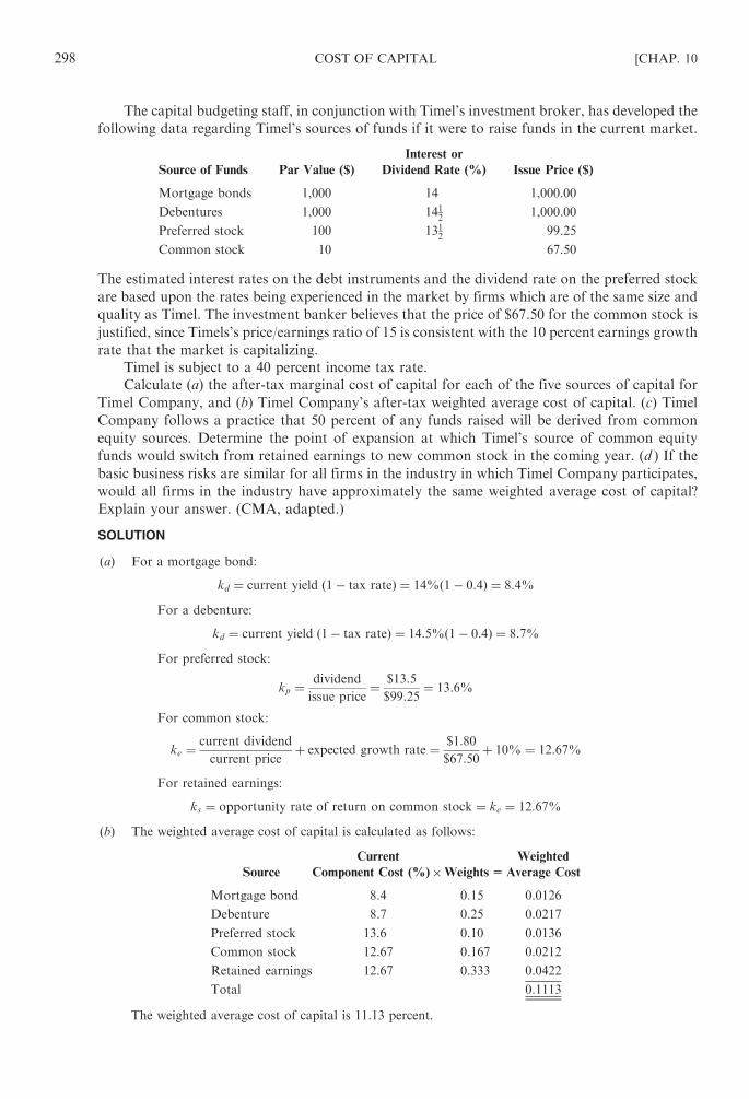
The capital budgeting staff, in conjunction with Timel’s investment broker, has developed the
following data regarding Timel’s sources of funds if it were to raise funds in the current market.
Source of Funds Par Value ($)
Interest or
Dividend Rate (%) Issue Price ($)
Mortgage bonds 1,000 14 1,000.00
Debentures 1,000 1412
1,000.00
Preferred stock 100 1312
99.25
Common stock 10 67.50
The estimated interest rates on the debt instruments and the dividend rate on the preferred stock
are based upon the rates being experienced in the market by firms which are of the same size and
quality as Timel. The investment banker believes that the price of $67.50 for the common stock is
justified, since Timels’s price/earnings ratio of 15 is consistent with the 10 percent earnings growth
rate that the market is capitalizing.
Timel is subject to a 40 percent income tax rate.
Calculate (a) the after-tax marginal cost of capital for each of the five sources of capital for
Timel Company, and (b) Timel Company’s after-tax weighted average cost of capital. (c) Timel
Company follows a practice that 50 percent of any funds raised will be derived from common
equity sources. Determine the point of expansion at which Timel’s source of common equity
funds would switch from retained earnings to new common stock in the coming year. (d ) If the
basic business risks are similar for all firms in the industry in which Timel Company participates,
would all firms in the industry have approximately the same weighted average cost of capital?
Explain your answer. (CMA, adapted.)
SOLUTION
(a) For a mortgage bond:
kd ¼ current yield 1� tax rateð Þ ¼ 14% 1� 0:4ð Þ ¼ 8:4%
For a debenture:
kd ¼ current yield 1� tax rateð Þ ¼ 14:5% 1� 0:4ð Þ ¼ 8:7%
For preferred stock:
kp ¼dividend
issue price¼ $13:5
$99:25¼ 13:6%
For common stock:
ke ¼current dividend
current priceþ expected growth rate ¼ $1:80
$67:50þ 10% ¼ 12:67%
For retained earnings:
ks ¼ opportunity rate of return on common stock ¼ ke ¼ 12:67%
(b) The weighted average cost of capital is calculated as follows:
Source
Current
Component Cost (%)�Weights=
Weighted
Average Cost
Mortgage bond 8.4 0.15 0.0126
Debenture 8.7 0.25 0.0217
Preferred stock 13.6 0.10 0.0136
Common stock 12.67 0.167 0.0212
Retained earnings 12.67 0.333 0.0422
Total 0.1113
The weighted average cost of capital is 11.13 percent.
298 COST OF CAPITAL [CHAP. 10

(c) The maximum expansion from retained earnings before a new common stock is required is calculated
as follows (in millions of dollars):
Net income ($4.50/common share
� 15 milion shares) $67.5
Less: Dividend payout ($1.80/common share
� 15 million shares) 27.0
Preferred stock dividend 6.75
Retained earnings available for expansion $33.75
If common equity is to be 50 percent of total capital, then the $33.75 million increase in retained
earnings would be matched by raising an additional $33.75 million from debt and preferred stock for a
total of $67.5 million expansion before common shares would be issued.
(d ) The weighted average cost of capital may vary among firms in the industry even if the basic business
risk is similar for all firms in the industry. This is true because each firm selects the degree of financial
leverage it desires. A firm with a high degree of financial leverage would be assigned a high-risk
premium by investors.
10.14 Cost of Capital and Weighting System. Electro Tool Co., a manufacturer of diamond drilling,
cutting, and grinding tools, has $1 million of its 8 percent debenture issue maturing on September
1, 20X1. The $1 million that has been accumulated to retire this debt is now going to be used to
acquire additional manufacturing machinery. To meet the debt and purchase of machinery, an
additional $1 million must be raised. One proposal that has been particularly appealing is the sale
and lease-back of the company’s general office building. This proposal has a lower interest cost
than the financing program proposed by the equipment vendor.
The building would be sold to FHR, Inc., for $1 million and leased back on a 25-year lease.
The lease calls for Electro Tool to pay $110,168 annually, which permits FHR, Inc., to recover its
investment and earn 10 percent on the investment. Electro Tool will pay for all maintenance costs,
property taxes, and insurance during the lease period. At the end of the 25 years Electro Tool will
reacquire the building for a very small payment. The sale and lease-back will be treated the same
for both financial reporting and income tax purposes.
The current capital structure and cost of the individual components for Electro Tool Co. are
shown below.
Capital Component
Amount per Recent
Balance Sheet
Before-Tax
Component Cost (%)
8% debentures (including
the $1,000,000 to be retired)
$ 5,000,000 8
9% preferred stock 1,000,000 9
Common stock 2,000,000 13
Retained earnings 2,000,000 12
$10,000,000
Electro Tool is subjected to a 40 percent income tax rate.
(a) Using the data provided, calculate the historical weighted average cost of capital of
Electro Tool Co. (1) before the retirement of the debentures and the sale and lease-back
action, and (2) after the retirement of the debentures and the sale and lease-back transaction.
(b) If the component costs and weightings used to calculate the weighted average cost of capital in
(a) (1) are different from those used in (a) (2), explain why. If the amounts used to calculate (a) (1)
are the same as those used in (a) (2), explain why. (c) Market values for the capital components
were not presented. What arguments are given to support the use of market values in calculating
the weighted average cost of capital? (CMA, adapted.)
CHAP. 10] COST OF CAPITAL 299
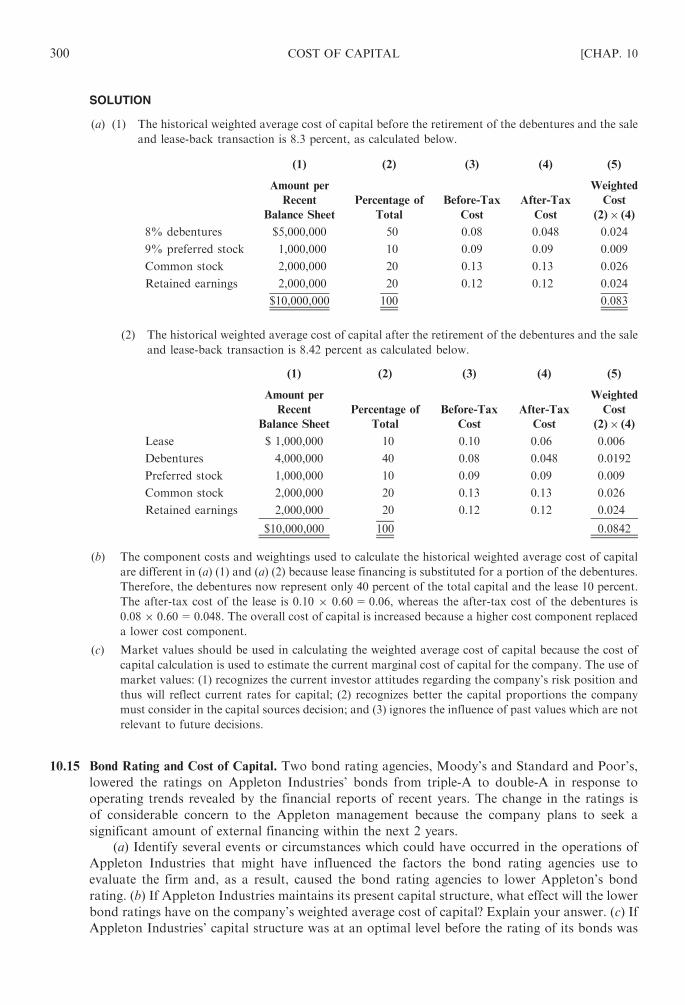
SOLUTION
(a) (1) The historical weighted average cost of capital before the retirement of the debentures and the sale
and lease-back transaction is 8.3 percent, as calculated below.
(1) (2) (3) (4) (5)
Amount per
Recent
Balance Sheet
Percentage of
Total
Before-Tax
Cost
After-Tax
Cost
Weighted
Cost
(2)� (4)
8% debentures $5,000,000 50 0.08 0.048 0.024
9% preferred stock 1,000,000 10 0.09 0.09 0.009
Common stock 2,000,000 20 0.13 0.13 0.026
Retained earnings 2,000,000 20 0.12 0.12 0.024
$10,000,000 100 0.083
(2) The historical weighted average cost of capital after the retirement of the debentures and the sale
and lease-back transaction is 8.42 percent as calculated below.
(1) (2) (3) (4) (5)
Amount per
Recent
Balance Sheet
Percentage of
Total
Before-Tax
Cost
After-Tax
Cost
Weighted
Cost
(2)� (4)
Lease $ 1,000,000 10 0.10 0.06 0.006
Debentures 4,000,000 40 0.08 0.048 0.0192
Preferred stock 1,000,000 10 0.09 0.09 0.009
Common stock 2,000,000 20 0.13 0.13 0.026
Retained earnings 2,000,000 20 0.12 0.12 0.024
$10,000,000 100 0.0842
(b) The component costs and weightings used to calculate the historical weighted average cost of capital
are different in (a) (1) and (a) (2) because lease financing is substituted for a portion of the debentures.
Therefore, the debentures now represent only 40 percent of the total capital and the lease 10 percent.
The after-tax cost of the lease is 0.10 � 0.60=0.06, whereas the after-tax cost of the debentures is
0.08 � 0.60=0.048. The overall cost of capital is increased because a higher cost component replaced
a lower cost component.
(c) Market values should be used in calculating the weighted average cost of capital because the cost of
capital calculation is used to estimate the current marginal cost of capital for the company. The use of
market values: (1) recognizes the current investor attitudes regarding the company’s risk position and
thus will reflect current rates for capital; (2) recognizes better the capital proportions the company
must consider in the capital sources decision; and (3) ignores the influence of past values which are not
relevant to future decisions.
10.15 Bond Rating and Cost of Capital. Two bond rating agencies, Moody’s and Standard and Poor’s,
lowered the ratings on Appleton Industries’ bonds from triple-A to double-A in response to
operating trends revealed by the financial reports of recent years. The change in the ratings is
of considerable concern to the Appleton management because the company plans to seek a
significant amount of external financing within the next 2 years.
(a) Identify several events or circumstances which could have occurred in the operations of
Appleton Industries that might have influenced the factors the bond rating agencies use to
evaluate the firm and, as a result, caused the bond rating agencies to lower Appleton’s bond
rating. (b) If Appleton Industries maintains its present capital structure, what effect will the lower
bond ratings have on the company’s weighted average cost of capital? Explain your answer. (c) If
Appleton Industries’ capital structure was at an optimal level before the rating of its bonds was
300 COST OF CAPITAL [CHAP. 10

changed, explain what effect the lower bond ratings will have on the company’s optimal capital
structure. (CMA, adapted.)
SOLUTION
(a) Factors or circumstances which may have caused the rating agencies to lower the bond rating of
Appleton Industries include:
1. Lowered long-term solvency reflected by a reduction in the times-interest-earned ratio or a reduc-
tion in the fixed-charge-coverage ratio
2. Lowered shot-term liquidity reflected by a decrease in the current ratio or quick ratio
3. Lowered profitability reflected by a reduced market share, lower return on sales, or decreased
profits
4. An increased risk of financial stability due to major pending litigation which would be damaging
to the firm or a large increase in earnings variability
5. A major change in management which is perceived negatively by the financial community
(b) The weighted average cost of capital can be expected to rise. The lower bond rating is usually relied
upon as an indication of greater risk being assumed by the bond investors. This change will be noted
by the investors of other Appleton securities. Thus the investors in each capital component of
Appleton Industries can be expected to require a higher return.
(c) Appleton Industries capital structure will shift toward greater equity with less debt. The fact that the
bond rating was lowered would indicate to investors that the risk has increased. To reduce the risk and
minimize the increase in the cost of capital, the optimal capital structure will have to shift toward one
with an increased percentage of equity.
10.16 Earnings Multiple and Cost of Capital. The Jefferson Corporation is contemplating a $50 million
expansion project. Over the years, the firm’s board of directors has adhered to a policy of
rejecting any investment proposal that would jeopardize the market value of the firm’s
common stock.
A preliminary analysis projected a rate of return on the new project of around 14
percent before taxes. Jefferson has reached tentative agreement with an insurance company
to finance the project through a private placement of the $50 million in the form of 10
percent notes.
The firm’s common stock has been historically selling at 10 times after-tax earnings. Current
earnings per share are $2.70 and the firm faces a 50 percent corporate income tax rate.
Long-term debt (8%) $10,000,000
Common stock ($2 par, 10,000,000
shares outstanding) 20,000,000
Paid-in capital, in excess of par 70,000,000
Retained earnings 100,000,000
Total capitalization $200,000,000
(a) One of the members of Jefferson Corporation’s board of directors argued that the firm
should immediately place the notes, since the before-tax marginal cost of capital for the
project is only 10 percent (the interest on the notes), and indications are that the project’s
before-tax rate of return would be greater than 10 percent. Discuss.
(b) Assuming Jefferson’s earnings multiple declines to 9, what level of annual earnings must the
new project generate in order to meet the director’s objective? (CMA, adapted).
SOLUTION
(a) The board members’ conclusion is not valid because the facts seem to indicate the Jefferson
Corporation’s capitalization is not in equilibrium. The issuance of the notes will move debt from
CHAP. 10] COST OF CAPITAL 301

5 percent of total capitalization (10/200) to 24 percent (60/250). This increases the financial risk that
common equity must bear through increased fixed interest payments, and the increased risk can be
expected to be manifested by a decline in the earnings multiple. While the marginal cost of capital
appears to be 10 percent (the cost of the private placement), the marginal cost of capital is a combina-
tion of explicit interest cost on the notes and the additional costs of earnings that must occur to
compensate the common stockholders for the decline in the earnings multiple.
Jefferson Corporation should have calculated the weighted average cost of capital according to
the following formula:
Percent of new funds
raised from debt
� �
� cost of debtð Þ þ percent of funds
raised from equity
� �
� additional cost of equityð Þ
The 14 percent rate of return on this project should be compared to the firm’s average cost of capital.
If the project’s return is at least as great as the weighted average cost of capital, then the value of the
firm’s stock will not decrease.
(b) The stock is now selling at 10 times earnings:
P0 ¼ 10ð$2:70Þ ¼ $27:00
This is the price that must be maintained upon taking on the new project. If the new project causes the
P/E ratio to fall to 9 and offers no additional earnings, the price of stock would fall by $2.70 to $24.30.
In order to get the price of stock back up to $27, the earnings provided by the new asset must
equal X:
ðNew P=EÞðnew EPSÞ ¼ $27
9ð$2:70þ XÞ ¼ $27
$2:70þ X ¼ $3
X ¼ $0:30
This assumes that currently held assets are capable of continuing to provide $2.70 in earnings per
share.
The annual earnings the new project must generate to meet Jefferson Corporation’s objective are
determined as follows:
(1) Required EPS to maintain $27 price with a multiple of 9:
$27:00
9¼ $3:00
(2) Required earnings after taxes:
$3:00� 10,000,000 shares ¼ $30,000,000
(3) Required earnings before taxes:
$30,000,000
0:5¼ $60,000,000
(4) Interest expense:
ð$10,000,000Þð0:08Þ þ ð$50,000,000Þð0:10Þ ¼ $800,000þ $5,000,000 ¼ $5,800,000
(5) Required earnings before interest and taxes:
$60,000,000þ $5,800,000 ¼ $65,800,000
(6) Old earnings before interest and taxes:
ð$2:70� 10,000,000 sharesÞ0:5
þ $800,000 ¼ $54,800,000
(7) Additional before interest and taxes earnings required:
Projected earnings $65,800,000
Old earnings 54,800,000
$11,000,000
302 COST OF CAPITAL [CHAP. 10

10.17 The MCC and IOS Schedules. Rhonda Pollak Company is considering three investments whose
initial costs and internal rates of return are given below:
Project Initial Cost ($) Internal Rate of Return (%)
A 100,000 19
B 125,000 15
C 225,000 12
The company finances all expansion with 40 percent debt and 60 percent equity capital. The
after-tax cost is 8 percent for the first $100,000, after which the cost will be 10 percent. Retained
earnings in the amount of $150,000 is available, and the common stockholders’ required rate of
return is 18 percent. If the new stock is issued, the cost will be 22 percent.
Calculate (a) the dollar amounts at which breaks occur, and (b) calculate the weighted cost of
capital in each of the intervals between the breaks. (c) Graph the firm’s weighted marginal cost of
capital (MCC) schedule and investment opportunities schedule (IOS). (d ) Decide which projects
should be selected and calculate the total amount of the optimal capital budget.
SOLUTION
(a) Breaks (increases) in the weighted marginal cost of capital will occur as follows:
For debt:
Debt
Debt=assets¼ $100,000
0:4¼ $250,000
For common stock:
Retained earnings
Equity=assets¼ $150,000
0:6¼ $250,000
The debt break is caused by exhausting the lower cost of debt, while the common stock break is caused
by using up retained earnings.
(b) The weighted cost of capital in each of the intervals between the breaks is computed as follows:
With $0–$250,000 total financing:
Source of Capital Weight Cost Weighted Cost
Debt 0.4 8% 3.2%
Common stock 0.6 18% 10.8
ko=14.0%
With over $250,000 total financing:
Source of Capital Weight Cost Weighted Cost
Debt 0.4 10% 4.0%
Common stock 0.6 22% 13.2
k=17.2%
(c) See Fig. 10-2.
(d ) Accept projects A and B for a total of $225,000, which is the optimal budget.
10.18 The MCC and IOS Schedules. John Constas & Company has to decide which of the following
four projects should be selected:
Project Initial Investment ($) Internal Rate of Return (%)
A 250,000 16
B 300,000 10
C 100,000 12
D 150,000 13
CHAP. 10] COST OF CAPITAL 303

The company has the following capital structure:
Debt (long-term only) 30%
Equity 70%
The company’s last earnings per share was $400.
It pays out 50 percent of its earnings as dividends. The company has $210,000 of retained
earnings available for investment purposes. The cost of debt (before taxes) is 10 percent for the
first $180,000. The cost of any additional debt (before taxes) is 14 percent. The company’s tax rate
is 40 percent; the current market price of its stock is $43; the flotation cost is 15 percent of the
selling price; the expected growth rate in earnings and dividends is 8 percent.
(a) How many breaks are there in the MCC schedule, and at what dollar amounts do the
breaks occur? (b) What is the weighted cost of capital in each of the intervals between the breaks?
(c) Graph the MCC and IOS schedules. (d ) Which projects should the company accept and what
is the total amount of the optimal capital budget?
SOLUTION
(a) There are two breaks in the MCC schedule:
For common stock:Retained earnings
Equity=assets¼ $210,000
0:7¼ $300,000
For debt:Debt
Debt=assets¼ $180,000
0:3¼ $600,000
(b) The weighted cost of capital in each of the intervals between the breaks is calculated as follows:
With 0$–$300,000:
Source of Capital Weight After-Tax Cost Weighted Cost
Debt 0.3 6%a 1.8%
Retained earnings 0.7 13%b 9.1
ko=10.9%
akd ¼ kt 1� tð Þ ¼ 10% 1� 0:4ð Þ ¼ 6%
b ks ¼D1
P0
þ g ¼ $2:00ð Þ 1þ 0:08ð Þ$43
þ 8% ¼ $2:16
$43þ 8% ¼ 13:0%
Fig. 10-2
304 COST OF CAPITAL [CHAP. 10

With $300,000–$600,000:
Source of Capital Weight After-Tax Cost Weighted Cost
Debt 0.3 6% 1.80%
External equity 0.7 13.9%a 9.73
ko=11.53%
a ke ¼D1
P0 1� fð Þ þ g ¼ ð$2:00Þð1þ 0:08Þ$43ð1� 0:15Þ þ 8% ¼ $2:16
$36:55þ 8% ¼ 13:9%
Above $600,000:
Source of Capital Weight After-Tax Cost Weighted Cost
Debt 0.3 8.4%a 2.52%
External equity 0.7 13.9%a 9.73
ko=12.25%
a kd ¼ kt 1� tð Þ ¼ 14% 1� 0:4ð Þ ¼ 8:4%
(c) The MCC and IOS schedules are shown in Fig. 10-3.
(d ) The company should select projects A, D, and C for a total optimal capital budget of $500,000.
Fig. 10-3
CHAP. 10] COST OF CAPITAL 305

Chapter 11
Leverage and Capital Structure
11.1 LEVERAGE DEFINED
Leverage is that portion of the fixed costs which represents a risk to the firm. Operating leverage,
a measure of operating risk, refers to the fixed operating costs found in the firm’s income statement.
Financial leverage, a measure of financial risk, refers to financing a portion of the firm’s assets, bearing
fixed financing charges in hopes of increasing the return to the common stockholders. The higher the
financial leverage, the higher the financial risk, and the higher the cost of capital. Cost of capital rises
because it costs more to raise funds for a risky business.
11.2 BREAK-EVEN POINT, OPERATING LEVERAGE, AND FINANCIAL LEVERAGE
A discussion of break-even analysis, broadly known as cost/volume/profit analysis, is necessary for
understanding the nature and importance of operating leverage.
Break-Even Analysis
The break-even point is the level of sales at which no profit or loss results. To determine the break-
even point, the costs must be divided into (1) variable costs, which are costs that vary in direct proportion
to a change in volume, and (2) fixed costs, which are costs that are constant regardless of volume.
The break-even point can be found easily by setting sales just equal to the total of the variable costs
plus the fixed costs:
Let S=Sales ($)
X=Sales volume in units
P=Selling price per unit
V=Unit variable cost
VC=Variable operating costs
FC=Fixed operating costs
Then
S ¼ VCþ FC
PX ¼ VXþ FC
ðP� VÞX ¼ FC
X ¼ FC
P� V
or
Break-even sales in units ¼ fixed operating costs
unit selling price� unit variable cost
EXAMPLE 11.1 The Wayne Company manufactures and sells doors to home builders. The doors are sold for $25
each. Variable costs are $15 per door, and fixed operating costs total $50,000. The company’s break-even point is:
X ¼ FC
P� V¼ $50,000
$25� $15¼ 5,000 doors
Therefore, the company must sell 5,000 doors to break even.
306
Copyright © 2007, 1998, 1986 by The McGraw-Hill Companies, Inc. Click here for terms of use.

Cash Break-Even Point
If a firm has a minimum of available cash or the opportunity cost of holding excess cash is high,
management may want to know the volume of sales that will cover all cash expenses during a period.
This is known as the cash break-even point.
Not all fixed operating costs involve cash payments. For example, depreciation expenses are noncash
charges. To find the cash break-even point, the noncash charges must be subtracted from total fixed
operating costs. Therefore, the cash break-even point is lower than the usual break-even point. The
formula is:
X ¼ FC� d
P� V
where d is depreciation expenses.
EXAMPLE 11.2 Assume from Example 11.1 that the total fixed operating costs of $50,000 include depreciation
in the amount of $2,000. Then the Wayne Company cash break-even point is:
X ¼ FC� d
P� V¼ $50,000� $2,000
$25� $15¼ $48,000
$10¼ 4,800 doors
The company has to sell 4,800 doors to cover only the fixed costs involving cash payments of $48,000 and to
break even.
Operating Leverage
Operating leverage is a measure of operating risk and arises from fixed operating costs. A simple
indication of operating leverage is the effect that a change in sales has on earnings. The formula is:
Operating leverage at a given level of sales ðX Þ ¼ percentage change in EBIT
percentage change in sales¼ ðP� VÞXðP� VÞX� FC
where
EBIT ¼ earnings before interest and taxes
¼ ðP� VÞX� FC
EXAMPLE 11.3 From Example 11.1, assume that the Wayne Company is currently selling 6,000 doors per year.
Its operating leverage is:
ðP� VÞXðP� VÞX� FC
¼ ð$25� $15Þð6,000Þð$25� $15Þð6,000Þ � $50,000
¼ $60,000
10,000¼ 6
which means if sales increase by 10 percent, the company can expect its net income to increase by six times that
amount, or 60 percent.
Financial Leverage
Financial leverage is a measure of financial risk and arises from fixed financial costs. One way
to measure financial leverage is to determine how earnings per share are affected by a change in
EBIT (or operating income).
Financial leverage at a given level of sales ðXÞ ¼ percentage change in EPS
percentage change in EBIT¼ ðP� VÞX� FC
ðP� VÞX� FC� IC
where EPS is earnings per share, and IC is fixed finance charges, i.e., interest expense or preferred
stock dividends. [Preferred stock dividend must be adjusted for taxes i.e., preferred stock dividend/
(1� t).]
CHAP. 11] LEVERAGE AND CAPITAL STRUCTURE 307

EXAMPLE 11.4 Using the data in Example 11.3, the Wayne Company has total financial charges of $2,000, half in
interest expense and half in preferred stock dividend. The corporate tax rate is 40 percent. What is their financial
leverage? First,
IC ¼ $1,000þ $1,000
ð1� 0:4Þ ¼ $1,000þ $1,667 ¼ $2,667
Therefore, Wayne’s financial leverage is computed as follows:
ðP� VÞX� FC
ðP� VÞX� FC� IC¼ ð$25� $15Þð6,000Þ � $50,000
ð$25� $15Þð6,000Þ � $50,000� $2,667¼ $10,000
$7,333¼ 1:36
which means that if EBIT increases by 10 percent, Wayne can expect its EPS to increase by 1.36 times, or by
13.6 percent.
Total Leverage
Total leverage is a measure of total risk. The way to measure total leverage is to determine how EPS
is affected by a change in sales.
Total leverage at a given level of sales ðX Þ ¼ percentage change in EPS
percentage change in sales
¼ operating leverage� financial leverage
¼ ðP� VÞXðP� VÞX� FC
� ðP� VÞX� FC
ðP� VÞX� FC� IC
¼ ðP� VÞXðP� VÞX� FC� IC
EXAMPLE 11.5 From Examples 11.3 and 11.4, the total leverage for Wayne Company is:
Operating leverage� financial leverage ¼ 6� 1:36 ¼ 8:16
or
ðP� VÞXðP� VÞX� FC� IC
¼ ð$25� $15Þð6,000Þð$25� $15Þð6,000Þ � $50,000� $2,667
¼ $60,000
$7,333¼ 8:18 ðdue to rounding errorÞ
11.3 THE THEORY OF CAPITAL STRUCTURE
The theory of capital structure is closely related to the firm’s cost of capital. Capital structure is
the mix of the long-term sources of funds used by the firm. The primary objective of capital
structure decisions is to maximize the market value of the firm through an appropriate mix of long-
term sources of funds. This mix, called the optimal capital structure, will minimize the firm’s overall
cost of capital. However, there are arguments about whether an optimal capital structure actually exists.
The arguments center on whether a firm can, in reality, affect its valuation and its cost of capital
by varying the mixture of the funds used. There are four different approaches to the theory of capital
structure:
1. Net operating income (NOI) approach
2. Net income (NI) approach
3. Traditional approach
4. Modigliani–Miller (MM) approach
308 LEVERAGE AND CAPITAL STRUCTURE [CHAP. 11

All four use the following simplifying assumptions:
1. No income taxes are included; they will be removed later.
2. The company makes a 100 percent dividend payout.
3. No transaction costs are incurred.
4. The company has constant earnings before interest and taxes (EBIT).
5. The company has a constant operating risk.
Given these assumptions, the company is concerned with the following three rates:
1. ki ¼I
B
where ki=yield on the firm’s debt (assuming a perpetuity)
I=annual interest charges
B=market value of debt outstanding
2. ke ¼EAC
S
where ke=the firm’s required rate of return on equity or cost of common equity (assuming
no earnings growth and a 100 percent dividend payout ratio)
EAC=earnings available to common stockholders
S=market value of stock outstanding
3. ko ¼EBIT
V
where ko=the firm’s overall cost of capital (or capitalization rate)
EBIT=earnings before interest and taxes (or operating earnings)
V=B+S and is the market value of the firm
In each of the four approaches to determining capital structure, the concern is with what happens to
ki, ke, and ko when the degree of leverage, as denoted by the debt/equity (B/S) ratio, increases.
The Net Operating Income (NOI) Approach
The net operating income approach suggests that the firm’s overall cost of capital, ko, and the value
of the firm’s market value of debt and stock outstanding, V, are both independent of the degree to which
the company uses leverage. The key assumption with this approach is that ko is constant regardless of the
degree of leverage.
EXAMPLE 11.6 Assume that a firm has $6,000 in debt at 5 percent interest, that the expected level of EBIT is
$2,000, and that the firm’s cost of capital, ko, is constant at 10 percent. The market value (V) of the firm is computed
as follows:
V ¼ EBIT
ko¼ $2,000
0:10¼ $20,000
The cost of external equity (ke) is computed as follows:
EAC ¼ EBIT� I ¼ $2,000� ð$6,000� 5%Þ
¼ $2,000� $300 ¼ $1,700
S ¼ V� B ¼ $20,000� $6,000 ¼ $14,000
ke ¼EAC
S¼ $1,700
$14,000¼ 12:14%
CHAP. 11] LEVERAGE AND CAPITAL STRUCTURE 309

The debt/equity ratio is
B
S¼ $6,000
$14,000¼ 42:86%
Assume now that the firm increases its debt from $6,000 to $10,000 and uses the proceeds to retire $10,000
worth of stock and also that the interest rate on debt remains 5 percent.
The value of the firm now is:
V ¼ EBIT
ko¼ $2,000
0:10¼ $20,000
The cost of external equity is
EAC ¼ EBIT� I ¼ $2,000� ð$10,000� 5%Þ¼ $2,000� $500 ¼ $1,500
S ¼ V� B ¼ $20,000� $10,000 ¼ $10,000
ke ¼EAC
S¼ $1,500
$10,000¼ 15%
The debt/equity ratio is now:
B
S¼ $10,000
$10,000¼ 100%
Since the NOI approach assumes that ko remains constant regardless of changes in leverage, the cost of capital
cannot be altered through leverage. Hence this approach suggests that there is no one optimal capital structure, as
evidenced in Fig. 11-1.
The Net Income (NI) Approach
Unlike the net operating income approach, the net income approach suggests that both the overall
cost of capital, ko and the market value of the firm, V, are affected by the firm’s use of leverage. The
critical assumption with this approach is that ki and ke remain unchanged as the debt/equity ratio
increases.
EXAMPLE 11.7 Assume the same data given in Example 11.6 except that ke equals 10 percent. The value of
the firm, V, is computed as follows:
EAC ¼ EBIT� I ¼ $2,000� ð$6,000� 5%Þ ¼ $1,700
V ¼ Sþ B ¼ EAC
keþ B
¼ $1,700
0:10þ $6,000 ¼ $17,000þ $6,000 ¼ $23,000
Fig. 11-1 Costs of capital: Net operating income approach
310 LEVERAGE AND CAPITAL STRUCTURE [CHAP. 11

The firm’s overall cost of capital is:
ko ¼EBIT
V¼ $2,000
$23,000¼ 8:7%
The debt/equity ratio in this case is:
B
S¼ $6,000
$17,000¼ 35:29%
Now assume, as before, that the firm increases its debt from $6,000 to $10,000, uses the proceeds to retire that
amount of stock, and that the interest rate on debt remains at 5 percent. Then the value of the firm is:
EAC ¼ EBIT� I ¼ $2,000� ð$10,000� 5%Þ ¼ $1,500
V ¼ Sþ B ¼ EAC
keþ B
¼ $1,500
0:10þ $10,000 ¼ $15,000þ $10,000 ¼ $25,000
The overall cost of capital is
ko ¼EBIT
V¼ $2,000
$25,000¼ 8%
The debt/equity ratio is now
B
S¼ $10,000
$15,000¼ 66:67%
The NI approach shows that the firm is able to increase its value, V, and lower its cost of capital, ko, as it
increases the degree of leverage. Under this approach, the optimal capital structure is found farthest to the right in
Fig. 11-2.
Traditional Approach
The traditional approach to valuation and leverage assumes that there is an optimal capital structure
and that the firm can increase its value through leverage. This is a moderate view of the relationship
between leverage and valuation that encompasses all the ground between the NOI approach and the NI
approach.
EXAMPLE 11.8 Assume the same data given in Example 11.6. Assume, however, that ke is 12 percent, rather than
the 12.14 percent or 10 percent with the NOI or NI approaches illustrated previously. The value of the firm is:
EAC ¼ EBIT� I ¼ $2,000� ð$6,000� 5%Þ ¼ $1,700
V ¼ Sþ B ¼ EAC
keþ B
¼ $1,700
0:12þ $6,000 ¼ $14,167þ $6,000 ¼ $20,167
Fig. 11-2 Cost of capital: Net income approach
CHAP. 11] LEVERAGE AND CAPITAL STRUCTURE 311

The overall cost of capital is:
ko ¼EBIT
V¼ $2,000
$20,167¼ 9:9%
The debt/equity ratio is:
B
S¼ $6,000
$14,167¼ 42:35%
Assume, as before, that the firm increases its debt from $6,000 to $10,000. Assume further that ki rises to 6
percent and ke at that degree of leverage is 14 percent. The value of the firm, then, is:
EAC ¼ EBIT� I
¼ $2,000� ð$10,000� 6%Þ ¼ $2,000� $600 ¼ $1,400
V ¼ Sþ B ¼ EAC
keþ B
¼ $1,400
0:14þ $10,000 ¼ $10,000þ $10,000 ¼ $20,000
The overall cost of capital is:
ko ¼EBIT
V¼ $2,000
$20,000¼ 10:0%
The debt/equity ratio is:
B
S¼ $10,000
$10,000¼ 100%
Thus the value of the firm is lower and its cost of capital slightly higher than when the debt is $6,000. This result
is due to the increase in ke and, to a lesser extent, the increase in ki. These two observations indicate that the optimal
capital structure occurs before the debt/equity ratio equals 100 percent as shown in Fig. 11-3.
Miller–Modigliani (MM) Position
Miller–Modigliani (MM) advocates that the relationship between leverage and valuation is
explained by the NOI approach. More specifically, MM’s propositions are summarized below.
1. The market value of the firm and its cost of capital are independent of its capital structure.
2. ke increases so as to exactly offset the use of cheaper debt money.
3. The cutoff rate for capital budgeting decisions is completely independent of the way in which an
investment is financed.
Fig. 11-3
312 LEVERAGE AND CAPITAL STRUCTURE [CHAP. 11

Factors Affecting Capital Structure
Many financial managers believe, in practice, that the following factors influence financial structure:
1. Growth rate of future sales
2. Stability of future sales
3. Competitive structures in the industry
4. Asset makeup of the individual firm
5. Attitude of owners and management toward risk
6. Control position of owners and management
7. Lenders’ attitude toward the industry and a particular firm
11.4 EBIT–EPS ANALYSIS
The use of financial leverage has two effects on the earnings that go to the firm’s common
stockholders: (1) an increased risk in earnings per share (EPS) due to the use of fixed financial
obligations, and (2) a change in the level of EPS at a given EBIT associated with a specific capital
structure.
The first effect is measured by the degree of financial leverage previously discussed. The second effect
is analyzed by means of EBIT–EPS analysis. This analysis is a practical tool that enables the financial
manager to evaluate alternative financing plans by investigating their effect on EPS over a range of
EBIT levels. Its primary objective is to determine the EBIT break-even, or indifference, points among
the various alternative financing plans. The indifference points between any two methods of financing
can be determined by solving for EBIT in the following equality:
ðEBIT� IÞð1� tÞ � PD
S1¼ ðEBIT� IÞð1� tÞ � PD
S2
where t=tax rate
PD=preferred stock dividends
S1 and S2=number of shares of common stock outstanding after financing for plan 1 and plan 2,
respectively.
EXAMPLE 11.9 Assume that ADI Company, with long-term capitalization consisting entirely of $5 million in
stock, wants to raise $2 million for the acquisition of special equipment by: (1) selling 40,000 shares of common stock
at $50 each; (2) selling bonds, at 10 percent interest; or (3) issuing preferred stock with an 8 percent dividend. The
percent EBIT is $8 million, the income tax rate is 50 percent, and 100,000 shares of common stock are now
outstanding. In order to compute the indifference points, we begin by calculating EPS at a projected level of $1
million.
All Common All Debt All Preferred
EBIT $1,000,000 $1,000,000 $1,000,000
Interest 200,000
Earnings before taxes (EBT) $1,000,000 $ 800,000 $1,000,000
Taxes 500,000 400,000 500,000
Earnings after taxes (EAT) $ 500,000 $ 400,000 $ 500,000
Preferred stock dividend 160,000
EAC $ 500,000 $ 400,000 $ 340,000
Number of shares 140,000 100,000 100,000
EPS $3.57 $4.00 $3.40
CHAP. 11] LEVERAGE AND CAPITAL STRUCTURE 313

Now connect the EPSs at the level of EBIT of $1 million with the EBITs for each financing alternative on the
horizontal axis to obtain the EPS–EBIT graphs. We plot the EBIT necessary to cover all fixed financial costs for
each financing alternative on the horizontal axis. For the common stock plan, there are no fixed costs, so the
intercept on the horizontal axis is zero. For the debt plan, there must be an EBIT of $200,000 to cover interest
charges. For the preferred stock plan, there must be an EBIT of $320,000 [$160,000/(1� 0.5)] to cover $160,000
in preferred stock dividends at a 50 percent income tax rate; so $320,000 becomes the horizontal axis intercept.
See Fig. 11-4.
In this example, the indifference point between all common and all debt is:
ðEBIT� IÞð1� tÞ � PD
S1¼ ðEBIT� IÞð1� tÞ � PD
S2ðEBIT� 0Þð1� 0:5Þ � 0
140,000¼ ðEBIT� 200,000Þð1� 0:5Þ � 0
100,000
Rearranging yields:
0:5ðEBITÞð100,000Þ ¼ 0:5ðEBITÞð140,000Þ � 0:5ð200,000Þð140,000Þ20,000 EBIT ¼ 14,000,000,000
EBIT ¼ $700,000
Similarly, the indifference point between all common and all preferred would be:
ðEBIT� IÞð1� tÞ � PD
S1¼ ðEBIT� IÞð1� tÞ � PD
S2ðEBIT� 0Þð1� 0:5Þ � 0
140,000¼ ðEBIT� 0Þð1� 0:5Þ � 160,000
100,000
Rearranging yields:
0:5ðEBITÞð100,000Þ ¼ 0:5ðEBITÞð140,000Þ � 160,000ð140,000Þ20,000 EBIT ¼ 22,400,000,000
EBIT ¼ $1,120,000
Based on the above computations, we can draw the following conclusions:
1. At any level of EBIT, debt is better than preferred stock.
2. At a level of EBIT above $700,000, debt is better than common stock. If EBIT is below $700,000, the
reverse is true.
Fig. 11-4
314 LEVERAGE AND CAPITAL STRUCTURE [CHAP. 11

3. At a level of EBIT above $1,120,000, preferred stock is better than common. At or below that point, the
reverse is true.
Review Questions
1. refers to the incurrence of fixed operating costs in the firm’s income state-
ment. It is a measure of .
2. The higher the , the higher the financial risk, and the higher
the .
3. The is the level of at which no profit or loss results.
4. To find the , noncash charges such as must be subtracted
from total fixed operating costs.
5. A simple indication of is to look at how earnings are affected by a change in
sales.
6. Total leverage is a measure of . It measures how is affected
by a change in sales.
7. Total leverage is the of and .
8. There are four positions regarding the relationship between valuation and leverage. They are
the , the , the , and the .
9. Under the , there is no such thing as optimal capital structure.
10. The key assumption underlying the net income approach is that the cost of
and the cost of remain unchanged as the increases.
11. The to valuation and leverage assumes that there is a(n)
capital structure and that the firm can increase through .
12. The primary objective of the is to determine the break-even,
or , points between the various alternative financing plans.
13. refers to the mix of long-term financing sources used.
14. Debt has a(n) advantage over preferred stock in that is a
tax-deductible expense while are not.
15. The theory of capital structure assumes no and no .
Answers: (1) Operating leverage, operating risk; (2) financial leverage, cost of capital; (3) break-even point,
sales; (4) cash break-even point, depreciation; (5) operating leverage; (6) total risk, EPS; (7) product, operating
leverage, financial leverage; (8) net income (NI) approach, net operating income (NOI) approach, traditional
approach, Miller–Modigliani (MM) approach; (9) net operating income (NOI) approach; (10) common equity,
debt, debt/equity ratio; (11) traditional approach, optimal, its value, leverage; (12) EBIT-EPS analysis, EBIT,
CHAP. 11] LEVERAGE AND CAPITAL STRUCTURE 315

indifference; (13) Capital structure; (14) tax, interest, preferred stock dividends; (15) income taxes, transaction
costs.
Solved Problems
11.1 Break-Even and Cash Break-Even Points. The following price and cost data are given for firms A,
B, and C:
A B C
Selling price per unit $25 $12 $15
Variable cost per unit $10 $6 $5
Fixed operating costs $30,000 $24,000 $100,000
Calculate (a) the break-even point for each firm, and (b) the cash break-even point for each
firm, assuming $5,000 of each firm’s fixed costs are depreciation. (c) Rank these firms in terms of
their risk.
SOLUTION
(a) X ¼ FC
P� V
Firm A:$30,000
$15¼ 2,000 units
Firm B:$24,000
$6¼ 4,000 units
Firm C:$100,000
$10¼ 10,000 units
(b) X ¼ FC� d
P� V
Firm A:$30,000� $5,000
$15¼ 1,667 units
Firm B:$24,000� $5,000
$6¼ 3,167 units
Firm C:$100,000� $5,000
$10¼ 9,500 units
(c) Firm A seems least risky, followed by B and then C, based on increasing break-even points. It is
important to recognize, however, that operating leverage is only one measure of risk.
11.2 Operating and Financial Leverages. John Tripper Soft Drinks, Inc., sells 500,000 bottles of soft
drinks a year. Each bottle produced has a variable cost of $0.25 and sells for $0.45. Fixed
operating costs are $50,000. The company has current interest charges of $6,000 and preferred
dividends of $2,400. The corporate tax rate is 40 percent.
(a) Calculate the degree of operating leverage, the degree of financial leverage, and the degree
of total leverage. (b) Do part (a) at the 750,000 bottle sales level. (c) What generalizations can you
make comparing (a) to (b) after first finding the break-even point?
SOLUTION
(a) Operating leverage ¼ ðP� VÞXðP� VÞX� FC
¼ ð$0:45� $0:25Þð500,000Þð$0:45� $0:25Þð500,000Þ � $50,000
¼ $100,000
$50,000¼ 2
316 LEVERAGE AND CAPITAL STRUCTURE [CHAP. 11
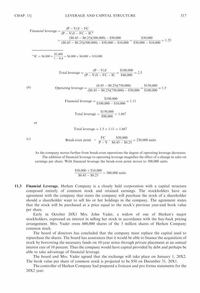
Financial leverage ¼ ðP� VÞX� FC
ðP� VÞX� FC� ICa
¼ ð$0:45� $0:25Þð500,000Þ � $50,000
ð$0:45� $0:25Þð500,000Þ � $50,000� $10,000¼ $50,000
$50,000� $10,000¼ 1:25
a IC ¼ $6,000þ $2,400
1� 0:4¼ $6,000þ $4,000 ¼ $10,000
Total leverage ¼ ðP� VÞXðP� VÞX� FC� IC
¼ $100,000
$40,000¼ 2:5
(b) Operating leverage ¼ ð0:45� $0:25Þð750,000Þð$0:45� $0:25Þð750,000Þ � $50,000
¼ $150,000
$100,000¼ 1:5
Financial leverage ¼ $100,000
$100,000� $10,000¼ 1:11
Total leverage ¼ $150,000
$90,000¼ 1:667
or
Total leverage ¼ 1:5� 1:11 ¼ 1:667
(c) Break-even point =FC
P� V� $50,000
$0:45� $0:25¼ 250,000 units
As the company moves further from break-even operations the degree of operating leverage decreases.
The addition of financial leverage to operating leverage magnifies the effect of a change in sales on
earnings per share. With financial leverage the break-even point moves to 300,000 units.
$50,000þ $10,000
$0:45� $0:25¼ 300,000 units
11.3 Financial Leverage. Herken Company is a closely held corporation with a capital structure
composed entirely of common stock and retained earnings. The stockholders have an
agreement with the company that states the company will purchase the stock of a shareholder
should a shareholder want to sell his or her holdings in the company. The agreement states
that the stock will be purchased at a price equal to the stock’s previous year-end book value
per share.
Early in October 20X1 Mrs. John Vader, a widow of one of Herken’s major
stockholders, expressed an interest in selling her stock in accordance with the buy-back pricing
arrangement. Mrs. Vader owns 600,000 shares of the 3 million shares of Herken Company
common stock.
The board of directors has concluded that the company must replace the capital used to
repurchase the shares. The board has assurances that it would be able to finance the acquisition of
stock by borrowing the necessary funds on 10-year notes through private placement at an annual
interest rate of 10 percent. Thus the company would have capital provided by debt and perhaps be
able to take advantage of financial leverage.
The board and Mrs. Vader agreed that the exchange will take place on January 1, 20X2.
The book value per share of common stock is projected to be $50 on December 31, 20X1.
The controller of Herken Company had prepared a forecast and pro forma statements for the
20X2 year.
CHAP. 11] LEVERAGE AND CAPITAL STRUCTURE 317
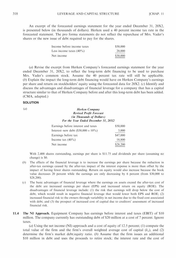
An excerpt of the forecasted earnings statement for the year ended December 31, 20X2,
is presented below (in thousands of dollars). Herken used a 40 percent income tax rate in the
forecasted statement. The pro forma statements do not reflect the repurchase of Mrs. Vader’s
shares or the new issue of debt required to pay for the shares.
Income before income taxes $50,000
Less income taxes (40%) 20,000
Net income $30,000
(a) Revise the excerpt from Herken Company’s forecasted earnings statement for the year
ended December 31, 20X2, to reflect the long-term debt financing to be used to purchase
Mrs. Vader’s common stock. Assume the 40 percent tax rate will still be applicable.
(b) Explain the impact the long-term debt financing would have on Herken Company’s earnings
per share and return on stockholders’ equity using the forecasted data for 20X2. (c) Identify and
discuss the advantages and disadvantages of financial leverage for a company that has a capital
structure similar to that of Herken Company before and after this long-term debt has been added.
(CMA, adapted.)
SOLUTION
(a) Herken Company
Revised Profit Forecast
(in Thousands of Dollars)
For the Year Ended December 31, 20X2
Earnings before interest and taxes $50,000
Interest–new debt ($30,000� 10%) 3,000
Earnings before tax $47,000
Income tax (40%) 18,800
Net income $28,200
With 2,400 shares outstanding, earnings per share is $11.75 and dividends per share (assuming no
change) is $0.
(b) The effects of the financial leverage is to increase the earnings per share because the reduction in
after-tax earnings caused by the after-tax impact of the interest expense is more than offset by the
impact of having fewer shares outstanding. Return on equity would also increase because the book
value decreases 20 percent while the earnings are only decreasing by 6 percent (from $30,000 to
$28,200).
(c) The basic advantages of financial leverage where the earnings on assets exceed the after-tax cost of
the debt are increased earnings per share (EPS) and increased return on equity (ROE). The
disadvantages of financial leverage include: (1) the risk that earnings will drop below the cost of
debt, which would result in negative financial leverage that would lower both EPS and ROE; (2)
increased financial risk to the owners through variability in net income due to the fixed cost associated
with debt; and (3) the prospect of increased cost of capital due to creditors’ assessment of increased
financial risk.
11.4 The NI Approach. Equipment Company has earnings before interest and taxes (EBIT) of $10
million. The company currently has outstanding debt of $20 million at a cost of 7 percent. Ignore
taxes.
(a) Using the net income (NI) approach and a cost of equity of 12.5 percent; (1) compute the
total value of the firm and the firm’s overall weighted average cost of capital (ko), and (2)
determine the firm’s market debt/equity ratio. (b) Assume that the firm issues an additional
$10 million in debt and uses the proceeds to retire stock; the interest rate and the cost of
318 LEVERAGE AND CAPITAL STRUCTURE [CHAP. 11

equity remain the same. (1) Compute the new total value of the firm and the firm’s overall cost of
capital, and (2) determine the firm’s market debt/equity ratio.
SOLUTION
(a) EBIT ¼ $10,000,000
I ¼ $20,000,000� 7% ¼ $1,400,000
ke ¼ 12:5%
(1) The total value of the firm, V, can be found as follows:
EAC ¼ EBIT� I ¼ 10,000,000� $1,400,000 ¼ $8,600,000
S ¼ EAC
ke¼ $8,600,000
0:125¼ $68,800,000
V ¼ Sþ B ¼ $68,800,000þ $20,000,000 ¼ $88,800,000
Therefore,
ko ¼EBIT
V¼ $10,000,000
$88,800,000¼ 11:26%
(2) The firm’s market debt/equity ratio is:
B
S¼ $20,000,000
$68,800,000¼ 29%
(b) (1) I ¼ $30,000,000� 7% ¼ $2,100,000
EAC ¼ EBIT� I ¼ $10,000,000� $2,100,000 ¼ $7,900,000
S ¼ EAC
ke¼ $7,900,000
0:125¼ $63,200,000
V ¼ Sþ B ¼ $63,200,000þ $30,000,000 ¼ $93,200,000
Therefore,
ko ¼EBIT
V¼ $10,000,000
$93,200,000¼ 10:73%
(2) The debt/equity ratio is:
B
S¼ $30,000,000
$63,200,000¼ 47%
11.5 The NOI Approach. Assume the same data as given in Problem 11.4. (a) Using the net operating
income (NOI) approach and an overall cost of capital of 12 percent; (1) compute the total value,
the stock market value of the firm, and the cost of equity; and (2) determine the firm’s market
debt/equity ratio. (b) Determine the answer to (a) if the company were to sell the additional $10
million in debt, as in Problem 11.4(b).
SOLUTION
(a) EBIT ¼ $10,000,000
ko ¼ 12%
EAC ¼ $8,600,000
(1) V ¼ EBIT
ko¼ $10,000,000
12%¼ $83,330,000
S ¼ V� B ¼ $83,330,000� $20,000,000 ¼ $63,330,000
CHAP. 11] LEVERAGE AND CAPITAL STRUCTURE 319

Therefore,
ke ¼EAC
S¼ $8,600,000
$63,330,000¼ 13:6%
(2) The debt/equity ratio is:
B
S¼ $20,000,000
$63,330,000¼ 31:58%
(b) (1) S ¼ V� B ¼ $83,330,000� $30,000,000 ¼ $53,330,000
Therefore,
ke ¼EAC
S¼ $8,600,000
$53,330,000¼ 16:1%
(2) The debt/equity ratio is:
B
S¼ $30,000,000
$53,330,000¼ 56:3%
11.6 The NI Approach. Happy-Day Industries, Inc., is financed entirely with 100,000 shares of
common stock selling at $50 per share. The firm’s EBIT is expected to be $400,000. The firm
pays 100 percent of its earnings as dividends. Ignore taxes.
(a) Using the NI approach, compute the total value of the firm and the cost of equity. (b) The
company has decided to retire $1 million of common stock, replacing it with 9 percent long-term
debt. Compute the total value of the firm and the overall cost of capital after refinancing.
SOLUTION
(a) Since there is no debt, B=0 and I=0.
S ¼ V� B ¼ 100,000 shares� $50ð Þ � 0 ¼ $5,000,000
EAC ¼ EBIT� I ¼ $400,000� 0 ¼ $400,000
Therefore,
ke ¼EAC
S¼ $400,000
$5,000,000¼ 8%
which is also ko
(b) I ¼ $1,000,000� 9% ¼ $90,000
EAC ¼ EBIT� I ¼ $400,000� $90,000 ¼ $310,000
S ¼ EAC
ke¼ $310,000
0:08¼ $3,875,000
V ¼ Sþ B ¼ $3,875,000þ $1,000,000 ¼ $4,875,000
Therefore,
ko ¼EBIT
V¼ $400,000
$4,875,000¼ 8:2%
11.7 The NOI Approach. Assume the same data as given in Problem 11.6. (a) Using the NOI approach
and an overall cost of capital of 10 percent, compute the total value, the stock market value of
the firm, and the cost of equity. (b) Determine the answers to (a) if the company decided to retire
$1 million of common stock, replacing it with 9 percent long-term debt.
320 LEVERAGE AND CAPITAL STRUCTURE [CHAP. 11
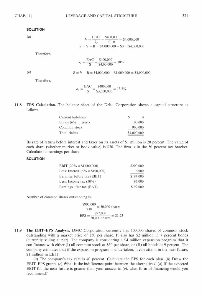
SOLUTION
(a)V ¼ EBIT
ko¼ $400,000
0:10¼ $4,000,000
S ¼ V� B ¼ $4,000,000� $0 ¼ $4,000,000
Therefore,
ke ¼EAC
S¼ $400,000
$4,00,000¼ 10%
(b) S ¼ V� B ¼ $4,000,000� $1,000,000 ¼ $3,000,000
Therefore,
ke ¼EAC
S¼ $400,000
$3,000,000¼ 13:3%
11.8 EPS Calculation. The balance sheet of the Delta Corporation shows a capital structure as
follows:
Current liabilities $ 0
Bonds (6% interest) 100,000
Common stock 900,000
Total claims $1,000,000
Its rate of return before interest and taxes on its assets of $1 million is 20 percent. The value of
each share (whether market or book value) is $30. The firm is in the 50 percent tax bracket.
Calculate its earnings per share.
SOLUTION
EBIT (20%� $1,000,000) $200,000
Less: Interest (6%� $100,000) 6,000
Earnings before tax (EBIT) $194,000
Less: Income tax (50%) 97,000
Earnings after tax (EAT) $ 97,000
Number of common shares outstanding is:
$900,000
$30¼ 30,000 shares
EPS ¼ $97,000
30,000 shares¼ $3:23
11.9 The EBIT–EPS Analysis. DMC Corporation currently has 100,000 shares of common stock
outstanding with a market price of $50 per share. It also has $2 million in 7 percent bonds
(currently selling at par). The company is considering a $4 million expansion program that it
can finance with either (I) all common stock at $50 per share, or (II) all bonds at 9 percent. The
company estimates that if the expansion program is undertaken, it can attain, in the near future,
$1 million in EBIT.
(a) The company’s tax rate is 40 percent. Calculate the EPS for each plan. (b) Draw the
EBIT–EPS graph. (c) What is the indifference point between the alternatives? (d) If the expected
EBIT for the near future is greater than your answer in (c), what form of financing would you
recommend?
CHAP. 11] LEVERAGE AND CAPITAL STRUCTURE 321

SOLUTION
(a) The EPS is computed as follows:
(I) All Stock (II) All Bonds
EBIT $1,000,000 $1,000,000
Interest 140,000a 500,000b
EBT $ 860,000 $ 500,000
Tax (40%) 344,000 200,000
EAT $ 516,000 $ 300,000
Number of shares 180,000c 100,000
EPS $2.87 $3.00
a$2,000,000� 7% ¼ $140,000
b$4,000,000� 9% ¼ $360,000
$360,000þ $140,000 ¼ $500,000c$4,000,000þ $50 per share ¼ 80,000 shares: Therefore;
100,000þ 80,000 ¼ 180,000 shares
(b) The EBIT–EPS graph is shown in Fig. 11-5.
(c) EPS ¼ EBIT� Ið Þ 1� tð Þ � PD
Number of shares outstanding
The EBIT–EPS indifference points between plans (I) and (II) are calculated as follows:
EPS under plan ðIÞ ¼ EPS under plan ðIIÞ
EBIT� 140,000ð Þ 1� 0:4ð Þ � 0
180,000¼ EBIT� 500,000ð Þ 1� 0:4ð Þ � 0
100,000
0:6 EBIT� 84,000ð Þ 100,000ð Þ ¼ 0:6 EBIT� 300,000ð Þ 180,000ð Þ
48,000 EBIT ¼ 45,600,000,000
EBIT ¼ $950,000
(d ) Plan (II), all bonds, is preferred.
Fig. 11-5
322 LEVERAGE AND CAPITAL STRUCTURE [CHAP. 11
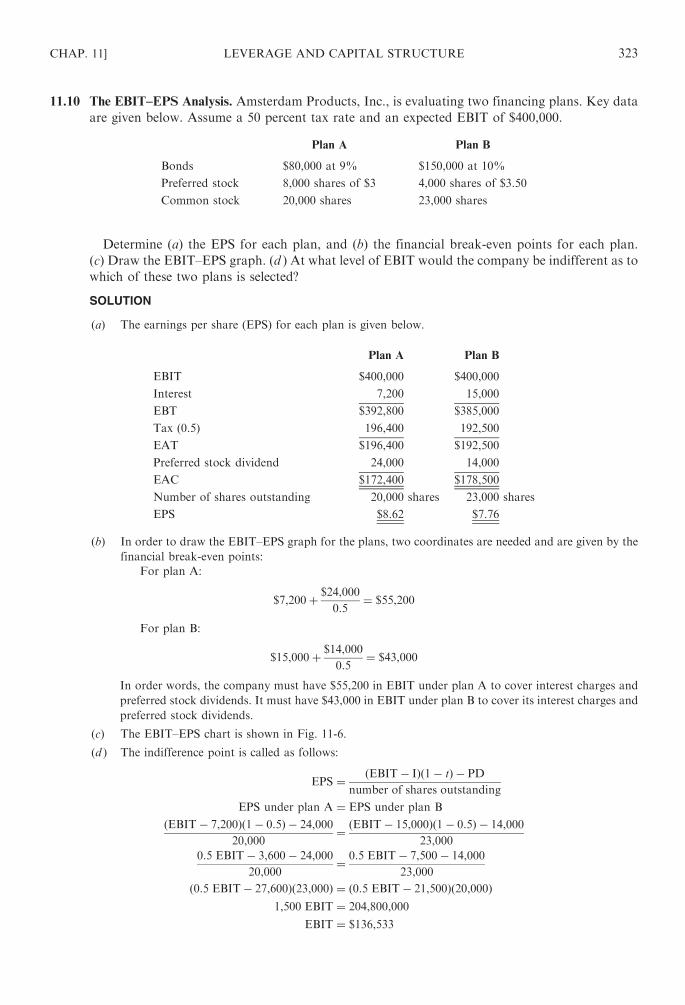
11.10 The EBIT–EPS Analysis. Amsterdam Products, Inc., is evaluating two financing plans. Key data
are given below. Assume a 50 percent tax rate and an expected EBIT of $400,000.
Plan A Plan B
Bonds $80,000 at 9% $150,000 at 10%
Preferred stock 8,000 shares of $3 4,000 shares of $3.50
Common stock 20,000 shares 23,000 shares
Determine (a) the EPS for each plan, and (b) the financial break-even points for each plan.
(c) Draw the EBIT–EPS graph. (d ) At what level of EBIT would the company be indifferent as to
which of these two plans is selected?
SOLUTION
(a) The earnings per share (EPS) for each plan is given below.
Plan A Plan B
EBIT $400,000 $400,000
Interest 7,200 15,000
EBT $392,800 $385,000
Tax (0.5) 196,400 192,500
EAT $196,400 $192,500
Preferred stock dividend 24,000 14,000
EAC $172,400 $178,500
Number of shares outstanding 20,000 shares 23,000 shares
EPS $8.62 $7.76
(b) In order to draw the EBIT–EPS graph for the plans, two coordinates are needed and are given by the
financial break-even points:
For plan A:
$7,200þ $24,000
0:5¼ $55,200
For plan B:
$15,000þ $14,000
0:5¼ $43,000
In order words, the company must have $55,200 in EBIT under plan A to cover interest charges and
preferred stock dividends. It must have $43,000 in EBIT under plan B to cover its interest charges and
preferred stock dividends.
(c) The EBIT–EPS chart is shown in Fig. 11-6.
(d ) The indifference point is called as follows:
EPS ¼ ðEBIT� IÞ 1� tð Þ � PD
number of shares outstanding
EPS under plan A ¼ EPS under plan B
EBIT� 7,200ð Þ 1� 0:5ð Þ � 24,000
20,000¼ EBIT� 15,000ð Þ 1� 0:5ð Þ � 14,000
23,000
0:5 EBIT� 3,600� 24,000
20,000¼ 0:5 EBIT� 7,500� 14,000
23,000
0:5 EBIT� 27,600ð Þ 23,000ð Þ ¼ 0:5 EBIT� 21,500ð Þ 20,000ð Þ1,500 EBIT ¼ 204,800,000
EBIT ¼ $136,533
CHAP. 11] LEVERAGE AND CAPITAL STRUCTURE 323

Therefore, below the level of $136,533, plan B is preferred; above the level of $136,533, plan A is
preferred.
11.11 The EBIT–EPS Analysis. Parker Brothers, Inc., is considering three financing plans. The key
information follows. Assume a 50 percent tax rate.
Plan A Plan B Plan C
Common stock: $200,000 Bonds at 8%: $100,000 Preferred stock at 8%: $100,000
Common stock: $100,000 Common stock: $100,000
In each case the common stock will be sold at $20 per share. The expected EBIT is $80,000.
Determine (a) the EPS for each plan, and (b) the financial break-even point for each plan.
(c) Draw the EBIT–EPS graph. (d ) Indicate over what EBIT range each plan is preferred.
SOLUTION
(a) The EPS calculation is shown below:
Plan A Plan B Plan C
EBIT $80,000 $80,000 $80,000
Interest 8,000
EBT $80,000 $72,000 $80,000
Tax (50%) 40,000 36,000 40,000
EAT $40,000 $36,000 $40,000
Preferred stock divided 8,000
Earnings available to
common stockholders (EAC) $40,000 $36,000 $32,000
Number of shares outstanding 10,000 5,000 5,000
EPS $4.00 $7.20 $6.40
(b) The financial break-even points are: for plan A, 0; for plan B, $8,000; and for plan C, $8,0007 0.5=
$16,000. In other words, plan B must have $8,000 in EBIT to cover the interest charge of $8,000; plan
C must have $16,000 in EBIT to pay the preferred stock divided of $8,000.
Fig. 11-6
324 LEVERAGE AND CAPITAL STRUCTURE [CHAP. 11

(c) See Fig. 11-7.
(d ) From Fig. 11-7, the EBIT–EPS graph in (c), we see that plan B will always dominate plan C at any
level of EBIT. Thus, only alternatives A versus B and A versus C need be evaluated. The indifference
points are computed as follows:
For plan A versus plan B:
EBIT� 0ð Þ 1� 0:5ð Þ � 0
10,000¼ EBIT� 8,000ð Þ 1� 0:5ð Þ � 0
5,000
0:5 EBIT 5,000ð Þ ¼ 0:5EBIT� 4,000ð Þ 10,000ð Þ2,500 EBIT ¼ 40,000,000
EBIT ¼ $16,000
For plan A versus plan C:
EBIT� 0ð Þ 1� 0:5ð Þ � 0
10,000¼ EBIT� 0ð Þ 1� 0:5ð Þ � 8,000
5,000
0:5 EBIT
10,000¼ 0:5 EBIT� 8,000
5,000
0:5 EBIT 5,000ð Þ ¼ 0:5 EBIT� 8,000ð Þ 10,000ð Þ2,500 EBIT ¼ 5,000 EBIT� 80,000,000
2,500 EBIT ¼ 80,000,000
EBIT ¼ $32,000
If EBIT is expected to exceed $16,000, plan B is preferred over plan A. If EBIT is expected to
exceed $32,000, plan C is preferred over plan A.
11.12 EBIT–EPS Analysis. The Morton Company is planning to invest $10 million in an expansion
program which is expected to increase earnings before interest and taxes by $2.5 million. The
company currently is earning $5 per share on 1 million shares of common outstanding. The
capital structure prior to the investment is:
Debt $10,000,000
Equity 30,000,000
$40,000,000
Fig. 11-7
CHAP. 11] LEVERAGE AND CAPITAL STRUCTURE 325

The expansion can be financed by sale of 200,000 shares at $50 net each, or by issuing long-term
debt at a 6 percent interest cost. The firm’s recent profit and loss statement was as follows:
Sales $101,000,000
Variable cost $ 60,000,000
Fixed cost 30,500,000
$ 90,500,000
Earnings before interest and taxes $ 10,500,000
Interest 500,000
Earnings before taxes $ 10,000,000
Taxes (50%) 5,000,000
Earnings after taxes $ 5,000,000
(a) Assuming the firm maintains its current earnings and achieves the anticipated earnings
from the expansion, what will be the earnings per share (1) if the expansion is financed by debt?
(2) if the expansion is financed by equity? (b) At what level of earnings before interest and taxes
will the earnings per share under either alternative be the same amount? (c) The choice of
financing alternatives influences the earnings per share. The choice might also influence the
earnings multiple used by the market. Discuss the factors inherent in the choice between the
debt and equity alternatives that might influence the earnings multiple. Be sure to indicate
the direction in which these factors might influence the earnings multiple. (CMA, adapted.)
SOLUTION
(a)
(1) (2)
Debt-Financed Equity-Financed
Earnings before interest
and taxes–present
$10,500,000 $10,500,000
Added earnings–expansion 2,500,000 2,500,000
$13,000,000 $13,000,000
Interest 1,100,000 500,000
$11,900,000 $12,500,000
Taxes 5,950,000 6,250,000
Net income $ 5,950,000 $ 6,250,000
Common shares outstanding 1,000,000 1,200,000
Earnings per share $5.95 $5.21
(b)EPS ¼ EBIT� Ið Þ 1� tð Þ
no: of shares
EBIT� 1,100,000ð Þ 1� 0:50ð Þ1,000,000
¼ ðEBIT� 500,000Þ 1� 0:50ð Þ1,200,000
EBIT ¼ $4,100,000
(c) A major factor that is inherent in the choice between debt and equity financing is the change in the
risk for the equity holders. If the expansion is financed by debt, the increase in risk appears in two
forms. (1) There is increased risk of insolvency because the debt requires regular fixed cash outlay
for interest and principal. Equity financing does not incur the legal obligations of the regular cash
outlay. (2) The other effect is on the variability of earnings to common stockholders. The fixed charges
against income reduces the amount of income available to stockholders. The relative variability of
earnings available to common stockholders increases. Both these risks would tend to reduce the
earnings multiple. (Note, the market value of a share does not necessarily decrease with the debt
expansion.)
326 LEVERAGE AND CAPITAL STRUCTURE [CHAP. 11

11.13 Rate of Return and Optimal Capital Structure. Central Furniture Company recently announced
plans to expand its production capacity by building and equipping two new factories to operate
in parallel with existing production facilities. The expansion will double the assets of the firm.
The proposed expansion has received a lot of attention from industry observers due to the
cyclical nature of the furniture industry and the size of the project. The new plants will require
fewer workers than current plants of similar capacity because the new facilities will be highly
automated.
Central Furniture must now decide how the plant expansion will be financed. The project will
require $5 million in new funds and the expected return on the new assets is estimated at 12
percent before taxes, the same return that is currently earned on the existing assets. The two
alternatives proposed to raise the needed funds are (1) private placement of long-term debt at an
interest rate of 10 percent, and (2) issuance of new common stock at $25 per share.
Currently the company is financed equally by debt and equity as follows:
Long-term debt (8%) $2,500,000
Common stock ($1 par) $ 100,000
Paid-in capital on common stock $ 400,000
Retained earnings $2,000,000
Central Furniture’s common stock is currently traded on a stock exchange at a market price
of $27 per share. Central Furniture is subject to a tax rate of 40 percent.
(a) Compute Central Furniture Company’s anticipated rate of return on stockholders’ equity
if the expansion project is financed by (1) private placement of long-term debt, and (2) issuance of
common stock. (b) One of the two alternatives–long-term debt or common stock–will move
Central Furniture Company to a more optimum capital structure. (1) What criteria are used to
judge optimum capital structure? (2) Explain what factors influence the determination of an
optimum capital structure. (CMA, adapted.)
SOLUTION
(a) (1) Earnings before interest and taxes
($10,000,000� 0.12)
$1,200,000
Less: Interest expense
Present debt (0.08� $2,500,000) $200,000
New debt (0.10� $5,000,000) 500,000 700,000
Earnings before taxes $ 500,000
Taxes (40%) 200,000
Net income $ 300,000
Return on stockholders’ equity ¼ $300,000
$2,500,000¼ 12%
(2) Earnings before interest and taxes
($10,000,000� 0.12)
$1,200,000
Less: Interest expense
(0.08� $2,500,000)
200,000
Earnings before taxes $1,000,000
Taxes (40%) 400,000
Net income $ 600,000
Return on stockholders’ equity ¼ $600,000
$7,500,000¼ 8%
CHAP. 11] LEVERAGE AND CAPITAL STRUCTURE 327

(b) (1) Optimum capital structure is the lowest weighted average cost of capital that a given firm is able
to obtain given its risk constraints. (2) The optimum capital structure for a firm is influenced by
the relationship of its return to the risks of earning the return. Specific factors influencing these
two items would include:
1. The growth rate of income
2. Cash flow available to service debt
3. The amount of operating risk
4. Lender and investor interpretation of the financial risk of the firm and industry
11.14 Alternative Sources of Financing. The Drew Furniture Company is considering the introduction
of a new product line. Plant and inventory expansion equal to 50 percent of present asset levels
will be necessary to handle the anticipated volume of the new product line. New capital will have
to be obtained to finance the asset expansion. Two proposals have been developed to provide
the added capital.
1. Raise the $100,000 by issuing 10-year 12 percent bonds. This will change the capital structure
from one with about 20 percent debt to one with almost 50 percent debt. The investment
banking house estimates the price/earnings ratio, now 12 to 1, will be reduced to 10 to 1 if this
method of financing is chosen.
2. Raise the $100,000 by issuing new common stock. The investment banker believes that the
stock can be issued to yield $3313. The price/earnings ratio would remain at 12 to 1 if the stock
were issued. The present market price is $36.
The company’s most recent financial statements are as follows:
Drew Furniture Company
Balance Sheet
As of December 31, 20XI
ASSETS EQUITIES
Current $ 65,000 Debt 5% $ 40,000
Plant and equipment 135,000 Common stock 100,000
Retained earnings 60,000
$200,000 $200,000
Income Statement
For the Year Ended December 31, 20X1
Sales $600,000
Operating costs 538,000
Operating income $ 62,000
Interest charges 2,000
Net income before taxes $ 60,000
Federal income taxes 30,000
Net income $ 30,000
(a) The vice-president of finance asks you to calculate the earnings per share and the market value
of the stock (assuming the price/earnings ratios given are valid estimates) for the two proposals
assuming total sales (including the new product line) of: (1) $400,000; (2) $600,000; and (3)
$800,000. Costs exclusive of interest and taxes are about 90 percent of sales. (b) Which proposal
would you recommend? Your answer should indicate: (1) the criteria used to judge the alterna-
tives; (2) a brief defense of the criteria used; and (3) the proposal chosen in accordance with the
criteria. (c) Would your answer change if a sales level of $1,200,000 or more could be achieved?
328 LEVERAGE AND CAPITAL STRUCTURE [CHAP. 11

Explain. (d ) What reasons(s) would the investment broker give to support the estimate of a lower
price/earnings ratio if debt is issued? (CMA, adapted.)
SOLUTION
(a) Proposal 1, for 10-year 12 percent bonds:
Drew Furniture Company
Income Statement
For the Year Ended December 31, 20X1
Estimated Sales Levels
Sales $400,000 $600,000 $800,000
Operating costs 360,000 540,000 720,000
Operating income $ 40,000 $ 60,000 $ 80,000
Interest charges 14,000 14,000 14,000
Net income before taxes $ 26,000 46,000 $ 66,000
Federal income taxes 13,000 23,000 33,000
Net income $ 13,000 $ 23,000 $ 33,000
Outstanding shares ¼ 30,000
3¼ 10,000
Earnings per share $1.30 $2.30 $3.30
Price/earnings ratio 10 times 10 times 10 times
Estimated market value $31 $23 $33
Proposal 2, for common stock issue to yield $3313:
Drew Furniture Company
Income Statement For the Year
Ended December 31, 20X1
Estimated Sales Levels
Sales $400,000 $600,000 $800,000
Operating costs 360,000 540,000 720,000
Operating income $ 40,000 $ 60,000 $ 80,000
Interest charges 2,000 2,000 2,000
Net income before taxes $ 38,000 $ 58,000 $ 78,000
Federal income taxes 19,000 29,000 39,000
Net income $ 19,000 $ 29,000 $ 39,000
Outstanding shares ¼ 100,000
3313
þ 10,000 ¼ 13,000 shares
Earnings per share $1.46 $2.23 $3.00
Price/earnings ratio 12 times 12 times 12 times
Estimated market value $17.52 $26.76 $36.00
(b) Within the constraints of this problem, two possible objectives emerge: profit maximization as mea-
sured by earnings per share, and wealth maximization as measured by the price of the common stock.
If profit maximization is used, the firm should choose to finance the new product by selling bonds,
since earnings per share is higher for each of the three levels of sales. On the other hand, wealth
maximization would require the sale of new common stock because stock price is higher at each sales
level.
CHAP. 11] LEVERAGE AND CAPITAL STRUCTURE 329

Wealth maximization is the preferred criterion for financial decision making. Unlike profit max-
imization, wealth maximization represents a measure of the total benefits to be enjoyed by the share-
holders, adjusted for both the timing of benefits and the risk associated with their receipt. A criterion
which ignores these two important determinants of value cannot be expected to provide a proper guide
to decision making.
Because wealth maximization is the preferred objective, the sale of common stock is the recom-
mended financing technique.
(c) Proposal 2 would still be the choice because the market value remains above that of proposal 1. The
difference is smaller than is shown with the lower sales estimates, which means that proposal 1 would
become attractive if sales reached a higher level (approximately $1.6 million).
(d ) The investment banker would suggest that the lower price/earnings ratio with debt financing is a
reflection of the greater returns demanded by stockholders in compensation for the greater variability
in earnings and higher risk of bankruptcy created by the fixed commitment to pay debt interest and
principal.
330 LEVERAGE AND CAPITAL STRUCTURE [CHAP. 11
Examination II
Chapters 6–11
I. Put a T (true) or F (false) in the space provided below:
1. Finding present values is simply the inverse of compounding.
2. A perpetuity is an annuity that continues for 20 years.
3. Risk is defined as the variation in returns about a standard deviation.
4. Through diversification, an investor can reduce the systematic risk, or beta.
5. A proxy for the risk-free rate is the Treasury bills yield.
6. The cost of capital is the weighted average of the various capital costs.
7. Total leverage is the product of operating leverage and financial leverage.
8. The optimal capital structure can be defined as the mix of financing sources that minimize
the company’s debt cost.
9. Projects that are negatively correlated tend to be less risky than those that move together in
the same direction.
10. The NPV method and the IRR approach assume the same rate for reinvestment.
II. Select the best answer:
1. Which of the following takes into account the time value of money?
(a) Average rate of return
(b) Payback period
(c) Internal rate of return
(d ) None of the above
2. The NPV method and the IRR method may produce conflicting ranking when
(a) projects are mutually exclusive
(b) projects are independent and not competing for limited funds
(c) both of the above
(d ) none of the above
3. Which of the following is concerned with the relationship between the firm’s EBIT and EPS?
(a) Beta
(b) Operating leverage
(c) Sales revenue
(d ) Financial leverage
4. Through diversification a firm can stabilize its earnings and most effectively reduce its risk when
projects are
(a) perfectly positively correlated
(b) independent of each other
(c) perfectly negatively correlated
(d ) none of the above
331
Copyright © 2007, 1998, 1986 by The McGraw-Hill Companies, Inc. Click here for terms of use.

5. Under the CAPM, the required rate of return on a security is the sum of a risk premium and
(a) financial risk
(b) operating risk
(c) diversifiable risk
(d ) risk-free rate
6. All the following elements are necessary for the computation of the cost of common stock under the
Gordon’s growth model, except
(a) tax rate
(b) growth rate in dividends or earnings
(c) market price
(d ) dividend
7. Which one of the following must be adjusted for taxes?
(a) Cost of retained earnings
(b) Cost of common stock
(c) Cost of preferred stock
(d ) Cost of debt
8. Which of the following is not a method for adjusting for risk in capital budgeting?
(a) Risk-adjusted rate
(b) Simulation
(c) Certainty equivalent approach
(d ) Break-even analysis
9. The traditional approach to capital structure implies
(a) there is a minimum cost of capital that is determined by an optimal capital structure
(b) there is no such things as optimal capital structure
(c) all the above
(d ) none of the above
10. The simple expression for the total value of the firm is
(a) stocks/bonds
(b) stocks� bonds
(c) stocks+bonds
(d ) none of the above
III.
1. If a firm’s earnings and dividends grow from $2.15 per share to $4 per share over an 8-year period,
what is the rate of growth?
2. How much would you be willing to pay today for an investment that would return $1,250 each year
for the next 10 years, assuming a discount rate of 12 percent?
3. The risk-free rate is 5 percent, the market return is 12 percent and the stock’s beta coefficient is 1.25.
If the dividend expected during the coming year is $3 and grows at an 8 percent rate, at what price
should the stock sell?
332 EXAMINATION II

4. The Sawyer Company has just issued $10 million of $1,000, 8 percent, 10-year bonds. Due to
the current market rates the firm had to sell the bonds at a discount of $40 from their face
value. (a) Calculate the before-tax cost, or yield to maturity, of the bond, using the shortcut
formula, and (b) calculate the after-tax cost of the bond, assuming the firm’s tax rate is 40 percent.
5. The Desert Products Company is considering six investment proposals of similar risk, for which the
funds available are limited. The projects are independent and have the following initial investment
and present values of cash inflows associated with them:
Project Initial Cost (I) ($) PV ($)
A 15,000 21,000
B 8,000 12,000
C 5,000 7,500
D 4,000 6,400
E 2,000 3,500
F 1,000 1,900
(a) Compute the profitability index and NPV for each project. (b) Under capital rationing, which
projects should be selected, assuming a total budget of $25,000? (c) Which projects should be
selected if the total budget is reduced to $24,000?
6. A firm is considering two alternative plans to finance a proposed $7 million investment. Plan A:
Issue debt (9 percent interest rate). Plan B: Issue common stock (at $20 per share, 1 million shares
currently outstanding). The company’s income tax rate is 40 percent. (a) Calculate the indifference
level of EBIT, or the break-even point for each plan, and (b) plot these two plans on the EBIT-EPS
chart.
7. ABC System, Inc., plans to sell new shares of common stock at $35. The flotation cost is 10 percent.
What is the cost of external equity? Both earnings and dividends are expected to grow at a constant
rate of 6 percent and the annual dividend per share is $2.
8. Alta-Data, Inc., is considering an investment proposal. The company’s board of directors indicated
that the firm’s present 70 percent owners’ equity and 30 percent long-term debt structure should be
maintained. The company’s projected earnings accompanied by periodic common stock sales will
permit it to maintain the present 70 percent owners’ equity structure of 40 percentage points from
retained earnings and 30 percentage points from common stock.
After consultation with the firm’s investment banker, the company has determined that the
debt could be sold to yield 9 percent and new common stock could be sold to provide proceeds of
$40 per share to the firm. The company is currently paying a dividend of $2 per share, and the
dividends are expected to grow at a constant rate of 6 percent. The firm’s income tax rate is 40
percent.
Calculate the after-tax cost of capital that the company can use for its capital budgeting
decision.
Answers to Examination II
I. 1. T; 2. F; 3. F; 4. F; 5. T; 6. T; 7. T; 8. F; 9. T; 10. F
II. 1. (c); 2. (a); 3. (d ); 4. (c); 5. (d ); 6. (a); 7. (d ); 8. (d ); 9. (a); 10. (c)
EXAMINATION II 333

III.
1. Fn ¼ PFVIFi;n
$4:00 ¼ $2:15 FVIFi;8
� �
FVIFi;8 ¼$4:00
$2:15¼ 1:8605
From Appendix A, FVIF8%,8=1.8509. Therefore, the firm’s approximate rate of growth is 8 percent.
2. PV ¼ $1,250 PVIFA12%;10
� �
¼ $1,250 5:6502ð Þ ¼ $7,062:75
3. r ¼ rf þ bðrm � rfÞ¼ 5%þ 1:25 12%� 5%ð Þ ¼ 5%þ 8:75% ¼ 13:75%
P0 ¼D1
r� g¼ $3
13:75%� 8%¼ $3
0:0575¼ $52:17
4. (a) Yield to maturity ¼ Iþ ððM� VÞ=nÞMþ Vð Þ=2 ¼ $80þ $1,000� $960ð Þ=10
$1,000þ $960ð Þ=2
¼ $80þ $4
$980¼ 8:57%
(b) After-tax cost of debt ¼ 8:57% 1� 0:4ð Þ ¼ 5:14%
5. (a) NPV=PV� I and the profitability index is PV/I.
Initial Cost Profitability
Project (I) ($) NPV ($) Index (PI)
A 15,000 6,000 1.40
B 8,000 4,000 1.50
C 5,000 2,500 1.50
D 4,000 2,400 1.60
E 2,000 1,500 1.75
F 1,000 900 1.90
(b) Project I PV NPV PI
A $ 5,100 $21,000 $ 6,000 1.40
C 5,000 7,500 2,500 1.50
D 4,000 6,400 2,400 1.60
F 1,000 1,900 900 1.90
Totals $25,000 $36,800 $11,800
No combination within the $25,000 total budget constraint would show as much NPV as the one listed
above. Note that project E is not included even though its 1.75 PI is higher than three of the included
projects.
(c) Project I PV NPV PI
B $ 8,000 $12,000 $ 4,000 1.50
C 5,000 7,500 2,500 1.50
D 4,000 6,400 2,400 1.60
E 2,000 3,500 1,500 1.75
F 1,000 1,900 900 1.90
Totals $20,000 $31,300 $11,300
334 EXAMINATION II
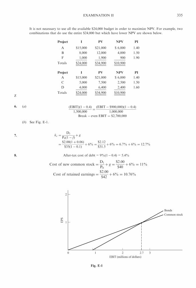
It is not necessary to use all the available $24,000 budget in order to maximize NPV. For example, two
combinations that do use the entire $24,000 but which have lower NPV are shown below.
Project I PV NPV PI
A $15,000 $21,000 $ 6,000 1.40
B 8,000 12,000 4,000 1.50
F 1,000 1,900 900 1.90
Totals $24,000 $34,900 $10,900
Project I PV NPV PI
A $15,000 $21,000 $ 6,000 1.40
C 5,000 7,500 2,500 1.50
D 4,000 6,400 2,400 1.60
Totals $24,000 $34,900 $10,900z
6. (a) EBITð Þ 1� 0:4ð Þ1,500,000
¼ EBIT� $900,000ð Þ 1� 0:4ð Þ1,000,000
Break� even EBIT ¼ $2,700,000
(b) See Fig. E-1.
7. ke ¼D1
P0 1� fð Þ þ g
¼ $2:00 1þ 0:06ð Þ$35 1� 0:1ð Þ þ 6% ¼ $2:12
$31:5þ 6% ¼ 6:7%þ 6% ¼ 12:7%
8. After-tax cost of debt=9%(1� 0.4)=5.4%
Cost of new common stock ¼ D1
P0
þ g ¼ $2:00
$40þ 6% ¼ 11%
Cost of retained earnings ¼ $2:00
$42þ 6% ¼ 10:76%
Fig. E-1
EXAMINATION II 335

Therefore, the after-tax cost of capital, or weighted average of individual capital component costs, is computed
as follows:
Weights
Weighted
Average
Debt, 5.4% 0.3 1.62%
New common stock, 11% 0.4 4.4
Retained earnings, 10.76% 0.3 3.23
After-tax cost of capital 9.25%
336 EXAMINATION II

Chapter 12
Dividend Policy
12.1 INTRODUCTION
Corporate earnings distributed to stockholders are called dividends. Dividends are paid in either
cash or stock and are typically issued quarterly. They may be paid only out of retained earnings and
not from invested capital such as capital stock or the excess received over stock par value. In general,
the more stable a company’s earnings, the more regular its issue of dividends.
A company’s dividend policy is important for the following reasons:
1. It bears upon investor attitudes. For example, stockholders look unfavorably upon the corpora-
tion when dividends are cut, since they associate the cutback with corporate financial problems.
Further, in setting a dividend policy, management must ascertain and fulfill the objectives of
its owners. Otherwise, the stockholders may sell their shares, which in turn may bring down
the market price of the stock. Stockholder dissatisfaction raises the possibility that control of the
company may be seized by an outside group.
2. It impacts the financing program and capital budget of the firm.
3. It affects the firm’s cash flow position. A company with a poor liquidity position may be forced
to restrict its dividend payments.
4. It lowers stockholders’ equity, since dividends are paid from retained earnings, and so results
in a higher debt-to-equity ratio.
If a company’s cash flows and investment requirements are volatile, the company should not
establish a high regular dividend. It would be better to establish a low regular dividend that can be
met even in years of poor earnings.
Relevant dates associated with dividends are as follows:
1. Declaration date. This is the date on which the board of directors declares the dividend. On this
date, the payment of the dividend becomes a legal liability of the firm.
2. Date of record. This is the date upon which the stockholder is entitled to receive the dividend.
3. Ex-dividend date. The ex-dividend date is the date when the right to the dividend leaves the
shares. The right to a dividend stays with the stock until 2 days before the date of record. That is,
on the second day prior to the record date, the right to the dividend is no longer with the
shares, and the seller, not the buyer of that stock, is the one who will receive the dividend.
The market price of the stock reflects the fact that it has gone ex-dividend and will decrease by
approximately the amount of the dividend.
EXAMPLE 12.1 The date of record for the dividend declared by the Acme Company is January 30. Harris sells
Jones her 100 shares of Acme Company on January 27. Harris, not Jones, will receive the dividend on the shares.
EXAMPLE 12.2 Assume that the date of record is 11th (Thursday):
Ex-dividend Date Record Date
# #
Mon Tues Wed Thurs Fri
8th 9th 10th 11th 12th
337
Copyright © 2007, 1998, 1986 by The McGraw-Hill Companies, Inc. Click here for terms of use.
If you buy it on the ex-dividend date (9th), you will not receive the dividend because your name will
not appear in the company’s record books until Friday (12th). If you want to buy the stock and receive the
dividend, you need to buy it on the 8th. If you want to sell the stock and still receive the dividend, you need to
sell on the 9th.
4. Date of payment. This is the date when the company distributes its dividend checks to its stockholders.
Dividends are usually paid in cash. A cash dividend is typically expressed in dollars and cents per
share. However, the dividend on preferred stock is sometimes expressed as a percentage of par value.
EXAMPLE 12.3 On November 15, 20X1, a cash dividend of $1.50 per share was declared on 10,000 shares of
$10 par value common stock. The amount of the dividend paid by the company is $15,000 (10,000� $1.50).
EXAMPLE 12.4 Jones Corporation has 20,000 shares of $10 par value, 12 percent preferred stock outstanding.
On October 15, 20X1, a cash dividend was declared to holders of record as of December 15, 20X1. The amount of
dividend to be paid by Jones Corporation is equal to:
20,000 shares � $10 par value ¼ $200,000� 12% ¼ $24,000
Some companies allow stockholders to automatically reinvest their dividend in corporate shares
instead of receiving cash. The advantage to the stockholder is that he or she avoids the brokerage fees
associated with buying new shares. However, there is no tax advantage since the stockholder must still
pay ordinary income taxes on the dividend received.
12.2 DIVIDEND POLICY
A finance manager’s objective for the company’s dividend policy is to maximize owner wealth while
providing adequate financing for the company. When a company’s earnings increase, management does
not automatically raise the dividend. Generally, there is a time lag between increased earnings and the
payment of a higher dividend. Only when management is confident that the increased earnings will be
sustained will they increase the dividend. Once dividends are increased, they should continue to be paid
at the higher rate. The various types of dividend policies are:
1. Stable dividend-per-share policy. Many companies use a stable dividend-per-share policy since it
is looked upon favorably by investors. Dividend stability implies a low-risk company. Even in a
year that the company shows a loss rather than profit the dividend should be maintained to
avoid negative connotations to current and prospective investors. By continuing to pay the
dividend, the shareholders are more apt to view the loss as temporary. Some stockholders
rely on the receipt of stable dividends for income. A stable dividend policy is also necessary
for a company to be placed on a list of securities in which financial institutions (pension funds,
insurance companies) invest. Being on such a list provides greater marketability for corporate
shares.
2. Constant dividend-payout-ratio (dividend per share/earnings per share) policy. With this policy a
constant percentage of earnings is paid out in dividends. Because net income varies, dividends
paidwill alsovaryusingthisapproach.Theproblemthispolicycauses is that ifacompany’s earnings
drop drastically or there is a loss, the dividends paid will be sharply curtailed or nonexistent. This
policy will not maximize market price per share since most stockholders do not want variability in
their dividend receipts.
3. Acompromisepolicy.Acompromisebetween thepoliciesof a stabledollaramount andapercentage
amount of dividends is for a company to pay a low dollar amount per share plus a percentage
increment in good years. While this policy affords flexibility, it also creates uncertainty in the
minds of investors as to the amount of dividends they are likely to receive. Stockholders generally
donot like suchuncertainty.However, the policymaybe appropriatewhen earnings vary consider-
ably over the years. The percentage, or extra, portion of the dividend should not be paid regularly;
otherwise it becomes meaningless.
338 DIVIDEND POLICY [CHAP. 12
4. Residual-dividend policy.When a company’s investment opportunities are not stable, management
may want to consider a fluctuating dividend policy. With this kind of policy the amount of
earnings retained depends upon the availability of investment opportunities in a particular
year. Dividends paid represent the residual amount from earnings after the company’s investment
needs are fulfilled.
Theoretical Position
Theoretically, a company should retain earnings rather than distribute them when the corporate
return exceeds the return investors can obtain on their money elsewhere. Further, if the company obtains
a return on its profits that exceeds the cost of capital, the market price of its stock will be maximized.
Capital gains arising from the appreciation of the market price of stock has a tax advantage over
dividends. On the other hand, a company should not, theoretically, keep funds for investment if it earns
less of a return than what the investors can earn elsewhere. If the owners have better investment
opportunities outside the firm, the company should pay a high dividend.
Although theoretical considerations from a financial point of view should be considered when
setting dividend policy, the practicality of the situation is that investors expect to be paid dividends.
Psychological factors come into play which may adversely affect the market price of the stock of a
company that does not pay dividends.
12.3 FACTORS THAT INFLUENCE DIVIDEND POLICY
Afirm’s dividendpolicy is a function ofmany factors, someofwhich have beendescribed.Other factors
that influence dividend policy are as follows:
1. Companygrowthrate.Acompany that is rapidlygrowing, even ifprofitable,mayhave torestrict its
dividend payments in order to keep needed funds within the company for growth opportunities.
2. Restrictive covenants. Sometimes there is a restriction in a credit agreement that will limit the
amount of cash dividends that may be paid.
3. Profitability. Dividend distribution is keyed to the profitability of the company.
4. Earnings stability. A companywith stable earnings ismore likely to distribute a higher percentage
of its earnings than one with unstable earnings.
5. Maintenance of control. Management that is reluctant to issue additional common stock because
it does not wish to dilute its control of the firm will retain a greater percentage of its earnings.
Internal financing enables control to be kept within.
6. Degree of financial leverage. A company with a high debt-to-equity ratio is more likely to retain
earnings so that it will have the needed funds to meet interest payments and debts at maturity.
7. Ability to finance externally. A company that is capable of entering the capital markets easily can
afford to have a higher dividend payout ratio. When there is a limitation to external sources of
funds, more earnings will be retained for planned financial needs.
8. Uncertainty. Payment of dividends reduces the chance of uncertainty in stockholders’ minds
about the company’s financial health.
9. Age and size. The age and size of the company bear upon its ease of access to capital markets.
10. Tax penalties. Possible tax penalties for excess accumulation of retained earnings may result in
high dividend payouts.
Stockholder Tax Considerations
The answer to the question of which is preferred by stockholders—income from dividends or from
capital gains (sale of stock)—depends on the individual stockholder’s tax bracket. Capital gains arising
from appreciation in market price is subject to a long-term capital gain deduction. Capital gains have been
CHAP. 12] DIVIDEND POLICY 339

taxed at somewhat lower rates. Dividends are considered ordinary income and are taxed at the full rate.
Taxpayers in low tax brackets or those who rely on a fixed income favor greater dividend distribution. The
theoretical dispute regarding dividend policy relates to investor psychology in terms of whether earnings
should be taken as capital gains or as dividends.
Controversy
The dividend policy controversy can best be described by presenting the approaches put forth by
various authors:
1. Gordonetal.believethatcashflowsofacompanyhavinga lowdividendpayoutwillbecapitalizedat
a higher rate because investors will perceive capital gains resulting from earnings retention to be
more risky than dividends.
2. Miller and Modigliani argue that a change in dividends impacts the price of the stock since
investors will perceive such a change as being a statement about expected future earnings. They
believe that investors are generally indifferent to a choice between dividends or capital gains.
3. Weston and Brigham et al. believe that the best dividend policy varies with the particular
characteristics of the firm and its owners, depending on such factors as the tax bracket and
income needs of stockholders, and corporate investment opportunities.
12.4 STOCK DIVIDENDS
A stock dividend is the issuance of additional shares of stock to stockholders. A stock dividend may
be declared when the cash position of the firm is inadequate and/or when the firm wishes to prompt
more trading of its stock by reducing its market price. With a stock dividend, retained earnings decrease
but common stock and paid-in capital on common stock increase by the same total amount. A stock
dividend, therefore, provides no change in stockholders’ wealth. Stock dividends increase the shares
held, but the proportion of the company each stockholder owns remains the same. In other words, if
a stockholder has a 2 percent interest in the company before a stock dividend, he or she will continue to
have a 2 percent interest after the stock dividend.
EXAMPLE 12.5 Mr. James owns 200 shares of Newland Corporation. There are 10,000 shares outstanding;
therefore, Mr. James holds a 2 percent interest in the company. The company issues a stock dividend of 10 percent.
Mr. James will then have 220 shares out of 11,000 shares issued. His proportionate interest remains at 2 percent
(220/11,000).
12.5 STOCK SPLIT
A stock split involves issuing a substantial amount of additional shares and reducing the par value
of the stock on a proportional basis. A stock split is often prompted by a desire to reduce the market
price per share, which will make it easier for small investors to purchase shares.
EXAMPLE 12.6 Smith Corporation has 1,000 shares of $20 par value common stock outstanding. The total par
value is $20,000. A 4-for-1 stock split is issued. After the split 4,000 shares at $5 par value will be outstanding. The
total par value thus remains at $20,000. Theoretically, the market price per share of the stock should also drop to
one-fourth of what it was before the split.
The differences between a stock dividend and a stock split are as follows:
(1) With a stock dividend, retained earnings are reduced and there is a pro rata distribution
of shares to stockholders. A stock split increases the shares outstanding but does not lower retained
earnings.
(2) The par value of stock remains the same with a stock dividend but is proportionally reduced in a
stock split.
340 DIVIDEND POLICY [CHAP. 12
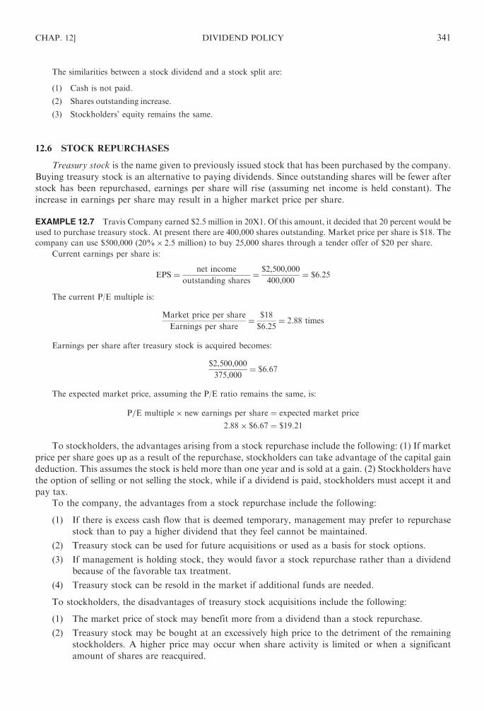
The similarities between a stock dividend and a stock split are:
(1) Cash is not paid.
(2) Shares outstanding increase.
(3) Stockholders’ equity remains the same.
12.6 STOCK REPURCHASES
Treasury stock is the name given to previously issued stock that has been purchased by the company.
Buying treasury stock is an alternative to paying dividends. Since outstanding shares will be fewer after
stock has been repurchased, earnings per share will rise (assuming net income is held constant). The
increase in earnings per share may result in a higher market price per share.
EXAMPLE 12.7 Travis Company earned $2.5 million in 20X1. Of this amount, it decided that 20 percent would be
used to purchase treasury stock. At present there are 400,000 shares outstanding. Market price per share is $18. The
company can use $500,000 (20%� 2.5 million) to buy 25,000 shares through a tender offer of $20 per share.
Current earnings per share is:
EPS ¼ net income
outstanding shares¼ $2,500,000
400,000¼ $6:25
The current P/E multiple is:
Market price per share
Earnings per share¼ $18
$6:25¼ 2:88 times
Earnings per share after treasury stock is acquired becomes:
$2,500,000
375,000¼ $6:67
The expected market price, assuming the P/E ratio remains the same, is:
P=E multiple� new earnings per share ¼ expected market price
2:88� $6:67 ¼ $19:21
To stockholders, the advantages arising from a stock repurchase include the following: (1) If market
price per share goes up as a result of the repurchase, stockholders can take advantage of the capital gain
deduction. This assumes the stock is held more than one year and is sold at a gain. (2) Stockholders have
the option of selling or not selling the stock, while if a dividend is paid, stockholders must accept it and
pay tax.
To the company, the advantages from a stock repurchase include the following:
(1) If there is excess cash flow that is deemed temporary, management may prefer to repurchase
stock than to pay a higher dividend that they feel cannot be maintained.
(2) Treasury stock can be used for future acquisitions or used as a basis for stock options.
(3) If management is holding stock, they would favor a stock repurchase rather than a dividend
because of the favorable tax treatment.
(4) Treasury stock can be resold in the market if additional funds are needed.
To stockholders, the disadvantages of treasury stock acquisitions include the following:
(1) The market price of stock may benefit more from a dividend than a stock repurchase.
(2) Treasury stock may be bought at an excessively high price to the detriment of the remaining
stockholders. A higher price may occur when share activity is limited or when a significant
amount of shares are reacquired.
CHAP. 12] DIVIDEND POLICY 341

To management, the disadvantages of treasury stock acquisition include the following:
(1) If investors feel that the company is engaging in a repurchase plan because its management does
not have alternative good investment opportunities, a drop in the market price of stock may
ensue.
(2) If the reacquisition of stock makes it appear that the company is manipulating the price of its
stock on the market, the company will have problems with the Securities and Exchange
Commission (SEC). Further, if the Internal Revenue Service (IRS) concludes that the repurch-
ase is designed to avoid the payment of tax on dividends, tax penalties may be imposed because
of the improper accumulation of earnings as specified in the tax code.
Review Questions
1. The basic types of dividends are and .
2. Dividends are usually issued .
3. The date that a dividend becomes a legal liability of the corporation is called
the .
4. The right to a dividend stays with the stock until days before the date of
record.
5. The receipt of dividends is favored by stockholders in tax brackets.
6. The dividend payout ratio is equal to divided by .
7. Under a residual-dividend policy, dividends are paid the firm’s investment
needs have been satisfied.
8. A stock dividend provides real income for investors.
9. Mr. X owned 100 shares of $10 par value stock. He then received in exchange 200 shares of $5
par value stock. This is referred to as a(n) .
10. refers to shares reacquired by the company.
Answers: (1) cash, stock; (2) quarterly; (3) declaration date; (4) 2; (5) lower; (6) dividends per share, earnings
per share; (7) after; (8) no; (9) stock split; (10) Treasury stock.
Solved Problems
12.1 Dividends per Share. Lakeside Corporation’s net income for 20X1 was $300,000. It retained
40 percent. The outstanding shares are 100,000. Determine the dividends per share.
342 DIVIDEND POLICY [CHAP. 12

SOLUTION
Dividends
Shares¼ $300,000� 60%
100,000 shares¼ $180,000
100,000¼ $1:80
12.2 Cash Dividend. The Dover Corporation has 10,000 shares of common stock outstanding.
On March 5, the company declared a cash dividend of $5 per share payable to stockholders
of record on April 5. What is the amount of the dividend?
SOLUTION
10,000� $5 ¼ $50,000
12.3 Tax. Ms. Jones is in the 35 percent tax bracket. How much tax will she have to pay in each of the
following cases?
(a) Dividend income ¼ $10,000
(b) Long-term capital gain ¼ $10,000
SOLUTION
(a) $10; 000� $100 ðdividend exclusionÞ ¼ $9,900� 35% ¼ $3,465
(b) $10,000� 40% ðcapital gain rateÞ ¼ $4,000 taxable� 35% ¼ $1,400
12.4 Dividend Policy. Robert Corporation pays out 70 percent of its earnings in the form of dividends.
(a) Evaluate this policy assuming most stockholders are senior citizens in low tax brackets.
(b) Evaluate this policy assuming most stockholders are in high tax brackets.
SOLUTION
(a) A high dividend payout is appropriate in the case of senior citizens since they rely on the fixed income.
Because they are in a low tax bracket, capital gains will not help them that much.
(b) A low dividend payout is called for with high-tax-bracket stockholders. Dividends serve as ordinary
income. Capital gain is most beneficial for them since only 28 percent of the gain is taxable for
securities held more than one year.
12.5 Residual Dividend Policy. The Bears Corporation practices a strict residual dividend policy and
maintains a capital structure of 60 percent debt, 40 percent equity. Earnings for the year are
$5,000. What is maximum amount of capital spending possible without selling new equity?
Suppose that planned investment outlays for the coming year are $12,000. Will Bears be
paying a dividend? If so, how much?
SOLUTION
Bears has a debt-equity ratio of 0.60/0.40=1.50. If the entire $5,000 in earnings were reinvested, then
$5,000� 1.50=$7,500 in new borrowing would be needed to keep the debt-equity ratio unchanged.
Total new financing possible without external equity is thus $5,000+7,500=$12,500. If planned outlays
are $12,000, then this amount will be financed with 40 percent equity. The needed equity is thus
$12,000� 0.40=$4,800. This is less than $5,000 in earnings, so a dividend of $5,000� 4,800=$200 will
be paid.
12.6 Repurchase versus Cash Dividend. Ambers Corporation is deciding whether to pay out $500
in excess cash in the form of an extra dividend or a share repurchase. Current earnings
CHAP. 12] DIVIDEND POLICY 343

are $2.50 per share, and the stock sells for $25. The market value balance sheet before paying out
the $500 is as follows:
Market Value Balance Sheet
(before paying excess cash)
Excess cash $500 Debt $500
Other assets 2,500 Equity 2,500
Total $3,000 Total $3,000
Evaluate the two alternatives in terms of the effect on the price per share of the stock, the EPS,
and the PE ratio.
SOLUTION
The market value of the equity is $2,500. The price per share is $25, so there are 100 shares outstanding. The
cash dividend would amount to $500/100=$5 per share. When the stock goes ex dividend, the price will
drop by $5 per share to $20. In other words, the total assets decrease by $500, so the equity value goes down
by this amount to $2,000. With 100 shares, the new stock price is $20 per share. After the dividend, EPS will
be the same, $2.50, but the PE ratio will be $20/2.50=8 times. With a repurchase, $500/25=20 shares will
be bought up, leaving 80. The equity will again be worth $2,000 total. With 80 shares, this is $2,000/80=$25
share, so the price doesn’t change. Total earnings for Ambers must be $2.50� 100=$250. After the
repurchase, EPS will be higher at $250/$80=$3.125. The PE ratio, however, will be $25/3.125=8 times.
12.7 Market Price per Share. Company A and company B are identical in every respect except for
their dividend policies. Company A pays out a constant percentage of its net income (60 percent
dividends), while company B pays out a constant dollar dividend. Company B’s market price per
share is higher than that of company A. The financial manager of company A does not understand
why her market price per share is lower even though in some good years company A’s
dividends exceed those of company B. Explain.
SOLUTION
The reason why company B has a higher market price per share than company A is because the stock
market looks favorably upon stable dollar dividends. They reflect less uncertainty about the firm.
12.8 External Equity to be Issued. Travis Company’s net income for the year was $3 million. It pays
out 30 percent of its earnings in dividends. The company will acquire $5 million in new assets of
which 35 percent will be financed by debt. What is the amount of external equity that must be
issued?
SOLUTION
Net income $3,000,000
Percent of net income retained �0.7Retained earnings $2,100,000
New assets $5,000,000
Percent financed by equity �0.65Equity financing required $3,250,000
Retained earnings 2,100,000
External equity to be issued $1,150,000
344 DIVIDEND POLICY [CHAP. 12
12.9 Dividend Payout. Most Corporation had a net income of $800,000 in 20X1. Earnings have grown
at an 8 percent annual rate. Dividends in 20X1 were $300,000. In 20X2, the net income was
$1,100,000. This, of course, was much higher than the typical 8 percent annual growth rate. It is
anticipated that earnings will go back to the 8 percent rate in future years. The investment in
20X2 was $700,000.
How much dividend should be paid in 20X2 assuming: (a) a stable dividend payout ratio of
25 percent? (b) a stable dollar dividend policy is maintained? (c) a residual-dividend policy is
maintained and 40 percent of the 20X2 investment is financed with debt? (d ) the investment for
20X2 is to be financed with 80 percent debt and 20 percent retained earnings? Any net income not
invested is paid out in dividends.
SOLUTION
(a) $1,100,000� 25% ¼ $275,000
(b) Dividend in 20X2 is:
$300,000� 1:08 ¼ $324,000
(c) The equity needed is:
$700,000� 60% ¼ $420,000
Because net income is greater than the equity needed, all the $420,000 of equity investment will be
derived from net income.
Dividend ¼ $1,100,000� $420,000 ¼ $680,000
(d ) Earnings retained ¼ $700,000� 20% ¼ $140,000
Dividend ¼ net income� earnings retained
$960,000 ¼ $1,100,000� $140,000
12.10 Trend in Dividends. Many corporations attempt to maintain a sustained rather than a fluctuating
cash dividend per share payment. The payment is gradually adjusted to changes in earnings over
time. As a consequence, corporations apparently establish a target payout ratio range. Explain
why corporation managements desire sustained cash dividends per share with an increasing trend
and attempt to avoid fluctuating cash dividend payments. (CMA, adapted.)
SOLUTION
Corporations tend to follow a policy of sustained cash dividends per share with an increasing and stable
trend over time because they believe that such a dividend policy helps maintain or increase the firm’s
common stock price over time. Corporations following this policy feel that investors will pay a higher
price for the stock of a firm with a stable dividend policy because stability provides investors with a reduced
level of uncertainty regarding the cash returns provided by the firm.
Another argument for a stable dividend policy leading to higher stock price is that many investors look
at cash dividends as a source of funds for their living expenses. Such investors cannot easily plan their
income when dividends are fluctuating. Thus, to assist their planning, investors will pay a premium for stock
with stable dividend policies.
12.11 Dividend Payout. The Xylon Company has experienced rapid growth in the past 5 years. In order
to finance the growth, the board of directors has followed a policy of controlled borrowing, a low
dividend payout ratio, and regular stock dividends.
The percent of debt in the capital structure has remained constant since 20X0. The funds
generated from operations have been reinvested in productive assets. Each January, for the past 4
years, Xylon’s board of directors has declared and paid a 10 percent dividend. A $0.20 per share
cash dividend on the stock outstanding on June 15 has been paid each July for the past 5 years.
Management estimates that the earnings for 20X7 will be $250,000. The closing price of Xylon
Company’s stock at November 30, 20X7 was $25.50 per share.
CHAP. 12] DIVIDEND POLICY 345

The board anticipates a challenge to its intention to continue this dividend policy by two
stockholders who are survivors of two of the founders. Selected data related to the company’s
earnings and dividends are presented below:
Shares
Outstanding as
Cash DividendsMarket
Price per
Share as ofYears Earnings ($) of December 31 Per Share ($) Total Payout ($) December 31 ($)
20X2 100,000 100,000 0.20 20,000 10.00
20X3 120,000 110,000 0.20 22,000 12.00
20X4 144,000 121,000 0.20 24,200 14.30
20X5 172,800 133,100 0.20 26,620 17.00
20X6 207,360 146,410 0.20 29,282 22.00
Prepare a response from the perspective of Xylon Company’s board of directors which
(a) justifies the low cash dividend payout, and (b) rationalizes the use of stock dividends.
(CMA, adapted.)
SOLUTION
(a) The low cash dividend payout is required to finance from internal sources investment opportunities
which exceed the cost of capital in order to continue the income and market value growth pattern
established. Financing growth through retained earnings has been good for the company and the
stockholders, as demonstrated by the increased earnings per share, the increased market price per
share, and the increase in total cash dividends paid because of the annual stock dividends.
(b) The continued use of stock dividends allows stockholders who need cash to sell a few shares without
reducing the original number of shares owned. In addition, those sales can be taxed at the capital gains
rate as opposed to ordinary income rates. This may be important to the shareholders of this company
because they are wealthy and likely to be in high tax brackets. The use of stock dividends increases the
payout in future years even though the dividend rate per share does not increase.
12.12 Stock Dividend. The Benson Corporation has 9,000 shares of common stock having a par value
of $120 outstanding. A 10 percent stock dividend is declared. The fair market value of the stock
is $124 per share.
(a) By how much will retained earnings be reduced? (b) What is the par value of the common
stock to be issued? (c) What is the paid-in capital on common stock?
SOLUTION
(a) 9,000 shares� 10% ¼ 900 shares� $124 ¼ $111,600
(b) 900 shares� $120 ¼ $108,000
(c) 900 shares� $4 ¼ $3,600
12.13 Reformulated Capital Structure. Blake Company’s capital structure on December 30, 20X1, was:
Common stock ($1 par, 100,000 shares) $100,000
Paid-in capital on common stock 20,000
Retained earnings 680,000
Total stockholders’ equity $800,000
The company’s net income for 20X1 was $150,000. It paid out 40 percent of earnings in
dividends. The stock was selling at $6 per share on December 30.
Assuming the company declared a 5 percent stock dividend on December 31, what is the
reformulated capital structure on December 31?
346 DIVIDEND POLICY [CHAP. 12

SOLUTION
The stock dividend is 5,000 shares (5%� 100,000 shares). Retained earnings is reduced by the fair
market value of the stock dividend of $30,000 ($6� 5,000 shares), paid-in capital on common stock is
increased by $25,000 ($5� 5,000 shares), and common stock is increased at the par value of the shares
issued of $5,000 ð$1� 5,000 sharesÞ.The reformulated capital structure on December 31 is:
Common stock ($100,000+$5,000) $105,000
Paid-in capital on common stock
($20,000+$25,000) 45,000
Retained earnings ($680,000� $30,000) 650,000
$800,000
Notice that after the stock dividend, total stockholders’ equity remains the same.
12.14 Stock Split. The Simpson Company has 50,000 shares of common stock having a par value of
$12 per share. The board of directors decided on a 2-for-1 stock split. The market price of the
stock was $20 before the split.
(a) Record the stock split. (b) What will the market price per share be immediately after the
split?
SOLUTION
(a) No entry is needed since the company’s account balances remain the same. However, there should be a
memorandum to the effect that there are now 100,000 shares having a par value of $6 per share.
(b) $10 ($20/2).
12.15 Dividend Last Year. Subsequent to a 3-for-1 stock split, Ace Corporation paid a dividend of $5
per share. This was a 10 percent increase over the prior year’s dividend (before the split).
Determine the dividend for last year.
SOLUTION
Dividend subsequent to split is: $5� 3=$15. Last year’s dividend is:
$15
1:10¼ $13:64
12.16 Earnings per Share. Blake Company’s net income for 20X2 was $3 million. Of this amount,
40 percent will be used to purchase treasury stock. Currently, there are 1 million shares
outstanding and the market price per share is $9.
(a) How many shares can the company buy back through a tender offer of $12 a share? (b)
What is the current earnings per share? (c) What is the current P/E ratio? (d ) What will earnings
per share be after the treasury stock acquisition? (e) What is the expected market price per share
assuming the present P/E ratio remains the same?
SOLUTION
(a) Funds available for repurchase of stock are computed as follows:
$3 million� 40% ¼ $1,200,000
Shares to be repurchased are computed as follows:
$1,200,000
$12¼ 100,000 shares
CHAP. 12] DIVIDEND POLICY 347

(b)EPS ¼ net income
shares outstanding¼ $3,000,000
1,000,000¼ $3
(c)P=E ratio ¼ market price per share
earnings per share¼ $9
$3¼ 3 times
(d )EPS ¼ $3,000,000
900,000¼ $3:333
(e) Market price per share ¼ P=E ratio� new EPS
3� $3:333
348 DIVIDEND POLICY [CHAP. 12

Chapter 13
Term Loans and Leasing
13.1 INTERMEDIATE-TERM BANK LOANS
Intermediate-term loans are loans with a maturity of more than 1 year. Intermediate-term loans are
appropriate when short-term unsecured loans are not, such as when a business is acquired. The interest
rate on an intermediate-term loan is generally higher than on a short-term loan because of the longer
maturity date. The interest rate may be either fixed or variable (according to, for example, changes in the
prime interest rate). The cost of an intermediate-term loan varies with the amount of the loan and the
financial strength of the borrower.
Ordinary intermediate-term loans are payable in periodic equal installments except for the last
payment, which may be higher (referred to as a balloon payment). The schedule of loan payments
should be based on the borrower’s cash flow position to satisfy the debt.
The amortization payment in a term loan equals:
Amortization payment ¼ amount of loan
present value factor
EXAMPLE 13.1 XYZ Company contracts to repay a term loan in five equal year-end installments. The amount of
the loan is $150,000 and the interest rate is 10 percent. The amortization payment each year is:
Amortization payment ¼ amount of loan
present value factor¼ $150; 000
3:7908a¼ $39; 569:48
a Present value of annuity for 5 years at 10 percent.
EXAMPLE 13.2 Charles Company takes out a term loan in 20 year-end annual installments of $2,000 each. The
interest rate is 12 percent. The amount of the loan is:
Amortization payment ¼ amount of loan
present value factor
$2; 000 ¼ amount of loan
7:4694a
Amount of loan ¼ $2; 000� 7,4694 ¼ $14,938:80
a Present value of annuity for 20 years at 12 percent.
The amortization schedule for the first 2 years is:
Year Payment Interesta Principal Balance
0 $14,938.80
1 $2,000 $1,792.66 $207.34 $14,731.46
2 $2,000 $1,767.78 $232.22 $14,499.24
a 12 percent times the balance of the loan at the beginning of the year.
Revolving credit, typically used for seasonal financing, may have a 3-year maturity, but the notes
evidencing the revolving credit are short-term, typically 90 days. The advantages of revolving credit are
349
Copyright © 2007, 1998, 1986 by The McGraw-Hill Companies, Inc. Click here for terms of use.

flexibility and readily available credit. Within the time period of the revolving credit agreement, the
company may renew a loan or engage in additional financing up to a specified maximum amount.
Compared to a line of credit arrangement, there are generally fewer restrictions on revolving credit but at
the cost of a slightly higher interest rate.
Restrictive provisions to protect the lender in an intermediate-term loan agreement may be in the
form of:
1. General provisions used in most agreements which vary depending upon the borrower’s situa-
tion. Examples are working capital and cash dividend requirements.
2. Routine (uniform) provisions that are used universally in most agreements. Examples are the
payment of taxes and the maintenance of proper insurance to assure maximum lender
protection.
3. Specific provisions that are tailored to a given situation. Examples are the placing of limits on
future loans and the carrying of adequate life insurance for executives.
The advantages of intermediate-term loans are:
1. Flexibility in that the terms may be altered as the financing requirements of the company
change.
2. Financial information of the company is kept confidential, since no public issuance is involved.
3. The loan may be arranged quickly, compared to a public offering.
4. It avoids the possible nonrenewal of a short-term loan.
5. Public flotation costs are not involved.
The disadvantages of intermediate-term loans are:
1. Collateral and possible restrictive covenants are required, as opposed to none for commercial
paper and unsecured short-term bank loans.
2. Budgets and financial statements may have to be submitted periodically to the lender.
3. ‘‘Kickers,’’ or ‘‘sweeteners,’’ such as stock warrants or a share of the profits are sometimes
requested by the bank.
13.2 INSURANCE COMPANY TERM LOANS
Insurance companies and other institutional lenders may extend intermediate-term loans to
companies. Insurance companies generally accept loan maturity dates exceeding 10 years, but their
rate of interest is often higher than that of bank loans. Insurance companies do not require
compensating balances, but usually there is a prepayment penalty involved, which is typically not the
case with a bank loan. A company may take out an insurance company loan when it desires a longer
maturity range.
13.3 EQUIPMENT FINANCING
Equipment may serve as collateral for a loan. An advance is made against the market value of
the equipment. The more marketable the equipment is, the higher the advance will be. Also considered is
the cost of selling the equipment. The repayment schedule is designed so that the market value of the
equipment at any given time exceeds the unpaid principal balance of the loan.
Equipment financing may be obtained from banks, finance companies, and manufacturers of
equipment. Equipment loans may be secured by a chattel mortgage or a conditional sales contract.
A chattel mortgage serves as a lien on property except for real estate. In a conditional sales contract,
the seller of the equipment keeps title to it until the buyer has satisfied all the agreed terms; otherwise
the seller will repossess the equipment. The buyer makes periodic payments to the seller over a
350 TERM LOANS AND LEASING [CHAP. 13
specified time period. A conditional sales contract is generally used by small companies with low credit
ratings.
13.4 LEASING
The parties involved in a lease are the lessor, who legally owns the property, and the lessee, who
uses it in exchange for making rental payments.
The following types of leases exist:
1. Operating (service) lease. This type of lease includes both financing and maintenance services.
The lessee leases property that is owned by the lessor. The lessor may be the manufacturer of
the asset or it may be a leasing company that buys assets from the manufacturer to lease to
others. The lease payments required under the contract are generally not sufficient to recover the
full cost of the property. There usually exists a cancelation clause that provides the lessee with
the right to cancel the contract and return the property prior to the expiration date of the
agreement.
2. Financial lease. This type of lease does not typically provide for maintenance services, is
noncancelable, and the rental payments equal the full price of the leased property.
3. Sale and lease-back. With this lease arrangement, a company sells an asset it owns to another
company (usually a financial institution) and then leases it back. This allows the firm to obtain
needed cash from the sale and still have the property for its use.
4. Leveraged lease. In a leveraged lease, there is a third party who serves as the lender. Here, the
lessor borrows money from the lender in order to buy the asset. The property is then leased to
the lessee.
Leasing has several advantages, including the following:
1. Immediate cash outlay is not required.
2. Typically, a purchase option exists, permitting the lessee to obtain the property at
a bargain price at the expiration of the lease. This provides the lessee with the flexibility to
make the purchase decision based on the value of the property at the termination date.
3. The lessor’s expert service is made available.
4. There are generally fewer financing restrictions (e.g., limitations on dividends) placed on the
lessee by the lessor than are imposed when obtaining a loan to buy the asset.
5. The obligation for future rental payment may not have to be reported on the balance sheet.
6. Leasing allows the lessee, in effect, to depreciate land, which is not allowed if land is purchased.
7. In bankruptcy or reorganization, the maximum claim of lessors against the company is 3 years
of lease payments. In the case of debt, creditors have a claim for the total amount of the
unpaid financing.
8. The lessee may avoid having the obsolescence risk of the property if the lessor, in determining
the lease payments, fails to accurately estimate the obsolescence of the asset.
There are several drawbacks to leasing, including the following:
1. A higher cost in the long run than if the asset is purchased.
2. The interest cost associated with leasing is typically higher than the interest cost on debt.
3. If the property reverts to the lessor at termination of the lease, the lessee must either sign a
new lease or buy the property at higher current prices. Also, the salvage value of the property is
realized by the lessor.
4. The lessee may have to retain property no longer needed (i.e., obsolete equipment).
CHAP. 13] TERM LOANS AND LEASING 351
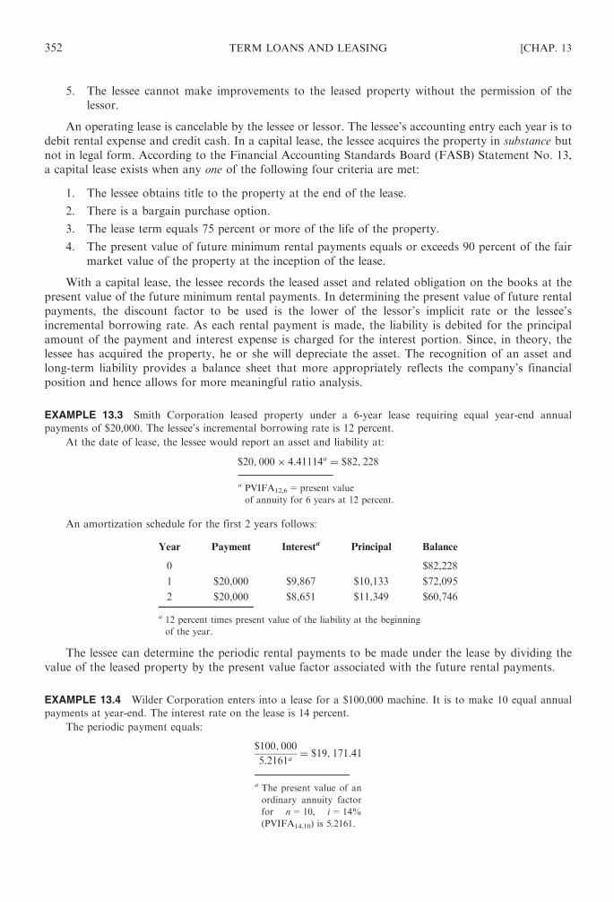
5. The lessee cannot make improvements to the leased property without the permission of the
lessor.
An operating lease is cancelable by the lessee or lessor. The lessee’s accounting entry each year is to
debit rental expense and credit cash. In a capital lease, the lessee acquires the property in substance but
not in legal form. According to the Financial Accounting Standards Board (FASB) Statement No. 13,
a capital lease exists when any one of the following four criteria are met:
1. The lessee obtains title to the property at the end of the lease.
2. There is a bargain purchase option.
3. The lease term equals 75 percent or more of the life of the property.
4. The present value of future minimum rental payments equals or exceeds 90 percent of the fair
market value of the property at the inception of the lease.
With a capital lease, the lessee records the leased asset and related obligation on the books at the
present value of the future minimum rental payments. In determining the present value of future rental
payments, the discount factor to be used is the lower of the lessor’s implicit rate or the lessee’s
incremental borrowing rate. As each rental payment is made, the liability is debited for the principal
amount of the payment and interest expense is charged for the interest portion. Since, in theory, the
lessee has acquired the property, he or she will depreciate the asset. The recognition of an asset and
long-term liability provides a balance sheet that more appropriately reflects the company’s financial
position and hence allows for more meaningful ratio analysis.
EXAMPLE 13.3 Smith Corporation leased property under a 6-year lease requiring equal year-end annual
payments of $20,000. The lessee’s incremental borrowing rate is 12 percent.
At the date of lease, the lessee would report an asset and liability at:
$20; 000� 4:41114a ¼ $82; 228
a PVIFA12,6=present value
of annuity for 6 years at 12 percent.
An amortization schedule for the first 2 years follows:
Year Payment Interesta Principal Balance
0 $82,228
1 $20,000 $9,867 $10,133 $72,095
2 $20,000 $8,651 $11,349 $60,746
a 12 percent times present value of the liability at the beginning
of the year.
The lessee can determine the periodic rental payments to be made under the lease by dividing the
value of the leased property by the present value factor associated with the future rental payments.
EXAMPLE 13.4 Wilder Corporation enters into a lease for a $100,000 machine. It is to make 10 equal annual
payments at year-end. The interest rate on the lease is 14 percent.
The periodic payment equals:
$100; 000
5:2161a¼ $19; 171:41
a The present value of an
ordinary annuity factor
for n=10, i=14%
(PVIFA14,10) is 5.2161.
352 TERM LOANS AND LEASING [CHAP. 13
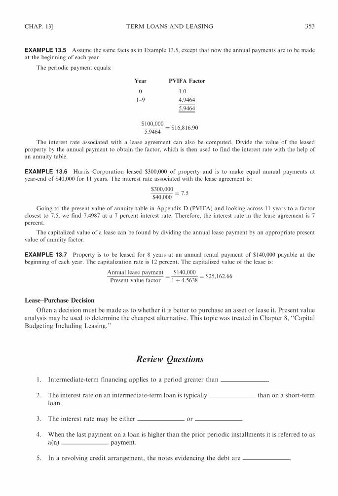
EXAMPLE 13.5 Assume the same facts as in Example 13.5, except that now the annual payments are to be made
at the beginning of each year.
The periodic payment equals:
Year PVIFA Factor
0 1.0
1–9 4.9464
5.9464
$100,000
5:9464¼ $16,816:90
The interest rate associated with a lease agreement can also be computed. Divide the value of the leased
property by the annual payment to obtain the factor, which is then used to find the interest rate with the help of
an annuity table.
EXAMPLE 13.6 Harris Corporation leased $300,000 of property and is to make equal annual payments at
year-end of $40,000 for 11 years. The interest rate associated with the lease agreement is:
$300,000
$40,000¼ 7:5
Going to the present value of annuity table in Appendix D (PVIFA) and looking across 11 years to a factor
closest to 7.5, we find 7.4987 at a 7 percent interest rate. Therefore, the interest rate in the lease agreement is 7
percent.
The capitalized value of a lease can be found by dividing the annual lease payment by an appropriate present
value of annuity factor.
EXAMPLE 13.7 Property is to be leased for 8 years at an annual rental payment of $140,000 payable at the
beginning of each year. The capitalization rate is 12 percent. The capitalized value of the lease is:
Annual lease payment
Present value factor¼ $140,000
1þ 4:5638¼ $25,162:66
Lease–Purchase Decision
Often a decision must be made as to whether it is better to purchase an asset or lease it. Present value
analysis may be used to determine the cheapest alternative. This topic was treated in Chapter 8, ‘‘Capital
Budgeting Including Leasing.’’
Review Questions
1. Intermediate-term financing applies to a period greater than .
2. The interest rate on an intermediate-term loan is typically than on a short-term
loan.
3. The interest rate may be either or .
4. When the last payment on a loan is higher than the prior periodic installments it is referred to as
a(n) payment.
5. In a revolving credit arrangement, the notes evidencing the debt are .
CHAP. 13] TERM LOANS AND LEASING 353

6. Restrictive provisions in a loan agreement that vary, based on the borrower’s situation, are
referred to as provisions.
7. A restriction in a loan agreement that puts a limitation on the borrower’s future loans is
referred to as a(n) provision.
8. A chattel mortgage has a lien against property except for .
9. In a(n) , the seller of equipment retains title until the purchaser has met the
terms of the contract.
10. In a(n) lease, there is a third party who acts as the lender.
11. When a company sells an asset it owns and then leases it back, this is referred to as
a(n) arrangement.
12. In an operating lease, the entry each year is to debit and
credit .
13. In a(n) lease, the lessee records the leased property on his or her books as
an asset at the of future minimum rental payments.
14. One of the criteria for a capital lease is that the lease term equals or exceeds of
the life of the property.
15. The lessor can pass the on to the lessee.
Answers: (1) 1 year; (2) higher; (3) fixed, variable; (4) balloon; (5) short-term; (6) general; (7)
specific; (8) real estate; (9) conditional sales contract; (10) leveraged; (11) sale and lease-back; (12) rent
expense, cash; (13) capital, present value; (14) 75 percent; (15) investment tax credit.
Solved Problems
13.1 Intermediate-Term Loans. What are the advantages and disadvantages to intermediate-term
loans?
SOLUTION
The advantages of intermediate-term loans are as follows:
1. Flexibility exists regarding terms, since they may be modified based on the changing financial
condition of the entity.
2. No public disclosure of the company’s financial data is required.
3. The loan may be obtained quickly relative to a public issuance.
The disadvantages of intermediate-term loans are as follows:
1. The company may have to put up collateral.
2. Budgets and financial statements may have to be periodically submitted to the lender.
3. There is a specified maturity date for repayment.
4. The company may have to give the bank ‘‘sweeteners’’ for the loan, such as a share of its net income.
354 TERM LOANS AND LEASING [CHAP. 13

13.2 Amortization Payment. ABC Company agrees to pay a $50,000 loan in eight equal year-end
payments. The interest rate is 12 percent.
(a) What is the annual payment? (b) What is the total interest on the loan?
SOLUTION
(a) Amortization payment ¼ amount of loan
present value factor¼ $50,000
4:9676¼ $10,065:22
(b) Total payments (8� $10,065.22) $80,521.76
Principal 50,000.00
Interest $30,521.76
13.3 Amount of Loan. Bank Corporation takes out a term loan payable in five year-end annual
installments of $3,000 each. The interest rate is 10 percent. What is the amount of the loan?
SOLUTION
$3,000� 3:7908 ¼ $11,372:40
13.4 Amortization Schedule. Using the data in Problem 13.3: (a) prepare an amortization schedule for
the loan repayment; and (b) explain why the interest is declining over the loan period.
SOLUTION
(a) Year Payment ($) Interest ($) Principal ($) Balance ($)
0 11,372.40
1 3,000 1,137.24 1,862.76 9,509.64
2 3,000 950.96 2,049.04 7,460.60
3 3,000 746.06 2,253.94 5,206.66
4 3,000 520.67 2,479.33 2,727.33
5 3,000 272.73 2,727.33a
a Adjusted for slight rounding difference.
(b) Interest is declining because the balance of the loan decreases over time.
13.5 Leasing. What are the advantages and disadvantages of leasing?
SOLUTION
The advantages of leasing include the following:
1. It is not necessary to pay out cash immediately.
2. The lease contract often provides a bargain purchase option that permits the lessee to buy the
property for a nominal sum at the lease termination date.
3. Typically, the service technology of the lessor is made available.
4. There are generally fewer financing restrictions set out by the lessor relative to those imposed under
other modes of financing.
5. In an operating lease, the lessee does not have to report a liability on his or her books.
The disadvantages of leasing include the following:
1. In the long run, the cost of leasing is higher than the cost of buying.
2. If the lessor receives the property at the end of the lease, the lessee must either enter into a new lease
agreement or purchase the property at high current prices.
3. The lessee may have to keep obsolete property.
CHAP. 13] TERM LOANS AND LEASING 355

13.6 Periodic Payment. Bard Corporation leases a $75,000 machine. It is required to make 15 equal
annual payments at year-end. The interest rate on the lease is 16 percent. What is the periodic
payment?
SOLUTION
$75,000
5:575¼ $13,452:91
13.7 Periodic Payment. Assume the same information as in Problem 13.6, except that now the annual
payments are to be made at the beginning of the year. What is the periodic payment?
SOLUTION
$75,000
1þ 5:468¼ $75,000
6:468¼ $11,595:55
13.8 Interest Rate. Tint Corporation leased $150,000 of equipment and is to make equal year-end
annual payments of $22,000 for 15 years. What is the interest rate on the lease?
SOLUTION
$150,000
$22,000¼ 6:818
Going to the present value of annuity table in Appendix D and looking across 15 years to a factor
closest to 6.818, we find 6.811 at a 12 percent interest rate.
13.9 Capitalized Value of Lease. Property is to be leased for 15 years at an annual rental payment of
$40,000 payable at the beginning of each year. The capitalization rate is 10 percent. What is the
capitalized value of the lease?
SOLUTION
Annual lease payment
Present value factor¼ $40,000
1þ 7:3667¼ $4,780:86
356 TERM LOANS AND LEASING [CHAP. 13

Chapter 14
Long-term Debt
14.1 INTRODUCTION
This chapter discusses the characteristics, advantages, and disadvantages of long-term debt
financing. In addition to the various types of debt instruments, the circumstances in which a particular
form of debt is most appropriate are mentioned. Bond refunding is also highlighted.
In formulating a financing strategy in terms of source and amount, consider the following:
1. The cost and risk associated with alternative financing strategies.
2. The future trend in capital market conditions and how they will affect future fund availability
and interest rates.
3. The existing ratio of debt to equity.
4. The maturity dates of present debt instruments.
5. The existing restrictions in loan agreements.
6. The type and amount of collateral required by long-term creditors.
7. The ability to alter financing strategy to adjust to changing economic conditions.
8. The amount, nature, and stability of internally generated funds.
9. The adequacy of present lines of credit for current and future needs.
10. The inflation rate, since with debt the repayment is made in cheaper dollars.
11. The earning power and liquidity position of the firm.
12. The tax rate.
Sources of long-term debt include mortgages and bonds.
14.2 MORTGAGES
Mortgages represent notes payable that have as collateral real assets and require periodic payments.
Mortgages can be issued to finance the acquisition of assets, construction of plant, and modernization of
facilities. The bank will require that the value of the property exceed the mortgage on that property.
Most mortgage loans are for between 70 percent and 90 percent of the value of the collateral. Mortgages
may be obtained from a bank, life insurance company, or other financial institution. It is easier to obtain
mortgage loans for multiple-use real assets than for single-use real assets.
There are two kinds of mortgages: a senior mortgage, which has first claim on assets and earnings,
and a junior mortgage, which has a subordinate lien.
A mortgage may have a closed-end provision that prevents the firm from issuing additional debt of
the same priority against the same property. If the mortgage is open-ended, the company can issue
additional first-mortgage bonds against the property.
Mortgages have a number of advantages, including favorable interest rates, less financing
restrictions, and extended maturity date for loan repayment.
14.3 BONDS PAYABLE
Long-term debt principally takes the form of bonds payable and loans payable. A bond is a
certificate indicating that the company has borrowed a given sum of money that it agrees to repay
at a future date. A written agreement, called an indenture, describes the features of the particular
357
Copyright © 2007, 1998, 1986 by The McGraw-Hill Companies, Inc. Click here for terms of use.

bond issue. The indenture is a contract between the company, the bondholder, and the trustee. The
trustee makes sure that the company is meeting the terms of the bond contract. In many cases, the trustee
is the trust department of a commercial bank. Although the trustee is an agent for the bondholder, it is
selected by the company prior to the issuance of the bonds. The indenture provides for certain restric-
tions on the company such as a limitation on dividends and minimum working capital requirements. If a
provision of the indenture is violated, the bonds are in default. The indenture may also have a negative
pledge clause, which precludes the issuance of new debt that would take priority over existing debt in the
event the company is liquidated. The clause can apply to assets currently held as well as to assets that
may be purchased in the future.
Interest
Bonds are issued in $1,000 denominations. Many bonds have maturities of 10 to 30 years. The
interest payment to the bondholder is called nominal interest, which is the interest on the face of
the bond. It is equal to the coupon (nominal) interest rate times the face value of the bond. Although
the interest rate is stated on an annual basis, interest on a bond is usually paid semiannually. Interest
expense is tax-deductible.
EXAMPLE 14.1 A company issues a 20 percent, 20-year bond. The tax rate is 46 percent. The annual after-tax cost
of the debt is:
20%� 54% ¼ 10:8%
EXAMPLE 14.2 A company issues a $100,000, 12 percent, 10-year bond. The semiannual interest payment is:
$100,000� 12%� 612¼ $6,000
Assuming a tax rate of 30 percent, the after-tax semiannual interest dollar amount is:
$6,000� 70% ¼ $4,200
A bond sold at face value is said to be sold at 100. If a bond is sold below its face value, it is being
sold at less than 100 and is issued at a discount. If a bond is sold above face value, it is being sold at more
than 100, that is, sold at a premium. A bond may be sold at a discount when the interest rate on the bond
is below the prevailing market interest rate for that type of security. A bond is sold at a premium
when the opposite market conditions exist. The discount or premium is amortized over the life of the
bond. The amortized discount is a tax-deductible expense, while the amortized premium is income
subject to tax.
Bond issue costs, also a tax-deductible expense, must also be amortized over the life of the bond.
EXAMPLE 14.3 Travis Corporation issues a $100,000, 14 percent, 20-year bond at 94. The maturity value of the
bond is $100,000. Annual cash interest payment is:
14%� $100,000 ¼ $14,000
The proceeds received for the issuance of the bond is:
94%� $100,000 ¼ $94,000
The amount of the discount is:
$100,000� $94,000 ¼ $6,000
The annual discount amortization is:
$6,000
20¼ $300
EXAMPLE 14.4 A bond having a face value of $100,000 with a 25-year life was sold at 102. The tax rate is
40 percent. The bond was sold at a premium since it was issued above face value. The total premium is $2,000
358 LONG-TERM DEBT [CHAP. 14

($100,000� 0.02). The annual premium amortization is $80 ($2,000/25). The after-tax effect of the premium
amortization is $48 ($80� 60%).
The yield on a bond is the effective interest rate the company is incurring on that bond. The two methods of
computing yield are the simple yield and the yield to maturity. These were fully discussed in Chapter 7.
The price of a bond depends on several factors such as its maturity date, interest rate, and collateral.
EXAMPLE 14.5 Harris Corporation’s 6 percent income bonds are due in 20X5 and are selling at $855. The
company’s 512% first-mortgage bonds are due in 20X0 and are selling at $950. The first-mortgage bonds which
have a lower interest rate compared to the income bonds are selling at a higher price because (1) the bonds are closer
to maturity, and (2) the bonds are backed by collateral.
Also, interest is not paid on the income bonds unless there are corporate earnings. This makes them unattractive
and hence they will be selling at a lower price.
Types of Bonds
The various types of bonds that may be issued are:
1. Debentures. Because debentures represent unsecured debt, they can be issued only by large,
financially strong companies with excellent credit ratings.
2. Subordinated debentures. The claims of the holders of these bonds are subordinated to those of
senior creditors. Debt having a prior claim over the subordinated debentures is set forth in the
bond indenture. Typically, in the event of liquidation, subordinated debentures come after
short-term debt.
3. Mortgage bonds. These are bonds secured by real assets.
4. Collateral trust bonds. The collateral for these bonds is the issuer’s security investments (bonds
or stocks), which are given to a trustee for safekeeping.
5. Convertible bonds. These may be converted to stock at a later date based on a specified
conversion ratio. Convertible bonds are typically issued in the form of subordinated
debentures. Convertible bonds are more marketable and are typically issued at a lower interest
rate than are regular bonds. Of course, if bonds are converted to stock, debt repayment is
not involved. Convertible bonds are discussed in detail in Chapter 16, ‘‘Warrants and
Convertibles.’’
6. Income bonds. These bonds require the payment of interest only if the issuer has earnings.
However, since interest accumulates regardless of earnings, the interest, if bypassed, must be
paid in a later year when sufficient earnings exist.
7. Guaranteed bonds. These are debt issued by one party with payment guaranteed by another
party.
8. Serial bonds. A specified portion of these bonds comes due each year. At the time serial bonds
are issued, a schedule is given showing the yields, interest rates, and prices applicable with each
maturity. The interest rate on the shorter maturities is lower than the interest rate on the longer
maturities. Serial bonds are primarily issued by government agencies.
9. Inflation-linked bonds. These bonds have coupons (and the principal amount as well) that are
adjusted according to the rate of inflation. The US Treasury Inflation Protection Securities
(TIPS) is an example.
10. Zero coupon bonds. These bonds do not pay interest; the return to the holder is in the form of
appreciation in price. Lower interest rates may be available for zero coupon bonds (and deep
discount bonds) because they cannot be called.
11. Floating (variable)-rate bonds. The interest rates on the bonds are adjusted periodically to
reflect changes in money market conditions (e.g., prime interest rate). These bonds are popular
when future interest rates and inflation are uncertain.
12. Eurobonds. Eurobonds are issued outside the country in whose currency the bonds are
denominated. Dollar-denominated Eurobonds cannot be sold by US issuers to US
CHAP. 14] LONG-TERM DEBT 359

investors. They may be sold only to foreign investors, because they are not registered with
the Securities and Exchange Commission (SEC).
13. Catastrophe (cat) bonds. These bonds are issued mostly by insurance companies to cover
extraordinary losses.
14. Put bonds. These bonds allow the holder to force the issuer to buy the bond back at a stated
price.
Bond Ratings
Financial advisory services (e.g., Standard and Poor’s, and Moody’s) rate publicly traded
bonds according to risk in terms of the receipt of principal and interest. An inverse relationship
exists between the quality of a bond issue and its yield. That is, low-quality bonds will have a
higher yield than high-quality bonds. Thus, a risk-return trade-off exists for the bondholder.
Bond ratings are important to financial management because they influence marketability and the
cost associated with the bond issue.
EXAMPLE 14.6 The following bond ratings are used by Moody’s and Standard & Poor’s:
Investment—Quality Bond Ratings
Low-Quality, Speculative,
and/or ‘‘junk’’ Bond Ratings
High Quality Medium Grade Low Grade Very Low Grade
Standard & Poor’s AAA AA A BBB BB B CCC CC C D
Moody’s Aaa Aa A Baa Ba B Caa Ca C D
14.4 DEBT FINANCING
The advantages of issuing long-term debt include:
1. Interest is tax-deductible, while dividends are not.
2. Bondholders do not participate in superior earnings of the firm.
3. The repayment of debt is in cheaper dollars during inflation.
4. There is no dilution of company control.
5. Financing flexibility can be achieved by including a call provision in the bond indenture.
A call provision allows the company to pay the debt before the expiration date of the bond.
6. It may safeguard the company’s future financial stability, for example, in times of tight money
markets when short-term loans are not available.
The disadvantages of issuing long-term debt include:
1. Interest charges must be met regardless of corporate earnings.
2. Debt must be repaid at maturity.
3. Higher debt infers greater risk in the capital structure, which may increase the cost of capital.
4. Indenture provisions may place stringent restrictions on the company.
5. Overcommitments may arise due to forecasting errors.
To investors, bonds have the following advantages:
1. There is a fixed interest payment each year.
2. Bonds are safer than equity securities.
360 LONG-TERM DEBT [CHAP. 14

To investors, bonds have the following disadvantages:
1. They do not participate in incremental profitability.
2. There is no voting right.
The proper mixture of long-term debt to equity in a company depends on the type of organization,
credit availability, and after-tax cost of financing. Where a high degree of financial leverage exists, the
firm may wish to take steps to minimize other corporate risks.
Debt financing is more appropriate when:
1. Stability in revenue and earnings exists.
2. There is a satisfactory profit margin.
3. There is a good liquidity and cash flow position.
4. The debt/equity ratio is low.
5. Stock prices are currently depressed.
6. Control considerations are a primary factor.
7. Inflation is expected.
8. Bond indenture restrictions are not burdensome.
An entity experiencing financial difficulties may wish to refinance short-term debt on a long-term
basis such as by extending the maturity dates of existing loans. This may alleviate current liquidity and
cash flow problems.
As the default risk of the firm becomes higher, so the interest rate will become high on the debt to
compensate for the greater risk.
EXAMPLE 14.7 Ari Corporation has $10 million of 12 percent mortgage bonds outstanding. The indenture
permits additional bonds to be issued provided all the following conditions are satisfied:
1. The pretax times-interest-earned ratio exceeds 5.
2. Book value of the mortgaged assets are at least 1.5 times the amount of debt.
3. The debt/equity ratio is below 0.6.
The following additional information is provided:
1. Income before tax is $9 million.
2. Equity is $30 million.
3. Book value of assets is $34 million.
4. There are no sinking fund payments for the current year. (A sinking fund is money set aside to be used to
retire a bond issue.)
5. Half the proceeds of a new issue would be added to the base of mortgaged assets.
Only $7 million more of 12 percent debt can be issued based on the following calculations:
1. The before-tax times-interest-earned ratio is:
Income before tax and interest
Interest¼ $9,000,000þ $1,200,000a
$1,200,000þ 0:12X¼ 5
$10,200,000
$1,200,000þ 0:12X¼ 5
$10,200,000 ¼ $6,000,000þ 0:60X
X ¼ $7,000,000
a Interest is:
$10,000,000� 0.12=$1,200,000
CHAP. 14] LONG-TERM DEBT 361
2. Book value of mortgaged assets
Debt¼ $34,000,000þ 0:5X
$10,000,000þ X¼ 1:5
$34,000,000þ 0:5X ¼ $15,000,000þ 1:5X
X ¼ $19,000,000
3. Debit
Equity¼ $10,000,000þ X
$30,000,000¼ 0:6
$10,000,000þ X ¼ $18,000,000
X ¼ $8,000,000
The first condition is controlling and hence limits the amount of new debt to $7 million.
14.5 BOND REFUNDING
Bonds may be refunded by the company prior to maturity through either the issuance of a serial
bond or exercising a call privilege on a straight bond. The issuance of serial bonds allows the company to
refund the debt over the life of the issue. A call feature in a bond enables the issuer to retire it before the
expiration date. The call feature is included in many corporate bond issues.
When future interest rates are anticipated to decline, a call provision in the bond issue is
recommended. Such a provision enables the firm to buy back the higher-interest bond and issue a
lower-interest one. The timing for the refunding depends on expected future interest rates. A call
price is usually established in excess of the face value of the bond. The resulting call premium equals
the difference between the call price and the maturity value. The issuer pays the premium to the
bondholder in order to acquire the outstanding bonds before the maturity date. The call premium is
generally equal to 1 year’s interest if the bond is called in the first year, and it declines at a constant rate
each year thereafter. Also involved in selling a new issue are flotation costs. Both the call premium and
flotation costs are tax-deductible expenses.
A bond with a call provision typically will be issued at an interest rate higher than one without the
call provision. The investor prefers not to have a situation where the company can buy back the bond at
its option prior to maturity. This is because the company will tend to buy back high-interest bonds early
and issue lower-interest bonds when interest rates decline. The investor would obviously want to hold
onto a high-interest bond when prevailing interest rates are low.
EXAMPLE 14.8 A $100,000, 10 percent, 20-year bond is issued at 95. The call price is 102. Four years after issue
the bond is called. The call premium is equal to:
Call price $102,000
Face value of bond 100,000
Call premium $ 2,000
EXAMPLE 14.9 A $40,000 callable bond was issued. The call price is 104. The tax rate is 35 percent. The after-tax
cost of calling the issue is:
$40,000� 0:04� 0:65 ¼ $1,040
The desirability of refunding a bond requires present value analysis. The present value technique was discussed
in Chapter 8, ‘‘Capital Budgeting.’’
EXAMPLE 14.10 Tracy Corporation has a $20 million, 10 percent bond issue outstanding that has 10 years to
maturity. The call premium is 7 percent of face value. New 10-year bonds in the amount of $20 million can be issued
at an 8 percent interest rate. Flotation costs associated with the new issue are $600,000.
362 LONG-TERM DEBT [CHAP. 14

Refunding of the original bond issue should take place as shown below.
Old interest payments
($20,000,000� 0.10) $2,000,000
New interest payments
($20,000,000� 0.08) 1,600,000
Annual savings $ 400,000
Call premium ($20,000,000� 0.07) $1,400,000
Flotation cost 600,000
Total cost $2,000,000
Year Calculation Present Value
Year 0 �$2,000,000� 1 �$2,000,000Years 1–10 $ 400,000� 6.71a +2,684,000
Net present value $ 684,000
a Present value of annuity factor for i=8%, n=10.
EXAMPLE 14.11 Ace Corporation is considering calling a $10 million, 20-year bond that was issued 5 years ago at
a nominal interest rate of 10 percent. The call price on the bonds is 105. The bonds were initially sold at 90. The
discount on bonds payable at the time of sale was, therefore, $1 million and the net proceeds received were $9
million. The initial flotation cost was $100,000. The firm is considering issuing $10 million, 8 percent, 15-year bonds
and using the net proceeds to retire the old bonds. The new bonds will be issued at face value. The flotation cost for
the new issue is $150,000. The company’s tax rate is 46 percent. The after-tax cost of new debt ignoring flotation
costs, is 4.32 percent (8%� 54%). With the flotation cost, the after-tax cost of new debt is estimated at 5 percent.
There is an overlap period of 3 months in which interest must be paid on the old and new bonds.
The initial cash outlay is:
Cost to call old bonds
($10,000,000� 105%) $10,500,000
Cost to issue new bond 150,000
Interest on old bonds for overlap period
($10,000,000� 10%� 3/12) 250,000
Initial cash outlay $10,900,000
The initial cash inflow is:
Proceeds from selling new bond $10,000,000
Tax-deductible items
Call premium $500,000
Unamortized discount
($1,000,000� 15/20) 750,000
Overlap in interest
($10,000,000� 10%� 3/12) 250,000
Unamortized issue cost of old bond
($100,000� 15/20) 75,000
Total tax-deductible items $1,575,000
Tax rate �0.46Tax savings 724,500
Initial cash inflow $10,724,500
CHAP. 14] LONG-TERM DEBT 363

The net initial cash outlay is therefore:
Initial cash outlay $10,900,000
Initial cash inflow 10,724,500
Net initial cash outlay $ 175,500
The annual cash flow for the old bond is:
Interest (10%� $10,000,000) $1,000,000
Less: Tax-deductible items
Interest $1,000,000
Amortization of discount
($1,000,000/20 years) 50,000
Amortization of issue cost
($100,000/20 years) 5,000
Total tax-deductible items $1,055,000
Tax rate �0.46Tax savings 485,300
Annual cash outflow with old bond $ 514,700
The annual cash flow for the new bond is:
Interest $800,000
Less: Tax-deductible items
Interest $800,000
Amortization of issue cost
($150,000/15 years) 10,000
Total tax-deductible items $810,000
Tax rate �0.46Tax savings 372,600
Annual cash outflow with new bond $427,400
The net annual cash savings with the new bond compared to the old bond is:
Annual cash outflow with old bond $514,700
Annual cash outflow with new bond 427,400
Net annual cash savings $ 87,300
The net present value associated with the refunding is:
Calculation Present Value
Year 0 �$175,500� 1 �$175,500Years 1–15 $87,300� 10.38a +906,174
Net present value $730,674
a Present value of annuity factor i=5%, n=15,=PVIFA5,15
Since a positive net present value exists, the refunding of the old bond should be made.
364 LONG-TERM DEBT [CHAP. 14

Sinking fund requirements may exist with regard to a bond issue. With a sinking fund, the company
is required to set aside money to purchase and retire a portion of the bond issue each year. Usually, there
is a mandatory fixed amount that must be retired, but occasionally the retirement may relate to the
company’s sales or profit for the current year. If a sinking fund payment is not made, the bond issue may
be in default.
In many cases, the company can handle the sinking fund in one of the following two ways:
1. It can call a given percentage of the bonds at a stipulated price each year, for example, 5 percent
of the original amount at a price of $1,080.
2. It can buy its own bonds on the open market.
The least expensive alternative should be selected. If interest rates have increased, the price of the
bonds will have decreased, and the open market option should be used. If interest rates have decreased,
the bond prices will have increased, and so calling the bonds is the preferred choice.
EXAMPLE 14.12 XYZ Company has to reduce bonds payable by $300,000. The call price is 104. The market price
of the bonds is 103. The company will elect to buy back the bonds on the open market because it is less expensive, as
indicated below.
Call price ($300,000� 104%) $312,000
Purchase on open market
($300,000� 103%) 309,000
Advantage of purchasing bonds
on the open market $ 3,000
Review Questions
1. A(n) mortgage prohibits the company from issuing further debt of the same
priority against the property.
2. A(n) is the written agreement specifying the terms of a bond issue.
3. A(n) clause in a bond agreement prevents the issuance of new debt having
priority over existing debt.
4. Bonds are stated in $ denominations.
5. The interest payment based on the face value of a bond is called interest.
6. As the maturity date of a bond lengthens, the interest rate .
7. When a bond is sold at an amount in excess of its face value, it is sold at a(n) .
8. A(n) is an unsecured bond.
9. A(n) bond pays interest only if the issuer has earnings.
10. Bond issues that mature periodically are called bonds.
CHAP. 14] LONG-TERM DEBT 365

11. The issuance of bonds has an advantage in times in that the company will be
paying back the debt in dollars.
12. A(n) provision enables the firm to buy back bonds at a date prior to maturity.
13. is tax-deductible, whereas dividends are not.
Answers: (1) closed-end; (2) indenture; (3) negative pledge; (4) 1,000; (5) nominal; (6) increases; (7) pre-
mium; (8) debenture; (9) income; (10) serial; (11) inflationary, cheaper; (12) call; (13) Interest.
Solved Problems
14.1 Interest. A company issues a $300,000, 10 percent, 20-year bond. The tax rate is 40 percent. What
is the after-tax semiannual interest dollar amount?
SOLUTION
$300,000� 10%� 612¼ $15,000 ðbefore taxesÞ
$15,000� 60% ¼ $9,000 ðafter taxesÞ
14.2 Bond Issuance. Boxer Corporation issues a $300,000, 16 percent, 10-year bond at 108.
(a) What is the maturity value? (b) What is the annual cash interest payment? (c) What are
the proceeds the company receives upon issuance of the bond? (d ) What is the amount of the
premium? (e) What is the annual premium amortization?
SOLUTION
ðaÞ $300,000
ðbÞ 16%� $300,000 ¼ $48,000
ðcÞ 108%� $300,000 ¼ $324,000
ðd Þ $324,000� $300,000 ¼ $24,000
ðeÞ $24,000
10¼ $2,400
14.3 Amortization. A bond with a face value of $200,000 with a 20-year life was sold at 105. The tax
rate is 35 percent. What is the after-tax effect of the premium amortization?
SOLUTION
Total premium is:
$200,000� 0:05 ¼ $10,000
Annual premium amortization is:
$10,000
20¼ $500
After-tax effect of premium amortization is:
$500� 0:65 ¼ $325
366 LONG-TERM DEBT [CHAP. 14

14.4 Bond Ratings. Match the description in column A with Moody’s bond rating in column B.
Column A Column B
(a) Speculative (1) C
(b) Prime quality (2) Aaa
(c) Lowest grade (3) Ba
(d ) Lower medium grade (4) B
(e) Near or in default (5) Ca
SOLUTION
(a) (4); (b) (2); (c) (1); (d ) (3); (e) (5).
14.5 Bond Rating. The two bond rating agencies, Moody’s and Standard & Poor’s, lowered the ratings
on Appleton Industries’ bonds from triple-A to double-A in response to operating trends revealed
by the financial reports of recent years. The change in the ratings is of considerable concern to the
Appleton management because the company plans to seek a significant amount of external
financing within the next 2 years.
(a) Identify several events or circumstances which could have occurred in the operations of
Appleton Industries which could have influenced the factors the bond rating agencies use to
evaluate the firm and, as a result, caused the bond rating agencies to lower Appleton’s bond
rating. (b) If Appleton Industries maintains its present capital structure, what effect will the lower
bond ratings have on the company’s weighted average cost of capital? Explain your answer. (c) If
Appleton Industries’ capital structure was at an optimal level before the rating of its bonds was
changed, explain what effect the lower bond ratings will have on the company’s optimal capital
structure. (CMA, adapted.)
SOLUTION
(a) Factors or circumstances which could have caused the rating agencies to lower the bond rating of
Appleton Industries include:
1. Lowered long-term solvency reflected by a reduction in the times-interest-earned ratio or a
reduction in the fixed-charge-coverage ratio
2. Lowered short-term liquidity reflected by a decrease in the current or quick ratios
3. Lowered profitability reflected by a reduced market share, lower return on sales, or decreased
profits
4. An increased risk of financial stability due to major pending litigation which would be damaging to
the firm or a large increase in earnings variability
5. A major change in management which is perceived negatively by the financial community
(b) The weighted average cost of capital can be expected to rise. The lower bond rating is usually relied
upon as an indication of greater risk being assumed by the bond investors. This change will be noted by
the investors of other Appleton securities. Thus the investors in each capital component of Appleton
Industries can be expected to require a higher return.
(c) Appleton Industries’ capital structure will shift toward greater equity with less debt. The fact that the
bond rating was lowered would indicate to investors that the risk has increased. To reduce the risk and
minimize the increase in the cost of capital, the optimal capital structure will have to shift toward one
with an increased percentage of equity.
14.6 Amount of Debt. Boston Corporation has $30 million of 10 percent mortgage bonds outstanding.
The indenture allows the issuance of additional bonds provided the following conditions are met:
(1) The before-tax times-interest-earned ratio exceeds 4; (2) book value of the mortgaged assets is
at least two times the amount of debt; and (3) the debt/equity ratio is less than 0.5.
CHAP. 14] LONG-TERM DEBT 367

The following additional data are provided: (1) Income before tax is $11 million; (2) equity is
$90 million; (3) book value of mortgaged assets is $80 million; and (4) forty percent of the
proceeds of a new issue would be added to the base of mortgaged assets.
How much additional debt can be issued?
SOLUTION
The before-tax times-interest-earned ratio is:
Income before tax and interest
Interest¼ $11,000,000þ $3,000,000a
$3,000,000þ 0:10X¼ 4
$14,000,000
$3,000,000þ 0:10X¼ 4
$14,000,000 ¼ $12,000,000þ 0:40X
X ¼ $5,000,000
a Interest $30,000,000� 0.10=$3,000,000
The book value of the mortgaged assets is:
Book value of mortgaged assets
Debt¼ $80,000,000þ 0:4X
$30,000,000þ X¼ 2
$80,000,000þ 0:4X ¼ $60,000,000þ 2X
X ¼ $12,500,000
The debt/equity ratio is:
Debt
Equity¼ $30,000,000þ X
$90,000,000¼ 0:5
$30,000,000þ X ¼ $45,000,000
X ¼ $15,000,000
The first condition is controlling and thus limits the amount of new debt to $5 million.
14.7 Call Premium. Mider Corporation issued a $100,000, 14 percent, 15-year bond at 98. The call
price is 104. Seven years after issue the bond is called. What is the call premium?
SOLUTION
Call price $104,000
Face value of bond 100,000
Call premium $ 4,000
14.8 After-Tax Cost of Call. A $30,000 callable bond was issued. The call price is 105. The tax rate is 46
percent. What is the after-tax cost of calling the issue?
SOLUTION
$30,000� 0:05� 0:54 ¼ $810
368 LONG-TERM DEBT [CHAP. 14

14.9 Bond Refunding. Smith Corporation has a $40 million, 14 percent bond issue outstanding, with
15 years remaining. The call premium is 8 percent of face value. A new 15-year bond issue for
$40 million can be issued at a 10 percent interest rate. Flotation costs applicable to the new issue
are $350,000. Should Smith Corporation call the original bond issue?
SOLUTION
Old interest payments
($40,000,000� 0.14) $5,600,000
New interest payments
($40,000,000� 0.10) 4,000,000
Annual savings $1,600,000
Call premium ($40,000,000� 0.08) $3,200,000
Flotation cost 350,000
Total cost $3,550,000
Calculations Present Value
Year 0 �$ 3,550,000� 1 �$ 3,550,000
Years 1–15 1,600,000� 7.6061a +12,169,760
Net present value $ 8,619,760
a Present value of annuity factor for i=10%, n=15.
The company should retire the original bond issue because doing so results in a positive net
present value.
14.10 Bond Refunding. Jones Corporation is considering calling a $20 million, 30-year bond that
was issued 10 years ago at a face interest rate of 14 percent. The call price on the bonds is
104. The bonds were initially sold at 97. The initial flotation cost was $200,000. The company
is considering issuing $20 million, 12 percent, 20-year bonds in order to net proceeds and retire
the old bonds. The new bonds will be issued at face value. The flotation costs for the new issue
are $225,000. The tax rate is 46 percent. The after-tax cost of new debt ignoring flotation costs
is 6.48 percent (12%� 54%). With flotation costs, the after-tax cost of new debt is anticipated
to be 7 percent. There is a 2-month overlap in which interest must be paid on the old bonds
and new bonds. Should refunding take place?
SOLUTION
The initial cash outlay is:
Cost to call old bonds
($20,000,000� 104%) $20,800,000
Cost to issue new bond 225,000
Interest on old bonds for overlap
period ($20,000,000� 14%� 2/12) 466,667
Initial cash outlay $21,491,667
CHAP. 14] LONG-TERM DEBT 369

The initial cash inflow is:
Proceeds from selling new bond $20,000,000
Tax-deductible items
Call premium $ 800,000
Unamortized discount
($600,000� 20/30) 400,000
Unamortized issue cost of old bond
($200,000� 20/30) 133,333
Overlap in interest
($20,000,000� 14%� 2/12) 466,667
Total tax-deductible items $1,800,000
Tax rate �0.46Tax savings 828,000
Initial cash inflow $20,828,000
The net initial cash outlay is therefore:
Initial cash outlay $21,491,667
Initial cash inflow 20,828,000
Net initial cash outlay $ 663,667
The annual cash flow for the old bond is:
Interest (14%� $20,000,000) $2,800,000
Less: Tax-deductible items
Interest $2,800,000
Amortization of discount
($600,000/30 years) 20,000
Amortization of issue cost
($200,000/30 years) 6,667
Total tax-deductible items $2,826,667
Tax rate �0.46Tax savings 1,300,267
Annual cash outflow with old bond $1,499,733
The annual cash flow for the new bond is:
Interest (12%� $20,000,000) $2,400,000
Less: Tax-deductible items
Interest $2,400,000
Amortization of issue cost
($225,000/20 years) 11,250
Total tax-deductible items $2,411,250
Tax rate �0.46Tax savings 1,109,175
Annual cash outflow with new bond $1,290,825
370 LONG-TERM DEBT [CHAP. 14
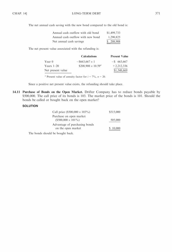
The net annual cash saving with the new bond compared to the old bond is:
Annual cash outflow with old bond $1,499,733
Annual cash outflow with new bond 1,290,825
Net annual cash savings $ 208,908
The net present value associated with the refunding is:
Calculations Present Value
Year 0 �$663,667� 1 �$ 663,667
Years 1–20 $208,908� 10.59a +2,212,336
Net present value $1,548,669
a Present value of annuity factor for i=7%, n=20.
Since a positive net present value exists, the refunding should take place.
14.11 Purchase of Bonds on the Open Market. Drifter Company has to reduce bonds payable by
$500,000. The call price of its bonds is 103. The market price of the bonds is 101. Should the
bonds be called or bought back on the open market?
SOLUTION
Call price ($500,000� 103%) $515,000
Purchase on open market
($500,000� 101%) 505,000
Advantage of purchasing bonds
on the open market $ 10,000
The bonds should be bought back.
CHAP. 14] LONG-TERM DEBT 371

Chapter 15
Preferred and Common Stock
15.1 INTRODUCTION
This chapter discusses equity financing. The advantages and disadvantages of issuing preferred and
common stock are addressed, along with the various circumstances in which either financing source is
most suited. Stock rights are also described. Consideration is given to the advantages and disadvantages
of public versus private placement, or sale. Also discussed is the role of the investment banker.
15.2 INVESTMENT BANKING
Investment banking involves public flotation, or sale, of a security issue. Investment bankers
perform the following functions:
1. Underwriting. The investment banker buys a new security issue, pays the issuer, and markets
the securities. The underwriter’s compensation is the difference between the price at which the
securities are sold to the public, and the price paid to the company for the securities.
2. Distributing. The investment banker markets the security issue.
3. Giving advice. The investment banker provides valuable advice to the company concerning the
best way to raise funds. The investment banker is familiar with the various sources of long-term
funds, debt and equity markets, and Securities and Exchange Commission (SEC) regulations.
4. Providing funds. The investment banker furnishes funds to the issuing company during the
distribution period.
When a number of investment bankers get together as a group because a particular issue is large
and/or risky, they are referred to as a syndicate. A syndicate is a temporary association of investment
bankers brought together for the purpose of selling new securities. One investment banker among the
group will be selected to manage the syndicate. The investment banker so selected is called the originating
house, which underwrites the major amount of the issue. One bid price for the issue is made on behalf of
the group, but the terms and features of the issue are established by the company.
There are two types of underwriting syndicates, divided and undivided. In a divided account, the
liability of each member investment banker is limited in terms of participation. Once a member sells the
securities assigned, that investment banker has no additional liability regardless of whether the other
members are able to sell their portion of the security or not. In an undivided account, each member is
liable for unsold securities up to the amount of its percentage participation irrespective of the number of
securities that investment banker has sold. Most syndicates are based on the undivided account
arrangement.
In another approach to investment banking, the investment banker agrees to sell the securities on a
best-efforts basis, or as an agent for the company. Here, the investment banker does not serve as
underwriter but rather sells the stock and receives a commission on the sale. An investment banker
may insist on this type of arrangement when he or she has reservations about the success of the security
offering in the market.
Besides investment bankers, there are firms that specialize in more specific financial functions with
regard to stock. A dealer buys securities and holds them in inventory for later resale, expecting to make a
profit on the spread. The spread is the price appreciation of the securities. A broker receives and forwards
purchase orders for securities to the applicable stock exchange or over-the-counter market. The broker is
compensated with a commission on each sale.
372
Copyright © 2007, 1998, 1986 by The McGraw-Hill Companies, Inc. Click here for terms of use.

15.3 PUBLIC VERSUS PRIVATE PLACEMENT OF SECURITIES
Equity and debt securities may be issued either publicly or privately. A consideration in determining
whether to issue securities publicly or privately is the type and amount of the needed financing.
In a public issuance, the shares are bought by the general public. In a private placement, the
company issues the securities directly to either one or a few large investors. The large investors involved
are financial institutions such as insurance companies, pension funds, and commercial banks.
Private placement has the following advantages, when compared to a public issuance:
1. The flotation cost is less. Flotation cost is the expense of registering and selling the stock issue.
Examples are brokerage commissions and underwriting fees. The flotation cost for common
stock exceeds that for preferred stock. Flotation cost expressed as a percentage of gross proceeds
is higher for smaller issues than for larger ones.
2. It avoids SEC filing requirements.
3. It avoids the disclosure of information to the public at large.
4. There is less time involved in obtaining funds.
5. It may not be practical to issue securities in the public market when a company is so small that
an investment banker would not find it profitable.
6. The company’s credit rating may be low, and as a consequence investors may not be interested
in buying securities when the money supply is limited.
Private placement has the following disadvantages, when compared to a public issuance:
1. It is more difficult to obtain significant amounts of money privately compared to publicly.
2. Large investors usually employ stringent credit standards requiring the company to be in a
strong financial position.
3. Large institutional investors may watch more closely the company’s activities than smaller
investors in a public issue.
4. Large institutional investors are more capable of obtaining voting control of the company.
15.4 GOING PUBLIC – ABOUT AN INITIAL PUBLIC OFFERING (IPO)
Going public, or often called an initial public offering (IPO), refers to selling formerly privately held
shares to new investors on the organized exchange (e.g. New York Stock Exchange) or the over-the-
counter market for the first time. For the individual company, going public marks a historic moment. It
often is the springboard for greater growth and success. There are advantages and disadvantages of
raising capital through a public offering. The market for stocks of companies that are going public is
called the new issue market.
The public sale of ownership interests can generate funds for business expansion, working capital,
repayment of debt, diversification, acquisitions, marketing, and other uses. In addition, a successful IPO
increases the visibility and appeal of your company, thereby escalating the demand and value for shares.
Investors can benefit from an IPO not only because of the potential increase in market value for their
stock but also because publicly held stock is more liquid and can be readily sold if the business appears to
falter or if the investor needs quick cash. The availability of a public market for shares will also help
determine the taxable values of the shares and assist in estate transfers.
15.5 VENTURE CAPITAL FINANCING
Venture capital (VC) firms supply funding from private sources for investing in select companies
that have a high, rapid growth potential, and a need for large amounts of capital. VC firms speculate on
certain high-risk businesses producing a very high rate of return in a very short time. The firms typically
invest for periods of 3 to 7 years and expect at least a 20 percent to 40 percent annual return on their
investment.
CHAP. 15] PREFERRED AND COMMON STOCK 373
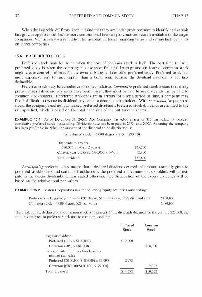
When dealing with VC firms, keep in mind that they are under great pressure to identify and exploit
fast growth opportunities before more conventional financing alternatives become available to the target
companies. VC firms have a reputation for negotiating tough financing terms and setting high demands
on target companies.
15.6 PREFERRED STOCK
Preferred stock may be issued when the cost of common stock is high. The best time to issue
preferred stock is when the company has excessive financial leverage and an issue of common stock
might create control problems for the owners. Many utilities offer preferred stock. Preferred stock is a
more expensive way to raise capital than a bond issue because the dividend payment is not tax-
deductible.
Preferred stock may be cumulative or noncumulative. Cumulative preferred stock means that if any
previous year’s dividend payments have been missed, they must be paid before dividends can be paid to
common stockholders. If preferred dividends are in arrears for a long period of time, a company may
find it difficult to resume its dividend payments to common stockholders. With noncumulative preferred
stock, the company need not pay missed preferred dividends. Preferred stock dividends are limited to the
rate specified, which is based on the total par value of the outstanding shares.
EXAMPLE 15.1 As of December 31, 20X6, Ace Company has 6,000 shares of $15 par value, 14 percent,
cumulative preferred stock outstanding. Dividends have not been paid in 20X4 and 20X5. Assuming the company
has been profitable in 20X6, the amount of the dividend to be distributed is:
Par value of stock ¼ 6,000 shares� $15 ¼ $90,000
Dividends in arrears
($90,000� 14%� 2 years) $25,200
Current year dividend ($90,000� 14%) 12,600
Total dividend $37,800
Participating preferred stock means that if declared dividends exceed the amount normally given to
preferred stockholders and common stockholders, the preferred and common stockholders will partici-
pate in the excess dividends. Unless stated otherwise, the distribution of the excess dividends will be
based on the relative total par values.
EXAMPLE 15.2 Boston Corporation has the following equity securities outstanding:
Preferred stock, participating—10,000 shares, $10 par value, 12% dividend rate $100,000
Common stock—4,000 shares, $20 par value $ 80,000
The dividend rate declared on the common stock is 10 percent. If the dividends declared for the year are $25,000, the
amounts assigned to preferred stock and to common stock are:
Preferred
Stock
Common
Stock
Regular dividend
Preferred (12%� $100,000) $12,000
Common (10%� $80,000) $ 8,000
Excess dividend—allocation based on
relative par value
Preferred [($100,000/$180,000)� $5,000] 2,778
Common [($80,000/$180,000)� $5,000] 2,222
Total dividend $14,778 $10,222
374 PREFERRED AND COMMON STOCK [CHAP. 15

Preferred stock may be callable, which means that the company can buy it back at a later date at a
specified call price. The call provision is advantageous when interest rates decline, since the company has
the option of discontinuing payment of dividends at a rate that has become excessive by buying back
preferred stock that was issued when bond interest rates were high. Unlike bonds, preferred stock rarely
has a maturity date associated with it. However, if preferred stock has a sinking fund associated with it,
this, in effect, establishes a maturity date for repayment.
In the event of corporate bankruptcy, preferred stockholders are paid after creditors and before
common stockholders. In such a case, preferred stockholders receive the par value of their shares,
dividends in arrears, and the current year’s dividend. Any asset balance then goes to the common
stockholders.
The cost of preferred stock can be determined by dividing the dividend payment by the net proceeds
received.
EXAMPLE 15.3 Blick Corporation sells preferred stock amounting to $2 million. The flotation cost is 11 percent
of gross proceeds. The dividend rate is 14 percent. The effective cost of the preferred stock is:
Dividend
Net proceeds¼ 0:14� $2,000,000
$2,000,000� ð0:11� $2,000,000Þ ¼$280,000
$1,780,000¼ 15:7%
The company should estimate the amount it will receive per share and the number of shares it must
sell in order to finance the business.
EXAMPLE 15.4 Brady Corporation is considering expanding its operations. It anticipates a need for $5 million to
finance the expansion through the issuance of preferred stock. The preferred stock has a par value of $100 and a
dividend rate of 10 percent. Similar issues, of preferred stock are currently providing a yield of 12 percent.
For each share, the company will receive:
Dividend
Market yield¼ 0:10 � $100
0:12¼ $10
0:12¼ $83:33
The amount of shares that must be issued is:
Funds required
Price per share¼ $5,000,000
$83:33¼ 60,002 shares ðroundedÞ
To a company, a preferred stock issue has the following advantages:
1. Preferred dividends do not have to be paid, whereas interest on debt must be paid.
2. Preferred stockholders cannot force the company into bankruptcy.
3. Preferred shareholders do not share in unusually high profits of the company.
4. A growth company can generate better earnings for its original owners by issuing preferred
stock having a fixed dividend rate than by issuing common stock.
5. Preferred stock issuance does not dilute the ownership interest of common stockholders in terms
of earnings participation and voting rights.
6. The company does not have to collateralize its assets as it may have to do if bonds are issued.
To a company, a preferred stock has the following disadvantages:
1. Preferred stock requires a higher yield than bonds.
2. Preferred dividends are not tax-deductible.
Several varieties of preferred stocks are available. Two of these are: adjustable rate and money market
auction preferred.
Adjustable-rate preferreds (ARPs), also called floating or variable-rate preferreds, are perpetual
preferreds with a floating dividend rate that resets each quarter. The rate is tied to the rate on
Treasury securities.
CHAP. 15] PREFERRED AND COMMON STOCK 375

Money market preferred stock (MMPS), also known as market auction or auction-rate preferred
stock, is very attractive to many investors since it offers the following advantages:
� Low market risk in the event of price decline
� Competitive yield
� Liquidity
15.7 COMMON STOCK
The owners of a corporation are called stockholders. They elect the board of directors, who in turn
select the officers of the firm. When the election occurs, management sends proxy statements, which
ask stockholders to give management the right to vote their stock. Effective control of the corporation
can exist with less than 50 percent common stock ownership since many stockholders do not bother to
vote. Stockholders have limited liability in that they are not personally liable for the debts of the
company.
Authorized shares represent the maximum amount of stock the company can issue according to the
corporate charter. Issued shares represent the number of authorized shares which have been sold by
the firm. Outstanding shares are the issued shares actually being held by the investing public. Treasury
stock is stock that has been reacquired by the firm. It is not retired but, rather, held for possible future
resale, a stock option plan, to use in purchasing another company, or to prevent a takeover by an outside
group. Outstanding shares are therefore equal to the issued shares less the treasury shares. Dividends are
based on the outstanding shares.
The par value of a stock is a stated amount of value per share specified in the corporate charter. The
firm typically cannot sell stock at a price below par value since stockholders would be liable to creditors
for the difference between par value and the amount received.
A closely held corporation is one having only a few stockholders. They keep full control and are not
required to publicly disclose financial information about the company. However, a company having
500 or more stockholders must file an annual financial statement with the Securities and Exchange
Commission.
A company may issue different classes of common stock. Class A is stock issued to the public and
usually has no dividends specified. However, it does have voting rights. Class B stock is usually kept by
the company’s organizers. Dividends are typically not paid on it until the company has generated
sufficient earnings.
Common stockholders enjoy the following rights:
1. The right to receive dividends.
2. The right to receive assets upon the dissolution of the business.
3. The right to vote.
4. The preemptive right to buy new shares of common stock prior to their sale to the general
public. In this way, current stockholders can maintain their proportionate percentage ownership
in the company.
5. The receipt of a stock certificate which evidences ownership in the firm. The stock certificate
may then be sold by the holder to another in the secondary security market.
6. The right to inspect the company’s books.
In some states there also exists cumulative voting, which allows for multiple votes for a
particular director. Cumulative voting is designed to allow a minority group to be able to elect
one director.
A number of options exist for equity financing in the case of small businesses, including:
1. Venture capital (investor) groups
2. Issuances directly to institutional investors
376 PREFERRED AND COMMON STOCK [CHAP. 15

3. Issuances to relatives or friends
4. Issuances to major customers and suppliers
A determination of the number of shares that must be issued to raise sufficient funds to meet the
capital budget may be required.
EXAMPLE 15.5 Brady Corporation presently has 650,000 shares of common stock outstanding. The capital
budget for the upcoming year is $1.8 million.
Assuming new stock may be issued for $16 a share, the number of shares that must be issued to provide the
necessary funds to meet the capital budget is:
Funds needed
Market price per share¼ $1,800,000
$16¼ 112,500 shares
The new shareholders will now own 14.8 percent of the total shares outstanding as computed below.
Newly issued shares
Total shares¼ 112,500
650,000þ 112,500¼ 112,500
762,500¼ 14:8%
EXAMPLE 15.6 Smith Corporation wishes to raise $3 million in its first public issue of common stock. After its
issuance, the total market value of stock is anticipated to be $7 million. Currently, there are 140,000 outstanding
shares that are closely held.
Determine the number of new shares that must be issued to raise the $3 million.
The new shares will have 37($3 million/$7 million) of the outstanding shares after the stock issuance. Therefore,
current stockholders will be holding 47of the shares.
140,000 shares ¼ 47of the total shares
Total shares ¼ 245,000
New shares ¼ 37� 245,000 ¼ 105,000 shares
Subsequent to the stock issuance, the anticipated price per share is:
Price per share ¼ market value
share outstanding¼ $7,000,000
245,000 shares¼ $28:57
A company that first issues its common stock publicly is referred to as ‘‘going public.’’ The estimated
price per share to sell the securities is equal to:
Anticipated market value of the company
Total outstanding shares
For an established company, the market price per share can be computed as follows:
Expected dividend
Cost of capital� growth rate in dividends
EXAMPLE 15.7 Golden Corporation expects the dividend for the year to be $10 a share. The cost of capital is
13 percent. The growth rate in dividends is expected to be constant at 8 percent. The price per share is:
Price per share ¼ expected dividend
cost of capital� growth rate in dividends¼ $10
0:13� 0:08¼ $10
0:05¼ $200
Another approach to pricing the share of stock for an existing company is through the use of the
price/earnings (P/E) ratio, which is equal to:
Market price per share
Earnings per share
CHAP. 15] PREFERRED AND COMMON STOCK 377

EXAMPLE 15.8 Grace Corporation’s earnings per share is $7. It is expected that the company’s stock should sell
at eight times its earnings. The market price per share is therefore
P=E ¼ market price per share
earnings per share
Market price per share ¼ P=E multiple� earnings per share ¼ 8� $7 ¼ $56
The financial manager may wish to determine the market value of a company’s stock. There are a
number of different ways to do this.
EXAMPLE 15.9 Assuming an indefinite stream of future dividends of $300,000 and a required rate of return of
14 percent, the market value of the stock equals:
Market value ¼ expected dividends
rate of return¼ $300,000
0:14¼ $2,142,857
If there are 200,000 shares, the market price per share is:
Market value
Number of shares¼ $2,142,857
200,000¼ $10:71
EXAMPLE 15.10 Technical Corporation is considering a public issue of its securities. The average price/earnings
multiple in the industry is 15. The company’s net income is $400,000. There will be 100,000 shares outstanding
subsequent to the issuance of the stock. The expected price per share is:
Total market value ¼ net income� price=earnings multiple
¼ $400,000� 15 ¼ $6,000,000
Price per share ¼ market value
number of shares¼ $6,000,000
100,000¼ $60
EXAMPLE 15.11 Pinston Corporation issues 400,000 new shares of common stock to present stockholders at
a $25 price per share. The price per share prior to the issue is $29. Currently, there are 500,000 outstanding shares.
The expected price per share after the new issue is:
Value of outstanding shares
(500,000� $29) $14,500,000
Value of newly issued shares
(400,000� $25) 10,000,000
Value of entire issue $24,500,000
Value per share ¼ value of entire shares
total number of shares¼ $24,500,000
900,000¼ $27:22
EXAMPLE 15.12 Prider Corporation is considering building a new plant. The firm has typically distributed all its
earnings in the form of dividends. Capital expansion has been financed through common stock issuance. In the
capital structure, there is no outstanding preferred stock or debt.
The following expectations exist:
Net income $23,000,000
Shares outstanding 5,000,000
Construction cost of new plant $16,000,000
378 PREFERRED AND COMMON STOCK [CHAP. 15

Incremental annual earnings expected because of the new plant is $2 million. The rate of return anticipated by
stockholders is 12 percent per annum. The total market value of the firm if the plant is financed through the issuance
of common stock is:
Total net income
Rate of return¼ $25,000,000
0:12¼ $208,330,000
The financial manager may wish to compute the company’s price/earnings ratio and required rate
of return.
EXAMPLE 15.13 Davis Corporation has experienced an 8 percent growth rate in earnings and dividends. Next
year, it anticipates earnings per share of $4 and dividends per share of $2.50. The company will be having its
first public issue of common stock. The stock will be issued at $50 per share.
The price/earnings ratio is:
Market price per share
Earnings per share¼ $50
$4¼ 12:5 times
The required rate of return on the stock is:
Dividends per share
Market price per shareþ growth rate in dividends
$2:50
$50þ0:08 ¼ 0:13
When the degree of financial leverage is excessive, the company would be better off financing with an
equity issue.
Financing with common stock has the following advantages:
1. There is no requirement to pay dividends.
2. There is no repayment date.
3. A common stock issue improves the company’s credit rating relative to the issuance of debt.
Financing with common stock has the following disadvantages:
1. Dividends are not tax-deductible.
2. Ownership interest is diluted. The additional voting rights could vote to take control away from
the current ownership group.
3. Earnings and dividends are spread over more shares outstanding.
4. The flotation costs associated with a common stock issue are higher than with preferred stock
and debt financing.
It is always cheaper to finance operations from internally generated funds. Financing out of retained
earnings involves no flotation costs.
Stockholders are generally better off when a firm cuts back on its dividends rather than issuing
common stock as a source of needed additional funds. First, when earnings are retained rather than new
stock issued, the market price per share of existing stock will rise, as indicated by higher earnings per
share. Second, if stock is held for more than one year and then sold at a gain, the investor will get a tax
advantage with a capital gain deduction. For 2005, the maximum capital gains rates are 5, 15, 25,
or 28%. However, cash dividends are fully taxable. Thus, there is a tax benefit to investors, with a
reduction in dividends. One caution, however: Lower dividend payments may be viewed negatively in the
market and may result in a reduction in the market price of stock due to psychological factors.
CHAP. 15] PREFERRED AND COMMON STOCK 379
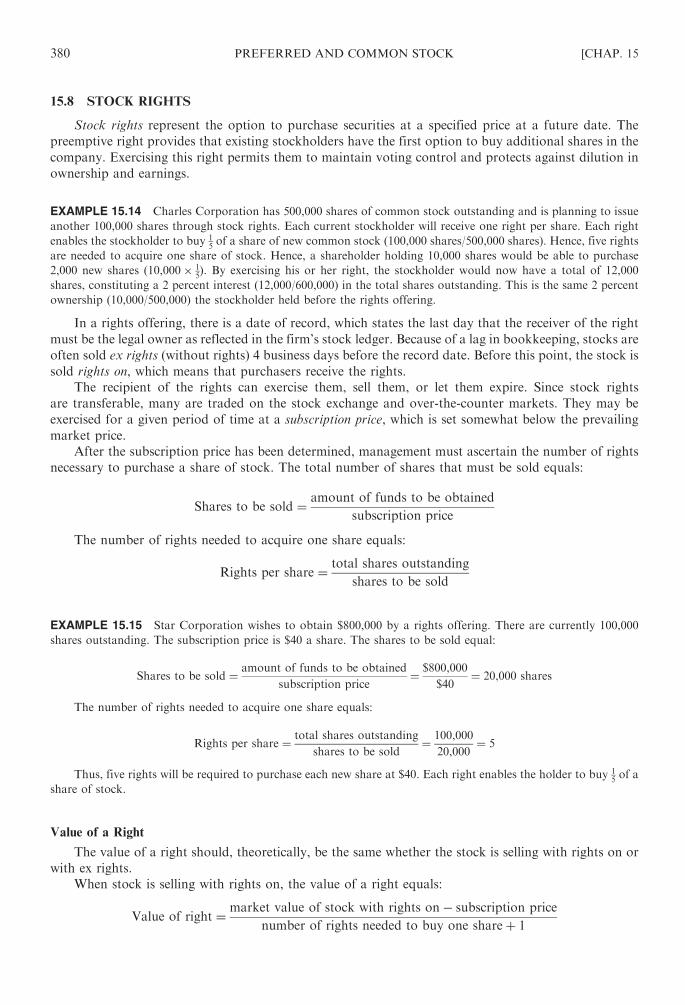
15.8 STOCK RIGHTS
Stock rights represent the option to purchase securities at a specified price at a future date. The
preemptive right provides that existing stockholders have the first option to buy additional shares in the
company. Exercising this right permits them to maintain voting control and protects against dilution in
ownership and earnings.
EXAMPLE 15.14 Charles Corporation has 500,000 shares of common stock outstanding and is planning to issue
another 100,000 shares through stock rights. Each current stockholder will receive one right per share. Each right
enables the stockholder to buy 15of a share of new common stock (100,000 shares/500,000 shares). Hence, five rights
are needed to acquire one share of stock. Hence, a shareholder holding 10,000 shares would be able to purchase
2,000 new shares ð10,000� 15Þ. By exercising his or her right, the stockholder would now have a total of 12,000
shares, constituting a 2 percent interest (12,000/600,000) in the total shares outstanding. This is the same 2 percent
ownership (10,000/500,000) the stockholder held before the rights offering.
In a rights offering, there is a date of record, which states the last day that the receiver of the right
must be the legal owner as reflected in the firm’s stock ledger. Because of a lag in bookkeeping, stocks are
often sold ex rights (without rights) 4 business days before the record date. Before this point, the stock is
sold rights on, which means that purchasers receive the rights.
The recipient of the rights can exercise them, sell them, or let them expire. Since stock rights
are transferable, many are traded on the stock exchange and over-the-counter markets. They may be
exercised for a given period of time at a subscription price, which is set somewhat below the prevailing
market price.
After the subscription price has been determined, management must ascertain the number of rights
necessary to purchase a share of stock. The total number of shares that must be sold equals:
Shares to be sold ¼ amount of funds to be obtained
subscription price
The number of rights needed to acquire one share equals:
Rights per share ¼ total shares outstanding
shares to be sold
EXAMPLE 15.15 Star Corporation wishes to obtain $800,000 by a rights offering. There are currently 100,000
shares outstanding. The subscription price is $40 a share. The shares to be sold equal:
Shares to be sold ¼ amount of funds to be obtained
subscription price¼ $800,000
$40¼ 20,000 shares
The number of rights needed to acquire one share equals:
Rights per share ¼ total shares outstanding
shares to be sold¼ 100,000
20,000¼ 5
Thus, five rights will be required to purchase each new share at $40. Each right enables the holder to buy 15of a
share of stock.
Value of a Right
The value of a right should, theoretically, be the same whether the stock is selling with rights on or
with ex rights.
When stock is selling with rights on, the value of a right equals:
Value of right ¼ market value of stock with rights on� subscription price
number of rights needed to buy one shareþ 1
380 PREFERRED AND COMMON STOCK [CHAP. 15

EXAMPLE 15.16 Charles Company’s common stock sells for $55 a share with rights on. Each stockholder is given
the right to buy one new share at $35 for every four shares held. The value of each right is:
Value of right ¼ market value with rights on� subscription price
number of rights needed to buy one shareþ 1
¼ $55� $35
4þ 1¼ $20
5¼ $4
When stock is traded ex rights, the market price is anticipated to decline by the value of the right.
The market value of stock trading ex rights should theoretically equal:
Market value of stock with rights on� value of a right when stock is selling rights on
The value of a right when stock is selling ex rights equals:
Value of right ¼ market value of stock trading ex rights� subscription price
number of rights needed to buy one new share
EXAMPLE 15.17 Assuming the same facts as those in Example 15.16, the value of the right of Charles Company
stock trading ex rights should equal:
Market value of stock with rights on� value of a right when stock is selling rights on
$55� $4 ¼ $51
The value of a right when stock is selling ex rights is therefore:
Value of right ¼ market value of stock trading ex rights� subscription price
number of rights needed to buy one new share
¼ $51� $35
4¼ $16
4¼ $4
Notice that the theoretical value of the right is identical when the stock is selling rights on or ex
rights.
15.9 STOCKHOLDERS’ EQUITY SECTION OF THE BALANCE SHEET
The stockholders’ equity section of a company’s balance sheet consists of:
1. Capital stock, which includes the stock issued by the corporation and stated at par value. The
two types of capital stock are preferred and common. Also included in the capital stock section
are stock rights.
2. Paid-in capital, which represents the excess over par value received by a corporation for the
issuance of stock.
3. Retained earnings, which refers to the accumulated earnings of the company less any dividends
paid out.
The company records the issuance of stock only when it initially sells it to the stockholder.
When one stockholder sells his or her shares, the transaction is not entered on the corporation’s
books. The company need only change the name on its records to that of the new stockholder so that
dividends may be properly paid.
Treasury stock is shown in the stockholders’ equity section as a deduction when computing total
stockholders’ equity.
CHAP. 15] PREFERRED AND COMMON STOCK 381

15.10 GOVERNMENTAL REGULATION
When securities are issued publicly, they must conform to federal and state regulations. State
rules are referred to as blue sky laws. The major federal laws are the Securities Act of 1933 and
the Securities Exchange Act of 1934. The 1934 act applies to existing security transactions, while
the 1933 act deals with regulation of new security issues. The acts require full disclosure to investors
concerning the company’s affairs. Prior to the issuance of a new security, the company must prepare
a prospectus for investors which contains a condensed version of the registration statement filed
with the SEC.
15.11 FINANCING STRATEGY
The corporation financial manager is concerned with selecting the best possible source of financing
based on the facts of the situation. This section describes various circumstances in which a particular
financing source is most suited.
EXAMPLE 15.18 Tart Corporation is considering issuing either debt or preferred stock to finance the acquisition
of a plant costing $1.3 million. The interest rate on the debt is 15 percent. The dividend rate on the preferred stock is
10 percent The tax rate is 46 percent.
The annual interest payment on the debt is:
15%� $1,300,000 ¼ $195,000
The annual dividend on the preferred stock is:
10%� $1,300,000 ¼ $130,000
The required earnings before interest and taxes to meet the dividend payment is:
$130,000
ð1� 0:46Þ ¼ $240,741
If the company anticipates earning $240,741 without difficulty, it should issue the preferred stock.
EXAMPLE 15.19 Charles Corporation has previously used short-term financing. It is now considering refinancing
its short-term debt with equity or long-term debt securities. The financial manager decided to list the factors
that should be taken into account when selecting an appropriate means of financing. These factors are:
1. The costs of the instruments
2. The company’s earnings compared to the cost of debt and preferred stock
3. The recurrence in sales and earnings
4. The degree of financial leverage
5. The maturity and degree of success of the firm
6. The degree of dilution in voting control to be tolerated
7. The firm’s solvency status
EXAMPLE 15.20 Pride Corporation has sales of $30 million a year. It needs $6 million in financing for capital
expansion. The debt/equity ratio is 68 percent. The company is in a risky industry, and net income is not stable year
to year. The common stock is selling at a high P/E ratio relative to the competition. Under consideration is either the
issuance of common stock or a convertible bond.
Because the company is in a high-risk industry and has a high debt/equity ratio and fluctuating earnings, the
issuance of common stock is preferred.
EXAMPLE 15.21 Wilson Corporation is a mature company in its industry. It has a limited ownership. The
company has a fluctuating sales and earnings stream. The firm’s debt/equity ratio is 70 percent relative to the
industry standard of 55 percent. The after-tax rate of return is 16 percent. Since Wilson’s is a seasonal business,
382 PREFERRED AND COMMON STOCK [CHAP. 15

there are given times during the year when its liquidity position is deficient. The company is undecided on the best
means of financing.
Preferred stock is one possible means of financing. Debt financing is not recommended because of the already
high debt/equity ratio, the variability in earnings, and the poor liquidity position. Because of the limited ownership,
common stock financing may not be appropriate since this would dilute the ownership.
EXAMPLE 15.22 A new company is established and it plans to raise $15 million in funds. The company anticipates
that it will obtain contracts that will provide $1,200,000 a year in before-tax profits. The firm is considering
whether to issue bonds only or an equal amount of bonds and preferred stock. The interest rate on AA corporate
bonds is 12 percent. The tax rate is 50 percent.
The firm will probably have difficulty issuing $15 million of AA bonds because the interest cost of $1,800,000
(12%� $15,000,000) associated with these bonds is greater than the estimated earnings before interest and taxes.
The issuance of debt by a new company is a risky alternative.
Financing with $7.5 million in debt and $7.5 million in preferred stock is also not recommended. While some
debt may be issued, it is not feasible to finance the balance with preferred stock. In the event that $7.5 million of AA
bonds were issued at the 12 percent rate, the company would be obligated to pay $900,000 in interest. In this event, a
forecasted income statement would look as follows:
Earnings before interest and taxes $1,200,000
Interest 900,000
Taxable income $ 300,000
Taxes 150,000
Net income $ 150,000
The amount available for the payment of preferred dividends is only $150,000. Hence, the maximum rate of
return that could be paid on $7.5 million of preferred stock is:
$150,000
$7,500,000¼ 0:02
Stockholders would not invest in preferred stock that offers only a 2 percent rate of return.
The company should consider financing with common stock.
EXAMPLE 15.23 Boyser Corporation wishes to construct a plant that will take about 112years to build. The plant
will be used to manufacture a new product line, for which Boyser anticipates a high demand. The new plant will
significantly increase the company’s size. The following costs are expected to occur:
1. The cost to build the plant, $800,000
2. Funds required for contingencies, $100,000
3. Annual operating costs, $175,000
The asset, debt, and equity positions of the firm are similar to industry standards. The market price of the firm’s
stock is less than it should be, considering the future earning power of the new product line. What would be an
appropriate way to finance the construction?
Because the market price of stock is less than it should be and considering the potential of the product line,
convertible bonds and installment bank loans might be appropriate means of financing, since interest expense is tax-
deductible. Further, the issuance of convertible bonds might not require repayment, since the bonds are likely to be
converted to common stock because of the firm’s profitability. Installment bank loans can be gradually paid off as
the new product generates cash inflow. Funds required for contingencies can be in the form of open bank lines of
credit.
If the market price of the stock was not at a depressed level, financing through equity would be an alternative
financing strategy.
CHAP. 15] PREFERRED AND COMMON STOCK 383

EXAMPLE 15.24 Davis Company wishes to acquire Gortman Corporation but has not decided on an optimum
means to finance the purchase. The current debt/equity position is within the industry guideline. In previous years,
financing has been accomplished through the issuance of short-term debt.
Earnings have shown instability over the years and consequently the market price of the stock has fluctuated.
At present, however, the market price of stock is strong.
The company’s tax bracket is low.
The acquisition should be financed through the issuance of equity securities for the following reasons:
1. The market price of stock is presently at a high level.
2. The issuance of long-term debt will result in more instability in earnings due to high fixed interest charges.
As a result, there will be greater instability in the company’s stock price.
3. The issuance of more debt will cause the firm’s debt/equity ratio to rise above the industry norm. This will
adversely affect the company’s cost of capital and availability of financing.
4. Because it will take a long time to derive the funds necessary for the acquisition cost, short-term debt should
not be issued. If short-term debt is issued, the debt would have to be met prior to the receipt of the return
from the acquired business.
EXAMPLE 15.25 Breakstone Corporation wishes to undertake a capital expansion program and must, therefore,
obtain $7 million in financing. The company has a good credit rating. The current market price of its common stock
is $60. The interest rate for long-term debt is 18 percent. The dividend rate associated with preferred stock is 16
percent, and Breakstone’s tax rate is 46 percent.
Relevant ratios for the industry and the company are:
Industry Breakstone
Net income to total assets 13% 22%
Long-term debt to total assets 31% 29%
Total liabilities to total assets 47% 45%
Preferred stock to total assets 3% 0
Current ratio 2.6 3.2
Net income plus interest to interest 8 17
Dividend per share is $8, the dividend growth rate is 7 percent, no sinking fund provisions exist, the
trend in earnings shows stability, and the present ownership group wishes to retain control. The cost of common
stock is:
Dividends per share
Market price per shareþ dividend growth rate
$8
$60þ 0:07 ¼ 20:3%
The after-tax cost of long-term debt is 9.7 percent (18%� 54%). The cost of preferred stock is 16 percent.
How should Breakstone finance its expansion?
The issuance of long-term debt is more appropriate for the following reasons:
1. Its after-tax cost is the lowest.
2. The company’s ratios of long-term debt to total assets and total liabilities to total assets are less than the
industry average, pointing to the company’s ability to issue additional debt.
3. Corporate liquidity is satisfactory based on the favorable current ratio relative to the industry standard.
4. Fixed interest charges can be met, taking into account the stability in earnings, the earning power of the
firm, and the very favorable times-interest-earned ratio. Additional interest charges should be met without
difficulty.
5. The firm’s credit rating is satisfactory.
384 PREFERRED AND COMMON STOCK [CHAP. 15

6. There are no required sinking fund provisions.
7. The leveraging effect can take place to further improve earnings.
In the case that the firm does not want to finance through further debt, preferred stock would be the next best
financing alternative, since its cost is lower than that associated with common stock and no dilution in the ownership
interest will take place.
EXAMPLE 15.26 Harris Corporation has experienced growth in revenue and net income but is in a
weak liquidity position. The inflation rate is high. At the end of 20X5, the firm needs $600,000 for the
following reasons:
New equipment $175,000
Research and development 95,000
Paying overdue accounts payable 215,000
Paying accrued liabilities 60,000
Desired increase in cash balance 55,000
$600,000
Presented below are the financial statements for 20X5.
Harris Corporation
Balance Sheet
December 31, 20X5
ASSETS
Current assets
Cash $ 12,000
Accounts receivable 140,000
Notes receivable 25,000
Inventory 165,000
Office supplies 20,000
Total current assets $362,000
Fixed assets 468,000
Total assets $830,000
LIABILITIES AND
STOCKHOLDERS’ EQUITY
Current liabilities
Loans payable $ 74,000
Accounts payable 360,000
Accrued liabilities 55,000
Total current liabilities $489,000
Long-term debt 61,000
Total liabilities $550,000
Stockholders’ equity
Common stock $200,000
Retained earnings 80,000
Total stockholders’ equity 280,000
Total liabilities and stockholders’
equity $830,000
CHAP. 15] PREFERRED AND COMMON STOCK 385

Harris Corporation
Income Statement
For the Year Ended December 31, 20X5
Sales $1,400,000
Cost of sales 750,000
Gross margin $ 650,000
Operating expenses 480,000
Income before tax $ 170,000
Tax 68,000
Net income $ 102,000
It is anticipated that sales will increase on a yearly basis by 22 percent and that net income will increase by
17 percent. What type of financing is best suited for Harris Corporation?
The most suitable source of financing is long-term. A company in a growth stage needs a large investment in
equipment, and research and development expenditure. With regard to 20X5, $270,000 of the $600,000 is required
for this purpose. A growth company also needs funds to satisfy working capital requirements. Here, 45.8 percent of
financing is necessary to pay overdue accounts payable and accrued liabilities. The firm also needs sufficient cash to
capitalize on lucrative opportunities. The present cash balance to total assets is at a low 1.4 percent.
Long-term debt financing is recommended for the following reasons:
1. The ratio of long-term debt to stockholders’ equity is a low 21.8 percent. The additional issuance of long-
term debt will not impair the overall capital structure.
2. The company has been profitable and there is an expectation of future growth in earnings. Internally
generated funds should therefore ensue, enabling the payment of fixed interest charges.
3. During inflation, the issuance of long-term debt generates purchasing power gains because the firm will be
repaying creditors in cheaper dollars.
4. Interest expense is tax-deductible.
Review Questions
1. The two sources of equity financing are and .
2. A(n) enables the future purchase of stock.
3. A(n) purchases and distributes new securities of a company.
4. When a group of investment bankers handle a large issue, the group is referred to as
a(n) .
5. The investment banker who manages the group is called the .
6. The two types of underwriting syndicates are and .
7. A(n) purchases securities and holds them in inventory for later resale.
8. A(n) handles transactions for securities on the stock exchanges.
9. When securities are they are sold to a few institutional investors.
386 PREFERRED AND COMMON STOCK [CHAP. 15

10. The expense related to registering and selling a security is called cost.
11. One advantage of a private placement is that it avoids filing requirements.
12. preferred stock means that if dividends are not paid in a particular
year, they must be paid in a later year before any distributions are given to common
stockholders.
13. Preferred dividends are based on the total of the outstanding shares.
14. preferred stock means that preferred shareholders will participate with
common shareholders in any excess dividends.
15. For corporate investors, dividends received are subject to a(n) dividend
exclusion.
16. A(n) statement gives management the right to vote common stockholders’
shares.
17. The maximum amount of shares the company can issue as per the corporate charter are
the shares.
18. Shares that have been sold to the public are called shares.
19. is stock which has been bought back by the company.
20. equal issued shares less treasury shares.
21. Each stock has a(n) that is specified in the corporate charter.
22. The right allows a stockholder to purchase new shares of stock before they
are sold to the general public.
23. The stockholders’ equity section of a company’s balance sheet consists of the
, , and sections.
Answers: (1) common stock, preferred stock; (2) stock right; (3) investment banker; (4) syndicate; (5) origi-
nating house; (6) divided, undivided; (7) dealer; (8) broker; (9) privately placed; (10) flotation; (11)
SEC; (12) Cumulative; (13) par value; (14) Participating; (15) 85%; (16) proxy; (17) authorized; (18)
issued; (19) Treasury stock; (20) Outstanding shares; (21) par value; (22) preemptive; (23) capital stock,
paid-in capital, retained earnings.
Solved Problems
15.1 Dividends Payable to Preferred. On December 31, 20X4, Arco Company had 5,000 shares of
$10 par value, 15 percent, cumulative preferred stock outstanding. Dividends are in arrears
for 3 years. Since 20X4 was a profitable year, the company paid its dividend in full. What is
the total dividend payable to preferred stockholders?
CHAP. 15] PREFERRED AND COMMON STOCK 387
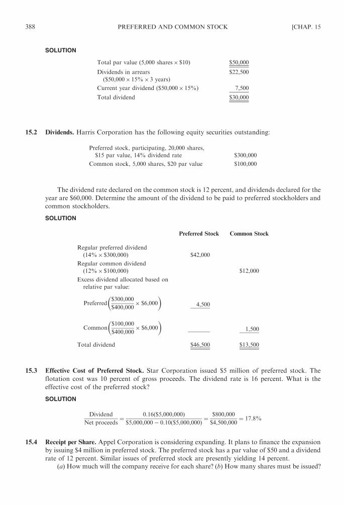
SOLUTION
Total par value (5,000 shares� $10) $50,000
Dividends in arrears
($50,000� 15%� 3 years)
$22,500
Current year dividend ($50,000� 15%) 7,500
Total dividend $30,000
15.2 Dividends. Harris Corporation has the following equity securities outstanding:
Preferred stock, participating, 20,000 shares,
$15 par value, 14% dividend rate $300,000
Common stock, 5,000 shares, $20 par value $100,000
The dividend rate declared on the common stock is 12 percent, and dividends declared for the
year are $60,000. Determine the amount of the dividend to be paid to preferred stockholders and
common stockholders.
SOLUTION
Preferred Stock Common Stock
Regular preferred dividend
(14%� $300,000) $42,000
Regular common dividend
(12%� $100,000) $12,000
Excess dividend allocated based on
relative par value:
Preferred$300,000
$400,000� $6,000
� �
4,500
Common$100,000
$400,000� $6,000
� �
1,500
Total dividend $46,500 $13,500
15.3 Effective Cost of Preferred Stock. Star Corporation issued $5 million of preferred stock. The
flotation cost was 10 percent of gross proceeds. The dividend rate is 16 percent. What is the
effective cost of the preferred stock?
SOLUTION
Dividend
Net proceeds¼ 0:16ð$5,000,000Þ
$5,000,000� 0:10ð$5,000,000Þ ¼$800,000
$4,500,000¼ 17:8%
15.4 Receipt per Share. Appel Corporation is considering expanding. It plans to finance the expansion
by issuing $4 million in preferred stock. The preferred stock has a par value of $50 and a dividend
rate of 12 percent. Similar issues of preferred stock are presently yielding 14 percent.
(a) How much will the company receive for each share? (b) How many shares must be issued?
388 PREFERRED AND COMMON STOCK [CHAP. 15

SOLUTION
(a) Dividend
Market Yield¼ 0:12� $50
0:14¼ $6
0:14¼ $42:86
(b) Funds required
Price per share¼ $4,000,000
$42:86¼ 93,327 shares ðroundedÞ
15.5 Shares to Be Sold. Simon Corporation has 800,000 common shares outstanding. The capital
budget for the upcoming year is $2 million. New stock may be sold for $20 a share.
(a) What is the number of shares that must be sold to obtain the needed funds? (b) What
percent of the total shares outstanding will the new stockholders own?
SOLUTION
(a) Funds needed
Market price per share¼ $2,000,000
$20¼ 100,000 shares
(b) Newly issued shares
Total shares¼ 100,000
800,000þ 100,000¼ 100,000
900,000¼ 11:1%
15.6 Expected Price. Saft Corporation wants to obtain $4 million in its first public issue of common
stock. After the issuance, the total market value of stock is estimated at $10 million. At present,
there are 120,000 closely held shares.
(a) What is the amount of new shares that must be issued to obtain the $4 million? (b) After
the stock issuance, what will be the expected price per share?
SOLUTION
(a) The new shares will be 40 percent ($4 million/$10 million) of the outstanding shares subsequent to the
stock issuance. Thus, current stockholders will be holding 60 percent of the shares.
120,000 shares ¼ 60% of the total shares
Total shares ¼ 200,000
New shares ¼ 40%� 200,000 ¼ 80,000 shares
(b) Price per share ¼ market value
outstanding shares¼ $10,000,000
200,000¼ $50
15.7 Price per Share. Gallagher Corporation anticipates a $6 dividend per share for the year. Its
minimum rate of return is 12 percent. The dividend growth rate is 6 percent. What is the price
per share?
SOLUTION
Expected dividend
Minimum return� dividend growth rate¼ $6
0:12� 0:06¼ $6
0:06¼ $100
15.8 Market Value. A company expects an indefinite stream of future dividends of $200,000 and a
required rate of return of 16 percent. There are 100,000 shares.
(a) What is the market value of the stock? (b) What is the market price per share?
SOLUTION
(a) Market value ¼ expected dividends
rate of return¼ $200,000
0:16¼ $1,250,000
CHAP. 15] PREFERRED AND COMMON STOCK 389

(b) Market price per share ¼ market value
number of shares¼ $1,250,000
100,000¼ $12:50
15.9 Expected Price. Wolinsky Corporation is considering a public issuance of its securities. The
average P/E ratio in the industry is 12. The firm’s reported earnings are $300,000. After the
issuance of the stock, there will be 200,000 shares outstanding. What is the expected price per
share?
SOLUTION
Total market value ¼ earnings� P=E ¼ $300,000� 12 ¼ $3,600,000
Price per share ¼ market value
shares outstanding¼ $3,600,000
200,000¼ $18
15.10 Expected Price. Nelson Corporation issues 200,000 new shares of common stock to current
stockholders at a $15 price per share. The price per share before the issue was $18. At present,
there are 300,000 shares outstanding. What is the expected price per share after the new issue?
SOLUTION
Value of outstanding shares
(300,000� $18) $5,400,000
Value of newly issued shares
(200,000� $15) 3,000,000
Value of entire issue $8,400,000
Value per share ¼ value of entire shares
total shares¼ $8,400,000
500,000¼ $16:80
15.11 Total Market Value. Stephens Corporation is thinking about constructing a new facility. The
company has usually distributed its earnings in the form of dividends. Common stock has
typically been issued to finance capital expansion. Preferred stock and debt are not in the capital
structure.
The company’s expectations follow:
Net income $18,000,000
Outstanding shares 2,000,000
Construction cost of new facility $10,000,000
The expected additional earnings due to the new facility is $2 million. The expected stock-
holder rate of return is 16 percent per annum. What is the total market value of the company,
assuming the facility is financed with common stock?
SOLUTION
Total net income
Rate of return¼ $20,000,000
0:16¼ $125,000,000
15.12 P/E Ratio. Wilson Corporation anticipates a 10 percent growth in net income and dividends.
Next year, the company expects earnings per share of $5 and dividends per share of $3. Wilson
will be having its first public issuance of common stock. The stock will be issued at $40 per share.
(a) What is the P/E ratio? (b) What is the required rate of return on the stock?
390 PREFERRED AND COMMON STOCK [CHAP. 15

SOLUTION
(a) Market price per share
Earnings per share¼ $40
$5¼ 8 times
(b) Dividends per share
Market price per shareþ dividend growth rate ¼ $3
$40þ 0:10 ¼ 17:5%
15.13 Preemptive Right. Barker Company has 400,000 shares of common stock outstanding and is
considering issuing another 100,000 shares through stock rights. Each current stockholder will
obtain one right per share. Mr. A owns 40,000 shares of common stock.
(a) What amount of each new share of common stock can a stockholder acquire by each
right? (b) How many rights are required to purchase one new share of common stock? (c) How
many new shares will Mr. A be able to obtain? (d ) What will Mr. A’s percentage interest in the
company be after exercising all his rights? (e) Did his percentage ownership change after exercis-
ing his rights relative to what it was before the rights offering?
SOLUTION
(a)Rights per share ¼ shares to be sold
shares outstanding¼ 100,000
400,000¼ 1
4
(b) Rights required for 1 share ¼ shares outstanding
shares to be sold¼ 400,000
100,000¼ 4
(c) Share available to a stockholder ¼ shares held� right per share ¼ 40,000� 1
4¼ 10,000 shares
(d ) % Ownership ¼ shares heldþ shares bought on rights
total shares outstanding¼ 50,000
500,000¼ 10%
(e) No. The percentage ownership is the same. Before the rights offering Mr. A also held a 10 percent
interest (40,000/400,000).
15.14 Rights per Share. Mason Corporation intends to raise $1.5 million in a rights offering. At present,
there are 240,000 shares outstanding. A subscription price of $25 a share is assigned.
(a) How many shares must be sold? (b) How many rights are needed to purchase one share of
stock?
SOLUTION
(a) Shares to be sold ¼ amount of funds to be obtained
subscription price¼ $1,500,000
$25¼ 60,000 shares
(b) The number of rights needed to acquire one share equals:
Rights per share ¼ total shares outstanding
shares to be sold¼ $40,000
60,000¼ 4
15.15 Value per Right. Charles Corporation stock sells at $78 a share with rights on. The subscription
price is $60, and five rights are needed to purchase a new share of stock. What is the value of each
right?
SOLUTION
Value of right ¼ market value with rights on� subscription price
number of rights to buy 1 share þ 1¼ $78� $60
5þ 1¼ $18
6¼ $3
CHAP. 15] PREFERRED AND COMMON STOCK 391

15.16 Value per Right. Assume the same facts as in Problem 15.15. (a) What will be the market
value of the stock trading ex rights? (b) What is the value of a right when the stock is selling
ex rights?
SOLUTION
(a) Value of stock, ex rights ¼ market value of stock with rights on� value of right ¼ $78� $3 ¼ $75
(b)Value of right ðwhen stock sells ex rightsÞ ¼ market value of stock, ex rights� subscription price
number of rights to buy 1 share
¼ $75� $60
5¼ $15
5¼ $3
15.17 Cost of Financing. Mason Corporation is considering the issuance of either debt or preferred
stock to finance the purchase of a facility costing $1.5 million. The interest rate on the debt is
16 percent. Preferred stock has a dividend rate of 12 percent. The tax rate is 46 percent.
(a) What is the annual interest payment? (b) What is the annual dividend payment? (c) What
is the required income before interest and taxes to satisfy the dividend requirement?
SOLUTION
(a) Annual interest ¼ 16%� $1,500,000 ¼ $240,000
(b) Annual dividend ¼ 12%� $1,500,000 ¼ $180,000
(c) Before-tax income required for dividend ¼ dividend
l� t¼ $180,000
ð1� 0:46Þ $333,333
15.18 Common Stock versus Debt. Blake Corporation has $20 million in sales a year. It requires $3.5
million in financing for capital expansion. The debt/equity ratio is 70 percent. The industry has
inherent risk, and earnings show variability. The common stock is selling at a high P/E ratio. The
company is considering issuing either common stock or debt. Which type of financing is
recommended?
SOLUTION
Since Blake is in a high-risk industry, has a high debt/equity ratio, and shows variability in earnings,
issuing more debt would be expensive, restrictive, and potentially dangerous to Blake’s future financial
health. Common stock should therefore be issued, although this will dilute ownership.
15.19 Type of Financing. Krul Corporation is an established company in its industry. It has a limited
ownership. The trend in revenue and earnings has shown variability. The company’s debt/equity
ratio is considerably higher than the industry norm. The after-tax rate of return is 18 percent. The
company’s business is seasonal. What method of financing is most suitable?
SOLUTION
Debt financing is inadvisable due to the high debt/equity ratio, the earnings variability, and the seasonal
nature of the business. Issuance of common stock is not suggested because of the limited ownership.
Preferred stock appears to be the best means of financing.
15.20 Financing Strategy. A new company plans to obtain $18 million financing. The company expects
to obtain a yearly income of $2 million before interest and taxes. The firm is considering issuing
bonds or an equal amount of bonds and preferred stock. The interest rate on bonds is 14 percent.
The tax rate is 46 percent. What financing strategy would you recommend?
392 PREFERRED AND COMMON STOCK [CHAP. 15

SOLUTION
It would be difficult to issue $18 million in bonds because the interest cost of $2,520,000
(14%� $18,000,000) exceeds the anticipated before-tax profit. Also, there is always risk when a new
company issues debt.
Financing equally with debt and preferred stock is not advisable. With the issuance of $9 million in debt
at 14 percent, the company incurs $1,260,000 in interest charges. The following forecasted income statement
applies to this plan:
Income before interest and taxes $2,000,000
Interest 1,260,000
Taxable income $ 740,000
Taxes 340,400
Net income $ 399,600
The amount available to pay preferred dividends is only $399,600. Thus, the maximum return that can
be derived on the $9 million of preferred stock is:
$399,600
$9,000,000¼ 4:4%
Investors would not be interested in buying preferred stock having a rate of return of only 4.4 percent.
15.21 Means of Financing. Midas Corporation wants to build a new facility that will produce a new
product line. The company expects the following costs to arise:
Cost to construct facility $1,100,000
Funds needed to meet contingencies $200,000
Annual operating costs $225,000
The new facility will materially increase the corporate size. The asset and debt ratios of the
firm are in conformity with industry norms. Taking into account the future earning potential of
the new product line, the company’s market price per share is less than what it should be. What is
an appropriate means of financing the new facility?
SOLUTION
Since the market price of stock is temporarily depressed and considering the potential success of the
product line, convertible bonds appear to be a wise financing strategy. With convertible bonds
interest expense is tax-deductible. Also, the issuance of convertible bonds will not mandate repayment
because the bonds will probably be converted to common stock as the company becomes more
profitable due to the new product line. Another possible financing source is installment bank loans,
which may be paid off gradually as cash flow is derived from the new product. Open bank lines of credit
may be used to meet possible contingencies.
15.22 Means of Financing. Sunder Corporation wants to acquire another company but is unsure of the
best basis to finance the purchase. The company’s financial leverage is about the same as the
industry average. In prior years, short-term debt has been used for financing. Net income and
price per share have shown variability over the years. However, the market price of stock is now
strong. The firm is in a low tax bracket.
What means of financing is recommended?
CHAP. 15] PREFERRED AND COMMON STOCK 393

SOLUTION
Equity securities appear to be a good financing source for the following reasons:
1. The price per share is currently high.
2. If long-term debt is issued, there will be higher fixed charges resulting in greater variability in
earnings. This in turn will cause instability in the price per share. Also, debt issuance will make
the company’s degree of financial leverage higher than the industry norm. This may impair the
firm’s cost of financing and availability of funds.
3. Short-term debt should not be employed, since the debt will have to be met before the receipt of the
return from the acquired business.
15.23 Cost of Financing. Morgan Corporation must obtain $8 million in financing for its expansion
plans. The firm’s credit rating is good. Common stock is now selling at $50 per share. Preferred
stock has a dividend rate of 15 percent. Long-term debt has an interest rate of 19 percent. The tax
rate is 46 percent.
Applicable ratios for Morgan and the industry are:
Industry Morgan
Net income to total assets 15% 24%
Long-term debt to total assets 29% 26%
Total liabilities to total assets 48% 44%
Preferred stock to total assets 4% 0
Current ratio 3.1 3.8
Net income plus interest to interest 9 15
Dividends per share are $6. The growth rate in dividends is 5 percent, there is no sinking fund
provision, net income and sales show stability, and the current ownership group wants to main-
tain its control.
(a) What is the cost of common stock? (b) What is the cost of preferred stock? (c) What is the
cost of long-term debt? (d ) What source of financing is recommended?
SOLUTION
(a) Dividends per share
Market price per shareþ growth rate in dividends
$6
$50þ 0:05 ¼ 17%
(b) 15%
(c) 19%� 54% = 10.3%
(d ) Long-term debt should be issued for the following reasons:
1. It has the lowest after-tax cost.
2. The firm’s debt ratios are below the industry norms, indicating that Morgan can take on additional
debt.
3. The company’s liquidity is satisfactory, as indicated by the favorable current ratio.
4. Additional interest charges can be satisfied based on the stability in revenue and earnings as well as
the favorable interest coverage ratio.
5. The firm has a good credit rating.
6. No sinking fund provisions exist.
394 PREFERRED AND COMMON STOCK [CHAP. 15

7. Assuming the return earned on debt funds exceeds the after-tax interest cost, increased profitability
will occur due to the leveraging effect.
8. No dilution in ownership will occur.
15.24 Recommended Financing. Frost Corporation has shown growth in sales and earnings but has a
liquidity problem. The rate of inflation is high. At year-end 20X8, the company requires $500,000
for the following reasons:
New machinery $200,000
Research and development 80,000
Paying overdue obligations 130,000
Paying accrued expenses 25,000
Desired increase in cash balance 65,000
$500,000
Partial financial statements for 20X8 are shown below.
Frost Corporation
Balance Sheet
December 31, 20X8
ASSETS
Current assets
Cash $10,000
Other current assets 320,000
Total current assets $330,000
Noncurrent assets 570,000
Total assets $900,000
LIABILITIES AND
STOCKHOLDERS’ EQUITTY
Current liabilities $500,000
Long-term debt 100,000
Total liabilities $600,000
Stockholders’ equity
Common stock $250,000
Retained earnings 50,000
Total stockholders’ equity 300,000
Total liabilities and stockholders’
equity $900,000
Frost Corporation
Income Statement
For the year Ended December 31, 20X8
Sales $1,300,000
Cost of sales 600,000
Gross margin $ 700,000
Operating expenses 500,000
Income before tax $ 200,000
Tax 86,000
Net income $ 114,000
CHAP. 15] PREFERRED AND COMMON STOCK 395
The company expects that sales and earnings will increase by 25 percent and 20 percent,
respectively.
What type of financing is recommended?
SOLUTION
The best type of financing is on a long-term basis. A growing company requires a significant investment
in machinery and in research and development. In 20X8, 56 percent of the financing is required for this
purpose. A growing company also requires financing to meet working capital needs. Here, 31 percent of the
financing is required to pay overdue obligations and accrued expenses. Money is also needed to take
advantage of favorable business opportunities. At the current time, the ratio of cash to total assets is a
low 1.1 percent.
Financing with long-term debt is recommended for the following reasons:
1. The ratio of long-term debt to stockholders’ equity is a low 33.3 percent. Further debt issuance will
not hurt the overall capital structure.
2. There is growth in revenue and earnings. As a result, internally generated funds will be able to be
used to satisfy the fixed interest charges.
3. In inflationary times, the company will be paying back debt in cheaper dollars.
4. Interest is tax-deductible.
396 PREFERRED AND COMMON STOCK [CHAP. 15

Examination III
Chapters 12–15
1. Travis Company has 10,000 shares of common stock with a par value of $10 per stock. A 4-for-1
stock split is made. The market price of the stock was $16 prior to the split. (a) Record the stock
split. (b) What will the market price per share be immediately subsequent to the stock split?
2. Barvo Corporation’s net income for the year was $2.5 million. It pays out 40 percent of its profit in
dividends. The company will buy $4 million in new assets, and 55 percent of the assets will be
financed by debt. What is the amount of external equity that must be issued?
3. Blake Company had net income of $600,000 in 20X1. Net income has grown at a 5 percent annual
rate. Dividends in 20X1 were $200,000. In 20X2, the net income was $700,000. This of course
exceeded the 5 percent annual growth rate. It is expected that earnings will return to a 5 percent
growth rate in later years.
What should the dividends paid out in 20X2 be, assuming (a) a stable dividend payout ratio of
20 percent, and (b) a stable dollar dividend policy is maintained?
4. Whitestone Corporation leases a $60,000 machine. It must make 10 equal year-end annual
payments. There is a 14 percent interest rate. What is the annual payment?
5. Mall Corporation leased $120,000 of equipment and is to make year-end annual payments of
$19,000 for 16 years. What is the interest rate on the lease?
6. Drake Corporation takes out a term loan payable in 12 year-end annual installments of $5,000 each.
The interest rate is 14 percent. (a) What is the amount of the loan? (b) Prepare an amortization
schedule for the loan repayment for the first 2 years.
7. Shillinglaw Corporation has $5 million of 16 percent mortgage bonds outstanding. The indenture
permits additional bonds to be issued as long as the following conditions are satisfied: (a) The
before-tax times-interest-earned ratio is greater than 3. (b) Book value of the mortgaged assets are at
least four times the amount of debt. (c) The debt/equity ratio is less than 0.8.
The following additional data are given: Income before tax is $12 million, equity is $30 million,
book value of mortgaged assets is $60 million, and 20 percent of the proceeds of a new issue would
be added to the base of mortgaged assets.
What amount of additional debt can be issued for each of the conditions (a), (b), and (c)?
8. Blake Company has a $30 million, 12 percent bond issue outstanding with 20 years remaining. The
call premium is 7 percent of face value. A new 20-year bond issue for $30 million can be issued at a
10 percent interest rate. Flotation costs related to the new issue are $800,000. Should a refunding of
the bond issue take place?
9. Ajax Corporation issued a $400,000, 15 percent, 20-year bond at 96. The call price is 102. Six years
after issue the bond is called. What is the call premium?
10. Sharav Corporation has the following equity securities outstanding:
Preferred stock, participating, 15,000 shares,
$10 par value, 12% dividend rate $150,000
Common stock, 10,000 shares, $20 par value $200,000
397
Copyright © 2007, 1998, 1986 by The McGraw-Hill Companies, Inc. Click here for terms of use.

The dividend rate declared on the common stock is 10 percent, and dividends declared for the year
are $50,000.
Determine the amount of the dividend to be paid to preferred stockholders and common
stockholders.
11. Smith Corporation issued $6 million of preferred stock. The flotation cost was 15 percent of gross
proceeds. The dividend rate is 18 percent. What is the effective cost of the preferred stock?
12. Knab Corporation expects to raise $2 million in a rights offering. Currently, there are 250,000
shares outstanding. A subscription price of $40 a share is assigned. (a) How many shares must be
sold? (b) How many rights are required to purchase one share of stock?
13. Barnum Company stock sells at $70 a share with rights on. The subscription price is $55. Four
rights are needed to purchase a new share of stock. What is the value of each right?
14. Assume the same facts as in Problem 13. (a) What will be the market value of the stock trading
ex rights? (b) What is the value of a right when the stock is selling ex rights?
Answers to Examination III
1. (a) No entry is required, because the company’s account balances remain the same. However, a memoran-
dum is required to the effect that there are now 40,000 shares having a par value of $2.50 per share.
(b) $16
4¼ $4
2. Net income $2,500,000
Percent of net income retained �0.6Retained $1,500,000
New assets $4,000,000
Percent financed by equity �0.45Equity financing required $1,800,000
Retained earnings 1,500,000
External equity to be issued $ 300,000
3. (a) $700,000� 20%=$140,000
(b) Dividend in 20X1=$200,000� 1.05=$210,000
4. $60,000
5:216¼ $11,503:07
5. $120,000
$19,000¼ 6:316
Looking at the present value of annuity table in Appendix D and going across 16 years to a factor nearest to
6.316 find 6.2651 at a 14 percent interest rate.
398 EXAMINATION III

6. (a) $5,000� 5.6603=$28,301.50
(b) Year Payment Interest Principal Balance
0 $28,301.50
1 $5,000 $3,962.21 $1,037.79 $27,263.71
2 $5,000 $3,816.92 $1,183.08 $26,080.63
7. (a) The before-tax times-interest-earned ratio is:
Income before tax and interest
Interest¼ $12,000,000þ $800,000a
$800,000þ 0:16X¼ 3
$12,800,000
$800,000þ 0:16X¼ 3
$12,800,000 ¼ $2,400,000þ 0:48X
X ¼ $21,666,667
a Interest $5,000,000� 0:16 ¼ $800,000
(b) Book value of mortgaged assets
Debt¼ $60,000,000þ 0:2X
$5,000,000þ X¼ 4
$60,000,000þ 0:2X ¼ $20,000,000þ 4X
X ¼ $10,526,315
(c) Debt
Equity¼ $5,000,000þ X
$30,000,000¼ 0:8
$5,000,000þ X ¼ $24,000,000
X ¼ $19,000,000
The second condition is controlling and thus restricts the amount of new debt to $10,526,315.
8. Old interest payments
($30,000,000� 0.12) $3,600,000
New interest payments
(30,000,000� 0.10) 3,000,000
Annual savings $ 600,000
Call Premium ($30,000,000� 0.07) $2,100,000
Flotation cost 800,000
Total cost $2,900,000
Calculations Present Value
Year 0 �$2,900,000� 1 �$2,900,000Years 1–20 +$600,000+8.5136a +5,108,160
Net present value +$2,208,160
a Present value of annuity factor for i=10%, n=20,=PVIFA10,20
A refunding of the bond issue should occur, since it results in a positive net present value.
9. Call price $408,000
Face value of bond 800,000
Call premium $ 8,000
EXAMINATION III 399

10.
Preferred
Stock
Common
Stock
Regular dividend
Preferred (12%� $150,000) $18,000
Common (10%� $200,000) $20,000
Excess dividend
Preferred
[($150,000/$350,000)� $12,000] 5,143
Common
[($200,000/$350,000)� $12,000] 6,857
Total dividend $23,143 $26,857
11. Dividend
Net proceeds¼ 18%� $6,000,000
$6,000,000� 0:15ð$6,000,000Þ ¼$1,080,000
$5,100,000¼ 21:18%
12. (a) Shares to be sold ¼ amount of funds to be obtained
subscription price¼ $2,000,000
$40¼ 50,000 shares
(b) Rights per share ¼ total shares outstanding
shares to be sold¼ 250,000
50,000¼ 5
13. $70� $55
4þ 1¼ $15
5¼ $3
14. (a) $70� $3 ¼ $67
(b) $67� $55
4¼ $12
4¼ $3
400 EXAMINATION III

Chapter 16
Hybrids, Derivatives, and Risk Management
16.1 INTRODUCTION
Warrants, stock rights, options, and futures are called leveraged investments since you will be able
to participate in these investment vehicles with a small sum of money. The value of these instruments is
derived from the value of their underlying securities.
Warrants and convertibles are unique relative to other types of securities in the sense that they
may be converted into common stock at will by the holder. This chapter defines warrants and conver-
tibles, discusses their valuation, presents their advantages and disadvantages, and discusses when their
issuance is most appropriate. Options and futures are also discussed as derivative instruments used for
hedging and speculating.
16.2 WARRANTS
A warrant refers to the option to purchase a given number of shares of stock at a given price.
Warrants can be either detachable or nondetachable. A detachable warrant may be sold separately from
the bond with which it is associated. Thus, the holder may exercise the warrant but not redeem the bond
if he or she wishes. A nondetachable warrant is sold with its bond to be exercised by the bond owner
simultaneously with the convertible bond.
To obtain common stock the warrant must be given up along with the payment of cash called
the exercise price. Although warrants typically expire on a given date, some are perpetual, that is,
never expire. A holder of a warrant may exercise it by purchasing the stock, sell it on the market to
other investors, or continue to hold it. The company cannot force the exercise of a warrant. An investor
may wish to hold a warrant rather than exercise or sell it because there exists a possibility of achieving
a high rate of return. But there are several drawbacks to warrants, including a high risk of losing money,
no voting rights, and no receipt of dividends.
If desired, a company may have the exercise price associated with a warrant vary over time (e.g.,
increase each year).
If there is a stock split or stock dividend before the warrant is exercised, the option price of the
warrant is typically adjusted for it.
Through warrants additional funds are received by the issuer. When a bond is issued with a warrant,
the warrant price is typically set between 10 percent and 20 percent above the stock’s market price. If
the company’s stock price goes above the option price, the warrants will, of course, be exercised at the
option price. The closer the warrants are to their expiration date, the greater the chance is that they will
be exercised.
Valuation of a Warrant
The theoretical value of a warrant may be computed by a formula. The formula value is typically
less than the market price of the warrant. This is because the speculative appeal of a warrant permits the
investor to obtain a good degree of personal leverage.
Value of a warrant ¼ ðmarket price per share� exercise priceÞ� number of shares that may be purchased through exercise of the warrant
401
Copyright © 2007, 1998, 1986 by The McGraw-Hill Companies, Inc. Click here for terms of use.
EXAMPLE 16.1 A warrant for XYZ stock gives the owner the right to buy one share of common stock at $25 a
share. The market price of the common stock is $53. The formula price of the warrant is:
Value of warrant ¼ ðmarket price per share� exercise priceÞ� number of shares which may be purchased through exercise
¼ ð$53� $25Þ � l ¼ $28
If the owner had the right to buy three shares of common stock with one warrant, the theoretical value of the
warrant would be
ð$53� $25Þ � 3 ¼ $84
In the event the stock is selling for an amount below the option price, there will be a negative value. Because this
is illogical, we use a formula value of zero.
EXAMPLE 16.2 Assume the same facts as in Example 16.1, except that the stock is selling at $21 a share. The
formula amount is
ð$21� $25Þ � l ¼ �$4
However, zero will be assigned.
Warrants do not have an investment value because there is no interest or dividends paid on
them. Hence, the market value of a warrant is solely attributable to its convertibility value into
common stock. But the market price of a warrant is typically more than its theoretical value, which
is referred to as the premium on the warrant. The lowest amount that a warrant will sell for is its
theoretical value.
The value of a warrant depends on the remaining life of the option, dividend payments on the
common stock, the fluctuation in the price of the common stock, whether the warrant is listed on the
exchange, and the opportunity cost of funds for the investor. A high value is associated with a warrant
when its life is long, the dividend payment on common stock is small, the stock price is volatile, it is listed
on the exchange, and the value of funds to the investor is great (because the warrant requires a lesser
investment).
EXAMPLE 16.3 ABC stock currently has a market value of $50. The exercise price of the warrant is also $50.
Therefore, the theoretical value of the warrant is $0. However, the warrant will sell at a premium (positive price) as
long as there is a possibility that the market price of the common stock will surpass $50 before the expiration date of
the warrant. The further into the future the expiration date is, the greater will be the premium, since there is a longer
period for possible price appreciation.
Of course, the lower the market price is relative to the exercise price, the less the premium is.
EXAMPLE 16.4 Assume the same facts as in Example 16.3, except that the current market price of the stock is
$35. The warrant’s premium in this case will be much lower, since it would take a long time for the stock’s price to
increase above $50 a share. If investors expected that the stock price would not rise above $50 at a later date, the
value of the warrant would be $0.
If the market price of ABC stock rises above $50, the market price of the warrant will increase and the premium
will decrease. In other words, when the stock price is in excess of the exercise price, the market price of the warrant
approximately equals the theoretical value causing the premium to disappear. The reduction in the premium arises
because of the lessening of the advantage of owning the warrant compared to exercising it.
Advantages and Disadvantages of Warrants
The advantages of issuing warrants include the following:
1. They allow for balanced financing between debt and equity.
2. They permit the issuance of debt at a low interest rate.
3. They serve as a ‘‘sweetener’’ for an issue of debt or preferred stock.
402 HYBRIDS, DERIVATIVES, AND RISK MANAGEMENT [CHAP. 16

The disadvantages of issuing warrants include the following:
1. When exercised they will result in a dilution of common stock.
2. They may be exercised at a time when the business has no need for additional capital.
Warrant versus Stock Right
There is a difference between a warrant and a stock right. A stock right is given free to current
stockholders, who may either exercise them by purchasing new shares or sell them in the market. Also, a
stock right has a shorter duration than a warrant.
16.3 CONVERTIBLE SECURITIES
A convertible security is one that may be exchanged for common stock by the holder according
to agreed upon terms. Examples are convertible bonds and convertible preferred stock. A specified
number of shares of stock are received by the holder of the convertible security when he or she makes
the exchange. This is referred to as the conversion ratio, which equals:
Conversion ratio ¼ par value of convertible security
conversion price
The conversion price applies to the effective price the holder pays for the common stock when the
conversion is effected. The conversion price and the conversion ratio are set at the time the convertible
security is issued. The conversion price should be tied to the growth potential of the company. The
greater the potential, the greater the conversion price should be.
A convertible bond is a quasi-equity security because its market value is tied to its value if converted
rather than as a bond.
EXAMPLE 16.5 If the conversion price of common stock is $25 per share, a $1,000 convertible bond is convertible
into 40 shares ($l,000/$25).
EXAMPLE 16.6 A $1,000 bond is convertible into 30 shares of stock. The conversion price is $33.33 ($1,000/30
shares).
EXAMPLE 16.7 A share of convertible preferred stock with a par value of $50 is convertible into four shares of
common stock. The conversion price is $12.50 ($50/4).
EXAMPLE 16.8 A $1,000 convertible bond is issued that entitles the holder to convert the bond into 10 shares
of common stock. Hence, the conversion ratio is 10 shares for 1 bond. Since the face value of the bond is
$1,000 the holder is tendering this amount upon conversion. The conversion price equals $100 per share
($1,000/10 shares).
EXAMPLE 16.9 An investor holds a $1,000 convertible bond that is convertible into 40 shares of common stock.
Assuming the common stock is selling for $35 a share, the bondholder can convert the bond into 40 shares worth
$1,400.
EXAMPLE 16.10 Y Company issued a $1,000 convertible bond at par. The conversion price is $40. The
conversion ratio is:
Conversion ratio ¼ par value of convertible security
conversion price¼ $1,000
$40¼ 25
The conversion value of a security is computed as follows:
Conversion value ¼ common stock price� conversion ratio
CHAP. 16] HYBRIDS, DERIVATIVES, AND RISK MANAGEMENT 403

When a convertible security is issued, it is priced higher than its conversion value. The difference is referred to
as the conversion premium. The percentage conversion premium is computed in the following manner:
Percentage conversion premium ¼ market value� conversion value
conversion value
EXAMPLE 16.11 LA Corporation issued a $1,000 convertible bond at par. The market price of the common stock
at the date of issue was $48. The conversion price is $55.
Conversion ratio ¼ par value of convertible security
conversion price¼ $1,000
$55¼ 18:18
Conversion value of the bond ¼ common stock price� conversion ratio ¼ $48� 18:18 ¼ $872
The difference between the conversion value of $872 and the issue price of $1,000 represents the con-
version premium of $128. The conversion premium may also be expressed as a percentage of the con-
version value. The percent in this case is:
Percentage conversion premium ¼ market value� conversion value
conversion value¼ $1,000� $872
$872¼ $128
$872¼ 14:7%
The conversion terms may not be static but may increase in steps over specified time periods. Thus,
as time goes on fewer common shares are exchanged for the bond. In some cases, after a specified period
of time the conversion option may expire.
Usually the convertible security contains a clause that protects it from dilution caused by stock
dividends, stock splits, and stock rights. The clause typically prevents the issuance of common stock at a
price lower than the conversion price. Also, the conversion price is reduced by the percentage amount of
any stock split or stock dividend. This enables the shareholder of common stock to maintain his or her
proportionate interest.
EXAMPLE 16.12 A 3-for-l stock split takes place, which requires a tripling of the conversion ratio. A 20 percent
stock dividend necessitates a 20 percent increase in the conversion ratio.
EXAMPLE 16.13 Assume the same facts as in Example 16.8 coupled with a 4-for-l split. The conversion ratio now
becomes 40, and the conversion price now becomes $25.
The voluntary conversion of a security by the holder depends on the relationship of the interest on
the bond compared to the dividend on the stock, the risk preference of the holder (stock has a greater
risk than a bond), and the current and expected market price of the stock.
Valuation of Convertibles
In a sense, a convertible security is a hybrid security, since it has attributes that are similar to
common stock and bonds. The expectation is that the holder will eventually receive both interest
yield and a capital gain. Interest yield relates to the coupon interest relative to the market price of the
bond when purchased. The capital gain yield applies to the difference between the conversion price and
the stock price at the issuance date and the anticipated growth rate in stock price.
EXAMPLE 16.14 A $10,000, 12 percent, 5-year bond is purchased at 95. The simple interest yield is:
Coupon interest
Market price of bond¼ 0:12� $10,000
$9,500¼ $1,200
$9,500¼ 12:6%
The interest yield of 12.6 percent is above the coupon interest rate of 12 percent because the bond was
purchased at a discount of 95 percent from its face value ($9,500). At maturity, the holder will get back the face
value of $10,000. By purchasing the bond at a discount, the holder has improved his or her rate of return.
The investment value of a convertible security is the value of the security, assuming it was not
convertible but had all other attributes. For a convertible bond, its investment value equals the present
404 HYBRIDS, DERIVATIVES, AND RISK MANAGEMENT [CHAP. 16

value of future interest payments plus the present value of the maturity amount. For preferred stock, the
investment value equals the present value of future dividend payments plus the present value of expected
selling price.
Conversion value refers to the value of stock received upon converting the bond. As the price of the
stock goes up so will its conversion value.
EXAMPLE 16.15 A $1,000 bond is convertible into 18 shares of common stock with a market value of $52 per
share. The conversion value of the bond equals:
$52� 18 shares ¼ $936
EXAMPLE 16.16 At the date a $100,000 convertible bond is issued, the market price of the stock is $18 a share.
Each $1,000 bond is convertible into 50 shares of stock. The conversion ratio is thus 50. The number of shares the
bond is convertible into is:
100 bonds ð$100,000=$1,000Þ � 50 shares ¼ 5,000 shares
The conversion value is:
$18� 5,000 shares ¼ $90,000
If the stock price is expected to grow at 6 percent per year, the conversion value at the end of year 1 is:
Shares 5,000
Stock price ($18� 1.06) $ 19.08
Conversion value $95,400
The conversion value at the end of year 2 is:
Shares 5,000
Stock price ($19.08� 1.06) $ 20.22
Conversion value $101,100
A convertible security will not sell at less than its value as straight debt (nonconvertible security).
This is because the conversion privilege has to have some value in terms of its potential convertibility to
common stock and in terms of reducing the holder’s risk exposure to a declining price in the bond
(convertible bonds fall off less in price than straight debt issues). Market value will equal investment
value only when the conversion privilege is worthless due to a low market price of the common stock
relative to the conversion price.
When convertible bonds are issued, the business expects that the value of common stock will
appreciate and that the bonds will eventually be converted. If conversion does take place, the company
could then issue another convertible bond. Such a financial policy is referred to as leapfrog financing.
Of course, if the market price of common stock declines rather than rises, there will be no conversion
of debt into equity. In this case, the convertible security remains as debt and is termed a hung convertible.
A convertible security holder may prefer to hold the security rather than convert it even though the
conversion value exceeds the price paid for it. First, as the price of the common stock goes up so will the
price of the convertible security. Second, the holder receives regular interest payments or preferred
dividends. To force conversion, companies issuing convertibles often have a call price. The call price
is above the face value of the bond (approximately 10 percent to 20 percent higher). This forces the
conversion of stock as long as the price of the stock is greater than the conversion price. Everyone would
rather have a higher-value common stock than a lower call price for the bond.
EXAMPLE 16.17 The conversion price on a $1,000 debenture is $40 and the call price is $1,100. In order for
the conversion value of the bond to equal the call price, the market price of the stock would have to be $44 ($1,100/
25). If the conversion value of the bond is 15 percent higher than the call price, the approximate market price of
CHAP. 16] HYBRIDS, DERIVATIVES, AND RISK MANAGEMENT 405

common stock would be $51 (1.15� $44). At a $51 price, conversion is virtually guaranteed, since if the investor did
not convert he or she would incur a material opportunity loss.
EXAMPLE 16.18 Max Company’s convertible bond has a conversion price of $80. The conversion ratio is 10. The
market price of the stock is $140. The call price is $1,100. The bondholder would rather convert to common stock
with a market value of $1,400 ($140� 10) than have his or her convertible bond redeemed at $1,100. In this case, the
call provision forces the conversion when the bondholder might be tempted to wait longer.
Corporate Financing Strategy
When a company’s stock price is currently depressed, convertible debt rather than common stock
issuance may be called for if the price of stock is expected to rise. Establishing a conversion price above
the current market price of stock will involve the issuance of fewer shares when the bonds are converted
relative to selling the shares at a current lower price. Also, less share dilution will be involved. Of course,
the conversion will take place only if the price of the stock goes above the conversion price.
The drawback here, however, is that if the stock price does not rise and conversion does not occur,
an additional debt burden is placed upon the firm.
The issuance of convertible debt is recommended when the company wishes to leverage itself in the
short run but wishes not to incur interest cost and pay principal on the convertible debt in the long run
(due to its conversion).
A convertible issue is often a good financing vehicle for a growth company. The quicker the growth
rate, the earlier the conversion. For example, a convertible bond may act as a temporary source of funds
in a construction period. It is a relatively inexpensive source for financing growth. A convertible issuance
is not recommended for a company with a modest growth rate, since it would take a long time to force
conversion. During such a time the company will not be able to easily issue additional financing. A long
conversion interval may imply to the investing public that the stock has not done as well as expected. The
growth rate of the firm is a prime consideration in determining whether convertibles are the best method
of financing.
Financial Statement Analysis
When engaging in financial statement analysis, the creditor should consider a convertible bond
having an attractive conversion feature as equity rather than debt since in all probability it will be
converted into common stock. The future payment of interest and principal on the debt, then, will
not be required.
Convertibles versus Warrants
The differences between convertibles and warrants are as follows:
1. Exercising convertibles does not generally provide additional funds to the firm, while the exer-
cise of warrants does.
2. When conversion takes place the debt ratio is reduced. However, the exercise of warrants adds
to the equity position with debt still remaining.
3. Due to the call feature, the company has greater control over the timing of the capital structure
with convertibles than with warrants.
16.4 OPTIONS
An option is a contract to give the investor the right – but not an obligation – to buy or sell
something. It has three main features. It allows you, as an investor, to ‘‘lock in’’:
1. A specified number of shares of stock
2. At a fixed price per share, called strike or exercise price
3. For a limited length of time.
406 HYBRIDS, DERIVATIVES, AND RISK MANAGEMENT [CHAP. 16

EXAMPLE 16.19 If you have purchased an option on a stock, you have the right to ‘‘exercise’’ the option at
any time during the life of the option. This means that, regardless of the current market price of the stock, you
have the right to buy or sell a specified number of shares of the stock at the strike price (rather than the current
market price).
Calls and puts are types of options. You can buy or sell them in round lots, typically 100 shares.
When you buy a call, you are buying the right to purchase stock at a fixed price. You do this when
you anticipate the price of the stock will go up. In buying a call you have the chance to make a significant
gain from a small investment if the stock price increases, but you also risk the loss of your entire
investment if the stock does not increase in price. Calls are in bearer negotiable form with a life of 1
month to 9 months.
The price per share for 100 shares, which the purchaser may buy at (call), is referred to as the striking
price (exercise price). For a put, it is the price at which the stock may be sold. The purchase or sale of the
stock is to the writer of the option. The striking price is set for the life of the option on the options
exchange. When stock price changes, new exercise prices are introduced for trading purposes reflecting
the new value.
The option expires on the last day it can be exercised. Conventional options can expire on any
business day while options have a standardized expiration date.
The cost of an option is termed the premium. It is the price the purchaser of the call or put has to pay
the writer.
Premium for a Call Option
The premium depends on the exchange the option is listed, prevailing interest rates, dividend trend
of the related security, trading volume, market price of the stock it applies to, amount of time remaining
before the expiration date, variability in price of the related security, and width of the spread in price of
the stock relative to the option’s exercise price (a wider spread means a higher price).
In-the-Money and Out-of-the-Money Call Options
When the market price exceeds the strike price, the call is said to be ‘‘in-the-money.’’ But when the
market price is less than the strike price, the call is ‘‘out-of-the-money.’’
XYZ Puts and Calls at 50 Strike Price
Stock Price
Calls Puts
In-the-money Under 50 Over 50
At-the-money 50 50
Out-of-the-money Over 50 Under 50
Call options in-the-money have an intrinsic value equal to the difference between the market price
and the strike price.
Value of call ¼ ðmarket price of stock� exercise price of callÞ � 100
EXAMPLE 16.20 Assume that the market price of a stock is $45 with a strike price of $40. The call has a value
of $500.
Note: Out-of-the-money call options have no intrinsic value.
If the total premium (option price) of an option is $7 and the intrinsic value is $3, there is an
additional premium of $4 arising from other considerations. In effect, the total premium consists of
CHAP. 16] HYBRIDS, DERIVATIVES, AND RISK MANAGEMENT 407

the intrinsic value plus speculative premium (time value) based on factors such as risk, variability,
forecasted future prices, expiration date, leverage, and dividend.
Total premium ¼ intrinsic valueþ speculative premium
The call purchaser takes the risk of losing the entire price he or she paid for the option if a price
increase does not incur.
EXAMPLE 16.21 Assume a 2-month call option allows you to acquire 500 shares of XYZ Company at $20 per
share. Within that time period, you exercise the option when the market price is $38. You make a gain of $9,000
before paying the brokerage commission. If the market price had declined from $20, you would not have exercised
the call option and you would have lost the cost of the option.
By buying a call, you can own common stock for a fraction of the cost of purchasing regular
shares. Calls cost significantly less than common stock. Leverage is obtained because a little change
in common stock price can result in a major change in the call option’s price. An element of the
percentage gain in the price of the call is the speculative premium attributable to the remaining time
left on the call. Calls can also be viewed as a means of controlling 100 shares of stock without a
large dollar investment.
Significant percentage gains on call options are possible from the low investment compared to the
price of the related common stock.
EXAMPLE 16.22 Assume that a stock has a present market price of $35. A call can be purchased for $300,
allowing an acquisition of 100 shares at $35 each. If the price of the stock increases, the call will also be worth
more. Assume that the stock is at $55 at the call’s expiration date. The profit is $20 ($55� $35) on each of the
100 shares of stock in the call, or a total of $2,000 on an investment of $300. A return of 667% ($2,000/$3,000)
is thus earned. In effect, when the holder exercises the call for 100 shares at $35 each, he or she can immediately
sell them at $55 per share. Note: The investor could have earned the same amount by investing directly in
the common stock, but the investment would have been $3,500, so the rate of return would have been
significantly lower.
In-the-Money and Out-of-the-Money Put Options
The definition of in-the-money and out-of-the-money are different for puts because puts permit the
owner to sell stock at the strike price. When strike price exceeds market price of stock, we have an
in-the-money put option. Its value is determined as follows:
Value of put ¼ ðexercise price of put�market price of stockÞ � 100
EXAMPLE 16.23 Assume the market price of a stock is $53 and the strike price of the put is $60. The value of the
put is $700.
When market price of stock exceeds strike price, there is an out-of-the money put. Because a stock
owner can sell it for a greater amount in the market than he could get by exercising the put, there is no
intrinsic value of the out-of-money put.
The theoretical value for calls and puts indicate the price at which the options should be traded. But
typically, they are traded at prices higher than true value when options have a long period to go.
This difference is referred to as investment premium.
Investment premium ¼ option premium � option value
option value
408 HYBRIDS, DERIVATIVES, AND RISK MANAGEMENT [CHAP. 16
EXAMPLE 16.24 Assume that a put has a theoretical value of $1,500 and a price of $1,750. It is therefore traded at
an investment premium of 16.67% [($1,750� $1,500)/$1,500=$250/$l,500]
16.5 THE BLACK–SCHOLES OPTION PRICING MODEL (OPM)
The model provides the relationship between call option value and the five factors that determine the
premium of an option’s market value over its expiration value:
1. Time to maturity. The longer the option period, the greater the value of the option.
2. Stock price volatility. The greater the volatility of the underlying stock’s price, the greater its
value.
3. Exercise price. The lower the exercise price, the greater the value.
4. Stock price. The higher the price of the underlying stock, the greater the value.
5. Risk-free rate. The higher the risk-free rate, the higher the value.
The formula is:
V ¼ P½Nðd1Þ� � Xe�rt½Nðd2Þ�
where V=Current value of a call option
P= current price of the underlying stock
N(d )= cumulative normal probability density function = probability that a deviation less than
d will occur in a standard normal distribution.
X= exercise or strike price of the option
t= time to exercise date (for example, 3 months means t= 3/12= 1/4= 0.25)
r= (continuously compounded) risk-free rate of interest
e= 2.71828
d1 ¼InðP=X Þ þ ½r þ s2=2�t
sffiffi
tp
d2 ¼ d1 � sffiffi
tp
s2= variance per period of (continuously compounded) rate of return on the stock
The formula, while somewhat imposing, actually requires readily available input data, with the exception
of s2, or volatility. P, X, r, and t are easily obtained.
The implications of the option model are the following:
1. The value of the option increases with the level of stock price relative to the exercise price (P/X ),
the time to expiration times the interest rate (rt), and the time to expiration times the stock’s
variability (s2t).
2. Other properties:
a. The option price is always less than the stock price.
b. The optional price never falls below the payoff to immediate exercise (P�X or zero,
whichever is larger).
c. If the stock is worthless, the option is worthless.
d. As the stock price becomes very large, the option price approaches the stock price less the
present value of the exercise price.
CHAP. 16] HYBRIDS, DERIVATIVES, AND RISK MANAGEMENT 409

EXAMPLE 16.25 You are evaluating a call option which has a $20 exercise price and sells for $1.60. It has 3
months to expiration. The underlying stock price is also $20 and its variance is 0.16. The risk-free rate is 12 percent.
The option’s value is:
First, calculate d1 and d2:
d1 ¼InðP=X Þ þ ½rþ s2=2�t
sffiffi
tp
¼ Inð$20=$20Þ þ ½0:12þ ð0:16=2Þ�ð0:25Þð0:40Þ
ffiffiffiffiffiffiffiffiffiffiffiffi
ð0:25Þp
¼ 0 þ 0:05
0:20¼ 0:25
d2 ¼ d1 � sffiffi
tp¼ 0:25 � 0:20 ¼ 0:05
Next, look up the values for N(d1) and N(d2):
Nðd1Þ ¼ Nð0:25Þ ¼ 1� 0:4013 ¼ 0:5987
Nðd2Þ ¼ Nð0:05Þ ¼ 1� 0:4801 ¼ 0:5199
Finally, use those values to find the option’s value:
V ¼ P½Nðd1Þ� � Xe�rt½Nðd2Þ�¼ $20½0:5987� � $20eð�0:12Þð0:25Þ ½0:5199�¼ $11:97� $19:41 ð0:5199Þ¼ $11:97� $10:09 ¼ $1:88
At $1.60, the option is undervalued according to the Black–Scholes model. The rational investor would buy one
option and sell 0.5987 shares of stock short.
16.6 FUTURES
A futures is a contract to purchase or sell a given amount of an item for a given price by a certain
date (in the future – thus the name ‘‘futures market’’). The seller of a futures contract agrees to deliver the
item to the buyer of the contract, who agrees to purchase the item. The contract specifies the amount,
valuation, method, quality, month and means of delivery, and exchange to be traded in. The month of
delivery is the expiration date; in other words, the date on which the commodity or financial instrument
must be delivered.
Commodity contracts are guarantees by a seller to deliver a commodity (e.g., cocoa or cotton).
Financial contracts are a commitment by the seller to deliver a financial instrument (e.g., a Treasury bill)
or a specific amount of foreign currency.
Future markets can be used for both hedging and speculating.
EXAMPLE 16.26 Investors use hedging to protect their position in a commodity. For example, a citrus
grower (the seller) will hedge to get a higher price for his products while a processor (or buyer) of the item will
hedge to obtain a lower price. By hedging an investor minimizes the risk of loss but loses the prospect of sizable
profit.
Forward Contracts
Forward contracts are similar to futures but are not uniform or standardized. They are not traded on
exchanges. In such a contract, goods are actually delivered at a future date or settlement may be in cash.
Forward contracts may be on commodities or instruments. The contract fixes the quantity, price, and
date of purchase or sale.
410 HYBRIDS, DERIVATIVES, AND RISK MANAGEMENT [CHAP. 16
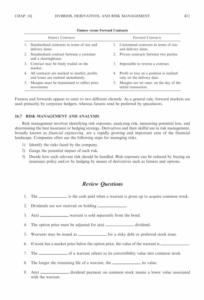
Futures versus Forward Contracts
Futures Contracts Forward Contracts
1. Standardized contracts in terms of size and
delivery dates.
1. Customized contracts in terms of size
and delivery dates.
2. Standardized contract between a customer
and a clearinghouse.
2. Private contracts between two parties.
3. Contract may be freely traded on the
market.
3. Impossible to reverse a contract.
4. All contracts are marked to market; profits
and losses are realized immediately.
4. Profit or loss on a position is realized
only on the delivery date.
5. Margins must be maintained to reflect price
movements.
5. Margins are set once, on the day of the
initial transaction.
Futures and forwards appear to cater to two different clientele. As a general rule, forward markets are
used primarily by corporate hedgers, whereas futures tend be preferred by speculators.
16.7 RISK MANAGEMENT AND ANALYSIS
Risk management involves identifying risk exposure, analyzing risk, measuring potential loss, and
determining the best insurance or hedging strategy. Derivatives and their skilful use in risk management,
broadly known as financial engineering, are a rapidly growing and important area of the financial
landscape. Companies often use the following steps for managing risks.
1) Identify the risks faced by the company.
2) Gauge the potential impact of each risk.
3) Decide how each relevant risk should be handled. Risk exposure can be reduced by buying an
insurance policy and/or by hedging by means of derivatives such as futures and options.
Review Questions
1. The is the cash paid when a warrant is given up to acquire common stock.
2. Dividends are not received on holding .
3. A(n) warrant is sold separately from the bond.
4. The option price must be adjusted for a(n) dividend.
5. Warrants may be issued as for a risky debt or preferred stock issue.
6. If stock has a market price below the option price, the value of the warrant is .
7. The of a warrant relates to its convertibility value into common stock.
8. The longer the remaining life of a warrant, the its value.
9. A(n) dividend payment on common stock means a lower value associated
with the warrant.
CHAP. 16] HYBRIDS, DERIVATIVES, AND RISK MANAGEMENT 411

10. The difference between a warrant and stock right is that the latter is to
existing stockholders.
11. The applies to the number of shares received by a holder of a convertible
security when he or she makes the exchange.
12. The effective price when a holder pays for common stock to effect conversion is termed
the .
13. The market value of a convertible bond relates to its value rather than its
bond value.
14. A(n) is a good financing tool for a growth company.
15. Convertible debt involves a(n) interest rate than straight debt.
16. The margin requirement on purchasing convertible bonds is than on purchas-
ing common stock.
17. Interest yield equals divided by the market price of the bond.
18. The investment value of a convertible bond equals the present value of plus
the present value of the .
19. is the term used when a new convertible security is issued after an old one has
been converted.
20. The term convertible is used when a convertible security continues as debt.
21. For financial statement analysis purposes, a convertible bond with an attractive conversion
feature is considered rather than .
22. Options are traded in terms of lots of shares.
23. When the market price is below the strike price, the call is said to be .
24. If you do not exercise a call option, you will lose your .
25. The total premium of an option consists of the intrinsic value plus based on
factors such as risk, variability, forecasted future prices, expiration date, leverage, and
dividend.
26. The provides the relationship between call option value and the five factors
that determine the premium of an option’s market value over its expiration value.
27. Future markets can be used for both and .
Answers: (1) exercise price; (2) warrants; (3) detachable; (4) stock; (5) ‘‘sweeteners’’; (6) zero; (7) market
value; (8) higher; (9) high; (10) free; (11) conversion ratio; (12) conversion price; (13) if
converted; (14) convertible security; (15) lower; (16) lower; (17) coupon interest; (18) future interest
payments, maturity amount; (19) Leapfrog financing; (20) hung; (21) equity, debt; (22) round, 100; (23)
out-of-the-money; (24) entire investment; (25) speculative premium (time value); (26) Black–Scholes Option
Pricing (OPM); (27) hedging, speculating.
412 HYBRIDS, DERIVATIVES, AND RISK MANAGEMENT [CHAP. 16

Solved Problems
16.1 Warrant Value. A warrant for Ace Corporation stock enables the holder to purchase one share of
common stock at $30 a share. The stock has a market price of $47 a share. What is the value of
the warrant?
SOLUTION
Warrant value ¼ ðmarket price per share� exercise priceÞ � number of shares that may be purchased
¼ ð$47� $30Þ � l ¼ $17
16.2 Warrant Value. Assume the same facts as in Problem 16.1, except that the holder can purchase
four shares of common stock for each warrant. What is the value of the warrant?
SOLUTION
ð$47� $30Þ � 4 ¼ $68
16.3 Warrant Value. Assume the same facts as Problem 16.1, except that the stock has a market price
of $28 a share. What is the value of the warrant?
SOLUTION
ð$28� $30Þ � l ¼ �$2
Since there can never be a negative value for a warrant, zero is the amount assigned to the warrant.
16.4 Premium. The market price of Harris Corporation stock is $45. Its exercise price is similarly $45.
Will the stock warrant sell at a premium?
SOLUTION
Yes. The warrant will sell at a premium, since there exists the possibility that the market price of the
common stock will exceed $45 prior to the expiration date of the warrant.
16.5 Bond to Common Shares. The conversion price of common stock is $20 a share. Into how many
shares will a $1,000 convertible bond be converted?
SOLUTION
$1,000
$20¼ 50 shares
16.6 Conversion Price. A $1,000 bond is convertible into 60 shares of stock. What is the conversion
price?
SOLUTION
$1,000
60 shares¼ $16:67
16.7 Conversion Ratio. A $1,000 convertible bond permits the holder to convert the bond into five
shares of common stock (a) What is the conversion ratio? (b) What is the conversion price?
CHAP. 16] HYBRIDS, DERIVATIVES, AND RISK MANAGEMENT 413

SOLUTION
(a) Five shares for each bond
(b) $1,000
5 shares¼ $200 per share
16.8 Conversion Ratio. T Corporation issued a $1,000 bond at par. The conversion price is $20. What
is the conversion ratio?
SOLUTION
Conversion ratio ¼ par value of convertible security
conversion price¼ $1,000
$20¼ 50
16.9 Convertibility. Tristar Corporation issued a $1,000 bond at par. The common stock has a market
price of $45. The conversion price is $58. (a) Into how many shares can the bond be converted?
(b) What is the conversion value of the bond? (c) What is the conversion premium?
SOLUTION
(a) $1,000
$58¼ 17:24 shares
(b) Conversion value ¼ ðcommon stock priceÞ � ðconversion ratioÞ ¼ $45� 17:25 ¼ $776
(c) $1,000� $776 ¼ $224
16.10 Percentage Conversion Premium. A $1,000 bond is issued at par. The market price of the common
stock at the issue date was $20. The conversion price is $25. (a) What is the conversion ratio?
(b) What is the conversion value? (c) What is the percentage conversion premium?
SOLUTION
(a) $1,000
$25¼ 40
(b) $20� 40 ¼ $800
(c)Percentage conversion premium ¼ market value� conversion value
conversion value¼ $1,000� $800
$800
¼ $200
$800¼ 25%
16.11 Conversion Ratio. What effect will a 2-for-l stock split have on a conversion ratio?
SOLUTION
The conversion ratio will double.
16.12 Conversion Value. A $1,000 bond is convertible into 25 shares of common stock having a market
value of $47 per share. What is the conversion value?
SOLUTION
$47� 25 shares ¼ $1,175
414 HYBRIDS, DERIVATIVES, AND RISK MANAGEMENT [CHAP. 16

16.13 Conversion Ratio. When a $50,000 convertible bond is issued, the market price of the stock is $25
a share. Each $1,000 bond is convertible into 40 shares of stock. (a) What is the conversion ratio?
(b) What is the conversion value? (c) Assuming the stock price is anticipated to grow at 8 percent
annually, what is the conversion value at the end of the first year?
SOLUTION
(a) $50,000
$1,000¼ 50 bonds� 40 shares ¼ 2,000 shares
(b) $25� 2,000 shares ¼ $50,000
(c) Shares 2000
Stock price ð$25� 1:08Þ �$27$54,000
16.14 Simple Interest Yield. A $30,000, 15 percent, 10-year bond is bought at 102. What is the simple
interest yield?
SOLUTION
Coupon interest
Market price of bond¼ 0:15� $30,000
$30,600¼ $4,500
$30,600¼ 14:7%
16.15 Market Price of Stock. For a $1,000 convertible bond, the conversion price is $50. The call price is
$1,200. (a) If the conversion value of the bond equals the call price, what should the market price
of the stock be? (b) What is the approximate market price of common stock if the conversion
value of the bond is 20 percent higher than the call price?
SOLUTION
(a) $1,200
20¼ $60
(b) $60� 1:20 ¼ $72
16.16 Call Price. Drake Corporation’s convertible bond has a conversion price of $90. The conversion
ratio is 15. The market price of the stock is $130. The call price is $1,800. Would the bondholder
rather convert to common stock or receive the call price?
SOLUTION
Market value of common stock received upon conversion is:
$130� 15 ¼ $1,950
Call price ¼ $1,800
The bondholder would rather convert, since he or she receives a benefit of $150.
16.17 Attractiveness of Convertible Debenture. Great Northern Oil Shale Company is a company
actively engaged in the oil services industry. The company provides replacement parts for drilling
rigs and has just begun to test a device that measures shale oil content in certain rock formations.
The company has an 8 percent convertible subordinated debenture outstanding due in the
year 2001. The convertible is callable at 106 and has a conversion price of $50. The common stock
CHAP. 16] HYBRIDS, DERIVATIVES, AND RISK MANAGEMENT 415

is currently paying a dividend of $1.40 on earnings per share of $3. Consensus among analysts is
that long-term interest rates will be stable to lower over the next year. The common stock is
currently selling for $30 and the convertible bond at 66. Nonconvertible bonds of companies in
this industry having similar quality ratings (triple-B) are yielding 14 percent to maturity.
(a) Discuss four characteristics of the convertible debenture, and (b) explain whether you
consider the convertible debenture or the common stock more attractive for purchase. (CFA,
adapted.)
SOLUTION
(a) Characteristics of this convertible industrial debenture include the following:
(1) The quality of the bond is not high but average for most convertible bonds.
(2) The outlook for interest rates is stable to lower. This is a plus, as bond prices should be stable to
rising.
(3) Minimum value as straight debt is around 60, or about 9 percent under current market of 66. This
is well within reasonable limits of, say, 15 percent or below.
(4) The current price of the common is 10 percent below the bonds’ conversion value. Conversion
value is [(1,000/50)� $30], This is within reasonable limits of, say, maximum of 20 percent or so.
(5) The current yield on the bond of 12.0 percent seems favorable at more than twice 4.7 percent on the
common.
(6) The call risk is remote (call price of 106 versus market price of 66).
(b) The convertible looks more attractive because of the modest premiums involved – upside leverage and
downside cushion, compared to the common. The convertible also looks more attractive because of the
higher income relative to the common, assuming that the common stock price has the potential to rise
by a sizable amount from the current price of 33 to the 40-plus level.
16.18 Options. You can buy XZ Company stock at $30 a share, or $3,000 for 100 shares. You can
acquire a $33 3-month call for $400. Thus, you could invest $2,600 cash and have the opportunity
to buy 100 shares at $33 per share. Assume, however, that you decide to invest your $2,600 in a
3-month CD earning 14 percent interest. The CD will return $91 (14%� $2,600� 3/12).
(a) If the YZ Company stock goes to $16, what is the option worth.
(b) If the stock goes to $43, would there be a gain or loss?
SOLUTION
(a) The option will be worthless but the significant loss on the stock of $14 a share did not occur. Instead,
the loss is limited to $309 ($400� $91). However, note that by not buying a stock you may have
forgone a dividend.
(b) If the stock went up to $43, the call would be exercised at $33 resulting in a significant gain with little
investment.
16.19 The Black–Scholes Option Pricing Model (OPM). Given:
Stock price ¼ $23
Exercise price ¼ $18
Risk-free tate ¼ 0:06
Time to expire ¼ 1:0ð1 yearÞStandard deviation of the stock’s return ¼ 0:50ðvariance is 0:25Þ
What is the value of this option?
416 HYBRIDS, DERIVATIVES, AND RISK MANAGEMENT [CHAP. 16

SOLUTION
First, calculate d1 and d2:
d1 ¼lnðP=XÞ þ ½rþ s2=2�t
sffiffi
tp
¼ lnð$23=$18Þ þ ½0:06þ ð0:25=2Þ�ð1:0Þð0:50Þ
ffiffiffiffiffiffiffi
1:0p
¼ 0:86
d2 ¼ d1 � sffiffi
tp¼ 0:86� ð0:50Þ
ffiffiffiffiffiffiffiffiffiffi
ð1:0Þp
¼ 0:36
Next, look up the values for N(d1) and N(d2):
Nðd1Þ ¼ Nð0:86Þ ¼ 1� 0:195 ¼ 0:805
Nðd2Þ ¼ Nð0:36Þ ¼ 1� 0:3595 ¼ 0:6405
Finally, use those values to find the option’s value:
V ¼ P½Nðd1Þ� � Xe�rt½Nðd2Þ�¼ $23½0:805� � $18eð�0:06Þð1:0Þ½0:6405�¼ $7:66
CHAP. 16] HYBRIDS, DERIVATIVES, AND RISK MANAGEMENT 417

Chapter 17
Mergers and Acquisitions
17.1 INTRODUCTION
Internal growth comes about when a company invests in products it has developed, while external
growth occurs when a company buys the existing assets of another company through a merger.
Financial managers are sometimes required to evaluate the attractiveness of a potential merger as well
as participate in merger negotiations. In addition to growth, mergers may allow an organization to
diversify.
There are three common ways of joining two or more companies. The following definitions will
distinguish the difference between a merger, consolidation, and a holding company:
Merger. A merger is the combination of two or more companies into one, where only the acquiring
company retains its identity. Typically, the larger of the two companies is the acquiring company whose
identity is maintained.
Consolidation. In a consolidation, two or more companies are combined to form a new company.
None of the consolidation firms legally survives. In effect, the consolidating firms are dissolved and a
new company is formed.
EXAMPLE 17.1 Companies X and Y give all their assets, liabilities, and stock to the new company, Z, in return
for Z’s stock, bonds, or cash. The combining of companies X and Y with new company Z emerging is a
consolidation.
Holding Company. A holding company holds, or owns, enough shares of common stock to have
voting control of one or more other companies. The holding company comprises a group of businesses,
each operating as a separate corporate entity. By holding more than 50 percent of the voting rights
through common stock, the holding company ensures control of the other companies. In reality, a
holding company can have effective control of another company with a smaller percent of ownership,
such as 20 percent. The holding company is called the parent, and each company controlled is called a
subsidiary.
Depending on the intent of the combination, there are three common ways businesses get together to
gain advantage in their market. The three types of mergers are:
1. Vertical. A vertical merger takes place when a company combines with a customer or supplier.
For example, when a furniture manufacturer combines with a chain of furniture stores, the
combination is vertical.
2. Horizontal. A horizontal combination is when two companies in a similar business combine, for
example, when one oil company buys another oil company.
3. Conglomerate. A conglomerate is when two companies in unrelated industries combine. For
example, when an appliance manufacturer combines with a book publisher, a conglomerate is
formed.
17.2 MERGERS
The merger of two companies can be accomplished in one of two ways. The acquiring company can
negotiate with management of the other company, which is the preferred approach, or it can make a
tender offer directly to the stockholders of the company it wants to take over. A tender offer is an offer of
cash for shares of stock held by stockholders.
418
Copyright © 2007, 1998, 1986 by The McGraw-Hill Companies, Inc. Click here for terms of use.

In negotiating with management, often the acquiring company makes a stock offer based on a
specified exchange ratio. The merger may take place if the acquired company receives an offer at an
acceptable premium over the present market price of its stock. Sometimes to satisfy the management of
the acquired business, certain contingent payments, such as stock purchase warrants, are made part
of the merger contract. If the negotiations break down, a tender offer may be made directly to the
company’s stockholders. The tender offer is made at a premium above the market price of the stock and
is offered to all stockholders of the company. Tender offers are fully discussed later in this chapter.
There are various financing packages that buyers may use for mergers such as common stock,
preferred stock, convertible securities, cash, debt, and warrants. A prime consideration in selecting the
final package is its impact on current earnings per share.
When common stock is exchanged, the seller’s stock is given in exchange for the buyer’s stock. The
advantage of a stock trade is that it represents a tax-free exchange. A disadvantage is that issuing the
stock increases the buyer’s outstanding shares, thus diluting earnings per share. When there is an
exchange of cash for common stock, the selling firm’s stockholders receive cash for their common
stock, resulting in a taxable transaction. Such an exchange may improve earnings per share because
the buying company is getting new earnings without increasing outstanding shares.
Reasons for Mergers
There are several reasons why a company would prefer external growth through merger rather than
internal growth:
1. The company may want diversification to reduce the risks involved with a seasonal business.
2. A company may expect a synergistic effect by merging with another. Through synergy the results
are greater than the sum of the parts. That is, greater earnings may be obtained from the
combined company than would be possible from each individual company because of efficiency
and cost savings. There is a greater chance of synergistic gains from a horizontal merger, since
duplicate facilities may be eliminated.
3. A merger may permit one firm to obtain something it lacks, such as superior management talent
or a research capability.
4. A company may improve its ability to raise funds when it combines with another having highly
liquid assets and low debt.
5. The net income of the new large company may be capitalized at a low rate, resulting in a high
market value for its stock. The stock of a large company is usually more marketable than that of
a small one. These attributes may result in a high P/E ratio for the stock.
6. In some cases, it is possible to finance an acquisition when it would not be possible to finance
internal expansion. For instance, acquiring another company by exchanging stock may be less
costly than constructing a new plant, which requires a substantial cash payment.
7. An acquisition can result in a good return on the investment when the market value of the
acquired company is significantly below its replacement cost.
8. By acquiring a company that has been operating at a net loss, the acquiring company may not
only get the acquired company at a good price, but will also obtain a tax benefit.
Disadvantages of Mergers
The disadvantages that may result from mergers are:
1. A merger may not work out financially because the anticipated benefits (e.g., cost reductions) do
not occur.
2. Friction may arise between the management of the two companies.
3. Dissenting minority stockholders may cause problems.
4. Government antitrust action may block or delay the proposed merger.
CHAP. 17] MERGERS AND ACQUISITIONS 419

Evaluating a Potential Merger
In evaluating a possible merger, the financial manager must consider the effect the merger may have
on the performance of the company, such as:
1. Earnings per share. The merger should improve earnings per share or enhance its stability.
2. Dividends per share. The dividends paid prior to the merger should be maintained to stabilize the
market price of stock.
3. Market price per share. The essential variable to consider is the effect of the merger on the
market price of the company’s stock.
4. Risk. The merger should reduce the business and financial risk of the resulting enterprise.
17.3 ACQUISITION TERMS
When determining the terms of the acquisition, consideration should be given to the following
factors:
1. The absolute amount of earnings as well as the earnings growth rate
2. Dividends
3. Market price of the stock
4. Book value per share
5. Net working capital per share
The weight each factor bears on a merger varies, based on the particular circumstances involved.
Earnings. In ascertaining the value of earnings in a merger, consideration should be given to
anticipated future profit and the projected P/E multiple. A company in a rapid growth stage is expected
to have a high P/E multiple.
EXAMPLE 17.2 Company S and company T are planning a merger. Company S has the higher P/E ratio. The
earnings of company S are expected to show a greater growth rate than that of company T. If the merger occurs, the
acquiring company T will be obtaining a company with superior growth potential. Therefore, company T’s
profitability subsequent to the merger should increase faster than before. The new growth rate will approximate
the weighted average growth rates on the individual companies with the weight based on the relative total earnings
prior to the merger. The key considerations involved in this analysis are the past and projected growth rates of the
business, their size, the P/E multipliers, and the exchange ratio. The combination of these factors influences the EPS
of the surviving company.
Dividends. Dividends impact the acquisition terms, since they constitute income to stockholders.
However, the greater a company’s growth rate and profitability, the lesser the impact dividends will have
on the per share market price of the companies. Conversely, when profits are declining, dividends will
have a more significant effect on the market price of the stock.
Market Price of the Stock. Since the price per share takes into account potential earnings and
dividends, current market value must be considered in the merger. The value given to the firm in the
acquisition will probably be greater than the current market price per share under the following
circumstances:
1. The company is in an industry with financial problems and thus will have a currently depressed
market price.
2. The acquired company may have more of a value to the acquirer (e.g., assist in diversification)
than to the stock market in general.
3. To encourage stockholders to give up their shares, an amount greater than the current market
price may be given.
420 MERGERS AND ACQUISITIONS [CHAP. 17

Book Value per Share. Generally speaking, book value is not an important ingredient in the merger
process because it is based on historical cost rather than current values. But book value may be relevant
when it exceeds market price. In such a case, there may be an expectation that the market price of the
stock will increase because of new and better management.
Net Working Capital per Share. Net working capital per share may impact the merger terms
due to the liquidity of one of the combining companies. For example, if the acquired company
has a very low debt position, the acquiring company may borrow the funds needed for the
acquisition by using the acquired company’s good liquidity position to meet the loan following
the merger. Or the liquid assets of the acquired company can provide needed collateral for the issuance
of debt.
17.4 MERGER ANALYSIS
The acquisition of a going concern is evaluated through capital budgeting techniques such as
discounted cash flow (DCF) analysis. When a company buys another having a financial structure
materially different from its own, the impact of the new capital structure on the company’s overall
cost of capital must be projected.
EXAMPLE 17.3 Sharav Company is considering purchasing Shillinglaw Corporation for $80,000 in cash. Sharav’s
current cost of capital is 15 percent. Shillinglaw’s estimated overall cost of capital is expected to become 12 percent
after the acquisition. The estimated cash inflows from years 1 to 12 are $10,000.
The net present value is:
Calculations Present Value
Year 0 –$80,000� 1 –$80,000
Years 1–12 +$10,000� 6.194a +61,940
Net present value –$18,060
a PVIFA12,12
Since the net present value is negative, the acquisition should not take place.
EXAMPLE 17.4 Boston Corporation is considering acquiring Masters Corporation for $200,000 in cash. Boston’s
cost of capital is 16 percent primarily due to its high debt position. If the acquisition is made, Boston expects that
its overall cost of capital will be 14 percent because Masters Corporation is financed mostly with equity. The
acquisition is anticipated to generate yearly cash inflows of $28,000 for the next 10 years.
The net present value is:
Calculations Present Value
Year 0 –$200,000� 1 –$200,000
Years 1–10 +$28,000� 5.216 +146,048
Net present value –$ 53,952
Since the net present value is negative, the acquisition should not take place.
Acquisition of Assets for Cash
When one company acquires another for cash, capital budgeting may be used to examine the
financial feasibility of the acquisition. To ascertain whether the purchase of assets is financially
justifiable, the company must predict the costs and benefits of the assets.
CHAP. 17] MERGERS AND ACQUISITIONS 421

EXAMPLE 17.5 The Davis Company wants to buy certain fixed assets of Boris Company. However, Boris wants
to sell out its entire business. The balance sheet for Boris Company follows:
ASSETS
Cash $ 3,000
Accounts receivable 7,000
Inventories 12,000
Equipment 1 15,000
Equipment 2 25,000
Equipment 3 40,000
Building 100,000
Total assets $202,000
LIABILITIES AND
STOCKHOLDERS’ EQUITY
Total liabilities $ 90,000
Total stockholders’ equity 112,000
Total liabilities and stockholders’
equity $202,000
Davis needs only equipment 2 and 3 and the building. The other assets excluding cash can be sold for $30,000.
The total cash received is therefore $33,000 ($30,000+$3,000 initial cash balance). Boris wants $45,000 for the
entire business. Davis will thus have to pay a total of $135,000, which is $90,000 in total liabilities and $45,000 for its
owners. The actual net cash outlay is therefore $102,000 ($135,000� $33,000). It is expected that the after-tax cash
inflows from the new equipment will be $25,000 per year for the next 6 years. The cost of capital is 10 percent.
The net present value associated with this acquisition follows:
Calculations Present Value
Year 0 �$102,000� 1 �$102,000Years 1–6 +$25,000� 4.355 +108,875
Net present value +$ 6,875
Since the net present value is positive, the acquisition is recommended.
EXAMPLE 17.6 Miles Corporation is thinking of acquiring Piston Corporation for $50,000. Piston has liabilities
of $75,000. Piston has equipment that Miles desires. The remaining assets would be sold for $58,000. By acquiring
the equipment, Miles will have an increase in cash flow of $17,000 each year for the next 12 years. The cost of capital
is 10 percent.
The net cost of the equipment is:
$50; 000þ $75; 000� $58; 000 ¼ $67; 000
Miles should make the acquisition since, as indicated below, the net present value is positive.
Calculations Present Value
Year 0 �$67,000� 1 �$ 67,000
Years 1–12 +$17,000� 6.814 +115,838
Net present value +$ 48,838
Acquisition by Exchanging Stock
A company is often acquired by exchanging common stock. The exchange will be in accordance
with a predetermined ratio. The amount the acquiring firm offers for each share of the acquired
422 MERGERS AND ACQUISITIONS [CHAP. 17

business is usually more than the current market price of the traded shares. The ratio of exchange
is equal to:
Amount paid per share of the acquired company
Market price of the acquiring company’s shares
EXAMPLE 17.7 Company A wants to acquire company B. Company A’s stock sells for $80 per share. Company
B’s stock sells for $55 per share. Because of the merger negotiations, company A offers $60 per share. The
acquisition is made through an exchange of securities.
Ratio of exchange ¼ amount paid per share of the acquired company
market price of the acquiring company’s shares¼ $60
$80¼ 0:75
Company A must exchange 0.75 share of its stock for one share of company B’s stock.
17.5 THE EFFECT OF A MERGER ON EARNINGS PER SHARE AND MARKET PRICE
PER SHARE OF STOCK
When a merger takes place, there may be a favorable or unfavorable effect on net income and
market price per share of stock. The effect on earnings per share can easily be seen in Example 17.9.
EXAMPLE 17.8 The following data are presented:
Company X Company Y
Net income $30,000 $54,000
Shares outstanding 4,000 9,000
Earnings per share $7.50 $6.00
P/E ratio 10 12.5
Market price $75 $75
Company Y is the acquiring company and will exchange its shares for company X’s shares on a one-for-one
basis. The exchange ratio is based on the market prices of X and Y. The impact on EPS follows:
Y Shares Owned
after Merger
EPS Prior
to Merger
EPS Subsequent
to Merger
X stockholders 4,000 $7.50 $6.46a
Y stockholders 9,000 $6.00 $6.46a
Total 13,000
a Total net income is calculated as follows:
4,000 shares� $7.50 $30,000
9,000 shares� $6.00 54,000
New EPS $84,000
EPS ¼ total net income
total shares¼ $84; 000
13; 000¼ $6:46
EPS decreases by $1.04 for X stockholders but increases by $0.46 for Y stockholders.
The impact on market price is not clear. Assuming the combined company has the same P/E ratio as that of
company Y, the market price per share will be $80.75 (12.5� $6.46). In this example, the stockholders of each firm
enjoy a higher market value per share. The increased market value comes about because the net income of the
combined company is valued at a 12.5 P/E ratio, the same as company Y, while before the merger, company X had a
CHAP. 17] MERGERS AND ACQUISITIONS 423

lower P/E multiple of 10. But if the combined company is valued at company X’s multiplier of 10, the market value
would be $64.60 (10� $6.46). In this instance, the stockholders in each firm will have experienced a decline in market
value of $10.40 ($75.00� $64.60).
Since the effect of a merger on market value per share is not clear, EPS is given the prime consideration.
EXAMPLE 17.9 The following data are given:
Case
Market Price per Share
of Acquiring Company
Market Price per Share
of Acquired Company
Price per Share
Offered
1 $60 $20 $25
2 $100 $130 $140
In each of the following cases, the exchange ratio in (1) shares and (2) market price is:
Exchange Ratio
Case Shares Market Price
1 $25/$60=0.42 $25/$20=1.25
2 $140/$100=1.4 $140/$130=1.08
EXAMPLE 17.10 Joy Corporation wishes to acquire Davis Corporation. Data for the companies follow:
Joy Davis
Net income $30,000 $14,000
Shares outstanding 22,000 7,000
Joy Corporation issues its shares to make the acquisition. The ratio of exchange is 2.2 to 1. The EPS based on
the original shares of each company follows:
EPS of the merged entity ¼ combined net income
total shares¼ $30,000þ $14,000
22,000þ 7,000� 2:2ð Þ
¼ $44,000
22,000þ 15,400¼ $44,000
37,400 shares¼ $1:18
EPS of Joy ¼ $1:18
EPS of Davis ¼ $1:18� 2:2 ¼ $2:60
EXAMPLE 17.11 Andrew Company wants to acquire Stella Company by exchanging 0.6 share of its stock for
each share of Stella. Financial data follow:
Andrew Stella
Net income $180,000 $36,000
Shares outstanding 60,000 18,000
EPS $3 $2
Market price $30 $14
P/E ratio 10 7
Andrew issues its shares to make the acquisition. The shares Andrew has to issue in the acquisition are:
18,000 shares� 0:6 ¼ 10,800 shares
424 MERGERS AND ACQUISITIONS [CHAP. 17

Assuming the earnings of each company remain the same, the EPS after the acquisition is:
$180,000þ $36,000
60,000þ 10,800¼ $216,000
70,800 shares¼ $3:05
The amount earned per share on the original shares of Stella stock is:
$3:05� 0:6 ¼ $1:83
The amount earned per share on the original shares of Andrew stock is $3.05.
EXAMPLE 17.12 Arnold Corporation wishes to acquire Jack Corporation by exchanging 1.5 shares of its stock
for each share of Jack. Arnold Corporation expects to have the same P/E ratio after the merger as before. The
following financial data are presented:
Arnold Jack
Net income $400,000 $100,000
Shares 200,000 25,000
Market price per share $40 $48
The exchange ratio of market price is:
Price per share offered
Market price of Jack¼ $40� 1:5
$48¼ $60
$48¼ 1:25
EPS and P/E multiples for each firm are:
Arnold Jack
EPS $400,000/200,000 shares=$2 $100,000/25,000 shares=$4
P/E ratio $40/$2=20 times $48/$4=12 times
The P/E ratio used in obtaining Jack is:
1:5� $40 ¼ $60
$60
$4¼ 15 times
The EPS of Arnold after the acquisition is:
$500,000
200,000þ 25,000� 1:5ð Þ ¼$500,000
237,500 shares¼ $2:11
The anticipated market price per share of the merged company is:
$2:11� 20 times ¼ $42:20
17.6 HOLDING COMPANY
A holding company is one that has the sole purpose of owning the stock of other businesses.
A holding company can acquire a small percent of another company (e.g., 10 percent), which may
be sufficient to obtain a significant influence over the other, especially when stock ownership
is widely disbursed. A holding company that wants to obtain voting control of a business may
make a direct market purchase or a tender offer to get the additional shares. What would prompt the
officers of a company to turn it into a holding company? A company in a declining industry, for
example, may decide to move out of its basic operations by liquidating assets and use the funds
obtained to invest in other companies having good growth potential.
Since the operating companies held by the holding company are distinct legal entities, the obligations
of any one are isolated from the others. If one of them goes under, there is no claim on the assets
of another. However, a loan officer that lends to one company may require a guarantee by the other
CHAP. 17] MERGERS AND ACQUISITIONS 425

companies. This will in effect join the assets of the companies. In any case, a major financial setback
involving one company is not the responsibility of the others.
The advantages of a holding company arrangement include the following:
1. The ability of the holding company to acquire a large amount of assets with a small investment.
In effect, the holding company can control more assets than it could acquire through a merger.
2. There is risk protection because the failure of one of the companies does not cause the failure of
the other companies or the holding company. The failure of one invested company would not
cost the holding company more than its investment in that firm.
3. It is easy to gain control of another company because all that is involved is buying enough stock
in the market place. Unlike a merger in which stockholder or management approval is needed,
no approval is needed for a holding company.
The disadvantages of a holding company arrangement are as follows:
1. There is multiple taxation since the income the holding company receives from its
subsidiaries is in the form of cash. Before paying dividends, the subsidiary must pay taxes on
its earnings.
2. A holding company is typically more costly to administer than a single company emanating
from a merger. The increased costs arise from not achieving the economies that would normally
occur in a merger.
3. The U.S. Department of Justice may consider the holding company a near monopoly and force
dissolution of some of the companies by disposal of stock.
4. By acquiring stock ownership in other companies there may occur a financial leverage effect
through increased debt which will magnify either earnings or losses. The more the financial
leverage involved, the higher the risk of variability in earnings.
A holding company can get a large amount of control for a small investment by obtaining
voting control in a company for a minimal amount and then using that firm to gain voting control in
another, and so on.
EXAMPLE 17.13 Matz Company holds stock in company X and company Y and has voting control over both.
Balance sheet information follows:
Matz Company
Investment Long-term liabilities $ 40,000
Company X $ 30,000 Preferred stock 20,000
Company Y 70,000 Common stock equity 40,000
Total $100,000 Total $100,000
Company X
Current assets $120,000 Current liabilities $100,000
Noncurrent assets 480,000 Long-term liabilities 350,000
Common stock equity 150,000
Total $600,000 Total $600,000
Company Y
Current assets $200,000 Current liabilities $150,000
Noncurrent assets 600,000 Long-term liabilities 400,000
Common stock equity 250,000
Total $800,000 Total $800,000
426 MERGERS AND ACQUISITIONS [CHAP. 17

The percent of total assets controlled by Matz Corporation emanating from its common stock equity is:
Common stock equity of Matz
Total assets of company X and company Y¼ $40,000
$1,400,000¼ 2:9%
Assuming another company owns 18 percent of the common stock of Matz and has voting control, the
percent of the total assets controlled by the other company’s equity is:
2:9%� 18% ¼ 0:52%
17.7 TENDER OFFER
The takeover of another company is often accomplished through negotiation. In the event the
management of the target company does not want to be merged, the company can be acquired against
its will by the buyer making a tender offer. A tender offer is made when the buyer goes directly to the
stockholders of the target business to tender (sell) their shares, typically for cash. The tender in some
cases may be shares in the acquiring company rather than cash. If the buyer obtains enough stock, it can
gain control of the target company and force the merger. Stockholders are induced to sell when the
tender price substantially exceeds the current market price of the target company stock. Typically, there
is an expiration date to the tender. Good takeover candidates are cash-rich businesses and those with low
debt/equity ratios.
The management of a targeted company can fight the takeover attempt, if it wishes, in the following
ways:
1. Furnish publicity against the raider.
2. Purchase treasury stock to make fewer shares available for tendering.
3. Initiate legal action to prevent the takeover, such as by applying antitrust laws.
4. Postpone the tender offer. Many states have laws that can delay the tender offer.
5. Seek out a merger with a different, friendlier, company.
6. Declare an attractive dividend to keep stockholders happy.
With regard to tender offers, the following disclosure requirements exist:
1. The acquiring business must furnish to the management of the potential acquired company
and to the SEC, 30 days’ notice of its intent to acquire.
2. The name of the group furnishing the money for the acquisition must be disclosed when
significant amounts of stock are purchased on the stock exchange. Typically, the acquired
stock is in the street name of the broker who is acting for the true owner.
Due to the disclosure requirements, competition may arise in the takeover attempt. The competing
acquiring companies may increase the acquisition price significantly by bidding higher than the
pretakeover market price of stock.
17.8 LEVERAGE BUYOUT (LBO)
A leveraged buyout occurs when an entity primarily borrows money (sometimes 90% or more) in
order to buy another company. Typically, the acquiring company uses as collateral the assets of the
acquired business. Generally, repayments of the debt will be made from the yearly operating funds flow
of the acquired company. A leveraged buyout may also be made when the acquiring company uses its
own assets as security for the loan. It may also be used if a firm wishes to go private. In most cases, the
CHAP. 17] MERGERS AND ACQUISITIONS 427

stockholders of the acquired company will receive an amount greater than the current price of the stock.
A leveraged buyout involves more risk than an acquisition done through the issuance of equity securities.
17.9 DIVESTITURE
The divestiture of business segments by corporations has become an accepted strategy for
growth rather than diversification. Divestiture is the sale of some of a firm’s operating assets. Prior to
formulating a divestiture strategy and determining which segments should be divested, the reasons for
divestiture need to be listed. The reasons given by management for divesting segments of their business
are the following:
1. Poor performance
2. Changes in plans
3. Excessive resource needs
4. Constraints in operation
5. Source of funds
6. Antitrust
Review Questions
1. A combination of two or more companies into one where only the acquiring company retains
its identity is referred to as a(n) .
2. A consolidation is when two or more companies combine to form a(n)
company.
3. A(n) company owns common stock of other companies.
4. A(n) business combination is when two companies in a similar business
combine.
5. A(n) is when two companies in unrelated industries combine.
6. A good combination may result in a(n) effect.
7. A occurs when an entity primarily borrows money (sometimes 90% or more)
in order to buy another company.
8. Divestiture is the of some of a firm’s operating assets.
9. A(n) is made when an acquiring company goes directly to the stockholders of
the target business to buy their shares.
Answers: (1) merger; (2) new; (3) holding; (4) horizontal; (5) conglomerate; (6) synergistic (7) leveraged
buyout (LBO); (8) sale; (9) tender offer.
428 MERGERS AND ACQUISITIONS [CHAP. 17

Solved Problems
17.1 Acquisition of a Company. Yohai Corporation is thinking of purchasing Klein Corporation for
$70,000 in cash. Yohai’s current cost of capital is 16 percent. Klein’s estimated overall cost of
capital is anticipated to be 14 percent after the acquisition. Forecasted cash inflows from years
1 to 15 are $8,000. Should the acquisition be made?
SOLUTION
Calculations Present Value
Year 0 �$70,000� 1 �$70,000Years 1–15 +$8,000� 6.142 +49,136a
Net present value �$20,864a Using 14 percent as the discount rate.
Since the net present value is negative, the acquisition should not be made.
17.2 Acquisition of Assets for Cash. Master Corporation wants to buy certain fixed assets of Smith
Corporation. However, Smith Corporation wants to dispose of its entire business. The balance
sheet of Smith follows:
ASSETS
Cash $ 2,000
Accounts receivable 8,000
Inventories 20,000
Equipment 1 10,000
Equipment 2 20,000
Equipment 3 35,000
Building 90,000
Total assets $185,000
LIABILITIES AND
STOCKHOLDERS’ EQUITY
Total liabilities $ 80,000
Total stockholders’ equity 105,000
Total liabilities and stockholders’
equity $185,000
Master needs only equipment 1 and 2 and the building. The other assets excluding cash can
be sold for $35,000. Smith wants $48,000 for the entire business. It is anticipated that the after-tax
cash inflows from the new equipment will be $30,000 a year for the next 8 years. The cost of
capital is 12 percent.
(a) What is the initial net cash outlay? (b) Should the acquisition be made?
SOLUTION
(a) Total payment:
Liabilities $80,000
Owners 48,000 $128,000
Cash available ($2,000+$35,000) 37,000
Initial net cash outlay $ 91,000
CHAP. 17] MERGERS AND ACQUISITIONS 429
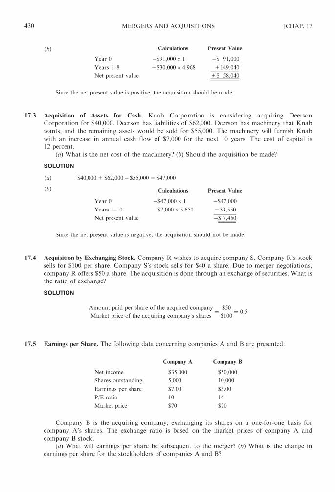
(b) Calculations Present Value
Year 0 �$91,000� 1 �$ 91,000
Years 1–8 +$30,000� 4.968 +149,040
Net present value +$ 58,040
Since the net present value is positive, the acquisition should be made.
17.3 Acquisition of Assets for Cash. Knab Corporation is considering acquiring Deerson
Corporation for $40,000. Deerson has liabilities of $62,000. Deerson has machinery that Knab
wants, and the remaining assets would be sold for $55,000. The machinery will furnish Knab
with an increase in annual cash flow of $7,000 for the next 10 years. The cost of capital is
12 percent.
(a) What is the net cost of the machinery? (b) Should the acquisition be made?
SOLUTION
(a) $40,000+$62,000� $55,000=$47,000
(b) Calculations Present Value
Year 0 �$47,000� 1 �$47,000Years 1–10 $7,000� 5.650 +39,550
Net present value �$ 7,450
Since the net present value is negative, the acquisition should not be made.
17.4 Acquisition by Exchanging Stock. Company R wishes to acquire company S. Company R’s stock
sells for $100 per share. Company S’s stock sells for $40 a share. Due to merger negotiations,
company R offers $50 a share. The acquisition is done through an exchange of securities. What is
the ratio of exchange?
SOLUTION
Amount paid per share of the acquired company
Market price of the acquiring company’s shares¼ $50
$100¼ 0:5
17.5 Earnings per Share. The following data concerning companies A and B are presented:
Company A Company B
Net income $35,000 $50,000
Shares outstanding 5,000 10,000
Earnings per share $7.00 $5.00
P/E ratio 10 14
Market price $70 $70
Company B is the acquiring company, exchanging its shares on a one-for-one basis for
company A’s shares. The exchange ratio is based on the market prices of company A and
company B stock.
(a) What will earnings per share be subsequent to the merger? (b) What is the change in
earnings per share for the stockholders of companies A and B?
430 MERGERS AND ACQUISITIONS [CHAP. 17

SOLUTION
(a) B Shares Owned
after Merger
EPS before
Merger
EPS after
Merger
A stockholders 5,000 $7.00 $5.67a
B stockholders 10,000 $5.00 $5.67a
Total 15,000
a Total net income is calculated as follows:
5,000 shares� $7 $35,000
10,000 shares� $5 50,000
New EPS $85,000
EPS ¼ total net income
total shares¼ $85; 000
15; 000¼ $5:67
(b) EPS decreases by $1.33 for company A stockholders but increases by $0.67 for company B
stockholders.
17.6 Exchange Ratio. The following information is provided:
Case
Market Price per Share
of Acquiring Company
Market Price per Share
of Acquired Company
Price per Share
Offered
1 $80 $40 $50
2 $120 $160 $180
For each case, determine (a) the exchange ratio in shares, and (b) the exchange ratio in
market price.
SOLUTION
Case (a) Shares (b) Market Price
1 $50/$80=0.625 $50/$40=1.25
2 $180/$120=1.5 $180/$160=1.125
17.7 Earnings per Share of Merged Company. Paula Company wants to acquire David Company.
Relevant data follow:
Paula David
Net income $40,000 $25,000
Shares outstanding 20,000 5,000
Paula issues its shares to make the acquisition. The ratio of exchange is 2.5. (a) What is
the earnings per share of the merged company based on the original shares of each company?
(b) What is the earnings per share of Paula? (c) What is the earnings per share of David?
SOLUTION
(a) The merged company’s earnings per share is:
Combined net income
Total shares¼ $65,000
20,000þ ð5,000� 2:5Þ ¼$65,000
20,000þ 12,500¼ $65,000
32,500 shares¼ $2
(b) Paula’s earnings per share is $2.
(c) David’s earnings per share is:
$2� 2:5 ¼ $5
CHAP. 17] MERGERS AND ACQUISITIONS 431

17.8 Earnings per Share. Shim Company wishes to acquire Siegel Company by exchanging 0.8 share of
its stock for each share of Siegel. Financial data follow:
Shim Siegel
Net income $200,000 $40,000
Shares outstanding 50,000 20,000
Earnings per share $4 $2
Market price $40 $16
P/E ratio 10 8
Shim issues its shares to make the acquisition. (a) How many shares must Shim issue in the
acquisition? (b) Assuming the net income of each firm remains the same, what is the earnings per
share after the acquisition? (c) What is the amount earned per share on the original shares of
Siegel stock? (d ) What is the amount earned per share on the original shares of Shim stock?
SOLUTION
(a) 20,000 shares � 0:8 ¼ 16,000 shares
(b) $200,000þ $40,000
50,000þ 16,000¼ $240,000
66,000¼ $3:64
(c) $3:64� 0:8 ¼ $2:91
(d ) $3.64
17.9 EPS, P/E Ratio, and Market Price. Harris Corporation wants to acquire Logo Corporation by
exchanging 1.6 shares of its stock for each share of Logo. Harris anticipates having the same P/E
ratio subsequent to the merger as prior to it. The following financial data are given:
Harris Logo
Net income $500,000 $150,000
Shares 100,000 25,000
Market price per share $35 $40
(a) What is the exchange ratio of market prices? (b) What is the EPS and the P/E ratio for
each company? (c) What was the P/E ratio used in obtaining Logo? (d ) What is the EPS of Harris
after the acquisition? (e) What is the expected market price per share of the merged company?
SOLUTION
(a) Price per share offered
Market price of Logo¼ $35� 1:6
$40¼ $56
$40¼ 1:4
(b)
Harris Logo
EPS $500,000/100,000 shares=$5 $150,000/25,000 shares=$6
P/E ratio $35/$5=7 times $40/$6=6.67 times
(c)1:6� $35 ¼ $56
$56
$6¼ 9:33 times
(d ) $650; 000
$100; 000þ ð25; 000� 1:6Þ ¼$650; 000
140; 000 shares¼ $4:64
(e) $4:64� 7 times ¼ $32:48
432 MERGERS AND ACQUISITIONS [CHAP. 17

17.10 Merger Value. Burger Queen, a national hamburger chain, is considering a smaller chain, Johns
Burger. Burger Queen’s analysts project that the merger will result in the following incremental
net cash flows (in millions of dollars):
Year 1 Year 2 Year 3 Year 4
1.5 2 3 5
Furthermore, Johns’ cash flows are expected to grow at a constant rate of 5 percent after Year 4.
Johns’ post merger beta is estimated to be 1.5, the risk-free rate is 6 percent, and the market risk
premium is 4 percent. Calculate the value of Johns’ Burger to Burger Queen.
SOLUTION
Johns’ required rate of return ¼ 6%þ 1:5ð4%Þ ¼ 12%:
So the terminal cash flow ¼ $5ð1þ 0:05Þ0:12� 0:05
¼ $5:25=0:07 ¼ $75
Year 4’s NCF then is $80 ð$5þ $75Þ
NCF
PV
Factor PV
1.5 0.8929 $1.34
2 0.7972 1.59
3 0.7118 2.14
80 0.6355 50.84
$55.91
NPV=$55.91 million
17.11 Holding Company. Usry Company holds stock in company A and company B and possesses
voting control over both. Balance sheet data follow:
Usry Corporation
Investment Long-term liabilities $ 30,000
Company A $ 20,000 Preferred stock 10,000
Company B 80,000 Common stock equity 60,000
Total $100,000 Total $100,000
Company A
Current assets $200,000 Current liabilities $100,000
Noncurrent assets 300,000 Long-term liabilities 200,000
Common stock equity 200,000
Total $500,000 Total $500,000
Company B
Current assets $300,000 Current liabilities $200,000
Noncurrent assets 400,000 Long-term liabilities 350,000
Common stock equity 150,000
Total $700,000 Total $700,000
CHAP. 17] MERGERS AND ACQUISITIONS 433

(a) What is the percent of total assets controlled by Usry Corporation resulting from its
common stock equity? (b) Assuming another company owns 25 percent of the common stock of
Usry and has voting control, what is the percent of the total assets controlled by the other firm’s
equity?
SOLUTION
(a) Common stock equity of Usry
Total assets of company A and company B¼ $60,000
$1,200,000¼ 5:0%
(b) 5:0%� 2:5% ¼ 1:25%
434 MERGERS AND ACQUISITIONS [CHAP. 17

Chapter 18
Failure and Reorganization
18.1 INTRODUCTION
When a business fails it can be either reorganized or dissolved depending on the circumstances.
A number of ways exist for business failure to occur, including a poor rate of return, technical
insolvency, and bankruptcy.
Deficient Rate of Return. A company may fail if its rate of return is negative or poor. If operating
losses exist, the company may not be able to meet its obligations. A negative rate of return will cause
a decline in the market price of its stock. When a company does not earn a return greater than its
cost of capital, it may fail. If corrective action is not forthcoming, perhaps the firm should liquidate.
A poor return, however, does not constitute legal evidence of failure.
Technical Insolvency. Technical insolvency means that the business cannot satisfy current debt
when due even if total assets are greater than total liabilities.
Bankruptcy. In bankruptcy, liabilities are greater than the fair market value of assets. There exists
a negative real net worth.
According to law, failure of a company can be either technical insolvency or bankruptcy. When
creditor claims against a business are in question, the law permits creditors recourse against
the company.
Some causes of business failure include:
1. Poor management
2. An economic downturn affecting the company and/or industry
3. The end of the life cycle of the firm
4. Overexpansion
5. Catastrophe
18.2 VOLUNTARY SETTLEMENT
A voluntary settlement with creditors permits the company to save many of the costs that would be
present in bankruptcy. Such a settlement is done out of court. The voluntary settlement enables the
company to either continue or be liquidated and is initiated to enable the debtor firm to recover some
of its investment.
A creditor committee may decide to allow the firm to continue to operate if it is expected that
the company will recover. Creditors may also continue to do business with the company. In sustaining
the firm’s existence, there may be:
1. An extension
2. A composition
3. Creditor control
4. Integration of each of the above
Extension
In an extension, creditors will receive the balances due but over an extended period of time. Current
purchases are made with cash. It is also possible that the creditors may agree not only to lengthen the
maturity date for payment but also to subordinate their claims to current debt for suppliers furnishing
435
Copyright © 2007, 1998, 1986 by The McGraw-Hill Companies, Inc. Click here for terms of use.

credit in the extension period. The creditors expect the debtor will be able to work out his or her
problems.
The creditor committee may require certain controls, including legal control over the company’s
assets or common stock, obtaining a security interest in assets, and approval of all cash payments.
If there are creditors dissenting to the extension agreement, they may be paid immediately to prevent
them from having the company declared bankrupt.
Composition
In a composition, there is a voluntary reduction of the amount the debtor owes the creditor. The
creditor obtains from the debtor a stated percent of the obligation in full settlement of the debt regardless
of how low the percent is. The agreement is designed to allow the debtor to continue to operate. The
creditor may try to work with the debtor in handling the firm’s financial problems, since a stable
customer may ensue. The advantages of a composition are that court costs are eliminated as well
as the stigma of a bankrupt company.
If there are dissenting stockholders, they may be paid in full or they may be permitted to recover
a higher percentage so that they do not force the business to close.
For an extension or composition to be practical, the following should exist:
1. An ethical debtor who will not use the company’s assets for personal use.
2. An expectation that the debtor will recover.
3. Present business conditions must be such as to promote the debtor’s recovery.
Creditor Committee Takes Control
A committee of creditors may decide to take control of the business if they are not happy with
present management. They will operate the business in order to satisfy their claims. Once paid, the
creditors may recommend that new management replace the old before further credit is given. The
drawback with such an agreement is the possibility of mismanagement lawsuits brought by stockholders
against the creditors.
Integration
The creditors and the company negotiate a plan that involves a combination of extension,
composition, and creditor control. For instance, the agreement may allow for a 20 percent cash payment
of the balance owed plus five future payments of 12 percent, typically in the form of notes. The total
payment is thus 80 percent.
The advantages of negotiated settlements are that:
1. They are less formal than bankruptcy proceedings.
2. They cost less (e.g., they avoid or reduce legal expenses).
3. They are easier to implement than bankruptcy proceedings.
4. They usually provide creditors with the greatest return.
The following disadvantages may arise:
1. If the troubled debtor still has control over its business affairs, there may occur further decline
in asset values. Creditor controls can, however, be implemented to provide some degree of
protection.
2. Unrealistic small creditors may make the negotiating process a drain by demanding full
payment.
436 FAILURE AND REORGANIZATION [CHAP. 18
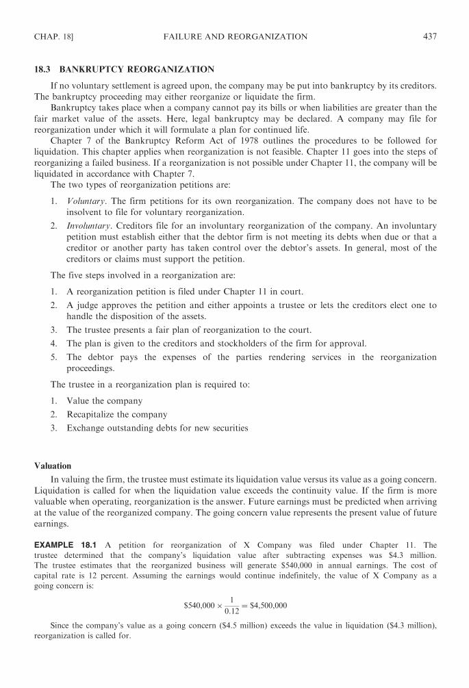
18.3 BANKRUPTCY REORGANIZATION
If no voluntary settlement is agreed upon, the company may be put into bankruptcy by its creditors.
The bankruptcy proceeding may either reorganize or liquidate the firm.
Bankruptcy takes place when a company cannot pay its bills or when liabilities are greater than the
fair market value of the assets. Here, legal bankruptcy may be declared. A company may file for
reorganization under which it will formulate a plan for continued life.
Chapter 7 of the Bankruptcy Reform Act of 1978 outlines the procedures to be followed for
liquidation. This chapter applies when reorganization is not feasible. Chapter 11 goes into the steps of
reorganizing a failed business. If a reorganization is not possible under Chapter 11, the company will be
liquidated in accordance with Chapter 7.
The two types of reorganization petitions are:
1. Voluntary. The firm petitions for its own reorganization. The company does not have to be
insolvent to file for voluntary reorganization.
2. Involuntary. Creditors file for an involuntary reorganization of the company. An involuntary
petition must establish either that the debtor firm is not meeting its debts when due or that a
creditor or another party has taken control over the debtor’s assets. In general, most of the
creditors or claims must support the petition.
The five steps involved in a reorganization are:
1. A reorganization petition is filed under Chapter 11 in court.
2. A judge approves the petition and either appoints a trustee or lets the creditors elect one to
handle the disposition of the assets.
3. The trustee presents a fair plan of reorganization to the court.
4. The plan is given to the creditors and stockholders of the firm for approval.
5. The debtor pays the expenses of the parties rendering services in the reorganization
proceedings.
The trustee in a reorganization plan is required to:
1. Value the company
2. Recapitalize the company
3. Exchange outstanding debts for new securities
Valuation
In valuing the firm, the trustee must estimate its liquidation value versus its value as a going concern.
Liquidation is called for when the liquidation value exceeds the continuity value. If the firm is more
valuable when operating, reorganization is the answer. Future earnings must be predicted when arriving
at the value of the reorganized company. The going concern value represents the present value of future
earnings.
EXAMPLE 18.1 A petition for reorganization of X Company was filed under Chapter 11. The
trustee determined that the company’s liquidation value after subtracting expenses was $4.3 million.
The trustee estimates that the reorganized business will generate $540,000 in annual earnings. The cost of
capital rate is 12 percent. Assuming the earnings would continue indefinitely, the value of X Company as a
going concern is:
$540,000� 1
0:12¼ $4,500,000
Since the company’s value as a going concern ($4.5 million) exceeds the value in liquidation ($4.3 million),
reorganization is called for.
CHAP. 18] FAILURE AND REORGANIZATION 437

Recapitalization
Assuming the trustee recommends reorganization, a plan must be developed to carry it out.
The obligations may be extended or equity securities may be issued in substitution of the debt.
Income bonds may be given for the debentures. With an income bond, interest is paid only when
there are earnings. This process of exchanging liabilities for other types of liabilities or equity securities
is referred to as recapitalization. In recapitalizing the firm, the purpose is to have a mixture of
debt and equity that will permit the company to meet its debts and provide reasonable profits for
the owners.
EXAMPLE 18.2 The current capital structure of Y Corporation is presented below.
Debentures $1,500,000
Collateral bonds 3,000,000
Preferred stock 800,000
Common stock 2,500,000
Total $7,800,000
There exists high financial leverage:
Debt
Equity¼ $4,500,000
$3,300,000¼ 1:36
Assuming the company is deemed to be worth $5 million as a going concern, the trustee can develop a less
leveraged capital structure having a total capital of $5 million as follows:
Debentures $1,000,000
Collateral bonds 1,000,000
Income bonds 1,500,000
Preferred stock 500,000
Common stock 1,000,000
Total $5,000,000
The income bond of $1.5 million is similar to equity in appraising financial leverage, since interest is not paid
unless there is income. The new debt/equity ratio is safer:
Debtþ Collateral bonds
Income bondsþ preferred stockþ common stock¼ $2,000,000
$3,000,000¼ 0:67
Exchange of Obligations
In exchanging obligations to achieve the best capital structure, priorities must be followed. Senior
claims are taken care of before junior claims. Senior debt holders must receive a claim on new capital
equal to their prior claims. The last priority goes to common stockholders in receiving new securities. A
debt holder usually receives a combination of different securities. Preferred and common stockholders
may receive nothing. Usually, however, they retain some small ownership. After the exchange, the debt
holders may become the firm’s new owners.
EXAMPLE 18.3 A $1 million mortgage bondholder may receive in exchange $500,000 in income bonds, $300,000
in preferred stock, and $200,000 in common stock.
Common stockholders receive nothing in exchange.
438 FAILURE AND REORGANIZATION [CHAP. 18

18.4 LIQUIDATION DUE TO BANKRUPTCY
When a company becomes bankrupt it may be liquidated under Chapter 7 of the Bankruptcy
Reform Act of 1978. The key elements of liquidation are legal considerations, claim priority, and
dissolution.
Legal Considerations
When a company is declared bankrupt, creditors must meet between 10 and 30 days subsequent to
that declaration. A judge or referee takes charge of the meeting in which the creditors provide their
claims. A trustee is appointed by the creditors. The trustee handles the property of the defaulted
company, liquidates the business, maintains appropriate records, evaluates the claims of creditors,
makes payments, and provides relevant information regarding the liquidation process. Many times
three trustees are appointed and/or an advisory committee of at least three creditors is formed.
Claim Priority
Some claims against the company take precedence over others in bankruptcy. The following rank
order exists in meeting claims:
1. Secured claims.
2. Bankruptcy administrative costs.
3. Unsecured salaries and commissions.
4. Unsecured customer deposit claims.
5. Taxes.
6. General creditor claims.
7. Preferred stockholders.
8. Common stockholders.
In most cases, once creditor obligations have been settled with the remaining assets there is nothing
left for stockholders.
Bankruptcy distribution in principle should be based on absolute priority, in which creditor
claims are satisfied strictly following the priority listing. Junior claims are supposed to be met
after senior claims are fully satisfied. However, in practice, courts sometimes use relative priority in
distributing assets in which junior claims receive a partial distribution even though all senior claims
have not been fully met.
Dissolution
After claims have been met in priority order and an accounting made of the proceedings, there may
then be instituted an application to discharge the bankrupt business. A discharge occurs when the court
releases the company from legitimate debts in bankruptcy, with the exception of debts that are immune
to discharge. As long as a debtor has not been discharged within the prior 6 years and was not bankrupt
due to fraud, the debtor may then start a new business.
EXAMPLE 18.4 The balance sheet of Ace Corporation for the year ended December 31, 20X4, follows:
Balance Sheet
Current assets $400,000 Current liabilities $475,000
Fixed assets 410,000 Long-term liabilities 250,000
Common stock 175,000
Retained earnings (90,000)
Total assets $810,000
Total liabilities and
stockholders’ equity $810,000
CHAP. 18] FAILURE AND REORGANIZATION 439
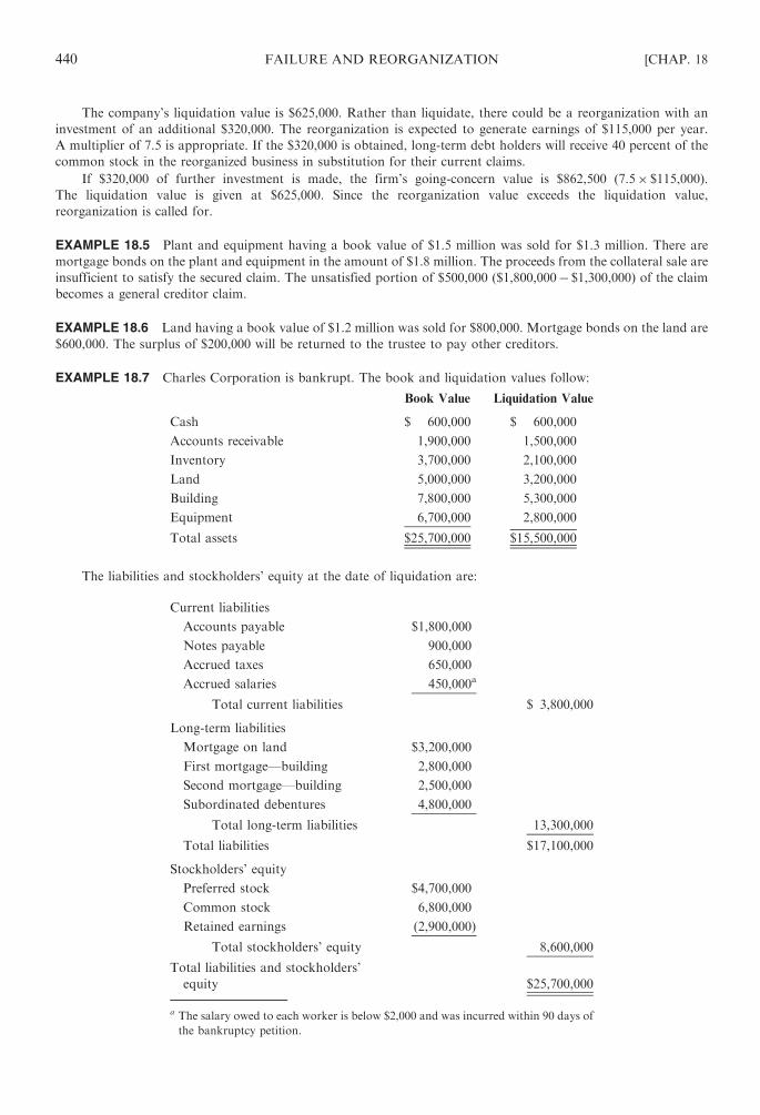
The company’s liquidation value is $625,000. Rather than liquidate, there could be a reorganization with an
investment of an additional $320,000. The reorganization is expected to generate earnings of $115,000 per year.
A multiplier of 7.5 is appropriate. If the $320,000 is obtained, long-term debt holders will receive 40 percent of the
common stock in the reorganized business in substitution for their current claims.
If $320,000 of further investment is made, the firm’s going-concern value is $862,500 (7.5� $115,000).
The liquidation value is given at $625,000. Since the reorganization value exceeds the liquidation value,
reorganization is called for.
EXAMPLE 18.5 Plant and equipment having a book value of $1.5 million was sold for $1.3 million. There are
mortgage bonds on the plant and equipment in the amount of $1.8 million. The proceeds from the collateral sale are
insufficient to satisfy the secured claim. The unsatisfied portion of $500,000 ($1,800,000� $1,300,000) of the claim
becomes a general creditor claim.
EXAMPLE 18.6 Land having a book value of $1.2 million was sold for $800,000. Mortgage bonds on the land are
$600,000. The surplus of $200,000 will be returned to the trustee to pay other creditors.
EXAMPLE 18.7 Charles Corporation is bankrupt. The book and liquidation values follow:
Book Value Liquidation Value
Cash $ 600,000 $ 600,000
Accounts receivable 1,900,000 1,500,000
Inventory 3,700,000 2,100,000
Land 5,000,000 3,200,000
Building 7,800,000 5,300,000
Equipment 6,700,000 2,800,000
Total assets $25,700,000 $15,500,000
The liabilities and stockholders’ equity at the date of liquidation are:
Current liabilities
Accounts payable $1,800,000
Notes payable 900,000
Accrued taxes 650,000
Accrued salaries 450,000a
Total current liabilities $ 3,800,000
Long-term liabilities
Mortgage on land $3,200,000
First mortgage—building 2,800,000
Second mortgage—building 2,500,000
Subordinated debentures 4,800,000
Total long-term liabilities 13,300,000
Total liabilities $17,100,000
Stockholders’ equity
Preferred stock $4,700,000
Common stock 6,800,000
Retained earnings (2,900,000)
Total stockholders’ equity 8,600,000
Total liabilities and stockholders’
equity $25,700,000
a The salary owed to each worker is below $2,000 and was incurred within 90 days of
the bankruptcy petition.
440 FAILURE AND REORGANIZATION [CHAP. 18

Expenses of the liquidation including legal costs were 15 percent of the proceeds. The debentures are subordi-
nated only with regard to the two first-mortgage bonds.
The distribution of the proceeds follows:
Proceeds $15,500,000
Mortgage on land $3,200,000
First mortgage—building 2,800,000
Second mortgage—building 2,500,000
Liquidation expenses
(15%� $15,500,000) 2,325,000
Accrued salaries 450,000
Accrued taxes 650,000
Total 11,925,000
Balance $ 3,575,000
The percent to be paid to general creditors is:
Proceeds balance
Total owed¼ $3,575,000
$7,500,000¼ 47:66667%
The balance due general creditors follows:
General Creditors Owed Paid
Accounts payable $1,800,000 $ 858,000
Notes payable 900,000 429,000
Subordinated debentures 4,800,000 2,288,000
Total $7,500,000 $3,575,000
EXAMPLE 18.8 The balance sheet of the Oakhurst Company is presented below.
ASSETS
Current assets
Cash $ 9,000
Marketable securities 6,000
Receivables 1,100,000
Inventory 3,000,000
Prepaid expenses 4,000
Total current assets $4,119,000
Noncurrent assets
Land $1,800,000
Fixed assets 2,000,000
Total noncurrent assets 3,800,000
Total assets $7,919,000
CHAP. 18] FAILURE AND REORGANIZATION 441

LIABILITIES AND
STOCKHOLDERS’ EQUITY
Current liabilities
Accounts payable $ 180,000
Bank loan payable 900,000
Accrued salaries 300,000a
Employee benefits payable 70,000b
Customer claims—unsecured 80,000c
Taxes payable 350,000
Total current liabilities $1,880,000
Noncurrent liabilities
First mortgage payable $1,600,000
Second mortgage payable 1,100,000
Subordinated debentures 700,000
Total noncurrent liabilities 3,400,000
Total liabilities $5,280,000
Stockholders’ equity
Preferred stock (3,500 shares) $ 350,000
Common stock (8,000 shares) 480,000
Paid-in capital 1,600,000
Retained earnings 209,000
Total stockholders’ equity 2,639,000
Total liabilities and stockholders’ $7,919,000
equity
a The salary owed to each worker is below $2,000 and was incurred within 90 days
of the bankruptcy petition.
b Employee benefits payable have the same limitations as unsecured wages and
satisfy for eligibility in bankruptcy distribution.
c No customer claim is greater than $900.
Additional data are as follows:
1. The mortgages apply to the company’s total noncurrent assets.
2. The subordinated debentures are subordinated to the bank loan payable. Therefore, they come after the
bank loan payable in liquidation.
3. The trustee has sold the company’s current assets for $2.1 million and the noncurrent assets for $1.9 million.
Therefore, a total of $4 million was received.
4. The business is bankrupt, since the total liabilities of $5.28 million are greater than the $4 million of the fair
value of the assets.
Assume that the administration expense for handling the bankrupt company is $900,000. This liability is not
reflected in the above balance sheet.
442 FAILURE AND REORGANIZATION [CHAP. 18

The allocation of the $4 million to the creditors is shown here.
Proceeds
Available to secured creditors $4,000,000
First mortgage—payable from
$1,900,000 proceeds of
noncurrent assets $1,600,000
Second mortgage—payable from
balance of proceeds of
noncurrent assets 300,000 1,900,000
Balance after secured creditors $2,100,000
Next priority
Administrative expenses $ 900,000
Accrued salaries 300,000
Employee benefits payable 70,000
Customer claims—unsecured 80,000
Taxes payable 350,000 1,700,000
Proceeds available to general creditors $ 400,000
Now that the claims on the proceeds from liquidation have been met, general creditors receive the balance on a
pro rata basis. The distribution of the $400,000 follows:
General Creditor Amount
Pro Rata
Allocation for
Balance to
Be Paid
Second-mortgage balance
($1,100,000� $300,000) $ 800,000 $124,031
Accounts payable 180,000 27,907
Bank loan payable 900,000 248,062a
Subordinated debentures 700,000 0
Total $2,580,000 $400,000
a Since the debentures are subordinated, the bank loan payable must be satisfied
in full before any amount can go to the subordinated debentures. The subordinated
debenture holders therefore receive nothing.
EXAMPLE 18.9 Nolan Company is having severe financial problems. Jefferson Bank holds a first mortgage on the
plant and has an $800,000 unsecured loan that is already delinquent. The Alto Insurance Company holds $4.7
million of the company’s subordinated debentures to the notes payable. Nolan is deciding whether to reorganize the
business or declare bankruptcy.
Another company is considering acquiring Nolan Company by offering to take over the mortgage of $7.5
million, pay the past due taxes, and pay $4.38 million for the firm.
Nolan’s balance sheet follows:
ASSETS
Current assets $ 2,800,000
Plant assets 11,700,000
Other assets 3,000,000
Total assets $17,500,000
CHAP. 18] FAILURE AND REORGANIZATION 443
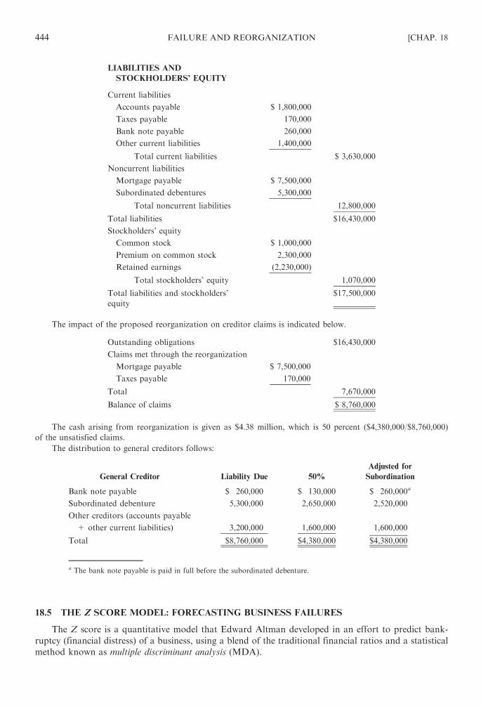
LIABILITIES AND
STOCKHOLDERS’ EQUITY
Current liabilities
Accounts payable $ 1,800,000
Taxes payable 170,000
Bank note payable 260,000
Other current liabilities 1,400,000
Total current liabilities $ 3,630,000
Noncurrent liabilities
Mortgage payable $ 7,500,000
Subordinated debentures 5,300,000
Total noncurrent liabilities 12,800,000
Total liabilities $16,430,000
Stockholders’ equity
Common stock $ 1,000,000
Premium on common stock 2,300,000
Retained earnings (2,230,000)
Total stockholders’ equity 1,070,000
Total liabilities and stockholders’
equity
$17,500,000
The impact of the proposed reorganization on creditor claims is indicated below.
Outstanding obligations $16,430,000
Claims met through the reorganization
Mortgage payable $ 7,500,000
Taxes payable 170,000
Total 7,670,000
Balance of claims $ 8,760,000
The cash arising from reorganization is given as $4.38 million, which is 50 percent ($4,380,000/$8,760,000)
of the unsatisfied claims.
The distribution to general creditors follows:
General Creditor Liability Due 50%
Adjusted for
Subordination
Bank note payable $ 260,000 $ 130,000 $ 260,000a
Subordinated debenture 5,300,000 2,650,000 2,520,000
Other creditors (accounts payable
+ other current liabilities) 3,200,000 1,600,000 1,600,000
Total $8,760,000 $4,380,000 $4,380,000
a The bank note payable is paid in full before the subordinated debenture.
18.5 THE Z SCORE MODEL: FORECASTING BUSINESS FAILURES
The Z score is a quantitative model that Edward Altman developed in an effort to predict bank-
ruptcy (financial distress) of a business, using a blend of the traditional financial ratios and a statistical
method known as multiple discriminant analysis (MDA).
444 FAILURE AND REORGANIZATION [CHAP. 18

The Z score is known to be about 90 percent accurate in forecasting business failure one year in the
future and about 80 percent accurate in forecasting it 2 years in the future. The model is
Z ¼ 1:2*X1 þ 1:4*X2 þ 3:3*X3 þ 0:6*X4 þ 0:999*X5
where X1=Working capital/Total assets
X2=Retained earnings/Total assets
X3=Earnings before interest and taxes (EBIT)/Total assets
X4=Market value of equity/Book value of debt
X5=Sales/Total assets
Altman also established the following guidelines for classifying firms:
Z score Probability of failure
1.8 or less Very high
1.81�2.99 Not sure
3.0 or higher Unlikely
EXAMPLE 18.10 Davidson Company has the following financial data selected from its financial statements:
Total assets ¼ $2,000
Retained earnings ¼ $750
EBIT ¼ $266
Sales ¼ $3,000
Market value of common and preferred stock ¼ $1,425
Book value of debt ¼ $1,100
The calculation of Davidson’s Z score is shown below:
X1 ¼ 400=2,000� 1:2 ¼ 0:240
X2 ¼ 750=2,000� 1:4 ¼ 0:525
X3 ¼ 266=2,000� 3:3 ¼ 0:439
X4 ¼ 1,425=1,100� 0:6 ¼ 0:777
X5 ¼ 3,000=2,000� 0:999 ¼ 1:499
Z ¼ 3:480
Since Davidson’s Z score of 3.480 is well into the ‘‘unlikely’’ zone, there is virtually no chance that Davidson will
go bankrupt within the next 2 years.
Review Questions
1. means that the company is unable to meet current debt when due.
2. If a company’s liabilities exceed the fair market value of its assets, it is .
3. In the case of a(n) , creditors receive the balances owed them over an extended
time period.
4. A voluntary reduction of the amount the debtor owes the creditor is referred to as a(n)
.
5. A bankruptcy proceeding may either or the business.
CHAP. 18] FAILURE AND REORGANIZATION 445

6. of the Bankruptcy Reform Act of 1978 outlines the procedures to be followed
in liquidation.
7. Liquidation is called for when the value is greater than the
value of the business.
8. is the process of exchanging liabilities for other types of liabilities or equity
securities.
9. creditors have a higher priority in bankruptcy than unsecured creditors.
10. In bankruptcy, unsecured salaries are limited to $ per individual.
11. In bankruptcy, are paid last.
12. A(n) means that the court releases the business from legitimate debts in
bankruptcy.
13. The is an effort to predict bankruptcy (financial distress) of a business, using
a blend of the traditional financial ratios and multiple discriminant analysis (MDA).
Answers: (1) Technical insolvency; (2) bankrupt; (3) extension; (4) composition; (5) reorganize, liqui-
date; (6) Chapter 7; (7) liquidation, continuity; (8) Recapitalization; (9) Secured; (10) 2,000; (11) common
stockholders; (12) discharge; (13) Z score model.
Solved Problems
18.1 Going-Concern Value. There was a petition for reorganization of Hazel Corporation filed under
Chapter 11. It was determined by the trustee that the firm’s liquidation value, after considering
expenses, was $5.3 million. The trustee predicts that the reorganized business will derive $500,000
in annual profit. The cost of capital rate is 10 percent. Assume profits will continue indefinitely.
Is reorganization or liquidation recommended?
SOLUTION
The value of the business as a going concern equals:
$500,000� 1
0:10¼ $5,000,000
Since the value of the company as a going concern ($5 million) is less than its value in liquidation ($5.3
million), the business should be liquidated.
18.2 Debt/Equity Ratio. The present capital structure of Jones Corporation is shown below.
Debentures $1,200,000
Collateral bonds 2,800,000
Preferred stock 700,000
Common stock 2,600,000
Total $7,300,000
446 FAILURE AND REORGANIZATION [CHAP. 18

There is a high financial leverage position:
Debt
Equity¼ $4,000,000
$3,300,000¼ 1:21
The business is worth $4.7 million as a going concern. The trustee has formulated a less
leveraged capital structure having a total capital of $4.7 million as follows:
Debentures $ 800,000
Collateral bonds 1,500,000
Income bonds 1,300,000
Preferred stock 400,000
Common stock 700,000
Total $4,700,000
What is the new debt/equity ratio?
SOLUTION
The income bond of $1.3 million is similar to equity in evaluating financial leverage because interest is
not paid unless income exists. The new debt/equity ratio is lower at:
Debtþ collateral bonds
Income bondsþ preferred stockþ common stock¼ $2,300,000
$2,400,000¼ 0:96
18.3 Reorganization of Liquidation. The balance sheet of Morris Corporation for the year ended
December 31, 20X3, follows:
Balance Sheet
Current assets $ 500,000 Current liabilities $ 550,000
Fixed assets 520,000 Long-term liabilities 300,000
Common stock 250,000
Retained earnings (80,000)
Total liabilities and
Total assets $1,020,000 stockholders’ equity $1,020,000
The firm’s liquidation value is $700,000. Instead of liquidating, there could be a reorganiza-
tion with an investment of an additional $400,000. The reorganization is anticipated to provide
earnings of $150,000 a year. A multiplier of 8 is appropriate. If the $400,000 is obtained,
long-term debt holders will receive 35 percent of the common stock in the reorganized firm
in substitution for their current claims. Is reorganization or liquidation recommended?
SOLUTION
Assuming the $400,000 of further investment is made, the company’s going-concern value is $1.2 million
(8 � $150,000). The liquidation value is stated at $700,000. Because the reorganized value is greater than the
liquidation value, reorganization is recommended.
18.4 Secured Creditors. Plant and equipment with a book value of $2.3 million was sold for $2 million.
The mortgage bonds on the plant and equipment are $2.6 million. How will the mortgage
bondholders be treated in liquidation?
CHAP. 18] FAILURE AND REORGANIZATION 447

SOLUTION
The proceeds from the collateral sale are not enough to meet the secured claim. The unsatisfied portion
of $600,000 of the claim becomes a general creditor claim.
18.5 Secured Creditors. Plant and equipment having a book value of $800,000 was sold for $600,000.
Mortgage bonds on the plant and equipment are $500,000. How will the mortgage bondholders
be treated in liquidation?
SOLUTION
The mortgage bondholders will be fully satisfied in liquidation. The surplus of $100,000 will be returned
to the trustee to pay other creditors.
18.6 Distribution in Bankruptcy. Blake Corporation is bankrupt. The book and liquidation values of its
assets follow.
Book
Value
Liquidation
Value
Cash $ 500,000 $ 500,000
Accounts receivable 1,700,000 1,400,000
Inventory 3,400,000 2,200,000
Land 4,700,000 3,500,000
Building 8,000,000 5,600,000
Equipment 7,000,000 3,000,000
Total assets $25,300,000 $16,200,000
The liabilities and stockholders’ equity at the liquidation date follow.
Current liabilities
Accounts payable $2,000,000
Notes payable 1,000,000
Accrued taxes 700,000
Accrued salaries 400,000a
Total current liabilities $ 4,100,000
Long-term liabilities
Mortgage on land $3,500,000
First mortgage—building 4,000,000
Second mortgage—building 1,600,000
Subordinated debentures 4,500,000
Total long-term liabilities 13,600,000
Total liabilities $17,700,000
Stockholders’ equity
Preferred stock $4,500,000
Common stock 6,500,000
Retained earnings (3,400,000)
Total stockholders’ equity 7,600,000
Total liabilities and stockholders’ equity $25,300,000
a The salary owed to each worker is below $2,000 and was incurred within 90 days of
the bankruptcy petition.
448 FAILURE AND REORGANIZATION [CHAP. 18

Expenses associated with the bankruptcy administration were 12 percent of the proceeds.
The debentures are subordinated only to the two first-mortgage bonds.
Determine the distribution of the proceeds.
SOLUTION
The distribution of the proceeds follows.
Proceeds $16,200,000
Mortgage on land $3,500,000
First mortgage—building 4,000,000
Second mortgage—building 1,600,000
Liquidation expenses
(12% � $16,200,000) 1,944,000
Accrued salaries 400,000
Accrued taxes 700,000
Total 12,144,000
Balance $ 4,056,000
The percent to be paid to general creditors is:
Proceeds balance
Total owed¼ $4,056,000
$7,500,000¼ 0:5408
General Creditor Owed Paid
Accounts payable $2,000,000 $1,081,600
Notes payable 1,000,000 540,800
Subordinated debentures 4,500,000 2,433,600
Total $7,500,000 $4,056,000
18.7 Distribution in Bankruptcy. The balance sheet of Larkin Corporation is shown below.
ASSETS
Current assets
Cash $7,000
Marketable securities 5,000
Receivables 1,000,000
Inventory 2,800,000
Prepaid expenses 3,500
Total current assets $3,815,500
Noncurrent assets
Land $1,700,000
Fixed assets 2,200,000
Total noncurrent assets 3,900,000
Total assets $7,715,500
CHAP. 18] FAILURE AND REORGANIZATION 449
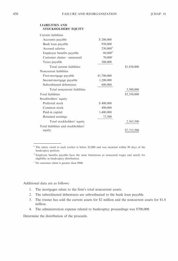
LIABILITIES AND
STOCKHOLDERS’ EQUITY
Current liabilities
Accounts payable $ 200,000
Bank loan payable 950,000
Accrued salaries 250,000a
Employee benefits payable 80,000b
Customer claims—unsecured 70,000c
Taxes payable 300,000
Total current liabilities $1,850,000
Noncurrent liabilities
First-mortgage payable $1,700,000
Second-mortgage payable 1,200,000
Subordinated debentures 600,000
Total noncurrent liabilities 3,500,000
Total liabilities $5,350,000
Stockholders’ equity
Preferred stock $ 400,000
Common stock 490,000
Paid-in capital 1,400,000
Retained earnings 75,500
Total stockholders’ equity 2,365,500
Total liabilities and stockholders’
equity $7,715,500
a The salary owed to each worker is below $2,000 and was incurred within 90 days of the
bankruptcy petition.
b Employee benefits payable have the same limitations as unsecured wages and satisfy for
eligibility in bankruptcy distribution.
c No customer claim is greater than $900.
Additional data are as follows:
1. The mortgages relate to the firm’s total noncurrent assets.
2. The subordinated debentures are subordinated to the bank loan payable.
3. The trustee has sold the current assets for $2 million and the noncurrent assets for $1.8
million.
4. The administration expense related to bankruptcy proceedings was $700,000.
Determine the distribution of the proceeds.
450 FAILURE AND REORGANIZATION [CHAP. 18

SOLUTION
Proceeds $3,800,000
First mortgage—payable from
$1,800,000 proceeds of noncurrent
assets
$1,700,000
Second mortgage—payable from
$1,800,000 proceeds of noncurrent
assets
100,000 1,800,000
Balance after secured creditors $2,000,000
Next priority
Administration expenses $700,000
Accrued salaries 250,000
Employee benefits payable 80,000
Customer claims–unsecured 70,000
Taxes payable 300,000 1,400,000
Proceeds available to general creditors $ 600,000
The distribution of the $600,000 to general creditors follows:
General Creditor Amount
Pro Rata
Allocation for
Balance to
Be Paid
Second-mortgage balance
($1,200,000� $100,000) $1,100,000 $231,579
Accounts payable 200,000 42,105
Bank loan payable 950,000 326,316a
Subordinated debentures 600,000 0
Total $2,850,000 $600,000
a Since the debentures are subordinated, the bank loan payable must be met in full
before any amount can go to the subordinated debentures. Thus, subordinated
debenture holders receive nothing.
The holders of preferred and common stock receive nothing, since the unsecured creditors
themselves have not been fully paid.
18.8 Distribution in Bankruptcy. Hover Company’s balance sheet follows:
ASSETS
Current assets $1,200,000
Land 3,000,000
Plant and equipment 2,400,000
Total assets $6,600,000
CHAP. 18] FAILURE AND REORGANIZATION 451
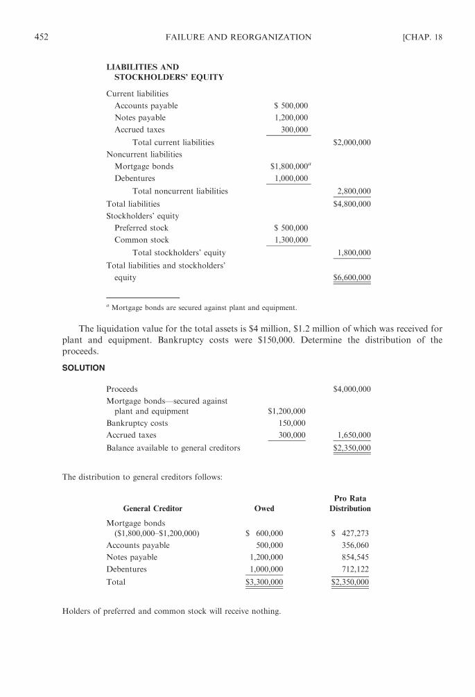
LIABILITIES AND
STOCKHOLDERS’ EQUITY
Current liabilities
Accounts payable $ 500,000
Notes payable 1,200,000
Accrued taxes 300,000
Total current liabilities $2,000,000
Noncurrent liabilities
Mortgage bonds $1,800,000a
Debentures 1,000,000
Total noncurrent liabilities 2,800,000
Total liabilities $4,800,000
Stockholders’ equity
Preferred stock $ 500,000
Common stock 1,300,000
Total stockholders’ equity 1,800,000
Total liabilities and stockholders’
equity $6,600,000
a Mortgage bonds are secured against plant and equipment.
The liquidation value for the total assets is $4 million, $1.2 million of which was received for
plant and equipment. Bankruptcy costs were $150,000. Determine the distribution of the
proceeds.
SOLUTION
Proceeds $4,000,000
Mortgage bonds—secured against
plant and equipment $1,200,000
Bankruptcy costs 150,000
Accrued taxes 300,000 1,650,000
Balance available to general creditors $2,350,000
The distribution to general creditors follows:
General Creditor Owed
Pro Rata
Distribution
Mortgage bonds
($1,800,000–$1,200,000) $ 600,000 $ 427,273
Accounts payable 500,000 356,060
Notes payable 1,200,000 854,545
Debentures 1,000,000 712,122
Total $3,300,000 $2,350,000
Holders of preferred and common stock will receive nothing.
452 FAILURE AND REORGANIZATION [CHAP. 18

18.9 Z Score Model. Compute and interpret the Z scores for companies A and B below.
Variables
Company X1 X2 X3 X4 X5
A 0.4 0.35 0.3 1.75 1
B 0.15 0.12 0.1 0.5 0.5
SOLUTION
For A: Z=1.2(0.4)+1.4(0.35)+3.3(0.3)+0.6(1.75)+0.999(1)
=4.01
For B: Z=1.2(0.15)+1 .4(0.12)+3.3(0.l)+0.6(0.5)+0.999(0.5)
=1.47
A’s Z score is 4.0142.99, no concern of bankruptcy, while Company B has a Z score of 1.47, well below
1.81 and is a likely candidate for failure.
CHAP. 18] FAILURE AND REORGANIZATION 453

Chapter 19
Multinational Finance
Many companies are multinational corporations (MNCs) that have significant foreign operations
deriving a high percentage of their sales overseas. Financial managers of MNCs require an
understanding of the complexities of international finance to make sound financial and investment
decisions. International finance involves consideration of managing working capital, financing the
business, control of foreign exchange and political risks, and foreign direct investments. Most
importantly, the financial manager has to consider the value of the US dollar relative to the value of
the currency of the foreign country in which business activities are being conducted. Currency exchange
rates may materially affect receivables and payables, and imports and exports of the US company in
its multinational operations. The effect is more pronounced with increasing activities abroad.
19.1 SPECIAL FEATURES OF A MULTINATIONAL CORPORATION (MNC)
Multiple-currency problem. Sales revenues may be collected in one currency, assets denominated
in another, and profits measured in a third.
Various legal, institutional, and economic constraints. There are variations in such things as tax laws,
labor practices, balance-of-payment policies, and government controls with respect to the types and sizes
of investments, types and amount of capital raised, and repatriation of profits.
Internal control problem. When the parent office of an MNC and its affiliates are widely located,
internal organizational difficulties arise.
19.2 FINANCIAL GOALS OF MNCS
A survey made on financial managers of MNCs lists the financial goals of MNCs in the following
order of importance:
1. Maximize growth in corporate earnings, whether total earnings, earnings before interest and
taxes (EBIT), or earnings per share (EPS).
2. Maximize return on equity.
3. Guarantee that funds are always available when needed.
19.3 TYPES OF FOREIGN OPERATIONS
Companies involved in multinational business may structure their activities in the following three
ways:
Wholly owned subsidiaries. A large, well-established company with much international experience
may eventually have wholly owned subsidiaries.
Import/export activities. A small company with limited foreign experience operating in ‘‘risky areas’’
may be restricted to export and import activity.
If the company’s sales force has minimal experience in export sales, it is advisable to use foreign
brokers when specialized knowledge of foreign markets is needed. When sufficient volume exists, the
company may establish a foreign branch sales office, including sales people and technical service staff.
As the operation matures, production facilities may be located in the foreign market. However, some
foreign countries require licensing before foreign sales and production can take place. In this case,
a foreign licensee sells and produces the product. A problem with this is that confidential information
and knowledge are passed on to the licensees who can then become a competitor at the expiration of the
agreement.
454
Copyright © 2007, 1998, 1986 by The McGraw-Hill Companies, Inc. Click here for terms of use.

Joint ventures. A joint venture with a foreign company is another way to proceed internationally and
share the risk. Some foreign governments require this to be the path to follow to operate in their
countries. The foreign company may have local goodwill to assure success. A drawback is less control
over activities and a conflict of interest.
19.4 FUNCTIONS OF AN MNC’S FINANCIAL MANAGER
In evaluating the impact that foreign operations have on the entity’s financial health, the financial
manager of an MNC should consider the extent of intercountry transactions, foreign restrictions
and laws, tax structure of the foreign country, and the economic and political stability of the country.
If a subsidiary is operating in a high-tax country with a double-tax agreement, dividend payments are
not subject to further US taxes. One way to transfer income from high tax areas to low tax areas is to
levy royalties or management fees on the subsidiaries.
19.5 THE FOREIGN EXCHANGE MARKET
Except in a few European centers, there is no central marketplace for the foreign exchange market.
Rather, business is carried out over telephone or telex. The major dealers are large banks. A company
that wants to buy or sell currency typically uses a commercial bank. International transactions and
investments involve more than one currency. For example, when a US company sells merchandise to a
Japanese firm, the former wants to be paid in dollars but the Japanese company typically expects
to receive yen. Due to the foreign exchange market, the buyer may pay in one currency while the
seller can receive payment in another currency.
19.6 SPOT AND FORWARD FOREIGN EXCHANGE RATES
An exchange rate is the ratio of one unit of currency to another. An exchange rate is established
between the different currencies. The conversion rate between currencies depends on the demand/supply
relationship. Because of the change in exchange rates, companies are susceptible to exchange rate
fluctuation risks because of a net asset or net liability position in a foreign currency.
Exchange rates may be in terms of dollars per foreign currency unit (called an direct quote) or units
of foreign currency per dollar (called an indirect quote). Therefore, an indirect quote is the reciprocal
of a direct quote and vice versa.
An indirect quote ¼ 1=direct quote
Pound=$ ¼ 1=ð$=poundÞ
Table 19-1 presents a sample of indirect and direc quotes for selected currencies.
EXAMPLE 19.1 A rate of 1.617/British pound means each pound costs the US company $1.735. In other words,
the US company gets 1/1.617=£0.6184 for each dollar.
The spot rate is the exchange rate for immediate delivery of currencies exchanged, while the forward rate is the
exchange rate for later delivery of currencies exchanged. For example, there may be a 90-day exchange rate. The
forward exchange rate of a currency will be slightly different from the spot rate at the current date because of future
expectations and uncertainties.
Forward rates may be greater than the current spot rate (premium) or less than the current spot rate (discount).
Cross Rates
A cross rate is the indirect calculation of the exchange rate of one currency from the exchange rates
of two other currencies.
CHAP. 19] MULTINATIONAL FINANCE 455

EXAMPLE 19.2 Hypothetical dollar per pound and the yen per dollar rates are given in Table 19-2. For example,
if the dollars per pound is $1.6124/£ and yen per dollar is ¥119.89/$, the cross rate between Japanese yen and British
pounds is
Cross rate between yen and pound ¼ dollars
pound� yen
dollar¼ yen
pound
¼ $=£ � ¥=$ ¼ ¥=£
¼ 1:6124 dollars per pound� 119:89 yen per dollar
¼ 193:31 yen per pound
Because most currencies are quoted against the dollar, it may be necessary to work out the cross rates for
currencies other than the dollar. The cross rate is needed to consummate financial transactions between two
countries.
EXAMPLE 19.3 On August 5, 20X5, forward rates on the British pound were at a discount in relation to the spot
rate, while the forward rates for the Japanese yen were at a premium from the spot rate. This means that participants
in the foreign exchange market anticipated that the British pound would depreciate relative to the US dollar in the
future but the Japanese yen would appreciate against the dollar.
The percentage premium (P) or discount (D) is computed as follows.
P ðor DÞ ¼ F� S
S� 12 months
n� 100
where F, S= the forward and spot rates and n= length of the forward contract in months.
If F4S, the result is the annualized premium in percent; otherwise, it is the annualized discount in percent.
Table 19-1. Foreign Exchange Rates (A Sample) August 5, 20X5
Country Contract US Dollar Equivalent Currency per US $
Britain (Pound) Spot 1.6124 0.6202
30-day future 1.6091 0.6215
90-day future 1.6030 0.6238
180-day future 1.5934 0.6276
Japan (Yen) Spot 0.008341 119.89
30-day future 0.008349 119.77
90-day future 0.008366 119.53
180-day future 0.008394 119.13
Table 19-2. Example of Key Currency Cross Rates
British Euro Japan US
British – 0.7054 0.05770 0.62020
Euro 1.4176 – 0.00733 0.87920
Japan 193.31 136.36 – 119.89
U.S. 1.6124 1.1374 0.00834 –
Note: The Wall Street Journal routinely publishes key currency cross rates, as shown in the hypothetical rates. They are also
available on www.bloomberg.com. The cross-currency table calculator can be accessed by www.xe.net/currency/table.htm.
456 MULTINATIONAL FINANCE [CHAP. 19

EXAMPLE 19.4 On August 5, 20X5, a 30-day forward contract in Japanese yen (see Table 19-1) was selling at a
1.15 percent premium:
0:008349� 0:008341
0:008341� 12 months
1 month� 100 ¼ 1:15%
19.7 CURRENCY RISK MANAGEMENT
Foreign exchange rate risk exists when the contract is written in terms of the foreign
currency or denominated in the foreign currency. The exchange rate fluctuations increase the
riskiness of the investment and incur cash losses. The financial manager must not only seek the
highest return on temporary investments but must also be concerned about changing values of
the currencies invested. You do not necessarily eliminate foreign exchange risk. You may only try to
contain it.
Financial Strategies
In countries where currency values are likely to drop, financial managers of the subsidiaries should:
� Avoid paying advances on purchase orders unless the seller pays interest on the advances suffi-
cient to cover the loss of purchasing power.
� Not have excess idle cash. Excess cash can be used to buy inventory or other real assets.
� Buy materials and supplies on credit in the country in which the foreign subsidiary is operating,
extending the final payment date as long as possible.
� Avoid giving excessive trade credit. If accounts receivable balances are outstanding for an
extended time period, interest should be charged to absorb the loss in purchasing power.
� Borrow local currency funds when the interest rate charged does not exceed US rates after taking
into account expected devaluation in the foreign country.
Types of Foreign Exchange Exposure
MNCs’ financial managers are faced with the dilemma of three different types of foreign exchange
risk. They are:
Translation exposure, often called accounting exposure, measures the impact of an exchange
rate change on the firm’s financial statements. An example would be the impact of an Euro devaluation
on a US firm’s reported income statement and balance sheet.
Transaction exposure measures potential gains or losses on the future settlement of outstanding
obligations that are denominated in a foreign currency. An example would be a US dollar loss after
the Euro devalues, on payments received for an export invoiced in francs before that devaluation.
Operating exposure, often called economic exposure, is the potential for the change in the present
value of future cash flows due to an unexpected change in the exchange rate.
Translation Exposure
A major purpose of translation is to provide data of expected impacts of rate changes on cash
flow and equity. In the translation of the foreign subsidiaries’ financial statements into the US parent’s
financial statements, the following steps are involved:
1. The foreign financial statements are put into US generally accepted accounting principles.
2. The foreign currency is translated into US dollars. Balance sheet accounts are translated using
the current exchange rate at the balance sheet date. If a current exchange rate is not available
at the balance sheet date, use the first exchange rate available after that date. Income statement
accounts are translated using the weighted-average exchange rate for the period.
CHAP. 19] MULTINATIONAL FINANCE 457

Current FASB rules require translation by the current rate method. Under the current rate method:
� All balance sheet assets and liabilities are translated at the current rate of exchange in effect on
the balance sheet date.
� Income statement items are usually translated at an average exchange rate for the reporting
period.
� All equity accounts are translated at the historical exchange rates that were in effect at the time
the accounts first entered the balance sheet.
� Translation gains and losses are reported as a separate item in the stockholders’ equity section of
the balance sheet.
Translation gains and losses are only included in net income when there is a sale or liquidation of
the entire investment in a foreign entity.
Transaction Exposure
Foreign currency transactions may result in receivables or payables fixed in terms of the amount
of foreign currency to be received or paid. Transaction gains and losses are reported in the income
statement.
Foreign currency transactions are those transactions whose terms are denominated in a currency
other than the entity’s functional currency. Foreign currency transactions take place when a business:
� Buys or sells on credit goods or services the prices of which are denominated in foreign
currencies.
� Borrows or lends funds, and the amounts payable or receivable are denominated in a foreign
currency.
� Is a party to an unperformed forward exchange contract.
� Acquires or disposes of assets, or incurs or settles liabilities denominated in foreign currencies.
EXAMPLE 19.5 Monblanc Trading Company imports French cheeses for distribution in the US. On July 1,
the company purchased cheese costing 100,000 Euro. Payment is due in Euro on October 1. The spot rate
on July 1 was $1.20 per Euro, and on October 1, it was $1.25 per Euro. The exchange loss would be:
Liability in dollars, October 1 $20,000 (100,000� $1.20)
Paid in dollars, October 1 25,000 (100,000� $1.25)
Exchange loss $ 5,000
Note that transaction losses differ from translation losses, which do not influence taxable income.
Long versus Short Position
When there is a devaluation of the dollar, foreign assets and income in strong currency countries are
worth more dollars as long as foreign liabilities do not offset this beneficial effect.
Foreign exchange risk may be analyzed by examining expected receipts or obligations in foreign
currency units. A company expecting receipts in foreign currency units (‘‘long’’ position in the foreign
currency units) has the risk that the value of the foreign currency units will drop. This results in
devaluing the foreign currency relative to the dollar. If a company is expecting to have obligations in
foreign currency units (‘‘short’’ position in the foreign currency units), there is risk that the value of the
foreign currency will rise and it will need to buy the currency at a higher price.
If net claims are greater than liabilities in a foreign currency, the company has a ‘‘long’’ position,
since it will benefit if the value of the foreign currency rises. If net liabilities exceed claims with respect to
foreign currencies, the company is in a ‘‘short’’ position because it will gain if the foreign currency drops
in value.
458 MULTINATIONAL FINANCE [CHAP. 19

Monetary Position
Monetary balance is avoiding either a net receivable or a net payable position. Monetary assets and
liabilities do not change in value with devaluation or revaluation in foreign currencies.
A company with a long position in a foreign currency will be receiving more funds in the foreign
currency. It will have a net monetary asset position (monetary assets exceed monetary liabilities) in that
currency.
A company with net receipts is a net monetary creditor. Its foreign exchange rate risk exposure has
a net receipts position in a foreign currency that is susceptible to a drop in value.
A company with a future net obligation in foreign currency has a net monetary debtor position.
It faces a foreign exchange risk of the possibility of an increase in the value of the foreign currency.
Ways to Neutralize Foreign Exchange Risk
Foreign exchange risk can be neutralized or hedged by a change in the asset and liability position
in the foreign currency. Here are some ways to control exchange risk.
Entering a money-market hedge. Here the exposed position in a foreign currency is offset by
borrowing or lending in the money market.
EXAMPLE 19.6 XYZ, an American importer, enters into a contract with a British supplier to buy merchandise for
£4,000. The amount is payable on the delivery of the good, 30 days from today. The company knows the exact
amount of its pound liability in 30 days. However, it does not know the payable in dollars. Assume that the 30-day
money-market rates for both lending and borrowing in the US and UK are 0.5% and 1%, respectively. Assume
further that today’s foreign exchange rate is $1.50 per pound.
In a money-market hedge, XYZ can take the following steps:
Step 1. Buy a 1-month UK money market security, worth of 4,000/(1+0.005)=£3,980. This investment will
compound to exactly £4,000 in 1 month.
Step 2. Exchange dollars on today’s spot (cash) market to obtain the £3,980. The dollar amount needed
today is
£3,980� $1:7350 per pound ¼ $6,905:30:
Step 3. If XYZ does not have this amount, it can borrow it from the US money market at the going rate of
1%. In 30 days XYZ will need to repay $6,905.30� (1+0.1)=$7,595.83. Note: XYZ need not wait
for the future exchange rate to be available. On today’s date, the future dollar amount of the contract
is known with certainty. The British supplier will receive £4,000, and the cost of XYZ to make the
payment is $7,595.83.
Hedging by purchasing forward (or futures) exchange contracts. Forward exchange contracts is a
commitment to buy or sell, at a specified future date, one currency for a specified amount of another
currency (at a specified exchange rate). This can be a hedge against changes in exchange rates during a
period of contract or exposure to risk from such changes. More specifically, you do the following: (1)
Buy foreign exchange forward contracts to cover payables denominated in a foreign currency and (2) sell
foreign exchange forward contracts to cover receivables denominated in a foreign currency. This way,
any gain or loss on the foreign receivables or payables due to changes in exchange rates is offset by the
gain or loss on the forward exchange contract.
EXAMPLE 19.7 In the previous example, assume that the 30-day forward exchange rate is $1.6153. XYZ may take
the following steps to cover its payable.
Step 1. Buy a forward contract today to purchase £4,000 in 30 days.
Step 2. On the 30th day pay the foreign exchange dealer £4,000� $1.6153 per pound=$6,461.20 and collect
£4,000. Pay this amount to the British supplier.
Note: using the forward contract XYZ knows the exact worth of the future payment in dollars ($6,461.20).
Note: the basic difference between futures contracts and forward contracts is that futures contracts are for
specified amounts and maturities, whereas forward contracts are for any size and maturity desired.
CHAP. 19] MULTINATIONAL FINANCE 459

Hedging by foreign currency options. Foreign currency options can be purchased or sold in three
different types of markets: (a) Options on the physical currency, purchased on the over-the-counter
(interbank) market; (b) options on the physical currency, on organized exchanges such as the
Philadelphia Stock Exchange and the Chicago Mercantile Exchange; and (c) options on futures
contracts, purchased on the International Monetary Market (IMM) of the Chicago Mercantile
Exchange. Note: The difference between using a futures contract and using an option on a futures
contract is that, with a futures contract, the company must deliver one currency against another, or
reverse the contract on the exchange, while with an option the company may abandon the option and use
the spot (cash) market if that is more advantageous.
Repositioning cash by leading and lagging the time at which an MNC makes operational or financial
payments. Often, money- and forward-market hedges are not available to eliminate exchange risk.
Under such circumstances, leading (accelerating) and lagging (decelerating) may be used to reduce
risk. Note: a net asset position (i.e., assets minus liabilities) is not desirable in a weak or potentially
depreciating currency. In this case, you should expedite the disposal of the asset. By the same token, you
should lag or delay the collection against a net asset position in a strong currency.
Maintaining balance between receivables and payables denominated in a foreign currency. MNCs
typically set up ‘‘multilateral netting centers’’ as a special department to settle the outstanding balances
of affiliates of an MNC with each other on a net basis. It is the development of a ‘‘clearing house’’ for
payments by the firm’s affiliates. If there are amounts due among affiliates they are offset insofar as
possible. The net amount would be paid in the currency of the transaction. The total amounts owed need
not be paid in the currency of the transaction; thus, a much lower quantity of the currency must be
acquired. Note: The major advantage of the system is a reduction of the costs associated with a large
number of separate foreign exchange transactions.
Positioning of funds through transfer pricing. A transfer price is the price at which an MNC sells
goods and services to its foreign affiliates or, alternatively, the price at which an affiliate sells to the
parent. For example, a parent that wishes to transfer funds from an affiliate in a depreciating-currency
country may charge a higher price on the goods and services sold to this affiliate by the parent or by
affiliates from strong-currency countries. Transfer pricing affects not only transfer of funds from one
entity to another but also the income taxes paid by both entities.
Operating Exposure
Operating (economic) exposure is the possibility that an unexpected change in exchange rates will
cause a change in the future cash flows of a firm and its market value. It differs from translation and
transaction exposures in that it is subjective and thus not easily quantified. Note: the best strategy to
control operation exposure is to diversify operations and financing internationally.
Key Questions to Ask That Help to Identify Foreign Exchange Risk
A systematic approach to identifying an MNC’s exposure to foreign exchange risk is to ask a series
of questions regarding the net effects on profits of changes in foreign currency revenues and costs. The
questions are:
� Where is the MNC selling? (Domestic versus foreign sales share)
� Who are the firm’s major competitors? (Domestic versus foreign)
� Where is the firm producing? (Domestic versus foreign)
� Where are the firm’s inputs coming from? (Domestic versus foreign)
� How sensitive is quantity demanded to price? (Elastic versus inelastic)
� How are the firm’s inputs or outputs priced? (Priced in a domestic market or a global market; the
currency of denomination)
Impacts of Changes in Foreign Exchange Rates
Table 19-3 summarizes the impacts of changes in foreign exchange rates on the company’s products
and financial transactions.
460 MULTINATIONAL FINANCE [CHAP. 19
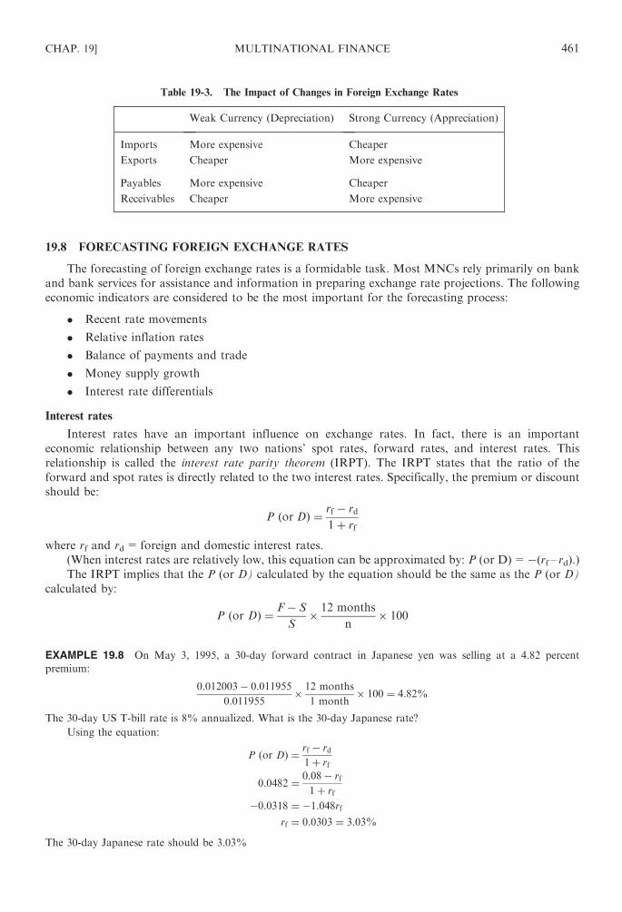
19.8 FORECASTING FOREIGN EXCHANGE RATES
The forecasting of foreign exchange rates is a formidable task. Most MNCs rely primarily on bank
and bank services for assistance and information in preparing exchange rate projections. The following
economic indicators are considered to be the most important for the forecasting process:
� Recent rate movements
� Relative inflation rates
� Balance of payments and trade
� Money supply growth
� Interest rate differentials
Interest rates
Interest rates have an important influence on exchange rates. In fact, there is an important
economic relationship between any two nations’ spot rates, forward rates, and interest rates. This
relationship is called the interest rate parity theorem (IRPT). The IRPT states that the ratio of the
forward and spot rates is directly related to the two interest rates. Specifically, the premium or discount
should be:
P ðor DÞ ¼ rf � rd
1þ rf
where rf and rd=foreign and domestic interest rates.
(When interest rates are relatively low, this equation can be approximated by: P (or D)=�(rf – rd).)The IRPT implies that the P (or D) calculated by the equation should be the same as the P (or D)
calculated by:
P ðor DÞ ¼ F� S
S� 12 months
n� 100
EXAMPLE 19.8 On May 3, 1995, a 30-day forward contract in Japanese yen was selling at a 4.82 percent
premium:
0:012003� 0:011955
0:011955� 12 months
1 month� 100 ¼ 4:82%
The 30-day US T-bill rate is 8% annualized. What is the 30-day Japanese rate?
Using the equation:
P ðor DÞ ¼ rf � rd
1þ rf
0:0482 ¼ 0:08� rf
1þ rf
�0:0318 ¼ �1:048rfrf ¼ 0:0303 ¼ 3:03%
The 30-day Japanese rate should be 3.03%
Table 19-3. The Impact of Changes in Foreign Exchange Rates
Weak Currency (Depreciation) Strong Currency (Appreciation)
Imports More expensive Cheaper
Exports Cheaper More expensive
Payables More expensive Cheaper
Receivables Cheaper More expensive
CHAP. 19] MULTINATIONAL FINANCE 461

Inflation
Inflation, which is a change in price levels, also affects future exchange rates. The mathematical
relationship that links changes in exchange rates and changes in price level is called the purchasing power
parity theorem (PPPT). The PPPT states that the ratio of the forward and spot rates is directly related to
the two inflation rates:
F
S¼ 1þ Pd
1þ Pf
where F=forward exchange rate (e.g., $/foreign currency)
S=spot exchange rate (e.g., $/foreign currency)
Pd=domestic inflation rate
Pf=foreign inflation rate
EXAMPLE 19.9 Assume the following data for US and UK:
Expected US inflation rate ¼ 5%
Expected UK inflation rate ¼ 10%
S ¼ $1:64=pound
Then,
F
1:64¼ 1:05
1:10
So
F ¼ $1:57=pound
Note: if UK has the higher inflation rate, then the purchasing power of the pound is declining faster than that
of the dollar. This will lead to a forward discount on the pound relative to the dollar.
19.9 ANALYSIS OF FOREIGN INVESTMENTS
Foreign investment decisions are basically capital budgeting decisions at the international level.
The decision requires two major components:
The estimation of the relevant future cash flows. Cash flows are the dividends and possible future sales
price of the investment. The estimation depends on the sales forecast, the effects on exchange rate
changes, the risk in cash flows, and the actions of foreign governments.
The choice of the proper discount rate (cost of capital). The cost of capital in foreign investment
projects is higher due to the increased risks of:
� Currency risk (or foreign exchange risk) – changes in exchange rates. This risk may adversely
affect sales by making competing imported goods cheaper.
� Political risk (or sovereignty risk) – possibility of nationalization or other restrictions with net
losses to the parent company.
Examples of Political Risks
� Expropriation of plants and equipment without compensation or with minimal compensation
that is below actual market value.
� Nonconvertibility of the affiliate’s foreign earnings into the parent’s currency – the problem of
‘‘blocked funds.’’
� Substantial changes in the laws governing taxation.
462 MULTINATIONAL FINANCE [CHAP. 19
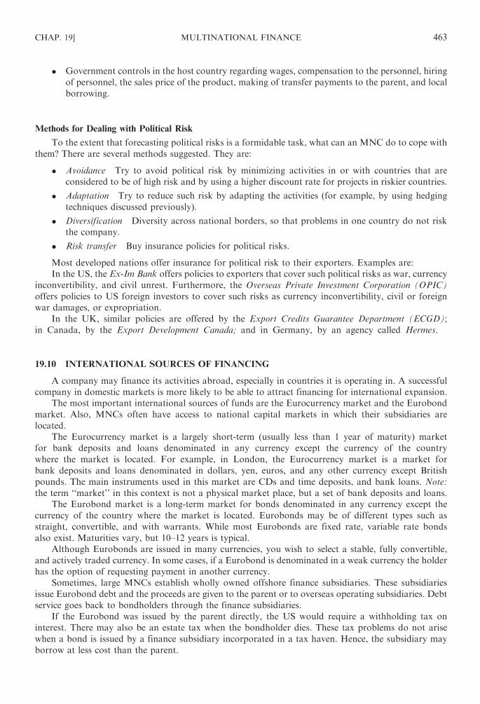
� Government controls in the host country regarding wages, compensation to the personnel, hiring
of personnel, the sales price of the product, making of transfer payments to the parent, and local
borrowing.
Methods for Dealing with Political Risk
To the extent that forecasting political risks is a formidable task, what can an MNC do to cope with
them? There are several methods suggested. They are:
� Avoidance Try to avoid political risk by minimizing activities in or with countries that are
considered to be of high risk and by using a higher discount rate for projects in riskier countries.
� Adaptation Try to reduce such risk by adapting the activities (for example, by using hedging
techniques discussed previously).
� Diversification Diversity across national borders, so that problems in one country do not risk
the company.
� Risk transfer Buy insurance policies for political risks.
Most developed nations offer insurance for political risk to their exporters. Examples are:
In the US, the Ex-Im Bank offers policies to exporters that cover such political risks as war, currency
inconvertibility, and civil unrest. Furthermore, the Overseas Private Investment Corporation (OPIC)
offers policies to US foreign investors to cover such risks as currency inconvertibility, civil or foreign
war damages, or expropriation.
In the UK, similar policies are offered by the Export Credits Guarantee Department (ECGD);
in Canada, by the Export Development Canada; and in Germany, by an agency called Hermes.
19.10 INTERNATIONAL SOURCES OF FINANCING
A company may finance its activities abroad, especially in countries it is operating in. A successful
company in domestic markets is more likely to be able to attract financing for international expansion.
The most important international sources of funds are the Eurocurrency market and the Eurobond
market. Also, MNCs often have access to national capital markets in which their subsidiaries are
located.
The Eurocurrency market is a largely short-term (usually less than 1 year of maturity) market
for bank deposits and loans denominated in any currency except the currency of the country
where the market is located. For example, in London, the Eurocurrency market is a market for
bank deposits and loans denominated in dollars, yen, euros, and any other currency except British
pounds. The main instruments used in this market are CDs and time deposits, and bank loans. Note:
the term ‘‘market’’ in this context is not a physical market place, but a set of bank deposits and loans.
The Eurobond market is a long-term market for bonds denominated in any currency except the
currency of the country where the market is located. Eurobonds may be of different types such as
straight, convertible, and with warrants. While most Eurobonds are fixed rate, variable rate bonds
also exist. Maturities vary, but 10–12 years is typical.
Although Eurobonds are issued in many currencies, you wish to select a stable, fully convertible,
and actively traded currency. In some cases, if a Eurobond is denominated in a weak currency the holder
has the option of requesting payment in another currency.
Sometimes, large MNCs establish wholly owned offshore finance subsidiaries. These subsidiaries
issue Eurobond debt and the proceeds are given to the parent or to overseas operating subsidiaries. Debt
service goes back to bondholders through the finance subsidiaries.
If the Eurobond was issued by the parent directly, the US would require a withholding tax on
interest. There may also be an estate tax when the bondholder dies. These tax problems do not arise
when a bond is issued by a finance subsidiary incorporated in a tax haven. Hence, the subsidiary may
borrow at less cost than the parent.
CHAP. 19] MULTINATIONAL FINANCE 463
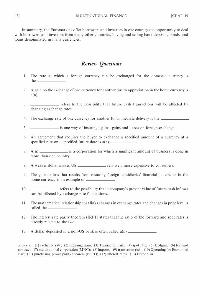
In summary, the Euromarkets offer borrowers and investors in one country the opportunity to deal
with borrowers and investors from many other countries, buying and selling bank deposits, bonds, and
loans denominated in many currencies.
Review Questions
1. The rate at which a foreign currency can be exchanged for the domestic currency is
the .
2. A gain on the exchange of one currency for another due to appreciation in the home currency is
a(n) .
3. refers to the possibility that future cash transactions will be affected by
changing exchange rates.
4. The exchange rate of one currency for another for immediate delivery is the
5. is one way of insuring against gains and losses on foreign exchange.
6. An agreement that requires the buyer to exchange a specified amount of a currency at a
specified rate on a specified future date is a(n) .
7. A(n) is a corporation for which a significant amount of business is done in
more than one country.
8. A weaker dollar makes US relatively more expensive to consumers.
9. The gain or loss that results from restating foreign subsidiaries’ financial statements in the
home currency is an example of .
10. refers to the possibility that a company’s present value of future cash inflows
can be affected by exchange rate fluctuations.
11. The mathematical relationship that links changes in exchange rates and changes in price level is
called the .
12. The interest rate parity theorem (IRPT) states that the ratio of the forward and spot rates is
directly related to the two .
13. A dollar deposited in a non-US bank is often called a(n) .
Answers: (1) exchange rate; (2) exchange gain; (3) Transaction risk; (4) spot rate; (5) Hedging; (6) forward
contract; (7) multinational corporation (MNC); (8) imports; (9) translation risk; (10) Operating (or Economic)
risk; (11) purchasing power parity theorem (PPPT); (12) interest rates; (13) Eurodollar.
464 MULTINATIONAL FINANCE [CHAP. 19

Solved Problems
19.1 Spot Rates. On June 1, Johnson, Inc. received an order from a Japanese customer for 2,500,000
yen to be paid upon receipt of the goods, scheduled for August 1. The rates for $1 US are as
follows:
Exchange Rates for $1 forYen
Spot rate, June 1 83
Forward rate, August 1 82
Spot rate, August 1 81
(a) Calculate what Johnson would receive from the Japanese customer in US dollars using the
spot rate at the time of the order.
(b) Calculate what Johnson would receive from the Japanese customer in US dollars using the
spot rate at the time of payment.
SOLUTION
(a) $30,120.48 (2,500,000 yen/83 yen per $)
(b) $30,864.20 (2,500,000 yen/81)
19.2 Forward Rates. Using the same data in Problem 19.1:
(a) Calculate Johnson’s exchange gain or loss, if Johnson receives payment from the Japanese
customer using the spot rate at the time of payment.
(b) Calculate the amount that Johnson expects to receive on August 1 if Johnson’s policy is to
hedge foreign currency transactions.
SOLUTION
(a) Loss of $743.72 ($30,864.20 � $30,120.48)
(b) $30,487.80 (2,500,000 yen/82)
19.3 Exchange Gain or Loss. Bonjur, Inc. imports French cheeses for distribution in the US.
On April 1, the company purchased cheese costing 400,000 euros. Payment is due in euros on
July 1. The spot rate on April 1 was $1.20 per euro, and on July 1, it was $1.25 per euro.
(a) How much would Bonjur have to pay in dollars for the purchase if it paid on April 1?
(b) How much would Bonjur have to pay in dollars for the purchase if it paid on July 1?
(c) If Bonjur paid for the purchase using the July 1 spot rate, what would be the exchange gain
or loss?
SOLUTION
(a) 400,000 euros� $1.20 per franc=$480,000
(b) 400,000 euros� $1.25 per franc=$500,000
(c) Liability in dollars, April 1 $480,000
Paid in dollars, July 1 $500,000
Exchange loss $20,000
CHAP. 19] MULTINATIONAL FINANCE 465

19.4 Spot Rates. On August 1, Kidd Trading received an order from a British customer for £1,000,000
to be paid on receipt of the goods, scheduled for November 1.
The rates for $1 US are as follows:
Exchange Rates for $1 British £
Spot rate, June 1 1.617
Forward rate, August 1 1.615
Spot rate, August 1 1.616
(a) How much does Kidd expect to receive from the British customer in dollars using the spot
rate at the time of the order?
(b) How much does Kidd expect to receive from the British customer in dollars using the spot
rate at the time of payment?
SOLUTION
(a) $618,429.19 (£1,000,000/1.617)
(b) $618,811.81 (£1,000,000/1.616)
19.5 Exchange Gain or Loss and Hedging. Using the same data in Problem 19.4:
(a) Calculate Kidd’s exchange gain or loss if Kidd receives payment from the British customer
using the spot rate at the time of payment.
(b) Calculate the amount Kidd expects to receive on November 1 in dollars, if Kidd’s policy is
to hedge foreign currency transactions.
SOLUTION
(a) Receivables in dollars, August 1 $618,811.81
Received in dollars, November 1 618,429.19
Exchange gain $ 382.62
(b) $619,195.05 (£1,000,000/1.615)
19.6 Arbitrage and Exchange Gain or Loss. You own $10,000. The dollar rate on the Swiss franc is
1.380 SFs.
Country Contract
US Dollar
Equivalent
(Direct)
Currency
per US$
(Indirect)
Switzerland Spot 0.7282 1.3733
(Franc) 30-day future 0.7290 1.3716
90-day future 0.7311 1.3677
Based on the table above, are arbitrage profits possible? What is the gain (loss) in dollars?
SOLUTION
The dollar rate on the Swiss franc (SF) is 1.380 francs while the table (indirect New York rate) shows
1.3773 (1/0.7282) francs. Note that the rates between Switzerland and New York are out of line. Thus,
arbitrage profits are possible. Since the SF is cheaper in Switzerland, buy $10,000 worth of francs in
Switzerland. The number of francs purchased would be 13,800 ($10,000� 1.380) francs. Simultaneously
466 MULTINATIONAL FINANCE [CHAP. 19

sell the francs in New York at the prevailing rate. The amount received upon sale of the francs would be
$10,049.16 (13,800 francs� $0.7282/SF)=$10,049.16. The net gain is $49.16, barring transactions costs.
19.7 Interest-Rate Parity. If the interest rates on the 30-day instruments in the US and Switzerland are
12 and 10 percent (annualized), respectively, what is the correct price of the 30-day forward SF?
(Use the table in Problem 19.6.)
SOLUTION
First, compute the premium (discount) on the forward rate using:
P ðorDÞ ¼ rf � rd
1þ rf
Thus,
0:10� 0:12
1þ 1:10¼ 0:0182
Compute the forward rate using the equation:
P ðor DÞ ¼ F� S
S� 12 months
n� 100
0:0182 ¼ F� 0:7282
0:7282� 12
1� 100
Solving this equation for F yields: 0.7293
19.8 Interest-Rate Parity. Almond Shoe, Inc. sells to a wholesaler in Switzerland. The purchase price
of a shipment is 50,000 SF with terms of 90 days. Upon payment, Almond will convert the SF to
dollars.
Country Contract
US Dollar
Equivalent
Currency
per US$
Switzerland Spot 0.730 1.37
(Franc) 90-day future 0.735 1.36
(a) If Almond’s policy is to hedge its foreign exchange risk, what would it do?
(b) Is the SF at a premium or at a discount?
(c) What is the implied differential in interest rates between the two nations, using the interest-
rate parity theory?
SOLUTION
(a) Almond would hedge by selling SFs forward 90 days. Upon delivery of 50,000 SFs in 90 days, it would
receive $36,764.71 (50,000 SFs/1.36). It was to receive payment today. It would get only $36,496.35
(50,000 SFs/1.37).
(b) The SF is at a premium because the 90-day forward rate of SF per dollar is less than the current spot
rate. The SF is expected to strengthen (fewer SF to buy a dollar).
(c) The differential in interest rates is �2.96 percent, as shown
Pðor DÞ ¼ F� S
S� 12 months
n� 100
ð7:35� 7:30Þ7:30
� 12
3� 100 ¼ �ðrf � rdÞ ¼ 2:73%
This means that if the interest parity theory holds, interest rates in the US should be 2.73 percent higher than
those in Switzerland.
CHAP. 19] MULTINATIONAL FINANCE 467

19.9 Interest-Rate Parity.
Country Contract
US Dollar
Equivalent
Currency
per US$
Japan Spot 0.011955 83.65
(Yen) 90-day future 0.012100 82.64
The interest rate in Japan on 90-day government securities is 4 percent; it is 8 percent in the US. If
the interest-rate parity theory holds, what is the implied 90-day forward exchange rate in yen per
dollar?
SOLUTION
First, compute the premium (discount) on the forward rate using:
P ðor DÞ ¼ rf � rd
1þ rf
Thus,
0:04� 0:08
1þ 0:04¼ 0:0385
Compute the forward rate using the equation:
P ðor DÞ ¼ F� S
S� 12 months
n� 100
0:0385 ¼ F� 0:011955
0:011955� 12
3� 100
Solving this equation for F yields: 0.012070
19.10 Purchasing Power Parity Theorem (PPPT). The inflation rate in the United States is projected
at 3 percent per year. The New Zealand rate is projected to be 5 percent. The exchange rate
is currently NZ$1.66. Based on PPP, what is the expected exchange rate in two years?
SOLUTION
The PPT states:
F
S¼ 1þ Pd
1þ Pf
F
1:66¼ 1þ 0:03
1þ 0:05so F=1:66 ¼ 1:03=1:05: Solving for F yields NZ$1:63
19.11 Covered Interest Arbitrage. The spot and 360-day forward rates on the Swiss franc are
SF 2.1 and SF 1.9, respectively. The risk-free interest rate in the US is 6 percent, and the risk-
free rate in Switzerland is 4 percent. Is arbitrage opportunity here? How would you exploit it?
SOLUTION
Based on IRPT, the forward rate should be (approximately):
F� S
S¼ rf � rd
1þ rfF� 2:1
2:1¼ 0:04� 0:06
1þ 0:041:04ðF� 2:1Þ ¼ �0:042; F ¼ 2:142=1:04 ¼ 2:06
Because the forward rate is actually SF 1.9, there is an arbitrage opportunity.
468 MULTINATIONAL FINANCE [CHAP. 19

To exploit the arbitrage opportunity, you first note that dollars are selling for SF 1.9 each in the forward
market. Based on IRPT, this is too cheap because they should be selling for SF 2.06. So you want to arrange
to buy dollars with Swiss francs in the forward market. To do this, you can:
1. Today, borrow, say, $1 million for 360 days. Convert it to SF 2.1 million in the spot market, and
buy a forward contract at SF 1.9 to convert it back to dollars in 360 days. Invest the SF 2.1 million
at 4 percent.
2. In 1 year, your investment has grown to SF 2.1 million� 1.04=SF 2.184 million. Convert this to
dollars at the rate of SF 1.9=$1. You will have SF 2.184 million/1.9=$1,149,174. Pay off your
loan with 6 percent interest at a cost of $1 million� 1.06=$1,060,000 and pocket the difference of
$89,474.
CHAP. 19] MULTINATIONAL FINANCE 469

Examination IV
Chapters 16–19
1. A warrant for Jack Corporation permits the holder to buy five shares of common stock at $25 a
share. The market price of the stock is $37. What is the value of the warrant?
2. Smith Corporation issued a $1,000 bond at par. The common stock has a market price of $34. The
conversion price is $40. (a) Into how many shares may the bond be converted? (b) What is the
conversion value of the bond? (c) What is the conversion premium?
3. Tunick Corporation’s convertible bond has a conversion price of $80. The conversion ratio is 12.
The market price of the stock is $115. The call price is $1,200. Would the bondholder rather convert
to common stock or receive the call price?
4. The following data are provided:
Company A Company B
Net income $40,000 $60,000
Shares outstanding 8,000 20,000
Earnings per share $5.00 $3.00
P/E ratio 9 15
Market price $45 $45
Company B is the acquiring company, exchanging on a one-for-one basis its shares
for the shares of company A. The exchange ratio is based on the market prices of A and B.
(a) What will the EPS be after the merger? (b) What is the change in EPS for the stockholders
of companies A and B?
5. The following data are provided:
Market Price per Share
of Acquiring Company
Market Price per Share
of Acquired Company
Price per Share
Offered
$75 $25 $35
What is the exchange ratio in: (a) shares? (b) market price?
6. Jones Company wishes to acquire Masters Company. Relevant data follow:
Jones Masters
Net income $60,000 $45,000
Shares outstanding 30,000 5,000
Jones Company issues its shares to make the acquisition. The ratio of exchange is 3.0 (a) What
is the EPS of the merged company based on the original shares of each firm? (b) What is the EPS of
Jones? (c) What is the EPS of Masters?
470
Copyright © 2007, 1998, 1986 by The McGraw-Hill Companies, Inc. Click here for terms of use.

7. Glory Corporation wishes to acquire Jerry Corporation by exchanging 1.5 shares of its stock for
each share of Jerry. Glory expects to have the same P/E ratio after the merger as before it. The
following data are given:
Glory Jerry
Net income $600,000 $200,000
Shares 200,000 25,000
Market price per share $50 $40
(a) What is the exchange ratio of market prices? (b) What are the EPS and P/E ratios for each
firm? (c) What was the P/E ratio used to obtain Jerry? (d ) What is the EPS of Glory after the
acquisition? (e) What is the anticipated market price per share of the merged company?
8. Brother Corporation is considering acquiring Davis Company for $190,000 in cash. Brother’s
current cost of capital is 12 percent. Davis has an estimated cost of capital of 10 percent after
the acquisition. Anticipated cash inflows from years 1 to 12 are $20,000. Should the acquisition be
made?
9. Company T wants to acquire company Z. Company T’s stock sells for $90 per share. Company Z’s
stock sells for $35 per share. Because of merger negotiations, company T offers $45 a share. The
acquisition is accomplished by an exchange of securities. What is the exchange ratio?
10. The balance sheet of Jason Corporation for the year ended December 31, 20X4, follows:
Balance Sheet
Current assets $ 800,000 Current liabilities $ 600,000
Noncurrent assets 300,000 Long-term liabilities 250,000
Common stock 300,000
Retained earnings (50,000)
Total assets $1,100,000
Total liabilities and
stockholders’ equity $1,100,000
The company’s liquidation value is $800,000. Rather than liquidating, a reorganization could
occur with an investment of another $350,000. The reorganization is expected to generate earnings
of $120,000 a year. A multiplier of 6 is appropriate. If the $350,000 is obtained, long-term debt
holders will receive 40 percent of the common stock in the reorganized business in substitution for
their current claims. Is reorganization or liquidation recommended?
11. Calcot Corporation is bankrupt. The book and liquidation values of its assets follow.
Book
Value
Liquidation
Value
Cash $ 400,000 $ 400,000
Accounts receivable 1,600,000 1,300,000
Inventory 3,200,000 2,000,000
Land 5,000,000 3,800,000
Building 10,000,000 6,000,000
Equipment 8,000,000 4,000,000
Total assets $28,200,000 $17,500,000
EXAMINATION IV 471
The liabilities and stockholders’ equity at the liquidation date follow.
Current liabilities
Accounts payable $3,000,000
Notes payable 1,500,000
Accrued taxes 800,000
Accrued salaries 300,000a
Total current liabilities $ 5,600,000
Long-term liabilities
Mortgage on land $3,800,000
First mortgage—building 4,000,000
Second mortgage—building 2,000,000
Subordinated debentures 4,200,000
Total long-term liabilities 14,000,000
Total liabilities $19,600,000
Stockholders’ equity
Preferred stock $3,500,000
Common stock 7,000,000
Retained earnings (1,900,000)
Total stockholders’ equity 8,600,000
Total liabilities and stockholders’ equity$28,200,000
a The salary owed to each worker is less than $2,000 and was incurred within 90 days of the
bankruptcy petition.
Expenses applicable to the bankruptcy administration were 15 percent of the proceeds.
The debentures are subordinated only with regard to the two first-mortgage bonds.
What is the distribution of the proceeds?
12. Michael Corporation’s balance sheet is presented below.
ASSETS
Current assets $1,400,000
Land 3,500,000
Plant and equipment 2,500,000
Total assets $7,400,000
LIABILITIES AND STOCKHOLDERS’ EQUITY
Current liabilities
Accounts payable $ 400,000
Notes payable 1,000,000
Accrued taxes 200,000
Total current liabilities $1,600,000
Noncurrent liabilities
Mortgage bonds $2,000,000a
Debentures 1,200,000
Total noncurrent liabilities 3,200,000
Total liabilities $4,800,000
Stockholders’ equity
Preferred stock $ 800,000
Common stock 1,800,000
Total stockholders’ equity 2,600,000
Total liabilities and stockholders’equity
$7,400,000
a Mortgage bonds are secured against plant and equipment.
472 EXAMINATION IV
The liquidation value of the total assets was $4.6 million, $1.4 million of which was received for
plant and equipment. Bankruptcy costs were $120,000.
What is the distribution of the proceeds?
Answers to Examination IV
1. ($37� $25)� 5=$60
2. (a)$1,000
40¼ 25 shares
(b) Conversion value=common stock price� conversion ratio=$34� 25=$850
(c) $1,000� $850=$150
3. The market value of common stock received upon conversion is:
$115� 12 ¼ $1,380
The call price is $1,200. The bondholder would rather convert, since he or she receives a benefit of $180.
4. (a) B Shares
Owned after
Merger
EPS
before
Merger
EPS
after
Merger
A stockholders 8,000 $5.00 $3.57a
B stockholders 20,000 $3.00 $3.57a
Total 28,000
a The new EPS is calculated as follows:
8,000 shares� $5 $40,000
20,000 shares� $3 60,000
Total net income $100,000
EPS ¼ total net income
total shares¼ $100,000
28,000¼ $3:57
(b) EPS is lower by $1.43 for A stockholders but rises by $0.57 for B stockholders.
5. (a)$35
$75¼ 0:467
(b)$35
$25¼ 1:4
6. (a)Combined net income
Total shares¼ $105,000
30,000þ 5,000� 3ð Þ ¼$105,000
45,000¼ $2:23
(b) $2.33
(c) $2.33� 3=$6.99
EXAMINATION IV 473

7. (a) Price per share offered
Market price of Jerry¼ $50� 1:5
$40¼ $75
$40¼ 1:875
(b) Glory Jerry
EPS (net income/number of shares) 3.0 8.0
P/E 16.67 5
(c)
1:5� $50 ¼ $75
$75
$8¼ 9:4 times
(d ) Total net income is:
200,000 shares� $3 $600,000
25,000 shares� $8 200,000
Total net income $800,000
Net EPS is:
Total net income
Total shares¼ $800,000
237,500¼ $3:37
(e) Anticipated market price=P/E� new EPS 16.67� $3.37=$56.18 (rounded)
8. Year Calculations Present Value
0 �$190,000� 1 �$190,0001–12 +$20,000� 6.814 +136,280a
�$ 53,720
a Using 10 percent as the discount rate.
The net present value is �$53,720. Since it is negative the acquisition should not be made.
9. Amount paid per share of the acquired company
Market price of the acquiring company’s shares¼ $45
$90¼ 0:5
10. Assuming the $350,000 of further investment is made, the company’s going concern value is $720,000
(6� $120,000). The liquidation value is given as $800,000. Since the liquidation value exceeds the going
concern value, liquidation is called for.
11. The distribution of the proceeds follows:
Proceeds $17,500,000
Mortgage on land $3,800,000
First mortgage—building 4,000,000
Second mortgage—building 2,000,000
Liquidation expenses
(15%� $17,500,000) 2,625,000
Accrued taxes 800,000
Accrued salaries 300,000
Total 13,525,000
Balance $ 3,975,000
474 EXAMINATION IV

Percent to be paid to general creditors:
Proceeds balance
Total owed¼ $3,975,000
$8,700,000¼ 0:4568965
General Creditor Owed Paid
Accounts payable $3,000,000 $1,370,690
Notes payable 1,500,000 685,345
Subordinated debentures 4,200,000 1,918,965
Total $8,700,000 $3,975,000
12. Proceeds $4,600,000
Mortgage bonds—secured against
plant and equipment
$1,400,000
Bankruptcy costs 120,000
Accrued taxes 200,000 1,720,000
Balance available to general
creditors
$2,880,000
The distribution to general creditors follows:
General Creditor Owed
Pro Rata
Distribution
Mortgage bonds
($2,000,000� $1,400,000) $ 600,000 $ 540,000
Accounts payable 400,000 360,000
Notes payable 1,000,000 900,000
Debentures 1,200,000 1,080,000
Total $3,200,000 $2,880,000
Preferred stock and common stockholders will receive nothing.
EXAMINATION IV 475

Appendix
AFuture Value of $1: FVIFi,n
Period 1% 2% 3% 4% 5% 6% 7% 8% 9% 10% 12% 14% 15% 16% 18% 20% 24% 28% 32% 36%
1 1.0100 1.0200 1.0300 1.0400 1.0500 1.0600 1.0700 1.0800 1.0900 1.1000 1.1200 1.1400 1.1500 1.1600 1.1800 1.2000 1.2400 1.2800 1.3200 1.3600
2 1.0201 1.0404 1.0609 1.0816 1.1025 1.1236 1.1449 1.1664 1.1881 1.2100 1.2544 1.2996 1.3225 1.3456 1.3924 1.4400 1.5376 1.6384 1.7424 1.8496
3 1.0303 1.0612 1.0927 1.1249 1.1576 1.1910 1.2250 1.2597 1.2950 1.3310 1.4049 1.4815 1.5209 1.5609 1.6430 1.7280 1.9066 2.0972 2.3000 2.5155
4 1.0406 1.0824 1.1255 1.1699 1.2155 1.2625 1.3108 1.3605 1.4116 1.4641 1.5735 1.6890 1.7490 1.8106 1.9388 2.0736 2.3642 2.6844 3.0360 3.4210
5 1.0510 1.1041 1.1593 1.2167 1.2763 1.3382 1.4026 1.4693 1.5386 1.6105 1.7623 1.9254 2.0114 2.1003 2.2878 2.4883 2.9316 3.4360 4.0075 4.6526
6 1.0615 1.1262 1.1941 1.2653 1.3401 1.4185 1.5007 1.5869 1.6771 1.7716 1.9738 2.1950 2.3131 2.4364 2.6996 2.9860 3.6352 4.3980 5.2899 6.3275
7 1.0721 1.1487 1.2299 1.3159 1.4071 1.5036 1.6058 1.7138 1.8280 1.9487 2.2107 2.5023 2.6600 2.8262 3.1855 3.5832 4.5077 5.6295 6.9826 8.6054
8 1.0829 1.1717 1.2668 1.3686 1.4775 1.5938 1.7182 1.8509 1.9926 2.1436 2.4760 2.8526 3.0590 3.2784 3.7589 4.2998 5.5895 7.2058 9.2170 11.703
9 1.0937 1.1951 1.3048 1.4233 1.5513 1.6895 1.8385 1.9990 2.1719 2.3579 2.7731 3.2519 3.5179 3.3080 4.4355 5.1598 6.9310 9.2234 12.166 15.916
10 1.1046 1.2190 1.3439 1.4802 1.6289 1.7908 1.9672 2.1589 2.3674 2.5937 3.1058 3.7072 4.0456 4.4114 5.2338 6.1917 8.5944 11.805 16.059 21.646
11 1.1157 1.2434 1.3842 1.5395 1.7103 1.8983 2.1049 2.3316 2.5804 2.8531 3.4785 4.2262 4.6524 5.1173 6.1759 7.4301 10.657 15.111 21.198 29.439
12 1.1268 1.2682 1.4258 1.6010 1.7959 2.0122 2.2522 2.5182 2.8127 3.1384 3.8960 4.8179 5.3502 5.9360 7.2876 8.9161 13.214 19.342 27.982 40.037
13 1.1381 1.2936 1.4685 1.6651 1.8856 2.1329 2.4098 2.7196 3.0658 3.4523 4.3635 5.4924 6.1528 6.8858 8.5994 10.699 16.386 24.748 36.937 54.451
14 1.1495 1.3195 1.5126 1.7317 1.9799 2.2609 2.5785 2.9372 3.3417 3.7975 4.8871 6.2613 7.0757 7.9875 10.147 12.839 20.319 31.691 48.756 74.053
15 1.1610 1.3459 1.5580 1.8009 2.0789 2.3966 2.7590 3.1722 3.6425 4.1772 5.4736 7.1379 8.1371 9.2655 11.973 15.407 25.195 40.564 53.358 100.71
16 1.1726 1.3728 1.6047 1.8730 2.1829 2.5404 2.9522 3.4259 3.9703 4.5950 6.1304 8.1372 9.3576 10.748 14.129 18.488 31.242 51.923 84.953 136.96
17 1.1843 1.4002 1.6528 1.9479 2.2920 2.6928 3.1588 3.7000 4.3276 5.0545 6.8660 9.2765 10.761 12.467 16.672 22.186 38.740 66.461 112.13 186.27
18 1.1961 1.4282 1.7024 2.0258 2.4066 2.8543 3.3799 3.9960 4.7171 5.5599 7.6900 10.575 12.375 14.462 19.673 26.623 48.038 85.070 148.02 253.33
19 1.2081 1.4568 1.7535 2.1068 2.5270 3.0256 3.6165 4.3157 5.1417 6.1159 8.6129 12.055 14.231 16.776 23.214 31.948 59.567 108.89 195.39 344.53
20 1.2202 1.4859 1.8061 2.1911 2.6533 3.2071 3.8697 4.6610 5.6044 6.7275 9.6463 13.743 16.366 19.460 27.393 38.337 73.864 139.37 257.91 468.57
21 1.2324 1.5157 1.8603 2.2788 2.7860 3.3996 4.1406 5.0338 6.1088 7.4002 10.803 15.667 18.821 22.574 32.323 46.005 91.591 178.40 340.44 637.26
22 1.2447 1.5460 1.9161 2.3699 2.9253 3.6035 4.4304 5.4365 6.6586 8.1403 12.100 17.861 21.644 26.186 38.142 55.206 113.57 228.35 449.39 866.67
23 1.2572 1.5769 1.9736 2.4647 3.0715 3.8197 4.7405 5.8715 7.2579 8.9543 13.552 20.361 24.891 30.376 45.007 66.247 140.83 292.30 593.19 1178.6
24 1.2697 1.6084 2.0328 2.5633 3.2251 4.0489 5.0724 6.3412 7.9111 9.8497 15.178 23.212 28.625 35.236 53.108 79.496 174.63 374.14 783.02 1602.9
25 1.2824 1.6406 2.0938 2.6658 3.3864 4.2919 5.4274 6.8485 8.6231 10.834 17.000 26.461 32.918 40.874 62.668 95.396 216.54 478.90 1033.5 2180.0
26 1.2953 1.6734 2.1566 2.7725 3.5557 4.5494 5.8074 7.3964 9.3992 11.918 19.040 30.166 37.856 47.414 73.948 114.47 268.51 612.99 1364.3 2964.9
27 1.3082 1.7069 2.2213 2.8834 3.7335 4.8223 6.2139 7.9881 10.245 13.110 21.324 34.389 43.535 55.000 87.259 137.37 332.95 784.63 1800.9 4032.2
28 1.3213 1.7410 2.2879 2.9987 3.9201 5.1117 6.6488 8.6271 11.167 14.421 23.883 39.204 50.065 63.800 102.96 164.84 412.86 1004.3 2377.2 5483.8
29 1.3345 1.7758 2.3566 3.1187 4.1161 5.4184 7.1143 9.3173 12.172 15.863 26.749 44.693 57.575 74.008 121.50 197.81 511.95 1285.5 3137.9 7458.0
30 1.3478 1.8114 2.4273 3.2434 4.3219 5.7435 7.6123 10.062 13.267 17.449 29.959 50.950 66.211 85.849 143.37 237.37 634.81 1645.5 4142.0 10143.
40 1.4889 2.2080 3.2620 4.8010 7.0400 10.285 14.974 21.724 31.409 45.259 93.050 188.88 267.86 378.72 750.37 1469.7 5455.9 19426 66520 *
50 1.6446 2.6916 4.3839 7.1067 11.467 18.420 29.457 46.901 74.357 117.39 289.00 700.23 1083.6 1670.7 3927.3 9100.4 46890 * * *
60 1.8167 3.2810 5.8916 10.519 18.679 32.987 57.946 101.25 176.03 304.48 897.59 2595.9 4383.9 7370.1 20555 56347 * * * *
*FVIF > 99.999
476
Copyright © 2007, 1998, 1986 by The McGraw-Hill Companies, Inc. Click here for terms of use.

Appendix
BSum of an Annuity of $1: FVIFAi,n
Number ofPeriods 1% 2% 3% 4% 5% 6% 7% 8% 9% 10% 12% 14% 15% 16% 18% 20% 24% 28% 32% 36%
1 1.0000 1.0000 1.0000 1.0000 1.0000 1.0000 1.0000 1.0000 1.0000 1.0000 1.0000 1.0000 1.0000 1.0000 1.0000 1.0000 1.0000 1.0000 1.0000 1.0000
2 2.0100 2.0200 2.0300 2.0400 2.0500 2.0600 2.0700 2.0800 2.0900 2.1000 2.1200 2.1400 2.1500 2.1600 2.1800 2.2000 2.2400 2.2800 2.3200 2.3600
3 3.0301 3.0604 3.0909 3.1216 3.1525 3.1836 3.2149 3.2464 3.2781 3.3100 3.3744 3.4396 3.4725 3.5056 3.5724 3.6400 3.7776 3.9184 4.0624 4.2096
4 4.0604 4.1216 4.1836 4.2465 4.3101 4.3746 4.4399 4.5061 4.5731 4.6410 4.7793 4.9211 4.9934 5.0665 5.2154 5.3680 5.6842 6.0156 6.3624 6.7251
5 5.1010 5.2040 5.3091 5.4163 5.5256 5.6371 5.7507 5.8666 5.9847 6.1051 6.3528 6.6101 6.7424 6.8771 7.1542 7.4416 8.0484 8.6999 9.3983 10.146
6 6.1520 6.3081 6.4684 6.6330 6.8019 6.9753 7.1533 7.3359 7.5233 7.7156 8.1152 8.5355 8.7537 8.9775 9.4420 9.9299 10.980 12.135 13.405 14.798
7 7.2135 7.4343 7.6625 7.8983 8.1420 8.3938 8.6540 8.9228 9.2004 9.4872 10.089 10.730 11.066 11.413 12.141 12.915 14.615 16.533 18.695 21.126
8 8.2857 8.5830 8.8923 9.2142 9.5491 9.8975 10.259 10.636 11.028 11.435 12.299 13.232 13.726 14.240 15.327 16.499 19.122 22.163 25.678 29.731
9 9.3685 9.7546 10.159 10.582 11.026 11.491 11.978 12.487 13.021 13.579 14.775 16.085 16.785 17.518 19.085 20.798 24.712 29.369 34.895 41.435
10 10.462 10.949 11.463 12.006 12.577 13.180 13.816 14.486 15.192 15.937 17.548 19.337 20.303 21.321 23.521 25.958 31.643 38.592 47.061 57.351
11 11.566 12.168 12.807 13.486 14.206 14.971 15.783 16.645 17.560 18.531 20.654 23.044 24.349 25.732 28.755 32.150 40.237 50.398 63.121 78.998
12 12.682 13.412 14.192 15.025 15.917 16.869 17.888 18.977 20.140 21.384 24.133 27.270 29.001 30.850 34.931 39.580 50.894 65.510 84.320 108.43
13 13.809 14.680 15.617 16.626 17.713 18.882 20.140 21.495 22.953 24.522 28.029 32.088 34.351 36.786 42.218 48.496 64.109 84.852 112.30 148.47
14 14.947 15.973 17.086 18.291 19.598 21.015 22.550 24.214 26.019 27.975 32.392 37.581 40.504 43.672 50.818 59.195 80.496 109.61 149.23 202.92
15 16.096 17.293 18.598 20.023 21.578 23.276 25.129 27.152 29.360 31.772 37.279 43.842 47.580 51.659 60.965 72.035 100.81 141.30 197.99 276.97
16 17.257 18.639 20.156 21.824 23.657 25.672 27.888 30.324 33.003 35.949 42.753 50.980 55.717 60.925 72.939 87.442 126.01 181.86 262.35 377.69
17 18.430 20.012 21.761 23.697 25.840 28.212 30.840 33.750 36.973 40.544 48.883 59.117 65.075 71.673 87.068 105.93 157.25 233.79 347.30 514.66
18 19.614 21.412 23.414 25.645 28.132 30.905 33.999 37.450 41.301 45.599 55.749 68.394 75.836 84.140 103.74 128.11 195.99 300.25 459.44 700.93
19 20.810 22.840 25.116 27.671 30.539 33.760 37.379 41.446 46.018 51.159 63.439 78.969 88.211 98.603 123.41 154.74 244.03 385.32 607.47 954.27
20 22.019 24.297 26.870 29.778 33.066 36.785 40.995 45.762 51.160 57.275 72.052 91.024 102.44 115.37 146.62 186.68 303.60 494.21 802.86 1298.8
21 23.239 25.783 28.676 31.969 35.719 39.992 44.865 50.442 56.764 64.002 81.698 104.76 118.81 134.84 174.02 225.02 377.46 633.59 1060.7 1767.3
22 24.471 27.299 30.536 34.248 38.505 43.392 49.005 55.456 62.873 71.402 92.502 120.43 137.63 157.41 206.34 271.03 469.05 811.99 1401.2 2404.6
23 25.716 28.845 32.452 36.617 41.430 46.995 53.436 60.893 69.531 79.543 104.60 138.29 159.27 183.60 244.48 326.23 582.62 1040.3 1850.6 3271.3
24 26.973 30.421 34.426 39.082 44.502 50.815 58.176 66.764 76.789 88.497 118.15 158.65 184.16 213.97 289.49 392.48 723.46 1332.6 2443.8 4449.9
25 28.243 32.030 36.459 41.645 47.727 54.864 63.249 73.105 84.700 98.347 133.33 181.87 212.79 249.21 342.60 471.98 898.09 1706.8 3226.8 6052.9
26 29.525 33.670 38.553 44.311 51.113 59.156 68.676 79.954 93.323 109.18 150.33 208.33 245.71 290.08 405.27 567.37 1114.6 2185.7 4260.4 8233.0
27 30.820 35.344 40.709 47.084 54.669 63.705 74.483 87.350 102.72 121.09 169.37 238.49 283.56 337.50 479.22 681.85 1383.1 2798.7 5624.7 11197.9
28 32.129 37.051 42.930 49.967 58.402 68.528 80.697 95.338 112.96 134.20 190.69 272.88 327.10 392.50 566.48 819.22 1716.0 3583.3 7425.6 15230.2
29 32.450 38.792 45.218 52.966 62.322 73.689 87.346 103.96 124.13 148.63 214.58 312.09 377.16 456.30 669.44 984.06 2128.9 4587.6 9802.9 20714.1
30 34.784 40.568 47.576 56.084 66.438 79.058 94.460 113.28 136.30 164.49 241.33 356.78 434.74 530.31 790.94 1181.8 2640.9 5873.2 12940 28172.2
40 48.886 60.402 75.401 95.025 120.79 154.76 199.63 259.05 337.88 442.59 767.09 1342.0 1779.0 2360.7 4163.2 7343.8 22728 63977 * *
50 64.463 84.579 112.79 152.66 209.34 290.33 406.52 573.76 815.08 1163.9 2400.0 4994.5 7217.7 10435 21813 45497 * * * *
60 81.669 114.05 163.05 237.90 353.58 533.12 813.52 1253.2 1944.7 3034.8 7471.6 18535 29219 46057 * * * * * *
*FVIFA>99.999
477
Copyright © 2007, 1998, 1986 by The McGraw-Hill Companies, Inc. Click here for terms of use.

Appendix
CPresent Value of $1: PVIFi,n
Period 1% 2% 3% 4% 5% 6% 7% 8% 9% 10% 12% 14% 15% 16% 18% 20% 24% 28% 32% 36%
1 .9901 .9804 .9709 .9615 .9524 .9434 .9346 .9259 .9174 .9091 .8929 .8772 .8696 .8621 .8475 .8333 .8065 .7813 .7576 .7353
2 .9803 .9612 .9426 .9246 .9070 .8900 .8734 .8573 .8417 .8264 .7972 .7695 .7561 .7432 .7182 .6944 .6504 .6104 .5739 .5407
3 .9706 .9423 .9151 .8890 .8638 .8396 .8163 .7938 .7722 .7513 .7118 .6750 .6575 .6407 .6086 .5787 .5245 .4768 .4348 .3975
4 .9610 .9238 .8885 .8548 .8227 .7921 .7629 .7350 .7084 .6830 .6355 .5921 .5718 .5523 .5158 .4823 .4230 .3725 .3294 .2923
5 .9515 .9057 .8626 .8219 .7835 .7473 .7130 .6806 .6499 .6209 .5674 .5194 .4972 .4761 .4371 .4019 .3411 .2910 .2495 .2149
6 .9420 .8880 .8375 .7903 .7462 .7050 .6663 .6302 .5963 .5645 .5066 .4556 .4323 .4104 .3704 .3349 .2751 .2274 .1890 .1580
7 .9327 .8706 .8131 .7599 .7107 .6651 .6227 .5835 .5470 .5132 .4523 .3996 .3759 .3538 .3139 .2791 .2218 .1776 .1432 .1162
8 .9235 .8535 .7894 .7307 .6768 .6274 .5820 .5403 .5019 .4665 .4039 .3506 .3269 .3050 .2660 .2326 .1789 .1388 .1085 .0854
9 .9143 .8368 .7664 .7026 .6446 .5919 .5439 .5002 .4604 .4241 .3606 .3075 .2843 .2630 .2255 .1938 .1443 .1084 .0822 .0628
10 .9053 .8203 .7441 .6756 .6139 .5584 .5083 .4632 .4224 .3855 .3220 .2697 .2472 .2267 .1911 .1615 .1164 .0847 .0623 .0462
11 .8963 .8043 .7224 .6494 .5847 .5268 .4751 .4289 .3875 .3505 .2875 .2366 .2149 .1954 .1619 .1346 .0938 .0662 .0472 .0340
12 .8874 .7885 .7014 .6246 .5568 .4970 .4440 .3971 .3555 .3186 .2567 .2076 .1869 .1685 .1372 .1122 .0757 .0517 .0357 .0250
13 .8787 .7730 .6810 .6006 .5303 .4688 .4150 .3677 .3262 .2897 .2292 .1821 .1625 .1452 .1163 .0935 .0610 .0404 .0271 .0184
14 .8700 .7579 .6611 .5775 .5051 .4423 .3878 .3405 .2992 .2633 .2046 .1597 .1413 .1252 .0985 .0779 .0492 .0316 .0205 .0135
15 .8613 .7430 .6419 .5553 .4810 .4173 .3624 .3152 .2745 .2394 .1827 .1401 .1229 .1079 .0835 .0649 .0397 .0247 .0155 .0099
16 .8528 .7284 .6232 .5339 .4581 .3936 .3387 .2919 .2519 .2176 .1631 .1229 .1069 .0930 .0708 .0541 .0320 .0193 .0118 .0073
17 .8444 .7142 .6050 .5134 .4363 .3714 .3166 .2703 .2311 .1978 .1456 .1078 .0929 .0802 .0600 .0451 .0258 .0150 .0089 .0054
18 .8360 .7002 .5874 .4936 .4155 .3503 .2959 .2502 .2120 .1799 .1300 .0946 .0808 .0691 .0508 .0376 .0208 .0118 .0068 .0038
19 .8277 .6864 .5703 .4746 .3957 .3305 .2765 .2317 .1945 .1635 .1161 .0829 .0703 .0596 .0431 .0313 .0168 .0092 .0051 .0029
20 .8195 .6730 .5537 .4564 .3769 .3118 .2584 .2145 .1784 .1486 .1037 .0728 .0611 .0514 .0365 .0261 .0135 .0072 .0039 .0021
25 .7798 .6095 .4776 .3751 .2953 .2330 .1842 .1460 .1160 .0923 .0588 .0378 .0304 .0245 .0160 .0105 .0046 .0021 .0010 .0005
30 .7419 .5521 .4120 .3083 .2314 .1741 .1314 .0994 .0754 .0573 .0334 .0196 .0151 .0116 .0070 .0042 .0016 .0006 .0002 .0001
40 .6717 .4529 .3066 .2083 .1420 .0972 .0668 .0460 .0318 .0221 .0107 .0053 .0037 .0026 .0013 .0007 .0002 .0001 * *
50 .6080 .3715 .2281 .1407 .0872 .0543 .0339 .0213 .0132 .0085 .0035 .0014 .0009 .0006 .0003 .0001 * * * *
60 .5504 .3048 .1697 .0951 .0535 .0303 .0173 .0099 .0057 .0033 .0011 .0004 .0002 .0001 * * * * * *
*The factor is zero to four decimal places.
478
Copyright © 2007, 1998, 1986 by The McGraw-Hill Companies, Inc. Click here for terms of use.

Appendix
DPresent Value of an Annuity of $1: PVIFAi,n
Number ofpayments 1% 2% 3% 4% 5% 6% 7% 8% 9% 10% 12% 14% 15% 16% 18% 20% 24% 28% 32%
1 0.9901 0.9804 0.9709 0.9615 0.9524 0.9434 0.9346 0.9259 0.9174 0.9091 0.8929 0.8772 0.8696 0.8621 0.8475 0.8333 0.8065 0.7813 0.7576
2 1.9704 1.9415 1.9135 1.8861 1.8594 1.8334 1.8080 1.7833 1.7591 1.7355 1.6901 1.6467 1.6257 1.6052 1.5656 1.5278 1.4568 1.3916 1.3315
3 2.9410 2.8839 2.8286 2.7751 2.7232 2.6730 2.6243 2.5771 2.5313 2.4869 2.4018 2.3216 2.2832 2.2459 2.1743 2.1065 1.9813 1.8684 1.7663
4 3.9020 3.8077 3.7171 3.6299 3.5460 3.4651 3.3872 3.3121 3.2397 3.1699 3.0373 2.9137 2.8550 2.7982 2.6901 2.5887 2.4043 2.2410 2.0957
5 4.8534 4.7135 4.5797 4.4518 4.3295 4.2124 4.1002 3.9927 3.8897 3.7908 3.6048 3.4331 3.3522 3.2743 3.1272 2.9906 2.7454 2.5320 2.3452
6 5.7955 5.6014 5.4172 5.2421 5.0757 4.9173 4.7665 4.6229 4.4859 4.3553 4.1114 3.8887 3.7845 3.6847 3.4976 3.3255 3.0205 2.7594 2.5342
7 6.7282 6.4720 6.2303 6.0021 5.7864 5.5824 5.3893 5.2064 5.0330 4.8684 4.5638 4.2883 4.1604 4.0386 3.8115 3.6046 3.2423 2.9370 2.6775
8 7.6517 7.3255 7.0197 6.7327 6.4632 6.2098 5.9713 5.7466 5.5348 5.3349 4.9676 4.6389 4.4873 4.3436 4.0776 3.8372 3.4212 3.0758 2.7860
9 8.5660 8.1622 7.7861 7.4353 7.1078 6.8017 6.5152 6.2469 5.9952 5.7590 5.3282 4.9464 4.7716 4.6065 4.3030 4.0310 3.5655 3.1842 2.8681
10 9.4713 8.9826 8.5302 8.1109 7.7217 7.3601 7.0236 6.7101 6.4177 6.1446 5.6502 5.2161 5.0188 4.8332 4.4941 4.1925 3.6819 3.2689 2.9304
11 10.3676 9.7858 9.2526 8.7605 8.3064 7.8869 7.4987 7.1390 6.8052 6.4951 5.9377 5.4527 5.2337 5.0286 4.6560 4.3271 3.7757 3.3351 2.9776
12 11.2551 10.5753 9.9540 9.3851 8.8633 8.3838 7.9427 7.5361 7.1607 6.8137 6.1944 5.6603 5.4206 5.1971 4.7932 4.4392 3.8514 3.3868 3.0133
13 12.1337 11.3484 10.6350 9.9856 9.3936 8.8527 8.3577 7.9038 7.4889 7.1034 6.4235 5.8424 5.5831 5.3423 4.9095 4.5327 3.9124 3.4272 3.0404
14 13.0037 12.1062 11.2961 10.5631 9.8986 9.2950 8.7455 8.2442 7.7862 7.3667 6.6282 6.0021 5.7245 5.4675 5.0081 4.6106 3.9616 3.4587 3.0609
15 13.8651 12.8493 11.9379 11.1184 10.3797 9.7122 9.1079 8.5595 8.0607 7.6061 6.8109 6.1422 5.8474 5.5755 5.0916 4.6755 4.0013 3.4834 3.0764
16 14.7179 13.5777 12.5611 11.6523 10.8378 10.1059 9.4466 8.8514 8.3126 7.8237 6.9740 6.2651 5.9542 5.6685 5.1724 4.7296 4.0333 3.5026 3.0882
17 15.5623 14.2919 13.1661 12.1657 11.2741 10.4773 9.7632 9.1216 8.5436 8.0216 7.1196 6.3729 6.0472 5.7487 5.2223 4.7746 4.0591 3.5177 3.0971
18 16.3983 14.9920 13.7535 12.6593 11.6896 10.8276 10.0591 9.3719 8.7556 8.2014 7.2497 6.4674 6.1280 5.8178 5.2732 4.8122 4.0799 3.5294 3.1039
19 17.2260 15.6785 14.3238 13.1339 12.0853 11.1581 10.3356 9.6036 8.9501 8.3649 7.3658 6.5504 6.1982 5.8775 5.3162 4.8435 4.0967 3.5386 3.1090
20 18.0456 16.3514 14.8775 13.5903 12.4622 11.4699 10.5940 9.8181 9.1285 8.5436 7.4694 6.6231 6.2593 5.9288 5.3527 4.8696 4.1103 3.5458 3.1129
25 22.0232 19.5235 17.4131 15.6221 14.0939 12.7834 11.6536 10.6748 9.8226 9.0770 7.8431 6.8729 6.4641 6.0971 5.4669 4.9476 4.1474 3.5640 3.1220
30 25.8077 22.3965 19.6004 17.2920 15.3725 13.7648 12.4090 11.2578 10.2737 9.4269 8.0552 7.0072 6.5660 6.1772 5.5168 4.9789 4.1601 3.5693 3.1242
40 32.8347 27.3555 23.1148 19.7928 17.1591 15.0463 13.3317 11.9246 10.7574 9.7791 8.2438 7.1050 6.6418 6.2335 5.5482 4.9966 4.1659 3.5712 3.1250
50 39.1961 31.4236 25.7298 21.4822 18.2559 15.7619 13.8007 12.2335 10.9617 9.9148 8.3045 7.1327 6.6605 6.2463 5.5541 4.9995 4.1666 3.5714 3.1250
60 44.9950 34.7609 27.8756 22.6235 18.9293 16.1614 14.0392 12.3766 11.0480 9.9672 8.3240 7.1401 6.6651 6.2492 5.5553 4.9999 4.1667 3.5714 3.1250
479
Copyright © 2007, 1998, 1986 by The McGraw-Hill Companies, Inc. Click here for terms of use.

Appendix E
Normal Probability Distribution Table
Area of normal distribution that is z standard deviations
to the left or right of the mean
Number of
Standard Deviations
from Mean (z)
Area to the
Left or Right
(One tail)
Number of
Standard Deviations
from Mean (z)
Area to the
Left or Right
(One tail)
0.00 0.5000 1.55 0.0606
0.05 0.4801 1.60 0.0548
0.10 0.4602 1.65 0.0495
0.15 0.4404 1.70 0.0446
0.20 0.4207 1.75 0.0401
0.25 0.4013 1.80 0.0359
0.30 0.3821 1.85 0.0322
0.35 0.3632 1.90 0.0287
0.40 0.3446 1.95 0.0256
0.45 0.3264 2.00 0.0228
0.50 0.3085 2.05 0.0202
0.55 0.2912 2.10 0.0179
0.60 0.2743 2.15 0.0158
0.65 0.2578 2.20 0.0139
0.70 0.2420 2.25 0.0122
0.75 0.2264 2.30 0.0107
0.80 0.2119 2.35 0.0094
0.85 0.1977 2.40 0.0082
0.90 0.1841 2.45 0.0071
0.95 0.1711 2.50 0.0062
1.00 0.1577 2.55 0.0054
1.05 0.1469 2.60 0.0047
1.10 0.1357 2.65 0.0040
1.15 0.1251 2.70 0.0035
1.20 0.1151 2.75 0.0030
1.25 0.1056 2.80 0.0026
1.30 0.0968 2.85 0.0022
1.35 0.0885 2.90 0.0019
1.40 0.0808 2.95 0.0016
1.45 0.0735 3.00 0.0013
1.50 0.0668
480
Copyright © 2007, 1998, 1986 by The McGraw-Hill Companies, Inc. Click here for terms of use.
Index
Abandonment value, 216
ABC inventory control method, 116–117
Absolute priority, 439
Acceptances, 136
Accounting exposure (see Translation exposure)
Accounting rate of return (ARR), 209
Accounts payable, 133
Accounts receivable, management of, 107–112
Accounts receivable ratio, 24
Accounts receivable turnover ratio, 24
Accrual basis of accounting, 39
Acid-test ratio, 23
Acquisitions (see Mergers and acquisitions)
Activity (asset utilization) ratios, 24–25
Adjustable-rate preferreds (ARPs), 375
Agency costs, 3
Agency problems, 3
Aging schedules, 25
Amortization:
bonds, 358
loan amortization schedules, 165
loans, 164–165, 349
Annual percentage rate (APR), 165
Annuities:
future value, 161–162
present value, 163
(see also Equivalent annual annuity)
Arbitrage pricing model (APM), 180–181
Asset turnover, 26
Asset utilization ratios, 24–25
Assignments of accounts receivable, 139
Auction-rate preferred stock, 376
Authorized shares, 376
Average tax rate, 7
Balance sheet:
budgeted balance sheet, 80–81
horizontal analysis, 18–21
pro forma statements, 71–73, 81
stockholders’ equity section, 381
vertical analysis, 21–22
(see also Financial statement analysis)
Balloon payments, 349
Bank accounts (see Concentration bank accounts)
Bank loans, 134–136
intermediate-term, 349–350
(see also Lines of credit)
Bankers (see Investment bankers)
Bankers’ acceptances, 136
Bankruptcy, 437–444
Chapter 7 liquidation, 439–444
Chapter 11 reorganization, 437–438
Baumol’s model, 106
Benefit/cost ratio, 207, 212
Beta coefficient, 179–180, 263–265
Billing policies, 108
Black–Scholes option pricing model (OPM), 409–410
Blue sky laws, 382
Bond Plus approach, for costing equity capital, 284
Bonds:
call features in, 362
Eurobond market, 463–464
expected rate of return, 184–185
for long-term finance, 357–365
interest on, 358–359
ratings, 360
refunding, 362–365
types of, 359–360
valuation of, 166, 181–182
Book value per share, 31
and acquisition terms, 421
Book value weights, 285
Break-even point/analysis, 306 (see also
Cash break-even point)
Brokers, 372
Budgets, 73–82
budgeted balance sheet, 80–81
budgeted income statement, 79–80
capital (see Capital budgeting)
cash budget, 78–79
computer models, 82
direct labor budget, 76–77
direct materials budget, 75–76
ending inventory budget, 77–78
factory overhead budget, 77
production budget, 75
sales budget, 74–75
selling and administrative expense budget, 78
481
Copyright © 2007, 1998, 1986 by The McGraw-Hill Companies, Inc. Click here for terms of use.
Budgets (continued )
shortcut approach to formulation, 81
structure, 73–74
Business failure, 435–445
bankruptcy, 437–444
causes, 435
forecasting, 444–445
voluntary settlement, 435–436
Business organization, forms of, 4–5
Business risk, 177
C corporations, 5
Call feature:
bonds, 362
convertible securities, 405
Call premium, 362
Capital asset pricing model (CAPM), 179–180
for costing equity capital, 284
in capital budgeting, 263–265
Capital budgeting, 205–224
abandonment value, 216
and income tax, 217–218
capital rationing in, 216–217
defined, 205
inflation, 223–224
leasing, 221–223
measuring cash flows in, 205–207
modified accelerated cost recovery system
(MACRS), 9, 218–221
mutually exclusive investments, 212–213
projects with unequal lives, 214–215
techniques, 207–212
using risk analysis, 256–265
viewed as real options, 215–216
(see also Cost of capital)
Capital gains/losses:
dividends versus, 339–340, 379
on convertible securities, 404
taxation of, 9
Capital leases (see Financial leases)
Capital markets, 6
Capital rationing, 216–217
Capital stock, 381
Capital structure, 308–315
assumptions, 308–309
EBIT–EPS analysis, 313–315
factors affecting, 313
Miller–Modigliani (MM) position, 312
net income (NI) approach, 310–311
net operating income (NOI) approach, 309–310
traditional approach, 311–312
Carrying (inventory) costs, 113–114
Cash basis preparation, 37–38
Cash break-even point, 307
Cash budget, 78–79
Cash burn rate, 23–24
Cash conversion cycle, 25–26
Cash coverage ratio, 27–28
Cash, defined, 101
Cash discounts, opportunity cost of forgoing, 105
Cash flow analysis, 17, 38
Cash flows:
correlation over time, 260–261
free cash flow (FCF), 28
in capital budgeting, 205–207
present value of mixed streams, 162–163
statement of, 39–40
(see also Discounted cash flow)
Cash management, 101–107
inflow acceleration, 102–104
outflow delay, 104–105
Cash ratio, 23–24
Catastrophe/cat bonds, 360
Certainty equivalent coefficients, 258–259
Chapter 7 liquidation, 439–444
claim priority, 439
dissolution, 439–444
legal considerations, 439
Chapter 11 reorganization, 437–438
Chattel mortgages, 350
Chief financial officer (CFO), 2
Closely held corporations, 376
Coefficient of variation, 176, 256 (see also Beta coefficient;
Certainty equivalent coefficients; Correlation coefficient;
Macaulay’s duration coefficient)
Collateral:
compensating balances, 102, 134–135
equipment as, 350
for bank loans, 134
for finance company loans, 478
in leveraged buyouts, 427
inventory as, 141
mortgage, 357
Collateral certificates, 141
Collateral trust bonds, 359
Collection period, 24
Collection policies, 108
Commercial finance company loans, 137
Commercial paper, 137–138
Common life approach, 214
Common size statement, 21
Common stock, 376–379
advantages/disadvantages, 379
classes of, 376
compared to preferred (see EBIT–EPS analysis)
cost of issuing, 283–284
expected rate of return, 185–186
maximizing price of, 1–2
stockholders rights acquired with, 376–377
valuation of, 182–184
(see also Return on common equity)
Compensating balances, 102, 134–135
Compositions, 436
Compounding (see Future value)
482 INDEX

Computer models, for budgeting and planning, 82
Computers:
in accounts receivable financing, 138
in cash management operations, 102
in MACRS table, 220
Concentration bank accounts, 104
Conglomerates, 418
Consolidations, defined, 418
Constant dividend-payout-ratio policy, 338
Controllable risk, 179
Controlled disbursement accounts, 105
Controller, 2
Conversion premium, 404
Conversion price, 403
Conversion ratio, 359, 403–406
Convertible bonds, 359
Convertible securities, 403–406
call feature, 405
defined, 403
financial strategy for, 406
valuation of, 404–406
versus warrants, 406
Corporate governance, Sarbanes–Oxley Act, 10
Corporate tax structure, 6–10
capital gains/losses, 9
carryback/forward, 8–9
dividends, 8
interest, 8
Modified accelerated cost recovery system (see Modified
accelerated cost recovery system)
‘‘pass-through’’ tax entities, 9–10
tax rate schedule, 7–8
Corporations, 5
Correlation coefficient, 178
Cost of capital, 282–289
defined, 282
individual costs of, 282–285
marginal, 287–289
measuring overall, 285–287
Cost/volume/profit analysis, 306 (see also Cash break-even
point)
Credit lines, 102, 134–135
Credit policies, 107–108
Creditor Committees, 435–436
Creditors, versus shareholders, 3
Cross rates, 455–457
Cumulative preferred stock, 374
Cumulative voting, 376
Currency options, for hedging, 459
Currency risk management, 457–461
Current assets, 22
Current liabilities, 22
Current rate method, 458
Current ratio, 23
Date of payment, 338
Date of record, 337
Dealers in securities, 372
Debentures, 359
Debt, cost of issuing, 282–283 (see also
Intermediate-term financing; Long-term debt;
Short-term financing)
Debt Ratio, 27, 406
Debt/equity ratio, 27, 310–312, 361
Decision trees, 259–260
Declaration date, 337
Default risk, 177
Deficient rate of return, 435
Department of Commerce Financial Report, 17
Deposit collection float, 102
Depository transfer checks (DTCs), 104
Derivatives (see Futures contracts; Options)
Descartes’ rule of signs, 211
Direct labor budget, 76–77
Direct materials budget, 75–76
Direct quotes, 455
Discount rate, 162
determining, 287–289
in foreign investment decisions, 462–463
risk adjusted, 258
(see also Modified internal rate of return)
Discounted cash flow (DCF) methods, 207, 421–422
Discounted payback period, 208–209
Discounting (see Present value)
Discounting loans, 135–136
Discounts, exchange rates, 455, 461
Dissolution in bankruptcy, 439–444
Diversifiable risk, 179
Diversification, 178
Divestiture, 428
Divided accounts, 372
Dividend income, 8
Dividend payout, 31
Dividend policy, 337–342
controversies, 340
factors influencing, 339–340
importance, 337–338
types of, 338–339
Dividend ratios, 31
Dividend yield, 31
Dividends, 340
and acquisition terms, 420
Corporate tax structure, 8
effect of merger, 420
significant dates, 337
Dividends paid, 8
Dividends received deduction, 8
Doomsday ratio (see Cash ratio)
Double taxation, 8, 10
Drafts, 104
Du Pont formula, 29
Dun and Bradstreet, 17
Duration coefficient (see Macaulay’s
duration coefficient)
INDEX 483

Earnings per share (EPS), 30–31
and acquisition terms, 420
effect of merger, 420, 423–425
(see also EBIT–EPS analysis)
EBIT (earnings before interest and taxes), 309
EBIT–EPS analysis, 313–315
Economic exposure (see Operating exposure)
Economic order point (EOP), 115–116
Economic order quantity (EOQ), 114
Economic value added (EVA�), 35–37
Effective interest rate, 135–136
Elasticity, interest rates, 186
Electronic data interchange (EDI), 102 (see also Computers, in
cash management operations)
Ending inventory budget, 77–78
Equipment financing, for intermediate-term finance, 350–351
Equities (see Common stock; Preferred stock; Securities)
Equity financing, 382–386
Equity multiplier, 30 (see also Debt/equity ratio)
Equivalent annual annuity (EAA) approach, 215
Eurobond market, 463–464
Eurobonds, 359–360
Eurocurrency market, 463
Ex-dividend date, 337–338
Ex-Im Bank (Export–Import Bank of the United States), 463
Ex rights, 380
Excel, for IRR calculations, 211
Exchange of obligations, 438
Exercise price, 401, 406
Expected rate of return, 174–175
bonds, 184–185
capital asset pricing model, 180
common stock, 185–186
Export Credits Guarantee Department (ECGD), 463
Export Development Canada (EDC), 463
Extensions, 435–436
Factoring, 138–141
Factory overhead budget, 77
FASB Requirements, statement of cash flows, 39
Financial analysis, 17 (see also Financial statement analysis)
Financial decisions, 3–4
Financial electronic data interchange (FEDI), 102
Financial engineering, 411
Financial forecasting, 71–73
Financial institutions, 6
Financial leases, 221, 351
Financial leverage, 307–308 (see also Leverage ratios;
Leveraged buyouts)
Financial managers, role of, 2–3, 4
Financial markets, 6
Financial statement analysis, 17–40
horizontal analysis, 18–21
ratio analysis, 22–34
trend analysis, 17–18, 21
types of comparisons, 17–18
vertical analysis, 21–22
Financing activities, cash flows statement, 39–40
Finished goods inventory, 77
Fixed costs, 306
Floating lien, 141
Floating-Rate Bonds, 359
Floating-rate preferreds, 375
Forecasting (see Business failure, forecasting; Financial
forecasting)
Foreign exchange, 455–457
and inflation, 462
and interest rates, 461
currency risk management, 457–461
exchange rates, 455–457
markets, 455
Forward contracts, 410–411, 459
Forward exchange rates, 455–457
Free cash flow (FCF), 28
Future value, 160–162
annuities, 161–162
applications of, 163–166
computation of, 160–161
intrayear compounding, 161
Futures contracts, 410–411, 459
Gordon growth model, 183, 283
Gross profit margin, 28–29
Growth:
calculating rate of, 165
dividend policy and, 339
sustainable rate of, 35
(see also Gordon growth model; Venture capital)
Guaranteed bonds, 359
Half-year convention, 218
Hedging (matching liabilities and financing terms), 101
Hedging (using compensating liabilities), 459–460
future markets use for, 410
risk management, 411
Hermes (credit insurer, Germany), 463
Historical weights, 285–286
Holding companies, 418, 425–427
Horizontal analysis, 18–21
Horizontal mergers, 418
Hung convertibles, 405
In-the-money options, 407, 408
Income:
interest and dividends as, 8
(see also Capital gains/losses)
Income bonds, 359, 438
Income statement:
budgeted, 79–80
pro forma, 81
(see also Financial statement analysis)
Income tax, and capital budgeting, 217–218
Incremental cash inflows, 206–207
Indentures, 357–358
484 INDEX
Indirect quotes, 455
Industry comparison, 17
Infinite horizon NPV, 215 (see also Perpetuities, present value)
Inflation, and foreign exchange, 462
Inflation-linked bonds, 359
Initial investment, 205–206
Initial public offerings (IPOs), 373
Insolvency (see Technical insolvency)
Installment loans, 135
Insurance company loans, 350 (see also Mortgages)
Interest:
as income, 8
bonds, 358–359
computation of, 135–136
paid, 8
Interest coverage ratio, 27
Interest rate parity theorem (IRPT), 461
Interest rate risk, 177, 186–187
Interest rates, and exchange rates, 461
Intermediate-term financing, 349–353
bank loans, 349–350
equipment financing, 350–351
insurance company loans, 350
leasing, 351–353
Internal rate of return (IRR), 210–211
mutually exclusive investments and, 212–213
(see also Modified internal rate of return)
Intrayear compounding, 161
Inventory:
carrying/ordering costs, 113–114
collateral, 141
ending inventory budget, 77–78
finished goods inventory, 77
just-in-time (JIT) inventory, 117
Inventory financing, 141–142
Inventory management, 112–117
Inventory ratios, 25
Inventory turnover, 25
Investing activities, on cash flows statement, 39
Investment bankers, 372
Investment opportunities schedule (IOS), 287
Investment timing option, 215–216
Issued shares, 376
Joint ventures, 455
Junior mortgages, 357
Just-in-time (JIT) inventory, 117
Kickers, 350
Leading and lagging, 460
Leapfrog financing, 405
Lease-back, 351
Leasing, 221–223
accounting for, 221–222
as Intermediate-term financing, 351–353
lease-purchase decision, 222–223, 353
Leverage, 306–308 (see also Collateral, in leveraged buyouts)
Leverage ratios, 27–28 (see also Equity multiplier)
Leveraged buyouts (LBOs), 427–428
Leveraged leases, 351
Limited liability, 376
Limited Liability Companies (LLCs), 5, 10
Limited partnerships, 5
Lines of credit, 102, 134–135
Liquidation (see Chapter 7 liquidation)
Liquidity, 22
Liquidity ratios, 22–24
Liquidity risk, 26, 177
Loan amortization schedules, 165
Loans (see Bank loans; Insurance company loans)
Lockboxes, 102–104
Long positions, 458
Long-term debt, 357–365
bonds, 357–365
considerations, 357
mortgages, 357 (see also Chattel mortgages)
Macaulay’s duration coefficient, 186
Mail float, 102–104
Managers, versus shareholders, 3 (see also Financial managers,
role of)
Marginal cost of capital (MCC), 287–289
Marginal tax rate, 7
Marginal weights, 286
Market auction preferred stock (see Money market preferred
stock)
Market price of stock, and acquisition terms, 420
Market risk, 177
Market value added, 31
Market value ratios, 30–31
Market value weights, 286
Material Requirements Planning (MRP), 117
Mathematical programming, 217
Mergers and acquisitions, 418–428
acquisition terms, 420–421
divestiture, 428
earnings per share, 420, 423–425
leveraged buyouts (LBOs), 427–428
merger analysis, 421–422
mergers, 418–420
tender offers, 418–419, 427
Miller–Modigliani (MM) position, 312
Miller–Orr model, 106–107
Minimum required rate of return, 282
Modified accelerated cost recovery system (MACRS), 9,
218–221
Modified internal rate of return (MIRR), 213–214
Monetary positions, 459
Money-market hedges, 459
Money market preferred stock (MMPS), 376
Money markets, 6
Monte Carlo simulation, 259
Moody’s Investment Service, 17
INDEX 485

Mortgage bonds, 359
Mortgages, 357 (see also Chattel mortgages)
Multilateral netting centers, 460
Multinational corporations (MNCs):
features, 454
financial goals, 454
multilateral netting centers, 460
type of operation, 454–455
Multinational finance, 454–464
foreign exchange, 455–462
foreign investments analysis, 462–463
international financing, 463–464
international sources of finance, 463–464
MNCs, 454–455
Multiple discriminant analysis (MDA), 444
Mutually exclusive investments, capital budgeting
for, 212–213
Net income (NI) approach, 310–311
Net operating income (NOI) approach, 309–310
Net present value (NPV), 209–210
and mutually exclusive investments, 212–213
excel formula for, 211
infinite horizon NPV, 215 (see also Perpetuities, present
value)
standardizing with normal distribution, 261–262
Net working capital, 22–23, 100
Net working capital per share, and acquisition terms, 421
Netting (see Multilateral netting centers)
Nominal interest, 358
Noncontrollable risk, 179
Noncumulative preferred stock, 374
Nondiversifiable risk, 179
Non-profit organizations, 4
Normal distribution, 261–262
Operating activities, cash flows statement, 39
Operating cycle, 25
Operating exposure, 457, 460–461
Operating leases, 221, 351
Operating leverage, 307
Operating loss carryback/forward, 8–9
Opportunity costs:
accounts receivable, 107
forgoing cash discounts, 105
Options, 406–409 (see also Black–Scholes option
pricing model)
Ordering (inventory) costs, 113–114
Originating houses, 372
Out-of-the-money options, 407, 408
Outstanding shares, 376
Over-the-counter markets, 6
Overseas Private Investment Corporation (OPIC), 463
Paid-in capital, 381
Par value, 376
Parent companies, 418
Participating preferred stock, 374
Partnerships, 4–5
‘‘Pass-through’’ tax entities, 9–10
Payback period, 208 (see also Discounted payback period)
Percent-of-sales method financial forecasting, 71–73
Perpetuities, present value, 163
Plowback ratio, 35
Political risk, 462–463
Portfolios:
return on, 177
risk calculation, 177–181
Preferred stock, 374–376
as perpetuity, 163
compared to common (see EBIT–EPS analysis)
convertible, 403, 405
cost of issuing, 283
Premiums:
bond call, 362
call options, 407
conversion, 404
exchange rates, 455, 461
warrants, 402
Present value, 162–166
annuities, 163
applications of, 163–166
discount rate, 162 (see also Modified internal rate of return),
287–289, 462–463, 258
mixed streams of cash flows, 162–163
perpetuities, 163
Price/earnings ratio/multiple, 31
Principals, 3
Pro forma statements:
balance sheet, 71–73, 81
income , 81
Probability distributions, 174, 257–258
Processing float, 102
Production budget, 75
Profit margin, 29
Profitability index, 207, 212
Profitability ratios, 28–30
Profits:
and dividend policy, 339
maximization versus wealth maximization, 1–2
(see also Gross profit margin; Non-profit organizations)
Purchasing power parity theorem (PPPT), 462
Purchasing power risk, 177
Put bonds, 360
Quick (Acid-test) ratio, 23
Ratio analysis, 22–34 (see also Trend analysis)
Real options, in capital budgeting, 215–216
Recapitalization, during bankruptcy, 438
Receivable financing, 138–141
Relative priority, 439
Relevant cash inflows (see Incremental cash inflows)
Reorganization (see Chapter 11 reorganization)
486 INDEX

Replacement chain approach, 214
Residual-dividend policy, 339
Restricted cash, 102
Retained earnings, 381
cost of, 285
Return on common equity (ROE), 30
Return on investment (ROI), 29–30
Return on total assets (ROA), 29–30
Revolving credit, 349–350
Rights offerings (see Stock rights)
Rights on, 380
Risk, 174–187
capital budgeting under, 256–265
defined, 174
derivatives, 411
diversifiable, 179
effect of merger, 420
foreign exchange rates, 457–461
interest rates, 177, 186–187
liquidity risk, 26, 177
measures of, 175–176, 256–257
political, 462–463
portfolios, 177–181
types of, 177
unsystematic, 179
Risk adjusted discount rate, 258
Risk analysis, simulations for, 259
Risk Management Association (RMA), 17
Risk-return trade-off, 3–4
working capital management, 100–101
Robert Morris Associate (see Risk Management Association)
S corporations (see Subchapter S corporations)
Safety stock, 114–115 (see also Just-in-time (JIT) inventory)
Sale and lease-back arrangements, 351
Sales budget, 74–75
Sarbanes–Oxley Act, 10
Secured loans, 134
Securities:
governmental regulation, 382
placement, 373
(see also Common stock; Preferred stock)
Securities and Exchange Commission (SEC), commercial paper
registration, 137
Security market line (see Capital asset pricing model)
Selling and administrative expense budget, 78
Senior mortgages, 357
Sensitivity analysis, 259
Serial bonds, 359, 362
Service leases (see Operating leases)
Shareholders (see Stockholders/Shareholders)
Short positions, 458
Short-term financing, 133–143
bank loans, 134–136
bankers’ acceptances, 136
commercial finance company loans, 137
commercial paper, 137
computation of interest, 135–136
installment loans, 135
inventory financing, 141–142
other assets, 143
receivable financing, 138–141
short-term, definition of, 133
trade credit, 133
Simulations, for risk analysis, 259
Sinking funds, 164, 365, 375
Sole proprietorships, 4
Solvency, 27
Spot exchange rates, 455–457
Spread, 372
Spreadsheets, for IRR calculations, 211
Stable dividend-per-share policy, 338
Standard and Poor’s, 17
Standard deviation, 175–176, 256–257
Stock dividends (see Dividends)
Stock repurchases, 341–342
Stock rights, 380–381
versus warrants, 403
Stock splits, 340–341
Stockholders/Shareholders:
rights acquired with common stock, 376–377
tax considerations and dividend policy, 339–340
versus creditors, 3
versus managers, 3 (see also Financial managers, role of)
wealth maximization, 1–2
Stockouts, 114–115
Striking price, 406
Subchapter S corporations, 5, 10
Subordinated debentures, 359
Subscription price, 380
Subsidiary companies, 418
Sustainable rate of growth, 35
Sweeteners, 350, 402
Syndicates, 372
Systematic risk, 179
Target weights, 286
Tax:
capital budgeting and income tax, 217–218
capital gains, 9
corporate tax structure (see Corporate tax structure)
double taxation, 8, 10
Tax rates, 7
Tax shield, 218
Technical insolvency, 435
Tender offers, 418–419, 427
Terminal cash flow, 207
Time value of money, 160–166
future value, 160–162
present value, 162–166
Times interest earned ratio, 27
Total asset turnover, 26
Total leverage, 308
Trade credit, 133
INDEX 487
Transaction exposure, 457, 458–460
Transfer pricing, 460
Translation exposure, 457–458
Treasurer, 2
Treasury stock, 341, 376, 381
Trend analysis, 17–18, 21
True interest rate (see Effective interest rate)
Trust receipts, 141
Turnover ratio, 24
Underwriting, 372
Undivided accounts, 372
Unsecured loans, 134
Unsystematic risk, 179
Valuation:
bonds, 166, 181–182
common stock, 182–184
convertible securities, 404–406
during bankruptcy, 437
stock rights, 380–381
warrants, 401–402
Value Line Investment Services, 17
Variable costs, 306
Variable-rate bonds, 359
Variable-rate preferreds (see Adjustable-rate preferreds)
Venture capital (VC), 373–374
Vertical analysis, 21–22
Vertical mergers, 418
Voluntary settlement, 435–436
Warehouse receipts, 141
Warrants, 401–403
advantages and disadvantages, 402–403
valuation of, 401–402
versus convertible securities, 406
versus stock rights, 403
Wealth maximization, 1–2
Working capital, 100
Working capital management, 100–117
accounts receivable management, 107–112
cash management, 101–107
current assets, 101
inventory management, 112–117
risk-return trade-off, 100–101
Yield:
dividend, 31
to maturity, 184–185, 282
Z score model, 444–445
Zero balance accounts (ZBAs), 104–105
Zero coupon bonds, 359
Zero-one programming (see Mathematical programming)
488 INDEX
Top Related
Copyright © 2022 FDOKUMEN

