


Bahasa
Halaman
Hukum


FIELD, LABORATORY AND EXPERIMENTAL WORK WITHIN THE MARMONI PROJECT – REPORT ON SURVEY RESULTS AND OBTAINED DATA

Nicklas Wijkmark et al.
FIELD, LABORATORY AND EXPERIMENTAL WORK WITHIN THE MARMONI PROJECT – REPORT ON SURVEY RESULTS AND OBTAINED DATA
Disclaimer
The analysis is produced in the frame of the LIFE+ Nature & Biodiversity pro-ject “Innovative approaches for marine biodiversity monitoring and assess-ment of conservation status of nature values in the Baltic Sea” (Project acro-nym -MARMONI). The content of this publication is the sole responsibility of the Baltic Environmental Forum and can in no way be taken to reflect the views of the European Union.
Prepared with a contribution from the LIFE financial instrument of the Euro-pean Community, Latvian Environmental Protection Fund and Estonian Environ-mental Investment Centre.
September 2014

EDITOR
Nicklas Wijkmark
AUTHORS
Mikaela Ahlman, Madara Alberte, Saku Anttila, Jenni Attila, Ainārs Auniņš, Ieva Bārda, Tomas Didrikas, Annely Enke, Gatis Erins, Jose A. Fernandes, Vivi Fleming-Lehtinen, Ola Hallberg, Thomas Hedvall, Kristjan Herkül, Heidi Hällfors, Vadims Jermakovs, Iveta Jurgensone, Martin Isaeus, Marko Jaale, Andres Jaanus, Dainis Jakovels, Sofia Junttila, Kaire Kaljurand, Milja Kalso, Sampsa Kiiskinen, Samuli Korpinen, Jonne Kotta, Ēriks Krūze, Ivan Kuprijanov, Andres Kuresoo, Sirpa Lehtinen, Maiju Lehtiniemi, Leho Luigujõe, Georg Martin, Petri Maunula, Atis Minde, Leif Nilsson, Henrik Nygård, Johan Näslund, Johanna Oja, Petra Philipson, Ingrīda Puriņa, Liis Rostin, Heta Rousi, Ari Ruuskanen, Tom Staveley, Lauri Saks, Stefan Simis, Solvita Strāķe, Niklas Strömbäck, Göran Sundblad, Siru Tasala, Juris Taskovs, Kaire Torn, Laura Uusitalo, Nicklas Wijkmark
FIELD STAFF
Mikaela Ahlman, Madara Alberte, Ainārs Auniņš, Anu Albert, Saku Anttila, Jenni Attila, Andris Avotiņš, Ieva Bārda, Ilze Bojāre, Daiga Brakmane, Mārtiņš Briedis, Igors Deņisovs, Tomas Didrikas, Dāvis Drazdovskis, Annely Enke, Redik Eschbaum, Jose A. Fernandes, Vivi Fleming-Lehtinen, Karl Florén, Kaspars Funts, Jānis Gorobecs, Gaidis Grandāns, Joakim Hansen, Kristjan Herkül, Kalvi Hubel, Marko Jaale, Andres Jaanus, Māra Janaus, Vadims Jermakovs, Sofia Junttila, Martin Isaeus, Kristiina Jürgens, Kaire Kaljurand, Milja Kalso, Juris Kazubiernis, Ivars Kažmers, Oskars Keišs, Martin Kesler, Sampsa Kiiskinen, Mareks Kilups, Andris Klepers, Samuli Korpinen, Ēriks Krūze, Ivan Kuprijanov, Andres Kuresoo, Aleksejs Kuročkins, Jānis Ķuze, Astra Labuce, Atis Labucis, Kārlis Lapiņš, Edgars Laucis, Sirpa Lehtinen, Maiju Lehtiniemi, Ulf Lindahl, Leho Luigujõe, Ieva Mārdega, Georg Martin, Lagle Matetski, Ruslans Matrozis, Petri Maunula, Miķelis Mazmačs, Kārlis Millers, Atis Minde, Oļegs Miziņenko, Tatjana Miziņenko, Leif Nilsson, Åsa Nilsson, Henrik Nygård, Jo-han Näslund, Martin Ogonowski, Johanna Oja, Viktors Pērkons, Ingrīda Puriņa, Teemar Püss, Edmunds Račinskis, Siiri Raudsep, Anett Reilent, Ritvars Rekmanis, Janis Reihmanis, , Mehis Rohtla, Katre Roopere, Svetlana Romanoviča, Liis Rostin, Heta Rousi, Kateriina Rumvolt, Ari Ruuskanen, Stefan Simis, Edgars Smislovs, Vladimirs Smislovs, Inta Soma, Andris Soms, Thomas Staveley, Antra Stīpniece, Māris Strazds, Roland Svirgsden, Imre Taal, Siru Tasala, Mārcis Tīrums, Jaak Timpson, Kaire Torn, Remi Treier, Laura Uusitalo, Aare Verliin, Markus Vetemaa, Kristaps Vilks, Nicklas Wijkmark, Arnis Zacmanis, Normunds Zeidaks, Ģirts Zembergs, Mārtiņš Zilgalvis

N. Wijkmark et al. FIELD, LABORATORY AND EXPERIMENTAL WORK WITHIN THE MARMONI PROJECT – REPORT ON SURVEY RESULTS AND OBTAINED DATA
3
Contents
1 Summary ........................................................................................................................................................................... 8 2 Introduction ..................................................................................................................................................................... 8 3 Results ................................................................................................................................................................................ 9
3.1 New methods and innovative approaches tested ........................................................... 11
3.1.1 Benthic methods ................................................................................................................. 12
3.1.1.1 Aquatic Crustacean Scan Analyser (ACSA) Image recognition software for monitoring zoobenthos community composition.......................................................... 13
3.1.1.2 Using sediment cores to measure the apparent redox potential discontinuity (aRPD) depth ............................................................................................................. 15
3.1.1.3 Satellite observations in monitoring a macroalgae indicator...................... 17
3.1.1.4 Simplified grab method using a small Van Veen grab .................................. 18
3.1.1.5 Further development of the drop-video method and combination with small Van Veen grabs ........................................................................................................................ 20
3.1.1.6 New developments in dive survey method for phytobenthic surveys .... 22
3.1.1.7 Using beach wrack for assessing coastal benthic biodiversity.................... 25
3.1.1.8 Colonisation pattern of new hard substrate as function of human stressors (e.g. Eutrophication) ........................................................................................................ 30
3.1.2 Pelagic methods ................................................................................................................. 34
3.1.2.1 Bio-optical methods for identifying phytoplankton community composition .......................................................................................................................................... 35
3.1.2.2 Satellite observations in phytoplankton bloom indicators ........................... 38
3.1.2.3 Continuous Plankton Recorder (CPR) in monitoring zooplankton community composition .................................................................................................................. 41
3.1.2.4 ZooImage software in monitoring zooplankton community composition 43
3.1.2.5 Application of hyperspectral airborne remote sensing for mapping of chlorophyll a distribution in the Gulf of Riga .......................................................................... 46
3.1.2.6 Ferrybox method (traffic line Rīga-Stockholm) for evaluation of the phytoplankton bloom intensity ..................................................................................................... 47
3.1.2.7 The use of hydroacoustics for surveys of zooplankton ................................. 48
3.1.3 Bird methods ........................................................................................................................ 52
3.1.3.1 Automatic identification of birds using aerial imaging.................................. 53
3.1.4 Fish methods ........................................................................................................................ 60
3.1.4.1 Bottom trawl, Net series and Nordic coastal multi-mesh net for monitoring fish community composition.................................................................................. 60
3.2 Surveys of benthic habitats and species ............................................................................. 63
3.2.1 Benthic surveys in Latvia: 1EST-LAT Irbe Strait and the Gulf of Riga ............. 63
3.2.1.1 Maps of benthic surveys in the Irbe Strait and the Gulf of Riga ................ 63

N. Wijkmark et al. FIELD, LABORATORY AND EXPERIMENTAL WORK WITHIN THE MARMONI PROJECT – REPORT ON SURVEY RESULTS AND OBTAINED DATA
4
3.2.1.2 Obtained data from benthic habitats in the Irbe Strait and the Gulf of Riga 64
3.2.1.3 Photographs from benthic surveys within the Irbe Strait and the Gulf of Riga 66
3.2.2 Benthic surveys in Estonia: 1EST-LAT the Eastern part of Gulf of Riga ......... 69
3.2.2.1 Maps of benthic surveys in the Irbe Strait and the Eastern part of Gulf of Riga 70
3.2.2.2 Obtained data from benthic habitats in the Irbe Strait and the Eastern part of Gulf of Riga ............................................................................................................................. 70
3.2.2.3 Photographs from benthic surveys within the Eastern part of Gulf of Riga 71
3.2.3 Benthic surveys in Sweden: 2SWE Hanö Bight ....................................................... 72
3.2.3.1 Maps of benthic surveys in the Hanö Bight ....................................................... 73
3.2.3.2 Obtained data from benthic surveys in the Hanö Bight ................................ 74
3.2.3.3 Photographs from benthic surveys in the Hanö Bight ................................... 76
3.2.3.4 References ........................................................................................................................ 77
3.2.4 Benthic surveys in Finland: 3FIN Coastal area of SW Finland ........................... 78
3.2.4.2 Maps of benthic surveys in the coastal area of SW Finland......................... 81
3.2.4.3 Obtained data from benthic habitats in the coastal area of SW Finland 82
3.2.4.4 Photographs from benthic surveys within the coastal area of SW Finland 84
3.3 Survey of fish populations ........................................................................................................ 86
3.3.1 Fish surveys in Latvia: 1EST-LAT Irbe Strait and the Gulf of Riga .................... 86
3.3.1.1 Maps of fish surveys in the Irbe Strait and the Gulf of Riga ........................ 86
3.3.1.2 Obtained data from fish populations in the Irbe Strait and the Gulf of Riga 87
3.3.1.3 Photographs from fish surveys in the Irbe Strait and the Gulf of Riga .... 87
3.3.2 Fish surveys in Estonia: 1EST-LAT Irbe Strait and the Eastern part of Gulf of Riga 89
3.3.2.1 Maps of fish surveys in the Irbe Strait and the Eastern part of Gulf of Riga 90
3.3.2.2 Obtained data from fish populations in the Irbe Strait and the Eastern part of Gulf of Riga ............................................................................................................................. 90
3.3.2.3 Photographs from fish surveys in the Irbe Strait and the Eastern part of Gulf of Riga ............................................................................................................................................ 95
3.3.3 Fish surveys in Sweden: 2SWE Hanö Bight .............................................................. 96
3.3.3.1 Maps of fish surveys in the Hanö Bight ............................................................... 96
3.3.3.2 Obtained data from fish populations in the Hanö Bight ............................... 97
3.3.3.3 Photographs from fish surveys in the Hanö Bight ........................................ 101
3.3.4 Fish surveys in Finland: 3FIN Coastal area of SW Finland ............................... 101

N. Wijkmark et al. FIELD, LABORATORY AND EXPERIMENTAL WORK WITHIN THE MARMONI PROJECT – REPORT ON SURVEY RESULTS AND OBTAINED DATA
5
3.3.4.1 Gill-net and juvenile flounder surveys ............................................................... 101
3.3.4.2 Pelagic surveys of fish larvae ................................................................................. 102
3.3.4.3 Maps of fish surveys in the Coastal area of SW Finland ............................. 102
3.3.4.4 Obtained data from fish populations in the Coastal area of SW Finland 104
3.3.4.5 Photographs from fish surveys in the Coastal area of SW Finland ........ 107
3.4 Surveys of the pelagic community ..................................................................................... 109
3.4.1 Pelagic surveys in Latvia: 1EST-LAT Irbe Strait and the Gulf of Riga .......... 109
3.4.1.1 Maps of pelagic surveys in the Irbe Strait and the Gulf of Riga .............. 109
3.4.1.2 Obtained data from pelagic community in the Irbe Strait and the Gulf of Riga 110
3.4.1.3 Photographs from pelagic surveys in the Irbe Strait and the Gulf of Riga 110
3.4.2 Pelagic surveys in Estonia: 1EST-LAT Eastern part of Gulf of Riga .............. 112
3.4.2.1 Maps of pelagic surveys in the the Eastern part of Gulf of Riga ............. 113
3.4.3 Pelagic surveys in Sweden: 2SWE Hanö Bight ..................................................... 114
3.4.3.1 Maps of pelagic surveys in the Hanö Bight ..................................................... 114
3.4.3.2 Obtained data from pelagic community in the Hanö Bight ..................... 114
3.4.4 Pelagic surveys in Finland: 3FIN Coastal area of SW Finland ......................... 114
3.4.4.1 Zooplankton ................................................................................................................. 114
3.4.4.2 Phytoplankton ............................................................................................................. 115
3.4.4.3 Maps of pelagic surveys in the Coastal area of SW Finland ..................... 117
3.4.4.4 Obtained data from pelagic populations in the Coastal area of SW Finland 117
3.4.4.5 Photographs from pelagic surveys in the Coastal area of SW Finland . 118
3.4.5 Pelagic surveys in Estonia and Finland: 4FIN-EST Gulf of Finland ............... 122
3.4.5.1 Phytoplankton ............................................................................................................. 122
3.4.5.2 Maps of pelagic surveys in the Gulf of Finland .............................................. 123
3.4.5.3 Obtained data from pelagic community in the Gulf of Finland .............. 123
3.4.5.4 Photographs from pelagic surveys in the Gulf of Finland ......................... 124
3.5 Bird surveys .................................................................................................................................. 125
3.5.1 Bird surveys in Latvia: 1EST-LAT Irbe Strait and the Gulf of Riga ................. 125
3.5.1.1 Bird counts from ground ......................................................................................... 125
3.5.1.2 Bird counts from ship ............................................................................................... 125
3.5.1.3 Bird counts from plane ............................................................................................ 125
3.5.1.4 Maps of bird surveys in the Irbe Strait and the Gulf of Riga .................... 126
3.5.1.5 Obtained bird data from in the Irbe Strait and the Gulf of Riga ............. 133
3.5.1.6 Photographs from bird surveys in the Irbe Strait and the Gulf of Riga 151

N. Wijkmark et al. FIELD, LABORATORY AND EXPERIMENTAL WORK WITHIN THE MARMONI PROJECT – REPORT ON SURVEY RESULTS AND OBTAINED DATA
6
3.5.2 Bird surveys in Estonia: 1EST-LAT Irbe Strait and the Eastern part of Gulf of Riga 157
3.5.2.1 Bird counts from ground ......................................................................................... 157
3.5.2.2 Breeding bird counts on islands........................................................................... 157
3.5.2.3 Bird counts from plane ............................................................................................ 157
3.5.2.4 Maps of bird surveys in the Irbe Strait and the Eastern part of Gulf of Riga 158
3.5.2.5 Obtained bird data from in the Irbe Strait and the Eastern part of Gulf of Riga 160
3.5.2.6 Photographs from bird surveys in the Irbe Strait and the Eastern part of Gulf of Riga ......................................................................................................................................... 167
3.5.3 Bird surveys in Sweden: 2SWE Hanö Bight ........................................................... 174
3.5.3.1 Maps of bird surveys in the Hanö Bight ........................................................... 175
3.5.3.2 Obtained bird data from in the Hanö Bight .................................................... 176
3.5.3.3 Photographs from bird surveys in the Hanö Bight ....................................... 184
3.5.3.4 References ..................................................................................................................... 185
3.6 Testing the application of the satellite and airborne remote sensing ................. 186
3.6.1 Latvia: 1EST-LAT Irbe Strait and the Gulf of Riga ............................................... 186
3.6.2 Sweden: 2SWE Hanö Bight .......................................................................................... 189
3.6.2.1 Secchi depth map ...................................................................................................... 189
3.6.2.2 Hypersectral airborne images for classification of bottom landscapes 189
3.6.3 Finland: 3FIN Coastal area of SW Finland .............................................................. 192
3.6.3.1 Secchi-depth map ...................................................................................................... 192
3.7 Modelling the distribution of habitats and species ..................................................... 193
3.7.1 Modelling and spatial indicators ............................................................................... 193
3.7.2 Environmental layers ...................................................................................................... 193
3.7.3 Modelling the distribution of habitats and species in Latvia: 1EST-LAT Irbe Strait and the Gulf of Riga ............................................................................................................... 194
3.7.3.1 Choice of species ........................................................................................................ 194
3.7.3.2 Detection probability ................................................................................................ 194
3.7.3.3 Gridding the observations and prediction grid ............................................. 195
3.7.3.4 Ecogeographical (environmental) variables .................................................... 195
3.7.3.5 Density surface modelling ...................................................................................... 197
3.7.3.6 Modelled distribution of birds in the Gulf of Riga and Irbe Strait.......... 197
3.7.4 Modelling the distribution of benthic habitats and species in Estonia: 1EST-LAT the Eastern part of Gulf of Riga ............................................................................................ 202
3.7.4.1 INTRODUCTION .......................................................................................................... 202
3.7.4.2 MATERIAL & METHODS .......................................................................................... 203
3.7.4.3 RESULTS ......................................................................................................................... 209

N. Wijkmark et al. FIELD, LABORATORY AND EXPERIMENTAL WORK WITHIN THE MARMONI PROJECT – REPORT ON SURVEY RESULTS AND OBTAINED DATA
7
References .......................................................................................................................................... 218
3.7.5 Modelling the distribution of habitats and species in Sweden: 2SWE Hanö Bight 220
3.7.5.1 Preparation of environmental layers .................................................................. 220
3.7.5.2 Spatial modelling of the distribution of habitats and species ................. 230
3.7.5.3 Validated map of habitat distribution in the Hanö Bight .......................... 233
3.7.5.1 Examples of predicted maps of distributions of species and other groups in the Hanö Bight ............................................................................................................................. 233
3.7.5.2 References ..................................................................................................................... 238
3.7.6 Modelling the distribution of habitats and species in Finland: 3FIN Coastal area of SW Finland ............................................................................................................................. 239
4 Acknowledgements ................................................................................................................................................. 241

N. Wijkmark et al. FIELD, LABORATORY AND EXPERIMENTAL WORK WITHIN THE MARMONI PROJECT – REPORT ON SURVEY RESULTS AND OBTAINED DATA
8
1 Summary In the LIFE+ Nature & Biodiversity project “Innovative approaches for marine biodiversity monitoring and assessment of conservation status of nature values in the Baltic Sea” (Pro-ject acronym MARMONI) extensive field surveys, laboratory work, spatial modelling and desktop work related to these tasks have been performed in the four study areas (parts of Sweden, Finland, Latvia and Estonia) within in Action A3: “Testing of new indicator set and monitoring methods”. The fieldwork, laboratory work and linked desktop work in Action A3 followed the planned time schedule in the application and inception report very well except a few delays due to weather and ice conditions. The main objectives in the action have been reached and large amounts of biological data have been collected and deliv-ered to subsequent actions within the project.
2 Introduction The overall objective of the LIFE+ Nature & Biodiversity project “Innovative approaches for marine biodiversity monitoring and assessment of conservation status of nature values in the Baltic Sea” project acronym MARMONI is to develop concepts for assessment of conservation status of marine biodiversity, including species and habitats and impacts of various human activities. Fieldworks, laboratory work, spatial modelling and linked desktop work within the project were performed in Action A3: “Testing of new indicator set and monitoring methods”. Action A3 is a complex action with many expected outcomes, which are supplied to other actions in the project so that their respective deliverables and objectives can be fulfilled. The field surveys and laboratory work with Action A3 serve several purposes such as test-ing of new methods, collection of data for indicator development and testing as well as for spatial modelling and to provide data for the integrated indicator based biodiversity assessment and other actions that are performed within the project. Some A3 outcomes are also delivered to planning authorities and available for use in marine spatial planning. Field works and laboratory studies are normally associated with desktop work including tasks such as planning, sampling design, data interpretation, data handling and analyses. Although the amount of desktop work varies between methods, this is often a substantial part of the time needed for field surveys and laboratory studies, in some cases greatly exceeding the time spent in field or lab. Much time is therefore also spent on desktop work, which also includes time demanding tasks such as spatial modelling and prepara-tion of environmental layers.

N. Wijkmark et al. FIELD, LABORATORY AND EXPERIMENTAL WORK WITHIN THE MARMONI PROJECT – REPORT ON SURVEY RESULTS AND OBTAINED DATA
9
3 Results The work in A.3 generally followed the planned time schedule in the application/inception report very well. The delays that occurred were mainly due to external factors, e.g. bird surveys in 1EST-LAT (problems with ice conditions and ship malfunction) and bird surveys in 2SWE (weather/ice-conditions). Other delays were relatively minor and fieldworks were either finished within the necessary timeframes or necessary data was obtained from other methods or collaborations with other ongoing projects in the study areas. Field surveys were carried out in four pilot areas with a total area of ca. four million ha. Table 1 lists expected results as listed in the application and achieved end results, which provides a simplified overview of results listed in the application. This large and complex action however created a large number of other results as well. Results from method test-ing are described in section 3.1 New Methods and Innovative Approaches Tested and field surveys are described in sections 3.2 – 3.6. Spatial modelling and related desktop work is described in section 3.7.

N. Wijkmark et al. FIELD, LABORATORY AND EXPERIMENTAL WORK WITHIN THE MARMONI PROJECT – REPORT ON SURVEY RESULTS AND OBTAINED DATA
10
Table 1. A summary of A.3 expected results in the application and their end results. This complex action has however produced many other results as well, described in this report.
A.3 expected results in the adjusted application End result Field surveys carried out in 4 pilot areas with total area of ca. 4 million ha (EE, LV, SE, FI)
Field surveys carried out in 4 pilot areas with total area of ca. 4 million ha (EE, LV, SE, FI)
Diving survey datasets in Hanö Bight (SE), the Gulf of Riga (EE/LV) and the Coastal area of SW Finland (FI)
Diving survey datasets including 17 transects in the Hanö Bight (SE), 27 in the Gulf of Riga (EE/LV) and 60 in the Coastal area of SW Finland (FI)
Drop-video datasets including at least 500 stations in Hanö Bight (SE), 350 stations in Irbe strait (EE/LV), Eastern Gulf of Riga (EE) and about 100 stations in the Coastal area of SW Finland (FI)
Drop-video datasets including 807 stations + 341 validation stations in Hanö Bight (SE), 215 stations in Irbe strait (LV) and the Eastern Gulf of Riga (EE – 722 stations). Drop-video surveys in the Coastal area of SW Finland (FI) were substi-tuted by >500 diving transects from the VELMU project.
Pelagic fish density distribution (abundance and biomass, geo-referenced) in Hanö Bight (SE). Pelagic fish species and size distribution in the Irbe Strait & Eastern Gulf of Riga (EE/LV), the Coastal area of SW Finland (FI)
Pelagic fish density distribution (abundance and biomass, geo-referenced) in Hanö Bight (SE). Pelagic fish species and size distribution in the Irbe Strait & Eastern Gulf of Riga (EE/LV), the Coastal area of SW Finland (FI)
Indicators for preferred herring spawning season and integrated biodiversity indicators (fish, bird, benthos) (SE)
Data collection and analyses were performed. The herring spawning indicator was rejected because of lack of herring observations in data from tested field methods. An integrated biodiversity indicator relating fish to shallow vegetated habi-tats was developed (SE). Tests were also performed to relate birds to benthos for integrated bird-benthos indicators (SE).
Geo-referenced optical and thermal images of surveyed territories (EE/LV)
Geo-referenced high resolution optical RGB (ca 9500) and thermal (ca 15000) images of surveyed territories (LV)
Polygon layer of image segments identified as birds (EE/LV)
Sample polygon layer of image segments identified as birds (LV)
Point layer of bird locations with attribute table providing info on species and sex (in Sweden no info on sex) (EE/LV, SE)
Point layers of bird locations with attribute table providing info on species and sex (in Sweden no info on sex) (EE – 14 layers LV – 37 layers, SE – >25 layers)
Secchi depth (water transparency) maps covering the Hanö Bight (SE), the Irbe Strait (EE/LV), and parts of the Coastal area of SW Finland (FI)
Secchi depth (water transparency) maps covering the Hanö Bight (SE – 1 map), Estonian waters of Gulf of Riga and the Irbe strait (EE/LV – 1 map) and parts of the Coastal area of SW Finland (FI – 1 map)
Validated maps on habitat distribution in the: Irbe Strait & Gulf of Riga (EE/LV) and the Hanö Bight (SE)
Validated maps on habitat distribution in the: Eastern Gulf of Riga (covering 3000 km2 of seafloor), Hanö Bight (SE – 1 map with 5 EUNIS/HUB habitat classes)
Maps on species distributions in the: Irbe Strait & Gulf of Riga (EE/LV), Hanö Bight (SE – ca 30 species maps); the Coastal area of SW Finland (FI)
Maps on species distributions in the: Irbe Strait & Gulf of Riga (EE – 10 maps, LV – 12 maps), Hanö Bight (SE – 79 maps of species and groups); the Coastal area of SW Finland (FI – 2 maps)
Estimates of seasonal variation in plankton community structure and variation in environmental variables in Gulf of Finland. Successful testing of newly developed phyto-plankton indicators. (FI)
Estimates of seasonal variation in plankton community struc-ture and variation in environmental variables in Gulf of Finland (EE). Successful testing of newly developed phyto-plankton indicators in the Gulf of Finland (FI – 3 indicators, FI-EE – 1 indicator, EE – 1 indicator) and in the Gulf of Riga (LV – 1 indicator)
Test results from new methods like aerial photo and ther-mal images analysis for more precise identification of birds. (EE/LV) Satellite and airborne remote sensing meth-ods for hyper-spectral data analysis to assess environ-mental quality of sea water. (LV, SE, FI)
Aerial photos and thermal images have been taken and testing of image analysis is being performed (EE/LV). Satellite remote sensing methods used to successfully test newly developed pelagic indicators (FI – 2 indicators) and benthic indicators (FI – 1 indicator). Satellite remote sensing methods used to test cost-effective monitoring method for newly developed benthic indicators (FI – 1 indicator) Chl-a distribution map of all flight lines covering ~81900 ha with 5 m/px resolution within the Gulf of Riga and modelled chl-a distribution map of all Gulf of Riga (LV) Clasification map of different bottom types of Hanö Bight ~ 33000 ha (SE)
Input maps for marine spatial management (SE) >70 Input maps for marine spatial management (SE) GIS maps of coastal fish reproduction areas in the Finnish study areas. (FI)
Two GIS maps of coastal fish reproduction areas in the Finnish study areas (FI)

N. Wijkmark et al. FIELD, LABORATORY AND EXPERIMENTAL WORK WITHIN THE MARMONI PROJECT – REPORT ON SURVEY RESULTS AND OBTAINED DATA
11
3.1 New methods and innovative approaches tested
In this section, the novel methods developed and the innovative utilization of existing methods are explained. For more information on the MARMONI indicators referred to below, please see the outcome of Action A2 MARMONI indicator database, (http://marmoni.balticseaportal.net/wp/category/biodiversity-indicators/#) and the forth-coming Action A2 final report. Several established methods were also performed for data collection for indicator testing, modelling and comparison reasons. These methods are not described in this section, but in sections 3.2 - 2.7 where performed field surveys are described.

N. Wijkmark et al. FIELD, LABORATORY AND EXPERIMENTAL WORK WITHIN THE MARMONI PROJECT – REPORT ON SURVEY RESULTS AND OBTAINED DATA
12
3.1.1 Benthic methods
Table 2. New benthic monitoring methods tested within the MARMONI project.
Method
Applicable for the following MARMONI indi-cators Study area
Primary aims of new method Evaluation
Aquatic Crustacean Scan Analyser (ACSA) image recognition software for monitoring zoobenthos community composition
2.9 Population structure of
Macoma balthica
3FIN Coastal Area of SW Finland and nearby sea areas
To increase effi-ciency by saving time and costs
Functional cost-saving alterna-tive to traditional sample analysis method, ready for application in marine monitor-ing programme
Using sediment cores to measure the apparent redox potential disconti-nuity (aRPD) depth
2.8 Condition of soft sediment habitats – the
aRDP approach
3FIN Coastal Area of SW Finland
To save costs by using less expen-sive technique
Functional in certain sediment types, but not in all. Present sampling method causes inac-curacies in measuring the oxygenated sediment layer
Satellite observations in monitoring a macroalgae indicator
2.10 Cladophora glomerata growth
rate
3FIN Coastal Area of SW Finland
To increase effi-ciency by saving time and costs
Promising method, but further work required to make the method operational
Simplified grab method using a small Van Veen grab
2.5 Habitat diver-sity index, 2.12
Community het-erogeneity, 2.13 Number of func-
tional traits, *2.14 Macrozoobenthos community index,
ZKI
2SWE Hanö Bight
To increase effi-ciency by saving time and costs
Functional cost saving moni-toring method, ready for ap-plication in marine monitoring programme
Further development of the drop-video method and the combination of drop-video and small Van Veen grabs
2.1 Accumulated cover of perennial macroalgae, 2.2
Accumulated cover of sub-
merged vascular plants, 2.5 Habitat
diversity index
2SWE Hanö Bight
To increase effi-ciency by saving time and costs
Functional cost saving moni-toring method and combina-tion, ready for application in marine monitoring programme
New developments in dive method for phyto-benthic monitoring
**2.1 Accumu-lated cover of
perennial macro-algae, **2.2 Ac-cumulated cover
of submerged vascular plants
2SWE Hanö Bight
More accurate and more statisti-cally sound
Technical issues need to be solved. Only useful in some environments. Labour inten-sive.
Using beachwrack for assessing coastal benthic biodiversity
2.3 Beachwrack Macrovegetation
index (BMI)
1EST-LAT Irbe Strait and the Gulf of Riga
Increase effi-ciency by saving time and costs
Promising cost effective alter-native to traditional methods. Its applicability in other areas needs to be tested, not appli-cable at open coasts.
Colonisation pattern of new hard substrate as function of human stress-ors (e.g. eutrophication)
None 1EST-LAT Irbe Strait and the Gulf of Riga
Provides new data
Promising method for moni-toring human pressure on benthic communities
* Samples need to be analyzed in lab if the method should be used for this indicator. **Applicable but not recommended for this indicator.

N. Wijkmark et al. FIELD, LABORATORY AND EXPERIMENTAL WORK WITHIN THE MARMONI PROJECT – REPORT ON SURVEY RESULTS AND OBTAINED DATA
13
3.1.1.1 Aquatic Crustacean Scan Analyser (ACSA) Image recognition software for monitoring zooben-
thos community composition Tested in: 3 FIN Coastal Area of SW Finland and nearby sea areas Tested by: Henrik Nygård, Marko Jaale, Sampsa Kiiskinen and Samuli Korpinen
3.1.1.1.1 Introduction The Marine Strategy Framework Directive (MSFD) addresses the need for indicators repre-senting state and structure of populations. In long-lived macrozoobenthic species, size distribution is often a good parameter to demonstrate the population structure, as co-horts often are separated in size. Additionally, different sized individuals of the same spe-cies often have functionally different roles, e.g. in sediment reworking capabilities, food preference, and prey quality. Size distribution is used as a parameter in the MARMONI indicator “2.9 Population structure of Macoma balthica”, and thus, in this study the suit-ability and efficiency of different methods to measure size were compared.
3.1.1.1.2 Description of the method The traditional method to measure the size of zoobenthic species is by vernier caliper, ruler or ocular micrometer on a stereomicroscope. This is a slow process, eventually mak-ing up a large part of the time spent on laboratory analysis of macrozoobenthos. To shorten the time needed for laboratory analyses, scanning or photographing the samples followed by image analysis to measure the lengths could potentially increase the effi-ciency of this work. We used two different software to test how a semi-automated image analysis approach performs in comparison to measurement by hand: ACSA, a program developed within MARMONI, as well as ImageJ.
3.1.1.1.3 Results of method testing We developed a Java-based program (Aquatic Crustacean Scan Analyser (ACSA), version 1.0.1. available from http://users.jyu.fi/~sapekiis/studies/ties504/acsa/1.0.1.zip), that rec-ognizes the specimens from scanned images and measures their size. In the first phase, priority was set on measuring the size of bivalves (Macoma balthica), the length of am-phipods (Monoporeia affinis) and the biomass of polychaetes (Marenzelleria sp.). The software was tested and proven accurate for bivalves. Adjustments are still needed to consistently measure amphipods (i.e. reliable recognition of head and telson is needed to measure the length) and further testing is needed for reliable estimates of polychaete biomass. The traditional method is accurate, but time-consuming. Storing the data involves manual data feeding, which increases the risk for errors. ACSA is also accurate. Scanning of the samples takes some time, but when samples are scanned, the analysis and measurement of bivalves is quite fast, as the scaling is based on the scanning resolution and the image handling is automatized. The data are stored in a text file from which they can be trans-ferred into a database. However, a careful quality check is needed to remove false results (Figure 1).

N. Wijkmark et al. FIELD, LABORATORY AND EXPERIMENTAL WORK WITHIN THE MARMONI PROJECT – REPORT ON SURVEY RESULTS AND OBTAINED DATA
14
Figure 1. A scanned image of a petri dish containing Macoma balthica, where ACSA was used to distinguish and measure the bivalves. The software measures precisely, but a quality check is needed to remove false determinations (4, 9 and 10; along the edge of the dish) and cases where bivalves touch each other (1).
Also with the other software tested to measure the size of bivalves, i.e. ImageJ (http://imagej.nih.gov/ij/), photographs can be analysed. This software too is precise in measurements (Figure 2), but is more time consuming than ACSA, because the scaling of the images, as well as the handling of images and measurements, needs to be done manually. An advantage of ImageJ is that ordinary photographs can be used, whereas in ACSA the automatized process can only handle scanned images reliably. However, when using photographs, it has to be noted that lens aberrations will affect the precision of measurements of objects close to the edges of the photo, a problem which is avoided when using flat scanned images. Since ImageJ only measures ‘particle size’, i.e. the long-est perimeter of particles, it can effectively only be used for measuring bivalves.

N. Wijkmark et al. FIELD, LABORATORY AND EXPERIMENTAL WORK WITHIN THE MARMONI PROJECT – REPORT ON SURVEY RESULTS AND OBTAINED DATA
15
Figure 2. Linear correlation between measurements made by hand and ImageJ (on the left), and ImageJ and ACSA (on the right).
3.1.1.1.4 Conclusions Both image-analysis based size-measurement approaches, i.e. ACSA, the software devel-oped in the present study, as well as ImageJ, proved accurate for bivalves (Figure 2), and are potential alternatives for increased cost-efficiency for the monitoring of the MARMONI indicator “2.9 Population structure of Macoma balthica”. ACSA has further ad-vantages, since it involves fewer data management related steps and because it is ex-pected that also amphipods can be measured after fine-tuning the software.
3.1.1.2 Using sediment cores to measure the apparent redox potential discontinuity (aRPD) depth Tested in: 3 FIN Coastal Area of SW Finland Tested by: Henrik Nygård and Heta Rousi
3.1.1.2.1 Introduction Oxygen condition is an important factor regulating macrozoobenthic communities. Soft bottom habitat quality can be illustrated e.g. with the depth of the oxidized sediment layer, i.e. the apparent redox potential discontinuity (aRPD) depth. This parameter has been used e.g. in the Benthic Habitat Quality-index (BHQ) using sediment profile imagery (Nilsson & Rosenberg 1997). We developed an alternative approach to measure the aRPD-depth by estimating the aRPD-depth from photographs of sediment cores. We wanted to determine whether reliable aRPD measurement results can be retrieved form sediment cores without the need to invest in expensive sediment imagery equipment.
3.1.1.2.2 Description of method Sediment cores were sampled using a GEMAX-corer. The cores were photographed while still inside the transparent plastic tube and the photos were later analyzed as desktop work. After adjusting the contrast, the aRPD-depth was estimated visually using ImageJ. In short, the brownish layer was marked and the area measured (Figure 3). This area was then divided by the width of the core to get the average depth of the aRPD.
y = 0,991x - 0,504 R² = 0,9393
0 2 4 6 8
10 12 14 16 18 20
0 5 10 15 20
Man
ual m
easu
rem
ent
ImageJ
y = 0,9998x - 0,078 R² = 0,9844
0 2 4 6 8
10 12 14 16 18 20
0 5 10 15 20
Imag
eJ
ACSA

N. Wijkmark et al. FIELD, LABORATORY AND EXPERIMENTAL WORK WITHIN THE MARMONI PROJECT – REPORT ON SURVEY RESULTS AND OBTAINED DATA
16
Figure 3. Picture of the sediment core with station data on the left. On the right, a closer look at how the aRPD depth was estimated. After adjusting the contrast, the yellow area was marked and measured, and divided by the width of the core to get the average aRPD depth. The scale is in centimeters. Photographs by Henrik Nygård.
3.1.1.2.3 Results of method testing The method worked reasonably well when the sediment mainly consisted of clay. Some smearing occurred on some photos, making the estimation of the aRPD-depth difficult. On sandy bottoms the aRPD was not distinguishable, whereas on coarser sediments cores could not be taken because of the risk of damaging the equipment. On very soft sedi-ments, the sediment surface was disturbed using the sampling and reliable estimates of the aRPD-depth could not be retrieved. The method should be further validated by sedi-ment redox measurements to calibrate the visually interpreted aRPD depth to the actual RPD depth.
3.1.1.2.4 Conclusions The utilization of sediment cores to estimate the aRPD-depth turned out to be somewhat difficult, since the method is not applicable in all sediment types, and also because when applicable, smearing of the sediment along the core led to inaccuracies in measuring the oxygenated sediment layer. The latter problem could be solved by splitting the core along its length and taking a photograph of the undisturbed surface of the core. This would, however, increase the time used per sample, thus having a negative effect on the cost-efficiency of the method.
3.1.1.2.5 References Nilsson HC, Rosenberg R (1997) Benthic habitat quality assessment of an oxygen stressed
fjord by surface and sediment profile images. J Mar Syst 11:249-264.

N. Wijkmark et al. FIELD, LABORATORY AND EXPERIMENTAL WORK WITHIN THE MARMONI PROJECT – REPORT ON SURVEY RESULTS AND OBTAINED DATA
17
3.1.1.3 Satellite observations in monitoring a macroalgae indicator
Tested in: 3 FIN Coastal Area of SW Finland Tested by: Ari Ruuskanen
3.1.1.3.1 Introduction The MARMONI indicator “2.10 Cladophora glomerata growth rate” was developed based on observations of Cladophora glomerata vegetation on discrete sea marks. The aim of this work was to investigate a cost-effective monitoring method to monitor the indicator over a wider geographical area and substrata than the indicator originally was developed for.
3.1.1.3.2 Description of the method The idea was to investigate whether the development of C. glomerata vegetation is similar on underwater skerries as it is on sea marks. First, we estimated the duration the seasonal growth period of C. glomerata and the number of underwater skerries by using high reso-lution World View-2 satellite images. The growth period was defined as the time period between the starting and ending dates of the seasonal occurrence of C. glomerata. Sec-ond, the growth rate and biomass of C. glomerata was measured using the indicator, which is based on sea marks. To ensure that the satellite images had been correctly inter-preted as regards underwater skerries with C. glomerata vegetation, dives and side scan sonar surveys were performed. For method development and control reasons, a 12m x 16m plastic sheet, which was possible to observe in the satellite images, was installed at a depth of 1,5 – 2 m to mimic actual skerries.
3.1.1.3.3 Results of method testing Preliminary results show that it is possible to estimate seasonal C. glomerata biomass on underwater skerries using satellite imagery; hence this work demonstrates that the method shows promise. However, in order to be made operational it will require further investigations, which unfortunately could not be undertaken given the limited time under the present Action.
3.1.1.3.4 Conclusions A cost-effective monitoring method for monitoring the MARMONI indicator “2.10 Clado-phora glomerata growth rate” was investigated using satellite images. The results demon-strate that the method is promising, but further work is required in order to make the new approach operational.
N. Wijkmark et al. FIELD, LABORATORY AND EXPERIMENTAL WORK WITHIN THE MARMONI PROJECT – REPORT ON SURVEY RESULTS AND OBTAINED DATA
18
3.1.1.4 Simplified grab method using a small Van Veen grab
Tested in: 2SWE Hanö Bight Tested by: Johan Näslund, Karl Florén, Nicklas Wijkmark
3.1.1.4.1 Introduction Traditionally grab surveys of zoobenthos in soft sediments in the Baltic Sea (HELCOM, 2003) and Sweden (Leonardsson, 2004) are performed using a Van Veen Grab with 0.1 m2 sampling area and samples are sorted and analyzed in lab. Although providing data of high quality including the possibility to also measure biomasses of species and individu-als, this method is relatively expensive and time consuming since large vessels and lab analyses are necessary. This method is therefore not cost-effective for the collection of large amounts of samples in the cases where a lower level of detail (in taxonomic resolu-tion) is acceptable or in areas with low community diversity (such as the Northern Baltic Sea). For purposes such as mapping and spatial modelling, or whenever many samples are needed, the cost is often too high for a practical applicability of the standard method. Therefore a simplified and faster grab-method was tested in order to facilitate the collec-tion of large datasets for monitoring and mapping purposes where large amounts sam-ples are needed.
3.1.1.4.2 Description of the method In order to decrease time needed for sampling, a smaller Van Veen grab (sampling area 0.025 m2) is used. This grab can easily be operated also from small vessels (the vessel used during testing was approximately 6 m long). Sieving is performed immediately using a 1 mm sieve and sorting and counting is thereafter performed on-board (often while heading towards next station). As the volume sediment sampled is approximately only a quarter of the standard sized grab, sieving time is decreased considerably. When ex-tremely large numbers of individuals of a specific species (hundreds or thousands) are encountered, an estimate is being made. Therefore sorting and counting in lab is not needed. This method produces abundance data but not biomasses, size distribution and such measures. It is however also possible to preserve samples for lab-analyses, if needed.

N. Wijkmark et al. FIELD, LABORATORY AND EXPERIMENTAL WORK WITHIN THE MARMONI PROJECT – REPORT ON SURVEY RESULTS AND OBTAINED DATA
19
Figure 4. Tom Staveley sieving soft bottom sample. Photo by Joakim Hansen. This vessel was used for both drop-video and grab.
3.1.1.4.3 Results of method testing During the surveys in the Hanö Bight 491 samples were collected and analyzed from a 6 m vessel with a staff of 3 people (a minimum of 2 is needed). The survey was a combined drop-video and grab-survey (performed from the same vessel, pictured in Figure 4). An average of 10 to 12 stations were sampled and analyzed per day. Since the survey was performed in combination with drop-video and many stations were on hard bottoms (video only), the actual number of stations per day would have been higher if only grabs were performed. Comparisons to data collected at monitoring stations with the standard method were also made and no statistically significant differences between methods were found in the Hanö Bight area. Similar data from the West Coast of Sweden (where species diversity is high), however, showed differences between methods. Compared to the cost of standard method (Svensson et al, 2011), it was estimated that it was possible to collect at least 5 times more samples, using the same amount of resources (money equivalents).
3.1.1.4.4 Conclusions This is a very time and cost efficient method and therefore suitable when many samples are needed. It is suitable for use in the Hanö Bight area, but its suitability in areas with high species diversity is more questionable. Lab analyses were not performed and only abundance data was collected. If needed, samples can be preserved for analyses of bio-masses and size distributions in lab, still with the advantages of fast and cost efficient field sampling. The combination of this method and drop-video has further advantages since a large dataset from both hard and soft bottoms can be produced in a short time using a minimum of staff and vessels.

N. Wijkmark et al. FIELD, LABORATORY AND EXPERIMENTAL WORK WITHIN THE MARMONI PROJECT – REPORT ON SURVEY RESULTS AND OBTAINED DATA
20
3.1.1.4.5 References HELCOM MONAS (2003) Manual for Marine Monitoring in the COMBINE Programme of
HELCOM. Directive on the sampling methods and the procedure for analysis of eutrophication variables. Annex C-8 Soft bottom macrozoobenthos.
Leonardsson, K. (2004). Metodbeskrivning för provtagning och analys av mjukbottenlevande makroevertebrater i marin miljö. 26 s.
Svensson, R. et al. (2011). Dimensionering av uppföljningsprogram: komplettering av uppföljningsmanual för skyddade områden. 80 s.
3.1.1.5 Further development of the drop-video method and combination with small Van Veen grabs Tested in: 2SWE Hanö Bight Tested by: Nicklas Wijkmark, Martin Isaeus, Karl Florén, Johan Näslund
3.1.1.5.1 Introduction For purposes where many stations are needed (such as mapping, spatial modelling or surveying spatial patterns over large areas) traditional survey methods of the phytoben-thic community are often less suitable. The well established method of diving in transects (e.g. HELCOM 1999) for instance would be too expensive and time demanding for survey-ing hundreds or thousands of stations in an area (Svensson et al. 2011). The drop-down underwater video (drop-video) is fairly new equipment, but is already commonly used for surveys of the phytobenthic community since it facilitates time and cost efficient sampling of many stations. However, the operator can hardly distinguish between different filamen-tous algae by observing the video-recordings, which is a limitation of the technique. An-other limitation is that only epibenthic species can be surveyed. Species such as infauna in soft bottoms cannot be detected with this method. A study comparing drop-video and dive surveys in an area at the Swedish/Norwegian boarder found that the results from the two methods were largely the same regarding cover, but that the taxonomic resolution was considerably higher in diving than drop-video. The difference was larger in areas with higher diversity (Sundblad et al. 2013). Further developments in order to enhance the taxonomic resolution of the method as well as the combination with a grab method for the sampling of soft bottoms are tested.
3.1.1.5.2 Description of the method Typically in drop-video surveys a small vessel with a staff of two to three people is used. One person operates the vessel while another one operates the camera and performs the survey. The interpretation of the recordings can be performed directly during the re-cording in field or afterwards in lab. Interpretation was performed directly in field by the camera operator during the surveys in the Hanö Bight. In order to enable identification of more filamentous species a sampling device in the shape of a fork was attached to the camera head for collection of algae samples. The op-erator lowered the camera into filamentous algae when seen on the screen in order to collect samples. Algal samples were identified on-board whenever possible or brought back for identification in lab if needed.

N. Wijkmark et al. FIELD, LABORATORY AND EXPERIMENTAL WORK WITHIN THE MARMONI PROJECT – REPORT ON SURVEY RESULTS AND OBTAINED DATA
21
Since infauna is not seen with drop-video, a small Van Veen grab was used simultane-ously in this survey for sampling of soft bottoms. This method is described in detail above. The grab was also used for the collection of extra algal sample on hard bottoms.
Figure 5. Frida Fyhr and Karl Florén during drop-video survey. Photo by Julia Carlström.
3.1.1.5.1 Sampling design The sampling was designed for a combined survey of drop-video and small Van Veen grabs, where soft bottoms are sampled with the grab. The sampling was performed in a randomized stratified way in order to sample all combinations of wave-exposure regime and depth (so that both deep sheltered, deep exposed, shallow exposed, shallow shel-tered bottoms, and so on were sampled). This sampling design with a large number of stations was intended to cover many other gradients as well such as bottom substrates, chemical and anthropogenic gradients etc. This creates a dataset which is well suited for purposes such as spatial modelling and spatial analyses of human activity gradients (HAGs) and other factors that may affect ben-thic communities.
3.1.1.5.2 Results of method testing The fork for collection of filamentous algae successfully grabbed algae most of the time. However, the samples were often lost before the camera head reached the surface, espe-cially in deeper places or places with stronger water movements. Instead, the small Van Veen grab proved to be very useful also for the collection of algae on hard bottoms and when needed, this was used also for sampling of algae. The taxonomic resolution was increased and most filamentous algae could be identified to species or genus-level. The simultaneous collection of samples also improved the in-terpretation skills of the operators directly in field.

N. Wijkmark et al. FIELD, LABORATORY AND EXPERIMENTAL WORK WITHIN THE MARMONI PROJECT – REPORT ON SURVEY RESULTS AND OBTAINED DATA
22
Grabs at soft bottom stations greatly improved the survey method since infauna also was sampled and hence an important gap filled.
3.1.1.5.3 Conclusions A combined drop-video and simplified grab survey is a fast and cost effective method when many samples are needed. The combined method provides data on both phytoben-thos and zoobenthos from all bottom types. Only a small vessel and a minimum of staff (2-3 people) are needed. The method performs well in the Hanö Bight, where it was tested and will most likely perform well also in other areas with similar diversity in the Baltic Sea. However, this method has not been developed for use in more diverse areas with high species richness (such as the Swedish west coast) where other methods or fur-ther developments of this method may be needed. The stratified randomized sampling design resulted in datasets well suited for spatial modelling and analyses of environmental gradients. Successful modelling of a large num-ber of phytobenthic and zoobenthic species were performed with these datasets and large scale anthropogenic and environmental gradients could be successfully analysed during the development and testing of indicators. The scale is however important in the analyses of gradients and the analysis of some environmental or anthropogenic gradients may require sampling specially designed for those gradients since some gradient may be sharp or only occur locally in certain areas.
3.1.1.5.4 References HELCOM. 1999. Guidelines for monitoring of phytobenthic plant and animal communities
in the Baltic Sea. Annex for HELCOM COMBINE programme. 12 p. Compiled by Sara Bäck, Finnish Environment Institute.
Sundblad G., Gundersen H., Gitmark J.K., Isaeus M., & Lindegarth M., 2013: Video or dive? Methods for integrated monitoring and mapping of marine habitats in the Hvaler-Koster area. AquaBiota Report 2013:04.
Svensson J. R., Gullström, M., Lindegarth, M. 2011. Dimensionering av uppföljningsprogram: Komplettering av uppföljningsmanual för skyddade områden. (In swedish) Swedish Institute for the Marine Environment.
3.1.1.6 New developments in dive survey method for phytobenthic surveys Tested in: 2SWE Hanö Bight Tested by: Nicklas Wijkmark, Karl Florén, Martin Isaeus, Ulf Lindahl
3.1.1.6.1 Introduction In this survey method for phytobenthic species divers swim in a transect along a depth gradient and perform inventory at each depth meter within a 50 x 50 cm frame in order to obtain a known sample size and minimize differences between divers. Similar methods are in being used in other areas such as the Swedish west coast (Karlsson 2006) where frames of the same size are used, but inventory is performed in lab, using still images taken in the frames.

N. Wijkmark et al. FIELD, LABORATORY AND EXPERIMENTAL WORK WITHIN THE MARMONI PROJECT – REPORT ON SURVEY RESULTS AND OBTAINED DATA
23
3.1.1.6.2 Description of the method
The divers swim along a depth transect from the deepest vegetation towards land (or no longer then 100 m if that depth is not reached in the area). Inventory is performed at each depth meter in a 50 x 50 cm metallic frame which is placed randomly by the by the divers when next depth meter or a new substrate type is encountered. Free estimates of cover (in percent) are made by the divers. A camera with two underwater strobes is attached to the frame and an image for backup is taken at each stop before inventory is performed. The divers tow a GPS attached to a buoy using a line reel. Tracks are saved in the GPS so that the exact shape and location of the transect is saved and can be plotted. The clocks in the camera, dive computers and GPS are synchronized so that the time of each image can be used to receive the exact location of each square.
3.1.1.6.3 Results of method testing The method was tested against a commonly used transect method where the divers make free estimates in sections along a transect line (e.g. Kautsky 1999). With the traditional method the sampled area may differ between divers since there is no visible boundary where the survey area ends. During the subsequent drop-video survey in the Hanö Bight, the same stations were also surveyed with the drop-video method. Results from the first testing in the Hanö Bight (26 transects, 13 of each type) show that less species are found with the square method (Figure 7). Photographic documentation of the squares was difficult in this environment since loose algae, sediment etc. often de-stroyed the visibility. As a result of this, further testing and development of this method was discontinued and resources were used in the development and testing of the grab and drop-video methods (also described in this report).

N. Wijkmark et al. FIELD, LABORATORY AND EXPERIMENTAL WORK WITHIN THE MARMONI PROJECT – REPORT ON SURVEY RESULTS AND OBTAINED DATA
24
Figure 6. The 50 x 50 cm frame during dive survey on a soft substrate with eelgrass (Zostera marina).
Figure 7. Number of species found with old (free) method and new (frame) method at six different locations.
0
5
10
15
20
25
30
35
40
Ekenabben, utanför piren
Sydvästra Torkö,
bredvid den gamla kajen
Sydvästra Torkö,
bredvid den gamla kajen
Uttorps Böte, öster om udden
Sydöstra hästholmen
Sydöstra hästholmen
Martin Isaeus
Karl Florén Nicklas Wijkmark
Martin Isaeus
Nicklas Wijkmark
Ulf Lindahl
Tot arter Kautsky
Tot arter Ram
N. Wijkmark et al. FIELD, LABORATORY AND EXPERIMENTAL WORK WITHIN THE MARMONI PROJECT – REPORT ON SURVEY RESULTS AND OBTAINED DATA
25
3.1.1.6.4 Conclusions
In theory, a method like this with a known sampling area would produce statistically more reliable data than transect methods where the sample sizes most likely differ between divers. The first results suggest that a sampling area of 50 x 50 cm is too small (in the Hanö Bight where this method was tested) for uses in monitoring of biodiversity. Another dive method with known but larger sampling area is more likely to produce data-sets useful for statistic analyses of benthic biodiversity in this environment. Such a method cannot be performed with metallic frames held the divers, but rather by placing ropes in squares or swimming in a circle with the help of a rope of a certain length at-tached to an anchor in the middle of the circle. Larger sampling areas will not be possible to picture with a still photo for backup or image analysis. In areas with relatively low diversity such as the Baltic Sea, drop-video will be a sufficient and cost-effective alternative to diving for many monitoring purposes.
3.1.1.6.5 References Karlsson J. 2006. In Swedish. Övervakning av vegetationsklädda hårdbottnar vid svenska
västkusten 1993-2006. Göteborgs Marina Forskningscentrum/University of Gothenburg.
Kautsky H. 1999. In Swedish. Miljöövervakning av de vegetationsklädda bottnarna kring Sveriges kuster. Institutionen för Systemekologi. Stockholm University. 33 p.
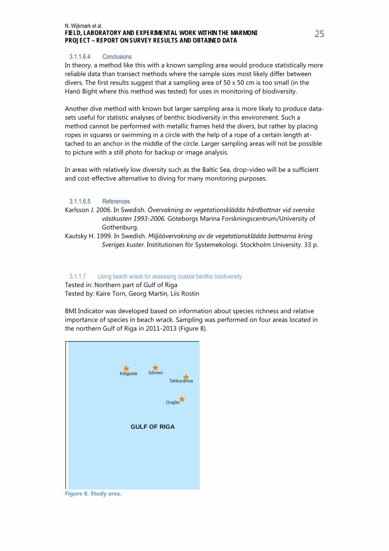
3.1.1.7 Using beach wrack for assessing coastal benthic biodiversity. Tested in: Northern part of Gulf of Riga Tested by: Kaire Torn, Georg Martin, Liis Rostin BMI Indicator was developed based on information about species richness and relative importance of species in beach wrack. Sampling was performed on four areas located in the northern Gulf of Riga in 2011-2013 (Figure 8).
Figure 8. Study area.
GULF OF RIGA
* *
**Kõiguste Sõmeri
Tahkuranna
Orajõe

N. Wijkmark et al. FIELD, LABORATORY AND EXPERIMENTAL WORK WITHIN THE MARMONI PROJECT – REPORT ON SURVEY RESULTS AND OBTAINED DATA
26
3.1.1.7.1 Collection of samples from beach wrack Wrack samples were collected from three area (Kõiguste, Sõmeri, Orajõe) in order to compare the methods of beach wrack sampling and seabed sampling (diver or underwa-ter video) once in a month (April to October) in year 2011. For testing the index, the wrack samples were collected from the four areas (Kõiguste, Sõmeri, Orajõe, Tahkuranna) once in a year (July) in years 2012 and 2013.
Figure 9. Examples of the beach wrack accumulations studied in the project.
Wrack samples were collected from three transects parallel to the shoreline in each area. The distance between the transects was about 60 m. The lengths of the transects were 5 m and five samples were collected from each transect. The samples were collected using a 20 cm × 20 cm metal frame at a distance of 1 m from one another. The freshest beach wrack closest to the sea was always chosen for sampling. The collected material was packed and kept frozen. In the laboratory, the species composition in the sample was determined. As wrack specimens were often fragmented and detailed identification was impossible, the morphologically very similar species were treated as one group. The fila-mentous brown algae Ectocarpus siliculosus (Dillwyn) Lyngbye and Pilayella littoralis (Lin-naeus) Kjellman were not separated. All characeans except Tolypella nidifica (O. F. Müller) Leonhardi were determined as Chara spp. Higher plants with similar morphology such as Zannichellia palustris L., Ruppia maritima L. and Stuckenia pectinata (L.) Börner were treated as one group. The biomasses of Fucus vesiculosus L. and Furcellaria lumbricalis (Hudson) J. V. Lamouroux and the rest of the sample were separated and weighed after drying at 60°C to constant weight. Biomass (grams dry weight) was calculated per square metre (g dw m−2).

N. Wijkmark et al. FIELD, LABORATORY AND EXPERIMENTAL WORK WITHIN THE MARMONI PROJECT – REPORT ON SURVEY RESULTS AND OBTAINED DATA
27
a) Location sampling frames along the transect.
b) Location of beach transects along the studied strip of coastline.
c) Location of diving transects and beach transects.
Figure 10 a – c. Locations of frames, beach transects and diving transects.
3.1.1.7.2 Data collection from phytobenthic community Sampling of seabed phytobenthic community was carried out in three areas (Kõiguste, Sõmeri and Orajõe) in May, July and September 2011. In each area, observation of macrophyta was performed along three parallel transects placed perpendicular to the shoreline with a distance of 500 m between the transects. The length of the transect was 2–4 km depending on the area. The depth intervals of the sampling sites along the tran-sects were 1–1.5 m. At each depth, coverage was estimated within a radius of 2–3 m around each sampling site. Coverage was assessed as a percentage of the sea bottom covered by vegetation or a certain species within the extent of the sampling site. Along the transects, the total coverage of the macrovegetation community, coverage of individ-

N. Wijkmark et al. FIELD, LABORATORY AND EXPERIMENTAL WORK WITHIN THE MARMONI PROJECT – REPORT ON SURVEY RESULTS AND OBTAINED DATA
28
ual species and character of substrate were registered visually by the diver or recorded with underwater video camera. Observations were carried out to the deepest limit of vegetation on the transect. In the Kõiguste and Sõmeri areas, 8–10 observations were made along the transects (the deepest vegetation at 10 m depth). In the Orajõe area the number of observations per transect was 7–9 (the deepest vegetation at 8.3 m depth).
Figure 11. Collection of benthic samples on the diving transects.
3.1.1.7.3 Hydrodynamic measurements and modelling In order to study possible relationships between biological beach wrack findings and coastal hydrodynamic conditions, measurements of sea level variations and a hydrody-namic modelling study were carried out. A Doppler effect-based oceanographic instru-ment RDCP-600 manufactured by Aanderaa Data Instruments was deployed to the sea-bed at two locations, off Sõmeri and Kõiguste. Near the Sõmeri Peninsula the upward looking instrument recorded currents from 13 June 2011 to 2 September 2011, at Kõiguste from 2 October 2010 to 11 May 2011. In order to obtain hydrodynamic forcing data other years and Orajõe and Tahkuranna area, the wave parameters were calculated using a locally calibrated SMB-type wave model and nearshore currents and sea level variations were calculated using a 2D hydrodynamic model (see Suursaar et al. 2012 and Suursaar 2013, for model calibration and validation details). Wind stress for forcing the models was calculated from the wind data measured at the Kihnu meteorological station (Suursaar 2013). In order to assess the impact of hydrodynamic effect to BMI compo-nents, mean heights of sea level, maximum wave heights and average alongshore current
N. Wijkmark et al. FIELD, LABORATORY AND EXPERIMENTAL WORK WITHIN THE MARMONI PROJECT – REPORT ON SURVEY RESULTS AND OBTAINED DATA
29
speeds were calculated for each location separately over two different review periods: 10 and 30 days prior to each beach wrack sampling date.
3.1.1.7.4 Conclusions. Coherence between the samples of beach wrack and submerged vegetation is hydrody-namically possible because (1) the alongshore currents in the practically tideless Estonian coastal sea are meteorologically driven and generally niether persistent nor strong; the material on the beach originates from the adjacent sea areas; (2) high sea level and wave events occur on an almost regular basis at least every 10–30 days, providing fresh beach wrack material. In general, the stronger the storm event, the richer the wrack. However, the relationships between wrack-forming hydrodynamic factors were somewhat site-dependent. For instance, at the more indented Kõiguste and Sõmeri areas, the rela-tionships with waves were strong and positive, but mixed at the exposed and straight coastal section at Orajõe. Also, among the study sites, the Kõiguste area had the highest macrovegetation biomass and coverage, whereas Orajõe had the scarcest vegetation based on beach wrack samples. The influence of water circulation on wrack samples is brought to bear by the coastline configuration, i.e. it depends on how easily and from which side of the site the material gets trapped. The study demonstrates that beach wrack sampling can be considered as an alternative cost-effective method for describing the species composition in the nearshore area and for assessing the biological diversity of macrovegetation. In fact, we even found more species from beach wrack samples than from the data collected by divers or by using a ‘drop’ video camera. Although hydrodynamic variability is higher in autumn and more biological material is cast ashore, the similarity between the two sampling methods was greater in spring and summer, making these seasons more suitable for such assess-ment exercises. However, the method, outlined as a case study in the Baltic Sea, can be somewhat site-dependent and its applicability in other areas of the Baltic Sea should be tested.
3.1.1.7.5 References Suursaar, Ü.; Torn, K.; Martin, G.; Herkül, K.; Kullas, T. (2014). Formation and species com-position of stormcast beach wrack in the Gulf of Riga, Baltic Sea. Oceanologia, 56(4), 673 - 695.
N. Wijkmark et al. FIELD, LABORATORY AND EXPERIMENTAL WORK WITHIN THE MARMONI PROJECT – REPORT ON SURVEY RESULTS AND OBTAINED DATA
30
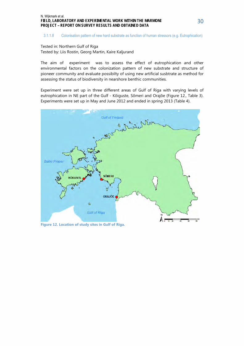
3.1.1.8 Colonisation pattern of new hard substrate as function of human stressors (e.g. Eutrophication)
Tested in: Northern Gulf of Riga Tested by: Liis Rostin, Georg Martin, Kaire Kaljurand The aim of experiment was to assess the effect of eutrophication and other environmental factors on the colonization pattern of new substrate and structure of pioneer community and evaluate possibilty of using new artificial susbtrate as method for assessing the status of biodiversity in nearshore benthic communities. Experiment were set up in three different areas of Gulf of Riga with varying levels of eutrophication in NE part of the Gulf - Kõiguste, Sõmeri and Orajõe (Figure 12., Table 3). Experiments were set up in May and June 2012 and ended in spring 2013 (Table 4).
Figure 12. Location of study sites in Gulf of Riga.

N. Wijkmark et al. FIELD, LABORATORY AND EXPERIMENTAL WORK WITHIN THE MARMONI PROJECT – REPORT ON SURVEY RESULTS AND OBTAINED DATA
31
Table 3. The coordinates of the experimental transects (B is beginning of transect, E is end of the transect)
Site Transect Beginning/End Latitude Longitude Kõiguste I B 58.35785 22.99423 E 58.33792 22.99141 II B 58.36010 22.99166 E 58.33372 22.98291 Sõmeri I B 58.35418 23.74051 E 58.35415 23.71303 II B 58.35187 23.73496 E 58.35228 23.71443 Site Transect Beginning/End Latitude Longitude Orajõe I B 57.95760 24.39039 E 57.95790 24.35952 II B 57.95493 24.38883 E 57.95607 24.35788
Table 4. Experiment timetabel
Date Kõiguste Orajõe Sõmeri 03.05.2012 experiment set up 08.06.2012 experiment set up experiment set up 03.08.2012 removing the transect I 11.09.2012 removing the transect I 12.09.2012 removing the transect I 25.11.2012 removing the transect II 08.12.2012 removing the transect II 07.05.2013 removing the transect II
2 transects were placed on the seabed (Figure 13) and put on the natural rustic granite stones in 5 depths (5 stones to each depth) assessing fouling communities (Figure 13) in Kõiguste and Sõmeri. In the Orajõe we put stones only in 4 depths (2, 4, 6, 8 m), because there was the limit of vegetation. The distance between 2 transects was about 200 meters.

N. Wijkmark et al. FIELD, LABORATORY AND EXPERIMENTAL WORK WITHIN THE MARMONI PROJECT – REPORT ON SURVEY RESULTS AND OBTAINED DATA
32
Figure 13. Scheme of in situ experiment.
The natural rustic granite stones transported to the sea floor in the bag (Fig. 3). The diver placed the stones quite close to each other and marked the underwater location with the anchor and the buoy (Figure 14). Each stones had a different symbol to recognize the transect number and depth (Figure 13).
Figure 14. Configuration of the incubation set on the seafloor.

N. Wijkmark et al. FIELD, LABORATORY AND EXPERIMENTAL WORK WITHIN THE MARMONI PROJECT – REPORT ON SURVEY RESULTS AND OBTAINED DATA
33
Transects I and II were taken off at different times (Tabel 2). Each stone was placed in a plastic bag by diver under the water and packed stones were placed in a bag and wrapped up into the boat. Benthos samples (control samples) were collected by divers with frames (25x25 cm) in triplicate in each depth. The collected sediment was sieved over a 1 mm sieve, then packaged in plastic bags, added a label were collected beside the stones. The natural rustic granite stones and benthos samples maintained at -20°C for laboratory analysis. Species of bottom flora and fauna determined in the laboratory, also abundance of benthic organisms. For each samples species placed in aluminium foil. Benthic flora species were dried for 2 weeks and fauna species 48 hours at 60°C. After cooling, the aluminium foils were weighed (dry weight of m2).
3.1.1.8.1 Conclusions. Colonisation of artificial substrate followed the general pattern of surrounding benthic vegetation and other communities. Differences between the areas were explained by dif-ferent level of eutrophication and the general conclusion was that colonisation pattern of artificial substrate could be used as measure for human pressure on benthic communities. Results of the experiment are currently compiled into scientific paper.
N. Wijkmark et al. FIELD, LABORATORY AND EXPERIMENTAL WORK WITHIN THE MARMONI PROJECT – REPORT ON SURVEY RESULTS AND OBTAINED DATA
34
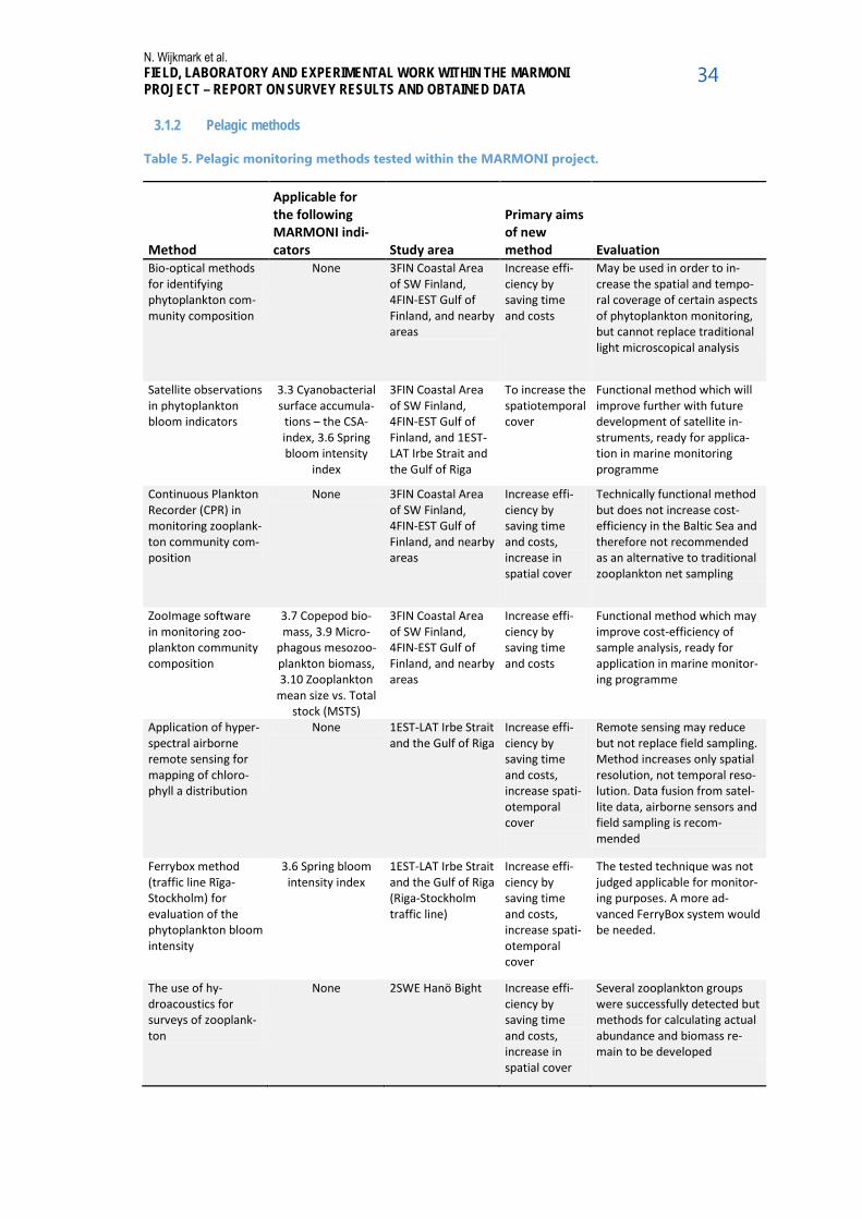
3.1.2 Pelagic methods
Table 5. Pelagic monitoring methods tested within the MARMONI project.
Method
Applicable for the following MARMONI indi-cators Study area
Primary aims of new method Evaluation
Bio-optical methods for identifying phytoplankton com-munity composition
None 3FIN Coastal Area of SW Finland, 4FIN-EST Gulf of Finland, and nearby areas
Increase effi-ciency by saving time and costs
May be used in order to in-crease the spatial and tempo-ral coverage of certain aspects of phytoplankton monitoring, but cannot replace traditional light microscopical analysis
Satellite observations in phytoplankton bloom indicators
3.3 Cyanobacterial surface accumula-
tions – the CSA-index, 3.6 Spring bloom intensity
index
3FIN Coastal Area of SW Finland, 4FIN-EST Gulf of Finland, and 1EST-LAT Irbe Strait and the Gulf of Riga
To increase the spatiotemporal cover
Functional method which will improve further with future development of satellite in-struments, ready for applica-tion in marine monitoring programme
Continuous Plankton Recorder (CPR) in monitoring zooplank-ton community com-position
None 3FIN Coastal Area of SW Finland, 4FIN-EST Gulf of Finland, and nearby areas
Increase effi-ciency by saving time and costs, increase in spatial cover
Technically functional method but does not increase cost-efficiency in the Baltic Sea and therefore not recommended as an alternative to traditional zooplankton net sampling
ZooImage software in monitoring zoo-plankton community composition
3.7 Copepod bio-mass, 3.9 Micro-
phagous mesozoo-plankton biomass, 3.10 Zooplankton
mean size vs. Total stock (MSTS)
3FIN Coastal Area of SW Finland, 4FIN-EST Gulf of Finland, and nearby areas
Increase effi-ciency by saving time and costs
Functional method which may improve cost-efficiency of sample analysis, ready for application in marine monitor-ing programme
Application of hyper-spectral airborne remote sensing for mapping of chloro-phyll a distribution
None 1EST-LAT Irbe Strait and the Gulf of Riga
Increase effi-ciency by saving time and costs, increase spati-otemporal cover
Remote sensing may reduce but not replace field sampling. Method increases only spatial resolution, not temporal reso-lution. Data fusion from satel-lite data, airborne sensors and field sampling is recom-mended
Ferrybox method (traffic line Rīga-Stockholm) for evaluation of the phytoplankton bloom intensity
3.6 Spring bloom intensity index
1EST-LAT Irbe Strait and the Gulf of Riga (Riga-Stockholm traffic line)
Increase effi-ciency by saving time and costs, increase spati-otemporal cover
The tested technique was not judged applicable for monitor-ing purposes. A more ad-vanced FerryBox system would be needed.
The use of hy-droacoustics for surveys of zooplank-ton
None 2SWE Hanö Bight Increase effi-ciency by saving time and costs, increase in spatial cover
Several zooplankton groups were successfully detected but methods for calculating actual abundance and biomass re-main to be developed

N. Wijkmark et al. FIELD, LABORATORY AND EXPERIMENTAL WORK WITHIN THE MARMONI PROJECT – REPORT ON SURVEY RESULTS AND OBTAINED DATA
35
3.1.2.1 Bio-optical methods for identifying phytoplankton community composition Tested in: 3FIN Coastal Area of SW Finland and 4FIN-EST Gulf of Finland and nearby areas Tested by: Stefan Simis and Sirpa Lehtinen
3.1.2.1.1 Introduction Within the scope of future MSFD monitoring, it is necessary to consider emerging meth-ods to enhance the efficacy of monitoring efforts, and the requirement for automation and cost-efficiency usually implies looking for suitable methods based on optics. The opti-cal metrics of phytoplankton include the size, shape, dimensions, and complexity of the phytoplankton cell, as well as its light absorption, scattering, and fluorescence characteris-tics, influenced by cell size, material, and pigmentation. Challenges in choosing a suitable approach are presented by every manual or automated observation method being some-how selective, either for a size range, sensitivity at low concentrations, and the ability to discern individual cells or analyze bulk volumes. The aim of this work was to analyse how phytoplankton taxonomic diversity is reflected in instrument responses of the optical and chemotaxonomical detection methods pigment HPLC, FlowCAM particle imaging, and scanning flow cytometry (for methodological details, see section 3.4.4).
3.1.2.1.2 Description of the method Phytoplankton species composition (i.e. biodiversity) monitoring is currently performed through light microscopical (LM) enumeration of phytoplankton abundance from fixed samples (HELCOM 2014). This method is precise with regard to taxonomic determination, and the well-documented traditional methodology produces data usable for long-term analyses and enables reliable comparisons between different monitoring data sets. The method is less sensitive to low species occurrences and limited to cells >1–2 µm. The limitation of this method is sample analysis time, which is in the order of 1/day. FlowCAM imaging allows rapid collection of image data in the order of 20 samples/day. Subsequently, classification aided by image recognition algorithms may speed up taxo-nomic classification, although machine learning is far from a replacement of expert analy-sis. The method may also enhance detection of species with low occurrences. For image analysis, camera resolution and fixed focal length are limiting factors. FlowCAM analysis, which can be done on fresh or fixed samples, can be seen as a complement to LM in a size range similar to that used with traditional LM (>2 µm). Pigment HPLC has thus far been little used in the Baltic Sea (Wanstrand et al. 2006, Ekker-Develi et al. 2008). Generally, pigment HPLC allows the expression of community compo-sition to a group level distinguished by the presence and absence of diagnostic pigments. In practise this analysis is limited to approximately 10 phytoplankton groups. Samples can be collected fresh, frozen, and analyzed in batches in the laboratory (20–30 samples/day). Flow cytometric analysis can be regarded as a combination of particle-based and pigment analysis methods. The taxonomic distinction of each particle is dependent on the number of lasers, detectors, and is limited to pigments that show autofluorescence. Fluorescence is best assessed in fresh samples or those treated with a fixative that retains fluorescence. Besides fluorescence, flow-cytometers allow basic size and shape characterization.

N. Wijkmark et al. FIELD, LABORATORY AND EXPERIMENTAL WORK WITHIN THE MARMONI PROJECT – REPORT ON SURVEY RESULTS AND OBTAINED DATA
36
3.1.2.1.3 Results of method testing
We performed an expert analysis of the complementary nature of various implementa-tions of existing and new optical detection methods, scrutinizing the response of each method to observe particle-specific traits (Table 6). The response for some traits is uniquely linked to the capacity of a method to determine a level of optical and taxonomic detail currently only present in LM (endosymbionts, flagellates, silicate dependence) – such traits therefore do not at present support complementary use of novel observation methods. On the other hand, traits for biomass, specific optical properties, and size can be supported with a combination of particle and sample-specific analysis methods that are either already available or can be readily developed with current technology. Table 6. Expert analysis of the complementary nature of optical phytoplankton analysis methods, based on functional traits. Scores indicate: 5-diagnostic and not selective, 4-method is diagnostic of the trait (not necessarily developed as an operational method); 3-trait can be derived using current methodology (assuming best available technology); 2-ready to be developed or some element (e.g. a model) missing; 1-not mature/key method missing/low level indicator; 0-not feasible or not applicable to this method.
Diversity metrics All comparisons of diversity derived from the novel methods were based on calculating the Shannon diversity index (Figure 15). It was quickly realized (see also section 3.4.4) that FlowCAM analysis could not be completed to any meaningful taxonomic level for this data set, given limited time under this project. Efforts with FlowCAM analysis focused instead on researching the best practices for data collection and a comparison of software tools for image treatment and pre-classification.
Functional Traits Particle-specific traits Inve
rted
ligh
t mic
rosc
opy
Part
icle
Imag
ing
(fix
ed s
ampl
es)
Part
icle
Imag
ing
(live
sam
ples
)
Flow
-Cyt
omet
ry
Scan
ning
Flo
w-C
ytom
etry
Pigm
ent H
PLC
Rem
ote
Sens
ing
Ecological niche Autotrophy 3 1 2 3 3 0 2Ecological niche Heterotrophy 3 1 1 1 1 0 0Ecological niche Endosymbionts 5 3 3 2 3 0 0nutrient harvesting N2 fix potential 3 3 3 1 2 0 0nutrient harvesting Silicate dependence 5 3 3 1 1 0 1Motility Flagellated 5 1 1 0 0 0 0Motility Buoyancy 3 3 3 1 1 0 3biomass Chlorophyll-a 1 0 1 5 5 5 4biomass Carbon 3 3 3 2 3 2 2biomass Food quality 2 2 2 3 3 1 1shape/size Size 4 4 4 3 5 0 1shape/size Size > 1 um 4 3 3 3 5 0 1shape/size Size < 1 um 0 0 0 3 5 0 1shape/size Chains/Colonies 5 5 5 3 5 0 2shape/size Surface-to-volume ratio 4 4 4 2 5 0 0optical properties Chlorophyll-b 2 1 1 3 3 5 1optical properties Chlorophyll-c 2 1 1 2 2 5 1optical properties Other photosynthetic pigme 2 1 1 3 3 5 1optical properties Other pigments 2 1 1 2 2 5 1optical properties Phycobilipigment 2 1 2 5 5 1 2optical properties Scattering efficiency 1 1 1 5 5 1 2hazards Toxicity potential 3 2 2 0 0 0 1
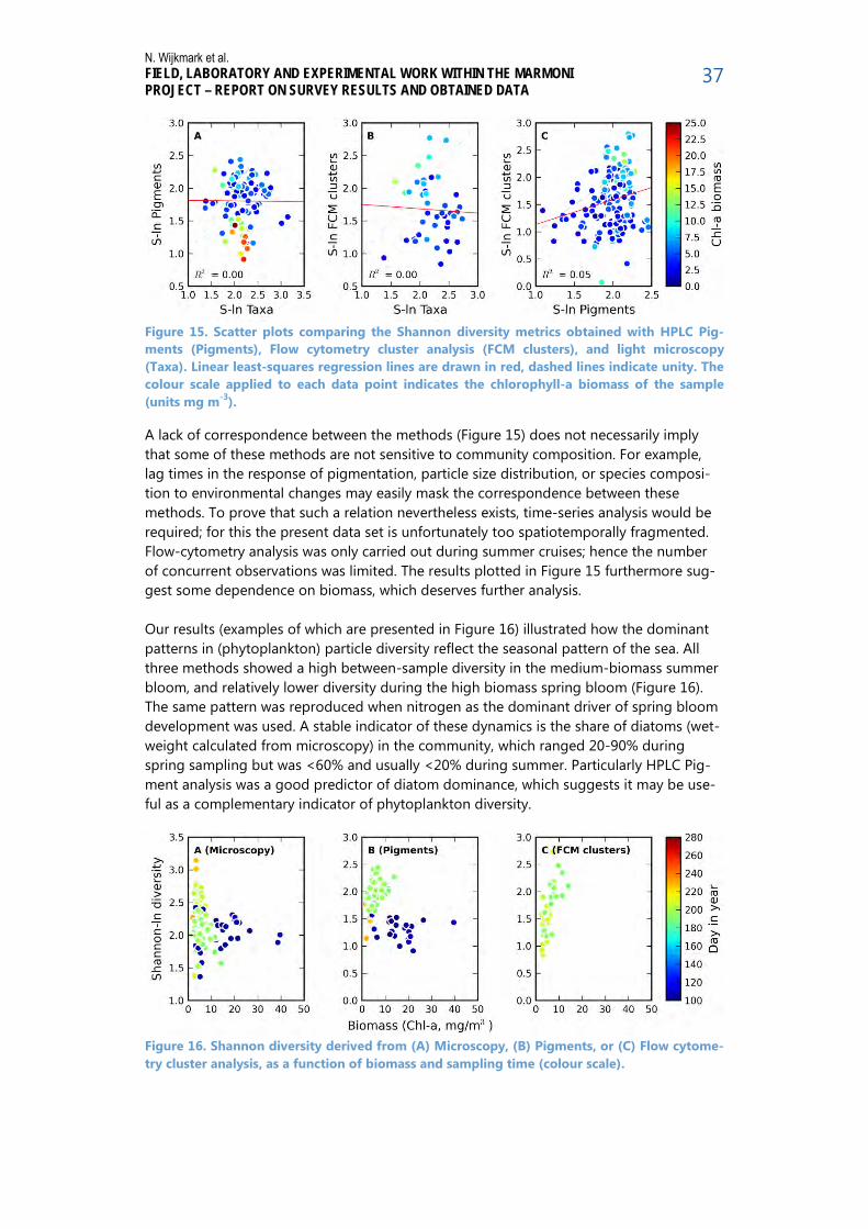
N. Wijkmark et al. FIELD, LABORATORY AND EXPERIMENTAL WORK WITHIN THE MARMONI PROJECT – REPORT ON SURVEY RESULTS AND OBTAINED DATA
37
Figure 15. Scatter plots comparing the Shannon diversity metrics obtained with HPLC Pig-ments (Pigments), Flow cytometry cluster analysis (FCM clusters), and light microscopy (Taxa). Linear least-squares regression lines are drawn in red, dashed lines indicate unity. The colour scale applied to each data point indicates the chlorophyll-a biomass of the sample (units mg m-3).
A lack of correspondence between the methods (Figure 15) does not necessarily imply that some of these methods are not sensitive to community composition. For example, lag times in the response of pigmentation, particle size distribution, or species composi-tion to environmental changes may easily mask the correspondence between these methods. To prove that such a relation nevertheless exists, time-series analysis would be required; for this the present data set is unfortunately too spatiotemporally fragmented. Flow-cytometry analysis was only carried out during summer cruises; hence the number of concurrent observations was limited. The results plotted in Figure 15 furthermore sug-gest some dependence on biomass, which deserves further analysis. Our results (examples of which are presented in Figure 16) illustrated how the dominant patterns in (phytoplankton) particle diversity reflect the seasonal pattern of the sea. All three methods showed a high between-sample diversity in the medium-biomass summer bloom, and relatively lower diversity during the high biomass spring bloom (Figure 16). The same pattern was reproduced when nitrogen as the dominant driver of spring bloom development was used. A stable indicator of these dynamics is the share of diatoms (wet-weight calculated from microscopy) in the community, which ranged 20-90% during spring sampling but was <60% and usually <20% during summer. Particularly HPLC Pig-ment analysis was a good predictor of diatom dominance, which suggests it may be use-ful as a complementary indicator of phytoplankton diversity.
Figure 16. Shannon diversity derived from (A) Microscopy, (B) Pigments, or (C) Flow cytome-try cluster analysis, as a function of biomass and sampling time (colour scale).

N. Wijkmark et al. FIELD, LABORATORY AND EXPERIMENTAL WORK WITHIN THE MARMONI PROJECT – REPORT ON SURVEY RESULTS AND OBTAINED DATA
38
3.1.2.1.4 Conclusions
The investigated optical observation methods revealed a high degree of complementarity in parameters related to biomass, shape/size, and optical properties, which can be ex-ploited in phytoplankton monitoring programmes to improve spatiotemporal coverage. However, several traits are specific to the LM identification of taxa which cannot be effi-ciently reproduced with the novel optical methods. Major seasonal phytoplankton/particle diversity patterns could be reproduced from all optical methods included in the comparison. However, sample-by-sample correspon-dence was negligible, which may suggest different lag times in the response of each method to environmental changes. It is recommended to include a time series of one or few stations in future work on this topic, so that these effects may be elucidated. Recently, it was suggested to reduce the observations used in calculating Shannon diver-sity to the dominant 95% taxa in the community, which may reduce the uncertainty of this metric associated with operator or sampling bias (Uusitalo et al. 2013). It is recommended to review these results accordingly in future work, as similar approaches may account for instrument sensitivity biases.
3.1.2.1.5 References Eker-Develi, E., J. F. Berthon, and D. Van Der Linde. 2008. Phytoplankton class determina-
tion by microscopic and HPLC-CHEMTAX analyses in the southern Baltic Sea. Mar. Ecol.-Prog. Ser. 359: 69-87. [doi: 10.3354/meps07319]
HELCOM 2014. Manual for Marine Monitoring in the COMBINE Programme of HELCOM, Annex C-6: Guidelines concerning phytoplankton species composition, abundance and biomass, in pages 285-300. Updated version: 17 January 2014. Available at: http://helcom.fi/Documents/Action%20areas/Monitoring%20and%20assessment/Manuals%20and%20Guidelines/Manual%20for%20Marine%20Monitoring%20in%20the%20COMBINE%20Programme%20of%20HELCOM.pdf
Uusitalo, L., V. Fleming-Lehtinen, H. Hällfors, A. Jaanus, S. Hällfors, and L. London. 2013. A novel approach for estimating phytoplankton biodiversity. ICES Journal of Marine Science: Journal du Conseil. [doi: 10.1093/icesjms/fss198]
Wanstrand, I., and P. Snoeijs. 2006. Phytoplankton community dynamics assessed by ships-of-opportunity sampling in the northern Baltic Sea: A comparison of HPLC pigment analysis and cell counts. Estuar. Coast. Shelf Sci. 66: 135-146. [doi: 10.1016/j.ecss.2005.08.003]
3.1.2.2 Satellite observations in phytoplankton bloom indicators Tested in: 3FIN Coastal Area of SW Finland, 4FIN-EST Gulf of Finland and 1EST-LAT Irbe Strait and the Gulf of Riga Tested by: Saku Anttila, Jenni Attila, Sofia Junttila and Vivi Fleming-Lehtinen
3.1.2.2.1 Introduction In the Baltic Sea, two distinctive seasonal phytoplankton maxima occur: the dinoflagellate and diatom dominated spring bloom in March–May, and the late summer cyanobacterial bloom in July–August. Both blooms show great variation in annual characteristics as well as in spatial and temporal variability (Fleming & Kaitala, 2006; Kutser et al., 2006; Klais et

N. Wijkmark et al. FIELD, LABORATORY AND EXPERIMENTAL WORK WITHIN THE MARMONI PROJECT – REPORT ON SURVEY RESULTS AND OBTAINED DATA
39
al., 2011). Therefore, discrete sampling methods are not suitable in quantifying such spa-tial and usually short-term phenomena as algae blooms. Spaceborne remote sensing has already a relative long history in detecting algae blooms (e.g. Öström, 1976). Remote sensing has been praised for its spatial and temporal abilities on many occasions (e.g. Klemas et al., 2011). However, turning the visually distinctive phenomena in remote sensing images into quantitative information usable in the assess-ment has been challenging (cf. Kahru et al., 2014). Platt et al. (2003) presented a method where series of remote sensed chlorophyll a (chl-a) observations are used to derive spring bloom characteristics. Distinction of the biomass of cyanobacteria from other phytoplank-ton species, however, is challenging with the satellite sensors currently available for large scale monitoring (Kutser et al., 2006). Therefore, the current remote sensing methods for cyanobacteria surface accumulations are mainly based on descriptive characteristics (e.g. Öberg, 2013). However, according to the present authors’ knowledge, information on neither spring bloom nor cyanobacteria bloom spatio-temporal characteristics have pre-viously been cultivated into indicators applicable in status assessments.
3.1.2.2.2 Description of the method We used remote sensing and FerryBox (ship-of-opportunity, Alg@line; e.g. Leppänen and Rantajärvi, 1994) fluorometer measurements to characterize the spring and cyanobacteria blooms in the Baltic Sea. Time series of seasonal observations were used to derive infor-mation on the annual bloom characteristics, which were further cultivated into the MARMONI indicators “3.3 Cyanobacterial surface accumulations - the CSA-index” and “3.6 Spring bloom intensity index”. For the “3.6 Spring bloom intensity index” indicator, we ap-plied a method developed by Platt et al. (2003, 2008) and Fleming and Kaitala (2006) in which the peak amplitude, timing of peak, timing of initiation and duration were derived from the remote sensed, or in latter case, from the Alg@line time series of chl-a. This information was used to derive the spring bloom intensity index used in the indicator. For the cyanobacteria blooms we developed a new method, in which annual bloom character-istic information, i.e. the duration, intensity and temporal volume of algal accumulations, is combined into a Cyanobacterial Surface Accumulation index (CSA-index). Bloom char-acteristics were estimated by using Empirical Cumulative Distribution Functions (ECDF) derived from seasonal time series of algae barometer values (Rapala et al., 2012). This indicator is also based on the remote sensing, but supplementary information can be added with specific weights. The main data source for both of the indicators was daily satellite images from 2003-2013. The “3.6 Spring bloom intensity index” indicator utilized chl-a estimated from MERIS-images. The “3.3 Cyanobacterial surface accumulations - the CSA-index” indicator used chl-a estimates from the MERIS and MODIS-instruments (MODerate Resolution Im-aging Spectroradiometer by NASA) from which cyanobacteria surface accumulations were estimated (see www.syke.fi/earthobservation). In addition, FerryBox fluorometer observa-tions of chl-a and phycocyanin fluorescence were used in the spring bloom and CSA indi-cators, respectively.
3.1.2.2.3 Results of method testing Remote sensing gives sufficient accuracy in parameter estimation and excellent spatial and temporal coverage that allows the description of both spring and cyanobacterial bloom characteristics. Furthermore, the developed methods allow the usage of auxiliary data sources that enhance the representativeness of indicators. Both developed
N. Wijkmark et al. FIELD, LABORATORY AND EXPERIMENTAL WORK WITHIN THE MARMONI PROJECT – REPORT ON SURVEY RESULTS AND OBTAINED DATA
40
MARMONI indicators showed good performance when compared with available reference data, but further work is still required in certain issues. These are related to the target setting (typically there is no quantitative historical observations from the blooms), further validation of the results (independent comparison data sets are rare) and careful har-monization of the time series derived from more than one satellite instruments. It needs also to be noted, that the spatial and spectral resolution of the satellite instruments cur-rently available for monitoring purposes restricts the assessment to relative large and continuous water bodies. However, Sentinel-satellites, to be launched in 2015 by the European Space Agency, will significantly improve the performance of satellite monitor-ing.
3.1.2.2.4 Conclusions Traditional methods in observing spatially variable and often dynamic phenomena such algal blooms are exposed to considerable spatial and temporal errors (e.g. Rantajärvi et al., 1998; Kutser et al., 2004). We developed and tested remote sensing methods com-bined with FerryBox observations in the assessment of spring and cyanobacteria blooms in the Baltic Sea; the work resulted in the development of the two MARMONI indica-tors“3.3 Cyanobacterial surface accumulations - the CSA-index” and “3.6 Spring bloom intensity index”.
3.1.2.2.5 References Fleming, V., Kaitala, S. (2006). Phytoplankton spring bloom intensity index for the Baltic
Sea estimated for the years 1992 to 2004. Hydrobiologia, 554, pp. 57–65. Kahru, M., & Elmgren, R. (2014). Satellite detection of multi-decadal time series of cyano-
bacteria accumulations in the Baltic Sea. Biogeosciences Discussions, 11, 3319-3364.
Klais, R., Tamminen, T., Kremp, A., Spilling, K., Olli, K. (2011) Decadal-Scale Changes of Dinoflagellates and Diatoms in the Anomalous Baltic Sea Spring Bloom. PLoS ONE 6(6): e21567. doi:10.1371/journal.pone.0021567
Klemas, V. (2011). Remote sensing of algal blooms: an overview with case studies. Journal of Coastal Research, 28(1A), 34-43.
Kutser, T. (2004). Quantitative detection of chlorophyll in cyanobacterial blooms by satel-lite remote sensing. Limnology and Oceanography, 49(6), 2179-2189.
Kutser, T., Metsamaa, L., Strömbeck, N., & Vahtmäe, E. (2006). Monitoring cyanobacterial blooms by satellite remote sensing. Estuarine, Coastal and Shelf Science, 67(1), 303-312.
Rantajärvi, E., Olsonen, R., Hällfors, S., Leppänen, J.-M., & Raateoja, M. (1998). Effect of sampling frequency on detection of natural variability in phytoplankton: Un-attended high-frequency measurements on board ferries in the Baltic Sea. ICES Journal of Marine Science, 55, 697–704.
Rantajärvi, E. and Leppänen, J.-M. (1994). Unattended algal monitoring on merchant ships in the Baltic Sea. TemaNord, 546: 1-60.
Platt, T., Fuentes-Yaco, C., & Frank, K. T. (2003). Marine ecology: spring algal bloom and larval fish survival. Nature, 423(6938), 398-399.
Platt, T., & Sathyendranath, S. (2008). Ecological indicators for the pelagic zone of the ocean from remote sensing. Remote Sensing of Environment, 112(8), 3426-3436.
Rapala, J., Kilponen, J., Järvinen, M., Lahti, K. (2012). FINLAND: Guidelines for monitoring of cyanobacteria and their toxins. In Chorus, I. (ed.). Current approaches to

N. Wijkmark et al. FIELD, LABORATORY AND EXPERIMENTAL WORK WITHIN THE MARMONI PROJECT – REPORT ON SURVEY RESULTS AND OBTAINED DATA
41
cyanotoxin risk assessment, risk management and regulations in different countries. Dessau-Rosslau, Germany: Federal Environment Agency (Umwelt-bundesamt); 2012. Available at http://www.umweltdaten.de/publikationen/fpdf-l/4390.pdf.
Simis, S. G., Ruiz-Verdú, A., Domínguez-Gómez, J. A., Peña-Martinez, R., Peters, S. W., & Gons, H. J. (2007). Influence of phytoplankton pigment composition on re-mote sensing of cyanobacterial biomass. Remote Sensing of Environment, 106(4), 414-427.
Öberg, B .(2013). Cyanobacterial blooms in the Baltic Sea in 2013. HELCOM Baltic Sea Environment Fact Sheets. Online. 11.6.2013, Available at http://www.helcom.fi/baltic-sea-trends/environment-fact-sheets/.
Öström, B. (1976). Fertilization of the Baltic by Nitrogen Fixation in the Blue-Green Alga Nodulada Spumina. Remote sensing of environment, 4, 305-310.
3.1.2.3 Continuous Plankton Recorder (CPR) in monitoring zooplankton community composition Tested in: 3FIN Coastal Area of SW Finland and 4FIN-EST Gulf of Finland and nearby areas Tested by: Maiju Lehtiniemi and Laura Uusitalo
3.1.2.3.1 Introduction The Continuous Plankton Recorder (CPR) methodology was initiated already in the 1930’s and has since then successfully been used in zooplankton monitoring, constituting the basis for e.g. North Atlantic and North Sea zooplankton monitoring (Warner and Hays 1994). CPR is usually utilised onboard ships-of-opportunity (merchant ships equipped with automated measuring and sampling apparatus) and is thus a cost-efficient method for frequent zooplankton sampling. Against this background, the aim of the present study was to test the applicability of CPR in the northern Baltic Sea in collecting spatially exten-sive data to support the HELCOM COMBINE zooplankton monitoring programme, con-ducted presently once a year onboard r/v Aranda by vertical zooplankton net tows.
3.1.2.3.2 Description of the method The CPR (Figure 17) is towed behind the research vessel in a chosen water layer. Water enters through the small frontal opening of the CPR and passes through the silk filtering mesh (mesh size 200 µm). Zooplankton is collected onto the silk and after towing can be washed into sample bottles and preserved. The obtained samples are counted in the laboratory either by traditional microscopical analysis or by semi-automatic image analy-sis (ZooImage; see section 3.1.2.4 below).

N. Wijkmark et al. FIELD, LABORATORY AND EXPERIMENTAL WORK WITHIN THE MARMONI PROJECT – REPORT ON SURVEY RESULTS AND OBTAINED DATA
42
Figure 17. The Continuous Plankton Recorder (CPR) onboard r/v Aranda in Au-gust 2012. Photograph by Laura Uusitalo.
3.1.2.3.3 Results of method testing The CPR method was tested for obtaining zooplankton samples in August 2012 on board r/v Aranda on 10 transects in the MARMONI project areas 3FIN and 4FIN-EST as well as in nearby sea areas. The results showed that this method does not bring cost-efficiency to the present zooplankton monitoring. This is because CPR can only be utilised on board r/v Aranda where also zooplankton sampling using net tows takes place, and not in the traditional manner of CPR, i.e. onboard ships of opportunity since the speed of these ves-sels is too high for the mesh size used in the Baltic Sea (200 µm). In addition, the opening of the CPR is so small that it does not sample all taxa properly, but underestimates certain taxa. Onboard r/v Aranda net tows can be performed with the same effort as the CPR tows; thus we concluded that CPR would not be tested further; instead zooplankton net samples were used for semi-automatic image analysis and identification (see section 3.1.2.4 below).
3.1.2.3.4 Conclusions The CPR method worked quite satisfactorily in our tests, but because it cannot in the Bal-tic Sea be utilized onboard merchant ships due to their too high travelling speed, it does not as such bring any cost-efficiency to the sampling. Thus we conclude that net sampling should be continued to be applied as the prioritized method in zooplankton monitoring in the Baltic Sea.
3.1.2.3.5 References Warner & Hays, 1994: Sampling by the continuous plankton recorder survey. – Progress in
Oceanography 34(2–3):237–256.
N. Wijkmark et al. FIELD, LABORATORY AND EXPERIMENTAL WORK WITHIN THE MARMONI PROJECT – REPORT ON SURVEY RESULTS AND OBTAINED DATA
43
3.1.2.4 ZooImage software in monitoring zooplankton community composition
Tested in: 3FIN Coastal Area of SW Finland and 4FIN-EST Gulf of Finland and nearby areas Tested by: Maiju Lehtiniemi, Laura Uusitalo, Siru Tasala and Jose A. Fernandes
3.1.2.4.1 Introduction A major problem with zooplankton monitoring is that the identification and measurement of individuals in zooplankton samples is very labour intensive, which can consequently restrict the availability of zooplankton data. However, recent advances in image analysis have shown promising results for semi-automated zooplankton classification in quickly and cost-efficiently estimating zooplankton abundance and biovolumes from large amounts of samples (e.g. Bell and Hopcroft, 2008; Irigoien et al., 2009; Manríquez et al., 2012), the drawback being that the organisms will not be identified to a very detailed level. Therefore, it is essential to evaluate whether the level of identification offered by the semi-automatic methods is sufficient to adequately assess zooplankton indicators which do not necessarily require data with very detailed taxonomic resolution. The aim of this study was to evaluate the accuracy of the semi-automatic classification method using ZooImage software in the northern Baltic Sea, arguably the most challenging area for this method due to the generally small body size of the dominant zooplankton species (Viitasalo et al., 1995).
3.1.2.4.2 Description of the method The methodology is based on taking a digital image of zooplankton samples using a scanner (Grosjean et al., 2004; Figure 18) or a digital camera (Bachiller et al., 2012), and using machine-learning algorithms to identify the zooplankton individuals from the im-age, classify them into taxonomic groups (defined by the user), and measuring each of these specimens separately. The ZooImage free software (http://www.sciviews.org/zooimage/) can be used for automated classification and meas-urement of individuals as well as the estimation of the biomass of individuals based on morphological measurements (Alcaraz et al., 2003), yielding estimates of abundance, biomass, and size spectrum of each taxon. In the establishment phase, a taxonomic expert creates a training set by classifying part of the images produced by the scans manually; later, the system will classify individuals into those classes automatically, based on their characteristics (see Di Mauro et al., 2011; Gislason and Silva, 2009 for a detailed description of the methodology). A major advantage of this methodology is that it only requires inexpensive equipment, and after the initial set-up and training, it is very fast and can be operated by non-specialist personnel.
Images were captured using an Epson Perfection V750 scanner at 2800 dpi resolution, meaning that the length of 1 mm includes approximately 110 pixels in the image. The pictures were scanned as colour pictures and analysed using colour picture algorithm.

N. Wijkmark et al. FIELD, LABORATORY AND EXPERIMENTAL WORK WITHIN THE MARMONI PROJECT – REPORT ON SURVEY RESULTS AND OBTAINED DATA
44
Figure 18. The scanner and computer used for semi-automatic image analysis for zooplank-ton identification. Photograph by Laura Uusitalo.
3.1.2.4.3 Results of method testing The scanning and classifying of the zooplankton samples using Automatic Classification software took place during autumn 2012 and winter 2013 (Figure 19). This work included building a training set for species identification. The training set was enhanced by picking individuals of only one species at the time by hand using a microscope. The images of these individuals were then added to the training set. Based on our results, the semi-automatic identification and counting method seems to be a promising tool, which could be used to analyse part of the monitoring net samples to cost-effectively increase the spatial and/or temporal resolution in sampling frequency. This method is capable of iden-tifying individuals to group level (copepods, cladocerans) very well, and in many cases also to genus level (e.g. the copepods Temora, Acartia, Eurytemora, and Pseudocalanus, and the cladocerans Evadne and Eubosmina). It is applicable in producing data for the MARMONI indicators "3.7 Copepod biomass", "3.9 Microphagous mesozooplankton bio-mass" and "3.10 Zooplankton mean size versus total stock (MSTS)", being best suited to the data need of the indicators “3.7 Copepod biomass” and “3.10 Zooplankton mean size vs. total stock (MSTS)”. This is because the microphagous species are the smallest taxa in the zooplankton community, and are thus more difficult to properly identify with the semi-automatic image analysis method. A manuscript (Uusitalo et al. in prep.) is being prepared where recommendations are presented on the use of the semi-automatic zooplankton analysis, and on the usability of this methodology for attaining data for zooplankton indi-cators to help producing ecosystem assessments e.g. for the MSFD.

N. Wijkmark et al. FIELD, LABORATORY AND EXPERIMENTAL WORK WITHIN THE MARMONI PROJECT – REPORT ON SURVEY RESULTS AND OBTAINED DATA
45
Figure 19. Zooplankton images taken with the semi-automatic image analysis method. Pho-tographs by Laura Uusitalo, compilation by Jose A. Fernandes.
3.1.2.4.4 Conclusions In conclusion, the results show that the semi-automatic zooplankton analysis method is applicable in obtaining zooplankton data for the proposed zooplankton indicators in the Baltic Sea, and it could add cost-efficiency to Baltic Sea zooplankton monitoring.
3.1.2.4.5 References Alcaraz, M., Saiz, E., Calbet, A., Trepat, I., Broglio, E., 2003. Estimating zooplankton biomass
through image analysis. Marine Biology 143, 307-315. Bachiller, E., Fernandes, J.A., Irigoien, X., 2012. Improving semiautomated zooplankton
classification using an internal control and different imaging devices. Limnol-ogy and Oceanography: Methods 10, 1-9.
Bell, J.L., Hopcroft, R.R., 2008. Assessment of ZooImage as a tool for the classification of zooplankton. J Plankton Res 30, 1351-1367.
Di Mauro, R., Cepeda, G., Capitanio, F., Viñas, M.D., 2011. Using ZooImage automated system for the estimation of biovolume of copepods from the northern Ar-gentine Sea. Journal of Sea Research 66, 69-75.
Gislason, A., Silva, T., 2009. Comparison between automated analysis of zooplankton using ZooImage and traditional methodology. J Plankton Res 31, 1505-1516.
Grosjean, P., Picheral, M., Warembourg, C., Gorsky, G., 2004. Enumeration, measurement,
and identification of net zooplankton samples using the ZOOSCAN digital imaging system. ICES Journal of Marine Science 61, 518-525.
Irigoien, X., Fernandes, J.A., Grosjean, P., Denis, K., Albaina, A., Santos, M., 2009. Spring zooplankton distribution in the Bay of Biscay from 1998 to 2006 in relation with anchovy recruitment. J Plankton Res 31, 1-17.
Manríquez, K., Escribano, R., Riquelme-Bugueño, R., 2012. Spatial structure of the zoo-plankton community in the coastal upwelling system off central-southern Chile in spring 2004 as assessed by automated image analysis. Progress in Oceanography 92-95, 121-133.

N. Wijkmark et al. FIELD, LABORATORY AND EXPERIMENTAL WORK WITHIN THE MARMONI PROJECT – REPORT ON SURVEY RESULTS AND OBTAINED DATA
46
Laura Uusitalo, Jose A. Fernandes, Eneko Bachiller, Siru Tasala, Maiju Lehti-niemi: Semi-
automated zooplankton classification: a promising tool for the MSFD as-sessments? (Manuscript in preparation).
Viitasalo, M., Koski, M., Pellikka, K., Johansson, S., 1995. Seasonal and long-term variations in the body size of planktonic copepods in the northern Baltic Sea. Marine Biology 123, 241-250.
3.1.2.5 Application of hyperspectral airborne remote sensing for mapping of chlorophyll a distribution in the Gulf of Riga
Tested in: 1EST-LAT Irbe Strait and the Gulf of Riga Tested by: Dainis Jakovels
3.1.2.5.1 Introduction Chlorophyll a (chl-a) concentration is an indicator for assessment of algae bloom intensity (Marmoni pelagic indicator 3.6). Regular monitoring is performed with field campaigns that usually take several days to measure all stations within the Gulf of Riga. Field meas-urements provide ground truth information about chl-a concentration and species of algea, but weak side is spatial and temporal coverage (point or track measurements, rare field missions). Remote sensing (RS) methods provide continuous coverage of the area at relatively cheap (or even free of charge) basis and can be acquired regularly, but field measurements are still required for RS data verification and development of algorithms.
3.1.2.5.2 Description of the method The application of hyperspectral airborne RS for mapping of chl-a distribution in the Gulf of Riga and potential data fusion with field measurements was tested in particular study. High resolution hyperspectral data was acquired from more than 80000 ha large area. Combination of different spectral channels for assessment of chl-a distribution was tested ending up with 2-band and 3-band infrared models suggested by Dall’Olmo et al. 2003. Obtained data can be used for calculation of spring bloom intensity index in order to obtain higher spatial resolution and also coverage. Overall distribution of chl-a was calculated by 2-band model for flight lines and interpo-lated for the rest of the area to demonstrate potential approach for modelling distribution of chl-a in the Gulf of Riga. Field measurements were used for calibration of remote sens-ing data. The validation and also further development of the interpolation model should be performed using satellite data that was not available for particular study.
3.1.2.5.3 Results and conclusions It was demonstrated that phytoplankton distribution is not stationary therefore it wasn’t possible to use standard way (applying linear regression) for calibration of the calculated chl-a values with the measured ones. The fusion of both techniques would reduce the number of necessary field samples, but careful planning of data acquisition campaigns is required. Satellite sensors could provide additional data covering large areas, but the resolution and also availability is limited. Data fusion from all three sources (field meas-urements, airborne and satellite sensors) would lead to more effective assessment of spring bloom intensity indicator. Classification of phytoplankton species of functional groups is next challenge for hyper-spectral airborne RS using its advantages - high spectral and spatial resolution and adaptability to spectral and flight time requirements. However, the data should be backed

N. Wijkmark et al. FIELD, LABORATORY AND EXPERIMENTAL WORK WITHIN THE MARMONI PROJECT – REPORT ON SURVEY RESULTS AND OBTAINED DATA
47
with adequate field measurements, including spectral measurements at water surface and in laboratory. More information and details about this study can be found in section 3.6.1 as well as in separate project report “Testing of new indicator set and monitoring methods. Testing the application of the hyperspectral airborne remote sensing”.
3.1.2.6 Ferrybox method (traffic line Rīga-Stockholm) for evaluation of the phytoplankton bloom inten-sity
Tested in: Riga-Stockholm traffic line Tested by: Ingrida Purina, Ieva Barda
3.1.2.6.1 Introduction Installation of ferrybox on the ferry traffic line Rīga-Stockholm presents a possibility for frequent sampling of phytoplankton. It is often suggested that the shift from diatom ver-sus dinoflagellates bloom has occurred in the Baltic Sea. This assumption is supported by Latvian Institute of Aquatic Ecology monitoring data obtained from yearly cruises in May. Spring diatom bloom is the major event in the seasonal succession of phytoplankton, providing up to 40-60% of yearly primary production in the ecosystem and crucially im-portant for benthic communities. Phytoplankton species dominating during spring bloom are characteristic for cold water complex and adapted to rapid utilization of high nutrient concentrations. As a consequence the species succession is very rapid and difficult to trace. Large part of the information escapes from the routine monitoring observations due to precisely unknown beginning of the event and its rapid development. The ferrybox provides the opportunity to perform frequent studies on the nutrient concentrations and phytoplankton species composition, following the ascending chlorophyll a trends. Thus the development and extent of spring diatom bloom can be easily measured, providing the valuable information on the phytoplankton species composition, species succession, biomass and primary production. Obtained data can be used for calculation of spring bloom intensity index of Fleming and Kaitala (2006).
3.1.2.6.2 Description of the method Automated measurements and water sampling onboard passenger ferries and other commercial ships are operating in the Baltic Sea already since 1993 (Rantajärvi, 2003). The systems installed onboard of ferries are called ferryboxes. These systems pump water constantly from the sea surface layer (from approximately at 5 m depth) through the sen-sors and measure temperature, salinity, chlorophyll a fluorescence and other parameters giving the spatial resolution of about 100-200 m depending on the speed of the ferry. Quantity of measurements depends on the time schedule of ferries. In 2012 altogether 6 ferries were equipped with such system in the Baltic Sea. On the ferry line Riga-Stockholm the Anderaa version of ferrybox system called SOOGUARD was installed. System was in-stalled on board of Tallink ship “Romantika”. It consists of an automated package of four different sensors for measuring oxygen, temperature, conductivity and chlorophyll a/turbidity. Additional samples were collected manually from the ferrybox sampling sys-tem once a week from 05.03.2014 till 22.05.2014. Collected water samples were used for phytoplankton, chlorophyll a and nutrient analysis. Chlorophyll a data from ferrybox automated measurements were used for comparison with chlorophyll a spectropho-tometric measurements. To construct the continuous lines for index calculation the inter-mediate results for both methods were interpolated.
N. Wijkmark et al. FIELD, LABORATORY AND EXPERIMENTAL WORK WITHIN THE MARMONI PROJECT – REPORT ON SURVEY RESULTS AND OBTAINED DATA
48
3.1.2.6.3 Results
The method was used for estimation of spring bloom intensity index (Fleming, Kaitala, 2006). Results calculated form spectrophotometric measurements of chlorophyll a gave the index values for the central part of the Gulf of Riga of 427-522, significantly lower than previously obtained results (576-783, years 2009-2011, MARMONI report) however, consistent, taking in to account the slow and atypical development of spring bloom in 2014. Index calculated from ferrybox automated measurements of chlorophyll a was ~30% lower than from spectrophotometric measurements (293-345). The main problem hindering the credibility of measurements was the rapid fouling of ferrybox system with epiphytic algae and other organisms. The fouling caused the false increase of chlorophyll a concentrations when the spectrophotometric measurements showed low results (over-estimation of results) and on the opposite- when the fouling was removed the automated measurements showed significantly lower results than spectrophotometric measurements (underestimation of results). Calculation of 7 days moving average smoothed the differ-ences between peaks and valleys however the false chlorophyll a peak values remained in all sampling stations creating the differences of 3-4 weeks between the real and false peak values (26.04.2014-false and 19.05.2014-real).
3.1.2.6.4 Conclusions At present the ferrybox system installed on the “Romantika” can be used only for manual water sampling for chlorophyll a, phytoplankton and nutrient samples. This could be used as a useful tool for monitoring program enabling to obtain better spatio-temporal resolu-tion of bloom events (either spring or summer). However no information can be obtained about water column characteristics- stratification, light penetration, vertical distribution of chlorophyll a. In future either the more complicated ferrybox system should be installed preferably with daily automated acid washing or very frequent manual cleaning is neces-sary (once in 1-2 days). The present automated chlorophyll a measurements are not ap-plicable for monitoring purposes.
3.1.2.6.5 References
Fleming, V, Kaitala S, 2006. Phytoplankton spring bloom intensity index for the Baltic Sea estimated for the years 1992 to 2004. Hydrobiologia 554:57-65.
Rantajärvi, E. (2003). Alg@line in 2003: 10 years of innovative plankton monitoring and research and operational information service in the Baltic Sea. MERI Report Series, 48. Finish Institute of Marine Research: Helsinki. 55 pp.
3.1.2.7 The use of hydroacoustics for surveys of zooplankton Tested in: 2SWE Hanö Bight Tested by: Tomas Didrikas and Martin Ogonowski
3.1.2.7.1 Introduction Traditional zooplankton sampling methods are costly and often limited on geographical and temporal scales. Currently hydroacoustic methods are widely used for pelagic fish assessments (Simmonds and MacLennan, 2005). However, it has been shown that using multi-frequency hydroacoustic is possible to detect and distinguish different zooplankton

N. Wijkmark et al. FIELD, LABORATORY AND EXPERIMENTAL WORK WITHIN THE MARMONI PROJECT – REPORT ON SURVEY RESULTS AND OBTAINED DATA
49
groups (meso-, macro and jellyfish) from fish in the water (different sources, for review see Simmonds and MacLennan, 2006).
3.1.2.7.2 Description of the method In order to analyse different groups of the pelagic organism in acoustical data, first they have to be identified, and if possible (and necessary) separated from each other. In gen-eral, echoes from the different organism depending on their size, body shape, inclusion of gas in the body has different strength at different frequencies. Therefore, frequency re-sponse curves of diverse organism groups looks different (Figure 20; e.g. Korneliussen and Ona, 2003). For example echoes of fish possessing a swim-bladder are well “seen” on all frequencies, but they are stronger on lower frequencies. They are also are strongest in comparison to other groups, and have to be removed/separated from data if weaker ech-oes from other organisms are of the interest. Here we present method which was devel-oped and tested using specialized hydroacoustic software package – Sonar5-Pro version 6.0.2 (Balk and Lindem 2012).
3.1.2.7.2.1 Removal of fish echoes from data Echoes from fish (with a swim bladder) are stronger than echoes from other organisms at most frequencies. Therefore, the fish echoes must be separated/removed before any fur-ther analysis. This can be done using different techniques, for example using masking tool in Sonar5 acoustical data analyses software package. The underlying concept of this tool is to identify and remove unwanted acoustic echoes from one frequency echogram and apply it as a mask to the other simultaneously recorded echogram(s) of same water vol-ume but at another acoustic frequency(s). Fish are best “seen” at lower frequencies; there-fore 70 kHz echogram was used to do this. After masking “fish free” echograms of all frequencies, further analysis were made using a frequency response thresholding tool, which makes it possible to identify echoes based on their frequency response signature (see Figure 20).
3.1.2.7.2.2 Mesozooplankton This group includes zooplankton with a size of 0.2-2 mm, dominated by large rotifers, water fleas, copepods and different larva of animals which are planktonic during certain developmental stages (meroplanktonic). Echoes of zooplankton-like organisms get stronger with increasing frequency (Figure 20). Therefore, data from the highest frequency (710 kHz) is most suitable to analyse meso-zooplankton. Three frequencies with a rule where volume backscattering strength (Sv) was 120<200<710 kHz and noise gap (NG) of 3 dB were used for thresholding in order identify meso-zooplankton echoes. 710 kHz echogram was used to output and store these data.
3.1.2.7.2.3 Macro-zooplankton This group includes zooplankton with a size of > 2 mm that drift with water currents or swim slowly. Macrozooplankton consists mainly of opossum shrimps (Mysida) and fish larvae. The fish larvae hydroacoustic characteristics are similar to that of opossum shrimp only before metamorphosis, i.e. before they develop a swim bladder (for those species that have one). The shape of the frequency response curve for meso- and macrozoo-plankton are quite similar at lower frequencies, but the curve is not as steep between 200 and 710 kHz for macrozooplankton as for mesozooplankton (Figure 20). Therefore the two curves could be separated with a rule where the volume backscattering strength (Sv) was 200<710 kHz, and the noise gap (NG) of 1 dB was used to separate macro zooplank-ton echoes. 200 kHz data was used for output.

N. Wijkmark et al. FIELD, LABORATORY AND EXPERIMENTAL WORK WITHIN THE MARMONI PROJECT – REPORT ON SURVEY RESULTS AND OBTAINED DATA
50
3.1.2.7.2.4 Jellyfish
Jellyfish also counts as zooplankton because they live freely in the water column and drift with currents or swim slowly. In the Baltic Sea, this group is mainly represented by the moon jellyfish (Aurelia aurita), which normally has a diameter of 10-15 cm as an adult. Jellyfish sometimes occur in very large numbers during late summer or early autumn when they can form large aggregations. The frequency response curve for jellyfish has a rather unique shape with a pronounced dip at intermediate frequencies (200 and/or 120 kHz), while at the low and high frequency backscattering is typically higher (Figure 20). Three frequencies with a rule where the volume backscattering strength (E) was 70>200<710 kHz, and a noise gap (NG) of 3 dB was used to identify jellyfish echoes. 70 kHz echogram was used for output and storage of data. Later, these data were analyzed using segments (approx. 1 km) and mean Sv used to model spatial distribution of each organism group separately.
Figure 20. Frequency response curves for different pelagic organisms.
3.1.2.7.3 Results It was shown that using multi-frequency hydroacoustics is possible to distinguish data from fish and three zooplankton groups: meso-, macro- and jellyfish. Acoustical abun-dance/biomass indexes of these groups were used for the spatial distribution modelling and mapping in the Hanö Bight. However, abundance was expressed relative acoustic indexes. Methods for calculating actual abundance and/or biomass remain to be devel-oped. For this reason hydroacoustic and biological ground trouthing data have to be collected simultaneously. An attempt to collect this data was made during joint MARMONI partners (AquaBiota, Sweden and SYKE, Finland) cruise in Gulf of Finland on board of R/V “Aranda” 6-10 August 2012.
3.1.2.7.4 Conclusions • Meso-, macro-zooplankton and jellyfish can be identified in multi-frequency hy-
droacoustic data and their acoustical relative abundance/biomass indexes calcu-lated. This geo-referenced data can be used for different purposes, e.g. spatial modelling.
• Methods for recalculating acoustical indexes to actual abundance/biomass re-main to be developed.

N. Wijkmark et al. FIELD, LABORATORY AND EXPERIMENTAL WORK WITHIN THE MARMONI PROJECT – REPORT ON SURVEY RESULTS AND OBTAINED DATA
51
3.1.2.7.5 References
Balk, H. and Lindem, T. Sonar4 and Sonar5-Pro post processing systems - operator man-ual version 6.0.2. Balk and Lindem, Norway, 2014.
Korneliussen, R.J. and Ona, E., 2003. Synthetic echograms generated from the relative
frequency response. ICES Journal of Marine Science, 60(3), 636-640. Simmonds, J. and MacLennan, D. Fisheries Acoustics: Theory and Practice. 2nd ed. Wiley-
Blackwell, 2006.

N. Wijkmark et al. FIELD, LABORATORY AND EXPERIMENTAL WORK WITHIN THE MARMONI PROJECT – REPORT ON SURVEY RESULTS AND OBTAINED DATA
52
3.1.3 Bird methods
Table 7. Summary of the new bird monitoring methods tested within the MARMONI project.
Method
Applicable method for following MARMONI-indicators Study area
Primary aims of new method Evaluation
Automatic identification of birds using aerial RGB imaging
4.1 Abundance of win-tering waterbird spe-
cies, 4.6 Distribution of wintering waterbird
species, 4.7 Distribution of wintering waterbirds
(multi-species), 4.8 Distribution of winter-
ing waterbirds of differ-ent feeding guilds
(multi-species)
1EST-LAT Irbe Strait and the Gulf of Riga
Improve precision of results, by improving bird detection and reducing biases due to incomplete (and differ-ing between observ-ers) detectability of birds in conventional methods; establish a sampling method which allows storing of collected samples for later use; reduce man-time needed during the field survey
Method allows obtaining unbiased data. Performance of the method decreases with worsening sea condi-tions, best results obtained at Beau-fort 0 and 1. Overlap of consecutive images by half an image or more is important to mask out sun affected areas. Bird recognition algorithm (rule-set) needs to be improved to reduce proportion of missed and false detected birds below 95%. Rule-set needs to be adjusted for each new batch of images. Attributing species to detected birds needs manual human input. The method is not yet ready to re-place the conventional methods.
Thermal imag-ing along with RGB imaging to improve detec-tion of birds
The same as above 1EST-LAT Irbe Strait and the Gulf of Riga
Improve bird detection using the method above and better separation between “true” and “false” bird detections by the algorithm.
Method has potential in improving the method above. Current shortcoming is differing fields of view of RGB and thermal cameras in the tested setup. The main methods (automated bird detection in RGB images) itself is not ready to replace the conventional methods for routine monitoring.
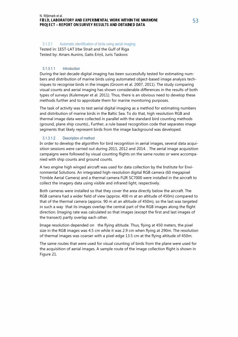
N. Wijkmark et al. FIELD, LABORATORY AND EXPERIMENTAL WORK WITHIN THE MARMONI PROJECT – REPORT ON SURVEY RESULTS AND OBTAINED DATA
53
3.1.3.1 Automatic identification of birds using aerial imaging Tested in: 1EST-LAT Irbe Strait and the Gulf of Riga Tested by: Ainars Aunins, Gatis Eriņš, Juris Taskovs
3.1.3.1.1 Introduction During the last decade digital imaging has been successfully tested for estimating num-bers and distribution of marine birds using automated object-based image analysis tech-niques to recognise birds in the images (Groom et al. 2007, 2011). The study comparing visual counts and aerial imaging has shown considerable differences in the results of both types of surveys (Kulemeyer et al. 2011). Thus, there is an obvious need to develop these methods further and to approbate them for marine monitoring purposes.
The task of activity was to test aerial digital imaging as a method for estimating numbers and distribution of marine birds in the Baltic Sea. To do that, high resolution RGB and thermal image data were collected in parallel with the standard bird counting methods (ground, plane ship counts)., Further, a rule based recognition code that separates image segments that likely represent birds from the image background was developed.
3.1.3.1.2 Description of method In order to develop the algorithm for bird recognition in aerial images, several data acqui-sition sessions were carried out during 2011, 2012 and 2014. . The aerial image acquisition campaigns were followed by visual counting flights on the same routes or were accompa-nied with ship counts and ground counts.
A two engine high winged aircraft was used for data collection by the Institute for Envi-ronmental Solutions. An integrated high-resolution digital RGB camera (60 megapixel Trimble Aerial Camera) and a thermal camera FLIR SC7000 were installed in the aircraft to collect the imagery data using visible and infrared light, respectively.
Both cameras were installed so that they cover the area directly below the aircraft. The RGB camera had a wider field of view (approx. 400 m at an altitude of 450m) compared to that of the thermal camera (approx. 90 m at an altitude of 450m), so the last was targeted in such a way that its images overlap the central part of the RGB images along the flight direction. Imaging rate was calculated so that images (except the first and last images of the transect) partly overlap each other.
Image resolution depended on the flying altitude. Thus, flying at 450 meters, the pixel size in the RGB images was 4.5 cm while it was 2.9 cm when flying at 290m. The resolution of thermal images was coarser with a pixel edge 13.5 cm at the flying altitude of 450m.
The same routes that were used for visual counting of birds from the plane were used for the acquisition of aerial images. A sample route of the image collection flight is shown in Figure 21.

N. Wijkmark et al. FIELD, LABORATORY AND EXPERIMENTAL WORK WITHIN THE MARMONI PROJECT – REPORT ON SURVEY RESULTS AND OBTAINED DATA
54
Figure 21. Route of the image collection flights in autumn 2011.
3.1.3.1.3 Results 1. Step: Aerial image data acquisition Aerial image acquisition was carried out at a ground speed of 100 knots (approx. 180 km/h). Data collected during a 3-hour long flight result in approximately 2’000 high reso-lution RGB images and 15’000 thermal images which correspond to approximately 500 GB of data. The collected images contain additional information such as time when the image is taken, the location (coordinates), and also settings of the camera.
2. Step: Visual recognition of bird species in RGB images Before starting the development of the software code for automatic recognition of, the images were visually inspected at 1:1 magnification on a computer screen trying to locate birds that could be later used as examples and a material for the training of the recogni-tion code.
Size and colour are important criterions to identify different species of birds in the im-ages. If pixel dimensions are known, then number of pixels along longitudinal or latitu-dinal axis of a bird can tell its size.
The following sample species show their characteristics in the obtained imagery.
Herring Gull Larus argentatus, large sized (54-60 cm; wingspan 123 – 148 cm) white gull, most often captured in flight above the sea surface; however, it can also be seen resting on water. Similar to other white-coloured gulls, usually the size is the main criterion for separating from other common species such as Common Gul, Black-headed gull or Little Gull in the images (Figure 2.). Rarer gulls of approximately the same size such as Greater and Lesser Black-backed Gulls currently are inseparable in the images.

N. Wijkmark et al. FIELD, LABORATORY AND EXPERIMENTAL WORK WITHIN THE MARMONI PROJECT – REPORT ON SURVEY RESULTS AND OBTAINED DATA
55
Figure 22. Herring Gull Larus argentatus in flight (left) and in obtained RGB images (right)
Long-tailed duck Clangula hyemalis, a rather small duck (39 – 47cm without tail that in males can reach 10-15 cm, wingspan 65 – 82cm). In RGB images they appear as brown and white patches (Figure 23).
Figure 23. A pair and small flock of Long-tailed Ducks Clangula hyemalis in breeding plum-age in flight (left) and a flock of Long-tailed Ducks in water (right).
3.1.3.1.4 Thermal imagery
In thermal images each image-forming pixel represents temperature of the object or sur-face captured in the image. Despite good thermal insulation by feathers, the birds are still warmer than the marine environment. In processed thermal images they appear as clus-ters of pixels with temperature differing from the water surface. Swimming birds also can stir up water and thus are followed by dark trail in the thermal images in calm sea condi-tions (Figure 24). It is not possible to tell the species from the thermal images. They can serve as a com-plementary data source to allow easier identification of bird locations in the RGB images (Figure 25) as well as describe bird behaviour captured in the RGB images thus allowing easier species identification.

N. Wijkmark et al. FIELD, LABORATORY AND EXPERIMENTAL WORK WITHIN THE MARMONI PROJECT – REPORT ON SURVEY RESULTS AND OBTAINED DATA
56
Figure 24. A fragment of thermal image with a flock of flushing waterbirds (bright dots fol-lowed by dark trails in the similar direction).
Figure 25. A fragment of RGB (left) and thermal (right) image with a flock of waterbirds.

N. Wijkmark et al. FIELD, LABORATORY AND EXPERIMENTAL WORK WITHIN THE MARMONI PROJECT – REPORT ON SURVEY RESULTS AND OBTAINED DATA
57
3.1.3.1.4.1 Non identifiable birds and artefacts
Figure 26. Visual artefacts (sun glints) resembling birds.
Not always it is possible to recognise the birds in the images. Some birds react to ap-proaching aircraft and try to escape by either diving or flushing. In case of flushing, if birds are still in the image frame when the aircraft reaches them, they are available for detection. Although it is not clear what proportion of birds goes unrecorded this way, it is presumably small. If the bird chooses to dive, the diving spots can be counted in the im-ages, however, it is not possible to tell the species.
Other object that at a first glance might appear as birds can appear in the images. The most characteristic artefacts in the images are sun glints (Figure 26). When data collection is carried out in a sunny weather one corner or one side of the image is affected by sun reflections. If birds are sought manually in the images, the sun glimpses make bird spot-ting difficult and also affect performance of automatic tools for bird recognition. When trying to locate birds automatically using software rule set, they are often mistakenly are confused with birds. Also the white caps of waves have a similar effect.
3. Step: Development of rule-set for automated recognition of birds in images Detection of birds in the RGB images is based on light (colour) properties and geometry of clusters of image-forming pixels. The following settings (rule-set) are applied: grouping of pixels with similar properties (quadtree based segmentation), background colour defi-nition (assign class 1), clustering of undefined pixels (merge region), pixel-based object resizing – adding marginal pixels to main cluster, merging of pixel clusters – applying minimal “bird” size rule and finally pixel cluster definition as object of interest - “bird” (assign class 2).

N. Wijkmark et al. FIELD, LABORATORY AND EXPERIMENTAL WORK WITHIN THE MARMONI PROJECT – REPORT ON SURVEY RESULTS AND OBTAINED DATA
58
Figure 27. Segmentation of objects vs background using applied rule-set
4. Step: Image analysis Each image is processed using rule-set described above. Time needed to analyse one image is assessed to be approx. 1 minute and 40 seconds, analysis of 2’000 images col-lected during one data acquisition campaign (3 h flight) takes approx. 60 hours of con-tinuous processing time for one computer work station. As outputs geo-referenced shape files are produced for detailed pixel cluster analysis – species detection (Figure 27) and for estimating numbers of birds on every image of the flight routes (Figure 29).
. Figure 28. Locations of detected birds on RGB image (close view)

N. Wijkmark et al. FIELD, LABORATORY AND EXPERIMENTAL WORK WITHIN THE MARMONI PROJECT – REPORT ON SURVEY RESULTS AND OBTAINED DATA
59
Figure 29. Locations of detected birds on RGB image (complete image)
5. Step: Data presentation
Estimated number of birds from each image after correction of count taking into consid-eration overlap of the images is linked to the geographical position of the particular im-age. GIS based data layer representing estimated number of birds within surveyed sea area is the final result. (Figure 30).
Figure 30. Bird survey results derived from automatic identification of birds using aerial imaging.
3.1.3.1.5 Conclusions The accuracy of bird recognition from airborne RGB and thermal images collected in ap-propriate weather conditions (calm sea) is assessed to be at 70-80% of pixel clusters iden-tified as birds are correctly identified (using visual identification and recognition as verifi-cation).
An essential condition for successful image data analysis is quality of collected images – increased amounts of sun glint and water disturbances reduce the number of correctly recognised birds.
The best results of automatic identification of birds using aerial imaging can be achieved if image collection is carried out on a calm sea, at flight altitudes that cause minimal dis-turbance for birds and flight route direction during data collection is close to the North or South.

N. Wijkmark et al. FIELD, LABORATORY AND EXPERIMENTAL WORK WITHIN THE MARMONI PROJECT – REPORT ON SURVEY RESULTS AND OBTAINED DATA
60
The combined use of high resolution RGB images and thermal images require data acqui-sition systems with a similar field of view (similar size of images) and high accuracy of data co-registration to ensure precise image overlap.
3.1.3.1.6 References Groom, G., Petersen, I.K., Anderson, M.D., Fox, A.D., 2011. Using object-based analysis of
image data to count birds: a mapping of lesser flamingo at Kamfers Dam, Northern Cape, South Africa. International Journal of Remote Sensing 32, 4611–4639.
Groom, G.B., Petersen, I.K. and Fox, T. (2007) Sea bird distribution data with object based mapping of high spatial resolution image data. In: Mills, J. & Williams, M. (Eds.): Challenges for earth observation - scientific, technical and commercial. Proceedings of the Remote Sensing and Photogrammetry Society Annual Conference 2007, 11th-14th September 2007, Newcastle University, Notting-ham, UK. The Remote Sensing and Photogrammetry Society. Paper 168.
Kulemeyer C., Schulz A., Weidauer A., Röhrbein V., Schleicher K., Foy T., Grenzdörffer G., Coppack T. 2011. Georeferenzierte Digitalfotografie zur objektiven und reproduzierbaren Quantifizierung von Rastvögeln auf See. Vogelwarte 49: 105–110
3.1.4 Fish methods
3.1.4.1 Bottom trawl, Net series and Nordic coastal multi-mesh net for monitoring fish community com-position
Tested in: 1EST-LAT Irbe Strait and the Gulf of Riga Tested by: Atis Minde, Eriks Kruze, Ivars Kazmers
3.1.4.1.1 Description of performed methods Three fish sampling methods are most commonly used in biodiversity surveys and moni-toring in the Baltic Sea region – trawling, survey Net series and Nordic coastal survey multi-mesh nets. Generally all sampling methods can be used in shallow coastal waters and in offshore areas. In Latvia benthic trawls as active fishing method providing quantita-tive data are used for monitoring the state of offshore benthic fish communities, espe-cially eelpout, cod, flounder populations (BITS surveys in Baltic Proper, trawl surveys in Riga Gulf). Gillnets are passive methods and provide mostly qualitative data. Survey Net series nets are used for coastal fish surveys/monitoring in shallow coastal areas. A third method - Nordic coastal survey multi-mesh nets are used for coastal fish monitoring in Sweden and Finland but have never been used or tested in Latvia so far and thus can be considered as new/innovative method. Introduction of Nordic nets also in Latvia would enable a possibility for better harmonisation of fish monitoring on Baltic scale and possi-bility for direct comparison of the survey results. Also the introduction and use of com-mon biodiversity indicators will greatly benefit from the common fish sampling methods used on a Baltic-wide scale.
Different types of gillnets are widely used for different fish survey purposes. In Baltic Net series nets were used for coastal fish monitoring since 1987 (HELCOM 2012). They are a fixed set of separate nets with different mesh sizes connected and set in one line. A new type of gillnet called Nordic coastal multi-mesh net have been developed in Sweden spe-cifically for coastal fish monitoring purpose and is used in Helcom coastal fish monitoring by Sweden and Finland since 2001 (HELCOM 2012). The Nordic coastal multi-mesh net is much shorter than Net series nets and has different mesh size panels incorporated in one

N. Wijkmark et al. FIELD, LABORATORY AND EXPERIMENTAL WORK WITHIN THE MARMONI PROJECT – REPORT ON SURVEY RESULTS AND OBTAINED DATA
61
gillnet. In Latvia coastal fish monitoring and coastal fish surveys begun in 1995 and 1998 respectively, and only Net series nets have been used. Local sea conditions as well as fish communities differ from those in Sweden and Finland so the performance of Nordic coastal multi-mesh nets in Latvia had to be tested in comparison to Net series nets. Within the Project also small benthic trawl was used in shallow coastal areas to enable the comparison between three fishing gears.
3.1.4.1.2 Results Within MARMONI project field data was gathered in May, July, August, October 2012 and May 2013. As all three fish sampling methods have been used almost simultaneously it is possible to compare the results. However, direct comparison is possible only between gillnet sampling methods. Results show that there are differences between species com-position and fish abundance in the two types of nets based on somewhat different catch selectivity of both gears. Net series are catching larger benthic species but Nordic Coastal nets - more small size benthic and pelagic fish.
Difference between species composition of the benthic trawl and both types of gillnets is that the trawl is catching also small benthic species like sand goby, lesser and greater sandeel, sticklebacks which are hard to catch with gillnets due to the small size of the specimens. However the occurence of dominant species like flounder, smelt, herring and sprat is similar in all three fish survey gears.
Advantage of both gillnet types is that they can be set practically on any type of sea bot-tom. Nordic coastal multi-mesh nets could be better choice if larger area has to be sur-veyed. Each Nordic coastal multi-mesh net can be set alone and it would be possible to set a number of them in transects keeping the total number of nets reasonable for smaller size scientific stuff to process them. Net series minimal length is 240m which consists of at least 8 separate nets. When using many such Net series simultaneously, the total amount of nets that needs to be processed each day is high and therefore more people in the scientific stuff will be needed.
Within MARMONI project developed indicator “Long term abundance and distribution of demersal fish in relation to benthic communities (fourhorn sculpin Myoxocephalus quad-ricornis and eelpout Zoarces viviparous example) is based on long-term (1980 – 2011) benthic trawl surveys data series. For this indicator benthic trawling would be the best sampling method as it provides accurate and quantitative data on benthic fish species like fourhorn sculpin and eelpout in offshore soft-bottom areas. In contrary the indicator “Abundance and impact of non-native fish species (round goby example)”, which is based on ratio between round goby (Neogobius melanostomus) and flounder (Platichthys fle-sus), although was developed using Net series nets, will be more precise if calculated using data from Nordic coastal multi-mesh net surveys. Nordic coastal multi-mesh net catches have more accurate representation of fish length spectrum especially regarding smaller and younger fish specimens (including round goby and flounder). This fact will make the Nordic coastal multi-mesh nets a best choice to use in future coastal fish moni-toring.
3.1.4.1.3 Conclusions All existing fish-based biodiversity indicators and the new ones developed by MARMONI are based on individual length/weight data and total number per species or ecologi-cal/taxonomical groups. Thus the data obtained from all three fishing methods can be

N. Wijkmark et al. FIELD, LABORATORY AND EXPERIMENTAL WORK WITHIN THE MARMONI PROJECT – REPORT ON SURVEY RESULTS AND OBTAINED DATA
62
used for calculation of indicators. However if the indicator is based on quantitative data only trawl survey has to be used.
3.1.4.1.4 References HELCOM 2012. Indicator based assessment of coastal fish community status in the Baltic Sea 2005-2009. Balt. Sea Environ. Proc. No. 131.

N. Wijkmark et al. FIELD, LABORATORY AND EXPERIMENTAL WORK WITHIN THE MARMONI PROJECT – REPORT ON SURVEY RESULTS AND OBTAINED DATA
63
3.2 Surveys of benthic habitats and species 3.2.1 Benthic surveys in Latvia: 1EST-LAT Irbe Strait and the Gulf of Riga
Benthic surveys in Latvia were performed using methods such as beachwrack surveys, drop-video and SCUBA-diving. Data for the following indicators were collected:
- 2.3 Beachwrack Macrovegetation Index (BMI) - 2.9 Population structure of Macoma balthica
Supporting data for bird indicators were also collected.
3.2.1.1 Maps of benthic surveys in the Irbe Strait and the Gulf of Riga
Figure 31. Sampling points of beachwrack macrovegetation survey in the Project area 1EST-LAT Gulf of Riga.

N. Wijkmark et al. FIELD, LABORATORY AND EXPERIMENTAL WORK WITHIN THE MARMONI PROJECT – REPORT ON SURVEY RESULTS AND OBTAINED DATA
64
Figure 32. Sampling points of benthos survey in the Project area 1EST-LAT Gulf of Riga.
3.2.1.2 Obtained data from benthic habitats in the Irbe Strait and the Gulf of Riga
3.2.1.2.1 Survey of Beachwrack Macrovegetation In the Latvian part of the Gulf of Riga Beachwrack Macrovegetation Index (BMI) elabo-rated in Estonia was tested to see whether the indicator is applicable also in the south-ern part of the Gulf.
In 2012 beachwrack macrovegetation samples were collected once in a month from April to October in two areas of the eastern and western coast (Vitrupe and Mērsrags) and in 2013 – once in a month from June to September in one area of the southern
N. Wijkmark et al. FIELD, LABORATORY AND EXPERIMENTAL WORK WITHIN THE MARMONI PROJECT – REPORT ON SURVEY RESULTS AND OBTAINED DATA
65
coast of the Gulf of Riga (Lapmežciems) (Figure 31). Altogether 230 beachwrack macrovegetation samples were collected and analyzed.
Related diving and video transects were performed in July/August 2012 in Vitrupe and Mērsrags. In each area two video transects and one diving transect with phytobenthos biomass sampling were performed. Altogether 41 video observation and 10 biomass samples were collected and analyzed.
Regarding the seasonal variability of SMI, index values showed the expected pattern with the highest values in summer months (June-August) due to the biomass dominance of filamentous opportunistic species. Comparing three sampling areas SMI ranges were similar while the average SMI value per site was lower (i.e. better biodiversity status) in Mērsrags and higher in Vitrupe and Lapmežciems thus coinciding with general observa-tion of more eutrophicated waters on the eastern than on the western Latvian coast of the Gulf of Riga. In each area two summer months showed SMI values out of presumed GES range.
Pearson correlation analysis was performed between SMI and eutrophication parame-ters such as Secchi depth, total phosphorus, total nitrogen, chlorophyll a and BSPI. Sig-nificant positive relationship was detected only between SMI and chlorophyll a.
3.2.1.2.2 Survey of Benthic habitats
Irbe strait is important overwintering, resting and foraging place for migratory birds. Underlaying reef area with rich benthic macrofauna and macroalgal communities is es-pecially important for sustainability of the area. Supporting data on benthic habitats for bird indicators and biodiversity assessment at 232 stations in Irbe strait were collected.
Drop video surveys were performed during the period from April to May 2012 and Au-gust - September 2013. Video record data on the type of substrate, coverage of Mytilus and coverage of dominant macroalgae species were collected from 215 stations.
Obtained drop video survey data shows that Irbe strait has good coverage of Mytilus colonies and dense macroalgal beds. In studied area the mean coverage of Mytilus was 27% but in several stations the coverage of Mytilus reached up to 70-80%. The most dominant macroalgal species with high coverage in the study area were annual species: Battersia, Ectocarpus, Pylaiella. The maximum coverage of macroalgal species was 70%.
Hard bottom samples from 17 stations selected according to depth, substrate type, bio-diversity and significant coverage of macrobenthic species were collected by SCUBA divers. The data were obtained on detailed macroalgal species composition and wet biomass as well as macrobenthic invertebrates’ species composition, abundance and wet biomass.
Altogether 9 macroalgal species were recorded. The average biomass of macroalgae in samples was 104 g/m2 but the maximum was 574 g/m2. In macrofauna 27 species were identified. The average abundance and biomass of benthic invertebrates in the study area was 27 594 ind/m2 and 532 g/m2 with maximum 69 400 ind/m2 and 1886 g/m2, respectively. The most abundant taxons of invertebrates in samples were Gammarus spp. and Mytilus.
Macrozoobenthos species soft-bottom Macoma balthica is dominant species in the Gulf of Riga and it’s size structure characterizing a population viability as well as quality of prey for predators, for example, birds. Within MARMONI project new indicator “2.9

N. Wijkmark et al. FIELD, LABORATORY AND EXPERIMENTAL WORK WITHIN THE MARMONI PROJECT – REPORT ON SURVEY RESULTS AND OBTAINED DATA
66
Population structure of Macoma balthica” was developed describing the complexity of benthic habitats and reflecting the population condition and abundance/biomass of a dominant long-living benthic species. Several field work campaigns in May and Septem-ber 2010, April and May 2011, July 2012 were organized to collect data at 34 stations from different parts of the Gulf of Riga (Figure 32).
Altogether 1244 specimens of Macoma balthica were measured and morphometrical data of bivalves shell obtained. To assess the state of the Macoma balthica population by size-distribution different sites in the Gulf of Riga was compared. Results showed slightly different size-distribution structure in shallow and deeper parts of investigated area - specimens in shallow parts were smaller while in the deeper parts they were big-ger in the size. Additionally, historical data from 1958 – 1961 year was analyzed to de-fine the natural state of a population.
For the development and setting of a target for the MARMONI indicator “2.9 Population structure of Macoma balthica” within the project area 1EST-LAT, the traditional method - Macoma balthica shell size measuring by ocular micrometer on a stereomicroscope - was applied. As the traditional method to measure the size of zoobenthic species is a slow process, Aquatic Crustacean Scan Analyser (ACSA), software developed in the framework of the MARMONI project, is a potential alternative for increased cost-efficiency for the future monitoring of the newly established indicator.
3.2.1.3 Photographs from benthic surveys within the Irbe Strait and the Gulf of Riga
Figure 33. Beachwrack sample collection in Vitrupe (Photo S. Strake)

N. Wijkmark et al. FIELD, LABORATORY AND EXPERIMENTAL WORK WITHIN THE MARMONI PROJECT – REPORT ON SURVEY RESULTS AND OBTAINED DATA
67
Figure 34. Beachwrack sampling station in Mersrags (Photo S. Strake)
Figure 35. Divers going to collect samples in the Irbe strait (Photo J. Aigars)

N. Wijkmark et al. FIELD, LABORATORY AND EXPERIMENTAL WORK WITHIN THE MARMONI PROJECT – REPORT ON SURVEY RESULTS AND OBTAINED DATA
68
Figure 36. Dense Mytilus colonies in Irbe strait (Photo J. Aigars).
Figure 37. Indicator species soft-bottom Macoma balthica population in the Gulf of Riga (Photo I. Barda)

N. Wijkmark et al. FIELD, LABORATORY AND EXPERIMENTAL WORK WITHIN THE MARMONI PROJECT – REPORT ON SURVEY RESULTS AND OBTAINED DATA
69
3.2.2 Benthic surveys in Estonia: 1EST-LAT the Eastern part of Gulf of Riga
The field works were carried out from May to September in 2011 and in June and July in 2012. Altogether 722 sampling stations were visited (Figure 38). Shallow areas were cov-ered with denser grid than deep areas because shallow areas host more heterogeneous benthic biota and habitats than deep areas. Benthic samples that were collected during development and testing of marine biodiversity indicators were also used for mapping purposes. Different sampling methods were used to collect data on seabed substrate, coverage, biomass, and abundance of benthic macrophytes and macroinvertebrates. Es-timates on seabed substrate and coverage of benthic organisms were obtained either by divers or recorded by deploying a remote underwater video device from a boat. All rec-orded videos were subsequently analyzed by estimating the coverage of different sub-strate types and benthic macrophyte and invertebrate species. Biomass samples from hard bottom areas were collected by divers by harvesting all macroscopic flora and fauna within a 20×20 cm metal frame. Ekman type bottom grab samplers (area 0.02 m2) were used to collect biomass samples from soft bottom areas. Underwater video was the most frequently used method as it is the most cost-efficient method for collecting data on sea-bed substrate and coverage of key benthic species. Coverage data was collected from 528 stations, both coverage and biomass data was obtained from 186 stations and only bio-mass samples were collected from eight stations (Figure 38). Biomass samples were sieved through a 0.25 mm mesh and all retained material was pre-served in plastic bags. The samples were stored deep frozen (–18 ºC) until analysis. In laboratory, all samples were sorted under a binocular microscope (20–40× magnification). All macrobenthic organisms were identified to species level except for oligochaetes, chi-ronomids, and juveniles of gammarid amphipods (length < 5 mm). Abundances and bio-masses of all invertebrate taxa and biomasses of plant species were quantified. Prior to weighing, animals and plants were dried at 60 ºC for 48 hours and two weeks, respective-ly. Abundances and biomasses were calculated per square meter. Biomass sampling and analysis followed the guidelines developed for the HELCOM COMBINE programme (HELCOM 2014). During the benthic sampling, Secchi-depth was measured in field. An interpolated Secchi-depth map covering Estonian waters of the Gulf of Riga and the Irbe Strait was created (Figure 39).

N. Wijkmark et al. FIELD, LABORATORY AND EXPERIMENTAL WORK WITHIN THE MARMONI PROJECT – REPORT ON SURVEY RESULTS AND OBTAINED DATA
70
3.2.2.1 Maps of benthic surveys in the Irbe Strait and the Eastern part of Gulf of Riga
Figure 38. Sampling stations.
Figure 39. Secchi-depth map created by interpolation of field measurements.
3.2.2.2 Obtained data from benthic habitats in the Irbe Strait and the Eastern part of Gulf of Riga Results of habitat modelling and mapping in mapping area in NE part of Gulf of Riga are presented in the section 3.7.4.

N. Wijkmark et al. FIELD, LABORATORY AND EXPERIMENTAL WORK WITHIN THE MARMONI PROJECT – REPORT ON SURVEY RESULTS AND OBTAINED DATA
71
3.2.2.3 Photographs from benthic surveys within the Eastern part of Gulf of Riga
Figure 40. Potamogeton perfoliatus near Kihnu island, 2 m depth.
Figure 41. Fucus vesiculosus at depth of 2,5 m, NE Gulf of Riga.

N. Wijkmark et al. FIELD, LABORATORY AND EXPERIMENTAL WORK WITHIN THE MARMONI PROJECT – REPORT ON SURVEY RESULTS AND OBTAINED DATA
72
3.2.3 Benthic surveys in Sweden: 2SWE Hanö Bight
Benthic surveys in the Swedish study area the Hanö Bight were carried out using drop-video, diving and grab sampling during summers and early autumn in 2011, 2012 and 2013. The aim was to collect data for development of benthic biodiversity indicators and spatial modelling of the distribution benthic of species and habitats. The sampling for drop-video and grab was performed in a randomized stratified way in order to cover all types benthic of environments with regards to depth and wave exposure. This procedure is performed to facilitate the spatial modelling in the Hanö Bight (section 3.7.5). Diving was carried out at 6 locations using two methods in June 2011. This was performed in order to test the applicability of a square-method alongside a traditional transect method. The aim was also to prepare the field staff before drop-video surveys since div-ing in an area provides a detailed picture of local species and conditions. Preliminary re-sults early indicated that the square method would not be useful for the intended pur-poses since and further testing of the method was cancelled in favour of more drop-video and grab samples. Drop-video was performed during August and September 2011 and 2012 with collection of ground-truthing data in September 2013. The aim was to collect data for development and testing of biodiversity indicators for phytobenthic communities as well as for spatial modelling of phytobenthic species and habitats. Grab samples using a small Van Veen sampler (sampling area 0.025 m2), were collected during the drop-video surveys from the same vessel. The sampling was performed in ac-cordance with existing methodology (Näslund 2011) and is suitable for the collection of numerous grabs for mapping purposes. Sieving was performed on the boat with a 1 mm sieve and the catch was counted and species determined directly. For large quantities, the number of individuals was estimated. The aim was to collect data for spatial modelling of zoobenthic species and habitats as well as testing the applicability of the combination of drop-video and grab surveys. Grabs provide data from soft bottom fauna which can’t be seen with drop-video. The method also provided data for development and testing of indicator substrate adjusted BQI which was rejected during the testing. Collected data was used in development and testing of following indicators Diving and drop-video: - 2.1 Accumulated cover of perennial macroalgae - 2.2 Accumulated cover of submerged vascular plants - Integrated indicators* Grab samples: - Substrate adjusted BQI ** * E.g. for relating long tailed ducks to blue mussels in the Hanö Bight (Staveley 2013) ** Indicator rejected during testing
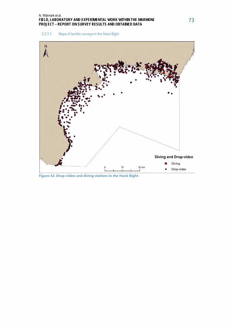
N. Wijkmark et al. FIELD, LABORATORY AND EXPERIMENTAL WORK WITHIN THE MARMONI PROJECT – REPORT ON SURVEY RESULTS AND OBTAINED DATA
73
3.2.3.1 Maps of benthic surveys in the Hanö Bight
Figure 42. Drop-video and diving stations in the Hanö Bight.

N. Wijkmark et al. FIELD, LABORATORY AND EXPERIMENTAL WORK WITHIN THE MARMONI PROJECT – REPORT ON SURVEY RESULTS AND OBTAINED DATA
74
Figure 43. Small Van Veen grabs performed during the combined drop-video and grab sur-veys in the Hanö Bight.
3.2.3.2 Obtained data from benthic surveys in the Hanö Bight
3.2.3.2.1 Diving In June 2011, 17 diving transects at six sites (Figure 42) in the Blekinge archipelago in the Hanö Bight were performed. The aim was to compare two diving survey methods (inven-tory of a 50x50 cm square, and free estimates in sections) and to give the inventory takers good knowledge of the species in the area before the drop-video inventories, which took place at exactly the same stations in August that year.
3.2.3.2.2 Drop-video During August and September 2011 and 2012, 807 drop-video stations were visited within the study area. In addition 341 stations for validation (ground-truthing) were vis-ited in 2013. Sampled stations are plotted in the map in Figure 42.
3.2.3.2.2.1 Drop-video data in development of integrated biodiversity indicators Drop-video data was not only used for benthic indicators and modelling, but also for the development of integrated biodiversity indicators. The cover of blue mussels in drop-video data was analysed related to abundance of long-tailed duck from aerial surveys described in chapter 3.5.3. Significant but weak relationships were found (Figure 44). Fur-

N. Wijkmark et al. FIELD, LABORATORY AND EXPERIMENTAL WORK WITHIN THE MARMONI PROJECT – REPORT ON SURVEY RESULTS AND OBTAINED DATA
75
ther research was suggested in order to create a basis for the use of long-tailed ducks as a suitable indicator of benthic biodiversity in the Baltic Sea. These analyses are described in detail in Staveley (2013).
Figure 44. Relationships between the long-tailed duck abundance (log10) and cover of blue mussel (log10 %) in 2012, using different grid cell sizes of data layers. A larger grid cell size gives a higher level of generalization. From Staveley (2013).
3.2.3.2.3 Grab samples 410 bottom grabs (using small Van-Veen grab) were performed in the Hanö Bight study area (Figure 43) during the drop-video surveys mentioned above. Another 50 grabs were performed in 2013.

N. Wijkmark et al. FIELD, LABORATORY AND EXPERIMENTAL WORK WITHIN THE MARMONI PROJECT – REPORT ON SURVEY RESULTS AND OBTAINED DATA
76
3.2.3.3 Photographs from benthic surveys in the Hanö Bight
Figure 45. Divers Martin Isaeus and Karl Florén testing square survey method in the Hanö Bight. Photo by Nicklas Wijkmark.
Figur 46. Diver Nicklas Wijkmark performing traditional transect survey method with “free” sampling area in the Hanö Bight. Photo by Martin Isaeus.

N. Wijkmark et al. FIELD, LABORATORY AND EXPERIMENTAL WORK WITHIN THE MARMONI PROJECT – REPORT ON SURVEY RESULTS AND OBTAINED DATA
77
Figure 47. Johan Näslund with small Van Veen grab, Hanö Bight. Photo by Karl Florén.
Figure 48. Field staff Karl Florén with Chara balthica sample taken during drop-video survey in the Hanö Bight. Photo by Johan Näslund.
3.2.3.4 References Staveley, T., A., B. 2013. Integrated Biodiversity indicators in the Baltic Sea. Masters Project
in Marine Ecology. AquaBiota Water Research.
N. Wijkmark et al. FIELD, LABORATORY AND EXPERIMENTAL WORK WITHIN THE MARMONI PROJECT – REPORT ON SURVEY RESULTS AND OBTAINED DATA
78
3.2.4 Benthic surveys in Finland: 3FIN Coastal area of SW Finland
3.2.4.1.1 Macrozoobenthos surveys in the coastal area of SW Finland The aim of this work was to test new approaches for biodiversity monitoring and collect data for the development and testing of the MARMONI indicators “2.8 Condition of soft sediment habitats – the aRPD approach” and “2.9 Population structure of Macoma balthica”. The work consisted of field work, laboratory analyses and desktop work. The field work comprised Van Veen grab and sediment core sampling as well as hydro-graphical data collection. This work was carried out in August 2012 in the Hanko-Tammisaari archipelago in the eastern part of the MARMONI project area 3FIN, where a total of 54 stations were visited (Figure 49). The field survey was concentrated to this par-ticular area, in order to in a cost-efficient manner study the characteristic features of the mosaic-like archipelago in the coastal area of the southwestern Finland. The studied area represents a characteristic gradient from the sheltered inner archipelago to the exposed outer archipelago zones. In the area salinity increases to the south (the outer archipelago), while the effect of nutrient runoff from land decreases, effectively resulting in both salinity and eutrophication gradients. Thus, it was possible to in a cost-effective manner to collect data for testing the response of the indicators to eutrophication. The data collected in 2012 was complemented with data from 56 stations collected in 2009-2011 in the FINMARINET project (http://www.ymparisto.fi/en-US/VELMU/VELMU_research_projects/FINMARINET), as well as data from 17 local envi-ronmental monitoring stations. Data from the Archipelago Sea in the western part of the MARMONI project area 3FIN was obtained from cooperation with the Finnish Inventory Programme for the Underwater Marine Environment, i.e. the VELMU project (http://www.ymparisto.fi/en-US/VELMU), and these data will be used in the assessment demonstration (Action 4.1) to increase the geographical coverage of the developed MARMONI indicators “2.8 Condition of soft sediment habitats – the aRPD approach” and “2.9 Population structure of Macoma balthica”. In the laboratory, the Van Veen grab samples were analysed for macrozoobenthos species composition, abundance and biomass, as well as size distribution of the Baltic clam, Macoma balthica. Sediment core samples were analysed for organic content using the loss of ignition (LOI) procedure. Sediment core photographs were analysed and the depth of the oxygenated sediment layer was measured. The results from this work have been utilized to develop, test and set targets for the MARMONI indicators “2.8 Condition of soft sediment habitats – the aRPD approach” and “2.9 Population structure of Macoma balthica”. Laboratory work also involved an innovative approach for size measurement of benthic fauna using image-recognition and measurement software. A Java-based program, Aquatic Crustacean Scan Analyser (ACSA), was developed and tested (see section 3.1.1.1). This novel method will save time as the measurements are partly automated and the method is thus more cost-efficient than the traditional measuring by hand. The greatest challenges in the macrozoobenthos work were presented by the innovative approach of using photographs of sediment cores for estimating the aRPD depth for the purposes of the indicator “2.8 Condition of soft sediment habitats – the aRPD approach”

N. Wijkmark et al. FIELD, LABORATORY AND EXPERIMENTAL WORK WITHIN THE MARMONI PROJECT – REPORT ON SURVEY RESULTS AND OBTAINED DATA
79
(see section 3.1.1.2). Overall, the macrozoobenthos work within Action A3 was performed successfully and without any unresolvable problems.
3.2.4.1.2 Surveys of macrophytobenthos and macrophytes in the coastal area of SW Finland The aim of this work was to test new approaches for biodiversity monitoring and collect data for the development and testing of the MARMONI indicators “2.10 Cladophora glomerata growth rate”, “2.11 Depth distribution of selected perennial macroalgae” and “2.15 Reed belt extent– the NDVI approach via high resolution satellite images”. The work consisted of field work, experimental work, laboratory analyses, and desktop work. Field work was carried out in May–October of 2011–2013 in the MARMONI project area 3FIN as well as in nearby coastal areas (Figur 50). When required in order to perform the work successfully, the strict (and in terms of the geographical area arbitrary) borders of the MARMONI area were deviated from. A total of 60 SCUBA dives were performed; 12 dives in 2011 in the Archipelago Sea, 22 dives in 2012 and 26 dives in 2013, both latter years diving was performed in the Hanko-Tammisaari archipelago. Side scan sonar sur-veys to map sea bottom structure suitable for indicator species to occupy in the Archipel-ago Sea in the western part of the project area were performed at 26 stations in July 2012 and at 25 stations in September2013; the surveys effectively covering the whole 3FIN project area. Nutrient measurements were performed in the field at Kuiva Hevonen island, Helsinki archipelago, in 2011 and at Långskär island, Tvärminne archipelago, in 2012. The frond length of Cladophora glomerata vegetation was investigated on sea marks at 16 stations in 2011 in the Tvärminne archipelago, and at 57 stations (27 in the Helsinki archi-pelago, 14 in the Archipelago Sea and 16 in the Tvärminne archipelago) in 2012. Field validation of satellite images for the purpose of investigating a cost-effective method for monitoring Cladophora glomerata vegetation over a wider geographical area and sub-strata than the MARMONI indicator “2.10 Cladophora glomerata growth rate” has been developed for (i.e. discrete sea marks) was performed in the summer 2013 at several loca-tions in the Tammisaari sea area. Furthermore, field validation of satellite images was per-formed to confirm the maximum extent of reed belts at 21 locations in June–July 2013 in the Tammisaari sea area. The results from this field work have been utilized to develop, test and set targets for the MARMONI indicators “2.10 Cladophora glomerata growth rate”, “2.11 Depth distribution of selected perennial macroalgae” and “2.15 Reed belt ex-tent– the NDVI approach via high resolution satellite images”. The development and testing of the indicator “2.11 Depth distribution of selected perennial macroalgae” was based on data collected by SCUBA diving at the Hanko peninsula in the eastern part of the MARMONI project area 3FIN. The applicability of the indicator is highly dependent on sea bottom topography and quality; therefore, in order to expand the indi-cator to cover the whole 3FIN MARMONI project area, a field survey by SCUBA diving and side scan sonar to map sea bottom structure in the Archipelago Sea in the western part of the project area was performed. Our results demonstrate that the indicator can basically be used in the whole MARMONI project area 3FIN. However, due to the large and vari-able area covered by the MARMONI 3FIN project area, the applicability of the indicator could not be investigated with a high resolution over the whole area. Therefore, based on other surveys carried out in the project area within the Finnish Inventory Programme for the Underwater Marine Environment, i.e. the VELMU project (http://www.ymparisto.fi/en-US/VELMU), a data set of over 500 diving transects was compiled to form a reserve data-base. The aim of this reserve database is to serve as an information source if the condition

N. Wijkmark et al. FIELD, LABORATORY AND EXPERIMENTAL WORK WITHIN THE MARMONI PROJECT – REPORT ON SURVEY RESULTS AND OBTAINED DATA
80
of the project area is evaluated at a later date. The drop-video data, which could not real-istically be collected within this Action, is replaced by this extensive compiled data set. The development work on the MARMONI indicator “2.10 Cladophora glomerata growth rate”, was completed in spring 2013. The indicator is based on observations of Cladophora glomerata vegetation on sea marks. Additional field work was performed in summer 2013 to investigate a cost-effective monitoring method to monitor the indicator over a wider geographical area and substrata than what the indicator has been developed for (discrete sea marks). This work demonstrates that the method shows promise, however, in order to be made operational it will require further investigations which were outside the scope of the present Action. Regarding the MARMONI indicator “2.15 Reed belt extent– the NDVI approach via high resolution satellite images”, which is based on satellite observations, the maximum extent of reed belts was confirmed by field measurements in summer 2013 in the Tammisaari area, eastern MARMONI 3FIN project area. In the field, we measured the location (coordi-nates) of the outer and inner rim of the vascular vegetation of the shoreline from several points with an accuracy of one meter by using a measurement line, thus attaining the width and geographical location of the reed belt. In order to validate the satellite inter-pretations, the field-obtained coordinates (i.e. the width of the reed belt in certain places) were plotted onto the satellite image. The field work confirmed the validity of the satellite image interpretations. The macrophytobenthos investigations included extensive laboratory work, performed in 2011. Experiments lasting approximately 60 days were conducted to measure Cladophora glomerata growth rates at different nutrient (NO3) concentrations. Further experiments lasting one week were conducted to determine lower growth-depth values (i.e. reference values) of perennial macroalgae, using Furcellaria lumbricalis as object of study. The macrophytobenthos and macrophyte work within Action A3 was performed success-fully and without any unresolvable problems.

N. Wijkmark et al. FIELD, LABORATORY AND EXPERIMENTAL WORK WITHIN THE MARMONI PROJECT – REPORT ON SURVEY RESULTS AND OBTAINED DATA
81
3.2.4.2 Maps of benthic surveys in the coastal area of SW Finland
Figure 49. Macrozoobenthos stations in the Hanko-Tammisaari archipelago in the MARMONI 3FIN area, sampled in August 2012 (red dots). Blue dots represent stations sampled during 2009-2011 within the framework of the FINMARINET project and local monitoring pro-grammes, which were used to complete the transect covering the eutrophication and salinity gradient from the inner archipelago to the outer archipelago and further to the open sea. Map by Henrik Nygård.

N. Wijkmark et al. FIELD, LABORATORY AND EXPERIMENTAL WORK WITHIN THE MARMONI PROJECT – REPORT ON SURVEY RESULTS AND OBTAINED DATA
82
Figur 50. Macrophytobenthos and macrophyte sampling stations in the MARMONI 3FIN pro-ject area (grey area to the left) and nearby coastal areas in 2011–2013. The blue arrow indi-cating validation of satellite images of Cladophora glomerata vegetation points to the Tvär-minne sea area; crowded by several sampling stations. The MARMONI 4FIN-EST project area indicated by grey area to the right. Map by Henrik Nygård.
3.2.4.3 Obtained data from benthic habitats in the coastal area of SW Finland Summarizing; the macrozoobenthos and hydrographical field data were collected at a total of 54 sampling stations in 2012. Additional field data (in total 73 stations) were acquired from the FINMARINET project and local monitoring programmes. For the pur-poses of Action 4.1., data (23 stations for the MARMONI indicator “2.9 Population struc-ture of Macoma balthica”, and 56 stations for MARMONI indicator “2.8 Condition of soft sediment habitats – the aRPD approach”) from the western part of the 3FIN area were acquired via cooperation with the VELMU project. Laboratory work, including the devel-opment and use of image-recognition software was performed in 2012–2014. The ob-tained data were used for:
• Indicator development and testing: two MARMONI indicators and their fact sheets were produced, i.e. “2.8 Condition of soft sediment habitats – the aRPD ap-proach” and “2.9 Population structure of Macoma balthica”. Furthermore, the data will be used in the assessment demonstration (Action 4.1) to increase the geo-graphical coverage of the developed MARMONI indicators.
• Monitoring method development and testing: the utilization of image-recognition software for the measurement of benthic fauna for the purposes of cost-efficient monitoring of the MARMONI indicator “2.9 Population structure of
N. Wijkmark et al. FIELD, LABORATORY AND EXPERIMENTAL WORK WITHIN THE MARMONI PROJECT – REPORT ON SURVEY RESULTS AND OBTAINED DATA
83
Macoma balthica” resulted in a novel method for monitoring this indicator. Addi-tionally, an innovative method for measuring the apparent redox potential dis-continuity (aRPD) was tested and used for development of the MARMONI indica-tor “2.8 Condition of soft sediment habitats – the aRPD approach”. However, this method turned out to be somewhat inaccurate and thus further development is needed to effectively take this method in use.
The methods used and methodology developed is explained in greater detail in the out-come of Action A2 (MARMONI indicator database, http://marmoni.balticseaportal.net/wp/category/biodiversity-indicators/#; as well as the forthcoming Action A2 final report) and in section 3.1 of the present report, respectively. The macrophytobenthos and macrophyte field surveys consisted of a total of 60 SCUBA dives in 2011–2013, side scan sonar surveys at 52 locations in 2012–2013, length measurements of Cladophora glomerata fronds at a total of 73 sea marks in 2011–2012, nutrient measurements in the field for 29 days in 2011–2012, as well as satellite image validation in the field in spring and summer 2013 at several locations. Additional field data were acquired from the national VELMU project. Laboratory experiments were per-formed for the duration of ca 60 days to measure Cladophora glomerata growth rates and 5 days to determine lower growth-depth values (i.e. reference values) of perennial macro-algae. The obtained data were used for:
• Indicator development and testing: three MARMONI indicators and their fact sheets were produced, i.e. “2.10 Cladophora glomerata growth rate”, “2.11 Depth distribution of selected perennial macroalgae” and “2.15 Reed belt extent– the NDVI approach via high resolution satellite images”.
• Monitoring method development and testing: the utilization of satellite im-agery for the purposes of cost-efficient monitoring the MARMONI indicator “2.10 Cladophora glomerata growth rate” was tested. The gained results were promis-ing; however, in order to be made operational further work, outside the scope of the present Action, will be required.
The methods used and methodology developed is explained in greater detail in the out-come of Action A2 (MARMONI indicator database, http://marmoni.balticseaportal.net/wp/category/biodiversity-indicators/#; as well as the upcoming Action A2 final report) and in section 3.1 of the present report, respectively.

N. Wijkmark et al. FIELD, LABORATORY AND EXPERIMENTAL WORK WITHIN THE MARMONI PROJECT – REPORT ON SURVEY RESULTS AND OBTAINED DATA
84
3.2.4.4 Photographs from benthic surveys within the coastal area of SW Finland
Figure 51. A schematic and authentic presentation of the laboratory experiment set up used to determine lower growth-depth values (i.e. reference values) of perennial macroalgae, us-ing Furcellaria lumbricalis as study object. Photograph by Ari Ruuskanen.
Figure 52. A nutrient measurement device in action at Tvärminne Långskär in the MARMONI 3FIN area in 2012. Photograph by Ari Ruuskanen.

N. Wijkmark et al. FIELD, LABORATORY AND EXPERIMENTAL WORK WITHIN THE MARMONI PROJECT – REPORT ON SURVEY RESULTS AND OBTAINED DATA
85
Figure 53. Laboratory experiment setup, where Cladophora glomerata was cultivated in water flow-thru tubes in different nutrient concentrations. Changes in frond length were observed by measurement marks on the tube. Photographs by Ari Ruuskanen.
Cladophora glomer-ata
Tube
Measurement marks
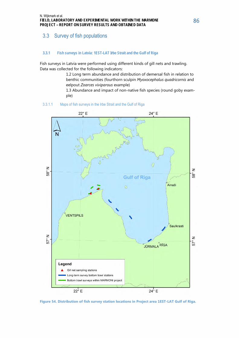
N. Wijkmark et al. FIELD, LABORATORY AND EXPERIMENTAL WORK WITHIN THE MARMONI PROJECT – REPORT ON SURVEY RESULTS AND OBTAINED DATA
86
3.3 Survey of fish populations
3.3.1 Fish surveys in Latvia: 1EST-LAT Irbe Strait and the Gulf of Riga Fish surveys in Latvia were performed using different kinds of gill nets and trawling. Data was collected for the following indicators:
1.2 Long term abundance and distribution of demersal fish in relation to benthic communities (fourthorn sculpin Myoxocephalus quadricornis and eelpout Zoarces viviparous example) 1.3 Abundance and impact of non-native fish species (round goby exam-ple)
3.3.1.1 Maps of fish surveys in the Irbe Strait and the Gulf of Riga
Figure 54. Distribution of fish survey station locations in Project area 1EST-LAT Gulf of Riga.

N. Wijkmark et al. FIELD, LABORATORY AND EXPERIMENTAL WORK WITHIN THE MARMONI PROJECT – REPORT ON SURVEY RESULTS AND OBTAINED DATA
87
3.3.1.2 Obtained data from fish populations in the Irbe Strait and the Gulf of Riga
The fish community in Irbe strait was sampled with gill nets (Net series and Nordic costal multi-mesh net) and trawl. A total of six combined gill net surveys (Net series and Nordic costal multi-mesh net) in 12 July (station Kolka), 20 July (station Mazirbe), 22 August (sta-tions Kolka and Mazirbe), 23 October (station Kolka) 2012, 14 May 2013 (Mazirbe) and four trawl surveys in Irbe strait in 19 May, 16 August, 16 October 2012 and 18 may 2013 were made. Obtained results were utilized to assess the differences in fish species compo-sition and size distribution in different sampling methods as well as to develop new fish biodiversity indicators.
The occurrence of dominant fish species like flounder, smelt, herring and sprat was similar in all three fish survey gears. However the proportion of small size benthic fish like sand goby, lesser and greater sandeel, sticklebacks were higher in the trawl catches. Even com-parison of Nordic coastal multi-mesh net and Net series catches shows differences in fish length spectrum. More detailed results of fish size can be obtained from the Nordic coastal multi-mesh net.
Long-term (1980 – 2011) benthic trawl survey data series as well as new field data gath-ered within the MARMONI project were used to develop two fish biodiversity indicators “Long term abundance and distribution of demersal fish in relation to benthic communi-ties (fourthorn sculpin Myoxocephalus quadricornis and eelpout Zoarces viviparous ex-ample)” and “Abundance and impact of non-native fish species (round goby example)”.
3.3.1.3 Photographs from fish surveys in the Irbe Strait and the Gulf of Riga
Figure 55. Fish trawl survey in the Irbe strait (Photo E. Kruze)

N. Wijkmark et al. FIELD, LABORATORY AND EXPERIMENTAL WORK WITHIN THE MARMONI PROJECT – REPORT ON SURVEY RESULTS AND OBTAINED DATA
88
Figure 56. Scientists going to coastal fishing with gillnets (Photo A. Minde)
Figure 57. The round goby Neogobius melanostomus in the Nordic multi-mesh net (Photo A. Minde).
N. Wijkmark et al. FIELD, LABORATORY AND EXPERIMENTAL WORK WITHIN THE MARMONI PROJECT – REPORT ON SURVEY RESULTS AND OBTAINED DATA
89
3.3.2 Fish surveys in Estonia: 1EST-LAT Irbe Strait and the Eastern part of Gulf of Riga
Mostly trawling and gill-net surveys were used for development of “Pikeperch indicator” [The length at sexual maturation of female pikeperch (Sander lucioperca) in monitoring catches] and “Large perch indicator” [Abundance index of large (TL>250 mm) perch (Perca fluviatilis) in monitoring catches] respectively. Also beach-seine surveys for juvenile flounder were undertaken for the “Juvenile flounder -indicator” development in the Gulf of Finland (described in the paragraph 3.3.4.). During all surveys individual total length (TL) and mass were recorded. Also data on maturity status and age was collected in case of perch and pikeperch. The main bulk of field work undertaken was concentrated on the trawl surveys in the Pärnu Bay, Eastern Gulf of Riga in order to develop and test the “Pikeperch indicator”. Altogether 40 trawl surveys were performed during the 2011-2012 and 15 additional trawl surveys were performed in 2013 on the fixed transects in Pärnu bay (Figure 58). The tran-sects were studied by pulling benthic (0.3 m from the seabed) trawl (doors with 20m, mouth width 12m, mouth height 2m) for 30 minutes with speed of 3 knots. Gill-net surveys were used to gather data for the development and testing of the “Large perch indicator” in three locations in the Gulf of Riga (Figure 59). Gill-net series stations included 12 nets with different mesh sizes (14, 17, 21.5, 25, 30, 33, 38, 42, 45, 50, 55 and 60 mm from knot to knot) in random sequence. Nets with mesh sizes 14-38 mm were made of spun nylon and 42-60 of monofilament nylon. Each net consisted of a 60-m-long stretched net bundle, which was attached to a 27 m upper and 33 m lower net-rope. Only bottom nets (net height 1.8 m) were used. 40 surveys 2011-2012, 15 surveys 2013 in the A3-deliverable?
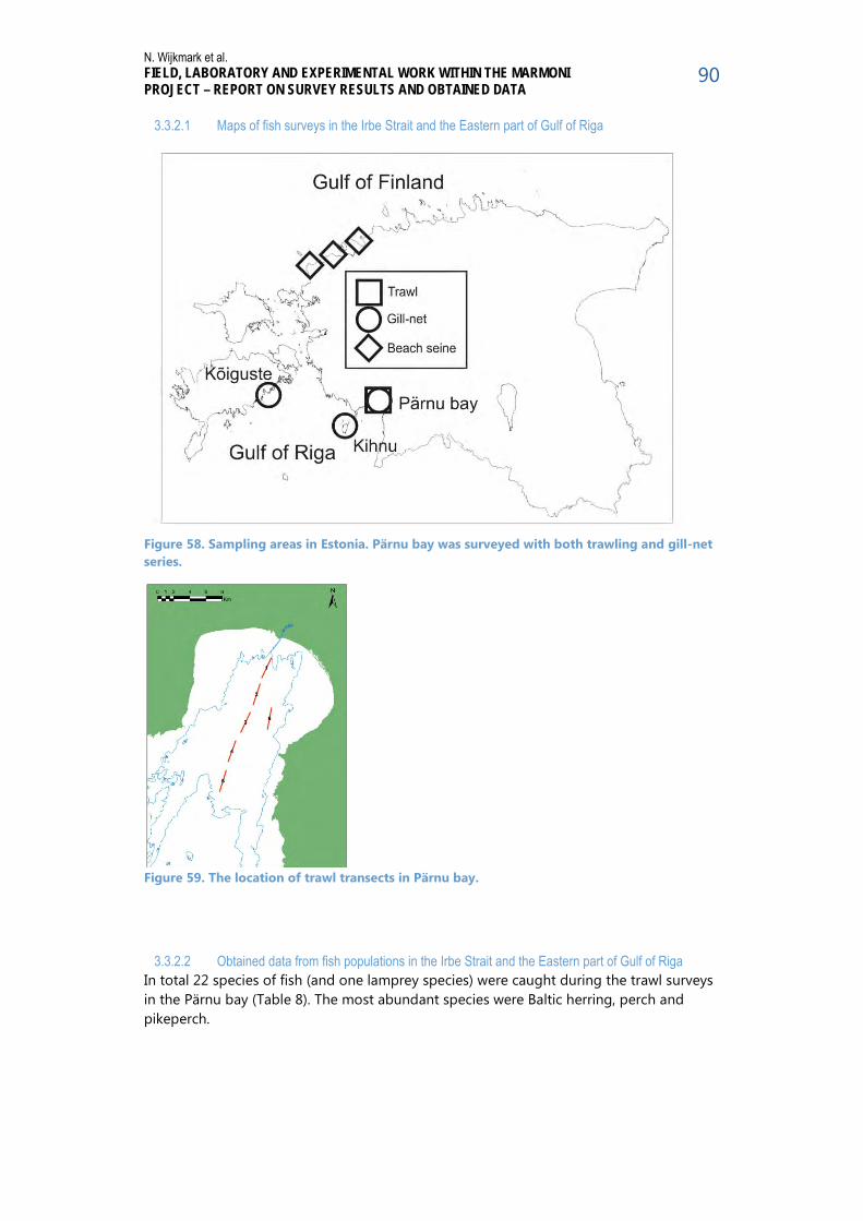
N. Wijkmark et al. FIELD, LABORATORY AND EXPERIMENTAL WORK WITHIN THE MARMONI PROJECT – REPORT ON SURVEY RESULTS AND OBTAINED DATA
90
3.3.2.1 Maps of fish surveys in the Irbe Strait and the Eastern part of Gulf of Riga
Figure 58. Sampling areas in Estonia. Pärnu bay was surveyed with both trawling and gill-net series.
Figure 59. The location of trawl transects in Pärnu bay.
3.3.2.2 Obtained data from fish populations in the Irbe Strait and the Eastern part of Gulf of Riga In total 22 species of fish (and one lamprey species) were caught during the trawl surveys in the Pärnu bay (Table 8). The most abundant species were Baltic herring, perch and pikeperch.

N. Wijkmark et al. FIELD, LABORATORY AND EXPERIMENTAL WORK WITHIN THE MARMONI PROJECT – REPORT ON SURVEY RESULTS AND OBTAINED DATA
91
Table 8. Fish species and number of individuals caught during trawl surveys in the Pärnu bay.
Species 2011 2012 2013 TOTAL Lampetra fluviatilis 17 1 6 24 Clupea harengus 1243 135 35345 36723 Sprattus sprattus 379 599 978 Salmo trutta 1 1 Coregonus lavaretus 1 5 2 8 Osmerus eperlanus 619 1580 2092 4291 Anguilla anguilla 1 1 Rutilus rutilus 144 152 189 485 Leuciscus cephalus 1 1 Alburnus alburnus 74 8 31 113 Abramis brama 879 82 161 1122 Blicca bjoerkna 1055 659 97 1811 Vimba vimba 620 383 311 1314 Carassius gibelio 2 8 10 Gasterosteus aculeatus 680 22 702 Pungitius pungitius 6 6 Nerophis opidion 1 1 2 Perca fluviatilis 763 3107 4870 8740 Sander lucioperca 2129 2483 2091 6703 Zoarces viviparus 17 17 44 78 Gymnocephalus cernuus 744 707 2743 4194 Pomatochistus minutus 2 2 Platichthys flesus 1 15 36 52 TOTAL 9376 9336 48649 67361
Collected data on the pikeperch population of the Pärnu bay enabled the development and testing of the “Pikeperch indicator”. Namely, level of maturation was determined by visual inspection of dissected fish. Length at maturation (L50) was determined using logis-tic regression model where individual TL is independent and the level of sexual maturity is dependent variable. Comparison with historical data (from the beginning of the 1990s) and with data from Finnish coastal waters showed that indicator values during recent years were lower than recorded in the past (Figure 60). These results indicate that that size-selective fishing pressure may have played a role in the development of the current local fish community and size structure of Pärnu bay pikeperch population (Figure 61). The similar trends in indicator values in Pärnu bay and Finland indicate that developed indicator is usable also on different datasets.

N. Wijkmark et al. FIELD, LABORATORY AND EXPERIMENTAL WORK WITHIN THE MARMONI PROJECT – REPORT ON SURVEY RESULTS AND OBTAINED DATA
92
Figure 60. Indicator values in areas with different pikeperch fishery regulations. Green dashed line marks the upper (optimistic, TL=41.4 cm) and red dashed line the lower (conservative, TL=40.3 cm) target values for Pärnu area according to Erm 1981 (Erm, V. 1981. Koha. Valgus, Tallinn).
Figure 61. The size distribution of pikeperch in Pärnu bay trawl surveys.
In total 24 species of fish were caught during the gill-net surveys in the Gulf of Riga (Table 9). The most abundant species were perch, bleak and ruffe. The initial studies in 2011 revealed that the most suitable area for collection of data for development and testing of the “Large perch indicator” was Kihnu.
0
50
100
150
200
250
7 9 11131517192123252729313335373941434547495153555862
Tota
l nr
TL (cm)
2011
2012
2013

N. Wijkmark et al. FIELD, LABORATORY AND EXPERIMENTAL WORK WITHIN THE MARMONI PROJECT – REPORT ON SURVEY RESULTS AND OBTAINED DATA
93
Table 9. Fish species and number of individuals caught during gill-net surveys in the Gulf of Riga.
Species Kihnu Kõiguste Pärnu TOTAL 2011 2012 2013 2011 2011
Clupea harengus 10 852 242 19 19 1142 Sprattus sprattus 2 28 11 41 Coregonus lavaretus 1 1 2 Osmerus eperlanus 17 6 23 Esox lucius 8 8 Rutilus rutilus 4 8 7 499 275 793 Scardinius erythophthalmus
6 23 24 27 80
Leuciscus leuciscus 5 6 11 Leuciscus idus 1 1 Gobio gobio 229 436 62 727 Alburnus alburnus 1173 1006 628 31 29 2867 Abramis brama 28 28 Blicca bjoerkna 2 577 579 Vimba vimba 3 8 5 146 162 Carassius gibelio 4 16 1 77 1 99 Misgurnus fossilis 1 1 Lota lota 1 1 Perca fluviatilis 2971 2904 5545 788 1012 13220 Sander lucioperca 52 51 26 1 34 164 Gymnocephalus cer-nuus
405 70 193 70 1960 2698
Zoarces viviparus 1 46 9 4 16 76 Neogobius melanostomus
2 5 7
Cottus gobio 1 1 Platichthys flesus 42 45 89 80 3 259 TOTAL 4908 5502 6849 1624 4107 22990 Collected data on the perch populations of the studied sites allowed to develop and test the “Large perch indicator”. To test if the indicator is sensitive to differences in fishing pressure the indicator values from the project area were compared to data from Vilsandi monitoring area (obtained during other studies). The results revealed that indicator values were much higher in the Vilsandi area, where the fishing pressure is lower (Figure 62). Thus it is possible that anthropogenic pressures may have played a role in the develop-ment of the local community and the current size structure of perch (Figure 63) in the Kihnu area.
N. Wijkmark et al. FIELD, LABORATORY AND EXPERIMENTAL WORK WITHIN THE MARMONI PROJECT – REPORT ON SURVEY RESULTS AND OBTAINED DATA
94
Figure 62. Comparison of indicator values from the project area (Kihnu) to the monitoring area with lower fishing pressure (Vilsandi) during 2013.
Figure 63. The size distribution of perch in gill-net surveys at the Kihnu area.
0
200
400
600
800
1000
1200
1400
7 8 9 10 11 12 13 14 15 16 17 18 19 20 21 22 23 24 25 26 27 28 29 30
Tota
l nr
TL (cm)
2011
2012
2013

N. Wijkmark et al. FIELD, LABORATORY AND EXPERIMENTAL WORK WITHIN THE MARMONI PROJECT – REPORT ON SURVEY RESULTS AND OBTAINED DATA
95
3.3.2.3 Photographs from fish surveys in the Irbe Strait and the Eastern part of Gulf of Riga
Figure 64. Trawling in the Pärnu bay. Photos by Anu Albert and Kalvi Hubel.
Figure 65. Gill-net surveys. Photos by Anett Reilent (see also: http://www.facebook.com/media/set/?set=a.556381951074726.1073741828.518817211497867&type=1).
Figure 66. Beach seineing for juvenile flounder in the Gulf of Finland. Photos by Kristiina Jürgens.

N. Wijkmark et al. FIELD, LABORATORY AND EXPERIMENTAL WORK WITHIN THE MARMONI PROJECT – REPORT ON SURVEY RESULTS AND OBTAINED DATA
96
3.3.3 Fish surveys in Sweden: 2SWE Hanö Bight
Fish surveys were carried out in the Hanö Bight using the methods small underwater detonations and hydroacoustics. Small underwater detonations were used in coastal areas for surveys of juvenile fish and hydroacoustics were used in offshore areas for surveys of pelagic fish. The aim was to provide data for development and testing of fish indicators, integrated indicators as well as spatial modelling. Collected data was used in development and testing of following indicators - 1.8 Trophic diversity index of juvenile fish - 1.8 Habitat-related functional diversity of juvenile fish * - Preferred herring spawning season ** * This is also an integrated indicator which relates juvenile fish with vegetated habitats ** Indicator rejected due to lack of juvenile herring observations in performed surveys
3.3.3.1 Maps of fish surveys in the Hanö Bight
Figure 67. Locations for small underwater detonations in the Hanö Bight (surveys of coastal fish reproduction areas).

N. Wijkmark et al. FIELD, LABORATORY AND EXPERIMENTAL WORK WITHIN THE MARMONI PROJECT – REPORT ON SURVEY RESULTS AND OBTAINED DATA
97
Figure 68. Hydroacoustic transects and verified by pelagic trawling (yellow). Total length of the transects is ca 140 km.
3.3.3.2 Obtained data from fish populations in the Hanö Bight
3.3.3.2.1 Pelagic fish density distribution Vertical mobile echo sounding (with the sensor mounted on a tractor sled operated from a boat) was used to study pelagic organisms. The surveys were conducted on four occa-sions between the 20th and 25th of August 2012 (Figure 68, Table 10). The surveys were conducted at night, when pelagic organisms are more evenly distributed in the water column, which means that the estimated error is less at night compared to the day when the fish often aggregate in shoals and are patchier distributed.
Table 10. Hydro acoustic transects in the Hanö Bight in August 2012.
Occasions Date start Time start
Date stop Time stop
Length (km)
1 2012-08-20 22:37 2012-08-21 04:47 37.7
2 2012-08-21 22:13 2012-08-22 04:47 34.8
3 2012-08-24 21:49 2012-08-25 04:46 35.5
4 2012-08-25 22:25 2012-08-26 04:48 31.7
A multi-frequency hydro-acoustic system (MFHAS) which consisted of 70, 120, 200 and 710 kHz sonar (Simrad EY60) (for description see Table 11) was used for echo sounding. The sonar and sensors were calibrated according to the manufacturer's recommendations and applicable standards (Foote 1982, Foote et al. 1987). Echo sounding was conducted from a commercial fishing boat "Nimrod" which is 18 m long with sensors mounted on a so-called "Tow-body" placed about two meters out on the starboard side in about one meters depth.
N. Wijkmark et al. FIELD, LABORATORY AND EXPERIMENTAL WORK WITHIN THE MARMONI PROJECT – REPORT ON SURVEY RESULTS AND OBTAINED DATA
98
Table 11. Specifications of the hydroacoustic system with multi-frequency (MFHAS) used in the studies
Frequency (kHz) Model Type Pulse length (ms)
Band width (kHz)
70 ES70-7c Split beam 0.512 4.69
120 ES120-7c Split beam 0.512 5.56
200 200-7F Single beam 0.512 5.97
710 710-36 Single beam 0.512 6.23
In order to relate the results from echo sounding to fish stocks, species and size composi-tion biological sampling was conducted in the form of a pelagic trawling per assessment point (Figure 68), directly associated to the echo sounding. Trawling focused on pelagic fish and the appropriate depth was determined at each assessment point with the sup-port of the distribution of fish observed at the previous echo sounding. Trawl depth was monitored in real time using a depth finder attached to the trawl (Simrad PI38). During trawling the boat held a speed of two to three knots. Mesh size in the cod end of the trawl was six mm (knot to knot) in order to catch small fish and fish larvae. The catch was species determined and measured for length and weight following morning. In connec-tion to the surveys depth profiles of temperature and salinity (CTD - conductivity, tem-perature and salinity; SD-204, Sensor Data AS, Bergen, Norway) were also made. Hydroacoustic data were processed and analysed by Sonar5-Pro Version 6.0.2 (Balk & Lindem 2012). In order to analyse different groups of the pelagic organism in acoustical data, first they have to be identified, and if possible (and necessary) separated from each other. Sonar 5 contains a module for multi-frequency analysis with several functions. In general, echoes from the different organism depending on their size, body shape, inclu-sion of gas in the body has different strength at different frequencies. Therefore, fre-quency response curves of diverse organism groups looks different. For example echoes of swim-bladdered fish are well “seen” on all frequencies, but they are stronger on lower frequencies. They are also are strongest in comparison to other groups, and have to be removed/separated from data if weaker echoes from other organisms are of interest.
Acoustical data analysis methods of fish are well established. Fish analysis was performed from 70 kHz acoustic data. Fish density and distribution were analysed after fish echoes from the hydroacoustic data had been divided into four size groups based on the results from trawling. Translation from echo strength (TS, dB) to fish length (L, mm) follows Didri-kas & Hansson (2004): TS = 25.5 log (L/10) – 73.6 The data from the pelagic trawling was used to interpret fish densities of different length classes along the acoustic transects. Pelagic species dominated the trawl catches. Smaller fish (2-6 cm) consisted mainly of sticklebacks, young of the year herring and/or sprat. Medium-sized fish (7-13 cm) was represented mainly by sprat and large fish (14.5 to 25 cm) consisted mainly of adult herring. Large fish> 51 cm occurred sparingly in the acous-tic data, and no fish of this size were caught in the trawl. Based on knowledge of the spe-cies composition of this type of habitat it can be assumed that echoes in this size class corresponds to fish-eating predatory fish such as cod, salmon or sea trout.

N. Wijkmark et al. FIELD, LABORATORY AND EXPERIMENTAL WORK WITHIN THE MARMONI PROJECT – REPORT ON SURVEY RESULTS AND OBTAINED DATA
99
3.3.3.2.2 Juvenile fish in coastal reproduction areas Young of the year (YOY) fish in coastal recruitment areas were inventoried during late summer (August or the first part of September) with small underwater detonations be-tween zero and six meters depth (Figure 67, Table 12). In total 391 detonations were per-formed between 2011 and 2013. The method is quantitative and has been used for differ-ent types of environments (Christensen et al 2007) since the 1970s (Karås and Neuman 1981). The same method is used in similar studies around the Baltic coast, and a method guideline will soon be finalized by the Swedish Environmental Protection Agency (Bergström et al. manuscript). Sample points were randomly distributed between the shoreline and six meters depth within selected areas and the presence of fish fry was inventoried with small underwater detonations. An explosive device consisting of a one grams detonator and ten grams of pentaerythritol tetranitrate was placed in the spark plug wire on the end of a fishing pole. The boat approached the sample point slowly with the blaster in the fore. At the site the explosive charge was lowered into the water a few feet from the boat and detonated at a depth of about one meter. At shallow depths, the aim was to detonate the explosive charge at half the water depth. The bursting point was marked with a float, after which floating fish were collected from the boat and sunken fish by snorkelling. The snorkeler also noted presence and coverage of macro vegetation, bottom substrate and the amount of filamentous algae. Temperature and depth were noted and water samples were taken for turbidity analysis at each sampling point. The fry inventories are described in detail in Lindahl et al. 2014. Obtained data on perch, pike, roach and sticklebacks were used in spatial modelling de-scribed in section 3.7.5.2.

N. Wijkmark et al. FIELD, LABORATORY AND EXPERIMENTAL WORK WITHIN THE MARMONI PROJECT – REPORT ON SURVEY RESULTS AND OBTAINED DATA
100
Table 12. Number of detonations per year and area for the inventory of young-of-the-year fish.
Area Year Number of detonations
Tosteberga - Landöbukten 2011 13
Valjeviken 2011 10
Valjeviken 2012 11
Valjeviken 2013 12
Sölvesborgsviken 2011 7
Sölvesborgsviken 2012 9
Sölvesborgsviken 2013 17
Eriksberg - Ronneby 2011 7
Eriksberg - Ronneby 2012 29
Eriksberg - Ronneby 2013 53
Bredasund 2012 7
Listerby - Karlskrona 2012 20
Listerby - Karlskrona 2013 41
Hallarumsviken 2011 5
Hallarumsviken 2012 20
Hallarumsviken 2013 16
Gåsefjärden - Torhamns skärgård 2011 9
Gåsefjärden - Torhamns skärgård 2012 41
Gåsefjärden - Torhamns skärgård 2013 19
Sibbaboda - Kristianopel 2012 12
Sibbaboda - Kristianopel 2013 33
3.3.3.2.3 Note on the use of data from fish surveys in the Hanö Bight in indicator development and modelling
Since the survey method “Small Underwater Detonations” includes both juvenile fish and the submerged vegetation at the sampling sites, the data was ideal for the development of integrated indicators. The two indicators 1.8 Trophic diversity index of juvenile fish and 1.8 Habitat-related functional diversity of juvenile fish were developed and tested using this dataset. Indicator 1.9 is an integrated indicator that relates the functional diversity of juvenile fish to shallow vegetated habitats. Data from this survey method was also used in spatial modelling of juvenile fish. The data from hydroacoustic surveys of pelagic fish density distribution was successfully used in the spatial modelling of pelagic fish in the offshore areas of the Hanö Bight. The same survey also tested this method for the inventory of zooplankton, which is new inno-vative application for this method. The testing of this method for zooplankton surveys is described in the tested section “New Methods and Innovative Approaches Tested” in this report.

N. Wijkmark et al. FIELD, LABORATORY AND EXPERIMENTAL WORK WITHIN THE MARMONI PROJECT – REPORT ON SURVEY RESULTS AND OBTAINED DATA
101
The planned indicator “Preferred Herring Spawning Season” could not be developed since enough data on juvenile herrings were not found in the area. Indicators for other juvenile fish were developed instead (see indicators 1.8 and 1.9 above).
3.3.3.3 Photographs from fish surveys in the Hanö Bight
Figure 69. Small underwater detonation during survey of juvenile fish.
3.3.4 Fish surveys in Finland: 3FIN Coastal area of SW Finland
3.3.4.1 Gill-net and juvenile flounder surveys Gill-net surveys have been conducted in co-operation with a monitoring program run by the FGFRI. The aim was to assess the various components of variation in the gill-net data in order to evaluate performance of present sampling programs and to optimize them using a power-analysis approach. Data obtained by gill net surveys were thus used for the “Cyprinid -indicator” as well as for the “Large perch -indicator”. The main efforts in the 3FIN -area, however, have been put in the beach-seine surveys for juvenile flounder. Juvenile flounder settled on the shallow areas have passed one very critical period (pelagic larval phase) and succeeded in finding a suitable nursery habitat. This means that they have already been exposed to environmental conditions and, thus, their abundance and distribution reflects the environmental state of both pelagic and shallow areas. The data collected have been used to test the new potential “Juvenile flounder -indicator”. In addition to these, a separate project took place in FGFRI during 2010-2013 aiming to estimate biomass of Cyprinid fish in shallow coastal areas by echo sounding and simulta-neous sampling of fish by a seine or a small trawl. Original idea was to utilize the results also for the “Cyprinid -indicator” for MARMONI-project. The horizontal echo-sounding

N. Wijkmark et al. FIELD, LABORATORY AND EXPERIMENTAL WORK WITHIN THE MARMONI PROJECT – REPORT ON SURVEY RESULTS AND OBTAINED DATA
102
provided reasonable estimates of the total fish biomasses in shallow areas. However, the sampling of fish appeared difficult and information of the proportions of various species in the total biomass could not be produced on an acceptable level. Thus, this data was finally not used for indicator development and testing in MARMONI.
3.3.4.2 Pelagic surveys of fish larvae The survey of pelagic fish larvae was performed in the shallow, complex and extensive archipelago area in the coastal area of SW Finland (Figure 72) in 2011 and 2012. The aim of this survey was to collect data for modelling of fish reproduction areas.
3.3.4.3 Maps of fish surveys in the Coastal area of SW Finland
Figure 70. Gill-net survey areas in the Archipelago Sea, SW Finland.
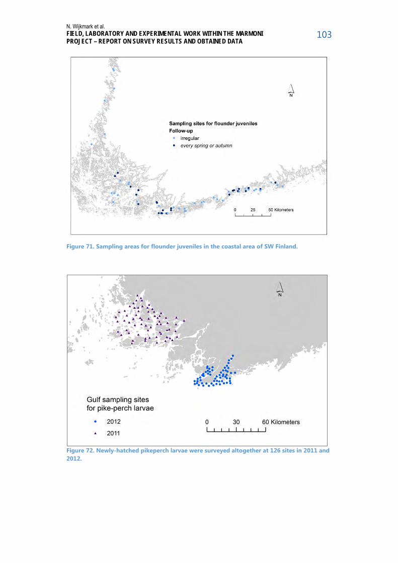
N. Wijkmark et al. FIELD, LABORATORY AND EXPERIMENTAL WORK WITHIN THE MARMONI PROJECT – REPORT ON SURVEY RESULTS AND OBTAINED DATA
103
Figure 71. Sampling areas for flounder juveniles in the coastal area of SW Finland.
Figure 72. Newly-hatched pikeperch larvae were surveyed altogether at 126 sites in 2011 and 2012.

N. Wijkmark et al. FIELD, LABORATORY AND EXPERIMENTAL WORK WITHIN THE MARMONI PROJECT – REPORT ON SURVEY RESULTS AND OBTAINED DATA
104
3.3.4.4 Obtained data from fish populations in the Coastal area of SW Finland
3.3.4.4.1 Obtained data from gill net and juvenile flounder surveys Nordic coastal multi-mesh gill-nets were used in the gill-net surveys. These are 1.8 m deep bottom gill-nets with a length of 45 m. The nets are made up of nine parts, each 5 m long. The parts have different mesh sizes and are placed in the following order: 30, 15, 38, 10, 48, 12, 24, 60 and 19 mm (mesh bar). In both of the two survey areas (Figure 70), the sampling was done in 30 (Tvärminne) or 38 (Brunskär) fixed net stations distributed evenly in three depth intervals (0-3 m, 3-6 m, 6-10 m). The nets were set in the evening and collected on the following morning. The length of each fish in the catch was meas-ured and the total weight of each species in each net was weighted. Gill-net surveys were carried out in late July - August in each survey year. During 2011-2013, 68 gill-net nights were fished annually. The most abundant species in the catch were perch, roach, ruffe and bream. There was often a lot of annual variation in the data as demonstrated in the abundance of cyprinids (Figure 73). The annual variation did not show any common pattern between the two areas and the differences in the abundance levels were high, suggesting that the gill-net survey results should not be extrapolated outside the original study areas.
Figure 73. Catch per unit effort (g/gill-net night) of Cyprinids in Brunskär and Tvärminne 2011-2013.
The surveys for juvenile flounder were conducted with a small beach-seine in shallow sandy beaches (Figure 71). The arm length of the seine was 8,4 m, the opening of the end was 2,0 m wide and the height was 1,8 m. Mesh-size in the end was 5 mm. The length of one haul varied approximately between 5 and 45 m depending on the profile of the sea-floor (availability of shallow area), but the results were counted per surface area of the hauls. Three parallel hauls were taken at each sampling area during each visit. Surveys were carried out in autumn (for young-of-the-year juveniles) and spring (for 1+ over-wintered juveniles).

N. Wijkmark et al. FIELD, LABORATORY AND EXPERIMENTAL WORK WITHIN THE MARMONI PROJECT – REPORT ON SURVEY RESULTS AND OBTAINED DATA
105
Beach seine surveys for juvenile flounders were conducted at 42 sites in autumn 2011, at 25 sites in spring 2012 and at 59 sites in autumn 2012. In 2013, 32 sites were visited in spring and 28 sites in autumn. In spring 2014, 33 sites were visited. In addition, four Esto-nian areas were visited in spring 2013 and 2014.In Finland, 18 “intensive areas” were se-lected for more detailed monitoring and those were visited annually (Figure 71). On an average, more juvenile flounder were caught during the spring sampling than autumn (Figure 74 and Figure 75). The annual variation in the abundance was, however, relatively high.
Figure 74. Mean abundance (blue dots) and occurrence of juvenile flounder in the 18 “inten-sive areas” during springs 2012-2014.

N. Wijkmark et al. FIELD, LABORATORY AND EXPERIMENTAL WORK WITHIN THE MARMONI PROJECT – REPORT ON SURVEY RESULTS AND OBTAINED DATA
106
Figure 75. Mean abundance (blue dots) and occurrence of juvenile flounder in the 18 “inten-sive areas” during autumns 2011-2013.
3.3.4.4.2 Obtained data from pelagic larval fish populations in the Coastal area of SW Fin-land The survey area was located in shallow, complex and extensive archipelago area in the coastal area of SW Finland (Figure 72). In 2011 the survey took place at 66 sites in the Archipelago Sea and in 2012 at 60 sites around Hanko Penin-sula. Sampling was carried out with paired surface Gulf ichthyoplankton samplers, which were attached bilaterally on the bow of the boat, with a fixed effort (500 m, 2.2 knots). The paired samplers had fixed depths of 0.5 m and 1.0 m. The sampling was carried out during daytime (8 am to 8 pm) and repeated three times in 2011 and two times in 2012 with two weeks intervals be-tween mid-May and end of June. The species identification, counting and measuring took place later in the laboratory. Data obtained from altogether 126 pelagic Gulf sampling sites was used to model the distribution of newly-hatched pikeperch larvae (section 3.7.6). Data from different sam-pling occasions was combined per sampling site for modelling purposes.
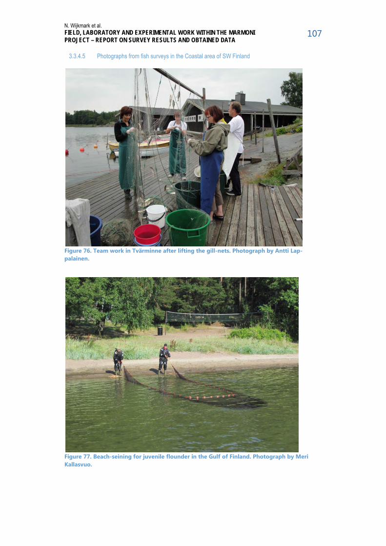
N. Wijkmark et al. FIELD, LABORATORY AND EXPERIMENTAL WORK WITHIN THE MARMONI PROJECT – REPORT ON SURVEY RESULTS AND OBTAINED DATA
107
3.3.4.5 Photographs from fish surveys in the Coastal area of SW Finland
Figure 76. Team work in Tvärminne after lifting the gill-nets. Photograph by Antti Lap-palainen.
Figure 77. Beach-seining for juvenile flounder in the Gulf of Finland. Photograph by Meri Kallasvuo.

N. Wijkmark et al. FIELD, LABORATORY AND EXPERIMENTAL WORK WITHIN THE MARMONI PROJECT – REPORT ON SURVEY RESULTS AND OBTAINED DATA
108
Figure 78. Paired Gulf samplers are used to sample newly-hatched pikeperch larvae. Photo-graph by Taija Pöntinen.
Figure 79. 5-mm-long pikeperch larvae caught in Gulf samplings. Photograph by Lauri Urho.

N. Wijkmark et al. FIELD, LABORATORY AND EXPERIMENTAL WORK WITHIN THE MARMONI PROJECT – REPORT ON SURVEY RESULTS AND OBTAINED DATA
109
3.4 Surveys of the pelagic community
3.4.1 Pelagic surveys in Latvia: 1EST-LAT Irbe Strait and the Gulf of Riga Pelagic community field data were collected in the MARMONI project area 1EST-LAT to verify new field methods for phytoplankton monitoring purposes and test the indicators “3.1 Phytoplankton species assemblage clusters based on environmental factors”, “3.6 Spring bloom intensity index” and “3.10 Zooplankton mean size vs. total stock (MSTS)” developed in the framework of the MARMONI project.
3.4.1.1 Maps of pelagic surveys in the Irbe Strait and the Gulf of Riga
Figure 80. Phytoplankton sampling sites in Project area 1EST-LAT in the Gulf of Riga

N. Wijkmark et al. FIELD, LABORATORY AND EXPERIMENTAL WORK WITHIN THE MARMONI PROJECT – REPORT ON SURVEY RESULTS AND OBTAINED DATA
110
3.4.1.2 Obtained data from pelagic community in the Irbe Strait and the Gulf of Riga
To test the applicability of the hyperspectral airborne remote sensing and ferrybox meth-ods for pelagic community monitoring purposes as well as to collect data for pelagic indi-cator testing, two field campaigns were performed. From 14 to 19 May 2012, a field cam-paign was performed to collect phytoplankton and zooplankton data in 16 monitoring stations for detailed species analysis and testing of indicators, and to collect chlorophyll a data in 29 monitoring stations for calibration of remote sensing data, which is a new monitoring method in the Gulf of Riga. In addition, desktop analyses related to develop-ing of indicator “3.1 Phytoplankton species assemblage clusters based on environmental factors” have been performed with 405 phytoplankton samples collected in the Gulf of Riga between 1993 and 2012. From March till May 2014, a field campaign was performed to collect 66 samples (once per week) from the ferrybox sampling system installed on board of Tallink ship “Roman-tika”. Collected water samples were used for phytoplankton, primary production, chloro-phyll a and nutrient analysis and testing of phytoplankton indicator “3.6 Spring bloom intensity index”.
3.4.1.3 Photographs from pelagic surveys in the Irbe Strait and the Gulf of Riga
Figure 81. Zooplankton sampling in the Project area 1 EST-LAT in the Gulf of Riga (Photo I. Purina).

N. Wijkmark et al. FIELD, LABORATORY AND EXPERIMENTAL WORK WITHIN THE MARMONI PROJECT – REPORT ON SURVEY RESULTS AND OBTAINED DATA
111
Figure 82. Pelagic habitat sampling in the Project area 1 EST-LAT in the Gulf of Riga (Photo I. Purina)

N. Wijkmark et al. FIELD, LABORATORY AND EXPERIMENTAL WORK WITHIN THE MARMONI PROJECT – REPORT ON SURVEY RESULTS AND OBTAINED DATA
112
3.4.2 Pelagic surveys in Estonia: 1EST-LAT Eastern part of Gulf of Riga In three different areas Kõiguste, Sõmeri and Orajõe (Figure 83) 18 sampling points were visited twice a month from May to November 2013. Sampling points were selected ac-cording to phytobenthos transects, and were situated in the beginning (at about 1m depth) and at the end of the transect (7-10m depth) (Figure 84). Distance between tran-sects were about 200 m. Every time integrated phytoplankton, chlorophyll a and nutrient samples were collected. Also CTD profile and Secchi depths were measured. Table 13. Coordinates of sampling points.
Location station name lat lon
Kõiguste KMAR1m 58,36214 22,98955
KMAR1s 58,33451 22,98397
KMAR2m 58,36085 22,99482
KMAR2s 58,31909 23,02027
KMAR3m 58,35917 23,00415
KMAR3s 58,33518 23,00582
Orajõe OMAR1m 57,96193 24,39635
OMAR1s 57,95234 24,33544
OMAR2m 57,95700 24,39111
OMAR2s 57,95698 24,33433
OMAR3m 57,96113 24,39652
OMAR3s 57,96152 24,35972
Sõmeri SMAR1m 58,35903 23,74397
SMAR1s 58,35886 23,70987
SMAR2m 58,35468 23,74076
SMAR2s 58,35470 23,71204
SMAR3m 58,35141 23,73430
SMAR3s 58,35049 23,71320
In laboratory chlorophyll a samples were filtered through Whatman GF/F filters. Filtered material was extracted in the dark with 96% ethanol overnight and chl a was quantified spec-trophotometrically. Phytoplankton samples were fixed with acid Lugol’s solution, species composition is analysed using Utermöhl technique and wet weight biomass is calculated from phytoplankton counts.

N. Wijkmark et al. FIELD, LABORATORY AND EXPERIMENTAL WORK WITHIN THE MARMONI PROJECT – REPORT ON SURVEY RESULTS AND OBTAINED DATA
113
3.4.2.1 Maps of pelagic surveys in the the Eastern part of Gulf of Riga
Figure 83. Location of sampling areas in the Gulf of Riga.
Figure 84. Layout scheme of the sampling points in Sõmeri. Altogether 216 phytoplankton, 216 chl a and 216 nutrient samples were collected during the year 2013.
N. Wijkmark et al. FIELD, LABORATORY AND EXPERIMENTAL WORK WITHIN THE MARMONI PROJECT – REPORT ON SURVEY RESULTS AND OBTAINED DATA
114
3.4.3 Pelagic surveys in Sweden: 2SWE Hanö Bight
The hydroacoustic survey of pelagic fish (described in section 3.3.3.2.1) was designed to also provide data for zooplankton and jellyfish in the area. See section 3.1.2.7 for more information on the method. The data was used in spatial modelling in the Hanö Bight.
3.4.3.1 Maps of pelagic surveys in the Hanö Bight See map in section 3.3.3.2.1.
3.4.3.2 Obtained data from pelagic community in the Hanö Bight 140 km hydroacoustic transects of with mesozooplankton, macrozooplankton and jellyfish data were collected.
3.4.4 Pelagic surveys in Finland: 3FIN Coastal area of SW Finland Finnish field work for investigating the pelagic communities (zooplankton and phyto-plankton) covered both MARMONI project areas 3FIN and 4FIN-EST as well as nearby sea areas in the northern Baltic proper and the Gulf of Finland. When required in order to perform the work successfully, the strict (and in terms of the geographical area arbitrary) borders of the MARMONI areas were deviated from. For convenience, all Finnish pelagic field and experimental work, except the Algaline FerryBox sampling performed in Finnish-Estonian cooperation, are reported here under area 3FIN.
3.4.4.1 Zooplankton The aim of this zooplankton field work was to assess the applicability of novel zooplank-ton sampling and analysis methodology, namely the Continuous Plankton Recorder and Automatic Classification (CPR-AC) method, ZooImage, in the Baltic Sea (see sections 3.1.2.3 and 3.1.2.4). The work consisted of field work, laboratory analyses, and desktop work. The zooplankton field work was carried out onboard r/v Aranda in August 2011 and 2012 in the MARMONI project areas 3FIN and 4FIN-EST as well as in other nearby coastal and open sea areas (Figure 85). The CPR method was used to collect zooplankton samples on 10 transects. CPR was towed behind r/v Aranda with 2.5 knots speed in different water layers to obtain zooplankton samples from above and below thermocline. In addition, routine zooplankton net (with vertical tows of WP-2 net) samples were taken from 3 dif-ferent water layers at each station (13 stations, Figure 85) close to the CPR transects ac-cording to HELCOM COMBINE monitoring manual (HELCOM 2014; from the bottom to the halocline, the halocline to the thermocline, the thermocline to the surface). Samples collected with CPR and by WP-2 net tows were compared in testing the semi-automatic image analysis method. In the laboratory, scanning and classifying of the zooplankton using the Automatic Classi-fication software ZooImage took place from September 2012 to February 2013. CPR sam-ples (8 samples) as well as conventional zooplankton net samples (8 samples) were util-ized. A relevant part of the work constituted building a training set for species identifica-tion. The performance of the training set was enhanced by picking individuals of only one species at the time by hand using a microscope. The images of these individuals were then added to the training set.

N. Wijkmark et al. FIELD, LABORATORY AND EXPERIMENTAL WORK WITHIN THE MARMONI PROJECT – REPORT ON SURVEY RESULTS AND OBTAINED DATA
115
The method testing was carried out with co-operation by Dr. Jose A. Fernandes (Plymouth Marine Laboratory, U.K.) and Dr. Eneko Bachiller (Institute of Marine Research, Norway), who have developed methodologies based on automatic classification and applied them to other ecosystems. Hence the expected results included research and development of methodology to collect spatially extensive data to support the HELCOM COMBINE zoo-plankton monitoring programme, as well as an understanding of whether Baltic Sea zoo-plankton can be determined using the scanner and semi-automatic identification method. The zooplankton work within Action A3 was performed successfully and without any un-resolvable problems. The CPR turned out not to add cost-efficiency to zooplankton moni-toring and therefore traditional net samples should be used in the future as well. How-ever, the semi-automatic image analysis method gave promising results for Baltic Sea zooplankton and could be promoted as a method for obtaining data for zooplankton indicators, i.e. the MARMONI indicators "3.7 Copepod biomass", "3.9 Microphagous meso-zooplankton biomass" and "3.10 Zooplankton mean size versus total stock (MSTS)".
3.4.4.1.1 Reference: HELCOM COMBINE monitoring manual
3.4.4.2 Phytoplankton The aim of this work was to analyse how phytoplankton taxonomic diversity is reflected in cost-efficient optical and chemotaxonomical detection methods, in particular pigment HPLC, flowCAM particle imaging, and scanning flow-cytometry. Field sampling and in situ data collection were carried out onboard r/v Aranda during spring (April) and summer months (July, August) of 2010–2012. Only sample and data analysis were supported within the MARMONI project and part of the data set overlaps with MARMONI areas 3FIN and 4FIN-EST (Figure 85). Other projects contributing to the analysis of the data are GES-REG (Good Environmental Status Through Regional Coordi-nation And Capacity Building, http://gesreg.msi.ttu.ee/en/) and DEVOTES (DEVelopment Of innovative Tools for understanding marine biodiversity and assessing good Environ-mental Status, http://www.devotes-project.eu/). Water samples for light microscopical analysis of phytoplankton species composition were collected from 3 m depth and fixed with acid Lugol’s solution. No nets or filters were used. A small number of samples were obtained from an integrated depth sample taken between 0–10 meters. Samples were stored for up to two years prior to counting follow-ing the Utermöhl method and following HELCOM protocols. Water samples for flow cy-tometry and FlowCAM were analysed on-board during the day of sampling. The flow cytometer was a Cytosense desktop Cytobuoy equipped with one laser and orange and red emission filters, courtesy of NIOZ (The Netherlands). The FlowCAM (by Fluid Imaging Technologies) was used at 10x magnification, recording RGB images. Pigment analysis by HPLC (up to 20 diagnostic pigments) was carried out from flash-frozen samples concen-trated onto glass fibre filters (details on the HPLC analysis protocol are excluded for brev-ity, but available as a separate document).

N. Wijkmark et al. FIELD, LABORATORY AND EXPERIMENTAL WORK WITHIN THE MARMONI PROJECT – REPORT ON SURVEY RESULTS AND OBTAINED DATA
116
The analyses reported on in this report are based on light microscopic analysis of phyto-plankton species composition, and data analysis of HPLC pigments, FlowCAM images, and flow cytometric data. The FlowCAM observations were subjected to classification algo-rithms using Visualspreadsheet (by the instrument manufacturer) as well as the independ-ently developed PhytoImage software. This led to an improved sample handling and analysis protocol so that future semi-automatic classification can be improved. However, the method used to collect FlowCAM observations during the cruises was considered unsuitable for further taxonomic classification, at least within the available time. FlowCAM image analysis is therefore not reported on further. The flow cytometry, light microscopy, and HPLC pigment data sets were analysed for phytoplankton diversity, and comparisons between the data sources were made. Flow cytometric data were only available for samples collected in summer, whereas the other sets included both spring and summer observations. The applicability of these methods in monitoring phytoplankton biodiversity were compared; see section 3.1.2 of the present report. The phytoplankton work described above was performed successfully and re-sulted in conclusions on the suitability of each method. The origin of the data set from multiple sea areas and from cruises that targeted spring and summer blooms raised some difficulties in data interpretation. This was partly due to the sparse nature of the data, and in part due to the inherent selectivity of each of the methods (particle size, extraction efficiency, sensitivity to live cells versus sensitivity to all particles). An analysis of a time-series where patterns in diversity can be shown in each method should better reveal the sensitivity of each method, in future studies. The present work was indeed intended as a first-order comparison of methods for Baltic Sea phytoplankton, and as such did not pose unex-pected problems.

N. Wijkmark et al. FIELD, LABORATORY AND EXPERIMENTAL WORK WITHIN THE MARMONI PROJECT – REPORT ON SURVEY RESULTS AND OBTAINED DATA
117
3.4.4.3 Maps of pelagic surveys in the Coastal area of SW Finland
Figure 85. Zooplankton (2011–2012) and phytoplankton (2010–2012) sampling stations in the northern Baltic proper and the western Gulf of Finland (excluding Algaline FerryBox phyto-plankton sampling, see section 3.4.5, below). The sampling stations are located in both MARMONI project area 3FIN (indicated by grey area to the left) and 4FIN-EST (indicated by grey area to the right), and in nearby sea areas. For phytoplankton diversity analysis, addi-tional stations outside the MARMONI areas were included. Map by Henrik Nygård.
3.4.4.4 Obtained data from pelagic populations in the Coastal area of SW Finland Summarizing; the zooplankton data were collected onboard r/v Aranda at a total of 13 stations with the WP-2 net in August 2011 and 2012, and a total of 10 CPR transects in August 2012. Laboratory work using image-recognition software was performed in 2012–2013. The obtained data were used for:
• Monitoring method development and testing, i.e. the testing of the applicabil-ity of the Continuous Plankton Recorder (CPR) method for zooplankton sampling and indicator development in the Baltic Sea, and the applicability of the Auto-matic Classification (AC) method for the analysis of Baltic Sea zooplankton com-munity composition. The latter resulted in a novel method for monitoring the MARMONI pelagic indicators “3.7 Copepod biomass”, “3.9 Microphagous meso-zooplankton biomass”, and “3.10 Zooplankton mean size vs. total stock (MSTS)”.
The tested methodology is explained in greater detail in section 3.1.2 of the present re-port. Also, a scientific manuscript (Uusitalo et al. in prep.) is being prepared where rec-ommendations are presented on the use of the semi-automatic zooplankton analysis, and on the usability of this methodology for attaining data for zooplankton indicators to help producing ecosystem assessments e.g. for the MSFD.
3.4.4.4.1 Reference Laura Uusitalo, Jose A. Fernandes, Eneko Bachiller, Siru Tasala, Maiju Lehtiniemi: Semi-automated zooplankton classification: a promising tool for the MSFD assessments? (Manuscript in preparation).
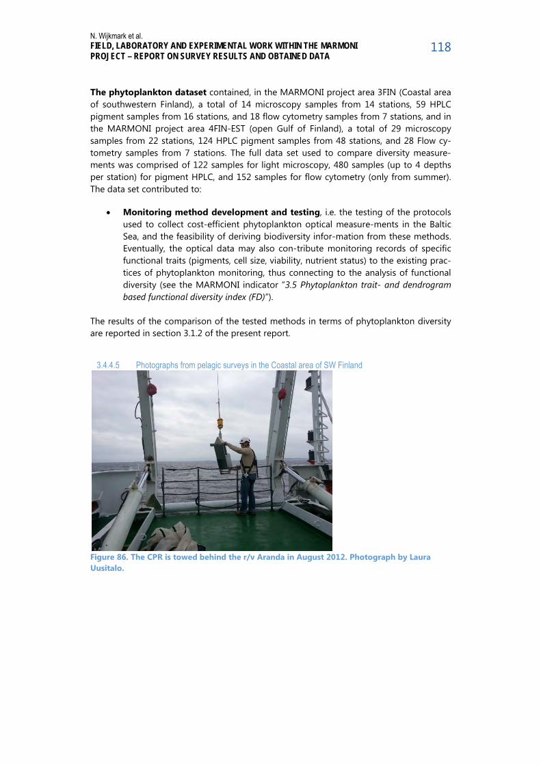
N. Wijkmark et al. FIELD, LABORATORY AND EXPERIMENTAL WORK WITHIN THE MARMONI PROJECT – REPORT ON SURVEY RESULTS AND OBTAINED DATA
118
The phytoplankton dataset contained, in the MARMONI project area 3FIN (Coastal area of southwestern Finland), a total of 14 microscopy samples from 14 stations, 59 HPLC pigment samples from 16 stations, and 18 flow cytometry samples from 7 stations, and in the MARMONI project area 4FIN-EST (open Gulf of Finland), a total of 29 microscopy samples from 22 stations, 124 HPLC pigment samples from 48 stations, and 28 Flow cy-tometry samples from 7 stations. The full data set used to compare diversity measure-ments was comprised of 122 samples for light microscopy, 480 samples (up to 4 depths per station) for pigment HPLC, and 152 samples for flow cytometry (only from summer). The data set contributed to:
• Monitoring method development and testing, i.e. the testing of the protocols used to collect cost-efficient phytoplankton optical measure-ments in the Baltic Sea, and the feasibility of deriving biodiversity infor-mation from these methods. Eventually, the optical data may also con-tribute monitoring records of specific functional traits (pigments, cell size, viability, nutrient status) to the existing prac-tices of phytoplankton monitoring, thus connecting to the analysis of functional diversity (see the MARMONI indicator “3.5 Phytoplankton trait- and dendrogram based functional diversity index (FD)”).
The results of the comparison of the tested methods in terms of phytoplankton diversity are reported in section 3.1.2 of the present report.
3.4.4.5 Photographs from pelagic surveys in the Coastal area of SW Finland
Figure 86. The CPR is towed behind the r/v Aranda in August 2012. Photograph by Laura Uusitalo.

N. Wijkmark et al. FIELD, LABORATORY AND EXPERIMENTAL WORK WITHIN THE MARMONI PROJECT – REPORT ON SURVEY RESULTS AND OBTAINED DATA
119
Figure 87. Image from of zooplankton sample taken with the CPR onboard r/v Aranda in August 2012. Photograph by Laura Uusitalo.
Figure 88. Sampling with the traditional WP-2 zooplankton net onboard r/v Aranda in August 2011. Photograph by Maiju Lehtiniemi.

N. Wijkmark et al. FIELD, LABORATORY AND EXPERIMENTAL WORK WITHIN THE MARMONI PROJECT – REPORT ON SURVEY RESULTS AND OBTAINED DATA
120
Figure 89. R/v Aranda in a rough sea on the pelagic habitats sampling cruise. Photograph by Maiju Lehtiniemi.
Figure 90. Sampling to test new methods for phytoplankton biodiversity assessment was targeted at spring and summer blooms. During summer, surface accummulations of filamen-tous cyanobacteria are common. View from r/v Aranda. Photograph by Stefan Simis.

N. Wijkmark et al. FIELD, LABORATORY AND EXPERIMENTAL WORK WITHIN THE MARMONI PROJECT – REPORT ON SURVEY RESULTS AND OBTAINED DATA
121
Figure 91. In spring, phytoplankton sampling cruises were planned to closely follow the melt of sea ice, when water temperature is still close to freezing. Photograph by Stefan Simis.
Figure 92. Filtration station to collect water samples for (among other parameters) HPLC pigment analysis, onboard r/v Aranda. Photograph by Stefan Simis.

N. Wijkmark et al. FIELD, LABORATORY AND EXPERIMENTAL WORK WITHIN THE MARMONI PROJECT – REPORT ON SURVEY RESULTS AND OBTAINED DATA
122
3.4.5 Pelagic surveys in Estonia and Finland: 4FIN-EST Gulf of Finland
Finnish field work for investigating the pelagic communities (zooplankton and phyto-plankton) covered both MARMONI project areas 3FIN and 4FIN-EST. For simplicity, all Finnish pelagic field and experimental work, except the Algaline FerryBox sampling per-formed in Finnish-Estonian cooperation, are reported in the previous section under area 3FIN.
3.4.5.1 Phytoplankton The aim of this work was to investigate phytoplankton variability in open sea areas during the vegetation period (from April to October) to give further recommendations for ap-propriate spatial phytoplankton sampling resolution. The analysis will be first performed with entire dataset and then by dividing the sampling stations between the two MARMONI areas – the Gulf of Finland and the northern Baltic proper. We assume that the natural spatial variability differs between these two areas requiring different geographical resolution for representative sampling. The work consisted of field work, laboratory analy-ses, and desktop work. The Finnish Environment Institute SYKE participated in collecting the Algaline FerryBox phytoplankton samples, while the Estonian Marine Institute per-formed the laboratory analysis of samples and statistical analysis of the counting results. The statistical treatment of obtained results is still ongoing. The field work consisted of Algaline FerryBox phytoplankton sampling performed simul-taneously onboard the passenger ferries m/s Finnmaid (travelling between Helsinki and Travemünde), m/s Silja Serenade (Helsinki–Stockholm), and m/s Victoria (Tallinn–Stockholm). In 2012, a total of 98 samples were collected on 7 sampling events at 15 sta-tions in MARMONI project areas 3FIN and 4FIN-EST, as well as in nearby sea areas in the northern Baltic proper and the western Gulf of Finland (Figure 93). Water was pumped through an inlet from a depth of about 5 m onboard the moving ship. The samples for laboratory analysis were taken with automatic water samplers (Figure 94). In addition to phytoplankton samples, data on physiochemical parameters were collected. Water tem-perature, salinity and in vivo fluorescence were recorded quasi-continuously with a spatial resolution of approximately 300–400 m, while the concentrations of nutrients (PO4-P, NO2+NO3-N, SiO4-Si, totN and totP) were analyzed from water samples. In the labora-tory, phytoplankton species composition was analysed and wet weight biomass was cal-culated from the phytoplankton counting results. The phytoplankton work described above was performed successfully and with only mi-nor problems. Depending on the schedules we could not guarantee the simultaneous (within 24–48 hrs) sampling from all three ferries for all events. The largest time span be-tween the earliest and latest monthly sampling was seven days in September. A minor but unfortunate setback was caused by seven samples being broken during the transporta-tion from Finland to Estonia.

N. Wijkmark et al. FIELD, LABORATORY AND EXPERIMENTAL WORK WITHIN THE MARMONI PROJECT – REPORT ON SURVEY RESULTS AND OBTAINED DATA
123
3.4.5.2 Maps of pelagic surveys in the Gulf of Finland
Figure 93. Algaline FerryBox phytoplankton sampling stations sampled in 2011–2013 from the three passenger ferries. The sampling stations are located in MARMONI project areas 3FIN (Archipelago Sea) and 4FIN-EST (Gulf of Finland) and in nearby sea areas in the northern Baltic proper and the western Gulf of Finland. Map by Ivan Kuprijanov (EMI).
3.4.5.3 Obtained data from pelagic community in the Gulf of Finland Summarizing; the Algaline FerryBox phytoplankton data were collected on a total of 7 sampling events at 15 stations in 2012. Laboratory work was performed in 2011–2013. The obtained data were used for monitoring method development and testing.

N. Wijkmark et al. FIELD, LABORATORY AND EXPERIMENTAL WORK WITHIN THE MARMONI PROJECT – REPORT ON SURVEY RESULTS AND OBTAINED DATA
124
3.4.5.4 Photographs from pelagic surveys in the Gulf of Finland
Figure 94. Flow-through equipment and automatic water sampler onboard m/s Victoria I. Photograph by Ivan Kuprijanov.

N. Wijkmark et al. FIELD, LABORATORY AND EXPERIMENTAL WORK WITHIN THE MARMONI PROJECT – REPORT ON SURVEY RESULTS AND OBTAINED DATA
125
3.5 Bird surveys
3.5.1 Bird surveys in Latvia: 1EST-LAT Irbe Strait and the Gulf of Riga Bird surveys in the Latvian part of the study area 1 EST-LAT “Riga Gulf and Irbe Strait” were carried out in whole territory of the study area using 3 “classical” data collection methods (counting birds from ground, ship and plane) along with an innovative method (imaging). Surveys were carried out in different seasons. All the methods were used to collect data needed for development and testing of marine biodiversity indicators related to birds as well as to compare effectiveness and applicability of different methods in dif-ferent seasons and circumstances.
3.5.1.1 Bird counts from ground Bird counts from ground were carried out to collect data on numbers and distribution of species with coastal distribution. Data collection took place in wintering season (January) as well as in the breeding/post-breeding season (June and July). The ground counting routes were placed along the coast of Riga Gulf and Irbe Strait (Figure 95). The obtained data was used for development and testing of the indicators related to wintering and breeding seasons for those species where method is applicable (i.e. species with very coastal distribution such as Goldeneye or Goosander) or as supplementary data for spe-cies with more offshore distribution. Data was used for the following indicators: 4.1 Abundance index of wintering waterbird species 4.2 Wintering waterbird index (WWBI) 4.3 Wintering indices for waterbirds of different feeding guilds (WWBIFG) 4.4 Abundance index of breeding waterbird species 4.5 Breeding waterbird index (BWBI) 4.6 Distribution of wintering waterbird species 4.9 Distribution of breeding waterbird species
3.5.1.2 Bird counts from ship Bird counts from ship were carried out in all parts of the study area in different seasons, except the winter season. The winter season was not used due to extremely short days preventing from cost-effective use of ship and due to ice and weather constraints. Ship counts were used all project years, except 2012 as no suitable ship was available to field-workers in that year. Ship availability in combination with weather constraints was the reason why some of works were postponed until spring 2014. The collected data was used for comparison of effectiveness and applicability of different data collection methods as well as to collect data for the indicator 4.11 Age/sex ratio of waterbird species (ARI/SRI)
3.5.1.3 Bird counts from plane Bird counts from plane were carried out in all parts of the study area in all seasons. The plane counting routes in 2011 – 2013 were placed so that they cover the same areas where data collection from ship and data imaging from plane was carried out (Figure 96

N. Wijkmark et al. FIELD, LABORATORY AND EXPERIMENTAL WORK WITHIN THE MARMONI PROJECT – REPORT ON SURVEY RESULTS AND OBTAINED DATA
126
to Figure 105). The counting routes for plane in winter 2014 were placed so that they systematically cover the whole Latvian part of the study area. (Figure 106).
The obtained data was used for development and testing of the indicators related to win-tering and breeding seasons for those species where method is applicable (i.e. species with very coastal distribution such as Goldeneye or Goosander) or as supplementary data for species with more offshore distribution.
The collected data was used for comparison of effectiveness and applicability of different data collection methods as well as to collect data for the following indicators:
4.1 Abundance index of wintering waterbird species 4.2 Wintering waterbird index (WWBI) 4.3 Wintering indices for waterbirds of different feeding guilds (WWBIFG) 4.6 Distribution of wintering waterbird species 4.7 Distribution of wintering waterbirds (multi-species) 4.8 Distribution of wintering waterbirds of different feeding guilds (multi-
species)
3.5.1.4 Maps of bird surveys in the Irbe Strait and the Gulf of Riga
Figure 95. Route of bird counts from ground in winters 2012 – 2014 and spring and summer 2011 – 2013.

N. Wijkmark et al. FIELD, LABORATORY AND EXPERIMENTAL WORK WITHIN THE MARMONI PROJECT – REPORT ON SURVEY RESULTS AND OBTAINED DATA
127
Figure 96. Route of bird counts from ship in Spring 2011.
Figure 97. Route of bird counts from ship in Autumn 2011.

N. Wijkmark et al. FIELD, LABORATORY AND EXPERIMENTAL WORK WITHIN THE MARMONI PROJECT – REPORT ON SURVEY RESULTS AND OBTAINED DATA
128
Figure 98. Route of bird counts from ship in Spring 2013.
Figure 99. Route of bird counts from ship in Summer 2013.

N. Wijkmark et al. FIELD, LABORATORY AND EXPERIMENTAL WORK WITHIN THE MARMONI PROJECT – REPORT ON SURVEY RESULTS AND OBTAINED DATA
129
Figur 100. Route of bird counts from ship in Spring 2013.
Figure 101. Transects of bird counts from plane in Spring 2011.
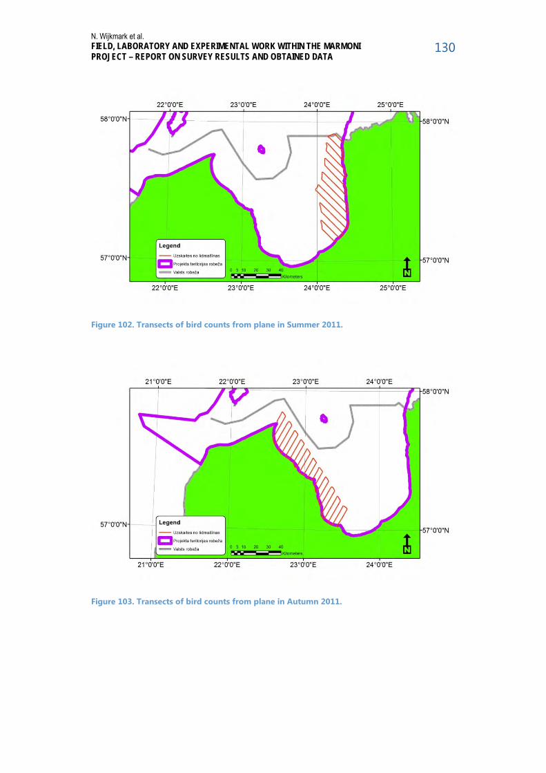
N. Wijkmark et al. FIELD, LABORATORY AND EXPERIMENTAL WORK WITHIN THE MARMONI PROJECT – REPORT ON SURVEY RESULTS AND OBTAINED DATA
130
Figure 102. Transects of bird counts from plane in Summer 2011.
Figure 103. Transects of bird counts from plane in Autumn 2011.

N. Wijkmark et al. FIELD, LABORATORY AND EXPERIMENTAL WORK WITHIN THE MARMONI PROJECT – REPORT ON SURVEY RESULTS AND OBTAINED DATA
131
Figure 104. Transects of bird counts from plane in Spring 2012.
Figure 105. Transects of bird counts from plane in Spring 2012.

N. Wijkmark et al. FIELD, LABORATORY AND EXPERIMENTAL WORK WITHIN THE MARMONI PROJECT – REPORT ON SURVEY RESULTS AND OBTAINED DATA
132
Figure 106. Transects of bird counts from plane in Winter 2014.

N. Wijkmark et al. FIELD, LABORATORY AND EXPERIMENTAL WORK WITHIN THE MARMONI PROJECT – REPORT ON SURVEY RESULTS AND OBTAINED DATA
133
3.5.1.5 Obtained bird data from in the Irbe Strait and the Gulf of Riga
3.5.1.5.1 Distribution and numbers of waterbirds in the wintering season The following species distribution maps show bird observations recorded during the fieldwork. Maps are given separately for different species (or species groups) and different years (Figure 107 to Figure 122).
In total 22 point layers of bird locations were created for the wintering season.
Figure 107. Wintering distribution of Common Goldeneye Bucephala clangula in winters 2012 (top) and 2013 (bottom).

N. Wijkmark et al. FIELD, LABORATORY AND EXPERIMENTAL WORK WITHIN THE MARMONI PROJECT – REPORT ON SURVEY RESULTS AND OBTAINED DATA
134
Figure 108. Wintering distribution of Long-tailed Duck Clangula hyemalis in winters 2012 (top) and 2013 (bottom).

N. Wijkmark et al. FIELD, LABORATORY AND EXPERIMENTAL WORK WITHIN THE MARMONI PROJECT – REPORT ON SURVEY RESULTS AND OBTAINED DATA
135
Figure 109. Wintering distribution of Velvet Scoter Melanitta fusca in winters 2012 (top) and 2013 (bottom).

N. Wijkmark et al. FIELD, LABORATORY AND EXPERIMENTAL WORK WITHIN THE MARMONI PROJECT – REPORT ON SURVEY RESULTS AND OBTAINED DATA
136
Figure 110. Wintering distribution of Common Scoter Melanitta nigra in winters 2012 (top) and 2013 (bottom).
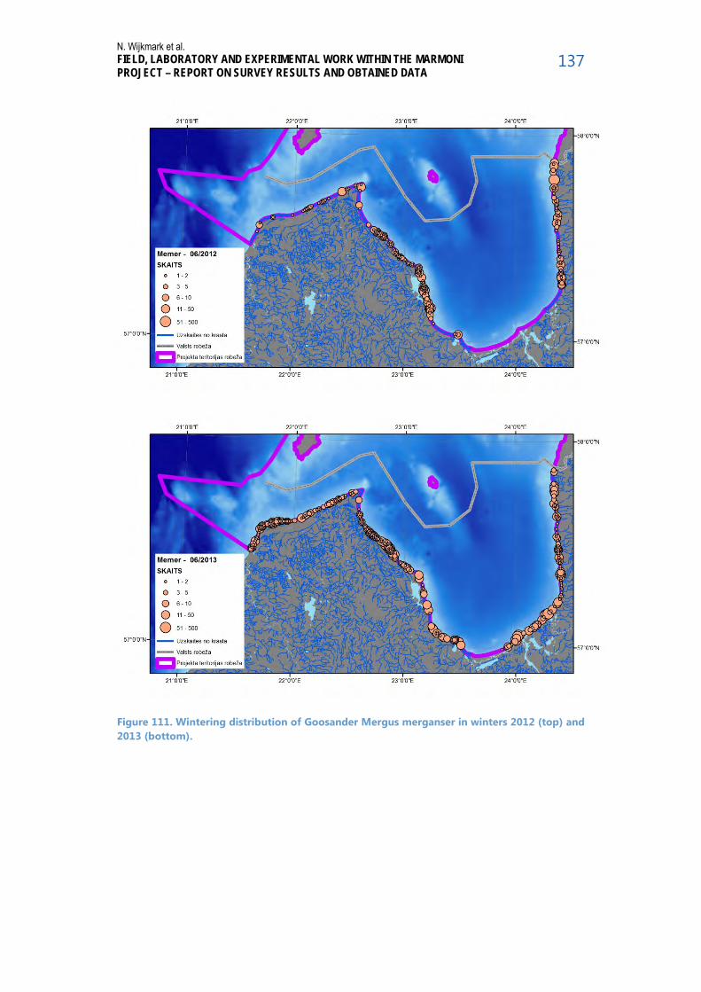
N. Wijkmark et al. FIELD, LABORATORY AND EXPERIMENTAL WORK WITHIN THE MARMONI PROJECT – REPORT ON SURVEY RESULTS AND OBTAINED DATA
137
Figure 111. Wintering distribution of Goosander Mergus merganser in winters 2012 (top) and 2013 (bottom).

N. Wijkmark et al. FIELD, LABORATORY AND EXPERIMENTAL WORK WITHIN THE MARMONI PROJECT – REPORT ON SURVEY RESULTS AND OBTAINED DATA
138
Figure 112. Wintering distribution of Red-breasted Merganser Mergus serrator in winters 2012 (top) and 2013 (bottom).
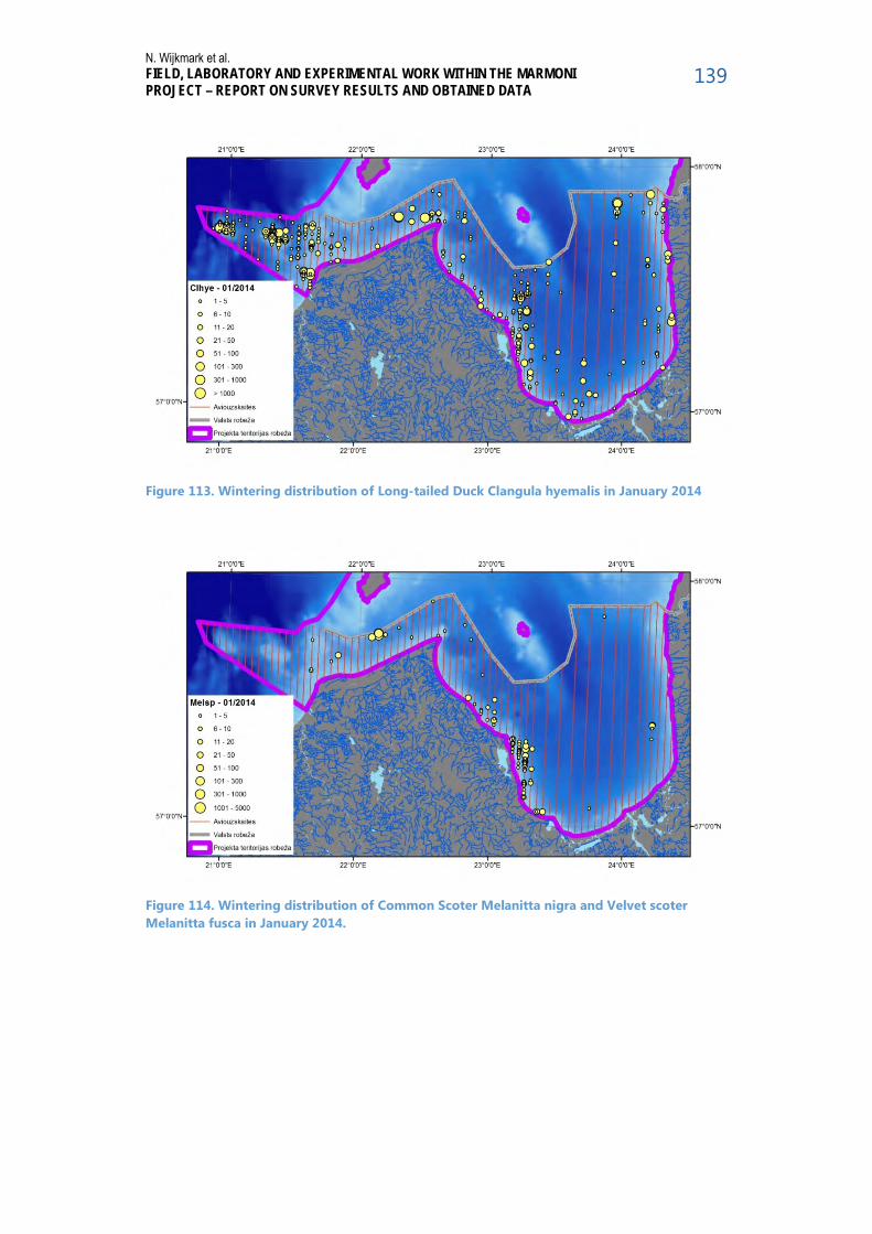
N. Wijkmark et al. FIELD, LABORATORY AND EXPERIMENTAL WORK WITHIN THE MARMONI PROJECT – REPORT ON SURVEY RESULTS AND OBTAINED DATA
139
Figure 113. Wintering distribution of Long-tailed Duck Clangula hyemalis in January 2014
Figure 114. Wintering distribution of Common Scoter Melanitta nigra and Velvet scoter Melanitta fusca in January 2014.

N. Wijkmark et al. FIELD, LABORATORY AND EXPERIMENTAL WORK WITHIN THE MARMONI PROJECT – REPORT ON SURVEY RESULTS AND OBTAINED DATA
140
Figure 115. Wintering distribution of Common Goldeneye Bucephala clangula in January 2014
Figure 116. Wintering distribution of benthos feeding bird species in January 2014

N. Wijkmark et al. FIELD, LABORATORY AND EXPERIMENTAL WORK WITHIN THE MARMONI PROJECT – REPORT ON SURVEY RESULTS AND OBTAINED DATA
141
Figure 117. Wintering distribution of divers (Gavia sp) in January 2014
Figur 118. Wintering distribution of Goosanders (Mergus merganser) and Red-breasted Mer-gansers (M. serrator) in January 2014.

N. Wijkmark et al. FIELD, LABORATORY AND EXPERIMENTAL WORK WITHIN THE MARMONI PROJECT – REPORT ON SURVEY RESULTS AND OBTAINED DATA
142
Figur 119. Wintering distribution of fish feeding species (divers, grebes, mergansers, auks) in January 2014
Figur 120. Wintering distribution of swans (Cygnus sp; mostly C. olor) in January 2014

N. Wijkmark et al. FIELD, LABORATORY AND EXPERIMENTAL WORK WITHIN THE MARMONI PROJECT – REPORT ON SURVEY RESULTS AND OBTAINED DATA
143
Figure 121. Wintering distribution of Little Gull (Larus minutus) in January 2014
Figure 122. Wintering distribution of Common Gull (Larus canus) and Herrihg Gull (L. argen-tatus) in January 2014
Breeding and postbreeding distribution
Breeding and postbreeding distribution was recorded in June and July when the species breeding along the seacoast have highest detection probability – their territorial behav-iour or presence of their chicks make them very noticeable. Only birds attributed to breeding are shown on the maps below (Figure 123 to Figure 129).
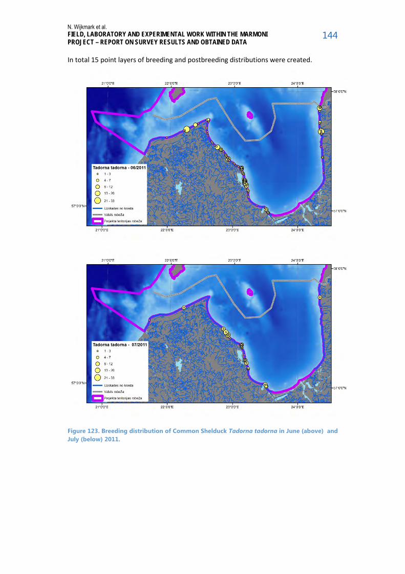
N. Wijkmark et al. FIELD, LABORATORY AND EXPERIMENTAL WORK WITHIN THE MARMONI PROJECT – REPORT ON SURVEY RESULTS AND OBTAINED DATA
144
In total 15 point layers of breeding and postbreeding distributions were created.
Figure 123. Breeding distribution of Common Shelduck Tadorna tadorna in June (above) and July (below) 2011.

N. Wijkmark et al. FIELD, LABORATORY AND EXPERIMENTAL WORK WITHIN THE MARMONI PROJECT – REPORT ON SURVEY RESULTS AND OBTAINED DATA
145
Figure 124. Breeding distribution of Common Shelduck Tadorna tadorna in June (above) and July (below) 2012.

N. Wijkmark et al. FIELD, LABORATORY AND EXPERIMENTAL WORK WITHIN THE MARMONI PROJECT – REPORT ON SURVEY RESULTS AND OBTAINED DATA
146
Figure 125. Breeding distribution of Common Shelduck Tadorna tadorna in June (above) and July (below) 2013.

N. Wijkmark et al. FIELD, LABORATORY AND EXPERIMENTAL WORK WITHIN THE MARMONI PROJECT – REPORT ON SURVEY RESULTS AND OBTAINED DATA
147
Figure 126. Breeding distribution of Little Riged Plover Charadrius dubius (above) and Ringed Plover Charadrius hiaticula (below) in June 2011.

N. Wijkmark et al. FIELD, LABORATORY AND EXPERIMENTAL WORK WITHIN THE MARMONI PROJECT – REPORT ON SURVEY RESULTS AND OBTAINED DATA
148
Figure 127. Breeding distribution of Little Riged Plover Charadrius dubius (above) and Ringed Plover Charadrius hiaticula (below) in June 2012.

N. Wijkmark et al. FIELD, LABORATORY AND EXPERIMENTAL WORK WITHIN THE MARMONI PROJECT – REPORT ON SURVEY RESULTS AND OBTAINED DATA
149
Figure 128. Breeding distribution of Little Riged Plover Charadrius dubius (above) and Ringed Plover Charadrius hiaticula (below) in June 2013.

N. Wijkmark et al. FIELD, LABORATORY AND EXPERIMENTAL WORK WITHIN THE MARMONI PROJECT – REPORT ON SURVEY RESULTS AND OBTAINED DATA
150
Figure 129. Post-breeding distribution of Goldeneye Bucephala clangula in July 2011 (avio and ground counts combined; top), July 2012 (ground counts; middle) and July 2013 (ground counts; bottom).

N. Wijkmark et al. FIELD, LABORATORY AND EXPERIMENTAL WORK WITHIN THE MARMONI PROJECT – REPORT ON SURVEY RESULTS AND OBTAINED DATA
151
3.5.1.6 Photographs from bird surveys in the Irbe Strait and the Gulf of Riga The following set of pictures describe the fieldwork carried out during the project. They show both the study objects themselves as well as the researchers during the data col-lection process.
Figure 130. Male (left) and female (right) Long-tailed ducks in spring plumage near Mērsrags (Gulf of Riga) (photo by A. Aunins)

N. Wijkmark et al. FIELD, LABORATORY AND EXPERIMENTAL WORK WITHIN THE MARMONI PROJECT – REPORT ON SURVEY RESULTS AND OBTAINED DATA
152
Figure 131. Male Long-tailed duck in winter plumage near Roja (Gulf of Riga) (photo by A. Aunins)
Figure 132. Flocks of migrating and staging Long-tailed Ducks in the southwestern part of the Riga Gulf (photo by A. Aunins).

N. Wijkmark et al. FIELD, LABORATORY AND EXPERIMENTAL WORK WITHIN THE MARMONI PROJECT – REPORT ON SURVEY RESULTS AND OBTAINED DATA
153
Figure 133. A flock of wintering Goldeneyes (photo by A. Aunins)
Figure 134. A flock of migrating Common Scoters (photo by A. Aunins)
Figure 135. A flock of migrating Velvet Scoters (photo by A. Aunins)

N. Wijkmark et al. FIELD, LABORATORY AND EXPERIMENTAL WORK WITHIN THE MARMONI PROJECT – REPORT ON SURVEY RESULTS AND OBTAINED DATA
154
Figure 136. Black-throated Diver in Irbe Strait (photo by A. Aunins)
Figure 137. Wintering waterbird counting from ground at the coast of Riga Gulf near Lap-mežciems (photo by A. Aunins).

N. Wijkmark et al. FIELD, LABORATORY AND EXPERIMENTAL WORK WITHIN THE MARMONI PROJECT – REPORT ON SURVEY RESULTS AND OBTAINED DATA
155
Figure 138. Waterbird counting from a ship in Irbe Strait near Kolka (photo by A. Kurochkin)
Figure 139. Collecting photos of seaduck flocks for sex and age ratio calculation (photo by V. Smislov).

N. Wijkmark et al. FIELD, LABORATORY AND EXPERIMENTAL WORK WITHIN THE MARMONI PROJECT – REPORT ON SURVEY RESULTS AND OBTAINED DATA
156
Figure 140. Twin-engine high-winged aircraft used for bird counting over sea in the project.
Figure 141. Bird counter (Antra Stīpniece) in a safety suit recording observations in a hand-held dictaphone during the data collection.

N. Wijkmark et al. FIELD, LABORATORY AND EXPERIMENTAL WORK WITHIN THE MARMONI PROJECT – REPORT ON SURVEY RESULTS AND OBTAINED DATA
157
3.5.2 Bird surveys in Estonia: 1EST-LAT Irbe Strait and the Eastern part of Gulf of Riga
Bird surveys in the Estonian part of the study area 1 EST-LAT “Riga Gulf and Irbe Strait” were carried out in whole territory of the study area using 2 data collection methods (counting birds from ground and plane). Surveys were carried out in different seasons. All the methods were used to collect data needed for development and testing of marine biodiversity indicators related to birds as well as to compare effectiveness and applicabil-ity of different methods in different seasons and circumstances.
3.5.2.1 Bird counts from ground Bird counts from ground were carried out to collect data on numbers and distribution of species with coastal distribution. Data collection took place in wintering (January 2012-2014). The ground counting routes were placed along the coast of Riga Gulf and Irbe Strait (Figure 142). The data were used for development and testing of the indicators re-lated to wintering seasons for those species where method is applicable (species with coastal distribution) or as supplementary data for species with more offshore distribution. Data was used for the following indicators:
4.1 Abundance index of wintering waterbird species 4.2 Wintering waterbird index (WWBI) 4.3 Wintering indices for waterbirds of different feeding guilds (WWBIFG) 4.6 Distribution of wintering waterbird species
3.5.2.2 Breeding bird counts on islands Data collection took place in May-June 2014. The study islands (104 islands) are distrib-uted along the coast of Riga Gulf and Irbe Strait (Figure 143) Data was used for the following indicators: 4.4 Abundance index of breeding waterbird species 4.5 Breeding waterbird index (BWBI) 4.9 Distribution of breeding waterbird species
3.5.2.3 Bird counts from plane Bird counts from plane were carried out both in coastal (all study area) and offshore wa-ters of eastern part of the Gulf of Riga in spring/breeding and post-breeding period. Off-shore transect counts planned on Jan-Feb of 2013 and 2014 were not performed due to extreme weather and ice conditions. The coastal counting aerial route in May 2014 was placed so that they cover the same areas where data collection from ground (islands) was performed in May-June 2014 (Figure 144, see also Figure 143). The aerial transect count in autumn 2012 was performed to cover the eastern part of the study area (Figure 145). The obtained data was used for development and testing of the indicators related to breeding and post-breeding seasons for those species where method is applicable (i.e. species with very coastal distribution) or as supplementary data for species with more offshore distribution. The collected data was used for comparison of effectiveness and applicability of different data collection methods as well as to collect data for the following indicators: 4.4 Abundance index of breeding waterbird species 4.5 Breeding waterbird index (BWBI) 4.9 Distribution of breeding waterbird species

N. Wijkmark et al. FIELD, LABORATORY AND EXPERIMENTAL WORK WITHIN THE MARMONI PROJECT – REPORT ON SURVEY RESULTS AND OBTAINED DATA
158
3.5.2.4 Maps of bird surveys in the Irbe Strait and the Eastern part of Gulf of Riga
Figure 142. Bird counts from ground in winters 2012 – 2014. Counts are performed from fixed points 1-2 km apart according national count units Aa 03 etc.
Figure 143. Distribution of bird islets covered by ground counts on May-June 2014.

N. Wijkmark et al. FIELD, LABORATORY AND EXPERIMENTAL WORK WITHIN THE MARMONI PROJECT – REPORT ON SURVEY RESULTS AND OBTAINED DATA
159
Figure 144. Track of coastal aerial flight in May 2014.
Figure 145. Track of the aerial transect count of bird in September 2012.

N. Wijkmark et al. FIELD, LABORATORY AND EXPERIMENTAL WORK WITHIN THE MARMONI PROJECT – REPORT ON SURVEY RESULTS AND OBTAINED DATA
160
3.5.2.5 Obtained bird data from in the Irbe Strait and the Eastern part of Gulf of Riga
3.5.2.5.1 Distribution and numbers of waterbirds in the wintering season The following species distribution maps (Figure 146Figur 151) show bird observations recorded during the fieldwork in 2012-2013 (2014 in prep.). Maps are given separately for different species (or species groups) and different years.
In total 12 point layers of distribution of birds in the wintering season were created.
Figure 146. Wintering distribution of Common Goldeneye Bucephala clangula in January of mild (2012) and cold winter (2013).

N. Wijkmark et al. FIELD, LABORATORY AND EXPERIMENTAL WORK WITHIN THE MARMONI PROJECT – REPORT ON SURVEY RESULTS AND OBTAINED DATA
161
Figure 147. Wintering distribution of Whooper Swan Cygnus cygnus in January of mild (2012) and cold winter (2013).

N. Wijkmark et al. FIELD, LABORATORY AND EXPERIMENTAL WORK WITHIN THE MARMONI PROJECT – REPORT ON SURVEY RESULTS AND OBTAINED DATA
162
Figure 148. Wintering distribution of Mute Swan Cygnus olor in January of mild (2012) and cold winter (2013).

N. Wijkmark et al. FIELD, LABORATORY AND EXPERIMENTAL WORK WITHIN THE MARMONI PROJECT – REPORT ON SURVEY RESULTS AND OBTAINED DATA
163
Figure 149. Wintering distribution of Smew Mergus albellus in January of mild (2012) and cold winter (2013).

N. Wijkmark et al. FIELD, LABORATORY AND EXPERIMENTAL WORK WITHIN THE MARMONI PROJECT – REPORT ON SURVEY RESULTS AND OBTAINED DATA
164
Figure 150. Wintering distribution of Goosander Mergus merganser in January of mild (2012) and cold winter (2013).

N. Wijkmark et al. FIELD, LABORATORY AND EXPERIMENTAL WORK WITHIN THE MARMONI PROJECT – REPORT ON SURVEY RESULTS AND OBTAINED DATA
165
Figur 151. Wintering distribution of Red-breasted Merganser Mergus serrator in January of mild (2012) and cold winter (2013).
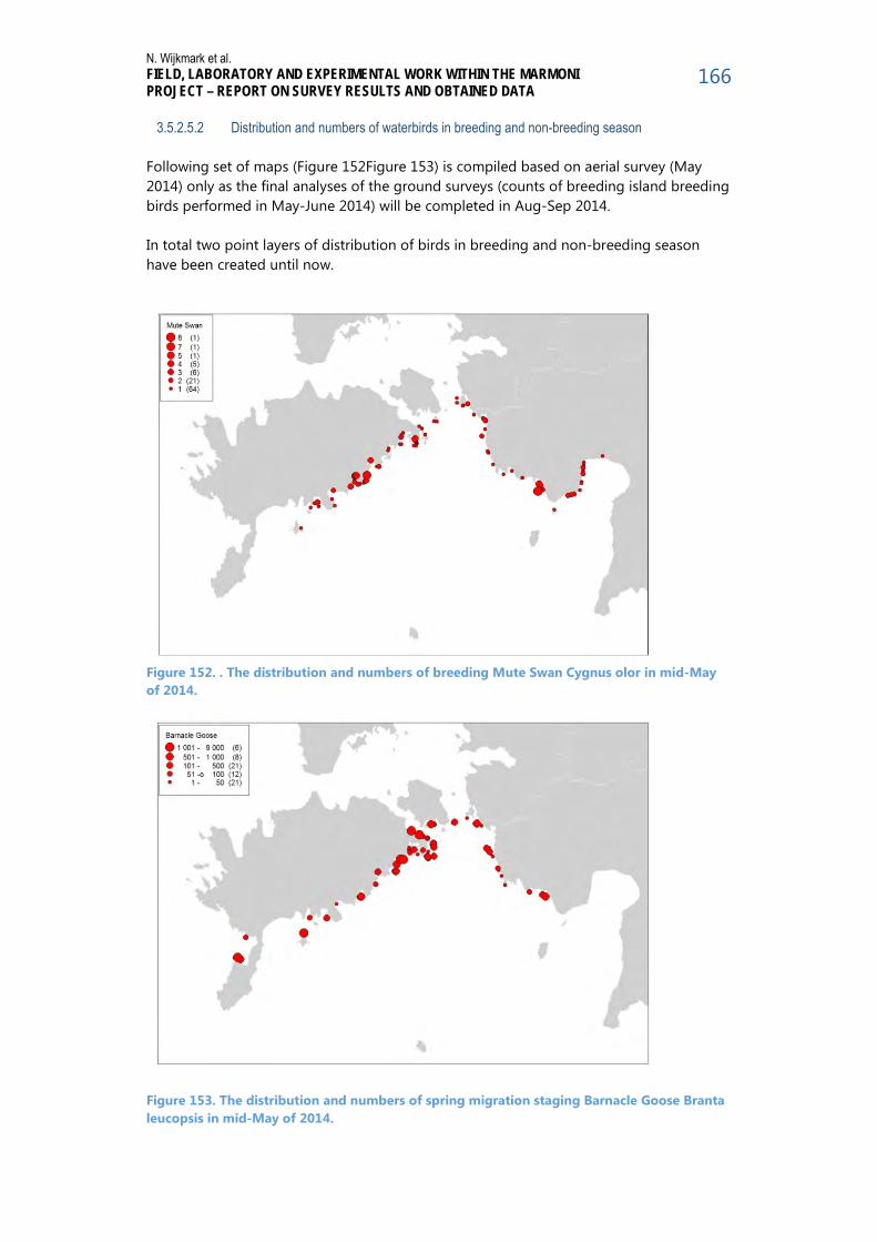
N. Wijkmark et al. FIELD, LABORATORY AND EXPERIMENTAL WORK WITHIN THE MARMONI PROJECT – REPORT ON SURVEY RESULTS AND OBTAINED DATA
166
3.5.2.5.2 Distribution and numbers of waterbirds in breeding and non-breeding season
Following set of maps (Figure 152Figure 153) is compiled based on aerial survey (May 2014) only as the final analyses of the ground surveys (counts of breeding island breeding birds performed in May-June 2014) will be completed in Aug-Sep 2014. In total two point layers of distribution of birds in breeding and non-breeding season have been created until now.
Figure 152. . The distribution and numbers of breeding Mute Swan Cygnus olor in mid-May of 2014.
Figure 153. The distribution and numbers of spring migration staging Barnacle Goose Branta leucopsis in mid-May of 2014.

N. Wijkmark et al. FIELD, LABORATORY AND EXPERIMENTAL WORK WITHIN THE MARMONI PROJECT – REPORT ON SURVEY RESULTS AND OBTAINED DATA
167
3.5.2.6 Photographs from bird surveys in the Irbe Strait and the Eastern part of Gulf of Riga The following set of pictures describe the fieldwork carried out during the project. They show both the study objects themselves as well as the researchers during the data collec-tion process.
Figure 154. Wintering waterbird counting from ground at Saaremaa Island (photo by A. Ku-resoo).

N. Wijkmark et al. FIELD, LABORATORY AND EXPERIMENTAL WORK WITHIN THE MARMONI PROJECT – REPORT ON SURVEY RESULTS AND OBTAINED DATA
168
Figure 155. Estimation of breeding numbers of birds in small islet in South Saaremaa in June 2014 (photo by L. Luigujõe).
Figure 156. Nest search of breeding birds nests in small islet in South Saaremaa in June 2014 (photo by L. Luigujõe).

N. Wijkmark et al. FIELD, LABORATORY AND EXPERIMENTAL WORK WITHIN THE MARMONI PROJECT – REPORT ON SURVEY RESULTS AND OBTAINED DATA
169
Figure 157. Boat expedition to small islets June 2014 (photo by A. Kuresoo).

N. Wijkmark et al. FIELD, LABORATORY AND EXPERIMENTAL WORK WITHIN THE MARMONI PROJECT – REPORT ON SURVEY RESULTS AND OBTAINED DATA
170
Figure 158. Aerial survey (offshore transect count) with Cessna 337 in Sep 2012. Pilot Janus List and bird expert Leho Luigujõe (photo by A. Kuresoo).
Figure 159. Aerial survey (coastal count) with Cessna 172 in May 2014. Bird experts A. Ku-resoo and A. Leito from Estonian Univ. Of Life Sciences (photo by L. Luigujõe).

N. Wijkmark et al. FIELD, LABORATORY AND EXPERIMENTAL WORK WITHIN THE MARMONI PROJECT – REPORT ON SURVEY RESULTS AND OBTAINED DATA
171
Figur 160. Aerial images of islets in South Saaremaa (photos by L. Luigujõe).

N. Wijkmark et al. FIELD, LABORATORY AND EXPERIMENTAL WORK WITHIN THE MARMONI PROJECT – REPORT ON SURVEY RESULTS AND OBTAINED DATA
172
Figure 161. Hatched Mute Swans Cygnus olor on bird islet on June 2014 (photo by L. Luigu-jõe).
Figure 162. Hatched Mallards Anas platyrhynchos on bird islet on June 2014 (photo by L. Luigujõe).

N. Wijkmark et al. FIELD, LABORATORY AND EXPERIMENTAL WORK WITHIN THE MARMONI PROJECT – REPORT ON SURVEY RESULTS AND OBTAINED DATA
173
Figure 163. Barnacle Geese Branta leucopsis adults flying on breeding island of Southern Saaremaa (photo by L. Luigujõe).
Figure 164. Threatened Baltic Dunlin Calidris alpina schinzii breeding in islet of South Saare-maa on June 2014 (photo by L. Luigujõe).
N. Wijkmark et al. FIELD, LABORATORY AND EXPERIMENTAL WORK WITHIN THE MARMONI PROJECT – REPORT ON SURVEY RESULTS AND OBTAINED DATA
174
3.5.3 Bird surveys in Sweden: 2SWE Hanö Bight
The ornithological studies within MARMONI were originally planned to cover the offshore seaducks (mainly the Long-tailed Duck) in Hanöbukten. The wintering waterbirds in the inshore parts of area (the archipelago and open coast) have been counted since 1967 as a part of the International Waterfowl Counts (IWC) coordinated by Wetlands International (Nilsson 2008). This data set has been used within the MARMONI-project to calculate indicators relating to wintering birds. These winter counts are a part of the national bird monitoring program. During the development of bird indicators it was clear that indicators should also be de-veloped to include the breeding seabirds. There were no such time series available from Sweden for this work so the field work within the MARMONI-project was extended to cover the test of methods for a monitoring program of the breeding seabirds in the ar-chipelago. Thus, in 2011 censuses of breeding seabirds were undertaken in three study areas in Hanöbukten. The studies also included the productivity of Eiders in two of the study areas and an aerial survey of breeding Mute Swans in the archipelago. Aerial surveys in Hanöbukten were also part of other studies on seaducks organized by the Swedish National Environment Protection Agency, which produced data that could be used in MARMONI, so resources could be made free for the items added to the project after the application was sent in. In the present report the bird projects undertaken within the MARMONI-project are cov-ered. Data from the IWC in the region are also included to describe the wintering water-bird populations in the inshore areas, which form the basis for the development of “the wintering waterbird indicator”.
Collected data was used for development and testing of the following indicators 4.1 Abundance index of wintering waterbird species 4.2 Wintering waterbird index (WWBI) 4.3 Wintering indices for waterbirds of different feeding guilds (WWBIFG) 4.4 Abundance index of breeding waterbird species 4.6 Distribution of wintering waterbird species 4.7 Distribution of wintering waterbirds (multi-species) 4.8 Distribution of wintering waterbirds of different feeding guilds (multi-species) Collected bird data was also used in analyses for integrated indicator development (more about this in chapter 3.2.3.2).

N. Wijkmark et al. FIELD, LABORATORY AND EXPERIMENTAL WORK WITHIN THE MARMONI PROJECT – REPORT ON SURVEY RESULTS AND OBTAINED DATA
175
3.5.3.1 Maps of bird surveys in the Hanö Bight
Figure 165. Overview of survey areas for the bird studies undertaken in Hanöbukten study area within MARMONI.
Figure 166. Left: The census area for breeding waterbirds Lindö – Hasslö. Right: The census area for breeding waterbirds SE Karlshamn. Islands and skerries covered are marked on the map and assigned an area code.
Figure 167. Map of the census area for breeding waterbirds NE Scania. Islands and skerries covered are marked on the map and assigned an area code. Gruarna (L001), Vållholmen (L002) och Lägerholmen (L003).

N. Wijkmark et al. FIELD, LABORATORY AND EXPERIMENTAL WORK WITHIN THE MARMONI PROJECT – REPORT ON SURVEY RESULTS AND OBTAINED DATA
176
Figure 168. Survey lines in the archipelago of Blekinge used in 2012.
3.5.3.2 Obtained bird data from in the Hanö Bight
3.5.3.2.1 Breeding birds The breeding seabirds were surveyed in three different areas, each covering a group of small islands and skerries in the archipelago (Figure 166 and Figure 167). The areas were covered with boat in late April to establish the number of pairs on the different islands. Waterbirds were counted in all three study areas, whereas gulls were only surveyed in the western area (L001- L003). On the island Vållholmen (L002 in Figure 167) nests were also counted by searching the island by foot on three occasions during the spring. In the two easterly areas a second survey was undertaken in early June to check for the production of young in the Eider. For the ducks the total number of pairs was established on the ba-sis of the total counts of birds in pairs plus groups of males numbering 1-3 males.
3.5.3.2.2 Breeding birds results The breeding bird fauna of the three study areas is shown in Table 14. Gulls and terns were only included in the western study areas, whereas Anatidae were surveyed in all three areas. The western area had large colonies of Herring gull, a species also occurring in the eastern areas where it was not surveyed. Among the Anatidae, Eiders dominated markedly in all three areas. Some islands also had good populations of breeding geese, especially the Greylag Goose but the Barnacle Goose had established a strong colony on one of the islands in the western study area. The Cormorant was not surveyed in 2011, but there is an important colony on Lägerholmen in the western area which had 702 pairs in 2009 and 498 in 2012.

N. Wijkmark et al. FIELD, LABORATORY AND EXPERIMENTAL WORK WITHIN THE MARMONI PROJECT – REPORT ON SURVEY RESULTS AND OBTAINED DATA
177
Table 14. Number of pairs of different species estimated to breed in the three study areas in the Blekinge archipelago in 2011.
Species NE Scania
Karlshamns archipelago
Lindö – Hasslö
Mallard Anas platyrhynchos 20 25 52 Goldeneye Bucephala clangula 0 5 1 Eider Somateria mollissima 652 325 249 Red-breasted Merganser Mergus serrator
0 12 3
Goosander Mergus merganser 0 26 18 Shelduck Tadorna tadorna 0 13 21 Greylag Goose Anser anser 16 83 141 Canada Goose Branta canadensis 4 21 34 Barnacle Goose Branta leucopsis 154 3 7 Mute Swan Cygnus olor 12 22 15 Herring Gull Larus argentatus 847 NOT COUNTED Black-backed Gull Larus marinus 1 Caspian Tern Hydropogne tsche-grava
The productivity of Eiders was low in the Blekinge archipelago with 1.0 and 1.1 respec-tively for the two areas there (Table 15).
Table 15. Number of females and young eiders counted in the two study areas in the Blekinge archipelago in June 2011.
Area Females Young Young/Female SE Karlshamn 562 553 1,0 Lindö-Hasslö 297 322 1,1
At an aerial survey in April 2011 170 stationary pairs (territories) of Mute Swans were lo-cated. 29 of these birds were seen on a nest and others had started with the nest. The survey was actually too early for a swan survey, but it was undertaken in connection with other surveys in the general area.

N. Wijkmark et al. FIELD, LABORATORY AND EXPERIMENTAL WORK WITHIN THE MARMONI PROJECT – REPORT ON SURVEY RESULTS AND OBTAINED DATA
178
Figure 169. Distribution of breeding pairs of Mute Swan Cygnus olor in the Blekinge archipel-ago at an aerial survey in the spring of 2011.
3.5.3.2.3 Wintering birds The international waterfowl counts (IWC) have been undertaken in Sweden every winter since the start in 1967 (Nilsson 2008).
The entire Swedish coast was divided into counting units for the IWC. Each sector covered was counted from the ground by voluntary observers. In 1987 the system was standard-ized and a number of reference areas were established. These areas have then been cov-ered in the same way each year.
The main aim of the counts was to produce data for calculation of annual indices to fol-low the population development of the different species on a national and international level. To get a control of how well the different waterbirds were covered country-wide surveys were undertaken on some occasions, last time was 2004 (Nilsson 2008). These counts were made by a combination of ground counts and aerial surveys. Offshore areas were not covered in this program but special studies were undertaken in 2007 -2011 (Nilsson 2012).
In this report annual indices have been calculated for the more important species as chain-indices, using the standard method from the Swedish IWC (Nilsson 2008). For sites counted two consecutive years the total in year 2 has been calculated as per cent of the total for year 1. This primary percentages have then been recalculated in relation to the base year = 100. The series of primary indices so obtained have then been normalized so that the mean index for a species over the survey period is 100. For further details see Nilsson (2008).
The offshore areas in Hanöbukten (Figure 165) were covered with aerial surveys along line transects on seven occasions between 2007 and 2011. The counts were made from a CESSNA 337 (Figure 175) flying at 180 km/h at an altitude of 50 – 70m. Survey lines were separated by 2 km. Counts were made by two observers covering each side of the plane. Waterbirds were counted in a survey belt extending 200 m on each side of the aircraft. All observations were noted continuously for later transformation to a data base. Navigation was based on a GPS in the aircraft and the actual track was registered on a separate GPS.

N. Wijkmark et al. FIELD, LABORATORY AND EXPERIMENTAL WORK WITHIN THE MARMONI PROJECT – REPORT ON SURVEY RESULTS AND OBTAINED DATA
179
As a complement to the ground counts in the archipelago two aerial surveys were under-taken there in March 2012 (Figure 168). The same method as in the offshore areas was used, but survey lines were separated by 4 km. More surveys were planned but could not be done due to ice conditions in the archipelago.
3.5.3.2.4 Wintering birds results for off-shore areas The wintering waterbird fauna in the offshore areas of Hanöbukten is markedly domi-nated by the Long-tailed Duck (Table 16). Normally Common Scoter and Velvet Scoter are to be found here in moderate numbers, but in 2007 and 2008 large numbers of especially the Common Scoter were found here.
Table 16. Estimated totals for Long-tailed Duck Clangula hyemalis, Common Scoter Melanitta nigra and Velvet Scoter Melanitta fusca at aerial surveys in Hanöbukten 2007 – 2012.
Date Long-tailed Duck Common Scoter Velvet Scoter
2007-03-04 23044 13500 3175
2008-12-07 8888 12981 138
2009-01-17 14381 463 44
2009-02-27 17075 63 288
2009-03-14 6231 1125 0
2011-01-30 7088 238 331
2012-02-13 6813 256 50
In addition to the three seaduck species mentioned, staging flocks of Eiders can be found in these areas during migration periods. Red-breasted mergansers are also sometimes found in the outer areas of Hanöbukten but in small numbers. In addition small numbers of other species have been seen at the aerial surveys in the area. Several of these were seen close to the shore at the end of the transects. The transect counts are not represen-tative for the occurrence of these species in the area. The Long-tailed ducks are found over large parts of Hanöbukten out to a depth of about 20m. Large flocks are often seen at a considerable distance from the shore as exemplified in the map in Figure 173. When comparing these maps a marked variation between dif-ferent counts is apparent. Outside the main areas covered in offshore Hanöbukten smaller numbers of Long-tailed Ducks are also found in the outer parts of the Blekinge archipel-ago but the total here is small. Small numbers are also found in Pukaviksbukten and along the coast of Scania south of the main area. These coastal areas only have small flocks of Long-tailed Ducks. The Velvet Scoter and the Common Scoter are to be found in more or less the same areas as the Long-tailed Ducks. In general the larger flocks of these species are found some-what more to the sea than flocks of the Long-tailed Ducks. In 2007, the first year in the new series of aerial surveys, the number of Long-tailed Ducks in the area was estimated to 23000, but in 2009 the total was only 2009 to be lower still in 2011 and 2012, close to 7000. Based on field work in the area during the 1960s and 1970s (Nilsson 1972a, 1980), the wintering population of Long-tailed Ducks in the area was es-timated to be around 25000. The density of Long-tailed Ducks in 2007 was estimated to be about 30/km2 for the water area out to a depth of about 20m compared to 10/km2 at the latest surveys (Figure 170). Densities on the main offshore banks for the species are normally considerably higher.

N. Wijkmark et al. FIELD, LABORATORY AND EXPERIMENTAL WORK WITHIN THE MARMONI PROJECT – REPORT ON SURVEY RESULTS AND OBTAINED DATA
180
Figure 170. Densities for the three seaduck species Long-tailed Duck Clangula hyemalis (CLAHY), Common Scoter Melanitta nigra (MELNI) and Velvet Scoter Melanitta fusca (MELFU) 2007 – 2012.
Wintering birds results for the archipelago and other inshore areas The numbers of waterbirds of different species counted in the inshore areas of the north-ern part of Hanöbukten during the MARMONI period are to be found in Table 17. Even if the counts do not cover the entire area (parts concealed behind islands could not always be covered) it gives a good indication of the importance of the area for the different spe-cies. As stated above the counts were organized to produce data for the calculation of annual indices and not total counts. A comparison between the annual ground counts and the last country wide survey for the area in 2004 showed a good agreement.
0
10
20
30
40
50
60
Jan
Feb
Mar
Dee
c
Jan
Feb
Mar
Dec
Jan
Feb
Mar
Dec
Jan
Feb
Mar
Dec
Jan
Feb
Mar
Dec
Jan
Feb
Mar
2007 2008 2009 2010 2011 2012
MELFU MELNI CLAHY
Birds/km 2
Densities of seaducks

N. Wijkmark et al. FIELD, LABORATORY AND EXPERIMENTAL WORK WITHIN THE MARMONI PROJECT – REPORT ON SURVEY RESULTS AND OBTAINED DATA
181
Table 17. Numbers counted in the inner parts of Hanöbukten (Åhus – Torhamn) during the winters 2010 – 2013.
Species 2010 2011 2012 2013
Black-throated Diver Gavia arctica 1 1 10 11
Red-throated Diver Gavia stellata 1 0 1 2
Great Crested Grebe Podiceps cristatus 270 182 479 205
Red-necked Grebe Podiceps griseigena 3 4 0 3
Slavonian Grebe Podiceps auritus 1 1 7 3
Little Grebe Tachybaptes ruficollis 70 9 13 15
Cormorant Phalacrocorax carbo 303 296 950 383
Heron Ardea cinerea 22 2 21 11
Mallard Anas platyrhynchos 7403 7446 15251 8784
Teal Anas crecca 6 8 364 12
Wigeon Anas penelope 1 0 65 2
Pintail Anas acuta 0 0 1 2
Gadwall Anas strepera 43 6 92 18
Scaup Aythya marila 980 333 403 510
Tufted Duck Aythya fuligula 29611 8228 47280 43236
Pochard Aythya ferina 1112 627 1397 1396
Goldeneye Bucephala clangula 2779 2824 3469 3532
Long-tailed Duck Clangula hyemalis 88 78 169 68
Velvet Scoter Melanitta fusca 6 1 0 1
Common Scoter Melanitta nigra 4 6 45 4
Eider Somateria mollissima 24 5 11 19
Red-breasted Merganser Mergus serra-tor
187 960 727 342
Goosander Mergus merganser 760 520 683 900
Smew Mergus albellus 1547 1221 953 1627
Whooper Swan Cygnus cygnus 240 139 183 166
Bewick Swan Cygnus bewickii 0 0 0 1
Mute Swan Cygnus olor 1602 1577 1530 1193
Coot Fulica atra 10753 1694 5361 3270
Common Guillemot Uria aalgae 1 0 0 1
Black Guillemot Cepphus grylle 0 0 1 2
Razorbill Alca torda 0 0 0 2
Proper seaducks are only found in small numbers during the counts in the archipelago. In the western parts of Blekinge there were some flocks of Long-tailed Ducks also relatively inshore but off the main part of the archipelago only small groups of Long-tailed Ducks were found. According to special surveys done here (for other projects) during the MARMONI period between 100 and 300 Long-tailed Ducks were estimated here. The most common species in the inshore waters was the Tufted Duck with a total count of between 45000 and 50000 for the MARMONI period. Other species that were common in the counts were the Mallard, Coot, Goldeneye, Pochard, Smew and Mute Swan. The Smew
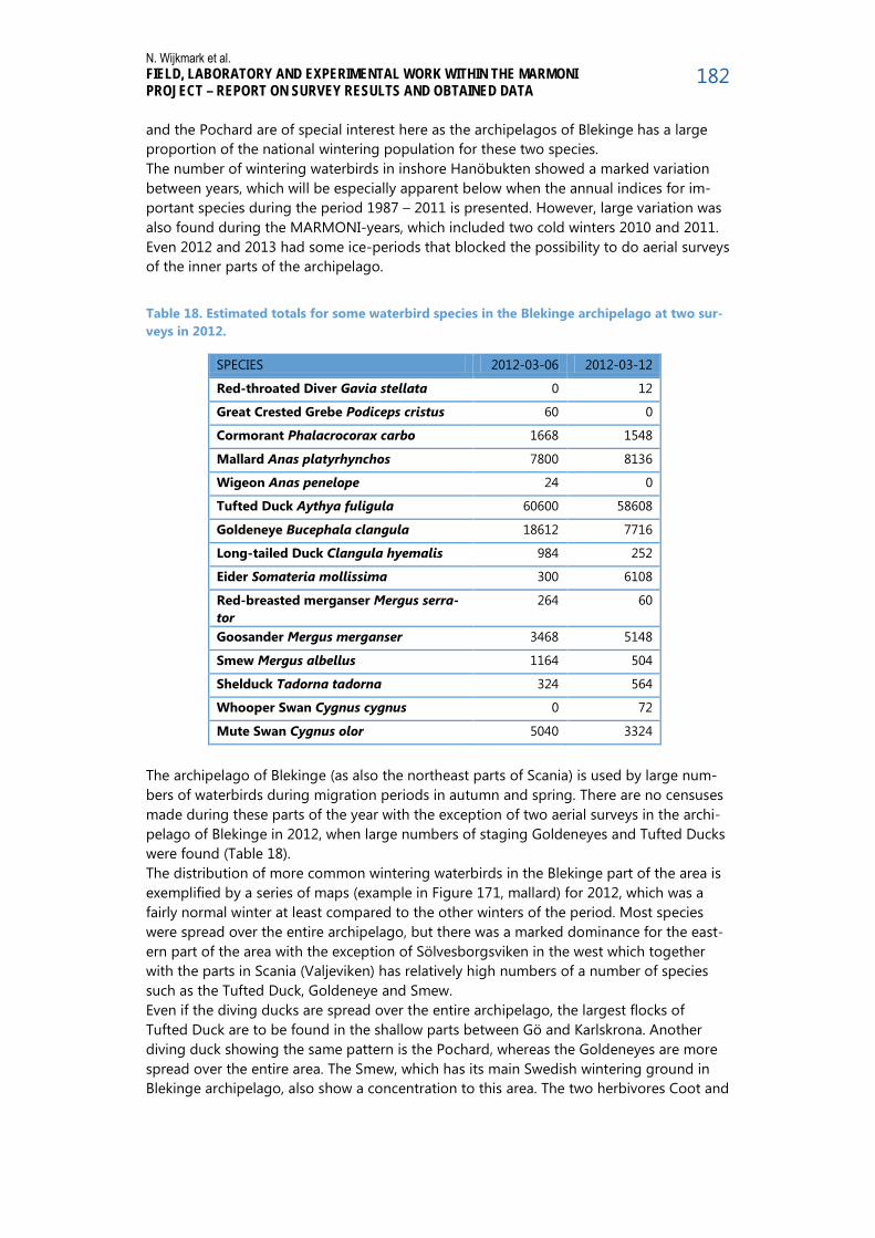
N. Wijkmark et al. FIELD, LABORATORY AND EXPERIMENTAL WORK WITHIN THE MARMONI PROJECT – REPORT ON SURVEY RESULTS AND OBTAINED DATA
182
and the Pochard are of special interest here as the archipelagos of Blekinge has a large proportion of the national wintering population for these two species. The number of wintering waterbirds in inshore Hanöbukten showed a marked variation between years, which will be especially apparent below when the annual indices for im-portant species during the period 1987 – 2011 is presented. However, large variation was also found during the MARMONI-years, which included two cold winters 2010 and 2011. Even 2012 and 2013 had some ice-periods that blocked the possibility to do aerial surveys of the inner parts of the archipelago.
Table 18. Estimated totals for some waterbird species in the Blekinge archipelago at two sur-veys in 2012.
SPECIES 2012-03-06 2012-03-12
Red-throated Diver Gavia stellata 0 12
Great Crested Grebe Podiceps cristus 60 0
Cormorant Phalacrocorax carbo 1668 1548
Mallard Anas platyrhynchos 7800 8136
Wigeon Anas penelope 24 0
Tufted Duck Aythya fuligula 60600 58608
Goldeneye Bucephala clangula 18612 7716
Long-tailed Duck Clangula hyemalis 984 252
Eider Somateria mollissima 300 6108
Red-breasted merganser Mergus serra-tor
264 60
Goosander Mergus merganser 3468 5148
Smew Mergus albellus 1164 504
Shelduck Tadorna tadorna 324 564
Whooper Swan Cygnus cygnus 0 72
Mute Swan Cygnus olor 5040 3324
The archipelago of Blekinge (as also the northeast parts of Scania) is used by large num-bers of waterbirds during migration periods in autumn and spring. There are no censuses made during these parts of the year with the exception of two aerial surveys in the archi-pelago of Blekinge in 2012, when large numbers of staging Goldeneyes and Tufted Ducks were found (Table 18). The distribution of more common wintering waterbirds in the Blekinge part of the area is exemplified by a series of maps (example in Figure 171, mallard) for 2012, which was a fairly normal winter at least compared to the other winters of the period. Most species were spread over the entire archipelago, but there was a marked dominance for the east-ern part of the area with the exception of Sölvesborgsviken in the west which together with the parts in Scania (Valjeviken) has relatively high numbers of a number of species such as the Tufted Duck, Goldeneye and Smew. Even if the diving ducks are spread over the entire archipelago, the largest flocks of Tufted Duck are to be found in the shallow parts between Gö and Karlskrona. Another diving duck showing the same pattern is the Pochard, whereas the Goldeneyes are more spread over the entire area. The Smew, which has its main Swedish wintering ground in Blekinge archipelago, also show a concentration to this area. The two herbivores Coot and

N. Wijkmark et al. FIELD, LABORATORY AND EXPERIMENTAL WORK WITHIN THE MARMONI PROJECT – REPORT ON SURVEY RESULTS AND OBTAINED DATA
183
Mute Swan are also found in largest numbers in the eastern part of the archipelago with its shallow areas. The concentration of many species of waterbirds to the eastern part of the Blekinge ar-chipelago is related to the occurrence of large shallow areas with rich food resources in the form of benthic vegetation and a rich benthic fauna in shallow waters. This concentra-tion to the east is mostly seen during mild and normal winters as these areas are the first to freeze during cold period making the waterbirds to move to areas further out at sea close to the ice edge. There was also a marked concentration of waterbirds to the eastern part of the archipel-ago area at the censuses during early spring in 2012 as seen in the overall map in Figure 172.
Figure 171. Example map of distribution of birds in the midwinter count in 2012: Mallard Anas platyrhynchos.
Figure 172. Distribution for all waterbird flocks seen at aerial surveys in the archipelago of Blekinge 2012-03-06.

N. Wijkmark et al. FIELD, LABORATORY AND EXPERIMENTAL WORK WITHIN THE MARMONI PROJECT – REPORT ON SURVEY RESULTS AND OBTAINED DATA
184
Figure 173. Example of map of long-tailed duck (Clangula hyemalis) in winter.
3.5.3.3 Photographs from bird surveys in the Hanö Bight
Figure 174. Habitat images from the survey area southeast of Karlshamn.

N. Wijkmark et al. FIELD, LABORATORY AND EXPERIMENTAL WORK WITHIN THE MARMONI PROJECT – REPORT ON SURVEY RESULTS AND OBTAINED DATA
185
Figure 175. A high-winged CESSNA 337 Skymaster was used for the surveys, providing good visibility for the observers.
3.5.3.4 References Nilsson, L. 2008. Changes in numbers and distribution of wintering waterfowl in Sweden during forty years, 1967 -2006. Ornis Svecica 18:135-226. Nilsson, L. 2012. Distribution and numbers of wintering sea ducks in Swedish offshore waters. Ornis Svecica 22:39-59.

N. Wijkmark et al. FIELD, LABORATORY AND EXPERIMENTAL WORK WITHIN THE MARMONI PROJECT – REPORT ON SURVEY RESULTS AND OBTAINED DATA
186
3.6 Testing the application of the satellite and airborne remote sensing
3.6.1 Latvia: 1EST-LAT Irbe Strait and the Gulf of Riga
Calculation of chlorophyll a (chl-a) concentration and mapping its distribution with re-mote sensing methods can be used as an indicator for assessment of phytoplankton bio-mass distribution. The field campaign was performed during the period from 14 to 19 May 2012 collecting data from 29 stations (carried out by the Latvian Institute of Aquatic Ecology). Chlorophyll a concentrations measurements and also classification of algae species were performed in laboratory for further calibration of remote sensing data. The flight campaign was performed by IES on 15 May 2012 during spring algal bloom and lasted for ~3.5 hours (form 8:45 am till 12:15 pm). Hyperspectral airborne data was ac-quired from more than 80000 ha large area (1.3 km width and 630 km total length of data acquisition flight lines) with spatial resolution 1 m/px, thus collecting more than 800 mil-lion measurement points. Each measurement point contained information from 18 spec-tral bands of CASI sensor at 432-797 nm range. The whole Baltic Sea belongs to Case-2 waters, and by its’ nature it is one of the most optically-complex and difficult water basins in the world. Due to very low water-exchange level with ocean and very high rivers inflow, bringing suspended and dissolved matter, Baltic Sea waters have high concentration of CDOM (coloured dissolved organic matter), which can be considered as conservative property of the water. CDOM strongly absorbs light in blue part of spectrum, which causes high error level (up to 200%) when working with standard (for case-1 waters) chl-a calculation algorithms – they are based on blue-green bands ratios. Therefore potential use of hyperspectral images for chl-a calculation has been demonstrated for 2-band and 3-band near infrared model, suggested by Dall’Olmo et al. 2003 and tested by other scientists in different Case-2 water bodies. An example of 3-band near infrared model is shown in Figure 3.1. The region of interest within the flight line 095014 is zoomed in and shown in two different modes. Real colour (RGB) image (Figure 176 a) is constructed of CASI channels in red, green and blue spectral range. Such image represents our perception of the sea surface during sunny day – no chl-a presence can be observed. False colour image (Figure 176 b) is constructed replac-ing true colour R, G and B channels with specific spectral bands of 3-band model (R = 666 nm, G = 712 nm and B = 744 nm). Chl-a is highlighted in green colour due to a local maximum of reflectance around 700 nm.
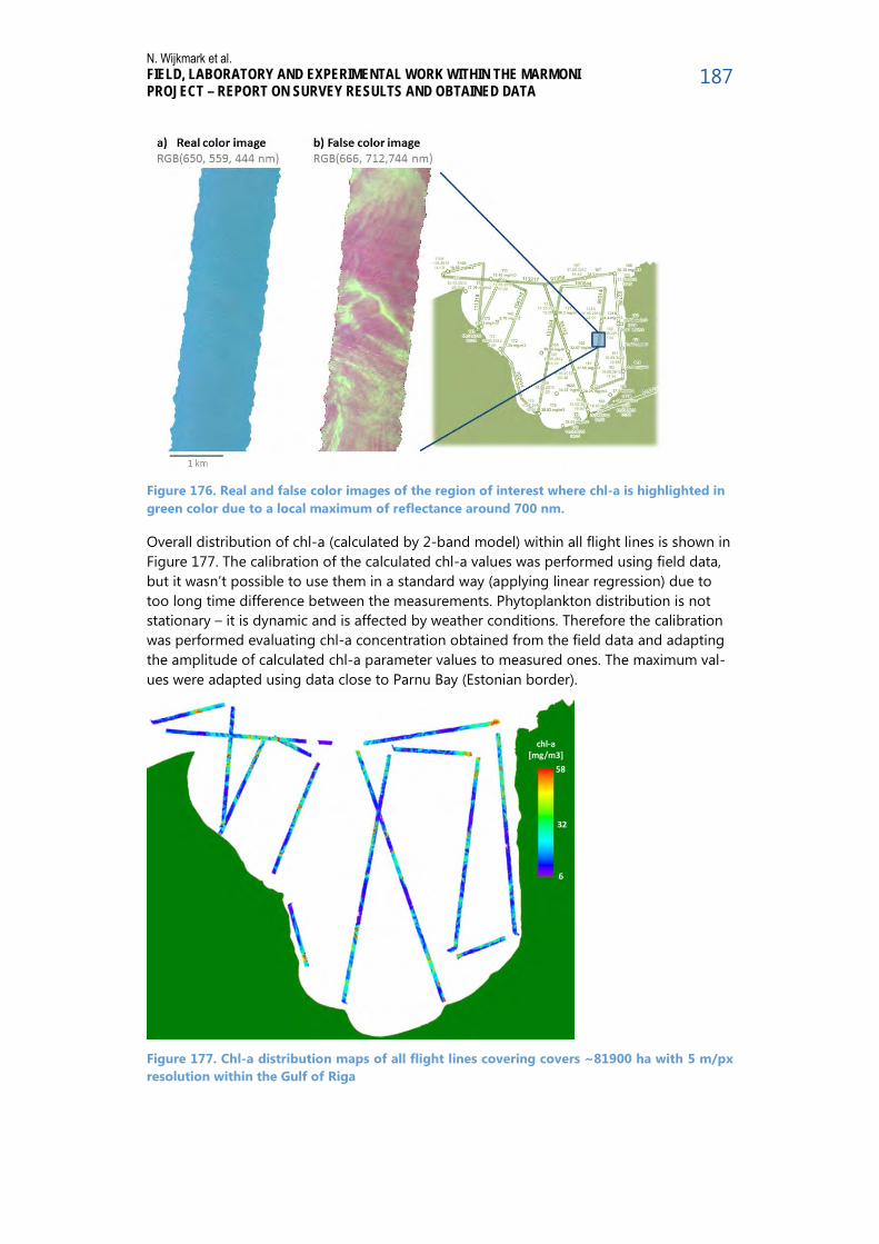
N. Wijkmark et al. FIELD, LABORATORY AND EXPERIMENTAL WORK WITHIN THE MARMONI PROJECT – REPORT ON SURVEY RESULTS AND OBTAINED DATA
187
Figure 176. Real and false color images of the region of interest where chl-a is highlighted in green color due to a local maximum of reflectance around 700 nm.
Overall distribution of chl-a (calculated by 2-band model) within all flight lines is shown in Figure 177. The calibration of the calculated chl-a values was performed using field data, but it wasn’t possible to use them in a standard way (applying linear regression) due to too long time difference between the measurements. Phytoplankton distribution is not stationary – it is dynamic and is affected by weather conditions. Therefore the calibration was performed evaluating chl-a concentration obtained from the field data and adapting the amplitude of calculated chl-a parameter values to measured ones. The maximum val-ues were adapted using data close to Parnu Bay (Estonian border).
Figure 177. Chl-a distribution maps of all flight lines covering covers ~81900 ha with 5 m/px resolution within the Gulf of Riga

N. Wijkmark et al. FIELD, LABORATORY AND EXPERIMENTAL WORK WITHIN THE MARMONI PROJECT – REPORT ON SURVEY RESULTS AND OBTAINED DATA
188
Detailed (1 m/px) chl-a distribution can be provided by airborne hyperspectral imaging, but spatial coverage is limited. Therefore modelling of chl-a distribution over all Gulf of Riga was performed using interpolation of airborne data. Bi-cubic interpolation was used for modelling chl-a distribution over all Gulf of Riga, see Figure 178Figure 179. The result depends on the grid size and reference data available. Validation and also further devel-opment of the model should be performed using satellite data that was not available for particular study. The results demonstrated in Figure 178 shouldn’t be taken as true chl-a distribution over all Gulf of Riga prior validation, but should be perceived as demonstra-tion of the potential.
Figure 178. Modelling chl-a distribution over all Gulf of Riga: bi-cubic interpolation of air-borne data.
Hyperspectral airborne data has a great potential for aquatic environmental studies – from single projects to long-term complex monitoring programs. Very high resolution data can be provided with required spectral range/bands at needed time and area. Such data cover the gap between discrete field measurements and satellite data. The advantage of airborne data over field measurements is representation of the distribu-tion of the parameter, for example, chlorophyll-a. Fusion of both techniques would re-duce the number of necessary field samples, and regular simultaneous measurements would allow developing and verifying remote sensing algorithms for routine use for spe-cific area. Satellite sensors could provide additional data covering large areas, but the resolution and also availability is limited. Careful planning of data acquisition campaigns would allow fusion of the data from all three sources – field measurements, airborne and satellite sensors. More information and details about this study can be found is separate project report “Testing of new indicator set and monitoring methods. Testing the application of the hy-perspectral airborne remote sensing”.

N. Wijkmark et al. FIELD, LABORATORY AND EXPERIMENTAL WORK WITHIN THE MARMONI PROJECT – REPORT ON SURVEY RESULTS AND OBTAINED DATA
189
3.6.2 Sweden: 2SWE Hanö Bight
3.6.2.1 Secchi depth map A Secchi depth map of the Hanö Bight study area was created from Landsat 7 data in 30 m resolution. A regression analysis between the Landsat image and a large number of field measure-ments (ca 15000) collected during 2011 was performed in order to calculate secchi-depth from the satellite image (Figure 179). Parts of the area were covered by clouds and cloud banks (mainly in the south-east) and appear as empty spaces in the secchi-depth map.
Figure 179. Secchi depth from Landsat 7 data. Holes and missing data (mainly in the south-eastern parts of the area) are results of clouds.
This secchi depth map was further processed for use in spatial modelling of species and habitats in the Hanö Bight (section 3.7.3) where parts with clouds were taken away and the holes filled with interpolated values from surrounding areas.
3.6.2.2 Hypersectral airborne images for classification of bottom landscapes This pilot study deals with the analysis of potential use of hyperspectral airborne images for classification of bottom landscapes near the coast of Sweden (Hanö Bight). The flight campaign was performed on 27 September 2011 acquiring spectral images from 25 spectral bands at 398-1045 nm range with spatial resolution 1 m/px. Data was

N. Wijkmark et al. FIELD, LABORATORY AND EXPERIMENTAL WORK WITHIN THE MARMONI PROJECT – REPORT ON SURVEY RESULTS AND OBTAINED DATA
190
acquired from more than 33000 ha large area (292 km total length and 1.49 km width of data acquisition flight lines with 30% overlap). Field data were collected from 13 stations within the field of view of airborne data. Spectral profiles have been built and analysed for different bottom types form airborne spectral data that matched to data obtained from field stations. Profiles at samples sites show peak (one or two) near 600 and 650 nm, which is signature of algae existence. How-ever, it does not look possible to separate red and mixed red-brown bottom coverage type by spectrum. Therefore, decision was made to apply two different approaches and compare their results – supervised and unsupervised pixel-based classifications, without definition or real bottom classes. Supervised classification is based on samples provided at the image for every class. Spec-tral Angle Mapper (SAM) algorithm was selected as it is relatively insensitive to absolute values of image. The algorithm determines the spectral similarity between two spectra by calculating the angle between the spectra and treating them as vectors in a space with dimensionality equal to the number of bands. It has shown good results in other bottom mapping studies and was implemented as a standard function in ENVI software. Definition of classes is a critical task for supervised classification methods. In this case it cannot be done absolutely correctly, as no data about bottom types are available. There-fore, classes were defined after very detailed visual and logical analysis of the image and of numerous spectral profiles taken from it. The names are given according to their visible colour properties on RGB composite. SAM classification results are presented on Figure 180. K-means method was used for unsupervised classification. It classifies the image into de-fined number of classes (without samples), which then can be merged, re-classified and re-named to meet the target. Therefore, at first step larger number of classes should be defined. In this particular case after series of tries it was revealed, that 25 classes show best de-lineation of visible objects and should be able to cover all variability of bottom types. Clusters can be merged in order to reduce to the total number of classes, as demon-strated partly on Figure 180. Spectrally well-programmed airborne hyperspectral images are very good source of in-formation for bottom classification, even in optically-shallow Baltic Sea conditions. They have sufficient spectral variability for good classification results. Additional field informa-tion would improve the results allowing definition of real classes. Planning of field meas-urements should be node carefully for this purpose. More detailed classification of the presented areas (or others from already available similar images) can be done later, after another field campaign, bringing the required data. Available images can be very useful for planning of such campaign – to pan the distribution of sampling points and coverage. More information and details about this study can be found is separate project report “Testing of new indicator set and monitoring methods. Testing the application of the hy-perspectral airborne remote sensing”.
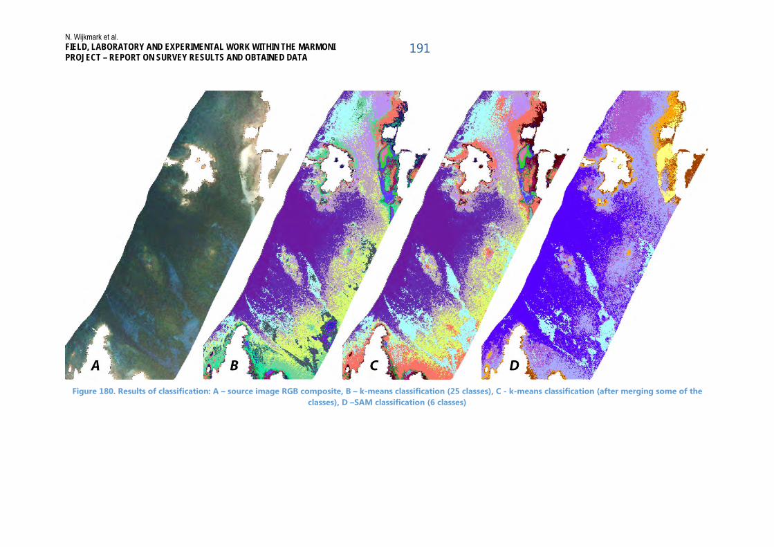
N. Wijkmark et al. FIELD, LABORATORY AND EXPERIMENTAL WORK WITHIN THE MARMONI PROJECT – REPORT ON SURVEY RESULTS AND OBTAINED DATA
191
Figure 180. Results of classification: A – source image RGB composite, B – k-means classification (25 classes), C - k-means classification (after merging some of the
classes), D –SAM classification (6 classes)

N. Wijkmark et al. FIELD, LABORATORY AND EXPERIMENTAL WORK WITHIN THE MARMONI PROJECT – REPORT ON SURVEY RESULTS AND OBTAINED DATA
192
3.6.3 Finland: 3FIN Coastal area of SW Finland
3.6.3.1 Secchi-depth map A secchi-depth map covering the coastal area of southwest Finland was created from satellite data (Figur 181). Two satellite images, a MERIS image from 2010-07-11 and a Landsat 5 image from 2010-07-12 were used as input data. This combination makes it possible to take advantage of both the good spectral properties of MERIS data and the high spatial resolution (30 m) of the Landsat 5 data. MERIS data has a spatial resolution of 300 m. In order to combine the satellite images a regression analysis was performed based on seven digitized areas (ROI) from open sea to inner archipelago (linear regression R2 = 0.75). This methodology is described in detail in Florén et al. (2012).
Figur 181. Secchi depth map produced from MERIS and Landsat 5 data.

N. Wijkmark et al. FIELD, LABORATORY AND EXPERIMENTAL WORK WITHIN THE MARMONI PROJECT – REPORT ON SURVEY RESULTS AND OBTAINED DATA
193
3.7 Modelling the distribution of habitats and species In spatial modelling, monitoring data (such as georeferenced points or transects) are transformed into layers or maps by statistical analyses and predictions. The modelling contributes with further information from the monitoring data. The extensive modelling performed in MARMONI includes important parts of the marine ecosystem such as birds, fish, plankton and benthic flora and fauna. A large number of maps from the modelling are now available for use in marine spatial planning and will be used interactively with planning authorities within MARMONI action A4.2. This chapter describes the modelling that was performed within MARMONI action A3 in the study areas.
3.7.1 Modelling and spatial indicators Modelled maps of distributions of species and habitats provide new possibilities in the development of indicators. Spatial indicators such as the newly developed MARMONI indicator 2.5 Habitat diversity index is an example of an indicator for which modelled maps provide valuable input data. Modelling techniques are also powerful analysis tools and can contribute significantly to the understanding of the effects of environmental gradients and human activities on the modelled variables (e.g. indicator value, species or habitat). Such analyses were performed during the development and testing of some indicators. Examples are the MARMONI indicators 2.1 Accumulated cover of perennial macroalgae and 2.2 Accumulated cover of submerged vascular plants whose relations to several human activity gradients were ana-lysed in a spatial context with the modelling technique random Forest. Spatial modelling and spatial analyses of gradients require sampling designs that cover important environ-mental gradients. Sampling designs and maps of sampled stations in different surveys are available in the chapters 3.1 to 3.5 in this report. Spatial modelling and prediction may also be used to visualise indicator values or status in maps, providing a powerful way of presenting results of indicator based assessments.
3.7.2 Environmental layers In order to perform successful spatial modelling, the environmental layers used for pre-diction of the response variable (e.g. species or habitat) must be highly accurate. Many new environmental layers were therefore created for use in the spatial modelling.

N. Wijkmark et al. FIELD, LABORATORY AND EXPERIMENTAL WORK WITHIN THE MARMONI PROJECT – REPORT ON SURVEY RESULTS AND OBTAINED DATA
194
3.7.3 Modelling the distribution of habitats and species in Latvia: 1EST-LAT Irbe Strait and the
Gulf of Riga
3.7.3.1 Choice of species Although all observed birds or seals regardless of species were recorded during the counts, only selected species or groups of species were used in further analyses. We considered following species for analysis:
Species of international conservation concern:
- Long-tailed Duck Clangula hyemalis
- both Scoter species (Black Scoter Melanitta nigra and Velvet Scoter Melanitta fusca)
- all Diver species (cf. Red-throated Diver Gavia stellata and Black-throated Diver Gavia arctica)
- Little Gull (Larus minutus)
Other important waterbird species in non-breeding seasons:
- Goldeneye (Bucephala clangula)
- Mergansers (cf. Goosander Mergus merganser and Red-breasted merganser Mergus serrator)
- Swans (all species; mainly Mute Swan Cygnus olor)
- Common Gull (Larus canus)
- Herring Gull (Larus argentatus)
Species groups:
- Benthos feeding species (Long-tailed Duck, Scoters, Goldeneye, Eider)
- Fish feeding species (divers, grebes, cormorants, mergansers, auks)
- All gulls (all Larus species)
-
3.7.3.2 Detection probability Software package Distance 6.2 release 1 was used for building detectability functions. Initially CDS and MCDS engines were used to assess the most appropriate form of detec-tion function as well as most appropriate covariates. Following covariates were tried in the models – observer, seat in the plane, flock size, behaviour of birds and sea state. Detec-tion functions were first built separately for each species/group and season combinations, then additional functions where data from all seasons were pooled and then also func-tions where data for similar species were pooled. When first insights on performance of different detection functions was obtained, the final versions were calculated using MRDS engine of the Distance software (Distance sends data for analysis to R statistical software using ‘mrds’ package). The final model was chosen using AIC and coefficient of variance as the main criteria. Where possible, single species models were chosen, however if per-formance of such a model was noticeably worse than “combined” model, the “combined” model was used instead. The chosen MRDS detectability model was used further for dis-tance correction of observation data that was used in density surface modelling.

N. Wijkmark et al. FIELD, LABORATORY AND EXPERIMENTAL WORK WITHIN THE MARMONI PROJECT – REPORT ON SURVEY RESULTS AND OBTAINED DATA
195
3.7.3.3 Gridding the observations and prediction grid
To prepare bird observation data for further use in density surface modelling, all transects were divided into section with ca 1km length. Then buffers of 500m were applied on both sides of transect section obtaining cells with average area of 1 km2, which is similar to area of cells used in the prediction grid. All terrestrial areas were removed from the cells. All bird observations were attributed to these cells (each transect section had unique ID which was assigned to all observations). Similarly a prediction grid was built – a grid starting from westernmost and northernmost edges of the study area with cell size of 1 km X 1km spread over the whole study area. Then terrestrial areas were clipped out of the cells.
3.7.3.4 Ecogeographical (environmental) variables To test relationship and build species-environmental variables relation models, a number of ecogeographical variables were calculated both for data collection units as well as 1-km prediction grid. The following variables were used:
- Depth (mean depth value of the grid cell; Figure 182 A), - Depth variation (SD of 100-m grid cell values within 1-km zones, Figure 182
B) - Distance from coast (Figure 182 C) - Distance from different sea bottom substrates (bedrock, gravel, sandy,
mixed, silty, muddy, soft and hard; Figure 182 D-I), - Proportion of different sea bottom substrates substrates (bedrock, gravel,
mixed, muddy, sandy, silty, soft and hard), - Shipping intensity (HELCOM 2011 data; Figure 182 J) - Ice coverage during the data collection
All ecogeographical variables were calculated using ArcGIS software and it’s Spatial Ana-lyst and 3D Analyst extensions.
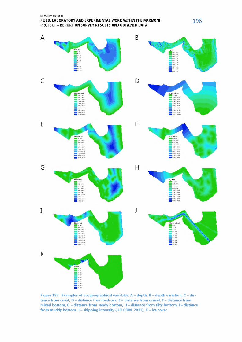
N. Wijkmark et al. FIELD, LABORATORY AND EXPERIMENTAL WORK WITHIN THE MARMONI PROJECT – REPORT ON SURVEY RESULTS AND OBTAINED DATA
196
A
B
C
D
E
F
G
H
I
J
K
Figure 182. Examples of ecogeographical variables: A – depth, B – depth variation, C – dis-tance from coast, D – distance from bedrock, E – distance from gravel, F – distance from mixed bottom, G – distance from sandy bottom, H – distance from silty bottom, I – distance from muddy bottom, J – shipping intensity (HELCOM, 2011), K – ice cover.

N. Wijkmark et al. FIELD, LABORATORY AND EXPERIMENTAL WORK WITHIN THE MARMONI PROJECT – REPORT ON SURVEY RESULTS AND OBTAINED DATA
197
3.7.3.5 Density surface modelling The first step was to find the “best” species-environmental variables relation models. We used GAM (Hastie, Tibsirhani 1990). To find the “best” models, scripts for ‘mgcv’ package of R statistical software were prepared and applied to a full distance-corrected dataset (i.e. using the species abundance and offsets prepared by the Distance 6.2 release 1 soft-ware). The scripts were written to test all possible combinations of available ecogeographical variables for particular species and season. The “best” models were those giving lowest GCV-scores, they most often provided the highest “Deviance ex-plained” and “R-squared” values. However, always at least 5 “best” models for each com-bination of specie/group and season were checked. Similar variables (such as “distance from bedrock” and “proportion of bedrock”) were not allowed in the same model formu-la). The chosen “best” models were re-used in Distance (which sends data for analysis to R using ‘dsm’ and ‘mgcv’ packages and reads back the result for further use). The second step was to apply the model to the prediction grid where values of explanato-ry variables were known. This was done in Distance using DSM analysis engine (which sends data for analysis to R using ‘dsm’ and ‘mgcv’ packages). The obtained result was density values of analysed species/group for each grid cell. They were linked to ArcGIS prediction grid layer and used in further calculations such as obtaining maximum densi-ties, etc. A bootstrapping procedure to obtain confidence intervals for the calculated densities in grid cells was not carried out due to enormous computing time demanded.
3.7.3.6 Modelled distribution of birds in the Gulf of Riga and Irbe Strait The maps below show modelled distribution of the key species and species groups in the Latvian part of the project area 1 EST-LAT Gulf of Riga and Irbe Strait according to GAM models calculated as described above.
Figure 183. Modelled distribution of Long-tailed Duck Clangula hyemalis in the Latvian part of the project area.

N. Wijkmark et al. FIELD, LABORATORY AND EXPERIMENTAL WORK WITHIN THE MARMONI PROJECT – REPORT ON SURVEY RESULTS AND OBTAINED DATA
198
Figur 184. Modelled distribution of Scoters Melanitta sp. in the Latvian part of the project area.

N. Wijkmark et al. FIELD, LABORATORY AND EXPERIMENTAL WORK WITHIN THE MARMONI PROJECT – REPORT ON SURVEY RESULTS AND OBTAINED DATA
199
Figure 185. Modelled distribution of Goldeneye Bucephala clangula in the Latvian part of the project area.

N. Wijkmark et al. FIELD, LABORATORY AND EXPERIMENTAL WORK WITHIN THE MARMONI PROJECT – REPORT ON SURVEY RESULTS AND OBTAINED DATA
200
Figure 186. Modelled distribution of benthos feeding species (long-tailed duck, scoters, gold-eneye, eider) in the Latvian part of the project area.
Figure 187. Modelled distribution of Goosander Mergus merganser and Red-breasted met-ganser M. serrator in the Latvian part of the project area.
Figure 188. Modelled distribution of fish feeding species (diver, grebes, cormorants, mergan-sers, auks)in the Latvian part of the project area.

N. Wijkmark et al. FIELD, LABORATORY AND EXPERIMENTAL WORK WITHIN THE MARMONI PROJECT – REPORT ON SURVEY RESULTS AND OBTAINED DATA
201
Figure 189. Modelled distribution of Little Gull Larus minutus in the Latvian part of the pro-ject area.
Figure 190. Modelled distribution of gulls Larus sp. in the Latvian part of the project area.

N. Wijkmark et al. FIELD, LABORATORY AND EXPERIMENTAL WORK WITHIN THE MARMONI PROJECT – REPORT ON SURVEY RESULTS AND OBTAINED DATA
202
3.7.4 Modelling the distribution of benthic habitats and species in Estonia: 1EST-LAT the Eastern part of Gulf of Riga
3.7.4.1 INTRODUCTION Mapping of seabed biota and habitats is increasingly being used for marine spatial plan-ning, inventories and planning of protected areas and environmental impact assessments. Mapping studies are more easily carried out and are more detailed for terrestrial land-scapes. While aerial photography and LIDAR are extensively applied in the mapping of terrestrial topography and habitats, these remote sensing approaches have a much more restricted application to seabed habitat mapping, where they are limited to very shallow waters. This explains why similar assessments are scarce in marine realm. Due to the very limited use of remote sensing, the data on seabed biota and habitats has been collected almost exclusively from field points that have been visited. Seabed habitat mapping by the means of conventional sampling-point-wise field work methods is expen-sive and time-consuming and it yields information only from the visited sites leaving most of the study area unsampled. These gaps in data collection can be filled with either inter-polation or predictive modeling. Interpolation is a mathematical method of constructing new data points within the range of a set of known data points. Interpolation is easy to apply and the results can be adequate if the study area is small, homogenous and the sampling grid is regular and dense. In predictive modeling a mathematical model fits a relationship between species or habitat distribution and predictor variables and that rela-tionship is then used to predict the occurrence of a species or habitat in the areas where there are no data on the species or habitat. The prerequisite for predictive modeling is that there exists a set of spatially continuous environmental variables that can be used for making the predictions. Given that spatially continuous predictor variables with reasona-ble accuracy area available, predictive modeling produces more accurate results than interpolation in the case of large sparsely sampled study areas. Although this technique cannot replace direct observations of seabed, the development of such models contrib-utes to the evaluation of areas where no direct seabed observations are available. In this study, the distribution of key seabed species and habitats was estimated using both de-tailed knowledge from in situ sampling points as well as environmental geospatial data, based on which predictive models were built. Combining detailed in situ sampling and predictive modeling we aimed to produce distri-bution maps of: • key macrobenthic plant and invertebrate species; • seabed habitat types “reefs” and “sandbanks” of the annex 1 of Council Directive
92/43/EEC of 21 May 1992 on the conservation of natural habitats and of wild fauna and flora (hereafter “Habitats Directive”).

N. Wijkmark et al. FIELD, LABORATORY AND EXPERIMENTAL WORK WITHIN THE MARMONI PROJECT – REPORT ON SURVEY RESULTS AND OBTAINED DATA
203
3.7.4.2 MATERIAL & METHODS Study area The mapping study area (3080 km2) was located in the Estonian waters of the northern Gulf of Riga, Baltic Sea (Figure 191). The Gulf of Riga is situated in the northern Baltic Sea and is a relatively shallow water-body with a surface area of 16330 km2. The gulf is con-nected to the Baltic Proper via narrow straits. The Gulf of Riga receives fresh water from a huge drainage area and therefore has reduced salinity of 5.0–6.5 psu. In general, the bot-tom relief of the area is quite flat, with gentle slopes towards deeps. The northern part of the gulf is characterized by a wide coastal zone with diverse bottom topography and ex-tensive reaches of boulders. The southern part of the Gulf of Riga is more exposed and with steeper coastal slope (Kotta et al. 2008). Water depth in the mapping area is approximately between 0 and 50 m. The deepest area is located in the southern part of the area. Only the eastern-northeastern mapping area is bordered by land: Island Kihnu and southwestern mainland Estonia. The eastern-northeastern area is also the shallowest part of the mapping area (Figure 192).
Figure 191. Location of mapping study area and MARMONI project area in the Estonian part of the Gulf of Riga.

N. Wijkmark et al. FIELD, LABORATORY AND EXPERIMENTAL WORK WITHIN THE MARMONI PROJECT – REPORT ON SURVEY RESULTS AND OBTAINED DATA
204
Figure 192. Water depth of the mapping area.
Modeling and map production The framework of species distribution modeling was applied to convert the point-wise data to raster data that covers the whole mapping area. Species distribution models (SDMs) are numerical tools that combine observations of species occurrence or abun-dance with environmental estimates and enable to predict species distributions across area of interest (Elith & Leathwick 2009). The mathematical model fits a relationship be-tween species distribution and predictor variables and that relationship is then used to predict the occurrence of a species in the areas where there are no data on the species (Figure 193). In this study this approach was used to estimate species occurrence in the areas between sampling stations. Additionally to species predictions, models were also used to predict the distribution of seabed substrate types.

N. Wijkmark et al. FIELD, LABORATORY AND EXPERIMENTAL WORK WITHIN THE MARMONI PROJECT – REPORT ON SURVEY RESULTS AND OBTAINED DATA
205
Figure 193. The conceptual framework of predictive modeling.
All data collected from the study area was included in the modeling. Additionally, data from more than 10 000 sampling stations from all over the Estonian sea area from the period 2005-2013 were used in model building (Figure 194). Higher number of input data points ensures more accurate predictions.
Figure 194. Locations of sampling points that were used for model building.
Response variable:point data of species
distribution
Predictor variables:GIS-layers of
environmental data
Mathematical model:
relationships between species and environment
Prediction:occurrence of species
over the study area
Model-derived information
• importance of predictors
• shapes of relationships between predictors and response

N. Wijkmark et al. FIELD, LABORATORY AND EXPERIMENTAL WORK WITHIN THE MARMONI PROJECT – REPORT ON SURVEY RESULTS AND OBTAINED DATA
206
Biomass and coverage data of species was converted to binary data (presence = 1, ab-sence = 0) because the binary input models generally produce more stable and accurate results than models based on a continuous response variable. There exists no single model algorithm that, regardless of input data, always yields the most accurate predictions. For that reason three different model algorithms were use: generalized additive models (GAM), boosted regression trees (BRT), and random forests (RF). All calculations were run in the freeware statistical program R 3.0.1 (The R Foundation for Statistical Computing 2013) GAM is a semi-parametric extension of generalized linear models that enables to fit com-plex non-linear relationships and handle different types of error distributions (Hastie & Tibshirani 1990). Due to these characteristics, GAM has been one of the most widely used methods for SDM (Elith et al. 2006). The package “mgcv” was used for building GAMs (Wood 2006). The models were built using penalized regression splines as the smoothing function, binomial error distribution, and automatic calculation of smoothing parameters. The maximum degree of freedom was set to three for each variable. BRT is an ensemble method that combines the strength of two algorithms: regression trees and boosting (Elith et al 2008). Regression trees are good at selecting relevant pre-dictor variables and can model interactions. Boosting enables a building of a large num-ber of trees in a way that each successive tree adds small modifications in parts of the model space to fit the data better (Friedman et al 2000). The algorithm keeps adding trees until finding the optimal number of trees that minimizes the predictive deviance of a model. The predictive performance of BRT has been shown to be superior to most other modeling methods (Elith et al 2006, Revermann et al 2012). The BRT modelling was per-formed using packages “gbm” (Ridgeway 2013) and “dismo” (Hijmans et al 2013). RF is a machine learning method that generates large number of regression trees, each calibrated on a bootstrap sample of the original data (Breiman 2001). Each node is split using a subset of randomly selected predictors and the tree is grown to the largest possi-ble extent without pruning. For predicting the value of a new data point, the data is run through each of the trees in the forest and each tree provides a value. The model predic-tion is then calculated as the average value over the predictions of all the trees in the forest (Breiman 2001). The package “party” (Hothorn et al. 2006) was used to run RF mod-els in R. 90% of randomly chosen data points were used for model training and the remaining 10% were used to assess the predictive accuracy of models. The best performing model was chosen for making the predictions. Model performance was assessed by ROC-analysis (Fielding & Bell 1997) and visual expert judgments. A total of 19 environmental variables were used to predict the distribution of key species and habitats. An overview of the environmental variables is presented in Table 19. All environmental variables were available as georeferenced raster datasets.

N. Wijkmark et al. FIELD, LABORATORY AND EXPERIMENTAL WORK WITHIN THE MARMONI PROJECT – REPORT ON SURVEY RESULTS AND OBTAINED DATA
207
Table 19. Environmental variables that were used to predict the distribution of key benthic species and habitats.
Name Information Source depth Water depth 1 depth2 Average water depth in 2 km radius 1 slope Seabed slope 1 slope2 Average seabed slope in 2 km radius 1 dist_land Distance to shoreline 1 dist_50 Distance to 50 m depth isoline 1 salinity Average salinity of bottom water layer 1,3 exposure Wave exposure 4 chlorophyll Chlorophyll a content based on satellite imagery; average over 2009-2010 1
turbidity Water turbidity estimated as attenuation coefficient based on satellite imagery; average over 2010-2012 1
ice_cover Ice coverage; average over 2009-2011 5 ice_thick Ice thickness; average over 2009-2011 5 ice_day Number of ice days per year; average over 2009-2011 5
temp_cold Temperature of bottom water layer in cold season; modeled average over 1996-2005 2
temp_warm Temperature of bottom water layer in warm season; modeled average over 1996-2005 2
temp_sat Temperature of surface water in summer (June-August) based on satellite imagery; average over 2009-2010 1
current Current velocity of bottom water layer; modeled average over 1996-2005 2
O2_avg Average oxygen concentration of bottom water layer; modeled average over 1996-2005 3
O2_min Minimum oxygen concentration of bottom water layer; modeled minimum over 1996-2005 3
sediment Modeled proportion of soft seabed sediment Sources: 1 – databases of Estonian Marine Institute, University of Tartu 2 – hydrodynamic model data by Marine Systems Institute at Tallinn Technical University, Estonia 3 – whole Baltic Sea scale hydrodynamic model data (Bendtsen 2009) 4 – silmplified wave model (SWM, Nikolopoulos & Isæus 2008) 5 – Finnish Meteorological Institute
The predictions were made to a grid of 200 m cell size that covered the whole study are. The output of prediction of a given species was a probability of occurrence (between 0 and 1) of the species in each grid cell. As the distribution of predicted probabilities de-pends on the proportions of presences and absences in the input data, the numerical values of predicted probabilities cannot be directly compared between species. In order to assess the distribution of reefs and sandbanks the predicted probabilities of character-istic species had to be converted to comparable measures: the predictions were binarized by setting a threshold to the probability. The threshold was calculated separately for each species prediction by using the method sensitivity-specificity difference minimizer (Jimé-nez-Valverde & Lobo 2007). All probability values below the threshold were converted to absences and all values above the threshold were converted to presences of a given spe-cies. The distribution maps of reefs and sandbanks were assessed by applying overlay analysis on the binarized species rasters and substrate rasters. A raster of photic seabed was additionally used in the overlay analysis of sandbanks habitat type.

N. Wijkmark et al. FIELD, LABORATORY AND EXPERIMENTAL WORK WITHIN THE MARMONI PROJECT – REPORT ON SURVEY RESULTS AND OBTAINED DATA
208
Modeled substrate types, species, and habitats In order to map the distribution of Habitats Directive habitat types – reefs and sandbanks – the distribution of the following seabed substrate types were modeled: • sandy seabed: the summed coverage of fine, medium, and coarse sand exceeds 50 %, • stoney/rocky seabed: the summed coverage stones, rocks, bedrock exceeds 50 %. Ten key macrobenthic species or groups of species were modeled. All the modeled spe-cies/groups are important primary or secondary producers and/or habitat-providing spe-cies/groups and they are characteristic to either reefs or sandbanks habitat type (Table 20). Seabed habitat types “reefs” and “sandbanks” of the annex 1 of Habitats Directive were modeled. Habitat type was assigned when the following criteria were met: • sandbanks:
– at least one of the characteristic species (Table 20) is present based on binarized distribution models
– sandy seabed is present based on binarized distribution model – area is in the photic zone
• reefs: – at least one of the characteristic species (Table 20) is present based on
binarized distribution models – stoney/rocky seabed is present based on binarized distribution model
Table 20. Modeled species/groups and their belonging to either reefs or sandbanks habitat type. *Filamentous algae signifies a large group of algae that includes mainly filamentous algae but also some siphonous, sheet-like, coarsely branched and other types of algae
SANDBANKS charophytes Chara spp., Tolypella nidifica vascular plants (excl. Zostera marina) Ceratophyllum spp., Myriophyllum spicatum, Najas marina, Potamogeton spp., Stuckenia pectinata, Ranunculus spp., Ruppia spp., Zannichellia palustris Zostera marina infaunal bivalves Macoma balthica, Mya arenaria, Cerastoderma glaucum REEFS Fucus vesiculosus, Fucus radicans filamentous algae* Aglaothamnion roseum, Battersia arctica, Capsosiphon fulvescens, Ceramium spp, Chaetomorpha linum, Chorda filum, Chroodactylon ornatum, Cladophora spp, Coccotylus truncatus, Dictyosiphon foeniculaceus, Ectocarpus siliculosus, Eudesme virescens, Halosiphon tomentosus, Leathesia marina, Monostroma balticum, Percursaria percursa, Pilayella littoralis, Polyides rotundus, Polysiphonia spp, Punctaria tenuissima, Rhizoclonium riparium, Rhodomela confervoides, Stictyosiphon tortilis, Ulothrix sp, Ulva spp, Urospora penicilliformis Mytilus trossulus Amphibalanus improvisus Dreissena polymorpha

N. Wijkmark et al. FIELD, LABORATORY AND EXPERIMENTAL WORK WITHIN THE MARMONI PROJECT – REPORT ON SURVEY RESULTS AND OBTAINED DATA
209
3.7.4.3 RESULTS Based on ROC tests the predictive accuracy of the models was good or excellent (AUC > 0.8). The best results were produced by GAM and BRT. The AUC values of BRT were slight-ly higher than those of GAM, but BRT models occasionally showed some slight indication of overfitting. In the cases of overfitting artifacts in BRT, GAM models were preferred re-gardless of somewhat lower AUC-values. AUC-values of RF models were almost as high as those of BRT but RF indicated more overfitting than BRT. Seabed substrate Mapping of seabed substrate is important in order to assess the distribution of reefs and sandbanks habitat types. Based on the field data and model predictions sandy seabed (Figure 195) is by far more common in the mapping area than stony/rocky seabed (Figure 196).
Figure 195. Distribution of sandy seabed: occurrence in sampling stations and modeled prob-ability of occurrence.

N. Wijkmark et al. FIELD, LABORATORY AND EXPERIMENTAL WORK WITHIN THE MARMONI PROJECT – REPORT ON SURVEY RESULTS AND OBTAINED DATA
210
Figure 196. Distribution of stoney/rocky seabed: occurrence in sampling stations and mod-eled probability of occurrence.
Characteristic species/groups of reefs habitat type The distribution of Fucus vesiculosus was limited to the most shallow hard bottom areas in the eastern and northeastern mapping area (Figure 197). Compared to F. vesiculosus, Furcellaria lumbricalis had broader distribution (Figure 198).

N. Wijkmark et al. FIELD, LABORATORY AND EXPERIMENTAL WORK WITHIN THE MARMONI PROJECT – REPORT ON SURVEY RESULTS AND OBTAINED DATA
211
Figure 197. Distribution of Fucus vesiculosus: occurrence in sampling stations and modeled probability of occurrence.
Figure 198. Distribution of Furcellaria lumbricalis: occurrence in sampling stations and mod-eled probability of occurrence.
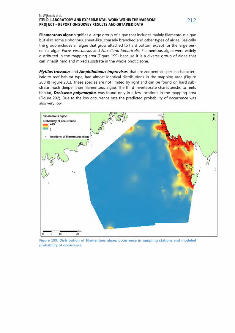
N. Wijkmark et al. FIELD, LABORATORY AND EXPERIMENTAL WORK WITHIN THE MARMONI PROJECT – REPORT ON SURVEY RESULTS AND OBTAINED DATA
212
Filamentous algae signifies a large group of algae that includes mainly filamentous algae but also some siphonous, sheet-like, coarsely branched and other types of algae. Basically the group includes all algae that grow attached to hard bottom except for the large per-ennial algae Fucus vesiculosus and Furcellaria lumbricalis. Filamentous algae were widely distributed in the mapping area (Figure 199) because it is a diverse group of algae that can inhabit hard and mixed substrate in the whole photic zone. Mytilus trossulus and Amphibalanus improvisus, that are zoobenthic species character-istic to reef habitat type, had almost identical distributions in the mapping area (Figure 200 & Figure 201). These species are not limited by light and can be found on hard sub-strate much deeper than filamentous algae. The third invertebrate characteristic to reefs habitat, Dreissena polymorpha, was found only in a few locations in the mapping area (Figure 202). Due to the low occurrence rate the predicted probability of occurrence was also very low.
Figure 199. Distribution of filamentous algae: occurrence in sampling stations and modeled probability of occurrence.

N. Wijkmark et al. FIELD, LABORATORY AND EXPERIMENTAL WORK WITHIN THE MARMONI PROJECT – REPORT ON SURVEY RESULTS AND OBTAINED DATA
213
Figure 200. Distribution of Mytilus trossulus: occurrence in sampling stations and modeled probability of occurrence
Figure 201. Distribution of Amphibalanus improvisus: occurrence in sampling stations and modeled probability of occurrence.

N. Wijkmark et al. FIELD, LABORATORY AND EXPERIMENTAL WORK WITHIN THE MARMONI PROJECT – REPORT ON SURVEY RESULTS AND OBTAINED DATA
214
Figure 202. Distribution of Dreissena polymorpha: occurrence in sampling stations and mod-eled probability of occurrence.
Characteristic species/groups of sandbanks habitat type The distribution of charophytes was limited to the most shallow soft bottom areas in the northeastern part of the mapping area (Figure 203). Vascular plants (excluding Zostera marina) also inhabit shallow soft bottom areas but compared to charophytes, their distri-bution extends to somewhat deeper and more wave exposed areas (Figure 204). Zostera marina was found only in three locations in the mapping area (Figure 205). Due to the low occurrence rate the modeled probability of occurrence was also very low. Among the modeled key species/groups, infaunal bivalves had the most extensive dis-tribution (Figure 206), because the species in this group can inhabit soft sediments in the whole depth range.

N. Wijkmark et al. FIELD, LABORATORY AND EXPERIMENTAL WORK WITHIN THE MARMONI PROJECT – REPORT ON SURVEY RESULTS AND OBTAINED DATA
215
Figure 203. Distribution of charophytes: occurrence in sampling stations and modeled proba-bility of occurrence.
Figure 204. Distribution of vascular plants: occurrence in sampling stations and modeled probability of occurrence.

N. Wijkmark et al. FIELD, LABORATORY AND EXPERIMENTAL WORK WITHIN THE MARMONI PROJECT – REPORT ON SURVEY RESULTS AND OBTAINED DATA
216
Figure 205. Distribution of Zostera marina: occurrence in sampling stations and modeled probability of occurrence.
Figure 206. Distribution of infaunal bivalves: occurrence in sampling stations and modeled probability of occurrence.
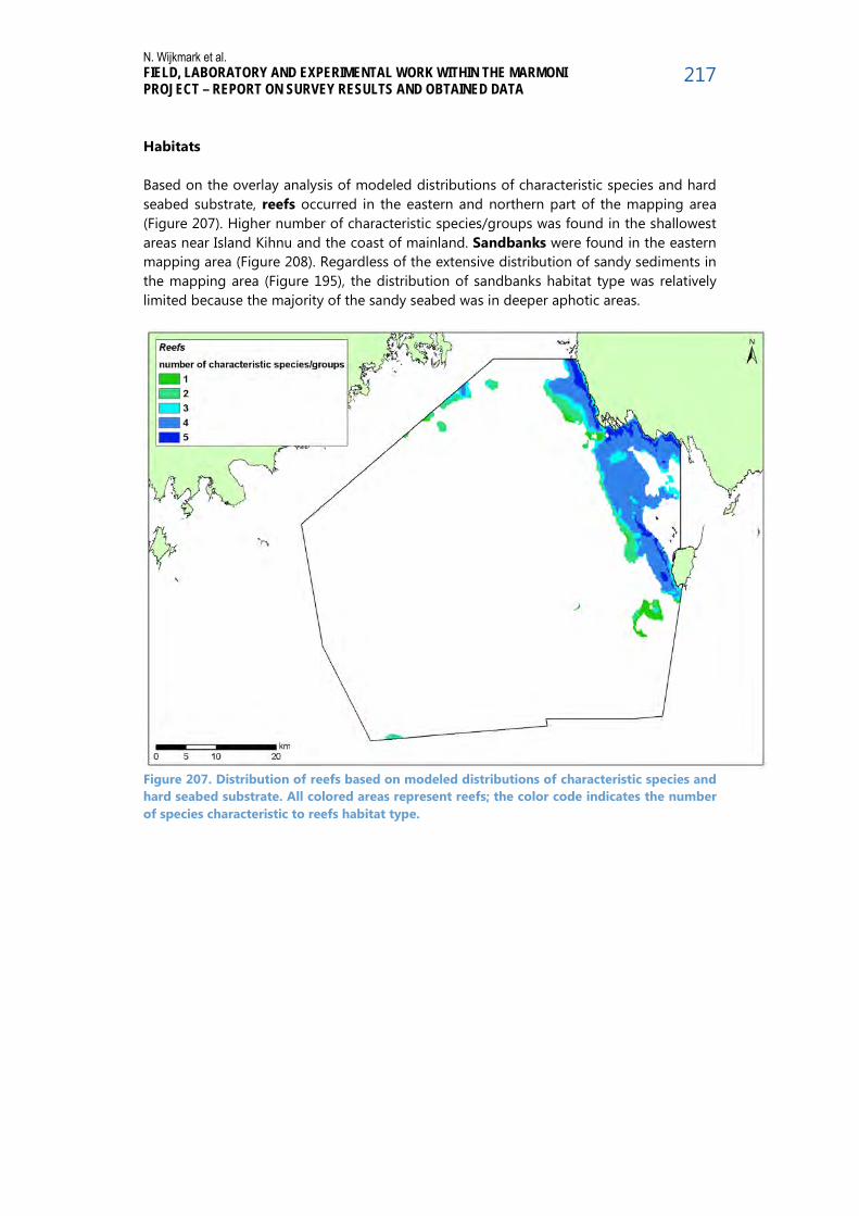
N. Wijkmark et al. FIELD, LABORATORY AND EXPERIMENTAL WORK WITHIN THE MARMONI PROJECT – REPORT ON SURVEY RESULTS AND OBTAINED DATA
217
Habitats Based on the overlay analysis of modeled distributions of characteristic species and hard seabed substrate, reefs occurred in the eastern and northern part of the mapping area (Figure 207). Higher number of characteristic species/groups was found in the shallowest areas near Island Kihnu and the coast of mainland. Sandbanks were found in the eastern mapping area (Figure 208). Regardless of the extensive distribution of sandy sediments in the mapping area (Figure 195), the distribution of sandbanks habitat type was relatively limited because the majority of the sandy seabed was in deeper aphotic areas.
Figure 207. Distribution of reefs based on modeled distributions of characteristic species and hard seabed substrate. All colored areas represent reefs; the color code indicates the number of species characteristic to reefs habitat type.

N. Wijkmark et al. FIELD, LABORATORY AND EXPERIMENTAL WORK WITHIN THE MARMONI PROJECT – REPORT ON SURVEY RESULTS AND OBTAINED DATA
218
Figure 208. Distribution of sandbanks based on modeled distributions of characteristic spe-cies and sandy seabed substrate. All colored areas represent sandbanks; the color code indi-cates the number of species characteristic to sandbanks habitat type.
References Bendtsen J, Gustafsson KE, Söderkvist J, Hansen JLS (2009) Ventilation of bottom water in the North Sea–Baltic Sea transition zone. J. Mar. Syst. 75, 138–149. Breiman L (2001) Random Forests. Machine Learning 45, 5-32 Elith J, Graham CH, Anderson RP, Dudik M, Ferrier S, Guisan A, Hijmans RJ, Huettmann F, Leathwick JR, Lehmann A, Li J, Lohmann LG, Loiselle BA, Manion G, Moritz C, Nakamura M, Nakazawa Y, Overton JMcC, Peterson AT, Phillips SJ, Richardson KS, Scachetti-Pereira R, Schapire RE, Soberón J, Williams S, Wisz MS, Zimmermann NE (2006) Novel methods im-prove prediction of species’ distributions from occurrence data. Ecography 29: 129-151. Elith J, Leathwick JR, Hastie T (2008) A working guide to boosted regression trees. Journal of Animal Ecology 77: 802-813. Elith J, Leathwick JR (2009) Species Distribution Models: Ecological Explanation and Prediction Across Space and Time. Annual Review of Ecology, Evolution, and Systematics 40, 677-697. Fielding AH, Bell JF (1997) A review of methods for the assessment of prediction errors in conservation presence/absence models. Environmental Conservation 24, 38-49.

N. Wijkmark et al. FIELD, LABORATORY AND EXPERIMENTAL WORK WITHIN THE MARMONI PROJECT – REPORT ON SURVEY RESULTS AND OBTAINED DATA
219
Friedman JH, Hastie T, Tibshirani R (2000) Additive logistic regression: a statistical view of boosting. Ann Stat 28: 337-407. Hastie TJ, Tibshirani RJ (1990) Generalised Additive Models. Chapman and Hall, New York, 352 pp HELCOM (2014) Manual for Marine Monitoring in the COMBINE Programme of HELCOM. http://helcom.fi/Documents/Action areas/Monitoring and assessment/Manuals and Guidelines/Manual for Marine Monitoring in the COMBINE Programme of HELCOM.pdf Hijmans RJ, Phillips S, Leathwick J, Elith J (2013) dismo: Species distribution modeling. R package version 0.9-3. Available: http://CRAN.R-project.org/package=dismo Hothorn T, Buehlmann P, Dudoit S, Molinaro A, Van Der Laan M (2006) Survival Ensem-bles. Biostatistics 7, 355-373 Jiménez-Valverde A, Lobo JM (2007) Threshold criteria for conversion of probability of species presence to either–or presence–absence. Acta Oecologica 31, 361-369. Kotta J, Lauringson V, Martin G, Simm M, Kotta I, Herkül K, Ojaveer H (2008) Gulf of Riga and Pärnu Bay. In: Schiewer, U. (Ed.), Ecology of Baltic Coastal Waters. Ecological Studies, vol. 197. Springer, pp. 217–243. Revermann R, Schmid H, Zbinden N, Spaar R, Schröder B (2012) Habitat at the mountain tops: how long can Rock Ptarmigan (Lagopus muta helvetica) survive rapid climate change in the Swiss Alps? A multi-scale approach. Journal of Ornithology 153: 891-905. Ridgeway G (2013) gbm: Generalized Boosted Regression Models. R package version 2.1-3.2. http://CRAN.R-project.org/package=gbm The R Foundation for Statistical Computing (2013) R version 3.0.1. http://www.r-project.org/ Wood SN (2006) Generalized Additive Models: An Introduction with R. Chapman and Hall/CRC.

N. Wijkmark et al. FIELD, LABORATORY AND EXPERIMENTAL WORK WITHIN THE MARMONI PROJECT – REPORT ON SURVEY RESULTS AND OBTAINED DATA
220
3.7.5 Modelling the distribution of habitats and species in Sweden: 2SWE Hanö Bight
3.7.5.1 Preparation of environmental layers Maps of environmental variables such as depth and depth derivatives, hydrographic vari-ables, wave exposure, Secchi depth, bottom substrate and anthropogenic pressures such as potentially polluted areas and marine commercial traffic were developed for the Hanö Bight study area. The GIS maps of environmental variables were used for two main purposes:
1) Analyses of how developed indicators respond to anthropogenic pressures and other environmental variables.
2) For modelling and predicting the distribution of species and habitats.
In total 42 layers of environmental variables were created in spatial resolutions ranging from 10 to 50 m pixel size. For some variables, several layers were created (such as mean, max, min, values at bottom and surface etc.). Depending on species or habitat, the ecol-ogically most relevant of the layers for each such variable was included in the modelling. Created layers were of the following types:
3.7.5.1.1 Bathymetric grid A detailed depth grid in 10 m resolution was created (Figure 209). The depth data is based on hydrographic surveys carried out at different times and with different method-ologies why point density varies within the area. Examples of digital depth data from vari-ous methods is single and parallel echo-sounding, digitized depth curves and multibeam. The most dense depth data is gained from multibeam. Areas measured by this method were delivered in five meter resolution. In addition to point data from the Swedish Mari-time Administration the property map's shoreline converted into points with a point every ten meters was also used. To convert point data into a continuous depth grid in 10-meter resolution, a semivariogram model for interpolation was used. During the interpolation, the search was performed in ten points (at least two) and eight directions. Root-mean-square-error, av-erage standard error, standard error, and standardized root-mean-square-error was re-corded for each square.
Figure 209. Interpolated depth grid for the Hanö Bight study area.

N. Wijkmark et al. FIELD, LABORATORY AND EXPERIMENTAL WORK WITHIN THE MARMONI PROJECT – REPORT ON SURVEY RESULTS AND OBTAINED DATA
221
3.7.5.1.2 Depth derivatives Grids describing the bottom slope, aspect and curvature were calculated based on the interpolated depth grid in 10 m resolution (example in Figure 210). The slope is calculated by taking the difference in depth from one raster grid to another, and is given in degrees where zero degrees describes a completely horizontal surface and 90 degrees a vertical surface. The aspect describes the bottom slope angle in degrees from 0 to 360. Curvature is a description of how the depth of each point in the map relate to the average depth around it and provides a snapshot of relative heights and sinks. The depth grid was also classed into nine different landforms in the GIS software SAGA. The method was per-formed according to Wilson and Gallant (2000).
Figure 210. Example of depth derivative, slope in degrees calculated from the depth grid.
3.7.5.1.3 Hydrographical variables from modelling A series of physical and chemical variables were created as a basis for the spatial model-ling based on two types of modelled data. Data from the coastal basin model HOME Wa-ter was compiled for coastal areas for bottom and surface values of temperature and sa-linity, near bottom values of oxygen, total nitrogen and phosphorous and integrated chlo-rophyll values for the water column. Comprehensive county maps were prepared for tem-perature and salinity at the surface or bottom with the addition of data from the hydro-dynamic model HIROMB. The initial plan was to collect data on variables such as total-Nitrogen, total-Phosphorus, Chlorophyll-a, salinity and temperature from the Ferrybox network. These variables were instead modelled with the HOME and HIROMB models described above. Some examples of maps of hydrographical variables are presented below (Figure 211 to Figure 215).
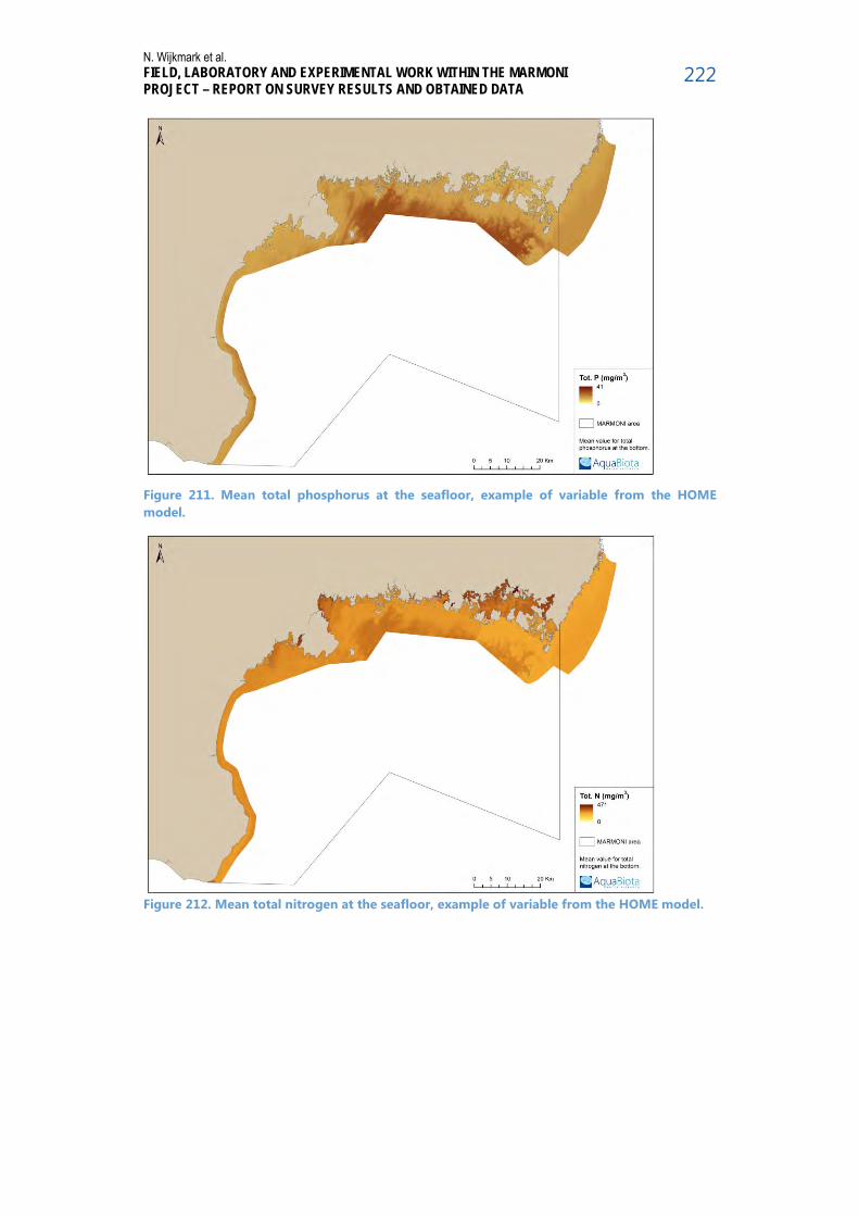
N. Wijkmark et al. FIELD, LABORATORY AND EXPERIMENTAL WORK WITHIN THE MARMONI PROJECT – REPORT ON SURVEY RESULTS AND OBTAINED DATA
222
Figure 211. Mean total phosphorus at the seafloor, example of variable from the HOME model.
Figure 212. Mean total nitrogen at the seafloor, example of variable from the HOME model.

N. Wijkmark et al. FIELD, LABORATORY AND EXPERIMENTAL WORK WITHIN THE MARMONI PROJECT – REPORT ON SURVEY RESULTS AND OBTAINED DATA
223
Figure 213. Mean chlorophyll-a, example of variable from the HOME model.
Figur 214. Mean temperature at the seafloor, variable from the HIROMB model.
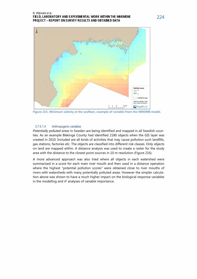
N. Wijkmark et al. FIELD, LABORATORY AND EXPERIMENTAL WORK WITHIN THE MARMONI PROJECT – REPORT ON SURVEY RESULTS AND OBTAINED DATA
224
Figure 215. Minimum salinity at the seafloor, example of variable from the HIROMB model.
3.7.5.1.4 Anthropogenic variables Potentially polluted areas in Sweden are being identified and mapped in all Swedish coun-ties. As an example Blekinge County had identified 2180 objects when the GIS layer was created in 2010. Included are all kinds of activities that may cause pollution such landfills, gas stations, factories etc. The objects are classified into different risk classes. Only objects on land are mapped within. A distance analysis was used to create a raster for the study area with the distance to the closest point sources in 10 m resolution (Figure 216).
A more advanced approach was also tried where all objects in each watershed were summarized in a score for each main river mouth and then used in a distance operation where the highest “potential pollution scores” were obtained close to river mouths of rivers with watersheds with many potentially polluted areas. However the simpler calcula-tion above was shown to have a much higher impact on the biological response variables in the modelling and rF analyses of variable importance.

N. Wijkmark et al. FIELD, LABORATORY AND EXPERIMENTAL WORK WITHIN THE MARMONI PROJECT – REPORT ON SURVEY RESULTS AND OBTAINED DATA
225
Figure 216. Distance to potentially polluted areas.
Proximity to densely populated places was calculated from densely populated areas from maps. A raster was created where a distance value was assigned to each cell using the operation “cost-distance” in ESRI ArcGIS. The cost for water was set to 1 and the cost for land was set to 1000. This results in a much larger impact from densely populated areas near the coast than inland (Figure 217).
Figure 217. Distance to densely populated places.
Commercial marine traffic This GIS layer was made from a national inventory of physical factors possibly affecting the marine environment by SEPA (Naturvårdsverket 2010). The layer was created from AIS-transponder data from both light and heavy commercial traf-fic. The polygon GIS-layer was converted to a raster in 10 m resolution (Figure 218).

N. Wijkmark et al. FIELD, LABORATORY AND EXPERIMENTAL WORK WITHIN THE MARMONI PROJECT – REPORT ON SURVEY RESULTS AND OBTAINED DATA
226
Figure 218. Commercial traffic intensity in the Hanö Bight.
3.7.5.1.5 Sediment map Sediment maps in Sweden are most often of a too low resolution for successful modelling of benthic species. The Geological Survey of Sweden (SGU) has on behalf of the Swedish Environmental Protection Agency produced modelled continuous bottom substrate maps of investigated Swedish marine areas. These maps show the bottom substrate in nine classes and are based on marine geological map databases and on seafloor observations classified according to the EUNIS system (Hallberg et al. 2010). In order to create sedi-ment maps of higher resolution more suitable for spatial modelling a new and more de-tailed sediment map was created for the northern part of the Hanö Bight. This was per-formed by SGU in cooperation with AquaBiota and the Swedish Nautical Administration Board. The process is described briefly below.
3.7.5.1.6 Creation of the detailed sediment map Data from the coastal waters of southern Blekinge County (Figure 219) within the Hanö Bight Study area were interpreted in detail at SGU in order to create a map of the surface sediment in highest possible detail. The data was collected during the regular mapping surveys performed by SGU (Figure 219).
Data was collected from the ship “Ocean Surveyor” and the smaller vessel “Ugglan” which was used in shallow areas. Data was collected using sub-bottom profiler, marine reflec-tion-seismic and side scan sonar. The sub-bottom profiler was mainly used for soft sedi-ments and the uppermost sediment layers whereas the seismic was used for coarser sediments. The side scan sonar provides surface “images” of the bottom depicting the acoustic “hardness” of the seafloor.
Samples are also taken from the ship where up to 6 m sediment cores and bottom surface samples can be taken. The smaller vessel can only take surface samples. 200 samples were taken in the area. An underwater camera was also used to take photos of the seafloor.

N. Wijkmark et al. FIELD, LABORATORY AND EXPERIMENTAL WORK WITHIN THE MARMONI PROJECT – REPORT ON SURVEY RESULTS AND OBTAINED DATA
227
Figure 219. Survey-lines in the coastal waters of southern Blekinge in the Hanö Bight. Map created by SGU.
Data from sub-bottom profiler and the marine reflection-seismic were interpreted in the software MDPS. From this interpretation the uppermost geologic layer represented as colour-coded georeferenced lines was created. This was placed on the sonar mosaic as well as other supporting material such as bathymetric grid and aerial images for areas near the shoreline. All this information was used in the final interpretation. Spatial model-ling was used in order to create a marine geological map of the area which was converted into a detailed map of the seafloor surface.
In order to create a comprehensive sediment map for the entire study area this detailed layer was merged with two older less detailed layers from SGU in order to create a seam-less substrate layer covering the entire study area (Figure 220). This was performed by AquaBiota.
During the development of the detailed sediment map, SGU also mapped vegetated bot-toms using data from the side scan sonar. This layer covers the same area as the most detailed bottom substrate (the coastal waters of southern Blekinge in the study area).

N. Wijkmark et al. FIELD, LABORATORY AND EXPERIMENTAL WORK WITHIN THE MARMONI PROJECT – REPORT ON SURVEY RESULTS AND OBTAINED DATA
228
Figure 220. Sediment map with bottom substrates in nine classes in the Hanö Bight.
Secchi depth
A regression analysis of a satellite image and a large number of field measurents was used to create a high resolution Secchi depth map over the study area (Philipson et al. 2013). Satellite data were derived from Landsat TM with an EO-sensor with 30 m spatial resolution. In the southern parts of the Secchi-depth image from August 10, 2010 are some clouds covering parts of the area. These were cut out and the holes were filled us-ing interpolation. A median filter was also applied to eliminate noise. The final secchi depth map is presented in Figure 221.
Figure 221. Secchi depth in the Hanö Bight.

N. Wijkmark et al. FIELD, LABORATORY AND EXPERIMENTAL WORK WITHIN THE MARMONI PROJECT – REPORT ON SURVEY RESULTS AND OBTAINED DATA
229
3.7.5.1.7 Wave exposure
Wave exposure refers to the spatial pattern of wave action degree that structures the shoreline species composition (Lewis 1964). Although the direction of waves and energy constantly varies the pattern for wave exposure is largely un-changed over time. This be-comes most evident in island environments where the benthic community is completely different in sheltered and exposed environments.
Since the wave activity constantly varies the degree of wave exposure is difficult to meas-ure in the field. Therefore, it’s normally estimated with a calculation method. There are several cartographical methods to choose from, and each one has its pros and cons. In this project the method Simplified Wave Model (SWM, Isæus 2004) has been used. The method is called simplified because it does not account for how the water depth affects the wave properties. The advantages of the SWM method are that it can be used in high resolution and that it provides an ecologically relevant picture of wave exposure patterns in island areas (see Eriksson et al. 2004, Bekkby et al. 2008, Sandman et al. 2008). Since the wave exposure for different areas are based on wind data from different stations there will be an overlap between areas where the values differ slightly. SWM was calculated along the coasts and hence SWM values from the open sea are missing. To cover all of the study area the Hanö Bight, SWM grids (25 m resolution) was merged with wave exposure grids from the EU - SEAMAP (about 335 m resolution). SWM values> 500 000 in this layer con-sists of significant wave height that has been created by DHI (DHI 2010) and then con-verted into the SWM, Figure 222 (Wijkmark & Isaeus 2010).
Figure 222. Wave exposure calculated as SWM and modeled wave height converted to SWM.

N. Wijkmark et al. FIELD, LABORATORY AND EXPERIMENTAL WORK WITHIN THE MARMONI PROJECT – REPORT ON SURVEY RESULTS AND OBTAINED DATA
230
3.7.5.1.8 Distance to coastal watercourses
The distance to river mouths of coastal watercourses in the area was calculated with a cost-distance operation in ESRI ArcGIS and a grid in 10 m resolution was created (Figure 223).
Figure 223. Distance to coastal watercourses.
3.7.5.2 Spatial modelling of the distribution of habitats and species
3.7.5.2.1 Modelling of species and habitats This chapter describes the creation of validated maps of distributions of habitats and spe-cies in the Hanö Bight.
3.7.5.2.2 Input maps for marine spatial management and MARMONI action A4.2 Knowledge of the marine environment is important in marine spatial management and marine spatial planning. The maps of environmental variables, habitats and species cre-ated within MARMONI will make up an important resource for spatial management in the Hanö Bight as they are the most detailed and comprehensive maps of seafloor species and habitats in the area. The created maps from the Hanö Bight have been delivered to the county administrative boards in Blekinge and Skåne Counties as well as the Swedish Agency for Marine and Water Management.
Within MARMONI action A4.2 these maps are used to demonstrate how species and habitat maps can increase the possibilities for spatial planning. This is performed in close contact with planning authorities in Sweden and will be presented in a separate report.

N. Wijkmark et al. FIELD, LABORATORY AND EXPERIMENTAL WORK WITHIN THE MARMONI PROJECT – REPORT ON SURVEY RESULTS AND OBTAINED DATA
231
3.7.5.2.3 Modelling procedure
In the modelling process collected biological data was used together with environmental data in order to create a statistical model. The model is then applied on maps of envi-ronmental variables over the area in order to create a predicted map of the modelled response variable (such as probability of occurrence of a species or habitat). Spatial mod-elling was performed using the methods randomForest, rF (Breiman, 2001; Cutler et al. 2007) and GAM (Hastie & Tibshirani, 1986) in R (R 2010).
The modelling procedure as well as creation of predictions will be presented in detail in a report (autumn 2014). This report will also present all predicted maps and environmental layers.
3.7.5.2.4 Modelling data and sampling design The sampling design is of critical importance for successful spatial modelling. Environ-ments that haven’t been sampled will not be modelled or predicted in a reliable way. Spe-cies and habitats have therefore only been modelled and predicted within the depth and exposure ranges in the modelling datasets.
Benthic flora and fauna were modelled with the drop-video and grab datasets that were collected simultaneously during combined surveys. These surveys were designed to cover the important gradients in the area and to deliver datasets well suited for spatial model-ling. Additional data from earlier surveys were also added in order to further increase the number of stations and environmental ranges sampled. These groups could therefore be predicted over the entire study area, limited only by the extent of the environmental lay-ers included in the models and the maximum depth in the modelling datasets. In order to further increase the modelling dataset, data from a few other recent surveys were also included (drop-video, snorkelling and similar methods).
Pelagic fish and zooplankton were modelled with data from hydroacoustic surveys from offshore areas. These groups were therefore not modelled in the coastal areas.
Modelling of juvenile fish was performed with data from an extensive sampling of juvenile fish which was performed in coastal recruitment areas in the study area.
Maps of collected modelling data are presented in the chapters 3.2 and 3.3 in this report.
3.7.5.2.5 Distribution of habitats (EUNIS/HUB-classes) Spatial modelling (randomForest) was used to create a validated map of the distribution of habitats in the Hanö Bight (Figure 224). First drop-video data was classed into EUNIS-classes (in the Baltic Sea represented by the HUB-classes, HELCOM Underwater Biotopes) as far as possible, resulting in 14 different benthic habitats (HUB-classes) at levels from 3 to 6.
At first, a test run was performed with a model including all classes. The test run showed that the modelling procedure could not discriminate between some classes, especially classes dominated by the same biota but on different substrates. The discrimination be-tween hard and mixed or between soft and mixed was rarely successful. Such classes were therefore grouped and a new model with a total of five grouped habitat classes was cre-ated. The predicted map from this model was 73 % correctly classed in an external valida-tion. The most important environmental variable in the models were depth (bathymetry), wave exposure (SWM) and bottom substrate (sediment map).
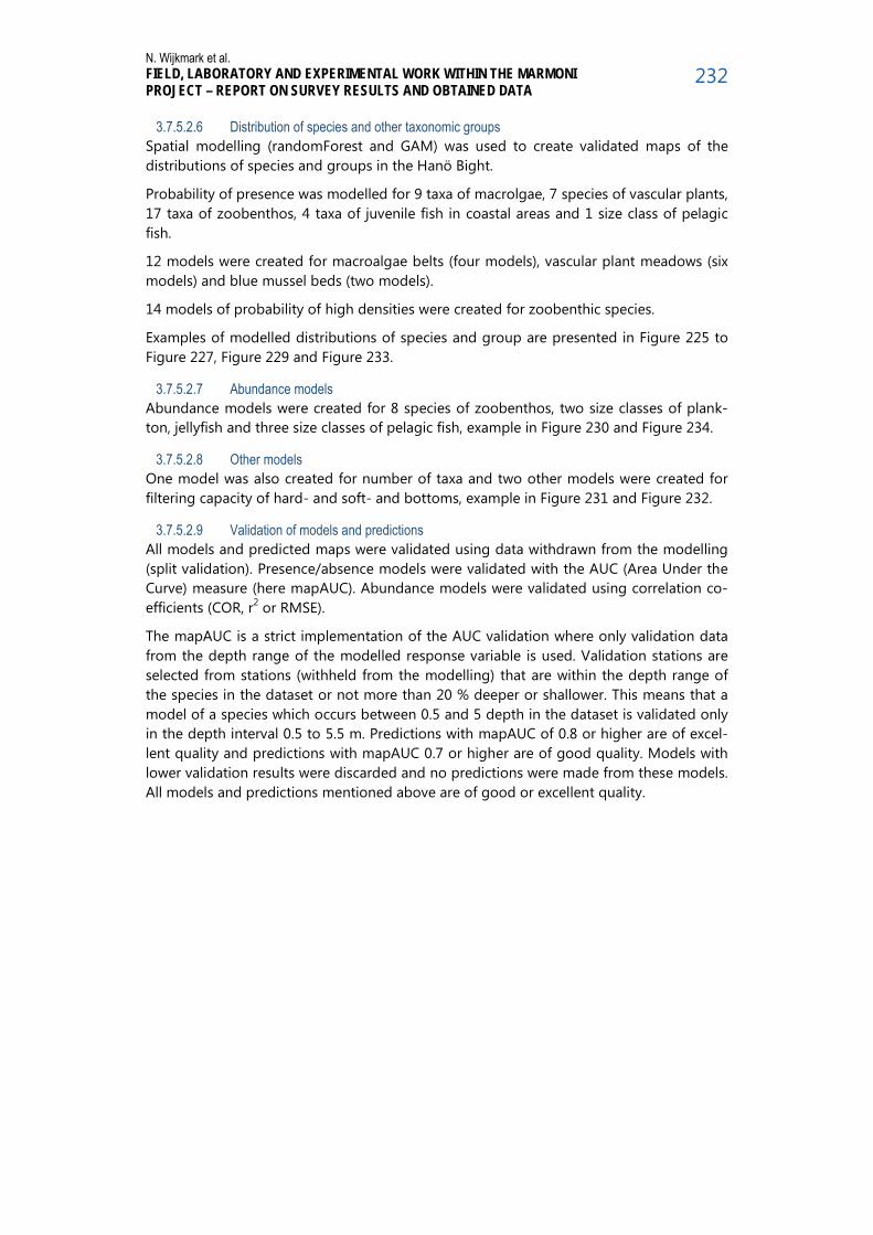
N. Wijkmark et al. FIELD, LABORATORY AND EXPERIMENTAL WORK WITHIN THE MARMONI PROJECT – REPORT ON SURVEY RESULTS AND OBTAINED DATA
232
3.7.5.2.6 Distribution of species and other taxonomic groups
Spatial modelling (randomForest and GAM) was used to create validated maps of the distributions of species and groups in the Hanö Bight.
Probability of presence was modelled for 9 taxa of macrolgae, 7 species of vascular plants, 17 taxa of zoobenthos, 4 taxa of juvenile fish in coastal areas and 1 size class of pelagic fish.
12 models were created for macroalgae belts (four models), vascular plant meadows (six models) and blue mussel beds (two models).
14 models of probability of high densities were created for zoobenthic species.
Examples of modelled distributions of species and group are presented in Figure 225 to Figure 227, Figure 229 and Figure 233.
3.7.5.2.7 Abundance models Abundance models were created for 8 species of zoobenthos, two size classes of plank-ton, jellyfish and three size classes of pelagic fish, example in Figure 230 and Figure 234.
3.7.5.2.8 Other models One model was also created for number of taxa and two other models were created for filtering capacity of hard- and soft- and bottoms, example in Figure 231 and Figure 232.
3.7.5.2.9 Validation of models and predictions All models and predicted maps were validated using data withdrawn from the modelling (split validation). Presence/absence models were validated with the AUC (Area Under the Curve) measure (here mapAUC). Abundance models were validated using correlation co-efficients (COR, r2 or RMSE).
The mapAUC is a strict implementation of the AUC validation where only validation data from the depth range of the modelled response variable is used. Validation stations are selected from stations (withheld from the modelling) that are within the depth range of the species in the dataset or not more than 20 % deeper or shallower. This means that a model of a species which occurs between 0.5 and 5 depth in the dataset is validated only in the depth interval 0.5 to 5.5 m. Predictions with mapAUC of 0.8 or higher are of excel-lent quality and predictions with mapAUC 0.7 or higher are of good quality. Models with lower validation results were discarded and no predictions were made from these models. All models and predictions mentioned above are of good or excellent quality.

N. Wijkmark et al. FIELD, LABORATORY AND EXPERIMENTAL WORK WITHIN THE MARMONI PROJECT – REPORT ON SURVEY RESULTS AND OBTAINED DATA
233
3.7.5.3 Validated map of habitat distribution in the Hanö Bight
Figure 224. Benthic habitats in the Hanö Bight modelled as HUB-classes (HUB: HELCOM Un-derwater Biotopes).
3.7.5.1 Examples of predicted maps of distributions of species and other groups in the Hanö Bight
Figure 225. Predicted probability of presence of the red algae Furcellaria lumbricalis.

N. Wijkmark et al. FIELD, LABORATORY AND EXPERIMENTAL WORK WITHIN THE MARMONI PROJECT – REPORT ON SURVEY RESULTS AND OBTAINED DATA
234
Figure 226. Predicted probability of presence of perennial macroalgae.
Figure 227. Predicted probability of presence of eelgrass.
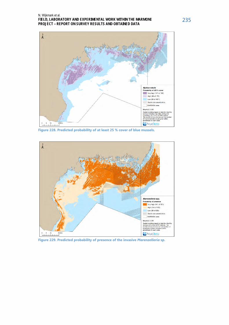
N. Wijkmark et al. FIELD, LABORATORY AND EXPERIMENTAL WORK WITHIN THE MARMONI PROJECT – REPORT ON SURVEY RESULTS AND OBTAINED DATA
235
Figure 228. Predicted probability of at least 25 % cover of blue mussels.
Figure 229. Predicted probability of presence of the invasive Marenzelleria sp.
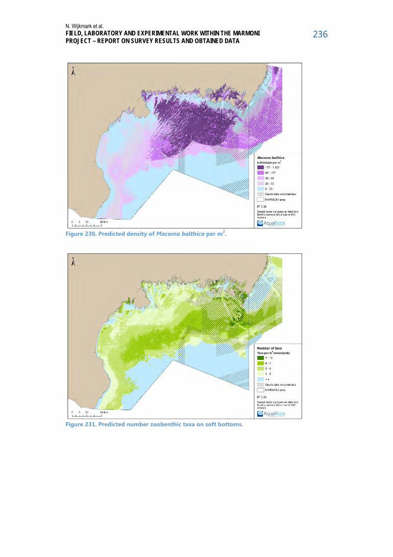
N. Wijkmark et al. FIELD, LABORATORY AND EXPERIMENTAL WORK WITHIN THE MARMONI PROJECT – REPORT ON SURVEY RESULTS AND OBTAINED DATA
236
Figure 230. Predicted density of Macoma balthica per m2.
Figure 231. Predicted number zoobenthic taxa on soft bottoms.
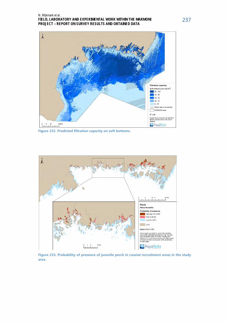
N. Wijkmark et al. FIELD, LABORATORY AND EXPERIMENTAL WORK WITHIN THE MARMONI PROJECT – REPORT ON SURVEY RESULTS AND OBTAINED DATA
237
Figure 232. Predicted filtration capacity on soft bottoms.
Figure 233. Probability of presence of juvenile perch in coastal recruitment areas in the study area.

N. Wijkmark et al. FIELD, LABORATORY AND EXPERIMENTAL WORK WITHIN THE MARMONI PROJECT – REPORT ON SURVEY RESULTS AND OBTAINED DATA
238
Figure 234. Predicted abundance of pelagic fish within the size class 7-13 cm. The class is dominated by sprat.
3.7.5.2 References Breiman, L., 2001. Random forests. Machine learning 45, 5–32. Cutler, D. R., T. C. Edwards, K. H. Beard, A. Cutler, K. T. Hess, J. Gibson, & J. J. Lawler. 2007.
Random forests for classification in ecology. Ecology 88:2783-2792. Florén K., Philison P., Strömbäck, N., Nyström Sandman, A., Isaeus, M., Wijkmark, N. 2012.
”Satellite Derived Secchi Depth for Improvement of Habitat Modelling in Coastal Areas”, Swedish National Space Board (Dnr 164/09), AquaBiota Report 2012-02.
Philipson, P., Hedvall T., Strömbäck N. 2013. In Swedish. Satellitbaserade siktdjupskartor –
Hanöbukten, Skåne, Skärgårdshavet och Stockholm. Delivery report. Brockmann Geomatics Sweden AB.

N. Wijkmark et al. FIELD, LABORATORY AND EXPERIMENTAL WORK WITHIN THE MARMONI PROJECT – REPORT ON SURVEY RESULTS AND OBTAINED DATA
239
3.7.6 Modelling the distribution of habitats and species in Finland: 3FIN Coastal area of SW
Finland
Modelling of fish reproduction areas The modelling efforts aimed at producing statistical models that linked the occurrence of early life stages of pikeperch to their surrounding environmental conditions. A logistic regression approach was applied with two environmental predictors, water turbidity and bottom topography. In situ field survey observations of the fish larvae and environmental predictors were gathered from 126 sites. In order to produce probability maps showing the potential reproduction areas of pikeperch in the coastal area of SW Finland (Figure 235 and Figure 236), the statistical models and predictor variables were exported to GIS and used to calculate cell-specific probabilities for the occurrence of newly-hatched pikeperch larvae. Validation of the distribution models and the outcome probability maps was conducted during the model building by estimating the accuracy of the model per-formance in practise using threshold-independent measures (classificatory power, ROC plots). Only models with reasonable to good discriminatory ability were used.
Figure 235. The modelled probability of occurrence of newly-hatched pikeperch larvae in the Archipelago Sea, SW Finland in 2011.

N. Wijkmark et al. FIELD, LABORATORY AND EXPERIMENTAL WORK WITHIN THE MARMONI PROJECT – REPORT ON SURVEY RESULTS AND OBTAINED DATA
240
Figure 236. The modelled probability of occurrence of newly-hatched pikeperch larvae around the Hanko Peninsula, SW Finland in 2012.

N. Wijkmark et al. FIELD, LABORATORY AND EXPERIMENTAL WORK WITHIN THE MARMONI PROJECT – REPORT ON SURVEY RESULTS AND OBTAINED DATA
241
4 Acknowledgements We thank the LIFE financial instrument of the European Community for funding, which has made possible the collection of highly needed biological data and the testing of innova-tive monitoring methods and approaches within the study areas.

LIFE+ Nature & Biodiversity project “Innovative approaches for marine biodiversity moni-toring and assessment of conservation status of nature values in the Baltic Sea” (Project acronym MARMONI).
Please visit the project website: http://marmoni.balticseaportal.net/ Project coordinating beneficiary: Baltic Environmental Forum – Latvia Antonijas street 3-8, Rīga, LV -1010, Latvia www.bef.lv
Copyright © 2022 FDOKUMEN

