Download - Effect of critical latitude and seasonal stratification on tidal current profiles along Ronne Ice Front, Antarctica

Effect of critical latitude and seasonal stratification on

tidal current profiles along Ronne Ice Front, Antarctica

Keith Makinson,1 Michael Schroder,2 and Svein Østerhus3

Received 18 May 2005; revised 2 December 2005; accepted 27 December 2005; published 30 March 2006.

[1] The ice front region of Ronne Ice Shelf lies near the critical latitude of the semidiurnalM2 tide, the principal tidal constituent in the southern Weddell Sea. Here the Coriolisfrequency almost equals the M2 tidal frequency, resulting in a strong dependence of theM2 tidal currents on depth and stratification and a boundary layer that can occupy theentire water column. Using data from four long-term moorings along Ronne Ice Front, weconfirm the presence of strongly depth-dependent semidiurnal tidal currents and theirsensitivity to changes in stratification. The time series show dramatic seasonal changes intidal current profiles and significant interannual variability. During periods ofstratification, the amplitude of the semidiurnal tides in the mid–water column shows atwofold increase and, despite being several kilometers offshore from the ice front, the tidalcurrents clearly show a second boundary layer originating from the adjacent ice shelfbase. Together, these two boundary layers occupy most of the water column, up to 600 mdeep, until intense sea ice formation and the production of High-Salinity Shelf Watererodes the vertical stratification. During winter when homogeneous conditions prevail, asingle bottom boundary layer occupies the entire water column at some locations. Thisstrong seasonality and sensitivity of the M2 tidal current to stratification highlights thedifficulties of interpreting current data from short-term moorings while demonstrating thatit is the best indicator for characterizing changes in stratification after direct observationsof density variations.

Citation: Makinson, K., M. Schroder, and S. Østerhus (2006), Effect of critical latitude and seasonal stratification on tidal current

profiles along Ronne Ice Front, Antarctica, J. Geophys. Res., 111, C03022, doi:10.1029/2005JC003062.

1. Introduction

[2] Winds blowing from Ronne Ice Shelf and tidaldivergence maintain a coastal polynya along Ronne IceFront in the southern Weddell Sea throughout much of theyear [Foldvik et al., 2001; Renfrew et al., 2002]. During thesummer melt season, solar radiation enlarges the polynyaand warms the surface waters. In wintertime however, thecoastal polynya is the focus of intense heat loss asrelatively warm water is exposed to the cold atmosphere,causing the seawater to cool to its surface freezing point,with further heat loss resulting in sea ice production.Sustained sea ice production is maintained as newly formedsea ice is transported northward away from the polynya byoffshore winds. Production rates are 1 or 2 orders ofmagnitude higher than for the surrounding sea, which isalready covered with ice. Hence about 6% of the entire seaice production is focused within a polynya that makes up

only 0.13% of the Weddell Sea [Renfrew et al., 2002]. Theassociated production of High-Salinity Shelf Water(HSSW) is likely to be equally intense, resulting inconvective overturning of the entire underlying watercolumn during winter [Foldvik et al., 2001; Nicholls etal., 2003]. At the ice front, this HSSW has been observedto flow along and toward the ice front [Foldvik et al., 2001;Woodgate et al., 1998] and drain deep into the sub–iceshelf cavity [Nicholls and Makinson, 1998; Nicholls et al.,2001]. Interactions with the base of Filchner-Ronne IceShelf (FRIS) convert HSSW into Ice Shelf Water (ISW), awater mass that is fresher, and by definition, colder than thesurface freezing point. Ultimately, this water reaches thenortherly point of Filchner Depression where it overflowsthe continental shelf break [Nicholls et al., 2001], making asignificant contribution to the production of Weddell SeaBottom Water [Foldvik et al., 2004], a precursor ofAntarctic Bottom Water.[3] The application of two-dimensional barotropic tidal

models to the southern Weddell Sea [Makinson and Nicholls,1999; Robertson et al., 1998] and observations offshore ofRonne Ice Front [Foldvik et al., 2001;Woodgate et al., 1998]show this region to be tidally active, with tidal currents of 20–40 cm s�1 during spring tides with excursions of 4–8 km[Makinson, 2002b]. In addition, the northwest corner of theRonne Ice Front region lies near the critical latitude (lcrit) ofthe M2 tidal constituent at 74�2801800S. Here the Coriolis

JOURNAL OF GEOPHYSICAL RESEARCH, VOL. 111, C03022, doi:10.1029/2005JC003062, 2006

1British Antarctic Survey, Natural Environment Research Council,Cambridge, UK.

2Alfred-Wegener-Institut fur Polar- undMeeresforschung, Bremerhaven,Germany.

3Bjerknes Centre for Climate Research, Geophysical Institute, Uni-versity of Bergen, Bergen, Norway.

Copyright 2006 by the American Geophysical Union.0148-0227/06/2005JC003062$09.00

C03022 1 of 15

frequency equals the tidal frequency and semidiurnal tidalcurrents near lcrit are known to have a strong depth depen-dence [Foldvik et al., 2001; Foldvik et al., 1990] and changesin stratification are likely to significantly affect the tidalcurrent profile [Makinson, 2002a]. In order to study thevertical structure of tidal currents, various analytical solutionsand numerical models have been successfully applied tocontinental shelf seas with a homogenous water column[e.g., Furevik and Foldvik, 1996; Nøst, 1994; Simpson andSharples, 1994; Soulsby, 1983]. Where the water column isstratified and close to lcrit, numerical modeling has shownthat stratification significantly affects how the polarization ofthe tidal current ellipse varies with depth [Makinson,2002a]. Using a one-dimensional turbulence closure modeland separating the tidal constituents into rotary compo-nents, Makinson [2002a] modeled tidal current profilesbeneath FRIS to determine the effects of polarization onvertical mixing. Polarization, P = m/M, was used todefine the shape and sense of rotation of a tidal currentellipse in terms of the semimajor (M) and semiminor (m) axes(Figure 1). The model showed that predominantly anti-clockwise tidal currents (P > 0) produce significantlyhigher levels of mixing than clockwise tidal currents (P <0). This effect was accounted for by decomposing theelliptical tidal current vector into purely anticlockwise(R+) and clockwise (R�) components and consideringtheir respective frictional boundary layers. The two,constant magnitude, rotary velocity components rotate atthe tidal frequency, and each has a characteristic frictionalboundary layer thickness, d+ and d�, given by Prandle[1982].

dþ � 2KM

wþ fj j

� �1=2

ð1aÞ

d� � 2KM

w� fj j

� �1=2

; ð1bÞ

where KM is the vertical eddy viscosity, f is the Coriolisparameter and w is the frequency of the tidal oscillation.Therefore, in the Southern Hemisphere, tidal currents withmore positive polarizations (anticlockwise rotation) havelarger boundary layers.

[4] At high southern latitudes, the boundary layer of R+

for semidiurnal tides is much larger than that of thecorresponding R� component, as jw + f j tends to zero atlcrit. At this latitude the tidal frequency equals the Coriolisor inertial frequency, w = j f j = 2W sin lcrit, where theEarth’s angular velocity W = 7.2921151 � 10�5 rad s�1.Beneath Ronne Ice Shelf, Makinson [2002a] showed thatthe combined upper and lower boundary layers couldoccupy the entire water column, as either lcrit wasapproached or the tidal amplitude increased. These thickerboundary layers produce less intense shear near a boundarybut extend the shear over a larger thickness of the watercolumn, near lcrit; effectively redistributing and modifyingthe profile of vertical mixing. At polar latitudes, this effectapplies to semidiurnal tides. For diurnal tides at polar lat-itudes, j f j is almost twice as large as w, hence they do notexhibit these large differences in the rotary boundary layers ofR+ and R�, and are generally barotropic [Robertson, 2005b].[5] The boundary layer thickness is further complicated

by stratification, which can dramatically affect the shape ofthe R+ tidal current profile, while the R� component remainsunaffected [Makinson, 2002a]. Stratification suppressesturbulent motions and inhibits the transfer of momentum,giving a reduced boundary layer thickness compared withthe homogenous case, and a reduced eddy viscosity, partic-ularly in the vicinity of a pycnocline [Souza and Simpson,1996]. Both observations and numerical modeling beneathfixed ice cover have found that the water column in thevicinity of the pycnocline becomes decoupled from theboundary layers at the seabed and ice base. This decou-pling of the water column around the pycnocline resultsin a significant increase in the tidal current as itapproaches or attains its free stream velocity [Makinson,2002a; Prinsenberg and Bennett, 1989].[6] One of the first comprehensive studies of seasonal

changes in tidal currents was presented by Howarth [1998],who showed the significant differences in tidal currentstructure between the well-mixed winter conditions andstratified summer conditions in the North Sea. Here, thesurface layer above the pycnocline became decoupled fromthe bottom boundary layer during summer months; withthe orientation of bottom currents rotated 25� relative to thesurface, and with their phase 30� (1 hour) in advance of thesurface. In the southern Weddell Sea few long-termmoorings have been deployed to enable studies of sea-sonal variations. However, Foldvik et al. [1990] consid-ered seasonal changes in tidal currents from moorings atthe continental shelf break, but found changes in bothdiurnal and semidiurnal tides and attributed these varia-tions to the interaction of barotropic shelf waves withtopography and a seasonal mean current. With the paucityof observational data, numerical models have been usedmore extensively in the southern Weddell Sea to studythe effects of lcrit and stratification. Although the focusof attention has been along the southern shelf break, themodels show a bottom boundary layer up to 150 m thickclose to lcrit, with changes in stratification producingonly small differences in tidal amplitude close to thepycnocline [Pereira et al., 2002; Robertson, 2001b].[7] Along Ronne Ice Front, previous observations of tidal

currents have mainly been confined to short summerobservations. However, four moorings with records greater

Figure 1. A tidal current vector, rotating at frequency (w),traces out an ellipse that is described by four basicparameters: semi-major (M) and semiminor (m) axes,orientation (y) and phase angle (f) or, alternatively, thesum of two counterrotating vectors with amplitudes R+ andR� and phases f+ and f�.

C03022 MAKINSON ET AL.: CRITICAL LATITUDE AND STRATIFICATION

2 of 15

C03022

than 1 year have been successfully recovered from theRonne Ice Front coastal polynya [Foldvik et al., 2001;Woodgate et al., 1998] and form the basis of the workpresented in this paper. With the exception of numericalmodeling, the effects on observed tidal current profiles ofseasonal changes in stratification and proximity to lcrit

have not been studied. The aim of this paper is to discuss theinfluence of lcrit and changes in stratification, on tidalcurrents and their vertical profiles along Ronne Ice Front. Insection 2 the moorings and other observational data are usedto give an outline of the hydrography along Ronne Ice Front.Section 3 outlines howharmonic analysis is used to generate atime series of the positive and negative rotary tidal compo-nents for each of the major tidal constituents. These timeseries, together with temperature and salinity data from themoorings are then used in section 4 to show how the tidalcomponents are influenced by seasonal stratification.

2. Ronne Ice Front: General Observations

[8] Almost all oceanographic observations along RonneIce Front have been made during the late austral summer,when light sea ice or openwater allow ships to access the area.Wintertime observations are only possible through the de-ployment of long-term moorings, and Figure 2 shows thelocations of four such moorings along Ronne Ice Front.All the moorings were deployed approximately 5–10 kmfrom the ice front, which can advance at up to 1.9 km yr�1

[Foldvik et al., 2001]. In total, nine instruments yieldedrecords of between 1.2 and 2.5 years in length and Figure 3shows their positions within the water column. The first long-term mooring, R2, was deployed in February 1993 roughlymidway along Ronne Ice Front. R2 contained two currentmeters, each with temperature and conductivity sensors thatremained operational until April 1994 [Foldvik et al., 2001].The other ice front moorings, one on Berkner Shelf (FR3) andtwo in Ronne Depression (FR5 and FR6), were deployed inearly 1995 and remained operational until May 1997. Each ofthe current meters on the FR moorings had temperaturesensors, with the shallowest instrument at FR6 and theinstrument at FR3 also having a conductivity sensor

Figure 2. Map showing the ice front region of Ronne IceShelf. The locations of the ice front moorings are indicatedtogether with arrows showing the time-averaged currents foreach instrument. The contours indicate the bedrock depthbelow sea level, with a 100-m contour interval [Vaughan etal., 1994], and the M2 critical latitude is marked by thedashed line at 74�2801800S.

Figure 3. Vertical profiles of potential temperature (thin line), salinity (thick line), and surface freezingpoint (dashed line) close to each mooring location at the time of deployment. The light shaded area showsthe part of the water column occupied by the adjacent ice shelf, and dark shading indicates the seabed.The thin horizontal lines show the depth of the moored instruments.


3 of 15

C03022

[Woodgate et al., 1998]. However, the resolution of conduc-tivity data from themoorings is only 0.072mS cm�1, whereasthe temperature resolution is 0.008�C, resulting in a derivedsalinity resolution of only 0.1. This poor resolution is most

apparent during winter months, when the water columnremains close to the surface freezing point and thesalinity tends to only a few values, even after smoothingthe data to obtain daily averages. Clear examples of this

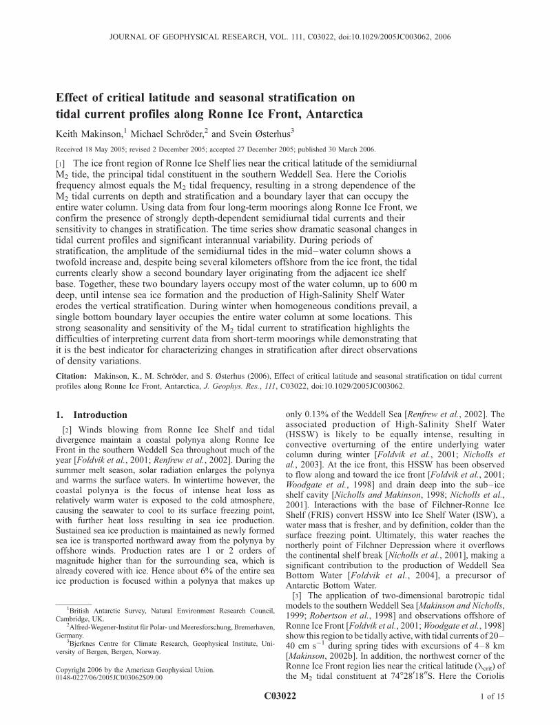
Figure 4. Time series data from mooring FR6. (a) High-pass-filtered (2-day) current componentperpendicular to the ice front at 442 m. (b) Raw and daily averaged salinity time series data from theupper instrument at 261 m. (c) Raw and daily averaged potential temperature time series data. The datafrom 261 and 588 m have been offset by 0.15�C and �0.05�C, respectively, to improve clarity, and thedotted line shows the surface freezing temperature of �1.91�C. (d) Time series of the anticlockwiserotary component amplitude (R+) for the M2 tidal constituent. The numbered vertical lines show when R+

observations are used for the vertical profiles in Figure 6. (e) Time series of the anticlockwise rotarycomponent phase (f+) for the M2 tidal constituent. At 558 m, f+ has been offset by 60�. (f) Bar chart ofsea ice production in the coastal polynya along Ronne Ice Front for each month of the mooring record.The shaded areas in each plot show the summer melting season [Renfrew et al., 2002].


4 of 15

C03022

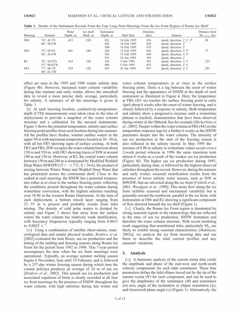
effect are seen in the 1995 and 1996 winter salinity data(Figure 4b). However, increased water column variabilityduring late summer and early winter, allows the smootheddata to reveal a more precise daily average, particularlyfor salinity. A summary of all the moorings is given inTable 1.[9] At each mooring location, conductivity-temperature-

depth (CTD) measurements were taken close to the time ofdeployment to provide a snapshot of the water columnstructure and a calibration for the moored instruments.Figure 3 shows the potential temperature, salinity and surfacefreezing point profiles from each location during late summer.All the profiles have fresher, warmer surface waters in theupper 50 mwith maximum temperatures located at 30–50 m,with all but FR5 showing signs of surface cooling. At bothFR5 and FR6, ISWoccupies the water column between about150 m and 550 m, with FR3 showing traces of ISWat around100 m and 150 m. However, at R2, the central water columnbetween 150m and 280m is dominated byModifiedWeddellDeepWater (MWDW) (T >�1.7�C, S < 34.6), the product ofmixing between Winter Water and Weddell Deep Water thathas penetrated across the continental shelf. Close to theseabed at each mooring, the HSSW has a potential tempera-ture either at or close to the surface freezing point, reflectingthe conditions present throughout the water column duringwintertime convection, with the highest salinities reachingover 34.86 in the western Ronne Depression. At the time ofeach deployment, a bottom mixed layer ranging from25–55 m is present and probably results from tidalmixing. The density of cold polar waters is dictated bysalinity and Figure 3 shows that away from the surfacewaters the water column has relatively weak stratification,with buoyancy frequencies typically ranging from 0.0015to 0.0025 s�1.[10] Using a combination of satellite observations, mete-

orological data and simple physical models, Renfrew et al.[2002] evaluated the heat fluxes, sea ice production and thetiming of the melting and freezing seasons along Ronne IceFront for the period from 1992 to 1998. This 7-year periodencompasses the time when the ice front moorings wereoperational. Typically, an average summer melting seasonbegins 6 November, lasts until 19 February, and is followedby a 257-day winter freezing season during which time thecoastal polynya produces an average of 24 m of sea ice[Renfrew et al., 2002]. This annual sea ice production andassociated expulsion of brine is clearly recorded at all fourice front moorings by the presence of HSSW throughout thewater column, with high salinities during late winter and

water column temperatures at or close to the surfacefreezing point. There is a lag between the onset of winterfreezing and the appearance of HSSW at the depth of eachinstrument as illustrated in Figure 4. Here, the temperatureat FR6 (261 m) reaches the surface freezing point in earlyApril about 6 weeks after the onset of winter freezing, and isclosely followed by a response in salinity. Both temperatureand salinity show a progressive increase until a wintertimeplateau is reached, characteristics that have been observedduring winter in the Okhotsk Sea for example [Shcherbina etal., 2003]. Deeperwithin thewater column at FR6 (442m) thetemperature response lags by a further 6 weeks as the HSSWpenetrates deeper into the water column. The intensity ofsea ice production at the start of the freezing season isalso reflected in the salinity record. In May 1995 theincrease of 0.08 in salinity to wintertime values occurs over a2-week period whereas in 1996 the same transition tookalmost 6 weeks as a result of the weaker sea ice production(Figure 4f). The higher sea ice production during 1995,particularly during June, is followed by the highest observedsalinities throughout the record. However, during the summerand early winter, seasonal stratification results from thepresence of lower salinity water masses, such as ISW orMWDW, that are advected along the ice front [Foldvik et al.,2001; Woodgate et al., 1998]. This mean flow along the icefront exhibits seasonal and interannual variability but isgenerally toward the northwest, parallel to the ice front, withinstruments at FR6 and R2 showing a significant componentof flow directed beneath the ice shelf (Figure 1).[11] Clearly, the Ronne Ice Front region is dominated by

strong seasonal signals in the meteorology that are reflectedin the rates of sea ice production, HSSW formation andtherefore the water column structure. With recent modelingwork suggesting that semidiurnal tides, particularly M2, arelikely to exhibit strong seasonal characteristics [Makinson,2002a], we analyze the ice front mooring data and usethem to describe the tidal current profiles and anyseasonal variations.

3. Analysis

[12] A harmonic analysis of the current meter data yieldsthe amplitude and phase of the east-west and north-southvelocity components for each tidal constituent. These fourparameters define the tidal ellipse traced out by the tip of thecurrent vector (V) for each component, and can be used togive the amplitudes of the semimajor (M) and semiminor(m) axis, angle of the inclination or ellipse orientation (y),and Greenwich phase angle (f) (Figure 1). Alternatively, the

Table 1. Details of the Instrument Records From the Four Long-Term Moorings From the Ice Front Region of Ronne Ice Shelf

Mooring PositionWater

Depth, mIce shelfDraft, m

InstrumentDepth, m Start Date

Duration,days Sensors

Distance fromM2 jcrit, km

FR6 74�, 42.30S 613 220 261 16 Feb 1995 816 speed, direction, T, C, P 2660�, 48.60W 442 16 Feb 1995 830 speed, direction, T

588 16 Feb 1995 679 speed, direction, TFR5 75�, 09.80S 601 240 204 15 Feb 1995 816 speed, direction, T, P 77

58�, 43.60W 305 15 Feb 1995 830 speed, direction, T, P551 29 Jun 1995 545 speed, direction, T

R2 76�, 28.850S 419 120 245 5 Feb 1993 435 speed, direction, T, C 22353�, 00.030W 400 5 Feb 1993 435 speed, direction, T, C

FR3 77�, 00.10S 254 120 203 26 Jan 1995 837 speed, direction, T, C 28149�, 01.30W


5 of 15

C03022

ellipse velocity vector can be represented by the sum of twocorotating vectors

V tð Þ ¼ Rþ exp i fþ þ wt� ��

þ R� exp �i f� � wtð Þð Þ; ð2Þ

where t is time, w is the tidal frequency, R+ and R� are theamplitudes of the positive and negative rotary components,and f+ and f� are the corresponding phases. From theseparameters the semimajor and semiminor axes of the ellipseare

M ¼ Rþ þ R� ð3Þ

m ¼ Rþ � R�; ð4Þ

and the orientation of the semimajor axis relative to east andGreenwich phase angle is

y ¼ fþ þ f��

=2 ð5Þ

f ¼ fþ � f��

=2: ð6Þ

[13] The sign of the semiminor axis represents the direc-tion of rotation of the tidal ellipse, with polarization, whichranges between ±1, describing both the shape and sense ofrotation. If positive, the current rotates anticlockwise; ifnegative, the current rotates clockwise. Close to lcrit orwhere large boundary layers occur, the ellipse polarizationin the Southern Hemisphere can become increasingly neg-ative toward the seabed because of the strong depth depen-dence of R+, possibly resulting in a change in the sense ofrotation. This characteristic has been observed for M2 in thesouthern Weddell Sea close to the shelf break [Foldvik etal., 1990] and at the ice front mooring, R2 [Foldvik et al.,2001]. Woodgate et al. [1998] analyzed the entire timeseries at FR5 and FR6 and showed that the semidiurnal

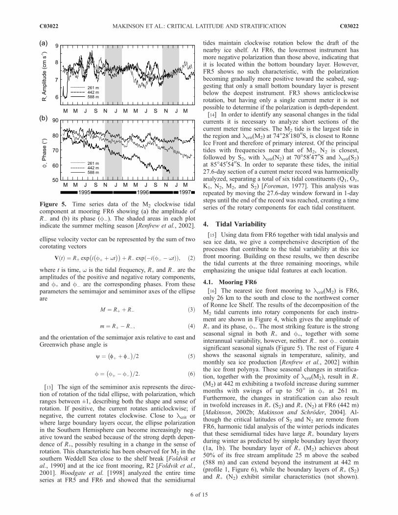
tides maintain clockwise rotation below the draft of thenearby ice shelf. At FR6, the lowermost instrument hasmore negative polarization than those above, indicating thatit is located within the bottom boundary layer. However,FR5 shows no such characteristic, with the polarizationbecoming gradually more positive toward the seabed, sug-gesting that only a small bottom boundary layer is presentbelow the deepest instrument. FR3 shows anticlockwiserotation, but having only a single current meter it is notpossible to determine if the polarization is depth-dependent.[14] In order to identify any seasonal changes in the tidal

currents it is necessary to analyze short sections of thecurrent meter time series. The M2 tide is the largest tide inthe region and lcrit(M2) at 74�28

018000S, is closest to RonneIce Front and therefore of primary interest. Of the principaltides with frequencies near that of M2, N2 is closest,followed by S2, with lcrit(N2) at 70�58

04700S and lcrit(S2)at 85�4505400S. In order to separate these tides, the initial27.6-day section of a current meter record was harmonicallyanalyzed, separating a total of six tidal constituents (Q1, O1,K1, N2, M2, and S2) [Foreman, 1977]. This analysis wasrepeated by moving the 27.6-day window forward in 1-daysteps until the end of the record was reached, creating a timeseries of the rotary components for each tidal constituent.

4. Tidal Variability

[15] Using data from FR6 together with tidal analysis andsea ice data, we give a comprehensive description of theprocesses that contribute to the tidal variability at this icefront mooring. Building on these results, we then describethe tidal currents at the three remaining moorings, whileemphasizing the unique tidal features at each location.

4.1. Mooring FR6

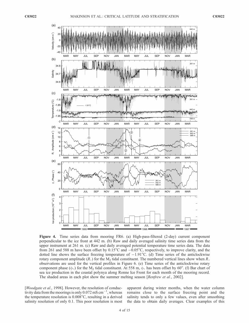
[16] The nearest ice front mooring to lcrit(M2) is FR6,only 26 km to the south and close to the northwest cornerof Ronne Ice Shelf. The results of the decomposition of theM2 tidal currents into rotary components for each instru-ment are shown in Figure 4, which gives the amplitude ofR+ and its phase, f+. The most striking feature is the strongseasonal signal in both R+ and f+, together with someinterannual variability, however, neither R� nor f� containsignificant seasonal signals (Figure 5). The rest of Figure 4shows the seasonal signals in temperature, salinity, andmonthly sea ice production [Renfrew et al., 2002] withinthe ice front polynya. These seasonal changes in stratifica-tion, together with the proximity of lcrit(M2), result in R+

(M2) at 442 m exhibiting a twofold increase during summermonths with swings of up to 50� in f+ at 261 m.Furthermore, the changes in stratification can also resultin twofold increases in R+ (S2) and R+ (N2) at FR6 (442 m)[Makinson, 2002b; Makinson and Schroder, 2004]. Al-though the critical latitudes of S2 and N2 are remote fromFR6, harmonic tidal analysis of the winter periods indicatesthat these semidiurnal tides have large R+ boundary layersduring winter as predicted by simple boundary layer theory(1a, 1b). The boundary layer of R+ (M2) achieves about50% of its free stream amplitude 25 m above the seabed(588 m) and can extend beyond the instrument at 442 m(profile 1, Figure 6), while the boundary layers of R+ (S2)and R+ (N2) exhibit similar characteristics (not shown).

Figure 5. Time series data of the M2 clockwise tidalcomponent at mooring FR6 showing (a) the amplitude ofR� and (b) its phase (f�). The shaded areas in each plotindicate the summer melting season [Renfrew et al., 2002].


6 of 15

C03022

Similar bottom boundary layer characteristics for the semi-diurnal tides also occur at mooring R2 during wintertimeand the occurrence of large R+ boundary layers (>100 m),which could respond to changes in stratification, arealso observed at other high-latitude sites located over 20�(2200 km) away from lcrit. Close to the M2 lcrit andthe continental shelf slope of the southern Weddell Sea,Foldvik et al. [1990] observed the R+ (S2) boundary layerextending through the lower 100 m of water column. Inarctic Canada, sites in Hudson Bay (63�N) and Peel Sound(73.5�N) also show the S2 boundary layer, up to 200 mthick, occupying almost the entirewater column [Prinsenbergand Bennett, 1989]. However, no studies regarding theinfluence of seasonal stratification on these tidal currentprofiles were undertaken, although simple boundary layertheory (equations (1a) and (1b)) predicts that the semidiurnaltides at high latitudes will remain sensitive to changes in KM,and therefore stratification. Conversely, the clockwise tidalcomponent of the semidiurnal tides and both components ofthe diurnal tides remain unaffected by the seasonal changes instratification.[17] At FR6, the seasonality of the semidiurnal tides

increases the peak spring tidal current in the mid–watercolumn (442 m) from around ±25 cm s�1 during midwinter,to almost ±40 cm s�1 during late summer and early winter,an increase of around 50% (Figure 4a), while the diurnaltides exhibit no seasonality. The changes in f+ for the othersemidiurnal tides can also be over 40�, equivalent to 20� in

ellipse orientation, which at FR6 is typically 55� duringwinter.[18] Another potential source of seasonal depth-depen-

dent tidal variability could result from the affect of strati-fication and the propagation of internal tides. Generatedover regions of steep topography, such as continental shelfslopes or an ice front, internal tides can result in strongvertical shears in the horizontal velocities. However, linearinternal wave theory for a continuously stratified fluidpredicts that internal tides will neither be generated norpropagate poleward of the critical latitude (a more extensiveexplanation of the relevant linear internal wave theory isgiven by Robertson [2001a]). Here the critical latitude actsas a turning latitude, preventing internal tides from propa-gating farther poleward although the critical latitude andturning latitude do not always coincide. Using equation10.26 from LeBlond and Mysak [1978] and assuming amean buoyancy frequency of 0.002 s�1 for the regionaround FR6, the M2 turning latitude is less than 5 km tothe south of the critical latitude. Therefore the turninglatitude remains remote from FR6 and the other ice frontmoorings, while the internal tide energy poleward of thecritical latitude is damped exponentially, potentially intro-ducing some residual internal wave energy to the morenorthern ice front observations.[19] While internal tides are not expected in a continuously

stratified water column, Robertson [2005a] and Robertson etal. [2003] found that internal tides can exist poleward of thecritical latitude at the front of and beneath Ross Ice Shelf,because of the hydrographic conditions within the cavity.Beneath the ice shelf the water column responded as a simpletwo-layer system, particularly deep within the cavity and to alesser degree at the ice front, potentially influencing tidalobservations at ice front moorings. Applying the same modelto the Weddell Sea and imposing a similarly simple layeredwater columnbeneath FRIS, resulted in no significant internalwave response within the cavity [Robertson, 2005b]. How-ever, Robertson [2005b] noted that diurnal continental shelfwaves generated over regions of steep topography, par-ticularly over the continental shelf edge, amplified thebaroclinic semidiurnal tides. Along Ronne Ice Front, lessvigorous continental shelf waves were observed withinthe model but no significant semidiurnal response wasreported. Clearly, these processes could contribute to theobserved seasonal variability, but the influence of strati-fication on semidiurnal tidal boundary layers appears tobe the primary source of seasonal tidal variability alongRonne Ice Front.[20] One feature common to all the ice front data is an

overall decrease in M2 f� of 8�–18� yr�1 in the instrumentsnearest the seabed and a decrease of 4�–7� yr�1 higher inthe water column. An example of this, Figure 5b shows thedecrease in M2 f� for mooring FR6. In addition, there is asimilar annual increase in M2 f+; hence the average ellipseorientation generally remains fixed (see equation (5)). Othersemidiurnal and diurnal tides show similar phase changes,which are presumably the result of the ice front advancingtoward the moorings. Using the tidal models of Makinsonand Nicholls [1999] and Padman et al. [2002] and convert-ing the tidal constituents in rotary vectors, the data showthat f+ and f� change significantly in the region of RonneIce Front. However, the magnitude of spatial gradients is

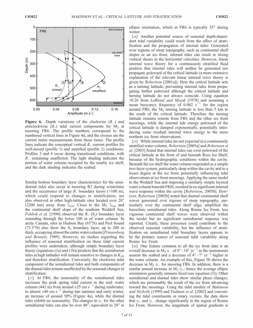
Figure 6. Depth variations of the clockwise (R�) andanticlockwise (R+) tidal current components for M2 atmooring FR6. The profile numbers correspond to thenumbered vertical lines in Figure 4d, and the crosses are thecurrent meter measurements from those times. The profilelines indicate the conceptual vertical R+ current profiles forwell-mixed (profile 1) and stratified (profile 2) conditions.Profiles 3 and 4 occur during transitional conditions, withR� remaining unaffected. The light shading indicates theportion of water column occupied by the nearby ice shelf,and the dark shading indicates the seabed.


7 of 15

C03022

underestimated, probably because the present models onlyhave 7–10 km grid spacing.[21] With three current meters at FR6, vertical profiles of

the rotary components can be created for various timesthroughout the year. On the basis of the analysis of therotary components at each instrument, the crosses in Figure6 show the observed R+ for the times indicated in Figure 4,but with almost no knowledge of the water column struc-ture, suggesting R+ profiles is difficult. However, Makinson[2002a] applied a 1-D vertical mixing model to the watercolumn beneath FRIS to examined the effect of criticallatitude and stratification on boundary layer structure andvertical mixing. The model showed that stratification sig-nificantly affects the R+ (M2) tidal current profile due, inlarge part, to the proximity of lcrit(M2), thus providinginsight into how changes in stratification influence theboundary layer structure close to lcrit(M2). On the basisof both observations from the Arctic [Prinsenberg andBennett, 1989] and qualitatively on profiles modeled byMakinson [2002a], the R+ profiles in Figure 6 are concep-tual curves used to show the evolution of R+ through theseasons.[22] The mooring data in Figure 4 show that by late

winter the potential temperature reaches a plateau as HSSWoccupies the entire water column and little or no stratifica-tion is likely to be present, particularly during 1995 whensea ice production was over 70% higher than in 1996.During this winter period, from June to September 1995, thewater temperature together with R+ and f+ remain relativelystable, suggesting a well-mixed water column. At times thefrictional bottom boundary layer at FR6 extends beyond theinstrument at 442 m, over 170 m from the seabed, as a resultof the proximity to lcrit(M2) (profile 1, Figure 6), with R�having an almost uniform profile. After the end of Septem-ber, the upper water column warms slightly and the earlierpeaks in salinity begin to decrease as sea ice formationdeclines throughout October, with almost no sea ice formedin November (Figure 4). There is no obvious response tothese changes in R+, but f+, which has been stable through-out the latter half of winter, diverges from its wintertimevalues during October as the supply of HSSW from sea iceformation diminishes and the water column begins tostratify. Through December and January R+ increases at

each of the instruments. By early February, a reduction intemperature and salinity at the upper instrument indicatesthe arrival of ISW with a correspondingly large increase ofR+. However, through this summer period and despite FR6being offshore, profile 2 in Figure 6 is similar to modeled[Makinson, 2002a] and observed [Prinsenberg and Bennett,1989] R+ current profiles found beneath fast ice cover. Itappears that during summer stratification, the presence ofthe ice shelf base influences tidal currents several kilometersoffshore, with R+ decreasing in the upper half of the watercolumn because of a second boundary layer originatingfrom the adjacent ice shelf base, while R� remains unaf-fected. The relatively strong stratification in the upper watercolumn (Figure 3) decouples the water column below theice shelf draft from that above in terms of the semidiurnalanticlockwise components. This decoupling allows aboundary layer, generated by the ice shelf base and extend-ing downward, to be present some distance from the icefront. Also, the decoupling of the upper water columneffectively creates a blockage of flow above the ice shelfbase for R+ and in the following section, this effect is clearlyseen at FR5 where one instrument is located above the iceshelf draft. However, within the limitations of these sparseobservations, the depth-averaged tidal current does notappear to change appreciably with the seasons. By ignoringthe fluctuations in f+ and assuming the depth averaged R+

remains similar throughout the year, the averaged R+ belowthe draft of the ice shelf, will increase by about 50% duringperiods of stratification. This increase in R+ accounts forsome of the seasonality; however, it is the proximity of theadjacent ice shelf base and the critical latitude that cause thedevelopment of the two large boundary layers which extendto occupy the entire water column below the draft of the iceshelf further amplifying R+ in the mid–water column(Figure 6).[23] The development of this mid–water column bound-

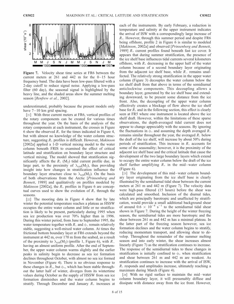
ary layer originating from the ice shelf base is clearlyillustrated by the semidiurnal tidal shear between the currentmeters at 261 m and 442 m (Figure 7). The velocity datawere high-pass filtered (15 hours) before the shear wascalculated and smoothed. Inclusion of the diurnal tides,which are principally barotropic and unaffected by stratifi-cation, would provide a small additional background shearof around 0.6 � 10�4 s�1 to the semidiurnal tidal shearshown in Figure 7. During the height of the winter freezingseason, the semidiurnal tides are more barotropic and theshear between 261 m and 442 m has a minimal plateau. Inthe latter part of the freezing season however, sea iceformation declines and the water column begins to stratify,reducing momentum transport, and allowing shear to de-velop. Throughout the remainder of the summer meltingseason and into early winter, the shear increases almostlinearly (Figure 7) as the stratification continues to increase.The response of the semidiurnal tides to these changes instratification is initially confined to f+ when stratificationand shear between 261 m and 442 m are weakest. Asstratification continues to increase with the arrival of ISW,R+ responds and amplitudes increase, ultimately reaching amaximum during March (Figure 4).[24] With no rigid surface to maintain the mid–water

column boundary layer, it will presumably diffuse anddissipate with distance away from the ice front. However,

Figure 7. Velocity shear time series at FR6 between thecurrent meters at 261 and 442 m for the 0–15 hourfrequency band. The data have been low-pass filtered with a2-day cutoff to reduce signal noise. Applying a low-passfilter (60 day), the seasonal signal is highlighted by theheavy line, and the shaded areas show the summer meltingseason [Renfrew et al., 2002].


8 of 15

C03022

it is unclear how far north the mid–water column boundarylayer extends beyond the ice front in the absence ofadditional observations. Nevertheless, using a three dimen-sional model to investigate tidal mixing in the southernWeddell Sea, Pereira et al. [2002] show the major axis ofthe M2 tidal ellipse remaining at a maximum in the mid–water column over 100 km from Ronne Ice Front. Althoughthe enhanced mid–water column major axis is much smallerthan observed at FR6, and is reliant on the stratificationprescribed in the model; the model results suggest that theice front influences the structure of the M2 tidal currentsmany tens of kilometers to the north of Ronne Ice Shelf.[25] Through February 1996 and into early March, R+

continues to increase with increasing stratification, as thetwo boundary layers develop and occupy the entire watercolumn below the ice shelf draft. The peaks in R+ occuraround mid-March (profile 2, Figure 6) about 20 days afterthe onset of the winter freezing season (25 February)[Renfrew et al., 2002]. The subsequent rapid decline of R+

signifies the switch from summer to winter conditions in thewater column, as HSSW begins to form at the surface anddescend into the water column.[26] The decline of R+ occurs soonest higher in the water

column and takes place over a 2–4 week period. At 261 m,R+ declines after mid-March and continues to a minimum inmid-April. At about the same time, the salinity begins toincrease and the temperature plateaus (Figure 4). Temper-atures close to the surface freezing point and an increasingsalinity signifies the passage of the deepening pycnoclinepast this instrument. The strong stratification associatedwith this pycnocline suppresses turbulence and inhibits

momentum transfer, causing the upper water column tobecome increasingly decoupled from that below. Thisdecoupling allows the influence of the adjacent ice shelfboundary layer to be intensified, further decreasing R+ at261 m and 442 m (profile 3, Figure 6). The response of f+

to the arrival of the HSSW is signaled at 261 m by a 30�increase and a similar decrease at 588 m. At 442 m, theresponse of f+ from 30� to 10� follows the response at 588 m,suggesting that both of these instruments are within the lowerboundary layer.[27] By mid-May f+ has reverted to its wintertime value

and the rapid decline of both R+ at 442 m (Figure 4) and thetidal current shear between 261 m and 442 m has ceased(Figure 7). These events coincide with the arrival of HSSWat 442 m, as the temperature approaches a plateau and thepycnocline passes the instrument. With HSSW occupyingthe water column down to 442 m, the boundary layergenerated by the ice shelf base is destroyed as R+ becomesincreasingly barotropic and the shear between 261 m and442 m reverts to its minimal plateau (Figure 7). By the endof May, R+ at 558 m reaches a minimum and f+ rapidlyincreases by 30� as the pycnocline reaches this instrument.Based qualitatively on the modeling work of Makinson[2002a], profile 4 in Figure 6 shows the high shear in R+

across the pycnocline as it descends toward the seabed andreducing the boundary layer thickness. At about this timethe salinity at 261 m attains its winter plateau, suggestingthat the water column may be fully mixed. At the lowestinstrument, however, the temperature does not finally pla-teau until July, when the R+ and f+ finally recover to theirwinter values. Only during July through to September do

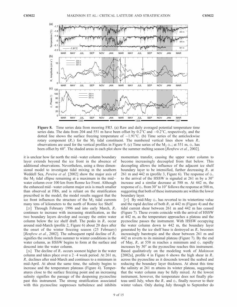
Figure 8. Time series data from mooring FR5. (a) Raw and daily averaged potential temperature timeseries data. The data from 204 and 551 m have been offset by 0.2�C and �0.2�C, respectively, and thedotted line shows the surface freezing temperature of �1.91�C. (b) Time series of the anticlockwiserotary component (R+) for the M2 tidal constituent. The numbered vertical lines show when R+

observations are used for the vertical profiles in Figure 9. (c) Time series of the M2 f+; at 551 m, f+ hasbeen offset by 60�. The shaded areas in each plot show the summer melting season [Renfrew et al., 2002].


9 of 15

C03022

the instrument sensors and tidal parameters suggest thatHSSW occupies the entire water column with little or nostratification present.[28] During the summer period in early 1995, very similar

changes in water column properties and tidal current re-sponse are observed, although absolute values and timingsdiffer slightly from those in 1996. At each instrument, f+

changes rapidly as the minimum in R+ is approached,coinciding with the arrival of the HSSW and the deepeningpycnocline. During early 1997, however, both the temper-ature structure and tidal response differed significantly fromthe previous 2 years. Only relatively small changes R+ areseen at 442 m although a strong response is observed in f+

as the water column stratifies, followed by a rapid recoveryto the wintertime f+ during March and early April. Theseobservations show that the tidal response to stratificationoccurs initially in f+, and that with increasing stratificationa threshold is reached after which R+ begins to respond. Theinterannual differences in stratification and the associatedtidal current response could be influenced by the extent ofthe ice front polynya and its associated heat flux or sea iceproduction. In the summer of 1994–1995 the oceanicenergy gain in the ice front polynya was 5.88 � 1019 J,reducing to 3.39 � 1019 and 1.66 � 1019 J in subsequentsummers, with the winters of 1994 and 1996 havingapproximately 50% less sea ice production than 1995[Renfrew et al., 2002]. In the summer of 1996–1997, it isthe combination of weak summer heat flux, preceded bylow sea ice production that may be responsible for theweaker tidal response.

4.2. Mooring FR5

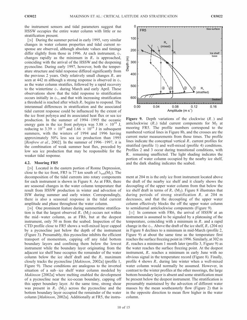
[29] Located in the eastern portion of Ronne Depression,close to the ice front, FR5 is 77 km south of lcrit(M2). Thedecomposition of the tidal currents into rotary componentsfor each instrument is shown in Figure 8. As at FR6, thereare seasonal changes in the water column temperature thatresult from HSSW production in winter and advection ofISW during summer and early winter. Correspondingly,there is also a seasonal response in the tidal currentamplitude and phase throughout the water column.[30] One prominent feature during summertime stratifica-

tion is that the largest observed R+ (M2) occurs not withinthe mid–water column, as at FR6, but at the deepestinstrument, only 50 m from the seabed. Inspection of theCTD profile close to FR5 shows a well-mixed layer cappedby a pycnocline just below the depth of the instrument(Figure 3). Presumably, this pycnocline inhibits the efficienttransport of momentum, capping off any tidal bottomboundary layers and confining them below the lowestinstrument while the boundary layer originating from theadjacent ice shelf base occupies the remainder of the watercolumn below the ice shelf draft and the R+ maximumclosely tracks the pycnocline [Makinson, 2002a] (profile 1,Figure 9). These conditions are analogous to the invertedsituation of a sub–ice shelf water column modeled byMakinson [2002a] where melting enabled the developmentof a pycnocline near the ice-ocean boundary, capping offthis upper boundary layer. At the same time, strong shearwas present in R+ (M2) across the pycnocline and thebottom boundary layer occupied the remainder of the watercolumn [Makinson, 2002a]. Additionally at FR5, the instru-

ment at 204 m is the only ice front instrument located abovethe draft of the nearby ice shelf and it clearly shows thedecoupling of the upper water column from that below theice shelf draft in terms of R+ (M2). Figure 8 illustrates thatduring periods of strong stratification R+ at 204 mdecreases, and that the decoupling of the upper watercolumn effectively blocks the off the upper water columnto semidiurnal anticlockwise components (Figure 9).[31] In common with FR6, the arrival of HSSW at an

instrument is assumed to be signaled by a plateauing of thetemperature, coinciding with a minimum in R+ and a rapidchange in the f+. Above the draft of the ice shelf, R+ (204 m)in Figure 8 declines to a minimum in mid-March (profile 2,Figure 9) at about the same time as the temperature firstreaches the surface freezing point in 1996. Similarly, at 302mR+ reaches a minimum 1 month later (profile 3, Figure 9) asthe water reaches the surface freezing point. At the deepestinstrument, R+ reaches a minimum in early June with noobvious signal in the temperature record (Figure 8). Finally,profile 4 shows R+ during late winter when a well-mixedwater column would normally be assumed. However, incontrast to the winter profiles at the other moorings, the largebottom boundary layer is absent and some stratification mustbe present below the deepest instrument. The stratification ispresumably maintained by the advection of different watermasses by the mean southeasterly flow (Figure 2) that isin the opposite direction to mean flow higher in the watercolumn.

Figure 9. Depth variations of the clockwise (R�) andanticlockwise (R+) tidal current components for M2 atmooring FR5. The profile numbers correspond to thenumbered vertical lines in Figure 8b, and the crosses are thecurrent meter measurements from those times. The profilelines indicate the conceptual vertical R+ current profiles forstratified (profile 1) and well-mixed (profile 4) conditions.Profiles 2 and 3 occur during transitional conditions, withR� remaining unaffected. The light shading indicates theportion of water column occupied by the nearby ice shelf,and the dark shading indicates the seabed.


10 of 15

C03022

[32] Throughout the FR5 time series, changes in f+ areassumed to correspond with changes in stratification, asobserved at FR6. With no available salinity measurements,temperature is used to defined when HSSW is present andtherefore if the water column is mixed or stratified. Duringwinter, when the water column is likely to be well mixed,f+ is around 45� at the upper two instruments; while duringsummer this can change to between 20� and 100� (Figure 8).These changes occur with the gradual increase in stratifica-

tion during summer, and with rapid changes associated withthe arrival of HSSW at an instrument in early winter. Of thethree instruments on this mooring, the upper instrument at204 m shows the strongest seasonal signal in f+, whichincreases during early winter to a maximum of between 90�and 110�. The maximum in f+ occurs soon after theminimum in R+ and the arrival of HSSW at the instrumentin March. A similar response is also seen a few weeks laterat 305 m. Here, the phase changes rapidly with the arrival ofHSSW, particularly in April 1995 when f+ changes from20� to 100�. This response to the arrival of HSSW is almostidentical to the upper instrument at FR6 that was alsolocated just below the draft of the ice shelf. In the subse-quent years, this response at 305 m is either weak or absent.At the deepest instrument (551 m), f+ is highly variablewith rapid changes of up to 40�, particularly during thewinter of 1996, suggesting that the nearby pycnocline isperiodically moving close to the instrument, although thereis no corresponding signal in temperature or R+. A furtheranomaly occurs in the tidal currents at the deepest instru-ment. Of all the ice front current data, only FR5 (551 m) haslarge fluctuations from about 7 cm s�1 to 11 cm s�1 in R�(not shown) that coincide principally with the stratifiedconditions in early 1996. Although the instrument is closeto the pycnocline observed in the CTD profile (Figure 3), itis unclear why such changes in phase and amplitude shouldoccur. Nevertheless, these fluctuations in amplitude andphase of the rotary components result in ellipse orientationswings of up to 35� and a doubling of the semimajor axisduring periods of stratification. Similar features are alsopresent in the S2 tidal currents, resulting in peak spring tideswith speeds of over 35 cm s�1, while during winter the peakspring tides can fall to less than 20 cm s�1.

4.3. Mooring R2

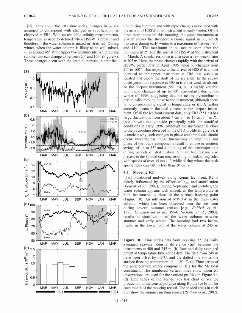
[33] Positioned midway along Ronne Ice Front, R2 isclearly influenced by the effects of lcrit and stratification[Foldvik et al., 2001]. During September and October, thewater column appears well mixed, as the temperature atboth instruments is close to the surface freezing point(Figure 10). An intrusion of MWDW in the mid–watercolumn, which has been observed near the ice frontduring several summer cruises [e.g., Foldvik et al.,1985; Gammelsrød et al., 1994; Nicholls et al., 2003],results in stratification of the water column betweensummer and early winter. The mooring had two instru-ments in the lower half of the water column at 245 m

Figure 10. Time series data from mooring R2. (a) Dailyaveraged seawater density difference (Dr) between theinstruments at 400 and 245 m. (b) Raw and daily averagedpotential temperature time series data. The data from 245 mhave been offset by 0.2�C, and the dotted line shows thesurface freezing temperature of �1.91�C. (c) Time series ofthe anticlockwise rotary component (R+) for the M2 tidalconstituent. The numbered vertical lines show when R+

observations are used for the vertical profiles in Figure 11.(d) Time series of the M2 f+. (e) Bar chart of sea iceproduction in the coastal polynya along Ronne Ice Front foreach month of the mooring record. The shaded areas in eachplot show the summer melting season [Renfrew et al., 2002].


11 of 15

C03022

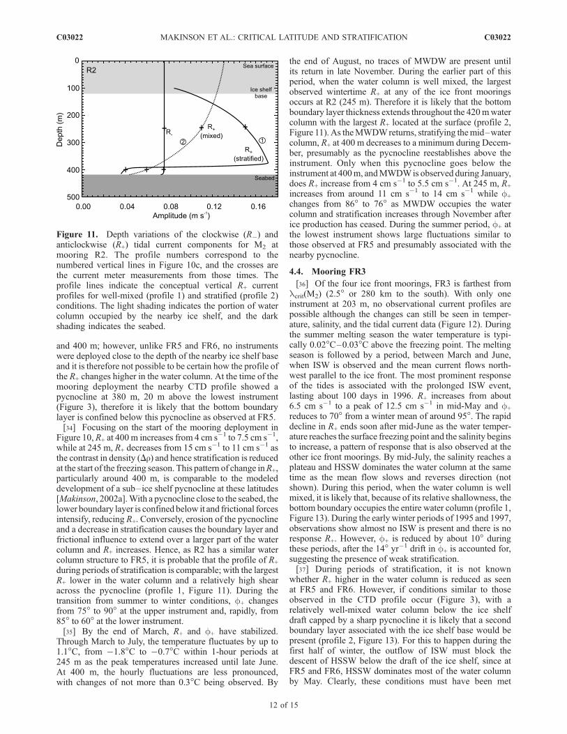
and 400 m; however, unlike FR5 and FR6, no instrumentswere deployed close to the depth of the nearby ice shelf baseand it is therefore not possible to be certain how the profile ofthe R+ changes higher in the water column. At the time of themooring deployment the nearby CTD profile showed apycnocline at 380 m, 20 m above the lowest instrument(Figure 3), therefore it is likely that the bottom boundarylayer is confined below this pycnocline as observed at FR5.[34] Focusing on the start of the mooring deployment in

Figure 10, R+ at 400 m increases from 4 cm s�1 to 7.5 cm s�1,while at 245 m, R+ decreases from 15 cm s�1 to 11 cm s�1 asthe contrast in density (Dr) and hence stratification is reducedat the start of the freezing season. This pattern of change inR+,particularly around 400 m, is comparable to the modeleddevelopment of a sub–ice shelf pycnocline at these latitudes[Makinson, 2002a].With a pycnocline close to the seabed, thelower boundary layer is confined below it and frictional forcesintensify, reducing R+. Conversely, erosion of the pycnoclineand a decrease in stratification causes the boundary layer andfrictional influence to extend over a larger part of the watercolumn and R+ increases. Hence, as R2 has a similar watercolumn structure to FR5, it is probable that the profile of R+

during periods of stratification is comparable; with the largestR+ lower in the water column and a relatively high shearacross the pycnocline (profile 1, Figure 11). During thetransition from summer to winter conditions, f+ changesfrom 75� to 90� at the upper instrument and, rapidly, from85� to 60� at the lower instrument.[35] By the end of March, R+ and f+ have stabilized.

Through March to July, the temperature fluctuates by up to1.1�C, from �1.8�C to �0.7�C within 1-hour periods at245 m as the peak temperatures increased until late June.At 400 m, the hourly fluctuations are less pronounced,with changes of not more than 0.3�C being observed. By

the end of August, no traces of MWDW are present untilits return in late November. During the earlier part of thisperiod, when the water column is well mixed, the largestobserved wintertime R+ at any of the ice front mooringsoccurs at R2 (245 m). Therefore it is likely that the bottomboundary layer thickness extends throughout the 420mwatercolumn with the largest R+ located at the surface (profile 2,Figure 11). As theMWDWreturns, stratifying themid–watercolumn, R+ at 400 m decreases to a minimum during Decem-ber, presumably as the pycnocline reestablishes above theinstrument. Only when this pycnocline goes below theinstrument at 400m, andMWDWis observed during January,does R+ increase from 4 cm s�1 to 5.5 cm s�1. At 245 m, R+

increases from around 11 cm s�1 to 14 cm s�1 while f+

changes from 86� to 76� as MWDW occupies the watercolumn and stratification increases through November afterice production has ceased. During the summer period, f+ atthe lowest instrument shows large fluctuations similar tothose observed at FR5 and presumably associated with thenearby pycnocline.

4.4. Mooring FR3

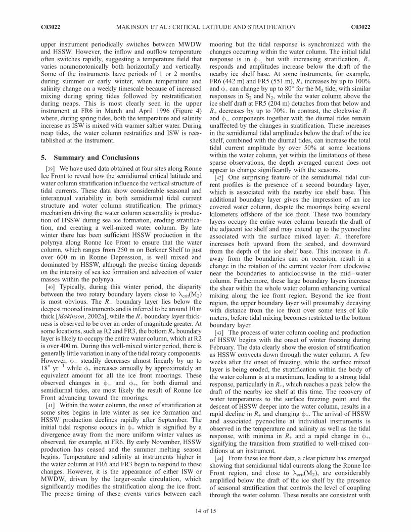
[36] Of the four ice front moorings, FR3 is farthest fromlcrit(M2) (2.5� or 280 km to the south). With only oneinstrument at 203 m, no observational current profiles arepossible although the changes can still be seen in temper-ature, salinity, and the tidal current data (Figure 12). Duringthe summer melting season the water temperature is typi-cally 0.02�C–0.03�C above the freezing point. The meltingseason is followed by a period, between March and June,when ISW is observed and the mean current flows north-west parallel to the ice front. The most prominent responseof the tides is associated with the prolonged ISW event,lasting about 100 days in 1996. R+ increases from about6.5 cm s�1 to a peak of 12.5 cm s�1 in mid-May and f+

reduces to 70� from a winter mean of around 95�. The rapiddecline in R+ ends soon after mid-June as the water temper-ature reaches the surface freezing point and the salinity beginsto increase, a pattern of response that is also observed at theother ice front moorings. By mid-July, the salinity reaches aplateau and HSSW dominates the water column at the sametime as the mean flow slows and reverses direction (notshown). During this period, when the water column is wellmixed, it is likely that, because of its relative shallowness, thebottom boundary occupies the entire water column (profile 1,Figure 13). During the early winter periods of 1995 and 1997,observations show almost no ISW is present and there is noresponse R+. However, f+ is reduced by about 10� duringthese periods, after the 14� yr�1 drift in f+ is accounted for,suggesting the presence of weak stratification.[37] During periods of stratification, it is not known

whether R+ higher in the water column is reduced as seenat FR5 and FR6. However, if conditions similar to thoseobserved in the CTD profile occur (Figure 3), with arelatively well-mixed water column below the ice shelfdraft capped by a sharp pycnocline it is likely that a secondboundary layer associated with the ice shelf base would bepresent (profile 2, Figure 13). For this to happen during thefirst half of winter, the outflow of ISW must block thedescent of HSSW below the draft of the ice shelf, since atFR5 and FR6, HSSW dominates most of the water columnby May. Clearly, these conditions must have been met

Figure 11. Depth variations of the clockwise (R�) andanticlockwise (R+) tidal current components for M2 atmooring R2. The profile numbers correspond to thenumbered vertical lines in Figure 10c, and the crosses arethe current meter measurements from those times. Theprofile lines indicate the conceptual vertical R+ currentprofiles for well-mixed (profile 1) and stratified (profile 2)conditions. The light shading indicates the portion of watercolumn occupied by the nearby ice shelf, and the darkshading indicates the seabed.


12 of 15

C03022

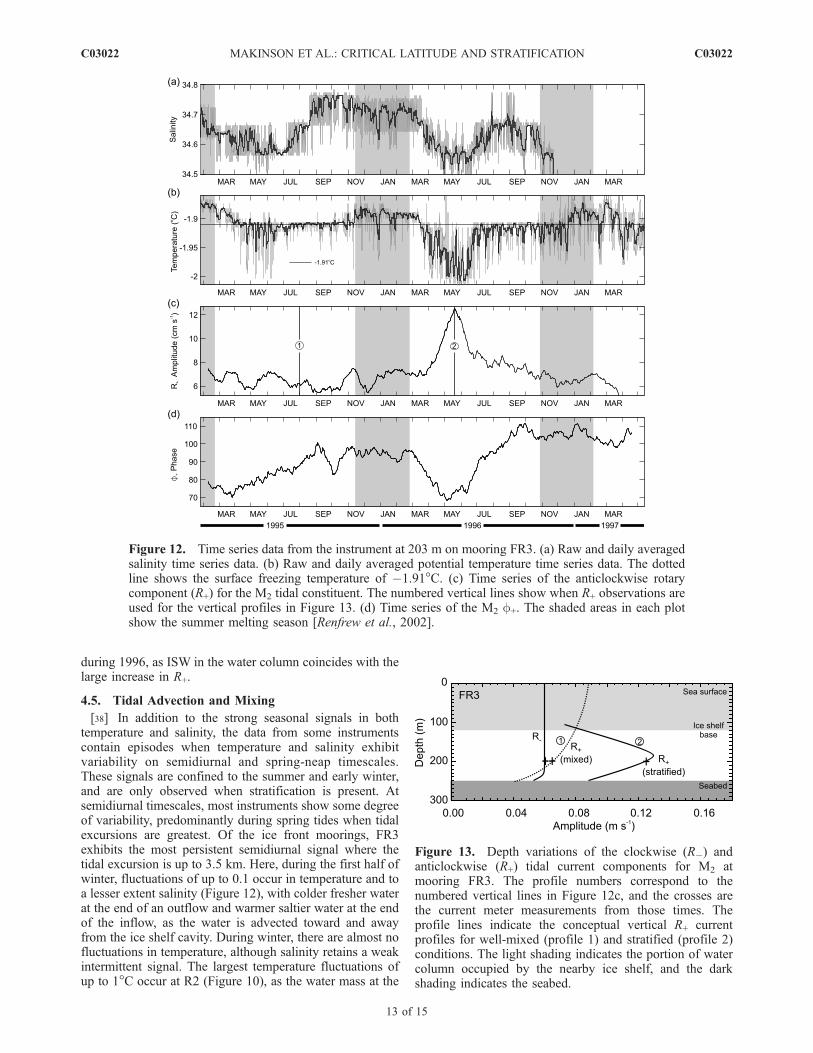
during 1996, as ISW in the water column coincides with thelarge increase in R+.

4.5. Tidal Advection and Mixing

[38] In addition to the strong seasonal signals in bothtemperature and salinity, the data from some instrumentscontain episodes when temperature and salinity exhibitvariability on semidiurnal and spring-neap timescales.These signals are confined to the summer and early winter,and are only observed when stratification is present. Atsemidiurnal timescales, most instruments show some degreeof variability, predominantly during spring tides when tidalexcursions are greatest. Of the ice front moorings, FR3exhibits the most persistent semidiurnal signal where thetidal excursion is up to 3.5 km. Here, during the first half ofwinter, fluctuations of up to 0.1 occur in temperature and toa lesser extent salinity (Figure 12), with colder fresher waterat the end of an outflow and warmer saltier water at the endof the inflow, as the water is advected toward and awayfrom the ice shelf cavity. During winter, there are almost nofluctuations in temperature, although salinity retains a weakintermittent signal. The largest temperature fluctuations ofup to 1�C occur at R2 (Figure 10), as the water mass at the

Figure 12. Time series data from the instrument at 203 m on mooring FR3. (a) Raw and daily averagedsalinity time series data. (b) Raw and daily averaged potential temperature time series data. The dottedline shows the surface freezing temperature of �1.91�C. (c) Time series of the anticlockwise rotarycomponent (R+) for the M2 tidal constituent. The numbered vertical lines show when R+ observations areused for the vertical profiles in Figure 13. (d) Time series of the M2 f+. The shaded areas in each plotshow the summer melting season [Renfrew et al., 2002].

Figure 13. Depth variations of the clockwise (R�) andanticlockwise (R+) tidal current components for M2 atmooring FR3. The profile numbers correspond to thenumbered vertical lines in Figure 12c, and the crosses arethe current meter measurements from those times. Theprofile lines indicate the conceptual vertical R+ currentprofiles for well-mixed (profile 1) and stratified (profile 2)conditions. The light shading indicates the portion of watercolumn occupied by the nearby ice shelf, and the darkshading indicates the seabed.


13 of 15

C03022

upper instrument periodically switches between MWDWand HSSW. However, the inflow and outflow temperatureoften switches rapidly, suggesting a temperature field thatvaries nonmonotonically both horizontally and vertically.Some of the instruments have periods of 1 or 2 months,during summer or early winter, when temperature andsalinity change on a weekly timescale because of increasedmixing during spring tides followed by restratificationduring neaps. This is most clearly seen in the upperinstrument at FR6 in March and April 1996 (Figure 4)where, during spring tides, both the temperature and salinityincrease as ISW is mixed with warmer saltier water. Duringneap tides, the water column restratifies and ISW is rees-tablished at the instrument.

5. Summary and Conclusions

[39] We have used data obtained at four sites along RonneIce Front to reveal how the semidiurnal critical latitude andwater column stratification influence the vertical structure oftidal currents. These data show considerable seasonal andinterannual variability in both semidiurnal tidal currentstructure and water column stratification. The primarymechanism driving the water column seasonality is produc-tion of HSSW during sea ice formation, eroding stratifica-tion, and creating a well-mixed water column. By latewinter there has been sufficient HSSW production in thepolynya along Ronne Ice Front to ensure that the watercolumn, which ranges from 250 m on Berkner Shelf to justover 600 m in Ronne Depression, is well mixed anddominated by HSSW, although the precise timing dependson the intensity of sea ice formation and advection of watermasses within the polynya.[40] Typically, during this winter period, the disparity

between the two rotary boundary layers close to lcrit(M2)is most obvious. The R� boundary layer lies below thedeepest moored instruments and is inferred to be around 10mthick [Makinson, 2002a], while the R+ boundary layer thick-ness is observed to be over an order of magnitude greater. Atsome locations, such as R2 and FR3, the bottom R+ boundarylayer is likely to occupy the entire water column, which at R2is over 400 m. During this well-mixed winter period, there isgenerally little variation in any of the tidal rotary components.However, f� steadily decreases almost linearly by up to18� yr�1 while f+ increases annually by approximately anequivalent amount for all the ice front moorings. Theseobserved changes in f� and f+, for both diurnal andsemidiurnal tides, are most likely the result of Ronne IceFront advancing toward the moorings.[41] Within the water column, the onset of stratification at

some sites begins in late winter as sea ice formation andHSSW production declines rapidly after September. Theinitial tidal response occurs in f+ which is signified by adivergence away from the more uniform winter values asobserved, for example, at FR6. By early November, HSSWproduction has ceased and the summer melting seasonbegins. Temperature and salinity at instruments higher inthe water column at FR6 and FR3 begin to respond to thesechanges. However, it is the appearance of either ISW orMWDW, driven by the larger-scale circulation, whichsignificantly modifies the stratification along the ice front.The precise timing of these events varies between each

mooring but the tidal response is synchronized with thechanges occurring within the water column. The initial tidalresponse is in f+, but with increasing stratification, R+

responds and amplitudes increase below the draft of thenearby ice shelf base. At some instruments, for example,FR6 (442 m) and FR5 (551 m), R+ increases by up to 100%and f+ can change by up to 80� for the M2 tide, with similarresponses in S2 and N2, while the water column above theice shelf draft at FR5 (204 m) detaches from that below andR+ decreases by up to 70%. In contrast, the clockwise R�and f� components together with the diurnal tides remainunaffected by the changes in stratification. These increasesin the semidiurnal tidal amplitudes below the draft of the iceshelf, combined with the diurnal tides, can increase the totaltidal current amplitude by over 50% at some locationswithin the water column, yet within the limitations of thesesparse observations, the depth averaged current does notappear to change significantly with the seasons.[42] One surprising feature of the semidiurnal tidal cur-

rent profiles is the presence of a second boundary layer,which is associated with the nearby ice shelf base. Thisadditional boundary layer gives the impression of an icecovered water column, despite the moorings being severalkilometers offshore of the ice front. These two boundarylayers occupy the entire water column beneath the draft ofthe adjacent ice shelf and may extend up to the pycnoclineassociated with the surface mixed layer. R+ thereforeincreases both upward from the seabed, and downwardfrom the depth of the ice shelf base. This increase in R+

away from the boundaries can on occasion, result in achange in the rotation of the current vector from clockwisenear the boundaries to anticlockwise in the mid–watercolumn. Furthermore, these large boundary layers increasethe shear within the whole water column enhancing verticalmixing along the ice front region. Beyond the ice frontregion, the upper boundary layer will presumably decayingwith distance from the ice front over some tens of kilo-meters, before tidal mixing becomes restricted to the bottomboundary layer.[43] The process of water column cooling and production

of HSSW begins with the onset of winter freezing duringFebruary. The data clearly show the erosion of stratificationas HSSW convects down through the water column. A fewweeks after the onset of freezing, while the surface mixedlayer is being eroded, the stratification within the body ofthe water column is at a maximum, leading to a strong tidalresponse, particularly in R+, which reaches a peak below thedraft of the nearby ice shelf at this time. The recovery ofwater temperatures to the surface freezing point and thedescent of HSSW deeper into the water column, results in arapid decline in R+ and changing f+. The arrival of HSSWand associated pycnocline at individual instruments isobserved in the temperature and salinity as well as the tidalresponse, with minima in R+ and a rapid change in f+,signifying the transition from stratified to well-mixed con-ditions at an instrument.[44] From these ice front data, a clear picture has emerged

showing that semidiurnal tidal currents along the Ronne IceFront region, and close to lcrit(M2), are considerablyamplified below the draft of the ice shelf by the presenceof seasonal stratification that controls the level of couplingthrough the water column. These results are consistent with


14 of 15

C03022

boundary layer theory. During periods of stratification, theprofile of R+ (M2) below the draft of the ice shelf matchesboth the observations from beneath fixed ice cover in theArctic [Prinsenberg and Bennett, 1989], and the R+ profilesderived from a tidally driven vertical mixing model appliedto the water column beneath FRIS [Makinson, 2002a]. Icefront observations such as these highlight the difficulties ininterpreting data from short-term moorings and provideinsight into how lcrit, stratification and the nearby RonneIce Shelf influence tidal current profiles throughout the year.In addition, the observed sensitivity of the M2 anticlockwisecomponent to changes in stratification along Ronne IceFront suggests that it is the best indicator for characterizingchanges in stratification after direct observations of densityvariations.

[45] Acknowledgments. The authors wish to express their gratitudeto the personnel of HMS Endurance and Polarstern and R/V Lance fortheir support during the cruises. We are also grateful to Keith Nicholls,Robin Robertson, and an anonymous reviewer for their careful reviews ofthe manuscript and constructive comments.

ReferencesFoldvik, A., T. Gammelsrød, N. Slotsvik, and T. Tørresen (1985), Oceano-graphic conditions on the Weddell Sea Shelf during the German AntarcticExpedition 1979/80, Polar Res., 3(2), 209–226.

Foldvik, A., J. H. Middleton, and T. D. Foster (1990), The tides of thesouthern Weddell Sea, Deep Sea Res., 37(8), 1345–1362.

Foldvik, A., T. Gammelsrød, E. Nygaard, and S. Østerhus (2001), Currentmeter measurements near Ronne Ice Shelf, Weddell Sea: Implicationsfor circulation and melting underneath the Filchner-Ronne ice shelves,J. Geophys. Res., 106(C3), 4463–4477.

Foldvik, A., T. Gammelsrød, S. Østerhus, E. Fahrbach, G. Rohardt,M. Schroder, K. W. Nicholls, L. Padman, and R. A. Woodgate (2004), Iceshelf water overflow and bottom water formation in the southern WeddellSea, J. Geophys. Res., 109, C02015, doi:10.1029/2003JC002008.

Foreman, M. G. G. (1977), Manual for Tidal Currents Analysis and Pre-diction, 70 pp., Inst. of Ocean Sci., Patricia Bay, Sidney, B. C., Canada.

Furevik, T., and A. Foldvik (1996), Stability at M2 critical latitude in theBarents Sea, J. Geophys. Res., 101(C4), 8823–8837.

Gammelsrød, T., A. Foldvik, O. A. Nøst, Ø. Skagseth, L. G. Anderson,E. Fogelqvist, K. Olsson, T. Tanhua, E. P. Jones, and S. Østerhus(1994), Distribution of water masses on the continental shelf in thesouthern Weddell Sea, in The Polar Oceans and Their Role in Shap-ing the Global Environment, Geophys. Monogr. Ser., vol. 85, edited byO. M. Johannesen, R. D. Muench, and J. E. Overland, pp. 159–176,AGU, Washington, D. C.

Howarth, M. J. (1998), The effect of stratification on tidal current profiles,Cont. Shelf Res., 18(11), 1235–1254.

LeBlond, P. H., and L. A. Mysak (1978), Waves in the Ocean, 602 pp.,Elsevier, New York.

Makinson, K. (2002a), Modeling tidal current profiles and vertical mixingbeneath Filchner-Ronne Ice Shelf, Antarctica, J. Phys. Oceanogr., 32(1),202–215.

Makinson, K. (2002b), Tidal currents and vertical mixing processes beneathFilchner-Ronne Ice Shelf, Ph.D. thesis, Open Univ., Milton Keynes,U. K.

Makinson, K., and K. W. Nicholls (1999), Modeling tidal currents beneathFilchner-Ronne Ice Shelf and on the adjacent continental shelf: Theireffect on mixing and transport, J. Geophys. Res., 104(C6), 13,449–13,465.

Makinson, K.. and M. Schroder (2004), Ocean processes and seasonal in-flow along Ronne Ice Front, in Forum for Research Into Ice Shelf Pro-cesses, edited by L. H. Smedsrud, Rep. 15, pp. 11–16, Bjerknes Cent. forClim. Res., Bergen, Norway.

Nicholls, K. W., and K. Makinson (1998), Ocean circulation beneaththe western Ronne Ice Shelf, as derived from in situ measurementsof water currents and properties, in Ocean, Ice, and Atmosphere:Interactions at the Antarctic Continental Margin, Antarct. Res. Ser.,

vol. 75, edited by S. S. Jacobs and R. F. Weiss, pp. 301–318, AGU,Washington, D. C.

Nicholls, K. W., S. Østerhus, K. Makinson, and M. R. Johnson (2001),Oceanographic conditions south of Berkner Island, beneath Filchner-Ronne Ice Shelf, Antarctica, J. Geophys. Res., 106(C6), 11,481–11,492.

Nicholls, K. W., L. Padman, M. Schroder, R. A. Woodgate, A. Jenkins, andS. Østerhus (2003), Water mass modification over the continental shelfnorth of Ronne Ice Shelf, Antarctica, J. Geophys. Res., 108(C8), 3260,doi:10.1029/2002JC001713.

Nøst, E. (1994), Calculating tidal current profiles from vertically integratedmodels near the critical latitude in the Barents Sea, J. Geophys. Res.,99(C4), 7885–7901.

Padman, L., H. A. Fricker, R. Coleman, S. Howard, and L. Erofeeva(2002), A new tidal model for the Antarctic ice shelves and seas, Ann.Glaciol., 34, 247–254.

Pereira, A. F., A. Beckmann, and H. H. Hellmer (2002), Tidal mixing in thesouthern Weddell Sea: Results from a three-dimensional model, J. Phys.Oceanogr., 32(7), 2151–2170.

Prandle, D. (1982), The vertical structure of tidal currents, Geophys. Astro-phys. Fluid Dyn., 22(1–2), 29–49.

Prinsenberg, S. J., and E. B. Bennett (1989), Vertical variations of tidalcurrents in shallow land fast ice-covered regions, J. Phys. Oceanogr.,19(9), 1268–1278.

Renfrew, I. A., J. C. King, and T. Markus (2002), Coastal polynyas in thesouthern Weddell Sea: Variability of the surface energy budget, J. Geo-phys. Res., 107(C6), 3063, doi:10.1029/2000JC000720.

Robertson, R. (2001a), Internal tides and baroclinicity in the southernWeddell Sea: 1. Model description, J. Geophys. Res., 106(C11),27,001–27,016.

Robertson, R. (2001b), Internal tides and baroclinicity in the southernWeddell Sea: 2. Effects of the critical latitude and stratification, J. Geo-phys. Res., 106(C11), 27,017–27,034.

Robertson, R. (2005a), Baroclinic and barotropic tides in the Ross Sea,Antarct. Sci., 17(1), 107–120.

Robertson, R. (2005b), Baroclinic and barotropic tides in the Weddell Sea,Antarct. Sci., 17(3), 461–474.

Robertson, R., L. Padman, and G. D. Egbert (1998), Tidal currents in theWeddell Sea, in Ocean, Ice, and Atmosphere: Interactions at the Antarc-tic Continental Margin, Antarct. Res. Ser., vol. 75, edited by S. S. Jacobsand R. Weiss, pp. 341–369, AGU, Washington, D. C.

Robertson, R., A. Beckmann, and H. Hellmer (2003), M2 tidal dynamics inthe Ross Sea, Antarct. Sci., 15(1), 41–46.

Shcherbina, A. Y., L. D. Talley, and D. L. Rudnick (2003), Direct observa-tions of North Pacific ventilation: Brine rejection in the Okhotsk Sea,Science, 302(5652), 1952–1955.

Simpson, J. H., and J. Sharples (1994), Does the Earth’s rotation influencethe location of the shelf sea fronts?, J. Geophys. Res., 99(C2), 3315–3319.

Soulsby, R. L. (1983), The bottom boundary layer of the shelf sea, inPhysical Oceanography of Coastal and Shelf Seas, Elsevier Oceanogr.Ser., vol. 35, edited by B. Johns, pp. 189–226, Elsevier, New York.

Souza, A. J., and J. H. Simpson (1996), The modification of tidal ellipsesby stratification in the Rhine ROFI, Cont. Shelf Res., 16(8), 997–1007.

Vaughan, D. G., J. Sievers, C. S. M. Doake, G. Grikurov, H. Hinze, V. S.Pozdeev, H. Sandhager, H. W. Schenke, A. Solheim, and F. Thyssen(1994), Map of subglacial and seabed topography, Filchner-Ronne-Schel-feis, Antarktis, scale 1:2,000,000, Inst. fur Angew. Geod., Frankfurt amMain, Germany.

Woodgate, R. A., M. Schroder, and S. Østerhus (1998), Moorings from theFilchner Trough and the Ronne Ice Shelf Front: Preliminary tesults, inFilchner Ronne Ice Shelf Programme Rep. 12, edited by H. Oerter, pp.85–90, Alfred Wegener Inst. for Polar and Mar. Res., Bremerhaven,Germany.

��K. Makinson, British Antarctic Survey, Natural Environment Research

Council, High Cross, Madingley Road, Cambridge CB3 0ET, UK.([email protected])S. Østerhus, Bjerknes Centre for Climate Research, c/o Geophysical

Institute, University of Bergen, Allegaten 70, N-5007 Bergen, Norway.([email protected])M. Schroder, Alfred-Wegener-Institut fur Polar- und Meeresforschung,

Columbusstraße, Postfach 120161, Bremerhaven D-27515, Germany.([email protected])


15 of 15

C03022