Eastern Illinois UniversityThe Keep

Masters Theses Student Theses & Publications

2016

Economic Growth Paradox in Nigeria: APerspective from Natural Resource Wealth TimeSeries Analysis for the Period 1980 - 2013Jamiu AmusaEastern Illinois UniversityThis research is a product of the graduate program in Economics at Eastern Illinois University. Find out moreabout the program.

This is brought to you for free and open access by the Student Theses & Publications at The Keep. It has been accepted for inclusion in Masters Thesesby an authorized administrator of The Keep. For more information, please contact tabruns@eiu.edu.

Recommended CitationAmusa, Jamiu, "Economic Growth Paradox in Nigeria: A Perspective from Natural Resource Wealth Time Series Analysis for thePeriod 1980 - 2013" (2016). Masters Theses. 2448.https://thekeep.eiu.edu/theses/2448

The Graduate School� £A)TERN !UJNOlS UNIVERSITY''

Thesis Maintenance and Reproduction Certificate

FOR: Graduate Candidates Completing Theses in Partial Fulfillment of the Degree Graduate Faculty Advisors Directing the Theses

RE: Preservation, Reproduction, and Distribution of Thesis Research

Preserving, reproducing, and distributing thesis research is an important part of Booth Library's responsibility to provide access to scholarship. In order to further this goal, Booth Library makes all graduate theses completed as part of a degree program at Eastern Illinois University available for personal study, research, and other not-for-profit educational purposes. Under 17 U.S.C. § 108, the library may reproduce and distribute a copy without infringing on copyright; however, professional courtesy dictates that permission be requested from the author before doing so.

Your signatures affirm the following: • The graduate candidate is the author of this thesis. • The graduate candidate retains the copyright and intellectual property rights associated with the

original research, creative activity, and intellectual or artistic content of the thesis. • The graduate candidate certifies her/his compliance with federal copyright law (Title 17 of the U.

S. Code) and her/his right to authorize reproduction and distribution of all copyrighted materials included in this thesis.

• The graduate candidate in consultation with the faculty advisor grants Booth Library the non­exclusive, perpetual right to make copies of the thesis freely and publicly available without restriction, by means of any current or successive technology, including by not limited to photocopying, microfilm, digitization, or internet.

• The graduate candidate acknowledges that by depositing her/his thesis with Booth Library, her/his work is available for viewing by the public and may be borrowed through the library's circulation and interlibrary loan departments, or accessed electronically.

• The graduate candidate waives the confidentiality provisions of the Family Educational Rights and Privacy Act (FERPA) (20 U.S. C. § 1232g; 34 CPR Part 99) with respect to the contents of the thesis and with respect to information concerning authorship of the thesis, including name and status as a student at Eastern Illinois University.

I have conferred with my graduate faculty advisor. My signature below indicates that I have read and agree with the above statements, and hereby give my permission to allow Booth Library to reproduce and distribute my thesis. My adviser's signature indicates concurrence to reproduce and distribute the thesis.

Graduate Candidate Signature ) Faculty Adviser Signature . _j �·�v"�""\ . ·tc· ·�.!-� • .Ab.md .A�\A.- �el Printed Name Printed Name

1- I ·-�--c I "�'\J( .£, . E�LtS. Graduate Degree Program Date

/ c:JJ) / Ja,t(, l

Please submit in duplicate.

Economic Growth Paradox in Nigeria: A Perspective from Natural Resource Wealth

Time Series Analysis for the Period 1980 - 2013

(TITLE)

BY

Jamiu Amusa

THESIS

SUBMITTED IN PARTIAL FULFILLMENT OF THE REQUIREMENTS FOR THE DEGREE OF

Master of Economics

IN THE GRADUATE SCHOOL, EASTERN ILLINOIS UNIVERSITY CHARLESTON, ILLINOIS

2016 YEAR

I HEREBY RECOMMEND THAT THIS THESIS BE ACCEPTED AS FULFILLING THIS PART OF THE GRADUATE DEGREE CITED ABOVE

THESIS COMMITTEE CHAIR DATE

THESIS c'oMfilTTEE �MBER DATE

DEPARTMENT/SCHO�HAIR OR CHAIR'S DESIGNEE

THESIS COMMITTEE MEMBER

THESIS COMMITTEE MEMBER

DATE

DATE

DATE

© Copyright 20 1 6 by Jamiu A. Amusa

Abstract

This thesis empirically examines the paradox of economic growth in Nigeria with a

viewpoint from natural resource wealth. The question involved in this study is that whether

natural resource wealth has a positive impact on economic growth in Nigeria or not . The

economy of Nigeria is observed to be growing on paper but deplorably, poverty and

unemployment is on a progressive increase in reality. The study uses the endogenous growth

theory (AK Model) in terms of how resource wealth can influence economic growth. It exploits

time series analysis (Unit Root and Co-integration) techniques to test for the existence of a

relationship. It also applies the Error Correction Mechanism (ECM) in testing for the existence

of a relationship as it captures the short-run dynamics and provides a measure to resolve the

behaviour of the series in the short run with its performance in the long run. The result confirms

that that natural resource (Oilrent and Agriculture) based growth strategy will not lead to

sustained economic growth for the Nigerian economy. Thus it was recommended that Nigeria

should follow an industrial growth strategy with a vibrant real sector that would result in the

diversification of the economy with the aim of addressing and tackle the issue of wide spread

corruption and mismanagement of public funds in all respective areas and sectors of its

economy. The involvement of this study lies in the reality that it provides additional

confirmation on the ongoing debate of resource wealth on the economic growth development

within a specific country.

2

Acknowledgements

My utmost gratitude goes to the almighty God, the unseen seer, Lord of the entire world,

provider for the whole universe and the uncreated creator for his peace and mercies, protection

and guidance, provision and sustenance upon my life right from admission to graduation. He

brought me this far. He is worthy of all praises and adoration.

I s incerely express my profound gratitude to Dr. Abou-Zaid, Dr. Mukti P Upadhyay and

Dr. Noel Brodsky for their painstaking efforts towards this study, of a truth sirs ' , I have gained

so much from you all.

It is pertinent that I express my deepest gratitude to my loving, caring and ever-listening

mother Mrs. Amusa. You are the best in the world. And also to my siblings, Amusa N. Busayo,

Amusa A. Yewande and Amusa M. Olamipo. To my elder brother, Amusa D . Babatunde.

My salute also goes to the Deeper Christian Life Ministry, Chicago Illinois. For their

support towards my study.

A special appreciation goes to Temitope Esther Olonade, my loving spouse and friend.

Indeed, meeting you is such a rear opportunity! You are special! Thank you for your support and

prayers . On the final note, to all that have contributed meaningfully in one way or the other to the

successful completion of my programme in this great citadel of learning, God sees you all .

3

Table of Contents

Certification

Abstract

Acknowledgement

Table of Contents

List of Tables

Chapter 1

Introduction.

1.1 Background to the Study . . . . . . . . . . . . . . . . . . . . . . . . . . . . . . . . . . . . . . . . . . . . . . . . . . . . . . . . . . . . . . . . . . . . . . . . . . . . . . . . . . . . . . . . . . . . . . . . . P.8

1 .2 Statement of the Problem .................................................................................. � ............. P .10

1.3 Objective and Motivation of the Study . . . . . . . . . . . . . . . . . . . . . . . . . . . . . . . . . . . . . . . . . . . . . . . . . . . . . . . . . . . . . . . . . . . . . . . . . . P.10

1 .4 Organization of the Study . . . . . . . . . . . . . . . . . . . . . . . . . . . . . . . . . . . . . . . . . . . . . . . . . . . . . . . . . . . . . . . . . . . . . . . . . . . . . . . . . . . . . . . . . . . . . . . P . 1 1

Chapter 2

A Review of Relevant Literature

2. 1 Introduction . . . . . . . . . . . . . . . . . . . . . . . . . . . . . . . . . . . . . . . . . . . . . . . . . . . . . . . . . . . . . . . . . . . . . . . . . . . . . . . . . . . . . . . . . . . . . . . . . . . . . . . . . . . . . . . . . . . . P . 1 2

2 .2 Resource-Based Growth Perspective Based on Mainstream Economists . . . . . . . . . . . . . . . . . . . . . P . 1 2

2 .3 The New Institutional Economics . . . . . . . . . . . . . . . . . . . . . . . . . . . . . . . . . . . . . . . . . . . . . . . . . . . . . . . . . . . . . . . . . . . . . . . . . . . . . . . . . P . 1 5

2.4 Structural Economists view . . . . . . . . . . . . . . . . . . . . . . . . . . . . . . . . . . . . . . . . . . . . . . . . . . . . . . . . . . . . . . . . . . . . . . . . . . . . . . . . . . . . . . . . . . . P . 1 8

2 .5 An Overview of the Nigerian Economy and its Growth . . . . . . . . . . . . . . . . . . . . . . . . . . . . . . . . . . . . . . . . . . . . . . . P . 1 9

2 .5 . 1 Pre-oil boom era (1960-1970) . . . . . . . . . . . . . . . . . . . . . . . . . . . . . . . . . . . . . . . . . . . . . . . . . . . . . . . . . . . . . . . . . . . . . . . . . . . . . . . . . . . . . . . P.21

2 .5 .2 Oil boom era (1971-77) . . . . . . . . . . . . . . . . . . . . . . . . . . . . . . . . . . . . . . . . . . . . . . . . . . . . . . . . . . . . . . . . . . . . . . . . . . . . . . . . . . . . . . . . . . . . . . . . . P . 21

2 .5 . 3 Stabilisation and structural adjustment (1978-1993) . . . . . . . . . . . . . . . . . . . . . . . . . . . . . . . . . . . . . . . . . . . . . . . . . . . . P.22

2 .5 .4 Deregulation Era (1994-1998) . . . . . . . . . . . . . . . . . . . . . . . . . . . . . . . . . . . . . . . . . . . . . . . . . . . . . . . . . . . . . . . . . . . . . . . . . . . . . . . . . . . . . . P.23

2 .5 . 5 Consolidation (1999-2007) . . . . . . . . . . . . . . . . . . . . . . . . . . . . . . . . . . . . . . . . . . . . . . . . . . . . . . . . . . . . . . . . . . . . . . . . . . . . . . . . . . . . . . . . . . . P .23

2 .6 Current trend in Nigerian Economic growth . . . . . . . . . . . . . . . . . . . . . . . . . . . . . . . . . . . . . . . . . . . . . . . . . . . . . . . . . . . . . . . . P . 24

4

Chapter 3

The Research Methodology

3 . 1 Research Methodology Techniques . . . . . . . . . . . . . . . . . . . . . . . . . . . . . . . . . . . . . . . . . . . . . . . . . . . . . . . . . . . . . . . . . . . . . . . . . . . . . . . . P .26

3 .2 Methods Used in for the Research and the Research Question . . . . . . . . . . . . . . . . . . . . . . . . . . . . . . . . . . . . . P . 26

3 . 3 Stationary, Unit Roots and Co-integration Methodology . . . . . . . . . . . . . . . . . . . . . . . . . . . . . . . . . . . . . . . . . . . . . P . 28

3 .4 Co-integration Tests and Limitations . . . . . . . . . . . . . . . . . . . . . . . . . . . . . . . . . . . . . . . . . . . . . . . . . . . . . . . . . . . . . . . . . . . . . . . . . . . . P . 30

3 . 5 Model Specification . ..................................................................................................... P . 3 1

3 . 6 Definition of Variables, Data Sources and Time Span . . . . . . . . . . . . . . . . . . . . . . . . . . . . . . . . . . . . . . . . . . . . . . . . . P .33

Chapter 4

Analysis of Results and Discussions.

4. 1 Introduction . . . . . . . . . . . . . . . . . . . . . . . . . . . . . . . . . . . . . . . . . . . . . . . . . . . . . . . . . . . . . . . . . . . . . . . . . . . . . . . . . . . . . . . . . . . . . . . . . . . . . . . . . . . . . . . . . . . . P.34

4 .2 Descriptive Results and Discussion . . . . . . . . . . . . . . . . . . . . . . . . . . . . . . . . . . . . . . . . . . . . . . . . . . . . . . . . . . . . . . . . . . . . . . . . . . . . . . . . P .34

4 .3 Correlation Analysis Results and Discussion . . . . . . . . . . . . . . . . . . . . . . . . . . . . . . . . . . . . . . . . . . . . . . . . . . . . . . . . . . . . . . . . P . 3 5

4.4 Time Series Properties of the Variables . . . . . . . . . . . . . . . . . . . . . . . . . . . . . . . . . . . . . . . . . . . . . . . . . . . . . . . . . . . . . . . . . . . . . . . . . P . 36

4.4. 1 Unit Root Test - Results and Discuss ion . ..................................................................... P . 36

4 .5 Johansen Co-integration Result and Discussion . . . . . . . . . . . . . . . . . . . . . . . . . . . . . . . . . . . . . . . . . . . . . , . . . . . . . . . . . . . . . P .39

4 .6 Error Correction Mechanism . . . . . . . . . . . . . . . . . . . . . . . . . . . . . . . . . . . . . . . . . . . . . . . . . . . . . . . . . . . . . . . . . . . . . . . . . . . . . . . . . . . . . . . . . . P .4 1

4 . 7 Test of Statistical Error and Discussion ......................................................................... P .4 7

Chapter 5

Summary and Conclusion

5 . 1 Introduction . . . . . . . . . . . . . . . . . . . . . . . . . . . . . . . . . . . . . . . . . . . . . . . . . . . . . . . . . . . . . . . . . . . . . . . . . . . . . . . . . . . . . . . . . . . . . . . . . . . . . . . . . . . . . . . . . . . P .48

5 .2 Summary and Conclusion . . . . . . . . . . . . . . . . . . . . . . . . . . . . . . . . . . . . . . . . . . . . . . . . . . . . . . . . . . . . . . . . . . . . . . . . . . . . . . . . . . . . . . . . . . . . . . P .48

5 . 3 Main Contributions of the Study . . . . . . . . . . . . . . . . . . . . . . . . . . . . . . . . . . . . . . . . . . . . . . . . . . . . . . . . . . . . . . . . . . . . . . . . . . . . . . . . . . . P .49

5 .4 Policy Implications and Recommendations . . . . . . . . . . . . . . . . . . . . . . . . . . . . . . . . . . . . . . . . . . . . . . . . . . . . . . . . . . . . . . . . . . . P .49

5 . 5 Limitations of the Study and Suggestions for Further Research . . . . . . . . . . . . . . . . . . . . . . . . . . . . . . . . . . P.49

5

References . . . . . . . . . . . . . . . . . . . . . . . . . . . . . . . . . . . . . . . . . . . . . . . . . . . . . . . . . . . . . . . . . . . . . . . . . . . . . . . . . . . . . . . . . . . . . . . . . . . . . . . . . . . . . . . . . . . . . . . . . . . . . . . . . . P .5 1

Appendix . . . . . . . . . . . . . . . . . . . . . . . . . . . . . . . . . . . . . . . . . . . . . . . . . . . . . . . . . . . . . . . . . . . . . . . . . . . . . . . . . . . . . . . . . . . . . . . . . . . . . . . . . . . . . . . . . . . . . . . . . . . . . . . . . . . . P .56

6

List of Tables

Table 3.6.1 Definition of Variables, Data Sources and Time Span . . . . . . . . . . . . . . . . . . . . . . . . . . . . . . . . . . . . . . . . . . P.33

Table 4.2 Descriptive Statistics . . . . . . . . . . . . . . . . . . . . . . . . . . . . . . . . . . . . . . . . . . . . . . . . . . . . . . . . . . . . . . . . . . . . . . . . . . . . . . . . . . . . . . . . . . . . . . . . . . P.34

Table 4.3 Correlation Matrix Analysis ....................................................................................... P.35

Table 4.4.1. Lag Selection Test Based on Akaike info Criterion (AIC) . . . . . . . . . . . . . . . . . . . . . . . . . . . . . . . . . . . . P .37

Table 4.4.2 ADF unit root test result at level. . . . . . . . . . . . . . . . . . . . . . . . . . . . . . . . . . . . . . .. . . . . . . . . . . . . . . . . . . . . . . . .. . . . . . . . . . . . . P.38

Table 4 .4 .3 ADF unit root test result at First difference . . . . . . . . . . . . . . . . . . . . . . . . . . . . . . . . . . . . . . . . . . . . . . . . . . . . . . . . . . . . P .39

Table 4.4.4 ADF unit root test result of the Error Term (u) at First difference . . . . . . . . . . . . . . . . . . . . . . . . . P .39

Table 4.5.1 Unrestricted Co-integration Rank Test (Trace) ....................................................... P.40

Table 4.5.2 Unrestricted Co-integration Rank Test (Maximum Eigenvalue) . . . . . . . . . . . . . . . . . . . . . . . . . . . . P.40

Table 4.6.1 Estimates of Error Correction Model. . . ................................................................... P.42

Table 4.7.1 Serial Correlation Test. . . . . . . . . . . . . . . . . . . . . . . . . . . . . .. . . . . . . . . . . .. . . . . . . .. . . . . . . . . . . . . . . . . . . . . . . . . . . . . . . . . . . . . . . . . . P.47

7

1.1 Background to the Study.

Chapter 1

Introduction.

Achieving sustainable economic growth and development in Nigeria has been a long­

standing concern over the past decades. Despite its full potentials, the "Giant of Africa" due to its

vast population of approximately 1 47 million, the most populous nation in Africa and abundant

wealth in fertile land fields, forestry, hunting and fishing (substituted by Agriculture) and Crude

oil resources, the Nigerian economy continues to struggle to alleviate its challenges ranging from

poverty, unemployment etc.

Nigeria is a region abundant in natural resources and rich in vast oil reserves. In recent

years, the economy has witnessed an accelerated GDP growth rate. In many cases the petroleum

industry has played a pivotal role in this growth. Some would see the widespread presence of oil

as route to unlocking growth and securing development in the region. Nigerian oil projects have

attracted substantial investment. The oil and gas sector is a foundational element of economic

growth for the nation as it accounts for a significant part of the state ' s revenues and represents a

prime mover for employment, domestic power development, and in many cases, infrastructure

development. In the last five years, Nigeria' s economy grew by an average of 7 per cent,

primarily driven by the oil sector which accounts for more than 30 per cent of gross domestic

product and 70 per cent of all exports (OECD 201 1). According to OECD, in 201 1 , mining and

quarrying (including oil) accounted for 33.5 per cent of total GDP. Unfortunately, Negative

growth of the oil sector has drag down overall growth. The performance of the oil sector was

hampered by supply disruptions arising mainly from oil theft, illegal oil bunkering and pipeline

vandalism. The non-passage of the Petroleum Industry Bill also seems to be contributing to weak

investment in exploration and exploitation of oil and gas, resulting in no new finds during 201 3.

8

As a result, crude-oil production dropped to an average of 2.2 1 million barrels per day (mbpd) in

20 1 3 from 2 .3 1 (mbpd) in 20 1 2 (World Bank, 20 1 3) .

Despite the oil sector' s dominance, agriculture is also an important contributor to the

economy. It contributed more than 75% of export earnings before 1 970 (World Bank, 20 1 3) . In

1 960, the proportion of the national output accounted for by agriculture (defined generally to

include crops, animal husbandry, fishing and forestry) stood at 67%. By the mid 1 990s, the

agriculture share of export had declined to less than 5% and the overall agricultural production

rose by 28% while per capita output rose by only 8 . 5% during the same decade. Agriculture has

suffered from years of mismanagement, inconsistency, poorly conceived government policies

and lack of basic infrastructure. However, the sector accounts for 33 .4% of the gross domestic

product (GDP) and two-thirds of employment (World Bank, 20 1 3) . The country has not been

able to satisfy internal demand and has to import a considerable amount of food products to meet

domestic demand.

Manufacturing sector has strengthened in recent years, the sector still accounted for less

than 5 per cent of GDP. The low share of the manufacturing sector in GDP reflects long-standing

problems of competitiveness . The loss of competitiveness of Nigerian industry appeared during

the oil-boom period of the early 1 970s with the resulting real appreciation of the exchange rate

which led to a surge in imports (World Bank, 20 1 3) . The inability to compete with imports can

also be traced to high costs of production caused by poor infrastructure and a deficient business

environment. The problems include : power shortages, poor transport infrastructure, widespread

insecurity and crime, lack of access to finance, corruption, and inefficient trade-facilitation

institutions . With incessant power cuts in Nigeria, manufacturers rely increasingly on expensive

generators . This problem is particularly acute for small and medium-sized enterprises (SMEs).

However, over the past decades, Nigeria has maintained impressive growth with a

record estimated at 7.4% growth of real gross domestic product (GDP) in 20 1 3 , up from 6 .5% in

9

20 1 2 (AEO 20 1 4) . This growth rate is higher than the West African sub regional level and far

higher than the sub-Saharan Africa level. Thus, are prospects in Nigeria for sustained growth

driven by an improved performance of the key non-oil sectors (agriculture, information and

communication technology, trade and services) . But decline in the contribution of the oil sector

may dampen the positive outlook. Nevertheless, there is much discussion on the topic of what

can be done to ensure continuous economic growth. Hence, there is a need for the Nigerian

economy to look to other, more manageable sources of earnings and government revenue to spur

economic growth.

1 .2 Statement of the Problem.

Does a resource based growth strategy lead to sustained economic growth? The resource

based growth strategy followed by Nigeria and many developing countries with an abundance of

natural resources appear to not be working. Most Latin American and African countries still

struggle to develop, while developed countries follow industrialization strategies which have led

to economic growth. Hence, it is important to better understand the roots of failure in natural

resource-led development.

1 .3 Objective and Motivation of the Study.

The primary objective of this research is to examine the paradox of economic growth in

Nigeria with a key focus on natural resource wealth (Oil and Agriculture.) To examine the

direction of causality between Oil, Agriculture and economic growth in Nigeria. To highlight

policy implications for Nigeria in view of the findings from the research.

In the empirical literature for developing countries, there seems to be a lack of clarity between

economic growth and natural resource wealth. Casual observation also confirms that extremely

resource abundant countries have not experienced sustained rapid economic growth. Is natural

resource wealth then a curse?

1 0

1 .4 Organization of the Study.

This study is divided into five chapters . Chapter one consist of the introduction to the

study. Chapter two covers the literature review. Various research work related to the study will

be examined with a remarkable conclusion drawn from them. Chapter three is the research

methodology which presents different statistical and econometric tools used to test the

hypothesis of the model. Chapter four discusses the data presentation and the analysis of result

generated from the research. Chapter five takes the account of the summary and conclusion,

main contributions of the Study, policy implications and recommendations, limitations of the

study and suggestions for further research.

1 1

2.1 Introduction.

Chapter 2

A Review of Relevant Literature

The trend of inconsistent growth in developing countries has been examined by many

economists over the years. Due to this trend, economists have propounded ways of solving the

problem of poor growth. This literature will address previous studies by mainstream economists

that suggest comparative advantage based on the Heckscher-Ohlin model of factor endowment.

It will also observe the perspective of new institutional economists and the structural economists

with concentration on the effects of commodity price volatility and specialization on growth.

Finally, the overview of the Nigerian economy will be discussed demonstrating the observed

gaps in existing literature.

2.2 Resource-Based Growth Perspective Based on Mainstream Economists.

These economists claim that countries should produce and export based on their

comparative advantage. The theory of comparative advantage proposed that a country benefits

the greatest economic gain relative to other countries by producing at lower overall cost which a

country has in abundance. Other countries will therefore benefit if they accept the cost advantage

of the country and focus on producing a commodity in which they have an advantage. This was

the theory that propelled mainstream economists belief in specialization, international division of

labour and free trade. In addition, (O'Toole 2007) it geared their notion on the need for some

nations to manufacture industrial goods and others fabricate agricultural and mineral goods.

Based on Heckscher-Ohlin (HO) theory, nations produce and export the commodities

which require the use of its abundant productive factors intensely.

In line with Feenstra 2003, the Heckscher-Ohlin (HO) theory is based on two countries, two

goods and two factors with the assumption that both countries have free trade in goods and

different factor endowments, the same technologies and equal tastes . Provided two countries

1 2

have diverse factor endowments, they will gain from trade. A mainstream economist asserts that

this will allows for efficient use of resources leading to additional gains from trade (WTO 20 1 0) .

According to (Clarke e t al. 2009 : 1 14), Heckscher and Ohlin proposed that nations with large

quantity of capital would import labor intensive goods and export capital intensive goods, while

nations with large quantity of labor would import capital intensive goods and export labor

intensive goods.

To prove the principle of comparative advantage, Leontief ( 1 953) studies the U .S

economy utilizing U.S . economy data on input-output accounts and U .S trade data from 1 947. To

evaluate the model, he measures labor and capital used directly and indirectly in each exporting

firm to determine the amount of labor and capital required in the production of one million

dollars of U.S exports and imports . He observed that each person employed works with about

$ 1 3 ,700 worth of capital in producing the exports and each person employed works with $ 1 8 ,200

worth of capital in producing the imports . While the U.S was capital abundant in 1 947,

Leontiefs findings appear to contradict the HO theory as his study translated into what is known

as the Leontief Paradox (Feenstra 2003 : 36) .

In a further study of the HO model in the perspective of natural resources, Kemp and

Long ( 1 984) came up with a three scenario test. in the first s ituation, the good is produced by

only exhaustible resources, while in the second circumstance, the good is produced by one

exhaustible and one non-exhaustible resource and finally in the third situation, the good is

produced by two non-exhaustible resources and an exhaustible resource. They observed that

nations well endowed in exhaustible resources will specialize in that resource sector and produce

goods related to the resource. This result deduced that trade is driven by comparative advantage

and disparity in factor endowments (World Trade Report 20 1 0) .

1 3

In an investigation by Clarke and Klkami (2009) with the use of data from Asia to test the

soundness of the HO model. Singapore, a capital rich country was compared with Malaysia a

fairly labor abundance country with less capital.

Their aim was to find out if the exports of both countries would be derived based on the

HO theory. Based on their hypothesis that capital abundant country will export capital goods and

the labor intensive country will export labour intensive goods. Comparing the data between the

two countries, they concluded that S ingapore ' s exports are fairly capital intensive in contrast to

Malaysia 's exports that are relatively labour intensive. They find out that capital intensive

exports were 32 per cent of all Singapore ' s exports which is relatively low by HO theory

standards . They concluded that the Singapore-Malaysia trade in 1 997 performed in line with the

theory of comparative advantage and therefore they will both experience growth.

The determining reason for a nation to exports primary goods or manufactured

commodities depends on the quantity of skilled labour relative to natural resource wealth Wood

and Berge ( 1 997). From their analysis, they enquiry on why East Asia has developed swiftly

with manufacturing however Africa has presented poorly producing primary goods. They

concluded that the disparity does not stem from the composition of exports but the availability of

human capital and natural resources . Using the HO model to test their hypothesis, a country with

an abundance of natural resources and unskilled labor will produce labor intensive goods . This is

for the reason that the skill needed for manufacturing is greater than for primary goods . For a

nation with a low skill/land endowment ratio, the comparative ad-vantage lies in agriculture and

resource extraction. Their findings suggest that cross-country correlation exist between

development and export composition. Conversely, they discover that manufacturing exporters

grow faster than primary good exporters. They attributed the correlation on the magnitude of

skill as a determinant of comparative advantage.

14

In line with mainstream economists, a country will certainly develop provided developing

countries continue to produce and export the goods they can produce hugely. Nonetheless,

numerous issues are raised by economists on the literature of comparative advantage for the

reason that markets and information are not perfect as most of the previous studies assume.

2.3 The New Institutional Economics.

This is a division of mainstream economics. They assume people don' t have perfect

information and thus requires the need for formal and informal institutions to guide the society

and reduce ambiguity. They assert that the performance of the economy dependent on the formal

and informal institutions, rules, laws and contracts (Menard et al. 2008 : 1 ) . They endeavour to

investigate the problem of countries to spur sustainable growth. Hence concentrating on the role

of institutions to profound solutions . Empirical evidence from 1 965 - 1 990 was provided by Sachs

and Warner ( 1 997) to elucidate the slow growth in Sub Saharan Africa. Their theory explains

that factors such as economic policy, geography and demography explain growth in Africa in

recent decades . They used a number of variables as determinants of growth and assess diverse

factors to influence growth in Africa. Natural resource endowments were found to associate with

sluggish growth. Their result confirms that as exports from natural resource increased gross

domestic product, annual growth was projected to decrease by 0 .33 percentage points . They also

affirm that the institutional quality index (bureaucratic quality index, risk of expropriation index,

rule of law index, corruption in government index and government repudiation of contract index)

is significant to growth in their result. As the institutional quality index increases by one unit,

growth rate will increase by 0.28 per cent annually. However, majority of the slow growth was

explained by poor quality of policies and institution in Africa.

In agreement with Sachs and Warner, Mehlum et al. (2006) posits that the natural

resource curse applies to nations with weak institutions. Using data from 8 7 resource abundant

countries with more than 1 0% of their GDP from resource exports and their average yearly

1 5

growth from 1 965 to 1 990, they assume that natural re-source abundance is hurtful for economic

development in countries with institutions which are 'grabber friendly' . Grabber friendly

institutions have competing production and rent-seeking activities while producer friendly

institutions have complementary production and rent-seeking activities . Testing their hypothesis

using similar data and methodology as Sachs and Warner, where the dependent variable is GDP

growth and explanatory variables comprise of openness, resource abundance, initial income

level, institutional quality (index ranges from zero upward) investment and an interaction term

(resource abundance and institutional quality) . Their regression analysis depicts that the

interaction term was significant and strong meaning that the resource curse deteriorate as the

institutional quality raises. Their conclusion was that divergence in growth losers and growth

winners results from the quality of institution.

In another study by Robinson et al. (2006) contend that the impact of re-source

abundance is largely dependent on the political motivation generated from the resource

endowments . To test their theory, they set up a two-period probabilistic voting model with two

parties . The design is that the current politician seeking re-election must settle on measures to

extract resources and redistribute rents to secure re-election votes through support. Results from

the study show that the presence of permanent resource abundance makes it further expensive for

the politician to remain in power in the future. Thus leading to increased efficiency of the

extraction path. They conclude that the choice chosen is decided by the quality of institution

administering the resources.

With the use of panel data from 1 980-2004 for 1 24 countries, Bhattacharyya et al. (20 1 0)

examine the relationship between natural resources and corruption and the consequence of the

quality of democratic institutions on the relationship. Presenting a game theoretic model where

one economy has current president and challenger. In equilibrium, a bad challenger is clever to

take off a good current president in the presence of quality democratic institutions . An expansion

1 6

in the variation in probability, the better the institutions . Their finding is that resource rents have

a statistically significant negative effect on natural resources and income. This proposes that

natural resource wealth relate to high levels of corruption. Adding an interaction term including

lagged democracy measure and resource rents to assess if corruption is effected by the quality of

institution. Their result showed that resource rents lead to corruption except the democracy score

is above 0.93 and a POLITY2 score of 8 .6 . They validate their findings by showing that in 2004,

Bolivia and Mexico had a POLITY2 score of 8 while Botswana had a POLITY2 score of 9 .

Lane and Tornell ( 1 998) contend that the combination of weak institutions and

fractionalization leads to rent-seeking behaviour and poor growth performance from their study

of economic growth, multiple powerful groups, political and legal institutions. They observed a

two-sector growth model with a formal sector that is efficient and an inefficient shadow sector.

While the formal sector is taxable, the shadow sector is not taxed as this is the event that occurs

in most economics. According to Hodler (2006), aggressive activities (rent-seeking) between

multiple rival groups result to an unproductive activities and thus slow growth. Setting up a

model to analyze natural resources and fractionalization and its effects on property rights and

incomes, natural resources are measured by World Bank proxies and "the share of natural capital

in the sum of physical, human and natural capital as a proxy for per capita natural resources".

Fractionalization is measured by the index of ethnic fractionalization as a proxy for the number

of rival groups . Property rights are measured by the Heritage Foundation and the Fraser Institute

indices of economic freedom. His finding depicts that as ethnic fractionalization increases, the

income effect on natural resources decreases.

Using a staple model and the hypothesis of rent cycling, Auty (2007) argues that natural

resource rich countries witness economic growth when resource rents are recycled into

productive and efficient, action. In a further argument, he affirms that government in resource

poor countries focuses on wealth building activities as a result of to low rent, while in resource

1 7

rich countries, government centres on rent seeking. New institutional economists ' literature

differs in the scope in which facts are presented. However institutional economists all agree that

the role of institutions is imperative. The lack of economic growth in developing countries is

traced to the weak institutions governing the countries .

2.4 Structural Economists view.

Structural economists support the concept of industrialization and less dependence on

primary product production. They considered that the economy is influenced by politics and

power. According to the structural Economists, markets are controlled by the elite with less

contribution to create growth. They argue that free trade leads to high development in developed

countries . Thus hurting growth in less developed countries . They encourage trade among

developing countries in order to reduce dependence on developed economies . According to

(O 'Toole 2007), a main consideration of the structural economics is the belief that developing

countries are all categorized by free market failures thus; the state has a significant role to certify

development. Prebisch and Singer ( 1 950) argue that agricultural and mineral good prices have a

downward pricing movement in the long-run in contrast to manufactured goods . As household

income rises, demand for manufactured goods turns out to be more elastic and increases more

rapidly than the demand for primary goods. Thus, primary goods demand as a share of GDP will

reduce. (Frankel 20 1 0), countries depending on primary goods grow slower than countries which

rely on manufactured goods .

According to all structural economists , diversification is a key factor to economic growth.

However, diversifying into manufactured goods will enhance long run sustainable growth. The

fast growth in East Asian countries has been linked with the change from a primary goods

exporter to industrial sector exports, while countries in Latin America and Sub Saharan Africa

are yet to advance towards manufacturing. Hesse (2008) who provided empirical facts that

diversified economies do better in the long run. In his argument, export diversification can

1 8

unravel problems of commodity dependent nations that repeatedly experience export instability

as a result of in-elastic and unstable global demand. In other to test the relationship between

export diversification and GDP per capita growth, he estimated an augmented Solow growth

model with a data set of average export concentration and cumulative GDP per capita growth. He

observed that most of the East Asian countries emerge in the lower right comer of his scatter plot

with moderately low levels of export concentration. Poor growth performers appear in the upper

left comer with high level of export concentration.

Le-derman and Maloney (2007) studied the connection between natural resource

exporters and GDP per capita between 1 980 and 2005 . From their result, they observed that GDP

per capita grew slower in natural resource exporters than in natural resource importing countries.

This implies that it becomes more complicated for countries specializing in mineral resources

like crude oil to diversify into other products due to the facility required for oil production.

Disagreement against many of the supposition of main-stream and new institutional

economist were put forward by Structural Economist, but do not disagree with the importance of

institutions . This literature centres on their argument for industrialization and manufacturing as

an explanation to poor growth.

2.5 An Overview of the Nigerian Economy and its Growth.

Historically the country has relied on exports of primary products to support the

economy. The country is highly dependent on exports of crude petroleum. Since the 1 970s

petroleum has become the most important single commodity in the Nigerian economy and sales

of petroleum make up about 90 per cent of the Nigeria' s export earnings and about 75 per cent of

government revenues. This reliance on petroleum as the main source of the country' s wealth has

contributed greatly to economic instability since the late 1 970s, as fluctuations in world

petroleum prices and high levels of corruption and mismanagement among government officials

have made sustainable development elusive and brought extreme poverty to the majority of

1 9

Nigeria' s citizens (Iyoha and Oriakhi 2002) . The World Bank has estimated that as a result of

corruption, 80% of energy revenues in the country only benefit 1 % of the population. Over the

past decades, Nigeria Economy continues to struggle to alleviate its challenges of poverty,

unemployment, corruption, mismanagement, huge population growth, unpredictable fluctuations

in crude oil prices and political instabilities despite its full potentials for economic growth and

abundant wealth in Agriculture and Crude oil resources. These issues have had major structural

effects on the economy, contributing to a massive shortfall between income and expenditure and

thereby having a negative effect on economic growth.

Agricultural products in Nigeria include cassava (tapioca), cocoa, com, millet, palm oil,

peanuts, rice, rubber, sorghum, and yams. Livestock products include cattle, chickens, goats,

pigs, and sheep. Its agricultural industry, which accounts for 1 7 .6% of GDP and two-thirds of

employment, has seen a decline in productivity due to years of neglect. The sector suffers from

extremely low productivity, reflecting reliance on antiquated methods . Agriculture has failed to

keep pace with Nigeria 's rapid population growth, so that the country, which once exported food,

now relies on imports for sustainability. With abundant deposits of solid minerals, including

barites, coal, columbite, gemstones, gold, graphite, gypsum, kaolin, marble, iron ore, salt, soda,

sulphur, tantalite, tin, and uranium. Notwithstanding, the mining industry, which exported

significant amounts of coal and tin until the 1 960s, has declined due to deterioration of publicly

controlled infrastructure and concentration on the petroleum industry. Today mining accounts

for only 1 % of GDP and a minor employer of labour. Mining suffers from extremely low

productivity and high production costs . Nigeria is seeking to strengthen its mining industry

through privatization and deregulation.

Industry and manufacturing accounts for 53 . 1 % of Nigeria' s gross domestic product

(GDP), much of which is attributable to the lucrative energy sector, employing about 1 0 percent

of the labor force. Manufacturing' s share of export revenues is estimated at 1 percent, a

20

relatively low rate that policy makers hoped to increase by reversing capital flight and removing

impediments to private-sector activity. Services accounted for an estimated 29 .3 percent of gross

domestic product. The most important branch of the services sector is banking and finance.

Overall, Nigeria' s economic structure is dominated by industry and services sector.The growth

and development of the Nigerian economy from self-rule to current times can be classify into

five diverse periods Balogun (2007). The pre-oil boom decade ( 1 960-70); the oil boom ( 1 97 1 -

1 977); stabilisation and structural adjustment ( 1 986-1 993); deregulation era ( 1 994- 1 998); and

consolidation ( 1 999-present) .

2.5.1 Pre-oil boom era (1960-1970):

The Nigerian economy was extremely dependent on agriculture as argued by Balogun

(2007), agriculture accounted for 65 per cent of GDP and about 70 per cent of total exports . The

sales of raw materials from agricultural produce to advanced nations were the main drive of the

economy. In other to address complete reliance on agricultural production, the federal

government formulated policies to encourage the growth of the economy.

The First National Development Plan (FNDP) 1 962- 1 968, earned state direct and indirect

contribution to economic activities. Hence, the government should supply the necessary and

sufficient investment, in other to enhance the rate of growth of the economy. An import

substitution industrialisation (ISI) strategy was established. Protective measures, such as tariffs

and quotas, were adopted to allow domestic industries grow as jobs were created in the short run.

Inflation and unemployment rates remained relatively low during this period. Increases in the

level of productivity helped to maintain price stability as unemployment decreased to about 1 . 5

per cent.

2.5.2 Oil boom era (197 1-77)

During this time, the economy was exemplified by an intense dependence on crude oil

production. Agriculture ' s contribution to the GDP turn down from 48 .23 per cent in 1 97 1 to

2 1

about 2 1 per cent in 1 977, a plummet of about 30 percent within 6 years . In the same phase the

agriculture ' s contribution to export fell from 20.7 per cent to 5 .7 1 per cent (Iyoha and Oriakhi,

2002).

Due to the quick increase in the price of oil, the Arab Oil prohibition of 1 973 caused a

shift from a high reliance on the agricultural sector to oil. The oil sector became the prevailing

sector and accounts for 85 per cent of total exports revenue (CBN 2008). Thus, guaranteeing that

foreign exchange inflows outweigh outflows, this encouraged a culture of import-oriented

consumption and Nigeria became a net importer. When the revenue from oil plummet, it led to a

negative balance of trade situation. Inflation rate and unemployment had increased, by 1 978

Nigeria was strained to borrow, to finance the shortfall from creditors in the European financial

market. The period had encouraged economic policies which were geared towards supporting

consumption at the expenses of production. The private sector had little contribution to the

economy, thus economic growth measured by GDP growth rate fell from 1 0.5 per cent to 5 .7 per

cent. Hence, the Nigerian economy began to witness recession, giving rise to additional

stabilisation policies to repeal the trend.

2.5.3 Stabilisation and structural adjustment (1978- 1993)

Ekpo and Egwakhide (2003) identified that the oil boom era lead to various alterations in

the real sector of the economy. With a weak productive base and heavy dependence on oil, the

economy was largely caused by imprudent policies that made it become heavily dependent on

the oil sector, with complete disregard of the other sectors . During this period, the bulk of

Nigeria' s external debt was attained Akpan (2009), as the debt increased substantially from $4.3

billion to $ 1 1 .2 billion. Majority of this borrowing consist of short-term loans at floating interest

rates. The terms of these loans became them expensive, as they required large amounts to

continue to service them. The nation cut down into arrears on some of the loans and deserves

penalties which further restrict the country' s access to credit at the global market. This added to

22

an increase in level of unemployment. In other to address the situation and structural problems

facing the economy, a structural adjustment programme (SAP) was adopted in 1 986 as a means

to appropriate and stabilise the imbalances within the Nigerian economy.

2.5.4 Deregulation Era (1994-1998)

The period of the Structural Adjustment Programme witnessed some gains and initially

appears to be achieving its intended objective Balogun (2007) . This s ituation led to problems

with commitment to the policies in the long term. The growth in the value of the GDP over this

period was from 1 .3 per cent in 1 994 to 2.4 per cent in 1 998, but whatever little growth occurred

was adjudge by the higher growth rate of the population, which grew on mean rate of 2 .83 per

cent (Osunubi et al 2003) .

The faster rate of growth of the population in relation to the GDP during this period

impacted negatively on the welfare of the population and increased unemployment from 3 .2 per

cent to 1 4 per cent from 1 994 to 1 998 . Beside the high unemployment rate, there was a very high

level of inflation that reduced the living standard of an average Nigerian. The private sector

during this period experienced very little growth and government policy to ameliorate demand to

help control price fluctuation further hampered the growth of the sector. These policies

constricted economic growth and worsened the problems of low capacity utilisation,

unemployment and inflation.

2.5.5 Consolidation ( 1999-2007)

The viewpoint of this period was that government should have a reduced role in the

economy and allow market forces to take lead in development (National P lanning Commission

2009) . The government adopted the ten broad proposal of the Washington Consensus, which

involved the imposition of fiscal discipline via a Fiscal Responsibility Bill. Tax reform to

encourage private investments and interest rate liberalisation were implemented, to allow banks '

and other financial institutions ' operations to be governed by market forces . Market-determined

23

exchange rates policies were practised within this period, which regrettably caused recurrent

currency devaluations . Thus, making foreign imports more expensive. Trade was liberalised and

regulation abandoned; inflows of foreign direct investment (FDI) were encouraged. The

government believed that foreign direct investment would act as an engine of growth for the

economy (Nzotta and Okereke, 2009).

The consolidation has witnessed revival in private enterprise taking the initiative in

addressing socio-economic problems. For instance, the telecommunications industry has become

one of the fastest growing sectors of the economy. The deregulation of this sector allowed entry

of foreign and local mobile telecommunications companies that have succeeded in creating

employment and income. However, not all privatisation exercises have been totally flourishing.

While the consolidation era has witnessed a significant gain, there are still issues of

unemployment and the low productive capacity of manufacturing sectors that are yet to be

addressed.

2.6 Current trend in Nigerian Economic growth.

Going by the official statistics, the Nigerian economy exhibited strong economy growth

over the last decade which averaged over 8% (World Bank 20 1 3 report) . This would imply that

the size of the Nigerian economy is 170% times larger today than at the beginning of the decade.

Reported growth in the non-oil economy has been even higher, meaning that the country' s non­

oil economy is now 240% times higher than a decade ago. More so, in contrast to the boom-bust

cycles of earlier years, the country didn't experienced general macroeconomic crisis over this

period, and the trend of annual GDP growth didn't decline below 6%. Growth in 20 1 2 slowed

fairly relative to the recent past, recorded at 6 .6% by initial estimates, as opposed to 7 .4% in

20 1 1 . Growth weakened particularly in oil, trade, and agriculture. The oil sector consists of 40%

of the nation' s gross domestic product at current prices, but growth in oil has been consistently

slower than that of the non-oil economy. Oil production (exports) in Nigeria was essentially

24

stagnant in 20 1 1 -20 12 . Growth in oil is expected to remain low over the medium term, until

potential investments that could expand production significantly occur. Non-oil growth has been

driven by domestic demand and hence concerted in sectors servicing the domestic market. Non­

oil exports remain quite small in Nigeria (5% of all exports) . As trade and agriculture comprise

75% of the non-oil economy, the strong registered growth rates in those sectors have been

chiefly important for explaining the non-oil economic expansion. The rapidly growing sector of

telecommunications has been significant. Real estate and housing/construction have also

witnessed twofold digit growth in recent years, although their shares in GDP remain modest.

25

Chapter 3

The Research Methodology

3.1 Research Methodology Tech niques.

This chapter centres on explaining the ideas supporting this research and considers the

practical approach taken and the kind of data that will provide evidence on economic growth

paradox in Nigeria. Gray (2009) identified that the choice of research technique is influenced by

the research methodology chosen. The theoretical perspective is influenced in turn by the

researcher' s position. This is pursued by a report of the methods and techniques used. The model

for the analysis is introduced and the choice of variables explained. How the data are sourced,

issues of data quality and reliability of the data.

3.2 Methods Used for the Research and the Research Question.

The most suitable methodology for this study is a time series econometric approach, s ince

the relationship under examination is a cause and effect association. Some measures of time­

series study or others are used in bulk of the studies relating to economic growth in a single

country. This research examines the paradox of economic growth using time series for a s ingle

country (Nigeria), similar to the studies explored in the literature; it is a suitable tool to answer

the research question. In addition, it is an accepted method within the literature for this kind of

research. It is expected that this method will give insights into the relationships between the

variables of interest and how they behave as a system. This method is mainly relevant because

the research aims to examine the strength of the relationships.

The primary research question of the study is weather a resource based growth strategy

lead to sustained economic growth or not? To better understand resource base growth strategy, it

is imperative to test for certain kind of relationship. Hence, is there a relationship among the

sectors of interest (AMSO) and economic growth in Nigeria? What are the direction in the

relationship among the variables of interest and economic growth? This question requires

26

inspection for evidence of the presence of a relationship among the variables of interest over

time. From the literature, the most appropriate method of doing this is an econometric

framework, specifically a time-series analysis .

In terms of econometric framework, co-integration approach proffers useful insights

towards testing for a relationship Engle and Granger ( 1 987). Co-integration is a pattern of time

series study frequently used by researchers within the literature to identify the continual patterns

of co-movement among variables and also to estimate long- run equilibrium. Two or more

variables are co-integrated when they share a familiar trend. If noticed that the variables have

unit roots (non- stationary), the testing procedure becomes more complex. For certain groups of

non-stationary variables, a linear arrangement of these variables may be stationary Engle and

Granger ( 1 987). The basic thought behind this is that, if two or more series move closely

together in the long run, the difference between the series is constant Engle and Granger ( 1 987).

Even if the series are trended, then it may be said that the variables exhibit a co-integration

relationship . Given that time-series data tends to be non-stationary, knowing the order of

integration of the variables becomes important Engle and Granger ( 1 987) . The order of

integration of a time series involve the number of times a time series must be differenced to

make it stationary Engle and Granger ( 1 987). Many economic time-series appear to be integrated

of order one i .e . I ( 1 ), necessitating to be differenced once to attain stationarity.

Newest advancement in non-stationarity and co-integration theory has added to a better

perceptive of the short-run and long-run dynamics in economics and the equilibrium behaviour

of economic variables . Co-integration testing provides proof in support of continued existence of

a linear relationship. The existence of relationships which attain equilibrium in the long-run have

important inference for the short-run behaviour of the core variables, given that there must be a

means that drives the variables to their long-run relationship. This adjustment procedure is

27

modelled by an error-correction mechanism as this leads to the specification of an error­

correction model (ECM). Intuitively, econometric evaluation technique should be able to :

"( 1 ) Integrate all prior knowledge about the existence of unit roots .

(2) Report the simultaneous determination of several variables in other avoid bias .

(3) Capture sufficiently both short and long run dynamics" Engle and Granger ( 1 987)

Using modern Econometric Approach, firstly, the test of the stationarity of the variables

is conducted by using Augmented Dickey-Fuller (ADF) test of unit root. The term 'augmented'

implies an improved version and more suitable than the basic Dickey-Fuller (Dickey and Fuller

1 98 1 ). Secondly, the test of co- integration of the variable and the error correction mechanism.

And finally, the test of causality among the variables of interest and economic growth. At the

conclusion of the econometric tests, a test of statistical error will be performed.

3.3 Stationary, Unit Roots and Co-integration Methodology.

A stationary time series with no deterministic components has an infinite moving average

representation that can be approximated by a finite process, Changes around its mean, and as the

lag increases, autocorrelation declines rapidly (Granger 1 986, Engle and Granger 1 987). If non

stationary time series (x) needs to be differenced the times until reaching stationary, then the

time series is said to integrated of order d, denoted by X 1 - I (d) .

For a pair of series, Xt and Yi, which are both integrated of the same order or I (d), any linear

combination of the form Zt = Yt - aXi, will be integrated of order (d), where 'a' is a constant. If

"a" fulfils the relations Z1, - I (d-b), b > 0, then Xi and Yi are integrated.

According to Engle and Granger methodology, the first step is to examine whether the

time series contained in the equation has a unit root. In the co integration literature, the more

frequently used test for a unit root are the Dickey - Fuller ( 1 979 and 1 98 1 ), Philips - Perron

( 1 988), and Person ( 1 986 and 1 988) test. These Tests agreed in their treatment to the intercept

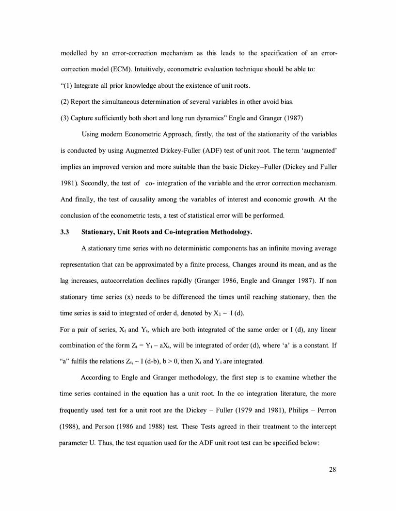
parameter U. Thus, the test equation used for the ADF unit root test can be specified below :

28

LlXt = a0 + 8Xt-i + a1 LlXt-i + a2'1Xt-z + . . . . . . . ixpLlXt-p + Ut

The test equation above has an intercept term but no time trend. The numbers of augmented lag p

is determined by minimizing the Akaike information criterion.

The null hypothesis model to test for unit root has the following forms :

Xt = µ + aX1-1 + et

And the model under the alternative hypothesis,

Xt = µ + 9(t-T/2) + aX1-1 + et

Where Xt is the logarithm of the time series and under the null hypothesis; a = 1 and e =

0. T represents the number of observations . The maximum likelihood procedure suggested by

Johansen ( 1 98 8 and 1 99 1 ) is particularly preferable when the number of variables in the study

exceeds two due to the possibility of existence of multiple co-integrating vectors . The advantage

of Johnson' s test is not only limited to multivariate case, but is also preferable than Engle -

Granger approach even with a two-variable model (Gonzalo, 1 994) . To determine the number of

co-integrating vectors, Johnson ( 1 988 and 1 99 1 ) and Johnson and Juselius ( 1 990) suggested two

statistic tests . The first one is the true test (A-trace). It tests the null hypothesis that the number of

distinct co-integrating vectors is less than or equal to (q) , against a general unrestricted

alternative (q - r) . The second statistical test is the maximal eigenvalue test (Amax) . This test

concerns a test of the null hypothesis that there is (r) co-integrating vectors against the alternative

that there is (r + 1 ) co-integrating vectors.

Conversely, determining the optimal number of lags is the most serious criticism of

Johansen's method. Where more than one co-integrating vector is found, it is often difficult to

interpret each economic relationship . If when the variables are not stationary at level 1(0) or first

difference I( 1 ) , the implementation of this technique becomes more complicated and somewhat

burdensome. The Granger representation theorem is one of the most vital implications of co-

29

integration .According to the theorem, if two or more variables are co-integrated, then the data

can be characterize by an error correction model, discussed below.

An error correction model (ECM) is for use with non-stationary series that are known to

be co-integrated (Lutkepohl, 2006). An easy example is to consider a model with two variables

and one co-integrating vector and no lags. The co-integrating equation is :

Yz,t = �Y1,t

Yz,t and y1,t are the variables and � is the coefficient.

The corresponding EC model is :

ilY1,t = a1 (Y2,t-1 - PY1,t-1) + E1,t

ilY2,t = <lz (Yz,t-1 - PY1,t-1 ) + Ez,t

The error correction term is identified by the right-hand side of the model equal to zero in

the long run (equilibrium) . y1 and y2 deviate from the equilibrium, the value of the error

correction term is found to be nonzero; thus, the y1 and y2 ' s continually adjust to return the

relationship to equilibrium. The a2 captures the rate at which the ith variables in the model revert

to their equilibrium state. The ECM model requirement can be relevant for application only in

series that are co-integrated, the first step is to run the Johansen co-integration test and determine

the number of co-integrating associations . This sequence is necessary as part of the estimation of

the error correction model (Lutkepohl 2006) .

3.4 Co-integration Tests and Limitations.

If two series shares a common stochastic trend, they are said to be co-integrated,

signifying a long-run relationship between the two series. The idea here is to study the co­

movement by testing correspondingly for stationarity and cointegration. Cointegration implies

that two or more variables move together over time and the difference between them is stable

over time. The most widely adopted co-integration methods are the two-step residual procedure

of Engle and Granger ( 1 987) and the system-based reduced rank approach of Johansen ( 1 99 1 ,

30

1 995). The advantage of the system-based reduced rank approach is that it can estimate the

number of co-integrating vectors in the system. The two-step residual procedure suppose that

there is only one unique co-integrating vector, while the system-based reduced rank approach

allows for the estimation of multiple co-integration vectors when tests involve more than two

variables . The maximum likelihood procedure recommended by Johansen ( 1 988 and 1 99 1 ) is

mainly preferable when the number of variables in the study is more than two due to the

possibility of the existence of multiple co-integrating vectors . Therefore, this present analysis

makes use of the Johansen methodology.

Limitations.

T�e exclusion of dynamics can create significant bias in finite samples and this sternly

weakens the performance of the estimator Hendry et al ( 1 986). In addition, endogeneity bias can

involve small sample estimates . Any errors introduced in the first step are passed on to the

second step (Enders 2004) . Park and Philips ( 1 988) argued that the ordinary least square

estimator in the frrst step has non-normal distributions. Hence, the t-statistics information on the

long-run parameters may be ambiguous.

3.5 Model Specification.

Theoretically, the model for this research can be viewed from endogenous growth theory (AK

Model) in terms of how resource wealth can influence economic growth. Lucas ( 1 988) and Romer

( 1 986). Assuming aggregate output is produced based on the constant return to scale production

function where A > 0 below:

h ti A Yt+ 1 Yt = AKt Such that: Yt+i = AKt+1 t ere ore, = -Kt+ l

Respectively K and t are the capital stock and time. A measures the level of total factor productivity.

At steady states, economic growth rate is a combination of the marginal productivity of capital,

proportion of total savings for investment and the savings ratio. In distinctive form, this can be

shown as :

3 1

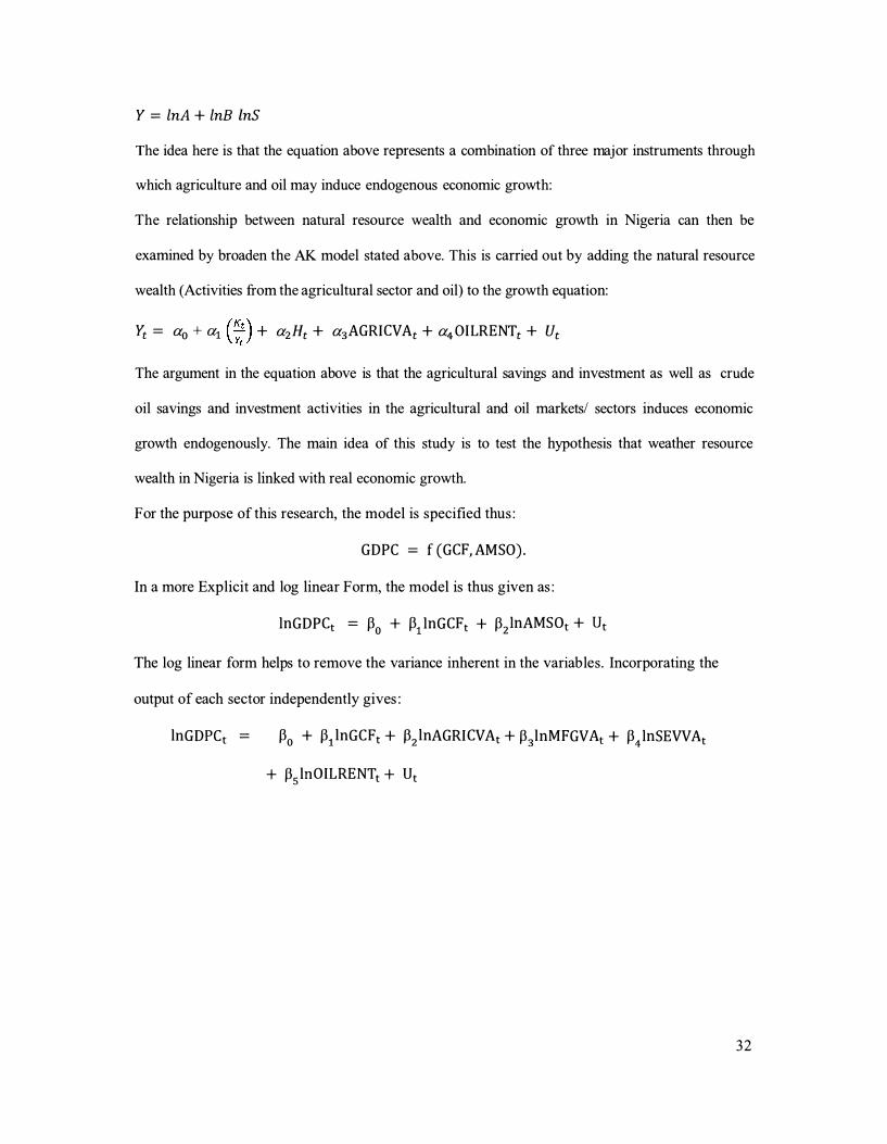
Y = lnA + lnB lnS

The idea here is that the equation above represents a combination of three major instruments through

which agriculture and oil may induce endogenous economic growth:

The relationship between natural resource wealth and economic growth in Nigeria can then be

examined by broaden the AK model stated above. This is carried out by adding the natural resource

wealth (Activities from the agricultural sector and oil) to the growth equation:

Yt = a0 + ai_ (�;) + a2 Ht + a3AGRI CVAt + a4 0I LRE NTt + Ut

The argument in the equation above is that the agricultural savings and investment as well as crude

oil savings and investment activities in the agricultural and oil markets/ sectors ii:iduces economic

growth endogenously. The main idea of this study is to test the hypothesis that weather resource

wealth in Nigeria is linked with real economic growth.

For the purpose of this research, the model is specified thus :

GDPC = f (GCF, AM SO) .

In a more Explicit and log linear Form, the model is thus given as :

lnGDPCt = Po + P1 lnGCFt + P2 lnAMS Ot + ut

The log linear form helps to remove the variance inherent in the variables. Incorporating the

output of each sector independently gives :

lnGDPCt = P0 + P1 lnGCFt + P2 lnAGRI CVAt + P3lnMFGVAt + P4 lnSEVVAt

+ P5 lnOILRE NTt + Ut

32

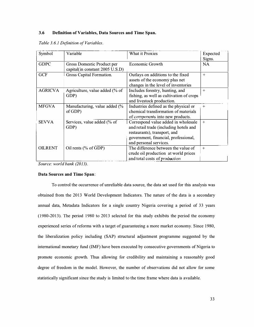
3.6 Definition of Variables, Data Sources and Time Span.

Table 3. 6. 1 Definition of Variables .

Symbol Variable What it Proxies

GDPC Gross Domestic Product per Economic Growth capital( in constant 2005 U.S .D)

GCF Gross Capital Formation. Outlays on additions to the fixed assets of the economy plus net changes in the level of inventories

AGRICVA Agriculture, value added (% of Includes forestry, hunting, and GDP) fishing, as well as cultivation of crops

and livestock production. MFGVA Manufacturing, value added (% Industries defined as the physical or

of GDP) chemical transformation of materials of components into new products .

SEVVA Services, value added (% of Correspond value added in wholesale GDP) and retail trade (including hotels and

restaurants), transport, and government, financial, professional, and personal services.

OILRENT Oil rents (% of GDP) The difference between the value of crude oil production at world prices and total costs of production

Source: world bank (2013) .

Data Sources and Time Span :

Expected Signs. NA

+

+

+

+

+

To control the occurrence of unreliable data source, the data set used for this analysis was

obtained from the 20 1 3 World Development Indicators. The nature of the data is a secondary

annual data, Metadata Indicators for a single country Nigeria covering a period of 33 years

( 1 980-20 1 3) . The period 1 980 to 20 1 3 selected for this study exhibits the period the economy

experienced series of reforms with a target of guaranteeing a more market economy. S ince 1 980,

the liberalization policy including (SAP) structural adjustment programme suggested by the

international monetary fund (IMF) have been executed by consecutive governments of Nigeria to

promote economic growth. Thus allowing for credibility and maintaining a reasonably good

degree of freedom in the model. However, the number of observations did not allow for some

statistically significant since the study is limited to the time frame where data is available.

3 3

4.1 Introduction

Chapter 4

Analysis of Results and Discussions.

As earlier stated that the main objective of this research work is to empirically investigate

the paradox of economic growth in Nigeria with perspective from natural resource wealth. This

chapter therefore concentrates on the presentation of annual time series data used, followed by

the descriptive analysis, correlation analysis, interpretation of the unit root tests, Johansen co-

integration analysis, error correction mechanism, and granger causality test.

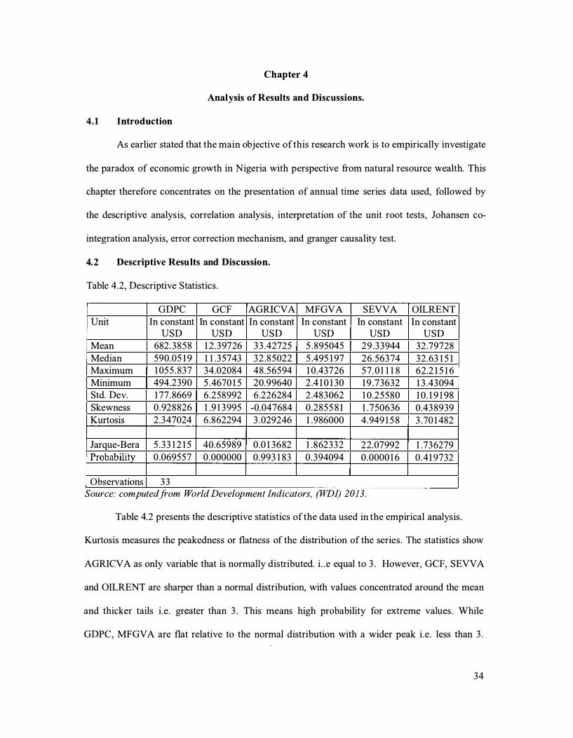
4.2 Descriptive Results and Discussion.

Table 4.2, Descriptive Statistics .

GDPC GCF AGRICVA

Unit In constant In constant In constant USD USD USD

Mean 682 .3858 1 2 .39726 33 .42725

Median 590.05 1 9 1 1 . 35743 32 .85022 Maximum 1 055 . 837 34.02084 48 .56594 Minimum 494.2390 5 .4670 1 5 20.99640 Std. Dev. 1 77. 8669 6.258992 6.226284 Skewness 0 .928826 1 .9 1 3995 -0.047684

Kurtosis 2 .347024 6 .862294 3 .029246

Jarque-Bera 5 . 33 1 2 1 5 40.65989 0.0 1 3682 Probability 0 .069557 0 .000000 0.993 1 83

Observations 3 3

MFGVA SEVVA In constant In constant

USD USD 5 . 895045 29 .33944

5 .495 1 97 26 .56374 1 0.43726 57. 0 1 1 1 8 2 .4 1 0 1 30 1 9 .73632 2 .483062 1 0.25580 0.2855 8 1 1 .750636

1 .986000 4 .949 1 5 8

1 . 862332 22.07992 0 .394094 0 .0000 1 6

Source: computed from World Development Indicators, (WDI) 2013.

OILRENT

In constant USD

32 .79728

32 .63 1 5 1 62.2 1 5 1 6 1 3 .43094 1 0 . 1 9 1 98

0.43 8939

3 .70 1 482

1 .736279

0 .41 9732

Table 4.2 presents the descriptive statistics of the data used in the empirical analysis .

Kurtosis measures the peakedness or flatness of the distribution of the series. The statistics show

AGRICVA as only variable that is normally distributed. i. . e equal to 3 . However, GCF, SEVV A

and OILRENT are sharper than a normal distribution, with values concentrated around the mean

and thicker tails i .e . greater than 3 . This means high probability for extreme values . While

GDPC, MFGVA are flat relative to the normal distribution with a wider peak i .e . less than 3 .

34

Skewness is a measure of asymmetry of the distribution of the series around the mean. The

statistic for skewness shows that all the variables except for AGRICV A is positively skewed,

implying that these distributions have long right tails . The Jarque-Bera which measures whether

the series is normally distributed or not also rejects the null hypotheses of normal distribution for

GCF and SEVV A.

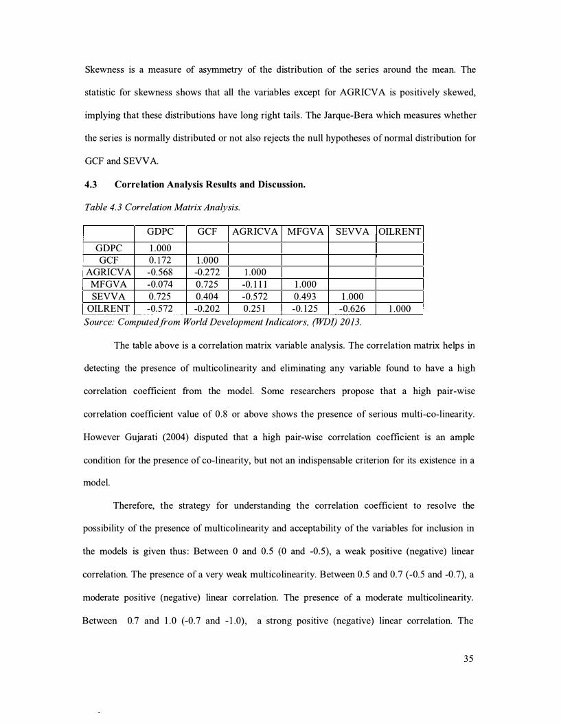
4.3 Correlation Analysis Results and Discussion.

Table 4. 3 Correlation Matrix Analysis.

GDPC GCF AGRICVA MFGVA

GDPC 1 .000

GCF 0.172 1 .000

AGRICVA -0.568 -0.272 1.000

MFGVA -0.074 0.725 -0. 1 1 1 1 .000

SEVVA 0.725 0.404 -0.572 0.493

QILRENT -0.572 -0.202 0 .25 1 -0. 1 25

SEVVA

1 .000

-0.626

Source: Computed from World Development Indicators, (WDI) 2013.

OILRENT

1 .000

The table above is a correlation matrix variable analysis. The correlation matrix helps in

detecting the presence of multicolinearity and eliminating any variable found to have a high

correlation coefficient from the model. Some researchers propose that a high pair-wise

correlation coefficient value of 0 . 8 or above shows the presence of serious multi-co-linearity.

However Gujarati (2004) disputed that a high pair-wise correlation coefficient is an ample

condition for the presence of co-linearity, but not an indispensable criterion for its existence in a

model.

Therefore, the strategy for understanding the correlation coefficient to reso lve the

possibility of the presence of multicolinearity and acceptability of the variables for inclusion in

the models is given thus : Between 0 and 0.5 (0 and -0.5), a weak positive (negative) linear

correlation. The presence of a very weak multicolinearity. Between 0.5 and 0.7 (-0.5 and -0.7), a

moderate positive (negative) linear correlation. The presence of a moderate multicolinearity.

Between 0.7 and 1 .0 (-0.7 and -1 .0), a strong positive (negative) linear correlation. The

35

presence of a very strong multicolinearity. Showing a poor acceptance of the variables to be

integrated in the model. The range of 0.4 for this study allows for the presence of very weak

multi-co-linearity as this is within the verge of 0 .5 highlighted by Gujarati (2004) thus retaining

an acceptable level of multicolinearity.

From the table 4 .3 above, it can be observed that, all the variables are correlated with

growth (GDPC). Oilrent shows a negative correlation with other estimated variables in the model

except for the Agricultural sector indicating a weak positive correlation. The implication of this

is that the proceed from oil rent has no significant effect on overall growth of the economy. What

might be causing the growth of the Nigerian Economy is largely due to the service sector

indicating a positive correlation with the exception of the agricultural sector and oilrent. The

implication of this is that the service sector provides information useful in gearing overall

growth.

4.4 Time Series Properties of the Variables.

To avoid the problem of spurious regression, it is necessary to examine the time series

properties of the variables . In literature, most economic time series are non-stationary and

including non-stationary variables in the model can lead to spurious regression coefficient

estimate (Granger and Newbold, 1 974) .

4.4.1 Unit Root Test - Results and Discussion.

The hypothesis of stationarity in the data employed is vital in the study of time series

data. The stationarity of data is significant because conditions of variance, constant covariance,

and mean need to be satisfied to certify the correctness of the parameters and model. Thus, it is

imperative to check if the data are stationary or not while estimating the relationship between the

determinants of economic growth. Phillips and Perron( 1 986) assert that conducting regressions

which uses non-stationary variables may lead to misleading results, showing actually significant

relationships, even where the variables are generated separately. (Patterson 2000) affirms that

36

spurious regression frequently takes place while dealing with time series data. A unit root test

can be practical to determine if the variables of interest are stationary or not.

Lag length selection of the Augmented Dikey-Fuller (ADF) Unit Root Test

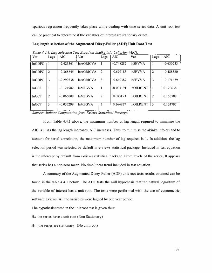
Table 4. 4. 1 . Lag Selection Test Based on Akaike info Criterion (AIC). Var Lags AIC Var Lags AIC Var Lags AIC

lnGDPC 1 -2.4233 6 1 lnAGRICVA 1 -0.748282 lnSEVVA 1 -0.630233

lnGDPC 2 -2 .368845 lnAGRICVA 2 -0.699 1 85 lnSEVVA 2 -0.488520

lnGDPC 3 -2 .29033 8 lnAGRICVA 3 -0.6403 87 lnSEVVA 3 -0. 1 7 1 679

lnGCF I -0. 1 24982 lnMFGVA 1 -0.003 1 9 1 lnOILRENT 1 0. 1 2063 8

lnGCF 2 -0.066008 lnMFGVA 2 0.083 1 93 lnOILRENT 2 0. 1 56788

lnGCF 3 -0.035299 lnMFGVA 3 0.264827 lnOILRENT 3 0. 1 24797

Source: Authors Computation from Eviews Statistical Package.

From Table 4.4. 1 above, the maximum number of lag length required to minimise the

AIC is 1 . As the lag length increases, AIC increases . Thus, to minimise the akinke info cri and to

account for serial correlation, the maximum number of lag required is 1 . In addition, the lag

selection period was selected by default in e-views statistical package. Included in test equation

is the intercept by default from e-views statistical package. From levels of the series, It appears

that series has a non-zero mean. No time/linear trend included in test equation.

A summary of the Augmented Dikey-Fuller (ADF) unit root tests results obtained can be

found in the table 4.4. 1 below. The ADF tests the null hypothesis that the natural logarithm of

the variable of interest has a unit root. The tests were performed with the use of econometric

software Eviews . All the variables were lagged by one year period.

The hypothesis tested in the unit root test is given thus:

Ho: the series have a unit root (Non Stationary)

H1 : the series are stationary (No unit root)

37

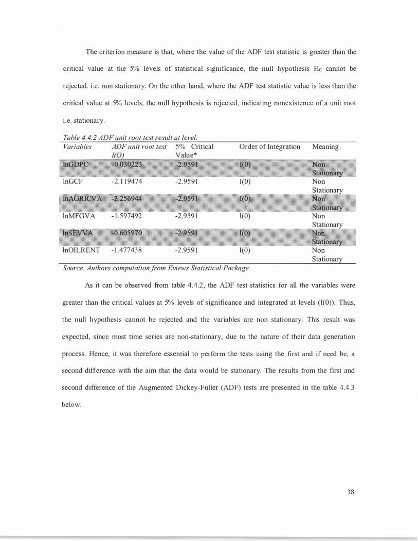
The criterion measure is that, where the value of the ADF test statistic is greater than the

critical value at the 5% levels of statistical s ignificance, the null hypothesis Ho cannot be

rejected. i .e . non stationary. On the other hand, where the ADF test statistic value is less than the

critical value at 5% levels, the null hypothesis is rejected, indicating nonexistence of a unit root

i .e . stationary.

Table 4. 4. 2 ADF unit root test result at level.

Variables ADF unit root test 5% Critical Order of Integration Meaning 1(0) Value*

lnGDPC -0.030223 -2.9591 1(0) Non Stationary

lnGCF -2. 1 1 9474 -2 .95 9 1 1(0) Non Stationary

lnAGRICVA -2.256944 -2.9591 1(0) Non Station�

lnMFGVA - 1 .597492 -2.959 1 1(0) Non Stationary

lnSEVVA -0.605970 -2.9591 1(0) Non Stationary

lnOILRENT - 1 .47743 8 -2 .95 9 1 1(0) Non Stationary

Source. Authors computation from Eviews Statistical Package.

As it can be observed from table 4 .4 .2, the ADF test statistics for all the variables were

greater than the critical values at 5% levels of significance and integrated at levels (1(0)) . Thus,

the null hypothesis cannot be rejected and the variables are non stationary. This result was

expected, since most time series are non-stationary, due to the nature of their data generation

process. Hence, it was therefore essential to perform the tests using the first and if need be, a

second difference with the aim that the data would be stationary. The results from the first and

second difference of the Augmented Dickey-Fuller (ADF) tests are presented in the table 4 .4 .3

below.

38

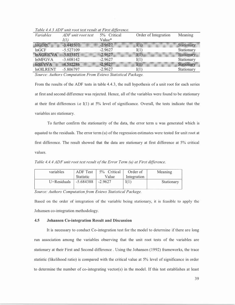
Table 4. 4. 3 ADF unit root test result at First difference.

Variables ADF unit root test 5% Critical Order of Integration Meaning

lnGDPC lnGCF lnAGRlCVA lnMFGVA lnSEVVA lnOILRENT

1(1) Value*

-3 .445507 -2 .9627 -5 .527 1 09 -2 .9627 -5 .835571 -2 .9627 -3 . 608 1 42 -2 .9627 -4.5 12286 -2.9627 -5 . 806797 -2 .9627

1( 1 ) 1( 1 ) 1( 1 ) I( l ) 1( 1) I( l )

Source: Authors Computation From Eviews Statistical Package.

Stationary Stationary Stationary Stationary Stationary -------Stationary

From the results of the ADF tests in table 4.4 . 3 , the null hypothesis of a unit root for each series

at first and second difference was rejected. Hence, all of the variables were found to be stationary

at their first differences i .e I( l ) at 5% level of significance. Overall, the tests indicate that the

variables are stationary.

To further confirm the stationarity of the data, the error term u was generated which is

equated to the residuals . The error term (u) of the regression estimates were tested for unit root at

first difference. The result showed that the data are stationary at first difference at 5% critical

values .

Table 4. 4. 4 ADF unit root test result of the Error Term (u) at First difference.

variables ADF Test 5% Critical Order of Meaning Statistic Value Integration

U=Residuals -5 .6843 88 -2 .9627 1( 1 ) Stationary

Source: Authors Computation from Eviews Statistical Package.

Based on the order of integration of the variable being stationary, it is feasible to apply the

Johansen co-integration methodology.

4.5 Johansen Co-integration Result and Discussion

It is necessary to conduct Co-integration test for the model to detem1ine if there are long

run association among the variables observing that the unit root tests of the variables are

stationary at their First and Second difference . Using the Johansen ( 1 992) frameworks, the trace

statistic (likelihood ratio) is compared with the critical value at 5% level of significance in order

to determine the number of co-integrating vector(s) in the model. If this test establishes at least

39

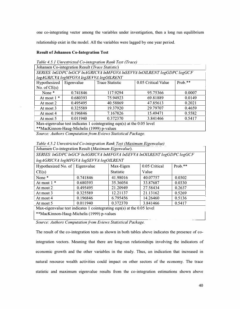
one co-integrating vector among the variables under investigation, then a long run equilibrium

relationship exist in the model. All the variables were lagged by one year period.

Result of Johansen Co-Integration Test

Table 4. 5. 1 Unrestricted Co-integration Rank Test (Trace)

Johansen Co-integration Result (Trace Statistic)

SERIES: lnGDPC lnGCF lnAGRICVA lnMFG VA lnSEVVA lnOILRENT logGDPC logGCF loKAGRICVA logMFG VA loKSEVVA loKOILRENT

Hypothesized Eigenvalue Trace Statistic 0.05 Critical Value Prob . * * No. of CE(s)

None * 0.74 1 846 1 1 7 .9294 95 .75366 0.0007 At most 1 * 0.680393 75 .94923 69 . 8 1 889 0.0 1 49 At most 2 0.495495 40.58869 47 .856 1 3 0.202 1

At most 3 0.325589 1 9.37920 29.79707 0.4659

At most 4 0. 1 96846 7 . 1 67826 1 5 .4947 1 0 .5582

At most 5 0.0 1 1 940 0.372370 3. 84 1 466 0.54 1 7 Max-eigenvalue test indicates 1 cointegrating eqn(s) at the 0.05 level * *MacKinnon-Haug-Michelis ( 1 999) p-values Source: Authors Computation from Eviews Statistical Package.

Table 4. 5. 2 Unrestricted Co-integration Rank Test (Maximum Eigenvalue)

Johansen Co-integration Result (Maximum Eigenvalue) .

SERIES: lnGDPC lnGCF lnAGRICVA lnMFG VA lnSEVVA lnOILRENT logGDPC logGCF

logAGRICVA logMFG VA logSEVVA logOILRENT

Hypothesized No. of Eigenvalue Max-Eigen 0.05 Critical Prob. **

CE(s) Statistic Value

None * 0.74 1 846 4 1 .980 1 6 40.07757 0.0302 At most 1 * 0.680393 35 .36054 33.87687 0.0330 At most 2 0.495495 2 1 .20949 27 .58434 0.2637

At most 3 0.325589 1 2 .2 1 1 37 2 1 . 1 3 1 62 0.5269 At most 4 0. 1 96846 6.795456 1 4.26460 0.5 1 36 At most 5 0.0 1 1 940 0.372370 3.84 1466 0.54 1 7 Max-eigenvalue test indicates 1 cointegrating eqn(s) at the 0.05 level

* *MacKinnon-Haug-Michelis ( 1 999) p-values

Source: Authors Computation fi·om Eviews Statistical Package.

The result of the co-integration tests as shown in both tables above indicates the presence of co-

integration vectors . Meaning that there are long-run relationships involving the indicators of

economic growth and the other variables in the study. Thus, an indication that increased in

natural resource wealth activities could impact on other sectors of the economy. The trace

statistic and maximum eigenvalue results from the co-integration estimations shown above

40

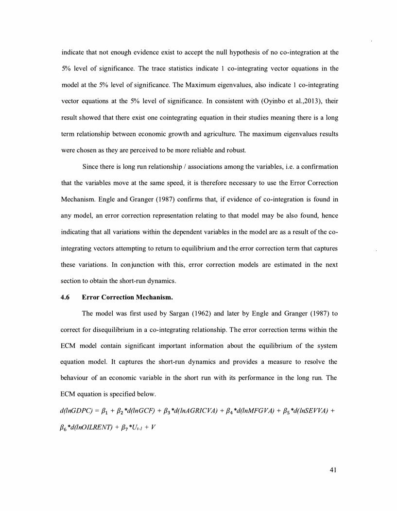
indicate that not enough evidence exist to accept the null hypothesis of no co-integration at the

5% level of significance. The trace statistics indicate 1 co-integrating vector equations in the

model at the 5% level of significance. The Maximum eigenvalues, also indicate 1 co-integrating

vector equations at the 5% level of significance. In consistent with (Oyinbo et al. ,20 1 3), their

result showed that there exist one cointegrating equation in their studies meaning there is a long

term relationship between economic growth and agriculture. The maximum eigenvalues results

were chosen as they are perceived to be more reliable and robust.

Since there is long run relationship I associations among the variables, i .e . a confirmation

that the variables move at the same speed, it is therefore necessary to use the Error Correction

Mechanism. Engle and Granger ( 1 987) confirms that, if evidence of co-integration is found in

any model, an error correction representation relating to that model may be also found, hence

indicating that all variations within the dependent variables in the model are as a result of the co­

integrating vectors attempting to return to equilibrium and the error correction term that captures

these variations . In conjunction with this, error correction models are estimated in the next

section to obtain the short-run dynamics .

4.6 Error Correction Mechanism.

The model was first used by Sargan ( 1 962) and later by Engle and Granger ( 1 987) to

correct for disequilibrium in a co-integrating relationship . The error correction terms within the

ECM model contain significant important information about the equilibrium of the system

equation model. It captures the short-run dynamics and provides a measure to resolve the

behaviour of an economic variable in the short run with its performance in the long run. The

ECM equation is specified below.

d(lnGDPC) = /31 + /32 *d(lnGCF) + /33 *d(lnAGRJCVA) + /34 *d(lnMFG VA) + /35 *d(lnSEVVA) +

/36 *d(lnOILRENT) + /37 *U1-1 + V

4 1

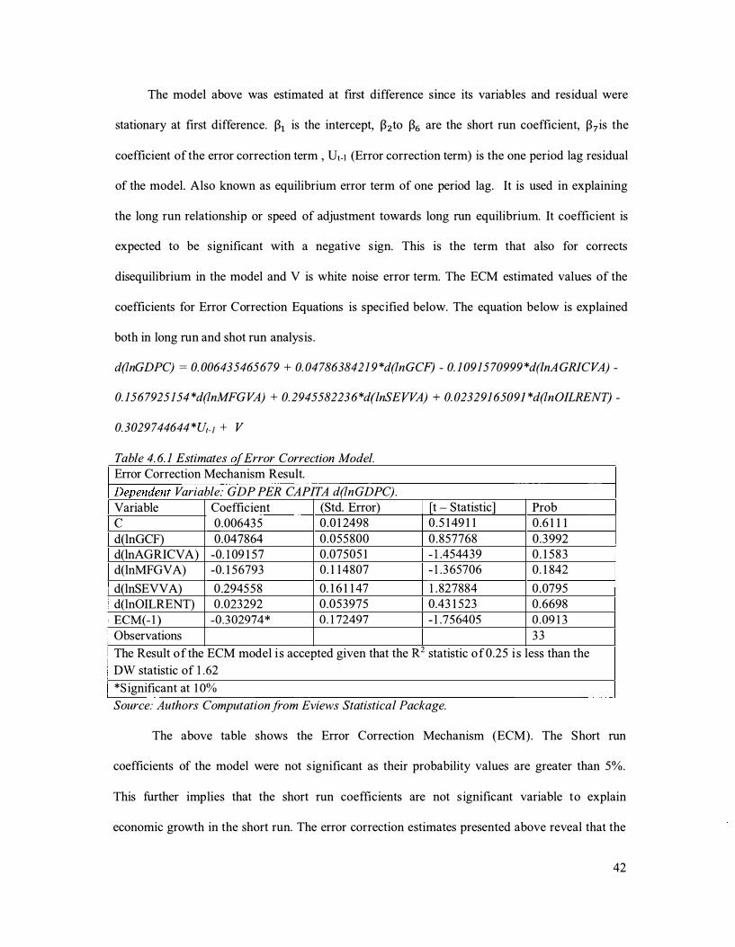
The model above was estimated at first difference since its variables and residual were

stationary at first difference. 131 is the intercept, 132to 136 are the short run coefficient, 137is the

coefficient of the error correction term , Ut-1 (Error correction term) is the one period lag residual

of the model. Also known as equilibrium error term of one period lag. It is used in explaining

the long run relationship or speed of adjustment towards long run equilibrium. It coefficient is

expected to be significant with a negative sign. This is the term that also for corrects

disequilibrium in the model and V is white noise error term. The ECM estimated values of the

coefficients for Error Correction Equations is specified below. The equation below is explained

both in long run and shot run analysis .

d(lnGDPC) = 0. 006435465679 + 0. 04786384219 *d(lnGCF) - 0. 1 0915 70999 *d(lnAGRICVA) -

0. 1567925154 *d(lnMFG VA) + 0.2945582236*d(lnSEVVA) + 0. 0232916509J *d(lnOILRENT) -

0. 3029744644 *U1-1 + V

Table 4. 6. 1 Estimates of Error Correction Model. Error Correction Mechanism Result.

Dependent Variable: GDP PER CAPITA d(lnGDPC).

Variable Coefficient (Std. Error) [t - Statistic] Prob

c 0.006435 0 .0 1 2498 0 .5 1 49 1 1 0 .6 1 1 1

d(lnGCF) 0.047864 0.055800 0 .857768 0 .3992 d(lnAGRICV A) -0. 1 09 1 57 0.07505 1 - 1 .454439 0 . 1 583 d(lnMFGVA) -0. 1 56793 0. 1 14807 - 1 .365706 0. 1 842

d(lnSEVVA) 0 .294558 0. 1 6 1 1 47 1 . 827884 0 .0795 d(lnOILRENT) 0 .023292 0.053975 0.43 1 523 0 .6698 ECM(- 1 ) -0.302974* 0 . 1 72497 - 1 .756405 0.09 1 3 Observations 33

The Result of the ECM model i s accepted given that the R2 statistic of 0.25 i s less than the

DW statistic of 1 .62

*S ignificant at 1 0% Source: Authors Computation from Eviews Statistical Package.

The above table shows the Error Correction Mechanism (ECM). The Short run

coefficients of the model were not significant as their probability values are greater than 5%.

This further implies that the short run coefficients are not s ignificant variable to explain

economic growth in the short run. The error correction estimates presented above reveal that the

42

error correction term [ECM(-1 )] or speed of adjustment towards long run equilibrium is correctly

signed with the expected negative Error Correction Term. This means that there is a tendency by

the model to correct and move towards the equilibrium path following disequilibrium in each

period. Hence, meaningful error correction is taking place annually. Therefore in each short-term

period, economic growth is adjusted by taking into account the previous time periods difference

between the independent variables and per capita real GDP growth. The ECM term, however

accounts for the correction of about 30.29% of the error generated in the last period. i .e . the

speed of adjustment is 30 .29% annually. The speed of the adjustment implies that by

computation, it will take between 6 to 7 years for the economy to close the gap between its

current state (short run period) and the long run equilibrium. In consistent with (Oyinbo et al. ,

20 1 4), their result indicated the expected negative sign of the error correction term, implying that

about 68% of disequilibria from the previous year ' s shock converge back to the long run

equilibrium in the current year in their study. The result of the ECM also keeps the validity that

there exist a long run equilibrium relationship between GDPC and other variable of interest.

However, the ECM term is not statistically significant at 5% level of significance but Significant

at 1 0% level of significance. Thus in the short run, agriculture is not significant to explain

economic growth. This is in line with (Oyinbo et al. , 20 1 3) as their heir Error Correction

Estimates of Economic Growth in Nigeria indicated that in the short run, the lagged value of

agriculture is negative and insignificant in influencing economic growth. They attributed this to

poor budgetary allocation to agriculture relative to other sectors of the economy (Oyinbo et al. ,

20 1 3) . Thus, the integral role of agricultural financing is lacking, thereby hindering growth of the

agricultural sector. Based on current supervision and assessment reports of 2007 and 2008 (Ujah

and Okoro, 2009) shows that agricultural budget was far below 25% and 1 0% recommendation

from the Food and Agricultural Organization and African Union respectively. The

insignificance of the agricultural sector in influencing the Nigerian economic growth in the short

43

run period is also essentially attributed to a number of problems and challenges faced by the

sector over the past decades . "International market opportunities for some exportable

commodities have been low on account of the sector ' s inability to be competitive" (UNDP report

20 12) . (Oni, T.O 20 1 3) identified numerous challenges such as : "marketing problem, storage and

processing problems, infrastructural inadequacies, unstable input and output Prices, seasonal

labour shortages due migration of able-bodied youths from the rural to urban areas, technical

constraint, inadequacies in past policies and programmes as well as impute supply problems". In

addition, resources from the agricultural sector are under utilized for the growth of the Nigerian

economy. Thus, there is little or no effort to add value to the sector from the returns of economic

growth. This is consistent with literature and empirically true for the Nigerian economy that

highlights the lack of attention, total neglect and investment in the agriculture sector in spite of

its proven potentials Awokuse (2008). Another reason why this sector has performed poorly on

economic growth stems from the land tenure system and its associated problems in Nigeria. In

Nigeria, Land is communally owned. Land is been shared out to families and individuals, while

the community or clan maintained absolute ownership. Although land has been heavily regulated

by the Nigerian government through the establishment of the Land Tenure Law of Northern

Nigeria of 1 962 and Land Use Act No. 6 of 1 978 , "the implementation of the Act in the past

decades has increasingly become an obstruction in the wheel of economic growth and

development as the Act is anti-people and oppressive" (Namnso et al. , 20 1 4) . The Land Use Act

has resulted to multiple forms of tenure system leading to unwarranted bureaucracy in getting

consent and approval for land transactions and certificate and insecurity of right of occupancy

granted under the Act. In terms of ease of registration of property, Nigeria is ranked among the

lowest, World Bank (20 1 4) . According to the provision of Section 1 of the Act, individuals

cannot own freehold interest in land in Nigeria. This implies that all land in the territory of each

state, government holds the absolute interest in land.

44

In connection with the above, the oil sector which has the bulk of the Nigerian federally

collected revenue has no significant impact in influencing the growth of the Nigerian economy.

(Akinlo, 20 1 2) argued that the oil sector has very little linkage with other sectors of the economy

since the sector does not offer much opportunity for employment. Nigeria is a country whose

relationship with oil over the decades has been volatile, plagued by corruption and

mismanagement. Volatility in oil price makes the exchange rate volatile thereby encouraging

excessive short term capital flow (Akinlo, 20 1 2) . Thus the efficiency of macroeconomic policy is

being constrained. The oil rich Niger Delta region has become the site of an intense and

controversial struggle between the state and the indigenous population (Omeje 2006) . Local

indigenous people have become incensed by foreign oil corporation reaping the rewards of this

resource, when they themselves have seen little if any improvement in their standard of living

(Omeje 2006) . The effects of oil extraction for the environment and the Niger Delta communities

have been devastating. According to Nigerian federal government figures, there were more than

7,000 oil spills between 1 970 and 2000 (Omeji 2006). This has led to serious ecological damage

in the fragile region. In the last decade, a militant group called the Movement for the

Emancipation of the Niger Delta (MEND) emerged. This group have launched many attacks on

oil workers and pipelines, attempting to shut down production in the region (Omeje 2006) . In

consistent with other empirical literature that oilrent is not influential to economic growth. Lane

and Tornell ( 1 998) note that oil-rich Venezuela' s terms of trade rose 1 3 .7% per year during

1 970- 1 990, while per capita output declined at a rate of 1 .4% per year. They also point out that

Saudi Arabia ' s real per capita GDP actually declined between 1 970 and 1 999 . Gylfason (200 1 , p .

848) claims that per capita GNP in OPEC countries fell 1 .3% per year during 1 965 - 1 998 .

In general, the bulk of the reasons why agriculture and oil has not been significant to the

growth of the Nigerian economy is chiefly due to gravity of corruption and mismanagement

entirely different from the rest of the world. Going by Transparency International report, Nigeria

45

was ranked among the 3 8 most corrupt countries in the world out of 1 75 countries examined

(Transparency International 20 1 4) . In addition, Global Corruption Barometer reports that the

population' s perception of corruption has increased significantly between 20 1 1 and 20 1 3 . From

the time Nigeria gained her in dependence, public funds amounting to about US$400 billion has

been vanished due to corruption. New and evident report indicates that about US$6.8 billion was

missing due to corruption in the subsidy program (Berne Declaration 20 1 3) . A search also

discovered between 200 1 and 2008, an astounding 3 00,000 barrels of oil were stolen per day and

a total of 1 5 fuel importers collected more than US$300 million in fuel subsidy funds without

importing any fuel (Nwaroh 20 1 2) .

The R2 of the model is 0 .246386. Although this value is low but i t i s warranted based on

the nature of the variables in the model. There are so many other variables that the growth of the

Nigerian economy depends on which are deliberately not included in the model. There exclusion

was aimed at concentrating on natural resource impact on the growth of the Nigerian Economy.

The Result of the ECM model is accepted given that the R2 statistic of 0 .25 is less than the DW

statistic of 1 .62. In confirmation to this is a test of statistical error below.

Overall, the findings in this chapter have important policy implications for the Nigerian

Economy and other developing countries with similar economic structures. The evidence

indicates that the agricultural and oil sectors plays important role in terms of the Nigerian

Economy. Thus, the development of these sectors would be beneficial and rewarding to the

Nigerian economic growth.

46

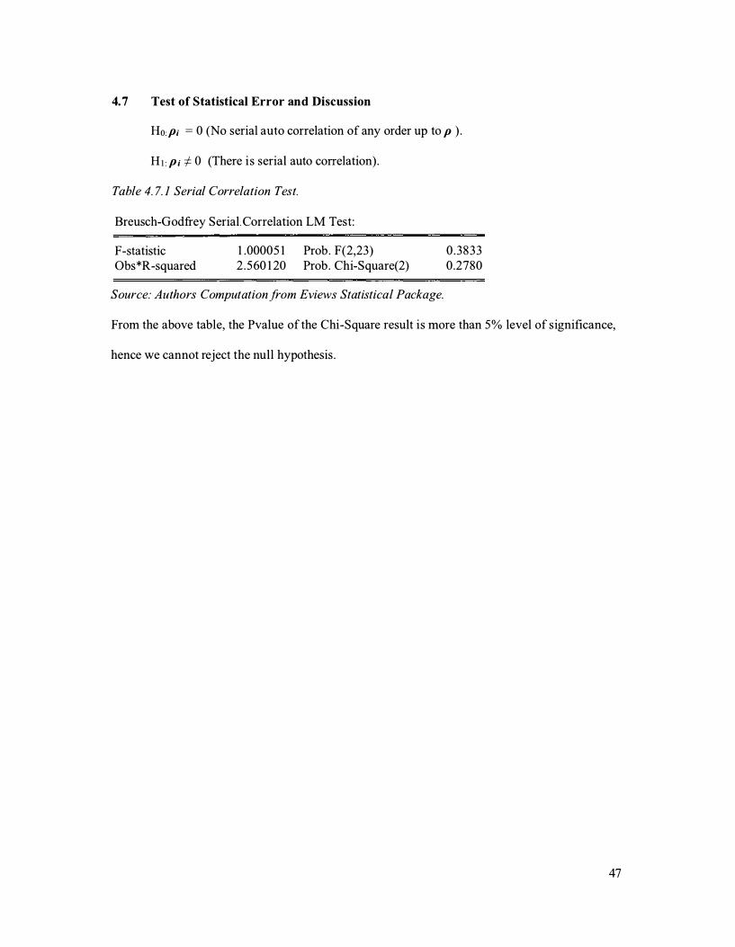
4.7 Test of Statistical Error and Discussion

Ho: p; = 0 (No serial auto correlation of any order up to p ) .

H i : p ; f 0 (There i s serial auto correlation) .

Table 4. 7. 1 Serial Correlation Test.

Breusch-Godfrey Serial Correlation LM Test:

F-statistic Obs*R-squared

1 .00005 1 Prob . F(2,23) 2 .560 1 20 Prob . Chi-Square(2)

Source: Authors Computation from Eviews Statistical Package.

0 .3833 0.2780

From the above table, the Pvalue of the Chi-Square result is more than 5% level of significance,

hence we cannot reject the null hypothesis .

47

5.1 Introduction.

Chapter 5

Summary and Conclusion

This chapter provides a summary and conclusion to the study and its main findings . Also,

it highlights the main contribution of the thesis, presents some policy implications and proffers

some recommendations on ways to improve the contributions of natural resource wealth to

economic growth. It then finishes by presenting the limitations of the study and proffers some

suggestions on areas for further research.

5.2 Summary and Conclusion

This thesis investigated the link between the natural resource wealth and economic

growth in Nigeria, using time series data form world development indicators . It applied the error

correction model (ECM) to evaluate the natural resource wealth and economic growth

relationship . In this research, two questions were addressed: does a resource based growth

strategy leads to sustained economic growth? What is the relationship between the natural

resource wealth and economic growth in Nigeria? And if there is a relationship what is the

direction of the relationship between natural resource wealth and economic growth in Nigeria?

Does natural resource wealth cause economic growth or does economic growth cause the

development of natural resources? Does Natural resource wealth cause inconsistency in the

growth of the Nigerian Economy?

The study utilised two measures of natural resource wealth, Agriculture and Oilrent. The

study established the existence of co-integration for all measures. Thus, the results obtained for

all measures of natural resource wealth used in this research point to the existence of long run

relationship between resource wealth and economic growth.

48

5.3 Main Contributions of the Study.

This thesis makes a contribution by providing time series evidence for a developing

country on natural resource wealth and economic growth relationship . To improve robustness

and avoid simultaneous bias as highlighted by Gujarati (2004), the study included the

manufacturing sector and the service sector since these sectors exhibits some sort of relationship

with resource wealth and growth.

In addition, the study re-examined the endogenous growth model to identify the

importance of capital formation and technical progress to economic growth. As it can be clearly

observed in the study that results obtained for any particular country cannot be generalised

readily for another country. Issues relating to the relationship are country specific. Thus, this

study makes a contribution by providing insight into the natural resource wealth and growth

relationship for a specific country (Nigeria) . The findings from this study can thus be readily

utilised as a reference for policy formulation for the Nigerian economy.

5.4 Policy Implications and Recommendations.

The empirical findings from this study highlight a policy implication issue relating to the

role of natural resource wealth in economic growth in Nigeria. A major policy implication from

the results is that natural resource based growth strategy will not lead to sustained economic

growth. Thus Nigeria should aim at pursuing industrial growth strategy with a vibrant real sector

that would result in the diversification of the economy. Also it is critically imperative for

Nigerians and it government to tackle the issue of wide spread corruption and mismanagement of

public funds in all respective areas and sectors of its economy.

5.5 Limitations of the Study and Suggestions for Further Research

The study' s result may be improved by removing some of the restrictions to it. This

study' s restrictions include the unavailability of sufficiently long time-series data for variables

that are included in the theoretical models . In some instances, data was available for an earli er

49

period of time than others. The researcher could collect annual data for only 3 3 years, which was

sufficient in statistical terms but less than was originally intended. In addition, natural resource

wealth indicators which the researcher used in the empirical analysis is limited to only two

indicators agriculture and oil; however, there are other sources of natural resource wealth and

other factors not considered having impact on the Nigerian economic growth. This study uses

annual time-series data to examine growth paradox in Nigerian. Since the study is a single­

country study, with the applications of the study limited to the country studied (Nigeria) . A

further extension of this research could be to conduct a similar study for other countries,

particularly other developing countries .

In addition, this research utilizes GDPC as a proxy for economic growth. However, there are

other variables which could be used as a proxy for economic growth including gross national

product, HDI indicators (health, education and living standards), household income,

technological advancement, savings, investments and many others . Also, this analysis was

conducted using annual time-series data but the analysis could be conducted using higher

frequency data, possibly quarterly and monthly, to confirm that the findings of this study are not

as a result of aggregations and could prove to be quite informative.

50

References

AfricanEconomicOutlook(20 1 4 )http ://www.africaneconomicoutlook.org/fileadmin/up loads/

eo/20 14/PD F /CN _Long_ EN/Nigeria_ EN. pdf

Akinlo (20 12) How Important is Oil in Nigeria 's Economic Growth ? Journal of Sustainable

Development. Vol 5 (4) pp 1 65 - 1 79 .

Akpan E. (2009) Oil price shocks and Nigeria 's Macroeconomy, A Paper Presented at the

Annual Conference of CSAE Conference, Economic Development in Africa, 22nd- 24th

March 2009, Oxford.

Auty, R.M (2007) Rent Recycling Theory, The Resource Curse, and Development Policy.

Developing Alternatives. 1 1 ( 1) pp7- 1 3

Awokuse, T. (2008) . Does Agriculture Really Matter for Economic Growth in Developing

Countries? American Agricultural Economics Association Annual Meeting. Milwaukee,

WI.

Balogun E. (2007b) 'Banking sector reforms and the Nigerian economy: performance, pitfalls

and future policy options ' , MPRA Paper 3804, University Library of Munich, Germany.

Berge, K. and A. Wood ( 1 997) Exporting Manufactures: Human Resources, Natural

Resources, and Trade Policy. The Journal of Development Studies. Vol 34( 1 ) . Pp. 35 -59 .

Berne Declaration (20 1 3) Traders collude in oil corruption, says Swiss NGO.

http ://www.swissinfo.ch/eng/ traders-collude-in-oil-corruption--says-swiss­

ngo/37260 1 52

Bhattacharyya, S . and R. Holder (20 1 0) Natural resources, democracy and corruption .

European Economic Review. Vol 54(4) . Pp . 608-62 1 .

Central Bank of Nigeria (CBN) (2008) Statistical Bulletins of 2006, Abuja: Central Bank of

Nigeria Publication.

Clarke, A and K. Kulkarni (2009). Testing the Application of Heckscher-Ohlin Theorem to

5 1

Contemporary Trade Between Malaysia and Singapore. Journal of Emerging Knowledge

on Emerging Markets . 1 ( 1 ) , pp . 1 1 3 - 1 28 .

Dickey, D.A. and Fuller W.A. ( 1 98 1 ) 'Likelihood Ratio statistics for Autoregressive Time

Series with a Unit Root" Econometrical, 49, 1 057- 1 072 .

Dickey, D. and Fuller, W. ( 1 979) 'Distribution of the estimators for autoregressive time

series with a unit root ' , Journal of the American Statistical Association, Vol. 74, pp 427-

443 .

Ekpo, A. and Egwakhide, F . (2003) 'Four decades of industrialization in Nigeria: a critical

analysis ' , Nigerian Journal of Economic and Social Sciences .

Enders W. (2004) Applied Econometric Time Series, USA. : John Wiley and Sons, Inc.

Engle, R. and Granger C. ( 1 987) 'Co-Integration and error correction: representation,

estimation and testing' , Econometrica, Vol. 55(2), pp 25 1 - 276.

Feenstra, R. C . (2003) Advanced International Trade: Theory and Evidence. Princeton,NJ:

Princeton University Press. Google eBook. Accessed 20 October 20 1 3 .

Frankel, J.A (20 1 0) The Natural Resource Curse: A Survey. National Bureau of Economic

Research. Working paper No. 1 5836 .

Granger, C. ( 1 969) ' Investigating causal relations by econometric models and cross- spectral

methods ' , Econometrica, Vol. 37, pp 424-438 .

Granger C. ( 1 986) 'Developments in the study o f cointegrated economics variables ' , Oxford

Bulletin of Economics and Statistics, Vol. 48, pp 2 1 3-228 .

Granger C. ( 1 987) ' Implications o f Aggregation with Common Factors ' , Econometric

The01y, Cambridge University Press , Vol. 3 (2), pp 208-222.

Granger, C . and Newbold, P . ( 1 974) ' Spurious Regressions in Econometrics ' , Journal of

Econometrics, Vol. 2, pp 1 1 1 - 1 20.

Gray D. (2009) Doing Research in the real world, 2nd Edition, London: Sage Publication.

52

Gonzalo, J. ( 1 994) 'Five alternative methods of estimating long-run equilibrium

relationships ' , Journal of Econometrics, Vol. 60( 1 ) , pp 203-233 .

Gujarati, D . (2004) Basic Econometrics, 4th edition, New Delhi : Tata McGraw-Hill

Publishing Company Limited.

Hendry, D. Pagan, A. and Sargan, J. ( 1 986) 'Dynamic specification' , In Griliches, Z.

and Intriligator M. (Eds .) Handbook of Econometrics, 3, North-Holland, Amsterdam.

Hesse, H. (2008) Export Diversification and Economic Growth . Working Paper N o.2 1 .

Commission on growth and Development. World Bank, Washington, DC.

Hodler, R.(20 1 0) The curse of natural resources infractionalized countries . The European

Economic Review. Vol 50(6) pp. 1 367- 1 386 .

Iyoha M. and Oriakhi, D (2002) Explaining African economic growth performance: the case

of Nigeria, Revisited Interim Report on Nigerian Case Study Prepared for The African

Economic Research Consortium Project.

Johansen S. ( 1 988) ' Statistical analysis of cointegration vectors ' , Journal of Economic

Dynamics and Control, Vol. 1 2, pp 23 1 -254.

Johansen S . ( 1 99 1 ) 'Estimation and hypothesis testing of cointegration vectors in gaussian

vector autoregressive models ' , Econometrica, Vol. 59(6), pp 1 55 1 - 1 580.

Liitkepohl, H. (2006) New Introduction to Multiple Time Series Analysis. Springer. -Verlag,

Berlin.

Mehlum, H. , K. Moene and R. Torvik (2006). Institutions and the Resource Curse. The

Economic Journal, vol. 1 1 6, no. 508, p . 1 -20.

National Bureau of Statistics (20 1 2) Review of the Nigerian Economy in 201 1 & Economic

Outlook/or 2012-2015. Abuja: National Bureau of Statistics .

Namnso. B et al. , (20 1 4) Land Ownership in Nigeria: Historical Development, Current

53

Issues and Future Expectations. Journal of Environment and Earth Science. Vol. 4 (2 1 )

pp 1 82- 1 88

National planning commission (2009), vision 2020 economic transformation blue print.

Nwaroh, 20 1 2 . Corruption in Nigeria 's Oil Sector: Fuel Subsidies Gone Missing. Financial

Transparency Coalition. http ://www.financialtransparency.org/20 1 2/08/ 1 7 /corruption-in­

nigerias-oil-sector-fuel-subsidies-gone-missing/

Nzotta, S . and Okereke, E (2009) 'Financial deepening and economic development of

Nigeria: an empirical investigation' , African Journal of Accounting Economics Finance

and Banking Research, Vol. 5(5), pp 55-66.

Omeje (2006) Oil Conflict and Accumulation Politics in Nigeria. Environmental Change and

Security Program Report, issue 1 2, (2006-2007), pp 44-49.

O'Toole, G. (2007) Politics Latin America. Harlow: Pearson Education Limited.

Osinubi, T.and Amaghionyeodiwe, L. (2003) . ' Stock market development and long-run

growth in Nigeria' , Journal of African Business, Vol. 4(3), pp 1 03 - 1 29 .

Oyinbo et al. , (20 1 3) Agricultural Budgetary Allocation and Economic Growth in Nigeria:

Implications for Agricultural Transformation in Nigeria . The Journal of Sustainable

Development. Vol. 1 0 ( 1 ) pp 1 6 - 27

Park, J. and Phillips, P. ( 1 988) ' Statistical inference in regressions with integrated processes.

Part 1 ' , Econometric Theory, Vol. 4, pp 468 - 497.

Patterson K (2000) An Introduction to Applied Econometrics . New York: St. Martin' s Press .

Perron P. (2006) Dealing with structural breaks, Palgrave handbook of econometrics .

Phillips, P and Perron, P. ( 1 986) 'Testing for a unit root in time series regression' ,

Biometrika, Vol. 75(2), pp 3 35-346.

Robinson, J .A, R. Torvik and T. Verdier (2006) Political foundations of the resource curse.

Journal of Development Economics Vol 79 (2) pp447-468 .

54

Sachs, J .D. and A. Warner ( 1 997) Sources of Slow Growth in African Economies.

Development Discussion Paper No. 545, Harvard Institute of International Development,

July 1 996.

Transparency International (20 1 4) Corruption Perceptions Index. www.transparency.org

Tornell, A. and P .R. Lane ( 1 998) Voracity and Growth. National Bureau of Economic

Resource. Working Paper No. 6498 .

World Bank (20 1 3) Nigeria Economic Report (No. 1 ) . Washington, DC : World Bank.

World Development Indicators (20 1 3) Metadata Indicators for Nigeria, The World Bank

Group. http://api.worldbank.org/v2/ en/country/nga ?downloadformat=excel

World Trade Organization (20 1 0) Trade theory and natural resources . Geneva; WTO.

55

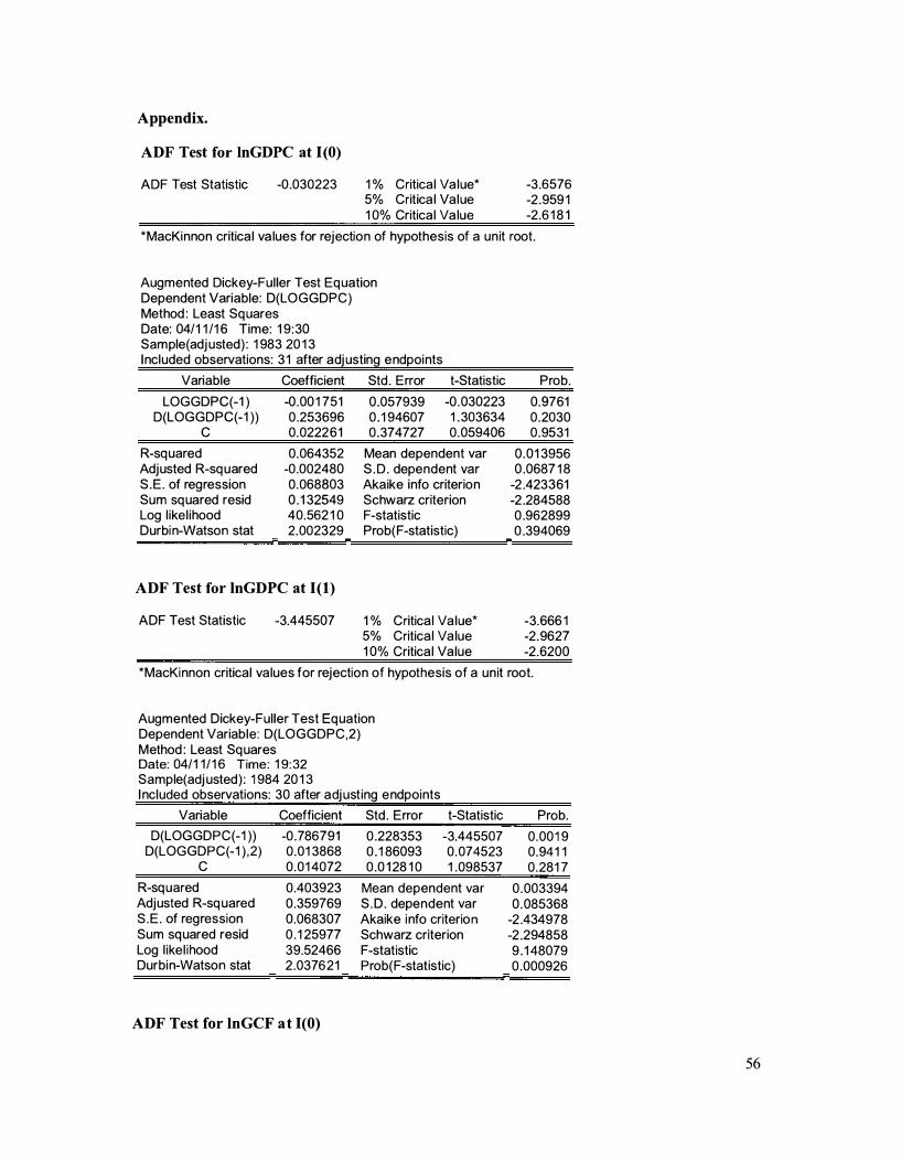
Appendix.

ADF Test for lnGDPC at 1(0)

ADF Test Statistic -0 .030223 1 % Critica l Va lue* 5% Crit ica l Va l ue 1 0% Critica l Va lue

-3 .6576 -2 . 959 1 -2 .6 1 8 1

*MacKi nnon critica l va lues for rej ection of hypothesis of a un it root .

Augmented Dickey-Ful ler Test Eq uation Dependent Variable: D(LOGGDPC) Method : Least Sq uares Date: 04/1 1 /1 6 Time: 1 9: 30 Sam ple(adj usted) : 1 983 20 1 3 I ncluded observations: 3 1 after adj usting e ndpoi nts

Variable Coefficient Std . Error t-Statistic Prob.

LOGGDPC(-1 ) D(LOGGDPC(-1 ))

c

R-sq uared Adj usted R-sq uared S . E . of regression Sum sq uared resid Log l ike l ihood Durbi n-Watson stat

-0 .00 1 751 0 .253696 0 .0222 6 1

0 .064352 -0 .002480 0 .068803 0 . 1 32549 40.562 1 0 2 .002329

ADF Test for lnGDPC at 1(1)

ADF Test Statistic -3.445507

0 .057939 0 . 1 94607 0 .374727

-0 .030223 1 . 303634 0 .059406

Mean dependent var S . D . dependent var Akaike info criterion Schwarz criterion F-statistic Prob(F-statistic)

1 % Critica l Va lue* 5% Critica l Va lue 1 0% Critica l Va lue

0.9761 0 .2030 0 .9531

0 . 0 1 3956 0 .0687 1 8

-2 .423361 -2 .284588 0 .962899 0 .394069

-3.666 1 -2 . 9627 -2 .6200

*MacKi nnon critical va lues for rejection of hypothesis of a un it root.

Augmented Dickey-Ful ler Test Eq uation Dependent Variab le : D(LOGGDPC,2) Method : Least Sq uares Date: 04/1 1 / 1 6 Time: 1 9: 32 Sample(adj usted) : 1 984 20 1 3 I ncluded observations: 30 after adj ust ing e ndpoints

Variable Coefficient Std . Error t-Statistic Prob.

D(LOGGDPC(- 1 )) D(LOGGDPC(- 1 ) , 2)

c

R-sq uared Adj usted R-sq uared S . E . of regression Sum sq uared resid Log l ike l ihood Durbi n-Watson stat

-0 .786791 0 .01 3868 0 .01 4072

0 .403923 0.359769 0.068307 0 . 1 25977 39.52466 2 .0376 2 1

ADF Test for lnGCF at 1(0)

0 .228353 0 . 1 86093 0 .0 1 28 1 0

-3.445507 0 . 074523 1 .098537

Mean dependent var S . D . dependent var Akaike i nfo criterio n Schwarz criterion F-statistic Prob(F-statistic)

0.00 1 9 0 .94 1 1 0 .28 1 7

0 . 003394 0 . 085368

-2 .434978 -2 .294858 9 . 1 48079 0 .000926

56

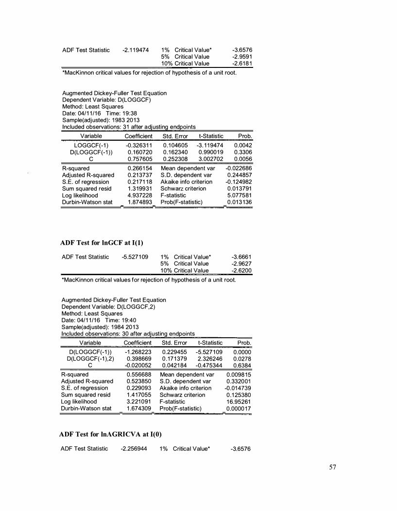
ADF Test Statistic -2 . 1 1 9474 1 % Critica l Va l ue* 5% Critica l Va l ue 1 0% Critica l Va lue

-3.6576 -2 . 959 1 -2 .6 1 8 1

*MacKi nnon critical va lues for rejection of hypothesis of a un it root.

Augmented D ickey-Ful ler Test Eq uation Dependent Variable : D(LOGGCF) Method : Least Sq uares Date: 04/ 1 1 /1 6 Time: 1 9: 38 Sample(adj usted) : 1 983 20 1 3 I ncluded observations: 3 1 after adj usti ng endpoints

Variable Coefficient Std . Error t-Statistic

LOGGCF(- 1 ) D(LOGGCF(- 1 ) )

c

R-sq uared Adj usted R-sq uared S . E . of regression Sum sq uared resid Log l ikel ihood Durbin-Watson stat

-0 . 3263 1 1 0 . 1 60720 0 .757605

0 .266 1 54 0 .21 3737 0 .2 1 7 1 1 8 1 .3 1 99 3 1 4 .937228 1 .874893

ADF Test for lnGCF at 1(1)

ADF Test Statistic -5 .527 1 09

0 . 1 04605 0 . 1 62340 0 .252308

-3 . 1 1 9474 0 . 9900 1 9 3 .002702

Mean dependent var S . D . dependent var Akaike info criterion Schwarz criterion F-statistic Prob(F-statistic)

1 % Critica l Val ue* 5% Critica l Va l ue 1 0% Critica l Va lue

Prob.

0 .0042 0 .3306 0 .0056

-0 .022686 0 .244857

-0 . 1 24982 0 . 0 1 3791 5 .077581 0 . 0 1 3 1 36

-3. 666 1 -2 . 9627 -2 .6200

*MacKinnon critica l va lues for rejection of hypothesis of a u n it root.

Augmented Dickey-Ful ler Test Eq uation Dependent Variable: D(LOGGCF,2) Method : Least Sq uares Date : 04/ 1 1 /1 6 Time: 1 9:40 Sample(adj usted) : 1 984 20 1 3 I ncluded observations: 30 after adj u sting endpoi nts

Variab le Coefficient Std . Error t-Statistic Prob.

D(LOGGCF(- 1 ) ) D(LOGGCF(-1 ) ,2)

c

R-sq uared Adj usted R-sq uared S . E . of regression Sum sq uared resid Log l ike l i hood Durbi n-Watson stat

-1 .268223 0 .398669

-0 .020052

0 .556688 0 .523850 0 .229093 1 .4 1 7055 3.221 0 9 1 1 .674309

0 .229455 0 . 1 7 1 379 0 . 042 1 84

-5.527 1 09 2 . 326246

-0.475344

Mean dependent var S . D . depe ndent var Akaike i nfo criterio n Schwarz criterion F-statistic Prob{ F-statistic)

ADF Test for lnAGRICV A at 1(0)

ADF Test Statistic -2 .256944 1 % Critica l Value*

0 .0000 0 .0278 0.6384

0 .0098 1 5 0 .3320 0 1

-0 . 0 1 4739 0 . 1 25380 1 6 .95261 0 .0000 1 7

-3.6576

57

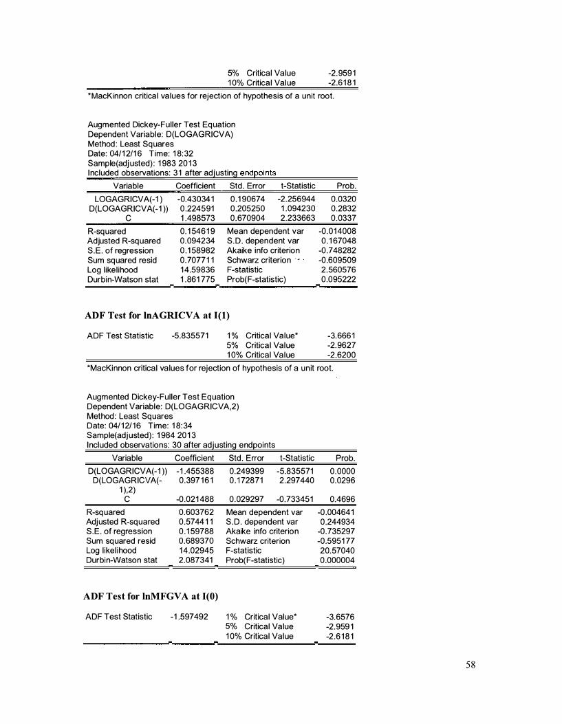
5% Critica l Va lue 1 0% Critica l Va l ue

-2 . 959 1 -2 .6 1 8 1

*MacKinnon critica l va lues for rejection of hypothesis of a un it root.

Augmented Dickey-Ful ler Test Eq uation Dependent Variable : D(LOGAG RICVA) Method : Least Sq uares Date: 04/1 2/1 6 Time: 1 8: 32 Sample(adj usted) : 1 983 20 1 3 I ncluded observations: 3 1 after adj usting endpoi nts

Variable Coefficient Std . Error t-Statistic Prob.

LOGAGRICVA(-1 ) D(LOGAGRICVA(- 1 ))

c

R-sq uared Adjusted R-sq uared S . E . of regression Sum sq uared resid Log l ike l ihood Durbi n-Watson stat

-0.43034 1 0 .224591 1 .498573

0 . 1 546 1 9 0 . 094234 0 . 1 58982 0 . 7077 1 1 1 4 .59836 1 .86 1 775

0 . 1 90674 0 .205250 0 . 670904

-2 .256944 1 .094230 2 .233663

Mean dependent var S . D . dependent var Akaike info criterion Schwarz criterion · - · F-statistic Prob( F-statistic)

0 .0320 0 .2832 0 . 0337

-0 . 0 1 4008 0 . 1 67048

-0 .748282 -0 .609509 2 . 560576 0 .095222

ADF Test for lnAGRICV A at 1(1)

ADF Test Statistic -5 .835571 1 % Critica l Va lue* 5% Critica l Val ue 1 0% Critica l Va l ue

-3. 666 1 -2. 9627 -2 .6200

*MacKi nnon critica l va lues for rejection of hypothesis of a u n it root.

Augmented Dickey-Ful ler Test Eq uation Dependent Variable : D(LOGAG RICVA,2) Method : Least Sq uares Date: 04/ 1 2/ 1 6 Time: 1 8: 34 Sample(adj usted) : 1 984 20 1 3 I ncluded observations: 30 after adj usting endpoi nts

Variable Coefficient Std . Error t-Statistic Prob.

D(LOGAGRICVA(- 1 )) D(LOGAGR ICVA(-

1 ) ,2) c

R-sq uared Adj usted R-sq uared S . E . of regression Sum sq uared resid Log l ike l i hood Durbi n-Watson stat

- 1 .455388 0 . 397 1 6 1

-0 .02 1 488

0 . 603762 0 .5744 1 1 0 . 1 59788 0 . 689370 1 4 .02945 2 .087341

ADF Test for lnMFGV A at 1(0)

ADF Test Statistic - 1 .597492

0.249399 0 . 1 728 7 1

-5.835571 2 .297440

0 . 0000 0 .0296

0 . 029297 -0 .73345 1 0.4696

Mean dependent var -0 .00464 1 S . D . dependent var 0 .244934 Akaike info criterio n -0 .735297 Schwarz criterion -0 .595 1 77 F-statistic 20. 57040 Prob( F-statistic) 0 .000004

1 % Critica l Value* 5% Critica l Va lue 1 0% Critica l Val ue

-3. 6576 -2 . 959 1 -2 .6 1 8 1

58

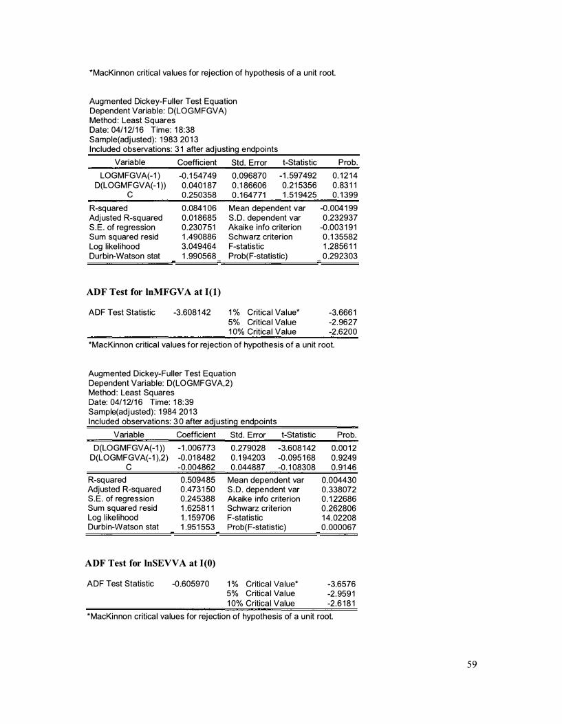
*MacKi nnon critica l va lues for rejection of hypothesis of a un it root.

Augmented Dickey-Ful ler Test Eq uation Dependent Variable: D(LO G M FGVA) Method : Least Sq uares Date: 04/1 2/1 6 Time: 1 8 : 38 Sample(adj usted} : 1 983 20 1 3 I ncluded observations: 3 1 after adj usting e ndpoi nts

Variable Coefficient Std . Error

LOGM FGVA(- 1 ) -0 . 1 54749 0 . 096870 D(LOGM FGVA(-1 )) 0 . 040 1 87 0 . 1 86606

c 0 .250358 0 . 1 64771

t-Statistic

- 1 . 597492 0 .21 5356 1 .5 1 9425

R-sq uared Adj usted R-sq uared S . E . of regression Sum sq uared resid Log l ike l ihood Durbi n-Watson stat

0 .084 1 06 0 . 0 1 8685 0 .230751 1 .490886 3 .049464 1 .990568

Mean dependent var S . D . dependent var Akaike info criterion Schwarz criterion F-statistic Prob(F-statistic)

ADF Test for lnMFGV A at 1(1)

ADF Test Statistic -3 .608 1 42 1 % Critica l Va l ue* 5% Critica l Va lue 1 0% Critica l Value

Prob.

0 . 1 2 1 4 0 . 83 1 1 0 . 1 399

-0 .004 1 99 0 .232937

-0 .003 1 9 1 0 . 1 35582 1 .2856 1 1 0 .292303

-3. 666 1 -2 . 9627 -2 .6200

*MacKinnon critica l va lues for rejection of hypothesis of a un it root.

Augmented Dickey-Ful ler Test Eq uation Dependent Variable: D(LOGMFGVA,2) Method : Least Sq uares Date: 04/ 1 2/1 6 Time: 1 8: 39 Sample(adj usted) : 1 984 20 1 3 I ncluded observations: 3 0 after adj usting endpoi nts

Variable Coefficient Std . Error

D(LOGMFGVA(- 1 )) - 1 .006773 0 .279028 D(LOGMFGVA(- 1 ) ,2 ) -0 .01 8482 0 . 1 94203

c -0.004862 0 . 044887

t-Statistic

-3.608 1 42 -0 . 095 1 68 -0 . 1 08308

R-sq uared Adj usted R-sq uared S . E . of regression Sum sq uared resid Log l ike l i hood Durbi n-Watson stat

0 .509485 0 .473 1 50 0.245388 1 .6258 1 1 1 . 1 59706 1 .95 1 553

Mean dependent var S . D . depe ndent var Akaike i nfo criterion Schwarz criterion F-statistic

ADF Test for lnSEVV A at 1(0)

ADF Test Statistic -0 .605970

Prob( F-statistic)

1 % Critica l Va lue* 5% Critica l Va lue 1 0% Critica l Value

Prob.

0 .00 1 2 0 . 9249 0 . 9 1 46

0 .004430 0 .338072 0 . 1 22686 0 . 262806 1 4 . 02208 0 . 000067

-3.6576 -2 . 959 1 -2 . 6 1 8 1

*MacKi n non critica l va lues for rejection of hypothesis of a u n it root.

59

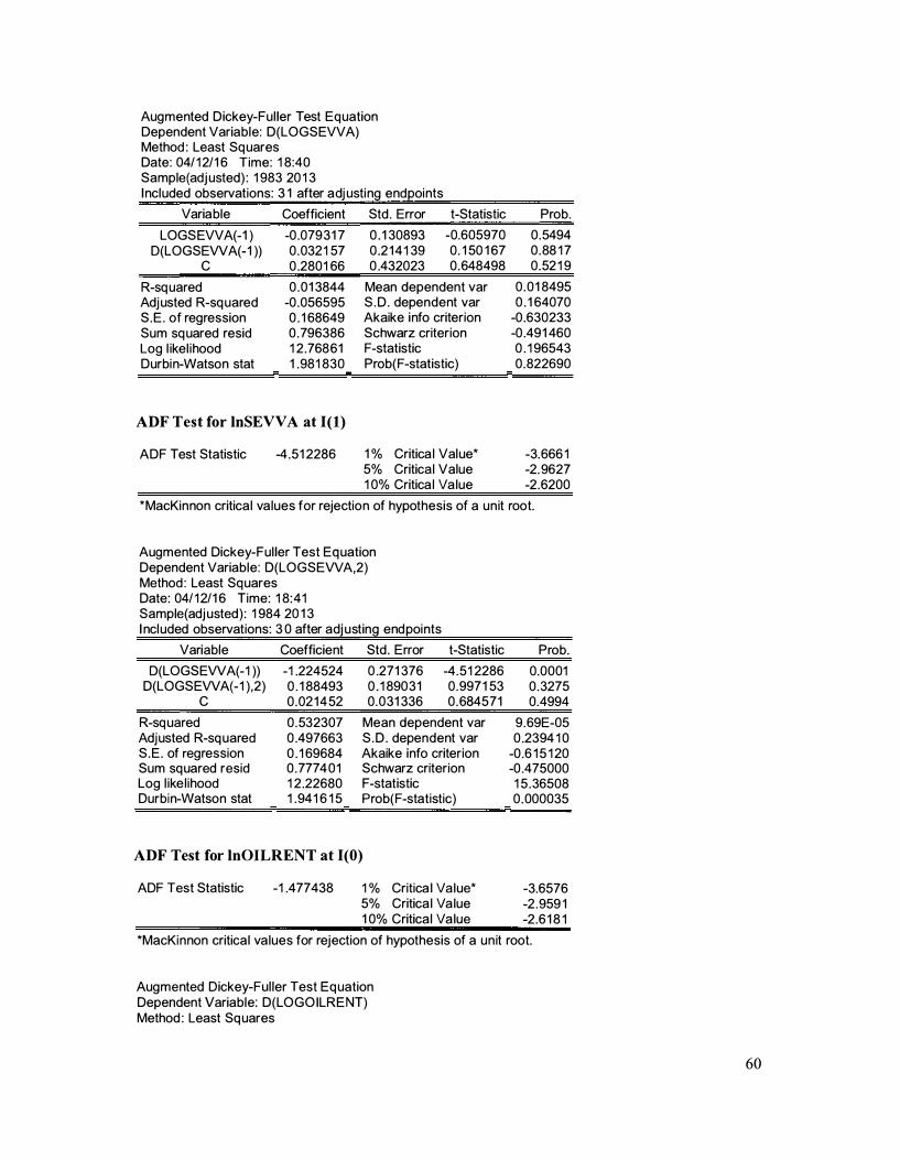
Augmented Dickey-Ful ler Test Eq uation Dependent Variable: D(LOGSEVVA) Method : Least Sq uares Date: 04/ 1 2/1 6 Time: 1 8:40 Sample(adj usted} : 1 983 20 1 3 I ncluded observations: 3 1 after adj usti ng endpoi nts

Variable Coefficient Std . Error t-Statistic Prob.

LOGS EVVA(-1 ) D(LOGSEWA(- 1 ))

c

R-sq uared Adj usted R-sq uared S . E . of regression Sum sq uared resid Log l ikel i hood Durbi n-Watson stat

-0 .079 3 1 7 0 . 032 1 57 0 .280 1 66

0 . 0 1 3844 -0 .056595 0 . 1 68649 0 . 796386 1 2 .768 6 1 1 .98 1 830

ADF Test for lnSEVV A at 1(1)

ADF Test Statistic -4 . 5 1 2286

0 . 1 30893 0 .2 1 4 1 39 0 .432023

-0.605970 0 . 1 50 1 67 0 . 648498

Mean dependent var S . D . dependent var Akaike i nfo criterion Schwarz criterion F-statistic Prob(F-statistic) ·

1 % Critica l Value* 5% Critica l Value 1 0% Critica l Va lue

0 . 5494 0 . 88 1 7 0 . 52 1 9

0 . 0 1 8495 0 . 1 64070

-0 .630233 -0 .49 1 460 0 . 1 96543 0 . 822690

-3.666 1 -2. 9627 -2 .6200

*MacKinnon critica l va lues for rejection of hypothesis of a u n it root.

Augmented Dickey-Ful ler Test Eq uation Dependent Variable : D(LOGSEWA,2) Method : Least Sq uares Date: 04/ 1 2/1 6 Time: 1 8: 4 1 Sample(adj usted} : 1 984 20 1 3 I ncl uded observations: 3 0 after adj usting end poi nts

Variable Coefficient Std . Error t-Statistic

D(LOGSEWA(-1 )) - 1 .224524 0 .271 376 -4 . 5 1 2286 D(LOGSEWA(- 1 ) ,2) 0 . 1 88493 0 . 1 890 3 1 0 . 997 1 53

c 0 . 02 1 4 52 0 .031 336 0 . 6845 7 1

R-sq uared 0 . 532307 Mean dependent var Adj usted R-sq uared 0 .497663 S . D . dependent var S . E . of regression 0 . 1 69684 Akaike info criterion Sum sq uared resid 0 . 7774 0 1 Schwarz criterion Log l ike l ihood 1 2 .22680 F-statistic Durbin-Watson stat 1 .94 1 6 1 5 Prob(F-statistic)

ADF Test for lnOILRENT at 1(0)

ADF Test Statistic - 1 .477438 1 % Critica l Va lue* 5% Critica l Va lue 1 0% Critica l Va lue

Prob.

0.0001 0 . 3275 0.4994

9 .69E-05 0 .2394 1 0

-0 .6 1 5 1 20 -0 .475000

1 5 . 36508 0 . 000035

-3.6576 -2 . 959 1 -2 .6 1 8 1

*MacKi nnon critica l va lues for rejection of hypothesis of a u n it root.

Augmented Dickey-Ful ler Test Eq uation Dependent Variable: D(LOGO ILRE NT} Method : Least Sq uares

60

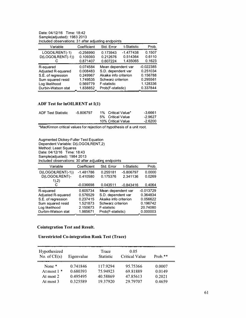
Date: 04/ 1 2/1 6 Time: 1 8:42 Sam ple(adj usted) : 1 983 20 1 3 I ncluded observations: 3 1 after adj usting endpoi nts

Variable Coefficient Std . Error

LOGO ILRENT(- 1 ) -0 .256990 0 . 1 73943 D(LOGO ILRENT(-1 ) ) 0 . 1 09393 0 . 2 1 2676

c 0.871 407 0 .607224

t-Statistic

- 1 .477438 0 . 5 1 4364 1 .435065

R-sq uared Adj usted R-sq uared S . E . of regression Sum sq uared resid Log l ikel i hood Durbin-Watson stat

0 .074584 0 .008483 0 .249967 1 .749535 0 .569779 1 .838852

Mean dependent var S . D . dependent var Akaike info criterion Schwarz criterion F-statistic Prob(F-statistic)

ADF Test for lnOILRENT at 1(1)

ADF Test Statistic -5 .806797 1 % Critica l Va lue* 5% Critica l Va l ue 1 0% Critica l Va l ue

Prob.

0 . 1 507 0 . 6 1 1 0 0 . 1 623

-0 .022385 0 .251 034 0 . 1 56788 0 .295561 1 . 1 28336 0 .337844

-3.666 1 -2 .9627 -2 .6200

*MacKinnon critica l va lues for rejection of hypothesis of a un it root.

Augmented Dickey-Ful ler Test Eq uation Dependent Variable: D(LOGO ILRENT,2) Method : Least Sq uares Date: 04/ 1 2/1 6 Time: 1 8:43 Sample(adj usted) : 1 984 20 1 3 I ncluded observations: 30 after adj usting endpoi nts

Variable Coefficient Std . Error t-Statistic

D(LOGO ILRE NT(-1 ) ) -1 .48 1 786 0 .2551 8 1 -5.806797 D(LOGO ILRE NT(- 0 .41 0580 0 . 1 75376 2 .34 1 1 36

1 ) ,2) c -0 .036698 0 .0435 1 1 -0.8434 1 6

R-sq uared Adj usted R-sq uared S . E . of regression Sum sq uared resid Log l ike l ihood Durbin-Watson stat

0 .605734 0 .576529 0 .2374 1 5 1 .521 873 2 . 1 50673 1 .98567 1

Cointegration Test and Result.

Mean dependent var S . D . depe ndent var Akaike info criterion Schwarz criterion F-statistic Prob( F-statistic)

Unrestricted Co-integration Rank Test (Trace)

Hypothesized Trace 0 .05

Prob.

0 . 0000 0 .0269

0 .4064

-0 . 0 1 3729 0 .364834 0 . 056622 0 . 1 96742 20.74080 0 . 000003

No. of CE(s) Eigenvalue Statistic Critical Value Prob. * *

None * 0 .74 1 846 1 1 7 .9294 95 .75366 0 .0007 At most 1 * 0 .680393 75 .94923 69 . 8 1 889 0 .0 1 49 At most 2 0.495495 40. 58869 47 .856 1 3 0 .202 1 At most 3 0 .325589 1 9 .37920 29.79707 0.4659

6 1

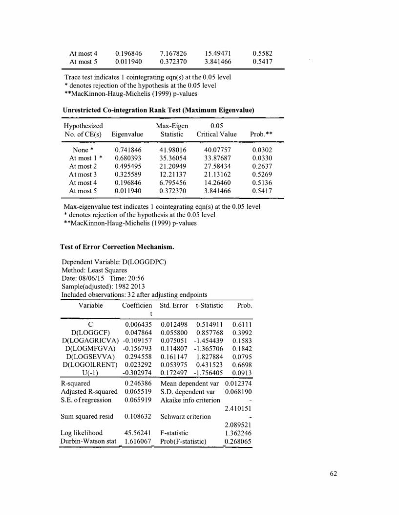
At most 4 At most 5

0 . 1 96846 0.0 1 1 940

7 . 1 67826 0 .372370

1 5 .4947 1 3 . 84 1 466

Trace test indicates 1 cointegrating eqn(s) at the 0 .05 level * denotes rejection of the hypothesis at the 0.05 level **MacKinnon-Haug-Michelis ( 1 999) p-values

0 .5582 0 .54 1 7

Unrestricted Co-integration Rank Test (Maximum Eigenvalue)

Hypothesized Max-Eigen 0.05 No. of CE(s) Eigenvalue Statistic Critical Value Prob . * *

None * 0 .74 1 846 4 1 .980 1 6 40.07757 0 .0302 At most 1 * 0.680393 35 . 36054 3 3 . 87687 0 .0330 At most 2 0.495495 2 1 .20949 27 .58434 0.2637 At most 3 0 .325589 12 .2 1 1 3 7 2 1 . 1 3 1 62 0 .5269 At most 4 0. 1 96846 6 .795456 1 4.26460 0 .5 1 3 6 At most 5 0 .01 1 940 0 .372370 3 .84 1 466 0 .54 1 7

Max-eigenvalue test indicates 1 cointegrating eqn(s) at the 0 .05 level * denotes rejection of the hypothesis at the 0.05 level * *MacKinnon-Haug-Michelis ( 1 999) p-values

Test of Error Correction Mechanism.

Dependent Variable : D(LOGGDPC) Method: Least Squares Date: 08/06/1 5 Time : 20 :56 Sample(adjusted) : 1 982 20 1 3 Included observations : 3 2 after adjusting endpoints

Variable Coefficien Std. Error t-Statistic Prob. t

c 0.006435 D(LOGGCF) 0.047864

D(LOGAGRICVA) -0. 1 09 1 57 D(LOGMFGVA) -0. 1 56793 D(LOGSEVV A) 0.294558

D(LOGOILRENT) 0 .023292 U(- 1 ) -0.302974

R-squared 0.2463 86 Adjusted R-squared 0.0655 1 9 S .E. o f regression 0 .065 9 1 9

Sum squared resid 0 . 1 08632

Log likelihood Durbin-Watson stat

45 .5624 1 1 .6 1 6067

0.0 1 2498 0 .5 1 49 1 1 0 .055800 0 .857768 0.07505 1 - 1 .454439 0. 1 1 4807 - 1 . 365706 0. 1 6 1 1 47 1 . 827884 0.053975 0.43 1 523 0. 1 72497 - 1 .756405

Mean dependent var S .D. dependent var Akaike info criterion

Schwarz criterion

F-statistic Prob(F-statistic)

0 .6 1 1 1 0 .3992 0. 1 583 0. 1 842 0.0795 0 .6698 0 .09 1 3

0.0 1 2374 0.068 1 90

2 .4 1 0 1 5 1

2 .08952 1 1 . 3 62246 0.268065

62