Download - Dynamic Analysis of a Light Structure in Outer Space: Short Electrodynamic Tether

Multibody System Dynamics 10: 125–146, 2003.© 2003 Kluwer Academic Publishers. Printed in the Netherlands.

125

Dynamic Analysis of a Light Structure in OuterSpace: Short Electrodynamic Tether

J. VALVERDE, J.L. ESCALONA, J. MAYO and J. DOMÍNGUEZDepartment of Mechanical and Materials Engineering, University of Seville, Camino de losDescubrimientos s/n, E-41092 Seville, Spain; E-mail: [email protected]

(Received: 30 December 2002; accepted in revised form: 24 January 2003)

Abstract. The SET (short electrodynamic tether) is an extremely flexible deployable structure.Unlike most other tethers that orbit with their axis of smallest moment of inertia pointing towardsthe Earth’s center (natural position), the SET must orbit with its axis of smallest inertia normal tothe orbit plane. The Faraday effect allows the SET to modify its orbit in this position. This is due tothe interaction of the Earth’s magnetic field with the tether, which is an electric conductor. In orderto maintain the aforementioned operating position, the SET is subjected to a spin velocity around itsaxis of smallest inertia. If the system were rigid, the generated gyroscopic pairs would guarantee thesystem’s stability.

The tether is not perfectly straight after deployment. This fact could make the rotation of thestructure unstable. The problem is similar to the instability of unbalanced rotors. The linear studyof unbalanced systems predicts the structural instability once a certain critical velocity is exceeded.Instability is due to internal damping forces. The spin velocity of the SET is greater than the criticalvelocity. Nevertheless, certain works that include the geometric nonlinearities show a stable behaviorunder such conditions. The object of this paper is to try to verify these results for the SET.

The SET consists of a 100-meter tether with a concentrated mass at its end. The system has beenmodeled using the floating reference frame approach with natural coordinates. The substructuringtechnique is used to include nonlinearities in the system.

Key words: space structures, spinning tether, rotordynamics, natural coordinates, co-rotationalmethod.

1. Introduction

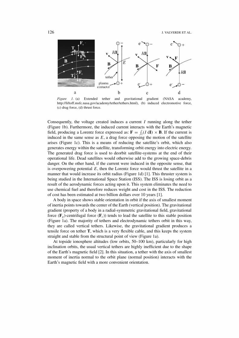
A space tether is a long cable used to connect spacecrafts to one another or to otherorbiting bodies (asteroids, space stations, boosters, etc.). The tether provides mech-anical connection between different modules that enables the transfer of energy andmomentum, (Figure 1a). In addition, an electrodynamic tether is designed to con-duct electricity. The tether, which is orbiting around the Earth, crosses the Earth’smagnetic field lines B, at orbit velocity v. Since the tether is a conductor, an electro-motive force E is induced in it, in accordance with Faraday’s law: E = ∫

l(v×B)dI

(Figure 1b). Two plasma contactors are placed at the ends of the tether to createelectric current. The satellite (contactors) thus captures electrons from the plasmain the ionosphere on one end and re-releases them into the plasma from the other.

126 J. VALVERDE ET AL.

Figure 1. (a) Extended tether and gravitational gradient (NASA academy,http://liftoff.msfc.nasa.gov/academy/tether/tethers.html), (b) induced electromotive force,(c) drag force, (d) thrust force.

Consequently, the voltage created induces a current I running along the tether(Figure 1b). Furthermore, the induced current interacts with the Earth’s magneticfield, producing a Lorentz force expressed as: F = ∫

l(I dI) × B. If the current is

induced in the same sense as E, a drag force opposing the motion of the satellitearises (Figure 1c). This is a means of reducing the satellite’s orbit, which alsogenerates energy within the satellite, transforming orbit energy into electric energy.The generated drag force is used to deorbit satellite-systems at the end of theiroperational life. Dead satellites would otherwise add to the growing space-debrisdanger. On the other hand, if the current were induced in the opposite sense, thatis overpowering potential E, then the Lorentz force would thrust the satellite in amanner that would increase its orbit radius (Figure 1d) [1]. This thruster system isbeing studied in the International Space Station (ISS). The ISS is losing orbit as aresult of the aerodynamic forces acting upon it. This system eliminates the need touse chemical fuel and therefore reduces weight and cost in the ISS. The reductionof cost has been estimated at two billion dollars over 10 years [1].

A body in space shows stable orientation in orbit if the axis of smallest momentof inertia points towards the center of the Earth (vertical position). The gravitationalgradient (property of a body in a radial-symmetric gravitational field, gravitationalforce (Fg)-centrifugal force (Fc)) tends to lead the satellite to this stable position(Figure 1a). The majority of tethers and electrodynamic tethers orbit in this way,they are called vertical tethers. Likewise, the gravitational gradient produces atensile force on tether T, which is a very flexible cable, and this keeps the systemstraight and stable from the structural point of view (Figure 1a).

At topside ionosphere altitudes (low orbits, 50–100 km), particularly for highinclination orbits, the usual vertical tethers are highly inefficient due to the shapeof the Earth’s magnetic field [2]. In this situation, a tether with the axis of smallestmoment of inertia normal to the orbit plane (normal position) interacts with theEarth’s magnetic field with a more convenient orientation.

DYNAMIC ANALYSIS OF A LIGHT STRUCTURE IN OUTER SPACE 127

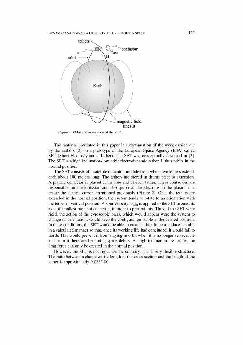
Figure 2. Orbit and orientation of the SET.

The material presented in this paper is a continuation of the work carried outby the authors [3] on a prototype of the European Space Agency (ESA) calledSET (Short Electrodynamic Tether). The SET was conceptually designed in [2].The SET is a high inclination-low orbit electrodynamic tether. It thus orbits in thenormal position.

The SET consists of a satellite or central module from which two tethers extend,each about 100 meters long. The tethers are stored in drums prior to extension.A plasma contactor is placed at the free end of each tether. These contactors areresponsible for the emission and absorption of the electrons in the plasma thatcreate the electric current mentioned previously (Figure 2). Once the tethers areextended in the normal position, the system tends to rotate to an orientation withthe tether in vertical position. A spin velocity ωspin is applied to the SET around itsaxis of smallest moment of inertia, in order to prevent this. Thus, if the SET wererigid, the action of the gyroscopic pairs, which would appear were the system tochange its orientation, would keep the configuration stable in the desired position.In these conditions, the SET would be able to create a drag force to reduce its orbitin a calculated manner so that, once its working life had concluded, it would fall toEarth. This would prevent it from staying in orbit when it is no longer serviceableand from it therefore becoming space debris. At high inclination-low orbits, thedrag force can only be created in the normal position.

However, the SET is not rigid. On the contrary, it is a very flexible structure.The ratio between a characteristic length of the cross section and the length of thetether is approximately 0.025/100.


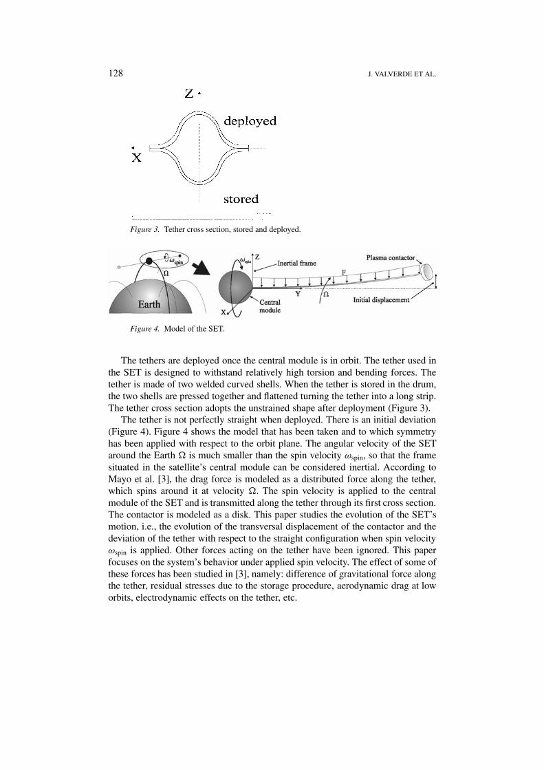
Figure 3. Tether cross section, stored and deployed.

Figure 4. Model of the SET.

The tethers are deployed once the central module is in orbit. The tether used inthe SET is designed to withstand relatively high torsion and bending forces. Thetether is made of two welded curved shells. When the tether is stored in the drum,the two shells are pressed together and flattened turning the tether into a long strip.The tether cross section adopts the unstrained shape after deployment (Figure 3).

The tether is not perfectly straight when deployed. There is an initial deviation(Figure 4). Figure 4 shows the model that has been taken and to which symmetryhas been applied with respect to the orbit plane. The angular velocity of the SETaround the Earth is much smaller than the spin velocity ωspin, so that the framesituated in the satellite’s central module can be considered inertial. According toMayo et al. [3], the drag force is modeled as a distributed force along the tether,which spins around it at velocity . The spin velocity is applied to the centralmodule of the SET and is transmitted along the tether through its first cross section.The contactor is modeled as a disk. This paper studies the evolution of the SET’smotion, i.e., the evolution of the transversal displacement of the contactor and thedeviation of the tether with respect to the straight configuration when spin velocityωspin is applied. Other forces acting on the tether have been ignored. This paperfocuses on the system’s behavior under applied spin velocity. The effect of some ofthese forces has been studied in [3], namely: difference of gravitational force alongthe tether, residual stresses due to the storage procedure, aerodynamic drag at loworbits, electrodynamic effects on the tether, etc.


The system is similar to the dynamic problem of unbalanced rotors. Accordingto literature on rotordynamics [4, 5], should the rotary system develop a non-synchronous motion between the shaft (tether) and the unbalanced disk (plasmacontactor + initial deviation) alternative stresses will arise on the shaft. Sub-sequently, were the material hysteresis of importance, internal damping forceswould arise within the system. In this situation, there is a running speed called the‘onset speed of instability’ or critical velocity, above which the system becomesunstable, i.e., the shaft suffers limitless vibration. This critical velocity is given by(for a simple model of unbalanced rotor [4, 5]): ωs = (1+ξe/ξr)

2λ, where ξe and ξrrepresent external and internal damping respectively and λ is the system’s first nat-ural bending frequency. This critical velocity is practically equal to the first naturalbending frequency of the rotor. In the case of the SET, the spin velocity appliedis much greater than the first natural frequency and there are internal dampingforces in the system (non-synchronous motion + hysteresis). Consequently, andin accordance with what has been stated earlier, transversal displacement of thecontactor (Figure 4) will experience limitless increase and the SET will becomeunstable from a structural point of view. A first approximation to the problem[3] corroborated the SET’s instability when critical speed was surpassed, wherea model of the tether allowing only small elastic displacements was executed withlinear finite elements.

In order to solve the problems of structural instability, rotary machinery includesexternal damping in the system through the rotor supports. This allows the valueof the critical velocity to increase to a point above operating conditions. However,this is not applicable to the SET, since it is orbiting in outer space and the onlysupport is fixed to the central module. There are other procedures in rotordynamicsto control critical velocities [4, 5] but they are not applicable to the SET either.

In the early seventies, Genin and Maybee [6–8] studied stability in rotary sys-tems. Until then, all studies regarding the stability of rotors [4] predicted instabilityfor supercritical operating conditions. Using a modified Jeffcott model [4], Geninand Maybee proved that in the event of a non-linear model of the internal dampingand elastic forces being included in the equations of motion, the system appears tobe stable for any running speed ω. Although the system studied in this paper, theSET, is more complex than the one Genin and Maybee used in their case studies,the results they obtained motivate a more in-depth study of the SET’s behavior.Given this situation, a study of the stability of equilibrium solutions and periodicsolutions for the system is required. However, this kind of study is very difficultfor a complex configuration such as the SET. Dynamic simulation, including ageometric non-linear model in elastic and internal damping forces, has been carriedout in this study case. In the event of the results obtained in this simulation beingpromising (periodic or quasi-periodic stable solutions for the simulation), moreformal and detailed studies will be carried out on the stability of solutions for theSET.


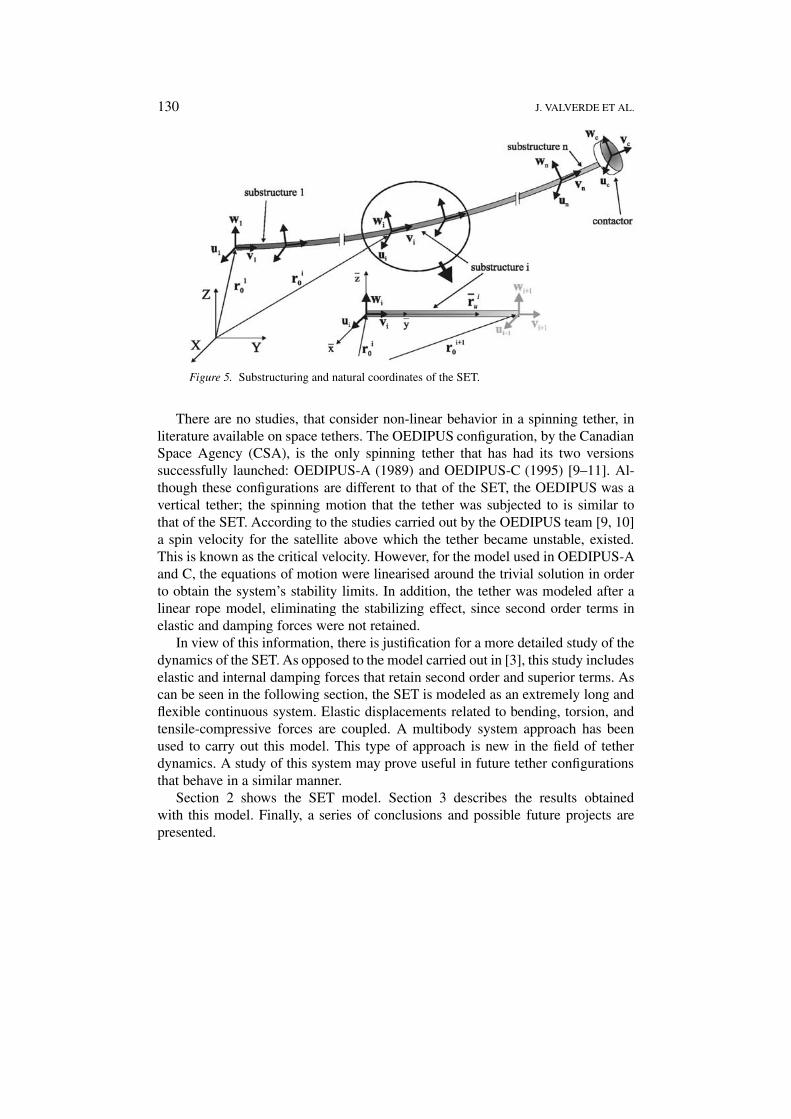
Figure 5. Substructuring and natural coordinates of the SET.

There are no studies, that consider non-linear behavior in a spinning tether, inliterature available on space tethers. The OEDIPUS configuration, by the CanadianSpace Agency (CSA), is the only spinning tether that has had its two versionssuccessfully launched: OEDIPUS-A (1989) and OEDIPUS-C (1995) [9–11]. Al-though these configurations are different to that of the SET, the OEDIPUS was avertical tether; the spinning motion that the tether was subjected to is similar tothat of the SET. According to the studies carried out by the OEDIPUS team [9, 10]a spin velocity for the satellite above which the tether became unstable, existed.This is known as the critical velocity. However, for the model used in OEDIPUS-Aand C, the equations of motion were linearised around the trivial solution in orderto obtain the system’s stability limits. In addition, the tether was modeled after alinear rope model, eliminating the stabilizing effect, since second order terms inelastic and damping forces were not retained.

In view of this information, there is justification for a more detailed study of thedynamics of the SET. As opposed to the model carried out in [3], this study includeselastic and internal damping forces that retain second order and superior terms. Ascan be seen in the following section, the SET is modeled as an extremely long andflexible continuous system. Elastic displacements related to bending, torsion, andtensile-compressive forces are coupled. A multibody system approach has beenused to carry out this model. This type of approach is new in the field of tetherdynamics. A study of this system may prove useful in future tether configurationsthat behave in a similar manner.

Section 2 shows the SET model. Section 3 describes the results obtainedwith this model. Finally, a series of conclusions and possible future projects arepresented.


2. Modeling the Problem

2.1. SUBSTRUCTURING AND NATURAL COORDINATES

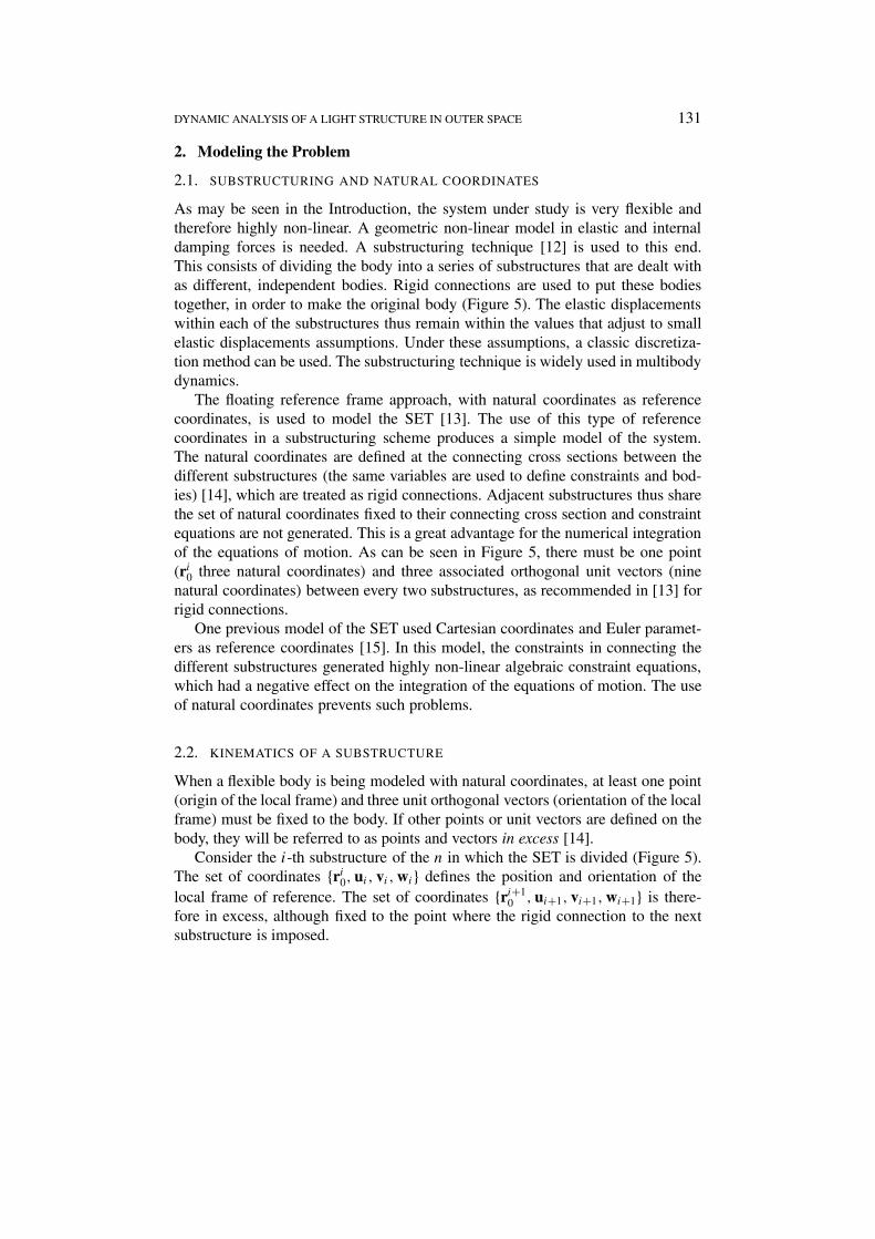
As may be seen in the Introduction, the system under study is very flexible andtherefore highly non-linear. A geometric non-linear model in elastic and internaldamping forces is needed. A substructuring technique [12] is used to this end.This consists of dividing the body into a series of substructures that are dealt withas different, independent bodies. Rigid connections are used to put these bodiestogether, in order to make the original body (Figure 5). The elastic displacementswithin each of the substructures thus remain within the values that adjust to smallelastic displacements assumptions. Under these assumptions, a classic discretiza-tion method can be used. The substructuring technique is widely used in multibodydynamics.

The floating reference frame approach, with natural coordinates as referencecoordinates, is used to model the SET [13]. The use of this type of referencecoordinates in a substructuring scheme produces a simple model of the system.The natural coordinates are defined at the connecting cross sections between thedifferent substructures (the same variables are used to define constraints and bod-ies) [14], which are treated as rigid connections. Adjacent substructures thus sharethe set of natural coordinates fixed to their connecting cross section and constraintequations are not generated. This is a great advantage for the numerical integrationof the equations of motion. As can be seen in Figure 5, there must be one point(ri0 three natural coordinates) and three associated orthogonal unit vectors (ninenatural coordinates) between every two substructures, as recommended in [13] forrigid connections.

One previous model of the SET used Cartesian coordinates and Euler paramet-ers as reference coordinates [15]. In this model, the constraints in connecting thedifferent substructures generated highly non-linear algebraic constraint equations,which had a negative effect on the integration of the equations of motion. The useof natural coordinates prevents such problems.

2.2. KINEMATICS OF A SUBSTRUCTURE

When a flexible body is being modeled with natural coordinates, at least one point(origin of the local frame) and three unit orthogonal vectors (orientation of the localframe) must be fixed to the body. If other points or unit vectors are defined on thebody, they will be referred to as points and vectors in excess [14].

Consider the i-th substructure of the n in which the SET is divided (Figure 5).The set of coordinates {ri0,ui , vi ,wi} defines the position and orientation of thelocal frame of reference. The set of coordinates {ri+1

0 ,ui+1, vi+1,wi+1} is there-fore in excess, although fixed to the point where the rigid connection to the nextsubstructure is imposed.


The position of any given point in the substructure is given by

ri = ri0 + Ai(riu + uif ), (1)

where vector riu represents the position of that point on local axis in the undeformedconfiguration and vector ui

f represents displacement due to deformation. The vec-tors with a bar are expressed in local axis. The rotation matrix is easily constructedsince the vectors selected as natural coordinates are unitary and orthogonal. ThusAi = [ui vi wi].

The Rayleigh–Ritz method is used in the discretization of the substruc-ture. It should be noted that variations of the natural coordinates in excess{ri+1

0 ,ui+1, vi+1,wi+1} deform the substructure. Therefore, a Rayleigh–Ritz dis-cretization with fixed boundaries is carried out [14]. This discretization uses aseries of static modes, related to the variations of the natural coordinates in excess,as well as dynamic modes with fixed boundaries. In this case, the dynamic modesare the vibration modes of a clamped-clamped beam, since the natural coordinatesat the ends of the substructure remain fixed [14]. Thus, the vector of displacementsdue to deformation can be expressed as

uif =

ns∑k=1

�kηk +nd∑l=1

� lξl, (2)

where ns and nd are the number of static and dynamic modes respectively; �k isa 3 × 1 vector that contains the static mode in the corresponding row, dependingon whether displacement produced in x, y or z, �l is a vector containing dynamicmodes in the same way as the previous vector, and ηk and ξl are the amplitudes ofthe static and dynamic modes respectively. The amplitudes of the static modes areknown functions of the natural coordinates, so they do not include new degrees offreedom [14].

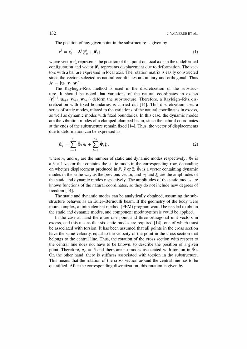
The static and dynamic modes can be analytically obtained, assuming the sub-structure behaves as an Euler–Bernoulli beam. If the geometry of the body weremore complex, a finite element method (FEM) program would be needed to obtainthe static and dynamic modes, and component mode synthesis could be applied.

In the case at hand there are one point and three orthogonal unit vectors inexcess, and this means that six static modes are required [14], one of which mustbe associated with torsion. It has been assumed that all points in the cross sectionhave the same velocity, equal to the velocity of the point in the cross section thatbelongs to the central line. Thus, the rotation of the cross section with respect tothe central line does not have to be known, to describe the position of a givenpoint. Therefore, ns = 5 and there are no modes associated with torsion in � l .On the other hand, there is stiffness associated with torsion in the substructure.This means that the rotation of the cross section around the central line has to bequantified. After the corresponding discretization, this rotation is given by


θ = �tηt +nt∑s=1

�tsζts, (3)

where nt is the number of dynamic modes of torsion, �t is the static mode associ-ated with torsion, �ts is the s-th dynamic mode of torsion, and ηt and ζts are theamplitudes associated with these modes.

The vector of generalized coordinates for the i-th substructure is therefore

qi = [ri

T

0 uTi vTi wT

i η1 . . . ηns ηt ξ1 . . . ξnd ξt1 ξtnt]T, (4)

where the analyst chooses the number of dynamic modes.The expression of the elastic forces [14] of a substructure is obtained from the

vector (the i superscript is removed for simplicity)

u = ru + uf = [ux uy uz]T (5)

and from the rotation of the cross section around its central line, which is given by(3).

The substructure deformation energy may be expressed as follows, assumingthat it behaves as an Euler–Bernoulli beam

U = U bendingx + U bending

z + U axial + U torsion

=∑m=x,z

1

2EIm

l∫0

(u′′m)

2 dy + 1

2EA

l∫0

(u′y)

2 dy + 1

2G(Ix + Iz)

l∫0

(θ ′)2 dy, (6)

where E is the Young modulus, G is the shear modulus, A is the area of the crosssection, Im is the second moment of area of the cross section (m = x, y), is acoordinate in the longitudinal direction and l is the length of the substructure.The symbol ( )′ denotes derivative with respect to coordinate y. Expression (6)in compact form would be

U = 1

2[ηT ξT ]

[Kest 0

0 Kdin

] [η

ξ

], (7)

where vectors η and ξ contain the amplitudes associated with the static and dy-namic modes, respectively. The matrix Kdin is a diagonal matrix since the dynamicmodes are orthogonal, and Kest is a symmetric matrix with non-zero terms insideand outside the diagonal. The static modes are orthogonal to the dynamic modes[14].

To obtain the inertia forces, expression (1) has to be differentiated with respectto time and introduced into the kinetic energy expression given by

T = 1

2

∫V

rT r dm. (8)


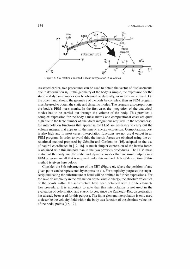
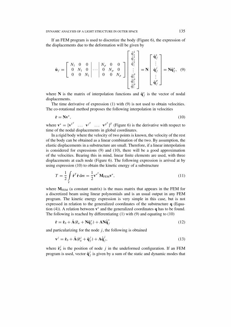
Figure 6. Co-rotational method. Linear interpolation in velocities.

As stated earlier, two procedures can be used to obtain the vector of displacementsdue to deformation uf . If the geometry of the body is simple, the expression for thestatic and dynamic modes can be obtained analytically, as in the case at hand. Onthe other hand, should the geometry of the body be complex, then an FEM programmust be used to obtain the static and dynamic modes. The program also proportionsthe body’s FEM mass matrix. In the first case, the integration of the analyticalmodes has to be carried out through the volume of the body. This provides acomplex expression for the body’s mass matrix and computational costs are quiethigh due to the large number of analytical integrations required. In the second case,the interpolation functions that appear in the FEM are necessary to carry out thevolume integral that appears in the kinetic energy expression. Computational costis also high and in most cases, interpolation functions are not usual output in anFEM program. In order to avoid this, the inertia forces are obtained using the co-rotational method proposed by Géradin and Cardona in [16], adapted to the useof natural coordinates in [17, 18]. A much simpler expression of the inertia forcesis obtained with this method than in the two previous procedures. The FEM massmatrix of the body and the static and dynamic modes that are usual outputs in aFEM program are all that is required under this method. A brief description of thismethod is given here below.

Consider the i-th substructure of the SET (Figure 6), where the position of anygiven point can be represented by expression (1). For simplicity purposes the super-script indicating the substructure at hand will be omitted in further expressions. Forthe sake of simplicity in the evaluation of the kinetic energy, the absolute velocitiesof the points within the substructure have been obtained with a finite element-like procedure. It is important to note that this interpolation is not used in theevaluation of deformation and elastic forces, since the Rayleigh–Ritz discretizationhas already been used for this purpose. The finite element interpolation is only usedto describe the velocity field within the body as a function of the absolute velocitiesof the nodal points [16, 17].


If an FEM program is used to discretize the body (Figure 6), the expression ofthe displacements due to the deformation will be given by

uf = N1 0 0

0 N1 00 0 N1

∣∣∣∣∣∣ · · ·∣∣∣∣∣∣Np 0 00 Np 00 0 Np

q1x

q1y

q1z...

qpx

qpy

qpz

= N

q1f

...

qj

f

...

qp

f

= Nq∗f , (9)

where N is the matrix of interpolation functions and q∗f is the vector of nodal

displacements.The time derivative of expression (1) with (9) is not used to obtain velocities.

The co-rotational method proposes the following interpolation in velocities

r = Nv∗, (10)

where v∗ = [v1T . . . vjT

. . . vpT ]T (Figure 6) is the derivative with respect to

time of the nodal displacements in global coordinates.In a rigid body where the velocity of two points is known, the velocity of the rest

of the body can be obtained as a linear combination of the two. By assumption, theelastic displacements in a substructure are small. Therefore, if a linear interpolationis considered for expressions (9) and (10), there will be a good approximationof the velocities. Bearing this in mind, linear finite elements are used, with threedisplacements at each node (Figure 6). The following expression is arrived at byusing expression (10) to obtain the kinetic energy of a substructure

T = 1

2

∫V

rT r dm = 1

2v∗T MFEMv∗, (11)

where MFEM (a constant matrix) is the mass matrix that appears in the FEM fora discretized beam using linear polynomials and is an usual output in any FEMprogram. The kinetic energy expression is very simple in this case, but is notexpressed in relation to the generalized coordinates of the substructure q (Equa-tion (4)). A relation between v∗ and the generalized coordinates q has to be found.The following is reached by differentiating (1) with (9) and equating to (10)

r = r0 + A(ru + Nq∗f ) + AN ˙q∗

f (12)

and particularizing for the node j , the following is obtained

vj = r0 + A(rju + qj

f ) + A ˙qj

f , (13)

where rju is the position of node j in the undeformed configuration. If an FEMprogram is used, vector qj

f is given by a sum of the static and dynamic modes that


the program provides as output when the component mode synthesis is used. Dueto the simplicity of the body under study in the case at hand, the static and dynamicmodes have been analytically obtained. The displacement due to deformation ofany given point of the substructure can thus be reached using (2). Therefore, thedisplacements of the nodes can be expressed as

qj

f = uj

f =ns∑k=1

�j

kηk +nd∑l=1

�j

l ξl, (14)

where �j

k is the k-th static mode, and �j

l is the l-th dynamic mode, particularizedin node j . The difference between the co-rotational method and the procedureused in this paper is that the static and dynamic modes are calculated analytic-ally whereas in other cases the modes are calculated by an FEM program usingcomponent mode synthesis. Given that the modes calculated analytically are quitesimilar to the modes calculated by the FEM program, the approximation reachedin this procedure (analytical modes) is similar to the approximation reached by theco-rotational method in terms of precision.

By introducing (14) and its derivative with respect to time in (13) andreorganizing, the following equation can be written, for all the nodes

v∗ =

I b11I b12I b13I A�11 . . . A�

1ns

A�11 . . . A�

1nd

......

......

......

......

......

......

......

......

......

I bp1I bp2I bp3I A�p

1 . . . A�p

nsA�

p

1 . . . A�p

nd

r0

uvwη1...

ηnsξ1...

ξnd

= B(q)q, (15)

where �r

k is the k-th static mode vector evaluated in node r (r = 1, . . . , p), �s

l isthe l-th dynamic mode vector evaluated in node s (s = 1, . . . , p), and

b11 = rux1 +ns∑k=1

�1kxηk +

nd∑l=1

�1lxξlb12 = ruy1 +

ns∑k=1

�1kyηk +

nd∑l=1

�1lyξlb13

= ruz1 +ns∑k=1

�1kzηk +

nd∑l=1

�1lzξl,

......

...


bp1 = ruxp +ns∑k=1

�p

kxηk +nd∑l=1

�p

lxξlbp2 = ruyp +ns∑k=1

�p

kyηk +nd∑l=1

�p

lyξlbp3

= ruzp +ns∑k=1

�p

kzηk +nd∑l=1

�p

lzξl. (16)

Kinetic energy can therefore be expressed as

T = 1

2qT BT MFEMBq = 1

2qT Mq, (17)

where M is the mass matrix of a substructure given by the equation

M = BT MFEMB. (18)

With this method, the FEM mass matrix of the body and the static and dynamicmodes that can be calculated either by means of the FEM program or analyticallyare the only things that must be known. In (17), kinetic energy is expressed inrelation to the generalized coordinates q. Adequate approximation to the inertiaforces exists and a fairly simple expression of the mass matrix has been achieved.Furthermore, the expression of the quadratic velocity vector Qv is

Qv = −BT MFEMBq, (19)

where the calculation of B from (15) is quite simple. If the co-rotational method(with analytical modes) had not been introduced for the calculation of the inertiaforces, the expression of Qv would have been much more complex [14, 18].

The mass matrix and the quadratic velocity vector have been obtained withthe co-rotational method with the modes having been analytically calculated. Aninterpolation in velocities that are non-consistent with the positions is carried outin this method. Avello [17] shows or demonstrates that this method maintains theFEM convergence. The fact that this method also provides a good approximationto the real velocities, and in some cases even gives the exact solution, is alsodemonstrated.

As seen at the beginning of this paper, the hysteretic damping of the mater-ial plays an essential role in the stability of the system. Hysteretic damping hasbeen modeled as viscous damping in this study case. This is a satisfactory ap-proximation given that viscous damping introduces the same destabilizing effectas hysteretic damping [4, 5]. The internal modal viscous damping coefficient ineach substructure was taken as being proportional to modal mass and stiffness. Itcan be expressed as

cij = 2ξ√mij kij , (20)

where i and j vary from one to the sum of static and dynamic modes, includingthose of torsion. Thus, mij and kij are the mass and stiffness associated with the


i-th and j -th modal amplitudes. ξ is the material’s internal damping constant. Thesame value for constant ξ has been taken for all cij . Damping will be subject tostricter modeling during the course of a more detailed study to be carried out onthe stability of the SET. However, expression (20) is valid as a first approximation.

The vector of external forces associated with the drag force (Figure 4) isobtained from the following expression:

Qext =l∫

0

FT ∂r∂q

dy, (21)

where r is given by (1) and q by (4). Vector F, which is expressed in global axis, isdefined as follows

FT = [F cos(t) 0 F sin(t)], (22)

where F is a distributed force (N/m).

2.3. SYSTEM SETUP AND RESOLUTION

Once the equations of motion of a substructure have been obtained, completesystem assembly is the only remaining task. The equations of motion of theplasma contactor are easily obtained from [13]. The rigid connection of differentsubstructures does not require kinematic constraint equations. These constraintsare intrinsically fulfilled, as explained at the beginning of Section 2 (Figure 5).However, other constraints must be included: the vectors associated with eachconnecting cross section should be unitary and orthogonal and the amplitudes ofthe static modes are known functions of the natural coordinates. The spin velocityapplied to the first cross section of the tether must also be included as a constraint.

Once the equations of the different substructures have been put together andthe pertinent constraints have been imposed, the resulting system of equations is asfollows:

Mq + �Tq λ = Q, �(q, t) = 0, (23)

where M is the mass matrix of the complete SET, q is the vector of generalizedcoordinates of the problem, � are the constraints, λ is the vector of Lagrangemultipliers, and Q is a vector containing a series of forces: external, elastic, internaldamping and quadratic velocity inertia forces. An index-3 Augmented Lagrangianmethod with mass-orthogonal projections of the velocities and accelerations totheir constraint manifolds is used to solve the equation. This formulation wasproposed by Bayo et al. and revised in [19]. The system to be solved has thereforethe following form:

Mq + �Tqα� + �T

q λ∗ = Q, (24)


where λ∗ is the vector of modified Lagrange multipliers and α is a penaltyfactor. The modified Lagrange multipliers are obtained from the following iterativeprocess in each time step

λ∗i+1 = λ∗

i + α�i+1, i = 0, 1, 2, . . . . (25)

In the limit, when the constraints are completely fulfilled, λ∗ = λ. The trapezoidalrule has been used for the integration of the equations. This rule is substituted inEquations (24), leaving displacements as primary variable. Consequently, expres-sion (24) is turned into a set of non-linear algebraic equations to be solved with amodified Newton–Raphson method.

The integration method used is quite robust [19]. Furthermore, it assures thatconstraints and their derivatives are fulfilled with the precision the analyst requires.

3. Results

Some results obtained for the SET’s dynamic simulation are given in this section.It is important to remember that periodic or quasi-periodic stable solutions forsupercritical velocities are searched.

The number of problem coordinates is very high due to the employed substruc-turing technique. A shorter length model of the SET, instead of the aforementioned100 m, is used to present interesting results. This enables one to work with a smallernumber of substructures without losing generality, and the size of the system ofequations is reduced. Therefore, two lengths are used for the tether in the integ-ration of equations, L = 30 m (reduced system) and L = 100 m (real length).Figure 3 shows the cross section of the tether (hollow and thin walled) with thefollowing properties: EIx = 38 Nm2, EIz = 21 Nm2, area A = 4.16 × 10−6 m2.The tether consists of a copper-beryllium alloy with the following properties [3]:Young modulus E = 132 GPa, Poisson ratio ν = 0.3, density ρ = 8,245.2 kg/m3

and internal damping constant ξ = 0.05. The plasma contactor, with a 3 kg mass,is modeled as a disk with a 0.2 m radius and 0.01 m thickness. The drag force(electromagnetic force) is a distributed force with value F = 40 × 10−6 N/m.The tether has an initial displacement of the contactor of between 10 and 15%of its total length L. The spin velocity is applied in the SET’s central module,starting from zero and gradually reaches the selected final constant velocity. Thetether is considered as being completely extended when angular velocity starts tobe applied.

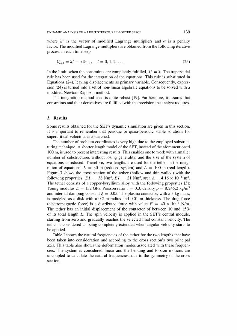
Table I shows the natural frequencies of the tether for the two lengths that havebeen taken into consideration and according to the cross section’s two principalaxis. This table also shows the deformation modes associated with these frequen-cies. The system is considered linear and the bending and torsion motions areuncoupled to calculate the natural frequencies, due to the symmetry of the crosssection.


Table I. Natural bending frequencies of the SET.

The results presented in this paper do not take the action of drag force intoconsideration (Figure 4). As stated in the introduction, this force rotates aroundglobal Y axis at a velocity � ωspin. The drag force is therefore applied to thetether at a velocity that is practically identical to its own spin velocity. Variousmodels of the tether have been solved with a drag force value of F = 40×10−6 N/m[1, 3]. It has been checked that the action of this force has no influence on thestability of the SET. In rotordynamics, a force perpendicular to the shaft inducesasynchronous motion [4, 5]. This asynchronous motion induces the appearance ofalternative stresses and therefore of internal damping. However, in the SET, withoutthe drag force, the motion of the tether is asynchronous, so that the applicationof this force does not introduce any additional phenomena. Moreover, additionaldisplacement caused in the system by the drag force is much smaller than what itwould be if this load were applied in static form. This is because the load is appliedto the SET with a frequency approximately equal (ωspin − ≈ ωspin) to the spin,which, under operating conditions, is very distant from the system’s first naturalfrequency. For a 30 m length for the SET, the static displacement of the contactorwould be approximately δ = 0.1 m. The difference in the displacement of thecontactor with and without electromagnetic force is still practically non-existent,two orders of magnitude less than δ.

The following are the results obtained for an L = 30 m tether in three cases:linear model n = 1 (n = number of substructures), non-linear model n = 3, andnon-linear model n = 6. The critical velocity of the system is close to its firstnatural bending frequency (Table I). The problem has been solved for subcriticalvelocity ω = 0.02 rad/s and supercritical velocity ω = 0.1 rad/s (Table I). Spinvelocity at starting time is zero in both cases and gradually reaches the desiredspin velocity in 10 seconds. Each substructure is divided into 10 finite elements tocarry out the approximation of the inertia forces (Equation (10)), and two dynamicbending modes are taken in each direction, two axial and two torsion modes. Thiscase requires 36 (n = 1), 108 (n = 3) and 216 (n = 6) coordinates to describe the


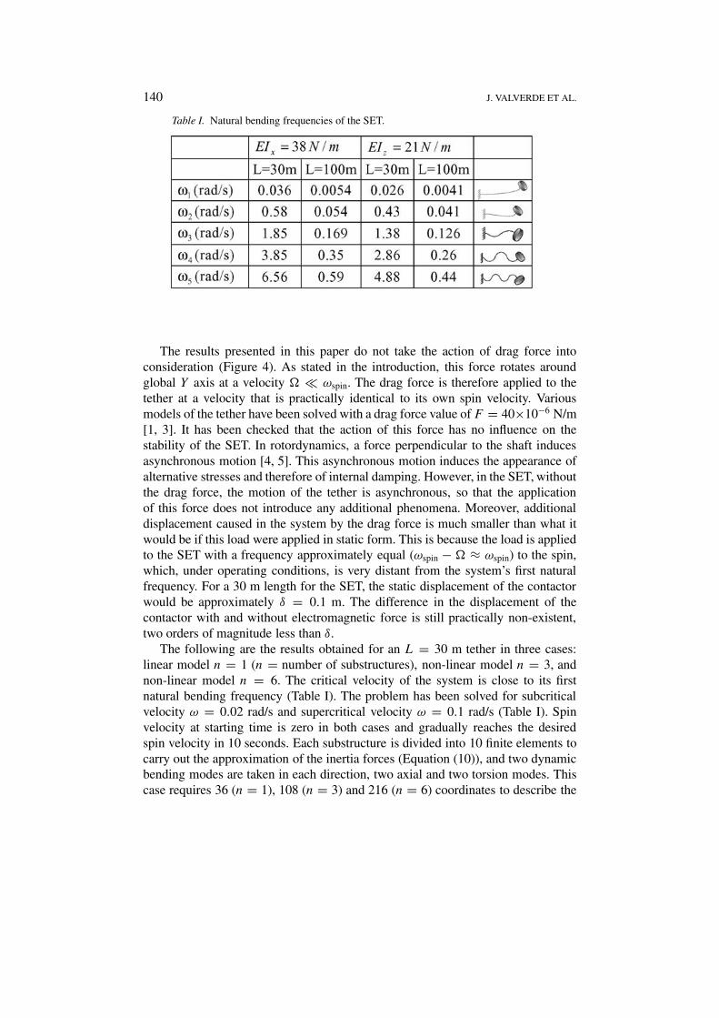
Figure 7. Trajectory of the contactor, non-linear model n = 6.

problem. This gives an idea of the size of the problem and of how it grows whenthere is an increase in the number of substructures. Figure 7 shows the trajectoryfollowed by the contactor and its projection on global axis X-Z (Figure 4) forn = 6 and supercritical velocity ω = 0.1 rad/s.

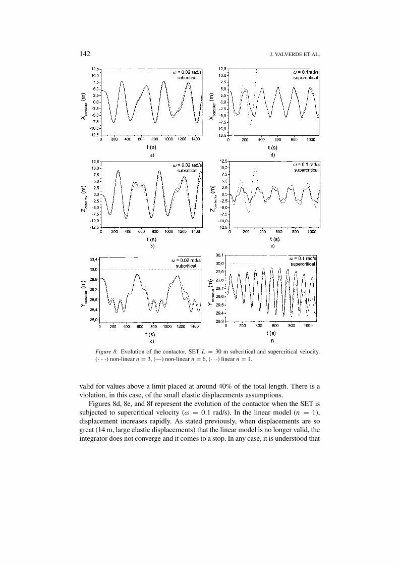
Figure 8 shows the evolution of the contactor projected on global axis (Fig-ure 4) for each of the analyzed cases. Figures 8a and 8b show how, in the case ofsubcritical velocity, the displacement developed by the contactor remains bounded(quasi-periodic stable solution), as the linear rotordynamics theory predicts, underthe value of 8 m in direction X (0.26L) and 10 m in direction Z (0.33L). Thisis the case for both the linear model (n = 1) and non-linear models (n = 3,n = 6). The linear and non-linear models behave globally in the same manner, butthere are differences between them locally. Figures 8c and 8f show that there is nodisplacement of the contactor in direction Y in the linear model, in spite of the factthat transversal displacement of the contactor differs from zero at all times. Thisis due to the fact that the bending and tensile-compressive forces are uncoupled inthe linear model and there are no forces to excite the axial modes. However, in thenon-linear models (n = 3, n = 6), bending is coupled with tensile-compressiveand torsion forces in such a way that an increase in the X-Z displacement ofthe contactor should translate into a decrease in its Y displacement. The effectproduced by this coupling can be observed in Figures 8a and 8b in t = 550 s andt = 1150 s, where linear and non-linear solutions are separated.

Displacements suffered by the tether in the case of subcritical velocity are ofconsiderable importance, given that they at times surpass 30% of the tether’s totallength. Nevertheless, as seen earlier on, the linear model behaves quite well. Underthese conditions, the system complies with the small elastic displacements assump-tions. On the other hand, Figures 8d and 8e show that the linear model is no longer


Figure 8. Evolution of the contactor, SET L = 30 m subcritical and supercritical velocity.(- - -) non-linear n = 3, (—) non-linear n = 6, (· · ·) linear n = 1.

valid for values above a limit placed at around 40% of the total length. There is aviolation, in this case, of the small elastic displacements assumptions.

Figures 8d, 8e, and 8f represent the evolution of the contactor when the SET issubjected to supercritical velocity (ω = 0.1 rad/s). In the linear model (n = 1),displacement increases rapidly. As stated previously, when displacements are sogreat (14 m, large elastic displacements) that the linear model is no longer valid, theintegrator does not converge and it comes to a stop. In any case, it is understood that


displacement is not bounded (unstable solution) as the linear rotordynamics theorypredicts. On the other hand, displacement remain bounded (quasi-periodic stablesolution) in the non-linear model under the value of 5 m (0.16L) in direction X and3 m (0.1L) in direction Z. The behavior for the linear and non-linear models arequite different in the supercritical regime. The geometric non-linearities in elasticand internal damping forces seem to stabilize the motion of the SET, as predictedin [6].

The qualitative change between one and various substructures is evident. Elasticand damping forces go from a linear to a non-linear model. Figure 8 reveals theinfluence of the number of substructures into which the tether is divided. Fig-ures 8d and 8e indicate how displacement for n = 6 is slightly smaller than forn = 3. The greater the number of substructures, the larger the coupling betweentransversal and longitudinal displacements, so that non-linear behavior is simulatedwith greater precision. The non-linearities have a stabilizing effect. This explainswhy displacement for n = 6 is smaller than for n = 3. Moreover, displacement forn = 3 is slowly destabilized; this does not occur for n = 6. The solution for n = 6is considered definitive, as it practically coincides with solutions found for n > 6.

In the numerical results, it has been noticed that during the start up, the torsionaldeformation is not large because the angular velocity is applied slowly. The rotationbetween the first and last section of the tether reaches a maximum value of 0.91◦ inthis period. Afterwards, the rotational vibration decays due to the internal dampingand there is only a small vibration of about 0.6◦ around the stable twisted position.These values are obtained for ωspin = 0.1 rad/s. The system behaves similarly as asimple beam subjected to pure torque.

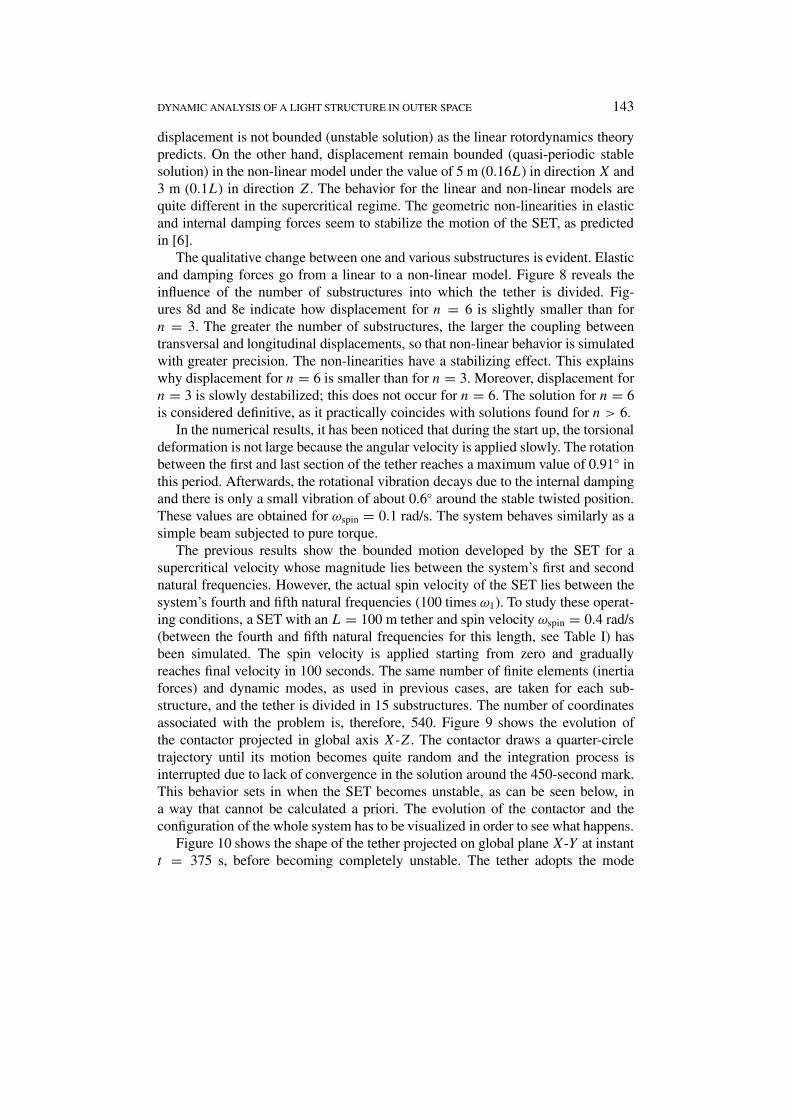
The previous results show the bounded motion developed by the SET for asupercritical velocity whose magnitude lies between the system’s first and secondnatural frequencies. However, the actual spin velocity of the SET lies between thesystem’s fourth and fifth natural frequencies (100 times ω1). To study these operat-ing conditions, a SET with an L = 100 m tether and spin velocity ωspin = 0.4 rad/s(between the fourth and fifth natural frequencies for this length, see Table I) hasbeen simulated. The spin velocity is applied starting from zero and graduallyreaches final velocity in 100 seconds. The same number of finite elements (inertiaforces) and dynamic modes, as used in previous cases, are taken for each sub-structure, and the tether is divided in 15 substructures. The number of coordinatesassociated with the problem is, therefore, 540. Figure 9 shows the evolution ofthe contactor projected in global axis X-Z. The contactor draws a quarter-circletrajectory until its motion becomes quite random and the integration process isinterrupted due to lack of convergence in the solution around the 450-second mark.This behavior sets in when the SET becomes unstable, as can be seen below, ina way that cannot be calculated a priori. The evolution of the contactor and theconfiguration of the whole system has to be visualized in order to see what happens.

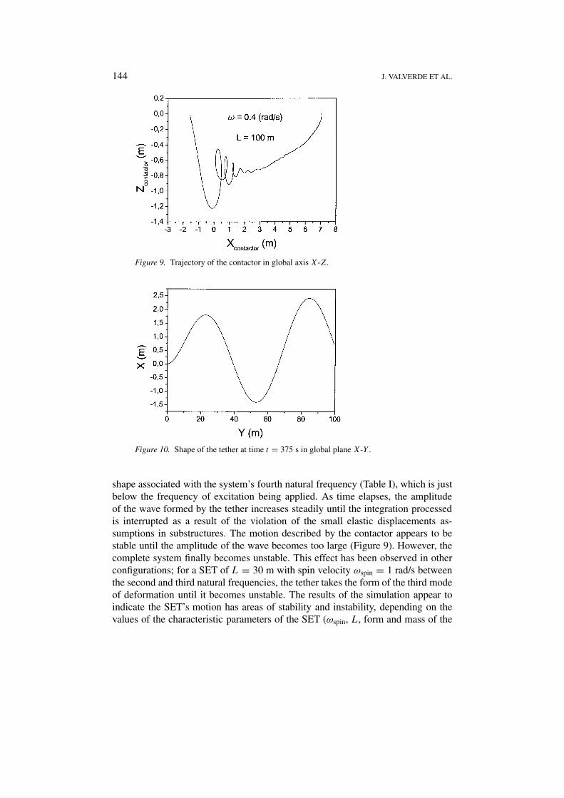
Figure 10 shows the shape of the tether projected on global plane X-Y at instantt = 375 s, before becoming completely unstable. The tether adopts the mode


Figure 9. Trajectory of the contactor in global axis X-Z.

Figure 10. Shape of the tether at time t = 375 s in global plane X-Y .

shape associated with the system’s fourth natural frequency (Table I), which is justbelow the frequency of excitation being applied. As time elapses, the amplitudeof the wave formed by the tether increases steadily until the integration processedis interrupted as a result of the violation of the small elastic displacements as-sumptions in substructures. The motion described by the contactor appears to bestable until the amplitude of the wave becomes too large (Figure 9). However, thecomplete system finally becomes unstable. This effect has been observed in otherconfigurations; for a SET of L = 30 m with spin velocity ωspin = 1 rad/s betweenthe second and third natural frequencies, the tether takes the form of the third modeof deformation until it becomes unstable. The results of the simulation appear toindicate the SET’s motion has areas of stability and instability, depending on thevalues of the characteristic parameters of the SET (ωspin, L, form and mass of the


contactor, etc.). The results obtained from the simulation encourage one to carryout a rigorous study on the stability of periodic solutions for the system.

4. Conclusions and Future Projects

In the dynamic simulation carried out in this work, in which a non-linear modelin elastic and internal damping forces has been used, quasi-periodic stable solu-tions (bounded motion of the SET) have been found for supercritical velocities, aspredicted by Genin and Maybee [6]. Unstable solutions have also been found forhigh spin velocities for this supercritical regime. The system clearly has a varietyof behaviors under the supercritical regime and probably will not have stable solu-tions for the whole range of spin supercritical velocities as predicted by Genin andMaybee for a simpler system [6].

The dynamic simulation helps with obtaining greater knowledge on the beha-vior of the SET and encourages the carrying out of in-depth study on the stabilityof the solutions for the system. Had stable solutions not been found for the dy-namic simulation, the stability study would probably never have been carried out.Therefore, the stability of the system will be subjected to more formal studies infuture projects.

In the dynamic simulation, a multibody system dynamic procedure has beendeveloped, in which substructuring and natural coordinates have been used. Amodel using the absolute nodal coordinate formulation [20] will be carried outto compare results and formalize the results obtained here.

As illustrated in Figure 8, the linear model is only valid for subcritical velocit-ies. In the configuration of OEDIPUS [9, 10], the tether was modeled as a linearrope. As a result, the stabilizing effect of non-linearities cannot appear. Likewise,the established boundaries of stability were obtained by linearizing the equationsof motion around the trivial solution. Therefore, the stability boundaries limit‘stable’ motion of the system to subcritical velocities alone. These analyticallycalculated stability boundaries were experimentally proven with a scale model ofthe OEDIPUS [11]. However, this does not prove the system is unstable abovecritical velocity. It proves that the linear model is valid below first critical velocityand determines this velocity with adequate precision. Moreover, experiments [11]revealed behavior that is typical of non-linear systems and the fact that the scalemodel was stable at supercritical velocity was demonstrated. All of this demon-strates the significance of non-linearities in this type of problem. Consequently, thisstudy may prove beneficial in the analysis of other spinning tether configurationsor similar rotary systems.

Acknowledgement

This research was supported by the Spanish Ministry of Science and Technology,under project reference DPI2000-0562.


References

1. Cosmo, M.L. and Lorenzini, E.C., Tethers in Space Handbook, 3rd edition, SmithsonianAstrophysical Observatory (NASA Marshall Space Flight Center), 1997.

2. Ahedo, E. and Sanmartín, J.R., ‘Analysis of bare-tether systems for deorbiting low-Earth-orbitsatellites’, Journal of Spacecrafts and Rockets 39(2), 2002, 198–205.

3. Mayo, J., Martínez, J., Escalona, J.L. and Domínguez, J., ‘Short electrodynamic tether WP-200Design and Mechanism’, Final Report, Department of Mechanical and Materials Engineering,University of Seville, 1999.

4. Den Hartog, J.P., Mecánica de las Vibraciones, 4th edition, McGraw-Hill, New York, 1972.5. Childs, D.W., Turbomachinery Rotordynamics, Wiley Interscience, New York, 1993.6. Genin, J. and Maybee, J.S., ‘Stability in the three dimensional whirling problem’, International

Journal of Non-Linear Mechanics 4, 1969, 205–215.7. Genin, J. and Maybee, J.S., ‘External and material damped three dimensional rotor system’,

International Journal of Non-Linear Mechanics 5, 1970, 287–297.8. Genin, J. and Maybee, J.S., ‘The role of material damping in the stability of rotating systems’,

Journal of Sound and Vibration 21(4), 1971, 399–404.9. Vigneron, F.R., Jablonski, A.M., Chandrashaker, R. and Tyc, G., ‘Damped gyroscopic modes

of spinning tethered space vehicles with flexible booms’, Journal of Spacecraft and Rockets34(5), 1997, 662–669.

10. Tyc, G., Han, R.P.S., Vigneron, F.R., Jablonski, A.M., Modi, V.J. and Misra, A.K., ‘Dynam-ics and stability of a spinning tethered spacecraft with flexible appendages’, Advances in theAstronautical Sciences 85(1), 1993, 877–896.

11. Modi, V.J., Pradhan, S., Chu, M., Tyc, G. and Misra, A.K., ‘Experimental investigation of thedynamics of spinning tethered bodies’, Acta Astronautica 39(7), 1996, 487–495.

12. Wu, S. and Haug, E.J., ‘Geometric non-linear substructuring for dynamics of flexible mech-anical systems’, International Journal for Numerical Methods in Engineering 26, 1988,2211–2226.

13. García de Jalón, J. and Bayo, E., Kinematic and Dynamic Simulation of Multibody Systems –The Real-Time Challenge, Springer-Verlag, New York, 1993.

14. Cuadrado, J., Cardenal, J. and García de Jalón, J., ‘Flexible mechanisms through naturalcoordinates and component synthesis: An approach fully compatible with the rigid case’,International Journal for Numerical Methods in Engineering 39, 1996, 3535–3551.

15. Valverde, J., ‘Análisis dinámico de la rotación de una estructura desplegable en el espacio’,M.D. Dissertation, Department of Mechanical and Materials Engineering, University of Seville,Spain, 2001 [in Spanish].

16. Géradin, M. and Cardona, A., Flexible Multibody Dynamics – A Finite Element Approach, JohnWiley and Sons, Chichester, 2001.

17. Avello, A., ‘Simulación dinámica interactiva de mecanismos flexibles con pequeñas deforma-ciones’, Ph.D. Thesis, Universidad de Navarra, Spain, 1995 [in Spanish].

18. Cuadrado, J., Gutiérrez, R., Naya, M.A. and Morer, P., ‘A comparison in terms of accuracyand efficiency between a MBS dynamic formulation with stress analysis and a non-linear FEAcode’, International Journal for Numerical Methods in Engineering 51(9), 2001, 1033–1052.

19. Cuadrado, J., Cardenal, J. and Bayo, E., ‘Modeling and solution methods for efficient real-timesimulation of multibody dynamics’, Multibody System Dynamics 1(3), 1997, 259–280.

20. Escalona, J.L., Hussien, H.A. and Shabana, A.A., ‘Application of the absolute nodal coordinateformulation to multibody system dynamics’, Journal of Sound and Vibration 214(5), 1998,833–851.