Divergence in India: Income Differentialsat the State Level, 1970–97

MICHELLE BADDELEY*, KIRSTY MCNAY**, &ROBERT CASSEN****Gonville & Caius College, Cambridge University, UK, **University of Oxford, Institute of Human

Sciences, Oxford, UK, ***London School of Economics, London, UK

Final version received June 2005

ABSTRACT We examine India’s regional disparities in economic performance between 1970–97.Our preliminary analysis shows that, in absolute terms, initially poorer states grew at slower ratesthan initially wealthier ones and that there is also evidence of increasing dispersion of incomelevels across the states. Our econometric analysis investigates the possibility of club convergenceand conditional convergence. Although we do not find evidence of the former, we can suggest someof the factors associated in the latter. Our research also indicates that the onset of economicpolicy reform in 1991 significantly intensified growth differentials between the states.

I. Introduction

The relative economic performance of India’s states has become a topical issue. Twoexplanations seem important: first, recent developments in economic growth theoryhave encouraged the investigation of regional growth experience and although mostwork has been carried out using international cross-sectional data, intra-countrystudies have also been made. The Indian case provides a still relatively rare exampleof developing country experience. It is well known that India’s national performancein many aspects masks considerable inter-state variation and economic growthperformance is no exception. Second, India’s economic policy reforms that began in1991 have had important implications for state-level growth; and increasingcompetition between the states has highlighted the issue of relative performance.Moreover, a consensus has emerged that greater policy decentralisation and state-level reform are pre-conditions for future economic growth.For India as a whole, annual per capita GDP growth averaged hardly 1.5 per cent

during the three decades from 1950–51 to 1980–81 (Acharya et al., 2003).However, during the 1980s, growth improved to 3.4 per cent. Following theintroduction of economic reforms in 1991, it increased to 3.6 per cent. However,these national trends conceal much state-level diversity. Table 1 summarises the

Correspondence Address: Michelle Baddeley, Fellow and College Lecturer in Economics, Faculty of

Economics and Gonville & Caius College, Cambridge CB2 1TA UK. Email: mb150@econ.cam.ac.uk

Journal of Development Studies,Vol. 42, No. 6, 1000–1022, August 2006

ISSN 0022-0388 Print/1743-9140 Online/06/061000-23 ª 2006 Taylor & Francis

DOI: 10.1080/00220380600774814

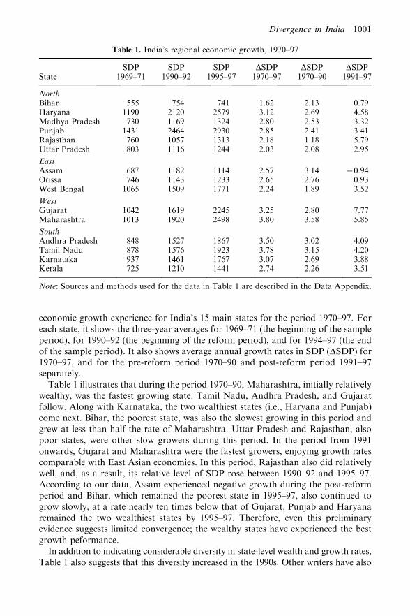
economic growth experience for India’s 15 main states for the period 1970–97. Foreach state, it shows the three-year averages for 1969–71 (the beginning of the sampleperiod), for 1990–92 (the beginning of the reform period), and for 1994–97 (the endof the sample period). It also shows average annual growth rates in SDP (DSDP) for1970–97, and for the pre-reform period 1970–90 and post-reform period 1991–97separately.

Table 1 illustrates that during the period 1970–90, Maharashtra, initially relativelywealthy, was the fastest growing state. Tamil Nadu, Andhra Pradesh, and Gujaratfollow. Along with Karnataka, the two wealthiest states (i.e., Haryana and Punjab)come next. Bihar, the poorest state, was also the slowest growing in this period andgrew at less than half the rate of Maharashtra. Uttar Pradesh and Rajasthan, alsopoor states, were other slow growers during this period. In the period from 1991onwards, Gujarat and Maharashtra were the fastest growers, enjoying growth ratescomparable with East Asian economies. In this period, Rajasthan also did relativelywell, and, as a result, its relative level of SDP rose between 1990–92 and 1995–97.According to our data, Assam experienced negative growth during the post-reformperiod and Bihar, which remained the poorest state in 1995–97, also continued togrow slowly, at a rate nearly ten times below that of Gujarat. Punjab and Haryanaremained the two wealthiest states by 1995–97. Therefore, even this preliminaryevidence suggests limited convergence; the wealthy states have experienced the bestgrowth peformance.

In addition to indicating considerable diversity in state-level wealth and growth rates,Table 1 also suggests that this diversity increased in the 1990s. Other writers have also

Table 1. India’s regional economic growth, 1970–97

SDP SDP SDP DSDP DSDP DSDPState 1969–71 1990–92 1995–97 1970–97 1970–90 1991–97

NorthBihar 555 754 741 1.62 2.13 0.79Haryana 1190 2120 2579 3.12 2.69 4.58Madhya Pradesh 730 1169 1324 2.80 2.53 3.32Punjab 1431 2464 2930 2.85 2.41 3.41Rajasthan 760 1057 1313 2.18 1.18 5.79Uttar Pradesh 803 1116 1244 2.03 2.08 2.95

EastAssam 687 1182 1114 2.57 3.14 70.94Orissa 746 1143 1233 2.65 2.76 0.93West Bengal 1065 1509 1771 2.24 1.89 3.52

WestGujarat 1042 1619 2245 3.25 2.80 7.77Maharashtra 1013 1920 2498 3.80 3.58 5.85

SouthAndhra Pradesh 848 1527 1867 3.50 3.02 4.09Tamil Nadu 878 1576 1923 3.78 3.15 4.20Karnataka 937 1461 1767 3.07 2.69 3.88Kerala 725 1210 1441 2.74 2.26 3.51

Note: Sources and methods used for the data in Table 1 are described in the Data Appendix.

Divergence in India 1001

noted increasing dispersion since 1991, when India’s introduction of economic policyreforms began (Ahluwalia, 2000, 2002). The reform process was a response to a fiscaland balance of payments crisis and involved opening up the economy and fosteringinvestment prospects. Although most of the reforms have so far taken place at thecentral level, gradual decentralisation has led to implementation by some stategovernments. Our data indicate that some of the most reform-orientated states havegrown fastest in the post-reform period (see also Bajpai and Sachs, 1996).There are numerous elements of state-level reform and notable differences in their

pace and scale across states. According to Bajpai and Sachs (1996), Andhra Pradesh,Gujarat, Karnataka, Maharashtra and Tamil Nadu can be classified as the mostreform-orientated states. Haryana, Orissa and West Bengal may be classified asintermediate reformers, while Assam, Bihar, Kerala, Madhya Pradesh, Punjab,Rajasthan and Uttar Pradesh are the slowest reformers. Important reforms havefocussed on infrastructure, industrial policy and investment incentives. Power sectorreform is a significant component of infrastructural reform and has involved tariffrevision, unbundling/restructuring of state electricity boards, and introduction ofregulation. Orissa has been the leader in power sector reforms, with the establish-ment of the Orissa Electricity Regulatory Commission, India’s first state-levelregulatory commission in the power sector (Bajpai and Sachs, 1996). Industrialpolicy reform includes introducing simpler procedures for clearance, and investmentincentives are aimed at encouraging private participation and include fiscalinducements such as capital subsidies and tax exemptions. For example, inKarnataka, the government has focused on upgrading industrial infrastructure inlocations that have attracted investment in large industrial projects. Fiscal reform isa priority, especially given the sharp deterioration in state fiscal health during the lastdecade. Reform-oriented states such as Andhra Pradesh have introduced measuresto reduce state fiscal deficits, including tax and expenditure reform. For example,there has been a significant reduction of rice subsidies and employment in AndhraPradesh and a corresponding increase in social and infrastructure expenditure. Onepositive recent fiscal reform has been the Medium Term Fiscal Reform Programmeby which states reach agreement with the centre, with some incentives from thecentre for them to do so. But by mid 2002, only Orissa of the large, poor states, hadsigned such agreements (Acharya et al., 2003).Bajpai and Sachs (1996) argue that one of the main consequences of state-level

reform has been increasing competition among the states involved, particularly inattracting both domestic and foreign private investment. Growth and reform indeedappear to go hand-in-hand in states such as Gujarat and Maharashtra. Unsurpris-ingly, once inter-state competition and private investment assumed greaterimportance, prosperous states with higher quality administrations, have been betterable to capitalise and build on their advantages.In terms of the pace of reform: on one hand, Rajasthan’s experience during the

1990s suggests that growth can also occur in a less reform-orientated environment.On the other hand since 1991, growth in Punjab, another slow reformer, has beennotably below what would have been expected given its high 1990–91 income level.But despite this relatively slow growth in the post-reform period, Punjab remainedthe wealthiest state in 1995–97, a position that largely reflects its favourable initialincome level.

1002 M. Baddeley et al.

The renewed interest in inter-regional growth patterns has focussed on theconvergence hypothesis (Durlauf, 1996). The aim of this paper is to assess the extentand nature of growth convergence across the Indian states. The evidence describedabove suggests that the Indian states may well fall into two distinct categories: a rich‘club’ of modern, high-growth states and a group of poor, slow-growing, ‘outsider’states. This paper aims to capture these tendencies using conditional convergenceand club convergence models. The findings have implications for government’s rolein achieving balanced regional development because evidence of divergence wouldimply that a greater proportion of regional development assistance should beconcentrated on the poorer states.

The paper proceeds with a summary of the theoretical literature on the causes ofeconomic growth, relating these theories to the Indian context. We then present theempirical analysis of convergence across the Indian states. We discuss bothpreliminary and econometric evidence of different types of convergence and, inparticular, we consider some of the possible factors underlying conditionalconvergence. It should be noted that for many variables, the availability of suitableannual state-level data is limited. These issues are discussed for each variable in theData Appendix.

II. Theories of Economic Growth Applied to India

Physical Investment

In the Swan–Solow neoclassical growth theory, convergence to a common steadystate is the outcome of natural market processes. In this view, convergence ishampered by government intervention. Instead, the accumulation of savings enablesinvestment and capital accumulation, and thus plays a crucial role in propellingeconomic growth (Solow, 1956; Swan, 1956). Once a steady state is reached, ‘break-even’ investment must take place to maintain the steady state in the short term.However, despite the importance of savings and investment, Solow (1957) alsoshowed that there are eventually diminishing returns to capital, and the long-runconstraint on growth is technology. If new technology is embodied in capitalstock, new investment should lead to growth in labour productivity, wages andemployment.

Clearly physical investment is essential to growth and its importance to Indiangrowth has been emphasised (Ahluwalia, 2000; Kurian, 2000). However, the absenceof infrastructure and equipment is often a key constraint, though countries caninvest without growing very much, and grow without investing, at least forconsiderable periods (Easterly, 2001). Infrastructural investment has been anextensively researched determinant of India’s regional disparities, with evidenceconfirming the importance of electric power, road and rail transport facilities,telecommunications and irrigation (Ghosh and De, 1998; Nagaraj et al., 2000).

In the post-reform period the role of foreign and domestic private investment hasalso been crucial. States now compete fiercely to attract investment thus exacerbatingregional disparities. In terms of foreign direct investment, Tamil Nadu, Karnatakaand Andhra Pradesh as well as Gujarat and Maharashtra are at the forefront,attracting car manufacturers (Ford and Mitsubishi) and software giants (Microsoft)

Divergence in India 1003

(Bajpai and Sachs, 1996). Clear links exist between such developments andstate-specific advantages in terms of human capital and relatively stable governance.Deliberate industrial policy shifts to accentuate the role of the private sector havealso been instrumental. Evidence demonstrates the importance of differentialpatterns in domestic private investment to regional economic growth disparities(Rao et al., 1999).To test for positive links between physical investment and regional growth

performance in our analysis we include three separate variables capturinginfrastructural investment, public expenditure, and private investment.Bernard and Jones (1996) also emphasise the importance of technology, arguing

that there has been an overemphasis on homogenous capital accumulation as asource of convergence; they argue that the key to convergence is technologicaltransfer yet empirical evidence suggests that there has been little internationalconvergence in, for example, manufacturing technologies. Lack of regional datameans, however, that we are not able empirically to analyse the impact of technologytransfer in this paper.

Human Capital

In contrast to neo-classical growth theorists, endogenous growth theorists questionthe assertion that economies will converge. In their view, persistently different ordiverging growth rates between economies suggest that different areas face differentsteady states. According to the endogenous growth theorists these are explained byincreasing returns to scale. Increasing returns occur as a result of positive investmentexternalities inducing technological progress. Human capital investment is particu-larly important and is argued to contribute to progress via spillover as well as viaprivate effects (Romer, 1990). So, the different inter-regional patterns are determinedby various economic and social conditions. Once these have been accounted for,there will be ‘conditional convergence’ dependent on initial conditions. Manyempirical studies of conditional convergence have shown that human capital is onedeterminant and a significant positive factor in economic performance (Levine andRenelt, 1992; Mankiw et al., 1992; Gemmell, 1996). Such findings suggest thatgovernment intervention to support economic and social progress will bolstereconomic growth.Many analysts comment on the relationships between human capital disparities

and India’s regional economic performance. The superior educational achievementof Kerala relative to the other states is frequently cited; Kerala’s literacy rate is90.9 per cent whereas Bihar’s rate is 47.5 per cent, the lowest in India (Census ofIndia, 2001). Maharashtra, Gujarat and Punjab follow Kerala with literacy rates ator above 70 per cent. Across the states, variation in underlying social features, suchas gender and caste structures, explains much of the difference in the publicschooling provision. Human capital is likely to become increasingly important inthe post-reform period as knowledge-based industries expand. Recent experiencesuch as that of East Asia during its rapid growth period up to the 1990s suggests adiminishing role for unskilled labour, and an increasing one for education andskills (World Bank, 1993). We test for the positive influence of human capital onSDP growth performance by including in our model an educational progress

1004 M. Baddeley et al.

variable. We expect higher levels of education to be associated with superiorgrowth.

Economic Structure

Transformation in economic structure is an important determinant of economicperformance in developing economies. However, two of the most prosperous andfastest growing Indian states, Punjab and Haryana, remain notably agricultural(Kurian, 2000). Both these states have benefited from increased agriculturalproductivity during the Green Revolution and its associated increases intechnological inputs. Other poorer performing areas, such as Bihar and MadhyaPradesh, have seen only marginal improvements in agricultural productivity. Paneldata growth regressions suggest a significant inverse relationship between Indianstates’ economic growth and agriculture’s share of SDP (Nagaraj et al., 2000); onaverage, more agricultural states are slower growing. However, cross-sectionalanalysis finds a strong positive association between economic growth and growth inagricultural income, suggesting that dynamic agricultural sectors are beneficial(Shand and Bhide, 2000). To investigate some of these relationships, we include ruralworkers as a proportion of all workers in order to capture the concentration of rurallabour in each state. We also include a variable to capture agricultural productivity.Controlling for agricultural productivity growth, we expect higher values of thelatter to enhance growth performance and that rural economies experience slowereconomic growth than urban economies.

Demographic Transition

Since Malthus, two main issues have been the focus of debates about therelationship between population growth and economic growth. One has linked theburden of dependency and savings, and related issues of capital widening versuscapital deepening – e.g., Coale and Hoover’s study, which used the Indianexample (Coale and Hoover, 1958). The second strand, associated with Boserup,stresses the role of population in inducing technological change and generatingeconomies of scale (Boserup, 1981). The first strand is more relevant here,particularly given the recent revival of interest in this view. Studies examining theEast Asian and other economies have found that reductions in the dependencyburden had a significant effect on savings (Birdsall et al., 2001). Reductions in theschool-age population also increased the quality of schooling, with valuableeffects on human capital (World Bank, 1993). Such positive influences of fertilitydecline have acquired the label of a ‘demographic bonus’; particularly relevant formost of India as the reversing effects of population ageing are still some decadesaway.

India’s regional demographic diversity is well known and is characterised by afundamental north/south divide (Dyson, 2001). Fertility and mortality are lower inthe southern and western states compared with the north. Demographic change hasbeen slowest in Bihar and Uttar Pradesh. No existing published econometric studyexamines the impact of variation in demographic progress on India’s regionaleconomic experience. In our analysis we include the birth rate and the worker/

Divergence in India 1005

population to capture demographic conditions. We expect high birth rates to slowgrowth and high worker/population rates to boost growth.

Income Inequality

Some economists have argued that inequality can promote growth by increasingsavings because the wealthy have a relatively high marginal propensity to save.Kuznets produced empirical evidence of a non-linear relationship between incomeand inequality and income per head, explained as reflecting the different stages ofdevelopment with equality first falling then rising with development (Kuznets, 1963).(Chenery, 1974) challenged this evidence, and more recently a negative relationshipbetween inequality and growth has been demonstrated (Aghion et al., 1999). Thisrecent evidence links into endogenous growth theories by linking the adverse effectsof inequality on human and physical capital investment either because inequality canlead to redistributive rather than productivity-oriented fiscal policies; and/or becauseit can generate political instability, discouraging investment. In our analysis, we userural and urban inequality measures to test these competing theories. Evidence ofbeneficial rural inequality effects might suggest that India’s prosperous farmers havebeen largely responsible for the technological advances driving aggregate perfor-mance (Walker and Ryan, 1990: 307).

Gender Inequality

There is relatively little research on the relationships between gender inequality andeconomic performance. Gender inequality takes several forms and its macroeco-nomic consequences may vary according to the context. Labour market inequalitymay promote growth if women’s relatively lower wages enhance profitability andinvestment (Seguino, 2000). But poor female access to education may lower thequality of human capital by stifling the positive externalities associated with femaleschooling, for example promotion of the education of the next generation (Klasen,1999). Gender inequality is very relevant in the Indian context, and state-levelvariation is striking. For example in education, male/female literacy rate ratios rangefrom a high of 1.8 in Bihar to a low of 1.1 in Kerala (Census of India, 2001). We testfor the influence on gender inequality of macroeconomic performance using agender-schooling variable and we expect that gender inequality will hamper SDPgrowth.

Governance

There is much research on the relationships between governance and economicgrowth, derived from research on democracy and development, social capital,inequality and growth, corruption and so forth (Knack and Keefer, 1997; Dethier,1999; MUHHDC, 1999). Many aspects of governance could be relevant. The corruptand inefficient administration of Bihar, for example, where the local elites acquired –and earned – the title of ‘jungle raj’, played a role in Bihar’s poor growthperformance. This context can explain the state’s poor record of foreign directinvestment. Poor quality governance is likely to be particularly important in the

1006 M. Baddeley et al.

post-reform period, as private investors were influenced by the willingness andability of governments to implement policy promises. To investigate whether there issuch an adverse association between poor governance and regional growthperformance we include state-level crime as a proxy variable.

III. Empirical Analysis

Preliminary Analysis

In this section, we summarise our preliminary analysis of the Indian regional data.(The econometric analysis will be presented in Section IV.) In analysing growth andconvergence two distinct, but related, concepts of convergence are typicallyexamined: weak convergence and strong convergence (Chatterji, 1992; Chatterjiand Dewhurst, 1996, Galor, 1996, Sala-I-Martin, 1996; Baddeley et al., 1998). Weak(b) convergence implies mean reversion – that is, a negative relationship betweengrowth rates and initial levels of real per capita income. Strong convergence impliesdeclining dispersion as well as mean reversion and is a more rigorous definition ofconvergence because it is not compromised by Galton’s fallacy. The conditions forstrong convergence will be violated when different groups of countries fall within oroutside a ‘convergence club’.

Concepts of absolute versus conditional convergence can also be distinguished.Absolute convergence implies that all regions are converging towards a commonsteady state. Conditional convergence implies that sub-sets of regions converge ondifferent steady states depending on inherent regional differences. Only if economieshave a common steady state will absolute convergence approximate conditionalconvergence.1

For the Indian states, previous studies have concentrated mainly on weakconvergence, and many only investigate absolute convergence (Marjit and Mitra,1996; Ghosh et al., 1998; Dasgupta et al., 2000). Conditional weak convergencehas received some attention (Rao et al., 1999; Nagaraj et al., 2000; Trivedi, 2000).Strong convergence has been investigated descriptively but not using econometricanalysis (Ghosh and De, 1998; Lall, 1999; Dasgupta et al., 2000; Nagaraj et al.,2000).

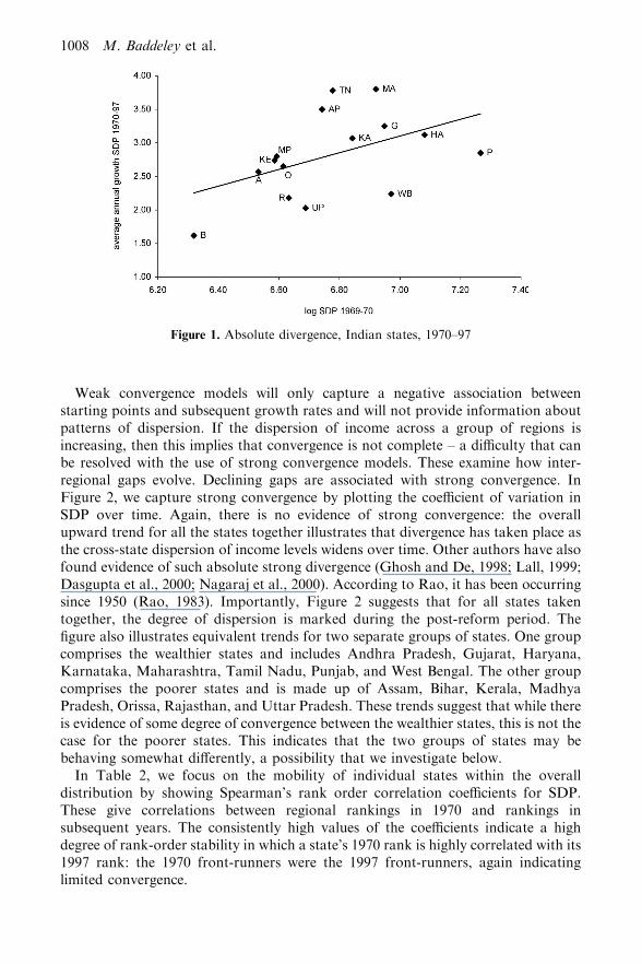
For our cross-section of states, absolute weak convergence is first examinedgraphically in Figure 1, which illustrates the relationship between average annualgrowth rates for each state between 1970–97 and corresponding initial levels ofincome in 1969–71 (data shown in Table 1). If states are weakly convergent thenthere will be a negative relationship between initial income levels and subsequentgrowth rates. Figure 1 suggests that weak convergence is limited for the Indianstates; instead absolute divergence seems more likely, with, on average, initiallypoorer states growing at slower rates than initially wealthier ones – accentuatingdivergences. This important finding is supported by most of the previous research onweak convergence (Bajpai and Sachs, 1996; Marjit and Mitra, 1996; Ghosh et al.,1998; Rao et al., 1999; Dasgupta et al., 2000; Nagaraj et al., 2000; Trivedi, 2000).2

Equivalent figures (not shown here) using the data in Table 1 for the pre- and post-reform periods illustrate that the degree of divergence appears to have increasedmarkedly in the post-reform period compared to before 1991.

Divergence in India 1007

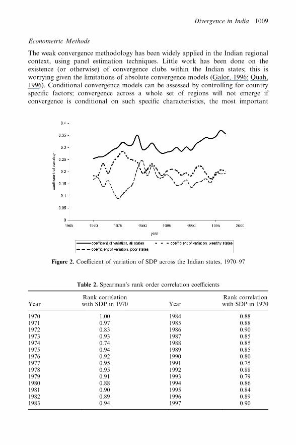
Weak convergence models will only capture a negative association betweenstarting points and subsequent growth rates and will not provide information aboutpatterns of dispersion. If the dispersion of income across a group of regions isincreasing, then this implies that convergence is not complete – a difficulty that canbe resolved with the use of strong convergence models. These examine how inter-regional gaps evolve. Declining gaps are associated with strong convergence. InFigure 2, we capture strong convergence by plotting the coefficient of variation inSDP over time. Again, there is no evidence of strong convergence: the overallupward trend for all the states together illustrates that divergence has taken place asthe cross-state dispersion of income levels widens over time. Other authors have alsofound evidence of such absolute strong divergence (Ghosh and De, 1998; Lall, 1999;Dasgupta et al., 2000; Nagaraj et al., 2000). According to Rao, it has been occurringsince 1950 (Rao, 1983). Importantly, Figure 2 suggests that for all states takentogether, the degree of dispersion is marked during the post-reform period. Thefigure also illustrates equivalent trends for two separate groups of states. One groupcomprises the wealthier states and includes Andhra Pradesh, Gujarat, Haryana,Karnataka, Maharashtra, Tamil Nadu, Punjab, and West Bengal. The other groupcomprises the poorer states and is made up of Assam, Bihar, Kerala, MadhyaPradesh, Orissa, Rajasthan, and Uttar Pradesh. These trends suggest that while thereis evidence of some degree of convergence between the wealthier states, this is not thecase for the poorer states. This indicates that the two groups of states may bebehaving somewhat differently, a possibility that we investigate below.In Table 2, we focus on the mobility of individual states within the overall

distribution by showing Spearman’s rank order correlation coefficients for SDP.These give correlations between regional rankings in 1970 and rankings insubsequent years. The consistently high values of the coefficients indicate a highdegree of rank-order stability in which a state’s 1970 rank is highly correlated with its1997 rank: the 1970 front-runners were the 1997 front-runners, again indicatinglimited convergence.

Figure 1. Absolute divergence, Indian states, 1970–97

1008 M. Baddeley et al.

Econometric Methods

The weak convergence methodology has been widely applied in the Indian regionalcontext, using panel estimation techniques. Little work has been done on theexistence (or otherwise) of convergence clubs within the Indian states; this isworrying given the limitations of absolute convergence models (Galor, 1996; Quah,1996). Conditional convergence models can be assessed by controlling for countryspecific factors; convergence across a whole set of regions will not emerge ifconvergence is conditional on such specific characteristics, the most important

Table 2. Spearman’s rank order correlation coefficients

YearRank correlationwith SDP in 1970 Year

Rank correlationwith SDP in 1970

1970 1.00 1984 0.881971 0.97 1985 0.881972 0.83 1986 0.901973 0.93 1987 0.851974 0.74 1988 0.851975 0.94 1989 0.851976 0.92 1990 0.801977 0.95 1991 0.751978 0.95 1992 0.881979 0.91 1993 0.791980 0.88 1994 0.861981 0.90 1995 0.841982 0.89 1996 0.891983 0.94 1997 0.90

Figure 2. Coefficient of variation of SDP across the Indian states, 1970–97

Divergence in India 1009

characteristics being those generally associated with increasing returns in anendogenous growth context. Club convergence models are more robust and can beanalysed econometrically in the context of weak convergence using the modellingstrategies of Baumol and Wolff (1988) and in the context of strong convergence usingthe modelling strategies of Chatterji (1992), Chatterji and Dewhurst (1996) andGalor (1996).For this paper, the following modelling strategy was used. First, models of weak

convergence were estimated. These suffered from signs of model misspecification.Therefore, the subsequent analysis focused on strong convergence models only. Clubconvergence models were estimated following Chatterji (1992) and Chatterji andDewhurst (1996):

Gi;T ¼X3

k¼1gk � ðGi;T�1Þk ð1Þ

where GT¼ ln(SDPPunjab)7ln(SDPi) for a given state i in each time period T. G is astate’s differential away from Punjab, the leading state. A small gap implies that astate is close to the leader, and visa versa for a large gap. In this analysis, Equation(1) is used to capture a cubic relationship between gaps and lagged gaps with regionsexperiencing smaller gaps forming a convergence club. Chatterji (1992) asserts that anumber of different patterns are possible depending on the magnitude andsignificance of the parameter estimates. If g1 is less than 1 numerically andg2¼ g3¼ 0, then strong convergence will emerge. If g1 and g2 are non-zero but g3¼ 0,then a diffusion model emerges in which there are two groups of regions: theexclusive convergence club and the non-converging regions. If all three coefficientsare non-zero, then there is no convergence.The evidence from the club convergence models does not suggest that the Indian

states divide into a convergent club versus a non-convergent group (as explainedbelow). So the next stage of our strategy involved a fuller analysis of thedeterminants of growth differentials across the states, an approach that is consistentwith conditional convergence models and endogenous growth theory. In this thirdstage of the estimation, conditional convergence models are estimated, controllingfor factors commonly associated with increasing returns – for example, educationand infrastructural investment. Additional conditioning explanatory variables usedinclude structural variables such as agricultural productivity, demographic transi-tion, income/gender inequality, and governance. (The potential significance of thesefactors has been explained in the theoretical section.) Details of the data andmeasures used to capture them are contained in the Data Appendix.To summarise, the following system of equations was estimated:

Gi;T ¼ gGi;T�1 þX

fjXj;i þX

ymZm;i þ ei ð2Þ

Zm;i ¼ u1Gi;T þ u2Gi;T�1 þX

ZjXj;i þ oi ð3Þ

where Xj represents j exogenous explanatory variables and Zm represents the mendogenous explanatory variables. Most of the economic structure and demographicvariables can be assumed to be exogenous because lagged economic structure/demographics are used; there will be no contemporaneous correlation between the

1010 M. Baddeley et al.

variables and the error term and OLS will be consistent. However, the governancevariable (as measured by crime rates) may be affected by endogeneity because crimein the current period will be affected by current economic conditions, some of whichwill be captured by the error. In the presence of such endogeneity, OLS will be bothbiased and inconsistent. Hausman tests confirmed evidence of endogeneity in thecrime variable, significant at a 1 per cent significance level. To correct this problem,crime has been instrumented using a two-stage least squares (2SLS) estimationprocedure. Current/lagged gaps and all the exogenous explanatory variables wereused as instruments in the first stage of 2SLS.

Another potential source of bias and inconsistency in panel estimations is thepresence of non-stationarity across the temporal dimension. So all variables weretested for non-stationarity. As emphasised by Levin and Lin (1992, 1993) andPhillips and Moon (1999), the conventional time-series testing procedures should bemodified for use with panel data. Here, Levin and Lin’s (1993) methodology isadopted and the null hypotheses of a unit root can be rejected at a 10 per centsignificance level for the food grain yield variable, a 5 per cent significance level forinfrastructure and a 1 per cent significance level for all other variables.

Econometric Results

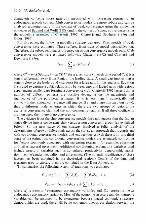
The econometric results from the various regressions are outlined in Tables 3 and 4.The regressions were initially estimated using ordinary least squares (OLS)techniques incorporating a fixed-effects panel data modelling strategy, as outlined

Table 3. Parameter estimates from weak and club convergence models (t ratios in brackets)

1 2 3 4Weak

convergenceWeak

convergenceClub

convergenceClub

convergence

Column:OLS GLS OLS GLS

Dependent variable: Regional SDP growth Regional SDP differential

Lagged SDP 70.0392*(72.074)

70.00233(70.169)

– –

Lagged differential – – 0.634*(2.506)

0.124(0.532)

Lagged differential2 – – 70.267(70.724)

0.842*(2.126)

Lagged differential3 – – 0.168(1.012)

70.523*(72.433)

Constant 0.325*(0.144)

0.0463*(.1047)

0.000(0.000)

0.000(0.000)

Goodness of fit R2 (adjusted)70.0206

Buse R2

þ0.0093R2 (adjusted)þ0.9308

Buse R2

þ0.8981Diagnostics SC, HET, RESET N/A HET N/A

Notes: *estimate in rejection region, 95% confidence interval; **estimate in rejection region,90% confidence interval; þ instrumented using 2SLS. SC¼Breusch Godfrey LM test forserial correlation in rejection region, 95% confidence interval. HET¼White’s LM test forheteroscedasticity in rejection region, 95% confidence interval. RESET¼Ramsey’s RESETtest for incorrect functional form in rejection region, 95% confidence interval.

Divergence in India 1011

in Griffiths et al. (1993). In practise, this was achieved using dummy variables tocontrol for shifts in regional intercepts emerging from regional fixed effects. Thesefixed effects were jointly significant. (In the interests of succinctness, the parameterestimates on these dummy variables are not recorded.) Diagnostic tests for incorrectfunctional form, heteroscedasticity and autocorrelation were used. Functionalform problems were statistically significant (at a 5% significance level) for weakconvergence models, reinforcing assertions discussed above about the fact that weakconvergence models do not effectively capture inter-regional patterns. There was also

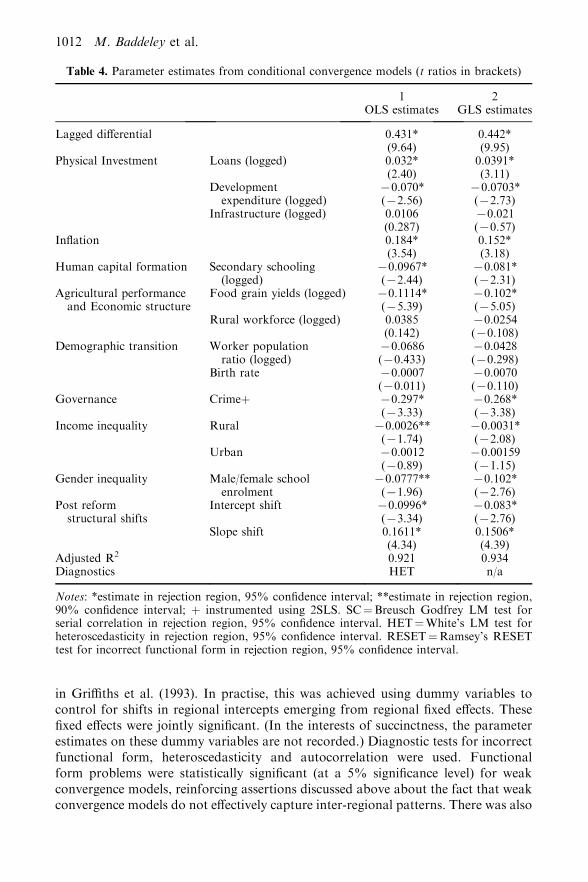
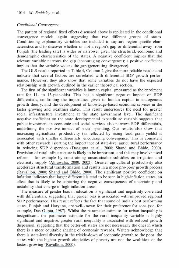
Table 4. Parameter estimates from conditional convergence models (t ratios in brackets)

1 2OLS estimates GLS estimates

Lagged differential 0.431*(9.64)

0.442*(9.95)

Physical Investment Loans (logged) 0.032*(2.40)

0.0391*(3.11)

Developmentexpenditure (logged)

70.070*(72.56)

70.0703*(72.73)

Infrastructure (logged) 0.0106(0.287)

70.021(70.57)

Inflation 0.184*(3.54)

0.152*(3.18)

Human capital formation Secondary schooling(logged)

70.0967*(72.44)

70.081*(72.31)

Agricultural performanceand Economic structure

Food grain yields (logged) 70.1114*(75.39)

70.102*(75.05)

Rural workforce (logged) 0.0385(0.142)

70.0254(70.108)

Demographic transition Worker populationratio (logged)

70.0686(70.433)

70.0428(70.298)

Birth rate 70.0007(70.011)

70.0070(70.110)

Governance Crimeþ 70.297*(73.33)

70.268*(73.38)

Income inequality Rural 70.0026**(71.74)

70.0031*(72.08)

Urban 70.0012(70.89)

70.00159(71.15)

Gender inequality Male/female schoolenrolment

70.0777**(71.96)

70.102*(72.76)

Post reformstructural shifts

Intercept shift 70.0996*(73.34)

70.083*(72.76)

Slope shift 0.1611*(4.34)

0.1506*(4.39)

Adjusted R2 0.921 0.934Diagnostics HET n/a

Notes: *estimate in rejection region, 95% confidence interval; **estimate in rejection region,90% confidence interval; þ instrumented using 2SLS. SC¼Breusch Godfrey LM test forserial correlation in rejection region, 95% confidence interval. HET¼White’s LM test forheteroscedasticity in rejection region, 95% confidence interval. RESET¼Ramsey’s RESETtest for incorrect functional form in rejection region, 95% confidence interval.

1012 M. Baddeley et al.

evidence of heteroscedasticity (a systematic pattern in the error variance) significantat 5 per cent. This was corrected using generalised least squares (GLS) proceduresfor panel data, as outlined in White (1997). This corrective procedure ensures thatthe results from the GLS regressions are more reliable than the results from theoriginal OLS regressions.

In all regressions, structural breaks between the pre-reform and post-reformperiods (that is 1970–90 and 1991 onwards respectively) were captured with theinclusion of additive and multiplicative dummy variables. Various tests wereconducted to assess the significance of these dummies and, for all regressions, thesetests revealed significant evidence of a structural break in the post-reform period, asexplained below.

Weak Convergence

The results from the first stage of estimation, focusing on weak convergence models,are reported in Columns 1 and 2 of Table 3 and confirm that models of weakconvergence do not effectively capture the evolution of SDP in the Indian states from1970 to 1997. Although there is a significant negative correlation between SDPgrowth over the period 1970 to 1997 and SDP in 1970, numerically consistent withthe hypothesis of weak convergence, the convergence parameter estimate is small.Ramsey’s RESET tests suggest that the linear functional form is inappropriate. Thepoor empirical performance of this model is also reflected in the anomalous adjustedR2. Overall, these results are not surprising given previous evidence and givencriticisms of weak convergence models by Chatterji (1992), Galor (1996) and Quah(1996).

Club Convergence

The results from the estimation of Chatterji’s club convergence model are reportedin Columns 3 and 4 in Table 3. As explained above, the evidence ofheteroscedasticity in the OLS estimations (see Column 3 of Table 3) necessitated acorrective GLS procedure (see results in Column 4). The results of the clubconvergence models are mixed. The OLS result suggests that g1 is non-zero andthe GLS result indicates that g2 and g3 are non-zero. Taken together, these resultssuggest that there is no significant evidence either for strong convergence or of clubconvergence.

Whilst the evidence on club convergence is mixed, an informal examination of theparameters on the regional fixed effects dummies does suggest that there are twobroad groups of Indian states: high performance and low performance states. All theregional dummies are jointly significantly different from zero (as mentioned above)and the magnitude of the regional fixed effects is reflected in the size of these regionaldummies. States with relatively small parameter estimates on their regional dummieshave low differentials relative to the leader (Punjab); such states include Haryana,Gujarat, Maharashtra, West Bengal, Tamil Nadu, Andhra Pradesh and Karnataka.Conversely, the states with relatively high parameter estimates on regional dummiesare relatively poorer and include Bihar, Madhya Pradesh, Rajasthan, Uttar Pradesh,Assam, Orissa and Kerala.

Divergence in India 1013

Conditional Convergence

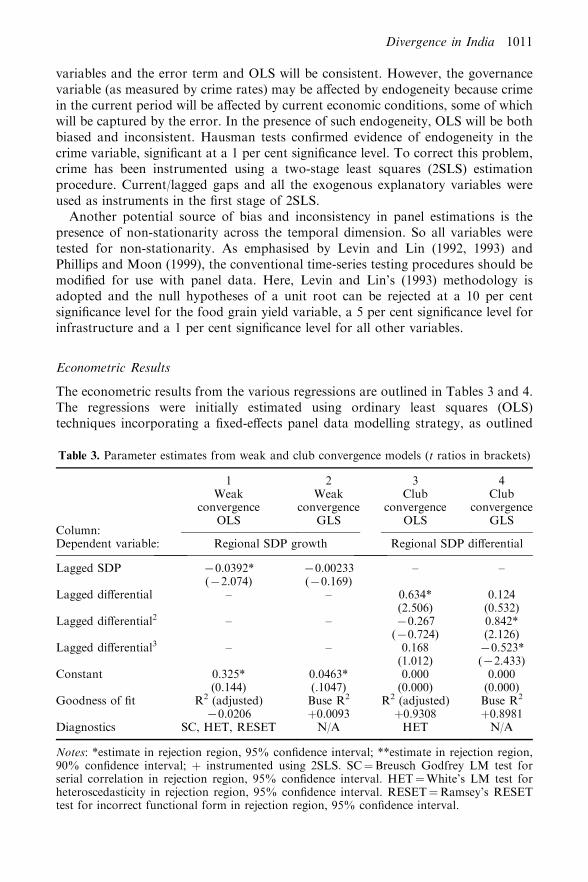
The pattern of regional fixed effects discussed above is replicated in the conditionalconvergence models, again suggesting that two different groups of states.Conditioning explanatory variables are included to capture region-specific char-acteristics and to discover whether or not a region’s gap or differential away fromPunjab (the leading sate) is wider or narrower given the structural, economic anddemographic characteristics of the states. A negative coefficient implies that therelevant variable narrows the gap (encouraging convergence); a positive coefficientimplies that the variable widens the gap (generating divergence).The GLS results reported in Table 4, Column 2 give the more reliable results and

indicate that several factors are correlated with differential SDP growth perfor-mance. However, they also show that some variables do not have the expectedrelationship with growth outlined in the earlier theoretical section.The first of the significant variables is human capital (measured as the enrolment

rate for 11- to 13-year-olds). This has a significant negative impact on SDPdifferentials, confirming the importance given to human capital in endogenousgrowth theory, and the development of knowledge-based economic services in thefaster growing and wealthier states. This result underscores the need for greatersocial infrastructure investment at the state government level. The significantnegative coefficient on the state developmental expenditure variable suggests thatpublic investment in economic and social services also narrows SDP differentials,underlining the positive impact of social spending. Our results also show thatincreasing agricultural productivity (as reflected by rising food grain yields) isassociated with smaller differentials, encouraging convergence. This is consistentwith other research asserting the importance of state-level agricultural performancein reducing SDP dispersion (Dasgupta et al., 2000; Shand and Bhide, 2000).Provision of rural infrastructure is likely to be important, and this may involve fiscalreform – for example by constraining unsustainable subsidies on irrigation andelectricity supply (Ahluwalia, 2000, 2002). Greater agricultural productivity alsoaccelerates structural transformation and results in a more pro-poor growth process(Ravallion, 2000; Shand and Bhide, 2000). The significant positive coefficient oninflation indicates that larger differentials tend to be seen in high-inflation states, aneffect that is likely to be capturing the negative consequences of uncertainty andinstability that emerge in high inflation areas.The measure of gender bias in education is significant and negatively correlated

with differentials, suggesting that gender bias is associated with improved regionalSDP performance. This result reflects the fact that some of India’s best performingstates, Punjab and Haryana, are well-known for their preference for sons (see, forexample, Das Gupta, 1987). Whilst the parameter estimate for urban inequality isinsignificant, the parameter estimate for the rural inequality variable is highlysignificant and negative: greater rural inequality is associated with reduced growthdispersion, suggesting that the better-off states are not necessarily the ones in whichthere is a more equitable sharing of economic rewards. Writers acknowledge thatthere is state-level diversity in the trickle-down of economic growth to the poor; thestates with the highest growth elasticities of poverty are not the wealthiest or thefastest growing (Ravallion, 2000).

1014 M. Baddeley et al.

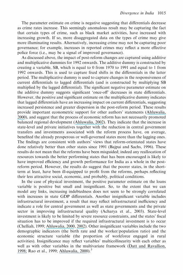
The parameter estimate on crime is negative suggesting that differentials decreaseas crime rates increase. This seemingly anomalous result may be capturing the factthat certain types of crime, such as black market activities, have increased withincreasing growth. If so, more disaggregated data on the types of crime may givemore illuminating results. Alternatively, increasing crime may not be capturing poorgovernance; for example, increases in reported crimes may reflect a more effectivepolice force (i.e., may be a signal of improved governance).

As discussed above, the impact of post-reform changes are captured using additiveand multiplicative dummies for 1992 onwards. The additive dummy is constructed bycreating a variable, SB, which is equal to 0 from 1970 to 1991 and equal to 1 from1992 onwards. This is used to capture fixed shifts in the differentials in the latterperiod. The multiplicative dummy is used to capture changes in the responsiveness ofcurrent differentials to lagged differentials (and is constructed by multiplying SBmultiplied by the lagged differential). The significant negative parameter estimate onthe additive dummy suggests significant ‘once-off’ decreases in state differentials.However, the positive and significant estimate on the multiplicative dummy indicatesthat lagged differentials have an increasing impact on current differentials, suggestingincreased persistence and greater dispersion in the post-reform period. These resultsprovide important econometric support for other authors’ statements (Ahluwalia,2000), and suggest that the process of economic reform has not necessarily promotedbalanced regional development (Ahluwalia, 2002). They indicate that the increase instate-level and private initiatives together with the reduction in central governmenttransfers and investments associated with the reform process have, on average,benefited the already prosperous or well-governed states more than the lagging ones.The findings are consistent with authors’ views that reform-orientated states havedone relatively better than other states since 1991 (Bajpai and Sachs, 1996). Theseresults do not mean that the reforms have been misguided; indeed any reallocation ofresources towards the better performing states that has been encouraged is likely tohave improved efficiency and growth performance for India as a whole in the post-reform period. However, the results do suggest that the poorer states, in the short-term at least, have been ill-equipped to profit from the reforms, perhaps reflectingtheir less attractive social, economic, and probably, political conditions.

In the case of physical investment, the positive parameter estimate on the loansvariable is positive but small and insignificant. So, to the extent that we canmodel any links, increasing indebtedness does not seem to be strongly correlatedwith increases in state GDP differentials. Another insignificant variable includesinfrastructural investment, a result that may reflect infrastructural inefficiency andindicate a role for central government as well as state governments and the privatesector in improving infrastructural quality (Acharya et al., 2003). State-levelinvestment is likely to be limited by severe resource constraints, and the states’ fiscalsituation has to be improved if the required infrastructural investment is to occur(Chelliah, 1999; Ahluwalia, 2000, 2002). Other insignificant variables include the twodemographic indicators (the birth rate and the worker/population ratio) and theeconomic structure variable (the proportion of workforce engaged in ruralactivities). Insignificance may reflect variables’ multicollinearity with each other aswell as with other variables in the multivariate framework (Datt and Ravallion,1998; Rao et al., 1999; Ahluwalia, 2000).3

Divergence in India 1015

IV. Conclusion

Regional disparities in economic growth performance across India appear to havewidened as some states have improved faster than others. Our analysis has shown thatneither weak nor strong absolute convergence has occurred and that club convergence,as described by Chatterji (1992), does not hold. However, we do find evidence ofconditional convergence to different steady states depending on the economic andsocial characteristics of the states.We have also been able to identify some of the factorsassociated with conditional convergence. Our results suggest the value of state-levelinvestment in economic and social sectors and the promotion of agriculturalproductivity. The importance of education in our models also indicates that India’srecent educational progress is likely to have been a significant factor in narrowing inter-state disparities. Despite the promotion of balanced regional development as anobjective of central government policy, these results suggest that it is areas in whichstate governments have investment responsibility that are important in explainingIndia’s regional growth disparities. The evidence above also suggests that increaseddispersion across the states has increased since the onset of reforms. This is animportant result indicating that not all states have been able to benefit equally from thepolicy shifts towards greater decentralisation. The poorer performing states must beassisted in identifying the specific deficiencies that are preventing them from takingadvantage of reform. Improvement in state-level fiscal health is a priority if investmentin developmental and social infrastructure, and agricultural productivity – shown hereto be some of the factors associated with the income gaps between states – is to be moreforthcoming (Ahluwalia, 2000). Despite decentralisation, it is likely that the centralgovernment has a role to play in assisting the states in this area, as the example of theMedium Term Fiscal Reform Programme discussed above.Overall, our work suggests that further analysis of the impact of reform on India’s

regional growth dispersion is needed. Here the reform process is treated as astructural break at 1991 because data constraints have made it difficult adequately to‘unpack’ the separate elements. However, a more qualitative approach focusing onspecific states may well yield further insights. Indeed, in the context of continuingreform, addressing this issue more thoroughly is a priority.The evidence of significant disparities in economic growth performance across India’s

states may also suggest the existence and development of regional differences at a moredisaggregated level than the state level. It is already well known that there are substantialintra-state disparities and their further analysis may uncover interesting patterns.4

Acknowledgement

The authors are grateful to the anonymous referees for their helpful comments andsuggestions.

Notes

1. For discussions of convergence models and of absolute versus conditional convergence, see Chatterji

(1992), Barro and Sala-I-Martin (1992, 1995), Chatterji and Dewhurst (1996), Galor (1996) and

Baddeley, Martin and Tyler (1998).

1016 M. Baddeley et al.

2. Some authors have found evidence of weak convergence, although this result seems to be largely

related to the inclusion of some of India’s smaller states and union territories, many of which are

outliers in cross-sectional analysis (Cashin and Sahay, 1996).

3. In the case of physical investment, for example, the 1991 break dummies discussed above (which

suggest that increased private sector activity has had a significant effect) may be capturing the

influence explaining why there is no further independent impact from our private investment proxy.

4. One possibility is the National Sample Survey’s data for approximately 80 Indian regions. These data

have been used to illustrate intra-state economic performance – for example by Dreze and Srinivasan

(1996), Murthi et al. (2001), Bhandari and Khare (2002), Deaton and Dreze (2002), Palmer-Jones and

Sen (2003).

5. SDP represents value added originating in each state and not income accruals to residents. Income

transferred from other parts of India and abroad is not included; this may bias the estimates

downwards in some cases, for example Kerala, where income transfers are substantial. The CSO

incorporates an adjustment to the data from the States’ Statistical Bureaux to ensure interstate

comparability (Nagaraj et al., 2000).

6. CPIAL is adjusted firewood price increases and incorporates rural inter-state cost of living differentials,

base year 1973–74. Similarly, CPIIW is adjusted for urban inter-state cost of living differentials, base

year 1973–74. The World Bank time series ends in 1995 for CPIAL and in 1994 for CPIIW. For later

years, we take unadjusted price indices from the Central Statistical Organisation’s 1999 Statistical

Abstract. The Statistical Abstract gives CPIIW at centre level. We follow the same procedure as the

World Bank to obtain state-level indices, averaging across the centres. Price indices are adjusted by

calculating a conversion factor for each state. For example, for the unadjusted CPIAL in the 1999

Statistical Abstract is 1986, 1986 CPIAL¼ 100; theWorld Bank’s adjusted CPIAL for Andhra Pradesh

in 1986 is 199.48, giving a conversion factor of 1.9948; this is multiplied by unadjusted Andhra

Paradesh value of 268 to give the adjusted 1996 Andhra Pradesh CPIAL of 26861.9948¼ 534.61.

7. For each state, this is equal to nominal per capita net domestic product divided by prices weighted

according to rural versus urban populations, i.e. adjusted CPIAL/100)6rural population)þ((adjusted CPIIW/100)6urban population). For Haryana, there is no adjusted price data so we

assume the same adjusted price indices as Punjab.

8. For each state, a least-squares linear regression line is fitted to the logarithmic annual values of SDP.

The growth rate is then calculated as ((exponential{b})71)6100, where b is the regression coefficient.

9. The CMIE’s index consists of seven components, including the three we use. We adjust the weights

applied to our index accordingly.

10. All-India Financial Institutions refers to the All-India Development Banks IDBI, IFCI, ICICI,

SIDBI, IRBI and SCICI, the Specialised Financial Institutions RCTC, TDICI and TFCI, and

investment institutions LIC, UTI and GIC.

11. The latter has a reference period of a year, those working for the major part of it are employed

according to usual principal status and those working for only a minor part of it are employed

according to usual subsidiary status.

References

Acharya, S., Cassen, R. and McNay, K. (2003) The economy—past and future, in T. Dyson, R. Cassen

and L. Visaria (eds), Twenty-First Century India. Population, Environment and Human Development

(New Delhi: Oxford University Press).

Ahluwalia, M. S. (2000) Economic performance of states in post-reforms period, Economic and Political

Weekly, May 6, pp. 1637–48.

Ahluwalia, M. S. (2002) State-level performance under economic reforms in India, in A. O. Krueger (ed.),

Economic Policy Reforms and the Indian Economy (Chicago: The University of Chicago Press).

Aghion, P., Caroli, E. and Garcıa-Penalosa, C. (1999) Inequality and economic growth: the perspective of

the new growth theories, Journal of Economic Literature, 37(4), pp. 1615–30.

Baddeley, M., Martin, R. and Tyler, P. (1998) European regional unemployment disparities: convergence

or persistence?, European Urban & Regional Studies, 5(3), pp. 195–215.

Bajpai, N. and Sachs, J. D. (1996) Trends in inter-state inequalities of income in India, Harvard Institute

for International Development, Development Discussion Paper, No. 528, Harvard University.

Divergence in India 1017

Barro, R. J. (1997) Determinants of Economic Growth (Boston: The MIT Press).

Barro, R. J. and Sala-I-Martin, X. (1992) Convergence, Journal of Political Economy, 100(2),

pp. 223–51.

Barro, R. J. and Sala-I-Martin, X. (1995) Economic Growth (New York: McGraw Hill).

Baumol, W. J. and Wolff, E. N. (1988) Productivity growth, convergence and welfare: reply, American

Economic Review, 78(1), pp. 1155–1159.

Behrman, J., Foster, A. D., Rosenzweig, M. R. and Vashishtha, P. (1999) Women’s schooling, home

teaching and economic growth, Journal of Political Economy, 107(4), pp. 682–714.

Bernard, A. B. and Jones, C. I. (1996) Technology and convergence, Economic Journal, 106(43),

pp. 1037–44.

Bhandari, L. and Khare, A. (2002) The Geography of Post 1991 Indian Economy (New Delhi: Indicus

Analytics).

Birdsall, N., Kelley, A. C. and Sinding, S. (2001) Population Matters: Demographic Change, Economic

Growth, and Poverty in the Developing World (Oxford: Oxford University Press).

Boserup, E. (1981) Population and Technology (Oxford: Blackwell).

Cashin, P. and Sahay, R. (1996) Internal migration, center–state grants and economic growth in the states

of India, IMF Working Paper, 66.

Centre for Monitoring the Indian Economy (1997) Profiles of states (New Delhi: CMIE).

Chatterji, M. (1992) Convergence clubs and endogenous growth, Oxford Review of Economic Policy, 8(4),

pp. 43–56.

Chatterji, M., and Dewhurst, J. H. (1996) Convergence clubs and relative economic performance in Great

Britain, 1977–91, Regional Studies, 30(1), pp. 31–40.

Chelliah, R. J. (1999) Economic reform strategy for the next decade, Economic & Political Weekly,

September 4.

Chenery, H. (1974) Redistribution with Growth (Oxford: Oxford University Press).

Coale, A. J. and Hoover, E. M. (1958) Population Growth and Economic Development in Low-Income

Countries (Princeton: Princeton University Press).

Dasgupta, D., Maiti, P., Mukerjee, R., Sarkar, S. and Chakrabarti, S. (2000) Growth and interstate

disparities in India, Economic & Political Weekly, July 1, pp. 2413–22.

Das Gupta, M. (1987) Selective discrimination against female children in rural Punjab, India, Population &

Development Review, 13(1), pp. 77–100.

Datt, G. and Ravallion, M. (1998) Why have some Indian states done better than others at reducing rural

poverty? Economica, 65, pp. 17–38.

Deaton, A. and Dreze, J. (2002) Poverty and inequality in India—a re-examination, Economic & Political

Weekly, September 7, pp. 3029–48.

Dethier, J. J. (1999) Governance and economic performance: a survey, ZEF Discussion Papers, No. 5,

Zentrum fur Entwicklungsforschung, Bonn University.

Dreze, J. and Khera, R. (2000) Crime, gender, and society in India: insights from homicide data,

Population & Development Review, 26(2), pp. 335–53.

Dreze, J. and Srinivasan, P. V. (1996) Poverty in India: regional estimates, 1987–98, Indira Ghandi Institute

of Development Research, Discussion Paper 129.

Durlauf, S. N. (1996) On the convergence and divergence of growth rates, Economic Journal, 106(43),

pp. 1016–8.

Dyson, T. (2001) The preliminary demography of the 2001 census of India, Population and Development

Review, 27(2), pp. 341–56.

Easterly, W. (2001) The Elusive Quest for Growth (London: MIT Press).

Galor, O. (1996) Convergence? Inferences from theoretical models, Economic Journal, 106(43),

pp. 1056–69.

Gemmell, N. (1996) Evaluating the impacts of human capital stocks and accumulation on economic

growth: some new evidence, Oxford Bulletin of Economics, 58(1), pp. 9–28.

Ghosh, B. and De, P. (1998) Role of infrastructure in regional development. A study over the plan period,

Economic & Political Weekly, November 21, pp. 3039–48.

Ghosh, B., Marjit, S. and Neogi, C. (1998) Economic growth and regional divergence in India, 1960 to

1995, Economic & Political Weekly, June 27, pp. 1623–30.

Griffiths, W. E. Carter Hill, R. and Judge, G. G. (1993) Learning and Practising Econometrics (New York:

Wiley).

1018 M. Baddeley et al.

Kingdon, G. G. and Dreze, J. (1998) Biases in education statistics, The Hindu, March 6, p. 21.

Knack, S and Keefer, P. (1997) Does social capital have an economic payoff ? A cross-country

investigation, Quarterly Journal of Economics, 112(4), pp. 1251–81.

Kurian, N. J. (2000) Widening regional disparities in India. Some indicators, Economic & Political Weekly,

February 12, pp. 538–55.

Kuznets, S. (1963) Quantitative aspects of the economic growth of nations, Economic Development &

Cultural Change, 11(2), pp. 1–80.

Lall, S. V. (1999) The role of public infrastructure investments in regional development. Experience of

Indian states, Economic & Political Weekly, March 20, pp. 717–25.

Levin, A. and Lin, C. F. (1992) Unit root tests in panel data: asymptotic and finite-sample properties,

Department of Economics Discussion Paper 92–23, University of California, San Diego, May.

Levin, A. and Lin, C. F. (1993) Unit root tests in panel data: new results, Department of Economics

Discussion Paper 93–56, University of California, San Diego, December.

Levine, R. and Renelt, D. (1992) A sensitivity analysis of cross-country growth regressions, American

Economic Review, 82(4), pp. 942–63.

Mankiw, N. G., Romer, D. and Weil, D. N. (1992) A contribution to the empirics of economic growth,

Quarterly Journal of Economics, 107(2), pp. 407–37.

Marjit, S. and Mitra, S. (1996) Convergence in regional growth rates. Indian research agenda, Economic &

Political Weekly, August 17, pp. 3133–41.

MUHHDC (1999) Human development report in South Asia 1999: The crisis of governance (Oxford:

Human Development Centre, Oxford University Press).

Murthi, M., Srinivasan, P. V. and Subramanian, S. V. (2001) Linking Indian census with national sample

survey, Economic & Political Weekly, March 3, pp. 783–93.

Nagaraj, R., Varoudakis, A. and Veganzones, M. A. (2000) Long-run growth trends and convergence

across Indian states, Journal of International Development, 12, pp. 45–70.

National Sample Survey Organisation (1998) Attending an Educational Institution in India. Its Level,

Nature and Cost, NSS 52nd Round, July 1995–June 1996 (Delhi: National Sample Survey

Organisation, Department of Statistics, Government of India).

Ozler, B., Datt, G. and Ravallion, M. (1996) A Database on Poverty and Growth in India (World Bank:

Poverty and Human Resources Division, Policy Research Department, The World Bank). http://

worldbank.org

Palmer Jones, R. and Sen, K. (2003) What has luck got to do with it? A regional analysis of poverty and

agricultural growth in rural India’ Journal of Development Studies, 40(1), pp. 1–31.

Phillips, P. C. B. and Moon, H. R. (1999) Nonstationary panel data analysis: an overview of some recent

developments, Cowles Foundation Discussion Paper 1221, Cowles Foundation, New Haven, Yale

University.

Quah, D. T. (1996) Twin peaks: growth and convergence in models of distribution dynamics, Economic

Journal, 106(43), pp. 1045–55.

Rao, V. K. R. V. (1983) India’s National Income 1950–80: An Analysis of Economic Growth and Change

(New Delhi: Sage Publications).

Rao, M. G., Shand, R. T. and Kalirajan, K. P. (1999) Convergence of Incomes across Indian states.

A divergent view, Economic & Political Weekly, March 27, pp. 769–78.

Ravallion, M. (2000) What is needed for a more pro-poor growth process in India? Economic & Political

Weekly, March 25, pp. 1089–93.

Romer, P. (1990) Human capital and growth: theory and evidence, Carnegie-Rochester Conference Series

on Public Policy, 32, pp. 251–86.

Romer, P. (1993) Idea gaps and object gaps in economic development, Journal of Monetary Economics,

32(3), pp. 543–73.

Sala-I-Martin, X. X. (1996) The classical approach to convergence analysis, Economic Journal, 106(43),

pp. 1019–36.

Sample Registration System, Sample Registration Bulletin, various issues, New Delhi, Ministry of Home

Affairs.

Seguino, S. (2000) Gender inequality and economic growth: a cross-country analysis, World Development,

28(7), pp. 1211–30.

Shand, R. and Bhide, S. (2000) Sources of economic growth: regional dimensions to reforms, Economic &

Political Weekly, October 14, pp. 3747–57.

Divergence in India 1019

Solow, R. M. (1956) A contribution to the theory of economic growth, Quarterly Journal of Economics,

70(1), pp. 65–94.

Solow, R. M. (1957) Technical change and the aggregate production function, Review of Economics and

Statistics, 39(3), pp. 312–20.

Swan, T. W. (1956) Economic growth and capital accumulation, Economic Record, 32(2), pp. 334–61.

Trivedi, K. (2000) Economic Growth, Convergence, and Levels of Income: Evidence from the States in India,

1960–90, M.Phil thesis, University of Oxford.

Visaria, P. (1999) Workforce and employment in India, 1961–94. Unpublished paper.

Walker, T. S. and Ryan, J. G. (1990) Village and Household Economies in India’s Semi-arid Tropics

(Baltimore: The John Hopkins University Press).

White, K. J. (1997) SHAZAM: Users’s Reference Manual Version 8.0 (Maidenhead: McGraw-Hill).

World Bank (1993) The East Asian Miracle (Oxford: Oxford University Press).

Data Appendix

Following Nagaraj et al. (2000) the estimations begin in 1970, and finish in 1997. Thechoice of 1970 as our starting date reflects data constraints prior to this year, for example– theSampleRegistrationSystem(whichwasused incollectingmuchof thedemographicdata) was established only in 1970 and two key states (Punjab and Haryana) were notdivided until 1966 and separable data is available only from 1967 onwards.The estimations end in 1997 because we are focussing primarily on short to

medium run impact of the 1991 reforms. In addition, data constraints prevented anextension of the estimation period forwards – for example, our SDP measures(described below) were derived using a complex weighting procedure based onagricultural price data from the World Bank’s Database on Poverty and Growth inIndia. This has not been updated since the mid 1990s.Given these data constraints, it must be emphasised that the results reported here

are representative only of our estimation period. When new data becomes available,further work could be done to separate the short run impacts of the 1991 reformsfrom the longer term impacts.

SDP and DSDP

The data in Table 1 and the dependent variables in Tables 3 and 4 are based on theCentral Statistical Organisation’s data on nominal per capita state domesticproduct.5 Rather than using an All-India price deflator to convert nominal valuesinto real ones, we construct state-level price deflators using the World Bank’sDatabase on Poverty and Growth in India adjusted Consumer Price Index forAgricultural Labourers (CPIAL) and adjusted Consumer Price Index for IndustrialWorkers (CPIIW) (Ozler et al 1996).6 We weight CPIAL and CPIIW by rural andurban populations, estimated by linear interpolation between Census years,respectively.7 In Table 1, we estimate each state’s average annual economic growthrate, DSDP, based on a log-linear trend.8

Investment

There are no data on total investment or gross fixed capital formation. As a proxyfor public investment, we developmental expenditure, that is spending on economic

1020 M. Baddeley et al.

and social services, as a proportion of SDP (Datt and Ravallion, 1997; Lall, 1999).These data are collected from the Reserve Bank of India’s Report on Currency andFinance. They are divided by nominal state domestic product to obtain a proportion.We measure infrastructural investment by a single weighted index consisting of threecommonly used indicators – per capita electricity consumption, vehicles per 1,000population and irrigated area as a proportion of total cropped area, incorporatingthe weights used by the Centre for Monitoring the Indian Economy 1997 infra-structural index.9 Data comes from from the Ministry of Energy’s Public ElectricitySupply All India Statistics, the Central Statistical Organisation’s Statistical Abstractand the Ministry of Agriculture’s Indian Agricultural Statistics.

Annual state-level data on private investment is elusive. One frequently used proxyfor domestic private investment is loans disbursed by All-India FinancialInstitutions) (Lall, 1999; Rao et al., 1999; Kurian, 2000).10 We use data from theReport on Currency and Finance and the Industrial Development Bank of India’spublications Report on Development Banking in India and Operational Statistics.Unfortunately, annual data on foreign investment are not available.

Human Capital

School enrolment rates published by the Department of Education are the onlyhuman capital variable annually available. However, writers argue that primaryschool rates are unreliable because numbers are inflated as a result of teachers’incentives to exaggerate them (Kingdon and Dreze, 1998). Comparison of theDepartment’s primary enrolment rates with single year data from other sources notsubject to such incentives, such as household surveys, supports this claim (NationalSample Survey, 1998). Some authors have ignored these discrepancies and includedprimary enrolments rates in growth regressions (Nagaraj et al., 2000). We useenrolment rates beyond the primary stage, where discrepancies between sources arelikely to be less severe. We include middle school enrolment rates (ages 11–13),collected from the Department of Education’s Education in India and SelectedEducational Statistics as well as the Central Statistical Organisation’s StatisticalAbstract. These enrolment data do not account for school dropouts or the quality ofeducation, both significant issues in India. An ‘outcome’ measure of education, suchas the literacy rate, would be preferable, but is only available decennially from thecensus. Similarly, state-level data on school attendance rather than enrolment arenot available annually.

Economic Structure

Rural workers as a percentage of total workers is our measure of economic structure,using the same source used for demographic transition variables, see below butcomplemented with an agricultural productivity indicator, measured as food grainyields, collected from the Ministry of Agriculture. Other authors have used yielddata to measure technological progress in Indian agriculture (Datt and Ravallion,1998). By attempting to control for agricultural progress, we hope to obtain a moreaccurate picture of the association between economic structure and relativeeconomic performance.

Divergence in India 1021

Demographic Transition

A basic measure of demographic transition – the crude birth rate, is used although itis likely that it is correlated with other variables, such as the human capital measure(Source: Sample Registration System’s Sample Registration Bulletin). Also, althoughwe cannot examine savings or school quality issues, we calculate worker/populationratios to give an indicator of (the inverse of) dependency. The ratios rely on age-distributions reflecting state-specific demographic history. These are more likely thanthe birth rate to be independent of other variables. We use Visaria’s worker/population ratio data (Visaria, 1999) from the 1961 Census and the National SampleSurvey Organisation’s employment–unemployment surveys: 1972–73, 1977–78,1983, 1987–88 and 1993–94. Visaria claims that since 1961, the censuses haveunder-reported female economic participation and that the NSS’s estimates ofemployment are more reliable. The ratios are based on both main and marginalworkers for the 1961 Census and on the NSS’s ‘usual status’ concept according toboth principal and subsidiary status.11 Estimates between the census and surveyyears are derived using linear interpolation.

Income Inequality

We use World Bank Gini coefficients data for rural and urban inequality (Ozleret al., 1996). The coefficients reflect consumption inequality but will not necessarilyproperly capture income inequality.

Gender Inequality

Male/female primary school enrolment rates 6- to 10-years-old are used as a measureof gender educational inequality using the human capital data sources, as mentionedabove. We assume that enrolment exaggeration is equal between the sexes.

Governance

Although there is plenty of anecdotal evidence suggesting that the quality of publicadministration in India has slowly declined over several decades (Acharya et al.,2003), annual state-level data on governance is elusive. No suitable measurescapture, for example, the effective implementation of development programmes orpolitical and bureaucratic corruption. So we use crime levels as a proxy. This isconsistent with Ahluwalia’s view that general conditions and effective administrationof law and order reflect overall governance levels. (Ahluwalia, 2000, 2002). Wecollected data on incidence of all crime from the Central Statistical Organisation’sStatistical Abstract and obtained per capita measures. Authors have cautioned thatthese statistics may well underreport the crime level as they are compiled from policerecords (Dreze and Khera, 2000).As a measure of economic governance, we have included inflation to capture

inflationary bias in government macroeconomic policy.

1022 M. Baddeley et al.