Direct numerical simulation of a mixing layer downstream a thicksplitter plate

Sylvain Laizet,1,2,a� Sylvain Lardeau,1 and Eric Lamballais2

1Department of Aeronautics, Imperial College London, London SW7 2AZ, United Kingdom2Laboratoire d’Etudes Aérodynamiques UMR 6609, Université de Poitiers, CNRS Téléport 2,Bd. Marie et Pierre Curie, BP 179, 86962 Futuroscope Chasseneuil Cedex, France

�Received 13 July 2009; accepted 19 October 2009; published online 11 January 2010�

In this numerical study, the flow obtained behind a trailing edge separating two streams of differentvelocities is studied by means of direct numerical simulation. The main originality of this work isthat the splitter plate itself is included in the computational domain using an immersed boundarymethod. The influence of the trailing-edge shape is considered through the analysis of thedestabilizing mechanisms and their resulting effect on the spatial development of the flow. Thestreamwise evolution of the different flows is found to be very different for each of theconfigurations considered, both in terms of mean quantities and flow dynamics. Present resultssuggest that the wake component, which dominates the flow close to the trailing edge, is stillinfluential further downstream, as already observed in pure wake flows but only conjectured inmixing layer. A detailed analysis of the vortex dynamics is proposed using instantaneousvisualizations, statistical/stability analysis considerations, and proper orthogonal decomposition inorder to better understand how the transition regime from the wake to the mixing layer occurs andwhy it can influence the self-similarity, in a region where no wake influence can be locallydetected. © 2010 American Institute of Physics. �doi:10.1063/1.3275845�

I. INTRODUCTION

It is well known that the spatial or temporal developmentof turbulent wakes or mixing layers is strongly influenced bythe dynamics of large-scale structures. In a wake flow, thealternating large vortices �called von Kàrmàn vortices� areinitially created through a vortex shedding mechanism occur-ring immediately behind the body considered. In a mixinglayer, the formation of primary structures leads to corotatingKelvin–Helmholtz vortices. In terms of stability, the mecha-nisms responsible for the growth and formation of thosestructures are of different nature. In typical wake flows, thevortex shedding is a self-excited phenomenon that can beinterpreted in terms of global instability.1,2 Furthermore, an-other well-known property of wake flows is their self-similardependence on the inflow �generation� conditions. For in-stance, the spreading rate of a turbulent wake behind a platediffers from the one behind a cylinder, as well as other tur-bulent statistics such as velocity fluctuations. This ability of awake to keep the memory of its generation, even in turbulentself-similar state, is discussed in Ref. 3. In addition, Kelvin–Helmholtz formation in spatially developing mixing layeradmits a strong sensitivity to upstream conditions,4 as a con-sequence of the convectively unstable character of this typeof flow.

Most of the numerical investigations of free shear layersare based on temporal simulations, with an initial mixing-layer profile given by a hyperbolic tangent function. How-ever, this assumption has been challenged recently since im-

portant discrepancies between experiments conducted atsimilar Reynolds number have been observed, e.g., Refs.5–7. The most representative examples of these discrepan-cies are the origin and the role of the large spanwise struc-tures first described in Ref. 8 that cannot be clearly under-stood or even reproduced in temporal simulations6 in acontext of fully developed turbulence. Furthermore, none ofthe temporal simulations is able to take into account the pres-ence of the splitter plate in the experiments. In Ref. 9 it wasshown that the splitter plate wake plays a very dominant rolein the development of the flow and strongly interacts withthe mixing layer.

In some cases, the flow over a given geometry can leadto an asymmetric wake that can be viewed as a flow with adouble component wake/mixing layer. Compared to a con-ventional wake configuration, a breaking in the symmetrycan deeply modify the spatial development of the flow. In thesame way, a wake component introduced in a pure mixinglayer is able to generate different mechanisms in the vortexgeneration behind the geometry. In order to investigate thedynamics of this type of hybrid flow, we consider in thisnumerical study the general flow configuration where twoindependent streams of velocities U1 and U2 �where U1 is thehigh-speed velocity and U2 is the low-speed velocity� flowon opposite sides of a semi-infinite thick trailing edge fordifferent shapes.

Very few direct numerical simulations of spatially devel-oping mixing layers have been published. The formation ofthree-dimensional �3D� vortices in spatially growing incom-pressible mixing layers by means of large eddy simulation�LES� was studied in Ref. 10 and some comparisons withprevious temporal simulations were made. Very large direct

a�Author to whom correspondence should be addressed. Electronic mail:s.laizet@imperial.ac.uk.

PHYSICS OF FLUIDS 22, 015104 �2010�

1070-6631/2010/22�1�/015104/15/$30.00 © 2010 American Institute of Physics22, 015104-1

Downloaded 12 Jan 2010 to 155.198.157.156. Redistribution subject to AIP license or copyright; see http://pof.aip.org/pof/copyright.jsp

numerical simulation �DNS� of a spatially developing mixinglayer was performed in Ref. 11, using a hyperbolic tangentprofile at the inlet, in order to investigate the relationshipbetween characteristics of the coherent fine-scale eddies andthe laminar-turbulent transition. In both studies, the inletmixing-layer velocity profile is prescribed using a hyperbolictangent without any modeling of the wake component intro-duced by the splitter plate.

The importance of trailing edge has transpired in veryfew studies and only recently has there been a regain ofinterest in studying the early flow development of turbulentand transitional mixing layers. The early development of aturbulent mixing layer downstream of a splitter plate withzero thickness between a turbulent and a laminar boundarylayer was investigated in Ref. 7. The geometry of the splitterplate itself is another factor which can be of importance inthe spatial development of free shear layers. Indeed, the au-thors of Ref. 5 observed in their recent temporal simulationsthe absence of large-scale spanwise structures. The authorsof Refs. 7 and 12–14 showed that the flow structure close tothe trailing edge is primarily influenced by the geometry ofthe splitter plate and can deeply influence the streamwiseevolution of the flow. It is important to notice that most ofthe stability analyses have eluded this particular aspect, ex-cept few studies such as Refs. 15 and 16. The influence ofthe ratio between the boundary layer thicknesses and thesplitter plate, for a wide range of flow conditions, was stud-ied experimentally in Ref. 17. Their main conclusion is thatthe spreading rate decreases with this ratio and that the self-similar region is shifted downstream as the trailing-edgethickness increases. They also showed that classical theoriesare insufficient to explain the behavior of this type of mixinglayer. However, they did not focus on the near trailing-edgeregion and did not relate this conclusion to any particularflow structures,15 and later the authors of Ref. 16 wereamong the first to study the stability of asymmetric wakes. Inparticular, they investigated the domain of absolute and con-vective instability for a family of plane wake-shear layervelocity profiles.

In this paper, following these previous studies, three dif-ferent geometries of splitter plate trailing edge are consid-ered, two of them are related to the experimental setup inRef. 14. The main purpose of this numerical work is to in-vestigate the role of the geometry of the splitter plate and itsrelated wake effect on the flow dynamic downstream thetrailing edge. As in Ref. 13, the modeling of the upstreamcondition is accurately ensured in the computation by animmersed boundary method �IBM� in order to take into ac-count the wake effect behind the thick trailing edge. Thisapproach has already been successfully used to simulate dif-ferent types of flow in presence of various bodygeometries.18–21

The organization of this paper is as follows. Section IIpresents the physical configuration, its numerical modeling,and the basis of the proper orthogonal decomposition �POD�method used in this study. Section III deals with the flowdynamics in the region close to the trailing edge where in-stantaneous visualizations, statistical, stability, and PODanalyses are presented. Then, investigations of the flow dy-

namics in the region further downstream are carried out inSec. IV, through instantaneous visualizations, statistical, andPOD analyses. Finally, the main results of this study arediscussed in Sec. V.

II. FLOW PARAMETERS AND NUMERICAL MODELING

A. Physical and numerical parameters

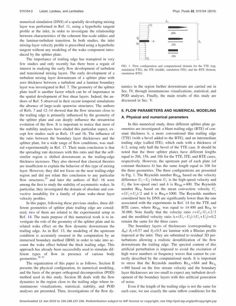
In this numerical study, three different splitter plate ge-ometries are investigated: a blunt trailing edge �BTE� of con-stant thickness h, a more conventional thin trailing edge�TTE� �with a bevel added to the BTE�, and an intermediatetrailing edge �called ITE�, which ends with a thickness ofh /2, using only half the bevel of the TTE case. It should benoted that the three splitter plates have different lengthsequal to 20h, 15h, and 10h for the TTE, ITE, and BTE cases,respectively. However, the upstream part of each plate �ofconstant thickness h� has the same length equal to 10h forthe three geometries. The three configurations are presentedin Fig. 1. The Reynolds number ReML based on the velocitydifference U1−U2 �where U1 is the high-speed velocity andU2 the low-speed one� and h is ReML=400. The Reynoldsnumber ReW based on the mean convection velocity Uc

= �U1+U2� /2 and h is ReW=1000. The Reynolds numbersconsidered here by DNS are significantly lower than the oneassociated with the experiments in Ref. 14 for the TTE andBTE cases, where ReML was equal to 14 400 and ReW to36 000. Note finally that the velocity ratio r=U2 /U1=2 /3and the modified velocity ratio �= �U1−U2� / �U1+U2�=0.2remain the same for the three cases.

The boundary layers of thicknesses �corresponding to�99� �1=0.57 and �2=0.5 are laminar with a Blasius profileimposed at the inlet. They are submitted to residual 3D per-turbations allowing a realistic destabilization of the flowdownstream the trailing edge. The spectral content of thisartificial perturbation is imposed to avoid the excitation ofhigh wave numbers or frequency waves that cannot be cor-rectly described by the computational mesh. It is importantto stress that the Reynolds numbers Re�1

=684 and Re�2=400 based on the free stream velocity and the boundarylayer thicknesses are too small to expect any turbulent devel-opment of the boundary layers with this artificial generationof noise.

Even if the length of the trailing edge is not the same foreach case, we use exactly the same inflow conditions for the

U1

U2

δ1

2δ

Lx

Lyh15h

10h

20h

FIG. 1. Flow configuration and computational domain for the TTE �top,simulation TTE�, the ITE �middle, simulation ITE�, and the BTE �bottom,simulation BTE�.

015104-2 Laizet, Lardeau, and Lamballais Phys. Fluids 22, 015104 �2010�

Downloaded 12 Jan 2010 to 155.198.157.156. Redistribution subject to AIP license or copyright; see http://pof.aip.org/pof/copyright.jsp

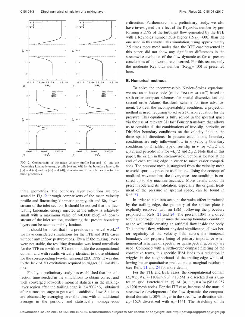
three geometries. The boundary layer evolutions are pre-sented in Fig. 2 through comparisons of the mean velocityprofile and fluctuating kinematic energy, 4h and 8h, down-stream of the inlet section. It should be noticed that the fluc-tuating kinematic energy injected at the inflow is relativelysmall with a maximum value of �0.000 15Uc

2, 4h down-stream of the inlet section, confirming that present boundarylayers can be seen as mainly laminar.

It should be noted that in a previous numerical work,22

we have considered simulations for the TTE and BTE caseswithout any inflow perturbations. Even if the mixing layerswere not stable, the resulting dynamics was found unrealisticfor the TTE case with no 3D motion inside the computationaldomain and with results virtually identical to those obtainedfor the corresponding two-dimensional �2D� DNS. It was dueto the lack of 3D excitations required to trigger 3D instabili-ties.

Finally, a preliminary study has established that the col-lection time needed in the simulations to obtain correct andwell converged low-order moment statistics in the mixing-layer region after the trailing edge is T=300h /Uc, obtainedafter a transient stage to get a well established flow. Statisticsare obtained by averaging over this time with an additionalaverage in the periodic and statistically homogeneous

z-direction. Furthermore, in a preliminary study, we alsohave investigated the effect of the Reynolds number by per-forming a DNS of the turbulent flow generated by the BTEwith a Reynolds number 50% higher �ReML=600� than theone used in this study. This simulation, using approximately2.5 times more mesh nodes than the BTE case presented inthis paper, did not show any significant differences in thestreamwise evolution of the flow dynamic as far as presentconclusions of this work are concerned. For this reason, onlythe moderate Reynolds number �ReML=400� is presentedhere.

B. Numerical methods

To solve the incompressible Navier–Stokes equations,we use an in-house code �called “INCOMPACT3D”� based onsixth-order compact schemes for spatial discretization andsecond order Adams–Bashforth scheme for time advance-ment. To treat the incompressibility condition, a projectionmethod is used, requiring to solve a Poisson equation for thepressure. This equation is fully solved in the spectral spacevia the use of relevant 3D fast Fourier transform that allowsus to consider all the combinations of free-slip, periodic, orDirichlet boundary conditions on the velocity field in thethree spatial directions. In present calculations, boundaryconditions are only inflow/outflow in x �velocity boundaryconditions of Dirichlet type�, free slip in y for −Ly /2 andLy /2, and periodic in z for −Lz /2 and Lz /2. Note that in thispaper, the origin in the streamwise direction is located at theend of each trailing edge in order to make easier compari-sons. The pressure mesh is staggered from the velocity meshto avoid spurious pressure oscillations. Using the concept ofmodified wavenumber, the divergence free condition is en-sured up to the machine accuracy. More details about thepresent code and its validation, especially the original treat-ment of the pressure in spectral space, can be found inRef. 23.

In order to take into account the wake effect introducedby the trailing edge, the geometry of the splitter plate isexplicitly resolved, with an IBM, following the procedureproposed in Refs. 21 and 24. The present IBM is a directforcing approach that ensures the no-slip boundary conditionat the wall while creating an artificial flow inside the body.This internal flow, without physical significance, allows bet-ter regularity of the velocity field across the immersedboundary, this property being of primary importance whennumerical schemes of spectral or quasispectral accuracy areused. Combined with a sixth-order compact filtering of theconvective terms, this specific IBM leads to a reduction inwiggles in the neighborhood of the trailing-edge while al-lowing better quantitative predictions at marginal resolution�see Refs. 21 and 24 for more details�.

For the TTE and BTE cases, the computational domain�Lx�Ly �Lz�= �108h�96h�13.5h� is discretized on a Car-tesian grid �stretched in y� of �nx�ny �nz�= �961�257�120� mesh nodes. For the ITE case, because of the unusualstreamwise development of the flow dynamic, the computa-tional domain is 50% longer in the streamwise direction withLx=162h discretized with nx=1441. The stretching of the

-2

-1

0

1

2

-0.2 0 0.2 0.4 0.6 0.8 1 1.2 1.4

y/h

U/Uc

TTEITE

BTE

-2

-1

0

1

2

-0.2 0 0.2 0.4 0.6 0.8 1 1.2 1.4

y/h

U/Uc

TTEITE

BTE

-2

-1

0

1

2

-5e-05 0 5e-05 0.00015

y/h

k/U2c

TTEITE

BTE

-2

-1

0

1

2

-5e-05 0 5e-05 0.00015

y/h

k/U2

c

TTEITE

BTE

(a) (b)

(c) (d)

FIG. 2. Comparisons of the mean velocity profile ��a� and �b�� and thefluctuating kinematic energy profile ��c� and �d�� for the boundary layers, 4h��a� and �c�� and 8h ��b� and �d��, downstream of the inlet section for thethree geometries.

015104-3 Direct numerical simulation of a mixing layer Phys. Fluids 22, 015104 �2010�

Downloaded 12 Jan 2010 to 155.198.157.156. Redistribution subject to AIP license or copyright; see http://pof.aip.org/pof/copyright.jsp

grid in the y-direction leads to a minimal mesh size of�ymin�0.03h. The time step �t=0.005h /Uc is low enoughto have a Courant–Friedrich–Levy condition of about 0.3.

C. POD analysis

POD offers particular advantages pertinent to the presentstudy. The objective of including POD is to try to identify therelevance and contribution of different modes to the behaviorobserved for each flow configuration. More informationabout POD can be found in Ref. 25. Different types of PODapproaches can be used. Experimentally, this decision is dic-tated by the measurement technique, i.e., for time-accuratemeasurements for which the spatial resolution is poor, suchas hot wire, classical POD can be used.26 For measurementtechniques with good spatial accuracy but poor temporal res-olution, such as particle image velocimetry �PIV�,27 the useof snapshot POD was suggested. The analysis of experimen-tal results for a plane mixing layer, at a Reynolds numberequivalent to the one use in present work, was presented inRef. 28. They showed that in the early stage of the mixing,most of the fluctuating energy is carried by very few modesand that the first two pairs of mode represents convectiveinstabilities, with a phase angle of � /8 between two modesof each pair. However, their analysis was 2D and limited tothe region where Kelvin–Helmholtz vortices are still mainlyhomogeneous in the spanwise direction �no helicoidalmodes�. We propose to go further and analyze the full 3Ddynamics for each simulation.

The snapshot variant has been applied herein, using 4803D snapshots, regularly sampled over 240 time units. Thevelocity field is decomposed into a sum of modes, each mul-tiplied with a corresponding time-dependent coefficient,

ui�x,y,z,t� = �n=1

N

an�t��in�x,y,z� , �1�

where ui�x ,y ,z , t� denotes the velocity component i, an�t� arethe time-dependent �so-called random� coefficients and arerepresentative of the flow dynamic, and the eigenfunctions�i

n�x ,y ,z� are representative of the flow organization. Sincethe flow is statistically homogeneous in the spanwise direc-tion, the empirical eigenfunctions can be regarded as planewaves29 and take the form

�in�x,y,z� = �i

q�x,y,k�exp�− �kz� �2�

with

k = 2�m/Lz, �3�

where q is the so-called quantum number and m is the num-ber of full waves in the homogeneous z-direction.

III. NEAR TRAILING-EDGE REGION

A. Instantaneous flow visualizations

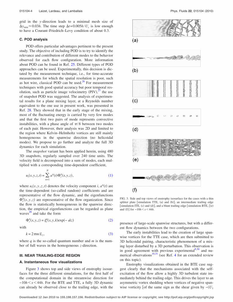
Figure 3 shows top and side views of enstrophy isosur-faces for the three different simulations, for the first half ofthe computational domain in the streamwise direction for−10hx44h. For the BTE and TTE, a fully 3D dynamiccan already be observed close to the trailing edge, with the

presence of large-scale spanwise structures, but with a differ-ent flow dynamics between the two configurations.

The early instabilities lead to the creation of large span-wise vortices for the TTE case, which are then submitted to3D helicoidal pairing, characteristic phenomenon of a mix-ing layer disturbed by a 3D perturbation. This observation isin good agreement with previous experimental9,30 and nu-merical observations10,31 �see Ref. 4 for an extended reviewon this topic�.

Enstrophy visualizations obtained in the BTE case sug-gest clearly that the mechanisms associated with the self-excitation of the flow allow a highly 3D turbulent state im-mediately behind the trailing edge. This drives the layer to anasymmetric vortex shedding where vortices of negative span-wise vorticity �of the same sign as the shear given by −�U1

FIG. 3. Side and top views of enstrophy isosurface for the cases with a thinsplitter plate �simulation TTE, �a� and �b��, an intermediate trailing edge�simulation ITE, �c� and �d��, and a blunt trailing edge �simulation BTE, ��e�and �f�� for −10hx44h.

015104-4 Laizet, Lardeau, and Lamballais Phys. Fluids 22, 015104 �2010�

Downloaded 12 Jan 2010 to 155.198.157.156. Redistribution subject to AIP license or copyright; see http://pof.aip.org/pof/copyright.jsp

−U2� /h� are promoted while their positive counterparts van-ish as the flow evolves in the streamwise direction. It shouldbe noted that no pairing can be observed in the first part ofthe flow, which seems to indicate that the wake effect isplaying a key role in the flow dynamics by delaying thepairing �by comparison with the TTE case where some heli-coidal pairing can be observed close to the trailing edge�.

For the ITE case, only a 2D dynamic can be observed inthe first half of the computational domain, with a lack ofstrong longitudinal vortices between the large-scale spanwisestructures. Even if the boundary layers have been disturbedby 3D perturbations, it seems that the shape of the splitterplate clearly favors the development of 2D primary struc-tures. Moreover, these large-scale vortices, oriented in thespanwise direction with a negative vorticity as in the TTEcase, are found to be clearly more stable with respect to 3Dperturbations compared to the two other cases.

A careful examination of the vortex shedding process inthe ITE case reveals that the formation of the primary struc-ture leads to vortices that are elongated in the horizontaldirection when they detach from the trailing edge. Then,each detached vortex keeps its shape while rotating aroundits center while it is convected further downstream. This spe-cific vortex shedding leads to a phase locking for the rotationof the elongated structures hence formed for a givenx-location, explaining the wavy behavior of the vorticitythickness that can be observed for the ITE case in Sec. III Bin Fig. 4. Note that we have checked in a preliminary 2DDNS of the same case that the wavy evolution of the vortic-ity thickness cannot be attributed to the lack of convergence,this wavy behavior being also recovered for a very long timeof integration.

B. Statistics

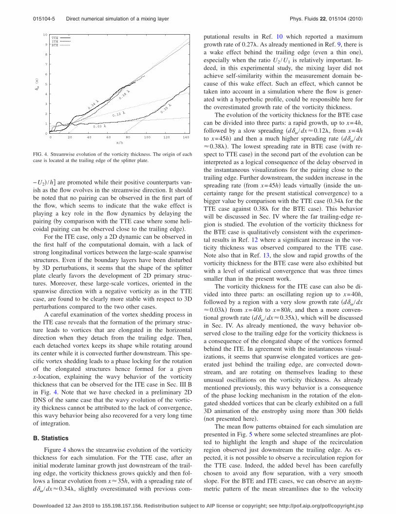
Figure 4 shows the streamwise evolution of the vorticitythickness for each simulation. For the TTE case, after aninitial moderate laminar growth just downstream of the trail-ing edge, the vorticity thickness grows quickly and then fol-lows a linear evolution from x�35h, with a spreading rate ofd� /dx�0.34�, slightly overestimated with previous com-

putational results in Ref. 10 which reported a maximumgrowth rate of 0.27�. As already mentioned in Ref. 9, there isa wake effect behind the trailing edge �even a thin one�,especially when the ratio U2 /U1 is relatively important. In-deed, in this experimental study, the mixing layer did notachieve self-similarity within the measurement domain be-cause of this wake effect. Such an effect, which cannot betaken into account in a simulation where the flow is gener-ated with a hyperbolic profile, could be responsible here forthe overestimated growth rate of the vorticity thickness.

The evolution of the vorticity thickness for the BTE casecan be divided into three parts: a rapid growth, up to x=4h,followed by a slow spreading �d� /dx�0.12�, from x=4hto x=45h� and then a much higher spreading rate �d� /dx�0.38��. The lowest spreading rate in BTE case �with re-spect to TTE case� in the second part of the evolution can beinterpreted as a logical consequence of the delay observed inthe instantaneous visualizations for the pairing close to thetrailing edge. Further downstream, the sudden increase in thespreading rate �from x=45h� leads virtually �inside the un-certainty range for the present statistical convergence� to abigger value by comparison with the TTE case �0.34� for theTTE case against 0.38� for the BTE case�. This behaviorwill be discussed in Sec. IV where the far trailing-edge re-gion is studied. The evolution of the vorticity thickness forthe BTE case is qualitatively consistent with the experimen-tal results in Ref. 12 where a significant increase in the vor-ticity thickness was observed compared to the TTE case.Note also that in Ref. 13, the slow and rapid growths of thevorticity thickness for the BTE case were also exhibited butwith a level of statistical convergence that was three timessmaller than in the present work.

The vorticity thickness for the ITE case can also be di-vided into three parts: an oscillating region up to x=40h,followed by a region with a very slow growth rate �d� /dx�0.03�� from x=40h to x=80h, and then a more conven-tional growth rate �d� /dx�0.35��, which will be discussedin Sec. IV. As already mentioned, the wavy behavior ob-served close to the trailing edge for the vorticity thickness isa consequence of the elongated shape of the vortices formedbehind the ITE. In agreement with the instantaneous visual-izations, it seems that spanwise elongated vortices are gen-erated just behind the trailing edge, are convected down-stream, and are rotating on themselves leading to theseunusual oscillations on the vorticity thickness. As alreadymentioned previously, this wavy behavior is a consequenceof the phase locking mechanism in the rotation of the elon-gated shedded vortices that can be clearly exhibited on a full3D animation of the enstrophy using more than 300 fields�not presented here�.

The mean flow patterns obtained for each simulation arepresented in Fig. 5 where some selected streamlines are plot-ted to highlight the length and shape of the recirculationregion observed just downstream the trailing edge. As ex-pected, it is not possible to observe a recirculation region forthe TTE case. Indeed, the added bevel has been carefullychosen to avoid any flow separation, with a very smoothslope. For the BTE and ITE cases, we can observe an asym-metric pattern of the mean streamlines due to the velocity

0

1

2

3

4

5

6

7

8

9

10

0 20 40 60 80 100 120 140

δ ω(x)

x/h

0.34

λ

0.03 λ

0.35

λ

0.12λ

0.38

λ

TTEITEBTE

FIG. 4. Streamwise evolution of the vorticity thickness. The origin of eachcase is located at the trailing edge of the splitter plate.

015104-5 Direct numerical simulation of a mixing layer Phys. Fluids 22, 015104 �2010�

Downloaded 12 Jan 2010 to 155.198.157.156. Redistribution subject to AIP license or copyright; see http://pof.aip.org/pof/copyright.jsp

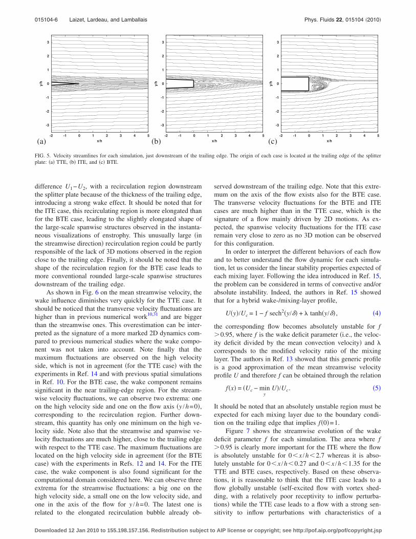
difference U1−U2, with a recirculation region downstreamthe splitter plate because of the thickness of the trailing edge,introducing a strong wake effect. It should be noted that forthe ITE case, this recirculating region is more elongated thanfor the BTE case, leading to the slightly elongated shape ofthe large-scale spanwise structures observed in the instanta-neous visualizations of enstrophy. This unusually large �inthe streamwise direction� recirculation region could be partlyresponsible of the lack of 3D motions observed in the regionclose to the trailing edge. Finally, it should be noted that theshape of the recirculation region for the BTE case leads tomore conventional rounded large-scale spanwise structuresdownstream of the trailing edge.

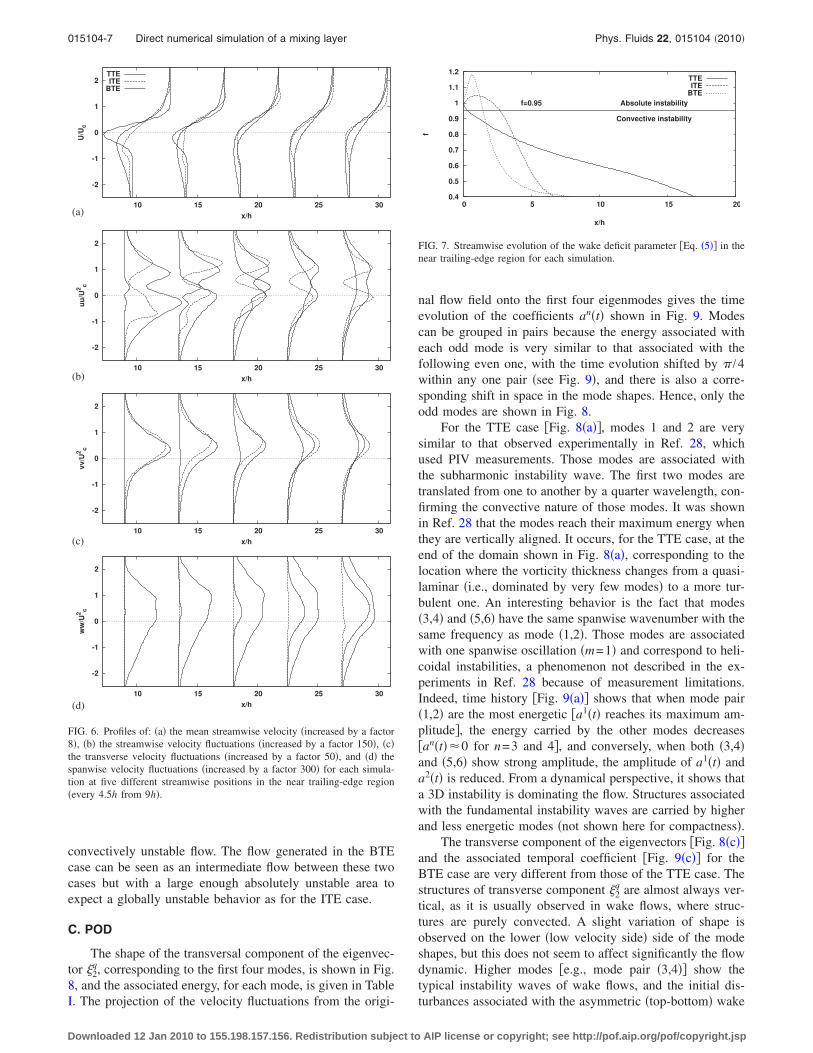
As shown in Fig. 6 on the mean streamwise velocity, thewake influence diminishes very quickly for the TTE case. Itshould be noticed that the transverse velocity fluctuations arehigher than in previous numerical work10,31 and are biggerthan the streamwise ones. This overestimation can be inter-preted as the signature of a more marked 2D dynamics com-pared to previous numerical studies where the wake compo-nent was not taken into account. Note finally that themaximum fluctuations are observed on the high velocityside, which is not in agreement �for the TTE case� with theexperiments in Ref. 14 and with previous spatial simulationsin Ref. 10. For the BTE case, the wake component remainssignificant in the near trailing-edge region. For the stream-wise velocity fluctuations, we can observe two extrema: oneon the high velocity side and one on the flow axis �y /h=0�,corresponding to the recirculation region. Further down-stream, this quantity has only one minimum on the high ve-locity side. Note also that the streamwise and spanwise ve-locity fluctuations are much higher, close to the trailing edgewith respect to the TTE case. The maximum fluctuations arelocated on the high velocity side in agreement �for the BTEcase� with the experiments in Refs. 12 and 14. For the ITEcase, the wake component is also found significant for thecomputational domain considered here. We can observe threeextrema for the streamwise fluctuations: a big one on thehigh velocity side, a small one on the low velocity side, andone in the axis of the flow for y /h=0. The latest one isrelated to the elongated recirculation bubble already ob-

served downstream of the trailing edge. Note that this extre-mum on the axis of the flow exists also for the BTE case.The transverse velocity fluctuations for the BTE and ITEcases are much higher than in the TTE case, which is thesignature of a flow mainly driven by 2D motions. As ex-pected, the spanwise velocity fluctuations for the ITE caseremain very close to zero as no 3D motion can be observedfor this configuration.

In order to interpret the different behaviors of each flowand to better understand the flow dynamic for each simula-tion, let us consider the linear stability properties expected ofeach mixing layer. Following the idea introduced in Ref. 15,the problem can be considered in terms of convective and/orabsolute instability. Indeed, the authors in Ref. 15 showedthat for a hybrid wake-/mixing-layer profile,

U�y�/Uc = 1 − f sech2�y/�� + � tanh�y/�� , �4�

the corresponding flow becomes absolutely unstable for f�0.95, where f is the wake deficit parameter �i.e., the veloc-ity deficit divided by the mean convection velocity� and �corresponds to the modified velocity ratio of the mixinglayer. The authors in Ref. 13 showed that this generic profileis a good approximation of the mean streamwise velocityprofile U and therefore f can be obtained through the relation

f�x� = �Uc − miny

U�/Uc. �5�

It should be noted that an absolutely unstable region must beexpected for each mixing layer due to the boundary condi-tion on the trailing edge that implies f�0�=1.

Figure 7 shows the streamwise evolution of the wakedeficit parameter f for each simulation. The area where f�0.95 is clearly more important for the ITE where the flowis absolutely unstable for 0x /h2.7 whereas it is abso-lutely unstable for 0x /h0.27 and 0x /h1.35 for theTTE and BTE cases, respectively. Based on these observa-tions, it is reasonable to think that the ITE case leads to aflow globally unstable �self-excited flow with vortex shed-ding, with a relatively poor receptivity to inflow perturba-tions� while the TTE case leads to a flow with a strong sen-sitivity to inflow perturbations with characteristics of a

-3

-2

-1

0

1

2

3

-2 -1 0 1 2 3 4 5

y/h

x/h

-3

-2

-1

0

1

2

3

-2 -1 0 1 2 3 4 5

y/h

x/h

-3

-2

-1

0

1

2

3

-2 -1 0 1 2 3 4 5

y/h

x/h(a) (b) (c)

FIG. 5. Velocity streamlines for each simulation, just downstream of the trailing edge. The origin of each case is located at the trailing edge of the splitterplate: �a� TTE, �b� ITE, and �c� BTE.

015104-6 Laizet, Lardeau, and Lamballais Phys. Fluids 22, 015104 �2010�

Downloaded 12 Jan 2010 to 155.198.157.156. Redistribution subject to AIP license or copyright; see http://pof.aip.org/pof/copyright.jsp

convectively unstable flow. The flow generated in the BTEcase can be seen as an intermediate flow between these twocases but with a large enough absolutely unstable area toexpect a globally unstable behavior as for the ITE case.

C. POD

The shape of the transversal component of the eigenvec-tor �2

q, corresponding to the first four modes, is shown in Fig.8, and the associated energy, for each mode, is given in TableI. The projection of the velocity fluctuations from the origi-

nal flow field onto the first four eigenmodes gives the timeevolution of the coefficients an�t� shown in Fig. 9. Modescan be grouped in pairs because the energy associated witheach odd mode is very similar to that associated with thefollowing even one, with the time evolution shifted by � /4within any one pair �see Fig. 9�, and there is also a corre-sponding shift in space in the mode shapes. Hence, only theodd modes are shown in Fig. 8.

For the TTE case �Fig. 8�a��, modes 1 and 2 are verysimilar to that observed experimentally in Ref. 28, whichused PIV measurements. Those modes are associated withthe subharmonic instability wave. The first two modes aretranslated from one to another by a quarter wavelength, con-firming the convective nature of those modes. It was shownin Ref. 28 that the modes reach their maximum energy whenthey are vertically aligned. It occurs, for the TTE case, at theend of the domain shown in Fig. 8�a�, corresponding to thelocation where the vorticity thickness changes from a quasi-laminar �i.e., dominated by very few modes� to a more tur-bulent one. An interesting behavior is the fact that modes�3,4� and �5,6� have the same spanwise wavenumber with thesame frequency as mode �1,2�. Those modes are associatedwith one spanwise oscillation �m=1� and correspond to heli-coidal instabilities, a phenomenon not described in the ex-periments in Ref. 28 because of measurement limitations.Indeed, time history �Fig. 9�a�� shows that when mode pair�1,2� are the most energetic �a1�t� reaches its maximum am-plitude�, the energy carried by the other modes decreases�an�t��0 for n=3 and 4�, and conversely, when both �3,4�and �5,6� show strong amplitude, the amplitude of a1�t� anda2�t� is reduced. From a dynamical perspective, it shows thata 3D instability is dominating the flow. Structures associatedwith the fundamental instability waves are carried by higherand less energetic modes �not shown here for compactness�.

The transverse component of the eigenvectors �Fig. 8�c��and the associated temporal coefficient �Fig. 9�c�� for theBTE case are very different from those of the TTE case. Thestructures of transverse component �2

q are almost always ver-tical, as it is usually observed in wake flows, where struc-tures are purely convected. A slight variation of shape isobserved on the lower �low velocity side� side of the modeshapes, but this does not seem to affect significantly the flowdynamic. Higher modes �e.g., mode pair �3,4�� show thetypical instability waves of wake flows, and the initial dis-turbances associated with the asymmetric �top-bottom� wake

-2

-1

0

1

2

10 15 20 25 30

U/U

c

x/h

TTEITE

BTE

-2

-1

0

1

2

10 15 20 25 30

uu

/U2

c

x/h

-2

-1

0

1

2

10 15 20 25 30

vv/U

2c

x/h

-2

-1

0

1

2

10 15 20 25 30

ww

/U2

c

x/h

(a)

(b)

(c)

(d)

FIG. 6. Profiles of: �a� the mean streamwise velocity �increased by a factor8�, �b� the streamwise velocity fluctuations �increased by a factor 150�, �c�the transverse velocity fluctuations �increased by a factor 50�, and �d� thespanwise velocity fluctuations �increased by a factor 300� for each simula-tion at five different streamwise positions in the near trailing-edge region�every 4.5h from 9h�.

0.4

0.5

0.6

0.7

0.8

0.9

1

1.1

1.2

0 5 10 15 20

f

x/h

f=0.95 Absolute instability

Convective instability

TTEITE

BTE

FIG. 7. Streamwise evolution of the wake deficit parameter �Eq. �5�� in thenear trailing-edge region for each simulation.

015104-7 Direct numerical simulation of a mixing layer Phys. Fluids 22, 015104 �2010�

Downloaded 12 Jan 2010 to 155.198.157.156. Redistribution subject to AIP license or copyright; see http://pof.aip.org/pof/copyright.jsp

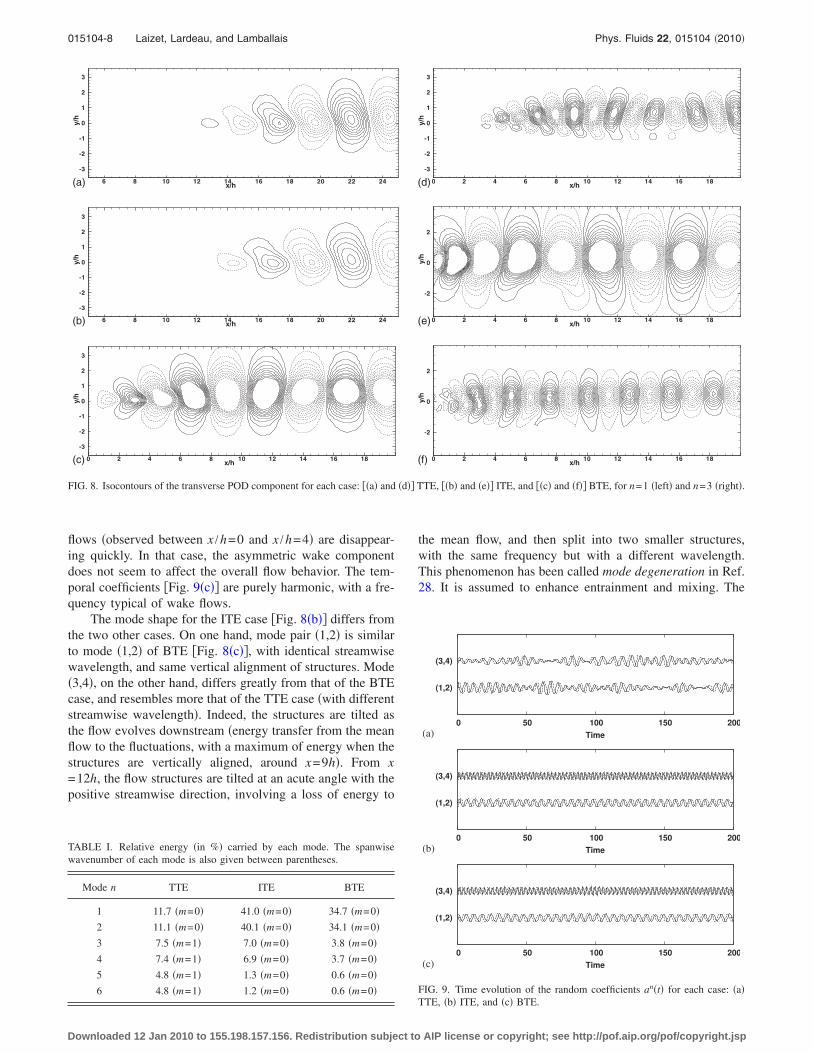
flows �observed between x /h=0 and x /h=4� are disappear-ing quickly. In that case, the asymmetric wake componentdoes not seem to affect the overall flow behavior. The tem-poral coefficients �Fig. 9�c�� are purely harmonic, with a fre-quency typical of wake flows.

The mode shape for the ITE case �Fig. 8�b�� differs fromthe two other cases. On one hand, mode pair �1,2� is similarto mode �1,2� of BTE �Fig. 8�c��, with identical streamwisewavelength, and same vertical alignment of structures. Mode�3,4�, on the other hand, differs greatly from that of the BTEcase, and resembles more that of the TTE case �with differentstreamwise wavelength�. Indeed, the structures are tilted asthe flow evolves downstream �energy transfer from the meanflow to the fluctuations, with a maximum of energy when thestructures are vertically aligned, around x=9h�. From x=12h, the flow structures are tilted at an acute angle with thepositive streamwise direction, involving a loss of energy to

the mean flow, and then split into two smaller structures,with the same frequency but with a different wavelength.This phenomenon has been called mode degeneration in Ref.28. It is assumed to enhance entrainment and mixing. The

x/h

y/h

6 8 10 12 14 16 18 20 22 24

-3

-2

-1

0

1

2

3

x/h

y/h

6 8 10 12 14 16 18 20 22 24

-3

-2

-1

0

1

2

3

x/h

y/h

0 2 4 6 8 10 12 14 16 18

-3

-2

-1

0

1

2

3

(b)

(a)

(c)

x/h

y/h

0 2 4 6 8 10 12 14 16 18

-3

-2

-1

0

1

2

3

x/h

y/h

0 2 4 6 8 10 12 14 16 18

-2

0

2

x/h

y/h

0 2 4 6 8 10 12 14 16 18

-2

0

2

(d)

(f)

(e)

FIG. 8. Isocontours of the transverse POD component for each case: ��a� and �d�� TTE, ��b� and �e�� ITE, and ��c� and �f�� BTE, for n=1 �left� and n=3 �right�.

TABLE I. Relative energy �in %� carried by each mode. The spanwisewavenumber of each mode is also given between parentheses.

Mode n TTE ITE BTE

1 11.7 �m=0� 41.0 �m=0� 34.7 �m=0�2 11.1 �m=0� 40.1 �m=0� 34.1 �m=0�3 7.5 �m=1� 7.0 �m=0� 3.8 �m=0�4 7.4 �m=1� 6.9 �m=0� 3.7 �m=0�5 4.8 �m=1� 1.3 �m=0� 0.6 �m=0�6 4.8 �m=1� 1.2 �m=0� 0.6 �m=0�

(1,2)

(3,4)

0 50 100 150 200

Time

(1,2)

(3,4)

0 50 100 150 200

Time

(1,2)

(3,4)

0 50 100 150 200

Time

(a)

(b)

(c)

FIG. 9. Time evolution of the random coefficients an�t� for each case: �a�TTE, �b� ITE, and �c� BTE.

015104-8 Laizet, Lardeau, and Lamballais Phys. Fluids 22, 015104 �2010�

Downloaded 12 Jan 2010 to 155.198.157.156. Redistribution subject to AIP license or copyright; see http://pof.aip.org/pof/copyright.jsp

mode shape for the ITE case hence shows that two differentbehaviors are competing: the dominating modes are associ-ated with the wake effect, while the secondary modes �3,4�are mixing-layer type. In any case, the modes are spanwisehomogeneous �m=0 for the first six modes, representingabout 98% of the total fluctuating energy�, and the temporalcoefficients again display a purely harmonic behavior.

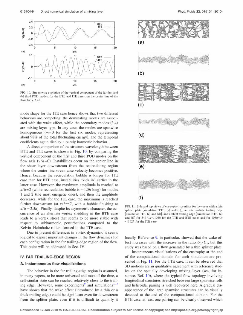
A direct comparison of the structure wavelength betweenBTE and ITE cases is shown in Fig. 10, by comparing thevertical component of the first and third POD modes on theflow axis �y /h=0�. Instabilities occur on the center line inthe shear layer downstream from the recirculating regionwhere the center line streamwise velocity becomes positive.Hence, because the recirculation bubble is longer for ITEcase than for BTE case, instabilities “kick in” earlier in thelatter case. However, the maximum amplitude is reached atx /h=2 �while recirculation bubble is �1.5h long� for modes1 and 2 �the most energetic ones�, and then the amplitudedecreases, while for the ITE case, the maximum is reachedfurther downstream �at x /h�7, with a bubble finishing atx /h�2.5h�. Finally, despite its asymmetric character, the oc-currence of an alternate vortex shedding in the BTE caseleads to a vortex street that seems to be more stable withrespect to subharmonic perturbations compared to theKelvin–Helmholtz rollers formed in the TTE case.

Due to present differences in vortex dynamics, it seemslogical to expect important changes in the flow dynamics foreach configuration in the far trailing-edge region of the flow.This point will be addressed in Sec. IV.

IV. FAR TRAILING-EDGE REGION

A. Instantaneous flow visualizations

The behavior in the far trailing-edge region is assumed,in many papers, to be more universal and most of the time, aself-similar state can be reached relatively close to the trail-ing edge. However, some experiments9 and simulations7,13

have shown that the wake effect �introduced by a thin or athick trailing edge� could be significant even far downstreamfrom the splitter plate, even if it is difficult to quantify it

locally. Reference 9, in particular, showed that the wake ef-fect increases with the increase in the ratio U2 /U1, but thisstudy was based on a flow generated by a thin splitter plate.

Instantaneous visualizations of the enstrophy at the endof the computational domain for each simulation are pre-sented in Fig. 11. For the TTE case, it can be observed that3D motions are in qualitative agreement with reference stud-ies on the spatially developing mixing layer �see, for in-stance, Ref. 10�, where the typical flow topology involvinglongitudinal structures stretched between large spanwise rollsand helicoidal pairing is well recovered here. A gradual dis-appearance of the large spanwise structures can be visuallydetected at the end of the computational domain. For theBTE case, at least one pairing can be clearly observed which

-0.4

-0.2

0

0.2

0.4

0 5 10 15 20

v(y

/h=

0)

x/h

BTEITE

-0.1

0

0.1

0 5 10 15 20

v(y

/h=

0)

x/h

BTEITE

(a)

(b)

FIG. 10. Streamwise evolution of the vertical component of the �a� first and�b� third POD modes, for the BTE and ITE cases, on the center line of theflow for y /h=0.

FIG. 11. Side and top views of enstrophy isosurface for the cases with a thinsplitter plate �simulation TTE, �a� and �b��, an intermediate trailing edge�simulation ITE, �c� and �d��, and a blunt trailing edge �simulation BTE, �e�and �f�� for 54hx108h for the TTE and BTE cases and for 108hx162h for the ITE case.

015104-9 Direct numerical simulation of a mixing layer Phys. Fluids 22, 015104 �2010�

Downloaded 12 Jan 2010 to 155.198.157.156. Redistribution subject to AIP license or copyright; see http://pof.aip.org/pof/copyright.jsp

seems to show that the wake effect disappear with a morelimited effect on the flow dynamic in the far trailing-edgeregion. It is well known that pairing contributes strongly tothe expansion of a mixing layer. Therefore, we could expectto have the same streamwise evolution for the vorticity thick-ness �discussed in Sec. IV B� for the TTE and BTE cases.Again, the large-scale spanwise coherence of structures startsto vanish at the end of the computational domain throughtheir twist by small-scale streamwise vortices. One of themain important points for the ITE case is that the flow dy-namic finally becomes 3D with the occurrence of streamwisevortices stretched between the large-scale spanwise struc-tures. However, these structures are still dominant for theITE case, which confirms that the flow remains strongly in-fluenced by the shape of the trailing edge. Unfortunately, thecomputational domain is not long enough to investigate fur-ther downstream the evolution of the flow and to see if thewake effect will finally disappear as it is observed for theothers cases.

B. Statistics

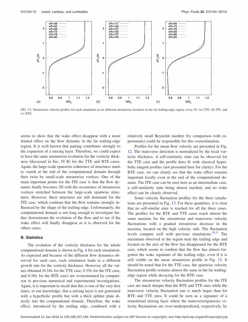
The evolution of the vorticity thickness for the wholecomputational domain is shown in Fig. 4 for each simulation.As expected and because of the different flow dynamics ob-served for each case, each simulation leads to a differentgrowth rate for the vorticity thickness. However, all the val-ues obtained �0.34� for the TTE case, 0.35� for the ITE case,and 0.38� for the BTE case� are overestimated by compari-son to previous numerical and experimental investigations.Again, it is important to recall that this is one of the very firsttimes, to our knowledge, that a mixing layer is not generatedwith a hyperbolic profile but with a thick splitter plate di-rectly into the computational domain. Therefore, the wakeeffect, introduced by the trailing edge, combined with a

relatively small Reynolds number �by comparison with ex-periments� could be responsible for this overestimation.

Profiles for the mean flow velocity are presented in Fig.12. The transverse direction is normalized by the local vor-ticity thickness. A self-similarity state can be observed forthe TTE case and the profile does fit with classical hyper-bolic tangent profiles �not presented here for clarity�. For theBTE case, we can clearly see that the wake effect remainsimportant locally even at the end of the computational do-main. The ITE case can be seen here as an intermediate case,a self-similarity state being almost reached, and no wakeeffect can be clearly observed.

Some velocity fluctuation profiles for the three simula-tions are presented in Fig. 13. For these quantities, it is clearthat no self-similar state is reached for all the three cases.The profiles for the BTE and TTE cases reach almost thesame maxima for the streamwise and transverse velocityfluctuations with a gradual streamwise decrease in themaxima, located on the high velocity side. The fluctuationlevels compare well with previous simulations.10,31 Themaximum observed in the region near the trailing edge andlocated on the axis of the flow has disappeared for the BTEcase, which seems to confirm that the flow has almost for-gotten the wake signature of the trailing edge, even if it isstill visible on the mean streamwise profile in Fig. 12. Itshould be noted that for the TTE case, the spanwise velocityfluctuation profile remains almost the same in the far trailing-edge region while decaying for the BTE case.

The streamwise velocity fluctuation profiles for the ITEcase are much sharper than the BTE and TTE ones while thetransverse velocity fluctuation one is much larger than forBTE and TTE ones. It could be seen as a signature of atransitional mixing layer where the transverse/spanwise ve-locity fluctuations are over-/underpredicted, respectively, by

-2

-1

0

1

2

0.8 0.9 1 1.1 1.2

y/δ ω

(x)

U/Uc

x/h=58x/h=63x/h=68x/h=73x/h=78x/h=83

-2

-1

0

1

2

0.8 0.9 1 1.1 1.2y/

δ ω(x

)U/Uc

x/h=117x/h=122x/h=127x/h=132x/h=137x/h=142

-2

-1

0

1

2

0.8 0.9 1 1.1 1.2

y/δ ω

(x)

U/Uc

x/h=68x/h=73x/h=78x/h=83x/h=88x/h=93

(b)(a) (c)

FIG. 12. Streamwise velocity profiles for each simulation at six different streamwise locations in the far trailing-edge region, every 5h: �a� TTE, �b� ITE, and�c� BTE.

015104-10 Laizet, Lardeau, and Lamballais Phys. Fluids 22, 015104 �2010�

Downloaded 12 Jan 2010 to 155.198.157.156. Redistribution subject to AIP license or copyright; see http://pof.aip.org/pof/copyright.jsp

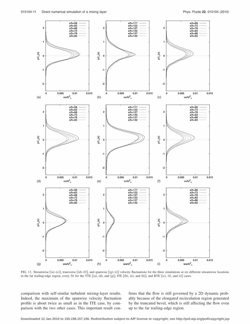
comparison with self-similar turbulent mixing-layer results.Indeed, the maximum of the spanwise velocity fluctuationprofile is about twice as small as in the ITE case, by com-parison with the two other cases. This important result con-

firms that the flow is still governed by a 2D dynamic prob-ably because of the elongated recirculation region generatedby the truncated bevel, which is still affecting the flow evenup to the far trailing-edge region.

-2

-1

0

1

2

0 0.005 0.01 0.015

y/δ ω

(x)

uu/U2c

x/h=58x/h=63x/h=68x/h=73x/h=78x/h=83

-2

-1

0

1

2

0 0.005 0.01 0.015

y/δ ω

(x)

uu/U2c

x/h=117x/h=122x/h=127x/h=132x/h=137x/h=142

-2

-1

0

1

2

0 0.005 0.01 0.015

y/δ ω

(x)

uu/U2c

x/h=68x/h=73x/h=78x/h=83x/h=88x/h=93

-2

-1

0

1

2

0 0.005 0.01 0.015

y/δ ω

(x)

vv/U2c

x/h=58x/h=63x/h=68x/h=73x/h=78x/h=83

-2

-1

0

1

2

0 0.005 0.01 0.015

y/δ ω

(x)

vv/U2c

x/h=117x/h=122x/h=127x/h=132x/h=137x/h=142

-2

-1

0

1

2

0 0.005 0.01 0.015

y/δ ω

(x)

vv/U2c

x/h=68x/h=73x/h=78x/h=83x/h=88x/h=93

-2

-1

0

1

2

0 0.005 0.01 0.015

y/δ ω

(x)

ww/U2c

x/h=58x/h=63x/h=68x/h=73x/h=78x/h=83

-2

-1

0

1

2

0 0.005 0.01 0.015

y/δ ω

(x)

ww/U2c

x/h=117x/h=122x/h=127x/h=132x/h=137x/h=142

-2

-1

0

1

2

0 0.005 0.01 0.015

y/δ ω

(x)

ww/U2c

x/h=68x/h=73x/h=78x/h=83x/h=88x/h=93

(b)(a) (c)

(d) (f)(e)

(g) (h) (i)

FIG. 13. Streamwise ��a�–�c��, transverse ��d�–�f��, and spanwise ��g�–�i�� velocity fluctuations for the three simulations at six different streamwise locationsin the far trailing-edge region, every 5h for the TTE ��a�, �d�, and �g��, ITE ��b�, �e�, and �h��, and BTE ��c�, �f�, and �i�� cases.

015104-11 Direct numerical simulation of a mixing layer Phys. Fluids 22, 015104 �2010�

Downloaded 12 Jan 2010 to 155.198.157.156. Redistribution subject to AIP license or copyright; see http://pof.aip.org/pof/copyright.jsp

C. POD

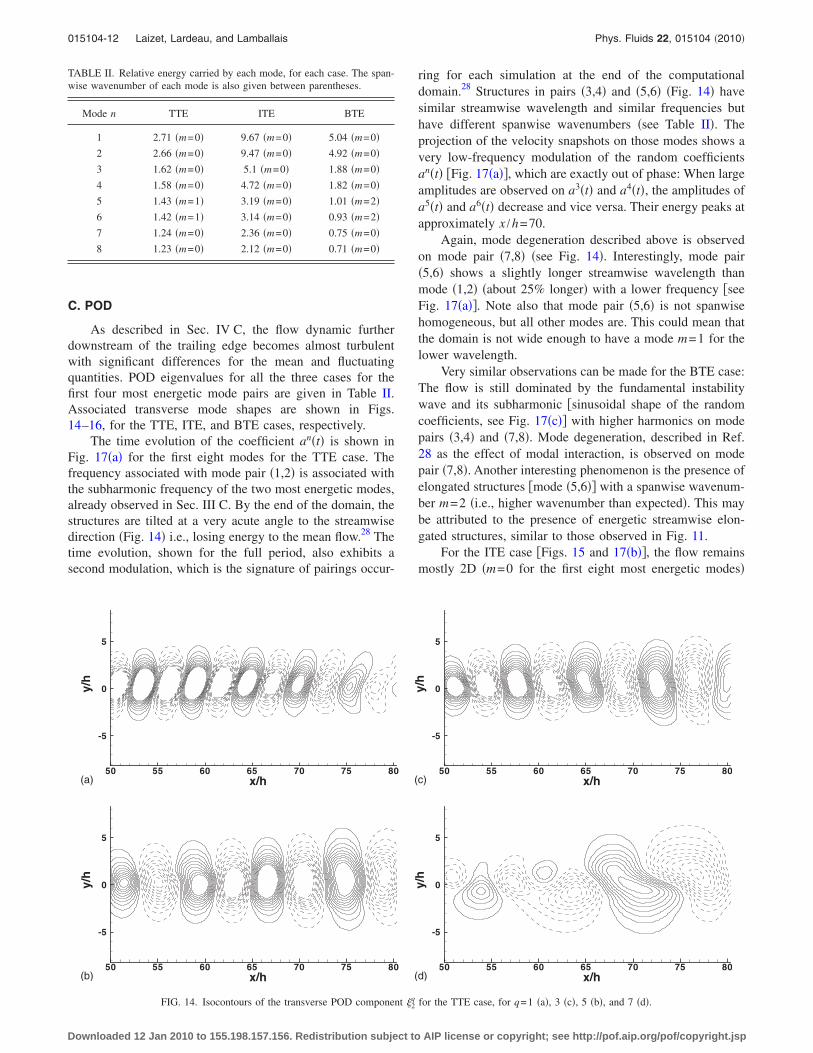
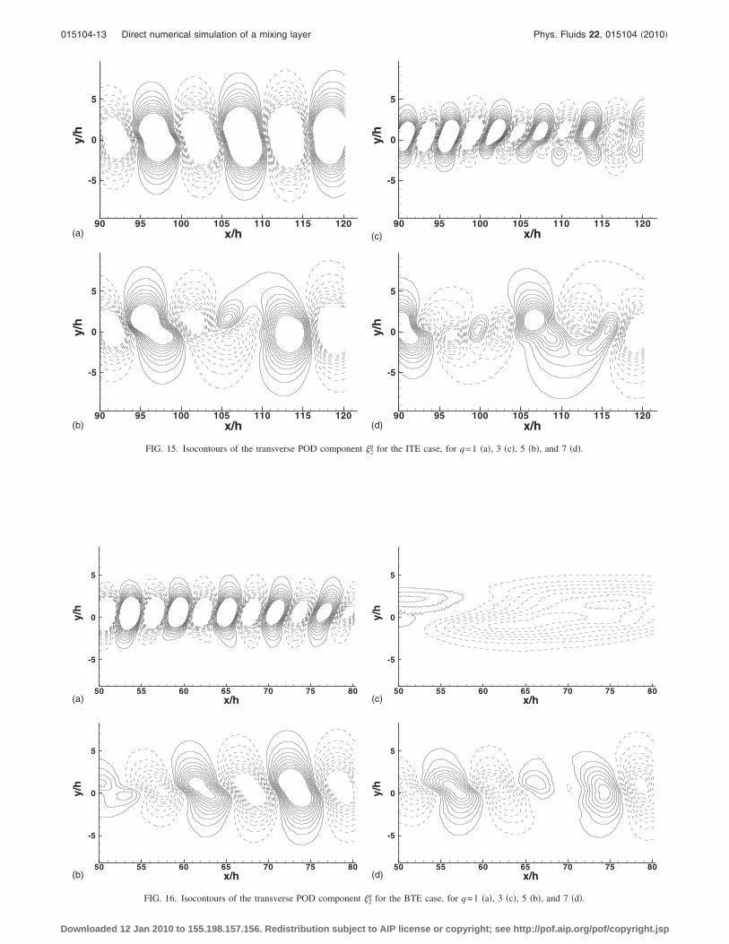
As described in Sec. IV C, the flow dynamic furtherdownstream of the trailing edge becomes almost turbulentwith significant differences for the mean and fluctuatingquantities. POD eigenvalues for all the three cases for thefirst four most energetic mode pairs are given in Table II.Associated transverse mode shapes are shown in Figs.14–16, for the TTE, ITE, and BTE cases, respectively.

The time evolution of the coefficient an�t� is shown inFig. 17�a� for the first eight modes for the TTE case. Thefrequency associated with mode pair �1,2� is associated withthe subharmonic frequency of the two most energetic modes,already observed in Sec. III C. By the end of the domain, thestructures are tilted at a very acute angle to the streamwisedirection �Fig. 14� i.e., losing energy to the mean flow.28 Thetime evolution, shown for the full period, also exhibits asecond modulation, which is the signature of pairings occur-

ring for each simulation at the end of the computationaldomain.28 Structures in pairs �3,4� and �5,6� �Fig. 14� havesimilar streamwise wavelength and similar frequencies buthave different spanwise wavenumbers �see Table II�. Theprojection of the velocity snapshots on those modes shows avery low-frequency modulation of the random coefficientsan�t� �Fig. 17�a��, which are exactly out of phase: When largeamplitudes are observed on a3�t� and a4�t�, the amplitudes ofa5�t� and a6�t� decrease and vice versa. Their energy peaks atapproximately x /h=70.

Again, mode degeneration described above is observedon mode pair �7,8� �see Fig. 14�. Interestingly, mode pair�5,6� shows a slightly longer streamwise wavelength thanmode �1,2� �about 25% longer� with a lower frequency �seeFig. 17�a��. Note also that mode pair �5,6� is not spanwisehomogeneous, but all other modes are. This could mean thatthe domain is not wide enough to have a mode m=1 for thelower wavelength.

Very similar observations can be made for the BTE case:The flow is still dominated by the fundamental instabilitywave and its subharmonic �sinusoidal shape of the randomcoefficients, see Fig. 17�c�� with higher harmonics on modepairs �3,4� and �7,8�. Mode degeneration, described in Ref.28 as the effect of modal interaction, is observed on modepair �7,8�. Another interesting phenomenon is the presence ofelongated structures �mode �5,6�� with a spanwise wavenum-ber m=2 �i.e., higher wavenumber than expected�. This maybe attributed to the presence of energetic streamwise elon-gated structures, similar to those observed in Fig. 11.

For the ITE case �Figs. 15 and 17�b��, the flow remainsmostly 2D �m=0 for the first eight most energetic modes�

TABLE II. Relative energy carried by each mode, for each case. The span-wise wavenumber of each mode is also given between parentheses.

Mode n TTE ITE BTE

1 2.71 �m=0� 9.67 �m=0� 5.04 �m=0�2 2.66 �m=0� 9.47 �m=0� 4.92 �m=0�3 1.62 �m=0� 5.1 �m=0� 1.88 �m=0�4 1.58 �m=0� 4.72 �m=0� 1.82 �m=0�5 1.43 �m=1� 3.19 �m=0� 1.01 �m=2�6 1.42 �m=1� 3.14 �m=0� 0.93 �m=2�7 1.24 �m=0� 2.36 �m=0� 0.75 �m=0�8 1.23 �m=0� 2.12 �m=0� 0.71 �m=0�

x/h

y/h

50 55 60 65 70 75 80

-5

0

5

x/h

y/h

50 55 60 65 70 75 80

-5

0

5

x/h

y/h

50 55 60 65 70 75 80

-5

0

5

x/h

y/h

50 55 60 65 70 75 80

-5

0

5

(b)

(a) (c)

(d)

FIG. 14. Isocontours of the transverse POD component �2q for the TTE case, for q=1 �a�, 3 �c�, 5 �b�, and 7 �d�.

015104-12 Laizet, Lardeau, and Lamballais Phys. Fluids 22, 015104 �2010�

Downloaded 12 Jan 2010 to 155.198.157.156. Redistribution subject to AIP license or copyright; see http://pof.aip.org/pof/copyright.jsp

x/h

y/h

90 95 100 105 110 115 120

-5

0

5

x/h

y/h

90 95 100 105 110 115 120

-5

0

5

x/h

y/h

90 95 100 105 110 115 120

-5

0

5

x/h

y/h

90 95 100 105 110 115 120

-5

0

5

(b)

(a) (c)

(d)

FIG. 15. Isocontours of the transverse POD component �2q for the ITE case, for q=1 �a�, 3 �c�, 5 �b�, and 7 �d�.

x/h

y/h

50 55 60 65 70 75 80

-5

0

5

x/h

y/h

50 55 60 65 70 75 80

-5

0

5

x/h

y/h

50 55 60 65 70 75 80

-5

0

5

x/h

y/h

50 55 60 65 70 75 80

-5

0

5

(b)

(a) (c)

(d)

FIG. 16. Isocontours of the transverse POD component �2q for the BTE case, for q=1 �a�, 3 �c�, 5 �b�, and 7 �d�.

015104-13 Direct numerical simulation of a mixing layer Phys. Fluids 22, 015104 �2010�

Downloaded 12 Jan 2010 to 155.198.157.156. Redistribution subject to AIP license or copyright; see http://pof.aip.org/pof/copyright.jsp

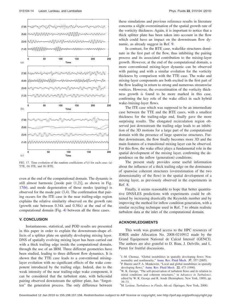
even at the end of the computational domain. The dynamic isstill almost harmonic �mode pair �1,2��, as shown in Fig.17�b�, and mode degeneration of those modes �pairing� isobserved for the mode pair �3,4�. The confirmation that pair-ing occurs for the ITE case in the near trailing-edge regionexplains the relative similarity observed on the growth rate�growth rate between 0.34� and 0.38�� at the end of thecomputational domain �Fig. 4� between all the three cases.

V. CONCLUSION

Instantaneous, statistical, and POD results are presentedin this paper in order to explain the downstream-shape ef-fects of a splitter plate on spatially developing mixing layer.DNS of spatially evolving mixing layer has been carried outwith a thick trailing edge inside the computational domain,through the use of an IBM. Three different geometries havebeen studied, leading to three different flow dynamics. It isshown that the TTE case leads to a conventional mixing-layer evolution with no significant effects of the wake com-ponent introduced by the trailing edge. Indeed, due to theweak intensity of the near trailing-edge wake component, itcan be considered that the turbulent state, with helicoidalpairing observed downstream the splitter plate, has “forgot-ten” the generation process. The only difference between

these simulations and previous reference results in literatureconcerns a slight overestimation of the spatial growth rate ofthe vorticity thickness. Again, it is important to notice that athick splitter plate has been taken into account in the flowwhich could have an impact on the downstream flow dy-namic, as already suggest in Ref. 9.

In contrast, for the BTE case, wakelike structures domi-nate in the first part of the flow, thus inhibiting the pairingprocess and its associated contribution to the mixing-layergrowth. However, at the end of the computational domain, amore conventional mixing-layer dynamic can be observedwith pairing and with a similar evolution for the vorticitythickness by comparison with the TTE case. The wake andmixing-layer components are both excited in the first part ofthe flow leading in return to strong and numerous streamwisevortices. However, the overestimation of the vorticity thick-ness growth is found to be more marked in this case,confirming the key role of the wake effect in such hybridwake-/mixing-layer flows.

The ITE case which was supposed to be an intermediatecase between the TTE and the BTE cases, with a smallestthickness for the trailing-edge end, finally gave the moresurprising results. The elongated recirculation region ob-served just downstream the trailing edge leads to an inhibi-tion of the 3D motions for a large part of the computationaldomain with the presence of large spanwise structures. Fur-ther downstream, the flow finally becomes more 3D and themain features of a transitional mixing layer can be observed.For this flow, the wake effect plays a fundamental role in thespatial development of the mixing layer, confirming the de-pendence on the inflow �generation� conditions.

The present study provides some useful informationabout the influence of a thick trailing edge on the dominanceof spanwise coherent structures �overestimation of the twodimensionality of the flow� in the spatial development of amixing layer, as previously observed in the experiments inRef. 8.

Finally, it seems reasonable to hope that better quantita-tive DNS/LES predictions with experiments could be ob-tained by increasing drastically the Reynolds number and byimproving the method for inflow condition generation, with asimilar recycling technique used in Ref. 7 to obtain realisticturbulent data at the inlet of the computational domain.

ACKNOWLEDGMENTS

This work was granted access to the HPC resources ofIDRIS under Allocation No. 2008-0210912 made by theGrand Equipement National de Calcul Intensif �GENCI�.The authors are also grateful to D. Biau, J. Delville, and L.Perret for fruitful discussions.

1J.-M. Chomaz, “Global instabilities in spatially developing flows: Non-normality and nonlinearity,” Annu. Rev. Fluid Mech. 37, 357 �2005�.

2P. Huerre and P. A. Monkewitz, “Local and global instabilities in spatiallydeveloping flows,” Annu. Rev. Fluid Mech. 22, 473 �1990�.

3W. K. George, “The self-preservation of turbulent flows and its relation toinitial conditions and coherent structures,” in Advances in Turbulence,edited by W. K. George and R. Arndt �Hemisphere, New York, 1989�, pp.39–73.

4M. Lesieur, Turbulence in Fluids, 4th ed. �Springer, New York, 2008�.

(1,2)

(3,4)

(5,6)

(7,8)

0 50 100 150 200 250

Time

(1,2)

(3,4)

(5,6)

(7,8)

0 50 100 150 200 250

Time

(1,2)

(3,4)

(5,6)

(7,8)

0 50 100 150 200

Time

(a)

(b)

(c)

FIG. 17. Time evolution of the random coefficients an�t� for each case: �a�TTE, �b� ITE, and �b� BTE.

015104-14 Laizet, Lardeau, and Lamballais Phys. Fluids 22, 015104 �2010�

Downloaded 12 Jan 2010 to 155.198.157.156. Redistribution subject to AIP license or copyright; see http://pof.aip.org/pof/copyright.jsp

5J. Mathew, I. Mahle, and R. Friedrich, “Effects of compressibility and heatrelease on entrainment processes in mixing layers,” J. Turbul. 9, 14�2009�.

6M. Rogers and R. Moser, “Direct simulation of a self-similar turbulentmixing layer,” Phys. Fluids 6, 903 �1994�.

7N. D. Sandham and R. D. Sandberg, “Direct numerical simulation of theearly development of a turbulent mixing layer downstream of a splitterplate,” J. Turbul. 10, 1 �2009�.

8G. Brown and A. Roshko, “On density effects and large structure in tur-bulent mixing layers,” J. Fluid Mech. 64, 775 �1974�.

9R. D. Metha, “Effect of velocity ratio on plane mixing layer development:Influence of the splitter plate wake,” Exp. Fluids 10, 194 �1991�.

10P. Comte, J. H. Silvestrini, and P. Bégou, “Streamwise vortices in large-eddy simulations of mixing layers,” Eur. J. Mech. B/Fluids 17, 615�1998�.

11Y. Wang, M. Tanahashia, and T. Miyauch, “Coherent fine scale eddies inturbulence transition of spatially-developing mixing layer,” Int. J. HeatFluid Flow 28, 1280 �2007�.

12C. Braud, D. Heitz, G. Arroyo, L. Perret, J. Delville, and J.-P. Bonnet,“Low-dimensional analysis, using POD, for two mixing layer-wake inter-actions,” Int. J. Heat Fluid Flow 25, 351 �2004�.

13S. Laizet and E. Lamballais, “Direct-numerical simulation of the splitting-plate downstream-shape influence upon a mixing layer,” C. R. Acad. Sci.,Ser. IIb: Mec., Phys., Chim., Astron. 334, 454 �2006�.

14L. Perret, J. Delville, and J.-P. Bonnet, “Investigation of the large scalestructures in the turbulent mixing layer downstream a thick plate,” Pro-ceedings of the Third International Symposium on Turbulence and ShearFlow Phenomena, Sendai, Japan, 2003.

15D. Wallace and L. G. Redekopp, “Linear instability characteristics ofwake-shear layers,” Phys. Fluids A 4, 189 �1992�.

16D. A. Hammond and L. G. Redekopp, “Global dynamics of symmetric andasymmetric wakes,” J. Fluid Mech. 331, 231 �1997�.

17B. Dziomba and H. E. Fiedler, “Effect of initial conditions on two-dimensional free shear layers,” J. Fluid Mech. 152, 419 �1985�.

18S. Laizet and J. C. Vassilicos, “Multiscale generation of turbulence,” Jour-nal of Multiscale Modelling 1, 177 �2009�.

19E. Lamballais, J. Silvestrini, and S. Laizet, “Direct numerical simulationof a separation bubble on a rounded finite-width leading edge,” Int. J. HeatFluid Flow 29, 612 �2008�.

20E. Laurendeau, P. Jordan, J. P. Bonnet, J. Delville, P. Parnaudeau, and E.Lamballais, “Subsonic jet noise reduction by fluidic control: The interac-tion region and the global effect,” Phys. Fluids 20, 101519 �2008�.

21P. Parnaudeau, J. Carlier, D. Heitz, and E. Lamballais, “Experimental andnumerical studies of the flow over a circular cylinder at Reynolds number3900,” Phys. Fluids 20, 085101 �2008�.

22S. Laizet and E. Lamballais, “Direct numerical simulation of a spatiallyevolving flow from an asymmetric wake to a mixing layer,” Direct andLarge-Eddy Simulation VI �Springer, Poitiers, 2006�.

23S. Laizet and E. Lamballais, “High-order compact schemes for incom-pressible flows: A simple and efficient method with quasi-spectral accu-racy,” J. Comput. Phys. 228, 5989 �2009�.

24P. Parnaudeau, E. Lamballais, D. Heitz, and J. H. Silvestrini, “Combina-tion of the immersed boundary method with compact schemes for DNS offlows in complex geometry,” Direct and Large-Eddy Simulation V�Springer, Munich, 2003�.

25P. Holmes, J. L. Lumley, and G. Berkooz, Turbulence, Coherent Struc-tures, Dynamical Systems and Symmetry �Cambridge University Press,Cambridge, 1996�.

26J. Delville, “Characterization of the organization in shear layers via theproper orthogonal decomposition,” Appl. Sci. Res. 53, 263 �1994�.

27L. Sirovich, “Turbulence and the dynamics of coherent structures. Part 1:Coherent structures,” Q. J. Mech. Appl. Math. 45, 561 �1987�.

28M. Rajaee, S. K. F. Karlsson, and L. Sirovich, “Low-dimensional descrip-tion of free-shear-flow coherent structures and their dynamical behaviour,”J. Fluid Mech. 258, 1 �1994�.

29L. Sirovich, K. S. Ball, and L. R. Keefe, “Plane waves and structures inturbulence channel flow,” Phys. Fluids A 2, 2217 �1990�.

30F. K. Browand and T. R. Troutt, “A note on spanwise structure in thetwo-dimensional mixing layer,” J. Fluid Mech. 93, 325 �1980�.

31P. Comte, M. Lesieur, and E. Lamballais, “Large- and small-scale stirringof vorticity and a passive scalar in a 3-D temporal mixing layer,” Phys.Fluids A 4, 2761 �1992�.

015104-15 Direct numerical simulation of a mixing layer Phys. Fluids 22, 015104 �2010�

Downloaded 12 Jan 2010 to 155.198.157.156. Redistribution subject to AIP license or copyright; see http://pof.aip.org/pof/copyright.jsp