


Bahasa
Halaman
Hukum


1 23
Stochastic EnvironmentalResearch and Risk Assessment ISSN 1436-3240 Stoch Environ Res Risk AssessDOI 10.1007/s00477-011-0515-3
DEM-based numerical modelling of runoffand soil erosion processes in the hilly–gully loess regions
Tao Yang, Chong-yu Xu, Qiang Zhang,Zhongbo Yu, Alexander Baron, XiaoyanWang & Vijay P. Singh

1 23
Your article is protected by copyright and
all rights are held exclusively by Springer-
Verlag. This e-offprint is for personal use only
and shall not be self-archived in electronic
repositories. If you wish to self-archive your
work, please use the accepted author’s
version for posting to your own website or
your institution’s repository. You may further
deposit the accepted author’s version on a
funder’s repository at a funder’s request,
provided it is not made publicly available until
12 months after publication.

ORIGINAL PAPER
DEM-based numerical modelling of runoff and soil erosionprocesses in the hilly–gully loess regions
Tao Yang • Chong-yu Xu • Qiang Zhang •
Zhongbo Yu • Alexander Baron • Xiaoyan Wang •
Vijay P. Singh
� Springer-Verlag 2011
Abstract For sake of improving our current understand-
ing on soil erosion processes in the hilly–gully loess
regions of the middle Yellow River basin in China, a
digital elevation model (DEM)-based runoff and sediment
processes simulating model was developed. Infiltration
excess runoff theory was used to describe the runoff gen-
eration process while a kinematic wave equation was
solved using the finite-difference technique to simulate
concentration processes on hillslopes. The soil erosion
processes were modelled using the particular characteris-
tics of loess slope, gully slope, and groove to characterize
the unique features of steep hillslopes and a large variety of
gullies based on a number of experiments. The constructed
model was calibrated and verified in the Chabagou catch-
ment, located in the middle Yellow River of China and
dominated by an extreme soil-erosion rate. Moreover,
spatio-temporal characterization of the soil erosion pro-
cesses in small catchments and in-depth analysis between
discharge and sediment concentration for the hyper-con-
centrated flows were addressed in detail. Thereafter, the
calibrated model was applied to the Xingzihe catchment,
which is dominated by similar soil erosion processes in the
Yellow River basin. Results indicate that the model is
capable of simulating runoff and soil erosion processes in
such hilly–gully loess regions. The developed model are
expected to contribute to further understanding of runoff
generation and soil erosion processes in small catchments
characterized by steep hillslopes, a large variety of gullies,
and hyper-concentrated flow, and will be beneficial to
water and soil conservation planning and management for
catchments dealing with serious water and soil loss in the
Loess Plateau.
Keywords Hilly–gully loess region � The Yellow River �High sediment concentration � Runoff � Soil erosion
processes � DEM-based model � Parameter sensitivity
analysis
1 Introduction
The Loess Plateau, located in the middle Yellow River
basin of China, has been commonly reported for the most
serious soil erosion and water losses all over the world
(World Wildlife Fund (WWF) 2004). About 73% of the
eroded soil enters the Yellow River, causing enormous
amounts of sedimentation and a high risk of flooding
T. Yang (&)
State Key Laboratory of Desert and Oasis Ecology,
Xinjiang Institute of Ecology and Geography, Chinese Academy
of Sciences, CAS, 818, Road BeijingNan, Urumqi,
Xinjiang 830011, The People’s Republic of China
e-mail: [email protected]
T. Yang � A. Baron � X. Wang
State Key Laboratory of Hydrology-Water Resources
and Hydraulic Engineering, Hohai University,
Nanjing 210098, China
C. Xu
Department of Geosciences, University of Oslo, Blindern,
P.O. Box 1047, Oslo 0316, Norway
Q. Zhang
Department of Water Resources and Environment, Sun Yat-sen
University, Guangzhou 510275, China
Z. Yu
Department of Geoscience, University of Nevada Las Vegas,
Las Vegas, NV 89154-4010, USA
V. P. Singh
Department of Biological and Agricultural Engineering, Texas A
& M University, College Station, TX 77843-2117, USA
123
Stoch Environ Res Risk Assess
DOI 10.1007/s00477-011-0515-3
Author's personal copy

downstream. Over 60% of the Loess Plateau suffers from
soil erosion as a result of irrational land use and poor
vegetation coverage, which have negatively impacted
regional eco-environments (BREST-CAS 1992; Fu 1989;
Fu and Gulinck 1994; Shi and Shao 2000; Yang et al. 2008,
2009a, 2009b). Agriculture accounts for a high percentage
of the local economic development; however, centuries of
deforestation and over-grazing, exacerbated by China’s
population increase, have resulted in degenerated ecosys-
tems, desertification, and poor local economies (Chen et al.
2001). The soil loss in the basin can reach four billion tons
per year due to deforestation and agricultural cultivation on
hillsides (WWF 2004).
With the recognition of the negative impacts of soil
erosion on the environment, a number of water and soil
conservation measures have been implemented in the
catchments of the Loess Plateau to control soil erosion,
maintain a healthy eco-environment and regional sustain-
able development since the 1950s. In 1999, the government
initiated a nationwide project to set aside cropland for
afforestation and soil conservation, known as the Grain-
for-Green Program, which has been recognized as one of
the world’s largest conservation projects (WWF 2004).
The Loess Plateau is one of the major target areas in the
Grain-for-Green Program. The program requested that
arable land with a slope higher than 25.8� should be con-
verted into woodland and pasture. Due to a vast cover area
(640,000 km2) and very rich coal resource, the Loess
Plateau is very important to regional eco-environmental
security and the sustainable development of western China
(Yang et al. 2009a). For this purpose, modelling of runoff
and sediment processes are of paramount importance to
understanding the soil erosion processes and formulating
effective countermeasures for soil erosion control for the
region.
Physically-based models such as ANSWERS (Beasley
et al. 1980), WEPP (Nearing et al. 1989), EUROSEM
(Morgan et al. 1998), GUEST (Misra and Rose 1989), and
LISEM (De Roo et al. 1996) are now widely accepted
mathematical models for simulating soil erosion processes.
Murakami et al. (2001) coupled the SWM model with
sediment discharge from overland flow to predict the out-
flow of soil from an agricultural watershed. Parlange et al.
(1999) and Hairsine and Rose (1991) developed a soil
erosion model to elucidate the rainstorm-induced sediment
transport process. Wongsa et al. (2002) developed a one-
dimensional hydrodynamic model for simulation of
mountain river systems by combining a kinematic runoff
model, hillslope erosion model, and sediment transport
model of a river channel. Chen et al. (2006) developed a
physiographic soil erosion–deposition model (PSD) by
coupling GIS with a physiographic typhoon-induced storm
event-based rainfall-runoff model for a tropical catchment
in Taiwan. Masoudi et al. (2006) developed a new model
for assessing the risk of water erosion, taking into con-
sideration nine indicators of water erosion the model
identifies areas with ‘Potential Risk’ (risky zones) and
areas of ‘Actual Risk’ as well as projects the probability of
the worse degradation in future. These models provide
significant insights into the dynamic processes of soil
erosion and sediment yield in watersheds.
However, the aforementioned models do not reflect the
unique characteristics of runoff and soil erosion processes
in loess regions with steep hillslopes, a number of gullies of
various sizes, and a high concentration of highly coarse
sediment. Therefore, they cannot be applied directly to
simulate runoff and sediment yield processes on the hilly
and gully-covered Loess Plateau of China. To overcome
these limitations, Tang and Chen (1990, 1997) developed
the Hohai University Model (HUM) with the aim of sim-
ulating runoff and sediment processes in small- and med-
ium-size river basins based on differential kinematic wave
theories, and used it to simulate those processes in hilly
Loess Plateau regions. Xie et al. (1990) developed a sedi-
ment yield model for medium- and large-size river basins.
Cai and Lu (1998, 1996) took into account the complex
topographical factors and spatial variability of sediment
yield in the loess region of northwestern China in modeling
runoff and sediment yield processes. It should be noted that
there are still several critical limitations to the models
mentioned above when they are used in a loess region: (1)
It is essential to build an appropriate GRID-based runoff
and sediment processes model for small catchments which
is capable of simulating spatial and temporal runoff-
induced soil erosion processes in this hilly–gully loess
region. However, reports addressing models that feature
these unique runoff and sediment processes are insufficient
so far. (2) A stream network that is not extracted using GIS
does not properly demonstrate the influence of the topog-
raphy of the river basin on runoff and sediment yield. (3)
Spatio-temporal characterization of the soil erosion pro-
cesses in small catchments and in-depth analysis between
discharge and sediment concentration in the hilly–gully
loess regions are still very limited. Therefore, this work
aimed: (1) to construct a Digital Elevation Model (DEM)-
based runoff and sediment model for sake of more precise
simulating based on improvement of the HUM model
developed by Tang and Chen (1990, 1997) and Yang et al.
(2005, 2007) for small catchments in the hilly and gully
region in order to understand the complex sediment
processes; (2) to assess the spatio-temporal soil erosion
processes based on topographical and geophysical charac-
teristics of loess slopes, gully slopes, and grooves of two
typical catchments in the middle Yellow River basin, the
Chabagou and Xingzihe catchments; and (3) to conduct
sensitivity analysis of the major model parameters using
Stoch Environ Res Risk Assess
123
Author's personal copy
Monte Carlo simulations to quantify different effects of
parameter sets for sake of parameter optimization in further
studies.
2 Study domain and data
2.1 Study domain
A DEM-based runoff and sediment processes numerical
model at the rainstorm event scale requires: (1) that the
study domain have adequate land cover data at a high
resolution (e.g., DEM, soil type distribution, vegetation
cover, and land use patterns, Bek and Jezek 2011), and
high-density runoff and sediment observations; and (2) that
the drainage area of the catchment not be too large (i.e.
\2000 km2) to investigate the physical runoff and sedi-
ment processes at this catchment scale, nor too small (i.e.
[100 km2) for application in actual practices of water and
soil loss planning and management in the catchments
(normally, 100–2000 km2 scale) of the Loess region.
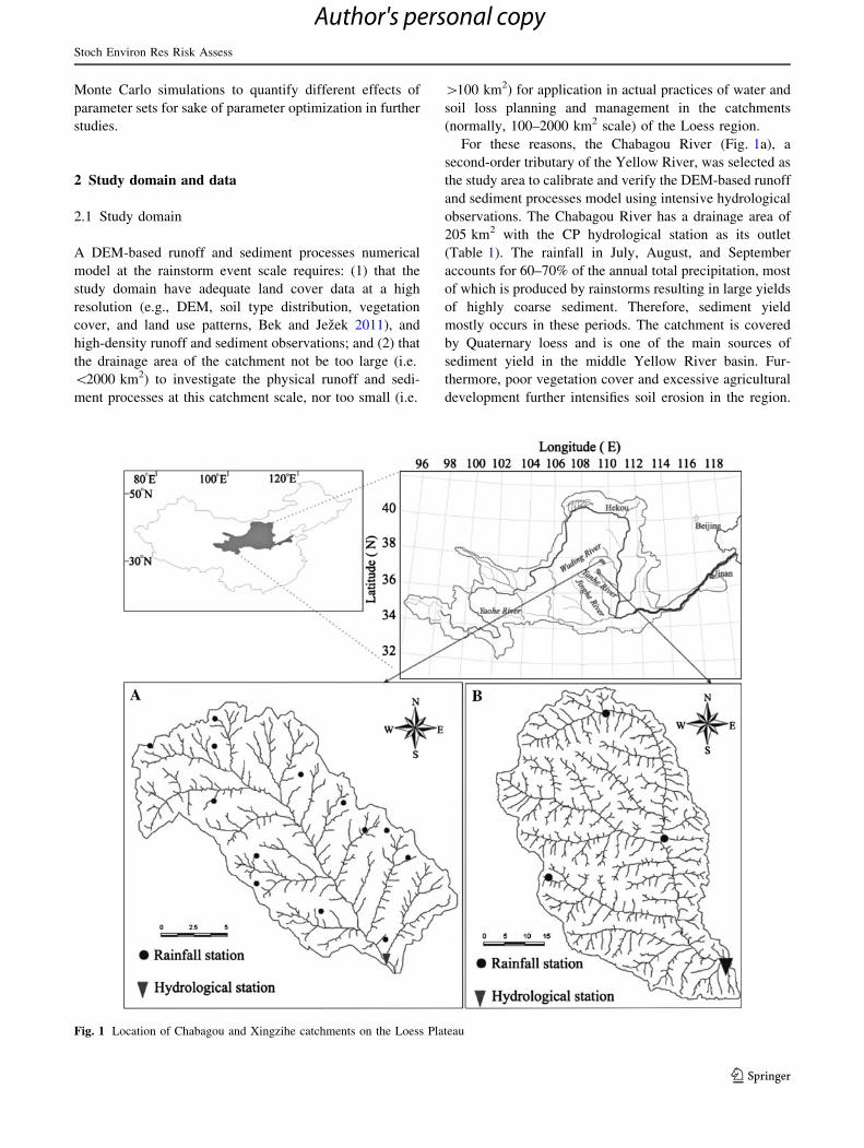
For these reasons, the Chabagou River (Fig. 1a), a
second-order tributary of the Yellow River, was selected as
the study area to calibrate and verify the DEM-based runoff
and sediment processes model using intensive hydrological
observations. The Chabagou River has a drainage area of
205 km2 with the CP hydrological station as its outlet
(Table 1). The rainfall in July, August, and September
accounts for 60–70% of the annual total precipitation, most
of which is produced by rainstorms resulting in large yields
of highly coarse sediment. Therefore, sediment yield
mostly occurs in these periods. The catchment is covered
by Quaternary loess and is one of the main sources of
sediment yield in the middle Yellow River basin. Fur-
thermore, poor vegetation cover and excessive agricultural
development further intensifies soil erosion in the region.
Fig. 1 Location of Chabagou and Xingzihe catchments on the Loess Plateau
Stoch Environ Res Risk Assess
123
Author's personal copy

Another similar hilly–gully loess region of the middle
Yellow River basin, the Xingzihe River catchment
(Fig. 1b; Table 1) is also characterized by high soil loss
rates in China. The main stream of the Xingzihe River is
102.8 km long and has a drainage area of 1,486 km2 at
Xingzihe Station. The calibrated model was applied to the
Xingzihe catchment to assess the model’s ability in simu-
lating runoff and sediment processes in the Loess Plateau
region.
2.2 Data
Observation data from seventeen typical storm events,
including half-hourly rainfall, streamflow, and sediment
load data from the CP gauge of the Chagbagou catchment
in the middle Yellow River basin (1970–2001), were col-
lected and used in this study (Table 2). These observations
were compiled and provided by the Hydrology Bureau of
the Yellow River Conservancy Commission (YRCC) of
China. Among these observations, nine storm events were
used for model calibration and the other eight were used for
validation. The slope, soil type, vegetation cover, land use,
Manning roughness, and erosion distribution of the catch-
ment are widely recognized as the basic information for a
runoff and sediment processes model (Chen et al. 2001;
Chen et al. 2006). Mean slope, land use, and topographical
features of the Chabagou catchment were extracted from
the catchment DEM and a Landsat ETM remote sensing
image with a grid resolution of 20 m 9 20 m, using the
ArcGIS software package and ERDAS image processing
tools (Yang et al. 2007). Raw soil distribution, vegetation
cover, and erosion distribution data were provided by the
YRCC, and processed using ArcGIS into raster format with
a 20 m 9 20 m resolution. Manning’s roughness parame-
ters were assigned to the study area in terms of the rec-
ommended Manning’s coefficients for overland flow linked
with different land use types (Engman 1986; Table 3).
Details can be found in the report by Yang (2007).
Table 1 List of hydrological and sediment stations for two typical catchments on the hilly–gully Loess Plateau
No. Stations Location Catchment Drainage area (km2)
1. CP-Caoping 110.25�E 37.14�N Cabagou Catchment 205
2. XH-Xinghe 110.52�E 37.42�N Xingzihe Catchment 1,486
Source of data: Hydrology Bureau, Yellow River Conservancy Commission
Table 2 List of selected storm events used for model calibration and
validation in Cabagou Catchment
No. Selected
storm
events
Total
rainfall
(mm)
Runoff
peak
(m3/s)
Sediment
peak
(kg/m3)
Purpose
1 19700701 10.2 70 875 Calibration
2 19700702 58.4 532 854 Calibration
3 19710701 14.8 131 741 Calibration
4 19720702 24.7 119 875 Calibration
5 19740702 59.7 106 742 Calibration
6 19780802 45.2 180 855 Calibration
7 19790701 18.9 32 858 Calibration
8 19800701 13.4 18.1 765 Calibration
9 19830702 35.8 88.8 911 Calibration
10 19880703 46.2 119 647 Validation
11 19890701 66.6 309 822 Validation
12 19940804 65.6 313 776 Validation
13 19950902 42.7 313 673 Validation
14 19960731 43.5 315 685 Validation
15 19990720 24.8 133 518 Validation
16 20000704 14.3 141 687 Validation
17 20010818 39.3 183 714 Validation
Source of data: Hydrology Bureau, Yellow River Conservancy
Commission
Table 3 Recommended Manning’s coefficients for overland flow
Cover or treatment Value recommended Range
Concrete or asphalt 0.011 0.010–0.013
Bare sand 0.01 0.010–0.016
Graveled surface 0.02 0.012–0.03
Bare clay—loam (eroded) 0.02 0.012–0.033
Fallow—no residue 0.05 0.006–0.16
Chisel plow 0.07 0.006–0.17
Disk/harrow 0.08 0.008–0.41
No till 0.04 0.03–0.07
Moldboard plow (Fall) 0.06 0.02–0.10
Coulter 0.10 0.05–0.13
Range (natural) 0.13 0.01–0.32
Range (Clipped) 0.10 0.02–0.24
Grass (bluegrass sod) 0.45 0.39–0.63
Short grass prairie 0.15 0.10–0.20
Dense grass 0.24 0.17–0.30
Bermuda grass 0.41 0.30–0.46s
Source: Engman 1986
Stoch Environ Res Risk Assess
123
Author's personal copy

3 Model structure
3.1 Overview of model components
A DEM-based model, utilizing the simplified St. Venant
equations over grid cells with the finite-difference numer-
ical solution, was developed to simulate the runoff and
sediment yield processes. The structure of the model is
shown in Fig. 2. The model parameters were calibrated
using nine observed storm events. The runoff and sediment
yield were routed from cell to cell in order to obtain the
processes at the catchment outlet. The soil-dependent
infiltration for each discretized cell was computed using the
Horton infiltration model. The cell topographical proper-
ties, including elevation, land use, and comprehensive
roughness for each discretized cell of the catchment, were
extracted using the GIS. In modeling storm events with
short durations, which are very common in arid areas,
actual evapotranspiration can be ignored. The calculation
procedure and major equations of the runoff and sediment
yield simulation model presented in the following sections
were modified from Tang and Chen (1990, 1997), Tang
(2003), and Yang et al. (2005, 2007). More detailed
information about the calculation procedure and major
equations can be referred to these literatures. For the sake
of better understanding of the modelling results, major
equations of the model are briefly presented in the
following section. In particular, this paper mainly presents
the spatio-temporal soil erosion processes using the DEM-
based sediment model, offers profound discussions of the
scaling and uncertainty issues in soil erosion processes with
aims to construct a series of runoff and soil erosion pro-
cesses models in the hilly–gully loess region eventually.
3.2 Infiltration excess runoff generation
The infiltration excess runoff generation is calculated as
follows:
RS ¼ 0 PE�FPE � F PE [ F
�ð1Þ
where RS is the excess runoff (mm/min), PE (mm/min) is
the precipitation minus evapotranspiration, and F is the
infiltration (mm/min). In this study, evapotranspiration was
ignored for high-intensity rainfall events with short
durations. Thus, PE = P, and
RS ¼ 0 P�FP� F P [ F
�ð2Þ
where P is precipitation (mm/min). The Horton infiltration
model was used in this study because of its clear physical
basis and simplicity. The Horton infiltration model is
ft ¼ fc þ f 0� fcð Þe�kdt ð3Þ
Com
putation priority
Infiltration
{ FP
FPFPRS≤
−= 0 Excess runoff
Overland runoff
Outlet sediment
Outlet discharge
Com
putation priority
Runoff generation component Runoff concentration component Soil erosion component
Precipitation
V, q, h
Soil erosion e Gully slope e2
Loess slope e1
Groove e3
Fig. 2 Overview of model structure and components
Stoch Environ Res Risk Assess
123
Author's personal copy

where ft is the infiltration rate at time t (mm/min); fc is the
constant or equilibrium infiltration rate after soil has been
saturated, or the minimum infiltration rate (mm/min); f0 is
the initial infiltration rate (mm/min); and kd is a decay
constant specific to the soil conditions (dimensionless).
3.3 Overland runoff computation
The partial differential equation for describing kinematic
wave flow, which is suitable for overland flow computation
for the steeper slopes in the Loess Plateau region, is as
follows:
oq
oxþ oh
ot¼ reðtÞ ð4Þ
Sf ¼ S0 ð5Þ
where q is the overland discharge per unit width (m2/s), h
is the water depth (m), x is the streamwise distance (m),
t is time (s), re(t) is the rainfall excess, or lateral inflow
(mm/min), Sf is the friction-induced head loss per unit
length between the moving fluid and the bed (m/m), and S0
is the slope of the land surface (m/m).
Equation 5 can be replaced with the Darcy–Weisbach
equation (Tang and Chen 1990, 1997):
Sf ¼ S0 ¼ fq2
8gh2Rð6Þ
where f is the Darcy–Weisbach friction loss coeffi-
cient (dimensionless), which can be determined from a
Moody diagram; g is the local gravitational acceleration
(g & 9.8 m/s2); and R is the hydraulic radius (here R = h for
overland flow (m)). Equation 5 can also be replaced by
Eq. 7:
v ¼ 1
nh
23S
12 ð7Þ
and
q ¼ 1
nh1þ2
3S12 ð8Þ
where n is the Manning’s roughness (dimensionless), S is
the slope of the flow surface (m/m), and S & S0 is
gradually varied flow. If r ¼ 23; k ¼ 1
2; e ¼ 1þ
r; and Ks ¼ 1n Sk
0; then Eqs. 7 and 8 can be written as
v ¼ Kshr ð9Þ
and
q ¼ Kshe ð10Þ
where Ks is the hydraulic roughness coefficient (dimen-
sionless), and e is a weighting factor in the Preissmann
implicit scheme (dimensionless). Thus, a first-order non-
linear differential equation can be derived as follows:
oq
oxþ 1
K1es
1
eq
1�ee
oq
ot¼ reðtÞ ð11Þ
where the boundary conditions are
qð0; tÞ ¼ 0 for t [ 0
qðx; 0Þ ¼ 0 for 0� x� l1 þ l2
reðtÞ ¼ 0 for t [ TreðtÞ ¼ QðtÞ for 0� t� T
8>><>>:where l1 is the length of the loess slope (m), l2 is the length
of the gully slope (m), T is the full duration of a storm
event (min), and Q(t) is accumulated runoff production
(mm).
A Preissmann implicit scheme is used to solve Eq. 11
for q as follows:
h2
qnþ1jþ1
� �1�ee þ qnþ1
j
� �1�ee
� �þ 1� h
2qn
jþ1
� �1�ee þ qn
j
� �1�ee
� �� �
�qnþ1
jþ1 � qnjþ1 þ qnþ1
j � qnj
2Dt¼ reðtÞ ð12Þ
where h is a weighting factor. With the Newton iterative
method, water depth and velocity of overland flow are
computed along the flow path at any time and place. More
details on the technical solution of the kinematic equation
for the Loess Plateau region can be found in previous lit-
erature (Tang and Chen 1990, 1997).
3.4 Sediment yield computation
Generally, the Loess Plateau soil erosion forms can be
categorized into three typical types: loess slope, gully
slope, and groove (Tang and Chen 1990, 1997; Yao and
Tang 2001; see Fig. 3). The soil erosion rates for gully
areas of the Loess Plateau can be derived from the energy
balance principle.
3.4.1 Loess slope erosion
The power of soil erosion on a loess slope per unit area
(Tang and Chen 1990, 1997; Yao and Tang 2001), Ws1; can
be determined as follows:
Ws1 ¼ g1
cs � cm
cm
e1 � g � tga1 ð13Þ
where g1 is a distance related coefficient 1m
� for loess slope
erosion, cs and cm are the bulk densities of dry and wet
sediments (kg/m3), respectively; e1 is the soil erosion rate
of the loess slope (kg/s); and a1 is the degree (or angle) of
the loess slope (�).
The effective power of soil erosion of the loess slope per
unit area (Tang and Chen 1990, 1997; Yao and Tang 2001),
Wf1, can be computed as follows:
Stoch Environ Res Risk Assess
123
Author's personal copy

Wf 1 ¼ A so � scð ÞV ð14Þ
where so is the shear stress (N/m2), sc is the critical yield
stress (N/m2), V is the cross-sectional average velocity of
surface flow (m/s), and A is a non-dimensional coefficient.
If Ws1 = Wf1, then
e1 ¼ A1
cm
cs � cm
so � scð ÞV ð15Þ
where A1 ¼ Ag�g1�tga1
is calibrated using the monitoring data,
and cm can be obtained from Eqs. 16, 17 and 18 as follows:
cm ¼ cþ 1� ccs
�SC ð16Þ
SC ¼ 1000c 1� Qc
Qh
�ð17Þ
Qh ¼ 1:2365Q1:030c J0:017
1 J0:0980 ð18Þ
where c is the bulk density of the clear water (kg/m3); SC is
the sediment concentration (kg/km3); Qh, and Qc are the
discharges of clear water and muddy water (m3/s),
respectively; J1 is the slope of the loess slope (%); and
J0 is the slope of the surface flow (%). Equation 18 is
proposed by Tang and Chen (1990, 1997) through a
number of field experiments for the hyper sediment
concentration and high coarseness runoff processes in
loess regions. s0 � scð Þ in Eqs. 14 and 15 can be calculated
as follows:
s0 � sc ¼ cmh1J1 þ cs � cmð Þd sin a1 � f cs � cmð Þd cos a1
ð19Þ
where d is the sediment diameter (cm).
3.4.2 Gully slope erosion
Similarly, the gully slope erosion rate e2 (Tang and Chen
1990, 1997; Yao and Tang 2001) can be calculated as
follows:
e2 ¼ f2A1
cm
cs � cm
s0 � scð ÞV ð20Þ
where f2 is the energy coefficient for gully soil erosion
(dimensionless). If A2 = f2A1, then
e2 ¼ A2
cm
cs � cm
ðs0 � scÞV ð21Þ
where
s0 � sc ¼ cmh2J2 þ cs � cmð Þd sin a2 � f cs � cmð Þd cos a2
ð22Þ
where h2 is the flow depth in the gully (m), d is the sedi-
ment diameter (cm), J2 is the slope of the gully (%), a2 is
the degree (or angle) of the gully slope (�), and other
variables are defined in the ‘‘Appendix 1’’ section.
3.4.3 Groove erosion
The soil erosion power of the groove per unit area (Tang
and Chen 1990, 1997; Yao and Tang 2001), Ws3, can be
obtained as follows:
Ws3 ¼ g3
cs � cm
cm
e3 � g �xV
ð23Þ
where g3 is a distance related coefficient 1m
� for groove
erosion, e3 is the groove soil erosion rate (kg/s), and x is
the settling velocity (cm/s).
The actual soil erosion power of the groove per unit
area (Tang and Chen 1990, 1997; Yao and Tang 2001),
Wf3, is
Wf 3 ¼CB0f3cmh3J3U�
jð24Þ
where U� ¼ffiffiffiffiffiffiffiffiffiffiffigh3J3
pis the friction velocity (m/s), h3 is the
groove depth (m), J3 is the groove slope (%), j is the
Karman constant, f3 is the energy coefficient for groove soil
erosion (dimensionless), and C and B0 are dimensionless
coefficients and can be calibrated with the observed data. If
Ws3 ¼ Wf 3; then
Fig. 3 Typical landscape and illustration of topography in the hilly
Loess Plateau
Stoch Environ Res Risk Assess
123
Author's personal copy
e3 ¼Cf3B0
jxg3g
cm
cs � cm
cmh3J3U�V ð25Þ
Let A3 ¼ Cf3Bo
jxg3; then,
e3 ¼ A3
c2m
cs � cmð Þ ffiffiffigp h32
3J32
3V ð26Þ
where A3 is a coefficient and can be calibrated using the
observed data. The choice of formulas for sediment yields e1
(loess slope), e2 (gully), and e3 (groove) was made using the
spatial map of soil erosion, including loess slopes, gullies,
and grooves. This method has been reported in the literature
(Tang and Chen 1990, 1997; Yao and Tang 2001; Yang et al.
2007). Yang et al. (2007) constructed a spatial map of soil
erosion for the Chabagou catchment covering loess slopes,
gullies, and grooves at a scale of 20 m 9 20 m, providing a
key reference for choosing the soil erosion formula.
Previous investigations (Bureau of Resource, Environ-
mental Science and Technology, Chinese Academy of
Sciences (BREST-CAS) 1992; Cai and Lu 1998; Tang and
Chen 1990, 1997; Tang 2003) demonstrated that the sedi-
ment transport rate of small catchments in loess regions is
approximately 1.0, which means the sediment yield in the
catchment has been transported almost to the outlet
downstream; hence, the sediment transport calculation has
been simplified in this model.
3.5 Sensitivity analysis of key model parameters
Generally, there are many different groups of grid element
parameters that can produce equally accurate predictions,
the so-called equifinality problem in hydrological modeling
(Beven 1992, 1993). Parameter uncertainty is one of the
main causes of model simulation uncertainty. Quantitative
determination of parameter uncertainty and its effect on
model simulation uncertainty is not the main focus of the
present study. However, in order to learn how serious the
equifinality problem is in the model and provide a basis for
future studies on the quantification of parameter uncer-
tainty, we tested key parameters using the Monte Carlo
simulation approach. To perform the test, the Nash–Sutc-
liffe efficiency measure (CE) as defined in Eq. 27 was
used:
CE ¼ 1� r2e=r
20
� ð27Þ
where r2e is the variance of model residuals, and r2
o is the
variance of observations.
Prior information about parameters may take a number
of forms, and uniform distribution of parameters was
chosen with a range wide enough to encompass the
expected models of the catchment response in this inves-
tigation. This procedure was applied to parameter sets,
rather than to individual parameter values, so that any
interactions between parameters were taken into account
implicitly in the procedure.
4 Results
4.1 Model calibration and validation
Four key model parameters (f0, fc, Kd, and h) were singled
out for evaluating uncertainty in the Monte Carlo simula-
tion. The ranges and mean values of the four parameters
are listed in Table 4. The likely values of the selected four
parameters derived through Monte Carlo simulations of the
Chabagou catchment are shown in Fig. 4. Two of the four
parameters, fc (the equilibrium infiltration rate) and Kd (the
flow generation parameter), were well confined by the
likelihood function, while the other two, fo (maximum
infiltration rate) and h (overland flow routing coefficient),
showed strong equifinality.
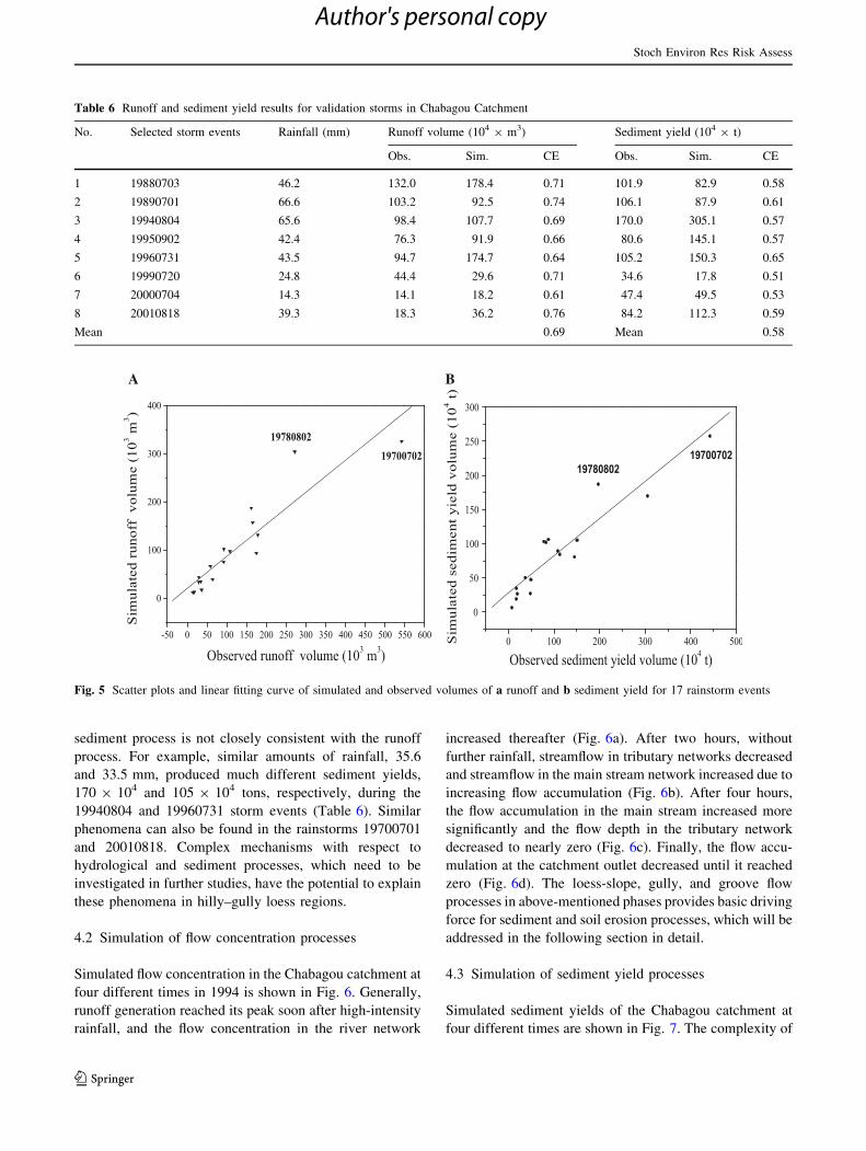
Table 5 shows that the CE values for modeling runoff
ranged from 0.60 to 0.89, with a mean CE of 0.76; the
sediment CE ranged from 0.58 to 0.79, with a mean CE of
0.65 in model calibration. Meanwhile, Table 6 shows that
the validation runoff CEs ranged from 0.61 to 0.76, with a
mean CE of 0.69, and the sediment CE ranged from 0.51 to
0.65, with a mean CE of 0.58. Figure 5 indicates that most
of the simulated results compared well with observed
runoff and sediment yield in calibration and validation,
except for those events 19700702 and 19780802. There-
fore, the simulation results are reliable and appropriate for
practical use.
Simulated results for event 19700702 had a CE of 0.60
for runoff and a CE of 0.58 for sediment yield, far below
Table 4 Parameter ranges used in Monte Carlo simulation for Chabagou Catchment
Parameter Physical meaning Minimum value Maximum value Mean value
fo Maximum (or initial) infiltration rate 8 mm/min 9 mm/min 8.5 mm/min
fc Minimum (or equilibrium) infiltration rate 1.6 mm/min 1.7 mm/min 1.65 mm/min
Kd Infiltration constant 0.1 0.5 0.25
h Overland flow routing coefficient (in formula 12) 0.6 1 0.8
Stoch Environ Res Risk Assess
123
Author's personal copy

the mean level in calibration. One of the reasons might be
that the model parameter sets used for simulation were
averages weighted by small, medium-size and large storm
events; thus, they did not reflect the properties of the runoff
and sediment yield for the largest flood events, such as
19700702. Furthermore, the studied drainage basin is a
complex system characterized by non-linear and dynamic
processes (Yang et al. 2008, 2009a). Temporal and spatial
variability of the meteorological factors, land use, human
activities, and other factors may contribute to increasing
uncertainties in the modeling of runoff and sediment pro-
cesses in the hilly–gully loess region.
The sediment yield process, controlled by a variety of
factors, including regional meteorological characteristics,
geometric features of sediment grain, different loess hill-
slopes, gullies, and grooves. Meanwhile, soil erosion and
deposition and transport processes, is far more complicated
than the runoff process (Yao and Tang 2001). Therefore,
0.0
0.2
0.4
0.6
0.8
Lik
elih
ood
mea
sure
Lik
elih
ood
mea
sure
Lik
elih
ood
mea
sure
Lik
elih
ood
mea
sure
f0 (mm/min)
8.0 8.2 8.4 8.6 8.8 9.0 1.60 1.62 1.64 1.66 1.68 1.700.0
0.2
0.4
0.6
0.8
fc (mm/min)
0.1 0.2 0.3 0.4 0.50.0
0.2
0.4
0.6
0.8
Kd
0.6 0.7 0.8 0.9 1.00.0
0.2
0.4
0.6
0.8
Fig. 4 Scatter plots of likelihood values for selected four parameters from Monte Carlo simulation of Chabagou catchment during storm event
on July, 2nd 1974
Table 5 Runoff and sediment yield results for calibration storms in Chabagou Catchment
No. Storm event Rainfall (mm) Runoff volume (104 9 m3) Sediment yield (104 9 t)
Obs. Sim. CE Obs. Sim. CE
1 19700701 10.2 34.7 29.2 0.68 26.5 19.6 0.61
2 19700702 58.4 326.8 541.9 0.60 257.6 441.7 0.58
3 19710701 14.8 40.3 64.3 0.81 27.1 47.7 0.69
4 19720702 24.7 67.8 58.6 0.79 50.5 37.2 0.62
5 19740702 59.7 188.3 161.9 0.74 103.2 77.9 0.61
6 19780802 45.2 305.5 271.9 0.77 187.2 196.7 0.63
7 19790701 18.9 35.4 34.4 0.79 19.1 17.5 0.66
8 19800701 13.4 13.1 14.0 0.76 6.7 7.6 0.65
9 19830702 35.8 158.2 165.4 0.89 89.4 108.1 0.79
Mean 0.76 Mean 0.65
Stoch Environ Res Risk Assess
123
Author's personal copy
sediment process is not closely consistent with the runoff
process. For example, similar amounts of rainfall, 35.6
and 33.5 mm, produced much different sediment yields,
170 9 104 and 105 9 104 tons, respectively, during the
19940804 and 19960731 storm events (Table 6). Similar
phenomena can also be found in the rainstorms 19700701
and 20010818. Complex mechanisms with respect to
hydrological and sediment processes, which need to be
investigated in further studies, have the potential to explain
these phenomena in hilly–gully loess regions.
4.2 Simulation of flow concentration processes
Simulated flow concentration in the Chabagou catchment at
four different times in 1994 is shown in Fig. 6. Generally,
runoff generation reached its peak soon after high-intensity
rainfall, and the flow concentration in the river network
increased thereafter (Fig. 6a). After two hours, without
further rainfall, streamflow in tributary networks decreased
and streamflow in the main stream network increased due to
increasing flow accumulation (Fig. 6b). After four hours,
the flow accumulation in the main stream increased more
significantly and the flow depth in the tributary network
decreased to nearly zero (Fig. 6c). Finally, the flow accu-
mulation at the catchment outlet decreased until it reached
zero (Fig. 6d). The loess-slope, gully, and groove flow
processes in above-mentioned phases provides basic driving
force for sediment and soil erosion processes, which will be
addressed in the following section in detail.
4.3 Simulation of sediment yield processes
Simulated sediment yields of the Chabagou catchment at
four different times are shown in Fig. 7. The complexity of
Table 6 Runoff and sediment yield results for validation storms in Chabagou Catchment
No. Selected storm events Rainfall (mm) Runoff volume (104 9 m3) Sediment yield (104 9 t)
Obs. Sim. CE Obs. Sim. CE
1 19880703 46.2 132.0 178.4 0.71 101.9 82.9 0.58
2 19890701 66.6 103.2 92.5 0.74 106.1 87.9 0.61
3 19940804 65.6 98.4 107.7 0.69 170.0 305.1 0.57
4 19950902 42.4 76.3 91.9 0.66 80.6 145.1 0.57
5 19960731 43.5 94.7 174.7 0.64 105.2 150.3 0.65
6 19990720 24.8 44.4 29.6 0.71 34.6 17.8 0.51
7 20000704 14.3 14.1 18.2 0.61 47.4 49.5 0.53
8 20010818 39.3 18.3 36.2 0.76 84.2 112.3 0.59
Mean 0.69 Mean 0.58
A B
Fig. 5 Scatter plots and linear fitting curve of simulated and observed volumes of a runoff and b sediment yield for 17 rainstorm events
Stoch Environ Res Risk Assess
123
Author's personal copy

influencing factors in the hilly–gully loess region led to
considerable difficulty and uncertainty in the simulation of
sediment yield from a temporal and spatial perspective.
Figure 7a indicates that high-intensity rainstorms triggered
and increased the sediment yield in areas of high elevation
in the northeast portion of the Chabagou catchment. In this
Fig. 6 Simulated temporal and
spatial variation of flow
concentration for Chabagou
Catchment during storm event
on a Aug. 4th 1994 at 19:00,
b Aug. 4th 1994 at 21:00,
c Aug. 4th 1994 at 23:00,
and d Aug 5th 1994 at 02:00
Fig. 7 Simulated temporal
and spatial variation of sediment
yield of Chabagou Catchment
during storm event on a Aug.
4th 1994 at 19:00, b Aug. 4th
1994 at 21:00, c Aug. 4th 1994
at 23:00, and d Aug 5th 1994 at
02:00
Stoch Environ Res Risk Assess
123
Author's personal copy

stage (Fig. 7a), raindrop splash-erosion and sheet flow-
erosion accounted for a major percentage in the total soil
erosion processes. Continuously increasing runoff induced
by high-intensity rainstorms intensified the sediment yield
processes throughout the drainage catchment (Fig. 7b).
Considerable gully soil erosion is dominated in the sedi-
ment processes of this stage. Meanwhile, gravitational soil
erosion occurred when highly sediment-concentration flow
passed through a variety of steep gullies. Gravitational
erosion further improved the sediment concentration of the
hyper-concentrated flow. Therefore, mixed soil-erosion
sources from runoff and gravitational erosion was together
responsible for the sediment processes during this phase.
In past years, some hydraulician and hydrologists have
strive to investigate the percentages of runoff and gravi-
tational erosion in the hilly–gully loess regions (e.g. Yao
and Tang 2001; Li et al. 2009). According to their reports,
the percentage for runoff and gravitational erosion in total
is 60–70% and 40–30% approximately. Of course, the
modeling of gravitational erosion in the loess regions is
limited currently and associated results are still very
coarse. Therefore, it is necessary to study the sediment
processes further to improve our model’s capability in the
region. In the third phase in sediment processes (Fig. 7c),
sediments were transported from tributary gullies to main
gullies, from gullies to grooves, from grooves to the main
channel, and from upstream to downstream. Although the
spatial sizes of channels and flow magnitude increased in
this stage, wide cross-sectional shape and smooth slope
collectively limits the increasing soil erosion and sediment
concentration. In this case, sediment concentration reaches
the maximum of the whole soil erosion processes and
tends to be a constant. The runoff-induced erosion con-
stitutes the majority of soil erosion, and gravitational
erosion can be neglected in this phase. At the last stage,
Fig. 7d illustrates decreasing sediment transport processes
along the main stream gradually followed by decreasing
rainstorms.
4.4 Simulated runoff and sediment yield hydrographs
and influence analysis
Simulated and observed runoff and sediment yield hydro-
graphs at the outlet (CP station) of Chabagou catchment
were compared for eight storm events in model validation,
as shown in Fig. 8. It can be observed from this figure that
the calculated hydrographs reasonably matched measured
hydrographs in most cases. Similar phenomena can be
found in the simulated and observed sediment processes at
the catchment outlet. There was an overestimation of
sediment yield for some large events; this may be due to
the average weighted parameters for these small, medium-
sized and large storm events. The performance of the
model can be improved when more detailed information is
available and used for parameter estimation.
The sediment and runoff processes have mutual impacts
on each other (Li et al. 2009), and it is important to explore
these influences. Figure 9 enables us to detect the typical
properties of hyper-concentrated flow processes dominated
in such regions. It indicates that the variability of sediment
concentration (S) is very high for low discharge (Q, blue-
color shaded area in Fig. 9), however, S tend to be a
constant when high discharge (Q, red-color shaded area in
Fig. 9) exceeds a certain upper-threshold. This is partly
because low discharges are generally triggered by a few
rainstorms in different homogeneous areas, different sedi-
ment-yielding mechanisms will result in a huge S vari-
ability of such homogeneous areas. Consequently, high S
variations are observed at the outlet gauge. Nevertheless,
when large-scale rainstorms occur in the whole catchment
and lead to high discharge, different impacts on S will be
mixed up and result in low S variations at the outlet gauge.
Moreover, both the range and the mean values of S tend to
approach a constant as discharge increases.
4.5 Application to the Xingzihe catchment
The calibrated model was then applied to the Xingzihe
catchment to test its validity under similar meteorological,
geographical, geomorphological, and hydrological condi-
tions as those in the Chabagou catchment. Table 7 shows
that the mean runoff CE was 0.62, and the mean sediment
CE was 0.55, suggesting that the calibrated model can be
used to simulate runoff and soil erosion processes in sim-
ilar hilly–gully loess regions. However, compared with the
Chabagou catchment (drainage area = 205 km2), Xingzihe
is a middle-size catchment (drainage area = 1,486 km2).
Runoff and soil erosion processes in middle- and large-size
catchments are more complex than in small catchment.
Therefore, attempts to simulate these processes in middle-
and large-size catchments with the model built for small
catchments may lead to imperfect results. This why the
average runoff CE (0.62) and sediment CE (0.55) in vali-
dation (Table 7) for Xingzihe catchment is lower than
Chabagou catchment (runoff CE 0.69, sediment CE 0.58,
Table 6).
5 Conclusion and discussion
In this study, a DEM-based numerical model was con-
structed and applied in simulating the runoff and sediment
processes for typical storm events (from 1970 to 2001) in
two hilly–gully loess regions along the middle reaches of
Yellow River. The Chabagou catchment with dense rainfall
stations was used to calibrate the model and the Xingzihe
Stoch Environ Res Risk Assess
123
Author's personal copy

catchment was used for model validation. The major find-
ings of this study include the following: (1) A DEM-based
spatial–temporal model of runoff and sediment processes
in the loess region can provide spatial variations of runoff
and sediment processes with a high grid resolution of
20 m 9 20 m. Comparisons between observed and simu-
lated runoff and sediment yield hydrographs indicate that
the model is capable of simulating runoff and soil erosion
processes for individual storm events in a hilly–gully loess
region. (2) Spatial modeling results of runoff and sediment
A B
C D
E F
G H
Fig. 8 Comparison between simulated and observed runoff and sediment yield hydrographs, in validation results of storm events in the
Chabagou Catchment: a, b 19880703, c, d 19890701, e, f 19940804, g, h 19950902, i, j 19960731, k, l 19990720, m, n 20000704, o, p 20010818
Stoch Environ Res Risk Assess
123
Author's personal copy

processes have been analyzed in detail to improve our
understanding of on the soil erosion processes in such
regions. (3) Parameter uncertainty analysis shows that
equifinality is one of the problems causing uncertainty in
the model simulation. Quantitative estimation of parameters
and model uncertainty will be further investigated in future
studies. This study presents an improvement over earlier
studies on loess regions, and the results will further our
understanding of spatio-temporal runoff and soil erosion
processes in small catchments characterized by serious
water and soil erosion. They are helpful in water and soil
conservation planning and management in catchments
I J
K L
M N
O P
Fig. 8 continued
Stoch Environ Res Risk Assess
123
Author's personal copy

dominated by serious water and soil loss, especially on the
Loess Plateau.
It should be noted that runoff and sediment processes are
highly associated with the geographical scales on which
they occur. Of course, 20 m in this research is not the
highest DEM resolution to date, which is possible to
neglect some gullies with a width less than 20 m in stream
network delineation. Hence, the modeling results are
expected to be improved further when high-resolution
spatial maps (e.g. the DEM, soil, vegetation cover, land use
pattern in 1–5 m) are available in the future. Meanwhile,
other sources of soil erosion, for example, the gravity-
induced soil erosion, one of key soil erosion processes
which are particularly active at several meters scale
(\10 m) in this region, contributes to the total soil erosion
considerably. This processes also should be considered and
modelled together with the runoff-induced soil erosion at
this scale (\10 m). Therefore, there is a lot of additional
work to do when developing a DEM-based runoff and
sediment processes model working at finer scales (e.g.
1 m–10 m). However, different runoff and sediment pro-
cess models at various scales are collectively recognized to
be beneficial, in providing profound insights into formu-
lating different measures for water and soil conservation
planning and management for different-sized catchments
dealing with serious water and soil loss in the Chinese
Loess Plateau. The model in such a scale (C20 m) pre-
sented in this paper mainly characterizes the runoff-
induced soil erosion processes (Yao and Tang 2001; Li
et al. 2009). The modelling approaches and associated
results presented in this study will still provide beneficial
references for researchers, decision makers and stake-
holders in water and soil conservation practices. For these
reasons, a series of DEM-based runoff and sediment model
at various scales (e.g. 1, 20, 100, and 1 km), aiming to
model different physical soil erosion processes, are all
essential to be build up toward improving our current
knowledge for the complex soil erosion processes in
Chinese hilly–gully loess regions. Those work will defi-
nitely constitute fresh research deliverables in future.
In addition, parameter sensitivity analysis performed in
the study shows that there exist many different sets of
parameters that could yield equally accurate or inaccurate
results. The equifinality problem, frequently discussed in the
past literature (e.g. Beven 1992; 1993), is also a significant
problem for the soil erosion processes model, which put
forwards essential needs to: (1) identify of the underlying
hydraulic or hydrological properties of soil erosion pro-
cesses through more specific field experiments for further
model improvement, (2) collect and use high-definition data
to refine model parameters, and (3) quantify uncertainties in
modelling those complex processes in future studies.
Acknowledgments The work was jointly supported by grants from
the National Natural Science Foundation of China (40901016,
40830639, 40830640), a grant from the State Key Laboratory of
Fig. 9 Sediment concentration
vs discharge at CP gauge, the
Chabagou catchment on 18th
August 2001
Table 7 Runoff and sediment validation results for Xingzihe
Catchment
No. Storm
event
Total rainfall
(mm)
Runoff
CE
Sediment
yield CE
1 19820729 76.2 0.63 0.55
2 19820806 86.6 0.53 0.50
3 19850511 55.6 0.66 0.62
4 19850712 72.4 0.67 0.54
Mean 0.62 0.55
Stoch Environ Res Risk Assess
123
Author's personal copy

Hydrology-Water Resources and Hydraulic Engineering (2009586612,
2009585512), the National Basic Research Program of China ‘‘973
Program’’ (2010CB428405, 2010CB951101, 2010CB951003), and
the Fundamental Research Funds for the Central Universities
(2010B00714). Cordial thanks are also extended to the editor, Professor
George Christakos and three referees for their valuable comments
which greatly improved the quality of this paper.
Appendix: List of symbols
RS The infiltration excess runoff (mm/min)
PE The precipitation minus evaporation
(mm/min)
F The infiltration rate (mm/min)
P The precipitation (mm/min)
ft The infiltration rate at time t (mm/min)
fc The constant or equilibrium infiltration rate
after soil has been saturated or minimum
infiltration rate (mm/min)
f0 The initial infiltration rate (mm/min)
kd A decay constant specific to the soil
(dimensionless)
Kc The concentration routing coefficient
(dimensionless)
v The cross-sectional velocity (m/s)
q The overland discharge per unit width (m2/s)
h The water depth in meters (m)
re(t) The rainfall excess rate, or lateral inflow
rate (mm/min)
l1 The length of loess slope (m)
l2 The length of gully slope (m)
l3 The length of groove (m)
T The duration of a storm event (min)
x The streamwise distance (m)
t Time (min)
Sf The friction-induced head loss per unit
length between the moving fluid and the
bed (m/m)
S0 The slope of the overland surface (m/m)
S The slope of the flow surface (m/m)
f The Darcy–Weisbach friction loss
coefficient (dimensionless), which can be
determined from the Moody diagram
g The local gravitational
acceleration, & 9.8 m/s2
R The hydraulic radius (m)
n The Manning’s roughness (dimensionless)
r, k Constant
h A weighting factor in the Preissmann
implicit scheme (dimensionless)
e A weighting factor in the Preissmann
implicit scheme (dimensionless)
Ks The hydraulic roughness coefficient
g1 A distance related coefficient 1m
� c The bulk density of clear water (kg/m3)
cs The bulk density of dry sediment (kg/m3)
cm The bulk density of wet sediment (kg/m3)
e1 The soil erosion rate of a loess slope (kg/s)
a1 The degree (or angle) of a loess slope (�)
Wf 1 The effective power of soil erosion of the
loess slope per unit area (W)
so The shear stress (N/m2)
sc The critical yield stress (N/m2)
V The average cross-sectional velocity of
surface flow (m/s)
A A non-dimensional coefficient
A1 ¼ Ag�g1�tga1
A sediment erosion model coefficient for
loess slope erosion (s2)
c The bulk density of the flow
SC The sediment concentration (kg/km3)
Qh The discharge of the clear-water flow (m3/s)
Qc The discharge of the muddy flow (m3/s)
J1 The loess slope (%)
J0 The slope of the surface flow (%)
e2 The gully slope erosion rate (kg/s)
f2 The energy coefficient for gully soil erosion
(dimensionless)
h2 The flow depth of the gully (m)
J2 The slope of the gully (%)
a2 The degree (or angle) of the gully slope (�)
A2 ¼ f2A1; A sediment erosion model coefficient for
gully slope erosion
Ws3 The power of soil erosion of the groove per
unit area (W)
g3 A distance related coefficient 1m
� for groove
erosion
e3 The groove soil erosion rate (kg/s)
x The settling velocity (cm/s)
Wf 3 The actual power of soil erosion of the
groove per unit area (W)
U* The friction velocity (m/s)
h3 The groove depth (m)
J3 The groove slope (%)
j The Karman constant
f3 The energy coefficient for groove soil
erosion (dimensionless)
C A dimensionless coefficient
B0 A dimensionless coefficient
A3 A sediment erosion model coefficient for
groove erosion
CE The model efficiency measure
(dimensionless)
r2e
Variance of model residuals
(dimensionless)
r2o
Variance of observations (dimensionless)
Stoch Environ Res Risk Assess
123
Author's personal copy

References
Beasley DB, Huggins LF, Monke EJ (1980) ANSWERS: a model for
watershed planning. Trans ASAE 23(4):938–944
Bek S, Jezek J (2011) Optimization of interpolation parameters when
deriving DEM from contour lines. Stoch Environ Res Risk
Assess. doi:10.1007/s00477-011-0482-8
Beven KJ (1992) The future of distributed models: model calibration
and uncertainty predication. Hydrol Process 6:279–298
Beven KJ (1993) Prophecy, reality and uncertainty in distributed
hydrological modeling. Adv Water Resour 16:41–51
Bureau of Resource, Environmental Science and Technology,
Chinese Academy of Sciences (BREST-CAS) (1992) Develop-
ment and comprehensive treatment on small catchment in Loess
Plateau. China Science and Technology Literature Press, Beijing
Cai QG, Lu ZX (1998) Sediment yield model and simulation in a
small watershed in the hilly loess region. Science Press, Beijing
Cai QG, Lu ZX, Wang GP (1996) Physical process-based soil erosion
model in a small watershed in the hilly loess region. Acta Geogr
Sinica 51(2):108–117 (in Chinese with English Abstract)
Chen LD, Wang J, Fu BJ, Qiu Y (2001) Land use change in a small
catchment of northern Loess Plateau, China. Agric Ecosyst
Environ 86:163–172
Chen CN, Tsai CH, Tsai CT (2006) Simulation of sediment yield
from watershed by physiographic soil erosion–deposition model.
J Hydrol 327(3–4):293–303
De Roo APJ, Wesseling CG, Ritsema CJ (1996) LISEM: a single-
event physically based hydrological and soil erosion model for
drainage basins: I. Theory, input and output. Hydrol Process 10:
1107–1117
Engman ET (1986) Roughness coefficients for routing surface runoff.
J Irrig Drain Eng 112(1):39–53
Fu BJ (1989) Soil erosion and its control in the Loess Plateau of
China. Soil Use Manag 5:76–82
Fu B, Gulinck H (1994) Land evaluation in an area of severe erosion:
the Loess Plateau of China. Land Degrad Rehabil 5:33–40
Hairsine PB, Rose CW (1991) Rainfall detachment and deposition:
sediment transport in the absence of flow-driven processes. Soil
Sci Soc Am J 55:320–324
Li T, Wang GQ, Xue H, Wang Kai (2009) Spatial scaling issues in
sediment yield and transport properties in hilly–gully loess
regions. Science China: E 39(6):1095–1103
Masoudi M, Patwardhan AM, Gore SD (2006) Risk assessment of
water erosion for the Qareh Aghaj subbasin, southern Iran. Stoch
Environ Res Risk Assess 21(1):15–24
Misra RK, Rose CW (1989) Manual for use of program GUEST.
Division of Australian Environmental Studies Report, Griffith
University, Brisbane, QLD, p 1411
Morgan RPC, Quinton JN, Smith RE, Govers G, Poesen JWA, Chisci
G, Torri D (1998) The EUROSEM model. In: Boardman J,
Favis-Mortlock D (eds) Global change: modeling soil erosion by
water. Springer, New York, pp 373–382
Murakami S, Hayashi S, Kameyama S, Watanabe M (2001)
Fundamental study on sediment routing through forest and
agricultural area in watershed. Ann J Hydraul Eng JSCE
45:799–804 (in Japanese)
Nearing MA, Foster GR, Lane LJ, Finkner SC (1989) A process-
based soil erosion model for USDA-Water erosion prediction
project technology. Trans ASAE 32(5):1587–1593
Parlange JY, Hogarth WL, Rose CW, Sander GC, Hairsine P, Lisle I
(1999) Addendum to unsteady soil erosion model. J Hydrol
217:149–156
Shi H, Shao MA (2000) Soil and water loss from the Loess Plateau in
China. J Arid Environ 45:9–20
Tang LQ (2003) Problems needed to be solved in sediment yield
model based on physical processes. J Sediment Res
14(16):35–41 (in Chinese with English Abstract)
Tang LQ, Chen GX (1990) The numerical model of sediment yield
for small loess basin. J Hohai Univ 12(6):23–28 (in Chinese with
English Abstract)
Tang LQ, Chen GX (1997) A dynamic model of runoff and sediment
yield from small watershed. J Hydrodyn12(2):44–54 (in Chinese
with English Abstract)
Wongsa S, Nakui T, Iwai M, Shimizu Y (2002) Runoff and sediment
transport modeling for mountain river. In: Proceeding of
international conference on fluvial hydraulic, Belgium, River
Flow, pp 683–691
World Wildlife Fund (WWF) (2004). Report suggests China’s ‘Grain-
to-Green’ plan is fundamental to managing water and soil
erosion. http://www.wwfchina.org/english/
Xie SN, Wang ML, Zhang R (1990) Study on storm event-based
sediment yield modeling in hilly–gully loess region in the middle
stream of the Yellow River. Beijing. Tsinghua University Press,
Beijing (in Chinese with English Abstract)
Yang T, Zhang Y, Chen JR, He S, Xie HH (2005) A distributed
hydrologic modelling in Chabagou basin of middle stream of
Yellow River based on digital platform. J Hydraul Eng
36(4):456–460 (in Chinese with English Abstract)
Yang T, Zhang Y, Chen JR, Li BH (2007) Distributed soil loss
evaluation and prediction modelling and simulation in an area
with high and coarse sediment yield of the Yellow River, China.
In: Methodology in hydrology, vol 311. IAHS Publications,
China, pp 118–125
Yang T, Zhang Q, Chen YD, Tao X, Xu CY, Chen X (2008) A spatial
assessment of hydrologic alteration caused by dam construction
in the middle and lower Yellow River, China. Hydrol Process
22:3829–3843
Yang T, Xu CY, Chen X, Singh VP, Shao QX, Hao ZC, Tao X (2009a)
Assessing the impact of conservation measures on hydrological
and sediment changes in nine major catchments of the Loess
Plateau. River Res Appl 24:1–19. doi:10.1002/rra.1267
Yang T, Xu CY, Shao QX, Chen X, Singh VP (2009b) Temporal and
spatial patterns of low-flow hydrological components in the
Yellow River during past 50 years. Stoch Environ Res Risk
Assess. doi:10.1007/s00477-009-0318-y
Yao W, Tang LQ (2001) Runoff-induced soil erosion processes and
modeling. The Yellow River Press (in Chinese)
Stoch Environ Res Risk Assess
123
Author's personal copy
Top Related
Copyright © 2022 FDOKUMEN

