Cross-Entropy Approach to Data VisualizationBased on the Neural Gas Network

Pablo A. Estevez, Cristiain J. FigueroaDepartment of Electrical Engineering

University of ChileCasilla 412-3, Santiago, Chile

E-mail: {pestevez, cfiguero}@ing.uchile.cl

Abstract-A new approach to mapping high-dimensional datainto a low-dimensional space embedding is presented. The aimof this approach is to project simultaneously the input dataand the codebook vectors into a low-dimensional output space,preserving the local neighborhood. The Neural Gas algorithmis used to obtain codebook vectors. A cost function based onthe cross-entropy (CE) between input and output probabilitiesis minimized by using a Newton-Raphson method. The newapproach is compared with multidimensional scaling (MDS)using a benchmark data set and three high-dimensional real-world data sets. In comparison with MDS, our method deliversa clear visualization of both data points and codebooks, andbetter CE and topology preservation measurements.

I. INTRODUCTIONIn the last decades, many methods have been developed to

embed objects, described by high-dimensional vectors, into alow-dimensional space in a way that preserves the topology.Multidimensional Scaling (MDS) [1] is a nonlinear projectionmethod that preserves the inter-point Euclidean distances. TheSammon mapping (or non-linear mapping, NLM) [2] is a well-known MDS technique.

Self-organizing feature map (SOM) neural networks asso-ciate input patterns of arbitrary dimensionality with points ina fixed grid of low dimensionality [3]. Each grid point hasassociated a codebook vector of the same dimension thanthe input vectors. The SOM defines a neighborhood functionin the fixed output grid, based on the Euclidean distance.Another self-organizing neural network is the Neural Gas (NG)[4], which produces a more efficient vector quantization thanSOM, because it does not have a fixed output structure thatconstraints the movement of the codebook vectors. In NG theneighborhood function is defined in the input space, based onthe rank order of the codebook vectors with respect to thewinner codebook (best matching unit, BMU).Some visualization schemes allow to move simultaneously

the codebook vectors in the input space and the codebookpositions, which represents the projection of the codebookvectors into the low-dimensional output space. In particularTOPSOM [5] is an extension of the original SOM that replacesthe traditional fixed grid by a dynamic and continuous outputspace. By changing the vector quantization method to NG,the TOPNG visualization method is obtained. The resultsof TOPSOM and TOPNG are comparable to those of the

Kazumi SaitoNTT Communication Science Laboratories

2-4 Hikaridai, Seika, Kyoto 619-0237, JapanE-mail: saito@cslab.kecl.ntt.cojp

SOM/NLM in terms of the Sammon stress function, E, andthe topology preservation measure, q, [6].A probabilistic approach to embedding objects into a low-

dimensional space with neighborhood preservation is the Sto-chastic Neighbor Embedding (SNE) [7]. The method mini-mizes the Kullback-Leibler divergence of Gaussian neighbor-hoods defined in the input and output spaces. SNE focusesmainly on visualizing a set of data points without consi-dering a model structure, such as the relationship betweencodebook vectors and input data. The Parametric Embedding(PE) method [8] is a kind of generalization of SNE, whichsimultaneously embeds high-dimensional objects and theirclasses into a low-dimensional space. It tries to preserve theoriginal classification structure based on posterior probabilitiesin the embedding space.

In this paper, a new visualization method that tries topreserve the relationship between codebook vectors and inputdata using the neighborhood function of the Neural Gasmodel is presented. The method minimizes a cross-entropycost function. Our algorithm for data visualization builds onprevious work in document [8] and network [9] embedding,but it combines these two methods in novel ways to enablenew capabilities. In addition, we have added two types of newfeatures, a technique for scaling initial positions and a proposalof the upper bound function. The former enables to utilize theresults obtained by other method, while the latter enables toachieve stable minimization by the Newton-Raphson method.Furthermore, the quality of the mappings is evaluated usingthe topology preserving measure qm, on a benchmark data setand three high-dimensional real-world data sets.

II. VISUALIZATION ALGORITHMIn this section, after explaining our problem setting, we

propose a cross-entropy approach to simultaneously visuali-zing both input and codebook vectors in a K dimensionalEuclidean space. Then we describe our visualization algorithmbased on the Newton-Raphson method, together with somepractical extensions.

A. Prvblem SettingLet {xi: 1 < i < M} and {wj : 1 < j < N} be input and

codebook vectors respectively. In the Neural Gas model, the

2724

neighborhood function of the input vector xi with respect tothe codebook vector wj is defined as follows:

hA(xi, wj) = exp(-k(xi, wj)/A). (1)

The parameter A controls the neighborhood function width,and k(xi, wj) E {O, 1,... N - 1} ranks the codebook vectorwj by the distance from the input vector xi. Here k = 0 isassociated with the nearest codebook vector.

For a given set of the trained codebook vectors in theNeural Gas model, our problem is to compute a K dimensionalvisualization of both the M input vectors and the N codebookvectors so as to preserve the relationships defined by theneighborhood function for each pair of input and codebookvectors. To this end, in what follows we propose a cross-entropy approach.

B. Cross-Entropy ApproachFirstly we regard each value of the neighborhood functions

as a probability that an input vector xi belongs to a codebookvector wj. An independent binomial distribution is assumedfor each pair of input and codebook vectors. Hereafter weexpress this probability as follows:

Pi,j = hA(xi, wj). (2)

Clearly we can confirm that 0 < Pi,j < 1.Let {yj: 1 < i < M} and {zj 1 < j < N} be

the positions of the corresponding M input vectors and Ncodebook vectors in a K dimensional Euclidean space. Theyi and zj vectors are called output vectors and codebookpositions, respectively. As usual, we define the Euclideandistance between yi and z; as follows:

K

dij, = 1ily- zj1II = Z(Yi,k - Zj,k) * (3)k=1

Here we introduce a monotonic decreasing function p(u) E[0, 1] with respect to u > 0, where p(O) = 1 and p(oo) = 0.Clearly the neighborhood function in the Neural Gas modelis a monotonic decreasing function of this type. Since p(di,j)can also be regarded as a probability between yi and zj, wecan introduce a cross-entropy (cost) function between p,j andp(di,j) as follows:

Ei = -Pi,j ln p(di,j) - (1 - pi,j) ln(l - p(di,j)). (4)Since Ei,j is minimized when p(di,j) = pij, this minimizationwith respect to yi and zj basically coincides with our problemsetting. In this paper, we employ p(u) = exp(-u/2) as themonotonic decreasing function, but note that our approach isnot restricted to this one. Then the total cost function (objectivefunction) can be defined as follows:

1M N

E= EEpi,jdi,j-i=l j=l

M N

- jE(1-Pi,j)ln(l-p(dj,j)). (5)i=l j=l

Namely our approach is formalized as a function minimizationproblem defined in (5) with respect to {yj : 1 < i < M} and{zj : 1 <j < N}.

C. Learning AlgorithmAs the basic structure of our learning algorithm, we

adopt a coordinate strategy just like the EM (Expectation-Maximization) algorithm. Firstly we move the output vectors,so as to minimize the objective function by freezing thecodebook positions, then we move the codebook positions byfreezing the output vectors. These two steps are repeated untilconvergence.

In the former minimization step, we need to calculate thederivative of the objective function with respect to Yi asfollows:

aE N-p(d2,) (Yj z3). (6)

Since yi, (i' f i) disappears in (6), we can update yi withoutconsidering the other output vectors. In the latter minimizationstep, from the following derivative,

j aE EI- p(d,j,)azj i=l1 -p(d2,j) (z' (7)

we can also update z; without considering the other codebookpositions. Then our algorithm can be summarized as follows:1. Initialize positions Yi, - - , ym and z1, - - *, ZN.2. Calculate gradient vectors Eyl *... EyAJ.3. Update output vectors Yi,I ... Ym-4. Calculate gradient vectors Ezl, . , EZN5. Update codebook positions zl, - -, ZN-6. Stop if maxc{IIEy, 11, - , 11Ey,, 11, IIEzl 11, ,IIEZN II} < 67. Return to 2.In the following, we give some details to several steps of theabove algorithm.

D. Initialization ProcedureIn Step 1 we might want to initialize the positions using

conventional methods such as the MDS technique. However,the scale of distance might be quite different from thosederived by our algorithm. In order to estimate an adequatescale of the initial positions, we introduce a scaling factorit > 0. Then the objective function with respect to It can bedefined as follows:

M N M N

F(p= p2jE,Pdi,j- (1 -Pi,j) ln(1 -p(adij,)).i=1 j=1 i=1 j=1

(8)The first-order derivative is as follows:

aF MN il (dij=p 2ZE E -p(p.di,j ) '

and the second-order derivative is as follows:

02F 1 S (1 -Pi',j)p(d'i,j)d2>' °-

(9)

(10)

Clearly the objective function F(a) is convex because thesecond-order derivative is always non-negative. Therefore we

2725

can obtain the optimal scaling 1* by using some minimizationalgorithm like the Newton-Raphson method described below.In summary, let {yj: 1 < i < M} and {zj: 1 < j < N}be the positions obtained by some method like MDS, thenthe scaled initial positions are {I/ Yiy: 1 < i < M} and{jv j: 1 < j < N}.

E. Update ProcedureIn Steps 3 and 5 we employ the Newton-Raphson method

for updating the current positions as mentioned earlier. In thissubsection, we focus on calculating the modification vectorAyi by freezing the codebook positions. According to theNewton-Raphson method, we can obtain the modificationvector, if the Hessian matrix of (5) with respect to yi is positivedefinite,

=[ay2E E (11)

where yT stands for the transposed vector of y. However,we cannot guarantee that this matrix becomes always positivedefinite as shown below.

a2E N

(9yi&y7=E gi,jIj=1

N

+E hij(yi - Zj)(Yi - zj)T, (12)j=l

here I stands for the identity matrix in the K dimensionalspace, and gi,j and hi,j are defined as follows:

Pi,j - p(di,j)1 - p(di,j)

(1 -pi,j)p(di,j)hii=(1 -p(di,j))2 (13)

Clearly =1 gi,j can be a negative value.To cope with this situation, we consider a relaxation prob-

lem. Firstly we define the updated distance as follows:

dij,(Ayi) = IIyi + Ayi -zjjj2, (14)

and the updated cost function as follows:1

Ej,j (Ayi) = -Pi,jdi,j (Ayi) -(1 -pi,j) ln(1- p(di,j (Ayi))).(15)

By replacing the second term of right-hand-side in (15) into

-(1 - pi,j) ln(1 - p(di,j(Ayi) - IIAy,II2)), (16)we can consider the upper bound cost function Uj,j(Ayj).Here we can easily see that Ui,j(Ayi) > Ej,j(Ay2) because- ln(1 - p(u)) monotonically increases as u > 0 decreases.By noting that Ejj = Ej,j(O) = Uj,j(O), if we can find someAyi that satisfies Ztj (12,3(0) > E.=1 U2,3(Ayi), we canobserve the following relationships:

N

j=l

N N> 1 Ui,j(Ayi) > E1 Eij(Ayi)-

j=l j=l(17)

Namely it is guaranteed that by minimizing the objectivefunction constructed by the upper bound cost function, wecan reduce the value of the original objective function. On

the other hand, the gradient vector of the objective functionderived from Ui,j is as follows:

au(o) N aE0(1(0) = E9gi,j(yi - zj)-,EOAyi ~-

(18)

and we can see that the corresponding Hessian matrix is non-negative definite as shown below.

192u(O) N__________ -

Pij I +E hi,j(yi- j)(Yi Zj)T. (19)aAYiAO9Yi j=1 j=1

As a consequence, in the case that Hessian matrix (12) isnot positive definite, we can use (19) and apply the Newton-Raphson method for updating the current positions.

F Penalty FunctionIn our preliminary experiments, the objective function de-

fined in (5) sometimes produced relatively poor results whenthe numbers of codebooks becomes large. The problem wasthat some groups of codebooks were placed so closely, andthus it was not easy to see the relationships between inputand codebook vectors.

In order to separate each codebook position slightly, weintroduce the following penalty function.

NQ =EE ij, ,ij =-In(l-exp(-IIzi -Zj312/2)).

i=1 j$i(20)

Clearly when IIzi- zj is near zero, Q becomes a very largepenalty. Therefore, we can define the final objective functionas follows:

M N

J= N1EEEjji=1 ,9=1

1 N

+ 1) =N(N - 1) SlS 4ni=1 j#i

(21)

Here the normalizing constants, 1/(MN) and 1/(N(N - 1)),are introduced as a tradeoff between both cost functions, Eand Q.

G. Topology Preservation MeasureThe topology preservation measure qm used in [6] is consid-

ered as a performance measure. It is based on an assessmentof rank order in the input and output spaces. The n nearestcodebook vectors NNjiu (i E [1, n]) of each codebook vectorj, (j E [1, N]) and the n nearest codebook positions NNj3.of each codebook position j are computed. A credit schemeis constructed for each pair of points, qnj1.

{ 3, if NNji- = NNji._=

2, if NNji3 = NNjLZ, I e [1,n], i $1=mi 1, if NNji3, = NNjtz, t E [n, k], n < k

0, else.

The global qm measure is defined as:

1 N n

qm = 3n x NEEqm_j=l i=l

(22)

(23)

2726

Typical parameter settings are n = 4 and k = 10. The rangeof the q. measure is between 0 and 1, where qm = 0 indicatesa poor neighborhood preservation between the input andoutput spaces, and qm = 1 indicates a perfect neighborhoodpreservation. The input and output vectors can be also used forcalculating the topology preservation measure qm. The lattermeasure will be denoted as q'y to distinguish from the qWZcalculated with the codebook vectors and positions.

III. SIMULATION RESULTSFor each data set, the simulation results obtained for the

proposed model, called NG-CE (Neural Gas Cross-Entropy)and the classical Togerson's MDS along with their respectivemeasures are presented.

A. Iris dataThe Iris data set is a widely used benchmark in pattern

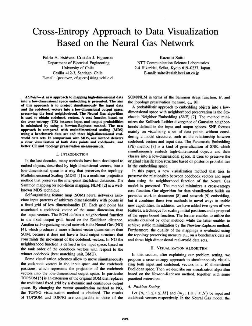
recognition. It contains three classes of 50 samples each,where each class refers to a type of Iris plant (Iris setosa,Iris versicolor and Iris virginica). Fig. 1 shows the projectionresults obtained with the Iris data set and 70 codebook vectorsfor a) MDS and b) NG-CE with A = 1.0 and penalty function.In Table I the quantifying measures are given for the modelsconsidered.

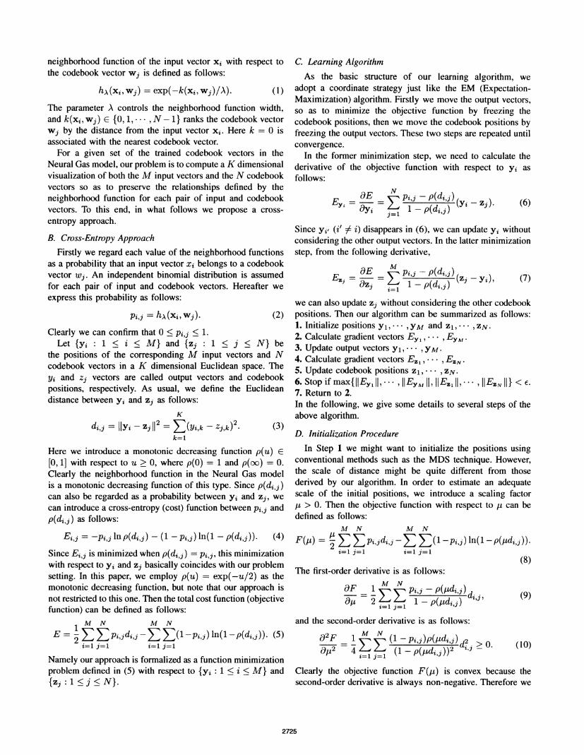
Fig. 2 shows the topology preserving measure qm as afunction of A, for the qm parameter combinations n = 10,k = 20 and n = 4, k = 10. It can be observed that the bestvalues of qm are obtained for A ranging from 1.0 to 3.0.

0.6

60*

-0.2 0-0.4 08 O-.

-OB *0

-02 -0.6 -4 -02 0 02 04 06 08

(a)

10 00O,o o0°oQQ 400)

0000° O 9oO 900O ° O00 Qo0

0 106 0eO°Q.0 o

0000

. 0

-158-0. -0. -0. 0. a c 0.4 06 O's

(b)

Fig. 1. Iris data set (150x4) projection results a) MDS codebook positions (o)and output vectors (.), (b) NG-CE codebook positions (o) and output vectors(C)

TABLE ICROSS-ENTROPY (CE) AND TOPOLOGY PRESERVATION MEASURE (qm)

FOR THE IRIS DATASET

Algorithm CE qwZ qm;MDS 0.0366 0.6737 0.54671NG-CE 0.0062 0.7417 0.6389

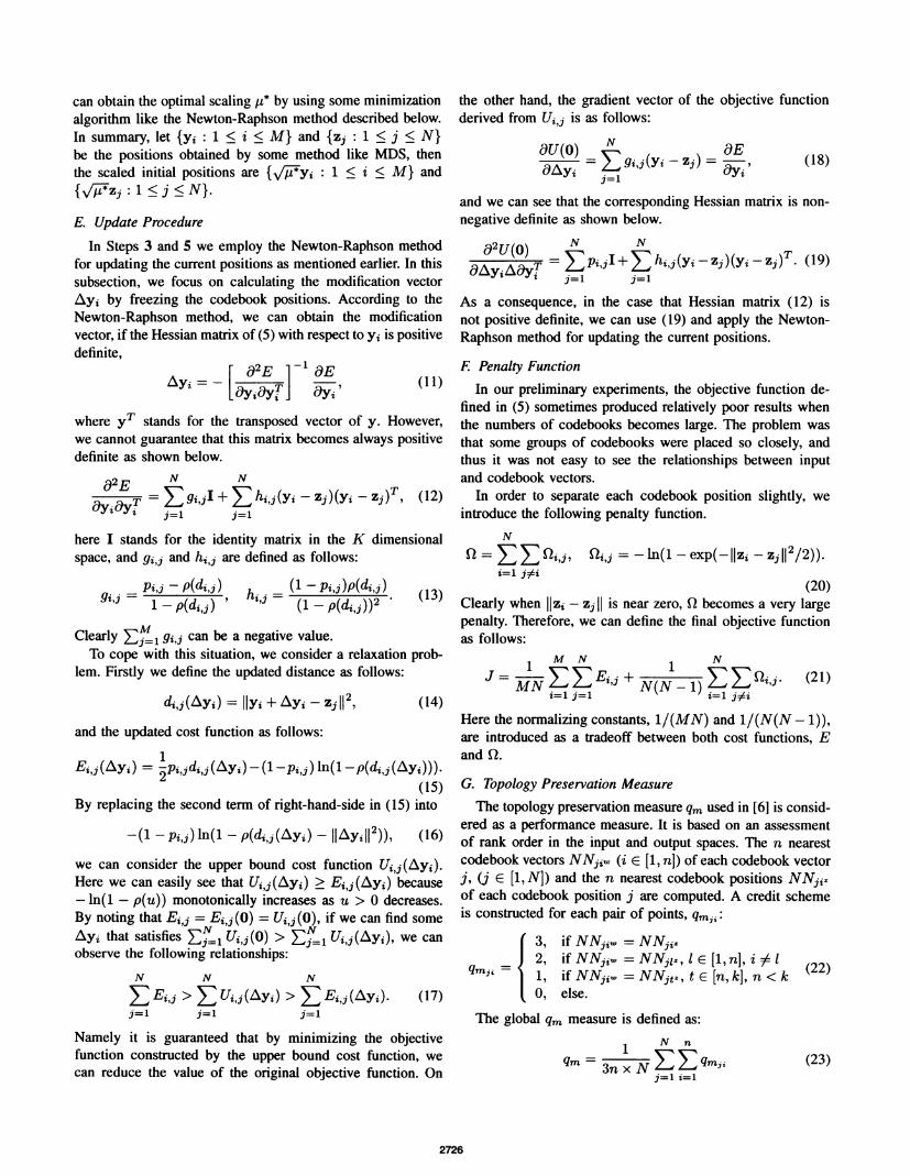
B. Fraud dataThe Fraud data set contains information about telephone

subscribers. It consists of 10721 samples of 26 features each[11]. The samples are divided into 4 classes: 705 Fraudsamples (red color), 5095 Insolvent samples (blue color), 4824Normal samples (green color), and 97 Other samples (yellowcolor). The vector quantization was performed using the NGalgorithm with 300 codebook vectors.

Fig. 3 shows the projection results obtained with the Frauddata set and 300 codebook vectors for a) MDS and b) NG-CEwith A = 1.0 and penalty function. In Table II the quantifyingmeasures are given for the models considered.

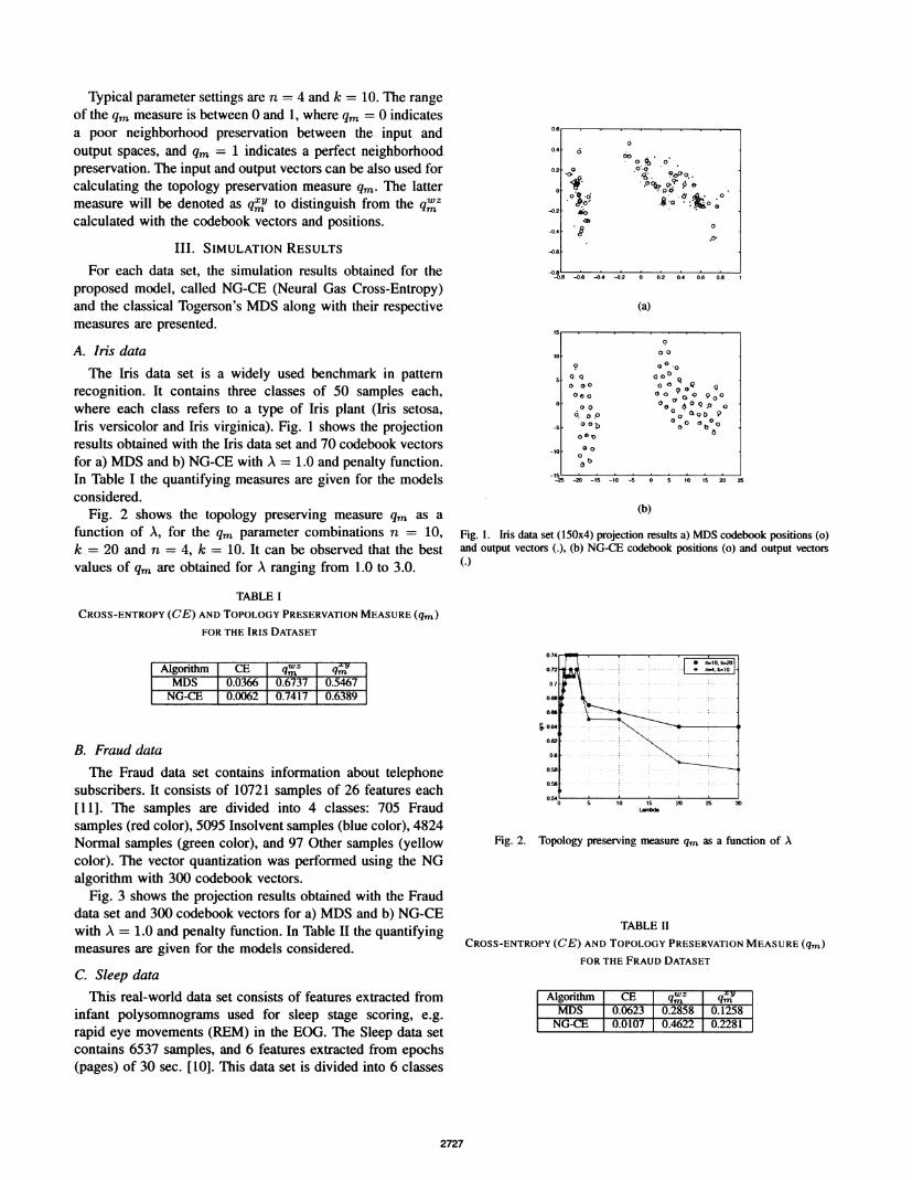
C. Sleep dataThis real-world data set consists of features extracted from

infant polysomnograms used for sleep stage scoring, e.g.rapid eye movements (REM) in the EOG. The Sleep data setcontains 6537 samples, and 6 features extracted from epochs(pages) of 30 sec. [10]. This data set is divided into 6 classes

0Q72

0.7

0.es

0oes

&0.640.e2

0.6

0.58

0.56

0 5 10 15 20 25 30

Fig. 2. Topology preserving measure qm as a function of A

TABLE IICROSS-ENTROPY (CE) AND TOPOLOGY PRESERVATION MEASURE (qm)

FOR THE FRAUD DATASET

Algorithm CE qwZ |qmyMDS 0.0623 0.2858 1 0.1258NG-CE 0.0107 0.4622 0.2281

2727

0.74.

0.54'

-25 -20 -15 -10 -S O 5 10 15 20 25

.....

ae

02

40244

4

"

t -'),9,0. j""^a ' e

O's

I, w _ .

',I 1 .05 0 05 * t5 2 2.5

(a)

(b)

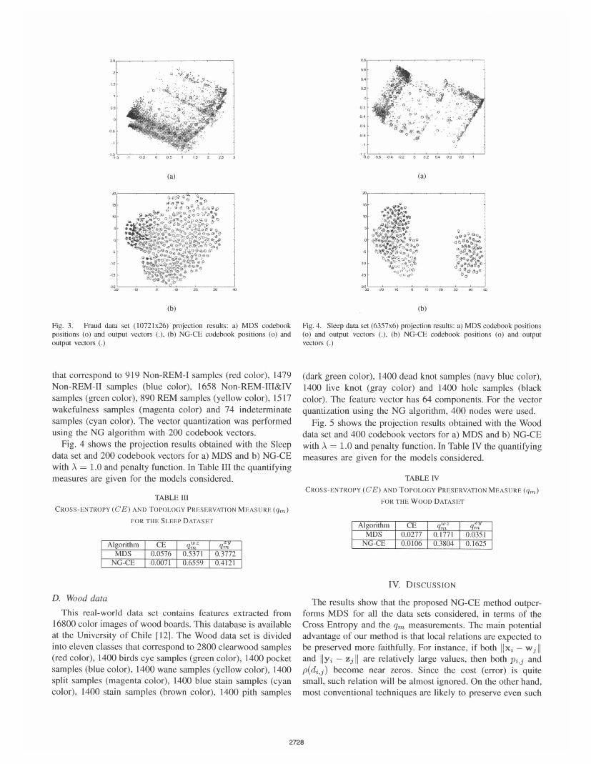
Fig. 3. Fraud data set (10721x26) projection results: a) MDS codebookpositions (o) and output vectors (.), (b) NG-CE codebook positions (o) andoutput vectors (.)

that correspond to 919 Non-REM-I samples (red color), 1479Non-REM-II samples (blue color), 1658 Non-REM-III&IVsamples (green color), 890 REM samples (yellow color), 1517wakefulness samples (magenta color) and 74 indeterminatesamples (cyan color). The vector quantization was performedusing the NG algorithm with 200 codebook vectors.

Fig. 4 shows the projection results obtained with the Sleepdata set and 200 codebook vectors for a) MDS and b) NG-CEwith A = 1.0 and penalty function. In Table III the quantifyingmeasures are given for the models considered.

TABLE IIICROSS-ENTROPY (CE) AND TOPOLOGY PRESERVATION MEASURE (qm)

FOR THE SLEEP DATASET

Algorithm CE qvz qMDS 0.0576 0.5371 0.3772NG-CE 0.0071 0.6559 0.4121

0A6 4.4 02 0 02 O. 00 OA I

(a)

(b)

Fig. 4. Sleep data set (6357x6) projection results: a) MDS codebook positions(o) and output vectors (.), (b) NG-CE codebook positions (o) and outputvectors (.)

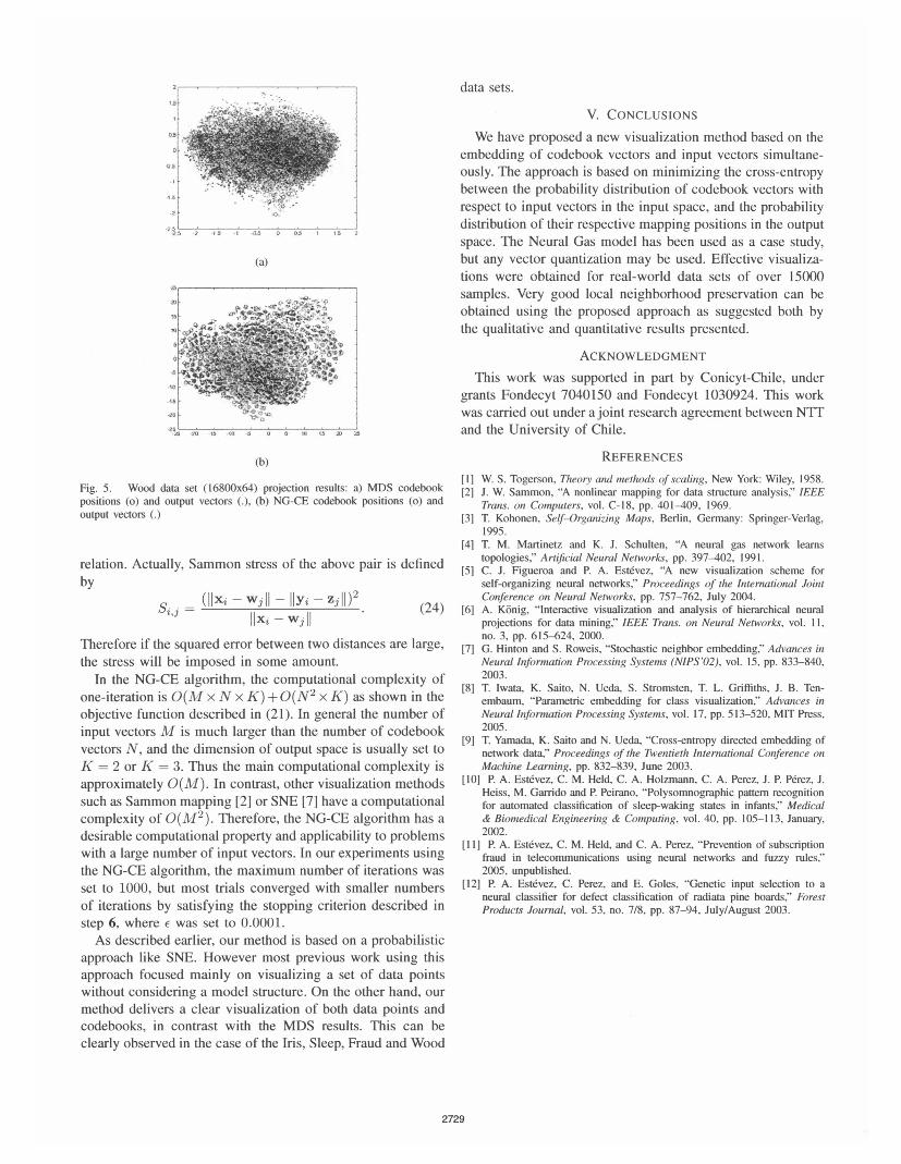
(dark green color), 1400 dead knot samples (navy blue color),1400 live knot (gray color) and 1400 hole samples (blackcolor). The feature vector has 64 components. For the vectorquantization using the NG algorithm, 400 nodes were used.

Fig. 5 shows the projection results obtained with the Wooddata set and 400 codebook vectors for a) MDS and b) NG-CEwith A = 1.0 and penalty function. In Table IV the quantifyingmeasures are given for the models considered.

TABLE IVCROSS-ENTROPY (CE) AND TOPOLOGY PRESERVATION MEASURE (qm)

FOR THE WOOD DATASET

Algorithm CE qtaZ qjMDS I0.0277 0.1771 0.0351NG-CE 0.0106 0.3804 0.1625

IV. DISCUSSIOND. Wood data

This real-world data set contains features extracted from16800 color images of wood boards. This database is availableat the University of Chile [12]. The Wood data set is dividedinto eleven classes that correspond to 2800 clearwood samples(red color), 1400 birds eye samples (green color), 1400 pocketsamples (blue color), 1400 wane samples (yellow color), 1400split samples (magenta color), 1400 blue stain samples (cyancolor), 1400 stain samples (brown color), 1400 pith samples

The results show that the proposed NG-CE method outper-forms MDS for all the data sets considered, in terms of theCross Entropy and the q, measurements. The main potentialadvantage of our method is that local relations are expected tobe preserved more faithfully. For instance, if both Ixi-Wj1Iand l1yi-zj are relatively large values, then both pi,j andp(di,j) become near zeros. Since the cost (error) is quitesmall, such relation will be almost ignored. On the other hand,most conventional techniques are likely to preserve even such

2728

l0.0114:. i. 1'

08,

3

laQt

25~ ~- (

-to t45W-.'0 .

(b)

Fig. 5. Wood data set (16800x64) projection results: a) MDS codebookpositions (o) and output vectors (.), (b) NG-CE codebook positions (o) andoutput vectors (.)

relation. Actually, Sammon stress of the above pair is definedby

__ - (llxi - wj - IlYi - zjIl)2 (24)sio ~lixi - w IIll4Therefore if the squared error between two distances are large,the stress will be imposed in some amount.

In the NG-CE algorithm, the computational complexity ofone-iteration is 0(M x N x K) + O(N2 x K) as shown in theobjective function described in (21). In general the number ofinput vectors M is much larger than the number of codebookvectors N, and the dimension of output space is usually set toK = 2 or K = 3. Thus the main computational complexity isapproximately O(M). In contrast, other visualization methodssuch as Sammon mapping [2] or SNE [7] have a computationalcomplexity of O(M2). Therefore, the NG-CE algorithm has adesirable computational property and applicability to problemswith a large number of input vectors. In our experiments usingthe NG-CE algorithm, the maximum number of iterations wasset to 1000, but most trials converged with smaller numbersof iterations by satisfying the stopping criterion described instep 6, where e was set to 0.0001.As described earlier, our method is based on a probabilistic

approach like SNE. However most previous work using thisapproach focused mainly on visualizing a set of data pointswithout considering a model structure. On the other hand, ourmethod delivers a clear visualization of both data points andcodebooks, in contrast with the MDS results. This can beclearly observed in the case of the Iris, Sleep, Fraud and Wood

data sets.

V. CONCLUSIONSWe have proposed a new visualization method based on the

embedding of codebook vectors and input vectors simultane-ously. The approach is based on minimizing the cross-entropybetween the probability distribution of codebook vectors withrespect to input vectors in the input space, and the probabilitydistribution of their respective mapping positions in the outputspace. The Neural Gas model has been used as a case study,but any vector quantization may be used. Effective visualiza-tions were obtained for real-world data sets of over 15000samples. Very good local neighborhood preservation can beobtained using the proposed approach as suggested both bythe qualitative and quantitative results presented.

ACKNOWLEDGMENTThis work was supported in part by Conicyt-Chile, under

grants Fondecyt 7040150 and Fondecyt 1030924. This workwas carried out under a joint research agreement between NTrand the University of Chile.

REFERENCES[I] W. S. Togerson, Theory and methods of scaling, New York: Wiley, 1958.[2] J. W. Sammon, "A nonlinear mapping for data structure analysis:' IEEE

Trans. on Computers, vol. C-18, pp. 401-409, 1969.[3] T. Kohonen, Self-Organizing Maps, Berlin, Germany: Springer-Verlag,

1995.[4] T. M. Martinetz and K. J. Schulten, "A neural gas network learns

topologies," Artificial Neural Networks, pp. 397-402, 1991.[5] C. J. Figueroa and P. A. Estevez, "A new visualization scheme for

self-organizing neural networks," Proceedings of the International JointConference on Neural Networks, pp. 757-762, July 2004.

[6] A. K6nig, "Interactive visualization and analysis of hierarchical neuralprojections for data mining:' IEEE Trans. on Neural Networks, vol. 11,no. 3, pp. 615-624, 2000.

[7] G. Hinton and S. Roweis, "Stochastic neighbor embedding:' Advances inNeural Information Processing Systems (NIPS'02), vol. 15, pp. 833-840,2003.

[8] T. Iwata, K. Saito, N. Ueda, S. Stromsten, T. L. Griffiths, J. B. Ten-embaum, "Parametric embedding for class visualization:' Advances inNeural Information Processing Systems, vol. 17, pp. 513-520, MIT Press,2005.

[9] T. Yamada, K. Saito and N. Ueda, "Cross-entropy directed embedding ofnetwork data," Proceedings of the Twentieth International Conference onMachine Learning, pp. 832-839, June 2003.

[10] P. A. Esthvez, C. M. Held, C. A. Holzmann, C. A. Perez, J. P Perez, J.Heiss, M. Garrido and P. Peirano, "Polysomnographic pattern recognitionfor automated classification of sleep-waking states in infants:' Medical& Biomedical Engineering & Computing, vol. 40, pp. 105-113, January,2002.

[11] P. A. Estevez, C. M. Held, and C. A. Perez, "Prevention of subscriptionfraud in telecommunications using neural networks and fuzzy rules:,2005, unpublished.

[12] P. A. Estevez, C. Perez, and E. Goles, "Genetic input selection to aneural classifier for defect classification of radiata pine boards:, ForestProducts Journal, vol. 53, no. 7/8, pp. 87-94, July/August 2003.

2729

.D ae .w -le > U w re l: W :D