![[2016] JMSC Civ. 221 - Supreme Court of Jamaica](https://static.fdokumen.com/doc/165x107/63245e343a06c6d45f0688d3/2016-jmsc-civ-221-supreme-court-of-jamaica.jpg)


Bahasa
Halaman
Hukum


CPSC 221 Priority Queues and Heaps Page 1
Hassan Khosravi January – April 2015
CPSC 221 Basic Algorithms and Data Structures
Priority Queues and Heaps
Textbook References: Koffman: 8.5

CPSC 221 Priority Queues and Heaps Page 2
Learning Goals • Provide examples of appropriate applications for
priority queues and heaps
• Determine if a given tree is an instance of a heap.
• Manipulate data in heaps
• Describe and apply the Heapify algorithm, and analyze its complexity

CPSC 221 Priority Queues and Heaps Page 3
Abstract Data Types
Data Structures
Stack Queue
Array Circular Array
Linked list
Tools
Asymptotic analysis
CPSC 221 Journey
Priority Queue
Binary Heap

CPSC 221 Priority Queues and Heaps Page 4
Tree Terminology • root: the single node with no parent • leaf: a node with no children • child: a node pointed to by me • parent: the node that points to me • Sibling: another child of my parent • ancestor: my parent or my parent’s ancestor • descendent: my child or my child’s descendent • subtree: a node and its descendants
A
E
B
D F
C
G
I H
L J M K N

CPSC 221 Priority Queues and Heaps Page 5
Tree Terminology
A
E
B
D F
C
G
I H
L J M K N
• depth: # of edges along path from root to node – depth of H?
• 3
• height: # of edges along longest path from node to leaf or, for whole tree, from root to leaf • height of tree? • 4

CPSC 221 Priority Queues and Heaps Page 6
Tree Terminology • degree: # of children of a node
– degree of B? • 3 A
E
B
D F
C
G
I H
L J M K N
• branching factor: maximum degree of any node in the tree
2 for binary trees, 5 for this weird tree

CPSC 221 Priority Queues and Heaps Page 7
One More Tree Terminology Slide
J I H
G F E D
C B
A
• binary: branching factor of 2 (each child has at most 2 children)
• n-ary: branching factor of n • complete: “packed” binary tree; as many nodes as possible for its height • nearly complete: complete plus some nodes on the left at
the bottom

CPSC 221 Priority Queues and Heaps Page 8
Trees and (Structural) Recursion
A tree is either: – the empty tree – a root node and an ordered list of subtrees
Trees are a recursively defined structure, so it
makes sense to operate on them recursively.

CPSC 221 Priority Queues and Heaps Page 9
Priority Queues • Let’s say we have the following tasks.
2 - Water plants 5 - Order cleaning supplies 1 - Clean coffee maker 3 - Empty trash 9 - Fix overflowing sink 2 - Shampoo carpets 4 - Replace light bulb 1 - Remove pencil sharpener shavings We are interested in finding the task with the highest priority quickly.

CPSC 221 Priority Queues and Heaps Page 10
Back to Queues • Some applications
– ordering CPU jobs – simulating events – picking the next search site
• We don’t want FIFO – short jobs should go first – shortest (simulated time) events should go first – most promising sites should be searched first
CPSC 221 Priority Queues and Heaps Page 11
Priority Queues
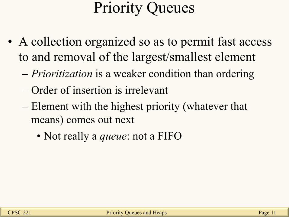
• A collection organized so as to permit fast access to and removal of the largest/smallest element – Prioritization is a weaker condition than ordering – Order of insertion is irrelevant – Element with the highest priority (whatever that
means) comes out next • Not really a queue: not a FIFO

CPSC 221 Priority Queues and Heaps Page 12
Priority Queue ADT
• Priority Queue operations – create – destroy – insert – deleteMin – isEmpty
• Priority Queue property: for two elements in the queue, x and y, if x has a lower priority value than y, x will be deleted before y
F(7) E(5) D(100) A(4)
B(6)
insert deleteMin G(9) C(3)
CPSC 221 Priority Queues and Heaps Page 13
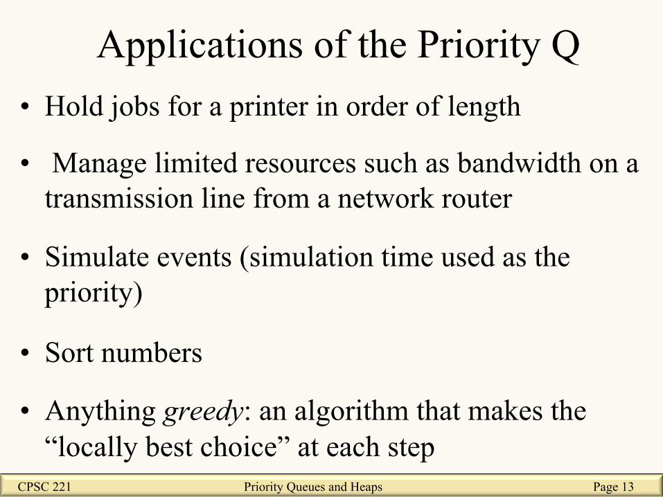
Applications of the Priority Q • Hold jobs for a printer in order of length
• Manage limited resources such as bandwidth on a transmission line from a network router
• Simulate events (simulation time used as the priority)
• Sort numbers
• Anything greedy: an algorithm that makes the “locally best choice” at each step

CPSC 221 Priority Queues and Heaps Page 14
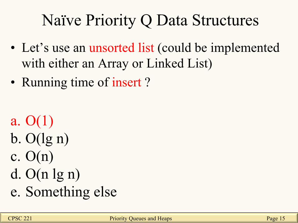
Naïve Priority Q Data Structures • Let’s use an unsorted list (could be implemented
with either an Array or Linked List) • Running time of insert ?
a. O(1) b. O(lg n) c. O(n) d. O(n lg n) e. Something else
CPSC 221 Priority Queues and Heaps Page 15
Naïve Priority Q Data Structures • Let’s use an unsorted list (could be implemented
with either an Array or Linked List) • Running time of insert ?
a. O(1) b. O(lg n) c. O(n) d. O(n lg n) e. Something else

CPSC 221 Priority Queues and Heaps Page 16
Naïve Priority Q Data Structures • Let’s use an unsorted list (could be implemented
with either an Array or Linked List) • Running time of deleteMin?
a. O(1) b. O(lg n) c. O(n) d. O(n lg n) e. Something else

CPSC 221 Priority Queues and Heaps Page 17
Naïve Priority Q Data Structures • Let’s use an unsorted list (could be implemented
with either an Array or Linked List) • Running time of deleteMin?
a. O(1) b. O(lg n) c. O(n) d. O(n lg n) e. Something else

CPSC 221 Priority Queues and Heaps Page 18
Naïve Priority Q Data Structures • Let’s use an sorted list (could be implemented
with either an Array or Linked List) • Running time of insert ?
a. O(1) b. O(lg n) c. O(n) d. O(n lg n) e. Something else

CPSC 221 Priority Queues and Heaps Page 19
Naïve Priority Q Data Structures • Let’s use an sorted list (could be implemented
with either an Array or Linked List) • Running time of insert ?
a. O(1) b. O(lg n) c. O(n) d. O(n lg n) e. Something else
CPSC 221 Priority Queues and Heaps Page 20
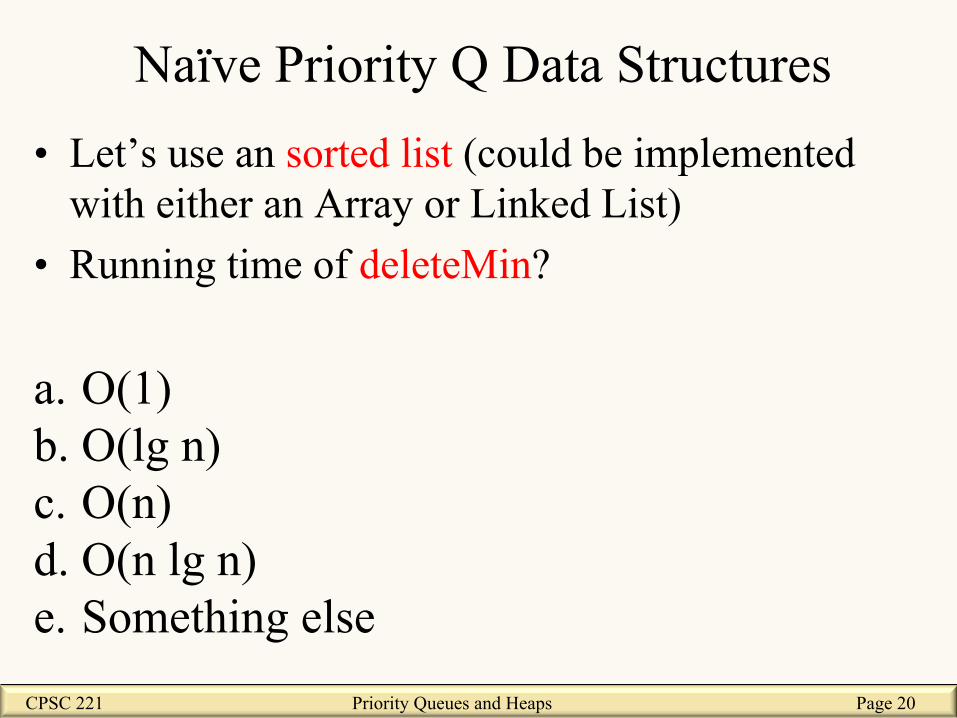
Naïve Priority Q Data Structures • Let’s use an sorted list (could be implemented
with either an Array or Linked List) • Running time of deleteMin?
a. O(1) b. O(lg n) c. O(n) d. O(n lg n) e. Something else
CPSC 221 Priority Queues and Heaps Page 21
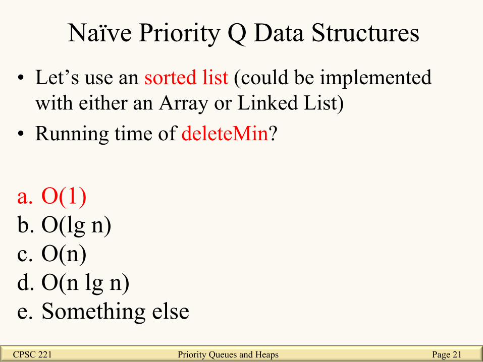
Naïve Priority Q Data Structures • Let’s use an sorted list (could be implemented
with either an Array or Linked List) • Running time of deleteMin?
a. O(1) b. O(lg n) c. O(n) d. O(n lg n) e. Something else

CPSC 221 Priority Queues and Heaps Page 22
The heap property• A node has the heap property if the priority of the
node is as high as or higher than the priority of its children
• All leaf nodes automatically have the heap property • A binary tree is a heap if all nodes in it have the
heap property
12
8 3 Red node has heap property
12
8 12 Red node has heap property
12
8 14 Red node does not have heap property

CPSC 221 Priority Queues and Heaps Page 23
• Given a node that does not have the heap property, you can give it the heap property by exchanging its value with the value of the child with the higher priority
• This is sometimes called Percolate-up(sifting up) • Notice that the child may have lost the heap
property
14
8 12 Red node has heap property
12
8 14 Red node does not have heap property
Percolate-up

CPSC 221 Priority Queues and Heaps Page 24
Binary Heap Priority Q Data Structure
20 14 12 9 11
8 10 6 7
5 4
2 • Heap-order property
– parent’s key is less than or equal to children’s keys
– result: minimum is always at the top
• Structure property – “nearly complete tree”
WARNING: this has NO SIMILARITY to the “heap” you hear about when people say “objects you create with new go on the heap”. 24
depth is always O(log n); next open location always known

CPSC 221 Priority Queues and Heaps Page 25
It is important to realize that two binary heaps can contain the same data but the data may appear in different positions in the heap:
2 5 7
5 7 8
2 5 5
7 7 8
Both of the minimum binary heaps above contain the same data: 2, 5, 5, 7, 7, and 8. Even though both heaps satisfy all the properties necessary of a minimum binary heap, the data is stored in different positions in the tree.

CPSC 221 Priority Queues and Heaps Page 26
(There’s also a maximum binary heap, where “parent ≤ each child” simply changes to “parent ≥ each child”.)
7 5 7
4 3 4
2 5 7
5 7 8
Min-heap Max-heap
Min-heap and Max-heap
CPSC 221 Priority Queues and Heaps Page 27
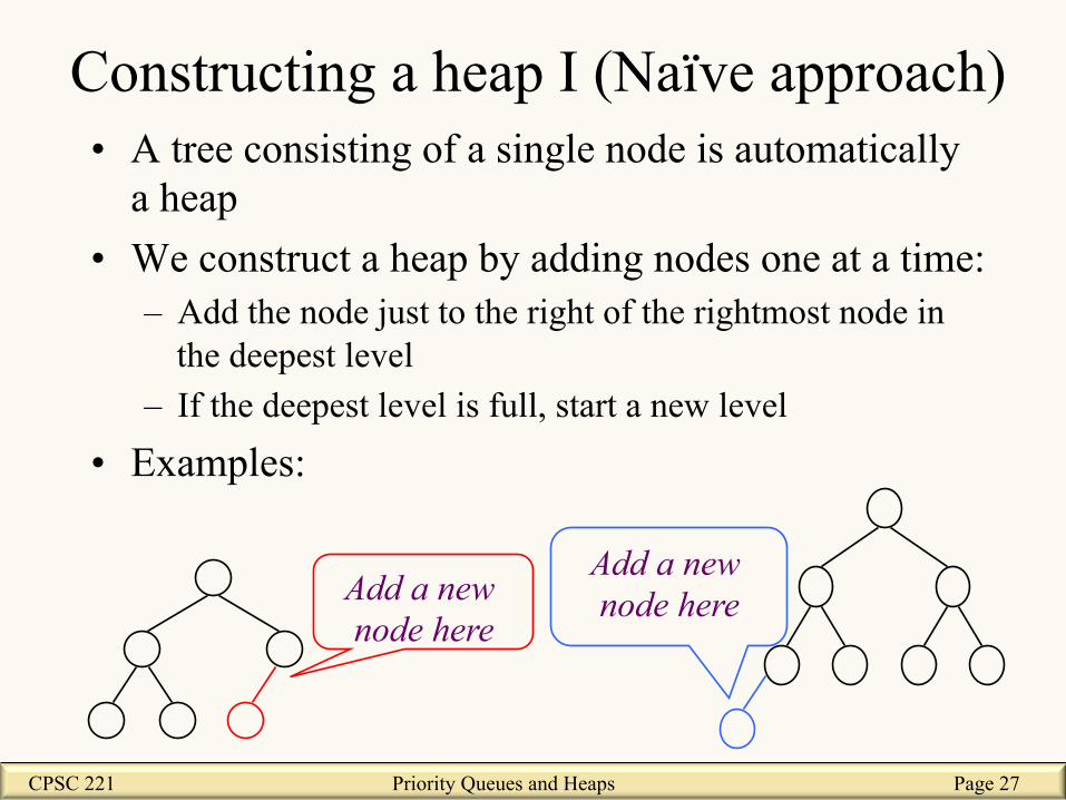
Constructing a heap I (Naïve approach) • A tree consisting of a single node is automatically
a heap • We construct a heap by adding nodes one at a time:
– Add the node just to the right of the rightmost node in the deepest level
– If the deepest level is full, start a new level
• Examples:
Add a new node here
Add a new node here

CPSC 221 Priority Queues and Heaps Page 28
Constructing a heap II (Naïve approach) • Each time we add a node, we may destroy the heap
property of its parent node. To fix this, we percolate-up • But each time we percolate-up, the value of the topmost
node in the sift may increase, and this may destroy the heap property of its parent node
• We repeat the percolate-up process, moving up in the tree, until either: – we reach nodes whose values don’t need to be
swapped (because the parent is still larger than both children), or
– we reach the root

CPSC 221 Priority Queues and Heaps Page 29
Constructing a heap III (Naïve approach)
8 8
10
10
8
10
8 5
10
8 5
12
10
12 5
8
12
10 5
8
1 2 3
4

CPSC 221 Priority Queues and Heaps Page 30
Other children are not affected
• The node containing 8 is not affected because its parent gets larger, not smaller
• The node containing 5 is not affected because its parent gets larger, not smaller
• The node containing 8 is still not affected because, although its parent got smaller, its parent is still greater than it was originally
12
10 5
8 14
12
14 5
8 10
14
12 5
8 10
CPSC 221 Priority Queues and Heaps Page 31
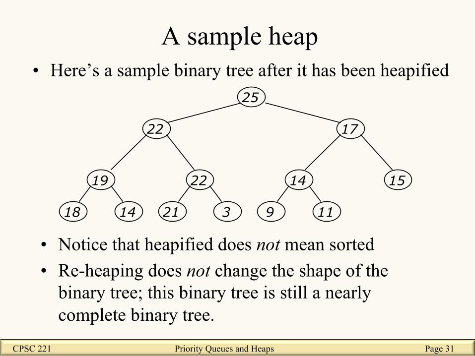
A sample heap • Here’s a sample binary tree after it has been heapified
• Notice that heapified does not mean sorted • Re-heaping does not change the shape of the
binary tree; this binary tree is still a nearly complete binary tree.
19
14 18
22
3 21
14
11 9
15
25
17 22

CPSC 221 Priority Queues and Heaps Page 32
Clicker Question • Is the following binary tree a maximum binary
heap?
– A: It is a maximum binary heap – B: It is not a maximum binary heap – C: I don’t know
19
18 14
23
5 21
16
6 9
15
25
17 22

CPSC 221 Priority Queues and Heaps Page 33
Clicker Question • Is the following binary tree a maximum binary
heap?
– A: It is a maximum binary heap – B: It is not a maximum binary heap – C: I don’t know
19
18 14
23
5 21
16
6 9
15
25
17 22
CPSC 221 Priority Queues and Heaps Page 34
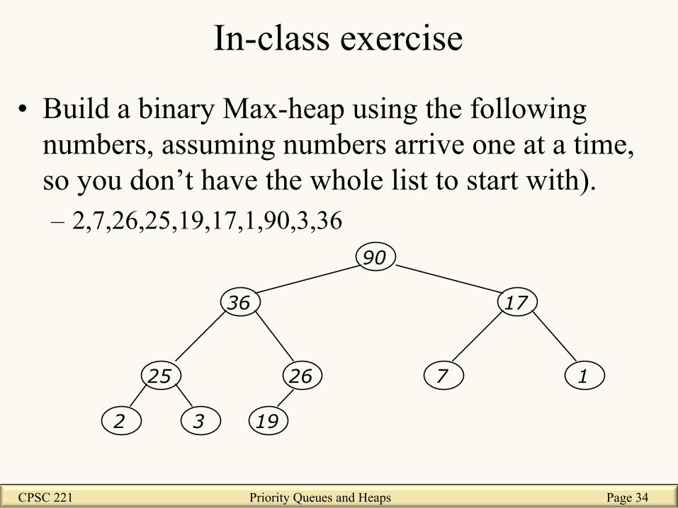
In-class exercise
• Build a binary Max-heap using the following numbers, assuming numbers arrive one at a time, so you don’t have the whole list to start with). – 2,7,26,25,19,17,1,90,3,36
25
3 2
26 7 1
90
17 36
19
CPSC 221 Priority Queues and Heaps Page 35
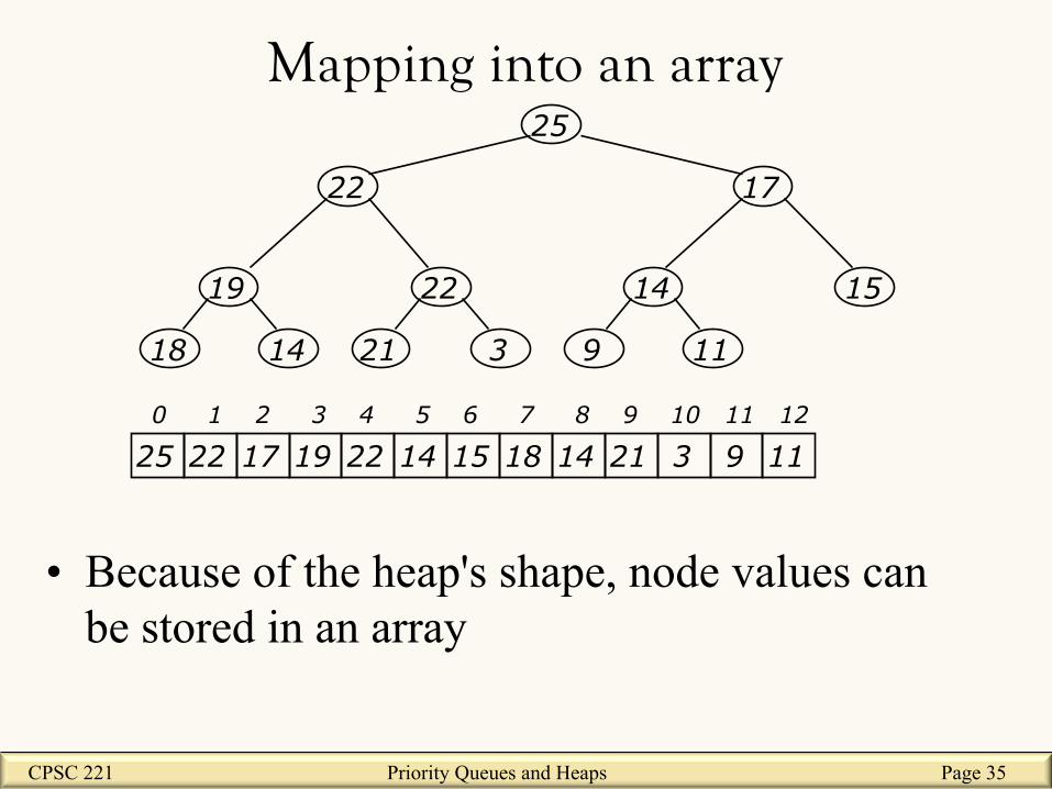
Mapping into an array
• Because of the heap's shape, node values can be stored in an array
19
14 18
22
3 21
14
11 9
15
25
17 22
25 22 17 19 22 14 15 18 14 21 3 9 11 0 1 2 3 4 5 6 7 8 9 10 11 12

CPSC 221 Priority Queues and Heaps Page 36
Mapping into an array
19
14 18
22
3 21
14
11 9
15
25
17 22
25 22 17 19 22 14 15 18 14 21 3 9 11 0 1 2 3 4 5 6 7 8 9 10 11 12
Left child = 2*node + 1 right child= 2*node + 2 parent = floor((node-1)/2) nextfree = length root = 0

CPSC 221 Priority Queues and Heaps Page 37
Adding an item to a heap • If a new item is added to the heap, use ReheapUp
(percolate-up ) to maintain a heap. /* This function performs the Reheapup operation on an array, to establish heap properties (for a subtree). ! ! PARAM: data – integer array containing the heap ! top – position of the root ! bottom - position of the added element ! */!void ReheapUp( int * data, int top, int bottom ){ ! if (bottom > top) { ! int parent = getparent(bottom); ! if (data[parent] < data[bottom]) { ! swap( &data[parent], &data[bottom]); ! ReheapUp(data, top, parent); ! } ! } !}

CPSC 221 Priority Queues and Heaps Page 38
• For the max-heap below draw the recursion tree of ReheapUp(data, 0, 12), where 25 is stored in data[0] !
19
14 18
22
3 21
14
26 9
15
25
17 22
ReheapUp(data, 0, 12)
ReheapUp(data, 0, 5)
ReheapUp(data, 0, 2)
In-class exercise
ReheapUp(data, 0, 0)

CPSC 221 Priority Queues and Heaps Page 39
Example (min-heap)
20 14 12 9 11
8 10 6 7
5 4
2
3 20 14 12 9 11
8 3 6 7
5 4
2
10
20 14 12 9 11
8 5 6 7
3 4
2
10 20 14 12 9 11
8 5 6 7
3 4
2
10

CPSC 221 Priority Queues and Heaps Page 40
Removing the root • So we know how to add new elements to our
heap. • We also know that root is the element with the
highest priority.
• But what should we do once root is removed? – Which element should replace root?

CPSC 221 Priority Queues and Heaps Page 41
One possibility
20 14 12 9 11
8 10 6 7
5 4
?
20 14 12 9 11
8 10 6 7
5 ?
4
20 14 12 9 11
8 10 ? 7
5 6
4
20 14 20 9 11
8 10 12 7
5 6
4

CPSC 221 Priority Queues and Heaps Page 42
Removing the root • Notice that the largest number is now in the root • Suppose we discard the root:
• How can we fix the binary tree so it is once again a nearly complete binary tree?
• Solution: remove the rightmost leaf at the deepest level and use it for the new root
19
14 18
22
3 21
14
11 9
15
17 22
11

CPSC 221 Priority Queues and Heaps Page 43
The percolate-down method • Our tree is now a nearly complete binary tree, but no
longer a heap • However, only the root lacks the heap property
• We can percolate-down the root • After doing this, one and only one of its children
may have lost the heap property
19
14 18
22
3 21
14
9
15
17 22
11

CPSC 221 Priority Queues and Heaps Page 44
The percolate-down method
• Now the left child of the root (still the number 11) lacks the heap property
• We can The percolate-down method this node • After doing this, one and only one of its children
may have lost the heap property
19
14 18
22
3 21
14
9
15
17 11
22

CPSC 221 Priority Queues and Heaps Page 45
The percolate-down method • Now the right child of the left child of the root (still the
number 11) lacks the heap property:
• We can percolate-down this node • After doing this, one and only one of its children may have
lost the heap property —but it doesn’t, because it’s a leaf
19
14 18
11
3 21
14
9
15
17 22
22

CPSC 221 Priority Queues and Heaps Page 46
The percolate-down method • Our tree is once again a heap, because every node
in it has the heap property
– Once again, the largest (or a largest) value is in the root
19
14 18
21
3 11
14
9
15
17 22
22

CPSC 221 Priority Queues and Heaps Page 47
In-class exercise • Build a binary Max-heap using the following numbers
– 2,7,26,25,19,17,1,90,3,36
– Now remove max and reheap
25
3 2
26 7 1
90
17 36
19
25
3 2
19 7 1
36
17 26

CPSC 221 Priority Queues and Heaps Page 48
• Use ReheapDown (percolate-down) to remove an item from a max heap
Removing an item from a heap
/* This function performs the ReheapDown operation on an array, to establish heap properties (for a subtree). ! !
PARAM: data – integer array containing the heap ! top – position of the root ! bottom – position of the final elements in heap !*/ !void ReheapDown( int * data, int top, int bottom){ ! if (!isLeaf(top, bottom)){ /* top is not a leaf */! int maxChild = getMaxChild(top) /* position of the ! child having largest data value */! !
if ( data[top] < data[maxChild] ){ ! swap( &data[top], &data[maxChild]) ! ReheapDown( data, maxChild, bottom); ! } ! } !} !
CPSC 221 Priority Queues and Heaps Page 49
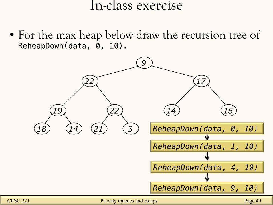
• For the max heap below draw the recursion tree of ReheapDown(data, 0, 10). !
19
14 18
22
3 21
14 15
9
17 22
ReheapDown(data, 0, 10)
ReheapDown(data, 1, 10)
ReheapDown(data, 4, 10)
ReheapDown(data, 9, 10)
In-class exercise

CPSC 221 Priority Queues and Heaps Page 50
CPSC 221 Administrative Notes • Lab3: Grades are finalized • Lab5: Feb 10 – Feb13, Feb 23 (Binary Heaps)
• No labs Feb 24, Feb 25, Feb 26
• Written Assignment #1 – Due Friday, Feb 13, at 5pm
• Midterm: Wed 25 6:00 pm – Make-up Wed 25 9:30pm
• Final: APR 22 2015 12:00 PM
• PeerWise: – Make sure you enter your question on PeerWise

CPSC 221 Priority Queues and Heaps Page 51
So, Where Were We? • Talked about priority queues and why unsorted or
sorted lists are not a suitable data structures for implementing them.
• Talked about the heap property and Binary Heaps.
• Talked about how you can add a node and remove a node from a Binary Heap.

CPSC 221 Priority Queues and Heaps Page 52
When performing either a ReheapUp or ReheapDown operation, the number of operations depends on the depth of the tree. Notice that we traverse only one path or branch of the tree. Recall that a nearly complete binary tree of height h has between 2h and 2h+1-1 nodes:
D F J
H K L M
D F J
H
We can now determine the height of a heap in terms of the number of nodes n in the heap. The height is lg n. The time complexity of the ReheapUp and ReheapDown operations is therefore O(lg n).
Time Complexity

CPSC 221 Priority Queues and Heaps Page 53
Building a Heap (Naïve) – Adding the elements one add a time with a reheapUp
• See http://visualgo.net/heap.html /* This function builds a heap from an array. ! ! PARAM: data – integer array (no order is assumed) ! top - position of the root ! bottom – position of the final elements in heap ! */!void Build_heap( int * data, int top, int bottom ) !{ ! int index = 0; ! while (index <= bottom){ ! ReheapUp(data, top, index); ! index ++; ! } !} !

CPSC 221 Priority Queues and Heaps Page 54
• Complexity analysis: – we add each of n nodes and each node has to be sifted up,
possibly as far as the root – Since the binary tree is a nearly complete binary tree, sifting up
a single node takes O(lg n) time – Since we do this N times, Heapify1 takes N*O(lg n) time, that
is, O(n lg n) time
8 8
10
10
8
10
8 5
10
8 5
12
10
12 5
8
12
10 5
8

CPSC 221 Priority Queues and Heaps Page 55
Heapify method • See http://visualgo.net/heap.html
/* This function builds a heap from an array. ! ! PARAM: data – integer array (no order is assumed) ! top - position of the root ! bottom – position of the final elements in heap !! */!void Heapify( int * data, int top, int bottom ) !{ ! int index = position of last parent node in entire tree; ! while (index => top){ ! /* go backwards from the last parent */! ReheapDown( data, index, bottom ); ! index --; ! } !}

CPSC 221 Priority Queues and Heaps Page 56
Example: Convert the following array to a min-heap:
8 9 7 3 2 5 0 1
8
9
3 2
7
5 0
1
To do so, picture the array as a nearly complete binary tree:
In-class exercise

CPSC 221 Priority Queues and Heaps Page 57
8
9
1 2
7
5 0
3
8
9
1 2
0
5 7
3
8
1
3 2
0
5 7
9
0
1
3 2
5
8 7
9

CPSC 221 Priority Queues and Heaps Page 58
Time complexity of Heapify • We can determine the time complexity of the Heapify function by
looking at the total number of times the comparison and swap operations occur while building the heap. Let us consider the worst case, which is
– when the last level in the heap is full, and all of the nodes with high priorities are in the leafs.
• We will colour all the paths from each node, starting with the lowest parent and working up to the root, each going down to a leaf node. The number of edges on the path from each node to a leaf node represents an upper bound on the number of comparison and swap operations that will occur while applying the ReheapDown operation to that node. By summing the total length of these paths, we will determine the time complexity of the Heapify function.

CPSC 221 Priority Queues and Heaps Page 59
In the worse possible case how many swaps are going to take place?
Relate the number of swaps first to the number of edges and then nodes.
Time complexity of Heapify

CPSC 221 Priority Queues and Heaps Page 60
Note that no edge is coloured more than once. Hence the work done by the Heapify function to build the heap can be measured in terms of the number of coloured edges.
Time complexity of Heapify

CPSC 221 Priority Queues and Heaps Page 61
Note that no edge is coloured more than once. Hence the work done by the Heapify function to build the heap can be measured in terms of the number of coloured edges.
Time complexity of Heapify

CPSC 221 Priority Queues and Heaps Page 62
Note that no edge is coloured more than once. Hence the work done by the Heapify function to build the heap can be measured in terms of the number of coloured edges.
Time complexity of Heapify
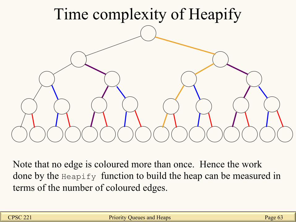
CPSC 221 Priority Queues and Heaps Page 63
Note that no edge is coloured more than once. Hence the work done by the Heapify function to build the heap can be measured in terms of the number of coloured edges.
Time complexity of Heapify

CPSC 221 Priority Queues and Heaps Page 64
Suppose H is the height of the tree, N is the number of elements in the tree, and E is the number of edges in the tree.
• How many edges are there in a nearly complete tree with N elements?
N-1
• Total number of coloured edges or swaps =
E – H = N - 1 - H = N – 1 – lg N
T(n) ∈ O (n)
Hence, in the worst case, the overall time complexity of the Heapify algorithm is:
O(n)
Time complexity of Heapify (sketch)

CPSC 221 Priority Queues and Heaps Page 65
Time complexity of Heapify (Induction)
The proof that this always works is inductive. The inductive step is that both of my sub-trees have an uncoloured path (leftmost) to the leaves. I colour the path thorough my right child and my left child provides an uncloured path that I offer to my parent

CPSC 221 Priority Queues and Heaps Page 66
Alternative Approach • Consider a complete heap:
– An n element heap has height
– An n element heap has at most nodes of any height • height 0 ~n/2 • height 1 ~n/4 • height lg n 1
– Cost for node at height k is O(K) – Therefore, run time is
n2i+1i=0
lgn
∑ O(i) =O(n i2i+1i=0
lgn
∑ ) ≤O(n2
i2ii=0
∞
∑ )
lgn!" #$
n2h+1!
""#
$$

CPSC 221 Priority Queues and Heaps Page 67
More Formally i2ii=0
∞
∑ =020+121+222+323+…=
121+1+122
+1+1+123
+…
=12ii=1
∞
∑ +12ii=2
∞
∑ +12ii=3
∞
∑ +…=12ii= j
∞
∑#
$%%
&
'((
j=1
∞
∑
= ( 12 j +
12 j+1 +
12 j+2 +...)
j=1
∞
∑ =12 j−1
12ii=1
∞
∑$
%&
'
()
j=1
∞
∑
12ii=1
∞
∑ =
12
1− 12
=1
=12 j−1
"
#$
%
&'
j=1
∞
∑ = 2 12 j
"
#$
%
&'
j=1
∞
∑ = 2

CPSC 221 Priority Queues and Heaps Page 68
More Formally • Consider a complete heap:
– An n element heap has height
– An n element heap has at most nodes of any height • height 0 ~n/2 • height 1 ~n/4 • height lg n 1
– Cost for node at height k is O(K) – Therefore, run time is
n2i+1i=0
lgn
∑ O(i) =O(n i2i+1i=0
lgn
∑ ) ≤O(n2
i2ii=0
∞
∑ )∈O(n)
lgn!" #$
n2h+1!
""#
$$

CPSC 221 Priority Queues and Heaps Page 69
Motivation: In this section, we examine a sorting algorithm that guarantees worst case O(n lg n) time.
We will use a binary heap to sort an array of data
The Heapsort algorithm consists of 2 phases:
1. [Heapify] Build a heap using the elements to be sorted.
2. [Sort] Use the heap to sort the data.
Let’s first consider the Naïve approach of building a heap
The Heapsort Algorithm

CPSC 221 Priority Queues and Heaps Page 70
Having built the heap, we now sort the array:
0
1
3 2
5
8 7
9
0 1 5 3 2 8 7 9
Note: In this section, we represent the data in both binary tree and array formats. It is important to understand that in practice the data is stored only as an array.
More about this later when we cover sorting!!!

CPSC 221 Priority Queues and Heaps Page 71
Time Complexity of Heapsort
We need to determine the time complexity of the Heapify O(n) operation, and the time complexity of the subsequent sorting operation.
The time complexity of the sorting operation once the heap has been built is fairly easy to determine. For each element in the heap, we perform a single swap and a ReheapDown. If there are N elements in the heap, the ReheapDown operation is O( lg n ), and hence the sorting operation is O( n lg n ).
Hence, in the worst case, the overall time complexity of the Heapsort algorithm is:
build heap from unsorted array
essentially perform N RemoveMin’s
O(n) + O(n lg n) = O(n lg n)

CPSC 221 Priority Queues and Heaps Page 72
Thinking about Binary Heaps • Observations
– finding a child/parent index is a multiply/divide by two – operations jump widely through the heap – deleteMins look at all (two) children of some nodes – inserts only care about parents of some nodes
• Realities – division and multiplication by powers of two are fast – looking at one new piece of data sucks in a cache line – with huge data sets, disk accesses dominate

CPSC 221 Priority Queues and Heaps Page 73
4
9 6 5 4
2 3
1
8 10 12
7
11
Solution: d-Heaps • Nodes have (up to) d children • Still representable by array • Good choices for d:
– optimize (non-asymptotic) performance based on ratio of inserts/removes
– make d a power of two for efficiency
– fit one set of children in a cache line – fit one set of children on a memory
page/disk block
3 7 2 8 5 12 11 10 6 9 1
d-heap mnemonic: d is for degree!

CPSC 221 Priority Queues and Heaps Page 74
Calculations in terms of d: – child:
– parent:
– root:
– next free: 4
9 6 5 4
2 3
1
8 10 12
7
11
d-Heap calculations
3 7 2 8 5 12 11 10 6 9 1
d-heap mnemonic: d is for degree!

CPSC 221 Priority Queues and Heaps Page 75
Calculations in terms of d: – child: i*d+1 through i*d+d
– parent: floor((i-1)/d)
– root: 0
– next free: size 4
9 6 5 4
2 3
1
8 10 12
7
11
d-Heap calculations
3 7 2 8 5 12 11 10 6 9 1
d-heap mnemonic: d is for degree!

CPSC 221 Priority Queues and Heaps Page 76
Learning Goals revisited • Provide examples of appropriate applications for
priority queues and heaps
• Determine if a given tree is an instance of a heap.
• Manipulate data in heaps
• Describe and apply the Heapify algorithm, and analyze its complexity
Top Related
Copyright © 2022 FDOKUMEN

