Discrete Optimization 8 (2011) 513–524

Contents lists available at SciVerse ScienceDirect

Discrete Optimization

journal homepage: www.elsevier.com/locate/disopt

Coordination mechanisms with hybrid local policiesKangbok Lee a, Joseph Y-T. Leung b,∗, Michael L. Pinedo c

a Department of Supply Chain Management & Marketing Sciences, Rutgers Business School, 1 Washington Park, Newark, NJ 07102, USAb Department of Computer Science, New Jersey Institute of Technology, Newark, NJ 07102, USAc Department of Information, Operations & Management Sciences, Stern School of Business, New York University, 44 West 4th Street, New York,NY 10012-1126, USA

a r t i c l e i n f o

Article history:Received 9 November 2009Received in revised form 1 April 2011Accepted 2 May 2011Available online 17 June 2011

Keywords:Coordination mechanismPrice of anarchyMixed local policyMakespanTotal completion timeEligibility constraints

a b s t r a c t

We study coordination mechanisms for scheduling n jobs on m parallel machines whereagents representing the jobs interact to generate a schedule. Each agent acts selfishly tominimize the completion time of his/her own job, without considering the overall systemperformance that is measured by a central objective. The performance deterioration dueto the lack of a central coordination, the so-called price of anarchy, is determined by themaximum ratio of the central objective function value of an equilibrium schedule dividedby the optimal value. In the first part of the paper, we consider a mixed local policy withsome machines using the SPT rule and other machines using the LPT rule. We obtain theexact price of anarchy for the problem of minimizing the makespan and some bounds forthe problem of minimizing the total completion time. In the second part of the paper, weconsider parallel machine scheduling subject to eligibility constraints.We devise new localpolicies based on the flexibilities and the processing times of the jobs. We show that thenewly devised local policies outperform both the SPT and the LPT rules.

© 2011 Elsevier B.V. All rights reserved.

1. Introduction

We consider the distributed scheduling of n independent jobs on m parallel machines in which all decisions areinteractively done by agents who are in charge of their own jobs. Each agent has a job and selects a machine to processhis/her own job so as to maximize his/her own utility, which is defined as the negation of the completion time of his/herown job.Without a central coordination, the jobs assigned to the samemachinewould compete to finish as early as possible,which will lead to chaos. To resolve the conflict, each machine will announce, in advance, the sequencing rule used by themachine to sequence the jobs assigned to that machine. For example, if the Shortest Processing Time first (SPT) rule is used,jobs assigned to that machine are sequenced in nondecreasing order of their processing times. Similarly, if the LongestProcessing Time first (LPT) rule is used, jobs are sequenced in nonincreasing order of their processing times. The sequencingrule used by a machine is usually referred to as the local policy of that machine.

However, there is a central objective function for evaluating the performance of the overall schedule. The central objectivemay be one of the classical scheduling objectives, such as makespan or total completion time. Due to the lack of a centralcoordination, the central objective may deteriorate, which is typically referred to as the Price Of Anarchy (POA). The POAis closely related to the concept of a Nash equilibrium. A Nash equilibrium schedule is defined as one where no agent canchange his/her current decision for a better schedule. In this paper we will only consider pure Nash equilibria which means

∗ Corresponding author. Tel.: +1 973 596 3387; fax: +1 973 596 5777.E-mail addresses: kangblee@andromeda.rutgers.edu (K. Lee), leung@cis.njit.edu, leung@oak.njit.edu (J.Y.-T. Leung), mpinedo@stern.nyu.edu

(M.L. Pinedo).

1572-5286/$ – see front matter© 2011 Elsevier B.V. All rights reserved.doi:10.1016/j.disopt.2011.05.001

514 K. Lee et al. / Discrete Optimization 8 (2011) 513–524

that each agent can only select one machine to process his/her own job. We assume that each agent is well aware of thelocal policy of each machine as well as all information about other jobs (including their processing times).

The POA can be formally defined as follows. LetI be the set of all instances andΛ(I) be the set of all equilibrium schedulesof instance I ∈ I. Let Z be the central objective function. Let σ ∗ be an optimal schedule. Then, the POA is defined as

POA = maxI∈I

maxσ∈Λ(I)

Z(σ )

Z(σ ∗)

.

Clearly, the local policy of each machine is a critical factor affecting the overall system performance, and hence the POA.In this paper, we consider the design of local policies in different environments.

1.1. Related works

In the literature, different machine environments and different local policies have been considered. Immorlica et al.[1] investigated four different machine environments, where job j has processing time pij on machine i. The four machineenvironments are: (1) identical machines—pij = pkj = pj for each job j and machines i and k; (2) uniform machines—pij = pj/si, where pj is the processing requirement of job j and si is the speed of machine i; (3) parallel machine schedulingwith assignment restrictions—job j can only be scheduled on a subset, Mj, of machines; i.e., pij = pj if i ∈ Mj, otherwise,pij = ∞; and (4) unrelated machines—pij is an arbitrary positive number. As for local policies, they considered SPT, LPT,Randomized and Makespan rules [1].

Most results in the literature are concerned with the makespan as the central objective function. For identical machines,the POA is 2− 1

m if the local policy is the SPT rule [2,1], and 43 −

13m if the local policy is the LPT rule [3,4]. For two uniform

machines, the POA is 1+√5

2 for both the SPT and LPT rules [5]. For three or more uniform machines, the POA is Θ(logm) for

SPT [1,6], while that of LPT lies within the interval [1.54, 1 +√33 ] [7,8]. For parallel machine scheduling with assignment

restrictions, the POA is Θ(logm) for both SPT and LPT [9,1]. For unrelated machines, the POA for SPT lies within the interval[logm,m] [5,10], while that for LPT is unbounded.

Christodoulou et al. [3] consider a hybrid local policy for two identical machines, where the first machine uses the SPTrule and the second machine uses the LPT rule. They show that the POA of this policy has a lower bound of 4

3 . As we shallsee in Section 2, we will show that 4

3 is also an upper bound for this special case.If the central objective is the total completion time and themachine environment consists of parallel identical machines,

the POA is 1 for SPT and nm for LPT [11]. If the central objective is the total weighted completion time and the machine

environment consists of identical machines in parallel, then the POA is√2+12 for theWeighted Shortest Processing Time first

(WSPT) rule [12,13].

1.2. Our contribution

In this paper we present new local policies for improving job utility or system performance. The paper consists of twoparts: (1) the first part deals with a mixed local policy that will avoid starvation of either long jobs or short jobs, and (2) thesecond part analyzes a local policy for parallel machine scheduling subject to eligibility constraints so as to improve thesystem performance.

In the first part we focus onmixed local policies. In the literature, all studies assume that all machines use the same localpolicy. For example, either all machines use SPT or all machines use LPT. The drawback of this approach is that either thelong jobs will be disadvantaged (if SPT is used) or the short jobs will be disadvantaged (if LPT is used). To overcome thisdrawback, we can consider a policy where some machines use SPT, while other machines use LPT. In this way, the long jobscan choose the machines that use LPT, while the short jobs can choose the machines that use SPT. We call this aMixed localpolicy and letMixed(h) denote the policywhere hmachines use SPT andm−hmachines use LPT, 1 ≤ h ≤ m−1.We assumethat all machines use the job index as a tie-breaking rule just in case two jobs have the same processing time; i.e., the jobwith the smaller job index will be scheduled before the job with the larger job index. In this paper we analyze the POA ofMixed local policies considering the makespan and the total completion time objectives on identical parallel machines.

In the second part of the paper, we consider parallel machine scheduling subject to eligibility constraints. The set ofeligible machines for job j,Mj, is called the eligible set of job j. Previous results have been obtained under the assumption ofarbitrary eligible sets [9,1]. However, in practice, eligible setsmay have structural properties that depend on the application.We consider two special types of eligibility constraints, namely Grade of Service (GoS) eligibility and Interval (Itrvl) eligibility.For applications of these two eligibilities, the reader is referred to the survey paper by Leung and Li [14]. For GoS eligibility,each job j has a grade gj and it is only allowed to be processed by machine i, where 1 ≤ i ≤ gj. Interval eligibility is a moregeneral version of GoS eligibility in that each job j has a pair of indexes uj and vj such that it can be processed by a machinei, where uj ≤ i ≤ vj. We analyze the POA of traditional local policies such as the SPT and LPT rules. We propose new localpolicies and show that they outperform the traditional ones.

K. Lee et al. / Discrete Optimization 8 (2011) 513–524 515

1.3. Model and notation

Throughout this paper, we use the following notations. There are n jobs to be scheduled onm parallel machines. Job j hasprocessing time pj, j = 1, . . . , n. Let Si and S∗i denote the sets of jobs scheduled on machine i, i = 1, . . . ,m, in the scheduleof context and in the optimal schedule, respectively. The starting time and completion time of job j are denoted by Bj and Cj,respectively. We consider two types of central objectives: the makespan and the total completion time. For the makespancase, the optimal makespan is denoted by Cmax(σ

∗) and the makespan of schedule σ is denoted by Cmax(σ ). For the totalcompletion time case, the optimal total completion time is denoted by

∑Cj(σ

∗) and the total completion time of scheduleσ is denoted by

∑Cj(σ ). For simplicity, we let P denote

∑nj=1 pj.

1.4. Organization of the paper

The paper is organized as follows. In the next section, we focus on Mixed local policies. In Section 2.1, we consider theproblem ofminimizing themakespan; in Section 2.2, we consider the problem ofminimizing the total completion time; andin Section 2.3 we summarize the results. In Section 3, we consider scheduling problems subject to eligibility constraints. InSection 3.1, we consider arbitrary eligibility; in Section 3.2, we consider GoS eligibility; in Section 3.3, we consider intervaleligibility; and in Section 3.4 we summarize the results. Finally, we draw some conclusions in Section 4.

2. Mixed local policies

In this section we consider Mixed local policies, with h machines using SPT and m − h machines use LPT to sequencetheir jobs. We useMixed(h) to refer to this local policy. Without loss of generality, we may assume that the first hmachinesuse SPT and the lastm− hmachines use LPT, where 1 ≤ h ≤ m− 1. We first consider the makespan objective and then thetotal completion time objective.

For the existence proof of the pure Nash equilibrium, we consider the following algorithm. We assume that jobs aresorted in increasing order of their processing times (p1 ≤ · · · ≤ pn).AlgorithmMixed (h)

s← 1, t ← n, Si ← ∅ for i = 1, . . . ,m.While (s ≤ t)

i1 ← argmin1≤i≤h∑

j∈Sipj

i2 ← argminh+1≤i≤m∑

j∈Sipj

If (∑

j∈Si1pj + ps ≤

∑j∈Si2

pj + pt)Then Si1 ← Si1 ∪ s, s← s+ 1Else Si2 ← Si2 ∪ t, t ← t − 1

EndWhileIn the resulting schedule there are two groups of machines; on the first h machines, jobs are scheduled in SPT order

while on the lastm− hmachines, jobs are scheduled in LPT order. By [1], LPT and SPT policies in identical parallel machineenvironments have pure Nash equilibria, respectively. Thus, no job scheduled in either one of the two groups will benefitfrom a move to another machine in the same group. Moreover, because of the structure of Algorithm Mixed (h), when ajob moves to a machine in the other group, no benefit is being obtained either. Thus, the resulting schedule is a pure Nashequilibrium schedule.

2.1. Makespan

For the makespan objective, the POA of Mixed(h) lies between that of the LPT policy and the SPT policy, as the nexttheorem shows.

Theorem 1. The POA of the distributed scheduling problem with m identical machines that follow the Mixed(h) local policy tominimize the makespan is 2−min

1h ,

2m+1

, 1 ≤ h ≤ m− 1.

Proof. We first establish an upper bound for the POA.Consider the Nash equilibrium schedule σ . Let j be the job that finishes last; i.e., Cmax(σ ) = Cj = Bj + pj. In the first h

machines, all the time slots before Bj must be occupied by other jobs according to the SPT local policy. When j is scheduledat time Bj, all the jobs scheduled before j in the lastm− hmachines have processing times that are equal or greater than pj,since they are sequenced according to LPT. Thus, P ≥ hBj + (m− h)pj + pj, and we have

Cj = Bj + pj ≤1hP +

1−

m− h+ 1h

pj.

We now consider two cases, depending on the sign of1− m−h+1

h

. First, we consider the case where

1− m−h+1

h

≥ 0,

or equivalently, h ≥ m+12 .

516 K. Lee et al. / Discrete Optimization 8 (2011) 513–524

Since Cmax(σ∗) ≥ P

m and Cmax(σ∗) ≥ pj, we have

Cmax(σ ) = Cj ≤mh

Pm+

1−

m− h+ 1h

pj ≤

2−

1h

Cmax(σ

∗).

Therefore, the POA has an upper bound

POA ≤Cmax(σ )

Cmax(σ ∗)≤ 2−

1h.

Second, we consider the case where1− m−h+1

h

< 0, or equivalently h < m+1

2 .

Cmax(σ ) = Cj ≤Ph−

m− h+ 1

h− 1

pj.

Since the time slots before Bj in the firstm− 1 machines are occupied by other jobs and the last machine has at least onejob which is not job j and has a processing time greater than or equal to pj, P ≥ (m − 1)Bj + 2pj. Thus, Bj ≤

P−2pjm−1 , and we

have

Cmax(σ ) = Cj = Bj + pj ≤1

m− 1P +

1−

2m− 1

pj.

If pj > 1m+1P , then Cj ≤

Ph −

m−h+1h − 1

pj < 2

m+1P since1− m−h+1

h

< 0. If pj ≤ 1

m+1P , then Cj ≤1

m−1P +1− 2

m−1

pj ≤ 2

m+1P .Thus, Cmax(σ ) ≤ 2

m+1P . Since Cmax(σ∗) ≥ P

m , we have

POA ≤Cmax(σ )

Cmax(σ ∗)≤

2m+1P

Pm

=2m

m+ 1= 2−

2m+ 1

.

From now on, we proceed with establishing a lower bound for the POA. We consider two cases, depending on whetherh ≥ m+1

2 or not. First, we consider the case where h ≥ m+12 . There are h(h − 1) jobs with processing time one unit and

m− h+ 1 jobs with processing time h units. For convenience, let the jobs with processing times 1 (respectively, h) be calledthe small (respectively, big) jobs. Obviously, in an optimal schedule σ ∗ with an optimal makespan of Cmax(σ

∗) = h, all smalljobs are assigned to the first h − 1 machines and all big jobs are assigned to the last m − h + 1 machines. Since the totalprocessing time is

∑pj = h(h− 1)× 1+ (m− h+ 1)× h = mh, this schedule is indeed optimal.

In theNash equilibrium scheduleσ , all small jobs are evenly assigned tomachines 1, . . . , h and all big jobs, except the lastone, are assigned to machines h+ 1, . . . ,m. The last big job is assigned to an arbitrary machine among the first hmachines.Thus, Cmax(σ ) = (h− 1)+ h = 2h− 1.

Therefore, the POA has the following lower bound.

POA ≥Cmax(σ )

Cmax(σ ∗)=

2h− 1h= 2−

1h.

Second, we consider the case where h < m+12 . There are mh jobs with a processing time of one unit and m− h+ 1 jobs

with a processing time of m units. For convenience, let the jobs with processing times 1 (respectively, m) be called small(respectively, big) jobs. In an optimal schedule σ ∗ with an optimal makespan of Cmax(σ

∗) = m + 1, each of the first h − 1machines has m + 1 small jobs, while each of the last m − h + 1 machines has a small job and a big job. Since the totalprocessing time is

∑pj = mh× 1+ (m− h+ 1)×m = m(m+ 1), this schedule is indeed optimal.

In the Nash equilibrium schedule σ , all small jobs are assigned to the first hmachines, and all big jobs, except the last one,are assigned to the lastm− hmachines. The last big job is assigned to an arbitrary machine. Thus, we have Cmax(σ ) = 2m.

Therefore, the POA has the following lower bound.

POA ≥Cmax(σ )

Cmax(σ ∗)=

2mm+ 1

= 2−2

m+ 1.

From the upper and lower bounds it follows that the POA is exactly 2− 1h for h ≥ m+1

2 and 2− 2m+1 for h < m+1

2 .

We note that the POA of Mixed(h) lies between that of the SPT case2− 1

m

[2,1] and that of the LPT case

43 −

12m

[3].

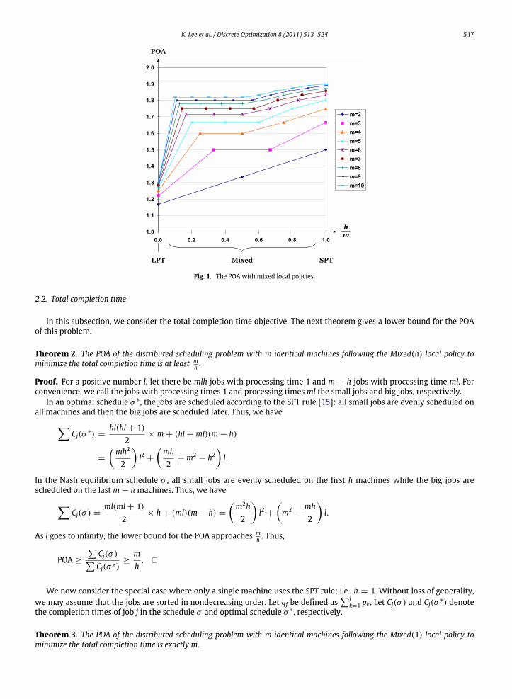
We summarize the results according to the value of h and m in a graphical way. In Fig. 1, h = 0 implies the LPT policy andh = m implies the SPT policy. The x-axis represents the ratio of machines using the SPT policy versus the total number ofmachines

hm

and the y-axis represents the POA. As can be seen from Fig. 1, the POA is dependent onm and h. Furthermore,

as the number of machines increases, there is a tendency that the POA of a mixed local policy is much closer to the POA ofthe SPT policy even when only one machine follows an SPT policy.

K. Lee et al. / Discrete Optimization 8 (2011) 513–524 517

Fig. 1. The POA with mixed local policies.

2.2. Total completion time

In this subsection, we consider the total completion time objective. The next theorem gives a lower bound for the POAof this problem.

Theorem 2. The POA of the distributed scheduling problem with m identical machines following the Mixed(h) local policy tominimize the total completion time is at least m

h .

Proof. For a positive number l, let there be mlh jobs with processing time 1 and m − h jobs with processing time ml. Forconvenience, we call the jobs with processing times 1 and processing timesml the small jobs and big jobs, respectively.

In an optimal schedule σ ∗, the jobs are scheduled according to the SPT rule [15]: all small jobs are evenly scheduled onall machines and then the big jobs are scheduled later. Thus, we have−

Cj(σ∗) =

hl(hl+ 1)2

×m+ (hl+ml)(m− h)

=

mh2

2

l2 +

mh2+m2

− h2l.

In the Nash equilibrium schedule σ , all small jobs are evenly scheduled on the first h machines while the big jobs arescheduled on the lastm− hmachines. Thus, we have−

Cj(σ ) =ml(ml+ 1)

2× h+ (ml)(m− h) =

m2h2

l2 +

m2−

mh2

l.

As l goes to infinity, the lower bound for the POA approaches mh . Thus,

POA ≥∑

Cj(σ )∑Cj(σ ∗)

≥mh

.

We now consider the special case where only a single machine uses the SPT rule; i.e., h = 1. Without loss of generality,we may assume that the jobs are sorted in nondecreasing order. Let qj be defined as

∑jk=1 pk. Let Cj(σ ) and Cj(σ

∗) denotethe completion times of job j in the schedule σ and optimal schedule σ ∗, respectively.

Theorem 3. The POA of the distributed scheduling problem with m identical machines following the Mixed(1) local policy tominimize the total completion time is exactly m.

518 K. Lee et al. / Discrete Optimization 8 (2011) 513–524

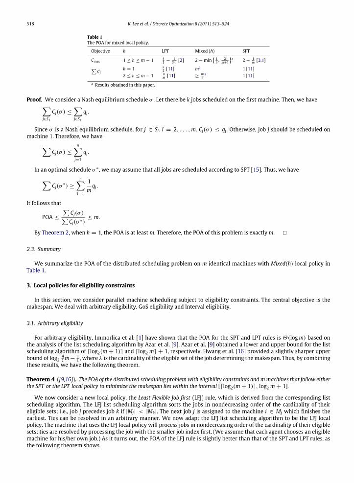
Table 1The POA for mixed local policy.

Objective h LPT Mixed (h) SPT

Cmax 1 ≤ h ≤ m− 1 43 −

13m [2] 2−min

1h , 2

m+1

a 2− 1

m [3,1]∑Cj

h = 1 n2 [11] ma 1 [11]

2 ≤ h ≤ m− 1 nm [11] ≥

mha 1 [11]

a Results obtained in this paper.

Proof. We consider a Nash equilibrium schedule σ . Let there be k jobs scheduled on the first machine. Then, we have−j∈S1

Cj(σ ) ≤−j∈S1

qj.

Since σ is a Nash equilibrium schedule, for j ∈ Si, i = 2, . . . ,m, Cj(σ ) ≤ qj. Otherwise, job j should be scheduled onmachine 1. Therefore, we have−

Cj(σ ) ≤

n−j=1

qj.

In an optimal schedule σ ∗, we may assume that all jobs are scheduled according to SPT [15]. Thus, we have−Cj(σ

∗) ≥

n−j=1

1m

qj.

It follows that

POA ≤∑

Cj(σ )∑Cj(σ ∗)

≤ m.

By Theorem 2, when h = 1, the POA is at leastm. Therefore, the POA of this problem is exactlym.

2.3. Summary

We summarize the POA of the distributed scheduling problem on m identical machines with Mixed(h) local policy inTable 1.

3. Local policies for eligibility constraints

In this section, we consider parallel machine scheduling subject to eligibility constraints. The central objective is themakespan. We deal with arbitrary eligibility, GoS eligibility and Interval eligibility.

3.1. Arbitrary eligibility

For arbitrary eligibility, Immorlica et al. [1] have shown that the POA for the SPT and LPT rules is Θ(logm) based onthe analysis of the list scheduling algorithm by Azar et al. [9]. Azar et al. [9] obtained a lower and upper bound for the listscheduling algorithm of ⌈log2(m + 1)⌉ and ⌈log2 m⌉ + 1, respectively. Hwang et al. [16] provided a slightly sharper upperbound of log2

4λm− 1

λ, where λ is the cardinality of the eligible set of the job determining themakespan. Thus, by combining

these results, we have the following theorem.

Theorem 4 ([9,16]). The POA of the distributed scheduling problemwith eligibility constraints andmmachines that follow eitherthe SPT or the LPT local policy to minimize the makespan lies within the interval [⌈log2(m+ 1)⌉, log2 m+ 1].

We now consider a new local policy, the Least Flexible Job first (LFJ) rule, which is derived from the corresponding listscheduling algorithm. The LFJ list scheduling algorithm sorts the jobs in nondecreasing order of the cardinality of theireligible sets; i.e., job j precedes job k if |Mj| < |Mk|. The next job j is assigned to the machine i ∈ Mj which finishes theearliest. Ties can be resolved in an arbitrary manner. We now adapt the LFJ list scheduling algorithm to be the LFJ localpolicy. The machine that uses the LFJ local policy will process jobs in nondecreasing order of the cardinality of their eligiblesets; ties are resolved by processing the job with the smaller job index first. (We assume that each agent chooses an eligiblemachine for his/her own job.) As it turns out, the POA of the LFJ rule is slightly better than that of the SPT and LPT rules, asthe following theorem shows.

K. Lee et al. / Discrete Optimization 8 (2011) 513–524 519

Theorem 5. The POA of the distributed scheduling problem on two identical machines with eligibility constraints and LFJ localpolicy to minimize the makespan is 3

2 .

Proof. We first obtain an upper bound for the POA.Let j be the job that finishes last in a Nash equilibrium schedule σ . If |Mj| = 1, then all jobs scheduled before j on the same

machine as j are eligible only for that machine. This implies that Cmax(σ ) = Cmax(σ∗). If Mj = 1, 2, then all time slots on

both machines before the starting time of j, Bj, must be occupied by other jobs. Therefore, P ≥ 2Bj + pj; i.e. Bj ≤12 (P − pj),

Therefore, we have

Cmax(σ ) = Cj = Bj + pj ≤12P +

12pj.

Since Cmax(σ∗) ≥ 1

2P and Cmax(σ∗) ≥ pj, we have

Cmax(σ ) ≤ Cmax(σ∗)+

12Cmax(σ

∗) =32Cmax(σ

∗).

Thus, the POA is at most 32 .

We proceed with determining a lower bound for the POA.We consider the following instance. There are three jobs with p1 = p2 = 1

2 and p3 = 1, and M1 = M2 = M3 = 1, 2.In an optimal schedule, Cmax(σ

∗) = 1 by setting S∗1 = 1, 2 and S∗2 = 3, while in a Nash equilibrium scheduleσ , Cmax(σ ) = 3

2 by setting S1 = 1, 3 and S2 = 2. Thus, the POA is at least 32 .

Theorem 6. The POA of the distributed scheduling problem on m identical machines with eligibility constraints and LFJ localpolicy to minimize the makespan lies within the interval

⌈log2(m+ 1)⌉ − 1, log2 m+

12

for m ≥ 3.

Proof. We first obtain an upper bound for the POA.By almost the same argument as Immorlica et al. [1], we can show that the set of Nash equilibrium schedules for the

LFJ local policy is precisely the set of schedules that can be obtained by the LFJ list scheduling algorithm. Due to a result byHwang et al. [16], the POA has an upper bound of log2

4λm − 1

λ, where λ is the number of machines eligible for processing

for the job with the last completion time.Let j be the job that finishes last in a Nash equilibrium schedule σ . If |Mj| = 1, then all jobs scheduled before j on the

same machine as j are eligible only for that machine. This implies that σ is an optimal schedule. If |Mj| ≥ 2, then the POA isupper bounded by log2

42m−

12 = log2 m+

12 . Therefore, the POA has an upper bound of log2 m+

12 .

We proceed with determining a lower bound for the POA.We consider the problem instance where 2k

≤ m < 2k+1 and n = 2k for some positive integer k. Every job has oneunit of processing time. There are k+ 1 groups of jobs. Let job (h, j) denote the j-th job in group h, h = 1 . . . , k+ 1. Grouph, h = 1, . . . , k, consists of 2k−h jobs and job (h, j) is eligible for the two machines j and j + 2k−h. Group k + 1 consists ofone job that is eligible for machines 1 and 2. Note that all jobs are eligible for twomachines. In an optimal schedule σ ∗, eachjob in group h, h = 1, . . . , k, selects the machine with the larger index in its eligible set and the job in group k + 1 selectsmachine 1. Thus, Cmax(σ

∗) = 1. In a Nash equilibrium schedule, σ , jobs are scheduled in increasing order of group indexand each job in group h, h = 1, . . . , k, selects the machine with the smaller index in its eligible set. Finally, the job in groupk+ 1 selects machine 2. Thus, Cmax(σ ) = k = ⌈log2(m+ 1)⌉ − 1. Therefore, the POA is at least ⌈log2(m+ 1)⌉ − 1.

From the upper and lower bounds it follows that the POA is exactly 32 form = 2 and lies within interval [⌈log2(m+1)⌉−

1, log2 m+12 ] form ≥ 3.

When the flexibility is utilized in the local policy, the POA is slightly improved for the scheduling problem subject toarbitrary eligibility constraints. However, when it is used for the case with more structured eligibility constraints, the POAcan be significantly improved, as we show in the following two subsections. Note that Immorlica et al. [1] have shown thatany deterministic local policy for the problem subject to arbitrary eligibility constraints has a POA of Θ(logm).

3.2. GoS eligibility

In this subsection, we consider the scheduling of jobs subject to GoS eligibility constraints. Hwang et al. [17] have givenexamples showing that the POA of the SPT and LPT rules is at least ⌈log2(m+ 1)⌉. Thus, we have the following theorem.

Theorem 7 ([17]). The POA of the distributed scheduling problem with GoS eligibility constraints and m machines that followeither the SPT or the LPT local policy to minimize the makespan is at least ⌈log2(m+ 1)⌉.

In a search for a better local policy, we consider one that is adapted from a list scheduling algorithm, which we refer toas the Lowest Grade and Longest Processing Time first (LG–LPT) algorithm. The LG–LPT algorithm works as follows. Initially,jobs are sorted such that job j precedes job k• if gj < gk or• if gj = gk and pj > pk or• if gj = gk and pj = pk and j < k.

520 K. Lee et al. / Discrete Optimization 8 (2011) 513–524

After the sorting, jobs are scheduled in this order. The next job j is assigned to a machine i ∈ Mj that finishes the earliest.Hwang et al. [17] have shown that the LG–LPT algorithm has a tight worst-case performance ratio of 5/4 for m = 2 and2− 1

m−1 for m ≥ 3.We adapt the LG–LPT algorithm as a local policy. A machine that uses the LG–LPT local policy schedules job j before job k• if gj < gk or• if gj = gk and pj > pk or• if gj = gk and pj = pk and j < k.

In the next theoremwe will show that the LG–LPT local policy has a POA that is the same as the worst-case performanceratio of the LG–LPT algorithm. This is a great improvement over SPT and LPT which have a POA of at least ⌈log2(m+ 1)⌉.

Theorem 8. The POA of the distributed scheduling problem with eligibility constraints and two machines that follow the LG–LPTlocal policy to minimize the makespan is 5/4.

Proof. We first establish an upper bound for the POA.Assume job j is the job that finishes last in a Nash equilibrium schedule σ . If gj = 1, then all jobs scheduled onmachine 1

must be scheduled onmachine 1, which implies that the current schedule is optimal. Therefore, wemay assume that gj = 2.Since σ is a Nash equilibrium schedule, if job j is scheduled on machine 1, then Cj = (

∑k∈S1\j

pk + pj) and Cj ≤

(∑

k∈S2\jpk + pj). If job j is scheduled on machine 2, then Cj ≤ (

∑k∈S1\j

pk + pj) and Cj = (∑

k∈S2\jpk + pj). So, in both

cases, we have

2Cmax(σ ) ≤

−k∈S1\j

pk + pj

+

−k∈S2\j

pk + pj

= P + pj.

Since Cmax(σ∗) ≥ 1

2P , we have

Cmax(σ ) ≤12P +

12pj ≤ Cmax(σ

∗)+12pj.

There are two cases to consider, depending on the value of pj. If pj ≤ 12Cmax(σ

∗), then we have

Cmax(σ ) ≤

1+

14

Cmax(σ

∗) =54Cmax(σ

∗).

On the other hand, if pj > 12Cmax(σ

∗), then we assert that Cmax(σ ) = Cmax(σ∗). First, we observe that the number of jobs

that start before j and are eligible for machine 2 cannot be more than one, since pj > 12Cmax(σ

∗). If there were no such jobs,then j must be scheduled on machine 2 first and Cj = pj ≤ Cmax(σ

∗). Therefore, we may assume that there is exactly onesuch job, denoted by l. Job l is scheduled onmachine 2 and pl ≥ pj > 1

2Cmax(σ∗). Therefore, in an optimal schedule σ ∗, j and

l cannot be scheduled on the same machine. If∑

k∈S1\jpk < pl, then j is scheduled on machine 1 in σ , just like an optimal

schedule σ ∗. On the other hand, if∑

k∈S1\jpk ≥ pl, then it is impossible to have a schedule with makespan Cmax(σ

∗). Thiscontradicts the fact that there is an optimal schedule with makespan Cmax(σ

∗).In both cases, Cmax(σ ) ≤ 5

4Cmax(σ∗). Therefore, whenm = 2, the POA has an upper bound of 5

4 .We now proceed with establishing a lower bound for the POA.Consider an instance where there are four jobs such that g1 = 1, g2 = g3 = g4 = 2, p1 = 1/4, p2 = 3/4 and

p3 = p4 = 1/2. The optimal makespan is 1 by setting S∗1 = 1, 2 and S∗2 = 3, 4. In a Nash equilibrium scheduleσ , S1 = 1, 3, 4 and S2 = 2. The makespan of σ is 5/4. Therefore, the POA is at least 5

4 form = 2.

Theorem 9. The POA of the distributed scheduling problem with eligibility constraints and m machines that follow the LG–LPTlocal policy to minimize the makespan is 2− 1

m−1 for m ≥ 3.

Proof. We first establish an upper bound for the POA.Assume again that job j is the one that finishes last in a Nash equilibrium schedule σ and let gj = i. If i = 1, then all

jobs scheduled on machine 1 must be scheduled on machine 1. Therefore, σ is an optimal schedule already. Thus, we mayassume that i ≥ 2.

All the time slots before the starting time of job j, Bj, on machines 1, . . . , i must be occupied by other jobs. Note thatmachine i has at least one job; otherwise, job j would be moved to machine i. Consider the jobs scheduled before Bj onmachine i. Since they are scheduled on machine i, their grades are greater than or equal to i. Also, since they are scheduledbefore Bj, their grades are smaller than or equal to i. Therefore, their processing times are greater than or equal to pj by theLG–LPT local policy. Thus, the total processing times of the jobs whose grades are at most i is

∑gk≤i

pk ≥ (i − 1)Bj + 2pj.Thus, we have

Cmax(σ ) = Bj + pj ≤

∑gk≤i

pk − 2pj

i− 1+ pj ≤

1i− 1

−gk≤i

pk +1−

2i− 1

pj.

K. Lee et al. / Discrete Optimization 8 (2011) 513–524 521

Since Cmax(σ∗) ≥ 1

i

∑gk≤i

pk and Cmax(σ∗) ≥ pj, we have

Cmax(σ ) ≤i

i− 1Cmax(σ

∗)+

1−

2i− 1

Cmax(σ

∗) ≤

2−

1m− 1

Cmax(σ

∗).

Therefore, an upper bound for the POA whenm ≥ 3 is 2− 1m−1 .

We now proceed with establishing a lower bound for the POA.Consider an instance where there are three groups of jobs. In the first group, there are m− 2 jobs with processing time

1− 1m−1 and gradem− 1. In the second group, there arem− 2 jobs with processing time 1

m−1 and gradem− 1. In the thirdgroup, there are two jobs with processing time 1 and gradem. Therefore, under the LG–LPT local policy, the jobs in the firstgroup have higher priority than the jobs in the second group, and the jobs in the second group have higher priority than thejobs in the third group.

In an optimal schedule σ ∗, one job from the first group and one job from the second group are scheduled on machinei, i = 1, . . . ,m − 2. On machines m − 1 and m, jobs from the third group are scheduled, one job per machine. Thus, theoptimal makespan is Cmax(σ

∗) = 1.In a Nash equilibrium schedule σ , all jobs in the first group are scheduled onmachines 1, . . . ,m−2, one job permachine.

All jobs in the second group are scheduled on machinem− 1. Finally, one job from the third group is scheduled on machinem and the other job is scheduled on machine 1. Thus, the makespan of σ is Cmax(σ ) = 2 − 1

m−1 . Therefore, the POA is atleast 2− 1

m−1 for m ≥ 3.

3.3. Interval eligibility

In the Interval eligibility case, job j has two indexes, uj and vj, such that Mj = i | uj ≤ i ≤ vj. Since GoS eligibility is aspecial case of Interval eligibility, the POA of the SPT and LPT local policy is at least ⌈log2 m+1⌉. In a search for a better localpolicy, we consider adapting a list scheduling algorithm called the Least Flexible and Longest Processing Time first (LF–LPT)algorithm. In the LF–LPT algorithm, jobs are sorted in nondecreasing order of their flexibility (which is simply the cardinalityof the eligible set of the job), and in case of a tie, in nonincreasing order of their processing times. After the jobs have beensorted, the next job j is assigned to the machine i ∈ Mj that finishes first. Lee [18] has shown that the LF–LPT algorithm hasa worst-case performance ratio is in the interval [4− 7

λ, 4− 3

λ] for λ ≥ 4, where λ is the cardinality of the eligible set of the

most flexible job.We adapt the LF–LPT rule as a local policy. Each machine schedules the jobs in nondecreasing order of the flexibility of

the job, and in case of a tie, in nonincreasing order of their processing times. Further ties will be broken by the job index;i.e., a job with a smaller job index will be scheduled before a job with a larger job index. In the next two theorems, wewill establish a value for the POA of the LF–LPT local policy by utilizing the worst-case performance ratio of the LF–LPT listscheduling algorithm.

Theorem 10. The POA of the distributed scheduling problem with Interval eligibility constraints and two machines that followthe LF–LPT local policy to minimize the makespan is 5

4 .

Proof. We first establish an upper bound for the POA. Let j be the job that finishes last in a Nash equilibrium schedule σ .If j is eligible for only one machine, then Cmax(σ ) = Cmax(σ

∗). Henceforth, we consider the case where j is eligible for bothmachines.

Without loss of generality, we may assume that j is scheduled on machine 1. Let L1 and L2 be the total processing timeof jobs whose eligible sets are 1 and 2, respectively. We now consider jobs that are eligible for both machines and startbefore j. If there are no such jobs, then σ is already optimal and Cmax(σ ) = Cmax(σ

∗). If there is such a job, let k be the job.Since k starts before j, we have pk ≥ pj. We consider two cases depending on the value of pj.

If pj > 12Cmax(σ

∗), then we have pk ≥ pj > 12Cmax(σ

∗). This implies that k is the only job eligible for both machines andstarting before j. Now, if k is scheduled on machine 1, then L2 ≥ pk > 1

2Cmax(σ∗). Otherwise, job j would not be scheduled

on machine 1. Thus, it is impossible to have a schedule with a makespan equal to Cmax(σ∗). Therefore, kmust be scheduled

on machine 2, which implies that L1 ≥ L2. Hence, j is scheduled on machine 1, k is scheduled on machine 2, and L1 ≥ L2 inσ . It is easy to see that σ is in fact an optimal schedule.

We now consider the case where pj ≤ 12Cmax(σ

∗). Since σ is a Nash equilibrium schedule, all time slots before Bj areoccupied by other jobs. Thus, P ≥ 2Bj + pj, where P is the total processing time of all the jobs. Thus, Bj ≤

12 (P − pj). Since

Cmax(σ∗) ≥ 1

2P and Cmax(σ∗) ≥ pj, we have

Cmax(σ ) = Cj = Bj + pj ≤12(P + pj) ≤

54Cmax(σ

∗).

Therefore, the POA has an upper bound of 54 .

522 K. Lee et al. / Discrete Optimization 8 (2011) 513–524

Since when m = 2, the lower bound example for the GoS case will work in this case as well, the POA for the problem isexactly 5

4 .

Theorem 11. The POA of the distributed scheduling problem with Interval eligibility constraints and m machines that follow theLF–LPT local policy to minimize the makespan is no more than 4− 3

m for m ≥ 3.

Proof. Let j be the job that finishes last in a Nash equilibrium schedule σ , and let λ be the cardinality of the eligible set of j,i.e. λ = |Mj| = vj − uj + 1.

Since σ is a Nash equilibrium schedule, all time slots before the starting time of j, Bj, are occupied by jobs with higherpriority than j under the LF–LPT local policy. We consider the set of jobs that can be scheduled on one of the machinesuj, . . . , vj. Each of these jobs must have the cardinality of their eligible sets bounded above by λ. Let J ′ be a super set of theset of such jobs defined as follows.

J ′ = k | uk ≥ uj − λ+ 1andvk ≤ vj + λ− 1.

Since the local policy is LF–LPT, all jobs occupying the time slots before Bj onmachines uj, . . . , vj must belong to J ′. Clearly,j belongs to J ′ as well. Thus,

∑k∈J ′ pk ≥ λBj + pj. Therefore, we have

Bj ≤1λ

−k∈J ′

pk − pj

.

Also, all jobs in J ′ must be scheduled on machines uj − λ+ 1, . . . , vj + λ− 1. Thus, Cmax(σ∗) ≥ 1

3λ−2

∑k∈J ′ pk. Note that

Cmax(σ∗) ≥ pj as well. Therefore, we have

Cmax(σ ) = Cj = Bj + pj ≤1λ

−k∈J ′

pk +1−

1λ

pj

≤

3λ− 2

λ

Cmax(σ

∗)+

1−

1λ

Cmax(σ

∗) =

4−

3λ

Cmax(σ

∗).

Since λ ≤ m, the POA is at most 4− 3m .

Theorem 12. The POA of the distributed scheduling problem with Interval eligibility constraints and m machines that follow theLF–LPT local policy to minimize the makespan is at least 4− 28

m+12 for m being a multiple of 8.

Proof. Consider the following instance: there are six groups of jobs to be scheduled on m machines. We assume that m isa multiple of eight and let q be m

4 . The information about the jobs are as follows. A group may consist of subgroups and asubgroup consists of jobs. Therefore, each job is denoted by a triplet (a, b, k), where a is the group index, b is the subgroupindex in the group and k is the job index in the subgroup. The jobs information are summarized as follows.

Gr. S.Gr. Job Range |Mj| uj vj pj

1 1 (1, 1, k) k = 1, . . . , q− 1 1 q+ k q+ k q−kq ϵ

2 (1, 2, k) k = 1, . . . , q− 1 1 3q− k+ 1 3q− k+ 1 q−kq ϵ

2 1 (2, 1, k) k = 1, . . . , q 1 k k ϵ

2 (2, 2, k) k = 1, . . . , q 1 3q+ k 3q+ k ϵ

3 1 (3, 1, k) k = 1, . . . , q q+ 1 k q+ k 1− ϵ

2 (3, 2, k) k = 1, . . . , q q+ 1 2q+ k 3q+ k 1− ϵ

4 1 (4, 1, k) k = 1, . . . , q2 − 1 q+ 2 q+ k 2q+ 1+ k 1− ϵ

2 (4, 2, k) k = 1, . . . , q2 − 2 q+ 2 2q− k 3q+ 1− k 1− ϵ

5 1 (5, 1, k) k = 1, . . . , (q+ 3) q2 + 1

q+ 2 q+ q

2 2q+ q2 + 1 1−ϵ

q+3

2 (5, 2, k) k = 1, . . . , (q+ 3) q2 + 1

q+ 2 q+ q

2 + 1 2q+ q2 + 2 1−ϵ

q+36 1 (6, 1, 1) q+ 3 q+ q

2 2q+ q2 + 2 1

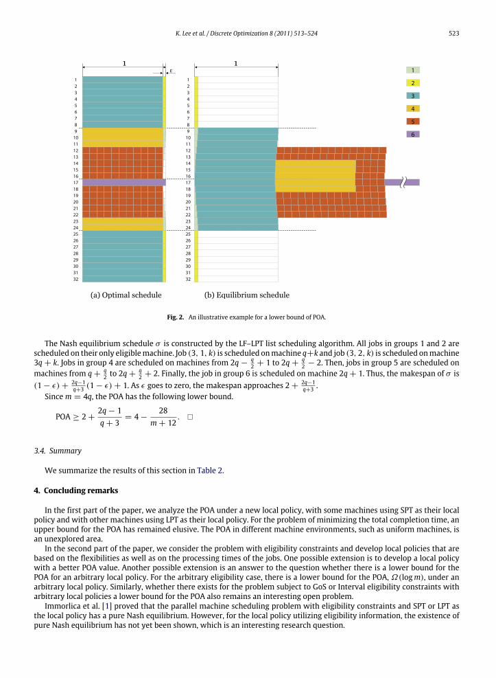
An illustrative example is presented in Fig. 2, wherem = 32.In an optimal scheduleσ ∗, all jobs in groups 1 and 2 are scheduled on their only eligiblemachine. Job (3, 1, k) is scheduled

on machine k and job (3, 2, k) is scheduled on machine 3q+ k. Job (4, 1, k) is scheduled on machine q+ k and job (4, 2, k)is scheduled on machine 3q + 1 − k. Jobs in subgroup (5,1) are scheduled on machines from q + q

2 to 2q evenly and jobsin subgroup (5, 2) are scheduled on machines from 2q + 2 to 2q + q

2 + 2 evenly. The last job in group 6 is scheduled onmachine 2q+ 1. Thus, the optimal makespan is 1.

K. Lee et al. / Discrete Optimization 8 (2011) 513–524 523

Fig. 2. An illustrative example for a lower bound of POA.

The Nash equilibrium schedule σ is constructed by the LF–LPT list scheduling algorithm. All jobs in groups 1 and 2 arescheduled on their only eligiblemachine. Job (3, 1, k) is scheduled onmachine q+k and job (3, 2, k) is scheduled onmachine3q+ k. Jobs in group 4 are scheduled on machines from 2q− q

2 + 1 to 2q+ q2 − 2. Then, jobs in group 5 are scheduled on

machines from q+ q2 to 2q+ q

2 + 2. Finally, the job in group 6 is scheduled on machine 2q+ 1. Thus, the makespan of σ is(1− ϵ)+

2q−1q+3 (1− ϵ)+ 1. As ϵ goes to zero, the makespan approaches 2+ 2q−1

q+3 .Sincem = 4q, the POA has the following lower bound.

POA ≥ 2+2q− 1q+ 3

= 4−28

m+ 12.

3.4. Summary

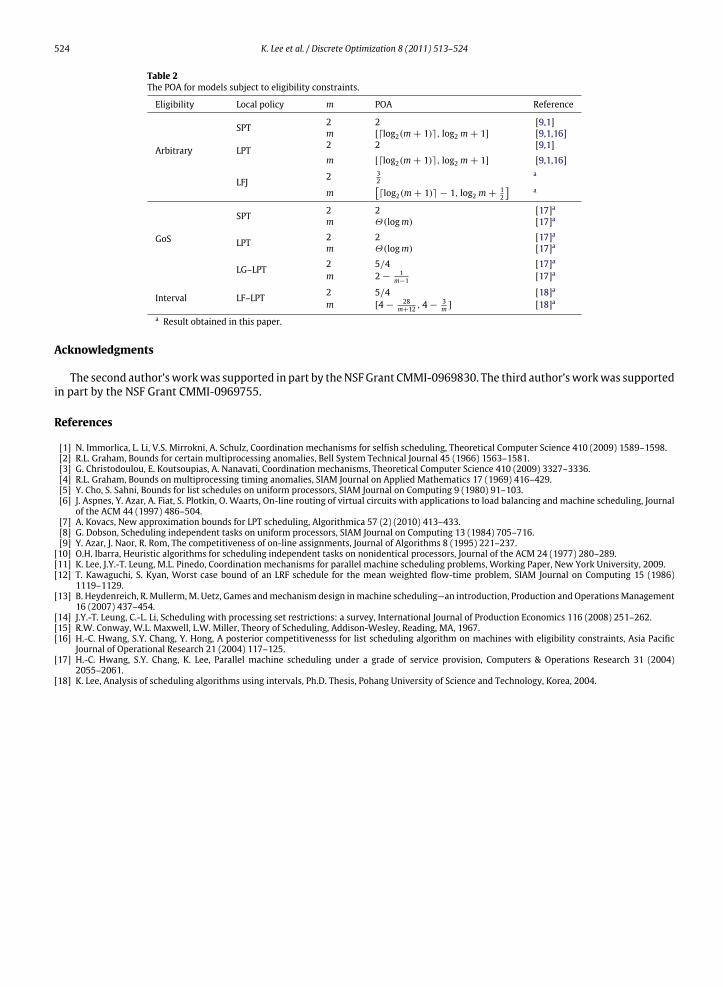
We summarize the results of this section in Table 2.

4. Concluding remarks

In the first part of the paper, we analyze the POA under a new local policy, with some machines using SPT as their localpolicy and with other machines using LPT as their local policy. For the problem of minimizing the total completion time, anupper bound for the POA has remained elusive. The POA in different machine environments, such as uniform machines, isan unexplored area.

In the second part of the paper, we consider the problem with eligibility constraints and develop local policies that arebased on the flexibilities as well as on the processing times of the jobs. One possible extension is to develop a local policywith a better POA value. Another possible extension is an answer to the question whether there is a lower bound for thePOA for an arbitrary local policy. For the arbitrary eligibility case, there is a lower bound for the POA, Ω(logm), under anarbitrary local policy. Similarly, whether there exists for the problem subject to GoS or Interval eligibility constraints witharbitrary local policies a lower bound for the POA also remains an interesting open problem.

Immorlica et al. [1] proved that the parallel machine scheduling problem with eligibility constraints and SPT or LPT asthe local policy has a pure Nash equilibrium. However, for the local policy utilizing eligibility information, the existence ofpure Nash equilibrium has not yet been shown, which is an interesting research question.

524 K. Lee et al. / Discrete Optimization 8 (2011) 513–524

Table 2The POA for models subject to eligibility constraints.

Eligibility Local policy m POA Reference

Arbitrary

SPT 2 2 [9,1]m [⌈log2(m+ 1)⌉, log2 m+ 1] [9,1,16]

LPT 2 2 [9,1]

m [⌈log2(m+ 1)⌉, log2 m+ 1] [9,1,16]

LFJ 2 32

a

m⌈log2(m+ 1)⌉ − 1, log2 m+

12

a

GoS

SPT 2 2 [17]am Θ(logm) [17]a

LPT 2 2 [17]am Θ(logm) [17]a

LG–LPT 2 5/4 [17]a

m 2− 1m−1 [17]a

Interval LF–LPT 2 5/4 [18]a

m [4− 28m+12 , 4− 3

m ] [18]a

a Result obtained in this paper.

Acknowledgments

The second author’sworkwas supported in part by theNSFGrant CMMI-0969830. The third author’sworkwas supportedin part by the NSF Grant CMMI-0969755.

References

[1] N. Immorlica, L. Li, V.S. Mirrokni, A. Schulz, Coordination mechanisms for selfish scheduling, Theoretical Computer Science 410 (2009) 1589–1598.[2] R.L. Graham, Bounds for certain multiprocessing anomalies, Bell System Technical Journal 45 (1966) 1563–1581.[3] G. Christodoulou, E. Koutsoupias, A. Nanavati, Coordination mechanisms, Theoretical Computer Science 410 (2009) 3327–3336.[4] R.L. Graham, Bounds on multiprocessing timing anomalies, SIAM Journal on Applied Mathematics 17 (1969) 416–429.[5] Y. Cho, S. Sahni, Bounds for list schedules on uniform processors, SIAM Journal on Computing 9 (1980) 91–103.[6] J. Aspnes, Y. Azar, A. Fiat, S. Plotkin, O. Waarts, On-line routing of virtual circuits with applications to load balancing and machine scheduling, Journal

of the ACM 44 (1997) 486–504.[7] A. Kovacs, New approximation bounds for LPT scheduling, Algorithmica 57 (2) (2010) 413–433.[8] G. Dobson, Scheduling independent tasks on uniform processors, SIAM Journal on Computing 13 (1984) 705–716.[9] Y. Azar, J. Naor, R. Rom, The competitiveness of on-line assignments, Journal of Algorithms 8 (1995) 221–237.

[10] O.H. Ibarra, Heuristic algorithms for scheduling independent tasks on nonidentical processors, Journal of the ACM 24 (1977) 280–289.[11] K. Lee, J.Y.-T. Leung, M.L. Pinedo, Coordination mechanisms for parallel machine scheduling problems, Working Paper, New York University, 2009.[12] T. Kawaguchi, S. Kyan, Worst case bound of an LRF schedule for the mean weighted flow-time problem, SIAM Journal on Computing 15 (1986)

1119–1129.[13] B. Heydenreich, R. Mullerm,M. Uetz, Games andmechanism design inmachine scheduling—an introduction, Production and OperationsManagement

16 (2007) 437–454.[14] J.Y.-T. Leung, C.-L. Li, Scheduling with processing set restrictions: a survey, International Journal of Production Economics 116 (2008) 251–262.[15] R.W. Conway, W.L. Maxwell, L.W. Miller, Theory of Scheduling, Addison-Wesley, Reading, MA, 1967.[16] H.-C. Hwang, S.Y. Chang, Y. Hong, A posterior competitivenesss for list scheduling algorithm on machines with eligibility constraints, Asia Pacific

Journal of Operational Research 21 (2004) 117–125.[17] H.-C. Hwang, S.Y. Chang, K. Lee, Parallel machine scheduling under a grade of service provision, Computers & Operations Research 31 (2004)

2055–2061.[18] K. Lee, Analysis of scheduling algorithms using intervals, Ph.D. Thesis, Pohang University of Science and Technology, Korea, 2004.