


Bahasa
Halaman
Hukum


This PDF is a selection from a published volume from theNational Bureau of Economic Research
Volume Title: Perspectives on the Economics of Aging
Volume Author/Editor: David A. Wise, editor
Volume Publisher: University of Chicago Press
Volume ISBN: 0-226-90305-2
Volume URL: http://www.nber.org/books/wise04-1
Conference Date: May 17-20, 2001
Publication Date: June 2004
Title: Healthy, Wealthy, and Wise? Tests for Direct CausalPaths between Health and Socioeconomic Status
Author: Peter Adams, Michael D. Hurd, Daniel L. McFadden,Angela Merrill, Tiago Ribeiro
URL: http://www.nber.org/chapters/c10350

This chapter consists of four components: (1) the paper Healthy, Wealthyand Wise? Tests for Direct Causal Paths between Health and SocioeconomicStatus by Peter Adams, Michael D. Hurd, Daniel McFadden, Angela Mer-rill, and Tiago Ribeiro, which originally was presented at the conferenceand then appeared in the Journal of Econometrics, Vol. 112: (2003); (2) anew addendum that describes updates in data and analysis since its publi-cation; (3) additional appendix tables; and (4) the authors’ response to com-ments on the paper.
11.1 Introduction
11.1.1 The Issue
The links between health, wealth, and education have been studied in anumber of populations, with the general finding that higher socioeconomicstatus (SES) is associated with better health and longer life.1 In a survey of
415
11Healthy, Wealthy, and Wise?Tests for Direct Causal Pathsbetween Health andSocioeconomic Status
Peter Adams, Michael D. Hurd, Daniel McFadden,Angela Merrill, and Tiago Ribeiro
Peter Adams is affiliated with the Department of Economics at the University of Califor-nia, Berkeley; Michael D. Hurd is affiliated with RAND Corporation; Daniel McFadden isaffiliated with the Department of Economics at the University of California, Berkeley; AngelaMerrill is affiliated with Mathematica; and Tiago Ribeiro is affiliated with the Department ofEconomics at the University of California, Berkeley.
We gratefully acknowledge financial support from the National Institute on Aging througha grant to the NBER Program Project on the Economics of Aging. Tiago Ribeiro acknowl-edges support from scholarship PRAXIS XXI/BD/16014/98 from the Portuguese Fundaçãopara a Ciência e a Tecnologia. We thank Laura Chioda, Victor Fuchs, Rosa Matzkin, JamesPoterba, and Jim Powell for useful comments.
1. See Backlund, Sorlie, and Johnson (1999); Barsky et al. (1997); Bosma et al. (1997);Chandola (1998, 2000); Davey-Smith, Blane, and Bartley (1994); Drever and Whitehead(1997); Ecob and Smith (1999); Elo and Preston (1996); Ettner (1996); Feinstein (1992);

this literature, Goldman (2001) notes that this association has been foundin different eras, places, genders, and ages, and occurs over the whole rangeof SES levels, so that it is not linked solely to poverty. The association holdsfor a variety of health variables (most illnesses, mortality, self-rated healthstatus, psychological well-being, and biomarkers such as allostatic load)and alternative measures of SES (wealth, education, occupation, income,level of social integration).2 There has been considerable discussion of thecausal mechanisms behind this association, but there have been relativelyfew natural experiments that permit causal paths to be definitively identi-fied.3 In this paper, we test for the absence of direct causal links in an el-derly population by examining whether innovations in health and wealth ina panel are influenced by features of the historical state.
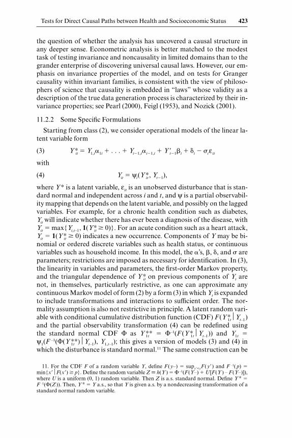
Figure 11.1 depicts possible causal paths for the health and SES innova-tions that occur over a short period. An individual’s life history is builtfrom these period-by-period transitions. First, low SES may lead to fail-ures to seek medical care and delay in detection of conditions, reduced ac-cess to medical services, or less effective treatment.4 Also, increased risk ofhealth problems may result from increased stress or frustration, or in-creased exposure to environmental hazards, that are associated with low
416 P. Adams, M. D. Hurd, D. McFadden, A. Merrill, and T. Ribeiro
Fitzpatrick et al. (1997); Fitzpatrick and Dollamore (1999); Fox, Goldblatt, and Jones (1985);Goldblatt (1990); Haynes (1991); Hertzman (1999); Humphries and van Doorslaer (2000);Hurd (1987); Hurd and Wise (1989); Kaplan and Manuck (1999); Karasek et al. (1988);Kitawaga and Hauser (1973); Lewis et al. (1998); Leigh and Dhir (1997); Luft (1978); Mar-mot et al. (1991); Marmot, Bobak, and Davey-Smith (1995); Marmot et al. (1997); Martinand Preston (1994); Martin and Soldo (1997); McDonough et al. (1997); Murray, Yang, andQiao (1992); Power, Matthews, and Manor (1996); Power and Matthews (1998); Rodgers(1991); Ross and Mirowsky (2000); Schnall, Landsbergis, and Baker (1994); Seeman et al.(2002); Shorrocks (1975); Stern (1983); Wadsworth (1991); Whitehead (1988); Wilkinson(1998); and Woodward et al. (1992).
2. The associations can become more complex when multiple health conditions and mul-tiple SES measures are studied. Competing risks may mask the hazard for late-onset diseases;for example, elevated mortality risk from cardiovascular diseases in low SES groups may in-duce an apparent reverse relationship between SES and later-onset cancer in the survivingpopulation (Adler and Ostrove 1999). Longer-run measures of SES such as education, occu-pation, and wealth appear to have a stronger association with health status than current in-come (Fuchs 1993). Using carefully measured wealth, we find that it explains most of the as-sociation with health, and education conditioned on wealth is not systematically correlatedwith health.
3. Papers examining explicit causal mechanisms include Chapman and Hariharran (1994);Dohrenwend et al. (1992); Evans (1978); Felitti et al. (1998); Fox, Goldblatt, and Johnson(1985); Goldman (1994); Kelley, Hertzman, and Daniels (1997); and McEwen and Stellar(1993).
4. There may be an important distinction between direct causal mechanisms influencingmortality, conditioned on health status, and direct causal mechanisms influencing onset ofhealth conditions. For mortality, an SES gradient could be due to differentially effective treat-ment of acute health conditions. For morbidity, an SES gradient could reflect differentials inprevention and detection of health conditions. These involve different parts of the health caredelivery system, and differ substantially in the importance of individual awareness and dis-cretion, and allocation of costs between Medicare and the individual.

SES.5 These factors could provide direct causal links from SES history tohealth events. Second, poor health may reduce the ability to work or lookafter oneself, and increase medical care expenditures, leading to reducedincome and less opportunity to accumulate assets. This could provide a di-rect causal link from health to changes in SES.
There may also be hidden common factors that lead to ecological associ-ation of health and SES. For example, unobserved genetic heterogeneitymay influence both resistance to disease and ability to work. Causal linksmay be reinforced or confounded by behavioral response. Behavioral fac-tors such as childhood nutrition and stress, exercise, and smoking may in-fluence both health and economic activity level. For example, tastes forwork and for “clean living,” whether genetic or learned, may influence bothhealth and earnings. Finally, rational economic decision making may in-duce robust consumers to accumulate in order to finance consumption overa long-expected retirement, or unhealthy individuals to spend down assets.
Preston and Taubman (1994), Smith and Kington (1997a, b), and Smith(1998, 1999) give detailed discussions of the various causal mechanismsthat may be at work and the role of behavioral response from economicconsumers. The epidemiological literature (Goldman 2001) uses a differentterminology for the causal paths: Links from SES to health innovations aretermed causal mechanisms, while links from health to SES are termed se-lection or reverse causation mechanisms. Apparent association due to mea-surement errors, such as overstatement of the SES of the healthy or under-
Tests for Direct Causal Paths between Health and Socioeconomic Status 417
Fig. 11.1 Possible causal paths for SES and health
5. For example, industrial and traffic pollution, and poor dwelling ventilation are risk fac-tors for lung disease, and housing prices and household income are negatively correlated withair pollution levels in census data (Chay and Greenstone 1998).

detection of illnesses among the poor, are called artifactual mechanisms.6
This literature classifies all common factors in terms of their implicit initialaction as either causal or selection mechanisms.7
11.1.2 This Study
We study the population of elderly Americans aged seventy and older,and in this population test for the absence of direct causal paths from SESto innovations in health, and from health status to innovations in SES.These hypotheses will in general be accepted only if no causal link is pres-ent and there are no persistent hidden factors that influence both initialstate and innovations. Rejection of one of these hypotheses does not dem-onstrate a direct causal link, because this may be the result of common hid-den factors. However, in an elderly population persistent hidden factorswill often be manifest in observed covariates, so that once these covariatesare controlled, the residual impact of the hidden factors on innovationswill be small. For example, genetic frailty that is causal to both healthproblems and low wages, leading to low wealth, may be expressed througha health condition such as diabetes. Then, onset of new health conditionsthat are also linked to genetic frailty may be only weakly associated withlow wealth, once diabetic condition has been entered as a covariate. Thus,in this population, rejection of the hypotheses may provide useful diagnos-tics for likely causal paths.
The objectives and conclusions of this paper are limited. We study onlyelderly Americans, for whom Medicare provides relatively homogeneousand comprehensive health care at limited out-of-pocket cost to the indi-vidual. This population is retired, so new health problems do not impactearnings. Statements about the presence or absence of direct causal mech-anisms in this population, given previous health and SES status, say noth-ing about the structure of these mechanisms in a younger population,where associations of health and SES emerge as a result of some pattern ofcausation and operation of common factors.
Our tests for the absence of causality do not address the question of howto identify invariant models and causal links when these tests fail. If a test
418 P. Adams, M. D. Hurd, D. McFadden, A. Merrill, and T. Ribeiro
6. Consider phenomena such as underestimation of the hazard of a disease due to compet-ing risks from other illnesses or death. In an unfortunate discrepancy in terminology, econo-mists would call this a selection effect, while epidemiologists would classify it as an artifactualmechanism rather than a selection mechanism.
7. Usually, one can argue that observed association must originate from some initial causalaction so that common factors originate from some initial direction of causation. However,there is no apparent initial causal action for genetically linked conditions such as Down syn-drome, which increase mortality risk and preclude work. Further, as a practical matter, it isoften impossible to make observations at the high frequencies that would be required to iden-tify causal chains when feedbacks are nearly instantaneous. Then common factors will ap-pear at feasible levels of detection to operate simultaneously, and their true causal structurewill not be identified. For these reasons, there would be considerable merit in adding commonmechanisms to the epidemiologist’s classification.

for the absence of a direct causal path is rejected, it may be possiblethrough natural or designed experiments to separate causal and ecologicaleffects; see Angrist, Imbens, and Rubin (1996), Heckman (2000, 2001).Suppose a strictly exogenous variable is causal to SES, and clearly not it-self directly causal to health or causal to common factors. Then, an asso-ciation of this variable with innovations in health conditions can only bethrough a direct causal link from SES to health. A variable with these prop-erties is termed a proper instrument or control variable for SES. Proper in-struments are hard to find. They can be obtained through designed exper-iments, where random treatment assignment precludes the possibility ofconfounding by common factors, provided recruitment and retention ofexperimental subjects does not reintroduce confounding. For example, anexperiment that randomly assigned co-payment rates and coverage withinMedicare for prescription drugs or assisted living could provide evidenceon direct causal links from SES to health conditions, provided attritionand compliance are not problems. Occasionally, natural experiments mayprovide random treatment assignment. Economic events that impact in-dividuals differently and that are not related to their prior SES or healthare potentially proper instruments. For example, a tax change that affectswealth differently in different states is arguably a proper instrument, as is a change in mandated Medicaid coverage that has a differential impactacross states. Individual events such as receipt of inheritances may beproper instruments, although they would be confounded if they are antic-ipated, or if the probability of their occurrence is linked to health status;see Meer, Miller, and Rosen (2001). Weak association between SES and aproper instrument for it makes it difficult to obtain precise estimates of di-rect causal effects; see Staiger and Stock (1997).
Section 11.2 of this paper discusses the foundation for econometriccausality tests, and sets out the models for the dynamics of health and SESthat will be used for our analysis. Section 11.3 describes the panel studyand data that we use. Section 11.4 describes the association of SES andprevalence of health conditions in the initial wave of the panel. Section 11.5analyzes incidence of new health conditions, and presents tests for non-causality of SES for the incidence of health innovations. Section 11.6 testsfor the absence of a causal link from health conditions to wealth accumu-lation and other SES indicators. Section 11.7 uses our estimated models forprevalence and incidence to simulate life histories for a current populationaged seventy under counterfactual (and unrealistically simplistic) inter-ventions that assume a major health hazard can be removed, or SES shiftedfor the entire population. This simulation accounts consistently for co-morbidities and competing hazards over the life course. The purpose ofthis exercise is to demonstrate the feasibility of using our modeling ap-proach for policy applications when the models pass the causality tests de-scribed in next section. Finally, section 11.8 gives conclusions and outlines
Tests for Direct Causal Paths between Health and Socioeconomic Status 419

topics for future research. The appendix to this paper, containing tables11A.1 to 11A.11 with detailed estimation results and the data and com-puter routines we use, are posted on the internet at http://elsa.berkeley.edu/wp/hww/hww202.html.
11.2 Association and Causality in Panel Data
11.2.1 Testing Causality
The primary purpose of this study is to test for direct causal links be-tween SES and health. There is a large literature on the nature of causalityand the interpretation of “causality tests.”8 Our analysis fits generallywithin the approach of Granger (1969), Sims (1972), and Hoover (2001),but our panel data structure permits some refinements that are not avail-able in a pure time series setting.
Let Yt denote a K-vector of demographic, health, and socioeconomicrandom variables for a household at date t and interpret a realization ofthese variables as an observation in one wave of a panel survey. Let Yt bethe information set containing the history of this vector through date t. Let
(1) f(YtYt�1)
� f1(Y1tYt�1) � f2(Y2tY1t , Yt�1) � . . . � fK (YKtY1t , . . . , YK�1,t , Yt�1 )
denote a model of the conditional distribution of Yt given Yt–1. Without lossof generality, we have written this model as a product of one-dimensionalconditional distributions, given history and given components of Yt deter-mined previously. Writing the model in this way does not imply that thecomponents of Yt form a causal chain, as they may be simultaneously de-termined, or determined in some causal sequence other than the specifiedsequence. However, the model structure simplifies if the current compo-nents of Yt in the specified order do form a causal chain or are condition-ally independent. If one takes Wold’s view that causal action takes time,then for sufficiently brief time intervals, fK (YKtY1t , . . . , YK–1,t , Yt–1 ) will notdepend on contemporaneous variables, and what Granger calls instanta-neous causality is ruled out. In practice, time aggregation to observation in-tervals can introduce apparent simultaneous determination. Conversely, inapplications where time aggregation is an issue, one can treat observedvariables as indicators for some latent causal chain structure defined forvery short time intervals.
420 P. Adams, M. D. Hurd, D. McFadden, A. Merrill, and T. Ribeiro
8. See Dawid (2000); Freedman (1985, 2001); Granger (1969); Sims (1972); Zellner (1979);Swert (1979); Engle, Hendry, and Richard (1983); Geweke (1984); Gill and Robins (2001);Heckman (2000, 2001); Holland (1986, 1988); Pearl (2000); Robins (1999); Sobel (1997,2000); Hendry and Mizon (1999); and Woodward (1999).

We shall focus on first-order Markov processes, specializations of (1) inwhich only the most recent history conveys information,
(2) f (YtYt�1 ) � f (YtYt�1)
� f1(Y1tYt�1) � f2(Y2tY1t , Yt�1)
� . . . � fK (YKtY1t , . . . , YK�1,t , Yt�1).
Note that if (1) is a higher-order Markov process, then (2) can be obtainedby expanding the variables in Yt to include higher-order lags. Greater gen-erality could be achieved via a hidden Markov structure in which the ob-served Yt are deterministic functions of a latent first-order Markov pro-cess.9 We leave this extension for future research.
Model (2) is valid for a given history Yt–1 if it is the true conditional dis-tribution of Yt given this history. Term f a structural or causal model, or a(probabilistic) law, for Yt relative to a family of histories if it has the invari-ance property that it is valid for each history in the family. Operationally,this means that within specified domains, f has the transferability prop-erty that it is valid in different populations where the marginal distributionof Yt–1 changes, and the predictability or invariance under treatments prop-erty that it remains valid following policy interventions that alter the mar-ginal distribution of Yt–1. By including temporal or spatial variables in Y, itis possible to weaken invariance requirements to fit almost any application.Done indiscriminately, this creates a substantial risk of producing an“overfitted” model that will be invalid for any “out-of-sample” policy in-terventions. Then, proposed models should be as generic as possible. How-ever, it may be necessary in some applications to model “regime shifts” thataccount for factors that are causal for some populations or time periods,and not for others.
Suppose the vector Yt � (Ht, St, Xt ) is composed of subvectors Ht , St ,and Xt , which will later be interpreted as health conditions, SES status, andstrictly exogenous variables, respectively. We say that S is conditionally non-causal for H, given X, if f(HtHt–1, Xt–1 ) is a valid model; that is, given Ht–1
and Xt–1, knowledge of St–1 is not needed to achieve the invariance proper-ties of a causal model. Conversely, if f(HtHt–1, St–1, Xt–1) � f (HtHt–1, Xt–1),then knowledge of St–1 contributes to the predictability of Ht. Note that ei-ther one or both conditional noncausality of S for H and conditional non-causality of H for S may hold. If either holds, then H and S can be arrayedin a (block) causal chain, and if both hold, then H and S are conditionallyindependent. Writing model (2) as a product of univariate conditional
Tests for Direct Causal Paths between Health and Socioeconomic Status 421
9. Any discrete-time stationary stochastic process can be approximated (in distribution forrestrictions to a finite number of periods) by a first-order hidden Markov model so there is noloss of generality in considering only models of this form; see Kunsch, Geman, and Kehagias(1995).

probabilities fi (HitH1t, . . . , Hi–1,t, Ht–1, St–1, Xt–1), one can test for condi-tional noncausality of S for each component Hi . It is possible to have acausal chain in which S is conditionally causal to a previous component ofH, and this component is in turn “instantaneously” causal to Hj , yet thereis no direct causal link from S to Hi . Placing S after H in the vector Y, wehave conditional probabilities f(StHt, Ht–1, St–1, Xt–1). There may be instan-taneous conditional independence of H and S, with the conditional distri-bution of St not depending on Ht or conditional noncausality of H for S,with the conditional distribution not depending on Ht–1, or both. The state-ment that X is strictly exogenous in a valid model (2) is equivalent to thecondition that H and S are conditionally noncausal for X in this model.10
The conventional definition of a causal model or probabilistic law re-quires that f be valid for the universe of possible histories (except possiblythose in a set that occurs with probability zero); see Pearl (2000). It is pos-sible to reject statistically a proposed causal model by showing that it ishighly improbable that an observed sample with a given history was gen-erated by this model. It is far more difficult using statistical analysis to con-clude inductively that a proposed model is valid for the universe of possiblehistories. We have the far more limited objective of providing a foundationfor policy analysis, where it is the invariance property under policy inter-ventions that is crucial to predicting policy consequences. We have definedvalidity and noncausality as properties of a model, and of the outcomes ofa process of statistical testing that could in principle be conducted on thismodel. Only within the domain where the model is valid, and invarianceconfirms that the model is accurately describing the true data generationprocess, can these limited positivistic model properties be related to thecausal structure embedded in the true data generation process. Further, wecan choose the domain over which invariance will be tested to make thedefinition operational and relevant for a specific analysis of policy inter-ventions. Similarly, our definition of conditional noncausality is a posi-tivistic construct in the spirit of the purely statistical treatment of “causal-ity” by Granger (1969), and the test we will use is simply Granger’s test forthe absence of causality, augmented with invariance conditions. Thus, forexample, if our analysis using this framework concludes that SES is notconditionally causal for new health events within the domain where theMedicare system finances and delivers health care, then this finding wouldsupport the conclusion that policy interventions in the Medicare system toincrease access or reduce out-of-pocket medical expenses will not alter theconditional probabilities of new health events, given the health histories ofenrollees in this system. It is unnecessary for this policy purpose to answer
422 P. Adams, M. D. Hurd, D. McFadden, A. Merrill, and T. Ribeiro
10. Econometricians have traditionally used the term strictly exogenous to refer to proper-ties of variables in the true data generation process, a stronger nonpositivistic version of thiscondition.
the question of whether the analysis has uncovered a causal structure inany deeper sense. Econometric analysis is better matched to the modesttask of testing invariance and noncausality in limited domains than to thegrander enterprise of discovering universal causal laws. However, our em-phasis on invariance properties of the model, and on tests for Grangercausality within invariant families, is consistent with the view of philoso-phers of science that causality is embedded in “laws” whose validity as adescription of the true data generation process is characterized by their in-variance properties; see Pearl (2000), Feigl (1953), and Nozick (2001).
11.2.2 Some Specific Formulations
Starting from class (2), we consider operational models of the linear la-tent variable form
(3) Y∗it � Y1,t�1i � . . . � Yi�1,t�i�1,i � Y �t�1�i � �i � iε it
with
(4) Yit � ψi(Y∗it , Yt�1),
where Y∗ is a latent variable, εit is an unobserved disturbance that is stan-dard normal and independent across i and t, and ψ is a partial observabil-ity mapping that depends on the latent variable, and possibly on the laggedvariables. For example, for a chronic health condition such as diabetes, Yit will indicate whether there has ever been a diagnosis of the disease, withYit � max{Yi,t–1, 1(Y∗
it 0)}. For an acute condition such as a heart attack,Yit � 1(Y∗
it 0) indicates a new occurrence. Components of Y may be bi-nomial or ordered discrete variables such as health status, or continuousvariables such as household income. In this model, the �’s, �, �, and areparameters; restrictions are imposed as necessary for identification. In (3),the linearity in variables and parameters, the first-order Markov property,and the triangular dependence of Y∗
it on previous components of Yt arenot, in themselves, particularly restrictive, as one can approximate anycontinuous Markov model of form (2) by a form (3) in which Yt is expandedto include transformations and interactions to sufficient order. The nor-mality assumption is also not restrictive in principle. A latent random vari-able with conditional cumulative distribution function (CDF) F (Y∗
1tYt–1)and the partial observability transformation (4) can be redefined using the standard normal CDF � as Y 1t
∗∗ � �–1(F (Y∗1tYt–1)) and Y1t �
ψ1(F–1(�(Y 1t
∗∗)Yt–1), Y1,t–1); this gives a version of models (3) and (4) inwhich the disturbance is standard normal.11 The same construction can be
Tests for Direct Causal Paths between Health and Socioeconomic Status 423
11. For the CDF F of a random variable Y, define F (y–) � supy�<yF (y�) and F –1( p) �min{x�F(x�) p}. Define the random variable Z � h(Y ) � � –1(F (Y–) � U [F (Y ) – F (Y–)]),where U is a uniform (0, 1) random variable. Then Z is a.s. standard normal. Define Y ∗ �F –1(�(Z )). Then, Y ∗ � Y a.s., so that Y is given a.s. by a nondecreasing transformation of astandard normal random variable.

applied to the remaining components of Yt . The causal chain assumptionis innocuous when the time interval is too short for most causal actions tooperate, and the components of Yt are conditionally independent. How-ever, the causal chain assumption is a more substantive restriction whenthe time interval is long enough for multiple events to occur, as it precludeseven the feedbacks that would appear in multiple iterations of a true causalchain. Of course, the generally nonrestrictive approximation properties ofmodels (3) and (4) do not imply that a particular specification chosen foran application is accurate, and failures of tests for invariance can also beinterpreted as diagnostics for inadequate specifications.
In models (3) and (4), a binomial component i of Yt with the partial ob-servability mapping max{Yi,t–1, 1(Y∗
it 0)} and the identifying restrictioni � 1 satisfies Yit � 1 if Yi,t–1 � 1, and otherwise is one with the probit prob-ability
(5) fi (Yit � 1Y1t , . . . , Yi�1,t , Yt�1)
� �(Y1,t�1i � . . . � Yi�1,t �i�1,i � Y �t�1 �i � �i ).
Analogous expressions can be developed for ordered or continuous com-ponents.
11.2.3 Measurement Issues
A feature of the panel we use is that the waves are separated by severalyears, and the interviews within a wave are spread over many months, withthe months between waves differing across households. If model (2) appliesto short intervals, say months, then the transition from one wave in montht to another in month t � s is described by the probability model
(6) f (Yt�sYt ) � ∑Yt�1,...,Yt�s�1
f (Yt�1Yt ) � . . . � f (Yt�sYt�s�1).
Direct computation of these probabilities will generally be intractable, al-though analysis using simulation methods is possible.
A major additional complication in our panel is that interview timingappears to be related to health status, with household or proxy interviewsdelayed for individuals who have died or have serious health conditions.This introduces a spurious correlation between apparent time at risk andhealth status that will bias estimation of structural parameters. To studyempirical approximations to (6) and corrections for spurious correlation,we consider a simple model of interview delay. Let p � �(� � �x) denotethe monthly survival probability for an individual who was alive at the pre-vious wave interview, where x is a single time-invariant covariate that takesthe value –1, 0, �1, each with probability 1/3. Counting from the time ofthe previous wave interview, let k denote the number of months this indi-vidual lives, and c denote the month that interviews begin for the current
424 P. Adams, M. D. Hurd, D. McFadden, A. Merrill, and T. Ribeiro

wave.12 There is a distribution of initial contact times; let q denote the prob-ability of a month passing without being contacted, and let m denote themonth of initial contact. Assume that an individual who is living at the timeof initial contact is interviewed immediately, but for individuals who havedied by the time of initial contact, there is an interview delay, with r denot-ing the probability of an additional month passing without a completed in-terview with a household member or proxy. Let n denote the number ofmonths of delay in this event. Assume that m and n are not observed, butthe actual interwave interval t, equal to m if the individual is alive at timeof initial contact, and equal to m � n otherwise, is observed. The density ofk is p k–1(1 – p) for k 1. The density of m is q m–c(1 – q) for m c. Let dbe an indicator for the event that the individual is dead at the time of initialcontact. The probability of t and d � 0 is h(0, t) � qt–c(1 – q)pt, the productof the probability of contact at t and the probability of being alive at t. Theprobability of t and d � 1, denoted h(1, t), is the sum of the probabilitiesthat the individual is dead at an initial contact month m, with c � m � t,and the subsequent interview delay is n � t – m, or
(7) h(1, t) � ∑t
m�c
(1 � pm)qm�c(1 � q)r t�m(1 � r).
If r pq, then h(1, t) � (1 – q)(1 – r){(q t–c�1 – r t–c�1) /(q – r) – pc(( pq)t–c�1 –r t–c�1) /(pq – r)}. Then, the probability of an observed interwave interval t ish(t) � h(0, t) � h(1, t), and the conditional probability of d � 1, given t, isP(1t) � h(1, t) /h(t). Absent interview delay, the conditional probability ofd � 1 given t would be simply p t–1(1 – p). The parameter values � � –2.47474, � � 0.3, c � 22, q � 0.85, and r � 0.5 roughly match our panel.For these values, the median interwave interval is 25.5 months, and at t �34, 87 percent of the interviews have been completed.
Figure 11.2 plots the inverse normal transformations of the true deathrate p t–1(1 – p) and the apparent death rate P(1t) against log(t) for eachvalue of the covariate x. The true relationship is to a reasonable empiricalapproximation linear in x and in log(t). Then, in the absence of interviewdelay, one could approximate p, given x, with reasonable accuracy by esti-mating a probit model for death of the form �(� � �x � � log(t)), and thenestimating p using the transformation p � (1 – �(� � �x � � log(t)))1/t forthe observed interwave interval t.13 However, the figure shows that inter-view delay induces a sharp gradient of apparent mortality hazard with in-terwave interval, so that an estimated model will not extrapolate to realis-tic mortality hazards over shorter periods. A simple imputation of time at
Tests for Direct Causal Paths between Health and Socioeconomic Status 425
12. It does not matter for the example if the previous wave interview month is fixed or hasa distribution, provided the relative interwave interval c is fixed, and current wave outcomesare independent of the timing of the previous wave interview.
13. A Box–Cox transformation of time at risk, z � 4(t1/4 – 1), gives a somewhat better ap-proximation in the probit model than log(t), but has no appreciable effect on the accuracy ofestimated monthly transition probabilities.

risk up to initial contact leads again to models that work well with the pro-cedure just outlined for estimation of p conditioned on x. A simple im-puted time of initial contact for those who have died is the observed inter-wave interval less the difference in the mean interwave interview times fordead and living respondents. This imputation can be adjusted further sothat the extrapolated annual death rate, �(� � � log(12) � �x), matches thesample average mortality rate. We do the additional adjustment for ourpanel, with results that are almost identical to the simple imputation oftime of initial contact.
We conducted a Monte Carlo calculation of the approximations abovein a sample of 50,000. In this simulation, the empirical approximation toobserved mortality in the absence of interview delay is �(–3.1053 �0.5327x � 0.652 log(t)). With interview delay and the simple imputationdescribed above, �(–2.9900 � 0.5349x � 0.6174 log(t)) is the empirical ap-proximation.14 Table 11.1 gives the annual mortality rates implied by theseapproximations. From these results, we conclude first that in the absence ofinterview delay, the probit model �(� � � log(t) � �x) provides an ade-quate approximation to exact annual mortality rates as a function of time
426 P. Adams, M. D. Hurd, D. McFadden, A. Merrill, and T. Ribeiro
Fig. 11.2 Effect of interview delay (cumulative mortality hazard � � –1
[death probability])
14. The model estimated with interview delay and without imputation, is �(–4.6639 �0.5349x � 1.1178 log(t)).

at risk, across values of the covariate x that substantially change relativerisk, and second that this remains true in the presence of interview delaywhen one imputes the initial contact time for dead subjects.
These conclusions on the accuracy of the approximation should extendto the exact interwave transition probabilities (6) in our Markov model,supporting use of the probit approximation
(8) fi (Yi,t�s � 1Y1t�s, . . . , Yi�1,t�s, Yt )
� �(Y1,t�s�1i � . . . � Yi�1,t�s�i�1,i � Y �t�i � �i � �i log(s)),
where s � ti2 – ti1 is the imputed months between initial contact for a waveand previous wave interview, for estimation of incidence between waves.For simulation of yearly transitions, we use the approximation
(9) fi (Yi,t�12 � 1Y1t�12, . . . , Yi�1,t�12, Yt )
� 1 � (1 � �(Y1,t�1�1i � . . . � Yi�1,t�1�i�1,i � Y�t�i � �i � �i log(s)))12/s
≈ �(Y1,t�1�1i � . . . � Yi�1,t�1�i�1,i �Y �t�i � �i � �i log(s))12/s,
where s is the median interwave interval, and the final approximation holdswhen the probability of a transition is small. Formula (9) generalizes to anyprobability of a transition from the status quo, with the probability of re-maining at the initial state defined so that all the transition probabilitiessum to one. We expect this formula to approximate well the probabilitiesof no new health conditions in a sample population over periods corre-sponding to the observed interwave intervals.
Estimation of models based on (2)–(8) is straightforward. Because of theindependence assumption on the disturbances and the absence of commonparameters across equations, the estimation separates into a probit, or-dered probit, or ordinary least-squares regression for each component ofY, depending on whether the partial observability mapping is binary,
Tests for Direct Causal Paths between Health and Socioeconomic Status 427
Table 11.1 Approximation Accuracy with Interview Delay (%)
Exact Approximate Approximate AnnualAnnual Annual Mortality Mortality Rate with
Mortality Rate without Interview Delay andx Rate Interview Delay Error Imputed Contact Time Error
0 7.71 7.90 2.41 7.93 2.79–1 3.27 3.06 –6.55 3.07 –6.03�1 16.41 16.71 1.80 16.75 2.05Avg. 9.13 9.22 0.98 9.25 1.34
Note: The approximate annual mortality rate is given by 1 – (1 – �(� � �x � � log(t)))12/t, where t is theexact or imputed initial contact time and the model is estimated from the data generated by the MonteCarlo experiment.

ordered, or linear. Conventional likelihood ratio tests can be used for thesignificance of explanatory variables.
11.3 The AHEAD Panel Data
11.3.1 Sample Characteristics
Our data come from the Asset and Health Dynamics among the OldestOld (AHEAD) study.15 This is a panel of individuals born in 1923 or earlierand their spouses. At baseline in 1993 the AHEAD panel contained 8,222individuals representative of the noninstitutionalized population, exceptfor oversamples of blacks, Hispanics and Floridians. Of these subjects,7,638 were over age sixty-nine; the remainder were younger spouses. Therewere 6,052 households, including individuals living alone or with others, inthe sample. The wave 1 surveys took place between October 1993 and Au-gust 1994, with half the total completed interviews finished before Decem-ber 1993. The wave 2 surveys took place approximately twenty-four monthslater, between November 1995 and June 1996, with half the total completedinterviews finished by the beginning of February 1996. The wave 3 surveystook place approximately twenty-seven months after that, between January1998 and December 1998, with half the total completed interviews finishednear the beginning of March 1998. In each wave, there was a long but thintail of late interviews, heavily weighted with subjects who had moved, or re-quired proxy interviews due to death or institutionalization. Subjects neverinterviewed, directly or by proxy, are excluded from the calculation of thedistribution of interview months. The AHEAD is a continuing panel, but ithas now been absorbed into the larger Health and Retirement Study(HRS), which is being interviewed on a three-year cycle.
The AHEAD panel has substantial attrition, with death being the pri-mary, but not the only, cause. A significant effort has been made to trackattritors, and identify those who have died through the National DeathRegister. Figure 11.3 describes outcomes for the full age-eligible sample.For subjects where a proxy interview was possible, an “exit interview” givesinformation on whether decedents had a new occurrence of cancer, heartattack, or stroke since the previous wave. From the 6,743 age-eligible indi-viduals who did not attrit prior to death, we formed a working sample foranalysis consisting of 6,489 by excluding 254 additional individuals withcritical missing information. Figure 11.4 describes their outcomes. In a fewcases, attritors in wave 2 rejoined the sample in wave 3, but we treat theseas permanent attritors because the missing interview makes the observa-tion unusable.
428 P. Adams, M. D. Hurd, D. McFadden, A. Merrill, and T. Ribeiro
15. The AHEAD survey is conducted by the University of Michigan Survey Research Cen-ter for the National Institute on Aging; see Soldo et al. (1997).

Fig. 11.3 Age-eligible sample outcomes
Fig. 11.4 Working sample outcomes

The restriction of the AHEAD panel to the noninstitutionalized elderlyin wave 1 selects against those with the highest mortality risk, particularlyat the oldest ages, but the impact of this selection attenuates over time. Forwhite females, figure 11.5 compares the observed annual mortality rate inthe AHEAD panel with the expected annual mortality rate from the 1997life tables for the United States (U.S. Census 1999).16 Between waves 1 and2, the AHEAD mortality risk is substantially below the life table for agesabove seventy-five, reflecting the selection effect of noninstitutionalization.
430 P. Adams, M. D. Hurd, D. McFadden, A. Merrill, and T. Ribeiro
Fig. 11.5 Mortality hazard for AHEAD white females
16. The AMR for the AHEAD sample is the actual death rate between waves for each five-year segment of ages in the initial wave, annualized using the median 25.5 month interval be-tween the waves. The AMR from the life tables is obtained by applying life table death ratesby month to the actual months at risk for each individual in the five-year segment of ages in

Between waves 2 and 3, this effect has essentially disappeared. There is apersistent divergence of the mortality risks above age ninety. In this range,the AHEAD data is sparse, so the curve is imprecisely determined. How-ever, the life tables derived from historical mortality experience may over-state current mortality risk at advanced ages. Figure 11.6 makes the samemortality experience comparisons for the full AHEAD working sampleand draws the same conclusions.17
Tests for Direct Causal Paths between Health and Socioeconomic Status 431
the initial wave to calculate expected deaths between waves. This is annualized. For these cal-culations, the distribution of months at risk for decedents is assumed to be the same as thatfor survivors.
17. The construction mimics figure 11.5, with life table rates applied using the age, sex, andrace of each subject.
Fig. 11.6 Mortality hazard for AHEAD working sample

11.3.2 Descriptive Statistics
The AHEAD survey provides data on health and socioeconomic status,as well as background demographics. A list of the health conditions westudy, with summary statistics, is given in table 11.2. A list of the socioeco-nomic conditions and demographic variables we use is given in table 11.3.Table 11A.2 lists the variable transformations used in our statistical anal-ysis.18 In setting up causality tests, using the framework set out in section11.2, we will use the health conditions, followed by the socioeconomic con-ditions, in the order given in these tables. We list cancer, heart disease, andstroke first because they may be instantaneously causal for death, and be-cause we have information from decedent’s exit interviews on new occur-rence of these diseases. We group the remaining health conditions by de-generative and chronic conditions, then accidents, then mental conditions,because if there is any contemporaneous causality, it will plausibly flow inthis order. Similarly, if there is contemporaneous causality between healthand socioeconomic conditions, it plausibly flows from the former to thelatter.
11.3.3 Constructed Variables
The collection and processing of some of the variables requires com-ment. The AHEAD has an extensive battery of questions about healthconditions, including mental health. Most health conditions are asked forin the form “Has a doctor ever told you that you had . . . ?” However, forcancer, heart disease, and stroke, subjects are also asked if there was a newoccurrence since the previous interview, and for some conditions such asarthritis, incontinence, and falls, the questions in wave 1 ask for an occur-rence in the past twelve months. We note that there are some major groupsof health conditions that were not investigated in AHEAD: degenerativeneurological diseases, kidney and liver diseases, immunological disordersother than arthritis, sight and hearing problems, back problems, and acci-dents other than falls. The body mass index (BMI) index is calculated fromself-reported height and weight. Information is collected on the number oflimitations for six activities of daily living (ADL), and on the number oflimitations for five instrumental activities of daily living (IADL). A highADL limitation count indicates that the individual has difficulty with per-sonal self-care, while a high IADL limitation count indicates difficulty inhousehold management. The study collects data on self-assessed healthstatus, where the subject is asked to rate his or her health as excellent, verygood, good, fair or poor. We use an indicator for a poor/fair response. Noreference is made to other groups such as “people your age.” The studycontains the Center for Epidemiologic Studies Depression scale (CESD)
432 P. Adams, M. D. Hurd, D. McFadden, A. Merrill, and T. Ribeiro
18. All appendices can be found at http://elsa.berkeley.edu/wp/hww/hww202.html.

Tab
le 1
1.2
Hea
lth
Con
diti
on V
aria
bles
in A
HE
AD
Wav
e 1
Wav
e 2
Wav
e 3
Lab
elV
aria
ble
NM
ean
SDV
aria
ble
NM
ean
SDV
aria
ble
NM
ean
SD
Hea
lth
cond
itio
n pr
eval
ence
Doc
eve
r to
ld h
ad c
ance
r?C
AN
CE
R1
6,48
90.
137
0.34
4C
AN
CE
R2
6,43
20.
176
0.38
1C
AN
CE
R3
5,68
50.
188
0.39
1D
oc e
ver
told
hea
rt a
ttac
k/di
seas
e?H
EA
RT
16,
489
0.31
70.
465
HE
AR
T2
6,43
20.
364
0.48
1H
EA
RT
35,
685
0.32
10.
467
Doc
eve
r to
ld h
ad s
trok
e?ST
RO
KE
16,
489
0.08
90.
285
STR
OK
E2
6,43
20.
123
0.32
9ST
RO
KE
35,
685
0.14
30.
350
Doc
eve
r to
ld h
ad lu
ng d
isea
se?
LU
NG
16,
489
0.11
50.
318
LU
NG
26,
432
0.12
40.
330
LU
NG
35,
685
0.12
70.
333
Doc
eve
r to
ld h
ad d
iabe
tes?
DIA
BE
T1
6,48
90.
134
0.34
0D
IAB
ET
25,
741
0.14
70.
354
DIA
BE
T3
4,86
70.
158
0.36
5D
oc e
ver
told
had
hig
h bl
ood
pres
sure
?H
IGH
BP
16,
489
0.50
20.
500
HIG
HB
P2
5,74
10.
525
0.49
9H
IGH
BP
34,
867
0.55
30.
497
Seen
Doc
for
arth
riti
s in
last
12
m?
AR
TH
RT
16,
489
0.26
70.
442
AR
TH
RT
25,
741
0.27
80.
448
AR
TH
RT
34,
867
0.27
90.
448
Inco
ntin
ence
last
12
m?
INC
ON
T1
6,48
90.
202
0.40
2IN
CO
NT
25,
741
0.30
10.
459
INC
ON
T3
4,86
70.
371
0.48
3F
all i
n la
st 1
2 m
req
uire
trea
tmen
t?FA
LL
16,
489
0.08
00.
271
FAL
L2
6,43
20.
180
0.38
4FA
LL
35,
685
0.26
70.
443
Eve
r fr
actu
red
hip?
HIP
FR
C1
6,48
90.
050
0.21
9H
IPF
RC
26,
432
0.06
80.
252
HIP
FR
C3
5,68
50.
084
0.27
8P
roxy
inte
rvie
wP
RO
XY
W1
6,48
90.
104
0.30
6P
RO
XY
W2
5,74
10.
132
0.33
9P
RO
XY
W3
4,86
70.
154
0.36
1A
ge-e
duc.
adj
ust c
ogni
tive
impa
irm
ent?
CO
GIM
16,
489
0.25
70.
437
CO
GIM
25,
741
0.34
90.
477
CO
GIM
34,
867
0.40
30.
491
Eve
r se
en D
oc fo
r ps
ych
prob
?P
SYC
H1
6,48
90.
109
0.31
2P
SYC
H2
5,74
10.
128
0.33
4P
SYC
H3
4,86
70.
143
0.35
0D
epre
ssed
(ces
d8 �
4)D
EP
RE
S16,
488
0.09
90.
299
DE
PR
ES2
5,74
10.
086
0.28
0D
EP
RE
S34,
862
0.10
80.
310
Bod
y m
ass
inde
x (Q
uete
let)
BM
I16,
475
25.4
4.5
BM
I25,
740
25.1
4.6
BM
I34,
866
25.0
4.6
Low
BM
I sp
line
�m
ax(0
, 20
– bm
i)L
OB
MI1
6,47
50.
155
0.65
4L
OB
MI2
5,74
00.
198
0.76
3L
OB
MI3
4,86
60.
223
0.81
0H
igh
BM
I sp
line
�m
ax(0
, bm
i – 2
5)H
IBM
I16,
475
1.88
93.
164
HIB
MI2
5,74
01.
808
3.14
3H
IBM
I34,
866
1.74
03.
037
Cur
rent
sm
oker
?SM
OK
NO
W1
6,48
90.
102
0.30
3SM
OK
NO
W2
5,74
10.
078
0.26
7SM
OK
NO
W3
4,86
70.
066
0.24
9N
o. o
f AD
Ls
(nee
ds h
elp/
diffi
cult
)N
UM
AD
L1
6,48
90.
725
1.39
1N
UM
AD
L2
6,43
20.
882
1.65
2N
UM
AD
L3
5,44
41.
035
1.77
4N
o. o
f IA
DL
s (n
eeds
hel
p/di
fficu
lt)
NU
MIA
DL
16,
489
0.61
81.
166
NU
MIA
DL
26,
432
0.58
21.
204
NU
MIA
DL
35,
685
0.71
11.
253
Poor
/fai
r se
lf-r
epor
ted
heal
thD
HLT
H1
6,48
30.
373
0.48
4D
HLT
H2
5,73
90.
368
0.48
2D
HLT
H3
4,85
90.
434
0.49
6
Hea
lth
cond
itio
n in
cide
nce
Can
cera
JCA
NC
ER
26,
432
0.05
00.
218
JCA
NC
ER
35,
685
0.06
10.
239
Hea
rt a
ttac
k/co
ndit
iona
JHE
AR
T2
6,43
20.
087
0.28
1JH
EA
RT
35,
685
0.15
40.
361
Stro
kea
JST
RO
KE
26,
432
0.05
00.
219
JST
RO
KE
35,
685
0.06
90.
254
Die
d si
nce
last
wav
e?T
DIE
D2
6,48
90.
115
0.31
9T
DIE
D3
5,74
10.
152
0.35
9
(con
tinu
ed)

Lun
g di
seas
eaIL
UN
G2
6,43
20.
024
0.15
4IL
UN
G3
5,68
50.
032
0.17
7D
iabe
tesa
IDIA
BE
T2
5,74
10.
024
0.15
3ID
IAB
ET
34,
867
0.02
50.
156
Hig
h bl
ood
pres
sure
(HB
P)a
IHIG
HB
P2
5,74
10.
053
0.22
5IH
IGH
BP
34,
867
0.05
50.
229
Art
hrit
isa
IAR
TH
RT
25,
741
0.11
20.
316
IAR
TH
RT
34,
867
0.11
70.
321
Inco
ntin
ence
in la
st 1
2 m
onth
sJI
NC
ON
T2
5,74
10.
233
0.42
3JI
NC
ON
T3
4,86
70.
258
0.43
8F
all r
equi
ring
trea
tmen
taJF
AL
L2
6,43
20.
128
0.33
5JF
AL
L3
5,24
00.
165
0.37
1H
ip fr
actu
rea
JHIP
FR
C2
6,43
20.
020.
150
JHIP
FR
C3
5,68
10.
033
0.17
8P
roxy
inte
rvie
wP
RO
XY
W2
5,74
10.
132
0.33
9P
RO
XY
W3
4,86
70.
154
0.36
1C
ogni
tive
impa
irm
ent
ICO
GIM
25,
741
0.12
10.
326
ICO
GIM
34,
867
0.10
00.
300
Psy
chia
tric
pro
blem
saIP
SYC
H2
5,74
10.
046
0.21
0IP
SYC
H3
4,86
70.
040
0.19
6D
epre
ssio
nID
EP
RE
S25,
741
0.05
10.
220
IDE
PR
ES3
4,86
20.
072
0.25
9B
MI
bett
er in
dica
tor
BM
IBT
25,
740
0.19
70.
397
BM
IBT
34,
866
0.19
00.
392
BM
I w
orse
indi
cato
rB
MIW
S25,
740
0.16
70.
373
BM
IWS3
4,86
60.
188
0.39
1
Not
es:N
�nu
mbe
r of
obs
erva
tion
s; S
D �
stan
dard
dev
iati
on.
a AH
EA
D W
aves
2 a
nd 3
: “Si
nce
the
last
inte
rvie
w .
.. ?
”.
Tab
le 1
1.2
(con
tinu
ed)
Wav
e 1
Wav
e 2
Wav
e 3
Lab
elV
aria
ble
NM
ean
SDV
aria
ble
NM
ean
SDV
aria
ble
NM
ean
SD

Tab
le 1
1.3
SE
S a
nd D
emog
raph
ic V
aria
bles
in A
HE
AD
Wav
e 1
Wav
e 2
Wav
e 3
Lab
elV
aria
ble
NM
ean
SDV
aria
ble
NM
ean
SDV
aria
ble
NM
ean
SD
SE
S v
aria
bles
Wea
lth
97 D
ol (V
.2) (
000)
C.2
W1
6,48
917
6.6
297.
8C
.2W
25,
741
237.
552
7.3
C.2
W3
4,86
724
7.7
736.
2N
onliq
uid
wea
lth
(000
)C
.2N
16,
489
112.
019
1.8
C.2
N2
5,74
112
1.2
312.
1C
.2N
34,
867
119.
240
0.7
Liq
uid
wea
lth
(000
)C
.2L
16,
489
64.7
185.
2C
.2L
25,
741
116.
330
9.6
C2.
L3
4,86
712
8.6
560.
6In
com
e 97
Dol
(V.2
) (00
0)C
.211
6,48
923
.828
.8C
.212
5,74
124
.558
.61s
t qua
rtile
wea
lth
indi
cato
rQ
1WB
16,
489
0.26
10.
654
Q1W
B2
5,74
10.
228
0.41
9Q
1WB
34,
867
0.25
50.
436
4th
quar
tile
wea
lth
indi
cato
rQ
4WB
16,
489
0.21
60.
412
Q4W
B2
5,74
10.
273
0.44
6Q
4WB
34,
867
0.26
80.
443
1st q
uart
ile in
com
e in
dica
tor
Q11
B1
6,48
90.
260
0.43
9Q
11B
25,
741
0.24
60.
431
4th
quar
tile
inco
me
indi
cato
rQ
41B
16,
489
0.24
70.
431
Q41
B2
5,74
10.
246
0.43
1C
hang
e re
side
nce?
NM
OV
ED
25,
642
0.06
80.
251
MO
VE
D3
4,86
70.
102
0.30
3O
wn
resi
denc
e?D
NH
OU
S16,
489
0.73
20.
443
DN
HO
US2
5,74
10.
721
0.44
9D
NH
OU
S34,
867
0.70
70.
455
Nei
ghbo
rhoo
d sa
fety
poo
r/fa
irH
OO
DP
F1
6,48
90.
147
0.35
4H
OO
DP
F2
5,74
10.
107
0.30
9H
OO
DP
F3
4,86
70.
101
0.30
1H
ouse
con
diti
on p
oor/
fair
CO
ND
PF
16,
489
0.14
60.
354
CO
ND
PF
25,
741
0.10
90.
312
CO
ND
PF
34,
867
0.12
30.
328
Dem
ogra
phic
var
iabl
esW
idow
?W
IDO
W1
6,48
90.
416
0.49
3W
IDO
W2
5,74
10.
443
0.49
7W
IDO
W3
4,86
70.
434
0.49
6D
ivor
ced/
sepa
rate
d?D
IVSE
P1
6,48
90.
054
0.22
6D
IVSE
P2
5,74
10.
054
0.22
6D
IVSE
P3
4,86
70.
055
0.22
8M
arri
edM
AR
RIE
D1
6,48
90.
498
0.50
0M
AR
RIE
D2
5,74
10.
465
0.49
9M
AR
RIE
D3
4,86
70.
477
0.50
0N
ever
mar
ried
?N
EV
MA
RR
16,
489
0.03
20.
176
NE
VM
AR
R2
5,74
10.
035
0.17
2N
EV
MA
RR
34,
867
0.03
10.
172
Age
at i
nter
view
in m
onth
sA
GE
M1
6,48
993
9.2
72.0
AG
EM
26,
432
962.
971
.9A
GE
M3
5,74
198
4.8
68.7
Mot
her’s
dea
th a
geM
AG
ED
IE1
6,48
973
.917
.4F
athe
r’s d
eath
age
PAG
ED
IE1
6,48
971
.515
.1E
ver
smok
e?SM
OK
EV
6,48
90.
526
0.49
9E
duca
tion
(yea
rs)
ED
UC
6,48
910
.73.
8E
duc
�10
yea
rs in
dica
tor
HS
6,48
90.
605
0.48
9E
duc
�14
yea
rs in
dica
tor
CO
LL
6,48
90.
143
0.35
0
Not
es: N
�nu
mbe
r of
obs
erva
tion
s; S
D �
stan
dard
dev
iati
on.

battery of questions measuring general mood, and from this we form an indicator for depression.
The AHEAD is linked to Medicare records. There is insufficient detailto permit reconciliation of self-reports on objective health conditionsagainst diagnoses in the medical records, but errors in self-reports are anissue. We find small, but significant, inconsistencies across waves ofAHEAD in reported chronic conditions. A study of Canadian data for ayounger population finds substantial discrepancies between self-reportedconditions and diagnoses from medical records, particularly for chronicconditions such as arthritis; see Baker, Stabile, and Deri (2001). Theseauthors also find support for a “self-justification” hypothesis that non-workers are more likely to make false positive claims for health conditions.If this reporting behavior carries into old age, then the reduction in SES asa consequence of spotty employment would induce an artifactual associa-tion of self-reported health conditions and SES.
The study measures cognition using a battery of questions which testseveral domains (Herzog and Wallace 1997): Learning and memory are as-sessed by immediate and delayed recall from a list of ten words that wereread to the subject; reasoning, orientation, and attention are assessed fromserial 7s, counting backwards by 1, and the naming of public figures, dates,and objects.19 This score reflects both long-term native ability and health-related impairments due to health events. We carry out the following sta-tistical analysis to reduce the effect of native ability so that we can concen-trate on health-related loss of cognitive function. First, we analyze a“nonimpaired” sample of younger individuals, born between 1942 and1947, who were administered the same cognitive battery in the 1998 Healthand Retirement Study (HRS) as were the AHEAD subjects. For theseyounger individuals, where health-related impairment of cognitive func-tion is rare, we carry out a least absolute deviation (LAD) regression of thecognitive score on education level, sex, and race. We use this fitted regres-sion to predict a “baseline” nonimpaired cognitive score for each memberof the AHEAD sample. An additional adjustment is required because av-erage education levels were rising rapidly early in the twentieth century,due to changes in child labor laws and introduction of compulsory educa-tion. We assign each AHEAD subject a “1923 cohort equivalent” educa-tion level by first regressing education on sex, race, and birth cohort, usinga specification search to find interactions and nonlinearities, and thenadding to their actual years of education the difference in the mean yearsof education for their sex–race cohort and the corresponding 1923 sex–race cohort. We then calculate for each AHEAD sample member the devi-ation of their cognitive score from this adjusted baseline. As a normaliza-
436 P. Adams, M. D. Hurd, D. McFadden, A. Merrill, and T. Ribeiro
19. Serial 7s asks the subject to subtract 7 from 100, and then to continue subtracting fromeach successive difference for a total of five subtractions.

tion, we assign a threshold such that 15 percent of AHEAD subjects agedseventy–seventy-four in wave 1 fall below the threshold. We then use thesame threshold in other age groups and other waves to define an indicatorfor cognitive impairment.20
11.3.4 Measurement of Wealth
The AHEAD individuals and couples are asked for a complete inventoryof assets and debts, and about income sources. Subjects are asked first ifthey have any assets in a specified category, and, if so, they are asked for theamount. A nonresponse to the amount is followed by unfolding bracketquestions to bound the quantity in question, and this may result in com-plete or incomplete bracket responses. Through the use of unfolding brack-ets, full nonresponse to asset values was reduced to levels usually less than5 percent, much lower than would be found in a typical household survey.Generally, median responses among full respondents for an asset categoryare comparable to other economic surveys, such as the Survey of Con-sumer Finance (SCF). However, changes in reported assets between wavescontain outliers that suggest significant response errors between waves.For couples, where both members are asked the questions on assets, thereis also substantial intersubject response variation. It is possible that theserepeated reports could be used to control statistically for response error incouples. However, there are systematic differences between respondents,and we use the asset responses only from the individual that a couple saysmanages the household finances. There may also be an issue of bias in re-sponses recovered by unfolding brackets. Hurd et al. (1998) used experi-mental variation in the bracket sequences for two financial questions onwave 2 of AHEAD, and found that anchoring to the bracket quantities wassignificant.
For complete or incomplete bracket responses in an asset category, weimpute continuous quantities using hot deck methods. In wave 1, if infor-mation on ownership of an asset is missing for a subject, but this subjectdoes give ownership status in wave 2, then we impute wave 1 ownership bydrawing from the conditional empirical distribution of those who have thesame response in wave 2 and give a response in wave 1. For subjects miss-ing ownership in both waves 1 and 2, we draw an ownership pair from theempirical distribution of ownership pairs for those giving responses. Givenownership and complete or incomplete bracket information, we draw fromthe empirical distribution of wave 1 continuous responses that are consis-tent with the subject’s bracket. In later waves, we have adopted a first-order
Tests for Direct Causal Paths between Health and Socioeconomic Status 437
20. When an interview was done with a proxy, the cognitive battery was not given, but theinterviewee was asked if the respondent was cognitively impaired. In our analysis, we treatproxy interview status as a component of the state that appears as a contemporaneous expla-nation of cognitive impairment; the coefficient on this variable compensates for differences inthe definitions of cognitive impairment.

Markov cross-wave hot deck imputation procedure that assigns a continu-ous quantity within the given response bracket. First, missing ownership isimputed by choosing randomly from respondents, conditional on owner-ship in the previous wave. Then, given ownership, we impute a quantitativechange in the item from the previous wave by drawing from the empiricaldistribution of subjects with complete responses that fall in the corres-ponding brackets in the current and the previous wave. This assures thatimputed changes will have the same empirical distribution as observedchanges, given the conditioning information available. This proceduredoes not revise previous wave imputations, so analyses based on earlierwaves are not affected. We have experimented with cross-item imputationmethods, where bracket information on some asset categories would beused to refine the conditioning used in the imputation of other asset cate-gories. We have found that this has very little effect on the imputed vari-ables or on the results obtained from analyses that use these variables.Therefore, we carry out all imputations one item at a time.
Measured wealth is accumulated over eleven asset categories, includingimputed items. We distinguish liquid wealth, composed of IRA balances,stocks, bonds, checking accounts, and certificates of deposit, less debt; andnonliquid wealth, composed of net homeowner equity, other real estate, ve-hicles and other transportation equipment, businesses, and other assets.The variation in reported wealth of AHEAD households by asset categoryis substantial from wave to wave, suggesting that in addition to real volatil-ity and reallocation of wealth portfolios, there are serious reporting prob-lems with assets. Values of businesses owned and real estate are problem-atic items, because current market valuations may be unavailable torespondents, and subjective valuations may be unreliable. Suppose that Wt
is measured wealth of household in wave t, in 1997 dollars, and that Wt �W t
∗ � � t , where W t∗ is true wealth and � t is reporting error. To minimize
the impact of extreme outliers in wealth and wealth changes, which we be-lieve are a particular problem due to gross reporting errors, our statisticalanalysis will use bounded transformations of measured wealth.
The equations of motion for real wealth satisfy dW i∗/dt � rW i
∗ � Si ,where i � T, N, L indexes total wealth or its nonliquid and liquid compo-nents, r is the instantaneous real rate of return, including unrealized capi-tal gains, and Si is the flow of savings to the wealth component. Make thelogistic transformation Zi � 1/(1 � exp(–ciWi � di )), where ci and di arechosen so that in AHEAD wave 1 the median and the semi-interquartilerange of Zi are one-half. Then, Zi is a monotone transformation of mea-sured wealth that is less sensitive to extremes. The equation of motion forZi is dZi /dt – rZi (1 – Zi )(log(Zi /(1 – Zi )) � di ) � ci Zi (1 – Zi )Si � ci Zi(1 –Zi )(d� /dt – r�). We assume that over an inter-wave interval, this equationof motion can be approximated by
438 P. Adams, M. D. Hurd, D. McFadden, A. Merrill, and T. Ribeiro

(10)
� Sit# � �it,
where t indexes the wave, mt is the interval in months between waves t – 1and t, Rt is the S&P real rate of return over the given interval, Sit
# is the mea-sured part of ci Zi,t–1(1 – Zi,t–1)Si,t–1, attenuated at extreme values of Zi,t–1, andthe disturbance �it includes the measurement error ci Zi,t–1(1 – Zi,t–1)((�it –�i,t–1) /mt–1 – r�t–1) and the unmeasured part of ci Zi,t–1(1 – Zi,t–1)Si,t–1. Weassume v is homoskedastic. This is consistent with a measurement error in observed wealth that is heteroskedastic, with gross measurement errorsmore likely when true wealth is near its extremes.21 The disturbance in (10)may be serially correlated; however, we have not incorporated this into ouranalysis. The effect of the transformation is to substantially reduce the in-fluence of outliers in the distribution of changes in measured wealth. Inapplication, we specify Sit
# to be a linear function of transformed nonliquidand liquid wealth, ZT,t–1(1 – ZT,t–1) log(ZN,t–1 / (1 – ZN,t–1)) and ZT,t–1(1 –ZT,t–1) log(ZL,t–1 / (1 – ZL,t–1)), and of other SES, demographic, and healthvariables, scaled by ZT,t–1(1 – ZT,t–1).
11.3.5 Mortality and Observed Wealth Change
A problem with the analysis of wealth changes is that terminal wealth isnot observed following the death of a single, or the death of both membersof a household, introducing a selection effect. A second problem is that ahousehold death may have a direct impact on the wealth of a survivor, dueto the expenses associated with a death and the disposition of the estate.There are also severe wealth measurement problems following a householddeath, because a death typically requires a valuation of assets, and in manycases changes the financially responsible respondent. For this reason, wewill analyze separately wealth changes for singles and for couples, allow aregime shift following the death of one member of a couple, and accountfor the selection that occurs when there are no survivors.
For a single female, we adopt a bivariate selection model,
(11) Y∗ft � Yf,t�1 �f � ε, yft � 1(Y∗
ft � 0), Ywt � Yw,t�1�w � Y�w,t�w � �ε � κ�,
Ywt observed if yft � 1,
Zit � Zi,t�1 � Rt�1Zi,t�1(1 � Zi,t�1)(log(Zi,t�1/(1 � Zi,t�1)) � di )�������
mt
Tests for Direct Causal Paths between Health and Socioeconomic Status 439
21. Heteroskedasticity in (10) will arise from selection effects, described later, as well as pos-sibly from a failure of the transformation to fully control the effects of gross reporting errors.When working with this model, we use standard error estimates that are robust with respectto heteroskedasticity of unknown form and do not attempt direct tests of the implicit errorspecification underlying transformation (10).

where the first latent equation determines survival, yft � 1, the second equa-tion corresponds to the transformed wealth change equation (10) with de-pendence on the previous state Yw,t–1 and the previously determined com-ponents Y �w,t of the current state, with the wealth change observed forsurvivors. The disturbance εf has mean zero, variance one, and a densityf (ε). The disturbance � is independent of ε, and has mean zero and vari-ance one. The correlation of the disturbances in the selection and wealthchange equations is � � � / (�2 � κ2)1/2, and the unconditional variance ofthe wealth change equation is 2 � �2 � κ2. When ε and � are standardnormal, this is the conventional bivariate normal selection model. How-ever, specification tests for normality fail, and for robustness we adopt amore flexible specification, approximating the density f (ε) by an Edge-worth expansion,
(12) f (ε) � ∑J
j�0
�j Hj (ε)�(ε),
where the �j are parameters and Hj(ε) are Hermite orthogonal polynomi-als; see Newey, Powell, and Walker (1990). Let �jk(a) � ��
a εkHj (ε)�(ε)dε.Then, the polynomials Hj (ε) and the partial moment functions �jk(a) canbe constructed using the recursions
(13) H0(ε) � 1, H1(ε) � ε, and Hj(ε) � εHj�1(ε) � ( j � 1)Hj�2(ε) for j � 1,
�00(a) � �(�a), �01(a) � �(a), and
�0k(a) � ak�1�(a) � (k � 1)�0,k�2(a) for k � 1,
�j0(a) � Hj�1(a)�(a) and �jk(a) � akHj�1(a)�(a) � k�j�1,k�1(a)
for k � 0, for j � 0.
Table 11A.1 derives these results and gives the leading terms for Hj and �jk :We require that f integrate to one and have unconditional mean zero andvariance one; this forces �0 � 1, �1 � 0, and �2 � 0. The free parameters �j
for j � 2 determine higher-order moments of ε. For example, skewness andkurtosis are determined by Eε3 � 6�3 and Eε4 � 3 � 24�4. With these re-strictions, we have, finally
(14) E(εε � a) � and
E(ε2ε � a) � .
We use the Edgeworth approximation and these conditional expectationswith J � 4. We then have
�(�a) � a�(a) � ∑ jj�3�j�j 2(a)
�����(�a) � ∑ j
j�3�j�j 0(a)
�(a) � ∑ jj�3 �j�j1(a)
����(�a) � ∑ J
j�3 �j�j 0(a)
440 P. Adams, M. D. Hurd, D. McFadden, A. Merrill, and T. Ribeiro

(15) E(Y∗wtε � � Yf,t�1�f )
� Yw,t�1�w � Y �w,t�w � � .
We estimate this conditional expectation in a two-step procedure. First, theparameters �f of the selection equation are estimated by maximum likeli-hood, and substituted into expression (15) for the expectation of the wealthchange equation.22 Then, the parameters in this conditional expectationare estimated using nonlinear least squares. The disturbance ζ � �ε � κ�– E(εε � – Yf,t–1�f ) has mean zero and variance:
(16) E(ζ2ε � � Yf,t�1 �f )
� κ2 � �2 � � � �2�.
We regress the squared residuals from the estimation of (15) on the right-hand-side variables in (16) to obtain an estimate of κ2. Finally, we estimatethe covariance matrix for the parameter estimates using the generalizedmethod of moments “sandwich” formula, with the Eicker-White proce-dure used for robustness against heteroskedasticity of unknown form, andthe delta method used to incorporate the effects of variance in the first-stage selection parameter estimates.
Next consider the effects of death and selection on couples. We adopt atrivariate selection model with selection equations
(17) Y∗ft � Yf,t�1 �f � εf , Y∗
mt � Ym,t�1�m � εm, yft � 1(Y∗ft � 0),
ymt � 1(Y∗mt � 0)
for the female and male members of the couple, respectively, where εf andεm are assumed to be independent with zero mean and unit variance, anddensities gf (εf ) and gm(εm ). The independence assumption could fail ifthere are hidden common factors in mortality risk for both householdmembers; for example, indirect effects of smoking. However, the frequencyof multiple deaths in a household between waves is sufficiently rare in theAHEAD data so that mortality risk interactions are empirically not iden-tified. We distinguish three regimes ( yf , ym ) in which wealth change is ob-served: intact couples where both members survive (1,1), the female sur-vives the death of her spouse (1,0), and the male survives the death of his
∑ Jj�0 �j�j1(�Yf,t�1�f )
���∑ J
j�0 �j�j 0(�Yf,t�1�f )
∑ Jj�0 �j�j 2(�Yf,t�1 �f )
���∑ J
j�0 �j�j 0(�Yf,t�1 �f )
�(Yf,t�1�f ) � ∑ 4j�3 �j�j1(�Yf,t�1�f )
�����(Yf,t�1�f ) � ∑ 4
j�3 �j�j 0(�Yf,t�1�f )
Tests for Direct Causal Paths between Health and Socioeconomic Status 441
22. We find that the coefficients of the index in the mortality model are not sensitive to theEdgeworth generalization, and in estimation of the model for wealth change use the first-stageprobit models for mortality estimated earlier, with invariance imposed, to obtain the indicesthat appear in the selection effects.

spouse (0,1). We will let Y t0 � [Yht–1Ymt–1 yft � Y �ft ymt � Y �mt ] denote the vector
of variables that explain wealth change, where Yht–1, Yft–1, and Ymt–1 are, re-spectively, previous wave common, female, and male variables, Y �ft are pre-viously determined components of the current state for females, observedonly for survivors and hence zeroed out for nonsurvivors, and Y �mt are theanalogous previously determined components of the current state formales, again observed only for survivors. We assume that in an observedregime jk the wealth change model takes the form
(18) Ywt � Yt0 �wjk � (�f � �f 1( j � k � 1))εf � (�m � �m1( j � k � 1))εm � κjk� ,
where � is independent of εf and εm, with zero mean and unit variance. Forintact couples, unobserved dependence of wealth change on selection is re-flected in the parameters �f and �m, a direct extension of the bivariate se-lection model to the trivariate case with two independent selection effects.For intact couples, the correlations of the disturbances in the selection andwealth change equations are �f � �f /(κ2
11 � �f2 � �2
m )1/2 and �m � �m /(κ211 �
�f2 � �2
m)1/2. The coefficients �jk and the standard deviation κ jk are allowedto vary by regime, to capture the observed and unobserved economiceffects of a death on valuation and reporting of assets. In addition, the se-lection effects are allowed to shift, from �f to �f – �f for the female selectiondisturbance, and from �m to �m – �m for the male selection disturbance. Weincorporate these effects to accommodate an apparent interaction in whichunexpected survival of a couple (for example, εf and εm large positive) in-creases dissaving, perhaps due to additional medical and living expenseslinked to overcoming high mortality hazards, but the unexpected death ofa spouse (for example, εf large negative) also increases dissaving, perhapsbecause revaluations of assets tend to be more drastic in circumstanceswhere mortality hazard is low.
We adopt the Edgeworth approximation (12) for each of the densitiesgf (εf ) and gm(εm). In regime jk with j � k � 0, letting sf � 2yf – 1 and sm �2ym – 1, one has
(19) E(Ywtjk) � Yt0�wjk � sf (�f � yf �f )
�
� sm(�m � Ym�m)
� .
As in the case of singles, we estimate the conditional expectation (19) bynonlinear least squares after plugging in estimates of �f and �m from theearlier mortality models. A final stage, analogous to (16), regresses the
�(Ym,t�1�m) � ∑ 4j�3 �j�j1(�Ym,t�1�m)
������(smYm,t�1�m) � sm ∑ 4
j�3 �j�j 0(�Ym,t�1�m)
�(Yf,t�1�f) � ∑ 4j�3 �j�j1(�Yft�1 �f )
������(sfYf,t�1�f ) � sf ∑ 4
j�3 �j�j 0(�Yf,t�1�f )
442 P. Adams, M. D. Hurd, D. McFadden, A. Merrill, and T. Ribeiro

squared residuals from (19) for each regime on an intercept, E(εf2sf ) –
(E(εfsf ))2, and E(ε2
msm ) – (E(εmsm ))2; the coefficient on the intercept is anestimate of κ2
jk. Because the number of deaths among couples is relativelysmall, we impose the constraints �w10 � �w01 for empirical identification.
Household income in AHEAD is also susceptible to measurement error,and to minimize its effect, we use income quartiles as explanatory variables.These are obtained by converting all incomes to 1997 dollars, determiningthe quartiles for the pooled incomes of all subjects in all waves, and usingthe thresholds thus established to classify each observed subject income.AHEAD respondents rate the safety of their neighborhood and the condi-tion of their dwelling on a five-point scale, from poor to excellent; we useindicators for poor or fair responses.
11.4 Socioeconomic Status and Prevalence of Health Conditions
11.4.1 Descriptive Statistics
We first give some descriptive statistics on the prevalence of health con-ditions in the AHEAD population. Table 11.4 shows prevalence rates inthe AHEAD sample in wave 1, classified by age and sex, for the health con-ditions listed in table 11.2. Generally, prevalence of health conditions doesnot show a strong age gradient, indicating broadly that morbidity ratesamong survivors do not increase much with age. Selection effects from ini-tial noninstitutionalization and from mortality may be responsible. Themajor exception is cognitive impairment, which rises as age increases. Theprevalence of acute and degenerative conditions among survivors fall afterabout age eighty, reflecting the effect of selection due to deaths from theseconditions. Males have higher prevalence of acute and degenerative dis-eases than do females, but females have higher prevalence of mental andchronic conditions, and accidents.
Figure 11.7 shows the age gradients of wealth, income, and education inwave 1 of the AHEAD sample. These gradients reflect substantial cohorteffects, as well as life-cycle and composition effects. Work, income, and as-set accumulation patterns of the AHEAD population were impacted byWorld War II, and those over age eighty experienced the Great Depressionduring their prime working years. The United States was substantially ruralwhen the AHEAD population was born, and education was truncated forwork for many members of this population. In addition to cohort effects,the curve for assets reflects life-cycle decumulation of assets through the re-tirement years, and the curve for income reflects the rising proportion ofwidows in the survivors to older ages. There is an additional compositionaleffect from the association of SES and mortality: Higher SES is selectedpreferentially among survivors. However, in aggregate cross section, thelife-cycle and cohort effects dominate the compositional effects.
Tests for Direct Causal Paths between Health and Socioeconomic Status 443

11.4.2 Models of Association
To examine the association of SES and health conditions, we estimate aseries of binomial probit models of the form
(20) P(Yit � 1Y1t , . . . , Yi�1,t , Wt , Xt ),
where the Yit are indicators for the prevalence of various health conditions,Wt denotes a vector of SES conditions, and Xt denotes other demographicvariables. The health conditions appear in the same sequence as in table11.2, with previous conditions in (20) providing information on associa-tion among health conditions. Included in Wt are indicators for the top andbottom quartiles of wealth and income, indicators for ten or more years ofeducation (high school) and for fourteen or more years of education (col-lege), and indicators for poor or fair neighborhood safety and dwellingcondition.
444 P. Adams, M. D. Hurd, D. McFadden, A. Merrill, and T. Ribeiro
Table 11.4 Prevalence of Health Conditions, by Age and Sex
White Females White Males
Condition 70–74 75–79 80–84 85–89 90� 70–74 75–79 80–84 85–89 90�
Cancera 0.122 0.137 0.168 0.141 0.127 0.132 0.185 0.202 0.187 0.093Heart diseasea 0.244 0.275 0.361 0.339 0.370 0.361 0.390 0.423 0.368 0.296Strokea 0.051 0.069 0.104 0.121 0.133 0.066 0.12 0.102 0.130 0.148Lung diseasea 0.109 0.123 0.108 0.082 0.055 0.151 0.171 0.173 0.093 0.056Diabetesa 0.121 0.097 0.107 0.088 0.055 0.133 0.145 0.112 0.104 0.074High blood
pressurea 0.481 0.510 0.537 0.582 0.448 0.433 0.477 0.418 0.321 0.167Arthritisb 0.222 0.285 0.267 0.328 0.254 0.167 0.205 0.196 0.161 0.167Incontinenceb 0.228 0.263 0.266 0.331 0.365 0.085 0.138 0.145 0.161 0.259Fallb 0.082 0.096 0.116 0.138 0.133 0.044 0.046 0.048 0.088 0.056Hip fracturea 0.032 0.052 0.079 0.127 0.138 0.020 0.031 0.041 0.067 0.056Cognitive
impairment 0.120 0.149 0.338 0.452 0.635 0.137 0.173 0.291 0.446 0.500Psychiatric
diseasea 0.149 0.137 0.105 0.082 0.044 0.094 0.092 0.071 0.036 0.056Depression 0.070 0.117 0.131 0.099 0.116 0.048 0.050 0.071 0.083 0.093Smoker 0.133 0.095 0.058 0.040 0.017 0.142 0.123 0.082 0.041 0.093ADL
impairmentc 0.375 0.544 0.829 1.266 2.16 0.285 0.499 0.691 1.114 1.444IADL
impairmentc 0.293 0.340 0.662 1.099 2.011 0.304 0.422 0.658 0.964 1.426Self-reported
health 0.273 0.348 0.387 0.393 0.42 0.263 0.364 0.437 0.332 0.296
aAHEAD 1993 (wave 1) question: “Has a doctor ever told you . . . /Do you have . . . /Have you ever. . . ?.”bAHEAD 1993 (wave 1) question: “During the last 12 months, have you . . . ?”.cAverage number; max(ADL) � 6, max(IADL) � 5.

The detailed estimation results can be found at http://elsa.berkeley.edu/wp/hww/hww202.html. Sample sizes are not adequate for comparablemodels for non-whites. We find the expected patterns of comorbidity, witha strong association of heart disease, stroke, lung disease, and arthritis, anda strong association of diabetes, heart disease, and high blood pressure. In-continence is associated with cancer and stroke, and for women with dia-betes, high blood pressure, and arthritis. Falls, hip fractures, and strokesare associated. Psychiatric diseases and depression are associated witharthritis and falls. BMI is positively associated with diabetes, high bloodpressure, and arthritis, and negatively associated with lung disease. Cur-rent smokers have lower BMI, are less likely to have diabetes, and are morelikely to be depressed. Numbers of ADLs and IADLs are positively asso-ciated with most acute diseases, arthritis, falls, hip fractures, cognitive im-pairment, and psychiatric disease. A poor or fair self-reported health sta-tus is associated with most acute and chronic diseases, with ADLs andIADLs, and with depression.
Some covariates are associated with health conditions, and may be riskfactors for these conditions. Widowhood is associated with increased can-cer and heart disease for women, increased psychiatric disease for men,and increased lung disease and depression for both men and women. For
Tests for Direct Causal Paths between Health and Socioeconomic Status 445
Fig. 11.7 Cohort gradients (education, wealth, and income)

women, father’s age at death is associated with heart disease, and mother’sage at death is associated with high blood pressure. For men, father’s age atdeath is associated with high blood pressure and arthritis.
We generally find a statistically significant association of SES and preva-lence of health conditions, as summarized in table 11.5. It is noteworthythat for males the prevalence of the acute diseases, cancer, heart disease,and stroke are not strongly associated with SES, contrary to literature find-ings for younger populations. This may be the result of early onset of thesediseases, particularly among the poor and among smokers, that selects outof the AHEAD population those males most at risk for these diseases.Overall, wealth is the SES component most commonly associated withhealth conditions. Education, neighborhood rating, and dwelling ratingare occasionally significant, and income is almost never significant. Table11.6 summarizes the SES components that are individually significant intheir association with various health conditions and indicates the sign ofthe correlation. For a number of these conditions, prevalence rates are in-sufficient to detect the effects of SES components with satisfactory power.However, for heart disease, high blood pressure, arthritis, cognitive im-pairment, and self-rated health status, sample sizes should guarantee reli-able indicators of association.
11.4.3 Relative Risk
To provide an indication of the direction and magnitude of the associa-tion of health conditions and SES, we calculate relative risk for low SESversus high SES, where the definition of low SES is bottom quartiles for in-come and wealth, less than a high school education, and a poor/fair neigh-borhood and dwelling, and the definition of high SES is top quartiles forincome and wealth, a college education, and a good or better neighbor-hood and dwelling. Relative risk is defined as the AHEAD sample averageof the ratio of the two probabilities, all other variables remaining at the ob-
446 P. Adams, M. D. Hurd, D. McFadden, A. Merrill, and T. Ribeiro
Table 11.5 Summary of Associations of SES and Health Conditions AHEAD Wave 1
SES Association White Females White Males
1 percent level Heart disease, stroke, lung disease, dia- Lung disease, cognitive impairment, betes, cognitive impairment, depression, BMI, current smoker, ADL impair-BMI, IADL impairment, self-reported ment, IADL impairment, self-reported health status health status
5 percent level Cancer, HBP, Arthritis HBP, depression
Not significant Incontinence, fall, hip fracture, psychi- Cancer, heart disease, stroke, diabetes, atric condition, current smoker, ADL arthritis, incontinence, fall, hip frac-impairment ture, psychiatric condition
Note: HBP � high blood pressure; BMI � body mass index (high or low); ADL � activities of daily liv-ing (impairment requiring assistance with personal care); IADL � instrumental activities of daily living(impairment requiring assistance with household management).

Table 11.6 Significant Associations of SES Components and Health Conditions, by Gender
Unsafe Dwelling Wealth Income Education Neighborhood Poor/Fair
Condition F M F M F M F M F M
Cancer R T
Heart disease TT RR
Stroke TT TT
Lung disease T
Diabetes T T T
HBP RR
Arthritis T T
Incontinence R R RR
Fall T R
Hip fractureCognitive
impairment TT TT TT TT R RR
Psychiatric condition T
Depression T T RR
BMI TT TT TT
Current smoker TT R
ADL impairment TT
IADL impairment TT TT
Poor/Fair self-rated health TT TT T R RR RR
Notes: The table summarizes 180 two-tailed significance tests, so that if the tests were independent, onewould expect about 9 of the 41 significant coefficients at the 5 percent level by chance, and about 2 of the23 significant coefficients at the 1 percent level by chance.
R � positive at 5 percent level; RR � positive at 1 percent level; T � negative at 5 percent level; TT� negative at 1 percent level. See table 11.5 notes for explanations of abbreviations.
Table 11.7 Relative Risk of High vs. Low SES for Various Health Conditions, by Gender
Relative Risk Relative Risk Relative Risk
Condition F M Condition F M Condition F M
Cancer 1.97 0.98 HBP 0.76∗∗ 0.65∗∗ Cognitive impairment 0.53∗∗ 0.17∗∗Heart disease 0.46∗∗ 0.75∗∗ Arthritis 0.80 0.60∗∗ Psychiatric 1.14 0.64Stroke 0.61 0.43∗∗ Incontinence 0.83 0.71 Depression 0.34∗∗ 0.21∗∗Lung disease 0.30∗∗ 0.33∗∗ Fall 0.68 0.44∗∗ Smoke now 0.27∗∗ 0.23∗∗Diabetes 0.19∗∗ 0.65 Hip fracture 0.82 0.83 Health poor/fair 0.31∗∗ 0.34∗∗
Notes: High SES is defined as top quartile in wealth and income, college education, and good neigh-borhood and welling; low SES is defined as bottom quartile in wealth and income, less than a high schooleducation, and poor neighborhood and welling. Associations in AHEAD wave 1. See table 11A.3 for anpdated version of these results.∗∗Relative risks that are significantly different from one at the 5 percent level.

served levels for the subjects. Table 11.7 summarizes the relative risks forthe various health conditions. Note that the prevalence models are de-scribing only association, not causation, so that relative risk numbers can-not be interpreted causally. With the statistically insignificant exception ofcancer and psychiatric conditions for females, high SES is associated withlower prevalence. Thus, we confirm in the AHEAD population the litera-ture findings of a systematic association of SES with mortality and mor-bidity risk and show that this association extends across a variety of acute,degenerative, chronic, and mental health impairments.
11.5 Incidence of Health Conditions and Tests for Causality in the AHEAD Panel
11.5.1 Models of Incidence
Following the format described in section 11.2, we use the incidence ofnew health problems (or recurrence of cancer, heart disease, stroke, incon-tinence, falls, and hip fractures), conditioned on initial demographic,health, and SES status, to test for the absence of direct causal pathways. Wedefine incidence for a group of health conditions to be the occurrence of acondition that was not previously reported, or a recorded reoccurrence inthe case of an acute condition (cancer, heart disease, stroke). The descrip-tive statistics in table 11.2 provide information on rates of incidence ofthese conditions between waves.23
We estimate models for incidence of each health condition, conditionedon previously considered incidences of health conditions, the prevalence ofhealth conditions in the previous wave of the panel, and on SES and de-mographic variables in the previous wave. The models are binomial probitexcept for BMI, which is fitted with a linear model using ordinary leastsquares (OLS), and numbers of ADL and IADL impairments, which arefitted as ordered probits. Detailed parameter estimates can be found athttp://elsa.berkeley.edu/wp/hww/hww202.html. Again, the data do not per-mit the same analysis of nonwhites. The models are estimated by stackingthe data for wave 1 to wave 2 transitions above the data for wave 2 to wave3 transitions. Table 11.8 summarizes the health conditions and covariatesthat are significant risk factors for the incidence of health conditions. Theassociations reflect a number of known comorbidities, but show relativelyfew associations of SES components and incidence of health conditions.
11.5.2 Causality Tests
Figure 11.8 gives the structure of the invariance and causality tests we re-port. We test only whether the model parameters are invariant between the
448 P. Adams, M. D. Hurd, D. McFadden, A. Merrill, and T. Ribeiro
23. The incidence rates in table 11.2 can be converted to crude annual rates via the formula0.4706 � log(1 � rate). These rates are uncorrected for population composition effects.

Tab
le 1
1.8
Sta
tist
ical
ly S
igni
fican
t Ris
k Fa
ctor
s fo
r In
cide
nce
of H
ealt
h C
ondi
tion
s
Hea
lth
Con
diti
ons
and
Com
orbi
diti
esSE
S C
ovar
iate
s
Inci
denc
eF
emal
eM
ale
Fem
ale
Mal
e
Can
cer
Can
cer
(R),
BM
I (T
),E
ver
smok
e (R
)
Hea
rt
Lun
g di
seas
e (R
), d
iabe
tes
(R),
poo
r/fa
ir
Dia
bete
s (R
), p
oor/
fair
sel
f-ra
ted
dise
ase
self
-rat
ed h
ealt
h (R
)he
alth
(R)
Stro
keSt
roke
(R),
new
hea
rt (R
)St
roke
(R),
HB
P (R
), p
sych
iatr
ic (R
), n
ew
Inco
me
(R)
hear
t (R
)
Mor
talit
yC
ance
r (R
), H
BP
(R),
art
hrit
is (T
), c
ogni
-C
ance
r (R
), lu
ng (R
), d
iabe
tes
(R),
inco
n-M
othe
r’s d
eath
age
(T)
tive
impa
irm
ent (R
), B
MI
(T),
AD
L (R
),
tine
nce
(T),
cog
niti
ve im
pair
men
t (R
),
poor
/fai
r se
lf-r
ated
hea
lth
(R),
new
can
-B
MI(
a ), A
DL
(R),
poo
r/fa
ir s
elf-
rate
d ce
r (R
), n
ew h
eart
(R),
new
str
oke
(R)
heal
th (R
), n
ew c
ance
r (R
), n
ew h
eart
(R),
ne
w s
trok
e (R
)
Lun
g H
eart
(R),
cur
rent
sm
oker
(R),
poo
r/fa
ir
Poor
/fai
r se
lf-r
ated
hea
lth
(R)
Wea
lth
(T)
dise
ase
self
-rat
ed h
ealt
h (R
)
Dia
bete
sB
MI
(R)
Lun
g di
seas
e (T
), B
MI
(R)
Eve
r sm
oke
(T)
Edu
cati
on (T
)
HB
PB
MI
(R),
new
hea
rt (R
), n
ew s
trok
e (R
),
Hea
rt (R
), a
rthr
itis
(R),
new
hea
rt (R
),
new
dia
bete
s (R
)ne
w s
trok
e (R
)
Art
hrit
isL
ung
(R),
dep
ress
ion
(R),
BM
I (R
),
HB
P (R
), B
MI
(R)
Edu
cati
on (T
),
AD
L (R
), p
oor/
fair
sel
f-ra
ted
heal
th (R
)m
othe
r’s d
eath
age
(R)
Inco
ntin
ence
Art
hrit
is (R
), in
cont
inen
ce (R
), fa
ll (R
),
Lun
g (R
), in
cont
inen
ce (R
), I
AD
L (R
),
BM
I (R
), A
DL
(R),
IA
DL
(R),
new
ne
w s
trok
e (R
)he
art (R
), n
ew s
trok
e (R
), n
ew a
rthr
itis
(R)
(con
tinu
ed)

Fal
lF
all (R
), h
ip fr
actu
re (R
), c
ogni
tive
im-
Fal
l (R
), n
ew s
trok
e (R
), n
ew in
cont
i-pa
irm
ent (R
), p
sych
iatr
ic (R
), n
ew in
con-
nenc
e (R
)ti
nenc
e (R
)
Hip
frac
ture
Fal
l (R
), h
ip fr
actu
re (R
), n
ew fa
ll (R
)H
ip fr
actu
re (R
), n
ew in
cont
inen
ce (R
)
Cog
niti
ve
New
str
oke
(R),
new
hip
frac
ture
(R)
HB
P (T
), I
AD
L (R
)E
duca
tion
(T)
impa
irm
ent
Psy
chia
tric
Hea
rt (R
), h
ip fr
actu
re (T
), c
ogni
tive
im-
Art
hrit
is (R
), B
MI
(T),
new
HB
P (R
),
Inco
me
(T),
wid
ow (T
),
pair
men
t (R
), d
epre
ssio
n (R
), n
ew
new
inco
ntin
ence
(R)
divo
rced
/sep
arat
ed (T
)in
cont
inen
ce (R
), n
ew c
ogni
tive
impa
ir-
men
t (R
),
Dep
ress
ion
Can
cer
(T),
hea
rt (R
), p
oor/
fair
sel
f-ra
ted
Lun
g (R
), n
ew in
cont
inen
ce (R
)E
ver
smok
e (R
)he
alth
(R),
new
art
hrit
is (R
), n
ew in
cont
i-ne
nce
(R),
new
psy
chia
tric
(R)
Self
-rat
ed
Hea
rt (R
), lu
ng (R
), d
iabe
tes
(R),
art
hri-
Hea
rt (R
), lu
ng (R
), H
BP
(R),
poo
r/fa
ir
Dw
ellin
g po
or/f
air
(R)
heal
thti
s(R
), c
ogni
tive
impa
irm
ent (R
), d
epre
s-se
lf-r
ated
hea
lth
(R),
new
can
cer
(R),
new
si
on (R
), p
oor/
fair
sel
f-ra
ted
heal
th (R
),
hear
t (R
), n
ew s
trok
e (R
), n
ew lu
ng (R
),
new
can
cer
(R),
new
hea
rt (R
), n
ew
new
cog
niti
ve im
pair
men
t (R
), n
ew p
sy-
stro
ke (R
), n
ew lu
ng (R
), n
ew a
rthr
itis
(R),
ch
iatr
ic (R
), n
ew d
epre
ssio
n (R
), n
ew
new
dep
ress
ion
(R),
new
AD
L (R
)B
MI
(a ), n
ew A
DL
(R)
Not
es:
One
per
cent
sig
nific
ance
leve
l. ne
w �
inci
denc
e si
nce
last
wav
e. T
he t
able
sum
mar
izes
app
roxi
mat
ely
1000
tes
ts o
f in
divi
dual
coe
ffici
ents
, so
that
if t
hey
wer
e in
dep
ende
nt, o
ne w
ould
exp
ect a
ppro
xim
atel
y 10
of t
he li
sted
ass
ocia
tion
s re
flect
typ
e 1
erro
rs. S
ee ta
ble
11.5
for
expl
anat
ions
of a
bbre
viat
ions
.a A
ny c
hang
e in
BM
I (b
ody
mas
s in
dex)
, up
or d
own,
low
ers
self
-rat
ed h
ealt
h.
Tab
le 1
1.8
(con
tinu
ed)
Hea
lth
Con
diti
ons
and
Com
orbi
diti
esSE
S C
ovar
iate
s
Inci
denc
eF
emal
eM
ale
Fem
ale
Mal
e

wave 1 to 2 transitions and the wave 2 to 3 transitions. We exclude inter-cepts, age splines, and log of time at risk terms from the invariance test. Thereason for doing so is that these terms will capture variations in survey re-contact procedure across waves. However, we find in most cases that thereis no significant difference in the age spline coefficients across the differenttransitions. The models are estimated unconstrained, and with the imposi-tion of invariance, noncausality of SES, or both. Likelihood ratio tests areconducted for invariance, with and without noncausality imposed, and fornoncausality conditioned on invariance. Because the invariance test with-out noncausality of SES imposed and the noncausality test conditioned oninvariance are nested, they should give the same conclusion, at compatiblesignificance levels, and as a joint test of invariance and noncausality. In ac-cordance with section 11.2, we take acceptance of the joint hypothesis asevidence that there is not a direct causal path from SES to incidence of thegiven health condition and take this as support for the proposition that dif-ferential access to medical care and SES-linked environmental hazards arenot causing incidence rates to vary with SES.
The test results are given in table 11.9. The columns of numbers in thesetables are, respectively, significance levels for the invariance test with SESvariables included, the invariance test with SES variables excluded, thenoncausality test conditioned on invariance, and the joint test of invari-ance and noncausality. The final columns in the table give the relative riskfor high versus low SES (see section 11.4.3), and the significance level of aT-test of the null hypothesis that the relative risk is one.
Tests for Direct Causal Paths between Health and Socioeconomic Status 451
Fig. 11.8 Invariance and causality testsNote: LL denotes log likelihood for specified condition, an unconditional invariance test isdenoted by “I,” a conditional test for no direct SES causality, given invariance, is denoted by“SI” and a joint test of invariance and no direct SES causality is denoted by “S&I.”

Tab
le 1
1.9
Hea
lth
Inno
vati
ons,
Tes
ts fo
r In
vari
ance
and
Cau
salit
y
Sign
ifica
nce
Lev
els
Rel
ativ
e R
isk
Con
diti
onIn
vari
ance
Inva
rian
ceN
o SE
SJo
int I
nvar
ianc
eH
igh
occu
rred
wit
h SE
Sw
/o S
ES
Cau
salit
y, G
iven
and
No
SES
vs. L
owC
ondi
tion
prev
ious
ly?
Sex
Var
iabl
esV
aria
bles
Inva
rian
ceC
ausa
lity
SES
Sign
ifica
nce
Can
cer
All
F0.
056
0.02
30.
311
0.05
71.
260
0.56
8N
oF
0.85
60.
865
0.31
50.
777
1.23
40.
633
Yes
F0.
133
0.33
50.
949
0.31
33.
729
0.60
8A
llM
0.00
00.
000
0.22
50.
000
0.56
90.
045
No
M0.
122
0.07
10.
059
0.04
40.
467
0.00
8Y
esM
0.00
20.
046
0.02
10.
000
14.7
310.
645
Hea
rtA
llF
0.00
00.
000
0.81
20.
000
0.88
90.
617
No
F0.
214
0.07
50.
447
0.24
00.
814
0.48
0Y
esF
0.69
00.
832
0.62
30.
744
0.96
30.
927
All
M0.
017
0.02
00.
290
0.01
81.
321
0.41
2N
oM
0.80
20.
571
0.00
70.
240
1.69
80.
350
Yes
M0.
472
0.60
10.
250
0.38
21.
225
0.71
0St
roke
All
F0.
068
0.03
40.
056
0.02
30.
765
0.41
0N
oF
0.37
10.
239
0.10
40.
205
0.74
80.
413
Yes
FN
C0.
529
0.59
7N
C1.
999
0.75
5A
llM
0.08
60.
042
0.29
00.
080
1.17
90.
717
No
M0.
248
0.16
20.
641
0.33
60.
874
0.75
6Y
esM
NC
0.00
20.
200
NC
8.30
00.
584
Mor
talit
yF
0.01
00.
006
0.81
20.
030
0.68
00.
122
M0.
021
0.03
20.
228
0.01
81.
196
0.66
4L
ung
dise
ase
F0.
493
0.47
90.
381
0.47
00.
341
0.00
0M
0.60
30.
620
0.01
30.
174
0.22
50.
000
Dia
bete
sF
0.11
00.
177
0.24
60.
091
0.84
70.
778
M0.
243
0.19
90.
043
0.08
52.
649
0.94
1

HB
PF
0.00
40.
009
0.77
70.
012
1.10
90.
779
M0.
220
0.12
10.
668
0.31
00.
886
0.80
9A
rthr
itis
F0.
041
0.01
70.
042
0.01
21.
126
0.62
3M
0.18
70.
276
0.14
50.
116
0.41
50.
000
Inco
ntin
ence
F0.
357
0.32
90.
080
0.18
30.
867
0.32
4M
0.16
10.
486
0.23
70.
129
0.98
00.
943
Fal
lF
0.86
40.
763
0.51
50.
861
1.01
60.
940
M0.
402
0.38
30.
507
0.43
80.
944
0.87
1H
ip fr
actu
reF
0.60
40.
470
0.27
50.
520
0.41
30.
048
M0.
056
0.05
10.
305
0.05
50.
198
0.00
3P
roxy
F0.
345
0.44
20.
250
0.28
30.
414
0.00
0M
0.42
40.
326
0.01
90.
131
0.44
70.
001
Cog
niti
veF
0.02
00.
007
0.00
10.
000
0.75
90.
162
M0.
429
0.24
50.
022
0.14
00.
522
0.00
3P
sych
iatr
icF
0.07
50.
031
0.01
20.
012
0.34
20.
000
M0.
194
0.54
60.
110
0.10
80.
102
0.00
0D
epre
ssio
nF
0.29
90.
347
0.07
80.
151
0.41
10.
000
M0.
767
0.85
60.
302
0.69
50.
352
0.00
1B
MI
F0.
419
0.33
00.
738
0.53
1M
0.01
00.
002
0.24
90.
009
Smok
e no
wF
0.50
90.
242
0.83
80.
650
0.64
90.
530
M0.
366
0.14
60.
064
0.18
26.
448
0.84
1A
DL
F0.
010
0.01
80.
818
0.02
7M
0.00
40.
044
0.37
00.
005
IAD
LF
0.67
30.
514
0.36
80.
636
M0.
016
0.00
30.
006
0.00
2Se
lf-r
ated
hea
lth
F0.
151
0.11
10.
001
0.00
90.
670
0.00
0M
0.58
10.
570
0.03
40.
282
0.65
60.
000
Not
e:Se
e ta
ble
11.5
for
expl
anat
ions
of a
bbre
viat
ions
.

In a majority of cases, our test for invariance is accepted. For cancer andheart disease incidence, it is necessary to separate models for those withand without a previous occurrence of the condition. For females, excep-tions where invariance is rejected at the 1 percent level are mortality andADL count. Exceptions for males are cancer with a previous occurrence,mortality, ADL count, BMI, and IADL count. The failure of the mortal-ity models to satisfy invariance may be related to the initial selection of anoninstitutionalized population in wave 1 of the AHEAD panel. Ofcourse, in addition to the question of the power of our test to detect in-variance failures, our single test of invariance across waves falls consider-ably short of the battery of invariance tests that would be desirable to es-tablish that the model system has the stability and sensitivity required forpolicy applications.
For females, the tests for noncausality of the SES variables, conditionedon a maintained hypothesis of invariance, are rejected for arthritis and psy-chiatric disease at the 5 percent level and for cognitive impairment and self-rated health at the 1 percent level. Notably, these are all chronic or mentalconditions where Medicare coverage is limited and the cost of drugs or as-sistance may be substantial. For males, this test for noncausality is rejectedfor cancer with a previous occurrence, heart disease with no previousoccurrence, lung disease, diabetes, cognitive impairment, and self-ratedhealth at the 5 percent level, and for IADL count at the 1 percent level. Theresults of the joint test for invariance and noncausality are roughly consis-tent with the separate tests. For conditions such as cancer with a previousoccurrence and IADL count for males, cognitive impairment for females,and mortality for both females and males, the noncausality test results maybe confounded by the failure of invariance.
The relative risks in table 11.9 should not be interpreted causally, sinceagain the cases where noncausality is rejected and the relative risks are sub-stantially different from one may be due to a common unobserved effectrather than a direct causal link. The pattern of fifteen relative risks exceed-ing one and eighteen less than one suggests no broad linkage between SESand health changes, given prior health, and the direct links that may be in-dicated from the significance levels (lung disease and hip fractures formales and females, some cancers and arthritis for males) appear to be re-lated to specific features of poverty, such as smoking history and poordwelling environment. There are a few cases where the relative risk for highversus low SES is substantially less than one, irrespective of statistical sig-nificance, indicating an unproven link of sufficient magnitude to warrantfurther investigation: lung disease, hip fracture, and the mental diseases forfemales, and lung disease, diabetes, arthritis, and the mental diseases formales. Large deviations in relative risk from one that are not statisticallysignificant suggest that acceptance of the joint hypothesis of invarianceand noncausality could be due to low power. Notably, death shows no re-
454 P. Adams, M. D. Hurd, D. McFadden, A. Merrill, and T. Ribeiro

lation to SES, once previous health state is controlled, and the relative risksare insignificantly different from one. This indicates that there are nostrong direct causal links from SES to mortality, which at the level of reso-lution of this study rules out differential access to medical treatment forlife-threatening illness. Thus, the association of SES and mortality amongthe elderly appears to come primarily from variation in the prevalence ofhealth conditions with SES, and more weakly from indirect causal linksfrom SES to incidence of health conditions that increase mortality risk.
The pattern of failures of the noncausality test for mental diseases sug-gests the possibility of a direct causal link related to differential access.Medicare limits the scope of care for mental conditions, so ability to paymay indeed be an important factor in efficacy of treatments that prevent orcontrol these conditions.
11.6 Tests for Noncausality from Health Status to Asset Accumulation
11.6.1 Models of Incidence
Health may influence asset accumulation of elderly households becauseof the cost of medical treatment and related services. Medicare coversacute conditions with limited copayments, but there is the possibility ofdirect effects from uncovered costs of drugs and living assistance. Also,health conditions may limit the consumption of other goods, and becausehealth status is an indicator of longevity, an individual planning consump-tion and precautionary reserves over remaining life may adjust targetwealth based on altered perceptions of longevity and anticipated medicalcosts; see Alessie, Lusardi, and Kapteyn (2000), Attanasio and Hoynes(2000), Hurd (1987), Hurd and Wise (1989), Hurd and McGarry (1997),Hurd, McFadden, and Gan (1998). These effects could induce an associa-tion of SES and health status even if there were no causal links from SESto health. In the elderly AHEAD population, we will not observe the mostlikely direct causal link from health status to accumulation among work-ers, the effect of health on current labor market participation and produc-tivity.
We analyze transitions in wealth from wave to wave using the frameworkof section 11.2 and model (11) for singles and (17) and (18) for couples,with demographics, previous wave health conditions, and current wave in-cidence of new health conditions as explanatory variables. Statistically sig-nificant selection coefficients are consistent with a direct causal link fromdeath to a change in household wealth, but also consistent with ecologicalfactors that induce an association of mortality risk and SES. Total, non-liquid, and liquid wealth are analyzed separately, with transformation (10)applied to each component.
Tables 11A.5, 11A.6, and 11A.7 give the detailed incidence models for
Tests for Direct Causal Paths between Health and Socioeconomic Status 455

total, nonliquid, and liquid wealth change. As in previous studies of sav-ings, we find that most of the variance in wealth changes over the popula-tion is not explained by observed economic variables. This remains true af-ter introduction of health conditions. We find dissaving rates out of liquidwealth, before realization of returns calculated from the S&P 500, that are5.3 percent for couples, 4.8 percent for singles, and 6.0 percent for survivorswhose spouses have died. The dissaving rates from nonliquid wealth, againbefore realization of returns, are, respectively, 6.9 percent, 6.3 percent, and8.0 percent for intact couples, singles, and survivors. The higher dissavingrates from nonliquid assets indicates that the wealth portfolios of the el-derly are rebalanced to become more liquid as they age. These dissavingrates can be compared to an average rate of dissaving of 8.3 percent of re-maining wealth in an age seventy-plus population with life-table survivalprobabilities who consume the expected annuitized value of their wealth.24
Then, observed dissaving rates out of wealth are not grossly lower thanwould be expected with pure life-cycle consumption averaging over retire-ment and full pooling of mortality risk. We find that low income couplesand individuals have significantly higher dissaving rates than their high in-come counterparts, but the differences are not quantitatively large. Homeownership is associated with significantly less dissaving for intact couples.
The models for both singles and couples show significant departuresfrom normality in the selection equations. The Edgeworth expansion pa-rameters show positive skewness and smaller than normal kurtosis for fe-male singles, negative skewness and insignificantly different from normalkurtosis for male singles. For couples, both males and females have nega-tive skewness and larger than normal kurtosis. We also find significant se-lection effects, with �f � –0.49 for couples and –0.21 for singles, and �m �–0.51 for couples and –0.89 for singles. These imply that households thatsurvive despite unfavorable mortality risks have increased dissaving, eitherbecause of increased cost of overcoming health problems or becausehouseholds at elevated risk spend down more rapidly. Equation (18) in-cludes shift parameters that modify the dependence of the wealth changedisturbance on the unobserved selection effects in regimes where a spousedies. These are statistically significant, and sufficiently large to reverse thedirection of the intact couple selection effects.
Table 11.10 summarizes the health conditions and other covariates thatare individually significant in explaining changes in wealth. For intact cou-ples, we find some acute conditions increase saving, perhaps because theyrestrict consumption, or perhaps because couples conserve assets for a po-tential surviving spouse. For the conditions that are associated with in-
456 P. Adams, M. D. Hurd, D. McFadden, A. Merrill, and T. Ribeiro
24. This calculation is made from the 1996 life tables and assumes the historical S&P rateof return from 1993 to 1997, and a 7 percent real rate of return on assets after 1997.

creased dissaving (cognitive impairment and stroke for single females),costs of maintenance associated with these conditions may be directlycausal to wealth changes.
11.6.2 Causality Tests
Table 11.11 summarizes our tests for invariance and absence of directcausal links. We test for common parameters in the wealth change modelsbetween waves 1–2 and waves 2–3, excepting intercepts and age effects toallow for the effects of sample timing. Invariance is convincingly rejectedfor each demographic group and wealth category, indicating that ourmodel fails to capture the structural determinants of wealth change. As aconsequence, our noncausality tests to follow may produce rejections dueto model misspecification, confounding the detection of direct causal
Tests for Direct Causal Paths between Health and Socioeconomic Status 457
Table 11.10 Statistically Significant Risk Factors for Wealth Changes
Component Health Conditions Covariates
Intact coupleTotal wealth M self-rated health poor/fair (R), M Nonliquid wealth (T), liquid wealth (T),
new heart (R), M new hip fracture (T), income (R), homeowner (R)F new cancer (R)
Nonliquid Nonliquid wealth (T), liquid wealth (R), wealth homeowner (R)
Liquid wealth M new heart (R), M BMI worse (T) Nonliquid wealth (R), liquid wealth (T), income (R), dwelling poor/fair (T)
Spouse diedTotal wealth Nonliquid wealth (T), liquid wealth (T),
income (R)
Nonliquid Nonliquid wealth (T)wealth
Liquid wealth F new stroke (T) Nonliquid wealth (R), liquid wealth (T), income (R)
SingleTotal wealth M new cancer (R), F new cancer (T), F M,F nonliquid wealth (T), M,F liquid
new depression (T) wealth (T), M,F income (R)
Nonliquid M hip fracture (R), M new cancer (R), M,F nonliquid wealth (T), M liquid wealth M new heart (R) wealth (R), F income (R), F home-
owner (R)
Liquid wealth F cognitive impairment (T), F new M,F nonliquid wealth (R), M,F liquid stroke (T), F new cognitive impair- wealth (T), M,F income (R), F dwel-ment (T) ling poor/fair (T)
Notes: One percent significance level. M � male; F � female; new � incidence since last wave; R indi-cates increased saving; T indicates decreased saving.

links. A deconstruction of the invariance failures, detailed in appendixtable 11A.8, shows that for nonliquid and liquid wealth, invariance passesfor demographic and health prevalence and incidence variables, but failsfor female SES variables, and for all male variables including SES taken to-gether. Thus, there was an unexplained regime shift before and after wave2 of AHEAD. Possible explanations for this are an interaction between thecriterion of noninstitutionalization in the initial panel recruitment andeconomic behavioral response; a wealth-linked interaction in panel reten-tion; problems in the measurement of wealth in the AHEAD population,which exhibits unexplained mean reversion; or a true behavioral shift withage in a single cohort that is not captured accurately by a model that poolswealth change observations across cohorts.
We expect that terminal medical and burial expenses, estate taxes andother estate settlement costs, insurance payments, and bequests will have asubstantial impact on the size of a decedent’s estate and surviving spouse’sreported wealth. We easily reject the hypothesis that the model coefficientsfor intact couples and for surviving spouses are the same, but note thatmeasurement problems associated with a change in financially responsiblerespondent could also produce this rejection.
The hypothesis of no direct causality of health conditions for totalwealth changes is rejected at the 1 percent level for intact couples andsingles. For nonliquid wealth, the hypothesis is rejected for intact couples,and for liquid wealth, the hypothesis is rejected for all demographic groups.
458 P. Adams, M. D. Hurd, D. McFadden, A. Merrill, and T. Ribeiro
Table 11.11 Wealth Changes, Tests for Invariance and Causality
Significance Levels
Noncausality
Demographic Group Previous Health Current Health All HealthWealth Component Invariance Conditions Conditions Conditions
Intact coupleTotal wealth 0.000 0.036 0.001 0.000Nonliquid wealth 0.000 0.014 0.028 0.001Liquid wealth 0.000 0.006 0.012 0.000
Spouse diedTotal wealth 0.000 0.811 0.776 0.074Nonliquid wealth 0.000 0.071 0.814 0.037Liquid wealth 0.000 0.676 0.456 0.023
SingleTotal wealth 0.000 0.004 0.022 0.001Nonliquid wealth 0.000 0.100 0.347 0.235Liquid wealth 0.000 0.000 0.028 0.000

The failure of the invariance tests, and the possibility of confounding bypersistent common factors and selection suggest that conclusions on thehealth to wealth link be interpreted with caution. Table 11A.9 deconstructsthe causality tests and identifies the health conditions and genders respon-sible for rejections. The pattern of results suggest that if there is indeed adirect causal link, then it is most likely to involve liquid wealth and healthconditions that require assisted living.
Table 11A.10 estimates models of income change, given health condi-tions and other covariates. One would not expect health status to have asignificant impact on the incomes of retirees, conditioned on previouswealth, and the empirical results are generally consistent with this expec-tation. We have not done formal tests of invariance or causality for income.Also included in the state vector Yt that describes individuals are changesin home ownership status, and dwelling and neighborhood conditions.We estimate incidence models for these components; results are in table11A.11.
11.7 Simulation of Life Courses under Counterfactual Conditions
11.7.1 The Simulation Experiment
For policy analysis of interventions that alter delivery or cost of medicalservices, or retirement financing, one would like to trace through the directand indirect causal links between wealth, health, and mortality. If Markovmodels of the sort developed in sections 11.2–11.6 satisfy the required in-variance properties, then they can be used to simulate the impacts of theseinterventions on the life courses of a synthetic population. In this section,we develop such a simulation analysis and apply it to illustrative interven-tions. Because we have not uniformly accepted invariance, and in a num-ber of cases find associations that may be either direct causal links or hid-den common factors, this simulation analysis assumes more than ourestimates support. It should be interpreted only as an exercise that showshow a model of this general structure might be used in a policy applicationto unravel the dynamics of comorbidities and forecast condition-specificmorbidity and mortality and life expectancy.
We simulate the life courses of a synthetic population in which heads ofhousehold are initially aged seventy–seventy-four. To synthesize this pop-ulation, we start from the 1,612 households in AHEAD wave 1 whoseheads are white and aged seventy–seventy-four. Using the SES and demo-graphic variables for each household in this subsample, we make tenMonte Carlo draws from the prevalence models in section 11.4 to createsynthetic initial health profiles for the household head, and spouse if pres-ent. This gives an initial synthetic sample of 16,120 households. We then
Tests for Direct Causal Paths between Health and Socioeconomic Status 459

create life courses for the members of each household by drawing recur-sively from the Markov incidence models in sections 11.5 and 11.6, ad-justed to annual transitions using (9) to approximate the probabilities ofmoving to new states.
We first consider a base scenario (S0) in which initial prevalence and in-cidence transitions are given by our models estimated on the AHEADdata. We note that the simulation outcomes can be expected to differ tosome degree from the cross-cohort patterns found in AHEAD, because thedistribution of conditions at ages seventy–seventy-four will differ from thedistributions of prevalence that actually prevailed for older individuals inAHEAD when they were aged seventy–seventy-four. They should alsodiffer to some degree from the actual experience that the aged seventy–sev-enty-four cohort in AHEAD will have through the remainder of their lives,because the simulation cannot anticipate the realized future distribution ofexogenous variables and because our models do not allow for drift-in dis-ease incidence or condition-specific mortality hazards that will result fromchanges in medical care. Historically, these drifts have been very signifi-cant, reducing morbidities and increasing life expectancies. If these trendscontinue, then the baseline simulations will underestimate actual survivalexperience.
We next consider two stylized policy interventions. The first alternativescenario (S1) examines the impact on life courses of the introduction of ahypothetical medical treatment that cures diabetes, for example, by stemcell and immune system therapy that rejuvenates the pancreas for bothtype I and type II diabetics. In this scenario, we assume that prevalence ofdiabetes at the start of the simulated panel drops to zero, and that there iszero incidence of this condition as the cohort ages. We do not alter the his-torical prevalence of conditions associated with diabetes. Thus, we assumethat the historical impact on individuals of type I diabetes, notably in-creased prevalence of heart disease and stroke at ages seventy–seventy-four, is not altered. The second alternative scenario (S2) examines the im-pact on life courses of reducing the entire population from their currentSES to our definition of a low-SES individual: bottom quartile for wealthand income, less than a high school education, and a poor or fair neigh-borhood and dwelling. This alternative is obviously hypothetical and is noteven a stylized approximation to any real policy alternative. However, itprovides an extreme in which the interactions of health and SES are per-mitted maximum play, giving an upper bound on the effect that SES couldpossibly have on health outcomes, and providing a finger exercise that teststhe plausibility of our model system.
11.7.2 Baseline Simulation
Table 11.12 summarizes the survival probabilities and prevalence ofhealth conditions among survivors in the simulated cohort as it ages, under
460 P. Adams, M. D. Hurd, D. McFadden, A. Merrill, and T. Ribeiro

Table 11.12 Simulation Outcomes
Age
Scenario 70 75 80 85 90 95
White femalesSurvival probabilitya S0 1.000 0.905 0.743 0.500 0.240 0.079
S1 1.000 0.906 0.757 0.517 0.257 0.087S2 1.000 0.884 0.662 0.359 0.125 0.027
Cancerb S0 0.112 0.174 0.219 0.245 0.257 0.262S1 0.112 0.169 0.217 0.243 0.258 0.252S2 0.112 0.208 0.273 0.298 0.302 0.336
Heart diseaseb S0 0.224 0.322 0.442 0.538 0.588 0.594S1 0.224 0.321 0.429 0.515 0.569 0.608S2 0.224 0.344 0.495 0.608 0.663 0.679
Strokeb S0 0.042 0.105 0.191 0.272 0.326 0.341S1 0.042 0.104 0.186 0.260 0.317 0.351S2 0.042 0.105 0.196 0.274 0.320 0.366
Lung diseaseb S0 0.105 0.151 0.179 0.190 0.168 0.143S1 0.105 0.150 0.183 0.190 0.175 0.154S2 0.105 0.193 0.258 0.278 0.276 0.286
Diabetesb S0 0.114 0.161 0.198 0.199 0.170 0.157S1 0.114 0.000 0.000 0.000 0.000 0.000S2 0.114 0.181 0.231 0.233 0.207 0.231
High Blood Pressureb S0 0.467 0.583 0.678 0.738 0.761 0.778S1 0.467 0.585 0.678 0.742 0.783 0.804S2 0.467 0.597 0.701 0.764 0.786 0.810
Arthritisb S0 0.232 0.501 0.677 0.791 0.857 0.901S1 0.232 0.501 0.670 0.784 0.856 0.905S2 0.232 0.567 0.769 0.876 0.925 0.965
Incontinenceb S0 0.232 0.416 0.601 0.751 0.843 0.891S1 0.232 0.427 0.611 0.749 0.844 0.906S2 0.232 0.444 0.664 0.814 0.891 0.917
Fallb S0 0.071 0.271 0.464 0.635 0.759 0.837S1 0.071 0.268 0.456 0.628 0.754 0.846S2 0.071 0.260 0.460 0.640 0.759 0.822
Hip fractureb S0 0.030 0.046 0.070 0.109 0.153 0.215S1 0.030 0.043 0.069 0.109 0.156 0.190S2 0.030 0.056 0.104 0.160 0.224 0.258
Proxy interview S0 0.038 0.056 0.103 0.163 0.230 0.294S1 0.038 0.063 0.095 0.155 0.222 0.271S2 0.038 0.103 0.211 0.316 0.409 0.521
Cognitive impairmentb S0 0.104 0.253 0.437 0.609 0.736 0.818S1 0.104 0.251 0.435 0.602 0.722 0.803S2 0.104 0.405 0.669 0.838 0.910 0.952
Psychiatric diseaseb S0 0.154 0.215 0.307 0.376 0.421 0.434S1 0.154 0.219 0.305 0.379 0.416 0.426S2 0.154 0.316 0.508 0.634 0.704 0.762
Depressionb S0 0.068 0.183 0.305 0.429 0.515 0.575S1 0.068 0.179 0.305 0.424 0.521 0.596S2 0.068 0.247 0.434 0.574 0.665 0.749
(continued)

Body Mass Indexc S0 25.7 24.7 23.6 22.3 21.0 20.5S1 25.7 24.7 23.6 22.3 21.1 20.3S2 25.7 24.7 23.4 22.2 21.2 20.8
Current smokerb S0 0.128 0.088 0.063 0.043 0.027 0.017S1 0.128 0.091 0.063 0.048 0.031 0.016S2 0.128 0.109 0.084 0.056 0.039 0.020
ADL limitsc S0 0.31 0.27 0.66 1.18 1.68 2.14S1 0.31 0.26 0.59 1.08 1.63 1.99S2 0.31 0.45 1.21 2.08 2.77 3.33
IADL limitsc S0 0.25 0.11 0.29 0.58 0.85 1.14S1 0.25 0.10 0.27 0.53 0.81 1.04S2 0.25 0.25 0.73 1.34 1.84 2.30
Poor/fair self-rated healthb S0 0.254 0.305 0.441 0.540 0.585 0.613S1 0.254 0.293 0.416 0.501 0.574 0.582S2 0.254 0.507 0.711 0.811 0.841 0.860
White malesSurvival probabilitya S0 1.000 0.828 0.558 0.279 0.091 0.019
S1 1.000 0.844 0.586 0.304 0.105 0.025S2 1.000 0.827 0.485 0.170 0.032 0.004
Cancerb S0 0.145 0.242 0.320 0.400 0.478 0.514S1 0.145 0.248 0.321 0.395 0.482 0.546S2 0.145 0.281 0.391 0.479 0.555 0.596
Heartb S0 0.352 0.490 0.611 0.709 0.774 0.733S1 0.352 0.488 0.626 0.701 0.752 0.766S2 0.352 0.443 0.554 0.627 0.632 0.681
Strokeb S0 0.075 0.140 0.213 0.282 0.317 0.310S1 0.075 0.142 0.213 0.287 0.323 0.351S2 0.075 0.190 0.317 0.423 0.517 0.596
Lung diseaseb S0 0.150 0.185 0.205 0.203 0.183 0.152S1 0.150 0.184 0.206 0.212 0.200 0.184S2 0.150 0.183 0.201 0.195 0.190 0.085
Diabetesb S0 0.135 0.171 0.183 0.190 0.177 0.171S1 0.135 0.000 0.000 0.000 0.000 0.000S2 0.135 0.135 0.119 0.095 0.085 0.128
High Blood Pressureb S0 0.443 0.553 0.636 0.699 0.719 0.743S1 0.443 0.551 0.637 0.702 0.740 0.784S2 0.443 0.565 0.643 0.689 0.692 0.638
Arthritisb S0 0.175 0.405 0.582 0.718 0.801 0.848S1 0.175 0.419 0.602 0.719 0.792 0.865S2 0.175 0.581 0.806 0.913 0.948 0.915
Incontinenceb S0 0.097 0.259 0.433 0.603 0.748 0.852S1 0.097 0.252 0.414 0.582 0.707 0.840S2 0.097 0.309 0.528 0.703 0.849 0.872
Fallb S0 0.041 0.162 0.300 0.435 0.547 0.667S1 0.041 0.163 0.292 0.440 0.559 0.681S2 0.041 0.214 0.410 0.588 0.728 0.809
Table 11.12 (continued)
Age
Scenario 70 75 80 85 90 95

the baseline scenario (S0), the no-diabetes scenario (S1), and the low-SESscenario (S2). Keeping in mind that we expect the simulation model todiffer from the historical cross-cohort record in AHEAD, the success ofthis model in plausibly mimicking observed conditions in the AHEADpopulation can be judged by comparing the results for scenario S0 with lifetable survival probabilities. Life expectancy for a cohort of white femalesaged seventy–seventy-four is 13.15 years from the 1996 life tables and 14.36years in our baseline simulation. The life table probability of survival for
Tests for Direct Causal Paths between Health and Socioeconomic Status 463
Hip fractureb S0 0.025 0.032 0.044 0.066 0.119 0.167S1 0.025 0.030 0.044 0.068 0.108 0.138S2 0.025 0.076 0.147 0.247 0.357 0.447
Proxy Interview S0 0.111 0.110 0.114 0.125 0.155 0.157S1 0.111 0.109 0.120 0.147 0.170 0.170S2 0.111 0.223 0.303 0.382 0.429 0.468
Cognitive impairmentb S0 0.146 0.326 0.505 0.662 0.768 0.857S1 0.146 0.329 0.509 0.657 0.772 0.897S2 0.146 0.484 0.743 0.881 0.934 0.936
Psychiatric diseaseb S0 0.085 0.133 0.186 0.240 0.268 0.291S1 0.085 0.135 0.187 0.240 0.263 0.319S2 0.085 0.237 0.430 0.557 0.621 0.660
Depressionb S0 0.038 0.105 0.184 0.233 0.262 0.281S1 0.038 0.110 0.196 0.259 0.263 0.344S2 0.038 0.199 0.344 0.421 0.445 0.404
Body Mass Indexc S0 26.1 25.5 24.9 24.6 24.4 24.4S1 26.1 25.6 25.0 24.7 24.6 24.1S2 26.1 24.6 23.6 23.2 23.2 22.9
Current smokerb S0 0.131 0.063 0.035 0.015 0.009 0.005S1 0.131 0.061 0.041 0.014 0.003 0.000S2 0.131 0.075 0.038 0.013 0.000 0.000
ADL limitsc S0 0.33 0.36 0.75 1.33 1.84 2.45S1 0.33 0.38 0.79 1.37 1.88 2.46S2 0.33 0.94 2.11 3.24 4.15 4.51
IADL limitsc S0 0.34 0.16 0.33 0.63 0.94 1.24S1 0.34 0.15 0.34 0.64 0.95 1.23S2 0.34 0.52 1.22 2.00 2.65 2.85
Poor/fair self-rated healthb S0 0.282 0.355 0.445 0.487 0.514 0.543S1 0.282 0.352 0.448 0.488 0.482 0.500S2 0.282 0.586 0.760 0.818 0.871 0.830
Notes: S0 � baseline; S1 � no diabetes; S2 � all low SES. See table 11.5 for explanation of abbreviations.aProportion of age 70 population surviving to the specified age.bProportion of surviving population at specified age who ever had condition.cMean in surviving population.
Table 11.12 (continued)
Age
Scenario 70 75 80 85 90 95

fifteen years for the aged seventy–seventy-four cohort is 0.535, while thecorresponding survival probability in the simulation model is 0.500. Forwhite males, the life expectancy at age seventy is 11.31 years from the lifetables and 10.81 years from the S0 simulation. The fifteen-year survivalprobability is 0.381 from the life tables and 0.279 from the simulationmodel. Thus, relative to the life tables, the simulation model underpredictsfemale mortality and overpredicts male mortality. The comparison of an-nual mortality rates for white females given in figure 11.5 indicates that ac-tual AHEAD mortality experience was more favorable than the life tablesbetween waves 1 and 2, presumably due to selection in panel recruitment,and very close to the life tables between waves 2 and 3. Then, the baselinesimulation appears to reproduce relatively accurately the cross-cohort sur-vival experience in AHEAD. This provides a reality check for the simula-tion model, but also suggests that if the survival experience of a current co-hort differs from the historical cross-cohort pattern, then the simulationmodel will miss the drift in mortality hazards that a single cohort will facein the future.
A comparison of prevalence rates for various health conditions amongsurvivors of various ages can be made between AHEAD at wave 1, givenin table 11.4, and the baseline simulation in table 11.12. There are issues ofcomparability in the definition of prevalence for some conditions, but thepattern that emerges is that the simulated prevalences are systematicallyhigher than the historical prevalences and increasingly so at older ages. Forexample, for white females aged eighty–eighty-four, the historical and sim-ulated prevalence rates are 0.168 versus 0.219 for cancer, 0.361 versus 0.442for heart disease, and 0.338 versus 0.437 for cognitive impairment. Onepossible explanation for this is that the links from morbidity to mortalityare stronger than the mortality model detects, perhaps because of under-reporting of health conditions that arise prior to death, so that the simula-tion model underestimates the selection effect of mortality that reducesprevalence among survivors. A second possible explanation is that there isstrong unobserved heterogeneity in susceptibility to various health condi-tions, so that cumulative prevalence is overestimated by our first-orderMarkov models which describe prevalence for most conditions as the resultof one or more positives in a series of Bernoulli trials. It is possible to testfor persistent unobserved heterogeneity by asking whether the frequencyof a negative for a condition between waves 1 and 3 of AHEAD is the prod-uct of the frequencies of a negative between successive waves. When we dothis, we do not find persistent unobserved heterogeneity. However, thepower of the test is modest, and it is possible that even a limited degree ofpersistent unobserved heterogeneity is enough to explain the differences inAHEAD and the simulation.
A comparison is given in table 11.13 between median wealth and incomeby age in the AHEAD panel and in the baseline simulation. The historical
464 P. Adams, M. D. Hurd, D. McFadden, A. Merrill, and T. Ribeiro

cross-cohort data shows sharply declining wealth and income with age,and a less liquid portfolio with age, reflecting strong cohort effects as wellas life-cycle and selection effects. The simulation results, which exclude co-hort effects, nevertheless show even more sharply declining wealth with ageand a strong shift toward a more liquid portfolio mix. If the simulation iscorrectly describing portfolio balance of a single cohort over its life course,then there is a strong cross-cohort effect, with older cohorts starting fromretirement portfolios that are more heavily invested in housing equity andother nonliquid forms. The simulated semi-interquartile range is narrowerthan its historical counterpart, particularly for older households. In the
Tests for Direct Causal Paths between Health and Socioeconomic Status 465
Table 11.13 Wealth and Income in AHEAD and in the Baseline Scenario, by Age
70–74 75–79 80–84 85–89 90�
AHEAD cross-cohort dataTotal wealth (000)
1st quartile 64.38 46.92 32.76 14.05 2.17Median 144.04 112.76 94.35 71.34 40.133rd quartile 314.27 242.68 203.20 185.91 117.93
Nonliquid wealth (000)1st quartile 47.72 28.20 10.81 0.86 0.00Median 94.94 80.48 62.01 44.19 5.443rd quartile 178.96 151.68 113.88 109.12 65.47
Liquid wealth (000)1st quartile 2.18 1.31 0.54 0.33 0.00Median 26.19 15.97 11.89 9.73 5.403rd quartile 98.21 70.93 70.93 55.31 37.83
Income (000)1st quartile 14.15 11.97 9.76 8.68 6.74Median 22.78 19.59 15.26 13.77 9.763rd quartile 34.92 31.65 28.06 25.10 15.29
Baseline simulation dataTotal wealth (000)
1st quartile 56.67 65.69 37.07 16.08 8.22Median 136.20 121.43 79.94 51.86 41.593rd quartile 299.13 206.63 136.38 91.16 74.29
Nonliquid wealth (000)1st quartile 42.72 37.39 17.56 2.97 –3.77Median 91.53 74.34 47.13 29.17 21.213rd quartile 171.34 118.09 78.90 55.44 45.07
Liquid wealth (000)1st quartile 1.64 19.16 10.91 4.96 3.61Median 22.79 43.77 31.16 22.01 19.383rd quartile 95.90 80.05 58.58 42.39 36.69
Income (000)1st quartile 13.56 13.57 11.25 8.62 7.92Median 21.82 18.19 15.89 13.58 11.923rd quartile 34.70 29.58 23.12 17.81 15.85

simulation, variability (defined as the ratio of the semi-interquartile rangedivided by the median) falls with age, whereas in the historical cross-cohortdata variability rises with age. This suggests that in addition to cross-cohort effects, that there may be persistent heterogeneity in savings behav-ior that is not captured in our model.
11.7.3 Alternative Scenarios
Table 11.12 gives the survival probabilities and prevalences of varioushealth conditions under our alternative no-diabetes scenario (S1) and thelow-SES scenario (S2). In the no-diabetes simulation, the direct mortalityrisk from diabetes, and the incidence of comorbidities with diabetes areeliminated, although our simulated population will display elevated preva-lence of heart disease and stroke at age seventy among former diabetics.Life expectancy at age seventy under this scenario increases from 14.36 to14.69 years for females, and from 10.81 to 11.26 years for males. Theserates imply in turn that a former diabetic’s life expectancy increases by 2.72years for females and 3.32 years for males. Other health condition preva-lences that fall in the absence of diabetes are heart disease, stroke, cogni-tive impairment, ADL and IADL impairment, and poor/fair self-ratedhealth. While reduction in mortality risk from one source must as a matterof accounting eventually lead to more deaths from competing risks, thereare no substantial movements in prevalences of the remaining health con-ditions.
The alternative low-SES scenario reduces our entire aged seventy simu-lated population to the bottom quartile for wealth and income, gives themless than a high school education and places them in a dwelling in poorcondition in an unsafe neighborhood. They are kept in this low-SES statusfor the remainder of their lives; that is, there is no opportunity in this sim-ulation for households to escape low SES by a lucky change in wealth orincome. However, our population displays the patterns of prevalence ofhealth conditions established in their earlier lives with their historical SESstatus. This scenario is quite artificial, but it demonstrates the holistic effecton the broad spectrum of health conditions of low SES. Life expectanciesat age seventy in this scenario drop dramatically, from 14.36 to 12.27 yearsfor females, and from 10.81 to 9.56 years for males. Prevalences of cancer,heart disease, lung disease, diabetes, arthritis, incontinence, hip fractures,cognitive impairment, psychiatric disease, and depression all increasesharply, as do the number of ADL and IADL impairments. Conditionswhose prevalence is not affected substantially by low SES are stroke, highblood pressure, and falls. These results indicate that if the associations ofSES and incidence of health conditions that we find in AHEAD were en-tirely the result of direct causal links from wealth to health, then the pro-tective effect of the prevailing pattern of higher SES is 1.26–2.08 years of
466 P. Adams, M. D. Hurd, D. McFadden, A. Merrill, and T. Ribeiro

added life expectancy. Thus, our findings that for most health conditionsthe evidence is against direct causal links from SES to incidence do not ap-pear to rule out a substantial cumulative effect of SES over conditions andtime that induce a noticeable SES gradient in mortality. Given our specificfindings against direct causal links from SES to incidence of acute condi-tions and mortality, the most obvious possible source for this gradient areSES-linked differences in genetic susceptibility and behavior.
We have emphasized that our stylized, hypothetical policy interventionand the changes in health they produce over the life course are strictly il-lustrative and should be interpreted with great caution. These finger exer-cises cannot be used to draw conclusions about any real policy initiatives.This is particularly true since we have included within our model systemcomponents that fail the invariance tests that we have emphasized must bemet by a valid policy model, and because in many cases our models displaysome wealth or income gradients for incidence that we cannot with our sta-tistical methods identify as the sole result of direct causal links. While mostof these effects are not statistically significant, it is possible that in a largeror longer panel with greater statistical power, they will prove to be signifi-cant. Then, it is essential to turn to the more advanced statistical methodsof Heckman (2001) and others to identify the direct causal components inthese incidence associations and improve the models to achieve invariance.Only after this is done, and realistically detailed policy scenarios are con-sidered, could policy makers take our model system seriously as a policytool. However, we believe that our results do demonstrate that it would beuseful for health policy analysis to utilize a system of invariant models witha causal chain structure to simulate policy impacts, in a framework thattakes into account indirect impacts, competing hazards, and direct causallinks between SES and health. We believe that analysis of the broad sweepof comorbidities and wealth effects over the life course is an importantcomplement to the diseasecentric orientation of many medical and epi-demiological studies of health outcomes.
11.8 Summary and Speculations for Further Research
This paper has used innovations in health conditions and in wealth in theAHEAD panel to carry out tests for the absence of direct causal links fromSES to health, and from health conditions to wealth. By advancing beyondthe detection of association to a framework in which there is some pos-sibility of detecting the absence of causal links, this paper provides amethodology that may be useful in winnowing the list of possible directcausal mechanisms, or delimiting their domain of action. For the AHEADsample, a panel of U.S. elderly aged seventy and older in 1993, we concludegenerally that for mortality and for acute, sudden-onset diseases, the hy-
Tests for Direct Causal Paths between Health and Socioeconomic Status 467

pothesis of no causal link from SES is accepted, and for incidence of men-tal problems the hypothesis is rejected. The results for chronic and degen-erative diseases are mixed. We generally reject the hypothesis of no directcausal link from health conditions to total wealth changes but cannot ruleout confounding of the test by invariance failures.
The pattern of results suggests that incidence of acute, sudden onsethealth conditions, conditioned on existing health conditions, does not ex-hibit a significant SES gradient, while incidence of some mental, chronic,and degenerative conditions appear to have an association to SES due tosome combination of direct causal links and common unobserved behav-ioral or genetic factors. The results suggest that there may be an SES gra-dient in seeking treatment for the second class of conditions that may in-fluence detection, or for maintaining preventative regimens that maymaintain some conditions below the reporting thresholds. Our findings arenot inconsistent with the possibility that for mental and chronic illnesseswhere the acute care procedures covered by Medicare are often inapplica-ble, ability to pay may be a causal factor in seeking and receiving treat-ment. We do not find systematic persuasive associations of health condi-tions and changes in total wealth, except for surviving spouses. Problemsin measuring and modeling wealth changes suggest caution in concludingfrom these results that there is generally no direct causal link from healthconditions to wealth changes.
We emphasize that our results apply only to elderly individuals in theUnited States, where Medicare and Medicaid programs limit out-of-pocket medical costs, particularly for acute care, and where retired statuseliminates a possible direct causal link from health status to ability towork. Further, in an elderly population, common factors may be manifestin prior health conditions and economic status, so they have little impactonce incidence is conditioned on prior state. Our results provide no evi-dence on the nature of the causal links at younger ages, during the stagesof life where association of health and wealth is emerging as a consequenceof some causal structure.
Future waves of the AHEAD (HRS) panel will allow the hypotheses ofinvariance and noncausality to be tested with greater power. This will par-ticularly be the case when full tracking of decedents, and determination ofcause of death from medical records, become part of the data. It seemslikely that some of the associations we have found between changes inhealth and wealth will survive more detailed analysis, and that suitably de-fined natural or designed experiments are likely to be needed to fully un-ravel the causal structure underlying these associations.
The modeling structure used in this paper is parametric, and the high di-mensionality of the vector of possible explanatory variables and the rela-tively limited information contained in binomial outcomes in the AHEADpanel make it difficult to move to a more robust nonparametric analysis.
468 P. Adams, M. D. Hurd, D. McFadden, A. Merrill, and T. Ribeiro
However, we have been flexible in specifying the variable transformationsthat appear in our models, and we interpret our analysis as conforming inspirit, if hardly in fact, to a method of sieves approach to nonparametricanalysis. One of the major limitations of our models, which would be likelyto lead them to fail invariance tests in situations where a sharp test is pos-sible, is that they do not account adequately for the multiple risk structureof health conditions and its implications for the duration patterns that canemerge, particularly over the relatively long intervals between waves. Someoutcomes, such as mortality and nonfatal heart disease, are competingrisks, while others, like diabetes and heart conditions, are complementaryrisks. For future research, we are investigating hidden Markov models inwhich a latent vector of propensities for all health and SES conditions fol-lows a first-order Markov process, conditioned on demographic state, andall possible causal links across the components of this latent vector appearin the model. Given thresholds that trigger observed states, this model pro-vides a consistent but computationally demanding data generation processfor the vector of Markov states month-by-month. Within this model, it ispossible to carry out joint tests for the absence of classes of causal links.The next wave of this research, incorporating wave 4 of AHEAD, will in-clude full development of flexible multiple-risk duration models.
Tests for Direct Causal Paths between Health and Socioeconomic Status 469

App
endi
x
Tab
le 1
1A.1
Fun
ctio
ns R
elat
ed to
Par
tial
Mom
ents
of a
n E
dgew
orth
Exp
ansi
on
j/k(0
)(1
)(2
)(3
)(4
)
0�
(–a)
�a�
��
(–a)
(a2
�2)
�(a
3�
3a)�
�3�
(–a)
1�
a��
�(–
a)(a
2�
2)�
(a3
�3a
)��
3�(–
a)(a
4�
4a2
�4)
�
2H
1�(a
H1
�1)
�(a
2 H1
�2a
)��
2�(–
a)(a
3 H1
�3a
2�
6)�
(a4 H
1�
4a3
�12
a)�
�12
�(–
a)3
H2�
(aH
2�
H1)�
(a2 H
2�
2aH
1�
2)�
(a3 H
2�
3a2 H
1�
6a)�
�6�
(–a)
(a4 H
2�
4a3 H
1�
12a2
�24
)�4
H3�
(aH
3�
H2)�
(a2 H
3�
2aH
2�
2H1)�
(a3 H
3�
3a2 H
2�
6aH
1�
6)�
(a4 H
3�
4a3 H
2�
12a2 H
1�
24a)
��
24�
(–a)
5H
4�(a
H4
�H
3)�
(a2 H
4�
2aH
3�
2H2)�
(a3 H
4�
3a2 H
3�
6aH
2�
6H1)�
(a4 H
4 �
4a3 H
3�
24a2 H
2�
24H
1)�
6H
5�(a
H5
�H
4)�
(a2 H
5�
2aH
4�
2H3)�
(a3 H
5�
3a2 H
4�
6aH
3�
6H2)�
(a4 H
5�
4a3 H
4�
24a2 H
3�
24H
2)�
Not
e:L
et H
j(ε)
den
ote
Her
mit
e po
lyno
mia
ls, d
efine
d by
Hj(
ε)�
(ε)
�(–
1)j �
(j)(ε
), w
here
�(
j)�
dj �
/dεj .
Thi
s de
finit
ion
impl
ies
the
recu
rsio
n H
j(ε)
�εH
j–1(
ε) –
dHj–
1(ε)
/dε
wit
h H
0(ε)
�1
and
H1(
ε) �
ε. O
ther
lead
ing
poly
nom
ials
are
H2(ε
) �ε2
– 1,
H3(
ε) �
ε3–
3ε, H
4(ε)
�ε4
– 6ε
2�
3, H
5(ε)
�ε5
– 10
ε3�
15ε,
and
H6(
ε) �
ε6–
15ε4
�45
ε2–
15. A
use
ful r
ecur
sion
for
com
puta
tion
is H
j(ε)
�εH
j–1(
ε) –
(j–
1)H
j–2(
ε). F
or j
�k,
rep
eate
d in
tegr
atio
n by
par
ts y
ield
s
�� ��
Hj(
ε)H
k(ε
)�(ε
)dε
�(�
1)k�� �
�H
j(ε)
�(k
) (ε)d
ε�
(�1)
k�
j�� �
�H
j(j)(ε
)�(k
�j)(ε
)dε
�(j
!) �� �
�H
k�
j(ε)
�(ε
)dε.
The
n, �� –�
Hj(
ε)2 �
(ε)d
ε�
j!, a
nd fo
r j
k, �� –�
Hj(
ε)H
k(ε
)�(ε
)dε
�0,
sin
ce �� –�
Hk
–j(ε
)�(ε
)dε
�(–
1)k
–j�� –�
�(k
–j) (ε
)dε
�0.
Defi
ne �
jk(a
) �
�� –�εk
Hj(
ε)�
(ε)d
ε. O
ne h
as�
00(a
) �
�(–
a),
�01
(a)
��
(a),
and
int
egra
ting
by
part
s, �
0k(a
) �
ak–1
�(a
) �
(k–
1)�
0,k
–2(a
). F
or j
�0,
one
has
�j0(a
) �
�� –�H
j(ε)
�(ε
)dε
��� –�
(–1)
j �(
j)(ε
)dε
�–(
–1)j �
(j–
1)(a
) �H
j–1(
a)�
(a).
Inte
grat
ion
by p
arts
for k
�0
give
s �jk
(a) �
�� –�εk
(–1)
j �(
j)(ε
)dε�
–ak(–
1)j �
(j–
1)(a
) – k
�� –�εk
–1(–
1)j �
(j–
1)(ε
)dε�
akH
j–1(
a)�
(a) �
k�j–
1,k
–1(a
).T
he ta
ble
belo
w g
ives
�jk
(a) f
or k
�4
and
j�6.
An
expa
nsio
n f(
ε) �
ΣJ j�0
�jH
j(ε)
�(ε
) sat
isfie
s �� –�
εkf(
ε)d
ε�
ΣJ j�0
�j�
jk(a
). T
hen,
�� –�f j(
ε)d
ε�
�0,
�� –�εf
j(ε)
dε
��
1, �� –�
ε2 f j(ε)
dε�
�0
�2�
2, �� –�
ε3 f j(ε)
dε�
3�1
�6�
3, a
nd �� –�
ε4 f j(ε)
dε�
3�0
�12
�2
�24
�4.
Whe
n J
�4,
�0
�1,
and
�1
��
2�
�3
�0,
a s
uffici
ent c
ondi
tion
for
fto
be p
os-
itiv
e is
0 �
�4
1/
6.
The
app
endi
x ta
bles
pub
lishe
d in
this
cha
pter
are
an
upda
ted
vers
ion
of th
ose
orig
inal
ly c
ited
in th
e 20
03 J
ourn
al o
f Eco
nom
etri
csar
ticl
e. A
s su
ch, s
ome
of th
e nu
-m
eric
al r
esul
ts r
epor
ted
in th
e pa
per
do
not d
irec
tly
mat
ch th
ose
pres
ente
d in
the
app
endi
x as
pub
lishe
d in
this
cha
pter
. The
ori
gina
l app
endi
x co
ntai
ning
det
aile
dpa
ram
eter
est
imat
es c
an b
e fo
und
at h
ttp:
//els
a.be
rkel
ey.e
du/w
p/hw
w/h
ww
202.
htm
l.

Tab
le 1
1A.2
Tra
nsfo
rmed
Var
iabl
es
Wav
e 1–
2W
ave
2–3
Var
iabl
eN
Mea
nSD
Var
iabl
eN
Mea
nSD
Fem
ales
Dem
ogra
phic
/SE
S v
aria
bles
1st q
uart
ile in
com
e in
dica
tor
XQ
1I1
3,99
20.
0655
0.10
68X
Q1I
23,
580
0.06
130.
1043
4th
quar
tile
inco
me
indi
cato
rX
Q4I
13,
992
0.03
850.
0825
XQ
4I2
3,57
80.
0339
0.07
71N
eigh
borh
ood
safe
ty p
oor/
fair
XH
OO
DP
F1
3,99
20.
0366
0.08
59X
HO
OD
PF
23,
580
0.03
240.
0814
Hou
se c
ondi
tion
poo
r/fa
irX
CO
ND
PF
13,
992
0.03
610.
0858
XC
ON
DP
F2
3,58
00.
0334
0.08
27O
wn
resi
denc
e?X
DN
HO
US1
3,99
20.
1306
0.11
50X
DN
HO
US2
3,57
80.
1209
0.11
39E
duc
�10
yrs
indi
cato
rX
HS1
3,99
20.
1270
0.11
47X
HS2
3,57
80.
1218
0.11
35E
duc
�14
yrs
indi
cato
rX
CO
LL
13,
992
0.02
220.
0665
XC
OL
L2
3,58
00.
0201
0.06
26X
AS7
01S
3,99
223
.228
118
.204
9X
AS7
02S
3,57
826
.235
718
.155
6X
AS8
01S
3,99
25.
4289
10.3
034
XA
S802
S3,
579
6.63
4511
.155
6N
ever
mar
ried
?X
NE
VM
AR
R1
3,99
20.
0082
0.04
34X
NE
VM
AR
R2
3,58
00.
0076
0.04
13W
idow
?X
WID
OW
13,
992
0.12
970.
1180
XW
IDO
W2
3,57
90.
1309
0.11
68D
ivor
ced/
Sepa
rate
d?X
DIV
SEP
13,
992
0.01
350.
0550
XD
IVSE
P2
3,58
00.
0133
0.05
47M
othe
r’s d
eath
age
XM
AG
ED
I13,
992
16.0
466
5.71
17X
MA
GE
DI2
3,57
815
.425
96.
2546
Fat
her’s
dea
th a
geX
PAG
ED
I13,
992
15.6
112
5.30
07X
PAG
ED
I23,
578
15.0
117
5.87
54E
ver
smok
e?X
SMO
KE
V1
3,99
20.
0814
0.11
15X
SMO
KE
V2
3,57
90.
0778
0.10
96
Hea
lth
cond
itio
n pr
eval
ence
Can
cera
XC
AN
CE
R1
3,99
20.
0274
0.07
54X
CA
NC
ER
23,
579
0.02
840.
0760
Hea
rt a
ttac
k/C
ondi
tion
aX
HE
AR
T1
3,99
20.
0657
0.10
57X
HE
AR
T2
3,57
90.
0698
0.10
72St
roke
aX
STR
OK
E1
3,99
20.
0186
0.06
36X
STR
OK
E2
3,58
00.
0209
0.06
67L
ung
dise
asea
XL
UN
G1
3,99
20.
0225
0.06
94X
LU
NG
23,
580
0.02
110.
0672
Dia
bete
saX
DIA
BE
T1
3,99
20.
0300
0.07
87X
DIA
BE
T2
3,58
00.
0331
0.08
19H
BP
aX
HIG
HB
P1
3,99
20.
1209
0.11
77X
HIG
HB
P2
3,58
00.
1195
0.11
67(c
onti
nued
)

Art
hrit
isa
XA
RT
HR
T1
3,99
20.
0672
0.10
64X
AR
TH
RT
23,
580
0.06
900.
1067
Inco
ntin
ence
in la
st 1
2 m
onth
sX
INC
ON
T1
3,99
20.
0536
0.09
84X
INC
ON
T2
3,57
90.
0729
0.10
73F
all r
equi
ring
trea
tmen
taX
FAL
L1
3,99
20.
0210
0.06
69X
FAL
L2
3,58
00.
0434
0.09
03H
ip fr
actu
rea
XH
IPF
RC
13,
992
0.01
330.
0545
XH
IPF
RC
23,
580
0.01
490.
0570
Pro
xy in
terv
iew
XP
RO
XY
W1
3,99
20.
0197
0.06
52X
PR
OX
YW
23,
580
0.02
740.
0755
Cog
niti
ve im
pair
men
tX
CO
GIM
13,
992
0.06
040.
1033
XC
OG
IM2
3,58
00.
0785
0.11
09P
sych
iatr
ic p
robl
emsa
XP
SYC
H1
3,99
20.
0275
0.07
55X
PSY
CH
23,
580
0.03
200.
0806
Dep
ress
ion
XD
EP
RE
S13,
992
0.02
630.
0745
XD
EP
RE
S23,
580
0.02
260.
0693
Low
BM
IX
LO
BM
I13,
983
0.04
450.
1704
XL
OB
MI2
3,57
90.
0557
0.20
12H
igh
BM
IX
HIB
MI1
3,98
30.
4588
0.79
38X
HIB
MI2
3,57
80.
4180
0.76
82C
urre
nt s
mok
erX
SMO
KN
OW
13,
992
0.01
860.
0635
XSM
OK
NO
W2
3,58
00.
0154
0.05
83N
o. o
f AD
Ls
XN
UM
AD
L1
3,99
20.
1836
0.33
75X
NU
MA
DL
23,
580
0.18
840.
3572
No.
of A
DL
sX
NU
MIA
DL
13,
992
0.14
730.
2755
XN
UM
IAD
L2
3,58
00.
1202
0.26
19F
air/
Poor
sel
f-re
port
ed h
ealt
hX
DH
LTH
13,
992
0.08
650.
1143
XD
HLT
H2
3,58
00.
0832
0.11
25
Hea
lth
cond
itio
n in
cide
nce
Can
cera
XJC
AN
CE
R2
3,95
10.
0094
0.04
59X
JCA
NC
ER
33,
547
0.00
920.
0449
Hea
rt a
ttac
k/C
ondi
tion
aX
JHE
AR
T2
3,95
10.
0292
0.07
80X
JHE
AR
T3
3,54
80.
0316
0.08
01St
roke
aX
JST
RO
KE
23,
951
0.01
260.
0533
XJS
TR
OK
E3
3,54
80.
0154
0.05
78L
ung
dise
asea
XIL
UN
G2
3,95
10.
0050
0.03
39X
ILU
NG
33,
548
0.00
680.
0393
Dia
bete
saX
IDIA
BE
T2
3,58
00.
0054
0.03
52X
IDIA
BE
T3
3,09
00.
0052
0.03
45H
BP
aX
IHIG
HB
P2
3,58
00.
0120
0.05
13X
IHIG
HB
P3
3,09
00.
0119
0.05
12A
rthr
itis
aX
IAR
TH
RT
23,
580
0.02
740.
0758
XIA
RT
HR
T3
3,09
00.
0244
0.07
08
Tab
le 1
1A.2
(con
tinu
ed)
Wav
e 1–
2W
ave
2–3
Var
iabl
eN
Mea
nSD
Var
iabl
eN
Mea
nSD

Inco
ntin
ence
in la
st 1
2 m
onth
sX
JIN
CO
NT
23,
951
0.05
880.
1015
XJI
NC
ON
T3
3,54
70.
0631
0.10
29F
all r
equi
ring
trea
tmen
taX
JFA
LL
23,
951
0.03
400.
0826
XJF
AL
L3
3,54
80.
0362
0.08
45H
ip fr
actu
rea
XJH
IPF
RC
23,
951
0.00
660.
0389
XJH
IPF
RC
33,
548
0.00
740.
0409
Pro
xy in
terv
iew
XP
RO
XY
W2
3,58
00.
0279
0.07
62X
PR
OX
YW
33,
090
0.03
310.
0819
Cog
niti
ve im
pair
men
tX
ICO
GIM
23,
992
0.02
330.
0705
XIC
OG
IM3
3,58
00.
0174
0.06
11P
sych
iatr
ic p
robl
emsa
XIP
SYC
H2
3,58
00.
0114
0.05
06X
IPSY
CH
33,
090
0.00
960.
0464
Dep
ress
ion
XID
EP
RE
S23,
580
0.01
310.
0539
XID
EP
RE
S33,
090
0.01
510.
0575
BM
I be
tter
Ind
icat
orX
BM
IBT
23,
992
0.04
020.
0889
XB
MIB
T3
3,58
00.
0378
0.08
63B
MI
wor
se I
ndic
ator
XB
MIW
S23,
992
0.03
410.
0829
XB
MIW
S33,
579
0.03
600.
0844
Cur
rent
sm
oker
XSM
OK
NO
W2
3,58
00.
0154
0.05
82X
SMO
KN
OW
33,
090
0.01
270.
0531
No.
of A
DL
sX
NU
MA
DL
23,
951
0.25
440.
4351
XN
UM
AD
L3
3,54
80.
2994
0.47
31N
o. o
f AD
Ls
XN
UM
IAD
L2
3,95
10.
1760
0.33
37X
NU
MIA
DL
33,
548
0.20
380.
3522
Fai
r/Po
or s
elf-
repo
rted
hea
lth
XD
HLT
H2
3,58
00.
0846
0.11
35X
DH
LTH
33,
089
0.09
480.
1149
Mal
esD
emog
raph
ic/S
ES
var
iabl
es1s
t qua
rtile
inco
me
indi
cato
rX
Q1I
12,
497
0.05
250.
0988
XQ
1I2
2,16
10.
0529
0.09
924t
h qu
arti
le in
com
e in
dica
tor
XQ
4I1
2,49
70.
0419
0.08
30X
Q4I
22,
158
0.03
550.
0764
Nei
ghbo
rhoo
d sa
fety
poo
r/fa
irX
HO
OD
PF
12,
497
0.03
100.
0797
XH
OO
DP
F2
2,16
10.
0294
0.07
77H
ouse
con
diti
on p
oor/
fair
XC
ON
DP
F1
2,49
70.
0318
0.08
10X
CO
ND
PF
22,
161
0.02
970.
0783
Ow
n re
side
nce?
XD
NH
OU
S12,
497
0.14
300.
1087
XD
NH
OU
S22,
158
0.13
230.
1089
Edu
c �
10 y
rs in
dica
tor
XH
S12,
497
0.11
260.
1111
XH
S22,
158
0.10
650.
1091
Edu
c �
14 y
rs in
dica
tor
XC
OL
L1
2,49
70.
0267
0.06
95X
CO
LL
22,
158
0.02
330.
0642
XA
S701
S2,
497
19.4
711
16.6
014
XA
S702
S2,
158
21.5
620
16.5
232
XA
S801
S2,
497
3.85
528.
2739
XA
S802
S2,
160
4.52
028.
8800
Nev
er m
arri
ed?
XN
EV
MA
RR
12,
497
0.00
550.
0349
XN
EV
MA
RR
22,
161
0.00
480.
0330
Wid
ow?
XW
IDO
W1
2,49
70.
0399
0.08
82X
WID
OW
22,
161
0.04
260.
0895
(con
tinu
ed)

Div
orce
d/Se
para
ted?
XD
IVSE
P1
2,49
70.
0104
0.04
86X
DIV
SEP
22,
159
0.01
020.
0478
Mot
her’s
dea
th a
geX
MA
GE
DI1
2,49
715
.192
56.
3133
XM
AG
ED
I22,
158
14.4
231
6.85
65F
athe
r’s d
eath
age
XPA
GE
DI1
2,49
714
.736
86.
0174
XPA
GE
DI2
2,15
813
.943
66.
5630
Eve
r sm
oke?
XSM
OK
EV
12,
497
0.15
890.
1064
XSM
OK
EV
22,
159
0.14
960.
1077
Hea
lth
cond
itio
n pr
eval
ence
Can
cera
XC
AN
CE
R1
2,49
70.
0306
0.07
79X
CA
NC
ER
22,
161
0.03
330.
0801
Hea
rt a
ttac
k/C
ondi
tion
aX
HE
AR
T1
2,49
70.
0740
0.10
72X
HE
AR
T2
2,16
00.
0748
0.10
68St
roke
aX
STR
OK
E1
2,49
70.
0214
0.06
74X
STR
OK
E2
2,16
10.
0231
0.06
92L
ung
dise
asea
XL
UN
G1
2,49
70.
0308
0.07
92X
LU
NG
22,
161
0.02
840.
0759
Dia
bete
saX
DIA
BE
T1
2,49
70.
0290
0.07
65X
DIA
BE
T2
2,16
10.
0298
0.07
72H
BP
aX
HIG
HB
P1
2,49
70.
0916
0.11
27X
HIG
HB
P2
2,16
00.
0927
0.11
17A
rthr
itis
aX
AR
TH
RT
12,
497
0.04
570.
0927
XA
RT
HR
T2
2,16
10.
0442
0.09
11In
cont
inen
ce in
last
12
mon
ths
XIN
CO
NT
12,
497
0.02
730.
0744
XIN
CO
NT
22,
159
0.04
330.
0891
Fal
l req
uiri
ng tr
eatm
enta
XFA
LL
12,
497
0.01
190.
0510
XFA
LL
22,
160
0.02
180.
0671
Hip
frac
ture
aX
HIP
FR
C1
2,49
70.
0079
0.04
24X
HIP
FR
C2
2,16
10.
0090
0.04
50P
roxy
inte
rvie
wX
PR
OX
YW
12,
497
0.02
930.
0778
XP
RO
XY
W2
2,16
10.
0325
0.08
10C
ogni
tive
impa
irm
ent
XC
OG
IM1
2,49
70.
0545
0.09
95X
CO
GIM
22,
160
0.07
050.
1069
Psy
chia
tric
pro
blem
saX
PSY
CH
12,
497
0.01
790.
0622
XP
SYC
H2
2,16
10.
0210
0.06
68D
epre
ssio
nX
DE
PR
ES1
2,49
70.
0168
0.06
09X
DE
PR
ES2
2,16
10.
0136
0.05
48L
ow B
MI
XL
OB
MI1
2,49
20.
0179
0.10
42X
LO
BM
I22,
161
0.02
140.
1199
Hig
h B
MI
XH
IBM
I12,
492
0.35
240.
6063
XH
IBM
I22,
160
0.33
180.
6056
Cur
rent
sm
oker
XSM
OK
NO
W1
2,49
70.
0283
0.07
62X
SMO
KN
OW
22,
161
0.01
960.
0645
Tab
le 1
1A.2
(con
tinu
ed)
Wav
e 1–
2W
ave
2–3
Var
iabl
eN
Mea
nSD
Var
iabl
eN
Mea
nSD

No.
of A
DL
sX
NU
MA
DL
12,
497
0.13
100.
2918
XN
UM
AD
L2,
160
0.13
230.
3130
No.
of A
DL
sX
NU
MIA
DL
12,
497
0.12
530.
2654
XN
UM
IAD
L2
2,16
10.
0860
0.22
64
Fai
r/Po
or s
elf-
repo
rted
hea
lth
XD
HLT
H1
2,49
70.
0804
0.11
13X
DH
LTH
22,
161
0.07
680.
1091
Hea
lth
cond
itio
n in
cide
nce
Can
cera
XJC
AN
CE
R2
2,48
10.
0162
0.05
91X
JCA
NC
ER
32,
137
0.01
600.
0588
Hea
rt a
ttac
k/C
ondi
tion
aX
JHE
AR
T2
2,48
10.
0291
0.07
69X
JHE
AR
T3
2,13
70.
0347
0.08
21St
roke
aX
JST
RO
KE
22,
481
0.01
250.
0524
XJS
TR
OK
E3
2,13
70.
0141
0.05
52L
ung
dise
asea
XIL
UN
G2
2,48
10.
0061
0.03
73X
ILU
NG
32,
137
0.00
740.
0408
Dia
bete
saX
IDIA
BE
T2
2,16
20.
0047
0.03
23X
IDIA
BE
T3
1,78
10.
0053
0.03
41H
BP
aX
IHIG
HB
P2
2,16
20.
0103
0.04
70X
IHIG
HB
P3
1,78
10.
0099
0.04
63A
rthr
itis
aX
IAR
TH
RT
22,
162
0.02
020.
0655
XIA
RT
HR
T3
1,78
00.
0211
0.06
49In
cont
inen
ce in
last
12
mon
ths
XJI
NC
ON
T2
2,48
10.
0378
0.08
54X
JIN
CO
NT
32,
135
0.03
980.
0865
Fal
l req
uiri
ng tr
eatm
enta
XJF
AL
L2
2,48
10.
0185
0.06
29X
JFA
LL
32,
135
0.01
910.
0629
Hip
frac
ture
aX
JHIP
FR
C2
2,48
10.
0033
0.02
80X
JHIP
FR
C3
2,13
70.
0029
0.02
56P
roxy
inte
rvie
wX
PR
OX
YW
22,
162
0.03
290.
0817
XP
RO
XY
W3
1,78
10.
0342
0.08
25C
ogni
tive
impa
irm
ent
XIC
OG
IM2
2,49
70.
0228
0.06
90X
ICO
GIM
32,
161
0.01
710.
0596
Psy
chia
tric
pro
blem
saX
IPSY
CH
22,
162
0.00
870.
0444
XIP
SYC
H3
1,78
10.
0065
0.03
83D
epre
ssio
nX
IDE
PR
ES2
2,16
20.
0086
0.04
42X
IDE
PR
ES3
1,78
00.
0111
0.04
92B
MI
bett
er I
ndic
ator
XB
MIB
T2
2,49
70.
0355
0.08
33X
BM
IBT
32,
161
0.03
160.
0788
BM
I w
orse
Ind
icat
orX
BM
IWS2
2,49
70.
0300
0.07
81X
BM
IWS3
2,16
10.
0282
0.07
48C
urre
nt s
mok
erX
SMO
KN
OW
22,
162
0.02
040.
0660
XSM
OK
NO
W3
1,78
00.
0169
0.06
03N
o. o
f AD
Ls
XN
UM
AD
L2
2,48
10.
2103
0.42
04X
NU
MA
DL
32,
136
0.22
520.
4362
No.
of A
DL
sX
NU
MIA
DL
22,
481
0.14
630.
3154
XN
UM
IAD
L3
2,13
70.
1594
0.31
59F
air/
Poor
sel
f-re
port
ed h
ealt
hX
DH
LTH
22,
162
0.07
900.
1106
XD
HLT
H3
1,78
00.
0883
0.11
15
Not
es:N
�nu
mbe
r of
obs
erva
tion
s; S
D �
stan
dard
dev
iati
on. S
ee ta
ble
11.5
for
expl
anat
ions
of a
bbre
viat
ions
.

Tab
le 1
1A.3
Pre
vale
nce
Reg
ress
ions
—C
ausa
lity
Test
s an
d R
elat
ive
Odd
s
Rel
ativ
e O
dds
(hig
h vs
. low
SE
S)
No.
of O
bser
vati
ons
Non
caus
alit
yF
emal
eM
ale
Fem
ale
Mal
eV
aria
ble
Fem
ale
Mal
e(p
-val
ue)
(p-v
alue
)O
dds
SEO
dds
SE
CA
NC
ER
3,15
32,
028
0.01
480.
1963
1.92
0.59
0.97
0.28
HE
AR
T3,
153
2,02
80.
0000
0.09
710.
46**
0.07
0.74
**0.
10ST
RO
KE
3,15
32,
028
0.00
610.
4981
0.70
0.23
0.41
**0.
15L
UN
G3,
153
2,02
80.
0005
0.00
070.
31**
0.10
0.42
**0.
12D
IAB
ET
ES
3,15
32,
028
0.00
000.
4123
0.19
**0.
070.
610.
21H
IGH
BL
OO
D P
RE
SSU
RE
3,15
32,
028
0.10
240.
0153
0.82
**0.
080.
63**
0.08
AR
TH
RIT
IS3,
153
2,02
80.
0076
0.07
700.
76**
0.12
0.61
**0.
15IN
CO
NT
INE
NC
E3,
153
2,02
80.
0114
0.28
860.
870.
140.
770.
24FA
LL
3,15
32,
028
0.00
340.
1508
0.60
**0.
170.
43**
0.25
HIP
FR
AC
TU
RE
3,15
32,
028
0.78
400.
5262
0.70
0.28
0.81
0.63
PR
OX
Y I
NT
ER
VIE
W3,
153
2,02
80.
0000
0.00
000.
900.
440.
16**
0.06
CO
GN
ITIV
E I
MPA
IRM
EN
T3,
153
2,02
80.
0000
0.00
000.
55**
0.09
0.14
**0.
04P
SYC
HIA
TR
IC3,
153
2,02
80.
2938
0.35
541.
160.
310.
560.
23D
EP
RE
SSIO
N3,
153
2,02
80.
0000
0.00
980.
36**
0.11
0.19
**0.
10B
OD
Y M
ASS
IN
DE
X—
—0.
0000
0.01
22—
——
—C
UR
RE
NT
SM
OK
ER
3,14
52,
027
0.05
910.
0001
0.21
**0.
270.
23**
0.09
AC
TIV
ITIE
S D
AIL
Y L
IVIN
G—
—0.
4505
0.00
08—
——
—IN
STR
UM
EN
TAL
AC
TIV
ITIE
S D
AIL
Y L
IVIN
G—
—0.
0000
0.00
92—
——
—SE
LF
RE
PO
RT
ED
HE
ALT
H3,
147
2,02
70.
0000
0.00
000.
32**
0.05
0.37
**0.
06
Not
e:SE
= s
tand
ard
erro
r.**
Rel
ativ
e ri
sks
that
are
sig
nific
antl
y di
ffer
ent f
rom
one
at t
he 5
per
cent
leve
l.

Table 11A.4 Incidence Regressions—Tests ( p-values)
Invariance
With SES Without SES
Variable Female Male Female Male
CANCER 0.5275 0.0155 0.3088 0.0071CANCER—no previous 0.8573 0.1291 0.8116 0.0639CANCER—previous 0.0682 0.0443 0.0789 0.0835HEART 0.0854 0.6901 0.0517 0.6188HEART—no previous 0.1704 0.8228 0.0604 0.4982HEART—previous 0.5468 0.6925 0.4918 0.7248STROKE 0.3842 0.2036 0.2663 0.1351STROKE—no previous 0.1719 0.2584 0.1603 0.1799STROKE—previous 0.9073 0.0448 0.7838 0.0866MORTALITY 0.2212 0.3777 0.3153 0.4915LUNG 0.5518 0.6892 0.4825 0.5021DIABETES 0.1893 0.2340 0.2810 0.1282HIGH BLOOD PRESSURE 0.0066 0.3934 0.0244 0.1718ARTHRITIS 0.0461 0.0709 0.0319 0.1665INCONTINENCE 0.7809 0.3505 0.5968 0.6817INCONTINENCE—no previous 0.7057 0.1019 0.4261 0.5548INCONTINENCE—previous 0.9620 0.7931 0.8921 0.7303FALL 0.9035 0.2626 0.7904 0.2072FALL—no previous 0.7918 0.1401 0.6119 0.1332FALL—previous 0.3649 0.0000 0.3576 0.0000HIP FRACTURE 0.4915 0.1261 0.2803 0.0530HIP FRACTURE—no previous 0.9297 0.2997 0.7237 0.1227PROXY INTERVIEW 0.3008 0.5908 0.4646 0.3777PROXY INTERVIEW—no previous 0.1275 0.7948 0.4442 0.6064COGNITIVE IMPAIRMENT 0.0053 0.2878 0.0083 0.1425PSYCHIATRIC 0.1266 0.2949 0.0516 0.3647DEPRESSION 0.2109 0.9437 0.2989 0.9343BODY MASS INDEX 0.2599 0.0089 0.2511 0.0020CURRENT SMOKER 0.4203 0.7097 0.2140 0.5042CURRENT SMOKER—no previous 0.1331 0.0328 0.0783 0.0401CURRENT SMOKER—previous 0.7966 0.7332ACTIVITIES DAILY LIVING 0.0010 0.0211 0.0069 0.0377INSTRUMENTAL ACTIVITIES
DAILY LIVING 0.6031 0.0077 0.3883 0.0027SELF RATED HEALTH 0.3761 0.6342 0.3408 0.6065SELF RATED HEALTH—no previous 0.5144 0.2515 0.5578 0.2151SELF RATED HEALTH—previous 0.2395 0.1652 0.1763 0.1886(continued )

Noncausality
Wave 1–2 Wave 2–3 Wave 1–3
Female Male Female Male Female Male
CANCER 0.9874 0.5883 0.4080 0.1653 0.6133 0.1980CANCER—no previous 0.7038 0.6584 0.2886 0.1730 0.3130 0.1658CANCER—previous 0.1428 0.2277 0.4719 0.0168 0.2989 0.0359HEART 0.5398 0.0538 0.3963 0.9964 0.3978 0.2430HEART—no previous 0.8722 0.3444 0.7495 0.4118 0.7360 0.0393HEART—previous 0.1040 0.0707 0.1533 0.7372 0.0192 0.1716STROKE 0.7567 0.8367 0.5845 0.0278 0.6573 0.0593STROKE—no previous 0.4147 0.9546 0.6708 0.0639 0.7128 0.2035STROKE—previous 0.8239 0.3012 0.8819 0.1548 0.7986 0.3827MORTALITY 0.0980 0.2753 0.8830 0.3056 0.6516 0.3636LUNG 0.1657 0.1739 0.8663 0.1224 0.3431 0.0097DIABETES 0.6152 0.1413 0.0197 0.2361 0.1096 0.0250HIGH BLOOD PRESSURE 0.3422 0.9956 0.0831 0.9409 0.5339 0.9897ARTHRITIS 0.1786 0.0285 0.2423 0.7129 0.0848 0.3947INCONTINENCE 0.7627 0.0191 0.2536 0.7999 0.1628 0.4632INCONTINENCE—no previous 0.9140 0.0369 0.6018 0.1970 0.4530 0.6408INCONTINENCE—previous 0.8996 0.2471 0.1675 0.6643 0.1490 0.2440FALL 0.5325 0.6875 0.953 0.4539 0.6003 0.5918FALL—no previous 0.5015 0.6973 0.9435 0.2509 0.5576 0.5321FALL—previous 0.3286 0.0000 0.8034 0.0000 0.6959 0.0529HIP FRACTURE 0.6125 0.5974 0.3700 0.6656 0.1586 0.4304HIP FRACTURE—no previous 0.4606 0.4610 0.7058 0.7249 0.1277 0.2344PROXY INTERVIEW 0.0172 0.4856 0.8700 0.1267 0.2540 0.0317PROXY INTERVIEW—no previous 0.0016 0.7935 0.5408 0.1207 0.0874 0.0732COGNITIVE IMPAIRMENT 0.0007 0.2587 0.2591 0.1995 0.0016 0.0262PSYCHIATRIC 0.0428 0.2376 0.2138 0.0685 0.0036 0.0649DEPRESSION 0.0071 0.1433 0.2605 0.3770 0.0113 0.0653BODY MASS INDEX 0.1876 0.8388 0.9308 0.7108 0.6729 0.6640CURRENT SMOKER 0.6031 0.2821 0.9741 0.6927 0.6251 0.1286CURRENT SMOKER—no previous 0.3355 0.1965 0.8744 0.9802 0.5148 0.9615CURRENT SMOKER—previous 0.3750 0.3248 0.5473 0.3248 0.2736 0.0249ACTIVITIES DAILY LIVING 0.0771 0.0137 0.3460 0.9714 0.8278 0.3577INSTRUMENTAL ACTIVITIES
DAILY LIVING 0.3738 0.0510 0.8166 0.2426 0.2408 0.0085SELF RATED HEALTH 0.0133 0.0476 0.0996 0.3006 0.0013 0.0204SELF RATED HEALTH—no previous 0.0149 0.1874 0.2022 0.1210 0.0071 0.0337SELF RATED HEALTH—previous 0.2250 0.1955 0.5565 0.2555 0.1934 0.1752
Table 11A.4 (continued)

Joint (Invariance � Noncausality)
Relative Odds (high vs. low SES)
Female Male
Female Male Odds SE Odds SE
CANCER 0.5999 0.0124 1.3099 0.4606 0.7316 0.2699CANCER—no previous 0.7778 0.0844 1.2423 0.4835 0.6733 0.2934CANCER—previous 0.0666 0.0110 5.8494 7.7533 2.6866 3.4206HEART 0.0986 0.5708 0.9739 0.2107 1.0196 0.2379HEART—no previous 0.2780 0.4464 0.8190 0.2525 1.3003 0.5022HEART—previous 0.1686 0.5161 1.1323 0.3180 0.8778 0.2629STROKE 0.4812 0.0800 0.7308 0.2537 0.9363 0.3517STROKE—no previous 0.2711 0.1893 0.6787 0.2666 0.8182 0.3603STROKE—previous 0.9477 0.0537 1.1538 0.9298 1.6050 1.2472MORTALITY 0.3076 0.3596 0.6881 0.2069 1.1677 0.4066LUNG 0.5039 0.2032 0.3272 0.1731 0.5043 0.4315DIABETES 0.1013 0.0622 0.6932 0.4119 1.4837 3.1948HIGH BLOOD PRESSURE 0.0127 0.6660 0.8959 0.2884 0.7425 0.3568ARTHRITIS 0.0204 0.0816 1.0309 0.2177 0.5433 0.1596INCONTINENCE 0.6148 0.3733 0.8501 0.1268 1.1093 0.3031INCONTINENCE—no previous 0.6954 0.1583 0.7738 0.1983 1.0196 0.3574INCONTINENCE—previous 0.8574 0.6836 0.9398 0.0903 1.1258 0.2871FALL 0.9133 0.3285 0.9845 0.1947 0.9228 0.3132FALL—no previous 0.8079 0.1809 1.0259 0.2536 0.8638 0.3220FALL—previous 0.4700 0.0000 1.0032 0.2718 89.6130 267.8210HIP FRACTURE 0.3475 0.1434 0.3270 0.2205 0.2096 0.2770HIP FRACTURE—no previous 0.7845 0.2381 0.2289 0.1690 0.1397 0.1924PROXY INTERVIEW 0.2482 0.2610 0.4587 0.1610 0.4756 0.1750PROXY INTERVIEW—no previous 0.0610 0.5310 0.2666 0.1094 0.3992 0.2009COGNITIVE IMPAIRMENT 0.0002 0.0888 0.7795 0.1721 0.5920 0.1852PSYCHIATRIC 0.0123 0.1372 0.3942 0.1529 0.1589 0.1243DEPRESSION 0.0422 0.7534 0.3753 0.1453 0.2856 0.1530BODY MASS INDEX 0.3452 0.0190CURRENT SMOKER 0.4918 0.5276 0.4609 0.3702 0.9187 1.1083CURRENT SMOKER—no previous 0.1652 0.0970 0.1055 0.1581 19.9184 132.7460CURRENT SMOKER—previous 0.7141 0.9262 0.1595 0.9499 0.1758ACTIVITIES DAILY LIVING 0.0036 0.0240INSTRUMENTAL ACTIVITIES
DAILY LIVING 0.5089 0.0008SELF RATED HEALTH 0.0444 0.2784 0.6749 0.0780 0.6445 0.0919SELF RATED HEALTH—no previous 0.1380 0.0907 0.5892 0.1224 0.5066 0.1290SELF RATED HEALTH—previous 0.1773 0.1159 0.8500 0.0754 0.9227 0.0824
Notes: SE � standard error. NC = nonconvergence.
Table 11A.4 (continued)

Table 11A.5 Total Wealth Regressions—(t-statistics)
Couples Spouse Died Single
Variable Estimate t-statistic Estimate t-statistic Estimate t-statistic
XONE1 0.0610 12.72 0.0917 5.35 0.0552 4.70XONE2 0.0487 9.94 0.0755 3.46 0.0430 3.45XLWLTH12 –0.0528 –10.98 –0.530 –4.23 –0.0503 –7.93XNWLTH12 –0.0673 –8.23 –0.1033 –5.61 –0.0629 –5.52XQ1I12 –0.0037 –3.88 –0.0052 –1.58 –0.0014 –0.53XQ4I12 0.0098 6.98 0.0040 0.58 0.0066 2.68XHOODPF12 –0.0001 –0.05 0.0066 1.59 0.0030 1.02XCONDPF12 –0.0031 –2.48 –0.0027 –0.52 0.0000 0.01XDNHOUS12 0.0085 5.29 0.0124 2.74 0.0015 0.66M_XHS12 0.0007 0.79 0.0019 0.51 0.0035 1.67M_XCOLL12 0.0008 0.57 0.0034 0.62 0.0034 0.86M_XAS701S 0.0000 1.69 0.0001 0.67 0.0001 1.94M_XAS801S 0.0000 –0.80 0.0000 0.05 –0.0001 –1.29M_XAS702S 0.0000 1.22 0.0000 –0.37 0.0001 1.82M_XAS802S 0.0000 –0.58 0.0001 0.47 –0.0001 –0.76M_XNEVMARR12 0.0131 1.62M_XWIDOW12 0.0123 1.64M_XDIVSEP12 0.0138 1.73M_XMAGEDI12 0.0000 1.24 –0.0001 –1.06 0.0000 –0.89M_XPAGEDI12 0.0000 –0.10 0.0001 0.86 –0.0001 –1.40M_XSMOKEV12 –0.0012 –1.17 –0.0046 –1.40 0.0012 0.44M_XCANCER12 0.0003 0.24 0.0025 0.76 0.0004 0.15M_XHEART12 –0.0004 –0.45 0.0009 0.28 –0.0007 –0.33M_XSTROKE12 –0.0003 –0.16 –0.0024 –0.47 –0.0015 –0.49M_XLUNG12 0.0039 2.15 –0.0057 –1.51 –0.0009 –0.33M_XDIABET12 –0.0013 –1.13 –0.0004 –0.11 0.0024 0.91M_XHIGHBP12 –0.0003 –0.36 0.0035 1.19 –0.0002 –0.09M_XARTHRT12 –0.0007 –0.56 0.0015 0.41 –0.0011 –0.54M_XINCONT12 0.0012 0.87 –0.0061 –1.77 –0.0008 –0.30M_XFALL12 –0.0018 –1.26 –0.0021 –0.39 –0.0051 –0.151M_XHIPFRC12 –0.0029 –0.84 0.0042 0.57 0.0059 1.49M_XPROXYW12 –0.0004 –0.20 –0.0027 –0.69 0.0055 1.04M_XCOGIM12 0.0011 0.88 –0.0048 –1.69 –0.0024 –1.10M_XPSYCH12 –0.0012 –0.61 0.0055 1.25 0.0015 0.43M_XDEPRES12 –0.0001 –0.02 0.0033 0.69 –0.0015 –0.54M_XLOBMI12 –0.0009 –0.20 –0.0002 –0.09 0.0020 0.99M_XHIBMI12 0.0000 0.25 0.0002 0.44 –0.0003 –0.88M_XSMOKNOW12 –0.0029 –1.71 –0.0030 –0.54 –0.0045 –1.59M_XNUMADL12 0.0001 0.17 –0.0001 –0.03 –0.0010 –1.05M_XNUMIADL12 –0.0010 –0.93 0.0002 0.05 0.0014 1.16M_XDHLTH12 0.0000 –0.04 0.0022 0.53 0.0039 1.62M_XJCANCER23 0.0007 0.22 0.0011 0.10 0.0091 2.21M_XJHEART23 0.0007 0.29 –0.0023 –0.19 0.0029 1.00M_XJSTROKE23 0.0043 1.22 –0.0024 –0.22 0.0051 1.33M_XILUNG23 –0.0021 –1.08 –0.0051 –0.35 –0.0033 –1.22M_XIDIABET23 –0.0012 –0.48 0.0250 1.94 –0.0015 –0.35M_XIHIGHBP23 –0.0006 –0.18 –0.0174 –1.15 0.0009 0.34M_XIARTHRT23 –0.0008 –0.53 –0.0016 –0.25 –0.0020 –0.67

M_XJINCONT23 –0.0006 –0.39 0.0015 0.17 0.0007 0.31M_XJFALL23 0.0003 0.24 0.0048 0.34 –0.0029 –1.30M_XJHIPFRC23 –0.0044 –0.57 –0.0006 –0.02 –0.0009 –0.14M_XPROXYW23 –0.0005 –0.29 0.0017 0.20 –0.0010 –0.27M_XICOGIM23 0.0001 0.06 –0.0057 –0.48 0.0020 0.84M_XIPSYCH23 –0.0003 –0.18 0.0008 0.06 0.0046 1.54M_XIDEPRES23 –0.0016 –0.72 0.0009 0.11 –0.0032 –1.07M_XBMIBT23 0.0004 0.36 –0.0020 –0.26 0.0022 1.14M_XBMIWS23 –0.0013 –1.00 –0.0031 –0.34 0.0008 0.39M_XSMOKNOW23 0.0040 2.08 –0.0069 –0.38 –0.0006 –0.24M_XNUMADL23 –0.0001 –0.12 –0.0055 –1.63 –0.0003 –0.56M_XNUMIADL23 0.0004 0.41 0.0006 0.20 –0.0008 –1.06M_XDHLTH23 –0.0007 –0.67 –0.0118 –1.32 0.0015 0.90F_XONE1 0.0753 12.84F_XONE2 0.0656 10.87F_XLWLTH12 –0.0503 –16.12F_XNWLTH12 –0.0640 –11.29F_XQ1I12 –0.0006 –0.81F_XQ4I12 0.0089 7.79F_XHOODPF12 –0.0010 –1.12F_XCONDPF12 –0.0012 –1.36F_XDNHOUS12 0.0035 3.54F_XHS12 0.0008 0.75 0.0069 1.66 0.0016 2.16F_XCOLL12 0.0019 1.34 0.0029 0.49 0.0026 1.80F_XAS701S 0.0000 1.14 –0.0001 –0.83 0.0000 –0.09F_XAS801S –0.0001 –0.75 0.0000 0.04 0.0000 0.04F_XAS702S 0.0000 –1.88 0.0000 0.66 0.0000 –0.35F_XAS802S 0.0001 1.96 –0.0001 –0.37 0.0000 0.51F_XNEVMARR12 0.0023 0.50F_XWIDOW12 0.0010 0.23F_XDIVSEP12 0.0001 0.01F_XMAGEDI12 0.0000 1.08 0.0000 –0.02 0.0000 0.44F_XPAGEDI12 0.0000 –0.79 0.0000 –0.40 0.0000 –0.47F_XSMOKEV12 0.0024 2.58 0.0007 0.17 0.0007 0.88F_XCANCER12 –0.0012 –0.87 –0.0049 –0.86 –0.0007 –0.69F_XHEART12 0.0002 0.21 –0.0025 –0.77 –0.0010 –1.42F_XSTROKE12 –0.0010 –0.52 0.0021 0.29 –0.0002 –0.20F_XLUNG12 0.0002 0.10 –0.0033 –0.71 –0.0015 –1.48F_XDIABET12 –0.0027 –1.99 0.0041 0.86 –0.0018 –1.89F_XHIGHBP12 0.0006 0.61 0.0047 1.55 –0.0010 –1.35F_XARTHRT12 0.0008 0.73 –0.0018 –0.40 0.0004 0.44F_XINCONT12 –0.0013 –1.01 0.0001 0.03 0.0006 0.66F_XFALL12 0.0001 0.09 –0.0002 –0.05 0.0010 0.99F_XHIPFRC12 0.0011 0.33 0.0018 0.28 –0.0005 –0.40F_XPROXYW12 –0.0013 –0.40 –0.0013 –0.20 –0.0004 –0.25F_XCOGIM12 –0.0003 –0.17 –0.0050 –1.11 –0.0023 –2.70(continued )
Table 11A.5 (continued)
Couples Spouse Died Single
Variable Estimate t-statistic Estimate t-statistic Estimate t-statistic

F_XPSYCH12 –0.0005 –0.44 0.0007 0.14 –0.0010 –0.97F_XDEPRES12 –0.0016 –0.91 –0.0012 –0.24 –0.0007 –0.61F_XLOBMI12 0.0007 0.34 0.0013 0.58 0.0001 0.10F_XHIBMI12 –0.0003 –1.79 –0.0011 –2.61 –0.0002 –1.47F_XSMOKNOW12 –0.0014 –0.60 –0.0013 –0.20 –0.0026 –1.48F_XNUMADL12 0.0013 1.58 0.0015 0.63 –0.0005 –1.64F_XNUMIADL12 0.0002 0.20 –0.0016 –1.00 –0.0006 –1.37F_XDHLTH12 0.0002 0.15 –0.0012 –0.21 –0.0004 –0.44F_XJCANCER23 0.0019 0.71 –0.0002 –0.01 –0.0077 –3.19F_XJHEART23 0.0033 1.69 –0.0045 –0.80 –0.0023 –2.00F_XJSTROKE23 0.0041 1.77 –0.0185 –2.60 –0.0034 –1.98F_XILUNG23 0.0044 1.15 –0.0039 –0.49 –0.0004 –0.26F_XIDIABET23 –0.0011 –0.37 –0.0002 –0.03 0.0000 0.02F_XIHIGHBP23 0.0023 1.09 0.0010 0.15 0.0001 0.06F_XIARTHRT23 0.0012 0.81 0.0029 0.44 0.0010 1.09F_XJINCONT23 0.0024 2.50 –0.0009 –0.24 0.0011 1.37F_XJFALL23 –0.0011 –0.60 –0.0036 –0.75 0.0003 0.35F_XJHIPFRC23 0.0010 0.27 0.0067 0.82 0.0006 0.036F_XPROXYW23 –0.0017 –0.67 –0.0036 –0.52 –0.0011 –0.82F_XICOGIM23 –0.0001 –0.05 –0.0023 –0.48 –0.0024 –2.42F_XIPSYCH23 –0.0014 –0.70 –0.0158 –2.49 0.0012 0.93F_XIDEPRES23 –0.0026 –1.52 0.0005 0.07 –0.0011 –0.78F_XBMIBT23 0.0006 0.39 0.0017 0.34 –0.0001 –0.19F_XBMIWS23 –0.0001 –0.10 0.0013 0.22 0.0001 0.11F_XSMOKNOW23 –0.0038 –1.56 0.0013 0.13 0.0012 0.70F_XNUMADL23 –0.0002 –0.33 0.0020 1.22 –0.0002 –0.93F_XNUMIADL23 0.0006 0.73 –0.0014 –0.65 –0.0003 –0.84F_XDHLTH23 –0.0032 –2.68 –0.0028 –0.60 –0.0003 –0.33CF4 –0.2411 –0.18 –0.2411 –0.18 –0.0128 –0.27CF3 –1.1433 –1.38 –1.1433 –1.38 0.5102 6.01CM4 0.1903 1.40 0.1903 1.40 –0.1306 –1.97CM3 –0.3582 –2.24 –0.3582 –2.24 –0.4368 –3.62AM –0.0025 –1.87 0.0012 2.80 –0.0076 –4.39AF –0.0008 –0.30 0.0004 0.45 –0.0019 –10.04C 0.0000 21.10 0.0000 7.74 0.0000 6.11VARM 0.0000 –0.88 0.0000 –0.89 0.0000 –0.81VARF 0.0000 –2.53 0.0000 1.20 0.0000 0.48SIGMA 0.0043 42.20 0.0000 7.74 0.0088 6.12THETA 2.4733 19.10RHOM –0.4882 –6.31 –0.8641 –17.28RHOF –0.1606 –3.11 –0.2103 –5.32
Notes: Prefixes M_ and F_ refer to males and females, respectively. For couples and spouse died regres-sions household-level variables are common for males and females. We report the estimates under themale section. CF3, CF4 � third/fourth order Edgeworth expansion terms for females; CM3, CM4 �third/fourth order Edgeworth expansion terms for males; AF, AM � estimates of � in equations (15) and(19); C � estimate of k2 in equation (16); VARM, VARF � estimates of �2 in equation (16) for males andfemales; SIGMA � estimate of as defined in page 440 of paper; THETA � estimate of � in equation(19); RHOF, RHOM � estimate of � as defined in page 442 of paper.
Table 11A.5 (continued)
Couples Spouse Died Single
Variable Estimate t-statistic Estimate t-statistic Estimate t-statistic

Table 11A.6 Nonliquid Wealth Regressions—(t-statistics)
Couples Spouse Died Single
Variable Estimate t-statistic Estimate t-statistic Estimate t-statistic
XONE1 0.0582 14.64 0.0752 4.68 0.0482 4.74XONE2 0.0459 11.33 0.0655 3.13 0.0438 3.94XLWLTH12 0.0046 1.03 0.0041 0.40 0.0128 2.56XNWLTH12 –0.1311 –15.98 –0.1646 –8.65 –0.1138 –8.91XQ1I12 –0.0010 –1.19 –0.0011 –0.37 –0.0012 –0.50XQ4I12 0.0021 2.17 0.0032 0.53 0.0015 0.66XHOODPF12 –0.0017 –1.47 0.0050 1.27 0.0002 0.07XCONDPF12 –0.0014 –1.19 –0.0008 –0.17 –0.0001 –0.03XDNHOUS12 0.0068 4.45 0.0074 1.80 0.0013 0.50M_XHS12 0.0000 0.04 0.0005 0.14 0.0010 0.47M_XCOLL12 0.0000 –0.01 0.0021 0.44 –0.0008 –0.25M_XAS701S 0.0000 0.22 0.0001 0.82 0.0001 2.71M_XAS801S –0.0001 –1.73 –0.0001 –0.43 –0.0001 –1.88M_XAS702S 0.0000 0.48 0.0000 0.10 0.0001 2.01M_XAS802S 0.0000 –1.16 0.0000 –0.19 –0.0001 –0.91M_XNEVMARR12 0.0078 1.13M_XWIDOW12 0.0078 1.26M_XDIVSEP12 0.0101 1.45M_XMAGEDI12 0.0000 0.33 –0.0001 –1.63 –0.0001 –1.64M_XPAGEDI12 0.0000 0.23 0.0000 0.37 –0.0001 –1.20M_XSMOKEV12 –0.0011 –1.33 –0.0044 –1.36 –0.0016 –0.67M_XCANCER12 –0.0004 –0.35 0.0037 1.44 0.0032 1.20M_XHEART12 0.0003 0.36 –0.0011 –0.42 0.0002 0.10M_XSTROKE12 0.0015 0.83 –0.0013 –0.29 0.0012 0.44M_XLUNG12 0.0022 1.30 –0.0018 –0.50 0.0001 0.05M_XDIABET12 –0.0019 –1.89 0.0024 0.83 0.0044 1.87M_XHIGHBP12 –0.0005 –0.71 0.0041 1.52 0.0007 0.37M_XARTHRT12 0.0019 1.62 0.0052 1.52 –0.0012 –0.60M_XINCONT12 0.0004 0.33 –0.0040 –1.48 –0.0034 –1.29M_XFALL12 –0.0002 –0.14 –0.0025 –0.50 –0.0059 –1.90M_XHIPFRC12 –0.0015 –0.48 0.0068 0.91 0.0100 2.32M_XPROXYW12 0.0025 1.43 –0.0049 –1.35 0.0057 1.14M_XCOGIM12 0.0024 2.07 –0.0018 –0.71 0.0017 0.81M_XPSYCH12 –0.0007 –0.41 –0.0058 –1.62 0.0009 0.35M_XDEPRES12 0.0018 0.48 –0.0027 –0.65 0.0018 0.57M_XLOBMI12 0.0010 0.21 –0.0025 –1.25 0.0061 2.21M_XHIBMI12 0.0003 2.04 0.0002 0.32 –0.0003 –0.70M_XSMOKNOW12 –0.0006 –0.44 0.0006 0.10 –0.0050 –1.98M_XNUMADL12 –0.0002 –0.24 0.0010 0.49 0.0004 0.51M_XNUMIADL12 –0.0013 –1.31 0.0007 0.22 0.0008 0.76M_XDHLTH12 –0.0017 –1.53 –0.0029 –0.81 0.0033 1.37M_XJCANCER23 0.0012 0.42 0.0022 0.22 0.0170 3.07M_XJHEART23 0.0020 0.93 0.0046 0.40 0.0097 2.51M_XJSTROKE23 0.0024 0.69 –0.0077 –0.65 0.0066 1.62M_XILUNG23 –0.0025 –1.54 –0.0010 –0.07 –0.0062 –2.39M_XIDIABET23 0.0001 0.06 0.0212 2.97 –0.0003 –0.07(continued )

M_XIHIGHBP23 –0.0025 –0.80 –0.0254 –1.90 0.0004 0.16M_XIARTHRT23 –0.0010 –0.80 0.0058 0.96 –0.0023 –0.82M_XJINCONT23 0.0000 0.00 –0.0069 –0.97 0.0014 0.78M_XJFALL23 0.0000 0.01 –0.0034 –0.23 –0.0009 –0.49M_XJHIPFRC23 –0.0038 –0.50 0.0221 0.91 –0.0040 –1.09M_XPROXYW23 0.0002 0.11 –0.0017 –0.23 0.0012 0.34M_XICOGIM23 0.0008 0.59 –0.0026 –0.20 –0.0013 –0.70M_XIPSYCH23 –0.0004 –0.27 0.0027 0.28 0.0036 1.37M_XIDEPRES23 –0.0007 –0.36 –0.0088 –1.15 –0.0001 –0.04M_XBMIBT23 –0.0001 –0.15 –0.0057 –0.86 0.0005 0.31M_XBMIWS23 –0.0004 –0.29 –0.0078 –0.97 0.0014 0.78M_XSMOKNOW23 0.0015 0.97 –0.0128 –0.64 0.0038 1.72M_XNUMADL23 0.0004 0.53 –0.0070 –2.30 –0.0005 –0.87M_XNUMIADL23 –0.0002 –0.15 0.0037 1.36 –0.0008 –1.17M_XDHLTH23 –0.0005 –0.55 –0.0044 –0.52 0.0015 0.92F_XONE1 0.0688 12.20F_XONE2 0.0619 10.64F_XLWLTH12 0.0033 1.42F_XNWLTH12 –0.1257 –20.66F_XQ1I12 0.0004 0.59F_XQ4I12 0.0030 3.13F_XHOODPF12 –0.0010 –1.21F_XCONDPF12 0.0002 0.26F_XDNHOUS12 0.0045 4.66F_XHS12 0.0004 0.41 0.0034 0.89 0.0001 0.21F_XCOLL12 0.0005 0.44 0.0095 1.88 0.0016 1.36F_XAS701S 0.0000 –0.51 0.0000 –0.32 0.0000 –1.70F_XAS801S 0.0000 0.69 –0.0001 –0.81 0.0000 0.28F_XAS702S 0.0000 –0.45 0.0000 0.45 0.0000 –1.09F_XAS802S 0.0001 1.26 0.0000 0.03 0.0000 0.54F_XNEVMARR12 0.0001 0.02F_XWIDOW12 0.0000 0.01F_XDIVSEP12 –0.0001 –0.01F_XMAGEDI12 0.0000 0.64 0.0000 0.73 0.0000 0.74F_XPAGEDI12 0.0000 –0.31 0.0000 0.32 0.0000 0.47F_XSMOKEV12 –0.0003 –0.40 –0.0025 –0.63 0.0001 0.20F_XCANCER12 0.0007 0.57 –0.0052 –1.00 0.0001 0.07F_XHEART12 –0.0009 –0.89 –0.0046 –1.51 –0.0006 –0.96F_XSTROKE12 0.0029 1.83 0.0010 0.13 –0.0005 –0.44F_XLUNG12 0.0000 –0.01 –0.0008 –0.20 –0.0012 –1.45F_XDIABET12 –0.0002 –0.13 0.0064 1.36 –0.0012 –1.38F_XHIGHBP12 0.0001 0.15 0.0046 1.82 –0.0014 –2.16F_XARTHRT12 –0.0002 –0.18 0.0029 0.68 0.0004 0.59F_XINCONT12 0.0000 –0.02 –0.0014 –0.42 0.0000 0.02F_XFALL12 0.0005 0.33 0.0012 0.31 0.0010 1.12F_XHIPFRC12 0.0039 1.29 –0.0018 –0.33 –0.0008 –0.69F_XPROXYW12 –0.0007 –0.24 –0.0011 –0.19 –0.0005 –0.32
Table 11A.6 (continued)
Couples Spouse Died Single
Variable Estimate t-statistic Estimate t-statistic Estimate t-statistic

F_XCOGIM12 0.0005 0.33 –0.0043 –1.04 –0.0014 –1.70F_XPSYCH12 0.0000 –0.01 0.0033 0.66 –0.0013 –1.48F_XDEPRES12 0.0006 0.40 –0.0025 –0.51 –0.0008 –0.83F_XLOBMI12 0.0017 0.90 0.0004 0.20 –0.0004 –1.16F_XHIBMI12 0.0000 0.17 –0.0012 –3.19 –0.0001 –0.87F_XSMOKNOW12 –0.0004 –0.18 0.0038 0.61 –0.0033 –2.14F_XNUMADL12 0.0001 0.18 0.0011 0.49 –0.0004 –1.28F_XNUMIADL12 0.0008 0.89 0.0000 0.00 0.0003 0.89F_XDHLTH12 0.0006 0.47 –0.0011 –0.21 –0.0008 –1.00F_XJCANCER23 –0.0010 –0.46 0.0028 0.33 –0.0063 –2.60F_XJHEART23 0.0007 0.38 –0.0039 –0.79 –0.0019 –1.76F_XJSTROKE23 0.0015 0.83 –0.0032 –0.44 –0.0022 –1.33F_XILUNG23 0.0060 1.74 –0.0070 –1.11 –0.0019 –1.41F_XIDIABET23 –0.0028 –1.41 –0.0050 –0.58 –0.0005 –0.31F_XIHIGHBP23 0.0002 0.09 –0.0009 –0.15 0.0002 0.14F_XIARTHRT23 0.0004 0.27 0.0001 0.01 0.0010 1.14F_XJINCONT23 0.0007 0.86 –0.0006 –0.17 0.0005 0.78F_XJFALL23 –0.0006 –0.32 –0.0042 –1.04 –0.0005 –0.73F_XJHIPFRC23 –0.0045 –1.86 –0.0025 –0.39 –0.0003 –0.23F_XPROXYW23 0.0006 0.23 –0.0043 –0.61 –0.0008 –0.61F_XICOGIM23 –0.0007 –0.41 –0.0016 –0.34 –0.0016 –1.98F_XIPSYCH23 –0.0005 –0.28 –0.0047 –0.65 –0.0001 –0.08F_XIDEPRES23 0.0007 0.42 –0.0041 –0.65 –0.0010 –0.88F_XBMIBT23 0.0033 0.24 0.0044 1.00 0.0024 0.61F_XBMIWS23 0.0001 0.06 0.0026 0.44 –0.0004 –0.62F_XSMOKNOW23 –0.0013 –0.56 –0.0075 –0.88 0.0033 2.22F_XNUMADL23 –0.0006 –0.91 0.0019 1.06 –0.0003 –1.45F_XNUMIADL23 0.0002 0.22 –0.0021 –1.02 –0.0007 –2.34F_XDHLTH23 –0.0027 –2.52 0.0032 0.76 0.0005 0.65CF4 0.1230 0.09 0.1230 0.09 0.0191 0.36CF3 –0.2322 –0.28 –0.2322 –0.28 0.4650 4.71CM4 0.1776 1.30 0.1776 1.30 –0.1248 –2.74CM3 –0.2742 –1.71 –0.2742 –1.71 –0.3308 –3.87AM –0.0015 –1.16 0.0006 2.09 –0.0118 –3.52AF –0.0004 –0.15 0.0001 0.30 –0.0015 –7.26C 0.0000 23.59 0.0000 0.00 0.0000 5.84VARM 0.0000 1.34 0.0000 0.00 0.0000 –0.56VARF 0.0000 –0.12 0.0000 0.00 0.0000 –0.23SIGMA 0.0041 47.19 0.0000 0.00 0.0125 4.00THETA 2.3623 11.32RHOM –0.3532 –3.29 –0.9434 –31.26RHOF –0.0939 –1.65 –0.1164 –3.53
Notes: See table 11A.5.
Table 11A.6 (continued)
Couples Spouse Died Single
Variable Estimate t-statistic Estimate t-statistic Estimate t-statistic

Table 11A.7 Liquid Wealth Regressions—(t-statistics)
Couples Spouse Died Single
Variable Estimate t-statistic Estimate t-statistic Estimate t-statistic
XONE1 0.0819 12.94 0.1150 5.73 0.0802 5.66XONE2 0.0705 10.88 0.1021 4.35 0.0652 4.39XLWLTH12 –0.1474 –22.15 –0.1581 –9.33 –0.1583 –13.68XNWLTH12 0.0222 2.68 0.0058 0.42 0.0272 2.55XQ1I12 –0.0077 –6.24 –0.0100 –2.50 –0.0012 –0.43XQ4I12 0.0103 5.38 0.0032 0.40 0.0108 3.44XHOODPF12 –0.0014 –0.86 0.0069 1.31 0.0032 0.91XCONDPF12 –0.0038 –2.58 –0.0066 –1.20 0.0010 0.30XDNHOUS12 0.0008 0.47 0.0104 2.36 –0.0007 –0.25M_XHS12 0.0003 0.28 0.0044 1.00 0.0037 1.46M_XCOLL12 0.0016 0.83 0.0061 0.88 0.0080 1.53M_XAS701S 0.0000 0.85 –0.0001 –1.13 0.0000 0.67M_XAS801S 0.0000 0.90 0.0003 1.62 0.0000 0.42M_XAS702S 0.0000 0.12 –0.0001 –0.90 0.0001 1.12M_XAS802S 0.0001 1.90 0.0003 1.69 0.0000 –0.28M_XNEVMARR12 0.0078 0.90M_XWIDOW12 0.0083 1.04M_XDIVSEP12 0.0069 0.81M_XMAGEDI12 0.0000 0.86 0.0000 –0.36 0.0000 –0.03M_XPAGEDI12 0.0000 –0.34 0.0000 –0.16 –0.0001 –1.02M_XSMOKEV12 0.0007 0.49 –0.0026 –0.68 0.0016 0.52M_XCANCER12 0.0027 1.72 0.0011 0.28 –0.0002 –0.08M_XHEART12 –0.0007 –0.63 –0.0042 –1.11 –0.0007 –0.28M_XSTROKE12 0.0013 0.55 –0.0051 –0.92 –0.0036 –1.06M_XLUNG12 0.0045 2.16 –0.0056 –1.22 –0.0047 –1.76M_XDIABET12 –0.0023 –1.47 –0.0059 –1.39 –0.0015 –0.46M_XHIGHBP12 0.0011 0.98 0.0021 0.66 –0.0017 –0.71M_XARTHRT12 –0.0039 –2.48 0.0024 0.56 0.0002 0.09M_XINCONT12 –0.0003 –0.15 –0.0015 –0.35 0.0005 0.19M_XFALL12 –0.0025 –1.12 0.0076 1.22 –0.0007 –0.22M_XHIPFRC12 –0.0021 –0.57 –0.0069 –0.81 0.0005 0.11M_XPROXYW12 –0.0022 –1.00 0.0030 0.63 0.0006 0.13M_XCOGIM12 –0.0002 –0.11 –0.0089 –2.49 –0.0070 –2.77M_XPSYCH12 0.0004 0.17 0.0087 1.47 0.0044 1.07M_XDEPRES12 –0.0064 –1.55 0.0109 1.99 –0.0034 –1.05M_XLOBMI12 –0.0003 –0.05 0.0008 0.34 0.0024 0.95M_XHIBMI12 –0.0003 –1.56 0.0012 1.76 0.0001 0.27M_XSMOKNOW12 –0.0021 –0.85 –0.0057 –0.96 0.0002 0.05M_XNUMADL12 0.0014 1.57 –0.0020 –0.89 –0.0011 –1.02M_XNUMIADL12 –0.0022 –1.90 0.0005 0.14 0.0001 0.09M_XDHLTH12 0.0031 2.01 0.0052 1.15 0.0030 1.10M_XJCANCER23 0.0011 0.32 0.0015 0.11 –0.0010 –0.24M_XJHEART23 0.0032 1.30 –0.0052 –0.45 0.0003 0.10M_XJSTROKE23 0.0012 0.30 0.0079 0.71 0.0045 1.09M_XILUNG23 0.0004 0.15 –0.0257 –1.76 –0.0024 –0.61M_XIDIABET23 –0.0030 –0.90 0.0105 0.84 –0.0007 –0.11M_XIHIGHBP23 0.0026 0.68 0.0003 0.02 –0.0064 –1.59

M_XIARTHRT23 –0.0011 –0.59 –0.0086 –1.40 –0.0046 –1.53M_XJINCONT23 –0.0005 –0.25 0.0043 0.50 –0.0023 –0.92M_XJFALL23 0.0021 1.05 0.0224 1.55 –0.0033 –1.05M_XJHIPFRC23 –0.0075 –0.94 –0.0264 –1.00 0.0093 0.97M_XPROXYW23 –0.0018 –0.83 0.0069 0.86 –0.0038 –1.12M_XICOGIM23 –0.0008 –0.47 –0.0046 –0.41 0.0008 0.28M_XIPSYCH23 0.0010 0.51 –0.0156 –0.74 0.0071 1.86M_XIDEPRES23 0.0009 0.32 0.0041 0.55 –0.0053 –1.24M_XBMIBT23 –0.0027 –2.02 –0.0038 –0.50 0.0004 0.15M_XBMIWS23 –0.0038 –2.47 –0.0055 –0.53 –0.0014 –0.55M_XSMOKNOW23 0.0020 0.68 0.0047 0.25 –0.0082 –2.11M_XNUMADL23 –0.0004 –0.46 –0.0011 –0.37 –0.0006 –0.86M_XNUMIADL23 0.0003 0.28 –0.0077 –2.41 0.0004 0.42M_XDHLTH23 0.0000 0.01 –0.0046 –0.51 0.0000 –0.02F_XONE1 0.0680 10.83F_XONE2 0.0547 8.51F_XLWLTH12 –0.1280 –20.62F_XNWLTH12 0.0203 4.26F_XQ1I12 –0.0020 –2.31F_XQ4I12 0.0118 7.73F_XHOODPF12 –0.0008 –0.69F_XCONDPF12 –0.0031 –2.93F_XDNHOUS12 0.0014 1.31F_XHS12 0.0022 1.55 0.0103 2.16 0.0025 2.84F_XCOLL12 0.0027 1.35 –0.0007 –0.09 0.0036 1.96F_XAS701S 0.0001 2.35 0.0000 0.33 0.0000 0.55F_XAS801S –0.0002 –2.04 –0.0002 –0.82 0.0000 0.15F_XAS702S 0.0000 –1.16 –0.0001 –0.79 0.0000 1.63F_XAS802S 0.0000 0.30 0.0000 0.24 0.0000 –0.81F_XNEVMARR12 0.0114 2.38F_XWIDOW12 0.0087 1.97F_XDIVSEP12 0.0061 1.33F_XMAGEDI12 0.0000 0.71 0.0000 –0.39 0.0000 0.66F_XPAGEDI12 0.0000 –1.31 –0.0001 –1.07 0.0000 0.36F_XSMOKEV12 0.0034 2.76 0.0063 1.38 0.0011 1.10F_XCANCER12 –0.0019 –1.10 –0.0024 –0.38 –0.0010 –0.82F_XHEART12 –0.0006 –0.41 0.0038 1.01 0.0001 0.15F_XSTROKE12 –0.0013 –0.52 0.0032 0.43 –0.0009 –0.67F_XLUNG12 –0.0001 –0.03 –0.0068 –1.28 –0.0011 –0.85F_XDIABET12 –0.0028 –1.66 –0.0027 –0.51 –0.0015 –1.27F_XHIGHBP12 –0.0010 –0.82 0.0094 2.55 –0.0006 –0.63F_XARTHRT12 0.0019 1.43 –0.0053 –1.13 –0.0005 –0.55F_XINCONT12 0.0004 0.22 0.0012 0.26 –0.0003 –0.29F_XFALL12 0.0026 1.28 0.0000 0.01 0.0003 0.27F_XHIPFRC12 0.0034 0.89 –0.0001 –0.01 0.0030 1.80(continued )
Table 11A.7 (continued)
Couples Spouse Died Single
Variable Estimate t-statistic Estimate t-statistic Estimate t-statistic

F_XPROXYW12 –0.0023 –0.62 –0.0017 –0.25 –0.0032 –1.54F_XCOGIM12 –0.0011 –0.56 –0.0064 –1.24 –0.0034 –3.27F_XPSYCH12 –0.0015 –0.99 –0.0009 –0.15 0.0017 1.31F_XDEPRES12 –0.0016 –0.74 0.0031 0.56 –0.0020 –1.59F_XLOBMI12 –0.0006 –0.31 0.0021 0.96 0.0002 0.32F_XHIBMI12 –0.0005 –2.31 –0.0005 –0.88 –0.0003 –2.14F_XSMOKNOW12 –0.0016 –0.43 –0.0136 –1.83 –0.0035 –1.71F_XNUMADL12 0.0023 2.35 0.0005 0.20 –0.0006 –1.44F_XNUMIADL12 0.0006 0.48 –0.0046 –2.31 –0.0011 –2.45F_XDHLTH12 –0.0019 –1.13 0.0003 0.05 –0.0006 –0.60F_XJCANCER23 0.0073 2.04 –0.0026 –0.21 –0.0066 –2.41F_XJHEART23 0.0029 1.36 –0.0038 –0.57 –0.0024 –1.77F_XJSTROKE23 0.0012 0.45 –0.0235 –2.53 –0.0041 –2.04F_XILUNG23 –0.0052 –1.48 –0.0040 –0.32 0.0012 0.62F_XIDIABET23 –0.0050 –1.26 0.0031 0.28 0.0012 0.54F_XIHIGHBP23 –0.0024 –0.93 0.0024 0.32 –0.0007 –0.44F_XIARTHRT23 0.0015 0.79 0.0077 1.14 0.0006 0.46F_XJINCONT23 0.0034 2.59 0.0041 0.86 0.0017 1.71F_XJFALL23 –0.0010 –0.48 –0.0074 –1.16 0.0017 1.56F_XJHIPFRC23 0.0034 0.69 0.0198 1.68 –0.0005 –0.26F_XPROXYW23 –0.0015 –0.50 –0.0001 –0.01 –0.0001 –0.04F_XICOGIM23 –0.0017 –0.67 0.0007 0.10 –0.0036 –2.86F_XIPSYCH23 –0.0015 –0.60 –0.0192 –2.81 0.0014 0.81F_XIDEPRES23 –0.0027 –1.22 0.0030 0.41 –0.0023 –1.46F_XBMIBT23 0.0007 0.41 –0.0001 –0.02 –0.0001 –0.11F_XBMIWS23 –0.0010 –0.67 0.0018 0.25 0.0005 0.56F_XSMOKNOW23 –0.0060 –1.59 0.0168 1.60 0.0013 0.64F_XNUMADL23 –0.0017 –2.52 0.0037 1.84 –0.0002 –0.46F_XNUMIADL23 0.0022 2.35 –0.0035 –1.29 0.0006 1.42F_XDHLTH23 –0.0002 –0.16 –0.0094 –1.81 0.0007 0.75CF4 0.0801 0.06 0.0801 0.06 –0.0320 –0.50CF3 –0.1813 –0.22 –0.1813 –0.22 0.5701 5.63CM4 0.1603 1.18 0.1603 1.18 0.0101 0.07CM3 –0.3138 –1.97 –0.3138 –1.97 –0.5973 –2.35AM –0.0027 –2.09 0.0014 3.13 –0.0038 –2.89AF –0.0018 –0.66 0.0009 0.93 –0.0016 –10.38C 0.0000 24.84 0.0000 4.23 0.0000 6.13VARM 0.0000 –0.51 0.0000 0.72 0.0000 –1.45VARF 0.0000 –0.38 0.0000 –0.67 0.0000 1.75SIGMA 0.0055 49.68 0.0000 4.23 0.0061 7.47THETA 2.5207 18.63RHOM –0.4243 –7.48 –0.6292 –5.06RHOF –0.2826 –5.64 –0.2579 –6.27
Notes: See table 11A.5.
Table 11A.7 (continued)
Couples Spouse Died Single
Variable Estimate t-statistic Estimate t-statistic Estimate t-statistic

Table 11A.8 Wealth Regressions—Invariance Tests
Total Nonliquid LiquidWealth (DF) CHISQ p-value CHISQ p-value CHISQ p-value
CouplesAll 97 468.6 0.000 355.1 0.000 377.2 0.000All less SES 90 219.4 0.0000 168.1 0.0000 243.9 0.0000All male 52 279.7 0.0000 232.5 0.0000 215.9 0.0000All male less SES 45 109.1 0.0000 80.0 0.0010 117.4 0.0000All female 52 277.2 0.0000 218.9 0.0000 200.1 0.0000All female less SES 45 90.0 0.0001 76.9 0.0021 104.9 0.0000All less prevalence 57 301.2 0.0000 224.6 0.0000 223.8 0.0000All less incidence 57 358.4 0.0000 259.8 0.0000 266.1 0.0000Only SES 7 123.4 0.0000 119.6 0.0000 69.8 0.0000Only male demographic 5 6.9 0.2292 4.1 0.5382 8.9 0.1129Only female demographic 5 5.2 0.3971 10.6 0.0590 4.9 0.4261Only male prevalence 20 58.8 0.0000 34.2 0.0246 69.9 0.0000Only female prevalence 20 57.2 0.0000 33.3 0.0310 45.8 0.0009Only male incidence 20 38.9 0.0070 33.2 0.0324 44.0 0.0015Only female incidence 20 31.1 0.0540 22.7 0.3060 53.5 0.0001
Spouse diedAll 97 672.2 0.0000 682.7 0.0000 700.2 0.0000All less SES 90 524.0 0.0000 645.3 0.0000 576.9 0.0000All male 52 268.2 0.0000 370.0 0.0000 224.6 0.0000All male less SES 45 244.1 0.0000 350.1 0.0000 161.4 0.0000All female 52 250.0 0.0000 181.5 0.0000 358.8 0.0000All female less SES 45 164.7 0.0000 142.7 0.0000 256.6 0.0000All less prevalence 57 223.4 0.0000 269.2 0.0000 361.1 0.0000All less incidence 57 240.4 0.0000 234.9 0.0000 277.3 0.0000Only SES 7 60.0 0.0000 34.2 0.0000 37.0 0.0000Only male demographic 5 7.8 0.1692 8.2 0.1473 12.7 0.0259Only female demographic 5 7.3 0.2020 5.6 0.3479 16.2 0.0063Only male prevalence 20 69.5 0.0000 65.8 0.0000 66.3 0.0000Only female prevalence 20 56.0 0.0000 49.9 0.0002 38.2 0.0085Only male incidence 20 71.7 0.0000 105.5 0.0000 41.5 0.0021Only female incidence 20 74.6 0.0000 65.0 0.0000 115.2 0.0000
SinglesAll 110 384.8 0.0000 353.6 0.0000 301.4 0.0000All less SES 96 118.5 0.0594 139.9 0.0023 129.8 0.0124All male 55 129.2 0.0000 139.4 0.0000 91.2 0.0015All male less SES 48 43.3 0.6639 60.3 0.1094 59.4 0.1261All female 55 255.6 0.0000 214.1 0.0000 210.1 0.0000All female less SES 48 75.2 0.0073 79.6 0.0028 70.4 0.0192All less prevalence 70 307.3 0.0000 296.7 0.0000 201.4 0.0000All less incidence 70 287.4 0.0000 275.7 0.0000 222.0 0.0000Only Male SES 7 30.2 0.0001 47.0 0.0000 16.4 0.0215Only female SES 7 153.3 0.0000 129.3 0.0000 89.8 0.0000Only male demographic 8 4.1 0.8446 6.5 0.5875 5.8 0.6742Only female demographic 8 13.9 0.0842 14.9 0.0603 16.3 0.0379Only male prevalence 20 19.0 0.5251 30.6 0.0613 30.8 0.0580Only female prevalence 20 26.4 0.1536 30.6 0.0601 26.3 0.1559Only male incidence 20 19.4 0.4955 23.3 0.2747 19.7 0.4759Only female incidence 20 41.0 0.0037 40.7 0.0040 30.2 0.0663

Table 11A.9 Wealth Regressions—Causality Tests
Total Nonliquid LiquidWealth (DF) CHISQ p-value CHISQ p-value CHISQ p-value
IncidenceCouple
Male 20 20.01 0.4575 16.03 0.7146 18.04 0.5847Female 20 36.65 0.0129 33.87 0.0270 37.47 0.0103Male & female 40 59.47 0.0243 51.44 0.1061 57.55 0.0356
Spouse diedMale 20 22.65 0.3061 51.36 0.0001 50.99 0.0002Female 20 23.02 0.2878 16.99 0.6533 30.71 0.0591Male & female 40 62.86 0.0120 75.29 0.0006 88.09 0.0000
SingleMale 20 18.78 0.5362 30.01 0.0696 24.38 0.2263Female 20 32.65 0.0369 53.88 0.0001 33.03 0.0335Male & female 40 51.43 0.1064 83.89 0.0001 57.41 0.0366
PrevalenceCouple
Male 20 27.85 0.1130 47.88 0.0004 45.58 0.0009Female 20 24.73 0.2120 14.50 0.8041 38.30 0.0081Male & female 40 58.87 0.0275 72.18 0.0014 111.42 0.0000
Spouse diedMale 20 20.72 0.4137 29.71 0.0746 32.32 0.0401Female 20 13.58 0.8511 16.95 0.6559 34.18 0.0249Male & female 40 49.79 0.1607 74.75 0.0007 76.24 0.0005
SingleMale 20 17.67 0.6093 18.07 0.5830 19.62 0.4818Female 20 35.84 0.0161 27.75 0.1155 53.83 0.0001Male & female 40 53.51 0.0749 45.82 0.2436 73.45 0.0010
Incidence and prevalenceCouple
Male 40 50.91 0.1157 70.14 0.0022 78.51 0.0003Female 40 72.00 0.0014 54.30 0.0651 88.95 0.0000Male & female 80 126.80 0.0007 124.70 0.0010 191.82 0.0000
Spouse diedMale 40 61.81 0.0150 104.07 0.0000 100.39 0.0000Female 40 51.95 0.0977 37.35 0.5904 70.08 0.0023Male & female 80 122.23 0.0017 174.89 0.0000 190.94 0.0000
SingleMale 40 35.35 0.6796 40.58 0.4448 49.87 0.1362Female 40 80.77 0.0001 84.39 0.0001 79.31 0.0002Male & female 80 116.11 0.0052 124.96 0.0010 129.18 0.0004

Table 11A.10 Income Regressions—(t-statistics)
Couples Spouse Died Single
Variable Estimate t-statistic Estimate t-statistic Estimate t-statistic
ONE –0.1417 –5.75 –0.0864 –0.79 –0.1386 –2.23WLTH12 0.1077 6.82 0.1249 1.41 0.1061 2.57Q1I12 0.0799 12.32 0.1009 3.42 0.0388 2.15Q4I12 –0.0882 –14.25 –0.1171 –3.05 –0.0908 –6.83HOODPF12 0.0019 0.23 –0.0054 –0.13 0.0261 1.55CONDPF12 –0.0028 –0.34 –0.0904 –2.31 –0.0304 –1.79DNHOUS12 0.0019 0.29 0.0191 0.60 0.0051 0.39M_HS12 –0.0013 –0.22 0.0210 0.70 0.0053 0.41M_COLL12 0.0293 4.59 0.0177 0.46 0.0040 0.23M_AS70S 0.0000 0.49 0.0000 0.09 –0.0001 –0.56M_AS80S 0.0001 0.52 –0.0004 –0.56 –0.0002 –0.65M_NEVMARR12 0.0925 2.18M_WIDOW12 0.1141 2.85M_DIVSEP12 0.1032 2.47M_MAGEDI12 0.0002 1.27 –0.0010 –1.56 0.0000 –0.13M_PAGEDI12 0.0001 0.49 –0.0002 –0.26 0.0003 0.94M_SMOKEV12 0.0087 1.60 0.0223 0.75 –0.0190 –1.47M_CANCER12 0.0073 1.19 0.0109 0.36 0.0331 2.18M_HEART12 –0.0008 –0.17 –0.0304 –1.16 0.0014 0.12M_STROKE12 –0.0107 –1.20 –0.0404 –1.08 –0.0122 –0.62M_LUNG12 –0.0005 –0.07 –0.0307 –0.99 –0.0072 –0.49M_DIABET12 0.0032 0.44 –0.0709 –2.28 –0.0145 –0.88M_HIGHBP12 0.0134 2.82 0.0456 1.89 0.0010 0.08M_ARTHRT12 0.0045 0.73 –0.0212 –0.65 0.0211 1.52M_INCONT12 –0.0017 –0.20 –0.0273 –0.82 –0.0006 –0.03M_FALL12 –0.0061 –0.52 0.0800 1.75 –0.0021 –0.09M_HIPFRC12 –0.0015 –0.11 –0.0192 –0.30 –0.0121 –0.41M_PROXYW12 –0.0193 –2.19 –0.0173 –0.57 –0.0052 –0.14M_COGIM12 0.0047 0.66 0.0041 0.15 0.0083 0.54M_PSYCH12 0.0056 0.66 –0.0334 –0.77 –0.0060 –0.33M_DEPRES12 –0.0245 –1.77 0.0050 0.12 –0.0187 –1.02M_LOBMI12 –0.0063 –0.70 –0.0262 –1.50 –0.0244 –1.55M_HIBMI12 0.0006 0.67 0.0031 0.67 –0.0016 –0.69M_SMOKNOW12 0.0139 1.20 0.0429 1.08 0.0316 1.37M_NUMADL12 –0.0054 –1.67 –0.0037 –0.34 0.0013 0.19M_NUMIADL12 0.0000 –0.01 0.0103 0.86 0.0059 0.66M_DHLTH12 –0.0090 –1.47 0.0394 1.30 –0.0117 –0.81M_JCANCER23 –0.0018 –0.18 –0.0330 –0.21 –0.0077 –0.35M_JHEART23 –0.0042 –0.56 0.1318 1.59 0.0118 0.64M_JSTROKE23 –0.0072 –0.59 0.0482 0.25 –0.0149 –0.59M_JLUNG23 –0.0041 –0.30 0.0001 0.00 0.0210 0.62M_IDIABET23 –0.0216 –1.50 –0.3218 –1.49 –0.0335 –0.93M_IHIGHBP23 –0.0123 –1.17 0.1396 0.83 0.0081 0.36M_IARTHRT23 –0.0161 –2.10 –0.2789 –3.54 0.0138 0.69M_JINCONT23 –0.0043 –0.58 0.0622 0.84 0.0032 0.20(continued )

M_JFALL23 –0.0018 –0.21 0.1214 0.98 –0.0080 –0.40M_JHIPFRC23 –0.0315 –1.44 –0.0491 –0.34 0.0231 0.51M_PROXYW23 –0.0028 –0.30 0.1074 1.70 0.0230 0.88M_ICOGIM23 0.0042 0.58 0.0835 1.09 0.0199 1.17M_IPSYCH23 0.0048 0.56 0.0548 0.47 –0.0164 –0.40M_IDEPRES23 –0.0119 –0.91 –0.0135 –0.23 0.0261 0.96M_BMIBT23 0.0068 1.09 –0.0380 –0.86 0.0219 1.53M_BMIWS23 –0.0026 –0.39 0.0709 0.87 –0.0108 –0.77M_SMOKNOW23 –0.0117 –0.85 –0.1375 –1.68 –0.0327 –1.32M_NUMADL23 –0.0036 –1.18 –0.0188 –0.61 –0.0154 –2.58M_NUMIADL23 0.0081 2.05 –0.0286 –0.97 0.0131 1.76M_DHLTH23 0.0015 0.25 0.0011 0.02 –0.0138 –1.02F_ONE –0.1196 –3.13F_WLTH12 0.0869 4.05F_Q1I12 0.0395 6.34F_Q4I12 –0.0967 –14.66F_HOODPF12 0.0012 0.16F_CONDPF12 –0.0037 –0.49F_DNHOUS12 0.0056 0.98F_HS12 0.0044 0.69 0.0250 0.88 0.0184 3.33F_COLL12 0.0126 1.89 0.0601 1.43 0.0275 3.54F_AS70S 0.0000 0.08 –0.0002 –0.47 0.0000 0.14F_AS80S 0.0000 –0.19 0.0007 0.78 0.0001 0.68F_NEVMARR12 0.0724 2.16F_WIDOW12 0.0589 1.84F_DIVSEP12 0.0552 1.67F_MAGEDI12 0.0002 1.17 0.0004 0.72 0.0002 1.14F_PAGEDI12 0.0002 1.26 0.0002 0.26 –0.0001 –0.47F_SMOKEV12 0.0059 1.17 –0.0297 –1.10 0.0079 1.44F_CANCER12 0.0104 1.47 –0.0399 –1.08 0.0105 1.57F_HEART12 0.0070 1.24 –0.0061 –0.22 –0.0016 –0.29F_STROKE12 0.0271 2.57 –0.0160 –0.37 –0.0008 –0.09F_LUNG12 –0.0058 –0.70 0.0561 1.41 0.0031 0.39F_DIABET12 0.0144 1.83 0.0003 0.01 0.0021 0.26F_HIGHBP12 0.0093 1.98 –0.0234 –0.96 0.0003 0.07F_ARTHRT12 0.0063 1.11 –0.0663 –2.31 0.0006 0.10F_INCONT12 0.0042 0.70 0.0280 0.84 –0.0005 –0.08F_FALL12 0.0117 1.40 –0.0098 –0.22 0.0008 0.10F_HIPFRC12 0.0435 3.59 –0.0526 –0.97 –0.0031 –0.32F_PROXYW12 0.0007 0.06 –0.0636 –1.14 –0.0005 –0.04F_COGIM12 0.0183 2.32 –0.0273 –0.93 0.0010 0.15F_PSYCH12 0.0027 0.41 –0.0275 –0.68 0.0082 1.07F_DEPRES12 –0.0043 –0.46 –0.0404 –0.99 –0.0010 –0.13F_LOBMI12 0.0039 0.99 –0.0079 –0.58 0.0017 0.46F_HIBMI12 –0.0006 –0.89 –0.0017 –0.28 0.0006 0.66F_SMOKNOW12 0.0079 0.44 –0.0286 –0.49 –0.0013 –0.11F_NUMADL12 0.0036 1.10 0.0289 1.73 –0.0026 –0.94
Table 11A.10 (continued)
Couples Spouse Died Single
Variable Estimate t-statistic Estimate t-statistic Estimate t-statistic

F_NUMIADL12 –0.0074 –1.73 –0.0039 –0.25 0.0001 0.04F_DHLTH12 –0.0050 –0.77 0.0368 1.21 0.0027 0.42F_JCANCER23 0.0064 0.47 –0.0632 –0.89 –0.0025 –0.18F_JHEART23 –0.0165 –1.92 –0.0496 –1.10 –0.0163 –2.08F_JSTROKE23 –0.0189 –1.46 –0.0688 –0.95 0.0083 0.64F_JLUNG23 –0.0075 –0.43 0.0216 0.18 –0.0003 –0.02F_IDIABET23 –0.0025 –0.14 0.0516 0.58 –0.0036 –0.23F_IHIGHBP23 0.0221 1.98 –0.0730 –1.32 0.0091 0.86F_IARTHRT23 0.0095 1.24 0.0417 0.80 –0.0062 –0.85F_JINCONT23 –0.0037 –0.64 –0.0334 –0.91 0.0056 0.89F_JFALL23 0.0009 0.13 0.0384 0.87 –0.0040 –0.58F_JHIPFRC23 –0.0325 –1.46 –0.0973 –0.95 0.0070 0.49F_PROXYW23 0.0005 0.05 0.1906 3.18 –0.0135 –1.29F_ICOGIM23 –0.0009 –0.10 –0.0727 –1.75 –0.0039 –0.53F_IPSYCH23 –0.0023 –0.25 –0.0264 –0.66 –0.0016 –0.13F_IDEPRES23 –0.0082 –0.71 0.0403 0.95 0.0091 0.85F_BMIBT23 –0.0172 –2.74 0.0032 0.09 0.0008 0.11F_BMIWS23 –0.0084 –1.33 0.0236 0.63 –0.0035 –0.53F_SMOKNOW23 –0.0056 –0.30 0.0571 0.73 –0.0128 –0.97F_NUMADL23 –0.0025 –0.87 –0.0088 –0.64 0.0006 0.24F_NUMIADL23 –0.0010 –0.26 –0.0165 –0.93 0.0049 1.61F_DHLTH23 –0.0016 –0.25 –0.0665 –1.86 –0.0124 –1.95
Table 11A.10 (continued)
Couples Spouse Died Single
Variable Estimate t-statistic Estimate t-statistic Estimate t-statistic

Table 11A.11 Mobility, Ownership, Neighborhood, and Dwelling ConditionRegressions—(t-statistics)
Females Males
Variable Coefficient t-statistic Coefficient t-statistic
Changed Residence Regressionsone1 –8.0824 –5.1883 –8.4228 –5.5322one2 –3.5406 –3.2190 –3.3344 –3.0886logm1 2.0472 4.1790 2.1521 4.4979logm2 0.5848 1.7574 0.5224 1.6023q1wb12 0.2458 4.1263 0.2213 3.7980q4wb12 –0.1640 –2.5800 –0.1952 –3.1669q1ib12 0.0881 1.5198 0.0965 1.7090q4ib12 0.1086 1.8830 0.1300 2.3259hoodpf12 0.0351 0.4949 0.0246 0.3560condpf12 –0.0950 –1.3343 –0.0855 –1.2402cwlth23 –0.5547 –2.9274 –0.5864 –3.1662male12 –0.0706 –1.0036 –0.0728 –1.0355single12 0.3399 4.9781 0.3471 4.1435spdied23 0.4072 3.1407 0.4890 3.3585mspdie23 0.2545 1.4573 0.2889 1.6484adl12 –0.0159 –0.6746 –0.0410 –1.7200iadl12 0.0643 2.2692 0.0382 1.3670dhlth12 –0.0307 –0.5561 0.0888 1.6706adl23 0.0454 2.3124 0.0549 2.8570iadl23 0.0429 1.8005 0.0539 2.2981dhlth23 0.0003 0.0062 –0.0551 –1.0606hmown23hoodpf23sadl12 0.0097 0.2181 0.0437 1.0901siadl12 –0.1377 –2.4472 –0.0614 –1.1688sdhlth12 0.1103 1.1330 –0.2603 –2.6730sadl23 0.0389 0.7989 0.0780 1.7261siadl23 0.0597 0.9476 –0.0663 –1.0395sdhlth23 –0.0846 –0.7577 0.1738 1.6609
Likelihood –2,080.6 –2,187.5Observations
Negative 5,395 (88.47) 6,019 (89.21)Positive 703 (11.53) 728 (10.79)
Home Ownership—Regressionsone1 7.6815 1.7802 5.1103 1.1990one2 –2.1898 –0.7730 –1.2400 –0.4581logm1 –2.3714 –1.7483 –1.5396 –1.1488logm2 0.6749 0.7907 0.4041 0.4973q1wb12 –1.0613 –5.2262 –1.1041 –5.4193q4wb12 1.1765 7.0422 1.0881 6.7074q1ib12 –0.0290 –0.1684 –0.0662 –0.3924q4ib12 0.0937 0.6125 0.1012 0.6812hoodpf12 –0.1658 –0.7884 –0.1677 –0.8208condpf12 0.2148 1.0574 0.2051 1.0496cwlth23 2.3604 5.2032 2.1317 4.8227

male12 0.0218 0.1130 –0.0011 –.0058single12 –0.8657 –5.5954 –0.8716 –4.0723spdied23 –0.0252 –0.0885 –0.0496 –0.1491mspdie23 –0.5329 –1.2507 –0.5408 –1.2679adl12 –0.0116 –0.1682 –0.0333 –0.4443iadl12 –0.1099 –1.2344 –0.1499 –1.5601dhlth12 –0.0646 –0.4219 0.0686 0.4644adl23 0.0338 0.6406 0.0291 0.5583iadl23 –0.1331 –1.9536 –0.1406 –2.0826dhlth23 –0.1977 –1.3659 –0.2537 –1.7724hmown23hoodpf23sadl12siadl12sdhlth12sadl23siadl23sdhlth23
Likelihood –297.19 –312.63Observations
Negative 510 (72.55) 521 (71.57)Positive 193 (27.45) 207 (28.43)
Neighborhood—Regressionsone1 –5.1638 –1.0797 –4.5901 –0.9643one2 0.2757 0.0596 2.9740 0.6733logm1 0.8645 0.5791 0.7609 0.5103logm2 –0.8698 –0.6188 –1.6126 –1.1976q1wb12 0.1013 0.5063 0.0948 0.4845q4wb12 –0.2939 –0.9384 –0.3117 –1.0448q1ib12 0.1348 0.7182 0.1480 0.8100q4ib12 –0.1193 –0.4647 –0.1579 –0.6348hoodpf12 0.8861 4.6151 0.8985 4.8188condpf12 –0.2322 –0.9571 –0.2772 –1.1564cwlth23 –0.7506 –0.9264 –0.7756 –0.9988male12 0.0804 0.3313 0.0758 0.3122single12 0.6373 2.0210 0.4454 1.3979spdied23 0.4967 1.1126 0.3041 0.6549mspdie23 –0.2941 –0.4464 –0.2635 –0.3990adl12 0.0176 0.2351 –0.0175 –0.2305iadl12 –0.0031 –0.0374 0.0065 0.0787dhlth12 0.0773 0.4279 0.0041 0.0231adl23 0.0088 0.1523 0.0196 0.3490iadl23 0.0110 0.1594 –0.0004 –0.0062dhlth23 0.3240 1.7316 0.3610 1.9610hmown23 0.2023 0.8696 0.1511 0.6839hoodpf23
Table 11A.11 (continued)
Females Males
Variable Coefficient t-statistic Coefficient t-statistic
(continued)

sadl12siadl12sdhlth12sadl23siadl23sdhlth23
Likelihood –151.63 –161.16Observations
Negative 655 (93.17) 677 (92.99)Positive 48 (6.83) 51 (7.01)
Dwelling Condition—Regressionsone1 –5.1743 –1.0939 –6.9663 –1.4421one2 –3.5792 –0.8303 –4.2874 –0.9590logm1 0.8286 0.5609 1.1817 0.7866logm2 0.2552 0.1961 0.2502 0.1862q1wb12 0.4419 2.2384 0.3250 1.5940q4wb12 0.1381 0.5095 0.1553 0.5661q1ib12 0.2242 1.2029 0.3016 1.5771q4ib12 0.0068 0.0291 0.0496 0.2087hoodpf12 –0.1940 –0.8174 –0.1418 –0.5920condpf12 1.2251 6.3478 1.2447 6.3933cwlth23 0.3107 0.4315 0.2390 0.3295male12 0.0589 0.2455 0.0409 0.1712single12 0.5441 1.9046 1.2591 2.8052spdied23 0.3015 0.7117 1.0219 1.8470mspdie23 0.2957 0.5383 0.3331 0.6089adl12 0.0211 0.2795 –0.0030 –0.0375iadl12 0.0308 0.3609 0.0119 0.1350dhlth12 0.1629 0.8842 0.0696 0.3692adl23 –0.0349 –0.5898 –0.0153 –0.2606iadl23 –0.0493 –0.6871 –0.0471 –0.6488dhlth23 0.1229 0.6586 0.1519 0.7975hmown23 0.4304 2.0561 0.4232 1.9598hoodpf23 0.7158 2.8877 0.7217 2.8960sadl12siadl12sdhlth12sadl23siadl23sdhlth23
Likelihood –160.73 –153.66Observations
Negative 644 (91.61) 671 (92.17)Positive 59 (8.39) 57 (7.83)
Note: Numbers in parentheses are percentages.
Table 11A.11 (continued)
Females Males
Variable Coefficient t-statistic Coefficient t-statistic

References
Adler, N., and J. Ostrove. 1999. Socioeconomic status and health: What we knowand what we don’t. Socioeconomic Status and Health in Industrialized Nations:Annals of the New York Academy of Sciences 896:3–15.
Alessie, R., A. Lusardi, and A. Kapteyn. 2000. Savings after retirement: Evidencefrom three different surveys. Labour Economics 6 (2): 277–310.
Angrist, J., G. Imbens, and D. Rubin. 1996. Identification of causal effects using in-strumental variables. Journal of the American Statistical Association 91:444–72.
Attanasio, O., and H. Hoynes. 2000. Differential mortality and wealth accumula-tion. Journal of Human Resources 35 (1): 1–29.
Backlund, E., P. Sorlie, and N. Johnson. 1999. A comparison of the relationships ofeducation and income with mortality: The National Longitudinal MortalityStudy. Social Science and Medicine 49:1373–84.
Baker, M., M. Stabile, and C. Deri. 2001. What do self-reported objective measuresof health measure? NBER Working Paper no. 8419. Cambridge, Mass.: NationalBureau of Economic Research, August.
Barsky, R., T. Juster, M. Kimball, and M. Shapiro. 1997. Preference parametersand behavioral heterogeneity: An experimental approach in the Health and Re-tirement Survey. Quarterly Journal of Economics 112:537–79.
Bosma, H., M. G. Marmot, H. Hemingway, A. C. Nicholson, E. Brunner, andS. A. Stansfeld. 1997. Low job control and risk of coronary heart disease inWhitehall II (prospective cohort) Study. British Medical Journal 314:558–565.
Chandola, T. 1998. Social inequality in coronary heart disease: A comparison ofoccupational classifications. Social Science and Medicine 47:525–33.
———. Social class differences in mortality using the new UK National StatisticsSocio-Economic Classification. Social Science and Medicine 50:641–49.
Chapman, K., and G. Hariharran. 1994. Controlling for causality in the link fromincome to mortality. Journal of Risk and Uncertainty 8 (1): 85–93.
Chay, K., and M. Greenstone. 1998. Does air quality matter? Evidence from thehousing market. NBER Working Paper no. 6826. Cambridge, Mass.: NationalBureau of Economic Research, December.
Davey-Smith, G., D. Blane, and M. Bartley. 1994. Explanations for socio-economicdifferentials in mortality: Evidence from Britain and elsewhere. European Jour-nal of Public Health 4:131–44.
Dawid, A. 2000. Causal inference without counterfactuals. Journal of the AmericanStatistical Association 95:407–48.
Dohrenwend, B. P., I. Levav, P. E. Shrout, S. Schwartz, G. Naveh, B. G. Link, A. E.Skodal, and A. Stueve. 1992. Socioeconomic status and psychiatric disorders: Atest of the social causation–social selection issue. Science 255:946–52.
Drever, F., and M. Whitehead. 1997. Health inequalities. London: ONS.Ecob, R., and G. Smith. 1999. Income and health: What is the nature of the rela-
tionship. Social Science and Medicine 48:693–705.Elo, I., and S. Preston. 1996. Educational differences in mortality: United States,
1979–85. Social Science and Medicine 42 (1): 47–57.Engle, R., D. Hendry, and J. Richard. 1983. Exogeneity. Econometrica 51:277–304.Ettner, S. 1996. New evidence on the relationship between income and wealth.
Journal of Health Economics 15:67–85.Evans, A. 1978. Causation and disease: A chronological journey. American Journal
of Epidemiology 108:249–58.Feigl, H. 1953. Notes on causality. In Readings in the philosophy of science, ed.
H. Feigl and M. Brodbeck, 408–18. New York: Appleton-Century-Crofts.
Tests for Direct Causal Paths between Health and Socioeconomic Status 497

Feinstein, J. 1992. The relationship between socioeconomic status and health: Areview of the literature. The Millbank Quarterly 71 (2): 279–322.
Felitti, V. J, R. F. Anda, D. Nordenberg, D. F. Williamson, A. M. Spitz, V. Ed-wards, M. P. Koss, and J. S. Marks. 1998. Relationship of childhood abuse andhousehold dysfunction to many of the leading causes of death in adults: The Ad-verse Childhood Experiences (ACE) Study. American Journal of PreventativeMedicine 14:245–58.
Fitzpatrick, R., M. Bartley, B. Dodgeon, D. Firth, and K. Lynch. 1997. Social vari-ations in health: Relationship of mortality to the interim revised social classifi-cation. In Constructing classes, ed. D. Rose and K. O’Reily. Swindon, England:ESRC/ONS.
Fitzpatrick, J., and G. Dollamore. 1999. Examining adult mortality rates using theNational Statistics Socio-Economic Classification. Health Statistics Quarterly2:33–40.
Florens, J. P., and J. Heckman. 2001. Conditioning versus fixing: Definitions ofcausality in static and dynamic models. Paper presented at DC2 conferences:CORE. 13 December, Louvain-la-Neuve, Belgium.
Fox, A., P. Goldblatt, and D. Jones. 1985. Social class mortality differentials: Arti-fact, selection, or life circumstances? Journal of Epidemiology and CommunityHealth 39:1–8.
Freedman, D. 1985. Statistics and the scientific method. In Cohort analysis in socialresearch, ed. W. Mason and S. Feinberg, 343–90. New York: Springer.
———. 2001. On specifying graphical models for causation and the identificationproblem. University of California, Berkeley, Department of Statistics. WorkingPaper.
Fuchs, V. 1993. Poverty and health: Asking the right questions. In Medical care andthe health of the poor, ed. D. Rogers and E. Ginzberg, 9–20. Boulder, Colo.: West-view Press.
Geweke, J. 1984. Inference and causality in economic time series models. In Hand-book of econometrics, Vol. 2, ed. Z. Griliches and M. Intriligator, 1101–44. Am-sterdam: North-Holland.
Gill, R., and J. Robins. 2001. Causal inference of complex longitudinal data: Thecontinuous case. Annals of Statistics, 29:1785–811.
Goldblatt, P. O. 1990. Longitudinal study, mortality, and social organization. Lon-don: HMSO.
Goldman, N. 1994. Social factors and health: The causation-selection issue revis-ited. Proceedings of the National Academy of Sciences 91:1251–55.
———. 2001. Social inequalities in health: Disentangling the underlying mecha-nisms. Strengthening the Dialogue between Epidemiology and Demography: An-nals of the New York Academy of Science 954:118–39.
Granger, C. 1969. Investigating causal relations by econometric models and cross-spectral methods. Econometrica 37:424–38.
Haynes, R. 1991. Inequalities in health and health service use: Evidence from theGeneral Household Survey. Social Science and Medicine 33:361–68.
Heckman, J. 2000. Causal parameters and policy analysis in econometrics: A twen-tieth century retrospective. Quarterly Journal of Econometrics 105:45–97.
———. 2001. Econometrics counterfactuals and causal models. University ofChicago, International Statistical Institute. Working Paper.
———. 2003. Conditioning, causality and policy analysis. Journal of Econometrics112 (1): 73–78.
Hendry, D., and G. Mizon. 1999. The pervasiveness of Granger causality in econo-metrics. In Cointegration, causality, and forecasting, ed. R. Engle and H. White,102–34. Oxford: Oxford University Press.
498 P. Adams, M. D. Hurd, D. McFadden, A. Merrill, and T. Ribeiro
Hertzman, C. 1999. Population health and human development. In Developmentalhealth and the wealth of nations, ed. D. Keating and C. Hertzman. New York:Guilford Press.
Herzog, R., and R. Wallace. 1997. Measures of cognitive functioning in theAHEAD Study. Journal of Gerontology B ser., 52:37–48.
Holland, P. 1986. Statistics and causal inference. Journal of the American Statisti-cal Association 81:945–60.
———. 1988. Causal inference, path analysis, and recursive structural equationmodels. In Sociological methodology, ed. C. Clogg, 449–84. Washington, D.C.:American Sociological Association.
Hoover, K. 2001. Causality in macroeconomics. Cambridge, U.K.: CambridgeUniversity Press.
———. 2003. Some causal lessons from macroeconomics. Joural of Econometrics112 (1): 121–125.
Humphries, K., and E. van Doorslaer. 2000. Income related health inequality inCanada. Social Science and Medicine 50 (5): 663–71.
Hurd, M. 1987. Savings of the elderly and desired bequests. American EconomicReview 77:298–312.
Hurd, M., D. McFadden, and L. Gan. 1998. Subjective survival curves and lifecycle behavior. In Inquiries in the economics of aging, ed. D. Wise, 259–305.Chicago: University of Chicago Press.
Hurd, M., D. McFadden, L. Gan, A. Merrill, and M. Roberts. 1998. In Frontiers inthe economics of aging, ed. D. Wise, 353–87. Chicago: University of Chicago Press.
Hurd, M., and K. McGarry. 1997. Evaluation of the subjective probabilities ofsurvival in the Health and Retirement Survey. Journal of Human Resources 30:S268–92.
Hurd, M., and D. Wise. 1989. Wealth depletion and life cycle consumption by theelderly. In Topics in the economics of aging, ed. D. Wise, 135–60. Chicago: Uni-versity of Chicago Press.
Kaplan, J., and S. Manuck. 1999. Status, stress, and arteriosclerosis: The role of en-vironment and individual behaviour. Socioeconomic Status and Health in Indus-trialized Nations: Annals of the New York Academy of Science 896:145–61.
Karasek, R. A., T. Theorell, J. Schwartz, P. Schnell, C. Peiper, and J. Michela. 1988.Job characteristics in relation to the prevalence of myocardial infarction in theUS Health Examination Survey (HES) and the Health and Nutrition Examina-tion Survey (NHANES). American Journal of Public Health 78:910–18.
Kelley, S., C. Hertzman, and M. Daniels. 1997. Searching for the biological path-ways between stress and health. Annual Review of Public Health 18:437–62.
Kitagawa, E., and P. Hauser. 1973. Differential mortality in the United States: Astudy in socioeconomic epidemiology. Cambridge, Mass.: Harvard UniversityPress.
Kunsch, H., S. Geman, and A. Kehagias. 1995. Hidden Markov random fields. An-nals of Applied Probability 5:577–602.
Leigh, J., and R. Dhir. 1997. Schooling and frailty among seniors. Economics ofEducation Review 16 (1): 45–57.
Lewis, G., P. Bebbington, T. Brugha, M. Farell, B. Gill, R. Jenkins, and H. Meltzer.1998. Socioeconomic status, standard of living and neurotic disorder. Lancet352:605–09.
Luft, H. 1978. Poverty and health: Economic causes and consequences of health prob-lems. Cambridge, Mass.: Ballinger.
Marmot, M. G., G. D. Smith, S. Stansfeld, C. Patel, F. North, J. Head, I. White,E. Brunner, and E. Feeney. 1991. Health inequalities among British civil ser-vants: The Whitehall II Study. Lancet 337:1387–93.
Tests for Direct Causal Paths between Health and Socioeconomic Status 499

Marmot, M., M. Bobak, and G. Davey-Smith. 1995. Explanations for social in-equalities in health. In Society and health, ed. B. Amick, S. Levine, A. R. Tarlov,and D. C. Walsh, 172–210 New York: Oxford University Press.
Marmot, M., H. Bosma, H. Hemingway, E. Brunner, and S. Stansfeld. 1997. Con-tribution of job control and other risk factors to social variations in coronaryheart disease incidence. Lancet 350:235–39.
Martin, L., and S. Preston. 1994. Demography of aging. Washington, D.C.: Na-tional Academy Press.
Martin, L., and B. Soldo. 1997. Racial and ethnic differences in the health of olderAmericans. Washington, D.C.: National Academy Press.
McDonough, P., G. Duncan, D. Williams, and J. House. 1997. Income dynamicsand adult mortality in the United States. American Journal of Public Health87:1476–83.
McEwen, B., and E. Stellar. 1993. Stress and the individual: Mechanisms leadingto disease. Archives of Internal Medicine 153:2093–2101.
Meer, J., D. Miller, and H. Rosen. 2001. Exploring the health-wealth nexus. Prince-ton University. Working Paper.
Murray, C. J. L., G. Yang, and X. Qiao. 1992. Adult mortality: Levels, patterns,and causes. In The health of adults in the developing world, ed. R. G. Feachem,T. Kjellstrom, C. J. L. Murray, M. Over, and M. Phillips, 23–111. New York: Ox-ford University Press.
Newey, W., J. Powell, and J. Walker. 1990. Semiparametric estimation of selectionmodels: Some empirical results. American Economic Review 80:324–28.
Nozick, R. 2001. Invariance: The structure of the objective world. Cambridge,Mass.: Harvard University Press.
Pearl, J. 2000. Causality: Models, reasoning, and inference. Cambridge, Mass.: Har-vard University Press.
Power, C., and S. Matthews. 1998. Accumulation of health risks across socialgroups in a national longitudinal study. In Human biology and social inequality,ed. S. Strickland and P. Shetty, 36–57. Cambridge, U.K.: Cambridge UniversityPress.
Power, C., S. Matthews, and O. Manor. 1996. Inequalities in self-rated health in the1958 birth cohort: Life time social circumstances or social mobility? BritishMedical Journal 313:449–53.
Preston, S., and P. Taubman. 1994. Socioeconomic differences in adult mortalityand health status. In Demography of aging, ed. L. Martin and S. Preston, 279–318. Washington, D.C.: National Academy Press.
Robins, J. 1999. Association, causation, and marginal structural models. Synthese121:151–79.
Rodgers, B. 1991. Socio-economic status, employment and neurosis. Social Psy-chiatry and Psychiatric Epidemiology 26:104–14.
Ross, C., and J. Mirowsky. 2000. Does medical insurance contribute to socioeco-nomic differentials in health? The Millbank Quarterly 78:291–321.
Schnall, P., P. Landsbergis, and D. Baker. 1994. Job strain and cardiovascular dis-ease. Annual Review of Public Health 15:381–411.
Seeman, T., B. Singer, G. Love, and L. Levy-Storms. 2002. Social relationships,gender, and allostatic load across two age cohorts. Psychosomatic Medicine64:395–406.
Shorrocks, A. 1975. The age-wealth relationship: A cross-section and cohort anal-ysis. Review of Economics and Statistics 57:155–63.
Sims, C. 1972. Money, income, and causality. American Economic Review 65:540–52.
500 P. Adams, M. D. Hurd, D. McFadden, A. Merrill, and T. Ribeiro

Smith, J. 1998. Socioeconomic status and health. American Economic Review 88:192–96.
———. 1999. Healthy bodies and thick wallets: The dual relation between healthand economic status. Journal of Economic Perspectives 13:145–66.
Smith, J., and R. Kington. 1997a. Demographic and economic correlates of healthin old age. Demography 34 (1): 159–70.
———. 1997b. Race, socioeconomic status, and health in late life. In Racial andethnic differences in the health of older Americans, ed. L. Martin and B. Soldo,106–62. Washington, D.C.: National Academy Press.
Sobel, M. 1997. Measurement, causation, and local independence in latent vari-able models. In Latent variable modeling and applications to causality, ed. M. Ber-kane, 11–28. Berlin: Springer.
———. 2000. Causal inference in the social sciences. Journal of the American Sta-tistical Association 95:647–51.
Soldo, B., M. Hurd, W. Rodgers, and R. Wallace. 1997. Asset and health dynamicsamong the oldest old: An overview of the AHEAD Study. Journal of GerontologyB ser., 52:1–20.
Staiger, D., and J. Stock. 1997. Instrumental variables regression with weak instru-ments. Econometrica 64:556–86.
Stern, J. 1983. Social mobility and the interpretation of social class mortality dif-ferentials. Journal of Social Policy 12:27–49.
Swert, W. 1979. Tests of causality. In Three aspects of policy and policymaking, ed.K. Brunner and A. Meltzer, 55–96. Amsterdam: North-Holland.
U.S. Bureau of the Census. 1999. National vital statistics reports: United States lifetables, 1997, Vol. 47. Washington, D.C.: GPO.
Wadsworth, M. 1991. The imprint of time: Childhood, history, and adult life. Ox-ford, Clarendon Press.
Whitehead, M. 1988. The health divide. London: Penguin.Wilkinson, R. 1998. Equity, social cohesion, and health. In Human biology and so-
cial inequity, ed. S. Strickland and P. Shetty. Cambridge: Cambridge UniversityPress.
Woodward, J. 1999. Causal interpretation in systems of equations. Synthese 212:199–247.
Woodward, M., M. Shewry, C. Smith, and H. Tunstall-Pedoe. 1992. Social statusand coronary heart disease: Results from the Scottish Heart Health Study. Pre-ventive Medicine 21:136–48.
Zellner, A. 1979. Causality and econometrics. In Three aspects of policy and policy-making, ed. K. Brunner and A. Meltzer, 9–54. Amsterdam: North-Holland.
Addendum
This addendum describes updates in data and analysis since the publica-tion of this paper in the Journal of Econometrics (2003), 112, 3–53. The dif-ferences result from correcting some coding errors, producing a new data-set with revised imputations, and a new treatment of the simulation of wealthevolution. We also include in this addendum results from Lagrange multi-plier (LM) tests of the Wold causal chain assumption that we impose on the
Tests for Direct Causal Paths between Health and Socioeconomic Status 501

system of innovation equations. We comment on each of these points inturn.
We have corrected a health condition coding problem in the AHEADdata, described in “Data alert: Correction to F1156 [B7. Heart Condi-tion],” from the HRS webpage. This coding problem produced a significantundercount of heart attack prevalence in wave 3. We have also corrected aproblem in our count of new incidences, given existing previous condition,for the variables heart attack, cancer, and stroke, which was producing un-dercounts for the incidence variables. Updated tables 11.2R and 11.3R givesummary statistics for the revised variables. These changes do not producesignificant alterations to our overall results, but there are some differencesin the coefficients of the incidence regressions. Table 11.8 in the publishedpaper is updated in table 11.8R, which summarizes the coefficients that arenow significant. A notable change is that, with the exception of cancer formales, we now obtain invariance of the models over time for the first threehealth conditions: cancer, heart disease, and stroke. The updated invari-ance and noncausality tests are given in table 11.9R. The wealth revisionshave some impact on simulation results, which are updated in tables11.12R and 11.13R.
In revising our code, we fixed the seed for the random number generatorand produced a data set in which all imputations can be replicated. How-ever, numerical imputations have changed, particularly imputed asset val-ues. The tables listed above reflect these changes. The numerical differencesfrom the previous published results are minor, and all the same results areobtained.
The simulations of wealth paths were producing, in some instances, un-reasonable results in the first few years of simulation, with excessive in-creases in wealth observed in some cases. Our simulations start from abaseline population of seventy–seventy-five-year-olds in the first wave ofthe AHEAD, and these changes in wealth in the initial years of simulationare inconsistent with changes for the same population observed in subse-quent waves. The observed pattern of wealth decrease is reproduced in thesimulation after a few years, leading us to postulate, in loose terms, thatour imputations and estimates capture the correct dynamics, but the wronginitial state of the baseline population. This is consistent with the findingsof other researchers that wealth appears to be undercounted in AHEADwave 1, due to undercounting of the categories in which assets are held.We therefore attempted to adjust to the correct initial state. We did this bycalibrating the constant term of the wealth regressions using a cross-validation procedure. We calibrated the intercept so that the first year ofsimulated wealth changes (in terms of rate of change) matched, at the me-dian, the observed transition for our baseline population. The changes inthe intercept required to obtain this match are minor, as can be seen fromtable 11.14. Although we effectively force the prediction to match the
502 P. Adams, M. D. Hurd, D. McFadden, A. Merrill, and T. Ribeiro

Tab
le 1
1.2R
Hea
lth
Con
diti
on V
aria
bles
in A
HE
AD W
ave
1W
ave
2W
ave
3
Lab
elV
aria
ble
NM
ean
SDV
aria
ble
NM
ean
SDV
aria
ble
NM
ean
SD
Hea
lth
cond
itio
n pr
eval
ence
Doc
eve
r to
ld h
ad c
ance
r?ca
ncer
16,
489
0.13
70.
344
canc
er2
6,43
20.
176
0.38
1ca
ncer
35,
709
0.19
00.
392
Doc
eve
r to
ld h
eart
att
ack/
dise
ase?
hear
t16,
489
0.31
70.
465
hear
t26,
432
0.36
40.
481
hear
t35,
709
0.40
10.
490
Doc
eve
r to
ld h
ad s
trok
e?st
roke
16,
489
0.08
90.
285
stro
ke2
6,43
20.
123
0.32
9st
roke
35,
709
0.14
30.
350
Doc
eve
r to
ld h
ad lu
ng d
isea
se?
lung
16,
489
0.11
50.
319
lung
26,
432
0.12
40.
329
lung
35,
709
0.12
90.
335
Doc
eve
r to
ld h
ad d
iabe
tes?
diab
et1
6,48
90.
134
0.34
0di
abet
25,
741
0.14
70.
354
diab
et3
4,86
70.
159
0.36
5D
oc e
ver
told
had
hig
h bl
ood
pres
sure
?hi
ghbp
16,
489
0.50
20.
500
high
bp2
5,74
10.
525
0.49
9hi
ghbp
34,
867
0.55
40.
497
Seen
Doc
for
arth
riti
c in
last
12
m?
arth
rt1
6,48
90.
267
0.44
2ar
thrt
25,
741
0.27
70.
448
arth
rt3
4,86
70.
279
0.44
9In
cont
inen
ce la
st 1
2 m
?in
cont
16,
489
0.20
30.
402
inco
nt2
6,48
90.
318
0.46
6in
cont
36,
489
0.40
50.
491
Fal
l in
last
12
m r
equi
re tr
eatm
ent?
fall1
6,48
90.
080
0.27
1fa
ll26,
489
0.18
00.
384
fall3
6,48
90.
266
0.44
2E
ver
frac
ture
d hi
p?hi
pfrc
16,
489
0.05
00.
218
hipf
rc2
6,48
90.
069
0.25
3hi
pfrc
36,
489
0.08
80.
283
Pro
xy I
nter
view
prox
yw1
6,48
90.
104
0.30
6pr
oxyw
25,
741
0.13
20.
339
prox
yw3
4,86
70.
154
0.36
1A
ge-e
duc
adju
st c
ogni
tive
impa
irm
ent?
cogi
m1
6,48
90.
256
0.43
6co
gim
26,
489
0.36
30.
481
cogi
m3
6,48
70.
438
0.49
6E
ver
seen
Doc
for
psyc
h pr
ob?
psyc
h16,
489
0.10
90.
312
psyc
h25,
741
0.12
80.
334
psyc
h34,
867
0.14
30.
351
Dep
ress
ed (c
esd8
�4)
depr
es1
6,48
90.
099
0.29
9de
pres
25,
741
0.08
60.
280
depr
es3
4,86
70.
100
0.30
0B
ody
Mas
s In
dex
(Que
tele
t)bm
i16,
475
25.3
694.
529
bmi2
6,47
525
.000
4.65
4bm
i36,
475
24.6
794.
680
Low
BM
I sp
line
�m
ax(0
,20-
bmi)
lobm
i16,
475
0.15
50.
653
lobm
i26,
475
0.22
10.
816
lobm
i36,
475
0.27
90.
927
Hig
h B
MI
splin
e �
max
(0,b
mi-
25)
hibm
i16,
475
1.89
03.
165
hibm
i26,
475
1.76
63.
116
hibm
i36,
475
1.64
62.
999
Cur
rent
sm
oker
?sm
okno
w1
6,48
90.
103
0.30
4sm
okno
w2
5,74
10.
079
0.27
0sm
okno
w3
4,86
70.
066
0.24
9N
o. o
f AD
Ls
(nee
ds h
elp/
diffi
cult
)nu
mad
l16,
489
0.72
51.
391
num
adl2
6,43
21.
058
1.85
5nu
mad
l35,
709
1.25
42.
016
No.
of I
AD
Ls
(nee
ds h
elp/
diffi
cult
)nu
mia
dl1
6,48
90.
618
1.16
6nu
mia
dl2
6,43
20.
728
1.40
8nu
mia
dl3
5,70
90.
867
1.49
3Po
or/F
air
self
-rep
orte
d he
alth
dhlt
h16,
489
0.37
30.
484
dhlt
h25,
741
0.36
80.
482
dhlt
h34,
867
0.43
40.
496
(con
tinu
ed)

Hea
lth
cond
itio
n in
cide
nce
Can
cera
jcan
cer2
6,43
20.
057
0.23
1jc
ance
r35,
685
0.05
80.
234
Hea
rt A
ttac
k/C
ondi
tion
ajh
eart
26,
432
0.13
20.
338
jhea
rt3
5,68
50.
154
0.36
1St
roke
ajs
trok
e26,
432
0.05
80.
233
jstr
oke3
5,68
50.
070
0.25
5D
ied
Sinc
e L
ast W
ave?
tdie
d26,
489
0.11
50.
319
tdie
d36,
489
0.13
50.
341
Lun
g D
isea
sea
ilung
26,
432
0.02
40.
153
ilung
35,
685
0.03
30.
178
Dia
bete
said
iabe
t25,
741
0.02
40.
154
idia
bet3
4,86
70.
025
0.15
6H
igh
Blo
od P
ress
ure
(HB
P)a
ihig
hbp2
5,74
10.
054
0.22
6ih
ighb
p34,
867
0.05
60.
229
Art
hrit
isa
iart
hrt2
5,74
10.
112
0.31
6ia
rthr
t34,
867
0.11
70.
322
Inco
ntin
ence
in la
st 1
2 m
onth
sjin
cont
26,
432
0.23
60.
425
jinco
nt3
5,70
90.
263
0.44
0F
all r
equi
ring
trea
tmen
tajf
all2
6,43
20.
129
0.33
5jf
all3
5,70
90.
144
0.35
1H
ip F
ract
urea
jhip
frc2
6,43
20.
023
0.15
1jh
ipfr
c35,
709
0.02
70.
163
Pro
xy I
nter
view
prox
yw2
5,74
10.
132
0.33
9pr
oxyw
34,
867
0.15
40.
361
Cog
niti
ve I
mpa
irm
ent
icog
im2
6,48
90.
107
0.31
0ic
ogim
36,
487
0.07
50.
263
Psy
chia
tric
Pro
blem
saip
sych
25,
741
0.04
60.
210
ipsy
ch3
4,86
70.
040
0.19
7D
epre
ssio
nid
epre
s25,
741
0.05
10.
220
idep
res3
4,86
70.
064
0.24
5B
MI
bett
er I
ndic
ator
bmib
t26,
489
0.17
40.
379
bmib
t36,
489
0.14
90.
356
BM
I w
orse
Ind
icat
orbm
iws2
6,48
90.
150
0.35
7bm
iws3
6,48
90.
143
0.35
0
Not
e:N
�nu
mbe
r of
obs
erva
tion
s; S
D �
stan
dard
dev
iati
on.
a AH
EA
D W
aves
2 a
nd 3
: “Si
nce
the
last
inte
rvie
w .
.. ?
”
Tab
le 1
1.2R
(con
tinu
ed)
Wav
e 1
Wav
e 2
Wav
e 3
Lab
elV
aria
ble
NM
ean
SDV
aria
ble
NM
ean
SDV
aria
ble
NM
ean
SD

Tab
le 1
1.3R
SE
S a
nd D
emog
raph
ic V
aria
bles
in A
HE
AD
Wav
e 1
Wav
e 2
Wav
e 3
Lab
elV
aria
ble
NM
ean
SDV
aria
ble
NM
ean
SDV
aria
ble
NM
ean
SD
Wea
lth
97 D
ol (V
.2) (
000)
c_2w
16,
489
0.64
30.
075
c_2w
25,
736
2.47
31.
122
c_2w
34,
862
2.50
81.
112
Non
liqui
d w
ealt
h (0
00)
c_2n
16,
489
0.64
30.
075
c_2n
25,
741
2.47
31.
122
c_2n
34,
866
2.50
81.
112
Liq
uid
wea
lth
(000
)c_
2l1
6,48
90.
643
0.07
5c_
2l2
5,73
72.
473
1.12
2c_
2l3
4,86
42.
508
1.11
2In
com
e 97
Dol
(V.2
) (00
0)c_
2i1
6,48
90.
643
0.07
5c_
2i2
5,74
12.
473
1.12
21s
t qua
rtile
wea
lth
indi
cato
rq1
wb1
6,48
90.
258
0.43
8q1
wb2
6,48
90.
208
0.40
6q1
wb3
6,48
90.
185
0.38
84t
h qu
arti
le w
ealt
h in
dica
tor
q4w
b16,
489
0.21
30.
409
q4w
b26,
489
0.24
10.
428
q4w
b36,
489
0.20
30.
402
1st q
uart
ile in
com
e in
dica
tor
q1w
b16,
489
0.25
60.
436
q1ib
26,
489
0.21
90.
414
4th
quar
tile
inco
me
indi
cato
rq4
ib1
6,48
90.
245
0.43
0q4
ib2
6,48
90.
219
0.41
4C
hang
e re
side
nce?
mov
ed2
5,74
10.
096
0.29
5m
oved
34,
867
0.10
20.
303
Ow
n re
side
nce?
dnho
us1
6,48
90.
667
0.47
2dn
hous
25,
741
0.66
00.
474
dnho
us3
4,86
70.
640
0.48
0N
eigh
borh
ood
safe
ty p
oor/
fair
hood
pf1
6,48
90.
150
0.35
7ho
odpf
25,
741
0.13
90.
346
hood
pf3
4,86
70.
110
0.31
2H
ouse
con
diti
on p
oor/
fair
cond
pf1
6,48
90.
148
0.35
6co
ndpf
25,
741
0.13
90.
346
cond
pf3
4,86
70.
131
0.33
7W
idow
?w
idow
16,
489
0.41
60.
493
wid
ow2
6,43
20.
453
0.49
8w
idow
35,
706
0.49
60.
500
Div
orce
d/Se
para
ted?
divs
ep1
6,48
90.
054
0.22
6di
vsep
26,
432
0.05
30.
225
divs
ep3
5,70
60.
055
0.22
7M
arri
edm
arri
ed1
6,48
90.
498
0.50
0m
arri
ed2
6,43
20.
459
0.49
8m
arri
ed3
5,70
60.
417
0.49
3N
ever
mar
ried
?ne
vmar
r16,
489
0.03
20.
176
nevm
arr2
6,43
20.
031
0.17
4ne
vmar
r35,
706
0.03
00.
171
Age
at i
nter
view
(mon
ths)
agem
16,
489
27.3
792.
662
agem
26,
489
26.9
582.
544
agem
35,
775
26.9
582.
544
Mot
her’s
dea
th a
gem
aged
ie1
6,48
973
.833
17.3
86F
athe
r’s d
eath
age
page
die1
6,48
971
.537
15.1
21E
ver
smok
e?sm
okev
6,48
90.
526
0.49
9E
duca
tion
(yea
rs)
educ
6,48
90.
605
0.48
9E
duc
�10
yrs
indi
cato
rhs
6,48
90.
605
0.48
9E
duc
�14
yrs
indi
cato
rco
ll6,
489
0.14
30.
35
Not
e:N
�nu
mbe
r of
obs
erva
tion
s; S
D �
stan
dard
dev
iati
on.

Tab
le 1
1.8R
Sta
tist
ical
ly S
igni
fican
t Ris
k Fa
ctor
s fo
r In
cide
nce
of H
ealt
h C
ondi
tion
s (t
wo
perc
ent s
igni
fican
ce le
vel)
Hip
F
ract
ure
Can
cer
Hea
rtSt
roke
Inco
ntin
ence
Fal
lSR
HS
Cog
nitiv
eP
sych
iatr
icM
orta
lity
Lun
gD
iabe
tes
HB
PA
rthr
itis
Impa
irm
ent
Pro
blem
Dep
ress
ion
AD
LIA
DL
No
Yes
No
Yes
No
Yes
(All)
(All)
(All)
(All)
(All)
No
Yes
No
Yes
No
Yes
(All)
(All)
(All)
(All)
(All)
No
Yes
Fem
ale
(pre
-exi
stin
g ri
sk fa
ctor
)as
70m
12�
��
��
as80
m12
––
––
q1w
b12
q4w
b12
q1ib
12�
��
q4ib
12hs
12–
–co
ll12
�
hood
pf12
�
cond
pf12
nevm
ar12
wid
ow12
–di
vsep
12–
mag
edi1
2�
–pa
gedi
12sm
okev
12�
��
–ca
nc12
�–
hear
t12
��
��
strk
12�
�
lung
12�
��
��
�
diab
12�
��
�
high
12�
arth
12–
��
�

inco
n12
fall1
2–
–hi
p12
�–
–�
cog1
2�
��
��
psyc
h12
–�
��
depr
12�
�
lobm
i12
��
––
��
hibm
i12
��
–�
smok
12�
�
adl1
2�
��
��
�
iadl
12�
��
�
dhlt
h12
��
��
��
�
jcan
c23
��
��
jhea
rt23
��
��
��
�
jstr
k23
��
��
��
��
ilung
23�
�
idia
b23
�_
ihig
h23
iart
h23
��
��
jinco
n23
��
��
jfal
l23
��
�
jhip
23�
�
icog
23�
��
ipsy
ch23
��
�
idep
r23
��
�
bmib
t23
bmiw
s23
�
smok
23–
adl2
3�
��
iadl
23�
(con
tinu
ed)

Mal
e (p
re-e
xist
ing
risk
fact
or)
as70
m12
��
��
as80
m12
q1w
b12
q4w
b12
––
q1ib
12q4
ib12
hs12
coll1
2–
hood
pf12
�
cond
pf12
––
�
nevm
ar12
wid
ow12
�–
divs
ep12
�
mag
edi1
2–
–pa
gedi
12–
–�
smok
ev12
canc
12�
hear
t12
��
�
strk
12lu
ng12
��
��
diab
12�
��
�–
�
high
12�
�–
�
arth
12�
�
inco
n12
Tab
le 1
1.8R
(con
tinu
ed)
Hip
F
ract
ure
Can
cer
Hea
rtSt
roke
Inco
ntin
ence
Fal
lSR
HS
Cog
nitiv
eP
sych
iatr
icM
orta
lity
Lun
gD
iabe
tes
HB
PA
rthr
itis
Impa
irm
ent
Pro
blem
Dep
ress
ion
AD
LIA
DL
No
Yes
No
Yes
No
Yes
(All)
(All)
(All)
(All)
(All)
No
Yes
No
Yes
No
Yes
(All)
(All)
(All)
(All)
(All)
No
Yes

fall1
2–
hip1
2co
g12
�–
��
psyc
h12
��
��
depr
12�
�
lobm
i12
��
hibm
i12
–�
��
smok
12–
adl1
2�
��
iadl
12�
�
dhlt
h12
��
��
��
jcan
c23
–�
��
��
�
jhea
rt23
��
��
��
��
jstr
k23
��
��
��
�
ilung
23�
�
idia
b23
ihig
h23
�
iart
h23
�
jinco
n23
��
��
��
jfal
l23
�
jhip
23�
icog
23�
��
ipsy
ch23
��
idep
r23
��
bmib
t23
bmiw
s23
smok
23ad
l23
��
�
iadl
23

Table 11.9R Health Innovations, Tests for Invariance and Causality ( p-values)
Invariance
With SES Without SES
Variable Female Male Female Male
CANCER 0.528 0.016 0.309 0.007CANCER—no previous 0.867 0.129 0.812 0.064CANCER—previous 0.068 0.044 0.079 0.083HEART 0.085 0.690 0.052 0.619HEART—no previous 0.170 0.823 0.060 0.498HEART—previous 0.547 0.692 0.492 0.725STROKE 0.384 0.204 0.266 0.135STROKE—no previous 0.172 0.258 0.160 0.180STROKE—previous 0.907 0.045 0.784 0.087MORTALITY 0.221 0.378 0.315 0.491LUNG 0.552 0.689 0.483 0.502DIABETES 0.189 0.234 0.281 0.128HIGH BLOOD PRESSURE 0.007 0.393 0.024 0.172ARTHRITIS 0.046 0.071 0.032 0.167INCONTINENCE 0.781 0.351 0.597 0.682INCONTINENCE—no previous 0.706 0.102 0.426 0.555INCONTINENCE—previous 0.962 0.793 0.892 0.730FALL 0.904 0.263 0.790 0.207FALL—no previous 0.792 0.140 0.612 0.133FALL—previous 0.365 0.000 0.358 0.000HIP FRACTURE 0.491 0.126 0.280 0.053HIP FRACTURE—no previous 0.930 0.300 0.724 0.123HIP FRACTURE—previousPROXY INTERVIEW 0.301 0.591 0.465 0.378PROXY INTERVIEW—no previous 0.127 0.795 0.444 0.606PROXY INTERVIEW—previousCOGNITIVE IMPAIRMENT 0.005 0.288 0.008 0.143PSYCHIATRIC 0.127 0.295 0.052 0.365DEPRESSION 0.211 0.944 0.299 0.934BODY MASS INDEX 0.260 0.009 0.251 0.002CURRENT SMOKER 0.420 0.710 0.214 0.504CURRENT SMOKER—no previous 0.133 0.033 0.078 0.040CURRENT SMOKER—previous 0.797 0.733ADL 0.001 0.021 0.007 0.038IADL 0.603 0.008 0.388 0.003SELF RATED HEALTH 0.376 0.634 0.341 0.607SELF RATED HEALTH—no previous 0.514 0.251 0.558 0.215SELF RATED HEALTH—previous 0.239 0.165 0.176 0.189

Table 11.9R (continued)
Noncausality
Wave 1–2 Wave 2–3 Wave 1–3
Female Male Female Male Female Male
CANCER 0.987 0.588 0.408 0.165 0.613 0.198CANCER—no previous 0.704 0.658 0.289 0.173 0.313 0.166CANCER—previous 0.143 0.228 0.472 0.017 0.299 0.036HEART 0.540 0.054 0.396 0.996 0.398 0.243HEART—no previous 0.872 0.344 0.750 0.412 0.736 0.039HEART—previous 0.104 0.071 0.153 0.737 0.019 0.172STROKE 0.757 0.837 0.584 0.028 0.657 0.059STROKE—no previous 0.415 0.955 0.671 0.064 0.713 0.203STROKE—previous 0.824 0.301 0.882 0.155 0.799 0.383MORTALITY 0.098 0.275 0.883 0.306 0.652 0.364LUNG 0.166 0.174 0.866 0.122 0.343 0.010DIABETES 0.615 0.141 0.020 0.236 0.110 0.025HIGH BLOOD PRESSURE 0.342 0.996 0.083 0.941 0.534 0.990ARTHRITIS 0.179 0.029 0.242 0.713 0.085 0.395INCONTINENCE 0.763 0.019 0.254 0.800 0.163 0.463INCONTINENCE—no previous 0.914 0.037 0.602 0.197 0.453 0.641INCONTINENCE—previous 0.900 0.247 0.168 0.664 0.149 0.244FALL 0.532 0.687 0.945 0.454 0.600 0.592FALL—no previous 0.501 0.697 0.944 0.251 0.558 0.532FALL—previous 0.329 0.000 0.803 0.000 0.696 0.053HIP FRACTURE 0.613 0.597 0.370 0.666 0.159 0.430HIP FRACTURE—no previous 0.461 0.461 0.706 0.725 0.128 0.234HIP FRACTURE—previousPROXY INTERVIEW 0.017 0.486 0.870 0.127 0.254 0.032PROXY INTERVIEW—no previous 0.002 0.793 0.541 0.121 0.087 0.073PROXY INTERVIEW—previousCOGNITIVE IMPAIRMENT 0.001 0.259 0.259 0.200 0.002 0.026PSYCHIATRIC 0.043 0.238 0.214 0.069 0.004 0.065DEPRESSION 0.007 0.143 0.261 0.377 0.011 0.065BODY MASS INDEX 0.188 0.839 0.931 0.711 0.673 0.684CURRENT SMOKER 0.603 0.282 0.974 0.693 0.625 0.129CURRENT SMOKER—no previous 0.335 0.196 0.874 0.980 0.515 0.962CURRENT SMOKER—previous 0.375 0.325 0.547 0.325 0.274 0.025ADL 0.077 0.014 0.346 0.971 0.828 0.358IADL 0.374 0.051 0.817 0.243 0.241 0.009SELF RATED HEALTH 0.013 0.048 0.100 0.301 0.001 0.020SELF RATED HEALTH—no previous 0.015 0.187 0.202 0.121 0.007 0.034SELF RATED HEALTH—previous 0.225 0.195 0.557 0.256 0.193 0.175(continued )

Joint (Invariance � Noncausality)
Relative Odds (high vs. low SES)
Female Male
Female Male Odds SE Odds SE
CANCER 0.600 0.012 1.31 0.46 0.73 0.27CANCER—no previous 0.778 0.084 1.24 0.48 0.67 0.29CANCER—previous 0.067 0.011 5.85 7.75 2.69 3.42HEART 0.099 0.571 0.97 0.21 1.02 0.24HEART—no previous 0.278 0.446 0.82 0.25 1.30 0.50HEART—previous 0.169 0.516 1.13 0.32 0.88 0.26STROKE 0.481 0.080 0.73 0.25 0.94 0.35STROKE—no previous 0.271 0.189 0.68 0.27 0.82 0.36STROKE—previous 0.948 0.054 1.15 0.93 1.61 1.25MORTALITY 0.308 0.360 0.69 0.21 1.17 0.41LUNG 0.504 0.203 0.33 0.17 0.50 0.43DIABETES 0.101 0.062 0.69 0.41 1.48 3.19HIGH BLOOD PRESSURE 0.013 0.666 0.90 0.29 0.74 0.36ARTHRITIS 0.020 0.082 1.03 0.22 0.54 0.16INCONTINENCE 0.615 0.373 0.85 0.13 1.11 0.30INCONTINENCE—no previous 0.695 0.158 0.77 0.20 1.02 0.36INCONTINENCE—previous 0.858 0.684 0.94 0.09 1.13 0.29FALL 0.913 0.328 0.98 0.19 0.92 0.31FALL—no previous 0.808 0.181 1.03 0.25 0.86 0.32FALL—previous 0.470 0.000 1.00 0.27 89.61 267.82HIP FRACTURE 0.347 0.143 0.33 0.22 0.21 0.28HIP FRACTURE—no previous 0.785 0.238 0.23 0.17 0.14 0.19HIP FRACTURE—previousPROXY INTERVIEW 0.248 0.261 0.46 0.16 0.48 0.17PROXY INTERVIEW—no previous 0.061 0.531 0.27 0.11 0.40 0.20PROXY INTERVIEW—previousCOGNITIVE IMPAIRMENT 0.000 0.089 0.78 0.17 0.59 0.19PSYCHIATRIC 0.012 0.137 0.39 0.15 0.16 0.12DEPRESSION 0.042 0.753 0.38 0.15 0.29 0.15BODY MASS INDEX 0.345 0.019CURRENT SMOKER 0.492 0.528 0.46 0.37 0.92 1.11CURRENT SMOKER—no previous 0.165 0.097 0.11 0.16 19.92 132.75CURRENT SMOKER—previous 0.714 0.93 0.16 0.95 0.18ADL 0.004 0.024IADL 0.509 0.001SELF RATED HEALTH 0.044 0.278 0.67 0.08 0.64 0.09SELF RATED HEALTH—no previous 0.138 0.091 0.59 0.12 0.51 0.13SELF RATED HEALTH—previous 0.177 0.116
Notes: SE � standard error.
Table 11.9R (continued)

Table 11.12R Simulation Outcomes
Scenario 70 75 80 85 90 95
White FemalesSurvival probabilitya S0 1.000 0.907 0.747 0.502 0.247 0.082
S1 1.000 0.912 0.761 0.526 0.268 0.092S2 1.000 0.887 0.664 0.354 0.117 0.024
Cancerb S0 0.117 0.180 0.229 0.264 0.280 0.267S1 0.117 0.174 0.222 0.257 0.275 0.259S2 0.117 0.213 0.277 0.309 0.335 0.301
Heart diseaseb S0 0.225 0.329 0.457 0.561 0.630 0.667S1 0.225 0.323 0.438 0.538 0.604 0.625S2 0.225 0.361 0.521 0.635 0.701 0.733
Strokeb S0 0.044 0.108 0.197 0.274 0.344 0.392S1 0.044 0.107 0.184 0.261 0.324 0.358S2 0.044 0.119 0.223 0.311 0.393 0.458
Lung diseaseb S0 0.104 0.153 0.183 0.193 0.177 0.159S1 0.104 0.147 0.174 0.183 0.174 0.142S2 0.104 0.196 0.266 0.289 0.275 0.211
Diabetesb S0 0.114 0.163 0.189 0.196 0.195 0.173S1 0.114 0.000 0.000 0.000 0.000 0.000S2 0.114 0.202 0.252 0.266 0.253 0.213
High blood pressureb S0 0.467 0.584 0.675 0.733 0.763 0.787S1 0.467 0.581 0.672 0.740 0.769 0.809S2 0.467 0.622 0.729 0.799 0.842 0.890
Arthritisb S0 0.227 0.495 0.677 0.794 0.871 0.916S1 0.227 0.506 0.676 0.800 0.874 0.935S2 0.227 0.574 0.775 0.885 0.944 0.961
Incontinenceb S0 0.231 0.410 0.591 0.732 0.831 0.892S1 0.231 0.422 0.601 0.747 0.842 0.901S2 0.231 0.438 0.646 0.796 0.879 0.938
Fallb S0 0.072 0.276 0.462 0.628 0.762 0.860S1 0.072 0.276 0.462 0.624 0.754 0.854S2 0.072 0.273 0.473 0.652 0.776 0.854
Hip fractureb S0 0.029 0.045 0.069 0.104 0.137 0.180S1 0.029 0.044 0.070 0.102 0.138 0.157S2 0.029 0.064 0.112 0.183 0.240 0.298
Proxy interview S0 0.036 0.057 0.090 0.149 0.215 0.282S1 0.036 0.062 0.089 0.144 0.209 0.279S2 0.036 0.102 0.185 0.295 0.405 0.469
Cognitive impairmentb S0 0.108 0.254 0.440 0.619 0.741 0.812S1 0.108 0.261 0.434 0.612 0.747 0.813S2 0.108 0.403 0.678 0.845 0.921 0.963
Psychiatric diseaseb S0 0.153 0.223 0.310 0.382 0.425 0.459S1 0.153 0.225 0.317 0.390 0.421 0.451S2 0.153 0.320 0.506 0.635 0.726 0.772
Depressionb S0 0.067 0.168 0.280 0.380 0.465 0.519S1 0.067 0.178 0.290 0.399 0.488 0.572S2 0.067 0.253 0.429 0.573 0.664 0.711
Body mass indexc S0 25.657 24.791 23.673 22.435 21.389 20.716S1 25.657 24.781 23.640 22.413 21.375 20.384S2 25.657 24.424 23.018 21.782 20.852 20.483
(continued )

Current smokerb S0 0.130 0.088 0.059 0.038 0.021 0.015S1 0.130 0.086 0.057 0.037 0.025 0.016S2 0.130 0.120 0.100 0.071 0.045 0.039
ADL limitsc S0 0.307 0.272 0.607 1.075 1.581 2.071S1 0.307 0.245 0.558 1.029 1.529 2.013S2 0.307 0.478 1.183 2.047 2.721 3.365
IADL limitsc S0 0.241 0.113 0.263 0.534 0.790 1.110S1 0.241 0.106 0.257 0.503 0.770 1.096S2 0.241 0.249 0.688 1.311 1.751 2.045
Poor/fair self-rated healthb S0 0.249 0.309 0.433 0.530 0.583 0.605S1 0.249 0.288 0.416 0.504 0.565 0.594S2 0.249 0.515 0.717 0.815 0.846 0.882
White MalesSurvival probabilitya S0 1.000 0.822 0.555 0.285 0.090 0.018
S1 1.000 0.838 0.592 0.313 0.116 0.026S2 1.000 0.834 0.513 0.201 0.040 0.005
Cancerb S0 0.138 0.235 0.319 0.402 0.491 0.631S1 0.138 0.242 0.326 0.411 0.493 0.578S2 0.138 0.233 0.309 0.391 0.480 0.660
Heartb S0 0.361 0.504 0.639 0.734 0.790 0.862S1 0.361 0.507 0.633 0.730 0.828 0.861S2 0.361 0.486 0.612 0.706 0.748 0.868
Strokeb S0 0.071 0.140 0.216 0.278 0.341 0.379S1 0.071 0.134 0.212 0.282 0.311 0.366S2 0.071 0.186 0.308 0.400 0.502 0.528
Lung diseaseb S0 0.153 0.185 0.218 0.254 0.241 0.222S1 0.153 0.184 0.224 0.242 0.241 0.272S2 0.153 0.167 0.181 0.211 0.232 0.189
Diabetesb S0 0.133 0.165 0.186 0.197 0.188 0.138S1 0.133 0.000 0.000 0.000 0.000 0.000S2 0.133 0.136 0.134 0.125 0.083 0.038
High blood pressureb S0 0.440 0.547 0.626 0.686 0.709 0.690S1 0.440 0.548 0.631 0.687 0.740 0.833S2 0.440 0.585 0.681 0.759 0.804 0.887
Arthritisb S0 0.175 0.398 0.576 0.706 0.782 0.803S1 0.175 0.412 0.587 0.707 0.775 0.826S2 0.175 0.512 0.732 0.857 0.944 1.000
Incontinenceb S0 0.099 0.250 0.416 0.584 0.724 0.808S1 0.099 0.247 0.402 0.580 0.726 0.808S2 0.099 0.294 0.501 0.684 0.846 0.962
Fallb S0 0.041 0.157 0.288 0.419 0.536 0.601S1 0.041 0.151 0.284 0.411 0.500 0.592S2 0.041 0.226 0.430 0.608 0.739 0.887
Hip fractureb S0 0.024 0.032 0.042 0.067 0.094 0.148S1 0.024 0.030 0.045 0.064 0.091 0.139S2 0.024 0.067 0.131 0.207 0.295 0.472
Table 11.12R (continued)
Scenario 70 75 80 85 90 95

Tests for Direct Causal Paths between Health and Socioeconomic Status 515
Proxy Interview S0 0.110 0.106 0.119 0.149 0.166 0.163S1 0.110 0.119 0.129 0.144 0.184 0.171S2 0.110 0.181 0.256 0.313 0.353 0.340
Cognitive impairmentb S0 0.144 0.323 0.505 0.660 0.768 0.837S1 0.144 0.326 0.508 0.668 0.778 0.829S2 0.144 0.435 0.686 0.835 0.920 0.868
Psychiatric diseaseb S0 0.085 0.136 0.188 0.225 0.272 0.310S1 0.085 0.133 0.183 0.237 0.268 0.265S2 0.085 0.188 0.323 0.429 0.498 0.604
Depressionb S0 0.039 0.098 0.169 0.240 0.263 0.291S1 0.039 0.097 0.171 0.239 0.295 0.338S2 0.039 0.206 0.350 0.473 0.538 0.623
Body mass indexc S0 26.113 25.608 25.125 24.654 24.542 24.734S1 26.113 25.682 25.207 24.786 24.503 24.650S2 26.113 24.879 23.968 23.508 23.506 25.136
Current smokerb S0 0.125 0.057 0.034 0.017 0.004 0.000S1 0.125 0.060 0.039 0.019 0.007 0.000S2 0.125 0.085 0.060 0.031 0.011 0.000
ADL limitsc S0 0.324 0.290 0.643 1.121 1.753 2.025S1 0.324 0.318 0.651 1.152 1.716 2.258S2 0.324 0.734 1.741 2.773 3.938 4.340
IADL limitsc S0 0.333 0.133 0.304 0.580 0.867 1.143S1 0.333 0.135 0.311 0.570 0.959 1.303S2 0.333 0.392 0.894 1.676 2.444 2.415
Poor/fair self-rated healthb S0 0.286 0.370 0.461 0.507 0.511 0.483S1 0.286 0.360 0.454 0.484 0.510 0.512S2 0.286 0.598 0.745 0.812 0.819 0.849
Notes: S0 � baseline; S1 � no diabetes; S2 � all low SES.
Table 11.12R (continued)
Scenario 70 75 80 85 90 95
sample values for the first year, this is not so for subsequent years of thesimulation, which produces no anomalous results in subsequent waves.
As mentioned in a note added in proof which appeared with our reply topublished comments, LM tests for the triangular Wold causal chain struc-ture of our model have been calculated. The results support that assump-tion in most cases. Table 11.15 reports the t-statistics of pairwise inde-pendence tests. The notable exceptions to acceptance of the causal chainstructure are the mortality, ADL, and IADL equations, whose pairwiseindependence fails with respect to most of the remaining conditions. Thejoint test for independences across equations is not rejected for the case ofmales and is rejected for the case of females. The rejection for females iseliminated by removing the equations for mortality, BMI, ADL, and IADL.

Table 11.13R Wealth and Income in AHEAD and in the Baseline Scenario, by Age
70–74 75–79 80–84 85–89 90�
AHEAD cross-cohort dataTotal wealth (000)
1st quartile 63.51 44.07 29.28 15.13 1.64Median 144.04 110.76 90.62 71.19 38.373rd quartile 307.29 239.41 190.23 180.84 113.49
Liquid wealth (000)1st quartile 2.18 1.09 0.54 0.32 0.00Median 27.28 15.24 10.91 8.64 4.363rd quartile 100.39 70.93 64.85 54.15 34.21
Nonliquid wealth (000)1st quartile 38.09 15.24 5.40 0.11 0.00Median 91.66 77.00 60.02 43.38 1.633rd quartile 176.84 147.31 110.25 108.45 63.29
Income (000)1st quartile 14.19 12.00 9.76 8.68 6.87Median 24.01 19.64 15.55 13.56 10.373rd quartile 37.96 32.54 28.37 23.94 15.71
Baseline simulation dataTotal wealth (000)
1st quartile 56.61 71.59 57.48 34.76 20.62Median 136.41 121.52 98.82 69.50 52.883rd quartile 292.45 202.94 148.19 107.54 86.91
Liquid wealth (000)1st quartile 1.64 10.24 6.68 0.98 –1.74Median 25.10 29.24 22.28 14.39 10.633rd quartile 96.35 60.16 41.96 29.10 23.25
Nonliquid wealth (000)1st quartile 34.10 53.69 43.52 26.45 15.76Median 87.84 87.54 73.89 53.80 42.453rd quartile 170.85 130.09 106.62 81.51 68.95
Income (000)1st quartile 13.69 13.36 11.98 10.00 8.68Median 22.22 22.99 21.59 18.89 17.013rd quartile 36.23 35.35 34.17 30.19 26.17
Table 11.14 Calibration of Wave 1 Wealth Levels
Model Calibrated Constant Estimated Constant Standard Deviation
LiquidCouples 0.0744 0.0751 0.0078Spouse died 0.0876 0.0839 0.0210Singles
Males 0.0567 0.0708 0.0156Females 0.0635 0.0794 0.0061
NonliquidCouples 0.0626 0.0592 0.0046Spouse died 0.1062 0.0954 0.0154Singles
Males 0.0554 0.0632 0.0104Females 0.0721 0.0824 0.0067

Tab
le 1
1.15
LM
Tes
ts o
f Wol
d C
ausa
l Cha
in T
rian
gula
r S
truc
ture
(t-s
tati
stic
s)
Pai
rwis
e T
ests
: Fem
ale
JCA
NC
ER
2JH
EA
RT
21.
49JS
TR
OK
E2
0.37
1.86
TD
IED
21.
804.
901.
83IL
UN
G2
0.31
–1.0
90.
31–0
.37
IDIA
BE
T2
0.43
–0.7
2–0
.12
1.68
0.15
IHIG
HB
P2
–0.0
5–0
.07
0.43
–0.0
60.
390.
25IA
RT
HR
T2
–0.0
9–0
.84
–0.2
51.
51–0
.09
–0.3
20.
11JI
NC
ON
T2
–0.6
40.
330.
40–3
.34
0.18
–0.0
80.
29–0
.25
JFA
LL
20.
160.
150.
24–1
.16
0.18
–0.3
40.
110.
210.
41JH
IPF
RC
2–0
.30
0.88
–0.3
7–2
.25
0.28
–0.3
4–0
.29
0.11
1.59
2.89
PR
OX
YW
20.
250.
680.
61–4
.87
0.06
–0.6
3–1
.22
–0.7
72.
401.
821.
91IC
OG
IM2
–0.4
71.
950.
98–4
.30
–0.6
5–1
.03
–0.2
2–1
.17
0.16
0.87
1.76
4.06
IPSY
CH
2–1
.03
–0.1
90.
75–0
.13
0.31
–0.0
1–0
.11
0.05
0.45
–0.0
1–0
.14
0.40
–0.1
7ID
EP
RE
S2–1
.87
0.82
0.77
–1.2
20.
36–0
.19
–0.2
80.
330.
53–0
.74
0.66
–0.5
41.
10–0
.30
BM
I2–0
.17
0.55
–0.5
62.
73–0
.32
0.62
–0.3
40.
53–0
.46
–0.4
7–1
.08
–1.4
1–0
.84
0.08
–0.7
6SM
OK
NO
W2
0.29
0.47
–0.4
11.
91–0
.39
0.43
0.12
0.01
0.16
–0.6
4–0
.90
–1.5
3–0
.99
–0.0
1–1
.18
–2.0
2N
UM
AD
L2
–0.3
82.
621.
07–5
.77
–0.0
7–0
.97
0.35
–0.2
72.
071.
542.
452.
602.
200.
272.
23–4
.78
–1.1
5N
UM
IAD
L2
–1.3
42.
200.
64–3
.71
0.20
–1.0
30.
13–0
.60
1.49
1.10
1.76
2.71
2.02
0.28
0.49
–4.3
7–0
.25
6.88
DH
LTH
20.
85–0
.25
–0.3
8–0
.38
0.01
0.43
0.34
–0.0
50.
33–0
.01
0.11
0.71
–0.6
20.
39–0
.50
–3.9
9–0
.40
1.65
2.88
Pai
rwis
e T
ests
: Mal
eJC
AN
CE
R2
JHE
AR
T2
1.03
JST
RO
KE
20.
461.
80(c
onti
nued
)
NUMIADL2
NUMADL2
SMOKNOW2
BMI2
IDEPRES2
IPSYCH2
ICOGIM2
PROXYW2
IHIPFRC2
JFALL2
JINCONT2
IARTHRT2
IHIGHBP2
IDIABET2
ILUNG2
TDIED2
JSTROKE2
JHEART2
JCANCER2

Tab
le 1
1.15
(con
tinu
ed)
TD
IED
22.
043.
831.
49IL
UN
G2
–0.7
5–0
.03
0.38
–0.5
4ID
IAB
ET
2–0
.13
–0.7
9–0
.16
0.04
–0.2
7IH
IGH
BP
2–0
.13
0.12
–0.0
5–0
.56
0.36
0.02
IAR
TH
RT
20.
20–0
.71
–0.1
90.
260.
080.
16–0
.15
JIN
CO
NT
2–0
.09
0.28
0.08
–0.8
10.
19–0
.11
–0.0
6–0
.01
JFA
LL
2–0
.13
1.14
0.82
–3.0
40.
48–0
.05
–0.2
50.
340.
55JH
IPF
RC
2–1
.32
–0.1
10.
60–0
.62
0.34
–0.1
30.
81–1
.58
1.00
2.19
PR
OX
YW
2–0
.57
–0.0
90.
90–1
.72
0.17
0.55
–0.0
5–0
.25
0.92
0.46
0.69
ICO
GIM
2–0
.64
0.12
1.04
–2.9
10.
570.
110.
090.
130.
450.
96–0
.31
1.60
IPSY
CH
2–0
.52
–0.6
30.
000.
60–0
.12
0.08
–0.1
10.
080.
17–0
.16
0.62
–0.3
7–0
.84
IDE
PR
ES2
–1.3
4–0
.58
0.50
–2.1
7–0
.32
0.04
–0.1
1–0
.08
1.33
0.92
–0.5
2–2
.12
1.74
–0.8
7B
MI2
0.40
–0.2
7–0
.40
2.78
–0.0
20.
130.
250.
160.
08–0
.52
0.23
–0.0
4–1
.43
0.14
–0.4
4SM
OK
NO
W2
0.20
0.06
–0.0
40.
350.
02–0
.58
0.71
–0.1
5–0
.77
0.12
–0.6
5–0
.28
–0.4
1–0
.32
–0.1
9–1
.85
NU
MA
DL
2–0
.64
0.32
0.86
–2.2
40.
910.
11–0
.11
0.20
0.81
1.31
0.40
0.94
2.08
–0.2
41.
86–4
.27
0.50
NU
MIA
DL
2–1
.49
–0.4
50.
77–1
.28
0.45
0.26
0.10
0.43
0.45
1.01
0.65
1.31
1.23
–0.1
91.
46–1
.84
–0.1
72.
85D
HLT
H2
–0.4
9–0
.23
0.20
–0.1
80.
18–0
.32
0.49
0.11
0.26
0.90
0.71
–0.0
60.
55–0
.46
1.15
–2.3
20.
592.
242.
20
Cum
ulat
ive
Tes
tsF
emal
eL
M2.
25.
537
.439
.944
.545
.248
.263
.265
.477
.810
5.3
136.
513
9.0
151.
721
1.9
230.
827
3.5
330.
537
0.5
p-va
lue
0.13
80.
138
0.00
00.
000
0.00
00.
002
0.01
00.
003
0.02
50.
023
0.00
20.
000
0.00
10.
002
0.00
00.
000
0.00
00.
000
0.00
0M
ale
LM
1.1
4.3
26.0
27.0
27.7
28.6
29.3
30.0
42.4
51.8
58.0
71.3
74.5
89.2
151.
616
5.6
184.
320
4.9
222.
2p-
valu
e0.
303
0.23
10.
000
0.00
30.
024
0.12
40.
399
0.75
10.
581
0.59
90.
747
0.69
20.
896
0.86
60.
027
0.04
30.
043
0.03
90.
055
DF
13
610
1521
2836
4555
6678
9110
512
013
615
317
119
0NUMIADL2
NUMADL2
SMOKNOW2
BMI2
IDEPRES2
IPSYCH2
ICOGIM2
PROXYW2
IHIPFRC2
JFALL2
JINCONT2
IARTHRT2
IHIGHBP2
IDIABET2
ILUNG2
TDIED2
JSTROKE2
JHEART2
JCANCER2

Tests for Direct Causal Paths between Health and Socioeconomic Status 519
Comment James M. Poterba
This paper presents a wealth of interesting new information on the rela-tionship between various measures of socioeconomic status (SES) and thehealth of elderly individuals. While most previous studies of the correla-tion between SES and health status have relied on cross-sectional data, thispaper exploits panel data. Repeated observations on the same individualsmake it possible to develop more refined tests than those in past studies.In particular, the authors are able to study how income, wealth, and othersocioeconomic conditions are associated with the onset of various healthconditions, rather than simply the point-in-time correlation between SESand health status.
The core of the study consists of two related empirical projects. The firstexplores how SES affects changes in health status, while the second ex-plores the relationship between changes in health status and changes in fi-nancial circumstances.
For the first project, the authors develop some “central tendency mea-sures” of socioeconomic status. They find that some of the components ofsocioeconomic status have greater impact on health than others. Wealth,for example, has a stronger link to health than some of the other compo-nents of SES. Many of their findings suggest only modest links betweenSES and the onset of adverse health conditions. One worry is that by usingmany different variables to construct a measure of socioeconomic status,the authors have increased the chance of finding weak links between theSES variables and health outcomes. It is always possible to find weakeffects by including many marginally influential variables in an empiricalanalysis. Focusing the analysis on a few key variables relating to socioeco-nomic status, such as wealth, income, and education, would seem like anatural direction for further analysis. It may ultimately be possible to rankdifferent measures of income, wealth, and other aspects of socioeconomicstatus in terms of their predictive power for various health events.
One by-product of the study of how SES affects the onset of health con-ditions is a comparison between measures of the incidence of chronic con-ditions in the AHEAD sample and the aggregate population. In somecases, there appear to be disparities between the two data sets; this seemslike a natural subject for future study. Another related suggestion for fur-ther work involves distinguishing between long-term and short-term mea-sures of socioeconomic status. It is possible that transitory shocks to socio-economic status, such as a temporary decline in income, may have a lessimportant effect on health status than persistent differences due to wealth.
James M. Poterba is the Mitsui Professor of Economics and associate head of the eco-nomics department at the Massachusetts Institute of Technology, and the director of thePublic Economics Research Program at the National Bureau of Economic Research.

520 P. Adams, M. D. Hurd, D. McFadden, A. Merrill, and T. Ribeiro
One of the most important advances in this study is the disaggregateanalysis of various measures of health status. By studying acute conditionsseparately from chronic conditions, and distinguishing mental conditionsfrom acute physical conditions due to accidents and other factors, the pa-per is able to show that there are important differences in the link betweenSES and the onset of different long-term health limitations. This is a keyinsight if one tries to forecast how changes in future economic circum-stances will affect the health of the future elderly population.
The second component of this study explores the extent to whichchanges in socioeconomic status can be explained by changes in health sta-tus. Because some changes in health status may require expensive treat-ment or movement to a nursing home or other costly facility, there is a pre-sumption that health changes might account for some changes in financialcircumstances. The results on the link from health status changes to finan-cial status changes are weak. This is one aspect of the paper that could ben-efit from further data analysis. Disaggregating survey respondents byhealth insurance status, and focusing on relatively expensive healthchanges, might reveal a stronger relationship between some types of healthstatus change and subsequent financial changes. For many AHEAD par-ticipants, income flows—pensions, Social Security, and related flows—arenot affected by health status. It is therefore possible that the links fromhealth changes to income changes for this age group are more muted thanthe changes for younger elderly.
In addition to its two significant empirical components, the paper alsoproposes a conceptual framework for analyzing how wealth and othermeasures of socioeconomic status are related to health. The “invariance”condition proposed here requires that the relationship between SES com-ponents and health status must be stable over time. Invariance is stipulatedas a logical precondition for a causal relationship between SES and healthstatus. It is not clear that this is a reasonable restriction, however. There aremany reasons to suspect that the relationship might change over time, evenif there is a true underlying link. For example, medical treatment technol-ogy may change. A procedure that was expensive at one point in time maybecome less expensive and widely available at a later date, thereby chang-ing the relationship between SES and observed health status. Even if in-come and wealth are positively correlated with access to this procedure atall points in time, a decline in the price of the technology might alter theslope of this relationship. Similarly, there could be changes over time inbehavior or other factors that affect health status. These could lead tochanges in the measured relationship between health status and socioeco-nomic status. Once again, the difficulty is that even if higher socioeconomicstatus is associated with a lower likelihood of chronic conditions at allpoints during the sample period, a test for the stability of coefficients overtime might reject this restriction. The diffusion of exercise or other per-

sonal behaviors across the socioeconomic spectrum could lead to time-varying coefficients even in the presence of a causal link.
This paper opens a broad new field of inquiry directly at the detailedmapping of links from income, wealth, and other aspects of socioeconomicstatus to the level of, and changes in, health status. As panel data sets be-come more common in the study of elderly populations and researchershave increased access to information on both medical conditions and eco-nomic circumstances, this research is likely to reveal more and more subtleaspects of these relationships. This paper represents a very important stepin this research program.
Response Peter Adams, Michael D. Hurd, Daniel McFadden,Angela Merrill, and Tiago Ribeiro
The problem of how to describe, detect, and measure causal effects has animportance in economic and social policy analysis that transcends thespecifics of our paper, and our discussants provide valuable perspectiveson possible approaches. We thank them for their comments. In this re-sponse, we identify points in the discussion that we find particularly useful,and try to clarify some issues where there appears to be disagreement.
The comment by Jérôme Adda, Tarani Chandola, and Michael Marmotfocuses on the association of health and wealth in panel data. They repli-cate our statistical analysis on two data sets, the Whitehall II panel in GreatBritain and the Swedish Survey of Living Conditions (ULF) and concludethat these replications give similar results. This is extremely valuable, pro-viding a powerful cross-population/cross-institutions test for model in-variance. However, their general assessment that our model is transferableto these data sets may be overly generous; a detailed comparison revealssome significant differences whose exploration would be a good startingpoint for further research. Their finding that mental diseases in the Britishand Swedish data also fail the test for no direct causality suggests stronglythat the sources of this rejection are behavioral factors, rather than ourproposal of a possible gradient in affordability of preventative mentalhealth services within Medicare. James Poterba points out that a detailedlook at disease-specific therapies and Medicare reimbursement rules maypermit a sharper test for a causal link from affordability of preventativecare to health outcomes, and changes in medical insurance coverage over
Tests for Direct Causal Paths between Health and Socioeconomic Status 521
Peter Adams is affiliated with the Department of Economics at the University of Califor-nia, Berkeley; Michael D. Hurd is affiliated with RAND Corporation; Daniel McFadden isaffiliated with the Department of Economics at the University of California, Berkeley; AngelaMerrill is affiliated with Mathematica; and Tiago Ribeiro is affiliated with the Department ofEconomics at the University of California, Berkeley.

time or with recipient age may induce invariance failures unless they areaccounted for explicitly.
Our discussants include central contributors to three major “schools” ofcausal analysis: time-series prediction criteria, or G-causality, grounded inthe empirical tests proposed by Granger and Sims (Clive Granger, JohnGeweke); the structural or functional approach grounded in econometricsimultaneous equations models (Jerry Hausman, Kevin Hoover); and thepotential outcomes or counterfactual approach grounded in the statisticalanalysis of experimental treatments (Jean-Pierre Florens, James Heck-man, Fabrizia Mealli, Donald Rubin, and James Robins). As a shorthand,we will refer to the structural approach as S-causality and the prospectiveoutcomes approach as P-causality. These schools differ substantially in ter-minology, perspective, and prescription for applications. Nevertheless,there are strong links between them. Pearl (2000, chapter 7) demonstratesa formal equivalence of S-causality and P-causality, and Heckman’s com-ment demonstrates the utility of interweaving the S and P formulations.Both the S and P schools are critical of G-causality, arguing that its rathersparse characterization of causal properties is not sufficient to predict theeffect of interventions. In the testing scheme we adopt in our paper, we startfrom G-causality and add invariance tests as a way to addressing this prob-lem. The questions then are whether our invariance requirements are con-sistent with the more complete S or P specifications for causal modeling;whether they are sufficient for the limited causality claims that we make;and, more broadly, whether on the road to a complete causal analysis ourapproach is a helpful way station or a dangerous diversion.
In linear econometrics, it is common to conduct exogeneity tests formodel specification, which can be interpreted as invariance tests for modelcoefficients when instrumental variables are used, and conditional on ac-ceptance of exogeneity tests, to use simple exclusion tests for the existenceof direct effects of explanatory variables. Features of this setup are that thealternatives to exogeneity are vague, an exogeneity test may be rejected fora variety of model misspecification reasons, and the procedure may havezero power against some alternatives in which direct exogeneity failuresare confounded by other model failures. Nevertheless, the procedure is auseful diagnostic whose robustness weighs against its lack of optimalityagainst specifically focused alternative structures. The scheme in our paperfor testing the absence of direct causal paths has a similar structure, and weargue that it has similar properties.
First, a universally valid causal model in the S or P framework will pre-dict successfully given any history, defined broadly to include any changesin geographical or temporal frame and any policy interventions. Each suc-cessful prediction constitutes, in our terminology, a model invariance.When one requires only that a more restricted class of invariance condi-tions be met, there will be a family of S or P models that are not necessar-
522 P. Adams, M. D. Hurd, D. McFadden, A. Merrill, and T. Ribeiro

ily universally valid, but which are valid and observationally equivalent forthe specified class; see Florens and Heckman (2001). For example, the twodirected acyclic graphs (DAGs) in in figure 11.9, only one of which has a di-rect causal path from St–1 to Ht, may nevertheless both be valid for a classof invariance conditions that does not include interventions in which theconditional distribution of St–1 given Ht–1 changes. The fact that a broaderclass of invariance conditions could distinguish these models is not neces-sarily important if one is interested only in policy interventions in whichthe conditional distribution of St–1 given Ht–1 is itself always invariant.James Heckman makes a related, and even more important point, statingthat “Evidence for invariance with respect to one class of manipulationsdoes not necessarily carry over to other classes of manipulations” (2003,77). The class of invariances tested should be precisely those needed for atargeted policy intervention, and these may or may not include transfer-ability of the model across time periods or locations.
An empirical rejection of a model invariance is evidence against the va-lidity of the family of S or P models that imply this invariance. Our pro-posed invariance tests are nothing more than the empirical counterpart ofthe logical relationships common to families of DAGs defining families ofS or P models. We claim that our setup, with suitable articulation, thus pro-vides a language for characterizing the empirical implications of causalanalysis in an S or P framework. We strongly support the suggestion thatDAGs and a full S or P analysis be used to map out the invariances thatneed to be satisfied by a valid model for predicting the effects of policy in-terventions in an application. However, we think there is methodologicalmerit in developing “bottom up” approaches to causality that seek thebroadest families of full causal models consistent with a particular policyapplication, to compliment “top down” approaches that start from fullcausal models embodying all prior information, and we then map out thepolicy applications for which they are valid. We recognize that the invari-ance test we actually conduct, for invariance of selected Markov transitionprobability parameters, falls far short of the battery of tests necessary toexhaust the empirical implications of a full causal model, or the relevantinvariances for many policy applications, and note further that there areclasses of causal models in which stationarity is not required.
Second, we claim in our paper that if our invariance and no directcausality (hereafter, NDC) tests are accepted, this is indeed evidenceagainst the existence of a direct causal path. There are obvious limits to ourclaim in finite samples, particularly given the dimensions of invariance thatremain untested. In light of the comments and the last paragraph, a moreprecise, and limited, statement is that acceptance of these tests is evidenceagainst the existence of a direct causal path that is active (or, in geneticterms, expressed ) within the class of invariances under consideration. Inaddition, there are an abundance of possible sources of model misspecifi-
Tests for Direct Causal Paths between Health and Socioeconomic Status 523

524 P. Adams, M. D. Hurd, D. McFadden, A. Merrill, and T. Ribeiro
cation that may confound our analysis and limit its power, particularly itslinear single-index structure, untested treatment of “instantaneous causal-ity,” and first-order Markov dynamics. The power of the tests againstplausible alternatives appears to be low; the observation that simulationusing the models “as is” generates strong wealth–health links despite theacceptance of our tests for most conditions suggests this to be the case.
Several discussants, and also David Bloom in a personal communica-tion, claim that our setup is statistically inconsistent so that there are cir-cumstances where NDC will be accepted even when a direct causal link ispresent in a valid fully specified causal model. Kevin Hoover states that “Afinding of invariance in the conditional model does not indicate a truecausal relationship unless there is simultaneously a failure of invariance inthe marginal model for the conditioning variable” (2003, 124). This is asuccinct way of stating that our tests have power only against active directcausal links. In particular, we agree that one can devise examples where adirect causal effect is exactly offset by an unobserved common factor, or anignored common factor exhibits no variation across populations that allowits effect to be identified, and our tests will have zero power against thesealternatives, but we believe it improbable that these will occur and go un-detected when the class of invariance tests is sufficiently broad. Speakingloosely, in the space of full causal models we expect manifolds on whicheffects are unvarying or exactly offsetting and thus not separately identifi-able to have a priori probability zero, and if alternatively the effects can beidentified under some circumstance, say by comparing populations withdifferent initial conditions, then there will be a corresponding invariancetest that should be rejected.
Finally, consider the broad question of whether our testing setup is a use-ful way station or a distraction. There are some legitimate concerns. Ourtesting procedure is generally insufficient for a full S or P causal analysis.Our treatment can be criticized as limited in applicability, because it issilent in the likely circumstance that direct causal effects are present but are
Fig. 11.9 Direct acyclic graph

confounded by unobserved common factors, and we offer no way of de-scribing and identifying direct causal effects when they are in fact present.We agree with the discussants’ suggestion that drawing conclusions oncausality within an incomplete framework for causal modeling invites mis-chief. We have ourselves used our model in a simulation mode with hypo-thetical policy alternatives, with an untested assumption that “instanta-neous causality” has a specific causal chain structure, and it is somewhatdisingenious for us to argue that the results can be used only for modelevaluation, not for policy analysis. On the positive side, we believe that forpolicy applications, framing causality analysis in terms of the minimalconditions needed to support evaluation of specific policy alternatives is auseful counterpoint to a full S or P analysis, and for this reason it is scien-tifically useful to provide “pullouts” on the road to causal modeling.
We conclude with a few specific responses to points raised by individualdiscussants. First, Jerry Hausman notes that if the first-order Markov as-sumption for our specified state vector is not satisfied, then our estimationprocedure is not statistically consistent. We agree; a test for this assump-tion will be practical when the panel is a little longer, and is important todo. He observes correctly that our invariance tests will have low power ifthere is limited variability in explanatory variables. For this reason, thetransferability invariance tested by Adda, Chandola, and Marmot is par-ticularly helpful.
Several discussants, including John Geweke, Jean-Pierre Florens, andJames Heckman, observe that our treatment of “instantaneous causality”is untested and possibly disputable. The order we have selected for healthconditions is based, roughly, on the etiology of the various diseases, but weagree that this is a potential source of serious model misspecification. Ifour hypothesized causal chain is not valid, then instantaneous causality in-duces a simultaneous equations problem that causes our model estimatesto be statistically inconsistent. We have emphasized time aggregation be-tween panel waves as a source of simultaneous causality, but agree thatacross some health conditions there could be true mutual instantaneouscausality, perhaps in the form of the multivariate jump processes discussedby Florens. If our hypothesized causal chain is incorrect, then this shouldbe detectable via a relatively straightforward invariance test using a jointprobit structure for the various health conditions. It is possible to conductsuch a test in a LM form that does not require estimation of the joint pro-bit model.
John Geweke comments that portfolio management under life-cycleconsumer theory may produce discontinuous shifts in portfolio mix, aswell as discrete changes in measured wealth due to transfers and tax-motivated reorganizations. In our models for wealth component changes,this would produce outliers that are linked across asset categories. Thismay explain some of the noise we observe in wealth components. A good
Tests for Direct Causal Paths between Health and Socioeconomic Status 525

solution will have to await further research. We note, however, that outliersin total wealth are sufficiently large and frequent to suggest that much ofthe noise we see is measurement error rather than true variation in theunderlying economic variables.
526 P. Adams, M. D. Hurd, D. McFadden, A. Merrill, and T. Ribeiro
The AHEAD study has notified users that incidence of new heart conditions in wave 3 wasnot collected and coded properly for subjects who had no previous history of a heart condi-tion. In our working sample, the recorded 310 wave 3 incidences are then an undercount, andwe estimate that approximately 122 additional incidences were not recorded. Because the in-tercepts for wave 2 to wave 3 incidence of heart conditions were allowed to vary freely in ourmodels, this data problem will not affect our substantive conclusions if the undercount occursat random, but will have a direct impact on our models for incidence of heart conditions be-tween waves 2 and 3, and on the invariance tests based on comparing these transitions to theextent that the undercount does not occur at random. Because remaining models for healthcondition incidence and wealth change are conditioned on heart condition incidence, any di-rect impact of this data problem will have some effect on all the models in our paper.
In response to reviewer comments, we suggest that it would be possible to conduct a LMtest for correlation of disturbances in our chain of incidence models. We have now calculatedthese tests and accept the hypothesis of no correlation of these disturbances in the equationsfor various health conditions. We note, however, that these tests are likely to have low power.
Top Related
Copyright © 2022 FDOKUMEN

