


Bahasa
Halaman
Hukum


ORIGINAL PAPER
CFD and digital particle tracking to assess flow characteristicsin the labyrinth flow path of a drip irrigation emitter
Yunkai Li Æ Peiling Yang Æ Tingwu Xu Æ Shumei Ren ÆXiongcai Lin Æ Runjie Wei Æ Hongbing Xu
Received: 9 March 2007 / Accepted: 14 March 2008 / Published online: 26 March 2008
� Springer-Verlag 2008
Abstract It is necessary to have a comprehensive
understanding of the flow mechanisms within drip irriga-
tion emitters to design emitters that have a high anti-
clogging performance. The use of computational fluid
dynamics (CFD) to research the flow characteristics is
appropriate because the labyrinth flow path is narrow and
its boundary is complex. In this paper, a CFD for numeric
model was developed for numerical simulation of the
velocity distribution and turbulence intensity distributions
within labyrinth emitters. A two-dimensional digital par-
ticle-tracking velocimetry (2D-DPIV) visual display
system of the full flow fields was also constructed using
plain laser inducement fluorescence velocity measurement
technology, custom-made fluorescent particles and a plane
model of the emitters. The object lens of a microscope was
fitted to a conventional charge coupled device (CCD)
camera to overcome the contradiction problems between
the image viewing area and resolution power within the
flow path. The measured turbulence and velocity distribu-
tion characteristics within the labyrinth flow path were in
good agreement with the calculated CFD results. This
enabled the optimal emitter design patterns to be deter-
mined based on the hydraulic characteristics and clogging
resistance in the labyrinth flow path.
Introduction
Labyrinth emitters provide the highest performance of the
non-compensating drip irrigation emitters. However, the
flow paths are easily clogged by the pollutants in the water
because the width and depth of the labyrinth is often small,
ranging in size from 0.5 to 1.2 9 10-3 m. While the use of
filters and system scouring reduces emitter clogging to
some extent, the key design issue is to ensure a sound flow
regime in the flow path (Adin et al. 1991; Dasberg et al.
1999; Li et al. 2006). To design emitters with high anti-
clogging performance, it is necessary to have a compre-
hensive understanding of the flow regime within the flow
path. Hence, the main requirement of the flow path
designers is to conduct flow analyses to visualize the full-
flow fields and supply effective theoretical guidance on
optimal flow path design.
The labyrinth flow path in drip emitters is narrow and
complex and conventional drip tubes or belts are not
transparent. Hence, there are difficulties in taking con-
ventional measurements of flow fields for evaluating
prototype designs. An augmented model of the emitter flow
path and Laser-Doppler velocimetry has been used to
observe the internal flow movement (Zhang et al. 2007).
Communicated by S. Raine.
Y. Li � P. Yang (&) � S. Ren � X. Lin
Center for Agricultural Water Research in China,
China Agricultural University, Beijing 100083, China
e-mail: [email protected]
T. Xu
International College at Beijing, China Agricultural University,
Beijing 100083, China
R. Wei
Beijing Lifangtiandi Sci-Tech Development Limited Company,
Beijing 100081, China
H. Xu
R&D Center for Plastic Manufacturing,
Beijing Chemical Engineering Research Institute,
Beijing 100013, China
123
Irrig Sci (2008) 26:427–438
DOI 10.1007/s00271-008-0108-1

However, this system focused on a single point, and the
augmented model did not take into account the boundary
layer similar to the prototype.
There are currently no published reports showing full-
field measurement within the labyrinth flow paths. Inade-
quate design theory has led to a series of ad hoc design
modifications involving experimental testing. Thus the
period of design and development of new emitters is often
lengthy and expensive. However, with the rapid develop-
ment of computer technology, simulation technology for
complex fluid flow has developed rapidly.
Computational fluid dynamics (CFD) has unique
advantages for analyzing fluid flow. It provides the
opportunity to combine numerical simulation with both
experimental and theoretical research to better understand
the fluid movement. CFD studies method possessed the
function of internal movement prediction, numerical
experiment and movement diagnosis, etc. It could help the
designers to select the most rapid and economical approach
to conveniently optimize the various alternatives, thus
significantly reducing the need for physical experimental
work. It could also help to achieve the optimal design,
subject to various constraints, and is an indispensable
component of modern emitter design theory (Wang et al.
2006).
CFD has been used to conduct exploratory research into
the property of flow movement within the labyrinth flow
path of drip irrigation emitter. Palau et al. (2004) simulated
the relationship between pressure and discharge rates for an
in-line emitter labyrinth with the commercially available
CFD software, FLUENT. Li et al. (2005) also simulated the
flow characteristics within three types of column labyrinth
path emitters using FLUENT, enabling the velocity mag-
nitude, vorticity magnitude, and the turbulence intensity
distribution to be visualized. Wei et al. (2006) simulated the
flow characteristics in triangular, rectangular, and trape-
zoidal labyrinth flow paths and Zhang et al. (2007)
simulated the relationship between flow rate and pressure
head, as well as the flow field distribution in the small arc
labyrinth channels. However, there is some debate regard-
ing the selection of an appropriate numerical model for
simulating the flow characteristic in drip irrigation emitters.
The discharge of the labyrinth path emitters is generally
only about 0.2–8 L h-1 at pressures of 10–150 kPa, the
cross-sectional area is about 0.6–1.0 9 10-6 m2, the cross-
sectional average velocity tð Þ is 0.1–1.0 m s-1, and the
value of Reynolds number (Re, Re ¼ tR=m; m is the moving
viscous coefficient of fluid and R is the hydraulic diameter)
is about 70–1,000. Hence, some scholars (Palau et al. 2004;
Zhang et al. 2007) have used laminar models to conduct the
CFD numerical simulation. However, the majority of the
emitter discharge exponents are in the range of 0.50–0.65,
which indicates that the internal flow is turbulent (Dasberg
et al.1999). Hence, some scholars (Li et al. 2005; Wei et al.
2006; Zhang et al. 2007) have recently used a turbulent
model for CFD research into emitters.
Evaluations of the fractal flow path of emitters have been
identified as an effective approach to realizing the goal of
simultaneously improving the hydraulic properties and
clogging resistance in emitters (Li et al. 2007). In this paper,
a CFD numerical simulation was used to analyze the fluid
movement in labyrinth flow paths and a two dimensional
digital particle image velocimetry (2D-DPIV) visual display
system was developed to validate the veracity of the CFD
method. Numerical experimental research was also con-
ducted to identify the optimal designs for labyrinth flow
paths.
Model construction and its solution
Construction of the theoretical model
The fluid in the emitter is water, as a result, it is assumed to
be viscous, steady, and incompressible at room temperature
under pressures of 10–150 kPa. The fluid gravity and the
surface roughness of the channel wall are considered, while
ignoring the surface tension. The mathematical–physical
simulation model could be established with basic control-
ling equations and solution-determination conditions as
follows (Murray 1970).
Continuum equation
ou
oxþ ov
oyþ ow
oz¼ 0 ð1Þ
Navier-Stokes equation system
oðquÞotþr � ðquUÞ ¼ � op
oxþ lr2uþ qfx
oðqvÞotþr � ðqvUÞ ¼ � op
oyþ lr2vþ qfy
oðqwÞotþr � ðqwUÞ ¼ � op
ozþ lr2wþ qfz
ð2Þ
Standard k-e equation
o
otðqkÞ þ o
oxiðqkUÞ ¼ o
oxi½ðlþ lt
rk
ok
oxiÞ� þ Gk þ Gb � qe
� YM
ð3Þo
otðqeÞ þ o
oxiðqeUÞ ¼ o
oxi½ðlþ lt
re
oeoxiÞ� þ C1e
ekðGk
þ ClGbÞ � C2eqe2
kð4Þ
428 Irrig Sci (2008) 26:427–438
123

Gk ¼ l 2ou
ox
� �2
þ otoy
� �2
þ ow
oz
� �2" #
þ ou
oyþ ov
ox
� �2(
þ ou
ozþ ow
ox
� �2
þ ov
ozþ ow
oy
� �2)
ð5Þ
where U denotes fluid velocity, U ¼ ui~þ vj~þ wk~ (m s-1),
u, v, w denote the projected values on axes of x, y, and z,
respectively; q (kg m-3) and l (Pa s) denote the water
density and dynamical viscidity coefficient, respectively; p
(Pa) is the fluid pressure; fx fy fz are projected values of
mass force (considering only gravity), fx = fy = 0,
fx = -g; lt denotes the viscidity coefficient of turbulent
flow; Gk and Gb denote the average velocity gradient and
the turbulent pulse kinetic energy caused by buoyancy,
Gb = 0; YM denotes the kinetic energy dissipation ratio
caused by the pulse dilation, YM = 0; The constants in the
model are: C1e = 1.44, C2e = 1.92, Cl = 0.09, rk = 1.0,
re = 1.3.
Finding the solution
Geometric model and computational domain
The emitter flow path consisted of the inlet, outlet and main
body. The local water head loss was the main energy-dis-
sipation pattern in the flow path of the emitter (Glaad et al.
1980), and about 98% of water head loss in dentation
labyrinth flow path occurred at the dentation structure
(Ozekici et al.1991). For the convenience of establishing
the computational domain model (Fig. 1) and for the pur-
pose of saving computational resources, the energy-
dissipating unit of the plastic prototype of the emitter was
simplified by neglecting the effects caused by the inlet and
outlet. Table 1 shows the geometric parameters of the flow
path.
Gridding
Grid selection is an important factor influencing the accu-
racy of the solution in numerical simulation methods
(Zhang et al. 2007). In order to obtain high quality grids,
each flow path unit was divided into five sections that were
meshed with structured hexahedron grids. GAMBIT was
used for gridding, and the length of the grid unit was
5 9 10-5 m. The finite volume method was solved using
Eqs. (1)–(5).
Boundary conditions
To perform the CFD analysis, the pressure inlet condition
was set at the emitter inlet boundary, while the pressure
outlet condition was set along the external zone boundary.
Except for the inlet and outlet of the flow path, the velocity
vectors on the other boundaries were set to zero. The wall
was assumed to behave under no-slip conditions, and a
standard log-law wall function was used for the near-wall
linear sub-layer.
Finding a solution to the model
The coupling implicit algorithm with definite constants was
used for the numerical calculation. The first-order conser-
vative upwind difference scheme was used for pressure
items. SIMPLEC was used for coupling between pressure
and velocity (Fluent Inc. 2003). The convergence accuracy
was chosen to be 1 9 10-4.
Construction of visual display system with 2D-DPIV
System integration and its key components
The 2D-DPIV system was used to display the internal flow
within the emitter and consisted of both hardware and
software components. The hardware included a dual-pulse
LASER, CCD camera, synchronic controller, image-col-
lection board, and a computer. The software required was
used for image-collection, display, velocity calculation,
and velocity field analysis.
Image collection and processing
The 2D-DPIV system of image collection and processing
consisted of a frame straddle CCD, wave-filtering slice,
image-collection board, and a computer. The digital cam-
era was a Kodak MEGAPLUS II [resolving power of
1,600 9 1,200 (2M)]. The dimension of emitter flow paths
is usually 0.5–1.2 9 10-3 m and dentation interval is
usually within 3.0–5.0 9 10-3 m. The large viewing area
associated with when using the conventional DPIV system
for measurement, resulted in low image quality and test
accuracy. In this application, the viewing area being
(0.5 9 10-3) m 9 (0.5 9 10-3) m, the system could not
WH
Inlet
Outlet
Fig. 1 Computational domain of the labyrinth flow path (M16)
Irrig Sci (2008) 26:427–438 429
123

display the flow movement characteristics around each
dentation, hence the CCD camera was modified by
installing a G10-2111 (Beijing Daheng Camera Company)
microscope object lens (fourfold) to obtain an appropriate
digital-image resolving power with a viewing area of
(4 9 10-3) m 9 (4 9 10-3) m.
Laser light source
Laser emitters have been used as the light source in the
DPIV measurement because they are high-energy mono-
chrome sources with high stability, directional control and
pulse control. The dual-pulse laser emitter used in this
DPIV system was a t Q Nd; YAG (LABEST Company).
The laser emitter had a work frequency of 10 Hz, wave
length of 5.32 9 10-7 m, laser energy of 0.05 J, pulse
width of (6–8) 9 10-9 s, radiating angle of 0.6 mrads,
super Gauss facula mode and a dual-pulse time interval of
less than 1 9 10-6 s.
Analysis software
The system analysis software used was MicroVec Version
2.0 developed by Wei Yunjie. Tecplot 9.0 was used for
displaying the whorl fields.
Tracing fluorescence particles of 2D-DPIV
An important factor in the operation of the DPIV system is
the tracing particle. Tracing particles have been developed
in some countries. However, during the process of manu-
facturing plain model, the existence of nick caused noise in
the shooting images and reduced the accuracy of velocity
measurement (Fig. 2). Hence this paper introduced plane
laser inducement fluorescence technology and used wave-
filtering slice to eliminate the noise beyond the fluores-
cence. Custom-made fluorescence particles that could be
suspended in water with a micro-disturbance were con-
structed from polystyrene (density of 1.02 kg m-3), with
an average diameter of (1–1.5) 9 10-5 m. The particles
produced an adequate dispersion response to the laser
(fluorescence wave band of 6.20 9 10-7 m) and a wave-
filtering slice was used to eliminate all noises in the plane
model.
The concentration of the tracing particles affects the
ability of the DPIV system to accurately identify the flows.
High concentrations of the particles affected the velocity
field and could cause 2-phase flow. However, low con-
centrations of tracing particles could affect the
measurement accuracy. Preliminary experiments showed
that 1–2% was an appropriate concentration of fluores-
cence particles for the DPIV system.
Characteristics of fluid flow in the fractal flow
path of emitters
Characteristics of velocity distribution
A digital camera was used to obtain photos of the flow
fields. The characteristic parameter distribution (e.g.,
velocity) on a profile was achieved by correlation analysis
between the two adjacent frames of particle images. Fig-
ure 3 shows images of the particle flow fields in the flow
path and Fig. 4 shows the resulting velocity distribution
under 10, 50, 100 and 150 kPa. Some whorls were
observed in the labyrinth flow path. However, the velocity
distributions were similar under the four different pressure
levels. The velocity distribution could be divided into
regions experiencing mainstream velocity and secondary
flow velocity regions. The mainstream swayed on both
sides of the flow path. The mainstream continuously mixed
into the secondary flow and energy exchange continuously
occurred to dissipate the pressured energy. From this, it is
concluded that the flow within the labyrinth flow paths
were turbulent at these pressures and that there was no
transition from laminar to turbulent flow within this
Table 1 Geometric parameters of the labyrinth flow path (M16)
Width of path W/10-3 m Depth of path D/10-3 m Length of path L/10-3 m Dentation height H/10-3 m Dentation number N
0.90 0.89 128 1.30 22
L denotes the central length of the fluid flow in the path
Fig. 2 Visual display for the flow fields in flow path unit. 1. 2: nick
430 Irrig Sci (2008) 26:427–438
123

pressure range. Hence, the turbulent model should be used
in CFD numerical simulation for pressures, in the range of
10–150 kPa.
The velocity in the mainstream was high, while the
velocity in the secondary flow region was low (Fig. 4). The
regions of low velocity included A, B, C and D (Fig. 4a).
Small particles tend to subside in regions of low velocity
and may eventually block the emitters. Hence, while
designing the rational flow paths, the design should elim-
inate regions of low velocity by creating smooth arc
connections in these regions. This will also enhance the
self-cleaning capacity by optimization of the flow path
boundaries. With increasing pressure, the region of low
velocity gradually diminished and the velocity adjacent to
the boundary increased. Hence, the optimal arc radius will
be different for emitters designed to operate at different
pressures.
Figure 5 shows the CFD analysis of velocity distribution
under different pressures. Comparison of Fig. 4 and Fig. 5
suggests that the CFD calculated results are in good
agreement with the physical testing, confirming the
appropriateness of using CFD analysis to evaluate emitter
performance in the 10–150 kPa pressure range.
Characteristics of turbulence intensity distribution
The turbulence intensity is one physical variable
describing the turbulence strength of the flow and it can
be used as one of the indices for describing the energy
dissipation properties of emitters. By experimental
research, Murray (1970) showed that the reduction in
particle sedimentation rate increased with respect to
increasing flow turbulence intensity. This indicated that
the pollutant carrying capacity of turbulent flow increased
with turbulence intensity. Hence, the turbulence intensity
could be used as one of the indices for describing the
clogging resistance of emitters.
Figure 6 shows the turbulence intensity distributions in
conventional labyrinth flow path and fractal flow path
under the pressure of 100 kPa. The figure also indicates
that the turbulence intensity in the fractal flow path was
higher than that in the labyrinth path. The turbulence
intensity along the whole mainstream was similar, which
could explain why the index of flow regime in the fractal
flow path was smaller than that in the conventional flow
path. Figure 6a, b indicates that the turbulence intensity in
the unit length of two labyrinth flow paths increases along
the flow direction (Li et al. 2005). The turbulence intensity
in the whole flow path displayed a cyclical repetition from
weak to strong but the straight-line portion of the flow path
weakened the turbulence intensity. Hence to increase the
turbulence intensity, the length of straight line in the flow
path should be reduced. Where there are more energy
dissipation nodes in the fractal flow path, the turbulence
intensity along the whole path is maintained at a relatively
high level.
Optimal designs for fractal flow path
There were some low velocity regions in the flow path
(Fig. 4). Because energy was dissipated in the low velocity
regions, pollutants could be deposited causing path clog-
ging (Shi et al. 1995). Based on the requirement for
emitters to enhance clogging resistance, the flow path
should be designed in order to avoid or limit the existence
of low velocity regions.
Numerical experimental design
Velocity in region D (Fig. 4) was relatively high, where the
arc connection had a radius of 0.5 W (W denotes the path
width). The same arc connection treatment was applied in
regions A and C where the secondary flow area was
Fig. 3 DPIV images of the
particle distribution flow fields
in flow path unit. a Former
frame. b Latter frame
Irrig Sci (2008) 26:427–438 431
123
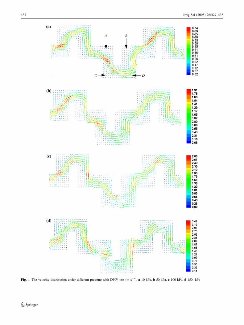
Fig. 4 The velocity distribution under different pressure with DPIV test (m s-1). a 10 kPa, b 50 kPa, c 100 kPa, d 150 kPa
432 Irrig Sci (2008) 26:427–438
123

Fig. 5 The velocity distribution
under different pressure with
CFD analysis (m s-1).
a 10 kPa, b 50 kPa, c 100 kPa,
d 150 kPa
Irrig Sci (2008) 26:427–438 433
123

Fig. 6 Turbulence intensity
distribution in unit length of the
fractal flow path (%).
a Common labyrinth flow path.
b Common labyrinth flow path-
II. c Fractal flow path
Table 2 Numerical experimental treatment for optimal deign of labyrinth flow path
Tr Region B (W) Region C (W) Gridding Tr. Region B (W) Region C (W) Gridding
1 0.5 0.5 a 6 1.0 0.5 f
2 0.8 0.8 b 7 0.5 1.0 g
3 1.0 1.0 c 8 0.8 0.5 h
4 0.5 0.8 d 9 1.0 0.8 i
5 0.8 1.0 e
Gridding: refer to Fig. 8 for details
Fig. 7 Numerical experiment
design for optional designs and
gridding
434 Irrig Sci (2008) 26:427–438
123

similar. Refer to Table 2 for details, and Fig. 7 shows the
gridding.
Effect on hydraulic characteristics of different designs
Table 3 shows the numerically simulated free discharges of
the prototype and optimized emitters modeled under dif-
ferent pressures. The results indicate that the discharge of
various optimized models were all smaller than that of the
prototype emitter with a discrepancy of less than 10.0%.
There was no significant difference in the free discharges
of the optimized emitters with various arc treatments. This
also reflected that the reduction in cross-section could
increase the friction-resistance and enhance the hydraulic
characteristics of the flow path.
Table 3 shows the results of the indices of flow regime
(x) and the discharge coefficient (Kd) by the regression
equation q = Kdhx (q is the free discharge and h is the
work pressure). The results indicate that the indices of flow
regime for various optimized emitters were all smaller than
that of the prototype emitter with a discrepancy of less than
6.0%. This also shows that the optimization treatment had
little effect on the hydraulic characteristics of the flow path.
Hence, the clogging resistance property should be consid-
ered in optimal design of emitter flow paths and the self-
cleaning capacity could be enhanced by increasing the
velocity of flow near the boundary wall of the path.
Effect on clogging resistance characteristics by
different optimization treatments
Changing the structure of the flow path is one approach to
enhancing the clogging resistance of the flow path. From
the perspective of the flow path, there are two main reasons
for clogging. One reason is that the flow path is narrow and
large suspended particles cannot pass easily. The other
reason is that the low-flow velocity causes some suspended
particles to deposit and reduce the cross-section of the flow.
The latter phenomenon is not apparent initially but the
effect worsens over time. Tong et al. (1998) showed that
the number of suspended particles deposited in the low
velocity region increased gradually. However, increasing
the velocity near the boundary wall of flow path could
prevent or alleviate clogging in the path.
Figure 8 shows the numerical experiment results of the
velocity distribution in the typical unit of the flow path with
treatments 1–9 at 100 kPa. These data show that the sec-
ondary flow developed in regions A and C with treatments
1–9 operating at 100 kPa. Howver, the velocity near the
boundary wall increased as the arc radius was reduced. For
region B, secondary flow was difficult to develop and the
velocity of secondary flows under various treatments were
not significantly different. Hence, in this region the sec-
ondary flow should be eliminated. Treatment 6 was
selected as the best combination of the arc radii and Fig. 9
shows the velocity in the typical unit length of the path.
Discussion
Direct particle imaging
This paper has reported on the development of a full-field
non-disturbance test for evaluating the flow path of emit-
ters. However, some problems with the system should be
noted:
(1) The experiment applied the plane model of labyrinth
flow path of cylindrical emitters and ignored the
Table 3 Free discharges and discharge–pressure relationships under various optimization treatments
No. of Tr. Free discharge q L-1/h Discharge–pressure relationship
Work pressure h/kPa Discharge
coefficient
Kd
Index of flow
regime xR2
10 30 50 70 90 100 110 130 150
0 0.87 1.38 1.81 2.12 2.42 2.59 2.74 2.91 3.19 0.84 0.49 0.99
1 0.79 1.32 1.68 1.97 2.25 2.33 2.48 2.69 2.89 0.78 0.48 0.99
2 0.80 1.37 1.75 2.06 2.29 2.37 2.48 2.69 2.89 0.81 0.47 0.99
3 0.82 1.36 1.74 2.05 2.31 2.42 2.55 2.76 2.97 0.81 0.48 0.99
4 0.80 1.34 1.70 1.99 2.24 2.36 2.55 2.68 2.87 0.80 0.47 0.99
5 0.82 1.36 1.74 2.04 2.37 2.42 2.54 2.83 3.06 0.81 0.48 0.99
6 0.79 1.35 1.69 2.01 2.27 2.35 2.52 2.71 2.91 0.79 0.48 0.99
7 0.82 1.39 1.76 2.07 2.32 2.42 2.53 2.81 2.93 0.82 0.47 0.99
8 0.79 1.34 1.72 2.05 2.34 2.44 2.50 2.71 2.89 0.79 0.48 0.99
9 0.81 1.35 1.73 2.07 2.30 2.38 2.58 2.76 3.02 0.80 0.48 0.99
Treatment 0 denoted the measured practical discharge of emitter prior to optimization
Irrig Sci (2008) 26:427–438 435
123

roughness of the model and the circumfluent issues.
From the geometric perspective, there is some
roughness on the path wall except for specially
processed fine surfaces. In engineering practice, the
roughness of the solid surface is usually 1.0–
25.0 9 10-6 m. For single-phase flow, considering
the path wall as geometrically smooth surface does
not cause irrational results in practice. However for 2-
phase flow, the particle dimension and path surface
roughness are on the same scale. In this case, if the
path wall is considered as geometrically smooth, then
the vertical velocity of the particle would approach
zero resulting in an inappropriate increase in colli-
sions between path wall and the particles. The DPIV
test showed that relatively large errors occur where
the particle concentration is high and there are
differences in manufacturing workmanship between
the plane model and the plastic model. In addition, the
boundary of labyrinth flow path and the collision
mechanism between particles and path wall are both
complex. Hence there is a need to conduct prototype
research using plastic emitters.
(2) This work has shown the presence of two-dimen-
sional flow within the labyrinth path of emitters.
Fig. 8 Effect on velocity
distribution in typical unit of
labyrinth flow path by various
optimization radii (work
pressure 100 kPa) (m/s)
Fig. 9 Velocity distribution in
typical unit length of labyrinth
flow path after the optimization
(Tr. 6) (work pressure100 kPa)
(m/s)
436 Irrig Sci (2008) 26:427–438
123

However, the properties of flow, adjacent to the path
wall and the possible existence of secondary flow on
the cross-section needs further research.
CFD analysis
Using CFD for analyzing the flow fields of irrigation
emitters is a relatively new research application and the
stable-status theory and the macro-dimension model are all
approximating approaches. Hence, there are three types of
problems for this area of research:
(1) Stable-status treatment. Treating the flow in the path
as a continuous stable-status flow cannot describe the
response of drips from the emitter outlet to the flow
process. Under high pressure, the stable-status treat-
ment could be appropriate but large errors may occur
under low pressures when a non-stable status treat-
ment should be implemented.
(2) Boundary wall treatment. Using a boundary wall
function to treat the flow near the boundary wall can
cause errors because the boundary wall function is
applicable only for parallel walls within a certain
range. The complex structure of emitters, complex
bending of the flow and different thickness of
boundary layers can all produce errors.
(3) Single-phase flow. This research on clogging resis-
tance was based on the assumption that the flow was
single-phase. Further research should focus on using
multi-phase flow assumptions for analyzing the flow
locus of microorganisms, viscous particles and sus-
pended sands. The critical non-depositing velocity of
the particles as well as the interactive effect between
particle concentration, particle sizes and the flow
should be further studied.
Conclusions
This paper used CFD analysis and direct particle imaging
to study the flow charateristics in labyrinth flow paths.
Custom-made fluorescence particles were developed and
used with DPIV measurement technology to measure the
flow fields of emitters and conduct two-dimensional non-
disturbance tests within the flow path of emitters. An object
lens-modified microscope fitted to a conventional CCD
camera was used to display the flow fields and successfully
solved the contradiction between viewing region and
imaging resolving power within the critical scale of the
flow path. Based on this research, the following findings
can be made:
(1) Velocity distribution differences were used to divide
the flow into mainstream and secondary flows. The
mainstream continuously mixed into the secondary
flow and energy exchange continuously occurred in
the flow path. The mainstream flow was turbulent at
pressures between 10 and 150 kPa and there was no
transition process from laminar to turbulent flow
observed with increasing pressure. Hence, the turbu-
lent model could be used for CFD numerical
simulation in this pressure range. The simulated
velocity distribution for the central cross-section of
the emitter flow path was similar to the measured
velocity distribution by the 2D-DPIV test. Hence, the
established numerical simulation model for flow in
the labyrinth flow path relatively described the flow
process accurately.
(2) Designing of rational flow paths should involve
eliminating the regions of low velocity by creating
smooth arc connections in these regions and enhanc-
ing the self-cleaning capacity by optimization of flow
path boundaries. Evaluations of nine optimization
treatments for labyrinth flow paths had little effect on
the hydraulic characteristics of the flow path. Hence,
the clogging resistance property should be given
consideration in optimal design of flow path of
emitter and the self-cleaning capacity should be
enhanced by increasing the velocity of flow near the
boundary wall of the path. This work suggests that the
value of 0.5 W arc radius should be used in regions A
and C, while the value of 1.0 W arc radius should be
used in region B.
Acknowledgments We are grateful for financial support from the
National Natural Science Fund of China (NSFC) (No. 50379053,
No.50609029) and support by the Program for Changjiang Scholars
and Innovative Research Team in University (PCSIRT)
(No.IRT0657) and the Initiating Research Fund from China Agri-
cultural University (No.2005065).
References
Adin A, Sacks M (1991) Drip-clogging factors in wastewater
irrigation. J Irrig Drain Div ASCE 117(6):813–826
Dasberg S, Or D (1999) Drip irrigation. Spinger, Heidelberg
Fluent Inc (2003) FLUENT User’s Guide. Fluent Inc
Glaad YK, Klous LZ (1980) Hydraulic and mechanical properties of
Drippers. In: Proceedings of the second international drip
irrigation congress. 7–14 July
Li GY, Wang JD, Alam M, Zhao YF (2006) Influence of geometrical
parameters of labyrinth flow path of drip emitters on hydraulic
and anti-clogging performance. Trans ASABE 49(3):637–643
Li YK, Yang PL, Ren SM, Wang Y. (2005) Analyzing and modeling
flow regime in labyrinth path drip irrigation column emitter with
CFD. J Hydrodyn Ser A 20(6):736–743 (in Chinese)
Irrig Sci (2008) 26:427–438 437
123

Li YK, Yang PL, Ren SM, Guan XY. (2007) Effects of fractal flow
path designing and its parameters of emitter hydraulic perfor-
mace. Chin J Mech Eng 43(7):109–114. (in Chinese)
Murray SP (1970) Settling velocities and vertical diffusion of
particles in turbulence water. J Geophys Res 75(9):73–84
Ozekici B, Ronald S (1991) Analysis of pressure losses in tortuous-
path emitters. ASAE, pp 112–115
Palau SG, Arviza VJ, Bralts VF. (2004) Hydraulic flow behavior
through an in-line emitter labyrinth using CFD techniques. In:
2004 ASAE/CSAE Annual international meeting. Fairmont
Chateau Laurier, the Westin, Government Centre Ottawa, ON,
Canada
Shi XL, Zhang MZ (1995) Chemical water quality treatment for
emitter clogging. Water Sav Irri (2):39–42 (in Chinese)
Tong ZY, Wang CL (1998) The physical–chemical mechanism for
solid particles to form and grow in water body of dripping
irrigation. Water Sav Irri (5):31–33 (in Chinese)
Wang FJ, Wang WE (2006) Development and issues of CFD analysis
researches on flow path of emitters. Trans CSAE 22(7):188–192
(in Chinese)
Wei QS, Shi YS, Dong WC, Lu G, Huang SH (2006) Study on
hydraulic performance of drip emitters by computational fluid
dynamics. Agric Water Manage 84(1–2):130–136
Zhang J, Zhao WH, Wei ZY, Tang YP, Lu BH (2007) Numerical and
experimental study on hydraulic performance of emitters with
arc labyrinth channels. Comp Electron Agric 56:120–129
438 Irrig Sci (2008) 26:427–438
123
Top Related
Copyright © 2022 FDOKUMEN

