Download - Bounding the role of black carbon in the climate system: A scientific assessment

Bounding the role of black carbon in the climate system: Ascientific assessment

T. C. Bond,1 S. J. Doherty,2 D. W. Fahey,3 P. M. Forster,4 T. Berntsen,5 B. J. DeAngelo,6

M. G. Flanner,7 S. Ghan,8 B. Kärcher,9 D. Koch,10 S. Kinne,11 Y. Kondo,12 P. K. Quinn,13

M. C. Sarofim,6 M. G. Schultz,14 M. Schulz,15 C. Venkataraman,16 H. Zhang,17

S. Zhang,18 N. Bellouin,19 S. K. Guttikunda,20 P. K. Hopke,21 M. Z. Jacobson,22

J. W. Kaiser,23 Z. Klimont,24 U. Lohmann,25 J. P. Schwarz,3 D. Shindell,26 T. Storelvmo,27

S. G. Warren,28 and C. S. Zender29

Received 26 March 2012; revised 6 December 2012; accepted 4 January 2013.

[1] Black carbon aerosol plays a unique and important role in Earth’s climate system.Black carbon is a type of carbonaceous material with a unique combination of physicalproperties. This assessment provides an evaluation of black-carbon climate forcing that iscomprehensive in its inclusion of all known and relevant processes and that is quantitativein providing best estimates and uncertainties of the main forcing terms: direct solarabsorption; influence on liquid, mixed phase, and ice clouds; and deposition on snow andice. These effects are calculated with climate models, but when possible, they are evaluatedwith both microphysical measurements and field observations. Predominant sources arecombustion related, namely, fossil fuels for transportation, solid fuels for industrial andresidential uses, and open burning of biomass. Total global emissions of black carbonusing bottom-up inventory methods are 7500 Gg yr�1 in the year 2000 with an uncertaintyrange of 2000 to 29000. However, global atmospheric absorption attributable to black

Additional supporting information may be found in the online version of this article.1University of Illinois at Urbana-Champaign, Urbana, Illinois, USA.2Joint Institute for the Study of the Atmosphere and Ocean, University of Washington, Seattle, Washington, USA.3NOAAEarth SystemResearch Laboratory and Cooperative Institute for Research in Environmental Sciences, University of Colorado, Boulder, Colorado, USA.4University of Leeds, Leeds, UK.5Center for International Climate and Environmental Research-Oslo and Department of Geosciences, University of Oslo, Oslo, Norway.6US Environmental Protection Agency, Washington, District of Columbia, USA.7University of Michigan, Ann Arbor, Michigan, USA.8Pacific Northwest National Laboratory, Richland, Washington, USA.9Deutsches Zentrum für Luft- und Raumfahrt Oberpfaffenhofen, Wessling, Germany.10US Department of Energy, Washington, District of Columbia, USA.11Max Planck Institute, Hamburg, Germany.12University of Tokyo, Tokyo, Japan.13NOAA Pacific Marine Environment Laboratory, Seattle, Washington, USA.14Forschungszentrum Jülich GmbH, Jülich, Germany.15Norwegian Meteorological Institute, Oslo, Norway.16Indian Institute of Technology, Bombay, India.17China Meteorological Administration, Beijing, China.18Peking University, Beijing, China.19Met Office Hadley Centre, Exeter, UK.20Division of Atmospheric Sciences, Desert Research Institute, Reno, Nevada, USA.21Clarkson University, Potsdam, New York, USA.22Stanford University, Stanford, California, USA.23European Centre for Medium-range Weather Forecasts, Reading, UK; King’s College London, London UK; Max Planck Institute for Chemistry,

Mainz, Germany.24International Institute for Applied System Analysis, Laxenburg, Austria.25Eidgenössische Technische Hochschule Zürich, Zurich, Switzerland.26NASA Goddard Institute for Space Studies, New York, New York, USA.27Yale University, New Haven, Connecticut, USA.28University of Washington, Seattle, Washington, USA.29University of California, Irvine, California, USA.

Corresponding author: T. C. Bond, University of Illinois at Urbana-Champaign, Urbana, IL, USA. ([email protected])

©2013 The Authors. Journal of Geophysical Research: Atmospheres published by Wiley on behalf of the American Geophysical Union.This is an open access article under the terms of the Creative Commons Attribution License, which permits use, distribution and reproduction in anymedium, provided the original work is properly cited, the use is non-commercial and no modifications or adaptations are made.2169-897X/13/10.1002/jgrd.50171

1

JOURNAL OF GEOPHYSICAL RESEARCH: ATMOSPHERES, VOL. 118, 1–173, doi:10.1002/jgrd.50171, 2013

carbon is too low in many models and should be increased by a factor of almost 3.After this scaling, the best estimate for the industrial-era (1750 to 2005) direct radiativeforcing of atmospheric black carbon is +0.71 W m�2 with 90% uncertainty bounds of(+0.08, +1.27) W m�2. Total direct forcing by all black carbon sources, without subtractingthe preindustrial background, is estimated as +0.88 (+0.17, +1.48) W m�2. Direct radiativeforcing alone does not capture important rapid adjustment mechanisms. A framework isdescribed and used for quantifying climate forcings, including rapid adjustments. The bestestimate of industrial-era climate forcing of black carbon through all forcing mechanisms,including clouds and cryosphere forcing, is +1.1 W m�2 with 90% uncertainty bounds of+0.17 to +2.1 W m�2. Thus, there is a very high probability that black carbon emissions,independent of co-emitted species, have a positive forcing and warm the climate. We estimatethat black carbon, with a total climate forcing of +1.1 W m�2, is the second most importanthuman emission in terms of its climate forcing in the present-day atmosphere; only carbondioxide is estimated to have a greater forcing. Sources that emit black carbon also emit othershort-lived species that may either cool or warm climate. Climate forcings from co-emittedspecies are estimated and used in the framework described herein. When the principal effectsof short-lived co-emissions, including cooling agents such as sulfur dioxide, are included innet forcing, energy-related sources (fossil fuel and biofuel) have an industrial-era climateforcing of +0.22 (�0.50 to +1.08) W m�2 during the first year after emission. For a few ofthese sources, such as diesel engines and possibly residential biofuels, warming is strongenough that eliminating all short-lived emissions from these sources would reduce net climateforcing (i.e., produce cooling). When open burning emissions, which emit high levels oforganic matter, are included in the total, the best estimate of net industrial-era climate forcingby all short-lived species from black-carbon-rich sources becomes slightly negative(�0.06 W m�2 with 90% uncertainty bounds of �1.45 to +1.29 W m�2). The uncertaintiesin net climate forcing from black-carbon-rich sources are substantial, largely due to lack ofknowledge about cloud interactions with both black carbon and co-emitted organic carbon.In prioritizing potential black-carbon mitigation actions, non-science factors, such astechnical feasibility, costs, policy design, and implementation feasibility play importantroles. The major sources of black carbon are presently in different stages with regard to thefeasibility for near-term mitigation. This assessment, by evaluating the large number andcomplexity of the associated physical and radiative processes in black-carbon climateforcing, sets a baseline from which to improve future climate forcing estimates.

Citation: Bond, T. C., et al. (2013), Bounding the role of black carbon in the climate system: A scientific assessment,J. Geophys. Res. Atmos., 118, doi:10.1002/jgrd.50171.

TABLE OF CONTENTS

1. Executive Summary1.1. Background and Motivation1.2. Major Findings

1.2.1. Black Carbon Properties1.2.2. Black Carbon Emissions and Abundance1.2.3. Synthesis of Black-Carbon Climate Forcing

Terms1.2.4. Black-Carbon Direct Radiative Forcing1.2.5. Black-Carbon Cloud Effects1.2.6. Black-Carbon Snow and Ice Effects1.2.7. Impacts of Black-Carbon Climate Forcing1.2.8. Net Climate Forcing by Black-Carbon-Rich

Source Categories1.2.9. Major Factors in Forcing Uncertainty1.2.10. Climate Metrics for Black Carbon Emissions1.2.11. Perspective on Mitigation Options for Black

Carbon Emissions

1.2.12. Policy Implications2. Introduction

2.1. What Is Black Carbon?2.2. How Does Black Carbon Affect the Earth’s

Radiative Budget?2.3. Assessment Terms of Reference

2.3.1. Assessment Structure2.3.2. Use of Radiative Forcing Concepts2.3.3. Contrast With Previous Assessments

3. Measurements and Microphysical Properties of BlackCarbon3.1. Section Summary3.2. Definitions

3.2.1. Black Carbon3.2.2. Organic Matter and Other Carbon Aerosols3.2.3. Other Particulate Light Absorbers

3.3. Black Carbon Formation and Evolution3.4. Measurement of BC Mass3.5. Optical Properties of Black Carbon

BOND ET AL.: BLACK CARBON IN THE CLIMATE SYSTEM

2

3.6. Measurement of Absorption Coefficients3.7. Microphysical Properties Affecting MAC and o0

3.7.1. Optical Models and Required Inputs3.7.2. Density3.7.3. Refractive Index3.7.4. Particle Size3.7.5. Configuration of BC-Containing Particles

3.8. Measured and Modeled MAC and o0

3.8.1. MACBC Derived From Measurements3.8.2. Microphysical Model Ability to Simulate

MAC3.8.2.1. MACBC of Unmixed BC3.8.2.2. MAC of BC Mixed With Other Substances3.8.3. Measured and Modeled Single-Scattering

Albedo3.8.4. Aerosol Properties in Global Models

3.9. CCN Activity of Black Carbon3.9.1. Measurements of CCN Activity3.9.2. Global Model Treatment of CCN Activity

4. Emission Magnitudes and Source Categories4.1. Section Summary4.2. Introduction

4.2.1. Geographic Aggregation4.2.2. Definitions and Aggregation of Emission

Sources4.3. Bottom-Up Inventory Procedures

4.3.1. Energy-Related Emissions4.3.2. Open Burning Emissions4.3.3. Waste Burning Emissions

4.4. Total BC Emissions and Major Source Categories4.4.1. Diesel Engines4.4.2. Industrial Coal4.4.3. Residential Solid Fuels4.4.4. Open Burning4.4.5. Other Emission Sources

4.5. Regional Emissions4.6. Comparison Among Energy-Related Emission

Estimates4.6.1. Differences in Power Generation Emissions4.6.2. Differences in Industrial Coal Emissions4.6.3. Differences in Diesel Engine Emissions4.6.4. Differences in Residential Solid Fuel Sector4.6.5. Asian Emission Inventories

4.7. Major Sources of Uncertainty in Emissions4.7.1. Energy-Related Combustion

4.7.1.1. Activity Data4.7.1.2. Emission Factors4.7.1.3. Summary of Uncertainties in Energy-Related

Emissions4.7.2. Open Biomass Burning

4.7.2.1. Burned Area4.7.2.2. Fuel Load and Combustion Completeness4.7.2.3. Emission Factors4.7.2.4. Summary of Uncertainties in Open Burning

Emissions4.8. Trends in BC Emissions

4.9. Receptor Modeling to Evaluate Source Contributions4.9.1. Receptor Modeling in Urban Areas4.9.2. Receptor Modeling in Continental Plumes4.9.3. Summary of Findings From Receptor

Modeling5. Constraints on Black-Carbon Atmospheric Abundance

5.1. Section Summary5.2. Introduction5.3. Atmospheric Absorption and Extinction by

Absorbing Species5.4. Observations of Atmospheric Black Carbon

Concentrations5.4.1. In Situ Monitoring

5.4.1.1. Intensive Field Campaigns5.4.1.2. Long-Term In Situ Monitoring5.4.2. Remote Sensing

5.4.2.1. Ground-Based Remote Sensing5.4.2.2. Remote Sensing From Space

5.5. Comparison Between Modeled and Observed BCConcentrations and AAOD5.5.1. Estimating Emissions by Integrating Models

and Observations5.6. Vertical Distribution of BC

5.6.1. Comparison Between Modeled and ObservedVertical Distributions

5.7. Causes of Model Biases5.8. Summary of Limitations in Inferring Black Carbon

Atmospheric Abundance6. Black-Carbon Direct Radiative Forcing

6.1. Section Summary6.2. Introduction6.3. Emission, Lifetime, and Burden6.4. Mass Absorption Cross Section6.5. Scaling Modeled BC AAOD to Observations

6.5.1. Sensitivities in AAOD Scaling6.5.2. Reasons for Low Bias in Modeled AAOD

6.6. Forcing Efficiency6.6.1. Vertical Location of BC6.6.2. Horizontal Location of BC

6.7. All-Source and Industrial-Era BC DRF6.7.1. Scaled Estimates of BC DRF6.7.2. Central Estimate of BC DRF6.7.3. Uncertainties in BC DRF

6.8. Previous Observationally Scaled Radiative-ForcingEstimates

6.9. Implications of Increased BC AAOD6.9.1. Apportionment of Bias in BC AAOD6.9.2. Revised Estimate of BC Emissions6.9.3. Scaling of Modeled AAOD in the Context of

Other Evidence6.10. Summary of Uncertainties in BC DRF

7. Black Carbon Interactions With Clouds7.1. Section Summary7.2. Introduction7.3. Black-Carbon Semi-Direct Effects on Cloud Cover

7.3.1. Cloud Scale and Regional Studies


3

7.3.2. Global Model Semi-Direct Estimates7.3.3. Increased Absorption by Cloud Droplet

Inclusions7.4. BC Indirect Effects on Liquid Clouds7.5. BC Indirect Effects on Mixed-Phase and Ice Clouds

7.5.1. Laboratory Evidence for BC Effectiveness asIN

7.5.2. BC Effects on Mixed-Phase Clouds7.5.2.1. Mechanisms7.5.2.2. Experimental Studies7.5.2.3. Modeling Results7.5.3. BC Effects on Ice-Phase Clouds

7.5.3.1. Mechanisms7.5.3.2. Field Evidence for BC Acting as IN7.5.3.3. Modeling Evidence for BC Atmospheric

Abundance and Mixing State7.5.3.4. Global Model Studies of BC Effects on Cirrus7.5.3.5. Aircraft Impacts on High Ice-Cloud Properties

7.6. Comprehensive Modeling of BC Cloud Effects7.7. Summary of Uncertainties in Estimating Indirect

Effects7.7.1. Model Uncertainties Beyond Aerosol-Cloud

Interactions7.7.2. Aerosol-Cloud Interactions

8. Cryosphere Changes: Black Carbon in Snow and Ice8.1. Section Summary8.2. Introduction8.3. Modeled Forcing

8.3.1. BC Concentrations in Snow and Sea Ice andthe Resulting Change in Albedo

8.3.2. Snow-Covered Area8.3.3. Masking by Clouds and Vegetation8.3.4. Snow Grain Size8.3.5. Albedo Dependence on Downwelling

Radiation8.3.6. Concentration of BC With Sublimation and

Melting8.3.7. Representation of All Light Absorbing

Particles in Snow8.4. Measurements of BC in Snow and Comparison With

Models8.4.1. Measurement Methods8.4.2. Arctic and Sub-Arctic Snow8.4.3. Mid-Latitude Snow Measurements8.4.4. BC in Mountain Glaciers8.4.5. Trends in Arctic Snow BC8.4.6. Trends in Mountain Snow

8.5. Sources of BC to Arctic and Himalayan Snow8.6. Estimate of Forcing by BC in the Cryosphere

8.6.1. Adjusted Forcing by BC in Snow8.6.2. Radiative Forcing by BC in Sea Ice8.6.3. Forcing by BC in Snow in the Himalaya and

Tibetan Plateau9. Climate Response to Black Carbon Forcings

9.1. Section Summary

9.2. Introduction to Climate Forcing, Feedback, andResponse

9.3. Surface Temperature Response to AtmosphericBlack Carbon9.3.1. Global-Mean Temperature Change9.3.2. Regional Surface Temperature Change

9.4. Precipitation Changes Due to Black-Carbon Directand Semi-Direct Effects

9.5. Climate Response to the Snow Albedo Effect9.6. Detection and Attribution of Climate Change Due to

Black Carbon9.7. Conclusions

10. Synthesis of Black-Carbon Climate Effects10.1. Section Summary10.2. Introduction10.3. Global Climate Forcing Definition10.4. BC Global Climate Forcing Components and

Uncertainties10.4.1. BC Direct Forcing10.4.2. BC Cloud Indirect Effects

10.4.2.1. Liquid Cloud and Semi-Direct Effects10.4.2.2. BC Inclusion in Cloud Drops10.4.2.3. Mixed-Phase Cloud Effect10.4.2.4. Ice Cloud Effect10.4.3. BC in Snow and Cryosphere Changes10.4.4. BC in Sea Ice10.4.5. Net Effect of BC and Co-Emitted Species

10.5. Uncertainties in BC Global Climate Forcings10.5.1. Atmospheric Burden, Emissions, and Rate of

Deposition10.5.2. Selection of Preindustrial Emissions10.5.3. Scaling to Emission Rate or Atmospheric

Burden10.5.4. Dependence on Atmospheric and Surface

State10.6. Total Forcing Estimates and Comparison With

Previous Work11. Net Climate Forcing by Black-Carbon-Rich Source

Categories11.1. Section Summary11.2. Introduction11.3. Approach to Estimating Forcing From BC-Rich

Source Categories11.4. Climate Forcing Per Emission for Co-Emitted

Aerosols and Precursors11.4.1. Direct Effect for Co-Emitted Aerosol and

Precursors11.4.2. Liquid Cloud Effect for Co-Emitted Aerosol

and Precursors11.4.3. Other Cloud Effects for Co-Emitted Aerosol

and Precursors11.4.4. Snow Albedo Forcing for Co-Emitted

Aerosol11.4.5. Forcing by Co-Emitted Gaseous Species11.4.6. Climate Forcing by Secondary Organic

Aerosol


4

11.4.7. Forcing in Clear and Cloudy Skies11.5. Net Climate Forcing by BC-Rich Source Categories

11.5.1. Diesel Engines11.5.2. Industrial Coal11.5.3. Residential Solid Fuel11.5.4. Open Biomass Burning11.5.5. Summary of BC-Rich Source Categories11.5.6. Cumulative Sum of Forcing by BC-Rich

Source Categories11.6. Climate Forcing by Selected Sources11.7. Comparison With Forcing on Longer Time Scales11.8. Cautions Regarding Net Forcing Estimates

11.8.1. Constraints on Emissions of BC and Co-Emitted Species Are Limited

11.8.2. Forcing Dependence on Emitting Region IsNot Captured

11.8.3. Regional Impacts Are Not Well Captured byGlobal Averages

11.8.4. Large Uncertainties Remain in Deriving andApportioning Cloud Impacts

11.8.5. Climate Forcing by Additional Co-EmittedSpecies May Affect Total Category Forcing

12. Emission Metrics for Black Carbon12.1. Section Summary12.2. Introduction12.3. The GWP and GTP Metrics12.4. Calculations of Metric Values for BC12.5. Uncertainties12.6. Shortcomings of Global Metrics12.7. Choice of Time Horizon12.8. Towards Metrics for the Net Effect of Mitigation

Options13. Mitigation Considerations for BC-Rich Sources

13.1. Section Summary13.2. Mitigation Framework for Comprehensive

Evaluation13.3. Costs and Benefits of Mitigation

13.3.1. Health Benefits13.3.2. Valuing Climate Benefits of BC Mitigation

13.4. Technical and Programmatic Feasibility forIndividual BC-Rich Source Categories13.4.1. Diesel Engines13.4.2. Industry13.4.3. Residential Solid Fuel: Heating13.4.4. Residential Solid Fuel: Cooking13.4.5. Open Burning13.4.6. Other Sources

13.5. International Perspective on BC Reductions inAggregate13.5.1. Projected Future Emissions13.5.2. Comprehensive International Assessments of

BC Mitigation Actions13.6. Policy Delivery Mechanisms13.7. Synthesis of Considerations for Identifying

Important Mitigation Options

1. Executive Summary

1.1. Background and Motivation

[2] Black carbon is emitted in a variety of combustionprocesses and is found throughout the Earth system. Blackcarbon has a unique and important role in the Earth’s climatesystem because it absorbs solar radiation, influences cloudprocesses, and alters the melting of snow and ice cover. Alarge fraction of atmospheric black carbon concentrationsis due to anthropogenic activities. Concentrations respondquickly to reductions in emissions because black carbon israpidly removed from the atmosphere by deposition. Thus,black carbon emission reductions represent a potential miti-gation strategy that could reduce global climate forcing fromanthropogenic activities in the short term and slow theassociated rate of climate change.[3] Previous studies have shown large differences between

estimates of the effect of black carbon on climate. To date,reasons behind these differences have not been extensivelyexamined or understood. This assessment provides a compre-hensive and quantitative evaluation of black carbon’s role inthe climate system and explores the effectiveness of a rangeof options for mitigating black carbon emissions. As such, thisassessment includes the principal aspects of climate forcingthat arise from black carbon emissions. It also evaluates thenet climate forcing of combustion sources that emit largequantities of black carbon by including the effects ofco-emitted species such as organic matter and sulfateaerosol precursors. The health effects of exposure toblack carbon particles in ambient air are not evaluatedin this assessment.

1.2. Major Findings

1.2.1. Black Carbon Properties[4] 1. Black carbon is a distinct type of carbonaceous ma-

terial that is formed primarily in flames, is directly emittedto the atmosphere, and has a unique combination of physi-cal properties. It strongly absorbs visible light, is refractorywith a vaporization temperature near 4000K, exists as an ag-gregate of small spheres, and is insoluble in water and com-mon organic solvents. In measurement and modeling stud-ies, the use of the term “black carbon” frequently has notbeen limited to material with these properties, causing a lackof comparability among results.[5] 2. Many methods used to measure black carbon can be

biased by the presence of other chemical components. Mea-sured mass concentrations can differ between methods by upto 80% with the largest differences corresponding to aerosolwith low black carbon mass fractions.[6] 3. The atmospheric lifetime of black carbon, its impact

on clouds, and its optical properties depend on interactionswith other aerosol components. Black carbon is co-emittedwith a variety of other aerosols and aerosol precursor gases.Soon after emission, black carbon becomes mixed withother aerosol components in the atmosphere. This mixingincreases light absorption by black carbon, increases itsability to form liquid-cloud droplets, alters its capacity toform ice nuclei, and, thereby, influences its atmosphericremoval rate.1.2.2. Black Carbon Emissions and Abundance[7] 1. Sources whose emissions are rich in black carbon

(“BC-rich”) can be grouped into a small number of categories,


5

broadly described as diesel engines, industry, residentialsolid fuel, and open burning. The largest global sources areopen burning of forests and savannas. Dominant emitters ofblack carbon from other types of combustion depend on thelocation. Residential solid fuels (i.e., coal and biomass) con-tribute 60 to 80% of Asian and African emissions, while on-road and off-road diesel engines contribute about 70%of emissions in Europe, North America, and Latin America.Residential coal is a significant source in China, the formerUSSR, and a few Eastern European countries. These catego-ries represent about 90% of black-carbon mass emissions.Other miscellaneous black-carbon-rich sources, includingemissions from aviation, shipping, and flaring, account foranother 9%, with the remaining 1% attributable to sourceswith very low black carbon emissions.[8] 2. Total global emissions of black carbon using

bottom-up inventory methods are 7500 Gg yr�1 in the year2000 with an uncertainty range of 2000 to 29,000. Emis-sions of 4800 (1200 to 15000) Gg yr�1 black carbon arefrom energy-related combustion, which includes all butopen burning, and the remainder is from open burning offorests, grasslands, and agricultural residues.[9] 3. An estimate of background black carbon abun-

dances in a preindustrial year is used to evaluate climateeffects. In this assessment, we use the term “industrial era”to denote differences in the atmospheric state betweenpresent day and the year 1750. We use a preindustrialvalue of 1400 Gg of black carbon per year from biofueland open biomass burning, although some fraction wasanthropogenic at that time.[10] 4. Current emission estimates agree on the major

sources and emitting regions, but significant uncertaintiesremain. Information gaps include the amounts of biofuelor biomass combusted, and the type of technology orburning, especially in developing countries. Emissionestimates from open biomass burning lack data on fuelconsumed, and black-carbon emission factors from thissource may be too low.[11] 5. Black carbon undergoes regional and interconti-

nental transport during its short atmospheric lifetime.Atmospheric removal occurs within a few days to weeksvia precipitation and contact with surfaces. As a result,black carbon is found in remote regions of the atmo-sphere at concentrations much lower than in sourceregions.[12] 6. Comparison with remote sensing observations

indicates that global atmospheric absorption attributableto black carbon is too low in many global aerosol models.Scaling atmospheric black carbon absorption to matchobservations increases the modeled globally averaged, in-dustrial-era black carbon absorption by a factor of 2.9.Some of the model underestimate can be attributed tothe models lacking treatment of enhanced absorptioncaused by mixing of black carbon with other constituents.The remainder is attributed to underestimates of theamount of black carbon in the atmosphere. Burdenunderestimates by factors of 1.75 to 4 are found inAfrica, South Asia, Southeast Asia, Latin America, and thePacific region. In contrast, modeled burdens inNorth America, Europe, and Central Asia areapproximately correct. The required increase in modeledBC burdens is compatible with in situ observations in

Asia and space-based remote sensing of biomass burningaerosol emissions.[13] 7. If all differences in modeled black carbon abun-

dances were attributed to emissions, total emissions wouldbe 17,000 Gg yr�1 compared to the bottom-up inventoryestimates of 7500 Gg yr�1. The industrial-era value of about14,000 Gg yr�1, obtained by subtraction of estimatedpreindustrial emissions, is used as the best estimate ofemissions to determine final forcing values in this assessment.However, some of the difference could be attributed to poorlymodeled removal instead of emissions. Both energy-re-lated burning and open biomass burning are implicatedin underestimates of emission rates, depending on theregion.1.2.3. Synthesis of Black-Carbon Climate Forcing Terms[14] 1. Radiative forcing used alone to estimate black-carbon

climate effects fails to capture important rapid adjustmentmechanisms. Black-carbon-induced heating and cloudmicrophysical effects cause rapid adjustments within theclimate system, particularly in clouds and snow. These rapidadjustments cause radiative imbalances that can be repre-sented as adjusted or effective forcings, accounting for thenear-term global response to black carbon more completely.The effective forcing accounts for the larger response ofsurface temperature to a radiative forcing by black carbon insnow and ice compared to other forcing mechanisms. Thesefactors are included in the climate forcing values reported inthis assessment.[15] 2. The best estimate of industrial-era climate forcing of

black carbon through all forcing mechanisms is +1.1 W m�2

with 90% uncertainty bounds of +0.17 to +2.1 W m�2.This estimate includes cloud forcing terms with very lowscientific understanding that contribute additional positiveforcing and a large uncertainty. This total climate forcingof black carbon is greater than the direct forcing given inthe fourth Intergovernmental Panel on Climate Change(IPCC) report. There is a very high probability that blackcarbon emissions, independent of co-emitted species, havea positive forcing and warm the climate. This black carbonclimate forcing is based on the change in atmosphericabundance over the industrial era (1750 to 2005). Theblack-carbon climate-forcing terms that make up this esti-mate are listed in Table 1. For comparison, the radiativeforcings including indirect effects from emissions of thetwo most significant long-lived greenhouse gases, carbondioxide (CO2) and methane (CH4), in 2005 were +1.56 and+0.86 W m�2, respectively.[16] 3. The fossil fuel direct effect of black carbon of

+0.29 W m�2 is higher than the value provided by the IPCCin 2007. This increase is caused by higher absorption permass and atmospheric burdens than used in models forIPCC. The black-carbon-in-snow forcing estimate in thisassessment is comparable, although more sophisticated.Our total climate forcing estimate of +1.1 W m�2 includesbiofuel and open-biomass sources of black carbon, as wellas cloud effects that the IPCC report did not explicitly isolatefor black carbon.1.2.4. Black-Carbon Direct Radiative Forcing[17] 1. Direct radiative forcing of black carbon is caused

by absorption and scattering of sunlight. Absorption heatsthe atmosphere where black carbon is present and reducessunlight that reaches the surface and that is reflected back to


6

space. Direct radiative forcing is the most commonly cited cli-mate forcing associated with black carbon.[18] 2. The best estimate for the industrial-era (1750 to

2005) direct radiative forcing of black carbon in the atmo-sphere is +0.71 W m�2 with 90% uncertainty bounds of+0.08 to +1.27 W m�2. Previous direct forcing estimatesranged from +0.2 to +0.9 W m�2, and the median valuewas much lower. The range presented here is alteredbecause we adjust global aerosol models with observationalestimates of black carbon absorption optical depth as done insome previous studies.[19] 3. Direct radiative forcing from all present-day sources

of black carbon (including preindustrial background sources)is estimated to be +0.88W m�2 with 90% uncertainty boundsof +0.17 to +1.48 W m�2. This value is 24% larger than in-dustrial-era forcing because of appreciable preindustrial emis-sions from open burning and biofuel use.[20] 4. Estimates of direct radiative forcing are obtained

from models of black carbon abundance and location. Theability to estimate radiative forcing accurately depends onthe fidelity of these models. Modeling of and observationalconstraints on the black-carbon vertical distribution areparticularly poor.1.2.5. Black-Carbon Cloud Effects[21] 1. Black carbon influences the properties of ice

clouds and liquid clouds through diverse and complexprocesses. These processes include changing the numberof liquid cloud droplets, enhancing precipitation in mixed-phase clouds, and changing ice particle number and cloudextent. The resulting radiative changes in the atmosphereare considered climate indirect effects of black carbon. Inaddition, in the semi-direct effect, light absorption byblack carbon alters the atmospheric temperature structurewithin, below, or above clouds and consequently alters

cloud distributions. Liquid-cloud and semi-direct effectsmay have either negative or positive climate forcings. Thebest estimates of the cloud-albedo effect and the semi-directeffect are negative. Absorption by black carbon within clouddroplets and mixed-phase cloud changes cause positive cli-mate forcing (warming). At present, even the sign ofblack-carbon ice-cloud forcing is unknown.[22] 2. The best estimate of the industrial-era climate

forcing from black carbon cloud effects is positive withsubstantial uncertainty (+0.23 W m�2 with a �0.47 to+1.0 W m�2 90% uncertainty range). This positiveestimate has large contributions from cloud effects with avery low scientific understanding and large uncertainties.The cloud effects, summarized in Table 1, are the largestsource of uncertainty in quantifying black carbon’s role inthe climate system. Very few climate model studies haveisolated the influence of black carbon in these indirecteffects.1.2.6. Black-Carbon Snow and Ice Effects[23] 1. Black carbon deposition on snow and ice causes

positive climate forcing. Even aerosol sources with negativeglobally averaged climate forcing, such as biomasscombustion, can produce positive climate forcing in theArctic because of their effects on snow and ice.[24] 2. The best estimate of climate forcing from black

carbon deposition on snow and sea ice in the industrialera is +0.13 W m�2 with 90% uncertainty bounds of+0.04 to +0.33 W m�2. The all-source present-day climateforcing including preindustrial emissions is somewhathigher at +0.16 W m�2. These climate forcings result froma combination of radiative forcing, rapid adjustments,and the stronger snow-albedo feedback caused byblack-carbon-on-snow forcing. This enhanced climatefeedback is included in the +0.13 W m�2 forcing estimate.

Table 1. Black Carbon Climate Forcing Terms, Evaluated for Industrial Era (1750–2005) Unless Otherwise Stated

Climate Forcing Term Forcing Components

Forcing (Wm�2)

(90% Uncertainty Range)

Black carbon direct effect Atmosphere absorption and scattering +0.71 (+0.09 to +1.26)

Direct radiative forcing split Fossil fuel sources +0.29Bio fuel sources +0.22Open burning sources +0.20

Black carbon cloud semi-direct and indirect effects Combined liquid cloud and semi-direct effect �0.2 (�0.61 to +0.10)Black carbon in cloud drops +0.2 (�0.1 to +0.9)Mixed phase cloud +0.18 (+0.0 to +0.36)Ice clouds 0.0 (�0.4 to +0.4)Combined cloud and semi-direct effects +0.23 (�0.47 to +1.0)

Black carbon in snow and sea-ice effects Snow effective forcing +0.10 (+0.014 to +0.30)Sea-ice effective forcing +0.03 (+0.012 to +0.06)Combined surface forcing terms +0.13 (+0.04 to 0.33)

Total climate forcingsa Black carbon only (all terms) +1.1 (0.17 to +2.1)Net effect of black carbon + co-emitted species:All sources �0.06 (�1.45 to +1.29)Excluding open burning +0.22 (�0.50 to +1.08)

All source (includes pre-industrial) forcings Direct radiative forcing +0.88 (+0.18 to +1.47)Snow pack effective forcing +0.12 (+0.02 to +0.36)Sea-ice effective forcing +0.036 (+0.016 to +0.068)

aNote that the total best estimate is the median of the combined probability distribution functions across all terms, which differs from the mean of thebest estimates.


7

[25] 3. Species other than black carbon are a large frac-tion of the absorbing aerosol mass that reduces reflectivityof snow and ice cover. These species include dust andabsorbing organic carbon; the latter is co-emitted with blackcarbon or may come from local soils.[26] 4. The role of black carbon in the melting of glaciers

is still highly uncertain. Few measurements of glacial black-carbon content exist, and studies of the impact on glacialsnow melt have not sufficiently accounted for naturalimpurities such as soil dust and algae or for the difficultyin modeling regions of mountainous terrain.1.2.7. Impacts of Black-Carbon Climate Forcing[27] 1. The black-carbon climate forcings from the direct

effect and snowpack changes cause the troposphere and thetop of the cryosphere to warm, inducing further climate re-sponse in the form of cloud, circulation, surface temperature,and precipitation changes. In climate model studies, black-carbon direct effects cause equilibrium global warming that isconcentrated in the Northern Hemisphere. The warmingresponse to black-carbon-in-snow forcing is greatest duringlocal spring and over mid-to-high northern latitudes. In termsof equilibrium global-mean surface temperature change, theBC total climate forcing estimate over the industrial era wouldcorrespond to a warming between 0.1 and 2.0K. Note that notall this warming has been realized in the present day, as the cli-mate takes more than a century to reach equilibrium and manyco-emitted species have a cooling effect, countering theglobal-mean warming of BC.[28] 2. Regional circulation and precipitation changes

may occur in response to black-carbon climate forcings.These changes include a northward shift in the Inter-Tropi-cal Convergence Zone and changes in Asian monsoon sys-tems where concentrations of absorbing aerosols are large.Black-carbon cloud indirect effects are also expected to in-duce a climate response. However, global models do notsimulate robust responses to these complex and uncertainclimate-forcing mechanisms.1.2.8. Net Climate Forcing by Black-Carbon-RichSource Categories[29] 1. Other species co-emitted with black carbon influ-

ence the sign and magnitude of net climate forcing byblack-carbon-rich source categories. The net climate forc-ing of a source sector is a useful metric when consideringmitigation options. Principal co-emitted species that canchange the sign of short-lived forcing are organic matterand sulfur species. The direct radiative forcing is positivefor almost all black-carbon-rich source categories, evenwhen negative direct forcings by sulfate and organic matterare considered. Liquid-cloud forcing by co-emitted aerosolspecies can introduce large negative forcing. Therefore, highconfidence in net positive total climate forcing is possibleonly for black-carbon source categories with low co-emittedspecies, such as diesel engines.[30] 2. The best estimate of the total industrial-era climate

forcing by short-lived effects from all black-carbon-richsources is near zero with large uncertainty bounds. Short-lived effects are defined as those lasting less than 1 year, in-cluding those from aerosols and short-lived gases. This total is+0.22 (�0.50 to +1.08) W m�2 for fossil fuel and biofuel-burning emissions and �0.06 W m�2 with 90% uncertaintybounds of �1.45 to +1.29 W m�2 when open burning emis-sions are included.

[31] 3. The climate forcings from specific sources withinblack-carbon source categories are variable dependingupon the composition of emissions. Some subsets of a cate-gory may have net positive climate forcing even if the wholecategory does not. Selecting such individual source typesfrom each category can yield a group of measures that, ifimplemented, would reduce climate forcing. However, thepositive forcing reduction would be much less than the totalclimate forcing of +1.1 W m�2 attributable to all industrial-era black-carbon emissions in 2005.[32] 4. Short-lived forcing effects from black-carbon-rich

sources are substantial compared with the effects of long-livedgreenhouse gases from the same sources, even when the forc-ing is integrated over 100 years. Climate forcing from changesin short-lived species in each source category amounts to 5 to75% of the combined longer-lived forcing by methane, effectson the methane system, and CO2, when the effects are inte-grated over 100 years.1.2.9. Major Factors in Forcing Uncertainty[33] 1. Observational constraints on global, annual aver-

age black carbon direct radiative forcing are limited by a lackof specificity in attributing atmospheric absorption to blackcarbon, dust, or organic aerosol. These constraints arerequired to correct demonstrated biases in the distributions ofatmospheric black carbon in climate models.[34] 2. Altitude and removal rates of black carbon are

strong controlling factors. They determine black-carbonabsorption forcing efficiency, microphysical effects onclouds, and the sign of semi-direct effects. Models donot accurately represent black-carbon vertical distribu-tions. Removal rates, particularly wet removal, affectmost facets of black carbon forcing, including its lifetime,horizontal, and vertical extent, and deposition to thecryosphere.[35] 3. Black-carbon emission rates from both energy-related

combustion and biomass burning currently appear underes-timated. Underestimates occur largely in Asia and Africa. Uncer-tainties in biomass burning emissions also affect preindustrialblack-carbon emission rates and net forcing.[36] 4. Black carbon effects on clouds are a large source

of uncertainty. Models of liquid-cloud and semi-directeffects disagree on signs and magnitudes of forcing. How-ever, potentially large forcing terms and uncertainties comefrom black carbon effects on mixed-phase clouds, cloud-ab-sorption, and ice clouds, which have been estimated in avery small number of studies.[37] 5. Estimates of forcing rely on accurate models of the

Earth system. Black-carbon cloud interactions rely on fidel-ity in representation of clouds without black carbon present,and likewise, reductions in snow and sea ice albedo by blackcarbon depend on accurate representation of coverage ofsnow and sea ice. Uncertainties due to model biases of thesedistributions have not been assessed.1.2.10. Climate Metrics for Black Carbon Emissions[38] 1. The 100 year global-warming-potential (GWP)

value for black carbon is 900 (120 to 1800 range) with allforcing mechanisms included. The large range derives fromthe uncertainties in the climate forcings for black carboneffects. The GWP and other climate metric values vary byabout �30% between emitting regions. Black-carbon metricvalues decrease with increasing time horizon due to theshort lifetime of black carbon emissions compared to CO2.


8

Black carbon and CO2 emission amounts with equivalent100 year GWPs have different impacts on climate, tempera-ture, rainfall, and the timing of these impacts. These andother differences raise questions about the appropriatenessof using a single metric to compare black carbon and green-house gases.1.2.11. Perspective on Mitigation Options for BlackCarbon Emissions[39] 1. Prioritization of black-carbon mitigation options is

informed by both scientific and non-scientific factors.Scientific issues include the magnitude of black carbonemissions by sector and region, and net climate forcingincluding co-emissions and impacts on the cryosphere. Non-science factors, such as technical feasibility, costs, policydesign, and implementation feasibility, also play roles. Themajor sources of black carbon are presently in differentstages with regard to technical and programmatic feasibilityfor near-term mitigation.[40] 2. Mitigation of diesel-engine sources appears to of-

fer the most confidence in reducing near-term climateforcing. Mitigating emissions from residential solid fuelsalso may yield a reduction in net positive forcing. Thenet effect of other sources, such as small industrial coalboilers and ships, depends on the sulfur content, andnet climate benefits are possible by mitigating someindividual source types.1.2.12. Policy Implications[41] 1. Our best estimate of black carbon forcing ranks it

as the second most important individual climate-warmingagent after carbon dioxide, with a total climate forcing of+1.1 W m�2 (+0.17 to +2.1 W m�2 range). This forcingestimate includes direct effects, cloud effects, and snowand ice effects. The best estimate of forcing is greater thanthe best estimate of indirect plus direct forcing of methane.The large uncertainty derives principally from the indirectclimate-forcing effects associated with the interactions ofblack carbon with cloud processes. Climate forcing fromcloud drop inclusions, mixed phase cloud effects, and icecloud effects together add considerable positive forcingand uncertainty. The relative importance of black carbonclimate forcing will increase following reductions in theemissions of other short-lived species or decrease if atmo-spheric burdens of long-lived greenhouse gases continueto grow.[42] 2. Black carbon forcing concentrates climate

warming in the mid-high latitude Northern Hemisphere. Assuch, black carbon could induce changes in the precipitationpatterns from the Asian Monsoon. It is also likely to be one ofthe causes of Arctic warming in the early twentieth century.[43] 3. The species co-emitted with black carbon also have

significant climate forcing. Black carbon emissions areprimarily attributable to a few major source categories. Fora subset of these categories, including diesel engines andpossibly residential solid fuel, the net impact of emissionreductions can be a lessening of positive climate forcing(cooling). However, the impact of all emissions fromblack-carbon-rich sources is slightly negative (�0.06 Wm�2) with a large uncertainty range (�1.45 to +1.29 Wm�2). Therefore, uniform elimination of all emissions fromblack-carbon-rich sources could lead to no change in climatewarming, and sources and mitigation measures chosen toreduce positive climate forcing should be carefully

identified. The uncertainty in the response to mitigation islarger when more aerosol species are co-emitted.[44] 4. All aerosol that is emitted or formed in the lower

atmosphere adversely affects public health. Mitigationof many of these sources would increase positive climateforcing (warming). In contrast, reduction of aerosolconcentrations by mitigating black-carbon-rich sourcecategories would be accompanied by very small or slightlynegative changes in climate forcing. These estimates ofclimate forcing changes from source mitigation are associatedwith large uncertainties.[45] 5. Forcings by greenhouse-gases alone do not convey

the full climate impact of actions that alter emission sources.Black-carbon-rich source sectors emit short-lived species,primarily black carbon, other aerosols and their precursors,and long-lived greenhouse gases (e.g., CO2 and CH4). Thetotal climate forcing from the short-lived components is asubstantial fraction of the total (up to 75%) even whenboth short-lived and long-lived forcings are integrated over100 years after emission.

2. Introduction

[46] In the year 2000, a pair of papers [Jacobson, 2000;Hansen et al., 2000] pointed out that black carbon—small,very dark particles resulting from combustion—might pres-ently warm the atmosphere about one third as much asCO2. Because black carbon absorbs much more light thanit reflects, it warms the atmosphere through its interactionwith sunlight. This warming effect contrasts with the coolingeffect of other particles that are primarily scattering and,thus, reduce the amount of energy kept in the Earth system.Radiative forcing (RF) by atmospheric BC stops withinweeks after emissions cease because its atmospheric lifetimeis short unlike the long timescale associated with theremoval of CO2 from the atmosphere. Thus, sustained reduc-tions in emissions of BC and other short-lived climatewarming agents, especially methane and tropospheric ozone(O3), could quickly decrease positive climate forcing andhence climate warming. While such targeted reductions willnot avoid climate change, their value in a portfolio tomanage the trajectory of climate forcing is acknowledgedin the scientific community [e.g., Molina et al., 2009;Ramanathan and Xu, 2010].[47] Discussions of black carbon’s role in climate rest on a

long history. Urban pollution had been a concern forhundreds of years [Brimblecombe, 1977], and blacknesswas used as an indicator of pollution since the early 1900s[Uekoetter, 2005]. Black carbon was first isolated in urbanpollution, as Rosen et al. [1978] and Groblicki et al.[1981] found that graphitic, refractory particles were respon-sible for light absorption. Shortly after McCormick andLudwig [1967] suggested that aerosols could influenceclimate, Charlson and Pilat [1969] pointed out that aerosolabsorption causes warming rather than cooling. The magni-tude of climate effects was first estimated hypothetically toexamine post-nuclear war situations [Turco et al., 1983]and later using realistic distributions from routine humanemissions [Penner et al., 1993; Haywood and Shine,1995]. It was known that particles traveled long distancesfrom source regions [Rodhe et al., 1972], reaching as far asthe Arctic [Heintzenberg, 1980]. International experiments


9

organized to examine aerosol in continental outflow wereinitiated in the late 1990s [Raes et al., 2000]. They con-firmed that absorbing aerosol was prevalent in some regionsand an important component of the atmospheric radiationbalance [Satheesh and Ramanathan, 2000]. This coincidentconfirmation of atmospheric importance and proposal ofpolicies for mitigation triggered further debate.[48] In the decade since the initial proposals, the speed of

Arctic climate change and glacial melt has increased thedemand for mitigation options which can slow near-termwarming, such as reductions in the emissions of short-livedwarming agents. The impact of air quality regulations thatreduce sulfate particles is also being recognized. Most parti-cles, including sulfates, cool the climate system, maskingsome of the warming from longer-lived greenhouse gases(GHGs) and BC. Thus, regulating these particles to protecthuman health may have the unintended consequence ofincreasing warming rapidly. BC also plays a direct role insurface melting of snow and ice and, hence, may have animportant role in Arctic warming [Quinn et al., 2008]; ifso, targeted reductions could have disproportionate benefitsfor these sensitive regions.[49] Particulate matter was originally regulated to improve

human health. Evidence supporting the link between parti-cles and adverse respiratory and cardiovascular healthcontinues to mount [Pope et al., 2009]. High human expo-sures to particulate matter in urban settings are linked tosources that emit black carbon [Grahame and Schlesinger,2007; Naeher et al., 2007; Janssen et al., 2011] and tointense exposures in indoor air [Smith et al., 2010]. Thus,reducing particulate matter is desirable to improve humanwelfare, regardless of whether those reductions reduceclimate warming.[50] For the past few years, the opportunity to reduce

black carbon has received pervasive policy attention at highlevels. The G8 declaration, in addition to promising GHGreductions, is committed to “. . .taking rapid action to ad-dress other significant climate forcing agents, such as blackcarbon.” [9 July 2009, L’Aquila, Italy]. The Arctic Council,recognizing that “. . .reductions of emissions have the poten-tial to slow the rate of Arctic snow, sea ice and sheet icemelting in the near-term. . .,” established a task force in2009 to offer mitigation recommendations [29 April 2009,Tromsø, Norway] and “encouraged” the eight member statesto implement certain black-carbon reduction measures[12 May 2011, Nuuk, Greenland]. The United States hascomplemented this international interest with passage of abill [H.R. 2996] requiring a study of the sources, climateand health impacts, and mitigation options for black carbonboth domestically and internationally. A proposed revisionto the Gothenburg Protocol [UNECE, 1999] states thatparties “should, in implementing measures to achieve theirnational targets for particulate matter, give priority, to theextent they consider appropriate, to emission reductionsmeasures which also significantly reduce black carbon.”[UNECE, 2011]. In February 2012, the Climate andClean Air Coalition was formed with the aim of reducingclimate warming and air pollutants through action onshort-lived pollutants—in particular, BC, methane, andhydrofluorocarbons (http://www.unep.org/ccac).[51] The prospect of achieving quick climate benefits by

reducing BC emissions is tantalizing, but the scientific basis

for evaluating the results of policy choices has not yet beenfully established. This assessment is intended to provide acomprehensive and quantitative scientific framework forsuch an evaluation. In the remainder of this section, webriefly define black carbon, present our terms of referencefor the assessment, and describe its structure.

2.1. What Is Black Carbon?

[52] Black carbon is a distinct type of carbonaceous mate-rial, formed only in flames during combustion of carbon-basedfuels. It is distinguishable from other forms of carbon and car-bon compounds contained in atmospheric aerosol because ithas a unique combination of the following physical properties:[53] 1. It strongly absorbs visible light with a mass absorp-

tion cross section of at least 5 m2g�1 at a wavelength of 550nm.[54] 2. It is refractory; that is, it retains its basic form at very

high temperatures, with a vaporization temperature near4000K.[55] 3. It is insoluble in water, in organic solvents includ-

ing methanol and acetone, and in other components ofatmospheric aerosol.[56] 4. It exists as an aggregate of small carbon spherules.[57] The strong absorption of visible light at all visible

wavelengths by black carbon is the distinguishing character-istic that has raised interest in studies of atmospheric radia-tive transfer. No other substance with such strong lightabsorption per unit mass is present in the atmosphere insignificant quantities. BC has very low chemical reactivityin the atmosphere; its primary removal process is wet ordry deposition to the surface. BC is generally found in atmo-spheric aerosol particles containing a number of other mate-rials, many of which are co-emitted with BC from a varietyof sources.[58] In this assessment, the term “black carbon” and the

abbreviation “BC” are used to denote ambient aerosol mate-rial with the above characteristics. Note that this definition ofblack carbon has not been used rigorously or consistentlythroughout most previous literature describing absorbingaerosol and its role in the atmosphere. Section 3 givesfurther discussion of terminology.

2.2. How Does Black Carbon Affect the Earth’sRadiative Budget?

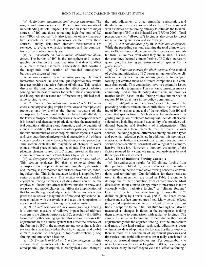
[59] Figure 1 illustrates the multi-faceted interaction of BCwith the Earth system. A variety of combustion sources,both natural and anthropogenic, emit BC directly to theatmosphere. The largest global sources are open burning offorests and savannas, solid fuels burned for cookingand heating, and on-road and off-road diesel engines. Industrialactivities are also significant sources, while aviation and ship-ping emissions represent minor contributions to emitted massat the global scale. The difficulty in quantifying emissions fromsuch diverse sources contributes to the uncertainty in evaluatingBC’s climate role. Once emitted, BC aerosol undergoesregional and intercontinental transport and is removed fromthe atmosphere through wet (i.e., in precipitation) and drydeposition to the Earth’s surface, resulting in an average atmo-spheric lifetime of about a week.[60] Radiative forcing over the industrial era (1750–present)

has typically been used (e.g., by the IPCC [Forster et al.,2007]) to quantify and compare first-order climate effects from


10

http://www.unep.org/ccac

different climate change mechanisms. Many of BC’s effectson clouds and within the cryosphere are not easily assessedwithin this framework. These effects result in rapid adjust-ments involving the troposphere and land surface that lead toa perturbed energy balance that can also be quantified in unitsof radiative forcing. We employ the term “climate forcing” toencompass both traditional radiative forcing and the rapidadjustment effects on clouds and snow (Table 2); this isdiscussed further in section 2.3.2.[61] The best quantified climate impact of BC is its atmo-

spheric direct radiative forcing—the consequent changes inthe radiative balance of the Earth due to an increase inabsorption of sunlight within the atmosphere. When BC islocated above a reflective surface, such as clouds or snow,it also absorbs solar radiation reflected from that surface.Heating within the atmosphere and a reduction in sunlightreaching the surface can alter the hydrological cycle throughchanges in latent heating and also by changing convectionand large-scale circulation patterns.[62] A particularly complex role of BC and other aerosols

in climate is associated with changes in the formation andradiative properties of liquid water and ice clouds. BCparticles may increase the reflectivity and lifetime of warm(liquid) clouds, causing net cooling, or they may reducecloudiness, resulting in warming. Aerosol particles canchange cloud droplet number and cloud cover in ice clouds,

or in mixed-phase clouds made up of both ice and liquidwater. Changes in droplet number may also alter cloudemissivity, affecting longwave radiation.[63] BC also produces warming when it is deposited on

ice or snow because BC decreases the reflectivity of thesesurfaces, causing more solar radiation to be absorbed. Thedirect absorption of sunlight produces warming whichaffects snow and ice packs themselves, leading to additionalclimate changes and ultimately to earlier onset of melt andamplified radiative forcing.[64] An important consideration in evaluating the climate

role of BC emissions is the role of co-emitted aerosols, aerosolprecursors, and other gases. Many of these co-emitted speciesarise in the same combustion sources that produce BC. Thegreatest emissions by mass include sulfur-containing particlesor precursors, organic aerosols that are directly emitted, organiccompounds that are precursors to aerosols and ozone, nitrogenoxides that play roles in ozone formation and methane destruc-tion and are precursors to nitrated aerosols, and long-livedGHGs. Sources also emit smaller quantities of ionic speciessuch as potassium and chloride. With the exception of “brown”organic carbon, non-BC particles absorb little or no light, sothey often cool rather than warm climate. They also play a rolein many, but not all, of the same cloud processes as BC.[65] In contrast to BC, most other aerosols and precursors

are chemically reactive in the atmosphere. Because of

Figure 1. Schematic overview of the primary black-carbon emission sources and the processes thatcontrol the distribution of black carbon in the atmosphere and determine its role in the climate system.


11

Table 2. Definition of Climate Forcing and Response Terms

Forcing Term Definition Model Calculation

Climate forcing Generic term encompassing all forcing types below,quantifying a perturbation to the Earth’s energy balancein Wm�2

Radiative forcing (RF) RF is the change in the net vertical irradiance at thetropopause caused by a particular constituent. Usually,RF is computed after allowing for stratospheric temperaturesto readjust to radiative equilibrium but with all troposphericproperties held fixed at their unperturbed values. Radiativeforcing without stratospheric adjustment is calledinstantaneous.

Difference between simulations:(1) with radiative effect of the constituent change(2) without radiative effect of constituent changeHeld constant: All other tropospheric quantities, including cloud

Rapid adjustment Globally averaged flux change from the adjustment of thetroposphere and land surface to a radiative forcing whileholding the globally averaged surface temperature constant.a

Energy balance perturbations arise from temperature, cloud,and constituent changes in the troposphere and from land-surface temperature and moisture changes. These changesoccur within 1 year after a forcing is applied, usually withina few days but up to a season in the case of snowpackchanges. For BC, the rapid adjustment to the direct effect isalso called the “semi-direct effect.” The radiative forcingplus the rapid adjustment gives the “adjusted forcing”(see below).

Difference between models:(1) with radiative effect of constituent change and changes incloud and land-surface temperature(2) with radiative effect of constituent change and notropospheric responseHeld constant: global mean surface temperaturea

Adjusted forcing Flux perturbation from a given mechanism, allowing forchanges in the stratosphere, troposphere, and some surfaceproperties but not allowing a full response of global surfacetemperatures. This is the sum of a radiative forcing plus itsrapid adjustment.

Difference between models:(1) with atmospheric constituent change and full atmosphericresponse(2) without atmospheric constituent changeHeld constant: sea-surface temperatures and/or global meansurface temperature responsea

Effective forcing A radiative forcing or adjusted forcing multiplied by itsefficacy (see below) to give a climate forcing that iscomparable to an equivalent climate forcing from apre-industrial to 2� pre-industrial carbon dioxidechange in terms of its globally averaged temperatureresponse. Effective radiative forcing includes rapidadjustments, and it also accounts for differences in globallyaveraged responses due to latitudinal dependence of forcing.

The efficacy is calculated for the constituent of interest in aclimate model (see below). This is then multiplied by theassociated radiative forcing or adjusted forcing to give theeffective forcing.b

Climate response Large-scale long-term changes in temperature, snow and icecover, and rainfall caused by a specific forcing mechanism.One of the most important climate responses is that ofequilibrium globally averaged surface temperature (ΔT).

Diagnostics from a global atmospheric climate model, coupledto either a mixed layer ocean for equilibrium experiments or afull ocean model for transient experiments

Climate sensitivity (l) Equilibrium globally averaged surface warming perWm�2 of forcing (F), either radiative forcing oradjusted forcing. l=ΔT/F.

Computed from the climate response and radiative forcingdiagnostics of a equilibrium climate model integration (see above)

Efficacy (E) Ratio of the climate sensitivity for a given forcing agent (li)to the climate sensitivity for pre-industrial to 2� pre-industrialCO2 changes (i.e., Ei = li / lCO2). Efficacy can then be used todefine an effective forcing (=EiFi), where Fi can either beradiative forcing or the adjusted forcing.

Computed from equilibrium climate model experiments with theconstituent of interest, compared these with equivalent climatemodel diagnostics for a 2�CO2 experiment. Global meanequilibrium temperature and radiative forcing diagnostics areneeded.

Climate impact Regional or local changes in weather and or climate indicatorssuch as heat waves and storms that impact human livelihoods.

Diagnosed from a climate model integration

aThe adjusted forcing can be computed in different ways. Either regression can be used to determine the forcing at zero global temperature change or afixed SST model forcing can be modified to account for a change in land temperatures, after Hansen et al. [2005], to give an estimate of the zero globalsurface T response forcing, or the fixed SST flux change can be used directly. The semi-direct effect is computed as the difference between the whole at-mosphere adjusted forcing and the radiative forcing when the aerosol direct effect is included. The adjusted forcing for the cryosphere terms employs a dif-ferent methodology (section 8.2.)

bFor all changes apart from the snow and sea ice terms, we assume that this effective forcing is the same as the adjusted forcing. This is justified fromHansen et al. [2005] and Shine et al. [2003] who showed that for most forcings, the rapid adjustment accounted for the non-unity efficacy of the radiativeforcing terms. However, for snow and sea ice changes, this is not the case. Their forcings directly influence surface snow and ice, and because they occur athigh latitudes, the resulting heating is confined to the near surface. These forcings accelerate snow and ice melt, leading to a strong positive surface albedofeedback. These feedbacks lead to a very high efficacy that their associated rapid adjustments do not account for. Hence, the snow and sea-ice forcings arescaled to account for their enhanced climate response to give an effective forcing.


12

transport and chemical and microphysical transformation af-ter emission, the atmospheric aerosol becomes a complex ar-ray of atmospheric particles, some of which contain BC.Pure BC aerosol rarely exists in the atmosphere, and becauseit is just one component of this mixed aerosol, it cannotbe studied in isolation. Compared with pure BC, mixed-composition particles differ in their lifetimes, interactionwith solar radiation, and interactions with clouds. Thecomponents of these mixed particles may come from thesame or different sources than BC.[66] The overall contribution of natural and anthropogenic

sources of BC to climate forcing requires aggregating the mul-tiple aspects of BC’s interaction with the climate system, aswell as the climate impacts of constituents that are co-emittedwith BC. Each contribution may lead to positive climateforcing (generally leading to a warming) or negative climateforcing (generally cooling). As discussed in the body of thisassessment, BC impacts include both warming and coolingterms. While globally averaged climate forcing is a usefulconcept, BC concentration and deposition are spatially hetero-geneous. This means that climate forcing by aerosols andclimate response to aerosols is likely distributed differentlythan the forcings and responses of well-mixed GHGs.

2.3. Assessment Terms of Reference

[67] We use the term “scientific assessment” to denote aneffort directed at answering a particular question by evaluat-ing the current body of scientific knowledge. This assess-ment addresses the question: “What is the contribution ofblack carbon to climate forcing?” The terms of reference ofthis assessment include its scope and approach. The primaryscope is a comprehensive evaluation of annually averaged,BC global climate forcing including all known forcingterms, BC properties affecting that forcing, and climateresponses to BC forcing. Climate forcing of BC is evaluatedfor the industrial era (i.e.,1750 to 2000). A secondary evalu-ation addresses the potential interest of BC sources for miti-gation. Therefore, we discuss the analyses and tools requiredfor a preliminary evaluation of major BC sources: climatechange metrics, net forcing for combined BC and co-emittedspecies, and factors relating to feasibility.[68] Our approach relies on synthesizing results of global

models from the published literature to provide centralestimates and uncertainties for BC forcing. This analysiswas guided by the principles of being comprehensive andquantitative, described in more detail as follows:[69] 1. Comprehensiveness with regard to physical effect.

As discussed in the foregoing section, BC affects multiplefacets of the Earth system, all of which respond to changesin emissions. In evaluating the total climate forcing of BCemissions, we included all known and relevant processes.The main forcing terms are direct solar absorption; influenceon liquid, mixed-phase, and ice clouds; and reduction of sur-face snow and ice albedo.[70] 2. Comprehensiveness with regard to existing studies.

Multiple studies have provided estimates of BC climate forc-ing caused by different mechanisms. These studies often relyon dissimilar input values and assumptions so that theresulting estimates are therefore not comparable. In order toinclude all possible studies, we sometimes harmonized dissim-ilar estimates by applying simplified adjustments.

[71] 3. Comprehensiveness with regard to source contri-bution. Atmospheric science has historically focused onindividual pollutants rather than the net impacts of sources.However, each pollutant comes from many sources, andeach source produces multiple pollutants. Mitigation of BCsources will reduce warming due to BC, but it will also alteremissions of cooling particles or their precursors; short-livedwarming gases, such as ozone precursors; and long-livedGHGs. Multi-pollutant analyses of climate impacts havebeen demonstrated in other work, and we continue that prac-tice here for key sources that account for most of the BCemissions. We include forcing for other pollutants emittedby BC sources by scaling published model results. Althoughsuch scaling may yield imprecise estimates of impact, we as-sert that ignoring species or effects could result in miscon-ceptions about the true impact of mitigation options.[72] 4. Quantification and diagnosis. For each aspect of

BC climate forcing, we provide an estimate of the centralvalue and of the uncertainty range representing the 90% con-fidence limits. When understanding of physical processes issufficiently mature that the factors governing forcing areknown, observations and other comparisons can assist inweighting modeled forcing estimates. Model sensitivitystudies based on this physical understanding allow estimatesof uncertainty. When the level of scientific understanding islow, an understanding of the dominant factors is not wellestablished. In this situation, the application of observationsto evaluate global models is not well developed, and onlymodel diversity was used to estimate the uncertainty. Whenpossible, we identified the causes of variation and keyknowledge gaps that lead to persistent uncertainties. In thispursuit, we highlighted critical details of individual studiesthat may not be apparent to a casual reader. This synthesisand critical evaluation is one of the major value-added con-tributions of this assessment. The terms of reference requirethat new calculations be conducted if and only if required toharmonize diverse lines of evidence, including differencesbetween simulations and observations.[73] The target audience for this assessment includes

scientists involved in climate, aerosol, and cloud researchand non-specialists and policymakers interested in the role ofBC in the climate system. The document structure reflects thisaudience diversity by including an Executive Summary(section 1), individual section summaries, and introductorymaterial that is required to support understanding of principles.2.3.1. Assessment Structure[74] The remaining eleven sections of this document

reflect the scope of this assessment. They include seven pro-viding in-depth analysis of the science surrounding BC alone(sections 3 to 9), a climate forcing synthesis (section 10), addi-tional necessary context for discussions of the net climate forc-ing from BC-rich sources (section 11), a climate metrics analy-sis (section 12), and mitigation considerations for BC-richsources (section 13). They are described in more detail asfollows:[75] 3. Measurements and microphysical properties of

black carbon. The assessment begins with a review of BC-specific properties, including the techniques used to measureBC. The interactions of BC with the climate system dependupon its microphysical properties, optical properties, andmixing with other aerosol components. These govern all im-pacts shown in Figure 1.


13

[76] 4. Emission magnitudes and source categories. Theorigins and emission rates of BC are basic components ofunderstanding its total impact. This section identifies majorsources of BC and those containing high fractions of BC(i.e., “BC-rich sources”). It also identifies other climate-ac-tive aerosols or aerosol precursors emitted from thesesources. Finally, data from ambient measurements arereviewed to evaluate emission estimates and the contribu-tions of particular source types.[77] 5. Constraints on black-carbon atmospheric abun-

dance. The burden of BC in the atmosphere and its geo-graphic distribution are basic quantities that directly affectall climate forcing estimates. Observations that constrainthe magnitude and location of modeled atmosphericburdens are discussed here.[78] 6. Black-carbon direct radiative forcing. The direct

interaction between BC and sunlight unquestionably resultsin a net positive radiative forcing of climate. This sectiondiscusses the basic components that affect direct radiativeforcing and the best estimates for each of these components,and it explores the reasons for differences in published radi-ative forcing values.[79] 7. Black carbon interactions with clouds. BC influ-

ences clouds by changing droplet formation andmicrophysicalproperties and by altering the thermal structure of theatmosphere. BC is not uniformly distributed with altitude inthe lower atmosphere. It directly warms the atmosphere whereit is located and alters atmospheric dynamics, the meteorolog-ical conditions affecting cloud formation, and the quantity ofclouds. In addition, BC, as well as other particles, influencesthe size and number of water droplets and ice crystals in waterand ice clouds through microphysical interactions. All of thesechanges produce climate forcing by altering cloud properties.This section evaluates the magnitude of changes in waterclouds, mixed-phase clouds, and ice clouds. The section em-phasizes changes caused by BC alone, instead of the morecommon examination of cloud changes by all particles.[80] 8. Cryosphere changes: Black carbon in snow and ice.

This section evaluates BC that is removed from theatmosphere both in precipitation and through dry depositionand, thereby, is incorporated into surface snow and ice, reduc-ing reflectivity. This initial radiative forcing is amplified by aseries of rapid adjustments. This section evaluates modeledcryosphere forcing estimates, including discussion of the mi-crophysical factors that affect radiative transfer in snow andice packs, and model choices that affect the amplification ofthat forcing through rapid adjustments. The section also com-pares the sources and magnitudes of modeled cryospheric BCconcentrations with observations and uses this comparison toscale model estimates of forcing for a best estimate.[81] 9. Climate response to black carbon forcings. Forcing

is a common measure of radiative impact but of ultimateconcern is the climate response to BC, especially if it differsfrom that of other forcing agents. This section discusses theadjustments in the climate system that affect the efficacy ofthe forcing by BC in the atmosphere and cryosphere. It alsoreviews the sparse knowledge about how regional and globalclimate respond to changes in top-of-atmosphere (ToA)forcing and atmospheric heating.[82] 10. Synthesis of black-carbon climate effects. In this

section, best estimates of climate forcing from directatmospheric light absorption, microphysical cloud changes,

the rapid adjustment to direct atmospheric absorption, andthe darkening of surface snow and ice by BC are combinedwith estimates of the forcing efficacy to estimate the total cli-mate forcing of BC in the industrial era (1750 to 2000). Totalpresent-day (i.e., “all-source”) forcing is also given for directradiative forcing and snow and ice forcings.[83] 11. Net climate forcing by BC-rich source categories.

While the preceding sections examine the total climate forc-ing for BC emissions alone, many other species are co-emit-ted from BC sources, even when they are BC rich. This sec-tion examines the total climate forcing of BC-rich sources byquantifying the forcing per emission of all species from agiven source.[84] 12. Emission metrics for black carbon. One method

of evaluating mitigation of BC versus mitigation of other cli-mate-active species like greenhouse gases is to compareforcing per emitted mass of different compounds in a com-mon framework. This comparison involves scientific issuesas well as value judgments. This section summarizes metricscommonly used in climate policy discussions and providesmetrics for BC based on the forcing values summarized insection 10 for direct use in the policy community.[85] 13.Mitigation considerations for BC-rich sources. The

preceding sections estimate the contributions to climate forc-ing of BC emissions alone and of the net effect from BC andco-emitted species from BC-rich sources. Future decisions re-garding mitigation of climate forcing will include other con-siderations, including cost and availability of alternatives, ad-ditional benefits, and feasibility of implementation. Thissection discusses these elements for the major BC-richsources, including regional differences among emission typesand potential reduction policies. In addition, this section de-scribes an evaluation framework that extends beyond purelyscientific considerations, consistent with our goal of a compre-hensive discussion. However, a thorough evaluation of thefactors required for a complete mitigation analysis is beyondthe scope of this assessment.2.3.2. Use of Radiative Forcing Concepts[86] In synthesizing results for BC climate forcing from

the published literature, inconsistencies are regularlyencountered in the use of radiative forcing concepts, conven-tions, and terminology. Our definitions for these terms asused in this assessment are listed in Table 2 along withdescriptions of their derivation from climate models. Mostdiscussions about climate change refer to measures that arevariously called “radiative forcing” or “climate forcing.”Our use of the term “radiative forcing” follows the IPCCdefinition given by Forster et al. [2007] that keeps tropo-spheric and surface temperatures fixed. Many aerosol effects(e.g., rapid adjustments in aerosol, cloud, or snow distribu-tions in response to the initial radiative forcing) can also bemeasured as changes in fluxes at the tropopause, makingthem amenable to comparison with radiative forcings. Thesum of the radiative forcing and forcing due to these rapidadjustments yields the adjusted forcing. For the atmosphereand most of the land surface, such rapid adjustments occurwithin a few days of applying the forcing. For the cryosphere,there is more of a continuum of adjustment processes andtimescales, and rapid adjustments are usually considered tooccur on seasonal timescales or less. For comparability toother forcing agents such as long-lived GHGs, these forcingscan be scaled by their efficacy to yield the “effective forcing.”


14

We give the sum of radiative forcing and all other forcing-liketerms the name “climate forcing,” and this usage is similar tothat in the IPCC assessments [IPCC, 2007].[87] Radiative forcing employed in IPCC reports assumes

that anthropogenic impact is well represented by the differ-ence between present day and the year 1750, the beginningof the industrial era. This may not be true for BC, wherethere is evidence of considerable anthropogenic biofueland open burning before 1750. For the purposes of thisassessment, the global climate forcings of BC and co-emitted species are evaluated from the beginning of theindustrial era (1750). This definition gives forcing that canbe compared with the temperature change since that time,without requiring attribution to a particular cause. Ratherthan assuming that this value represents the present-daycontribution of humans to climate forcing, we refer to thedifference between year-2000 forcing and year-1750 forcingas “industrial-era forcing.” For direct and cryosphereforcing, we also estimate forcing from all sources, eventhose that might have been ongoing before 1750. This isreferred to as the “all-source” forcing.2.3.3. Contrast With Previous Assessments[88] Motivation to undertake this assessment derived,

in part, from the scope of previous and concurrent assess-ments, namely, the IPCC Fourth Assessment Report (AR4)[IPCC, 2007] and the UNEP/WMO Integrated Assessmentof Black Carbon and Tropospheric Ozone [UNEP/WMO,2011a, 2011b], respectively. A comprehensive and quantita-tive evaluation of BC sources and associated climate forcingterms was beyond the scope of IPCC AR4 (see section 10.6for more details). The primary focus in AR4 was the directradiative forcing of fossil fuel sources of BC, and that forc-ing was estimated by weighting all studies equally withoutexamining variation. Other terms beyond direct forcing werenot evaluated; without these, even the sign of the total forc-ing cannot be estimated. The focus of the UNEP/WMOassessment was identification of mitigation strategies forshort-lived climate forcing agents that would significantlyreduce short-term anthropogenic climate forcing throughexamination with two climate models. Evaluation of modelresults in the context of observations, the microphysicalproperties of BC, and findings from other models werebeyond the scope of the UNEP/WMO effort.

3. Measurements and Microphysical Properties ofBlack Carbon


[89] 1. The term “black carbon” has not been used rigor-ously or consistently in measurement studies or in modelingstudies that use measurements. For future work, werecommend that the term “refractory black carbon,” orrBC, be adopted for the distinctive material defined hereinas black carbon.[90] 2. Either during or soon after emission, BC becomes

internally mixed with other aerosol components such that itand other chemical species exist together within the sameparticle. This mixing can alter the optical properties of BCand influence its atmospheric lifetime and ability to formcloud droplets and ice crystals. Hence, the climate impactsof BC must be evaluated in the context of changes in its

physico-chemical properties due to interactions with otheraerosol components.[91] 3. Freshly emitted BC particles are small in diameter

and hydrophobic and, therefore, make very poor cloudcondensation nuclei. Aging of BC after emission and associ-ated accumulation of soluble mass increases the size and hy-groscopicity of the internally mixed BC and enhances itscloud condensation nuclei (CCN) activity.[92] 4. The mass absorption cross section of BC

(MACBC) is a fundamental input to models of radiativetransfer. Measured values for freshly generated BC fallwithin a relatively narrow range of 7.5 � 1.2 m2g�1 at550 nm. MACBC increases by approximately 50% as BCbecomes internally mixed with other aerosol chemicalcomponents.[93] 5. Filter-based measurements of both absorption co-

efficient and BC mass concentrations can be biased by thepresence of other chemical components in internally or ex-ternally mixed aerosol. Measured mass concentrations candiffer between methods by up to 80% with the largest dif-ferences corresponding to aerosol with lower BC to or-ganic carbon (OC) ratios. These measurement uncertaintiesmay confound our understanding of trends, spatial andtemporal variability, and impacts on climate.

3.2. Definitions

3.2.1. Black Carbon[94] Black carbon (BC) is distinct from other forms of

carbon and carbon compounds contained in atmosphericaerosol. As stated in section 2.1, it has a unique combina-tion of properties. These properties are strong visible lightabsorption of at least 5 m2g�1 at 550 nm [Bond andBergstrom, 2006], refractory with vaporization temperaturenear 4000K [Schwarz et al., 2006], aggregate morphology[Medalia and Heckman, 1969], and insolubility in waterand common organic solvents [Fung, 1990]. Its absorptionis consistent with a wavelength-independent refractiveindex across the visible spectrum [Marley et al., 2001].The combination of these properties distinguishes BC fromother light absorbing material, such as some organic car-bon compounds. The individual spherules are formed inflames, and the aggregate nature is caused by rapid coag-ulation [Haynes and Wagner, 1981], differentiating blackcarbon from planar graphite.[95] In this assessment, the term “black carbon” and the

notation “BC” are used to denote ambient aerosol materialthat has the above characteristics. The term “black carbon”given here has not been used rigorously or consistentlythroughout all previous modeling and measurement litera-ture, and as we discuss later in this section, most measure-ment techniques do not respond only to this substance.Measurements and nomenclature that uniquely identify thissubstance would assist in more rigorous evaluation.3.2.2. Organic Matter and Other Carbon Aerosols[96] “Organic aerosol” (OA) is a broad term indicating

carbon-containing compounds that contain hydrogen and,usually, oxygen. All sources that emit BC also emit primaryorganic aerosol (POA), as well as gases that may becomesecondary organic aerosol (SOA) in the atmosphere. Inatmospheric chemistry, the combination of BC and OA isoften called “carbonaceous aerosol.” As used in this assess-ment, this term excludes primary organic particles directly


15

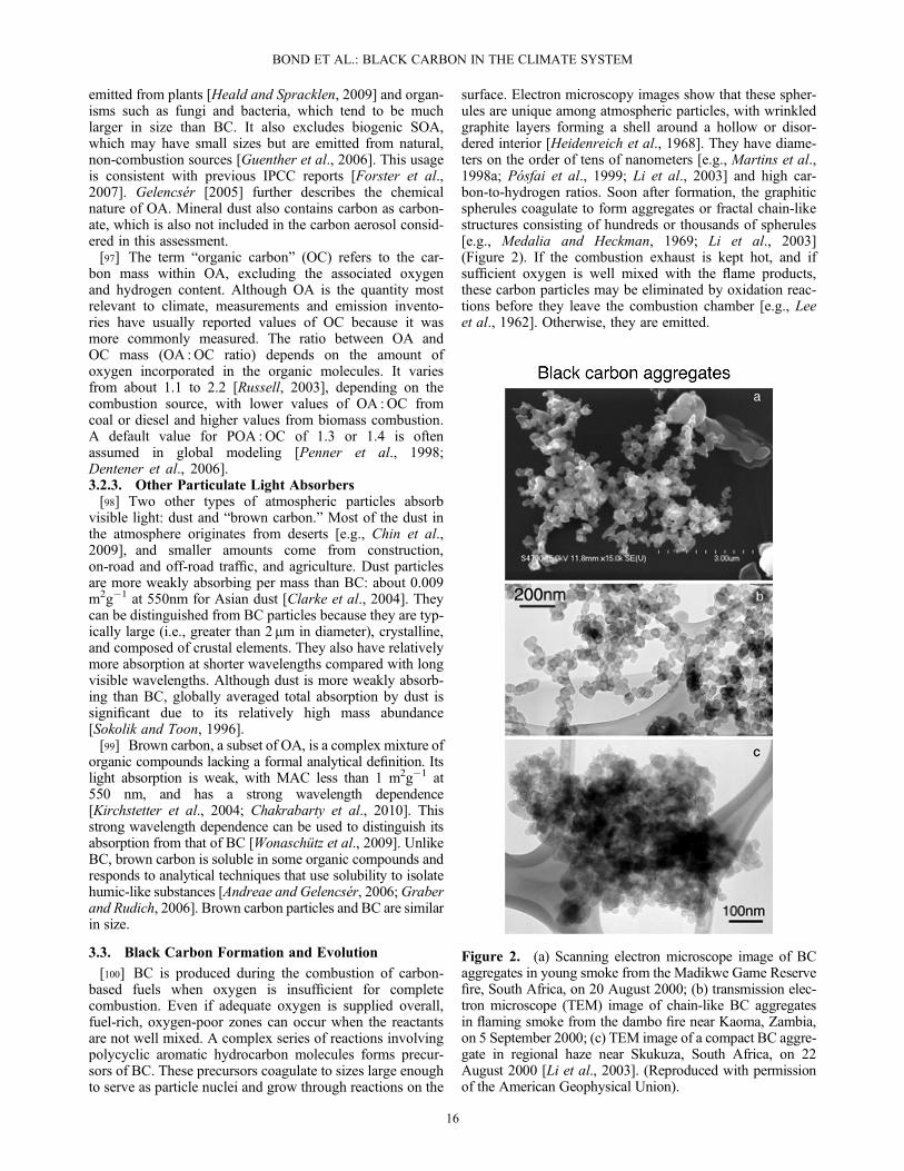
emitted from plants [Heald and Spracklen, 2009] and organ-isms such as fungi and bacteria, which tend to be muchlarger in size than BC. It also excludes biogenic SOA,which may have small sizes but are emitted from natural,non-combustion sources [Guenther et al., 2006]. This usageis consistent with previous IPCC reports [Forster et al.,2007]. Gelencsér [2005] further describes the chemicalnature of OA. Mineral dust also contains carbon as carbon-ate, which is also not included in the carbon aerosol consid-ered in this assessment.[97] The term “organic carbon” (OC) refers to the car-

bon mass within OA, excluding the associated oxygenand hydrogen content. Although OA is the quantity mostrelevant to climate, measurements and emission invento-ries have usually reported values of OC because it wasmore commonly measured. The ratio between OA andOC mass (OA :OC ratio) depends on the amount ofoxygen incorporated in the organic molecules. It variesfrom about 1.1 to 2.2 [Russell, 2003], depending on thecombustion source, with lower values of OA :OC fromcoal or diesel and higher values from biomass combustion.A default value for POA :OC of 1.3 or 1.4 is oftenassumed in global modeling [Penner et al., 1998;Dentener et al., 2006].3.2.3. Other Particulate Light Absorbers[98] Two other types of atmospheric particles absorb

visible light: dust and “brown carbon.” Most of the dust inthe atmosphere originates from deserts [e.g., Chin et al.,2009], and smaller amounts come from construction,on-road and off-road traffic, and agriculture. Dust particlesare more weakly absorbing per mass than BC: about 0.009m2g�1 at 550nm for Asian dust [Clarke et al., 2004]. Theycan be distinguished from BC particles because they are typ-ically large (i.e., greater than 2 mm in diameter), crystalline,and composed of crustal elements. They also have relativelymore absorption at shorter wavelengths compared with longvisible wavelengths. Although dust is more weakly absorb-ing than BC, globally averaged total absorption by dust issignificant due to its relatively high mass abundance[Sokolik and Toon, 1996].[99] Brown carbon, a subset of OA, is a complex mixture of

organic compounds lacking a formal analytical definition. Itslight absorption is weak, with MAC less than 1 m2g�1 at550 nm, and has a strong wavelength dependence[Kirchstetter et al., 2004; Chakrabarty et al., 2010]. Thisstrong wavelength dependence can be used to distinguish itsabsorption from that of BC [Wonaschütz et al., 2009]. UnlikeBC, brown carbon is soluble in some organic compounds andresponds to analytical techniques that use solubility to isolatehumic-like substances [Andreae and Gelencsér, 2006;Graberand Rudich, 2006]. Brown carbon particles and BC are similarin size.

3.3. Black Carbon Formation and Evolution

[100] BC is produced during the combustion of carbon-based fuels when oxygen is insufficient for completecombustion. Even if adequate oxygen is supplied overall,fuel-rich, oxygen-poor zones can occur when the reactantsare not well mixed. A complex series of reactions involvingpolycyclic aromatic hydrocarbon molecules forms precur-sors of BC. These precursors coagulate to sizes large enoughto serve as particle nuclei and grow through reactions on the

surface. Electron microscopy images show that these spher-ules are unique among atmospheric particles, with wrinkledgraphite layers forming a shell around a hollow or disor-dered interior [Heidenreich et al., 1968]. They have diame-ters on the order of tens of nanometers [e.g., Martins et al.,1998a; Pósfai et al., 1999; Li et al., 2003] and high car-bon-to-hydrogen ratios. Soon after formation, the graphiticspherules coagulate to form aggregates or fractal chain-likestructures consisting of hundreds or thousands of spherules[e.g., Medalia and Heckman, 1969; Li et al., 2003](Figure 2). If the combustion exhaust is kept hot, and ifsufficient oxygen is well mixed with the flame products,these carbon particles may be eliminated by oxidation reac-tions before they leave the combustion chamber [e.g., Leeet al., 1962]. Otherwise, they are emitted.

Figure 2. (a) Scanning electron microscope image of BCaggregates in young smoke from the Madikwe Game Reservefire, South Africa, on 20 August 2000; (b) transmission elec-tron microscope (TEM) image of chain-like BC aggregatesin flaming smoke from the dambo fire near Kaoma, Zambia,on 5 September 2000; (c) TEM image of a compact BC aggre-gate in regional haze near Skukuza, South Africa, on 22August 2000 [Li et al., 2003]. (Reproduced with permissionof the American Geophysical Union).


16

[101] The morphology of emitted chain-like aggregateschanges rapidly after emission. Water vapor and other gas-phase species condense upon the aggregates, which collapseinto more densely packed clusters [Huang et al., 1994;Ramachandran and Reist, 1995; Weingartner et al., 1997;Martins et al., 1998b]. Other particulate and gas phase spe-cies present in the surrounding atmosphere also coagulatewith the combustion aerosol. Electron microscopy imagesand measurements of optical properties indicate that freshlyemitted particles often exist as an external mixture in whichorganic and inorganic light-scattering components andstrongly light-absorbing components (BC) reside in differentparticles [Pósfai et al., 2003; Li et al., 2003; Mallet et al.,2004]. After emission, condensation and coagulation causeindividual chemical components to become internally mixed(i.e., different aerosol components existing together within asingle particle). Such particles are no longer pure BC butcontain sulfate and organic material [Lee et al., 2002;Shiraiwa et al., 2007]. We refer to these internally mixedparticles as “BC-containing” particles. Mixing has beenobserved to occur within a few hours after emission at somelocations [Moteki et al., 2007; Moffet and Prather, 2009],but there are insufficient measurements to estimate the

extent of internal mixing throughout the atmosphere. Globalaerosol models that simulate microphysical processes pre-dict that most BC is mixed with other substances within 1to 5 days [Jacobson, 2001a] and this prevalent internalmixing is found at all altitudes [Aquila et al., 2011].[102] The top portion of Figure 3 summarizes particle

properties that are used as input into global and radiativetransfer models and that can be constrained by measure-ments. Each characteristic may affect the representation ofatmospheric processes and resulting modeled concentra-tions, as shown in the lower portion of Figure 3. Pure BCand BC-containing particles are separated in Figure 3 be-cause their microphysical, optical, hygroscopic, and cloud-nucleating properties differ [Abel et al., 2003; Slowik et al.,2004]. For example, as BC ages, it becomes coated or inter-nally mixed with non-BC components and the resulting BC-containing particles become more hydrophilic, which canlead to a reduced lifetime and atmospheric loading [Stier etal., 2006b]. Internal mixing with other compounds can en-hance absorption of solar radiation according to microphys-ical models [Fuller et al., 1999; Jacobson, 2001a; Lack andCappa, 2010] and measurements, primarily laboratory based[Schnaiter et al., 2005; Slowik et al., 2007]. As a result, the

Figure 3. Schematic of the connections between properties of BC and BC-containing particles. A com-bination of these properties determines the contribution of BC and BC-containing particles to climate forc-ing. The properties depend on those of other substances produced in the atmosphere or co-emitted withBC and on atmospheric processes such as nucleation and condensation. Mass and number of BC andBC-containing particles (extensive variables) depend, in part, on particle properties that affect the lifecycleof BC (not represented here).


17

additional material in BC-containing particles must be takeninto account when modeling both radiative transfer and at-mospheric lifetime [Stier et al., 2006a].[103] In the remainder of this section, we discuss the phys-

ical properties that affect estimates of climate forcing, mea-surements of these properties, and representation of theseproperties in global models. We begin with a discussion ofBC mass concentration in section 3.4. Important opticalproperties of BC, including absorption, are discussed insection 3.5, followed by a review of absorption measure-ments in section 3.6. Section 3.7 reviews microphysicalproperties affecting the mass absorption cross section andsingle-scattering albedo, while section 3.8 discusses mea-surements and modeling of these two parameters. Finally,section 3.9 discusses properties of BC and BC-containingparticles that are relevant to nucleating liquid cloud droplets.The discussion of microphysical properties, which alsoaffect the interaction of BC-containing particles with iceclouds, appears in section 7.5.

3.4. Measurement of BC Mass

[104] Ambient air samples of particles that contain BCalways contain other constituents as well. The mass fractionof BC in atmospheric aerosol is typically less than 10%.Thus, BC mass concentration (in g m�3) cannot be measureddirectly by collecting aerosol in an air sample and weighingit. Instead, BC mass must be determined indirectly, usuallythrough optical methods, thermal heating combined withoptical methods, or laser-induced incandescence (Table 3).BC is associated with high sp2-bonded carbon content[Hopkins et al., 2007] and with Raman spectroscopicresponses similar to graphite [Rosen et al., 1979; Dippelet al., 1999], but these analyses do not respond uniquely toall materials identified as BC.[105] The measurement of BC mass concentrations by

some methods can be biased when BC is sampled with otheraerosol components. This mixing can take place eitherwithin ambient aerosol particles before sampling or in thesample itself if BC and other particles are collected and mea-sured simultaneously. Biases occur either because themixing increases absorption or extinction (section 3.6),because BC is incorrectly classified as another material, orbecause another material is incorrectly classified as BC(i.e., lack of specificity). Most techniques measure similarBC mass concentrations when they are applied to pure BCor when other aerosol components are removed by applyingheat [Knox et al., 2009; Kondo et al., 2009] or by solventrinsing [Subramanian et al., 2006]. For that reason, mea-surements of untreated samples are usually in closeragreement for diesel exhaust, which contains little non-BCmaterial, than they are for aged (i.e., internally mixed) aero-sol [Schmid et al., 2001; Chow et al., 2004; Hitzenbergeret al., 2006] or biomass burning aerosol (BB), which has ahigh content of organic matter and other inorganic sub-stances that could cause interferences [Novakov andCorrigan, 1995; Reid et al., 1998]. The major uncertaintyin some measurements of BC mass is associated with isolat-ing BC from the other constituents with which it is internallyor externally mixed. A summary of measurement techniquesfor BC mass is listed in Table 3 along with common termi-nology and any directions and causes of bias. In addition,more explicit names for the measured quantities are

suggested; some of these follow Andreae and Gelencsér[2006]. Details of the measurement of BC mass concentra-tions are given below.[106] The most common separation between BC and OC is

accomplished by volatilizing and combusting materialcollected on a filter and by detecting the CO2 produced asa function of temperature. The discrimination between thesetwo classes of aerosol is based on the idea that BC is non-volatile or refractory, whereas OC is volatile. This thermalmethod does not detect BC directly, and the amount ofrefractory material detected depends on the details ofthe method. The analytical result is therefore an opera-tional definition and is traditionally called elementalcarbon (EC).[107] In thermal methods based on volatility, the sample

filter is first heated in inert gas to volatilize OC and thenheated again with oxygen to combust the EC; cooling some-times occurs before the second heating [e.g., Chow et al.,1993; Birch and Cary, 1996;Watson et al., 2005]. This tech-nique measures all OC, not just combustion-derived primaryaerosol. Inaccuracies in this method result from interpretingOC as EC, or vice versa, when properties of the samplecause EC to be released too early or OC to be held too long.One complication is “charring” of OC (i.e., conversion ofOC to EC) at high temperatures, which reduces its volatility.Variations of thermal methods include different temperatureramping programs and correcting for the charring of OCduring pyrolysis by monitoring the optical reflectance ofthe sample filter [Huntzicker et al., 1982] or light transmis-sion [Turpin et al., 1990]. Comparisons among protocolswith differing temperature and optical corrections show thatderived EC concentrations can differ by over an order ofmagnitude [Schmid et al., 2001] and that large differencescan be caused by the lack of correction for charring, whichleads to considerable overestimates of EC. There are alsosignificant differences between methods that correct forcharring using optical reflectance or light transmission[Chow et al., 2001; Chow et al., 2004]. The two correctionsyield comparable EC concentrations if the filter contains ashallow surface deposit of EC. If EC and OC are distributedthroughout the filter, the two corrections yield different ECvalues, and the variability also depends on the temperatureprotocol used. Hence, the difference between the twomethods depends, in part, on the OC/EC ratio in the sample.As a result, the correction schemes yield similar resultsfor diesel exhaust, which is dominated by EC, but candiffer widely for complex atmospheric mixtures. Optimiza-tion of temperature programs seeks to minimize charringand release EC and OC during the expected period of theanalysis [Conny et al., 2003; Cavalli et al., 2010]. The accu-racy of thermal measurements can also be increased byextracting OC with organic solvents before analysis, sinceBC is insoluble [Fung, 1990; Subramanian et al., 2006].[108] Detection of refractory BC (rBC) mass by laser-

induced incandescence (i.e., visible thermal radiation) hasbecome increasingly widespread [Schwarz et al., 2006,2008a; Moteki and Kondo, 2010]. The Single Particle SootPhotometer (SP2) is able to provide continuous, real-time,size and coating information for individual particlescontaining rBC over a wide dynamic range of mass concen-tration. In the SP2, the rBC component of individual parti-cles is heated to vaporization temperatures (i.e., about


18

Tab

le3.

TechniquesforMeasuring

BCMass,Method-DefinedTerminologyforBC,andSources

ofSystematic

Biases

Technique

Com

mon

Nam

eSuggested

Nam

eCom

mon

Instruments

Sources

ofBias

Directio

nof

Biasa

Optical

absorptio

nwith

insitu

detection

BC

EquivalentBC(BC+other

absorbingmaterial)

Photoacoustic

Changein

MACwith

aerosolagingb

+,�

Presenceof

otherabsorbers(dust,organic

carbon)c

+

Optical

absorptio

nby

collectionon

filters

BC

EquivalentBC

Aethalometer;Particle

SootAbsorption

Photometer

(PSAP);

Sam

eas

optical

absorptio

nabove,plus:

Optical

interactions

betweenparticles

andfiltermatrixd

+

Multi-angleAbsorptionPhotometer

(MAAP)

Modificatio

nof

particle

morphology

byorganiccarbon

+

Optical

absorptio

nwith

heated

inlet

BC

EquivalentBC

Contin

uous

SootMonito

ring

System

(COSMOS)

Charringof

low

volatility

organicspecies

+

Therm

alheatingandoptical

absorptio

nElementalcarbon

(EC)

Apparentelem

entalcarbon

(ECa)

Therm

alOptical

Reflectance(TOR);

Therm

alOptical

Transmittance

(TOT)

Failure

toaccurately

correctforcharred

organiccarbon;

+

Catalytic

oxidationof

BCin

presence

ofmetalsor

metal

oxides;

�

Absorptionby

charredmaterialaffects

split

betweenOCandECe

�

Detectio

nof

less

volatileorganiccarbon

+

Laser-induced

incandescence

BCor

RefractoryBC(rBC)

RefractoryBC(rBC)

SingleParticle

SootPhotometer

(SP2)

Lackof

detectionof

smallparticlesf

�a (+)=

BCmeasuredtoohigh;(�

)=BCmeasuredtoolow.

bIfcalib

ratedwith

fresh,

unmixed

BC,measurementoverestim

ates

BCmassaftermixingwith

non-absorbingspeciesandincrease

inabsorptio

n.c D

epends

onwavelength;

measurementsaround

630nm

oftenareunaffected

unless

dustconcentrations

arehigh.

dPositive

bias

ifuncorrectedfilter-basedmeasurementsareused;otherw

ise,itcanbe

either

positiv

eor

negativ

e.e M

oreextrem

efortransm

ission-based

monito

ring

ofcharring.

f Particleswith

massbelow

about0.5fg,correspondingto

asphericalparticle

ofabout80

nmdiam

eter.


19

4000K) with an infrared intra-cavity laser, and incandes-cence proportional to rBC mass is detected. Essentially allrBC particles between 80 and 700 nm mass-equivalentdiameter are measured, assuming void-free rBC has a den-sity of 2 g cm�3. The response of the SP2 to rBC massand the lack of interference in measuring rBC mass whennon-rBC aerosol components are present have been evalu-ated in the laboratory [Schwarz et al., 2006; Slowik et al.,2007; Moteki and Kondo, 2007]. The dominant uncertaintyin the measured mass lies in calibrating its sensitivity to am-bient rBC material. The range of this sensitivity is around15% [Moteki and Kondo, 2010; Laborde et al., 2012]. How-ever, the limitations of the size range detected by the SP2may introduce additional uncertainty, depending on the airmass. Typically, in remote regions, the size range capturedby the SP2 contains most of the rBC mass and about 50%of the rBC number [Schwarz et al., 2008b; Shiraiwa et al.,2008]. In urban environments, a correction to total measuredmass concentration of about 25% may be required. Pulsedlaser-induced incandescence has also been used for environ-mental rBC measurements [Chan et al., 2011].

3.5. Optical Properties of Black Carbon

[109] Models of radiative transfer require the amountof particulate absorption and scattering in the atmosphere,known as the absorption and scattering coefficients(m2 m�3 or simply m�1). Atmospheric models convertmodeled mass concentrations to these optical coefficientsusing intensive properties (i.e., optical cross section permass in m2g�1) known as the mass absorption cross sec-tion (MAC) and mass scattering cross section (MSC).Estimates of these values are needed at all wavelengths,and the directional distribution of scattering (dimension-less) is also needed for radiative transfer models.[110] From atmospheric measurements, MAC can be

calculated in reverse: the light-absorption coefficientdivided by mass concentration. Throughout this assessment,we often refer to MAC that is determined for BC alone(MACBC). MACBC is calculated by dividing the absorptioncoefficient attributable to BC by the BC mass concentration.The simple term MAC indicates the value determined by di-viding by the total mass concentration of BC-containing par-ticles, which is smaller than MACBC. All other properties areusually measured for BC-containing particles, not for pureBC. Optical properties depend on refractive index, density,size distribution, mixing state, and particle shape. The propen-sity for water uptake affects the MSC and MAC of BC-containing particles, as well as their ability to form clouddroplets and their atmospheric lifetime due to removal by pre-cipitation. For sub-saturated conditions (i.e., relative humiditybelow 100%), this water uptake is characterized in terms ofhygroscopicity or growth factor. When air is supersaturated,the climate-relevant quantity is the fraction of particles thatact as CCN [Hallett et al., 1989].[111] The MAC was mentioned earlier as a

distinguishing feature of BC. Values of MAC and MSCare fundamental inputs to radiative transfer models,required for all aerosols or aerosol components. Thesequantities are necessary to translate mass concentrationssimulated by chemical transport models to their effectson radiative transfer. The wavelength dependence ofMAC must also be represented in models for the full

solar spectrum. As its name implies, BC strongly absorbslight at all visible wavelengths. In contrast, other atmo-spheric aerosols that absorb light (OA, soil, and dust)are more yellow, brown, or red, meaning they absorbmore blue light than red light. The quantity generallyused to characterize the spectral dependence of lightabsorption is the absorption Ångstrom exponent:

Åabs ¼ �log MAC l1ð Þ=MAC l2ð Þð Þ=log l1=l2ð Þ (3.1)

where MAC(l1) and MAC(l2) are the mass absorption crosssections at wavelengths l1 and l2, respectively. Two wave-lengths spanning the visible range are commonly used, suchas 450 and 650 nm. Alternatively, Åabs can be calculatedfrom absorption coefficients at the two wavelengths. Thevalue of Åabs for particles is usually greater than that of thebulk material. If the refractive index of the bulk materialhas no wavelength dependence, as does graphite [Borghesiand Guizzetti, 1991], then Åabs=1 for particles much smallerthan the wavelength of light [Rosen et al., 1979;Moosmülleret al., 2011].[112] Measurement studies have confirmed the value of

Åabs = 1 in regions where externally mixed BC dominatesabsorption [Rosen et al., 1978; Bergstrom et al., 2002,2007; Kirchstetter et al., 2004; Clarke et al., 2007]. WhenBC becomes coated, Åabs can theoretically be as low as 0.8or as high as 1.9 [Lack and Cappa, 2010]. In contrast, Åabs

for OA has been observed to be between 3.5 to 7[e.g., Kirchstetter et al., 2004; Sun et al., 2007; Lewiset al., 2008; Yang et al., 2009]. Åabs for dust is typicallyabout 2 to 3 but can be higher for very red (iron-rich) dust[e.g., Fialho et al., 2006; Alfaro et al., 2004; Bergstromet al., 2007]. This difference in the wavelength dependenceof absorption of BC versus other absorbing aerosol has beenused to approximate relative fractions of BC versus otherlight-absorbing constituents.[113] The single-scattering albedo, o0, is scattering di-

vided by extinction (i.e., the sum of scattering and absorp-tion) or

o0 ¼ MSC= MSCþMACð Þ (3.2)

[114] Values of o0 near 1 indicate that the aerosol ismainly scattering. Values below about 0.8 indicate that theparticles could have a net warming effect [Haywood andShine, 1995]. The value that divides warming from coolingalso depends on the albedo of the underlying surface orclouds and the fraction of light that is scattered upward bythe particles [Chylek and Wong, 1995]. When the additionof aerosol causes a local increase in the planetary albedo,more shortwave radiative energy is reflected back to space,and aerosol exerts a negative forcing. In contrast, when aero-sols locally decrease the planetary albedo, the forcing is pos-itive. MAC and o0 are the aerosol properties most relevantto the balance between negative and positive forcing, sowe emphasize these two parameters in this section insteadof MSC. Forcing is not very sensitive to o0 for stronglyabsorbing aerosol with values below 0.4.

3.6. Measurement of Absorption Coefficients

[115] Comprehensive reviews of absorption measurementshave been provided by Horvath [1993] and by Moosmüller


20

et al. [2009]. Here we summarize only the major challengesin these measurements. The most widely used technique tomeasure the absorption coefficient involves collecting aero-sol on a filter and inferring atmospheric absorption fromthe resulting change in transmission of light through thefilter [Gundel et al., 1984], often at one mid-visible wave-length but sometimes at multiple wavelengths. Commoninstruments using this approach are the Particle SootAbsorption Photometer (PSAP) [Bond et al., 1999; Virkkulaet al., 2005], which has been used to obtain a worldwidedata base through the Global Atmospheric Watch program;the Hybrid Integrating Plate System (HIPS), which hasbeen used to collect data by the Interagency Monitoringof Protected Visual Environments (IMPROVE) in U.S.National Parks [Malm et al., 1994]; and the Aethalometer[Hansen et al., 1982]. Other filter-based absorption instru-ments include the Integrating Plate [Lin et al., 1973] andthe Multi-Angle Absorption Photometer (MAAP) [Petzoldet al., 2005b]. These filter-based methods overestimateabsorption if light transmission is also affected by particu-late light scattering [Horvath, 1997; Bond et al., 1999].With the application of empirical corrections to overcomethis artifact, accuracies of the PSAP, IP, HIPS, andAethalometer range between 20 and 30% [Bond et al.,1999; Weingartner et al., 2003, Virkkula et al., 2005],and accuracy of the MAAP is about 12% [Petzold et al.,2005b]. However, these correction schemes are based onlaboratory-generated aerosols that may limit their applica-tion and accuracy for the measurement of atmosphericaerosols. In addition, coating of BC with volatile com-pounds can greatly contribute to variation in filter-basedmeasurements of light absorption [Lack et al., 2008; Cappaet al., 2008; Kondo et al., 2009]. For example, PSAPabsorption coefficients can be biased high (50 to 80%)when the ratio of organic aerosol to BC is high (15 to20). Lack et al. [2008] postulated that this high bias wasdue to the redistribution of liquid-like OC that affectedeither light scattering or absorption. This difficulty can beovercome by removing most of the mass of volatile aerosolcomponents before the BC particles are collected on filters.This removal can be accomplished without significantcharring of organic compounds with a heated samplinginlet. This technique is used for the Continuous SootMonitoring System (COSMOS) instrument [Kondo et al.,2011b]. Under those conditions, comparisons of ambientBC mass concentrations measured by light absorption(COSMOS), thermal-optical measurements, and laser-induced incandescence (i.e., SP2) measurements have beenfound to agree within 10% [Kondo et al., 2011b].[116] Filter-based optical measurements of absorption are

sometimes used to derive “effective” BC mass concentra-tions by using an assumed MACBC to convert measuredabsorption to BC mass [e.g., Sharma et al., 2002]. Giventhe artifacts and uncertainties associated with filter-basedmeasurements and the choice of MACBC, the resulting BCmass concentrations also can be highly uncertain.[117] Techniques that do not use filters are also available for

the measurement of absorption by BC. In the photoacousticspectrometer (PAS) [Petzold and Niessner, 1996; Arnottet al., 1997; Lack et al., 2006], particles are drawn into anacoustic cavity and irradiated by power-modulated laser light.The heat that is produced when the particles absorb laser light

is transferred to the surrounding gas creating an increase inpressure. Sensitive microphones are used to detect the stand-ing acoustic wave that results from the pressure change, andthis signal is interpreted to infer the absorption coefficient.Gas phase absorbers can interfere with BC detection inPAS systems. The overall uncertainty of the PAS with respectto aerosol absorption has been reported at about 5%[Lack et al., 2006].[118] Absorption techniques, whether filter based or non-

filter based, are not specific for BC. Any light-absorbingaerosol other than BC that absorbs at the measurementwavelength is detected. The degree to which other lightabsorbing species interfere with the measurement of BCabsorption depends on the relative abundance of lightabsorbing species and the size range and wavelength of themeasurement. Measurement of the chemical compositionof the aerosol and measurement of absorption at severalwavelengths can help determine the interference from allatmospheric species. BC-containing aerosol generally fallinto the submicron size range, so measurements of thesubmicron aerosol only can also reduce the interference ofdust absorption.

3.7. Microphysical Properties Affecting MAC and v0

3.7.1. Optical Models and Required Inputs[119] Values of MAC and o0 can be predicted with

several theories that describe how the particles interactwith light. Particle density and refractive index of the bulkmaterial are required to calculate MAC for all models.The assumed particle shape and size affect the modelchosen. Common optical-modeling treatments that accountfor the fractal nature of fresh BC particles include theRayleigh-Debye-Gans approximation [Nelson, 1989;Dobbinsand Megaridis, 1991], superposition T-matrix theory[Mishchenko et al., 2004], and discrete-dipole approximation[Draine and Flatau, 1994]. Sorenson et al. [2001] reviewsmany of the key optical relationships for aggregates. Thesemodels are useful for exploring how particle properties affectparticle optics [e.g., Liu and Mishchenko, 2005].[120] Global-model calculations of radiative transfer usu-

ally do not account for complex particle shapes. Instead,they use Mie theory, which can describe homogeneousor core-shell spherical particles. Although BC particles,especially freshly emitted ones, are not spherical, modelingradiative transfer accurately requires only that MAC, o0,and angular scattering are correct.[121] BC non-sphericity creates difficulties in inferring

other properties used in optical modeling from measure-ments. Air drag is different between spherical and non-spherical particles and affects inferences of particle sizebased on mobility [Lall and Friedlander, 2006]. The SP2measurement detects BC mass and provides equivalentspherical diameters. Inferences of refractive index are oftentaken from optical measurements with the assumption ofspherical particles or from particles that are collected andcompacted into a pellet. In either case, the material is notpure BC but contains an unknown fraction of voids. Ideally,the refractive index, density, and size used for modelingwould be obtained for the pure material, but observedproperties may be obtained for material with unknownand inconsistent void fractions. Despite these


21

uncertainties, measurements of material properties and sizesare described below.3.7.2. Density[122] Fuller et al. [1999] compiled reported densities for

several types of graphitic material and found values rangingfrom 0.625 to 2.25 g cm�3. Based on the type of BC emittedfrom diesel combustion, they adopted the highest density,which was measured for paracrystalline graphite, as repre-sentative of strongly absorbing atmospheric BC. BC is notperfectly crystalline, so its microstructure, density, andrefractive index differ from those of graphite. The density ofpure graphite is 1.9 to 2.1 g cm�3 [Hess and Herd, 1993].Densities for pressed pellets of BC with corrections for airvolume fractions in the surface layer are slightly lower at1.8 to 1.9 g cm�3 [Medalia and Richards, 1972; Janzen,1980]. Park et al. [2004] reported a density of 1.8 g cm�3, andKondo et al. [2011b] found 1.718� 0.004 g cm�3 for fullerenesoot. Some global models still use the density of 1 g cm�3

recommended by OPAC (Optical Properties of Aerosols andClouds), which would result in an overestimate of absorption ifall other factors are correct.3.7.3. Refractive Index[123] The refractive index of a material is critical in deter-

mining the scattering and absorption of light, with the imag-inary part of the refractive index having the greatest effect onabsorption. Refractive index values are derived by assuminga theory for the interaction of BC with light (i.e., reflectanceor absorption) and adjusting optical parameters (includingrefractive index) until predictions match measurements.Three possible methods include (1) fitting Fresnel’s formulato reflectance and transmittance data measured for a com-pressed pellet, (2) fitting Mie theory to light-scattering datafor individual spherical particles, and (3) fitting either Mietheory or an approximation formula to scattering and extinc-tion data for particle ensembles. Method 1 has been usedwidely to estimate refractive indices of solid aerosols likecombustion-generated BC [Mullins and Williams, 1987].However, direct evidence of the optical flatness of pellet sur-faces, which is necessary for application of Fresnel’s for-mula, has never been shown for wavelengths shorter thanthe infrared region [Janzen, 1979]. Method 2, which is lim-ited to spherical particles, uses measurements of resonancestructures in Mie scattering to determine the refractive index[Chylek et al., 1983a], but its application to strongly absorb-ing particles is limited. In method 3, the refractive index anda size distribution function are inferred simultaneously fromextinction or scattering data for an ensemble of particles.Solving this inversion problem requires a theory to connectmicrophysical and light-scattering properties; Mie theoryhas been used for spherical particles [Lack et al., 2009]and the Rayleigh-Gans approximation for non-sphericalparticles [Charalampopoulos et al., 1989; Van-Hulle et al.,2002]. For polydisperse or non-spherical particles, theinversion results may have large errors if the assumed sizedistributions or shapes differ from those of the actual parti-cles. Moteki et al. [2010] developed a method to estimaterefractive indices that accounted for non-spherical particlesby measuring the relationship between the scattering crosssection and the particle volume.[124] A variety of values for the refractive index of BC has

been used in global climate models including the OPACvalue of 1.74� 0.44i [Hess et al., 1998]. As reviewed by

Bond and Bergstrom [2006], reported values of the refrac-tive index of light absorbing carbon vary widely; the realpart, n, appears to vary from that of water to that of diamond,and the imaginary part, k, varies from that of negligibly ab-sorbing material to that of graphite. Bond and Bergstrom[2006] hypothesize that strongly absorbing carbon with asingle refractive index exists and that some of the variationin reported values results from void fractions in the material.Based on agreement between measured real and imaginaryparts of the refractive index of light absorbing carbon, Bondand Bergstrom [2006] recommended a value of 1.95� 0.79iat 550 nm. They caution, however, that this value may notrepresent void-free carbon. Stier et al. [2007] found that thisvalue led to better agreement with observed atmosphericabsorption, compared with the OPAC value. Moteki et al.[2010] found that the refractive index of ambient BC in theTokyo urban area was about 2.26� 1.26i at 1064 nm. TheOPAC assumption for imaginary refractive index is nottaken from combustion-generated particles, is lower thaneither of the latter two recommendations, and would leadto a MAC prediction about 30% lower if all other factorswere equal.[125] Radiative inversion methods can also infer values of

refractive indices from remote-sensing measurements[Dubovik and King, 2000], but only for the entire mixed aero-sol, which includes water and many other constituents otherthan BC. Currently, such data are available from about 500globally distributed Aerosol Robotic Network (AERONET)surface sites [Holben et al., 1998].3.7.4. Particle Size[126] Size distributions of the BC component in ambient

aerosol are affected by the size of BC at emission and bysubsequent coagulation. Condensation of non-BC materialchanges the overall aerosol size distribution, but the underly-ing size distribution of BC does not change except throughcoagulation. BC size can be diagnosed separately. The firstmeasurements of ambient BC size distributions relied onimpactors, which identify the size at which greatest massappears [Mallet et al., 2003; Riddle et al., 2008]. SP2 mea-surements have provided BC number distributions in freshurban plumes dominated by fossil fuel (FF) combustion[e.g., Kondo et al., 2011c; Schwarz et al., 2008b], in agedplumes in Asian outflow [Shiraiwa et al., 2008], and in theremote upper troposphere and lower stratosphere [Schwarzet al., 2006; 2008b]. In the urban areas of Tokyo andNagoya (Japan) and Seoul (Korea), the mass median diame-ter (MMD) and count median diameter (CMD) of fresh BCranged from 120 to 160 nm and 50 to 80 nm, respectively.In plumes associated with wildfires, the MMD was mea-sured to be about 200 nm and the CMD to be 120 nm[Kondo et al., 2011a]. The distinct difference in the sizebetween BC particles from fossil fuel combustion and bio-mass burning seems to be a general feature (Figure 4). TheCMD and MMD of BC observed in the Asian outflow weresignificantly higher than those in fresh urban plumes[Shiraiwa et al., 2008], suggesting the growth of BC sizeby coagulation during transport after emissions. BC particlesare largely found in the Aitken mode (i.e., less than 100 nmdiameter) and the accumulation mode because of theirformation mechanism. Large concentrations of BC in theAitken mode can result from high combustion temperaturesand efficient fuel burn. For example, BC particles produced


22

by aircraft jet engines have mean number diameters of about30 nm [Petzold et al., 2005a].3.7.5. Configuration of BC-Containing Particles[127] Internal mixing between BC and other compounds

increases absorption of visible light, in part because thenon-absorbing material can refract light toward theabsorbing particle [Ackerman and Toon, 1981]. BecauseBC is insoluble, it is always distinctly separated fromthe other material in an internally mixed particle. It isoften assumed that non-BC material surrounds the BCcompletely and approximately symmetrically, known asa “core-shell” configuration. However, BC may also existnear the surface of the particle [Sedlacek et al., 2012].The presence, relative quantities, and location of non-absorbing material in BC-containing particles require a

complex characterization commonly summarized in thesingle term “mixing state.”

3.8. Measured and Modeled MAC and v0

[128] As discussed above, optical models can either repre-sent aggregates or rely upon Mie theory with the assumptionof spherical particles. Here we review measured values ofMACBC and o0, and discuss whether models can simulatethese values.3.8.1. MACBC Derived From Measurements[129] Empirical values of MACBC have been obtained from

measurements of light absorption by filter or photoacousticmethods, divided by measurements of EC mass from thermalevolution methods [e.g., Martins et al., 1998a; Moosmülleret al., 2001]. Measured values for freshly generated BC, wherecare has been taken to eliminate non-BC material, fall within arelatively narrow range of 7.5 � 1.2 m2g�1 [Clarke et al.,2004; Bond and Bergstrom, 2006]. The MACBC may bereduced as the particles collapse intomore compact forms withhigher fractal dimensions [Schnaiter et al., 2003; Lewis et al.,2009]. Instrumental artifacts, as shown in Table 3, can hamperaccurate inferences of MACBC.[130] Laboratory measurements show that absorption

increase is low for very thin coatings [Slowik et al., 2007]and reaches a factor of 1.8 to 2 for thicker coatings[Schnaiter et al., 2005; Khalizov et al. 2009; Shiraiwaet al., 2010; Cross et al., 2010; Bueno et al., 2011]. Filter-based and photoacoustic measurements report differentdegrees of enhancement in the measured absorption [Slowiket al., 2007; Knox et al., 2009].[131] Values of MACBC enhancement are harder to con-

firm for atmospheric aerosol and require measuring MACBC

before and after removal of coatings. Knox et al. [2009]found enhancement by a factor of 1.2 to 1.6 near sourceregions. Lack et al. [2012] observed a factor of 1.4 enhance-ment for BC in biomass burning plumes. In contrast, similarmeasurements of absorption enhancement using a PAS inlarge urban centers revealed an average absorption enhance-ment of only 6%, although the MACBC of aged aerosol was20 to 40% higher than that of freshly generated BC [Cappaet al., 2012]. Cappa et al. hypothesize that the low values ofenhancement are caused by BC inclusions at the edge ofthe sampled particles. Measurements made downwind(up to hundreds of kilometers) of BC source regions alsogive a wide range of enhancements. Chan et al. [2011]found MACBC values ranging from 10 to 50 m2g�1, show-ing a rough relationship with the ratio between non-BCand BC components. This study, which derived time-resolved MACBC from a photoacoustic spectrometer andlaser-induced incandescence instrument system, appearedto contradict earlier work by the same group [Chan et al.,2010] that found no apparent increase in MACBC using aPSAP to measure absorption and thermal-optical techniqueto measure EC. MACBC values inferred from filter-basedtechniques are more plentiful but may suffer from artifacts;Cheng et al. [2011] summarized MACBC from severalstudies ranging from 2 to 17 m2g�1 but used empiricalcorrection factors to adjust some of the methods prior tocalculating MACBC. A series of intensive experiments withidentical sampling and analysis protocols gave MACBC

values ranging from 6 to 20 m2g�1 [Quinn and Bates, 2005].

Figure 4. Mass and number size distributions of BC parti-cles observed in three fresh urban (red) and two freshbiomass burning (black) plumes as identified in the legend.The measurements are made on board an aircraft using anin situ, single-particle detection instrument (SP2). Thevariable coatings on the BC particles is not shown. Theobserved (a) mass and (b) number amounts are plotted as sym-bols versus volume equivalent diameter based on assuming aspherical particle shape. The mass distributions are normalizedto the same peak value. The observations are fit by a lognormalfunction between 90 and 600 nm (solid lines). The numberdistribution fits are those consistent with the fit to the respec-tive mass distribution and are scaled to represent the sameBC mass. From Schwarz et al. [2008b].


23

[132] Most of the above measurements of MACBC aftermixing with non-BC material were made under dry condi-tions or at relatively low humidity. However, water is alsoa component of mixed aerosols, both in clear air at highrelative humidity and in clouds. Particles that have takenup water become even larger than mixed, dry atmosphericparticles, but measurements at such elevated humiditiesare difficult. Mikhailov et al. [2006] measured a threefoldincrease in absorption of BC at 100% relative humidity.Brem et al. [2012] also found an amplification factor ofup to 2.7 for an absorbing organic material at 95% rela-tive humidity.3.8.2. Microphysical Model Ability to Simulate MAC3.8.2.1. MACBC of Unmixed BC[133] Particle size distribution has almost no influence on

calculated MAC when particle diameter is below about 80nm [Bergstrom, 1973]. The simplest theory that accounts foraggregate particles indicates that MAC depends only on thesize of the component spherules. Therefore, modeled MACBC

should not be very sensitive to particle size if either small,spherical particles are assumed or if modeled aggregates arecomposed of spherules below 80 nm. However, measuredMACBC values, at 7.5 � 1.2 m2g�1, are about 30% higherthan values calculated with either method, using best estimatesof refractive indices and density. This comparison remainsunchanged even with the higher refractive index values foundby Moteki et al. [2010]. Bond and Bergstrom [2006] suggestthat the 30% higher absorption of actual particles could becaused by interactions between neighboring BC spherules[Iskander et al., 1991; Fuller, 1995]. Liu and Mishchenko[2005] calculated a 15 to 25% increase for many changes inaggregate parameters, compared with no interaction but upto 20% decrease for spherule sizes larger than 30 nm. Kahnert[2010] showed that spherule interaction alone could notaccount for the discrepancy of 30%, and MAC modeled byAdachi et al. [2010] was similar for aggregates and spheres.The inability of microphysical models to reproduce measuredMAC from best estimates of refractive index and densityremains unresolved.[134] Although MACBC is sensitive to the large differ-

ences in both refractive index and density used by differentmodels, Bond and Bergstrom [2006] note some compensat-ing errors. For models using OPAC refractive index anddensity, the low refractive imaginary index would underesti-mate MACBC, while the low assumed density (1 g cm�3)would overestimate it. Therefore, the MACBC simulatedwith the OPAC refractive index and density is comparableto MAC using the values of refractive index and densityrecommended by Bond and Bergstrom [2006], althoughthe model inputs are quite different. However, it may notbe possible to simulate MAC and o0 of mixed particlesusing these erroneous values.3.8.2.2. MAC of BC Mixed With Other Substances[135] Internal mixtures of BC and non-absorbing material,

including water, are usually modeled either as a core-shellconfiguration or as a homogeneous particle for which theeffective refractive index is obtained using “mixing rules.”Some frequently used mixing rules are volume mixing, inwhich refractive indices are proportional to substancevolume; Bruggeman or Maxwell-Garnet effective mediumapproximations [Heller, 1965]; or the dynamic effectivemedium approximation [Chylek et al., 1996].

[136] Different representations of mixing often producecomparable estimates of absorption. For example, usingthe Bond and Bergstrom [2006] refractive index and den-sity, Adachi et al. [2010] calculated MACBC for uncoatedspheres as 6.4 m2g�1, with increases for volume mixing(13.6 m2g�1), core shell (13.3 m2g�1), Maxwell-Garneteffective medium approximation (12.0 m2g�1), and realisticcoated BC particles (9.9 m2g�1) at 550 nm wavelength.The assumption of a perfectly concentric core within a shellgives the highest absorption among core-shell particles[Fuller, 1995]. However, Jacobson [2006] showed thatthe dynamic effective medium approximation suggestedfor cloud droplets produced a much higher MACBC than acore-shell treatment. The absorption efficiency of BC mayalso be higher when it is coated by water, such as in clouddroplets (section 7.3.3).[137] The optics of mixed particles vary widely in space

and time because they depend on the relative concentrationsof BC and non-BC components, which may include water,liquid, and solid components. A single value of MAC foran internally mixed aerosol is not appropriate due to thewidely varying amounts of non-absorbing material sur-rounding BC cores. Moffet and Prather [2009] estimate thatthe increase above unmixed aerosol could be 80 to 200% forindividual particles. This increase depends upon the relativesizes of the shell and the core, and the location of the corewithin the particle [Fuller, 1995]. Bond et al. [2006] suggesta smaller enhancement, concluding that MACBC is 80%higher for mixed than for unmixed spheres. However,because the absorption of aggregate BC appears to be 30%higher than that of spheres, the increase between uncoated,aggregate BC to coated, mixed spherical particles might beonly 50%. The MACBC of 7.5 m2g�1 for freshly emittedBC, plus an enhancement of 50%, agrees approximatelywith observed MACBC at dry conditions. A more preciseevaluation of the agreement between models and observa-tions is hampered by artifacts in the measurements.3.8.3. Measured and Modeled Single-Scattering Albedo[138] Single-scattering albedo of freshly generated BC has

been measured as 0.10 to 0.28, as summarized by Bond andBergstrom [2006]. Khalizov et al. [2009] and Cross et al.[2010] report similar values of o0 for fresh BC. Models ofaggregate, pure-BC particles predict o0 of 0.1 to 0.3 [Liu andMishchenko, 2005]. This value depends strongly on compo-nent spherule size but not on overall particle size [Sorensen,2001]. Scattering and o0 for spherical BC depend greatly onthe size distribution chosen. For example, o0 for particles of50 and 250 nm diameter is 0.02 and 0.44, respectively, for arefractive index of 1.95� 0.79i. Forcing by BC scattering issmall compared to that by BC absorption, so small variationsin o0 produce only small changes in total forcing.[139] As BC becomes mixed with other components, a

large increase in scattering and, hence, in o0 occurs[Khalizov et al., 2009; Cross et al., 2010]. For mixed parti-cles, values of o0 range from that of fresh particles to 0.9,depending upon the amount of added material. For these par-ticles, forcing can be quite sensitive to o0. However, muchof the added scattering and the tendency toward negativeforcing are attributable to other chemical components, notto BC. Therefore, the forcing by BC alone should be esti-mated with the difference of two radiative-transfer scenarios,not just the change in o0.


24

3.8.4. Aerosol Properties in Global Models[140] In global simulations of radiative transfer, BC parti-

cles are assumed to be either externally or internally mixedwith other aerosol components. For external mixing, thematerial properties of pure BC are used. If internal mixingis assumed, the non-BC material is either treated as a spher-ical shell around a BC core, or the refractive index anddensity of BC and non-BC material are averaged and ahomogeneous particle is modeled. Koch et al. [2009b] sum-marize predicted MACBC and treatments of aging, removal,and optical properties for many global models.[141] All global models consider how aging affects removal

rates of BC. Early models of atmospheric BC expressed theaging of BC by prescribing a timescale for converting hydro-phobic BC to hydrophilic BC, typically about 1 day [Kochet al., 2009b]. Many models have evolved to express agingexplicitly in terms of coagulation with sulfate particles andcondensation of sulfuric acid and secondary organic vaporon BC. Some models represent BC-containing aerosol withdiscrete size-resolved bins [Jacobson, 2001a]. Others, knownas “multi-modal” models, represent different aerosol classes,such as unmixed BC and BC coagulated with other material[Whitby and McMurry, 1997]. Representations of removalrates vary from constant empirical values, to parameterizationbased on composition and particle number [Abdul-Razzak andGhan, 2000], to explicit dependence on aerosol and clouddroplet size and composition [Jacobson, 2002].[142] Although global models of BC consider mixing when

determining removal rates, some do not incorporate enhancedMACBC due to mixing. Values of MACBC used in globalmodels range from 2.3 to 18 m2g�1 [Koch et al., 2009b;Jacobson, 2012]. The diversity in MACBC arises eitherfrom whether the mixing state is assumed or calculated, fromwhether it is determined at ambient RH or constant RH, or fromother choices of aerosol properties. Many of the values aresimilar to or lower than the value for unmixed BC and are,therefore, lower than the average value of BC in the atmosphere.

3.9. CCN Activity of Black Carbon

3.9.1. Measurements of CCN Activity[143] Particle size, hygroscopicity, and mixing state also

affect the interaction of particles and clouds [Pruppacherand Klett, 1997; McFiggans et al., 2006]. While BC-inducedcloud changes are mainly discussed in section 7, wereview the processes of CCN activation here becausethey are closely related to the microphysical properties ofBC-containing aerosol.[144] Aerosol particles serve as nucleation sites for

forming cloud droplets through a process known as activa-tion. The ability of an aerosol particle to act as a cloud con-densation nucleus depends on its size, composition, andmixing state, and the supersaturation with respect to watervapor within the cloud. The critical supersaturation for agiven particle is the lowest supersaturation at which that par-ticle activates and produces a cloud droplet. Any particle canactivate in extremely supersaturated air. Particles that acti-vate more easily (i.e., that have a lower critical supersatura-tion) have a greater chance of affecting cloud droplet num-ber concentration and cloud reflectivity, and they may alsobe more easily removed by wet deposition. Early studiesfound that soluble species were incorporated in cloud drop-lets more often than BC [e.g., Hallberg et al., 1994] but

could not confirm whether this was caused by differencesin activation or in scavenging.[145] If all other factors are equal, small particles require

greater supersaturation to activate than do large particles.Less hygroscopic particles have larger critical supersatura-tions than more hygroscopic particles. Because freshly emit-ted BC particles are small in diameter and hydrophobic, theyhave very large critical supersaturations and make very poorCCN [Dusek et al., 2006a]. Aging of BC after emissionlowers the critical supersaturation of the BC-containing par-ticle, as the addition of soluble mass increases both particlevolume and hygroscopicity. Figure 5 shows the dependenceof the critical supersaturation on particle diameter and BCmass fraction as simulated by a particle-resolved model[Riemer et al., 2009]. For a given particle size, a higherBC mass fraction increases the critical supersaturation,although particle size has a stronger effect on CCN than doeschemical composition [Dusek et al., 2006b].[146] “Closure” studies compare measured CCN concen-

trations with values predicted from particle size and compo-sition, assuming that only soluble components serve asCCN. Predicted CCN concentrations are usually greater thanmeasured values, with large variability in the degree ofagreement [Medina et al., 2007]. This overprediction is

Figure 5. Critical supersaturation required to activate parti-cles of varying size and BC content into cloud condensationnuclei. Higher supersaturation values mean that particles areless likely to become cloud droplets. Results are from a parti-cle-resolved model that simulates coagulation and condensa-tion in ambient air onto individual particles. The twobranches show aged particles from diesel exhaust (70% BC)and gasoline exhaust (20% BC), assuming that Köhler theorydescribes activation. Particle diameter has the greatest effecton activation, with BC content inhibiting activation to a lesserextent. Figure is based on simulations [Deville et al., 2011] ofparticle-resolved model [Riemer et al., 2009].


25

worse with a mixture of hydrophobic and hygroscopic parti-cles [Wex et al., 2010]. Near source regions, externallymixed BC plays little role in CCN [Rose et al., 2011] andclosure is improved when externally mixed BC is assumednot to be CCN active [Lance et al., 2009]. However, closurestudies to date have insufficient precision to confirm the con-tribution of coated BC to CCN. A comparison of heatedand unheated particle size distributions can indicate thequantity of non-refractory material in atmospheric particles[Sakurai et al., 2003; Philippin et al., 2004; Kuwata et al.,2007]. Figure 6 shows the relationship between the con-densed mass per particle and the CCN activity of 100 nmBC particles observed in Tokyo [Kuwata et al., 2009]. Thenumber fraction of CCN-active BC particles increases withincreasing condensed mass, indicating that 0.18� 10�15 gof condensed coating material is required to activate theseBC-containing particles at 0.9% supersaturation. In thiscase, the condensed compounds were primarily organic.3.9.2. Global Model Treatment of CCN Activity[147] Treatment of BC in global climate models (GCMs)

does not always reflect the theoretical dependence on sizeand soluble fraction. In some GCMs, the activation of BCto form cloud droplets is not considered at all. The simplestformulation, a mass-based parameterization, assumes thatthe number of cloud droplets activated is empirically relatedto the submicron aerosol mass. In turn, that mass is deter-mined from the hydrophilic aerosol species sulfate, submi-cron sea salt, and hydrophilic carbonaceous aerosol, wherecarbonaceous aerosol is the sum of OA and BC [Rotstayn

et al., 2009]. This simple parameterization ignores differ-ences in activation for particles of different sizes andcomposition. Many models have advanced to represent thisbehavior. Cloud droplet number concentration is sometimesempirically related to aerosol number concentration of cer-tain sizes and to updraft velocities [Lohmann et al., 2007].Parameterizations of cloud droplet formation derived fromKöhler theory have been developed by Abdul-Razzak andGhan [2000] and Nenes and Seinfeld [2003]. In theseschemes, dependence on size and hygroscopicity can betaken into account, including the competition betweendifferent types of particles. For example, large hygroscopicparticles take up water, reduce supersaturation, and thereforeresult in less activation of smaller or less hygroscopic parti-cles such as those containing BC [Ghan et al., 1998].Models of greater complexity represent size-resolved incor-poration of aerosols in cloud droplets and their removal[Jacobson, 2006]. Section 7 describes studies of BC effectson clouds using some of these advanced representations.

4. Emission Magnitudes and Source Categories


[148] 1. Global emission estimates use the “bottom-up”method of multiplying emission factors by activity data. Withthis method, a bottom-up estimate of total global emissions inthe year 2000 is about 7500 Gg BC yr�1, with an uncertaintyrange of 2000 to 29,000 Gg yr�1. About 4800 Gg BC yr�1 isfrom energy-related burning, with the remainder of about 2800Gg BC yr�1 from open biomass burning. Total primary or-ganic aerosol (POA) emissions excluding biogenic matter are47,000 Gg POA yr�1 for the global total, with an uncertaintyrange of 18,000 to 180,000 Gg POA yr�1. Energy-relatedburning and open burning produce 16,000 and 31,000 GgPOA yr�1, respectively; the largest uncertainties are in openburning.[149] 2. Industrial-era emissions are the difference be-

tween present-day and the preindustrial background year,1750. These values are 6100 Gg BC yr�1 (4400 Gg BCyr�1 from energy-related burning and the remainder of about1700 Gg BC yr�1 from open burning) and 33,000 Gg POAyr�1 (14,000 Gg POA yr�1 from energy-related sources andthe rest from open burning).[150] 3. Black-carbon emission sources are changing rapidly

due to greater energy consumption, which increases emis-sions, and cleaner technology and fuels, which decreasesthem. Bottom-up inventories indicate that Asian emissionsmay have increased by 30% between 2000 and 2005.[151] 4. Sources whose emissions are rich in BC can be

grouped into a small number of categories, broadly describedas diesel engines, industry, residential solid fuel, and open burn-ing. Dominant emitters of BC from energy-related combustiondepend on the location. Asia and Africa are dominated by resi-dential coal and biomass fuels (60–80%), while on-road andnon-road diesel engines are leading emitters (about 70%) in Eu-rope, North America, and Latin America. Residential coal con-tributes significantly in China, the former USSR, and a fewEastern European countries.[152] 5. Estimates of energy-related emissions agree broadly

on the major contributing sectors and approximate magnitudesof BC emission. However, current inventories in many worldregions lack information regarding the factors governing

Figure 6. The number fraction of CCN-active BC particlesversus mass of coating material for supersaturation of 0.9%.The data represent the response of 100 nm BC particles sam-pled in Tokyo in April 2007. The black points with 1 s errorbars are averages of the individual runs shown as gray datapoints. The solid curve is a sigmoidal fit to the averaged datapoints. A sigmoidal function is used because the ordinateshould fall in the region between 0 and 1 by definition,although some deviations are apparent likely due to the mea-surement errors as well as some deviations from the assump-tions employed for the calculation. Adapted from Kuwataet al. [2009, Figure 11].


26

emissions. These include the type of technologies or burning,and the amounts of biofuel (BF) combusted. Major differencesin estimates of energy-related emissions result from a fewknowledge gaps. For energy-related emissions, these includesparse emission measurements of sources with the highestemissions. In industrialized countries, these may be a smallfraction of the emitting sources. Only energy-use inventoriesin North America, Europe, and urban East Asia provide a highlevel of detail. Measurements in developing countries arescarce for all source types.[153] 6. Current emission factors from biomass burning, and

thus emission estimates, might be biased low by a factor of atleast two. Emission estimates from open burning are generallyuncertain due to insufficient data on burned area and fuel con-sumed. Quantification of BC emissions from this source is alsodifficult because they strongly depend on the burning behaviorand because of inherent problems with sampling and analyz-ing BC in smoke plumes from vegetation fires.[154] 7. The majority (80%) of open fire emissions occurs

in tropical latitudes, and inter-annual variability of BC emis-sions from forest or savanna fires can exceed one order ofmagnitude in some regions.[155] 8. Because the net aerosol effect on climate depends

on the ratio of absorbing to reflective particles such as OAand sulfate, we group emission sources into categories basedon their combustion type and co-emissions. Major sources ofBC, ranked in order of increasing POA :BC ratio, are dieselvehicles, residential burning of coal, small industrial kilnsand boilers, burning of wood and other biomass for cookingand heating, and all open burning of biomass. A few of thesesources also emit significant quantities of SO2.[156] 9. Receptor modeling studies of BC in urban areas that

use chemical composition to identify dominant emissionsources find source categories that are qualitatively similar tothose in bottom-up inventories based on activity data.

4.2. Introduction

[157] Emission inventories, or global and regional tabula-tions of emission quantities, have a dual role. They arerequired inputs for atmospheric models that assess theenvironmental consequences of these emissions, and theyalso provide necessary information for the development ofair quality and climate policies by indicating the largest ormost easily manageable sources of emission. For BC andPOA, inventories used in global models are typically“bottom-up” tabulations constructed from estimates of activ-ity (e.g., mass of fuel burned or number of kilometersdriven) combined with emission factors (e.g., grams BCemitted per mass of fuel burned or per kilometer driven).To address major fractions of particulate air pollution, or cli-mate forcing related to BC, identification of the sources thatcontribute to total emissions is needed. The identification ofemitting sectors is important not only for mitigation policiesbut also for historical reconstructions and future projections,as each sector has a different temporal evolution. The majorBC emitters in each country or region depend on technolog-ical development and on practices common in each society.[158] In this section, we first provide definitions of the terms,

groupings of emission sources, and groupings of countriesused throughout this assessment. Section 4.3 outlines generalprocedures for producing bottom-up inventories. We thenpresent global totals and major source sectors, and regional

contributions in section 4.4, and several regional estimatesare tabulated in section 4.5. Major causes of differencesamong inventories are reviewed in section 4.6. Section 4.7discusses major sources of uncertainty in emission estimates,focusing on the sectors identified as most important. Section4.8 briefly discusses trends in BC emissions and causesof change. In section 4.9, we discuss studies that have in-ferred the major sources of particulate matter based on thechemical composition of ambient aerosol, known asreceptor modeling. These studies have been conducted pri-marily in urban areas.[159] The forcing by species co-emitted with BC is impor-

tant in determining the net radiative forcing by BC sources(section 11). In this section, we also discuss emissions ofPOA, the aerosol species most commonly emitted withBC. For BC sources, we also summarize co-emissions ofSO2, which is a precursor to sulfate. Dust and sea salt areother major aerosol components, but they are generally notco-emitted with BC and they usually have larger particlesizes than BC or its co-emissions. Aged aerosol, however,may contain all of these components. The discussion ofuncertainties in this section emphasizes BC emissions.4.2.1. Geographic Aggregation[160] In this assessment, we summarize emissions and

concentrations based on 10 groups of countries (called“regions”), depicted in Figure 7. These groups were chosenbased on proximity, development status, and basic meteoro-logical similarity, although there is heterogeneity withineach region. Countries in each region are listed in the auxil-iary material (Table S1).4.2.2. Definitions and Aggregation of Emission Sources[161] 1. Activity. The term “activity,” as it is commonly used

in the emission community, indicates a quantitative measureof an event that leads to emission, such as the quantity of fuelburned, product manufactured, or kilometers driven.[162] 2. Emission factor. The term “emission factor” gives

mass of BC emission per activity, as opposed to total

Figure 7. Regions (country groups) used for summarizingemissions and concentrations in this assessment. EECCA=Eastern Europe, Caucasus and Central Asia. The regionalcountry groups are listed in Table S1.


27

emissions. Emission factors for BC vary by region and end-use, even for the same fuel.[163] 3. Source categories. Because this assessment fo-

cuses on BC sources and their impacts, we isolate sourcesthat contain large fractions of BC relative to other aerosolcomponents or precursors. We group sources with somesimilarities into aggregates called “source categories,”although there are some heterogeneities within these cat-egories. For example, we lump both modern diesel en-gines with emission reduction technology and high-emitting, poorly maintained diesel engines into the cate-gory “on-road diesel engines.” These categories arediscussed further in section 4.4.[164] 4. BC-rich sources. This assessment examines

sources that have non-negligible BC emissions and that,therefore, have a positive component of forcing. We differ-entiate between sources that are rich in BC with respect toco-emitted species and those whose aerosol forcing isdominated by inorganic species. For our purposes in this as-sessment, a “BC-rich” source is defined as having an esti-mated SO2 : BC emission ratio below 200 : 1.[165] 5. Sectors. The term “sectors,” as used throughout

emission literature, refers to broad activity categories usedfor reporting by the International Energy Agency and theUnited Nations. These sectors are energy or transformation(which includes electricity generation), industrial activity,transportation, agriculture, and residential. The sector fre-quently termed “residential combustion” may also containcommercial, agriculture, and miscellaneous activities. En-ergy-related combustion is conducted deliberately in pursuitof economic activity or to meet personal or industrial energydemands. Open biomass burning also produces large quan-tities of atmospheric pollutants, and this activity has also be-come known as a sector in atmospheric literature. Becausesectors consist of many types of activity, they include bothBC-rich sources and sources that emit little BC. For that rea-son, we present emissions from source categories ratherthan from sectors.[166] 6. Aggregated emissions. We use some additional

terms to describe aggregated emission categories. “En-ergy-related” emissions include power plants, industrialactivity, transportation, and residential fuel use. “Openburning” includes combustion of forests and grasslandsor savannah, regardless of the cause of the fire. We also in-clude open burning of waste for disposal, including cropresidue or urban waste, in the latter category. The term“fossil fuel” indicates emissions from combustion of allfossil fuels, including diesel fuel and coal used in residen-tial and industrial sectors. The term “biofuel” denotes bio-mass burned intentionally to meet energy needs and in-cludes solid, unprocessed biofuel such as wood andagricultural waste.[167] 7. Industrial-era versus anthropogenic emissions. A

distinction of importance to the IPCC, among others, is theidentification of “anthropogenic” emission sources. Asdiscussed in section 2.3.2, we follow IPCC practice anduse a time-based definition of climate forcing that is moreaccurately described as “industrial-era” forcing: the differ-ence between the near-current year 2000 and the backgroundyear 1750. Industrial-era emissions are required to evaluateclimate changes since 1750. “All-source” emissions includethe component that occurred both in 1750 and in the present

day. Industrial-era emissions are more uncertain than all-source emissions because of the large uncertainties in activ-ity during the background year, especially for open biomassburning. Anthropogenic emissions may not be the same asindustrial-era emissions, as some emissions in 1750 mayhave been human caused. Nominally, energy-related sourcesare all anthropogenic, as are sources associated with wastedisposal. Vegetation fires are the only BC emission sourcethat sometimes occurs without human activity.

4.3. Bottom-Up Inventory Procedures

[168] Emissions from energy-related combustion and fromopen vegetative burning are derived from different types ofinput data and often created by separate communities. In thissection, we summarize information needed to create inven-tory estimates to clarify the sources of uncertainties.4.3.1. Energy-Related Emissions[169] Emission estimates for activities related to energy

use were first developed to evaluate air quality in urbanareas, where both high concentrations and high populationled to severe exposure to health risks. Urban regulationshave historically targeted total particulate matter mass con-centrations, not individual chemical species. For that reason,early source characterization focused on mass emissions,and many source measurements did not provide emissionrates of individual components such as BC.[170] Bottom-up inventory estimates from energy use are

based on the following simple equation:

Emission ¼Xi

Ai EFi 1� ef fið Þ (4.1)

[171] In the equation above, Ai represents activity of aparticular type (e.g., fuel consumption or commodity pro-duction, conducted in a specific way), EFi is an emissionfactor in grams per activity, and effi is the pollutant removalefficiency by a particular type of abatement. The subscript irepresents different types of activity that result in emissionsof the same pollutant. Both emission factors and removalefficiency depend on the type of activity and the pollutant.For global or regional emission inventories, activity isalmost always given as mass of fuel burned.[172] BC emission inventories from energy-related emis-

sions are available for all countries. However, the level ofdetail used in each inventory varies greatly. Quantificationof emissions and the identification of major contributingsources could be substantially refined by disaggregatingthe activity definitions used in equation (4.1). For example,activity for a country might be given as total coal consump-tion in the residential sector, with a single emission factorused for all coal burning installations. This lumping ignoresthe fact that large boilers might have very different emissionfactors or better control devices than small coal stoves.[173] Bottom-up inventories can be graded based on the

level of refinement used in emission estimation. Table 4 pro-poses such criteria for grading energy-related emissions.Major uncertainties in current bottom-up inventories includeinsufficient knowledge of activity rates and emission charac-teristics. Emission factors are not as well understood forsources largely found in rural areas, such as off-road dieselengines. Furthermore, measurement resources have beenconcentrated in developed countries, so there are stillrelatively few measurements of key emission sources in


28

developing countries. Section 4.7 gives further details onuncertainties, which vary by emission sector and by region.4.3.2. Open Burning Emissions[174] In contrast to energy use, open burning emissions are

usually not included in national activity reports. There arethousands of open fires burning globally each day, and mostof these are caused by humans, either purposefully or invol-untarily. Open fires are ignited for many purposes, and theiremissions differ by region and ecosystem type. In contrastto residential and industrial emission sources, which arepredominantly located in the northern hemisphere mid-latitudes, open fires occur largely in tropical regions, with80% of emissions occurring there. National regulationsabout fire use and their enforcement vary among countries.Another important distinction between emissions from openfires and emissions from energy use is the very large inter-annual variability of the former. This is caused by variationsin the accumulation of wooded or grass fuels, in fuel charac-teristics such as dryness, and in other factors influencing firespread and fire severity. An extreme case in point is fires inIndonesia that are strongly influenced by the El Niño-Southern Oscillation in combination with the draining ofpeatlands. According to Schultz et al. [2008], BC emissionsfrom Indonesian fires ranged between 40 and 1400 Gg yr�1

during the 1990s. Mack et al. [2011] report a single tundrafire whose fuel consumption was similar in magnitude tothe annual net carbon sink for the entire Arctic tundra biome.[175] The method for estimating emissions from large open

fires is similar to equation (4.1) but using different input data.

Memitted ¼Xi

BAi FLi CCi EFi (4.2)

[176] Here BAi is the burned area (km2), FLi the availablefuel load (kg dry matter per km2), CCi the combustioncompleteness (fraction), and EFi the emission factor (g com-pound per kg dry matter). The first three parameters combineto produce activity, or total mass burned. The index i usuallystands for one ecosystem type in each inventory grid cell. Asfire activity has a pronounced seasonal cycle, BA, FL, andCC must also consider temporal variability of fires, althoughthis is not yet state of the art in global inventories for FL andCC. Similar to estimates of energy-related combustion,emissions for open burning can be accomplished at differentlevels of refinement, as summarized in Table 5.[177] Burned area is either derived from aerial surveillance

or retrieved from satellite instruments that measure surfacetemperature and reflectance [Stocks et al., 2002; Kasischkeand French, 1995]. Space-borne retrievals of burned area

are generally based on the changes in surface reflectanceas a result of the dark burn scar after a fire, but they occa-sionally make use of active fire detection as well [Giglioet al., 2009]. These retrievals can be confounded byapparent changes caused by the viewing geometry, cloudshadows, snow melt or temporary flooding, and other factors[Roy et al., 2002; Simon et al., 2004]. Some studies havealso related fire radiative power from active burns to theamount of biomass combusted [e.g., Wooster et al., 2005;Kaiser et al. 2009; Kaiser et al., 2012] or to the amount ofaerosol emitted [e.g., Ichoku and Kaufman, 2005; Sofievet al., 2009].[178] Fuel loads and combustion completeness are

normally extrapolated from smaller-scale field studies.Grassland fires often consume nearly 100% of the above-ground biomass [e.g., Shea et al., 1996; Keene et al.,2006]. In contrast, the combustion completeness in forestsvaries strongly depending on the fuel and burning condi-tions. If the fuel is sufficiently dry, the dead plant materialand plant litter are often consumed almost completely.Larger branches and stems rarely burn entirely, and livingtree biomass is generally affected only in severe fires. Theactual consumption of biomass in a given fire dependsstrongly on the ecosystem type and the fire size, severity,and persistence. Fires can consume substantial amounts ofsoil material, which can dominate fire emissions, for exam-ple, in peat areas of Indonesia or Siberia [e.g., Goldammerand Seibert, 1990; Soja et al., 2004].[179] Emission factors are obtained from laboratory exper-

iments or field measurements in the smoke plumes of actualopen burns. Different measurement methods for BC in eachfield study, systematic sampling biases, and the use of eco-system mean emission factors to represent both flamingand smoldering combustion introduce uncertainties in theestimated emissions (section 4.7.2.3).4.3.3. Waste Burning Emissions[180] Combustion may be used to dispose of agricultural,

household, or industrial waste. Well-controlled combustionsystems, such as incinerators, emit little particle mass, andthe discussion here focuses on uncontrolled burning. Activ-ity data are among the most difficult to estimate, as they arenot of economic interest and, therefore, not quantified byany organization. Large agricultural fires are detected withremote sensing, but the smaller fires are not and may beexcluded from open burning emission estimates.[181] Agricultural wastes, such as cereal straws, woody

stalks, and sugarcane leaves and tops, are generated duringharvest periods. Some of this biomass finds use as animal

Table 4. Recommended Grade Levels for Inventories of Energy-Related Emissions

Level Activity Data Emission Factors

Low National fuel use for each fuel and sector or commodity Sectoral averagesLow�: Global averageLow+: Regionally specific average

Medium National fuel use for each fuel and sector or commodity, apportionedby technology

Specific to each technology and fuelMedium�: Some extrapolation from other countriesMedium+: Full participation of country in specifying activity

High Country tabulations of technology divided by substantially differentemission characteristics; identification of major individual point sources

Measured at each installation or closely matched toemitting technology, including control


29

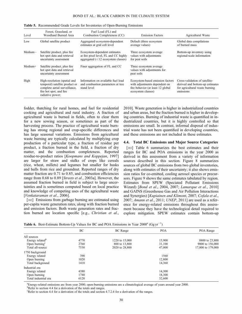
fodder, thatching for rural homes, and fuel for residentialcooking and agricultural and rural industry. A fraction ofagricultural waste is burned in fields, often to clear themfor a new sowing season, or sometimes as part of theharvesting process. The practice of agricultural waste burn-ing has strong regional and crop-specific differences andhas large seasonal variations. Emissions from agriculturalwaste burning are typically calculated by multiplying cropproduction of a particular type, a fraction of residue perproduct, a fraction burned in the field, a fraction of drymatter, and the combustion completeness. Reportedresidue-to-product ratios [Koopmans and Koppejan, 1997]are larger for straw and stalks of crops like cereals(rice, wheat, millets) and legumes but smaller for husksand hulls from rice and groundnut. Reported ranges of drymatter fraction are 0.71 to 0.85, and combustion efficienciesrange from 0.68 to 0.89 [Streets et al., 2003a]. However, theassumed fraction burned in field is subject to large uncer-tainties and is sometimes computed based on local practiceand knowledge of competing uses of the agricultural waste[Venkataraman et al., 2006].[182] Emissions from garbage burning are estimated using

per-capita waste generation rates, along with fraction burnedand emission factors. Both waste generation rates and frac-tion burned are location specific [e.g., Christian et al.,

2010]. Waste generation is higher in industrialized countriesand urban areas, but the fraction burned is higher in develop-ing countries. Burning of industrial waste is quantified in in-dustrialized countries, but it is highly controlled so thatemissions are small. In contrast, informal disposal of indus-trial waste has not been quantified in developing countries,and these emissions are not included in these estimates.

4.4. Total BC Emissions and Major Source Categories

[183] Table 6 summarizes the best estimates and theirranges for BC and POA emissions in the year 2000 asderived in this assessment from a variety of informationsources described in this section. Figure 8 summarizessources of global BC emissions from two global inventories,along with estimates of their uncertainty; it also shows emis-sion ratios for co-emitted, cooling aerosol species or precur-sors. Figure 9 shows the same estimates tabulated by region.Estimates from SPEW (Speciated Pollutant EmissionsWizard) [Bond et al., 2004, 2007; Lamarque et al., 2010]and GAINS (Greenhouse Gas and Air Pollution Interactionsand Synergies) [Kupiainen and Klimont, 2007; Cofala et al.,2007; Amann et al., 2011; UNEP, 2011] are used as a refer-ence for energy-related emissions throughout this assess-ment because they have the technological detail required toexplore mitigation. SPEW estimates contain bottom-up

Table 5. Recommended Grade Levels for Inventories of Open-Burning Emissions

LevelForest, Grassland, or

Woodland Burned AreaFuel Load (FL) and

Combustion Completeness (CC) Emission Factors Agricultural Waste

Low Global satellite product Aggregated ecosystem-dependentestimates at grid cell level

Default (three ecosystemaverage values)

Global data compilationsof burned mass

Medium� Satellite product, plus firehot spot data and retrievaluncertainty assessment

Ecosystem-dependent estimatesat fire pixel level, FL and CC highlyaggregated (<12 ecosystem classes)

Three ecosystem averagevalues with adjustmentsfor peat soils

Bottom-up inventory usingregional-scale information

Medium+ Satellite product, plus firehot spot data and retrievaluncertainty assessment

Finer aggregation of FL and CC Three ecosystem averagevalues with adjustments forpeat soils

High High-resolution (spatial andtemporal) satellite product orcomplete aerial surveillance,fire hot spot, and fireradiative power;

Information on available fuel loadand combustion parameters at treestand level

Ecosystem-based emission factorswith adjustments dependent onfire behavior (at least 12 globalecosystem classes)

Cross-validation of satellite-derived and bottom-up estimatesfor agricultural waste burningemissions

Table 6. Best-Estimate Bottom-Up Values for BC and POA Emissions in Year 2000a (Gg yr�1)

BC BC Range POA POA Range

All sourcesEnergy relatedb 4770 1220 to 15,000 15,900 8800 to 23,800Open burningc 2760 800 to 13,800 31,100 9000 to 156,000Total all-source 7530 2020 to 28,800 47,000 17,800 to 179,000

1750 backgroundEnergy related 390 1560Open burning 1020 12,800Total background 1410 14,360

Industrial eraEnergy related 4380 14,300Open burning 1740 18,300Total industrial era 6120 32,600

aEnergy-related emissions are from year 2000; open-burning emissions are a climatological average of years around year 2000.bRefer to section 4.4 for a derivation of the totals and ranges.cRefer to section 4.4 for a derivation of the totals and section 4.7.2.4 for a derivation of the ranges.


30

uncertainties and are therefore used as the basis for Figure 8.GAINS estimates have the advantage of providing all co-emitted species, including gaseous emissions, and are usedin the discussion of source category impacts in section 11.Section 4.6 discusses differences between these inventoriesand compares other global and regional emission estimates.[184] Figure 8 and Table 7 also give bottom-up estimates

from open burning. Both RETRO (REanalysis of the TROpo-sphere over the last 40 years) [Schultz et al., 2008] and GFED(Global Fire Emissions Database) [van der Werf et al., 2006]incorporate remote sensing information on fires to provide sea-sonal and inter-annual emission variation and are frequentlyused by atmospheric models. Figure 10 shows the seasonaland inter-annual variability of open burning in five regions.However, because remote sensing poorly detects small

agricultural fires, we rely on estimated activity data (SPEWand GAINS) for agricultural waste burning emissions. The fig-ure and table also compare SPEW open-burning emissions,which are based on country information about total quantitiesburned.[185] The left panel of Figure 8 presents total BC emis-

sions for each source category, also indicating the regionsof emission. This panel shows ranges calculated from uncer-tainties in both activity data and emission factors in SPEW,and a comparison with the same sectors in the GAINS data-base. Although totals for each category vary, there is generalagreement that the three largest contributors are open burn-ing, diesel engines, and residential solid fuels. A smallnumber of industrial sources in developing countries alsomake a significant contribution.

Figure 8. Emission rates of BC in the year 2000 by source category and ratios of co-emitted aerosols(e.g., primary organic aerosol, POA) and aerosol precursors (e.g., SO2) to BC. For reference, it is oftenassumed that the ratio of OA to primary organic carbon (OC) varies from 1.1 to 1.4, depending on thesource (section 3.2.2). SPEW emissions are shown as colored bars and are described by Lamarqueet al. [2010]. GAINS estimates are from UNEP/WMO [2011a, 2011b], and RETRO emissions for openburning are described by Schultz et al. [2008]. Sulfur emissions from Streets et al. [2009] were used forratios to SPEW. Regions are shown in Figure 7.


31

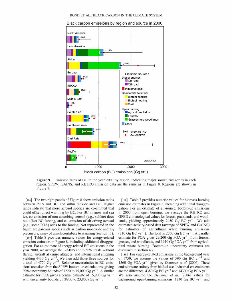
[186] The two right panels of Figure 8 show emission ratiosbetween POA and BC, and sulfur dioxide and BC. Higherratios indicate that more aerosol species are co-emitted thatcould offset direct warming by BC. For BC in snow and seaice, co-emission of non-absorbing aerosol (e.g., sulfate) doesnot affect BC forcing, and co-emission of absorbing aerosol(e.g., some POA) adds to the forcing. Not represented in thefigure are gaseous species such as carbon monoxide and O3

precursors, many of which contribute to warming (section 11).[187] Table 8 provides numeric values for energy-related

emission estimates in Figure 8, including additional disaggre-gation. For an estimate of energy-related BC emissions in theyear 2000, we average the GAINS and SPEW totals withoutflaring, aircraft at cruise altitudes, and international shippingyielding 4430 Gg yr�1. We then add those three sources fora total of 4770 Gg yr�1. Relative uncertainties in BC emis-sions are taken from the SPEW bottom-up calculations, giving90% uncertainty bounds of 1220 to 15,000 Gg yr�1. A similarestimate for POA gives a central estimate of 15,900 Gg yr�1

with uncertainty bounds of (8800 to 23,800) Gg yr�1.

[188] Table 7 provides numeric values for biomass-burningemission estimates in Figure 8, including additional disaggre-gation. For an estimate of all-source, bottom-up emissionsin 2000 from open burning, we average the RETRO andGFED climatological values for forests, grasslands, and wood-lands, yielding approximately 2450 Gg BC yr�1. We addestimated activity-based data (average of SPEW and GAINS)for estimates of agricultural waste burning emissions(310 Gg BC yr�1). The total is 2760 Gg BC yr�1. A parallelestimate for POA gives 29,200 Gg POA yr�1 from forests,grasses, and woodlands, and 1910 Gg POA yr�1 from agricul-tural waste burning. Bottom-up uncertainty estimates arediscussed in section 4.7.[189] For energy-related emissions in the background year

of 1750, we assume the values of 390 Gg BC yr�1 and1560 Gg POA yr�1 given by Dentener et al. [2006]. Theseemissions are entirely from biofuel use. Industrial-era emissionsare the difference, 4380 Gg BC yr�1 and 14300 Gg POA yr�1.We also assume the Dentener et al. [2006] values forbackground open-burning emissions: 1230 Gg BC yr�1 and

Figure 9. Emission rates of BC in the year 2000 by region, indicating major source categories in eachregion. SPEW, GAINS, and RETRO emission data are the same as in Figure 8. Regions are shown inFigure 7.


32

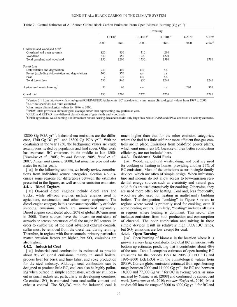
12800 Gg POA yr�1. Industrial-era emissions are the differ-ence, 1740 Gg BC yr�1 and 18300 Gg POA yr�1. With noconstraints in the year 1750, the background values are crudeassumptions, scaled by population and land cover. Other workhas estimated BC emissions in the middle to late 1800s[Novakov et al., 2003; Ito and Penner, 2005; Bond et al.,2007; Junker and Liousse, 2008], but none has provided esti-mates for earlier years.[190] In the following sections, we briefly review contribu-

tions from individual source categories. Section 4.6 dis-cusses some reasons for differences between the estimatespresented in the figures, as well as other emission estimates.4.4.1. Diesel Engines[191] On-road diesel engines include diesel cars and

trucks, while off-road engines include engines used inagriculture, construction, and other heavy equipment. Thediesel-engine category in this assessment specifically excludesshipping emissions, which are summarized separately.Diesel engines contributed about 20% of global BC emissionsin 2000. These sources have the lowest co-emissions ofaerosols or aerosol precursors of all the major BC sources. Inorder to enable use of the most advanced exhaust controls,sulfur must be removed from the diesel fuel during refining.Therefore, in regions with fewer controls, primary particulatematter emission factors are higher, but SO2 emissions arealso higher.4.4.2. Industrial Coal[192] Industrial coal combustion is estimated to provide

about 9% of global emissions, mainly in small boilers,process heat for brick and lime kilns, and coke productionfor the steel industry. Although coal combustors can bedesigned to produce little BC, coal can also be highly pollut-ing when burned in simple combustors, which are still pres-ent in small industries, particularly in developing countries.Co-emitted SO2 is estimated from coal sulfur content andexhaust control. The SO2/BC ratio for industrial coal is

much higher than that for the other emission categories,where the fuel has little sulfur or more efficient flue-gas con-trols are in place. Emissions from coal-fired power plants,which emit much less BC because of their better combustionefficiency, are not included here.4.4.3. Residential Solid Fuels[193] Wood, agricultural waste, dung, and coal are used

for cooking or heating in homes, providing another 25% ofBC emissions. Most of the emissions occur in single-familydevices, which are often of simple design. When infrastruc-ture and income do not allow access to low-emission resi-dential energy sources such as electricity and natural gas,solid fuels are used extensively for cooking. Otherwise, theyare used more often for heating. Coal and, less frequently,wood are also used for heating in multi-family buildingboilers. The designation “cooking” in Figure 8 refers toregions where wood is primarily used for cooking, even ifsome heating occurs. Similarly, “heating” includes all usesin regions where heating is dominant. This sector alsoincludes emissions from both production and consumptionof charcoal. The poor combustion and mixing in thesesimple devices result in relatively high POA :BC ratios,but SO2 emissions are low except for coal.4.4.4. Open Burning[194] Open burning of biomass in the location where it is

grown is a very large contributor to global BC emissions, withbottom-up estimates predicting that it contributes about 40%of the total. Table 7 compares estimates of open-burning BCemissions for the periods 1997 to 2006 (GFED 3.1) and1996–2000 (RETRO) with the climatological values fromSPEW. Current global emissions estimated from open burningrange between 2000 and 11,000 Gg yr�1 for BC and between18,000 and 77,000 Gg yr�1 for OC in average years, as sum-marized by Schultz et al. [2008] and confirmed by subsequentwork [Lamarque et al., 2010; van der Werf et al., 2010]. Moststudies fall into the range of 2000 to 6000 Gg yr�1 for BC and

Table 7. Central Estimates of All-Source Global Black-Carbon Emissions From Open Biomass Burning (Gg yr�1)

Inventory

GFEDa RETROb RETROc GAINS SPEW

2000 clim. 2000 clim. 2000 clim.d

Grassland and woodland firese

Grassland and open savanna 820 850 310 290Woodland 330 350 1220 1220Total grassland and woodland 1150 1200 1530 1510 1710

Forest firesDeforestation and degradation 230 440 n.s. n.s.Forest (excluding deforestation and degradation) 300 370 n.s. n.s.Peat 2 130 n.s. n.s.Total forest fires 530 940 830 1240 1240

Agricultural waste burningf 50 60 n.e. n.e. 290 330

Grand total 1730 2200 2370 2750 3280

aVersion 3.1 from http://www.falw.vu/~gwerf/GFED/GFED3/tables/emis_BC_absolute.txt; clim.: mean climatological values from 1997 to 2006.bn.s. = not specified; n.e. = not estimated.cclim.: mean climatological values for 1996 to 2000.dSPEW totals provide a climatological average rather than representing any particular year.eGFED and RETRO have different classifications of grasslands and woodlands.fGFED agricultural waste burning is inferred from remote-sensing data and includes only large fires, while GAINS and SPEW are based on activity estimates.


33

http://www.falw.vu/~gwerf/GFED/GFED3/tables/emis_BC_absolute.txt

20,000 to 27,000 Gg yr�1 for OC. The highest BC and OCemission estimates by Chin et al. [2002] resulted from theuse of larger emission factors. A smaller contribution origi-nates from open burning in agricultural fields, which is oftendone to clear residues after harvest. This source contributesabout 300 Gg yr�1 BC and 1500 Gg yr�1 OC. In regions likesouth Asia, this source can contribute about 20% of carbona-ceous aerosol emissions [Venkataraman et al., 2006].[195] The average of 2760 GgBC yr�1 in Table 7 (including

emissions from agricultural waste burning) agrees well withthe mean value of global BC estimates from the review ofSchultz et al. [2008] after they adjusted the literature estimatesto standard emission factors. However, modeling studies thatconstrain emissions using satellite observations indicatesubstantially larger biomass burning emissions of particulatematter. Section 5.5.1 discusses these studies further.[196] Because fuel-air mixing is completely unmanaged in

open burning, large quantities of organic matter can escapeand average POA :BC ratios are highest of all sectors. Thisratio can vary greatly depending on the burning conditions;

Andreae and Merlet [2001] give an inter-quartile range of 4to 14. If the burning is natural or accidental, vegetation mayburn while it is still rooted and standing, thus allowing forsome greater ventilation and oxygen supply. Deliberateburning may involve land clearing before collecting, piling,and burning the material, which tends to favor oxygen-poorconditions.4.4.5. Other Emission Sources[197] BC emissions from the four major source types

above are about 90% of the global total. Significant contrib-utors of the remainder of BC emissions are listed in Table 8.Two of the largest groups are industrial and residentialemissions that are not included in one of the preceding cate-gories. In industry, biofuels are responsible for the higherBC emissions estimated by SPEW. Like coal-burningsources, these small sources are challenging to characterize.About half of the miscellaneous residential emissions comefrom middle distillate oil, and stationary diesel engines usedfor distributed power generation are estimated to produceabout 85% of that. Charcoal, kerosene, and liquefied petro-leum gas make up the remainder of residential emissions.[198] Although aviation emits BC at altitudes that other-

wise have low aerosol concentrations, its contribution toBC mass is quite small. Likewise, shipping emits aerosol

Table 8. Bottom-Up Central Estimates of All-Source GlobalBlack Carbon Emissions From Energy-Related Combustion in theYear 2000 (Gg yr�1)a

Inventory

Source SPEW GAINS

Diesel enginesOn-road diesel engines 840 780Off-road diesel engines 480 370Total diesel 1320 1150

Industrial coalAll coal in industry 740 340Total industrial coal 740 340

Residential solid fuelWood, cooking regions 1000 1580Other biofuel, cooking regionsb 290 310All biofuel, heating regionsb 260 200Coal, cooking, and heating 330 420Total residential solid fuel 1880 2510

Other sourcesNon-coal industry, including biofuel 170 30On-road gasoline engines 110 80Residential, including diesel generation 100 170Aviation 20 1c

Shipping 100 40d

Flaring -e 260All other BC-rich sources 70 20Power plants f 20 20Other low-BC sources -e 60Total other sources 590 690

Grand total 4510 4690

aData are based on year-2000 energy data and technology. Totals do notmatch exactly due to rounding.

b“Cooking regions” are those where solid fuel is primarily used forcooking, even if some heating occurs; the opposite is true for the definitionof “heating regions.”

cThis inventory only includes landing and takeoff (i.e., no cruise)emissions.

dThis inventory only does not include international shipping.eNot estimated.fConsidered to be low-BC sources.

Figure 10. Seasonality of BC emissions from forest, grass-land, and woodland burning. Average monthly emissions esti-mated by RETRO for the period 1996–2000 are shown[Schultz et al., 2008]. Error bars indicate minima and maximaduring each period. Regions correspond to those in Figure 7.Africa, which includes the small Middle East emissions, hastwo burning seasons because the equator bisects it. The groupof East, Southeast, and South Asia (E, SE, and S Asia)includes emissions from Oceania. The very large error barsin that region results from the very high fire season in 1997.Note the different vertical scales in the two panels.


34

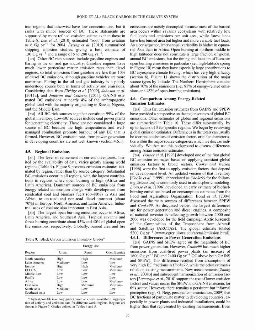
into regions that otherwise have low concentrations, but itranks with minor sources of BC. These statements aresupported by more refined emission estimates than those inTable 8. Lee et al. [2010] estimated “soot” from aviationas 6 Gg yr�1 for 2004. Eyring et al. [2010] summarizedshipping emission studies, giving a best estimate of130 Gg yr�1 and a range of 5 to 280 Gg yr�1.[199] Other BC-rich sources include gasoline engines and

flaring in the oil and gas industry. Gasoline engines havemuch lower particulate matter emission rates than dieselengines, so total emissions from gasoline are less than 10%of diesel BC emissions, although gasoline vehicles are morenumerous. Flaring in the oil and gas industry is a poorlyunderstood source both in terms of activity and emissions.Considering data from Elvidge et al. [2009], Johnson et al.[2011a], and Johnson and Coderre [2011], GAINS esti-mated BC emissions at nearly 4% of the anthropogenicglobal total with the majority originating in Russia, Nigeria,and the Middle East.[200] All BC-rich sources together constitute 99% of the

global inventory. Low-BC sources include coal power plantsfor generating electricity. These are not considered a largesource of BC because the high temperatures and well-managed combustion promote burnout of any BC that isformed. However, BC emission rates from power generationin developing countries are not well known (section 4.6.1).

4.5. Regional Emissions

[201] The level of refinement in current inventories, lim-ited by the availability of data, varies greatly among worldregions (Table 9). Figure 9 presents emission estimates tab-ulated by region, rather than by source category. SubstantialBC emissions occur in all regions, with the largest contribu-tions in regions where open burning is high (Africa andLatin America). Dominant sources of BC emissions fromenergy-related combustion change with development fromresidential coal and biomass fuels (60–80%) in Asia andAfrica, to on-road and non-road diesel transport (about70%) in Europe, North America, and Latin America. Indus-trial uses of coal are also important in East Asia.[202] The largest open burning emissions occur in Africa,

Latin America, and Southeast Asia. Tropical savanna andforest burning contribute about 45% and 40% of global openfire emissions, respectively. Globally, burned area and fire

emissions are mostly decoupled because most of the burnedarea occurs within savanna ecosystems with relatively lowfuel loads and emissions per unit area, while forest landshave less burned area but higher and more variable fuel loads.As a consequence, inter-annual variability is higher in equato-rial Asia than in Africa. Open burning at northern middle tohigh latitudes does not constitute a large fraction of global,annual BC emissions, but the timing and location of Eurasianopen burning emissions in particular (i.e., high-latitude springin Figure 10) mean they have especially large contributions toBC cryosphere climate forcing, which has very high efficacy(section 8). Figure 11 shows the distribution of the majorsource types by latitude. The Northern Hemisphere containsabout 70% of the emissions (i.e., 85% of energy-related emis-sions and 45% of open-burning emissions).

4.6. Comparison Among Energy-RelatedEmission Estimates

[203] Thus far, emission estimates from GAINS and SPEWhave provided a perspective on the major sources of global BCemissions. Other estimates of global and regional emissionsare summarized in Table 10. These differ substantially, byup to factors of 3 for specific regions. We begin by reviewingglobal emission estimates. Differences in the totals can usuallybe ascribed to choices of emission factors or other characteris-tics within the major source categories, which we discuss indi-vidually. We then use this background to discuss differencesamong Asian emission estimates.[204] Penner et al. [1993] developed one of the first global

BC emission estimates based on applying constant globalemission factors to broad sectors. Cooke and Wilson[1996] were the first to apply emission factors that dependon development level. An updated version of that inventory[Cooke et al. [1999], abbreviated as Cooke99 for the follow-ing discussion] is commonly used in atmospheric modeling.Liousse et al. [1996] developed an early estimate of biofuel-burning emissions based on consumption estimates from theFood and Agriculture Organization. Bond et al. [2004]discussed the main sources of differences between SPEWand Cooke99. As discussed below, the largest differencesare for power generation and diesel engines. A compositeof national inventories reflecting growth between 2000 and2006 was developed for the field campaign Arctic Researchof the Composition of the Troposphere from Aircraftand Satellites (ARCTAS). The global estimate totaled5200 Gg yr�1 [www.cgrer.uiowa.edu/arctas/emission.html].4.6.1. Differences in Power Generation Emissions[205] GAINS and SPEW agree on the magnitude of BC

from power generation. However, Cooke99 has much higheremissions from coal-fired power plants (an increase of1600 Gg yr�1 BC and 2400 Gg yr�1 OC above both GAINSand SPEW). This difference resulted from assumptions ofvery high BC fractions in Cooke99, while the other estimatesrelied on existing measurements. New measurements [Zhanget al., 2008b] and subsequent harmonization of emission fac-tors [Lamarque et al., 2010] support the use of lower emissionfactors and values nearer the SPEW and GAINS emissions forthis sector. However, there remains a persistent but informalperception (e.g., G. Beig, personal communication, 2009) thatBC fractions of particulate matter in developing countries, es-pecially in power plants and industrial installations, could behigher than that represented by existing measurements. Even

Table 9. Black Carbon Emission Inventory Gradesa

Energy Use

Region Urban Rural Open Burning

North America High High Medium+Latin America Medium+ Low LowEurope High High Medium+EECCA Low Low Medium�Middle East Low Low LowPacific Low Low LowAfrica Low Low Medium�East Asia High Medium+ Medium�South Asia Medium+ Low LowSoutheast Asia Low Low Low

aHighest possible inventory grades based on current available disaggrega-tion of activity and emission data for different world regions. Regions areshown in Figure 7. Grades defined in Tables 4 and 5.


35

http://www.cgrer.uiowa.edu/arctas/emission.html

if older, poorly operating power plants have high BC emissionfactors, there is no evidence that newly installed, modernpower plants do. Thus, rapid growth in electricity generationis unlikely to cause sharp increases in BC emissions.4.6.2. Differences in Industrial Coal Emissions[206] SPEW estimates of industrial coal emissions are about

double those of GAINS. This difference is almost entirelydue to assumptions in emission factors and BC fractions forthe two major emitting categories, brick kilns, and coke ovens.A few particulate matter (PM)measurements were available forbrick kilns, but no measurements of total PM from uncapturedcoking were available at the time of inventory development.Composition measurements for both sources were estimatedbased on expert judgment, as no composition measurementswere available for either source.4.6.3. Differences in Diesel Engine Emissions[207] GAINS and SPEW have similar emissions for year

2000 from on-road and off-road diesel engines, with SPEWbeing somewhat higher due to different assumptions aboutemission factors and the fraction of high-emitting vehicles.In previous versions of SPEW [e.g., Bond et al., 2007],diesel emissions were higher than those given here due todifferent assumptions about the implementation of stan-dards. The Cooke99 inventory had much higher emissionsfrom diesel engines, resulting from very large assumedemission factors in developing countries that were notbased on measurements. Measurements have confirmedhigher emission factors in locations with delayed emissionstandards [Subramanian et al., 2009; Assamoi and Liousse,2010], although no measurements are as high as theassumptions in the Cooke99 inventory. However, an evalu-ation of trends in California [Kirchstetter et al., 2008] indi-cates that emissions prior to regulation could have been

higher by a factor of 10, greater than either the emissionfactors used in SPEW and GAINS, or in any reportedmeasurements.4.6.4. Differences in Residential Solid Fuel Sector[208] Small-scale residential combustors constitute the

largest difference between SPEW and GAINS. Estimatesfrom SPEW are lower by 30% for biofuel used in cookingand all uses of coal, and higher by 35% for biofuel used inheating. The discrepancies in heating biofuel and coal emis-sions are largely due to activity data. For cooking stoves,activity in SPEW is lower by about 15%, and emission fac-tor choices cause the remainder of the difference. GAINSuses the highest emission factor from fireplace measure-ments for cooking stoves (about 1.1 g BC [kg fuel]�1), whileSPEW uses an average of cooking stove measurements(about 0.8 g BC [kg fuel]�1). Both are consistent withobserved emission factors.4.6.5. Asian Emission Inventories[209] Detailed emission inventories have been developed

for the Asian region and for individual countries withinAsia. Here we compare these inventories and identify somereasons for differences. Similar studies are not available inother world regions.[210] Three emission inventories have been developed

for Asia alone. Streets et al. [2003b] provided inventoriesto support modeling during the TRACE-P field campaign[Jacob et al., 2003]. Emission factors in that inventorywere an earlier version of those in SPEW [Bond et al.,2004]. Two primary differences were the addition of smallindustries (brick kilns and coking) in SPEW and adjust-ment of emission factors for residential fuel, where BCemission factors were reduced slightly and those fororganic matter were greatly reduced. In addition, the

Figure 11. Latitude plot of the data shown in Figures 8 and 9 using 5� latitude bins.


36

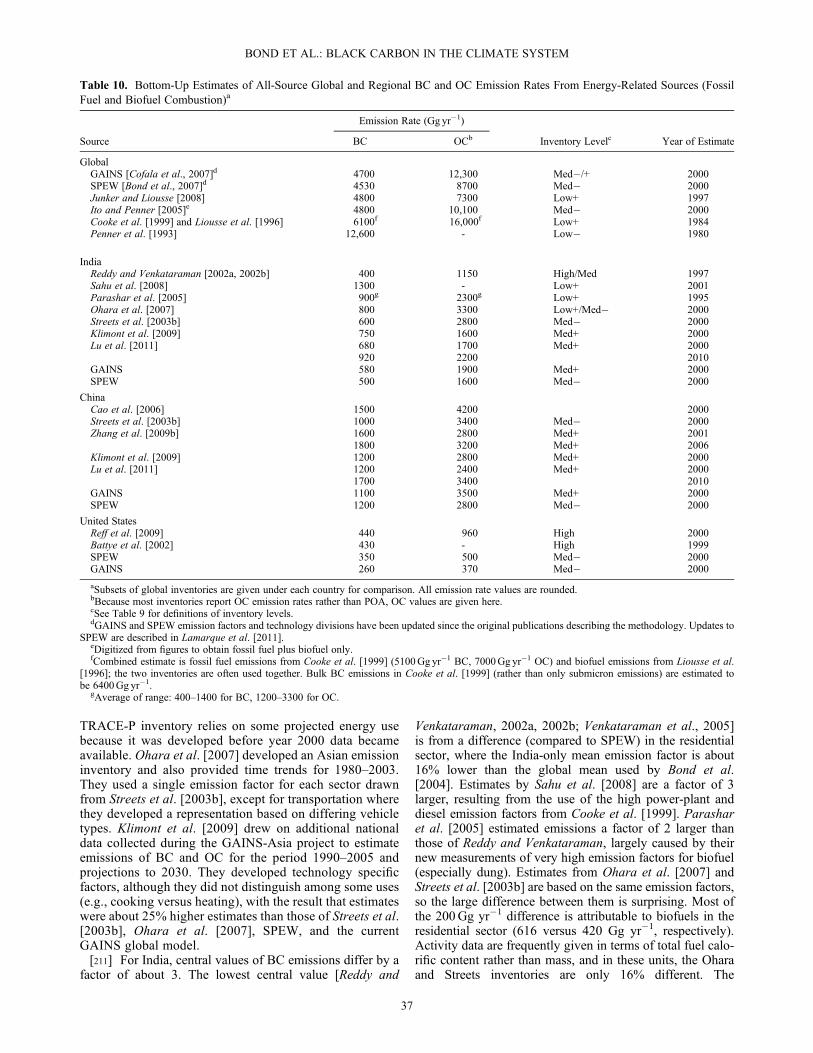
TRACE-P inventory relies on some projected energy usebecause it was developed before year 2000 data becameavailable. Ohara et al. [2007] developed an Asian emissioninventory and also provided time trends for 1980–2003.They used a single emission factor for each sector drawnfrom Streets et al. [2003b], except for transportation wherethey developed a representation based on differing vehicletypes. Klimont et al. [2009] drew on additional nationaldata collected during the GAINS-Asia project to estimateemissions of BC and OC for the period 1990–2005 andprojections to 2030. They developed technology specificfactors, although they did not distinguish among some uses(e.g., cooking versus heating), with the result that estimateswere about 25% higher estimates than those of Streets et al.[2003b], Ohara et al. [2007], SPEW, and the currentGAINS global model.[211] For India, central values of BC emissions differ by a

factor of about 3. The lowest central value [Reddy and

Venkataraman, 2002a, 2002b; Venkataraman et al., 2005]is from a difference (compared to SPEW) in the residentialsector, where the India-only mean emission factor is about16% lower than the global mean used by Bond et al.[2004]. Estimates by Sahu et al. [2008] are a factor of 3larger, resulting from the use of the high power-plant anddiesel emission factors from Cooke et al. [1999]. Parasharet al. [2005] estimated emissions a factor of 2 larger thanthose of Reddy and Venkataraman, largely caused by theirnew measurements of very high emission factors for biofuel(especially dung). Estimates from Ohara et al. [2007] andStreets et al. [2003b] are based on the same emission factors,so the large difference between them is surprising. Most ofthe 200Gg yr�1 difference is attributable to biofuels in theresidential sector (616 versus 420 Gg yr�1, respectively).Activity data are frequently given in terms of total fuel calo-rific content rather than mass, and in these units, the Oharaand Streets inventories are only 16% different. The

Table 10. Bottom-Up Estimates of All-Source Global and Regional BC and OC Emission Rates From Energy-Related Sources (FossilFuel and Biofuel Combustion)a

Emission Rate (Gg yr�1)

Source BC OCb Inventory Levelc Year of Estimate

GlobalGAINS [Cofala et al., 2007]d 4700 12,300 Med�/+ 2000SPEW [Bond et al., 2007]d 4530 8700 Med� 2000Junker and Liousse [2008] 4800 7300 Low+ 1997Ito and Penner [2005]e 4800 10,100 Med� 2000Cooke et al. [1999] and Liousse et al. [1996] 6100f 16,000f Low+ 1984Penner et al. [1993] 12,600 - Low� 1980

IndiaReddy and Venkataraman [2002a, 2002b] 400 1150 High/Med 1997Sahu et al. [2008] 1300 - Low+ 2001Parashar et al. [2005] 900g 2300g Low+ 1995Ohara et al. [2007] 800 3300 Low+/Med� 2000Streets et al. [2003b] 600 2800 Med� 2000Klimont et al. [2009] 750 1600 Med+ 2000Lu et al. [2011] 680 1700 Med+ 2000

920 2200 2010GAINS 580 1900 Med+ 2000SPEW 500 1600 Med� 2000

ChinaCao et al. [2006] 1500 4200 2000Streets et al. [2003b] 1000 3400 Med� 2000Zhang et al. [2009b] 1600 2800 Med+ 2001

1800 3200 Med+ 2006Klimont et al. [2009] 1200 2800 Med+ 2000Lu et al. [2011] 1200 2400 Med+ 2000

1700 3400 2010GAINS 1100 3500 Med+ 2000SPEW 1200 2800 Med� 2000

United StatesReff et al. [2009] 440 960 High 2000Battye et al. [2002] 430 - High 1999SPEW 350 500 Med� 2000GAINS 260 370 Med� 2000

aSubsets of global inventories are given under each country for comparison. All emission rate values are rounded.bBecause most inventories report OC emission rates rather than POA, OC values are given here.cSee Table 9 for definitions of inventory levels.dGAINS and SPEW emission factors and technology divisions have been updated since the original publications describing the methodology. Updates to

SPEW are described in Lamarque et al. [2011].eDigitized from figures to obtain fossil fuel plus biofuel only.fCombined estimate is fossil fuel emissions from Cooke et al. [1999] (5100Gg yr�1 BC, 7000Gg yr�1 OC) and biofuel emissions from Liousse et al.

[1996]; the two inventories are often used together. Bulk BC emissions in Cooke et al. [1999] (rather than only submicron emissions) are estimated tobe 6400Gg yr�1.

gAverage of range: 400–1400 for BC, 1200–3300 for OC.


37

difference, therefore, must be caused by differing assump-tions in the conversion between fuel calorific content andmass. Klimont et al. [2009] used higher emission factorsfor cooking and national energy use statistics and estimatednearly 30% higher BC than current global GAINS imple-mentation or SPEW, while OC was well within the rangeof GAINS and SPEW. Lu et al. [2011] obtained similar esti-mates to Klimont et al. [2009] and also estimated that BCemissions rose 35% between 2000 and 2010. The Lu et al.[2011] trends in Asian aerosol emissions compare favorablywith remote-sensing data.[212] For China, regional inventories are in broad agree-

ment with global inventories on magnitudes and sourcesof BC emissions. Cao et al. [2006] developed an emissioninventory based on Chinese data and some new emissionfactors. SPEW and the inventory of Cao et al. [2006] arequite similar. The Streets et al. [2003b] inventory lackstreatment of small industry. Zhang et al. [2009b] includedsmall industry, particularly brick and cement kilns, follow-ing the approach of Streets et al. [2006] and estimated sig-nificantly higher total BC emissions from China. Lu et al.[2011] estimated generally higher growth in BC emissionsbetween 2000 and 2010 (+46%) than previous studies.Organic matter emissions in Cao et al. [2006] are higherthan those of the other studies due to the use of differentemission factors. Klimont et al. [2009] estimates for BCare higher by about 15% than Streets et al. [2003b] andglobal inventories but lower than Zhang et al. [2009b].While comparing total emissions for China yields ingeneral fairly good agreement across the studies, there aresignificant sectoral shifts resulting primarily from uncer-tainties in coal versus briquette use in the residential sectorand assumptions for the brick-making sector. For example,Zhang et al. [2009b] and GAINS use comparable assump-tions for coal, while Klimont et al. [2009] assumes morebriquettes, leading to lower emissions from this sector inKlimont et al. On the other hand, for brick making bothZhang et al. and Klimont et al. rely on Bond et al. [2004]emission factors and estimate higher emissions thanGAINS, which considers anecdotal evidence about thetransition in this industry that leads to significantly loweremission factors.

4.7. Major Sources of Uncertainty in Emissions

4.7.1. Energy-Related Combustion[213] As discussed in section 4.6, large differences

between emission estimates are attributable to a few choicesregarding emission factors made by inventory developers.Some of the diversity is not supported by measurements atemission sources, while other disagreements reflect trueuncertainty in knowledge. A bottom-up estimate of uncer-tainty is about a factor of two using either a simple uncer-tainty combination for global emissions [Bond et al., 2004]or a Monte Carlo approach for individual countries[Lu et al., 2011].4.7.1.1. Activity Data[214] For fossil fuel combustion, activity estimates

for many inventories in Table 10 have the same source(International Energy Agency (IEA), or United Nations fuel-consumption data), although many inventory developersadjust these data when inconsistencies are found or whenfiner allocation of activities is required (e.g., road and off-

road vehicles or vehicle type). For several larger countries,regional statistics are also available and using them allowsfor better spatial resolution; however, national and interna-tional statistics are not always consistent. Finally, somemodels chose to use data sets specifically developed for par-ticular projects. For example, GAINS often uses nationalfuel-consumption estimates for most of the European coun-tries, China, India, and Pakistan. These may differ fromIEA statistics, especially with regard to sectoral allocation.Total fuel consumption can be affected by the use ofregional information on the calorific value of fuels.[215] Consumption of residential solid fuels, especially

biofuel, is not well constrained. Biofuel consumption dataare frequently drawn from disparate sources. For example,GAINS relies on IEA and national data, while SPEW usesthe tabulation of Fernandes et al. [2007]. Fuel productionand sales are not centralized in this sector, and many fuelsare collected by the consumers or by small sellers. Activitydata are therefore much more uncertain than for liquid orgaseous fuels or consumption in large installations. Esti-mates of fuel consumption are often based on per-capita con-sumption estimates multiplied by the number of peopleusing solid fuels. Comparison of the residential biofuel con-sumption for the past years in India and China [Streets andAunan, 2005; Venkataraman et al., 2005; Ohara et al.,2007; GAINS] shows significant differences, typically rang-ing within about �25%.

4.7.1.2. Emission Factors[216] Emission rates of both BC and organic carbon

depend on the combustion process, including fuel composi-tion, flame temperature, mixing between fuel and air duringcombustion, and post-combustion treatment of the exhaust.Carbonaceous aerosols can be destroyed if the exhaust iskept hot and well mixed with air. Large, properly operatingcombustors, such as power plants and some modern installa-tions using biofuel, tend to achieve this burnout, resulting inlittle emitted BC. Mixing between fuel and air before com-bustion also limits BC formation, so that gasoline enginesemit much less BC than do diesel engines. Finally, BCmay be removed through end-of-pipe controls that capturefine particles, as it is in particulate filters after diesel engines.[217] The strong dependence of BC emissions on combus-

tion processes means that the disaggregation of activity torepresent combustion quality explicitly is an important com-ponent of inventories. The dependence also demands thedevelopment of emission factors under realistic operatingconditions. Because most sources have several operatingmodes, it is important to obtain emission factors by measur-ing during a realistic sequence. This sequence of conditionsmay be called “driving cycles” for vehicles, or “burn cycles”for stoves, small boilers, or open combustion. Althoughdesign of existing cycles seeks to represent real-world oper-ation, unrealistic choices of operating conditions may yieldemission factors that are poorly representative. For example,very cold conditions or startup phases, which promote poorefficiency and high emissions, may be omitted from vehicleand stove emission testing or tests may not include thepoorest quality fuels.[218] Uncertainties are particularly acute outside the

United States and Europe. A few measurements are becom-ing available, but the limited number of studies has not


38

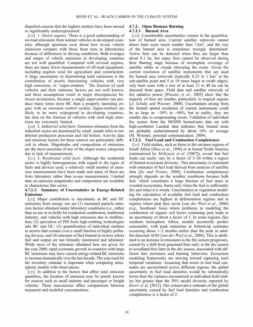
dispelled concern that the highest emitters have been missedor significantly underrepresented.[219] 1. Diesel engines. There is a good understanding of

on-road emissions from normal vehicles in developed coun-tries, although questions exist about how in-use vehicleemissions compare with those from tests in laboratoriesbecause of differences in driving conditions. Both averagesand ranges of vehicle emissions in developing countriesare not well quantified. Compared with on-road engines,there are many fewer measurements of off-road equipment,including engines used for agriculture and construction.A large uncertainty in determining total emissions is thecontribution of poorly functioning vehicles with veryhigh emissions, or “super-emitters.” The fraction of suchvehicles and their emission factors are not well known,and these assumptions result in major discrepancies be-tween inventories, because a single super-emitter can pro-duce many times more BC than a properly operating en-gine with an emission control system. Super-emitters arelikely to be more widespread in developing countries,but data on the fraction of vehicles with such high emis-sions are extremely limited.[220] 2. Industrial solid fuels. Emission estimates from the

industrial sector are dominated by small, simple kilns in tra-ditional production processes and old boilers. Activity dataand emission factors for these sources are particularly diffi-cult to obtain. Magnitudes and composition of emissionsare the most uncertain of any of the major source categoriesdue to lack of measurements.[221] 3. Residential solid fuels. Although the residential

sector is highly heterogeneous with regard to the types offuels and devices used, a relatively small number of emis-sion measurements have been made and many of these arefrom laboratory rather than in-use measurements. Limiteddata on emission magnitudes and composition are availableto characterize this sector.4.7.1.3. Summary of Uncertainties in Energy-RelatedEmissions[222] Major contributors to uncertainty in BC and OC

emissions from energy use are (1) measured particle emis-sion factors obtained under laboratory conditions (i.e., ratherthan in-use or in-field) for residential combustion, traditionalindustry, and vehicles with high emissions due to malfunc-tion; (2) speciation of PM from high-emitting technologiesinto BC and OC; (3) quantification of individual emittersin sectors that contain even a small fraction of highly pollut-ing devices; and (4) amounts of fuel burned in sectors wherefuel and output are not formally monitored and tabulated.While most of the estimates tabulated here are given forthe year 2000, rapid economic growth in countries with largeBC emissions may have caused energy-related BC emissionsto increase dramatically over the last decade. The year used forthe inventory estimate is important when comparing atmo-spheric models with observations.[223] In addition to the factors that affect total emission

quantities, the location of emission may be poorly knownfor sources such as small industry and passenger or freightvehicles. These inaccuracies affect comparisons betweenmeasured and modeled concentrations.

4.7.2. Open Biomass Burning4.7.2.1. Burned Area[224] Considerable uncertainties remain in the quantifica-

tion of burned area. Current satellite retrievals cannotdetect burn scars much smaller than 1 km2, and the sizeof the burned area is sometimes wrongly determined.Active fires can be detected when they are larger thanabout 0.1 ha, but many fires cannot be observed duringtheir flaming stage because of incomplete coverage ofsatellite orbits or clouds obscuring the scene. Given thecurrent resolution of satellite instruments that are usedfor burned area retrievals (typically 0.25 to 1 km2 at thesub-satellite point and 5 to 10 times larger at swath edges),only burn scars with a size of at least 12 to 40 ha can bedetected from space. Field data and satellite retrievals offire radiative power [Wooster et al., 2005] show that themajority of fires are smaller, particularly in tropical regions[cf. Schultz and Wooster, 2008]. Uncertainties arising fromthe limited spatial resolution of current instruments couldbe as large as �30% to +40%, but in reality, they aresmaller due to compensating errors. Validation of individualfire scenes from the MODIS burned-area data set withhigh-resolution Landsat data indicates that burned areasare probably underestimated by about 10% on average(M. Wooster, personal communication, 2009).4.7.2.2. Fuel Load and Combustion Completeness[225] Field studies, such as those in the savanna regions of

South Africa [Shea et al., 1996] or in boreal North America(summarized by McKenzie et al. [2007]), reveal that fuelloads can easily vary by a factor of 3–20 within a regionof limited ecosystem diversity. This uncertainty is consistentwith estimates of fuel load derived from analysis of satellitedata [Ito and Penner, 2004]. Combustion completenessstrongly depends on the weather conditions because bulkfuel, which constitutes a large fraction of fuel mass inwooded ecosystems, burns only when the fuel is sufficientlydry and when it is windy. Uncertainties in vegetation model-ing for calculation of available fuel load and combustioncompleteness are highest in deforestation regions and inregions where peat fires occur [van der Werf et al., 2006](e.g., Southeast Asia) where problems in modeling thecombustion of organic soil layers containing peat leads toan uncertainty of about a factor of 5. In some regions, likesouthern hemisphere Africa, models incorrectly predictseasonality, with peak emissions in bottom-up estimatesoccurring about 1–2 months earlier than the peak in satel-lite-detected AOD [van der Werf et al., 2006]. This is attrib-uted to an increase in emissions as the fire season progresses,caused by a shift from grassland fires early in the dry seasonto woodland fires later in the dry season, associated with dif-ferent fuel moistures and burning behaviors. Ecosystemmodeling frameworks are moving toward capturing suchtemporal variations. Assuming that errors in fuel load esti-mates are uncorrelated across different regions, the globaluncertainty in fuel load densities would be substantiallylower than the variance encountered in individual field stud-ies but greater than the 50% model diversity reported byKnorr et al. [2012]. Our conservative estimate of the globaluncertainty caused by fuel load densities and combustioncompleteness is a factor of 2.


39

4.7.2.3. Emission Factors[226] As shown in section 5.5, current models of the atmo-

sphere underestimate absorption aerosol optical depth(AAOD) in Africa and Latin America, which are major bio-mass burning regions [Koch et al., 2009b]. Some of the extraabsorption in Africa could be caused by dust, but an expla-nation is needed for the underestimate in Latin America.The underestimate could be caused by low biases in burnedarea or fuel loads (see above), but inverse models [Arellanoet al., 2004; Arellano et al., 2006; Stavrakou and Müller,2006] indicate little bias in carbon monoxide (CO) emis-sions from biomass burning in these regions. The remainingsuspects are fire emission factors, the relationship betweenemitted mass of BC and optical absorption in fire plumes,or incorrectly modeled aerosol lifetimes.[227] Although biomass burning is a large component of

global BC emissions, particulate and BC emission factorsfor this source are poorly constrained. As discussed in sec-tion 3, measurements of BC depend on the analysis method.These method-dependent biases are more critical for bio-mass-burning emissions than for other sources, becausethese emissions pyrolyze and also contain materials thatcatalyze BC emission. The comprehensive literature reviewof Andreae and Merlet [2001] has become widely used, inparticular for the compilation of global inventories [e.g.,van der Werf et al., 2006; Schultz et al., 2008]. However,this review included only values based on thermal oxidationtechniques and excluded optical absorption measurements.Even the highest BC emission factor in Andreae and Merlet[2001] is lower than values inferred from absorption measure-ments, which have been used in other studies [Patterson andMcMahon, 1984; Liousse et al, 1996; Chin et al., 2002; Lileyet al., 2003]. In part due to higher emission factors, Liousseet al. [2010] estimated African biomass burning emissions thatwere about 2.5 higher than GFED. Martins et al. [1998a]showed that thermal oxidation measurements underestimatedBC mass, leading to unrealistically high MACBC values.Therefore, it is possible that the use of imperfect thermalmethods yields BC emission factors that are too low.[228] Comparisons between chemical and optical measure-

ments would increase confidence in biomass-burning emis-sion factors for BC. A review by Watson et al. [2005]showed differences of up to a factor of 7 between differentBC field measurements and discussed the various uncer-tainties related to both thermal and optical measurements.In contrast to Martins et al. [1998a], thermal measurementsdid not always yield lower BC mass estimates than absorp-tion measurements.[229] Representativeness of measured emission factors is

another concern. Open fires have a high inherent variability.Some emission factors and characteristics are inferred fromsmall, better-controlled fires in laboratory settings. The com-bustion intensity and the burning and airflow characteristicsof these small fires may differ from those of fires in the realworld [Reid et al., 2005]. Oxygen-rich flaming combustionis generally associated with more BC and more heat release,while lower-temperature smoldering fires have higher over-all particulate matter emission factors and CO emissionsthan flaming fires [Lobert et al., 1991; Ward et al., 1992;Yokelson et al., 1997]. If a sample is dominated by emissionsfrom one of these phases, then ratios of BC to total PM, orBC to CO, do not represent the overall emission profile.

[230] The relationship between emitted mass of BC andabsorption of the fire plume can be biased because of agingprocesses. As smoke ages, organic material condenses, butno further BC is created. BC/PM ratios in aged plumes arelower than those in fresh plumes, and single-scattering albedosare higher (more scattering relative to absorption). Emissionratios are generally determined in fresh smoke plumes, whilemodels are evaluated with data from long-term regional aver-ages, which are mostly of aged aerosol. If the relatively lowBC ratios are then applied to fresh plumes, either BC emis-sions or absorption by BC could be underestimated.[231] Data are presently insufficient to support firm conclu-

sions about what updates should be made to BC emission ratesfrom open burning of vegetation. However, thermal measure-ments may underpredict absorption, and using regional-averageoptical properties as constraints could also underpredictabsorption at the time of emission. This body of evidence sug-gests that current emission factors from biomass burningmight be biased low. Based on the data from Andreae andMerlet [2001], we estimate the lower uncertainty of BC emis-sion factors to be a factor of 0.6multiplied by the central value.Our estimate for the upper bound is a factor of 4.4.7.2.4. Summary of Uncertainties in OpenBurning Emissions[232] The dominant uncertainty term for open burning

emissions is the emission factor (error range: factor of 0.6to 4). Fuel load and combustion completeness are uncertainby about a factor of 2, while burned area is probably knownwithin 10% on the global scale, although regional differ-ences can be larger (cf. auxiliary material of Schultz et al.[2008]). Neglecting the independent error estimates fromagricultural waste burning and assuming that errors are inde-pendent, error propagation yields an uncertainty range of afactor of 0.29 to 5. Based on the emission estimates insection 4.4, bottom-up uncertainty ranges are 740 to12,800 Gg yr�1 for BC, and 8400 to 144,000 Gg yr�1 forPOA. These ranges are quite asymmetric.

4.8. Trends in BC Emissions

[233] Novakov et al. [2003], Ito and Penner [2005], Bondet al. [2007], and Junker and Liousse [2008] all estimatelarge changes in BC emissions during the industrial era.All of these studies demonstrate that BC emissions arerelated but not directly proportional to fuel consumption.Typically, emission rates become greater as population andeconomic activity increase and then decrease as cleanertechnology is deployed. The resulting trend is an emissionincrease followed by a decrease and is broadly consistentwith measurement records downwind of industrializingcountries [McConnell et al., 2007].[234] This discussion has focused primarily on the situation

in the year 2000, but historical trends suggest how emissionsmay have changed since the year 2000 and how they will con-tinue to change (see also section 13.5). In regions where emis-sion factors decrease faster than fuel consumption is growing,BC emissions and concentrations decline. Murphy et al.[2011] observed a 25% decrease across the United States be-tween 1990 and 2004, and Bahadur et al. [2011] found a50% decrease over a similar period in California, a state withmore stringent standards. Ice-core measurements in Europe[Legrand et al., 2007] also indicate a decrease in BC deposi-tion since the 1970s. In contrast, when growth is rapid and


40

clean technology has not yet been implemented, BC emissionsand concentrations rise. Lei et al. [2011] suggests a 30% in-crease in Chinese BC emissions between 2000 and 2005.Lu et al. [2011] conclude that Asian BC emissions increasedstrongly since 2000, with emissions from the largest contribu-tors, China and India, growing by about 40%. Increasing BCdeposition is recorded in Himalayan ice cores [Ming et al.,2008], although more measurements would help constrainthe high spatial variability in deposition in this region.[235] Besides increases in fuel use and decreases in emis-

sion factors, other trends in fuel use affect net emissions.Cleaner fuels are chosen because of environmental regula-tions. Households switch to more convenient fuels asincome rises, and those fuels tend to be cleaner. Fuels maybe adopted for different uses (e.g., energy production fromagricultural waste).[236] Historical records of charcoal deposits and anecdotal

evidence suggest a decline of global emissions from openburning between the end of the nineteenth century and pres-ent day, with strong regional differences [Moulliot andField, 2005; Power et al., 2008; Marlon et al., 2008]. Thesechanges have been attributed to the expansion of intensivegrazing, agriculture, and fire management [Marlon et al.,2008]. Fire records from North America suggest that fireseverity, and hence carbon loss, increased during the lastthree decades [Turetsky et al., 2010]. This is consistent withclimate model simulations indicating that fire activity willincrease in the future because of increased temperaturesand reduced rainfall [Pechony and Shindell, 2010;Liu et al., 2010]. However, there have not yet been estimatesof BC emissions from future increases in open burning.

4.9. Receptor Modeling to Evaluate Source Contributions

[237] Most BC is emitted from sources that are either smalland numerous or large but episodic, so monitoring data forindividual sources are not available to validate emissioninventories. The quality of emission inventories and thecontributions of dominant sources can be determined onlyby inferences drawn from atmospheric measurements. Theuse of measured atmospheric chemical composition to de-duce the influence of emission source types is generallyknown as receptor modeling. Another type of study that usesthe magnitude and spatial distribution of atmospheric con-stituents to infer emission source strengths is called inversemodeling. The latter type of study requires atmospheric mea-surement networks, which are discussed in section 5.4. Adiscussion of inverse modeling results is given in section5.5. In this section, we summarize information from receptorstudies that have used chemical composition to identifyparticular source categories.[238] Receptor methods based on the chemical composi-

tion of particles include examining the ratios of targetchemical compounds, such as isotope ratios measured intime-averaged aerosol samples [Gustafsson et al., 2009] orin single particles [Guazzotti et al., 2003]. Other approachesuse an expanded suite of chemical species to elucidate addi-tional sources, including elemental and ionic compositionand organic and elemental carbon [Watson et al., 1994]and additional organic molecular markers [Schauer et al.,1996; Zheng et al., 2002]. A limitation common to all recep-tor models is the inability to distinguish sources whose emis-sions have a very similar chemical composition.

[239] Among receptor models, the chemical mass balancemodel [Friedlander, 1973; Watson et al., 1984; Chow andWatson, 2002, Watson et al., 2002] and positive matrix fac-torization [Paatero, 1997; Hopke, 2010] have seen wideapplication in air quality assessment. Receptor modelingmay also exploit ensembles of atmospheric trajectories[Ashbaugh et al., 1985]. The outcome is the identificationof the pollution source types and estimates of the contribu-tion of each source type to the observed concentrations.Elemental carbon (as measured by thermal techniques) isoften used as a tracer of certain emission sources. Asdiscussed in section 3, this measurement may not be equiv-alent to light-absorbing carbon. However, it is referred toas BC in this section for congruency with other sections.4.9.1. Receptor Modeling in Urban Areas[240] Table 11 summarizes source apportionment studies

conducted to determine the sources of particulate matterpollution, usually in urban areas. The most detailed informa-tion exists in the United States, based on measurements fromthe U.S. Environmental ProtectionAgency’s network of speci-ation samplers. Source contributions shown are specific to BC,in decreasing order of influence. For United States urban areas,it is possible to separate approximately 6–10 major sources ofBC, including diesel, gasoline, biomass, residual oil, and localtraffic. Several other sources also contribute to BC concentra-tions, depending on the location: steel mills, railroad emissions,and metal processing facilities.[241] For Europe and other world regions, no separate

apportionment of BC has been done. Instead, reviews[e.g., Viana et al., 2008; Johnson et al., 2011b] were usedto identify the largest contributors to the mass of particlessmaller than 2.5 mm diameter (PM2.5). Major sources ofBC are also major sources of PM2.5, but the converse isnot always true; major sources of PM2.5 may produce littleBC if their emissions are primarily inorganic. Sources thatare BC and OC emitters are shown in the table. Resuspendeddust, secondary pollutants like sulfate and nitrate, or sea salt,could also be contributors to PM2.5 at some locations but arenot included in Table 11.[242] Globally, BC from gasoline combustion is only

about 10% that from diesel (Table 8), but in the urban atmo-sphere, this source may constitute a significant fraction ofparticulate emissions. There are considerable problems inseparating emissions from diesel and gasoline vehicles. Forexample, Shah et al. [2004] showed that slow-moving andstop-and-go diesel vehicles emit organic and elemental car-bon in patterns that are very similar to those of gasolinepowered vehicles. Thus, their mass contributions of dieselengines might be mis-allocated to gasoline engines. In agrowing number of urban centers, especially in the develop-ing countries like India and Bangladesh, Guttikunda andJawahar [2012] showed that a significant fraction of BCemissions also originate from the brick kilns surroundingthe city administrative boundaries, which consume a mixof coal, agricultural waste, and bunker fuel (in coastal cities).[243] For European urban areas, the main sources of BC

are vehicles, oil or solid-fuel combustion, and industrialand shipping emissions. Emissions from burning of biomassor biofuel were originally reported to be significant only inDenmark and Spain. Later, this source was shown to con-tribute relatively large fractions in rural and even urban areas[Szidat et al., 2006; Alfarra et al., 2007; Puxbaum et al.,


41

2007] suggesting that this source was not discriminated inthe earlier studies.[244] Information on urban areas in other world regions is

largely qualitative, because many studies in these regionsdid not measure the complete suite of pollutants used forreceptor modeling. Furthermore, they often use source pro-files that were not locally measured and therefore may beunrepresentative [Johnson et al., 2011b]. Table 11 showsthat in Latin America, traffic, oil combustion, and small in-dustry, including copper smelters, are important sources offine particle mass. Mugica et al. [2009] attributed 42% offine particulate matter in Mexico City to vehicles, but theywere unable to separate wood burning due to their similaritywith diesel sources. In Africa, open burning of biomass andrefuse, residential coal combustion, and traditional industries(brick making, lead smelters, and foundries) are significantcontributors. In East Asia, coal burning industries are domi-nant sources followed by traffic and biomass burning. Resi-dential coal burning is a large wintertime contributor. InSoutheast Asia, traffic is the dominant source in more urban-ized locations, while local burning (for cooking and brickmaking) is important in less urban locations. In South Asia,traffic and burning of refuse and biomass are importantsources, followed by industrial sources. Brick kilns are im-portant in some locations, while lumped small industrialsources contribute 10 to 30% of fine particle mass. Overall,where traffic is an important source, an aging motor vehiclefleet containing high emitters is of concern. Coal and bio-mass combustion for residential cooking and heatingand small-scale industrial applications is widespread, likelyunder poor combustion conditions.

4.9.2. Receptor Modeling in Continental Plumes[245] Urban studies constrain sources that affect cities, but

many emissions, such as residential solid-fuel burning oragricultural use of diesel engines, occur preferentially out-side urban areas. Source apportionment studies have beenapplied to carbonaceous aerosol in the continental plumefrom South Asia. Novakov et al. [2000] suggested that fossilfuel was responsible for 80% of the BC in the continentaloutflow, while studies in Dhaka [Salam et al., 2003] indi-cated a negligible contribution of biomass burning in SouthAsian cities. However, these findings relied on ratiosbetween total carbon and BC that are representative of openbiomass burning but not biofuel burning. Studies that doconsider differences between emissions from biomass and bio-fuel burning estimate an approximately equal contribution ofbiofuel and fossil fuel [Stone et al., 2007]. In continentaloutflow, a strong biofuel influence on total carbonaceousparticles is indicated by single-particle measurements (74%)[Guazzotti et al., 2003] and radiocarbon measurements(66%) [Gustafsson et al., 2009]. In Indian cities, fossil fuelburning dominates fine particulate matter concentrations, butbiofuel burning is not negligible, according to organic markerstudies [Chowdhury et al., 2007]. Fossil fuel and biofuel burn-ing contribute 20 to 60% and 7 to 20%, respectively.4.9.3. Summary of Findings From Receptor Modeling[246] Results from receptor modeling agree qualitatively

that major BC sources identified by global or regional emis-sion inventories are similar to the major sources of fine partic-ulate matter. Traffic is the largest source in North and LatinAmerica and Europe, and contributions from residentialsolid-fuel burning and open burning are found in Asia and

Table 11. Major Sources Contributing to Urban BC (USA) and PM2.5 (Other World Regions)a,b

Region Sources Cities Sample References

North America TR, IN, SA, RE Anchorage, Atlanta, Baltimore, Buffalo,Burlington, Camden, Chester, Chicago,Cleveland, Detroit, Dover, Elizabeth,Indianapolis, Los Angeles, New Brunswick,New York City, Portland, Rochester,San Jose, San Diego, Seattle, St Louis, Wilmington

Chen et al. [2010b]; Sheesley et al.[2010]; Zhou et al. [2009]; Watson et al.[2008]; Gildemeister et al. [2007];Kim and Hopke [2007]

Latin America TR, IN, RE Mexico City, Santiago, Sao Paolo Johnson et al. [2006]; Johnson et al. [2011b]

Europe TR, IN, SA Areao, A Coruña, Ballinasloe, Birkenes,Skrealaden, Coimbra, Lisbon, L’Hospitalet,Milan, Gent, Waasmunster, Amsterdam,Dublin, Cork, Birmingham, Duisburg,Erfurt, Helsinki, Dresden, Huelva

Viana et al. [2008]; van Dingenen et al. [2004];Hazenkamp-von Arx et al. [2004]; Manoli et al. [2002];Gotschi et al. [2005]; Houthuijs et al. [2001]

Africa OB, RE, IN, TR Cairo, Oalabotjha, Addis Ababa (qualitative) Abu-Allaban et al. [2002]; Engelbrecht et al.[2002]; Etyemezian et al. [2005]

East Asia IN, RE, TR Shanghai (TC), Beijing, Xi’an Song et al. [2006]; Zheng et al. [2005];Cao et al. [2005]

South Asia TR, IN, OB, RE Delhi, Mumbai, Kolkata, Chandigarh,Hyderabad, Dhaka, Rajshahi

Chowdhury et al. [2007]; Johnson et al. [2011b]

Southeast Asia TR, IN, RE Bangkok, Hanoi, Bandung, Manila Hien et al. [2004]

aEstimated from receptor modeling, in order of decreasing importance. TR= transport (vehicle exhaust including gasoline and diesel); IN = industryincluding coal and oil and biomass burning; coal burning power plants; RE= residential energy; OB=open burning of biomass and refuse; SA= secondaryaerosols; O =Others.

bIn receptor modeling, quantity assessed is usually elemental carbon from thermal-optical analysis rather than BC. Here, the major sources of bothsubstances are assumed to be the same.


42

Africa. This broad agreement lends confidence to the identifi-cation of the largest BC sources. However, receptor modelingof regional aerosols with specific source markers capable ofresolving similar sources is needed before the approach canbe extended beyond this qualitative assessment. Further exam-ination of both urban and rural sources is required to constrainthe dominant sources in continental plumes.

5. Constraints on Black-Carbon AtmosphericAbundance


[247] 1. Black carbon concentrations, like those of all short-lived species, are variable in space and time and are largestaround source regions. Constraints on black carbon abundanceare provided by in situ measurements of BC concentration andby ground- and satellite-based remote sensing of AAOD.Aerosol absorption inferred from satellite-based remote sen-sors is nearly global in coverage, but these data are less quan-titative than ground-based data.[248] 2. Ground-based remote sensing provides information

on the atmospheric aerosol column burden and optical proper-ties, which is directly relevant to radiative forcing. However,BC AAOD is inferred indirectly from these measurements.Aerosol can be sensed only when the sky is cloud free, ab-sorption sensing has large uncertainties when aerosol loadingis low, and the interpretation of BC amount is confounded bythe presence of other light-absorbing aerosol in the column.[249] 3. National and global networks of measurements are

used to evaluate chemical transport models that provide esti-mates of BC surface concentrations (in situ monitoring) andcolumn AAOD (ground-based remote sensing). Measure-ments are most sparse in some of the regions with thehighest BC loadings: Africa and most of Asia. Measure-ments from field campaigns, which typically sample onlyone region over periods shorter than a year, can also be usedto test processes within models more comprehensively butwithin a limited domain and time.[250] 4. Comparisons with in situ observations indicate

that many models simulate near-surface BC concentrationsapproximately correctly for North America and East Asia,have a slight high bias in Europe, and have a strong low biasin parts of Asia.[251] 5. On the other hand, many model estimates of col-

umn BC AAOD over continents have a low bias in all re-gions. In many regions, this underestimate can be explainedat least in part by the fact that these models do not accountfor aerosol internal mixing, and thus, their modeled mass ab-sorption cross section (MACBC) is too low. However, evenif this factor is taken into account, models would still under-estimate AAOD in some regions.[252] 6. Comparisons with satellite observations indicate

that bottom-up estimates of aerosol emitted from biomassburning are too low by factors of 2–4, and emissionestimates should be revised upward.[253] 7. Airborne campaigns measuring vertical profiles of

BC now allow for comparisons of vertically resolved con-centrations away from continents. These measurements sug-gest that models overpredict BC in remote Pacific regions—on average by a factor of five—and that the overestimate isgenerally greatest in the upper troposphere. An exceptionis in the Arctic, where models appear to underpredict upper

tropospheric BC. While concentrations in these regions aregenerally low, the large spatial area and bright underlyingsurfaces means the contribution of Arctic BC to globally av-eraged radiative forcing may be significant.[254] 8. These combined results suggest that modeled re-

moval of BC is an important source of model error. Further,inter-model comparisons indicated that differences betweenmodeled BC concentrations and AAOD can only beattributed in part to differences in assumed emissions;differences in vertical transport and aerosol removal also playa large role, and MACBC differs between models.

5.2. Introduction

[255] The impact of BC on climate depends on its atmo-spheric abundance. Aerosol concentrations vary in spaceand time, and coverage by observations is insufficient tocapture all such variations. Therefore, atmospheric modelsmust be used to determine global concentration fields, andthese models can be partially evaluated by comparisons with

Figure 12. Aerosol absorption optical depth (AAOD) at550 nm attributable to BC and dust. BC-AAOD fields arefrom the AeroCom median model fields [Schulz et al.,2006] of all-source BC, including AAOD that would havebeen present before the pre-industrial era. Dust distributionis from Luo et al. [2003], with AAOD calculated from parti-cle size in Mahowald et al. [2006] and optical properties inYoshioka et al. [2007].


43

available observational data. Figure 12 shows modeledatmospheric absorption by two absorbing aerosols: BC anddust. The figure shows that BC, like all short-lived species,is most concentrated around source regions. For energy-related combustion, sources and concentrations are largestwhere population density is highest, as can be seen bycomparing the east and west coasts of the United States, orEastern Asia with Central Asia. Large BC concentrationsalso occur in and around biomass burning regions,especially South America and central Africa. Continentaloutflow also contains high concentrations, especially to theeast of Asia and the west of Africa. Although BC is not wellmixed throughout the atmosphere, some of it is carried toremote regions. Most energy-related BC emissions occurin the Northern Hemisphere, and BC is found in remoteregions there, including in the deep Arctic. In contrast, thereis very little BC throughout large remote regions in theSouthern Hemisphere.[256] Section 5.3 discusses atmospheric absorption and

extinction by absorbing species. This section highlights thefact that if all absorption is attributed to BC, then concentra-tions of BC using measured absorption would beoverestimated, especially in dusty regions. In section 5.4,we review measurements that report the spatial and temporalvariation of BC concentrations. Section 5.5 examines howwell global models simulate BC concentration over broadregions, and section 5.6 compares modeled vertical BC dis-tributions with observations. These evaluations are used insection 6 to derive a best estimate of BC direct radiativeforcing. Throughout this assessment, modeled BC concen-trations are often drawn from an intercomparison projectknown as AeroCom (Aerosol Comparisons between Obser-vations and Models) [Kinne et al., 2006; Schulz et al.,2006]. The AeroCom results described here reflect the firstround of model experiments, known as Phase I.

5.3. Atmospheric Absorption and Extinction byAbsorbing Species

[257] Section 3.4 discussed measurements of BC massconcentration (with units of g m�3). Another measure ofparticle abundance, albeit indirect, is AOD, which is the ver-tically integrated extinction of aerosols in an atmosphericcolumn. Aerosol light extinction and AOD values are givenfor a specific wavelength; small (submicron) aerosols havehigher AOD at shorter solar wavelengths. For illustration,if we neglect losses of sunlight to molecular scattering bygases, an aerosol AOD of 1.0 at a given wavelength indi-cates that only 37% [e�1] of the direct solar beam at thatwavelength reaches the surface without being scattered orabsorbed, if the sun is directly overhead.[258] Of particular relevance for inferring absorbing aero-

sol amount is the column single-scattering albedo (o0),which relates the amount of light scattered to the amountattenuated (similar to equation (3.2)). The value of o0 isinfluenced by microphysical properties (section 3.7) and bycompositional properties, which are quantified by refractiveindices. These optical coefficients are usually determinedthrough laboratory or in situ measurements. The fraction ofAOD attributable to absorption, or AAOD, is

AAOD ¼ AOD� 1� o0ð Þ (5.1)

whereo0 denotes a column-averaged single-scattering albedo.For any species, the product of mass concentration (with unitsof g m�3) and mass absorption cross section (MAC) (m2g�1)is the absorption coefficient (m�1). AAOD (dimensionless)is the result of integrating absorption coefficient over the entireatmospheric column and is the quantity shown in Figure 12.AAOD is more closely related to BC column abundance thanAOD because BC is responsible for a much larger fraction oftotal absorption than of total extinction.[259] As discussed in section 3, atmospheric concentrations

of BC are often inferred from observations of absorption.Absorption measured in the atmosphere is attributable toall light-absorbing aerosols: BC, mineral dust, soil, andlight-absorbing organic carbon (i.e., brown carbon) fromcombustion. If all AAOD is attributed to BC, then infer-ences of BC may be overestimated, especially in dustyregions. Measured absorption may also include contribu-tions from nitrogen dioxide and ozone. The relative contri-butions of each component to AAOD are required to inferBC column abundance.[260] Figure 12 shows that although the regions most

affected by BC and dust are somewhat different, both spe-cies make significant contributions to globally averagedabsorption, and in some regions, the contributions are equal.Dust has a much greater total AOD than does BC, but asmaller fraction of that AOD is absorption (i.e., o0 is larger),so globally averaged AAOD of BC and dust are of similarmagnitudes at visible wavelengths.

5.4. Observations of Atmospheric Black CarbonConcentrations

[261] Monitoring studies provide information about BCconcentrations in the atmosphere. These studies incorporateeither in situ observations, in which sampled air is drawninto an instrument for measurement, or remote observations,which measure the intensity of light coming from the atmo-sphere, and from this infer information on the atmosphericdistributions and properties of aerosols. In this section, weillustrate the contributions of different types of studies tothe understanding of BC and other aerosol concentrationsand properties (Table 12).[262] Data gathered from intensive field campaigns or

observational networks are subject to the limitations of themeasurement techniques used, as discussed in section 3.Furthermore, when measurements are made at a single point,the measured values may not represent an average of thesurrounding area, so comparisons between these point mea-surements and the average of a large model grid box shouldbe done cautiously [e.g., Tegen et al., 1997; Vignati et al.,2010]. Thus, model simulations of the BC burden are evalu-ated by comparison with observations, which themselvesmay be biased. If the bias were known for each observation,or if it were the same for all observations, it might not affectour understanding of BC’s life cycle, but this is not the case.Some biases may depend on aerosol age, source type, orlocation, and these relationships are poorly known.5.4.1. In Situ Monitoring[263] The in situ BC measurement techniques described in

section 3, especially thermal-optical measurements on filtersamples and optical measurements, have been employed inseveral intensive field campaigns (section 5.4.1.1) and in


44

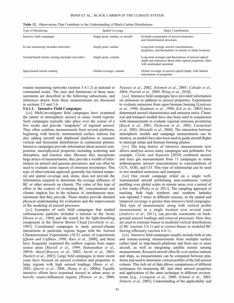
routine monitoring networks (section 5.4.1.2) at national orcontinental scales. The uses and limitations of these mea-surements are described in the following subsections, andinferences drawn from these measurements are discussedin sections 5.5 and 5.6.5.4.1.1. Intensive Field Campaigns[264] Multi-investigator field campaigns have examined

the nature of atmospheric aerosol in many world regions.Such campaigns typically take place over the course of afew weeks and provide “snapshots” of regional aerosol.They often combine measurements from several platforms,beginning with heavily instrumented surface stations butalso adding aircraft and shipboard platforms to measurevertical and horizontal distributions in continental plumes.Intensive campaigns provide information about aerosol com-position, microphysical properties including scattering andabsorption, and reaction rates. Because they incorporatelarge arrays of measurements, they provide a wealth of infor-mation on aerosol and gaseous precursors, and can often beused to evaluate some aspects of emission inventories. Thistype of observational approach generally has limited tempo-ral and spatial coverage and, alone, does not provide theinformation required to determine the average influence ofBC or other aerosols on climate. The value of this type ofeffort in the context of evaluating BC concentrations andclimate impacts lies in the richness of simultaneous mea-surements that they provide. These studies provide detailedphysical understanding for evaluation and the improvementof the modeling of aerosol processes.[265] Examples of early field campaigns that studied

carbonaceous particles included a mission to the Arctic[Rosen et al., 1984] and the search for the light-absorbingcomponent in the Denver Brown Cloud [Groblicki et al.,1981]. Coordinated campaigns to study aerosol-climateinteractions in particular regions began with the AerosolCharacterization Experiments (ACE) series of experiments[Quinn and Coffman, 1998; Raes et al., 2000], and thesehave frequently examined the outflow regions from majorsource areas [Russell et al., 1999; Ramanathan et al.,2001b; Mayol-Bracero et al., 2002; Jacob et al., 2003;Huebert et al., 2003]. Large field campaigns in more recentyears have focused on aerosol evolution and properties inlarge regions with high aerosol loadings [Bates et al.,2005, Querol et al., 2008, Zhang et al., 2008a]. Equallyintensive efforts have examined aerosol in urban areas orheavily source-influenced regions [Watson et al., 2000;

Neususs et al., 2002; Solomon et al., 2003; Cabada et al.,2004; Parrish et al., 2009; Wang et al., 2010].[266] Intensive field campaigns have provided information

on emissions in addition to aerosol properties. Experimentsto evaluate emissions from open biomass burning [Lindesayet al., 1996; Kaufman et al., 1998; Eck et al., 2003] havedetermined aerosol characteristics and emission ratios. Chem-ical and transport models have also been used in conjunctionwith measurements to evaluate regional emission inventories[Rasch et al., 2001; Dickerson et al., 2002; Carmichaelet al., 2003; Minvielle et al., 2004]. The interaction betweenatmospheric models and campaign measurements can beiterative, as models have also been used to guide aircraft flightsto intercept urban and biomass burning plumes.[267] The long history of intensive measurements now

allows analyses across many campaigns and pollutants. Forexample, Clarke and Kapustin [2010] combined aerosoland trace gas measurements from 11 campaigns to relateanthropogenic aerosol concentrations to concentrations ofCCN, AOD, and CO. This type of relationship can be usedto test modeled emissions and transport.[268] One recent campaign relied on a single well-

instrumented aircraft performing near-continuous verticalprofiling over global scales in remote areas over a period ofa few weeks [Wofsy et al, 2011]. The sampling approach ofreaching both high northern and southern latitudeswas repeated 5 times in different seasons, so the spatial andtemporal coverage is greater than intensive field campaigns.This type of measurement, along with vertical profilemeasurements in a single location over several years[Andrews et al., 2011], can provide constraints on back-ground aerosol loadings and removal processes. Here theyare used to estimate biases in modeled vertical distributionsof BC (section 5.6.1) and to correct biases in modeled BCforcing efficiency (section 6.6.1).[269] Intensive field campaigns usually include both in situ

and remote-sensing measurements from multiple surface(either land- or ship-based) platforms and from one or moreaircraft, as well as integrating satellite remote sensingmeasurements. Research aircraft often fly over surface stationsand ships, so measurements can be compared between plat-forms and used to determine vertical profiles of the full aerosolcolumn. This rich set of data allows comparisons of differenttechniques for measuring BC and other aerosol propertiesand applications of the same technique in different environ-ments [e.g., Livingston et al., 2000; Schmid et al., 2003;Doherty et al., 2005]. Understanding of the applicability and

Table 12. Observations That Contribute to the Understanding of Black-Carbon Distributions

Type of Monitoring Spatial Coverage Major Contributions

Intensive field campaigns Single point, surface, or aircraft In-depth examination of aerosol propertiesand transformation processes

In situ monitoring (includes networks) Single point, surface Long-term average aerosol concentrations,properties, and fluctuations in remote or urban locations

Ground-based remote sensing (includes networks) Single point, column Long-term averages and fluctuations of aerosol opticaldepth and inferences about other optical properties, oftenwith unattended operation

Space-based remote sensing Global coverage, column Global coverage of aerosol optical depth, with limitedinformation on properties


45

limitations of each type of measurement is fostered by com-parisons between properties measured at the surface, columnarproperties measured by satellite-based remote sensing, andvertically resolved information from aircraft measurements[e.g., Redemann et al., 2000; Magi et al., 2003].5.4.1.2. Long-Term In Situ Monitoring[270] Long-term monitoring networks usually combine

relatively simple measurement techniques with tens or evenhundreds of stations to create a widely spaced network ofobservations that operate under uniform techniques. Surfacesites may be influenced by orography and local sources,although such effects are usually considered when selectingsites. Because network sites are spatially sparse and haverelatively simple data products, they do not provide the samelevel of insight into the fine details of aerosol processes asintensive field campaigns. However, they do provide valuableinformation on aerosol trends and broad spatial concentrationpatterns, and these long records contribute strongly to evalua-tion of the modeling of emissions, transport, and removal.[271] Table 13 lists the major networks contributing infor-

mation on aerosol absorption and BC concentrations. Contin-uous in situ measurements to monitor pollution levels wereinitiated as early as 1962 [Novakov and Hansen, 2004]. TheIMPROVE network in the United States [Malm et al., 1994]and the European Monitoring and Evaluation Programme net-work in Europe [Kahnert et al., 2004] are among the mostextensive and have historically focused on chemical speciationrather than on aerosol properties. Stations participating in theWMO Global Atmosphere Watch monitor aerosol propertiesrelevant to climate, including light absorption, in a sparse,but worldwide, network of rural and remote sites that are pre-dominantly operated in the EUSAAR- and NOAA-coordi-nated sub-networks.While they have achieved broad coveragewithin their regions, similar coverage is not available in manyother world regions, such as South America and Africa. Mon-itoring stations are being developed throughout Asia [Oanh etal., 2006; Cao et al., 2007; Ramana and Ramanathan, 2006;Marcq et al., 2010], although coverage is still poor.[272] As multiple measurement locations are required to

evaluate emissions, transport, and removal processes in global

and regional models, measurements from all of these networkshave been used for model evaluation [Cooke et al., 2002; Parket al., 2003; Solmon et al., 2006; Koch et al., 2009b]. Mostnational networks have rigorous quality control proceduresthat ensure comparability of their measurements amongsimilar network stations. However, as discussed in section 3,important differences in sampling or measurement practicesmay affect comparisons between networks.5.4.2. Remote Sensing[273] Remote sensing methods measure changes in the

amount of sunlight reaching the Earth’s surface, or the amountof radiation leaving the Earth’s atmosphere, rather than theactual atmospheric BC or aerosol content. Through a processknown as inversion, the nature and quantity of aerosol isinferred from its observed physical effect on the light. Theprocedure is also called a retrieval, because aerosol propertiesare retrieved from observed changes in radiance. Radianceproperties that may be measured include wavelength depen-dence, angular distribution, and polarization. These can beused to infer the columnar amount of aerosol, the average aero-sol size, the presence of non-spherical particles (such as dust),and even estimates of columnar light absorption.[274] Advantages of remote sensing are the multi-year nature

of the measurements and the ability to obtain measurementswithout continuous maintenance. Remote measurements sensecolumn properties of aerosol, rather than concentrations at thesurface as are typically quantified by in situ measurements.Column properties are more directly relevant for quantifyingclimate impacts. The relationship between surface in situobservations and column data depends on many factors,including the stability of the boundary layer, the presence ofatmospheric layers, and measurement conditions that affectin situ and remote measurements differently. When in situmeasurements are made from an aircraft that profiles thedepth of the atmosphere, however, robust comparisons withcolumn-integrated remote sensing measurements are possible.Disadvantages of passive remote sensing include a lack ofspecificity to individual chemical species and an inability toretrieve the properties of aerosols in distinct layers indepen-dently, such as a dust layer overlying a pollution layer.

Table 13. Largest Global or Regional Ground-Based Observations Providing Long-Term Measurement Information Related to AerosolAbsorption or Black-Carbon Abundances in the Atmosphere

Network Location and # of Sites Dates Products Comments (Reference or URL)

AERONET World 400+ 1996–present AAOD (column) AOD*(1-SSA), less accuracy at lowerAOD (http://aeronet.gsfc.nasa.gov/)

IMPROVE US 100+ 1985–present Absorption coefficient, ECmeasurement (ground)

http://vista.cira.colostate.edu/improve/

EMEP Europe 70 1989–present PM and EC/OC (ground) http://www.emep.int/

WMO/GAW World 39 1994–present Absorption coefficient (ground) http://www.gaw-wdca.org/(EUSAAR 19 Europe,NOAA: 15 World)

http://www.eusaar.nethttp://www.esrl.noaa.gov/gmd/aero

ABC 10 2004–present Absorption coefficient, EC (ground) Ramanathan et al. [2007]Bonasoni et al. [2010]

AIRPET Asia 6 2001–2004+ EC/OC, BC by reflectance, PM2.5 (ground) Oanh et al. [2006]

CARIBIC 1 commercial aircraft 2005–Present Impactor with single-particle carbon content Nguyen et al. [2008]


46

http://aeronet.gsfc.nasa.gov/

http://vista.cira.colostate.edu/improve/

http://www.eusaar.net/

http://www.esrl.noaa.gov/gmd/aero/net/index.html

[275] Information from retrievals may be used to infer thecolumn burdens of chemical species that have distinctivephysical or optical characteristics. However, many assump-tions are required for these inferences, resulting in largeuncertainties, especially at low optical depths (low concen-trations). Furthermore, most remote sensing techniques canobtain valid data only in cloud-free conditions.5.4.2.1. Ground-Based Remote Sensing[276] The utility of ground-based remote sensing for

constraining BC atmospheric abundance is similar to thatof long-term in situ sampling. Networks of measurementscan be combined to evaluate model performance, but theydo not provide fine-scale or global coverage. However,unlike ground-based in situ measurements, they do measurethe whole atmospheric column which is more directlyrelevant to radiative forcing.[277] Passive, ground-based remote sensing with upward-

looking sun or sky photometers can be used to estimateAAOD. AERONET is the largest global network of thesephotometers [Holben et al. 1998;Dubovik et al., 2002]. Theseinstruments use informationmeasured at multiple wavelengthsand multiple angles by sun- and sky-photometers [Dubovikand King, 2000]. Properties derived from the sky radiancemeasurements include the aerosol size distribution, AOD,and refractive indices at four solar wavelengths; from this,single-scattering albedo can be determined. However, theretrieved refractive indices are obtained for the total aerosol.No distinction is made between the fine and coarse modeaerosol components, which are compositionally different andhave different refractive indices. Thus, when both dust andBC are present in an aerosol column, the retrieved imaginaryrefractive index (which dictates aerosol absorption) does notaccurately reflect that of BC alone.[278] We have calculated values of BCAOD from retrievals

of AAOD at AERONET sites and use these values in section 6to produce a scaled estimate of BC direct radiative forcing.The process of extracting BC AAOD from total AAODrequires certain assumptions. Limitations in the derivation ofAAOD and specifically BC AAOD are discussed next.[279] First, AAOD values are overestimated by the aver-

aged AERONET Version 2.0 data product. Values ofAAOD are based on aerosol extinction optical depth andsingle-scatter albedo, and single-scatter albedo can onlybe retrieved reliably for rather polluted conditions. For thisreason, the AERONET Version 2.0 values of AAOD arepublished only when AOD is greater than 0.33 at 550 nm.The exclusion of low-AAOD conditions introduces a sig-nificant sampling bias that Reddy et al. [2005b] estimateto be a factor of two. This issue, and its implication for in-ferred BC quantities, is explored further in section 6.5.1and Appendix B.[280] Second, not all solar absorption by aerosol is caused

by BC; some is due to dust and some to organic matter. Dustis less absorbing per mass than BC, but its AOD is oftenmuch larger. The net effect is that global average dustAAOD is comparable to that of BC AAOD but differentlydistributed in space and time. Thus, the BC contribution toAAOD needs to be isolated to use AERONET absorptionfor model evaluation. Dust particles tend to be larger thanBC particles, so retrieved size distribution data might beused to attribute absorption by super-micron particles todust, and absorption by submicron particles to BC and

light-absorbing organic matter. However, AERONETretrievals provide a single o0 and refractive index for theentire size distribution. Although this refractive index canbe used to estimate AAOD of the total aerosol, the composi-tion and, hence, the refractive indices and o0 of the separatefine and coarse modes may differ greatly [Quinn and Bates,2005]. As a consequence, a method is needed to apportionAAOD among the two modes. Separating the sub-micronAAOD into contributions of organic matter and BC wouldrequire a further inference not based on size distribution.The spectral absorption properties of the total aerosol havebeen combined with assumptions about the wavelengthdependence of absorption for dust, BC, and organic matterto estimate their contributions to AAOD [Arola et al.,2011; Chung et al., 2012].[281] Third, sample biases may occur because AERONET

AAOD retrievals are made only during daylight hours and incloud-free conditions. Two potential sources of bias opposeeach other. Clear conditions can be expected to favor largerconcentrations and column burdens of BC because fires aremore likely and because scavenging by clouds (i.e., theprimary removal mechanism for BC) cannot occur underclear skies. To estimate biases in retrievals of BC AAOD,we averaged modeled BC AAOD at AERONET locationsonly during days when AERONET retrievals were possible.Bias was determined by comparing with the average BCAAOD. For four AeroCom models, biases were regionallydependent, but the average was only 1%. This is consistentwith a small global clear-sky bias in AOD found by Zhangand Reid [2009]. Another factor is that solar absorption byBC is enhanced when BC is coated by water, which maybe much more likely in the vicinity of clouds. The modelof Jacobson [2010] estimated solar absorption enhancementto be a factor of 2 to 4, depending on the size of the BCparticle. Clear-sky measurements, which exclude partiallycloudy scenes, likely miss this near-cloud absorptionenhancement. To explore this sensitivity, we used theGATOR model [Jacobson, 2010], the only aerosol modelthat treats the full effect of optical focusing on absorption,to compare the AAOD for clear-sky versus all conditions.Although the global mean MACBC for cloudy conditions(14.4 m2g�1) was higher than that for clear-sky(13.9 m2g�1) conditions, the global mean burden wasgreater by 35% and BC AAOD was 20% higher for clearsky conditions than for cloudy conditions, so it is unlikelythat AERONET observations are missing large enhancedabsorption under cloudy conditions. However, this findingis not specific to AERONET sites or days of retrieval.[282] A method to infer BC column mass loading is to

determine the volume concentrations of components of aero-sol mixtures required to fit the AERONET retrieved totalcolumn refractive index. These can then be used, along withassumptions about densities, to determine the column massof each component, including BC [Schuster et al., 2005].The BC column mass uncertainty is estimated at �15% to+40%, although the imaginary refractive indices used affectthe retrieval and the AAOD. For analyses in this assessment,we use AAOD rather than inferred BC column loadings, asthe former requires fewer assumptions.5.4.2.2. Remote Sensing From Space[283] Knowledge of BC concentrations is needed in regions

with few or no ground sites, such as over oceans. Remote


47

sensing from space-borne sensors on satellites has near-globalcoverage and can, therefore, fill observational gaps in ground-based networks. AOD can be inferred from retrievals from sat-ellite data, but the procedure also requires general assumptionsregarding environmental properties (e.g., surface reflectance),and aerosol properties [Torres et al., 1998; Levy et al., 2007;Kahn et al., 2010], so that uncertainties are greater than thosein ground-based sensing. Satellite-based instruments that pro-vide data on column aerosol absorption and, therefore, infor-mation specific to constraining light-absorbing aerosol, arediscussed below.[284] The longest satellite data record on aerosol absorp-

tion, dating to 1978, is provided by the TOMS sensor (TotalOzone Mapping Spectrometer, http://jwocky.gsfc.nasa.gov/aerosols/aerosols_v8.html). The TOMS Aerosol Index is aretrieved quantity that indicates whether the column aerosolis largely absorbing or scattering. Over the last decade,TOMS-type retrievals have been continued with measure-ments from OMI (Ozone Measurement Instrument, http://disc.sci.gsfc.nasa.gov/Aura/data-holdings/OMI). This in-strument senses reflection and its spectral variability in theultraviolet region (UV) of the solar spectrum [Torres et al.,2002]. Aerosol retrieval at UV wavelengths has two advan-tages: first, surface contributions to the signal are small,especially over land, and second, small aerosols havestronger signals in the UV than at visible wavelengths. Onthe other hand, in addition to BC, both dust and organiccarbon contribute to UV absorption. Another complicationis a reduced sensitivity towards the surface, so that BC nearthe surface (approximately the lowest kilometer) may not bedetected. Therefore, a separate estimate of the verticaldistribution of aerosol is an essential element of the retrieval.In the past, the vertical profile of aerosol concentration wasprescribed using estimates from global modeling; morerecently, aerosol profiles inferred from the CALIPSOspace-borne lidar have been applied [Winker et al., 2010].Even with this constraint, this type of retrieval is mostlyuseful for identifying atmospheric aerosol from large eventssuch as biomass burning [Zhang et al., 2005].[285] Satellite-based aerosol sensors that provide spec-

trally resolved information allow general estimates of aero-sol size and separate contributions from fine and coarseparticles. Moderate Resolution Imaging Spectroradiometer(MODIS) sensors have the greatest temporal resolution[Remer et al., 2005]. Additional information on aerosolshape and difficult retrievals over bright surface come frompolarization sensing (e.g., POLDER) [Deuzé et al., 2001]and multiple views of the same scene (e.g., Multi-angleImaging Spectro-Radiometer (MISR)) [Kahn et al.,2009b]. Active remote sensing with a space-borne lidar(CALIPSO) [Winker et al., 2010] offers information onaerosol vertical distribution. This information may provideestimates of total aerosol amount, or even total fine-modeaerosol, but they do not constrain the amount of absorbingaerosol.[286] The satellite-based MISR instrument [Kahn et al.,

2009b] provides another constraint on aerosol absorption.The MISR instrument detects radiance at multiple anglesand multiple wavelengths. This additional information isused to estimate surface radiance, and it allows inversionfor additional aerosol properties, including estimates ofaerosol absorption. The MISR standard retrieval algorithm

identifies two to four classes of absorbing aerosol, ratherthan providing exact values of absorption. The atmospheremust be relatively uniform and cloud free, and the mid-visible AOD must be at least 0.15 or 0.2 [Chen et al.,2008; Kahn et al., 2009c].[287] While all these satellite-based instruments provide

some constraint on atmospheric absorption, several factorslimit their utility in determining global, annual averageBC AAOD. Signals reaching satellite-based sensors areinfluenced by both atmospheric constituents and by thereflectance properties of the Earth’s surface. This increasesthe uncertainty in AOD and, especially, AAOD, particularlyover spatially heterogeneous or highly reflective surfaces.Thus, quantitative atmospheric aerosol absorption cannotbe retrieved from existing satellite-based sensors. Conver-sion of AOD to AAOD requires use of an assumed columnaerosol single-scatter albedo, such as from a model[e.g., as employed by Chung et al., 2012]. Although satelliteretrievals may infer the separation between fine and coarseparticles, they cannot distinguish AOD from BC versus thatfrom other fine mode aerosols like OA or sulfate. The divi-sion must be estimated either from the relative magnitudeof modeled concentration fields or from ground-based obser-vations. The relatively coarse resolution at which mostsatellite sensors can provide retrieved aerosol fields alsomakes them susceptible to cloud contamination. Finally,while polar-orbiting satellites have nearly global coverage,data coverage at any given location is limited and does notalways allow for sufficient sampling for good statistics.

5.5. Comparison Between Modeled and Observed BCConcentrations and AAOD

[288] Estimates of forcing by individual aerosol species,including BC, are all based on aerosol distributions gener-ated by global chemistry transport models (CTMs). Evenestimates that incorporate observations require model resultsto expand concentration fields beyond observed locations orto separate observed aerosol influences among chemical spe-cies. Evaluation of BC concentrations in these models istherefore critical in assessing our understanding of climateforcing. A first-order evaluation of these models is accom-plished by comparing either simulated aerosol concentrationsor simulated optical depths with independent observations.This comparison requires long-term, spatially distributedaerosol measurements, so that observations from nationwideor global networks, such as the ones discussed above, are par-ticularly useful.[289] Comparisons between models and observations shed

light on our understanding of the quantity of BC in the atmo-sphere, but they often cannot distinguish between variouspossible causes of model error. For example, a model couldunderestimate atmospheric concentrations if its emissionsare too low or if its overall removal rate is too high.[290] Koch et al. [2009b] evaluated the AeroCom suite of

global models by comparing modeled BC concentrationswith observations from several intensive campaigns andlong-term in situ measurements. Figure 13 summarizes thiscomparison, showing the ratio between observed andmodeled surface concentrations of BC. The figure showsthat the median model predicts surface BC concentrationsin the North America fairly closely, slightly overestimatesBC in Europe, and clearly underestimates it in Asia. The


48

http://jwocky.gsfc.nasa.gov/aerosols/aerosols_v8.html

http://jwocky.gsfc.nasa.gov/aerosols/aerosols_v8.html

http://disc.sci.gsfc.nasa.gov/Aura/data-holdings/OMI

http://disc.sci.gsfc.nasa.gov/Aura/data-holdings/OMI

global annual average difference among models in this suitewas about 30% of the median concentration; variations in in-dividual seasons can be greater.[291] Koch et al. [2009b] also comparedmodeled fields with

values of AAOD inferred from AERONET. Modeled AAODwas lower than observed values in all regions. Column BCAAOD is the sum over altitude of the product of BC concen-tration and MACBC. Because most of the models used in thecomparison do not represent internal mixing, the modeledMACBC (section 3.7) was underestimated. This bias could ex-plain the disagreement in North America and Europe but not inother areas of the world. However, AAOD data were not sep-arated into contributions from BC and dust. A refined analysis,which considers this separation and incorporates moreAERONET stations, appears in section 6 and is more fully de-scribed in Appendix B.[292] The sources of differences between model predic-

tions are not completely understood. For any given location,the inter-quartile range of the concentrations predicted bythe 15 models participating in AeroCom was a factor ofabout 3, and the range excluding outliers was a factor ofabout 5 [Kinne et al., 2006; Schulz et al., 2006]. Kochet al. [2009b] provided sensitivity experiments to explorethe sources of this variability by using one model from thesuite (GISS, shown as symbols in Figure 13). Simulationswith different emission inventories are given in red, and

concentrations with removal rates increased or decreasedby a factor of 2 are shown as blue squares. Filled symbolsindicate base-case results. Varying removal rates and emis-sions do cause significant variations in a single model, butthese uncertainties do not explain most of the inter-modeldifferences. Textor et al. [2007] also found that inter-modeldifferences were only partially explained by differences inemission inventories. Large differences in modeled horizon-tal and vertical transport are largely responsible for thediversity. Once BC is lifted into the free troposphere,removal processes are slower, and its atmospheric lifetimemay be extended.[293] Figure 14 compares modeled and observed values of

BC AAOD. The left panel shows BC AAOD inferred fromAERONET observations (Appendix B). Although thesevalues include absorption by organic matter, we use themas our observational estimate for BCAAOD. Section 11.4 dis-cusses implications of this combination. Modeled BC AAODfrom the 15 AeroCom models are shown in the middle panelsof the figure. We use this particular collection because it con-tains a large number of consistent modeled fields, but this pre-sentation excludes subsequent improvements in many of thesemodels. The AAOD fields shown in Figures 12 and 14 arefrom the AeroCom “median model,” for which a median ofthe local (1� � 1� grid resolution) values from all AeroCommodels was calculated every month. These median fields,unlike averages, lose their additivity, but the use of medianvalues excludes the influence of individual outlier models.Figure 14 also presents differences in BC AAOD betweenco-located AERONET and model median values, showingthat these models tend to underestimate BC AAOD. Theregional dependence of model biases are discussed further insection 6.[294] The quantity and representativeness of observation

sites is fundamentally important in interpreting comparisonsbetween models and measurements. North America andEurope have the best coverage of all long-term measurementsites, followed by Asia. The number of sites is not in propor-tion to the strength of emissions, and concentrations inregions with large emissions and, therefore, highest aerosolforcing, are relatively poorly constrained.[295] Remote regions with low concentrations also have few

measurement sites and hence are also poorly constrained.Although aerosol forcing in these regions is small, their largespatial coverage means that contribution to the global-averageforcing may be important. Compared with BC concentrationsmeasured during a field campaign over the remote PacificOcean (Figure 15) [Schwarz et al., 2010], the median modeloverpredicted remote BC concentrations by a factor of 5.Some models, such as the lower quartile of the AeroCommodel suite or GATOR [Jacobson, 2012], show better com-parisons with these remote measurements.[296] Koch et al. [2009b] note that model diversity in

atmospheric BC concentrations is particularly high for theArctic. Models almost universally underestimated concentra-tions in the free troposphere during spring, and they did notmatch the observed decrease in concentrations from spring tosummer. This finding is based on a very limited data set fromintensive field campaigns, but it is consistent with multi-yearobservations from surface sites in the Arctic, which show thatmost models underestimate BC concentrations in the winterand spring and generally do not capture strong seasonal

Figure 13. Evaluation of model performance and modelsensitivities for simulating BC concentrations in surface airfor specific regions and the rest of the world. Box plots showratios between observations and models (i.e., the factor bywhich modeled values are multiplied to obtain observedvalues). The middle bar in each box shows the median modelvalue. Box boundaries show 25th and 75th percentiles. Datapoints outside 1.5 times the interquartile distance from thebox are marked as outliers; otherwise, they are included inthe whiskers. Symbols show sensitivity experiments usingdifferent emission databases (red triangles) and removal rates(blue squares) in a single model (GISS) with the base caseshown as filled symbols. For emission experiments, SPEWis shown with red fill and GAINS with black fill; unfilled sym-bols show results using two other emission databases. Thenumber of surface observations is shown below each regionname. Data from Koch et al. [2009b].


49

variations in boundary-layer BC concentrations [Shindell etal., 2008; Huang et al., 2010; Liu et al., 2011].5.5.1. Estimating Emissions by Integrating Models andObservations[297] The comparisons between modeled and observed BC

concentrations and column absorption described above are afirst step in evaluating model performance. More detailedevaluations have been conducted, usually focusing on infer-ring the most likely sources of error. The simplest of thesecompare the temporal or spatial dependence of atmosphericconcentrations with that given by models. More complexapproaches use a mathematically strict evaluation of sourcesand sinks using a formulation of Bayes’ theorem, whichhas been demonstrated for CO2, CO, and aerosols [e.g.,Chevallier et al., 2005; Dubovik et al., 2008; Chevallier

et al., 2009; Huneeus et al., 2012]. Evaluation methods thatuse measurements of atmospheric abundance in combinationwith modeled fields are broadly called inverse methods.Inverse modeling of gaseous concentrations on continentalscales, particularly CO and oxides of nitrogen (NOx), canalso provide information about emission sources. Althoughthis technique has usually been applied to infer emissions,it should not be forgotten that model processes such as trans-port and removal can also contribute to errors and that theinitial estimate of emissions has a strong influence on theinferred emissions. Here we summarize the results of inversemodeling studies that have focused on particular regions.[298] 1. North America. An inverse model by Hu et al.

[2009] found that USA BC emission estimates using datamainly from a rural network (IMPROVE) was about 30 to

Figure 14. Seasonal absorption aerosol optical depth (AAOD) at 550 nm due to BC as inferred from obser-vations and from models. The left panels show seasonal averages for BC AAOD at AERONET sites, as theywere derived from sky-inversion data that were sampled during the last decade (2000–2010). Each symbolrepresents an AERONET site. The middle panels show seasonal BC-AAOD median maps of AeroCommodels (listed in Table 14) for year 2000 conditions (see text for methods). The right panel shows differencesbetween the BC-AAOD values inferred from AERONET observations (left column) and AeroCommodelingefforts (middle column) at each location, illustrating deficiencies in global modeling of BC.


50

35% lower than an estimate that also included urban sites.This implies that in order to constrain concentrations oncontinental scales, measurements in high-concentrationareas should be included if models have sufficient resolu-tion, and that this inclusion may affect the total continentalburden of aerosol. There are also differences in the thermalevolution methods for measuring BC (section 3.3) betweenurban and rural sites in the United States. The former tendsto use a transmittance-corrected thermal-optical method,while the latter corrects using reflectance and heats thesample to a lower temperature. Before performing an inverseestimate, these authors had to multiply the transmittance-corrected values by factors ranging from 1.7 to 2.6,depending on the season. The resulting emission estimateswere similar to the bottom-up emission estimate in Figure 9.On the other hand, an inverse model by Park et al. [2003]estimated a BC emission rate of about 750 Gg yr�1, whichis about 70% higher than the bottom-up estimate.[299] Bhave et al. [2007] used organic markers to show that

USA emission estimates of total aerosol carbon (OC plus BC)from vehicle exhaust and biomass combustion were notbiased. They did find a large unexplained source of totalaerosol carbon unassociated with combustion, but this wouldnot affect BC totals.[300] Inverse modeling of carbon monoxide has indicated

that inventories overestimate fossil fuel sources in NorthAmerica by a factor of 3 in summer and two in spring[Miller et al., 2008]. Kopacz et al. [2010] found a largeunderestimation especially in winter, ascribing this differ-ence to heating and poor vehicle efficiency at cold tempera-tures. Although BC model results in the United States donot appear highly biased, these findings indicate thatsome small sources that could affect BC emissions are notwell understood.[301] 2. Europe. Tsyro et al. [2007] found that a model

based on the IIASA inventory underestimated BC concen-trations by about 20%. Significant overestimate andunderestimate of BC were correlated with concentrationsof levoglucosan, a tracer of wood smoke, indicating thatbiofuel or open biomass burning could be responsible forthe difference. Modeled concentrations were generally toohigh in Northern Europe and too low in Southern Europe.Mobile source emissions were thought to be underestimatedin Austria and some Eastern European countries.[302] 3. East Asia. Hakami et al. [2005] used BC concen-

trations observed in field campaigns to constrain emissionover eastern Asia. They found that the magnitude of the totalemission inventory given by Streets et al. [2003b] did notchange significantly as a result of the assimilation. However,anthropogenic emissions over southeastern China werereduced, while those in northeast China and Japan wereincreased. The increase in the industrialized regions is con-sistent with the low bias in estimates of CO emissions[Kasibhatla et al., 2002; Heald et al., 2004], which is morestrongly associated with the more northern industrializedregions [Yumimoto and Uno, 2006]. The observed CO biashas been largely resolved by improving the fraction of smallcombustors [Streets et al., 2006], as discussed in section4.6.5. Tan et al. [2004] suggested that modeled particulatecarbon emissions in East Asia should increase in order tobe consistent with observations, but they did not separateBC and OC nor account for the formation of secondary

organic aerosol, which could increase atmospheric con-centrations. Studies that compare ground and aircraftmeasurements with modeled BC values over the EastChina Sea estimate an annually averaged BC emissionflux of 1920 Gg yr�1 [Kondo et al., 2011a], close tobottom-up emission estimates for the late 2000s. Inversemodeling of NOx emissions in East Asia indicates rapidgrowth in high-temperature sources [Kurokawa et al.,2009], although high-NOx sources are presently a smallpart of the East Asian BC inventory.[303] 4. South Asia. Rasch et al. [2001] estimated that

increases of about 10 to 20% in fine-mode aerosols wereneeded in the model to match satellite observations overSouth Asia, but this study did not specifically identify biasesin BC. Dickerson et al. [2002] suggested a BC emission rateof 2000–3000 Gg yr�1, much higher than bottom-up esti-mates, based on atmospheric ratios of BC and CO that aremuch higher than is given by bottom-up estimates. Menonet al. [2010] also find that modeled concentrations in SouthAsia are much too low compared with in situ measurements.[304] The inverse modeling studies discussed above rely

on in situ data from a small number of sites to representcontinental-scale concentrations of aerosols. Satellite mea-surements have much broader spatial coverage and couldproduce global emission estimates. This approach has beenapplied in biomass burning regions, where optical depthsare large and seasonal. Freitas et al. [2005] found that emis-sion estimates derived from observed AOD were larger thanbottom-up estimates. Zhang et al. [2005] used aerosol indexfrom the TOMS instrument to estimate BC from biomassburning as 5700 to 6900 Gg yr�1, depending on the assump-tions used, and total smoke (BC plus OM) emissions as60,000 to 73,000 Gg yr�1. Reid et al. [2009] estimated thatbottom-up emission estimates of particulate matter from bio-mass burning need to be enhanced by factors of 1.5 to 3. Theglobal emission flux derived for 2006 to 2008 was about140,000 Gg yr�1, as compared with the value of 30,000 to44,000 Gg yr�1 BC plus POA given in section 4.4.4, ifOA is assumed to be 1.4 times OC. Similarly, Kaiser et al.[2012] derived a global average enhancement factor of 3.4for the OA and BC resulting from biomass burning, summa-rizing several other top-down studies that recommendedemissions 2–4 times larger than the bottom-up estimates.These studies indicate that BC emissions from biomassburning should be much larger than represented in models,although they may not scale linearly with total aerosol emis-sions. However, the fraction of the discrepancy attributableto BC is uncertain. Formation of SOA may contribute tothe observed OA and particulate matter loading.[305] In summary, inverse modeling studies have

produced inconsistent results for North America, indicatingthat either BC emissions are estimated well or are too lowby 70%. European BC concentrations appear slightlyunderestimated. East Asian concentrations appear reason-able, especially after the addition of small combustors.Although observations are limited, measurements in SouthAsia suggest that concentrations are greatly underestimatedthere. All of the studies described have used single modelsand await further confirmation. On the other hand, there isa consensus that aerosol concentrations, including BC, maybe too low in biomass burning regions. Considering alsothe likely bias in emission factors (section 4.7.2.3), emission


51

values that are greater than bottom-up estimates appearwarranted.

5.6. Vertical Distribution of BC

[306] As discussed in sections 6 and 7, the vertical distri-bution of absorbing aerosol affects its forcing. Verticallyresolved measurements below 8 km of the refractory aerosolconcentration, which correlates strongly with BC concentra-tion, have been carried out since the 1990s [Clarke andKapustin, 2010]. Remotely piloted airborne sensors havemeasured optical properties and total aerosol absorptionbelow 3 km [Corrigan et al., 2008].[307] BC vertical profiles extending through the tropo-

sphere have been made with a variety of measurementmethods, but the development of the SP2 instrument(section 3.5) has allowed measurements of vertical profilesof BC in very clean air where they were previouslyunobtainable [Schwarz et al., 2006, Schwarz et al., 2010].These profiles extend vertically from near the surface tothe lower stratosphere, as shown in Figure 15. AlthoughBC vertical profiles are quite variable, in polluted regionsthey generally show a declining BC mass mixing ratio fromthe surface to about 4 km altitude, and relatively constantvalues up to well above the tropopause. However, in remoteregions influenced by the transport of pollution from sourceregions, BC loadings tend to peak in the free troposphere orabove. BC that has been lifted above the low altitude rangeswhere aerosol removal is fast due to precipitation is morelikely to have a longer lifetime in the atmosphere.

[308] Important BC properties, such as mixing state(section 3), also change with altitude. One set of vertical pro-file observations in the tropics indicates that the coatings ofBC-containing particles become thicker and more prevalentwith increasing altitude between the surface and the lowerstratosphere [Schwarz et al., 2008a]. The fraction of coatedBC particles and the acquired coating mass depend on boththe BC source and the history of the particle and the air itis contained in. Thus, MACBC (section 3.8) can be expectedto depend on altitude.5.6.1. Comparison Between Modeled and ObservedVertical Distributions[309] Correctly modeling the vertical distribution of AAOD

is important for calculations of direct radiative forcing, asdiscussed in section 6.6.1. Schwarz et al. [2010] comparedthe AeroCom set of models with a global-scale “snapshot”of SP2 BC measurements from remote locations (Figure 15).The AeroCom model ensemble captured the vertical trendsof BC concentration in the southern mid to high latitudes,but in northern middle and equatorial latitudes, the modelsunderestimated the decrease in concentration with altitude.This comparison in regions far from sources suggests thatmodeled removal of BC is an important source of error. How-ever, the aircraft data in this comparison were obtained over alimited time range; in particular, the profile for the northern-most band (60–80�N) was from a single flight. Koch et al.[2009b] also compared BC vertical distributions betweenAeroCom models and SP2 measurements from several inten-sive field campaigns, mainly over North America and the

Figure 15. Airborne, in situ measurements of BC made in the remote Pacific Ocean between 80�N and67�S in January 2009 using an SP2 instrument. Upper left panel: average measured BC mass concentra-tions observed in five latitude bands with whiskers representing atmospheric variability. In the additionalpanels, colored lines repeat the observed average profiles and include the range of BC mass mixing ratiosfrom the AeroCom model suite. The legend explains lines and shading used to represent model results.The whiskers are numerically symmetric about the average values but are omitted on the left side to sim-plify the presentation on a log scale. Adapted from Schwarz et al. [2010].


52

Arctic. That comparison indicated that models overestimatemiddle and upper troposphere BC at mid-latitudes, consistentwith Schwarz et al. [2010], but underestimate BC in the Arctic.In urban areas, model predictions of column loadings wereconsistent with observations [Schwarz et al., 2006], but thevertical distribution was not well predicted.[310] Observations of the vertical distribution of AOD have

become available in recent years with active remote sensing bythe space-borne CALIOP lidar [Winker et al., 2010], for whichmulti-year averages are shown in Figure 16. AOD includesscattering and absorption by BC, dust, and other aerosol types(e.g., sulfates, organics, and sea salt) with sizes greater than0.1mm diameter [Omar et al., 2009]. Although chemical spe-ciation is not possible, limited inferences about aerosol typecan be obtained through depolarization data that identifynon-spherical particles and permit estimates of dust contribu-tions. Geographical distributions of full-column CALIOPAOD (Figure 16) are very similar to BC and dust AAOD fromAeroCom models (Figures 12 and 14), with high loadings inSouth and East Asia, the Middle East, Africa, and Latin Amer-ica. Maximum total AAOD values are a few percent of maxi-mum AOD values. The panels in Figure 16 show that AOD isconfined largely to altitudes below about 4 km. Although

interpretation of CALIOP data is still undergoing refinement,these data also indicate that models tend to place aerosol athigher altitudes than is observed [Koffi et al., 2012].

5.7. Causes of Model Biases

[311] The comparisons between models and observationsand the inverse model studies discussed above provide someconsistent messages regarding modeled atmospheric distri-butions of BC. In the following sections, these observationsare used to adjust modeled BC AAOD and direct radiativeforcing (section 6) and cloud forcing (section 7). The sourceof these model biases is less clear. Large underestimates inmodeled BC concentrations strongly argue that there arelow biases in emission estimates. However, it is difficult toattribute these biases wholly to errors in model emissions,because transport patterns and removal rates can also affectspatial distributions. Transport and removal rates are notindependent factors, because aerosol transported to higheraltitudes is less likely to be removed and, therefore, has alonger lifetime and greater horizontal transport.[312] At least one model sensitivity study [Koch et al.,

2009b] (section 5.5; Figure 13) indicates that varyingremoval rates by a factor of 2 cannot fully explain the

Figure 16. Multi-year averages of the global vertical distribution of mid-visible (532 nm) AOD from theCloud-Aerosol Lidar with Orthogonal Polarization (CALIOP) spaceborne lidar on the NASA CALIPSOsatellite. The panel colors show average AOD derived from CALIOP observations from June 2006 toDecember 2011 (version 3) for specific altitude intervals referenced to sea level (see legends). The colorbar has separate scales for the 0 to 6 km and full-column data panels as indicated. The full-column AOD isshown in the bottom right panel. The gray shading indicates “no observations” usually because of elevatedland surfaces. CALIOP statistics were provided by D.Winker of NASA Langley Research Center (Hampton,VA, USA).


53

inter-model range in concentrations or the bias betweenmodels and observations. Significant overestimates in BCconcentrations over the remote Pacific are consistent withvertical transport that is too strong or scavenging rates thatare too low, but significant underestimates in concentrationsin the Arctic free troposphere indicate opposite biases inthese processes. Across-the-board adjustments such as alter-ing wet scavenging rates may improve biases in one regionbut make them worse in another. It is likely that differentregions have different sensitivities to each of these pro-cesses, requiring focused studies in regions where biaseshave been observed. For example, Garrett et al. [2010] ar-gue that scavenging plays a dominant role in controllingArctic BC distributions, but this may not be true in other re-gions such as the remote Pacific. Concentrations nearsources are most sensitive to emissions, while concentra-tions in remote regions depend on transport and removalas well as emissions. Although concentration biases couldbe reduced by first constraining emissions with near-sourceconcentration measurements and then focusing on transportand removal using measurements downstream from sources,such an activity is beyond the scope of this study, which in-stead resorted to an after-simulation adjustment that can be ap-plied to all previous simulations that save the requisiteinformation.

5.8. Summary of Limitations in Inferring BlackCarbon Atmospheric Abundance

[313] Like all aerosols, BC concentrations are spatially andtemporally variable. No measurement strategy provides globalcoverage of BC concentrations or of AAOD. Space-based sen-sors have varying limitations: they detect aerosol abundancebut not composition (MODIS), provide qualitative measure-ments of absorption (MISR), or preferentially detect BC atgreater altitudes (OMI). Estimating global distributions ofBC or absorbing aerosol must therefore rely on modeled aero-sol fields, which in turn are constrained by ground-basedobservations. Ground-based AERONET stations are wide-spread and produce reasonably accurate AAOD, but coverageis not complete and techniques to separate BC, OM, and dustabsorption from these observations are not yet mature. In situsurface measurements have less coverage than AERONETbut greater specificity in identifying individual species. Thesemeasurements have been used to broadly evaluate modeledglobal fields and to assess modeled emissions in selectedregions. However, observations are sparse in some of theregions with the greatest emissions. A systematic evaluationof model biases caused by emissions, removal rates, and verti-cal transport, leveraging near-source and remote measure-ments, has not yet been accomplished.

6. Black-Carbon Direct Radiative Forcing


[314] 1. Black carbon in the atmosphere reduces theplanetary albedo by increasing the absorption of sunlight.The perturbation in the radiative balance resulting fromthis change is called black-carbon direct radiative forcing(BC DRF).[315] 2. The best estimate for the BC DRF in the industrial-

era is +0.71 W m�2 with an uncertainty range of +0.08 to+1.27 W m�2. The best estimate of the global annual mean

all-source BC DRF is +0.88 W m�2 with an uncertainty of+0.17 to +1.48 W m�2. Locally, BC-DRF forcing can belarger, on the order of +10 Wm�2, for example, over regionsof East and South Asia. These values are estimated by scalingmodeled forcing to the observationally constrained estimateof BC absorption aerosol optical depth (BC AAOD) and re-ducing the estimated forcing by 15% to account for the incor-rect vertical distribution of BC. Our estimate of BC AAOD in-cludes absorption by organic aerosol (OA).[316] 3. Most BC-DRF estimates originate with simula-

tions of BC lifecycle and radiative transfer using globalaerosol models. To improve confidence in these estimates,model-derived fields, such as aerosol optical depth, BCAAOD, or BC distributions, are often adjusted to match ob-servations of AOD, BC AAOD, or concentration, either bydirect scaling or by tuning removal rates.[317] 4. BC DRF can be considered the product of four

factors: emissions, lifetime, mass absorption cross section(MACBC), and radiative forcing per unit absorption opticaldepth (termed forcing efficiency). Diversity in previousglobal annual estimates of industrial-era BC DRF (+0.2 to0.9 W m�2) is caused by variations in modeling assump-tions, as evident in the modeled diversity of these fourfactors: 6000 to 18,000 Gg yr�1 for industrial-era BC emis-sions, 3.8 to 11.4 days for BC lifetime, 4.4 to 13.4 m2g�1 forMACBC, and 90 to 270 W m�2 per AAOD for forcingefficiency.[318] 5. BC emissions, lifetime, and mass absorption cross

section—three of the governing factors—combine to pro-duce BC AAOD, which can be constrained by measure-ments. Comparison with remote-sensing fields indicates thatBC AAOD from most models appears too low. Applyingregionally dependent scale factors to match observationsincreases globally averaged, industrial-era BC AAOD by afactor of 2.9, from 0.0017 to 0.0049. Some of the underesti-mate can be attributed to the lack of modeled enhancedabsorption due to internal mixing, which would increaseBC AAOD by about 50%.[319] 6. If the remaining model bias is caused by burdens

that are too low, then model burdens should be increasedby factors of 1.75 to 4 in five regions (Africa, South Asia,Southeast Asia, Latin America, Middle East, and the Pacificregion). Simulated burdens in North America, Europe, andCentral Asia are approximately correct considering uncer-tainty in BC AAOD and MAC.[320] 7. The altitude of BC in the atmosphere and its lo-

cation relative to clouds affects its interaction with solarradiation and hence the forcing efficiency. Solar absorp-tion by BC above low clouds is particularly importantand is poorly constrained in models. Limited observa-tions suggest that most models overestimate high-altitudeBC at tropical and mid-latitudes and, thus, BC DRF. Ourcentral estimate of forcing includes a 15% reduction toaccount for this bias.[321] 8. If all of the differences in modeled burden were at-

tributed to emissions, global emissions would be 17,000 GgBC yr�1, or an 87% increase above modeled emissions and a100% increase above the bottom-up emissions in section 4.Industrial-era emissions would be 13,900 Gg BC yr�1.These values are associated with concentrations in approxi-mately the year 2005. We use the latter value as a bestestimate of emissions throughout the remainder of this


54

assessment, although poorly modeled aerosol lifetimes couldalso explain the discrepancies.[322] 9. The interpretation of remote-sensing data involves

assumptions that affect the amount of absorption and, hence,radiative forcing, that is attributed to BC versus dust. Uncer-tainties in this division are responsible for nearly half theuncertainty in BC forcing.[323] 10. If OA does contribute significantly to absorp-

tion at 550 nm, then our estimate of observationallyconstrained BC DRF is biased high, but total forcing byOA would correspondingly become less negative or morepositive. About 10% of our BC AAOD may be due toabsorption by OA.[324] 11. The uncertainty range (+0.08 to +1.27 W m�2)

for the best estimate of industrial-era BC DRF includes rel-ative uncertainties of about 40% associated with the extrap-olation of global BC AAOD, about 50% in the radiativeforcing efficiency per unit BC AAOD, and asymmetric un-certainty due to the difficulty in separating BC AAOD fromdust AAOD.

6.2. Introduction

[325] Direct radiative forcing by BC refers to the change inthe energy balance at the top of the atmosphere due toabsorption and scattering of sunlight by BC in the atmo-sphere. All estimates of BC DRF are based on the differencebetween radiative transfer calculations for the atmospherewith present-day BC and with a background level of BC.The BC spatial distribution is generally taken from globalmodels of the BC atmospheric lifecycle, which includesemissions, transport, aging, and removal. As described insection 2.3.2, the background level of BC for industrial-eraradiative forcing is set by models using year-1750 emis-sions. For all-source radiative forcing, the background levelof BC is zero. Thus, “industrial-era” in this section, whenused for any quantity including BC burden, means the differ-ence between modeled quantities with present-day emissionsand the same quantities modeled with 1750 emissions.[326] As with aerosol concentrations, radiative forcing is

highly variable in space and time. Global modeling of BCconcentrations [Liousse et al., 1996; Cooke and Wilson,1996] and radiative forcing [Penner et al., 1998] began inthe middle to late 1990s. Since then, many groups haveestimated both concentration and radiative forcing fields.An example of modeled direct forcing is illustrated inFigure 17, which shows radiative forcing simulated by theCommunity Atmosphere Model CAM5 [Ghan et al.,2012]. As discussed in section 2.3.2, any estimated indus-trial-era forcing depends on the selection of the“preindustrial background.” Industrial-era BC DRF is esti-mated to be negative in regions such as the eastern UnitedStates and the United Kingdom, due to declines in biomassburning since 1750. However, the emission inventoriesused for the background are associated with considerableuncertainties, especially for open burning. The largest forc-ing is over the Congo Basin in Africa and southeast China,and Bangladesh, with significant forcing also in the AmazonBasin, over northern India and Indonesia, and off the easterncoasts of South America and Africa where BC is transportedover low clouds from distant fires.[327] To understand the factors that affect radiative forcing

in models, it is useful to express the global-mean direct

radiative forcing by BC, BC DRF, as the product of four fac-tors [Schulz et al., 2006]:

BC DRF ¼ E � L�MACBC � AFE (6.1)

where E is the global mean BC emission rate, L is the globalmean lifetime of BC governed by removal, MACBC is theglobal-mean mass absorption cross section discussed insection 3.7.3.3, and AFE is the global mean absorptionforcing efficiency (forcing per aerosol absorption opticaldepth). This relationship is summarized in Figure 18. Three-dimensional models simulate many complex processes thatare captured only to first order by the factors in equation (6.1).[328] Additional diagnostics shown in Figure 18 can be

used to compare model results and identify the reasons fordifferences in simulated radiative forcing. Modeled L canbe determined from the ratio of global mean column burdenof BC to E, and global average MACBC is the ratio of theglobal mean absorption optical depth of BC to the globalmean burden. Modeled AFE can be determined from the ra-tio of the global mean BC radiative forcing to BC AAOD,which is the global mean product of E, L, and MACBC.BC AAOD is a particularly powerful diagnostic that canbe compared with atmospheric measurements and is there-fore emphasized in this section. Although AOD can alsobe used to evaluate modeled aerosol quantities, atmosphericAOD is dominated by scattering and thus has large contribu-tions from other non-absorbing aerosol components.[329] Table 14 summarizes modeled global mean esti-

mates of each term in equation (6.1) as well as other modeldiagnostics. Many of these models were used as the basisfor IPCC radiative forcing estimates [Forster et al., 2007].Estimates of industrial-era BC DRF range from +0.2 to+0.9 W m�2. The large diversity is due to differentmodel choices that affect one or more of the factors in equa-tion (6.1). Global emissions of BC range from 5700 to

Figure 17. Annualmean direct radiative forcing by BC from1850 to present day, as estimated by the CAM5 AeroCommodel and adjusted according to the global annual-meanBC-AAOD scale factor of 3.0 derived in the comparison withAERONET observations (Table 15 and section 6.7.1). Forcingis negative in regions where biomass or fossil fuel (e.g., coal)emissions were large in 1850. Year 1750 emissions from theseregions would be lower, so the total radiative forcing would bemore positive. Based on Liu et al. [2012] and Ghan et al.[2012].


55

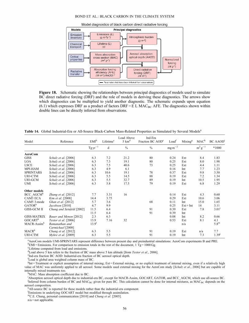
Table 14. Global Industrial-Era or All-Source Black-Carbon Mass-Related Properties as Simulated by Several Modelsa

Model Reference EMIb LifetimecLoad Above

5 kmdInd-Era

Fraction BC AODe Loadf Mixingg MACh BC AAODi

Tg yr�1 d % % mgm�2 m2 g�1 *1000

AeroComGISS Schulz et al. [2006] 6.3 7.2 21.2 80 0.24 Ext 8.4 1.83LOA Schulz et al. [2006] 6.3 7.3 19.1 80 0.25 Ext 8.0 1.98LSCE Schulz et al. [2006] 6.3 7.5 40.6 73 0.25 Ext 4.4 1.11MPI-HAM Schulz et al. [2006] 6.3 4.9 6.1 0.16 Int 7.7 1.23SPRINTARS Schulz et al. [2006] 6.3 10.6 19.1 78 0.37 Ext 9.8 3.50UIO-CTM Schulz et al. [2006] 6.3 5.5 14.5 88 0.19 Ext 7.2 1.34UIO-GCM Schulz et al. [2006] 6.3 5.5 32.7 89 0.19 Int 10.5 1.95UMI Schulz et al. [2006] 6.3 5.8 17.5 79 0.19 Ext 6.8 1.29

Other modelsBCC_AGCMk Zhang et al. [2012] 7.7 3.31 16 0.14 Ext 4.3 0.60CAM3 ECA Kim et al. [2008] 14.4 3.75 0.29 Ext 10.6 3.06CAM5 3-mode Ghan et al. [2012] 5.7 3.6 68 0.11 Int 15.0 1.65GATORk Jacobson [2010] 4.7 9.9 0.25 Ext + Int 14 3.11GISS-GCM II Chung and Seinfeld [2002] 11.5 6.4 91 0.39 Ext 7.8 3.01j

11.5 6.4 91 0.39 IntGISS-MATRIX Bauer and Menon [2012] 2.3 6.3 0.08 Int 8.2 0.66GOCARTk Textor et al. [2006] 13.9 7.16 32 0.53 Ext 8.1 4.1MACR-Assimk Ramanathan and

Carmichael [2008]13.9l n/a 5.8m

MACRk Chung et al. [2012] 6.3 5.5 91 0.19 Ext n/a 7.7UIO-CTM Myhre et al. [2009] 6.3 5.5 91 0.19 Int 7.3 1.39j

aAeroCom models UMI-SPRINTARS represent difference between present day and preindustrial simulations: AeroCom experiments B and PRE.bEMI =Emissions. For comparison to emission totals in the rest of the document, 1 Tg= 1000Gg.cLifetime computed from load and emissions.dLoad above 5 km refers to the fraction of BC mass above 5 km altitude [from Textor et al., 2006].eInd-era fraction BC AOD: Industrial-era fraction of BC aerosol optical depth.fLoad is global area weighted column mass of BC.gInt = Treatment or explicit assumption of internal mixing; Ext =External mixing, or no explicit treatment of internal mixing, even if a relatively high

value of MAC was uniformly applied to all aerosol. Some models used external mixing for the AeroCom study [Schulz et al., 2006] but are capable ofinternally mixed treatments too.

hMAC: Mass absorption coefficient due to BC.iAbsorption aerosol optical depth due to industrial-era BC, except for MACR-Assim, GOCART, GATOR, and BCC_AGCM, which use all-source BC.jInferred from column burden of BC and MACBC given for pure BC. This calculation cannot be done for internal mixtures, as MACBC depends on the

aerosol composition.kAll-source BC is reported for these models rather than the industrial-era component.lEmissions in underlying GOCART model but modified through assimilation.mC.E. Chung, personal communication [2010] and Chung et al. [2005].n/a = not applicable.

Figure 18. Schematic showing the relationships between principal diagnostics of models used to simulateBC direct radiative forcing (DRF) and the role of models in deriving these diagnostics. The arrows showwhich diagnostics can be multiplied to yield another diagnostic. The schematic expands upon equation(6.1) which expresses DRF as a product of factors DRF=E L MACBC AFE. The diagnostics shown withindouble lines can be directly inferred from observations.


56

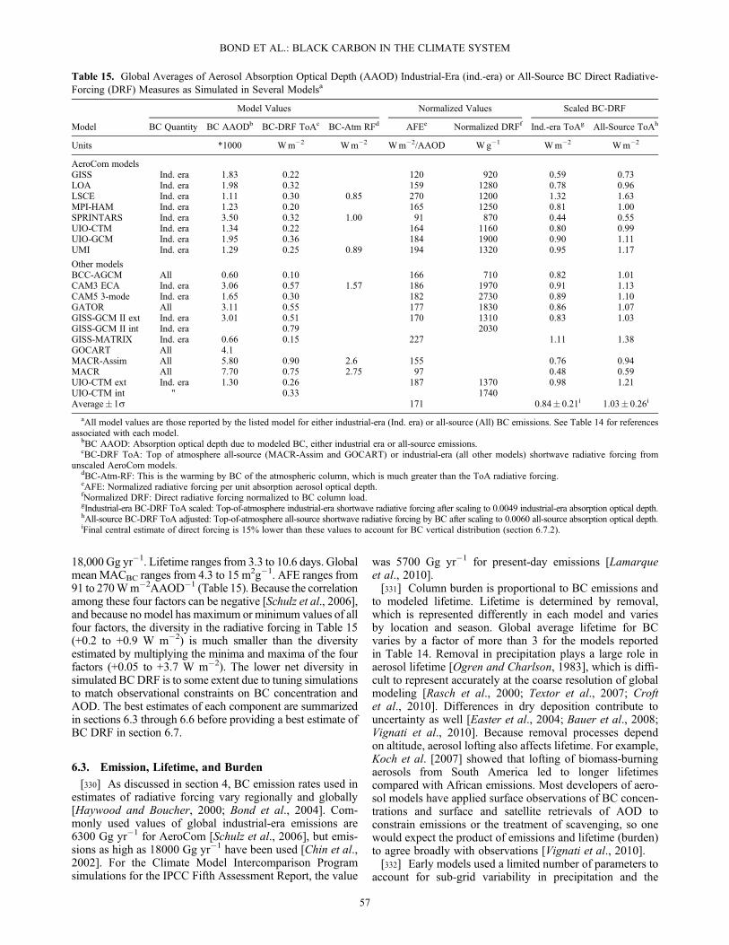
18,000 Gg yr�1. Lifetime ranges from 3.3 to 10.6 days. Globalmean MACBC ranges from 4.3 to 15 m2g�1. AFE ranges from91 to 270Wm�2AAOD�1 (Table 15). Because the correlationamong these four factors can be negative [Schulz et al., 2006],and because no model has maximum or minimum values of allfour factors, the diversity in the radiative forcing in Table 15(+0.2 to +0.9 W m�2) is much smaller than the diversityestimated by multiplying the minima and maxima of the fourfactors (+0.05 to +3.7 W m�2). The lower net diversity insimulated BCDRF is to some extent due to tuning simulationsto match observational constraints on BC concentration andAOD. The best estimates of each component are summarizedin sections 6.3 through 6.6 before providing a best estimate ofBC DRF in section 6.7.

6.3. Emission, Lifetime, and Burden

[330] As discussed in section 4, BC emission rates used inestimates of radiative forcing vary regionally and globally[Haywood and Boucher, 2000; Bond et al., 2004]. Com-monly used values of global industrial-era emissions are6300 Gg yr�1 for AeroCom [Schulz et al., 2006], but emis-sions as high as 18000 Gg yr�1 have been used [Chin et al.,2002]. For the Climate Model Intercomparison Programsimulations for the IPCC Fifth Assessment Report, the value

was 5700 Gg yr�1 for present-day emissions [Lamarqueet al., 2010].[331] Column burden is proportional to BC emissions and

to modeled lifetime. Lifetime is determined by removal,which is represented differently in each model and variesby location and season. Global average lifetime for BCvaries by a factor of more than 3 for the models reportedin Table 14. Removal in precipitation plays a large role inaerosol lifetime [Ogren and Charlson, 1983], which is diffi-cult to represent accurately at the coarse resolution of globalmodeling [Rasch et al., 2000; Textor et al., 2007; Croftet al., 2010]. Differences in dry deposition contribute touncertainty as well [Easter et al., 2004; Bauer et al., 2008;Vignati et al., 2010]. Because removal processes dependon altitude, aerosol lofting also affects lifetime. For example,Koch et al. [2007] showed that lofting of biomass-burningaerosols from South America led to longer lifetimescompared with African emissions. Most developers of aero-sol models have applied surface observations of BC concen-trations and surface and satellite retrievals of AOD toconstrain emissions or the treatment of scavenging, so onewould expect the product of emissions and lifetime (burden)to agree broadly with observations [Vignati et al., 2010].[332] Early models used a limited number of parameters to

account for sub-grid variability in precipitation and the

Table 15. Global Averages of Aerosol Absorption Optical Depth (AAOD) Industrial-Era (ind.-era) or All-Source BC Direct Radiative-Forcing (DRF) Measures as Simulated in Several Modelsa

Model Values Normalized Values Scaled BC-DRF

Model BC Quantity BC AAODb BC-DRF ToAc BC-Atm RFd AFEe Normalized DRFf Ind.-era ToAg All-Source ToAh

Units *1000 Wm�2 Wm�2 Wm�2/AAOD Wg�1 Wm�2 Wm�2

AeroCom modelsGISS Ind. era 1.83 0.22 120 920 0.59 0.73LOA Ind. era 1.98 0.32 159 1280 0.78 0.96LSCE Ind. era 1.11 0.30 0.85 270 1200 1.32 1.63MPI-HAM Ind. era 1.23 0.20 165 1250 0.81 1.00SPRINTARS Ind. era 3.50 0.32 1.00 91 870 0.44 0.55UIO-CTM Ind. era 1.34 0.22 164 1160 0.80 0.99UIO-GCM Ind. era 1.95 0.36 184 1900 0.90 1.11UMI Ind. era 1.29 0.25 0.89 194 1320 0.95 1.17

Other modelsBCC-AGCM All 0.60 0.10 166 710 0.82 1.01CAM3 ECA Ind. era 3.06 0.57 1.57 186 1970 0.91 1.13CAM5 3-mode Ind. era 1.65 0.30 182 2730 0.89 1.10GATOR All 3.11 0.55 177 1830 0.86 1.07GISS-GCM II ext Ind. era 3.01 0.51 170 1310 0.83 1.03GISS-GCM II int Ind. era 0.79 2030GISS-MATRIX Ind. era 0.66 0.15 227 1.11 1.38GOCART All 4.1MACR-Assim All 5.80 0.90 2.6 155 0.76 0.94MACR All 7.70 0.75 2.75 97 0.48 0.59UIO-CTM ext Ind. era 1.30 0.26 187 1370 0.98 1.21UIO-CTM int " 0.33 1740Average� 1s 171 0.84� 0.21i 1.03� 0.26i

aAll model values are those reported by the listed model for either industrial-era (Ind. era) or all-source (All) BC emissions. See Table 14 for referencesassociated with each model.

bBC AAOD: Absorption optical depth due to modeled BC, either industrial era or all-source emissions.cBC-DRF ToA: Top of atmosphere all-source (MACR-Assim and GOCART) or industrial-era (all other models) shortwave radiative forcing from

unscaled AeroCom models.dBC-Atm-RF: This is the warming by BC of the atmospheric column, which is much greater than the ToA radiative forcing.eAFE: Normalized radiative forcing per unit absorption aerosol optical depth.fNormalized DRF: Direct radiative forcing normalized to BC column load.gIndustrial-era BC-DRF ToA scaled: Top-of-atmosphere industrial-era shortwave radiative forcing after scaling to 0.0049 industrial-era absorption optical depth.hAll-source BC-DRF ToA adjusted: Top-of-atmosphere all-source shortwave radiative forcing by BC after scaling to 0.0060 all-source absorption optical depth.iFinal central estimate of direct forcing is 15% lower than these values to account for BC vertical distribution (section 6.7.2).


57

efficiency with which particles are scavenged. These scav-enging treatments used crude parameters that were appliedglobally. More advanced models treat the coating of BCwith hygroscopic material to form particles that are morereadily activated to form cloud droplets and scavenged moreefficiently. The representation of scavenging affects themagnitude and seasonality of BC concentrations, especiallyat remote locations [Croft et al., 2005]. Model representationof the BC seasonal cycle in the Arctic improves with moreaccurate microphysical treatments [Vignati et al., 2010;Lund and Berntsen, 2012; Park et al., 2011].[333] The global mean column burden of BC ranges from

0.11 to 0.53 mg m�2 in Table 14. The studies with the larg-est radiative forcing estimate (MACR-Assim) [Ramanathanand Carmichael, 2008; Chung et al., 2012] did not calculatea burden, but the BC simulation [Chin et al., 2002] thatthe studies relied on for absorption far from AERONET sites[Chung et al., 2005] had a global mean BC columnburden of 0.6 mg m�2. Some of the models did not constrainthe combination of emissions and lifetime with BC concen-tration measurements [Vignati et al., 2010], including themodel that estimated the largest BC burden (i.e.,SPRINTARS; Table 15) [Takemura et al., 2005]. Some ofthe diversity in the column burden of BC in Table 14 canbe attributed to differences in emissions. Yet many of the es-timates used the same BC emission inventory and stillyielded BC burdens differing by more than a factor of 2(0.16 to 0.38 mg m�2) due to differences in lifetime [Schulzet al., 2006]. As discussed in section 5.5, most modelssimulate surface BC concentrations within a factor of 2 ofmeasurements in most regions, with weak over-predictionsin Europe, underpredictions in biomass burning regions,and large underpredictions for eastern and southern Asia[Koch et al., 2009b].[334] Vertical lofting of BC affects its prospects for wet

scavenging and hence its lifetime. Vertical profiles of BCshow that simulated concentrations have large biases inthe free troposphere [Koch et al., 2009b]. High biasesof a factor of 3 to 15 (average 8) are found in tropo-spheric BC concentrations above the boundary layer attropical and subtropical latitudes, while most modelsunderestimate the BC concentrations in the Arctic tropo-sphere, on average by a factor of 2.5 [Koch et al., 2009b,Table 8]. Adjustments to simple scavenging treatments cannotreproduce these observed distributions; increased removal intropical regions would reduce the over-prediction at highaltitudes there (section 5.5) but would enhance the lowbias in the Arctic troposphere where abundances may becontrolled by scavenging processes [Garrett et al., 2010].However, improved treatments of scavenging may result ingreater fidelity.

6.4. Mass Absorption Cross Section

[335] Section 3.5 discussed measured and modeled MACof BC and particles that contain BC. Section 3.5 also sum-marized how mixing of BC with other aerosol componentswould increase MACBC, and field measurements have foundthat BC particles are largely mixed with other components.Since MAC depends on refractive index, water content,particle size, and mixing with other aerosol components,measured MACBC data provide a useful diagnostic

check for models when information about each variable isalso known.[336] The global mean MACBC listed in Table 14 ranges

from 4.3 to 15 m2g�1, with the AeroCom median aroundabout 6.5 m2g�1. Many models have MACBC values similarto the Bond and Bergstrom [2006] estimate of 7.5 �1.2 m2g�1 for freshly emitted, externally mixed BC, and afew others are close to the estimates of about 12.5 m2g�1

for internally mixed aerosol. Two models (LSCE andBCC-AGCM) are much lower than this range. If models thatassumed external mixing were excluded or adjusted for theincrease in MACBC, the model average MACBC and theaverage estimated DRF would increase [Jacobson, 2000;Myhre et al., 2009]. The internally mixed value of MACBC

may be an upper limit on the global mean value becausethe actual global mean depends on how much of the BC ismixed with other components throughout the atmosphere.[337] All global models that represent internal mixing

report a large increase in absorption and positive forcingfor internally mixed particles. Haywood and Shine [1995]reported doubled forcing due to internal versus externalmixing in a simple model. Jacobson [2001a] was the firstto confirm that finding with realistic BC spatial distributionsand accounting for the evolution of mixing state. Chung andSeinfeld [2002] found a forcing increase of 36% for BC withhomogeneous internal mixing compared with externalmixing. Bauer et al. [2010] included a core-shell representa-tion in a multi-modal model. Flanner et al. [2007] andMyhre et al. [2009] associated internally mixed values ofMACBC with aged BC, and Adachi et al. [2010] exploredseveral mixing assumptions in a global model. Model treat-ment of aging and mixing affects both absorption and life-time, often with compensating effects. Ghan et al. [2012]found that two treatments of BC produced similar forcingestimates, as internally mixed BC had higher MACBC butwas removed faster. Stier et al. [2006b] found regionaldifferences in which effect of BC mixing state dominates.

6.5. Scaling Modeled BC AAOD to Observations

[338] BC AAOD is the product of three of the factors thatdetermine BC DRF (i.e., E, L, and MACBC in equation(6.1)), and constraining this product can reduce uncertaintyin radiative forcing. In this section, we present an estimateof observationally constrained BC AAOD that is used toproduce scaled forcing estimates in section 6.7.[339] Measurements of AAOD are sparsely distributed,

and many models underestimate BC AAOD, as shown inFigure 14. In section 5.4.2.1, we cautioned that both sam-pling bias and dust absorption could produce a high bias inBC AAOD inferred from AERONET AAOD. Comparisonsbetween model and observationally derived total AAOD inKoch et al. [2009b] include contributions from both BCand dust. As a result, either or both BC and dust could beresponsible for model discrepancies. However, AAOD com-parisons for regions and seasons not affected by dust stillshow that many models simulate too little absorption in theatmosphere and, therefore, underestimate BC DRF.[340] To obtain an estimate of BC AAOD constrained

more closely by observations, a method was developed toscale modeled BC AAOD fields using BC AAOD inferredfrom the AERONET ground-based network. Appendix Bgives the details and background of this method. Briefly,


58

sampling biases in the AERONET retrievals of total AAODwere removed, and BC AAOD was estimated from totalaerosol AAOD by subtracting the contribution to AAODby dust. This process allocates all non-dust absorption toBC. To the extent that organic aerosol contributes to AAOD,our estimate of BC AAOD is biased high. Biases in theAeroCom median model BC AAOD were quantified bycalculating the ratio of the observationally constrained andmodeled values at the same month and location. The scalefactors so determined were then extended to other grid boxeswithin the region, including outflow from that region overthe ocean. This expansion of scale factors relies on thespatial distribution of BC in the AeroCom median model.[341] BC AAOD estimated this way is found to be much

greater than modeled BC AAOD, so the procedure increasesthe globally averaged estimate of total BC AAOD from0.0021 before scaling to 0.0060 after scaling. As discussedin section 6.9, causes of the resulting BC AAOD changeswould likely have affected preindustrial BC AAOD as well,so we applied the same scaling factors to preindustrial BCAAOD. Hence, the global mean industrial-era BC AAODincreases by the same factor, from 0.0017 before scaling to0.0049 after scaling. These increases in BC AAOD are large,but previous estimates that employ observations havealso found BC AAOD much greater than model values(section 6.8).6.5.1. Sensitivities in AAOD Scaling[342] A summary of modeled BC AAOD values before

scaling is presented in Table 15 and summarized inFigure 19. Industrial-era, global-mean BC AAOD frommodels without any scaling ranges from 0.0006 to 0.0035,with two models that included internal mixing giving values

above 0.0030 and the remainder lying within 30% of the me-dian value. Figure 19 also shows BC AAOD estimates scaledto observations for industrial-era sources and for all sources.For both scaled and unscaled fields, all-source BC AAOD ishigher than the industrial-era average by about 23%.[343] Error bars in the scaled estimates in Figure 19 reflect

uncertainty in the spatial distribution of BC in the modelused to extend scaling to regions without observations. Thisuncertainty is estimated by applying the full scaling proce-dure to three additional modeled fields (SPRINTARS,GOCART, and UMI) that were chosen to represent highand low average BC AAOD. The scaled value of globalBC AAOD ranges from 0.0046 for SPRINTARS to 0.0064for UMI, so the highest initial model field results in the low-est scaled value.[344] The BC AAOD values derived in Appendix B are

very sensitive to assumptions imposed in the use of theAERONET data fields, as discussed in Appendix B. Todemonstrate this, Figure 19 shows estimates of all-sourceBC AAOD with three different changes in basic assump-tions used in deriving BC AAOD from AERONET observa-tions. The revised AERONET fields are then used to rescalethe AeroCom model fields, and a new global estimate is cal-culated. First, BC AAOD is separated from total AAOD bycombining the AERONET size distribution for submicronparticles and the retrieved AERONET refractive index. Thismethod of separation reduces the mean BC AAOD from thebaseline estimate of 0.0060 to 0.0034 but does not accountfor the differing properties of submicron and super-micronaerosol. This method ascribes a relatively small AAOD toBC and a large AAOD to dust. Second, the selection ofAERONET stations introduces an uncertainty of 30%. When

Figure 19. Summary of the sensitivity of global BC-AAOD derived from AeroCom models. The scalingof AeroCom BC-AAOD values is based on AERONET observations following the method in Appendix Band discussed in section 6.5. Separate unscaled and scaled AeroCom model values are shown in Table 15.Data points (circles) are AeroCom median values. Ranges are shown with lines and uncertainty with whis-kers. Not shown on the figure due to limited scale is an estimate of scaling to average BC AAOD inferredfrom AERONET version 2.0 averages (0.0143). The sensitivity of scaled all-source BC-AAOD to keyassumptions in using the AERONET observations is shown for three cases (see text). Three other modelstudy results are shown at the bottom for comparison. Central estimates, value ranges, and uncertaintyranges are shown in the right-hand column.


59

four different subsets of stations were used for the scaling ofall-source BC AAOD, global averages ranged from 0.0057to 0.0071. The analysis presented here includes this uncer-tainty. Third, if all absorption were attributed to BC, themodeled BC-AAOD field would increase by a factor of1.33 to 0.0086. Fourth, the AERONET Version 2.0 dataexclude low-AOD conditions, so that average AAOD valuesin that dataset are biased high. If the AERONET Version2.0 data were used, estimated BC AAOD would increaseby a factor of 2.2, to 0.0143 (not shown in Figure 19 dueto limited scale). The interpretation applied here does notsuffer from this bias because of the method used to interpretthe AERONET data. BC-DRF estimates relying on averagesof published AERONET AAOD data cannot account for thisbias and are expected to be much greater than those derivedin this assessment. These sensitivity calculations highlightthe importance of clearly stating assumptions and theirconsequences when using AERONET observations to scalemodeled fields of absorbing aerosol. Other uncertainties inthis analysis, used to set bounds on BC DRF, are discussedin section 6.7.3.6.5.2. Reasons for Low Bias in Modeled AAOD[345] Because BC AAOD is the product of MACBC and

BC burden (section 6.2), the mismatch between modeledand observed BC AAOD may derive from errors in

modeling both factors. Apportionment is considered sepa-rately for AAOD resulting from open biomass burning andenergy-related combustion in the ten regions shown inFigures 7–9.[346] We first assume that the MACBC scale factor for all

months and regions is 1.5 (i.e., the approximate ratiobetween the MAC of internally and externally mixed BC).Most models in the Phase I AeroCom group described heredid not account for internal mixing, and the AeroCommedian BC AAOD at each grid box likely represents aerosolwith this lower MACBC. We also assume that AAOD attribut-able to open burning and energy-related sources are propor-tional to their emissions; that is, aerosol lifetimes from thetwo sources are similar in each month. The scaled BC AAODvalues for each source are then averaged over the year toproduce an annual BCAAOD and then divided by the originalBC AAOD to give an annually averaged scaling factor.[347] Figure 20 displays the annual scale factors for each

region and source group. Although our assumption of simi-lar lifetimes between the source groups may be questionable,the method should produce dissimilar scale factors if morecorrection is needed during months with high or lowbiomass burning. The bars for each scale factor show theportions attributable to BC burden (closed) and MACBC

(open). The middle panel of Figure 20 also shows the annual

Figure 20. Summary of regional BC aerosol absorption optical depth (BC AAOD) scaling and contribu-tions. Left: Summary of regional scaling factors required for AeroCom median model values to match BCAAOD constrained by AERONET observations. The regions are shown in Figure 7. Scaling factors areeffective annual averages apportioned between open biomass burning and energy-related burning. Eachfactor is an annual average of monthly scaling factors in each region and includes a prescribed MACBC

scaling of 1.5 for all months and regions (open bar), the approximate ratio between the MACBC of inter-nally and externally mixed BC. The remainder of the scaling is attributed to burden. Center: Estimate ofBC AAOD fraction in each region due to energy-related combustion, biomass burning, and dust; the dustcontribution is not a true estimate of dust AAOD but of dust AAOD in AERONET. The small blue rect-angles indicate where the left boundary of the dust AAOD would lie if BC AAOD were determined byapplying AERONET refractive indices to the fine mode of the retrieved size distribution. Right: Contribu-tion of modeled, scaled BC AAOD over land to global total BC AAOD. These percentages do not sum to100% because BC AAOD over oceans is excluded.


60

fraction of BC AAOD attributed to energy-related emissionsversus biomass burning emissions and also shows estimatesof the amount attributed to dust in each region. This fractionis not a true estimate of regional dust AAOD, as it does notaccount for the difference in the dust spatial distribution.Instead, it shows the amount of AAOD that would be addedif BC-AAOD fields were scaled to total AAOD instead ofBC AAOD. Regions with a high apparent dust fraction havegreater uncertainty in BC AAOD because of the difficultiesin separating the two. The narrow blue box shows the dustfraction that would be inferred using an alternate technique:applying the AERONET-retrieved refractive index to thefine fraction of the retrieved size distribution. Finally, therightmost panel of Figure 20 shows the contribution of eachland region to scaled global BC AAOD. These percentagesdo not sum to 100% because 35% of the BC AAOD occursover oceans. Over half of this BC AAOD, or 20% of theglobal total, occurs in outflow regions for which scalingwas affected by adjacent continents.[348] Burden scale factors greater than unity (solid bars) in

Figure 20 indicate that the AeroCom median model usuallyunderestimates the burden. Differences between energy-related and biomass burning scaling factors are small, indicat-ing that corrections are not wholly attributable to either one.The greatest burden underestimates, by factors of 3–4, arefound in South and Southeast Asia. Most other regions requiresignificant increases of 60 to 160%.Modeled burdens are morerealistic, within 40%, in North America, EECCA, and Europe;this analysis is consistent with surface observations in Europe(Figure 13 and section 5.5). Some regions requiring large scal-ing factors are dominated by energy-related emissions, and theunderestimate must occur in those emissions. In other regions,particularly Africa and Southeast Asia, open burning is a largefraction of BCAAOD. Uncertainties in attribution between BCand dust are greatest when apparent dust fractions are large,which could affect the global burden greatly in Africa. Section6.9 discusses the implications for emission rates, and comparesthe findings presented here with previous model-measurementcomparisons.

6.6. Forcing Efficiency

[349] Radiative effects of BC are estimated by comparingradiative transfer calculations with and without BCemissions, accounting for scattering and absorption by thesurface and by gases, clouds, and other aerosol componentsthroughout the atmosphere. Aerosol optical properties areimportant inputs to determine the magnitude and locationof aerosol absorption and scattering. However, once theoptical depths and single-scattering albedo are known,variations in global-average radiative forcing per absorptionoptical depth are largely driven by environmental variables,especially the reflectivity of the underlying surface. BCaerosol alters the ToA net energy balance much more overa bright reflective surface or cloud layer than above adark one [Haywood and Shine, 1995; Chylek and Coakley,1974]. This sensitivity produces the threefold diversityin the global mean absorption forcing efficiencies(AFE) listed in Table 15, with values ranging from 91 to270 W m�2AAOD�1. Figure 21 shows the spatial distribu-tion of annually averaged AFE from the AeroCom medianmodel. It tends to be higher for aerosol located over landand stratus clouds, and the highest values occur over snow.

6.6.1. Vertical Location of BC[350] Top-of-atmosphere AFE is enhanced considerably

when BC is located over clouds compared with over the darkocean surface. Thus, some of the diversity in AFE is caused bydifferences in the BC vertical distribution because elevated BCis more likely to overlie low clouds [Haywood andRamaswamy, 1998]. BC over low clouds increases forcingdisproportionately compared with BC in clear skies, whileBC under clouds has a decreased contribution [Haywoodand Ramaswamy, 1998; Zarzycki and Bond, 2010]. Greatersolar flux at high altitudes can also increase forcing by high-altitude BC [Samset and Myhre, 2011]. Comparing forcingfrom models that all use the same emissions, the model withthe lowest AFE of 91Wm�2AAOD�1 places 14% of the totalBCmass above 5 km, and the model that simulates the highestforcing efficiency of 270 W m�2AAOD�1 has 37% of its BCabove 5 km. Textor et al. [2006] find that the fraction of thesimulated BC mass above 5 km ranges from 7 to 37% for 16AeroCom models. Direct forcing by BC can be greatly inten-sified when aerosol-cloud collocation on sub-grid scales isconsidered [Chand et al., 2009], and this is not treated inglobal models or in this estimate.[351] How realistic are simulated vertical distributions of

BC? As discussed in section 5.5, recent measurements haveshown that aerosol models generally simulate too much BCin the upper troposphere, especially at tropical and mid-latitudes [Schwarz et al., 2010]. Models also underestimatethe decrease in aerosol extinction with altitude [Yu et al.,2010]. Adjustments to reduce these biases are likely to putmore of the BC below rather than above clouds and, hence,reduce estimates of the ToA radiative forcing by BC. Thus,the highest values of AFE shown in Table 15 are probablyunrealistic. Zarzycki and Bond [2010] estimate that radiativeforcing would decrease by approximately 15% if a modelwith an intermediate BC vertical profile was scaled to matchmeasured profiles. Koffi et al. [2012] compared AeroCommodels and CALIPSO measurements and found that aerosol

Figure 21. Global distribution of absorption forcing effi-ciency (AFE) defined as direct radiative forcing divided byaerosol absorption optical depth (AAOD). Both forcingand AAOD used are AeroCom median values as describedin section 5.3.


61

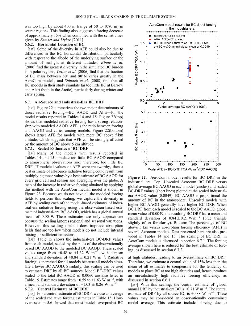
was too high by about 400 m (range of 50 to 1080 m) insource regions. This finding also suggests a forcing decreaseof approximately 15% when combined with the sensitivitiesgiven by Samset and Myhre [2011].6.6.2. Horizontal Location of BC[352] Some of the diversity in AFE could also be due to

differences in the BC horizontal distribution, particularlywith respect to the albedo of the underlying surface or theamount of sunlight at different latitudes. Kinne et al.[2006] find the greatest diversity in the simulated BC burdenis in polar regions, Textor et al. [2006] find that the fractionof BC mass between 80� and 90�N varies greatly in theAeroCom models, and Shindell et al. [2008] find that allBC models in their study simulate far too little BC at Barrowand Alert (both in the Arctic), particularly during winter andearly spring.

6.7. All-Source and Industrial-Era BC DRF

[353] Figure 22 summarizes the two major determinants ofdirect radiative forcing—BC AAOD and AFE—for themodel results reported in Tables 14 and 15. Figure 22(top)shows that modeled radiative forcing has a strong relation-ship with modeled AAOD. AFE is the ratio between forcingand AAOD and varies among models. Figure 22(bottom)shows larger AFE for models with more BC above 5 kmaltitude, which suggests that AFE can be strongly affectedby the amount of BC above 5 km altitude.6.7.1. Scaled Estimates of BC DRF[354] Many of the models with results reported in

Tables 14 and 15 simulate too little BC AAOD comparedto atmospheric observations and, therefore, too little BCDRF. If modeled values of AFE were trustworthy, then abest estimate of all-source radiative forcing could result frommultiplying those values by a best estimate of BC AAOD forevery grid cell and season and averaging over the globe. Amap of the increase in radiative forcing obtained by applyingthis method with the AeroCom median model is shown inFigure 23. Because we do not have all the modeled forcingfields to perform this scaling, we capture the diversity inAFE by scaling each of the model-based estimates of indus-trial-era radiative forcing using the observation-based esti-mate of industrial-era BC AAOD, which has a global annualmean of 0.0049. These estimates are only approximatebecause the scaling ignores regional and seasonal variations.However, this scaling method does improve absorptionfields that are too low when models do not include internalmixing or sufficient emissions.[355] Table 15 shows the industrial-era BC-DRF values

from each model, scaled by the ratio of the observationallybased BC AAOD to the modeled BC AAOD. These scaledvalues range from +0.48 to +1.32 W m�2, with a meanand standard deviation of +0.84 � 0.21 W m�2. Radiativeforcing is increased for all models because all models simu-late a lower BC AAOD. Similarly, this scaling can be usedto estimate DRF by all BC sources. Model BC-DRF valuesscaled to the total BC AAOD of 0.0060 are also listed inTable 15. Estimates range from +0.59 to +1.63 W m�2, witha mean and standard deviation of +1.03 � 0.26 W m�2.6.7.2. Central Estimate of BC DRF[356] For a central estimate of BC DRF, we use an average

of the scaled radiative forcing estimates in Table 15. How-ever, section 5.6 showed that most models overpredict BC

at high altitudes, leading to an overestimate of BC DRF.Therefore, we estimate a central value of 15% less than themean of all estimates to compensate for the tendency ofmodels to place BC at too high altitudes and, hence, producean unrealistically high radiative forcing efficiency, asdiscussed in section 6.6.1.[357] With this scaling, the central estimate of global

annual DRF by industrial-era BC is +0.71Wm�2. The centralestimate of DRF by all-source BC is +0.88 W m�2. Thesevalues may be considered an observationally constrainedmodel average. This estimate includes forcing due to

Figure 22. AeroCom model results for BC DRF in theindustrial era. Top: Unscaled Aerocom BC DRF versusglobal average BC AAOD in each model (circles) and scaledBC-DRF values (short lines) plotted at the scaled industrial-era AAOD value (0.0049). BC AAOD is proportional theamount of BC in the atmosphere. Unscaled models withhigher BC AAOD generally have higher BC DRF. WhenBC DRF from each model is scaled to the BC AAOD globalmean value of 0.0049, the resulting BC DRF has a mean andstandard deviation of 0.84� 0.21Wm�2 (blue triangleslightly offset for clarity). Bottom: The percentage of BCabove 5 km versus absorption forcing efficiency (AFE) inseveral Aerocom models. Data presented here are also pro-vided in Tables 14 and 15. The scaling of BC DRF inAeroCom models is discussed in section 6.7.1. The forcingaverage shown here is reduced for the best estimate of forc-ing, as discussed in section 6.7.2.


62

atmospheric absorption by organic carbon since our estimateof BC AAOD includes absorption by both BC and OA. In sec-tion 11, total aerosol DRF from sources that emit BC is esti-mated, and there we do not account for atmosphericabsorption by OA, so while BC DRF may be biased high,the total forcings by emissions from sources that include bothBC and OA do not include this bias.[358] The modeled forcing discussed above was calcu-

lated only at visible wavelengths, except for the work ofJacobson [2010]. Aerosols can also interact with infraredradiation, especially in source regions [Lubin and Simpson,1994]. Reddy et al. [2005a] estimated infrared forcing byBC as +0.006 W m�2. Jacobson [2001b] presented a graph-ical summary in which ToA direct infrared forcing by BCwas small relative to forcing at visible wavelengths. There-fore, we assume that the central estimate given aboveencompasses infrared forcing, even if most models haveneglected it.6.7.3. Uncertainties in BC DRF[359] A 90% confidence range for BC DRF is based on in-

dependent uncertainties in the industrial-era BC AAOD andthe radiative forcing efficiency, AFE. The final estimate ofuncertainty is higher than that reflected in the diversity ofscaled BC DRF estimates listed in Table 15, which do notaccount for uncertainty in BC AAOD.[360] Appendix B provides an estimate of the uncertainty

in BC AAOD. Uncertainties are caused by the spatial pat-terns of BC AAOD used in filling gaps betweenAERONET sites, ambiguity in how the scale factor is de-fined, the limited number of AERONET sites, clear-skybiases in the BC AAOD, the influence of BC transport fromsources to oceanic regions, and the impacts of fine-modedust and OA on the estimate of BC AAOD. The indus-trial-era BC-AAOD estimate has an additional 18% uncer-tainty due to a 50% uncertainty in the estimate of thepreindustrial background. We assume that the overall un-certainty of the total AAOD retrieval contributes to theabove-mentioned sources of uncertainty, although the

degree of this contribution is unknown, and we thus do notaccount separately for it. One factor that could decrease theBCDRF is the attribution of more AAOD to dust. As discussedin Appendix B, we allow this factor to introduce an asymmetricuncertainty. The 90% uncertainty range is from 0.0023 to0.0087 for all-source BC AAOD and from 0.0014 to 0.0078for industrial-era BC AAOD.[361] The uncertainty in AFE is estimated from the stan-

dard deviation of the model AFE values listed in Table 15.This uncertainty is attributable to the vertical and horizontallocation and the temporal covariance of the clouds and BC.Other uncertainties included are the vertical location of BC rel-ative to clouds (25%) [Zarzycki and Bond, 2010], the effect ofsurface albedo (20%), and the choice of radiative transfer code(20%) [Boucher et al., 1998]. Schulz et al. [2006] attributed avariation in total aerosol cloudy-sky radiative forcing of�0.26 W m�2 among nine AeroCom models mainly to diver-sity in forcing above clouds. However, this diversity in AFEhas not been apportioned to individual sources of uncertainty.[362] Our final estimate of 90% uncertainty bounds comes

from combining the uncertainties in AAOD and the 50%uncertainty in AFE. The global annual DRF by industrial-eraBC is estimated to have an uncertainty range of +0.08 to+1.27 W m�2 about the central estimate of +0.71 W m�2.This range spans all scaled estimates listed in Table 15.The uncertainty range for all-source BC is +0.17 to+1.48 W m�2 about the central estimate of +0.88 W m�2.[363] A final uncertainty not estimated here is caused by

interpretation of AERONET remote-sensing data. Such datasets are subject to periodic revision, and changes in the inter-pretation would shift the estimate of AAOD and forcingpresented here.

6.8. Previous Observationally Scaled Radiative-Forcing Estimates

[364] Three previous studies have reported similarestimates of all-source BC DRF by scaling to AERONETdata. Sato et al. [2003] scaled modeled fields to theAERONET Version 2.0 product to obtain modeled forcingof +1.0 W m�2. As discussed previously (section 6.5.1), thisproduct eliminates low-AOD observations, with the resultthat the average AAOD has a high bias, and any scaling ofBC AAOD using that product is also biased high. The Satoet al. BC AAOD relied on data from earlier years, so theirvalue of 0.006 is not as high as our value extracted fromAERONET Version 2.0 averages (0.0143).[365] Ramanathan and Carmichael [2008] estimated forc-

ing of +0.9 W m�2 by combining modeled fields withAERONET data, MODIS data, and estimated o0. Modeledfields were based on Chung et al. [2005], which reportsBC AAOD of about 0.0068. Both BC AAOD and AFE aresimilar to those derived here, and the DRF estimate for all-source BC (+0.9 W m�2) is similar to the value given here.Chung et al. [2005] also point out that correcting MODISAOD with those of AERONET decreases the estimatedglobal AOD by 25%.[366] The most recent observationally based estimate, by

Chung et al. [2012], used a combination of AERONETretrievals, partitioning to distinguish BC AAOD from contri-butions by dust and organic carbon, satellite retrievals ofAOD, and model estimates of single-scattering albedo. Theirestimate of BC AAOD (0.0077) is 28% larger than our best

Figure 23. Adjustments to the annual mean, direct radia-tive forcing (Wm�2) by BC in the median AeroCom modelrequired for consistency with the AERONET retrieved aero-sol absorption optical depth (AAOD).


63

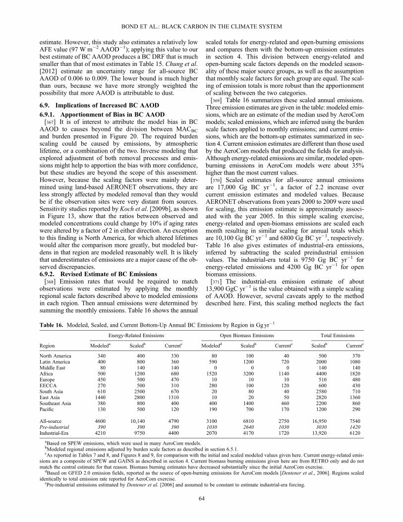
estimate. However, this study also estimates a relatively lowAFE value (97 W m�2 AAOD�1); applying this value to ourbest estimate of BC AAOD produces a BC DRF that is muchsmaller than that of most estimates in Table 15. Chung et al.[2012] estimate an uncertainty range for all-source BCAAOD of 0.006 to 0.009. The lower bound is much higherthan ours, because we have more strongly weighted thepossibility that more AAOD is attributable to dust.

6.9. Implications of Increased BC AAOD

6.9.1. Apportionment of Bias in BC AAOD[367] It is of interest to attribute the model bias in BC

AAOD to causes beyond the division between MACBC

and burden presented in Figure 20. The required burdenscaling could be caused by emissions, by atmosphericlifetime, or a combination of the two. Inverse modeling thatexplored adjustment of both removal processes and emis-sions might help to apportion the bias with more confidence,but these studies are beyond the scope of this assessment.However, because the scaling factors were mainly deter-mined using land-based AERONET observations, they areless strongly affected by modeled removal than they wouldbe if the observation sites were very distant from sources.Sensitivity studies reported by Koch et al. [2009b], as shownin Figure 13, show that the ratios between observed andmodeled concentrations could change by 10% if aging rateswere altered by a factor of 2 in either direction. An exceptionto this finding is North America, for which altered lifetimeswould alter the comparison more greatly, but modeled bur-dens in that region are modeled reasonably well. It is likelythat underestimates of emissions are a major cause of the ob-served discrepancies.6.9.2. Revised Estimate of BC Emissions[368] Emission rates that would be required to match

observations were estimated by applying the monthlyregional scale factors described above to modeled emissionsin each region. Then annual emissions were determined bysumming the monthly emissions. Table 16 shows the annual

scaled totals for energy-related and open-burning emissionsand compares them with the bottom-up emission estimatesin section 4. This division between energy-related andopen-burning scale factors depends on the modeled season-ality of these major source groups, as well as the assumptionthat monthly scale factors for each group are equal. The scal-ing of emission totals is more robust than the apportionmentof scaling between the two categories.[369] Table 16 summarizes these scaled annual emissions.

Three emission estimates are given in the table: modeled emis-sions, which are an estimate of the median used by AeroCommodels; scaled emissions, which are inferred using the burdenscale factors applied to monthly emissions; and current emis-sions, which are the bottom-up estimates summarized in sec-tion 4. Current emission estimates are different than those usedby the AeroCom models that produced the fields for analysis.Although energy-related emissions are similar, modeled open-burning emissions in AeroCom models were about 35%higher than the most current values.[370] Scaled estimates for all-source annual emissions

are 17,000 Gg BC yr�1, a factor of 2.2 increase overcurrent emission estimates and modeled values. BecauseAERONET observations from years 2000 to 2009 were usedfor scaling, this emission estimate is approximately associ-ated with the year 2005. In this simple scaling exercise,energy-related and open-biomass emissions are scaled eachmonth resulting in similar scaling for annual totals whichare 10,100 Gg BC yr�1 and 6800 Gg BC yr�1, respectively.Table 16 also gives estimates of industrial-era emissions,inferred by subtracting the scaled preindustrial emissionvalues. The industrial-era total is 9750 Gg BC yr�1 forenergy-related emissions and 4200 Gg BC yr�1 for openbiomass emissions.[371] The industrial-era emission estimate of about

13,900 GgC yr�1 is the value obtained with a simple scalingof AAOD. However, several caveats apply to the methoddescribed here. First, this scaling method neglects the fact

Table 16. Modeled, Scaled, and Current Bottom-Up Annual BC Emissions by Region in Gg yr�1

Energy-Related Emissions Open Biomass Emissions Total Emissions

Region Modeleda Scaledb Currentc Modeledd Scaledb Currentc Scaledb Currentc

North America 340 400 330 80 100 40 500 370Latin America 400 800 360 590 1200 720 2000 1080Middle East 80 140 140 0 0 0 140 140Africa 500 1200 680 1520 3200 1140 4400 1820Europe 450 500 470 10 10 10 510 480EECCA 270 500 310 280 100 120 600 430South Asia 610 2500 670 20 80 40 2580 710East Asia 1440 2800 1310 10 20 50 2820 1360Southeast Asia 380 800 400 400 1400 460 2200 860Pacific 130 500 120 190 700 170 1200 290

All-source 4600 10,140 4790 3100 6810 2750 16,950 7540Pre-industrial 390 390 390 1030 2640 1030 3030 1420Industrial-Era 4210 9750 4400 2070 4170 1720 13,920 6120

aBased on SPEW emissions, which were used in many AeroCom models.bModeled regional emissions adjusted by burden scale factors as described in section 6.5.1.cAs reported in Tables 7 and 8, and Figures 8 and 9, for comparison with the initial and scaled modeled values given here. Current energy-related emis-

sions are a composite of SPEW and GAINS as described in section 4. Current biomass burning emissions given here are from RETRO only and do notmatch the central estimate for that reason. Biomass burning estimates have decreased substantially since the initial AeroCom exercise.

dBased on GFED 2.0 emission fields, reported as the source of open-burning emissions for AeroCom models [Dentener et al., 2006]. Regions scaledidentically to total emission rate reported for AeroCom exercise.

ePre-industrial emissions estimated by Dentener et al. [2006] and assumed to be constant to estimate industrial-era forcing.


64

that burden in some regions may be caused by emissions inother regions. According to tagged-tracer modeling given inBond et al. [2011], Middle Eastern concentrations areaffected by South Asian emissions, Southeast Asian concen-trations have significant contributions from both South Asiaand East Asia, and the Pacific region is affected by all Asianemissions. However, the model used tends to over-transportaerosol, as evidenced by atmospheric burdens at highaltitudes. A true inverse modeling approach would give abetter estimate of emissions in each region, but modeledtransport and removal should be more thoroughly evaluatedbefore embarking on such a study. We caution that inferredemissions in Southeast Asia and the Pacific are particularlyuncertain.[372] Second, as discussed above, uncertainties in modeled

lifetimes could also contribute to errors in burdens. Changesin modeled lifetime were shown to alter modeled BC byabout 10% at the observation sites (Figure 13), which wouldalter inferred emissions by the same amount. Third, theMACBC scale factor used here is also simplified because itassumes that BC is always internally mixed and, therefore,amplifies absorption at the observation sites. If BC wereexternally mixed at observation sites, the MACBC scale factorwould decrease and the burden scale factor would increase. Ifthe appropriate MACBC scaling were a 20% increaseinstead of 50%, all-source emissions would be estimated as21,000 Gg BC yr�1. For an assumed increase of 80%, theestimate would be 14,000 Gg BC yr�1. Finally, observationsare sparse in many of the regions with the largest emissionsand the largest estimated increases. In the absence of moredefinitive studies that explain biases in aerosol absorption,the central value is used as a best estimate of industrial-eraBC emissions throughout this assessment.6.9.3. Scaling of Modeled AAOD in the Contextof Other Evidence[373] Inverse modeling studies and other comparisons be-

tween models and measurements were discussed in section5.5.1. As these studies have attributed errors to emissionbiases rather than modeling of any other factor, we comparethem with the emission increases in Table 16.[374] Scaled emissions for total biomass burning BC of

6800 Gg yr�1 are in good agreement with the upper limitderived by Zhang et al. [2005]. The increase by a factor of2.5 falls within the large uncertainty ranges for biomasssmoke given by Reid et al. [2009] and Kaiser et al.[2012]. Carbon monoxide measurements do not indicatesuch a large discrepancy, so either modeled emission factorsor modeled aerosol lifetimes are suspect. Section 4.7.2.3discussed some reasons why modeled biomass burningemission factors could be too low. These proposed adjust-ments should also apply to the preindustrial backgroundused here, and hence, the scaling described here is alsorepresented in our estimate of preindustrial AAOD.[375] The finding that small to moderate emission

increases are required in North America and Europe is inreasonable agreement with inverse modeling studies. Scaledemissions in Figure 20 suggest that emissions for East Asiashould increase as suggested by Kondo et al. [2011a], but by90% instead of 30%. Since inverse modeling by Hakamiet al. [2005] suggested that BC emissions in East Asia wereapproximately correct at an earlier date, the increasedemissions may be related to growth, estimated as 30 to

50% [Lu et al., 2011]. The higher emission estimates forSouth Asia are 30% greater than those estimated byDickerson et al. [2002] for a much earlier year, and theyagree with observations that modeled burdens in that regionare too low by about a factor of 4 to 5.[376] Total emissions are in reasonable agreement with

predictions of a Kalman filter inverse estimate [Jason BlakeCohen, personal communication, 2012]. Scaled global en-ergy-related emissions are estimated at 10,100 Gg yr�1, with80% of the increase appearing in Africa, South, East, andSoutheast Asia. Although the apportionment between en-ergy-related emissions and biomass burning is not certain,it would be difficult for the small amount of biomass burningin South and East Asia to cause such a large discrepancy.Applying the higher BC emission factors recommended byCooke et al. [1999] for power generation would cause muchgreater discrepancies in North America and Europe than cur-rently exist. The evidence points to underestimation of emis-sions in regions with low regulation, so that sources such aspoorly operating vehicles, industrial installations, or highsolid-fuel combustion may be responsible.[377] Land regions of Latin America, Africa, Southeast

Asia, and the Pacific region (Figure 7) are, together, respon-sible for 40% of the global BC AAOD and suggested scalingfactors in these regions are 2 to 3.5. Especially uncertain arefindings for Africa, where 25% of global AAOD is found,and partitioning between BC and dust affects inferencesabout the magnitude of BC AAOD. Inverse modelingstudies or continent-wide comparisons with long-termmeasurements have not been reported for these regions.[378] In summary, we find that global AAOD from

AeroCom models is low compared to that suggested byobservations, that this underestimate occurs in particularregions, and that it cannot be fully explained by the absorp-tion enhancement produced by internal mixing or by uncer-tainties in retrievals. Modeled absorption is reasonable inregions with the best measurement coverage, relevant emis-sion measurements, and low biomass-burning emissions:North America and Europe. The dominance of differentsource categories and larger uncertainties in the otherregions (Figure 9 and section 4.7.1) that require increasedscaling to match observations suggests that poorly modeledemissions are a potential cause. Studies using space-basedremote sensing indicate that modeled aerosol concentrationsand absorption from biomass burning are too low(section 5.5.1), and an independent line of argument indi-cates that biomass-burning emission factors could lead tounderestimates of absorption (section 4.7.2.3). Surfacemeasurements in South and East Asia indicate that modelsusing the emissions summarized in section 4 would underes-timate observed BC concentrations (section 5.5.1). InAsia, where emissions have increased since the global emis-sion fields were developed (section 4.8), some of the under-estimation is to be expected. Although we cannot fullyexclude modeled lifetimes, instrumental uncertainties, andthe division of remotely-sensed AAOD into BC and dustcomponents in some regions (particularly Africa) as explan-atory factors, multiple lines of evidence support the positionthat AeroCom models using year-2000 BC emissionssubstantially underestimate absorption and direct radiativeforcing. Despite the inherent limitations of these models,they are required to produce estimates of global forcing,


65

because global space-based observations cannot separateradiative impact by chemical component. Model fieldsscaled to observations are therefore used to develop our bestestimate of direct radiative forcing.

6.10. Summary of Uncertainties in BC DRF

[379] The discussion in this section shows that several fac-tors affecting BC radiative forcing are not well constrained.First, the most quantitative and widespread data set for deter-mining atmospheric absorption is remote sensing providedby AERONET, but use of these observations requires anestimate of the division between AAOD attributable to BCand dust. Different plausible assumptions can greatly alterthe inferred BC AAOD, up to a factor of 2. Parametersretrieved from AERONET observations, such as sizedistributions or wavelength dependence of absorption,have been used in interpreting AAOD data, but thesehave not been thoroughly evaluated with in situ measure-ments. Second, the dust refractive index may have largevariability within regions [Moosmüller et al., 2012;Wagner et al., 2012] and could greatly affect the estimateof dust AAOD and the inference of BC AAOD. Third,despite the uncertainties, observations indicate more BCAAOD than is modeled by about a factor of 2.5. A sim-ple scaling procedure indicates that a large increase inemission estimates is warranted for biomass burningand for energy-related sources in developing regions.Emission factors may explain low biases in modeledbiomass burning emissions, but the cause of errors inenergy-related emissions is unknown. Fourth, despitethe fact that emission rates are implicated in underesti-mates of BC AAOD, a full attribution of differences inBC distributions to errors in model emissions, transport,or removal rates is not yet possible. No simple adjust-ment to modeled transport can explain the range ofmodel biases (section 5.7). Fifth, the contribution ofabsorbing organic aerosol to AAOD has not been eluci-dated. Attribution of some of the absorption to OA ratherthan BC would reduce the direct forcing estimate for BCand make that of OA less negative or more positive.Finally, model evaluations are limited in regions thatcontribute large fractions of the global AAOD, becausefew long-term observations are available.[380] Although present-day observations can be used to

adjust modeled forcing terms, a lack of understanding ofthe causes of bias limits the accuracy of modeled forcingfor the past and future. Further, vertical transport andtherefore location of BC is poorly modeled, so thatmodeled absorption forcing efficiency also contains errors.While biases in BC distributions in the Arctic produceonly small errors in global, annual average BC AAOD(and thus forcing), they produce large biases in forcingwithin the Arctic, where BC may contribute to greater-than-expected warming and declines in sea ice [Quinnet al., 2008, 2011]. In subsequent sections, horizontaland vertical distributions are shown to affect the interac-tion with clouds (section 7) and forcing in snow and seaice (section 8). Thus, a lack of understanding of processfundamentals and the resulting modeled biases are largesources of uncertainty in all BC forcing terms.[381] The amount of aerosol in the preindustrial atmo-

sphere is also poorly known. Biomass burning produced

much of this aerosol, and preindustrial estimates usedhere were based on the emissions given by Denteneret al. [2006]. Although biomass burning has increasedoverall during the industrial era, charcoal records suggestthat activity in some regions was similar between 1750and today [Marlon et al., 2008]. Although thispreindustrial background does not affect the estimate oftotal radiative forcing, it does affect industrial-era forcingand temperature change since preindustrial times. Weretain conventional nomenclature and refer to this back-ground value as that of 1750, but we caution that itrepresents a reference atmosphere rather than a truepreindustrial value.

7. Black Carbon Interactions With Clouds


[382] 1. Black carbon may change cloud cover, emissivity,or brightness in four ways: (1) by changing the vertical tem-perature structure of the atmosphere, which could shift clouddistributions (semi-direct effect); (2) by changing the num-ber concentration of liquid cloud droplets and the lifetimeof liquid clouds; (3) by changing phase partitioning and pre-cipitation in mixed-phase clouds; and (4) by changing iceparticle number concentration. These effects may cause ei-ther positive or negative radiative forcing. Very few modelstudies isolate the influence of BC on each effect. All aerosoleffects on clouds are highly uncertain, and the isolated ef-fects of BC have even greater relative uncertainty.[383] 2. Many of the cloud effects described here may be

considered rapid adjustments, either to direct radiative forc-ing or to the presence of BC. However, all effects can bequantified in units of climate forcing, a practice wecontinue here for consistency with previous studies and forconvenience.[384] 3. In the semi-direct effect, cloud cover can increase

or decrease, depending on region and conditions. Some stud-ies examining regional cloud reduction have suggested a pos-itive forcing, but global model studies indicate that the BCsemi-direct effect averages �0.1 � 0.2 W m�2 for industrial-era forcing if all BC is emitted at the surface. An additional�0.28 W m�2 is added to the lower uncertainty range to ac-count for the potential reduction of high-level clouds from bio-mass-burning BC, making the 90% uncertainty range –0.44 to+0.1 W m�2 over the industrial era. Major uncertainties in-clude poorly modeled BC vertical distributions and the fidelityof modeled cloud responses.[385] 4. BC has two competing indirect effects on liquid

clouds. First, adding BC increases the aerosol number con-centration. If the number of cloud droplets also increased,negative forcing by clouds would increase, but BC-rich par-ticles are inferior cloud-forming particles. Second, BC parti-cles may also serve as sites to collect soluble material, reduc-ing overall cloud droplet number concentration andproducing a positive forcing. BC alone is estimated to havean indirect climate forcing of about �0.1 W m�2. Manystudies do not separate this effect from the semi-direct effectdiscussed above, so an isolated estimate is difficult to obtain.Therefore, we estimate the combined industrial-era climateforcing from liquid-cloud and semi-direct effects as �0.2(with a 90% uncertainty range of �0.61 to +0.1 W m�2).


66

[386] 5. Greater absorption by BC within cloud droplets de-creases cloud albedo, heats clouds, and dissipates them. This isa special case of the semi-direct effect that we estimateseparately as a climate forcing of +0.2Wm�2, with a 90% un-certainty range of�0.1 to +0.9 W m�2 over the industrial era.Model results for this effect are very sensitive to the represen-tation of optical properties for the mixed BC and cloud droplet.[387] 6. The liquid-cloud indirect effect is sensitive to BC

particle size and to mixing with other particles. Many modelstudies indicate that particles emitted from biofuelcombustion appear to have more negative forcing per emis-sion than do particles from fossil fuel combustion, possiblybecause of size or co-emitted POA.[388] 7. The BC mixed-phase indirect effect acts on clouds

that are part liquid and part ice. BC may act as ice nuclei(IN) that enhance ice formation and increase ice fall-out.An estimate for this effect is +0.18 � 0.18 W m�2 for indus-trial-era climate forcing and 90% uncertainty range, but themagnitude would be reduced for BC mixed with sulfate.[389] 8. In the ice-cloud indirect effect, greater IN concen-

trations either increase or decrease the concentrations of iceparticles and the lifetime of cirrus clouds, depending on con-ditions. Cirrus clouds affect both shortwave and longwaveradiative fluxes. The cloud cover change and forcing may,therefore, be positive or negative. Two model studies esti-mate effects of opposite signs: �0.4 and +0.4 W m�2. Lab-oratory and field observations suggest that both BC concen-tration and BC’s ability to act as IN are probably less thanassumed in these model estimates. We estimate an indus-trial-era climate forcing of 0 � 0.4 W m�2 (90% uncertaintyrange) for this highly uncertain effect, which excludes the ef-fects of aviation. These effects are sensitive to assumptionsabout BC’s role as IN and to the number concentration andmixing state of BC particles in the free and upper tropo-sphere. Ice-cloud effects also depend on the assumed back-ground conditions, including concentrations of other INand updraft velocities.[390] 9. Few modeling and measurement studies are able

to constrain cloud-absorption, mixed-phase and ice-cloud in-direct effects. Consequently the uncertainties are large.Model diversity, rather than true uncertainty propagation,provides uncertainties in cloud radiative forcing.

7.2. Introduction

[391] Clouds and their responses to aerosol addition intro-duce a large uncertainty in the understanding of total climateforcing and climate response [Heintzenberg and Charlson,2009]. The general term “indirect effects” refers to the suiteof climate forcings that aerosols impose through the modifi-cation of cloud properties [Forster et al., 2007; Denmanet al., 2007]. Aerosol indirect effects on clouds have beenextensively studied, but the influence of BC alone hasreceived less attention. Although BC makes a small contri-bution to aerosol mass load in the atmosphere, it may playan important role in determining the CCN or IN particlenumber concentration that in turn alters indirect effects.Aerosol indirect effects and BC’s role in the indirect effectdiffer depending on the cloud phase: liquid, ice, or “mixed”containing both liquid and ice, and these are discussed individ-ually. Furthermore, absorption by BC embedded within clouddroplets is greater than that of BC alone or with coatings.

[392] Figure 24 summarizes the mechanisms by which BCcan influence clouds. A brief overview is given here beforethe detailed discussions in the remainder of this section.The first general class of effects involves perturbations tothe atmospheric temperature structure, which affect clouddistributions. These mechanisms are commonly termed“semi-direct effects,” a term that is sometimes used todescribe evaporation of cloud droplets when absorbing aero-sols heat a cloud layer [Hansen et al., 1997; Ramanathanet al., 2001a]. Additional BC radiative effects have also beendocumented whereby cloud cover may be either enhanced orreduced, depending on factors such as its altitude relative tocloud cover [e.g., Hansen et al., 2005; Johnson et al., 2004],and meteorological conditions. BC’s semi-direct effects are arapid adjustment to BC direct radiative forcing, through localwarming of the atmosphere. Somemodel calculations treat thisadjustment as a distinct forcing term. Following these studies,and consistent with other treatments in this assessment, we re-view semi-direct estimates in forcing units.[393] Another general category, commonly termed “indi-

rect effects,” involves changes in concentrations of clouddroplets or ice crystals that alter cloud brightness, emissiv-ity, and lifetime, which produce a radiative forcing. Thiscategory includes the groups titled “liquid-cloud effects,”“mixed-phase cloud effects,” and “ice-cloud effects” inFigure 24. These cloud effects are driven by changes in thenumber of CCN or IN, aerosols on which cloud droplets orice particles may form. The process of forming a stableliquid droplet or ice particle is known as activation. In princi-ple, any particle can activate in either liquid or ice clouds ifhigh enough supersaturation is reached. However, when manyaerosol types are present, the particles that activate the mosteasily do so first and have the greatest potential influence onthe resulting number concentration of cloud particles. Micro-physical characteristics of a particular type of aerosol are thusvery important in determining its cloud effects.[394] Warm cloud indirect effects include two compo-

nents. The cloud albedo effect (i.e., the first indirect orTwomey effect) [Twomey, 1959] refers to the change in radi-ation caused by a change in cloud albedo or brightnessresulting from a change in the cloud droplet size distribution.Increased CCN lead to more and smaller cloud liquid drop-lets for a given cloud water content (case LC1 in Figure 24).This effect can be observed in ship-track studies [e.g., Fereket al., 1998]. However, if BC attracts condensing gases thatwould otherwise form particles, the net result is a decrease inCCN and cloud droplets and is, therefore, a positive radia-tive forcing (case LC2) [Bauer et al., 2010].[395] The cloud lifetime effect (LC3, second indirect

effect) refers to the fact that in the presence of increasedaerosol concentrations, more and smaller cloud dropletsform, and these collide less efficiently. Factors such as dropevaporation rates and depletion of water vapor can also altercloud lifetimes. While cloud resolving models suggest thatthis effect could lead to either an increase or decrease in liq-uid water [Ackerman et al., 2004; Sandu et al., 2008], theGCMs are parameterized such that this effect can only leadto longer cloud lifetimes with greater overall cloud reflectiv-ity [Lohmann and Feichter, 2005]. Thus, although thisforcing could be either positive or negative, GCM globalestimates of LC3 are always negative. Altered lifetime alsoplays a role in mixed-phase clouds, where temperatures


67

typically fall between 0 and �35�C. Two competing effectshave been suggested: first, glaciation, which refers to anincrease in ice nuclei causing more frequent glaciation ofsupercooled clouds, and second, de-activation. In the glacia-tion effect, ice crystals grow at the expense of water dropletsbecause of the difference in vapor pressure between waterand ice, referred to as the Bergeron-Findeisen effect. Anincrease in IN would enhance this process, causing cloudsto precipitate more readily (case MC1 in Figure 24) andthereby reducing cloud amount [Lohmann, 2002]. However,

deactivation occurs when sulfur or secondary organic aero-sol coat IN and make them less efficient [Girard et al.,2005] in mixed-phase clouds by changing the mode of freez-ing from contact to immersion freezing. In global climatemodels, this leads to less sedimentation and more cloudcover [Storelvmo et al., 2008; Hoose et al., 2008] (caseMC2 in Figure 24).[396] BC may also affect cirrus clouds that occur at high

altitude in the upper troposphere [Kärcher and Spichtinger,2009]. Aerosol particles at these high altitudes have long

Figure 24. Schematic of the causes and effects that lead to cloud effects from BC emissions. Each rowbegins with an identifying label followed by a cause, namely, an atmospheric or microphysical parameterrepresenting a potential perturbation to cloud properties. To the right of each cause are the response(s) tothe perturbation. On the far right is the associated effect, namely, the cloud parameter that changes in re-sponse to the perturbation. The single color of the components in a row indicates a climate system re-sponse of warming (red) or cooling (blue). The split coloring in LC3 indicates that the response can beeither warming or cooling (section 7.2). Although MC2 is not attributable directly to BC, it is includedhere because it alters the effects of BC.


68

atmospheric lifetimes [e.g., 4–30 days;Williams et al., 2002]and, therefore, extended opportunities for mixing with otheraerosol components. Thin, high cirrus clouds are believed tohave net positive cloud forcing [Chen et al., 2000]. Absorp-tion of infrared radiation and re-emission at colder tempera-tures dominates scattering of solar radiation, which results ina net positive forcing. Efficient IN may either increase orreduce cirrus cloud forcing. Cirrus cloud particles are mostlyformed through homogeneous ice nucleation. Even a smallnumber of particles can initiate heterogeneous freezing wellbelow the homogeneous freezing threshold, depleting someof the supersaturated water vapor, partially preventinghomogeneous formation of solution droplets and reducingthe number of particles [e.g., Kärcher et al., 2006]. Earlyonset of nucleation from a few efficient BC particles affectsforcing less than enhanced sedimentation, yielding case IC1in Figure 24. If high concentrations of IN already exist,heterogeneous freezing dominates the cloud and additionalIN increase the number concentration of cloud particles(case IC2 in Figure 24).[397] Some challenges are common in obtaining forcing

from models of aerosol-cloud interactions. First, modelsuse different emission levels and input assumptions, andvariation in values of direct forcing may result from thesedifferences alone. Second, each model study may have adifferent set of impacts, such as treating aerosol interactionswith only liquid or ice clouds, or allowing certain climateresponses. The net effect on radiation is usually inferredfrom two sets of simulations—one with and one withoutperturbed pollution conditions [Lohmann et al., 2010]—sothat the individual effects contributing to the changes aredifficult to distinguish without well-designed diagnostics.The combination of varying inputs and inconsistent selec-tion of effects makes global cloud-forcing estimates difficultto compare. Third, some aerosol-induced changes are bestsimulated at scales smaller than a global model grid box.Physical confirmation of the factors governing cloud dynam-ics and cloud microphysical interactions must also occur onrelatively small scales. Cloud-resolving models (CRMs) andlarge-eddy simulations (LES) may be most appropriate formodeling these scales, but these simulations do not havethe spatial extent to calculate globally averaged forcing,and do not always agree with the results of global modelsthat use coarser resolutions. The reasons for these disagree-ments is not always understood, making it difficult to infera global, annual average forcing from either set of modelstudies. Fourth, some effects that cause cloud redistributionon large scales are best simulated with global models, buttheir broad spatial or temporal extent makes their existenceand magnitude difficult to confirm. Fifth, the fidelity of aero-sol-cloud simulations depends on accurate representation ofthe cloud amount and location, yet these factors are not oftenverified in the model studies. Finally, inter-annual andspatial variability of modeled cloud forcing is large com-pared with the magnitude of the aerosol-induced changes.Therefore, extracting statistically significant changes ischallenging.[398] While aerosol effects on clouds are complex,

accounting for them is critical because they may inducechanges similar to or greater than aerosol direct forcing.For a perspective on all aerosol effects, Denman et al.[2007] summarized studies ranging from a mean of

�1.2 W m�2 with a range of �0.2 to �2.3 W m�2 for thetotal effect of all anthropogenic aerosols on climate, includ-ing direct forcing, cloud albedo, cloud lifetime, and semi-direct effects. Using a combination of 10 models and inputfrom relationships observed by satellite, Quaas et al.[2009] estimated the total aerosol effect on stratiform cloudsas �1.5 � 0.5 W m�2. The global annual mean climateforcing for just the first indirect effect of all aerosols hasbeen estimated from GCMs with some guidance fromsatellite observations as �0.7 W m�2 with a range between�0.3 and �1.8 W m�2 [Forster et al., 2007]. Notably,Lohmann et al. [2010] showed that estimates of totalanthropogenic aerosol effects have become smaller withtime. GCMs have added processes, such as aerosoleffects on mixed-phase clouds, or treating rain as a prog-nostic variable, which place more emphasis on accretioninstead of autoconversion. These more advanced GCMsarrive at smaller total anthropogenic cloud forcing comparedwith earlier versions. GCMs that are constrained bysatellite data also predict a smaller total anthropogenicaerosol effect.[399] This assessment mainly presents global, annually

averaged climate forcing by semi-direct and indirect effects.However, forcing within a given region may differ signifi-cantly from this average. For example, in the Arctic thecombined semi-direct and indirect effect of aerosols mayproduce a much smaller negative forcing than on the globalaverage, or possibly even a positive forcing [Koch et al.,2009a; Jacobson, 2010; Alterskjær et al., 2010], becauseof the Arctic’s high surface albedo and because changes incloud emissivity due to aerosol microphysical effects mayproduce significant positive forcing in late winter and spring[Garrett and Zhao, 2006].[400] In summary, BC may affect clouds by perturbing

the atmospheric thermal structure, or by changing liquidcloud droplet number concentration, ice crystal numberconcentration, or some combination of the two in mixed-phase clouds. Each of these processes affects the distribu-tions or reflectivity of clouds, which, in turn, alters theradiative balance of the Earth. As such, these are rapidadjustments to the climate system that can be quantifiedas adjusted forcings (section 2.3 and Table 2). The role ofBC in each of these cloud effects is presented below,including increased absorption by BC inclusions in clouddroplets (section 7.3.3), semi-direct effects (section 7.3.2),indirect effects on liquid clouds (section 7.4), and mixedand ice phase clouds (section 7.5). Although modeledcloud forcing depends on assumed emission rates or simu-lated atmospheric burden, this dependence may not belinear, so scaling modeled forcing to the new emission ratesor forcing determined in section 6 is also discussed for eacheffect. Best estimates of adjusted forcings are calculated forthe combined semi-direct and liquid-cloud effects formixed-phase clouds and ice clouds. These estimates arefollowed by a discussion of uncertainties (section 7.7).All cloud forcings discussed here are industrial-era forc-ings; all-source forcings are not estimated. Clouds in aclean atmosphere are much more susceptible to changethan clouds in an atmosphere with even a small aerosolbackground [Boucher and Pham, 2002], so cloud forcingis always calculated against a preindustrial background.


69

7.3. Black-Carbon Semi-Direct Effects on Cloud Cover

[401] Atmospheric BC absorbs solar radiation, perturbs thetemperature structure of the atmosphere and, therefore, influ-ences the cloud distribution. The first of these effects to bedocumented, the original semi-direct effect, is the evapora-tion and dissolution of clouds by BC suspended near orwithin clouds [Hansen et al., 1997]. Since then, numerousstudies have demonstrated this effect, as well as additionalmechanisms by which BC either increases or reduces cloudcover. Some of these studies use cloud-scale models, someare observational—typically with focus on a particularregion—and some use global models. Koch and Del Genio[2010] reviewed many studies on this topic, which aresummarized here. The top segment of Figure 24 summarizesa framework proposed by Koch and Del Genio [2010] toclassify previous studies.[402] Each of the effects shown in the top portion of

Figure 24 is the result of a rapid adjustment to the initialdirect radiative forcing by BC. Following the terminologydefined in section 2, the sum of the direct effect and thesemi-direct effect can be interpreted as a single “adjustedforcing.” However, model studies to date have eithercalculated the semi-direct effect as an independent forcing,derived a combined forcing for the semi-direct and liquidcloud effects, or report a reduced efficacy for BC direct radi-ative forcing, attributing this decrease to semi-direct effects.Because semi-direct effects are diverse, all changes otherthan cloud microphysical changes might be grouped underthis label [e.g., Ghan et al., 2012]. For consistency withthe existing literature, we also discuss the semi-direct effecthere as a climate forcing term and include the efficacystudies in our estimate of that forcing.

7.3.1. Cloud Scale and Regional Studies[403] The altitude of BC relative to a cloud or potential

cloud layer plays an important role in determining thecloud response. For aerosols embedded near cloud, cloudevaporation is enhanced due to their heating and reductionof relative humidity (Figure 24, case SD4). This effect wasdemonstrated in the LES experiments of Ackerman et al.[2000] for trade cumulus and Hill and Dobbie [2008] andJohnson et al. [2004] for marine stratocumulus clouds.[404] Absorbing aerosol aloft increases atmospheric stabil-

ity. Increased stability over stratocumulus clouds reducescloud-top entrainment of overlying dry air and tends tostrengthen the underlying clouds (Figure 24, case SD1).LES experiments by Johnson et al. [2004] showed thatabsorbing aerosols above cloud increased cloud cover,because they increased the difference in potential temperatureacross the inversion, decreased entrainment rate, and caused ashallower, moister boundary layer with higher liquid-waterpath. The same model had demonstrated cloud reductionwhen absorbing aerosols were within the cloud layer(Figure 24, case SD4). Brioude et al. [2009] analyzed satellitecloud observations and modeled biomass-burning tracers for afield study near the coast of California. They found thatbiomass-burning aerosols enhanced cloud cover, especiallyfor high-humidity conditions and for low lower troposphericstability conditions, when the aerosols increased lowertropospheric stability. Similarly, Wilcox [2012] analyzed sat-ellite data of subtropical, South Atlantic biomass-burningsmoke overlying marine stratocumulus clouds and found

that the smoke enhanced the cloud liquid-water path, counter-ing more than 60% of the smoke direct radiative effect.[405] While the stabilizing effect of absorbing aerosols

aloft can enhance stratocumulus cloud cover, they may sup-press cumulus cloud development (Figure 24, case SD2).Fan et al. [2008] performed experiments in a cloud-resolvingmodel for the Houston area and demonstrated that absorbingaerosols aloft decreased the temperature lapse rate, leading toa more stable atmosphere and decreased convection. MODISobservational studies for the Amazon biomass burning seasonbyKoren et al. [2004, 2008] also demonstrated cumulus cloudcover reduction due to increased smoke. They argued thatsmoke plumes stabilized the boundary layer, reducing convec-tive activity and boundary layer cloud formation. The smokealso reduced radiation penetration to the surface, thereforereducing evaporation and atmospheric moisture. Ten Hoeveet al. [2011] used satellite observations of biomass-burningregions to show that cloud optical depth increased withAOD for low values, consistent with cloud brightening (caseLC1). At higher AOD values, cloud optical depth decreasedwith AOD, possibly due to cloud evaporation (case SD4).[406] On the other hand, in some land regions, lofted

absorbing aerosols may enhance upper level convection,promoting low-level moisture convergence of oceanic airmasses, which could increase continental clouds (Figure 24,case SD3). Monsoon enhancement due to lofted absorbingaerosols (known as the “Elevated Heat Pump” hypothesis)was shown in the global model studies of Lau et al.[2006], Randles and Ramaswamy [2008], and Chung et al.[2002]. However, global climate models are limited by rela-tively coarse spatial resolution, which may preclude accuraterepresentation of aerosol transport over the Tibetan Plateau.In a study using observed vertically resolved aerosol distri-butions over the Tibetan Plateau and surrounding regions,Kuhlmann and Quaas [2010] use observed surface albedoand a radiative transfer model to show that aerosols donot produce the large elevated heating needed to drive theElevated Heat Pump. In the non-monsoon season, winter-time pollution as observed in the Indian Ocean Experimentreduced the meridional temperature gradient in the globalmodel study of Ramanathan et al. [2005], which includeda coupled ocean response. These SST shifts were found toenhance precipitation over sub-Saharan Africa [Chung andRamanathan, 2006]. Many studies predicting enhancedconvergence over land indicate a shift in clouds and precip-itation rather than an overall enhancement.[407] BC below cloud generally promotes convective activ-

ity and can enhance cloud cover (Figure 24, case SD6). Cloudresolving model studies ofMcFarquhar and Wang [2006] fortrade wind cumuli demonstrated that absorbing aerosolsplaced below cloud promoted vertical motion and increasedliquid water path. Similarly, LES experiments of Feingoldet al. [2005] found that Amazon smoke emitted at the surfacecould destabilize the surface layer and increase convection andcloud cover. However, smoke at cloud level decreased cloudcover and promoted dissipation in both of these studies.7.3.2. Global Model Semi-Direct Estimates[408] Consistent with the variety of responses found in

regional studies, global model studies also find that regionalvariations and global-average forcing include positive andnegative forcing effects over all regions. Although semi-direct effects cause positive forcing in some regions, most


70

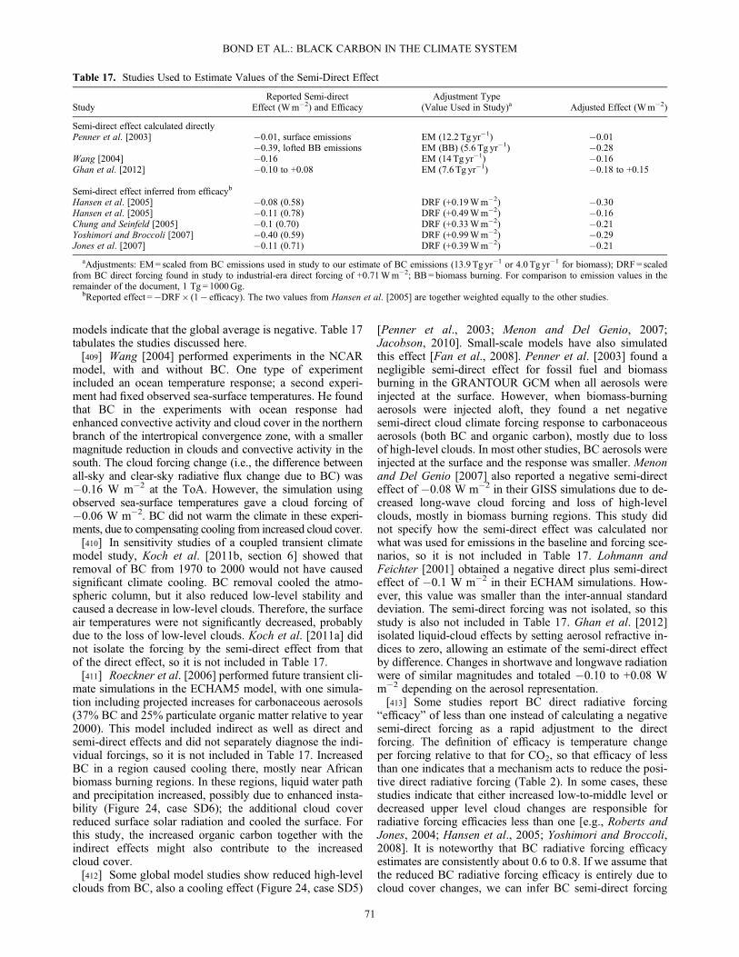
models indicate that the global average is negative. Table 17tabulates the studies discussed here.[409] Wang [2004] performed experiments in the NCAR

model, with and without BC. One type of experimentincluded an ocean temperature response; a second experi-ment had fixed observed sea-surface temperatures. He foundthat BC in the experiments with ocean response hadenhanced convective activity and cloud cover in the northernbranch of the intertropical convergence zone, with a smallermagnitude reduction in clouds and convective activity in thesouth. The cloud forcing change (i.e., the difference betweenall-sky and clear-sky radiative flux change due to BC) was�0.16 W m�2 at the ToA. However, the simulation usingobserved sea-surface temperatures gave a cloud forcing of�0.06 W m�2. BC did not warm the climate in these experi-ments, due to compensating cooling from increased cloud cover.[410] In sensitivity studies of a coupled transient climate

model study, Koch et al. [2011b, section 6] showed thatremoval of BC from 1970 to 2000 would not have causedsignificant climate cooling. BC removal cooled the atmo-spheric column, but it also reduced low-level stability andcaused a decrease in low-level clouds. Therefore, the surfaceair temperatures were not significantly decreased, probablydue to the loss of low-level clouds. Koch et al. [2011a] didnot isolate the forcing by the semi-direct effect from thatof the direct effect, so it is not included in Table 17.[411] Roeckner et al. [2006] performed future transient cli-

mate simulations in the ECHAM5 model, with one simula-tion including projected increases for carbonaceous aerosols(37% BC and 25% particulate organic matter relative to year2000). This model included indirect as well as direct andsemi-direct effects and did not separately diagnose the indi-vidual forcings, so it is not included in Table 17. IncreasedBC in a region caused cooling there, mostly near Africanbiomass burning regions. In these regions, liquid water pathand precipitation increased, possibly due to enhanced insta-bility (Figure 24, case SD6); the additional cloud coverreduced surface solar radiation and cooled the surface. Forthis study, the increased organic carbon together with theindirect effects might also contribute to the increasedcloud cover.[412] Some global model studies show reduced high-level

clouds from BC, also a cooling effect (Figure 24, case SD5)

[Penner et al., 2003; Menon and Del Genio, 2007;Jacobson, 2010]. Small-scale models have also simulatedthis effect [Fan et al., 2008]. Penner et al. [2003] found anegligible semi-direct effect for fossil fuel and biomassburning in the GRANTOUR GCM when all aerosols wereinjected at the surface. However, when biomass-burningaerosols were injected aloft, they found a net negativesemi-direct cloud climate forcing response to carbonaceousaerosols (both BC and organic carbon), mostly due to lossof high-level clouds. In most other studies, BC aerosols wereinjected at the surface and the response was smaller. Menonand Del Genio [2007] also reported a negative semi-directeffect of �0.08 W m�2 in their GISS simulations due to de-creased long-wave cloud forcing and loss of high-levelclouds, mostly in biomass burning regions. This study didnot specify how the semi-direct effect was calculated norwhat was used for emissions in the baseline and forcing sce-narios, so it is not included in Table 17. Lohmann andFeichter [2001] obtained a negative direct plus semi-directeffect of �0.1 W m�2 in their ECHAM simulations. How-ever, this value was smaller than the inter-annual standarddeviation. The semi-direct forcing was not isolated, so thisstudy is also not included in Table 17. Ghan et al. [2012]isolated liquid-cloud effects by setting aerosol refractive in-dices to zero, allowing an estimate of the semi-direct effectby difference. Changes in shortwave and longwave radiationwere of similar magnitudes and totaled �0.10 to +0.08 Wm�2 depending on the aerosol representation.[413] Some studies report BC direct radiative forcing

“efficacy” of less than one instead of calculating a negativesemi-direct forcing as a rapid adjustment to the directforcing. The definition of efficacy is temperature changeper forcing relative to that for CO2, so that efficacy of lessthan one indicates that a mechanism acts to reduce the posi-tive direct radiative forcing (Table 2). In some cases, thesestudies indicate that either increased low-to-middle level ordecreased upper level cloud changes are responsible forradiative forcing efficacies less than one [e.g., Roberts andJones, 2004; Hansen et al., 2005; Yoshimori and Broccoli,2008]. It is noteworthy that BC radiative forcing efficacyestimates are consistently about 0.6 to 0.8. If we assume thatthe reduced BC radiative forcing efficacy is entirely due tocloud cover changes, we can infer BC semi-direct forcing

Table 17. Studies Used to Estimate Values of the Semi-Direct Effect

StudyReported Semi-direct

Effect (Wm�2) and EfficacyAdjustment Type

(Value Used in Study)a Adjusted Effect (Wm�2)

Semi-direct effect calculated directlyPenner et al. [2003] �0.01, surface emissions EM (12.2 Tg yr�1) �0.01

�0.39, lofted BB emissions EM (BB) (5.6 Tg yr�1) �0.28Wang [2004] �0.16 EM (14Tg yr�1) �0.16Ghan et al. [2012] �0.10 to +0.08 EM (7.6 Tg yr�1) �0.18 to +0.15

Semi-direct effect inferred from efficacyb

Hansen et al. [2005] �0.08 (0.58) DRF (+0.19Wm�2) �0.30Hansen et al. [2005] �0.11 (0.78) DRF (+0.49Wm�2) �0.16Chung and Seinfeld [2005] �0.1 (0.70) DRF (+0.33Wm�2) �0.21Yoshimori and Broccoli [2007] �0.40 (0.59) DRF (+0.99Wm�2) �0.29Jones et al. [2007] �0.11 (0.71) DRF (+0.39Wm�2) �0.21

aAdjustments: EM= scaled from BC emissions used in study to our estimate of BC emissions (13.9 Tg yr�1 or 4.0 Tg yr�1 for biomass); DRF= scaledfrom BC direct forcing found in study to industrial-era direct forcing of +0.71Wm�2; BB= biomass burning. For comparison to emission values in theremainder of the document, 1 Tg = 1000Gg.

bReported effect =�DRF� (1� efficacy). The two values from Hansen et al. [2005] are together weighted equally to the other studies.


71

estimates for these models. This is justified by the fact thatadjusted forcing efficacies for absorbing aerosol are muchcloser to 1.0, implying that rapid adjustment accounts formost of the small radiative forcing efficacy [Shine et al.,2003; Hansen et al., 2005; Crook et al., 2011].[414] Roberts and Jones [2004] found that the radiative

forcing efficacy of BC was 0.62, due mostly to reductionof high-altitude clouds. Hansen et al. [2005] found BCradiative forcing efficacy of 0.78 for fossil fuel BC and0.58 for biomass-burning BC and direct forcing values of+0.49 W m�2 and +0.19 W m�2, respectively. If theirsmaller than 1.0 radiative forcing efficacies are all due torapid adjustment of clouds, the semi-direct effect forcingsare �0.11 and �0.08 W m�2, respectively. Yoshimori andBroccoli [2008] had efficacy of 0.59 for direct BC radiativeforcing of +0.99 W m�2, giving a maximum semi-directeffect forcing of �0.4 W m�2. Jones et al. [2007] report aBC radiative forcing efficacy of 0.71 for BC forcing of+0.39 W m�2, for an inferred semi-direct effect of�0.11 W m�2. Chung and Seinfeld [2005] calculated a0.70 radiative forcing efficacy for 0.33 W m�2 directforcing, giving a �0.1 W m�2 semi-direct effect. Theseefficacy studies give a range of �0.4 to �0.08 W m�2 ofinferred semi-direct effect of BC. The finding of a narrowrange of efficacies implies that this effect is approximatelylinear with direct forcing. The range is altered to �0.30 to�0.15 W m�2 when each study is scaled to either directforcing of +0.71 W m�2 (for those studies that reportedforcing) or to industrial-era emissions of 13,900 Gg yr�1.These scaled estimates are given in Table 17.[415] Our estimate of the climate forcing from the BC

semi-direct effect for emissions that do not have significantlofting, scaled to 13,900 Gg yr�1 emissions, is �0.1 �0.2 W m�2. The central value is the average of the Wang[2004] climate forcing estimate, scaled as described above,the near-zero sum of fossil fuel and biomass values fromPenner et al. [2003], the Ghan et al. [2012] value, and thefive efficacy estimates scaled to a BC climate forcing of+0.71 W m�2. Most of these estimates come from studiesthat isolate pure BC, but the Penner et al. [2003] estimateis for BC and OC. All estimates used in this average camefrom models where emissions were injected at the surface.The magnitude of our uncertainty estimate is larger thanthe standard deviation of the studies but reflects inter-annualvariability and sensitivity analyses reported by individualstudies.[416] The semi-direct estimate is influenced by the five

studies that cast the response in terms of radiative forcingefficacy. These studies may have included other climateresponses in addition to changes in cloud amount, so wecaution against comparing this value with pure estimates ofthe semi-direct effect.[417] As noted above, Penner et al. [2003] also estimated

a large negative semi-direct effect when all aerosols fromopen biomass burning were injected aloft (�0.39 W m�2).This estimate was given for a larger emission rate; scaledto our anthropogenic biomass-burning estimate of 4000 GgBC yr�1, the additional semi-direct forcing would be�0.28 W m�2, with a 100% uncertainty given by the inter-annual variability. We do not have estimates of the quantityof biomass burning aerosol that is lofted, but it is less than100%. We have added this value as an asymmetric

uncertainty to the lower bound of the semi-direct forcing.When we estimate forcing by individual source categories(section 11), this uncertainty for lofted aerosol is attributedentirely to biomass-burning emissions. All other BCemissions are emitted near the surface.[418] Semi-direct effects are strongly dependent on the

amount of absorption [e.g., Johnson et al., 2004; Fanet al., 2008; Randles and Ramaswamy, 2008; Perlwitz andMiller, 2010; Wang, 2004]. For example, Perlwitz andMiller [2010] showed that in GISS model climate simula-tions, dust with sufficiently large and absorbing AODcaused global mean cloud cover to increase. For weaklyabsorbing dust, mean cloud cover decreased. Johnson et al.[2004] showed that absorbing aerosols above stratocumuluscloud level strongly increase cloud cover, an effect that didnot appear with scattering aerosols. Two global modelstudies found net decreased cloud cover in response to totalpollution aerosols, and positive semi-direct effect [Allen andSherwood, 2010; Lohmann and Feichter, 2005], but BCeffects were not separated in these studies.[419] Although global models simulate a negative semi-

direct effect, the models have substantial uncertainties.Because cloud enhancement is caused mostly by BC abovecloud level, model BC altitude distributions must beaccurate. As discussed in section 6.6.1, models are espe-cially diverse in their simulated altitude distribution ofBC, and measurements to verify vertical distributions aresparse (section 5.6). Many of the models that simulate neg-ative semi-direct effects overestimate BC at high altitude,when compared with a few available BC measurementsover North America [Koch et al., 2009b]. Further, globalmodel cloud schemes may not be able to reproduce somesmall-scale features that would influence the semi-directeffect, such as cloud layer thickness, cloud-top entrain-ment, cloud fraction, and the tendency to drizzle, whichare affected by the scale of interactions among radiation,turbulence, and moist physics on small horizontal andvertical scales. However, the models should capture manylarger-scale features, such as stabilizing or destabilizingof the boundary layer, cloud burn-off, and impacts onlarger circulation.[420] Model cloud responses to absorbing aerosols have

not been compared carefully with cloud-scale model andfield studies for specific conditions. The frameworkpresented here, and in greater detail in Koch and Del Genio[2010], requires ongoing revision as future studies provideinformation.7.3.3. Increased Absorption by CloudDroplet Inclusions[421] Absorption by BC increases when it is covered with

non-absorbing material [Graßl, 1975; section 2.7.3.2],including water. This increase affects both the amount ofatmospheric absorption attributable to BC and the estimatedabsorption that is collocated with clouds, with both effectspossibly leading to positive forcing. The lack of simulatedabsorption by mixed or cloud-borne BC in most modelsprobably affects the general prediction of the global averagesemi-direct effect.[422] Forcing due to altered cloud albedo was first

estimated by Chylek et al. [1984, 1996] as 1 to 3 W m�2

in a simple analysis that assumed fixed volume fractions ofBC within cloud droplets. Chuang et al. [2002] used a


72

chemical transport model to estimate the positive forcing as+0.07 W m�2, although it was not clear how they deter-mined the fraction of BC within droplets. Models that simu-late the dynamics of aerosols and clouds find that althoughmore than 90% of BC in the atmosphere passes throughand is removed by clouds, the short residence time of BCin clouds results in only a few percent of the global BC bur-den being present in cloud droplets at a given time[Jacobson, 2012; Ghan et al., 2012]. Stier et al. [2007]and Ghan et al. [2012] estimated direct forcing by BC indroplets as +0.02 W m�2 and less than +0.01 W m�2,respectively, using the Bruggeman mixing rule to representBC-droplet absorption. The dynamic effective mediumapproximation predicts the greatest absorption increase forwetted particles [Jacobson, 2006]. It is consistent with thesmall number of laboratory studies measuring absorption athigh relative humidity (section 3.7.1) and results in a directforcing change of +0.05 to 0.07 Wm�2. Another mechanisminvolves droplet heating by BC and subsequent deactivationof CCN, but this has been shown to be insignificant at appre-ciable supersaturation levels [Conant et al., 2002].[423] A potentially greater forcing results from cloud burn-

off when cloud-borne BC increases absorption withinclouds. The forcing results summarized in the precedingparagraph do not account for this effect. The choice ofmodel to represent absorption by BC residing within clouddroplets greatly affects the modeled absorption and, thus,the thermodynamic effect on clouds. In the model withlower absorption described above, cloud absorption causeda small negative semi-direct effect [�0.07 W m�2, Ghanet al., 2012]. However, predicted heating rates within cloudsare 2 to 2.3 times greater when the dynamic effectivemedium approximation is used, compared with a core-shelltreatment [Jacobson, 2012]. Jacobson [2010] found anincrease in temperature of +0.18K for fossil fuel soot and+0.31K for fossil fuel plus biofuel soot and gases, whencloud absorption by BC and its resulting feedbacks wereincluded versus excluded (see their Figure 1a). With the equi-librium climate-sensitivity of this model (0.6K (W m�2)�1),these temperature changes correspond to a forcing increaseof +0.30 W m�2 for the effect of cloud absorption byfossil fuel soot effect alone. Cloud absorption by fossilfuel plus biofuel soot and gases has a greater forcing of+0.52 W m�2, but these simulations may include effectsother than those of BC. All of these forcing estimates in-clude the small forcing change caused by cloud albedo.When the soot-only values are scaled to our industrial-eraemission rate of 13,900 Gg yr�1, this climate forcing wouldbe +0.76 W m�2. However, some plausible optical treat-ments produce much lower in-cloud heating rates inJacobson [2012] and lower forcing in Jacobson [2006].[424] The cloud absorption effect is highly uncertain

because there are few measurements of aerosol opticalproperties at cloud conditions or of the relationship be-tween in-cloud aerosol absorption and cloud dissipation.Although it is difficult to assign a central estimate underthese circumstances, we average the negative estimate ofGhan et al. [2012] and an average of the highest and a mid-range estimate from the Jacobson studies (+0.54 W m�2) toobtain a very uncertain central estimate of +0.2 W m�2 forthis effect, with uncertainty bounds of (�0.1, +0.9) W m�2.The upper bound comes from using the highest forcing-

per-emission obtained from Jacobson [2010] for the caseof fossil fuel and biofuel soot.

7.4. BC Indirect Effects on Liquid Clouds

[425] Although aerosol liquid-cloud indirect effects havebeen extensively studied, only a few studies isolate the influ-ence of BC alone. Many models do not have adequatesophistication to simulate aerosol microphysics, includingmixing between BC and other aerosol species and theevolution of aerosol size distribution. Earlier model studieshad minimal treatment of the aerosol microphysics that areimportant for capturing the gaseous and aerosol interactionsthat dominate CCN concentrations and, hence, the BCindirect effect. Below we review earlier literature, discussthe importance of aerosol microphysics, and summarizeresults from studies that include the microphysics ofaerosol-cloud interactions.[426] Two simple global model studies estimated the effect

of BC on liquid-cloud indirect effects and found a negativeBC indirect effect. Hansen et al. [2005] estimated that BCcontributed 5% of the aerosol indirect effect in a modelstudy with the net indirect effect magnitude prescribed andparameterized so that cloud cover and cloud albedo areaugmented proportionately to the logarithm of the aerosolnumber concentration. Aerosol number concentration wasderived from aerosol mass and assumed size, and aerosolswere externally mixed. Chuang et al. [2002] estimated theliquid-cloud effects of carbonaceous aerosols, using aparameterization of cloud droplet number concentration(CDNC or the number of cloud droplets per volume ofcloud). CDNC was parameterized based on Köhler theorybut without explicit aerosol microphysics. They estimatedthat carbonaceous aerosols from biomass-burning and fossilfuels contributed 63% and 28% of the indirect effect, respec-tively; these aerosols contained both BC and organic carbon.Sulfate had a smaller effect because of its lower burden. Thetotal indirect effect was approximately proportional to theatmospheric burden, but the effects of different species wereslightly less than additive.[427] BC could have a substantial influence on the indirect

effect due to its potentially large contribution to aerosolnumber concentration rather than aerosol mass. However,number concentration of aerosol and BC mass are not line-arly related. BC also provides a surface upon which volatileinorganic or organic compounds may condense. In theabsence of BC, sulfate might preferentially nucleate freshparticles and additional sulfate would condense upon puresulfate particles. In general, larger particles make betterCCN or IN, although CCN activity increases when BC isinternally mixed with soluble species such as sulfate orOA, while there is evidence that IN activity is optimal forunmixed or pure BC. CCN activation for BC is discussedin section 3.8, where methodology for applying Köhlertheory to a BC-solute mixture is described. Activationdepends upon particle size, moles of solute in the particle,and water supersaturation in the environment (Figures 5and 6). The indirect effect dependence on particle numberconcentration is also nonlinear. Additional particlesgenerally have a greater effect on clouds in clean conditionsand relatively less in more polluted environments [e.g.,Twomey, 1991; Lohmann and Feichter, 2005; Hoose et al.,2008]. Given these nonlinearities, it is difficult to model


73

BC-cloud effects without models that include detailed aerosolmicrophysical schemes.[428] Several model studies used aerosol microphysical

schemes in simulations of the warm-cloud indirect effectof BC (Table 18). These model studies were done bycomparing a simulation with all aerosols with anothersimulation in which BC, or BC and OA, have been re-moved. For consistency, we report all results as the re-sponse to the addition of BC. Below, we discuss theforcing changes actually reported by each study. How-ever, each investigation used different changes in emis-sions, and Table 18 shows values scaled to the relevantBC emission rate.

[429] Kristjansson [2002] calculated a BC indirect forcingof �0.1 W m�2 (5–10 % of the total aerosol indirect effect),with regional values reaching about �0.25 W m�2 in morepolluted regions where BC was an important component ofthe accumulation mode aerosols. In some remote oceanicregions, the sign was positive because BC reduced aerosolhygroscopicity.[430] Chen et al. [2010a] modeled liquid-cloud indirect

effects due to BC and OA emissions. Their results show that50% of present-day BC and OA emissions from fossil fuelcause a �0.13 W m�2 indirect forcing, and 50% of all BCand OA emissions (including biomass-burning emissions)cause a �0.31 W m�2 indirect forcing. Fossil fuel BC

Table 18. Studies That Provide Indirect Effect Estimates

StudyReported IndirectEffect (Wm�2)

Emissions Changed inStudy; (BC/OC (Tg yr�1))a

Adjusted IE for BC(Wm�2); Adjustment Methodb

Effectsc; DiagnosticMethodd

Liquid clouds (microphysics and lifetime)

Kristjansson [2002] �0.1 100% BC; 12.4/0 ALL: �0.11 WIE(1/2), SD (DE); M1EM

Chen et al. [2010a] �0.13� 0.33 50% FF BC+OC; 1.5/2.2 FF: �0.13 WIE(1/2); M1EM, SZ

�0.31� 0.33 50% ALL BC+OC; 3.9/30 ALL: �0.13EM

Bauer et al. [2010] +0.05 100% FF BCf; 3.0/0 FF: +0.18; EM, SD WIE(1/2), SD (DE); M1�0.12 50% FF+BF BC; 2.3/0 BF: �0.10; EM, SD�0.2 100% BF BC+OC; 1.6/6.4 FF +BF: �0.32; EM, SD

Koch et al. [2011b]e �0.08 to +0.31 100% FF BCf; 3.0/0 FF: +0.05 (�0.15 to +0.26);EM, SD, DE

WIE(1/2), SD, DE; M3

�0.2 to +0.08 100% BF BC+OC; 1.6/6.4 BF: �0.05 (�0.12 to +0.02);EM, SD, DE

Spracklen et al. [2011] �0.23 100% FF+BF BC+OC 16.9 total FF +BF: �0.13 EM WIE(1)�0.34 100% ALL BC+OC 54.6 total ALL: �0.09

EMStorelvmo [2012] 0.01 100% FF ALL: 0.01 WIE

Mixed-phase clouds

Lohmann and Hoose [2009] +0.12 g 100% BC; 6.3/0 ALL: +0.12; Noneh MIE (WIE, SD); M2+0.2 g ALL: +0.2; Noneh

Storelvmo et al. [2011] +0.16� 0.08 100% BC; 6.3/0 ALL: +0.16; Noneh MIE (WIE, SD); M2Yun and Penner [2012]i +0.15 BC (PCT) ALL: +0.15h MIE; M4

+0.71 to 0.93 BC+OM (YCT)Ice cloudsPenner et al. [2009] �0.3, �0.4 100% BC+OC; 13.5/97 ALL: �0.27; None IIE; M1Gettelman et al. [2012] �0.06 100% BC ALL: �0.06; None IIE; M2Liu et al. [2009a] +0.22, +0.39 100% BC+OC; 13.5/97 ALL: +0.24; None IIE, SD (WIE, DE); M3

All effects, including direct and cryosphereJacobson [2010]j,k +0.47 100% FF BC+OC; 3.2/2.4 FF: +0.47 WIE, SD, DE, MIE,

IIE, CRY, CLIM+0.68 100% FF+BF BC+OC, BF gases FF +BF: +0.68

aFF= fossil fuel, BF = biofuel, BB= biomass burning; ALL=FF+BF+BB. When a percentage reduction is given, it refers to all-source emissions. Forcomparison to emission values in the remainder of the document, 1 Tg= 1000Gg.

bAdjustments: EM= scaled from mass of emissions used in study to our estimate of BC emissions (FF 5.6, BF 4.3, OB 4.0, ALL 13.9Tg yr�1); SD= estimateof semi-direct effect deducted assuming �30% of direct forcing; DE = estimate of direct effect in cloudy skies removed by assuming 65% of directforcing; SZ = adjusted from particle size used in study to 100 nm diameter using dependence reported by Bauer et al. [2010].

cWIE=warm cloud indirect effect, with 1=first indirect effect (cloud-albedo) and 2= second indirect effect (lifetime); MIE=mixed-phase cloud indirecteffect, IIE = ice cloud indirect effect, DE=direct effect, SD= semi-direct effect, CRY=cryosphere, CLIM=climate response. Effects in parentheses are includedin the simulations but did not affect the indirect effect diagnostic and, therefore, are not included in the values in the “Reported indirect effect” column.

dM1=Change in ToA cloud forcing with and without BC; M2=Difference between model runs with and without mixed-phase indirect effects; M3=Changein cloud forcing with and without BC+OC; M4=Change in cloud forcing with and without BC+OC in mixed-phase clouds only.

eValues exclude those from the GISS model, which are reported separately in Bauer et al. [2010].fSimulations were also done with reductions of 50% BC+OC emitted from diesel. The results were very similar to those for fossil-fuel BC emissions.gThe two estimates use different parameterizations of the Bergeron-Findeisen process.hAll estimates were first averaged without adjustment to obtain +0.15Wm�2 and then scaled for emissions as described in the text.iContact nucleation parameterizations: PCT=Phillips et al. [2008]; YCT= Young et al. [1974]. The main effect in PCT is constrained by findings of BC

within ice nuclei; YCT includes all OM as contact nucleus, but because the response is quite nonlinear, OM cannot be extracted from the latter treatment andis not used as an estimate of BC effect.

jThis study included a simulation with biofuel and biomass emissions removed. Emissions of short-lived and long-lived GHGs emitted from BF and BBwere also removed, so the results are not comparable with the aerosol-only effects summarized here.

kEffective forcing values from this study were not separated by mechanism, so the total forcing is discussed in section 10.


74

particles were assumed to have quite small sizes of 25 nmdiameter at emission (compare to section 3.6.2). Theindirect effects more than offset the calculated direct effectsfor fossil fuel and all carbonaceous emissions of +0.07 and+0.12 W m�2, respectively. In the Chen et al. model exper-iments, indirect effects were isolated from semi-direct effectsby running the simulation without aerosol-radiation coupling.The authors also estimated the standard deviation of theforcing over multiple years, which was as large as or greaterthan the forcings for 15 year simulations. While the absolutechange in BC+OA emissions was larger for biomassemissions, so one would expect a larger effect,Chen et al. alsoattribute the larger forcing mostly to the larger size of thebiomass and biofuel combustion particles as well as to thegreater hygroscopicity of the non–fossil fuel emissions.[431] Bauer et al. [2010] performed three BC reduction

experiments. Adding either fossil fuel BC or fossil fuel plusbiofuel BC decreased CDNC, probably because BC reducesthe number of pure sulfate aerosols. The semi-direct effect inthese cases was negative (more low-level clouds). The com-bined warm cloud indirect plus semi-direct effects resultedin positive forcing when fossil fuel BC only was added butnegative forcing when a mix of biofuel and fossil fuel BCwas added. Adding biofuel combustion emissions appar-ently produces a larger semi-direct effect, especially at highlatitudes of both hemispheres, perhaps due to lofted BC inthese regions (section 6.2). A third experiment tested thecombined effect of BC and OA from biofuels only. In thiscase, aerosols caused increased CDNC and cloud cover witha larger negative forcing. The indirect effect was found todepend greatly on assumed particle sizes, with a factor of2 decrease or increase in diameter producing a 45% increaseand 30% decrease in magnitude, respectively.[432] Koch et al. [2011a] presented a multi-model study of

the effects of BC and OA from fossil fuel and biofuel burn-ing. Six models examined alterations in cloudy-sky fluxesdue to the same emission changes. The response to fossilfuel BC was �0.08 to +0.31 W m�2 with an average of+0.08 W m�2, while the response to 50% of biofuel BCand OA ranged from�0.20 to +0.08 Wm�2 with an averageof �0.10 W m�2. Cloud response in this study was diag-nosed using the difference in cloudy-sky fluxes betweensimulations with and without BC, except for one model(GISS, reported separately by Bauer et al. [2010] anddiscussed above). Therefore, these values include not onlycloud semi-direct effects and warm-cloud indirect effectsbut also direct radiative forcing in cloudy skies, which canbe more than half of the direct radiative forcing [Zarzyckiand Bond, 2010]. Removing the above-cloud direct forcingeffect would result in more negative liquid-cloud effect.[433] Many model studies do not separate microphysical

effects from semi-direct effects, although such a divisioncould be useful for comparing across studies that do estimatethese effects separately. To isolate liquid-cloud microphysi-cal effects in the Koch et al. [2011a] study, we estimatedsemi-direct and direct radiative forcing in cloudy skies foreach model. Adjusted values, scaled to our emission esti-mates, are summarized in Table 18.[434] Spracklen et al. [2011] modeled liquid-cloud effects,

comparing CCN against observations. They found that thecontribution of carbonaceous aerosols was required toexplain observed CCN concentrations. Their estimate of

forcing for BC plus OA emissions from fossil fuel and biofuelcombustion was �0.23 W m�2 and reached �0.34 W m�2

with the addition of BC andOA emissions from biomass burn-ing. Storelvmo [2012] found that BC had only a +0.01 Wm�2 indirect effect in a study using four modes to representBC and OA, while �0.25 W m�2 was attributed to OA.[435] Jacobson [2010] studied the effects of fossil fuel and

biofuel combustion on climate. Fossil fuel emissions, includ-ing BC, OA (some of which absorbs light), and primarysulfate, caused a net decrease in liquid cloud cover. Biofuelcombustion emissions, including these species as well as co-emitted gaseous species, caused a net increase in liquidcloud cover. In this case, the cloud effects include thesemi-direct effect, which is reported to be a cloud loss in thismodel. Jacobson [2010] argued that fossil fuel emissionscontain fewer hygroscopic particles and, therefore, have lesserindirect effect, while the more hygroscopic biofuel combus-tion particles affect liquid clouds more significantly. Thisstudy includes all effects (direct, liquid, mixed, semi-direct,and ice clouds, as well as cryosphere forcing), and they werenot separated.[436] For the studies discussed above, the mean value of

the isolated liquid-cloud indirect effect, when scaled to themagnitude of industrial-era BC, from the three studies thatmodeled all carbonaceous aerosol, is about �0.1 W m�2.These three models give similar forcings when scaled toemissions of 13,900 GgC yr�1. We use the model variationfrom the Koch et al. [2011a] study, about 0.2 W m�2, as thetotal uncertainty in this effect. However, models are fre-quently unable to distinguish separate mechanisms, so theseparation between liquid-cloud indirect effect and semi-directeffect is somewhat arbitrary. We therefore estimate thecombined indirect and semi-direct effect, excluding forcingby cloud droplet inclusions, as �0.2 � 0.3 W m�2, wherethe central value is the sum of the separate estimates and theuncertainties have been added in quadrature. This value ismore robust than the separate estimates. When the asymmetricuncertainty due to lofted biomass emissions is also added, theuncertainty bounds become �0.82 to 0.08 W m�2.[437] A common result among the models summarized in

Koch et al. [2011a] is that aerosol emissions from biofuelcombustion cause larger indirect effects per mass than doemissions from fossil fuel. Table 18 shows how the studiesdiscussed above were scaled for emission rate and, in onecase, particle size. Studies that isolate fossil fuel or dieselemissions suggest a small positive liquid-cloud forcing,scaled to emissions, averaging +0.08 W m�2, while thosethat isolate biofuel combustion emissions have a smallnegative forcing averaging �0.08 W m�2. However, studiesthat examine the two in combination estimate a larger nega-tive forcing that is greater than the near-zero sum. This find-ing suggests that the liquid-cloud system contains significantnonlinearities so that the total effect is not equal to the sumof the parts. In contrast, Spracklen et al. [2011] attributegreater negative forcing to fossil fuel and biofuel particlescompared with particles emitted from open burning.[438] Biofuel and fossil fuel combustion emissions are dif-

ferent in four ways that may affect cloud responses. The firstis chemical; the ratio of organic to black carbon is larger forbiofuel and organic carbon is generally more hygroscopicthan BC. However, some models do not explicitly treat thedifference in hygroscopicity, so that modeled BC and OA


75

particles are identical. Second, co-emitted aerosol species orprecursors also affect the number of particles. For example,altering biofuel sources to remove 1 Gg of BC also removesabout 4 Gg of primary OC, so it could reduce primary parti-cle number concentrations much more effectively than alter-ing fossil fuel sources to achieve the same reduction. Third,models assume different emitted particle sizes. Both Chen etal. [2010a] and Bauer et al. [2010] assumed larger particlesize in biofuel combustion emissions than in fossil fuel emis-sions. Since particles must grow large enough to act as CCN,biofuel combustion particles are closer to activation than fossilfuel particles. Conversely, an assumption of smaller diameteryields many more particles for the same mass emission. Themodeled indirect effect depends on assumptions aboutsource-specific particle size, number concentration, and com-position, but such observations are limited. Fourth, cloud re-sponse has a regional dependence. Fossil fuel consumptionis more prevalent at temperate latitudes, where cloud typesand atmospheric dynamics differ greatly from tropical regions.Few models have conducted experiments that isolate sensitiv-ities to these factors.

7.5. BC Indirect Effects on Mixed-Phase and Ice Clouds

[439] The influence of aerosols on both mixed-phase andice clouds depends upon whether they can effectively nucle-ate ice. Typical IN are mineral dust, biological particles, andpossibly BC. Although coating of BC with sulfate or organicmaterial increases its ability to act as a CCN, coatings mightreduce BC’s IN activity, although there is less evidence forthis change. In order to have an influence on ice particleformation, it is not enough that BC have the capability toserve as IN; it must also be equally or more efficient thanother types of aerosols.

7.5.1. Laboratory Evidence for BC Effectiveness as IN[440] The mechanisms by which BC can affect ice clouds

require that it activates heterogeneously. In general, IN needto be larger than 0.1mm in order to have ice-active sites[Marcolli et al., 2007]. Such sites can be thought of as imper-fections that aid ice nucleation and may result from surfaceroughness or crevasses. IN activity is thought to be favoredfor hydrophilic particles, particles with crystallographicstructure or with chemical bonds similar to those of water[Pruppacher and Klett, 1997]. These requirements mean thatdust and crystalline sulfate are good IN and organic carbonor sulfuric acid is a poor IN. The IN behavior of BC is opento question. Two parameters are commonly reported to conveythe effectiveness of IN. First, the ice nucleation threshold is thesupersaturation with respect to ice at which the IN activates (e.g., a threshold of 1.5 means that the particle initiates nucle-ation of ice crystals at a relative humidity with respect to ice,RHi, of 150%). Second, the ice-active fraction is the fractionof particles that serve as IN under any conditions.[441] Figure 25 summarizes laboratory studies that have

examined IN activity of BC-containing samples as afunction of temperature. It includes particles from varioussources and with different degrees of aging or processing[Kärcher et al., 2007]. The figure shows the nucleationthreshold of each material, and the dashed (solid) curvesindicate the point where supercooled solution droplets (purewater droplets) activate by homogeneous nucleation. Inorder for BC to compete with solution droplets such assulfate, it should activate at a lower threshold (i.e., those aero-sols that fall below the dashed line in Figure 25). Graphitespark-generated aerosol samples (two red areas in Figure 25)made efficient heterogeneous IN [Möhler et al., 2005b],but they are probably least chemically similar to atmosphericBC-containing particles. The remainder of the samples

Figure 25. Compilation of heterogeneous ice nucleation threshold ranges of combustion aerosol samplesfrom BC sources as a function of temperature. The ice nucleation threshold is the supersaturation with re-spect to ice at which the aerosol activates. Color-shaded regions show data from DeMott [1990] (DM90),DeMott et al. [1999] (DM99), Möhler et al. [2005a, 2005b] (M05a/b), Petters et al. [2009] (P09), DeMottet al. [2009a] (DM09), Köhler et al. [2009] (K09), and Twohy et al. [2010] (T10). The dashed curve rep-resents the equilibrium ice saturation ratio required to freeze an aqueous solution droplet of diameter 500nm in 1 s [Koop et al., 2000]. The solid curve is the water saturation curve, or the vapor pressure ratio ofsupercooled liquid water to hexagonal ice [Murphy and Koop, 2005]. Figure updated from Kärcher et al.[2007].


76

lie near the homogeneous nucleation line. Thus, despitedifferences in nucleation threshold definitions and otheraspects between studies, the vast majority of studies suggestthat combustion particles from a large number of sources areinefficient ice nuclei, regardless of the mode of nucleation[Kärcher et al., 2007].[442] While some studies suggest that coatings reduce the

ice nucleation efficiency of BC [Möhler et al., 2005b;Crawford et al., 2011], others find that they do not signifi-cantly alter the IN behavior of BC [Friedman et al., 2011]or even enhance it [DeMott et al., 1999] or that the influenceof sulfuric acid coatings depends on the organic matterwithin the soot [Crawford et al., 2011]. This contrasts withBC CCN activity in liquid clouds, which is always enhancedby coating.[443] Extensive comparisons of the IN and CCN activity

of BC-containing aerosol were reported by Köhler et al.[2009], using samples of different hygroscopicity and sur-face porosity. Larger particles were more ice active thansmaller ones, although the size range investigated was lim-ited. The processes that promote water adsorption facilitatedboth CCN activation and ice nucleation. At 233K, nocombustion aerosol particles nucleated ice better than didaqueous solutions of similarly sized particles. At 216–221K,1 in 100 particles of oxidized combustion aerosol and 1 in1000 particles of non-oxidized combustion aerosol andaviation kerosene promoted heterogeneous nucleation of ice.BC particles coated with soluble material behaved like fullysoluble particles with the same liquid volume and wateractivity. This suggests, overall, a limited role for BC inpromoting ice nucleation.[444] Biomass burning emissions, composed of BC and

OA, also have limited IN activity, due to inhibition byorganic carbon. DeMott et al. [2009a] found that biomass-burning aerosol from controlled laboratory burns had thesame or lower nucleation activity when compared withliquid solution particles. Aerosol with high OC : BC ratiosimpeded heterogeneous ice nucleation most strongly. Asimilar impact has been reported for organic coatings onemissions from propane flames [Möhler et al., 2005a].At warmer temperatures, significant IN activity of poly-disperse samples of small biomass burning particles(number mode diameters 60–140 nm) has been observedonly when they have low organic carbon fraction andhigh water-soluble ion content, associated with flamingfires [Petters et al., 2009]. At warmer temperatures (i.e.,greater than 240K), dynamic cloud chamber studies ofacetylene combustion emissions suggest no significantIN activity [DeMott, 1990], in agreement with thebiomass burning aerosol studies.[445] In contrast, many laboratory studies suggest that

mineral dust particles are good to moderate IN as long asthey remain uncoated with soluble material [Kärcher et al.,2007, section 4.2 and references therein]. The IN activityof dust particles decreases once coated with soluble material,so that the few processed mineral dust particles reaching theupper troposphere and lower stratosphere (UTLS) are likelythose with moderate IN activity [Wiacek and Peter, 2009].Therefore, dust is a major competitor for BC with regardto ice formation. Other competitors include some crystallineinorganic and organic phases within partially soluble aero-sols such as ammonium sulfate [Abbatt et al., 2006], oxalic

acid [Zobrist et al., 2006], biological particles [Pratt et al.,2009], or mineral dusts with lead [Cziczo et al., 2009].[446] The laboratory studies summarized in Figure 25

employed a wide array of combustion sources andsurrogates of BC-containing particles for measurements ofIN activity. These studies do not provide fully conclusiveinformation about the behavior of BC in the atmospherefor two reasons. First, not all studies provide sufficient infor-mation to judge their relevance for cloud formation (i.e., iceactive fractions and presence of solutes). Second, most studieshave not investigated potentially important atmosphericprocesses that could affect the particles’ IN activity, such assurface oxidation or cloud processing. Moreover, a fundamen-tal understanding of the physico-chemical nature of ice nucle-ation is lacking, although there is some progress in linkingsource-dependent surface properties of BC-containing aerosoland their ability to adsorb water [Popovicheva et al., 2008].7.5.2. BC Effects on Mixed-Phase Clouds[447] Mixed-phase clouds occur at temperatures between

0�C and approximately �35�C because water droplets andice crystals can co-exist at these temperatures. The watervapor pressure in a mixed-phase cloud lies between waterand ice saturation, so the cloud is supersaturated with re-spect to ice. In these clouds, an increase in IN promotesice nucleation, and subsequently large ice particles growin the supersaturated environment. Eventually, this cloudcompletely becomes an ice cloud (glaciate). This processis called the Bergeron-Findeisen process. As the icecrystals grow in a supersaturated environment, theygrow rapidly and start to sediment. The overall effectmay be a reduction in cloud cover, causing a positiveforcing (Figure 24, case MC1). Reduction in IN maycause the opposite effect (case MC2).7.5.2.1. Mechanisms[448] Ice formation in mixed-phase clouds occurs by

heterogeneous freezing, with the aid of insoluble IN[Pruppacher and Klett, 1997]. Heterogeneous freezingcan be initiated either by collision of a supercooled clouddroplet and an IN (contact mode) or from within a clouddroplet on an IN that is immersed in it (immersion mode).Condensation freezing refers to the condensation of watervapor onto a nucleus followed by freezing. Immersionand condensation freezing are conceptually similar andare not easily distinguishable in measurements. At relativehumidities below 100% with respect to water but above100% with respect to ice, nucleation of ice directly on bareIN could take place (deposition mode). Based on lidarobservations of Saharan dust particles, Ansmann et al.[2008] argue that the time available for deposition nucle-ation may be too short and, hence, is negligible formixed-phase clouds. Contact nucleation is initiated athigher temperatures than immersion nucleation [e.g., Shawet al., 2005; Fornea et al., 2009], but it is limited by colli-sion rates, especially for accumulation mode particles thatare large enough to serve as IN. Therefore, the immersionmode may be the most important ice-forming mechanismin mixed-phase clouds.7.5.2.2. Experimental Studies[449] Laboratory and field measurements give conflicting

views on the viability of BC as an effective IN. As summa-rized above, laboratory results indicate that BC appears tobe one of the least efficient IN in the atmosphere, because


77

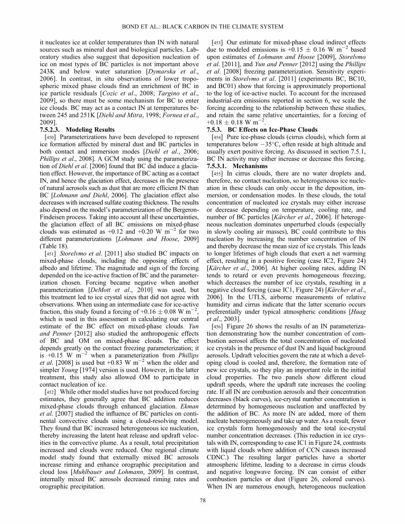
it nucleates ice at colder temperatures than IN with naturalsources such as mineral dust and biological particles. Lab-oratory studies also suggest that deposition nucleation ofice on most types of BC particles is not important above243K and below water saturation [Dymarska et al.,2006]. In contrast, in situ observations of lower tropo-spheric mixed phase clouds find an enrichment of BC inice particle residuals [Cozic et al., 2008; Targino et al.,2009], so there must be some mechanism for BC to enterice clouds. BC may act as a contact IN at temperatures be-tween 245 and 251K [Diehl and Mitra, 1998; Fornea et al.,2009].7.5.2.3. Modeling Results[450] Parameterizations have been developed to represent

ice formation affected by mineral dust and BC particles inboth contact and immersion modes [Diehl et al., 2006;Phillips et al., 2008]. A GCM study using the parameteriza-tion of Diehl et al. [2006] found that BC did induce a glacia-tion effect. However, the importance of BC acting as a contactIN, and hence the glaciation effect, decreases in the presenceof natural aerosols such as dust that are more efficient IN thanBC [Lohmann and Diehl, 2006]. The glaciation effect alsodecreases with increased sulfate coating thickness. The resultsalso depend on the model’s parameterization of the Bergeron-Findeisen process. Taking into account all these uncertainties,the glaciation effect of all BC emissions on mixed-phaseclouds was estimated as +0.12 and +0.20 W m�2 for twodifferent parameterizations [Lohmann and Hoose, 2009](Table 18).[451] Storelvmo et al. [2011] also studied BC impacts on

mixed-phase clouds, including the opposing effects ofalbedo and lifetime. The magnitude and sign of the forcingdepended on the ice-active fraction of BC and the parameter-ization chosen. Forcing became negative when anotherparameterization [DeMott et al., 2010] was used, butthis treatment led to ice crystal sizes that did not agree withobservations. When using an intermediate case for ice-activefraction, this study found a forcing of +0.16 � 0.08 W m�2,which is used in this assessment in calculating our centralestimate of the BC effect on mixed-phase clouds. Yunand Penner [2012] also studied the anthropogenic effectsof BC and OM on mixed-phase clouds. The effectdepends greatly on the contact freezing parameterization; itis +0.15 W m�2 when a parameterization from Phillipset al. [2008] is used but +0.83 W m�2 when the older andsimpler Young [1974] version is used. However, in the lattertreatment, this study also allowed OM to participate incontact nucleation of ice.[452] While other model studies have not produced forcing

estimates, they generally agree that BC addition reducesmixed-phase clouds through enhanced glaciation. Ekmanet al. [2007] studied the influence of BC particles on conti-nental convective clouds using a cloud-resolving model.They found that BC increased heterogeneous ice nucleation,thereby increasing the latent heat release and updraft veloc-ities in the convective plume. As a result, total precipitationincreased and clouds were reduced. One regional climatemodel study found that externally mixed BC aerosolsincrease riming and enhance orographic precipitation andcloud loss [Muhlbauer and Lohmann, 2009]. In contrast,internally mixed BC aerosols decreased riming rates andorographic precipitation.

[453] Our estimate for mixed-phase cloud indirect effectsdue to modeled emissions is +0.15 � 0.16 W m�2 basedupon estimates of Lohmann and Hoose [2009], Storelvmoet al. [2011], and Yun and Penner [2012] using the Phillipset al. [2008] freezing parameterization. Sensitivity experi-ments in Storelvmo et al. [2011] (experiments BC, BC10,and BC01) show that forcing is approximately proportionalto the log of ice-active nuclei. To account for the increasedindustrial-era emissions reported in section 6, we scale theforcing according to the relationship between these studies,and retain the same relative uncertainties, for a forcing of+0.18 � 0.18 W m�2.7.5.3. BC Effects on Ice-Phase Clouds[454] Pure ice-phase clouds (cirrus clouds), which form at

temperatures below �35�C, often reside at high altitude andusually exert positive forcing. As discussed in section 7.5.1,BC IN activity may either increase or decrease this forcing.7.5.3.1. Mechanisms[455] In cirrus clouds, there are no water droplets and,

therefore, no contact nucleation, so heterogeneous ice nucle-ation in these clouds can only occur in the deposition, im-mersion, or condensation modes. In these clouds, the totalconcentration of nucleated ice crystals may either increaseor decrease depending on temperature, cooling rate, andnumber of BC particles [Kärcher et al., 2006]. If heteroge-neous nucleation dominates unperturbed clouds (especiallyin slowly cooling air masses), BC could contribute to thisnucleation by increasing the number concentration of INand thereby decrease the mean size of ice crystals. This leadsto longer lifetimes of high clouds that exert a net warmingeffect, resulting in a positive forcing (case IC2, Figure 24)[Kärcher et al., 2006]. At higher cooling rates, adding INtends to retard or even prevents homogeneous freezing,which decreases the number of ice crystals, resulting in anegative cloud forcing (case IC1, Figure 24) [Kärcher et al.,2006]. In the UTLS, airborne measurements of relativehumidity and cirrus indicate that the latter scenario occurspreferentially under typical atmospheric conditions [Haaget al., 2003].[456] Figure 26 shows the results of an IN parameteriza-

tion demonstrating how the number concentration of com-bustion aerosol affects the total concentration of nucleatedice crystals in the presence of dust IN and liquid backgroundaerosols. Updraft velocities govern the rate at which a devel-oping cloud is cooled and, therefore, the formation rate ofnew ice crystals, so they play an important role in the initialcloud properties. The two panels show different cloudupdraft speeds, where the updraft rate increases the coolingrate. If all IN are combustion aerosols and their concentrationdecreases (black curves), ice-crystal number concentration isdetermined by homogeneous nucleation and unaffected bythe addition of BC. As more IN are added, more of themnucleate heterogeneously and take up water. As a result, fewerice crystals form homogeneously and the total ice-crystalnumber concentration decreases. (This reduction in ice crys-tals with IN, corresponding to case IC1 in Figure 24, contrastswith liquid clouds where addition of CCN causes increasedCDNC.) The resulting larger particles have a shorteratmospheric lifetime, leading to a decrease in cirrus cloudsand negative longwave forcing. IN can consist of eithercombustion particles or dust (Figure 26, colored curves).When IN are numerous enough, heterogeneous nucleation


78

dominates the formation of ice crystals, and the suppression ofhomogeneous nucleation has little effect on the final numberconcentration. Therefore, the addition of IN causes an increasein the number concentration of ice crystals (case IC2 in Fig-ure 24). Under some conditions, ice formation on combustionaerosol could entirely suppress homogeneous freezing.[457] At small updraft rates (top panel), few ice crystals

form and the influence of adding IN occurs at lower combus-tion aerosol number concentration. Large updraft velocities(bottom panel) cause the formation of a large number ofice crystals, since homogeneous freezing dominates iceformation (the number of aerosol droplets is not a limitingfactor). In this case, BC is not capable of causing a notableindirect effect. At intermediate updraft velocities, BCdepletes the air mass of moisture, causing much fewer (butstill more than BC) background particles to freezehomogenously. This discussion, focused largely on micro-physics, addresses only processes that affect the initial icecrystal concentration in single air parcels. This sensitivitystudy gives a first-order estimate of IN in young clouds butdoes not quantify the changes in the cloud as it evolvesand, therefore, does not reflect global averages.7.5.3.2. Field Evidence for BC Acting as IN[458] Laboratory studies indicate that IN activity of BC is,

at best, moderate. Field studies, summarized below, confirmthese findings. They indicate that homogeneous freezing is

the prevalent ice formation mode [DeMott et al., 2003;Cziczo et al., 2004a]. This is consistent with the ubiquityof high ice supersaturations in cloud free areas of the uppertroposphere [Jensen et al., 2001; Haag et al., 2003; Kahnet al., 2009a] and with the fact that total cirrus ice-crystalnumber densities often far exceed estimated IN concentra-tions [Gayet et al., 2002; Hoyle et al., 2005].[459] Field measurements using single-particle mass

spectrometry, electron microscopy, and X-ray emission orparticle elastic scattering analysis demonstrate that BC andorganic carbon are present in the troposphere and lowerstratosphere [Murphy et al., 2007; Nguyen et al., 2008].Often, the predominant particles are composed of organiccarbon that originates mainly from surface sources. Evenparticles that reach the stratosphere may have acquired smallamounts of carbon during transport through the upper tropo-sphere. Some measurements suggest that BC’s effectivenessas an IN is greatest if it is uncoated, but this finding is not yetdefinitive. Presumably, uncoated BC rarely exists in theUTLS region, and because it is difficult to detect thin coat-ings on BC, the number of such particles in this region ispoorly known.[460] A constraint that could ascertain whether BC affects

ice cloud formation would be direct airborne sampling ofparticles at high altitudes, along with simultaneous charac-terization of their chemical composition and measurements

Figure 26. Calculated total number concentration of nucleated ice crystals as a function of BC combus-tion particle number concentration. Ice particle number results from the competition of three particle types(liquid H2SO4/H2O droplets acting as homogeneous freezing nuclei, and dust and BC particles acting as het-erogeneous IN) during ice formation in adiabatically rising air parcels (sharp ice nucleation thresholds for theIN given in the legend). Results are shown for an updraft velocity of 5 cm/s (top panel: synoptic-scale verticalwinds), and 100 cm/s (bottom panel: strong orographic waves or convective cells). In the simulations, air par-cels start rising at 250 hPa and 220 K at ice saturation and contain mineral dust particles with concentrationsnoted in the legends, a wide range of BC (103 L�1 = 1 cm�3) concentrations, and a fixed concentration of log-normally distributed aqueous H2SO4 particles. Dust and soot particles are assumed to be monodisperse.Adapted from Kärcher et al. [2007].


79

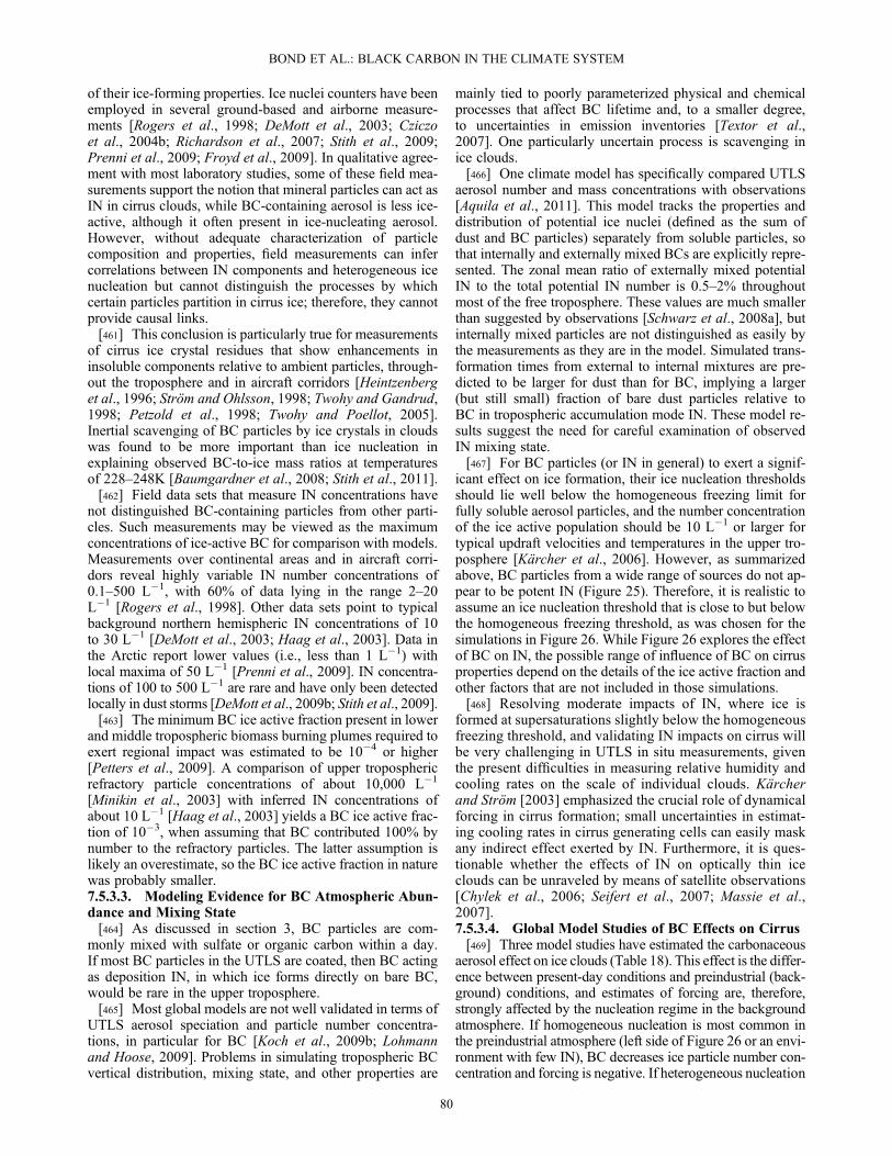
of their ice-forming properties. Ice nuclei counters have beenemployed in several ground-based and airborne measure-ments [Rogers et al., 1998; DeMott et al., 2003; Cziczoet al., 2004b; Richardson et al., 2007; Stith et al., 2009;Prenni et al., 2009; Froyd et al., 2009]. In qualitative agree-ment with most laboratory studies, some of these field mea-surements support the notion that mineral particles can act asIN in cirrus clouds, while BC-containing aerosol is less ice-active, although it often present in ice-nucleating aerosol.However, without adequate characterization of particlecomposition and properties, field measurements can infercorrelations between IN components and heterogeneous icenucleation but cannot distinguish the processes by whichcertain particles partition in cirrus ice; therefore, they cannotprovide causal links.[461] This conclusion is particularly true for measurements

of cirrus ice crystal residues that show enhancements ininsoluble components relative to ambient particles, through-out the troposphere and in aircraft corridors [Heintzenberget al., 1996; Ström and Ohlsson, 1998; Twohy and Gandrud,1998; Petzold et al., 1998; Twohy and Poellot, 2005].Inertial scavenging of BC particles by ice crystals in cloudswas found to be more important than ice nucleation inexplaining observed BC-to-ice mass ratios at temperaturesof 228–248K [Baumgardner et al., 2008; Stith et al., 2011].[462] Field data sets that measure IN concentrations have

not distinguished BC-containing particles from other parti-cles. Such measurements may be viewed as the maximumconcentrations of ice-active BC for comparison with models.Measurements over continental areas and in aircraft corri-dors reveal highly variable IN number concentrations of0.1–500 L�1, with 60% of data lying in the range 2–20L�1 [Rogers et al., 1998]. Other data sets point to typicalbackground northern hemispheric IN concentrations of 10to 30 L�1 [DeMott et al., 2003; Haag et al., 2003]. Data inthe Arctic report lower values (i.e., less than 1 L�1) withlocal maxima of 50 L�1 [Prenni et al., 2009]. IN concentra-tions of 100 to 500 L�1 are rare and have only been detectedlocally in dust storms [DeMott et al., 2009b; Stith et al., 2009].[463] The minimum BC ice active fraction present in lower

and middle tropospheric biomass burning plumes required toexert regional impact was estimated to be 10�4 or higher[Petters et al., 2009]. A comparison of upper troposphericrefractory particle concentrations of about 10,000 L�1

[Minikin et al., 2003] with inferred IN concentrations ofabout 10 L�1 [Haag et al., 2003] yields a BC ice active frac-tion of 10�3, when assuming that BC contributed 100% bynumber to the refractory particles. The latter assumption islikely an overestimate, so the BC ice active fraction in naturewas probably smaller.7.5.3.3. Modeling Evidence for BC Atmospheric Abun-dance and Mixing State[464] As discussed in section 3, BC particles are com-

monly mixed with sulfate or organic carbon within a day.If most BC particles in the UTLS are coated, then BC actingas deposition IN, in which ice forms directly on bare BC,would be rare in the upper troposphere.[465] Most global models are not well validated in terms of

UTLS aerosol speciation and particle number concentra-tions, in particular for BC [Koch et al., 2009b; Lohmannand Hoose, 2009]. Problems in simulating tropospheric BCvertical distribution, mixing state, and other properties are

mainly tied to poorly parameterized physical and chemicalprocesses that affect BC lifetime and, to a smaller degree,to uncertainties in emission inventories [Textor et al.,2007]. One particularly uncertain process is scavenging inice clouds.[466] One climate model has specifically compared UTLS

aerosol number and mass concentrations with observations[Aquila et al., 2011]. This model tracks the properties anddistribution of potential ice nuclei (defined as the sum ofdust and BC particles) separately from soluble particles, sothat internally and externally mixed BCs are explicitly repre-sented. The zonal mean ratio of externally mixed potentialIN to the total potential IN number is 0.5–2% throughoutmost of the free troposphere. These values are much smallerthan suggested by observations [Schwarz et al., 2008a], butinternally mixed particles are not distinguished as easily bythe measurements as they are in the model. Simulated trans-formation times from external to internal mixtures are pre-dicted to be larger for dust than for BC, implying a larger(but still small) fraction of bare dust particles relative toBC in tropospheric accumulation mode IN. These model re-sults suggest the need for careful examination of observedIN mixing state.[467] For BC particles (or IN in general) to exert a signif-

icant effect on ice formation, their ice nucleation thresholdsshould lie well below the homogeneous freezing limit forfully soluble aerosol particles, and the number concentrationof the ice active population should be 10 L�1 or larger fortypical updraft velocities and temperatures in the upper tro-posphere [Kärcher et al., 2006]. However, as summarizedabove, BC particles from a wide range of sources do not ap-pear to be potent IN (Figure 25). Therefore, it is realistic toassume an ice nucleation threshold that is close to but belowthe homogeneous freezing threshold, as was chosen for thesimulations in Figure 26. While Figure 26 explores the effectof BC on IN, the possible range of influence of BC on cirrusproperties depend on the details of the ice active fraction andother factors that are not included in those simulations.[468] Resolving moderate impacts of IN, where ice is

formed at supersaturations slightly below the homogeneousfreezing threshold, and validating IN impacts on cirrus willbe very challenging in UTLS in situ measurements, giventhe present difficulties in measuring relative humidity andcooling rates on the scale of individual clouds. Kärcherand Ström [2003] emphasized the crucial role of dynamicalforcing in cirrus formation; small uncertainties in estimat-ing cooling rates in cirrus generating cells can easily maskany indirect effect exerted by IN. Furthermore, it is ques-tionable whether the effects of IN on optically thin iceclouds can be unraveled by means of satellite observations[Chylek et al., 2006; Seifert et al., 2007; Massie et al.,2007].7.5.3.4. Global Model Studies of BC Effects on Cirrus[469] Three model studies have estimated the carbonaceous

aerosol effect on ice clouds (Table 18). This effect is the differ-ence between present-day conditions and preindustrial (back-ground) conditions, and estimates of forcing are, therefore,strongly affected by the nucleation regime in the backgroundatmosphere. If homogeneous nucleation is most common inthe preindustrial atmosphere (left side of Figure 26 or an envi-ronment with few IN), BC decreases ice particle number con-centration and forcing is negative. If heterogeneous nucleation


80

was dominant in the preindustrial case (toward the upwardslope of Figure 26 or an environment with more dust), BCincreases ice particle number concentration and forcing be-comes positive. A predominance of droplets or sulfate par-ticles corresponds to natural conditions with homogeneousnucleation, while predominance of refractory particles likedust would result in heterogeneous domination. The influ-ence of adding IN on ice formation is largely controlledby cloud-scale dynamics, and changes in the dynamic re-gime since the preindustrial era are not fully included in thisforcing estimate.[470] Penner et al. [2009] used off-line estimates from a

CTM aerosol scheme coupled to the NCAR CAM3. Theyused two parameterizations that allowed for competitionbetween homogeneous and heterogeneous nucleation in anaerosol mass-only and a three-mode, two-moment versionsof the model. Sulfate droplets were assumed to act as homo-geneous freezing agents, BC was assumed to be coated withsoluble material and, therefore, to act as immersion IN,and dust was assumed to act as IN in the deposition or con-densation mode. For the more sophisticated (three-mode)parameterization, two different ice nucleation schemes gavea forcing from fossil fuel and biomass burning emissions of�0.3 to �0.4 W m�2. The dominant effect was that hetero-geneous IN activity of BC decreased relative humidity withrespect to ice, inhibited homogeneous nucleation, decreasedthe number concentration of ice particles, and reduced posi-tive forcing by high-level clouds.[471] The mass-only version of the aerosol model was

applied by Liu et al. [2009a] in the NCAR CAM3 globalmodel with a double moment ice microphysical scheme.Adding BC resulted in increased high-level clouds,especially over polar regions but also somewhat over tropicalregions. The resulting change in forcing due to BC emitted atthe surface was +0.22 W m�2 or +0.39 W m�2 when criticalsupersaturations of 1.2 to 1.3 or 1.4, respectively, wereassigned to BC. The larger forcing for higher ice nucleationthreshold is due to a larger decrease in negative shortwavecontribution. The change in sign between this study and thePenner et al. [2009] results reflects the large uncertainty in thisforcing, stemming from the fact that cirrus clouds affect bothshortwave and longwave radiative fluxes, and the change ineach is determined by specific cloud properties. The forcingis, therefore, a small value calculated by adding two largevalues of opposing sign, making it very sensitive to changesin the magnitude of either one. Similar uncertainties are seenin the estimation of the climate effects of aviation BC emis-sions, which are not included here. There are three majordifferences between this study and Penner et al. [2009]. Inthe preindustrial atmosphere, homogeneous nucleation domi-nated in Penner et al. [2009] while heterogeneous nucleationdominated background conditions in Liu et al. [2009a]. Liuet al. used a prognostic treatment of the ice-crystal numberconcentration including source and sink terms while Penneret al. diagnosed ice-crystal number concentration from nucle-ation. Liu et al. [2009a] included climate feedbacks, so thataerosols in the UTLS region tended to enhance relative humid-ities there; however, they were unable to reproduce theobserved supersaturations in the atmosphere, so that themodeled supersaturations were never high enough to allowhomogeneous nucleation [Liu et al., 2007, Figure 3].

[472] Gettelman et al. [2012] analyzed the BC effect on iceclouds as part of a more comprehensive study of ice nucle-ation in the CAM5 model, exploring the effect ofparameterisation changes on background cloud propertiesand the aerosol indirect effect. They compared study pairswith 1850 and 2000 aerosol emissions. One member of thepair had fixed ice nuclei as a function of temperature andthe other used a more complete parameterization, allowingcompetition between heterogeneous nucleation on dust withhomogeneous nucleation on sulphate. The standard modelused only coarse-mode dust as potential ice nuclei. BC wasincorporated into this scheme by assuming it had the sameice nucleation properties as dust. The ice active fraction forBC was set to 0.1%, 2%, and 100% in different simulations.Only the simulation assuming a 0.1% ice active fractiongave realistic ice water mass and cloud radiative properties,and this simulation was used to estimate the indirect effect.Forcings were estimated from the full ToA radiative-fluxchange, a cloud forcing change, and a cloud forcing changewith a clear-sky flux change correction applied; the quotedresult is the average of these three. This study estimates+0.27 � 0.10 W m�2 (1s uncertainty) for the total icecloud aerosol indirect effect. The BC component was�0.06 W m�2 and was not statistically significant.[473] Jacobson [2010] included ice-cloud effects in a

model of the effect of BC on climate. Ice crystal sizesincreased slightly due to BC. The study used a temperature-dependent ice-nucleation threshold for uncoated BC(section 7.5.1) that ranged between 1.15 and 1.35. Thesevalues are within the range for uncoated spark-generated sootat moderate and low temperatures but below the range ofcoated soot in Figure 25. Cloud drop and ice-crystal numberconcentration were calculated by simultaneously solving themass balance equations for water vapor, liquid, and ice, con-sidering all aerosol and cloud particle sizes. BC in this modelstudy is a more efficient IN than is observed in the laboratory.In the study, relative humidity increased at high altitudes andin the Arctic, and ice clouds increased due to BC, which areresults similar to those in Liu et al. [2009a]. Forcing due tothis IN mechanism was not isolated, but the direction of ice-cloud changes suggests a positive forcing.[474] In a global model study by Hendricks et al. [2011], a

multiple-mode ice microphysical scheme was applied in theECHAM GCM to simulate IN effects on global cirrusproperties. The ice nucleation parameterization by Kärcheret al. [2006] was applied to simulate the competitionbetween homogeneous and heterogeneous ice formation.Hendricks et al. [2011] assumed that only small fractionsof the modeled BC and mineral dust particles (0.25% and1%, respectively) could act as IN, resulting in IN concen-trations in the order of 10 L�1 at cirrus levels. BC anddust-related IN had similar contributions. Heterogeneousnucleation on both types of particles produced significantreductions in the mean cirrus ice particle number concen-trations. The effect was most pronounced in the tropics,where the zonal mean annual average ice particle numberconcentration decreased by up to 20%. Reductions in themean ice water content, likely resulting from efficientsedimentation and precipitation of large ice particlesgenerated by heterogeneous nucleation, also occurred.This effect led to reductions in the zonal mean, annuallyaveraged, water-vapor mixing ratio of up to 5% at cirrus


81

levels. The BC contribution to these effects was compara-ble to that related to mineral dust IN only when theassumed ice nucleation threshold is significantly lowerthan that assumed for dust particles (threshold of 1.2for BC and 1.3 for mineral dust). When a larger criticalvalue (ice nucleation threshold of 1.40) was assumedfor BC, heterogeneous freezing was dominated by min-eral dust particles.[475] Compared to the global model studies by Liu et al.

[2009a] and Penner et al. [2009], Hendricks et al. [2011]and Gettelman et al. [2012] simulated a much smallereffect of BC on cirrus ice crystal number concentrations.

These differences could result from either a smaller avail-ability of active ice nuclei in the Hendricks et al. [2011]and Gettelman et al. [2012] studies or from differences inthe representation of relative humidity and cooling rates.Gettelman et al. [2012] found that an ice active fractionof 0.1% gave realistic ice water content and radiativeproperties, and ice active fractions of 2% and 100%did not.[476] Compared with the measurements discussed in

section 7.5.3.2, the Liu et al. [2009a] and Penner et al.[2009] studies may overestimate UTLS BC and IN and may,therefore, overestimate the magnitude of the ice-cloud indirect

Table 19. Model Studies Used to Derive the Adjusted Forcing of Black Carbon in Snow and Icea

Hansen andNazarenko [2004] Jacobson [2004a]

Hansen et al. [2005, 2007];b

Shindell and Faluvegi [2009]

Emissions year and global, annual BC emissions used toderive forcing (GgCyr�1)

n/a FF +BF: 3920 Year 1880, 2000:BB: 3140 FF: 500, 5700

BF: 500, 1000BB: 2300, 4600

Total: 7060

Total 1880, 2000:3300, 11300

Emission inventories used n/a Early version ofBond et al. [2004]e

for year 1996

FF: Penner et al.[2001] (via D.Koch, personalcommunication)BB and BF:Liousse et al. [1996]

Gridbox size (latitude � longitude) 4� � 5� 4� � 5� 4� � 5�BC forcing medium g n/a SNL, SNI, SI SNL, SNI

Present-day adjusted forcing for FF+BF only (Wm�2) n/a 0.06h {0.05}Pre-industrial-to-present (years)adjusted forcing for FF+BF+BB

n/a n/a (1880–2000)Hansen et al. [2005, 2007]0.08; 0.05

Present-day adjusted forcing, for FF+BF+BB(Wm�2)

0.16 {0.08} {0.07}

Climate forcing per emission (mWm�2)(GgCyr�1)�1 for all-source forcing

n/a {11} {6}

a“Adjusted forcing” here refers to radiative forcing plus the rapid adjustments to that forcing (Table 20), producing the adjusted forcing as defined inTable 2. However, as shown in Table 20, studies included different rapid adjustments; for the Rypdal et al. [2009b], Skeie et al. [2011], and Wang et al.[2011] studies, no rapid adjustments were included so the climate forcing equals the radiative forcing. Shown are the model BC emission sources andstrengths (global, annual average; FF = fossil fuel; BF = biofuel; BB= biomass burning), model gridbox size, and the global, annual average, adjusted forc-ing for FF +BF only and for FF +BF+BB. The global, annual average forcing per emissions for FF +BF+BB is also given. Values that are either directlyreported in the studies or which can be calculated from reported values are given in bold face. Values shown in {brackets} are estimates based on scaling thereported values, as described in section 8.6.1.

bHansen et al. [2007] revised down the total BC-in-snow forcing given by Hansen et al. [2005] after correcting a programming error. Both sets of data aregiven here.

cFlanner et al. [2007] provided calculations for high (1998) and low (2001) biomass burning years.dFlanner et al. [2009] selected 2002 biomass burning emissions because this is a “typical” boreal fire year (versus the “high” and “low” cases selected for

Flanner et al. [2007]).eJacobson [2004a] used an “early version” of the Bond et al. [2004] inventory for submicron BC emissions, where FF +BF ~20% lower (global, annual

average) than was ultimately given in Bond et al. [2004]. However, Jacobson [2004a] also included super-micron BC emissions, set at 25% of the mass ofsub-micron emissions, so the total BC emissions were, in terms of mass, close to those of Bond et al. [2004], though the differing size distributions affectdeposition rates and therefore spatial distribution of deposited BC. Bond et al. [2004] annual biomass burning emissions were used to determine monthlyemissions by scaling using the monthly inventory of Cooke and Wilson [1996].

fPre-industrial (1890) BF emissions comes from taking van Aardenne et al. [2001] SO2 biofuel emissions and calculating BC+OC BF emissions usingthe ratios of SO2 : BC and SO2 :OC in 1990 from van Aardenne (SO2) and Bond et al. [2004] (BC and OC).

gForcing by BC in snow on land (SNL), BC in snow on sea ice (SNI), and BC in bare (non-snow-covered) sea ice (SI).hEstimated value provided via personal communication (M. Z. Jacobson). Radiative forcing was not reported in Jacobson [2004a].iRypdal et al. [2009b] BF includes only energy-related biofuel burning.jRypdal et al. [2009b] did not include biomass burning emissions, so here we have used the Flanner et al. [2009] 2.7 TgCyr�1 for BB emissions and have

scaled the Rypdal et al. (FF + contained BF) forcing linearly to get a forcing for FF +BF+BB.kSkeie et al. [2011] include BB aerosols in their model, but forcing is calculated for FF +BF emissions only and all reported forcings are relative to base

year 1750.lWang et al. [2011] is surface forcing; ToA forcing was not reported but would be lower than the surface forcing because of the effect of atmospheric

transmission.n/a = not applicable.


82

effect. Liu et al. [2009a] reported BC concentrations ofabout 300 to 3000 L�1, which when compared to a fewmeasurements were roughly a factor of 2 too high. Penneret al. [2009] reported reasonable agreement with measure-ments of IN from one field campaign, but the concentrationsexceed those summarized in section 7.5.3.2 for a moregeographically diverse set of regions. IN concentrationsin the UTLS region are smaller in Liu et al. [2009a] thanin Penner et al. [2009].[477] Our estimate of the BC influence on ice-cloud in-

direct effects is 0.0 � 0.4 W m�2 based on theGettelman et al. [2012] study and the average and rangeof Liu et al. [2009a] and Penner et al. [2009]. Both Penneret al. [2009] and Liu et al. [2009a] lack fidelity in some as-pects, so that there is no clear choice between the two oppos-ing results. However, we use them to bound the uncertaintyrange. Unlike all other cloud forcings, this estimate has notbeen scaled to our best estimate of industrial-era BCemission rate. For ice-cloud effects, many factors other thanemission rate affect ice-active BC concentrations in theupper troposphere. Most models, including those used inthe Penner et al. [2009] and Liu et al. [2009a] studies,overestimate these concentrations. Therefore, the modelresults may represent an upper bound on the magnitude ofice-cloud impact. In the Gettelman et al. [2012] study, theBC ice cloud impact was not significant.7.5.3.5. Aircraft Impacts on High Ice-Cloud Properties[478] BC emissions from aviation are a very small fraction

of direct forcing because they are a very small fraction ofglobal emissions. However, aviation emissions of BC pro-vide an especially potent source of potential ice nuclei[Kärcher et al., 1996; Schröder et al., 1998]. The Liu et al.[2009a] and Penner et al. [2009] modeling studies estimatethe effect of aviation BC alone on ice cloud to be between�0.16 W m�2 to +0.26 W m�2. Aviation emissions

potentially have a larger effect on ice clouds than compara-ble emissions at the surface [Lee et al., 2010]. The totalBC climate forcing in Figure 35 explicitly excludes aviationemissions. We mention these studies here because they mayprovide additional clues about how BC particles affect cirrusclouds, although BC emitted from aviation may undergo lessmixing with tropospheric particles and gases.[479] Although contrails would form even in the absence

of BC emissions, the optical properties of the contrails andcirrus impacts depend on BC emission levels [Kärcher andYu, 2009; Lee et al., 2010]. Water supersaturated conditionsduring contrail ice formation below approximately 225Kactivate even rather hydrophobic BC particles into rapidlyfreezing water droplets [Kärcher et al., 1996; Köhler et al.,2009]. A decrease in ice cloud particle size for cirrus cloudsaltered by aircraft may imply that aircraft BC increases theconcentration of available IN for these aged contrails or cir-rus clouds [Lee et al., 2010]. Jacobson et al. [2011]found that an assumption of efficient ice nuclei (i.e., icenucleation threshold of 1.35 at 185K) was required for a goodmatch with observed contrail cloud fractions. The modelstudy of Hendricks et al. [2005] suggests that aircraft BCincreases IN by 10 to 40% in aircraft cruise altitudes innorthern mid-latitudes. However, the ice nucleating prop-erties of aircraft exhaust for the exact composition andcoating of exhaust particles, at the temperature and watervapor conditions in cirrus, remain poorly known. The im-pact of aircraft BC emissions on cirrus cloud formationin the absence of contrail formation remains veryuncertain.

7.6. Comprehensive Modeling of BC Cloud Effects

[480] Although the discussion above has separatedeffects on individual cloud types, one series of modelresults [Jacobson, 2001b; Jacobson, 2002; Jacobson,

Flanner et al. [2007] Flanner et al. [2009]Koch et al.[2009a]

Rypdal et al.[2009b]

Skeie et al.[2011] k

Wang et al.[2011]

Year 1996 Year 1996 Year 1890, 1995: FF + contained BFburning: 5300

Year 1750, 2000: n/aFF + BF: 4700 FF + BF: 4700 FF + BF: 1800, 4500 FF+BF: 0400, 4500Year 1998 c BB: 4100 Year 2002 BB d: 2700 BB: 2200, 3700 BB: 1000, 2600Year 2001 BB: 2000 Total: 7400 Total 1890, 1995: Total 1750, 2000:Total 1998, 2001: 4000, 8200 1400, 71008800, 6700

Bond et al.[2004] +GFEDv2[van der Werf et al.,2006] for open burn

Bond et al.[2004] +GFEDv2[van der Werf et al.,2006] for open burn

BB: GFEDv1; Pre-indust.FF: Lefohn et al. [1999]BF: van Aardenne et al.[2001]f;Present day FF +BF:Bond et al. [2004]

Cofala et al.[2007]

FF+BF: Bondet al. [2007]

n/a

BB: Lamarqueet al. [2010]

2.8� � 2.8� 2.8� � 2.8� 4� � 5� 1� � 1� 1� � 1� 2.8� � 2.8�SNL, SNI SNL, SNI SNL, SNI SNL, SNI, SI SNL, SNI, SI n/a0.043 0.037 {0.02} 0.03i {0.018} n/an/a n/a (1890–1995) n/a (1750-2000) n/a

0.01 {0.021}

0.054 (1998) 0.047 0.03 {0.04} {0.024} 0.042 l

0.049 (2001)6 (1998 BB), 6 4 {5} j {3} n/a7 (2001 BB)

Table 19. (Continued)


83

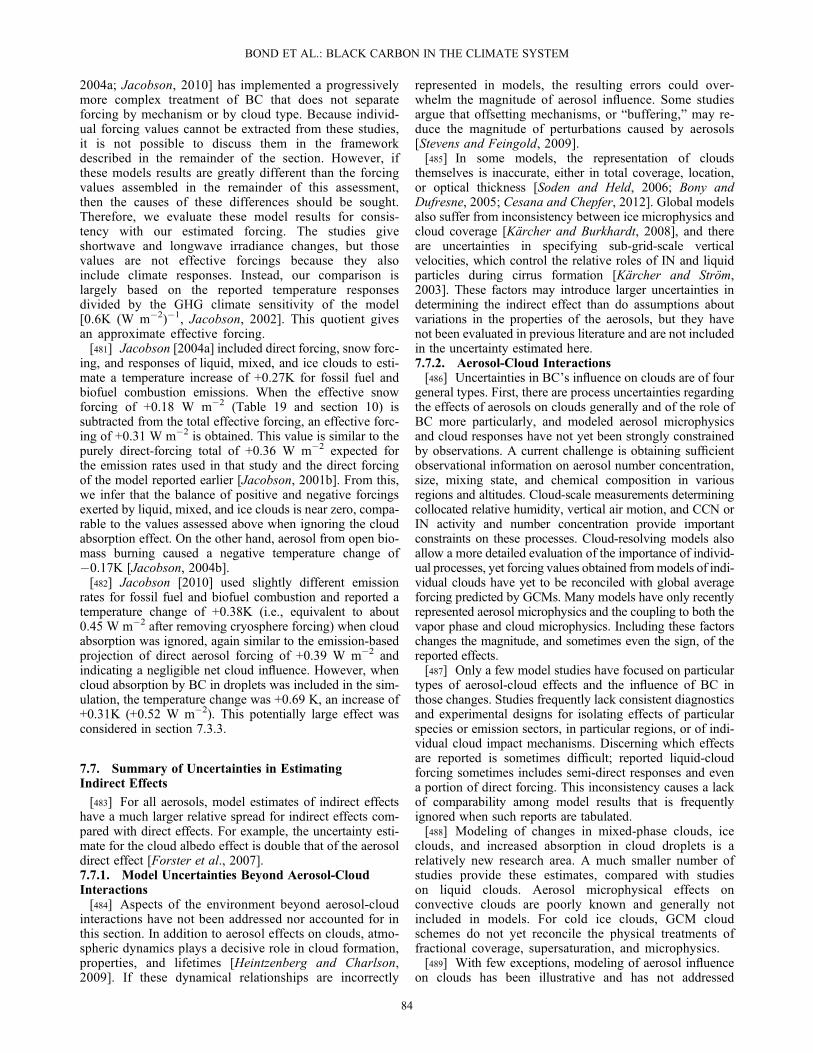
2004a; Jacobson, 2010] has implemented a progressivelymore complex treatment of BC that does not separateforcing by mechanism or by cloud type. Because individ-ual forcing values cannot be extracted from these studies,it is not possible to discuss them in the frameworkdescribed in the remainder of the section. However, ifthese models results are greatly different than the forcingvalues assembled in the remainder of this assessment,then the causes of these differences should be sought.Therefore, we evaluate these model results for consis-tency with our estimated forcing. The studies giveshortwave and longwave irradiance changes, but thosevalues are not effective forcings because they alsoinclude climate responses. Instead, our comparison islargely based on the reported temperature responsesdivided by the GHG climate sensitivity of the model[0.6K (W m�2)�1, Jacobson, 2002]. This quotient givesan approximate effective forcing.[481] Jacobson [2004a] included direct forcing, snow forc-

ing, and responses of liquid, mixed, and ice clouds to esti-mate a temperature increase of +0.27K for fossil fuel andbiofuel combustion emissions. When the effective snowforcing of +0.18 W m�2 (Table 19 and section 10) issubtracted from the total effective forcing, an effective forc-ing of +0.31 W m�2 is obtained. This value is similar to thepurely direct-forcing total of +0.36 W m�2 expected forthe emission rates used in that study and the direct forcingof the model reported earlier [Jacobson, 2001b]. From this,we infer that the balance of positive and negative forcingsexerted by liquid, mixed, and ice clouds is near zero, compa-rable to the values assessed above when ignoring the cloudabsorption effect. On the other hand, aerosol from open bio-mass burning caused a negative temperature change of�0.17K [Jacobson, 2004b].[482] Jacobson [2010] used slightly different emission

rates for fossil fuel and biofuel combustion and reported atemperature change of +0.38K (i.e., equivalent to about0.45 W m�2 after removing cryosphere forcing) when cloudabsorption was ignored, again similar to the emission-basedprojection of direct aerosol forcing of +0.39 W m�2 andindicating a negligible net cloud influence. However, whencloud absorption by BC in droplets was included in the sim-ulation, the temperature change was +0.69 K, an increase of+0.31K (+0.52 W m�2). This potentially large effect wasconsidered in section 7.3.3.

7.7. Summary of Uncertainties in EstimatingIndirect Effects

[483] For all aerosols, model estimates of indirect effectshave a much larger relative spread for indirect effects com-pared with direct effects. For example, the uncertainty esti-mate for the cloud albedo effect is double that of the aerosoldirect effect [Forster et al., 2007].7.7.1. Model Uncertainties Beyond Aerosol-CloudInteractions[484] Aspects of the environment beyond aerosol-cloud

interactions have not been addressed nor accounted for inthis section. In addition to aerosol effects on clouds, atmo-spheric dynamics plays a decisive role in cloud formation,properties, and lifetimes [Heintzenberg and Charlson,2009]. If these dynamical relationships are incorrectly

represented in models, the resulting errors could over-whelm the magnitude of aerosol influence. Some studiesargue that offsetting mechanisms, or “buffering,” may re-duce the magnitude of perturbations caused by aerosols[Stevens and Feingold, 2009].[485] In some models, the representation of clouds

themselves is inaccurate, either in total coverage, location,or optical thickness [Soden and Held, 2006; Bony andDufresne, 2005; Cesana and Chepfer, 2012]. Global modelsalso suffer from inconsistency between ice microphysics andcloud coverage [Kärcher and Burkhardt, 2008], and thereare uncertainties in specifying sub-grid-scale verticalvelocities, which control the relative roles of IN and liquidparticles during cirrus formation [Kärcher and Ström,2003]. These factors may introduce larger uncertainties indetermining the indirect effect than do assumptions aboutvariations in the properties of the aerosols, but they havenot been evaluated in previous literature and are not includedin the uncertainty estimated here.7.7.2. Aerosol-Cloud Interactions[486] Uncertainties in BC’s influence on clouds are of four

general types. First, there are process uncertainties regardingthe effects of aerosols on clouds generally and of the role ofBC more particularly, and modeled aerosol microphysicsand cloud responses have not yet been strongly constrainedby observations. A current challenge is obtaining sufficientobservational information on aerosol number concentration,size, mixing state, and chemical composition in variousregions and altitudes. Cloud-scale measurements determiningcollocated relative humidity, vertical air motion, and CCN orIN activity and number concentration provide importantconstraints on these processes. Cloud-resolving models alsoallow a more detailed evaluation of the importance of individ-ual processes, yet forcing values obtained frommodels of indi-vidual clouds have yet to be reconciled with global averageforcing predicted by GCMs. Many models have only recentlyrepresented aerosol microphysics and the coupling to both thevapor phase and cloud microphysics. Including these factorschanges the magnitude, and sometimes even the sign, of thereported effects.[487] Only a few model studies have focused on particular

types of aerosol-cloud effects and the influence of BC inthose changes. Studies frequently lack consistent diagnosticsand experimental designs for isolating effects of particularspecies or emission sectors, in particular regions, or of indi-vidual cloud impact mechanisms. Discerning which effectsare reported is sometimes difficult; reported liquid-cloudforcing sometimes includes semi-direct responses and evena portion of direct forcing. This inconsistency causes a lackof comparability among model results that is frequentlyignored when such reports are tabulated.[488] Modeling of changes in mixed-phase clouds, ice

clouds, and increased absorption in cloud droplets is arelatively new research area. A much smaller number ofstudies provide these estimates, compared with studieson liquid clouds. Aerosol microphysical effects onconvective clouds are poorly known and generally notincluded in models. For cold ice clouds, GCM cloudschemes do not yet reconcile the physical treatments offractional coverage, supersaturation, and microphysics.[489] With few exceptions, modeling of aerosol influence

on clouds has been illustrative and has not addressed


84

sensitivities nor constrained sensitive parameters withobservations. Models agree that forcing usually increasesas emissions increase, yet some studies do not even reportthe emission rates used, again making comparability diffi-cult. Forcing may not be linear with regard to emissions orother inputs such as particle size, but sensitivity studies arenot available to provide more constrained scaling for caseswhen modeled aerosol concentrations differ from observedvalues. Uncertainties estimated for cloud effects are obtainedfrom model diversity rather than from true uncertainty prop-agation, as the latter has not been achieved with currentmodels and scientific understanding.[490] Multiple indirect effects exist and the combination of

forcings may be nonlinear. Forcing inferred from satelliteobservations may include the combined response, but in situobservations may be more likely to isolate individual effects.A constraining approach that combines the strengths of allapproaches has not yet appeared.[491] Because of sub-linearity in cloud response to

increasing aerosol concentrations, the dependence ofindustrial-era forcing on assumed preindustrial values iseven greater for indirect effects than for direct effects.To determine the impacts of future aerosol changes andfor comparison with temperature changes in recent years,examining changes from present-day conditions couldprovide a more reliable measure than comparison with anominal preindustrial condition [Menon et al., 2002a].

8. Cryosphere Changes: Black Carbon in Snowand Ice


[492] 1. Light-absorbing particles in snow can significantlyreduce snow albedo. Because of the high albedo of snow,even aerosol with relatively high single-scatter albedo (e.g., aerosol with a high OA :BC ratio) causes positive radia-tive forcing.[493] 2. Small initial snow albedo reductions may have a

large adjusted forcing because the resulting warming affectsthe snow morphology (grain size), snow sublimation rates, andsnowmelt rates, all of which enhance BC-induced snowpack al-bedo reductions, leading to an amplification of the radiativeforcing. Albedo feedback triggered by this forcing drives a largesurface temperature response (section 9).[494] 3. The best estimates for all-source and industrial-era

adjusted forcing by BC in snow are +0.04 W m�2 and+0.035 W m�2, respectively. The all-source estimate is de-rived by scaling the results of a suite of model studies toachieve consistent estimates of forcing from all present-daysources (fossil fuel, biofuel, and biomass burning). Measure-ments of the BC content of Arctic snow were also used toadjust two of the model studies’ derived forcing for biasesin snow BC concentrations. Industrial-era forcing is calcu-lated by scaling by the ratio of industrial-era to all-sourceBC emissions, accounting for changes 1750 to present dayin the fraction of global emissions from fossil fuel-plus-bio-fuel and from open biomass burning which are deposited tosnow. Changes in snow and ice cover 1750 to present dayare not accounted for. These central estimates also do not ac-count for forcing by BC in sea ice but do account for forcingby BC in snow on sea ice.

[495] 4. The bounds for all-source snowBC adjusted forcingare estimated at +0.01 W m�2 to +0.09 W m�2 and for indus-trial-era forcing at +0.008 W m�2 and +0.078 W m�2. Thesebounds include rapid adjustments in snow grain size and sur-face snow BC concentrations due to changes in sublimationand melt rates resulting from the initial snow albedo reductiondue to BC. They are based on results of model sensitivity stud-ies applying low and high values of snow cover fraction, rateof snow aging and resulting grain size evolution, scavengingof BC out of the snowpack during melt, and BC emissions,as well as a model estimate of the reduction in forcing byBC caused by the concurrent presence of light-absorbingsoil dust. These bounds do not account for uncertainty inhow forcing is affected by patchy snow cover, byuncertainties in modeled cloud cover and vegetation cover,or for possible biases in modeled mid-latitude snow BCconcentrations.[496] 5. The best estimate for all-source and industrial-era

radiative forcings by BC in melting snow-free sea ice are+0.012 W m�2 and +0.011 W m�2, respectively. These forc-ings do not account for rapid adjustments that may amplifythe initial radiative forcing. They are derived using Arctic-wide averages for sea-ice BC concentration, sea-ice area, meltpond fraction, snow cover fraction, and solar irradiance. Thebounds on sea-ice BC radiative forcing are +0.008 and+0.017 W m�2 for all-source forcing and +0.007 and+0.016 W m�2 for industrial-era forcing, based on indepen-dently calculating negative and positive deviations from themean given by realistic possible minima and maxima in thesefactors.[497] 6. Chemical analysis of springtime surface snow

samples indicate that most BC and other light-absorbingparticles in the North American and Russian Arctic snowand in Greenland are associated with biomass burning.Fossil fuel plays a prominent role in the high-latitudeArctic Ocean and in Greenland in the summertime, butin Greenland, concentrations are low. Indirect evidenceindicates that pollution may also play a significant rolein the Arctic north of Europe, where concentrations arehigher.[498] 7. A large fraction of particulate light absorption in

Arctic snow (about 30 to 50%) is due to non-BC constitu-ents. Most of the absorption appears to be due to light-absorbing organic carbon from biofuel and agricultural orboreal forest burning. The forcing estimates given above ac-count for only BC. The total forcing by a source which emitsboth BC and light-absorbing organic carbon is larger than isgiven by BC forcing alone.[499] 8. In some regions, especially areas with thin and

patchy snow cover or mountainous regions, soil dust signif-icantly lowers snow albedo, lessening the influence of BC.Models do not capture these potentially large sources of lo-cal dust to the snowpack and, therefore, may beoverestimating BC forcing, and this is not accounted forhere.[500] 9. There is evidence that snow BC concentrations in

the Arctic, Europe, and North America were higher in theearly and middle twentieth century than presently. Also,snow cover is declining with time. Thus, snow BC forcingis likely decreasing in many regions.[501] 10. BC in glacial snow is a concern primarily be-

cause of its possible role in altering melt cycles of


85

glaciers in regions that rely on glacial melt to balance thewater supply through the seasons. Forcing due to BC insnow in the Himalaya and Tibetan Plateau is significantin the limited model studies available to date, but thereare indications these estimates are biased high due tooverestimates in modeled snow BC concentrations andsnow cover or by not accounting for the role of dustand soil in snow reducing snow albedo. The availablemeasurements of glacial snow BC in this region showhigh spatial variability and a springtime maximum thatcoincides with a maximum in dust deposition to snow,emphasizing the need for accurate model representationof both BC and dust in snow.

8.2. Introduction

[502] Light-absorbing particles in snow can significantlyreduce snow albedo and increase the amount of absorbedsolar radiation because the albedo of pristine snow at visiblewavelengths is high and because snow scatters visible

Figure 27. Top: Spectrally resolved, hemispheric albedofor snowpack effective grain sizes of radii (r) of 50 and1000 mm, with and without BC mixing ratios of 200 ng/g,for a semi-infinite snowpack and with diffuse incident solarradiation. Changes in grain size most strongly affect albedoat near infrared wavelengths, whereas BC lowers albedomost strongly at visible and ultraviolet wavelengths.Bottom: the reduction in hemispheric albedo caused by vari-ous mixing ratios of BC as a function of wavelength, for asnowpack with effective grain size of 200 mm. BC opticalproperties are those used by Flanner et al. [2007, 2009] forhydrophobic (uncoated) particles, tuned to match recommen-dations from Bond and Bergstrom [2006]. Albedo calculationswere made following Flanner et al. [2007, 2009].

Figure 28. Daily-mean (top) top-of-atmosphere and(bottom) surface changes in net solar power (radiative forc-ing) as a function of single-scattering co-albedo (1�oo)for all aerosol at 500 nm. Extinction optical depth of theatmospheric aerosol is fixed at 0.2, and the environmentrepresents a clear-sky atmosphere overlying a snowpackwith effective grain radius of 200 mm on 1 April at 45�N.Curves are shown for different values of a, which is the ratioof particle mixing ratio in snow to atmospheric columnburden ((kg kg�1) (kgm�2)�1). Radiative forcings representthe combined influence of particles in the atmosphere andsnow. For reference, the change in downwelling surfaceinsolation (“dimming”) is also depicted. Vertical lines depictcommon co-albedo values of BC and organic matter, andthat measured during the Indian Ocean Experiment(INDOEX) [Ramanathan et al., 2001b]. Also shown areco-albedo values of strongly and weakly absorbing compo-nents of dust aerosols. The plot illustrates that (1) anymixture of atmospheric BC and organic matter exerts a pos-itive ToA radiative forcing over snowpack and (2) a smallamount of aerosol mixed within the underlying snowpackexerts a darkening effect that exceeds the loss of absorbedenergy from surface dimming caused by the atmosphericconstituents. Figure from Flanner et al. [2009].


86

radiation very efficiently, producing a large photon pathlength that amplifies the influence of impurities (Figure 27)[Warren and Wiscombe, 1980; Warren, 1982; Chyleket al., 1983b]. In contrast to atmospheric aerosol radiativeforcing, which may be positive or negative depending on theunderlying surface albedo and what species are co-emittedwith BC, aerosols with a visible-band single-scatter albedoless than that of ice grains (about 0.9999+), which includesnearly all species except sulfate and sea salt, exert a positiveradiative forcing when incorporated into surface layers ofoptically thick pure snowpacks (Figure 28). Thus, evensources with a high OA :BC ratio produce a warming whendeposited on snow exposed to sunlight.[503] Critically, the large climate effects from BC in snow

do not come from the initial change in snow albedo but fromthe rapid adjustments that follow (Figure 29). Increased solar

heating with lower snow albedo affects the snow agingprocess, in general causing more rapid growth of the snoweffective grain size through warmer snowpack temperatures.Coarse-grained snow has a lower albedo than fine-grainedsnow (GRA in Figure 29), and the reduction in albedo dueto BC increases with grain size (GRB in Figure 29) [Warrenand Wiscombe, 1980, Figure 7] (Figure 27) so the acceler-ated aging caused by the warmer snowpack further reducesthe snowpack albedo, again increasing the amount ofabsorbed sunlight. The GRA and GRB feedback processeslead to earlier melt onset. (A competing effect of BC in snowmay be to reduce the snowpack temperature gradient, whichcould slow the rate of snow aging [Flanner and Zender,2006], but this effect has not been studied in-depth). BCaccumulates at the surface with snow sublimation, andsublimation may increase or decrease as surface airtemperatures increase, depending on ambient humiditychanges. This either enhances or decreases surface snowBC concentrations, albedo reduction, and warming (SBC inFigure 29). When melt commences, some of the hydropho-bic BC is left at the snow surface [Conway et al., 1996;Doherty et al., 2010, Figure 10], increasing surface snow BCconcentrations, further lowering the snow albedo and acceler-ating melting [Flanner et al., 2007] (MBC in Figure 29).Climate changes driven by reduced snow and ice albedomay affect atmospheric transport pathways and wet and drydeposition rates, in turn affecting snow BC concentrations,albedo, and climate forcing (see DAC in Figure 29). Themagnitude and direction of the feedback is currently unknown.On the other hand, accelerated melting caused by BC insnow leads to earlier exposure of the underlying surface(vegetation, soil, sea ice, etc.), which has a dramaticallylower albedo (about 0.2 for tundra or soil [Bøggild et al.,2010]; 0.3–0.6 for sea ice [Perovich et al., 2002]) than snow(about 0.8 for new snow; about 0.7 for melting snow)[Warren and Wiscombe, 1985, Figure 1] and thereby warmsthe surface and adjacent atmosphere, a process commonlyknown as the snow albedo feedback (SAF in Figure 29).The SAF feedback only occurs when melt of seasonal snowuncovers a land or ocean surface; the melting of snow on icesheets (e.g., on Greenland) or on mountain glaciers revealsan almost equally high albedo sub-layer so the strongalbedo feedback is missing. The SAF feedback facilitateslarge temperature changes (section 9) in response to theBC snow and ice forcings discussed here. BC-inducedchanges in snow cover occur on a weeks to months time-scale, but the climate system also has a longer-term (monthsto years) memory for snow cover [e.g., Déry and Brown,2007]. Northern hemisphere albedo feedback is strongestin springtime when the combined effect of snow cover andinsolation is maximum, and the snowpack is at or near itsmelt point [e.g., Hall and Qu, 2006; Flanner et al., 2011].Melt onset and local albedo feedback vary with latitudeand altitude, however, for example, occurring later in theyear on parts of the Greenland plateau that experience meltand in high-elevation mountain areas.[504] The rapid adjustments GRB, MBC, SBC, and DAC

affect the concentrations of BC in the snow (MBC andSBC) or the change in albedo for a given BC concentration(GRB) and constitute “rapid adjustments” to the initial radi-ative forcing, as defined in section 2.3.2 and Table 2.Modeled radiative forcing is the net effect of the initial

Figure 29. Schematic of the parameters and feedbacks thatinfluence climate forcing by BC in surface snow. BC in thesnowpack leads to reduced albedo of the snow surface, withthe albedo change depending on BC amounts, snow grainsize, and snow depth. Reduced snowpack albedo reducesregional surface albedo and leads to increased snowpack andsurface air temperatures. The temperature changes feed backto snow albedo through changes in snow parameters viaseveral processes, as noted in the legend and discussed in thetext. This figure emphasizes feedbacks specific to forcing byBC in snow. Changes in climate of any origin may also affectBC emissions, atmospheric transport, rates of BC depositionto the snowpack, and snow accumulation rate.


87

radiative forcing and these rapid adjustments, which to-gether constitute what we have defined here as the adjustedforcing (Table 2). The rapid adjustments GRA and SAF af-fect the climate state itself (i.e., the snow cover, SAF, andsnow grain size, GRA), increasing the efficacy of the ad-justed forcing. Together the adjusted forcing and high effi-cacy of that forcing produce an enhanced climate forc-ing—the effective forcing (section 10).

8.3. Modeled Forcing

[505] Warren and Wiscombe [1985] and Vogelmann et al.[1988] originally highlighted the climatic importance ofsnow albedo reduction by pollutants by examining thepotential impacts of a “nuclear winter” scenario. At aroundthe same time, measurements demonstrated that sufficientBC was already present in snow around the Arctic marginto affect climate [Clarke and Noone, 1985; Warren andWiscombe, 1985, Figure 2]. In contrast, concentrations inAntarctica are too small to be climatically important [Chyleket al., 1987; Warren and Clarke, 1990; Bisiaux et al., 2012].The subject received little attention again until 2004, whenHansen and Nazarenko [2004] and Jacobson [2004a]published model studies on climate forcing by changes tosnow and ice albedos. Hansen and Nazarenko used the smallnumber of BC-in-snow measurements available at the timeto estimate the change in visible-wavelength (l less than770nm) snow albedo due to BC for the Arctic (2.5%),Greenland (1%), and other snow-covered areas in thenorthern hemisphere (5%). The authors imposed these snowalbedo changes and then calculated the radiative forcing andclimate response. Subsequent studies have either followedthe model of Hansen and Nazarenko [2004] in applyingregionally uniform snow albedo changes [Wang et al.,2011], have scaled albedo changes based on model-derivedBC deposition rates [Hansen et al., 2005; Hansen et al.,2007; Shindell and Faluvegi, 2009, which used as inputthe radiative forcing from Hansen et al. 2005], or haveprognostically determined the concentrations of BC in snow[Jacobson, 2004a; Flanner et al., 2007; Flanner et al., 2009;

Koch et al., 2009a; Rypdal et al., 2009b; Skeie et al., 2011],and then calculated the change in snow albedo and finallythe forcing and climate response. All of these studies(Table 19) indicate that BC in snow produces warming bothin the Arctic and across the northern hemisphere and that theclimate efficacy of BC in snow is about 2 to 4 times that ofCO2, so that BC in snow has larger climatic effects than itssmall direct radiative forcing would suggest.[506] These studies have raised interest because they indi-

cate that BC may be playing a significant role in two criticalareas: the unexpectedly rapid warming of the Arctic and theretreat of mountain glaciers, particularly in areas such as theHimalaya which has high levels of pollution and where localpopulations rely heavily on a seasonally balanced hydro-logic cycle with glacial melt as a water supply in summer[Menon et al., 2010]. BCs in snow may also have contrib-uted to the marked decline in Eurasian springtime snowcover since 1979, which has not been reproduced by modelsthat only account for warming due to GHGs [Flanner et al.,2009]. Accurately modeling these climatic effects requires,first, accurate representation of BC deposition fluxes (i.e.,the endpoint of emissions, transport, and deposition alongthe transport pathway), snow accumulation rates, meltwaterscavenging of BC in the snowpack, and snow and sea-icedistributions and cloud cover. All of these vary from modelto model. Second, climate forcing calculations must accountfor the feedback processes shown in Figure 29, not all ofwhich are included in current studies (Table 20). Finally,the climate response to the radiative forcing and rapidadjustments must be accurately represented (section 9,Climate Response).[507] Interpretation across different model studies is com-

plicated by the fact that they differ in terms of which feed-backs are included in each model (Figure 29 and Table 20)and in that different sources and types of light-absorbing aerosol are used in different models for the base-line and forcing scenarios. Adjusted forcing by BC in thecryosphere was calculated by Jacobson [2004a] and Flanneret al. [2009] using as a baseline a snowpack that included

Table 20. Indirect Effects and Feedback Processes Induced by Black Carbon in Snow in Model Studies Which Produce Rapid Adjust-ments to the Radiative Forcing (GRB, MBC, and SBC) or Which Increase the Efficacy of BC-in-Snow Forcing (GRA and SAF)a

Process in Model Studies

Hansen andNazarenko [2004];

Hansen et al. [2005];Wang et al. [2011] Jacobson [2004a]

Flanner et al.[2007, 2009] Koch et al. [2009a]

Rypdal et al. [2009b];Skeie et al. [2011]

Indirect effects and feedbacksdriving the climate impactof BC in snow

SAF SBC, DAC, SAF GRA, GRB, MBC,SBC, DAC, SAF

GRA, GRB, SBC,DAC, SAF

MBC

Not included GRA, GRB, MBC,SBC, DAC

GRA, GRB, MBC MBC GRA, GRB,SBC, DAC, SAF

aProcess in model studies that influence the calculation of forcing in various studies, where the processes are as shown in Figure 29 and described in thetext. For the MBC process, where hydrophobic soot is left at the snow surface during melt, Flanner et al. [2007; 2009] allow for a fraction of the BC toconsolidate at the snow surface; Rypdal et al. [2009b] leave all BC at the surface when melt commences; and all other models allow the BC to be washedaway with the melt water. Jacobson [2004a] and Rypdal et al. [2009b] used a fixed snow grain radius (150mm and 500mm, respectively), so snow grain sizedoes not change with climate. Jacobson [2004a] also allows dry-deposited BC to “fall” through the snowpack at a rate of 9mm/day, and both Jacobson[2004a] and Flanner et al. [2007, 2009] include frost deposition to the snow surface, which results in a decrease in snow BC concentration. Both of theseeffects are small and are not included here or in Figure 29.The abbreviations are snow albedo feedback (SAF); albedo reduction via growth of snow grains with accelerated snow aging (GRA); increase in albedo

reduction for a given BC concentration in coarse grained versus fine-grained snow (GRB; see Figure 27); increase in surface snow BC concentration viaenhanced sublimation (SBC); increase in surface snow BC concentration via enhanced surface snow melt (MBC), and changes in deposition resulting fromclimate changes due to BC in snow and sea ice climate forcings (DAC).


88

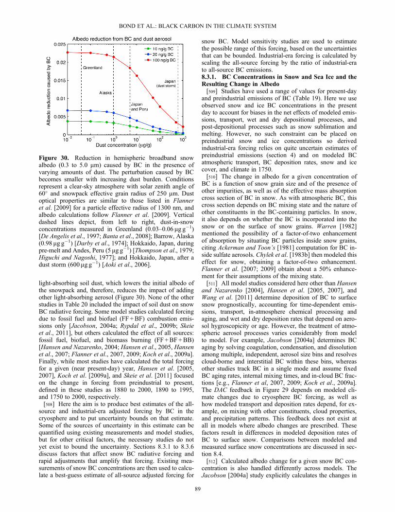
light-absorbing soil dust, which lowers the initial albedo ofthe snowpack and, therefore, reduces the impact of addingother light-absorbing aerosol (Figure 30). None of the otherstudies in Table 20 included the impact of soil dust on snowBC radiative forcing. Some model studies calculated forcingdue to fossil fuel and biofuel (FF +BF) combustion emis-sions only [Jacobson, 2004a; Rypdal et al., 2009b; Skeieet al., 2011], but others calculated the effect of all sources:fossil fuel, biofuel, and biomass burning (FF +BF+BB)[Hansen and Nazarenko, 2004; Hansen et al., 2005, Hansenet al., 2007; Flanner et al., 2007, 2009; Koch et al., 2009a].Finally, while most studies have calculated the total forcingfor a given (near present-day) year, Hansen et al. [2005,2007], Koch et al. [2009a], and Skeie et al. [2011] focusedon the change in forcing from preindustrial to present,defined in these studies as 1880 to 2000, 1890 to 1995,and 1750 to 2000, respectively.[508] Here the aim is to produce best estimates of the all-

source and industrial-era adjusted forcing by BC in thecryosphere and to put uncertainty bounds on that estimate.Some of the sources of uncertainty in this estimate can bequantified using existing measurements and model studies,but for other critical factors, the necessary studies do notyet exist to bound the uncertainty. Sections 8.3.1 to 8.3.6discuss factors that affect snow BC radiative forcing andrapid adjustments that amplify that forcing. Existing mea-surements of snow BC concentrations are then used to calcu-late a best-guess estimate of all-source adjusted forcing for

snow BC. Model sensitivity studies are used to estimatethe possible range of this forcing, based on the uncertaintiesthat can be bounded. Industrial-era forcing is calculated byscaling the all-source forcing by the ratio of industrial-erato all-source BC emissions.8.3.1. BC Concentrations in Snow and Sea Ice and theResulting Change in Albedo[509] Studies have used a range of values for present-day

and preindustrial emissions of BC (Table 19). Here we useobserved snow and ice BC concentrations in the presentday to account for biases in the net effects of modeled emis-sions, transport, wet and dry depositional processes, andpost-depositional processes such as snow sublimation andmelting. However, no such constraint can be placed onpreindustrial snow and ice concentrations so derivedindustrial-era forcing relies on quite uncertain estimates ofpreindustrial emissions (section 4) and on modeled BCatmospheric transport, BC deposition rates, snow and icecover, and climate in 1750.[510] The change in albedo for a given concentration of

BC is a function of snow grain size and of the presence ofother impurities, as well as of the effective mass absorptioncross section of BC in snow. As with atmospheric BC, thiscross section depends on BC mixing state and the nature ofother constituents in the BC-containing particles. In snow,it also depends on whether the BC is incorporated into thesnow or on the surface of snow grains. Warren [1982]mentioned the possibility of a factor-of-two enhancementof absorption by situating BC particles inside snow grains,citing Ackerman and Toon’s [1981] computation for BC in-side sulfate aerosols. Chylek et al. [1983b] then modeled thiseffect for snow, obtaining a factor-of-two enhancement.Flanner et al. [2007; 2009] obtain about a 50% enhance-ment for their assumptions of the mixing state.[511] All model studies considered here other than Hansen

and Nazarenko [2004], Hansen et al. [2005, 2007], andWang et al. [2011] determine deposition of BC to surfacesnow prognostically, accounting for time-dependent emis-sions, transport, in-atmosphere chemical processing andaging, and wet and dry deposition rates that depend on aero-sol hygroscopicity or age. However, the treatment of atmo-spheric aerosol processes varies considerably from modelto model. For example, Jacobson [2004a] determines BCaging by solving coagulation, condensation, and dissolutionamong multiple, independent, aerosol size bins and resolvescloud-borne and interstitial BC within these bins, whereasother studies track BC in a single mode and assume fixedBC aging rates, internal mixing times, and in-cloud BC frac-tions [e.g., Flanner et al, 2007, 2009; Koch et al., 2009a].The DAC feedback in Figure 29 depends on modeled cli-mate changes due to cryosphere BC forcing, as well ashow modeled transport and deposition rates depend, for ex-ample, on mixing with other constituents, cloud properties,and precipitation patterns. This feedback does not exist atall in models where albedo changes are prescribed. Thesefactors result in differences in modeled deposition rates ofBC to surface snow. Comparisons between modeled andmeasured surface snow concentrations are discussed in sec-tion 8.4.[512] Calculated albedo change for a given snow BC con-

centration is also handled differently across models. TheJacobson [2004a] study explicitly calculates the changes in

Figure 30. Reduction in hemispheric broadband snowalbedo (0.3 to 5.0 mm) caused by BC in the presence ofvarying amounts of dust. The perturbation caused by BCbecomes smaller with increasing dust burden. Conditionsrepresent a clear-sky atmosphere with solar zenith angle of60� and snowpack effective grain radius of 250 mm. Dustoptical properties are similar to those listed in Flanneret al. [2009] for a particle effective radius of 1300 nm, andalbedo calculations follow Flanner et al. [2009]. Verticaldashed lines depict, from left to right, dust-in-snowconcentrations measured in Greenland (0.03–0.06 mg g�1)[De Angelis et al., 1997; Banta et al., 2008]; Barrow, Alaska(0.98 mg g�1) [Darby et al., 1974]; Hokkaido, Japan, duringpre-melt and Andes, Peru (5 mg g�1) [Thompson et al., 1979;Higuchi and Nagoshi, 1977]; and Hokkaido, Japan, after adust storm (600 mg g�1) [Aoki et al., 2006].


89

solar albedo of snow and snow thermal-IR emissivity as afunction of zenith angle by solving radiative transfer throughthe atmosphere, snow and ice grains together, by adding asnow or ice layer to the bottom of the atmospheric layersand solving for the upward divided by downward irradianceat the top of the snow layer. The calculation is done forboth interstitial BC particles and BC inclusions withinsnow grains, treated with a core-shell approximation.Jacobson [2004a] found that the modeled effect of BCon emissivity is small, as also shown in Warren [1982, Ta-ble 2]. Effects of BC on IR emissivity are disregarded inall other model studies. The Flanner et al. [2007; 2009]studies explicitly calculate the change in solar snow albedoby solving radiative transfer through multiple layers ofsnow, based on theory from Warren and Wiscombe [1980]and the two-stream, multiple scattering radiative approxima-tion of Toon et al. [1989]. The snow albedo is then added in-teractively at each time step as a bottom boundary conditionto an atmospheric model that accounts for the effects of at-mospheric optics (e.g., aerosol, clouds, etc.) on downwellingsolar radiation. They treat sulfate-coated and interstitial BCspecies with coated BC absorbing about 50% more solar ra-diation per mass of BC. Koch et al. [2009a] parameterizesthe change in albedo based on the study of Warren andWiscombe [1985], which treated the BC as being externallymixed with the snow and accounts for absorption enhance-ment through multiple scattering in the snow. This parame-terization provides a spectrally averaged change in albedo,with dependence on snow grain size and BC concentration,but it ignores the zenith angle and atmospheric optical de-pendence of the albedo. Rypdal et al. [2009b] and Skeie etal. [2011] use look-up tables of albedo based on snow grainsize and BC concentration; these tables are based on Mietheory and radiative transfer calculations. Radiative transfercalculations are done with a multi-stream model using thediscrete ordinate method [Stamnes et al., 1988], where twosnow layers have been added below their atmosphericlayers. Hansen and Nazarenko [2004], Hansen et al.[2005, 2007], andWang et al. [2011] impose albedo changesso there is no dependence on BC concentration or otherfactors.[513] As with snow, BC concentrations in bare (non snow-

covered) sea ice similarly depend on the amount of BC wetand dry deposition to the surface. However, because sea iceis usually snow-covered in the winter to spring season, theBC concentrations in multi-year summer ice are likely astrong function of how much BC resides in the winter andspring snowpack and on how much is retained in the seaice during melting. A few measurements of sea-ice BC con-centrations are available to test models; they indicate thatBC in sea ice is comparable to that in snow from the sameregion [Doherty et al., 2010].[514] A given concentration of BC produces a larger

change in albedo in sea ice than in snow, because the surfaceof sea ice behaves as large-grained snow. However, sea icealso can contain significant amounts of other light-absorbingimpurities, such as sediment, which as discussed below maysignificantly decrease the forcing by BC. Only three studiesin Table 19 include radiative forcing by BC in sea ice:Jacobson [2004a], Rypdal et al. [2009b], and Skeie et al.[2011]. This may explain, in part, the relatively large forcingper emission of Jacobson [2004a]. However, forcing by BC

in snow on sea ice and by BC in sea ice were not separatelydiagnosed so it is not possible to know how large a role theseforcings played in either study. Below independent estimatesare made for forcing by BC in sea ice and its possible upperand lower bounds.8.3.2. Snow-Covered Area[515] Climate forcing by BC in snow is a direct function of

the amount of land or ice area covered by snow, so seasonaland sub-grid-scale variations in snow cover must be accu-rately represented. Models allow for fractional snow coverwithin model grid boxes by employing snow depth depen-dent parameterizations. The adjusted forcings calculated byFlanner et al. [2007] for low and high cases of snow coverare used here to help bound uncertainty in forcing due toerrors in fraction of snow covered area.[516] The allowance for fractional snow coverage within a

grid box might not, however, account for very small-scalesnow patchiness, which occurs particularly in areas withlow snowfall amounts or broken up sea ice. Melt rates arehigher in patchy snow than in uniform snowpacks, and meltrates increase with degree of snow patchiness and exposedarea [Liston, 1995, 1999, 2004; Essery, 1997]. Accountingfor this patchiness is expected to have two competingeffects: Patchy snow warms and starts to melt more quicklydue to local heat advection, and when the snowpack is closeto its melt point, the feedbacks enhance the effect of the ini-tial direct forcing most powerfully. On the other hand,patchy snow on land is more likely to be loaded with localsoil dust, thereby lowering the “baseline” snowpack albedoand decreasing the impact of BC (Figure 30). It is not knownif accurately accounting for these two effects would producea larger or a smaller radiative effect by BC in snow, so this isan unbounded uncertainty.8.3.3. Masking by Clouds and Vegetation[517] The planetary albedo of cloud-covered areas is rela-

tively insensitive to surface albedo, so cloud cover must beaccurately represented. Similarly, BC in snow masked byvegetation contributes little to ToA forcing, so vegetativecover must be accurately represented. Both cloud coverand vegetation are sub-grid-scale features, complicatingtheir representation in models. Model representation of andforcing sensitivity to realistic ranges of cloud cover andvegetation have not been tested, and this is currently anunbounded uncertainty in cryosphere BC adjusted forcing.8.3.4. Snow Grain Size[518] As noted above, snow albedo is highly sensitive to

snow grain size. Further, the change in albedo for a givensnow BC concentration is greater in larger grained snowthan in smaller grained snow (Figure 27). Thus, the snow-pack BC concentration and snow-grain size must be wellconstrained down to the penetration depth of sunlight (about30 cm for a typical snow density of 0.3 g cm�3) [Warrenand Wiscombe, 1980, Figure 13c]. “Grain size” must alsobe defined consistently: in field measurements, reportedvalues are optical grain sizes, which are proportional to thevolume-to-area ratio [e.g., Grenfell et al., 2005] andinversely proportional to the “specific surface area” [e.g.,Matzl and Schneebeli, 2006]. Jacobson [2004a], Rypdalet al. [2009b], and Skeie et al. [2011] use globally fixedsnow-grain radii in their models of 150, 500, and 500 mm,respectively. Grain radii for new snow are less than150 mm, and for old, melting snow, they are larger than


90

500 mm, so the feedbacks that involve grain size (GRA, GRBin Figure 29) are not captured. The net effect of applying afixed snow grain size is not known. However, Flanner etal. [2007] used a model to determine how a reasonable rangein snow aging rate (i.e., the rate of grain size growth) affectsthe derived annual mean adjusted forcing. These results areused to help bound the possible range of forcings by BC insnow.8.3.5. Albedo Dependence on Downwelling Radiation[519] In addition to being a function of snowpack proper-

ties, both pure and contaminated snow albedo depend onsolar zenith angle and the fraction of direct versus diffusesolar radiation. Models that prescribe solar-zenith-angle-independent albedos may have a bias in clear-sky albedo ofseveral percent for pristine snow [Wiscombe and Warren,1980, Figure 6], which is of the same magnitude as the albedoperturbation by BC. Direct and diffuse solar radiation mustalso be accurately represented, in turn requiring accuraterepresentation of cloud cover.8.3.6. Concentration of BC With Sublimationand Melting[520] Precipitation rates and relative humidity in much

of the Arctic are low, so in some areas appreciable (up to30–50%) [Liston and Sturm, 2004] surface snow is lost tosublimation. This process removes snow water but leavesBC and other non-volatile particulate constituents at thesnow surface, increasing their concentration. Similarly, var-iable fractions of BC are left behind at the snow surface withmelt, depending on the hygroscopicity of accompanyingconstituents [Conway et al., 1996]. Flanner et al. [2009]apply a “scavenging efficiency” for BC with melt of 0.2for hydrophilic BC and 0.03 for hydrophobic BC, based onthe Conway et al. [1996] study. Rypdal et al. [2009b] andSkeie et al. [2011] leave all BC at the snow surface as thesnow melts, and all other models cited here allow all BCto be washed away with snow meltwater. While there aresome observational evidence of BC remaining at the surfaceduring melt [Conway et al., 1996; Xu et al., 2006; Dohertyet al., 2010], an appropriate BC scavenging ratio remainsto be determined. A model sensitivity study which appliesa range of melt scavenging efficiencies is used to help boundthis source of uncertainty.8.3.7. Representation of All Light Absorbing Particlesin Snow[521] Particulate matter in snow is never pure BC. BC

from biomass, biofuel, and fossil fuel burning is accompa-nied by varying amounts of brown organic carbon. Othersources also produce light-absorbing carbon [Andreae andGelencsér, 2006] and light-absorbing crustal material (e.g.,hematite in soil dust). Calculation of BC effects on snow andice albedo and melt rates must consider all light-absorbingconstituents in the snow. Glacial snow especially often hashigh concentrations of locally sourced soil dust and sand thatsignificantly reduce its albedo. While the Jacobson [2004a]and Flanner et al. [2009] studies included soil dust in snowin their baseline calculations, these models do not accountfor very local sources of coarse-grained (i.e., much greaterthan 10mm diameter) dust and sand, which have a very shortatmospheric lifetime (i.e, less than a few days). Particularlyin areas with patchy snow cover, local soil and sand may bepresent in the snow at high concentrations. This observationwas made along the Arctic coast of Siberia (S. Warren and

T. Grenfell, personal communication, 2011), in Inner Mongo-lia [Huang et al., 2011], and on summertime Arctic sea ice(B. Light and T. Grenfell, personal communication, 2011) dur-ing snow and ice sampling surveys. The bias this introduces tomodeled forcing cannot currently be bounded. However, theFlanner et al. [2009] model can be used to help constrainthe impact of including dust deposition to snow. In this model,when dust is included the snow BC radiative forcing isdecreased by about 25% for the global mean dust burden of4.3 ppm calculated in the model. This result is consistent withFigure 30, which shows a snow albedo reduction of about0.006 for a pristine snowpack with 20 ng g�1 of BC and analbedo reduction of about 0.005 for a snowpack with4000 ng g�1 of dust and 20 ng g�1 of BC. These results indi-cate that the albedo reduction due to BC is 20% less in thepresence of dust.[522] Importantly, most studies that have measured

[Xu et al., 2006; Ming et al., 2009] or estimated [Yasunariet al., 2010; Castelvecchi, 2009] BC concentrations forHimalayan glaciers have estimated a significant radiativeforcing, but this was by comparing clean (dust- and algae-free) snow to clean snow with BC added. In the spring sea-son when the glacier snow starts to melt and when BC mayhave its maximum impact, it is also late in the dry season,with minimal precipitation and large dust events over theTibetan Plateau and across the Himalaya [Ming et al.,2009; Marinoni et al., 2010]. In addition to being exposedto dust from Central Asia and the Middle East, the south sideof the Himalaya can experience significant dust loading fromsources in northern India [Marinoni et al., 2010]. Similarly,dust storms from the Sahara can account for a significantfraction of the impurities in Alpine snow [Thevenon et al.,2009; Haeberli, 1977], and dust from the Colorado Plateaudrives a very large radiative forcing of snowpack in theSan Juan Mountains [Painter et al., 2007]. The lower partsof many Himalayan glaciers are entirely hidden by thickdebris cover [Nakawo et al., 2000], actually inhibiting melt.Future studies must account for the effects of crustal andother light-absorbing material (e.g., algae) [Jones et al.,2001] in mountain glaciers when determining the effects ofBC on snow melt.[523] Measurements from across the Arctic indicate

that typically 30 to 50% of sunlight absorbed in the snow-pack by impurities is due to constituents other than BC[Doherty et al., 2010]. Either organic matter or soil dustcould be responsible, and the spectral absorption measure-ments cannot distinguish them, but chemical analysis of ageographically diverse subset of these Arctic samplesindicates that the non-BC light absorbing particulate matteris overwhelmingly light-absorbing OC, not mineral dust[Hegg et al., 2010]. These samples were collected specifi-cally trying to avoid snow that obviously contained signif-icant amounts of soil, dust, or sand, so they may somewhatunderrepresent the role of these particles in snow. Regard-less, these measurements make it clear that particles otherthan BC play a significant role in changing snow albedo.While Flanner et al. [2007; 2009] did not include snowOC light absorption in their published forcing calculations,they did test for the effect of OC on snow albedo andfound it to be sufficiently small that omitting it wouldnot significantly change their results. If organic matteris in fact a significant source of light absorption in snow,


91

the forcing by sources high in OC (i.e., BF and BB)would be larger because of the addition of light-absorbing OC. However, if biomass burning and soil dustemissions are considered a “natural” source of aerosol,this would mean the natural snowpack has a lower albedo,thus lessening the effect of mitigating anthropogenic sources.On the other hand, mitigating biofuel-burning emissionsor any burning which produces light-absorbing OC ordecreasing soil dust emissions would have a largerimpact than would be implied by only considering the effectof BC.[524] These results highlight the importance of determin-

ing not only the concentration of snow BC but also light-absorbing OC and soil dust in snow. In addition, whilethe wavelength dependence of absorption of BC has beenstudied and is relatively well constrained to follow l�1,the wavelength dependence of absorption (or, equivalently,the size distribution and spectrally resolved indices ofrefraction) for light-absorbing organics and soil dust appearto be quite variable [e.g., Bond, 2001; Kirchstetter et al.,2004; Bergstrom et al., 2007; Sun et al., 2007; Russellet al., 2010], making estimates of the impact of OC anddust on light absorption in snow highly uncertain.

8.4. Measurements of BC in Snow and ComparisonWith Models

[525] As shown in Table 19, model studies to date haveused a range of assumptions about the sources and quantityof BC emissions. Similarly, atmospheric transport processesdiffer from model to model, as do deposition rates. Forexample for the suite in Table 19, the fraction of BC depos-ited to surface snow by wet (versus dry) deposition rangesfrom 71% [Koch et al., 2009a] to 98% [Jacobson, 2004a].Measurements of snow BC concentrations can be used totest models for the combined influence of all of these factors.Data are available from the Arctic and sub-Arctic, a fewmid-latitude locations in the northern hemisphere and theAntarctic. Here we limit model/measurement comparisonsto northern hemisphere sites, because concentrations inAntarctic are too small (i.e., generally less than 1 ng g�1)[Chylek et al., 1987; Warren and Clarke, 1990; Bisiauxet al., 2012] to be important for forcing evaluations.

8.4.1. Measurement Methods[526] BC concentrations in snow have been measured

using variations of the thermo-optical method [Chyleket al., 1987; Cachier and Pertuisot, 1994; Lavanchy et al.,1999; Xu et al., 2006; Jenk et al., 2006; Hagler et al.,2007a, 2007b; Legrand et al., 2007; Ming et al., 2008;Forsström et al., 2009; Ming et al., 2009; Thevenon et al.,2009; Xu et al., 2009a, 2009b; Hadley et al., 2010] and withan SP2 instrument [McConnell et al., 2007; McConnell andEdwards, 2008], both of which are described in section 3.5.They have also been measured using a third, filter-basedmethod that optically analyzes BC concentrations, used firstby Clarke and Noone [1985] in the form of the IP Spectro-photometer and later with an improved instrument, theISSW Spectrophotometer [Grenfell et al., 2011; Dohertyet al., 2010]. Using the wavelength-dependence of the mea-sured light absorption on the filter, it is possible, assumingknown BC MAC, to calculate the maximum possible BCconcentration, an estimated BC concentration, and the

fraction of absorbed solar radiation (integrated 300–750nm) that is due to species other than BC, such as light-absorbing organic carbon and crustal material [Grenfell etal., 2011; Doherty et al., 2010]. Here modeled values arecompared with BC concentrations from the IP and ISSWspectrophotometers, thermo-optical measurements and fromthe SP2.8.4.2. Arctic and Sub-Arctic Snow[527] Table 21 gives measured concentrations of BC in

surface snow for various regions of the Arctic. Because thesnow albedo feedback is greatest in spring, most of thesemeasurements were of surface snow in March, April, orearly May; all are from snow that has not yet experiencedmelting (and therefore the feedback MBC in Figure 29) butwhich may have experienced sublimation (feedback SBCin Figure 29). These are compared to average surface snow(top 2 cm) concentrations from the Flanner et al. [2009]study and to the concentration of BC deposited in snow(via both wet and dry deposition) in the Koch et al.[2009a] study. Model average values were calculated usingthe modeled concentrations from the same month and loca-tion (grid box) as the measurements. In addition, Skeieet al. [2011] include a comparison of their modeled snowBC concentrations with measured values reported byForsström et al. [2009] and Doherty et al. [2010] for Arcticand sub-Arctic regions. These comparisons are imperfect butallow a first-order check of how well the models arerepresenting BC deposition to the snowpack. The concentra-tions shown in Table 21 produce a change in snow albedo ofless than 5%, which would not be visible to the human eye.In common images of snow visibly darkened by light-absorbing impurities, the impurities are often sand and soil,not BC.[528] The comparison herein has been limited to two of the

six studies which calculated snow BC concentrations[Flanner et al., 2009; Koch et al., 2009a] (Table 20) forwhich modeled snow BC is readily available, and to discus-sion of the Skeie et al. [2011] model and observation com-parison. For reference, total, present-day BC emissions fromFlanner et al. [2009] (7400 Gg yr�1) and Koch et al.[2009a] (8200 Gg yr�1) are between the central bottom-upall-source estimate of 7300 Gg yr�1 (section 4) and the all-source emissions (10,100 Gg yr�1) based on a comparisonof modeled and measured AAOD (section 6). The Hansenet al. [2005] total present-day BC emissions (11,000 Ggyr�1) are larger than either of these estimates. Jacobson[2004a] total BC emissions are within 5% of the total emis-sions of Flanner et al. [2009], though there is a higher frac-tion of BB emissions in Jacobson et al. than in Flanner et al.(44% versus 35%), and BB emissions are less likely to bedeposited to snow [Flanner et al., 2009; Skeie et al.,2011]. The Rypdal et al. [2009b] FF +BF emissions are13% and 18% higher, respectively, than those in Flanneret al. [2009] and Koch et al. [2009a] studies; Rypdal et al.[2009b] did not include BB emissions in their analysis.The Flanner et al. [2009] study was specifically run for arepresentative biomass-burning year and so is a better com-parison to measurements than the Flanner et al. [2007]study, which explored two extreme (high and low) BB years.Differences in transport and deposition rates also affect theconcentration of BC in snow, but this comparison stillprovides a first-order test of the models. Broad patterns in


92

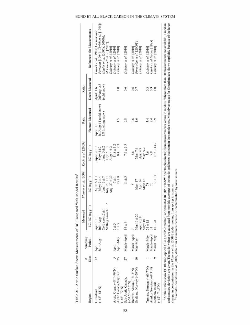
Tab

le21.Arctic

Surface

Snow

Measurementsof

BCCom

paredWith

Model

Resultsa

Region

#Sites

Sam

pling

Period

Measured

Flanner

etal.[2009]

Kochet

al.[2009a]

Ratio

Ratio

EC,BC(ngg�

1)

BC(ngg�

1)

BC(ngg�

1)

Flanner:Measured

Koch:

Measured

ReferencesforMeasurements

Greenland

12April

Apr:3�1

April:

5�1

April:

6�6

April:

1.3

April:

1.6

Chyleket

al.,1987;Cachier

and

(~63

� –81

� N)

Jul+

Aug

Jul+

Aug:

Coldsnow

:2�1

Meltin

gsnow

:16�5

May:7�4

June:13

�7

July:29

�18

Aug:27

�30

May:4�

2June:5�2

July:5�3

Aug:4�2

Jul/A

ug:14

(coldsnow

)1.8(m

eltin

gsnow

)Jul/A

ug:2.3

(coldsnow

)Pertuisot

[1994];Chyleket

al.[1995];

Hagleret

al.[2007a,2007b];

McC

onnellet

al.[2007];

Doherty

etal.[2010]

Arctic

Ocean

(~84

� –90

� N)

5April

5�3

7�1

11.8�1.2

Doherty

etal.[2010]

Arctic

Canada,May:9.2

(~66

� –77

� N)

25April–

May

8�3

13�8

8.4�2.3

1.5

1.0

Doherty

etal.[2010]

Sub-A

rctic

Canada,

(~63.5

� –67.5

� N)

27March–A

pril

14�9

11�3

7.6�3.3

0.8

0.6

Doherty

etal.[2010]

Barrow,Alaska(~71.3

� N)

1March–A

pril

95

5.8

0.6

0.6

Doherty

etal.[2010]

Svalbard,

Norway

(~79

� N)

10Mar–M

ayMar:10�20

Mar:17

Mar:7.6

1.6

0.7

Forsström

etal.[2009]

b;

Doherty

etal.[2010]

Apr:9�8

Apr:14

Apr:4.9

May:10

May:16

May:9.2

Tromso,Norway

(~69.7

� N)

1March–M

ay21

�12

787.6

3.4

0.3

Doherty

etal.[2010]

Abisko,

Sweden

(~68.3

� N)

1March–A

pril

3176

7.8

2.4

0.3

ClarkeandNoone

[1985]

NorthernRussia

(~62

� –74.5

� N)

9March–M

ay18

�28

17�14

17.2�13.2

0.9

1.0

Doherty

etal.[2010]

a Arctic

surfacesnow

EC(therm

o-optical(T.O.)or

SP-2

method)

orestim

ated

BC(IPor

ISSW

Spectrophotom

eter)from

measurementsversus

inmodels.Wheremorethan

10measurementsareavailable,amedian

andstandard

deviationaregiven.The

modelvalues

arecalculated

from

monthlyaverages

ofthemodelgridboxesthatcontainthesamplesites.Monthlyaverages

forGreenland

areshow

nexplicitlybecauseof

thelarge

change

inconcentrationin

theFlanner

etal.[2009]

studymovingfrom

spring

tosummer.

bExcludesForsström

etal.[2009]

data

from

Linnébreenbecauseof

contam

inationby

localsources.


93

the observed spatial variability of snow BC concentrationsare qualitatively consistent with the model results. Both havehigher concentrations of BC in snow over northwesternRussia, Europe, and Scandinavia than across the westernArctic and Greenland. However, there are important quanti-tative differences.[529] The Koch et al. [2009a] modeled values are in

agreement with the measured values for Arctic Canada andnorthern Russia, are biased high in the Arctic Ocean, andare biased low compared to the measurements in all other re-gions other than Greenland, where they are about a factor of2 too high. In contrast, the Flanner et al. [2009] modelvalues are somewhat lower than the measured values fornorthern Russia, Barrow, and sub-Arctic Canada but arehigher than the measured values at all other sites. The differ-ences are particularly profound for the Scandinavian sites,where they are 1.6 to 3.4 times the measured concentrations.Notably, these sites also have the highest concentrations andso carry more weight than the other sites at similar latitudesin terms of global radiative forcing. For Greenland, valuesare shown for both spring (April) and summer (July to Au-gust). Only about 25% of the Greenland Ice Sheet is in the“dry snow zone;” everywhere else some melting occurs dur-ing summer. There is a striking increase in Greenland valuesin the Flanner et al. model when moving from spring tosummer that is also present in the measurements but not aspronounced (Table 21). Based on the timing and spatialpattern of the increase, it appears to be caused by theconcentration of BC at the surface with melt, indicating thatthe MBC feedback (Figure 29) may be too strong in Flanneret al. [2009] study. The timing and extent of melt is clearlycritical in this process and needs to be validated againstobservations; the limited data presented here are insufficient.Furthermore, improved model treatment may be needed forparticle accumulation in perennial snow and ice sheets,where (in the absence of glacier dynamics) snow eitheraccumulates year after year or is “capped.”[530] Skeie et al. [2011] prognostically determined snow

BC concentrations from all sources (FF +BF+BB) andcompared these to measured concentrations. Their forcingwas calculated for the FF +BF sources only, but biomassburning only accounted for 4 to 12% of BC in snow northof 65�N. Their comparison with the Forsström et al.[2009] measurements indicates that the modeled snow BCconcentrations for 2001 to 2008 vary over about the samerange as the measured concentrations in 2007 in NyÅlesund, Svalbard. However, Doherty et al. [2010] find con-centrations in this region that are about a factor of 2 higherthan that measured by Forsström et al. The Skeie et al.modeled concentrations are much lower than is observedby Forsström et al. at the Scandinavian sites Pallas,Tromso, and Abisko, sometimes by more than a factorof 4 and typically by a factor of 2. The exception is inthe later spring when the snow starts to melt, and inthe model, all BC consolidates at the snow surface. Atthis time, modeled surface snow BC concentrationsincrease by approximately 10-fold. The comparison withthe geographically broader snow BC data set of Dohertyet al. [2010] only includes snow samples that had not yetexperienced springtime melt. This comparison shows rea-sonable agreement for the Canadian and Alaskan Arcticand for Greenland; it indicates a low bias in the model

over the Arctic Ocean, and it shows large model underes-timates for the Canadian sub-Arctic, across Russia, andin Svalbard. Model underestimates vary from about a fac-tor of 2 (Svalbard) up to a factor of 5 (Eastern Russia).Notably, this is the region where BC concentrations(and, thus, forcing) are expected to be largest.8.4.3. Mid-Latitude Snow Measurements[531] Few measurements of mid-latitude snow exist,

despite the fact that the climate impacts of BC in snow atthese latitudes may be larger than for Arctic snow becauseof the combination of higher BC concentrations and higherinsolation. Flanner et al. [2007] include a comparison oftheir modeled values for 1998 and 2001 to those measuredin the 1980s and 1990s at select mid-latitude sites in NorthAmerica and Europe (see their Table 2). Modeled concentra-tions at some sites are about one third to one half themeasured values (in rural and urban Michigan, USA, andin Lithuania). At other sites, they are about equal to the mea-sured values (Cascade mountains in Washington State in theUSA and the French Alps in Europe) or are higher by factorsof about 1.5 to 7.7 (West Texas and NewMexico in the USAand Halifax, Nova Scotia, in Canada). Hadley et al. [2010]measured snow BC concentrations at three remote sites inNorthern California and found they were a factor of 2–4lower than predicted by Flanner et al. [2007] and Qianet al. [2009]. The sparseness of these data and the mismatchbetween the years modeled versus the time of the measure-ments make it difficult to draw conclusions.[532] A snow survey described by Huang et al. [2011]

provides the possibility of a more robust comparison ofmid-latitude snow concentrations. Huang and colleaguessampled snow across north China, reporting concentrations,for example, in northeast China of 600 � 300 ng g�1 atlatitudes of 41 to 46�N that decreased to about 40 ng g�1

at more northerly latitudes (51�N). These values are basedon visual estimates of filter samples; estimates for samplesfrom central and western China were not provided.[533] No other geographically broad data set exists of mid-

latitude snow BC concentrations, so it is not possible at thistime to bound how well models represent mid-latitude snowBC albedo reductions.8.4.4. BC in Mountain Glaciers[534] BC in mountain snow and glaciers is of concern

primarily because of the potential for affecting melt ratesand, therefore, the seasonality of trends in water supplies.The effect of BC in glacial snow differs from BC’s effecton seasonal snow because in the former melting does notlead to exposure of the underlying Earth surface, exceptperhaps at the very margins of the glacier which are anyhowoften loaded with light-absorbing soil dust. Thus, thepowerful albedo feedback present for seasonal snow (SAFin Figure 29) is absent. On longer timescales, if BC leadsto glacial retreat, a positive albedo feedback would likelyaccelerate warming and melt near the glacial terminus.[535] Few measurements exist of BC in mountain glaciers,

and in most cases, they do not permit separation of the roleof local versus remote sources nor are they accompaniedby coincident measurements of other light-absorbing impuri-ties. Using a global model to determine snowfall and aerosoldeposition to glaciers is particularly difficult because of theirsmall size relative to a model grid box (Table 19), allowingfor only one BC concentration per grid box, regardless of,


94

for example, the dramatic altitude variations in mountainousregions. As discussed above, forcing by BC in snow alsodepends on accurate representation of snow and glaciercover. The coarse resolution of most models makes thisrepresentation quite difficult in mountainous areas and inareas with sparse snow cover, such as the Tibetan Plateau[e.g., Qian et al., 2011, Figure 2].[536] Ice cores from the European Alps provide his-

torical time series but do not reach present day andare reflective of glacial ice concentrations, not snow con-centrations. Nonetheless, they provide information on thetrends in BC deposition to the European Alps and some in-dication of near-present-day levels. Jenk et al. [2006] founda 1900–1940 average BC concentration of 31 ng g�1

(range: 9 to 22 ng g�1), Thevenon et al. [2009] found a1950–1980 average of about 20 ng g�1, and Legrand et al.[2007] reported concentrations for 1960–1990 of about10 to 17 ng g�1, with the peak concentrations around1960 and a decline thereafter. These studies also indicatea shift in the dominant source of BC from biomass burn-ing in the nineteenth century to coal and later to non-coalfossil fuel. Modeled snow concentrations for present dayfrom Flanner et al. [2009] grid boxes corresponding tothe measurement sites in these studies range from approx-imately 115 to 160 ng g�1 in January through March andthen decline to about 10 to 50 ng g�1 in April. Summer-time (May–August) concentrations are zero, because allsurface snow is assumed to have melted and BC in the gla-cier itself is not accounted for. In contrast, BC in the de-posited snow in the Koch et al. [2009a] model increasesfrom about 20 to 25 ng g�1 in January to about 50 ngg�1 by early summer, much more in line with the mea-sured concentrations in mid-twentieth century glacial ice.[537] Analysis by Xu et al. [2006], Xu et al. [2009a,

2009b], and Ming et al. [2009] of surface snow samplestaken June–October in the Himalaya and in the TibetanPlateau region yield typical concentrations of BC insurface snow of about 10 to 40 ng g�1. Excluding samplescollected from a site where the surrounding rock is rich incoal, the highest average surface snow concentration was107 ng g�1, and the lowest less than 1 ng g�1. However,samples from deeper in the glacial snow [Xu et al., 2006;Ming et al., 2009] and glacier cores [Xu et al., 2009a,2009b] show that BC concentrations are a factor of about 3to 6 higher outside the summer monsoon (October–May)than during the monsoon (June–September). BC concentra-tions are highest when snow cover is also highest(October–May), but the concentration maximum also corre-sponds to a maximum in dust deposition in this region [Minget al., 2009], so the impact of the BC on snow albedo ismoderated. The only measurements from the south side ofthe Himalaya were from the East Rongbuk glacier onMt. Everest, with concentrations of about 10 to 20 ng g�1

[Xu et al., 2009b; Ming et al., 2009].[538] Snow samples in these studies were from summer

and early fall, but in the model study of Flanner et al.[2009], almost all grid boxes corresponding to the samplesites are snow free from May to September. However, aqualitative comparison is possible of monthly averagedmodel snow BC concentrations from October–April forthe grid boxes corresponding to the sample sites. Concen-trations in the Flanner et al. [2009] model study decrease

with latitude across the plateau, with the lowest concentra-tions corresponding to the measurements sites in northwestChina. In contrast, this was where some of the higher con-centrations were found in the measurements. Concentra-tions also are a strong function of season, increasing fromabout 20 to 30 ng g�1 in September (where there is snow)to a high of 70 to 500 ng g�1 (median 250 ng g�1 ) inFebruary. Concentrations remain high in March but dropby about a third in April and by May are back to about10 to 40 ng g�1. Thus, both the measurements and themodels show maximum concentrations in the spring, butthe concentrations in the model are notably higher than inthe measurements. The Koch et al. [2009a] modeledmedian concentrations are lower (January–May monthlymedian across sample sites of 30 to 45 ng g�1), they donot exhibit a systematic latitudinal dependence, and theyshow only a moderate seasonal dependence, peaking inMarch–April. Thus, they are in better general agreementwith the median measured concentrations but perhaps missstrong peaks in springtime BC concentrations seen in someof the measurements. Kopacz et al. [2011] compare theirmodeled snow BC concentrations with this same measure-ment data set and find both overestimates and underesti-mates at individual sites but no overall systematic bias inthe modeled values.8.4.5. Trends in Arctic Snow BC[539] While most model studies (e.g., as given in Table 19)

have focused primarily on the role of BC in recent warmingtrends, anthropogenic emissions of BC in some regions weremuch higher in the past and are declining, while in others,they are rapidly increasing above historical levels. A smallnumber of ice core records of BC are available to testmodels’ historical representation of BC trends, and atmo-spheric BC trends for the Arctic can be used as an indicatorof likely trends of BC deposition to snow in this region,though atmospheric and snow concentrations are not directlyrelated.[540] Near-surface atmospheric measurements since 1989

at Alert, Ellesmere Island (82�300N 62�190W) [Sharmaet al., 2006; Gong et al., 2010] and since 1998 at NyÅlesund, Svalbard, Norway (78�550N 11�560E) [Hicks andIsaksson, 2006; Eleftheriadis et al., 2009; Forsström et al.,2009] show that Arctic atmospheric BC concentrations havebeen declining in recent decades. Measurements starting in1989 at Barrow, Alaska (71�190N 156�370W) [Sharmaet al., 2006] show moderate declines in atmospheric BC upto 2003 and then a possible slight increase from 2003 to2006. Hirdman et al. [2010a] argue that only a fraction ofthese trends is driven by changes in transport and that mostof the observed trends are attributable to emissions changesin source regions, especially northern Eurasia.[541] Ice cores from the Greenland plateau provide insight

to longer-term Arctic trends. The Greenland cores reflectfree-troposphere concentrations of BC and are most stronglyinfluenced by fires and anthropogenic activity in NorthAmerica [McConnell et al., 2007]. These records indicate thatGreenland snow, preceding any human activity, had BC con-centrations of about 1.1 to 2.5 ng g�1 (i.e., 4–6000 ybp)[Chylek et al., 1987] or about half the concentrationsfor the past few decades (1 to 4 ng g�1) [Cachier andPertuisot, 1994; Chylek et al., 1995] (Table 21). Ice coreanalyses by McConnell et al. [2007] and McConnell and


95

Edwards [2008] that span the industrial era show that from1788 to about 1850, Greenland had relatively low concen-trations (about 2 ng g�1) of BC associated with biomass orbiofuel burning and then a rise occurred to an average ofabout 10 ng g�1 (D4 core) or about 20 ng g�1 (ACT2 core),peaking around 1910. After this, BC concentrations de-clined steadily through the 1940s, finally dropping sharplyin 1952 to nearly pre-1850 values. This post-1850 peak inBC was associated with coal burning, with the decline inBC in the mid-1900s associated with air pollution controls,improved combustion, and a fuel shift from coal to oil andgas. An ice core on Mt. Logan in the St. Elias range, Yukon,Canada [Holdsworth et al., 1996], shows a similar BCincrease starting in the mid-1800s, though these data onlyextend to about 1950 so it is not possible to determine ifthere was a subsequent decline. An ice core from theSt. Elias range is being analyzed and may help elucidatecentury-timescale trends on that side of the Arctic(J. McConnell, personal communication).[542] Notably, the early twentieth century peak in BC in

the Greenland ice core (about 1890–1950) leads by about20 years a period of strong positive regional surface-air tem-perature anomalies from 1920 to 1965 [e.g., Polyakov et al.,2002, Figure 2; Shindell and Faluvegi, 2009, Figure 3]. It isexpected that the full climate response to a forcing lags theimposed forcing, because of the ocean’s heat capacity, forexample, so this does not necessarily negate the possibilitythat the high BC concentrations led to the observedwarming. This warming has generally been attributed tosolar and natural variability. However, Shindell andFaluvegi [2009] point out that in their model, only about halfof the early twentieth century Arctic (60� to 90�N) tempera-ture rise can be attributed to the combined effects of GHGs,natural forcings, and tropospheric O3. Natural variability isunable to account for the remainder in most models, imply-ing that a portion of the warming should be interpreted asdue to aerosol climate forcing. In a model study of historicaerosol impacts on climate, Koch et al. [2011b] calculate amaximum in BC deposition to Arctic snow around 1950and a peak BC radiative forcing between 1940 and 1970,with declines since then. The peak in radiative forcing corre-lates well with the Greenland trends of McConnell et al.[2007]. Skeie et al. [2011] modeled trends in snow BC radi-ative forcing by fossil fuel and biofuel sources, reportingforcing relative to year 1750 in the year 1850 and then onceper decade from 1900 to 2000. Forcing relative to 1750 isabout 0.005 Wm�2 in 1850, more than doubles between1850 and 1900 to about 0.013 Wm�2 and increases steadilyfrom 1900 to 1960 to about 0.019 W m�2. After this, forcingvaries by about 0.03 W m�2 with no apparent trend from1960 to 2000 [Skeie et al., 2011, Figure 16b]. Thus, thisstudy does not show a forcing peak in the mid-1900s, butit does indicate that snow BC forcing has not appreciablyincreased since 1960.[543] In summary, both observations and model studies

indicate that BC may in fact have played a significant rolein the observed early twentieth century Arctic warming. Fur-ther, radiative forcing by BC in Arctic snow likely has notincreased since the mid-1900s and may instead be declining.8.4.6. Trends in Mountain Snow[544] Several ice core studies from the European Alps pro-

vide insight into trends and sources of BC in snow through

the industrial era. These data show two features: first, a sharpincrease in BC starting in the late nineteenth century and,second, a transition to fossil fuel as a significant source ofBC. At the three locations studied, concentrations increasedfrom the turn of the century to 1940–1950, with peak con-centrations of about 15 to 25 ng g�1 [Jenk et al., 2006;Legrand et al., 2007; Thevenon et al., 2009]. Only two ofthe three records extend past 1940 with one showing a slightincreasing trend and the other showing a declining trend.These differences may be due to differences in exposure tolocal pollution sources.[545] Trends in BC deposition to the Himalaya or Tibetan

regions have been measured using ice cores from Mt.Everest [Ming et al., 2008; Xu et al., 2009b] and at fourother sites on the Tibetan Plateau [Xu et al., 2009b] usingthe thermal-optical method, with records extending about1952–2004. These records show a great deal of spatial andtemporal variability in concentrations, reflecting the varia-tions in source regions and meteorology. Values typicallyaverage about 10–40 ng g�1. However, some commonalitiesare apparent: all but the easternmost site show elevated con-centrations from about 1950 (the earliest part of the record)to the early to mid-1970s, which Xu et al. attribute to easternEuropean sources. Concentrations then remain somewhatlower up until about 1990–1995, after which concentrationsat most sites indicate increasing but variable concentrations.Thus, unlike the Arctic, it appears that BC radiative forcingmay be increasing in the Himalaya.

8.5. Sources of BC to Arctic and Himalayan Snow

[546] Currently, there are few sources of pollution withinthe Arctic itself so almost all BC is transported there fromthe mid-latitudes. In the winter and spring seasons, whenBC deposition to snow is most climatically important, a“dome” of cold air over the Arctic makes it difficult for airfrom lower latitudes to enter the Arctic troposphere.Typically, the front formed by this dome reaches to lowerlatitudes on the Eurasian side of the Arctic than on the NorthAmerican side, making it easier for Eurasian sources toinfluence the Arctic troposphere [Stohl, 2006]. In order forair masses to cross the Arctic front, they must originate incold, dry locations, and typically follow surfaces of constantpotential temperature into the Arctic [Iversen, 1984; Lawand Stohl, 2007]. Thus, air masses originating along the rel-atively warmer, moister North American, and Asian eastcoasts cannot readily enter the Arctic troposphere. Whilethey can be lifted (e.g., in warm conveyor belts) to highaltitudes where they can be transported over the Arctic, thispollution is unlikely to be deposited to the snow surface viawet or dry deposition, except on the high Greenland plateau.[547] A model study by Koch and Hansen [2005] evaluat-

ing regional contributions to the Arctic haze found thatAsian sources dominated total atmospheric column aerosolload, but near-surface concentrations were dominated bysources in Europe and Russia. Stohl [2006] also found lowertropospheric aerosol sources to be dominated by Europeanand Russian emissions. This was reinforced by a multi-model study of pollutant transport to the Arctic from thesource regions of North America, Europe, South Asia, andEast Asia, which found that the greatest impact on surface-deposited BC in the Arctic comes from European emissions[Shindell et al., 2008], but this study did not include


96

northern Eurasia as a source region. Hirdman et al. [2010b]used a Langrangian particle dispersion model and reanalysisdata and found northern Eurasia to be the dominant sourceregion associated specifically with high atmospheric concen-trations of BC at Barrow, Alert, and Svalbard. This finding isconsistent with the Koch and Hansen [2005] and Stohl[2006] model studies and with other studies of the sourceof atmospheric BC at Barrow [Polissar et al., 2001] andSvalbard [Eleftheriadis et al., 2009].[548] In the springtime, when deposition of BC to snow is

climatically important, there is extensive agricultural burn-ing in western Russia and widespread forest fires, particu-larly in the east. The former is clearly an anthropogenicsource, and it may be that a significant fraction of the lattermay be as well [Mollicone et al., 2006]. Given this result,the high latitude of this region (50 to 70�N), the tendencyof the Arctic front to drop to lower latitudes in the Russiansector, and the model findings cited above, the impact ofnorthern Eurasian biomass burning emissions to Arctic-wideBC (and OC) in snow, may be significant.[549] Indeed, biomass burning appears to be the source of

high-concentration plumes observed in the Arctic in recentyears, with Russian biomass burning playing a particularlyprominent role during the measurements of the InternationalPolar Year (2007–2008) [Stohl et al., 2007; Warneke et al.,2009; Paris et al., 2009; Jacob et al., 2010]. Chemical anal-ysis of snow samples from 36 sites across the Arctic(Alaska, Canada, Greenland, Russia, and the Arctic Oceannear the north pole) also indicates that the majority (in mostcases, greater than 75%) of the BC in surface snow is asso-ciated with biomass or biofuel burning [Hegg et al., 2009;Hegg et al., 2010]. Those analyses are from a geographicallybroad but limited number of samples, all from 2007 to 2009,and they do not yet include samples from the Scandinaviansector of the Arctic, where both models and measurements[Forsström et al., 2009; Doherty et al., 2010] indicate thatconcentrations are relatively higher and more influenced byfossil fuel burning than in the rest of the Arctic. These fac-tors may be biasing the conclusions of Hegg et al. [2009,2010] toward the role of biomass or biofuel burning emis-sions in Arctic BC. The model experiments of Flanneret al. [2007] attribute 4.5 ng g�1 BC in Arctic snow to FFsources, 1.7 ng g�1 to BF sources, and 1.9 to 4.7 ng g�1 toBB sources, depending on the strength of the boreal fireyear, also suggesting a potentially dominant contributionfrom biomass or biofuel sources. However, Skeie et al.[2011] attribute only about 10% of snow BC to biomassburning sources, and Flanner et al. [2009] attribute only25% of present-day snow BC forcing to biomass burningin a “typical” biomass-burning year. Despite the uncertainty,it is important in the context of mitigation decisions torecognize that biomass and biofuel burning emissions maybe a significant source of BC to Arctic snow.[550] Consistent with Greenland’s physical location, the

Shindell et al. [2008] multi-model study determined that sur-face-deposited BC in Greenland comes predominantly fromNorth America and Europe in the fall and winter. In thespring, synoptic systems in Asia loft pollutants to higheraltitudes, where they can be transported long distances. Ac-cordingly, they calculated that for the Greenland Ice Sheet—most of which is at high altitudes—BC deposition is moststrongly influenced in the spring by East Asian emissions.

Hirdman et al. [2010b] similarly found that the surface airat Summit, Greenland, was strongly influenced by EastAsian emissions in the summer, whereas other Arctic siteswere not. They emphasize that the high altitude of theGreenland plateau makes it unique in the Arctic in being ex-posed to free troposphere air. Consistent with these findings,chemical analysis of surface snow samples from theGreenland plateau indicate that the BC is largely from bio-mass or biofuel burning sources in the spring and that fossilfuel sources dominate in the summer [Hegg et al., 2009,2010]. In any case, as noted above, the Greenland Ice Sheethas very low concentrations of BC in its surface snow (i.e.,typically less than 3 ng g�1) and so the radiative forcingby BC in Greenland snow is likely small, except duringthe melting season when BC becomes concentrated at thesurface [Doherty et al., 2010, Figure 10a].[551] At lower latitudes, sources of BC in snow can be

either local or the end-point of long-range transport andcan be highly variable not only with season but even withina day, due to the influence of, for example, thermal windsin lifting pollution from populated areas up onto the highmountain glaciers [Marinoni et al., 2010]. Local sourcesof BC, terrain, and meteorology are sufficiently varied thatit is difficult to make generalized statements about thesources of BC to Himalayan snow using a global model.Acknowledging this, Kopacz et al. [2011] used a chemicaltransport model to determine the seasonally resolvedsource of BC in year 2001 to the atmospheric columnabove one site on Mt. Everest and four sites across theTibetan Plateau. They found that BC in the atmosphereabove the Everest site was predominantly from India,China, and Nepal; at the eastern Tibetan Plateau sites, itwas primarily from western China, secondarily from India,and also influenced by emissions in Nepal, the Middle East,and Pakistan; and at the western Tibetan Plateau site, it wasprimarily from western China and secondarily fromPakistan and the Middle East. At all sites, source regionsvaried with season, with atmospheric BC concentrationsat a minima in the summer, consistent with measurements[Xu et al., 2006; Xu et al., 2009a,2009b; Ming et al.,2009]. Lu et al. [2012] used a combination of emissionsdata and modeling to study the source regions and typesfor BC transported to the boundary layer over the Himalayaand Tibetan Plateau region as a whole for the period 1996to 2010. They found that India, other South Asian coun-tries, and China were the dominant source regions, butthere were also significant contributions from biomassburning in Russia and from the Middle East. The majorityof the BC came from residential fuel combustion, withindustry and land transport playing secondary roles,agricultural burning a small but significant role, and, insome years, open forest burning made a notable contribu-tion. Over the period studied, total contributions of BC tothe region increased by over 40%, which they link toemissions increases in China and India.[552] These studies focus on the source of BC to the atmo-

sphere, either the entire column [Kopacz et al., 2011] or theboundary layer [Lu et al., 2012]. Forcing due to reducedsnow albedo is driven by BC deposited to snow, which isdetermined not only by atmospheric BC distributions butby their incorporation into precipitation and inclusion inthe surface snowpack. It remains to be seen if the sources


97

of BC in snow on the Himalaya and Tibetan Plateau are thesame as for the atmosphere above it. Further, because of theextreme terrain variations in this region, accuraterepresentation of BC distributions, sources, and depositionto snow will likely require the use of a high-resolutionregional model.

8.6. Estimate of Forcing by BC in the Cryosphere

8.6.1. Adjusted Forcing by BC in Snow[553] Forcing by BC in snow results from the radiative

forcing due to the initial albedo reduction when BC is depos-ited in snow and the rapid adjustment to that forcing throughthe positive feedbacks MBC, SBC and GRB (Figure 29),resulting in the adjusted forcing. Comparable values ofglobal, annual average forcing by BC in snow are calculatedby scaling forcing as derived in model studies to the com-mon base of present-day forcing due to all sources (FF +BF+BB). The Flanner et al. [2009] and Koch et al.[2009a] modeled adjusted forcings are then scaled basedon the biases found in the measurement-model comparisonof snow BC concentrations. From these, a representative cen-tral estimate is determined. In addition, all studies are normal-ized to forcing per emission (mWm�2 per GgC yr�1) to isolatedifferences in total emissions from differences in all othermodel processes that lead to cryosphere BC climate forcing(Table 20). For studies that do not report present-day forcingby BC emissions from FF+BF only, the adjusted forcing iscalculated by scaling total to FF+BF emissions, in order toprovide comparable forcings for what roughly might beconsidered the minimum “anthropogenic” BC. Industrial-era(1750 to 2010) forcing is estimated by scaling total present-day forcing based on the ratio of present-day to preindustrialBC emissions. In scaling by emissions, we use two modelstudies to account for differences in the amount of biomassburning versus fossil and biofuel burning emissions that aredeposited to snow. Finally, the model sensitivity studies ofFlanner et al. [2007] and runs from Flanner et al. [2009] areused to establish low and high uncertainty forcing boundsbased on uncertainties in emissions, rate of snow aging (grainsize), the efficiency with which BC is scavenged from surfacesnow during snow melt, snow cover fraction, the light absorp-tion efficiency of BC, and the reduction in snow BC radiativeforcing due to the presence of dust in the snow.[554] This analysis does not encompass all sources of

uncertainty in snow BC adjusted forcing, only those whereinformation is available to set bounds. There are two weak-nesses in this approach. First, forcing does not scale linearlywith snow BC concentration. This affects both our uncer-tainty analysis and the scaling of all-source to industrial-era forcing, which is based on scaling by emissions. As withother agents, the forcing increase per unit mass of additionalBC decreases with increasing BC amount, as indicated inFlanner et al. [2007, Figure 3a]. Second, snow BC concen-trations do not scale linearly with global, annual averagechanges in BC emissions, since the amount of BC depositedin snow from any given source depends on its location andseason—i.e., a large increase in sub-Saharan Africa biomassburning has very little effect on BC concentrations in Arcticsnow. We attempt to account for this using information frommodels on the relative role of biomass burning in snowforcing versus its fraction of global, annual emissions.However, there are likely significant but unquantified

uncertainties associated with this adjustment, especially forpreindustrial snow BC forcing.[555] The relative roles of biomass burning, fossil fuel, and

biofuel burning in BC cryosphere forcing is a function oftheir relative emissions, of seasonal timing of emissions,and of the fraction of each that are deposited to surface snowand ice. The present-day fraction of emissions due to BBreported in the studies in Table 20 range from a low of30% in a low BB year (2001) [Flanner et al. [2007]) to ahigh of 47% in a high BB year (1998) [Flanner et al.,2007], with the rest falling in the range 35 to 45% (all otherstudies in Table 19). Flanner et al. [2009] attributed 25% ofpresent-day BC-in-snow forcing to biomass burning emis-sions. However, Skeie et al. [2011] attribute only 10% ofthe present-day BC in snow north of 65�N to BB. In bothstudies, biomass burning is about 35% of global, annualaverage present-day BC emissions, so this discrepancy mustbe due to differences in modeled source locations, aerosoltransport, BC mixing ratios in falling snow, and dry deposi-tion rates from BB versus BF +FF sources, and to feedbacksincluded in the two models (Table 20). Seasonality and non-linearities in forcing per change in snow BC concentrationmay also be contributing, since Flanner et al. [2009] reportthe fraction of forcing whereas Skeie et al. [2011] report thefraction of BC in snow due to BB. The source attributionanalyses of Hegg et al. [2009, 2010] indicate that both ofthese studies may be underestimating the fraction ofcryosphere forcing by BC from biomass burning. Further,the 35% of total emissions attributed to BB by Flanneret al. [2009] and Skeie et al. [2011] is at the low end ofthe range (35–45%) by all studies in Table 19. Therefore,the higher value of 25% is selected as the best estimateof the fraction of present-day BC cryosphere forcing due tobiomass burning. Skeie et al. [2011] also reported that inthe year 1750, 20% of snow BC north of 65�N was frombiomass burning sources. For consistency with the assump-tion that present-day cryosphere forcing due to BB is higherthan reported by Skeie et al., we estimate that approximately30% of preindustrial (i.e., before 1750) forcing by BC insnow was due to BB.[556] As noted earlier, Hansen and Nazarenko [2004]

conducted a sensitivity study based on uniformly imposedalbedo changes. Wang et al. [2011] followed this approach,applying similar fixed, snow albedo changes within a fewbroadly defined regions. Thus, there is no basis for applyingadjustments for emission sources or amounts to these twostudies’ reported forcings. The focus of these studies wasunderstanding the climate response to the imposed albedochange, rather than on accurately modeling the forcing.Therefore, these two studies are not included here in deter-mining the estimate or bounds on BC cryosphere forcing.[557] Jacobson [2004a] did not report a forcing value in

his study, only the climate response. The adjusted forcingvalue of 0.06 W m�2 for FF +BF emissions shown in Ta-ble 19 is an estimate based on this study provided by M.Z. Jacobson. Biomass burning was included in the baseline,with fossil fuel and biofuel burning emissions as the forcingagents. All-source adjusted forcing is estimated as 0.08 Wm�2 using the assumption that 25% of present-day BCcryosphere forcing is due to BB emissions. This all-sourceforcing is used to calculate forcing per emission, based onthe emissions reported by Jacobson [2004a].


98

[558] Hansen et al. [2005] (whose radiative forcing distri-bution was used directly by Shindell and Faluvegi [2009])followed the approach of Hansen and Nazarenko [2004] ofimposing a snow albedo change, rather than prognosticallycalculating snow BC concentrations. However, in thisupdated study they scaled the imposed albedo based on thedeposition rates from the study of Koch [2001]. Hansenet al. [2005] note they use the emissions of Koch [2001] inthis context, but emission amounts were also not reportedby Koch [2001]. The FF emissions provided by D. Koch(private communication) for this study were based on global,annual averages from Penner et al. [2001] for year 2000,with 1880 emissions approximated as 10% of the year2000 emissions, and both biomass and biofuel burning emis-sions were taken from Liousse et al. [1996] (D. Koch, per-sonal communication), resulting in the BC emissions shownin Table 19. To get atmospheric abundances, Hansen et al.[2005] scaled these BC emissions by a factor of 1.9, so thattheir global, annual average direct (atmospheric) radiativeforcing by BC matched the 1 W m�2 given by Sato et al.[2003] based on AERONET observations. The model-measurement discrepancy could result from a bias in emis-sions, deposition rates or BC mass absorption efficiency,so it is not clear how the model might be biased in termsof light absorption by deposited aerosol. It is specified thatthe “. . .resulting albedo effect in the region of Arctic seaice in our present model is only several tenths of 1%, asopposed to the 1.5% spectrally integrated (2.5% visiblewavelengths) albedo change assumed by [Hansen andNazarenko, 2004].” [Hansen et al., 2005; also, see theirFigure 16]. The Hansen and Nazarenko [2004] and Hansenet al. [2005] studies did not include the feedbacks MBC,SBC, or GRA (Table 20), so their forcing is a direct radiativeforcing due to the initial albedo change alone. This albedochange results in a preindustrial-to-present (1880 to 2000)radiative forcing by BC in snow of 0.08 W m�2, whichwas later revised down to 0.05 W m�2 after correcting fora programming error that caused the modeled albedo changein Hansen et al. [2005] to be too high in partially snow-covered land grid boxes and too low for snow on sea ice[Hansen et al., 2007]. In Table 19, the present-day adjustedforcings for FF +BF+BB and for FF +BF only are calcu-lated based on the corrected 0.05 W m�2 forcing value. Scal-ing is done by accounting for the change in emissions 1850 to2000 and by assuming that the fraction of snow BC forcingdue to BB is 30% in 1880 and 25% in 2000. Forcing per emis-sion is calculated from this all-source forcing.[559] The studies of Flanner et al. [2007, 2009]

calculated present-day adjusted forcing for all emissionsources (FF +BF +BB) as well as calculating forcing for(FF +BF) emissions only, as given in Table 19. Koch et al.[2009a] report both preindustrial-to-present (1890 to 1995)and present-day (1995) adjusted forcings for all sources(FF +BF +BB). Present-day forcing from FF+BF only iscalculated by assuming that 75% of present-day forcing isdue to these sources.[560] Rypdal et al. [2009b] do not include biomass

burning emissions in either their baseline or forcingscenarios, including BC emissions only from fossil fueland closed-container biofuel burning. The amount of open-versus closed-container biofuel BC emissions is notsufficiently constrained to apply an adjustment to account for

this missing source of BC. Total present-day forcing includingbiomass burning is calculated by scaling the reported FF+BFforcing, assuming the latter accounts for 75% of total present-day forcing. Forcing per emission is calculated using the sumof the Rypdal et al. [2009b] reported FF+BF emissions andthe Flanner et al. [2009] “typical year” BB emissions of2700 GgC yr�1.[561] Skeie et al. [2011], using the same model as Rypdal

et al. [2009b], reported an industrial-era (1750 to 2000) forc-ing by FF and BF of only 0.016 W m�2. This gives a forcingper emission for FF +BF of 3.9 mW m�2 (GgC yr�1)�1,which in turn yields FF +BF forcing of 0.018 W m�2 forpresent-day (year 2000) emissions. Assuming 25% of pres-ent-day BC cryosphere forcing is due to biomass burningemissions, present-day all-source forcing is 0.024 W m�2.This implies an industrial-era forcing by FF +BF+BB of0.021 W m�2.[562] With all studies adjusted to the common metrics of

all-source forcing and forcing per emissions, a greaterdegree of convergence is reached. Total present-dayadjusted forcings from the five most recent studies thatprognostically calculated forcing span a range of a factor of2 (0.024 to 0.050 W m�2). The Hansen et al. [2005] andJacobson [2004a] forcings are notably higher at 0.07 and0.08Wm�2, respectively. However, when normalized to forc-ing per emission, all but the Jacobson [2004a] study fall in therange of 3 to 7 (mW m�2)(GgC yr�1)�1. If the high biomass-burning year (1998) of Flanner et al. [2009] is excluded, thisrange narrows to 3 to 6 (mW m�2)(GgC yr�1)�1.[563] The Jacobson [2004a] study stands out in two

regards: it includes forcing by BC in bare (non–snow-covered) sea ice as well as by BC in snow, and it includesUV and blue absorption of certain types of OC in the derivedforcing. Rypdal et al. [2009b] and Skeie et al. [2011] alsoinclude forcing by BC in sea ice, but otherwise, all otherstudies discussed only include light absorption by BC andonly in snow (not sea ice). Other studies include BC in snowon sea ice, but not in the sea ice itself. Flanner et al. [2007]excluded light absorption by OC in snow because a sensitiv-ity study indicated that snow forcing from OC was a factorof 200 smaller than BC but acknowledged that modernoptical measurements of light-absorbing OC could alter thisconclusion. The inclusion of BC in sea ice and OC absorp-tion might explain why the forcing per emission of theJacobson [2004a] study is higher than in the other studies.However, the forcing provided is estimated, not calculated,so it is not possible to know the fraction of forcing due toBC in sea ice versus snow or due to OC versus BC, and itis difficult to know quantitatively how much these factorsaccount for the comparatively high adjusted forcing andforcing per emission of the Jacobson [2004a] study. TheRypdal et al. [2009b] forcing per emission is more in linewith that from the other studies, though again it is not knownwhat fraction of this forcing is due to BC in snow versusbare sea ice. On the other hand, forcing per emission in theSkeie et al. [2011] study, which also included BC in seaice, are lower than in the other studies.[564] The comparison of measured versus modeled

snow BC concentrations (section 8.4) allow us to make afirst-order adjustment for biases in the Flanner et al.[2009], Koch et al. [2009a], and Skeie et al. [2011] studiesfor all-source adjusted forcing. The results of this


99

comparison (Table 21) indicate that the Flanner et al. [2009]model tends to overestimate snow BC concentrations, partic-ularly in locations with relatively higher concentrations (e.g.,Scandinavia). There are also indications that this model mayexaggerate the enhancement of surface snow BC concen-trations with melt and therefore feedback process MBC(Figure 29). The Koch et al. [2009a] model, on the otherhand, tends to underestimate snow BC concentrations(Table 21), and it does not include the MBC feedbackat all. Some data indicate that this feedback is significant(Dye-3 Greenland samples of Clarke and Noone [1985]and work in Norway, Greenland, and Alaska [Dohertyet al., 2010; Doherty et al., 2013]), if perhaps not aslarge as is given by Flanner et al. [2009]. The Skeieet al. [2011] comparison indicates that the model tends to un-derestimate surface snow BC concentrations in manylocations by a factor of approximately 2–5 for cold snow.Once the snow starts to melt, the modeled MBC feedbackleads to large increases in surface snow BC amounts becausenone of the BC is washed away with the meltwater. Based onthese data, the all-source adjusted radiative forcing for FF +BF+BB from Flanner et al. [2009] is scaled down from0.047 W m�2 to 0.04 W m�2, and the forcing from Koch etal. [2009a] is scaled up from 0.03 W m�2 to 0.04 W m�2.The Flanner et al. [2009] study accounted for dust impuritiesin the snowpack (which lessens the impact of adding BC) andso should be a more accurate representation of snow BC forc-ing than is given by Flanner et al. [2007]. Applying a correc-tion factor to the all-source forcing derived from the reportedSkeie et al. [2011] industrial-era FF +BF forcing based on thecomparison to observations is somewhat more difficult. Thelow bias in modeled concentrations, especially in areas whereforcing is expected to be greatest, is both large and variable.While forcing is likely biased low by at least a factor of 2 forcold snow (i.e., winter to early spring), once the surface snowstarts to melt, it is assumed that all meltwater BC remains atthe snow surface, maximizing theMBC feedback (Figure 29).Thus, adjusted forcing is likely underestimated initially butoverestimated once the model snowpack warms to the pointof melting. It is unclear what the net effect on adjusted forc-ing would be of increased cold snow BC concentrationscoupled with a more realistic, reducedMBC feedback. How-ever, an approximate doubling of the all-source radiativeforcing from the Skeie et al. [2011] study from 0.024 Wm�2 is reasonable given the reported large underestimatesin snow BC concentrations across much of the Arctic. Acomparison of snow BC concentrations is not made for theRypdal et al. [2009b] study, but notably the emissions andforcing are intermediate to the Flanner et al. [2009] andKoch et al. [2009a] values. With this suite of information,the best estimate of all-source adjusted forcing by BC insnow is estimated to be 0.04 W m�2. This yields a forc-ing per emission of 5 (mW m�2)(GgC yr�1)�1 for thespatial and temporal emission patterns applied in themodels.[565] Industrial-era adjusted forcing is estimated from the

total present-day forcing through scaling by the ratio ofindustrial era to all-source BC emissions, accounting forchanges in the relative fractions of FF +BF versus BB fromthe industrial era to present day and accounting fordifferences in the fractions of FF +BF versus BB emissionsthat are deposited to snow. Caveats in this scaling are that

significant uncertainties are associated with the preindustrialBC emissions, especially from biomass burning; that forcingdoes not necessarily scale linearly with emissions; andthat for forcing by BC in the cryosphere the forcing-per-emission is very sensitive to the season and location ofthe emissions. Biomass-burning emissions in 1750 were ap-proximately 39% of present-day biomass-burning emissions,and industrial-era FF +BF emissions were approximately4% of present-day emissions (see “scaled” values inTable 16). In present day, about 25% of the BC-in-snow forc-ing is due to biomass-burning emissions and 75% to fossil fueland biofuel-burning emissions, and in 1750, the split was about30%/70% (section 8.6.1, para. [555]). Thus, biomass forcingin 1750 was about 0.005 W m�2 (0.04 W m�2� 0.25�0.39� (30/25)) and FF+BF forcing was 0.001 W m�2

(0.04 W m�2� 0.75� 0.04� (70/75)), for a total forcingin 1750 of 0.006 Wm�2. This yields an industrial-era forcingfrom all sources of 0.034Wm�2. This forcing is the differencebetween present-day forcing and forcing in 1750. Asnoted earlier, snow (and likely sea ice) forcing in the later1800s and early 1900s may have been greater than in1750 or present day.[566] As noted earlier, it is not possible at this time to

account for all known sources of uncertainty in model calcu-lations of the radiative forcing and feedbacks that amplifythat forcing as rapid adjustments. However, it is certain thatsnow BC radiative forcing is greater than zero (section 8.1and Figure 28). Further, it is amplified by the rapid adjust-ments GRA, SBC and MBC (section 8.1 and Figure 29).Thus, the bounds on snow BC forcing are asymmetric aboutthe best estimate.[567] Flanner et al. [2007] calculated ranges of global-

mean adjusted forcings resulting from plausible uncertaintybounds of different factors. Ranges of BC emissionsproduced a forcing range of �46% to +100% of their centralestimate; ranges of snow aging (effective grain size): �42%to +58%; ranges of the fraction of BC scavenged from thesnowpack with melt: �31% to +8%; ranges of snow coverfraction: �17% to +8%; and ranges of BC mass absorptionefficiency �12% to +12%. From these results, uncertaintyin three of the factors that directly affect snow BC radiativeforcing (emissions or, equivalently, snow BC concentra-tions; BC absorption efficiency; and snow cover) can bedetermined, as well as for two of the feedback processes thatamplify snow BC radiative forcing (MBC and GRA;Figure 29). Some bounds can also be placed on the uncer-tainty in BC radiative forcing due to the presence of soil dustusing the Flanner et al. [2009] study model, where includingdust deposition decreased BC adjusted forcing by 20% rela-tive to adding combustion aerosol to a pristine snowpack.Based on this result, the role of dust in reducing BC forcingis allowed to be as low as 10% or as high as 40%.[568] The lower (upper) bounds on snow BC adjusted

forcing are calculated by adding in quadrature the forcingfrom low (high) bounds in emissions, rate of snow aging,BC mass absorption efficiency, and snow cover fraction,and using the high (low) bounds in the efficiency of BCscavenging with melt and in the role of dust in reducingsnowpack albedo. The resulting lower and upper boundson the forcing are calculated by subtracting 79% and adding117% of the central estimate, giving an all-source adjustedforcing uncertainty range of 0.01 to 0.09 W m�2 with a


100

central estimate of 0.04 W m�2 and an industrial-era forcingof 0.034 W m�2 with a range of 0.007 to 0.074 W m�2.These bounds do not account for uncertainty in how forcingis affected by patchy snow cover or by uncertainties inmodeled cloud cover and vegetation cover. They also donot account for possible biases in modeled mid-latitudesnow BC concentrations.8.6.2. Radiative Forcing by BC in Sea Ice[569] As noted above, both the Jacobson [2004a] and

Rypdal et al. [2009b] studies include forcing by BC in baresea ice in their calculated climate impact of BC in thecryosphere. However, since these studies do not separateforcing by BC in snow versus in sea ice they cannot be usedto estimate forcing by BC in sea ice, and the other studiesconsidered do not include forcing by BC in bare sea ice.Therefore, an independent first-order estimate of this forcingis provided here. This estimate only accounts for the directradiative forcing by BC in sea ice and does not include feed-backs that may alter sea ice BC concentrations as the icewarms.[570] After the snow melts in June on Arctic sea ice, the

surface then consists of a mixture of puddles (“melt ponds”)and drained hummocks. The hummocks have a surface gran-ular layer that resembles coarse-grained snow, with effectivegrain radii about 2 mm. The BC content of the surface gran-ular layer has been measured in several summer expeditions;it is similar to that of the springtime snow that recently cov-ered it. The median is about 8 ng g�1 with estimated boundsof 3 and 15 ng g�1 from tables in Doherty et al. [2010]. Thecorresponding broadband albedo reductions under overcastsky (the normal situation in summer) are 0.010 and 0.028,respectively.[571] The radiative forcing of BC in sea ice is bounded as

follows. Only the months June, July, August, and Septemberare considered because the ice is assumed to be completelysnow covered in all other months. (New ice forming in win-ter is not immediately snow covered, but it is exposed tovery little sunlight in the dark winter.)[572] 1. The upper bound on sea ice area is taken as the av-

erage for 1978 to 1987 [Gloersen et al., 1992, Figure 3.1.45];the lower bound as that of the extreme summer of 2007[Comiso et al., 2008, Table 1]. These estimates of “ice area”are of ice only; they are smaller than the tabulated “ice ex-tent” because the extent includes areas of open water withinthe ice pack.[573] 2. Melt-pond fractions are given in Fetterer and

Untersteiner [1998, Figure 3]; 100% uncertainty isassumed to get upper and lower bounds for each month.

[574] 3. The average snow depth for each month is givenin Warren et al. [1999, Figure 13]; using these data, thesnow-cover fractions are estimated and an approximately50% uncertainty assumed to get upper and lower bounds.[575] 4. The year-to-year variability in downward solar ir-

radiance is mainly determined by varying extent and thick-ness of the widespread stratus clouds covering the ArcticOcean in summer. The mean monthly values of surface solarirradiance are adopted, as given in Fletcher [1968, Figure 5]and tabulated in Maykut and Untersteiner [1971, Table 1];15% is added or subtracted to get upper and lower bounds.[576] These values are shown in Table 22 and used to

estimate the lower and upper bounds on all-source radiativeforcing by BC in bare sea ice. The uncertainties arecombined in quadrature. For example, for June, the relativestandard deviations for ice area, non-ponded fraction, non–snow-covered fraction, downward solar flux, and albedoreduction are 0.095, 0.02, 0.33, 0.15, and 0.5, respectively,giving a combined relative standard deviation of 0.625.The bounding values for global annual radiative forcing atthe surface are 0.008 and 0.017 W m�2. The central estimateis 0.012 W m�2. As for BC in snow, the industrial-era sea-ice forcing is estimated to be 85% of the all-source forcing(i.e., 0.010 W m�2 with bounds of 0.006 and 0.015 W m�2).8.6.3. Forcing by BC in Snow in the Himalaya andTibetan Plateau[577] The Himalaya and Tibetan Plateau comprise a large

area of seasonal snow cover and a high concentration ofglaciers. This region is also in close proximity to East andSouth Asia, where BC emissions are large (Figure 9) andincreasing (section 4.8), consistent with observed increasingconcentrations of BC in glacial snow at some sites [Minget al., 2009, Xu et al., 2009a, Lu et al., 2012]. These aspectshave led to the hypothesis that greater than average warmingrates [Xu et al., 2009a] and observed acceleration of glacialmelt rates [Lau et al., 2010] in this region may be in partcaused by BC in snow.[578] Indeed, Flanner et al. [2009], in their model study,

found that the largest annual average forcing due to BC insnow is over the Tibetan Plateau, namely, 1.3 W m�2 aver-aged over the whole region. The forcing averaged only oversnow-covered surfaces reached a maximum of about 10 to20 W m�2 in spring. These forcings are adjusted forcingsin that they include the feedbacks MBC, SBC, and GRB(Figure 29). This model study also included reduction insnow albedo due to dust, which moderates the forcing byBC. However, this model may be overestimating snow BCconcentrations in this region, especially in spring (section

Table 22. Factors Affecting Albedo Reduction by BC in Bare Sea Icea

Factors June July August September

Arctic ice area (1012 m2) 9.6, 11.4 6.7, 10.0 4.4, 8.0 3.8, 7.5Area not covered by melt ponds (fraction) 0.95, 1.00 0.7, 0.9 0.85, 0.95 1.0Area not snow covered (fraction) 0.4, 0.8 0.8, 0.95 0.8, 1.0 0.1, 0.7Downward solar flux at surface (Wm�2) 260, 360 190, 250 120, 170 50, 70Energy absorbed by BC in sea ice (1018 J month�1) 94� 59 63� 36 32� 20 7� 6

Energy absorbed by BC in sea ice during one Arctic summer (1018 J) 196� 72

Global annual radiative forcing (Wm�2) 0.008� 0.017

aLower and upper bounds are shown for each quantity.


101

8.4.4), as well as overestimating snow cover on the TibetanPlateau [Qian et al., 2011], both of which would lead to ahigh bias in modeled radiative forcing. Modeled snow dustconcentrations have not been evaluated.[579] Using snow BC concentrations that show general

agreement with measured values, Kopacz et al. [2011] cal-culate snow-cover averaged radiative forcing at the sitesmeasured by Xu et al. [2006], Xu et al. [2009a, 2009b] andMing et al. [2009] of 4 to 16 W m�2, with minima in thewinter (4 to 8 W m�2 across the different sites) and maximain summer (8 to 16 W m�2). Total surface forcing (i.e.,accounting for snow covered area) is not calculated, andthe reported forcings are instantaneous, not adjusted forc-ings. The forcing is also calculated as the difference betweenradiative fluxes for clean snow and for snow with BC only;reduction in albedo due to dust or soil in the snow is notaccounted for.[580] A robust estimate of forcing by BC in snow in the

Tibetan Plateau region is thus hindered by limited measure-ments of snow BC concentrations, which show large spatialand seasonal variations, limited knowledge of snow dustconcentrations in a region subject to dust storms that occurin the same season as maximum deposition of BC to snow,and the inherent difficulty of using a global model to accu-rately represent snow cover and atmospheric transport anddeposition of BC and dust in a region that is mountainousand in close proximity to a range of intense BC and dustemission sources.

9. Climate Response to Black Carbon Forcings


[581] 1. The BC direct, in-snow and in-sea-ice radiativeforcings cause the troposphere and the top of the cryosphereto warm, which induces further rapid adjustments and cli-mate response in the form of cloud, circulation, surface tem-perature, snow cover, and precipitation changes. BC micro-physical effects on clouds also induce adjustments andclimate response, but models have not yet separated the fullclimate responses to these complicated and uncertain climateforcing mechanisms and their adjustments (section 7).[582] 2. BC direct radiative forcing causes a surface

warming that is concentrated in the Northern Hemispherebut may exhibit a different pattern to that of the forcing.In-cloud absorption by BC, semi-direct effects and the effi-cacy of high latitude BC-in-snow and BC-in-sea-ice forcingsneed to be properly accounted for in the overall climate forc-ing estimate of BC. This can be done through the concept ofthe effective forcing, which scales a radiative or adjustedforcing with its climate efficacy.[583] 3. Climate models show that effective forcing and

adjusted forcing are equal within their respective uncer-tainties for most effects other than snow and ice forcing.This justifies deriving the radiative effects associated withthe semi-direct effect from the efficacy of the radiative forc-ing by atmospheric BC.[584] 4. There is a threefold range across model studies in

temperature response per radiative forcing but only a two-fold range in temperature response per adjusted forcing.Therefore, differences in rapid adjustments included in

different models account for a fraction of the range ofreported temperature responses.[585] 5. The all-source BC-in-snow adjusted forcing

(0.01 to 0.09 W m�2 globally averaged) drives equilib-rium climate warming of 0.05 to 0.20K in recent climatemodel studies. Climate response is greatest during localspring and over middle to high northern latitudes. The ef-ficacy of this adjusted forcing is much greater than 1 pri-marily because all radiative energy is deposited directlywithin the cryosphere, causing earlier melt of snowpackand driving strong albedo feedback. The adjusted-forcingefficacy is estimated to be 3 with a range of 2 to 4.[586] 6. Various studies suggest regional circulation and

precipitation changes in response to the BC climate forcing.These changes include a northward shift in the Inter-Tropi-cal Convergence Zone and changes in Asian monsoonsystems where concentrations of absorbing aerosols arelarge.[587] 7. The suggested impact of BC on glacier melting is

potentially important, but no model studies sufficiently re-solve the glacier energy budget, aerosol transport, and circu-lation changes in regions of complex topography to assessthe importance of this process.

9.2. Introduction to Climate Forcing, Feedback,and Response

[588] A climate forcing is a mechanism that induces achange in the climate system. Most climate forcings areradiative forcings, whereby the induced climate changeoriginates from a modification in the radiative budget ofthe Earth. More specifically, a radiative forcing is definedby the IPCC as the change in ToA net radiation caused bya climate agent, after stratospheric adjustment, but witheverything else being held fixed [Forster et al., 2007]. Therealso exist some rapid adjustments (e.g., some aspects of landuse, microphysical effects on precipitation, or the CO2

physiological forcing). Such forcings do not have an initialradiative driver, but after a rapid adjustment leads to a radi-ative energy change in the climate system. We term radiativeforcings and rapid adjustments as “adjusted forcings”(Table 2 and section 2.3).[589] The climate system responds to a radiative imbal-

ance through a complex set of mechanisms (called feed-backs), eventually returning to a near equilibrium state [Boerand Yu, 2003; Soden and Held, 2006]. Climate models showthat the equilibrium global temperature change in responseto a climate agent is generally linear in radiative forcing,and the proportionality coefficient between these twoquantities, denoted l, is called the climate sensitivity (unitK (W m�2)�1). Climate models further show that althoughthe climate sensitivity is model dependent, it is relativelyindependent of the climate agent under consideration (within�20 to 30%, except for snow albedo forcings discussedbelow). One can define the climate efficacy of a climateagent as the ratio of the climate sensitivity for this climateagent to that for the forcing by CO2 [Hansen et al., 2005].Efficacies can be defined for either radiative forcing oradjusted forcing (Table 2).[590] Some studies have shown that climate responses can

be categorized into fast feedbacks, also known as rapidadjustments, which respond to forcings on a short timescale(typically days), and slow feedbacks, which are associated


102

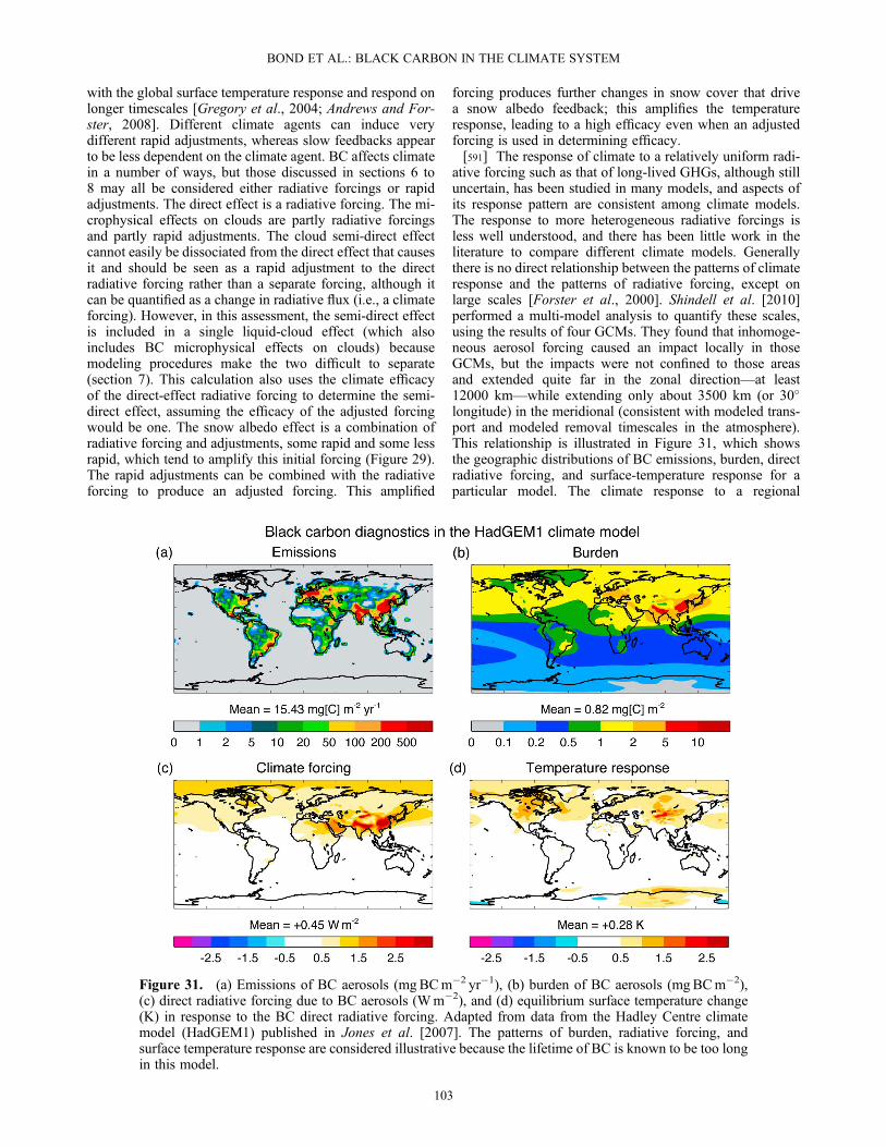
with the global surface temperature response and respond onlonger timescales [Gregory et al., 2004; Andrews and For-ster, 2008]. Different climate agents can induce verydifferent rapid adjustments, whereas slow feedbacks appearto be less dependent on the climate agent. BC affects climatein a number of ways, but those discussed in sections 6 to8 may all be considered either radiative forcings or rapidadjustments. The direct effect is a radiative forcing. The mi-crophysical effects on clouds are partly radiative forcingsand partly rapid adjustments. The cloud semi-direct effectcannot easily be dissociated from the direct effect that causesit and should be seen as a rapid adjustment to the directradiative forcing rather than a separate forcing, although itcan be quantified as a change in radiative flux (i.e., a climateforcing). However, in this assessment, the semi-direct effectis included in a single liquid-cloud effect (which alsoincludes BC microphysical effects on clouds) becausemodeling procedures make the two difficult to separate(section 7). This calculation also uses the climate efficacyof the direct-effect radiative forcing to determine the semi-direct effect, assuming the efficacy of the adjusted forcingwould be one. The snow albedo effect is a combination ofradiative forcing and adjustments, some rapid and some lessrapid, which tend to amplify this initial forcing (Figure 29).The rapid adjustments can be combined with the radiativeforcing to produce an adjusted forcing. This amplified

forcing produces further changes in snow cover that drivea snow albedo feedback; this amplifies the temperatureresponse, leading to a high efficacy even when an adjustedforcing is used in determining efficacy.[591] The response of climate to a relatively uniform radi-

ative forcing such as that of long-lived GHGs, although stilluncertain, has been studied in many models, and aspects ofits response pattern are consistent among climate models.The response to more heterogeneous radiative forcings isless well understood, and there has been little work in theliterature to compare different climate models. Generallythere is no direct relationship between the patterns of climateresponse and the patterns of radiative forcing, except onlarge scales [Forster et al., 2000]. Shindell et al. [2010]performed a multi-model analysis to quantify these scales,using the results of four GCMs. They found that inhomoge-neous aerosol forcing caused an impact locally in thoseGCMs, but the impacts were not confined to those areasand extended quite far in the zonal direction—at least12000 km—while extending only about 3500 km (or 30�longitude) in the meridional (consistent with modeled trans-port and modeled removal timescales in the atmosphere).This relationship is illustrated in Figure 31, which showsthe geographic distributions of BC emissions, burden, directradiative forcing, and surface-temperature response for aparticular model. The climate response to a regional

Figure 31. (a) Emissions of BC aerosols (mgBCm�2 yr�1), (b) burden of BC aerosols (mgBCm�2),(c) direct radiative forcing due to BC aerosols (Wm�2), and (d) equilibrium surface temperature change(K) in response to the BC direct radiative forcing. Adapted from data from the Hadley Centre climatemodel (HadGEM1) published in Jones et al. [2007]. The patterns of burden, radiative forcing, andsurface temperature response are considered illustrative because the lifetime of BC is known to be too longin this model.


103

radiative forcing, such as that by BC, has a regional compo-nent and a global component. While the patterns of burdenand direct radiative forcing are quite similar, there is no cor-respondence between the fine-scale patterns of radiativeforcing and the surface temperature response. However, boththe forcing and the surface temperature response are concen-trated in the extratropics of the northern hemisphere.

9.3. Surface Temperature Response to AtmosphericBlack Carbon

9.3.1. Global-Mean Temperature Change[592] Earlier studies on the climate effect of large injec-

tions of smoke and dust aerosols (i.e., so-called nuclearwinter) are relevant to understanding forcing by BC. Cesset al. [1985] showed that for increasing smoke loadingsthere is a transition from a surface-troposphere heating,induced by the convective coupling of the surface and thetroposphere to a surface cooling when this convectivecoupling breaks down as the vertical structure of the atmo-sphere is modified. The climate response to BC may differfrom a nuclear winter because the aerosol is concentratedin the lower atmosphere, and if the presence of co-emittedspecies is limited, it may be more absorbing than smoke.Cook and Highwood [2004], Hansen et al. [2005], andBan-Weiss et al. [2011] added BC to different altituderanges and showed that radiative forcing was not an effec-tive measure of determining the surface temperatureresponse to BC. The efficacy of the radiative forcing termcould even change sign. In contrast, the efficacy of theadjusted forcing that accounted for semi-direct effects wasmuch closer to unity [Shine et al., 2003; Hansen et al.,2005; Crook et al., 2011; Ban-Weiss et al., 2011]. The mostconsistent forcing measure appears to be calculated byallowing tropospheric response but no global mean surfacetemperature response, either from fixing surface temperatureeverywhere [Shine et al., 2003] or using a regression method[Ban-Weiss et al., 2011]. Hansen et al. [2005] furthershowed that for BC in snow the large efficacy of the high-latitude forcing needs to be properly accounted for (seebelow). The adjusted forcing implicitly accounts for some ofthe variable efficacy of the direct radiative forcing. Theadjusted forcing or the effective forcing (i.e., forcing weightedby efficacy (Table 2)) is a more appropriate measure of BC’sultimate effect on global average temperature.[593] Table 23 reports BC radiative forcing, adjusted forc-

ing, effective forcing, and surface-temperature responsefrom various climate models. Note that these experimentsare generally based on unrealistic BC perturbations and, assuch, they are representative of sensitivity rather than theexpected magnitude of temperature change or forcing.Therefore, the results in Table 23 should be used qualita-tively. Quantitative temperature changes are estimated insection 10, employing our revised forcing estimate. The dif-ferent models vary in their experimental designs (e.g., BCalone versus BC and co-emitted species, slab ocean modelversus fully coupled ocean-atmosphere model), emissionrates, and treatment of the effects of BC on climate. Somehave a more sophisticated treatment of BC optics, someare better documented in their ability to simulate the pres-ent-day climate and the historical period, and some simulatebetter cloud properties than others. Nevertheless, theseresults show that effective forcing and adjusted forcings from

a single model agree to within their respective uncertainties,justifying our approach for calculating the semi-direct effect.While there is a large range in equilibrium temperature re-sponses across the studies the spread in temperature responseper radiative forcing is smaller, covering a threefold range.When the forcings are appropriately scaled to account for rapidadjustments agreement is even better, with only a twofoldrange in temperature response per adjusted forcing. This find-ing suggests that differences in rapid adjustments or aerosolprocesses included in each model are responsible for some ofthe difference in global average temperature change.[594] The climate models clearly differ in their cloud

responses. For instance, fossil fuel BC causes an increasein high-level clouds in the model of Jacobson [2010] dueto an enhancement of upper tropospheric water vapor dueto surface warming and evaporation and a decrease in lowclouds due to enhanced BC warming, including that withincloud drops and interstitially between cloud drops, asdiscussed in section 7.3.3. These experiments, unlike mostother studies, considered OA and other co-emitted species,and included the microphysical effects of BC on liquid andice clouds.9.3.2. Regional Surface Temperature Change[595] As discussed in the introduction, the pattern of

surface temperature response can be quite different fromthe pattern of forcing. The temperature response to BC is acombination of regional response and hemispheric response,with polar and land amplification. There is a reasonableagreement among models that the BC warming is concen-trated in the Northern Hemisphere with some polar amplifi-cation (Figure 32). However, there is disagreement on therelative warming of the different continents, with somemodels showing significant warming over North Americaand Eurasia while others do not. It is unlikely that the differ-ences in experimental setup and range of BC effectsincluded in the four models presented in Figure 32 are suffi-cient to explain the diversity of results. Some of the modeldifferences could be due to differences in forcing and cli-mate efficacy (or sign of the semi-direct effect). It is difficult,however, to attribute the differences among the models to aparticular process or reason without performing a more com-prehensive intercomparison. While some models includemore BC forcing mechanisms that have been evaluated atdifferent scales (e.g., GATOR), others have been morethoroughly tested regarding their ability to represent theglobal historical temperature record and climate variability(e.g., NCAR CAM, GISS, and HadGEM2).[596] There are few systematic studies of the regional

impact of BC aerosols from different regions with the excep-tion of the work by Shindell and Faluvegi [2009], wholooked at the regional impact of atmospheric BC from fourlatitudinal bands in the GISS climate model. A summaryof their results relevant to BC is shown in Figure 33. BCin the 28�N–60�N band is most efficient at inducingwarming in the 60�N–90�N band and vice versa. Tropical(28�S to 28�N) BC warms all latitudinal bands, with forcingefficiency increasing in moving from lower to higher lati-tudes. Finally, it should be noted that atmospheric BC inthe 60�N–90�N band cools the surface in that region, possi-bly because the coupling between the atmosphere and thesurface is not strong enough to overwhelm the decrease insolar radiation at the surface induced by BC or because of


104

Tab

le23.Sum

maryof

ResultsforBlack

Carbonin

Clim

ateModelsa

Study

Processes

Included

Emissionsb

(TgBCyr

�1)Radiativ

eForcing

(Wm

�2)A

djustedForcing

(Wm

�2)

Effectiv

eForcing

(Wm

�2)

Equilibrium

Tem

perature

Response(K

)Notes

RobertsandJones[2004]

Directand

semi-direct

effects

20.24(�

4)0.78

(�4)

0.48

(�4)

0.44

(�4)

HadSM4.

Fossil-fuel

BCem

issionswere

quadrupled

toincrease

signal

tonoise.

Wang[2004]

Directandsemi-direct

effects

140.35

0.14

�0.3

0.07

NCARCCM3with

slab

oceanmodel

from

CCM3.6.6.

CO2clim

atesensitivity

notknow

n.

Hansenet

al.[2005]

Directandsemi-

direct

effects

Not

specified

1.03

(�6)

BB

0.71

�0.17

(�6)

0.76

(�6)

0.27

(�6)

GISSmodel

E.BB=BiomassburningBConly.

Experim

entE2B

CB�6(biomassburningBC

emissionsweremultip

liedby

6)andE2B

CI�

2(industrialBCem

issionsweredoubled).

0.59

(�2)

0.35

(�2)

0.96

(�2)

FF

0.5�0.1(�

2)

Chung

andSeinfeld

[2005]

Directandsemi-

direct

effects

7.9

0.33

(Ext)

0.47

(Ext)

0.20

(Ext)

GISSmodel

II-primewith

external

(Ext)

andinternal

(Int)mixtures

0.37

(Int)

0.60

(Int)

0.85

(Int)

Sokolov[2006]


effects

2.36

(�10)

3.0(�

10)

1.76

(�10)

Earth

System

Model

ofInterm

ediate

Com

plexity

.The

change

inBChasbeen

multip

liedby

10.

Joneset

al.[2007]


effects.Externalmixture.

7.9(year2000)

versus

0.45

0.39

�0.09

0.28

0.28

Improved

versionof

HadGEM1coupledto

amixed-layer

ocean.


effects

only.Fossil-fuel

BConly.

0.6(year1860)

Jacobson

[2010]

Direct(external+

internal

mixtures),BCinclusion

inclouddroplets,snow

albedo

effect,semi-direct

andallcloudeffects.

3.18

FSc

0.47

d0.49

Forcing

isan

estim

atebasedon

anearlierversion

ofthemodel.CO2clim

atesensitivity

0.6K

(Wm

�2)�

1.

7.92

FSBSGc

0.78

d0.71

a Adjustedforcingincludes

radiativeforcingandrapidadjustmentstothatforcingquantifi

edas

atop-of-atm

osphere(ToA

)flux

change;effectiv

eforcingiseitherradiativeor

adjusted

forcingmultip

liedby

itsefficacy

(Table

2).Multip

liers

inbracketsreferto

thescalings

oftheBCeffect

used

inintegrations

togenerate

astatistically

significant

response

intheclim

atemodels.

bFF=fossil-fuel

BC;FS=fossil-fuel

BC+POA;BB=biom

assburningBC;FSBSG=fossil-fuel

andbiofuelBC+POA.

c Co-em

itted

POA

isincluded

forFSandallaerosolsandgasesforFSBSG.

dTop-of-atmosphereirradiance

changesthat

includeclim

ateresponse

and,

thus,arenottrue

effectiveforcings.


105

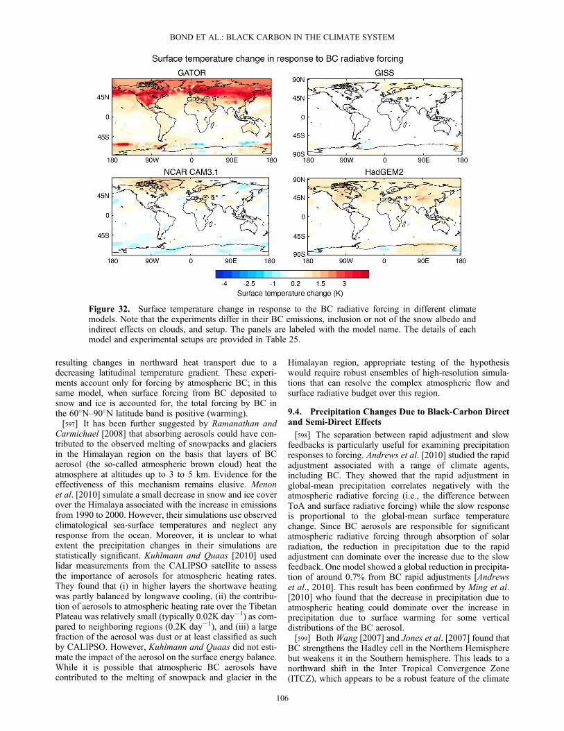
resulting changes in northward heat transport due to adecreasing latitudinal temperature gradient. These experi-ments account only for forcing by atmospheric BC; in thissame model, when surface forcing from BC deposited tosnow and ice is accounted for, the total forcing by BC inthe 60�N–90�N latitude band is positive (warming).[597] It has been further suggested by Ramanathan and

Carmichael [2008] that absorbing aerosols could have con-tributed to the observed melting of snowpacks and glaciersin the Himalayan region on the basis that layers of BCaerosol (the so-called atmospheric brown cloud) heat theatmosphere at altitudes up to 3 to 5 km. Evidence for theeffectiveness of this mechanism remains elusive. Menonet al. [2010] simulate a small decrease in snow and ice coverover the Himalaya associated with the increase in emissionsfrom 1990 to 2000. However, their simulations use observedclimatological sea-surface temperatures and neglect anyresponse from the ocean. Moreover, it is unclear to whatextent the precipitation changes in their simulations arestatistically significant. Kuhlmann and Quaas [2010] usedlidar measurements from the CALIPSO satellite to assessthe importance of aerosols for atmospheric heating rates.They found that (i) in higher layers the shortwave heatingwas partly balanced by longwave cooling, (ii) the contribu-tion of aerosols to atmospheric heating rate over the TibetanPlateau was relatively small (typically 0.02K day�1) as com-pared to neighboring regions (0.2K day�1), and (iii) a largefraction of the aerosol was dust or at least classified as suchby CALIPSO. However, Kuhlmann and Quaas did not esti-mate the impact of the aerosol on the surface energy balance.While it is possible that atmospheric BC aerosols havecontributed to the melting of snowpack and glacier in the

Himalayan region, appropriate testing of the hypothesiswould require robust ensembles of high-resolution simula-tions that can resolve the complex atmospheric flow andsurface radiative budget over this region.

9.4. Precipitation Changes Due to Black-Carbon Directand Semi-Direct Effects

[598] The separation between rapid adjustment and slowfeedbacks is particularly useful for examining precipitationresponses to forcing. Andrews et al. [2010] studied the rapidadjustment associated with a range of climate agents,including BC. They showed that the rapid adjustment inglobal-mean precipitation correlates negatively with theatmospheric radiative forcing (i.e., the difference betweenToA and surface radiative forcing) while the slow responseis proportional to the global-mean surface temperaturechange. Since BC aerosols are responsible for significantatmospheric radiative forcing through absorption of solarradiation, the reduction in precipitation due to the rapidadjustment can dominate over the increase due to the slowfeedback. One model showed a global reduction in precipita-tion of around 0.7% from BC rapid adjustments [Andrewset al., 2010]. This result has been confirmed by Ming et al.[2010] who found that the decrease in precipitation due toatmospheric heating could dominate over the increase inprecipitation due to surface warming for some verticaldistributions of the BC aerosol.[599] Both Wang [2007] and Jones et al. [2007] found that

BC strengthens the Hadley cell in the Northern Hemispherebut weakens it in the Southern hemisphere. This leads to anorthward shift in the Inter Tropical Convergence Zone(ITCZ), which appears to be a robust feature of the climate

Figure 32. Surface temperature change in response to the BC radiative forcing in different climatemodels. Note that the experiments differ in their BC emissions, inclusion or not of the snow albedo andindirect effects on clouds, and setup. The panels are labeled with the model name. The details of eachmodel and experimental setups are provided in Table 25.


106

response to BC also supported by earlier experiments[Roberts and Jones, 2004; Chung and Seinfeld, 2005].[600] A number of studies have investigated the regional

climate responses to BC in particular regions of the world,generally focusing on precipitation changes. Many of thesestudies examine Asia because of the large concentrationsof absorbing aerosols there. Using the GISS model, Menonet al. [2002b] simulated a surface warming over mostregions in response to absorbing aerosols but a moderatecooling over China. The model also simulates increased pre-cipitation in southern China and over India with a band ofdecreased precipitation to the south. Zhang et al. [2009a]obtained the opposite result using the Community Atmo-sphere Model (CAM3) when considering carbonaceousaerosol (BC+OC) together. In this case, surface temperatureincreased in southern China and India and total cloudcover and precipitation decreased. Using the same model,Liu et al. [2009b] found that sulfate and BC aerosols havethe effect of weakening East Asia monsoons in both thesummer and winter seasons.[601] Lau et al. [2006] used the GEOS GCM with fixed

sea surface temperature to show that absorption of solar radi-ation by dust heats the air on the northern and southernslopes of the Tibetan Plateau, which can then rise and create

a positive temperature anomaly in the middle to upper tropo-sphere over the Tibetan Plateau. On the southern side, theatmospheric heating is reinforced by anthropogenic emis-sions of BC over the Indian subcontinent. This can lead toan intensification of the Indian summer monsoon andsurface warming over the Tibetan Plateau. While Lau et al.found that the effect of BC is important in initiating themonsoon rainfall anomalies over India, it is not enoughto produce statistically significant change in the monsoonregime on its own (i.e., without the synergy with dustabsorption). Like most of the other earlier studies lookingat the regional climate response to BC, this study wasperformed with an atmosphere-only model, which is a sig-nificant limitation because sea surface temperatures are notallowed to respond to the forcing by BC. One could ima-gine anthropogenic aerosols causing a decrease in sea sur-face temperature, for example, during the winter monsoonover the Indian Ocean, with consequences for the summermonsoon.[602] Wang et al. [2009a] used the NCAR Community

Climate Model version 3 (CAM3) coupled to a slab oceanmodel to investigate the response of the Indian summermonsoon to scattering and absorbing aerosols. They foundthat absorbing aerosols cause a northward shift in rainfall(both during the onset of the monsoon and averaged overthe monsoon period) that is only weakly offset by the effectof scattering aerosols.[603] Meehl et al. [2008] performed a six-member ensem-

ble of twentieth century simulations with a fully coupledocean-atmosphere climate model, which confirmed someof the earlier results found with atmospheric modelscoupled to a slab ocean. In their experiments, BC and OAaerosols increase lower tropospheric heating over southAsia and reduce the amount of solar radiation reachingthe surface during the dry season, enhancing precipitationover India in the months of March–April–May. With theonset of the monsoon, the reduced surface temperatures inthe Bay of Bengal, Arabian Sea, and over India that extendto the Himalaya act to reduce monsoon rainfall over Indiaitself, with some small increases over the Tibetan Plateau.Precipitation over China generally decreases due to theBC effects. Analysis of single ensemble members fromthe multiple-forcings experiment suggests that the ob-served increasing precipitation trends over southern Chinaappear to be associated with natural variability connectedto surface temperature changes in the northwest PacificOcean. Rotstayn et al. [2007] suggest that the effects ofAsian aerosols on rainfall could be seen in Australia withan increase in cloudiness and rainfall during the period1951 to 1996, especially in northwestern Australia.Bollasina et al. [2011] and Shindell et al. [2012] investi-gated the impact of aerosol forcing on the South Asianmonsoon in the GFDL and GISS GCMs, respectively.Shindell et al. found distinct perturbations to the SouthAsian monsoon as well as to precipitation in the Saheland southern Europe. Bollasina et al. found similarchanges and suggested that the changes were part oflarge-scale circulation changes and had little to do withdirect local forcing. Shindell et al showed that the precip-itation responses were in many places similar to those in-duced by GHGs but with much greater amplitude per unitforcing.

Figure 33. Normalized global and regional surface airtemperature (SAT) changes (�C (Wm�2)�1) in response toregional radiative forcings due to CO2 (blue bars), BC aerosol(no cryosphere) (red bars), and sulfate aerosol (yellow bars).The forcing regions are defined on the horizontal axis as latitu-dinal bands (Southern Hemisphere middle- and high-latitudes,28�S–90�S; tropics, 28�S–28�N; Northern Hemisphere mid-latitudes, 28�N–60�N; and Northern Hemisphere high-latitudes, 60�N–90�N). The SAT response regions are labeledin each panel. Adapted from Shindell and Faluvegi [2009].


107

[604] Tosca et al. [2010] also applied the NCAR CAM3model with a slab ocean model to explore effects of biomassburning emissions over the western equatorial Pacific duringintense El Niño episodes, such as the 1997–1998 event.They found that BC and OA emissions from extreme fireyears caused sea surface temperature to cool and the atmo-sphere to warm and that this reduced precipitation by about10% over greater Indonesia, potentially exacerbating localdrought conditions because evapotranspiration reductionswere smaller than precipitation changes.[605] Generally, these studies show that atmospheric

heating by BC can have significant effects on precipitation,causing a global reduction via rapid adjustment processes.Model studies have also shown that BC can alter regionalprecipitation by about 10% and affect circulation patternssuch as the monsoon.

9.5. Climate Response to the Snow Albedo Effect

[606] BC deposited to snowpack can significantly reducesnow and ice albedo because of the approximately 5 order-of-magnitude difference in mass absorption cross sectionbetween ice and BC, and strong multiple scattering withinsnow, which enables small mixing ratios of impurities toabsorb a disproportionate amount of radiative energy [e.g.,Warren and Wiscombe, 1980]. BC-induced snow albedochanges exert a small global-mean forcing through radiativeforcing and rapid adjustments (i.e., all-source adjustedforcing range of +0.01 to +0.09 W m�2 in section 8), butmodels indicate that snow albedo forcing is unusually effec-tive at warming climate, even when rapid adjustments areaccounted for. The high efficacy of the adjusted forcingstems from the following factors:[607] 1. By definition, all of the forcing energy associated

with this mechanism is deposited directly within thecryosphere, a component of the Earth System responsiblefor strong positive feedback [e.g., Budyko, 1969] throughthe snow (and ice) albedo feedback (SAF in Figure 29).Warming of snow and sea ice by deposited BC exacerbatesthis feedback mechanism in comparison to forcing mecha-nisms that distribute energy more evenly throughout theplanetary envelope, such as GHG forcing.[608] 2. The mechanism operates mostly at high latitudes,

which are uniquely susceptible to surface energy forcingsbecause of stable atmospheric conditions. Smaller lapse ratesin high-latitude regions induce shallower mixed layers thatpermit surface energy forcings to drive larger surface tem-perature changes. In stratified conditions, the mass of airresponding to a surface energy forcing is small, and the en-ergy is not transferred efficiently throughout the system.This condition breaks down with strong warming, however,so that larger forcings have smaller efficacies. It is weakerduring summer, when insolation (and therefore radiativeforcing via darkening of snow or ice) is greatest [Forster etal., 2000].[609] 3. In some studies, feedbacks driven by changes in

snow grain size may also contribute to larger efficacy[Flanner et al., 2007] (GRA in Figure 29). The reasoningfor this result is that BC absorption warms snowpacks sothat they age more rapidly, which lowers snow albedo inthe near-infrared spectrum. A key uncertainty associatedwith this process is that snowpack temperature gradient isoften a greater controller of snow age than mean temperature

[Flanner and Zender, 2006], and the influence of absorbingimpurities on temperature gradient depends on many factors,including the vertical distribution of impurities and solar ab-sorption, snowpack thermal conductivity, and snowpack-at-mosphere coupling.[610] The relative roles of these three factors are uncertain.

Bellouin and Boucher [2010] obtained a large climate effi-cacy in idealized model experiments that do not includethe third factor.[611] Climate response to BC in snow is particularly

strong during boreal spring (March–May) over middle tohigh latitudes [Flanner et al., 2009; Wang et al., 2011].Increasing springtime insolation and widespread snowcover in the Northern Hemisphere drive the greatest radia-tive forcing during this season, and climate response andefficacy are large when the mechanism induces earliersnow melt, as the contrast in albedo between snow-coveredand snow-free surfaces is generally much greater than thereduction in albedo caused by BC. A source of enhancedspringtime forcing is the retention of impurities at the snowsurface during melt (MBC in Figure 29; section 8.3.5), butthe importance of this effect is largely uncertain and likelyvaries considerably with location and type of snowpack.Koch et al. [2011b] have suggested that even in the absenceof the MBC feedback (Table 20), 20% of Arctic warmingand snow-ice cover loss is a consequence of the BC albedoeffect.[612] Table 24 reports estimates of the BC snow albedo

forcing, surface temperature response, and climate efficacyfrom different model studies. The equilibrium change inglobal-mean surface temperature ranges from +0.06 to+0.20K for the trustworthiest experiments. The climateresponse is more localized than that for the BC direct andsemi-direct effects with most of the warming over the Arcticregion and the Tibetan Plateau and Himalaya. EquilibriumArctic temperature responses reported from three simula-tions [Flanner et al., 2007; Koch et al., 2009a] are 0.50,0.50, and 1.6K (the latter occurring with strong boreal fireBC emissions in 1998). Climate efficacy for the adjustedforcing is much larger than 1 in all models with most modelsshowing values of 2.0 or more. Based on the spread ofadjusted-forcing efficacies given in Table 24, the efficacyof the adjusted forcing by BC in the cryosphere is estimatedto be 3, with a range of 2 to 4. These efficacies are used insection 10 to derive effective forcings due to BC in snowand sea ice (Table 2).[613] Most studies of the climate impact of BC in snow

have focused on the global, annual impact or on impacts inthe Arctic. However, because most of the energy from thisforcing directly impacts snowpack temperatures, localimpacts may be large, especially where snowmelt is reliedupon as a water source. Recognizing this, Qian et al.[2009] applied the Weather Research and Forecasting(WRF) regional model to study the influence of BC deposi-tion on western North America snowpack. They found thelargest response during late winter and early spring, withincreased net solar radiation caused by reduced snow cover,and subsequent increases in surface air temperature. Climatechanges and deposition of BC on snow were both largestover the central Rockies and southern Alberta, where shiftsin regional stream flow were also found. An experimentwith doubling of regional BC emissions showed a much


108

greater-than-linear climate response in this region. Qianet al. [2011] used a global model to look at the influenceof BC and dust on the Tibetan Plateau snowpack with aspecific focus on the impacts on the Asian hydrologicalcycle and monsoon climate. In this study, BC and dust insnow were found to produce 5 to 25 W m�2 adjustedforcing during spring, reducing spring snowpack over theTibetan Plateau more than does warming by anthropogenic

CO2 and atmospheric BC. However, Qian et al. acknowledgethat the global model used grossly overpredicts snow cover inthis region (their Figure 2) and, therefore, likely also forcingby BC and dust in snow. These studies highlight the possiblestrong regional impacts of BC in snow but also emphasizethe need for studies that can account for the large variationsin terrain, snow cover and BC deposition, especially in moun-tainous terrain.

Table 24. Summary of Climate Model Studies Focusing on the Snow Albedo Effecta

Study Forcingb (Wm�2)

EquilibriumTemperatureResponse (K)

ClimateSensitivity(KW�1m2)

ClimateEfficacy (%) Note

Hansen andNazarenko [2004]

0.16 0.24 1.5 212 Idealized snow albedo decrease (2.5% inArctic, 1% in Greenland, and 5% in NorthernHemisphere land snow)

Jacobson [2004a] 0.06c GATOR GCMM range 0.03–0.11KHansen et al. [2005] 0.082 0.065 171 GISS model EFlanner et al. [2007] 0.054e 0.15 452d 1998 central estimate. NCAR CAM3Flanner et al. [2007] 0.049e 0.10 329d 2001 central estimate. NCAR CAM3Flanner et al. [2007] 0.043e Fossil-fuel and biofuel BC onlyFlanner et al. [2007] 0.033e Fossil-fuel BC onlyFlanner et al. [2009] 0.057 0.08 1.4 231f Experiment PI4 (pre-industrial climate with

fossil and biofuel BC only) NCAR CAM3.1Koch et al. [2009a] 0.01 0.18 GISS model E. RF is estimated as difference in

fluxes from experiments with fixed SST and isnot a good approximation.

Bellouin andBoucher [2010]

0.28 0.72 2.6 260 Idealized experiment with HadGEM2-AML.The radiative forcing is for an ad hoc decreasein the land snow albedo of 0.05.

Wang et al. [2011] 0.042g 0.071h Idealized snow albedo decrease (2.5% inArctic, 1% in Greenland, and 5% in NorthernHemisphere land snow)

aSpecifics of the forcing calculations for all but the Bellouin and Boucher [2010] study can be found in Table 19. Bellouin and Boucher [2010] werespecifically looking at climate response, so this study is excluded from Table 19.

bBellouin and Boucher [2010], Hansen and Nazarenko [2004], and Hansen et al. [2005] forcings are radiative forcings. All other studies included rapidadjustments in the forcings and so are adjusted forcings.

cNot equilibrium temperature but 10 year average (including spin up).dResults from Flanner et al. [2007] show a large range of climate efficacies which could be due to noise.eToA forcing is estimated as Fa = 0.91 Fs,snow. CO2 climate sensitivity is estimated to be 2.47 3.58 = 0.69KW�1m2.fCO2 climate sensitivity in Flanner et al. [2009] is estimated as 0.89/(5.35ln(380/289)) = 0.89/1.46 = 0.61KW�1m2.gSurface forcing, Fs.hTemperature response is not equilibrium temperature but a 10 year average, with 1 year spin up. Equilibrium temperature response is not reported so

climate sensitivity and climate efficacy are not given.

Table 25. Description of the Model and Experimental Setup for Figure 32a

Model Experimental DesignBC Sources andState of Mixture Effects Included References

GATOR Present-day emissions versus no emissions;“quasi-equilibrium” climate responseusing last 10 year average from15 year experiment;full ocean model

FF +BF (BC+POA+otherco-emitted species);evolution from externalto internalmixture

Direct; semi-direct;cloud indirect; BCinclusion in water dropsand ice crystals; snowalbedo effects

Jacobson [2010]

GISS 80% of present-day emissions;Equilibrium climate response;full ocean model

80% of FF +BF(only BC); external mixture

Direct; semi-direct; cloudindirect; snow-albedo effects

Koch and Hansen [2005];Shindell and Faluvegi [2009].

NCAR CAM3.1 Present-day emissions versus noemissions; equilibrium climateresponse; slab ocean model

FF +BF (BC+POA);external mixture

Direct; semi-direct; snowalbedo effects (and indirecteffects)

Collins et al. [2006];Flanner et al. [2009]

HadGEM2 Present-day versus pre-industrialemissions; equilibrium climate response;slab ocean model

FF (only BC); externalmixture

Direct; semi-direct Jones et al. [2007]

aRefer to section 8 for a more detailed description of snow albedo effect.


109

9.6. Detection and Attribution of Climate Change Dueto Black Carbon

[614] As sections 9.3 to 9.5 have outlined, there isevidence of regional climate responses to BC that is manifestin observations. In particular, there is some evidence for aBC effect on (1) regional temperature and precipitationchanges [e.g., Menon et al., 2010], (2) Arctic temperaturesand snow-ice cover [e.g., Flanner et al., 2009; Koch et al.,2011b], (3) monsoon and other circulation changes [e.g.,Rotstayn et al., 2007; Bollasina et al., 2011; Shindellet al., 2012], and (4) Himalayan and North American snowand ice cover [Qian et al., 2009; Qian et al., 2011]. However,it should be noted that none of these studies formally attributechanges to BC in a statistically rigorous sense.[615] It is desirable to find a confirmation of the model

results on the climate response to BC in the observationalclimate records. Methods have been developed to detectand attribute climate change to particular climate agents byregressing the spatial and temporal patterns of climatechange simulated by the models against the observedpatterns. Scaling factors that maximize the fit to the observa-tions provide a measure of whether a particular forcing isdetected, by testing the hypothesis that the scaling factorsare consistent with a value of zero. When a particular combi-nation of forcings is detected, the scale factors can be used toreconstruct the contribution of each individual forcing totemperature change. Detection and attribution methods haveestablished that the anthropogenic “. . .greenhouse gas forc-ing has very likely caused most of the observed globalwarming over the last 50 years.” The cooling due to sulfateaerosols could also be detected [Hegerl et al., 2007]. How-ever, it has proven to be more difficult to detect the warmingdue to BC.[616] Jones et al. [2005] included fossil fuel BC in a detec-

tion and attribution analysis with GHG and sulfate aerosols.While the introduction of BC did not affect the attribution ofthe warming to GHGs, it was not possible to detect thepattern due to BC because it was too similar to the coolingpattern of sulfate aerosols. The influence of carbonaceousaerosols (BC and OA from fossil fuel and biomass burningsources) was detected by Nagashima et al. [2006] in themid part of the twentieth century. However, the relativecontribution from BC cannot be deduced from this study.[617] Jones et al. [2011] revisited their earlier work using

an ensemble of HadGEM1 model simulations that includedifferent combinations of the GHGs, sulfate aerosols, BC,and natural radiative forcings. They used their detectionand attribution method to examine the climate influence ofBC from fossil fuel and biofuel combustion sources. TheBC forcing included the direct and semi-direct effect butnot the snow albedo effect. The climate response to BCwas obtained as the difference between a simulation withall forcings and a simulation with all forcings except thatfrom BC. BC was found to have a detectable contributionto the warming over the period 1950–1999 but not overthe period 1900–1999 or 1957–2006. The attributed climatechange due to BC was 0.41K(century)�1 (range 0.20 to0.60K(century)�1) for the period 1950–1999. This corre-sponds to a warming of about 0.20K (range 0.10 to 0.30K)for the 50 year period. Global warming by industrial-eraBC would be about twice as large because 1950 emissionsof BC were about half of present-day emissions. Moreover,

any committed warming would add only slightly to the equilib-rium climate response. Accounting for the snow albedo effectwould possibly improve the detection and narrow theuncertainties in the scale factors but would not necessarily resultin a larger contribution of BC to the observed warming becausethe scale factor can compensate for the missing warming in theclimate simulations. For the period 1957–2006, the attributedclimate change due to BC—not statistically significant—is0.10K(century)�1 (range �0.03 to 0.21K(century)�1). Failureto detect the climate response to BC over this period can bedue to the discontinuities introduced in the simulations bymerging the historical emission inventories until 2000 withthe SRES emission projections after 2000.[618] In conclusion, it can be said that the global warming

due to BC can be detected in the observational temperaturerecord but the detection remains very sensitive to the modelingassumptions. The deduced contribution of BC to the observedwarming is comparable to that obtained from models alone,but it is not accurate enough to constrain further the variousestimates obtained from the models so far. Inclusion of thepattern of warming due to the snow albedo effect andregression of the simulated patterns against both the observedsurface and vertical temperature change patterns couldcontribute to a better detection of the BC signal.

9.7. Conclusions

[619] Figure 34 summarizes our knowledge on the effects ofBC on climate. There is agreement among climate models thatBC causes a warming that is essentially located in the northernhemisphere. Existing studies have different experimentalconfigurations and consider different processes by which BCaffects climate, making comparisons between them difficult.However, there is a smaller range in surface temperatureresponse per unit effective forcing than in effective forcing.Climate models also consistently simulate a northward shiftin the Intertropical Convergence Zone in response to BCforcing. Other changes in precipitation are likely, especiallythe Asian monsoon systems as these regions experience largeburdens of BC. However, there is no agreement amongmodelson the patterns of rainfall changes in these regions. High-resolution simulations with coupled ocean-atmosphere modelsover the Asian region could better address the issue of circula-tion and precipitation changes due to BC. Darkening of snowand ice surfaces by BC is associated with enhanced meltingand an amplification of the surface temperature response inthese regions, but the role of BC on glacier melting in theHimalayan and Tibetan Plateau region remains unclear. Theclimate response to the indirect effect of BC on liquid andice clouds has not been studied in isolation of the direct andsemi-direct effects and remains largely unknown. Detectionand attribution studies, which seek the expected patterns ofthe climate response to the BC forcing in the observationalrecords, have had some limited success, probably because ofimperfect modeling assumptions but also because of thedisruptive effect of sulfate aerosols.

10. Synthesis of Black-Carbon Climate Effects


[620] 1. The industrial-era (1750 to 2005) climate forcingof BC is made up of components from its direct radiativeforcing, its effect on cloud microphysics, rapid adjustments


110

to its atmospheric heating, and the effect of BC deposited onsnow and sea ice.[621] 2. Employing radiative forcing alone is inadequate

for assessing the climate role of BC in terms of its globallyaveraged, surface temperature response. In particular, semi-direct effects and the efficacy of high-latitude forcing termsneed to be properly accounted for.[622] 3. The level of scientific understanding of these com-

ponents is generally assessed as low or very low, makingtheir uncertainty bounds difficult to characterize accurately.It is also difficult to quantify how uncertainties of differentterms are correlated, making errors difficult to combine.[623] 4. With these caveats, the industrial-era total climate

forcing of BC is assessed to be +1.1 W m�2 with a 90% un-certainty range of +0.17 to 2.1 W m�2, allowing for the cor-relation of emission uncertainty. This climate forcing has alarger uncertainty range and is likely greater than the radia-tive forcing from the BC direct effect (+0.71 W m�2 witha 90% uncertainty range of +0.08 to +1.27 W m�2). Thisbest estimate of black carbon forcing ranks it as the secondmost important individual climate-warming agent after car-bon dioxide when both direct and indirect effects areincluded.[624] 5. In terms of equilibrium global-mean surface tem-

perature change, the total BC climate-forcing estimate for theindustrial era would correspond to a warming between 0.1and 2.0K. Note that not all this warming has been realized inthe present day as the climate takes more than a century toreach equilibrium and many co-emitted species have a coolingeffect, countering the global-mean warming of BC.[625] 6. In addition to the direct radiative forcing of BC,

adding the positive climate forcings and accounting forthe efficacies of BC in snow and BC in sea ice increasesthe best estimate of forcing. Semi-direct and liquid-cloudeffects add negative climate forcing, and cloud absorption

and mixed-cloud changes add positive climate forcing.The total of BC cloud effects is estimated to be positive. In-cluding these effects makes the estimate of total BC climateforcing estimate considerably more uncertain than that of di-rect radiative forcing. In particular, the two positive cloudterms have a very low level of scientific understanding. With-out these terms, BC total climate forcing would be +0.65 Wm�2 with a 90% uncertainty of +0.03 to +1.1 W m�2.[626] 7. The components of BC climate forcing in addition

to the direct radiative forcing are cloud, cloud droplet inclu-sions, and semi-direct effects (+0.23 W m�2 with a 90% un-certainty range of �0.47 to 1.0 W m�2); and BC in snowand BC in ice (+0.13 W m�2 with a 90% uncertainty range+0.04 to +0.33 W m�2). See Table 1 for a further breakdownof forcing components.

10.2. Introduction

[627] Earlier sections have discussed emissions of BC, themechanisms by which BC affects the Earth’s radiativebalance and BC’s various effects on climate. Here wesynthesize these discussions to provide best estimates anduncertainty bounds for the role of BC in the current climateusing the metric of globally averaged climate forcing.Section 9 pointed out that regional changes and especiallychanges to the hydrological cycle are how we experienceclimate change and that such impacts are not representedby global forcing metrics. Nonetheless, in this assessment,we have chosen to use a global forcing metric as it is morecomparable across mechanisms and better constrained thanother choices.

10.3. Global Climate Forcing Definition

[628] We are ultimately interested in quantifying theimpact of BC emissions on the Earth’s climate. The defini-tion of radiative forcing employed in IPCC reports [Forster

Figure 34. Qualitative summary of our current understanding of the global climate impacts ofBC emissions.


111

et al., 2007] is the change in net energy (down minus up) atthe tropopause since 1750 due to a given mechanism orclimate forcing agent, after allowing stratospheric tempera-tures to adjust to radiative equilibrium. As discussed insection 2.3.2, we retain this definition of forcing relative toa base year but use the term “industrial-era forcing” toindicate that the forcing is based on time rather than whollyattributable to anthropogenic activity. The overall globalclimate response to BC (encompassing direct, snow, sea-ice, and cloud effects) is also very different from theresponse to other forcing agents such as the long-livedGHGs (section 9). BC emissions affect clouds, snow, andsea ice (sections 7 and 8). In IPCC reports, some of theseeffects are classified as part of the cloud albedo effect orrepresented separately as BC snow albedo forcing,while others are considered part of the climate response.In this assessment, “rapid adjustments” to the forcing areincluded in the total climate forcing term. Rapid adjustmentsare where the atmosphere, land, or cryosphere responds tothe forcing on a relatively short timeframe compared to thatof the global-mean temperature response (Table 2 andsection 2.3). In addition for both BC in snow and BC insea ice, we implicitly include both the rapid adjustment ofthe snowpack and the climate response to the BC snowand ice albedo changes (i.e., the snow albedo feedback) byaccounting for the efficacy of BC snow and ice albedochange in our climate forcing estimate, employing the conceptof “effective forcing” discussed next.[629] The notion of effective forcing means that the

radiative forcing is scaled by an efficacy which incorpo-rates the relative strengths of climate feedbacks. Thiseffective forcing is then more representative of the actualradiative impacts of BC [e.g., Hansen et al., 2005] (alsosee Tables 2 and 23). Alternatively, forcings can be calcu-lated from fixed sea-surface temperature experiments orregression techniques [Hansen et al., 2005, Andrews et al.,2010]. In practice, diverse forcing definitions are used inthe different studies we assess and care is required when com-paring reported forcings (section 9 and Table 23). Forexample, the separation of BC forcing into direct, cloud-albedo forcing, and semi-direct forcing is not straightforward(section 7). In this assessment, we have been particularlycareful to include all relevant terms when assessing the total cli-mate forcing from BC without double counting (section 2.3.2).

10.4. BC Global Climate Forcing Components andUncertainties

[630] In this section, we summarize the best estimates ofindividual climate forcing components for global BC emis-sions in 2005, compared to 1750. These values are shownin Figure 35 along with 90% uncertainty range estimates.The combined climate forcings represent the known directand indirect (cloud, snow, and ice) radiative forcings fromBC changes plus all known rapid adjustments of cloudsand the snowpack (section 8.4). They also capture the highefficacy of high-latitude snow and ice forcings. The sum ofthese terms represents the total climate forcing of BC.Table 26 summarizes each of the terms evaluated, describestheir relation to the forcing definitions described in section2.3.2, explains how the uncertainty range was determined,and identifies where in this assessment the radiative forcingis estimated in detail. It also presents our general level of

scientific understanding, which, following IPCC terminol-ogy [Forster et al., 2007], is based on an assessment of thenature of assumptions involved, the uncertainties prevailingabout the processes that govern the forcing, and the resultingconfidence in the numerical value of the estimate. Thefollowing sections review these choices.10.4.1. BC Direct Forcing[631] The best estimate and range of the direct BC radia-

tive forcing arises from scaled AeroCom model results basedon observationally constrained estimates of BC AAOD fromAERONET sites (section 6). The finding that large increasesin modeled concentrations are warranted in some regions isbroadly consistent with comparisons with in situ measure-ments and space-based observations (sections 5.5.1 and6.9.3). Emission factors may be the cause of low biomass-burning emissions (section 4.7.2.3). The reason for apparentunderestimates in energy-related emissions is unknown, butthey occur preferentially in regions with lower emissionregulations and sparse combustion source measurements.The uncertainty range comes from a 60 to 70% uncertaintyin BC AAOD and a 50% uncertainty in absorption forcingefficiency, due to uncertainties, respectively, in the amountof atmospheric absorption attributed to BC and dust and inthe underlying reflectivity of the surface and atmosphere,particularly the presence of clouds below BC (section 6.7).Our assessment of the direct radiative forcing from BC is a+0.71 W m�2 best estimate with a 90% uncertainty rangeof +0.08Wm�2 to 1.27 Wm�2. Fossil fuel BC emission con-tributes approximately +0.29 W m�2, biofuel +0.22 W m�2,and open burning +0.20 W m�2 (section 11). Figure 35 alsopresents the preindustrial background plus industrial-era directforcing fromBC. This comprised of emissions from all anthro-pogenic and natural sources. This all-source climate forcing isevaluated to be +0.88 Wm�2 with a 90% uncertainty range of+0.17 to +1.48 W m�2.10.4.2. BC Cloud Indirect Effects[632] BC effects on clouds, discussed in section 7, are

particularly poorly constrained. Many GCM cloud schemesdo not reconcile treatments of clouds with small-scale cloudmodels. The vertical location of BC-containing particles rel-ative to clouds is not well modeled. BC must be collocatedwith clouds for microphysical effects, and the sign and mag-nitude of semi-direct effects depend on the BC locationrelative to the cloud and cloud type. There are general uncer-tainties regarding the microphysical effects of all aerosols onclouds, and effects of individual species are even moreuncertain. Only a few model studies with appropriate diag-nostics have focused on the role of BC on these cloud ef-fects. Modeled aerosol microphysics and cloud responseshave not yet been closely constrained by observations orcomparison with cloud-resolving models. The magnitudeof aerosol-induced cloud changes is small compared to thespatial and inter-annual variability in modeled cloud forcing,so quantifying changes due to aerosol forcing is difficult.Our best attempt at assessing likely ranges for these cloudeffects is discussed below. These ranges are based on acombination of model results and subjective assessment(Table 26 and section 7). Modeling of aerosol influenceon clouds has not elucidated sensitivities to all factors,so it is not possible to develop a true uncertainty as wehave for other forcing terms. Instead, the uncertainty isbased on model diversity.


112

10.4.2.1. Liquid Cloud and Semi-Direct Effects[633] The semi-direct effect follows from the in situ

heating of the atmosphere from the direct radiative forcingof BC. Heating causes several observed and modeled effectson cloud properties and their distribution, via changes inatmospheric stability and regional circulation. These cloudrapid adjustments can be quantified in W m�2. There isgood agreement in models that realistic distributions of BChave a semi-direct effect that yields a negative forcing. Ourbest estimate of the climate forcing from the semi-directeffect (�0.10 � 0.2 W m�2) is based on two modeling

studies that explicitly calculate the forcing and on fivemodel studies that calculated a reduced radiative-forcingefficacy of BC direct forcing. The reduced efficacy wasinterpreted as being an adjustment in cloud distributionsresulting from BC direct forcing and, therefore, a semi-direct forcing. Semi-direct effects are more properlyassociated with the “rapid adjustment” component of thedirect radiative forcing term. Yet, for consistency with howthe cloud indirect effects are estimated in climate models,this forcing is combined with the warm liquid-cloud forcingestimate.

Figure 35. Globally averaged climate forcing in units of Wm�2 from BC emissions in the year 2005compared to those in 1750 (the industrial era). The bars and whiskers show the best estimates and uncer-tainties, respectively, of the different climate forcing terms from BC acting alone. The exception is the bot-tom bar which shows the net climate forcing from BC and its co-emitted species from BC-rich sources.Whiskers represent the assessed 90% uncertainty range (5% to 95%). The three smaller bars immediatelybelow the direct forcing bar and legend display the separate contributions to industrial-era radiative forc-ing from fossil fuel, biofuel, and open burning emissions. The white line on the combined liquid-cloudforcing bar indicates the �0.10� 0.2Wm�2 contribution from semi-direct effects. The additional directforcing of +0.17Wm�2 shown with the dashed line represents the direct radiative forcing from pre-indus-trial emissions (i.e., prior to 1750). The combined colored and dashed bar represents our estimate of theall-source (i.e., natural plus anthropogenic) direct radiative forcing, namely, a +0.88Wm�2 best estimatewith a +0.18 to +1.47Wm�2 uncertainty range (section 6). Likewise, the dashed line on the snow and sea-ice terms corresponds to their additional climate forcing prior to 1750, and the combined bars give their allsource forcing (section 8). For snow and ice effects, their adjusted forcing and radiative forcings, respec-tively, have been scaled by their higher efficacy to give effective forcings as shown. The total climate forc-ing from all BC effects is shown as 1.1Wm�2. The uncertainty for this bar is assessed using a MonteCarlo method that assumes correlated errors in some of the forcing terms (see text for details). The col-umns on the right give the numeric value for each climate forcing and its uncertainty; they also presenta level of scientific understanding (LOSU) for each forcing term. LOSU follows IPCC practice [Forsteret al., 2007] and represents our assessment of confidence in our own evaluation of a given climate forcing(see Table 26 and section 10 for further details). See Figure 38 and section 11 for details of the total cli-mate forcing resulting from co-emissions from BC-rich sources shown in the bottom bar.


113

Tab

le26.Black-CarbonClim

ateForcing

Terms,Uncertainties,andLevel

ofScientificUnderstanding

(LOSU)a

Clim

ateForcing

Term

Clim

ateForcing

Type

Sectio

nBasisforBestEstim

ateand

Uncertainty

Range

Scientifi

cUnderstanding

Basis

LOSU

Directeffect

Radiativ

eforcingfrom

absorptio

nand

scattering

6.7

Accountsforuncertaintyin

optical

depthand

radiativeforcingefficiency.Range

comes

from

model

results

constrainedby

ground-based

observations.

Well-understood

processesandgood

know

ledge

ofradiativeforcingin

clearskies.General

emission

estim

ates

andbackground

clouds

arerelativ

elypoorly

know

n.Uncertainty

remains

inreasonsforbiases

inmodels,comparedto

observations.

Med

Liquidcloudeffect

Anadjusted

forcingmadeup

from

the

radiativeforcingfrom

microphysical

cloud-albedo

BC-drivenchanges,

includingcloudlifetim

eandsemi-direct

(rapid

adjustment)effects.

7.4

Range

from

severalmodel

results

with

differentapproaches

Microphysical

processeswellunderstood.Lim

itedstudies

have

isolated

BCeffects.Different

modelingapproaches

make

separatio

nof

semi-direct

effectsdifficult.

Low

Sem

i-direct

effect

Rapid

adjustmentassociated

with

dynamical

cloudchangesdriven

bytheBCdirect

effect

7.3

Range

from

twomodel

studiesandfrom

averageefficacy

estim

ates.Im

plicitly

included

inliq

uidcloudforcingestim

ate.

Basic

mechanism

sobserved

andwellmodeled

with

good

understandingof

major

processes.

Low

Morecomplex

fastresponsesin

cloudarepoorly

constrained.

BCin

clouddroplets

Adjustedforcingfrom

changesto

cloud

dropletabsorptio

ncharacteristics

7.3.3

Based

onthreestudies,exploringdifferent

radiativetransfer

approaches

Uncertainty

intheoptical

propertiesof

mixed

particlesand

therelativ

esize

ofinclusions;uncertaintyin

rapidadjustment

component.

Verylow

Mixed

phase

cloudeffect

Adjustedforcingfrom

cloudalbedo

and

emissivity

BC-drivenchanges.

7.5.2

Range

ofthreemodel

studies

Com

petin

gphysical

mechanism

sonly

partly

understood

andpoorly

quantifi

ed.Lackof

observations.

Verylow

Icecloudeffect

Adjustedforcingfrom

cloudalbedo

and

emissivity

BC-drivenchanges.

7.5.3

Twomodel

results

highlig

htdifferent

mechanism

sto

give

awiderangeof

estim

ated

forcing,

aviatio

neffectscurrently

excluded.

Plausible

physical

mechanism

spartly

understood.

Verylow

Observedaviatio

nBCeffectson

iceclouds.

BC-in-snow

effect

The

effectiveforcingof

BC-drivensnow

albedo

changes,includingBCin

snow

that

isin

seaice.Includes

rapidadjustments

tothesnow

layerandthesnow

albedo

feedback.

8.6.1

Model

results

constrainedby

observations,accountin

gforuncertaintyin

emission,BCaging,

BCconsolidationat

the

surfacewith

melt,snow

coverfractio

nandmassabsorptio

nefficiency.

Derived

from

acombinatio

nof

snow

reflectiv

itychange

andsnow

pack-surface

feedbacks.Failure

toadequately

accountforlocaldustor

soilcontributio

nsto

snow

pack

albedo

anderrors

inmodel

snow

pack

clim

atologymay

lead

tobias.

Med

BCsea-iceeffect

The

effectiveforcingfrom

albedo

changesfrom

BCon

bare

summer

seaice;

does

notinclude

rapidadjustmentsto

theseaiceor

snow

onseaice.

8.6.2

Anestim

atederivedfrom

know

nphysics,observations

ofBCin

Arctic

seaice,andestim

ates

ofcloud,

snow

,iceandmeltpond

areas.

Poorlyquantifi

edsnow

coverestim

ates

forsea-iceand

poor

know

ledgeof

stratusclouddistributio

n.Not

yetdiagnosedin

models.

Low

a Allforcings

areassumed

tobe

over

theindustrial

era(1750–2000).For

thedirect

effect

andsnow

andiceeffects,theall-source

forcings

(i.e.,from

allanthropogenicandnaturalforcings)arealso

included.


114

[634] Climate forcing due to changes in warm liquidclouds occurs principally from changes in cloud micro-physics. Uncertainty results from lack of constraint on par-ticle size, number, and composition. A small amount of BCmay reduce CCN by suppressing new particle formation.BC with co-emitted OA make more and better CCN, caus-ing increased cloud albedo and an overall negative radia-tive forcing. This estimate is based on a limited numberof microphysical models that have isolated the effectcaused by BC.[635] BC also causes additional rapid adjustments to

cloud, inducing both semi-direct and cloud lifetime changes.These semi-direct and lifetime effects are also included inthe estimate of the warm liquid-cloud climate forcing, asthe models used to estimate this effect have not separatedthe microphysical component. The main uncertainty arisesfrom the fact that lifetime effects are inferred from totalanthropogenic aerosol studies and the impact of BC aerosolon cloud lifetime has not yet been isolated. The climate forc-ing for the BC effect on liquid cloud including rapid adjust-ment and semi-direct effects is assessed to be �0.2 W m�2

with a 90% uncertainty range of �0.61 to +0.10 W m�2.10.4.2.2. BC Inclusion in Cloud Drops[636] BC, when present in cloud drops, changes their

absorption characteristics and increases absorption within acloud. A small number of studies have assessed this radia-tive forcing and have explored assumptions about the opticalproperties of mixed particles and their shape. Uncertaintiesarise due to different optical representations of the BC anddroplet combination, which affects in-cloud heating rates,leading to rapid adjustments. This adjustment would beseparate from other semi-direct effects. The climate forcingfor the effect of BC inclusion in cloud drops, including theirrapid adjustment, is assessed to be +0.2 W m�2 with a 90%uncertainty range of �0.1 W m�2 to +0.9 W m�2.10.4.2.3. Mixed-Phase Cloud Effect[637] Climate forcing through changes in mixed-phase

clouds is a mixture of radiative forcing and rapid adjust-ments. BC acts as an ice nucleus and can thereby produceincreased glaciation rates, changes in precipitation, andchanges in lifetime (section 7.6.2). The forcing estimate isbased on a range of three studies employing anthropogenicBC emissions that has been scaled to total BC emissions inyear 2005. Confidence in this forcing value and range is verylow as the physical processes are not properly understood.Major uncertainties are that this estimate is based largelyon a single model and does not have any observationalconstraint. The climate forcing for the BC effect on mixedphase cloud is assessed to be +0.18 W m�2 with a 90%uncertainty range of +0.0 to +0.36 W m�2.10.4.2.4. Ice Cloud Effect[638] BC may affect ice clouds via two mechanisms. First,

BC could increase the number of ice particles, which canlead to increased cloud amounts and positive forcing.Second, it can lead to increased numbers of supercooledsolution droplets, thereby reducing the atmospheric relativehumidity and cloud cover, and resulting in negative forcing.Both these effects are seen in modeling studies. Our estimateof the BC influence on ice cloud is based on two modelingapproaches that lead to forcings of different signs for totalBC emissions and a third modeling study that found nosignificant effect (section 7.5.3.4). This climate forcing term

is also a mixture of radiative forcing and rapid adjustment.The climate forcing for the BC effect on ice cloud isassessed to be 0.0 W m�2 with a 90% uncertainty range of�0.4 to +0.4 W m�2.10.4.3. BC in Snow and Cryosphere Changes[639] The BC-in-snow forcing estimates arise from

changes in snowpack reflectivity and rapid adjustments tothat forcing, constituting an adjusted forcing. The best esti-mate and range is based on a number of model resultsadjusted based on comparisons to observations of Arcticsnow BC concentrations (sections 8.4 and 8.6.1). The lower(upper) bounds on snowpack BC forcing are calculated byadding in quadrature the forcing from low (high) bounds inemissions, rate of snow aging, BC mass absorption effi-ciency, and snow cover fraction, and using the high (low)bounds in the efficiency of BC scavenging with melt andin the role of dust in reducing snowpack albedo. The rangein forcing does not account for uncertainty in the patchinessof snow cover or uncertainties in modeled cloud cover andvegetation cover. It also does not account for possible biasesin modeled mid-latitude snow BC concentrations.[640] The climate forcing for snowpack shown on

Figure 35 scales the adjusted forcing by an efficacy of3 (2 to 4 range) to give an effective forcing that accounts forboth rapid adjustments in the snowpack, the strong impact ofthis forcing on near-surface temperature and the strong snowalbedo feedback (section 9). The industrial-era effectiveforcing for BC in snow is assessed to be +0.10 W m�2 witha 90% uncertainty range of +0.014 to +0.30 W m�2. The all-source effective forcing is assessed to be +0.12 W m�2 witha 90% uncertainty range of +0.02 to +0.36 W m�2.10.4.4. BC in Sea Ice[641] Radiative forcing by BC on summertime sea ice after

snow has melted (bare sea ice) is assessed separately andonly includes forcing by the direct change in ice albedo withthe inclusion of BC; unlike BC in snow, this forcing doesnot account for rapid adjustments to the snowpack and, thus,is a radiative forcing. Most model studies to date have notincluded this forcing by BC on bare sea ice, and those thathave do not separately diagnose this forcing term. Whilesnow BC forcing is dominant in the spring, bare sea-ice forc-ing arises due to the enhanced absorption of sunlight inJune–July–August–September in the Arctic Ocean. Theradiative forcing bounds presented in section 8 are basedon estimates of sea-ice coverage, melt-pond area, area ofsea ice covered in snow, sea-ice grain size, cloud cover,and average solar irradiance (section 8.6.2). The climateforcing in Figure 35 scales the direct radiative forcing of seaice by an efficacy of 3 (2 to 4 range). Currently, no modelingstudy has explicitly calculated this efficacy for BC in sea ice,so we assume the same efficacy as for BC-in-snow effects,as forcing by BC in sea ice directly warms the sea ice and leadsto ice melt and, thus, also leads to enhanced albedo feedback.The industrial-era effective forcing for BC in sea ice isassessed to be +0.030 W m�2 with a 90% uncertainty rangeof +0.012 to +0.06 W m�2. The all-source effective forcingis estimated to be +0.036Wm�2 with a 90% uncertainty rangeof +0.016 to +0.068 W m�2.10.4.5. Net Effect of BC and Co-Emitted Species[642] It is important to remember that BC is not emitted in

isolation. Co-emitted aerosol species such as organic matter,sulfate, and O3 precursors also affect climate, and many


115

mitigation actions could affect all of these species. Thus,“climate forcing by BC” is a useful paradigm for exploringphysical effects, but it is not a practical one: this forcingcould neither be measured individually nor removed fromthe aerosol mix through mitigation actions.[643] The lower two bars in Figure 35 demonstrate

how the total climate forcing by BC (top bar), compareswith the total climate forcing from the mix of BC and itsco-emitted species (bottom bar). These combined forcingvalues require estimates of climate forcing by non-BCspecies, and section 11 describes how we estimate andcombine these values based on previous literature. Theseadditional climate-forcing terms are introduced inFigure 35 to remind the reader of the close couplingbetween BC and co-emitted species. The remainder ofthis section continues the discussion of BC alone, andsection 11 explores the question of co-emitted speciesin more depth.

10.5. Uncertainties in BC Global Climate Forcings

[644] Uncertainties in BC global climate forcings arisefrom many potential sources as discussed below. Except asnoted, we have assumed that diversity in model resultsalready reflects these uncertainties.10.5.1. Atmospheric Burden, Emissions, and Rateof Deposition[645] Concentrations of BC in the atmosphere and in snow

are affected by emissions, lifetime, and removal rates. Therange of lifetime estimates is largely due to uncertainties inwet deposition, leading to uncertain concentrations in boththe atmosphere and cryosphere. Uncertainties in depositionrates appear to lead to large errors in the atmospheric burdenin remote areas (section 5). In the Arctic, variations in wetdeposition strongly affect atmospheric BC concentrations[Garrett et al., 2010] and wet deposition rates directly affectsurface snow and ice concentrations. Our atmospheric directforcing estimate is constrained by observations (section 6),although this constraint itself has significant uncertainties.If modeled BC emission rates were larger, they would nothave a great effect on forcing estimated here, as modelswould have a larger burden, and a lower correction toobservations would result. A similar argument applies toatmospheric lifetime, although observational constraints areless stringent over oceans. In situ observations of surfacesnow concentrations have similarly been used to adjust forapparent biases in modeled surface snow concentrations(section 8), though this adjustment does not account forinter-annual variability in snow concentrations.[646] Large uncertainties in atmospheric burden estimates

may result from interpretation of observations. It is difficultto distinguish absorption optical depth attributable to dustfrom that attributable to BC (sections 5 and 6). Also impor-tant for direct radiative forcing and cloud effects is the atmo-spheric vertical distribution of BC. Vertical distributionvaries between models and can lead to factor of 2 differencesin direct forcing (section 6). Uncertainties in BC distribu-tion, especially aloft, may cause large changes in cloudeffects that are affected by BC concentration (section 7).Although recent observations can help constrain thisuncertainty range for the direct forcing, this has not beenpossible for the cloud effect terms, where this uncertainty

is assumed to be captured by the range of model forcingresults (section 7).10.5.2. Selection of Preindustrial Emissions[647] Industrial-era BC forcing depends on the magnitude

and distribution of preindustrial emissions and on atmo-spheric aerosol transport pathways and deposition rates inthe preindustrial climate. Forcing by BC in the cryospherefurther depends on the distribution of snow and ice coverin 1750. Shifts in the latitudinal distribution of emissions af-fect BC atmospheric lifetimes, forcing efficiency, proximityto clouds, and deposition to surface snow and ice.Preindustrial open burning emissions are particularly uncer-tain, and changes in assumptions about both the magnitudeand location of these emissions would alter the estimate ofpreindustrial forcing. Presently, the largest open-burningemissions are in sub-tropical Africa and South Americaand are largely anthropogenic (section 4). In contrast, in1750 there was likely significant open burning from land-clearing activities at northern mid-latitudes. The assumedpreindustrial level of aerosol particularly affects non-linearcloud forcing terms.10.5.3. Scaling to Emission Rate orAtmospheric Burden[648] We assume in this work that the components of BC

forcing generally scale with global emissions or atmosphericburdens. This assumption is reasonably valid for direct forc-ing. For cloud and cryosphere forcing (sections 7 and 8),this scaling may be valid for small deviations from themodeled state, but it has not been properly evaluated formany of the effects considered here. In particular, this linearscaling may not hold over highly polluted regions or forlarge estimated changes. For cryosphere BC forcing,changes in the latitudinal distribution of BC emissionsbetween preindustrial and present day makes scaling byemissions to estimate preindustrial forcing particularlyuncertain. This is accounted for using modeled estimates ofthe fraction of total emissions from biomass burning depos-ited to snow in 1750 versus in present day.[649] Emissions of co-emitted species and other aero-

sol, such as dust, also affect direct forcing, cloud forc-ing, and snow and ice forcing by BC. Uncertainties inthe regional pattern of emission are also important forglobal forcing, as BC emitted in different regions cangive different climate forcing per emission due to longeratmospheric lifetime, snow deposition, or above-cloudfraction.10.5.4. Dependence on Atmospheric and Surface State[650] Climate forcing estimates depend on the latitudinal

distribution of BC, background clouds, surface albedo, thepresence of other aerosol, and especially on the relativevertical distributions of clouds and BC. Underlying surfacereflectivity, particularly from distributions of snow and ice,are important both for BC-in-snow forcing and accuratedetermination of the direct effect. For BC in snow, we useuncertainties from one model study to derive the bounds inpresent-day forcing, which include uncertainty in snowcover. For BC in sea ice, bounds are calculated based on arange in sea-ice cover, snow cover on sea ice, melt pondson sea ice, and cloud cover. Changes in snow and ice coverfrom preindustrial to present day are not accounted for inthe industrial-era estimates of BC cryosphere forcing(section 8). For the other terms, uncertainty due to atmospheric


116

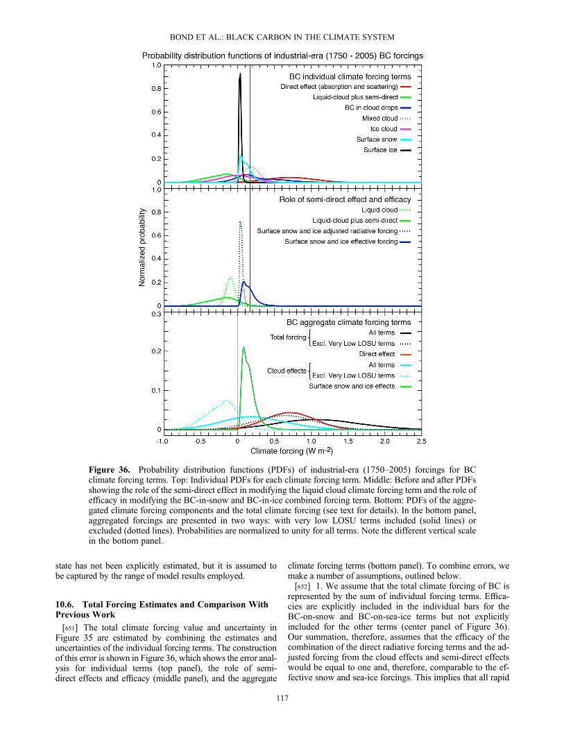
state has not been explicitly estimated, but it is assumed tobe captured by the range of model results employed.

10.6. Total Forcing Estimates and Comparison WithPrevious Work

[651] The total climate forcing value and uncertainty inFigure 35 are estimated by combining the estimates anduncertainties of the individual forcing terms. The constructionof this error is shown in Figure 36, which shows the error anal-ysis for individual terms (top panel), the role of semi-direct effects and efficacy (middle panel), and the aggregate

climate forcing terms (bottom panel). To combine errors, wemake a number of assumptions, outlined below.[652] 1. We assume that the total climate forcing of BC is

represented by the sum of individual forcing terms. Effica-cies are explicitly included in the individual bars for theBC-on-snow and BC-on-sea-ice terms but not explicitlyincluded for the other terms (center panel of Figure 36).Our summation, therefore, assumes that the efficacy of thecombination of the direct radiative forcing terms and the ad-justed forcing from the cloud effects and semi-direct effectswould be equal to one and, therefore, comparable to the ef-fective snow and sea-ice forcings. This implies that all rapid

Figure 36. Probability distribution functions (PDFs) of industrial-era (1750–2005) forcings for BCclimate forcing terms. Top: Individual PDFs for each climate forcing term. Middle: Before and after PDFsshowing the role of the semi-direct effect in modifying the liquid cloud climate forcing term and the role ofefficacy in modifying the BC-in-snow and BC-in-ice combined forcing term. Bottom: PDFs of the aggre-gated climate forcing components and the total climate forcing (see text for details). In the bottom panel,aggregated forcings are presented in two ways: with very low LOSU terms included (solid lines) orexcluded (dotted lines). Probabilities are normalized to unity for all terms. Note the different vertical scalein the bottom panel.


117

adjustment effects are accounted for and the resulting geo-graphical pattern of forcing would not be that different toan equivalent forcing from CO2 to make a material differ-ence to the efficacy.[653] 2. To account for covariance between errors in com-

ponent terms, we assume that emission uncertainties providethe only commonality between the uncertainties of eachterm. We also assume that emission uncertainty has a negli-gible effect on the cloud forcing uncertainty, as the large un-certainties are caused by differences in model processes.Emission uncertainty accounts for 50% of the relative uncer-tainty in direct forcing (section 6) and 32% of the relativeuncertainty in snow and sea-ice effective forcing (section8). This leads to a 0.16 correlation between the direct forcingand the snow and sea-ice terms, and a correlation of 0.1 be-tween the snow and sea-ice terms themselves.[654] 3. We assume that uncertainties, shown by whiskers

on the contributing forcings in Figure 35, represent a 90%(5%–95%) uncertainty range and construct the probabilitydistribution functions (PDFs) in Figure 36 accordingly.The uncertainty of the total climate forcing also assumesthat the distribution of probability within a given range isformed from combining either normal or log-normal distri-butions. Symmetric normal distributions are used for themixed-phase cloud, ice-cloud, and cloud-droplet inclusioneffects. Asymmetric normal distributions are used for thedirect effect and the liquid-cloud and semi-direct effects.Asymmetric log-normal distributions are used for the BC-in-snow and the BC-in-sea-ice effects.[655] Using these assumptions, a Monte Carlo model was

run one million times to produce the estimate of climateforcing. The random number sequences generated are usedto choose a point to sample in the forcing range, based ona fraction of the area under the probability distribution curve.The forcing value defined by the fractional area is then cho-sen to represent the forcing for that mechanism during thegiven iteration. Correlated errors are allowed for by makingthe appropriate fraction of the random numbers generatedmatch between the direct forcing and the snow and sea-iceterms. To generate correlated errors, a subset of the samerandom number sequences is used for the correlated forcingterms. For example, 10% of the random number sequence forsnow and sea ice identically matches, giving their million-point forcing series a correlation of 0.1. The PDFs for thedifferent climate-forcing terms are shown in Figure 36. Usingthis methodology, the individual forcing terms are combinedto estimate the overall error shown in the total climate-forcingerror bar in Figure 35 and the PDF (black line) shown in thebottom panel of Figure 36. The bottom panel also showssubgroups of terms from which the least certain terms areexcluded in order to highlight the role of uncertainty in the bestestimates. In this assessment, we include all these uncertainterms in our best estimate of the total climate forcing of BC,acknowledging that they add large uncertainty.[656] Our assessment is that the overall climate forcing for

BC is more positive and more uncertain than that from thedirect radiative forcing alone (i.e., comparing red and solidblack PDFs in the bottom panel of Figure 36). Introducingadditional cloud forcing terms increase both the medianand spread of climate forcing. Principal results from thisuncertainty analysis combined with those in sections 6, 7,and 8 are as follows:

[657] 1. Radiative forcing from the BC direct effect is +0.71Wm�2, with a 90% uncertainty range of +0.08 to +1.27Wm�2.[658] 2. The estimate of all-source (i.e., 1750 background

plus industrial-era) direct radiative forcing of +0.88 W m�2

with a range of +0.17 to +1.48 W m�2 is similar to the+0.9 W m�2 given by Ramanathan and Carmichael [2008].[659] 3. The globally averaged, industrial-era, total climate

forcing from BC is +1.1 W m�2 with a 90% uncertaintyrange of +0.17 to +2.1 W m�2. This distribution gives a2% chance that the total effect of BC in isolation is actuallya cooling effect (negative climate forcing), rather than awarming. It is, therefore, extremely likely (greater than95% chance) that BC emissions acting alone lead to a pres-ent-day overall positive forcing and climate warming. Thisbest estimate of black carbon forcing ranks it as the secondmost important individual climate-warming agent after carbondioxide when both direct and indirect effects are included. Forcomparison, the radiative forcings including indirect effectsfrom emissions of the two most significant long-lived green-house gases, carbon dioxide (CO2) and methane (CH4), in2005 were +1.56 and +0.86 W m�2, respectively [IPCC,2007, Table 2.13]. The Monte Carlo procedure produces acentral estimate that is slightly different than a simple sum ofthe forcing terms.[660] 4. Considering only radiative forcings ignores the

changes imposed by rapid adjustments. For BC, all effectsneed to be considered to get a true representation of the climateforcing. These additional effects are demonstrated in the mid-dle panel of Figure 36, where accounting for many semi-directeffects leads to a more-negative liquid-cloud climate forcing,and accounting for the higher efficacies of BC-in-snow andBC-in-ice forcings leads to a more positive forcing.[661] 5. While there are large uncertainties in the role of

BC effects on clouds, the best estimate of their combinednet effect, including the semi-direct effect and cloud drop-let inclusions, is +0.23 W m�2 with a 90% uncertaintyrange of �0.47 to +1.0 W m�2. This value is also slightlydifferent than a simple sum of the terms. Therefore,studies that exclude all these cloud effects may have a neg-ative bias in forcing. Many model studies agree that semi-direct and liquid-cloud estimates are negative. However,only a few studies have examined how BC affects cloud ab-sorption and subsequent burnoff, as well as mixed-phaseclouds, and these poorly understood effects increase the to-tal positive forcing from +0.65 to +1.1 W m�2. Only onegroup has estimated the BC forcing effect for ice clouds,indicating that the magnitude could be large but the signis unknown.[662] 6. These cloud adjustments also significantly increase

the uncertainty in their respective climate forcings and greatlyincrease the overall large uncertainty in the total climateforcing.[663] 7. The combined BC on snow and BC on sea-ice ef-

fective forcing over the industrial era is estimated to be+0.13 W m�2 with a 90% uncertainty range of +0.04 to+0.33 W m�2. The effects of BC on snow and ice isunequivocally a net positive forcing, so any study of BC cli-mate forcing that does not include those effects is biased to-wards a smaller warming effect.[664] 8. Uncertainties in cloud forcing are of a different

character than uncertainties in direct or snow forcing, andare determined using model diversity rather than the more


118

rigorous method of identifying governing factors and propa-gating uncertainties in those factors.[665] The IPCC Fourth Assessment Report only consid-

ered radiative forcing of BC and did not consider its totalclimate forcing [Forster et al., 2007]. IPCC estimated a1750-to-2005 fossil fuel BC direct radiative forcing of+0.2� 0.15 W m�2, somewhat lower than our direct-forcingestimate of BC from fossil fuel of only +0.29 W m�2. IPCCdid not explicitly evaluate the direct forcing of other sourcesof BC, including biofuel combustion. Forster et al. [2007,Table 2.13] lists the direct radiative forcing values for“anthropogenic” BC as obtained from published studiesand AeroCom models, which together yield an average of+0.34 W m�2 (+0.09 to +0.59 W m�2 range). This value issmaller than the best estimate found here of +0.71 W m�2

(+0.08 to +1.27 W m�2 range). The evolution of forcing esti-mates between the IPCC tabulation and the present assessmentis explained as follows:[666] 1. Some of the studies in the IPCC tabulation used rel-

atively larger emission estimates. Forcing adjusted to a com-mon bottom-up emission inventory would be lower, asreflected in the reported AeroCom average of +0.27 W m�2.[667] 2. AAOD and, hence, forcing increase by about 50%

when the change in MACBC due to internal mixing is con-sidered. Applying this correction to the IPCC value wouldgive +0.41 W m�2.[668] 3. The apparent BC burden in the atmosphere is

greater than that in the models. The adjustment required tomatch industrial-era observations, even after the considerationof increased MACBC, is an additional factor of 1.9, giving+0.77Wm�2. This value is similar to the +0.84 average in Ta-ble 15 but not identical because it is not based on the samemodels.[669] 4. The estimated model-average forcing was de-

creased by 15% to account for the fact that models placeBC too high in the atmosphere. This adjustment to the IPCCestimate gives a radiative forcing of +0.65 W m�2.[670] 5. The remaining difference between the scaled

IPCC value of +0.65 W m�2 and our direct-forcing estimateof +0.71 comes from the inclusion of model results pub-lished since the last IPCC report.[671] 6. The higher value of forcing presented here is

supported by observations of increased MACBC andunderestimated atmospheric absorption. Therefore, our esti-mate is more robust than the purely model-based estimate inIPCC.[672] Caution is required when considering total, global-

average forcing as the sole metric for expressing the impactof BC emissions on climate change. The climate forcing ofBC, and all aerosols, is much more regionally variable thanfor long-lived GHGs, and this metric does not relate toexpected precipitation changes (section 9). These factorsmay affect the consideration of how BC would be includedin climate mitigation strategies (section 13).[673] The equilibrium surface temperature change associ-

ated with the BC climate forcing can be estimated by multiply-ing the forcing values with estimates of climate sensitivity.IPCC [2007] estimated a 5 to 95% likely range for equilibriumwarming from a 2�CO2 change of 2.0 to 4.5K. Usinga 2�CO2 RF of 3.7 W m�2 [Forster et al., 2007] gives aclimate sensitivity range between 0.54 and 1.22K W�1 m2.Combining errors of sensitivity in quadrature with the

industrial-era total climate-forcing range for BC leads toan equilibrium warming for global mean temperature inthe range of 0.1 to 2.0K. This temperature change has notbeen realized in the present day as the Earth systemtakes more than a century to reach equilibrium, and manyco-emitted species counter the warming of BC. For compar-ison, the estimated equilibrium warming from the combinedeffects of all short-lived species from BC-rich sources isbetween �1.5 and 1.4K.

11. Net Climate Forcing by Black-Carbon-RichSource Categories


[674] 1. The net climate forcing of emissions from BC-richsource categories or individual source types depends on the ef-fects of co-emitted species, such as organic carbon, sulfate,and gaseous constituents in addition to all effects of BC.[675] 2. We use previously developed forcing-per-emission

values to provide a comprehensive estimate of forcing fromBC-rich source emissions. As for BC, large uncertainties areintroduced in estimating cloud effects of co-emitted aerosolsand aerosol precursors.[676] 3. Attribution of direct forcing and cryosphere changes

to emitting sources is relatively straightforward. For these ef-fects, net forcing is positive for all BC-rich source categories.[677] 4. Attribution of forcing by cloud changes and nitrate

formation to emitting sources is uncertain because effects oncloud droplets are nonlinear and complex. When this indi-rect forcing contribution is included, using a simple linearproportionality to emission rate, net climate forcing becomesneutral to negative for all source categories except diesel en-gines and, with greater uncertainty, some residential solidfuel.[678] 5. Source categories are often heterogeneous. Indi-

vidual sources within each category have different profilesof chemical emission components and may have relativelymore positive or more negative forcing than the category av-erage might indicate.[679] 6. Our best estimate of the net climate forcing in the

first year after emission from BC-rich sources is �0.06 Wm�2 with 90% uncertainty bounds of (�1.45, +1.29) Wm�2. This net forcing would be +0.22 with a range of(�0.50, +1.08 W m�2) if open burning emissions, which emithigh levels of organic matter, were excluded. These values in-clude all effects lasting less than one year, including thosefrom aerosols and short-lived gases.[680] 7. For most of these source categories, short-lived

species have substantial forcing in the first year after emis-sion, and this forcing is significant in comparison with forc-ing by emissions of all species over longer time scales.When climate forcing by all co-emitted species isintegrated over 100 years, the magnitude of integrated forc-ing by short-lived species from each source category rangesfrom 5 to 75% of forcing by longer-lived species, includingCH4 and CO2. The sign of short-lived species can be eitherpositive, enhancing GHG warming, or negative.[681] 8. Integrating net forcing by aerosols, O3, CH4, and

CO2 masks complex spatial patterns in forcing that differover time. Climate forcing through effects on the CH4 sys-tem tends to offset some of the effects of short-lived species.For diesel engines, longer-term negative forcing via NOx


119

offsets short-lived positive forcing; for biofuel sources, lon-ger-term positive forcing via organic gases offsets short-lived negative forcing that is largely attributable to cloudeffects.[682] 9. Reduction of aerosol concentrations by mitigating

BC-rich source categories would be accompanied by smallto no changes in short-term climate forcing. In contrast, miti-gation of other aerosol sources would increase positive short-term climate forcing. All aerosol that is emitted or formed inthe lower atmosphere adversely affects public health, so miti-gation of most BC-rich source categories offers a method ofreducing health impacts with lower risk of adverse effects onclimate.

11.2. Introduction

[683] Until this point, we have focused entirely on how BCaffects radiative and climate forcing. However, BC is neveremitted in isolation. Changes in source magnitudes affectall emitted species, whether those changes are deliberatelychosen for mitigation, or occur without intention. Estimatesof climate changes caused by BC forcing alone weresummarized in the previous section, but those values donot reflect the net climate effect of altering sources whoseemissions contain high concentrations of BC (i.e., BC-richsources).[684] In this section, we estimate the net climate forcing of

emissions from BC-rich sources, considering the major emit-ted species. Some species that make minor contributions tomass have been ignored. In order to provide the net climateforcing by these sources, estimates of forcing by otherspecies that are co-emitted with BC are also required.As in the presentation for BC, we require considerationof all effects. However, this assessment does not includerecommendations for climate forcing by other speciesand we rely mainly on previous published summariesfor these values. Therefore, the resulting quantificationshould be viewed cautiously. Although accounting forforcing by co-emitted species is fraught with uncertainty,ignoring these effects may convey a mistaken impressionabout the magnitude or even the sign of net climate forc-ing by BC-rich sources.[685] We first discuss the approach to estimating net forc-

ing values for a particular source activity. In section 11.3, wedescribe methods to estimate forcing-per-emission valuesfor each co-emitted species. Then, in section 11.4, we esti-mate the net climate effect of the BC-rich source categoriessummarized in section 4. These categories are aggregatesof many individual source types, such as certain types of die-sel engines or cooking stoves, whose emission componentprofile may differ from that of the aggregate category.Estimates of forcing for a few of these individual sources aresummarized in section 11.5. In these first sections, we presentonly forcing by short-lived species (i.e., those with lifetimesless than one year). This near-immediate forcing is attributableprimarily to aerosols, their precursors, and emitted O3 precur-sors. In section 11.6, this forcing in the very short term iscompared with GHG forcing on decadal scales.

11.3. Approach to Estimating Forcing From BC-RichSource Categories

[686] Determining the net change in climate forcing perchange in emission or per change in activity is the goal of

this section. This quantitative measure may be thought ofas the slope of a curve representing forcing versus activity,at present-day conditions. A fully comprehensive measurewould aggregate all effects caused by all emitted pollutantsfrom a particular source. Previous work on this topic hasestimated the influence of a particular source either by sum-marizing direct forcing by all pollutants [Fuglestvedt et al.,2010], or by examining the influence of all pollutants fromsource sectors with a model that represents multiple climatemechanisms [Jacobson, 2004a; Unger et al. 2010].[687] Missing in these progressive studies are systematic

methods for incorporating scientific uncertainties, for incor-porating findings from other studies that may differ, or foraltering findings as knowledge advances. Here, we presentthe foundations of such a framework. Its essential elementsare expert recommendations of the following for eachchemical species emitted from a source:[688] 1. Emission factors for a source activity;[689] 2. Central values and uncertainties for the radiative

forcings, obtained for a defined emission rate;[690] 3. Central values and uncertainties for rapid adjust-

ments, fast enough to be considered as part of a climate forc-ing, normalized to a defined emission rate.[691] We begin with a source activity that emits I pollutants.

Each pollutant may have J effects that are best expressed asradiative forcing values, and K effects that are expressed asrapid adjustments. To a first approximation, total climateforcing CF (in W m�2) caused by an emission category (suchas diesel), summed across all species emitted, is

CF ¼XIi¼1

EFi

XJj¼1

rforci;j þXKk¼1

frespi;k

!(11.1)

where FC is fuel consumption by the activity in kg s�1, and EFiis the emission factor of pollutant i (kg pollutant (kg fuel)�1).The bracket contains forcing terms: rforci,j is the change in radi-ative forcing for effect j and species i per emission rate of spe-cies i ((W m�2) (kg s�1)�1), and frespi,k is the rapidadjustment for effect k and species i given in the same units.Each effect must be carefully distributed among the summa-tions to avoid double counting. Further, this calculationassumes that forcings are additive. Although slight variants ofthe units given here are used in this section, the principleremains the same.[692] Ideally the value rforci,j would be determined as:

rforci;j ¼ @fj@ei

jPD

(11.2)

[693] where fj is the forcing via mechanism j, ei isthe emission of species i, the notation PD indicatespresent day, and the partial derivative indicates that noother effects are operating and all other species are held con-stant. The same is true for the rapid adjustments. In practice,models usually provide total forcing or anthropogenic forc-ing, not partial derivatives. The assumption of linearity withrespect to emission rate is adequate for many of the effectsdiscussed here, but it breaks down for cloud microphysicalforcings, as noted in the last section. Incremental changesin emissions are more realistic than removal or addition ofentire source categories or pollutant categories. Model stud-ies examining smaller emission changes may clarify whether


120

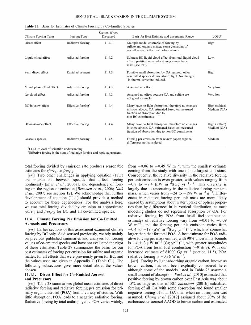
total forcing divided by emission rate produces reasonableestimates for rforci,j or fresp,j.[694] Two other challenges in applying equation (11.1)

are interactions between species that affect forcingnonlinearly [Stier et al., 2006a], and dependence of forc-ing on the region of emission [Berntsen et al., 2006; Naiket al., 2007; see section 12]. We acknowledge that furtherdevelopment of equation (11.1) should provide a methodto account for these dependences. For the analysis here,we use total forcing divided by emission to approximaterforci,j and frespi,j for BC and all co-emitted species.

11.4. Climate Forcing Per Emission for Co-EmittedAerosols and Precursors

[695] Earlier sections of this assessment examined climateforcing by BC only. As discussed previously, we rely mainlyon previous published summaries and analyses for forcingvalues of co-emitted species and have not evaluated the rigorof these estimates. Table 27 summarizes the basis for ourbest estimates of forcing per emission for sulfate and organicmatter, for all effects that were previously given for BC, andthe values used are given in Appendix C (Table C1). Thefollowing subsections give more detail about the valueschosen.11.4.1. Direct Effect for Co-Emitted Aerosoland Precursors[696] Table 28 summarizes global mean estimates of direct

radiative forcing and radiative forcing per emission for pri-mary organic aerosol (POA) from a variety of studies. Withlittle absorption, POA leads to a negative radiative forcing.Radiative forcing by total anthropogenic POA varies widely,

from �0.06 to �0.49 W m�2, with the smallest estimatecoming from the study with one of the largest emissions.Consequently, the relative diversity in the radiative forcingper unit emission is even greater, with values ranging from�0.8 to �7.4 (mW m�2)(Gg yr�1)�1. This diversity islargely due to uncertainty in the radiative forcing per unitmass, which varies from �24 to �198 W m�2 g�1. Differ-ences in radiative forcing per unit mass are more likelycaused by assumptions about water uptake or optical proper-ties than by differences in its vertical distribution, as mostmodeling studies do not represent absorption by OA. Forradiative forcing by POA from fossil fuel combustion,estimates of radiative forcing vary from �0.01 to �0.09W m�2, and the forcing per unit emission varies from�0.4 to �19 (mW m�2)(Gg yr�1)�1, which is somewhatlarger than that for total POA. A best estimate for POA radi-ative forcing per mass emitted with 90% uncertainty boundsis �4 � 3 mW m�2 (Gg yr�1)�1, with greater magnitudesfor POA from fossil fuel combustion (�9 � 9). With ourincreased estimate of 81000 Gg yr�1 (section 11.5), POAradiative forcing is �0.36 W m�2.[697] Forcing by light-absorbing organic carbon, known as

brown carbon, has not been explicitly considered here,although some of the models listed in Table 28 assume asmall amount of absorption. Park et al. [2010] estimated thatpositive forcing by brown carbon over East Asia was about15% as large as that of BC. Jacobson [2001b] calculatedforcing of all OA with some absorption and found smallernegative forcing of total OA than when no absorption wasassumed. Chung et al. [2012] assigned about 20% of thecarbonaceous aerosol AAOD to brown carbon and estimated

Table 27. Basis for Estimates of Climate Forcing by Co-Emitted Species

Climate Forcing Term Forcing TypeSection WhereDiscussed Basis for Best Estimate and uncertainty Range LOSUa

Direct effect Radiative forcing 11.4.1 Multiple-model ensemble of forcing bysulfate and organic matter; some constraint ofoverall aerosol effect with observations

High

Liquid cloud effect Adjusted forcing 11.4.2 Subtract BC liquid-cloud effect from total liquid-cloudeffect; partition remainder among atmosphericmass (see text)

Low

Semi direct effect Rapid adjustment 11.4.3 Possible small absorption by OA ignored; otherco-emitted species do not absorb light. No changesin thermal structure induced.

High

Mixed phase cloud effect Adjusted forcing 11.4.3 Assumed no effect Very low

Ice cloud effect Adjusted forcing 11.4.3 Assumed no effect because OA and sulfate arenot good ice nuclei

Very low

BC-in-snow effect Effective forcingb 11.4.4 Many have no light absorption; therefore no changesin snow albedo. OA estimated based on measuredfraction of absorption due tonon-BC constituents.

High (sulfate)Medium (OA)

BC-in-sea-ice effect Effective forcing 11.4.4 Many have no light absorption; therefore no changesin snow albedo. OA estimated based on measuredfraction of absorption due to non-BC constituents.

High (sulfate)Medium (OA)

Gaseous species Radiative forcing 11.4.5 Forcing per emission from review paper; regionaldifferences not considered

Medium

aLOSU= level of scientific understanding.bEffective forcing is the sum of radiative forcing and rapid adjustment.


121

that it had zero forcing rather than negative forcing. Afraction of our BC forcing estimate may in fact be attribut-able to brown carbon. If brown carbon contributes toatmospheric absorption, its contribution should be removedfrom the estimate of BC AAOD that is based on observa-tions. The net forcing of brown carbon would be a combina-tion of forcing by absorbing aerosol (presently subsumed inBC) and aerosol that is more highly scattering (presentlysubsumed in OA), and brown-carbon direct forcing wouldbe about zero. Thus, although we have not explicitly isolatedthe contribution of brown carbon, the total forcing by BCand OA together would remain about the same.[698] The most recent IPCC report provides a best estimate

of �0.4 � 0.2 W m�2 for direct radiative forcing by anthro-pogenic sulfate [Forster et al., 2007]. Assuming theAeroCom estimate of 109,000 Gg S yr�1 [Dentener et al.,2006], this translates to a range of �3.7 � 1.8 (mW m�2)(Gg yr�1)�1 for radiative forcing per mass of S emitted.Emissions used here are 96000 Gg S yr�1 from the GAINSdatabase, giving �0.35 W m�2 direct forcing.11.4.2. Liquid Cloud Effect for Co-Emitted Aerosoland Precursors[699] The effect of co-emitted aerosol on liquid clouds has

large uncertainties, both because estimates of the totalliquid-cloud radiative forcing of anthropogenic aerosol varywidely, and because studies that isolate the contributions ofindividual pollutants or sources are scarce. (Exceptions areJacobson [2002] and Bauer et al. [2010].) We adopt apreliminary approach to estimating changes in liquid-cloudforcing due to co-emitted species, which we describe firstbefore listing several cautions.[700] Our preliminary estimate of cloud climate forcing

assumes that: (1) the liquid-cloud effect using AeroComemissions has a central value of �0.9 W m�2 for the albedoeffect and a range of �1.4 to �0.3 W m�2, as summarizedby Isaksen et al. [2009]; (2) the lifetime effect is negligible,as inferred from comparisons between GCMs and cloud-resolving models [Wang et al., 2012]; (3) the liquid-cloudchange in the studies contributing to the estimate is attribut-able to submicron species that are considered anthropogenic:BC, organic matter, and sulfate; (4) except for BC, the cloudeffect may be apportioned among individual species bymass; and (5) the values of forcing per mass so determinedcan be used to scale to the new estimates of emission. Thelatter assumption is approximately justified if particle sizeis the dominant factor determining the number of CCN,because organic matter and sulfate have similar size distribu-tions. Individual studies to determine liquid-cloud forcingmay have used different emission rates; in particular, studiesprior to the mid-2000s tended to use much higher OMemissions. However, Quaas et al. [2009] gave direct plusindirect forcing values of �1.25 W m�2 for 10 models evenwhen they used the lower AeroCom emissions.[701] Details of the liquid-cloud estimate are given in

Appendix C (Tables C2 and C3). Indirect forcing usingAeroCom emissions is divided as �0.58 and �0.27 W m�2

for sulfate and organic matter, respectively. Sulfate is scaledto the total GAINS emission estimate and organic matter isscaled according to the regional BC scaling in Figure 20.Liquid-cloud indirect effect attributable to 96 Tg yr�1 of SO2

emissions is estimated as �0.51 W m�2, with an uncertaintyrange of �0.21 to �0.76 W m�2. Liquid-cloud forcingT

able

28.Model

ResultsUsedto

DetermineDirectForcing

perEmission

forOrganic

Mattera

Model

Reference

Emission

(TgCyr

�1)

Load(m

gm

�2)

Radiativ

eForcing

(Wm

�2)

NRFmass(W

g�1)

RFperEmission

(Wm

�2)(Tgyr

�1)�

1

Total

POA

FFPOA

Total

POA

Total

POA

FFPOA

Total

POA

Total

POA

FFPOA

AeroC

ommodels

GISS

Schulzet

al.[2006]

32.5

3.2

1.22

�0.14

�0.03

�115

�0.0043

�0.009

LOA

Schulzet

al.[2006]

32.5

3.2

1.41

�0.16

�0.04

�113

�0.0049

�0.012

LSCE

Schulzet

al.[2006]

32.5

3.2

1.50

�0.17

�0.04

�113

�0.0052

�0.012

MPI-HAM

Schulzet

al.[2006]

32.5

3.2

1.0

�0.10

�0.03

�100

�0.0031

�0.009

SPRIN

TARS

Schulzet

al.[2006]

32.5

3.2

1.84

�0.10

�0.01

�54

�0.0031

�0.003

UMI

Schulzet

al.[2006]

32.5

3.2

1.16

�0.23

�0.06

�198

�0.0071

�0.019

UIO

-CTM

Schulzet

al.[2006]

32.5

3.2

1.12

�0.16

�0.04

�143

�0.0049

�0.012

UIO

-GCM

Schulzet

al.[2006]

32.5

3.2

0.88

�0.06

�0.02

�68

�0.0018

�0.006

Other

models

CAM3

Bondet

al.[2011]

30—

—�0

.12

——

�0.0040

—CAM3ECA

Kim

etal.[2008]

54.4

—1.49

�0.19

—�1

28�0

.0035

—GATORG

Jacobson

[2001b]

7328

2.55

�0.06

�0.01

�24

�0.0008

�0.0004

LOA

Reddy

etal.,[2005a,2005b]

907.0

2.33

�0.25

�0.02

�107

�0.0028

�0.003

MOZART

Minget

al.[2005]

4610.1

2.33

�0.34

�0.09

�146

�0.0074

�0.009

SPRIN

TARS

Takem

uraet

al.[2005]

8814.7

—�0

.49

——

�0.0056

—

a Globalmeanem

issionsof

anthropogenicprim

aryorganicaerosol(POA)andPOA

from

fossilfuelcombustion(FFPOA),meancolumnburden

(load)

ofPOA,m

eanradiativeforcingby

totalandFFPOA,m

ean

radiativeforcingnorm

alized

bymeanburden

(NRFmass),andradiativeforcingnorm

alized

byem

issions.For

comparisonto

emission

values

intheremainder

ofthedocument,1Tg=1000

Gg.


122

attributable to 81 Tg yr�1 of organic matter is estimated as�0.74 W m�2 with an uncertainty range of �1.09 to�0.30 W m�2. The apportionment by mass may overestimatenegative forcing by organic matter, as its lower solubility hasnot been considered in the apportionment. However, a rela-tionship with aerosol optical depth, as suggested by Quaaset al. [2009], would yield the same apportionment betweensulfate and OA.[702] Our treatment of liquid-cloud effects deserves

several caveats. We caution that the liquid-cloud estimatefor SO2 and POA has not undergone a thorough examinationas have the effects of BC. We have chosen to present a morerealistic but less rigorous picture for net forcing by sourcesthat are BC-rich, rather than a physically unrealistic depic-tion that evaluates BC alone. Modeling studies rarely exam-ine the validity of apportioning total liquid-cloud effectsamong individual species, although Chuang et al. [2002]showed that cloud forcing per burden differed by less than15% for sulfate only, carbonaceous aerosol only, and thecombination.[703] The relationship between cloud forcing, CCN, and

emissions is not expected to be linear. Cloud forcing is moresensitive to increased particle concentration in a cleaneratmosphere, as demonstrated for global averages by Boucherand Pham [2002]. This is consistent with inferences of lowindirect effect over land [Ruckstuhl et al., 2010]. Therefore,our linear apportionment could overestimate the impactof the small fraction of total particle mass attributable toBC-rich sources.[704] Studies disagree on the importance of primary parti-

cles, and the relationship between cloud forcing and theemission of primary particles such as BC or POA may noteven be monotonic. One study indicates that primary parti-cles play a larger role in cloud formation than other particles[Adams and Seinfeld, 2003], while others find that primaryemissions suppress nucleation [Bauer et al., 2010], andtherefore have a much lower influence on CCN than wouldbe expected in the absence of gas-particle interactions[Merikanto et al., 2009].[705] The discussion above indicates that the linear

apportionment used here is a zero-order estimate. Yet, presentunderstanding is insufficient to support a different appor-tionment. Although there is some evidence that forcing-per-emission values may be overestimated, models thataccount for microphysical interactions [Bauer et al., 2010;Koch et al., 2011a] have indicated greater forcing-per-emissionof POA via liquid-cloud changes than our central value.The uncertainties given here reflect only the uncertainty inthe magnitude of the indirect effect, not the uncertainty inapportionment, or regional differences in cloud behavior.11.4.3. Other Cloud Effects for Co-Emitted Aerosoland Precursors[706] Other cloud effects (i.e., mixed-phase, ice-cloud, and

semi-direct effects) considered for BC are assumed negligi-ble for sulfate and organic matter. These two species mayinfluence water condensation and ice nucleation activity ifthey are emitted with BC (sections 3.9 and 7.5). This is par-ticularly relevant for cold ice clouds, where BC particles donot become water droplets prior to ice formation. In thiscase, it is not possible to separate or scale cloud effects fromthe amount of co-emitted species. Two GCM studies [Hooseet al., 2008; Storelvmo et al., 2008] suggest that sulfate

coating decreases the ability of mineral dust to act as IN.This increases the lifetime of supercooled water clouds,producing negative forcing. These effects have not yet beenquantified and are not included here.[707] In current understanding, aerosols with minimal light

absorption have little effect on semi-direct forcing. All suchchanges are caused by light absorption that heats the atmo-sphere at various vertical locations (Figure 24). We also donot include the effects of other absorbing material withincloud droplets, although absorbing OA may also contributeto enhanced cloud-droplet absorption [Jacobson, 2012]. Asan approximation, we have captured the effect of absorbingaerosol by attributing all non-dust AAOD to BC and calcu-lating all effects for that AAOD.11.4.4. Snow Albedo Forcing for Co-Emitted Aerosol[708] Doherty et al. [2010] found that the light-absorbing

aerosol in Arctic snow and sea ice had a strong wavelengthdependence, and inferred from this the amount of lightabsorption due to BC versus other species, specificallybrown carbon, mineral dust and soil dust. They reported that40% of the spectrally weighted light absorption in snow andsea ice is due to these non-BC constituents. Because ourestimate of snow albedo forcing was scaled to observationsof BC, not of absorbing aerosol, total forcing must beincreased to account for additional absorbing material. Onlya small fraction of this absorption is due to mineral and soildust, so we estimate global snow and sea-ice forcing byorganic matter from combustion as 20% that of BC. We thenscale this value to emissions of organic matter to produce aneffective forcing per emission of 0.9 mW m�2 (Gg yr�1)�1

with a range of 0 to 3.0, assuming an efficacy with a centralvalue of 3 and an upper bound of 4. POA from solid-fuel com-bustion is known to absorb light, while other organic matter isnot. Therefore, this forcing was applied only to POA emittedfrom solid fuel: biofuel, coal, and open biomass burning.11.4.5. Forcing by Co-Emitted Gaseous Species[709] Short-lived, co-emitted gaseous species considered

here include carbon monoxide (CO), volatile organic com-pounds (VOCs), and NOx. These species produce indirectforcing by interacting with tropospheric O3 and CH4 and,for NOx, by producing nitrate. Fuglestvedt et al. [2010] sum-marized studies on radiative forcing by these compounds forthe development of metrics. They did not provide recom-mendations for central values of forcing per emission, buta later study [Uherek et al., 2010] used their summary toprovide GWP values. We inferred a best estimate of forcingper emission using studies cited by Fuglestvedt et al. [2010],as shown in Appendix C (Table C4). For each species, forc-ing is separated by mechanism, as suggested by Shindell etal. [2005]. All species increase O3, representing a positiveforcing that occurs within the first year. NOx increases ni-trate aerosol, giving a negative first-year forcing. These spe-cies also alter the lifetime of CH4, causing forcing that lasts afew decades. CO and VOCs cause a positive forcing, whileNOx causes a negative forcing.[710] Studies cited in Fuglestvedt et al. [2010] gave forc-

ing values for the effects of NOx emissions on CH4 andtropospheric O3 abundances but not for nitrate aerosolresulting from NOx emission. We estimated a value of forcingper emission by nitrate by assuming that the nitrate forcingsummarized by Forster et al. [2007] had the same emissionbase as that for O3 from NOx. This method is legitimate for


123

short-lived species, such as nitrate and O3 caused by emissionsof NOx or volatile organic compounds. (Present-day forcingvalues for long-lived species result from all historical emis-sions that remain in the atmosphere, and cannot be used toestimate forcing per emission.) While Forster et al. [2007]attributed all nitrate forcing to NOx emissions, Unger et al.[2010] reported that sectors with substantial ammoniaemissions also affect nitrate forcing. The nonlinearity ofammonium, sulfate, nitrate, and NOx chemistry means thatchanges in nitrate forcing are difficult to attribute to particularsectors. We assign only 44% of the total nitrate forcing to NOx

emissions, based on the ratio of NOx-related to total nitrateforcing reported by Unger et al. [2010].11.4.6. Climate Forcing by Secondary Organic Aerosol[711] Estimating the climate impact of sources using POA

alone ignores the complex evolution of organic aerosolthroughout the atmosphere. Emitted precursors lead to for-mation of substantial quantities of SOA [de Gouw andJimenez, 2009]. Oxygenated organic aerosol, thought to beequivalent to SOA, is found wherever measurements aremade [Zhang et al., 2007]. SOA yields from diesel enginesand wood stoves were estimated to be small in comparisonto POA emissions [Chan et al., 2009]. However, observedSOA appears to be much more prevalent than could beexplained by models that treat identified SOA precursormolecules [Robinson et al., 2007]. For that reason, mecha-nisms that account for SOA production have been proposed,using the fraction of emitted vapors with low volatility asinputs [Donahue et al., 2006].[712] SOA associated with individual sources has not been

resolved in climate models. Direct forcing is often providedfor POA alone [Schulz et al., 2006], and models of cloudforcing have usually not distinguished POA versus SOAburdens. Simulations by O’Donnell et al. [2011] gave adirect effect due to SOA of �0.29 W m�2 and an indirecteffect of +0.20 W m�2. In this model, which did not includethe volatility representation of SOA formation, 90% of theSOA burden came from biogenic sources.[713] POA :BC ratios may underestimate the total atmo-

spheric OA attributable to each source. Nevertheless, in thisanalysis, we neglect direct and indirect forcing by SOA. Thesingle estimate of net SOA forcing given above is small, andthe chain that relates precursor emissions to concentrationsand global forcing is presently limited. We acknowledge,however, that this omission could be a source of bias.11.4.7. Forcing in Clear and Cloudy Skies[714] Modeled radiative forcing has been compared with

clear-sky and cloudy-sky radiative fluxes observed fromspace [Quaas et al., 2009; Lohmann et al., 2010]. For thatreason, we summarize the clear- and cloudy-sky forcingshere. We assume that 30% of BC direct forcing takes placein clear skies [Zarzycki and Bond, 2010]. The remainderwould be observed in cloudy skies. Clear-sky forcingincludes 30% of BC direct forcing (+0.21 W m�2), all OAand sulfate direct forcing, (�0.36 and�0.35 W m�2, respec-tively), and nitrate direct forcing (�0.16 W m�2) for a totalof �0.66 W m�2. Cloudy-sky forcing over liquid cloudsincludes BC direct forcing in cloudy skies (+0.50 W m�2),BC liquid-cloud forcing including semi-direct effects(�0.20 W m�2), the cloud absorption effect(+0.20 W m�2), and liquid-cloud forcing by OA and sulfate(�0.74 and �0.51 W m�2, respectively) for a total of

�0.76 W m�2. It is not clear whether the mixed-phase cloudforcing of +0.18 W m�2 would be observed in the analysisof radiances that primarily focus on liquid clouds. Quaaset al. [2009] scaled model estimates according to relation-ships determined from satellite observations to obtainforcing estimates of �0.38 W m�2 for clear-sky and�0.70 W m�2 for cloudy-sky fluxes. The total forcing esti-mated here is more negative for clear skies and similar forcloudy skies.

11.5. Net Climate Forcing by BC-Rich SourceCategories

[715] Using the values developed in the previous section, totalclimate forcing by BC-rich source categories can be estimated.Forcing per emission for each effect in W m�2 (Gg yr�1)�1

is multiplied by total emissions, yielding units of W m�2.Forcings by each species emitted within each category are thensummed to provide the total industrial-era forcing representingthe net forcing from each category. Annual emissions of BC,POA, SO2, CO, non-methane volatile organic compounds(NMVOCs), and NOx from each source category were sum-marized from the GAINS database for the year 2000 for en-ergy-related emissions. Open burning estimates come fromthe RETRO database. Emissions were adjusted to reflect theobservationally based scale factors given in section 6.7, so thatenergy-related emissions were scaled by factors of 1.1 to 2.5,depending on the category, and open-burning estimates wereincreased by a factor of about 1.5. Emission rates used aregiven in Appendix C (Table C5). For energy-related burning,we have assumed that the most uncertain factor is levels ofactivity with relatively high emission rates, and have adjustedthose emissions associated with incomplete combustion(BC, POA, CO, NMVOC) with the scale factors used forBC. For open biomass burning, we assume that the cause ofthe uncertainty could be the low bias in emission factors ofparticulate matter (section 4.7.2.3) and adjust BC and OAemissions. Only the effects of POA are included here; someof the gaseous NMVOCs from these sources could formSOA after emission, adding to aerosol-driven forcing mecha-nisms. This possibility is discussed in section 11.4.6.[716] Figure 37 shows forcing by short-lived emissions in

the BC-rich source categories summarized in Figure 8.These categories comprise 99% of the BC emissions, andthe climate forcing includes all aerosol direct, indirect, andsnow effects. We also include forcing changes caused bythe interaction of CO, VOCs and NOx with troposphericO3. These effects capture most of the forcing that occurs inthe first year after emission.[717] The forcings shown in Figure 37 result from the

same treatment as applied in Forster et al. [2007]: that is,the values are those that would be observed if year-2000emission rates continued indefinitely. It differs from IPCCfigures because forcing is grouped by source category in-stead of by species, and because it gives total climate forcingvalues instead of direct forcing. The species chosen for thisfigure exert their forcing entirely within the first year afteremission. Other emitted species or effects that act overlonger time scales are discussed in section 11.7. We havenot included effective forcing due to vegetation changes[Collins et al., 2010].[718] The top bar in Figure 37 shows the forcing compo-

nents that can be attributed to emissions with high


124

confidence: direct forcing by aerosol and gases, effectivecryosphere forcing, and cloud response to aerosol absorp-tion. Attribution of liquid-cloud forcing to individual aerosolspecies or to particular sources is not well developed. Wetherefore segregate these forcing terms in the second (middle)bar, for which we have less confidence in attribution.The combined liquid-cloud effect, including the albedo andsemi-direct effect, is separated from cloud effects that havelarger uncertainties and were derived in fewer studies: the cloud

absorption effect, the mixed-phase cloud effect, and the ice-cloud effect. Also included in this low-confidence bar is thenegative forcing due to nitrate aerosol. The bottom bar showsestimated net forcing by each emission source, or the combina-tion of high-confidence and low-confidence components.[719] Uncertainties in aerosol forcing only, as discussed

throughout this assessment for BC and in earlier sectionsfor other aerosol species, are reflected in Figure 37. Uncer-tainties in emission factors and gaseous forcing are also

Figure 37. Total climate forcing for BC-rich source categories continuously emitting at year-2000 ratesscaled to match observations in 2005. Three sets of climate forcings are shown for each source as bars witha best estimate (black circle) and uncertainty range. The top bar contains the components for which attri-bution to particular species is straightforward: direct forcing by aerosol and most gases, and cryosphereforcing by aerosol (including climate feedback). The second bar shows the components for which thereis less confidence in apportionment to individual species and, therefore, to sources. These components in-clude all cloud indirect effects and forcing by nitrate from NOx. Effects of BC on liquid clouds include thecloud albedo and semi-direct effects. Other BC-cloud forcings represent the effects of cloud absorption,mixed-phase clouds, and ice clouds. The bottom bar in each group shows estimated net climate forcingby each emission source, combining all forcings and their uncertainties.


125

important and are not represented here. A bar centered onthe zero line means that forcing has equal probability of be-ing positive or negative; a bar that barely crosses the zeroline means that there is a slight uncertainty that the forcinghas a different sign than the central estimate. In combininguncertainties, most of the effects are assumed to be indepen-dent. However, the best estimates and uncertainties for theeffects of individual aerosol species on liquid clouds werederived by a simple subtraction. These cloud uncertaintiesare assumed to be fully correlated with each other.[720] As the top bars in Figure 37 demonstrate, the net

effect of direct and cryosphere forcing by aerosols and gasesis positive with high confidence for many source categories.Inclusion of cloud forcing components (middle bar for eachsource) makes forcing more negative and increases uncer-tainty, especially when sources have comparatively largeemissions of other aerosols or precursors. Cloud forcing alsoincreases uncertainty in the sign of net forcings (lowest barfor each source). This simple apportionment is subject toseveral uncertainties, as detailed in section 11.8.[721] Positive and negative forcing components and

sources of uncertainty differ among source categories, asdiscussed in more detail below. We also compare the valuesin Figure 37 with the few studies that have examined thetotal impact of economic sectors. This comparison must beinterpreted in light of the fact that BC-rich source categoriesdiffer from total sectors.11.5.1. Diesel Engines[722] Forcing that can be easily attributed to diesel emis-

sions is positive with high confidence. Both cloud andnitrate forcing reduce the net forcing and increase uncertainty.[723] BC is a large fraction of aerosol emissions from both

on-road and off-road diesel engines. The relative impact oforganic matter is low, and negative forcing in the high-confidence category comes primarily from the semi-directeffect. In the low-confidence group, negative cloud forcing,attributable to sulfur, approximately cancels the net positivecloud forcing by BC. This impact is greater in regions wherelow-sulfur fuel has not been mandated.[724] In Unger et al. [2010], total cloud effects (including

semi-direct effects) from all on-road engines are stronglypositive and greater than one-half the direct BC forcing.Bauer et al. [2010] find that diesel emissions give positivecloud forcing equal to the direct forcing, but this study didnot include sulfur emissions. Jacobson [2010] found a netdecrease in cloud optical depth attributable to total fossil fuelBC, OA, and sulfur, although this study examined the effectof only primary sulfur and aerosol components in order toexamine the effect of end-of-pipe particulate controls. Theeffects of sulfur dioxide co-emitted from diesel engines werenot examined.[725] Negative forcing by nitrate is also substantial in

comparison with other forcing mechanisms, in agreementwith Unger et al. [2010]. Neither Bauer et al. [2010] norJacobson [2010] considered changes in NOx emissions.11.5.2. Industrial Coal[726] Like diesel engines, industrial coal emissions

(mostly from small industry) have a relatively large BCcomponent and a small POA component. These emissionsalso include substantial sulfur, which causes negative forc-ing for both direct and cloud categories. These strong nega-tive forcings agree with the results of Unger et al. [2010].

11.5.3. Residential Solid Fuel[727] Direct and snow forcings that are easily attributable

to residential biofuel (top bar) are also strongly positive.Although POA-to-BC ratios are higher than for diesel en-gines, negative direct forcing by POA counteracts onlyabout 20% of the BC direct forcing. This negative forcingwould be greater if secondary organic aerosol was includedhere, but it still would not cancel BC forcing. In addition,absorption by OA deposited on snow and changes in tropo-spheric O3 due to carbon monoxide and VOC add to posi-tive forcing.[728] Because these sources also emit POA, however,

large negative forcing due to liquid-cloud interactions ispredicted and introduces very large uncertainty. With oursimple apportionment, these cloud changes are sufficient tomake the net forcing near zero. NOx emissions are low forthese sources, so NOx effects on either O3 or nitrate forcingplay very little role.[729] A critical question is whether the cloud response due

to residential solid fuels offsets the strong positive directforcing. Models tend to agree that cloud interactions addsome negative forcing for these sources, but they disagreeon the magnitude. Unger et al. [2010] report a positive indi-rect effect, citing the portion of the semi-direct effect thatburns off clouds, but without using aerosol microphysics.Bauer et al. [2010] added aerosol microphysics to the sameGCM used by Unger et al. and found net negative cloudforcing three times greater than the positive direct forcingby BC. Jacobson [2010] shows increased cloud opticaldepth due to biofuel-burning emissions (including gases),but also finds a positive ToA forcing and a warming,suggesting that the cloud changes do not overwhelm thedirect forcing. This study also includes ionic componentsof biofuel-burning emissions that affect water uptake andclimate response.[730] Residential coal emits more BC compared to POA

than do residential biofuels. The sulfur-to-BC ratio is muchhigher than for residential biofuels, and much lower thanfor industrial coal. This category has net positive direct forc-ing mainly attributable to BC, and net negative cloud forcingmainly caused by sulfur. The result, with low certainty, is aslight net positive forcing.11.5.4. Open Biomass Burning[731] All three categories of open biomass burning emis-

sions contain large POA fractions. As with residential solidfuel, the direct forcing by POA emissions does not fullycounteract BC forcing, and forcing via O3 has a substantialpositive contribution. Once again, POA interaction withclouds is responsible for the large negative forcing, and largeuncertainties. Unger et al. [2010] agree that cloud changesare large and negative. They also simulate a small negativenitrate forcing and a much larger POA direct forcing thancalculated here.11.5.5. Summary of BC-Rich Source Categories[732] For almost all source categories, net forcing that

is easily attributable to individual species (i.e., withoutclouds and nitrate) is positive with high confidence; thatis, the lower limit of uncertainty is well above zero. Cat-egories that emit relatively large quantities of sulfur areexceptions.[733] The inclusion of forcing via clouds and nitrate makes

the estimated impact of each category more negative and


126

greatly increases the uncertainty. The origins of thisnegative, uncertain forcing differ among source categories.Sulfate effects on clouds are the primary cause for bothresidential and industrial coal. For diesel engines, the possi-ble negative forcing comes from nitrate and cloud interac-tions with sulfate. Interactions between organic matter andclouds are the main source of uncertainty for residentialbiofuel and open biomass burning.

[734] Confidence in positive net forcing is highest forcategories with relatively small quantities of co-emittedaerosols or precursors, such as diesel engines. Except forindustrial coal, other energy-related combustion sources havea high probability of producing either positive or negativeforcing. These source categories are quite heterogeneous, asdiscussed further in section 11.6, so that individual emittersmay still have net positive forcing.

Figure 38. Probability density functions for total climate forcing of short-lived species during the firstyear after emission by the source categories in Figure 37. Sources emit continuously at year-2000 levels,scaled to match atmospheric concentrations in 2005. Curves labeled “BC-all effects” (red lines) show alleffects attributable to BC, including cloud effects. Curves labeled “BC, POA, SO2” (purple lines) showdirect and snow effects for the most commonly considered aerosol species and precursors. Total climateforcing (blue lines) is the sum of first-year forcings by all effects due to BC and co-emitted species, includ-ing clouds, gaseous species, and nitrate forcing. Progressing from top to bottom, each curve representsforcing by the sum of the labeled category and all categories above it. The total value and its uncertaintyfrom BC-rich sources and co-emitted species are reproduced as the bottom bar in Figure 35. The lowest setof curves labeled “Other low-BC sources” represents the total effect of aerosol sources. The arrow labeled“energy-balance” represents the central value and one standard deviation of total aerosol forcing from an en-ergy-balance calculation [Murphy et al., 2009]. The curve labeled “All aerosol effects” (green line) ex-cludes gaseous species but includes all other aerosol effects, so is most directly comparable to theenergy-balance inference. All curves have identical vertical scales and are normalized to unity. Blue dotson total curves represent central values, 68% confidence intervals (1 s), and 90% confidence intervals(1.65 s). Values outside of 95% confidence intervals are not plotted, so the curves do not meet the zero line.


127

11.5.6. Cumulative Sum of Forcing by BC-RichSource Categories[735] Figure 38 demonstrates the fact that BC forcing re-

sults from an aggregate of multiple sources by presentingthe cumulative sum of source-category forcing from top tobottom. For example, the values listed for “Industrial coal”are the forcing by industrial coal, on-road diesel and off-roaddiesel. This figure shows probability density functions fortotal climate forcing by BC alone (red line), for directforcing by BC and all co-emitted species including organicmatter and sulfate (purple line), and by all these species plusthe forcing due to cloud changes (blue line). The highestpoint of each curve is the most likely value. The curvelabeled “Other BC sources” is the sum of all categories inFigure 37 and matches the total net forcing in Figure 35.In addition, Figure 38 includes forcing by emissions fromtwo other source groups that emit large quantities of aerosolsor precursors, but little BC (less than 1% of the global total).[736] Figure 38 repeats some messages that appear in

Figure 37. The best estimate of BC-only forcing is positivewith high confidence, even when cloud forcing is considered.The best estimate of direct and snow forcing by BC and co-emitted species is also positive. However, when cloud forcingis considered, the best estimate of first-year forcing frommany categories is only slightly positive because of thecounteracting effects of co-emitted species. The figure alsoemphasizes the important distinctions between source catego-ries. More than half the BC forcing in the aerosol mixture(red line in Figure 38) comes from diesel engines, industrialcoal, and residential solid fuels (first six categories). Thesepositive forcings are accompanied by negative direct andcloud forcings that result in climate forcing that is close to neu-tral (blue line in Figure 38). The remaining BC forcing comesfrom open burning, and it is accompanied by larger negativeforcing. The thick black line separates BC-rich sources fromothers. The cumulative sum of forcing for the sources abovethat line is �0.06 W m�2 with 90% uncertainty bounds of(�1.45, +1.29 W m�2). This total corresponds to the bars inFigure 35, which indicate the net climate effect of BC andco-emitted species. The total of all BC-rich sources excludingopen biomass burning (i.e., energy-related sources) is+0.21 W m�2 (�0.50, +1.08 W m�2). This value is similarto the forcing estimate for energy-related emissions ofBC and OA by Kopp and Mauzerall [2010]. However, thisagreement is somewhat coincidental, as our estimate also in-cludes direct and indirect sulfate forcing, semi-direct effects,cloud absorption, and mixed-phase and ice cloud effects. Forthat reason, our uncertainty is much greater than the Koppand Mauzerall [2010] range of (+0.02, +0.37 W m�2).[737] The bottom two source categories in Figure 38 are

power generation and a conglomeration of other low-BCsources. These categories emit very low BC amounts butare rich in sulfur and organic matter, and produce most ofthe net negative aerosol forcing. Including these two catego-ries, forcing by aerosols, short-lived gases, and cloudchanges is �0.70 W m�2 with 90% uncertainty bounds of(�2.32, +0.91 W m�2). Thus, most of the net negative forc-ing is confined to source categories that are not BC rich. Allaerosol that is emitted or formed in the lower atmosphere ad-versely affects public health, so mitigation of most BC-richsource categories offers a method of reducing health impactswith a lower risk of increasing positive climate forcing.

[738] The green line in the bottom category shows theprobability distribution due to aerosol sources alone, exclud-ing short-lived gases. The total is �0.95 W m�2 with 90%uncertainty bounds of (�2.57, +0.67 W m�2). The centralvalue is slightly less negative than forcing estimated usingan energy-balance approach and relying on observations[Murphy et al., 2009]. However, our forcing estimate, whichdraws on ranges of modeled values, has much greater uncer-tainty bounds both above and below the central estimatethan does the forcing estimate based on observations. It ispossible that the broad uncertainty range from indirecteffects is overstated.

11.6. Climate Forcing by Selected Sources

[739] Figure 37 presents the magnitude of net forcing bysources in each category, emphasizing the sources withlargest activities. These aggregated source categories arenot homogeneous, but are made up of individual sourceswith different chemical emission profiles and rates. InFigure 39, we show forcing by individual sources thatare contained within the major emitting categories. To doso, we obtain values for climate forcing per mass of fuelburned by multiplying emission factors (given in TableC6), in mass of pollutant per mass of fuel burned, by thesame forcing-per-emission values used for Figure 37(Tables C1 and C4). Figure 39 shows total climate forcingper source activity, or quantity of fuel burned, emphasizingthe difference in emission rates within categories. Sourceswith higher emission factors for a particular pollutant—usually those with the poorest combustion—have largerclimate forcing per fuel burned. These sources are ofteneasier or less expensive to mitigate (section 13). This pre-sentation contrasts with Figure 37, which accentuates cate-gories with large total emissions.[740] The units of forcing in Figure 39 differ from those

in Figure 37 and the standard treatment by IPCC becausecontinuous emissions are not assumed. Instead, the forcingcaused by consuming one kg of fuel is integrated overtime to give units of (mW m�2 yr) (Gg fuel burned)�1. Thisdifference is necessary because individual sources areunlikely to continue in perpetuity. However, the species oreffects included in this figure have short atmosphericlifetimes, and this forcing occurs entirely during thefirst year after emission. For this reason, the values in thisfigure would be the same whether they representedcontinuous forcing for constant emissions, with units ofmW m�2 (Gg fuel yr�1)�1, or integrated forcing from finiteconsumption, with units of mW m�2 yr (Gg fuel)�1.Likewise, the values in Figure 37 could represent integratedemissions from the year 2000, with units of W m�2 yr.[741] As in Figure 37, the top bar for each source includes

direct forcing by aerosol and gases, cryosphere forcing, andcloud response to aerosol absorption. Other cloud responsesand nitrate forcing are given in the middle bar, and thebottom bar shows the total of the two. Uncertainties arecalculated in the same manner as for Figure 37 and, again, un-certainties in emission factors are not represented. Similar tothe message in Figure 37, the sum of direct, cryosphere andsemi-direct forcing by many source types is estimated to bepositive. Cloud and nitrate forcing reduce the positive forcingand increase the possibility that the net forcing is negative.


128

[742] On-road diesel engines are a mix of low-emitting(controlled) engines using low-sulfur fuel and higher-emittingengines implemented in regions with limited regulations. Thelatter typically use fuel with higher sulfur content. Off-roaddiesel engines are presently more similar to the high-emittingengines. Modern engines with better combustion emit moreNOx and less PM, as seen in the positive forcing of NOx onthe ozone system. This positive forcing in the first year iscounteracted by negative forcing in interactions with methanein later years (section 11.7). In contrast, the positive forcing byless advanced engines is dominated by BC.[743] As in the category graph in Figure 37, direct and

cloud forcing by sulfur are large for both residential andindustrial coal sources. Industrial boilers have net negativeforcing, but the high BC emission rates more than balancethe negative forcing by sulfur for brick kilns and coalcooking stoves. This forcing is highly dependent on coalsulfur content. For example, the brick kiln emissions used

in Figure 39 were measured in India, where sulfur contentis low. The same source in a region with high-sulfur coalmight have a different net forcing. Sources with poor com-bustion produce more BC compared with sulfur, and aremore likely to have positive forcing.[744] Wood used in many heating stoves (i.e., conventional

wood stoves) produces a higher POA :BC ratio than wood forcooking (i.e., mud cooking stoves), while larger heating tech-nologies (i.e., “wood boiler”) can have low POA :BC ratiosdepending on the operation. This difference is apparent inFigure 39, which indicates a lower cloud impact from a con-ventional wood stove and a near-zero forcing. On the otherhand, the best estimate of cooking stove emissions is net pos-itive forcing, although the uncertainty is high. For this specificcooking type of stove, emission factors were taken from in-field measurements. Its net positive forcing contrasts withthe net negative value for the entire source category given inFigure 37. This difference results from the choice of emission

Figure 39. Climate forcing during the first year after emission, for selected individual sources that aresubsets of the the categories in Figure 37. As in Figure 37, the three bars for each source correspond to(1) climate-forcing components for which attribution to species and sources can be done with high confi-dence (direct forcing by gases and aerosols), (2) components for which attribution to individual sources isdifficult (cloud changes and nitrate forcing), and (3) total of all components.


129

factors within the GAINS model (section 4.6.4). Emissionfactors specific to individual technologies need to be chosencarefully when sources, rather than categories, are scrutinizedclosely to determine the net effect on forcing.[745] Profiles of field and forest burning are similar to

the category graphs, with important contributions to directforcing from organic matter and gases, and a net negativeforcing due to cloud interactions with POA.[746] The values in Figure 39 represent the total climate

impact of particular sources. They do not reflect the change

caused by mitigation actions, which would be the differencebetween the current climate impact and the impact of thechosen alternative.

11.7. Comparison With Forcing on Longer Time Scales

[747] It is important to consider contributions to climatechange beyond the first year after emission. Forcing resultsboth from direct emissions of GHGs (e.g., CO2 and CH4)and from short-lived air pollutants interacting with CH4.While CH4 is considered a shorter-lived pollutant in some

Figure 40. First-year and longer-term climate forcing of BC sources. The forcings are shown by cate-gory (top panel) and by source activity (bottom panel) corresponding to the categories in Figures 37and 39. Totals and individual terms that make up integrated long-term (1–100 year) climate forcings, ex-cluding the first-year forcing, are shown for individual terms and the total forcing with the first-year forc-ing excluded. The total for the first-year forcing and its uncertainty are also shown in both panels. Thisfigure shows integrated forcing from (a) a single year of emissions (top: 2000 emission rates scaled tomatch atmospheric observations) or (b) a finite quantity of fuel burned, and does not assume that emis-sions are sustained.


130

discussions, its forcing is not contained solely within the firstyear after emissions as are the forcings of the other constitu-ents discussed earlier in this section. Common practice is tointegrate these forcings over 100 years after emission, andthese integrated forcings are shown in Figure 40 as bars.Figure 40a shows the longer-lived forcings for year 2000emissions within each source category in Figure 37, andFigure 40b shows the total forcing per mass of fuel burnedfor each individual source in Figure 39. For biofuel and openbiomass burning, the contribution of CO2 may not be treatedas forcing in traditional GHG accounting, if the biomassconsumed is regrown. Only combustion emissions areshown here, so, for example, refrigerants emitted fromvehicles are not included.[748] Figure 40 also shows the estimated forcing from

Figures 37 and 39 for comparison (red circles). Because noforcing is exerted by these species or effects after the firstyear, the 100 year integral is identical to the values alreadygiven. The two types of forcing in the figure are distinct:one acts during the first year (“first-year forcing”) and onerequires longer integration times (“longer-term forcing”).These two groups form a mutually exclusive and collectivelyexhaustive set of forcing impacts by combustion emissions.Although forcing by CH4 during the first year after emissionis about 10% of its integrated forcing, we classify this aslonger-term forcing because of the need for integration.[749] First-year forcing by BC-rich source categories is

substantial but not dominant, with absolute values rangingfrom 5 to 75% of the integrated long-term forcing. Further-more, first-year values that appear small in comparison withlong-term forcings are usually the small net of two largervalues with opposing signs. Thus, emissions from thesesources can immediately produce climate forcing that issignificant in comparison with the long-term forcing, evenif the latter is integrated over 100 years. Regardless ofwhether any of these sources are chosen for mitigation to re-duce climate forcing, changes in these emitters will affectthe radiation budget substantially in the near future.[750] Of particular note are the opposing effects of first-

year forcing and longer-term effects on CH4 for two majorsource categories. For both on-and off-road diesel engines,the best estimate of first-year forcing is positive, althoughthe uncertainty is high. However, this forcing is counteredby the negative forcing after the first year, caused by NOx

emissions that reduce CH4 concentrations. The opposite ef-fect is seen in another large source, biofuel used for cooking.Its first-year forcing is estimated to be nearly neutral, largelydue to the cancelation of cloud and direct forcing. The inter-action of short-lived pollutants with the CH4 budget opposesthis negative forcing, and the best estimate of biofuel-burning emissions impact is a slightly positive forcing fromaerosol, O3 and CH4 interactions. For both of these largeBC-rich source categories, the combined forcing by aerosols,O3 and CH4 is deceptively small, masking large offsettingterms that may occur during different decades.

11.8. Cautions Regarding Net Forcing Estimates

[751] The values given here represent our best estimate ofthe global response to worldwide source categories, based oncurrent knowledge. Nevertheless, they should be interpretedin light of the cautions below.

11.8.1. Constraints on Emissions of BC and Co-EmittedSpecies Are Limited[752] Total emission estimates are acknowledged to

contain uncertainty, and those used for Figures 37 and 38 aredetermined by scaling modeled atmospheric concentrationsto observations. This analysis is hampered because the regionsin which the greatest scaling occurs have few observations.We acknowledge that this scaling treatment is subject tomany assumptions.[753] The net forcing and total rely on our assumption that

BC and other products of incomplete combustion scaleequally. This equal-scaling assumption, especially for OAand BC, affects net forcing in source categories where positiveforcing by BC is balanced by negative direct and indirectforcing by OA. The large scaling of OA awaits confirmationbeyond the general finding that emissions from biomass burn-ing should increase, and the treatment here has increased OAdirect and indirect forcing well above values summarized forthe last IPCC report [Forster et al., 2007]. If BC alone shouldbe increased to match atmospheric absorption—perhaps dueto poor measurements of BC mass at the point of emission—then all categories in Figure 37 would have greater positiveforcing. On the other hand, if larger increases in particulatematter are required to match satellite observations—perhapsdue to formation of secondary organic aerosol—then negativeforcing in some categories would increase.11.8.2. Forcing Dependence on Emitting Region IsNot Captured[754] In developing the figures in this section, we applied

globally averaged values of forcing per unit of emission.Some values of forcing per emission depend on the emittingregion. The climate forcing per emission of short-lived pol-lutants depends on the region (and timing) of emission.Thus, the summed climate forcing of all species for a sourcecategory emitting in a particular region (or season) may havea different magnitude than the global average, or even a dif-ferent sign. Atmospheric forcing per emission of BC mayvary by about 50% [Rypdal et al., 2009b], and cryosphereforcing is quite dependent on emitting region [Reddy andBoucher, 2007; Shindell et al., 2008]. Bond et al. [2011]showed that direct radiative forcing by BC and OA ispositive in any region when the OA-to-BC ratio was lessthan 12:1, but when cryosphere forcing was considered forregions near ice, even sources with an OA-to-BC ratio of30:1 could have positive forcing.[755] Forcing per emission by gases is also regionally

dependent, especially for NOx, for which values of forcing-per-emission vary by an order of magnitude between thetropics and higher latitudes [Wild et al., 2001].11.8.3. Regional Impacts Are Not Well Capturedby Global Averages[756] As discussed at the end of section 10, the presenta-

tion here measures impact in terms of globally averaged,ToA climate forcing. Globally averaged forcing does notreflect the strong regional impacts of short-lived climateforcers. Forcing that appears small in the global averagemay be significant over a smaller area and near zero overthe rest of the globe. Such regional forcing may induceclimate responses different than those of long-lived, well-mixed climate forcers (section 9).[757] ToA climate forcing does not reflect some societally

relevant changes, such as shifts in precipitation. Forcing that


131

is zero at the top of the atmosphere but alters the distributionof radiation within the atmosphere may still have significantimpacts.11.8.4. Large Uncertainties Remain in Derivingand Apportioning Cloud Impacts[758] Uncertainty about the sign of forcing is most

directly attributable to the uncertainty in cloud forcingby co-emitted species and to lack of knowledge aboutthe magnitude of the total indirect effect itself. This largeuncertainty is not unique to BC-rich sources, but reflectsthe existing state of knowledge regarding clouds. In thisanalysis, we have included an estimate of cloud impactsbecause direct forcing alone may give a misleadingimpression of net impact in terms of both certainty andsign of effect.[759] Using column burden to assign indirect forcing to

OA or sulfate is one plausible method of apportioning theforcing and is consistent with some model studies. This orother methods of apportionment have not been explored bystudies combining models and observations. The larger indi-rect effect predicted by scaling the OA burden has not beenevaluated with observations, either.[760] Reconciling modeled and observed indirect effects is

an area of active research. Estimates of warm-cloud forcinghave altered over time as models incorporate constraintsfrom satellite measurements [Lohmann et al., 2010]. If thebest estimate of warm-cloud microphysical interactions islater revised to be less negative, estimates of net first-yearforcing will become more positive for transportation andsolid-fuel sources, and less negative for open-burning andsulfur-rich sources.[761] Negative forcing is ascribed to semi-direct effects of

BC, but model responses may depend on BC overlyingclouds, an assumption that is questionable in light of obser-vations. If estimates of this effect were weakened (becomingless negative), forcing by all BC sources would also becomeless negative or more positive.[762] Enhanced absorption within clouds is highly uncer-

tain. If the forcing attributable to such absorption is as greatas that estimated by Jacobson [2010], forcing by all BC-richsources would become strongly positive. Forcing by sourcesthat emit light-absorbing OA or OA precursors, such asbiofuel and open biomass burning, would also have greatereffects. This potentially large effect is included within ouruncertainty bounds, but our central estimate has been moreconservative.[763] The net effect of BC and co-emitted species on

mixed-phase and ice clouds depends on the fraction of BCthat is ice active. If BC is found to be ice active in the uppertroposphere, then the estimate of BC effects on ice cloudsmay warrant increased positive forcing estimates. On theother hand, if coatings or co-emitted species cause less icenucleation, then mixed-phase cloud forcings may becomemore positive.[764] Forcing by all cloud effects may depend strongly on

the region of emission, on co-emissions, or on the environ-ment in which emissions occur, but no study has examinedsuch differences. A more robust treatment would involveexamining each individual source with a model that in-cludes all effects described in this assessment, and that alsohas the ability to examine sensitivity to critical modelinputs.

11.8.5. Climate Forcing by Additional Co-EmittedSpecies May Affect Total Category Forcing[765] Although forcing by SOA is not included here, it

is known to be a large fraction of the atmospheric aero-sol. If SOA has a small negative forcing, as some modelspredict, and if BC-rich sources emit large quantities ofSOA precursors, then net forcing estimates will becomemore negative.[766] Ionic species such as magnesium and calcium are

small fractions of emitted mass and were not included inthis analysis. These species are included in biofuel simula-tions by Jacobson [2010], but their effects have not beenisolated.

12. Emission Metrics for Black Carbon


[767] 1. The purpose of an emission metric like the GlobalWarming potential (GWP) or the Global TemperatureChange Potential (GTP) is to put future climate impacts ofunit emissions of compounds with different lifetimes and ra-diative efficiencies on a common scale. Such metrics can beuseful not only in legally binding agreements, but also in as-sessments of net climate impact of different mitigation op-tions affecting emissions of many compounds.[768] 2. Physically based metrics like the GWP and the

GTP for BC emissions can be calculated from estimates ofglobal annual mean climate forcing normalized to BC emis-sions. For the GTP additional information about theresponse times of the climate system are needed.[769] 3. Based on the total climate forcing of BC as given

in section 10, the GWP20-yr, GWP100-yr and GWP500-yr forBC are 3200, 910 and 280, respectively. The GTP20-yr,GTP50-yr and GTP100-yr estimates are 925, 150 and 130, re-spectively. Uncertainties are (�90, +100%) for the GWPsand (�90, +165%) for the GTPs.[770] 4. The GWP and GTP metrics vary with the region

where BC is emitted by about �30% based on the resultsfrom two studies.[771] 5. The GWP and GTP metric values (which are all

relative to CO2) increase with decreasing time horizon dueto the short lifetime of BC (i.e., removal within a few daysto weeks via precipitation and contact with surfaces). Thechoice of time horizon is a value judgment related to theoverall target of the climate policy being considered.[772] 6. Current climate policies seem to move in the di-

rection of achieving some temperature target. Under suchan approach, the time horizon is initially long and the valueof a short-lived forcer such as BC is small but grows as thetemperature target is approached. A stricter temperature tar-get implies the value of BC grows faster as the temperaturetarget is approached.[773] 7. BC is not well mixed in the atmosphere because of

its short lifetime and has climate forcing mechanisms thatdiffer from most GHGs. Thus, regional changes andimpacts on climate variables other than temperaturedifferentiate BC from how most GHGs affect climate. Met-rics that attempt to place BC and GHGs on a common globalscale are useful in the context of decision making, but be-cause of these differences any such metric should be usedwith caution.


132

[774] 8. Co-emission effects, discussed in section 11, arenot captured by BC metrics presented here but can be calcu-lated in a similar approach.

12.2. Introduction

[775] The United Nations Framework Convention onClimate Change [UNFCCC, 1992, article 3] carried strongstatements about the need for comprehensive (i.e., acrossall components and sectors) measures that are also costeffective. To achieve this goal, climate policies may targetnot only CO2 but also other compounds leading to warmingof the system. To facilitate the evaluation of multiplespecies, a measure that puts climate impacts of emissionsof different compounds on a common scale, or a metric, isneeded [IPCC, 1990; Kandlikar, 1996; Fuglestvedt et al.,2003; Forster et al., 2007]. In this context, climate impactsare understood as all future impacts imposed from the timeof the emission. Since BC has such a short lifetime com-pared to the long-lived GHGs, the length of time over whichfuture impacts are evaluated (e.g., through the choice of atime horizon in the common metric, the GWP, or througha discount rate) strongly influences the metric value. Thisis an inevitable challenge in constructing metrics as itfundamentally involves value judgments with respect tohow one treats short-term versus long-term climate impacts[e.g., O’Neill, 2000; IPCC, 2009].[776] Reductions are often presented in terms of total

“CO2-equivalent” emissions. Based on a metric value MBC

for BC and the emissions of EMBC of BC, CO2-equivalentemissions that can be compared with similarly calculatedemissions of other species, are calculated through

EMCO2 eq ¼ EMBC �MBC (12.1)

[777] This CO2-equivalent value means that emitting EMBC

kg of BC would have the same effect (in terms of the impactparameter used in the metric definition) as emitting EMCO2-eq

kg of CO2 at the same time. In a multi-component climateagreement, such as the Kyoto Protocol, a set of metric valuesare decided for each component included in the agreement.Note that the Kyoto Protocol does not include BC or otheraerosol components. The overall commitments are given interms of reductions in total CO2-equivalent emissions,summed up over the all components included in the agree-ment, and it is then up to each party to the agreement to decidethe composition of the total mitigation, depending on the costsof reducing the individual components. An alternative to this“basket” approach would be to agree on commitments forindividual components. The role of a metric would then beto provide guidance with respect to how much emissions ofone component should be reduced relative to another compo-nent, involving the same value judgments discussed above.So-called “multi-basket” approaches have also been proposed[Fuglestvedt et al., 2000; Rypdal et al., 2005; Jackson, 2009],where components with similar lifetimes are lumped inseparate baskets. Again metrics can be used to help determinethe targets for each basket.[778] The use of metrics is not restricted to legal agreements,

but is also very useful for comparing different policies or tech-nological options [e.g., Jacobson, 2002] or in assessments ofdifferent economic sectors [e.g., Fuglestvedt et al., 2008;Boucher and Reddy, 2008; Berntsen and Fuglestvedt, 2008].

[779] Metrics have been defined both in terms of physicaland economic impacts on climate [Kandlikar, 1996;Fuglestvedt et al., 2003, 2010; Forster et al., 2007]. Welimit the discussion here to physical metrics, especially thosemetrics that have already been used in climate change policy.Metrics based on economics are extensions of physical metricsand the extension is of a more generic nature, not particularlyrelated to BC. Metrics based on economics can be designed toallow for cost-benefit optimization by taking damage costfunctions into account [Tol et al., 2012]. Different metricconcepts can be defined to serve specific policies such as thosewith a long-term temperature target (e.g., the maximum 2�C asincluded in the 2009 Copenhagen Accord of the Conference ofParties-15 (COP-15) meeting) [Manne and Richels, 2001].[780] Using equation (12.1) to derive a value of CO2-

equivalent emissions does not ensure that all aspects of climatechange are equivalent to those from actual CO2 emissions, inparticular for a very short-lived compound like BC. Equiva-lence is only obtained with respect to the physical impactchosen in calculating the metric [O’Neill, 2000]. Differentcombinations of compounds with equal total CO2-equivalentemissions, for example, do not provide equivalence withrespect to regional climate impacts or the temporal develop-ment of climate change. Although these latter impacts are thekey end points of concern, they are farther down the causalchain and, thus, are more difficult to capture with simplifiedand policy-friendly metrics.

12.3. The GWP and GTP Metrics

[781] Two purely physically based metrics, the GWPand the GTP, have been established in the literature. Theabsolute GWP (AGWP) can be defined as the integratedclimate forcing (F) of a unit-mass pulse emission over a timehorizon H. Using climate forcing can take efficacy intoaccount as necessary. The AGWP for a component i withan atmospheric lifetime of ti and specific climate forcingof Ai (forcing per unit burden change, W m�2 kg�1) canbe calculated as:

AGWPi Hð Þ �ZHt¼0

F tð Þdt ¼

ZHt¼0

Ai exp �t=tið Þ dt ¼

Aiti 1� exp �H=tið Þð Þ � Aiti

(12.2)

[782] For all forcing mechanisms involving BC, ti is muchless than H. The product Ai ti (W m�2 (kg yr�1)�1) is thespecific normalized climate forcing at steady state for acontinuous unit emission. These values can be derived frommodel simulations that calculate the annual mean climateforcing (Fi) for a given emission, such as the values tabu-lated in Appendix C.[783] The generic definition of the absolute GTP (AGTP)

can be given as

AGTPi Hð Þ ¼ZH0

Fi tð Þ�R H � tð Þdt (12.3)

where an impulse-response function for the climate systemR(H� t) gives the surface temperature response at time H due


133

to a climate forcing at time t [Shine et al., 2005; Fuglestvedtet al., 2010]. For both the GWP and the GTP the metricvalues are obtained by dividing the AGWPs and AGTPsby the corresponding AGWP or AGTP values for the refer-ence gas CO2. The AGWP values for CO2 for 20, 100 and500 years time horizon of 2.47�10�14, 8.69�10�14 and28.6�10�14 W m�2 yr (kg CO2)

�1 are used to calculate theGWPs [Forster et al., 2007]. Joos et al. [2012] show thatthere is an uncertainty of about �27% in these values dueto various assumptions. The AGTP values for CO2 usedhere [Fuglestvedt et al., 2010] are 6.8�10�16, 5.8�10�16

and 5.1�10�16 K (kg CO2)�1 for 20, 50 and 100 year time

horizons. The GTP is commonly referred to as an end-pointmetric since equation (12.3) gives the global mean tempera-ture response at time H.[784] The Kyoto Protocol regulates a basket of six gases,

or groups of gases, that are primarily long-lived GHGs.The global warming potential with a 100 year time horizonwas chosen as the metric for use in this legal agreement.Metrics are most commonly defined for pulse emissions,since comparisons of future scenarios can readily be carriedout by regarding each emission trajectory as a series of pulseemissions [Berntsen and Fuglestvedt, 2008]. A special caseof a future scenario is constant sustained emissions. Hansenet al. [2007] used an alternative GWP defined as change inforcing per change in emission. Jacobson [2010] calculateda STRE (Surface Temperature Response per unit Emission)emission index that is defined for sustained emissions, butwith a non-standard response function for CO2.[785] More recently some alternative physical metrics

have been proposed. Gillett and Matthews [2010] and Peters

et al. [2011] introduced the mean GTP and the integratedGTP (iGTP), which are equal concepts, while Bond et al.[2011] introduced the specific forcing pulse, which is identi-cal to the AGWP without a time horizon and which may beapplied to individual regions. The iGTP is a pulse-basedemission metric integrating the temperature change fromthe time of the emission to a given time horizon. There is aclose relation between the GWP and the iGTP, with largerdifferences for short-lived forcers and short time horizons.For BC with a time horizon of 20 years the iGTP is about40% higher than the GWP [Peters et al., 2011]. Althoughall of these metrics can be calculated from forcing or effec-tive-forcing values, similar to the GWP and GTP, each isslightly different in the assumption of the response functiondesired for comparison.

12.4. Calculations of Metric Values for BC

[786] Based on equations (12.2) and (12.3) above, metricvalues for BC emissions including all relevant processescan be calculated (i.e., the processes summarized in section10) when the specific normalized climate forcings and theimpulse-response function are given. Here we have usedthe impulse response function from Boucher and Reddy[2008]. The detailed method for calculating the AGTPs isgiven in Fuglestvedt et al. [2010] and is not comparable tothe equilibrium temperature changes discussed in section 9.Using the estimates for global climate forcing given insection 10 (Figure 35) and the estimated industrial-eraemissions of BC of 13,900 Gg yr�1 (section 4), the GTPand GWP values for direct BC forcing as well as for the totalclimate forcing of BC were derived as shown in Figure 41.

Figure 41. GTP and GWP values for several time horizons for BC climate forcing. Values are shown forthe BC direct effect and the total climate forcing. The calculations use the industrial-era climate forcingvalues displayed in Figure 35 and an annual BC emission of 8700Gg yr�1. The whiskers represent the un-certainty range as described in the text.


134

Due to the short lifetime of all BC forcing mechanisms, theannual mean product Ai ti can be accurately estimated as theratio between the annual mean climate forcings (Figure 35)and the annual emissions.[787] Figure 41 gives global GWP values for the standard

100 year time horizon, as well as values for 20 and 500 years,and GTP values for 20, 50 and 100 years. Since the lifetimesfor all forcing mechanisms discussed in section 10 are muchshorter than any of the time horizons chosen, each mecha-nism has the same relative contribution to either GWP orGTP. Although the total forcing assessed in this report isgreater than that in previous estimates, the GWP has notincreased correspondingly because the estimate of emissionshas also increased. It should be noted that the values forGWP100 and GTP20 are about equal, which is a robust findingin general for short-lived climate forcers [Fuglestvedt et al.,2010]. The GWP and GTP values for the direct effect as givenin Figure 41 are about a factor 2 higher than the values given inFuglestvedt et al. [2010]. This is partly because Fuglestvedtet al. only considered the direct effects of BC and partlybecause the estimate for the radiative forcing per unit emissionfor the direct effects used here (cf. section 6) is higher than thevalues used by Fuglestvedt et al.

12.5. Uncertainties

[788] Relative uncertainties in metric values are assumedto be the same as those given in section 10 for total climateforcing. Normalization of the observationally constrainedclimate forcing by uncertain annual emissions could in prin-ciple change the uncertainty range of the normalized forcing,either increasing or decreasing the uncertainty. Since theforcing estimates are commonly based on combinations ofmodel results and measurements, rigorous propagation ofuncertainty is difficult to determine. Although uncertaintiesin the metric values are of little practical use in formal agree-ments or trading schemes, where only the central estimatesof the metrics are used, they become important when themetric values are used as a first-order assessment of the neteffects of different mitigation options. For GTPs, the uncer-tainties are much larger than for GWPs due to uncertaintiesin the climate sensitivity and, hence, the temporal responseof the climate system. For GTPs in Figure 41, a factor of 2uncertainty in the impulse response function is includedbased on the result of Fuglestvedt et al. [2010] for GTP50of BC.[789] Uncertainties in the values of metrics can be classi-

fied as structural or scientific. Structural uncertainties referto the consequences of using different types of metrics fora given application, or to choices about key aspects of ametric such as its time horizon and whether discounting isapplied. Scientific uncertainties refer to the range of valuesthat can be calculated for a given metric due to incompleteknowledge of the important aspects of the climate oreconomic system that relate some anthropogenic emissionto climate impacts, damages, or mitigation costs [IPCC,2009]. In previous sections of this paper we present thescientific uncertainties based on the uncertainties for eachof the forcing mechanisms for BC as presented in sections6, 7, and 8, and illustrated in Figure 35. The structural uncer-tainties, which can be very large, are demonstrated bypresenting numerical values for different metrics (GWP andGTP) and for a range of time horizons. The range is between

95 and 2400 for the central estimate for GTP20, and between120 and 1800 for GWP100. The central value of GWP variesfrom 280 to 3200 for different time horizons, and that ofGTP varies from 120 to 910. Thus, the scientific uncertaintiesare of the same magnitude as the structural uncertainties.

12.6. Shortcomings of Global Metrics

[790] Some important differences between BC and thelong-lived GHGs are not well captured by globally averagedmetrics. Because BC absorbs incoming shortwave radiation,BC in the atmosphere causes surface dimming and changesthe vertical temperature profile differently than the long-lived GHGs. The various hydrological impacts caused bythe dimming from BC are not captured in metrics that arebased on global climate forcing or global mean surfacetemperature change.[791] Another issue for BC and other short-lived climate

forcers is that metric values for global impact (global meanclimate forcing for the GWP and global mean temperaturefor the GTP) depend on the region of the emissions and alsoon the timing of the emissions due to the short lifetime ofBC. Since there have been no studies of the climate forcingdue to emissions during different seasons, metric values can-not be differentiated according to when the emission takesplace. Two studies have calculated normalized radiativeforcings or GWPs for the direct effect and the snow albedoeffect for regional emissions [Rypdal et al., 2009b; Bondet al., 2011]. They both find a regional variability of�30–40% for the direct effect, with the largest forcingstypically found for emissions from regions located at lowlatitudes since there is more solar radiation available. Forthe snow albedo effect the regional variation is much largerwith higher values for high latitude regions where the emittedBC is more likely to be deposited on snow surfaces. The snowalbedo effect ranges from practically zero for emissions inthe tropics to values that reach 30 to 60 % of the direct effectfor emissions in Russia and the former Soviet Union [Rypdalet al. [2009b] and Bond et al. [2011], respectively], not includ-ing an enhanced efficacy factor for the snow albedo effect.Since there is a certain cancelation effect depending on thelatitude of the emissions (i.e., high direct forcing occurs withlow snow-albedo forcing and vice versa) the total of the twomechanisms shows less regional dependence.[792] In addition to the potential for different global

impacts resulting from BC emitted in different regions, theimpact on climate in a given region may depend on wherethe climate forcing occurs [Shindell and Faluvegi, 2009]. Sofar there has only been one GCM study on this topic, but if itproves to be a robust finding, the location where emissionreductions occur to achieve a designed climate benefit willnot be completely flexible [Sarofim et al., 2010].

12.7. Choice of Time Horizon

[793] The choice of time horizon for either the GWP orGTP metric is essentially a value judgement, conceptuallyrelated to discounting future costs of the impacts of climatechange. As discussed by several authors [Aaheim et al.,2006; Bradford, 2001; Johansson et al., 2006; Manne andRichels, 2001; Shine et al., 2007], for a cost-effective policythat sets a long-term limit on the allowed change in globaltemperatures [e.g., COP-15, 2009], the relative importanceof different emissions (i.e., the metric values) will depend


135

on how far into the future that threshold is likely to bereached. Thus, if the global temperature continues toincrease, the metric values of short-lived components willincrease as global temperatures get closer to the temperatureconstraint. If a metric with a dynamic time horizon wereincorporated in legally binding agreements or tradingschemes, it would be important for the stakeholders to knownot only the metric values at the time of the investment inemission reductions, but to have information about thepotential change of the metric values over the lifetime ofthe investment due to shortening of the time horizon asglobal temperatures get closer to the temperature constraint.Once a threshold is set (e.g., as the 2�C threshold agreedupon in the Copenhagen Accord [COP-15, 2009]), it is pos-sible to estimate, with uncertainties, what is the relevanttimeframe and how the metric values will evolve over time[e.g.,Manne and Richels, 2001]. This information can be com-municated to decision makers, so that it is taken into accountwhen there are investments in new long-lasting equipment(e.g., power-plants that will be in operation for 40–50 years).[794] There has been some concern that a policy that

increases the focus on short-lived climate forcers like BCwould reduce the focus on reduction of CO2 and other longlived GHGs, with possible severe irreversible long-term cli-mate effects. An assessment by the U.S. National Academyof Sciences went so far as stating that CO2 emission mitiga-tion and short-term forcing emission mitigation are“. . .separate control knobs that affect entirely distinctaspects of the Earth’s climate, and should not be viewed assubstituting for one another” [NRC, 2011]. If a metric witha dynamic time-horizon were to be applied to all climateforcers in a cost-effective framework with a long-term tem-perature constraint (e.g., in accordance with the Copenhagenaccords [COP-15, 2009]), it can be shown that within thisframework short- and long-lived climate forcers can betreated in a common framework and that an increased miti-gation of BC does not displace additional CO2 mitigation[Berntsen et al., 2010]. This is because in a cost-effectiveframework increased mitigation of BC is only consistentwith a higher metric value for BC, which is equivalent to ashorter time horizon. In this framework the only politicaldecision that can shorten the time horizon is to lower theacceptable temperature threshold. The key to this argumentis that with a lower threshold the total CO2-equivalentemissions must be reduced significantly more. Due to thedominant role of CO2 this means that even if the relativereductions of BC are enhanced, the absolute CO2 reductionsmust also be greater if the temperature threshold is decreased[Berntsen et al., 2010].

12.8. Towards Metrics for the Net Effect ofMitigation Options

[795] As shown in section 11 and further discussed insection 13, any mitigation strategy targeting BC reductionswill inevitably also change emissions of other species thataffect climate. Metrics are suitable tools to make first-orderestimates of the net effect of all emission changes [Berntsenet al., 2006; Boucher and Reddy, 2008]. Using pre-calculated metrics for all the relevant species allows formuch quicker assessments. Simulating the broader climateeffects, including end-point risks and impacts, requires Earthsystem models which include full coupling between

chemistry, radiation, dynamics, clouds, vegetation, etc.However, even if such an Earth system model is applied,the question of how to weigh responses occurring at differ-ent times in the future remains.[796] Section 11 presented the net effect of short-lived

emissions from individual source categories. This analysisrequired estimates of normalized climate forcing for individ-ual species (Appendix C), largely drawing on the compre-hensive review of Fuglestvedt et al. [2010] but also includ-ing the cloud forcing attributable to aerosols andprecursors. Although this section presents metric values onlyfor BC, GWPs and GTPs can be derived for the other speciesby dividing by the appropriate value of AGWP or AGTP forCO2.

13. Mitigation Considerations for BC-RichSources


[797] 1. Prioritization of BC mitigation options is informedby science questions such as the magnitude of BC emissionsby sector and region (section 4), net climate forcing by cat-egories including co-emissions (section 11), impacts on theArctic (section 8), and direct effects on precipitation (section9.4). In addition, information on technical and financial fea-sibility, costs and benefits of mitigation, policy design, and im-plementation feasibility also inform mitigation options. Themajor sources of BC are presently in different stages of evolu-tion with regard to technical and programmatic feasibility fornear-term mitigation actions.[798] 2. Regardless of net climate forcing or other climatic

effects, all BCmitigation options bring health benefits throughreduced particulate matter exposure.[799] 3. The quality of cost estimates of BC mitigation

vary, ranging from robust estimates, for example, for dieselretrofits in industrialized countries to poor estimates forsources such as improved brick kilns in developing countriesor open burning.[800] 4. Diesel engine sources of BC appear to offer the best

mitigation potential to reduce near-term climate forcing. In de-veloped countries, retrofitting older diesel vehicles and en-gines is a key mitigation strategy; in developing countries,transitioning a growing vehicle fleet to a cleaner fleet will beimportant.[801] 5. Mitigating emissions from residential solid fuels

may yield a reduction in net positive forcing, especially whenthe longer-term effects on the methane budget are considered.The net effect remains uncertain because of uncertain knowl-edge regarding the impacts of co-emitted species on clouds.Furthermore, for biofuel use, technology and programs to ac-complish mitigation are still emerging.[802] 6. The net effect of small industrial sources depends

on the sulfur content of individual sources, and the feasibil-ity of mitigation is in the emerging phase. Net climate bene-fits may be possible from individual source types with lowsulfur emissions when technology is available.[803] 7. Estimation, and especially monetization, of the

benefits of BC mitigation is a nascent field. CO2-equiva-lency metrics serve as a first-order guide to estimating theclimate benefits of BC mitigation but do not capture all po-tential objectives.


136

[804] 8. Unlike long-lived GHGs, the location, and insome cases timing, of BC emissions may change the climateforcing effect compared to the global average. For example,BC sources that affect the Arctic or other regions with exten-sive snow and ice cover may offer mitigation potential to re-duce climate forcing for those regions. Such regionally spe-cific benefits have not yet been quantified.[805] 9. Mitigation considerations are ideally informed by

how emissions are projected to change over time based onexisting policies, so that emphasis is placed on sources whoseemissions are expected to grow or remain significant.

13.2. Mitigation Framework for ComprehensiveEvaluation

[806] The introduction to this assessment describes apotential role for BC in climate mitigation. Because BChas a short atmospheric lifetime, changes in source activityaffect radiative forcing within a few weeks and, therefore,actions that reduce emissions from BC-rich sources couldcontribute to managing the trajectory of climate forcing.Until this point, this assessment has focused wholly onclimate-related physical science. We have treated the suiteof climate forcings of BC comprehensively rather than lim-iting the analysis to direct forcing (section 10), and we havebroadened the examination of impacts beyond those of BCalone by including co-emitted species (section 11). Indiscussing mitigation in this section, we also take a compre-hensive view by outlining factors beyond climate science:first, feasibility in technical and policy-related terms;second, health co-benefits from BC mitigation; and third,an economic assessment of whether benefits of mitigationare commensurate with costs. While these factors areimportant in evaluating mitigation potential, a detailedappraisal of the state of science and policy for mitigatingeach BC source and in each region is beyond the scope ofthis assessment. Additional analyses of the potential forBC mitigation can be found in reports such as UNEP/WMO [2011a; 2011b], Arctic Council, [2011] andEPA [2012].[807] In considering the mitigation of a climate-forcing

agent, several principal aspects are involved as illustratedin Figure 42. In the case of BC and co-emitted species,

scientific understanding addresses what is known aboutthe environmental and health effects of BC emissions andtheir accumulation in the atmosphere. The net impact ofmitigation actions is proportional to the reduction in theseeffects. For climate, this net impact depends critically onunderstanding how actions affect both BC and co-emittedspecies.[808] Mitigation is generally accomplished with alterna-

tives that provide the same service or function with lowerenvironmental impacts or by reducing the level of service.Technical feasibility refers to the availability of these work-able alternatives. Even with scientific understanding andtechnical feasibility in hand, successful mitigation actionsfurther depend on institutional and policy frameworks thatcan facilitate or enforce widespread implementation ofmitigation options. This programmatic feasibility refers tothe existence of an effective framework, which increasesconfidence that significant emission reductions could beachieved over a known time frame.[809] The evolution of each of these principal aspects can

be divided into four stages as illustrated in Figure 42.Scientific understanding moves from recognition of an effect(nascent stage), to simple estimation that may rely heavilyon expert judgment (emerging stage). When increasedattention to emission sources motivates more sophisticatedquantification, advanced models and observations areapplied (solidifying stage). When multiple estimates areavailable for the effects, the community can move towardconsensus regarding their magnitude and importance(mature stage). The goal of this assessment has been movingthe understanding of physical science toward the solidifyingand mature stages with regard to climate effects.[810] Evolution or growth of knowledge also occurs with

regard to technical feasibility. This evolution often occursseparately from, but parallel to, the development of scientificunderstanding. It also has a nascent stage, where technicalsolutions are first envisioned. The emerging stage consistsof initial, limited efforts to provide technical solutions anddelivery programs. Not until the solidifying stage does theincreased attention to environmental or health effectsdemand effective solutions, so that formal research, develop-ment, and evaluation approach completion. Resources are

Figure 42. Conceptual framework for evaluating the feasibility of mitigating environmental impacts. Theprincipal aspects are scientific understanding and technical and programmatic feasibility. Each aspect has evo-lutionary phases that reach maturity in several steps. Different emission sources are generally at differentphases in the evolution of knowledge associated with each mitigation aspect. This assessment has primarilyfocused on the aspect of scientific understanding.


137

invariably required to support this leap in capacity. Finally,at the mature stage, the most promising technical mitigationoptions have been identified that can be carried out at thescales required and with well known costs and benefits. Asimilar evolution occurs in programmatic feasibility begin-ning with experimental interventions. Specialized programsthen emerge that lead to pilot programs and finally topolicies, regulations and institutions that can facilitate,enforce and implement mitigation plans at regional, nationalor even international scales.[811] The major sources of BC are presently in different

stages with regard to technical and programmatic feasibility.This disparity does not diminish the importance of anysource, but it does mean that the near-term feasibility ofmobilizing mitigation activities differs among sourcecategories. Section 13.4 gives a brief review of what isknown about technical and policy-related feasibility for eachof the major BC-rich source categories.

13.3. Costs and Benefits of Mitigation

[812] Mitigation actions generally have both benefits andcosts. If the benefits exceed the costs then the action isgenerally considered desirable. On the other hand, if the costsexceed the benefits, then the action is generally not considereddesirable. Formally, a policy is considered optimal if the mar-ginal benefit of the next unit of reductions equals the marginalcosts of that unit of reductions, and the current net benefitsresulting from that action are greater than zero.[813] If the benefits of mitigation have been valued in

monetary terms, then a cost-benefit approach is possible,but when benefits are difficult or impossible to estimate,the approach of cost effectiveness is often used. Cost effec-tiveness does not attempt to equate cost and benefits, butrather to identify the least-cost method of reaching a givengoal, or most effective use of a given quantity of resources.The goal still requires a metric for comparison; often, this isthe total quantity of pollutants reduced or, in more sophisti-cated analyses, the reduction in physical impacts or damagesassociated with lower emissions. For example, cost effec-tiveness can be calculated based on cost per Mg BC reduced,per Mg CO2 equivalent (section 12), or per degree of globalmean temperature reduction. In the case of a cost-benefitanalysis, the cost can be compared to the monetized benefits(where feasible for health, climate, or both) of mitigation.Because cost is an important part of such analyses, it isdiscussed in the next section. Although earlier sectionspresented emissions in terms of Gg per year, costs are usu-ally tabulated in terms of Mg reductions (1 Gg = 1000 Mg).[814] The engineering costs of a reduction measure can

include capital costs, installation or adoption costs, and fixedor variable operating costs such as changes in fuel demand,future maintenance needs, or labor demands. Estimatingthe reductions could involve calculating the expected differ-ence in emissions between the baseline and a new projectionor using an approximation of calculating the annual reduc-tions multiplied by the expected lifetime of the mitigationproject.13.3.1. Health Benefits[815] BC is one component of particulate matter that can

have adverse effects on human health [Pope et al., 2009].The location of the emission source affects exposure and,hence, the magnitude of health benefit that can come from

mitigating that source. To date, public health agencieshave not addressed the health effects of BC specifically;rather, the health effects of BC have generally been con-sidered to be associated with the health effects that havebeen linked to PM2.5. As a result, the mitigation literaturehas traditionally focused on PM rather than explicitly onthe BC component. Presently, there is a growing literatureon efforts to isolate the specific health effects of BC expo-sure. As with climate forcing, however, mitigation affectsall emissions from a source, so that health effects of BCalone may not be a good estimate of potential benefitsfrom mitigation.[816] Short-term exposure to PM2.5 is likely to be causally

associated with mortality from cardiopulmonary diseases,hospitalization and emergency department visits for cardiopul-monary diseases, increased respiratory symptoms, decreasedlung function, and physiological changes or biomarkers forcardiac changes [EPA, 2009a]. Long-term exposure to PM2.5

is likely to be causally associated with mortality fromcardiopulmonary diseases and lung cancer, and effects on therespiratory system such as decreased lung function or thedevelopment of chronic respiratory disease [EPA, 2009a].Epidemiological evidence explicitly linking BC to such healtheffects is limited [Smith et al., 2009], and simply assigning afraction of PM2.5 health effects to the portion of PM2.5 madeup by BC is not common, as there are known differentialtoxicities among PM components, uncertainties about howdifferent mixtures of particulate materials may change toxic-ity, as well as heterogeneity in the exposure of a populationto different PM components. Several studies [Janssen et al.,2011; Ostro et al., 2010; Smith et al., 2010; Bell et al., 2009;Brunekreef et al., 2009; Cooke et al., 2007] describe attemptsto differentiate health outcomes among specific components orsources of PM2.5.[817] A study by Fann et al. [2009] monetized, on a US

dollar per Mg basis (USD Mg�1), the health benefits ofreducing carbonaceous particulate material by assuming adifferentiated proximity of the receptor populations tosources of carbonaceous PM versus other PM components.Fann et al. estimated the health benefits of reducing carbo-naceous PM to be on the order of 72 thousand to 2.8 mil-lion USD Mg�1 in the USA. UNEP/WMO [2011a; 2011b]and Shindell et al. [2012] assessed the global health bene-fits of implementing a number of BC measures and founda reduction in annual premature deaths due to outdoor airpollution of 2.3 million (+2.2/�1.6) persons over 30 yearsof age in 2030. Using a country-specific value of a statisticallife, these studies determined a monetized benefit of this mor-tality reduction of USD 5.1 trillion (+4.7/�3.6). Residentialsolid-fuel sources of BC also produce high indoor exposureswhose effects have been monetized [Mehta and Shahpar,2004].13.3.2. Valuing Climate Benefits of BC Mitigation[818] While earlier sections in this assessment discussed

climate impact, no value was placed on the reduction ofthese impacts for use in a cost-benefit assessment. With re-gard to climate change, the term “benefits” refers to theavoided risks and impacts (Figure 34) associated with lessclimate change that would be the result of decreased BCemissions. No direct monetization of the benefits of BC re-ductions for climate change has yet been reported in theliterature.


138

[819] One possible approach to valuation is using metrics(for example, GWP, see section 12) to convert BC emissionsinto estimates of CO2-equivalent emissions. BC mitigationestimates in these CO2-equivalent units would then representfirst-order, proxy measures for the climate benefits of BCmitigation actions. Furthermore, the CO2-equivalent metricalso provides a first-order approximation for how theBC mitigation measures compare to other CO2 and GHGmitigation options. Using the GWP estimates presented inFigure 41, costs of BC mitigation options expressed asUSD per tonne of CO2-equivalent emissions could be com-pared to consider their competitiveness alongside a range ofcurrent monetized per-tonne CO2 emission estimates. Higher(or lower) CO2 prices, and a higher (or lower) GWP for BC,would imply more (or fewer) BC mitigation options wouldbe considered to be cost-effective for climate purposes (notaccounting for the health benefits described in the previoussection).[820] Monetizing climate benefits of CO2 reduction is even

more uncertain than estimation of health benefits. Impacts ofCO2 emissions are felt globally, over long time periods, aredifficult to quantify, and affect a large number of health, eco-nomic and environmental systems. Despite these uncer-tainties, there have been a number of attempts to quantifyand monetize these impacts in USD (Mg CO2)

�1 (equivalentto USD (tonne CO2)

�1) units (referred to as the social cost ofCO2). A meta-analysis of the literature found a median valuefor the social cost of CO2 emissions of 47 USD (Mg C)�1

under one set of assumptions, with a wide uncertainty range[Tol, 2008]. A recent U.S. Department of Energy rulepresented a range of values from 17 to 238 USD (Mg C)�1

for the year 2010 [DOE, U. S. Department of Energy,2010, Table IV.19]. The few existing policies to date thathave resulted in a CO2 market price can provide anothermeans of gauging acceptable monetization values, as thesepolicies implicitly assigned a value to the reduction of emis-sions; however, such prices are determined in a mannermuch different than the analytical approach described above.One example is the European Union Emission TradingScheme, where European Union Allowance futures pricesranged from about 30 to 90 USD (Mg C)�1 during 2011[see www.theice.com].[821] It may be feasible to use CO2-equivalent emissions

of BC and the social cost of CO2 to approximate a moneti-zation of the climate benefits of BC reductions. Along withmonetized estimates of the health benefits, this valuationwould enable comparison of the net benefits of a BC reduc-tion measure to the net costs of that measure. For example,UNEP/WMO [2011b] and Shindell et al. [2012] found a netpresent climate benefit of USD 225 billion (+118/�212)from the reduction of BC and co-emitted species in theyear 2030 due to the implementation of several BCmeasures. However, there are many caveats about usingthe social cost of CO2 in such an analysis. Most estimatesof the social cost of CO2 come from evaluating impacts thatoccur decades in the future. Some estimates of the socialcost of carbon even show near-term benefits from slightwarming which are outweighed by the larger negativeimpacts from more extreme warming in the future. In con-trast, BC has a very short lifetime. Therefore, bothimpacts of CO2 and the resulting valuation should differfrom those of BC.

[822] Additionally, several BC impacts are not capturedin a globally averaged, climate-forcing based metric.Depending on the location of emission, sources may affectsnow- and ice-dominated regions such as the Arctic and theHimalaya. They may also affect climate in ways not repre-sented by global-average climate forcing such as changesin the Asian monsoons (section 9). Some of these issuesare outlined in sections 8 and 9, but targeted scientific stud-ies have not yet supported quantification of these additionalfactors. Therefore, these inquiries are in the emergingphase.

13.4. Technical and Programmatic Feasibility forIndividual BC-Rich Source Categories

[823] We briefly review here key mitigation options foreach of the major emission source categories, and discussthe mitigation potential for each source with regard to thekey factors presented above. The potential for reducingclimate forcing presented here is largely based on the globalresults for emission and forcing categories shown in Figs. 8,9, 37, and 39. A key caveat is that the analysis in sections 4and 11 reflect the contribution of all emissions from a givensource sector, whereas a mitigation technology may notreduce all of those emissions proportionally. In particular,mitigation that improves combustion without altering activityrates affects only non-CO2 gases, aerosols, and aerosolprecursors.[824] To date, almost no policies have specifically sought

to reduce BC. Most related policies have addressed the moreaggregated particulate matter, of which BC is a component,for purposes of improving local air quality and public health.There is therefore a significant amount of literature on thepotential and costs of PM emission reductions, but much lessliterature focused on mitigation options addressing BCspecifically.[825] Many of the mitigation options for PM are identical

for BC, but this is not always the case. While a number ofstudies estimate the costs of mitigating PM, mitigationmeasures often affect primary PM emissions in a differentmanner than they affect secondary PM precursor emissions,and sometimes lead to differing reductions of the componentsof primary PM such as POA and BC. Therefore, mitigationanalyses that explicitly determine effects on BC emissionsare important. Furthermore, reductions in PM have typicallybeen sought in areas of high concentration, mainly urbanareas, and are most easily developed for sources for whichend-of-pipe mitigation options are available, such as powerplants, vehicles and some industrial processes. Research intomitigation for sources that are more rural in nature is justbeginning, especially for those sources that are predominantlylocated in developing countries, and many of these sourcesmay be important for climate change considerations.13.4.1. Diesel Engines[826] Mitigating BC emissions from on-road and off-road

diesel sources appears to offer the best potential to reducenet forcing because the net climate forcing is positive andlarger than found for other principal source categories. Theseoff-road sources include agricultural, construction and otherland-based mobile equipment. From these sources, morethan the others in Figure 8, the emission ratio of BC:POAis higher, which reduces the magnitude of negative aerosolforcing terms relative to direct positive forcing. For Euro II


139

http://www.theice.com

heavy-duty vehicles as shown in Figure 39, NOx emissions area substantial contributor to the climate impacts, with offsettingO3 (warming) and nitrate (cooling) effects in the short termand additional longer-term negative forcing from the NOx in-teraction with methane. Therefore, for some diesel sources,the net impact of mitigation options depends on how co-emit-ted NOx is affected.[827] Reductions in mobile-source emissions have been

pursued since the 1960s, and technology to reduce emissionsfrom diesel engines is mature. Programs to implement thistechnology differ by region and type of engine use.[828] 1. In industrialized countries such as the USA, Euro-

pean Union, and Japan, PM emission standards already effec-tively control BC emissions from most new diesel vehicles.With the introduction of more stringent PM standards, dieselemissions in these countries are projected to decrease. The rateof reduction largely depends on how quickly older vehicles areretired and replaced with cleaner new vehicles [EPA, 2012]. Inthese countries, continued enforcement and monitoring will beimportant to deliver the expected emission reductions. Furthermitigation of BC from diesel engines is available mainly fromretrofits and accelerated vehicle retirement.[829] 2. In some developing countries, higher-emitting vehi-

cles are still being sold. Accelerating implementation of ad-vanced emission standards in these countries, which requiresthe use of low-sulfur fuels, would lead to reductions of BC.Monitoring to ensure compliance is also required.[830] 3. Even in countries with on-road vehicle emission

standards, some unregulated or poorly controlled sources re-main. For example, regulations may not cover some stationarydiesel engines or off-road sources, and better inspection andmaintenance programs could address poorly maintained,high-emitting vehicles.[831] 4. Finally, work still remains to determine the most ef-

fective ways to apply existing technology to marine and otheroff-road engines.[832] The costs of a diesel particulate-filter retrofit for a

heavy duty truck ranging from 5000 to 17,000 USD per ve-hicle have been reported [Schrooten et al., 2006; CARB,2009], and in some locations (such as the USA, and particu-larly California) there have been investments of hundreds ofmillions of dollars in such retrofits. A diesel particulate filterreduces more BC when installed on a large truck than on asmall truck if all else is equal, while older vehicles are morepolluting per mile but have a shorter remaining lifetime.Therefore, the cost-effectiveness of a diesel retrofit willdepend on both the type and age of a vehicle. Sarofimet al. [2010] analyzed the potential of diesel retrofits foron-road vehicles to reduce BC emissions in the USA; thestudy focused on diesel engines that do not meet the morerigorous particulate emission standards that were introducedin the USA in 2007. The study found that costs ranged from36 thousand USD Mg�1 to 318 thousand USD Mg�1 BCabated, depending on the age and type of vehicle beingretrofitted. The study did not address high emitters or anyabatement options besides retrofits. UNEP [2011] reportedcomparable costs for heavy-duty diesel vehicles (i.e., 120to 200 thousand USD per Mg BC). Installation of filters innew diesel vehicles costs less than retrofitting older vehicles[EPA, 2012].[833] Most developing countries have not yet implemented

strict emission standards, and in many cases their fuels are

still too sulfur rich to be compatible with diesel particulatefilters. Except in the United States, Canada, the EuropeanUnion, Japan, and some large metropolitan areas in Asia,sulfur fuel levels of 50 ppm or less are not common [EPA,2012, Appendix 4]. Diesel particulate filters can be usedwith low sulfur fuel (50 ppm) but are more effective whenthe sulfur content is even lower [Blumberg et al., 2003].Diesel oxidation catalysts, which can be used toreduce PM emissions even with fuel compositions ofseveral-hundred-ppm sulfur, are ineffective at controllingBC. Some projections [e.g., Streets, 2007] reflect the possi-bility that BC emissions could continue to grow in the trans-port sector in these regions absent policy interventions,given projected growth in vehicle fleets. Shindell et al.[2011] found climate benefits in 2030 as a result of applyingEuropean emission standards for diesel vehicles in India andLatin America, with health benefits resulting from the tighterstandards in all regions. However, reductions of organiccarbon and sulfates make the net climate effect less clearor even lead to warming in some other developing countriessuch as China.[834] Non-retrofit reduction options also exist. Reduction

of idling through regulation, education, electrification of reststops, and other means has been explored [e.g., EPA,2009b]. Improved inspection and maintenance, acceleratedvehicle retirement, improved efficiency, smart transportalgorithms to plan shipping routes, low emission zones,and shifting transport modes to rail and non-motorized trans-port, can also lead to decreased emissions. These abatementpossibilities may generate fuel savings, as well as GHGreductions. Biodiesel use may also lead to lower particulateemissions [EPA, 2002].[835] Diesel retrofits are a good example of how mitigation

options do not always reduce all POA species proportion-ally. Diesel oxidation catalysts reduce OC emissions butoffer little BC mitigation benefit [Shah et al., 2007], whereasdiesel particulate filters reduce BC with equal or greatereffectiveness to other PM components. Diesel particulatefilters are also a case where mitigation of some pollutants(BC and POA) may lead to changes in emissions of otherpollutants such as an increased NO2 to NO ratio leading tothe potential for higher local O3 concentrations [Millsteinand Harley, 2010] or a possible fuel penalty resulting fromincreased back pressure. As with any end-of-pipe abatementtechnology, the net climate effect of the installation of adiesel particulate filter will be different from the net effectof the diesel category overall because a filter does not reduceall pollutants equally.[836] Technical mitigation of diesel engines is in the

mature stage for end-of-pipe control, but may have reachedonly the solidifying stage for retrofit programs. In addition,programs that promote mitigation are in a wide range ofphases in less-industrialized countries.13.4.2. Industry[837] Figure 37 shows that emissions from industrial

sources as a whole are likely to produce net negative directand indirect climate forcings due to co-emissions, espe-cially sulfur. However, industrial sources are quite hetero-geneous, and the aggregated value in Figure 37 masks thefact that individual source profiles have more positive ormore negative forcing. For example, emissions from theBull’s trench brick kiln shown in Figure 39, which is an


140

Indian brick kiln using low-sulfur coal, likely producespositive forcing. Other industrial coal combustion activitiesdiscussed in section 4 include small boilers, process heatfor brick and lime kilns, and coke production for the steelindustry. Knowledge regarding this source category is inan emerging state. Data availability for both activity andemission factors for these sources are poor; estimates ofemission magnitudes and composition sometimes have nomeasurement support.[838] Extensive work has addressed emission reductions

from industrial and manufacturing sources, but thesemeasures may not apply to installations such as brick kilnsor coke ovens, which are widespread in developing coun-tries and almost completely absent in developed countries.Likewise, although technical and programmatic feasibilityis in advanced stages in industrialized countries, it is stillin emerging stages in the developing countries where mostBC emissions occur.[839] Lower-emitting technology and controls exist for

both brick kilns [Heierli and Maithel, 2008] and coke ovens[Polenske and McMichael, 2002; EPA, 2008]. These alterna-tives usually require complete replacement of the installationwith more modern technology and thus require large capitaloutlays (at least 25,000 USD for a more energy efficienttechnology identified by Heierli and Maithel [2008]). Tothe extent that lower-emitting technologies emit less BCper unit fuel, they would be more beneficial for climatepurposes than technologies that strictly improve efficiency(and would therefore reduce BC or sulfur per unit outputin equal proportions).[840] Rypdal et al. [2009b] found that industrial source

abatement makes up a significant fraction of the least expen-sive abatement options globally based on extrapolatingGAINS model cost curves to the developing world. Rypdalet al. did not consider fuel switching as a mitigation option,which is especially important for reductions of residentialcombustion emissions. Streets [2007] found that East Asiawas a source of potential industrial reductions of BC emis-sions, but that existing regulations have already captured alarge portion of those reductions in other regions.[841] In some regions, both coke ovens and brick kilns are

being phased out due to developing government action. Thefraction of coke produced by traditional or beehive ovens inChina has declined after the 1990s [Huo et al., 2012], andseveral South Asian countries have introduced regulationsto limit brick kiln operation near urban areas. Improved kilnscould also improve efficiency for charcoal production andthereby reduce emissions in Kenya [Bailis, 2009]. Potentialfor addressing these sources could be large. Replacementof a single industrial source would reduce larger quantitiesof emissions than a replacement of a residential or mobilesource and, thus, transaction costs could be lower.13.4.3. Residential Solid Fuel: Heating[842] As shown in Figures 8 and 9, wood for heating

purposes is a significant source in northern regions such asEurope, North America, and central Asia [see also ArcticCouncil, 2011]. Figure 37 shows little to no potential forreducing global climate forcing from conventional woodstoves by targeting BC emissions because co-emitted speciescontribute a negative climate forcing, and the net effect ofemissions from the residential heating category is uncertainin sign. Like industrial sources, this sector is also

heterogeneous. Figure 39 shows that wood boilers specifi-cally offer potential to reduce positive forcing associatedwith BC emissions. Further, the potential for mitigating cli-mate forcing might be greater in certain regions such as theArctic. Quinn et al. [2011] states that OA co-emitted withBC is unlikely to offset positive climate forcing due to BCwhen emissions reach the Arctic. Over snow and ice coveredsurfaces, even OA may exert a positive forcing. Further-more, as noted in section 7.2, the net aerosol indirect andsemi-direct effects in the Arctic may lead to a smaller nega-tive forcing or even positive forcing compared with theglobal average. UNEP/WMO [2011a; 2011b] explored theeffect of widespread adoption of pellet stoves and boilersin industrialized countries as well as use of coal briquettesin China, Russia and Eastern Europe, and found that thecombination resulted in 0.05�C of avoided warming globallyand 0.1�C of avoided warming in the Arctic by 2040.[843] Wood stoves serving single-family homes can be

used as the primary source of heat or as a supplement to con-ventional heating systems. Stove emissions can be reducedthrough changes in the stove technology or changes in thenature of the fuel. In the USA, emission limits have beenin place for new stoves since 1988. Three major categoriesof stoves meet modern particulate emission standards: non-catalytic, catalytic, or pellet stoves. Non-catalytic stovesinclude baffles and secondary combustion chambers foremission reductions whereas catalytic stoves reduce emis-sions through the use of metals that increase oxidation rates.Catalytic stoves are slightly cleaner and more efficient, butare more expensive and require more maintenance andupkeep. Pellet stoves are designed to burn pellets of saw-dust, wood, or other biomass materials. In Europe, severalcountries (e.g., Nordic countries, Germany, Sweden, andAustria) have introduced voluntary eco-labeling of stoveswith standards for efficiency and emissions. Some countries(e.g., Austria, Sweden, Norway, Denmark, Germany) alsoissued national emission standards for small residentialinstallations; the most comprehensive at this time is a Germanlaw from 2010 (Federal Law Gazette, 2010). Finally, theEuropean Commission Renewable Directive (2009/28/EC)set combustion efficiency standards while the EcodesignDirective (2009/125/EC) is being extended to include smallresidential combustion of solid fuels. These developmentsmean that the technical feasibility of alternatives is in themature phase, although programmatic feasibility for wide-spread implementation may vary considerably by country.While pellet stoves are cleaner than many other options, theymay not be cost-effective for users who harvest their ownwood for fuel. Prices for these kinds of stoves range from1000 to 3000 USD; one estimate suggests that the cost-effectiveness of reductions for replacement of a wood stoveranges from 130 USD (Mg PM)�1 for a non-catalytic stoveto almost 1000 USD (Mg PM)�1 for a pellet stove [Houckand Eagle, 2006]. Few studies have examined the relativeBC to POA ratios for each of these technologies and, there-fore, the net climate effect of switching to a less pollutingtechnology may differ from the net climatic impact of theentire category.[844] Larger boilers for multi-family homes may also

be wood-fired, and such installations are found in severalEuropean countries. These boilers can range from 150 kWup to 1 MW in size. Little information is available about the


141

quantities and technologies used in these installations.Cyclones are sometimes used to reduce PM emissions in olderinstallations, but more advanced controls would be requiredfor effective removal of submicron particles, including BC.Newly built installations are often efficient, low-emissionpellet, chip, or sawdust boilers.13.4.4. Residential Solid Fuel: Cooking[845] Figure 37 shows a slight net positive forcing, with

large uncertainty, from biofuel cooking based on emissionfactors within the GAINS model. Positive forcing by BC isoffset by direct and indirect effects of co-emitted organicmatter. In contrast, Figure 39 shows a more strongly positiveforcing from residential cooking stoves based on in-fieldmeasurements, so careful scrutiny of specific technologiesis necessary to have confidence in the net effect of mitigationchoices. For wood use, changes in the methane budgetcaused by direct methane and CO emissions add positiveforcing in the long term. Therefore, mitigation options thatreduce all products of incomplete combustion have thepotential to reduce long-term forcing even if first-yearforcing is uncertain.[846] Residential solid fuel is used for cooking primarily in

developing countries, and consists of wood, agriculturalresidues, dung, charcoal, and coal. Improved householdenergy solutions have been sought for several years. In theearly 1980s, forest depletion was the main reason for con-cern. More recently, in addition to forest depletion, concernis also driven by high PM exposures resulting from indoorsolid-fuel use; these exposures lead to severe respiratoryailments and premature deaths numbering in the millionsannually [Smith et al., 2004]. These activities have largelytaken place in the context of development programs withoutthe large-scale investment in environmental measurement orengineering solutions that characterizes the move towardmature technology development.[847] Stove improvements and fuel switching are the

main solutions to reduce environmental and health impactsof household energy use. Early programs that focused onstove efficiency did not always improve air quality [Smithet al., 2007], implying that they had little effect on BC.Since that time, stove improvements have included insulat-ing combustion chambers, adding chimneys, and managingair-fuel mixing before and after combustion [Bryden et al.,2006]. Chimneys can reduce indoor air pollution andimprove combustion by adding draft through the chamber,although some of the reduction in indoor pollution isaccomplished by shifting the particulate matter outside[Johnson et al., 2006]. Improved stove design has resultedfrom the advent of emission testing by non-governmentalorganizations [MacCarty et al., 2010], and efforts to pro-mote mass manufacture are also occurring. More advancedcombustion technology coupled with a broader understand-ing of the field has resulted in renewed interest[World Bank, 2011]. Nevertheless, understanding of in-useefficiency and emissions as compared with laboratoryperformance is still limited [Roden et al., 2009; Johnsonet al., 2006; Johnson et al., 2008; Christian et al., 2010],with in-use emissions typically higher than thosemeasured in laboratory settings. While enhancing effi-ciency of these stoves decreases total emissions, fieldmeasurements indicate that particulate emission per unit

fuel is reduced by only up to 50% [Roden et al., 2009].Much of the emission reduction may be POA rather thanBC, so that not all mitigation options may reduce totalclimate forcing.[848] Air flow management in stoves and cleaner fuels

may be required to reduce emissions further. The formercan be accomplished either with fans that introduce second-ary air or with gasification stoves, which separate fueldevolatilization and combustion. Both fan stoves [Jetterand Kariher, 2009] and gasification stoves [Mukundaet al., 2010] show very good emission performance in labo-ratory settings, but they are rare enough in the field thatin-use performance is not well characterized. Stoves withoutchimneys are in the 10–20 USD range, while those withchimneys require more material, individual installation andpresently range from 40 to 100 USD. Gasifier stoves aretypically 50–100 USD.[849] Emissions from residential cooking are greatly

reduced when the users switch to modern fuels such asliquefied petroleum gas, kerosene, or electricity [Smithet al., 2000a; 2000b]. Cleaner fuels can also be providedby processing solid fuels and producing briquettes, pellets,and charcoal made from either wood or agricultural waste.Some programs deliver both stove and fuel [Zhi et al.,2009], because performance depends on the combinationof the two. However, emissions from fuel production inaddition to end-use must be considered in the calculationof climate impact [Bailis et al., 2005].[850] Implementation of cookstove replacement programs

is challenging. Cookstove initiatives that do not offer afford-able, reliable operation that meets the needs of the main userin real-world settings may not have long-term success[Hanna et al., 2012]. Historical programs in China had somesuccess in delivering better wood stoves with chimneys[Smith et al., 2007, Sinton et al., 2004] but a large, long-standing national program in India may not have affectedemissions. These are examples of the importance of address-ing implementation feasibility alongside cost and environ-mental attributes. Most recently, the Global Alliance forClean Cookstoves was launched as a public-private initiativeto address public health and climate change by “. . .creating athriving global market for clean and efficient householdcooking solutions.” Technical and programmatic feasibilityfor this source category is in the emerging phase.13.4.5. Open Burning[851] Figures 37 and 39 show either near-zero or net

negative forcing estimates for current baseline emissions fromagricultural burning, forest burning and grassland burning.The negative climate forcing from co-emitted POA is substan-tial for each category, even offsetting the long-term positiveforcing caused by effects on the methane budget. Thesesources, therefore, are not good candidates for BC-focusedmitigation actions, if near-term global climate change is themain concern. The exception here, as with residential heating,is if some burning sources affect the Arctic or other snow- andice-dominated areas or have other significant regional climateimpacts (section 8) [Quinn et al., 2011].[852] Work on open burning reduction for BC mitigation

is moving from the nascent to the emerging phase of analy-sis in Figure 42. For open burning sources the preliminarynature of the analysis, resistance to changing management


142

practices, and difficulties in quantifying reductions maypresent barriers to implementing mitigation options.[853] Sarofim et al. [2010] analyzed biomass burning

abatement potential in the USA by considering mitigationoptions such as using propane burners on stacked cropresidues, backing fires, conservation tillage, soil incorporation,central processing sites, and a number of forestry prescribed-burn mitigation options [derived from Ottmar et al., 2001;EPA, 1992, 2005; Massey, 1997; WRAP, 2002; USDA,2005]. Some of the options are estimated to have negativecosts: mainly conservation tillage for agriculture [Massey,1997], but also mechanical removal of small trees followedby use of the biomass as feedstock for electricity generationfacilities [USDA, 2005]. The remaining options for reducingBC emissions for less than 40 thousand USD (Mg)�1 all relateto adoption of practices to reduce emissions from prescribedburning of forests or grasslands. While this analysis serves asa representative example of how to develop mitigation costestimates for open burning, extension of this analysis toregions outside the USA is only appropriate for regions withsimilar properties in terms of managed forests, grasslands,and agricultural practices.13.4.6. Other Sources[854] Marine shipping contributes about 2% of global

BC emissions, but may constitute a larger fraction of directBC emissions in remote regions. In particular, the Arcticis a sensitive region with few other direct sources of BCemissions, where the high surface albedo due to snow andice cover will reduce the cooling by co-emissions, andwhere there is potential for increased ship routes in thefuture as sea ice recedes (though the reduction of sea-icecover will also lead to a reduced albedo and, therefore, asmaller BC impact over time). If sulfate emissions fromships are controlled for non-climate reasons, the BC-to-sulfate ratio will increase and increase the probabilitythat mitigation would have net climate benefits. For exam-ple, new regulations of the United Nations InternationalMaritime Organization will require sulfur content in fuelfor marine vessels to be reduced to 0.5% by 2020[Winebrake et al., 2009], and some proposed and existingEmission Control Areas currently have stricter standardsthan the global standard of 4.5%. However, the fact thatmost BC emissions from ships occur over low-albedosurfaces in regions where hydrological impacts are lesscritical means that mitigation of emissions globally is lesslikely to have climate benefits.[855] There is interest in better quantifying BC emissions

from oil and gas flaring but the work in this area is still pre-liminary [Arctic Council, 2011]. As shown in Table 8, thereare a number of other smaller BC sources such as powergeneration and gasoline engines that have traditionally notbeen a major target of BC mitigation analysis. However,there have been some exceptions. Shindell et al. [2011]show that BC reductions are a key contributor to net coolingresulting from tighter gasoline vehicle standards. There hasalso been occasional interest in the impacts of BC emissionsfrom aviation despite being less than 1% of global emis-sions. However, due in part to the altitude of the emissions[Hendricks et al., 2005; Koch and Hansen, 2005] there islittle BC mitigation data available for these sources.

13.5. International Perspective on BC Reductionsin Aggregate

[856] In addition to understanding the BC mitigationopportunities and potential for each individual source, asbriefly provided above, we present here a moremacro perspec-tive for evaluating BC mitigation.13.5.1. Projected Future Emissions[857] Mitigation considerations are informed by how emis-

sions are projected to change over time. Future emissiondrivers include economic development, implementation ofair quality policies, technological changes, fuel consumptionand quality (including sulfur content), land-use change, andbehavioral changes. When using projections to prioritizemitigation, it is important to differentiate between thoseprojections which are solely based on existing policies anddrivers, and those that make projections based on a presump-tion of future regulations due to, for example, an assumptionthat a richer society will demand cleaner air. For projectionsbased on existing regulations, sectors where emissions areexpected to grow over time or remain significant are of moreimportance than those where emissions are expected todecline—however, for projections which include assump-tions about future policies, it is important not to discountmitigation actions that are assumed but not yet implemented.A few studies have looked at future BC projections:Streets et al. [2004], Streets [2007], Streets et al. [2011],Cofala et al. [2007], and Rypdal et al. [2009b] globally;Klimont et al. [2009] in Asia; Sarofim et al. [2010] andEPA [2012] in the USA, Rypdal et al. [2009a] in the USA,European Union, and China; and Walsh [2008] for theglobal transport sector. Using the RAINS (Regional AirPollution Information and Simulation) model, Cofala et al.[2007] estimated a 17% reduction of global anthropogenicBC emissions by 2030 relative to present, mainly due toreductions in the mobile sector (diesel particulate controls)and the domestic sector (less coal use and replacement oftraditional stoves). Streets [2007] also shows global reduc-tions in BC emissions of 9 to 34% by 2030 relative to pres-ent, and highlights some regions and sectors where projectedemissions may increase under some scenarios over that timeperiod. The changes depend on assumptions about growth,technology development, and environmental policy creationand enforcement. The growth regions and sectors includeresidential emissions in Africa, open biomass burning emis-sions in South America, and transportation emissions in thedeveloping world. Projections by Streets et al. [2011] showsimilar regional differentiation in future trends but with lessoverall global BC emissions decline by 2030. In these pro-jections, decreases between 2005 and 2030 in NortheastAsia, Southeast Asia, the Pacific, North America and Europedue to further air pollution legislation result in slight netglobal decreases despite increases in most other regions. Ithas also been suggested that retreat of Arctic sea ice mayincrease marine shipping in the Arctic [Granier et al., 2006;Corbett et al., 2010], which might lead to increased emis-sions in a region with higher sensitivity to carbonaceousemissions due to snow albedo effects.[858] Because of the short atmospheric lifetime of BC, the

timescale of projections most pertinent to mitigation decisionsare those on timescales similar to the lifetime of infrastructure


143

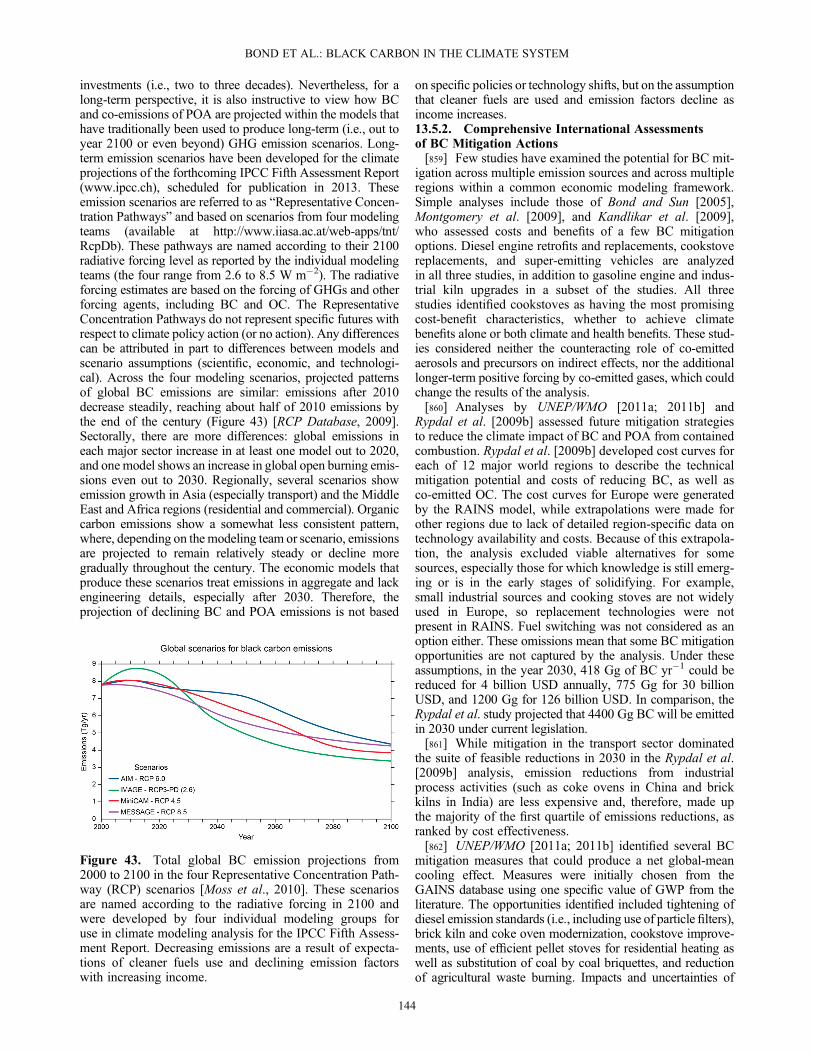
investments (i.e., two to three decades). Nevertheless, for along-term perspective, it is also instructive to view how BCand co-emissions of POA are projected within the models thathave traditionally been used to produce long-term (i.e., out toyear 2100 or even beyond) GHG emission scenarios. Long-term emission scenarios have been developed for the climateprojections of the forthcoming IPCC Fifth Assessment Report(www.ipcc.ch), scheduled for publication in 2013. Theseemission scenarios are referred to as “Representative Concen-tration Pathways” and based on scenarios from four modelingteams (available at http://www.iiasa.ac.at/web-apps/tnt/RcpDb). These pathways are named according to their 2100radiative forcing level as reported by the individual modelingteams (the four range from 2.6 to 8.5 W m�2). The radiativeforcing estimates are based on the forcing of GHGs and otherforcing agents, including BC and OC. The RepresentativeConcentration Pathways do not represent specific futures withrespect to climate policy action (or no action). Any differencescan be attributed in part to differences between models andscenario assumptions (scientific, economic, and technologi-cal). Across the four modeling scenarios, projected patternsof global BC emissions are similar: emissions after 2010decrease steadily, reaching about half of 2010 emissions bythe end of the century (Figure 43) [RCP Database, 2009].Sectorally, there are more differences: global emissions ineach major sector increase in at least one model out to 2020,and one model shows an increase in global open burning emis-sions even out to 2030. Regionally, several scenarios showemission growth in Asia (especially transport) and the MiddleEast and Africa regions (residential and commercial). Organiccarbon emissions show a somewhat less consistent pattern,where, depending on the modeling team or scenario, emissionsare projected to remain relatively steady or decline moregradually throughout the century. The economic models thatproduce these scenarios treat emissions in aggregate and lackengineering details, especially after 2030. Therefore, theprojection of declining BC and POA emissions is not based

on specific policies or technology shifts, but on the assumptionthat cleaner fuels are used and emission factors decline asincome increases.13.5.2. Comprehensive International Assessmentsof BC Mitigation Actions[859] Few studies have examined the potential for BC mit-

igation across multiple emission sources and across multipleregions within a common economic modeling framework.Simple analyses include those of Bond and Sun [2005],Montgomery et al. [2009], and Kandlikar et al. [2009],who assessed costs and benefits of a few BC mitigationoptions. Diesel engine retrofits and replacements, cookstovereplacements, and super-emitting vehicles are analyzedin all three studies, in addition to gasoline engine and indus-trial kiln upgrades in a subset of the studies. All threestudies identified cookstoves as having the most promisingcost-benefit characteristics, whether to achieve climatebenefits alone or both climate and health benefits. These stud-ies considered neither the counteracting role of co-emittedaerosols and precursors on indirect effects, nor the additionallonger-term positive forcing by co-emitted gases, which couldchange the results of the analysis.[860] Analyses by UNEP/WMO [2011a; 2011b] and

Rypdal et al. [2009b] assessed future mitigation strategiesto reduce the climate impact of BC and POA from containedcombustion. Rypdal et al. [2009b] developed cost curves foreach of 12 major world regions to describe the technicalmitigation potential and costs of reducing BC, as well asco-emitted OC. The cost curves for Europe were generatedby the RAINS model, while extrapolations were made forother regions due to lack of detailed region-specific data ontechnology availability and costs. Because of this extrapola-tion, the analysis excluded viable alternatives for somesources, especially those for which knowledge is still emerg-ing or is in the early stages of solidifying. For example,small industrial sources and cooking stoves are not widelyused in Europe, so replacement technologies were notpresent in RAINS. Fuel switching was not considered as anoption either. These omissions mean that some BC mitigationopportunities are not captured by the analysis. Under theseassumptions, in the year 2030, 418 Gg of BC yr�1 could bereduced for 4 billion USD annually, 775 Gg for 30 billionUSD, and 1200 Gg for 126 billion USD. In comparison, theRypdal et al. study projected that 4400 Gg BC will be emittedin 2030 under current legislation.[861] While mitigation in the transport sector dominated

the suite of feasible reductions in 2030 in the Rypdal et al.[2009b] analysis, emission reductions from industrialprocess activities (such as coke ovens in China and brickkilns in India) are less expensive and, therefore, made upthe majority of the first quartile of emissions reductions, asranked by cost effectiveness.[862] UNEP/WMO [2011a; 2011b] identified several BC

mitigation measures that could produce a net global-meancooling effect. Measures were initially chosen from theGAINS database using one specific value of GWP from theliterature. The opportunities identified included tightening ofdiesel emission standards (i.e., including use of particle filters),brick kiln and coke oven modernization, cookstove improve-ments, use of efficient pellet stoves for residential heating aswell as substitution of coal by coal briquettes, and reductionof agricultural waste burning. Impacts and uncertainties of

Figure 43. Total global BC emission projections from2000 to 2100 in the four Representative Concentration Path-way (RCP) scenarios [Moss et al., 2010]. These scenariosare named according to the radiative forcing in 2100 andwere developed by four individual modeling groups foruse in climate modeling analysis for the IPCC Fifth Assess-ment Report. Decreasing emissions are a result of expecta-tions of cleaner fuels use and declining emission factorswith increasing income.


144

http://www.iiasa.ac.at/web-apps/tnt/RcpDb

http://www.iiasa.ac.at/web-apps/tnt/RcpDb

the selected measures were then evaluated in more detail. Theultimate analysis of temperature impacts was based onmodeling the change in radiative forcing when the mitigationmeasures were applied in two climate models. The percentageof industrial-era forcing reductions achieved by the measureswas scaled by a best estimate and central range of industrial-era forcings. Thus, as in this assessment, modeled BC DRFwas increased based on the models’ underestimate of BCAAOD relative to observational constraints.[863] Total BC climate forcing is larger in this assess-

ment (+1.1 W m�2, with uncertainty range of (+0.17 to,+2.1) W m�2) than in the UNEP/WMO Assessment (+0.60,(0.0, +1.0) W m�2) [UNEP/WMO, 2011a; 2011b]. Largeuncertainties are attributed to indirect effects in both reports.Major differences of our BC forcing compared with theUNEP/WMO assessment are the adjustment to observedabsorption, which increases direct forcing; explicit inclusionof the cloud absorption effect; and selection of more negativeliquid-cloud effect andmore positive mixed-phase cloud effectbased on tabulating individual studies.[864] Additional differences between the two assessments

are attributable to the treatment of co-emitted POA, espe-cially its indirect effect. The present assessment attributedindirect forcing to different aerosol species based on totalatmospheric mass. Given the lack of constraints from theliterature and the lower solubility of OA, the UNEP/WMOAssessment instead attributed indirect effects entirely tosulfate. The total net forcing from co-emitted POA is muchsmaller in the UNEP/WMO assessment, so that climatebenefits of measures tend to be larger than those estimatedhere. Both assessments stress the uncertainty in attributionof aerosol indirect effects to individual species, and bothinclude large ranges in assessed climate impact.[865] In the UNEP/WMO Assessment, BC measures

were grouped into “technical” and “regulatory” groups.The technical group included primarily diesel measuresand the emission reductions produced net cooling, as alsosuggested here. The regulatory group of measures hadimpacts whose range encompassed zero, as also found here.[866] Shindell et al. [2012] used the same emission scenar-

ios described above along with detailed climate modeling,and found global mean temperature impacts consistent withthe simplified estimates in the UNEP/WMO Assessment. Inthat model, the combined indirect and semi-direct aerosolforcings resulting from the measures were negative and,hence, augmented rather than offset the reductions in BCDRF. In addition to radiative forcing and global meanclimate response, both the UNEP/WMO Assessment andShindell et al. [2012] estimated the impacts of the mitigationmeasures on health, crop yields, and Arctic temperatures,with large regional precipitation shifts attributed to BC inthe climate modeling study.

13.6. Policy Delivery Mechanisms

[867] At the international level, there are forums andagreements where BC mitigation strategies could beaddressed. The eight-nation Arctic Council is currentlyexploring mitigation opportunities for BC, and the Conventionon Long-Range Transboundary Air Pollution is exploring thequestion of how BC could be addressed within its currentstructure. In 2012, a growing number of nations haveannounced their support of the voluntary Climate and Clean

Air Coalition [http://www.unep.org/ccac] to Reduce Short-Lived Climate Pollutants. Barriers include questions aboutaddressing both long-lived GHGs and short-lived forcerssuch as BC in a common framework (section 12), andconcerns about the consequences of de-emphasizing theimportance of long-lived GHGs.[868] Even if international agreement occurs to move

forward with BC reductions, implementation must takeplace within individual countries. Existing air quality poli-cies may offer the means to deliver near-term mitigationstrategies for BC in developed countries and, where suchpolicy frameworks exist, in developing countries wheremost growth in BC emissions is expected to occur. Forexample, existing vehicle emission standards for new vehi-cles, and scrappage and retrofit programs may provide ameans of implementing additional BC mitigation in thetransportation sector. Other sources may require additionalinfrastructure for implementation on a large scale, such asreductions of residential cooking emissions in remote areasof developing countries. Some important BC emissionsources, such as remote open burning, may lack a policy orprogram infrastructure supporting reduction. The portfolioof regulations, policies, and programs capable of deliveringBC mitigation varies by country, and in some cases couldeven vary within a country where some air-quality or land-use policies are administered at sub-national levels.

13.7. Synthesis of Considerations for IdentifyingImportant Mitigation Options

[869] Table 29 provides a matrix that presents multiplecriteria discussed in this section, and evaluated elsewhere inthis assessment, to help identify important mitigation strate-gies. It summarizes the level of understanding for the follow-ing key considerations for identifying promising mitigationopportunities for BC: the magnitude of the emission source(and thus a first-order indication of technical mitigation poten-tial), the potential to reduce net climate forcing, the potentialto benefit sensitive regions such as the Arctic, the availabilityof technologies and management practices, the costs of thesestrategies, potential health benefits, and implementationfeasibility. Not all of the factors for all emission sources cancurrently be quantified with uniform, or even robust, levelsof understanding. The “level of understanding” evaluationsin this table are intended to be illustrative and are informedboth by quantitative analysis from previous sections of thisassessment and by qualitative judgment for some of the non-science factors briefly discussed in this section.[870] There is considerable variation across BC sources

regarding the potential to reduce globally averaged, positivenet climate forcing, with many broad emission categoriessuch as residential coal burning, field burning and forestburning offering at best uncertain potential in this regard.If controlling some of these sources preferentially reducesclimate forcing in the Arctic or other snow- and ice-dominated regions, or avoids interference with the AsianMonsoon, climate benefits not reflected in Figure 39 mayaccrue. With regard to technical feasibility, there are knownemission mitigation options for most BC sources. However,there is variation in the degree to which these mitigationoptions are characterized with regard to impacts on BC andco-emissions and costs. Programmatic feasibility also varies.Some emission sources are already associated with a policy


145

http://www.unep.org/ccac

infrastructure to deliver mitigation practices at large scale(e.g., diesel sources), whereas other sources (e.g., forest burn-ing) are less amenable to near-term and large-scale policyintervention.[871] While health effects are not evaluated in this report,

there is always the potential to obtain some degree of healthbenefits by mitigating BC emissions. Emissions that preferen-tially occur in populated areas have large health impacts, whileemissions that occur indoors expose fewer people, but athigher concentrations. The lowest health impacts occur foroutdoor emissions that occur at low population density.UNEP/WMO [2011a; 2011b] and Anenberg et al. [2012] pro-vide detailed evaluations of health impacts from outdoor air.[872] Diesel sources of BC appear to offer the most promis-

ing mitigation opportunities in terms of near-term forcing andmaturity of technology and delivery programs. Although someoptions, such as diesel retrofits, may be costly relative to otherBCmitigation options, they may also deliver significant healthbenefits. Mitigating emissions from residential solid fuels mayyield a reduction in net positive forcing. The near-term neteffect remains uncertain because of uncertain knowledgeregarding the impacts of co-emitted species on clouds, but lon-ger-term forcing by co-emitted species interacting with themethane budget is positive. Furthermore, the evolution of fea-sibility is still in the emerging phase for these sources. The neteffect of small industrial sources depends greatly on the sulfurcontent of individual sources, and the feasibility of mitigationis in the emerging phase. Individual source types that have lowsulfur emissions and for which alternative technology isavailable could offer net climate benefits.

[873] Acknowledgments. This assessment is a contribution of theIGBP-IGAC/WCRP-SPARC Atmospheric Chemistry and Climate Initiative(AC&C). The authors acknowledge financial and technical support from theInternational Global Atmospheric Chemistry (IGAC) project (http://igac.jisao.washington.edu/index.php), C. Koblinsky of the Climate Program

Office of the National Oceanic and Atmospheric Administration (NOAA),H. Maring of the Radiation Sciences Program of the National Aeronauticand Space Administration (NASA), Rose Kendall of CSC, and Beth Tullyof Tully Graphics. IGAC funding for this project is via the Joint Institutefor the Study of the Atmosphere and Ocean (JISAO) under NOAA Cooper-ative Agreement NA10OAR4320148, Contribution No. 2035. The authorsare grateful to Ray Minjares and the International Council on CleanTransportation (ICCT) and Catherine Witherspoon of the ClimateWorksFoundation for encouragement to undertake this effort. The authors wishto thank the AeroCom modeling community and the AERONET data pro-viders for their great help in providing basic data sets, further analyzed here.Olivier Boucher is thanked for his substantial contribution to section 9 andhis careful review and subsequent discussion with the author team on theentire manuscript. We also thank N. Riemer of the University of Illinoisfor particle-resolved simulation results in Figure 6, N. Mahowald of CornellUniversity for dust fields in Figure 12, and D. M. Winker of NASA forproviding the CALIPSO data in Figure 16. A. Heil is thanked for providinginformation on biomass fuel loads and M. O. Andreae for providing updatesof his biomass burning emission factor compilation. E. Baum, J. Bachmann,R. Minjares, K. Ram, V. Ramanathan, and D. Zaelke are thanked forreading and providing comments that improved the document. T. C. Bondacknowledges support for related work under U.S. EPA RD-83503401,NASA RD-83503401, NSF ATM 08-52775, and DOE DE-SC0006689.Piers Forster acknowledges support from a Royal Society Wolfson ResearchMerit award. N. Bellouin was supported by the Joint DECC/Defra MetOffice Hadley Centre Climate Programme (GA01101). S. Ghan wassupported by the U.S. Department of Energy (DOE), Office of Science,Scientific Discovery through Advanced Computing (SciDAC) program,and the DOE Decadal and Regional Climate Prediction using Earth SystemModels (EaSM) program. The Pacific Northwest National Laboratory isoperated for the DOE by Battelle Memorial Institute under contractDE-AC06-76RLO 1830. Y. Kondo was supported by the Ministry ofEducation, Culture, Sports, Science, and Technology (MEXT), strategicinternational cooperative program of Japan Science and Technology Agency(JST), and the global environment research fund of the Japanese Ministry ofthe Environment (A-1101). For P. K. Quinn’s work, this is NOAA PMELcontribution no. 3786. M. Schulz received funding support through theEUCAARI project (EU-FP6 Contract 34684). M. Z. Jacobson receivedfunding from the U.S. National Science Foundation. J. W. Kaiser wassupported by the European Union Seventh Research Framework Programme(MACC project, contract number 218793). S. G.Warren acknowledges supportfrom U.S. NSF grant ARC-06-12636. H. Zhang was funded by the NationalBasic Research Program of China (2011CB403405). The views expressed inthis paper are those of the authors and do not necessarily reflect the views orpolicies of the U.S. Environmental Protection Agency.

Table 29. Evaluation of Criteria for Mitigation of BC Emission Sourcesa

Emission Source

Criteria

SourceMagnitudeb

Global ClimateForcingc

Arctic ClimateForcingd

MitigationTechnologiesor Practicese

Mitigation CostEffectivenessf

HealthBenefitg Implementationh

On-road diesel H H H H H H HOff-road diesel M H-M M H M H HIndustrial coal M L L M M-L H MBiofuel cooking H H-L L M M H LBiofuel heating L M-L H M M H M-LResidential coal L H-M M M M H MAgriculturalfield burning

L M-L M M-L M H-M M-L

Forest burning H L H-M M-L H-L H-L LGrass and woodlandburning

H L L M-L H-L H-L L

aThis table presents a qualitative evaluation of several criteria for a range of emission sources that may inform priorities for BC mitigation actions. Thefirst two columns represent criteria for which comprehensive, quantitative analysis is available from previous sections of this assessment. Indicators desig-nate criteria potential as high (H), medium (M), or low (L).

bSources with greater magnitude are considered to have greater technical mitigation potential. See section 4.cPotential to reduce globally averaged climate forcing, based on best estimates from section 11. “High” reflects likely warming effect globally, “Medium”

reflects uncertainty regarding global effect, and “Low” reflects likely cooling effect globally.dPotential to reduce Arctic climate forcing, reflecting near-Arctic sources of emissions and albedo effects. See section 8. Other regional effects not

captured by global climate forcing, such as changes to Asian Monsoons, could also be considered.eAvailability and characterization of mitigation technologies or practices. See section 13.fMagnitude of mitigation costs per unit of BC reduced. See section 13.gPotential to provide health benefits, reflecting likely population exposure. See section 13 for brief discussion.hPotential for near-term implementation at large scales. See section 13 for brief discussion.


146

http://igac.jisao.washington.edu/index.php

http://igac.jisao.washington.edu/index.php

Appendix A: Author Contributions

[874] The development of this assessment required a large,diverse group of dedicated authors. They synthesized multipletopics in the individual sections and interlinked the topicsthroughout. Each section required lead-author commitmentequivalent to the production of a typical journal paper. The pub-lication of this assessment in a peer-reviewed journal necessi-tates a first author, thereby precluding the section lead authorsfrom receiving the lead-author credit normally accorded for thislevel of effort. The author order begins with the first author andthree coordinating lead authors (Doherty, Fahey and Forster)followed by the lead authors and contributing authors in alpha-betical order. The table below acknowledges the principal con-tributions of each author in an attempt to further recognizetheir substantial investment in this assessment.

Appendix B: Using Sky-Photometer AerosolAbsorption Optical Depth Retrievals to ConstrainBlack Carbon Models

B1. Background and Methods[875] Aerosol absorption optical depth (AAOD) associated

with BC column amounts is a key factor controlling modelestimates of BC DRF. The diversity in modeled BC AAOD isone of the major factors contributing to diversity in estimatesof BC DRF. To reduce BC-DRF uncertainty, we use retrievalsfrom a global network of ground-based sun-/sky-radiance

observations (AERONET) to adjust the BC AAOD simulatedby models. Our AAOD estimates use measurements that covercomplete annual cycles for 2000 to 2010 at 171 land sitesdistributed worldwide, and data from an additional 78 sites withincomplete annual cycles. By applying some assumptions,detailed below, values of BC column absorption (BC AAOD)can be extracted from the AERONET retrievals. These valuescan be compared to those simulated bymodels at the same loca-tion and time, and regional scale factors for BC AAOD can bedetermined from the ratio of observationally estimated to simu-lated BCAAOD. These scale factors are used in this assessmentto reduce the bias in models used to determine BC DRF.[876] Sun and sky radiance observations [Dubovik and

King, 2000] in the mid-visible range allow inference ofthe aerosol column absorption in terms of the AAOD(=AOD � [1�o0]) from retrievals of AOD and single-scattering albedo (o0) at 550 nm. Regular retrievals forcloud-free conditions with identical instrumentation at manyAERONET locations [Holben et al., 1998] provide extensivecoverage over continents and islands. A comparison of AAODretrievals with in situ measurements showed good agreementfrom 300 to 700 nm and a possible high bias in AERONETAAOD at 880 nm [Corrigan et al., 2008, Figure 16]. However,because retrievals of o0 are less certain at low AOD [Duboviket al., 2000], absorption data for low AOD cases are removedfrom the official AERONET Version 2.0 product. This filterintroduces a positive bias for local statistics of AAOD becauseonly cases with high AOD are counted. To remove this AAODbias, missing refractive index data in the Version 2.0 data prod-uct have been recovered from the lower-quality Version 1.5data product, so that now low AOD cases are included as well.This procedure adds noise to the retrieved AAOD data set but isexpected to reduce the sampling bias (O. Dubovik, personalcommunication, 2008). However, a small positive samplingbias may still exist, because values of o0 greater than 1 (nega-tive absorption) are excluded from the data set. The retrievedAAOD is very similar to that from an alternative procedure inwhicho0 is retrieved only from high-AOD observations at eachstation and applied to all AOD values at that station, thusmaximizing the use of Version 2.0 data. The mean AAODaveraged over all samples at all AERONET sites is 0.018 usingthe Version 1.5o0, which is a factor of 2 smaller than the meanvalue (0.040) from the version 2.0 retrieval of AAOD.[877] Refractive indices at 440 nm and 670 nm inferred from

the AERONET data are interpolated to 550 nm. Real refractiveindices are interpolated linearly and imaginary refractive indi-ces are interpolated in log-log space, which would producespectral absorption that is well described by the absorptionÅngström exponent (equation (3.1)). In the mid-visible solarspectral region, non-BC contributions to absorption are mainlyfrom relatively coarse dust particles. To separate BC AAODfrom total AAOD, we assume that BC controls the mid-visibleabsorption of small (i.e., “fine-mode”) aerosol particles anddust controls the absorption of particles larger than 1mm diam-eter. This implies that any mid-visible absorption by organicmatter, brown carbon or small-sized dust is attributed to BC.This separation by size is possible because the AERONETinversion method provides detailed size-distribution data. Weestimate dust AAOD from the super-micron part of theretrieved size distribution and an assumed refractive index of1.55+ 0.0015i [Dubovik et al., 2002, Table 1]. Finally, BC

Table A1. Author Principal Contributions

Section—Topic Lead Authors Contributing Authors

2—Introduction T. C. Bond3—Measurements andmicrophysical properties

P. K. Quinn S. GhanY. Kondo U. Lohmann

J. P. Schwarz4—Emissions C. Venkataraman T. C. Bond

M. G. Schultz S. K. GuttikundaP. K. HopkeJ. W. KaiserZ. Klimont

5—Constraints on abundance S. Kinne M. SchulzT. C. Bond

6—Direct radiative forcing S. GhanM. SchulzS. KinneT. C. BondH. Zhang

7—Cloud effects D. Koch T. StorelvmoB. Kärcher U. Lohmann

8—Cryosphere changes S. J. Doherty S. G. WarrenM. G. Flanner

9—Climate response P. M. Forster N. BellouinD. KochM. G. FlannerS. J. DohertyM. Z. JacobsonD. ShindellC. S. Zender

10—Synthesis P. M. ForsterD. W. Fahey

11—Net climate forcing T. C. Bond12—Emission metrics T. Berntsen13—Mitigation considerations B. J. DeAngelo

M. C. SarofimS. Zhang


147

AAOD is estimated as the difference between the AERONETtotal AAOD and the dust AAOD. All calculations areperformed at 550 nm.[878] The AERONET retrieval also provides an estimate of

the refractive index, but it applies to the entire aerosol in thecolumn which almost always contains a combination of constit-uents; thus, the index is not applicable for individual compo-nents of the column aerosol such as BC, OA and dust. Thus,we use an assumed value for the dust refractive index ratherthan a retrieved value from AERONET to calculate the dustcontribution to total AAOD. Similarly, assuming the imagi-nary part of the retrieved refractive index applies to submicronparticles yields BC AAOD estimates that are too low if thedust absorption dominates the retrieved refractive index,because the retrieval is strictly valid only for the entire sizedistribution (section B2).[879] If AERONET stations provided globally uniform

high-resolution coverage for ocean as well as land locations,the AERONET BC-AAOD retrievals could be directly usedto constrain model simulations. However, Figure 14 showsthat although there are hundreds of AERONET stationsdistributed across the Earth, coverage is limited to land andis far from homogeneous over land. Additional assumptionsare required for locations without AERONET data.[880] To fill in the gaps between stations we use spatial dis-

tributions of BC AAOD from AeroCom simulations [Kinneet al., 2006]. Median values of the set of 15 AeroCommodelsare used for each month and mapped onto a 1� � 1� latitude-longitude grid. The model ensemble median is, henceforth,referred to as the AeroCom median. The AeroCom BCAAOD is estimated from the BC AOD saved for each model.Based on Mie theory and the assumption of the same BC sizedistribution (i.e., lognormal with 0.065mmnumber mode radiusand geometric standard deviation of 1.7) and refractive index(1.7, 0.7i) for all models, we use ano0 of 0.36 for BC to convertfrom BC AOD to BC AAOD. To compare AeroCom modelsthat estimate only industrial-era BC AAOD with AERONETobservations of total AAOD, we rely on one AeroCommodel (LOA) to provide the industrial-era fraction of BC (i.e.,(all-source BC AAOD� preindustrial BC AAOD) / (all-sourceBC AAOD)), thus estimating a preindustrial backgroundAAOD of 0.0004. Using global mean values for both the indus-trial-era and all-source BC AAOD, this ratio in the LOAmodelis 0.80, but the ratio among model grid boxes (1� � 1�) varieswidely, from near zero in regions with large natural emissionsto 97% in regions with large anthropogenic emissions.Modeledglobal mean values without any scaling are 0.00172 for indus-trial era BC AAOD and 0.00212 for all-source BC AAOD.[881] The AeroCom BC-AAOD values do not agree with

the AERONET retrievals, so the BC-AAOD distribution fromAeroCom is scaled to agree with the AERONET retrievals atthe station locations. Errors in emissions or BC scavengingvary spatially, producing different biases, so separate scalefactors are calculated for each region (Table B1 and Figure 7).For each region, all AERONET data available for a givenmonth are combined, and from this data set a characteristicregional value is calculated using the average values betweenthe 25% and 75% percentiles. This average is chosen insteadof the mean to avoid the impacts of extreme outliers. The samequantity is determined for the AeroCom median field at thelocations of AERONET observations. These averages arereferred to as the “characteristic values” from AERONET

and AeroCom. The ratios of the AERONET toAeroCom char-acteristic values then define the regional (monthly) scalefactors.[882] Table B1 lists annual mean characteristic values of BC

AAOD for each region from theAERONET retrievals and fromthe AeroCommedian model at the samemonth and locations asthe AERONET retrievals. The ratios of the characteristic values(AERONET/AeroCom), also listed in Table B1, define regionalscale factors that can be applied to the AeroCom BC AAODwithin each region to compensate for regional AeroCom biases.According to Table B1, the ratios are larger than 1 for allregions, but vary widely from region to region (e.g., 1.6 to 6.2for annual means) and from month to month within a region(e.g., 0.6 to 10.5). The global annual mean of the resultingscaled AeroCom BC AAOD is 0.00605, which is smallerthan the average listed in Table B1 for AERONET locationsonly. The table lists BC AAOD at AERONET sites, whereAAOD is higher than the global average, so the global meanafter scaling is smaller than the average of the values in thetable. This estimate of BC AAOD attributes all fine-modeabsorption to BC. When combined with an estimate of fine-mode AOD from MODIS [Remer et al., 2008], this AAODyields a global, annual average fine-mode single scatter albedoof 0.92.[883] After scaling to AERONET observations, all-source

BC AAOD is 0.00605, and industrial-era BC AAOD is0.00489, assuming the same scaling applies to preindustrialbackground BC AAOD because the same biases in BC emis-sion factors, lifetime, and optics apply to preindustrial and pres-ent-day simulations. The global average all-source BC AAODand the industrial-era BC AAOD both increase by a factor of2.9 because the same scaling is applied to preindustrial condi-tions. These fractional increases depend on the value ofo0 assumed in deriving unscaled BC AAOD from the modelBC AOD fields, but the scaled BC AAOD value does not. Ifa more-absorbing aerosol (i.e., lower o0) had been chosen,the unscaled model BC AAOD would be greater, the final BCAAOD would be identical, and the percentage increase wouldbe lower. This has no implications for BCDRF, but it does haveimplications for the emissions inferred after accounting forscaling of BC AAOD.

B2. Uncertainties

[884] Table B2 summarizes estimates of eight sources ofuncertainty (95% confidence) in BC AAOD and how each isestimated. We assume that the eight factors contributing touncertainty are uncorrelated, so that they can be added inquadrature. Two of the uncertainties are asymmetric. Thelower and upper uncertainties for all-source BC AAOD areestimated to be �61% and +44%, respectively. Forindustrial-era BC AAOD, the uncertainties are �71% and+60%, respectively.[885] 1. Impact of model spatial pattern. The regional

monthly BC AAOD scale factors are based on existing datapairs (AeroCom/AERONET) for each region and month.The derived scale factor is then applied to all data points ofthe reference model in that region and month. However, spa-tial distributions can vary significantly among models,which introduce uncertainty. To quantify this uncertainty,the analysis was performed after replacing the AeroCommedian field with fields from three individual models. This


148

resulted in the following scaled all-source BC AAODvalues—AeroCom median model: 0.0060; SPRINTARS:0.0046; GOCART: 0.0052; and UMI: 0.0064. From thestandard deviation of these values, we derive a 25% uncer-tainty due to the model spatial pattern.[886] 2. Characteristic value. The BC AAOD scale

factors for each month and region are based on characteris-tic values of BC AAOD at the AERONET sites. Inthis study, the characteristic value is defined by theinterquartile average. Other statistical calculations lead tothe following all-source BC-AAOD values—average ofthe 25, 50, and 75 percentile values of the probabilitydistribution: 0.00577; median value: 0.00596; mean:0.00733; 7 percentiles between 10% and 90% averaged:0.00635; and interpercentile range of values between 10%and 90% percentiles averaged: 0.00582. From the standarddeviation of these estimates, we derive a 18% uncertaintydue to the statistical derivation of the BC AAOD character-istic values.[887] 3. Limited AERONET sites and sampling. To quantify

the influence of the limited number of AERONET sites used,sub-samples were used to re-estimate the scale factors. Usinghalf of all available AERONET sites in four randomly selectedways produced the following global all-source scaled AeroComBC-AAOD values: 0.0061, 0.0064, 0.0071, and 0.0057. Fromthis, we derive a 16% uncertainty due to the limited AERONETnetwork coverage.[888] 4. Clear-sky bias of AERONET. A related sampling

uncertainty is that AERONET data are acquired only duringtimes of direct sunlight whereas model-simulated BC-AAODvalues refer to all times (section 5.4.2.1). This bias is esti-mated with four AeroCommodels (GEOS-Chem, GOCART,OSLO-CTM2, and SPRINTARS) because AERONET re-trievals are not possible under cloudy conditions. SimulatedBC AAOD on days with AERONET BC-AAOD retrievalswere compared to simulated values on all days. Averagingacross all models and AERONET sites yields an annual aver-age clear-sky bias of 1%� 5%, with the largest bias in SEAsia (15%). An uncertainty of �5% is therefore applied toour estimate of global, annual average BC AAOD. No cor-rection is made for the 1% annual bias. The effect on radia-tive forcing could be different than the effect on AAODdepending on the location of BC relative to clouds, but wehave not accounted for this uncertainty.[889] 5. Transport to unsampled regions. Scaling burdens

over land areas, where AERONET stations are located,should also affect burdens in regions affected by continentaloutflow. The land-based definition in Figure 7 neglectsthis influence. To address this deficiency, we extendedsome regions with large BC outflows partway across theoceans. This procedure increased the global mean BCAAOD by 16%, so we estimate the associated uncertaintyto be 16%.[890] 6. Dust impact on estimated BC AAOD. The attribu-

tion of AAOD between BC and dust is one of the largestuncertainties. Here we have taken a specific approach toremoving dust absorption from the total AAOD, but doingso requires imperfect assumptions. We estimate an asymmet-ric uncertainty due to the partitioning of AAOD between dustand BC by performing other estimates of BC AAOD fromAERONET and propagating these through the model exten-sion. The upper bound of AAOD is obtained by assuming a

smaller imaginary refractive index for dust, 0.0006. Thisyields a BC AAOD of 0.0074, 23% larger than the estimatewith imaginary refractive index of 0.0015. For the lowerbound, we use the AERONET retrieved refractive index forthe total column aerosol, assume that it applies to particlessmaller than 1mm diameter, assume that all absorption bythese particles is due to BC, and then integrate absorption overthe retrieved sub-1mm size distribution to estimate BCAAOD. This procedure yields a global mean all-source BCAAOD of 0.0034, 43% smaller than the value estimated fromour primary approach. Using the refractive index retrieved forthe entire size distribution provides a lower bound forBC AAOD because fine-mode refractive index is generallygreater than dust refractive index, as evidenced by thefact that AERONET o0 is usually lower than dust o0.This method ascribes an AAOD of 0.0052 to non-BCmaterial. For comparison, AeroCom models have a medianAOD of 0.023 for dust and compare reasonably well withAERONET observations in dusty regions [Huneeus et al.,2011]. Even with a relatively low o0 of 0.95, modeled dustAAOD would be only 0.0011.[891] 7. Organic matter impact on BC AAOD. To extract

the AAOD associated with BC, it was assumed that aftercontributions of larger (dust) aerosol sizes to absorption areremoved, the remaining absorption by small particles can beattributed to BC. However, organic aerosol may absorb andis contained in small particles, and it is usually co-emittedwith BC. Initial tests with AeroCom median AOD maps forOA and BC and a plausible OA mid-visible imaginary partof the refractive index of 0.005 yielding a co-albedo of0.027 suggest that 20% of the AAOD of small particles couldbe attributable to OA. Such an attribution would reduce ourestimate of BC AAOD. An asymmetric uncertainty of (0,20%) is applied to account for this possibility. Chung et al.[2012] concluded that absorption by OA is sufficient to offsetscattering, so the best estimate of DRF attributable to BC plusabsorbing OA would be little affected. Estimates of forcingper emission developed in section 11 may be reasonablyaccurate, as long as both BC and OA are emitted fromthe same source.[892] 8. Pre-industrial contribution to BC. Compared with

all-source BC, industrial-era BC has an additional uncertaintybecause the pre-industrial background is unknown. Therelative uncertainty in pre-industrial BC emissions may becomparable to the estimated 50% uncertainty in emissionsfrom biomass burning [Akagi et al., 2011; Vermote et al.,2009]. However, the uncertainty in applying the scalingadjustment to pre-industrial AAOD is greater than 50%. Weuse the previously estimated AAOD of 0.0004 as a lowestimate for this preindustrial background and the scaled esti-mate of 0.0012 as a high estimate. The low pre-industrial valueis subtracted from the high value of AAOD for a high estimate,and vice versa.[893] We acknowledge that there are other sources of

uncertainty in using AERONET data that have not beenquantified here. These include interpolation of AAOD to550 nm, removal of climatological NO2 absorption fromthe aerosol absorption values, and accounting for dust thatabsorbs in the fine mode or BC that absorbs in the coarsemode. In addition, the AERONET algorithm is subjectto periodic revision and updates that could affect theinferences here.


149

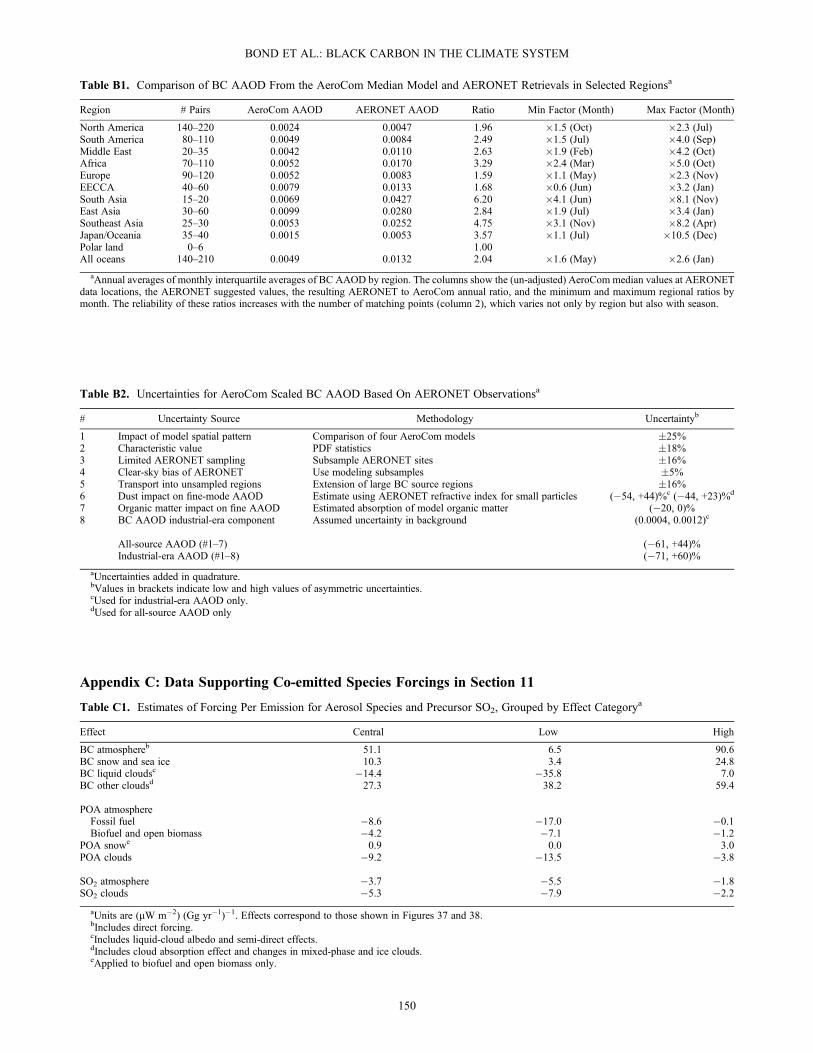
Table B1. Comparison of BC AAOD From the AeroCom Median Model and AERONET Retrievals in Selected Regionsa

Region # Pairs AeroCom AAOD AERONET AAOD Ratio Min Factor (Month) Max Factor (Month)

North America 140–220 0.0024 0.0047 1.96 �1.5 (Oct) �2.3 (Jul)South America 80–110 0.0049 0.0084 2.49 �1.5 (Jul) �4.0 (Sep)Middle East 20–35 0.0042 0.0110 2.63 �1.9 (Feb) �4.2 (Oct)Africa 70–110 0.0052 0.0170 3.29 �2.4 (Mar) �5.0 (Oct)Europe 90–120 0.0052 0.0083 1.59 �1.1 (May) �2.3 (Nov)EECCA 40–60 0.0079 0.0133 1.68 �0.6 (Jun) �3.2 (Jan)South Asia 15–20 0.0069 0.0427 6.20 �4.1 (Jun) �8.1 (Nov)East Asia 30–60 0.0099 0.0280 2.84 �1.9 (Jul) �3.4 (Jan)Southeast Asia 25–30 0.0053 0.0252 4.75 �3.1 (Nov) �8.2 (Apr)Japan/Oceania 35–40 0.0015 0.0053 3.57 �1.1 (Jul) �10.5 (Dec)Polar land 0–6 1.00All oceans 140–210 0.0049 0.0132 2.04 �1.6 (May) �2.6 (Jan)

aAnnual averages of monthly interquartile averages of BC AAOD by region. The columns show the (un-adjusted) AeroCom median values at AERONETdata locations, the AERONET suggested values, the resulting AERONET to AeroCom annual ratio, and the minimum and maximum regional ratios bymonth. The reliability of these ratios increases with the number of matching points (column 2), which varies not only by region but also with season.

Table B2. Uncertainties for AeroCom Scaled BC AAOD Based On AERONET Observationsa

# Uncertainty Source Methodology Uncertaintyb

1 Impact of model spatial pattern Comparison of four AeroCom models �25%2 Characteristic value PDF statistics �18%3 Limited AERONET sampling Subsample AERONET sites �16%4 Clear-sky bias of AERONET Use modeling subsamples �5%5 Transport into unsampled regions Extension of large BC source regions �16%6 Dust impact on fine-mode AAOD Estimate using AERONET refractive index for small particles (�54, +44)%c (�44, +23)%d

7 Organic matter impact on fine AAOD Estimated absorption of model organic matter (�20, 0)%8 BC AAOD industrial-era component Assumed uncertainty in background (0.0004, 0.0012)c

All-source AAOD (#1–7) (�61, +44)%Industrial-era AAOD (#1–8) (�71, +60)%

aUncertainties added in quadrature.bValues in brackets indicate low and high values of asymmetric uncertainties.cUsed for industrial-era AAOD only.dUsed for all-source AAOD only

Appendix C: Data Supporting Co-emitted Species Forcings in Section 11

Table C1. Estimates of Forcing Per Emission for Aerosol Species and Precursor SO2, Grouped by Effect Categorya

Effect Central Low High

BC atmosphereb 51.1 6.5 90.6BC snow and sea ice 10.3 3.4 24.8BC liquid cloudsc �14.4 �35.8 7.0BC other cloudsd 27.3 38.2 59.4

POA atmosphereFossil fuel �8.6 �17.0 �0.1Biofuel and open biomass �4.2 �7.1 �1.2

POA snowe 0.9 0.0 3.0POA clouds �9.2 �13.5 �3.8

SO2 atmosphere �3.7 �5.5 �1.8SO2 clouds �5.3 �7.9 �2.2

aUnits are (mW m�2) (Gg yr�1)�1. Effects correspond to those shown in Figures 37 and 38.bIncludes direct forcing.cIncludes liquid-cloud albedo and semi-direct effects.dIncludes cloud absorption effect and changes in mixed-phase and ice clouds.eApplied to biofuel and open biomass only.


150

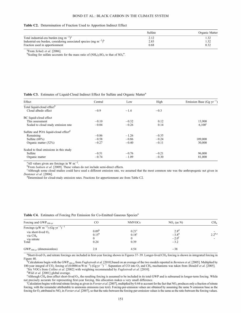
Table C3. Estimates of Liquid-Cloud Indirect Effect for Sulfate and Organic Mattera

Effect Central Low High Emission Base (Gg yr�1)

Total liquid-cloud effectb

Cloud albedo effect �0.9 �1.4 �0.3

BC liquid-cloud effectThis assessment �0.10 �0.32 0.12 13,900Scaled to cloud study emission rate �0.04 �0.26 0.14 6,100c

Sulfate and POA liquid-cloud effectd

Remaining �0.86 �1.26 �0.35Sulfate (68%) �0.58 �0.86 �0.24 109,000Organic matter (32%) �0.27 �0.40 �0.11 30,000

Scaled to final emissions in this studySulfate �0.51 �0.76 �0.21 96,000Organic matter �0.74 �1.09 �0.30 81,000

aAll values given are forcings in W m�2.bFrom Isaksen et al. [2009]. These values do not include semi-direct effects.cAlthough some cloud studies could have used a different emission rate, we assumed that the most common rate was the anthropogenic net given in

Dentener et al. [2006].dDetermined for cloud-study emission rates. Fractions for apportionment are from Table C2.

Table C4. Estimates of Forcing Per Emission for Co-Emitted Gaseous Speciesa

Forcing and GWP100-yr CO NMVOCs NOx (as N) CH4

Forcings (mW m�2) (Gg yr�1)�1

via short-lived O30.09b 0.21c 2.8d -

via CH40.15b 0.18c �3.8d 2.2b,e

via nitrate 0 0 �2.0f -Total 0.24 0.39 �3.2

GWP100-yr (dimensionless) 2.8 4.54 �38

aShort-lived O3 and nitrate forcings are included in first-year forcing shown in Figures 37–39. Longer-lived CH4 forcing is shown in integrated forcing inFigure 40.

bCalculations begin with the GWP100-yr from Fuglestvedt et al. [2010] based on an average of the two models reported in Berntsen et al. [2005]. Multiplied by100-year integral of CO2 forcing of (0.0086mWm�2) (Gg yr�1)�1. Separation of CO into O3 and CH4 mechanisms was taken from Shindell et al. [2005].

cSix VOCs from Collins et al. [2002] with weighting recommended by Fuglestvedt et al. [2010].dWild et al. [2001] global average.eAlthough CH4 does affect short-lived O3, the resulting forcing is assumed to be included in its total GWP and is subsumed in longer-term forcing. While

not precisely accurate for representing first-year forcing, this allocation makes a very small difference.fCalculation begins with total nitrate forcing as given inForster et al. [2007], multiplied by 0.44 to account for the fact that NOx produces only a fraction of nitrate

forcing, with the remainder attributable to ammonia emissions (see text). Forcing-per-emission values are obtained by assuming the same N emission base as theforcing for O3 attributed to NOx in Forster et al. [2007], so that the ratio between the forcing-per-emission values is the same as the ratio between the forcing values.

Table C2. Determination of Fraction Used to Apportion Indirect Effect

Sulfate Organic Matter

Total industrial-era burden (mg m�2)a 2.12 1.32Industrial-era burden, considering associated species (mg m�2)b 2.83 1.32Fraction used in apportionment 0.68 0.32

aFrom Schulz et al. [2006].bScaling for sulfate accounts for the mass ratio of (NH4)2SO4 to that of SO4

═.


151

Table C6. Emission Factors in (g kg�1) Used to Develop Figures 39 and 40b

Emission Source BC POA SO2 CO CH4 NMVOC NOx CO2

Euro II heavy-duty vehiclea 0.47 0.1 0.9 7 0.2 1.4 35.3 3087Pre-regulation trucka 2.39 1.3 11.9 11 0.4 3.0 11.2 3087Bull’s Trench brick kilnb 2.44 0.1 10.5 41 1.5 0.3 0.0 2182Industrial coal boilerc 0.01 0.0 5.2 5 0.4 0.7 2.1 1947Mud cooking stoved 0.80 5.7 0.3 67 5.6 2.7 1.0 1833Conventional wood stovee 0.36 3.9 0.2 130 15.0 23.6 2.8 1833Wood boilerf 1.09 1.5 0.3 105 9.0 14.0 1.2 1833Coal cooking stoveg 0.58 0.8 0.2 166 0.9 0.5 2.2 2130Field burningh 0.69 4.6 0.4 92 2.7 7.0 1.2 1833Forest burningh 0.56 11.2 1.0 107 4.7 5.7 1.4 1833

aGAINS implementation of COPERT4 emission factors [Ntziachristos and Samaras, 2009].bGreentech [2011], except CH4 and NMVOC values which were not measured. For those gases, one half of Zhang et al. [2000] values for coal stoves

were used, assumed to scale approximately with CO emissions.cWang et al. [2009b]dRoden et al. [2009] in-field data for BC, POA, and CO; Smith et al. [2000a, 2000b] for other gases.eMcDonald et al. [2000], except SO2, CH4 and NMVOC from EPA [1996].fJohansson et al. [2004]; Rau [1989].gZhang et al. [2000]; Zhi et al. [2008].hAndreae and Merlet [2001], except CO2 from carbon balance.

Table C5. Emission Rates Used for Figures 37, 39, and 40aa

Category BC POA SO2 (as S) CO CH4 NMVOC NOx (as N) CO2

On-road 1630 1100 1500 42,000 700 4400 6300 2342Off-road 810 600 900 7000 0 2800 2400 922Industry 850 1600 9900 51,000 0 500 1100 4372Wood/cook 4060 25,300 1200 362,000 17,100 85,200 500 7638Wood/heat 230 900 100 8000 600 2700 0 344Coal 930 1100 2500 32,000 200 1300 100 2090Ag fields 280 1500 100 15,000 1800 2400 0 414Forests 1470 22,100 2000 96,000 5800 7000 900 2349Savannas 2230 21,800 1800 121,000 4200 6300 2100 5278Other rich 1160 4100 3300 557,000 3200 70,500 7500 10,234Power 20 0 50,100 2000 0 700 6300 7328Other low 100 300 22,500 51,000 244,500 19,300 3900 5092

Industrial-era total 13,770 80,400 95,900 1,344,000 278,100 203,100 31,100 48,403

aAll emissions are in Gg yr�1 except CO2, which is in Tg. Values are developed beginning with year 2000 emissions given by GAINS (Table 8) andRETRO, scaled to inferred BC emission rates in each region using the scale factors given in section 6 and Appendix B.

Table R1. Acronyms and Abbreviations

Acronym Definition

AAOD aerosol absorption optical depthAeroCom Aerosol Comparison between Observations and ModelsAERONET Aerosol Robotic NETworkAGTP absolute global temperature change potentialAGWP absolute global warming potentialAOD aerosol optical depthBB biomass burningBC-DRF black-carbon direct radiative forcingCALIPSO Cloud Aerosol Lidar and Infrared Pathfinder Satellite ObservationsCAM Community Atmosphere ModelCAM3 Community Atmosphere Model3CAM5 Community Atmosphere Model5CAM-Oslo Community Atmosphere Model-OsloCTM chemical transport modelDRF direct radiative forcing


152

Table 1.(continued)

Acronym Definition

ECHAM European Centre HAmburg ModelEECCA Eastern Europe, Caucasus and Central AsiaFF fossil fuelGAINS Greenhouse Gas and Air Pollution Interactions and SynergiesGATOR Gas, Aerosol, TranspOrt, Radiation modelGATOR-GCMOM Gas, Aerosol, TranspOrt, Radiation - General Circulation, Mesoscale, and Ocean ModelGCM global climate modelGHG greenhouse gasGISS Goddard Institute for Space StudiesGOCART Goddard Chemistry Aerosol Radiation and Transport modelGRA albedo reduction via growth of snow grains with accelerating snow agingGRB increase in albedo reduction for a given BC concentration in coarse grained vs. fine-grained snowGTP global temperature change potentialGWP global warming potentialHadGEM Hadley Centre Global Environmental ModelHIPS Hybrid Integrating Plate SystemIE indirect effectIEA International Energy AgencyIIE ice cloud indirect effectIMPACT Lawrence Livermore National Laboratory (LLNL) Integrated Massively Parallel Atmospheric (IMPACT) ModelIMPROVE Interagency Monitoring of Protected Visual EnvironmentsIN ice nucleiIPCC Intergovernmental Panel on Climate ChangeISSW Integrating Sphere Sandwich SpectrophotometerLES large-eddy simulationlidar light detection and rangingLOSU level of scientific understandingLSCE Laboratoire des Sciences du Climat et de l’EnvironnementMAC mass absorption cross sectionMBC Increase in surface snow BC concentration via enhanced surface snow melt and retention of BCMIE mixed-phase cloud indirect effectMISR Multi-angle Imaging SpectroradiometerMODIS Moderate Resolution Imaging SpectroradiometerMPI-HAM Max Planck Institute-Meterology, HamburgMSC mass scattering cross-sectionNASA National Aeronautics and Space AdministrationNCAR National Center for Atmospheric ResearchOMI Ozone Measurement InstrumentOPAC Optical Properties of Aerosols and CloudsPAS photoacoustic spectrometerppm part per millionPSAP Particle Soot Absorption PhotometerRAINS Regional Air Pollution Information and Simulation modelRETRO Reanalysis of the TROposphere over the last 40 yearsRF radiative forcingSAF snow albedo feedbackSBC change in surface snow BC concentration via change in sublimationSPEW Speciated Pollutant Emissions WizardSPRINTARSSP2 Single Particle Soot PhotometerSST sea-surface temperatureToA top of the atmosphereTRACE-P Transport and Chemical Evolution over the PacificUIO-CTM University of Oslo CCMUMI University of MichiganUSSR Union of Soviet Socialist RepublicsUTLS upper-tropsphere-lower-stratosphereUV ultravioletWIE warm cloud indirect effectW wattWRF Weather Research and Forecasting model

Table R1. (Continued)


153

ReferencesAaheim, H. A., J. S. Fuglestvedt, and O. Godal (2006), Costs savings of aflexible multi-gas climate policy, Energ. J., S13, 485–502.

van Aardenne, J. A., F. J. Dentener, J. G. J. Olivier, C. G. M.Klein Goldewijk, and J. Lelieveld (2001), A 1� � 1� resolution dataset of historical anthropogenic trace gas emissions for the period1890–1990. Global Biogeochem Cycles, 15(4), 909–928, doi:10.1029/2000gb001265.

Abbatt, J. P. D., S. Benz, D. J. Cziczo, Z. Kanji, U. Lohmann, andO. Möhler (2006), Solid ammonium sulfate aerosols as ice nuclei: Apathway for cirrus cloud formation, Science, 313(5794), 1770–1773,doi:10.1126/science.1129726.

Abdul-Razzak, H., and S. J. Ghan (2000), A parameterization ofaerosol activation: 2. Multiple aerosol types, J. Geophys. Res., 105(D5),6837–6844, doi:10.1029/1999JD901161.

Abel, S. J., J. M. Haywood, E. J. Highwood, J. Li, and P. R. Buseck (2003),Evolution of biomass burning aerosol properties from an agricultural fire insouthern Africa, Geophys. Res. Lett., 30(15), doi:10.1029/2003GL017342.

Abu-Allaban, M., A. W. Gertler, and D. H. Lowenthal (2002), A prelimi-nary apportionment of the sources of ambient PM10, PM2.5, and VOCsin Cairo, Atmos. Environ.., 36(35), 5549–5557, doi:10.1016/S1352-2310(02)00662-3.

Ackerman, T. P., and O. B. Toon (1981), Absorption of visible radiation inatmosphere containing mixtures of absorbing and nonabsorbing particles,Appl. Opt., 20(20), 3661–3667, doi:10.1364/AO.20.003661.

Ackerman, A. S., M. P. Kirkpatrick, D. E. Stevens, and O. B. Toon (2004),The impact of humidity above stratiform clouds on indirect aerosolclimate forcing, Nature, 432(7020), 1014–1017, doi:10.1038/nature03174.

Ackerman, A. S., O. B. Toon, D. E. Stevens, A. J. Heymsfield, V. Ramanathan,and E. J. Welton (2000), Reduction of tropical cloudiness by soot, Science,288(5468), 1042–1047, doi:10.1126/science.288.5468.1042.

Adachi, K., S. H. Chung, and P. R. Buseck (2010), Shapes of soot aerosolparticles and implications for their effects on climate, J. Geophys. Res.,115, D15206, doi:10.1029/2009JD012868.

Adams, P. J., and J. H. Seinfeld (2003), Disproportionate impact of partic-ulate emissions on global cloud condensation nuclei concentrations,Geophys. Res. Lett., 30(5), 1239, doi:10.1029/2002GL016303.

Akagi, S. K., R. J. Yokelson, C. Wiedinmyer, M. J. Alvarado, J. S. Reid,T. Karl, J. D. Crounse, and P. O. Wennberg (2011), Emission factorsfor open and domestic biomass burning for use in atmospheric models,Atmos. Chem. Phys., 11, 4039–4072, doi:10.5194/acp-11-4039-2011.

Alfaro, S. C., S. Lafon, J. L. Rajot, P. Formenti, A. Gaudichet, andM. Maille (2004), Iron oxides and light absorption by pure desert dust:An experimental study, J. Geophys. Res., 109, D08208, doi:10.1029/2003JD004374.

Alfarra, M. R., A. S. H. Prevot, S. Szidat, J. Sandradewi, S. Weimer, V. A.Lanz, D. Schreiber, M. Mohr, and U. Baltensperger (2007), Identificationof the mass spectral signature of organic aerosols from wood burningemissions, Environ. Sci. Technol., 41(16), 5770–5777, doi:10.1021/es062289b.

Allen, R. J., and S. C. Sherwood (2010), Aerosol-cloud semi-direct effectand land-sea temperature contrast in a GCM, Geophys. Res. Lett., 37,L07702, doi:10.1029/2010GL042759.

Alterskjær, K., J. E. Kristjansson, and C. Hoose (2010), Do anthropogenicaerosols enhance or suppress the surface cloud forcing in the Arctic?, J.Geophys. Res., 115, D22204, doi:10.1029/2010JD014015.

Amann, M., et al. (2011), Cost-effective control of air quality and green-houses gases in Europe: Modeling and policy applications, Environ.Modell. Softw., 26(12), 1489–1501, doi:10.1016/j.envsoft.2011.07.012.

Andreae, M. O., and A. Gelencsér (2006), Black carbon or brown carbon?The nature of light-absorbing carbonaceous aerosols, Atmos. Chem.Phys., 6, 3131–3148, doi:10.5194/acp-6-3131-2006.

Andreae, M. O., and P. Merlet (2001), Emission of trace gases andaerosols from biomass burning, Global Biogeochem. Cycles, 15(4),955–966, doi:10.1029/2000GB001382.

Andrews, T., and P. M. Forster (2008), CO2 forcing induces semi-directeffects with consequences for climate feedback interpretations, Geophys.Res. Lett., 35(L04), 802, doi:10.1029/2007GL032273.

Andrews, T., P. M. Forster, O. Boucher, N. Bellouin, and A. Jones (2010),Precipitation, radiative forcing and global temperature change, Geophys.Res. Lett., 37, L14701, 701, doi:10.1029/2010GL043991.

Andrews, E., P. J. Sheridan, and J. A. Ogren (2011), Seasonal differencesin the vertical profiles of aerosol optical properties over ruralOklahoma, Atmos. Chem. Phys., 11, 10661–10676, doi:10.5194/acp-11-10661-2011.

Anenberg, S. C., et al. (2012), Global air quality and health co-benefits ofmitigating near-term climate change through methane and black carbonemission controls, Environ. Health Perspect., 120(6), 831–839.

Ansmann, A., et al. (2008), Influence of Saharan dust on cloud glaciationin southern Morocco during the Saharan Mineral Dust Experiment,J. Geophys. Res., 113, D04210, doi:10.1029/2007JD008785.

Aoki, T., H. Motoyoshi, Y. Kodama, T. J. Yasunari, S. Konosuke, andH. Kobayashi (2006), Atmospheric aerosol deposition on snow surfacesand its effect on albedo, Scientific Online Letters on the Atmosphere(SOLA), 2, 13–16, doi:10.2151/sola.2006-004.

Aquila, V., et al. (2011), MADE-in: A new aerosol microphysics submodelfor global simulation of insoluble particles and their mixing state, Geosci.Model Dev., 4, 325–355, doi:10.5194/gmd-4-325-2011.

Arctic Council (2011), An Assessment of Emissions and MitigationOptions for Black Carbon for the Arctic Council, 173 pp., Arctic CouncilTask Force on Short-Lived Climate Forcers, Arctic Council.

Arellano, A. F., P. S. Kasibhatla, L. Giglio, G. R. van der Werf, andJ. T. Randerson (2004), Top-down estimates of global CO sourcesusing MOPITT measurements, Geophys. Res. Lett., 31(1), L01104,doi:10.1029/2003GL018609.

Arellano, A. F., P. S. Kasibhatla, L. Giglio, G. R. van der Werf,J. T. Randerson, and G. J. Collatz (2006), Time-dependent inversion esti-mates of global biomass-burning CO emissions using Measurement ofPollution in the Troposphere (MOPITT) measurements, J. Geophys.Res., 111(D9), 303, doi:10.1029/2005JD006613.

Arnott, W. P., H. Moosmüller, and C. F. Rogers (1997), Photoacousticspectrometer for measuring light absorption by aerosol: Instrumentdescription, Atmos. Environ., 33(17), 2845–2852.

Arola, A., G. Schuster, G. Myhre, S. Kazadzis, S. Dey, andS. N. Tripathi (2011), Inferring absorbing organic carbon content fromAERONET data, Atmos. Chem. Phys., 11, 215–225, doi:10.5194/acp-11-215-2011.

Ashbaugh, L. L., W. C. Malm, and W. Z. Sadeh (1985), A residence timeprobability analysis of sulfur concentrations at Grand-Canyon-National-Park, Atmos. Environ., 19(8), 1263–1270.

Assamoi, E. M., and C. Liousse (2010), A new inventory for two-wheelvehicle emissions in West Africa for 2002, Atmos. Environ., 44(32),3985–3996, doi:10.1016/j.atmosenv.2010.06.048.

Bahadur, R., Y. Feng, L. M. Russell, and V. Ramanathan (2011), Impactof California’s air pollution laws on black carbon and their implicationsfor direct radiative forcing, Atmos. Environ., 45, 1162–1167,doi:10.1016/j.atmosenv.2010.10.054.

Bailis, R. (2009), Modeling climate change mitigation from alternativemethods of charcoal production in Kenya, Biomass Bioenerg., 33(11),1491–1502, doi:10.1016/j.biombioe.2009.07.001.

Bailis, R., M. Ezzati, and D. M. Kammen (2005), Mortality and greenhousegas impacts of biomass and petroleum energy futures in Africa, Science,308(5718), 98–103, doi:10.1126/science.1106881.

Banta, J. R., J. R. McConnell, R. Edwards, and J. P. Engelbrecht (2008),Delineation of carbonate dust, aluminous dust, and sea salt depositionin a Greenland glaciochemical array using positive matrix factorization,Geochem. Geophys. Geosyst., 9(7), Q07013, doi:10.1029/2007GC001908.

Ban-Weiss, G. A., L. Cao, G. Bala, and K. Caldeira (2011), Dependenceof climate forcing and response on the altitude of black carbon aerosols,Climate Dyn., 38, 897–911, doi:10.1007/s00382-011-1052-y.

Table R2. Chemical Definitions

Chemical Definition

BC black carbonCH4 methaneCO carbon monoxideCO2 carbon dioxideEC elemental carbonMgCO2 megragram carbon dioxideNMVOC non-methane volatile organic compoundsNO nitric oxideNO2 nitrogen dioxideNOx sum of nitric oxide and nitrogen dioxideOC organic carbonOM organic matterO3 ozonePM particulate matterPM2.5 particulate matter less than 2.5 micron in diameterPOM particulate organic matterrBC refractory black carbonS sulfurSO2 sulfur dioxideVOC volatile organic compounds


154

Bates, T. S., P. K. Quinn, D. J. Coffman, J. E. Johnson, andA. M. Middlebrook (2005), Dominance of organic aerosols in the marineboundary layer over the Gulf of Maine during NEAQS 2002 and theirrole in aerosol light scattering, J. Geophys. Res., 110(D18), 202,doi:10.1029/2005JD005797.

Battye, W., K. Boyer, and T. G. Pace (2002), Methods for improving globalinventories of black carbon and organic carbon particulates, Report No.68-D-98-046, prepared for U.S. Environmental Protection Agency,Research Triangle Park, NC, by EC/R Inc., Chapel Hill, NC.

Bauer, S. E., S. Menon, D. Koch, T. C. Bond, and K. Tsigaridis (2010),A global modeling study on carbonaceous aerosol microphysicalcharacteristics and radiative forcing, Atmos. Chem. Phys., 10, 4543–4592,doi:10.5194/acpd-10-4543-2010.

Bauer, S. E., D. L. Wright, D. Koch, E. R. Lewis, R. McGraw, L. S. Chang,S. E. Schwartz, and R. Ruedy (2008), MATRIX (MulticonfigurationAerosol TRacker of mIXing state): An aerosol microphysical modulefor global atmospheric models, Atmos. Chem. Phys., 8(20), 6003–6035,doi:10.5194/acp-8-6003-2008.

Baumgardner, D., R. Subramanian, C. Twohy, J. Stith, and G. Kok (2008),Scavenging of black carbon by ice crystals over the northern Pacific,Geophys. Res. Lett., 35, L22815, doi:10.1029/2008GL035764.

Bell, M. L., K. Ebisu, R. D. Peng, J. M. Samet, and F. Dominici (2009),Hospital admissions and chemical composition of fine particle airpollution, Am. J. Resp. Crit. Care, 179(12), 1115–1120, doi:10.1164/rccm.200808-1240OC.

Bellouin, N., and O. Boucher (2010), Climate response and efficacy of snowforcing in the HadGEM2-AML climate model, Hadley Centre TechnicalNote, No. 82, 8 pp., Met Office, United Kingdom.

Bergstrom, R. W. (1973), Extinction and absorption coefficients of theatmospheric aerosol as a function of particle size, Contrib. Atmos. Phys.,46, 223–234.

Bergstrom, R. W., P. Pilewskie, P. B. Russell, J. Redemann, T. C. Bond,P. K. Quinn, and B. Sierau (2007), Spectral absorption properties ofatmospheric aerosols, Atmos. Chem. Phys., 7(23), 5937–5943,doi:10.5194/acp-7-5937-2007.

Bergstrom, R. W., P. B. Russell, and P. Hignett (2002), Wavelength depen-dence of the absorption of black carbon particles: Predictions and resultsfrom the TARFOX experiment and implications for the aerosol singlescattering albedo, J. Atmos. Sci., 59(3), 567–577.

Berntsen, T., and J. S. Fuglestvedt (2008), Global temperature responsesto current emissions from the transport sectors, P. Natl. Acad. Sci. USA,105 (49), 19254–19159.

Berntsen, T. K., J. S. Fuglestvedt, M. M. Joshi, K. P. Shine, N. Stuber,M. Ponater, R. Sausen, D. A. Hauglustaine, and L. Li (2005), Responseof climate to regional emissions of ozone precursors: Sensitivitiesand warming potentials, Tellus B, 57(4), 283–304, doi:10.1111/j.1600-0889.2005.00152.x.

Berntsen, T., J. Fuglestvedt, G. Myhre, F. Stordal, and T. F. Berglen (2006),Abatement of greenhouse gases: Does location matter?, J. Climate, 74,377–411.

Berntsen, T. K., K. Tanaka, and J. S. Fuglestvedt (2010), Does blackcarbon abatement hamper CO2 abatement?, Climatic Change Lett., 103,627–633, doi:10.1007/s10584-010-9941-3.

Bhave, P. V., G. A. Pouliot, and M. Zheng (2007), Diagnostic modelevaluation for carbonaceous PM2.5 using organic markers measuredin the southeastern US, Environ. Sci. Technol., 41(5), 1577–1583,doi:10.1021/es061785x.

Birch, M. E., and R. A. Cary (1996), Elemental carbon-based methodfor monitoring occupational exposures to particulate diesel exhaust,Aerosol Sci. Technol., 25, 221–241.

Bisiaux, M. M., R. Edwards, J. R. McConnell, M. A. J. Curran, T. D. VanOmmen, A. M. Smith, T. A. Neumann, D. R. Pasteris, J. E. Penner, andK. Taylor (2012), Large scale changes in 20th century black carbon depo-sition to Antarctica, Atmos. Chem. Phys., 12, 4107–4115, doi:10.5194/acp-12-4107-2012.

Blumberg, K., M. P. Walsh, and C. Pera (2003), Low-sulfur gasoline anddiesel: The key to lower vehicle emissions, Prepared for the InternationalCouncil on Clean Transportation. (http://www.walshcarlines.com/mpwdocs.html), edited.

Boer, G. J., and B. Yu (2003), Climate sensitivity and response, ClimateDyn., 20(4), 415–429, doi:10.1007/s00382-002-0283-3.

Bøggild, C. E., R. E. Brandt, K. J. Brown, and S. G. Warren (2010), Theablation zone in northeast Greenland: Ice types, albedos and impurities,J. Glaciol., 56, 101–113, doi:10.3189/002214310791190776.

Bollasina, M. A., Y. Ming, and V. Ramaswamy (2011), Anthropogenicaerosols and the weakening of the South Asian summer monsoon,Science, 334(6055), 502–505, doi:10.1126/science.1204994.

Bonasoni, P., et al. (2010), Atmospheric brown clouds in the Himalayas:First two years of continuous observations at the Nepal Climate

Observatory-Pyramid (5079 m), Atmos. Chem. Phys., 10(15), 7515–7531, doi:10.5194/acp-10-7515-2010.

Bond, T. C. (2001), Spectral dependence of visible light absorption by -carbonaceous particles emitted from coal combustion, Geophys. Res.Lett., 28(21), 4075–4078.

Bond, T. C., and R. W. Bergstrom (2006), Light absorption by carbona-ceous particles: An investigative review, Aerosol Sci. Technol., 40(1),27–67.

Bond, T. C., and H. Sun (2005), Can reducing black carbon emissionscounteract global warming?, Environ. Sci. Technol., 39(16), 5921–5926,doi:10.1021/es0480421.

Bond, T. C., T. L. Anderson, and D. Campbell (1999), Calibration andintercomparison of filter-based measurements of visible light absorptionby aerosols, Aerosol Sci. Technol., 30, 582–600.

Bond, T. C., E. Bhardwaj, R. Dong, R. Jogani, S. K. Jung, C. Roden,D. G. Streets, and N. M. Trautmann (2007), Historical emissions of blackand organic carbon aerosol from energy-related combustion, 1850–2000,Global Biogeochem. Cycles, 21(2), doi:10.1029/2006GB002840.

Bond, T. C., G. Habib, and R. W. Bergstrom (2006), Limitations in theenhancement of visible light absorption due to mixing state, J. Geophys.Res., 111(D20), 211, doi:10.1029/2006JD007315.

Bond, T. C., D. G. Streets, K. F. Yarber, S. M. Nelson, J. H. Woo, andZ. Klimont (2004), A technology-based global inventory of black andorganic carbon emissions from combustion, J. Geophys. Res., 109(D14),203, doi:10.1029/2003JD003697.

Bond, T. C., C. Zarzycki, M. G. Flanner, and D. M. Koch (2011),Quantifying immediate radiative forcing by black carbon and organicmatter with the Specific Forcing Pulse, Atmos. Chem. Phys., 11(4),1505–1525, doi:10.5194/acp-11-1505-2011.

Bony, S., and J.-L. Dufresne (2005), Marine boundary layer clouds at theheart of tropical cloud feedback uncertainties in climate models, Geophys.Res. Lett., 32, L20806, doi:10.1029/2005GL023851.

Borghesi, A., and G. Guizzetti (1991), Graphite (C), in Handbook of OpticalConstants of Solids, Volume II, edited by E. D. Palik, 449–460 pp.,Academic Press, Boston, MA.

Boucher, O., and M. Pham (2002), History of sulfate aerosol radiativeforcings, Geophys. Res. Lett., 29(9), 1308, doi:10.1029/2001GL014048.

Boucher, O., and M. S. Reddy (2008), Climate trade-off between blackcarbon and carbon dioxide emissions, Energ. Policy, 36, 193–200.

Boucher, O., et al. (1998), Intercomparison of models representingdirect shortwave radiative forcing by sulfate aerosols, J. Geophys. Res.,103(D14), 16979–16998.

Bradford, D. F. (2001), Global change—Time, money and tradeoffs,Nature, 410(6829), 649–650, doi:10.1038/35070707.

Brem, B. T., F. C. M. Gonzalez, S. R. Meyers, T. C. Bond, and M. J. Rood(2012), Laboratory-measured optical properties of inorganic and organicaerosols at relative humidities up to 95%, Aerosol Sci. Technol., 46(2),178–190, doi:10.1080/02786826.2011.617794.

Brimblecombe, P. (1977), London air-pollution, 1500–1900, Atmos. Environ.,11(12), 1157–1162, doi:10.1016/0004-6981(77)90091-9.

Brioude, J., et al. (2009), Effect of biomass burning on marine stratocumulusclouds off the California coast, Atmos. Chem. Phys., 9(22), 8841–8856,doi:10.5194/acp-9-8841-2009.

Brunekreef, B., R. Beelen, G. Hoek, L. Schouten, S. Bausch-Goldbohm,P. Fischer, B. Armstrong, E. Hughes, M. Jerrett, and P. van den Brandt(2009), Effects of long-term exposure to traffic-related air pollution on respi-ratory and cardiovascular mortality in the Netherlands: The NLCS-AIRstudy, Research Report, 139, Health Effects Institute, Boston, MA.

Bryden, M., D. Still, P. Scott, G. Hoffa, D. Ogle, R. Bailis, and K. Goyer(2006), Design principles for wood burning cook stoves, EPA-402-K-05-004, Aprovecho Research Center.

Budyko, M. I. (1969), The effect of solar radiation variations on the climateof the Earth, Tellus, 21(5), 611–619.

Bueno, P. A., D. K. Havey, G. W. Mulholland, J. T. Hodges, K. A. Gillis,R. R. Dickerson, and M. R. Zachariah (2011), Photoacoustic measurementsof amplification of the absorption cross section for coated soot aerosols,Aerosol Sci. Technol., 45, 1217–1230, doi:10.1080/02786826.2011.587477.

Cabada, J. C., S. Rees, S. Takahama, A. Khlystov, S. N. Pandis, C. I.Davidson, and A. L. Robinson (2004), Mass size distributions andsize resolved chemical composition of fine particulate matter at thePittsburgh supersite, Atmos. Environ., 38(20), 3127–3141,doi:10.1016/j.atmosenv.2004.03.004.

Cachier, H., and M. H. Pertuisot (1994), Particulate carbon in Arctic ice,Analusis, 22(7), M34–M37.

Cao, G. L., X. Y. Zhang, and F. C. Zheng (2006), Inventory of black carbonand organic carbon emissions from China, Atmos. Environ., 40(34),6516–6527, doi:10.1016/j.atmosenv.2006.05.070.

Cao, J. J., et al. (2005), Characterization and source apportionment ofatmospheric organic and elemental carbon during fall and winter of


155

http://www.walshcarlines.com/mpwdocs.html

http://www.walshcarlines.com/mpwdocs.html

2003 in Xi’an, China, Atmos. Chem. Phys., 5, 3127–3137, doi:10.5194/acp-5-3127-2005.

Cao, J. J., et al. (2007), Spatial and seasonal distributions of carbonaceousaerosols over China, J. Geophys. Res., 112, D22s11, doi:10.1029/2006JD008205.

Cappa, C. D., D. A. Lack, J. B. Burkholder, and A. R. Ravishankara (2008),Bias in filter-based aerosol light absorption measurements due to organicaerosol loading: Evidence from laboratory measurements, Aerosol Sci.Technol., 42(12), 1022–1032, doi:10.1080/02786820802389285.

Cappa, C. D., et al. (2012), Radiative absorption enhancements due to themixing state of atmospheric black carbon, Science, 337, 1078–1081,doi:10.1126/science.1223447.

CARB (2009), Technical Support Document: Proposed Regulation forIn-Use On-Road Diesel Vehicles, 303, Table XIII-301 pg. 175 pp.,California Air Resources Board, Sacramento, CA.

Carmichael, G. R., et al. (2003), Evaluating regional emission estimatesusing the TRACE-P observations, J. Geophys. Res., 108(D21), 8810,doi:10.1029/2002JD003116.

Castelvecchi, D. (2009), Subcontinental smut: Is soot the culprit behindmelting Himalayan glaciers?, Sci. Amer., December 15, http://www.scientificamerican.com/article.cfm?id=subcontinental-smut-himalayas.

Cavalli, F., M. Viana, K. E. Yttri, J. Genberg, and J.-P. Putaud (2010),Toward a standardised thermal-optical protocol for measuring atmosphericorganic and elemental carbon: The EUSAAR protocol, Atmos. Meas. Tech.,3(1), 79–89, doi:10.5194/amt-3-79-2010.

Cesana, G., and H. Chepfer (2012), How well do climate models simulatecloud vertical structure? A comparison between CALIPSO-GOCCPsatellite observations and CMIP5 models, Geophys. Res. Lett., 39, L20803,doi:10.1029/2012GL053153.

Cess, R. D., G. L. Potter, S. J. Ghan, and W. L. Gates (1985), The climaticeffects of large injections of atmospheric smoke and dust—A study ofclimate feedback mechanisms with one-dimensional and 3-dimensionalclimate models, J. Geophys. Res., 90(D7), 2937–2950.

Chakrabarty, R. K., H. Moosmüller, L.-W. A. Chen, K. Lewis, W. P. Arnott,C.Mazzoleni, M.K. Dubey, C. E.Wold,W.M.Hao, and S.M.Kreidenweis(2010), Brown carbon in tar balls from smoldering biomass combustion,Atmos. Chem. Phys., 10(13), 6363–6370, doi:10.5194/acp-10-6363-2010.

Chan, T. W., J. R. Brook, G. J. Smallwood, and G. Lu (2011), Time-resolved measurements of black carbon light absorption enhancement inurban and near-urban locations of southern Ontario, Canada, Atmos.Chem. Phys., 11(20), 10407–10432, doi:10.5194/acp-11-10407-2011.

Chan, A. W. H., K. E. Kautzman, P. S. Chhabra, J. D. Surratt, M. N. Chan,J. D. Crounse, A. Kurten, P. O. Wennberg, R. C. Flagan, andJ. H. Seinfeld (2009), Secondary organic aerosol formation from photoox-idation of naphthalene and alkylnaphthalenes: Implications for oxidationof intermediate volatility organic compounds (IVOCs), Atmos. Chem.Phys., 9, 3049–3060, doi:10.5194/acp-9-3049-2009.

Chan, T. W., et al. (2010), Observations of OM/OC and specific attenuationcoefficients (SAC) in ambient fine PM at a rural site in central Ontario,Canada, Atmos. Chem. Phys., 10(5), 2393–2411, doi:10.5194/acp-10-2393-2010.

Chand, D., R. Wood, T. L. Anderson, S. K. Satheesh, and R. J. Charlson(2009), Satellite-derived direct radiative effect of aerosols dependent oncloud cover, Nature Geosci., 2(3), 181–184, doi:10.1038/ngeo437.

Charalampopoulos, T. T., H. Chang, and B. Stagg (1989), The effectsof temperature and composition on the complex refractive-index offlame soot, Fuel, 68(9), 1173–1179.

Charlson, R. J., and M. J. Pilat (1969), Climate: The influence of aerosols,J. Appl. Met., 8(5), 1001–1002.

Chen, W. T., R. A. Kahn, D. Nelson, K. Yau, and J. H. Seinfeld (2008),Sensitivity of multiangle imaging to the optical and microphysical proper-ties of biomass burning aerosols, J. Geophys. Res., 113(D10), 203,doi:10.1029/2007JD009414.

Chen, W. T., Y. H. Lee, P. J. Adams, A. Nenes, and J. H. Seinfeld (2010a),Will black carbon mitigation dampen aerosol indirect forcing?, Geophys.Res. Lett., 37, L09801, doi:10.1029/2010GL042886.

Chen, T., W. B. Rossow, and Y. C. Zhang (2000), Radiative effects ofcloud-type variations, J. Climate, 13, 264–286, doi:10.1175/1520-0442(2000)013<0264:REOCTV>2.0.CO;2.

Chen, L. W. A., J. G. Watson, J. C. Chow, D. W. DuBois, andL. Herschberger (2010b), Chemical mass balance source apportionmentfor combined PM2.5 measurements from U. S. non-urban and urban long-term networks, Atmos. Environ., 44(38), 4908–4918, doi:10.1016/j.atmosenv.2010.08.030.

Cheng, Y., et al. (2011), Mass absorption efficiency of elemental carbonand water-soluble organic carbon in Beijing, China, Atmos. Chem. Phys.,11(22), 11497–11510, doi:10.5194/acp-11-11497-2011.

Chevallier, F., M. Fisher, P. Peylin, S. Serrar, P. Bousquet, F. M. Breon,A. Chedin, and P. Ciais (2005), Inferring CO2 sources and sinks from

satellite observations: Method and application to TOVS data, J. Geophys.Res., 110(D24), 309, doi:10.1029/2005JD006390.

Chevallier, F., A. Fortems, P. Bousquet, I. Pison, S. Szopa, M. Devaux, andD. A. Hauglustaine (2009), African CO emissions between years 2000and 2006 as estimated from MOPITT observations, Biogeosciences,6(1), 103–111.

Chin, M., T. Diehl, O. Dubovik, T. F. Eck, B. N. Holben, A. Sinyuk, andD. G. Streets (2009), Light absorption by pollution, dust, and biomassburning aerosols: A global model study and evaluation with AERONETmeasurements, Ann. Geophys., 27(9), 3439–3464, doi:10.5194/angeo-27-3439-2009.

Chin, M., P. Ginoux, S. Kinne, O. Torres, B. N. Holben, B. N. Duncan,R. V. Martin, J. A. Logan, A. Higurashi, and T. Nakajima (2002),Tropospheric aerosol optical thickness from the GOCART model andcomparisons with satellite and Sun photometer measurements, J. Atmos.Sci., 59(3), 461–483.

Chow, J. C., and J. G. Watson (2002), Review of PM2.5 and PM10 apportion-ment for fossil fuel combustion and other sources by the chemical mass bal-ance receptor model, Energy Fuel, 16(2), 222–260, doi:10.1021/Ef0101715.

Chow, J. C., J. G. Watson, L.-W. A. Chen, W. P. Arnott, and H. Moosmüller(2004), Equivalence of elemental carbon by thermal/optical reflectance andtransmittance with different temperature protocols, Environ. Sci. Technol.,38, 4414–4422.

Chow, J. C., J. G. Watson, D. Crow, D. H. Lowenthal, and T. Merrifield(2001), Comparison of IMPROVE and NIOSH carbon measurements,Aerosol Sci. Technol., 34(1), 23–34.

Chow, J. C., J. G. Watson, L. C. Pritchett, W. R. Pierson, C. A. Frazier, andR. G. Purcell (1993), The DRI thermal/optical reflectance carbon analysis sys-tem: Description, evaluation and applications in U.S. air quality studies,Atmos. Environ., 27A(8), 1185–1201, doi:10.1016/0960-1686(93)90245-T.

Chowdhury, Z., M. Zheng, J. J. Schauer, R. J. Sheesley, L. G. Salmon,G. R. Cass, and A. G. Russell (2007), Speciation of ambient fine organiccarbon particles and source apportionment of PM2.5 in Indian cities,J. Geophys. Res., 112(D15), doi:D15303, 10.1029/2007JD008386.

Christian, T. J., R. J. Yokelson, B. Cardenas, L. T. Molina, G. Engling, andS. C. Hsu (2010), Trace gas and particle emissions from domestic andindustrial biofuel use and garbage burning in central Mexico, Atmos.Chem. Phys., 10(2), 565–584, doi:10.5194/acp-10-565-2010.

Chuang, C. C., J. E. Penner, J. M. Prospero, K. E. Grant, G. H. Rau, andK. Kawamoto (2002), Cloud susceptibility and the first aerosol indirectforcing: Sensitivity to black carbon and aerosol concentrations,J. Geophys. Res., 107(D21), 4564, doi:10.1029/2000JD000215.

Chung, C. E., and V. Ramanathan (2006), Weakening of North IndianSST gradients and the monsoon rainfall in India and the Sahel, J. Climate,19(10), 2036–2045.

Chung, S. H., and J. H. Seinfeld (2002), Global distribution and climateforcing of carbonaceous aerosols, J. Geophys. Res., 107, doi:10.1029/2001JD001397.

Chung, S. H., and J. H. Seinfeld (2005), Climate response of direct radiativeforcing of anthropogenic black carbon, J. Geophys. Res., 110(D11), 102,doi:10.1029/2004JD005441.

Chung, C. E., V. Ramanathan, and D. Decremer (2012), Observationallyconstrained estimates of carbonaceous aerosol radiative forcing, Proc.Natl. Acad. Sci. U.S.A., 109(29), doi:10.1073/pnas.1203707109.

Chung, C. E., V. Ramanathan, and J. T. Kiehl (2002), Effects of theSouth Asian absorbing haze on the northeast monsoon and surface-airheat exchange, J. Climate, 15(17), 2462–2476.

Chung, C. E., V. Ramanathan, D. Kim, and I. A. Podgorny (2005),Global anthropogenic aerosol direct forcing derived from satellite andground-based observations, J. Geophys. Res., 110(D24), 207,doi:10.1029/2005JD006356.

Chylek, P., and J. A. Coakley (1974), Aerosols and climate, Science, 183,75–77.

Chylek, P., and J. Wong (1995), Effect of absorbing aerosol on globalradiation budget, Geophys. Res. Lett., 22(8), 929–931.

Chylek, P., M. K. Dubey, U. Lohmann, V. Ramanathan, Y. J. Kaufman,G. Lesins, J. Hudson, G. Altmann, and S. Olsen (2006), Aerosol indirecteffect over the Indian Ocean, Geophys. Res. Lett., 33, L06806,doi:10.1029/2005GL025397.

Chylek, P., B. Johnson, P. A. Damiano, K. C. Taylor, and P. Clement(1995), Biomass burning record and black carbon in the GISP2 Ice Core,Geophys. Res. Lett., 22(2), 89–92, doi:10.1029/94GL02841.

Chylek, P., G. B. Lesins, G. Videen, J. G. D.Wong, R. G. Pinnick, D.Ngo, andJ. D. Klett (1996), Black carbon and absorption of solar radiation by clouds,J. Geophys. Res., 101(D18), 23365–23371, doi:10.1029/96JD01901.

Chylek, P., V. Ramaswamy, A. Ashkin, and J. M. Dziedzic (1983a), Simul-taneous determination of refractive-index and size of spherical dielectricparticles from light-scattering data, Appl. Opt., 22(15), 2302–2307,doi:10.1364/AO.22.002302.


156

http://www.scientificamerican.com/article.cfm?id=subcontinental-smut-himalayas

http://www.scientificamerican.com/article.cfm?id=subcontinental-smut-himalayas

Chylek, P., V. Ramaswamy, and R. J. Cheng (1984), Effect of graphiticcarbon on the albedo of clouds, J. Atmos. Sci., 41(21), 3076–3084,doi:10.1175/1520-0469(1984)041<3076:EOGCOT>2.0.CO;2.

Chylek, P., V. Ramaswamy, and V. Srivastava (1983b), Albedo of soot-contaminated snow, J. Geophys. Res., 88(C15), 10837–10843,doi:10.1029/JC088iC15p10837.

Chylek, P., V. Srivastava, L. Cahenzli, R. G. Pinnick, R. L. Dod,T. Novakov, T. L. Cook, and B. D. Hinds (1987), Aerosol and graphiticcarbon content of snow, J. Geophys. Res., 92(D8), 9801–9809,doi:10.1029/JD092iD08p0980.

Clarke, A., and V. Kapustin (2010), Hemispheric aerosol verticalprofiles: Anthropogenic impacts on optical depth and cloud nuclei,Science, 329(5998), 1488–1492, doi:10.1126/science.1188838.

Clarke, A. D., and K. J. Noone (1985), Soot in the Arctic snowpack—Acause for perturbations in radiative transfer, Atmos. Environ., 19(12),2045–2053, doi:10.1016/0004-6981(85)90113-1.

Clarke, A. D., et al. (2004), Size distributions and mixtures of dust andblack carbon aerosol in Asian outflow: Physiochemistry and opticalproperties, J. Geophys. Res., 109, D15S09, doi:10.1029/2003JD004378.

Clarke, A., et al. (2007), Biomass burning and pollution aerosol overNorth America: Organic components and their influence on spectraloptical properties and humidification response, J. Geophys. Res.,112, D12s18, doi:10.1029/2006JD007777.

Cofala, J., M. Amann, Z. Klimont, K. Kupiainen, and L. Hoglund-Isaksson(2007), Scenarios of global anthropogenic emissions of air pollutantsand methane until 2030, Atmos. Environ., 41(38), 8486–8499,doi:10.1016/j.atmosenv.2007.07.010.

Collins, W. J., R. G. Derwent, C. E. Johnson, and D. S. Stevenson (2002),The oxidation of organic compounds in the troposphere and theirglobal warming potentials Clim. Chang., 52(4), 453–479, doi:10.1023/A:1014221225434.

Collins, W. D., P. J. Rasch, B. A. Boville, J. J. Hack, J. R. McCaa,D. L. Williamson, B. P. Briegleb, C. M. Bitz, S.-J. Lin, and M. Zhang(2006), The formulation and atmospheric simulation of the CommunityAtmosphere Model Version 3 (CAM3), J. Climate, 19, 2144–2161,doi:10.1175/JCL13760.1.

Collins, W. J., S. Sitch, and O. Boucher (2010), How vegetation impactsaffect climate metrics for ozone precursors, J. Geophys. Res.,115, D23308, doi:10.1029/2010JD014187.

Comiso, J. C., C. L. Parkinson, R. Gersten, and L. Stock (2008), Acceler-ated decline in the Arctic sea ice cover, Geophys. Res. Lett., 35(1), 703,doi:10.1029/2007GL031972.

Conant, W. C., A. A. Nenes, and J. H. Seinfeld (2002), Black carbonradiative heating effects on cloud microphysics and implications for theaerosol indirect effect—1. Extended Kohler theory, J. Geophys. Res.,107, 4604, doi:10.1029/2002jd002094.

Conny, J. M., D. B. Klinedienst, S. A. Wight, and J. L. Paulsen (2003),Optimizing thermal-optical methods for measuring atmospheric elemental(black) carbon: A response surface study, Aerosol Sci. Technol., 37(9),703–723, doi:10.1080/02786820300920.

Conway, H., A. Gades, and C. F. Raymond (1996), Albedo of dirty snowduring conditions of melt, Water Resour. Res., 32(6), 1713–1718.

Cook, J., and E. J. Highwood (2004), Climate response to troposphericabsorbing aerosols in an intermediate general-circulation model, QuartJ. Roy. Meteor. Soc., 130(596), 175–191, doi:10.1256/qj.03.64.

Cooke, W. F., and J. J. N. Wilson (1996), A global black carbon aerosolmodel, J. Geophys. Res., 101(D14), 19395–19409.

Cooke, W. F., C. Liousse, H. Cachier, and J. Feichter (1999), Constructionof a 1� � 1� fossil fuel emission data set for carbonaceous aerosol and im-plementation and radiative impact in the ECHAM4 model, J. Geophys.Res., 104(D18), 22137–22162.

Cooke, W. F., V. Ramaswamy, and P. Kasibhatla (2002), A generalcirculation model study of the global carbonaceous aerosol distribution,J. Geophys. Res., 107(D16), doi:10.1029/2001JD001274.

Cooke, R. M., A. M. Wilson, J. T. Tuomisto, O. Morales, M. Tainio,and J. S. Evans (2007), A probabilistic characterization of therelationship between fine particulate matter and mortality: Elicitationof European experts, Environ. Sci. Technol., 41(18), 6598–6605,doi:10.1021/es0714078.

COP-15 (2009), COP-15, Copenhagen Accord, Report of the Conferenceof the Parties on Its Fifteenth Session, Held in Copenhagen From 7 to19 December 2009. Addendum. Part Two: Action Taken by theConference of the Parties at Its Fifteenth Session, United Nations Frame-work Convention on Climate Change, http://unfccc.int/meetings/copenhagen_dec_2009/items/5262.php2009, 2009.

Corbett, J. J., D. A. Lack, J. J. Winebrake, S. Harder, J. A. Silberman, and M.Gold (2010), Arctic shipping emissions inventories and future scenarios,Atmos. Chem. Phys., 10, 9689–9704, doi:10.5194/acpd-10-9689-2010.

Corrigan, C. E., G. C. Roberts, M. V. Ramana, D. Kim, and V. Ramanathan(2008), Capturing vertical profiles of aerosols and black carbon over the

Indian Ocean using autonomous unmanned aerial vehicles, Atmos. Chem.Phys., 8(3), 737–747, doi:10.5194/acp-8-737-2008.

Cozic, J., S. Mertes, B. Verheggen, D. J. Cziczo, S. J. Gallavardin, S. Walter,U. Baltensperger, and E. Weingartner (2008), Black carbon enrichmentin atmospheric ice particle residuals observed in lower troposphericmixed phase clouds, J. Geophys. Res., 113(D15), 209, doi:10.1029/2007JD009266.

Crawford, I., et al. (2011), Studies of propane flame soot acting as heterogeneousice nuclei in conjunction with single particle soot photometer measurements.,Atmos. Chem. Phys., 11(18), 9549–9561, doi:10.5194/acp-11-9549-2011.

Croft, B., U. Lohmann, R. V. Martin, P. Stier, S. Wurzler, J. Feichter,C. Hoose, U. Heikkila, A. van Donkelaar, and S. Ferrachat (2010),Influences of in-cloud aerosol scavenging parameterizations on aerosolconcentrations and wet deposition in ECHAM5-HAM, Atmos. Chem.Phys., 10(4), 1511–1543, doi:10.5194/acp-10-1511-2010.

Croft, B., U. Lohmann, and K. von Salzen (2005), Black carbon ageingin the Canadian Centre for Climate modeling and analysis atmosphericgeneral circulation model, Atmos. Chem. Phys., 5, 1931–1949,doi:10.5194/acp-5-1931-2005.

Crook, J. A., P. M. Forster, and N. Stuber (2011), Spatial patterns ofmodeled climate feedback and contributions to temperature responseand polar amplification, J. Climate, 24, 3575–3592, doi:10.1175/2011JCLI3863.1

Cross, E. S., et al. (2010), Soot particle studies—Instrument inter-comparison—Project overview, Aerosol Sci. Technol., 44(8), 592–611, P

Cziczo, D. J., P. J. DeMott, S. D. Brooks, A. J. Prenni, D. S. Thomson,D. Baumgardner, J. C. Wilson, S. M. Kreidenweis, and D. M. Murphy(2004a), Observations of organic species and atmospheric ice formation,Geophys. Res. Lett., 31(12), 116, doi:10.1029/2004GL019822.

Cziczo, D. J., D. M. Murphy, P. K. Hudson, and D. S. Thomson (2004b),Single particle measurements of the chemical composition of cirrusice residue during CRYSTAL-FACE, J. Geophys. Res., 109(D4), 201,doi:10.1029/2003JD004032.

Cziczo, D. J., et al. (2009), Inadvertent climate modification due to anthro-pogenic lead, Nature Geosci., 2(5), 333–336, doi:10.1038/ngeo499.

Darby, D. A., L. H. Burckle, and D. L. Clark (1974), Airborn dust on Arcticpack ice, its composition and fallout rate, Earth Planet Sci.Lett, 24(2),166–172.

De Angelis, M., J. P. Steffensen, M. Legrand, H. Clausen, and C. Hammer(1997), Primary aerosol (sea salt and soil dust) deposited in Greenland iceduring the last climatic cycle: Comparison with east Antarctic records,J. Geophys. Res., 102(C12), 26681–26698.

DeMott, P. J. (1990), An exploratory-study of ice nucleation by sootaerosols, J. Appl. Meteorol., 29(10), 1072–1079.

DeMott, P. J., Y. Chen, S. M. Kreidenweis, D. C. Rogers, and D. E. Sherman(1999), Ice formation by black carbon particles, Geophys. Res. Lett., 26,2429–2432, doi:10.1029/1999GL900580.

DeMott, P. J., D. J. Cziczo, A. J. Prenni, D. M. Murphy, S. M. Kreidenweis,D. S. Thomson, R. Borys, and D. C. Rogers (2003), Measurements of theconcentration and composition of nuclei for cirrus formation, P. Natl.Acad. Sci. USA, 100(25), 14655–14660, doi:10.1073/pnas.2532677100.

DeMott, P. J., M. D. Petters, A. J. Prenni, C. M. Carrico, S. M. Kreidenweis,J. L. Collett, and H. Moosmüller (2009a), Ice nucleation behavior ofbiomass combustion particles at cirrus temperatures, J. Geophys. Res.,114(D16), 205, doi:10.1029/2009JD012036.

DeMott, P. J., A. J. Prenni, Z. Liu, S.M.Kreidenweis,M.D. Petters, C.H. Twohy,M. S. Richardson, T. Eidhammer, and D. C. Rogers (2010), Predicting globalatmospheric ice nuclei distributions and their impact on climate, P. Natl. Acad.Sci. USA, 107, 11217–11222, doi:10.1073/pnas.0910818107.

DeMott, P. J., K. Sassen, M. R. Poellot, D. Baumgardner, D. C. Rogers,S. D. Brooks, A. J. Prenni, and S. M. Kreidenweis (2009b), Africandust aerosols as atmospheric ice nuclei, Geophys. Res. Lett., 36(L07),808, doi:10.1029/2009GL037639.

Denman, K. L., et al. (2007), Couplings between changes in the climate sys-tem and biogeochemistry, in Climate Change 2007: The Physical ScienceBasis, edited by S. Solomon, D. Qin, M. Manning, Z. Chen, M. Marquis,K. B. Averyt, M. Tigor and H. L. Miller, 129–234 pp., CambridgeUniversity Press, Cambridge, United Kingdom.

Dentener, F., et al. (2006), Emissions of primary aerosol and precursorgases in the years 2000 and 1750: Prescribed data-sets for AeroCom,Atmos. Chem. Phys., 6, 4321–4344, doi:10.5194/acp-6-4321-2006.

Déry, S. J., and R. D. Brown (2007), Recent northern hemisphere snowcover extent trends and implications for the snow-albedo feedback,Geophys. Res. Lett., 34(22), L22504, doi:10.1029/2007GL031474.

Deuzé, J. L., et al. (2001), Remote sensing of aerosol over land surfacesfrom POLDER/ADEOS-1 polarized measurements, J. Geophys. Res.,106, 4913–4926, doi:10.1029/2000JD900364.

Deville, R. E. L., N. Riemer, and M. West (2011), Weighted FlowAlgorithms (WFA) for stochastic particle coagulation, J. Comput. Phys.,230(23), 8427–8451, doi:10.1016/j.jcp.2011.07.027.


157

http://unfccc.int/meetings/copenhagen_dec_2009/items/5262.php2009

http://unfccc.int/meetings/copenhagen_dec_2009/items/5262.php2009

Dickerson, R. R., M. O. Andreae, T. Campos, O. L. Mayol-Bracero,C. Neusuess, and D. G. Streets (2002), Analysis of black carbon andcarbon monoxide observed over the Indian Ocean: Implications foremissions and photochemistry, J. Geophys. Res., 107(D19), 8017,doi:10.1029/2001JD000501.

Diehl, K., and S. K. Mitra (1998), A laboratory study of the effects of akerosene-burner exhaust on ice nucleation and the evaporation rate ofice crystals, Atmos. Environ., 32(18), 3145–3151.

Diehl, K., M. Simmel, and S. Wurzler (2006), Numerical sensitivitystudies on the impact of aerosol properties and drop freezing modes onthe glaciation, microphysics, and dynamics of clouds, J. Geophys. Res.,111(D07), 202, doi:10.1029/2005JD005884.

Dippel, B., H. Jander, and J. Heintzenberg (1999), NIR FT Ramanspectroscopic study of flame soot, Phys. Chem. Chem. Phys., 1,4707–4712.

Dobbins, R. A., and C. M. Megaridis (1991), Absorption and scattering oflight by polydisperse aggregates, Appl. Opt., 30(33), 4747–4754.

DOE, U. S. Department of Energy (2010), Final Rule Technical SupportDocument: Energy Efficiency Program for Commercial and IndustrialEquipment: Small Electric Motors, Appendix 15A. Social Cost of Carbonfor Regulatory Impact Analysis under Executive Order 12866 13. http://www.epa.gov/oms/climate/regulations/scc-tsd.pdf.

Doherty, S. J., P. K. Quinn, A. Jefferson, C. M. Carrico, T. L. Anderson,and D. Hegg (2005), A comparison and summary of aerosol optical prop-erties as observed in situ from aircraft, ship, and land during ACE-Asia,J. Geophys. Res., 110(D4), 201, doi:10.1029/2004JD004964.

Doherty, S. J., S. G. Warren, T. C. Grenfell, A. D. Clarke, and R. E. Brandt(2010), Light-absorbing impurities in Arctic snow, Atmos. Chem. Phys.,10(23), 11647–11680, doi:10.5194/acp-10-11647-2010.

Doherty, S. J., T. C. Grenfell, S. Forsström, D. L. Hegg, S. G. Warren, andR. Brandt (2013), Observed vertical redistribution of black carbon andother light-absorbing particles in melting snow. J. Geophys. Res., 118,doi:10.1029/2012JD018956.

Donahue, N. M., A. L. Robinson, C. O. Stanier, and S. N. Pandis (2006),Coupled partitioning, dilution, and chemical aging of semivolatileorganics, Environ. Sci. Technol., 40(8), 2635–2643, doi:10.1021/es052297c.

Draine, B. T., and P. J. Flatau (1994), Discrete-dipole approximation forscattering calculations, J. Opt. Soc. Am. A, 11(4), 1491–1499.

Dubovik, O., and M. D. King (2000), A flexible inversion algorithm forretrieval of aerosol optical properties from Sun and sky radiance measure-ments, J. Geophys. Res., 105(D16), 20673–20696.

Dubovik, O., B. Holben, T. F. Eck, A. Smirnov, Y. J. Kaufman, M. D. King,D. Tanre, and I. Slutsker (2002), Variability of absorption and optical prop-erties of key aerosol types observed in worldwide locations, J. Atmos. Sci.,59(3), 590–608.

Dubovik, O., T. Lapyonok, Y. J. Kaufman, M. Chin, P. Ginoux, R. A. Kahn,and A. Sinyuk (2008), Retrieving global aerosol sources from satellites usinginverse modeling, Atmos. Chem. Phys., 8(2), 209–250, doi:10.5194/acp-8-209-2008.

Dubovik, O., A. Smirnov, B. N. Holben, M. D. King, Y. J. Kaufman, T. F. Eck,and I. Slutsker (2000), Accuracy assessment of aerosol optical propertiesretrieved from Aerosol Robotic Network (AERONET) Sun and sky radiancemeasurements, J. Geophys. Res., 105(D8), 9791–9806.

Dusek, U., G. P. Reischl, and R. Hitzenberger (2006a), CCN activation ofpure and coated carbon black particles, Environ. Sci. Technol., 40(4),1223–1230.

Dusek, U., et al. (2006b), Size matters more than chemistry for cloud-nucleating ability of aerosol particles, Science, 312(5778), 1375–1378.

Dymarska, M., B. J. Murray, L. M. Sun, M. L. Eastwood, D. A. Knopf, andA. K. Bertram (2006), Deposition ice nucleation on soot at temperaturesrelevant for the lower troposphere, J. Geophys. Res., 111(D04), 204,doi:10.1029/2005JD006627.

Easter, R. C., S. J. Ghan, Y. Zhang, R. D. Saylor, E. G. Chapman,N. S. Laulainen, H. Abdul-Razzak, L. R. Leung, X. D. Bian, and R. A. Zaveri(2004), MIRAGE: Model description and evaluation of aerosols and tracegases, J. Geophys. Res., 109(D20), 210, doi:10.1029/2004JD004571.

Eck, T. F., et al. (2003), Variability of biomass burning aerosol opticalcharacteristics in southern Africa during the SAFARI 2000 dry seasoncampaign and a comparison of single scattering albedo estimates fromradiometric measurements, J. Geophys. Res., 108(D13), 8477,doi:10.1029/2002JD002321.

Ekman, A. M. L., A. Engstrom, and C. Wang (2007), The effect ofaerosol composition and concentration on the development and anvilproperties of a continental deep convective cloud, Quart J. Roy. Meteor.Soc., 133(627), 1439–1452, doi:10.1002/qj.108.

Eleftheriadis, K., S. Vratolis, and S. Nyeki (2009), Aerosol black carbonin the European Arctic: Measurements at Zeppelin station, Ny-Ålesund,Svalbard from 1998–2007, Geophys. Res. Lett., 36, L0809, doi:10.1029/2008GL035741.

Elvidge, C. D., K. Baugh, B. Tuttle, D. Ziskin, T. Ghoshet, M. Zhizhin,and D. Pack (2009), Improving satellite data estimation of gas flaringvolumes: Year two final report to the GGFR.

Engelbrecht, J. P., L. Swanepoel, J. C. Chow, J. G. Watson, andR. T. Egami (2002), The comparison of source contributions fromresidential coal and low-smoke fuels, using CMB modeling, Environ.Sci. Technol., 5(2), 157–167.

EPA (1992), Particulate Matter Best Available Control Measure TechnicalGuidance Documents for Prescribed Burning and Fugitive Dust, U. S.Environmental Protection Agency, Research Triangle Park, NC.

EPA (1996), Compilation of Air Pollution Emission Factors, Vol. 1,Stationary Point and Area Sources, AP42, Fifth ed., U.S. EnvironmentalProtection Agency, Washington, DC.

EPA (2002), A Comprehensive Analysis of Biodiesel Impacts on ExhaustEmissions, U. S. Environmental Protection Agency, Draft TechnicalReport, Ann Arbor, MI.

EPA (2005), AirControlNET Version 4.1 Documentation Report, Preparedby E.H. Pechan & Associates Inc., Springfield, VA.

EPA (2008), Emission Factor Documentation for AP-42: Section 12.2,Coke Production. Finalized by RTI International for U.S. EnvironmentalProtection Agency., Research Triangle Park, NC.

EPA (2009a), Integrated Science Assessment for Particulate Matter, U. S.Environmental Protection Agency, Washington, DC.

EPA (2009b), Available from http://www.epa.gov/ne/eco/diesel/idling.html.EPA (2012), Report to Congress on Black Carbon, US EnvironmentalProtection Agency, Washington, DC, in preparation.

Essery, R. (1997), Modelling fluxes of momentum, sensible heat andlatent heat over heterogeneous snow cover, Quart J. Roy. Meteor. Soc.,123(543), 1867–1883.

Etyemezian, V., M. Tesfaye, A. Yimer, J. C. Chow, D. Mesfin, T. Nega,G. Nikolich, J. G. Watson, and M. Wondmagegn (2005), Results from apilot-scale air quality study in Addis Ababa, Ethiopia, Atmos. Environ.,39(40), 7849–7860, doi:10.1016/j.atmosenv.2005.08.033.

Eyring, V., I. S. A. Isaksen, T. Berntsen, W. J. Collins, J. J. Corbett,O. Endresen, R. G. Grainger, J. Moldanova, H. Schlager, and D. S. Stevenson(2010), Transport impacts on atmosphere and climate: Shipping, Atmos.Environ. 44, 4735–4771, doi:10.1016/j.atmosenv.2009.04.059.

Fan, J. W., R. Y. Zhang, W. K. Tao, and K. I. Mohr (2008), Effects ofaerosol optical properties on deep convective clouds and radiative forcing,J. Geophys. Res., 113(D08), 209, doi:10.1029/2007JD009257.

Fann, N., C. Fulcher, and B. Hubbell (2009), The influence of location,source, and emission type in estimates of the human health benefits ofreducing a ton of air pollution, Air Quality, Atmosphere & Health, 2(3),doi:10.1007/s11869-009-0044-0.

Federal Law Gazette (2010), First Regulation Implementing theFederal Pollution Control Act, Ordinance on Small and Medium-SizedCombustion Plants—1. BimSchV, 26 January 2010, Federal LawGazette, Part I, No. 4, Bonn, 2010.

Feingold, G., H. L. Jiang, and J. Y. Harrington (2005), On smoke suppres-sion of clouds in Amazonia, Geophys. Res. Lett., 32(2), 804, doi:10.1029/2004GL021369.

Ferek, R. J., D. A. Hegg, P. V. Hobbs, P. Durkee, and K. Nielsen (1998),Measurements of ship-induced tracks in clouds off the Washington coast,J. Geophys. Res., 103(D18), 23199–23206.

Fernandes, S. D., N. M. Trautmann, and D. G. Streets (2007), Globalbiofuel use, 1850–2000, Global Biogeochem. Cycles, 21(2),doi:10.1029/2006GB002836.

Fetterer, F., and N. Untersteiner (1998), Observations of melt pondson Arctic sea ice, J. Geophys. Res., 103(C11), 24821–24835,doi:10.1029/98JC02034.

Fialho, P., M. C. Freitas, F. Barata, B. Vieira, A. D. A. Hansen, andR. E. Honrath (2006), The Aethalometer calibration and determination ofiron concentration in dust aerosols, J. Aerosol. Sci., 37(11), 1497–1506,doi:10.1016/j.jaerosci.2006.03.002.

Flanner, M. G., and C. S. Zender (2006), Linking snowpack microphysicsand albedo evolution, J. Geophys. Res., 111(D12), 208, doi:10.1029/2005JD006834.

Flanner, M. G., K. M. Shell, M. Barlage, D. K. Perovich, and M. A. Tschudi(2011), Radiative forcing and albedo feedback from the NorthernHemisphere cryosphere between 1979 and 2008, Nature Geosci., 4,151–155, doi:10.1038/ngeo1062.

Flanner, M. G., C. S. Zender, P. G. Hess, N. M. Mahowald, T. H. Painter,V. Ramanathan, and P. J. Rasch (2009), Springtime warming and reducedsnow cover from carbonaceous particles, Atmos. Chem. Phys., 9(7),2481–2497, doi:10.5194/acp-9-2481-2009.

Flanner, M. G., C. S. Zender, J. T. Randerson, and P. J. Rasch (2007),Present-day climate forcing and response from black carbon in snow,J. Geophys. Res., 112(D11), 202, doi:10.1029/2006JD008003.

Fletcher, J. O. (1968), The influence of the Arctic pack ice on climate,Meteor. Monogr., 8(30), 93–99.


158

http://www.epa.gov/oms/climate/regulations/scc-tsd.pdf

http://www.epa.gov/oms/climate/regulations/scc-tsd.pdf

http://www.epa.gov/ne/eco/diesel/idling.html

Fornea, A. P., S. D. Brooks, J. B. Dooley, and A. Saha (2009), Heteroge-neous freezing of ice on atmospheric aerosols containing ash, soot, andsoil, J. Geophys. Res., 114, D13201, doi:10.1029/2009JD011958.

Forsström, S., J. Ström, C. A. Pedersen, E. Isaksson, and S. Gerland (2009),Elemental carbon distribution in Svalbard snow, J. Geophys. Res., 114(D19),112, doi:10.1029/2008JD011480.

Forster, P. M., M. Blackburn, R. Glover, and K. P. Shine (2000), An exam-ination of climate sensitivity for idealised climate change experiments inan intermediate general circulation model, Climate Dyn., 16(10–11),833–849.

Forster, P., et al. (2007), Changes in atmospheric constituents and inradiative forcing, in Climate Change 2007: The Physical Science Ba-sis. Contribution of Working Group I to the Fourth Assessment Reportof the Intergovernmental Panel on Climate Change edited byS. Solomon, D. Qin, M. Manning, Z. Chen, M. Marquis, K. B.Averyt, M. Tignor, and H. L. Miller, Cambridge University Press,New York, NY.

Freitas, S. R., K. M. Longo, M. Diasb, P. L. S. Diasb, R. Chatfield, E. Prins,P. Artaxo, G. A. Grell, and F. S. Recuero (2005),Monitoring the transport ofbiomass burning emissions in South America, Environ. Fluid Mech., 5(1-2),135–167.

Friedlander, S. K. (1973), Chemical element balances and identification ofair-pollution sources, Environ. Sci. Technol., 7(3), 235–240.

Friedman, B., G. Kulkarni, J. Beránek, A. Zelenyuk, J. A. Thornton, andD. J. Cziczo (2011), Ice nucleation and droplet formation by bareand coated soot particles, J. Geophys. Res., 116, D17203, doi:10.1029/2011JD015999.

Froyd, K. D., D. M. Murphy, T. J. Sanford, D. S. Thomson, J. C. Wilson,L. Pfister, and L. Lait (2009), Aerosol composition of the tropical uppertroposphere, Atmos. Chem. Phys., 9(13), 4363–4385.

Fuglestvedt, J. S., T. K. Berntsen, O. Godal, R. Sausen, K. P. Shine, andT. Skodvin (2003), Metrics of climate change: Assessing radiative forcingand emission indices, Clim. Chang., 58(3), 267–331.

Fuglestvedt, J. S., T. Berntsen, O. Godal, and T. Skodvin (2000), Climateimplications of GWP based reductions in greenhouse gas emissions,Geophys. Res. Lett., 27, 409–412.

Fuglestvedt, J. S., T. Berntsen, G. Myhre, K. Rypdal, and R. B. Skeie(2008), Climate forcing from the transport sectors, P. Natl. Acad. Sci.USA, 105(2), 454–458.

Fuglestvedt, J. S., K. P. Shine, T. Berntsen, J. Cook, D. S. Lee, A. Stenke,R. B. Skeie, G. J. M. Velders, and I. A. Waitz (2010), Transportimpacts on atmosphere and climate: Metrics, Atmos. Environ., 44(37),4648–4677, doi:10.1016/j.atmosenv.2009.04.044.

Fuller, K. A. (1995), Scattering and absorption cross sections of compoundedspheres. III. Spheres containing arbitrarily located spherical inhomogenei-ties, J. Opt. Soc. Am. A, 12(5), 893–904, doi:10.1364/JOSA.A.12.000893.

Fuller, K. A., W. C. Malm, and S. M. Kreidenweis (1999), Effects of mixingon extinction by carbonaceous particles, J. Geophys. Res., 104(D13),15941–15954, doi:10.1029/1998JD100069.

Fung, K. (1990), Particulate carbon speciation by MnO2 oxidation, AerosolSci. Technol., 12, 122–127.

Garrett, T. J., and C. Zhao (2006), Increased Arctic cloud longwaveemissivity associated with pollution from mid-latitudes, Nature, 440,787–789, doi:10.1038/nature04636.

Garrett, T. J., C. Zhao, and P. C. Novelli (2010), Assessing the relativecontributions of transport efficiency and scavenging to seasonalvariability in Arctic aerosol, Tellus B, 62(3), 190–196, doi:10.1111/j.1600-0889.2010.00453.x.

Gayet, J. F., F. Auriol, A. Minikin, J. Strom, M. Seifert, R. Krejci,A. Petzold, G. Febvre, and U. Schumann (2002), Quantitative measure-ment of the microphysical and optical properties of cirrus clouds with fourdifferent in situ probes: Evidence of small ice crystals, Geophys. Res.Lett., 29(24), 2230, doi:10.1029/2001GL014342.

Gelencsér, A. (2005), Carbonaceous Aerosol, 350 pp, Springer, Dordrecht,The Netherlands.

Gettelman, A., X. Liu, D. Barahona, U. Lohmann, and C. Chen (2012),Climate impacts of ice nucleation, J. Geophys. Res., 117, D20201,doi:10.1029/2012JD017950.

Ghan, S. J., G. Guzman, and H. Abdul-Razzak (1998), Competitionbetween sea salt and sulfate particles as cloud condensation nuclei,J. Atmos. Sci., 55(22), 3340–3347, doi:10.1175/1520-0469(19980055<3340:CBSSAS>2.0.CO;2.

Ghan, S. J., X. Liu, R. C. Easter, R. Zaveri, P. J. Rasch, J.-H. Yoon, andB. Eaton (2012), Toward a minimal representation of aerosols in climatemodels: Comparative decomposition of aerosol direct, semidirect, andindirect radiative forcing, J. Climate, 25(19), 6461–6476, doi:http://dx.doi.org/10.1175/ JCLI-D-11-00650.1.

Giglio, L., T. Loboda, D. P. Roy, B. Quayle, and C. O. Justice (2009), Anactive-fire based burned area mapping algorithm for the MODIS sensor,Remote Sens. Environ., 113(2), 408–420, doi:10.1016/j.rse.2008.10.006.

Gildemeister, A. E., P. K. Hopke, and E. Kim (2007), Sources of fineurban particulate matter in Detroit, MI, Chemosphere, 69(7), 1064–1074,doi:10.1016/j.chemosphere.2007.04.027.

Gillett, N. P., and H. D. Matthews (2010), Accounting for carboncycle feedbacks in a comparison of the global warming effects of green-house gases, Environ. Res. Lett., 5, 034011, doi:10.1088/1748-9326/5/3/034011.

Girard, E., J. P. Blanchet, and Y. Dubois (2005), Effects of Arctic sulphuricacid aerosols on wintertime low-level atmospheric ice crystals, humidityand temperature at Alert, Nunavut, Atmos. Res., 73(1–2), 131–148,doi:10.1016/j.atmosres.2004.08.002.

Gloersen, P., W. J. Campbell, D. J. Cavalieri, J. C. Comiso, andC. L. Parkinson (1992), Arctic and Antarctic Sea-Ice, 1978–1987: Satel-lite Passive-Microwave Observations and Analysis NASA Publication,SP-511, 290 pp., NASA, Washington, DC.

Goldammer, J. G., and B. Seibert (1990), in Fire in the Tropical Biota.Ecosystem Processes and Global Challenges edited by J. G. Goldammer,11–31 pp., Springer-Verlag, Berlin-Heidelberg-New York, NY.

Gong, S. L., T. L. Zhao, S. Sharma, D. Toom-Sauntry, D. Lavoue,X. B. Zhang, R. Leaitch, and L. A. Barrie (2010), Identification of trendsand inter-annual variability of sulphate and black carbon in the CanadianHigh Arctic: 1981 to 2007, J. Geophys. Res., 115, D07305, doi:10.1029/2009JD012943.

Gotschi, T., et al. (2005), Elemental composition and reflectance ofambient fine particles at 21 European locations, Atmos. Environ., 39(32),5947–5958, doi:10.1016/j.atmonsenv.2005.06.049.

de Gouw, J. A., and J. L. Jimenez (2009), Organic aerosols in theEarth’s atmosphere, Environ. Sci. Technol., 43, 7614–7618, doi:10.1021/es9006004.

Graber, E. R., and Y. Rudich (2006), Atmospheric HULIS: How humic-likeare they? A comprehensive and critical review, Atmos. Chem. Phys., 6,729–753, doi:10.5194/acp-6-729-2006.

Grahame, T. J., and R. B. Schlesinger (2007), Health effects of airborneparticulate matter: Do we know enough to consider regulating specificparticle types or sources?, Inhal. Toxicol., 19(6–7), 457–481,doi:10.1080/08958370701382220.

Granier, C., U. Niemeier, J. H. Jungclaus, L. Emmons, P. Hess,J. F. Lamarque, S. Walters, and G. P. Brasseur (2006), Ozone pollutionfrom future ship traffic in the Arctic northern passages, Geophys. Res.Lett., 33(13), 807, doi:10.1029/2006GL026180.

Graßl, H. (1975), Albedo reduction and radiative heating of clouds byabsorbing aerosol particles, Cont. Atmos. Phys., 48, 199–210.

Greentech (2011), Monitoring of Brick Kilns and Strategies forCleaner Brick Production in India, Shakti Sustainable Energy, GreentechKnowledge Solutions, New Delhi, India.

Gregory, J. M., W. J. Ingram, M. A. Palmer, G. S. Jones, P. A. Stott,R. B. Thorpe, J. A. Lowe, T. C. Johns, and K. D. Williams (2004), Anew method for diagnosing radiative forcing and climate sensitivity,Geophys. Res. Lett., 31(3), 205, doi:10.1029/2003GL018747.

Grenfell, T. C., S. J. Doherty, A. D. Clarke, and S. G. Warren (2011),Light absorption by particulate impurities in snow and ice deter-mined by spectrophotometric analysis of filters, Appl. Opt., 50(14),2037–2048.

Grenfell, T. C., S. P. Neshyba, and S. G. Warren (2005), Representation ofa nonspherical ice particle by a collection of independent spheres forscattering and absorption of radiation: 3. Hollow columns and plates,J. Geophys. Res., 110(D17), 203, doi:10.1029/2005JD005811.

Groblicki, P. J., G. T. Wolff, and R. J. Countess (1981), Visibility-reducing species in the Denver “brown cloud”—I. Relationships betweenextinction and chemical composition, Atmos. Environ., 15(12), 2473–2484.

Guazzotti, S. A., et al. (2003), Characterization of carbonaceousaerosols outflow from India and Arabia: Biomass/biofuel burning andfossil fuel combustion, J. Geophys. Res., 108(D15), 4485, doi:10.1029/2002JD003277.

Guenther, A., T. Karl, P. Harley, C. Wiedinmyer, P. I. Palmer, and C. Geron(2006), Estimates of global terrestrial isoprene emissions using MEGAN(Model of Emissions of Gases and Aerosols from Nature), Atmos. Chem.Phys., 6, 3181–3210.

Gundel, L. A., R. L. Dod, H. Rosen, and T. Novakov (1984), The relation-ship between optical attenuation and black carbon concentration forambient and source particles, Sci. Total Environ., 36, 197–202.

Gustafsson, O., M. Krusa, Z. Zencak, R. J. Sheesley, L. Granat,E. Engstrom, P. S. Praveen, P. S. P. Rao, C. Leck, and H. Rodhe(2009), Brown clouds over South Asia: Biomass or fossil fuel combus-tion?, Science, 323(5913), 495–498, doi:10.1126/science.1164857.

Guttikunda, S. K., and P. Jawahar (2012), Application of SIM-air modelingtools to assess air quality in Indian cities, Atmos. Environ., 62, 551–561,http://dx.doi.org/10.1016/j.atmosenv.2012.08.074.

Haag, W., B. Karcher, J. Strom, A. Minikin, U. Lohmann, J. Ovarlez,and A. Stohl (2003), Freezing thresholds and cirrus cloud formation


159

http://dx.doi.org/10.1175/

http://dx.doi.org/10.1175/

http://dx.doi.org/10.1016/j.atmosenv.2012.08.074

mechanisms inferred from in situ measurements of relative humidity,Atmos. Chem. Phys., 3(5), 1791–1806, doi:10.5194/acp-3-1791-2003.

Hadley, O. L., C. E. Corrigan, T. W. Kirchstetter, S. S. Cliff, andV. Ramanathan (2010), Measured black carbon deposition on the SierraNevada snow pack and implication for snow pack retreat, Atmos. Chem.Phys., 10, 7505–7513, doi:10.5194/acpd-10-7505-2010.

Haeberli, W. (1977), Sahara dust in the Alps—A short review, Z. Gletscher.Glazialgeol., 13, 206–208.

Hagler, G. S. W., M. H. Bergin, E. A. Smith, and J. E. Dibb (2007a),A summer time series of particulate carbon in the air and snow atSummit, Greenland, J. Geophys. Res., 112(D21), 309, doi:10.1029/2007JD008993.

Hagler, G. S. W., M. H. Bergin, E. A. Smith, J. E. Dibb, C. Anderson,and E. J. Steig (2007b), Particulate and water-soluble carbon measuredin recent snow at Summit, Greenland, Geophys. Res. Lett., 34(16),L16505, doi:10.1029/2007GL030110.

Hakami, A., D. K. Henze, J. H. Seinfeld, T. Chai, Y. Tang,G. R. Carmichael, and A. Sandu (2005), Adjoint inverse modelingof black carbon during the Asian Pacific Regional Aerosol Character-ization Experiment, J. Geophys. Res., 110(D14), 301, doi:10.11029/12004JD005671.

Hall, A., and X. Qu (2006), Using the current seasonal cycle toconstrain snow albedo feedback in future climate change, Geophys. Res.Lett., 33(3), L03502, doi:10.1029/2005GL025127.

Hallberg, A., J. A. Ogren, K. J. Noone, K. Okada, J. Heintzenberg, andI. B. Svenningson (1994), The influence of aerosol particle compositionon cloud droplet formation, J. Atmos. Chem., 19, 153–171.

Hallett, J., J. G. Hudson, and C. F. Rogers (1989), Characterization ofcombustion aerosols for haze and cloud formation, Aerosol Sci. Technol.,10, 70–83.

Hanna, R., E. Duflo, and M. Greenstone (2012), Up in Smoke: The Influ-ence of Household Behavior on the Long-Run Impact of ImprovedCooking Stoves, Massachusetts Institute of Technology, Department ofEconomics Working Paper No. 12-10, Social Science Research Network,http://ssrn.com/abstract=2039004.

Hansen, J., and L. Nazarenko (2004), Soot climate forcing via snow andice albedos, P. Natl. Acad. Sci. USA, 101(2), 423–428, doi:10.1073/pnas.2237157100.

Hansen, A. D. A., H. Rosen, and T. Novakov (1982), Real-time measurementof the absorption coefficient of aerosol particles, Appl. Opt., 21(17),3060–3062.

Hansen, J., M. Sato, P. Kharecha, G. Russell, D. W. Lea, and M. Siddall(2007), Climate change and trace gases, Philos. Trans. R. Soc. A—Math.Phys. Eng. Sci., 365 (1856), 1925–1954, doi:10.1098/rsta.2007.2052.

Hansen, J., M. Sato, and R. Ruedy (1997), Radiative forcing and climateresponse, J. Geophys. Res., 102(D6), 6831–6864.

Hansen, J. E., M. Sato, R. Ruedy, A. Lacis, and V. Oinas (2000), Globalwarming in the twenty-first century: An alternative scenario, P. Natl.Acad. Sci. USA, 97(18), 9875–9880.

Hansen, J., et al. (2005), Efficacy of climate forcings, J. Geophys. Res.,110(D18), D18104, doi:10.1029/2005JD005776.

Haynes, B. S., and H. G. Wagner (1981), Soot formation, Prog. EnergyCombust. Sci., 7, 229–273.

Haywood, J., and O. Boucher (2000), Estimates of the direct and indirectradiative forcing due to tropospheric aerosols: A review, Rev. Geophys.,38(4), 513–543.

Haywood, J. M., and V. Ramaswamy (1998), Global sensitivity studies ofthe direct radiative forcing due to anthropogenic sulfate and black carbonaerosols, J. Geophys. Res., 103(D6), 6043–6058.

Haywood, J. M., and K. P. Shine (1995), The effect of anthropogenic sulfateand soot aerosol on the clear sky planetary radiation budget, Geophys.Res. Lett., 22(5), 603–606.

Hazenkamp-von Arx, M. E., et al. (2004), PM2.5 and NO2 assessment in21 European study centres of ECRHS II: Annual means and seasonaldifferences, Atmos. Environ., 38(13), 1943–1953, doi:10.1016/j.atmosenv.2004.01.016.

Heald, C. L., and D. V. Spracklen (2009), Atmospheric budget ofprimary biological aerosol particles from fungal spores, Geophys. Res.Lett., 36, L09806, doi:10.1029/2009GL037493.

Heald, C. L., D. J. Jacob, D. B. A. Jones, P. I. Palmer, J. A. Logan,D. G. Streets, G. W. Sachse, J. C. Gille, R. N. Hoffman, and T. Nehrkorn(2004), Comparative inverse analysis of satellite (MOPITT) and aircraft(TRACE-P) observations to estimate Asian sources of carbon monoxide,J. Geophys. Res., 109(D23), 306, doi:10.1029/2004JD005185.

Hegerl, G. C., F.W. Zwiers, P. Braconnot, N. P. Gillett, Y. Luo, J. A.MarengoOrsini, N. Nicholls, J. E. Penner, and P. A. Stott (2007), Understanding andattributing climate change, in Climate Change 2007: The Physical ScienceBasis, edited by S. Solomon, D. Qin, M. Manning, Z. Chen, M. Marquis,K. B. Averyt, M. Tigor and H. L. Miller, 129–234 pp., CambridgeUniversity Press, Cambridge, United Kingdom.

Hegg, D. A., S. G. Warren, T. C. Grenfell, S. J. Doherty, and A. D. Clarke(2010), Sources of light-absorbing aerosol in Arctic snow and theirseasonal variation, Atmos. Chem. Phys., 10, 10923–10938, doi:10.5194/acp-10-10923-2010.

Hegg, D. A., S. G. Warren, T. C. Grenfell, S. J. Doherty, T. V. Larson,and A. D. Clarke (2009), Source attribution of black carbon in Arcticsnow, Environ. Sci. Technol., 43(11), 4016–4021.

Heidenreich, R. D., W. M. Hess, and L. L. Ban (1968), A test objectand criteria for high resolution electron microscopy, J. Appl. Crystallogr.,1(1–19).

Heierli, U., and S. Maithel (2008), Brick by brick: The Herculean task ofcleaning up the Asian brick industry, in Swiss Agency for Developmentand Cooperation (SDC), edited by P. Osborn, Natural Resources andEnvironment Division, Berne, Switzerland.

Heintzenberg, J. (1980), Particle size distribution and optical properties ofArctic haze, Tellus, 32, 251–260.

Heintzenberg, J., and R. J. Charlson (Eds.) (2009), Clouds in the perturbedclimate system: Their Relationship to energy balance, atmosphericdynamics, and precipitation, Strüngmann Forum Report, Volume 2,ISBN-10: 0-262-01287-1, The MIT Press, Cambridge, MA.

Heintzenberg, J., K. Okada, and J. Strom (1996), On the composition ofnon-volatile material in upper tropospheric aerosols and cirrus crystals,Atmos. Res., 41(1), 81–88.

Heller, W. (1965), Remarks on refractive index mixture rules, J. Phys.Chem., 69, 1123–1129.

Hendricks, J., B. Kärcher, and U. Lohmann (2011), Effects of ice nuclei oncirrus clouds in a global climate model, J. Geophys. Res., 116, D18206,doi:10.1029/2010JD015302.

Hendricks, J., B. Karcher, U. Lohmann, and M. Ponater (2005), Do aircraftblack carbon emissions affect cirrus clouds on the global scale?, Geophys.Res. Lett., 32, L12814, doi:10.1029/2005GL022740.

Hess, W. M., and C. R. Herd (1993), Microstructure, morphology, andgeneral physical properties, in Carbon Black, edited by J.-B. Donnet,R. C. Bansal and M.-J. Wang, Marcel Dekker, New York, NY.

Hess, M., P. Koepke, and I. Schult (1998), Optical properties of aerosolsand clouds: The software package OPAC, Bull. Amer. Meteorol. Soc.,79(5), 831–844.

Hicks, S., and E. Isaksson (2006), Assessing source areas of pollutantsfrom studies of fly ash, charcoal, and pollen from Svalbard snow andice, J. Geophys. Res., 111(D2), D02113, doi:10.1029/2005JD006167.

Hien, P. D., V. T. Bac, and N. T. H. Thinh (2004), PMF receptormodelling of fine and coarse PM10 in air masses governing monsoon con-ditions in Hanoi, northern Vietnam, Atmos. Environ., 38(2), 189–201,doi:10.1016/j.atmosenv.2003.09.064.

Higuchi, K., and A. Nagoshi (1977), Effect of particulate matter in surfacesnow layers on the albedo of perennial snow patches, in Isotopes andImpurities in Snow and Ice, IAHS, Publ. No. 118, 95–97 pp., Interna-tional Association of Hydrological Sciences, Washington, DC.

Hill, A. A., and S. Dobbie (2008), The impact of aerosols on non-precipitatingmarine stratocumulus. II: The semi-direct effect,Quart J. Roy. Meteor. Soc.,134(634), 1155–1165, doi:10.1002/qj.277.

Hirdman, D., J. F. Burkhart, H. Sodemann, S. Eckhardt, A. Jefferson,P. K. Quinn, S. Sharma, J. Ström, and A. Stohl (2010a), Long-term trendsof black carbon and sulphate aerosol in the Arctic: Changes inatmospheric transport and source region emissions, Atmos. Chem. Phys.,10, 9351–9368, doi:10.5194/acp-10-9351-2010.

Hirdman, D., H. Sodemann, J. F. Burkhart, A. Jefferson, T. Mefford,P. K. Quinn, S. Sharma, J. Ström, and A. Stohl (2010b), Source identifi-cation of short-lived air pollutants in the Arctic using statistical analysis ofmeasurement data and particle dispersion model output, Atmos. Chem.Phys., 10, 669–693, doi:10.5194/acp-10-669-2010.

Hitzenberger, R., A. Petzold, H. Bauer, P. Ctyroky, P. Pouresmaeil,L. Laskus, and H. Puxbaum (2006), Intercomparison of thermal andoptical measurement methods for elemental carbon and black carbon at anurban location, Environ. Sci. Technol., 40(20), 6377–6383, doi:10.1021/es051228v.

Holben, B. N., et al. (1998), AERONET—A federated instrument networkand data archive for aerosol characterization, Remote Sens. Environ.,66, 1–16.

Holdsworth, G., K. Higuchi, G. A. Zielinski, P. A. Mayewski, M. Wahlen,B. Deck, P. Chylek, B. Johnson, and P. Damiano (1996), Historicalbiomass burning: Late 19th century pioneer agriculture revolution innorthern hemisphere ice core data and its atmospheric interpretation,J. Geophys. Res., 101(D18), 23317–23334, doi: 10.1029/96JD01158.

Hoose, C., U. Lohmann, R. Erdin, and I. Tegen (2008), The global influenceof dust mineralogical composition on heterogeneous ice nucleationin mixed-phase clouds, Environ. Res. Lett., 3(2), 5003, doi:10.1088/1748-9326/3/2/025003.

Hopke, P. K. (2010), The application of receptor modeling to air qualitydata, Pollution Atmosphérique, Special Issue, 91–109.


160

http://ssrn.com/abstract=2039004

Hopkins, R. J., A. V. Tivanski, B. D. Marten, and M. K. Gilles (2007),Chemical bonding and structure of black carbon reference materials andindividual carbonaceous atmospheric aerosols, J. Aerosol Sci, 38(6),573–591, doi:10.1016/j.jaerosci.2007.03.009.

Horvath, H. (1993), Atmospheric light-absorption - A review, Atmosphericenvironment part A, 27(3), 293–317, doi:10.1016/0960-1686(93)90104-7.

Horvath, H. (1997), Systematic deviations of light absorption measurementsby filter transmission methods, J. Aerosol Sci., 28, S55–S56.

Houck, J. E., and B. N. Eagle (2006), Control Analysis and Documentation forResidential Wood Combustion in the MANE-VU Region, OMNI Environ-mental Services, Alliance for Green Heat, Takoma Park, MD 20912.

Houthuijs, D., et al. (2001), PM10 and PM2.5 concentrations in Central andEastern Europe: Results from the Cesar study, Atmos. Environ., 35(15),2757–2771.

Hoyle, C. R., B. P. Luo, and T. Peter (2005), The origin of high ice crystalnumber densities in cirrus clouds, J. Atmos. Sci., 62(7), 2568–2579.

Hu, Y. T., S. L. Napelenok, M. T. Odman, and A. G. Russell (2009),Sensitivity of inverse estimation of 2004 elemental carbon emissionsinventory in the United States to the choice of observational networks,Geophys. Res. Lett., 36(L15), 806, doi:10.1029/2009GL039655.

Huang, J., Q. Fu, W. Zhang, X. Wang, R. Zhang, H. Ye, and S. G. Warren(2011), Dust and black carbon in seasonal snow across northern China,Bull. Am. Meteor. Soc., 92, 175–781.

Huang, L., S. L. Gong, C. Q. Jia, and D. Lavoue (2010), Importance ofdeposition process in simulating the seasonality of the Arctic black carbonaerosol, J. Geophys. Res., 115, D17207, doi:10.1029/2009JD013478.

Huang, P.-F., B. J. Turpin, M. J. Pipho, D. B. Kittleson, and P. H. McMurry(1994), Effects of water condensation and evaporation on diesel chain-aggregate morphology, J. Aerosol Sci, 23(3), 447–459.

Huebert, B. J., T. S. Bates, P. B. Russell, G. Shi, Y. J. Kim, K. Kawamura,G. Carmichael, and T. Nakajima (2003), An overview of ACE-Asia:Strategies for quantifying the relationships between Asian aerosols andtheir climatic impacts, J. Geophys. Res., 108(D23), 8633, doi:10.1029/2003JD003550.

Huneeus, N., F. Chevallier, andO.Boucher (2012), Estimating aerosol emissionsby assimilating observed aerosol optical depth in a global aerosol model,Atmos. Chem. Phys., 12, 4585–4606, doi:10.5194/acpd-12-4585-2012.

Huneeus, N., et al. (2011), Global dust model intercomparison inAeroCom phase I, Atmos. Chem. Phys., 11(15), 7781–7816, doi:10.5194/acp-11-7781-2011.

Huntzicker, J. J., R. L. Johnson, J. J. Shah, and R. A. Cary (1982), Analysisof organic and elemental carbon in ambient aerosols by a thermal-opticalmethod, in Particulate Carbon: Atmospheric Life Cycle, edited byG. T. Wolff and R. L. Klimisch, 79–88 pp., Plenum Press, New York, NY.

Huo, H., Y. Lei, Q. Zhang, L. Zhao, and K. He (2012), China’s coke indus-try: Recent policies, technology shift, and implication for energy and theenvironment, Energ. Policy, 51, 397–404 (2012) http://dx.doi.org/10.1016/j.enpol.2012.08.041.

Ichoku, C., and Y. J. Kaufman (2005), A method to derive smoke emissionrates from MODIS fire radiative energy measurements, IEEE Trans.Geosci. Remote Sens., 43(11), 2636–2649.

IPCC (1990), Intergovernmental Panel on Climate Change (IPCC): TheScientific Assessment, UNEP/WMO, Cambridge, United Kingdom.

IPCC (2007), Climate Change 2007: The Physical Science Basis. Contributionof Working Group I to the Fourth Assessment, Report of the Intergovern-mental Panel on Climate Change, 996 pp., Cambridge University Press,Cambridge, United Kingdom, and New York, NY, USA.

IPCC (2009), IPCC Expert Meeting on the Science of Alternative MetricsMeeting Report, 82 pp., Grand Hotel, Oslo, Norway.

Isaksen, I. S. A., et al. (2009), Atmospheric composition change: Climate-chemistry interactions, Atmos. Environ., 43(33), 5138–5192,doi:10.1016/j.atmosenv.2009.08.003.

Iskander, M. F., H. Y. Chen, and J. E. Penner (1991), Resonance opticalabsorption by fractal agglomerates of smoke aerosols, Atmos. Environ.,25A(11), 2563–2569.

Ito, A., and J. Penner (2004), Global estimates of biomass burning emis-sions based on satellite imagery for the year 2000, J. Geophys. Res.,109(D14), doi:10.1029/2003JD004423, issn: 0148-0227.

Ito, A., and J. Penner (2005), Historical emissions of carbonaceous aerosolsfrom biomass and fossil fuel burning for the period 1870–2000, GlobalBiogeochem. Cycles, 19(2), doi:10.1029/2004GB002374.

Iversen, T. (1984), On the atmospheric transport of pollution to the Arctic,Geophys. Res. Lett., 11, 457–460.

Jackson, S. C. (2009), Parallel pursuit of near-term and long-termclimate mitigation, Science, 326(5952), 526–527, doi:10.1126/science.1177042.

Jacob, D. J., J. H. Crawford, M. M. Kleb, V. S. Connors, R. J. Bendura, J. L.Raper, G. W. Sachse, J. C. Gille, L. Emmons, and C. L. Heald (2003),Transport and Chemical Evolution over the Pacific (TRACE-P)

aircraft mission: Design, execution, and first results, J. Geophys. Res.,108(D20), 1–19, doi:10.1029/2002JD003276.

Jacob, D. J., et al. (2010), The Arctic Research of the Composition ofthe Troposphere from Aircraft and Satellites (ARCTAS) mission: Design,execution, and first results, Atmos Chem Phys, 10(11), 5191–5212,doi:10.5194/acp-10-5191-2010.

Jacobson, M. Z. (2000), A physically-based treatment of elemental carbonoptics: Implications for global direct forcing of aerosols, Geophys. Res.Lett., 27(2), 217–220, doi:10.1029/1999GL010968.

Jacobson, M. Z. (2001a), Strong radiative heating due to the mixing stateof black carbon in atmospheric aerosols, Nature, 409, 695–697.

Jacobson, M. Z. (2001b), Global direct radiative forcing due tomulticomponent anthropgenic and natural aerosols, J. Geophys. Res.,106, 1551–1568, doi:10.1029/2000JD900514.

Jacobson, M. Z. (2002), Control of fossil-fuel particulate black carbonand organic matter, possibly the most effective method of slowingglobal warming, J. Geophys. Res., 107(D19), 4410, doi:10.1029/2001JD001376.

Jacobson, M. Z. (2004a), Climate response of fossil fuel and biofuel soot,accounting for soot’s feedback to snow and sea ice albedo and emissivity,J. Geophys. Res., 109(D21), D21201, doi:10.1029/2004JD004945.

Jacobson, M. Z. (2004b), The short-term cooling but long-term globalwarming due to biomass burning, J. Climate, 17(15), 2909–2926.

Jacobson, M. Z. (2006), Effects of externally-through-internally-mixed sootinclusions within clouds and precipitation on global climate, J. Phys.Chem. A, 110(21), 6860–6873, doi:10.1021/jp056391r.

Jacobson, M. Z. (2010), Short-term effects of controlling fossil-fuel soot,biofuel soot and gases, and methane on climate, Arctic ice, and air pollutionhealth, J. Geophys. Res., 115, D14209, doi:10.1029/2009JD013795.

Jacobson, M. Z. (2012), Investigating cloud absorption effects: Globalabsorption properties of black carbon, tar balls, and soil dust in clouds andaerosols, J. Geophys. Res., 117, D06205, doi:10.1029/2011JD017218.

Jacobson, M. Z., J. T. Wilkerson, A. D. Naiman, and S. K. Lele (2011),The effects of aircraft on climate and pollution. Part I: Numerical methodsfor treating the subgrid evolution of discrete size- and composition-resolved contrails from all commercial flights worldwide, J. Comput.Phys., 230, 5115–5132, doi:10.1016/j.jcp.2011.03.031.

Janssen, N. A., et al. (2011), Black carbon as an additional indicator of theadverse health effects of airborne particles compared with PM10 andPM2.5, Environ. Health Perspect., 119, 1691–1699, doi:10.1289/ehp.1003369.

Janzen, J. (1979), The refractive index of carbon black, J. Colloid Interf.Sci., 69(3), 436–447.

Janzen, J. (1980), Extinction of light by highly nonspherical stronglyabsorbing colloidal particles—Spectrophotometric determination of vol-ume distributions for carbon-blacks, Appl. Opt., 19(17), 2977–2985,doi:10.1364/AO.19.002977.

Jenk, T. M., S. Szidat, M. Schwikowski, H. W. Gäggeler, S. Brütsch,L. Wacker, H. A. Synal, and M. Saurer (2006), Radiocarbon analysis inan Alpine ice core: Record of anthropogenic and biogenic contributionsto carbonaceous aerosols in the past (1650–1940), Atmos. Chem. Phys.,6(12), 5381–5390, doi:10.5194/acp-6-5381-2006.

Jensen, E. J., O. B. Toon, S. A. Vay, J. Ovarlez, R. May, T. P. Bui,C. H. Twohy, B. W. Gandrud, R. F. Pueschel, and U. Schumann(2001), Prevalence of ice-supersaturated regions in the upper troposphere:Implications for optically thin ice cloud formation, J. Geophys. Res., 106(D15),17253–17266.

Jetter, J. J., and P. Kariher (2009), Solid-fuel household cook stoves:Characterization of performance and emissions, Biomass Bioenerg., 33,294–305, doi:10.1016/j.biombioe.2008.05.014.

Johansson, L. S., B. Leckner, L. Gustavsson, D. Cooper, C. Tullin, andA. Potter (2004), Emission characteristics of modern and old-type resi-dential boilers fired with wood logs and wood pellets, Atmos. Environ.,38(25), 4183–4195, doi:10.1016/j.atmosenv.2004.04.020.

Johansson, D. J. A., U. M. Persson, and C. Azar (2006), The cost of usingglobal warming potentials: Analysing the trade off between CO2, CH4 andN2O, Clim. Chang., 77(3–4), 291–309, doi:10.1007/s10584-006-9054-x.

Johnson, M. R., and A. R. Coderre (2011), An analysis of flaringand venting activity in the Alberta upstream oil and gas industry,J. Air Waste Manage. Assoc., 61(2), 190–200, doi:10.3155/1047-3289.61.2.190.

Johnson, K. S., B. de Foy, B. Zuberi, L. T. Molina, M. J. Molina, Y. Xie,A. Laskin, and V. Shutthanandan (2006), Aerosol composition and sourceapportionment in the Mexico City metropolitan area with PIXE/PESA/STIM and multivariate analysis, Atmos. Chem. Phys., 6, 4591–4600,doi:10.5194/acp-6-4591-2006.

Johnson, M. R., R. W. Devillers, and K. A. Thomson (2011a), Quantitativefield measurement of soot emission from a large gas flare using Sky-LOSA, Environ. Sci. Technol., 45(1), 345–350, doi:10.1021/es102230y.


161

http://dx.doi.org/10.1016/j.enpol.2012.08.041

http://dx.doi.org/10.1016/j.enpol.2012.08.041

Johnson, M., R. Edwards, C. A. Frenk, and O. Masera (2008), In-field green-house gas emissions from cookstoves in rural Mexican households, Atmos.Environ., 42(6), 1206–1222, doi:10.1016/j.atmosenv.2007.10.034.

Johnson, T.M., S. Guttikunda, G. J.Wells, P. Artaxo, T. C. Bond, A. G. Russell,J. G. Watson, and J. West (2011b), Tools for Improving Air Quality Man-agement: A Review of Top-Down Source Apportionment Techniques andTheir Application in Developing Countries, ESMAP Publication Series,The World Bank, Washington, DC, USA.

Johnson, B. T., K. P. Shine, and P. M. Forster (2004), The semi-directaerosol effect: Impact of absorbing aerosols on marine stratocumulus,Quart J. Roy. Meteor. Soc., 130(599), 1407–1422, doi:10.1256/qj.03.61.

Jones, G. S., N. Christidis, and P. A. Stott (2011), Detecting the influenceof fossil fuel and bio-fuel black carbon aerosols on near surface temper-ature changes, Atmos. Chem. Phys., 11, 799–816, doi:10.5194/acpd-11-799-2011.

Jones, A., J. M. Haywood, and O. Boucher (2007), Aerosol forcing,climate response and climate sensitivity in the Hadley Centre climatemodel, J. Geophys. Res., 112(D20), 211, doi:10.1029/2007JD008688.

Jones, G. S., A. Jones, D. L. Roberts, P. A. Stott, and K. D. Williams(2005), Sensitivity of global-scale climate change attribution results toinclusion of fossil fuel black carbon aerosol, Geophys. Res. Lett., 32(14),701, doi:10.1029/2005GL023370.

Jones, H. G., J. W. Pomeroy, D. A. Walker, and R. W. Hoham (Eds.) (2001),Snow Ecology, 398 pp., Cambridge University Press, New York, NY.

Joos, F., et al. (2012), Carbon dioxide and climate impulse responsefunctions for the computation of greenhouse gas metrics: A multi-modelanalysis, Atmos. Chem. Phys. Discuss., 12, 19799–19869, doi:10.5194/acpd-12-19799-2012.

Junker, C., and C. Liousse (2008), A global emission inventory of carbona-ceous aerosol from historic records of fossil fuel and biofuel consumptionfor the period 1860–1997, Atmos. Chem. Phys., 8, 1195–1207,doi:10.5194/acp-8-1195-2008.

Kahn, B. H., A. Gettelman, E. J. Fetzer, A. Eldering, and C. K. Liang(2009a), Cloudy and clear-sky relative humidity in the upper troposphereobserved by the A-train, J. Geophys. Res., 114, D00h02, doi:10.1029/2009JD011738.

Kahn, R. A., D. L. Nelson, M. J. Garay, R. C. Levy, M. A. Bull, D. J. Diner,J. V. Martonchik, S. R. Paradise, E. G. Hansen, and L. A. Remer (2009b),MISR aerosol product attributes and statistical comparisons with MODIS,IEEE Trans. Geosci. Remote Sens., 47(12), 4095–4114, doi:10.1109/tgrs.2009.2023115.

Kahn, R. A., B. J. Gaitley, M. J. Garay, D. J. Diner, T. F. Eck, A. Smirnov,and B. N. Holben (2010), Multiangle Imaging SpectroRadiometer globalaerosol product assessment by comparison with the Aerosol RoboticNetwork, J. Geophys. Res., 115, D23209, doi:10.1029/2010JD014601.

Kahn, R., et al. (2009c), Desert dust aerosol air mass mapping in thewestern Sahara, using particle properties derived from space-basedmulti-angle imaging, Tellus B, 61(1), 239–251, doi:10.1111/j.1600-0889.2008.00398.x.

Kahnert, M. (2010), On the discrepancy between modeled and measuredmass absorption cross sections of light absorbing carbon aerosols, AerosolSci. Technol., 44(6), 453–460, doi:10.1080/02786821003733834.

Kahnert, M., M. Lazaridis, S. Tsyro, and K. Torseth (2004), Requirements fordeveloping a regional monitoring capacity for aerosols in Europe withinEMEP, J. Environ. Monit., 6(7), 646–655, doi:10.1039/b315136k.

Kaiser, J. W., Suttie, M., Flemming, J., Morcrette, J.-J., Boucher, O., andSchultz, M. G. (2009), Global real-time fire emission estimates basedon space-borne fire radiative power observations, AIP Conf. Proc.,1100, 645–648, doi:10.1063/1.3117069.

Kaiser, J. W., et al. (2012), Biomass burning emissions estimated with aglobal fire assimilation system based on observed fire radiative power,Biogeosciences, 9, 527–554, doi:10.5194/bg-9-527-2012.

Kandlikar, M. (1996), Indices for comparing greenhouse gas emissions:Integrating science and economics, Energ. Econ., 18, 265–281.

Kandlikar, M., C. Reynolds, and A. Grieshop (2009), A perspectivepaper on black carbon mitigation as a response to climate change, Reportprepared for the Copenhagen Consensus on Climate, CopenhagenConsensus Center, Frederiksberg, Denmark.

Kärcher, B., and U. Burkhardt (2008), A cirrus cloud scheme forgeneral circulation models, Q. J. R. Meteorol. Soc., 134, 1439–1461,doi:10.1002/qj.301.

Kärcher, B., and P. Spichtinger (2009), Cloud-controlling factors of cirrus, inClouds in the Perturbed Climate System: Their Relationship to Energy Bal-ance, Atmospheric Dynamics, and Precipitation, edited by J. Heintzenbergand R. J. Charlson, 235–268 pp., MIT Press, Cambridge, MA.

Kärcher, B., and J. Ström (2003), The roles of dynamical variabilityand aerosols in cirrus cloud formation, Atmos. Chem. Phys., 3, 823–838,doi:10.5194/acp-3-823-2003.

Kärcher, B., and F. Yu (2009), Role of aircraft soot emissions in contrailformation, Geophys. Res. Lett., 36, L01804, doi:10.1029/2008GL036649.

Kärcher, B., J. Hendricks, and U. Lohmann (2006), Physically based param-eterization of cirrus cloud formation for use in global atmospheric models,J. Geophys. Res., 111(D1), 205, doi:10.1029/2005JD006219.

Kärcher, B., O. Möhler, P. J. DeMott, S. Pechtl, and F. Yu (2007), Insightsinto the role of soot aerosols in cirrus cloud formation, Atmos. Chem.Phys., 7(16), 4203–4227, doi:10.5194/acp-7-4203-2007.

Kärcher, B., T. Peter, U. M. Biermann, and U. Schumann (1996), Theinitial composition of jet condensation trails, J. Atmos. Sci., 53(21),3066–3083.

Kasibhatla, P., A. Arellano, J. A. Logan, P. I. Palmer, and P. Novelli (2002),Top-down estimate of a large source of atmospheric carbon monoxideassociated with fuel combustion in Asia, Geophys. Res. Lett., 29(19),doi:10.1029/2002GL015581.

Kasischke, E. S., and N. H. F. French (1995), Locating and estimating theareal extent of wildfires in Alaskan boreal forests using multiple-seasonAVHRR NDVI composite data, Remote Sens. Environ., 51(2), 263–275.

Kaufman, Y. J., et al. (1998), Smoke, clouds, and radiation—Brazil (SCAR-B)experiment, J. Geophys. Res., 103(D24), 31783–31808.

Keene, W. C., R. M. Lobert, P. J. Crutzen, J. R. Maben, D. H. Scharffe,T. Landmann, C. Hely, and C. Brain (2006), Emissions of major gaseousand particulate species during experimental burns of southern Africanbiomass, J. Geophys. Res., 111(D4), 301, doi:10.1029/2005JD006319.

Khalizov, A. F., H. X. Xue, L. Wang, J. Zheng, and R. Y. Zhang (2009),Enhanced light absorption and scattering by carbon soot aerosol internallymixed with sulfuric acid, J. Phys. Chem. A, 113, 1066–1074, doi:10.1021/jp807531n.

Kim, E., and P. K. Hopke (2007), Source identifications of airborne fineparticles using positive matrix factorization and US environmentalprotection agency positive matrix factorization, J. Air Waste Manage.Assoc., 57(7), 811–819, doi:10.3155/1047-3289.57.7.811.

Kim, D., C. Wang, A. M. L. Ekman, M. C. Barth, and P. J. Rasch (2008),Distribution and direct radiative forcing of carbonaceous and sulfate aero-sols in an interactive size-resolving aerosol-climate model, J. Geophys.Res., 113(D16), 309, doi:10.1029/2007JD009756.

Kinne, S., et al. (2006), An AeroCom initial assessment—optical propertiesin aerosol component modules of global models, Atmos. Chem. Phys., 6,1815–1834, doi:10.5194/acp-6-1815-2006.

Kirchstetter, T. W., J. Aguiar, S. Tonse, and T. Novakov (2008), Black carbonconcentrations and diesel vehicle emission factors derived from coefficientof haze measurements in California: 1967–2003, Atmos. Environ., 42,480–491.

Kirchstetter, T. W., T. Novakov, and P. V. Hobbs (2004), Evidence that thespectral dependence of light absorption by aerosols is affected by organiccarbon, J. Geophys. Res., 109(D21), D21208, doi:10.1029/2004JD004999.

Klimont, Z., et al. (2009), Projections of SO2, NOx, and carbonaceousaerosol emissions in Asia, Tellus B, 61(4), 602–617, doi:10.1111/j.1600-0889.2009.00428.X.

Knorr, W., V. Lehsten, and A. Arneth (2012), Determinants and predictabilityof global wildfire emissions, Atmos. Chem. Phys., 61(4), 6845–6861.

Knox, A., G. J. Evans, J. R. Brook, X. Yao, C. H. Jeong, K. J. Godri,K. Sabaliauskas, and J. G. Slowik (2009), Mass absorption cross-sectionof ambient black carbon aerosol in relation to chemical age, Aerosol Sci.Technol., 43(6), 522–532, doi:10.1080/02786820902777207.

Koch, D. (2001), Transport and direct radiative forcing of carbonaceousand sulfate aerosols in the GISS GCM, J. Geophys. Res., 106(D17),20311–20332, doi:10.1029/2001JD900038.

Koch, D., and A. D. Del Genio (2010), Black carbon semi-direct effectson cloud cover: Review and synthesis, Atmos. Chem. Phys., 10(16),7685–7696, doi:10.5194/acp-10-7685-2010.

Koch, D., and J. Hansen (2005), Distant origins of Arctic black carbon:A Goddard Institute for Space Studies ModelE experiment, J. Geophys.Res., 110(D4), 204, doi:10.1029/2004JD005296.

Koch, D., S. Menon, A. Del Genio, R. Ruedy, I. Alienov, and G. A. Schmidt(2009a), Distinguishing aerosol impacts on climate over the past century,J Climate, 22(10), 2659–2677, doi:10.1175/2008jcli2573.1.

Koch, D., T. C. Bond, D. Streets, N. Unger, and G. R. van der Werf (2007),Global impacts of aerosols from particular source regions and sectors,J. Geophys. Res., 112, D02205, doi:10.1029/2005JD007024.

Koch, D., et al. (2009b), Evaluation of black carbon estimations in globalaerosol models, Atmos. Chem. Phys., 9(22), 9001–9026, doi:10.5194/acp-9-9001-2009.

Koch, D., et al. (2011a), Soot microphysical effects on liquid clouds,a multi-model investigation, Atmos. Chem. Phys., 11(3), 1051–1064,doi:10.5194/acp-11-1051-2011.

Koch, D., et al. (2011b), Coupled aerosol-chemistry-climate twentieth centurytransient model investigation: Trends in short-lived species and climateresponses, J. Climate, 24, 2693–2714, doi:10.1175/2011JCL13582.1.

Koffi, B., et al. (2012), Application of CALIOP layer product to evaluate thevertical distribution of aerosols estimated by global models: AeroCom phaseI results, J. Geophys. Res., 117, D10201, 2012 doi:10.1029/2011JD016858.


162

Köhler, K. A., P. J. DeMott, S. M. Kreidenweis, O. B. Popovicheva,M. D. Petters, C. M. Carrico, E. D. Kireeva, T. D. Khokhlova, andN. K. Shonija (2009), Cloud condensation nuclei and ice nucleationactivity of hydrophobic and hydrophilic soot particles, Phys. Chem.Chem. Phys., 11(36), 7906–7920, doi:10.1039/b905334b.

Kondo, Y., N. Oshima, M. Kajino, R. Mikami, N. Moteki, N. Takegawa,R. L. Verma, Y. Kajii, S. Kato, and A. Takami (2011a), Emissions ofblack carbon in East Asia estimated from observations at a remote sitein the East China Sea, J. Geophys. Res., 116, D16201, doi:10.1029/2011JD015637.

Kondo, Y., L. Sahu, N. Moteki, F. Khan, N. Takegawa, X. Liu, M. Koike,and T. Miyakawa (2011b), Consistency and traceability of black carbonmeasurements made by laser-induced incandescence, thermal-opticaltransmittance, and filter-based photo-absorption techniques, Aerosol Sci.Technol., 45(2), 295–312, doi:10.1080/02786826.2010.533215.

Kondo, Y., et al. (2009), Stabilization of the mass absorption cross sectionof black carbon for filter-based absorption photometry by the use of aheated inlet, Aerosol Sci. Technol., 43(8), 741–756, doi:10.1080/02786820902889879.

Kondo, Y., et al. (2011c), Emissions of black carbon, organic, and inorganicaerosols from biomass burning in North America and Asia in 2008,J. Geophys. Res., 116, D08204, doi:10.1029/2010JD015152.

Koop, T., B. P. Luo, A. Tsias, and T. Peter (2000), Water activity as thedeterminant for homogeneous ice nucleation in aqueous solutions,Nature, 406(6796), 611–614.

Koopmans, A., and J. Koppejan (1997), Agricultural and forest residues:Generation, utilization and availability, in Regional Consultation onModern Applications of Biomass Energy, FAO, edited, Paper presentedat the Regional Consultation on Modern Applications of Biomass Energy,6-10 January 1997, Kuala Lumpur, Malaysia (see United Nations Foodand Agriculture Organization (FAO), 1998) .

Kopacz, M., D. L. Mauzerall, J. Wang, E. M. Leibensperger, D. K. Henze,and K. Singh (2011), Origin and radiative forcing of black carbontransported to the Himalayas and Tibetan Plateau, Atmos. Chem. Phys.,11, 2837–2852, doi:10.5194/acp-11-2837-2011.

Kopacz, M., et al. (2010), Global estimates of CO sources with high resolu-tion by adjoint inversion of multiple satellite datasets (MOPITT, AIRS,SCIAMACHY, TES), Atmos. Chem. Phys., 10(3), 855–876.

Kopp, R. E., and D. L. Mauzerall (2010), Assessing the climatic benefits ofblack carbon mitigation, Proc. Natl. Acad. Sci. USA, 107, 11703–11708,doi:10.1073/pnas.0909605107.

Koren, I., Y. J. Kaufman, L. A. Remer, and J. V. Martins (2004),Measurement of the effect of Amazon smoke on inhibition ofcloud formation, Science, 303(5662), 1342–1345, doi:10.1126/science.1089424.

Koren, I., J. V. Martins, L. A. Remer, and H. Afargan (2008), Smoke invig-oration versus inhibition of clouds over the Amazon, Science, 321(5891),946–949, doi:10.1126/science.1159185.

Kristjansson, J. E. (2002), Studies of the aerosol indirect effect fromsulfate and black carbon aerosols, J. Geophys. Res., 107(D15), 4246,doi:10.1029/2001JD000887.

Kuhlmann, J., and J. Quaas (2010), How can aerosols affect the Asiansummer monsoon? Assessment during three consecutive pre-monsoonseasons from CALIPSO satellite data, Atmos. Chem. Phys., 10(10),4673–4688, doi:10.5194/acp-10-4673-2010.

Kupiainen, K., and Z. Klimont (2007), Primary emissions of fine carbona-ceous particles in Europe, Atmos. Environ., 41, 2156–2170,doi:10.1016/j.atmosenv.2006.10.066.

Kurokawa, J., K. Yumimoto, I. Uno, and T. Ohara (2009), Adjoint inversemodeling of NOx emissions over eastern China using satellite observationsof NO2 vertical column densities, Atmos. Environ., 43(11), 1878–1887,doi:10.1016/j.atmosenv.2008.12.030.

Kuwata, M., Y. Kondo, M. Mochida, N. Takegawa, and K. Kawamura(2007), Dependence of CCN activity of less volatile particles on theamount of coating observed in Tokyo, J. Geophys. Res., 112, D11207,doi:10.1029/2006JD007758.

Kuwata, M., Y. Kondo, and N. Takegawa (2009), Critical condensedmass for activation of black carbon as cloud condensation nuclei inTokyo, J. Geophys. Res., 114, D20202, doi:10.1029/2009JD012086.

Laborde, M., P. Mertes, P. Zieger, J. Dommen, U. Baltensperger, andM. Gysel (2012), Sensitivity of the Single Particle Soot Photometer todifferent black carbon types, Atmos. Meas. Tech., 5, 1031–1043,doi:10.5194/amt-5-1031-2012.

Lack, D. A., and C. D. Cappa (2010), Impact of brown and clear carbonon light absorption enhancement, single scatter albedo and absorptionwavelength dependence of black carbon, Atmos. Chem. Phys., 10(9),4207–4220, doi:10.5194/acp-10-4207-2010.

Lack, D. A., C. D. Cappa, D. S. Covert, T. Baynard, P. Massoli, B. Sierau,T. S. Bates, P. K. Quinn, E. R. Lovejoy, and A. R. Ravishankara (2008),Bias in filter-based aerosol light absorption measurements due to organic

aerosol loading: Evidence from ambient measurements, Aerosol Sci.Technol., 42(12), 1033–1041.

Lack, D. A., C. D. Cappa, E. S. Cross, P. Massoli, A. T. Ahern,P. Davidovits, and T. B. Onasch (2009), Absorption enhancement of coatedabsorbing aerosols: Validation of the photo-acoustic technique for measur-ing the enhancement, Aerosol Sci. Technol., 43(10), 1006–1012,doi:10.1080/02786820903117932.

Lack, D. A., J. M. Langridge, R. Bahreinia, C. D. Cappa, A. M. Middlebrook,and J. P. Schwarz (2012), Brown carbon and internal mixing in biomassburning particles, P. Natl. Acad. Sci. USA, doi:10.1073/pnas.1206575109.

Lack, D. A., E. R. Lovejoy, T. Baynard, A. Pettersson, and A. R. Ravishankara(2006), Aerosol absorption measurement using photoacoustic spectroscopy:Sensitivity, calibration, and uncertainty developments, Aerosol Sci.Technol., 40(9), 697–708, doi:10.1080/02786820600803917.

Lall, A. A., and S. K. Friedlander (2006), On-line measurement ofultrafine aggregate surface area and volume distributions by electrical mobil-ity analysis: I. Theoretical analysis, J. Aerosol. Sci., 37(3), 260–271,doi:10.1016/j.jaerosci.2005.05.021.

Lamarque, J. F., et al. (2010), Historical (1850–2000) gridded anthropo-genic and biomass burning emissions of reactive gases and aerosols:methodology and application, Atmos. Chem. Phys., 10(15), 7017–7039,doi:10.5194/acp-10-7017-2010.

Lance, S., et al. (2009), Cloud condensation nuclei activity, closure, anddroplet growth kinetics of Houston aerosol during the Gulf of MexicoAtmospheric Composition and Climate Study (GoMACCS), J. Geophys.Res.-Atmos., 114, doi:10.1029/2008JD011699.

Lau, K. M., M. K. Kim, and K. M. Kim (2006), Asian summer monsoonanomalies induced by aerosol direct forcing: The role of the Tibetan Plateau,Climate Dyn., 26(7–8), 855–864, doi:10.1007/s00382-006-0114-z.

Lau, W. K. M., M. K. Kim, K. M. Kim, and W. S. Lee (2010), Enhancedsurface warming and accelerated snow melt in the Himalayas andTibetan Plateau induced by absorbing aerosols, Environ. Res. Lett., 5(2),doi:10.1088/1748-9326/5/2/025204.

Lavanchy, V. M. H., H. W. Gäggeler, U. Schotterer, M. Schwikowski,and U. Baltensperger (1999), Historical record of carbonaceous particleconcentrations from a European high-alpine glacier (Colle Gnifetti,Switzerland), J. Geophys. Res., 104(D17), 21227–21236, doi:10.1029/1999JD900408.

Law, K. S., and A. Stohl (2007), Arctic air pollution: Origins and impacts,Science, 315(5818), 1537–1540, doi:10.1126/science.1137695.

Lee, S. H., D. M. Murphy, D. S. Thomson, and A. M. Middlebrook (2002),Chemical components of single particles measured with Particle Analysisby Laser Mass Spectrometry (PALMS) during the Atlanta SuperSiteProject: Focus on organic/sulfate, lead, soot, and mineral particles,J. Geophys. Res., 107(D1–D2), 4003, doi:10.1029/2000JD000011.

Lee, K. B., M. W. Thring, and J. M. Beér (1962), On the rate of combustionof soot in a laminar soot flame, Combustion and Flame, 6, 137–145.

Lee, D. S., et al. (2010), Transport impacts on atmosphere and climate: Aviation,Atmos. Environ., 44(37), 4678–4734, doi:10.1016/j.atmosenv.2009.06.005.

Lefohn, A. S., J. D. Husar, and R. B. Husar (1999), Estimating historicalanthropogenic global sulfur emission patterns for the period 1850–1990,Atmos. Environ., 33(21), 3435–3444.

Legrand, M., S. Preunkert, M. Schock, M. Cerqueira, A. Kasper-Giebl,J. Afonso, C. Pio, A. Gelencsér, and I. Dombrowski-Etchevers (2007),Major 20th century changes of carbonaceous aerosol components(EC, WinOC, DOC, HULIS, carboxylic acids, and cellulose) derivedfrom Alpine ice cores, J. Geophys. Res., 112(D23), D23S11,doi:10.1029/2006JD008080.

Lei, Y., Q. Zhang, K. B. He, and D. G. Streets (2011), Primary anthropo-genic aerosol emission trends for China, 1990–2005, Atmos. Chem. Phys.,11, 931–954, doi:10.5194/acp-11-931-2011.

Levy, R. C., L. A. Remer, S. Mattoo, E. F. Vermote, and Y. J. Kaufman(2007), Second-generating operational algorithm: Retrieval of aerosolproperties over land from inversion of Moderate Resolution ImagingSpectroradiometer spectral reflectance, J. Geophys. Res., 112, D13211,doi:10.1029/2006JD007811.

Lewis, K., W. P. Arnott, H. Moosmüller, and C. E. Wold (2008), Strongspectral variation of biomass smoke light absorption and single scatteringalbedo observed with a novel dual-wavelength photoacoustic instrument,J. Geophys. Res., 113, D16203, doi:10.1029/2007JD009699.

Lewis, K. A., et al. (2009), Reduction in biomass burning aerosol lightabsorption upon humidification: roles of inorganically-induced hygro-scopicity, particle collapse, and photoacoustic heat and mass transfer,Atmos. Chem. Phys., 9(22), 8949–8966, doi:10.5194/acp-9-8949-2009.

Li, J., M. Posfai, P. V. Hobbs, and P. R. Buseck (2003), Individual aerosolparticles from biomass burning in southern Africa: 2. Compositions andaging of inorganic particles, J. Geophys. Res., 108(D13), 8484,doi:10.1029/2002JD002310.

Liley, J. B., et al. (2003), Black carbon in aerosol during BIBLE B,J. Geophys. Res., 108(D3), doi:10.1029/2001JD000845.


163

Lin, C.-I., M. Baker, and R. J. Charlson (1973), Absorption coefficientof atmospheric aerosol: A method for measurement, Appl. Opt., 12(6),1356–1363.

Lindesay, J. A., M. O. Andreae, J. G. Goldammer, G. Harris,H. J. Annegarn, M. Garstang, R. J. Scholes, and B. W. vanWilgen(1996), International geosphere-biosphere programme internationalglobal atmospheric chemistry SAFARI-92 field experiment: Backgroundand overview, J. Geophys. Res., 101(D19), 23521–23530.

Liousse, C., J. E. Penner, C. Chuang, J. J. Walton, H. Eddleman, andH. Cachier (1996), A global three-dimensional model study of carbona-ceous aerosols, J. Geophys. Res., 101(D14), 19411–19432.

Liston, G. E. (1995), Local advection of momentum, heat, and moisture duringthe melt of patchy snow covers, J. Appl. Meteorol., 34(7), 1705–1715.

Liston, G. E. (1999), Interrelationships among snow distribution, snowmelt,and snow cover depletion: Implications for atmospheric, hydrologic, andecologic modeling, J. Appl. Meteorol., 38(10), 1474–1487.

Liston, G. E. (2004), Representing subgrid snow cover heterogeneities inregional and global models, J. Climate, 17(6), 1381–1397.

Liston, G. E., and M. Sturm (2004), The role of winter sublimation in theArctic moisture budget, Nordic Hydrology, 35(4–5), 325–334.

Liu, L., and M. I. Mishchenko (2005), Effects of aggregation on scatteringand radiative properties of soot aerosols, J. Geophys. Res., 110, D11211,doi:11210.11029/12004JD005649.

Liu, J., S. Fan, L. W. Horowitz, and H. Levy II (2011), Evaluation of factorscontrolling long-range transport of black carbon to the Arctic, J. Geophys.Res., 116, D04307, doi:10.1029/2010JD015145.

Liu, X., J. E. Penner, S. J. Ghan, and M. Wang (2007), Inclusion of icemicrophysics in the NCAR Community Atmospheric Model Version 3(CAM3), J. Climate, 20, 4526–4547, doi:10.1175/JCL14264.1.

Liu, X. H., J. E. Penner, and M. H. Wang (2009a), Influence of anthropo-genic sulfate and black carbon on upper tropospheric clouds in the NCARCAM3 model coupled to the IMPACT global aerosol model, J. Geophys.Res., 114(D03), 204, doi:10.1029/2008JD010492.

Liu, Y. Q., J. Stanturf, and S. Goodrick (2010), Trends in global wildfirepotential in a changing climate, Forest Ecol. Manag., 259, 685–697,doi:10.1016/j.foreco.2009.09.002.

Liu, Y., J. R. Sun, and B. Yang (2009b), The effects of black carbonand sulphate aerosols in China regions on East Asia monsoons, TellusB, 61(4), 642–656, doi:10.1111/j.1600-0889.2009.00427.X.

Liu, X., et al. (2012), Toward a minimal representation of aerosols in climatemodels: Description and evaluation in the Community Atmosphere ModelCAM5, Geosci. Model Dev., 5, 709–739, doi:10.5194/gmd-5-709-2012.

Livingston, J. M., et al. (2000), Shipboard sunphotometer measurementsof aerosol optical depth spectra and columnar water vapor during ACE-2, and comparison with selected land, ship, aircraft, and satellite measure-ments, Tellus B, 52(2), 594–619.

Lobert, J. M., D. H. Scharffe, W.-M. Hao, T. A. Kuhlbusch, R. Seuwen,P. Warneck, and P. J. Crutzen (1991), Experimental evaluation ofbiomass burning emissions: Nitrogen and carbon containing compounds,in Global Biomass Burning: Atmospheric, clImatic, and Biospheric Impli-cations, edited by J. S. Levine, Massachussetts Institute of Technology,The MIT Press, Cambridge, Massachusetts.

Lohmann, U. (2002), A glaciation indirect aerosol effect caused by sootaerosols, Geophys. Res. Lett., 29(4), 1052, doi:10.1029/2001GL014357.

Lohmann, U., and K. Diehl (2006), Sensitivity studies of the importance ofdust ice nuclei for the indirect aerosol effect on stratiform mixed-phaseclouds, J. Atmos. Sci., 63(3), 968–982.

Lohmann, U., and J. Feichter (2001), Can the direct and semi-direct aerosoleffect compete with the indirect effect on a global scale?, Geophys. Res.Lett., 28(1), 159–161, doi:10.1029/2000GL012051.

Lohmann, U., and J. Feichter (2005), Global indirect aerosol effects: Areview, Atmos. Chem. Phys., 5, 715–737, doi:10.5194/acp-5-715-2005.

Lohmann, U., and C. Hoose (2009), Sensitivity studies of different aerosoindirect effects in mixed-phase clouds, Atmos. Chem. Phys., 9(22),8917–8934, doi:10.5194/acp-9-8917-2009.

Lohmann, U., L. Rotstayn, T. Storelvmo, A. Jones, S. Menon, J. Quaas,A. M. L. Ekman, D. Koch, and R. Ruedy (2010), Total aerosol effect:Radiative forcing or radiative flux perturbation?, Atmos. Chem. Phys.,10(7), 3235–3246, doi:10.5194/acp-11-931-2011.

Lohmann, U., P. Stier, C. Hoose, S. Ferrachat, S. Kloster, E. Roeckner, andJ. Zhang (2007), Cloud microphysics and aerosol indirect effects in theglobal climate model ECHAM5-HAM, Atmos. Chem. Phys., 7(13),3425–3446, doi:10.5194/acp-7-3425-2007.

Lu, Z., D. G. Streets, Q. Zhang, and S. Wang (2012), A novel back-trajectoryanalysis of the origin of black carbon transported to the Himalayas and Ti-betan Plateau during 1996–2010, Geophys. Res. Lett., 39, L01809,doi:10.1029/2011GL049903.

Lu, Z., Q. Zhang, and D. G. Streets (2011), Sulfur dioxide and primarycarbonaceous aerosol emissions in China and India, 1996–2010, Atmos.Chem. Phys., 11, 9839–9864, doi:10.5194/acp-11-9839-2011.

Lubin, D., and A. S. Simpson (1994), The longwave emission signatureof urban pollution: Radiometric FTIR measurement, Geophys. Res. Lett.,21(1), 37–40, doi:10.1029/93GL03374.

Lund, M. T., and T. Berntsen (2012), Parameterization of black carbonaging in the OsloCTM2 and implications for regional transport to theArctic, Atmos. Chem. Phys., 12, 6999–7014, www.atmos-chem-phys.net/12/6999/2012/, doi:10.5194/acpd-11-6999-2012.

Luo, C., N. Mahowald, and J. del Corral (2003), Sensitivity study of meteoro-logical parameters on mineral aerosol mobilization, transport and distribu-tion, J. Geophys. Res., 108(D15), 4447, doi:10.1029/2003JD0003483.

MacCarty, N., D. Still, and D. Ogle (2010), Fuel use and emissions perfor-mance on fifty cooking stoves in the laboratory and related benchmarks ofperformance, Energ. Sust. Dev., 14, 161–171.

Mack, M. C., M. S. Bret-Harte, T. N. Hollingsworth, R. R. Jandt, E. A. G.Schuur, G. R. Shaver, and D. L. Verbyla (2011), Carbon loss from anunprecedented Arctic tundra wildfire, Nature, 475(7357), 489–492,doi:10.1038/nature10283.

Magi, B. I., P. V. Hobbs, B. Schmid, and J. Redemann (2003), Verticalprofiles of light scattering, light absorption, and single scattering albedoduring the dry, biomass burning season in southern Africa and compari-sons of in situ and remote sensing measurements of aerosol opticaldepths, J. Geophys. Res., 108(D13), 8504, doi:10.1029/2002JD002361.

Mahowald, N. M., D. R. Muhs, S. Levis, P. J. Rasch, M. Yoshioka,C. S. Zender, and C. Luo (2006), Change in atmospheric mineralaerosols in response to climate: Last glacial period, preindustrial, modern,and doubled carbon dioxide climates, J. Geophys. Res., 111, D10202,doi:10.1029/2005JD006653.

Mallet, M., J. C. Roger, S. Despiau, O. Dubovik, and J. P. Putaud (2003),Microphysical and optical properties of aerosol particles in urban zoneduring ESCOMPTE, Atmos. Res., 69(1–2), 73–97.

Mallet, M., J. C. Roger, S. Despiau, J. P. Putaud, and O. Dubovik (2004),A study of the mixing state of black carbon in urban zone, J. Geophys.Res., 109, D04202, doi:04210.01029/02003JD003940.

Malm, W. C., J. F. Sisler, D. Huffman, R. A. Eldred, and T. A. Cahill(1994), Spatial and seasonal trends in particle concentration and opticalextinction in the United States, J. Geophys. Res., 99(D1), 1347–1370.

Manne, A. S., and R. G. Richels (2001), An alternative approach to establishingtrade-offs among greenhouse gases, Nature, 410(6829), 675–677.

Manoli, E., D. Voutsa, and C. Samara (2002), Chemical characterizationand source identification/apportionment of fine and coarse air particlesin Thessaloniki, Greece, Atmos. Environ., 36(6), 949–961.

Marcolli, C., S. Gedamke, T. Peter, and B. Zobrist (2007), Efficiency ofimmersion mode ice nucleation on surrogates of mineral dust, Atmos.Chem. Phys., 7(19), 5081–5091, doi:10.5194/acp-7-5081-2007.

Marcq, S., P. Laj, J. C. Roger, P. Villani, K. Sellegri, P. Bonasoni, A.Marinoni,P. Cristofanelli, G. P. Verza, and M. Bergin (2010), Aerosol optical proper-ties and radiative forcing in the high Himalaya based onmeasurements at theNepal Climate Observatory-Pyramid site (5079 m a.s.l.), Atmos. Chem.Phys., 10(13), 5859–5872, doi:10.5194/acp-10-5859-2010.

Marinoni, A., P. Cristofanelli, P. Laj, R. Duchi, F. Calzolari, S. Decesari,K. Sellegri, E. Vuillermoz, G. P. Verza, P. Villani, and P. Bonasoni (2010),Aerosol mass and black carbon concentrations, two year-round observations atNCO-P (5079 m, Southern Himalayas), Atmos. Chem. Phys., 10, 8551–8562,www.atmos-chem-phys.net/10/8551/2010/, doi:10.5194/acpd-10-8551-2010.

Marley, N. A., J. S. Gaffney, J. C. Baird, C. A. Blazer, P. J. Drayton, andJ. E. Frederick (2001), An empirical method for the determination ofthe complex refractive index of size-fractionated atmospheric aerosolsfor radiative transfer calculations, Aerosol Sci. Technol., 34, 535–549.

Marlon, J. R., P. J. Bartlein, C. Carcaillet, D. G. Gavin, S. P. Harrison,P. E. Higuera, F. Joos, M. J. Power, and I. C. Prentice (2008), Climateand human influences on global biomass burning over the past twomillennia, Nature Geosci., 1, 697–702, doi:10.1038/ngeo313.

Martins, J. V., P. Artaxo, C. Liousse, J. S. Reid, P. V. Hobbs, and Y. Kaufman(1998a), Effects of black carbon content, particle size, and mixing on lightabsorption by aerosol from biomass burning in Brazil, J. Geophys. Res.,103(D24), 32041–32050.

Martins, J. V., P. V. Hobbs, R. E. Weiss, and P. Artaxo (1998b), Sphericityand morphology of smoke particles from biomass burning in Brazil,J. Geophys. Res., 103(D24), 32051–32057.

Massey, R. (1997), No-Tillage and Conservation Tillage: EconomicConsiderations, University of Missouri Extension Publication G355,University of Missouri, Columbia, MO.

Massie, S. T., A. Heymsfield, C. Schmitt, D. Muller, and P. Seifert (2007),Aerosol indirect effects as a function of cloud top pressure, J. Geophys.Res., 112(D6), 202, doi:10.1029/2006JD007383.

Matzl, M., and M. Schneebeli (2006), Measuring specific surface area ofsnow by near infrared photography, J. Glaciol., 52, 558–564.

Maykut, G. A., and N. Untersteiner (1971), Some results from a time-dependent thermodynamic model of sea ice, J. Geophys. Res., 76(6),1550–1575, doi:10.1029/JC076i006p01550.


164

http://www.atmos-chem-phys.net/12/6999/2012/



Mayol-Bracero, O. L., R. Gabriel, M. O. Andreae, T. W. Kirchstetter,T. Novakov, J. Ogren, P. Sheridan, and D. G. Streets (2002), Carbonaceousaerosols over the Indian Ocean during the Indian Ocean Experiment(INDOEX): Chemical characterization, optical properties, and probablesources, J. Geophys. Res., 107(D19), 8030, doi:10.1029/2000JD000039.

McConnell, J. R., and R. Edwards (2008), Coal burning leaves toxicheavy metal legacy in the Arctic, P. Natl. Acad. Sci. USA, 105(34),12140–12144, doi:10.1073/pnas.0803564105.

McConnell, J. R., R. Edwards, G. L. Kok, M. G. Flanner, C. S. Zender,E. S. Saltzman, J. R. Banta, D. R. Pasteris, M. M. Carter, and J. D. W. Kahl(2007), 20th-century industrial black carbon emissions altered Arctic climateforcing, Science, 317(5843), 1381–1384, doi:10.1126/science.1144856.

McCormick, R. A., and J. H. Ludwig (1967), Climate modification byatmospheric aerosols, Science, 156(3780), 1358–1359, doi:10.1126/science.156.3780.1358.

McDonald, J. D., B. Zielinska, E. M. Fujita, J. C. Sagebiel, J. C. Chow,and J. G. Watson (2000), Fine particle and gaseous emission rates fromresidential wood combustion, Environ. Sci. Technol., 34, 2080–2091.

McFarquhar, G. M., and H. L. Wang (2006), Effects of aerosols on tradewind cumuli over the Indian Ocean: Model simulations, Quart J. Roy.Meteor. Soc., 132(616), 821–843, doi:10.1256/qj.04.179.

McFiggans, G., et al. (2006), The effect of physical and chemical aerosolproperties on warm cloud droplet activation, Atmos. Chem. Phys., 6,2593–2649, doi:10.5194/acp-6-2593-2006.

McKenzie, D., C. L. Raymond, L.-K. B. Kellogg, R. A. Norheim, A. G.Andreu, A. C. Bayard, K. E. Kopper, and E. Elman (2007), Mapping fuelsat multiple scales: landscape application of the Fuel Characteristic Classi-fication System, Can. J. Forest Res., 37, 2421–2437, doi:10.1139/X07-056.

Medalia, A. I., and F. A. Heckman (1969), Morphology of aggregates—II.Size and shape factors of carbon black aggregates from electron micros-copy, Carbon, 7, 569–582.

Medalia, A. I., and L. W. Richards (1972), Tinting strength of carbon black,J. Colloid Interf. Sci., 40(2), 233–252.

Medina, J., A. Nenes, R. E. P. Sotiropoulou, L. D. Cottrell, L. D. Ziemba,P. J. Beckman, and R. J. Griffin (2007), Cloud condensation nuclei clo-sure during the International Consortium for Atmospheric Research onTransport and Transformation 2004 campaign: Effects of size-resolvedcomposition, J. Geophys. Res., 112(D10), doi:10.1029/2006JD007588.

Meehl, G. A., J. M. Arblaster, and W. D. Collins (2008), Effects of blackcarbon aerosols on the Indian monsoon, J. Climate, 21(12), 2869–2882,doi:10.1175/2007jcli1777.1.

Mehta, S., and C. Shahpar (2004), The health benefits of interventions to re-duce indoor air pollution from solid fuel use: A cost-effectiveness analysis,Energy Sustain. Dev., 8(3), doi:10.1016/S0973-0826(08)60466-4.

Menon, S., and A. D. Del Genio (2007), Evaluating the impacts of carbona-ceous aerosols on clouds and climate, in Human-Induced ClimateChange: An Interdisciplinary Assessment edited by M. E. Schlesinger,H. Kheshgi, J. B. Smith, F. C. D. L. Chesnaye, J. M. Reilly, T. Wilsonand C. Kolstad, 34–48 pp., Cambridge University Press, CambridgeUK, Cambridge Books Online, doi:10.1017/CBO9780511619472.005.

Menon, S., A. D. Del Genio, D. Koch, and G. Tselioudis (2002a), GCMSimulations of the aerosol indirect effect: Sensitivity to cloud parameter-ization and aerosol burden, J. Atmos. Sci., 59(3), 692–713, doi:10.1175/1520-0469(2002)059<0692:gsotai>2.0.co;2.

Menon, S., J. Hansen, L. Nazarenko, and Y. F. Luo (2002b), Climate effects ofblack carbon aerosols in China and India, Science, 297(5590), 2250–2253.

Menon, S., D. Koch, G. Beig, S. Sahu, J. Fasullo, and D. Orlikowski (2010),Black carbon aerosols and the third polar ice cap, Atmos. Chem. Phys.,10 (10), 4559–4571, doi:10.5194/acp-10-4559-2010.

Merikanto, J., D. V. Spracklen, G. W. Mann, S. J. Pickering, andK. S. Carslaw (2009), Impact of nucleation on global CCN, Atmos. Chem.Phys., 9(21), 8601–8616, doi:10.5194/acp-9-8601-2009.

Mikhailov, E. F., S. S. Vlasenko, I. A. Podgorny, V. Ramanathan, andC. E. Corrigan (2006), Optical properties of soot-water drop agglomerates:An experimental study, J. Geophys. Res., 111, D07209, doi:10.1029/2005JD006389.

Miller, S. M., et al. (2008), Sources of carbon monoxide and formaldehydein North America determined from high-resolution atmospheric data,Atmos. Chem. Phys., 8(24), 7673–7696, doi:10.5194/acp-8-7673-2008.

Millstein, D. E., and R. A. Harley (2010), Effects of retrofitting emissioncontrol systems on in-use heavy diesel vehicles, Environ. Sci. Technol.,44(13), 5042–5048, doi:10.1021/es1006669.

Ming, J., H. Cachier, C. Xiao, D. Qin, S. Kang, S. Hou, and J. Xu (2008),Black carbon record based on a shallow Himalayan ice core and its cli-matic implications, Atmos. Chem. Phys., 8(5), 1343–1352, doi:10.5194/acp-8-1343-2008.

Ming, Y., V. Ramaswamy, P. A. Ginoux, and L. H. Horowitz (2005),Direct radiative forcing of anthropogenic organic aerosol J. Geophys.Res., 110, D20208, doi:10.1029/2004JD005573.

Ming, Y., V. Ramaswamy, and G. Persad (2010), Two opposing effectsof absorbing aerosols on global-mean precipitation, Geophys. Res. Lett.,37(L13), 701, doi:10.1029/2010GL042895.

Ming, J., C. Xiao, H. Cachier, D. Qin, X. Qin, Z. Li, and J. Pu (2009), BlackCarbon (BC) in the snow of glaciers in west China and its potential effectson albedos, Atmos. Res., 92(1), 114–123.

Minikin, A., A. Petzold, J. Strom, R. Krejci, M. Seifert, P. van Velthoven,H. Schlager, and U. Schumann (2003), Aircraft observations of theupper tropospheric fine particle aerosol in the Northern and SouthernHemispheres at midlatitudes, Geophys. Res. Lett., 30(10), 1503,doi:10.1029/2002GL016458.

Minvielle, F., G. Cautenet, M. O. Andreae, F. Lasserre, G. Foret,S. Cautenet, J. F. Leon, O. L. Mayol-Bracero, R. Gabriel, P. Chazette,and R. Roca (2004), Modelling the transport of aerosols during INDOEX1999 and comparison with experimental data—1: Carbonaceous aerosoldistribution, Atmos. Environ., 38(12), 1811–1822, doi:10.1016/j.atmosenv.2003.07.017.

Mishchenko, M. I., L. Liu, L. D. Travis, and A. A. Lacis (2004), Scatter-ing and radiative properties of semi-external versus external mixturesof different aerosol types, J. Quant. Spectrosc. Radiat. Transfer, 88,139–147.

Moffet, R. C., and K. A. Prather (2009), In-situ measurements of the mixingstate and optical properties of soot with implications for radiative forcingestimates, P. Natl. Acad. Sci. USA, 106(29), 11872–11877.

Möhler, O., C. Linke, H. Saathoff, M. Schnaiter, R. Wagner, A. Mangold,M. Kramer, and U. Schurath (2005a), Ice nucleation on flame sootaerosol of different organic carbon content, Meteor. Z., 14(4), 477–484,doi:10.1127/0941-2948/2005/0055.

Möhler, S., et al. (2005b), Effect of sulfuric acid coating on heterogeneousice nucleation by soot aerosol particles, J. Geophys. Res., 110, D11210,doi:10.1029/2004JD005169.

Molina, M., D. Zaelke, K. M. Sarma, S. O. Andersen, V. Ramanathan, andD. Kaniaru (2009), Reducing abrupt climate change risk using theMontreal Protocol and other regulatory actions to complement cuts inCO2 emissions, P. Natl. Acad. Sci. USA, 106(49), 20616–20621,doi:10.1073/pnas.0902568106.

Mollicone, D., H. D. Eva, and F. Achard (2006), Human role in Russianwild fires, Nature, 440(7083), 436–437, doi:10.1038/440436a.

Montgomery, W. D., R. E. Baron, and S. D. Tuladhar (2009), An Analysisof Black Carbon Mitigation as a Response to Climate Change, ReportPrepared for the Copenhagen Consensus on Climate, CopenhagenConsensus Center, Frederiksberg, Denmark.

Moosmüller, H., W. P. Arnott, C. F. Rogers, J. L. Bowen, J. A. Gillies,W. R. Pierson, J. F. Collins, T. D. Durbin, and J. M. Norbeck (2001),Time-resolved characterization of diesel particulate emissions. 2. Instru-ments for elemental and organic carbon measurements, Environ. Sci.Technol., 35(10), 1935–1942.

Moosmüller, H., R. K. Chakrabarty, and W. P. Arnott (2009), Aerosol lightabsorption and its measurement: A review, J. Quant. Spectrosc. Radiat.Transfer 110(11), 844–878 doi:10.1016/j.jqsrt.2009.02.035.

Moosmüller, H., R. K. Chakrabarty, K. M. Ehlers, and W. P. Arnott (2011),Absorption Angström coefficient, brown carbon, and aerosols: Basic con-cepts, bulk matter, and spherical particles, Atmos. Chem. Phys., 11(3),1217–1225, doi:10.5194/acp-11-1217-2011.

Moosmüller, H., J. P. Engelbrecht, M. Skiba, G. Frey, R. K. Chakrabarty,and W. P. Arnott (2012), Single scattering albedo of fine mineraldust aerosols controlled by iron concentration, J. Geophys. Res., 117,D11210, doi:10.1029/2011JD016909.

Moss, R. H., et al. (2010), The next generation of scenarios for climatechange research and assessment, Nature, 463, 747–756, doi:10.1038/nature08823.

Moteki, N., and Y. Kondo (2007), Effects of mixing state on black carbonmeasurements by laser-induced incandescence, Aerosol Sci. Technol.,41(4), 398–417, doi:10.1080/02786820701199728.

Moteki, N., and Y. Kondo (2010), Dependence of laser-induced incandes-cence on physical properties of black carbon aerosols: Measurementsand theoretical interpretation, Aerosol Sci. Technol., 44(8), 663–675,doi:10.1080/02786826.2010.484450.

Moteki, N., Y. Kondo, Y. Miyazaki, N. Takegawa, Y. Komazaki, G. Kurata,T. Shirai, D. R. Blake, T. Miyakawa, and M. Koike (2007), Evolution ofmixing state of black carbon particles: Aircraft measurements over the west-ern Pacific in March 2004, Geophys. Res. Lett., 34, L11803, doi:10.1029/2006GL028943.

Moteki, N., Y. Kondo, and S. Nakamura (2010), Method to measurerefractive indices of small nonspherical particles: Application to blackcarbon particles, J. Aerosol. Sci., 41(5), 513–521, doi:10.1016/J.JAEROSCI.2010.02.013.

Moulliot, F., and C. B. Field (2005), Fire history and the global carbonbudget: A 1� � 1� fire history reconstruction for the 20th century, Glob.Chang. Biol., 11, 398–420, doi:10.1111/j.1365-2486.2005.00920.X.


165

Mugica, V., E. Ortiz, L. Molina, A. De Vizcaya-Ruiz, A. Nebot,R. Quintana, J. Aguilar, and E. Alcantara (2009), PM compositionand source reconciliation in Mexico City, Atmos. Environ., 43(32),5068–5074, doi:10.1016/j.atmosenv.2009.06.051.

Muhlbauer, A., and U. Lohmann (2009), Sensitivity studies of aerosol-cloud interactions in mixed-phase orographic precipitation, J. Atmos.Sci., 66(9), 2517–2538, doi:10.1175/2009jas3001.1.

Mukunda, H. S., S. Dasappa, P. J. Paul, N. K. S. Rajan, M. Yagnaraman,D. R. Kumar, and M. Deogaonkar (2010), Gasifier stoves—Science,technology and field outreach, Curr. Sci., 98(5), 627–638.

Mullins, J., and A. Williams (1987), The optical properties of soot: a com-parison between experimental and theoretical values, Fuel, 66, 277–280.

Murphy, D. M., and T. Koop (2005), Review of the vapour pressures ofice and supercooled water for atmospheric applications, Quart J. Roy.Meteor. Soc., 131(608), 1539–1565, doi:10.1256/qj.04.94.

Murphy, D. M., J. C. Chow, E. M. Leibensperger, W. C. Malm,M. Pitchford, B. A. Schichtel, J. G. Watson, and W. H. White (2011),Decreases in elemental carbon and fine particle mass in the United States,Atmos. Chem. Phys., 11, 4679–4686, doi:10.5194/acp-11-4679-2011.

Murphy, D. M., D. J. Cziczo, P. K. Hudson, and D. S. Thomson (2007),Carbonaceous material in aerosol particles in the lower stratosphere andtropopause region, J. Geophys. Res., 112(D4), 203, doi:10.1029/2006JD007297.

Murphy, D. M., S. Solomon, R. W. Portmann, K. H. Rosenlof, P. M. Forster,and T. Wong (2009), An observationally based energy balance forthe Earth since 1950, J. Geophys. Res., 114(D17), 107, doi:10.1029/2009JD012105.

Myhre, G., et al. (2009), Modelled radiative forcing of the direct aerosoleffect with multi-observation evaluation, Atmos. Chem. Phys., 9,1365–1392, doi:10.5194/acp-9-1365-2009.

Naeher, L. P., M. Brauer, M. Lipsett, J. T. Zelikoff, C. D. Simpson,J. Q. Koenig, and K. R. Smith (2007), Woodsmoke health effects: Areview, Inhal. Toxicol., 19(1), 67–106.

Nagashima, T., H. Shiogama, T. Yokohata, T. Takemura, S. A. Crooks,and T. Nozawa (2006), Effect of carbonaceous aerosols on surface tem-perature in the mid twentieth century, Geophys. Res. Lett., 33(4), 702,doi:10.1029/2005GL024887.

Naik, V., D. L. Mauzerall, L. W. Horowitz, M. D. Schwarzkopf,V. Ramaswamy, and M. Oppenheimer (2007), On the sensitivity of radi-ative forcing from biomass burning aerosols and ozone to emission loca-tion, Geophys. Res. Lett., 34(3), L03818, doi:10.1029/2006GL028149.

Nakawo, M., C. F. Raymond, and A. Fountain (Eds.) (2000), Debris-Covered Glaciers, 288 pp, IAHS Publication 264, International Associa-tion of Hydrological Sciences Press, Oxfordshire, United Kingdom.

Nelson, J. (1989), Fractality of sooty smoke: Implications for the severity ofnuclear winter, Nature, 339, 611–613.

Nenes, A., and J. H. Seinfeld (2003), Parameterization of cloud dropletformation in global climate models, J. Geophys. Res., 108(D14),doi:10.1029/2002JD002911.

Neususs, C., H. Wex, W. Birmili, A. Wiedensohler, C. Koziar, B. Busch,E. Bruggemann, T. Gnauk, nNames>M. Ebert, and D. S. Covert(2002), Characterization and parameterization of atmospheric particlenumber-, mass-, and chemical-size distributions in central Europeduring LACE 98 and MINT, J. Geophys. Res., 107(D21), 8127,doi:10.1029/2001JD000514.

Nguyen, H. N., et al. (2008), Chemical composition and morphology ofindividual aerosol particles from a CARIBIC flight at 10 km altitudebetween 50 degrees N and 30 degrees S, J. Geophys. Res., 113(D23),209, doi:10.1029/2008JD009956.

Novakov, T., and C. E. Corrigan (1995), Thermal characterization ofbiomass smoke particles, Microchim. Acta, 119, 157–166.

Novakov, T., and J. E. Hansen (2004), Black carbon emissions in theUnited Kingdom during the past four decades: An empirical analysis,Atmos. Environ., 38(25), 4155–4163.

Novakov, T.,M.O.Andreae, R.Gabriel, T.W.Kirchstetter, O. L.Mayol-Bracero,and V. Ramanathan (2000), Origin of carbonaceous aerosols over thetropical Indian Ocean: Biomass burning or fossil fuels?,Geophys. Res. Lett.,27(24), 4061–4064.

Novakov, T., V. Ramanathan, J. E. Hansen, T. W. Kirchstetter, M. Sato,J. E. Sinton, and J. A. Satahye (2003), Large historical changes offossil-fuel black carbon aerosols, Geophys. Res. Lett., 30(6), 1324,doi:10.1029/2002GL016345.

NRC (2011), National Research Council, Climate Stabilization Targets:Emissions, Concentrations, and Impacts Over Decades to Millennia,The National Academies Press, Washington, DC.

Oanh, N. T. K., et al. (2006), Particulate air pollution in six Asian cities:Spatial and temporal distributions, and associated sources, Atmos.Environ, 40(18), 3367–3380, doi:10.1016/j.atmosenv.2006.01.050.

O’Donnell, D., K. Tsigaridis, and J. Feichter (2011), Estimating thedirect and indirect effects of secondary organic aerosols using

ECHAM5-HAM, Atmos. Chem. Phys., 11, 8635–8659, doi:10.519/acp-11-8635-2011.

Ogren, J. A., and R. J. Charlson (1983), Elemental carbon in the atmo-sphere: Cycle and lifetime, Tellus, 35B, 241–254.

Ohara, T., H. Akimoto, J. Kurokawa, N. Horii, K. Yamaji, X. Yan, andT. Hayasaka (2007), An Asian emission inventory of anthropogenicemission sources for the period 1980–2020, Atmos. Chem. Phys., 7(16),4419–4444, doi:10.5194/acp-7-4419-2007.

Omar, A. H., et al. (2009), The CALIPSO automated aerosol classificationand lidar ratio selection algorithm, J. Atmos. Oceanic Technol., 26,1994–2014, doi:10.1175/2009JTECHA1231.1.

O’Neill, B. C. (2000), The jury is still out on global warming potentials,Clim. Change, 44, 427–443.

Ostro, B., M. Lipsett, P. Reynolds, D. Goldberg, A. Hertz, C. Garcia,K. D. Henderson, and L. Bernstein (2010), Long-term exposure toconstituents of fine particulate air pollution and mortality: Resultsfrom the California teachers study, Environ. Health Perspect., 118(3),363–369, doi:10.1289/ehp.0901181.

Ottmar, R. D., J. L. Peterson, B. Leenhouts, and J. E. Core (2001), Smokemanagement: techniques to reduce or redistribute emissions, in SmokeManagement Guide for Prescribed and Wildland Fire: 2001 Edition,editors C.C. Hardy, R. D. Hardy, R. D. Ottmar, J. L. Peterson, J. E. Core,P. Seamon, National Wildfire Coordination Group, Boise, ID 83705,www.nwcg.gov/pms/pubs/SMG/SMG-72.pdf.

Paatero, P. (1997), Least squares formulation of robust non-negative factoranalysis, Chemometr. Intell. Lab., 37(1), 23–35.

Painter, T. H., A. P. Barrett, C. C. Landry, J. C. Neff, M. P. Cassidy,C. R. Lawrence, K. E. McBride, and G. L. Farmer (2007), Impact ofdisturbed desert soils on duration of mountain snow cover, Geophys.Res. Lett., 34(12), 502, doi:10.1029/2007GL030284.

Parashar, D. C., R. Gadi, T. K. Mandal, and A. P. Mitra (2005),Carbonaceous aerosol emissions from India, Atmos. Environ., 39(40),7861–7871, doi:10.1016/j.atmosenv.2005.08.034.

Paris, J. D., A. Stohl, P. Nédélec, M. Y. Arshinov, M. V. Panchenko,V. P. Shmargunov, K. S. Law, B. D. Belan, and P. Ciais (2009), Wildfiresmoke in the Siberian Arctic in summer: Source characterizationand plume evolution from airborne measurements, Atmos. Chem. Phys.,9(23), 9315–9327, doi:10.5194/acp-9-9315-2009.

Park, S. H., S. L. Gong, V. S. Bouchet, W. Gong, P. A. Makar,M. D. Moran, C. A. Stroud, and J. Zhang (2011), Effects of black carbonaging on air quality predictions and direct radiative forcing estimation,Tellus B, 63, 1026–1039, doi:10.1111/j.1600-0889.2011.00558.X.

Park, R. J., D. J. Jacob, M. Chin, and R. V. Martin (2003), Sources ofcarbonaceous aerosols over the United States and implications fornatural visibility, J. Geophys. Res., 108(D12), 4355, doi:10.1029/2002JD003190.

Park, R. J., M. J. Kim, J. I. Jeong, D. Youn, and S. Kim (2010), Acontribution of brown carbon aerosol to the aerosol light absorption andits radiative forcing in East Asia, Atmos. Environ., 44(11), 1414–1421,doi:10.1016/j.atmosenv.2010.01.042.

Park, K., D. B. Kittelson, M. R. Zachariah, and P. H. McMurry (2004),Measurement of inherent material density of nanoparticle agglomerates,J. Nanopart. Res., 6(267–272).

Parrish, D. D., D. T. Allen, T. S. Bates, M. Estes, F. C. Fehsenfeld,G. Feingold, R. Ferrare, R. M. Hardesty, J. F. Meagher, J. W. Nielsen-Gammon, R. B. Pierce, T. B. Ryerson, J. H. Seinfeld, and E. J. Williams(2009), Overview of the second Texas air quality study (TexAQS II)and the gulf of Mexico atmospheric composition and climatestudy (GoMACCS), J. Geophys. Res., 114, D00f13, doi:10.1029/2009JD011842.

Patterson, E. M., and C. K. McMahon (1984), Absorption characteristicsof forest fire particulate matter, Atmos. Environ., 18(11), 2541–2551.

Pechony, O., and D. T. Shindell (2010), Driving forces of globalwildfires over the past millennium and the forthcoming century,P. Natl. Acad. Sci. USA, 107(45), 19167–19170, doi:10.1073/pnas.1003669107.

Penner, J. E., Y. Chen, M. Wang, and X. Liu (2009), Possible influence ofanthropogenic aerosols on cirrus clouds and anthropogenic forcing,Atmos. Chem. Phys., 9(3), 879–896.

Penner, J. E., C. C. Chuang, and K. Grant (1998), Climate forcing bycarbonaceous and sulfate aerosols, Climate Dyn., 14(12), 839–851.

Penner, J. E., H. Eddleman, and T. Novakov (1993), Towards the develop-ment of a global inventory for black carbon emissions, Atmos. Environ.,27A(8), 1277–1295.

Penner, J. E., S. Y. Zhang, and C. C. Chuang (2003), Soot and smokeaerosol may not warm climate, J. Geophys. Res., 108(D21), 4657,doi:10.1029/2003JD003409.

Penner, J. E., et al. (2001), Aerosols: Their direct and indirect effects, inIPCC, 2001: Climate Change 2001: The Scientific Basis. Contributionof Working Group I to the Third Assessment Report of the


166

http://www.nwcg.gov/pms/pubs/SMG/SMG-72.pdf

Intergovernmental Panel on Climate Change, 289–348 pp., CambridgeUniversity Press, Cambridge, United Kingdom and New York, NY, USA.

Perlwitz, J., and R. L. Miller (2010), Cloud cover increase with increasingaerosol absorptivity: A counterexample to the conventional semidirect aero-sol effect, J. Geophys. Res., 115(D08), 203, doi:10.1029/2009JD012637.

Perovich, D. K., T. C. Grenfell, B. Light, and P. V. Hobbs (2002),Seasonal evolution of the albedo of multiyear Arctic sea ice, J. Geophys.Res., 107(C10), 8044, doi:10.1029/2000JC000438.

Peters, G. P., B. Aamaas, T. Berntsen, and J. S. Fuglestvedt (2011), Theintegrated global temperature change potential (iGTP) and relationshipsbetween emission metrics, Environ. Res. Lett., 6, 044021, doi:10.1088/1748-9326/6/4/044021.

Petters, M. D., M. T. Parsons, A. J. Prenni, P. J. DeMott, S. M. Kreidenweis,C. M. Carrico, A. P. Sullivan, G. R. McMeeking, E. Levin, C. E. Wold,J. L. Collett, and H. Moosmüller (2009), Ice nuclei emissions frombiomass burning, J. Geophys. Res., 114(D07), 209, doi:10.1029/2008JD011532.

Petzold, A., and R. Niessner (1996), Photoacoustic soot sensor for in-situblack carbon monitoring, Appl. Phys. B—Lasers Opt., 63(2), 191–197.

Petzold, A., M. Gysel, X. Vancassel, R. Hitzenberger, H. Puxbaum,S. Vrochticky, E. Weingartner, U. Baltensperger, and P. Mirabel(2005a), On the effects of organic matter and sulphur-containingcompounds on the CCN activation of combustion particles, Atmos. Chem.Phys., 5, 3187–3203.

Petzold, A., H. Schloesser, P. J. Sheridan, W. P. Arnott, J. A. Ogren, andA. Virkkula (2005b), Evaluation of multiangle absorption photometryfor measuring aerosol light absorption, Aerosol Sci. Technol., 39, 40–51.

Petzold, A., J. Strom, S. Ohlsson, and F. P. Schroder (1998), Elementalcomposition and morphology of ice-crystal residual particles in cirrusclouds and contrails, Atmos. Res., 49(1), 21–34.

Philippin, S., A. Wiedensohler, and F. Stratmann (2004), Measurementsof non-volatile fractions of pollution aerosols with an eight-tube volatil-ity tandem differential mobility analyzer (VTDMA-8), J. Aerosol. Sci.,35(2), 185–203, doi:10.1016/j.jaerosci.2003.07.004.

Phillips, V. T. J., P. J. DeMott, and C. Andronache (2008), An empiricalparameterization of heterogeneous ice nucleation for multiple chemicalspecies of aerosol, J. Atmos. Sci., 65(9), 2757–2783, doi:10.1175/2007jas2546.1.

Polenske, K. R., and F. C. McMichael (2002), A Chinese cokemakingprocess-flow model for energy and environmental analyses, Energ.Policy, 30(10), 865–883, doi:10.1016/S0301-4215(01)00147-1.

Polissar, A., P. Hopke, and J. Harris (2001), Source regions for atmo-spheric aerosol measured at Barrow, Alaska, Environ. Sci. Technol.,35, 4214–4226.

Polyakov, I. V., G. V. Alekseev, R. V. Bekryaev, U. Bhatt, R. L. Colony, M.A. Johnson, V. P. Karklin, A. P. Makshtas, D. Walsh, and A. V. Yulin(2002), Observationally based assessment of polar amplification of globalwarming, Geophys. Res. Lett., 29(18), 1878, doi:10.1029/2001GL011111.

Pope, C. A., M. Ezzati, and D. W. Dockery (2009), Fine-particulate air pol-lution and life expectancy in the united states, N. Engl. J. Med., 360(4),376–386.

Popovicheva, O., N. M. Persiantseva, N. K. Shonija, P. Demott, K. Köhler,M. Petters, S. Kreidenweis, V. Tishkova, B. Demirdjian, and J. Suzanne(2008), Water interaction with hydrophobic and hydrophilic soot parti-cles, Phys. Chem. Chem. Phys., 10, 2332–2344, doi:10.1039/B718944N.

Pósfai, M., J. R. Anderson, P. R. Buseck, and H. Sievering (1999), Sootand sulfate particles in the remote marine troposphere, J. Geophys. Res.,104(D17), 21685–21693.

Pósfai, M., R. Simonics, J. Li, P. V. Hobbs, and P. R. Buseck (2003),Individual aerosol particles from biomass burning in southern Africa: 1.Compositions and size distributions of carbonaceous particles,J. Geophys. Res., 108(D13), 8483, doi:10.1029/2002JD002291.

Power, M. J., et al (2008), Changes in fire regimes since the Last Glacial Max-imum: An assessment based on a global synthesis and analysis of charcoaldata, Climate Dyn., 30, 887–907, doi:10.1007/s00382-007-0334-X.

Pratt, K. A., P. J. DeMott, J. R. French, Z. Wang, D. L. Westphal,A. J. Heymsfield, C. H. Twohy, A. J. Prenni, and K. A. Prather (2009),In situ detection of biological particles in cloud ice-crystals, NatureGeosci., 2(6), 397–400, doi:10.1038/ngeo521.

Prenni, A. J., P. J. Demott, D. C. Rogers, S. M. Kreidenweis,G. M. McFarquhar, G. Zhang, and M. R. Poellot (2009), Ice nucleicharacteristics fromM-PACE and their relation to ice formation in clouds,Tellus B, 61(2), 436–448, doi:10.1111/j.1600-0889.2009.00415.X.

Pruppacher, H. R., and J. D. Klett (1997), Microphysics of Clouds and Precip-itation, 954 pp., Kluwer Academic Publishers, Dordrecht, The Netherlands.

Puxbaum, H., A. Caseiro, A. Sanchez-Ochoa, A. Kasper-Giebl, M. Claeys,A. Gelencsér, M. Legrand, S. Preunkert, and C. Pio (2007), Levoglucosanlevels at background sites in Europe for assessing the impact of biomasscombustion on the European aerosol background, J. Geophys. Res.,112, D23s05, doi:10.1029/2006JD008114.

Qian, Y.,M.G. Flanner, L. R. Leung, andW.Wang (2011), Sensitivity studiesof the impacts of Tibetan Plateau snowpack pollution on the Asian hydro-logic cycle and monsoon climate, Atmos. Chem. Phys., 11, 1929–1948,doi:10.5194/acp-11-1929-2011.

Qian, Y., W. I. Gustafson, L. R. Leung, and S. J. Ghan (2009), Effects ofsoot-induced snow albedo change on snowpack and hydrological cyclein western United States based on Weather Research and Forecastingchemistry and regional climate simulations, J. Geophys. Res., 114(D03),108, doi:10.1029/2008JD011039.

Quaas, J., et al. (2009), Aerosol indirect effects—General circulationmodel intercomparison and evaluation with satellite data, Atmos. Chem.Phys., 9(22), 8697–8717, doi:10.5194/acp-9-8697-2009.

Querol, X., et al (2008), PM speciation and sources in Mexico duringthe MILAGRO-2006 Campaign, Atmos. Chem. Phys., 8(1), 111–128,doi:10.5194/acp-8-111-2008.

Quinn, P. K., and T. S. Bates (2005), Regional aerosol properties:Comparisons of boundary layer measurements from ACE 1, ACE 2,aerosols99, INDOEX, ACE Asia, TARFOX, and NEAQS, J. Geophys.Res., 110(D14), 202, doi:10.1029/2004JD004755.

Quinn, P. K., and D. J. Coffman (1998), Local closure during theFirst Aerosol Characterization Experiment (ACE1): Aerosol massconcentration and scattering and backscattering coefficients, J. Geophys.Res., 103(D13), 16575–16596.

Quinn, P. K., T. S. Bates, E. Baum, N. Doubleday, A. M. Fiore, M. Flanner, A.Fridlind, T. J. Garrett, D. Koch, S. Menon, D. Shindell, A. Stohl, and S. G.Warren (2008), Short-lived pollutants in theArctic: Their climate impact andpossible mitigation strategies, Atmos. Chem. Phys., 8, 1723–1725.

Quinn, P. K., et al. (2011), The impact of black carbon on Arctic Climate, 128pp., Arctic Monitoring and Assessment Programme (AMAP), Oslo, Norway.

Raes, F., T. Bates, F. McGovern, and M. Van Liedekerke (2000), The 2ndaerosol characterization experiment (ACE-2): General overview and mainresults, Tellus B, 52(2), 111–125.

Ramachandran, G., and P. C. Reist (1995), Characterization of morpholog-ical changes in agglomerates subject to condensation and evaporationusing multiple fractal dimensions, Aerosol Sci. Technol., 23, 431–442.

Ramana, M. V., and V. Ramanathan (2006), Abrupt transition fromnatural to anthropogenic aerosol radiative forcing: Observations at theABC-Maldives Climate Observatory, J. Geophys. Res., 111(D20),doi:10.1029/2006JD007063.

Ramanathan, V., et al (2007), Atmospheric brown clouds: Hemisphericaland regional variations in long-range transport, absorption, and radiativeforcing, J. Geophys. Res., 112, D22S21, doi:10.1029/2006JD008124.

Ramanathan, V., and G. Carmichael (2008), Global and regionalclimate changes due to black carbon, Nature Geosci., 1(4), 221–227,doi:10.1038/ngeo156.

Ramanathan, V., and Y. Y. Xu (2010), The Copenhagen Accord for limitingglobal warming: Criteria, constraints, and available avenues, P. Natl.Acad. Sci. USA, 107(18), 8055–8062, doi:10.1073/pnas.1002293107.

Ramanathan, V., C. Chung, D. Kim, T. Bettge, L. Buja, J. T. Kiehl,W. M. Washington, Q. Fu, D. R. Sikka, and M. Wild (2005), Atmosphericbrown clouds: Impacts on South Asian climate and hydrological cycle,P. Natl. Acad. Sci. USA, 102(15), 5326–5333, doi:10.1073/pnas.0500656102.

Ramanathan, V., P. J. Crutzen, J. T. Kiehl, and D. Rosenfeld (2001a), Aerosols,climate, and the hydrological cycle, Science, 294(5549), 2119–2124.

Ramanathan, V., et al (2001b), Indian ocean experiment: An integratedanalysis of the climate forcing and effects of the great Indo-Asian haze,J. Geophys. Res., 106(D22),28371–28398, doi:10.1029/2001JD900133.

Randles, C. A., and V. Ramaswamy (2008), Absorbing aerosols over Asia: AGeophysical Fluid Dynamics Laboratory general circulation model sensitiv-ity study of model response to aerosol optical depth and aerosol absorption,J. Geophys. Res., 113(D21), 203, doi:10.1029/2008JD010140.

Rasch, P. J., W. D. Collins, and B. E. Eaton (2001), Understanding theIndian Ocean Experiment (INDOEX) aerosol distributions with an aero-sol assimilation, J. Geophys. Res., 106(D7), 7337–7355.

Rasch, P. J., et al. (2000), A comparison of scavenging and depositionprocesses in global models: Results from the WCRP CambridgeWorkshop of 1995, Tellus, 52B, 1025–1056.

Rau, J. A. (1989), Composition and size distribution of residential woodsmoke particles, Aerosol Sci. Technol., 10(1), 181–192, doi:10.1080/02786828908959233.

RCP Database (2009), Representative Concentration Pathways (RCP) Database(Version 2.0), International Institute for Applied Systems Analysis (IIASA),http://www.iiasa.ac.at/web-apps/tnt/RcpDb/dsd?Action=htmlpage&page=about.,edited.

Reddy, M. S., and O. Boucher (2007), Climate impact of black carbonemitted from energy consumption in the world’s regions, Geophys. Res.Lett., 34, L11802, doi:10.1029/2006GL028904.

Reddy, M. S., O. Boucher, Y. Balkanski, and M. Schulz (2005a), Aerosoloptical depths and direct radiative perturbations by species and sourcetype, Geophys. Res. Lett., 32(12), 803, doi:10.1029/2004GL021743.


167

http://www.iiasa.ac.at/web-apps/tnt/RcpDb/dsd?Action=htmlpage&page=about

Reddy, M. S., O. Boucher, N. Bellouin, M. Schulz, Y. Balkanski,J. L. Dufresne, and M. Pham (2005b), Estimates of global multicomponentaerosol optical depth and direct radiative perturbation in the Laboratoire deMeteorologie Dynamique general circulation model, J. Geophys. Res.,110, D10s16, doi:10.1029/2004jd004757.

Reddy, M. S., and C. Venkataraman (2002a), Inventory of aerosol andsulphur dioxide emissions from India: Part I—Fossil fuel combustion,Atmos. Environ., 36, 677–697.

Reddy, M. S., and C. Venkataraman (2002b), Inventory of aerosol andsulphur dioxide emissions from India, Part II—Biomass combustion,Atmos. Environ., 36(4), 699–712, doi:10.1016.S1352-2310(01)00464-2.

Redemann, J., et al. (2000), Retrieving the vertical structure of the effectiveaerosol complex index of refraction from a combination of aerosol in situand remote sensing measurements during TARFOX, J. Geophys. Res.,105(D8), 9949–9970.

Reff, A., P. V. Bhave, H. Simon, T. G. Pace, G. A. Pouliot, J. D. Mobley,and M. Houyoux (2009), Emissions inventory of PM2.5 trace elementsacross the United States, Environ. Sci. Technol., 43(15), 5790–5796,doi:10.1021/es802930X.

Reid, J. S., R. Koppmann, T. F. Eck, and D. P. Eleuterio (2005), A reviewof biomass burning emissions part II: Intensive physical properties ofbiomass burning particles, Atmos. Chem. Phys., 5, 799–825, doi:10.5194/acp-5-799-2005.

Reid, J. S., P. V. Hobbs, C. Liousse, J. v. Martins, R. E. Weiss, andT. F. Eck (1998), Comparisons of techniques for measuring shortwaveabsorption and black carbon content of aerosols from biomass burningin Brazil, J. Geophys. Res., 103(D24), 32031–32040.

Reid, J. S., et al. (2009), Global monitoring and forecasting of biomass-burning smoke: Description of and lessons from the fire locating andmodeling of burning emissions (FLAMBE) program, IEEE J. Sel. Top.Appl. Earth Observ. Remote Sens., 2(3), 144–162, doi:10.1109/jstars.2009.2027443.

Remer, L. A., et al (2005), The MODIS aerosol algorithm, products,and validation, J. Atmos. Sci., 62(4), 947–973.

Remer, L. A., et al. (2008), Global aerosol climatology from theMODIS satellite sensors, J. Geophys. Res., 113, D14S07, doi:10.1029/2007JD009661.

Richardson, M. S., et al. (2007), Measurements of heterogeneous icenuclei in the western United States in springtime and their relation toaerosol characteristics, J. Geophys. Res., 112(D2), 209, doi:10.1029/2006JD007500.

Riddle, S. G., M. A. Robert, C. A. Jakober, M. P. Hannigan, and M. J. Kleeman(2008), Size-resolved source apportionment of airborne particle mass in aroadside environment, Environ. Sci. Technol., 42(17), 6580–6586.

Riemer, N., M. West, R. A. Zaveri, and R. C. Easter (2009), Simulatingthe evolution of soot mixing state with a particle-resolved aerosol model,J. Geophys. Res., 114(D9), 202, doi:10.1029/2008JD011073.

Roberts, D. L., and A. Jones (2004), Climate sensitivity to blackcarbon aerosol from fossil fuel combustion, J. Geophys. Res., 109(D16),202, doi:10.1029/2004JD004676.

Robinson, A. L., N. M. Donahue, M. K. Shrivastava, E. A. Weitkamp,A. M. Sage, A. P. Grieshop, T. E. Lane, J. R. Pierce, and S. N. Pandis(2007), Rethinking organic aerosols: Semivolatile emissions and photo-chemical aging, Science, 315, 1259–1262, doi:10.1126/science.1133061.

Roden, C. A., T. C. Bond, S. Conway, A. B. S. Pinel, N. MacCarty, andD. Still (2009), Laboratory and field investigations of particulate and carbonmonoxide emissions from traditional and improved cookstoves, Atmos.Environ., 43(6), 1170–1181, doi:10.1016/j.atmosenv.2008.05.041.

Rodhe, H., O. Akesson, and C. Persson (1972), An investigation intoregional transport of soot and sulfate aerosols, Atmos. Environ., 6(9),675–693, doi:10.1016/0004-6981(72)90025-X.

Roeckner, E., P. Stier, J. Feichter, S. Kloster, M. Esch, and I. Fischer-Bruns(2006), Impact of carbonaceous aerosol emissions on regional climatechange, Climate Dyn., 27(6), 553–571, doi:10.1007/s00382-006-0147-3.

Rogers, D. C., P. J. DeMott, S. M. Kreidenweis, and Y. L. Chen (1998),Measurements of ice nucleating aerosols during SUCCESS, Geophys.Res. Lett., 25(9), 1383–1386.

Rose, D., et al. (2011), Cloud condensation nuclei in polluted air andbiomass burning smoke near the mega-city Guangzhou, China—Part 2:Size-resolved aerosol chemical composition, diurnal cycles, and externallymixed weakly CCN-active soot particles, Atmos. Chem. Phys., 11(6),2817–2836, doi:10.5194/acp-11-2817-2011.

Rosen, H., A. D. A. Hansen, L. Gundel, and T. Novakov (1978), Identifica-tion of the optically absorbing component in urban aerosols, Appl. Opt.,17(24), 3859–3861.

Rosen, H., A. D. A. Hansen, L. Gundel, and T. Novakov (1979), Identifica-tion of the graphitic carbon component of source and ambient particulatesby Raman spectroscopy and an optical attenuation technique, in Carbona-ceous Particles in the Atmosphere, 229–232 pp. Lawrence BerkeleyLaboratory, Berkeley, CA.

Rosen, H., A. D. A. Hansen, and T. Novakov (1984), Role of graphiticcarbon particles in radiative transfer in the Arctic haze, Sci. Total Envi-ron., 36(JUN), 103–110.

Rotstayn, L. D., M. D. Keywood, B. W. Forgan, A. J. Gabric, I. E. Galbally,J. L. Gras, A. K. Luhar, G. H. McTainsh, R. M. Mitchell, and S. A. Young(2009), Possible impacts of anthropogenic and natural aerosols onAustralianclimate: A review, Int. J. Climatol., 29, 461–479, doi:10.1002/joc.1729.

Rotstayn, L. D., et al. (2007), Have Australian rainfall and cloudinessincreased due to the remote effects of Asian anthropogenic aerosols?,J. Geophys. Res., 112(D9), 202, doi:10.1029/2006JD007712.

Roy, D. P., P. E. Lewis, and C. O. Justice (2002), Burned area mappingusing multi-temporal moderate spatial resolution data—A bi-directionalreflectance model-based expectation approach, Remote Sens. Environ.,83(1–2), 263–286.

Ruckstuhl, C., J. R. Norris, and R. Philipona (2010), Is there evidence for anaerosol indirect effect during the recent aerosol optical depth decline inEurope?, J. Geophys. Res., 115, D04204, doi:10.1029/2009JD012867.

Russell, L. (2003), Aerosol organic-mass-to-organic-carbon ratios, Environ.Sci. Technol., 37, 2982–2987.

Russell, P. B., R. W. Bergstrom, Y. Shinozuka, A. D. Clarke, P. F. DeCarlo,J. L. Jimenez, J. M. Livingston, J. Redemann, O. Dubovik, and A. Strawa(2010), Absorption Angstrom Exponent in AERONET and related data as anindicator of aerosol composition, Atmos. Chem. Phys., 10(3), 1155–1169,doi:10.5194/acp-10-1155-2010.

Russell, P. B., P. V. Hobbs, and L. L. Stowe (1999), Aerosol properties andradiative effects in the United States East Coast haze plume: An overviewof the Tropospheric Aerosol Radiative Forcing Observational Experiment(TARFOX), J. Geophys. Res., 104(D2), 2213–2222.

Rypdal, K., N. Rive, T. Berntsen, H. Fagerli, Z. Klimont, T. K. Mideksa,and J. S. Fuglestvedt (2009a), Climate and air quality-driven scenariosof ozone and aerosol precursor abatement, Environ. Sci. Policy, 12(7),855–869, doi:10.1016/j.envsci.2009.08.002.

Rypdal, K., N. Rive, T. K. Berntsen, Z. Klimont, T. K. Mideksa, G. Myhre, andR. B. Skeie (2009b), Costs and global impacts of black carbon abatementstrategies, Tellus B, 61(4), 625–641, doi:10.1111/j.1600-0889.2009.00430.X.

Rypdal, K., F. Stordal, J. S. Fuglestvedt, and T. Berntsen (2005), Introducingtop-down methods in assessing compliance with the Kyoto Protocol,Climate Policy, 5(4), 393–405.

Sahu, S. K., G. Beig, and C. Sharma (2008), Decadal growth of black carbonemissions in India,Geophys. Res. Lett., 35(2), doi:10.1029/2007GL032333.

Sakurai, H., K. Park, P. H. McMurry, D. D. Zarling, D. B. Kittelson, andP. J. Ziemann (2003), Size-dependent mixing characteristics of volatileand nonvolatile components in diesel exhaust aerosols, Environ. Sci.Technol., 37, 5487–5495.

Salam, A., H. Bauer, K. Kassin, S. M. Ullah, and H. Puxbaum (2003),Aerosol chemical characteristics of a mega-city in Southeast Asia (Dhaka-Bangladesh), Atmos. Environ., 37(18), 2517–2528, doi:10.1016/s1352-2310(03)00135-3.

Samset, B. H., and G. Myhre (2011), Vertical dependence of black carbon,sulphate and biomass burning aerosol radiative forcing, Geophys. Res.Lett., 38, L24802, doi:10.1029/2011GL049697.

Sandu, I., J. L. Brenguier, O. Geoffroy, O. Thouron, and V. Masson (2008),Aerosol impacts on the diurnal cycle of marine stratocumulus, J. Atmos.Sci., 65(8), 2705–2718, doi:10.1175/2008jas2451.1.

Sarofim, M., B. DeAngelo, R. Beach, K. Weitz, M. Bahner, and A. Zapata(2010), Marginal abatement curves for U.S. black carbon emissions, J.Integr. Environ. Sci., 7(S1), 279–288, doi:10.1080/19438151003774455.

Satheesh, S. K., and V. Ramanathan (2000), Large differences in tropicalaerosol forcing at the top of the atmosphere and Earth’s surface, Nature,405, 60–63, doi:10.1038/35011039.

Sato, M., J. Hansen, D. Koch, A. Lacis, R. Ruedy, O. Dubovik, B. Holben,M. Chin, and T. Novakov (2003), Global atmospheric black carboninferred from AERONET, P. Natl. Acad. Sci. USA, 100(11), 6319–6324,doi:10.1073/pnas.0731897100.

Schauer, J. J., W. F. Rogge, L. M. Hildemann, M. A. Mazurek, andG. R. Cass (1996), Source apportionment of airborne particulate matterusing organic compounds as tracers, Atmos. Environ., 30(22), 3837–3855.

Schmid, H., et al. (2001), Results of the “carbon conference” internationalaerosol carbon round robin test stage I, Atmos. Environ., 35, 2111–2121.

Schmid, B., et al. (2003), Coordinated airborne, spaceborne, and ground-basedmeasurements of massive thick aerosol layers during the dry season in south-ern Africa, J. Geophys. Res., 108(D13), 8496, doi:10.1029/2002JD002297.

Schnaiter, M., H. Horvath, O. Möhler, K.-H. Naumann, H. Saathoff, andO. Schock (2003), UV-VIS-NIR spectral optical properties of soot andsoot-containing aerosols, J. Aerosol Sci., 34, 1421–1444, doi:10.1016/S0021-8502(03)00361-6.

Schnaiter, M., C. Linke, O. Möhler, K.-H. Naumann, H. Saathoff, R. Wagner,U. Schurath, and B. Wehner (2005), Absorption amplification of blackcarbon internally mixed with secondary organic aerosol, J. Geophys. Res.,110(D19), 204, doi:10.1029/2005JD006046.


168

Schröder, F. P., B. Karcher, A. Petzold, R. Baumann, R. Busen, C. Hoell,and U. Schumann (1998), Ultrafine aerosol particles in aircraft plumes:In situ observations, Geophys. Res. Lett., 25(15), 2789–2792.

Schrooten, L., I. De Vlieger, F. Lefebre, and R. Torfs (2006), Costs andbenefits of an enhanced reduction policy of particulate matter exhaustemissions from road traffic in Flanders, Atmos. Environ., 40(5), 904–912,doi:10.1016/j.atmosenv.2005.10.013.

Schultz, M. G., and M. Wooster (2008), Evaluation of a fire radiative powerproduct derived fromMETEOSAT 8/9 and identification of operational userneeds, FREEVAL final report, Band/Volume 23, Darmstadt, Germany.

Schultz, M. G., A. Heil, J. J. Hoelzemann, A. Spessa, K. Thonicke,J. G. Goldammer, A. C. Held, J. M. C. Pereira, and M. van het Bolscher(2008), Global wildland fire emissions from 1960 to 2000, GlobalBiogeochem. Cycles, 22(2), doi:10.1029/2007GB003031.

Schulz, M., et al. (2006), Radiative forcing by aerosols as derived fromthe AeroCom present-day and pre-industrial simulations, Atmos. Chem.Phys., 6, 5225–5246, doi:10.5194/acp-6-5225-2006.

Schuster, G. L., O. Dubovik, B. N. Holben, and E. E. Clothiaux (2005),Inferring black carbon content and specific absorption from AerosolRobotic Network (AERONET) aerosol retrievals, J. Geophys. Res., 110,D10S17, doi:10.1029/2004JD004548.

Schwarz, J. P., J. R. Spackman, R. S. Gao, L. A. Watts, P. Stier, M. Schulz,S. M. Davis, S. C. Wofsy, and D. W. Fahey (2010), Global-scale blackcarbon profiles observed in the remote atmosphere and compared tomodels, Geophys. Res. Lett., 37(L18), 812, doi:10.1029/2010GL044372.

Schwarz, J. P., et al. (2006), Single-particle measurements of midlatitudeblack carbon and light-scattering aerosols from the boundary layer tothe lower stratosphere, J. Geophys. Res., 111(D16), 207, doi:10.1029/2006JD007076.

Schwarz, J. P., et al. (2008a), Coatings and their enhancement of blackcarbon light absorption in the tropical atmosphere, J. Geophys. Res.,113(D3), 203, doi:10.1029/2007JD009042.

Schwarz, J. P., et al. (2008b), Measurement of the mixing state, mass,and optical size of individual black carbon particles in urban and biomassburning emissions, Geophys. Res. Lett., 35(13), 810, doi:10.1029/2008GL033968.

Sedlacek, A. J., E. R. Lewis, L. Kleinman, J. Xu, and Q. Zhang (2012),Determination of and evidence for non-core-shell structure of particlescontaining black carbon using the Single-Particle Soot Photometer(SP2), Geophys. Res. Lett., 39, doi:10.1029/2012GL050905.

Seifert, P., A. Ansmann, D. Mueller, U. Wandinger, D. Althausen,A. J. Heymsfield, S. T. Massie, and C. Schmitt (2007), Cirrus optical prop-erties observed with lidar, radiosonde, and satellite over the tropical IndianOcean during the aerosol-polluted northeast and clean maritime southwestmonsoon, J. Geophys. Res., 112(D17), 205, doi:10.1029/2006JD008352.

Shah, S. D., D. R. Cocker, K. C. Johnson, J. M. Lee, B. L.n Soriano,and J. W. Miller (2007), Reduction of particulate matter emissionsfrom diesel backup generators equipped with four different exhaustaftertreatment devices, Environ. Sci. Technol., 41(14), 5070–5076,doi:10.1021/es0614161.

Shah, S. D., D. R. Cocker, J. W. Miller, and J. M. Norbeck (2004), Emissionrates of particulate matter and elemental and organic carbon from in-usediesel engines, Environ. Sci. Technol., 38, 2544–2550.

Sharma, S., E. Andrews, L. A. Barrie, J. A. Ogren, and D. Lavoué (2006),Variations and sources of the equivalent black carbon in the highArctic revealed by long-term observations at Alert and Barrow: 1989–2003,J. Geophys. Res., 111, D14208, doi:10.1029/2005JD006581.

Sharma, S., J. R. Brook, H. Cachier, J. Chow, A. Gaudenzi, and G. Lu(2002), Light absorption and thermal measurements of black carbonin different regions of Canada, J. Geophys. Res., 107(D24), 4771,doi:10.1029/2002JD002496.

Shaw, R. A., A. J. Durant, and Y. Mi (2005), Heterogeneous surfacecrystallization observed in undercooled water, J. Phys. Chem. B, 109(20),9865–9868, doi:10.1021/jp0506336.

Shea, R. W., B. W. Shea, J. B. Kauffman, D. E. Ward, C. I. Haskins, andM. C. Scholes (1996), Fuel biomass and combustion factors associatedwith fires in savanna ecosystems of South Africa and Zambia, J. Geophys.Res., 101(D19), 23551–23568, doi:10.1029/95JD02047.

Sheesley, R. J., J. J. Schauer, and M. L. Orf (2010), Assessing the impactof industrial source emissions on atmospheric carbonaceous aerosol con-centrations using routine monitoring networks, J. Air Waste Manage.Assoc., 60(2), 149–155, doi:10.3155/1047-3289.60.2.149.

Shindell, D., and G. Faluvegi (2009), Climate response to regionalradiative forcing during the twentieth century, Nature Geosci., 2(4),294–300, doi:10.1038/ngeo473.

Shindell, D. T., G. Faluvegi, N. Bell, and G. A. Schmidt (2005), Anemissions-based view of climate forcing by methane and troposphericozone, Geophys. Res. Lett., 32, L04803.

Shindell, D., G. Faluvegi, M. Walsh, S. C. Anenberg, R. V. Dingenen,N. Z. Muller, J. Austin, D. Koch, and G. Milly (2011), Climate, health,

agricultural and economic impacts of tighter vehicle-emission standards,Nature Climate Change, 1, 59–66, doi:10.1038/nclimate1066.

Shindell, D., M. Schulz, Y. Ming, T. Takemura, G. Faluvegi, andV. Ramaswamy (2010), Spatial scales of climate response to inhomogeneousradiative forcing, J. Geophys. Res., 115, D19110, doi:10.1029/2010jd014108.

Shindell, D. T., et al. (2008), A multi-model assessment of pollutiontransport to the Arctic, Atmos. Chem. Phys., 8(17), 5353–5372,doi:10.5194/acp-8-5353-2008.

Shindell, D., et al. (2012), Simultaneously mitigating near-termclimate change and improving human health and food security, Science,335(6065), 183–189, doi:10.1126/science.1210026.

Shine, K. P., T. K. Berntsen, J. S. Fuglestvedt, R. B. Skeie, and N. Stuber(2007), Comparing the climate effect of emissions of short- and long-lived climate agents, Philos. Trans. R. Soc. A—Math. Phys. Eng. Sci.,365(1856), 1903–1914, doi:10.1098/rsta.2007.2050.

Shine, K. P., J. Cook, E. J. Highwood, and M. M. Joshi (2003), An alterna-tive to radiative forcing for estimating the relative importance of climatechange mechanisms, Geophys. Res. Lett., 30(20), 2047, doi:10.1029/2003GL018141.

Shine, K. P., J. S. Fuglestvedt, K. Hailemariam, and N. Stuber (2005),Alternatives to the global warming potential for comparing climateimpacts of emissions of greenhouse gases, Clim. Chang., 68, 281–302.

Shiraiwa, M., Y. Kondo, T. Iwamoto, and K. Kita (2010), Amplificationof light absorption of black carbon by organic coating, Aerosol Sci.Technol., 44(1), 46–54, doi:10.1080/02786820903357686.

Shiraiwa, M., Y. Kondo, N. Moteki, N. Takegawa, Y. Miyazaki, and D.R. Blake (2007), Evolution of mixing state of black carbon in polluted airfrom Tokyo, Geophys. Res. Lett., 34, L16803, doi:10.1029/2007GL029819.

Shiraiwa, M., Y. Kondo, N. Moteki, N. Takegawa, L. K. Sahu, A. Takami,S. Hatakeyama, S. Yonemura, and D. R. Blake (2008), Radiative impactof mixing state of black carbon aerosol in Asian outflow, J. Geophys.Res., 113, D24210, doi:10.1029/2008JD010546.

Simon, M., S. Plummer, F. Fierens, J. J. Hoelzemann, and O. Arino (2004),Burnt area detection at global scale using ATSR-2: The GLOBSCARproducts and their qualification, J. Geophys. Res., 109(D14),doi:10.1029/2003JD003622.

Sinton, J. E., K. R. Smith, J. W. Peabody, L. Yaping, Z. Xiliang,R. Edwards, and G. Quan (2004), An assessment of programs to promoteimproved household stoves in China, Energy Sustain. Dev., 8(3), 33–52.

Skeie, R. B., T. Berntsen, G. Myhre, C. A. Pedersen, J. Ström, S. Gerland,and J. A. Ogren (2011), Black carbon in the atmosphere and snow, frompre-industrial times until present, Atmos. Chem. Phys., 11, 6809–6836,doi:10.5194/acp-11-6809-2011.

Slowik, J. G., K. Stainken, P. Davidovits, L. R. Williams, J. T. Jayne,C. E. Kolb, D. R. Worsnop, Y. Rudich, P. F. DeCarlo, and J. L. Jimenez(2004), Particle morphology and density characterization by combinedmobility and aerodynamic diameter measurements. Part 2: Application tocombustion-generated soot aerosols as a function of fuel equivalence ratio,Aerosol Sci. Technol., 38, 1206–1222.

Slowik, J. G., et al. (2007), An inter-comparison of instruments measuringblack carbon content of soot particles, Aerosol Sci. Technol., 41(3),295–314, doi:10.1080/02786820701197078.

Smith, K. R., R. Uma, V. V. N. Kishore, K. Lata, V. Joshi, J. Zhang,R. A. Rasmussen, and K. A. Khalil (2000a), Greenhouse gases fromsmall-scale combustion devices in developing countries: Householdstoves in India, EPA-600/R-00-052, Environmental Protection Agency,Research Triangle Park, NC.

Smith, K. R., R. Uma, V. V. N. Kishore, J. Zhang, V. Joshi, andM. A. K. Khalil(2000b), Greenhouse implications of household stoves: An analysis forIndia, Ann. Rev. Energy Environ., 25, 741–763.

Smith, K. R., K. Dutta, C. Chengappa, P. P. S. Gusain, O. Masera,V. Berrueta, R. Edwards, R. Bailis, and K. N. Shields (2007), Monitoringand evaluation of improved biomass cookstove programs for indoor airquality and stove performance: Conclusions from the Household Energyand Health Project, Energy Sustain. Dev., 11(2), 5–18.

Smith, K. R., J. P. McCracken, L. Thompson, R. Edwards, K. N. Shields,E. Canuz, and N. Bruce (2010), Personal child and mother carbon monox-ide exposures and kitchen levels: Methods and results from a randomizedtrial of woodfired chimney cookstoves in Guatemala (RESPIRE), J. Expo.Sci. Env. Epid., 20(5), 406–416, doi:10.1038/jes.2010.30.

Smith, K. R., S. Mehta, and M. Maeusezahl-Feuz (2004), Indoor SmokeFrom Household Solid Fuels, 1435–1493 pp., World Health Organiza-tion, Geneva, Switzerland.

Smith, K. R., et al. (2009), Health and climate change 5 public healthbenefits of strategies to reduce greenhouse-gas emissions: Health implica-tions of short-lived greenhouse pollutants, Lancet, 374(9707), 2091–2103,doi:10.1016/s0140-6736(09)61716-5.

Soden, B. J., and I. M. Held (2006), An assessment of climate feedbacksin coupled ocean-atmosphere models, J. Climate, 19(23), 3354–3360,doi:10.1175/JCLI3799.1.


169

Sofiev, M., R. Vankevich, M. Lotjonen, M. Prank, V. Petukhov,T. Ermakova, J. Koskinen, and J. Kukkonen (2009), An operationalsystem for the assimilation of the satellite information on wild-land firesfor the needs of air quality modelling and forecasting, Atmos. Chem.Phys., 9(18), 6833–6847, doi:10.5194/acp-9-6833-2009.

Soja, A. J., W. R. Cofer, H. H. Shugart, A. I. Sukhinin, P. W. Stackhouse,D. J. McRae, and S. G. Conard (2004), Estimating fire emissions anddisparities in boreal Siberia (1998–2002), J. Geophys. Res., 109,D14s06, doi:10.1029/2004JD004570.

Sokolik, I. N., and O. B. Toon (1996), Direct radiative forcing by anthropo-genic airborne mineral aerosols, Nature, 381, 681–683.

Sokolov, A. P. (2006), Does model sensitivity to changes in CO2 provide ameasure of sensitivity to other forcings?, J. Climate, 19, 3294–3306,doi:10.1175/JCL13791.1.

Solmon, F., F. Giorgi, and C. Liousse (2006), Aerosol modelling forregional climate studies: Application to anthropogenic particles andevaluation over a European/African domain, Tellus B, 58(1), 51–72,doi:10.1111/j.1600-0889.2005.00155.X.

Solomon, P. A., et al. (2003), Overview of the 1999 Atlanta supersiteproject, J. Geophys. Res., 108(D7), 8413, doi:10.1029/2001JD001458.

Song, Y., Y. H. Zhang, S. D. Xie, L. M. Zeng, M. Zheng, L. G. Salmon,M. Shao, and S. Slanina (2006), Source apportionment of PM2.5 inBeijing by positive matrix factorization, Atmos. Environ., 40(8), 1526–1537,doi:10.1016/j.atmosenv.2005.10.039.

Sorensen, C. M. (2001), Light scattering by fractal aggregates: a review,Aerosol Sci. Technol., 35, 648–687.

Spracklen, D. V., K. S. Carslaw, U. Poschl, A. Rap, and P. M. Forster(2011), Global cloud condensation nuclei influenced by carbonaceouscombustion aerosol, Atmos. Chem. Phys., 11(17), 9067–9087,doi:10.5194/acp-11-9067-2011.

Stamnes, K., S. C. Tsay,W.Wiscombe, andK. Jayaweera (1988), Numericallystable algorithm for discrete-ordinate-method radiative-transfer in multiple-scattering and emitting layered media, Appl. Opt., 27, 2502–2509.

Stavrakou, T., and J. F. Müller (2006), Grid-based versus big regionapproach for inverting CO emissions using Measurement of Pollutionin the Troposphere (MOPITT) data, J. Geophys. Res., 111(D15), 304,doi:10.1029/2005JD006896.

Stevens, B., and G. Feingold (2009), Untangling aerosol effects on cloudsand precipitation in a buffered system, Nature, 461(7264), 607–613,doi:10.1038/nature08281.

Stier, P., J. Feichter, S. Kloster, E. Vignati, and J. Wilson (2006a), Emission-induced nonlinearities in the global aerosol system: Results from theECHAM4-HAM aerosol-climate model, J. Climate, 19, 3845–3862.

Stier, P., J. H. Seinfeld, S. Kinne, and O. Boucher (2007), Aerosol absorp-tion and radiative forcing, Atmos. Chem. Phys., 7, 5237–5261.

Stier, P., J. H. Seinfeld, S. Kinne, J. Feichter, and O. Boucher (2006b),Impact of nonabsorbing anthropogenic aerosols on clear-sky atmosphericabsorption, J. Geophys. Res., 111(D18), D18201, doi:10.1029/2006JD007147.

Stith, J. L., C .H. Twohy, P. J. DeMott, D. Baumgardner, T. Campos,R. Gao, and J. Anderson (2011), Observations of ice nuclei and heteroge-neous freezing in a Western Pacific extratropical storm, Atmos. Chem.Phys., 11(13), 6229–6243, doi:10.5194/acp-11-6229-2011.

Stith, J. L., et al. (2009), An overview of aircraft observations from thePacific Dust Experiment campaign, J. Geophys. Res., 114(D05), 207,doi:10.1029/2008JD010924.

Stocks, B. J., et al. (2002), Large forest fires in Canada, 1959–1997,J. Geophys. Res., 108(D1), doi:10.1029/2001JD000484.

Stohl, A. (2006), Characteristics of atmospheric transport into theArctic troposphere, J. Geophys. Res., 111(D11), D11306, doi:10.1029/2005JD006888.

Stohl, A., et al. (2007), Arctic smoke and ash: Record high air pollution levelsin the European Arctic due to agricultural fires in Eastern Europe in spring2006, Atmos. Chem. Phys., 7(2), 511–534, doi:10.5194/acp-7-511-2007.

Stone, E. A., G. C. Lough, J. J. Schauer, P. S. Praveen, C. E. Corrigan,and V. Ramanathan (2007), Understanding the origin of black carbon inthe atmospheric brown cloud over the Indian Ocean, J. Geophys. Res.,112(D22), D22s23, doi:10.1029/2006JD008118.

Storelvmo, T. (2012), Uncertainties in aerosol direct and indirect effectsattributed to uncertainties in convective transport parameterizations,Atmos. Res., 118, 357–369, doi:10.1016/j.atmosres.2012.06.022.

Storelvmo, T., C. Hoose, and P. Eriksson (2011), Global modelingof mixed-phase clouds: The albedo and lifetime effects of aerosols, J.Geophys. Res., 116, D05207, doi:10.1029/2010JD014724.

Storelvmo, T., J. E. Kristjansson, and U. Lohmann (2008), Aerosolinfluence on mixed-phase clouds in CAM-Oslo, J. Atmos. Sci., 65(10),3214–3230, doi:10.1175/2008jas2430.1.

Streets, D. G. (2007), Dissecting future aerosol emissions: Warmingtendencies and mitigation opportunities, Clim. Chang., 81(3–4), 313–330,doi:10.1007/s10584-006-9112-8.

Streets, D. G., and K. Aunan (2005), The importance of China’s householdsector for the black carbon emissions, Geophys. Res. Lett., 32, 1–4.

Streets, D., H. Akimoto, P. Artaxo, Z. Klimont, K. Kupiainen, G. Janssens-Maenhout, and H. Vallack (2011), Black carbon and tropospheric ozoneprecursors: Driver, emissions and trends, in Integrated Assessment ofBlack Carbon and Tropospheric Ozone, edited, 282 p., United NationsEnvironment Programme, Nairobi, Kenya, and World MeteorologicalOrganization, Geneva, Switzerland.

Streets, D. G., T. C. Bond, T. Lee, and C. Jang (2004), On the future ofcarbonaceous aerosol emissions, J. Geophys. Res., 109(D24),doi:10.1029/2004JD004902.

Streets, D. G., F. Yan, M. Chin, T. Diehl, N. Mahowald, M. Schultz,M. Wild, Y. Wu, and C. Yu (2009), Anthropogenic and natural contribu-tions to regional trends in aerosol optical depth, 1980–2006, J. Geophys.Res., 114, doi:10.1029/2008JD011624.

Streets, D. G., K. F. Yarber, J. H. Woo, and G. R. Carmichael (2003a), Biomassburning in Asia: Annual and seasonal estimates and atmospheric emissions,Global Biogeochem. Cycles, 17(4), 1099, doi:10.1029/2003gb002040.

Streets, D. G., Q. Zhang, L. Wang, K. He, J. Hao, Y. Wu, Y. Tang, andG. R. Carmichael (2006), Revisiting China’s CO emissions after theTransport and Chemical Evolution over the Pacific (TRACE-P) mission:Synthesis of inventories, atmospheric modeling, and observations,J. Geophys. Res., 111(D14), 306, doi:10.1029/2006JD007118.

Streets, D. G., et al. (2003b), An inventory of gaseous andprimary aerosol emissions in Asia in the year 2000, J. Geophys. Res.,108(D21), 8809, doi:10.1029/2002JD003093.

Ström, J., and S. Ohlsson (1998), In situ measurements of enhanced crystalnumber densities in cirrus clouds caused by aircraft exhaust, J. Geophys.Res., 103(D10), 11355–11361.

Subramanian, R., T. C. Bond, W. Thiansathit, N. T. K. Oanh, K. G. Duleep,I. Paw-armart, and E. Winijkul (2009), Source characterization to supportquantification of co-benefits: A piggyback study in Bangkok, Thailand,Environ. Sci. Technol., 43, 4213–4218.

Subramanian, R., A. Y. Khlystov, and A. L. Robinson (2006), Effectof peak inert-mode temperature on elemental carbon measured usingthermal-optical analysis, Aerosol Sci. Technol., 40(10), 763–780,doi:10.1080/02786820600714403.

Sun, H., L. Biedermann, and T. C. Bond (2007), Color of brown carbon: Amodel for ultraviolet and visible light absorption by organic carbon aero-sol, Geophys. Res. Lett., 34(17), L17813, doi:10.1029/2007GL029797.

Szidat, S., T. M. Jenk, H. A. Synal, M. Kalberer, L. Wacker, I. Hajdas,A. Kasper-Giebl, and U. Baltensperger (2006), Contributions of fossilfuel, biomass-burning, and biogenic emissions to carbonaceous aerosolsin Zurich as traced by C-14, J. Geophys. Res., 111, D07206,doi:10.1029/2005JD006590.

Takemura, T., T. Nozawa, S. Emori, T. Y. Nakajima, and T. Nakajima(2005), Simulation of climate response to aerosol direct and indirecteffects with aerosol transport-radiation model, J. Geophys. Res., 110(D2),202, doi:10.1029/2004JD005029.

Tan, Q., W. L. Chameides, D. Streets, T. Wang, J. Xu, M. Bergin, andJ. Woo (2004), An evaluation of TRACE-P emission inventories fromChina using a regional model and chemical measurements, J. Geophys.Res., 109, D22305, doi:10.1029/2004JD005071.

Targino, A. C., et al. (2009), Influence of particle chemical composition onthe phase of cold clouds at a high-alpine site in Switzerland, J. Geophys.Res., 114(D18), 206, doi:10.1029/2008JD011365.

Tegen, I., P. Hollrig, M. Chin, I. Fung, D. Jacob, and J. Penner (1997),Contribution of different aerosol species to the global aerosol extinctionoptical thickness: Estimates from model results, J. Geophys. Res.,102 (D20), 23895–23915, doi:10.1029/97JD01864.

Ten Hoeve, J. E., L. A. Remer, and M. Z. Jacobson (2011), Microphysical andradiative effects of aerosols onwarm clouds during the Amazon biomass burn-ing season as observed by MODIS: Impacts of water vapor and land cover,Atmos. Chem. Phys., 11, 3021–3036, doi:10.5194/acp-11-3021-2011.

Textor, C., et al. (2006), Analysis and quantification of the diversitiesof aerosol life cycles within AeroCom, Atmos. Chem. Phys., 6,1777–1813, doi:10.5194/acp-6-1777-2006.

Textor, C., et al. (2007), The effect of harmonized emissions on aerosolproperties in global models—An AeroCom experiment, Atmos. Chem.Phys., 7(17), 4489–4501, doi:10.5194/acp-7-4489-2007.

Thevenon, F., F. S. Anselmetti, S. M. Bernasconi, and M. Schwikowski(2009), Mineral dust and elemental black carbon records from an Alpineice core (Colle Gnifetti glacier) over the last millennium, J. Geophys.Res., 114(D17), 102, doi:10.1029/2008JD011490.

Thompson, L. G., S. Hastenrath, and B. Morales-Arnao (1979), Climatic icecore records from the tropical Quelccaya ice cap, Science, 203(4386),1240–1243.

Tol, R. S. J. (2008), The social cost of carbon: Trends, outliers and catastro-phes, Economics: The Open-Access, Open-Assessment E-Journal, 2,2008–25.


170

Tol, R. S. J., T. K. Berntsen, B. C. O’Neill, J. S. Fuglestvedt, andK. P. Shine (2012), A unifying framework for metrics for aggregatingthe climate effect of different emissions, Environ. Res. Lett., 7, 044006,doi:10.1088/1748-9326/7/4/044006.

Toon, O. B., C. P. McKay, T. P. Ackerman, and K. Santhanam (1989),Rapid calculation of radiative heating rates and photodissociationrates in Inhomogeneous multiple scattering atmospheres, J. Geophys.Res., 94(D13), 16287–16301, doi:10.1029/JD094iD13p16287.

Torres, O., P. K. Bhartia, J. R. Herman, and Z. Ahmad (1998), Derivationof aerosol properties from satellite measurements of backscattered ultravi-olet radiation: Theoretical basis, J. Geophys. Res., 103, 17099–17110,doi:10.1029/98JD00900.

Torres, O., P. K. Bhartia, J. R. Herman, A. Sinyuk, P. Ginoux, andB. Holben (2002), A long-term record of aerosol optical depth fromTOMS observations and comparison to AERONET measurements,J. Atmos. Sci., 59(3), 398–413.

Tosca, M. G., J. T. Randerson, C. S. Zender, M. G. Flanner, and P. J. Rasch(2010), Do biomass burning aerosols intensify drought in equatorial Asiaduring El Nino?, Atmos. Chem. Phys., 10(8), 3515–3528, doi:10.5194/acp-10-3515-2010.

Tsyro, S., D. Simpson, L. Tarrason, Z. Klimont, K. Kupiainen, C. Pio, andK. E. Yttri (2007), Modeling of elemental carbon over Europe, J.Geophys. Res., 112, D23s19, doi:10.1029/2006JD008164.

Turco, R. P., O. B. Toon, T. P. Ackerman, J. B. Pollack, and C. Sagan(1983), Nuclear winter: Global consequences of multiple nuclearexplosions, Science, 222(4630), 1283–1292.

Turetsky, M. R., E. S. Kane, J. W. Harden, R. D. Ottmar, K. L. Manies,E. Hoy, and E. S. Kasischke (2010), Recent acceleration of biomassburning and carbon losses in Alaskan forests and peatlands, NatureGeosci., 4, 27–31, doi:10.1038/ngeo1027.

Turpin, B. J., R. A. Cary, and J. J. Huntzicker (1990), An in situ, time-resolved analyzer for aerosol organic and elemental carbon, Aerosol Sci.Technol., 12, 161–171.

Twohy, C. H., and B. W. Gandrud (1998), Electron microscope analysis ofresidual particles from aircraft contrails, Geophys. Res. Lett., 25(9), 1359–1362.

Twohy, C. H., and M. R. Poellot (2005), Chemical characteristics ofice residual nuclei in anvil cirrus clouds: Evidence for homoge-neous and heterogeneous ice formation, Atmos. Chem. Phys., 5,2289–2297.

Twohy, C. H., P. J. DeMott, D. A. Pratt, R. Subramanian, G. L. Kok,S. M. Murphy, T. Lersch, A. J. Heymsfield, Z. E. Wang, K. A. Prather,and J. H. Seinfeld (2010), Relationships of biomass-burning aerosols toice in orographic wave clouds, J. Atmos. Sci., 67(8), 2437–2450,doi:10.1175/2010JAS3310.1.

Twomey, S. A. (1959), The nuclei of natural cloud formation. Part II:The supersaturation in natural clouds and the variation of cloud dropletconcentrations, Geofis. Pura. Appl, 43, 227–242.

Twomey, S. A. (1991), Aerosols, clouds and radiation, Atmos. Environ.,25A(11), 2435–2442.

Uekoetter, F. (2005), The strange career of the Ringelmann smokechart, Environ. Monit. Assess., 106(1–3), 11–26, doi:10.1007/s10661-005-0756-z.

Uherek, E., et al. (2010), Transport impacts on atmosphere and climate:Land transport, Atmos. Environ., 44(37), 4772–4816, doi:10.1016/j.atmosenv.2010.01.002.

UNECE (1999), Protocol to the 1979 Convention on Long-RangeTransboundary Air Pollution to Abate Acidification, Eutrophicationand Ground-Level Ozone. Adopted in Gothenburg, Sweden, on30 November, 1999. http://www.unece.org/env/lrtap/multi_h1.html.

UNECE (2011), Options for Revising the 1999 Gothenburg Protocol toAbate Acidification, Eutrophication and Ground-level Ozone. ECE/EB.AIR/2011/8 Revised at the 29th Session of the Executive Body of the LRTAPConvention; http://www.unece.org/fileadmin/DAM/env/documents/2011/eb/ebbureau/ece.eb.air.2011.8.-REVISED_1612am_AK.doc.

UNEP (2011), Near-Term Climate Protection and Clean Air Benefits:Actions for Controlling Short-Lived Climate Forcers, 78 pp., United Na-tions Environment Programme, Nairobi, Kenya.

UNEP/WMO (2011a), Integrated Assessment of Black Carbon andTropospheric Ozone: Summary for Decision Makers, 38 pp., UnitedNations Environment Programme, Nairobi, Kenya, and World Meteoro-logical Organization, Geneva, Switzerland.

UNEP/WMO (2011b), Integrated Assessment of Black Carbon and Tropo-spheric Ozone, 282 pp., United Nations Environment Programme, Nairobi,Kenya, and World Meteorological Organization, Geneva, Switzerland.

UNFCCC (1992), United Nations Framework Convention on ClimateChange, 24 pp., United Nations.

Unger, N., T. C. Bond, J. S.Wang, D.M. Koch, S.Menon, D. T. Shindell, andS. Bauer (2010), Attribution of climate forcing to economic sectors, P. Natl.Acad. Sci. USA, 107(8), 3382–3387, doi:10.1073/pnas.0906548107.

USDA (2005), A strategic assessment of forest biomass and fuel reduc-tion treatments in Western states, Gen. Tech. Rep., RMRS-GTR-149,U.S. Department of Agriculture, Forest Service, Rocky Mountain Re-search Station.

Van Dingenen, R., et al. (2004), A European aerosol phenomenology—1:Physical characteristics of particulate matter at kerbside, urban, ruraland background sites in Europe, Atmos. Environ., 38(16), 2561–2577,doi:10.1016/j.atmosenv.2004.01.040.

Van-Hulle, P., M. Talbaut, M. Weill, and A. Coppalle (2002), Inver-sion method and experiment to determine the soot refractive index:Application to turbulent diffusion flames, Meas. Sci. Technol., 13(3), 375–382.

Venkataraman, C., G. Habib, A. Eiguren-Fernandez, A. H. Miguel, andS. K. Friedlander (2005), Residential biofuels in south Asia: Carbonaceousaerosol emissions and climate impacts, Science, 307, 1454–1456.

Venkataraman, C., G. Habib, D. Kadamba, M. Shrivastava, J. F. Leon,B. Crouzille, O. Boucher, and D. G. Streets (2006), Emissions from openbiomass burning in India: Integrating the inventory approach with high-resolution Moderate Resolution Imaging Spectroradiometer (MODIS)active-fire and land cover data, Global Biogeochem. Cycles, 20,Gb2013, doi:10.1029/2005gb002547.

Vermote, E., E. Ellicott, O. Dubovik, T. Lapyonok, M. Chin, L. Giglio, andG. J. Roberts (2009), An approach to estimate global biomass burningemissions of organic and black carbon from MODIS fire radiative power,J. Geophys. Res., 114, D18205, doi:10.1029/2008JD011188.

Viana, M., et al. (2008), Source apportionment of particulate matter inEurope: A review of methods and results, J. Aerosol. Sci., 39(10), 827–849, doi:10.1016/j.jaerosci.2008.05.007.

Vignati, E., M. Karl, M. Krol, J. Wilson, P. Stier, and F. Cavalli(2010), Sources of uncertainties in modelling black carbon at theglobal scale, Atmos. Chem. Phys., 10(6), 2595–2611, doi:10.5194/acp-10-2595-2010.

Virkkula, A., N. C. Ahlquist, D. S. Covert, W. P. Arnott, P. J. Sheridan,P. K. Quinn, and D. J. Coffman (2005), Modification, calibration and afield test of an instrument for measuring light absorption by particles,Aerosol Sci. Technol., 39, 68–83.

Vogelmann, A. M., A. Robock, and R. G. Ellingson (1988), Effects of dirtysnow in nuclear winter simulations, J. Geophys. Res., 93(D5), 5319–5332.

Wagner, R., T. Ajtai, K. Kandler, K. Lieke, C. Linke, T. Muller, M. Schnaiter,and M. Vragel (2012), Complex refractive indices of Saharan dust samplesat visible and near UV wavelengths: A laboratory study, Atmos. Chem.Phys., 12(5), 2491–2512, doi:10.5194/acp-12-2491-2012.

Walsh, M. P. (2008), Ancillary benefits for climate change mitigation andair pollution control in the world’s motor vehicle fleets, Annu. Rev. PublicHealth, 29, 1–9, doi:10.1146/annurev.publhealth.29.091307.183257.

Wang, C. (2004), A modeling study on the climate impacts of black carbonaerosols, J. Geophys. Res., 109(D3), 106, doi:10.1029/2003JD004084.

Wang, C. (2007), Impact of direct radiative forcing of black carbon aerosolson tropical convective precipitation, Geophys. Res. Lett., 34(5), 709,doi:10.1029/2006GL028416.

Wang, C., D. Kim, A. M. L. Ekman, M. C. Barth, and P. J. Rasch (2009a),Impact of anthropogenic aerosols on Indian summer monsoon, Geophys.Res. Lett., 36(L21), 704, doi:10.1029/2009GL040114.

Wang, Z. L., H. Zhang, and X. S. Shen (2011), Radiative forcing andclimate response due to black carbon in snow and ice, Adv. Atmos. Sci.,28(6), 1336–1344, doi:10.1007/s00376-011-0117-5.

Wang, S., X. Zhao, X. Li, W. Wei, and J. Hao (2009b), Emission character-istics of fine particles from grate firing boilers (in Chinese), Environ. Sci.,30(4), 963–968.

Wang, S. X., M. Zhao, J. Xing, Y. Wu, Y. Zhou, Y. Lei, K. B. He, L. X. Fu,and J. M. Hao (2010), Quantifying the air pollutants emission reduc-tion during the 2008 Olympic games in Beijing, Environ. Sci.Technol., 44(7), 2490–2496, doi:10.1021/es9028167.

Wang, M., et al. (2012), Constraining cloud lifetime effects of aerosolsusing A-Train satellite observations, Geophys. Res. Lett., 39, L15709,doi:10.1029/2012GL052204.

Ward, D. E., R. A. Susott, J. B. Kauffman, R. E. Babbitt, D. L. Cummings,B. Dias, B. N. Holben, Y. J. Kaufman, R. A. Rasmussen, andA. W. Setzer (1992), Smoke and fire characteristics for cerrado and defor-estation burns in Brazil—BASE-B experiment, J. Geophys. Res.,97 (D13), 14601–14619.

Warneke, C., et al. (2009), Biomass burning in Siberia and Kazakhstanas an important source for haze over the Alaskan Arctic in April 2008,Geophys. Res. Lett., 36(2), L02813, doi:10.1029/2008GL036194.

Warren, S. G. (1982), Optical-properties of snow, Rev. Geophys., 20(1), 67–89.Warren, S. G., and A. D. Clarke (1990), Soot in the atmosphere and snowsurface of Antarctica, J. Geophys. Res., 95(D2), 1811–1816.

Warren, S. G., and W. J. Wiscombe (1980), A model for the spectralalbedo of snow. II: Snow containing atmospheric aerosols, J. Atmos.Sci., 37(12), 2734–2745.


171

http://www.unece.org/env/lrtap/multi_h1.html

http://www.unece.org/fileadmin/DAM/env/documents/2011/eb/ebbureau/ece.eb.air.2011.8.-REVISED_1612am_AK.doc

http://www.unece.org/fileadmin/DAM/env/documents/2011/eb/ebbureau/ece.eb.air.2011.8.-REVISED_1612am_AK.doc

Warren, S. G., and W. J. Wiscombe (1985), Dirty snow after nuclear-war,Nature, 313(6002), 467–470.

Warren, S. G., I. G. Rigor, N. Untersteiner, V. F. Radionov, N. N. Bryazgin,Y. I. Aleksandrov, and R. Colony (1999), Snow depth on Arctic sea ice,J. Climate, 12(6), 1814–1829.

Watson, J. G., L. W. A. Chen, J. C. Chow, P. Doraiswamy, andD. H. Lowenthal (2008), Source apportionment: Findings from the USSupersites program, J. Air Waste Manage. Assoc., 58(2), 265–288,doi:10.3155/1047-3289.58.2.265.

Watson, J. G., J. C. Chow, J. L. Bowen, D. H. Lowenthal, S. He-ring, P. Ouchida, and W. Oslund (2000), Air quality measurementsfrom the Fresno Supersite, J. Air Waste Manage. Assoc., 50(8),1321–1334.

Watson, J. G., J. C. Chow, and L.-W. A. Chen (2005), Summary of organicand elemental carbon/black carbon analysis methods and intercompari-sons, Aerosol Air Qual. Res., 5(1), 65–102.

Watson, J. G., J. C. Chow, D. H. Lowenthal, L. C. Pritchett, C. A. Frazier,G. R. Neuroth, and R. Robbins (1994), Differences in the carbon compo-sition of source profiles for diesel-powered and gasoline-poweredvehicles, Atmos. Environ., 28(15), 2493–2505.

Watson, J. G., J. C. Chow, D. H. Lowenthal, N. F. Robinson, C. F. Cahill,and D. L. Blumenthal (2002), Simulating changes in source profilesfrom coal-fired power stations: Use in chemical mass balance of PM2.5in the Mount Zirkel Wilderness, Energy & Fuels, 16(2), 311–324,doi:10.1021/Ef010202w.

Watson, J. G., J. A. Cooper, and J. J. Huntzicker (1984), The effectivevariance weighting for least-squares calculations applied to the massbalance receptor model, Atmos. Environ., 18(7), 1347–1355.

Weingartner, E., H. Burtscher, and U. Baltensperger (1997), Hygroscopicproperties of carbon and diesel soot particles, Atmos. Environ., 31(15),2311–2327.

Weingartner, E., H. Saathof, M. Schnaiter, N. Streit, B. Bitnar, andU. Baltensperger (2003), Absorption of light by soot particles: Determina-tion of the absorption coefficient by means of aethalometers, J. Aerosol.Sci., 34, 1445–1463.

van der Werf, G. R., J. T. Randerson, L. Giglio, G. J. Collatz,P. S. Kasibhatla, and A. F. Arellano Jr (2006), Interannual variability inglobal biomass burning emissions from 1997 to 2004, Atmos. Chem.Phys., 6(11), 3423–3441, doi:10.5194/acp-6-3423-2006.

van der Werf, G. R., J. T. Randerson, L. Giglio, G. J. Collatz, M. Mu,P. S. Kasibhatla, D. C. Morton, R. S. DeFries, Y. Jin, and T. T. vanLeeuwen (2010), Global fire emissions and the contribution of deforesta-tion, savanna, forest, agricultural, and peat fires (1997–2009), Atmos.Chem. Phys., 10, 11707–11735.

Wex, H., G. McFiggans, S. Henning, and F. Stratmann (2010), Influenceof the external mixing state of atmospheric aerosol on derived CCNnumber concentrations, Geophys. Res. Lett., 37, L10805, doi:10.1029/2010gl043337.

Whitby, E. R., and P. H. McMurry (1997), Modal aerosol dynamicsmodeling, Aerosol Sci. Technol., 27(6), 673–688.

Wiacek, A., and T. Peter (2009), On the availability of uncoated mineraldust ice nuclei in cold cloud regions, Geophys. Res. Lett., 36(L17), 801,doi:10.1029/2009GL039429.

Wilcox, E. M. (2012), Direct and semi-direct radiative forcing ofsmoke aerosols over clouds, Atmos. Chem. Phys., 12, (1), 139–149,doi:10.5194/acp-12-139-2012.

Wild, O., M. J. Prather, and H. Akimoto (2001), Indirect long-termglobal radiative cooling from NOx emissions, Geophys. Res. Lett.,28 (9), 1719–1722, doi:10.1029/2000GL012573.

Williams, J., M. deReus, R. Krejci, H. Fischer, and J. Ström (2002), Appli-cation of the variability-size relationship to atmospheric aerosol studies:Estimating aerosol lifetimes and ages, Atmos. Chem. Phys., 2, 133–145,doi:10.5194/acp-2-133-2002.

Winebrake, J. J., J. J. Corbett, E. H. Green, A. Lauer, and V. Eyring (2009),Mitigating the health impacts of pollution from oceangoing shipping: Anassessment of low-sulfur fuel mandates, Environ. Sci. Technol., 43(13),4776–4782, doi:10.1021/es803224q.

Winker, D. M., et al. (2010), The CALIPSO Mission. A Global 3D viewof aerosols and clouds, Bull. Amer. Meteorol. Soc., 91(9), 1211–1229,doi:10.1175/2010bams3009.1.

Wiscombe, W. J., and S. G. Warren (1980), A model for the spectral albedoof snow. I: Pure snow, J. Atmos. Sci., 37, 2712–2733.

Wofsy, S. C., et. al (2011), HIAPER Pole-to-Pole Observations (HIPPO):Fine-grained, global-scale measurements of climatically important atmo-spheric gases and aerosols, Philos. Trans. R. Soc. A-Math. Phys. Eng.Sci., 369(1943), 2073–2086, doi:10.1098/rsta.2010.0313.

Wonaschütz, A., R. Hitzenberger, H. Bauer, P. Pouresmaeil, B. Klatzer,A. Caseiro, and H. Puxbaum (2009), Application of the intergratingsphere method to separate the contributions of brown and black carbon

in atmospheric aerosols, Environ. Sci. Technol., 43(4), 1141–1146,doi:10.1021/es8008503.

Wooster, M. J., G. Roberts, G. L. W. Perry, and Y. J. Kaufman (2005),Retrieval of biomass combustion rates and totals from fire radiative powerobservations: FRP derivation and calibration relationships betweenbiomass consumption and fire radiative energy release, J. Geophys.Res., 110(D24), 311, doi:10.1029/2005JD006318.

World Bank (2011), Household Cookstoves, Environment, Healthand Climate Change: A New look at an Old Problem, The Interna-tional Bank for Reconstruction and Development/The World Bank,Washington, DC.

WRAP (2002), Non-Burning Management Alternatives on AgriculturalLands in the Western United States, Volume II: Non-Burning Mana-gement Alternatives and Implementation Plan Strategies, Western AirRegional Partnership, Prepared by Eastern Research Group, Inc. (ERG),Sacramento, CA.

Xu, B., M. Wang, D. Joswiak, J. Cao, T. Yao, G. Wu, W. Yang, andH. Zhao (2009a), Deposition of anthropogenic aerosols in a southeastern Ti-betan glacier, J. Geophys. Res., 114, D17209, doi:10.1029/2008JD011510.

Xu, B., T. Yao, X. Liu, and N. Wang (2006), Elemental and organic carbonmeasurements with a two-step heating gas chromatography system insnow samples from the Tibetan Plateau, Ann. Glaciol., 43, 257–262,doi:10.3189/172756406781812122.

Xu, B., et al. (2009b), Black soot and the survival of Tibetan glaciers,P. Natl. Acad. Sci. USA, 106(52), 22114–22118, doi:10.1073/pnas.0910444106.

Yang, M., S. G. Howell, J. Zhuang, and B. J. Huebert (2009), Attribu-tion of aerosol light absorption to black carbon, brown carbon, anddust in China—Interpretations of atmospheric measurements duringEAST-AIRE, Atmos. Chem. Phys., 9(6), 2035–2050, doi:10.5194/acp-9-2035-2009.

Yasunari, T. J., P. Bonasoni, P. Laj, K. Fujita, E. Vuillermoz, A. Marinoni,P. Cristofanelli, R. Duchi, G. Tartari, and K. M. Lau (2010), Estimatedimpact of black carbon deposition during pre-monsoon season fromNepal Climate Observatory—Pyramid data and snow albedo changesover Himalayan glaciers, Atmos. Chem. Phys., 10(14), 6603–6615,doi:10.5194/acp-10-6603-2010.

Yokelson, R. J., R. Susott, D. E. Ward, J. Reardon, and D. W. T. Griffith(1997), Emissions from smoldering combustion of biomass measuredby open-path Fourier transform infrared spectroscopy, J. Geophys. Res.,102(D15), 18865–18877, doi:10.1029/97JD00852.

Yoshimori, M., and A. J. Broccoli (2008), Equilibrium response of anatmosphere-mixed layer ocean model to different radiative forcingagents: Global and zonal mean response, J. Climate, 21(17), 4399–4423,doi:10.1175/2008jcli2172.1.

Yoshioka, M., N. Mahowald, A. Conley, W. Collins, D. Fillmore,C. Zender, and D. Coleman (2007), Impact of desert dust radiative forcingon Sahel precipitation: Relative importance of dust compared to seasurface temperature variations, vegetation changes and greenhouse gaswarming, J. Climate, 20, 1445–1467, doi:10.1175/JCL14056.1.

Young, K. C. (1974), A numerical simulation of wintertime, orographicprecipitation. Part I: Description of model microphysics and numericaltechnique, J. Atmos. Sci., 31, 1735–1748.

Yu, H., M. Chin, D. M. Winker, A. H. Omar, Z. Liu, C. Kittaka, andT. Diehl (2010), Global view of aerosol vertical distributions fromCALIPSO lidar measurements and GOCART simulations: Regional andseasonal variations, J. Geophys. Res., doi:10.1029/2009JD013364.

Yumimoto, K., and I. Uno (2006), Adjoint inverse modeling of COemissions over Eastern Asia using four-dimensional variational dataassimilation, Atmos. Environ., 40(35), 6836–6845, doi:10.1016/j.atmosenv.2006.05.042.

Yun, Y., and J. E. Penner (2012), Global model comparison ofheterogeneous ice nucleation parameterizations in mixed phase clouds,J. Geophys. Res., 117, D07203, doi:10.1029/2011JD016506.

Zarzycki, C. M., and T. C. Bond (2010), How much can the verticaldistribution of black carbon affect its global direct radiative forcing?,Geophys. Res. Lett., 37, L20807, doi:10.1029/2010GL044555.

Zhang, J., and J. S. Reid (2009), An analysis of clear sky and contextualbiases using an operational over ocean MODIS aerosol product, Geophys.Res. Lett., 36, L15824, doi:10.1029/2009GL038723.

Zhang, Y. H., M. Hu, L. J. Zhong, A. Wiedensohler, S. C. Liu,M. O. Andreae, W. Wang, and S. J. Fan (2008a), Regional integratedexperiments on air quality over Pearl River Delta 2004 (PRIDE-PRD2004): Overview, Atmos. Environ., 42(25), 6157–6173,doi:10.1016/j.atmosenv.2008.03.025.

Zhang, S., J. E. Penner, and O. Torres (2005), Inverse modeling ofbiomass burning emissions using Total Ozone Mapping Spectrometeraerosol index for 1997, J. Geophys. Res., 110, D21306, doi:10.1029/2004JD005738.


172

Zhang, Y. X., J. J. Schauer, Y. Zhang, L. Zeng, Y. Wei, Y. Liu, and M. Shao(2008b), Characteristics of particulate carbon emissions from real-worldChinese coal combustion, Environ. Sci. Technol., 42, 5068–5073.

Zhang, J., K. R. Smith, Y. Ma, S. Ye, F. Jiang, W. Qi, P. Liu, M. A. K. Khalil,R. A. Rasmussen, and S. A. Thorneloe (2000), Greenhouse gases and otherairborne pollutants from household stoves in China: A database for emissionfactors, Atmos. Environ., 34, 4537–4549.

Zhang, H., Z.-L. Wang, P.-W. Guo, and Z.-Z. Wang (2009a), A modelingstudy of the effects of direct radiative forcing due to carbonaceous aerosolon the climate in East Asia, Adv. Atmos. Sci., 26(1), 57–66, doi:10.1007/s00376-009-0057-5.

Zhang, H., Z.-L. Wang, Z.-Z. Wang, Q.-X. Liu, S. Gong, X.-Y. Zhang,Z.-P. Shen, P. Lu, X.-D. Wei, H.-Z. Che, and L. Li (2012), Simulation ofdirect radiative forcing of aerosols and their effects on East Asian climateusing an interactive AGCM-aerosol coupled system, Clim. Dyn., 38,1675–1693, doi:10.1007/s00382-011-1131-0.

Zhang, Q., et al. (2007), Ubiquity and dominance of oxygenated speciesin organic aerosols in anthropogenically-influenced Northern Hemi-sphere midlatitudes, Geophys. Res. Lett., 34, L13801, doi:10.1029/2007gl029979.

Zhang, Q., et al. (2009b), Asian emissions in 2006 for the NASA INTEX-Bmission, Atmos. Chem. Phys., 9(14), 5131–5153, doi:10.5194/acp-9-5131-2009.

Zheng, M., G. R. Cass, J. J. Schauer, and E. S. Edgerton (2002), Sourceapportionment of PM2.5 in the southeastern United States using solvent-extractable organic compounds as tracers, Environ. Sci. Technol., 36(11),2361–2371, doi:10.1021/es011275x.

Zheng, M., L. G. Salmon, J. J. Schauer, L. M. Zeng, C. S. Kiang, Y. H. Zhang,and G. R. Cass (2005), Seasonal trends in PM2.5 source contributions inBeijing, China, Atmos. Environ., 39(22), 3967–3976, doi:10.1016/j.atmosenv.2005.03.036.

Zhi, G., Y. Chen, Y. Feng, S. Xiong, J. Li, G. Zhang, G. Sheng, and J. Fu(2008), Emission characteristics of carbonaceous particles fromvarious residential coal-stoves in China, Environ. Sci. Technol., 42(9),3310–3315, doi:10.1021/es702247q.

Zhi, G. R., C. H. Peng, Y. J. Chen, D. Y. Liu, G. Y. Sheng, and J. M. Fu(2009), Deployment of coal briquettes and improved stoves: Possibly anoption for both environment and climate, Environ. Sci. Technol., 43,5586–5591, doi:10.1021/es802955d.

Zhou, L., P. K. Hopke, and W. X. Zhao (2009), Source apportionmentof airborne particulate matter for the speciation trends network site inCleveland, OH, J. Air Waste Manage. Assoc., 59(3), 321–331,doi:10.3155/1047-3289.s9.3.321.

Zobrist, B., et al. (2006), Oxalic acid as a heterogeneous ice nucleus inthe upper troposphere and its indirect aerosol effect, Atmos. Chem. Phys.,6(10), 3115–3129, doi:10.5194/acp-6-3115-2006.


173