


Bahasa
Halaman
Hukum


Old Dominion UniversityODU Digital Commons
Biological Sciences Theses & Dissertations Biological Sciences
Spring 2014
Benthic and Planktonic Microalgal CommunityStructure and Primary Productivity in LowerChesapeake BayMatthew Reginald SemcheskiOld Dominion University
Follow this and additional works at: https://digitalcommons.odu.edu/biology_etds
Part of the Biology Commons, Ecology and Evolutionary Biology Commons, EnvironmentalSciences Commons, and the Marine Biology Commons
This Dissertation is brought to you for free and open access by the Biological Sciences at ODU Digital Commons. It has been accepted for inclusion inBiological Sciences Theses & Dissertations by an authorized administrator of ODU Digital Commons. For more information, please [email protected].
Recommended CitationSemcheski, Matthew R.. "Benthic and Planktonic Microalgal Community Structure and Primary Productivity in Lower ChesapeakeBay" (2014). Doctor of Philosophy (PhD), dissertation, Biological Sciences, Old Dominion University, DOI: 10.25777/j7nz-k382https://digitalcommons.odu.edu/biology_etds/79

BENTHIC AND PLANKTONIC MICROALGAL COMMUNITY STRUCTURE AND
PRIMARY PRODUCTIVITY IN LOWER CHESAPEAKE BAY
by
Matthew Reginald Semcheski B.S. May 2003, East Stroudsburg University M.S. August 2008, Old Dominion University
A Dissertation Submitted to the Faculty of Old Dominion University in Partial Fulfillment of the
Requirements for the Degree of
DOCTOR OF PHILOSOPHY
ECOLOGICAL SCIENCES
OLD DOMINION UNIVERSITY MAY 2014
Approved by:
Harold G. Marshall
Kneeland K. Nesius (Member)
John R. McConaugha (Member)

ABSTRACT
BENTHIC AND PLANKTONIC MICROALGAL COMMUNITY STRUCTURE AND PRIMARY PRODUCTIVITY IN LOWER CHESAPEAKE BAY
Matthew Reginald Semcheski Old Dominion University, 2014 Director: Dr. Harold G. Marshall
Microalgal populations are trophically important to a variety of micro- and
macroheterotrophs in marine and estuarine systems. In Chesapeake Bay, microalgae
facilitate the survival and development of ecologically and economically relevant fauna,
including shellfish and finfish populations. While regarded as significant components of
coastal environments, microphytobenthic communities are historically understudied. In
Chesapeake Bay, the importance of phytoplankton to the ecosystem is understood, but the
contribution of microphytobenthos remains unclear. This project surveys intertidal
microphytobenthic communities, in relation to phytoplankton communities, around lower
Chesapeake Bay describing the taxonomic makeup of these populations, coupled with
quantification of cell abundance, biomass, and primary production. Whole water samples
and sediment cores were collected at eight sites throughout lower Chesapeake Bay for
phytoplankton and microphytobenthic community analysis over a two-year period. Over
the span of the study, a total of 142 taxa were identified (124 phytoplankton; 95 benthos).
Microphytobenthic community composition, abundance and biomass were dominated by
diatoms in spring, autumn and winter, while cyanobacteria were dominant during
summer. Similarly, within the water column, diatoms were the most diverse group with
greatest cell abundance and biomass throughout the sampling period. Algal abundance,
biomass, species richness, and productivity rates all differed between the phytoplankton

and benthos. Abundance and biomass values were significantly higher in the benthos than
in the phytoplankton throughout the study. Conversely, species richness and productivity
rates were significantly higher in the phytoplankton. These results provide evidence that
the microphytobenthos are an important, diverse community similar to, but significantly
different than neighboring planktonic populations.

This dissertation is dedicated to my parents, Jean and Stan.

ACKNOWLEDGMENTS
There are many people who have played a large part in the completion of this
dissertation. I cannot offer enough thanks to my advisor, Dr. Harold G. Marshall who
afforded me the opportunity to work in his lab when I first entered graduate school as a
master’s student. From day one, I was welcomed with open arms, and introduced to the
world of phytoplankton, a subject foreign to me at the time, and an area to which I would
dedicate the next 10 years of my life. Over the course of my time in Dr. Marshall’s lab,
the experiences and opportunities I was given were second to none. I am forever indebted
to Dr. Marshall, who has not only served as my advisor, but a father-figure, and a friend.
Many thanks are given to lab members Dr. Todd Egerton and Matthew Muller. Todd and
Matt were immensely important not only in the development and completion of this
project, but also fostering a wonderful work environment, and providing life-long
friendship. Special appreciation is due to Angela Mojica, for her undying support
throughout this process, as well as all members of the phytoplankton lab, past and
present. Much gratitude is also due my committee members, Dr. Kneeland Nesius, Dr.
John McConaugha, Dr. Deborah Waller, and Dr. Rich Whittecar, each of whom was
always accessible, supportive, and above all, constantly enthusiastic regarding this
project. Finally, I certainly would not have attained any of my achievements without the
perpetual support of my family. My parents, Jean and Stan, and my sister Rachael have
been unhesitant with their support, both emotionally, and financially, not only during this
project, but throughout my academic career and life. I am forever grateful to all those
who have made this journey as great as it has been.

TABLE OF CONTENTS
Page
LIST OF TABLES.............................................................................................................................. ix
LIST OF FIGURES.................................................................................................................. x
Chapter
I. INTRODUCTION..................................................................................................................1MICROPHYTOBENTHIC COMMUNITY COMPOSITION................................ 3MICROPHYTOBENTHIC VARIABILITY..............................................................5BIOMASS AND PRODUCTIVITY RELATIONSHIPS.........................................8DISTURBANCE AND DISTRIBUTION..................................................................9SEDIMENT-BENTHIC ALGAL RELATIONSHIPS............................................ 11OBJECTIVES............................................................................................................. 16
II. METHODS.........................................................................................................................17STUDY SITES........................................................................................................... 17SITE DESCRIPTIONS...............................................................................................18SAMPLING FREQUENCY......................................................................................22FIELD SAMPLING................................................................................................... 23PHYTOPLANKTON AND SEDIMENT COMMUNITY ANALYSIS............... 24SEDIMENT GRAIN-SIZE ANALYSIS..................................................................25PRIMARY PRODUCTIVITY...................................................................................26STATISTICAL ANALYSES....................................................................................28
III. RESULTS - COMMUNITY COMPOSITION, ABUNDANCE,AND BIOMASS.........................................................................................................30COMMUNITY COMPOSITION............................................................................. 32PHYTOPLANKTON ABUNDANCE.....................................................................42PHYTOPLANKTON BIOMASS............................................................................. 48MICROPHYTOBENTHIC ABUNDANCE............................................................54MICROPHYTOBENTHIC BIOMASS...................................................................60
IV. RESULTS - PRIMARY PRODUCTIVITY..................................................................66PHYTOPLANKTON................................................................................................ 66MICROPHYTOBENTHOS......................................................................................72
V. RESULTS - SEDIMENT GRAIN-SIZE ANALYSIS................................................... 78
VI. RESULTS - MICROALGAL COMMUNITY RELATIONSHIPS............................ 84
VII. DISCUSSION......................................................................... 98

VI I I
VIII. CONCLUSIONS.......................................................................................................108
REFERENCES......................................................................................................................113
VITA...................................................................................................................................... 118

i x
LIST OF TABLES
Table Page
1. Summary of analysis of variance tests of phytoplanktonparameters across all stations.....................................................................................31
2. Summary of analysis of variance tests of microphytobenthicparameters across all stations.....................................................................................31
3. Species inventory of taxa identified in the phytoplankton and benthos............... 33
4. Phytoplankton diversity indices for each year and season o f study.......................................37
5. Microphytobenthos diversity indices for each year and season o f study............................. 37
6. Two-year average of sediment properties across all stations................................ 83
7. Pearson correlation coefficients (r) for multiple correlations of phytoplankton abundance, biomass, productivity rates, speciesrichness (SR), Shannon index (H'), salinity (%o), and temperature (T)................. 85
8. Pearson correlation coefficients (r) for multiple correlations of microphytobenthic abundance, biomass, productivity rates, species richness (SR), Shannon index (H r), salinity (%o),temperature (T) and phi value (<{>)............................................................................. 87

X
LIST OF FIGURES
Figure Page
1. Sampling sites located in the lower Chesapeake Bay, January 2010 —December 2011........................................................................................................... 19
2. Two-year average species richness in phytoplankton and benthic samples......... 36
3. Two-year average of Shannon Index of biodiversity in phytoplanktonand benthic samples................................................................................................... 38
4. Two-year average phytoplankton abundance (cells/ml) across all stations..........40
5. Two-year average phytoplankton biomass (ug C/ ml) across all stations............ 40
6. Two-year average microphytobenthos abundance (cells/cm3) acrossall stations................................................................................................................... 41
7. Two-year average microphytobenthic biomass (ug C/cm3) acrossall stations................................................................................................................... 41
8. Phytoplankton abundance for winter 2010.............................................................. 43
9. Phytoplankton abundance for spring 2010.................... .......................................... 43
10. Phytoplankton abundance for summer 2010............................................................44
11. Phytoplankton abundance for fall 2010....................................................................44
12. Phytoplankton abundance for winter 2011...............................................................46
13. Phytoplankton abundance for spring 2011...............................................................46
14. Phytoplankton abundance for summer 2011............................................................47
15. Phytoplankton abundance for fall 2011....................................................................47
16. Phytoplankton biomass for winter 2010...................................................................49
17. Phytoplankton biomass for spring 2010...................................................................49
18. Phytoplankton biomass for summer 2010................................................................50

x i
Figure Page
19. Phytoplankton biomass for fall 2010........................................................................ 50
20. Phytoplankton biomass for winter 2011...................................................................52
21. Phytoplankton biomass for spring 2011...................................................................52
22. Phytoplankton biomass for summer 2011................................................................53
23. Phytoplankton biomass for fall 2011........................................................................ 53
24. Microphytobenthic abundance for winter 2010....................................................... 55
25. Microphytobenthic abundance for spring 2010....................................................... 55
26. Microphytobenthic abundance for summer 2010.................................................... 56
27. Microphytobenthic abundance for fall 2010.............................................................56
28. Microphytobenthic abundance for winter 2011....................................................... 58
29. Microphytobenthic abundance for spring 2011....................................................... 58
30. Microphytobenthic abundance for summer 2011.................................................... 59
31. Microphytobenthic abundance for fall 2011.............................................................59
32. Microphytobenthic biomass for winter 2010............................................................61
33. Microphytobenthic biomass for spring 2010............................................................62
34. Microphytobenthic biomass for summer 2010........................................................ 62
35. Microphytobenthic biomass for fall 2010.................................................................63
36. Microphytobenthic biomass for winter 2011........................................................... 63
37. Microphytobenthic biomass for spring 2011............................................................64
38. Microphytobenthic biomass for summer 2011........................................................ 64
39. Microphytobenthic biomass for fall 2011.................................................................65
40. Two-year average phytoplankton primary productivity rates................................. 67

Figure Page
41. Winter 2010 phytoplankton primary productivity rates..........................................67
42. Spring 2010 phytoplankton primary productivity rates...........................................68
43. Summer 2010 phytoplankton primary productivity rates........................................68
44. Fall 2010 phytoplankton primary productivity rates...............................................69
45. Winter 2011 phytoplankton primary productivity rates..........................................69
46. Spring 2011 phytoplankton primary productivity rates...........................................70
47. Summer 2011 phytoplankton primary productivity rates........................................70
48. Fall 2011 phytoplankton primary productivity rates............................................... 71
49. Two-year average microphytobenthic primary productivity rates.........................73
50. Winter 2010 microphytobenthic primary productivity rates.................................. 73
51. Spring 2010 microphytobenthic primary productivity rates................................... 74
52. Summer 2010 microphytobenthic primary productivity rates................................ 74
53. Fall 2010 microphytobenthic primary productivity rates........................................75
54. Winter 2011 microphytobenthic primary productivity rates.................................. 75
55. Spring 2011 microphytobenthic primary productivity rates................................... 76
56. Summer 2011 microphytobenthic primary productivity rates................................ 76
57. Fall 2011 microphytobenthic primary productivity rates........................................77
58. Two-year average of sediment grain size (pm) distribution atCape Charles..................................................................... 79
59. Two-year average of sediment grain size (pm) distribution atGreat Wicomico..........................................................................................................79
60. Two-year average of sediment grain size (pm) distribution at Hampton.............. 80
61. Two-year average of sediment grain size (pm) distribution at Harborton............ 80

XI I I
Figure Page
62. Two-year average of sediment grain size (pm) distribution at Lafayette.............. 81
63. Two-year average of sediment grain size (pm) distribution at Lynnhaven........... 81
64. Two-year average of sediment grain size (pm) distribution atNew Point Comfort.....................................................................................................82
65. Two-year average of sediment grain size (pm) distribution at Saxis.....................82
66. Phytoplankton salinity-biomass scatterplot..............................................................85
67. Phytoplankton salinity-species richness scatterplot................................................. 86
68. Phytoplankton salinity-Shannon diversity scatterplot.............................................86
69. Microphytobenthic biomass-species richness scatterplot........................................87
70. Microphytobenthic biomass-phi value scatterplot................................................... 88
71. Microphytobenthic Shannon diversity-phi value scatterplot.................................. 88
72. Ordination of microalgal community composition among the phytoplankton and microphtyobenthos using abundance data............................... 91
73. Ordination of phytoplankton community composition among stations................ 92
74. Ordination of phytoplankton community composition among seasons................ 93
75. Ordination of microphytobenthic community composition among stations.........94
76. Ordination of microphytobenthic community composition among seasons.........95
77. Ordination of microphytobenthic community analysis with collectionevents classified into Wentworth sediment class..................................................... 96
78. Ordination of microphytobenthic community composition with collections categorized according to substrate type (sand vs. mud)..........................................97

1
CHAPTER I
INTRODUCTION
Estuaries are among the most productive aquatic ecosystems in the world (van der
Wal et al. 2010). Microalgae living in the water column as phytoplankton and the algae
of the microphytobenthos growing on intertidal and subtidal sediment are the major
sources of this productivity and constitute the initial components of vital food webs in
estuaries (Underwood and Kromkamp 1999). Our knowledge of estuarine phytoplankton
dynamics is extensive for Chesapeake Bay. The first phytoplankton surveys began with
descriptions of community composition by Wolfe et al. (1926) and Cowles (1930), and
this has continued into the present century (Marshall et al. 2003, 2005, 2006). In
comparison, fewer studies both globally and regionally have focused on the benthic
microalgae, which represent a major component in estuarine food webs (Underwood and
Kromkamp 1999). For definition, the benthic microalgae, also described as
microphytobenthos, are the microscopic algae inhabiting the upper few centimeters of
sediment in aquatic ecosystems. They are fast-growing, readily grazed, and may
constitute a greater and more stable source of organic matter to higher trophic levels than
estuarine macrophytes (Rizzo et al. 1996). The microphtyobenthos are also vital
facilitators of carbon cycling in the world’s coastal ecosystems, with production estimates
of ca. 500 million tons of carbon annually (van der Wal et al. 2010). Production estimates
for microphytobenthos in various mid-Atlantic coastal systems range between 29 and 234
g C m'2 yr'1, compared to 7 and 875 g C m'2 yr'1 for phytoplankton (Underwood and
Kromkamp 1999). Numerous authors have suggested that benthic microalgal primary

production contributes significantly to the overall production in shallow aquatic
environments, and may equal or exceed phytoplankton productivity rates in these waters
(Admiraal and Peletier 1980, Leach 1970, Blasutto et al. 2005, Underwood and
Kromkamp 1999, Cahoon and Cooke 1992). In some locations, benthic microalgae may
contribute up to 50% of the total primary production in estuarine systems (Underwood
and Kromkamp 1999).
Along with their importance as a food source to the global carbon cycle,
sediments dominated by benthic microalgae exhibit lower rates of ammonium, nitrite,
and nitrate release, indicating these communities may also function as nutrient sinks,
rather than a source of nutrient release into the water column (Rizzo et al. 1996). Benthic
microalgae also influence water quality by stabilizing fine sediments, thereby reducing
turbidity in the water column and reducing the release of nutrients from re-suspended
sediments (Rizzo et al. 1996). They are generally localized and concentrated in the
intertidal regions and shallow subtidal sediments of coastal and estuarine ecosystems.
These are euphotic areas that are favorable locations for algal development comprising
23-42% of the estuaries in the U.S. mid-Atlantic region (Rizzo et al. 1996). Although
these are mainly surface biofilms of benthic microalgae, other studies have reported
between 30% - 50% of the estuarine benthic microagal biomass can be resuspended into
the water column (Underwood and Kromkamp 1999). This suggests portions of what has
been considered phytoplankton biomass is often of benthic origin.
Benthic algal assemblages have been defined according to differences in their
adhesive tendencies and/or their affinity for different sediments. The “epipelic” algae
favor fine silty/muddy sediments, whereas sandy sediments support the growth of

3
“epipsammon”, or attached algal cells (Yallop et al. 1994). These terms have typically
been applied to only diatoms, often neglecting to include other microalgal groups in the
sediment, e.g. cyanobacteria, chlorophytes, cryptophytes, etc. To be more inclusive,
MacIntyre and Cullen (1995) used the term microphytobenthos to describe any of these
algal organisms associated with the substrate. In this study, all benthos-associated
microalgae are referred to as microphytophenthos.
Studies of microphytobenthic populations in Chesapeake Bay are especially
sparse, with few studies conducted in the Bay over the last 30 years (Rizzo and Wetzel
1985, Rizzo and Wetzel 1986, Murray and Wetzel 1987, Reay et al. 1995, Rizzo et al.
1996, Wendker et al. 1997, Stribling and Cornwell 1997, Buzzelli 1998). None of these
provide a Bay-wide review of microalgal production or species composition, but rather
report productivity rates involving small temporal periods and limited spatial ranges.
Microphytobenthic studies have also been considered more complex than the
phytoplankton since the benthic environment in the intertidal zone is more heterogeneous
than the water column, with additional physical forcing interactions operating at different
time and spatial scales compared to the pelagic environment (Guarini et al. 2000).
Cahoon (1999) summarized these variables and the importance of benthic microalgae in
neritic ecosystems and the intrinsic difficulty of measuring the natural properties and
responses of these organisms in coastal communities.
Microphytobenthic Community Composition
The majority of microphytobenthic studies treat algal assemblages as a single
functional algal component. However, the benthic microalgal communities are typically

4
composed of a great diversity of taxa, each with unique photosynthetic requirements and
behavioral features (Janousek 2009, Underwood and Kromkamp 1999). Previous studies
have also noted the general lack of specific taxonomic information available regarding
the microphytobenthos composition (Fielding et al. 1998, Janousek et al. 2007, Saburova
et al. 1995). When examining these communities, biomass data is generally recorded as
chlorophyll a measurements, with little or no attention given to species present, their
abundances, or diversity. Reporting biomass in terms of a photosynthetic pigment is also
questionable, since algal cells in deeper sediment layers may possess lower or greater
chlorophyll a content than surface cells, even though their true biomass is unchanged. For
instance, Fielding et al. (1998) reported diatom biomass at depths below 10 cm in some
sediments, emphasizing the inconsistency associated with pigment-only measures of
surface algal biomass. While biomass (e.g. as chlorophyll a) and abundance
measurements provide an instantaneous and general appraisal of existing algal
communities, they provide no information regarding community dynamics, such as
seasonal species composition and turnover (Pinckney et al. 2003). Furthermore, a
quantification of the taxonomic makeup of a benthic algal community can reveal insights
into nutrient cycling, sediment stabilization, organic matter content, and the ecological
niches that each major algal group may occupy. The value of diversity and abundance
studies of microphytobenthic communities are key to a more complete understanding the
productive value of these taxa and the habitats in which they reside.

5
Microphytobenthic Variability
Microphytobenthic community composition and biomass vary widely across and
within benthic habitats (Janousek 2009). These communities tend to be heterogeneous on
spatial scales ranging from millimeters to kilometers. The environmental factors driving
the microphytobenthic composition and biomass are wide-ranging, with general
agreement that no single, stand-alone variable is controlling microphytobenthic
dynamics. Instead, these populations are influenced by a suite of interacting physical and
biological conditions, working in concert to shape these communities. These factors
include varying combinations of changing temperatures and salinities, terrestrial
elevation gradients, emersion time (intertidal), bathymetry, light intensities, and
sediment-nutrient availability. Other factors often involve the presence or absence of
deposit and suspension feeders, bioturbation, physical turbulence (wave and current
intensity), the shoreline aspect, plus others (Orvain et al. 2012). Several authors have
attributed sediment type as being one of the most significant variables driving
microphytobenthic algal biomass and community structure in estuarine environments
(Jesus et al. 2009; Skinner et al. 2006). Sediment type and porosity will control water
content and water residence time, and therefore the rate of allochthonous nutrient
delivery to the microalgal community. Viable benthic algae below the sediment’s surface
layers are also limited in their development due to the extremely small euphotic zone
common to benthic habitats, especially those composed of fine sediments. Because of
limited light, the majority of microphytobenthic biomass commonly occurs in the surface
layer to depths of less than several centimeters.

6
Microphytobenthic communities are exposed to the interaction of numerous
variables that influence their abundance, biomass, photosynthesis, and species
composition. The intertidal zone also presents a particularly harsh and dynamic
environment for algal communities which respond to a variety of stressors that commonly
include sediment scour, varying light gradients during periods of emersion/immersion,
extreme temperature variation, and variable salinities. While no single stress factor may
be the sole driving force shaping these communities, a select few have been singled out
as most significant. Salinity has been considered the main ecological constraint to
microphytobenthic composition in some studies (e.g. Blasutto et al. 2005), along with
temperature as major factors influencing microphytobenthic biomass (Blanchard et al.
1997). Large daily temperature fluctuations, particularly during low tides often have
deleterious effects on microphytobenthic populations and their photosynthetic capacity
(Blanchard et al. 1997). Microphytobenthic spatial and temporal patterns of composition
and abundance are also attributed to available nutrient concentrations and grazing
(Bennett et al. 2000). Though nutrient limitation is often a controlling factor in
phytoplankton dynamics, this condition is less prevalent in the benthos where nitrogen
and phosphorous are readily available due to remineralization processes in the sediment
(MacIntyre et al. 1996). While nutrients and grazing may play a role in shaping the
floristic community of the benthos, evidence of nutrient limitation is scarce (Underwood
and Kromkamp 1999), and even grazing pressure may not be significant, particularly in
areas overlain with thick microbial mats.
Light limitation is a major factor influencing spatial and temporal distributions of
the microphytobenthos. Shallow coastal systems are characterized by high surface area to

7
water volume ratios, leaving a significant benthic habitat within the photic zone. While
this appears favorable for benthic algal growth and high production, coastal areas are also
characterized by having increased sediment loads. Higher concentrations of suspended
matter yields increased turbidity, and reduced light intensity which can negatively affect
species composition and production by the microphytobenthos (Blasutto et al. 2005).
Steep gradients of irradiance may occur within estuarine sediments, particularly in
silty/muddy habitats. These sites are characterized by high organic matter content with
intertidal areas subjected to extreme illumination cycles during tidal periods of emersion
and immersion. Greater quantities of algal biomass may be found higher in the intertidal
zone due to the overall longer exposure times, and higher light levels. In some instances
the sediment itself can affect irradiance. In sandy sediments, light intensity at the surface
can be higher than incident light, due to backscattering effects, creating increases in light
intensity of 200% at the surface (Underwood and Kromkamp 1999), with this effect
reduced in more cohesive sediments. Light intensity in the sediment is highly variable, as
irradiance values, particularly at the upper end of typical irradiance ranges, may not
affect microphytobenthic development. However, there is no evidence of benthic
microalgal photosynthetic inhibition at full light intensity. Though
photosynthesis/irradiance relationships among the microphytobenthos are well
documented, the role of their species composition is rarely explored, and often these
communities are simply described as “diatom biofilms”, without fully exploring their
taxonomic makeup.

8
Biomass and Productivity Relationships
A review of the benthic algal role as producers in nearshore waters (Cahoon
1999) revealed a wide range of primary production rates (< 1 to > 500 mg C m'2 hr'1)
worldwide, while in Chesapeake Bay, a smaller, yet still considerable range of rates (1 to
90 mg C m'2 hr'1) is reported (Rizzo and Wetzel 1985, Wendker et al. 1997). Observed
differences in microalgal biomass and productivity measurements are often attributed to
spatial variability of the algae or habitat type. Temporal factors also play a role in
establishing these communities. Blanchard et al. (2001) described common small-scale
daily oscillations in the microphytobenthos, highlighting the potential rapid increase of
sediment surface biomass during daytime exposure. This response is followed by a net
decrease in biomass and productivity during immersion, due to resuspension, grazing,
and natural mortality. This subsequently produces a high localized turnover leading to
major differences in biomass and productivity estimates (Rizzo and Wetzel 1985,
Thornton et al. 2002). A series of fluctuating tidal and light regimes may then produce a
predictable sequence of biomass and productivity flux as a consequence of these physical
and biotic factors. Though small-scale variation is well documented, more studies need to
be focused on large-scale, seasonal variations in microphytobenthic biomass and
productivity. For example, seasonal biomass-productivity relationships have been
documented with conflicting conclusions (Tilman et al. 1996). In temperate
microphytobenthic communities, Yallop et al. (2000) found a negative relationship
between algal biomass and productivity, particularly in the higher biomass ranges. Others
have noted production peaking at various times throughout the year, including the
warmer summer and colder winter months (Thornton et al. 2002). In these studies, the

9
benthic microalgal communities did not follow the often predictable growth patterns
occuring in the plankton, which in many estuaries is associated with rising water
temperatures, and nutrient delivery via seasonal precipitation and river flow events
(Marshall et al. 2006).
In addition to complications associated with high spatial and temporal
heterogeneity in measuring productivity of microphytobenthic communities, the
methodology followed is also a concern. Caution must be exercised when extrapolating
small scale productivity measurements to predict large scale trends. Not only do methods
differ, but different approaches yield different measures of production (e.g. gross
productivity, net productivity, potential productivity), each of which is not explicitly
comparable (Underwood and Kromkamp 1999). Of the microphytobenthic productivity
data available for Chesapeake Bay, it is difficult to compare data due to methodological
differences. Another common methodological issue is the frequency of sampling. For
example, variations in microphytobenthic productivity may occur on scales from hours to
days. This variability is not detected by typical month to month (if not longer) sampling
designs (Rizzo and Wetzel 1985). This high temporal variation reinforces the hesitancy
of extrapolating hourly production to daily, monthly, and annual rates.
Disturbance and Distribution
In estuarine systems, sediment landscapes are altered frequently via temporal
events such as seasonal river flow, tidal extremes, and storm events (van der Wal et al.
2010). These recurrent, physical forces, along with the transient and resident meio- and

10
megafauna in the sediment, subject the physical benthic environment to high levels of
disturbance, particularly in the intertidal zones, and affect the distribution and
composition of resident flora and fauna. Spatial and temporal heterogeneity of the
microphytobenthos is most apparent in the intertidal zone where irradiance, temperature,
and turbidity often reach extremes and relate directly to their lengths of exposure.
Temporal variations are generally considered on a seasonal basis. However, the intertidal
microphytobenthos exhibit high microscale temporal variation of a shorter time scale.
This is due to rapid fluctuations in sediment biomass due to both biotic and abiotic
disturbances involving rhythmic vertical migrations of the biota within the sediment
strata. The depth of algal migrations within the sediment is influenced by emersion time
and the sediment grain size. While the majority of the microphytobenthic biomass is
within the top few millimeters of the sediment, bioturbation by grazers and sediment
mixing (due to wave action) and tidal currents can relocate algal cells to depths of more
than 10 centimeters (Middleburg et al. 2000). Despite being buried below the euphotic
zone, these displaced cells can maintain some photosynthetic activity (Steele and Baird
1968). Thus, a simple surface sediment sample may be insufficient to collect and
characterize these benthic communities.
Microphytobenthic vertical and horizontal (spatial) distributions are also
influenced by temporal microalgal migration. Long-term, resident distributions may be
attributed to the degree of physical disturbance and sediment grain size. However, it is
often difficult to differentiate between the two since currents and turbulence are also
major particle sorting mechanisms (Fielding et al. 1998, Saburova et al. 1995). While
vertical sampling may be ameliorated by extending the depth of sampling cores,

11
horizontal variability at the microscale level becomes more problematic. Austen et al.
(1999) noted a cross-shore variability in microphytobenthic biomass, with a gradient of
high to low biomass along a transect from the upper to lower shore regions in an
intertidal zone. This apparent elevation gradient is not only apparent in
microphytobenthic biomass, but also common in species composition and distribution.
This gradient is suggested as a product of extended exposure/illumination time in the
upper reaches, as well as the higher water content of lower and middle shore sediments.
Higher water content results in less stable environments, especially during high tidal
flow, causing sediment scour and resuspension of loose sediment particles and associated
algal cells (Underwood and Kromkamp 1999). Conflicting reports suggest either an equal
distribution of microalgal species throughout the intertidal zone, with density differences
along elevation gradients, or patterns of heterogeneity on both vertical and horizontal
scales (Saburova et al. 1995).
Sediment-Benthic Algal Relationships
Sediment type
In addition to light and temperature among the major drivers of
microphytobenthic productivity and biomass, the sedimentary characteristics and the role
of granulometry (grain size characteristics) are also significant (Cahoon et al. 1999).
Numerous studies have identified substrate type as a major variable driving
microphytobenthic composition within estuaries (Riznyk and Phinney 1972, Colijn and
Dijkema 1981, Davis and Mclntire 1983, Shaffer and Onuf 1983, Fielding et al. 1988,

12
Mclntire and Amspoker 1986, Whiting and Mclntire 1985). In reference to grain size and
its relationship to microphytobenthos biomass, Cahoon et al. (1999) reviewed the
literature noting algal biomass positively correlates with coarse-grained sediments
(Skinner et al. 2006; Cahoon et al. 1999; Colijn and Dijkema 1981), but others indicated
a positive correlation to finer sediments (Grippo et al. 2010, van der Wal et al. 2010,
Underwood and Kromkamp 1999, Mclntire and Amspoker 1986). In contrast to these
studies, others have found no relationships to sediment grain size (Cammen 1982,
Janousek 2009, Du et al. 2010, Gottschalk et al. 2007). However, the general consensus
has been that fine sediments support higher algal biomass (Fielding et al. 1998).
Concentrated at or near the surface, the algal biomass is dependent upon the ability of
algal cells to actively migrate vertically through the sediment. Algae in sandy, and larger
coarse sediments, typically have a lower algal representation, but the cells may be
distributed to a deeper depth, with light able to penetrate into these layers. Daily tidal
mixing will also enhance the resuspension and subsequent settling of algal cells in the
sediment. Van der Wal et al. (2010) noted that microscale disturbances involving these
algae are often more pronounced in muddy sediments, where temporal fluctuations are
less apparent, compared to the lower nutrient concentrations and higher resuspension
rates associated with a sandy substrate.
The substrate type grain size not only influences the accumulation of algal
biomass, but different estuarine substrates have been associated with distinct algal
assemblages (Amspoker and Mclntire 1978, Whiting and Mclntire 1978, Mclntire and
Amspoker 1986, Gottschalk et al. 2007). Brotas and Plante-Cuny (1998) noted the
highest microphytobenthic diversity occurred in fine muddy estuarine sediments, whereas

13
Jesus et al. (2009) reported sediment type controls the presence/absence of specific
microphytobenthic groups. They found fine cohesive sediments were dominated almost
exclusively by diatoms, and the coarse, sandy sediments contained a more diverse
community that included diatoms, cyanobacteria and euglenoids. Several authors have
concluded that sandy sediments favor the growth of attached algal cells, not only due to
the ample surface area of coarse sand grains, but also the necessity for attachment to exist
in these turbulent environments (Mclntire and Amspoker 1986, Amspoker and Mclntire
1978, Whiting and Mclntire 1985). In contrast, muddy surface sediments are dominated
by mobile (epipelic) algae, since these habitats are generally sheltered from wind/wave
action, and often have reduced tidal turbulence (van der Wal et al. 2010, Yallop et al.
1994, Thornton et al. 2002). In this study, all algal components of the microphytobenthic
biomass are included. This approach counters the ambiguity and subjectivity of many
early algal studies of the benthos by only considering the diatoms either as epipelic
(mobile), or epipsammic (attached) taxa. Such groupings are problematic in that they
ignore other functional groups capable of motility and productivity (e.g. cyanobacteria,
euglenoids, dinoflagellates, etc.).
While there is evidence describing differences in algal species composition along
particle size gradients, these are not always reflected in their biomass or productivity
rates, which rely more heavily on other variables, such as irradance and nutrient
concentrations. (Mclntire and Amspoker 1986). There is also linkage between nutrients,
sediment type, and their collective influence on the composition of the microphytobenthic
communities. Finer, muddy sediments tend to have higher organic matter content, thereby
more bacterial decomposition, leading to higher levels of dissolved nutrients available in

14
the sediment. In contrast, sandflats tend to be more porous, and oligotrophic in
comparison, suggesting the possibility of nutrient limitation in coarse-grained
environments. Underwood and Kromkamp (1999) suggest that while nutrients may not
directly limit photosynthesis or biomass levels in cohesive sediments, nutrient limitation
can occur in coarse, sandy sediments. Nutrient limitation in concert with various physical
forces (e.g. sediment composition, irradance), would be a factor in determining species
composition across these sediment/habitat types. Despite ample evidence supporting
sediment as a major factor in shaping microphytobenthic dynamics, this viewpoint
remains controversial, particularly when considering the multitude of factors interacting
within these intertidal communities.
Sediment Stability
While it is decidedly apparent that sediment characteristics influence the
composition and abundance of microphytobenthic communities, these microalgal
populations will also influence the nature of the sediment. One key
microphytobenthos/sediment interaction is the ability of diatoms and cyanobacteria to
produce large amounts of extracellular polymeric substances (EPS), which increases the
stability of the surrounding sediment and supports sediment accretion. These extracellular
carbohydrates enhance the attachment of cells to sediment grains, and influence the
movement and migration of raphid diatoms (both vertically and horizontally) in the
sediment (Blasutto et al. 2005). Cellular biomass alone is not an indicator of EPS
production. The mechanisms by which microphytobenthos stabilize sediments are
dependent on the algal taxa present. Thornton et al. (2002) stated diatoms produce a

15
carbohydrate-rich EPS that is extruded from these cells during their movement.
Conversely, cyanobacteria form amorphous linkages between non-cohesive sediment
grains, as well as accumulating an EPS matrix (Yallop et al. 1994). This sediment
stabilizing of the microphytobenthos, will also be influenced by the abundance of
predators grazing these algae. However, in cohesive sediments, high algal biomass may
be the most critical factor, in contrast to any negating grazer effects (Austen et al. 1999).
Chapman et al. (2010) emphasized that several levels of environmental factors
impact the presence and composition of the microphytobenthic community. These
conditions may initiate a response directly or indirectly, even at extremely small response
levels. Results of small-scale studies should not be extrapolated to represent large scale
patterns. However, small-scale variations are often real responses to the habitat at the
micro-scale level, and should not be relegated as simply noise (Chapman et al. 2010).
There are a number of conditions interacting to influence the estuarine microphytobenthic
communities, with perhaps even more complex relationships in intertidal zones. The most
important factor(s) may be difficult to decipher, as the strength of each of these variables
and their effects may vary from habitat to habitat. Continued investigations of
microphytobenthic communities, their diversity, biomass, abundances, and productivity,
along with their spatial and temporal dynamics will provide further insight into the
environmental variables that drive these populations, and the functional roles they play in
coastal wetland habitats.

16
Objectives
This broad scale analysis regarding the microphytobenthos was focused on
expanding the current knowledge and importance of this unique community in the
shallow bottom sediment of estuarine habitats, and to provide additional information
regarding its role as a primary producer in the Chesapeake Bay ecosystem. Emphasis
was placed on the algal constituents within the various estuarine and sediment habitats of
Chesapeake Bay. This study emphasized the following objectives: 1) identify and
quantify the seasonal microphytobenthic algal species composition, 2) provide
information regarding their biomass and community composition, 3) determine seasonal
primary productive rates from both this community and the phytoplankton within the
water column for comparisons, 4) describe seasonal and spatial trends regarding the
benthic micro-algal abundance, biomass, community composition, and primary
productivity, and 5) examine the conditions which shape these micro-algal communities.

17
CHAPTER II
METHODS
Study Sites
Eight study sites were located in the lower Chesapeake Bay estuarine system from
the Maryland/Virginia border on the Delmarva Peninsula to the Chesapeake Bay
entrance, then extending west from Hampton Roads, north along the western shoreline of
the Bay, ending in the Great Wicomico River, south of the Potomac River (Fig. 1). A
major impediment to site selection was the limited direct public access to the Bay’s
shoreline. Thus, several sites located in a tributary or embayment, flowing into, adjacent,
or otherwise directly connected to the Chesapeake Bay were included in this study. They
were exposed to meso- or polyhaline tidal waters of the lower Bay, including their
indigenous pelagic and benthic algal flora. These locations represent a broad and diverse
geographic area that includes the dominant and characteristic shoreline habitats in lower
Chesapeake Bay along with the associated habitat sites at the mouths of the various
creeks and rivers bordering the Bay. For sites not directly along the Bay shoreline, the
average distance from Chesapeake Bay proper is 2.7 km, with the Lafayette River site the
furthest at 14.5 km upstream. These sites were considered representative of the intertidal
benthic habitats within the lower Chesapeake Bay regarding their substrate, accessibility,
and adjacent wetlands.
The collection sites will be referred to as: 1) “Saxis” - Saxis Wildlife
Management Area, Saxis, VA, 2) “Harborton” - Pungoteague Creek, Harborton, VA, 3)
“Cape Charles” - Old Plantation Creek, Cape Charles, VA, 4) “Lynnhaven” - Lynnhaven

18
Inlet, Virginia Beach, VA, 5) “Lafayette” - Lafayette River, Norfolk, VA, 6) “Hampton”
- Back River, Hampton, VA 7) “New Point Comfort” - New Point Comfort Natural Area
Preserve, Mathews County, VA, and 8) “Great Wicomico” - Cranes Creek,
Northumberland County, VA.
Site descriptions
1). Saxis (37° 54’ 19.09” N, 75° 41’ 02.23” W) - the northernmost site on the eastern
shore is located within the Saxis Wildlife Management Area in Accomack County, VA.
Managed by the Virginia Department of Game and Inland Fisheries, this area is
comprised of ca. 26 km2 of predominantly tidal wetland (tidal range 0.7 m), with higher
hummocky areas inland. The sample site is along a small tidal gut flowing south into
Messongo Creek, with muddy sediments dominated by Spartina alterniflora, S. patens,
and Juncus roemerianus.
2). Harborton (37° 39’ 58.32” N, 75° 49’ 50.23” W) - located within Pungoteague Creek
in the town of Harborton, Accomack County, VA. The location is adjacent to the
Harborton public boat ramp (tidal range 0.5 m), and is comprised of sandy sediments,
with a thin line of vegetation (S. alterniflora, Iva frutescens) separating the shoreline
from a gravel parking lot.

19
Fig. 1 Sampling sites located in the lower Chesapeake Bay, January 2010 - December 2011. 1) Saxis, 2) Harborton, 3) Cape Charles, 4) Lynnhaven, 5) Lafayette, 6) Hampton, 7) New Point Comfort, and 8) Great Wicomico.

20
3). Cape Charles (37° 14’ 9.79” N, 76° 00’ 33.42” W) - the southernmost site on the
Delmarva Peninsula, is located on the property of Bay Creek Resort and Club, Cape
Charles, Northampton County, VA. This is an un-vegetated muddy sediment (tidal range
0.7 m) on the backside of a sand spit within Old Plantation Creek. While the sampling
area is un-vegetated, the immediate area surrounding the site is heavily vegetated with S.
alterniflora, S. patens, I. frutescens, and Baccharis halimifolia along with a variety of
other wetland and upland vegetation.
4). Lynnhaven (36° 54’ 28.17” N, 76° 05’ 37.08” W) - located directly on the southern
shore of Chesapeake Bay, at the mouth of the Lynnhaven Inlet (tidal range 0.7), west of
the Lesner Bridge, Virginia Beach, VA. This site is characterized as a high-energy, un-
vegetated, coarse, sandy sediment, with heavy human impact, in terms of foot traffic,
particularly during the summer months. This habitat is also subject to extreme turbulence
from wind driven waves and boat wakes, as well as tidal currents.
5). Lafayette (36° 53’ 25.67” N, 76° 17’ 55.43” W) - the furthest upstream (14.5 km) of
all sites sampled, this area is located within Colley Bay, a heavily developed urban tidal
embayment of the Lafayette River, Norfolk, VA. The specific sampling location is
between a recently restored tidal wetland (tidal range 0.8 m), and a small channel leading
from a storm water culvert to a large mudflat. The area is characterized by both naturally-
occurring and planted S. alterniflora and S. patens, as well as other planted upland
vegetation (/. frutescens, Panicum virgatum). Additionally, a large portion of the
shoreline in this area is comprised of concrete and asphalt rip-rap, along with fallen trees
as a result of erosion via sheet flow from a landward athletic field. All sampling at this
site was conducted outside of, but adjacent to the restored wetland area.

21
6). Hampton (37° 05’ 41.71” N, 76° 17’ 37.62” W) - located adjacent to the Dandy Point
public boat ramp, Hampton, VA. The sampling site consists of muddy sediment within a
heavily vegetated S. alterniflora marsh (tidal range 0.7 m) at the bottom of a steep
embankment, and subject to runoff from a landward asphalt parking lot. A variety of
mixed vegetation separates the shoreline from the parking area, including I. frutescens,
and Phragmites australis.
7). New Point Comfort (37° 19’ 12.62” N, 76° 16’ 54.77” N) - located on the eastern
shore of Mobjack Bay, within the New Point Comfort Natural Area Preserve, Mathews
County, VA. This site is a pristine mixed -S. alterniflora!S. patens marsh (tidal range 0.7
m), with a predominantly fine grained sand and clay sediment.
8). Great Wicomico (37° 49’ 02.47” N, 76° 19’ 39.25” W) - located on private property
in Cranes Creek, a tidal creek to the south of the Great Wicomico River, Northumberland
County, VA. This site (tidal range 0.4 m) consists of muddy shoreline with fibrous
sediments, sheltered from wind and wave action, bordered landward by a thin band of S.
alterniflora, abruptly transitioning to a regularly mowed lawn.
Benthic fauna frequently observed on, or in the immediate vicinity of most sites
included the ribbed mussel (Geukensia demissa), Virginia oyster (Crassostrea virginica),
marsh periwinkle (Littorina irrorata), eastern mudsnail (Ilyanassa 21iatom a), Atlantic
blue crab (Callinectes sapidus), Atlantic ghost crab (Ocypode quadrata), fiddler crab
ifJca sp.), hermit crab (Pagurus sp.), and barnacle (Balanus sp.), along with a variety of
other benthic infaunal organisms. Additionally, an assortment of transient and resident
shorebirds and wading birds were present at these sites throughout the sampling period,

22
and on occasion, the northern raccoon (Procyon lotor) and white-tailed deer (Odocoileus
virginianus) tracks were observed, as well as sightings of muskrat (Ondatra zibethicus)
and nutria (Myocastor coypus).
Sampling frequency
During a 2-year period (January 2010 - December 2011), sites were sampled 5
times annually. The 5 sampling periods were separated seasonally as: winter (January -
February), spring (March - April), summer (2 collections, June - July, August -
September), and autumn (October - December). Seasonal months for collections were
based according to their average water temperatures from Murray and Wetzel (1987). All
samples were taken during low tide/emersion during daylight hours.
Benthic algae are also known to migrate in response to light stimulus, as well as
migration related to diel and tidal cycles (Thornton et al 2002). Sampling any less than 1
cm in coarse sandy sediments would exclude a large portion of the active
microphytobenthic community (Skinner et al. 2006). In finer sediments, the photic zone
is often limited to depths of 2.5 - 5.0 mm (Rizzo et al 1996). Based on preliminary
sampling and that the majority of sites sampled were characterized by finer sands and
silts, 0.5 cm cores were taken to collect all algae biomass present, including the migratory
fraction.
23
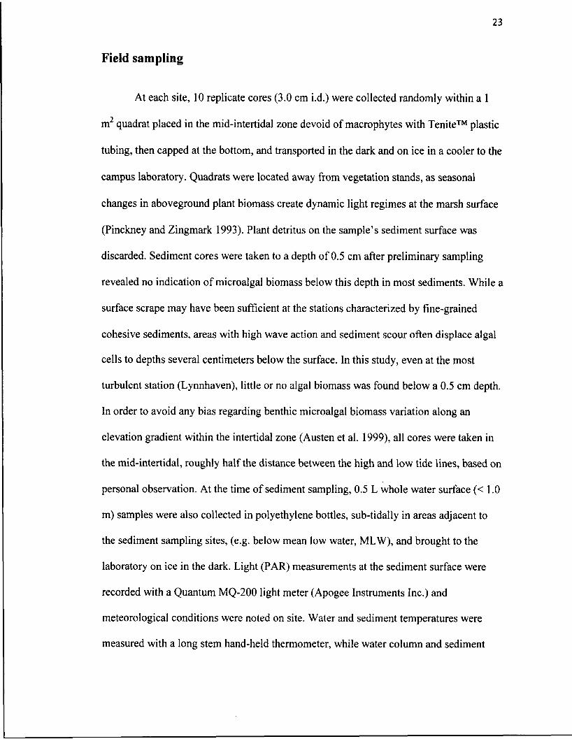
Field sampling
At each site, 10 replicate cores (3.0 cm i.d.) were collected randomly within a 1
m quadrat placed in the mid-intertidal zone devoid of macrophytes with Tenite™ plastic
tubing, then capped at the bottom, and transported in the dark and on ice in a cooler to the
campus laboratory. Quadrats were located away from vegetation stands, as seasonal
changes in aboveground plant biomass create dynamic light regimes at the marsh surface
(Pinckney and Zingmark 1993). Plant detritus on the sample’s sediment surface was
discarded. Sediment cores were taken to a depth of 0.5 cm after preliminary sampling
revealed no indication of microalgal biomass below this depth in most sediments. While a
surface scrape may have been sufficient at the stations characterized by fine-grained
cohesive sediments, areas with high wave action and sediment scour often displace algal
cells to depths several centimeters below the surface. In this study, even at the most
turbulent station (Lynnhaven), little or no algal biomass was found below a 0.5 cm depth.
In order to avoid any bias regarding benthic microalgal biomass variation along an
elevation gradient within the intertidal zone (Austen et al. 1999), all cores were taken in
the mid-intertidal, roughly half the distance between the high and low tide lines, based on
personal observation. At the time of sediment sampling, 0.5 L whole water surface (< 1.0
m) samples were also collected in polyethylene bottles, sub-tidally in areas adjacent to
the sediment sampling sites, (e.g. below mean low water, MLW), and brought to the
laboratory on ice in the dark. Light (PAR) measurements at the sediment surface were
recorded with a Quantum MQ-200 light meter (Apogee Instruments Inc.) and
meteorological conditions were noted on site. Water and sediment temperatures were
measured with a long stem hand-held thermometer, while water column and sediment

24
pore-water salinity were determined with water placed in a hand-held refractometer
(Fisher Scientific). Sediment grain size was analyzed for every benthic collection (n = 78)
via the same coring method used for taxonomic and productivity analyses. Grain size
measurements were carried out using a Malvern Mastersizer laser particle analyzer.
Phytoplankton and Sediment Community Analysis
Water column samples for taxonomic analysis were processed by a modified
Utermohl protocol (Marshall et al. 2006). Upon arrival in the laboratory, replicate water
samples (500 ml) were fixed with Lugol’s solution, and pooled to create a composite
sample, and processed through a series of settling and siphoning steps to produce a 30 -
40 ml concentrated phytoplankton sample. The concentrate was then settled via serial
dilution into a settling chamber and examined with an inverted light microscope (Nikon
Eclipse TS100) for algal species composition and abundance.
Sediment algal samples were sectioned to a depth of 0.5 cm (core area: 7.065
cm ), ensuring that the sediment surface was perpendicular to the long axis of the cores to
minimize unevenness in the thickness of the surficial 0.5 cm. Two 0.5 cm subsections
were pooled together, fixed with Lugol’s solution, and diluted to 500 ml with filtered
water from each site. From this volume, a known volume was placed in a settling
chamber, and examined with an inverted light microscope (Nikon Eclipse TS100) for
species composition and abundance.
Microalgae from both the water column and sediment were counted using a
minimum-count basis of 200 cells and 10 random fields at 315X to determine dominant

25
taxa, after which, the entire settling chamber surface was scanned at 125X for net
microalgal abundance. Algal taxa were identified to the generic level, and when possible,
to species. Microalgal biomass both in the water column and the sediment was calculated
based on a carbon content per bio-volume estimate according to Smayda (1978).
Sediment Grain-Size Analysis
A superficial 0.5 cm slice of sediment core from each site was also examined for
sediment grain size analysis during each sampling period at every site. Sediment cores for
grain size analysis were processed following the protocol of Folk (1980). Initially,
sediment core slices were dried at 100°C for 24 hrs to remove all water from the samples.
Samples were weighed to obtain dry weight and combusted at 550°C for 6 hrs in a muffle
furnace (Jesus et al. 2009). Granulometric analysis was completed via laser analysis in a
Malvern Mastersizer 2000 (Malvern Instruments Ltd.). Statistics of grain size distribution
were calculated according to Folk (1980). Sediments were categorized according to mean
grain size (Wentworth 1922) and placed into the following classes: coarse silt or silts and
clays (<63 pm), very fine sands (63 - 125 pm), fine sands (125 - 250 pm), medium sands
(250 - 500 pm), and coarse sands (>500 pm).

26
Primary Productivity
The protocol described below has been the standard method for determination of
Chesapeake Bay phytoplankton primary productivity since 1989 (Marshall and Nesius
1996). This protocol involves exposing the organisms of interest (sediment and water
column microalgae) to inorganic radio-labeled carbon (14C) which is then taken up by the
microalgae during incubation and incorporated in their biomass, which can then be
quantified using a scintillation counter (Beckman LSI701).
While there is no current standard method in place for the measurement of
microphytobenthic primary production, there are several widely used methods. Two
common approaches are the oxygen microelectrode method (Revsbech and Jorgensen
1983) and the l4C uptake method (Strickland and Parsons 1972), with the latter having
several variations. The 14C uptake/slurry method chosen for the measurement of
microphytobenthic primary productivity in this study was based primarily on logistical
constraints. Unlike intact sediment cores, the slurry method allows the radioisotope to
evenly reach all layers of sediment and microalgae within those layers (Jonsson 1991,
Underwood and Kromkamp 1999, Cibic et al. 2008). Additionally, depending on the
consistency of the sediments being sampled, obtaining and maintaining a complete intact
sediment core may not be possible. One drawback of the slurry method is that it destroys
existing microgradients at the sediment surface, which may affect algal photosynthetic
rates, in addition to exposing microalgae from deeper layers to the same light regimes as
microalgae at the sediment surface. Therefore, this method measures the rate of potential
primary production (Underwood and Kromkamp 1999).

27
Cores were sectioned to 0.5 cm depth, obtaining a 3 ml volume equivalent, and
diluted to 100 ml in filtered seawater from each corresponding site. Each dilution was
sub-sampled (2.0 ml) and re-suspended up to 100 ml with filtered seawater from each site
following a modified protocol from Cibic et al. (2008). Sediment samples were placed in
250 ml acid-washed milk-dilution bottles inoculated with 50 pi NaH14C03 and incubated
at saturated light conditions for ca. 2 hr.
Similar to the sediment samples, water column samples were inoculated with 50
pi NaH14CC>3 and incubated simultaneously with sediment samples, with incubator water
temperature maintained at the same temperature as that recorded at the collection site.
Light intensity in the incubator was kept constant at 500 pE, which is sufficient for near
maximum potential for autotrophy (Rizzo et al. 1996).
For both sediment and water column samples, triplicate light and duplicate dark
samples were incubated, along with a time-zero 14C-incorporation control. After
incubation, 15 ml subsamples of each sample were filtered through a 0.45 p Millipore
filter. Filtered samples were then fumed over HC1 for 24 hr and added to 7 ml
scintillation cocktail (Scintisafe). Samples were analyzed on a Beckman LSI701 liquid
scintillation counter along with 14C standards to determine reactivity of the isotope added
to each sample. Sample alkalinity was measured via standard titration methods (Palmer
1992) to calculate the amount of inorganic carbon present at each sampling site. Carbon
fixation rates for the water column were determined according to Strickland and Parsons
(1972) using the following formula:

28
(Rs - R b) x A x Ft x 1 .0 5
R x N
Where:
R s = counting rate of sample Rb = counting rate of blank A = total carbonate alkalinityFt = approximated to 0.95; coverts carbonate alkalinity to total carbon dioxide 1.05 = isotope coefficient, since uptake of l4C is 5% lower than the uptake of l2C R = reactivity of l4C N = incubation time (hr)
Rates for the sediment community, expressed as a rate per area (mg C m'2 hr'1) were
calculated following a modified equation from Cibic et al. (2008):
C02 x * 0 . 0 0 1 ) x DPMl„d x K l x 1 .0 5
DPM ( 5 7 ) X T x 7 .0 6 5 x 1 0 ~ 4
Where:
CO2 = alkalinity of the overlying water used to suspend the sediment 15/100 = the filtered volume from the 100 ml incubated3.4 = coverts volume of incubation bottle from ml to LDPMl-d = average disintegrations per minute (3 light minus 2 dark)K1 = 1416, the dilution factor derived from all dilutions of initial core1.05 = isotope coefficient, since uptake of 14C is 5% lower than the uptake of 12C DPM (ST) = activity of the 14C standard solutionT = incubation time (hr)7.065 = core area in cm2 1 O'4 = converts cm2 of the core area into m2
Statistical Analyses
Variability of productivity rates, both temporally (within stations) and spatially
(between stations) was tested using an analysis of variance (ANOVA) series using IBM

29
SPSS version 20. Variability of community structure, both temporally and spatially was
tested using ordination analysis. Ordination analyses were used to determine the effects
of multiple environmental factors (temperature, salinity, grain size (sediment samples
only) controlling the variability of both primary productivity and community structure.
Non-metric multidimensional scaling (NMS) was carried out using PC-ORD version 5.33
on the “slow and thorough” autopilot mode, using a Bray-Curtis distance matrix.

30
CHAPTER III
RESULTS - COMMUNITY COMPOSITION, ABUNDANCE, AND
BIOMASS
This study included a total of 78 collection events, with both the phytoplankton
and microphytobenthos sampled during each collection event. Two stations (Cape
Charles and Great Wicomico) were not collected during 2010 winter due to adverse
weather restrictions. Twice yearly summer collections were averaged to create a
composite summer season at each station. Initial analysis of all data collected indicated
significant differences between habitats with the phytoplankton and microphytobenthos
differing across all attributes. The phytoplankton community had significantly higher
species richness (p = 0.024) and primary productivity rates (p = 0.004), however, total
abundance (p < 0.0001), biomass (p = 0.005), and the Shannon Index of diversity (p <
0.0001) were significantly higher in the benthos. As such, further analyses treated each
habitat as separate data sets. In instances where significant differences were found within
each habitat, Tukey post-hoc tests were performed to identify significant differences
among stations. Among all phytoplankton collections, no significant differences were
observed for any of the measured parameters (Table 1). Conversely, among the
microphytobenthos, significant differences were recorded for all parameters except
species richness (Table 2). In several instances, primary productivity measurements were
discarded, as control experiments revealed abnormally low reactivity of stock solutions,
and considering the sensitivity of the method, these rates were deemed inaccurate.

31
Table 1 Summary of analysis of variance tests of phytoplankton parameters across all stations.
Df f PAbundance 7 1.505 0.186Biomass 7 1.056 0.404Productivity 7 1.371 0.243Species Richness 7 2.014 0.070Shannon Index 7 0.552 0.791
Table 2 Summary of analysis of variance tests of microphytobenthic parameters across all stations. * indicates significance at the p < 0.05 level._________ ________________
Df f PAbundance 7 3.151 0.007*Biomass 7 2.434 0.030*Productivity 7 5.411 0.000*Species Richness 7 1.996 0.072Shannon Index 7 6.578 0.000*Phi value 7 15.802 0.000*

32
Community Composition
Over the 2-year study, a total of 142 taxa were identified (Table 3). These
included 124 taxa in the phytoplankton, with 64 diatoms representing 52% of the taxa,
dinoflagellates 17%, chlorophytes 11%, and cyanobacteria 10%. Other taxa present
included charophytes, cryptophytes, chrysophytes, euglenophytes, haptophytes, and
ochrophytes. The microphytobenthic communities were represented by 95 taxa and were
similarly dominated by diatoms (61%), followed by cyanobacteria (18%), and
chlorophytes (8%), with other groups less common and rarely present.
Species richness was significantly higher in the phytoplankton than in the benthos
(p = 0.024) throughout the duration of the study (Fig. 2), with a broad range of species
present across both habitats (Tables 4 and 5). The phytoplankton species richness
averaged 33 and ranged from a high of 47 (Lynnhaven, winter 2011), to a low of 20
(Great Wicomico spring 2011). Among the microphytobenthos, species richness
averaged 22 and ranged from 41 (Harborton, winter 2010) to its lowest of 7 (New Point
Comfort, winter 2011). Conversely, the Shannon Index of diversity (Hf) (Fig. 3) was
significantly higher in the benthos than in the phytoplankton (p = 0.000). Shannon indices
in the phytoplankton (avg. 1.67) ranged from a high of 2.29 (Lynnhaven, spring 2010) to
a low of 0.36 (Great Wicomico, fall 2011). In the benthos, H' (avg. 2.39) ranged from
3.57 (Lafayette, winter 2010) to 0.64 (Lynnhaven, winter 2011), and differed
significantly across all stations sampled (p < 0.0001).

Table 3 Species inventory of taxa identified in the phytoplankton and benthos.Phytoplankton Benthos
BacillariophytaAmphiprora sp. X XAmphora sp. X XAsterionellaformosa XAsterionellopsis glacial is X XAulacoseira granulata X XAulacoseira sp. X XBacillaria paxillifer X XCerataulina pelagica X XChaetoceros neogracilis XChaetoceros pendulus XChaetoceros sp. X XChaetoceros subtilis X XCocconeis sp. X XCorethron sp. X XCoscinodiscus sp. X XCyclotella spp. X XCyclotella striata X XCylindrotheca closterium X XCymbella sp. X XDactyliosolen fragilissimus X XDelphineis surirella X33iatom asp. X XDiploneis sp. X XDitylum brightwellii X XEucampia zodiacus XEunotia sp. X XFragilaria sp. X XGomphonema sp. XGrammatophora sp. X XGuinardia delicatula X XGuinardiaflaccida XGyrosigma balticum X XGyrosigma fasciola X XGyrosigma sp. X XHemiaulus hauckii X XHemiaulus sp. X XLeptocylindrus danicus XLeptocylindrus minimus XLicmophora sp. X XMelosira moniliformis X XMelosira varians XNavicula sp. X XNitzschia sp. X XOdontella mobiliensis XOdontella rhombus f. trigona X

Table 3 ContinuedPhytoplankton Benthos
BacillariophytaOdontella sinensis X XOdontella sp. X XParalia sulcata X XPinnularia sp. X XPlagiogramma sp. X XPleurosigma angulatum XPleurosigma sp. X XProboscla alata X XPseudo-nitzschia pungens XPseudo-nitzschia seriata X XRhaphoneis amphiceros X XRhaphoneis sp. X XRhizosolenia imbricata XRhizosolenia setigera X XRhizosolenia sp. XRhizosolenia styliformis XSkeletonema costatum X XSkeletonema potamos XStephanopyxis palmeriana XStriatella sp. X XSurirella sp. X XSynedra sp. X XTabellaria sp. XThalassionema nitzschioides X XThalassiorsira leptopus XThalassiosira sp. XTriceratium sp. X X
CharophytaCosmarium sp. XDesmidium sp. XSpirogyra sp. X XStaurastrum sp. X
ChlorophytaAnkistrodesmus falcatus X XAnkistrodesmus falcatus var. mirabilis
X
Chlamydomonas sp. XCrucigenia irregularis XCrucigenia sp. XCrucigenia tetrapedia XDictyosphaerium sp. XDimorphococcus lunatus XOocystis sp. XPandorina sp. X

Table 3 ContinuedPhytoplankton Benthos
ChlorophytaPediastrum duplex XPediastrum duplex gracilimum XPyramimonas sp. X XScenedesmus acuminatus XScenedesmus dimorphus XScenedesmus quadricauda X XTetraedron sp. XUlothrix sp. X X
CryptophytaCryptomonas erosa X XCryptomonas sp. X X
ChrysophytaEbria tripartita X X
CyanobacteriaAnabaena sp. X XAphanocapsa sp. XAphanothece gelatinosa XAphanothece sp. XChroococcus dispersus XChroococcus sp. X XChroococcusturgidus XDactylococcopsis raphidioides X XDactylococcopsis sp. XLyngbya aestuarii X XLyngbya sp. XMerismopedia elegans X XMerismopedia tenuissima X XMicrocystis incerta X XPhormidium sp. X XPseudanabaena sp. X XSpirulina sp. X X
DinophytaAmphidinium sp. XCeratium furca XCeratium fusus XCeratium schroeteri XCochlodinium heterolobatum XDinophysis sp. XDiplopsalis lenticula XGonyaulax sp. XGymnodinium sp. X XGyrodinium aureolum X

Table 3 ContinuedPhytoplankton Benthos
DinophytaGyrodinium sp. X XHeterocapsa triquetra XKatodinium rotundatum XPolykrikos kofoidii XProrocentrum gracile XProrocentrum micans X XProrocentrum minimum X XProrocentrum triestinum XProtoperidinium mite XProtoperidinium sp. XScrippsiella trochoidea X X
EuglenophytaEuglena acus XEuglena elastic X XEuglena proximo XEuglena sp. X X
HaptophytaRhabdosphaera hispida X
OchrophytaDictyocha fibula X XSynura uvella X X
El p h y to p la n k to n
B b e n t h o s
w in t e r s u m m e rsp r in g
Fig. 2 Two-year average species richness in phytoplankton and benthic samples.

Table 4 Phytoplankton diversity indices for each year and season of study. SR = species richness, H' = Shannon Index, NC = not collected. Stations denoted as: SXS = Saxis, HARB = Harborton, CC = Cape Charles, LYNN = Lynnhaven, LAF = Lafayette, HAMP = Hampton, NPC = New Point Comfort, GWR = Great Wicomico._______________________________________________________ _
2010 2011
Winter Spring Summer Fall Winter Spring Summer FallSXS 42; 0.41 34; 1.64 35; 1.58 40; 2.03 33; 1.44 31; 1.90 30; 1.62 30; 1.86HARB 33; 0.79 38; 2.12 33; 1.63 30; 2.05 38; 1.91 26; 1.88 27; 1.41 35; 2.19CC NC 27; 2.14 37; 1.88 46; 1.64 29; 1.69 31; 1.58 37; 1.88 42; 2.25LYNN 37; 1.30 37; 2.29 41; 1.81 43; 1.71 47; 1.87 34; 1.21 33; 1.23 37; 2.09LAF 33; 0.60 27; 1.93 29; 1.93 30; 1.82 30; 0.85 30; 1.85 23; 1.59 27; 1.74HAMP 41; 1.79 28; 2.13 33; 1.30 31; 1.75 46; 1.94 25; 1.17 28; 1.39 31; 1.96NPC 37; 1.42 25; 1.72 36; 1.98 36; 2.12 23; 1.60 35; 1.50 33; 1.67 33; 2.02GWR NC 25; 2.00 32; 1.95 32; 1.96 29; 2.06 20; 1.17 32; 1.23 21; 0.36
Table 5 Microphytobenthos diversity indices for each year and season o f study. SR = species richness, H' = Shannon Index, NC = not collected. Stations denoted as: SXS = Saxis, HARB = Harborton, CC = Cape Charles, LYNN = Lynnhaven, LAF = Lafayette, HAMP = Hampton, NPC = New Point Comfort, GWR = Great Wicomico._________________________________________________________
2010 2011
Winter Spring Summer Fall Winter Spring Summer FallSXS 30; 2.98 22; 2.83 21; 1.75 25; 3.26 21; 2.53 19; 2.13 18; 2.30 22; 2.53
HARB 41; 2.74 22; 1.95 29; 2.34 23; 0.77 22; 1.74 19; 0.81 23; 1.05 22; 1.50CC NC 25; 2.45 23; 2.85 24; 1.38 23; 2.68 26; 2.64 22; 2.50 25; 2.96
LYNN 23; 2.43 25; 2.86 18; 2.16 19; 2.60 15; 0.64 16; 1.59 16; 2.08 19; 0.90LAF 33; 3.57 25; 3.17 24; 2.46 21; 2.31 29; 3.32 16; 2.47 19; 2.53 24; 3.02
HAMP 35; 3.55 29; 2.92 28; 3.11 22; 2.72 18; 2.54 23; 2.32 21; 2.73 23; 2.63NPC 11; 1.84 25; 2.60 22; 2.57 18; 2.45 7; 1.60 13; 1.56 19; 1.74 13; 1.44GWR NC 21; 3.27 31; 3.43 25; 2.56 27; 3.49 14; 2.41 20; 2.80 25; 3.16

38
El p h y to p la n k to n
□ b e n t h o s
w in t e r sp r in g s u m m e r
Fig. 3 Two-year average of Shannon Index of biodiversity in phytoplankton and benthic samples.

39
Seasonal trends in composition and biomass were apparent throughout the study
in both habitats. The phytoplankton community was dominated by diatoms in winter and
early spring, with dinoflagellates co-dominating with diatoms from late spring throughout
summer and early fall, before returning to a winter, diatom-rich community (Figs. 4, 5).
The micophytobenthos followed a similar pattern of seasonality, with these habitats
comprised of diatoms throughout winter and spring, with a gradual shift to a mixed
community of diatoms, cyanobacteria, and chlorophytes during late spring and early
summer, before returning to mainly a fall/winter diatom population (Figs. 6, 7). These
trends were apparent in both cell abundance and biomass for both phytoplankton and
microphytobenthic communities.

40
1 8 ,0 0 0
1 6 ,0 0 0
1 4 ,0 0 0
12,000
E 1 0 ,0 0 0
g 8,000
6,000
4 ,0 0 0
2,000
0 H w in te r
ll O th e r s
*'• D in o p h y ta
■ C y a n o b a c te r ia
= C ry p to p h y ta
IB C h lo ro p h y ta
□ B acillia rio p h y ta
sp rin g s u m m e r fall
Fig. 4 Two-year average phytoplankton abundance (cells/ml) across all stations.
PIKS 'S 'S ,
PPPPPPPPPi**ls*A*A*A*A»S*N'S'V'S'S*v..
r^^^^ppppppppppppppiPpr>yM>f pppppppppppppppwfifip'™™S'S • •"» . *» . ■» ■*.•■»•■.**» "S« ■»
NjSrt,
ll O th e r s
* D in o p h y ta
■ C y a n o b a c te r ia
:= C ry p to p h y ta
m C h lo ro p h y ta
□ B acillia rio p h y ta
w in te r sp r in g su m m e r
Fig. 5 Two-year average phytoplankton biomass (ug C/ ml) across all stations.

o H- - - - - - - - - - - - - - - - - - - - - - - - 1- - - - - - - - - - - - - - - - - - - - - - - - - 1- - - - - - - - - - - - - - - - - - - - - - - -w in te r sp r in g su m m e r fall
I-----------------------------------------------------------------------------------------------------------------------------------------------------------------------------*-----------------------1Fig. 6 Two-year average microphytobenthos abundance (cells/cm ) across all stations.
2 5 0
200
150
uBO3 100
5 0
0 Hw in te r sp r in g su m m e r
ll O th e r s
* D in o p h y ta
■ C y a n o b a c te r ia
= C ry p to p h y ta
■ C h lo ro p h y ta
□ B acillia rio p h y ta
fall
Fig. 7 Two-year average microphytobenthic biomass (ug C/cm ) across all stations.

42
Phytoplankton Abundance
Phytoplankton Abundance - 2010
Total phytoplankton cell abundance was highest during the 2010 winter (Fig. 8),
with cell densities at all stations > 104 cells/ml, with a peak density (> 7.0 X 10⁴ cells/ml)
at the Saxis station, which was mainly composed of dense concentrations of the centric
diatom Skeletonema costatum (> 6.5 X 10⁴ cells/ml). Diatoms dominated cell abundances
at all stations during 2010. Densities dropped in the 2010 spring (Fig. 9), with all
concentrations < 7.0 X 10³ cells/ml at each station, and were again highest at the Saxis
station (> 6.0 X 10³ cells/ml). The cyanobacteria and dinoflagellates were present at all
stations. Cell abundances increased during the 2010 summer (Fig. 10), but did not attain
densities noted in winter. Diatoms, along with filamentous cyanobacteria composed the
majority of algal taxa. Fall densities mirrored those in the spring (103- 4.0 X 10³
cells/ml), with an assemblage of diatoms, cyanobacteria, and cryptophytes representing
the dominant algae present (Fig. 11). Prominent algal taxa throughout the 2010 sampling
period included the diatoms S. costatum, Cerataulina pelagica, Cylindrotheca closterium,
and Chaetoceros sp., plus the dinoflagellate Gonyaulax sp., cryptomonad Cryptomonas
sp., and cyanobacteria Pseudanabaena sp.

43
8 0 ,0 0 0
7 0 .0 0 0
6 0 .0 0 0
_ 5 0 ,0 0 0 E
^ 4 0 ,0 0 0
8 3 0 ,0 0 0
20,000 -
10,000
0 Q
K°
m o t h e r s
0 D in o p h y ta
■ C y a n o b a c te r ia
□ C ry p to p h y ta
■ C h lo ro p h y ta
□ B ac illa rio p h y ta
Fig. 8 Phytoplankton abundance for winter 2010. Cape Charles and Great Wicomico not collected due to weather.
7 .0 0 0
6.000
5 .0 0 0
E 4 ,0 0 0JAg 3 ,0 0 0
2.000
1,000
0
^ 4 ?<? <sc°J ' ^ cr „$■
\?X*'x°
□ O th e r s
□ D in o p h y ta
■ C y a n o b a c te r ia
0 C ry p to p h y ta
11 C h lo ro p h y ta
□ B acillia rio p h y ta
Fig. 9 Phytoplankton abundance for spring 2010.

44
12,000
10,000
8,000
v> 6 ,0 0 0
I4 ,0 0 0
2,000 -
ID O th e rs
ES D in o p h y ta
■ C y a n o b a c te r ia
H C ry p to p h y ta
O C h lo ro p h y ta
□ B acillia rio p h y ta
Fig. 10 Phytoplankton abundance for summer 2010.
5 .0 0 0
4 .000
1 3 ,0 0 0
8 2,000
1.000
0
□ O th e r s
Q D in o p h y ta
■ C y a n o b a c te r ia
B C ry p to p h y ta
■ C h lo ro p h y ta
&
xc, □ B a c il l ia r io p h y ta
Fig. 11 Phytoplankton abundance for fall 2010.

45
Phytoplankton Abundance - 2011
Microalgal abundances in 2011 followed similar trends as those the previous year.
In winter, cell densities ranged from 1.0 X 10³ - 1.4 X 10⁴ cells/ml (Fig. 12), with the
diatom S. costatum again dominant. Spring densities regressed, with all but one station
(Saxis) having cell abundances < 4.0 X 10³ cells/ml (Fig. 13). Taxonomic composition
was generally split between diatoms and cyanobacteria during spring, with the diatoms
S.costatum and C. closterium, and cyanobacteria Pseudanabaena sp. and Merismopedia
elegans being dominant. In the 2011 summer there was an increase of phytoplankton cell
densities, though no station had densities > than 1.0 X 10⁴ cells/ml (Fig. 14). The diatom
C. closterium was in high densities at every station during the 2011 summer, with the
highest density at the Hampton site (> 7.0 X 10³ cells/ml). In general, diatoms and
filamentous cyanobacteria dominated cell abundances at every station during the
summer. Fall cell densities exhibited a similar pattern in 2011 (as those in 2010), with
abundances between 103 and 5.0 X 10³ cell/ml (Fig. 15), except for high numbers at
Great Wicomico (> 1.3 X 10⁴ cells/ml) and Saxis (> 1.8 X 10⁴ cells/ml), that were driven
by high densities of C. closterium and several pennate diatoms, respectively.

46
1 6 ,0 0 0
1 4 .0 0 0
12.000
_ 10,000 Ejir 8,ooo 8 6,000
4 .0 0 0
2.000
0 -E 3 -
m
vA'
ID O th e r s
□ D in o p h y ta
■ C y a n o b a c te r ia
B C ry p to p h y ta
□ C h lo ro p h y ta
n □ B acillia rio p h y ta
Fig. 12 Phytoplankton abundance for winter 2011.
8,000
7 ,0 0 0
6,0005 ,0 0 0
^ 4 ,0 0 0
3 ,0 0 0
2,000
1,000
□ O th e r s
□ D in o p h y ta
■ C y a n o b a c te r ia
B C ry p to p h y ta
□ C h lo ro p h y ta‘“I□ B acillia rio p h y ta
Fig. 13 Phytoplankton abundance for spring 2011.
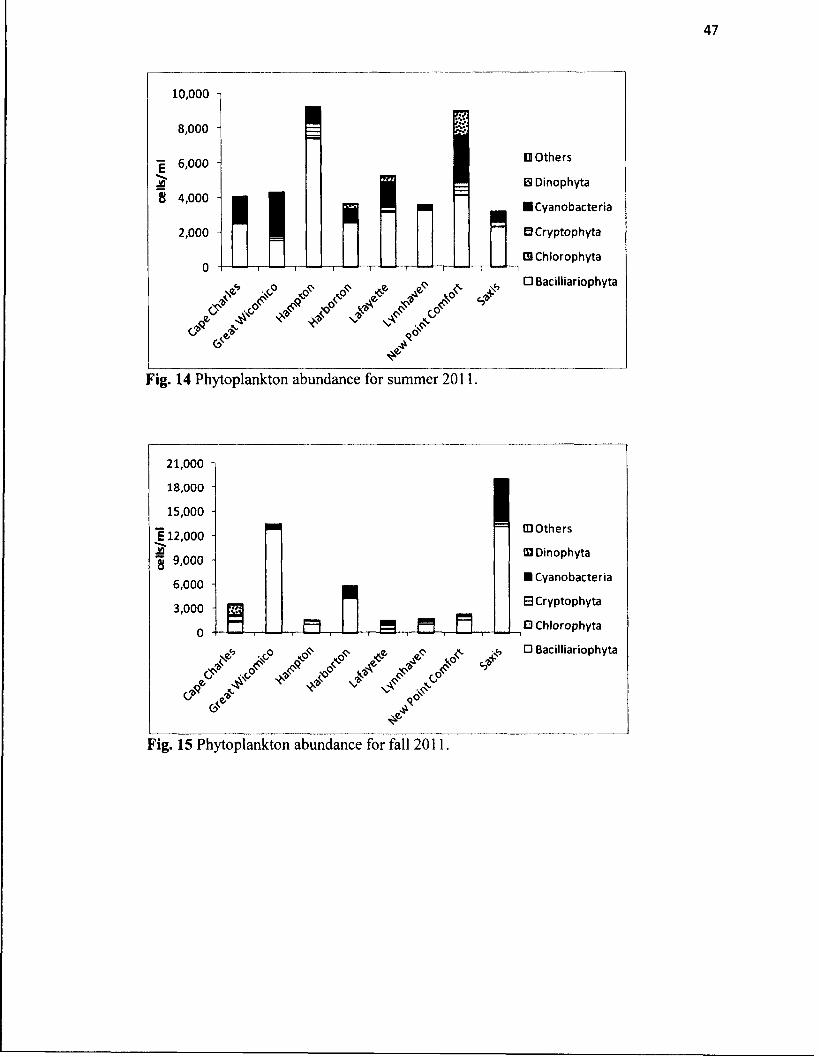
47
10,000 -)
8,000
g 6,000
8 4 ,0 0 0
2,000
0 ~r T t ~r
□ O th e r s
B D in o p h y ta
■ C y a n o b a c te r ia
B C ry p to p h y ta
El C h lo ro p h y ta
<T
tK ,h □ B acillia rio p h y ta
Fig. 14 Phytoplankton abundance for summer 2011.
21,000
18,000
1 5 ,0 0 0
112,000 -
I 9 ,0 0 0
6,000 -
3 ,0 0 0
0
<N*<? a?'
f t ^ < /
vP'
I
oF•O' f o
✓
m o t h e r s
EJ D in o p h y ta
■ C y a n o b a c te r ia
E C ry p to p h y ta
£3 C h lo ro p h y ta
□ B acillia rio p h y ta
Fig. 15 Phytoplankton abundance for fall 2011.

48
Phytoplankton Biomass
Phytoplankton Biomass - 2010
The 2010 phytoplankton biomass values for winter ranged from 0.6 - 3.3 ug
C/ml, and consisted mainly of diatoms, which were the dominant flora during this
sampling period (Fig. 16). In spring there was a shift in biomass, produced by a diatom-
dominated flora, to that of dinoflagellates, with these taxa almost doubling the biomass of
diatoms across all stations (Fig. 17). The dinoflagellate biomass was highest in the
Lafayette (2.08 ug C/ml), where Gymnodinium sp. and Gonyaulax sp. were the dominant
taxa, and in the Great Wicomico site (1.12 ug C/ml), where high Gyrodinium sp.,
Gymnodinium sp., and Scrippsiella trochoidea were present. The summer of 2010 had
similar distributions of diatom and dinoflagellate biomass across all stations (Fig. 18).
New Point Comfort contained the highest dinoflagellate biomass (2.10 ug C/ml) during
this sampling period, with the Lafayette having values (1.21 ug C/ml) also high, and
likely the result of a Cochlodinium polykrikoides bloom in August of that year. The fall
had similar patterns of algal biomass with the winter (Fig. 19) dominated by diatoms, but
these values were lower at most stations < 0.5 ug C/ml).

49
3.5
3 i
2.5
E 2 o'Sf 1.5
1 - 0.5 -
0
<S>*
222
O'rP IT^ . <v*
vO •t?
[D O th e rs
□ D in o p h y ta
■ C y a n o b a c te r ia
□ C ry p to p h y ta
□ C h lo ro p h y taI□ B ac illa rio p h y ta
Fig. 16 Phytoplankton biomass for winter 2010. Cape Charles and Great Wicomico not collected due to weather.
2.5 i
i 15
S’ i
0.5 i
0
xP■ xP*v
nto &
01 O th e r s
□ D in o p h y ta
■ C y a n o b a c te r ia
0 C ry p to p h y ta
□ C h lo ro p h y taI
□ B acillia rio p h y ta
Fig. 17 Phytoplankton biomass for spring 2010.

50
3.5
3
2.5
E 2 Zj» 1.5
10.5
0
to
1*7*1tolM
vv\«s
. B , -
JBto?to)&>•/!>•/<
Ctoj r / <■*
■toO'0.0t o
to"
t oto
t o .tot o
vOt o
•o’oto
t o t o "
t o
Q] O th e r s
C9 D in o p h y ta
■ C y a n o b a c te r ia
0 C ry p to p h y ta
DD C h lo ro p h y ta
□ B acillia rio p h y ta
Fig. 18 Phytoplankton biomass for summer 2010.
0.8
sta0 .4
0.2
t o t o t o/ <** * t o
t o
t o to* t oto
O'" .o’" ^
to
toto
to
□ O th e r s
□ D in o p h y ta
■ C y a n o b a c te r ia
S C ry p to p h y ta
ID C h lo ro p h y ta
□ B a c il l ia r io p h y ta
Fig. 19 Phytoplankton biomass for fall 2010.

51
Phytoplankton Biomass - 2011
High microalgal diatom biomass during the 2011 winter was similar to the
previous year, except for two stations (Lafayette and Great Wicomico) that had high
dinoflagellate biomass of 0.48 ug C/ml and 0.39 ug C/ml respectively (Fig. 20). These
high dinoflagellate values came from the same taxa present during the winter and spring
of 2010. These were Gymnodinium sp., and S. trochoidea, plus Gyrodinium aureolum.
The spring biomass values were below 0.5 ug C/ml at most stations (Fig. 21) that were
dominated by diatom biomass, except for high concentrations of the dinoflagellates
Gymnodinium sp. and Heterocapsa rotundatum at the Lafayette site. The 2011 summer
had a slight increase in overall biomass, though most stations had values below 1.0 ug
C/ml including several stations < 0.5 ug C/ml (Fig. 22). Diatoms continued to constitute
the majority of the biomass at all stations, except for New Point Comfort, which had
elevated dinoflagellate biomass (1.85 ug C/ml) due to the increased Gonyaulax sp.
concentrations. Fall 2011 exhibited a broad range of biomass values, from 0.1 ug C/ml in
the Lafayette, to 2.6 ug C/ml at Saxis (Fig. 23). Diatoms again composed the majority of
the biomass at all stations except Cape Charles, which had increased densities and
biomass of the dinoflagellates Gymnodinium sp., Prorocentrum minimum, and
Heterocapsa triquetra.
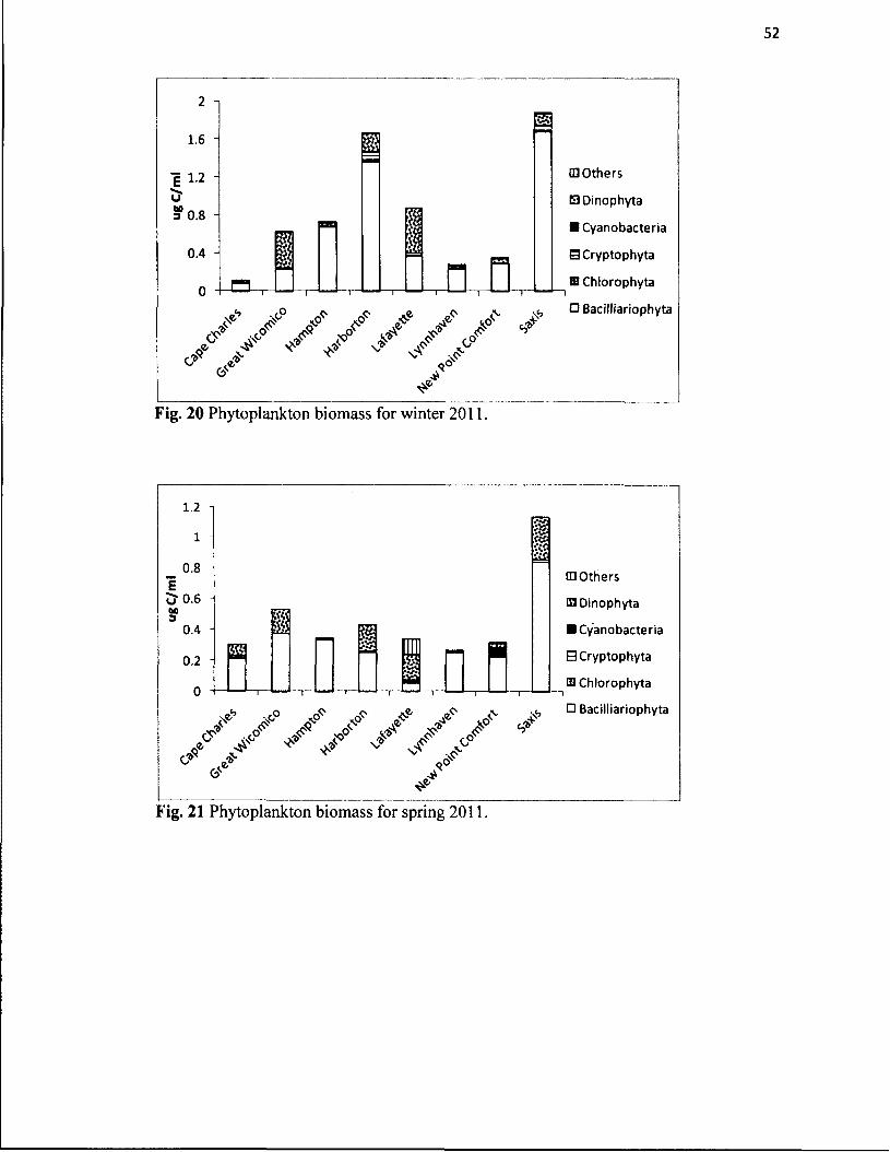
52
1.6 -
£ 1.2
a 0.8
0 .4
0
Ww•s+s
PPHi
n.«• rP .cf" -O •$?' ,
,e r _J* jo? ' g ? X < /'?"
is0V'
(S'
[□ O th e r s
□ D in o p h y ta
■ C y a n o b a c te r ia
S C ry p to p h y ta
E C h lo ro p h y ta
[V Ne, O B acillia rio p h y ta
Fig. 20 Phytoplankton biomass for winter 2011.
1.2
l
_ 0.8 Eu 0.6as3
0 .4
0.2
0
< /
■Aiii.itfiw
^ o°'
/K° ■is’
m o t h e r s
□ D in o p h y ta
■ C y a n o b a c te r ia
0 C ry p to p h y ta
E C h lo ro p h y ta1□ B acillia rio p h y ta
Fig. 21 Phytoplankton biomass for spring 2011.

53
3 i
2 .5
2Eo ' 1-5 00 3
1
0 .5
0 n< f a?
w4jS
55•U
v0oV" .X
<P X^^ V*
#f X•V O'
*P rf?
□ O th e r s
□ D in o p h y ta
■ C y a n o b a c te r ia
B C ry p to p h y ta
t ! C h lo ro p h y ta
i> □ B a c il l ia r io p h y ta
Fig. 22 Phytoplankton biomass for summer 2011.
3
2.5 i
2Eo ' 1.5 w3
1
0.5
0
<? <<? rV* oS
n✓
^ << « x>°
V
^ 4 ^ vP
*V / /
£>
m o t h e r s
□ D in o p h y ta
■ C y a n o b a c te r ia
B C ry p to p h y ta
□ C h lo ro p h y ta
□ B acillia rio p h y ta
Fig. 23 Phytoplankton biomass for fall 2011.

54
Microphytobenthic Abundance
Microphytobenthic Abundance - 2010
Across all stations during both sampling years, the benthic microalgal abundance
was significantly higher (p < 0.0001) than the pelagic phytoplankton abundance. The cell
densities were generally in the 1.0 X 10⁵ cells/cm3 range and frequently eclipsing 106
cells/cm3, whereas phytoplankton densities were generally below 5.0 X 10³ cells/ml. In
the winter of 2010, the benthic cell abundance was mainly comprised of diatoms except
at one station (Harborton) where cell densities > 106 cells/cm3 of the cyanobacteria
Phormidium sp. were present (Fig. 24). In spring, the benthos remained dominated by
diatoms (Fig. 25), though increasing numbers of cyanobacteria were present, namely
Anabaena sp., Aphanocapsa sp., and Lyngbya aestuarii. The diatoms Fragilaria sp.,
Gyrosigma sp., Navicula sp., and Melosira moniliformis were most abundant at all
stations during spring 2010. During the 2010 summer, algal densities increased (Fig. 26)
with all but two stations having counts over 106 cells/cm3. These algae were dominated
by cyanobacteria at nearly every station, with L. aestuarii, Merismopedia elegans,
Chroococcus sp., and Anabaena sp. the most abundant taxa. Cyanobacteria continued to
dominate into the fall of 2010 at all stations (Fig. 27). During summer the total cell
abundance declined at the Saxis, Lynnhaven, and Hampton sites, while increasing in the
other locations, with most remaining above 106 cells/cm3. Much like the previous
sampling season, L. aestuarii, and M. elegans were the dominant taxa.

3 .0 0 0 .0 0 0
2 ,5 0 0 ,0 0 0
2.000.000§
> 1 ,5 0 0 ,0 0 0
81,000,000
5 0 0 ,0 0 0
0 n 1 - □vp
/V
□ O th e r s
□ D in o p h y ta
■ C y a n o b a c te r ia
□ C ry p to p h y ta
O C h lo ro p h y ta
□ B acillia rio p h y ta
Fig. 24 Microphytobenthic abundance for winter 2010. Cape Charles and Great Wicomico not collected due to weather.
1 .4 0 0 .0 0 0
1.200.000
1,000,000
§ 8 0 0 ,0 0 0
I 6 0 0 ,0 0 0
4 0 0 .0 0 0
200.000
0
j&
c*•*
x>° < yX
m o t h e r s
0 D in o p h y ta
■ C y a n o b a c te r ia
B C ry p to p h y ta
■ C h lo ro p h y ta
□ B acillia rio p h y ta
Fig. 25 Microphytobenthic abundance for spring 2010.

56
4.500.000 4,000,0003.500.000
n 3,000,000 g 2,500,000
= 2,000,0008 1,500,000
1,000,000500,000
0
I
□ O th e r s
□ D in o p h y ta
■ C y a n o b a c te r ia
B C ry p to p h y ta
IS C h lo ro p h y ta
□ B acillia rio p h y ta
Fig. 26 Microphytobenthic abundance for summer 2010.
8,000,000
7 .0 0 0 .0 0 0
6.000.000 " 5,000,000
4.000.000
8 3,000,000
2.000.000 -
1,000,000
0
□ O th e r s
O D in o p h y ta
■ C y a n o b a c te r ia
0 C ry p to p h y ta
n ® C h lo ro p h y ta
•i? □ B acillia rio p h y ta
Fig. 27 Microphytobenthic abundance for fall 2010.

57
Microphytobenthic Abundance - 2011
Similar to 2010, diatoms were most abundant in the benthos during the 2011
winter sampling (Fig. 28). Overall cell densities were < 1.0 X 10⁶ cells/cm3 at all but two
stations (Lynnhaven, New Point Comfort). Dominant taxa were Bacillaria paxillifer,
Thalassionema nitzschioides, Gyrosigma sp., and Navicula sp., which had high densities
at all stations. The spring 2011 benthic communities shifted to cyanobacteria, with
densities within the 5.0 X 10⁵ - 106 cells/cm3 range (Fig. 29). The cyanobacteria L.
aestuarii, Anabaena sp., and M. elegans were dense during this season, particularly at the
Harborton site, where M. elegans densities exceeded 3.0 X 10⁶ cells/cm3. Cell densities in
2011 summer increased compared to the previous season, with almost all stations having
abundances > 10 cells/cm (Fig. 30), and all but one station (Lynnhaven) dominated by
cyanobacteria (e.g. Anabaena sp., M. elegans, and L. aestuarii). Microphytobenthic
abundance in the fall of 2011 reverted back to winter conditions, with most stations
falling below the 1.0 X 10⁶ cells/cm3 level, with diatoms the dominant microalgal group
(Fig. 31).
Analysis of variance tests showed significant differences in microphytobenthic
average abundance across stations over the span of this study. Tukey post-hoc tests
revealed both Cape Charles (p = 0.018) and Harborton (p = 0.013) had significantly
higher cell abundances than the Lynnhaven station.

58
2 ,000,000
1 ,6 0 0 ,0 0 0
1,200,000
g 8 0 0 ,0 0 0
4 0 0 ,0 0 0
□ O th e r s
D in o p h y ta
■ C y a n o b a c te r ia
0 C ry p to p h y ta
0 C h lo ro p h y ta
□ B acillia rio p h y ta
v'*' vy J ' > ** < /
Fig. 28 Microphytobenthic abundance for winter 2011.
5 .0 0 0 .0 0 0
4 .0 0 0 .0 0 0
1 3 ,0 0 0 ,0 0 0 -
g 2 ,0 0 0 ,0 0 0
1,000,000
□ O th e r s
13 D in o p h y ta
■ C y a n o b a c te r ia
0 C h lo ro p h y ta
□ B acillia rio p h y ta
Fig. 29 Microphytobenthic abundance for spring 2011.

59
7 .0 0 0 .0 0 0 -|
6.000.0005 .0 0 0 .0 0 0
"§ 4 ,0 0 0 ,0 0 0
= 3 ,0 0 0 ,0 0 0
2.000.000 1,000,000
0
□ O th e r s
E3 D in o p h y ta
■ C y a n o b a c te r ia
B C ry p to p h y ta
El C h lo ro p h y ta
□ B acillia rio p h y ta
?ig. 30 Microphytobenthic abundance for summer 2011.
1,200,000
1,000,000 -
8 0 0 ,0 0 0
6 0 0 ,0 0 0
4 0 0 .0 0 0
200.000
0
I n< /
I
GE3
-P7or<v v'S' ,
v* ^
tD O th e r s
Q D in o p h y ta
■ C y a n o b a c te r ia
□ C ry p to p h y ta
B1 C h lo ro p h y ta
□ B acillia rio p h y ta
Fig. 31 Microphytobenthic abundance for fall 2011.

60
Microphytobenthic Biomass
Microphytobenthic Biomass - 2010
The microphytobenthic biomass had a similar pattern as their abundance, with
values significantly higher (p < 0.0001) than phytoplankton biomass over the course of
the sampling period. Within the benthos, only Cape Charles and Lynnhaven were had
significantly different biomass values (p = 0.042). Biomass during the 2010 winter
ranged from 11 - 280 ug C/cm3, with the majority from the diatoms (Fig. 32). Algal
biomass increased at nearly every station in the 2010 spring, again dominated by diatoms
at most stations, as well as having an increased overall cyanobacteria biomass (Fig. 33).
Algal biomass increased at every sampling station during the 2010 summer, with a high
of 529 ug C/cm3 at the Saxis site, with all but one station over 110 ug C/cm3 (Fig. 34).
The fall biomass was split evenly between diatoms and cyanobacteria (Fig. 35), and in
general, the biomass decreased from summer values.
Microphytobenthic Biomass - 2011
The 2011 microalgal biomass of the benthos followed the same trends as in 2010,
with the majority of algal biomass consisting of diatoms, that included a wide range of
values across sites (Fig. 36). Spring sampling produced slightly lower overall biomass
values in the benthos (Fig. 37), with increasing cyanobacteria biomass occurring at most
stations. A pronounced cyanobacteria increase was at the Harborton site due to the
colonial cyanobacteria M. elegans having a biomass value of 93.48 ug C/cm3. Similar to
2010, the 2011 summer had increased overall biomass (Fig. 38) along with generally an

61
even distribution of diatom and cyanobacteria biomass across all stations. The fall
microphytobenthic biomass returned to trends noted the previous winter, with overall
biomass lower than in summer and diatoms dominating at every station (Fig. 39).
300
250
200
150
100
50
0
I<0°xV
vp
CD O th e r s
ED D in o p h y ta
■ C y a n o b a c te r ia
B C ry p to p h y ta
IB C h lo ro p h y ta1□ B acillia rio p h y ta
Fig. 32 Microphytobenthic biomass for winter 2010. Cape Charles and Great Wicomico not collected due to weather.

62
100
8 0
6 0
*> 4 0
20
0
I IiT
K°
I■P*
□ O th e r s
E D in o p h y ta
■ C y a n o b a c te r ia
B C ry p to p h y ta
E3 C h lo ro p h y ta
□ B acillia rio p h y ta
Fig. 33 Microphytobenthic biomass for spring 2010.
uas
6 0 0
5 0 0
4 0 0
3 0 0
200
100 i
0&
<T
I
o f
lj_.fo
* & J?
^vv/VP
□ O th e r s
B D in o p h y ta
■ C y a n o b a c te r ia
5 C ry p to p h y ta
■ C h lo ro p h y taI□ B acillia rio p h y ta
Fig. 34 Microphytobenthic biomass for summer 2010.

500
400
300
Sp 200
100
0
I<\a
&
II* < /
dpdp
\r~
□ O th e r s
□ D in o p h y ta
■ C y a n o b a c te r ia
B C ry p to p h y ta
U C h lo ro p h y ta
□ B acillia rio p h y ta
Fig. 35 Microphytobenthic biomass for fall 2010.
obfl
300
250
200
150
100
50
0 n
0>'vo<> ^ (-o'
T— r
A
[□ O th e r s
H D in o p h y ta
■ C y a n o b a c te r ia
□ C ry p to p h y ta
El C h lo ro p h y ta
□ B acillia rio p h y ta
Fig. 36 Microphytobenthic biomass for winter 2011.

140
120
100m§ 80uM3 60
40
20
0
&
f l
**
XT
I*e
9 □ O th e r s
Q D in o p h y ta
■ C y a n o b a c te r ia
■ C h lo ro p h y ta
n □ B acillia rio p h y ta
o!T
Fig. 37 Microphytobenthic biomass for spring 2011.
350 -1
300 -
250 -
§200 ■
*15031
100
50
U
</
f l
' I 1* * /
x°
□ O th e r s
H D in o p h y ta
■ C y a n o b a c te r ia
0 C ry p to p h y ta
0 C h lo ro p h y ta
□ B acillia rio p h y ta
Fig. 38 Microphytobenthic biomass for summer 2011.

<f A' •A*i?«v*
Av*■£
□ O th e r s
□ D in o p h y ta
■ C y a n o b a c te r ia
B C ry p to p h y ta
E C h lo ro p h y ta1□ B acillia rio p h y ta
7ig. 39 Microphytobenthic biomass for fall 2011.

66
CHAPTER IV
RESULTS - PRIMARY PRODUCTIVITY
Phytoplankton
Two-year average phytoplankton primary productivity rates ranged from a high of
755 mg C/m3/hr at the Lafayette station, to a low of 141 mg/C/m3/hr at the New Point
Comfort station (Fig. 40). Overall, productivity rates in the phytoplankton were variable
across all stations, showing no apparent seasonal trends, however these differences in
rates were not significant (p = 0.243). The 2010 winter saw a high of 1270 mg C/m3/hr at
the Lafayette station, and a low at Hampton, with a rate of 89 mg C/m3/hr (Fig. 41).
Spring productivity increased overall, though the highest rate decreased from the winter,
with 734 mg C/m3/hr at Harborton and New Point Comfort again showing the lowest rate
at 90 mg C/m3/hr (Fig. 42). Summer and fall rates continued to be variable, with New
Point Comfort again having the lowest rate, and Harborton the highest, with a station-
wide average of 277 mg C/m3/hr in the spring (Fig. 43, while rates averaged 130 mg
C/m3/hr in the fall (Fig. 44). Productivity rates in 2011 winter decreased from 2010, with
an average of 139 mg C/m3/hr (Fig. 45). From 2011 winter through the spring and
summer, the Lafayette station continued to have the highest phytoplankton productivity
rates (Figs. 46,47), and average rates increased through fall to a two-year high of 728 mg
C/m3/hr (Fig. 48).

67
400
Fig. 40 Two-year average phytoplankton primary productivity rates. Error bars = s.e.
1,600
1,400
1,200
£ 1,000
800
600
400
200
aH a m p to n H a rb o r to n L afay ette L y n n h av en N ew P o in t Saxis
C o m fo rt
Fig. 41 Winter 2010 phytoplankton primary productivity rates. Error bars = s.e.
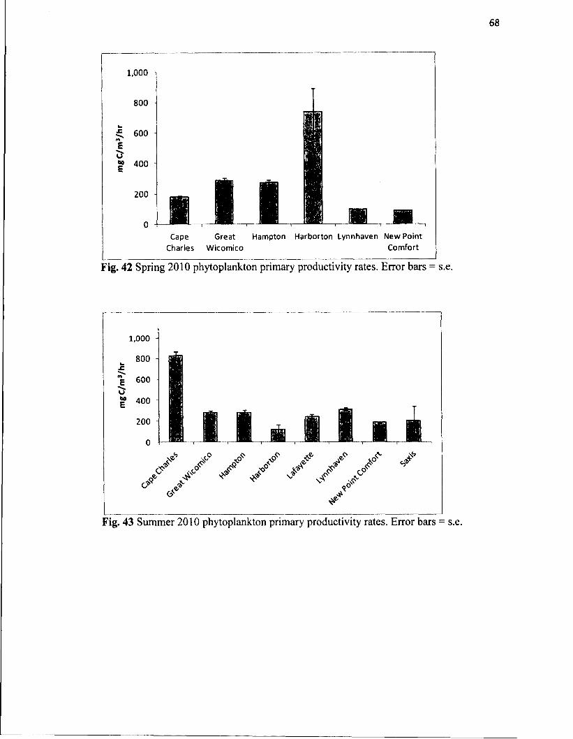
1,000 1
800
C ape G re a t H am p to n H a rb o r to n L y n n h av e n N ew P o in t
C h a rle s W ic o m ic o C o m fo rt
Fig. 42 Spring 2010 phytoplankton primary productivity rates. Error bars = s.e.
1,000 -
Fig. 43 Summer 2010 phytoplankton primary productivity rates. Error bars = s.e.

69
Fig. 44 Fall 2010 phytoplankton primary productivity rates. Error bars = s.e.
300
250
200
too -
L afa y e tte L y n n h av enH a rb o r to nH am p to n Saxis
Fig. 45 Winter 2011 phytoplankton primary productivity rates. Error bars = s.e.

Fig. 46 Spring 2011 phytoplankton primary productivity rates. Error bars = s.e.
Fig. 47 Summer 2011 phytoplankton primary productivity rates. Error bars = s.'

71
jimE
60E
2,000
1,800
1,4001,200
1,000
?ig. 48 Fall 2011 phytoplankton primary productivity rates. Error bars = s.e.

72
Microphytobenthos
Microphytobenthic primary productivity rates had similar variability as those in
the phytoplankton, with fluctuating values throughout the sampling period. The Cape
Charles station had higher productivity rates over the course of the study, and overall
significantly higher than Great Wicomico (p = 0.004), Hampton (p = 0.001), Harborton
(p = 0.001), Lynnhaven (p < 0.0001), New Point Comfort (p < 0.0001), and Saxis (p =
0.018). The two year average rate was 2.75 mg C/m3/hr, with a high of 20 mg C/m3/hr at
Cape Charles in 2011 spring. Cape Charles also recorded the highest overall average
productivity rate at 10.33 mg C/m3/hr during the study (Fig. 49). In 2010 winter, rates
ranged from 0.95 mg C/m3/hr at New Point Comfort to 5.92 mg C/m3/hr at the Lafayette
station (Fig. 50). Rates decreased slightly in the 2010 spring to an average of 1.95 mg
C/m3/hr (Fig. 51), down from 2.02 mg C/m3/hr in 2010 winter. The Cape Charles and
Saxis stations showed large increases of rates in the 2010 summer, with overall rates
averaging 4.78 mg C/m3/hr (Fig. 52), while average fall rates dropped to 1.49 mg C/m3/hr
(Fig. 53). Winter microphytobenthic productivity rates dropped to a two-year low
average of 0.81 mg C/m3/hr (Fig. 54), then an increase in 2011 spring, with Cape Charles
showing a high of 20.7 mg C/m3/hr (Fig. 55). Average summer productivity rates
dropped to 1.75 mg C/m3/hr (Fig. 56), before reaching an average seasonal high of 4.55
mg C/m3/hr in 2011 fall (Fig. 57).

73
12
10
8
6
4
2
0G re a t H am p to n H a rb o r to n L afa y e tte L y n n h av e n N ew P o in t SaxisC ap e
C h a r le s W ic o m ic o C o m fo rt
Fig. 49 Two-year average microphytobenthic primary productivity rates. Error bars = s.e.
7
6
5
4
3
2
1
0H a m p to n H a rb o r to n L afa y e tte L y n n h av en N ew P o in t Saxis
C o m fo rt
Fig. 50 Winter 2010 microphytobenthic primary productivity rates. Error bars = s.e.
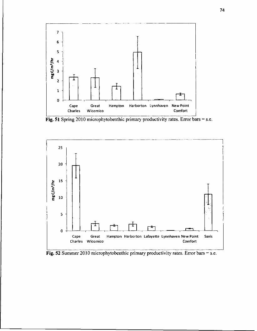
74
7
6
5
4
3
2
1
0C ap e G re a t H am p to n H a rb o r to n L y n n h av e n N ew P o in t
C h a rle s W ico m ico C o m fo rt
Fig. 51 Spring 2010 microphytobenthic primary productivity rates. Error bars = s.e.
20 -
I I _______ I 1 I __________r——i-*------ 1---- 1 1------1-----1-----1---------—i----- -—1 1——— , ■— 1--------- 1----- L
G re a t H am p to n H a rb o r to n L a fa y e tte L y n n h av e n N ew P o in t SaxisC o m fo rt
C apeC h a rle s W ico m ico
Fig. 52 Summer 2010 microphytobenthic primary productivity rates. Error bars = s.e.

75
7
6
5
4
3
2
1
0C ap e G re a t H am p to n H a rb o r to n L y n n h av e n N ew P o in t Saxis
C h a rle s W ico m ico C o m fo rt
Fig. 53 Fall 2010 microphytobenthic primary productivity rates. Error bars = s.e.
3
2
l
oH a rb o r to n L afay e tte L y n n h av enH am p to n Saxis
Fig. 54 Winter 2011 microphytobenthic primary productivity rates. Error bars = s.e.

76
25
20
15
u| io H
r-^-iC ape G re a t H am p to n H a rb o rto n L afay ette L y n n h av en N ew P o in t Saxis
C h a rle s W ico m ico C o m fo rt
Fig. 55 Spring 2011 microphytobenthic primary productivity rates. Error bars = s.e.
5 3asE
2 -
C ap e G re a t H a m p to n H a rb o r to n L afa y e tte L y n n h av e n N ew P o in t Saxis C h a rle s W ico m ico C o m fo rt
'ig. 56 Summer 2011 microphytobenthic primary productivity rates. Error bars = s.e.

77
25
20
15
10
5
0G re a t H a m p to n H a rb o r to n L afay e tte L y n n h av e n N ew P o in t SaxisC ape
C h a r le s W ic o m ic o C o m fo rt
Fig. 57 Fall 2011 microphytobenthic primary productivity rates. Error bars = s.e.

78
CHAPTER V
RESULTS - SEDIMENT GRAIN-SIZE ANALYSIS
Grain size distribution for each site was averaged over the course of the 2-year
study (Figs. 58-65), assigning a Wentworth size class to each station. A range of
sediment classes were observed, the coarsest being Lynnhaven, with a mean grain size of
442 pm, followed by Harborton (427 pm), Great Wicomico (302 pm), New Point
Comfort (198 pm), Lafayette (153 pm), Cape Charles (126 pm), Hampton (97 pm), and
Saxis (63 pm). Sediment properties are summarized in Table 6. These include phi units
(<j>), a logarithmic transformation of millimeters into whole integers, Wentworth size
class, mean grain size, sorting <j>, and sorting class, which describes the grain-size
variation of a sample by encompassing the largest parts of the size distribution as
measured from a cumulative curve (Folk 1980). Significant differences in sediment grain
size were found between stations, (p < 0.0001), with stations categorized into the
following size classes: medium sand (Great Wicomico, Harborton, Lynnhaven), fine sand
(Lafayette, New Point Comfort), very fine sand (Cape Charles, Hampton) and coarse silt
(Saxis).

79
6
5
4
2
1
00 5 0 0 1000 1 5 0 0 2000
Grain Size (|im)
Fig. 58 Two-year average of sediment grain size (pm) distribution at Cape Charles.
7
6
5
4
3
2
1
00 5 0 0 1000 1 5 0 0 2000
Grain Size (|im)
Fig. 59 Two-year average of sediment grain size (pm) distribution at Great Wicomico.

80
6
5
4
2
1
00 5 0 0 1000 1 5 0 0 2000
Grain Size (nm)
Fig. 60 Two-year average of sediment grain size (pm) distribution at Hampton.
9
8
7
6
5
4
3
2
1
00 5 0 0 1000 1 5 0 0 2000
Grain Size (|zm)
Fig. 61 Two-year average of sediment grain size (pm) distribution at Harborton.

81
4 .5
3 .5
2 .5
1.5
0 .5
5 0 0 1000 Grain Size (um)
1 5 0 0 2000
7ig. 62 Two-year average of sediment grain size (|im) distribution at Lafayette.
9
8
7
6
5
4
3
2
1
00 5 0 0 1000 1 5 0 0 2000
Grain Size (um)
7ig. 63 Two-year average of sediment grain size (|im) distribution at Lynnhaven.
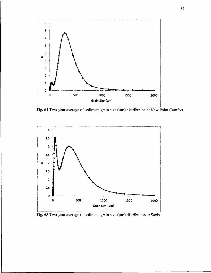
82
9
8
7
6
5
4
3
2
1
00 5 0 0 1000 1 5 0 0 2000
Grain Size (um)
Fig. 64 Two-year average of sediment grain size (^m) distribution at New Point Comfort.
4
3.5
3
2.5
2
1.5
1
0 .5
00 5 0 0 1000 1 5 0 0 2000
Grain Size (|zm)
Fig. 65 Two-year average of sediment grain size (|im) distribution at Saxis.

Table 6 Two-year average o f sediment properties across all stations.Sediment Properties
Station * Wentworth class Sorting <j> Sorting Mean grain size (pm)
Cape Charles 3.13 fine sand 1.64 poorly 126Great Wicomico 1.90 medium sand 1.51 poorly 302Hampton 3.50 very fine sand 1.49 poorly 97Harborton 1.26 medium sand 0.78 moderately 427Lafayette 2.83 fine sand 2.04 very poorly 153Lynnhaven 1.26 medium sand 0.73 moderately 442New Point Comfort 2.63 fine sand 1.29 poorly 198Saxis 4.00 coarse silt 2.12 very poorly 63

84
CHAPTER VI
RESULTS - MICROALGAL COMMUNITY RELATIONSHIPS
Pearson correlation analysis was performed to determine the effects of measured
parameters and environmental variables on microalgal abundance, biomass, and
productivity. In the phytoplankton, salinity proved to be a strong environmental variable,
significantly correlating with abundance, biomass, species richness and the Shannon
index of diversity (Table 7). Biomass-salinity correlation (Fig. 66) had a significant
negative relationship (r = -0.286, p = 0.024), while both species richness (Fig. 67) and
Shannon diversity (Fig. 68), gave positive correlations with salinity (r = 0.450, p <
0.0001; r = 0.349, p = 0.005). While salinity factored significantly in shaping
phytoplankton communities, it did not have an effect on the microphytobenthos.
However, multiple significant correlations were within this dataset (Table 8). Among
environmental variables, phi value proved to be a significant factor, positively correlating
with species richness (Fig. 69), biomass (Fig. 70) and Shannon diversity (Fig.71).

Table 7 Pearson correlation coefficients (r) for multiple correlations o f phytoplankton abundance, biomass, productivity rates, species richness (SR), Shannon index (H'), salinity ( % o ) , and temperature (T). N = 62 in all cases except productivity correlations (N = 56). * p < 0.05, * * p < 0 . 0 1
Biomass Productivity SR H' %0 TAbundance 0.534** 0.247 0.034 -0.164 -0.408** -0.254*
Biomass 1 0.016 0.109 -0.130 -0.286* -0.046Productivity 1 -0.011 0.143 -0.103 0.146
SR 1 0.207 0.450** 0.217H' 1 0.349** 0.023%0 1 0.058
4 .5
4
3 .5
r= -0 .2 8 6 p = 0 .0 2 4
3
2 .5
2
1 .5
10 .5
020 3015 25100 5
Salinity (%o)
Fig. 66 Phytoplankton salinity-biomass scatterplot.

86
r= 0 .4 5 0
p < 0 .0 0 0 1
4 0 ♦ ♦ ♦
♦ ♦
Salinity (%o)
Fig. 67 Phytoplankton salinity-species richness scatterplot.
2 .5
A i t * . .r= 0 .3 4 9
p = 0 .0 0 5
TS
JZ</>0 .5
Salinity (%o)
Fig. 68 Phytoplankton salinity-Shannon diversity scatterplot.

Table 8 Pearson correlation coefficients (r) for multiple correlations of microphytobenthic abundance, biomass, productivity rates, species richness (SR), Shannon index (H'), salinity (%o), temperature (T) and phi value ($). N = 62 in all cases except productivity
Biomass Productivity SR H' %0 TAbundance 0.736** 0.094 0.282* -0.294* 0.062 0.046 0.061
Biomass 1 0.243 0.433** 0.104 0.080 0.175 0.334**Productivity 1 0.138 0.279* 0.043 0.235 0.183
SR 1 0.488** -0.081 0.257* 0.012H' 1 -0.213 0.092 0.280*%0 1 0.058 -0.153T 1 0.069
6 0 0
5 0 0
r = 0 .4 3 3p < 0 .0 0 0 1
4 0 0
3 0 0♦ ♦ H
♦ ♦200
100
0503 0 4 010 200
Species Richness
Fig. 69 Microphytobenthic biomass-species richness scatterplot.

88
6 0 0
5 0 0r= 0 .3 3 4
p = 0 .0 0 84 0 0
3 0 0♦ ♦ ♦
200
100
Fig. 70 Microphytobenthic biomass-phi value scatterplot.
3 .5♦ ♦
2.5
♦ ♦1.5
10r= 0 .2 8 0 p = 0 .0 2 70 .5
Figure 71. Microphytobenthic Shannon diversity-phi value scatterplot.

89
Ordination of microalgal communities was performed on abundance data of both
algal groups examined (phytoplankton and microphytobenthos) using non-metric
multidimensional scaling (NMS). Initial analysis revealed a distinct separation of both
microalgal groups, with the relative distance between points indicating relative similarity
(closer together) or dissimilarity (farther apart), and each point representing species
abundance of individual collections (Fig. 72). As a result of the differences in species
composition between habitats (water column vs. benthos), further ordination analyses
were conducted separately on each algal group to assess patterns corresponding to spatial
(stations), or temporal (seasonal) factors. Among the phytoplankton, while some stations
appear closer to each other than others, no strong spatial relationships are apparent (Fig.
73). A clearer relationship is seen when seasons are examined, with winter and summer
abundance data opposite each other in the ordination plot, while spring and summer
collections are between the two (Fig. 74).
Ordination among the microphytobenthos had stronger spatial relationships than
those in the phytoplankton, with several within-station clusters and among-station groups
(Fig. 75). Five stations displayed a strong similarity between each other, with Cape
Charles, Great Wicomico, Hampton, Lafayette, and Saxis forming a cluster, while the
remaining stations (Harborton, Lynnhaven, New Point Comfort) were not only separated
(dissimilar) from each other, but also indicated within-station dissimilarity.
Microphytobenthic ordination analyses indicated less seasonal patterns than in the
phytoplankton, with no temporal patterns present (Fig. 76). Sediment type or grain size
was also examined as a predictor of microphytobenthic community structure. Ordination
presented a pattern of increasing similarity as sediment grain size decreased from the

90
coarsest sediment type (medium sand) to the finest (coarse silt), where the station with
the finest sediment characteristics (Saxis) formed a tight grouping (Fig. 77). Additionally,
the same ordination was performed defining stations characterized as either sand, or mud.
Distinction was made between sand and mud, where a station was classified as sand if <
20% of the sediment sample particles were < 63 pm, and classified as mud if > 20% of
the sediment particles were < 63 pm. Stations having a greater proportion of larger
sediment particles (sand) tended to be more dissimilar than those classified as mud,
which had greater similarity (Fig. 78).

91
Habitat A water O sediment
AA
A
tA A
A
V *
S/AA A
C)O
oo <9
CD
° W ;
uo ooD O o CCD . 0 8 °
$P"b'6 V o
o o
cb
▲Fig. 72 Ordination of microalgal community composition among the phytoplankton and microphtyobenthos using abundance data. Distances between points are proportional to differences in composition.

Y
OStationA Cape Charles0 G reat W icom ico H H am pton-f- H arborton A Lafayette • Lynnhaven Y New Point C om fort1 Saxis
A
AO
O ▲
4A
+ I
A Y Y
o.+ *
c #
+ o+ Y
Y"A Y
* •
*
A
Fig. 73 Ordination of phytoplankton community composition among stations.

o o
o ++
■bo
oo +
+ +A
+
A
+
SeasonA W in te r O Spring B S u m m er + Fall
o
1 #
o
o +
+A
+
+
AAA
+ ■
OO
Fig. 74 Ordination of phytoplankton community composition among seasons.

94
A+
OO
* ■ a A A* "<«>A
a ph,m % l A +
YO
Y
Y
+++
+
Station▲ CapoCharlaj O Groat Wicomico H Hampton -f- Harborton A lafay ttta # lynnhawan Y Nov* Point Comfort y Saxo
Y
YFig. 75 Ordination of microphytobenthic community composition among stations.

95
SeasonA W in te r O Spring B S u m m e r + Fall
o
O A
+ O
*4“o +
of i - °O B
+ +
o
+ +Fig. 76 Ordination of microphytobenthic community composition among seasons.

96
Sediment type A Medium send O Fine sand | Very fine sand + Coarse s it
sal
Fig. 77 Ordination of microphytobenthic community analysis with collection eventsclassified into Wentworth sediment class.

97
Sediment typeA SandO Mud
o o
Fig. 78 Ordination of microphytobenthic community composition with collections categorized according to substrate type (sand vs. mud).

98
CHAPTER VII
DISCUSSION
These results constitute the most comprehensive survey regarding the
composition of benthic microalgae in the Chesapeake Bay to date. Data analysis has
indicated significant differences were present between the water column phytoplankton
and the microphytobenthos regarding every parameter measured, and further testing
revealed significant differences among the benthic stations, suggesting a highly variable
benthic microalgal community, in contrast to a somewhat homogeneous pelagic
phytoplankton environment. Previous Chesapeake Bay microphytobenthic studies are
generally focused on a single parameter, or function. The scope of this project reports
microphytobenthic densities, biomass, and primary productivity rates over a broad
geographic area along with detailed taxonomic information, community structure and
trends, plus providing baseline data of the benthic algal communities in lower
Chesapeake Bay.
Community Composition, Abundance, and Biomass
The phytoplankton and benthic microalgal communities in this study were
considerably different. Ordination analysis of taxonomic data displayed a clear separation
of the phytoplankton and benthic microalgal communities. Further investigation into each
habitat yielded significant differences throughout the dataset. The phytoplankton was
significantly more diverse than the benthos, with all stations having species richness

99
values > 20 at every sampling, and values consistently > 30. In contrast, the benthic
habitat had significantly higher Shannon indices of biodiversity (H'), indicating a more
even distribution of algal taxa. Both habitats were dominated by diatoms in terms of
species richness, though overall taxomonic makeup of these populations varied between
habitats and stations. In the phytoplankton, the centric diatom Skeletonema costatum was
the most abundant species and diatoms in general were the most abundant microalgal
group throughout the study. Aside from the prominence of diatoms, community
composition at each phytoplankton station displayed no apparent patterns. NMS
ordination analysis did not completely resolve the high variability among phytoplankton
community composition, with no apparent similarities within stations. Ordination
indicated a somewhat weak seasonal composition relationship, with winter and spring
grouping together (e.g. taxonomic similarity). This seasonal similarity may have been
driven by the increased densities of cyanobacteria and dinoflagellates present during the
spring and summer of both years. High dinoflagellate biomass occurred at several
stations during spring and summer seasons, particularly in the 2010 spring/summer, when
high values were at the Lafayette, Great Wicomico, and New Point Comfort stations.
Relatively large-sized dinoflagellates were in the Lafayette, where C. polykrikoides and
P. micans were in high numbers. Winter/fall relationships were more ambiguous,
possibly due to dominance of diatoms and varying combinations of lesser algal groups
during these months.
Supporting seasonality as a potential driver of phytoplankton communities was a
significant negative correlation between temperature and abundance. While this evidence
presents a strong case for temperature as a major driver of these microalgal communities,

100
phytoplankton data from this study was most influenced by salinity. Significant negative
correlations were found between salinity and abundance as well as salinity and biomass
(Fig. 65). Conversely, salinity positively correlated with both species richness (Fig. 66)
and the Shannon diversity index (Fig 67).
In the benthos, and contrary to available taxonomic data, cyanobacteria were the
most prominent group throughout much of the sampling period. In the few publications
available that report benthic microalgal taxonomy, diatoms are in most cases described as
the dominant microalgal group, and in some instances, although present, no phyla other
than diatoms were considered. In this case, although pennate diatoms dominated taxon
counts (species richness), cyanobacteria were the most abundant in terms of overall
numbers. Though other taxonomic groups were present throughout the year, diatoms and
cyanobacteria persisted as the most common and abundant algae in both cell densities
and biomass at nearly every station in every sampling season. Diatoms maintained stable
cell densities and biomass values throughout the entire sampling period, while
cyanobacteria experienced seasonal fluctuations, with particularly high densities during
the warmer summer months. High densities of the colonial cyanobacteria M. elegans and
the filamentous L. aestuarii were present during spring and summer seasons,
predominantly at the eastern shore stations (Cape Charles, Harborton, and Saxis). While
other stations consistently had greater abundance and biomass values (Cape Charles,
Saxis), in general, among-station microphytobenthic density and biomass fluctuated
erratically throughout the study. Divergent from earlier data, salinity and temperature had
little effect on the microphytobenthic communities observed here. Though
microphytobenthic community dynamics appeared to be correlated with temperature

101
based on seasonal increases of algal abundance and biomass during the warm summer
months, these relationships were not statistically significant, with only species richness
significantly affected by temperature based on Pearson correlation analysis.
NMS ordination analysis indicated weak seasonal effects on community structure,
with the majority of spring and summer collections grouping near each other, and
fall/winter collections more widely spread, indicating dissimilarity, though these seasonal
associations are speculative at best. Spatial relationships in community structure were
more apparent however, with several stations clustering near each other (Cape Charles,
Hampton, Lafayette, Saxis). Considering the microphytobenthic ordination results in
terms of sediment grain size/Wentworth size class at each site, a much clearer picture
emerges. As presented in Figure 76, collections in the larger size range (Wentworth
1922) tend to be more taxonomically dissimilar, with stations classified as medium sand
and fine sand spread throughout the NMS plot. As size class decreases, stations become
clustered together, with the finest-grained sediment type (in this case, coarse silt), being
the tightest grouping. The Wentworth size classes are based on phi value (which
correspond to mean grain size), with larger phi values corresponding to smaller sediment
grain size. In this case, it appears that sediment grain size effects community
composition, particularly in sediments with smaller grain sizes. Further supporting
sediment grain size effect on microphytopbenthic communities, Pearson correlation
analysis gave significantly positive correlations of grain size to both biomass and
Shannon diversity. Biomass data from stations with smaller grain sizes (larger phi values)
consistently have similar values from season to season, regardless of seasonal variations.
It has been suggested that temporal fluctuations of microphytobenthic communities are

102
less prevalent in fine, muddy sediments compared to less stable, low nutrient sandy
sediments (Van der Wal et al. 2010). Microphytobenthic biomass data presented here
provides a similar pattern, with only small variations in biomass at sites characterized by
fine-grained sediments, while coarse-grained sites were exhibiting larger fluctuations
throughout the sample period.
Algal biomass is not the only parameter affected by sediment grain size. As noted
elsewhere (Mclntire and Amspoker 1986, Gottschalk et al. 2007) and in the current data,
grain size is capable of producing taxonomic distinctness among algal assemblages.
Typically, sheltered habitats with fine, muddy substrates are taxonomically more diverse
than those with larger sediment grains and exposed to more turbulent conditions.
Taxonomic data illustrated here concurs with those findings, as stations with fine-grained
sediments were consistently more diverse in species richness and Shannon diversity, than
stations characterized by coarse sediments. The significant correlation between phi value
and Shannon diversity reinforces the results of microphytobenthic community NMS
analysis, in that sediment grain size has significant effects on microalgal community
composition within the sediment. While the type and strength of sediment grain size
effects related to microphytobenthic communities will continue to be debated, this study
confirms that sediment type plays a critical role.
However, sediment type alone is not the sole driver of microphytobenthic community
dynamics, as a tight linkage exists among both biotic and abotic factors in these
environments. Benthic habitats with finer grains tend to be in areas with heavy vegetation
and high organic matter, allowing for higher rates of nutrient cycling within the sediment.
Cohesive sediments are less porous than coarse sandy sediments, thereby reducing the

103
rate of nutrient delivery to the water column. The cohesive nature of these sediments,
particularly in areas with extensive benthic microalgal development would bind nutrients
via sediment stabilization, reducing sediment resupension, and acting as a barrier of
sediment-water column nutrient exchange while still being available to sediment surface
biofilms. This would negate any effects of nutrient limitation and allowing for growth of
a diverse benthic flora. Conversely, habitats with coarse sediment profiles may have low
pore water content unable to retain nutrients, thus retarding continued growth of the algal
biomass. For example, the Lynnhaven station had the lowest biodiversity, abundance and
microalgal biomass throughout the study, as well as the largest mean sediment grain size.
The low algal biomass and productivity rates in the coarse-sediment stations of this study
may be the product of nutrient limitation, which, while generally a non-factor in fine
sediments, is not uncommon in sandy, porous sediments (Underwood and Kromkamp
1999).
Primary Productivity
The range of phytoplankton productivity rates measured here (28 - 1,907 mg
C/m /hr) were higher than historical Chesapeake Bay productivity rates (0.3 - 400 mg
C/m3/hr), though still within published ranges (Marshall and Nesius 1996). A plausible
cause for elevated rates may have been the close proximity of sampling locations to a
variety of nutrient sources. While historical Chesapeake Bay productivity measurements
are based on pelagic mainstem Bay stations where nutrients are derived from large scale
downstream transport (Marshall and Nesius 1996), stations in this study were along the
shoreline, and located within several meters of the low tide line. Therefore, nutrients

104
derived from terrestrial runoff would generally be at higher concentrations in these near
land areas than those in pelagic waters, and readily available for algal uptake.
Additionally, water temperatures in these shallow sub-tidal areas are often considerably
elevated during seasonal periods of increased algal development compared with those in
deeper waters, and when combined with terrestrially-derived nutrient concentrations,
yield higher productivity rates. In general, phytoplankton productivity rates at these sites
increased with rising temperatures, though this trend was not significant. The highest
average phytoplankton productivity rate (2-year avg. = 755 mg C/m3/hr) was recorded at
the Lafayette station, which is located in a heavily urbanized embayment of the tidal
Lafayette River. This waterway has undergone extensive eutrophication, and is subject to
frequent algal blooms, particularly after prolonged periods of precipitation and increased
nutrient entry occurring during late summer and early fall. Furthermore, the Cape Charles
station had elevated productivity rates (2-year avg. = 734 mg C/m3/hr) similar to the
Lafayette, even though situated in a more rural setting. This station is located adjacent to
a golf course, in a semi-enclosed portion of Old Plantation Creek, thrus with low tidal
flushing it is subject to increased nutrient input in the form of commercial fertilizers. The
Cape Charles station also had the highest productivity during the study, at 1,907 mg
C/m3/hr during the 2011 fall season. The lowest average phytoplankton productivity rates
were seen at the New Point Comfort station (avg. 141 mg C/m3/hr), which, as noted
earlier, is considered a more pristine location, with little surrounding human
development, and has an unrestricted path of water exchange with Chesapeake Bay.
While much of the reported data regarding microphytobenthic productivity rates■y
are reported as “mg C/m /hr”, an aerial rate, data presented here is expressed as “mg

105
C/m3/hr”, a volumetric rate, since productivity was measured considering the entire algal
community within the sediment core, instead of just the surface component. Comparison
of aerial rates to volumetric microphytobenthic primary productivity rates is commonly
accepted in microphytobenthic studies. Benthic microalgal primary productivity rates (0
- 21 mg C/m /hr), while significantly lower than rates for the neighboring phytoplankton,
still are within the range of published results both in the intertidal Chesapeake Bay (1 -
90 mg C/m2/hr), and worldwide (Cahoon 1999). When considering microphytobenthic
biomass values measured in this study, benthic productivity rates recorded here are
unexpectedly low (2-year average = 2.80 mg C/m3/hr), particularly when compared with
rates in the phytoplankton (2-year average = 390 mg C/m3/hr). While microphytobenthic
productivity rates were considerably lower than those of the phytoplankton, their biomass
values were significantly higher than the phytoplankton, indicating an important role as a
food source for benthic fauna. Evidence of an inverse relationship between biomass and
productivity, similar to patterns seen in some terrestrial producers (Tilman et al. 1996)
was explored, though no significant correlations could be made. Possibly explaining the
high biomass/low productivity rates, much of the biomass quantified in this study may
have been from sediment layers below the narrow euphotic zone, particularly in the
muddy/silty sediment habitats, where many algal cells may not be photosynthetically
active, or have reduced photosynthetic capacity. In general, microphytobenthic
productivity rates remained static throughout the sampling period, having rates at most
stations in the 0 - 5 mg C/m /hr range, with little apparent divergence. However, data
evaluation on a station by station basis indicated erratic patterns of productivity
throughout the year regardless of biomass, season, or any other environmental variable, a

106
phenomenon similarly observed in other studies (Thornton 2002). Large scale and high
frequency variations in biomass and productivity are a common feature of
microphytobenthic communities (Kromkamp and Forster 2006). A review of annual rates
by Cahoon (1999) highlight the extreme variability in estimates of microphytobenthic
primary production , with an average rate of 104 g C/m2/yr with a standard deviation of
93 (North America only), with worldwide rates exhibiting similar variability. Both
phytoplankton and microphytobenthic communities are patchy in their distribution, both
at the meso- and microscale level, leading to significant variation in biomass values and
primary productivity rates, complicating attempts at measuring these parameters.
Phytoplankton patchiness, both on small and large scales is often the result of turbulent
flow, shear, and tidal energy (Mitchell et al. 2008). In the benthos, this phenomenon may
be more pronounced than in the fluid pelagic environment, as benthic habitats are subject
to a wider range and magnitude of variables, both natural and human-influenced.
Variability seen in microphytobenthic primary productivity rates may be the product of
both actual variability and the differences in methodology used to measure those rates
(Forster and Kromkamp 2006). In order to accurately evaluate trends in productivity,
precise quantitative methodology must be employed. In the case of microphytobenthic
communities, this may not be easy due to the complex set of changing interactions
between the biological, chemical, and physical processes occurring in the benthic
environment.
Though no clear productivity trends are apparent, some congruence with
phytoplankton data was present, with productivity generally increasing with increasing
temperature, yet no significant relationship was present. Also similar to the

107
phytoplankton, both the Lafayette and Cape Charles stations exhibited the highest
average microphytobenthic productivity rates (2-year averages = 5.54 mg C/m3/hr and
10.33 mg C/m3/hr, respectively) over the course of the study. This reinforces the concept
of nutrient loading in these areas as a driver of increased algal productivity. The lowest
average benthic productivity rate (0.05 mg C/m3/hr) was observed at the Lynnhaven
station. This site, is characterized by heavy wave action/disturbance plus large, coarse
grained sediment, and usually with little, or no obvious algal growth. This was
consistently the benthic station with the lowest abundance and biomass values. Unlike
evidence from previous studies summarized by Cahoon (1999), when compared with
phytoplankton productivity rates, the current data does not suggest microphytobenthos as
a large contributor to estuary-wide primary productivity for the entire Chesapeake Bay
ecosystem, relative to phytoplankton productivity.

108
CHAPTER VIII
CONCLUSIONS
Results of this study have identified a significant microalgal biomass
(microphytobenthos) within the benthic environment occurring year-round in the near
shore waters of lower Chesapeake Bay. Unlike many estuarine macrophytes which enter
dormancy during the colder fall and winter months, the microphytobenthos in these
waters represent a continuous source of carbon to higher trophic levels of the common
biota regardless of season. This study has identified specific relationships in this
microalgal community and drivers of community composition and related dynamics.
Productivity rates measured here indicate increased phytoplankton and benthic
production in eutrophic habitats and other areas of high nutrient input. Based on these
results, intertidal microphytobenthic primary production accounts for roughly 1% of the
total microalgal production in the habitats surveyed. Although this percentage is low
compared to the phytoplankton productivity, when considering the extent of the intertidal
habitats in the Chesapeake Bay estuarine system, it represents a substantial amount of
biomass available to constituents within the Bay complex.
These estimates do not include sub-tidal microphytobenthos or intertidal periphyton, and
are restricted to the sediment-associated microalgae. Based on the sampling of only one
benthic microalgal compartment, methodological constraints, and the characteristic
patchiness of benthic microproducer communities, these results are believed to be an
underestimate of benthic microalgal production in lower Chesapeake Bay.
As noted previously, phytoplankton and microphytobenthic populations
are often generalized into a single group referred to as “microalgae”. These findings

109
suggest that while some taxonomic overlap exists between these groups, their diversity,
cell densities, biomass, productivity rates and community dynamics are very different,
and reinforce the theory that they are indeed separate communities and should not be
categorized as a single functional group. Considering the microphytobenthos alone,
previous taxonomic studies of microphytobenthic communities often stress the presence
of diatoms, and in many cases ignore the occurrence of other algal groups. Data presented
here are to the contrary, in that a great diversity of benthic microalgal flora is present in
these habitats. In several cases, other algal groups such as cyanobacteria and chlorophytes
dominated the algal biomass at these benthic stations. As such, it is not recommended
that all microphytobenthic communities be treated similarly, as these data reveal unique
benthic microalgal assemblages, often showing site-specific diversity, significantly
different from that in the neighboring phytoplankton.
While a number of factors interact to complicate microphytobenthic biomass and
productivity measurements in the intertidal such as sediment type, light attenuation,
spatial patchiness, and physiological variability driven by temperature, light, and other
environmental gradients, it may be that microphytobenthic taxonomic diversity may itself
account for much of the observed variability in primary productivity rates (Kromkamp
and Forster 2006), with certain microalgal groups possessing unique physiological and
photosynthetic capabilities.
While this project quantifies microphytobenthic properties on large scales, both
spatially and temporally, small-scale variation must be explored as well. Evidence of
daily oscillations of biomass, productivity, and highly localized species turnover may
explain the high variability and lack of seasonal patterns in the biomass and primary

110
productivity measurements in this study. The heterogeneity observed in the benthic
environment may be due to harsh and rapidly changing local or regional environmental
conditions commonly associated with this algal community; the magnitude of which is
not present in the pelagic environment. Intertidal benthic organisms, both flora and fauna,
are subject to extreme physical, temperature, light, and salinity changes during ebb and
flood tides, along with the obvious issues of daily periods of desiccation during emersion.
Additionally, the benthos, and particularly the intertidal zone, may be more prone to
human impacts than neighboring sub-tidal environments. Due to high human impacts in
estuarine environments, and particularly in the shoreline areas where this study was
focused, discerning natural microphytobenthic variability from that caused
anthropogenically may be difficult. The presence both naturally-occurring and human-
influenced disturbance-driven patchiness may affect these communities on a daily basis,
thereby making broad conclusions regarding microphytobenthos dynamics across
Chesapeake Bay not prudent.
Looking toward the future, predicted increased eutrophication of estuaries and
coastal ecosystems worldwide will no doubt have a significant effect, not only on
microphytobenthic communities, but the habitats in which they persist, and all associated
local flora and fauna. What these effects may be however, are difficult to discern, and are
hardly predictable. In one scenario, increased anthropogenic nutrient input would lead to
extensive phytoplankton blooms, which may create a positive feedback, with a surplus of
carbon entering the system, and eventually decomposing, thereby releasing nutrients back
into the system. As noted earlier, microphytobenthic biofilms are adept at remineralizing
nutrients bound in the sediments. Potentially, this would be advantageous for

I l l
microphytobenthic communities, allowing for increased productivity and extensive
benthic microalgal biomass development. This situation would not only alter biomass and
productivity rates, but could potentially affect the taxonomic makeup of these benthic
microproducers. In the presence of recurrent dense phytoplankton blooms, turbidity
becomes a factor, particularly in shallow near shore areas. In this case, temporary, yet
frequent shading of the benthos would favor those algal taxa that either have an affinity
for low-light conditions, or are otherwise better adapted at thriving in such an
environment.
When considering eutrophication and habitat degradation in general, other
human-influenced effects cannot be ignored. Coastal development and the hardening of
shorelines is a serious threat to estuarine ecosystems, and particularly coastal wetlands,
which are at the forefront of such development. A combination of rising sea levels and
the construction of more bulkheads, seawalls, and other such non-natural shoreline
structures, wetland vegetation is obstructed from a landward migration, thereby
“drowning” such habitats. With the loss of wetlands, so comes the loss of those flora and
fauna that inhabited these environments. In many cases, and especially in the vast
wetlands of Chesapeake Bay and its associated tributaries, these coastal wetlands provide
crucial habitat and rearing grounds for countless numbers of economically vital and
ecologically essential marine and estuarine species.
While the specific role(s) and dynamics of microphytobenthos in these systems is
still debatable, their importance is no longer in question. The results presented here,
including biomass, abundance, productivity, and taxonomic information characterize the
microphytobenthic communities and provides an essential framework for future

112
Chesapeake Bay microphytobenthic research, and identifies the importance of this crucial
and significant component of the Bay’s estuarine ecosystem.

113
REFERENCES
Admiraal, W. and H. Peletier. 1980. Influence of seasonal variations of temperature and light on the growth rate of cultures and natural populations of intertidal diatoms. Marine Ecology Progress Series 2:35-43.
Amspoker, M.C. and C.D. Mclntire. 1978. Distribution of intertidal diatoms associated with sediments in Yaquina Estuary, Oregon. Journal of Phycology 14(4):387-395.
Austen, I., T.J. Anderson, and K. Edelvang. 1999. The influence of benthic diatoms and invertebrates on the erodibility of an intertidal mudflat, the Danish Wadden Sea. Estuarine, Coastal and Shelf Science 49:99-111.
Bennett, A. T. S. Bianchi, and J. C. Means. 2000. The effects of PAH contamination and grazing on the abundance and composition of microphytobenthos in salt marsh sediments (Pass Fourchon, LA, USA): II: The use of plant pigments as biomarkers. Estuarine Coastal and Shelf Science 50(3): 425-439.
Blanchard, G. F., J.M. Guarini, F. Orvain, and P.G. Sauriau. 2001. Dynamic behaviour of benthic microalgal biomass in intertidal mudflats. Journal of Experimental.Marine Biology and Ecology 264: 85-100.
Blanchard, G. F., J.M. Guarini, P. Gros, and P. Richard. 1997. Seasonal effect on therelationship between the photosynthetic capacity of intertidal microphytobenthos and temperature. Journal o f Phycology 33: 723-728.
Blasutto, O., T. Cibic, C. De Vittor, and S.E. Umani. 2005. Microphytobenthic primary production and sedimentary carbohydrates along salinity gradients in the lagoons of Grado and Marano (Northern Adriatic Sea). Hydrobiologia 550:47-55.
Brotas, V. and M. R. Plante-Cuny. 1998. Spatial and temporal patterns ofmicrophytobenthic taxa of estuarine tidal flats in the Tagus Estuary (Portugal) using pigment analysis by HPLC. Marine Ecology Progress Series 171: 43-57.
Buzzelli, C.P. 1998. Dynamic simulation of littoral zone habitats in lower Chesapeake Bay. I. Ecosystem characterization related to model development. Estuaries 21:659-672.
Cahoon, L.B. 1999. The role of benthic microalgae in neritic ecosystems. In: Ansell,A.D., R.N. Gibson, and M. Barnes (eds.) Oceanography and Marine Biology: an Annual Review. Taylor and Francis, New York, pp 47-86.
Cahoon, L.B., J.E. Nearhoof, and C.L. Tilton. 1999. Sediment grain size effect on benthic microalgal biomass in shallow aquatic ecosystems. Estuaries 22:735-741.
Cahoon, L.B. and J.E. Cooke. 1992. Benthic microalgal production in Onslow Bay, North Carolina, USA. Marine Ecology Progress Series 84:185-196.
Cammen, L.M. 1982. Effect of particle size on organic content and microbial abundance within four marine sediments. Marine Ecology Progress Series 9:273-280.
Chapman, M. G., T. J. Tolhurst, R. J. Murphy, A. J. Underwood. 2010. Complex and inconsistent patterns of variation in benthos, micro-algae and sediment over multiple spatial scales. Marine Ecology Progress Series 398: 33-47.
Cibic, T., O. Blasutto, N. Burba, and S. Fonda Umani. 2008. Microphytobenthic primary production as 14C uptake in sublittoral sediments of the Gulf of Trieste (northern

114
Adriatic Sea): Methodological aspects and data analyses. Estuarine, Coastal and Shelf Science 77(1): 113-122.
Colijn, F. and K.S. Dijkema. 1981. Species distribution of benthic diatoms anddistribution of chlorophyll a on an intertidal flat in the Dutch Wadden Sea.Marine Ecology Progress Series 4:9-21.
Cowles, R. 1930. A biological study of the offshore waters of Chesapeake Bay. Bulletin, Bureau of Fisheries 46:277-381.
Davis, M. W. and C. D. Mclntire 1983. Effects of physical gradients on the production dynamics of sediment-associated algae. Marine Ecology Progress Series 13(2-3): 103-114.
Du, G. Y., Moonho Son, Soonmo An, and Ik Kyo Chung. 2010. Temporal variation in the vertical distribution of microphytobenthos in intertidal flats of the Nakdong River estuary, Korea. Estuarine Coastal and Shelf Science 86(1): 62-70.
Fielding, P. J., K. S. J. Damstra, and G.M. Branch. 1988. Benthic diatom biomass, production and sediment chlorophyll in Langebaan lagoon, South-Africa. Estuarine Coastal and Shelf Science 27(4): 413-426.
Folk, R.L. 1980. The petrology of sedimentary rocks. 2nd ed,, 182 pp., Hemphill Publishing Company, Austin, TX.
Forster, R.M. and J.C. Kromkamp. 2006. Estimating benthic primary production: scaling up from point measurements to the whole estuary, p. 109-120. In Kromkamp,J.C., de Brouwer, J.F.C., Blanchard, G.F., Forster, R.M., and V. Creach (eds.), Functioning of microphytbenthos in estuaries. Royal Netherlands Academy of Arts and Sciences, Amsterdam.
Gottschalk, S., S. Uthicke, and K. Heimann. 2007. Benthic diatom communitycomposition in three regions of the Great Barrier Reef, Australia. Coral Reefs 26:345-357.
Grippo, M. A., J. W. Fleeger, N. N. Rabalais, R. Condrey, and K. R. Carman. 2010.Contribution of phytoplankton and benthic microalgae to inner shelf sediments of the north-central Gulf of Mexico. Continental Shelf Research 30(5): 456-466.
Guarini, J. M., G.F. Blanchard, and P. Gros 2000. Quantification of themicrophytobenthic primary production in European intertidal mudflats - a modelling approach. Continental Shelf Research 20: 1771-1788.
Janousek, C. N. 2009. Taxonomic composition and diversity of microphytobenthos in southern California marine wetland habitats. Wetlands 29(1): 163-175.
Janousek, C.N., C.A. Currin, and L.A. Levin. 2007. Succession of microphytobenthos in a restored coastal wetland. Estuaries and Coasts 30: 265-76.
Jesus, B., V. Brotas, L. Ribeiro, C.R. Mendes, P. Cartaxana, and D.M. Paterson. 2009. Adaptations of microphytobenthos assemblages to sediment type and tidal position. Continental Shelf Research 29(13): 1624-1634.
Jonsson, B. 1991. A 14C-incubation technique for measuring microphytobenthic primary productivity in intact sediment cores. Limnology and Oceanography 36(7): 1485- 1492.
Kromkamp, J.C. and R. M. Forster. 2006. Developments in microphytobenthos primary productivity studies, p. 9-30. In Kromkamp, J.C., de Brouwer, J.F.C., Blanchard, G.F., Forster, R.M., and V. Creach (eds.), Functioning of microphytbenthos in estuaries. Royal Netherlands Academy of Arts and Sciences, Amsterdam.

115
Leach, J. H. 1970. Epibenthic algal production in an intertidal mudflat. Limnology and Oceanography 15(4): 514-521.
MacIntyre, H. L., R. J. Geider, and D. C. Miller. 1996. Microphytobenthos: Theecological role of the "secret garden" of unvegetated, shallow-water marine habitats. 1. Distribution, abundance and primary production. Estuaries 19(2A): 186-201.
MacIntyre, H. L. and J.J. Cullen 1995. Fine-scale vertical resolution of chlorophyll and photosynthetic parameters in shallow water benthos.. Marine Ecology Progress Series 122: 227-237.
Marshall, H.G., R.V. Lacouture, C. Buchanan, and J.M. Johnson. 2006. Phytoplankton assemblages associated with water quality and salinity regions in Chesapeake Bay, USA. Estuarine, Coastal, and Shelf Science 69(1): 10-18.
Marshall, H.G., T.A. Egerton, L. Burchardt, S. Cerbin, and M. Kokocinski. 2005. Long term monitoring results of harmful algal populations in Chesapeake Bay and its major tributaries in Virginia, USA. Oceanological and Hydrobiological Studies 34:35-41.
Marshall, H.G., M.F. Lane, and K.K. Nesius. 2003. Long-term phytoplankton trends and related water quality trends in the lower Chesapeake Bay, Virginia, USA. Environmental Monitoring and Assessment 81:349-360.
Marshall, H.G. and K.K. Nesius. 1996. Phytoplankton composition in relation to primary production in Chesapeake Bay. Marine Biology 125(3): 611-617.
Mclntire, C.D. and M.C. Amspoker. 1986. Effects of sediment properties on benthic primary production in the Columbia River estuary. Aquatic Botany 24:249-67.
Middleburg, J.J., C. Barranguet, H.T.S. Boschker, P.M.J. Herman, T. Moens, and C.H.R. Heip. 2000. The fate of intertidal microphytobenthos carbon: An in situ Relabeling study. Limnology and Oceanography 45:1224-1234.
Mitchell, J.G., Yamazaki, H., Seuront, L., Wolk, F., and H. Li. 2008. Phytoplanktonpatch patterns: seascape anatomy in a turbulent ocean. Journal of Marine Systems 69:247-253.
Murray, L. and R.L. Wetzel. 1987. Oxygen production and consumption associated with the major autotrophic components in two temperate seagrass communities.Marine Ecology Progress Series 38: 231-239.
Orvain, F., S. Lefebvre, J. Montepini, M. Sebire, A. Gangery, and B. Sylvand. 2012. Spatial and temporal interaction between sediment and microphytobenthos in a temperate estuarine macro-intertidal bay. Marine Ecology Progress Series 458:53.
Palmer, M. 1992. Standard operating procedure for GLNPO total alkalinity titration. U.S. EPA Great Lakes National Program Office, Chicago, IL.
Pinckney, J. L., K.R. Carman, S.E. Lumsden, and S.N. Hymel 2003. Microalgal-meiofaunal trophic relationships in muddy intertidal estuarine sediments. Aquatic Microbial Ecology 31: 99-108.
Pinckney, J. and R.G. Zingmark. 1993. Biomass and production of benthic microalgal communities in estuarine habitats. Estuaries 16(4): 887-897.
Revsbech, N.B., and B.B. Jorgensen. 1983. Microelectrodes: Their use in microbial ecology. Advances in Microbial Ecology 9: 293-352.

116
Riznyk, R.Z. and H.K. Phinney. 1972. Manometric assessment of interstitial microalgae production in two estuarine sediments. Oecologia 10:193-203.
Reay, W.G., D.L. Gallagher, and G.M. Simmons. 1995. Sediment-water column oxygen and nutrient fluxes in near shore environments of the lower Delmarva peninsula, USA. Marine Ecology Progress Series 118:215-227.
Rizzo, W. M., S.K. Dailey, G.J. Lackey, R.R. Christian, B.E. Berry, and R.L. Wetzel. 1996. A metabolism-based trophic index for comparing the ecological values of shallow-water sediment habitats. Estuaries 19(2): 247-256.
Rizzo, W.M. and R.L. Wetzel. 1986. Temporal variability in oxygen metabolism of an estuarine shoal sediment, p. 227-239. In D.A. Wolfe (ed.), Estuarine Variability. Academic Press, New York.
Rizzo, W.M. and R.L. Wetzel. 1985. Intertidal and shoal benthic community metabolism in a temperate estuary: studies of spatial and temporal scales of variability. Estuaries 8:342-351.
Saburova, M. A., I.G. Polikarpov, and I.V. Burkovsky. 1995. Spatial structure of an intertidal sandflat microphytobenthic community as related to different spatial scales. Marine Ecology Progress Series 129(1-3): 229-239.
Shaffer, G.P. and C.P. Onuf. 1983. An analysis of factors influencing the primary production of the benthic microflora. Netherlands Journal of Sea Research 17:126-144.
Skinner, T., J.B. Adams, and P.T. Gama. 2006. The effect of mouth opening on thebiomass and community structure of microphytobenthos in a small oligotrophic estuary. Estuarine, Coastal and Shelf Science 70(1-2): 161-168.
Smayda, T. 1978. From phytoplankton to biomass. In: Soumia, A. (Ed.), Phytoplankton Manual. UNESCO, Paris, pp. 273-279.
Steele, J.H. and I.E. Baird. 1968. Production ecology of a sandy beach. Limnology and Oceanography 13:14-25.
Stribling, J.M. and J.C. Cornwell. 1997. Identification of important primary producers in a Chesapeake Bay tidal system using stable isotopes of carbon and sulfur. Estuaries 20:77-85.
Strickland, J.D.H. and T.R. Parsons. 1972. A practical handbook of seawater analysis. 2nd ed., Bullentin of Fisheries Research Board of Canada 167: 1-310.
Tilman D, D. Wedin, and J. Knops. 1996. Productivity and sustainability influenced by biodiversity in grassland ecosystems. Nature 379:718-20.
Thortnon, D.C.O., L.F. Dong, G.J.C. Underwood, and D.B. Nedwell. 2002. Factorsaffecting microphytobenthic biomass, species composition and production in the Colne Estuary (UK). Aquatic Microbial Ecology 27: 285-300.
Underwood, G.J.C., and J. Kromkamp. 1999. Primary production by phytoplankton and microphytobenthos in estuaries. Advances in Ecological Research 29: 92-153.
van der Wal, Daphne, Annette Wielemaker-van den Dool, and Peter M. J. Herman. 2010. Spatial Synchrony in Intertidal Benthic Algal Biomass in Temperate Coastal and Estuarine Ecosystems. Ecosystems 13(2): 338-351.
Wendker, S., H.G. Marshall, and K. Nesius. 1997. Primary microbenthic algal production in Chesapeake Bay. Marine Nature 5:15-19.
Wentworth, C.K. 1922. A scale of grade and class terms for clastic sediments. Journal of Geology 30: 377-392.

117
Whiting, M.C. and C.D. Mclntire. 1985. An investigation of distributional patterns in the diatom flora of Netarts Bay, Oregon, by correspondence analysis. Journal of Phycology 21:655-661.
Wolfe, J.J., B. Cunningham, N. Wilkerson, and J. Barnes. 1926. An investigation of the microplankton of Chesapeake Bay. Elisha Mitchell Scientific Society 42:25-54.
Yallop, M.L., D.M. Patterson, and P. Wellsbury. 2000. Interrelationships between rates of microbial production, exopolymer production, microbial biomass, and sediment stability in biofilms of intertidal sediments. Microbial Ecology 39:116- 127.
Yallop, M.L., B. de Winder, D.M. Paterson, and L.J. Stal. 1994. Comparative structure, primary production, and biogenic stabilization of cohesive and non-cohesive marine sediments inhabited by microphytobenthos. Estuarine, Coastal and Shelf Science 39(6):565-582.

118
VITA
Matthew Reginald Semcheski Graduate Research Assistant Phytoplankton Analysis Laboratory Department of Biological Sciences Old Dominion University,Norfolk, VA 23529
Education
Ph.D., Ecological Sciences, Old Dominion University, 2014M.S., Biology, Old Dominion University, 2008B.S., Biology, Marine Science, East Stroudsburg University, 2003
Selected Publications and Abstracts
Semcheski, M.R., T.A. Egerton, and H.G. Marshall. 2014. Comparative analyses ofcomposition and productivity of phytoplankton and intertidal benthic microalgal communities in lower Chesapeake Bay. Ocean Sciences Meeting (American Society of Limnology and Oceanography). Honolulu, HI.
Semcheski, M.R., T.A. Egerton, M.T. Muller, and H.G. Marshall. 2012. Structure, biomass, and productivity comparisons of benthic microalgal assemblages of lower Chesapeake Bay. Atlantic Estuarine Research Society Meeting. Chincoteague, VA.
Semcheski, M.R., T.A. Egerton, and H.G. Marshall. 2012. Seasonal variability inestuarine planktonic and benthic algal populations. Ecological Society of America Meeting. Portland, OR.
Marshall, H.G., L. Burchardt, M. Kokocinski, K. Stefaniak, and M. Semcheski. 2007.Phytoplankton composition and abundance at surface depths within different lake habitats. International Journal of Oceanography and Hydrobiology. 37 (1): 233- 240.
Filippino, K.C., M.R. Mulholland, P.W. Bernhardt, G.E. Boneillo, R.E. Morse, M.Semcheski, H.G. Marshall, N.G. Love, Q. Roberts, and D.A. Bronk. 2011. The bioavailability of effluent-derived organic nitrogen along an estuarine salinity gradient. Estuaries and Coasts. 34: 269-280.
Semcheski, M.R., T.A. Egerton, W. B. Myers, and H.G. Marshall. 2013. Benthicmicroalgal composition in lower Chesapeake Bay intertidal wetlands. Association of Southeastern Biologists Meeting. Charleston, WV.
Top Related
Copyright © 2022 FDOKUMEN

