


Bahasa
Halaman
Hukum

Available online at www.sciencedirect.com
Energy Procedia 00 (2013) 000–000
www.elsevier.com/locate/procedia
1876-6102 © 2013 The Authors. Published by Elsevier Ltd.
Selection and peer review by the scientific conference committee of SolarPACES 2013 under responsibility of PSE AG.
SolarPACES 2013
Assessment of the overall efficiency of gas turbine-driven CSP
plants using small particle solar receivers
P. Fernándeza,b
, F. Millera*
a Department of Mechanical Engineering, San Diego State University, San Diego, CA 92182-1323, United States b Escuela de Ingenierías Industriales, Universidad de Valladolid, 47011 Valladolid, Spain
Abstract
While current commercial Concentrated Solar Power (CSP) plants utilize Rankine steam cycles in the power block, there is a
goal to develop higher-efficiency plants based on Brayton cycles or on combined cycles. In this paper, we present an assessment
of a gas turbine-driven CSP plant using small particle solar receivers. In particular, a recuperated, single-shaft gas turbine engine
and a Small Particle Heat Exchange Receiver –a high temperature receiver for solar tower power plants developed in the
framework of the U.S. DOE’s SunShot Program– are the technologies employed for the gas turbine and the receiver,
respectively. The curves of the solar receiver and the gas turbine engine were first obtained using in-house codes, and then
coupled together. A backup combustor fueled with natural is used to compensate the variable nature of the solar resource. For a
more flexible and optimum operation, the guide vane angle of the compressor is allowed to vary, and so is the position of the
valves of the receiver and combustor bypasses. Two different operational strategies were analyzed: maximizing the overall
efficiency of the plant and maximizing the net output power. Hence, the overall efficiency of a gas turbine-driven CSP plant
based on a Small Particle Heat Exchange Receiver is estimated, and the potential to generate electricity is assessed. This analysis
reveals the strengths of small particle receivers with respect to molten salt tubular receivers due to the much higher temperatures
that can be achieved while maintaining (or even increasing) the receiver efficiency.
© 2013 The Authors. Published by Elsevier Ltd.
Selection and peer review by the scientific conference committee of SolarPACES 2013 under responsibility of PSE AG.
Keywords: Brayton cycle; Concentrated solar power; CSP; Gas turbine; Small Particle Heat Exchange Receiver; Solar-fossil hybrid power
generation; Solar receiver
* Corresponding author. Tel.: +1 619-594-5791; fax: +1 619-594-3599.
E-mail address: [email protected]
P. Fernández, F. Miller / Energy Procedia 00 (2013) 000–000
1. Introduction
Commercial concentrated solar power (CSP) plants suffer from the relatively low temperatures that current
receivers and heat transfer fluids can achieve; which in turn limits the thermodynamic efficiency of the power
conversion. Small particle receivers for heating air to very high temperature and driving a gas turbine or a combined
cycle engine, while still under development, are expected to increase the thermodynamic efficiency compared to
lower-temperature liquid cooled receivers and subcritical Rankine cycles. The advantages of this technology are
apparent: (1) It leads to higher thermodynamic efficiency (due to the higher temperatures) [1]; (2) it requires much
less cooling water; and (3) the air is a non-problematic heat transfer fluid in the temperature range of interest. In
addition, gas turbines are generally easier to operate than steam turbines, and are expected to withstand more stops
and starts. As such, they are better suited to the intermittent nature of solar energy, which can require nightly
shutdown. One proposed receiver to drive a gas turbine or a combined cycle in solar tower power plants is the Small
Particle Heat Exchange Receiver (SPHER). This concept, first proposed by Hunt in 1979 [2], utilizes an air-particle
mixture to volumetrically absorb highly concentrated solar irradiation and produce outlet temperatures in excess of
1300 K. Moreover, it produces much less pressure drop, is probably less costly to construct and can withstand much
higher incident flux levels (with the corresponding size and thermal losses reduction) than current tubular receivers.
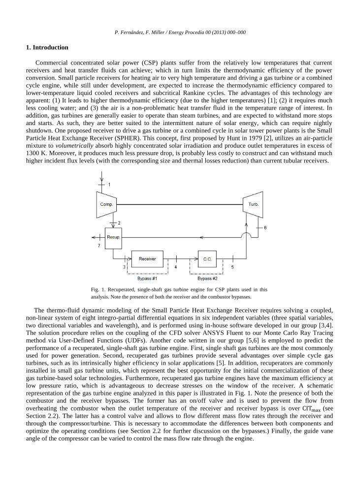
Fig. 1. Recuperated, single-shaft gas turbine engine for CSP plants used in this
analysis. Note the presence of both the receiver and the combustor bypasses.
The thermo-fluid dynamic modeling of the Small Particle Heat Exchange Receiver requires solving a coupled,
non-linear system of eight integro-partial differential equations in six independent variables (three spatial variables,
two directional variables and wavelength), and is performed using in-house software developed in our group [3,4].
The solution procedure relies on the coupling of the CFD solver ANSYS Fluent to our Monte Carlo Ray Tracing
method via User-Defined Functions (UDFs). Another code written in our group [5,6] is employed to predict the
performance of a recuperated, single-shaft gas turbine engine. First, single shaft gas turbines are the most commonly
used for power generation. Second, recuperated gas turbines provide several advantages over simple cycle gas
turbines, such as its intrinsically higher efficiency in solar applications [5]. In addition, recuperators are commonly
installed in small gas turbine units, which represent the best opportunity for the initial commercialization of these
gas turbine-based solar technologies. Furthermore, recuperated gas turbine engines have the maximum efficiency at
low pressure ratio, which is advantageous to decrease stresses on the window of the receiver. A schematic
representation of the gas turbine engine analyzed in this paper is illustrated in Fig. 1. Note the presence of both the
combustor and the receiver bypasses. The former has an on/off valve and is used to prevent the flow from
overheating the combustor when the outlet temperature of the receiver and receiver bypass is over (see
Section 2.2). The latter has a control valve and allows to flow different mass flow rates through the receiver and
through the compressor/turbine. This is necessary to accommodate the differences between both components and
optimize the operating conditions (see Section 2.2 for further discussion on the bypasses.) Finally, the guide vane
angle of the compressor can be varied to control the mass flow rate through the engine.
P. Fernández, F. Miller / Energy Procedia 00 (2013) 000–000
2. Model description
2.1. Receiver model
A coupled fluid flow and radiative heat transfer model developed in our group [3,4] is employed to simulate the
Small Particle Heat Exchange Receiver. The steady-state Reynolds-averaged Navier-Stokes (RANS) equations,
together with the two equations of the SST κ-ω turbulence model and the corresponding constitutive relations, are
solved numerically by the CFD package ANSYS Fluent. An in-house Monte Carlo Ray Tracing method [3,4] is
employed for the radiative heat transfer due to the highly directional intensity distribution from the heliostat field [7]
and the strong spectral dependence of the radiative properties of the particles [4], which cannot be properly solved
by conventional numerical techniques such as the Spherical Harmonics or the Discrete Ordinates method. The
absorption and scattering properties of the carbon particles are calculated using Mie theory. The gas phase is
modeled as radiatively non-participating due to the negligible amount of CO2 generated in the receiver ( vs.
for the solar spectrum and the axial path length.) Particle oxidation is not yet included as the oxidation
model is still being developed and validated. Physically, this corresponds with a nitrogen-driven receiver, which is
an alternative for the closed-loop operation of the receiver [5].
The CFD solver and the Monte Carlo method have been coupled together via User-Defined Functions (UDFs)
and iterate alternatively until convergence. The adaptive solution procedure was optimized to prevent numerical
oscillations and minimize the simulation time. The Monte Carlo method is coupled with a heliostat field model [7]
and can simulate real solar irradiations, i.e. the spatial, directional and wavelength dependence of the concentrated
solar irradiation at different times and days is exactly modeled by our software. Moreover, it can simulate any
axisymmetric geometry for the solar receiver; as well as flat, ellipsoidal and spherical cap windows (note that a
window is necessary to allow the solar irradiation to enter into the receiver, and its geometry must be curved to
withstand the pressurized environment inside the receiver, which is located in the high-pressure side of the gas
turbine.) For a much more detailed description of our software, the interested reader is referred to [3].
In this paper we will use this numerical-stochastic model to generate the curves of the solar receiver, i.e. to
predict the performance as a function of the solar thermal input and the mass flow rate in the receiver. In reality, the
inlet pressure and temperature are also necessary to describe the state of the Small Particle Heat Exchange Receiver.
We will, however, neglect the dependence of these two factors since the required effort is exponential in the number
of degrees of freedom and the simulation time of the coupled model is around one week. While the influence of the
pressure is negligible [3], the inlet temperature does have an effect on the efficiency and this simplifying hypothesis
is only valid as a first approximation (it is assumed that the inlet temperature is 700 K while it can actually vary
from 675 K to 800 K, depending on the operation conditions).
2.2. Gas turbine model
The in-house Small Particle Receiver Gas Turbine (SPRGT) code [6] is employed to simulate and generate the
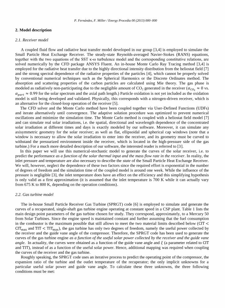
curves of a recuperated, single-shaft gas turbine engine operating at constant speed in a CSP plant. Table 1 lists the
main design point parameters of the gas turbine chosen for study. They correspond, approximately, to a Mercury 50
from Solar Turbines. Since the engine speed is maintained constant and further assuming that the fuel consumption
in the combustor is the maximum possible that still allows to meet the two material limits described below ( and ), the gas turbine has only two degrees of freedom, namely the useful power collected by
the receiver and the guide vane angle of the compressor. Therefore, the SPRGT code has been used to generate the
curves of the gas turbine engine as a function of the useful solar power collected by the receiver and the guide vane
angle. In actuality, the curves were obtained as a function of the guide vane angle and (a parameter related to
and ), instead of as a function of the useful solar power. Hence, additional mapping was required when coupling
the curves of the receiver and the gas turbine.
Roughly speaking, the SPRGT code uses an iterative process to predict the operating point of the compressor, the
expansion ratio of the turbine and the outlet temperature of the recuperator; the only implicit unknowns for a
particular useful solar power and guide vane angle. To calculate these three unknowns, the three following
conditions must be met:
P. Fernández, F. Miller / Energy Procedia 00 (2013) 000–000
Table 1. Design point parameters of the gas turbine engine chosen for study.
Parameter Value Parameter Value Parameter Value
Mass flow rate
Thermodynamic efficiency
Net power
Ambient conditions:
- Temperature
- Pressure
- Relative humidity
- Intake pressure drop factor
20 kg/s
40.65%
4.94 MWe
288.15 K
1 atm
0.6
0.99
Recuperator:
- Effectiveness
- Cold side pressure drop factor
- Hot side pressure drop factor
Combustor:
- Pressure drop factor
- Inlet temperature
80%
0.98
0.96
0.97
1123 K
Compressor:
- Pressure ratio
- Isentropic efficiency
Turbine:
- Inlet temperature
- Isentropic efficiency
Exit duct:
- Pressure drop factor
9.90
85%
1273 K
89%
0.98
1. Conservation of mass from the compressor to the turbine. The addition of carbon particles to the air flow prior to
entering into the receiver is neglected.
2. Conservation of energy in the recuperator. Note that the recuperator effectiveness is a function of the corrected
mass flow, which further complicates the iterative process.
3. Outlet pressure boundary condition (the outlet pressure of the engine must equal the atmospheric pressure.)
The compressor and turbine maps, as well as the thermophysical properties of the air as a function of the
temperature, pressure and composition, are also required to model the gas turbine. As for the former, the commercial
program GasTurb 11 [8] is used to generate the curves of both turbine and compressor using a guide vane angle of
0º. The compressor map is then scaled using proper correlations [8] to generate the curves for different guide vane
angles (from -25º to 25º in increments of 1º.) As for the thermophysical properties, our software is coupled with the
publically available code Chemical Equilibrium with Applications (CEA) [9], whose results are interpolated for
higher accuracy. A more detailed description of the SPRGT software can be found in [6].
The two main material limits of a gas turbine engine previously mentioned are:
Combustor Inlet Temperature ( ): The combustor liner temperature should remain below about 850ºC [10],
depending on the specific material used. For that, the air entering the combustor generally flows across the liner
providing convective cooling, which implies that the inlet temperature of the combustor must remain below that
value. Actually, the cooler the liner, the longer its lifespan; so it is advisable to keep it as cool as possible. In this
paper, we will employ 850ºC as the maximum combustor inlet temperature.
Turbine Inlet Temperature ( ): Similarly, the maximum turbine inlet temperature is limited by material
considerations. In this paper, it will be assumed that for consistency with previous research
[5].
In addition to controlling the fuel flow rate, it is necessary to introduce a combustor bypass with an on/off valve
to meet both and limits, as illustrated in Fig. 1. This way, the flow of hot air is kept from entering the
combustor if the outlet temperature of the receiver and the receiver bypass exceeds . This operational strategy
regarding the natural gas, based on burning the maximum amount of fuel that still meets both and limits,
leads to three different modes of operation, depending on the useful power collected by the receiver: Mode 1
(normal solar-fossil hybrid operation), Mode 2 (transition mode) and Mode 3 (solar only). Further details on these
three modes of operation can be found in [5].
2.3. Coupling between the curves of the receiver and the gas turbine
The curves of the solar receiver were obtained as a function of the solar input (
) and the mass flow rate
through the receiver ( ); while the gas turbine maps were generated as a function of the guide vane angle ( ) and
(a parameter related to and ); albeit and the solar power collected by the receiver (
) can be easily
mapped. Both curves happen to be uncoupled and the points of the receiver curves can be readily translated to the
gas turbine curves. The mapping function from the
plane to the plane must be a bijection,
which is true since
|
and
| are bijections as well (the former is obvious
from Fig. 2-b as the lines do not intersect each other, and the latter is also true except for small discontinuities
between modes of operation.) It should be noted that, for the curves of the solar receiver and the gas turbine to be
uncoupled, it is necessary to further assume that the pressure drop between the outlet of the recuperator and the inlet
P. Fernández, F. Miller / Energy Procedia 00 (2013) 000–000
of the combustor is as expressed in Eq. 1 (the law employed in the SPRGT software [6]), rather than implementing
the exact contribution of the pressure drop through the receiver obtained from simulation. This is acceptable for two
reasons. First, Eq. 1 fits well the dependence of the pressure drop in the receiver obtained by simulation [3]. Second,
and more importantly, the pressure drop through the receiver (< 90 Pa) is negligible compared to the pressure drop
through the pipes that connect the recuperator to the receiver and the receiver to the combustor. Therefore, the total
pressure drop between the recuperator and the combustor (including both pipes and receiver) is essentially due to
pressure drop in the piping system, which is properly modeled by Eq. 1.
(
)
(
√
⁄
( √
⁄
)
)
(1)
As stated previously, a bypass through the receiver was introduced to accommodate the differences between
receiver and gas turbine (the range of mass flow rates that the turbine and the compressor can accommodate is much
narrower than the one of the solar receiver), and thus optimize the operation of the engine. Therefore, any mass flow
rate greater than the one of the solar receiver and smaller than the maximum allowed by the gas turbine, , can circulate through the engine by varying the aperture of the receiver bypass control valve. This
implies that the mapping from
to is not quite a bijection as previously mentioned, but rather it
also depends on the position of the bypass valve, which serves to control the ratio of mass flow rate through the
receiver vs. mass flow rate through the bypass. However, the position of the control valve will be chosen based on a
particular operational strategy (e.g. maximize the overall efficiency of the plant or the electric power generated),
which in turn makes the mapping a bijection again.
3. Numerical results
3.1. Solar receiver
The receiver has been simulated under three different solar irradiation conditions to predict its behavior at
different times: 12:00 PM, 2:00 PM and 4:00 PM on an average day (namely, the Spring equinox.) The location
employed for the plant is the Albuquerque (NM, USA), where the Small Particle Heat Exchange Receiver will be
tested. The spectral intensity field on the inner surface of the window was generated by a coupled heliostat field
(MIRVAL) and window model based on the Monte Carlo Ray Tracing method [7]. For each solar input, the mass
flow rate through the receiver has been varied to accommodate the irradiation differences and optimize the
efficiency. Table 2 collects a summary of the fifteen simulations performed for different cross combinations of time
of the day and mass flow rate through the receiver.
Table 2. Summary of simulations performed (Day: Spring equinox. Location:
Albuquerque, USA.)
Time 12:00 PM 2:00 PM 4:00 PM
Solar Input 18.4 MW 15.8 MW 7.9 MW
4 kg/s - - Sim. 3-1
6 kg/s - - Sim. 3-2
8 kg/s Sim. 1-1 Sim. 2-1 Sim. 3-3
10 kg/s - - Sim. 3-4
12 kg/s Sim. 1-2 Sim. 2-2 Sim. 3-5
16 kg/s Sim. 1-3 Sim. 2-3 -
20 kg/s Sim. 1-4 Sim. 2-4 -
24 kg/s Sim. 1-5 Sim. 2-5 -
Fig. 2 shows the efficiency (left) and the outlet temperature (right) of the SPHER for the fifteen simulations
presented in Table 2. The extra points were obtained through spline interpolation of the data available from
simulation. The efficiency of the receiver is defined as the useful thermal output divided by the radiative power that
reaches the outer surface of the window coming from the heliostat field. The useful power is not shown since it is
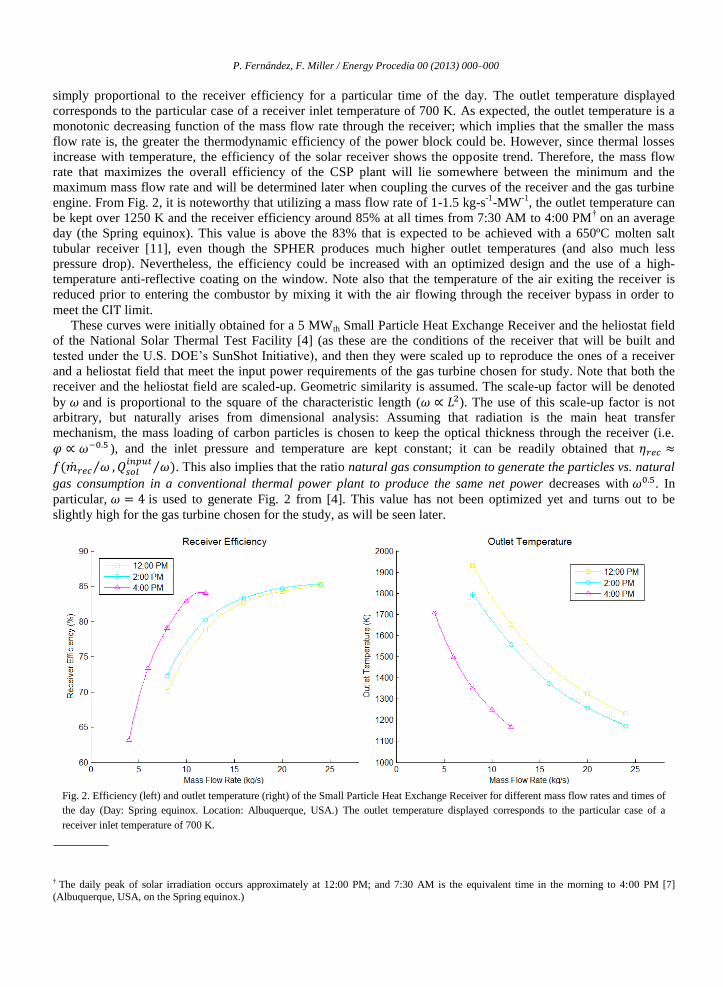
P. Fernández, F. Miller / Energy Procedia 00 (2013) 000–000
simply proportional to the receiver efficiency for a particular time of the day. The outlet temperature displayed
corresponds to the particular case of a receiver inlet temperature of 700 K. As expected, the outlet temperature is a
monotonic decreasing function of the mass flow rate through the receiver; which implies that the smaller the mass
flow rate is, the greater the thermodynamic efficiency of the power block could be. However, since thermal losses
increase with temperature, the efficiency of the solar receiver shows the opposite trend. Therefore, the mass flow
rate that maximizes the overall efficiency of the CSP plant will lie somewhere between the minimum and the
maximum mass flow rate and will be determined later when coupling the curves of the receiver and the gas turbine
engine. From Fig. 2, it is noteworthy that utilizing a mass flow rate of 1-1.5 kg-s-1
-MW-1
, the outlet temperature can
be kept over 1250 K and the receiver efficiency around 85% at all times from 7:30 AM to 4:00 PM† on an average
day (the Spring equinox). This value is above the 83% that is expected to be achieved with a 650ºC molten salt
tubular receiver [11], even though the SPHER produces much higher outlet temperatures (and also much less
pressure drop). Nevertheless, the efficiency could be increased with an optimized design and the use of a high-
temperature anti-reflective coating on the window. Note also that the temperature of the air exiting the receiver is
reduced prior to entering the combustor by mixing it with the air flowing through the receiver bypass in order to
meet the limit.
These curves were initially obtained for a 5 MWth Small Particle Heat Exchange Receiver and the heliostat field
of the National Solar Thermal Test Facility [4] (as these are the conditions of the receiver that will be built and
tested under the U.S. DOE’s SunShot Initiative), and then they were scaled up to reproduce the ones of a receiver
and a heliostat field that meet the input power requirements of the gas turbine chosen for study. Note that both the
receiver and the heliostat field are scaled-up. Geometric similarity is assumed. The scale-up factor will be denoted
by and is proportional to the square of the characteristic length ( ). The use of this scale-up factor is not
arbitrary, but naturally arises from dimensional analysis: Assuming that radiation is the main heat transfer
mechanism, the mass loading of carbon particles is chosen to keep the optical thickness through the receiver (i.e.
), and the inlet pressure and temperature are kept constant; it can be readily obtained that
⁄
⁄ . This also implies that the ratio natural gas consumption to generate the particles vs. natural
gas consumption in a conventional thermal power plant to produce the same net power decreases with . In
particular, is used to generate Fig. 2 from [4]. This value has not been optimized yet and turns out to be
slightly high for the gas turbine chosen for the study, as will be seen later.
Fig. 2. Efficiency (left) and outlet temperature (right) of the Small Particle Heat Exchange Receiver for different mass flow rates and times of
the day (Day: Spring equinox. Location: Albuquerque, USA.) The outlet temperature displayed corresponds to the particular case of a
receiver inlet temperature of 700 K.
† The daily peak of solar irradiation occurs approximately at 12:00 PM; and 7:30 AM is the equivalent time in the morning to 4:00 PM [7]
(Albuquerque, USA, on the Spring equinox.)
P. Fernández, F. Miller / Energy Procedia 00 (2013) 000–000
3.2. Gas turbine engine
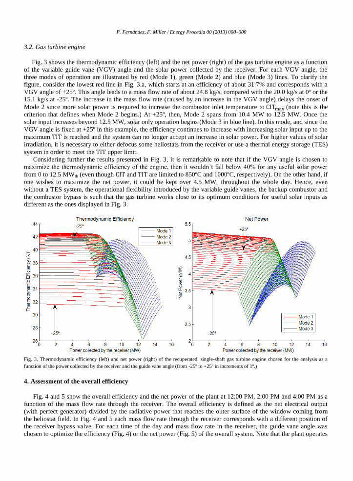
Fig. 3 shows the thermodynamic efficiency (left) and the net power (right) of the gas turbine engine as a function
of the variable guide vane (VGV) angle and the solar power collected by the receiver. For each VGV angle, the
three modes of operation are illustrated by red (Mode 1), green (Mode 2) and blue (Mode 3) lines. To clarify the
figure, consider the lowest red line in Fig. 3.a, which starts at an efficiency of about 31.7% and corresponds with a
VGV angle of +25º. This angle leads to a mass flow rate of about 24.8 kg/s, compared with the 20.0 kg/s at 0º or the
15.1 kg/s at -25º. The increase in the mass flow rate (caused by an increase in the VGV angle) delays the onset of
Mode 2 since more solar power is required to increase the combustor inlet temperature to (note this is the
criterion that defines when Mode 2 begins.) At +25º, then, Mode 2 spans from 10.4 MW to 12.5 MW. Once the
solar input increases beyond 12.5 MW, solar only operation begins (Mode 3 in blue line). In this mode, and since the
VGV angle is fixed at +25º in this example, the efficiency continues to increase with increasing solar input up to the
maximum is reached and the system can no longer accept an increase in solar power. For higher values of solar
irradiation, it is necessary to either defocus some heliostats from the receiver or use a thermal energy storage (TES)
system in order to meet the upper limit.
Considering further the results presented in Fig. 3, it is remarkable to note that if the VGV angle is chosen to
maximize the thermodynamic efficiency of the engine, then it wouldn’t fall below 40% for any useful solar power
from 0 to 12.5 MWth (even though and are limited to 850ºC and 1000ºC, respectively). On the other hand, if
one wishes to maximize the net power, it could be kept over 4.5 MWe throughout the whole day. Hence, even
without a TES system, the operational flexibility introduced by the variable guide vanes, the backup combustor and
the combustor bypass is such that the gas turbine works close to its optimum conditions for useful solar inputs as
different as the ones displayed in Fig. 3.
Fig. 3. Thermodynamic efficiency (left) and net power (right) of the recuperated, single-shaft gas turbine engine chosen for the analysis as a
function of the power collected by the receiver and the guide vane angle (from -25º to +25º in increments of 1º.)
4. Assessment of the overall efficiency
Fig. 4 and 5 show the overall efficiency and the net power of the plant at 12:00 PM, 2:00 PM and 4:00 PM as a
function of the mass flow rate through the receiver. The overall efficiency is defined as the net electrical output
(with perfect generator) divided by the radiative power that reaches the outer surface of the window coming from
the heliostat field. In Fig. 4 and 5 each mass flow rate through the receiver corresponds with a different position of
the receiver bypass valve. For each time of the day and mass flow rate in the receiver, the guide vane angle was
chosen to optimize the efficiency (Fig. 4) or the net power (Fig. 5) of the overall system. Note that the plant operates
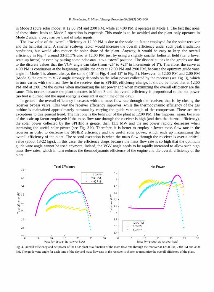
P. Fernández, F. Miller / Energy Procedia 00 (2013) 000–000
in Mode 3 (pure solar mode) at 12:00 PM and 2:00 PM, while at 4:00 PM it operates in Mode 1. The fact that none
of these times leads to Mode 2 operation is expected: This mode is to be avoided and the plant only operates in
Mode 2 under a very narrow band of solar inputs.
The low value of the overall efficiency at 12:00 PM is due to the scale-up factor employed for the solar receiver
and the heliostat field. A smaller scale-up factor would increase the overall efficiency under such peak irradiation
conditions, but would also reduce the solar share of the plant. Anyway, it would be easy to keep the overall
efficiency in Fig. 4 around 33-35.5% also at 12:00 PM just by using a slightly smaller heliostat field (i.e. a lower
scale-up factor) or even by putting some heliostats into a “stow” position. The discontinuities in the graphs are due
to the discrete values that the VGV angle can take (from -25º to +25º in increments of 1º). Therefore, the curve at
4:00 PM is continuous at the beginning, unlike the ones at 12:00 PM and 2:00 PM, because the optimum guide vane
angle in Mode 1 is almost always the same (-15º in Fig. 4 and 12º in Fig. 5). However, at 12:00 PM and 2:00 PM
(Mode 3) the optimum VGV angle strongly depends on the solar power collected by the receiver (see Fig. 3), which
in turn varies with the mass flow in the receiver due to SPHER efficiency change. It should be noted that at 12:00
PM and at 2:00 PM the curves when maximizing the net power and when maximizing the overall efficiency are the
same. This occurs because the plant operates in Mode 3 and the overall efficiency is proportional to the net power
(no fuel is burned and the input energy is constant at each time of the day.)
In general, the overall efficiency increases with the mass flow rate through the receiver; that is, by closing the
receiver bypass valve. This way the receiver efficiency improves, while the thermodynamic efficiency of the gas
turbine is maintained approximately constant by varying the guide vane angle of the compressor. There are two
exceptions to this general trend. The first one is the behavior of the plant at 12:00 PM. This happens, again, because
of the scale-up factor employed: If the mass flow rate through the receiver is high (and then the thermal efficiency),
the solar power collected by the SPHER is greater than 13.5 MW and the net power rapidly decreases when
increasing the useful solar power (see Fig. 3.b). Therefore, it is better to employ a lower mass flow rate in the
receiver in order to decrease the SPHER efficiency and the useful solar power, which ends up maximizing the
overall efficiency of the plant. The second exception is when the mass flow through the receiver is over a critical
value (about 18-22 kg/s). In this case, the efficiency drops because the mass flow rate is so high that the optimum
guide vane angle cannot be used anymore. Indeed, the VGV angle needs to be rapidly increased to allow such high
mass flow rates, which in turn reduces the thermodynamic efficiency of the engine and the overall efficiency of the
plant.
Fig. 4. Overall efficiency and net power of the CSP plant as a function of the mass flow rate through the receiver at 12:00 PM, 2:00 PM and 4:00
PM. The guide vane angle for each time of the day and mass flow rate in the receiver is chosen to maximize the overall efficiency of the plant.
P. Fernández, F. Miller / Energy Procedia 00 (2013) 000–000
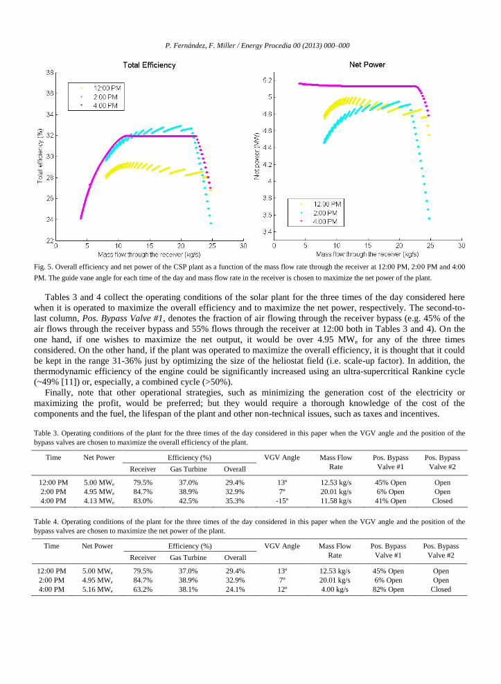
Fig. 5. Overall efficiency and net power of the CSP plant as a function of the mass flow rate through the receiver at 12:00 PM, 2:00 PM and 4:00
PM. The guide vane angle for each time of the day and mass flow rate in the receiver is chosen to maximize the net power of the plant.
Tables 3 and 4 collect the operating conditions of the solar plant for the three times of the day considered here
when it is operated to maximize the overall efficiency and to maximize the net power, respectively. The second-to-
last column, Pos. Bypass Valve #1, denotes the fraction of air flowing through the receiver bypass (e.g. 45% of the
air flows through the receiver bypass and 55% flows through the receiver at 12:00 both in Tables 3 and 4). On the
one hand, if one wishes to maximize the net output, it would be over 4.95 MWe for any of the three times
considered. On the other hand, if the plant was operated to maximize the overall efficiency, it is thought that it could
be kept in the range 31-36% just by optimizing the size of the heliostat field (i.e. scale-up factor). In addition, the
thermodynamic efficiency of the engine could be significantly increased using an ultra-supercritical Rankine cycle
(~49% [11]) or, especially, a combined cycle (>50%).
Finally, note that other operational strategies, such as minimizing the generation cost of the electricity or
maximizing the profit, would be preferred; but they would require a thorough knowledge of the cost of the
components and the fuel, the lifespan of the plant and other non-technical issues, such as taxes and incentives.
Table 3. Operating conditions of the plant for the three times of the day considered in this paper when the VGV angle and the position of the
bypass valves are chosen to maximize the overall efficiency of the plant.
Time Net Power Efficiency (%) VGV Angle Mass Flow
Rate
Pos. Bypass
Valve #1
Pos. Bypass
Valve #2 Receiver Gas Turbine Overall
12:00 PM 5.00 MWe 79.5% 37.0% 29.4% 13º 12.53 kg/s 45% Open Open
2:00 PM 4.95 MWe 84.7% 38.9% 32.9% 7º 20.01 kg/s 6% Open Open
4:00 PM 4.13 MWe 83.0% 42.5% 35.3% -15º 11.58 kg/s 41% Open Closed
Table 4. Operating conditions of the plant for the three times of the day considered in this paper when the VGV angle and the position of the
bypass valves are chosen to maximize the net power of the plant.
Time Net Power Efficiency (%) VGV Angle Mass Flow
Rate
Pos. Bypass
Valve #1
Pos. Bypass
Valve #2 Receiver Gas Turbine Overall
12:00 PM 5.00 MWe 79.5% 37.0% 29.4% 13º 12.53 kg/s 45% Open Open
2:00 PM 4.95 MWe 84.7% 38.9% 32.9% 7º 20.01 kg/s 6% Open Open
4:00 PM 5.16 MWe 63.2% 38.1% 24.1% 12º 4.00 kg/s 82% Open Closed
P. Fernández, F. Miller / Energy Procedia 00 (2013) 000–000
5. Conclusions
The overall efficiency of a gas turbine-driven CSP plant using a Small Particle Heat Exchange Receiver –a high
temperature receiver developed in the framework of the U.S. DOE’s SunShot Initiative– has been estimated at
different times of the day. First, the curves of the receiver and the gas turbine engine were obtained using in-house
codes, extensively discussed in [3] and [5] respectively. On the one hand, the receiver efficiency can be kept as high
as 85% for any time between 7:30 AM and 4:00 PM of the Spring equinox by properly adjusting the mass flow rate
through the receiver. This value is above the 83% that is expected to be achieved with a 650ºC tubular receiver [11],
even though the SPHER produces much higher outlet temperatures (and also much less pressure drop). The SPHER
efficiency could be further increased with an optimized design and with the use of a high-temperature anti-reflective
coating on the window. On the other hand, the thermodynamic efficiency of the gas turbine is around 38-42.5%
when choosing the guide vane angle of the compressor to maximize the efficiency and around 37-39% when
choosing it to maximize the net power (the exact value of the engine efficiency depends on the solar input.)
Then, both curves were coupled together in an effort to assess the performance of the overall system. The guide
vane angle of the compressor was allowed to vary and two bypasses were introduced –in the receiver and in the
combustor– in order to accommodate the variable nature of the solar input and the differences between receiver and
gas turbine. Two different operational strategies were analyzed, namely maximizing the overall efficiency of the
solar plant and maximizing the net power. As for the former, it is thought that the overall efficiency can always be
kept in the range 31-36% by using a receiver and heliostat field of optimum size for the gas turbine engine; while in
the latter the net power wouldn’t fall below 4.95 MWe for any of the three times considered here.
While several difficulties still need to be overcome for its commercialization (e.g. thermal energy storage or
validation of large-scale small particle receivers), the results presented in this paper reveal the strengths of gas
turbine-driven CSP plants using small particle receivers over the lower-temperature state-of-the-art Rankine cycles
and molten salt tubular receivers. Furthermore, gas turbine operation is only one of the several possibilities to
exploit the very high temperatures that can be achieved with small particle receivers: Other options, such as
supercritical Rankine cycles [11] or, especially, combined cycles, are likely to further increase the overall efficiency
of the plant to over 40-42%.
Acknowledgements
The authors gratefully acknowledge the U.S. Department of Energy for providing funding for this research
through the SunShot Initiative under the Award #DE-EE0005800. We would also like to thank Aerojet Rocketdyne,
Solar Turbines and Thermaphase Energy for their collaboration in the project.
References
[1] Gehring, B. and Miller, F. “Thermodynamic Cycle Analysis and Energy Storage for Concentrating Solar Power Plants”, IECEC 2011, San
Diego, USA, July 31st – August 3rd, 2011.
[2] Hunt, A. “A New Solar Thermal Receiver Utilizing Small Particles”, Proceedings of the International Solar Energy Society Conference,
Atlanta, USA, 1362-1366, 1979.
[3] Fernández, P. “Numerical-Stochastic Modeling, Simulation and Design Optimization of a Small Particle Solar Receiver for Concentrated
Solar Power Plants”, Proyecto Fin de Carrera, University of Valladolid, Spain, 2013.
[4] Fernández, P., Miller, F and Crocker, A. “Three-Dimensional Fluid Dynamics and Radiative Heat Transfer Modeling of a Small Particle Solar
Receiver”, ASME 2013 7th International Conference on Energy Sustainability, Minneapolis, USA, July 14th-19th, 2013.
[5] Kitzmiller, K. and Miller, F. “Thermodynamic Cycles for Small Particle Solar Receivers used in Concentrating Solar Power Plants”, ASME
Journal of Solar Engineering, vol. 133, 031014, 2011.
[6] Kitzmiller, K. and Miller, F. “Effect of Variable Guide Vanes and Natural Gas Hybridization for Accommodating Fluctuations in Solar Input
to a Gas Turbine”, Journal of Solar Energy Engineering, vol. 134, 041008, 2012.
[7] Mecit, A. M. “Optical Analysis and Modeling of a Window of the Small Particle Solar Receiver using the Monte Carlo Ray Trace Method”,
Master’s Thesis, Department of Mechanical Engineering, San Diego State University, 2013.
[8] Kurzke, J. “GasTurb11: Design and Off-Design Performance of Gas Turbines”, 2007.
[9] NASA Glenn Research Center, “CEA History”, 2010.
[10] Lefebvre, A. “Gas Turbine Combustion”, 2nd Ed., Taylor and Francis, Philadelphia, 1999.
[11] Kolb, G. J. “An Evaluation of Possible Next-Generation High-Temperature Molten-Salt Power Towers”, Sandia National Laboratories
Technical Report, SAND2011-9320, 2011.
Top Related
Copyright © 2022 FDOKUMEN

