Download - Arab QTCP: Improving Throughput Performance Evaluation with High-Speed Networks

Arab J Sci EngDOI 10.1007/s13369-012-0483-z

RESEARCH ARTICLE - COMPUTER ENGINEERING AND COMPUTER SCIENCE

QTCP: Improving Throughput Performance Evaluationwith High-Speed Networks

Barkatullah Qureshi · Mohamed Othman ·Shamala Subramaniam · Nor Asila Wati

Received: 4 April 2011 / Accepted: 10 January 2012© King Fahd University of Petroleum and Minerals 2012

Abstract High-speed TCP (HSTCP) is one of the severalpopular variants of TCP aimed at the optimization of TCPfor high-speed networks. Like all other variants, HSTCPalso fails to take full shared bandwidth utilization and offerslow throughput rate, high packet loss rate and poor fairness.To overcome these problems, a new adaptive congestioncontrol algorithm with high-speed delay product network,named, the Quick Transport Control Protocol (QTCP) hasbeen designed through this research. The basic idea of QTCPhas been inspired by the HSTCP and CUBIC, which sup-ported to enhance the algorithm. Three main component ofQTCP window control algorithm are α phase, β phase andmultiplicative decrease. An experimental setup was designedfor the evaluation of QTCP. In this experiment, the QTCPwas evaluated based on average throughput and fairnessbetween multiple flows with the same RTT. QTCP performstuning of the sender side modification based on slow startand AIMD algorithms of HSTCP and CUBIC. QTCP pro-vides higher throughput and enhanced fairness as comparedto most of the currently available TCP variants for high-speednetworks. The improved throughput and fairness remainsintact even in the presence of background traffic. NS-2

B. Qureshi (B) ·M. Othman · S. Subramaniam · N. A. WatiDepartment of Communication Technology and Network,Faculty of Computer Science and Information Technology,Universiti Putra Malaysia, 43400 UPM,Serdang, Selangor D.E., Malaysiae-mail: [email protected]

M. Othmane-mail: [email protected]

S. Subramaniame-mail: [email protected]

N. A. Watie-mail: [email protected]

simulator-based results with different configurations are pre-sented, discussed in detail, and evaluated with other popularalgorithms.

Keywords HSTCP · AIMD · Congestion control ·Throughput · Fairness

1 Introduction

The availability of high-speed networks coupled with high-end computational power has fuelled the development ofdistributed collaborative applications, which are used byscientists to analyze the large datasets. This development and

123

Arab J Sci Eng

analysis, however, require a reliable and fast mechanism forsharing the data and, hence, researchers have investigatedseveral ways of optimization of the standard TCP protocolin the context of high-speed networks. Mostly, the optimiza-tion of the TCP is achieved in terms of the modification ofits congestion control algorithm in such a way that it avoidsthe collapses of different flows and finetunes the availablebandwidth. Congestion control is an important componentof a transport protocol in a packet-switched shared networkand most congestion control algorithms for the widely usedconnection-oriented TCP are responsible for detecting con-gestion and reacting to overloads in the Internet. These algo-rithms have proved to be the key to the Internet’s operationalsuccess. As demonstrated in [1], the basic role of the conges-tion control algorithm is to adjust the transmission windowof the sender side in such a manner that buffer overflow isprevented not only at the receiver but also at the intermediaterouters.

The problem of congestion collapse occurs when senderswith no end-to-end flow and congestion control keep trans-mitting packets even though they will be discarded down-stream, e.g. by a bottleneck link, before reaching their finaldestinations [2]. This could become a major problem as alarge amount of bandwidth can be wasted by these unde-livered packets. In a worst-case scenario, some applicationsmay even increase their transmission rates in response toa higher packet drop rate. Traditionally, while handling thedata, TCP’s congestion control performs well in most caseswhere the bandwidth is not extremely high, it shares the avail-able bandwidth and offers fairness to millions of Internetusers. However, when the available bandwidth becomes veryhigh, TCP, as tuned today, does not perform well. This isbecause in the congestion avoidance phase, TCP takes a longtime to increase the window size and cannot fully utilize theavailable bandwidth [3,4].

To ameliorate this issue, several high-speed variants ofTCP have been implemented, such as High-Speed TCP(HSTCP) [5], Reno and New Reno TCP [6,7], ScalableTCP (STCP) [8], Binary Increase Congestion Control TCP(BIC TCP) [9], CUBIC TCP [10], Hamilton TCP (HTCP)[11], FAST TCP [12], Compound TCP [13] and TCP Illi-nois [14]. Each of these algorithms is optimized accordingto the network, hardware and data transfer demands, at thetime when the algorithms were designed, while, nowadaysmore optimized and advanced hardware and heavy enter-prise data transfer demands. The existing algorithms havesome weaknesses that are the reason behind low utiliza-tion of link and hardware. According to current needs anddemands, optimization of existing congestion control mecha-nism is required. In this article we propose our new approach,named the Quick Transport Control Protocol (QTCP) basedon the modification of HSTCP. The QTCP takes a dif-ferent approach in terms of congestion control over high-

speed networks, and, hence, achieves improved through-put performance and fairness. The comparative analysis ofdifferent high-speed protocols with QTCP is described inTable 1.

The Quick Transport Control Protocol (QTCP) algorithmis based on optimization of HSTCP slow start algorithm andAdditive Increase and Multiplicative Decrease (AIMD) algo-rithm. A modified algorithm has been developed by usingan additive increase approach to grow window with normalspeed and to increase scalability by putting constant valueof stability of timeline in congestion avoidance phase. Thisconstant timeline gives long stability time; it provides manybenefits as compared to other high-speed TCP protocols.The main features of QTCP are to maintain the stability ofthe flow, increase packet sending rate per RTT and control thecwnd. In this way QTCP promotes stability, utilization andminimum packet loss rate until the flow completes its datatransfer. The improved algorithm increased throughput anddecreased packet loss rate and fairly share link utilization.The experiment has been conducted to compare the resultsof QTCP with other high-speed protocols. This experimentshows the impact of background traffic on the performanceof QTCP and observed that QTCP achieves better averagethroughput and fairness as compared to other high-speed pro-tocols, such as Nreno, HSTCP, CUBIC, BIC, STCP, HTCP,FAST, Illinois and CTCP The comparison of results are basedon the Network Simulator (NS-2) with several experimentalconfigurations.

2 Related Works

As the aforementioned content, numbers of new protocolshave been developed to replace the standard TCP and achieveefficient bandwidth utilization in high-speed networks. Therouter-based protocols, such as XCP and VCP, require theexplicit feedback information from routers to guide theircontrol strategies. However, it is impractical to modify allthe existing routers in a real world. Therefore, a majority ofthe existing protocols focus on the end-to-end method ratherthan the router-based method for the performance improve-ment of high-speed networks. The end-to-end protocols canbe mainly classified into two categories: loss-based conges-tion control algorithms, e.g. HSTCP, STCP, HTCP, BIC TCP,CUBIC TCP, etc and delay-based congestion control algo-rithms such as FAST TCP. The loss-based congestion con-trol algorithms utilize packet loss as the congestion measure,the window size increases for each ACK and decreases perpacket loss. HSTCP and STCP are the early works along theloss-based methods. To quickly catch-up the available band-width, HSTCP uses step-wise functions for the increase anddecrease of window size while STCP sets the increasing anddecreasing values proportional to the current window size.

123

Arab J Sci Eng

Tabl

e1

Com

para

tive

anal

ysis

ofQ

TC

Pw

ithhi

gh-s

peed

TC

Ppr

otoc

ols

TC

Psc

hem

esFa

irne

ss/u

nfai

rnes

sT

CP

frie

ndlin

ess

Fast

conv

erge

nce

Agg

ress

iven

ess

Win

dow

Stab

ility

Scal

abili

ty

NR

eno

Shor

tRT

Tfa

ir/lo

ngN

otfr

iend

lyC

onve

rges

slow

lyM

ore

aggr

essi

veU

nsta

ble

with

all

Mod

erat

esc

alab

ility

RT

Tun

fair

prot

ocol

HST

CP

Fair

with

back

grou

ndtr

affic

/Sev

erel

yR

TT

unfa

ir

Les

sT

CP

frie

ndlin

ess

Con

verg

esve

rysl

owly

,in

crea

ses

prop

agat

ion

dela

y,do

esno

thav

ean

yde

dica

ted

fast

conv

erge

nce

mec

hani

sm

Agg

ress

ive

insh

ortR

TT

and

low

loss

rate

envi

ronm

ent

Goo

dst

abili

tyin

smal

lw

indo

wsi

ze/N

otst

able

inlo

ngR

TT

netw

orks

Mod

erat

esc

alab

ility

CU

BIC

Effi

cien

tand

RT

Tfa

irw

ithin

tra

prot

ocol

s/un

fair

toth

eflo

wst

artin

gat

ala

ter

time

Les

sfr

iend

lyw

ithot

her

TC

Psan

dno

tfri

endl

yw

ithM

IMD

and

aggr

essi

veT

CP

sche

mes

Con

verg

essl

owly

,inc

reas

espa

cket

slo

ssra

teA

ggre

ssiv

ein

very

shor

tR

TT

Goo

dst

abili

tyG

ood

scal

abili

ty

BIC

Fair

inH

igh-

spee

den

viro

nmen

t,go

odfa

irne

ssin

pres

ence

ofba

ckgr

ound

traf

fic/R

TT

unfa

ir

Not

frie

ndly

Con

verg

essl

owly

Too

aggr

essi

vesh

ortR

TT

inlo

wsp

eed

netw

ork

Goo

dst

abili

tyin

smal

lw

indo

wsi

zeG

ood

scal

abili

ty

STC

PSe

vere

lyR

TT

un-f

air

Not

frie

ndly

Doe

sno

thav

ean

yde

dica

ted

fast

conv

erge

nce

mec

hani

sm

Ver

yag

gres

sive

for

shor

tdi

stan

celin

ksan

dge

ntle

for

long

dist

ance

links

Not

stab

leG

ood

scal

abili

ty

HT

CP

RT

Tfa

irFr

iend

lyw

ithot

her

prot

ocol

sW

hen

setti

nga

para

met

erpr

oduc

ebe

tter

utili

zatio

nA

ggre

ssiv

e,w

hen

Rou

ndT

rip

Del

ayin

crea

ses

Stab

ility

degr

aded

unde

rba

ckgr

ound

traf

ficM

oder

ate

scal

abili

ty

FAST

Unf

air

insm

allb

uffe

rsan

dlo

ngde

lay

netw

orks

Not

frie

ndly

Doe

sno

thav

ean

yde

dica

ted

fast

conv

erge

nce

mec

hani

sm

Agg

ress

ive

Not

stab

leα

para

met

erm

odifi

catio

nin

crea

ses

scal

abili

ty

ILL

INO

ISR

easo

nabl

efa

irne

ss,R

TT

fair

ness

slig

htly

wor

seL

ess

frie

ndly

Con

vex

curv

etr

ansm

issi

onra

tein

crea

ses

initi

ally

slow

lyla

ter

quic

kly

inco

nvex

curv

e

Agg

ress

ive

inco

ncav

ecu

rve

tran

smis

sion

rate

Lim

ited

Stab

ility

Poor

scal

ing

beha

viou

rw

hen

BD

Pin

crea

ses

C-T

CP

RT

Tfa

irne

sssl

ight

lybe

tter

With

γau

totu

ning

C-T

CP

keep

sgo

odT

CP

frie

ndlin

ess

inpr

esen

ceof

mul

tiple

conc

urre

ntflo

ws

Con

verg

ence

time

ofC

-TC

Pis

tobe

prop

ortio

nalt

oth

eC

onge

stio

nep

och

Slig

htly

mor

eag

gres

sive

whe

nm

ore

pack

etlo

sses

occu

r

Lim

ited

stab

ility

Poor

scal

ing

beha

viou

rw

hen

BD

Pin

crea

ses

QT

CP

Inte

ran

dIn

tra

fair

ness

impr

oves

with

high

-spe

edpr

otoc

ols

flow

sw

ithdi

ffer

entR

TT

s

Mor

efr

iend

lyw

ithot

her

TC

Psex

cept

thos

ew

hich

are

base

don

MIM

Dco

ncep

tor

they

are

aggr

essi

ve

Gro

ws

win

dow

inm

oder

ate

way

that

incr

ease

sst

abili

ty,

utili

zatio

nan

dde

-cre

ases

pack

etlo

ssra

te

Ver

ylit

tleag

gres

sive

inve

rysh

ortR

TT

Win

dow

isst

able

for

long

time

whe

nco

mpa

red

toot

her

TC

Psc

hem

es

Mod

erat

esc

alab

ility

123

Arab J Sci Eng

However, both the two protocols have a serious problem onRTT-fairness performance.

Using these protocols, as the multiple flows competingfor the bottleneck band-width have different RTT delays, thefair utilization of the bandwidth cannot be achieved. HTCPsets a function of the elapsed time since last packet loss forincrease parameter and uses an adaptive backoff strategy atcongestion events so as to achieve a perfect performance onresponsiveness and efficiency in high-speed networks. Forthe above three protocols, the increment of window size isstill fast even the network is close to the congestion event,thus the congestion in network will be caused more easilyamong the competing flows and result in the degradation ofthroughput. BIC TCP is an effective protocol that has drawnmuch attention in research area. The protocol adjusts thewindow size using a binary search method to reach a refer-ence value. When updating the window size, it sets the refer-ence value as the mid point between the maximum referencevalue Winmax and the minimum reference value Winmin. Ifthe length between Winmin and the midpoint is larger than amaximum value Smax, the window size increases linearly bythe value Smax. Hence, the increment of the window size islinear at the initial stage and then becomes logarithmic whenapproaching to the reference point. BIC TCP performs bet-ter than the earlier approaches. However, it also suffers theRTT unfairness problem. Subsequently, an enhanced version,CUBIC TCP, is developed to improve the RTT-fairness per-formance of BIC TCP.

On the other hand, fundamentally different from loss-based congestion control algorithms, delay-based conges-tion control algorithms use queuing delay as the con-gestionmeasure. FAST TCP is a typical delay-based high-speed TCPvariant derived from TCP Vegas [15]. The protocol maintainsqueue occupancy at routers for a small but not zero value soas to lead the network around full bandwidth utilization andachieve a higher average throughput. On the contrary, thethroughput of loss-based algorithms oscillates between fullutilization and under utilization in terms of the probing actionpurposely generates packet losses. In addition, FAST TCP isable to rapidly converge to the equilibrium state and doesnot suffer the RTT unfairness problem. However, despite theunique advantages mentioned above, it also has some inher-ent limitations.

FAST TCP is a delay-based approach and uses the RTTsfor congestion measure; its throughput performance is sig-nificantly affected by the reverse traffic, and the throughputof the source traffic decreases as the queuing delay increaseson the reverse path. Some works have focused on the reversetraffic problem in delay-based congestion control algorithmsand use a variety of schemes that relies on the measurement ofone-way delay to conquer this problem, e.g. in [16–19]. How-ever, these schemes are not designed for highspeed networks.

In addition to the reverse traffic problem, FAST TCP requiresthe buffer size to be larger than the specified value which indi-cates the total packet amount maintained in routers along theflow’s path.

Although any of the loss-based and delay-basedapproaches can achieve higher throughput than the standardTCP, both of them have their pros and cons. In order to per-form more efficiently and effectively in high-speed networks,some approaches, like CTCP and TCP-Illinois, focus on thesynergy of loss-based and delay-based approach. CTCP uti-lizes loss and delay information as the primary congestionindi-cators in different stages to determine direction of win-dow size change, and keeps the traditional Slow-Start at thestart-up period while uses a delay-based component derivedfrom TCP Vegas in congestion avoidance phase. TCP-Illi-nois uses loss information as the primary congestion indica-tor and uses delay information to be the second congestionindicator. During the operation, it utilizes the loss informa-tion to determine the direction of window change and thedelay information issued for adjusting the pace of windowsize change. In order to achieve a concave window size curveand a high throughput, TCP-Illinois set two parameters α andβ, in the protocol operation. When network is far from con-gestion, it sets α to be large and β to be small. Otherwise,α is small and β is large when network is close to conges-tion. These approaches inherit the advantages from both theloss-based and delay-based approaches. However, due to thedelay-based components still uses RTTs to measure the con-gestion, their throughput performance is also affected by thereverse traffic.

There is a plethora of algorithms aimed at optimization ofthe standard TCP in terms of its congestion control mech-anism to tune the requirements of applications that sharelarge data over high-speed networks. Each of these algo-rithms has its own specific set of pros and cons. A new algo-rithm named the Quick Transport Control Protocol (QTCP)has been developed in this research. This algorithm imple-ments a new congestion control mechanism based on themodifications in the slow start phase of HSTCP and AIMD.The modification is done in such a way that it provides sig-nificantly improved convenience, throughput, fairness andefficiency. The design and working philosophy of the QTCPis presented in the following section.

3 QTCP Congestion Control

The proposed algorithm QTCP is inspired by the idea ofHSTCP and CUBIC [5,10]. The deep study about HSTCPand CUBIC approaches have supported to enhance the QTCPalgorithm. The following section gives details of HSTCP andCUBIC with improved QTCP algorithm.

123

Arab J Sci Eng

TCP Protocol Processing

Multiplicative Decrease

α window Growth β α β window Growth

Fig. 1 QTCP Architecture

Fig. 2 Window growth function of QTCP for α part in slow-start phase

Fig. 3 Window growth function of QTCP for β part

3.1 HSTCP and CUBIC

HSTCP is the one of the most popular TCP Congestion con-trol algorithm that is giving the idea of AIMD. The idea ofAIMD is fine; however, the way it increases in cwnd is con-tinuous, while HSTCP increasing window is based on some

Fig. 4 Behaviour of the QTCP in Flow 1 and Flow 2

90°QT

CP

cw

nd w

ave

beha

vior

Time

45°

Fig. 5 Wind wave behaviour

equations. The addition to cwnd on each RTT is big, thuscwnd reaches to maximum saturation point with in short spanof time. This results in low scalability, stability, and higherloss rate but good throughput and fairness.

CUBIC TCP gives an idea, that window should not begrown continually and increase in cwnd should not be big,since cwnd is reaching to its maximum saturation point within short span of time, that does not bring good results. Finally,based on AIMD concept, CUBIC adopts different approachin which it is using cubic function of t (time). The CUBICfunction is able to increase window in two different ways.One is concave just after the reduction of cwnd on loss event,and the other one is convex just before the reduction of cwnd.There is a plateau between the concave and convex ways,which makes it more scalable when compared to HSTCP,because the plateau is before reaching to saturation point.CUBIC keeps increasing cwnd in convex way, right afterit passes plateau, finally cwnd hits its maximum saturation

123

Arab J Sci Eng

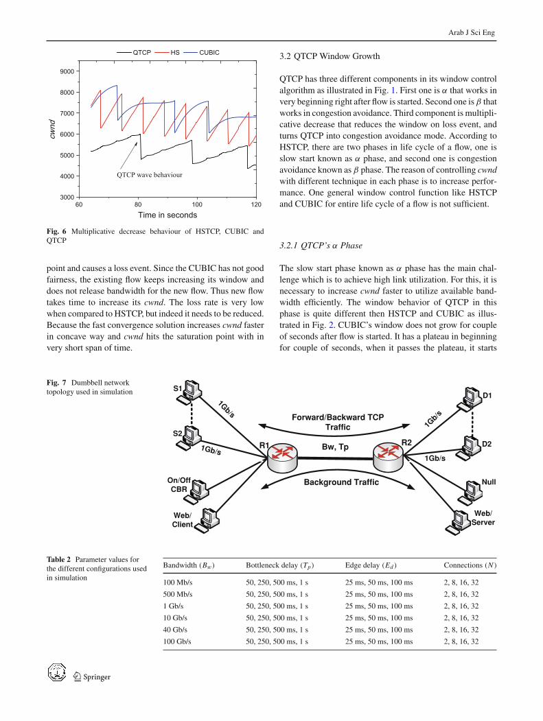
Fig. 6 Multiplicative decrease behaviour of HSTCP, CUBIC andQTCP

point and causes a loss event. Since the CUBIC has not goodfairness, the existing flow keeps increasing its window anddoes not release bandwidth for the new flow. Thus new flowtakes time to increase its cwnd. The loss rate is very lowwhen compared to HSTCP, but indeed it needs to be reduced.Because the fast convergence solution increases cwnd fasterin concave way and cwnd hits the saturation point with invery short span of time.

3.2 QTCP Window Growth

QTCP has three different components in its window controlalgorithm as illustrated in Fig. 1. First one is α that works invery beginning right after flow is started. Second one is β thatworks in congestion avoidance. Third component is multipli-cative decrease that reduces the window on loss event, andturns QTCP into congestion avoidance mode. According toHSTCP, there are two phases in life cycle of a flow, one isslow start known as α phase, and second one is congestionavoidance known as β phase. The reason of controlling cwndwith different technique in each phase is to increase perfor-mance. One general window control function like HSTCPand CUBIC for entire life cycle of a flow is not sufficient.

3.2.1 QTCP’s α Phase

The slow start phase known as α phase has the main chal-lenge which is to achieve high link utilization. For this, it isnecessary to increase cwnd faster to utilize available band-width efficiently. The window behavior of QTCP in thisphase is quite different then HSTCP and CUBIC as illus-trated in Fig. 2. CUBIC’s window does not grow for coupleof seconds after flow is started. It has a plateau in beginningfor couple of seconds, when it passes the plateau, it starts

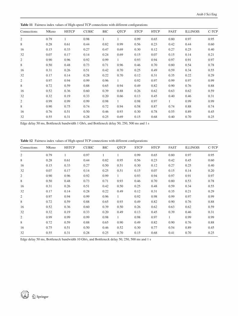
Fig. 7 Dumbbell networktopology used in simulation

1Gb/s

Bw, Tp

Forward/Backward TCPTraffic

Background Traffic

S1

S2

On/OffCBR

Web/Client

R1

Null

Web/Server

D1

D2R21Gb/s

1Gb/s

1Gb/s

Table 2 Parameter values forthe different configurations usedin simulation

Bandwidth (Bw) Bottleneck delay (Tp) Edge delay (Ed ) Connections (N )

100 Mb/s 50, 250, 500 ms, 1 s 25 ms, 50 ms, 100 ms 2, 8, 16, 32

500 Mb/s 50, 250, 500 ms, 1 s 25 ms, 50 ms, 100 ms 2, 8, 16, 32

1 Gb/s 50, 250, 500 ms, 1 s 25 ms, 50 ms, 100 ms 2, 8, 16, 32

10 Gb/s 50, 250, 500 ms, 1 s 25 ms, 50 ms, 100 ms 2, 8, 16, 32

40 Gb/s 50, 250, 500 ms, 1 s 25 ms, 50 ms, 100 ms 2, 8, 16, 32

100 Gb/s 50, 250, 500 ms, 1 s 25 ms, 50 ms, 100 ms 2, 8, 16, 32

123

Arab J Sci Eng

(a) (b)

(c) (d)

Fig. 8 Average throughput amount (with 95 % confidence interval) of high-speed TCP flows with 100 Mb bottleneck bandwidth and 25 ms EdgeDelay. This measures the impact of high-speed TCP protocols on regular TCP traffic

growing too fast and hits saturation point within short spanof time.

This is not the efficient way to increase cwnd, since theavailable bandwidth is not utilized in beginning and alsoreaching maximum saturation point with a short span of time.There are two common problems low utilization and packetloss. HSTCP’s window grows too fast, it starts growing itswindow right after the flow is started and increasing witha big increment until it hits maximum saturation point. Butagain the same thing that cwnd hits its maximum saturationpoint within very short span of time. Again there are havingtwo issues, scalability and packet loss. A new growth func-tion of QTCP is designed for α Phase, which is defined inEq. 2. When flow starts QTCP increases window exponen-tially same like HSTCP as defined in Eq. 2, but later its α

increase (t) function increases the window in moderate way,that increases link utilization and reduces packet loss rate.While inc is a variable that is used to control cwnd, t denotestime, and � is a constant parameter that is set to 3, the valueof t is used to increase packet sending rate until t reaches to�, it makes little ramp, inc α is a constant parameter set to 4,

that is used to increase inc until inc reaches to δ. δ is constantparameter denotes maximum increase in α phase, that is setto its best default value 30.

inc = Qupdate(t) =⎧⎨

⎩

1cwnd ,

αincrease(t),βincrease(t),

i f cwnd < low_window

i f modeC A = F AL SEotherwise

(1)

αincrease(t) =⎧⎨

⎩

t,inc + incα,

t_lastupdate = t

i f t < �

i f inc < δ (2)

Once inc reaches to δ it stops increasing, but QTCP keepsincreasing packet sending rate by adding inc to cwnd. Whencwnd hits its maximum saturation point, it causes to packetloss event, multiplicative decrease component decreasescwnd by half of window size same like HSTCP to reducecongestion, in meantime QTCP does not make any changeto value of inc; after reducing cwnd, QTCP starts increas-ing packet sending rate by adding inc to cwnd until thathits it saturation point, again packet loss event occurs, thistime mul-tiplicative decrease component decreases window

123

Arab J Sci Eng

(a) (b)

(c) (d)


by factor of β = 0.8, and it switches QTCP mode to conges-tion avoidance. QTCP’s congestion avoidance is discussed inthe following section QTCP’s β Phase. All default values forconstant parameters are set according their best performance.QTCP function for α phase is performing outstanding whencompared to HSTCP and CUBIC in most common scenariosthat are tested and validated, QTCP performance and Evalu-ation were discussed in following section. However, QTCPcan be tuned for α phase according to the scenario that isunexpected by adjusting the values for � and δ parameters.Increase in the value for δ increases packet loss rate anddecreases utilization since cwnd increases too fast and hitsmaximum saturation point with short span of time. Pseudocode for α phase is shown in Algorithm.

3.2.2 QTCP’s β Phase

The main challenges in β Phase are to maintain stability, uti-lize the link efficiently and release for new flows and reducepacket loss rate. HSTCP releases the link for new flowsmore efficiently when compared to CUBIC. HSTCP win-dow grows faster that causes rapid congestion. Its windowhas sawtooth wave behavior as illustrated in Fig. 3. Saw-

tooth wave has applications in music, but using sawtoothwave behavior for congestion avoidance is not suitable idea.Therefore, the sawtooth wave does not have that much sta-bility. CUBIC’s window has concave–plateau–convex andconcave behavior as illustrated in Fig. 3. Its concave–pla-teau–convex region gives stability while the region with onlyconcave is not stable. Hence CUBIC does not release win-dow so efficiently. When the new flow joins the link, theexisting flow keeps growing its window, instead of releasinglink for the new flow.

β increase(t)

=⎧⎨

⎩

inc + incβ, t_lastupdate = t, i f t − t_lastupdate≥ updteI nterval

1, i f inc > max I nc(3)

The new function βIncrease(t) has been designed anddefined in Eq. 3 for QTCP that has wind-wave behavior asillustrated in Fig. 3. This function gives more stability, uti-lization, fairness and lower loss rate. In this function incβis a constant parameter set to 1, used to increase inc. inc isa variable that is used to control cwnd, and t_lastastupdateis a variable that holds the information about the time when

123

Arab J Sci Eng

(a) (b)

(c) (d)

Fig. 10 Average throughput amount (with 95 % confidence interval) of high-speed TCP flows with 100 Mb bottleneck bandwidth and 100 msEdge Delay. This measures the impact of high-speed TCP protocols on regular TCP traffic

inc is updated. The updatelnterval is a constant parameterset to 0.5 second that is an update interval between eachupdate of inc. maxlnc is a constant parameter set to 10 thatis maximum increment in cwnd per RTT in β phase. WhenQTCP starts working in β phase, it starts increasing cwndby adding inc per RTT to it. Initially value of inc is 1, thenafter passing a time interval that is defined by updatelnter-val, it updates inc by adding incβ to it. This way QTCPmakes a curve, when the value of inc reaches to maxlnc, itcompletes its curve. Now cwnd reaches to higher positionfrom its last position, therefore reset the value of inc to 1,so that it starts making a new curve. When it starts mak-ing new curve again cwnd increases slower, this way cwndcan stay longer on that position, it keeps working in thisway and completes its wave as illustrated in Fig. 3. Whena packet loss event occurs, immediately decreasing cwndby the factor of β, that is discussed in the following sec-tion Multiplicative Decrease. Since to avoid link congestion

as soon as possible, so the wave has not been completed.When new flow joins, it causes link congestion since exist-ing flow is utilizing the link fully. Therefore, reduces cwndby the factor of β so that new flow can get its link share, assoon as, it joins the link. The QTCP’s existing flows comesdown immediately instead of growing its window up andcompleting its wave as illustrated in Fig. 4. All parametersin this function are set to their best default values. QTCP’sβIncrease(t) is performing outstanding with its default val-ues, when compared to other TCP Schemes. However, QTCPcan be tuned for its β phase, by adjusting the values for β

Inc and maxlnc. Adjusting values for these two parameterswill impact on depth of wave’s curve. More depth will givemore utilization, but less stability and higher loss rate. Butstill it can be adjusted to get it to best performance for someunknown scenarios. The updatelnterval has been discussedin the following section. Pseudo code for β phase is shownin Algorithm.

123

Arab J Sci Eng

(a) (b)

(c) (d)


Algorithm 1: Pseudo code of the QTCP

1 Initialization:2 modeC A ← False, first_decrease ← False, decrease_

factor← 0.83 �← 3, δ← 30, inca← 44 Updatelnterval← 0.5, incβ← 1, t_lastupdate← 05 On Each ACK:6 if cwnd ≤ low-window then7 inc = 1/cwnd8 else9 ifmodeC A ← False then

10 aIncrease (now) // now is current time t11 else12 βIncrease (now)13 end14 end15 Packet Loss:16 if first_decrease← True then17 modeC A ← True18 first-decrease← True19 cwnd = decrease_factor * cwnd

20 end21 alncrease(now) :22 if now < � then23 inc← now24 ifnow < δ then25 inc← inc + inca26 t_lastupdate← now27 end28 end29 βIncrease(now) :30 if (now — t_lastupdate) < updatelnterval then31 inc← inc + incβ, t_lastupdate← now32 end33 if inc > maxlnc then34 inc← 135 end

3.3 Wave Behavior

The ocean surface wave model [20], is one of the mostsuitable models for wind-wave behavior, and finally for

123

Arab J Sci Eng

(a) (b)

(c) (d)


QTCP design wind-wave behaviour has been selected, andangled it at certain angle as illustrated in Fig. 5. QTCP’swind-wave behaviour gives more utilization, scalability, fair-ness and lower packet loss rate. HSTCP grows its windowfaster, that causes to rapid congestion and for reducing con-gestion it reduces window. CUBIC grows its window inconcave–plateau–convex form that does not give desired uti-lization since during plateau it does not increase its win-dow, and during fast convergence it grows its window inconcave form that reduces scalability. While QTCP doesnot grow its window too fast, also it does not make anylong plateau before maximum saturation point. It does notincrease its window in any concave form that causes rapidcongestion. It keeps increasing its sending rate, in waveform, that increases packet sending rate slower and graduallymakes it faster, when it completes its curve, again it increasespacket sending rate slower and gradually makes it faster. Inwave behaviour window reaches to certain height and thenbecomes slower that causes window to be more stable. ThusQTCP performs outstanding when compared to HSTCP andCUBIC.

3.4 QTCP’s Multiplicative Decrease

On a packet loss event, the window reduces according tothe b factor in QTCP, the β factor is set to its default value0.8. CUBIC reduces its window by the factor of β as well,but CUBIC is setting its value to 0.2, that causes slow con-vergence problem for CUBIC. If the value for CUBIC’s β

factor sets higher than 0.5, it causes higher loss rate. There-fore, CUBIC keeps it 0.2 for the sake of lower loss rate, andits trying to use fast convergence to regain its window posi-tion. The issue resolved successfully, because of the wind-wave behaviour is able to reduce the window by 0.8, sincewind-wave behaviour gives enough stability even to reduc-ing the window by 0.8. The value higher than 0.5 meansare not going too much down and window should not bestable, but still there are good fairness, stability and lowerloss rate. While CUBIC is decreasing its window by 0.2, itmeans it has to be more stable, but its window behaviour doesnot allow it to be more stable. Stability of a window can beseen by the interval between last loss event and current lossevent as illustrated in Fig. 6. In this experiment the value of

123

Arab J Sci Eng

(a) (b)

(c) (d)

Fig. 13 Average throughput amount (with 95 % confidence interval) of high-speed TCP flows with 500 Mb bottleneck bandwidth and 100 msEdge Delay. This measures the impact of high-speed TCP protocols on regular TCP traffic

CUBIC β set to 0.8 that is discussed in the following sectionPerformance and Evaluation. There are still more researchis needed on this issue, for adoptive adjustment of betafactor.

3.5 TCP Friendliness and Fairness

QTCP design gives desired fairness. QTCP has Intra-Pro-tocol and Inter-Protocol fairness; also it has Intra-RTT andInter-RTT fairness. However its fairness is slightly lower thanHSTCP but still it gives desired fairness when compared toCUBIC. QTCP flows are friendly with TCP schemes’ flowsexcept those which are very aggressive as STCP’s flows.QTCP is more friendly as compare CUBIC, but still reason-able TCP Friendliness have been achieved, more research isneeded to be done to adjust TCP schemes to gain desiredTCP friendliness.

3.6 Update Interval

QTCP’s parameter for update interval is the most importantparameter, since aggressiveness of the protocol is controlled

by this parameter. While aggressiveness of the protocoldepends on window growth speed. Faster window growthmakes protocol aggressive, slower window growth reducesaggressiveness. It is set to its best default value 0.5, whichresults in good throughput, scalability and link utilization andreduces packet loss rate. Its performance is outstanding; how-ever, value for update interval can be tuned easily, for somespecial scenarios. The value greater than 0.5 results in slowwindow growth, and lesser than 0.5 results in faster windowgrowth. Let us say if there is some scenario in which RTT istoo short, and reducing QTCP’s aggressiveness is required,for this case, the update interval should be set greater than 0.5.This will make it less aggressive. Its default value performsoutstanding in short, medium and long RTTs.

4 QTCP: Performance Evaluation

There is no any congestion between source and destinationin a single flow, when multiple flows S1, S2, S3…, shared thesame path R1 and the bottleneck, produced congestion. Gen-erally, dumbbell topology used when there is only one shared

123

Arab J Sci Eng

(a) (b)

(c) (d)

Fig. 14 Average throughput amount (with 95 % confidence interval) of high-speed TCP flows with 1 Gb bottleneck bandwidth and 25 ms EdgeDelay. This measures the impact of high-speed TCP protocols on regular TCP traffic

path for the multiple flows. In summary, the dumbbell topol-ogy is required for congestion events. The QTCP, is an algo-rithm based on congestion control, therefore, the dumbbelltopology has been selected in this experiment. Several exist-ing models of TCP congestion control have been developedfor the dumbbell topology [21–23]. The performance of con-gestion control algorithm QTCP has been evaluated in thefollowing experiment, based on the average throughput andfairness between multiple flows with the same RTT.

4.1 Experimental Setup

Performance evaluation of the QTCP algorithm was carriedout with several experiments using the Network Simulator(NS-2) [24] software. The experiments were aimed at com-paring the average throughput and fairness (under differentnetwork scenarios/configurations) of the QTCP with thoseof New-Reno, HSTCP, HTCP, BIC, CUBIC, STCP, FAST,CTCP and TCP Illinois. The simple dumbbell topology usedin these experiments as shown in Fig. 7. Dumbbell topologyconnects a group of sender nodes (S1, S2. . .. . . Sn) to a sin-gle router R1, the R1 is serially connected to another router

R2, which, in turn, is connected to another group of receivernodes (D1, D2 . . .. Dn). The dotted line shows the connec-tion link between the sender/receiver nodes with the capacityof 100 Mbps. The bandwidth of the serial link between thetwo routers could be different for different configurations andis represented with Bw. The bottleneck delay is representedwith Tp. Two other parameters used in this topology includethe edge delay (Ed) and number of connections (N ).

Table 2 shows the values of these parameters used for dif-ferent scenarios. With these values, 288 configurations wererun for each protocol. For the valid results, the simulationfor each configuration was repeated 10 times for experimentswith N less than 16, and 5 times in the case when N was 16or greater.

The start time of different flows was randomly varied(between 0 and 2 s) for each simulation in order to get itsexact flow time. All TCP connections were attached withftp agents and then each simulations were run for 500 s.The first start time was set to use the first TCP connection,the second start time used the second TCP connection andso forth for all 10 runs. At the end of each configuration,the next configuration was set to be scheduled and the same

123

Arab J Sci Eng

(a) (b)

(c) (d)


process repeated with the same set of start times in order toestablish the legitimacy of the evaluation. Two nodes wereused to cater for the routers R1 and R2 connected through aduplex link. The queue limit was computed for each routerand the time for the reception of the acknowledgement wasset to 2 Tp. The best scenario with full bandwidth utilizationwas set to twice the bandwidth-delay product, that is, 2 * Bw

* Tp (2 being the queue size).

4.2 Throughput Evaluations with Multiple Flows

Throughput is the amount of data that traverse the networksuccessfully per unit time. To determine the throughput ofQTCP and to compare it with other high-speed protocols,different experiments were designed with different values ofnetwork parameters, as shown in Table 2. In each experimentfirst 100 Mb/s bandwidth; 50, 250, 500 ms and 1 s bottleneckdelay; and 2, 8, 16 and 32 connections evaluates with only oneedge delay 25 ms. Afterwards, the same bandwidths, bottle-neck delays and connections have been evaluated with edgedelay 50 ms and 100 ms respectively. Each experiment wasrun for 500 s and the total amount of data traversed during thistime was computed as No of packets transmitted ∗1000∗8.

Where 1000 is the number of bytes per packet and is multi-plied with 8 to express the amount of data in terms of bits.The total amount of data was then divided with 500 s to getthe throughput. Each experiment was repeated several timesand the average throughput was computed for each protocolwith different configurations, as presented in the followingsections.

Throughput mean was computed from the number of con-nections and standard deviation, for the further study of sim-ulation results. The standard error of the mean was computedby the standard deviation divided by the number of connec-tions and finally computed as the 95 % confidence interval.The confidence interval can be found in Figs. 8, 9, 10, 11,12, 13, 14, 15, 16, 17, 18 and 19, it implies that QTCP showsbetter throughput than the other protocols.

4.2.1 Configurations with Link Capacity of 1 00Mbps, EdgeDelay 25, 50, 100 (ms) and Bottleneck Delay 50, 250,500 (ms), 1 (s)

Figures 8, 9 and 10, show the results of the experiments withthe above configuration using multiple TCP flows (N : 2, 8,

123

Arab J Sci Eng

(a) (b)

(c) (d)


16, and 32). The simulation results show that the increasein the edge delay Ed and the bottleneck link delay causesa corresponding increase in the average throughput, wherethe increase in the number of nodes lessens the throughput.With 50 ms bottleneck delay the average throughput of theQTCP is higher by 1 % to 2 % than all the other protocols,as indicated in Figs. 8a, 9a and 10a. Increasing the value ofbottleneck delay to 250 ms raises the average throughput ofthe QTCP to 16.5 4 and 6.96 % higher than the correspondingaverage throughput of New Reno and HTCP, respectively, asshown in Fig. 9b. With 500 ms bottleneck delay in Fig. 9cthe average throughput of the QTCP becomes 41.66 %, 26.68and 9.62 % higher than the corresponding average through-put of New Reno, HTCP and Illinois, respectively. Finally,with 1 bottleneck delay and edge delay Ed of 100 ms, inFig. 9d the average throughput of QTCP becomes signif-icantly high as compared to all other protocols, such as93.24 % with respect to New Reno, 22.20 % with respectto HSTCP, 9.86 % with respect to CUBIC, 6.12 % withrespect to BIC, 43.77 % with respect to STCP, 52.51 % withrespect to HTCP, 21.34 % with respect to FAST, 20.30 %with respect to Illinois and 10.00 % with respect to CTCP.

The corresponding 95 % confidence intervals of the through-put for the results as in Figs. 8, 9 and 10 and find that QTCP ismore compatible with Nreno, HSTCP, CUBIC, BIC, HTCP,STCP, FAST, Illinois and C-TCP.

4.2.2 Configurations with Link Capacity of 500 Mbps, EdgeDelay 25, 50, 100 (ms) and Bottleneck Delay 50, 250,500 (ms), 1 (s)

Increasing the bandwidth link capacity from 100Mbps to500Mbps gives slightly different results for the averagethroughput; however, the average throughput of the QTCPis still significantly higher than many of the other protocolsas shown in Figs.11, 12, and 13. In particular, with 50 msbottleneck delay, indicated in Fig. 12a the QTCP’s averagethroughput is 3.41 % higher than FAST protocol. With 250 msbottleneck delay, the QTCP gives 16.27 % higher throughputthan HTCP as shown in Fig. 12b. From Fig. 12c, similarly,with 500 ms bottleneck delay, the average through-put ofthe QTCP is 16.58 and 21.22 % higher than HTCP andNew Reno TCP, respectively. Finally, with 1 second delayreports that, there is significant throughput difference with

123

Arab J Sci Eng

(a) (b)

(c) (d)

Fig. 17 Average throughput amount (with 95 % confidence interval) of high-speed TCP flows with 10Gb bottleneck bandwidth and 25 ms EdgeDelay. This measures the impact of high-speed TCP protocols on regular TCP traffic

New Reno, HSTCP, STCP, HTCP, FAST and Illinois as com-pared to QTCP, as indicated in Figs. 11d, 12d and 13d. TheCorresponding 95 % confidence intervals of the throughputfor the results as in Figs. 11, 12, 13 and find that QTCP ismore compatible with Nreno, HSTCP, CUBIC, BIC, HTCP,STCP, FAST, Illinois and C-TCP.

4.2.3 Configurations with Link Capacity of 1 Gb,EdgeDelay 25, 50, 100 (ms) and Bottleneck Delay 50, 250,500 (ms), 1(s)

Throughput evaluations of different protocols with 1 GBbandwidth are illustrated in Figs. 14, 15, and 16. We achievedbetter results for the QTCP algorithm with 50 ms bottleneckdelay and 25 ms edge delay (Ed). In this case, as depicted inFig. 14a, the QTCP gives an average throughput of 8.82 %higher than New Reno and 1 % to 4 % higher than all otherprotocols, as indicated in Figs. 14a, 15a and 16a. In Fig. 15b,the QTCP average throughput results in 250 ms bottleneckdelays, which shows a difference of 13.23 % with respect

to New Reno, 4.15 % with respect to CUBIC, 17.69 % withrespect to HTCP, 9.44 % with respect to FAST TCP, 4.23 %with respect to Illinois and 3.48 % with respect to CTCPFig. 14c shows, that for the 500 ms bottleneck delay and25 ms edge delay (Ed) the difference becomes 22.12 % withrespect to New Reno, 19.72 % with respect to HTCP, 9.07 %with respect to FAST and 6.57 % with respect to Illinois.Finally, with 1 sec bottleneck delay and 25 ms (Ed), the NewReno average throughput difference is 17.35 %, as indicatedin Fig. 14d, the HSTCP is 4.16 %, as shown in Fig. 15d with50 ms (Ed), CUBIC is 3.45 % with 100 ms (Ed) represents inFig. 16d, BIC is 1.15 % in Fig. 15d. With 100 ms (Ed),FASTis 6.83 % in Fig. 16d and Illinois is 4.47 % with 25 ms inFig. 14d. The most striking result emerging from this data isthe highest average throughput of the QTCP, as compared toNew Reno irrespective of any delay between routers and thenumber of nodes in the topology. The Corresponding 95 %confidence intervals of the throughput for the results as inFigs. 14, 15, 16 and find that QTCP is more compatible withNreno, HSTCP, CUBIC, BIC, HTCP, STCP, FAST, Illinoisand C-TCP.

123

Arab J Sci Eng

(a) (b)

(c) (d)

Fig. 18 Average throughput amount (with 95 % confidence interval) of high-speed TCP flows with 10-Gb bottleneck bandwidth and 50 ms EdgeDelay. This measures the impact of high-speed TCP protocols on regular TCP traffic

4.2.4 Configurations with Link Capacity of 10 Gb,40 Gb,100 Gb, Edge Delay 25, 50, 100 (ms) and BottleneckDelay 50, 250, 500 (ms), 1 (s)

The simulation results for this configuration (using 10 Gblink capacity) are shown in Figs. 17, 18, and 19. With 50 msbottleneck delay, the QTCP’s average throughput is 1 % to4 % higher than all the other protocols. Whereas, in Fig.17b with 250 ms bottleneck delay the average throughput ofQTCP is 13.40 % higher than New Reno, 17.99 % higher thanHTCP, 9.76 % higher than FAST, 4.15 % higher than Illinoisand 3.59 % higher than C-TCP With 500 ms bottleneck delaythe difference is 21.26 % with respect to New Reno in Fig.19c, 19.17 % with respect to HTCP in Fig. 17c, 8.49 % withrespect to FAST in Fig. 18c, 6.31 % with respect to Illinois inFig. 17c and 3.37 % with respect to C-TCP in Fig. 19c. Thedifference with 1 sec bottleneck delay is 16.8 % with respectto New Reno in Fig. 17d, 4.29 % with respect to HTCP,2.46 % with respect to CUBIC and 7.40 % with respect toSTCP, as shown in Fig. 19d, 10.71 % with respect to HTCPin Fig. 17d, 4.20 % with respect to FAST in Fig. 18d, 4.11 %with respect to Illinois in Fig. 17d and 1.90 % with respect

to C-TCP, as shown in Fig. 19d. It has been observed thatthe results obtained with 40 Gb and 100 Gb link capacity arealmost the same as that of 10 Gb. The Corresponding 95 %confidence intervals of the throughput for the results as inFigs. 17, 18, 19 and find that QTCP is more compatible withNreno, HSTCP, CUBIC, BIC, HTCP, STCP, FAST, Illinoisand C-TCP.

4.3 Fairness Index

In wired and wireless network development, when multipleflows share the same resource, there may be a situationwhen the flow cannot share the link fairly. Therefore, weevaluated how the link can be fairly shared and achieveend-to-end throughput for each flow. TLAS-SAF one ofthe unique algorithms, which provide the size, based andthe direction based fairness, and improved performance ofshort lived and long lived flows, in the WLAN [25]. Inmax-min fairness, it is pointed out that each flow’s through-put is as large as other flows in the network that are shar-ing the same bottleneck [26]. Each flow with minimum

123

Arab J Sci Eng

(a) (b)

(c) (d)

Fig. 19 Average throughput amount (with 95 % confidence interval) of high-speed TCP flows with 10-Gb bottleneck bandwidth and 100 ms EdgeDelay. This measures the impact of high-speed TCP protocols on regular TCP traffic

demand achieves the maximum share of resources; there-fore, all flows receive an equal share of resources. Variousresearchers have worked on it and have found that the pro-portional fairness is used to maximize the utility functionfor the set of flows [27,28]. However, such fairness methodslike, Randomized TCP and max-min fairness have a numberof limitations. It would be more advantageous to use a spe-cific metric for fairness as it can be facilitated with measure-ment, which is related to the flow’s performance (end-to-endthroughput).

One of the most widely used methods for assessing fair-ness is the Jain Fairness index (JFI) [29]. Different TCP stackperformances have been evaluated to examine how the differ-ent protocols behave fairly towards each other [30]. In thisresearch, we computed the fair share link metric by usingEq. 4, which describes the Jain fairness index, as stated byChiu and Jain [29].

F =(∑n

i=1 xi)

n∑n

i=1 x2i

2

(4)

where n is number of flows, 1/n capacity of bottleneck link,xt average bandwidth of each source i. In this method whenF = 1, it specifies the perfect value of fairness index, andwhen F = 0, it indicates no fairness at all.

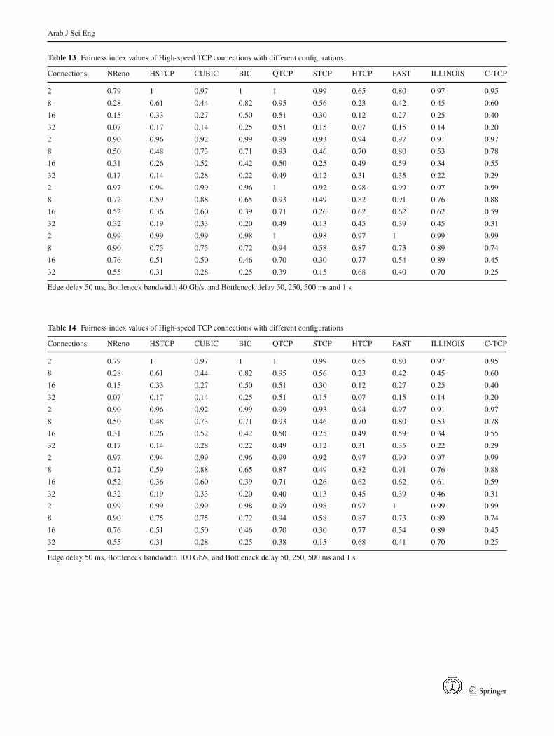
We conducted a series of experiments for the evaluationof multiple high-speed flows in different configurations, asshown in Tables 3, 4, 5, 6, 7, 8, 9, 10, 11, 12, 13, 14, 15,16, 17, 18, 19, and 20 in the Appendix. In this perspec-tive, we compared the fairness of multiple connections thatshares same bottleneck link capacity 100 Mb, 500 Mb, 1 Gb,10 Gb, 40 Gb and 100 Gb under different edge delays (Ed)(25 ms, 50 ms and 100 ms, bottleneck delays 50, 250, 500 msand 1 s). As described in the above sections, the simulationswere run 10 times by randomly changing the start time ofthe multiple flows. Analysis of different configurations indi-cates that fairness performance of the QTCP is much bettercompared to other high-speed protocols. When we comparedthe fairness of multiple flows on 50 ms bottleneck delayunder different link capacities, the result obtained showsthat the QTCP is a bit higher than other protocols. After-wards, we analysed 250 and 500 ms bottleneck delay where

123

Arab J Sci Eng

Fig. 20 Evaluation of QTCP and other high-speed TCP variantsaverage throughput with background Traffic

Fig. 21 The fairness of various high-speed protocols with backgroundtraffic

the QTCP achieved better fairness compared to other proto-cols. Subsequently, after examining the 1 s bottleneck delaywe achieved the most significant fairness. The results of allflows achieved with 10 Gb, 40 Gb and 100 Gb are signif-icantly fairer than other protocols. The remarkable obser-vation from the comparison of these flows is that when thenumber of flow increases the link flow utilization becomesmore fair.

4.4 Impact of Background Traffic on the Performanceof QTCP1

It has been observed that high-speed protocols must be eval-uated in terms of background traffic otherwise it might lead

to incorrect conclusions [31]. Therefore, we examined theaverage throughput and fairness of the QTCP in the presenceof background traffic and compared it with other high-speedprotocols as shown in Figs. 20, and 21. The results showthat even with the presence of background traffic, the aver-age throughput and fairness of the QTCP remains high ascompared to other protocols. It could also be observed thatalthough HTCP and STCP exhibit slightly improved through-put in the presence of background traffic, their fairness ismoderate and low, respectively. BIC and CUBIC moderatelyimproved the throughput as well as the fairness. Illinois TCPand C-TCP offer slightly improved fairness but their through-put becomes degraded. The throughput of New Reno fluc-tuates (increases and decreases), while no increment in thethroughput of FAST TCP was detected.

5 Conclusions

The QTCP, a new variant of high-speed TCP, was proposedand studied in this article. The most significant finding thatemerged from this study is that the QTCP achieves improvedfairness in terms of the multiple flows sharing the link andit also offers high throughput in terms of complex networkresources compared to most of the existing high-speed TCPvariants. The sender side modification in the code makesit easy to set out in the Internet. Multiple simulations andexperiments revealed that the new approach could vigor-ously adjust the HSTCP slow start and AIMD algorithmto overcome the unfairness problem in single bottlenecklink capacity. It has been observed that the improvement inthe throughput and the fairness persists even in the pres-ence of background traffic. The 95 % confidence intervalunder difference confidence levels it is found that the resultsof QTCP are quite stable and confirm the effectiveness ofQTCP. The limitation in the current analysis is that underthe bandwidth bottleneck capacity 100 Mb, as the number ofnodes increases; concurrently the throughput becomes verysmall. Consequently, it is recommended that the future tri-als should analyse the parallel flows that use multiple effec-tive TCP connections. It is assumed that as the parallel TCPwould aggregate, the throughput would increase, the loss ratewould decrease and, hence, even better throughput would beachieved.

Acknowledgments This work was supported by the Research Uni-versity Grant Scheme (RUGS Number: 05/01/07/0180RU)

Appendix

See Tables 3, 4, 5, 6, 7, 8, 9, 10, 11, 12, 13, 14, 15, 16, 17,18, 19 and 20.

123

Arab J Sci Eng

Table 3 Fairness index values of High-speed TCP connections with different configurations

Connections NReno HSTCP CUBIC BIC QTCP STCP HTCP FAST ILLINOIS C-TCP

2 0.66 0.67 0.67 0.67 1 0.59 0.76 1 0.78 0.99

8 0.19 0.32 0.76 0.37 0.99 0.32 0.66 1 0.47 0.54

16 0.14 0.16 0.70 0.18 0.88 0.17 0.59 0.53 0.26 0.57

32 0.08 0.08 0.74 0.08 0.79 0.08 0.44 0.31 0.13 0.32

2 0.97 0.95 0.96 1 1 0.84 0.98 1 0.97 1

8 0.73 0.67 0.97 0.68 0.98 0.46 0.94 1 0.74 0.99

16 0.52 0.42 0.97 0.43 0.95 0.27 0.93 0.99 0.56 0.93

32 0.33 0.29 0.87 0.23 0.88 0.20 0.71 0.79 0.34 0.61

2 0.99 0.98 0.94 0.95 1 0.95 0.98 1 0.99 0.99

8 0.88 0.82 0.98 0.84 0.96 0.70 0.99 0.99 0.88 1

16 0.74 0.65 0.80 0.70 0.88 0.51 0.91 0.99 0.73 0.96

32 0.54 0.74 0.62 0.35 0.71 0.29 0.72 0.66 0.55 0.58

2 1 1 1 1 1 1 0.99 1 1 1

8 0.97 0.95 0.98 0.91 0.98 0.95 0.97 0.98 0.97 0.96

16 0.90 0.83 0.73 0.54 0.94 0.59 0.92 0.64 0.86 0.59

32 0.76 0.81 0.57 0.27 0.69 0.30 0.75 0.36 0.80 0.30

Edge delay 25 ms, Bottleneck bandwidth 100 Mb/s, and Bottleneck delay 50, 250, 500 ms and 1 s



2 0.97 1 1 1 1 1 0.79 0.90 0.99 0.99

8 0.47 0.68 0.76 0.78 0.99 0.83 0.35 0.60 0.58 0.73

16 0.25 0.43 0.64 0.60 0.89 0.50 0.21 0.44 0.37 0.50

32 0.14 0.26 0.47 0.37 0.69 0.27 0.12 0.30 0.21 0.30

2 0.97 0.99 0.98 0.99 1 0.98 0.99 0.99 0.97 0.99

8 0.73 0.79 0.85 0.87 0.95 0.70 0.85 0.91 0.77 0.90

16 0.51 0.56 0.74 0.73 0.70 0.42 0.72 0.81 0.64 0.76

32 0.32 0.37 0.54 0.54 0.69 0.25 0.51 0.59 0.49 0.53

2 0.99 0.98 1 0.99 1 0.98 0.98 1 0.99 1

8 0.88 0.81 0.97 0.88 0.95 0.71 0.94 0.96 0.90 0.96

16 0.73 0.64 0.88 0.78 0.88 0.49 0.83 0.91 0.77 0.88

32 0.53 0.40 0.60 0.56 0.71 0.27 0.64 0.63 0.64 0.58

2 1 1 1 1 1 1 0.99 1 1 1

8 0.96 0.95 0.91 0.94 0.98 0.94 0.96 0.99 0.97 0.98

16 0.90 0.75 0.74 0.72 0.94 0.58 0.88 0.74 0.89 0.74

32 0.76 0.51 0.51 0.48 0.69 0.30 0.79 0.55 0.89 0.45


123

Arab J Sci Eng



2 0.97 1 1 1 1 1 0.79 0.90 0.99 0.99

8 0.47 0.91 0.63 0.98 0.99 0.85 0.35 0.60 0.70 0.78

16 0.26 0.59 0.42 0.81 0.70 0.54 0.21 0.44 0.44 0.60

32 0.14 0.32 0.26 0.48 0.70 0.29 0.12 0.29 0.24 0.40

2 0.97 0.99 0.98 1 1 0.98 0.99 0.99 0.97 0.99

8 0.73 0.73 0.85 0.93 0.95 0.74 0.85 0.91 0.74 0.90

16 0.51 0.46 0.76 0.69 0.70 0.45 0.72 0.82 0.54 0.79

32 0.32 0.26 0.53 0.41 0.70 0.24 0.51 0.59 0.35 0.56

2 0.99 0.98 1 0.99 1 0.98 0.98 1 0.99 1

8 0.88 0.8 0.97 0.85 0.95 0.71 0.94 0.96 0.9 0.96

16 0.73 0.60 0.88 0.65 0.88 0.49 0.83 0.91 0.76 0.88

32 0.53 0.37 0.60 0.39 0.72 0.27 0.64 0.63 0.63 0.59

2 1 1 1 1 1 1 0.99 1 1 1

8 0.96 0.95 0.91 0.94 1 0.94 0.96 0.99 0.97 0.98

16 0.90 0.75 0.74 0.72 0.93 0.58 0.88 0.74 0.88 0.74

32 0.76 0.51 0.49 0.46 0.90 0.30 0.79 0.55 0.89 0.45

Edge delay 25 ms, Bottleneck bandwidth 1 Gb/s, and Bottleneck delay 50, 250, 500 ms and 1 s



2 0.97 1 1 1 1 1 0.79 0.90 0.99 0.99

8 0.47 0.91 0.63 0.98 0.99 0.85 0.35 0.60 0.70 0.78

16 0.26 0.59 0.42 0.81 0.70 0.54 0.21 0.44 0.44 0.60

32 0.14 0.32 0.26 0.48 0.70 0.29 0.12 0.29 0.24 0.40

2 0.97 0.99 0.98 1 1 0.98 0.99 0.99 0.97 0.99

8 0.73 0.73 0.85 0.93 0.95 0.74 0.85 0.91 0.74 0.90

16 0.51 0.46 0.76 0.69 0.70 0.45 0.72 0.82 0.54 0.79

32 0.32 0.26 0.53 0.41 0.70 0.24 0.51 0.59 0.35 0.56

2 0.99 0.98 1 0.99 1 0.98 0.98 1 0.99 1

8 0.88 0.80 0.97 0.85 0.95 0.71 0.94 0.96 0.9 0.96

16 0.73 0.60 0.88 0.65 0.88 0.49 0.83 0.91 0.76 0.88

32 0.53 0.37 0.60 0.39 0.72 0.27 0.64 0.63 0.63 0.59

2 1 1 1 1 1 1 0.99 1 1 1

8 0.96 0.95 0.91 0.94 1 0.94 0.96 0.99 0.97 0.98

16 0.90 0.75 0.74 0.72 0.93 0.58 0.88 0.74 0.88 0.74

32 0.76 0.51 0.49 0.46 0.90 0.30 0.79 0.55 0.89 0.45


123

Arab J Sci Eng



2 0.97 1 1 1 1 1 0.79 0.90 0.99 0.99

8 0.47 0.91 0.63 0.98 0.99 0.85 0.35 0.60 0.70 0.78

16 0.26 0.59 0.42 0.81 0.89 0.54 0.21 0.44 0.44 0.60

32 0.14 0.32 0.26 0.48 0.69 0.29 0.12 0.3 0.24 0.40

2 0.97 0.99 0.98 1 1 0.98 0.99 0.99 0.97 0.99

8 0.73 0.73 0.85 0.93 0.95 0.74 0.85 0.91 0.74 0.90

16 0.51 0.46 0.76 0.69 0.70 0.45 0.72 0.81 0.54 0.79

32 0.32 0.26 0.53 0.41 0.70 0.24 0.51 0.59 0.35 0.56

2 0.99 0.98 1 0.99 1 0.98 0.98 1 0.99 1

8 0.88 0.80 0.97 0.85 0.95 0.71 0.94 0.96 0.90 0.95

16 0.73 0.60 0.87 0.65 0.87 0.49 0.83 0.91 0.76 0.88

32 0.53 0.37 0.60 0.39 0.71 0.27 0.64 0.63 0.63 0.59

2 1 1 1 1 1 1 0.99 1 1 1

8 0.96 0.95 0.91 0.94 0.99 0.94 0.96 0.99 0.97 0.97

16 0.90 0.75 0.74 0.72 0.93 0.58 0.88 0.74 0.88 0.74

32 0.76 0.51 0.50 0.46 0.90 0.30 0.79 0.55 0.89 0.45




2 0.97 1 1 1 1 1 0.79 0.90 0.99 0.99

8 0.47 0.91 0.63 0.98 0.99 0.85 0.35 0.60 0.70 0.78

16 0.26 0.59 0.42 0.81 0.89 0.54 0.21 0.44 0.44 0.60

32 0.14 0.32 0.26 0.48 0.69 0.29 0.12 0.30 0.24 0.40

2 0.97 0.99 0.98 1 1 0.98 0.99 0.99 0.97 0.99

8 0.73 0.73 0.85 0.93 0.95 0.74 0.85 0.91 0.74 0.90

16 0.51 0.46 0.76 0.69 0.70 0.45 0.72 0.81 0.54 0.79

32 0.32 0.26 0.53 0.41 0.70 0.24 0.51 0.59 0.35 0.55

2 0.99 0.98 1 0.99 1 0.98 0.98 1 0.99 1

8 0.88 0.80 0.97 0.85 0.95 0.71 0.94 0.96 0.90 0.96

16 0.73 0.60 0.88 0.65 0.87 0.49 0.83 0.91 0.76 0.88

32 0.53 0.37 0.60 0.39 0.71 0.27 0.64 0.63 0.63 0.59

2 1 1 1 1 1 1 0.99 1 1 1

8 0.96 0.95 0.91 0.94 0.98 0.94 0.96 0.99 0.97 0.97

16 0.90 0.75 0.74 0.72 0.93 0.58 0.88 0.74 0.88 0.74

32 0.76 0.51 0.50 0.46 0.89 0.30 0.79 0.55 0.89 0.45


123

Arab J Sci Eng



2 0.58 0.89 1 0.89 1 0.83 0.85 1 0.63 0.86

8 0.16 0.19 0.70 0.22 0.99 0.18 0.55 0.97 0.23 0.38

16 0.09 0.10 0.66 0.09 0.88 0.09 0.39 0.39 0.12 0.33

32 0.05 0.05 0.40 0.05 0.79 0.04 0.28 0.21 0.06 0.16

2 0.91 0.86 0.99 0.98 1 0.76 0.96 1 0.88 0.98

8 0.51 0.46 0.94 0.66 0.98 0.36 0.87 0.99 0.51 0.87

16 0.31 0.27 0.90 0.36 0.95 0.19 0.74 0.79 0.31 0.63

32 0.17 0.14 0.62 0.16 0.88 0.09 0.48 0.43 0.18 0.29

2 0.97 0.94 0.97 0.97 1 0.87 0.97 1 0.97 0.99

8 0.73 0.60 0.96 0.80 0.96 0.45 0.91 0.98 0.73 0.89

16 0.52 0.50 0.91 0.43 0.88 0.24 0.86 0.62 0.54 0.52

32 0.33 0.37 0.47 0.21 0.71 0.12 0.58 0.34 0.35 0.26

2 0.99 0.99 1 0.99 1 0.98 0.98 1 0.99 0.99

8 0.90 0.78 0.91 0.61 0.98 0.58 0.90 0.69 0.87 0.67

16 0.76 0.61 0.68 0.28 0.94 0.30 0.82 0.44 0.81 0.36

32 0.55 0.46 0.35 0.16 0.42 0.15 0.65 0.27 0.60 0.19




2 0.79 1 0.98 1 1 0.99 0.65 0.80 0.97 0.95

8 0.28 0.49 0.46 0.56 0.94 0.50 0.23 0.42 0.42 0.59

16 0.15 0.25 0.31 0.34 0.88 0.26 0.12 0.27 0.22 0.36

32 0.07 0.13 0.16 0.18 0.66 0.13 0.07 0.15 0.13 0.19

2 0.90 0.96 0.92 0.99 0.99 0.94 0.94 0.97 0.91 0.97

8 0.50 0.47 0.73 0.61 0.93 0.45 0.70 0.80 0.54 0.78

16 0.31 0.27 0.52 0.42 0.50 0.24 0.49 0.59 0.35 0.54

32 0.17 0.14 0.28 0.21 0.49 0.12 0.31 0.35 0.23 0.29

2 0.97 0.94 0.99 0.96 1 0.92 0.97 0.99 0.97 0.99

8 0.72 0.59 0.88 0.67 0.88 0.49 0.82 0.90 0.76 0.88

16 0.52 0.36 0.60 0.44 0.70 0.26 0.63 0.62 0.64 0.59

32 0.32 0.19 0.33 0.24 0.41 0.13 0.45 0.40 0.47 0.31

2 0.99 0.99 0.99 0.98 1 0.98 0.97 0.99 0.99 0.99

8 0.90 0.75 0.74 0.72 0.94 0.58 0.87 0.74 0.89 0.74

16 0.76 0.51 0.50 0.46 0.70 0.30 0.77 0.54 0.90 0.45

32 0.55 0.31 0.28 0.25 0.38 0.15 0.68 0.40 0.71 0.25


123

Arab J Sci Eng



2 0.79 1 0.98 1 1 0.99 0.65 0.80 0.97 0.95

8 0.28 0.61 0.44 0.82 0.99 0.56 0.23 0.42 0.44 0.60

16 0.15 0.33 0.27 0.47 0.69 0.30 0.12 0.27 0.25 0.40

32 0.07 0.17 0.14 0.24 0.69 0.15 0.07 0.15 0.14 0.21

2 0.90 0.96 0.92 0.99 1 0.93 0.94 0.97 0.91 0.97

8 0.50 0.48 0.73 0.71 0.96 0.46 0.70 0.80 0.54 0.78

16 0.31 0.26 0.51 0.42 0.70 0.25 0.49 0.59 0.34 0.55

32 0.17 0.14 0.28 0.22 0.70 0.12 0.31 0.35 0.22 0.29

2 0.97 0.94 0.99 0.96 1 0.92 0.97 0.99 0.97 0.99

8 0.72 0.59 0.88 0.65 0.94 0.49 0.82 0.90 0.76 0.88

16 0.52 0.36 0.60 0.39 0.88 0.26 0.62 0.63 0.62 0.59

32 0.32 0.19 0.33 0.20 0.66 0.13 0.45 0.40 0.46 0.31

2 0.99 0.99 0.99 0.98 1 0.98 0.97 1 0.99 0.99

8 0.90 0.75 0.74 0.72 0.94 0.58 0.87 0.74 0.88 0.74

16 0.76 0.51 0.50 0.46 0.93 0.30 0.78 0.55 0.89 0.45

32 0.55 0.31 0.28 0.25 0.69 0.15 0.68 0.40 0.70 0.25




2 0.79 1 0.97 1 1 0.99 0.65 0.80 0.97 0.95

8 0.28 0.61 0.44 0.82 0.95 0.56 0.23 0.42 0.45 0.60

16 0.15 0.33 0.27 0.50 0.51 0.30 0.12 0.27 0.25 0.40

32 0.07 0.17 0.14 0.25 0.51 0.15 0.07 0.15 0.14 0.20

2 0.90 0.96 0.92 0.99 1 0.93 0.94 0.97 0.91 0.97

8 0.50 0.48 0.73 0.71 0.93 0.46 0.70 0.80 0.53 0.78

16 0.31 0.26 0.51 0.42 0.50 0.25 0.48 0.59 0.34 0.55

32 0.17 0.14 0.28 0.22 0.49 0.12 0.31 0.35 0.21 0.29

2 0.97 0.94 0.99 0.96 1 0.92 0.98 0.99 0.97 0.99

8 0.72 0.59 0.88 0.65 0.93 0.49 0.82 0.90 0.76 0.88

16 0.52 0.36 0.60 0.39 0.50 0.26 0.62 0.63 0.62 0.59

32 0.32 0.19 0.33 0.20 0.49 0.13 0.45 0.39 0.46 0.31

2 0.99 0.99 0.99 0.98 1 0.98 0.97 1 0.99 0.99

8 0.72 0.59 0.88 0.65 0.90 0.49 0.82 0.90 0.76 0.88

16 0.75 0.51 0.50 0.46 0.52 0.30 0.77 0.54 0.89 0.45

32 0.55 0.31 0.28 0.25 0.70 0.15 0.68 0.41 0.70 0.25


123

Arab J Sci Eng



2 0.79 1 0.97 1 1 0.99 0.65 0.80 0.97 0.95

8 0.28 0.61 0.44 0.82 0.95 0.56 0.23 0.42 0.45 0.60

16 0.15 0.33 0.27 0.50 0.51 0.30 0.12 0.27 0.25 0.40

32 0.07 0.17 0.14 0.25 0.51 0.15 0.07 0.15 0.14 0.20

2 0.90 0.96 0.92 0.99 0.99 0.93 0.94 0.97 0.91 0.97

8 0.50 0.48 0.73 0.71 0.93 0.46 0.70 0.80 0.53 0.78

16 0.31 0.26 0.52 0.42 0.50 0.25 0.49 0.59 0.34 0.55

32 0.17 0.14 0.28 0.22 0.49 0.12 0.31 0.35 0.22 0.29

2 0.97 0.94 0.99 0.96 1 0.92 0.98 0.99 0.97 0.99

8 0.72 0.59 0.88 0.65 0.93 0.49 0.82 0.91 0.76 0.88

16 0.52 0.36 0.60 0.39 0.71 0.26 0.62 0.62 0.62 0.59

32 0.32 0.19 0.33 0.20 0.49 0.13 0.45 0.39 0.45 0.31

2 0.99 0.99 0.99 0.98 1 0.98 0.97 1 0.99 0.99

8 0.90 0.75 0.75 0.72 0.94 0.58 0.87 0.73 0.89 0.74

16 0.76 0.51 0.50 0.46 0.70 0.30 0.77 0.54 0.89 0.45

32 0.55 0.31 0.28 0.25 0.39 0.15 0.68 0.40 0.70 0.25




2 0.79 1 0.97 1 1 0.99 0.65 0.80 0.97 0.95

8 0.28 0.61 0.44 0.82 0.95 0.56 0.23 0.42 0.45 0.60

16 0.15 0.33 0.27 0.50 0.51 0.30 0.12 0.27 0.25 0.40

32 0.07 0.17 0.14 0.25 0.51 0.15 0.07 0.15 0.14 0.20

2 0.90 0.96 0.92 0.99 0.99 0.93 0.94 0.97 0.91 0.97

8 0.50 0.48 0.73 0.71 0.93 0.46 0.70 0.80 0.53 0.78

16 0.31 0.26 0.52 0.42 0.50 0.25 0.49 0.59 0.34 0.55

32 0.17 0.14 0.28 0.22 0.49 0.12 0.31 0.35 0.22 0.29

2 0.97 0.94 0.99 0.96 0.99 0.92 0.97 0.99 0.97 0.99

8 0.72 0.59 0.88 0.65 0.87 0.49 0.82 0.91 0.76 0.88

16 0.52 0.36 0.60 0.39 0.71 0.26 0.62 0.62 0.61 0.59

32 0.32 0.19 0.33 0.20 0.40 0.13 0.45 0.39 0.46 0.31

2 0.99 0.99 0.99 0.98 0.99 0.98 0.97 1 0.99 0.99

8 0.90 0.75 0.75 0.72 0.94 0.58 0.87 0.73 0.89 0.74

16 0.76 0.51 0.50 0.46 0.70 0.30 0.77 0.54 0.89 0.45

32 0.55 0.31 0.28 0.25 0.38 0.15 0.68 0.41 0.70 0.25


123

Arab J Sci Eng



2 0.54 0.97 0.73 0.65 1 1 0.88 1 0.55 0.64

8 0.14 0.15 0.51 0.16 0.88 0.14 0.39 0.52 0.16 0.31

16 0.07 0.08 0.35 0.08 0.66 0.07 0.22 0.27 0.08 0.15

32 0.04 0.04 0.19 0.04 0.41 0.04 0.13 0.14 0.04 0.07

2 0.78 0.73 1 0.91 0.99 0.71 0.88 0.96 0.75 0.94

8 0.31 0.28 0.84 0.56 0.66 0.26 0.71 0.81 0.30 0.57

16 0.17 0.14 0.51 0.23 0.50 0.15 0.48 0.42 0.18 0.29

32 0.09 0.07 0.32 0.13 0.49 0.07 0.25 0.22 0.09 0.14

2 0.90 0.83 0.93 0.88 1 0.72 0.97 0.97 0.92 0.97

8 0.51 0.42 0.92 0.60 0.88 0.24 0.62 0.57 0.51 0.55

16 0.31 0.29 0.51 0.30 0.70 0.12 0.41 0.31 0.34 0.28

32 0.17 0.15 0.26 0.14 0.41 0.06 0.25 0.16 0.19 0.14

2 0.97 0.95 0.90 0.95 1 0.95 0.95 0.99 0.98 0.98

8 0.75 0.63 0.67 0.59 0.94 0.35 0.78 0.53 0.86 0.44

16 0.54 0.37 0.40 0.31 0.70 0.18 0.68 0.35 0.64 0.23

32 0.33 0.20 0.17 0.16 0.38 0.09 0.53 0.20 0.38 0.12




2 0.61 0.97 0.72 0.99 1 0.93 0.57 0.69 0.77 0.83

8 0.17 0.35 0.27 0.43 0.88 0.32 0.17 0.28 0.26 0.39

16 0.09 0.18 0.14 0.22 0.66 0.16 0.09 0.15 0.14 0.2

32 0.04 0.09 0.07 0.11 0.41 0.08 0.05 0.08 0.07 0.1

2 0.78 0.80 0.83 0.97 0.99 0.81 0.87 0.92 0.79 0.92

8 0.31 0.28 0.49 0.42 0.66 0.26 0.47 0.59 0.33 0.55

16 0.17 0.14 0.26 0.22 0.50 0.13 0.29 0.34 0.21 0.29

32 0.09 0.07 0.13 0.11 0.49 0.07 0.18 0.19 0.11 0.15

2 0.90 0.83 0.98 0.88 1 0.77 0.97 0.97 0.91 0.97

8 0.51 0.35 0.61 0.39 0.88 0.27 0.62 0.62 0.61 0.58

16 0.31 0.19 0.33 0.20 0.70 0.14 0.43 0.39 0.44 0.31

32 0.17 0.10 0.17 0.10 0.41 0.07 0.30 0.23 0.26 0.16

2 0.97 0.95 0.87 0.95 1 0.95 0.95 0.99 0.97 0.97

8 0.75 0.52 0.51 0.48 0.94 0.35 0.75 0.57 0.89 0.48

16 0.54 0.31 0.29 0.26 0.70 0.18 0.66 0.42 0.70 0.26

32 0.33 0.17 0.15 0.13 0.38 0.09 0.54 0.28 0.44 0.14


123

Arab J Sci Eng



2 0.61 0.97 0.72 0.99 1 0.93 0.57 0.69 0.77 0.83

8 0.17 0.36 0.27 0.52 0.99 0.32 0.17 0.28 0.26 0.4

16 0.09 0.18 0.14 0.27 0.50 0.16 0.09 0.15 0.14 0.2

32 0.04 0.09 0.07 0.13 0.49 0.08 0.05 0.08 0.07 0.1

2 0.78 0.80 0.83 0.97 1 0.81 0.87 0.92 0.79 0.92

8 0.31 0.28 0.49 0.44 0.95 0.26 0.47 0.59 0.33 0.55

16 0.17 0.14 0.26 0.23 0.49 0.13 0.29 0.34 0.21 0.29

32 0.09 0.07 0.13 0.11 0.49 0.07 0.18 0.19 0.11 0.15

2 0.90 0.83 0.98 0.88 0.99 0.77 0.97 0.97 0.91 0.97

8 0.51 0.35 0.62 0.39 0.95 0.27 0.62 0.61 0.61 0.58

16 0.31 0.19 0.33 0.20 0.48 0.14 0.43 0.39 0.44 0.31

32 0.17 0.10 0.17 0.10 0.42 0.07 0.30 0.24 0.26 0.16

2 0.97 0.95 0.87 0.95 1 0.95 0.93 0.99 0.97 0.97

8 0.75 0.52 0.51 0.48 0.71 0.35 0.75 0.57 0.89 0.48

16 0.54 0.31 0.28 0.26 0.46 0.18 0.65 0.42 0.70 0.26

32 0.33 0.17 0.15 0.13 0.45 0.09 0.54 0.28 0.44 0.14




2 0.61 0.97 0.72 0.99 0.99 0.93 0.57 0.69 0.79 0.83

8 0.17 0.36 0.27 0.52 0.95 0.32 0.17 0.28 0.26 0.39

16 0.09 0.18 0.14 0.27 0.49 0.16 0.09 0.15 0.14 0.2

32 0.04 0.09 0.07 0.13 0.45 0.08 0.05 0.08 0.07 0.10

2 0.78 0.80 0.83 0.97 0.97 0.81 0.87 0.91 0.79 0.92

8 0.17 0.36 0.27 0.52 0.92 0.32 0.17 0.28 0.26 0.39

16 0.17 0.14 0.26 0.23 0.48 0.13 0.29 0.34 0.20 0.29

32 0.09 0.07 0.13 0.11 0.44 0.07 0.18 0.19 0.11 0.15

2 0.90 0.83 0.98 0.88 0.99 0.77 0.96 0.97 0.91 0.97

8 0.51 0.35 0.62 0.39 0.89 0.27 0.62 0.61 0.60 0.58

16 0.31 0.19 0.33 0.20 0.46 0.14 0.43 0.39 0.44 0.31

32 0.17 0.10 0.17 0.10 0.41 0.07 0.30 0.23 0.26 0.16

2 0.97 0.95 0.87 0.95 0.99 0.95 0.93 0.99 0.97 0.97

8 0.75 0.52 0.50 0.48 0.71 0.35 0.75 0.57 0.88 0.48

16 0.54 0.31 0.29 0.26 0.43 0.18 0.65 0.41 0.70 0.26

32 0.33 0.17 0.14 0.13 0.39 0.09 0.54 0.28 0.44 0.14


123

Arab J Sci Eng



2 0.61 0.97 0.72 0.99 0.99 0.93 0.57 0.69 0.79 0.83

8 0.17 0.36 0.27 0.52 0.95 0.32 0.17 0.28 0.27 0.39

16 0.09 0.18 0.14 0.27 0.49 0.16 0.09 0.15 0.14 0.2

32 0.04 0.09 0.07 0.13 0.45 0.08 0.05 0.08 0.07 0.10

2 0.78 0.80 0.83 0.97 0.97 0.81 0.87 0.92 0.78 0.92

8 0.31 0.28 0.49 0.44 0.92 0.26 0.47 0.59 0.33 0.55

16 0.17 0.14 0.26 0.23 0.48 0.13 0.29 0.34 0.20 0.29

32 0.09 0.07 0.13 0.11 0.44 0.07 0.18 0.20 0.11 0.15

2 0.90 0.83 0.98 0.88 0.99 0.77 0.96 0.96 0.91 0.97

8 0.51 0.35 0.63 0.39 0.89 0.27 0.62 0.62 0.60 0.58

16 0.31 0.19 0.33 0.20 0.46 0.14 0.43 0.39 0.44 0.31

32 0.17 0.10 0.17 0.10 0.41 0.07 0.30 0.23 0.26 0.16

2 0.97 0.95 0.87 0.95 0.99 0.95 0.93 0.98 0.97 0.97

8 0.75 0.52 0.51 0.48 0.71 0.35 0.75 0.57 0.89 0.48

16 0.54 0.31 0.29 0.26 0.43 0.18 0.65 0.41 0.70 0.26

32 0.33 0.17 0.15 0.13 0.39 0.09 0.54 0.27 0.44 0.14


Table 20 Fairness index values of high-speed TCP connections with different configurations


2 0.61 0.97 0.72 0.99 0.99 0.93 0.57 0.69 0.78 0.83

8 0.17 0.36 0.27 0.52 0.95 0.32 0.17 0.28 0.27 0.39

16 0.09 0.18 0.14 0.27 0.49 0.16 0.09 0.15 0.14 0.2

32 0.04 0.09 0.07 0.13 0.45 0.08 0.05 0.08 0.07 0.1

2 0.78 0.80 0.83 0.97 0.97 0.81 0.87 0.92 0.79 0.92

8 0.31 0.28 0.49 0.44 0.92 0.26 0.47 0.59 0.33 0.55

16 0.17 0.14 0.26 0.23 0.48 0.13 0.29 0.35 0.20 0.29

32 0.09 0.07 0.13 0.11 0.44 0.07 0.18 0.20 0.11 0.15

2 0.90 0.83 0.98 0.88 0.99 0.77 0.97 0.97 0.91 0.97

8 0.51 0.35 0.62 0.39 0.89 0.27 0.62 0.61 0.60 0.58

16 0.31 0.19 0.33 0.20 0.46 0.14 0.43 0.39 0.44 0.31

32 0.17 0.10 0.17 0.10 0.41 0.07 0.30 0.24 0.26 0.16

2 0.97 0.95 0.87 0.95 0.99 0.95 0.93 0.98 0.98 0.97

8 0.75 0.52 0.51 0.48 0.71 0.35 0.75 0.58 0.88 0.48

16 0.54 0.31 0.29 0.26 0.43 0.18 0.66 0.41 0.70 0.26

32 0.33 0.17 0.14 0.13 0.39 0.09 0.54 0.28 0.44 0.14


123

Arab J Sci Eng

References

1. Qureshi, B.; Othman, M.; Hamid, N.A.W.: Progress in various TCPvariants: issues, enhancement and solution. Mausam J. Comput.1(4), 493–500 (2009)

2. Floyd, S.; Fall, K.: Promoting the use of end-to-end congestioncontrol, in the Internet. IEEE/ACM Trans. Netw. 7(4), 458–472(1999)

3. Xue-zeng, P.; Fan-jun, S.; Yong, L.; Ling-di, P.: CW-HSTCP: fairTCP in high-speed networks. J. Zhejiang Univ. Sci. 7(2), 172–178(2006)

4. Fan-jun, S.; Xue-zeng, P.; Jie-bing, W.; Zhengi, W.: An algorithmfor reducing loss rate of high-speed TCP. J. Zhejiang Univ. Sci.7(supp.II), 245–251 (2006)

5. Floyd, S.; Ratnasamy, S.; Shenker, S.: Modifying TCP’s conges-tion control for high speeds. Technical note available at: http://www.icir.org/floyd/papers/hstcp.pdf, pp. 1–5 (2002)

6. Zhang, Y.; Lemin, L.; Wang, S.: Improving Reno and New-Reno’sperformances over OBS networks without SACK. Int. J. Electron.Commun. 63(4), 294–303 (2009)

7. Floyd, S.; Henderson, T.; Gurtov, A.: The NewReno modificationto TCP’s fast recovery algorithm (2004). Available at http://www.faqs.org/rfcs/rfc3782.html

8. Kelly, T.: Scalable TCP: improving performance in high-speedwide area networks. ACM SIGCOMM Comput. Commun. Rev.33(2), 83–91 (2003)

9. Xu, L.; Harfoush, K.; Rhee, I.: Binary increase congestion controlfor fast, long distance networks. In: Proceeding of NETWORK-ING’06, pp. 476–487 (2006)

10. Rhee, I.; Xu, L.: CUBIC: a new TCP-friendly high-speed TCPvariant. In: Proceeding of PFLDnet (2005)

11. Shorten, R.; Leith, D.: H-TCP: TCP for high-speed and long-dis-tance networks. In: Proceeding of Second International Workshopon Protocols for Fast-long Distance Networks (2004)

12. Wei, D.X.; Jin, C.; Low, S.H.; Hegde, S.: FAST TCP:moti-vation,architecture, algorithms, performance. IEEE/ACM Trans.Netw. 14(6), 1246–1259 (2006)

13. Tan, K.; Song, J.; Zhang, Q.; Sridharan, M.: A compound tcpapproach for high-speed and long distance networks. In: INFO-COM Proceeding 25th IEEE International Conference on Com-puter Communications (2006)

14. Liu, S.; Basar, T.; Srikant, R.: TCP-Illionois: a loss- and delay-based congestion control algorithms for high-speed networks. Per-form. Eval. 65, 417–440 (2008)

15. Brakmo, L.S.; Peterson, L.L.: TCP Vegas: end to end congestionavoidance on a Global internet. IEEE J. Select. Areas. Commun.13(8), 1465–1480 (1995)

16. Parsa, C.; Garcia-Luna-Aceves, J.J.: Improving TCP congestioncontrol over internets with heteroge-neous transmission media.In: Proceedings of International Conference on Network Protocols(1999)

17. Fuand, C.P.; CLiew, S.:A remedy for performance degradation ofTCP Vegas in asymmetric networks. IEEE Commun. Lett. 7(1),42–44 (2003)

18. Kuzmanovic, A.; Knightly, E.W.: TCP-LP: a distributed algorithmfor low priority data transfer. In: Proceedings of IEEE INFOCOM(2003)

19. Chan, Y.C.; Chan, C.T.; Chen, Y.C.: Design and performance evalu-ation of an improved TCP con-gestion avoidance scheme. In: IEEEProc. Commun. 151(1), 107–111 (2004)

20. Fournier, A.; Reeves, W.T.: A simple model of ocean waves. Proc.ACM/SIGGRAPH Comput. Graph. 20(4), 75–84 (1986)

21. Fall, K.; Floyd, S.: Simulation-based comparisons of Tahoe Renoand SACK TCP. Comput. Commun. Rev. 26(3), 5–21 (1996)

22. Mathis, M.; Semke, J.; Mahdavi, J.; Ott, T.: The macroscopicbehavior of the TCP congestion avoid-ance algorithm. Commun.Rev. 27(3), 67–82 (1997)

23. Morris, R.: Scalable TCP Congestion Control, PhD thesis, HarvardUniversity, Cambridge, MA (1999)

24. NS-2 The Network Simulator, [online] Available: http://www.isi.edu/nsnam/ns/

25. Khademi, N.; Othman, M.: Size-Based and Direction-Based TCPFairness Issues in IEEE 802.11 WLANs. EURASIP J. Wirel. Com-mun. Netw. 2010, 16 (2010). doi:10.1155/2010/818190

26. Jaffe, J.: Bottleneck flow control. IEEE Trans. Commun. 29(7),954–962 (1981)

27. Kelly, F.; Maulloo, A.; Tan, D.: Rate control in communication net-works: shadow prices, proportional fairness and stability. J. Oper.Res. Soc. 49(3), 237–252 (1998)

28. Kunniyur, S.; Srikant, R.: End-to-end congestion control schemes:utility functions, random losses and ECN marks. IEEE/ACM Trans.Netw. 11(5), 689–702 (2003)

29. Chiu, D.; Jain, R.: Analysis of the increase/decrease algorithm forcongestion avoidance in computer networks. Comput. Netw. ISDN17(1), 1–14 (1989)

30. Bullot, H.; Cottrell, R.L.; Hughes-Jones, R.: Evaluation ofadvanced TCP stacks on fast long-distance production networks.J. Grid Comput. 1(4), 345–359 (2003)

31. Sangtae, H.; Le, L.; Rhee, I.; Xu, L.: Impact of background traf-fic on performance of high-speed TCP variant protocols. Comput.Netw. 51, 1748–1762 (2007)

123

http://www.icir.org/floyd/papers/hstcp.pdf

http://www.icir.org/floyd/papers/hstcp.pdf

http://www.faqs.org/rfcs/rfc3782.html

http://www.faqs.org/rfcs/rfc3782.html

http://www.isi.edu/nsnam/ns/

http://www.isi.edu/nsnam/ns/

http://dx.doi.org/10.1155/2010/818190