Download - Analysis of polynomial-phase signals by the integrated generalized ambiguity function

316 IEEE TRANSACTIONS ON SIGNAL PROCESSING, VOL. 45, NO. 2, FEBRUARY 1997

Analysis of Polynomial-Phase Signals by theIntegrated Generalized Ambiguity Function

Sergio Barbarossa,Member, IEEE, and Valentina Petrone

Abstract—The aim of this work is the performance analysis ofa method for the detection and parameter estimation of monoor multicomponent polynomial-phase signals (PPS) embeddedin white Gaussian noise and based on a generalized ambiguityfunction. The proposed method is shown to be asymptoticallyefficient for second-order PPS and nearly asymptotically efficientfor third-order PPS’s. The method presents some advantageswith respect to similar techniques, like the polynomial-phasetransform, for example, in terms of

i) a closer approach to the Cramer-Rao lower bounds,ii) a lower SNR threshold,iii) a better capability of discriminating multicomponent sig-

nals.

I. INTRODUCTION

T HE AIM of this paper is to propose a method for the pa-rameter estimation of multicomponent (MC) polynomial-

phase signals (PPS) embedded in additive white Gaussiannoise (AWGN). The observed signal is modeled as follows:

(1)

where the instantaneous phase of each component is apolynomial, and is a white Gaussian noise. Polynomial-phase signals can be a good model in a variety of applicationslike, for example, radar, sonar, and communication over time-varying channels. In these cases, in fact, the received signalexhibits an instantaneous phase modulation due to the relativemotion between sensor and target in the radar or sonar case orbetween transmitter and receiver in mobile communications.The phase modulation is directly proportional to the distancebetween sensor and target or between transmitter and receiver.Since the distance is certainly a continuous smooth function oftime, it can be well approximated by a low-order polynomialwithin a finite duration interval, according to the Weierstrasstheorem. Several approaches have been proposed for analyzingthis class of signals. An excellent overview of the methodsfor estimating the instantaneous frequency is provided in[9]. The maximum likelihood (ML) approach is known topossess good asymptotic properties but is also difficult toimplement because it requires the solution of a multivariate

Manuscript received December 30, 1994; revised June 5, 1996. Theassociate editor coordinating the review of this paper and approving it forpublication was Dr. Patrick Flandrin.

S. Barbarossa is with the INFOCOM Department, University of Rome “LaSapienza,” Rome, Italy (e-mail: [email protected]).

V. Petrone is with the Consortium for Research on Telecommunications(CoRiTel), 00133 Rome, Italy (e-mail: [email protected]).

Publisher Item Identifier S 1053-587X(97)01196-3.

nonlinear optimization problem; the problem is even moredifficult in the case of multicomponent signals. Some simplerapproaches were proposed by Abatzoglou [1] and O’Shea[16] for linear FM signals that are valid for monocomponentsignals. A simple method for estimating the instantaneousphase of sinusoids embedded in noise was proposed by Tretter[24], where the estimation was obtained by linear regressionof the instantaneous phase calculated directly from the signalafter phase unwrapping. The method provides good results forsignal-to-noise ratio (SNR) above 15 dB. The approach wasthen extended by Djuri´c and Kay [12] for analyzing PPS’sof a generic degree. The method exhibited a threshold ofapproximately 8 dB. In addition, however, these methods arevalid only for monocomponent signals because the sum ofPPS’s is not a PPS, in general. In fact

(2)

where

(3)

and

(4)

Therefore, even in the absence of noise, it is not possibleto recover the instantaneous phase of each componentstarting from the instantaneous phase of the sum signal.A different approach that is not based on the direct estimationof the instantaneous phase was suggested by Kumaresan andVerma [15], who proposed a sequential estimation technique.Given a PPS of degree , if we take the product

(5)

we obtain a PPS of order . Repeating this operationtimes, we obtain a first-order PPS that is a complex

sinusoid. It is straightforward to show, by direct substitution,that the frequency of the sinusoid is proportional to theth-order coefficient of the original signal . The estimationof the highest order coefficient can then be formulated asa frequency estimation problem, which can be solved byconventional harmonic analysis, using FFT-based approachesor by signal-subspace projection techniques. Once the high-est order coefficient has been estimated, it can be removed

1053–587X/97$10.00 1997 IEEE

BARBAROSSA AND PETRONE: ANALYSIS OF POLYNOMIAL-PHASE SIGNALS 317

from the signal , thus obtaining an th-orderPPS. The technique can then be iterated to estimate all thephase coefficients from the highest order to the first orderone. This approach was then further analyzed by Peleg andPorat, who introduced the polynomial-phase transform (PPT)[17], [13], which was later called the high-order ambiguityfunction (HAF) [20]. A similar approach was also proposedby Giannakis and Dandawate in the framework of th-order cyclostationary processes [11]. The approach was thenextended to the case of random amplitude PPS’s in [23].A different but related approach was proposed by Boashashans O’Shea, who suggested the use of a generalized Wigner-Ville Distribution (WVD) [10]. In [3], the relationship betweenambiguity function (AF) and WVD-related techniques for theanalysis of linear FM signals was shown. The goodness ofthe approaches proposed in [17], [11], [10], and [3], withrespect to previous techniques, is their capability of dealingwith multicomponent signals.

In this paper, we generalize the approach proposed in [3]to PPS’s of any order. The proposed method is able to dealwith multicomponent signals and offers some advantages withrespect to conventional techniques in the presence of noise. Inparticular, the method exhibits a smaller SNR threshold withrespect to conventional techniques [24], [12], [17]. Further-more, the threshold is not a fixed number, but it depends onthe number of samples. In particular, the threshold decreases asthe number of samples increases. This property is particularlyimportant in those applications where the SNR is limited by themaximum peak power of the transmitter or by the minimumnoise figure of the receiver. For a fixed threshold system,to raise the SNR above the threshold requires an increaseof the transmitter power or a decrease of the receiver noisefigure; both actions can be very costly from the economicalpoint of view. On the other hand, having a method with athreshold decreasing with the number of samples allows usto decrease the threshold below the given SNR by simplyincreasing the observation interval and then increasing thenumber of samples.

In the paper, we will provide a theoretical performance anal-ysis of the proposed method, together with some simulationresults. Part of the results shown in this paper were reportedin a condensed form in [4]. The paper is organized as follows.The generalized ambiguity function (GAF) and the integratedGAF (IGAF) are introduced in Sections II and III, respectively.The performance analysis is reported in Sections IV and V.Section IV provides a closed-form expression of the SNR gainobtainable using the IGAF; in Section V, the accuracy of theproposed approach is evaluated for a finite sample sequenceby using the small perturbation method.

II. GENERALIZED AMBIGUITY FUNCTION

Given a finite energy signal , we define its genericth-order kernel according to the

following recursive rule:

(6)

We define the th-order GAF of as the Fouriertransform of the th-order kernel with respect to the variable

(7)

In particular, the first-order GAF is simply the Fourier trans-form of the signal, whereas the second-order GAF is equal tothe conventional ambiguity function (AF). If the signal is afinite duration signal defined over the intervalcharacterized by a constant envelope and anth-degreepolynomial phase

rect (8)

its th-order kernel is a complex sinusoid whose frequencydepends only on the coefficient and whose initial phasedepends only on the coefficient

rect (9)

where

(10)

The function rect is equal to 1 in the intervaland 0 outside. The correspondingth-order

GAF is

(11)

where . This expression suggests a methodfor estimating the parameters of a polynomial-phase signal:The th-order coefficient is estimated as the position ofthe maximum absolute value of the th-order GAF of .Let us denote by the estimate of . The th-orderphase term is then removed from by multiplying by

. If the estimation is correct , theresulting signal is an th-order polynomial phase. Wecan thus proceed recursively by computing the th-order GAF of the resulting signal, estimating the positionof the maximum and so on, up to the first-order coefficient.Stated in this form, the method is essentially the same as themethod based on the PPT [17], [20], the only difference beingthe apparently nonessential fact that the PPT is a particularcase of the GAF-based method corresponding to the case inwhich the lags are all equal to each other. More precisely, thePPT coincides with a hyperdiagonal of the GAF evaluated on


the hypersurface of equation .However, it is exactly the redundancy implicit in the multilagdefinition that will produce a performance improvement, withrespect to the PPT, as will be shown in the ensuing sections.

III. I NTEGRATED GENERALIZED AMBIGUITY FUNCTION

From (11), we can observe that the th-order GAF ofan th-order polynomial phase signal assumes its maximumvalue, in modulus, over the hyper-surface of equation

(12)

The property of having the maxima distributed over theprevious surface is obviously strictly related to the model ofuseful signal. Other signals, or the noise, do not share thisproperty; therefore, we can envisage the following strategyfor discriminating th-order polynomial phase signals fromother kinds of signals: We can integrate the modulus of the

th-order GAF over all the surfaces of equation

(13)

as a function of , thus obtaining a function : Themaximum of lies on the value . The estimateof is then reconducted to the search for the maximum of

. An even better approach can be followed by consideringa coherent integration of the GAF instead of the noncoherentintegration proposed before. We have already observed thatthe GAF assumes its maximum values in modulus on thesurface defined by (12). On that surface, its phase depends onlyon . We can exploit this property to devise a coherentintegration that provides better performance.

A. Definition

We define the IGAF as

(14)

or, equivalently, by using (7)

(15)

B. Properties

Some properties of the IGAF are useful in order to under-stand its characteristics.

Property 1: The th-order IGAF, for greater than 1, isreal and positive.

Proof: By inserting (6) in (15) and exchanging the inte-gration order, we obtain

If we now apply the change of variables

(16)

(17)

to the two inner integrals, we obtain

This expression is certainly real and positive. Q.E.D.It is important to notice that the number of integrals neces-

sary to compute the th-order IGAF is instead of .This property is exploited in the computation of the IGAF toreduce the computational cost.

Property 2: The th-order IGAF of an th-degree poly-nomial phase signal (8) assumes its maximum value in thepoint of coordinates .

Proof: Let us first demonstrate that the first-order partialderivatives of the th-order IGAF of an th-degree PPS areequal to zero in the point . If we derive (15) withrespect to , we obtain

Evaluating this expression in the point of coordinatesand taking into account (9), it is easy to verify

that, given the antisymmetry of the integrand function and thesymmetry of the integration interval, the integral is equal tozero. The derivative with respect to satisfies the sameproperty, and then, the two first-order partial derivativesare both equal to zero. Therefore, the point of coordinates

is a point of extreme. By following a similarprocedure with the second-order partial derivatives, it is


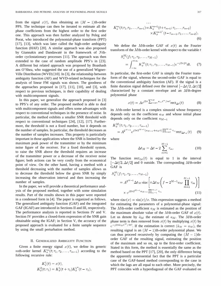
Fig. 1. IGAF of a cubic phase signal embedded in 0-dB WGN.

possible to show that the point is, in fact, the point wherethe IGAF is maximum. Q.E.D.

C. Examples

Some examples of application are useful to show the effectof the coherent integration operated by the IGAF in thepresence of signal plus noise or of multicomponent signals.

1) Signal Plus Noise:Fig. 1 shows the third-order IGAF ofa cubic phase signal embedded in a 0-dB white Gaussian noise.The IGAF has been computed on a sequence of 128samples. The phase coefficients of the signal are:and . The function has been evaluatedon the grid of values: and , for

(the normalization factors have been chosenin order to respect the Nyquist’s criterion). The samplingperiod is equal to 1 s. From Fig. 1, it is possible to noticethe following aspects:

• In spite of the presence of a 0-dB noise, the peak ofthe IGAF is still quite evident—the strong attenuationof the noise contribution is due to the multiple coherentintegration.

• The peak is centered around the correct position andexhibits a width proportional to along andalong . The peak is larger along a line, in theplane, of . This means thatin the presence of multicomponent signals, the methodhas a different resolution capability in the plane :Components whose two highest order coefficients liealong that line are less distinguishable than componentswhose coefficients lie on a line that is perpendicular to theaforementioned line. It also means that in the presence ofnoise, there is a direction where is more likely to haveerrors. This last aspect will be further analyzed in SectionV.

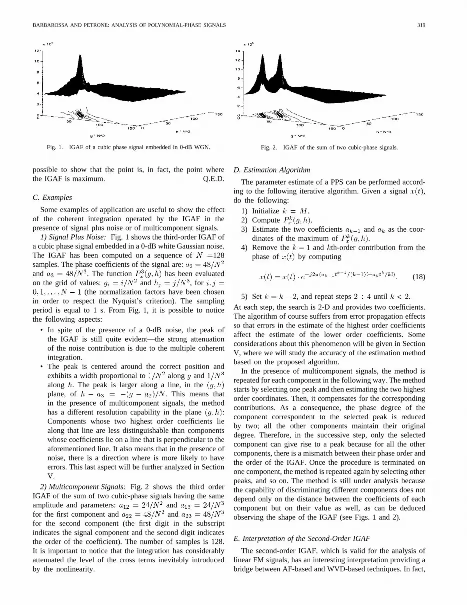
2) Multicomponent Signals:Fig. 2 shows the third orderIGAF of the sum of two cubic-phase signals having the sameamplitude and parameters: andfor the first component and andfor the second component (the first digit in the subscriptindicates the signal component and the second digit indicatesthe order of the coefficient). The number of samples is 128.It is important to notice that the integration has considerablyattenuated the level of the cross terms inevitably introducedby the nonlinearity.

Fig. 2. IGAF of the sum of two cubic-phase signals.

D. Estimation Algorithm

The parameter estimate of a PPS can be performed accord-ing to the following iterative algorithm. Given a signal ,do the following:

1) Initialize .2) Compute .3) Estimate the two coefficients and as the coor-

dinates of the maximum of .4) Remove the and th-order contribution from the

phase of by computing

(18)

5) Set , and repeat steps until .

At each step, the search is 2-D and provides two coefficients.The algorithm of course suffers from error propagation effectsso that errors in the estimate of the highest order coefficientsaffect the estimate of the lower order coefficients. Someconsiderations about this phenomenon will be given in SectionV, where we will study the accuracy of the estimation methodbased on the proposed algorithm.

In the presence of multicomponent signals, the method isrepeated for each component in the following way. The methodstarts by selecting one peak and then estimating the two highestorder coordinates. Then, it compensates for the correspondingcontributions. As a consequence, the phase degree of thecomponent correspondent to the selected peak is reducedby two; all the other components maintain their originaldegree. Therefore, in the successive step, only the selectedcomponent can give rise to a peak because for all the othercomponents, there is a mismatch between their phase order andthe order of the IGAF. Once the procedure is terminated onone component, the method is repeated again by selecting otherpeaks, and so on. The method is still under analysis becausethe capability of discriminating different components does notdepend only on the distance between the coefficients of eachcomponent but on their value as well, as can be deducedobserving the shape of the IGAF (see Figs. 1 and 2).

E. Interpretation of the Second-Order IGAF

The second-order IGAF, which is valid for the analysis oflinear FM signals, has an interesting interpretation providing abridge between AF-based and WVD-based techniques. In fact,


the second-order IGAF can be expressed as

(19)

By introducing the WVD of

we can rewrite the IGAF as

(20)

This means that computing the second-order IGAF ofis equivalent to performing the line integrals of the WVD of

over all possible lines in the time-frequency plane. Thisis equivalent to computing the Radon transform (or the Houghtransform) of the WVD. The parametersand assume, inthis sense, the meaning of the two parameters in the equationdescribing straight lines in the time-frequency domain. Thisapproach was shown to be optimal by Kay and Boudreaux-Bartels [14] for linear FM signals with random amplitude andwas analyzed in detail in [3]. Given the relationship betweenWVD and AF, it is not surprising to find an interpretation ofthe second-order IGAF in terms of AF as well. In fact, (19)can be rewritten, by exchanging the integration order, as

(21)

If we introduce the AF of

(22)we can write the IGAF as

(23)

This means that the IGAF can also be computed by taking theFourier transform of all the slices of the AF passing throughthe origin of the AF plane. A similar approach was proposedby Ristic and Boashash [22], who suggested to compute theAF and evaluate the line integrals over all the lines passingthrough the origin of themodulusof the AF. That approach issimpler than the approach proposed here because it involvesonly a final 1-D function, which was obtained by integratinga real 2-D function, but its performance is worse than theIGAF’s because the integration is noncoherent. Indeed, (23)states that the integration has to be coherent and, in particular,turns out to be the Fourier transform of slices of the AF.

Moreover, as far as the computational cost is concerned,the second-order IGAF requires only the computation of a

1-D integral. In fact, by applying the substitution

we can compute the second-order IGAF as follows:

This formula is useful for the implementation. The result is a 2-D function, as opposed to the method proposed in [22], wherethe result of the integration was a 1-D function. However, theIGAF allows the estimation of two parameters.

IV. SENSITIVITY

We have observed that the th-order IGAF ofan th-degree PPS assumes its maximum value in apoint , whose coordinates are the values of thetwo highest order coefficients of the instantaneous phase of

. In the presence of noise, there are, inevitably, errors.In particular, the value assumed by the IGAF inis a random variable whose statistical properties depend onthe noise, and the absolute maximum of the IGAF does notnecessarily lie in but falls in a generic point ofcoordinates , thus causing an estimationerror. The aim of this section and of the following one is toprovide a statistical analysis of the errors due to the noise.In particular, in this section, we will provide the statisticalcharacteristics of the value assumed by the IGAF in the point

, thus arriving at a definition of SNR equal to theone given in [17], which will be used as a comparison term.We will provide a statistical analysis of the estimation errors

and in Section V.We analyze the relationship between the SNR at the input

and at the output of the IGAF, which is considered to be anonlinear system. The analysis is carried out in the case of amonocomponent signal embedded in a white Gaussian noise.In the presence of an th-order PPS , expressed as in(8), without noise, the maximum absolute value oflies on the point of coordinates , as indicated byProperty 2. Let us indicate such a value by. In the presenceof signal plus noise, the IGAF, evaluated in the point ofcoordinates , is a random variable that will bedenoted . We define the output SNR as

SNRvar

(24)

where var indicates the variance of the random variable. The definition of the output SNR is analogous to the one

given in [17], which will be used as a comparison term. Wewill examine the performance in the second- and third-ordercases in the presence of a sequence ofsamples of a complexsignal having a constant amplitudeembedded in a complex


Fig. 3. Output SNR, normalized toN , versus input SNR (in decibels) forM = 2; IGAF (solid line). (a)N = 1024. (b) N = 256. (c) N = 64. (d)N = 16; PPT (dashed line).

Fig. 4. Output SNR, normalized toN , versus input SNR (in decibels) forM = 3; IGAF (solid line). (a)N = 1024. (b) N = 256. (c) N = 64. (d)N = 16; PPT (dashed line).

white Gaussian noise with zero-mean and variance. Theinput SNR is defined as SNR .

The relationships between the input and output SNR havebeen explicitely derived in Appendix A, and the results arethe following. For , we have

SNRSNR

SNR(25)

whereas for , we have

SNR

SNR

SNR SNR SNR(26)

These expressions are plotted in Figs. 3 and 4, respectively. Inthe same figures, we reported the corresponding relationshipsobtained using the polynomial-phase transform [17] to be usedas a comparison term. The expressions relative to the PPT arereported here:

SNRSNR

SNR(27)

and

SNRSNR

SNR SNR SNR(28)

In each figure, we plotted the output SNR normalized withrespect to the number of samples versus the input SNR,assuming the number of samplesas a parameter. The solid

line curves refer to the IGAF, whereas the dashed line refers tothe PPT. There is only one dashed line for the PPT because thecorresponding output SNR, after normalization with respectto , does not depend on anymore (see (27) and (28)).From the behaviors shown in Figs. 3 and 4, we can draw thefollowing considerations:

• Both methods (IGAF and PPT) exhibit a threshold effectin the sense that below a certain minimum SNR value(the threshold), the output SNR decreases very rapidly.

• The threshold effect is more evident as the polynomialorder increases.

• The IGAF has a threshold that decreases as the numberof samples increases; conversely, the PPT has a thresholdthat does not depend on the number of samples.

This last point is indeed one of the major advantages of theIGAF with respect to the PPT because it extends its range ofapplicability to lower SNR scenariouses.

V. ACCURACY

The accuracy in the estimation of the signal phase parame-ters is evaluated theoretically by a perturbation method appliedto the proposed transformation. The method is valid for highSNR and for a finite number of samples. The perturbationmethod is described in Appendix B, where is applied to thesecond- and third-order cases. The results are the following.The estimates are asymptotically unbiased. Considering thesecond-order case (quadratic phase signals), the variancescorresponding to the estimation of the two highest orderphase coefficients are, respectively ( denotes the variancein the estimate of the th-order coefficient of anth-degreepolynomial)

SNR SNR(29)

SNR SNR(30)

As far as the third-order case is concerned (cubic phasesignals), the variances of the estimates of the two highestorder coefficients are

SNR SNR(31)

SNR SNR(32)

The expressions of the variance obtained by the perturbationanalysis are approximated and the approximation is validfor high SNR. The limit of validity has been checked byMontecarlo simulations, whose results are reported in Figs. 5and 6, which show the variances obtained in the estimationof the second– and third-order coefficients, respectively, ofa cubic phase signal, as a function of the input SNR. Thenumber of samples is .

It is possible to notice the good agreement between the the-oretical formulas and the simulation for SNR greater or equalthan 0 dB. For SNR less than 0 dB, the theoretical analysis isno longer valid because the hypotheses underlying the use ofthe perturbation method are not satisfied. The results shown


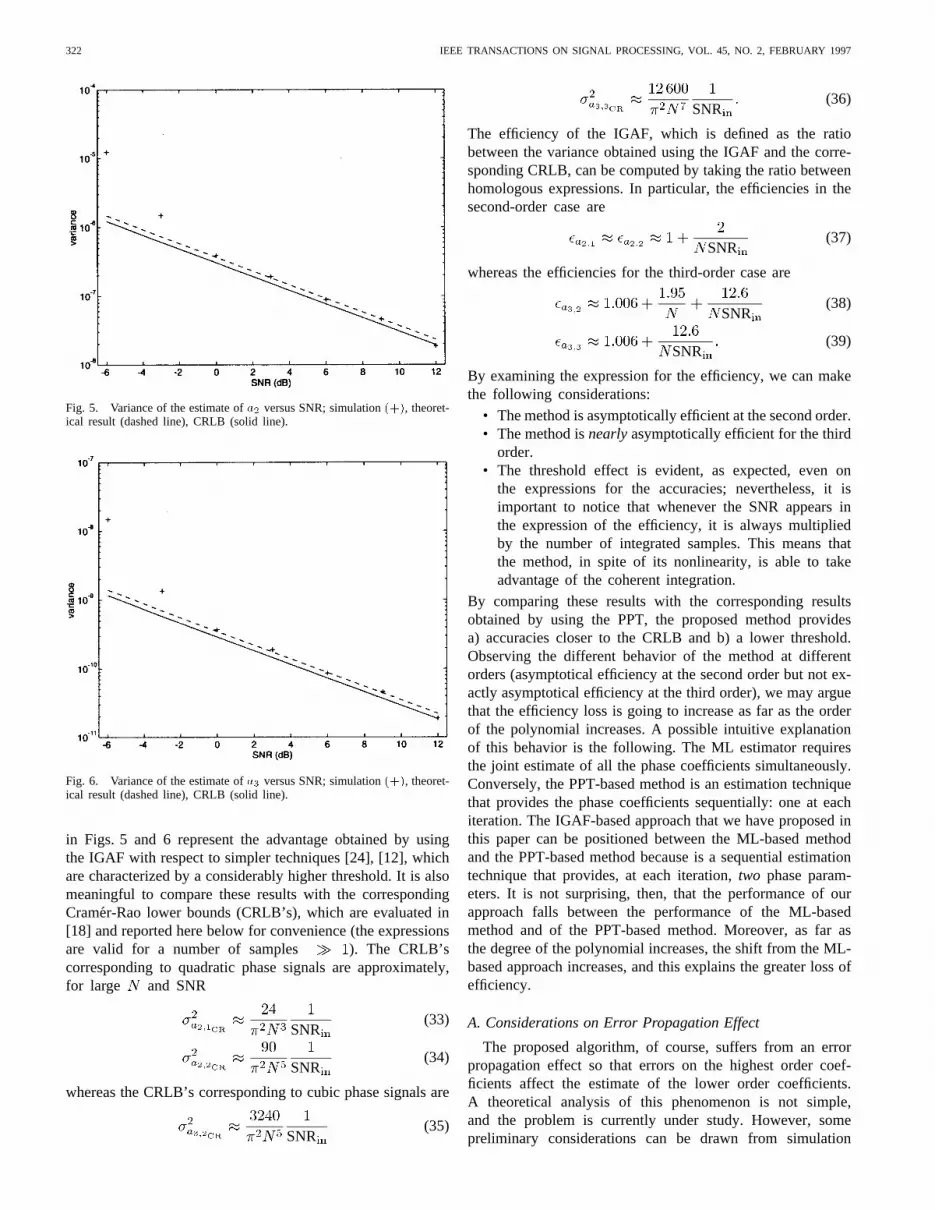
Fig. 5. Variance of the estimate ofa2 versus SNR; simulation(+), theoret-ical result (dashed line), CRLB (solid line).

Fig. 6. Variance of the estimate ofa3 versus SNR; simulation(+), theoret-ical result (dashed line), CRLB (solid line).

in Figs. 5 and 6 represent the advantage obtained by usingthe IGAF with respect to simpler techniques [24], [12], whichare characterized by a considerably higher threshold. It is alsomeaningful to compare these results with the correspondingCramer-Rao lower bounds (CRLB’s), which are evaluated in[18] and reported here below for convenience (the expressionsare valid for a number of samples ). The CRLB’scorresponding to quadratic phase signals are approximately,for large and SNR

SNR(33)

SNR(34)

whereas the CRLB’s corresponding to cubic phase signals are

SNR(35)

SNR(36)

The efficiency of the IGAF, which is defined as the ratiobetween the variance obtained using the IGAF and the corre-sponding CRLB, can be computed by taking the ratio betweenhomologous expressions. In particular, the efficiencies in thesecond-order case are

SNR(37)

whereas the efficiencies for the third-order case are

SNR(38)

SNR(39)

By examining the expression for the efficiency, we can makethe following considerations:

• The method is asymptotically efficient at the second order.• The method isnearlyasymptotically efficient for the third

order.• The threshold effect is evident, as expected, even on

the expressions for the accuracies; nevertheless, it isimportant to notice that whenever the SNR appears inthe expression of the efficiency, it is always multipliedby the number of integrated samples. This means thatthe method, in spite of its nonlinearity, is able to takeadvantage of the coherent integration.

By comparing these results with the corresponding resultsobtained by using the PPT, the proposed method providesa) accuracies closer to the CRLB and b) a lower threshold.Observing the different behavior of the method at differentorders (asymptotical efficiency at the second order but not ex-actly asymptotical efficiency at the third order), we may arguethat the efficiency loss is going to increase as far as the orderof the polynomial increases. A possible intuitive explanationof this behavior is the following. The ML estimator requiresthe joint estimate of all the phase coefficients simultaneously.Conversely, the PPT-based method is an estimation techniquethat provides the phase coefficients sequentially: one at eachiteration. The IGAF-based approach that we have proposed inthis paper can be positioned between the ML-based methodand the PPT-based method because is a sequential estimationtechnique that provides, at each iteration,two phase param-eters. It is not surprising, then, that the performance of ourapproach falls between the performance of the ML-basedmethod and of the PPT-based method. Moreover, as far asthe degree of the polynomial increases, the shift from the ML-based approach increases, and this explains the greater loss ofefficiency.

A. Considerations on Error Propagation Effect

The proposed algorithm, of course, suffers from an errorpropagation effect so that errors on the highest order coef-ficients affect the estimate of the lower order coefficients.A theoretical analysis of this phenomenon is not simple,and the problem is currently under study. However, somepreliminary considerations can be drawn from simulation


Fig. 7. Efficiency of the estimates versus the SNR;a1 (solid line), a2(dashed line),a3 (dot and dashed line).

Fig. 8. Histogram of the maxima of the IGAF.

results. Obviously the most critical step is the estimate ofthe highest order coefficient. At this regard, Fig. 7 shows thevariances obtained in estimating the parameters, , andof a cubic phase signal normalized to their respective CRLB’s[18]. The estimates have been obtained by simulation on asequence of 32 samples by averaging over 200 independenttrials. We can observe that, for SNR greater than the threshold(about 0 dB), the estimates are very close to their CRLB, butunder the threshold, there is a rapid performance degradation.In particular, the estimate of the first-order coefficient isstrongly affected by the propagation of the errors done inestimating the higher order coefficients. Even if the problemneeds further investigation, from an engineering point of view,we can reasonably argue that the limit of validity of thealgorithm is imposed by the threshold on the estimate of thehighest order coefficient.

The theoretical analysis of the error propagation phenom-enon is also complicated by the correlation between errors.To illustrate this aspect, Fig. 8 shows the contour plot of thehistogram of the maxima of the IGAF. The number of samples

is 64, and the SNR is 12 dB. The axes have been centeredon the exact values of and and are scaled with respect tothe theoretical standard deviations and (see Section V)for the given values of and SNR.

Ideally, without noise, we should observe a spike on thecenter of the figure. Due to the noise, the peak of the IGAF

moves in the plane, thus causing an estimation error. Aswe can see, the maximum moves mainly along a diagonal inthe plane, which means that the two errors alongand arecorrelated. This behavior is perfectly justifiable by recallingthe shape of the IGAF observed in Fig. 1.

VI. CONCLUSION

In this work, we have computed the performance, in termsof SNR and estimation accuracy, of a parameter-estimationmethod based on the integrated generalized ambiguityfunction, which was purposefully introduced for analyzingpolynomial-phase signals. The proposed approach providessome advantages with respect to conventional techniques interms of a lower SNR threshold and a better capability ofdiscriminating multiple components signals. The price paidfor these advantages is an increased computational cost. Withregard to this aspect of the problem, there are some simplermethods still based on the multilag definition of the IGAFthat are currently under analysis. A possible abrupt methodto reduce the computational cost consists of substituting oneterm in the kernel by its complex sign in order to avoidmultiplications in computing the kernel itself. In spite ofthe hard nonlinearity, the coherent integration implicit in theIGAF allows a consistent recovery if the number of samplesis sufficiently high. Some preliminary results were presentedin [6]. Another aspect that needs further investigation isthe analysis of multicomponent signals. The redundancyimplicit in the multilag definition introduced in this paper hasproduced certain advantages with respect to the polynomial-phase transform. The redundancy was exploited by taking theintegral over all possible sets of lags. However, other methodsfor exploiting the same redundancy can be envisaged to furtherimprove the capability of discriminating the components ofmulticomponent polynomial-phase signals. Some preliminaryresults about these new approaches have been presented in [7]and [8]. Finally, we wish to mention that the method proposedin this paper has been successfully employed on simulatedsynthetic aperture radar (SAR) images, as an autofocusingtechnique [5], as well as on real SAR data.

APPENDIX ASIGNAL-TO-NOISE RATIO

In this appendix, we will examine how the signal-to-noiseratio (SNR) varies by computing the IGAF of the observedsignal. We will consider the case of a sequence ofsamples

given by the superposition of a polynomial-phase signal(PPS) plus white Gaussian noise

(40)

The noise is assumed to be ergodic with zero mean andvariance . The PPS is assumed to have a constant envelope

. The input SNR is SNR . As we have shown inSection III, the estimation method is based on the simultaneousestimation of the two highest order coefficients of the signalinstantaneous phase. Let us denote byand the twocoefficients. In the presence of anth-order PPS, withoutnoise, the maximum of the th-order IGAF lies on


the point of coordinates . In the presence of noise, thevalue assumed by the IGAF in is a random value,and the position of the peak moves in a position , thusproducing an estimation error. The two errorsand are also random variables. In this appendix,we will evaluate the statistical properties of for

2 and 3, whereas in Appendix B, we will examine thestatistical properties of the errors and . We define theoutput SNR as

SNRvar

(41)

having indicated by and the valueassumed by the IGAF in the point in the presenceof signal only and of signal plus noise, respectively.

A. Second-Order Case

The second order IGAF of a sequence is

(42)

where and assume all the values such thatand . The value assumed by the

maximum of the IGAF, in the presence of the signal only, is

(43)

In the presence of white noise, the expected value ofis

(44)

(45)

having indicated by the unit pulse.The second-order moment is

(46)

having set, for notation simplicity,

and. By exploiting

the properties of the moments of zero mean complex Gaussianrandom variables [21], we obtain

(47)

(48)

This expression is independent of the signal coefficients.

In fact, we can prove, by direct substitution, the followingidentities:

(49)

It is important to notice that, thanks to the previous identities,the second-order moment of the IGAF, and then the SNR,is independent of the signal phase parametersand . Bysubstituting these expressions into (48), we obtain

(50)

Combining (50) and (45), we obtain the variance

var (51)

Substituting (51) and (43) in (41), we obtain the desiredformula for the output SNR

SNRSNR

SNR(52)

B. Third-Order Case

The third-order IGAF of a sequence is

(53)

where the summation indices assume all the values such thatthe following conditions hold simultaneously:

,and ; furthermore, the indices and

must be different from 0. In the presence of signal only,the maximum of the IGAF is

(54)

The IGAF of signal plus noise is

Let us introduce the following variables for simplicity ofnotation:

, .


In the presence of signal plus noise, the expected value of theIGAF in is

(55)

The last approximation is valid for . The value foundbefore is equal to the value assumed by the IGAF of a PPSwithout noise.

With regard to the second-order moment, setting for sim-plicity , we have

By carrying out the multiplications and considering the whitenoise case, we obtain

It is important to point out that these expressions, as thecorresponding expressions in the second-order case, are alsoindependent of the signal phase parameters. A closed-formexpression of these summations has been obtained with thehelp of Mathematica and is

(56)

(57)

Combining (57) and (55), we obtain the variance that, for, can be simplified into the following expression:

var

(58)

Substituting (54) and (58) into (41), we obtain the expressionfor the SNR reported in (26).

APPENDIX BEVALUATION OF THE VARIANCE BY PERTURBATION METHOD

The perturbation method has already been applied to thecomputation of the variance of the estimation errors for linearfrequency modulation (LFM) signals embedded in AWGN in[18]. The method was 1-D because the approach proposed in[18] estimated one parameter at the time. The perturbationmethod was then extended in [3] to find the variances of theerrors done in locating the maximum of a real 2-D functionof complex random variables. The method was used in [3] toprovide the variance of the estimate of the mean frequencyand sweep rate of LFM signals embedded in AWGN byusing the Wigner–Hough transform (WHT). Since the WHT isexactly equivalent to the second-order IGAF, the results for thesecond-order case are obviously the same as in [3]. We initiallyrecall the main steps of the perturbation method proposed in[3], and then, we extend the analysis to the third-order case.

In the presence of signal plus noise, the IGAFcan be written as the sum of a term due only to the signal

plus a residue term (theperturbation)due to the noise and to its interaction with the signal

(59)

In the presence of a third-order PPS, without noise, the func-tion assumes its maximum value in , where

and are the second- and third-order phase coefficientsof the signal, according to Proposition 2 (see Section III-B).In the presence of signal plus noise, the absolute maximumfalls into a generic point of coordinates ,where and are the errors along the axes and ,respectively. Since the perturbation depends on the noise, theerrors are random variables. The aim of this section is tocompute expected value and variance of the errorsand

. By definition of maximum, we can write

(60)

(61)

having indicated by the partialderivative of , with respect to the variable, computedin the point of coordinates , and so on. Ata first-order approximation, which is valid for small errors

and (and then for high SNR), we can approximatethe previous expressions by their first-order series expansionaround the point of coordinates

(62)


(63)

The first term in both expressions is equal to zero (seeProposition 2 in Section III-B). If we introduce the constants

(64)

and the random variables

(65)

we can set up the following system of two equations

This system can be inverted to find the relationships that givethe errors and in terms of the random variablesand

We can use these expressions to find expected values andvariance of the errors

(66)

(67)

(68)

(69)

The intermediate computations necessary to obtain the ex-pected values involving the random variablesand are quitelengthy and are omitted (they exploit the same properties ofthe summations already used in Appendix A). We only reportthe final results. In particular, the expected values ofandare equal to zero, which implies, using (66) and (67), that theestimates are unbiased, at least at a first-order approximation.With regard to the second-order moments, we have

SNR SNR

SNR SNR

SNR SNR

In addition, the constants , , and , which are defined in(64), can be expressed in a closed form, depending only on

the signal amplitude and on the number of samples

Inserting the above expressions into (68) and (69), we obtainthe final formulas for the variance given in (31) and (32).

REFERENCES

[1] T. J. Abatzoglou, “Fast maximum likelihood joint estimation of fre-quency and frequency rate,”IEEE Trans. Aerospace Electron. Syst., vol.AES-22, pp. 708–715, Nov. 1986.

[2] S. Barbarossa, “Detection and estimation of the instantaneous frequencyof polynomial-phase signals by multilinear time-frequency representa-tion,” in Proc. IEEE-SP Workshop Higher Order Statistics, Lake Tahoe,CA, June 1993, pp. 168–172.

[3] , “Analysis of multicomponent LFM signals by a combinedwigner-hough transform,”IEEE Trans. Signal Processing, vol. 43, pp.1511–1515, June 1995.

[4] S. Barbarossa and G. Schiappa, “Analysis of multicomponent signals bymultilinear time-frequency representations,” inProc. Int. Conf. Acoust.,Speech, Signal Processing, ICASSP’94, Adelaide, Australia, Apr. 19–22,1994, pp. III-341–344.

[5] S. Barbarossa and R. Mascolo, “Autofocusing techniques for imagingmoving targets by SAR based on a multilinear time-frequency represen-tation,” in Proc. Int. Conf. Radar, Paris, May 1994, pp. 284–289.

[6] S. Barbarossa and G. Scarano, “Analysis of polynomial-phase signalsby a fast hybrid nonlinear generalized ambiguity function,” inProc.IEEE Workshop Higher Order Statistics, Parador de Aiguablava, Spain,June 1995.

[7] S. Barbarossa, A. Scaglione, and A. Porchia, “Multiplicative multi-lag high order ambiguity function,” inProc. Int. Conf. Acoust., SpeechSignal Processing, ICASSP’96, Atlanta, GA, May 1996, pp. 3022–3025.

[8] S. Barbarossa, “Parameter estimation of multicomponent polynomial-phase signals by intersection of signal subspaces,” inProc. Eighth IEEEWorkshop on Statistical Signal and Array, Corfu, Greece, June 1996.

[9] B. Boashash, “Estimating and interpreting the instantaneous frequencyof a signal,” inProc. IEEE, vol. 80, pp. 520–568, Apr. 1992.

[10] B. Boashash and P. O’Shea, “Polynomial wigner-ville distributions andtheir relationship to time-varying higher order spectra,”IEEE Trans.Signal Processing, vol. 42, Jan. 1994.

[11] A. V. Dandawate and G. Giannakis, “Nonparametric polyspectral esti-mators forkth-order (almost) cyclostationary processes,”IEEE Trans.Inform. Theory, vol. 40, no. 1, Jan. 1994.

[12] P. M. Djuric and S. M. Kay, “Parameter estimation of chirp signals,”IEEE Trans. Acoust., Speech, Signal Processing, vol. 38, pp. 2118–2126,Dec. 1990.

[13] B. Friedlander, “Parametric signal analysis using the polynomial phasetransform,” in Proc. IEEE Workshop Higher-Order Statistics, StanfordSierra Camp, June 1993.

[14] S. M. Kay and G. F. Boudreaux-Bartels, “On the optimality of thewigner distribution,” inProc. Int. Conf. Acoust., Speech Signal Process-ing, ICASSP’85, Mar. 1985, pp. 27.2.1–4.

[15] R. Kumaresan and S. Verma, “On estimating the parameters of chirpsignals using rank reduction techniques,” inProc. 21st Asilomar Conf.Signals, Syst. Comput., Pacific Grove, CA, 1987, pp. 555–558.

[16] P. O’Shea, “Fast parameter estimation algorithms for linear FM signals,”in Proc. IEEE Int. Conf. Acoust., Speech Signal Processing, ICASSP’94,Adeaide, Australia, Apr. 1994, pp. IV-17–20.

[17] S. Peleg and B. Porat, “Estimation and classification of polynomial-phase signals,”IEEE Trans. Inform. Theory, vol. 37, pp. 422–430, Mar.1991.


[18] , “The Cramer-Rao lower bound for signals with constant am-plitude and polynomial phase,”IEEE Trans. Signal Processing, vol. 39,no. 3, Mar. 1991.

[19] , “Linear FM signal parameter estimation from discrete-timeobservations,” IEEE Trans. Aerospace Electron. Syst., vol. 27, pp.607–615, July 1991.

[20] B. Porat, Digital Processing of Random Signals, Theory & Methods.Englewood Cliffs, NJ: Prentice-Hall, 1994.

[21] I. S. Reed, “On a moment theorem for complex gaussian processes,”IRE Trans. Inform. Theory, pp. 194–195, Apr. 1962.

[22] B. Ristic and B. Boashash “Kernel design for time-frequency signalanalysis using the radon transform,”IEEE Trans. Signal Processing,vol. 41, May 1993.

[23] S. Shamsunder, G. B. Giannakis, and B. Friedlander, “Estimating ran-dom amplitude polynomial phase signals: A cyclostationary approach,”IEEE Trans. Signal Processing, vol. 43, pp. 492–505, Feb. 1995.

[24] S. Tretter, “Estimating the frequency of a noisy sinusoid by linearregression,”IEEE Trans. Inform. Theory, vol. IT-31, pp. 832–835, Nov.1985.

[25] G. Zhou, G. B. Giannakis, and A. Swami, “On polynomial-phase signalswith time-varying amplitudes,”IEEE Trans. Signal Processing, vol. 44,pp. 848–861, Apr. 1996.

Sergio Barbarossa(M’88) received the degree inelectronic engineering from the University of Rome,“La Sapienza,” in 1984 and the Ph.D. degree in1989.

In 1984, he joined the Radar System AnalysisGroup of Alenia, Italy, where he worked until 1986when he joined the Information and Communica-tion Department of the University of Rome “LaSapienza,” where he is now an associate profes-sor. In 1988, he was a research engineer at theEnvironmental Research Institute of Michigan, Ann

Arbor, and in 1995, he was a visiting professor at the University of Virginia,Charlottesville. He holds one patent for industrial invention and is author orco-author of more than 50 papers in international journals or conferences. Hismain research interests are in the area of statistical signal processing withapplications to radar and communications.

Dr. Barbarossa has been a member of the technical committee for theEighthIEEE Signal Processing Workshop on Statistical Signal and Array Processing.

Valentina Petrone received the degree in elec-tronic engineering from the University of Rome, “LaSapienza,” in 1993.

In 1994, she was with Harpa Italia, and in 1995,she worked at the Space Division of Vitrociset,Italy. Since September 1995, she has been with theConsortium for Research on Telecommunications(CoRiTel), Rome, Italy, where she is involved withmulticube, which is a project aimed to providea high-speed multimedia-multipoint infrastructurebased on the existing broadband network. Her main

research interests are in the area of telecommunications networks.